Structural Modelling, Exogeneity, and Causality

Michel MOUCHARTa , Federica RUSSOb and Guillaume WUNSCHc

a Institute of Statistics, Universite catholique de Louvain, Belgium

b Institute of Philosophy, Universite catholique de Louvain, Belgium.

c Institute of Demography, Universite catholique de Louvain, Belgium.

October 25, 2007

Abstract

This paper deals with causal analysis in the social sciences. We first present a conceptual

framework according to which causal analysis is based on a rationale of variation and invariance,

and not only on regularity. We then develop a formal framework for causal analysis by means of

structural modelling. Within this framework we approach causality in terms of exogeneity in a

structural conditional model based which is based on (i) congruence with background knowledge,

(ii) invariance under a large variety of environmental changes, and (iii) model fit. We also tackle

the issue of confounding and show how latent confounders can play havoc with exogeneity. This

framework avoids making untestable metaphysical claims about causal relations and yet remains

useful for cognitive and action-oriented goals.

Keywords: Causality, Confounding, Exogeneity, Latent Variables, Partial Observability, Struc-

tural Modelling.

Corresponding Author: Guillaume Wunsch, Institute of Demography, UCLouvain, Place Mon-

tesquieu 1/17, B-1348 Louvain-la-Neuve , Belgium. e-mail: wunsch@demo.ucl.ac.be

1

Contents

1 Causal analysis in the social sciences 3

1.1 Goals of causal analysis . . . . . . . . . . . . . . . . . . . . . . . . . . . . . . . . . . 3

1.2 Variation and regularity in causal analysis . . . . . . . . . . . . . . . . . . . . . . . . 4

1.3 Background knowledge in causal analysis . . . . . . . . . . . . . . . . . . . . . . . . 5

1.4 Probabilistic modelling in causal analysis . . . . . . . . . . . . . . . . . . . . . . . . 7

2 Structural modelling 8

2.1 The meaning of structurality . . . . . . . . . . . . . . . . . . . . . . . . . . . . . . . 8

2.2 The statistical model . . . . . . . . . . . . . . . . . . . . . . . . . . . . . . . . . . . 9

2.3 Statistical inference and structural models. . . . . . . . . . . . . . . . . . . . . . . . 10

3 Conditional models, exogeneity and causality 11

3.1 Conditional models . . . . . . . . . . . . . . . . . . . . . . . . . . . . . . . . . . . . . 11

3.2 Conditional model and exogeneity . . . . . . . . . . . . . . . . . . . . . . . . . . . . 13

3.3 Exogeneity and causality . . . . . . . . . . . . . . . . . . . . . . . . . . . . . . . . . . 15

4 Confounding, complex systems and completely recursive systems 15

4.1 Confounders and confounding . . . . . . . . . . . . . . . . . . . . . . . . . . . . . . . 15

4.2 Complex systems and completely recursive systems . . . . . . . . . . . . . . . . . . . 18

5 Partial observability and latent variables 20

5.1 A three-component system . . . . . . . . . . . . . . . . . . . . . . . . . . . . . . . . . 20

5.2 The general case . . . . . . . . . . . . . . . . . . . . . . . . . . . . . . . . . . . . . . 23

6 Discussion and conclusion 23

References 26

2

1 Causal analysis in the social sciences

1.1 Goals of causal analysis

Whilst it might seem uncontroversial that the health sciences search for causes - that is, for causes of

disease and for effective treatments - the causal perspective is less obvious in social science research,

perhaps because it is apparently harder to glean general laws in the social sciences than in other

sciences, due the probabilistic character of human behaviour. Thus the search for causes in the

social sciences is often perceived to be a vain enterprise and it is often thought that social studies

merely describe the phenomena.

On the one hand, an explicit causal perspective can already be found in pioneering works of

Adolphe Quetelet (1869) and Emile Durkheim (1897) in demography and sociology respectively,

and the social sciences have taken a significant step in quantitative causal analysis by following

Sewall Wright’s path analysis (1934), first applied in population genetics. Subsequent developments

of path analysis - such as structural models, covariance structure models or multilevel analysis -

have the merit of making the concept of cause operational by introducing causal relations into the

framework of statistical modelling. However, these developments in causal modelling leave a number

of issues at stake, for instance a deeper understanding of exogeneity and its causal importance.

On the other hand, an explicit causalist perspective still needs justification. Different social

sciences study society and humans from different angles and perspectives. Sociology studies the

structure and development of human society, demography attends to the vital statistics of popula-

tions, economics studies the management of goods and services, epidemiology studies the distribution

of disease in human populations and the factors determining that distribution, etc. In spite of these

differences, social sciences share a common objective: to understand, predict and intervene on indi-

viduals and society. In these three moments of the scientific demarche, knowledge of causes becomes

essential. The importance of causal knowledge is twofold. Firstly, we pursue a cognitive goal in

detecting causes and thus in gaining general knowledge of the causal mechanisms that govern the

development of society. Secondly, such general causal knowledge is meant to guide and inform so-

cial policies, that is we also pursue an action-oriented goal. If the social sciences merely described

phenomena, it would not be possible to design efficient policies or prescribe treatments that rely on

the results of research.

As stated above, the social sciences do not establish laws as physics does. Whether this is an

intrinsic issue of these sciences, or merely a contingent problem due to the specifity of social problems,

is still matter of debate and falls far beyond the scope of the present paper. In the following, we

will rather reverse the perspective and try to tackle the issue: under what conditions can structural

models give us causal knowledge?

3

1.2 Variation and regularity in causal analysis

The first thing worth mentioning is that we need to abandon in favour of a more flexible framework

the paradigm of regularity as regular succession of events in time, a heritage of Hume. Hume

believed that causality lies in the constant conjunction of causes and effects. In his Treatise Hume

(1748) says that, in spite of the impossibility of providing rational foundations for the existence of

objects, space, or causal relations, believing in their existence is a “built in” habit of human nature.

In particular, belief in causal relations is granted by experience. For Hume, simple impressions

always precede simple ideas in our mind, and by introspective experience we also know that simple

impressions are always associated with simple ideas. Simple ideas are then combined in order to

form complex ideas. This is possible thanks to imagination, which is a normative principle that

allows us to order complex ideas according to (i) resemblance, (ii) contiguity in space and time, and

(iii) causality. Of the three, causation is the only principle that takes us beyond the evidence of

our memory and senses. It establishes a link or connection between past and present experiences

with events that we predict or explain, so that all reasoning concerning matters of fact seem to be

founded on the relation of cause and effect. The causal connection is thus part of a principle of

association that operates in our mind. Regular successions of impressions are followed by regular

successions of simple ideas, and then imagination orders and conceptualizes successions of simple

ideas into complex ideas, thus giving birth to causal relations. The famed problem is that regular

successions so established by experience clearly lack the logical necessity we would require for causal

successions. Hume’s solution is that if causal relations cannot be established a priori, then they

must be grounded in our experience, in particular, in our psychological habit of witnessing effects

that regularly follow causes in time and space.

If we want causality to be an empirical and testable matter rather than a psychological one, we

need to replace the Humean paradigm of regularity with a paradigm of variation. In this framework

structural models do not only aim at finding regular successions of events. Rather, causal models

model causal relations by analysing suitable variations among variables of interest (See Russo 2005,

2007). Differently put, causal models are governed by a rationale of variation, not of regularity. A

rationale is a principle of some opinion, action, hypothesis, phenomenon, model, reasoning, or the

like. The quest for a rationale of causality is then the search for the principle that guides causal

reasoning and thanks to which we can draw causal conclusions. This principle lies in the notion of

variation.

The rationale of variation manifestly emerges, for instance, in the basic idea of probabilistic

theories of causality and in the interpretation of structural equations. Probabilistic theories of

causality, see Suppes (1970), focus on the difference between the conditional probability P (E|C) and

the marginal probability P (E). To compare conditional and marginal probability means to analyse

a statistical relevance relation, i.e. probabilistic independence. The underlying idea is that if C is a

4

cause of E, then C must be statistically relevant for E. Hence, the variation hereby produced by C in

the effect E will be detected because the conditional and the marginal probability differ. Analogously,

quantitative probabilistic theories focus on the difference between the conditional distribution P (Y ≤

y|X ≤ x) and the marginal distribution P (Y ≤ y). Again, to compare conditional distribution with

marginal distribution means to measure the variation produced by the putative cause X on the

putative effect Y .

In structural equation models, the basic idea is that, given a a system of equations, we can test

whether variables are interrelated through a set of linear relationships, by examining the variances

and covariances of variables. Sewall Wright, as early as 1934, has taught us to write the covariance

of any pair of observed variables in terms of path coefficients. The path coefficient quantifies the

(direct) causal effect of X on Y ; given the numerical value of the path coefficient β, the equation

Y = βX + ε claims that a unit increase in X would result in a β unit increase of Y . In other

words, β quantifies the variation of Y associated to a variation of X, provided that X doesn’t have

null variance. Another way to put it is that structural equations attempt to quantify the change

in X that accompanies a unit change in Y . It is worth noting that the equality sign in structural

equations does not state an algebraic equivalence. Jointly with the associated graph, the structural

equation is meant to uncover a causal structure. That is, given a structural equation of the simple

form Y = βX + ε1, the reverse equation X = γY + ε2 is not causally equivalent. Pearl (2000, p.

159-160) makes a similar point.

1.3 Background knowledge in causal analysis

Variation, however, is not itself a causal notion and consequently cannot guarantee, alone, the

causal interpretations of probabilistic inequalities. Good epistemology ought to tell us under what

conditions, i.e. what the constraints are, for variations to be causal. A complete account of the

guarantee of the causal interpretation should focus on the difference between purely associational

models and causal models, pointing to the features proper to the richer apparatus of causal models

(see Russo (2005) and Russo, Mouchart, Ghins and Wunsch(2006)). For a model to be causal, we

shall particularly focus on two types of constraints: background knowledge and structural stability.

In a nutshell, concomitant variations will be deemed causal if they are structurally stable and if they

are congruent with background knowledge; see e.g. Engle, Hendry and Richard (1983), Florens and

Mouchart (1985), Hendry and Richard (1983) or Thomas (1996). In this way regularity, which would

be better understood here in terms of invariance of the model’s structure (variables and relations),

becomes a constraint that participates in the causal interpretation of variations.

On the one hand, background knowledge, both theoretical and empirical, serves three roles: (i)

it provides a relevant causal context for the formulation of hypotheses, (ii) it guides the choice

of variables and of the relations to be tested for structural stability, and (iii) it constitutes the

5

sounding board for results as they have to be congruent with background knowledge. On the other

hand, structural stability is a constraint we impose on a relation for being causal, in order to

rule out accidental relations. Differently put, the crucial step in Hume’s argument is significantly

different from the rationale hereby proposed. We claim that we firstly look for variations. Once

concomitant variations are detected, a condition of invariance or structural stability (among others)

is imposed on them. What does structural stability give us? Not logical necessity, nor mere constant

conjunction as Hume advocated. Invariance, an empirical feature, recalls Humean regularity but

the scope of the former is wider than that of the latter. Structural stability is a condition required

in order to ensure that the model correctly specifies the data generating process and that the

model does not confuse accidental and/or spurious relations with causal ones. It is worth noting

that, in the search for structurality, background knowledge and invariance play a complementary

role. In particular, unexplained stable relations may lead to questioning background knowledge and

eventually to modifying it.

It might be objected that if structural stability does not give us logical necessity either, it does

not any better than regularity. Undoubtedly necessity is an essential feature for those who would like

the social sciences to discover universal laws, or for those who question their scientific legitimacy on

this ground. However, independently of whether it is a built-in impossibility of the social sciences to

glean laws, this would be too a rigid framework, for society and individuals are too mutable objects

of study to be fettered in immutable and even regular deterministic or probabilistic laws.

The philosophical gain of adopting this paradigm is twofold. Firstly, we go beyond the Humean

tradition that somehow denies causation by reducing it to regularity. Secondly, we do not fall into

untestable metaphysical positions either, because structural models stay at the level of knowledge.

Let us clarify this last point. Structural modelling intends to represent an underlying causal struc-

ture, mathematically, by means of equations, and pictorially, by means of directed acyclic graphs.

However, structural models don’t pretend to attain the ontic level, i.e. to open the black box, so

to speak. They stay at the level of field knowledge and theory: if concomitant variations between,

say, X and Y are structurally stable and are congruent with available field knowledge, then we have

no reasons not to believe that X causes Y . In this sense structural models mediate epistemic access

to causal relations without claiming that the true causes have been discovered. Differently put,

structural modelling allows us to take a sensible causalist stance that guides actions and policies

without overflowing into untestable metaphysical claims.

The practical gain of adopting this paradigm is having a clearer understanding of the causal

import of background knowledge and of testing stability. Those aspects, in fact, turn out to be of

fundamental importance for the interpretation of results.

6

1.4 Probabilistic modelling in causal analysis

Structural models belong to the category of probabilistic models. This leads us to consider also the

following issue. Is a probabilistic characterization of causation a symptom of indeterministic causality

or rather of our incomplete and uncertain knowledge? In physics, quantum mechanics raised quite

substantial issues about the possibility of indeterminism. However, whether or not the world is

actually indeterministic, needs not to be decided once and for all. In fact, from an epistemological

viewpoint, a probabilistic characterization of causal relations in structural models only commits us

to state that our knowledge is incomplete and uncertain. Our endeavour to gain causal knowledge

requires reducing, as far as possible, bias and confounding by building good structural models, that

is models that pick up structurally stable relations consistent with background knowledge.

So far we have seen that the concept of variation plays a crucial role in the interpretation of

structural equations. A simple form of a structural equation such as Y = βX + ε, can be interpreted

as follows: variations in X lead to or are responsible for variations in Y . In other words, X is

statistically relevant for Y , i.e. P (Y |X) 6= P (Y ). However, statistical relevance, and consequently

also variation, are symmetrical notions. So how do we know that X causes Y and not the other way

around? There are three different but nonetheless related elements that participate in determining

the direction of the causal relations: background knowledge, invariance, and time. Let us focus on

time. In the social sciences we need temporal direction. This is for several reasons.

Firstly, causal mechanisms - were they physiological, social or socio-physiological - are embedded

in time. Smoking at time t causes cancer at t′

(t < t′), but not the other way around. To give

another example, use of contraceptives is followed by changes in the intensity and tempo of fertility.

Secondly, although the two causal relations marriage dissolution influences migration or migration

influences marriage dissolution both make sense, we need to know whether marriage dissolution

or migration is the temporally prior cause for cognitive and/or policy reasons. One out of the

two claims might be eventually disproved due to problems of observability or lack of theory. For

instance, the causal chain migration influences marriage dissolution might be incorrect: although

marriage dissolution is observed after migration, there might exist a temporally prior process -

marital problems and the subsequent decision to divorce - causing migration.

This oversimplified example clearly shows that causal modelling requires a constant interplay

between observation, theory and testing. Indeed, this is the core of a hypothetico-deductive method-

ology of structural modelling (see Russo (2005) and Russo, Mouchart, Ghins and Wunsch (2006)).

Causal hypotheses need to be confirmed or disconfirmed (i.e. accepted or rejected in the statistical

jargon) based on empirical testing: the model has to fit observations, but the causal hypothesis

itself has to be formulated, along with the model building stage, in accordance with available well

established theories and background knowledge. However, we also need structural models to be

flexible enough to revise our theories in the light of new data disconfirming prior theories.

7

Following the H-D methodology, causal hypotheses are confirmed or disconfirmed depending on

the results of empirical testing. Suppose, for the sake of the argument, that the causal hypothesis

is rejected. Such a negative result can be nonetheless useful as it can suggest that improvement is

needed in the theory backing the causal model, or that data may contain some source of bias. In

other words, the rejection of a causal hypothesis can trigger further research. Suppose now, again

for the sake of the argument, that the causal hypothesis is accepted. Such a positive result is not an

immutable one, written on the stone, so to speak. Although the causal hypothesis is not rejected,

this may be subject to revision (and even to rejection) in the future, due to new discoveries. It

is worth stressing that the acceptance of the causal model is highly dependent on its structural

stability. Unlike the traditional falsificationist account (see Popper 1959), hypothetico-deductivism

in structural modelling allows and indeed encourages us to use at any stage of research all available

information. Williamson (2005) also makes a similar point in putting forward a hybrid of inductive

and hypothetico-deductive methodologies in which the hypothesising stage is always informed by

previous results, whether positive or negative. This is indeed the advantage of handling structural

models that are assumed to represent underlying causal structures without pretending to uncover

immutable metaphysical causes. The following sections make more explicit and formal these ideas

about causality and structural modelling.

2 Structural modelling

2.1 The meaning of structurality

Inspired by the seminal works of Wright, Haavelmo, Blalock, Pearl and others, we will develop in

this section a structural modelling approach to causation. In essence, a model is deemed structural

if it uncovers a structure underlying the data generating process. As discussed in section 1.3, this

approach systematically blends two ingredients. First, the model must be congruent with background

knowledge: modelling the data generating process must be operated in the light of the current

information on the relevant field. Second, the model must show stability in a wide sense: both the

structure of the model and the parameters have to be stable or invariant with respect to a large class

of interventions or of modifications of the environment. Often, but not always, structural models

make use of latent variables. By integrating out the latent variables, the statistical model is thus

obtained as the marginal distribution of the manifest or observable variables. It is crucial to note

that this concept of structural modelling is wider than the framework of structural equations models,

also known as covariance structure models or LISREL type models, widely used in psychology or in

sociology, and of simultaneous equations models, widely used in econometrics.

A first consequence of this approach is that the notion of causality becomes relative to the model

itself, rather than to the data, as is the case, for instance, in the Granger-type concept of causality.

8

Also, this means that we do not aim at making metaphysical claims about causal relations, but

rather at saying when we have enough reasons - specifically, reasons about background knowledge

and about structural stability - to believe that we hit upon a causal relation. A second consequence

of this model-based concept of causality, involving both background knowledge and stability, is that

the model does not simply derive from theory as is often the case in the econometric tradition.

Therefore structural modelling is much more than a sophisticated statistical tool. Good structural

modelling ought to be accompanied by a broad and sensible account of what a statistical model is

and represents, of what statistical inference is, and of what rationale guides model building and

testing. The last point has been dealt with in the previous section. The first and the second will be

the object of the following sections. We first recall the formal nature of a statistical model and of the

basic concepts of conditional modelling and of exogeneity, we then define the concept of causality in

such a framework.

2.2 The statistical model

Formally, a statistical model M is a set of probability distributions, explicitly:

M = S, Pω ω ∈ Ω (1)

where S, called the sample space or observation space, is the set of all possible values of a given

observable variable (or vector of variables) and for each ω ∈ Ω , Pω is a probability distribution on the

sample space, also called the sampling distribution; thus, ω is a characteristic, also called parameter,

of the corresponding distribution and Ω describes the set of all possible sampling distributions

belonging to the model. The basic idea is that the data can be analyzed as if they were a realization

of one of those distributions. For example, in a univariate normal model, the sample space S is the

real line and the normal distributions are characterized by a bivariate parameter, for instance the

expectation (µ) and the variance (σ2 ); in this case: ω = (µ, σ2) .

A statistical model is based on a stochastic representation of the world. Its randomness delineates

the frontier or the internal limitation of the statistical explanation, since the random component

represents what is not explained by the model. A statistical model is made of a set of assumptions

under which the data are to be analyzed. Typical assumptions of statistical models are: the observed

random variables follow or not identical distributions; the observations are, or are not, independent;

the basic sampling distributions are, or are not, continuous and may pertain, or not, to a family

characterized by a finite number of parameters (e.g. the normal distributions).

If assumptions are satisfied, the statistical model correctly describes co-variations between vari-

ables, but no causal interpretation is allowed yet. In other words, it is not necessary that causal

information be conveyed by the parameters, nor is it generally legitimate to give the regression

coefficients a causal interpretation. It is worth noting that in specifying the assumptions typical of

9

a statistical model, the problem is not to evaluate whether an assumption is true. A (frequentist)

statistician may however want to test in due course whether a hypothesis is confirmed or not. If a

model-builder could prove that an assumption were (exactly) true, this would not be an assumption

anymore, but a description of the real world. Rather, the main issue is to evaluate whether an

assumption is useful, in the sense of making possible a process of learning-by-observing on some

aspects of interest of the real world.

2.3 Statistical inference and structural models.

Statistical inference is concerned with the problem of learning-by-observing and is inductive since

it implies drawing conclusions about what has not been observed from what has been observed.

Therefore, statistical inference is always uncertain and the calculus of probability is the natural,

and in a sense logically necessary tool, see e.g. de Finetti (1937), Savage (1954), for expressing the

conclusions of statistical inference. Therefore, the stochastic aspect of statistical models involves a

stochastic representation of the world and a vehicle for the learning-by-observing process.

Here, two aspects ought to be distinguished. On the one hand, learning-by-observing conveys

the idea of learning about some features of interest, namely the characteristics of a distribution or

the values of a future realization. On the other hand, learning-by-observing is also concerned with

the problem of accumulating information as observations accumulate. These two aspects actually

refer to the usefulness of the model. Structural models are precisely designed for making the process

of statistical inference meaningful and operational.

To better understand the idea behind this last claim, it is worth distinguishing two families of

models. In the first family we find purely statistical models, also called associational or descriptive

models, and exploratory data analysis, also called data mining. In these approaches, the assumptions

are either not made explicit or restricted to a minimum allowing us to interpret descriptive summaries

of data. Interest may accordingly focus on the distributional characteristics of one variable at a time,

such as mean or variance, or on the associational characteristics among several variables, such as

correlation or regression coefficients. It is worth noting that the absence or the reduced number of

assumptions constituting the underlying model make these associational studies insufficient to infer

a causal relation and leaves open a wide scope for interpreting the meaning of the results.

The second family consists in the so-called structural models. “Structural” conveys the idea of a

representation of the world that is stable under a large class of interventions or of modifications of

the environment. Structural models are also called “causal models”. Here, the concept of causality

is internal to a model which is itself stable, in the sense of structurally stable. As a matter of fact,

structural models incorporate not only observable, or manifest, variables but also, in many instances,

unobservable, or latent, variables. The possible introduction of latent variables is motivated by the

help they provide in making the observations understandable; for instance, the notion of “intelli-

10

gence quotient” or of “associative imagination” might help to shape a model which explains how

an agent succeeds in answering the questions of a test in mathematics. Thus a structural model

aims at capturing an underlying structure; modelling this underlying structure requires taking into

account the contextual knowledge of the field of application. The characteristics, or parameters, of

a structural model are of interest because they correspond to relevant properties of the observed

reality and can be safely used for accumulating statistical information, precisely because of their

structural stability. In this context, a structural model is opposed to a “purely statistical model”,

understood as a model that accounts for observable associations without linking those associations

to stable properties of the world.

The invariance condition of a structural model is actually a complex issue. Two aspects have

to be considered. A first one is a condition of stability of the causal relation. The idea is that

each variable depends upon a set of other variables through a relationship that remains invariant

when those other variables are subject to external influence. This condition allows us to predict the

effects of changes in the environment or of interventions. A second condition is the stability of the

distributions to ensure that the parameters will not be affected by changes in the environment or

interventions.

3 Conditional models, exogeneity and causality

3.1 Conditional models

Originally, the concept of exogeneity appears with regression models. A first, and naive, approach

was to consider an exogenous variable as a non-random variable, the endogenous variable being the

only random one. That this approach was unsatisfactory became clear when considering complex

models where the same variable could be exogenous in one equation and endogenous in another one.

A first progress came through a proper recognition of the nature of a conditional model. Here, we

present a heuristic account of the basic concepts; for a more formal presentation, see e.g. Mouchart

and Oulhaj (2000) and Oulhaj and Mouchart (2003).

Let us start with an (unconditional) parameterized statistical model MωX given in the following

form:

MωX = pX(x | ω) : ω ∈ Ω (2)

where for each ω ∈ Ω, pX(x | ω) is a (sampling) probability density on an underlying sample

space corresponding to a (well-defined) random variable X and Ω is the parameter space, aimed

at describing the set of sampling distributions considered to be of interest. A conditional model is

constructed through embedding this concept into the usual concept of an unconditional statistical

model (2). For expository purposes, this paper only considers the case where a random vector X of

11

observations is decomposed into X ′ = (Y ′ , Z ′) (where ′ denotes transposition) and the model is

conditional on Z.

The basic idea of a conditional model is the following: starting from a global model MωX as

given in (2), each sampling density pX(x | ω) is first decomposed through a marginal-conditional

product:

pX(x | ω) = pZ(z | φ) pY |Z(y | z, θ) ω = (φ, θ) (3)

where pZ(z | φ) is the marginal density of Z, parametrized by φ, and pY |Z(y | z, θ) is the conditional

density of (Y | Z), parametrized by θ. Next, one makes specific assumptions on the conditional

component leaving virtually unspecified the marginal component. Thus a conditional model may be

represented as follows :

MZ , θ;ΦY = pX(x | ω) = pZ(z | φ) pY |Z(y | z, θ) ω = (θ, φ) ∈ Ω = Θ× Φ (4)

where Φ parametrizes a typically large family of sampling probabilities on Z only and for each

θ ∈ Θ, pY |Z(y | z, θ) represents a conditional density of (Y | Z). The essential features of a

conditional model are therefore:

1. θ indexes a well specified family of conditional distributions. This family constitutes the kernel

of the concept of a conditional model. The concept of conditional model relates, however, to a

family of joint distributions pX(x | ω) obtained by crossing the family of conditional densities

pY |Z(y | z, θ) with a family of marginal distributions pZ(z | φ).

2. φ is a nuisance parameter which is identified by definition (because Φ is a set of distributions

of Z). Furthermore θ and φ are variation free. The notation MZ , θ;ΦY conveys the idea that θ

is the only parameter of actual interest, leaving to φ no explicit role.

3. The modelling restrictions are concentrated on the conditional component, i.e. the set PZ,θY :

θ ∈ Θ embodies the main hypotheses of the model, whereas in most cases, the set Φ embodies

a minimal amount of restrictions, typically only the hypotheses necessary to guarantee essen-

tial properties for the inference on θ, such as identifiability or convergence of estimators. For

instance, in a linear regression model, suitable asymptotic properties of the Ordinary Least

Squares estimators require conditions such as stationarity or ergodicity of the process gener-

ating the explanatory variables. Consequently, in most situations, but not in all, Φ represents

a “thick” subset of the set of all probability distributions of Z. The role of Φ is to stress

the random character of Z at the same time as the vague specification of its data generating

process; Φ may nevertheless play an important role because its specification may determine

desirable properties of the estimators of θ, the parameter of interest. Oulhaj and Mouchart

(2003) provides more information on conditional models.

12

Let us give an example. Consider four variables: tabacism (T ), cancer of the respiratory

system(C), asbestos exposure (A) and socio-economic status (SES). A global (unconditional) model

would consider a family of distributions on the four variables (T,C,A, SES) parametrized by, say,

ω, as in (2). A conditional modelling approach would run as follows. Suppose we are interested

in the impact of T , A and SES on C. Attention would therefore focus on a particular component

of the global model, namely the conditional distribution of C given T , A and SES, leaving the

marginal distribution of T , A and SES with a minimum amount of specification. In other words,

for each distribution indexed by ω in the global model (2), we have in mind a marginal-conditional

decomposition as in (3):

pC,T,A,SES(c, t, a, ses | ω) = pC|T,A,SES(c | t, a, ses, θ) pT,A,SES(t, a, ses | φ) ω = (φ, θ) (5)

The basic idea of the conditional model, as in (4), is to endow the global model (2) with two prop-

erties. Firstly, the parameters characterizing the marginal (φ) and the conditional (θ) components

are independent. Here, “independence” means “variation-free” in a sampling theory framework, i.e.

ω = (θ, φ) ∈ Ω = Θ × Φ, or independent in the (prior) probability in a Bayesian framework, i.e.

φ⊥⊥θ in Bayesian terms. Secondly to leave almost unspecified the marginal component, i.e. the set

Φ represents a “very large” set of possible distributions for (T,A, SES).

3.2 Conditional model and exogeneity

Suppose we analyze data set X = (Y, Z). A challenging issue is to decide whether it is admissible,

in the sense of losing no relevant information, to only specify a conditional model MZ , θ;ΦY rather

than specifying the model MωX . This is the issue of exogeneity.

The motivation for specifying a conditional model rather than a model on the complete data

set X is parsimony: some specifications on the marginal process may not be avoided for ensuring

suitable properties of the inference on the parameters of the conditional process but by specifying

less stringently the marginal process, generating Z, one looks for protection against specification

error. The cost could however be substantial if the marginal process generating Z contains relevant

information, an example of which is given in section 5.1.

Formally, the condition of exogeneity is therefore: the parameter of interest should only depend

on the parameters identified by the conditional model and the parameters identified by the marginal

process should be “independent” of the parameters identified by the conditional process. It should

be stressed that the independence among parameters has no bearing on a (sampling) independence

among the corresponding variables.

In order to make the argument more transparent, we slightly modify the notation. In section 3.1

we constructed a model on the X-space, where X = (Y ′, Z ′)′, by crossing a family of distributions

on Z, indexed by φ, and a family of conditional distributions on (Y | Z), indexed by θ, and

13

eventually obtained a joint model, parametrized by ω = (φ, θ). We now start from a joint model on

X, parametrized by ω, and deduce from the decomposition (3) the parameters characterizing the

family of marginal distributions of Z, denoted by θZ , and the parameters characterizing the family

of conditional distributions of (Y | Z), denoted by θY |Z . Equation (3) is accordingly rewritten as

follows:

pX(x | ω) = pZ(z | θZ) pY |Z(y | z, θY |Z) (6)

where θZ , respectively θY |Z , represents the parameter identified by the marginal, respectively con-

ditional, process. The condition of independence, namely:

(θZ , θY |Z) ∈ ΘZ ×ΘY |Z or θZ⊥⊥θY |Z (7)

is a condition of (Bayesian) cut (see Barndorff-Nielsen (1978) in a sampling theory framework

and Florens, Mouchart and Rolin (1990) in a Bayesian framework), and is deemed to allow for a

separation between the inference on the parameters of the marginal process and the inference on the

parameters of the conditional process. More explicitly, condition (7) implies that any inference on

θZ , respectively, θY |Z , be based only on the marginal, respectively conditional, model characterized

by the marginal distributions pZ(z | θZ), respectively conditional distributions pY |Z(y | z, θY |Z).

This condition along with the condition that the parameter of interest, say λ, depends only on

the parameters identified by the conditional process, i.e. λ = f(θY |Z) , formalizes the concept of

“losing no relevant information” when basing the inference on the conditional model rather than on

the complete model, characterized by the distributions pX(x | ω). In this setting, the concept of

exogeneity appears as a binary relation between a function of the data, namely Z, and a function of

the parameters, namely λ. Thus, Florens, Mouchart and Rolin (1990) suggests the expression “Z and

λ are mutually exogenous” (or Z is exogenous for λ), to stress the idea that a variable is not exogenous

by itself but is exogenous in a particular inference problem. Treating Z as exogenous means therefore

that the (marginal) process generating Z is minimally specified (and may be heuristically qualified

as “left unspecified”) and that the inference on the parameter of interest, although based on the

joint distribution of all the variables in X, is nevertheless invariant with respect to any specific choice

of the marginal distribution of Z. Summarizing: exogeneity is the condition that makes admissible

the use of the conditional model as a reduction of the complete model

The consequences of a failure of exogeneity may be twofold. There may be a loss of efficiency in

the inference if the failure comes from a restriction (equality or inequality), or a lack of independence

in a Bayesian framework, between the parameters of the marginal model and those of the conditional

model. There may also be an impossibility of finding a suitable, e.g. unbiased or consistent, estimator

if the parameter of interest is not a function of θY |Z only. A typical example, well known in the field

of simultaneous equations in econometrics, is that the parameter of interest in a structural equation

may not be a function of the parameters identified by the conditional model corresponding to a

14

specific equation.

3.3 Exogeneity and causality

In general, the specification of a parameter of interest is a contextual rather than a statistical

issue. A most usual rationale for specifying the parameter of interest is based on the notion of a

structural model. In this framework, Russo, Mouchart, Ghins and Wunsch (2006) approach causality

as exogeneity in a structural conditional model. In the very simple case of two variables Y and

Z, this concept may be paraphrased as follows: if the conditional distribution of Y given Z is

structurally stable and reflects a good scientific knowledge of the field, there is no reason not to

believe that Z causes Y . This approach might be considered empirical because the observations

providing the ground for a causal interpretation are not only the data under immediate scrutiny

but also the whole body of observations underlying the “field knowledge” and leading accordingly

to the present state of scientific knowledge. In this sense, causal attribution “Z causes Y” is an issue

of structural modelling, namely this is the question whether the conditional model characterized by

pY |Z(y | z, θY |Z) is actually structural.

4 Confounding, complex systems and completely recursive

systems

4.1 Confounders and confounding

In many circumstances, the same effect can be produced by several causes or the same cause can pro-

duce several effects. We may however focus our interest on a particular cause, say X and a particular

effect, say Y . In this case, the causal relation X → Y can be subject to confounding. In epidemiol-

ogy and in demography, for example, when one examines the impact of a treatment/exposure on a

response/outcome, a confounding variable - or confounder - is often defined as a variable associated

both with the putative cause and with its effect, see e.g. Jenicek and Cleroux (1982), Elwood (1988).

Sometimes the definition is more precise, such as in Anderson, Auquier, Hauck, Oakes, Vandaele

and Weisberg (1980) or in Leridon and Toulemon (1997). According to these authors, a variable is

a confounder whenever two conditions simultaneously hold:

1. The risk groups differ on this variable;

2. The variable itself influences the outcome.

Some authors gloss condition 1 adding that the variable, as a background factor, should not be a

consequence of the putative cause, see e.g. Schlesselman (1982).

15

For instance, if we examine the impact of cigarette smoking on the incidence of cancer of the

respiratory system, a variable such as exposure to asbestos dust confounds the relation between

smoking and this type of cancer. Indeed, exposure to asbestos dust and smoking are associated,

i.e. proportionally there are more persons exposed to asbestos in the smoking group than in the

non-smoking group. Condition 1 is therefore satisfied. In addition, inhalation of asbestos dust is a

strong cause of cancer of the pleura; condition 2 is thus also satisfied. Cancer is the outcome variable

in this example, smoking a potential cause, and exposure to asbestos a confounder. Vice-versa if

one were to examine the impact of asbestos exposure on the incidence of cancer of the respiratory

system, smoking this time would be the confounding factor, as it is associated with asbestos exposure

and is a cause of lung cancer. This simplified example is discussed in Russo, Mouchart, Ghins and

Wunsch (2006) but a real study would also consider other causal factors and paths, and the synergy

between smoking and asbestos exposure.

Condition 1 needs to be clarified however; on this subject, see also McNamee (2003). Why are

smoking and asbestos exposure associated? In demography and in epidemiology, one knows that

both smoking and asbestos exposure are dependent upon one’s socio-economic status (SES): those

with a lower SES tend more to smoke and work in unhealthy environments than those with a

higher SES. The causal graph can therefore be drawn as in Figure 1, where A represents exposure

to asbestos, T tabacism, and C cancer incidence. It is worth noting that Figure 1 incorporates two

assumptions, namely: A⊥⊥T | SES and C⊥⊥SES | A, T .

A

SES C

T

@@@R

@@@R

Figure 1: Socio-economic status, smoking, asbestos exposure and cancer of the respiratory system

This graph shows that tabacism and asbestos exposure are in fact not independent from one

another as they are both related to one’s SES, i.e. they have a common cause. Note that SES is

also a common cause of T and C as it has an impact on cancer through the intervening or intermediate

variable A. However an association between two variables such as smoking and asbestos exposure

could also be due to a causal relation between them. T could be a cause of A or vice-versa. The

two corresponding causal graphs are given in Figure 2 and 3 respectively.

This distinction leads to a more precise definition of a confounder: a confounding variable, or

confounder, is a variable which is a common cause of both the putative cause and its outcome (Bollen

(1989), Pearl (2000), Wunsch (2007)). In graphical representations, a common cause is a common

16

A

T C

@@R-

Figure 2: The relation between T and A, A being an intervening variable between T and C

T

A C

@@R-

Figure 3: The relation between T and A, A being a common cause of T and C

ancestor to both putative cause and effect. For example, A is a confounder in Figure 3 because in

this model it is a common cause of both T and C. For the same reason, SES is a confounder in

Figure 1, as it is a common cause of both T and C (the latter via A). In Figure 2, A is not a common

cause of T and C; therefore A is not a confounder. Notice that confounding is always relative to a

particular cause and a particular effect. The confounder can be either latent (i.e. unobserved) or

observed; the issue of latent confounding is considered in Section 5. This definition avoids taking an

intervening (intermediate) variable between the putative cause and the outcome such as in Figure

2 as a confounder, even though it is associated with the putative cause (as the latter has a causal

influence on the former) and it has an impact on the outcome.

Judea Pearl (2000) proposes two criteria for controlling confounding bias: the back-door and the

front-door. The back-door criterion tackles the problem of which variables to control for in cases of

possible confounding of a cause (C) and effect (E) relation. A variable or a set of variables Z should

be controlled for, according to the back-door criterion, if (i) Z is not a descendant of the cause C

and (ii) Z blocks every path between C and E that contains an arrow into C. For example, in figure

4 taken from Pearl (2000), the sets (X4, X3) and (X3, X5) meet the back-door criterion by blocking

every path between C and E containing an arrow into C, while (X3) alone does not. The variable

X3 is a collider depending upon the inverted fork X1 and X2. If we condition on X3, the variables

X1 and X2 become dependent (Pearl 2000, Wunsch 2007) and thus controlling for the sole variable

X3 does not block the path (C, X4, X1, X3, X2, X5, E).

The front-door criterion uses the presence of an intervening variable between cause and effect

to estimate the causal relation. As an example of Pearl’s front-door criterion, consider the relation

between smoking and lung cancer. If the impact of smoking on lung cancer is mediated by the

amount of tar in the lungs, one can estimate on the one hand, the impact of smoking on the amount

of tar and on the other hand, the impact of the amount of tar on lung cancer. If these relations

are not confounded by other variables, one can then combine the two effects in order to obtain an

17

X1 X2

X4 X3 X5

C E

?

@@@R ?

?

@@@R ?-

Figure 4: An example of Pearl’s back-door criterion

estimate of the impact of smoking on lung cancer. If the relations between smoking and tar and

between tar and lung cancer are confounded, it is sometimes possible to assess the two relations in

the absence of confounding if one can control for another variable causing tar accumulation (such

as environmental pollution) which blocks the back-door paths from smoking to tar and from tar to

lung cancer An example is given in Pearl (2000, pp. 67 and 83). An application of the front-door

criterion to the more complex problem of the causal effect of Catholic schooling on learning is given

in Morgan and Winship (2007, p. 183).

4.2 Complex systems and completely recursive systems

In the previous sections, only small systems of a few variables have been discussed. Let us now con-

sider a decomposition of X into p components: X = (X1, X2, · · ·Xp). Once p increases, the analysis

sketched above requires more structure because unrestricted systems become quickly unmanageable.

In this section, we show how to use field knowledge with the purpose of obtaining a recursive de-

composition of complex systems, giving space to further contextually meaningful restrictions.

Suppose that the components of X have been ordered in such a way that in the complete

marginal-conditional decomposition:

pX(x | ω) = pXp|X1,X2,···Xp−1(xp | x1, x2, · · ·xp−1, θp|1,···p−1)

· pXp−1|X1,X2,···Xp−2(xp−1 | x1, x2, · · ·xp−2, θp−1|1,···p−2) · · · pX1(x1 | θ1) (8)

each component of the right hand side may be considered as a structural model with mutually

independent parameters, i.e. in a sampling theory framework:

ω = (θp|1,···p−1, θp−1|1,···p−2 · · · , θ1) ∈ Θp|1,···p−1 ×Θp−1|1,···p−2 · · · ×Θ1 (9)

Equations (8) and (9) characterize a completely recursive system. For p = 3, equation (8) may be rep-

resented by Figure 5, for p = 4 by Figure 6. Once the value of p increases, graphical representations

become quickly unmanageable unless some assumptions, in the form of conditional independences,

operate simplifications on the system. This is indeed a main issue in structural modelling: field

18

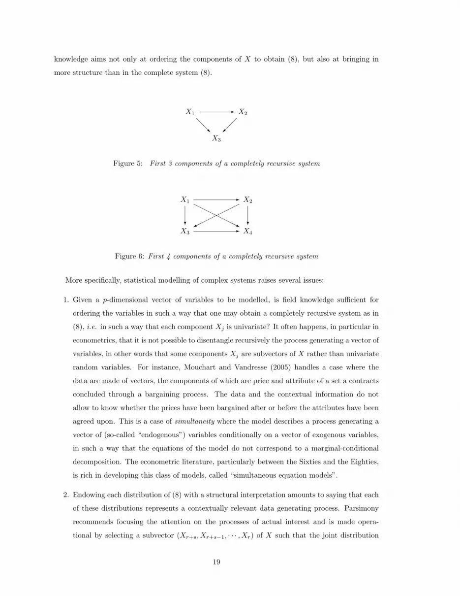
knowledge aims not only at ordering the components of X to obtain (8), but also at bringing in

more structure than in the complete system (8).

X1 X2

X3

-

@@R

Figure 5: First 3 components of a completely recursive system

X1 X2

X3 X4

-H

HHHHHHj?

?-

Figure 6: First 4 components of a completely recursive system

More specifically, statistical modelling of complex systems raises several issues:

1. Given a p-dimensional vector of variables to be modelled, is field knowledge sufficient for

ordering the variables in such a way that one may obtain a completely recursive system as in

(8), i.e. in such a way that each component Xj is univariate? It often happens, in particular in

econometrics, that it is not possible to disentangle recursively the process generating a vector of

variables, in other words that some components Xj are subvectors of X rather than univariate

random variables. For instance, Mouchart and Vandresse (2005) handles a case where the

data are made of vectors, the components of which are price and attribute of a set a contracts

concluded through a bargaining process. The data and the contextual information do not

allow to know whether the prices have been bargained after or before the attributes have been

agreed upon. This is a case of simultaneity where the model describes a process generating a

vector of (so-called “endogenous”) variables conditionally on a vector of exogenous variables,

in such a way that the equations of the model do not correspond to a marginal-conditional

decomposition. The econometric literature, particularly between the Sixties and the Eighties,

is rich in developing this class of models, called “simultaneous equation models”.

2. Endowing each distribution of (8) with a structural interpretation amounts to saying that each

of these distributions represents a contextually relevant data generating process. Parsimony

recommends focusing the attention on the processes of actual interest and is made opera-

tional by selecting a subvector (Xr+s, Xr+s−1, · · · , Xr) of X such that the joint distribution

19

of (Xr+s, Xr+s−1, · · · , Xr | X1, · · ·Xr−1) gathers all data generating processes of actual inter-

est. In such a case the subvector (X1, · · ·Xr−1) becomes globally exogenous for the system of

interest.

5 Partial observability and latent variables

5.1 A three-component system

In this paper, the concept of causality is not rooted in latent variables, as in the literature on

counterfactuals (see for instance Morgan and Winship (2007)). However, this section shows that

when latent variables are present in a structural model, causal attribution becomes substantially

more complex.

Historically, latent variables have been object of interest since at least the Forties and early Fifties,

see e.g. Reiersøl (1950), Neyman and Scott (1948, 1951). Latent variables appear in measurement

error models and in factor analytic and LISREL type models, among others. Also those models and

simultaneous equation models have been shown to be mathematically equivalent as they are all based

on the idea that mathematical expectations are required to lie in a linear space (Florens, Mouchart

and Richard (1976, 1979)). The last years have seen a voluminous amount of publications on the

large role of latent variables in statistical modelling. Thus chapter 1 of Skrondal and Rabe-Hesketh

(2004) speaks of “the omni-presence of latent variables”, and the book presents an interesting account

of methodological issues and of applications. Rabe-Hesketh, Skrondal and Pickels (2004) suggest

how to use a latent variable framework as a unifying device for a large class of models including

multilevel and structural equation models.

We begin by considering a three-variate case and next extend the analysis to a p-dimensional

vector. Consider a three-variate completely recursive system, represented in Figure 7, for data in

the form X = (Y,Z, U) :

pX(x | θ) = pY |Z,U (y | z, u, θY |Z,U ) pZ|U (z | u, θZ|U ) pU (u | θU ) (10)

where each of the three components of the right hand side may be considered as structural models

with mutually independent parameters, i.e. in a sampling theory framework:

θ = (θY |Z,U , θZ|U , θU ) ∈ ΘY |Z,U ×ΘZ|U ×ΘU (11)

This diagram suggests that U causes Z and (U,Z) cause Y . Thus, according to the definition offered

above, U is a confounding variable for the effect of Z on Y . Also, equations (10) and (11) say that

U is exogenous for θZ|U and that (U,Z) are jointly exogenous for θY |Z,U .

20

U Z

Y

-

@@R

Figure 7: 3-component completely recursive system

Now suppose that U is not observable. It might be tempting to collapse the diagram in Figure 7

into that of Figure 8. Formally, Figure 8 may be obtained by integrating the latent variable U out

of (10):

pY |Z(y | z, θY |Z) =

∫pY |Z,U (y | z, u, θY |Z,U ) pZ|U (z | u, θZ|U ) pU (u | θU ) du∫ ∫pY |Z,U (y | z, u, θY |Z,U ) pZ|U (z | u, θZ|U ) pU (u | θU ) du dy

(12)

pZ(z | θZ) =∫

pZ|U (z | u, θZ|U ) pU (u | θU ) du (13)

Z Y-

Figure 8: 2-component system

Therefore:

θY |Z = f1(θY |Z,U , θZ|U , θU ) θZ = f2(θZ|U , θU ) (14)

Two remarks are in order:

1. In general, Z is not exogenous anymore because (14) shows that the parameter θY |Z and θZ

are, in general, not independent; indeed some components of θZ|U and of θU may be common

to θY |Z and θZ . Therefore, Figure 8 is an inadequate simplification of Figure 7 (see however

next remark);

2. the non-observability of U typically implies a loss of identification: the functions f1 and f2

are not one-to-one; thus Z might still be exogenous because potentially common parameters

in θY |Z and θZ might not be identified;

One might also look for further conditions deemed to recover the exogeneity of Z. A simplifying

assumption frequently used is the sampling independence between Z and U :

Z⊥⊥U | θ (15)

This assumption implies that θZ|U is now written as θZ and Figure 7 becomes Figure 9 suggesting

that U and Z both cause Y (without U causing Z).

Under condition (15), when U is not observable Figure 8 is again obtained under the following

integration of U :

21

U Z

Y

@@R

Figure 9: 3-component completely recursive system with marginal independence

pY |Z(y | z, θY |Z) =∫

pY |Z,U (y | z, u, θY |Z,U ) pU (u | θU ) du (16)

Therefore:

θY |Z = f3(θY |Z,U , θU ) (17)

is independent of θZ and the exogeneity between Z and θY |Z may be recovered. In particular, under

condition (15 ), U is not a common cause of Z and Y anymore, but, from (17), meaning of θY |Z

comes from a combination of the causal action of U along with that of Z, represented by θY |Z,U ,

and of the distribution of U , represented by θU .

An example may be useful to better grasp some difficulties. Suppose, for simplifying the argu-

ment, that the joint distribution of X in (10) is multivariate normal; thus the regression functions

are linear and the conditional variances are homoscedastic, i.e. they do not depend on the value of

the conditioning variables. Let us compare the following two regression functions:

IE [Y | Z,U, θY |Z,U ] = α0 + Zα1 + Uα2 (18)

α1 = [cov(Y, Z | U)][V (Z | U)]−1

= [cov(Y, Z) − cov(Y,U)[V (U)]−1cov(U,Z)]

×[V (Z) − cov(Z,U)[V (U)]−1cov(U,Z)]−1 (19)

IE [Y | Z, θY |Z ] = β0 + Zβ1 β1 = [cov(Y,Z)][V (Z)]−1 (20)

Therefore, if the effect on Y of the cause Z is measured by the regression coefficient, the correct

measure would be α1 rather than β1, once the conditional model generating (Y | Z,U) is structural.

Note that, in this particular case, α1 = β1 when Z⊥⊥U , but this is a particular feature of the normal

distribution for which Z⊥⊥U implies that cov(Y, Z | U) = cov(Y, Z), and cov(Y, U | Z) = cov(Y, U),

which is in general not true. Moreover, α1 = β1 is also true when α2 = 0, i.e. when Y⊥⊥U | Z,

which is contextually different from Z⊥⊥U .

This example makes two issues explicit:

(i) measuring the effect of a cause should be operated relatively to a completely specified

structural model; failing to properly recognize this issue may lead to fallacious conclusions

because in general: α1 6= β1

22

(ii) prima facie ancillary specifications, such as a normality assumption, may be more restrictive

than first thought; indeed, under a normality assumption, the hypotheses U⊥⊥Z and Y⊥⊥U | Z

each imply that α1 = β1, although they are contextually different once the normality assump-

tion is not retained. This happens because, in the normal case, independence is equivalent to

uncorrelatedness, and because the regression functions are linear.

5.2 The general case

A difficult issue in structural modelling is bound to the fact that many theories in the social sciences

involve latent or nonobservable variables. These are introduced in order to help structuring a

theoretical framework; think, for instance, of the concept of “anomy” in sociology or of “permanent

income” in economy. In such a case, the initial model includes both latent and manifest or observable

variables, from which a statistical model is obtained by integrating out all the latent variables.

A typical benefit of such an approach is to obtain a statistical model with more structure, i.e.

more restrictions, than a “saturated” statistical model constructed independently of a structural

approach. A well-known case is provided by the LISREL type model, or covariance structure model.

However this structural approach has also a cost, sometimes difficult to handle. Indeed, the analysis

performed around the simplest case of one unobservable variable along with two observable variables,

given through equation (12) and (13), suggests that the analysis of exogeneity at the level of the

statistical model bearing on the manifest variables only soon becomes intractable, jeopardizing most

exogeneity properties and making the interpretation of the identifiable parameters difficult.

6 Discussion and conclusion

Philosophers have wandered for long time in search of the ultimate concept of causality, i.e. in

search of what causality in fact is. Hume (1748), unable to find what gives logical necessity to causal

relations, came to the conclusion that causality is nothing more than a regular succession of events

deemed to be causal only thanks to our psychological habit to experience such regular sequences.

In his System of Logic, John Stuart Mill, as early as 1843, put forward an experimentalist notion of

cause. Causes are physical, i.e. one physical fact is said to be the cause of another. In the System of

Logic the experimental approach is seen as the privileged way for ascertaining what phenomena are

related to each other as causes and effects. We have, says Mill, to follow the Baconian rule of varying

the circumstances, and for this purpose we may have recourse to observation and experiment. Mill

believed that his four methods - Method of Agreement, Method of Difference, Method of Residues,

and Method of Concomitant Variation - were particularly well suited to natural science contexts but

not at all to social sciences. The inapplicability of the experimental method to the social sciences

ruled them out straight away from the realm of the sciences and still nowadays leads to a skeptical

23

despair about the very possibility of establishing causal relations in social contexts.

Causal analysis has indeed proved to be a challenging enterprise in the social sciences. There

are at least two difficulties in establishing causal relations. A first difficulty is, as just mentioned,

that a pure randomized experimentation is rarely possible. A second one, already discussed in the

Introduction, is that society and individuals are too mutable to generate “laws of social physics”

a la Quetelet. However, is this reason enough to give up causal analysis? Should we then content

ourselves with Humean regular successions?

Interestingly enough, Durkheim (1895, ch VI) strongly argued against the Millian attempt to

dismiss social sciences as sciences and therefore against any attempt to dismiss causal analysis. In

particular, he maintained that the method of concomitant variation is fruitfully used in sociology

and indeed this is what makes sociology scientific. Although an explicit causalist perspective has

been adopted by the forefathers of quantitative causal analysis, in more recent times practising

scientists have, mistakenly, hardly ever taken a clear stance in this respect. As we have suggested in

the opening of this paper, a cognitive goal and an action-oriented goal justify our effort in making

causality an empirical and testable, i.e. scientific, matter.

We have argued that structural modelling tries to make causality meaningful and operational

and we have seen that this objective can be achieved if two fundamental ingredients are incorpo-

rated. The first one is an epistemological element - viz. the rationale of variation, and the second

is a methodological element - viz. the concept of structural model. Structural modelling aims at

uncovering a structure underlying the actual data generating process. Clearly there is an infinity

of conceivable structural models leading to a same statistical model “explaining” the data under

scrutiny. A main issue for the model builder is selecting one of those structures, taking into ac-

count the knowledge of the field and desirable properties of invariance/stability. Thus the practical

implication of this paper is twofold. Firstly, causation may be attributed only within a structural

model reflecting the state of knowledge of the domain considered. Secondly, the structural stabil-

ity of the relationships and of the parameters of the distributions should be thoroughly checked.

This approach is therefore at variance with purely statistical ones where causation is supposedly

tested from correlations without making explicit a suitable structural model. Furthermore, causa-

tion should not be attributed from a model only based on purely theoretical considerations. Finally,

the search for agreement with background knowledge and for structural stability leaves a lesser role

to the goodness of fit.

However, although the development of a more adequate rationale of causality and of an accurate

concept of structural model give a meaningful framework for causal analysis, we claimed that specific

issues still needed to be addressed, e.g. exogeneity and confounding. In this causal framework, the

concepts of exogeneity and of confounding have been explicitly defined. On the one hand, exogeneity

is a condition of separability of inference that allows us to concentrate on the conditional distribution

24

leaving aside the marginal one. On the other hand, we have adopted a definition of confounders as

common ancestors of both cause and effect. However, we have shown that the impact of confounders

complicates substantially the analysis and the operational interpretation of exogeneity, because a

variable may lose its exogenous status under the impact of a latent confounder. Furthermore, if a

latent variable U is a determinant of an outcome Y but is independent of another cause Z of this

outcome, Z remains exogenous but, at the level of the manifest variables, the measure of the effect of

Z on Y depends upon the original causal effect of Z and upon the distribution of the latent variable

U .

Let us now give some general conclusions. In the framework of structural modelling what is

the meaning of the claim X causes Y ? Not metaphysical: by means of structural modelling we do

not pretend to attain the ontic level and to discover the true and ultimate causes. If causal claims

cease to have metaphysical meaning, then they must have an epistemic one: we have reasons to

believe that X causes Y . Causality thus becomes a matter of knowledge generated by the sensible

use of structural modelling. A major task of epistemology and methodology is then to make explicit

the conditions under which our causal beliefs are justified and to inform us correctly about causal

relations in the world. The net advantage of spousing an epistemic view is to avoid committing to

the discovery of the “true” causes or of the “true” model. Instead, causal beliefs are part of our

knowledge of the world, and thus are naturally subject to change and improvement.

Acknowledgments The research underlying this paper is part of a research project conducted

by the three authors on Causality and Statistical Modelling in the Social Sciences. Parts of this

paper have been prepared for the workshop Causality, Exogeneity and Explanation, Causality Study

Circle - Evidence Project, UCL, London, May 5, 2006, and for the conference Causal Analysis in

Population Studies: Concepts, Methods and Applications held in Vienna November 30 - December

1, 2007, at the Vienna Institute of Demography, Austrian Academy of Sciences. Financial support

to M.Mouchart from the IAP research network nr P5/24 of the Belgian State (Federal Office for

Scientific, Technical and Cultural Affairs) is gratefully acknowledged. F. Russo wishes to thank

the FSR (Fonds Special de Recherche, Universite catholique de Louvain), the British Academy,

and the FNRS (Belgian National Science Foundation) for financial support. G. Wunsch thanks the

Austrian Academy of Sciences for financial assistance. Comments from an anonymous referee are

also gratefully acknowledged.

25

References

Anderson S., Auquier A., Hauck W.W. , Oakes D., Vandaele W., and Weisberg H.I.

(1980), Statistical Methods for Comparative Studies, Wiley, New York.

Barndorff-Nielsen O. (1978), Information and Exponential Families in Statistical Theory, New

York: John Wiley.

Bollen K.A. (1989), Structural Equations with Latent Variables, New York: John Wiley & Sons.

de Finetti B. (1937), La prevision, ses lois logiques, ses sources subjectives, Annales de l’Institut

Henri Poincare, 7, 1-68.

Durkheim E. (1895 - 1912), Les regles de la methode sociologique, Libraire Felix Arcan, Paris,

6th edition.

Durkheim E. (1897 - 1960), Le suicide, Presses Universitaires de France, Paris.

Elwood J.M. (1988), Causal Relationships in Medicine, Oxford University Press, Oxford.

Engle R.F., Hendry D.F. and Richard J.-F. (1983), Exogeneity, Econometrica, 51(2), 277-

304.

Florens J.-P. and Mouchart M. (1985) Conditioning in dynamic models, Journal of Time

Series Analysis, 53 (1), 15-35.

Florens J.-P., Mouchart M. and Richard J.-F. (1976), Likelihood analysis of linear models,

CORE Discussion Paper 7619, Universite catholique de Louvain, Belgium.

Florens J.-P., Mouchart M. and Richard J.-F. (1979), Specification and inference in linear

models, CORE Discussion Paper 7943, Universite catholique de Louvain, Belgium.

Florens J.-P., Mouchart M. and Rolin J.-M. (1990), Elements of Bayesian Statistics, New

York: Marcel Dekker.

Hendry D.F. and Richard J.-F. (1983), The econometric analysis of economic time series,

International Statistical Review, 51, 111-163.

Hume D. (1748), An Enquiry Concerning Human Understanding, Bobbs-Merrill, Indianapolis,

1955.

Jenicek M. and Cleroux R. (1982), Epidemiologie, Maloine, Paris.

Leridon H. and Toulemon L. (1997), Demographie. Approche statistique et dynamique des

populations, Economica, Paris.

26

McNamee R. (2003). Confounding and confounders, Occupational and Environmental Medicine,

60(3), 227-234.

Mill J.S. (1843), A system of logic, Longmans, Green and Co., London, 1889.

Morgan S.L. and C. Winship (2007). Counterfactuals and causal inference, Cambridge Univer-

sity Press, New York.

Mouchart M. and A. Oulhaj (2000), On Identification in Conditional Models, Discussion

paper DP0015, Institut de statistique, UCL, Louvain-la-Neuve (B).

Mouchart M. and Vandresse M. (2007), Bargaining Power and Market Segmentation in Freight

Transport, to appear in Journal of Applied Econometrics, 22.

Neyman J. and Scott E., (1948), Consistent estimates based on partially consistent observations,

Econometrica, 16, 1-2.

Neyman J. and Scott E. (1951), On certain methods of estimating the linear structural rela-

tionship, The Annals of Mathematical Statistics, 22, 352-361. (Corrections: 23 (1952), 135.)

Oulhaj A. and M. Mouchart (2003), The Role of the Exogenous Randomness in the Identifi-

cation of Conditional Models, Metron, LXI, 2, 267-283.

Pearl J. (2000), Causality, Cambridge University Press, Cambridge.

Popper K. (1959), The Logic of Scientific Discovery, Hutchinson, London.

Quetelet A. (1869), Physique sociale. Ou Essai sur le developpement des facultes de l’homme,

Muquardt, Bruxelles.

Rabe-Hesketh S., Skrondal A., Pickels A.(2004), Generalized multilevel structural equation

modeling, Psychometrika, 69, 167-190.

Reirsøl O. (1950), Identifiability of a linear relation between variables which are subject to error,

Econometrica, 18, 375-389.

Russo F. (2005), Measuring variations. An epistemological account of causality and causal mod-

elling, Ph.D Thesis, Universite catholique de Louvain, Belgium.

Russo F. (2007), The rationale of variation in methodological and evidential pluralism, Philosoph-

ica, in press.

Russo F., M. Mouchart, M. Ghins and G. Wunsch (2006), Statistical Modelling and Causal-

ity in Social Sciences, Discussion Paper 0601, Institut de Statistique, Universite catholique de

Louvain.

27

Savage L.J. (1954), The Foundations of Statistics, John Wiley, New York.

Schlesselman J.J. (1982), Case-Control Studies - Design, Conduct, Analysis, Oxford University

Press, New York.

Skrondal A. and Rabe-Hesketh S. (2004), Generalized Latent Variable Modeling: Multilevel,

Longitudinal, and Structural Equation Modeling, Chapman & Hall/CRC, Boca Raton, FL.

Suppes P. (1970), A Probabilistic Theory of Causality, Amsterdam: North Holland Publishing

Company.

Thomas, R. L.(1996), Modern Econometrics, Harlow, Addison-Wesley, 535 p.

Wright S. (1934), The Method of Path Coefficients, Annals of Mathematical Statistics, 5(3), pp.

161-215.

Williamson J. (2005), Bayesian nets and causality, Oxford University Press, Oxford.

Wunsch G. (2007), Confounding and Control, Demographic Research, 16, pp. 15-35.

28