Statistics, Causality and Bell’s Theorem

Submitted to the Statistical Science

Statistics, Causality and Bell’sTheoremRichard D. Gill

Mathematical Institute, University of Leiden, Netherlands

Abstract. Bell’s (1964) theorem is popularly supposed to establish the non-locality of quantum physics. Violation of Bell’s inequality in experimentssuch as that of Aspect et al. (1982) then provides empirical proof of non-locality in the real world. This paper reviews recent work on Bell’s theorem,linking it to issues in causality as understood by statisticians. The paperstarts with a simple proof of a finite sample version of Bell’s theorem, whichstates that quantum theory is incompatible with the conjunction of threeuncontroversial physical principles, called locality, realism, and freedom.Locality is the principle that causal influences need time to propagate spa-tially. Realism and freedom are also part of statistical thinking on causality:they relate to counterfactual reasoning, and to the distinction between se-lecting on X = x and do-ing X = x, respectively. The paper arguesthat Bell’s theorem (and its experimental confirmation) should lead us torelinquish not locality, but realism, as a universal physical principle. Exper-imental loopholes in state-of-the-art Bell type experiments are related tostatistical issues of post-selection in observational studies. Methodologicaland statistical issues in the design of quantum Randi challenges (QRC) arediscussed. The QRC is a public computer experiment testing a simulationof a local hidden variables theory alleged to contradict Bell’s theorem.

AMS 2000 subject classifications: Primary 62P35, ; secondary 62K99.Key words and phrases: counterfactuals, Bell inequality, CHSH inequality,Tsirelson inequality, Bell’s theorem, Bell experiment, Bell test loophole,non-locality, local hidden variables, quantum Randi challenge.

1. INTRODUCTION

In this paper I want to discuss Bell’s (1964) theorem from the point of view ofcausality as understood in statistics and probability.

Bell’s theorem states that certain predictions of quantum mechanics are incom-patible with the conjunction of three fundamental principles of classical physicswhich are sometimes given the short names “realism”, “locality” and “freedom”.Corresponding real world experiments, Bell experiments, are supposed to demon-strate that this incompatibility is a property not just of the the theory of quantummechanics, but also of Nature itself. The consequence is that we are forced to re-ject at least one of these three principles.

http: // www. math. leidenuniv. nl/ ~ gill (e-mail: [email protected])

1imsart-sts ver. 2012/04/10 file: gill-causality-rev.tex date: August 19, 2013

http://www.imstat.org/sts/

http://www.math.leidenuniv.nl/~gill

mailto:[email protected]

2 R.D. GILL

Both theorem and experiment hinge around an inequality constraining proba-bility distributions of outcomes of measurements on spatially separated physicalsystems; an inequality which must hold if all three fundamental principles aretrue. In a nutshell, the inequality is an empirically verifiable consequence of theidea that the outcome of one measurement on one system cannot depend on whichmeasurement is performed on the other. This idea, called locality or, more pre-cisely, relativistic local causality, is just one of the three principles. Its formulationrefers to outcomes of measurements which are not actually performed, so we haveto assume their existence, alongside of the outcomes of those actually performed:the principle of realism, or more precisely, counterfactual definiteness. Finally weneed to assume that we have complete freedom to choose which of several mea-surements to perform – this is the third principle, also called the no-conspiracyprinciple or no super-determinism.

We shall implement the freedom assumption as the assumption of statisticalindependence between the randomisation in a randomised experimental design,and the outcomes of all the possible experiments combined. This includes the“counterfactual” outcomes of those experiments which were not actually per-formed, as well as the “factual” outcome of the experiment actually chosen. Byexistence of the outcomes of not actually performed experiments, we only meantheir mathematical existence within some mathematical-physical theory of thephenomenon in question. The concepts of realism and locality together are oftenconsidered as one principle called local realism. Local realism is implied by the ex-istence of local hidden variables, whether deterministic or stochastic. In a precisemathematical sense, the reverse implication is also true: local realism implies thatwe can construct a local hidden variable (LHV) model for the phenomenon understudy. However one likes to think of this assumption (or pair of assumptions),the important thing to realize is that it is a completely unproblematic feature ofall classical physical theories; freedom (no conspiracy) even more so.

The connection between Bell’s theorem and statistical notions of causality hasbeen noted many times in the past. For instance, in a short note Robins, Vander-Weele, and Gill (2011) derive Bell’s inequality using the statistical language ofcausal interactions. The reader familiar with graphical models is invited to drawthe causal graph of observed and unobserved variables corresponding to a clas-sical causal picture of what could be happening in one run of that experiment.Assuming this causal model places restrictions on the joint distribution of theobserved variables, see for instance Ver Steeg and Galstyan (2011).

In view of the experimental support for violation of Bell’s inequality, thepresent writer prefers to imagine a world in which “realism” is not a fundamen-tal principle of physics but only an emergent property in the familiar realm ofdaily life. In this way we can keep quantum mechanics, locality and freedom. Thisposition does entail taking quantum randomness very seriously: it becomes an ir-reducible feature of the physical world, a “primitive notion”; it is not “merely” anemergent feature. He believes that within this position, the measurement problem(Schrodinger cat problem) has a decent mathematical solution, in which causalityis the guiding principle (Slava Belavkin’s “eventum mechanics”).

imsart-sts ver. 2012/04/10 file: gill-causality-rev.tex date: August 19, 2013

STATISTICS, CAUSALITY AND BELL’S THEOREM 3

2. BELL’S INEQUALITY

To begin with I will establish a new version of the famous Bell inequality(more precisely: Bell-CHSH inequality). My version is not an inequality abouttheoretical expectation values, but is a probabilistic inequality about experimen-tally observed averages. Probability derives purely from randomisation in theexperimental design.

Consider a spreadsheet containing an N × 4 table of numbers ±1. The rowswill be labelled by an index j = 1, . . . , N . The columns are labelled with namesA, A′, B and B′. I will denote the four numbers in the jth row of the table byAj , A

′j , Bj and B′j . Denote by 〈AB〉 = (1/N)

∑Nj=1AjBj , the average over the

N rows of the product of the elements in the A and B columns. Define 〈AB′〉,〈A′B〉, 〈A′B′〉 similarly.

Suppose that for each row of the spreadsheet, two fair coins are tossed indepen-dently of one another, independently over all the rows. Suppose that dependingon the outcomes of the two coins, we either get to see the value of A or A′, andeither the value of B or B′. We can therefore determine the value of just one ofthe four products AB, AB′, A′B, and A′B′, each with equal probability 1

4 , foreach row of the table. Denote by 〈AB〉obs the average of the observed products ofA and B (“undefined” if the sample size is zero). Define 〈AB′〉obs, 〈A

′B〉obs and〈A′B′〉obs similarly.

Fact 1 For any four numbers A, A′, B, B′ each equal to ±1,

AB +AB′ +A′B −A′B′ = ± 2. (1)

Proof. Notice that

AB +AB′ +A′B −A′B′ = A(B +B′) +A′(B −B′).

B andB′ are either equal to one another or unequal. In the former case,B−B′ = 0and B + B′ = ±2; in the latter case B − B′ = ±2 and B + B′ = 0. ThusAB + AB′ + A′B − A′B′ equals either A or A′, both of which equal ±1, times±2. All possibilities lead to AB +AB′ +A′B −A′B′ = ±2. �

Fact 2〈AB〉+ 〈AB′〉+ 〈A′B〉 − 〈A′B′〉 ≤ 2. (2)

Proof. By (1),

〈AB〉+ 〈AB′〉+ 〈A′B〉 − 〈A′B′〉

= 〈AB +AB′ +A′B −A′B′〉 ∈ [−2, 2]. �

Formula (2) is known as the CHSH inequality (Clauser, Horne, Shimony andHolt, 1969). It is a generalisation of the original Bell (1964) inequality.

When N is large one would expect 〈AB〉obs to be close to 〈AB〉, and the samefor the other three averages of observed products. Hence, equation (2) shouldremain approximately true when we replace the averages of the four productsover all N rows with the averages of the four products in each of four disjoint sub-samples of expected size N/4 each. The following theorem expresses this intuitionin a precise and useful way. Its straightforward proof, given in the appendix, usestwo Hoeffding (1963) inequalites (exponential bounds on the tail of binomial andhypergeometric distributions) to probabilistically bound the difference between〈AB〉obs and 〈AB〉, etc.


4 R.D. GILL

Theorem 1 Given an N × 4 spreadsheet of numbers ±1 with columns A, A′, Band B′, suppose that, completely at random, just one of A and A′ is observed andjust one of B and B′ are observed in every row. Then, for any η ≥ 0,

Pr(〈AB〉obs+ 〈AB

′〉obs+ 〈A′B〉obs−〈A

′B′〉obs ≤ 2 + η)≥ 1− 8e−N(

η16)2 . (3)

Traditional presentations of Bell’s theorem derive the large N limit of this result.If for N → ∞, experimental averages converge to theoretical mean values, thenby (3) these must satisfy

〈AB〉lim + 〈AB′〉lim + 〈A′B〉lim − 〈A′B′〉lim ≤ 2. (4)

Like (2), this inequality is also called the CHSH inequality.I conclude this section with an open problem. An analysis by Vongehr (2013) of

the original Bell inequality, which is “just” the CHSH inequality in the situationthat one of the four correlations is identically equal to ±1, suggests that thefollowing conjecture might be true. I come back to this in the last section of thepaper.

Conjecture 1 Under the assumptions of Theorem 1,

Pr(〈AB〉obs + 〈AB′〉obs + 〈A′B〉obs − 〈A

′B′〉obs > 2)≤

1

2. (5)

3. BELL’S THEOREM

Both the original Bell inequality, and Bell-CHSH inequality (4), can be usedto prove Bell’s theorem: quantum mechanics is incompatible with the principlesof realism, locality and freedom. If we want to hold on to all three principles,quantum mechanics must be rejected. Alternatively, if we want to hold on toquantum theory, we have to relinquish at least one of those three principles.

An executive summary of the proof of Bell’s theorem consists of the followingremark: certain models in quantum physics predict

〈AB〉lim + 〈AB′〉lim + 〈A′B〉lim − 〈A′B′〉lim = 2

√2. (6)

Almost no-one is prepared to abandon freedom. It seems to be a matter offashion, which changes over the years, whether one blames locality or realism. Iwill argue that we must place the blame on realism, and not in the weak sense ofthe Copenhagen interpretation which forbids one to speak of “what is actuallygoing on behind the scenes”, but in the positive sense: the positive assertion thatthere is nothing going on behind the scenes. What is going on is up-front intrinsic,non-classical, irreducible quantum randomness.

For present purposes we do not need to understand any of the quantum me-chanics behind (6): we just need to know the specific statistical predictions whichfollow from a particular model in quantum physics called the EPR-B model. Theinitials refer here to the celebrated paradox of Einstein, Podolsky and Rosen(1935) in a version introduced by David Bohm (1951), and the EPR-B model isa model which predicts the statistics of the measurement of spin on an entangledpair of spin-half quantum systems in the singlet state.

In one run of this stylised experiment, two particles are generated togetherat a source, and then travel to two distant locations. Here, they are measured



by two experimenters Alice and Bob. Alice and Bob are each in possession of ameasurement apparatus which can “measure the spin of a particle in any chosendirection”. Alice (and similarly, Bob) can freely choose (and set) a setting on hermeasurement apparatus. Alice’s setting is an arbitrary direction in real three-dimensional space represented by a unit vector ~a. Her apparatus will then registeran observed outcome ±1 which is called the observed spin of Alice’s particle indirection ~a. At the same time, far away, Bob chooses a direction ~b and also gets toobserve an outcome ±1. This is repeated many times – the complete experimentwill consist of a total of N runs. We’ll imagine Alice and Bob repeatedly choosingnew settings for each new run, in the same fashion as in Section 2: each tossinga fair coin to make a binary choice between just two possible settings, ~a and ~a′

for Alice, ~b and ~b′ for Bob.First we will complete our description of the quantum mechanical predictions

for each run separately. For a pairs of particles in the singlet state, the predictionof quantum mechanics is that in whatever directions Alice and Bob performtheir measurements, their outcomes ±1 are perfectly random (i.e., equally likely+1 as −1). However, there is a correlation between the outcomes of the twomeasurements at the two locations, depending on the two settings. In fact, theexpected value of the product of the outcomes is given by −~a ·~b = − cos(θ) whereθ is the angle between the two directions.

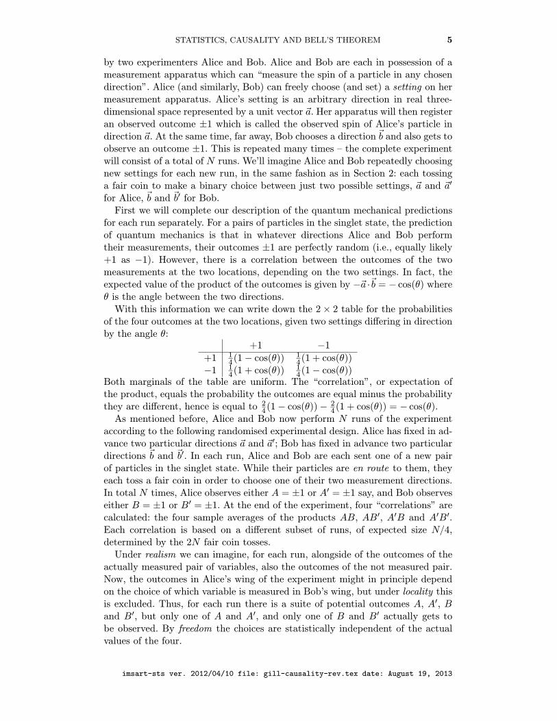
With this information we can write down the 2× 2 table for the probabilitiesof the four outcomes at the two locations, given two settings differing in directionby the angle θ:

+1 −1

+1 14(1− cos(θ)) 1

4(1 + cos(θ))−1 1

4(1 + cos(θ)) 14(1− cos(θ))

Both marginals of the table are uniform. The “correlation”, or expectation ofthe product, equals the probability the outcomes are equal minus the probabilitythey are different, hence is equal to 24(1− cos(θ))− 24(1 + cos(θ)) = − cos(θ).

As mentioned before, Alice and Bob now perform N runs of the experimentaccording to the following randomised experimental design. Alice has fixed in ad-vance two particular directions ~a and ~a′; Bob has fixed in advance two particulardirections ~b and ~b′. In each run, Alice and Bob are each sent one of a new pairof particles in the singlet state. While their particles are en route to them, theyeach toss a fair coin in order to choose one of their two measurement directions.In total N times, Alice observes either A = ±1 or A′ = ±1 say, and Bob observeseither B = ±1 or B′ = ±1. At the end of the experiment, four “correlations” arecalculated: the four sample averages of the products AB, AB′, A′B and A′B′.Each correlation is based on a different subset of runs, of expected size N/4,determined by the 2N fair coin tosses.

Under realism we can imagine, for each run, alongside of the outcomes of theactually measured pair of variables, also the outcomes of the not measured pair.Now, the outcomes in Alice’s wing of the experiment might in principle dependon the choice of which variable is measured in Bob’s wing, but under locality thisis excluded. Thus, for each run there is a suite of potential outcomes A, A′, Band B′, but only one of A and A′, and only one of B and B′ actually gets tobe observed. By freedom the choices are statistically independent of the actualvalues of the four.


6 R.D. GILL

I’ll assume furthermore that the suite of counterfactual outcomes in the jthrun does not actually depend on which particular variables were observed inprevious runs. This memoryless assumption can be completely avoided by usingthe martingale version of Hoeffding’s inequality, Gill (2003). But the presentanalysis is already applicable if we imagine N copies of the experiment each withonly a single run, all being done simultaneously in different laboratories.

The assumptions of realism, locality and freedom have put us firmly in thesituation of the previous section. Therefore by Theorem 1, the four sample cor-relations (empirical raw product moments) satisfy (3).

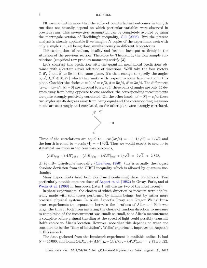
Let’s contrast this prediction with the quantum mechanical predictions ob-tained with a certain clever selection of directions. We’ll take the four vectors~a, ~a′, ~b and ~b′ to lie in the same plane. It’s then enough to specify the anglesα, α′, β, β′ ∈ [0, 2π] which they make with respect to some fixed vector in thisplane. Consider the choice α = 0, α′ = π/2, β = 5π/4, β′ = 3π/4. The differences|α−β|, |α−β′|, |α′−β| are all equal to π±π/4: these pairs of angles are only 45 de-grees away from being opposite to one another; the corresponding measurementsare quite strongly positively correlated. On the other hand, |α′−β′| = π/4: thesetwo angles are 45 degrees away from being equal and the corresponding measure-ments are as strongly anti-correlated, as the other pairs were strongly correlated.

α

α′β′

β

Three of the correlations are equal to − cos(3π/4) = −(−1/√

2) = 1/√

2 andthe fourth is equal to − cos(π/4) = −1/

√2. Thus we would expect to see, up to

statistical variation in the coin toss outcomes,

〈AB〉obs + 〈AB′〉obs + 〈A′B〉obs − 〈A′B′〉obs ≈ 4/

√2 = 2

√2 ≈ 2.828,

cf. (6). By Tsirelson’s inequality (Cirel’son, 1980), this is actually the largestabsolute deviation from the CHSH inequality which is allowed by quantum me-chanics.

Many experiments have been performed confirming these predictions. Twoparticularly notable ones are those of Aspect et al. (1982) in Orsay, Paris, and ofWeihs et al. (1998) in Innsbruck (later I will discuss two of the most recent).

In these experiments, the choices of which direction to measure were not lit-erally made with coin tosses performed by human beings, but by rather morepractical physical systems. In Alain Aspect’s Orsay and Gregor Weihs’ Inns-bruck experiments the separation between the locations of Alice and Bob waslarge; the time it took from initiating the choice of random direction to measureto completion of the measurement was small: so small, that Alice’s measurementis complete before a signal traveling at the speed of light could possibly transmitBob’s choice to Alice’s location. However, note that this depends on what oneconsiders to be the “time of initiation”. Weihs’ experiment improves on Aspect’sin this respect.

The data gathered from the Innsbruck experiment is available online. It hadN ≈ 15 000; and found 〈AB〉obs+〈AB

′〉obs+〈A′B〉obs−〈A

′B′〉obs = 2.73±0.022,



the statistical accuracy (standard deviation) following from a standard delta-method calculation assuming i.i.d. observations per setting pair. The reader cancheck that this corresponds to accuracy obtained by a standard computation usingbinomial variances of the counts for each of the four roughly equal subsamples.By (3), under realism, locality and freedom, the chance that 〈AB〉obs+〈AB

′〉obs+〈A′B〉obs − 〈A

′B′〉obs would exceed 2.73 is less than 10−12.The experiment deviates in several ways from what has been described so far,

and I will summarise them here. An unimportant feature is the physical systemused: polarisation of entangled photons rather than spin of entangled spin-halfparticles (e.g., electrons).

An important difference between the idealisation and the truth concerns theidea that picture of Alice and Bob repeating some actions N times with N fixed inadvance. The experimenters do not control when a pair of photons will leave thesource nor how many times this happens. Even talking about “pairs of photons” isusing classical physical language which can be acutely misleading. In actual fact,all we observe are individual detection events (time, current setting, outcome) ateach of the two detectors, i.e., at each measurement apparatus.

Complicating this still further is the fact that many particles fail to be detectedat all. One could say that the outcome of measuring one particle is not binary butternary: +, −, or no detection. If neither particle of a pair is detected, then we donot even know there is a pair at all. N was not only not fixed in advance: it is noteven known. The data cannot be summarised in a list of pairs of settings and pairsof outcomes (whether binary of ternary), but consists of two lists of the randomtimes of definite measurement outcomes in each wing of the experiment togetherwith the settings in force at the time of the measurements. The settings are beingextremely rapidly, randomly switched, between the two alternative values. Whendetection events occur close together in time they are treated as belonging to apair of photons.

In Weihs’ experiment, only about one in twenty of the events in each wingof the experiment are paired with an event in the other. It would appear thatof every 400 pairs of photons, one pair leads to a paired event, 2 × 19 lead tounpaired events, and the remaining 361 to no observed event at all.

We will return to the issue of whether the idealized picture N pairs of particles,each separately being measured, each particle in just one of two ways, is reallyappropriate, in a later section; we will also take a look then at two more, veryrecent, experiments. However, the point is that quantum mechanics does seemto promise that experiments of this nature could in principle be done, and if so,there seems no reason to doubt they could violate the CHSH inequality. Threecorrelations more or less equal to 1/

√2 and one equal to −1/

√2 have been

measured in the lab. Not to mention that the whole curve − cos(θ) has beenexperimentally recovered.

Right now the situation is that at least three major experimental groups (Sin-gapore, Brisbane, Vienna) seem to be vying to be the first to perform a successfuland completely “loophole free” experiment, predictions being that this is no morethan five years away (cf. Marek Zukowski, quoted in Merali, 2010). It will be amajor achievement, the crown of more than fifty years labour.


8 R.D. GILL

4. REALISM, LOCALITY, FREEDOM

This section and the next are about metaphysics and can safely be skipped bythe reader impatient to learn more about statistical aspects of Bell experiments.

The EPR-B correlations have a second message beyond the fact that theyviolate the CHSH inequality. They also exhibit perfect anti-correlation in thecase that the two directions of measurement are exactly equal – and perfectcorrelation in the case that they are exactly opposite. This brings us straight tothe EPR argument not for the non-locality of quantum mechanics, but for theincompleteness of quantum mechanics.

Einstein, Podolsky and Rosen (1935) were revolted by the idea that the “lastword” in physics would be a “merely” statistical theory. Physics should explainwhy, in each individual instance, what actually happens does happen. The beliefthat every “effect” must have a “cause” has driven Western science since Aristotle.Now according to the singlet correlations, if Alice were to measure the spin ofher particle in direction ~a, it’s certain that if Bob were to do the same, he wouldfind exactly the opposite outcome. Since it is inconceivable that Alice’s choicehas any immediate influence on the particle over at Bob’s place, it must be thatthe outcome of measuring Bob’s particle in the direction ~a is predetermined “inthe particle” as it were. The measurement outcomes from measuring spin in allconceivable directions on both particles must be predetermined properties of thoseparticles. The observed correlation is merely caused by their origin at a commonsource.

Thus Einstein used locality, together with the predictions of quantum mechan-ics itself, to infer realism, in the sense of counterfactual definiteness, the notionthat the outcomes of measurements on physical systems are predefined proper-ties of those systems, merely revealed by the act of measurement. From this heargued the incompleteness of quantum mechanics – it describes some aggregateproperties of collectives of physical systems, but does not even deign to talk aboutphysically definitely existing properties of individual systems.

Whether it needed external support or not, the notion of counterfactual def-initeness is nothing strange in all of physics (prior to the invention of quantummechanics). It belongs with a deterministic view of the world as a collectionof objects blindly obeying definite rules. Note however that the CHSH proof ofBell’s theorem does not start by inferring counterfactual definiteness from otherproperties. A wise move, since in actual experiments, we would never observeexactly perfect correlation (or anti-correlation). And even if we have observed itone thousand times, this does not prove that the “true correlation” is +1; it onlyproves, statistically, that it is very close to +1.

Be that as it may, Bell’s theorem uses three assumptions to derive the CHSHinequality, and the first is counterfactual definiteness. We must first agree that ifonly A and B are actually measured in one particular run, still A′ and B′ alsoexist alongside of the two other (in a mathematical sense, at least). Only afterthat does it make sense to discuss locality : the assumption that which variableis being observed at Alice’s location does not influence the values taken by theother two at Bob’s location.

Having assumed realism and locality we can bring the freedom assumptioninto play, but we already discuss it in advance of using it. Some writers like toassociate the freedom assumption with the free will of the experimenter, oth-



ers with the existence of “true” randomness in other physical processes: eitherway, one metaphysical assumption is justified by another. I would rather think ofthis in a practical way, and use Occam’s razor to reject the opposite of freedom,which has been variously named conspiracy, super-determinism, predetermina-tion. Do we really want to believe that the observed correlations 1/

√2, 1/

√2,

1/√

2, −1/√

2 occur through some as yet unknown physical mechanism by whichthe outcomes of Alice’s random generators are exquisitely tuned to the mea-surement outcomes of Bob’s photons? And that this delicate mechanism is onlymanifest in extremely special circumstances (involving at least two coin tossesand two photo-detectors), and at the same time is unable to generate a largerviolation of the CHSH inequality than 2

√2? Why not 4?

This means we have to make a choice between two other inconceivable possi-bilities: do we reject locality, or do we reject realism?

Here I would like to call on Occam’s principle again. Suppose realism is true.Instead of invoking the fact that a collection of four coin toss outcomes andphoto-detector clicks were jointly predetermined in the deep past, we now haveto invoke instantaneous communication across large distances of the outcomes ofthese processes, by as yet unknown processes, and again with only the extremelysubtle and special effects which quantum mechanics seems to predict.

It seems to me that we are pretty much forced into rejecting realism, which,please remember, is actually an idealistic concept: outcomes “exist” of measure-ments which were not performed. However, I admit it goes against all instinct.In the case of equal settings, how can it be that the outcomes are equal andopposite, if they were not predetermined at the source?

Though it is perhaps only a comfort blanket, I would like here to appeal to thelimitations of our own brains, the limitations we experience in our “understand-ing” of physics due to our own rather special position in the universe. Accordingto cognitive scientists (see for instance Spelke and Kinzler, 2007) our brains areat birth hardwired with various basic conceptions about the world. These “mod-ules” are called systems of core knowledge. The idea is that we cannot acquire newknowledge from our sensory experiences (including learning from experiments: wecry, and food and/or comfort is provided!) without having a prior framework inwhich to interpret the data of experience and experiment. It seems that we havemodules for elementary algebra and for analysis: basic notions of number and ofspace. We also have modules for causality. We distinguish between objects andagents (we learn that we ourselves are agents). Objects are acted on by agents.Objects have continuous existence in space time, they are local. Agents can act onobjects, also at a distance. Together this seems to me to be a built-in assumptionof determinism; we have been created (by evolution) to operate in an Aristotelianworld, a world in which every effect has a cause.

The argument (from physics, and by Occam’s razor, not from neuroscience)for abandoning realism is made eloquently by Boris Tsirelson in an internet ency-clopaedia article on entanglement (Citizendium: entanglement). It was Tsirelsonfrom whom I borrowed the terms counterfactual definiteness, relativistic localcausality, and no-conspiracy. He points out that it is a mathematical fact thatquantum physics is consistent with relativistic local causality and with no-conspiracy.In all of physics, there is no evidence against either of these two principles.

I would like to close this section by just referring to a beautiful paper by


http://en.citizendium.org/wiki/Entanglement_(physics)

10 R.D. GILL

Masanes, Acin and Gisin (2006) who argue in a very general setting (i.e., notassuming quantum theory, or local realism, or anything) that quantum non-locality, by which they mean the violation of Bell inequalities, together withnon-signalling, which is the property that the marginal probability distributionseen by Alice of A does not depend on whether Bob measures B of B′, togetherimplies indeterminism: that is to say: that the world is stochastic, not determin-istic.

5. RESOLUTION OF THE MEASUREMENT PROBLEM

The measurement problem, also known as Schrodinger’s cat problem) is theproblem of how to reconcile two apparently mutually contradictory parts of quan-tum mechanics. When a quantum system is isolated from the rest of the world, itsquantum state (a vector, normalised to have unit length, in Hilbert space) evolvesunitarily, deterministically. When we look at a quantum system from outside, bymaking a measurement on it in a laboratory, the state collapses to one of theeigenvectors of an operator corresponding to the particular measurement, and itdoes so with probabilities equal to the squared lengths of the projections of theoriginal state vector into the eigenspaces. Yet the system being measured togetherwith the measurement apparatus used to probe it form together a much largerquantum system, supposedly evolving unitarily and deterministically in time.

Accepting that quantum theory is intrinsically stochastic, and accepting thereality of measurement outcomes, led Slava Belavkin (2007) to a mathematicalframework which he called eventum mechanics which (in my opinion) indeedreconciles the two faces of quantum physics (Schrodinger evolution, von Neumanncollapse) by a most simple device. Moreover, it is based on ideas of causality withrespect to time. I have attempted to explain this model in as simple terms aspossible in Gill (2009). The following words will only make sense to those withsome familiarity with quantum mechanics.

The idea is to model the world in the conventional way with a Hilbert space,a state on that space, and a unitary evolution. Inside this framework we look fora collection of bounded operators on the Hilbert space which all commute withone another, and which are causally compatible with the unitary evolution ofthe space, in the sense that they all commute with past copies of themselves (inthe Heisenberg picture, one thinks of the quantum observables as changing, thestate as fixed; each observable corresponds to a time indexed family of boundedoperators). We call this special family of operators the beables: they correspondto physical properties in a classical-like world which can coexist, all having defi-nite values at the same time, and definite values in the past too. The state andthe unitary evolution together determine a joint probability distribution of thesetime-indexed variables, i.e., a stochastic process. At any fixed time we can condi-tion the state of the system on the past trajectories of the beables. This leads toa quantum state over all bounded operators which commute with all the beables.

The result is a theory in which the deterministic and stochastic parts of tra-ditional quantum theory are combined into one harmonious whole. In fact, thenotion of restricting attention to a subclass of all observables goes back a longway in quantum theory under the name superselection rule; and abstract quan-tum theory (and quantum field theory) has long worked with arbitrary algebrasof observables, not necessarily the full algebra of a specific Hilbert space. With



respect to those traditional approaches the only novelty is to suppose that theunitary evolution when restricted to the sub-algebra is not invertible. It is anendomorphism, not an isomorphism. There is an arrow of time.

6. LOOPHOLES

In real world experiments, the ideal experimental protocol of particles leavinga source at definite times, and being measured at distant locations according tolocally randomly chosen settings cannot be implemented.

Experiments have been done with pairs of entangled ions, separated only bya short distance. The measurement of each ion takes a relatively long time, butat least it is almost always successful. Such experiments are obviously blemishedby the so-called communication or locality loophole. Each particle can know verywell how the other one is being measured.

Many very impressive experiments have been performed with pairs of entangledphotons. Here, the measurement of each photon can be performed very rapidlyand at huge distance from one another. However, many photons fail to be detectedat all. For many events in one wing of the experiment, there is often no event atall in the other wing, even though the physicists are pretty sure that almost alldetection events do correspond to (members of) entangled pairs of photons. Thisis called the detection loophole. Popularly it is thought to be merely connectedto the efficiency of photo-detectors and that it will be easily overcome by thedevelopment of better and better photodetectors. Certainly that is necessary,but not sufficient, as I’ll explain.

In Weihs’ experiment mentioned earlier, only 1 in 20 of the events in each wingof the experiment is paired with an event in the other wing. Thus of every 400pairs of photons – if we assume that detection and non-detection occur indepen-dently of one another in the two wings of the experiment – only 1 pair resultsin a successful measurement of both the photons; there are 19 further unpairedevents in each wing of the experiment; and there were 361 pairs of photons notobserved at all.

Imagine (anthropocentrically) classical particles about to leave the source andaiming to fake the singlet correlations. If they are allowed to go undetected oftenenough, they can engineer any correlations they like, as follows. Consider twonew photons about to leave the source. They agree between one another withwhat pair of settings they would like to be measured. Having decided on thedesired setting pair, they next generate outcomes ±1 by drawing them fromthe joint probability distribution of outcomes given settings, which they wantthe experimenter to see. Only then do they each travel to their correspondingdetector. There, each particle compares the setting it had chosen in advancewith the setting chosen by Alice or Bob. If they are not the same, it decides togo undetected. With probability 1/4 we will have successful detections in bothwings of the experiment. For those detections, the pair of settings according towhich the particles are being measured is identical to the pair of settings theyhad aimed at in advance.

This example illustrates that if one wants to experimentally prove a violationof local realism without making the untestable statistical assumption of “missingat random”, known as the fair-sampling assumption in this context, one has toput limits on the amount of “non-detections”. There is a long history and big


12 R.D. GILL

literature on this topic. I will just mention one of such results.Jan-Ake Larsson (1998, 1999) has proved variants of the CHSH inequality

which take account of the possibility of non-detections. The idea is that underlocal realism, as the proportion of “missing” measurements increases from zero,the upper bound “2” in the CHSH inequality (4) increases too. We introducea quantity γ called the efficiency of the experiment : this is the minimum overall setting pairs of the probability that Alice sees an outcome given Bob sees anoutcome (and vice versa). It is not to be confused with “detector efficiency”. Itturns out that the (sharp) bound on 〈AB〉lim+〈AB′〉lim+〈A′B〉lim−〈A

′B′〉lim setby local realism is no longer 2 as in (4), but 2 + δ, where δ = δ(γ) = 4(γ−1 − 1).

As long as γ ≥ 1/√

2 ≈ 0.7071, the bound 2 + δ is smaller than 2√

2. Weihs’experiment has an efficiency of 5%. If only we could increase it to above 71%and simultaneously get the state and measurements even closer to perfection, wecould have definitive experimental proof of Bell’s theorem.

This would be correct for a “clocked” experiment. Suppose now particles de-termine themselves the times that they are measured. Thus a local realist pairof particles trying to fake the singlet correlations could arrange between them-selves that their measurement times are delayed by smaller or greater amountsdepending on whether the setting they see at the detector is the setting theywant to see, or not. It turns out that this gives our devious particles even morescope for faking correlations. Larsson and Gill (2004) showed the sharp bound on〈AB〉lim+ 〈AB′〉lim+ 〈A′B〉lim−〈A

′B′〉lim set by local realism is 2+ δ, where nowδ = δ(γ) = 6(γ−1 − 1). As long as γ ≥ 3(1− 1/

√2) ≈ 0.8787, the bound 2 + δ is

smaller than 2√

2. We need to get experimental efficiency above 88%, and haveeverything else perfect, at the very limits allowed by quantum physics.

How far is there still to go? In 2013 the Vienna group published a paper inthe journal Nature entitled “Bell violation using entangled photons without thefair-sampling assumption” (Giustina et al., 2013). The authors write “this is thevery first time that an experiment has been done using photons which does notsuffer from the detection loophole”, and moreover the experiment “makes thephoton the first physical system for which each of the main loopholes has beenclosed, albeit in different experiments.”

It was however rapidly pointed out that the experiment was actually vulner-able to the coincidence loophole, not “just” to the detection loophole. Now, itactually should be possible to simply reanalyse the data from that experiment,defining coincidences with respect to an externally defined lattice of time inter-vals instead of relative to observed detection times only. Ideally, this will onlyslightly increase the “singles rate” and slightly decrease the number of coinci-dences, thereby slightly decreasing both size and statistical significance of the Bellviolation, but hopefully without altering the substantive conclusion. Re-analysisis presently underway.

In the meantime, exploiting this gap between results and claims, a consortiumled by researchers from Illinois have published their own experimental results,also reporting that theirs is “the first experiment that fully closes the detectionloophole with photons, which are then the only system in which both loopholeshave been closed, albeit not simultaneously” (Christensen et al., 2013). They usedthe Larsson and Gill (2004) inequality.

Is this just a question of prestige? No: various new quantum technologies de-



pend on quantum entanglement, and in particular, various cryptographic com-munication protocols are not secure as long as it is possible to “fake” violationof Bell inequalities with classical systems.

7. BELL’S THEOREM WITHOUT INEQUALITIES

In recent years new proofs of Bell’s theorem have been invented which appear toavoid probability or statistics altogether, such as the famous GHZ (Greenberger,Horne, Zeilinger) proof. Experiments have already been done implementing theset-up of these proofs, and physicists have claimed that these experiments provequantum-nonlocality by the outcomes of a finite number of runs: no statistics, noinequalities (yet their papers do exhibit error bars!).

Such a proof runs along the following lines. Suppose local realism is true. Sup-pose also that some event A is certain. Suppose that it then follows from localrealism that another event B has probability zero, while under quantum mechan-ics it can be arranged that the same event B has probability one. Paradoxical,but not a contradiction in terms: the catch is that events A and B are events un-der different experimental conditions: it is only under local realism and freedomthat the events A and B can be situated in the same sample space. Moreover,freedom is needed to equate the probabilities of observable events with those ofunobservable events.

As an example, consider the following scenario, generalizing the Bell-CHSHscenario to the situation where the outcome of the measurements on the twoparticles is not binary, but an arbitrary real number. This situation has beenstudied by Zohren and Gill (2008), Zohren, Reska, Gill and Westra (2010).

Just as before, settings are chosen at random in the two wings of the experi-ment. Under local realism we can introduce variables A, A′, B and B′ representingthe outcomes (real numbers) in one run of the experiment, both of the actuallyobserved variables, and of those not observed.

It turns out that it is possible under quantum mechanics to arrange thatPr{B′ ≤ A} = Pr{A ≤ B} = Pr{B ≤ A′} = 1 while Pr{B′ ≤ A′} = 0. On theother hand, under local realism, Pr{B′ ≤ A} = Pr{A ≤ B} = Pr{B ≤ A′} = 1implies Pr{B′ ≤ A′} = 1.

Note that the four probability measures under which, under quantum mechan-ics, Pr{A ≤ B}, Pr{A ≥ B′}, Pr{A′ ≥ B}, Pr{A′ ≥ B′} are defined, refer to fourdifferent experimental set-ups, according to which of the four pairs (A,B) etc.we are measuring.

The experiment to verify these quantum mechanical predictions has not yetbeen performed though some colleagues are interested. Interestingly, though itrequires a quantum entangled state, that state should not be the maximallyentangled state. Maximal “quantum non-locality” is quite different from maximalentanglement. And this is not an isolated example of the phenomenon.

Note that even if the experiment is repeated a large number of times, it cannever prove that probabilities like Pr{A ≤ B} are exactly equal to 1. It can onlygive strong statistical evidence, at best, that the probability in question is veryclose to 1 indeed. But actually experiments are never perfect and more likelyis that after a number of repetitions, one discovers that {A > B} actually haspositive probability – that event will happen a few times. Thus though the proofof Bell’s theorem that quantum mechanics is in conflict with local realism appears


14 R.D. GILL

to have nothing to do with probability, and only to do with logic, in fact, as soonas we try to convert this into experimental proof that Nature is incompatiblewith local realism, we will be in the business of proving (statistically) violationof inequalities, again (as the next section will make clear).

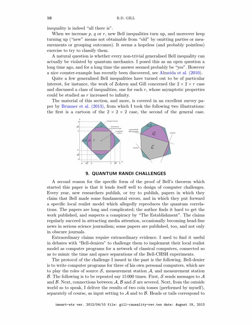
8. BETTER BELL INEQUALITIES

Why all the attention to the CHSH inequality? There are others around, aren’tthere? And are there alternatives to “inequalities” altogether? I will argue herethat the whole story is “just” a collection of inequalities, and the reason behindthis can be expressed in a simple geometric picture.

In a precise sense the CHSH inequality is the only Bell inequality worth men-tioning in the scenario of two parties, two measurements per party, two outcomesper measurement. Let’s generalise this scenario and consider p parties, each choos-ing between one of q measurements, where each measurement has r possibleoutcomes (further generalisations are possible to unbalanced experiments, multi-stage experiments, and so on). I want to explain why CHSH plays a very centralrole in the 2× 2× 2 case, and why in general, generalised Bell inequalities are allthere is when studying the p× q× r case. The short answer is: these inequalitiesare the bounding hyperplanes of a convex polytope of “everything allowed by lo-cal realism”. The vertices of the polytope are deterministic local realistic models.An arbitrary local realist model is a mixture of the models corresponding to thevertices. Such a mixture is a hidden variables model, the hidden variable being theparticular random vertex chosen by the mixing distribution in a specific instance.

From quantum mechanics, after we have fixed a joint p-partite quantum state,and sets of q r-valued measurements per party, we will be able to write downprobability tables p(a, b, ...|x, y, ...) where the variables x, y, etc. take values in1, . . . , q, and label the measurement used by the first, second, . . . party. The vari-ables a, b, etc., take values in 1, . . . , r and label the possible outcomes of themeasurements. Altogether, there are qprp “elementary probabilities” in this listof tables. More generally, any specific instance of a theory, whether local-realist,quantum mechanical, or beyond, generates such a list of probability tables, anddefines thereby a point in qprp-dimensional Euclidean space.

We can therefore envisage the sets of all local-realist models, all quantum mod-els, and so on, as subsets of qprp-dimensional Euclidean space. Now, whatever thetheory, for any values of x, y, etc., the sum of the probabilities p(a, b, . . . |x, y, . . . )must equal 1. These are called normalisation constraints. Moreover, whatever thetheory, all probabilities must be nonnegative: positivity constraints. Quantum me-chanics is certainly local in the sense that the marginal distribution of the out-come of any one of the measurements of any one of the parties does not depend onwhich measurements are performed by the other parties. Since marginalizationcorresponds again to summation of probabilities, these so-called no-signallingconstraints are expressed by linear equalities in the elements in the probabilitytables corresponding to a specific model. Not surprisingly, local-realist modelsalso satisfy the no-signalling constraints.

We will call a list of probability tables restricted only by positivity, normalisa-tion and no-signalling, but otherwise completely arbitrary, a no-signalling model.The positivity constraints are linear inequalities which place us in the positiveorthant of Euclidean space. Normalisation and no-signalling are linear equalities



which place us in a certain affine subspace of Euclidean space. Intersection oforthant and affine subspace creates a convex polytope: the set of all no-signallingmodels. We want to study the sets of local-realist models, of quantum models,and of no-signalling models. We already know that local-realist and quantum arecontained in no-signalling. It turns out that these sets are successively larger,and strictly so: quantum includes all local-realist and more (that’s Bell’s theo-rem); no-signalling includes all quantum and more (that’s Tsirelson’s inequalitycombined with an example of a no-signalling model which violates Tsirelson’sinequality).

Let’s investigate the local-realist models in more detail. A special class of local-realist models are the local-deterministic models. A local-deterministic model isa model in which all of the probabilities p(a, b, . . . |x, y, . . . ) equal 0 or 1 andthe no-signalling constraints are all satisfied. This implies that for each possiblemeasurement by each party, the outcome is prescribed, independently of whatmeasurements are made by the other parties. Now, it is easy to see that any local-realist model corresponds to a probability mixture of local-deterministic models.After all, it “is” a joint probability distribution of simultaneous outcomes of eachpossible measurement on each system, and thus it “is” a probability mixture ofdegenerate distributions: fix the random element ω, and each outcome of eachpossible measurement of each party is fixed; we recover their joint distributionby picking ω at random.

This makes the set of local-realist models a convex polytope: all mixtures of afinite set of extreme points. Therefore it can also be described as the intersectionof a finite collection of half-spaces, each half-space corresponding to a boundaryhyperplane.

It can also be shown that the set of quantum models is closed and convex, butits boundary is very difficult to describe.

Let’s think of these three models from “within” the affine subspace of no-signalling and normalisation. Relative to this subspace, the no-signalling modelsform a full (non-empty interior) closed convex polytope. The quantum modelsform a strictly smaller closed, convex, full set. The local-realist models form astrictly smaller still, closed, convex, full polytope.

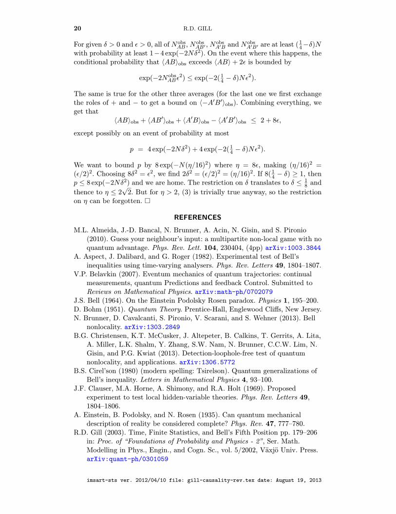
Slowly we have arrived at a rather simple picture (see figures at the end of thissection). Imagine a square, with a circle inscribed in it, and with another smallersquare inscribed within the circle. The outer square represents the boundary ofthe set of all no-signalling models. The circle is the boundary of the convex setof all quantum models. The square inscribed within the circle is the boundaryof the set of all local-realist models. The picture is oversimplified. For instance,the vertices of the local-realist polytope are also extreme points of the quantumbody and vertices of the no-signalling polytope.

A generalised Bell inequality is simply a boundary hyperplane, or face, ofthe local-realist polytope, relative to the normalisation and no-signalling affinesubspace, and excluding boundaries corresponding to the positivity constraints.I will call these interesting boundary hyperplanes “non-trivial”. In the 2× 2× 2case, for which the affine subspace where all the action lies is 8 dimensional,the local-realist polytope has exactly 8 non-trivial boundary hyperplanes. Theycorrespond exactly to all possible CHSH inequalities (obtained by permutingoutcomes, measurements and parties). Thus in the 2× 2× 2 case, the Bell-CHSH


16 R.D. GILL

inequality is indeed “all there is”.When we increase p, q or r, new Bell inequalities turn up, and moreover keep

turning up (“new” means not obtainable from “old” by omitting parties or mea-surements or grouping outcomes). It seems a hopeless (and probably pointless)exercise to try to classify them.

A natural question is whether every non-trivial generalised Bell inequality canactually be violated by quantum mechanics. I posed this as an open question along time ago, and for a long time the answer seemed probably be “yes”. Howevera nice counter-example has recently been discovered, see Almeida et al. (2010).

Quite a few generalised Bell inequalities have turned out to be of particularinterest, for instance, the work of Zohren and Gill concerned the 2 × 2 × r caseand discussed a class of inequalities, one for each r, whose asymptotic propertiescould be studied as r increased to infinity.

The material of this section, and more, is covered in an excellent survey pa-per by Brunner et al. (2013), from which I took the following two illustrations:the first is a cartoon of the 2 × 2 × 2 case, the second of the general case.

STsirelson’s bound

deterministic local-realistic model

S’

4

2

-2

-4

-4 -2 2 4

completelyrandom

22

22-

22- 22

a generalizedBell inequality

another

another

9. QUANTUM RANDI CHALLENGES

A second reason for the specific form of the proof of Bell’s theorem whichstarted this paper is that it lends itself well to design of computer challenges.Every year, new researchers publish, or try to publish, papers in which theyclaim that Bell made some fundamental errors, and in which they put forwarda specific local realist model which allegedly reproduces the quantum correla-tions. The papers are long and complicated; the author finds it hard to get thework published, and suspects a conspiracy by “The Establishment”. The claimsregularly succeed in attracting media attention, occasionally becoming head-linenews in serious science journalism; some papers are published, too, and not onlyin obscure journals.

Extraordinary claims require extraordinary evidence. I used to find it usefulin debates with “Bell-deniers” to challenge them to implement their local realistmodel as computer programs for a network of classical computers, connected soas to mimic the time and space separations of the Bell-CHSH experiments.

The protocol of the challenge I issued in the past is the following. Bell-denieris to write computer programs for three of his own personal computers, which areto play the roles of source S, measurement station A, and measurement stationB. The following is to be repeated say 15 000 times. First, S sends messages to Aand B. Next, connections between A, B and S are severed. Next, from the outsideworld so to speak, I deliver the results of two coin tosses (performed by myself),separately of course, as input setting to A and to B. Heads or tails correspond to



a request for A or A′ at A, and for B or B′ at B. The two measurement stationsA and B now each output an outcome ±1. Settings and outcomes are collectedfor later data analysis, Bell-denier’s computers are re-connected; next run.

Bell-denier’s computers can contain huge tables of random numbers, sharedbetween the three, and of course they can use pseudo-random number numbergenerators of any kind. By sharing the pseudo-random keys in advance, they haveresources to any amount of shared randomness they like.

In Gill (2003) I showed how a martingale Hoeffding inequality gives an expo-nential bound like (3) in the situation just described. This enabled me to chooseN , and a criterion for win/lose (say, halfway between 2 and 2

√2), and a guaran-

tee to Bell-denier (at least so many runs with each combination of settings), suchthat I would happily bet 3000 Euros any day that the Bell-denier’s computerswill fail the challenge.

The point (for me) was not to win money for myself, but to enable the Bell-denier who considers accepting the challenge (a personal challenge between thetwo of us, with adjudicators to enforce the protocol) to discover for him or herselfthat “it cannot be done”. It’s important that the adjudicators do not need to lookinside the programs written by the Bell-denier, and preferably don’t even need tolook inside his computers. They are black boxes. The only thing that has to beenforced are the communication rules. However, there are difficulties here. Whatif Bell-denier’s computers are using a wireless network which the adjudicatorscan’t detect?

A new kind of computer challenge, called the “quantum Randi challenge”, wasproposed in 2011 by Sascha Vongehr (Science2.0: QRC). It is inspired by the wellknown challenge to “paranormal phenomena” by James Randi (scientific scep-tic and fighter against pseudo-science, see Wikipedia: James Randi). Vongehr’schallenge (see Vongehr 2012, 2013) differs in a number of fundamental respectsfrom mine, which indeed was not a quantum Randi challenge in Vongehr’s sense.

Sascha Vongehr’s QRC completely cuts out any necessity for communication,protocol verification, adjudication. In fact, the Bell-denier no longer has to coop-erate with myself or with any other member of the establishment. They simplyhave to write a program which should perform a certain task. They post theirprogram on internet. If others find that it does indeed perform that task, thenews will spread like wildfire.

Vongehr prefers Bell’s original inequality, and I prefer CHSH, so I will herepresent an (unauthorised) “CHSH style” modification of his QRC.

Suppose someone has invented a local hidden variables theory. He can use itto simulate N = 800 runs of a CHSH experiment. Typically he will simulate thesource, the photons, the detectors, all in one program. Let us suppose that hiscomputer code produces reproducible results, which means that the code or theapplication is reasonably portable, and will give identical output when run onanother computer with the same inputs. In particular, if it makes use of a pseudorandom number generator (RNG), it must have the usual “save” and “restore”facilities for the seed of the RNG. Let’s suppose that the program calls the RNGthe same number of times for each run, and that the program does not make usein any way of memory of past measurement settings. The program must acceptany legal stream of pairs of binary measurement settings of any length N .

In particular then, the program can be run with N = 1 and all four possible


http://www.science20.com/alpha_meme/official_quantum_randi_challenge-80168

http://en.wikipedia.org/wiki/James_Randi

18 R.D. GILL

pairs of measurement settings, and the same initial random seed, and it willthereby generate successively four pairs (A,B), (A′, B), (A,B′), (A′, B′). If theprogrammer neither cheated nor made any errors, in other words, if the programis a correct implementation of a genuine LHV model, then both values of A arethe same, and so are both values of A′, both values of B, and both values of B′.We now have the first row of the N × 4 spreadsheet of Section 2 of this paper.

The random seed at the end of the previous phase is now used as the initialseed for another phase, the second run, generating a second row of the spread-sheet. This is where the prohibition of exploiting memory comes into force. Thesecond row of counterfactual outcomes has to be completed without knowingwhich particular setting pair Alice and Bob will actually pick for the first row.

Notice that the LHV model is allowed to use time, since the saved random seedscould also include the current run number and the initial random seed value, too:in other words, when doing the calculations for the nth run, the LHV model hasaccess to everything it did in the previous n− 1 runs.

My claim is that a correct implementation of a bona-fide LHV model whichdoes not exploit the memory loophole can be used to fill in theN×4 spreadsheet ofSection 2. When we now generate random settings and calculate the correlations,we get the same results as if they had been submitted in a single stream to thesame program, run once with the same initial seed.

My new CHSH-style QRC to any local realist out there who is interested, isthat they program their LHV model, modified so that it simply accepts a randomseed and value of N , and outputs an N × 4 spreadsheet. They should post it oninternet and draw attention to it on any of the many internet fora devoted to dis-cussions of quantum foundations. Anyone interested runs the program, generatesN × 2 settings, and calculates CHSH. If the program reproducibly, repeatedly(significantly more than half the time, cf. Conjecture 1 of Section 2), violatesCHSH, then the creator has created a classical physical system which system-atically violates the CHSH inequalities, thereby disproving Bell’s theorem. Noestablishment conspiracy can stop this news from spreading round the world,everyone can replicate the experiment. The creator will get the Nobel prize andthere will be incredible repercussions throughout physics.

Some local realists will however insist on using memory. They cannot rewritetheir programs to create one N×4 spreadsheet. Instead, N rounds of communica-tion are needed between themselves and some trusted neutral vetting agency. Toborrow an idea I learnt from Han Geurdes, we should think of some kind of ratingagency such as those for banks, an independent agency which carries out “stresstests”, on demand, but at a reasonable price, to anyone who is interested and willpay. The procedure is almost as before: it ensures yet again that the LHV modelis legitimate, or more precisely, is legitimate in its implemented form. The agencygenerates a first run of settings (i.e., one setting pair), but keeps it secret for themoment. The LHV theorist supplies a first run-set of values of (A,A′, B,B′). Theagency reveals the first setting pair, the LHV theorist generates a second run set(A,A′, B,B′). This is repeated N = 800 times. The whole procedure can be re-peated any number of times, the results are published on internet, everyone canjudge for themselves.



ACKNOWLEDGEMENTS

I’m grateful to the anonymous referees and to Gregor Weihs, Anton Zeilinger,Stefano Pironio, Jean-Daniel Bancal, Nicolas Gisin, Samson Abramsky, and SaschaVongehr for ideas, criticism, references. . . . I especially thank Bryan Sanctuary,Han Geurdes and Joy Christian for their tenacious and spirited arguments againstBell’s theorem which motivated several of the results presented here.

APPENDIX: PROOF OF THEOREM 1

The proof of (3) will use the following two Hoeffding inequalities:

Fact 3 (Binomial) Suppose X ∼ Bin(n, p) and t > 0. Then

Pr(X/n ≥ p+ t) ≤ exp(−2nt2).

Fact 4 (Hypergeometric) Suppose X is the number of red balls found in asample without replacement of size n from a vase containing pM red balls and(1− p)M blue balls and t > 0. Then

Pr(X/n ≥ p+ t) ≤ exp(−2nt2).

Proof of Theorem 1 In each row of our N×4 table of numbers ±1, the productAB equals ±1. For each row, with probability 1/4, the product is either observedor not observed. Let NobsAB denote the number of rows in which both A and B areobserved. Then NobsAB ∼ Bin(N, 1/4), and hence by Fact 3, for any δ > 0,

Pr(NobsABN

≤ 14 − δ

)≤ exp(−2Nδ2).

Let N+AB denote the total number of rows (i.e., out of N) for which AB = +1,

define N−AB similarly. Let Nobs,+AB denote the number of rows such that AB = +1among those selected for observation of A and B. Conditional on NobsAB = n,

Nobs,+AB is distributed as the number of red balls in a sample without replacement

of size n from a vase containing N balls of which N+AB are red and N−AB are blue.Therefore by Fact 4, conditional on NobsAB = n, for any ε > 0,

Pr(Nobs,+AB

NobsAB≥N+ABN

+ ε)≤ exp(−2nε2).

Recall that 〈AB〉 stands for the average of the product AB over the wholetable; this can be rewritten as

〈AB〉 =N+AB −N

−AB

N= 2

N+ABN− 1.

Similarly, 〈AB〉obs denotes the average of the product AB just over the rows ofthe table for which both A and B are observed; this can be rewritten as

〈AB〉obs =Nobs,+AB −Nobs,−AB

NobsAB= 2

Nobs,+AB

NobsAB− 1.


20 R.D. GILL

For given δ > 0 and ε > 0, all of NobsAB , NobsAB′ , NobsA′B and NobsA′B′ are at least (14−δ)N

with probability at least 1−4 exp(−2Nδ2). On the event where this happens, theconditional probability that 〈AB〉obs exceeds 〈AB〉+ 2ε is bounded by

exp(−2NobsABε2) ≤ exp(−2(14 − δ)Nε

2).

The same is true for the other three averages (for the last one we first exchangethe roles of + and − to get a bound on 〈−A′B′〉obs). Combining everything, weget that

〈AB〉obs + 〈AB′〉obs + 〈A′B〉obs − 〈A′B′〉obs ≤ 2 + 8ε,

except possibly on an event of probability at most

p = 4 exp(−2Nδ2) + 4 exp(−2(14 − δ)Nε2).

We want to bound p by 8 exp(−N(η/16)2) where η = 8ε, making (η/16)2 =(ε/2)2. Choosing 8δ2 = ε2, we find 2δ2 = (ε/2)2 = (η/16)2. If 8(14 − δ) ≥ 1, thenp ≤ 8 exp(−2Nδ2) and we are home. The restriction on δ translates to δ ≤ 1

8 and

thence to η ≤ 2√

2. But for η > 2, (3) is trivially true anyway, so the restrictionon η can be forgotten. �

REFERENCES

M.L. Almeida, J.-D. Bancal, N. Brunner, A. Acin, N. Gisin, and S. Pironio(2010). Guess your neighbour’s input: a multipartite non-local game with noquantum advantage. Phys. Rev. Lett. 104, 230404, (4pp) arXiv:1003.3844

A. Aspect, J. Dalibard, and G. Roger (1982). Experimental test of Bell’sinequalities using time-varying analysers. Phys. Rev. Letters 49, 1804–1807.

V.P. Belavkin (2007). Eventum mechanics of quantum trajectories: continualmeasurements, quantum Predictions and feedback Control. Submitted toReviews on Mathematical Physics. arXiv:math-ph/0702079

J.S. Bell (1964). On the Einstein Podolsky Rosen paradox. Physics 1, 195–200.D. Bohm (1951). Quantum Theory. Prentice-Hall, Englewood Cliffs, New Jersey.N. Brunner, D. Cavalcanti, S. Pironio, V. Scarani, and S. Wehner (2013). Bell

nonlocality. arXiv:1303.2849B.G. Christensen, K.T. McCusker, J. Altepeter, B. Calkins, T. Gerrits, A. Lita,

A. Miller, L.K. Shalm, Y. Zhang, S.W. Nam, N. Brunner, C.C.W. Lim, N.Gisin, and P.G. Kwiat (2013). Detection-loophole-free test of quantumnonlocality, and applications. arXiv:1306.5772

B.S. Cirel’son (1980) (modern spelling: Tsirelson). Quantum generalizations ofBell’s inequality. Letters in Mathematical Physics 4, 93–100.

J.F. Clauser, M.A. Horne, A. Shimony, and R.A. Holt (1969). Proposedexperiment to test local hidden-variable theories. Phys. Rev. Letters 49,1804–1806.

A. Einstein, B. Podolsky, and N. Rosen (1935). Can quantum mechanicaldescription of reality be considered complete? Phys. Rev. 47, 777–780.

R.D. Gill (2003). Time, Finite Statistics, and Bell’s Fifth Position pp. 179–206in: Proc. of “Foundations of Probability and Physics - 2”, Ser. Math.Modelling in Phys., Engin., and Cogn. Sc., vol. 5/2002, Vaxjo Univ. Press.arXiv:quant-ph/0301059


http://arXiv.org/abs/1003.3844

http://arXiv.org/abs/math-ph/0702079



http://arXiv.org/abs/quant-ph/0301059


R.D. Gill (2009). Schrodinger’s cat meets Occam’s razor. Preprint.arXiv:0905.2723

M. Giustina, A. Mech, S. Ramelow, B. Wittmann, J. Kofler, J. Beyer, A. Lita,B. Calkins, T. Gerrits, S. W. Nam, R. Ursin, and A. Zeilinger (2013). Bellviolation using entangled photons without the fair-sampling assumption.Nature 497, 227–230. See also preprint (2012), arXiv:1212.0533

W. Hoeffding (1963). Probability inequalities for sums of bounded randomvariables. J. Amer. Statist. Assoc. 58, 13–30.

J.-A. Larsson (1998). Bells inequality and detector inefficiency. Phys. Rev. A57, 3304–3308.

J.-A. Larsson (1999). Modeling the singlet State with local variables. Pys. Lett.A 256 245–252. arXiv:quant-ph/9901074

J.-A.Larsson and R.D. Gill (2004). Bell’s inequality and the coincidence-timeloophole, Europhysics Letters 67, 707–713, arXiv:quant-ph/0312035

Ll. Masanes, A. Acin and N. Gisin (2006). General properties of nonsignalingtheories. Phys. Rev. A 73, 012112 (9 pp.) arXiv:quant-ph/0508016

Z. Merali. Quantum Mechanics Braces for the Ultimate Test. Science 18 March2011: 1380–1382. Science Magazine

E.S. Spelke and K.D. Kinzler (2007). Core knowledge. Developmental Science10, 89–96.

J.M. Robins, T.J. VanderWeele, and R.D. Gill (2011). A proof of Bell’sinequality in quantum mechanics using causal interactions. Working Paper83, Dept. Biostatistics, Univ. of Ca., Berkeley. Under revision for Scand. J.Statist. biostats.bepress:cobra/83

G. Ver Steeg and A. Galstyan (2011).. A sequence of relaxations constraininghidden variable models. In Proceedings of the Twenty-seventh Conferenceon Uncertainty in Artificial Intelligence (UAI 2011). arXiv:1106.1636[cs.AI]

S. Vongehr (2012). Quantum Randi challenge. arXiv:1207.5294S. Vongehr (2013). Exploring inequality violations by classical hidden variables

numerically. Annals of Physics, to appear.G. Weihs, T. Jennewein, C. Simon, H. Weinfurter, and A. Zeilinger (1998).

Violation of Bell’s inequality under strict Einstein locality conditions. Phys.Rev. Lett. 81, 5039–5043.

S. Zohren and R.D. Gill (2008). On the maximal violation of the CGLMPinequality for infinite dimensional states. Phys. Rev. Lett. 100, 120406(4pp.). arXiv:quant-ph/0612020

S. Zohren, P. Reska, R.D. Gill, and W. Westra (2010). A tight Tsirelsoninequality for infinitely many outcomes. Europhysics Letters 90, 10002 (4pp.) arXiv:1003.0616







http://www.sciencemag.org

http://biostats.bepress.com/cobra/art83






Documents

Statistics, Causality and Bell’s Theorem