Stochastic pattern formation and spontaneous polarisation:

the linear noise approximation and beyond

Alan J. McKane1, Tommaso Biancalani1 and Tim Rogers1,2

1Theoretical Physics Division, School of Physics and Astronomy, University of Manch-ester, Manchester M13 9PL, United Kingdom

2Department of Mathematical Sciences, University of Bath, Claverton Down, Bath BA27AY, United Kingdom

Abstract

We review the mathematical formalism underlying the modelling of stochasticity in bio-logical systems. Beginning with a description of the system in terms of its basic constituents,we derive the mesoscopic equations governing the dynamics which generalise the more fa-miliar macroscopic equations. We apply this formalism to the analysis of two specific noise-induced phenomena observed in biologically-inspired models. In the first example, we showhow the stochastic amplification of a Turing instability gives rise to spatial and temporalpatterns which may be understood within the linear noise approximation. The second ex-ample concerns the spontaneous emergence of cell polarity, where we make analytic progressby exploiting a separation of time-scales.

1. Introduction

The evidence from the talks delivered at this meeting should leave little doubt thatstochastic models are required to understand a wide range of biological phenomena. Themodels do need to be carefully formulated, with the nature of the interactions between theconstituents clearly specified, but when this is carried out in an unambiguous fashion, theiranalysis can begin. In the great majority of cases this will be numerical, and many of thecontributions at this meeting were concerned with the development and implementation ofefficient algorithms for carrying this analysis out.

In this paper we will take a different path. We will similarly take care in formulating theprecise form of the model, stressing the need to begin from a microscopic individual-basedmodel (IBM). However we will be primarily be interested in using mathematical analysis tounderstand the model. To facilitate this, the interactions between the constituents of themodel will be represented by chemical-like reactions occurring at specified rates (Black andMcKane, 2012). If the underlying stochastic process is Markov, which will usually be thecase, a master equation can be written down which will describe the time evolution of theprobability of the system being in a given state (van Kampen, 2007).

arX

iv:1

211.

0462

v1 [

q-bi

o.PE

] 2

Nov

201

2

One analytic procedure that can always be carried out on the master equation is tocalculate the equations describing the time evolution of the averages of the state variables.These deterministic equations give a macroscopic description of the dynamics of the system.They are the other major methodology for the theoretical study of biological systems, andtheir use is exemplified by the book by Murray (2008). This older tradition involved both thestudy of simple, analytically tractable, models and dynamical systems theory. The formerwas concerned with the mathematical investigation of specific differential equations of fewvariables and the latter with general results on stability of attractors, topological notions,bifurcation theory, and so on (Wiggins, 2003).

A parallel methodology for the mathematical analysis of the full stochastic model alsoexists, however it is much less widely appreciated than that for the corresponding determin-istic analysis. Stochastic differential equations (SDEs) can be derived when the number ofconstituents is large (but not infinite); the stochasticity originating from the discreteness ofthe underlying IBM. Techniques from the theory of stochastic processes, as well as generalresults from this theory, can be used to understand these equations analytically, just as inthe deterministic case.

Here we will describe this methodology with reference to two specific models in orderto illustrate the basic ideas and techniques. We will begin in section 2 with the definitionof the state variables of the model, and the specification of the interactions between themin terms of chemical reactions. This allows us to write down the master equation for theprocess. In section 3 we derive the macroscopic and mesoscopic equations governing thedynamics of the process from this master equation. We then go on to illustrate the use ofthis formalism, within the linear noise approximation (LNA), to the particular example of theBrusselator model in section 4. However, the LNA is not always able to capture the detailsof stochastic ordering phenomena, and in section 5 we show that, in some situations, we areable to go beyond the LNA. This is illustrated on the spontaneous emergence of cell polarity;this example being motivated by the talk given by Linda Petzold at the meeting. Finallywe conclude with an overview of the techniques and applications that we have discussed insection 6.

2. Definition of the models and the master equation

The stochastic effects that will interest us here occur when the number of constituents,N , is large but finite. In this case a mesoscopic description is required: the state variablesare assumed continuous — unlike in the microscopic IBM description — but the effect ofthe discreteness is not lost: it is manifested in the form of Gaussian distributed ‘noise’.The mesoscopic form of the model is not obvious; we have to begin from a microscopicIBM and derive it as an approximation which holds when N is large. It cannot be foundfrom a macroscopic description, since this consists of time evolution equations for averagequantities, whereas the micro- or mesoscopic formulations describe the time evolution ofthe entire probability density function (pdf). But many stochastic processes have the sameaverage, so there is in principle no unique way of determining the micro- or mesoscopic modelfrom the macroscopic one. This will be especially clear later, when we derive the mesoscopicform of the equations and compare them to their macroscopic counterparts.

To set up the IBM we first need to decide what are the variables which describe the stateof the system. For the simplest case of a single type of constituent with no spatial, class,or other structure, it would be a single integer n = 1, 2, . . . , N representing the number ofconstituents in the system. In ecological models this could be the number of individualsin the population. There would then be a transition rate from state n to state n′ causedby births, deaths, competition, predation, etc. This rate will be denoted by T (n′|n), withthe initial state on the left (the other convention with the initial state on the right is alsosometimes used).

The probability of finding the system in state n at time t, Pn(t), changes according tothe master equation:

dPn(t)

dt=∑n′ 6=n

T (n|n′)Pn′(t)−∑n′ 6=n

T (n′|n)Pn(t). (1)

The first term on the right-hand side describes the rate at which Pn(t) increases due totransitions into the state n from all other states n′ while the second term on the right-handside describes the rate at which Pn(t) decreases due to transitions out of the state n to allother states n′. The net change then gives dPn(t)/dt. Although it is intuitively clear, it canalso be derived from the Chapman-Kolmogorov equation for Markov processes (Gardiner,2009). It gives the ‘microscopic’ description of the system and will be the starting point forderiving the meso- and macroscopic descriptions.

All this generalises to several types of constituents with numbers `,m, . . . at a giventime. Spatial structure can also be introduced with constituents located in a particularsmall volume j = 1, 2 . . . at a given time. For notational simplicity we will combine theindex i labelling these small volumes with an index s which labels the types or classesof constituent, into one label J = j, s. Later, when carrying out the analysis of thedifferential equations we will separate the indices, and may also take the continuum limitin which volume labels become continuous. An additional comment is worth making at thisstage. There is no agreed nomenclature for the small volumes: describing them as ‘cells’ ispotentially confusing in a biochemical context and the term ‘patches’ is usually only usedin an ecological context when the constituents are individuals. We will use the neutral term‘domain’ and talk about their ‘volume’ V , even when they are one- or two-dimensional, aswill be the case with the models we discuss in this paper.

If we now write nI for the number of constituents of a particular type in a particulardomain, we can specify the state of the system through the vector of integers n = (n1, n2, . . .).The master equation is then simply Eq. (1) with n replaced by n:

dPn(t)

dt=∑n′ 6=n

T (n|n′)Pn′(t)−∑n′ 6=n

T (n′|n)Pn(t). (2)

Having decided what the fundamental constituents of the system are, and so how thestates of the system are defined, the next step is to give the transition rates T (n|n′). Thiswill define the model, and is best done through examples. We will naturally choose asexamples the models that will be analysed later in the paper. The first is the Brusselator

(Glansdorff and Prigogine, 1971) and the second is a model of cell polarity introduced byAltschuler et al. (2008).

The notation used to describe the chemical types and the rates in the Brusselator modelfollows that of Cross and Greenside (2009). In every domain i molecules of two species Xand Y interact through the reactions of the Brusselator model (Glansdorff and Prigogine,1971):

∅ a→ Xi,

Xib→ Yi,

2Xi + Yic→ 3Xi,

Xid→ ∅. (3)

In order, these reactions describe: (i) the creation of a new X molecule, (ii) an X moleculespontaneously transforming into a Y molecule, (iii) two X molecules reacting with a Y ,changing it to an X, and (iv) X molecules being removed from the system. The rates atwhich the reactions occur are denoted by a, b, c and d, and Xi and Yi are the molecules thatare in domain i at the time that the reaction occurs. Each of these reactions are assumed tooccur independently, and without memory of the previous states of the system. In additionto the reactions given in Eq. (3), migration reactions, which describe molecular diffusionfrom one domain to another, have to be specified. For every pair of neighbouring domainsi and j, molecules of the two species X and Y may diffuse from one domain to the otheraccording to

Xiα→ Xj, Yi

β→ Yj . (4)

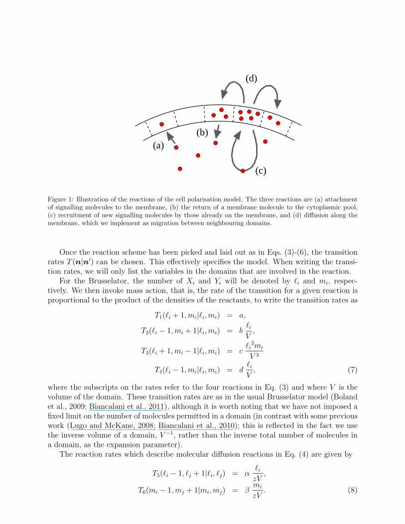
The second example consists of a two-dimensional ‘cell’ enclosed within a perfectly circularmembrane (Altschuler et al., 2008). The centre of the cell is known as the ‘cytoplasmic pool’and contains signalling molecules which we denote by C. In our implementation, the one-dimensional circular membrane is divided up into domains labelled by an index i; moleculeslying within domains i are denoted by Mi. The following reactions take place:

Ckon→ Mi,

Mikoff→ C,

Mi + Ckfb→ 2Mi. (5)

The first two reactions describe a molecule in the cytoplasmic pool attaching itself to arandom domain on the membrane and a molecule detaching and returning to the cytoplasmicpool, respectively. The third reaction represents a molecule on the membrane attemptingto recruit another molecule from the cytoplasmic pool to the same domain. As for theBrusselator, there is also diffusion, in this case along the membrane:

Miα→ Mj , (6)

for any pair of neighbouring membrane domains i and j. The reaction scheme is illustratedin Fig. 1 (after Altschuler et al).

(a)

(c)

(d)

(b)

Figure 1: Illustration of the reactions of the cell polarisation model. The three reactions are (a) attachmentof signalling molecules to the membrane, (b) the return of a membrane molecule to the cytoplasmic pool,(c) recruitment of new signalling molecules by those already on the membrane, and (d) diffusion along themembrane, which we implement as migration between neighbouring domains.

Once the reaction scheme has been picked and laid out as in Eqs. (3)-(6), the transitionrates T (n|n′) can be chosen. This effectively specifies the model. When writing the transi-tion rates, we will only list the variables in the domains that are involved in the reaction.

For the Brusselator, the number of Xi and Yi will be denoted by `i and mi, respec-tively. We then invoke mass action, that is, the rate of the transition for a given reaction isproportional to the product of the densities of the reactants, to write the transition rates as

T1(`i + 1,mi|`i,mi) = a,

T2(`i − 1,mi + 1|`i,mi) = b`iV,

T3(`i + 1,mi − 1|`i,mi) = c`i

2mi

V 3

T4(`i − 1,mi|`i,mi) = d`iV, (7)

where the subscripts on the rates refer to the four reactions in Eq. (3) and where V is thevolume of the domain. These transition rates are as in the usual Brusselator model (Bolandet al., 2009; Biancalani et al., 2011), although it is worth noting that we have not imposed afixed limit on the number of molecules permitted in a domain (in contrast with some previouswork (Lugo and McKane, 2008; Biancalani et al., 2010); this is reflected in the fact we usethe inverse volume of a domain, V −1, rather than the inverse total number of molecules ina domain, as the expansion parameter).

The reaction rates which describe molecular diffusion reactions in Eq. (4) are given by

T5(`i − 1, `j + 1|`i, `j) = α`izV

,

T6(mi − 1,mj + 1|mi,mj) = βmi

zV. (8)

Here z is the number of nearest neighbours of a domain and the index j denotes a nearestneighbour of domain i.

To model spontaneous cell polarisation we denote the number of C and Mi molecules by` and mi, respectively. The transition rates are then taken to be

T1(`− 1,mi + 1|`,mi) = kon`

V

T2(`+ 1,mi − 1|`,mi) = koffmi

V,

T3(`− 1,mi + 1|`,mi) = kfb`mi

V 2, (9)

for the reactions (5) and

T4(mi − 1,mj + 1|mi,mj) = αmi

2V, (10)

for the reactions (6).The transition rates for these two models can be substituted into Eq. (2) which can then,

together with suitable initial and boundary conditions, be used to solve for Pn(t). They canalso be used as the basis for setting up a simulation using the Gillespie algorithm (Gillespie,1976, 1977). Our approach in this paper will be to devise approximation schemes for themaster equation and to check the results obtained from such schemes with simulations basedon the Gillespie algorithm.

We end this section by generalising the above formulation so that it applies to a generalbiochemical network and by extension to any network of interacting agents. To do this,suppose that there are L different constituents in the system. These could be labelled bytheir type, the domain they occupy, etc. We will denote them by ZI , I = 1, . . . , L and ata given time there will be nI of them, so that the state of the system can be specified byn = (n1, . . . , nL), as described earlier in this section. We suppose that there are M reactionswhich interconvert species:

L∑I=1

rIµZI −→L∑I=1

pIµZI , µ = 1, 2, ...M. (11)

Here the numbers rIµ and pIµ (I = 1, . . . , L;µ = 1, . . . ,M) describe respectively the popu-lation of the reactants and the products involved in the reaction. The reactions Eqs. (3)-(6)are simple examples of this general set of reactions.

A quantity which is central to the structure of both the mesoscopic and macroscopicequations is the stoichiometry matrix, νIµ ≡ rIµ− pIµ, which describes how many moleculesof species ZI are transformed due to the reaction µ. In the notation introduced above forthe master equation, n′ = n − ν, where νµ = (ν1µ, . . . , νLµ) is the stoichiometric vectorcorresponding to reaction µ. Therefore the master equation (2) may be equivalently writtenas

dPn(t)

dt=

M∑µ=1

[Tµ(n|n− νµ)Pn−νµ(t)− Tµ(n+ νµ|n)Pn(t)

]. (12)

Many models of interest involve only a handful of different reactions; in this situation, it isoften convenient to rewrite the master equation as a sum over reactions as in Eq. (12), ratherthan over pairs of states n and n′ as in Eq. (2). In the next section we will describe how themesoscopic description of the models can be obtained from the master equation (12). Thesecan then be used as the basis for the calculational schemes which we wish to implement.

3. Derivation of the macro- and mesoscopic equations

3.1. Macroscopic equation

Before we derive the mesoscopic equations from the master equation, we will carry outthe simpler task of deriving the macroscopic equations. This will be done for the case of thegeneral biochemical network described in section 2.

This is achieved by multiplying Eq. (12) by n, and summing over all possible values ofn. After making the change of variable n→ n+ ν in the first summation, one finds that

d〈n(t)〉dt

=M∑µ=1

νµ⟨Tµ(n+ νµ|n)

⟩, (13)

where the angle brackets define the expectation value:

〈· · · 〉 =∑n

(· · · )Pn(t) . (14)

In the limit where both the particle numbers and the volume become large, we willtake the state variables to be the concentration of the constituents nI/V , rather than theirnumber nI . These will be assumed to have a finite limit as V → ∞. Specifically, the stateof the system will be determined by the new variables

yI = limV→∞

〈nI〉V

, where I = 1, . . . , L .

From Eq. (13) we have that

dyIdτ

=M∑µ=1

νIµfµ(y), I = 1, . . . , L, (15)

where τ = t/V and where

fµ(y) = limV→∞

⟨Tµ(n+ νµ|n)

⟩= lim

V→∞Tµ(〈n〉+ νµ|〈n〉

)= lim

V→∞Tµ(V y + νµ|V y) . (16)

In the above we have used the fact that in the macroscopic limit the probability distributionfunctions are Dirac delta functions and so, for instance, 〈nm〉 = 〈n〉m, for any integer m.

The equationdyIdτ

= AI(y), (17)

where

AI(y) ≡M∑µ=1

νIµfµ(y), I = 1, . . . , L, (18)

is the macroscopic equation corresponding to the microscopic master equation (12). It canbe calculated from a knowledge of the stoichiometric matrix νIµ and the transition ratesTµ(n + νµ|n). We scaled time by a factor of V simply because the choice we made for thetransition rates (7)-(10) were finite as V → ∞, but we could have easily incorporated anextra factor of V in these rates through a time rescaling. We also chose particularly simpleforms for these transition rates in that they were all functions of the species concentrationnI/V . More generally, they might separately be functions of nI and V , which becomefunctions of the species concentration nI/V only when both the particle numbers and thevolume become large, so that in the limit V →∞ they become functions of the macroscopicstate variable y.

3.2. Mesoscopic equation

It is perhaps useful at this stage to recall precisely what is meant by the terms ‘micro-scopic’, ‘mesoscopic’ and ‘macroscopic’. The microscopic description is the one based onthe fundamental constituents whose reactions are described by relations such as those inEqs. (3)-(6). The dynamics of the processes are described by the master equation or by theGillespie algorithm. The macroscopic description has been derived from this microscopicdescription above: it only involves average quantities and their time evolution. In betweenthese two levels of description is the ‘meso’-level description, where the continuous variableof the macro-description is used, but where the stochastic effects due to the discrete natureof the individuals is retained. Some other authors include master equations at the meso-levelleaving the micro-level for the world of atoms and molecules, but this does not seem sucha useful assignment in the biological context in which we are working. The derivation ofthe mesoscopic equation follows similar lines to the calculation above, with the importantdifference that we do not take an average, or equivalently, do not take the limit V →∞.

We begin by substituting yI = nI/V directly into the master equation. Since, as discussedabove, our transition rates are all functions of nI/V we simply replace Tµ(n + νµ|n) byfµ(y) in the notation of Eq. (16). In addition we will denote the pdf Pn(t) where n has beenreplaced by V y as P (y, t). With these changes we may write the master equation (12) as

∂P (y, t)

∂t=

M∑µ=1

[fµ

(y − νµ

V

)P(y − νµ

V, t)− fµ(y)P (y, t)

]For V large, the steps νµ/V are likely to be very small, suggesting that we may expand the

functions P and f as Taylor series around y. Truncating at order O(V −2), we arrive at

∂P (y, τ)

∂τ= −

M∑µ=1

∑I

νIµ∂

∂yI[fµ(y)P (y, τ)] (19)

+M∑µ=1

1

2V

∑I,J

νIµνJµ∂2

∂yI∂yJ[fµ(y)P (y, τ)] ,

where as before we have absorbed a factor of V into the rescaled time variable τ = t/V .This is a Fokker-Planck equation which can be cast into the standard form (Risken, 1989;Gardiner, 2009)

∂P (y, τ)

∂τ= −

∑I

∂

∂yI[AI(y)P (y, τ)] +

1

2V

∑I,J

∂2

∂yI∂yJ[BIJ(y)P (y, τ)] , (20)

where AI(y) is defined by Eq. (18) and where

BIJ(y) =M∑µ=1

νIµνJµfµ(y), I, J = 1, . . . , L. (21)

In the Fokker-Planck equation (20), the continuous nature of the state variables indicatesthat the individual nature of the constituents has been lost. However, the stochasticity dueto this discreteness has not: it now manifests itself through the function BIJ(y). We cansee this is the case through the presence of the factor 1/V .

One might ask if this approach is consistent with the previous macroscopic derivation.As V →∞, the Fokker-Planck equation reduces to the Liouville equation

∂P (y, τ)

∂τ= −

∑I

∂

∂yI[AI(y)P (y, τ)] . (22)

One can check by direct substitution that the solution to this equation is P (y, τ) = δ(y(τ)−y) where δ is the Dirac delta function and where y(τ) is the solution of the macroscopicsystem (17); see (Gardiner, 2009) for details.

It is also natural to ask if it is useful to include higher order terms in V −1. There aresound mathematical reasons for not going to higher order, for instance the pdf may becomenegative (Risken, 1989). As we will see, for the problems that we are interested in here(and many others) very good agreement with simulations can be found by working with theFokker-Planck equation (20).

The Fokker-Planck equation (20) provides a mesoscopic description of the system but,like the master equation (2) from which it originated, it is an equation for a pdf. It istherefore quite distinct from the macroscopic equation (17), which is an equation for thestate variables themselves. There does, however, exist an equation for the state variableswhich is completely equivalent to the Fokker-Planck equation (20) (Gardiner, 2009). Thisequation takes the form

dyIdτ

= AI(y) +1√V

∑J

gIJ(y)ηJ(τ), (23)

where the ηJ(τ) are Gaussian white noises with zero mean and correlator

〈ηI(τ)ηJ(τ ′)〉 = δIJδ(τ − τ ′), (24)

and where gIJ(y) is related to BIJ(y) by

BIJ(y) =∑K

gIK(y)gJK(y). (25)

The mesoscopic equation (23) generalises the macroscopic ordinary differential equation(17) with the addition of noise terms η(τ) and so is a stochastic differential equation (SDE).As we will discuss below we need to specify that it is to be interpreted in the sense of Ito(Gardiner, 2009). Notice the direct relationship between this SDE and the macroscopicODE: sending V →∞ in Eq. (23) immediately yields equation (17).

It is important to point out that the matrices gIJ(y) which define the behaviour of thenoise cannot be found from the macroscopic equations, and a knowledge of the microscopicstochastic dynamics is essential if one is to understand the effects of noise. It is not per-missible in this context to simply ‘add noise terms’ to the macroscopic equations to obtaina mesoscopic description, as some authors have done in the past. The only situation inwhich it is permissible to do this is if the noise is external to the system, that is, it does notoriginate from the internal dynamics of the system.

We end this section with two general comments on the mesoscopic equation (23). Thefirst is that while there are no strong restrictions on the form of AI(y), there are on BIJ(y).From Eq. (21) we see that the matrix B is symmetric, but also that for any non-zero vectorw, ∑

I,J

wIBIJwJ =M∑µ=1

(w · ν)2 fµ(y) ≥ 0, (26)

since fµ(y) ≥ 0. Thus B is positive semi-definite (Mehta, 1989). It follows that B = g gT

for some non-singular matrix g, where T denotes transpose (Mehta, 1989). One way ofconstructing such a matrix is to note that since B is symmetric, it can be diagonalisedby an orthogonal transformation defined through a matrix OIJ . Then since B is positivesemi-definite, its eigenvalues are non-negative, and so

B = OΛOT = g gT, where g = OΛ1/2, (27)

and where Λ and Λ1/2 are the diagonal matrices with respectively the eigenvalues and squareroot of the eigenvalues of B as entries. We can take the positive roots of the eigenvalueswithout loss if generality, since the sign can always be absorbed in the ηJ factor in Eq. (23)(its distribution is Gaussian and so invariant under sign changes). It should also be pointedout that we can go further and make an orthogonal transformation on the noise, ζJ =∑

I SIJηJ , and leave Eq. (24), and so its distribution, unchanged. The transformation matrixS can then be used to define a new matrix GIJ =

∑K gIKSJK , so that the form of the

mesoscopic equation (23) is unchanged. So while the procedure outlined above gives us away of constructing gIJ(y) from BIJ(y), it is not unique.

The second comment relates to the statement made earlier, that Eq. (23) is to be inter-preted in the Ito sense. The singular nature of white noise means that in some cases SDEsare not uniquely defined by simply writing down the equation, but have to be supplementedwith the additional information on how the singular nature of the process is to be interpreted(van Kampen, 2007; Gardiner, 2009). This happens when gIJ depends on the state of thesystem y; the noise is then said to be multiplicative. As we will see in the next section, thissubtlety is not relevant within the LNA, since there the gIJ is evaluated at a fixed point ofthe dynamics, and so ceases to depend on the state of the system. However, when goingbeyond the LNA, it is an important consideration. If one wishes to manipulate a multiplica-tive noise SDE like Eq. (23), then one must employ modified rules of calculus which takeinto account the contribution from the noise. We refer to Gardiner (2009) for details, and acomplete discussion on the relationship between the Ito formulation and the alternatives.

This completes our general discussion of the derivation and form of the mesoscopic equa-tion. In the next two sections we will apply it to the two models which we introduced inSection 2. In the first case we will consider use of the LNA is sufficient for our requirements,but in the second case we have to go beyond the LNA.

4. Stochastic patterns in population models

One of the reasons why deterministic reaction-diffusion systems are interesting is thefact that they may give rise to ordered structures, either in space or time. Many modelsdisplaying several different kinds of patterns have been extensively discussed in the literature(Murray, 2008; Cross and Greenside, 2009). However, the mathematical mechanisms whichare responsible for the pattern formation are few and universal, and they can be convenientlyanalysed using the simplest models. Perhaps the most famous of these mechanisms was putforward by Turing in his pioneering study of morphogenesis (Turing, 1952), and it is nowreferred to as the ‘Turing instability’ (Murray, 2008; Cross and Greenside, 2009). It is invokedas a central paradigm in various areas of science to explain the emergence of steady spatialstructures which typically look like ‘stripes’, ‘hexagons’ or ‘spots’ (Murray, 2008; Cross andGreenside, 2009).

In this section, we will be interested in reaction-diffusion systems exhibiting a Turinginstability which are composed of discrete entities as described in section 2. The intrinsicnoise in the system will render it stochastic. As we shall see, by means of the LNA, one isable to make analytical progress and so clarify the role of demographic noise in the patternformation process. We shall show that systems of this kind display ‘stochastic patterns’in addition to the conventional ‘Turing patterns’. It has been suggested that stochasticpatterns are responsible for the robustness of the patterning observed in population systems(Butler and Goldenfeld, 2009, 2011; Biancalani et al., 2010) and they have been appliedin several ecological models (Butler and Goldenfeld, 2009; Bonachela et al., 2012), in thedynamics of hallucination (Butler et al., 2012) and in a biological model with stochasticgrowth (Woolley et al., 2011). In a similar way, the emergence of stochastic travelling waveshas been studied (Biancalani et al., 2011), which has found application in a marine predator-prey system (Datta et al., 2010). There is also an existing literature on stochastic patterningin arid ecosystems (Ridolfi et al., 2011b) where the origin of the noise is extrinsic rather than

intrinsic.The following analysis employs the Brusselator model to exemplify the general theory.

This is a reaction scheme introduced by Lefever and Prigogine in the 1960s (Glansdorff andPrigogine, 1971) as a model of biochemical reactions which showed oscillatory behaviour.For our purposes, its interest lies in the fact that its spatial version is one of the simplestmodels which exhibits a Turing instability.

Before we begin the analysis of this model we need to discuss some aspects of the notationwe will use. As explained in section 2 the labels that we have been using so far combine aspatial index with an index for the type of constituent, for example J = j, s. This wasdone in order to reduce the clutter of indices. However in the analysis below we will needto separate them, since we will assume a regular lattice structure for the domains, whichwill allow us to use Fourier analysis to effectively diagonalise the spatial part of the system.The Fourier components of a given function will be labelled through the argument of thatfunction, leaving only the index (e.g. s) labelling the type. Specifically we will choose thespatial structure to be a regular D-dimensional hypercubic lattice with periodic boundaryconditions and domain length l. Following the conventions of (Chaikin and Lubensky, 2000),the discrete spatial Fourier transform is then defined as:

fk = lDΩ∑j=1

e−ilk·jfj, with fj = l−DΩ−1

Ω∑k=1

eilk·j fk, (28)

where Ω is the number of lattice points, j is a D-dimensional spatial vector and k is itsFourier conjugate. Note that i here is imaginary unit and not a spatial index, and althoughboth j and k are D-dimensional vectors, we do not explicitly show this, in line with thenotation adopted in section 2.

We begin the analysis by deriving the well-known deterministic Brusselator equationsfrom this microscopic description using Eqs. (17) and (18):

duidτ

= a− (b+ d)ui + cu2i vi + α∆ui,

dvidτ

= bui − cu2i vi + β∆vi, (29)

where ui = `i/V and vi = mi/V , where u is the density of chemical species X and v isthe density of chemical species Y . The symbol ∆ represents the discrete Laplacian operator∆fj = (2/z)

∑j′∈∂j (fj − fj′) where j′ ∈ ∂j indicates that the domain j′ is a nearest neigh-

bour of the domain j and z is the co-ordination number of the lattice. The spatial Fouriertransform of the discrete Laplacian operator reads (Lugo and McKane, 2008):

∆k =2

D

D∑s=1

[cos (ks l)− 1] . (30)

It is possible to obtain a continuous spatial description, in the deterministic limit, bytaking the limit of small domain length scale, l→ 0 (Lugo and McKane, 2008). By doing so,

one can recover the traditional partial differential equations for reaction-diffusion systems:

∂u

∂τ= a− (b+ d)u+ cu2v +D1∇2u,

∂v

∂τ= bu− cu2v +D2∇2v, (31)

where D1 and D2 are obtained by scaling the diffusivities α and β according to:

1

2Dl2α 7→ D1,

1

2Dl2β 7→ D2. (32)

However, we shall keep the space discrete in the following analysis because the theory issimpler to describe and it is most convenient for carrying out stochastic simulations. Weshall also set l = 1, since this simply amounts to a choice of length scale, and this is thesimplest choice.

The macroscopic equations (29) are Eq. (17) for the particular case of the Brusselatormodel. To find the corresponding mesoscopic equations we need to find the particular formof Eq. (23) for the Brusselator. This we can do by calculating BIJ(y), defined in Eq. (21),but we will find that we do not need to utilise the non-linear equation (23) to take thefluctuations into account; it is sufficient to use only a linearised form. This is the LNA, andis implemented by writing

yI(t) = 〈yI(t)〉+ξI(t)√V, (33)

where 〈yI(t)〉 satisfies the macroscopic equation (17). Substituting Eq. (33) into Eq. (23),we expand in powers of 1/

√V . The terms which are proportional to 1/

√V give an equation

for ξI :dξIdτ

=∑J

JIJ(〈y〉)ξJ +∑J

gIJ(〈y〉)ηJ(τ), (34)

where J is the Jacobian of the system.In many situations, including the one we are describing here, we are only interested in

the fixed points of the macroscopic equation, in which case 〈y〉 = y∗ and the matrices Jand g can be replaced by their values at the fixed point y∗. The SDE (34) now involves onlyconstant matrices:

dξIdτ

=∑J

J ∗IJξJ +∑J

g∗IJηJ(τ). (35)

For the specific case of the Brusselator the index I includes the spatial index i and anindex s = 1, 2 which distinguishes between the variables u and v. If we take the spatialFourier transform of Eq. (35), translational invariance implies that the matrices J ∗ and g∗

are diagonalised in the spatial variables, and so this equation becomes

∂ξγ(k, τ)

∂τ=

2∑δ=1

J ∗γδ(k) ξδ(k, τ) +2∑δ=1

g∗γδ(k) ηδ(k, τ). (36)

We are now in a position to discuss both the classical Turing patterns found in determinis-tic equations such as Eqs. (31) and the stochastic Turing patterns found in the correspondingmesoscopic equations. The homogeneous fixed point of Eqs. (31) is given by

u∗ =a

d, v∗ =

bd

ac, (37)

although from now on we will set c = d = 1, as is common in the literature (Glansdorff andPrigogine, 1971). In the deterministic case, the linear stability analysis about this fixed pointis a special case of that carried out above in the stochastic picture, and corresponds to ignor-ing the noise term in Eq. (36). Therefore the small, deterministic, spatially inhomogeneous,perturbations ξγ(k, τ) satisfy the equation

∂ξγ(k, τ)

∂τ=

2∑δ=1

J ∗γδ(k) ξγ(k, τ), (38)

where the Jacobian is found to be

J ∗(k) =

(b− 1 + α∆k a2

−b −a2 + β∆k

). (39)

The eigenvalues of the Jacobian, λγ(k) (γ = 1, 2), give information about the stability ofthe homogeneous state. In particular, the perturbations ξγ(k, τ) grow like linear combina-tions of eλγ(k) t, therefore if Re[λγ(k)] is positive for some k and some γ, then the perturbationwill grow with time and the homogeneous state will be unstable for this value of k. Turing’sinsight was that the pattern eventually formed as a result of the perturbation is charac-terised by this value of k. The overall scenario is complicated by the nature of the boundaryconditions, the presence of other attractors and the effect of the non-linearities (Cross andGreenside, 2009), but in the following we shall ignore these, and consider only the simplestcase in order to understand the main concepts.

In this most straightforward situation, the small perturbation which excites the unstablek-th Fourier mode will cause the concentrations u and v to develop a sinusoidal profileabout their fixed point values characterised by the wave-number k. The pattern is steady orpulsating depending on whether or not the imaginary part Im[λγ(k)] is zero. In both cases,the amplitude of sinusoidal profile increases exponentially with a time-scale 1/Re[λγ(k)], andso clearly the eigenvalue with the largest real part will dominate. By moving away from thehomogeneous state the linear approximation will eventually lose its validity and the effect ofthe non-linear terms will become relevant. If the system admits no solutions which diverge,the growth will be damped by the non-linearities to some non-zero value, which defines thefinal amplitude of the spatial pattern.

Typically, the interesting case occurs when a control parameter triggers the patternformation by making the real part of one of the eigenvalues positive. For the Brusselatorthis is illustrated in Fig. 2, where the relevant eigenvalue of J , (i.e. the one which becomespositive) is shown for different values of the parameter b. Here b is the control parameterwith the other free parameter a fixed and equal to 1.5. For b < bc ≈ 2.34, the real partof both eigenvalues is negative and thus the homogeneous state is stable. This corresponds

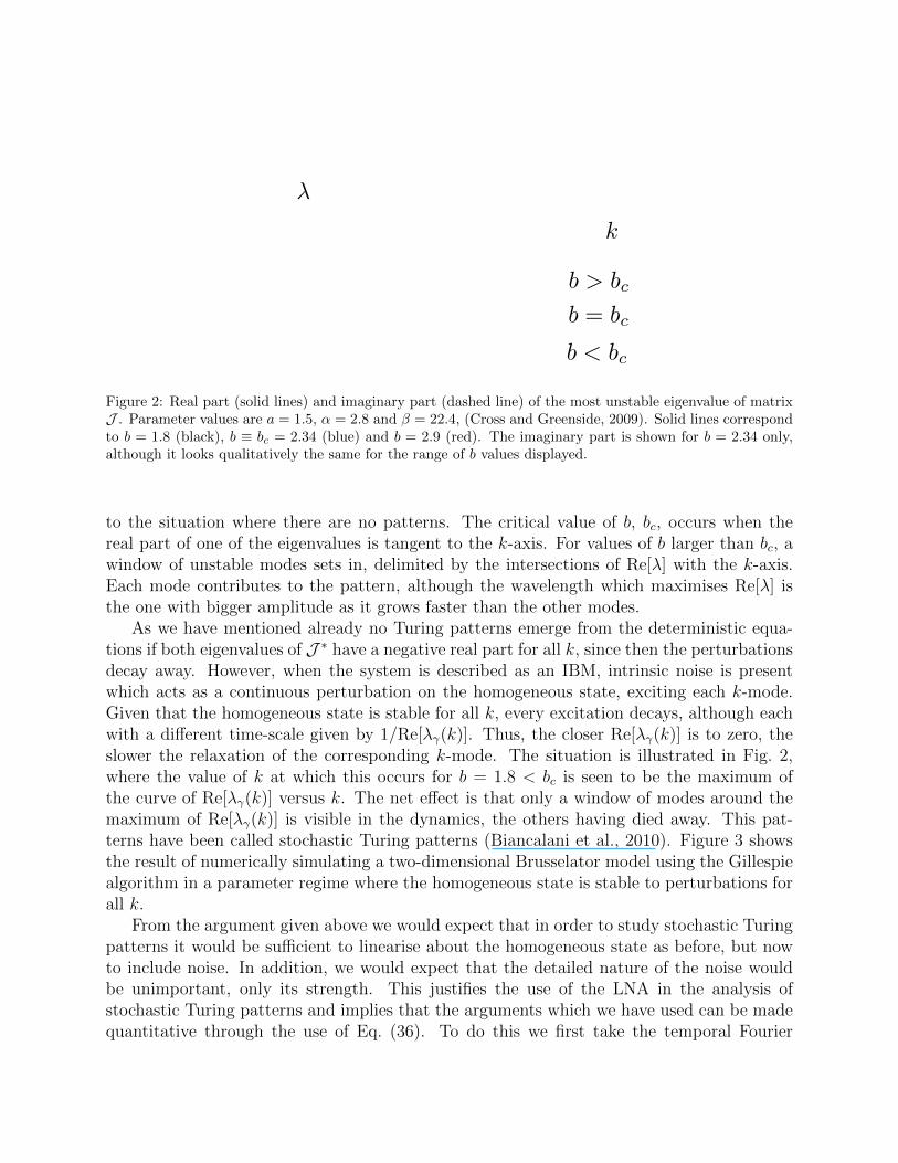
Figure 2: Real part (solid lines) and imaginary part (dashed line) of the most unstable eigenvalue of matrixJ . Parameter values are a = 1.5, α = 2.8 and β = 22.4, (Cross and Greenside, 2009). Solid lines correspondto b = 1.8 (black), b ≡ bc = 2.34 (blue) and b = 2.9 (red). The imaginary part is shown for b = 2.34 only,although it looks qualitatively the same for the range of b values displayed.

to the situation where there are no patterns. The critical value of b, bc, occurs when thereal part of one of the eigenvalues is tangent to the k-axis. For values of b larger than bc, awindow of unstable modes sets in, delimited by the intersections of Re[λ] with the k-axis.Each mode contributes to the pattern, although the wavelength which maximises Re[λ] isthe one with bigger amplitude as it grows faster than the other modes.

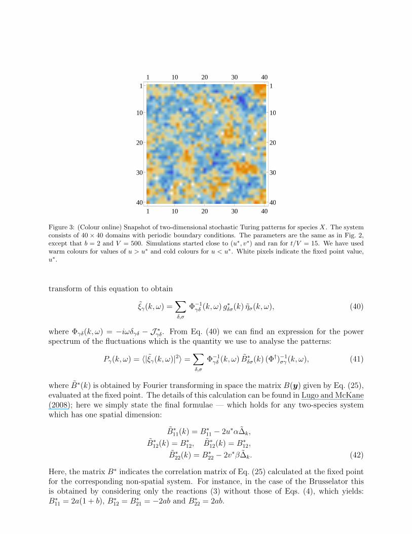
As we have mentioned already no Turing patterns emerge from the deterministic equa-tions if both eigenvalues of J ∗ have a negative real part for all k, since then the perturbationsdecay away. However, when the system is described as an IBM, intrinsic noise is presentwhich acts as a continuous perturbation on the homogeneous state, exciting each k-mode.Given that the homogeneous state is stable for all k, every excitation decays, although eachwith a different time-scale given by 1/Re[λγ(k)]. Thus, the closer Re[λγ(k)] is to zero, theslower the relaxation of the corresponding k-mode. The situation is illustrated in Fig. 2,where the value of k at which this occurs for b = 1.8 < bc is seen to be the maximum ofthe curve of Re[λγ(k)] versus k. The net effect is that only a window of modes around themaximum of Re[λγ(k)] is visible in the dynamics, the others having died away. This pat-terns have been called stochastic Turing patterns (Biancalani et al., 2010). Figure 3 showsthe result of numerically simulating a two-dimensional Brusselator model using the Gillespiealgorithm in a parameter regime where the homogeneous state is stable to perturbations forall k.

From the argument given above we would expect that in order to study stochastic Turingpatterns it would be sufficient to linearise about the homogeneous state as before, but nowto include noise. In addition, we would expect that the detailed nature of the noise wouldbe unimportant, only its strength. This justifies the use of the LNA in the analysis ofstochastic Turing patterns and implies that the arguments which we have used can be madequantitative through the use of Eq. (36). To do this we first take the temporal Fourier

1 10 20 30 40

1

10

20

30

40

1 10 20 30 401

10

20

30

40

Figure 3: (Colour online) Snapshot of two-dimensional stochastic Turing patterns for species X. The systemconsists of 40 × 40 domains with periodic boundary conditions. The parameters are the same as in Fig. 2,except that b = 2 and V = 500. Simulations started close to (u∗, v∗) and ran for t/V = 15. We have usedwarm colours for values of u > u∗ and cold colours for u < u∗. White pixels indicate the fixed point value,u∗.

transform of this equation to obtain

ξγ(k, ω) =∑δ,σ

Φ−1γδ (k, ω) g∗δσ(k) ησ(k, ω), (40)

where Φγδ(k, ω) = −iωδγδ − J ∗γδ. From Eq. (40) we can find an expression for the powerspectrum of the fluctuations which is the quantity we use to analyse the patterns:

Pγ(k, ω) = 〈|ξγ(k, ω)|2〉 =∑δ,σ

Φ−1γδ (k, ω) B∗δσ(k) (Φ†)−1

σγ (k, ω), (41)

where B∗(k) is obtained by Fourier transforming in space the matrix B(y) given by Eq. (25),evaluated at the fixed point. The details of this calculation can be found in Lugo and McKane(2008); here we simply state the final formulae — which holds for any two-species systemwhich has one spatial dimension:

B∗11(k) = B∗11 − 2u∗α∆k,

B∗12(k) = B∗12, B∗12(k) = B∗12,

B∗22(k) = B∗22 − 2v∗β∆k. (42)

Here, the matrix B∗ indicates the correlation matrix of Eq. (25) calculated at the fixed pointfor the corresponding non-spatial system. For instance, in the case of the Brusselator thisis obtained by considering only the reactions (3) without those of Eqs. (4), which yields:B∗11 = 2a(1 + b), B∗12 = B∗21 = −2ab and B∗22 = 2ab.

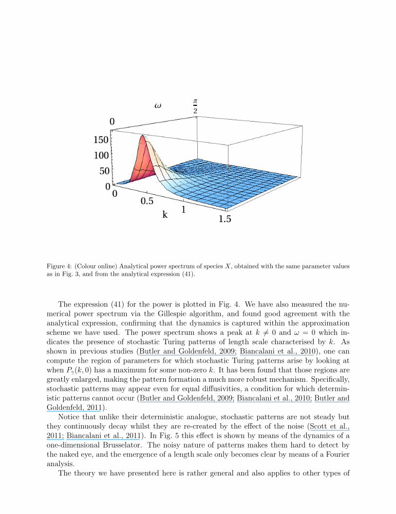
Figure 4: (Colour online) Analytical power spectrum of species X, obtained with the same parameter valuesas in Fig. 3, and from the analytical expression (41).

The expression (41) for the power is plotted in Fig. 4. We have also measured the nu-merical power spectrum via the Gillespie algorithm, and found good agreement with theanalytical expression, confirming that the dynamics is captured within the approximationscheme we have used. The power spectrum shows a peak at k 6= 0 and ω = 0 which in-dicates the presence of stochastic Turing patterns of length scale characterised by k. Asshown in previous studies (Butler and Goldenfeld, 2009; Biancalani et al., 2010), one cancompute the region of parameters for which stochastic Turing patterns arise by looking atwhen Pγ(k, 0) has a maximum for some non-zero k. It has been found that those regions aregreatly enlarged, making the pattern formation a much more robust mechanism. Specifically,stochastic patterns may appear even for equal diffusivities, a condition for which determin-istic patterns cannot occur (Butler and Goldenfeld, 2009; Biancalani et al., 2010; Butler andGoldenfeld, 2011).

Notice that unlike their deterministic analogue, stochastic patterns are not steady butthey continuously decay whilst they are re-created by the effect of the noise (Scott et al.,2011; Biancalani et al., 2011). In Fig. 5 this effect is shown by means of the dynamics of aone-dimensional Brusselator. The noisy nature of patterns makes them hard to detect bythe naked eye, and the emergence of a length scale only becomes clear by means of a Fourieranalysis.

The theory we have presented here is rather general and also applies to other types of

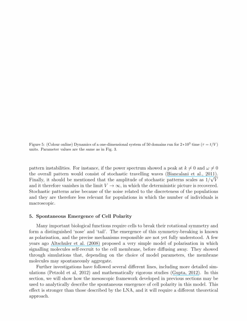
Figure 5: (Colour online) Dynamics of a one-dimensional system of 50 domains run for 2∗103 time (τ = t/V )units. Parameter values are the same as in Fig. 3.

pattern instabilities. For instance, if the power spectrum showed a peak at k 6= 0 and ω 6= 0the overall pattern would consist of stochastic travelling waves (Biancalani et al., 2011).Finally, it should be mentioned that the amplitude of stochastic patterns scales as 1/

√V

and it therefore vanishes in the limit V →∞, in which the deterministic picture is recovered.Stochastic patterns arise because of the noise related to the discreteness of the populationsand they are therefore less relevant for populations in which the number of individuals ismacroscopic.

5. Spontaneous Emergence of Cell Polarity

Many important biological functions require cells to break their rotational symmetry andform a distinguished ‘nose’ and ‘tail’. The emergence of this symmetry-breaking is knownas polarisation, and the precise mechanisms responsible are not yet fully understood. A fewyears ago Altschuler et al. (2008) proposed a very simple model of polarisation in whichsignalling molecules self-recruit to the cell membrane, before diffusing away. They showedthrough simulations that, depending on the choice of model parameters, the membranemolecules may spontaneously aggregate.

Further investigations have followed several different lines, including more detailed sim-ulations (Petzold et al, 2012) and mathematically rigorous studies (Gupta, 2012). In thissection, we will show how the mesoscopic framework developed in previous sections may beused to analytically describe the spontaneous emergence of cell polarity in this model. Thiseffect is stronger than those described by the LNA, and it will require a different theoreticalapproach.

Before beginning the analysis, it is worth noticing that in this model the total numberof molecules does not change; there is thus no need to distinguish between this and thevolume, so we write N = V . Moreover, the variables ` (giving the number of molecules inthe cytoplasmic pool) and mi (the number of molecules in membrane domain i) are relatedby: `+

∑imi = V .

As usual, we first explore the behaviour of the macroscopic equations. Substituting thetransition rates (5) and (6) into equations (17) and (16), we arrive at

du

dτ= (koff − u kfb)

∑i

vi − u kon

dvidτ

= u kon + (u kfb − koff) vi + α∆vi .

Conservation of the total number of molecules implies that u +∑

j vj = 1, so we mayeliminate u from the above system to obtain

dvidτ

=(

1−∑j

vj

)(kon + vi kfb

)− vikoff + α∆vi . (43)

In the appropriate continuum limit, this equation agrees with that of Altschuler et al. (2008).As with the Brusselator, there is a homogeneous fixed point. Putting vi ≡ v and setting

dvi/dτ = 0, we find the quadratic equation

(1− Ω v)(kon + v kfb)− v koff = 0 . (44)

For simplicity, we consider the case in which kon ≈ 0 (that is, almost all membrane moleculesexist as result of the feedback mechanism). In this limit, the homogeneous fixed point isgiven by v = v∗/Ω, where v∗ is the mean fraction of molecules on the membrane:

v∗ =

(

1− koff

kfb

)if kfb > koff

0 otherwise.(45)

To gain further insight, we pass to Fourier space, where Eq. (43) with kon = 0 becomes

dvkdt

= vk

[kfb(1− l−1v0)− koff + α

(cos(lk)− 1

)]. (46)

The Jacobian for this system is diagonal, and it is straightforward to read off the eigenvaluesat the fixed point vk = δw,0 l v

∗ as

λk =

koff − kfb , if k = 0

α(

cos(lk)− 1)

if k 6= 0 .

We can conclude from this analysis that provided kfb > koff the homogeneous fixed point isnon-zero and stable. This is a puzzle: the homogeneous state corresponds to the signalling

molecules being spread uniformly around the membrane, if this state is stable, then how canpolarisation occur?

We postulate that the answer lies in the following observation. Notice that if the diffusioncoefficient α is small then the modes with wave number k 6= 0 are only marginally stable;their associated eigenvalues are close to zero. In this regime, a small random perturbation(resulting from intrinsic noise, for example) may be enough to push the system very far fromits equilibrium state. Moreover, the stochastic dynamics in this regime cannot be understoodwithin the framework of the LNA, for the simple reason that when the system has beenpushed far from its steady state, linearisation around that state is no longer representativeof the true dynamics. To make analytical progress, we will need to deal with the non-linearityof the model some other way.

We begin by writing down the mesoscopic equations. For our purposes, the Fokker-Planckequation (20) is the most useful, with A and B given by

Ai(v) =(

1−∑j

vj

)(kon + vi kfb

)− vikoff + α∆vi ,

Bij(v) = δij

[(1−

∑k

vk

)(kon + vi kfb

)+ vikoff

].

Note that we have neglected terms of order α/V from the noise, as we are interested inbehaviour when α is small and V large, so α/V is negligible. As with the macroscopicequations, this system is easier to analyse in Fourier space. We introduce the distributionP (v, τ) of Fourier variables vk, which satisfies the Fokker-Planck equation

∂P (v, τ)

∂τ= −

∑k

∂

∂vk

[Ak(v)P (v, τ)

](47)

+1

2V

∑k,k′

∂

∂vk

∂

∂vk′

[Bk,k′(v)P (v, τ)

],

where

Ak(v) = vk

[kfb(1− l−1v0)− koff + α

(cos(lk)− 1

)]Bk,k′(v) = vk+k′ l

[kfb(1− l−1v0) + koff

]. (48)

Note that the Fourier modes may take complex values, and we use ∂/∂vk′ to denote differ-entiating with respect to the complex conjugate. For later convenience, we assume Ω is oddand number the modes by k ∈ −(Ω− 1)/2, . . . , (Ω− 1)/2, so that v−k = vk.

Our remaining analysis is informed by two observations. First, we note that the non-linearity in equation (48) arises only from terms involving v0. Second, in the interestingregime kfb − koff α, we have that the eigenvalues of the macroscopic system satisfy λ0 λk < 0 and thus v0 is (comparatively) very stable near v∗. This implies a separation of time-scales in the problem: we expect v0 to relax very quickly to a value near its equilibrium,whilst the other modes fluctuate stochastically on much slower time-scales. Combining these

facts suggests the following strategy: we restrict our attention to only those trajectories inwhich v0 is held constant at lv∗.

Conditioning on the value of v0 alters the structure of the noise correlation matrix forthe other modes; details of the general formulation are given in Appendix B of Rogerset al. (2012b). The result is a Fokker-Planck equation for the distribution P (c)(v, τ) of theremaining Fourier modes vk with k 6= 0, conditioned on v0 taking the value lv∗:

∂P (c)(v, τ)

∂τ= −

∑ki6=0

∂

∂vi

[A

(c)k (v)P (v, τ)

](49)

+1

2V

∑k,k′ 6=0

∂

∂vk

∂

∂vk′

[B

(c)k,k′(v)P (v, τ)

],

where

A(c)k (v) = α vk

(cos(lk)− 1

)B

(c)k,k′(v) = 2koff

[l vk+k′ −

vkvk′

v∗

]. (50)

Multiplying (50) by vk and integrating over all v we obtain a differential equation for themode averages:

d

dτ〈vk〉 = α〈vk〉

(cos(lk)− 1

). (51)

Thus, for all α > 0 we have〈vk〉 → δk,0 lv

∗ . (52)

For the second-order moments the behaviour is not so trivial. Multiplying (50) this time byvkvk′ and integrating yields

d

dτ〈vkvk′〉 =

lkoff

V〈vk+k′〉+ 〈vkvk′〉

[α(

cos(lk) + cos(lk′)− 2)− 1

V

koff

v∗

]. (53)

The equilibrium values are thus 〈vkvk′〉 → 0 if k + k′ 6= 0 mod Ω, and

〈|vk|2〉 →(lv∗)2

1 + αV (1− cos(lk))v∗/koff

. (54)

This is our main result, although further analysis is required to interpret the implicationsfor the behaviour of the model.

In Altschuler et al. (2008) it was observed that simulations of a continuum version of thismodel exhibited the curious phenomenon of the membrane molecules grouping together,despite the macroscopic equations suggesting they should be spread uniformly around themembrane. We introduce a summary statistic to measure this effect. Suppose the membranemolecules are distributed according to an angular density field v(x), and let Λ denote themean angular separation of two molecules:

Λ =

(1

v∗

)2 ∫ π

−π

∫ π

−πd(x, y)

⟨v(x)v(y)

⟩dx dy , (55)

where

d(x, y) =

|x− y| if |x− y| < π

2π − |x− y| otherwise.(56)

To compute Λ from our result (54) we pass to the continuum limit, taking Ω→∞ and usingthe modes vk as the coefficients of the Fourier series of the membrane angular density fieldv(x). Taking an angular prescription for the membrane so that l = 2π/Ω, we renormaliseby a factor of 1/2πl and reverse the Fourier transform to obtain

v(x) = limΩ→∞

1

2πl

Ω∑k=1

eikxvk , for x ∈ [−π, π) . (57)

The calculation proceeds thus:

Λ = 2π

(1

v∗

)2 ∫ π

−π|x|⟨v(x)v(0)

⟩dx

=1

2π

(1

lv∗

)2∑k,k′

〈vkvk′〉∫ π

−π|x|eikx dx

=π

2+∑k 6=0

1

1 + ϕ2k2

∫ π

−π|x|eikx dx , (58)

where ϕ = (αV l2v∗/koff)1/2, which we assume to have a finite value in the limit l → 0. Thefirst equality above comes from the rotational invariance of the model meaning that we mayfix y = 0, after which we employ Eq. (57) and Eq. (54) in turn. Now, for k 6= 0∫ π

−π|x|eikx dx =

−4k−2 for odd k

0 for even k.

Also, the following infinite series (Bromwich, 1926) will be useful:∑k odd

1

x2 + k2=

π

2xtanh

(πx2

).

Altogether, we have

Λ(ϕ) =π

2− 2

π

∑k odd

(1

1 + ϕ2k2

)(1

k2

)

=π

2− 2

π

(∑k odd

1

k2−∑k odd

1

ϕ−2 + k2

)

= ϕ tanh

(π

2ϕ

). (59)

The limits are Λ(∞) = π/2, which corresponds to molecules spread uniformly around themembrane, and Λ(0) = 0, which corresponds to complete localisation. In figure 6 we compare

10−2

100

102

0

0.4

0.8

1.2

1.6

ϕ

Λ(ϕ)

(a)

(b)

(a)

(b)

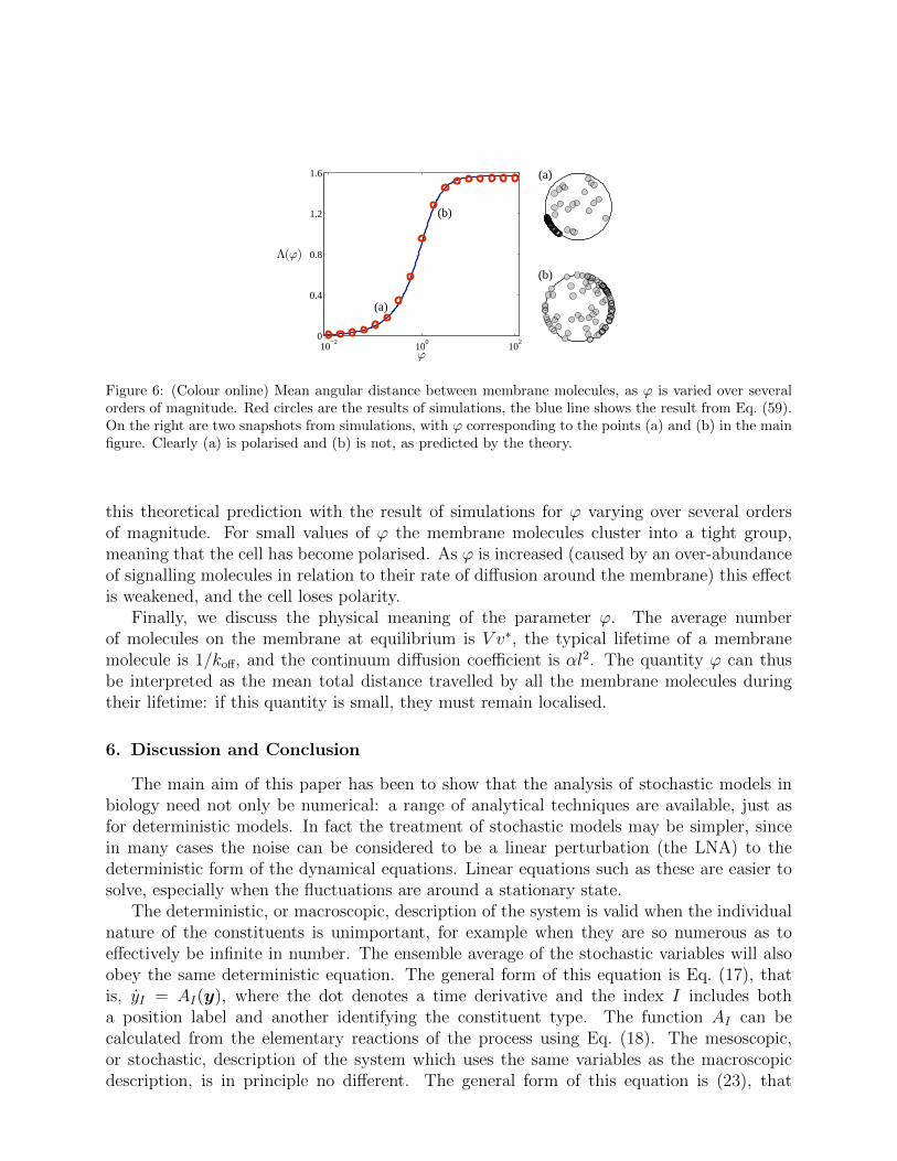
Figure 6: (Colour online) Mean angular distance between membrane molecules, as ϕ is varied over severalorders of magnitude. Red circles are the results of simulations, the blue line shows the result from Eq. (59).On the right are two snapshots from simulations, with ϕ corresponding to the points (a) and (b) in the mainfigure. Clearly (a) is polarised and (b) is not, as predicted by the theory.

this theoretical prediction with the result of simulations for ϕ varying over several ordersof magnitude. For small values of ϕ the membrane molecules cluster into a tight group,meaning that the cell has become polarised. As ϕ is increased (caused by an over-abundanceof signalling molecules in relation to their rate of diffusion around the membrane) this effectis weakened, and the cell loses polarity.

Finally, we discuss the physical meaning of the parameter ϕ. The average numberof molecules on the membrane at equilibrium is V v∗, the typical lifetime of a membranemolecule is 1/koff, and the continuum diffusion coefficient is αl2. The quantity ϕ can thusbe interpreted as the mean total distance travelled by all the membrane molecules duringtheir lifetime: if this quantity is small, they must remain localised.

6. Discussion and Conclusion

The main aim of this paper has been to show that the analysis of stochastic models inbiology need not only be numerical: a range of analytical techniques are available, just asfor deterministic models. In fact the treatment of stochastic models may be simpler, sincein many cases the noise can be considered to be a linear perturbation (the LNA) to thedeterministic form of the dynamical equations. Linear equations such as these are easier tosolve, especially when the fluctuations are around a stationary state.

The deterministic, or macroscopic, description of the system is valid when the individualnature of the constituents is unimportant, for example when they are so numerous as toeffectively be infinite in number. The ensemble average of the stochastic variables will alsoobey the same deterministic equation. The general form of this equation is Eq. (17), thatis, yI = AI(y), where the dot denotes a time derivative and the index I includes botha position label and another identifying the constituent type. The function AI can becalculated from the elementary reactions of the process using Eq. (18). The mesoscopic,or stochastic, description of the system which uses the same variables as the macroscopicdescription, is in principle no different. The general form of this equation is (23), that

is, yI = AI(y) + V −1/2∑

J gIJ(y)ηJ , where ηJ is a Gaussian white noise with zero meanand unit strength. The only additional function which appears over and above that in thedeterministic equation is gIJ , which can, like AI , be calculated from the elementary reactionsof the process using Eqs. (21) and (25). Although Eq. (23) is a straightforward generalisationof Eq. (17), it is much less well-known.

There are several reasons for the perceived difficulty of using Eq. (23), probably the mostimportant being the unfamiliarity of many biologists with the general theory of stochasticprocesses. We have tried to show in this paper that the stochastic theory which is requiredneed not be more complicated than that of dynamical systems theory, which is applicable toequations such as (17). This is especially true if the LNA is a valid approximation for theparticular system under study. If the multiplicative nature of the noise cannot be neglected,as in section 5, then care is required because of the singular nature of white noise. However,even in this case, a systematic theory has been developed that may be applicable in situationsin which there is a separation of time-scales (Rogers et al., 2012a; Biancalani et al., 2012;Rogers et al., 2012b).

We applied Eq. (23) to two sets of processes, one for which the LNA was applicableand one for which it was not. The former situation was discussed in section 4 where werevisited the problem of the emergence of spatial structures for systems of populations,in the paradigmatic example of the Brusselator model. Intrinsic fluctuations, which areintuitively thought of as a disturbing source, appear instead to be critical for the emergenceof spatial order. More specifically, we showed how Turing patterns can arise for parametervalues for which the macroscopic equations predict relaxation to a homogeneous state. Wecalled these patterns ‘stochastic patterns’, as they are generated by the continuous actionof noise present in the system. However, it can be argued that the amplitude of stochasticpatterns might be so small that they can hardly be observed in a real population, given thatthe amplitude of the noise is small as well. Whilst this might be true for some systems, arecent study (Ridolfi et al., 2011a) has suggested that the response to a small perturbationin a pattern-forming system can be unexpectedly large, if the system displays a sufficientdegree of ‘non-normality’. The connection between non-normality and stochastic patternsis so far largely unexplored, and constitutes a possible further investigation in this line ofresearch.

In section 5 we discussed an example of a stochastic phenomenon which goes beyond whatcan be understood within the LNA. The stochastic patterns appearing in the Brusselator arenoise-driven perturbations around the homogeneous state, having characteristic magnitude1/√V (and thus disappearing in the limit V →∞). By contrast, the spontaneous emergence

of cell polarity in the model of Altschuler et al requires the noise to have a more complexstructure, which can lead the system to a state very far removed from the homogeneousfixed point of the deterministic equations. To characterise this process, it was necessary tostudy the full effect of the non-linear terms in the mesoscopic equations. To achieve this, weexploited the natural separation of time-scales occurring between the dynamics of the zerothFourier mode (which relaxes quickly to its equilibrium value) and the remaining degrees offreedom. This is a non-standard technique, however, it can be made relatively systematicand general, as will be outlined in a forthcoming paper. The LNA has played an importantrole in boosting the recognition of the importance of stochastic effects in the literature; we

hope that methods employing the separation of time-scales may provide the next theoreticaladvance.

Acknowledgements. This work was supported in part under EPSRC Grant No.EP/H02171X/1 (A.J.M and T.R). T.B. also wishes to thank the EPSRC for partial sup-port.

References

Altschuler, S.J., Angenent, S.B., Wang, Y., Wu, L.F., 2008. On the spontaneous emergenceof cell polarity. Nature 454, 886–889.

Biancalani, T., Fanelli, D., Di Patti, F., 2010. Stochastic Turing patterns in the Brusselatormodel. Phys. Rev. E 81, 046215. doi:10.1103/PhysRevE.81.046215.

Biancalani, T., Galla, T., McKane, A.J., 2011. Stochastic waves in a Brusselator model withnonlocal interaction. Phys. Rev. E 84, 026201. doi:10.1103/PhysRevE.84.026201.

Biancalani, T., Rogers, T., McKane, A.J., 2012. Noise-induced metastability in biochemicalnetworks. Phys. Rev. E 86, 010106(R). doi:10.1103/PhysRevE.86.010106.

Black, A.J., McKane, A.J., 2012. Stochastic formulation of ecological models and theirapplications. Trends Ecol. Evol. 27, 337–345. doi:10.1016/j.tree.2012.01.014.

Boland, R.P., Galla, T., McKane, A.J., 2009. Limit cycles, complex Floquet multipliers andintrinstic noise. Phys. Rev. E. 79, 051131.

Bonachela, J.A., Munoz, M.A., Levin, S.A., 2012. Patchiness and demographic noise in threeecological examples. J. Stat. Phys. 148, 723–739.

Bromwich, T., 1926. An Introduction to the Theory of Infinite Series. Chelsea PublishingCompany, London.

Butler, T.C., Benayounc, M., Wallace, E., van Drongelenc, W., Goldenfeld, N., Cowane,J., 2012. Evolutionary constraints on visual cortex architecture from the dynamics ofhallucinations. PNAS 109, 606–609. doi:10.1073/pnas.1118672109.

Butler, T.C., Goldenfeld, N., 2009. Robust ecological pattern formation induced by demo-graphic noise. Phys. Rev. E 80, 030902(R). doi:10.1103/PhysRevE.80.030902.

Butler, T.C., Goldenfeld, N., 2011. Fluctuation-driven Turing patterns. Phys. Rev. E 84,011112. doi:10.1103/PhysRevE.84.011112.

Chaikin, P.M., Lubensky, T.C., 2000. Principles of Condensed Matter Physics. Third ed.,Cambridge University Press, Cambridge.

Cross, M.C., Greenside, H.S., 2009. Pattern Formation and Dynamics in Non-EquilibriumSystems. Cambridge University Press, New York.

Datta, S., Delius, G.W., Law, R., 2010. A jump-growth model for predator-prey dynamics:derivation and application to marine ecosystems. Bull. Math. Biol. 72, 1361–1382. doi:10.1007/s11538-009-9496-5.

Gardiner, C.W., 2009. Handbook of Stochastic Methods for Physics, Chemistry and theNatural Sciences. Fourth ed., Springer, New York.

Gillespie, D.T., 1976. A general method for numerically simulating the stochastic timeevolution of coupled chemical reactions. J. Comput. Phys. 22, 403–434.

Gillespie, D.T., 1977. Exact stochastic simulation of coupled chemical reactions. J. Phys.Chem. 81, 2340–2361.

Glansdorff, P., Prigogine, I., 1971. Thermodynamic Theory of Structure, Stability andFluctuations. Wiley-Interscience, Chichester.

Gupta, A., 2012. Stochastic model for cell polarity. Annals of Applied Probability 22,827–859.

van Kampen, N.G., 2007. Stochastic Processes in Physics and Chemistry. Third ed., ElsevierScience, Amsterdam.

Lugo, C.A., McKane, A.J., 2008. Quasi-cycles in a spatial predator-prey model. Phys. Rev.E. 78, 051911.

Mehta, M.L., 1989. Matrix Theory. Hindustan Publishing Corporation, India.

Murray, J.D., 2008. Mathematical Biology vol. II. Third ed., Springer-Verlag, Berlin.

Petzold et al, 2012. Submitted .

Ridolfi, L., Camporeale, C., D’Odorico, P., Laio, F., 2011a. Transient growth induces un-expected deterministic spatial patterns in the Turing process. Europhys. Lett. 95, 18003.doi:10.1209/0295-5075/95/18003.

Ridolfi, L., D’Odorico, P., Laio, F., 2011b. Noise-Induced Phenomena in the EnvironmentalSciences. Cambridge University Press, Cambridge.

Risken, H., 1989. The Fokker-Planck Equation - Methods of Solution and Applications.Second ed., Springer, Berlin.

Rogers, T., McKane, A.J., Rossberg, A.G., 2012a. Demographic noise can lead to thespontaneous formation of species. Europhys. Lett. 97, 40008. doi:10.1209/0295-5075/97/40008.

Rogers, T., McKane, A.J., Rossberg, A.G., 2012b. Spontaneous genetic clustering in popu-lations of competing organisms. To appear in Physical Biology .

Scott, M., Poulin, F.J., Tang, H., 2011. Approximating intrinsic noise in continuous multi-species models. Proc. R. Soc. A (London) 467, 718–737. doi:10.1098/rspa.2010.0275.

Turing, A.M., 1952. The Chemical Basis of Morphogenesis. Phil. Trans. R. Soc. B (London)237, 37–72. doi:10.1098/rstb.1952.0012.

Wiggins, S., 2003. Introduction to Applied Nonlinear Dynamical Systems and Chaos. Seconded., Springer, Berlin.

Woolley, T.E., Baker, R.E., Gaffney, E.A., Maini, P.K., 2011. Stochastic reaction anddiffusion on growing domains: Understanding the breakdown of robust pattern formation.Phys. Rev. E 84, 046216. doi:10.1103/PhysRevE.84.046216.