Université de Montréal

Stochastic Optimization of Staffing

for Multiskill Call Centers

par

Thuy Anh Ta

Département d’informatique et de recherche opérationnelleFaculté des arts et des sciences

Thèse présentée à la Faculté des études supérieuresen vue de l’obtention du grade de Philosophiæ Doctor (Ph.D.)

en informatique

Décembre 2019

c©Thuy Anh Ta, 2019

“Life is like riding a bicycle. To keep your balance you must keep moving.”

Albert Einstein

Abstract

In this thesis, we study the staffing optimization problem in multiskill call centers, in which

we aim at minimizing the operating cost while delivering a high quality of service (QoS) to

customers. We also introduce the use of chance constraints which require that the QoSs are

met with a given probability. These constraints are adequate in the case when the performance

is measured over a short time interval as QoS measures are random variables in a given time

period. The proposed staffing problems are challenging in the sense that the stochastic con-

straints have no-closed forms and need to be approximated by simulation. In addition, the QoS

functions are typically non-linear and non-convex. We consider staffing optimization problems

in different settings and study the proposed models in both theoretical and practical aspects.

The methodologies developed are general, in the sense that they can be adapted and applied to

other staffing/scheduling problems in queuing-based systems.

The thesis consists of three articles dealing with different challenges in modeling and solving

staffing optimization problems in multiskill call centers. The first and second articles concern a

two-stage staffing optimization problem under uncertainty. While in the first one, we study a

general two-stage discrete stochastic programming model to provide a theoretical guarantee for

the consistency of the sample average approximation (SAA) when the sample sizes go to infinity,

the second one applies the SAA approach to solve the two-stage staffing optimization problem

under arrival rate uncertainty. Both papers indicate the viability of the SAA approach in our

context, in both theoretical and practical aspects.

To be more precise, in the first article, we consider a general two-stage discrete stochastic problem

with expected value constraints. We formulate its SAA with nested sampling. We show that

under some assumptions that hold in call center examples, one can obtain the optimal solutions

of the original problem by solving its SAA with large enough sample sizes. Moreover, we show

that the probability that the optimal solution of the sample problem is an optimal solution

of the original problem, approaches one exponentially fast as we increase the sample sizes.

These theoretical findings are important, not only for call center applications, but also for other

decision-making problems with discrete decision variables.

The second article concerns solution methods to solve a two-stage staffing problem under arrival

rate uncertainty. It is motivated by the fact that the SAA version of the two-stage staffing

problem becomes expensive to solve with a large number of scenarios, as for each scenario, one

needs to use simulation to approximate the QoS constraints. We develop an algorithm that

combines simulation, cut generation, cut strengthening and Benders decomposition to solve the

SAA problem. We show the efficiency of the approach, especially when the number of scenarios

is large.

ii

In the last article, we consider problems with chance constraints on the service level measures.

Our methodology proposed in this article is motivated by the fact that the QoS functions gener-

ally display “S-shape” curves and might be well approximated by appropriate sigmoid functions.

Based on this idea, we develop a novel approach that combines non-linear regression, simulation

and trust region local search to efficiently solve large-scale staffing problems in a viable way.

The main advantage of the approach is that the optimization procedure can be formulated as a

sequence of steps of performing simulation and solving linear programming models. Numerical

results based on real-life call center examples show the practical viability of our approach.

The methodologies developed in this thesis can be applied in many other settings, e.g., staffing

and scheduling problems in other queuing-based systems with other types of QoS constraints.

These also raise several research directions that might be interesting to investigate. For exam-

ples, a clustering approach to mitigate the expensiveness of the two-stage staffing models, or a

distributionally robust optimization version to better deal with data uncertainty.

Keywords: call center, staffing optimization, simulation, stochastic programming, chance con-

straint, sample average approximation, Benders decomposition, nonlinear regression.

Résumé

Dans cette thèse, nous étudions le problème d’optimisation des effectifs dans les centres d’appels,

dans lequel nous visons à minimiser les coûts d’exploitation tout en offrant aux clients une qualité

de service (QoS) élevée. Nous introduisons également l’utilisation de contraintes probabilistes

qui exigent que la qualité de service soit satisfaite avec une probabilité donnée. Ces contraintes

sont adéquates dans le cas où la performance est mesurée sur un court intervalle de temps,

car les mesures de QoS sont des variables aléatoires sur une période donnée. Les problèmes de

personnel proposés sont difficiles en raison de l’absence de forme analytique pour les contraintes

probabilistes et doivent être approximées par simulation. En outre, les fonctions QoS sont

généralement non linéaires et non convexes. Nous considérons les problèmes d’affectation per-

sonnel dans différents contextes et étudions les modèles proposés tant du point de vue théorique

que pratique. Les méthodologies développées sont générales, en ce sens qu’elles peuvent être

adaptées et appliquées à d’autres problèmes de décision dans les systèmes de files d’attente.

La thèse comprend trois articles traitant de différents défis en matière de modélisation et de

résolution de problèmes d’optimisation d’affectation personnel dans les centres d’appels à com-

pétences multiples. Les premier et deuxième articles concernent un problème d’optimisation

d’affectation de personnel en deux étapes sous l’incertitude. Alors que dans le second, nous

étudions un modèle général de programmation stochastique discrète en deux étapes pour fournir

une garantie théorique de la consistance de l’approximation par moyenne échantillonnale (SAA)

lorsque la taille des échantillons tend vers l’infini, le troisième applique l’approche du SAA

pour résoudre le problème d’optimisation d’affectation de personnel en deux étapes avec les

taux d’arrivée incertain. Les deux articles indiquent la viabilité de l’approche SAA dans notre

contexte, tant du point de vue théorique que pratique.

Pour être plus précis, dans le premier article, nous considérons un problème stochastique discret

général en deux étapes avec des contraintes en espérance. Nous formulons un problème SAA avec

échantillonnage imbriqué et nous montrons que, sous certaines hypothèses satisfaites dans les

exemples de centres d’appels, il est possible d’obtenir les solutions optimales du problème initial

en résolvant son SAA avec des échantillons suffisamment grands. De plus, nous montrons que la

probabilité que la solution optimale du problème de l’échantillon soit une solution optimale du

problème initial tend vers un de manière exponentielle au fur et à mesure que nous augmentons

la taille des échantillons. Ces résultats théoriques sont importants, non seulement pour les

applications de centre d’appels, mais également pour d’autres problèmes de prise de décision

avec des variables de décision discrètes.

Le deuxième article concerne les méthodes de résolution d’un problème d’affectation en personnel

en deux étapes sous incertitude du taux d’arrivée. Le problème SAA étant coûteux à résoudre

lorsque le nombre de scénarios est important. En effet, pour chaque scénario, il est nécessaire

iv

d’effectuer une simulation pour estimer les contraintes de QoS. Nous développons un algorithme

combinant simulation, génération de coupes, renforcement de coupes et décomposition de Ben-

ders pour résoudre le problème SAA. Nous montrons l’efficacité de l’approche, en particulier

lorsque le nombre de scénarios est grand.

Dans le dernier article, nous examinons les problèmes de contraintes en probabilité sur les mesures

de niveau de service. Notre méthodologie proposée dans cet article est motivée par le fait que les

fonctions de QoS affichent généralement des courbes en S et peuvent être bien approximées par

des fonctions sigmoïdes appropriées. Sur la base de cette idée, nous avons développé une nouvelle

approche combinant la régression non linéaire, la simulation et la recherche locale par région de

confiance pour résoudre efficacement les problèmes de personnel à grande échelle de manière

viable. L’avantage principal de cette approche est que la procédure d’optimisation peut être

formulée comme une séquence de simulations et de résolutions de problèmes de programmation

linéaire. Les résultats numériques basés sur des exemples réels de centres d’appels montrent

l’efficacité pratique de notre approche.

Les méthodologies développées dans cette thèse peuvent être appliquées dans de nombreux autres

contextes, par exemple les problèmes de personnel et de planification dans d’autres systèmes

basés sur des files d’attente avec d’autres types de contraintes de QoS. Celles-ci soulèvent égale-

ment plusieurs axes de recherche qu’il pourrait être intéressant d’étudier. Par exemple, une

approche de regroupement de scénarios pour atténuer le coût des modèles d’affectation en deux

étapes, ou une version d’optimisation robuste en distribution pour mieux gérer l’incertitude des

données.

Mots clés: centre d’appels, optimisation des effectifs, simulation, programmation stochastique,

contraintes probabilistes, approximation par moyenne échantillonnale, décomposition de Benders,

régression non linéaire.

Acknowledgements

Firstly, I would like to express my sincere gratitude to my thesis supervisor Prof. Pierre L’Écuyer

for the extraordinary support during my Master and Ph.D. studies, for his patience, motivation,

and immense knowledge. His guidance helped me in all the time of research. I always feel

extremely lucky to be his student and a member of his research team.

I am thankful to Prof. Fabian Bastin who is my co-supervisor during my Master and Ph.D.

studies. I cannot imagine my life in Montreal without his support and encouragement. He is

not only my professor but also like my relative. He has been listening carefully all the problems

in my research and my personal life and always gave me the best advises. I am very thankful to

him.

I thank my lab-mate Wyean Chan for the stimulating discussions, and for all the fun we have

had in the last seven years. Also I thank my friend Che Quang Thien Huong Bastin for her

kindness and encouragement. She is like my dear sister in Montreal.

This research was supported by the Canada Research Chair on “Stochastic Simulation and Op-

timization" and Hydro Quebec. I am also very thankful to Département d’Informatique et

de Recherche Opérationelle (DIRO), Centre Inter-universitaire de Recherche sur les Réseaux

d’Entreprise, la Logistique et le Transport (CIRRELT), Faculté des Études Supérieures et Post-

doctorales (FESP - Université de Montréal) for their financial supports during my studies.

A special thanks to my family. Words cannot express how grateful I am to my parents, my

parents-in-law and my two sisters for all of the sacrifices that they have made on my behalf.

They always support me spiritually throughout doing my Ph.D. and my life in general.

Last by not least, I would like to express appreciation to my beloved husband Tien Mai. He is

also my lab-mate and co-author of two papers in this thesis. Without his precious support, it

would not be possible to conduct this research. He has answered all my questions with the best

of his knowledge and his love. I am really lucky to have him in my life.

vi

Contents

Page

Abstract ii

Résumé iv

Acknowledgements vi

List of Figures x

List of Tables xi

Abbreviations xii

1 Introduction 11.1 Background, Motivation and Objectives . . . . . . . . . . . . . . . . . . . . . . . 11.2 Thesis Contributions and Outline . . . . . . . . . . . . . . . . . . . . . . . . . . . 5

2 Literature Review 82.1 Call Center Modeling . . . . . . . . . . . . . . . . . . . . . . . . . . . . . . . . . . 9

2.1.1 Model Description . . . . . . . . . . . . . . . . . . . . . . . . . . . . . . . 92.1.2 Modeling a Call Center . . . . . . . . . . . . . . . . . . . . . . . . . . . . 92.1.3 Performance Measures . . . . . . . . . . . . . . . . . . . . . . . . . . . . . 122.1.4 Evaluation of Performance Measures . . . . . . . . . . . . . . . . . . . . . 15

2.1.4.1 Queuing Models . . . . . . . . . . . . . . . . . . . . . . . . . . . 152.1.4.2 Simulation of Call Centers . . . . . . . . . . . . . . . . . . . . . 17

2.2 Staffing and Scheduling in Call Centers . . . . . . . . . . . . . . . . . . . . . . . . 172.2.1 Staffing and Scheduling Optimization Models . . . . . . . . . . . . . . . . 182.2.2 Optimization Methods . . . . . . . . . . . . . . . . . . . . . . . . . . . . . 24

2.2.2.1 Stationary Independent Period by Period (SIPP) Approach . . . 242.2.2.2 Simulation and Linear Programming . . . . . . . . . . . . . . . . 25

2.3 Stochastic Programming . . . . . . . . . . . . . . . . . . . . . . . . . . . . . . . . 272.3.1 An Introduction to Stochastic Programming . . . . . . . . . . . . . . . . . 272.3.2 Consistency of the Sample Average Approximation . . . . . . . . . . . . . 292.3.3 Solution Methods for Two-stage Linear Programs . . . . . . . . . . . . . . 31

vii

viii

3 Consistency of the Sample Average Approximation Approach for DiscreteTwo-stage Stochastic Programs 353.1 Introduction . . . . . . . . . . . . . . . . . . . . . . . . . . . . . . . . . . . . . . . 363.2 Consistency of the SAA Estimators . . . . . . . . . . . . . . . . . . . . . . . . . . 413.3 Convergence of Large-deviation Probabilities . . . . . . . . . . . . . . . . . . . . . 493.4 Illustration with a Staffing Optimization Problem . . . . . . . . . . . . . . . . . . 57

3.4.1 A Two-stage Staffing Problem with Chance Constraints . . . . . . . . . . 583.4.2 Numerical Experiments . . . . . . . . . . . . . . . . . . . . . . . . . . . . 62

3.5 Conclusion . . . . . . . . . . . . . . . . . . . . . . . . . . . . . . . . . . . . . . . . 63

4 Simulation-based Decomposition Method for Two-stage Staffing Optimization 644.1 Introduction . . . . . . . . . . . . . . . . . . . . . . . . . . . . . . . . . . . . . . . 654.2 Literature Review . . . . . . . . . . . . . . . . . . . . . . . . . . . . . . . . . . . . 684.3 Problem Formulation and the Sample Average Approximation . . . . . . . . . . . 69

4.3.1 Call Center Model . . . . . . . . . . . . . . . . . . . . . . . . . . . . . . . 694.3.2 Random Arrival Rates . . . . . . . . . . . . . . . . . . . . . . . . . . . . . 704.3.3 Service Level Constraint . . . . . . . . . . . . . . . . . . . . . . . . . . . . 704.3.4 Chance Constraints on the SL . . . . . . . . . . . . . . . . . . . . . . . . . 714.3.5 Staffing Problem with Recourse . . . . . . . . . . . . . . . . . . . . . . . . 724.3.6 The Sample Average Approximation Problem . . . . . . . . . . . . . . . . 73

4.4 General Methodology . . . . . . . . . . . . . . . . . . . . . . . . . . . . . . . . . . 744.4.1 Hypothesis on Concavity of the Probability Function . . . . . . . . . . . . 754.4.2 Cut Generation . . . . . . . . . . . . . . . . . . . . . . . . . . . . . . . . . 754.4.3 L-shaped Algorithm . . . . . . . . . . . . . . . . . . . . . . . . . . . . . . 794.4.4 Strengthening the Cutting Plane . . . . . . . . . . . . . . . . . . . . . . . 814.4.5 Simulation-based Decomposition Algorithm . . . . . . . . . . . . . . . . . 83

4.5 Numerical Experiments . . . . . . . . . . . . . . . . . . . . . . . . . . . . . . . . 854.5.1 Experimental Settings . . . . . . . . . . . . . . . . . . . . . . . . . . . . . 864.5.2 Case Study 1: A Small Call Center . . . . . . . . . . . . . . . . . . . . . . 874.5.3 Case Study 2: A Medium Call Center . . . . . . . . . . . . . . . . . . . . 884.5.4 Case Study 3: A Larger Call Center . . . . . . . . . . . . . . . . . . . . . 904.5.5 Value of Stochastic Solution . . . . . . . . . . . . . . . . . . . . . . . . . . 924.5.6 A Comparison of the Single-cut and Multi-cut LS Approaches . . . . . . . 93

4.6 Conclusion . . . . . . . . . . . . . . . . . . . . . . . . . . . . . . . . . . . . . . . . 94

5 Staffing Optimization via Nonlinear Regression and Linear Programming 965.1 Introduction . . . . . . . . . . . . . . . . . . . . . . . . . . . . . . . . . . . . . . . 975.2 Literature Review . . . . . . . . . . . . . . . . . . . . . . . . . . . . . . . . . . . . 995.3 Chance-constrained Staffing Optimization in Multiskill Call Centers . . . . . . . . 100

5.3.1 Call Center Models . . . . . . . . . . . . . . . . . . . . . . . . . . . . . . . 1005.3.2 Service Level . . . . . . . . . . . . . . . . . . . . . . . . . . . . . . . . . . 1015.3.3 Chance-constrained Staffing Optimization . . . . . . . . . . . . . . . . . . 1025.3.4 Sample Average Approximation Formulation . . . . . . . . . . . . . . . . . 102

5.4 General Methodology . . . . . . . . . . . . . . . . . . . . . . . . . . . . . . . . . . 1035.4.1 Approximating the QoS Functions on SL by Sigmoid Functions . . . . . . 1045.4.2 Regression-based Optimization Model . . . . . . . . . . . . . . . . . . . . 1095.4.3 Cut Generation . . . . . . . . . . . . . . . . . . . . . . . . . . . . . . . . . 111

ix

5.4.4 Trust Region Local Search . . . . . . . . . . . . . . . . . . . . . . . . . . . 1135.4.5 Algorithm . . . . . . . . . . . . . . . . . . . . . . . . . . . . . . . . . . . . 115

5.5 Numerical Experiments . . . . . . . . . . . . . . . . . . . . . . . . . . . . . . . . 1175.5.1 Experimental Settings . . . . . . . . . . . . . . . . . . . . . . . . . . . . . 1185.5.2 Medium Call Center . . . . . . . . . . . . . . . . . . . . . . . . . . . . . . 1205.5.3 Large Call Center . . . . . . . . . . . . . . . . . . . . . . . . . . . . . . . . 121

5.6 Conclusion . . . . . . . . . . . . . . . . . . . . . . . . . . . . . . . . . . . . . . . . 123

6 Conclusions and Future Research Perspectives 1256.1 Conclusion . . . . . . . . . . . . . . . . . . . . . . . . . . . . . . . . . . . . . . . . 1256.2 Future Research . . . . . . . . . . . . . . . . . . . . . . . . . . . . . . . . . . . . . 126

Bibliography 130

List of Figures

2.1 Example of SL function showing an “S” shaped curve. . . . . . . . . . . . . . . . 262.2 Block structure of the constraint matrix of the deterministic equivalent of the

two-stage linear program . . . . . . . . . . . . . . . . . . . . . . . . . . . . . . . 31

3.1 Gaps between the costs given by SAA solutions with M = N = 50, 100, 200, 400,600, 800, 1000 and the optimal cost given by the validation problem. . . . . . . . 62

4.1 Example of the cumulative distribution function F (z; ξ) with fixed ξ, displayingan “S” shape, taken from Chan et al. (2016). . . . . . . . . . . . . . . . . . . . . . 75

4.2 Strengthening the cutting plane with MIR inequalities . . . . . . . . . . . . . . . 83

5.1 An “S” shaped curve of gk,M (xi) (Chan et al., 2016). . . . . . . . . . . . . . . . . 1045.2 Fitting gk,M (x) with sigmoid and ln(1/gk,M (x)− 1) with linear functions. . . . . 1065.3 Fitting different functions gk,M (xi) and ln(1/gk,M (xi)−1) with sigmoid and linear

functions. . . . . . . . . . . . . . . . . . . . . . . . . . . . . . . . . . . . . . . . . 1065.4 3D surface plots of gk,M (xi, xj) and ln(1/gk,M (xi, xj)− 1) . . . . . . . . . . . . . 1075.5 Fitting h(xi, α) with gk,M with different sample sizes. . . . . . . . . . . . . . . . . 1085.6 ANN representative of the QoS approximation model . . . . . . . . . . . . . . . . 109

x

List of Tables

4.1 Costs of adding and removing agents . . . . . . . . . . . . . . . . . . . . . . . . . 864.2 Agent costs, CPU times and out-of-sample costs given by the retained first-stage

solutions for the small call center . . . . . . . . . . . . . . . . . . . . . . . . . . . 884.3 Agent costs, CPU times and out-of-sample costs given by the retained first-stage

solutions for the medium-size call center . . . . . . . . . . . . . . . . . . . . . . . 904.4 First-stage solutions, first-stage costs and averaged numbers of adding/removing

agents for N = 70 for the medium call center . . . . . . . . . . . . . . . . . . . . 904.5 Agent costs, CPU times and out-of-sample costs given by the retained first-stage

solutions for the large-size call center . . . . . . . . . . . . . . . . . . . . . . . . . 914.6 First-stage solutions, first-stage costs and averaged numbers of adding/removing

agents for N = 70 for the large call center . . . . . . . . . . . . . . . . . . . . . . 924.7 Value of stochastic solution (VSS) for the medium and large examples . . . . . . 934.8 Comparison of the single-cut and multi-cut approaches . . . . . . . . . . . . . . . 94

5.1 Agent costs, CPU times and out-of-sample results for the medium call centerexamples . . . . . . . . . . . . . . . . . . . . . . . . . . . . . . . . . . . . . . . . . 121

5.2 Agent costs, CPU times and out-of-sample results for the large call center examples123

xi

Abbreviations

AWT Average Waiting Time

FCFS First-Come-First-Served

i.i.d Independent and Identically Distributed

cdf Cumulative Distribution Function

LISF Longest-Idle-Server-First

QoS Quality Of Service

RSPP Random Static Planning Problem

SAA Sample Average Approximation

SIPP Stationary Independent Period by Period

SL Service Level

SP Stochastic Programming

SPP Static Planning Problem

w.p.1 With Probability 1

DRO Distributionally Robust Optimization

xii

To my husband, my parents and sisters

xiii

Chapter 1

Introduction

1.1 Background, Motivation and Objectives

A contact center can be broadly defined as a center for handling individual communications,

including, for instance, telephone calls, letters, faxes and e-mail. A call center is a specific

type of contact center. In particular, a call center is a central office used for receiving or

transmitting customers requests by telephone. In general, call centers play an important role in

our real life. Some essential call centers are in a government agency, financial institution or 911

emergency services. Many businesses are interested in using call centers to provide information

and assistance to their customers. In recent years, the call center industry is growing rapidly

and steady. For instance, in the United States, in 2016, the number of employees working as

customers service representatives was about 2.7 million, compared to 2.5 million in 2014 (Bureau

of Labor Statistics, 2015, 2016). The annual salary cost of agents was estimated at US $95.2

billion in 2016, compared to $91.5 billion in 2014.

Typically, call centers spend 60% to 80% of their budgets of labor, i.e., the cost of staff handling

the phone calls (Gans et al., 2003). This is the reason why optimizing the management of labor is

very important in call centers. The call center managers are facing a challenge of delivering both

low cost and high service quality. They face difficulties with forecasting arrival rates of calls,

deploying resources, acquiring capacity and managing service delivery. Call center management

is a complicated problem and is a major area of application for operations research.

A general introduction on the functioning of a call center, and a description of all the stages

that a call needs to pass before being handled by an agent can be found in Koole (2013). In call

centers, a day can be divided into periods. A call (or contact) can be generally understood as a

communication between a client and a service by telephone. An employee who interacts with the

customers on the phone is called an agent. In general, calls are classified by type, representing

1

2

the type of service that they require. Agents are classified by groups according to the subset of

call types they can handle. Each of them requires special skills, for example, language, technical

knowledge of a specific product. A group of agents is called specialist if it is assigned to very

few (one or two) call types and general in the case of multiple tasks. When the number of

skills required to handle calls is low, each agent is trained to serve every type of calls and the

calls may be served according to the first come, first served (FCFS) rule and/or the longest idle

server first (LISF) rule. Otherwise, if too many skills are required, each agent may be trained to

handle only a subset of the types of calls, and “skill-based routing” may be used to route calls

to appropriate agents. Sometimes, a customer may be transferred through several agents before

being satisfied.

Customers may call for various reasons. When a call arrives, a free agent is selected to serve the

call (if there is one available). According to the type of call, the router determines which agents

are allowed to handle the call, and how agents are chosen when several agents are free. The call

is then sent to an agent, and that agent serves the call for a certain service time. If no agent

is suitable to serve a call, the call is then sent to a waiting queue if the total queue capacity is

not exceeded. A call entering a queue balks if it abandons immediately. A queued caller can

become impatient, and abandon without service. Those who abandon may call again later, and

are designed as retrials. If the queue is full at the time of an arriving call, the call is blocked

instead of entering the queue, i.e., the caller receives a busy signal.

In call center systems, performance measures are used to assess the quality of service and effi-

ciency of a call center. The main purpose of these performance measures is to ensure that the call

center is meeting its goal and objectives. Service level (SL) is one of the most common measures

of performance for the overall call center. It is defined as the fraction of calls served within less

than an acceptable waiting time. The constraint on the SL is most commonly stated as s percent

of calls answered in τ seconds or less, where τ is a parameter, and is usually denoted by s/τ .

The SL can be measured and controlled separately by time period (hour, day, etc.) and by call

type, or in an aggregated day. For example, many contact center managers simply assume that

a target of 80/20 is the industry standard, and therefore use that as their own target (Reynolds,

2010). The requirement means that 80% of calls must be answered within 20 seconds. Other

centers such as the 911 call center in Montreal or emergency set their standards to 95/2 (Ta,

2013). This measure plays an important role, because for some types of call centers that provide

services, in several countries, there are government regulations on the minimal acceptable SL

and the call centers may have to pay a fine when this SL is not met. In practice, SL can be

defined as an expectation over an infinite time horizon, or as a random variable over a time

period. Given the fact that over a given time period, the SL is a random variable, from the

optimization point of view, one may use chance constraints to ensure the target of SL over finite

duration. One may prefer to define the SL over a long-term (infinite-horizon) so that we can

work with its expectation only, but this only ensures that the target is met on average.

3

The SL is very important, but it is definitely not a perfect measure. As a matter of fact, while

the SL indicates the percentage of calls that are answered within the waited threshold, it does

not provide any information regarding the remaining calls. For this reason, it is important to

look at a measure that represents all the callers, such as the average waiting time (AWT), also

called average speed of answer. AWT is a common key performance indicator and is used by

many call centers instead of, or in addition to, service level. The AWT in a period is the average

(or mean) time a customer waited to have a service for this period. For example, if half the calls

go into queue and wait there for an average of sixty seconds, and the other calls go immediately

to an agent, the AWT is thirty seconds. Service level and average waiting time are two quality

of service (QoS) measures. Another important measure is the abandonment ratio, defined as

the fraction of calls that abandon, this could also per call type, per period, and aggregated.

Managers also often look at the occupation ratio of agents, per agent group and per period. It

is the percentage of time an agent is busy on a call or doing after-call work. If the occupancy is

too low, agents are idle. On the other hand, if the occupancy is too high, agents are overworked,

so they may be exhausted and they will be less effective.

In order to minimize the operating cost of a call center under a set of constraints on certain

performance measures, call center managers must decide how many agents of each group to have

in the center at each time of the day, must construct working schedules for the available agents,

and must decide on the call routing rules (Cezik and L’Ecuyer, 2008). In general, depending

on the system, call center managers have to deal with a staffing or a scheduling problem. In

a staffing problem, the day is divided into periods (e.g., 30 minutes or one hour each) and the

goal is to decide the number of agents of each group for each time period. A scheduling problem

is to determine how many agents to assign to a set of predefined shifts. This determines the

staffing indirectly, while making sure that it corresponds to a feasible set of work schedules.

When there is a fixed set of available agents to be scheduled for the day or the week, and each

agent has a specific set of skills, we have a scheduling and rostering problem. These problems

could be used not only in long-term planning that will decide how many agents to hire and

which skills to train them for, but also for short-term planning, to decide which agents will work

on a given day and what would be their work schedule. Staffing and scheduling problems can

be formulated in a setting where the arrival rates are deterministic and known, or in a setting

where they are random and constitute a source of uncertainty. For the latter, one can benefit

from the stochastic programming literature, which consists of various models and methods to

deal with decision-making under uncertainty.

Stochastic programming (SP) appeared in early 1950’s and provides various models to address

the presence of random data in optimization problem, such as two- and multi-stage models,

chance constrained models, and models involving risk measures (Birge and Louveaux, 2011).

In SP, two-stage programming has received a great deal of attention. In a standard two-stage

stochastic programming model, decision variables are divided into two groups, first-stage and

4

second-stage variables. First-stage variables are decided before the realization of the random

parameters. After that, a random event occurs, affecting the outcome of the first-stage decision.

A recourse decision then can be made in the second stage. A generalization of two-stage models

are models with more stages. Multi-stage problems involve a sequence of decisions that react to

outcomes that evolve over time. This leads to dynamic programming (Bertsekas et al., 1995).

There are several approaches to solve two-stage SP models numerically. Two standard meth-

ods are scenario approximation and sample average approximation (SAA). After using these

techniques, the two-stage program can be formulated as a large linear programming problem.

Benders decomposition is a well-known method in mathematical programming that allows the

solution of very large linear programming problems that have a special block structure.

In addition, in SP, the chance-constrained method is one of the major approaches to deal with

optimization problems under uncertainty. The chance-constrained approach does not require

that the decisions are feasible for (almost) every outcome of random parameters, but ensures

that the probability of meeting a certain set of constraints is above a certain level. A general and

popular way to deal with chance-constrained programs is to build conservative approximations

of chance constraints using the SAA method (Nemirovski and Shapiro, 2006).

Staffing optimization is an important but challenging problem in the management of call centers,

especially when uncertainty is taken into consideration. In this thesis, we focus on multiskill

call centers, which are realistic but the corresponding QoS has no closed form and requires

simulation to approximate them. The stochasticity and nonlinearity of the QoS require a careful

and innovative algorithmic developments to make the problems viably solvable in practice. In

this thesis, we study the staffing optimization problem and address various challenges raised

from different uncertainty settings, in both theoretical and practical aspects. We define the

main objectives in the following (the text in bold indicates the keywords).

The overall objective of our studies is to model realistic call center systems using probabilistic

constraints under uncertainty and develop efficient optimization methods that allow to solve

the resulting problems in a practical way. Within this, the first objective is to formulate a

two-stage stochastic staffing optimization model in multiskill call center systems using

chance constraints on the QoS and under arrival rate uncertainty. Secondly, we aim at developing

solution methods to solve the resulting stochastic problem numerically. A standard approach is

to use the SAA method, in which it is important to establish the consistency of the SAA

approach when the sample sizes grow to infinity. Moreover, since we observe that the

two-stage stochastic staffing problems are difficult to solve in a direct way, in particular with

real-size call centers, our third objective is to develop solution algorithms that allow us to

efficiently solve large-scale two-stage staffing optimization with real-life data. Lastly,

this thesis aims to make the methodologies general enough to allow their application in

other settings.

5

The work under these objectives has resulted in three articles as we outline in the following

section.

1.2 Thesis Contributions and Outline

This thesis makes some important contributions to the optimization of operations in contact

centers as well as stochastic programming. Moreover, the methodologies developed can be

potentially applied to other problems such as optimization problems in other queuing-based

systems with “S-shaped” constraints. Our work also raises several research directions that could

be interesting and important for the management of call centers or other service systems. We

summarize our contributions in more detail in the following.

In the first and second articles, we consider a two-stage stochastic programming model for the

staffing optimization under uncertainty. Even though we target optimization problems in call

centers, the work of the first article is general and can be applied to any two-stage discrete

stochastic programs with stochastic constraints. More precisely, we consider the SAA approach

for two-stage stochastic discrete programs in which constraints in the second-stage problem are

stochastic and need to be approximated by simulation. This approach provides an approximate

solution to the two-stage problem. We show that, in the second-stage problem, given a sce-

nario, the optimal values and solutions of the SAA converge to those of the true problem with

probability one when the sample sizes go to infinity. Nevertheless, in the two-stage problem,

these convergence results of the second-stage problem do not hold uniformly over all possible

scenarios, and this complicates convergence proofs. However, we are able to show that the op-

timal values and solutions of the SAA converge to the true ones with probability one when the

sample sizes at both stages increase to infinity, and we also prove exponential convergence of the

probability of making incorrect first-stage decisions. We illustrate our theoretical findings using

a two-stage staffing optimization problem in call centers with stochastic constraints on the QoS.

As mentioned, the work of the paper can be applied in other two-stage stochastic problems, and

provides a theoretical guarantee for the use of the SAA approach in our third paper.

In the second article, we propose and study a two-stage stochastic staffing optimization model in

multiskill call centers, aiming at designing algorithms allowing to solve large instance problems

in reasonable computing time. In this work, we consider the case where the arrival rates cannot

be forecasted perfectly. We model the arrival rates as random variables with large variance

(uncertainty) in the first stage, and smaller variance in the second stage. The challenge lies in

the complexity of the stochastic model, as the queuing system needs to be simulated for a large

number of scenarios and days. To solve the problem numerically, we sample the scenarios and

solve the SAA version instead, with a note that the consistency of the approach can be guaranteed

through the results of the second article. We propose a simulation-based decomposition method

6

that combines simulation, L-shaped decomposition and cut strengthening to solve this SAA

problem in reasonable computing time. We provide numerical studies based on three call center

examples to illustrate the practical efficiency of our decomposition approach.

In the last article, we consider a staffing optimization problem with stochastic constraints on

the QoS. Observing that the constraints are based on functions of “S-shaped” curves, we propose

an innovative approach to approximate the QoS functions by sigmoid ones. This allows us to

design a regression-based optimization model to quickly find staffing solutions that satisfy the

chance constraints. Moreover, the main advantage of the approach is that, even though the

QoS functions are approximated by nonlinear functions, we can reformulated the optimization

procedure as a sequence of steps of performing simulation and solving linear programs. Our

numerical results using large-scale and real call center data show the efficiency of the approach

as compared to the state-of-the-art one (i.e., the cutting plane method). Importantly, our

approach is general, in the sense that it can be used to improve solutions found from the two-

stage stochastic problem considered in this thesis, as well as be useful in other settings, e.g.,

problems with other types of QoS constraints.

The thesis is based on three articles where each chapter corresponds to one article. Following

the guideline of Université de Montréal, a short description of the paper and the contributions

precedes each article. In the following we present the outline of the thesis.

• Chapter 2 presents a literature review. We discuss the state-of-the-art of modeling and

optimizing a call center. Moreover, we review two-stage stochastic linear programming,

the consistency of the sample average approximation approach, as well as solution methods

that are relevant to the models and methods developed in the thesis.

• Chapter 3 (Ta Thuy Anh, Mai Tien, Bastin Fabian, L’Ecuyer Pierre) studies the con-

sistency of the SAA approach for two-stage stochastic discrete programs with stochastic

constraints. The article is currently under review in Mathematical Programming.

• Chapter 4 (Ta Thuy Anh, Chan Wyean, Bastin Fabian, L’Ecuyer Pierre) presents a

simulation-based decomposition method for a two-stage chance-constrained staffing opti-

mization problem in multiskill call centers under arrival rate uncertainty.

• Chapter 5 (Ta Thuy Anh, Mai Tien, Bastin Fabian, L’Ecuyer Pierre) proposes a solution

method that combines nonlinear regression, simulation and linear programming in order

to efficiently solve staffing problems in multiskill call centers.

• Chapter 6 presents conclusions and future research perspectives that have arised from

the results of this dissertation.

Author contributions:

7

• The initial ideas of the three articles were from several discussions with my supervisors

(Pierre L’Ecuyer and Fabian Bastin) and my colleagues (Tien Mai and Wyean Chan)

• The proofs were mainly done by me. I also took the main responsibility for algorithm

design, implementing and analyzing the numerical results.

• The articles were written mainly by me, and they were reviewed and corrected by my

co-authors.

Chapter 2

Literature Review

In this chapter we present a short literature review relevant to the problems considered and

methodologies developed in the thesis. More precisely, a short introduction to call center model-

ing, the staffing and scheduling problems is given. We will also briefly go through some models

and methods in stochastic programming, which are in line with the rest of the thesis. We assume

that all vectors are column vectors, and we note that aT denotes the transpose of a matrix (or

a vector) a while E and P represent the mathematical expectation and probability, respectively.

Contents2.1 Call Center Modeling . . . . . . . . . . . . . . . . . . . . . . . . . . . . 9

2.1.1 Model Description . . . . . . . . . . . . . . . . . . . . . . . . . . . . . . 9

2.1.2 Modeling a Call Center . . . . . . . . . . . . . . . . . . . . . . . . . . . 9

2.1.3 Performance Measures . . . . . . . . . . . . . . . . . . . . . . . . . . . . 12

2.1.4 Evaluation of Performance Measures . . . . . . . . . . . . . . . . . . . . 15

2.2 Staffing and Scheduling in Call Centers . . . . . . . . . . . . . . . . . 17

2.2.1 Staffing and Scheduling Optimization Models . . . . . . . . . . . . . . . 18

2.2.2 Optimization Methods . . . . . . . . . . . . . . . . . . . . . . . . . . . . 24

2.3 Stochastic Programming . . . . . . . . . . . . . . . . . . . . . . . . . . 27

2.3.1 An Introduction to Stochastic Programming . . . . . . . . . . . . . . . . 27

2.3.2 Consistency of the Sample Average Approximation . . . . . . . . . . . . 29

2.3.3 Solution Methods for Two-stage Linear Programs . . . . . . . . . . . . . 31

8

9

2.1 Call Center Modeling

2.1.1 Model Description

We consider a model of call centers with only incoming calls where different types of calls arrive

at random and different groups of agents answer these calls. The calls arrive according to

arbitrary stochastic processes that could be non-stationary, and perhaps doubly stochastic, (see

Avramidis et al., 2004, for instance). Arriving calls that find all servers occupied line up in an

infinite buffer queue.

Our model of a call center is composed of a set of K call types, labeled from 1 to K, and I agent

groups, labeled from 1 to I. Agent group i has a skill set Si ⊆ 1, . . . ,K. A call type k can be

served by a set of agent groups Tk ⊆ 1, . . . , I. A day is divided into P periods of given length,

labeled from 1 to P . We denote by λk,p the mean arrival rate for call type k in period p and by

µk,i the mean service rate for call type k by an agent of group i. In the case when the service

time depends only on call type, the service rate is given by µk.

In the scheduling problem we aim at determining the number of agents assigned by group and

by shift. We consider the same shift structure and notations as in Avramidis et al. (2010). A

shift is defined by a set of working periods over P periods. In practice, there may be constraints

on the shifts based on the working convention, the break rules, etc. Let 1, . . . , Q be the

set of all admissible shifts. The admissible shifts are specified via a P × Q matrix A whose

element (p, q) is Ap,q = 1 if an agent with shift q works in period p, and 0 otherwise. A vector

x = (x1,1, . . . , x1,Q, . . . , xI,1, . . . , xI,Q)T, where xi,q is the number of agents of type i working

shift q, is a schedule. The matrix A of size PI ×QI is defined as a block-diagonal matrix with I

identical blocks A, if we assume that each agent of type i works as a type-i agent for the entire

shift. The vector y = (y1,1, . . . , y1,P , . . . , yI,1, . . . , yI,P )T contains the number of agents by group

and by period and we have Ax = y. We make the following natural assumption that every

period is covered by at least one shift.

Assumption 2.1. For every period p there is at least one shift q such that Ap,q = 1.

2.1.2 Modeling a Call Center

Any modeling study of call centers must necessarily starts with a careful data analysis. Since

there is always a lack of detailed information and data in real system, it results in a big challenge

in modeling call centers. We often only have the averages for each call type over each period of

a day (half-hour or one hour, for instance), some of them are the total number of arrivals, the

number of abandonments, the average service time. With respect to the agent group, we may

have the total number of agents and the occupancy ratio over each time period. Finding out

10

the appropriate distributions and dependencies between random variables with such aggregated

data is a hard problem. In the following, we discuss some state of the art researches on modeling

arrival process, service time, and patience time in call centers.

The arrival process records the timelinesses at which calls arrive to call centers. Arrivals to

call centers are typically random. For the sake of mathematical simplicity, we often make an

assumption that the arrival of calls follow a homogeneous Poisson process with deterministic rate.

More recent studies suggest a doubly stochastic process, e.g., Poisson-gamma, if the arrival rate

of the Poisson process is a random variable (for instance Avramidis et al., 2004, Brown et al.,

2005). In a case of a Poisson-gamma process, the arrival rate is a random variable of gamma

distribution. For example, the arrival rate could have the following form Λ(t) = Bλ(t) where

λ(t) is constant by period and B is a gamma random variable. The variable B, with mean 1,

represents the “busyness factor ” of the day. This variable may depend on the factors mentioned

earlier such as the day of the week, the month, etc. We refer the readers to Ibrahim et al. (2012,

2016b) for a more complete review of the existing literature on modeling and forecasting call

arrivals.

Several new stochastic models for the daily arrival rate in a call center are proposed and compared

in Oreshkin et al. (2016). They consider one day of operation of a call center. The opening hours

are divided into P time periods of equal length. Let X = (X1, . . . , XP ) be the vector of arrival

counts in those P periods. Assuming that the arrivals are from a Poisson process with a random

rate Λp, constant over period p. Suppose Λ = (Λ1, . . . ,ΛP ) and Λp = Bpλp where Bp is a

non-negative random variable with E[Bp] = 1 for each p. Bp is called the busyness factor for

period p. In summary, Λp = Bpλp and Xp ∼ Poisson(Λp), where Poisson(λ) denotes the Poisson

distribution with mean λ. Let Γ(a, b) denote a gamma distribution with mean a/b and variance

a/b2. There are several arrival processes that have been studied so far, namely, (i) the degenerate

case where Bp = 1 for all p, which gives an ordinary nonhomogenous Poisson arrival process

with piecewise constant rate (e.g., Brown et al., 2005), (ii) the PGsingle model in which Bp = B

for all p, assuming that B has a gamma distribution Γ(γ, γ) (Avramidis et al., 2004) and (iii)

the PGindep model relying on independent busyness factors Bp for the different periods of the

day (Jongbloed and Koole, 2001), supposing that Bp has a gamma distribution Γ(ρp, ρp).

Oreshkin et al. (2016) propose several new arrival processes which are more general than those

discussed earlier. First, they combine the PGsingle and PGindep models into a two-level busy-

ness factor model that includes both a daily busyness factor and a busyness factor per period.

They consider the following two-level arrival process model, based on the multiplicative combi-

nation of independent period busyness factors Bp and the busyness factor for the day, B. They

assume that B, B1,. . . , BP are independent with

B ∼ Γ(β, β) and Bp ∼ Γ(αp, αp) for each p,

11

for some positive parameters β, α1,. . . , αP , and they take Bp = BpB as the busyness factor of

period p. Note that in this model, α1,. . . , αP can be specified independently from each other,

without any functional relationship between them. They also consider a model that imposes an

additional constraint that αp as a function of p belongs to some classes of smooth functions, e.g.,

a cubic spline. Moreover, to remove the restriction that the business factor B for the day affects

all the periods in exactly the same way, and to add flexibility in matching the correlations, they

raise the factor B to some power %p in each period p, where the exponents %p ’s may differ across

periods, and they normalize so that the expectation of B%p remains equal to 1 in each period

Bp = BpB%p/γ(%p),

where γ(%p) = E[B%p

] = β−%pΓ(%p + β)/Γ(β), where Γ(.) is a gamma function. In the last

case, the model is based on a normal copula for the vector B = (B1, . . . , BP ). More specifically,

each Bp is assumed to have a Γ(αp, αp) distribution, with cumulative distribution function

(cdf) Gp, and can be expressed as Bp = G−1p (Φ(Zp)), where Φ is the standard normal cdf and

Z = (Z1, . . . , ZP ) ∼ Normal(0, RZ), a normal vector with mean zero and co-variance matrix

RZ . Then, Oreshkin et al. (2016) test the fitting of the different models discussed previously to

real data sets obtained from three call centers located in Canada, e.g., a 24-hour emergency call,

a Hydro-Quebec call center of the Quebec electricity provider and a Bell call center. In those

studies, the new models proposed fit the data better than the existing models.

Traditionally, the service times of calls are assumed as i.i.d exponential random variables with

a constant mean. Nevertheless, there are not many case studies which fit these models. Brown

et al. (2005) perform a detailed statistical analysis of call center data and suggest that the

log-normally distribution is a much better fit. More recently, Ibrahim et al. (2016a) propose

alternative models for the process of service times. In these models, the service time distribution

is also assumed to be lognormal. By investigating the service time in a call center with many

heterogeneous agents and multiple call types, they find that the mean service time does not

only depend on the agent group and call type. They observe that the service time distribution

depends strongly on the individual agent, that it is time varying and the average service times

are correlated across successive days or weeks. In their models, the service time is supposed to

be lognormally distributed with a mean that follows a linear mixed-effects model with a weekly

Gaussian random effect, and these successive weekly effects obey an autoregressive process of

order one. They then compare these new models to some simpler models, e.g., where the mean

service time depends only on the agent group and call type, or only on the call type. It leads

to a conclusion that these new models have a better goodness-of-fit, both in-sample and out-of-

sample.

There has been a growing number of studies on delay time prediction and announcement for

call centers. As in Ibrahim and Whitt (2009a), there are two main families of delay predictors:

12

queue-length-based delay and history-based delay estimators. We remind that queue-length-

based predictors essentially use the state of the queues and the parameters of the systems, and the

delay history-based predictors use past delay information, to estimate the waiting time. Ibrahim

and Whitt (2009b) propose other variants of queue-length-based predictor. Simple heuristic

predictors for the delay time which is obtained based on previous customers are proposed in

Ibrahim and Whitt (2009a). Ibrahim and Whitt (2011) compare these two major families of

delay predictors in the case of a single queue, by using simulation and analytical comparisons.

Thiongane et al. (2015) introduce two new predictors for delay time in multiskill call centers, one

use cubic regression splines and the other one use artificial networks. Their parameters are both

estimated from observation data obtained by simulation. Ibrahim et al. (2016c) concentrate on

the last-to-enter-service delay announcement and study its performance in many server-single-

class Markovian queues with customer abandonment.

In general, the patience time can be defined as the time a customer is willing to wait before

giving up. It is important to model the patience time distribution correctly because it can have

a significant effect on the SL and abandonment ratio. Dai and He (2010) study the phenomenon

of customer abandonment in a G/G/n+GI queue that serves as a building block to model large-

scale call centers. By assuming that the customer patience times are i.i.d following a general

distribution, they propose an estimator for the patience time density at zero. They also prove

the consistence of this estimator in queues with time-nonhomogeneous arrival processes. Roubos

and Jouini (2012) show that they can realistically model the patience distribution from real data

by the hyper-exponential distribution.

2.1.3 Performance Measures

In this section, we describe in more detail the performance measures typically used in call center

modeling. At the end of a period or a day, based on the observed data, the performance measures

can be estimated. There are different formulations to define these measures, and among them,

there is no convention of the standard formula. In many optimization problems studied so far, a

general approach is to consider the expected performance measures over an infinite time horizon.

However, in our work, we consider not only the expected value but also the distributions of these

measures in a given time interval. We distinguish here a QoS defined over a given period of time,

which is random variable, from a QoS in the long run, which is an average over an infinite number

of customers. Nevertheless, the latter can be defined for a non-stationary model of the call center,

for which one takes average over an infinite number of days. In the following, for each way to

define a QoS, we give two formulas, one is a random variable, and the other with an over-bar,

which is presented in Chan (2013), is the expected value in the long run.

13

The service level (SL) is one of the measures which is most used in industry. The formula for

the SL is not unique, but we can sum up it as the fraction of calls answered within a given

time τ , where τ is called acceptable waiting time. We present here only some formulas of SL

and distinguish the definitions of SL over a given time period and in the long run. Many other

formulas are proposed in Jouini et al. (2013). Let A(τ, t1, t2) be the number of calls served after

a waiting time less than or equal to τ during time interval [t1, t2]. Let N(t1, t2) be the total

number of calls arriving during time interval [t1, t2] and L(τ, t1, t2) be the number of calls having

abandoned after a waiting time smaller than or equal to τ during the same time interval.

Since the arrival and service times of calls are not known but are random, the service level in

a given time period [t1, t2] will be a random variable and a formula of service level in the time

interval [t1, t2] is

f1S(τ, t1, t2) =

A(τ, t1, t2)

N(t1, t2)− L(τ, t1, t2). (2.1)

This definition of service level (2.1) is used in our formulation with chance constraints. For any

given fixed staffing of agents, no reliable formula or quick algorithm is available to estimate the

distribution of service level; it can be estimated with a long (stochastic) simulation only. An

example of chance-constraint on the service level is, for example, the probability that at least

95% of calls are answered within τ = 2 seconds in a given time period is equal to or greater than

85%.

Another formula defines the SL over a long run, that is:

f1S(τ, t1, t2) =

E[A(τ, t1, t2)]

E[N(t1, t2)− L(τ, t1, t2)]. (2.2)

In this definition, the numerator is the expected number of calls answered within τ and the

denominator is the expected number of arriving calls (without abandonments), over an infinite

time horizon. The service level defined in (2.2) is equal to the fraction of calls answered within

τ over an infinite number of independent and identically distributed (i.i.d) copies of intervals

[t1, t2]. It was used in several articles on staffing and scheduling optimization (e.g., Atlason

et al. (2004), Avramidis et al. (2009), Avramidis et al. (2010), etc). In these contexts, the

authors approximate f1S by simulation, the expectations are estimated by the sample averages.

Multiple measures of SL are of interest: for a given time period of a day, for a given call type, for

a given combination of call type and period, aggregated over the whole day and all call types,

and so on. A typical constraint on the SL is, for example, that 80% of calls are answered within

τ = 20 seconds.

Here is an alternative definition of the SL. Again, we can also distinguish two situations: the

random variable in a given time period or the expected value over an infinite time horizon :

f2S(τ, t1, t2) =

A(τ, t1, t2) + L(τ, t1, t2)

N(t1, t2),

14

and

f2S(τ, t1, t2) =

E[A(τ, t1, t2) + L(τ, t1, t2)]

E[N(t1, t2)].

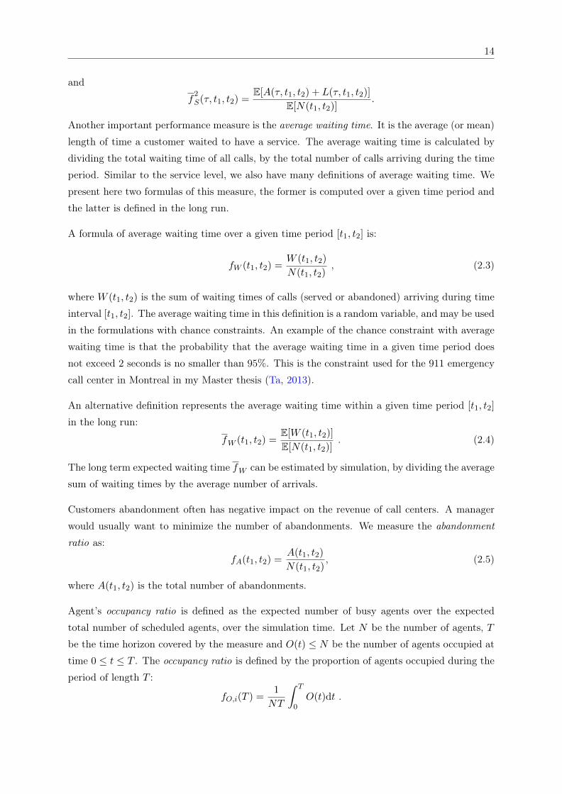
Another important performance measure is the average waiting time. It is the average (or mean)

length of time a customer waited to have a service. The average waiting time is calculated by

dividing the total waiting time of all calls, by the total number of calls arriving during the time

period. Similar to the service level, we also have many definitions of average waiting time. We

present here two formulas of this measure, the former is computed over a given time period and

the latter is defined in the long run.

A formula of average waiting time over a given time period [t1, t2] is:

fW (t1, t2) =W (t1, t2)

N(t1, t2), (2.3)

where W (t1, t2) is the sum of waiting times of calls (served or abandoned) arriving during time

interval [t1, t2]. The average waiting time in this definition is a random variable, and may be used

in the formulations with chance constraints. An example of the chance constraint with average

waiting time is that the probability that the average waiting time in a given time period does

not exceed 2 seconds is no smaller than 95%. This is the constraint used for the 911 emergency

call center in Montreal in my Master thesis (Ta, 2013).

An alternative definition represents the average waiting time within a given time period [t1, t2]

in the long run:

fW (t1, t2) =E[W (t1, t2)]

E[N(t1, t2)]. (2.4)

The long term expected waiting time fW can be estimated by simulation, by dividing the average

sum of waiting times by the average number of arrivals.

Customers abandonment often has negative impact on the revenue of call centers. A manager

would usually want to minimize the number of abandonments. We measure the abandonment

ratio as:

fA(t1, t2) =A(t1, t2)

N(t1, t2), (2.5)

where A(t1, t2) is the total number of abandonments.

Agent’s occupancy ratio is defined as the expected number of busy agents over the expected

total number of scheduled agents, over the simulation time. Let N be the number of agents, T

be the time horizon covered by the measure and O(t) ≤ N be the number of agents occupied at

time 0 ≤ t ≤ T . The occupancy ratio is defined by the proportion of agents occupied during the

period of length T :

fO,i(T ) =1

NT

∫ T

0O(t)dt .

15

2.1.4 Evaluation of Performance Measures

In call centers, the manager must plan the number of agents to serve calls, in order to meet

certain service qualities. The performance measures are complex functions so that optimization

algorithms have to resort to approximation methods or simulation.

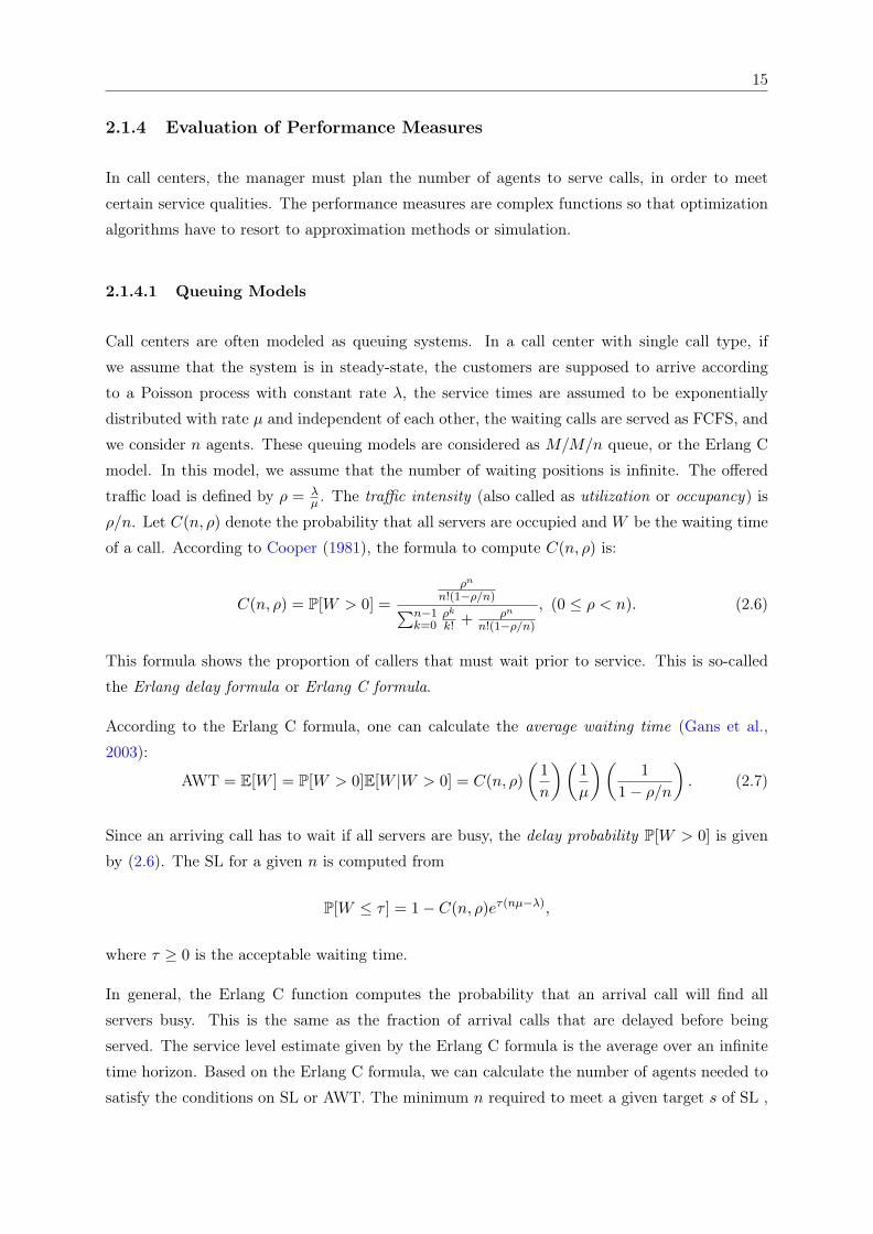
2.1.4.1 Queuing Models

Call centers are often modeled as queuing systems. In a call center with single call type, if

we assume that the system is in steady-state, the customers are supposed to arrive according

to a Poisson process with constant rate λ, the service times are assumed to be exponentially

distributed with rate µ and independent of each other, the waiting calls are served as FCFS, and

we consider n agents. These queuing models are considered as M/M/n queue, or the Erlang C

model. In this model, we assume that the number of waiting positions is infinite. The offered

traffic load is defined by ρ = λµ . The traffic intensity (also called as utilization or occupancy) is

ρ/n. Let C(n, ρ) denote the probability that all servers are occupied and W be the waiting time

of a call. According to Cooper (1981), the formula to compute C(n, ρ) is:

C(n, ρ) = P[W > 0] =

ρn

n!(1−ρ/n)∑n−1k=0

ρk

k! + ρn

n!(1−ρ/n)

, (0 ≤ ρ < n). (2.6)

This formula shows the proportion of callers that must wait prior to service. This is so-called

the Erlang delay formula or Erlang C formula.

According to the Erlang C formula, one can calculate the average waiting time (Gans et al.,

2003):

AWT = E[W ] = P[W > 0]E[W |W > 0] = C(n, ρ)

(1

n

)(1

µ

)(1

1− ρ/n

). (2.7)

Since an arriving call has to wait if all servers are busy, the delay probability P[W > 0] is given

by (2.6). The SL for a given n is computed from

P[W ≤ τ ] = 1− C(n, ρ)eτ(nµ−λ),

where τ ≥ 0 is the acceptable waiting time.

In general, the Erlang C function computes the probability that an arrival call will find all

servers busy. This is the same as the fraction of arrival calls that are delayed before being

served. The service level estimate given by the Erlang C formula is the average over an infinite

time horizon. Based on the Erlang C formula, we can calculate the number of agents needed to

satisfy the conditions on SL or AWT. The minimum n required to meet a given target s of SL ,

16

i.e., minn≥0n : PW ≤ τ ≥ s can be obtained by some methods, using the fact that the SL

is monotone in n. In Ta (2013), we use the Erlang C formula and the binary search to find the

required number of staffs.

Robbins et al. (2010) analyze the goodness of fit to data of the Erlang C models. They relax many

assumptions of the Erlang C call center model, then use simulation to obtain some performances,

and compare those with the theoretical performance predictions of the Erlang C model. They

show that the Erlang C model works reasonably well for large call centers with low to moderate

occupancy ratio. On the other hand, the model error becomes quite large when there exists

factors that tend to generate caller abandonment, such as high occupancy, small number of

agents, and impatient callers.

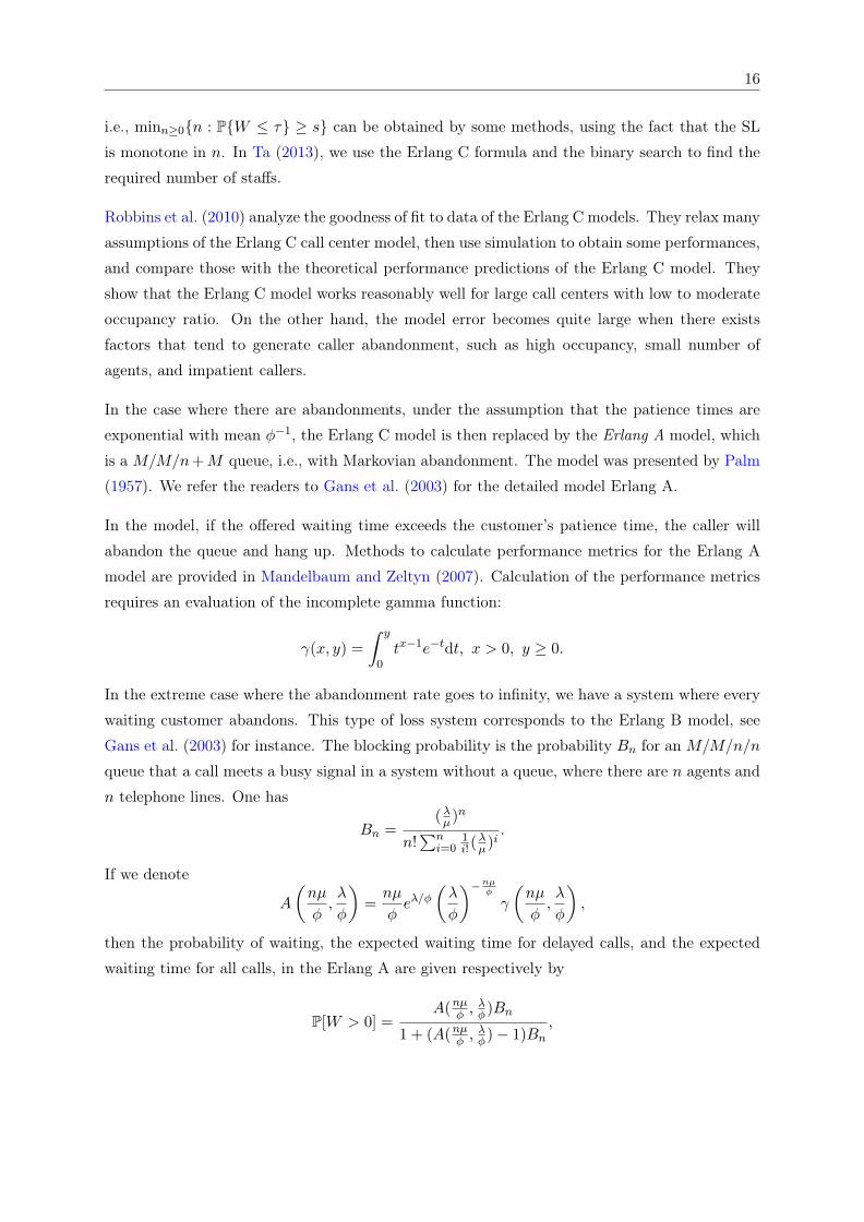
In the case where there are abandonments, under the assumption that the patience times are

exponential with mean φ−1, the Erlang C model is then replaced by the Erlang A model, which

is a M/M/n+M queue, i.e., with Markovian abandonment. The model was presented by Palm

(1957). We refer the readers to Gans et al. (2003) for the detailed model Erlang A.

In the model, if the offered waiting time exceeds the customer’s patience time, the caller will

abandon the queue and hang up. Methods to calculate performance metrics for the Erlang A

model are provided in Mandelbaum and Zeltyn (2007). Calculation of the performance metrics

requires an evaluation of the incomplete gamma function:

γ(x, y) =

∫ y

0tx−1e−tdt, x > 0, y ≥ 0.

In the extreme case where the abandonment rate goes to infinity, we have a system where every

waiting customer abandons. This type of loss system corresponds to the Erlang B model, see

Gans et al. (2003) for instance. The blocking probability is the probability Bn for an M/M/n/n

queue that a call meets a busy signal in a system without a queue, where there are n agents and

n telephone lines. One has

Bn =(λµ)n

n!∑n

i=01i!(

λµ)i

.

If we denote

A

(nµ

φ,λ

φ

)=nµ

φeλ/φ

(λ

φ

)−nµφ

γ

(nµ

φ,λ

φ

),

then the probability of waiting, the expected waiting time for delayed calls, and the expected

waiting time for all calls, in the Erlang A are given respectively by

P[W > 0] =A(nµφ ,

λφ)Bn

1 + (A(nµφ ,λφ)− 1)Bn

,

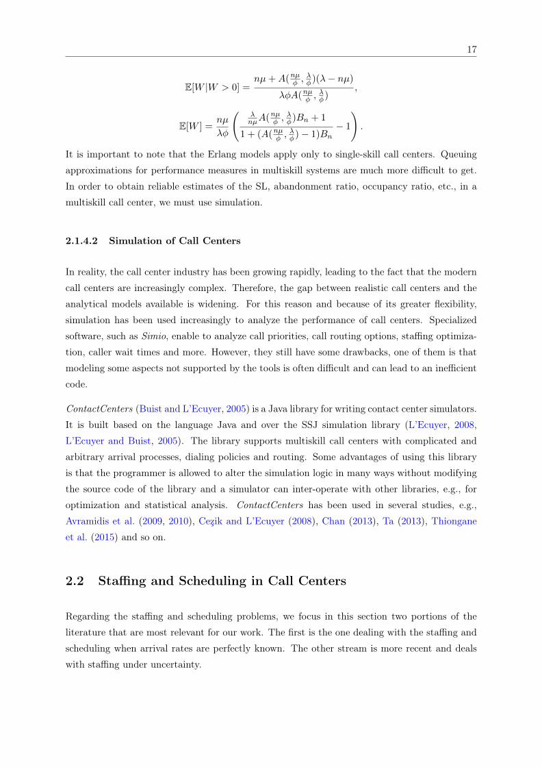
17

E[W |W > 0] =nµ+A(nµφ ,

λφ)(λ− nµ)

λφA(nµφ ,λφ)

,

E[W ] =nµ

λφ

(λnµA(nµφ ,

λφ)Bn + 1

1 + (A(nµφ ,λφ)− 1)Bn

− 1

).

It is important to note that the Erlang models apply only to single-skill call centers. Queuing

approximations for performance measures in multiskill systems are much more difficult to get.

In order to obtain reliable estimates of the SL, abandonment ratio, occupancy ratio, etc., in a

multiskill call center, we must use simulation.

2.1.4.2 Simulation of Call Centers

In reality, the call center industry has been growing rapidly, leading to the fact that the modern

call centers are increasingly complex. Therefore, the gap between realistic call centers and the

analytical models available is widening. For this reason and because of its greater flexibility,

simulation has been used increasingly to analyze the performance of call centers. Specialized

software, such as Simio, enable to analyze call priorities, call routing options, staffing optimiza-

tion, caller wait times and more. However, they still have some drawbacks, one of them is that

modeling some aspects not supported by the tools is often difficult and can lead to an inefficient

code.

ContactCenters (Buist and L’Ecuyer, 2005) is a Java library for writing contact center simulators.

It is built based on the language Java and over the SSJ simulation library (L’Ecuyer, 2008,

L’Ecuyer and Buist, 2005). The library supports multiskill call centers with complicated and

arbitrary arrival processes, dialing policies and routing. Some advantages of using this library

is that the programmer is allowed to alter the simulation logic in many ways without modifying

the source code of the library and a simulator can inter-operate with other libraries, e.g., for

optimization and statistical analysis. ContactCenters has been used in several studies, e.g.,

Avramidis et al. (2009, 2010), Cezik and L’Ecuyer (2008), Chan (2013), Ta (2013), Thiongane

et al. (2015) and so on.

2.2 Staffing and Scheduling in Call Centers

Regarding the staffing and scheduling problems, we focus in this section two portions of the

literature that are most relevant for our work. The first is the one dealing with the staffing and

scheduling when arrival rates are perfectly known. The other stream is more recent and deals

with staffing under uncertainty.

18

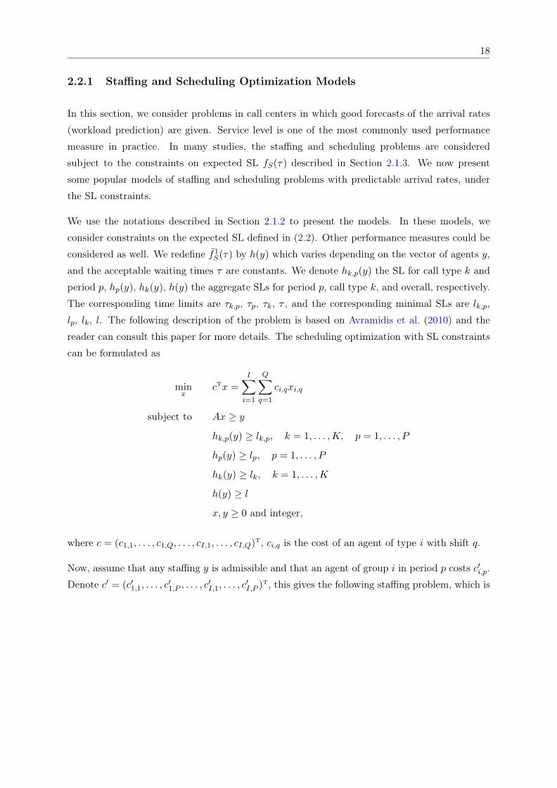
2.2.1 Staffing and Scheduling Optimization Models

In this section, we consider problems in call centers in which good forecasts of the arrival rates

(workload prediction) are given. Service level is one of the most commonly used performance

measure in practice. In many studies, the staffing and scheduling problems are considered

subject to the constraints on expected SL fS(τ) described in Section 2.1.3. We now present

some popular models of staffing and scheduling problems with predictable arrival rates, under

the SL constraints.

We use the notations described in Section 2.1.2 to present the models. In these models, we

consider constraints on the expected SL defined in (2.2). Other performance measures could be

considered as well. We redefine f1S(τ) by h(y) which varies depending on the vector of agents y,

and the acceptable waiting times τ are constants. We denote hk,p(y) the SL for call type k and

period p, hp(y), hk(y), h(y) the aggregate SLs for period p, call type k, and overall, respectively.

The corresponding time limits are τk,p, τp, τk, τ , and the corresponding minimal SLs are lk,p,

lp, lk, l. The following description of the problem is based on Avramidis et al. (2010) and the

reader can consult this paper for more details. The scheduling optimization with SL constraints

can be formulated as

minx

cTx =I∑i=1

Q∑q=1

ci,qxi,q

subject to Ax ≥ y

hk,p(y) ≥ lk,p, k = 1, . . . ,K, p = 1, . . . , P

hp(y) ≥ lp, p = 1, . . . , P

hk(y) ≥ lk, k = 1, . . . ,K

h(y) ≥ l

x, y ≥ 0 and integer,

where c = (c1,1, . . . , c1,Q, . . . , cI,1, . . . , cI,Q)T, ci,q is the cost of an agent of type i with shift q.

Now, assume that any staffing y is admissible and that an agent of group i in period p costs c′i,p.

Denote c′ = (c′1,1, . . . , c′1,P , . . . , c

′I,1, . . . , c

′I,P )T, this gives the following staffing problem, which is

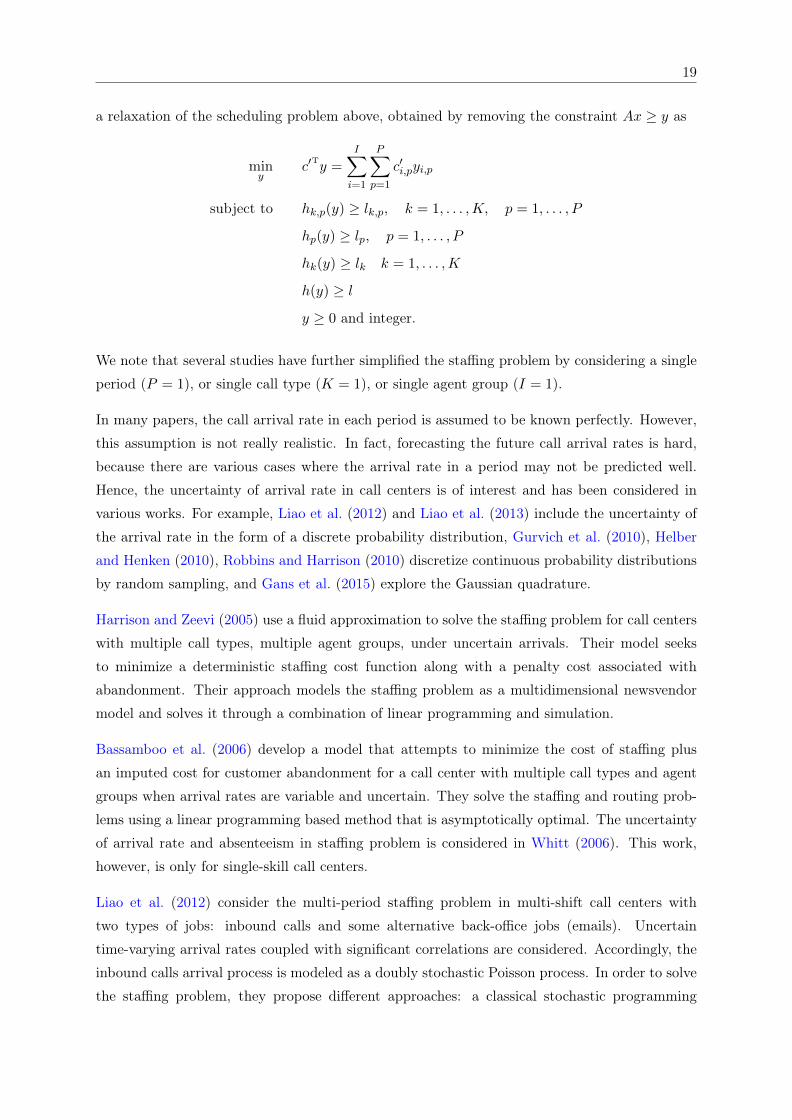
19

a relaxation of the scheduling problem above, obtained by removing the constraint Ax ≥ y as

miny

c′Ty =

I∑i=1

P∑p=1

c′i,pyi,p

subject to hk,p(y) ≥ lk,p, k = 1, . . . ,K, p = 1, . . . , P

hp(y) ≥ lp, p = 1, . . . , P

hk(y) ≥ lk k = 1, . . . ,K

h(y) ≥ l

y ≥ 0 and integer.

We note that several studies have further simplified the staffing problem by considering a single

period (P = 1), or single call type (K = 1), or single agent group (I = 1).

In many papers, the call arrival rate in each period is assumed to be known perfectly. However,

this assumption is not really realistic. In fact, forecasting the future call arrival rates is hard,

because there are various cases where the arrival rate in a period may not be predicted well.

Hence, the uncertainty of arrival rate in call centers is of interest and has been considered in

various works. For example, Liao et al. (2012) and Liao et al. (2013) include the uncertainty of

the arrival rate in the form of a discrete probability distribution, Gurvich et al. (2010), Helber

and Henken (2010), Robbins and Harrison (2010) discretize continuous probability distributions

by random sampling, and Gans et al. (2015) explore the Gaussian quadrature.

Harrison and Zeevi (2005) use a fluid approximation to solve the staffing problem for call centers

with multiple call types, multiple agent groups, under uncertain arrivals. Their model seeks

to minimize a deterministic staffing cost function along with a penalty cost associated with

abandonment. Their approach models the staffing problem as a multidimensional newsvendor

model and solves it through a combination of linear programming and simulation.

Bassamboo et al. (2006) develop a model that attempts to minimize the cost of staffing plus

an imputed cost for customer abandonment for a call center with multiple call types and agent

groups when arrival rates are variable and uncertain. They solve the staffing and routing prob-

lems using a linear programming based method that is asymptotically optimal. The uncertainty

of arrival rate and absenteeism in staffing problem is considered in Whitt (2006). This work,

however, is only for single-skill call centers.

Liao et al. (2012) consider the multi-period staffing problem in multi-shift call centers with

two types of jobs: inbound calls and some alternative back-office jobs (emails). Uncertain

time-varying arrival rates coupled with significant correlations are considered. Accordingly, the

inbound calls arrival process is modeled as a doubly stochastic Poisson process. In order to solve

the staffing problem, they propose different approaches: a classical stochastic programming

20

approach, a robust programming approach and a mixed robust programming approach. By

conducting a numerical study, they evaluate the performance of their proposed methods. They

analyze the necessity of considering the uncertainty in the call demand parameters. They also

find out that the flexibility of the back-office jobs, e.g., emails can be stored, can help to mitigate

the effect of the uncertainty of the call demand. In another work, Liao et al. (2013) consider a

call center with a single type of inbound calls in a multi-period multi-shift setting with uncertain

arrival rates, that vary according to an intra-day seasonality and a global busyness factor. They

propose an approach combining stochastic programming and distributionally robust optimization

in order to minimize the total salary costs under service level constraints. After that, two

different constructions for the uncertainty set are introduced: the first one is based on statistical

confidence sets and the second does not make reference to probabilistic arguments. By simulating

the robust solution via Monte Carlo techniques, they show that the two approaches perform very

similarly.

Both Robbins and Harrison (2010) and Gans et al. (2015) consider a stochastic programming

approach to shift scheduling under arrival rate uncertainty for single-call type, single-group call

centers with the average constraint formulation. However, while Robbins and Harrison (2010)

consider a global service level requirement aiming at minimizing the sum of the total cost of

staffing and the expected penalty cost associated with failure, Gans et al. (2015) minimize the

total staffing cost under constraints on expected abandonment.

In Robbins and Harrison (2010), a sample of realizations of call arrivals are generated. Then

they formulate the model as a two-stage (without recourse) mixed-integer stochastic program:

staffing decisions are made in the first stage, and in the second stage, call volume is realized.

The SL target in each period of each scenario of arrival rate is estimated based on a convex

linear approximation of the SL curve. Then, the branch-and-bound method is used to solve the

problem. Gans et al. (2015) use recourse action (add or remove agents) to adjust per-scheduled

staffing levels from arrival rate forecasts. They suppose that a forecast update is obtained at

midday, and agents can be added or removed to correct the schedules. Constraints on the

fraction of abandonments are considered, and the abandonment function of a Markovian queue

are approximated by a piecewise-linear function, similar to Robbins and Harrison (2010).

In typical problem formulations, constraints with respect to the average performance measures

in the long run are considered. Gurvich et al. (2010) propose a different problem formulation

in which they consider probabilistic constraints on the (random) values over a given time pe-

riod. The arrival rates are assumed to be random but time-independent. They consider the

chance constraints on the abandonment ratios. Let δ be a risk level chosen by the call center’s

management. The requirement is that the QoS could be violated on at most a fraction δ of

the arrival rate realizations. The single-call type, single-agent group call center is modeled as

an M(Λ)/M(µ)/N + M(φ) queue. Assuming that the service rate µ and the patience rate φ

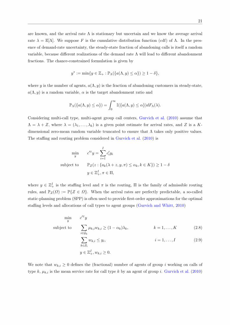
21

are known, and the arrival rate Λ is stationary but uncertain and we know the average arrival

rate λ = E[Λ]. We suppose F is the cumulative distribution function (cdf) of Λ. In the pres-

ence of demand-rate uncertainty, the steady-state fraction of abandoning calls is itself a random

variable, because different realizations of the demand rate Λ will lead to different abandonment

fractions. The chance-constrained formulation is given by

y∗ := miny ∈ Z+ : PΛ(a(Λ, y) ≤ α) ≥ 1− δ,

where y is the number of agents, a(Λ, y) is the fraction of abandoning customers in steady-state,

a(Λ, y) is a random variable, α is the target abandonment ratio and

PΛ(a(Λ, y) ≤ α) =

∫ ∞0

I(a(Λ, y) ≤ α)dFΛ(λ).

Considering multi-call type, multi-agent group call centers, Gurvich et al. (2010) assume that

Λ = λ + Z, where λ = (λ1, . . . , λk) is a given point estimate for arrival rates, and Z is a K-

dimensional zero-mean random variable truncated to ensure that Λ takes only positive values.

The staffing and routing problem considered in Gurvich et al. (2010) is

miny

c′Ty =I∑i=1

c′iyi

subject to PZ(z : ak(λ+ z, y, π) ≤ αk, k ∈ K) ≥ 1− δ

y ∈ ZI+, π ∈ Π,

where y ∈ ZI+ is the staffing level and π is the routing, Π is the family of admissible routing

rules, and PZ(Ω) := PZ ∈ Ω. When the arrival rates are perfectly predictable, a so-called

static-planning problem (SPP) is often used to provide first-order approximations for the optimal

staffing levels and allocations of call types to agent groups (Gurvich and Whitt, 2010)

miny

c′Ty

subject to∑i∈Gk

µk,iwk,i ≥ (1− αk)λk, k = 1, . . . ,K (2.8)

∑k∈Si

wk,i ≤ yi, i = 1, . . . , I (2.9)

y ∈ ZI+, wk,i ≥ 0.

We note that wk,i ≥ 0 defines the (fractional) number of agents of group i working on calls of

type k, µk,i is the mean service rate for call type k by an agent of group i. Gurvich et al. (2010)

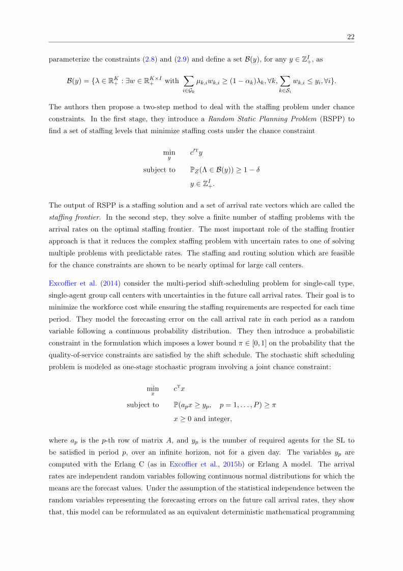
22

parameterize the constraints (2.8) and (2.9) and define a set B(y), for any y ∈ ZI+, as

B(y) = λ ∈ RK+ : ∃w ∈ RK×I+ with∑i∈Gk

µk,iwk,i ≥ (1− αk)λk,∀k,∑k∈Si

wk,i ≤ yi,∀i.

The authors then propose a two-step method to deal with the staffing problem under chance

constraints. In the first stage, they introduce a Random Static Planning Problem (RSPP) to

find a set of staffing levels that minimize staffing costs under the chance constraint

miny

c′Ty

subject to PZ(Λ ∈ B(y)) ≥ 1− δ

y ∈ ZI+.

The output of RSPP is a staffing solution and a set of arrival rate vectors which are called the

staffing frontier. In the second step, they solve a finite number of staffing problems with the

arrival rates on the optimal staffing frontier. The most important role of the staffing frontier

approach is that it reduces the complex staffing problem with uncertain rates to one of solving

multiple problems with predictable rates. The staffing and routing solution which are feasible

for the chance constraints are shown to be nearly optimal for large call centers.

Excoffier et al. (2014) consider the multi-period shift-scheduling problem for single-call type,

single-agent group call centers with uncertainties in the future call arrival rates. Their goal is to

minimize the workforce cost while ensuring the staffing requirements are respected for each time

period. They model the forecasting error on the call arrival rate in each period as a random

variable following a continuous probability distribution. They then introduce a probabilistic

constraint in the formulation which imposes a lower bound π ∈ [0, 1] on the probability that the

quality-of-service constraints are satisfied by the shift schedule. The stochastic shift scheduling

problem is modeled as one-stage stochastic program involving a joint chance constraint:

minx

cTx

subject to P(apx ≥ yp, p = 1, . . . , P ) ≥ π

x ≥ 0 and integer,

where ap is the p-th row of matrix A, and yp is the number of required agents for the SL to

be satisfied in period p, over an infinite horizon, not for a given day. The variables yp are

computed with the Erlang C (as in Excoffier et al., 2015b) or Erlang A model. The arrival

rates are independent random variables following continuous normal distributions for which the

means are the forecast values. Under the assumption of the statistical independence between the

random variables representing the forecasting errors on the future call arrival rates, they show

that, this model can be reformulated as an equivalent deterministic mathematical programming

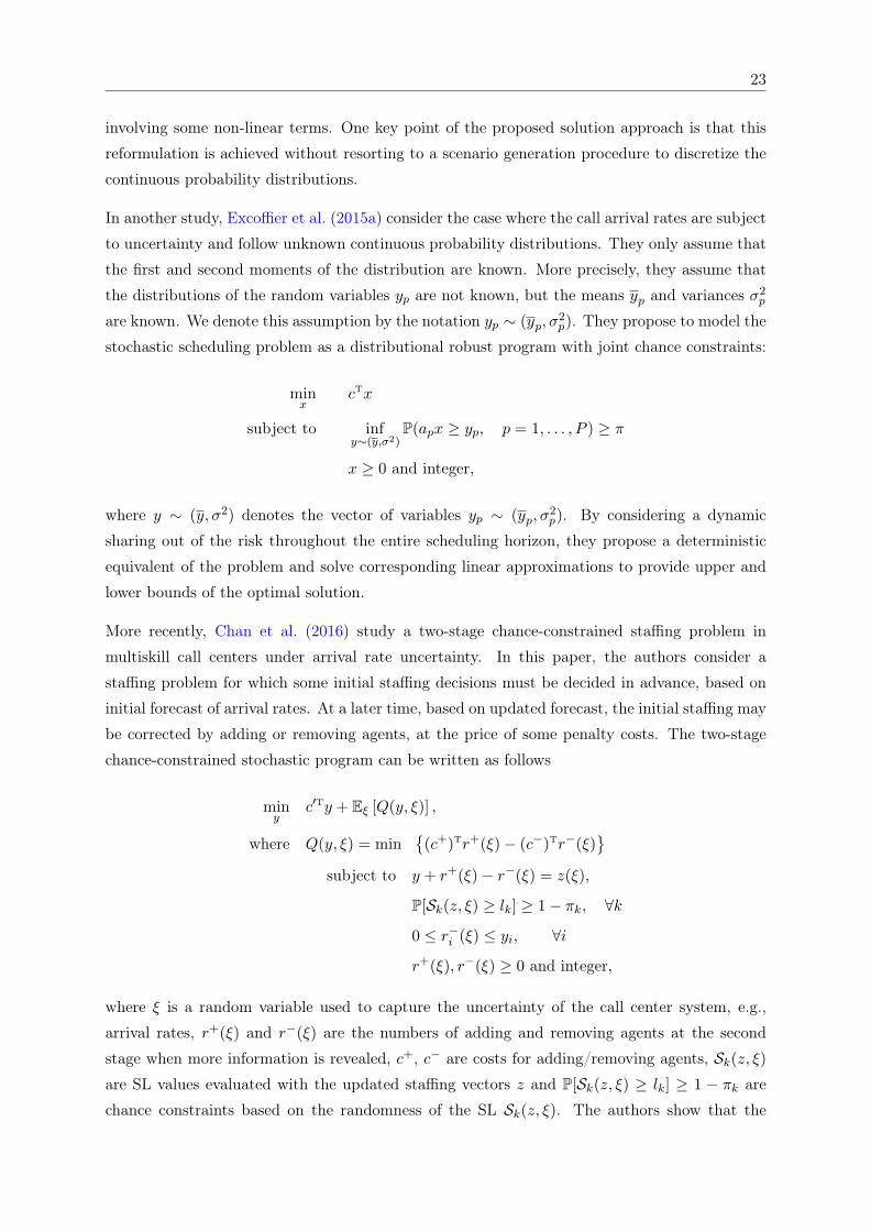
23

involving some non-linear terms. One key point of the proposed solution approach is that this

reformulation is achieved without resorting to a scenario generation procedure to discretize the

continuous probability distributions.

In another study, Excoffier et al. (2015a) consider the case where the call arrival rates are subject

to uncertainty and follow unknown continuous probability distributions. They only assume that

the first and second moments of the distribution are known. More precisely, they assume that

the distributions of the random variables yp are not known, but the means yp and variances σ2p

are known. We denote this assumption by the notation yp ∼ (yp, σ2p). They propose to model the

stochastic scheduling problem as a distributional robust program with joint chance constraints:

minx

cTx

subject to infy∼(y,σ2)

P(apx ≥ yp, p = 1, . . . , P ) ≥ π

x ≥ 0 and integer,

where y ∼ (y, σ2) denotes the vector of variables yp ∼ (yp, σ2p). By considering a dynamic

sharing out of the risk throughout the entire scheduling horizon, they propose a deterministic

equivalent of the problem and solve corresponding linear approximations to provide upper and

lower bounds of the optimal solution.

More recently, Chan et al. (2016) study a two-stage chance-constrained staffing problem in

multiskill call centers under arrival rate uncertainty. In this paper, the authors consider a

staffing problem for which some initial staffing decisions must be decided in advance, based on

initial forecast of arrival rates. At a later time, based on updated forecast, the initial staffing may

be corrected by adding or removing agents, at the price of some penalty costs. The two-stage

chance-constrained stochastic program can be written as follows

miny

c′Ty + Eξ [Q(y, ξ)] ,

where Q(y, ξ) = min

(c+)Tr+(ξ)− (c−)Tr−(ξ)

subject to y + r+(ξ)− r−(ξ) = z(ξ),

P[Sk(z, ξ) ≥ lk] ≥ 1− πk, ∀k

0 ≤ r−i (ξ) ≤ yi, ∀i

r+(ξ), r−(ξ) ≥ 0 and integer,

where ξ is a random variable used to capture the uncertainty of the call center system, e.g.,

arrival rates, r+(ξ) and r−(ξ) are the numbers of adding and removing agents at the second

stage when more information is revealed, c+, c− are costs for adding/removing agents, Sk(z, ξ)are SL values evaluated with the updated staffing vectors z and P[Sk(z, ξ) ≥ lk] ≥ 1 − πk are

chance constraints based on the randomness of the SL Sk(z, ξ). The authors show that the

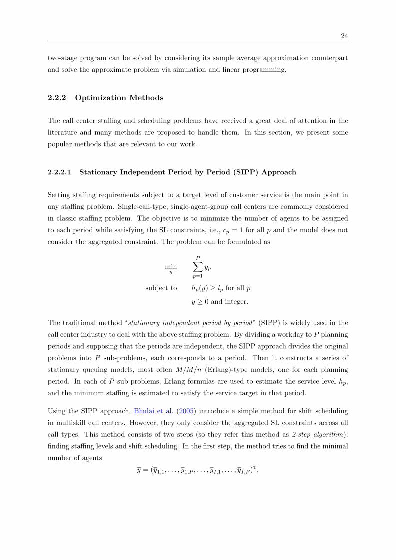
24

two-stage program can be solved by considering its sample average approximation counterpart

and solve the approximate problem via simulation and linear programming.

2.2.2 Optimization Methods

The call center staffing and scheduling problems have received a great deal of attention in the

literature and many methods are proposed to handle them. In this section, we present some

popular methods that are relevant to our work.

2.2.2.1 Stationary Independent Period by Period (SIPP) Approach

Setting staffing requirements subject to a target level of customer service is the main point in

any staffing problem. Single-call-type, single-agent-group call centers are commonly considered

in classic staffing problem. The objective is to minimize the number of agents to be assigned

to each period while satisfying the SL constraints, i.e., cp = 1 for all p and the model does not

consider the aggregated constraint. The problem can be formulated as

miny

P∑p=1

yp

subject to hp(y) ≥ lp for all p

y ≥ 0 and integer.

The traditional method “stationary independent period by period ” (SIPP) is widely used in the

call center industry to deal with the above staffing problem. By dividing a workday to P planning

periods and supposing that the periods are independent, the SIPP approach divides the original

problems into P sub-problems, each corresponds to a period. Then it constructs a series of

stationary queuing models, most often M/M/n (Erlang)-type models, one for each planning

period. In each of P sub-problems, Erlang formulas are used to estimate the service level hp,

and the minimum staffing is estimated to satisfy the service target in that period.

Using the SIPP approach, Bhulai et al. (2005) introduce a simple method for shift scheduling

in multiskill call centers. However, they only consider the aggregated SL constraints across all

call types. This method consists of two steps (so they refer this method as 2-step algorithm):

finding staffing levels and shift scheduling. In the first step, the method tries to find the minimal

number of agents

y = (y1,1, . . . , y1,P , . . . , yI,1, . . . , yI,P )T,

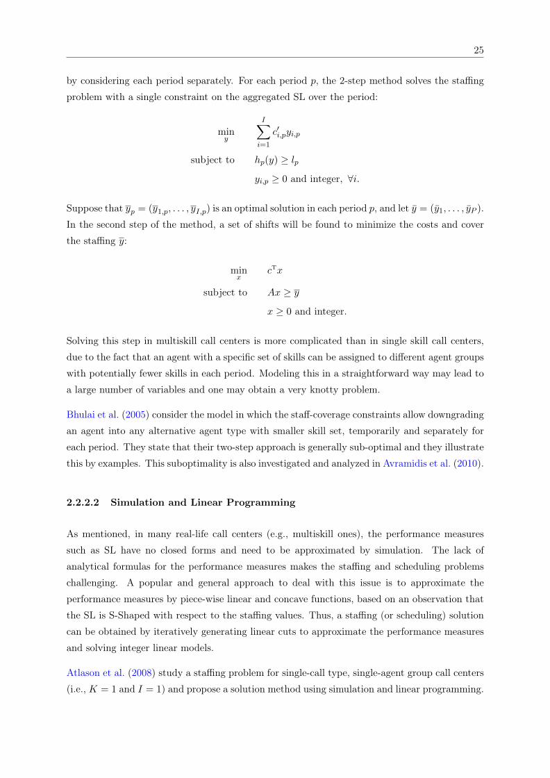
25

by considering each period separately. For each period p, the 2-step method solves the staffing

problem with a single constraint on the aggregated SL over the period:

miny

I∑i=1

c′i,pyi,p

subject to hp(y) ≥ lp

yi,p ≥ 0 and integer, ∀i.

Suppose that yp = (y1,p, . . . , yI,p) is an optimal solution in each period p, and let y = (y1, . . . , yP ).

In the second step of the method, a set of shifts will be found to minimize the costs and cover

the staffing y:

minx

cTx

subject to Ax ≥ y

x ≥ 0 and integer.

Solving this step in multiskill call centers is more complicated than in single skill call centers,

due to the fact that an agent with a specific set of skills can be assigned to different agent groups

with potentially fewer skills in each period. Modeling this in a straightforward way may lead to

a large number of variables and one may obtain a very knotty problem.

Bhulai et al. (2005) consider the model in which the staff-coverage constraints allow downgrading

an agent into any alternative agent type with smaller skill set, temporarily and separately for

each period. They state that their two-step approach is generally sub-optimal and they illustrate

this by examples. This suboptimality is also investigated and analyzed in Avramidis et al. (2010).

2.2.2.2 Simulation and Linear Programming

As mentioned, in many real-life call centers (e.g., multiskill ones), the performance measures

such as SL have no closed forms and need to be approximated by simulation. The lack of

analytical formulas for the performance measures makes the staffing and scheduling problems

challenging. A popular and general approach to deal with this issue is to approximate the

performance measures by piece-wise linear and concave functions, based on an observation that

the SL is S-Shaped with respect to the staffing values. Thus, a staffing (or scheduling) solution

can be obtained by iteratively generating linear cuts to approximate the performance measures

and solving integer linear models.

Atlason et al. (2008) study a staffing problem for single-call type, single-agent group call centers

(i.e., K = 1 and I = 1) and propose a solution method using simulation and linear programming.

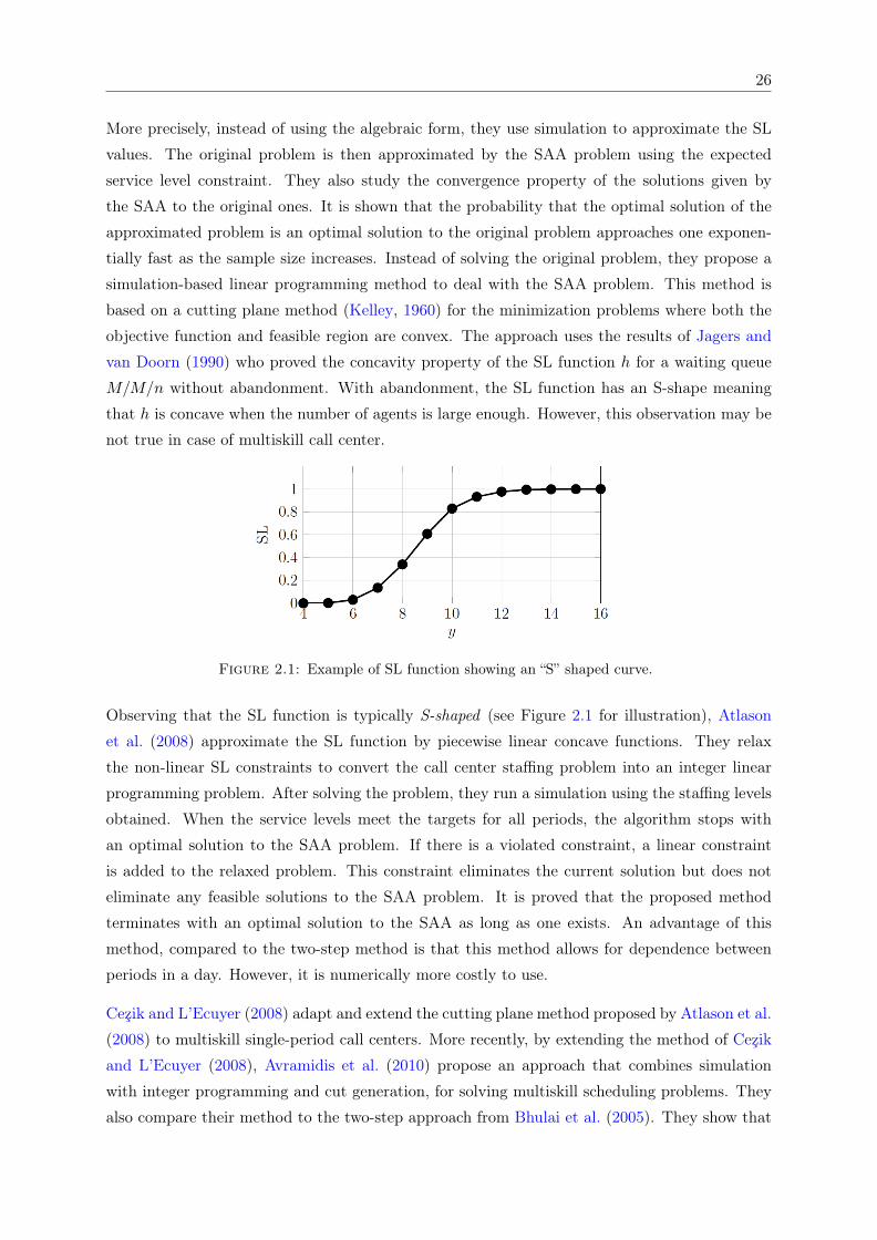
26

More precisely, instead of using the algebraic form, they use simulation to approximate the SL

values. The original problem is then approximated by the SAA problem using the expected

service level constraint. They also study the convergence property of the solutions given by

the SAA to the original ones. It is shown that the probability that the optimal solution of the

approximated problem is an optimal solution to the original problem approaches one exponen-

tially fast as the sample size increases. Instead of solving the original problem, they propose a

simulation-based linear programming method to deal with the SAA problem. This method is

based on a cutting plane method (Kelley, 1960) for the minimization problems where both the

objective function and feasible region are convex. The approach uses the results of Jagers and

van Doorn (1990) who proved the concavity property of the SL function h for a waiting queue

M/M/n without abandonment. With abandonment, the SL function has an S-shape meaning

that h is concave when the number of agents is large enough. However, this observation may be

not true in case of multiskill call center.

Figure 2.1: Example of SL function showing an “S” shaped curve.

Observing that the SL function is typically S-shaped (see Figure 2.1 for illustration), Atlason

et al. (2008) approximate the SL function by piecewise linear concave functions. They relax

the non-linear SL constraints to convert the call center staffing problem into an integer linear

programming problem. After solving the problem, they run a simulation using the staffing levels

obtained. When the service levels meet the targets for all periods, the algorithm stops with

an optimal solution to the SAA problem. If there is a violated constraint, a linear constraint

is added to the relaxed problem. This constraint eliminates the current solution but does not

eliminate any feasible solutions to the SAA problem. It is proved that the proposed method

terminates with an optimal solution to the SAA as long as one exists. An advantage of this

method, compared to the two-step method is that this method allows for dependence between

periods in a day. However, it is numerically more costly to use.

Cezik and L’Ecuyer (2008) adapt and extend the cutting plane method proposed by Atlason et al.

(2008) to multiskill single-period call centers. More recently, by extending the method of Cezik

and L’Ecuyer (2008), Avramidis et al. (2010) propose an approach that combines simulation

with integer programming and cut generation, for solving multiskill scheduling problems. They

also compare their method to the two-step approach from Bhulai et al. (2005). They show that

27

the two-step method sometimes yields solutions that are highly sub-optimal and inferior to those

obtained by their proposed method.

2.3 Stochastic Programming

In this section we give a short introduction to the field of stochastic programming. To keep the

exposition in line with the rest of the thesis, we only focus on models and methods that are

relevant to our work, namely, two-stage linear stochastic programming and the sample average

approximation approach. For more knowledge, we refer the readers to Birge and Louveaux

(2011). The notations used in the section related to the review of stochastic programming may be

re-used in other sections related to the description of call centers, with different interpretations.

2.3.1 An Introduction to Stochastic Programming

The field of stochastic programming is concerned with mathematical optimization under uncer-

tainty. Whereas deterministic optimization problems are formulated under the assumption that

the parameters are known, real world problems mostly include parameters which are unknown

at the time decisions should be made. Since the parameters are uncertain, one might seek a

solution that is feasible for all possible realizations of the random components. This approach is

however too conservative in many applications. Stochastic programming models deal with the

uncertainty by taking advantage of the fact that probability distributions governing the data

can be estimated through historical observations.

The two-stage stochastic program with recourse actions is the most basic stochastic recourse

problem that has been intensively studied and has many real-life applications. In the problem,

we assume that non-anticipative decisions represent the main decisions that have already been

made and that a temporary violation of the random constraints is allowed. Recourse actions

then can be made until the realization of uncertainty is observed. In this fashion, the decisions

are partitioned into two stages according to the availability of the information. We refer to them

as first-stage and second-stage decisions. The classical two-stage linear stochastic programming

problems can be formulated as

minx∈Xg(x) = cTx+ Eξ[Q(x, ξ)] , (2.10)

where Q(x, ξ) is the optimal value of the second-stage problem

miny∈Y

qTy subject to Tx+Wy = h, (2.11)

28

where X,Y ⊆ Rn are the sets of first-stage and second-stage decision vectors, respectively,

T, W ∈ Rn×n and h ∈ Rn. ξ = (q, T,W, h) contains the data of the second-stage problem.

In this formulation, at the first stage we have to make a “here-and-now ” decision x before the

realization of the uncertain data ξ is known. At the second stage, after a realization of ξ becomes

available, we make recourse actions by solving the second-stage optimization problem.

The expectation in the two-stage formulation above requires a knowledge on the distribution of

the random vector ξ. A standard approach is to assume that ξ has a finite number of realizations,

called scenarios, say ξ1, . . . , ξK with respective probabilities p1, . . . , pK . Then, the expectation

can be written as the summation

E[Q(x, ξ)] =

K∑k=1

pkQ(x, ξk),

and the two-stage problem (2.10)-(2.11) can be formulated as a large one-stage programming

problem (deterministic equivalent problem) as

(DE)

min

x,y1,...,yKcTx+

K∑k=1

pkqTk yk

subject to Tkx+Wkyk = hk, k = 1, . . . ,K

x ∈ X, yk ∈ Y, k = 1, . . . ,K.

In (DE) we make a copy yk of the second-stage decision vector y for each scenario k. By

solving (DE) we obtain an optimal solution x∗ for the first-stage problem and optimal solutions

y∗1, . . . , y∗K for the second-stage problem for each scenario k ∈ 1, . . . ,K.

A serious issue in the context is that for some x ∈ X and scenario ξk, the system Tkx+Wkyk = hk

may have no solution yk ∈ Y , i.e., the second-stage problem may be infeasible. In this case, the

standard practice is to set Q(x, ξk) =∞ and we do that. That is, we impose an infinite penalty

if the second-stage problem is infeasible and such a solution x ∈ X cannot be an optimal solution

of the first-stage problem. This will make sense if such a scenario results in a catastrophic event.

We say that the two-stage problem has relatively complete recourse if such infeasibility does not

happen, i.e., for every x ∈ X and every scenario ξk, the second-stage problem is always feasible.

In many situations, the random vector ξ has an infinite or very large support set. A common

approach is to reduce the scenario set to a manageable size by using Monte Carlo simulation.

That is, suppose that we can generate an i.i.d sample ξ1, . . . , ξN of N realizations of the random

vector ξ, i.e., each ξn is independent of each other, for n = 1, . . . , N . Given this sample, we can

approximate the objective function by the average

Q∧

N (x) =1

N

N∑n=1

Q(x, ξn),

29

and the two-stage problem can be approximated by the problem

(SAA) minx∈X

cTx+

1

N

N∑n=1

Q(x, ξn)

.

This approach is typically referred to as the SAA method (Shapiro and Philpott, 2007). Solving

the SAA problem will give an approximate solution to the true problem. A question here is how

large the sample size N (i.e., how many scenarios should be generated) in order for the SAA

problem to give a reasonably accurate solution to the true problem. We will discuss this in more

details in the next section.

2.3.2 Consistency of the Sample Average Approximation

We consider the following stochastic programming problem

(SP) minx∈X

f(x) := Eξ[F (x, ξ)]

, (2.12)

where X is a nonempty closed subset of Rn, ξ is a random vector whose probability distribution

P is supported on a set Ω ⊂ Rd, and F : X × Ω → R. Suppose that we have an independent

random sample ξ1, . . . , ξN of ω from P. The corresponding SAA program of the “true” problem

(2.12) is

minx∈X

fN (x) :=

1

N

N∑i=1

F (x, ξi)

. (2.13)

We refer to (2.12) and (2.13) as the true and SAA problems, respectively. An optimal solution

xN = arg minx∈X fN (x) for (2.13) and the corresponding optimal value vN = fN (xN ) are the

approximations of an optimal solution x∗ and of the optimal value v∗ for the true problem (2.12).

We denote by X∗ and X∗N the set of optimal solutions of the true problem (2.12) and the SAA

problem (2.13), respectively. We assume that X∗ is not empty and that a finite minimum is

attained. We assume that the set X has a norm ‖.‖ (e.g., the Euclidean norm if X is the real

space). The distance from a given solution x to optimality is dist(x,X∗) = infx∈X∗ ‖x− x∗‖.

It is important to establish upper bounds for the three error measures dist(xN , X∗), f(xN )−v∗,and vN − v∗ when the sample size N →∞. Actually, one can show that, under different set of

(mild) conditions (see Dupacová and Wets, 1988, Shapiro, 2003b, for instance), these measures

will converge to zero, w.p.1, when the sample size N grows to infinity. This convergence holds,

for example, if there exists a compact set C ⊂ Rn such that (i) X∗ ⊂ C, (ii) the function f(x)

is finite valued and continuous on C, (iii)fN (x) converges to f(x) w.p.1, as N →∞, uniformly

in x ∈ C, (iv) w.p.1 for N large enough the set X∗N is nonempty and X∗N ⊂ C; see Proposition

6 in Shapiro (2003b).

30

When the problem (2.12) has a unique optimal solution x∗, X ⊂ Rn contains a neighborhood of

x∗, and F (·, ξ) is a sufficiently smooth function with bounded variance, Central limit theorems

give estimates of order Op(N−1/2) for the three error measures mentioned above (Shapiro, 1993).

For ε ≥ 0, we denote by

Xε := x ∈ X : f(x) ≤ v∗ + ε and XεN := x ∈ X : fN (x) ≤ vN + ε

the sets of ε-optimal solutions of the true and the SAA problem, respectively. Under appropriate

conditions, by using large deviation theory (Dai et al., 2000, Kaniovski et al., 1995, Kleywegt

et al., 2002, Shapiro, 2003b, Shapiro and Homem-de Mello, 2000), one can prove exponential

convergence to zero for the probability of selecting a solution with an optimality gap that ex-

ceeds a given value. For example, let F (x, ξ) have a finite moment generating function in a

neighborhood of 0, and let ε > δ > 0. If X is finite, or if X is a bounded subset of Rn and f is

Lipschitz-continuous over X, then there are constants K and η = η(δ, ε) such that

P[XδN ⊂ Xε] ≥ 1−K exp[ηN ].

It means that the probability that any δ-optimal solution to the SAA problem is an ε-optimal

solution to the true problem converges to 1 exponentially fast in N . The constant K can be (at

worst) proportional to |X| when X is finite. In fact, this result allows to give an estimate of the

sample size which guarantees that any δ-optimal solution of the SAA problem is an ε-optimal

solution of the true problem with probability at least 1−α. The required sample size N depends

logarithmically both on the size of the feasible set X and the tolerance probability α.

We now consider the two-stage problem (2.10)-(2.11). Since Q(x, ξ) is the value of a linear

program, it can be computed exactly for a given x and ξ ∈ Ω. By taking F (x, ξ) = cTx+Q(x, ξ)

we are back to the setting of (SP) and we can apply the corresponding results to establish

the consistency of the SAA approach (see Shapiro, 2003b, Shapiro et al., 2014b, for further

discussion)

Stochastic programming with stochastic constraints is also a topic of interest in the SP literature

(e.g. Vogel, 1994). A general formulation for such problems is

minx∈X

f(x) subject to gi(x) := Eξ[Gi(x, ξ)] ≥ 0, i = 1, . . . , I,

where Gi(x, ξ) : X × Ω → R, f(x) is easy to evaluate exactly for all x ∈ X, whereas the

expectations in the constraints are estimated by Monte Carlo. In the SAA, we replace the

expectation by a sample average approximation

giN (x) =1

N

N∑n=1

Gi(x, ξn), i = 1, . . . , I,

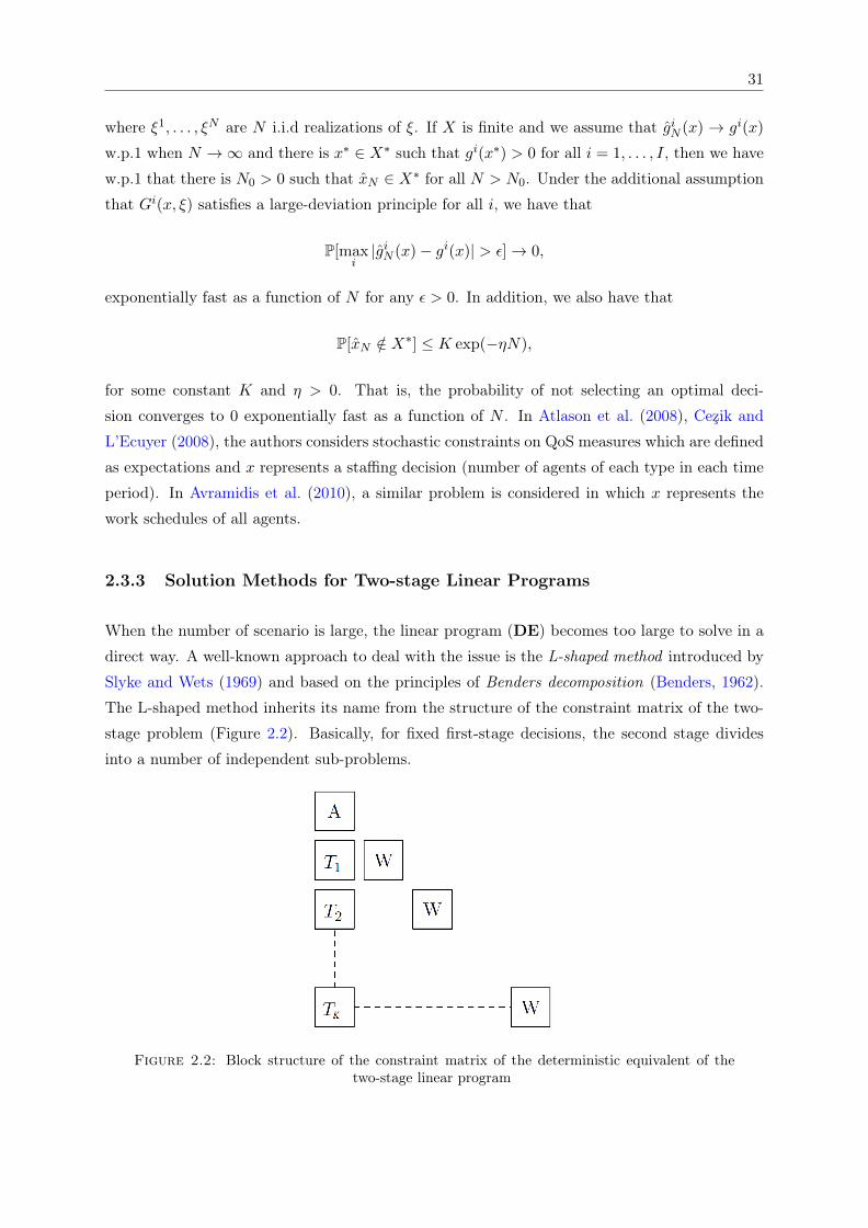
31

where ξ1, . . . , ξN are N i.i.d realizations of ξ. If X is finite and we assume that giN (x) → gi(x)

w.p.1 when N →∞ and there is x∗ ∈ X∗ such that gi(x∗) > 0 for all i = 1, . . . , I, then we have

w.p.1 that there is N0 > 0 such that xN ∈ X∗ for all N > N0. Under the additional assumption

that Gi(x, ξ) satisfies a large-deviation principle for all i, we have that

P[maxi|giN (x)− gi(x)| > ε]→ 0,

exponentially fast as a function of N for any ε > 0. In addition, we also have that

P[xN /∈ X∗] ≤ K exp(−ηN),

for some constant K and η > 0. That is, the probability of not selecting an optimal deci-

sion converges to 0 exponentially fast as a function of N . In Atlason et al. (2008), Cezik and

L’Ecuyer (2008), the authors considers stochastic constraints on QoS measures which are defined

as expectations and x represents a staffing decision (number of agents of each type in each time

period). In Avramidis et al. (2010), a similar problem is considered in which x represents the

work schedules of all agents.

2.3.3 Solution Methods for Two-stage Linear Programs

When the number of scenario is large, the linear program (DE) becomes too large to solve in a

direct way. A well-known approach to deal with the issue is the L-shaped method introduced by

Slyke and Wets (1969) and based on the principles of Benders decomposition (Benders, 1962).

The L-shaped method inherits its name from the structure of the constraint matrix of the two-

stage problem (Figure 2.2). Basically, for fixed first-stage decisions, the second stage divides

into a number of independent sub-problems.

Figure 2.2: Block structure of the constraint matrix of the deterministic equivalent of thetwo-stage linear program

32

The general idea of the L-shaped method is to approximate the recourse function (or the second-

stage objective function) by a piece-wise linear and convex function. Since the non-linear ob-

jective term involves a solution to all the second-stage programs, we want to avoid numerous

function evaluations for it. Therefore, we define a master linear model in x, but we only evaluate

the recourse function as a sub-problem. This can be done based on the duality properties of the

second-stage problem.

Consider (DE), assume that Y = Rm+ and we consider the fixed recourse, i.e., the Wk are the

same for all scenarios, say Wk = W for all k. In the case that the support set of ξ is very

large or infinite, we can use Monte Carlo simulation to sample scenarios and formulate the SAA

problem. The L-shaped method proceeds as follows

• Step 0: Set r = s = v = 0.

• Step 1: Set v = v + 1. Solve the following master linear program

minx∈X

cTx+ θ

subject to Dlx ≥ dl, l = 1, . . . , r (2.14)

Elx+ θ ≥ el, l = 1, . . . , s (2.15)

θ ∈ R.

At the first iteration (i.e., r = s = 0), Constraints (2.15) and (2.14) are empty, i.e., there

are no cuts added to the master problem. When r ≥ 1, constraints (2.14) are referred to

feasible cuts added in Step 2, and when s ≥ 1, (2.15) consit of optimality cuts added in

Step 3. Let (xv, θv) be an optimal solution to the master problem. If no constraint (2.15)

is present, θv is set equal to −∞ and is not considered in the computation of xv.

• Step 2: For k = 1, . . . ,K, solve the following linear program:

min w = eTv+ + eTv−

subject to Wy + Iv+ − Iv− = hk − Tkxv

y ≥ 0, v+ ≥ 0, v− ≥ 0,

where eT = (1, . . . , 1) and I is an identity matrix, until for some k the optimal value w > 0.

In this case, let σv be the associated simplex multipliers and define Dr+1 := (σv)TTk and

dr+1 := (σv)Thk to generate a constraint (called a feasibility cut) of type (2.14). Add

Dr+1x ≥ dr+1 to the constraint set (2.14), set r := r+ 1 and return to Step 1. If for all k,

w = 0, go to Step 3.

33

• Step 3: For k = 1, . . . ,K, solve the linear program:

min w′ = qTk y

subject to Wy = hk − Tkxv (2.16)

y ≥ 0.

Let πvk be the simplex multipliers associated with the optimal solution of Problem k of

type (2.16). Define

Es+1 :=K∑k=1

pk(πvk)Tk and es+1 :=

K∑k=1

pk(πvk)hk.

Let w′v = es+1 −Es+1xv. If θv ≥ w′v; stop, xv is an optimal solution. Otherwise, add cut

Es+1x+ θ ≥ er+1 (called an optimality cut) to the constraint set (2.15), set s := s+ 1 and

return to Step 1.

In summary, the above method approximates Q(x) = E[Q(x, ξ)] using an outer linearization.

Two types of constraints are sequentially added :(i) feasibility cuts (2.14) determining x|Q(x) <

+∞ and (ii) optimality cuts (2.15), which are linear approximations to Q(x) on its domain of

finiteness.

It is also possible to add several cuts per each master iteration based on the idea of the multi-cut

L-shaped method (Birge and Louveaux, 1988). In Step 3 of the L-shaped method, all K real-

izations of the second-stage program are optimized to obtain their optimal simplex multipliers.

These multipliers are then aggregated to generate one cut. In multicut version, one cut per

realization in the second stage is placed. It is expected that the multi-cut method involves fewer

iterations and often outperforms the single-cut L-shaped method, which is supported by the nu-

merical tests of Birge and Louveaux (1988). Moreover, one can show that the L-shaped method,

both in the single-cut and multi-cut versions, will terminate with an optimization solution to

the two-stage problem.

Extensions and alternatives to the traditional L-shaped method have been proposed in the SP

literature. For example, an improvement to the L-shaped method is the regularized decompo-

sition proposed by Ruszczyński (1986). The method combines the multi-cut L-shaped with the

inclusion of a quadratic regularizing objective function term, which yields the following objective

function

cTx+

L∑l=1

θl +1

2α||x− xi−1||2,

where α is a positive constant and xi−1 is the solution of the previous iteration. This formu-

lation prevents initial solutions from oscillating and allows for cut removal in order to avoid

34

final degeneracy in the master problem. Moreover, Dantzig and Wolfe (1960) propose another

decomposition method to solve two-stage linear programs. The method, so-called Dantzig-Wolfe

decomposition, can be regarded as solving the dual to the L-shaped master problem and uses, in

contrast to outer linearization and cut generation, inner linearization and column generation. In

general, people have shown that the L-shaped method outperforms Dantzig-Wolfe decomposition

in most cases due to smaller bases of the master problem.

Chapter 3

Consistency of the Sample Average

Approximation Approach for Discrete

Two-stage Stochastic Programs

In this chapter we consider a two-stage discrete stochastic program with stochastic constraints

in the second-stage problem. We study the SAA approach with nested sampling, focusing on

the consistency of the SAA when the sample sizes go to infinity. We prove that the optimal

values and first-stage solutions of the SAA converge to the true ones with probability one when

the sample sizes at both stages increase to infinity. Moreover, we show that the probability of

making incorrect first-stage decisions converges to zero exponentially fast. The results of this

chapter provide a theoretical guarantee for the use of the SAA in the other chapters, i.e., Chapter

4 and Chapter 5. The work has been presented during the Optimization Day (Montréal, June

2018) and the 2016 INFORMS Annual Meeting (Nashville, U.S, November 2016). An article

based on this work is currently under review in Mathematical Programming.

Contents3.1 Introduction . . . . . . . . . . . . . . . . . . . . . . . . . . . . . . . . . 36

3.2 Consistency of the SAA Estimators . . . . . . . . . . . . . . . . . . . 41

3.3 Convergence of Large-deviation Probabilities . . . . . . . . . . . . . . 49

3.4 Illustration with a Staffing Optimization Problem . . . . . . . . . . . 57

3.5 Conclusion . . . . . . . . . . . . . . . . . . . . . . . . . . . . . . . . . . 63

35

36

On a Two-stage Discrete Stochastic OptimizationProblem with Stochastic Constraints and Nested

Sampling

Thuy Anh Ta1, Tien Mai2, Fabian Bastin1, and Pierre L’Ecuyer1

1Department of Computer Science and Operational Research, Université de Montréal and CIRRELT,

Canada

2Singapore-MIT Alliance for Research and Technology (SMART), 1 Create Way, Singapore

Abstract

We consider a two-stage stochastic discrete program in which some of the second stage constraints

involve expectations that cannot be computed easily and are approximated by simulation. We

study a sample average approximation (SAA) approach that uses nested sampling, in which a

number of second stage scenarios are examined, and a number of simulation replications are

performed for each scenario to estimate the second stage constraints. This approach provides

an approximate solution to the two-stage problem. We show that in the second-stage problem,

given a scenario, the optimal values and solutions of the SAA converge to those of the true

problem with probability one when the sample sizes go to infinity. In the two-stage problem,

these convergence results of the second-stage problem do not hold uniformly over all possible

scenarios, and this complicates convergence proofs. We are nevertheless able to prove that the

optimal values and solutions of the SAA converge to the true ones with probability one when the

sample sizes at both stages increase to infinity. As an illustration, we apply this SAA method

to a staffing problem in a call center, in which the goal is to optimize the numbers of agents of

each type under some constraints on the quality of service (QoS). The staffing allocation has to

be decided under an uncertain arrival rate with a prior distribution in the first stage, and can be

adjusted at some additional cost when better information on the arrival rate becomes available

in the second stage.

Keywords: Sample average approximation; two-stage stochastic program; expected value con-

straints; convergence rate; staffing optimization.

3.1 Introduction

We are interested in a class of two-stage stochastic optimization problems in which at each stage,

a decision must be taken among a finite set of possibilities, under uncertainty. After making the

decision x at the first stage, some information ξ is revealed, then the second-stage decision y is

made, under a set of constraints that depend on x and ξ. Some of these constraints at the second

37

stage involve mathematical expectations that cannot be computed exactly and are estimated by

Monte Carlo simulation. We pay a cost that depends on x in the first stage, plus a cost that

depends on (x, ξ, y) in the second stage. Our first goal is to find an optimal decision x∗ for the

first stage, to minimize the expected total cost, under the assumption that we will be able to

make an optimal decision y in the second stage. Then, given x = x∗ and the observation of ξ,

our second goal is to select an optimal y = y∗(x, ξ) for that pair (x, ξ).

More formally, the problem can be formulated as follows:

(P3.1)

minx∈X

f(x) = f1(x) + Eξ[Q(x, ξ)]

where Q(x, ξ) = miny∈A(x,ξ)

f2(x, ξ, y)

subject to g(x, ξ, y) = Ew[G(x, ξ, y, w)] ≥ 0,

(3.1)

(3.2)

where ω = (ξ, w) ∈ Ω = Ξ × W is distributed according to some probability measure P over

the sample space Ω, and Eξ and Ew denote the expectations with respect to ξ and w. In the

applications we have in mind, ξ and w can be taken as independent. In particular, both ξ and w

can be viewed as infinite sequences of independent random variables uniformly distributed over

(0, 1) and the required randomness is extracted from them (in a Monte Carlo context, these will

be the random numbers that drive the simulation), but this interpretation is not essential. The

first-stage decision xmust be taken from the finite setX. Then ξ is observed and the second-stage

recourse decision must be taken from the set A(x, ξ) ⊆ Y , which may depend on x and ξ, where

Y is a finite set. This set A(x, ξ) could be specified by a set of linear inequalities, for example,

as will be the case in our illustrations. We also define Y (x, ξ) as the set of second-stage feasible

solutions given the pair (x, ξ), i.e., Y (x, ξ) = y ∈ A(x, ξ) | g(x, ξ, y) ≥ 0. The functions

f1 : X → R and f2 : X × Ξ× Y → R are measurable, while G = G(x, ξ, y, w) = (G1, . . . , GK) is

a random vector for which Ew[|G(x, ξ, y, w)|] <∞ for all (x, ξ, y) such that y ∈ A(x, ξ). We are

interested in the situation in which the expected value functions Eξ[Q(x, ξ)] and Ew[G(x, ξ, y, w)]

cannot be written in a closed form or computed numerically, and are estimated by Monte Carlo.

The stochastic optimization problem considered here occurs in several real-life situations. It

was motivated by a staffing optimization problem in telephone call centers, in which one must

select a staffing, i.e., decide how many agents of each type to have in the center for each time

period of the day, to minimize the operating cost while satisfying some quality of service (QoS)

constraints, under uncertainty in the arrival rate process. In the first stage, the manager selects

a staffing x for the given day some time in advance, based on an initial forecast of the arrival

rate of calls. This staffing has cost f1(x). Later on, for example in the morning of the given day,

an updated (better) forecast of the arrival rate, represented by ξ, becomes available. Based on

this new information, the manager can modify the initial staffing by adding or removing some

agents to better match the updated forecast by paying some penalty cost f2(x, ξ, y), where y

38

represents the staffing modification. This y must satisfy a set of linear constraints that generally

involve x, ξ, and y, captured here by y ∈ A(x, ξ), and also some QoS constraints expressed as

expectations: Ew[G(x, ξ, y, w)] ≥ 0, where w represents all the uncertainty that remains after ξ

is known (e.g., the arrival times and service times of calls, abandonments, etc.). For example,

one may ask that the expected total waiting time of all calls during the day does not exceed

the expected number of calls multiplied by 30 seconds, or that the probability p that at least

95% of calls during the day are answered within 6 seconds is at least 0.90. The choice of these

chance constraints reflects the decision maker’s risk preferences. We assume that the arrival rate

is bounded and that the finite set A(x, ξ) always contains a staffing large enough to satisfy the

QoS constraints, uniformly over x and ξ. For more details on this application, see for example

Cezik and L’Ecuyer (2008), Chan et al. (2014b, 2016), Ta et al. (2016).

In this paper, we study a sample average approximation (SAA) approach to solve (P1). The

general idea of SAA is to use Monte Carlo sampling to construct sample average functions

that approximate the expectations Eξ[Q(x, ξ)] and Ew[G(x, ξ, y, w)] as functions of x and of

(x, ξ, y), respectively. In the SAA version of the problem (P1), the expectations are replaced

by the sample averages, or equivalently, the exact distributions of ξ and w are approximated by

empirical distributions. This permits one to easily compute the expectations as functions of x

and y in the SAA problem, and then solve this problem.

The SAA approach itself is not new; see, e.g., Ahmed and Shapiro (2008), Bastin et al. (2006),

Robinson (1996), Rubinstein and Shapiro (1993), Shapiro (2003a), Shapiro et al. (2014a). It is

widely used and has been studied at length for solving various types of stochastic optimization

problems. A common simple setting is a stochastic programming problem of the form

(P3.2) minx∈Xf(x) := Eω[F (x, ω)] (3.3)

where F (x, ω) is a random variable defined over a probability space (Ω,F ,P), the expectation

over ω is with respect to the measure P, and X is a set of admissible decisions, often a subset of

Rn. The corresponding SAA program is

minx∈X

fN (x) :=

1

N

N∑i=1

F (x, ωi)

(3.4)

where ω1, . . . , ωN is an independent random sample from P. This independence assumption is

relaxed in some papers (not here), e.g., to allow randomized quasi-Monte Carlo sampling (Kim

et al., 2015). We refer to (3.3) and (3.4) as the true and SAA problems, respectively. An optimal

solution xN ∈ arg minx∈X fN (x) for (3.4) and the corresponding optimal value vN = fN (xN ) are

approximations of an optimal solution x∗ and of the optimal value v∗ for the true problem (3.3).

Typically, one has E[vN ] < v∗; see Shapiro (2003a). Another important quantity (perhaps the

most relevant) is f(xN ), the exact value of a solution xN obtained from the SAA. The difference

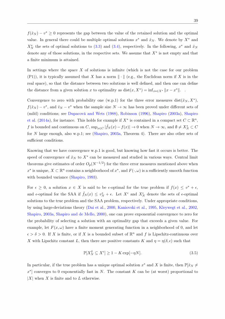
39

f(xN ) − v∗ ≥ 0 represents the gap between the value of the retained solution and the optimal

value. In general there could be multiple optimal solutions x∗ and xN . We denote by X∗ and

X∗N the sets of optimal solutions to (3.3) and (3.4), respectively. In the following, x∗ and xN

denote any of those solutions, in the respective sets. We assume that X∗ is not empty and that

a finite minimum is attained.

In settings where the space X of solutions is infinite (which is not the case for our problem

(P1)), it is typically assumed that X has a norm ‖ · ‖ (e.g., the Euclidean norm if X is in the

real space), so that the distance between two solutions is well defined, and then one can define

the distance from a given solution x to optimality as dist(x,X∗) = infx∗∈X∗ ‖x− x∗‖. .

Convergence to zero with probability one (w.p.1) for the three error measures dist(xN , X∗),

f(xN )− v∗, and vN − v∗ when the sample size N →∞ has been proved under different sets of

(mild) conditions; see Dupacová and Wets (1988), Robinson (1996), Shapiro (2003a), Shapiro

et al. (2014a), for instance. This holds for example if X∗ is contained in a compact set C ⊂ Rn,f is bounded and continuous on C, supx∈C |fN (x)− f(x)| → 0 when N →∞, and ∅ 6= X∗N ⊂ Cfor N large enough, also w.p.1; see (Shapiro, 2003a, Theorem 4). There are also other sets of

sufficient conditions.

Knowing that we have convergence w.p.1 is good, but knowing how fast it occurs is better. The

speed of convergence of xN to X∗ can be measured and studied in various ways. Central limit

theorems give estimates of order Op(N−1/2) for the three error measures mentioned above when

x∗ is unique, X ⊂ Rn contains a neighborhood of x∗, and F (·, ω) is a sufficiently smooth function

with bounded variance (Shapiro, 1993).

For ε ≥ 0, a solution x ∈ X is said to be ε-optimal for the true problem if f(x) ≤ v∗ + ε,

and ε-optimal for the SAA if fN (x) ≤ v∗N + ε. Let Xε and XεN denote the sets of ε-optimal

solutions to the true problem and the SAA problem, respectively. Under appropriate conditions,

by using large-deviations theory (Dai et al., 2000, Kaniovski et al., 1995, Kleywegt et al., 2002,

Shapiro, 2003a, Shapiro and de Mello, 2000), one can prove exponential convergence to zero for

the probability of selecting a solution with an optimality gap that exceeds a given value. For

example, let F (x, ω) have a finite moment generating function in a neighborhood of 0, and let

ε > δ > 0. If X is finite, or if X is a bounded subset of Rn and f is Lipschitz-continuous over

X with Lipschitz constant L, then there are positive constants K and η = η(δ, ε) such that

P[XδN ⊆ Xε] ≥ 1−K exp[−ηN ]. (3.5)

In particular, if the true problem has a unique optimal solution x∗ and X is finite, then P[xN 6=x∗] converges to 0 exponentially fast in N . The constant K can be (at worst) proportional to

|X| when X is finite and to L otherwise.

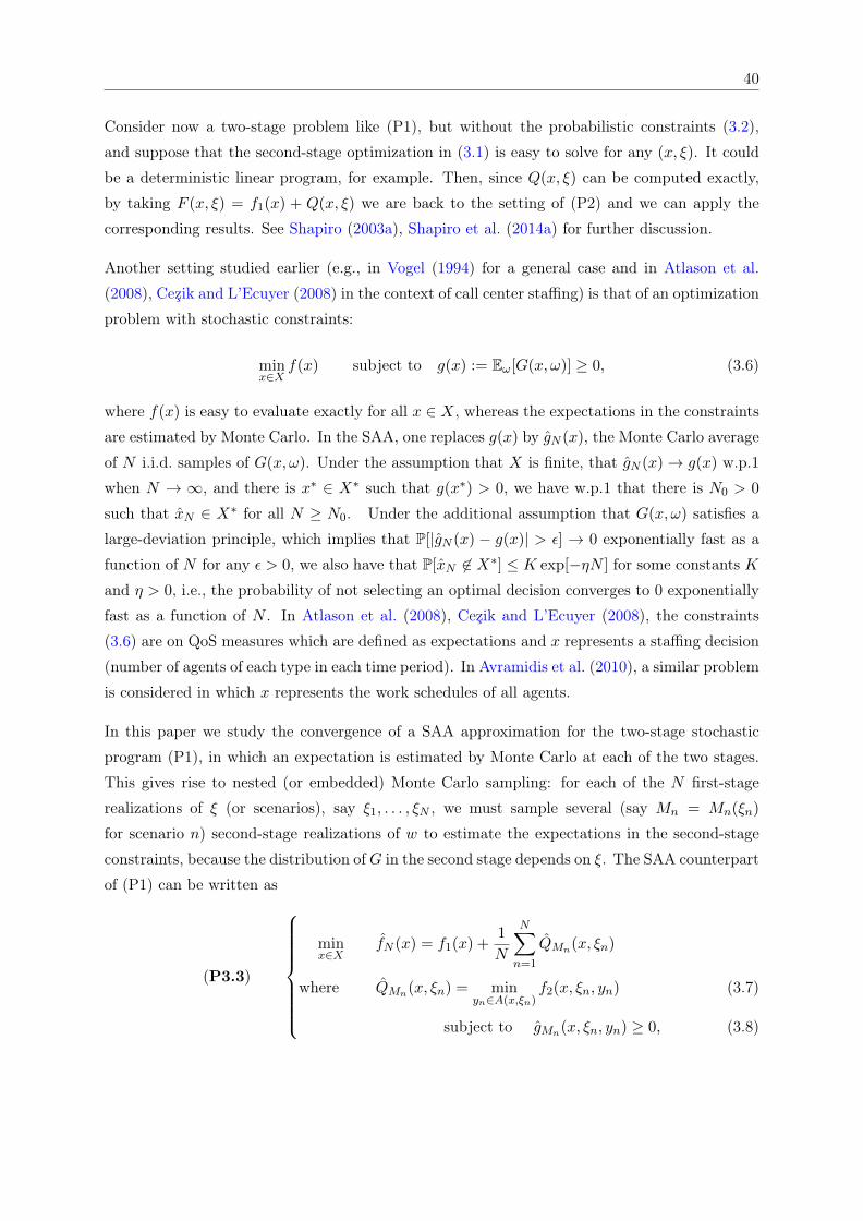
40

Consider now a two-stage problem like (P1), but without the probabilistic constraints (3.2),

and suppose that the second-stage optimization in (3.1) is easy to solve for any (x, ξ). It could

be a deterministic linear program, for example. Then, since Q(x, ξ) can be computed exactly,

by taking F (x, ξ) = f1(x) + Q(x, ξ) we are back to the setting of (P2) and we can apply the

corresponding results. See Shapiro (2003a), Shapiro et al. (2014a) for further discussion.

Another setting studied earlier (e.g., in Vogel (1994) for a general case and in Atlason et al.

(2008), Cezik and L’Ecuyer (2008) in the context of call center staffing) is that of an optimization

problem with stochastic constraints:

minx∈X

f(x) subject to g(x) := Eω[G(x, ω)] ≥ 0, (3.6)

where f(x) is easy to evaluate exactly for all x ∈ X, whereas the expectations in the constraints

are estimated by Monte Carlo. In the SAA, one replaces g(x) by gN (x), the Monte Carlo average

of N i.i.d. samples of G(x, ω). Under the assumption that X is finite, that gN (x)→ g(x) w.p.1

when N → ∞, and there is x∗ ∈ X∗ such that g(x∗) > 0, we have w.p.1 that there is N0 > 0

such that xN ∈ X∗ for all N ≥ N0. Under the additional assumption that G(x, ω) satisfies a

large-deviation principle, which implies that P[|gN (x) − g(x)| > ε] → 0 exponentially fast as a

function of N for any ε > 0, we also have that P[xN 6∈ X∗] ≤ K exp[−ηN ] for some constants K

and η > 0, i.e., the probability of not selecting an optimal decision converges to 0 exponentially

fast as a function of N . In Atlason et al. (2008), Cezik and L’Ecuyer (2008), the constraints

(3.6) are on QoS measures which are defined as expectations and x represents a staffing decision

(number of agents of each type in each time period). In Avramidis et al. (2010), a similar problem

is considered in which x represents the work schedules of all agents.

In this paper we study the convergence of a SAA approximation for the two-stage stochastic

program (P1), in which an expectation is estimated by Monte Carlo at each of the two stages.

This gives rise to nested (or embedded) Monte Carlo sampling: for each of the N first-stage

realizations of ξ (or scenarios), say ξ1, . . . , ξN , we must sample several (say Mn = Mn(ξn)

for scenario n) second-stage realizations of w to estimate the expectations in the second-stage

constraints, because the distribution ofG in the second stage depends on ξ. The SAA counterpart

of (P1) can be written as

(P3.3)

minx∈X

fN (x) = f1(x) +1

N

N∑n=1

QMn(x, ξn)

where QMn(x, ξn) = minyn∈A(x,ξn)

f2(x, ξn, yn)

subject to gMn(x, ξn, yn) ≥ 0,

(3.7)

(3.8)

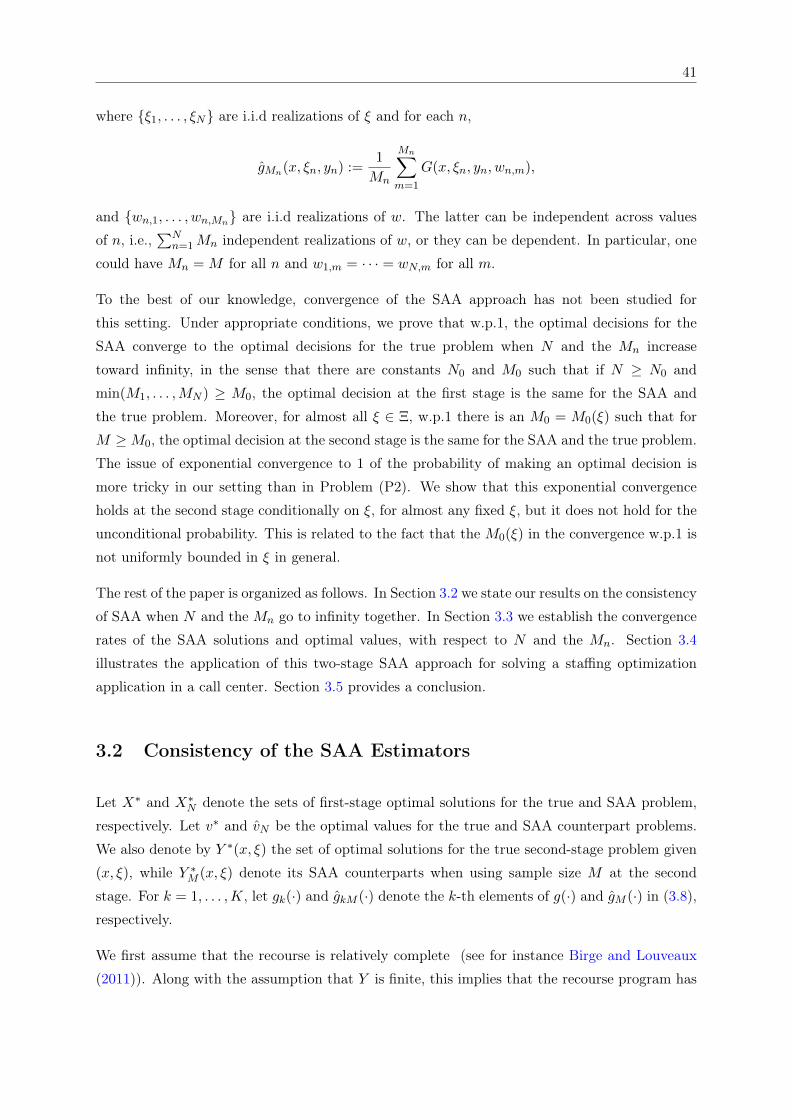
41

where ξ1, . . . , ξN are i.i.d realizations of ξ and for each n,

gMn(x, ξn, yn) :=1

Mn

Mn∑m=1

G(x, ξn, yn, wn,m),

and wn,1, . . . , wn,Mn are i.i.d realizations of w. The latter can be independent across values

of n, i.e.,∑N

n=1Mn independent realizations of w, or they can be dependent. In particular, one

could have Mn = M for all n and w1,m = · · · = wN,m for all m.

To the best of our knowledge, convergence of the SAA approach has not been studied for

this setting. Under appropriate conditions, we prove that w.p.1, the optimal decisions for the

SAA converge to the optimal decisions for the true problem when N and the Mn increase

toward infinity, in the sense that there are constants N0 and M0 such that if N ≥ N0 and

min(M1, . . . ,MN ) ≥ M0, the optimal decision at the first stage is the same for the SAA and

the true problem. Moreover, for almost all ξ ∈ Ξ, w.p.1 there is an M0 = M0(ξ) such that for

M ≥M0, the optimal decision at the second stage is the same for the SAA and the true problem.

The issue of exponential convergence to 1 of the probability of making an optimal decision is

more tricky in our setting than in Problem (P2). We show that this exponential convergence

holds at the second stage conditionally on ξ, for almost any fixed ξ, but it does not hold for the

unconditional probability. This is related to the fact that the M0(ξ) in the convergence w.p.1 is

not uniformly bounded in ξ in general.

The rest of the paper is organized as follows. In Section 3.2 we state our results on the consistency

of SAA when N and the Mn go to infinity together. In Section 3.3 we establish the convergence

rates of the SAA solutions and optimal values, with respect to N and the Mn. Section 3.4

illustrates the application of this two-stage SAA approach for solving a staffing optimization

application in a call center. Section 3.5 provides a conclusion.

3.2 Consistency of the SAA Estimators

Let X∗ and X∗N denote the sets of first-stage optimal solutions for the true and SAA problem,

respectively. Let v∗ and vN be the optimal values for the true and SAA counterpart problems.

We also denote by Y ∗(x, ξ) the set of optimal solutions for the true second-stage problem given

(x, ξ), while Y ∗M (x, ξ) denote its SAA counterparts when using sample size M at the second

stage. For k = 1, . . . ,K, let gk(·) and gkM (·) denote the k-th elements of g(·) and gM (·) in (3.8),

respectively.

We first assume that the recourse is relatively complete (see for instance Birge and Louveaux

(2011)). Along with the assumption that Y is finite, this implies that the recourse program has

42

at least one optimal solution for every x and P-almost every ξ. Moreover, we assume that the

second-stage objective function is almost surely uniformly bounded.

Assumption 3.1. X and Y are finite, and for each x ∈ X and P-almost every ξ ∈ Ξ, Y (x, ξ) 6=∅. Moreover, f2 is bounded uniformly for P-almost every (x, ξ) ∈ X × Ξ.

We next assume that for P-almost every scenario ξ, the SAA of the second-stage constraint

asymptotically coincide with the true second-stage constraint, and that the true constraint is

not active at any true second-stage solution , as otherwise, the SAA constraint could be violated

at this solution with a strictly positive probability, for any arbitrary large second-stage sample.

Note that in the continuous case, this assumption could be relaxed by assuming that the true and

SAA active sets are the same with probability one when the sample size is large enough Bastin

et al. (2006), Shapiro (2003a).

Assumption 3.2. For all x ∈ X and P-almost all ξ, for all y ∈ Y , gM (x, ξ, y) → g(x, ξ, y)

w.p.1 when M →∞, and there exists y ∈ Y ∗(x, ξ) such that g(x, ξ, y) 6= 0 .

Under Assumption 3.2, we can apply the known results for the Problem (P2) to the second stage

of our problem (P1), to obtain the following proposition, whose proof can be found in Atlason

et al. (2004), Atlason et al. (2008).

Proposition 3.1. Under Assumptions 3.1 and 3.2, and there exists y ∈ Y ∗(x, ξ) such that

g(x, ξ, y) 6= 0, which occurs for P-almost any ξ, w.p.1 there is a finite M0 = M0(ξ) such that

for all M ≥ M0, ∅ 6= Y ∗M (x, ξ) ⊆ Y ∗(x, ξ) and QM (x, ξ) = Q(x, ξ). That is, for all M ≥ M0,

the SAA in the second-stage has at least one optimal solution and any such optimal solution is

optimal for the true second-stage problem.

Moreover, again if there exists y ∈ Y ∗(x, ξ) such that g(x, ξ, y) 6= 0, there are positive constants

C and b(ξ) such that

P [Y ∗M (x, ξ) ⊆ Y ∗(x, ξ)] ≥ 1− C exp[−b(ξ)M ]. (3.9)

That is, for P-almost any ξ, the probability of missing optimality at the second stage decreases

to zero exponentially in M .

It is important to note here is that the sample size M0 and the constant b in Proposition 3.1

depend on ξ, and there may be no M0 and b for which the result holds uniformly in ξ. We give

an example of that in the following.

43

Example 3.1. Consider the following example of a two-stage program

minx∈X

f(x) = x+ Eξ[Q(x, ξ)]

where Q(x, ξ) = miny∈Y

2y

subject to Ew[x+ y − 2ξ − w] ≥ 0,

where ξ ∼ U(0, 1) (the uniform distribution), w ∼ N (0, 1) (the standard normal distribution),

and X = Y = 0, 1, 2. Given x ∈ X, the set of optimal solutions in the second-stage is

Y ∗(x, ξ) = arg min2y | y ∈ Y, y ≥ 2ξ − x.

Now, consider the SAA counterpart

minx∈X

fN (x) = x+1

N

N∑n=1

QM (x, ξn)

where QM (x, ξ) = miny∈Y

2y

subject to x+ y − 2ξ − wM ≥ 0,

where wM is a sample average approximation of w by a Monte Carlo method. In this example,

for notational simplicity we set M1 = . . . = MN = M . Let x = 1, we have Y ∗(1, ξ) = 0 if

ξ ≤ 1/2, and Y ∗(1, ξ) = 1 if ξ > 1/2. So, for a given ξ ∈ [0, 1/2], if we have wM > 1−2ξ in the

second-stage of the SAA, then the SAA does not return a true second-stage optimal solution,

i.e, Y ∗M (x, ξ) * Y ∗(x, ξ). Therefore, we have

P [Y ∗M (x, ξ) * Y ∗(x, ξ)] ≥ P [wM ≥ 1− 2ξ] . (3.10)

Since wM ∼ N (0, 1/M), for any M > 0 we have

lim1−2ξ→0

P [wM ≥ 1− 2ξ] = P [wM ≥ 0] =1

2. (3.11)

Hence, if 1 − 2ξ can be arbitrarily close to zero, for any given 0 ≤ ε < 1/4, then there is no

M0 > 0 such that P [wM ≥ 1− 2ξ] < ε for all M > M0 and all ξ ∈ [0, 1/2), and therefore, there

is no M0 > 0 such that P [Y ∗M (x, ξ) * Y ∗(x, ξ)] < ε for all M > M0 and all ξ ∈ [0, 1/2). This

also means that there is no M0 such that, w.p.1, QM (x, ξ) = Q(x, ξ) for all M > M0 and all

ξ ∈ [0, 1/2).

We now show that exponential convergence of the probability of making a wrong decision at the

second stage does not hold uniformly in ξ. By contradiction, if there are positive constants C0, b0

for which the exponential convergence Proposition 3.1 holds uniformly in ξ, then for P-almost

44

every ξ ∈ Ξ, we have

ln (P [Y ∗M (x, ξ) * Y ∗(x, ξ)]) ≤ lnC0 −Mb0, for all M > 0. (3.12)

From (3.10) we have, for P-almost every ξ ∈ [0, 1/2)

lnP [wM ≥ 1− 2ξ]

M≤ lnC0

M− b0. (3.13)

However, we can always choose M∗ large enough such that

ln(1/4)− lnC0

M∗> −b0,

and ξ∗ ∈ [0, 1/2) such that P [wM∗ ≥ 1− 2ξ∗] > 1/4. The latter can be done using (3.11). Then,

we havelnP [wM∗ ≥ 1− 2ξ∗]

M∗− lnC0

M∗>

ln(1/4)− lnC0

M∗> −b0,

meaning that (3.13) cannot hold for any M > 0 and for almost every ξ ∈ [0, 1/2).

We now look at the convergence of the optimal value and optimal solution at the first stage

of the SAA problem to those of the true problem. We want to show that w.p.1, we have

X∗N ⊆ X∗ when min(N,M1, . . . ,MN ) is large enough. Since X is finite, there is a fixed δ > 0

such that for every x ∈ X \ X∗, f(x) − v∗ ≥ δ. Then, a sufficient condition for X∗N ⊆ X∗ is

that |fN (x) − f(x)| < ε := δ/2 for all x ∈ X. One could think that this last inequality would

follow from the observation that since for each ξn, QMn(x, ξn) converges to its expectation

w.p.1 when Mn → ∞, |fN (x) − f(x)| should converge to 0 w.p.1, so it will eventually be

smaller than ε. But this simple argument does not really stand (it is not rigorous), because

the convergence is not uniform in ξ, so the required M0 above which |fN (x) − f(x)| < ε when

N > N0 and min(M1, . . . ,MN ) > M0 may increase without bound when N increases. A more

careful argument is needed and this is what we will do now, under our two assumptions. We

first introduce some notations, then prove two lemmas which will be used to prove Theorems

3.4 and 3.5, which are our main results in this section.

For any x ∈ X and ξ ∈ Ξ, we define

Y−(x, ξ) = y ∈ A(x, ξ) | ∃ k such that gk(x, ξ, y) < 0),

δ(x, ξ) =1

2max

y∈Y (x,ξ),1≤k≤Kgk(x, ξ, y) | gk(x, ξ, y) < 0,

δ(x, ξ) = miny∈Y ∗(x,ξ),1≤k≤K

gk(x, ξ, y) | gk(x, ξ, y) > 0,

δ(x, ξ) = min−δ(x, ξ), δ(x, ξ) > 0, and

δ(ξ) = minx∈X

δ(x, ξ) > 0. (3.14)

45

By convention, if Y−(x, ξ) = ∅ then δ(x, ξ) = −∞, and if (y, k)| y ∈ Y ∗(x, ξ), gk(x, ξ, y) >

0 = ∅, then δ(x, ξ) =∞. Under Assumption 3.2 we have δ(x, ξ) <∞ for P-almost every ξ ∈ Ξ.

Lemma 3.2. maxx∈X |fN (x)− f(x)| ≥ |vN − v∗|.

Proof. Let x∗ and x∗N be optimal solutions to (P1) and (P3), respectively. If f(x∗) < fN (x∗N ),

since fN (x∗N ) ≤ fN (x∗), we have:

|vN − v∗| = |fN (x∗N )− f(x∗)| ≤ |fN (x∗)− f(x∗)| ≤ maxx∈X|fN (x)− f(x)|.

If f(x∗) ≥ fN (x∗N ), since f(x∗) ≤ f(x∗N ), we have:

|v∗ − vN | = |f(x∗)− fN (x∗N )| ≤ |f(x∗N )− fN (x∗N )| ≤ maxx∈X|fN (x)− f(x)|.

In both cases, we have |vN − v∗| ≤ maxx∈X |fN (x)− f(x)|.

Lemma 3.3. Under Assumptions 3.1, and 3.2, for any x ∈ X and for P-almost every ξ ∈ Ξ, if

|gkM (x, ξ, y) − gk(x, ξ, y)| ≤ δ(x, ξ) for all y ∈ Y (x, ξ) and k = 1, . . . ,K, then ∅ 6= Y ∗M (x, ξ) ⊆Y ∗(x, ξ).

Proof. Let YM (x, ξ) be the set of feasible solutions of the SAA counterpart second-stage prob-

lems. Given ξ such that δ(x, ξ)<∞, which holds for P-almost every ξ ∈ Ξ, we have

|gkM (x, ξ, y)− gk(x, ξ, y)| ≤ δ(x, ξ) = min−δ(x, ξ), δ(x, ξ).

If y ∈ Y−(x, ξ), there exists some k such that gk(x, ξ, y) < 0 and

gkM (x, ξ, y) ≤ gk(x, ξ, y)− δ(x, ξ) < 0.

Thus y ∈ A(x, ξ)\YM (x, ξ), and A(x, ξ)\Y (x, ξ) ⊆ A(x, ξ)\YM (x, ξ). Since YM (x, ξ) ⊆ A(x, ξ),

we have YM (x, ξ) ⊆ Y (x, ξ). Moreover, w.p.1, there exists y∗ ∈ Y ∗(x, ξ) such that g(x, ξ, y∗) > 0,

we have that for all k,

gkM (x, ξ, y∗) ≥ gk(x, ξ, y∗)− δ(x, ξ) ≥ 0,

implying y∗ ∈ YM (x, ξ). Moreover, for all y∗M ∈ Y ∗M (x, ξ), we have f2(y∗) ≥ f2(y∗M ). As

YM (x, ξ) ⊆ Y (x, ξ), we also have f2(y∗) ≤ f2(y∗M ), and therefore f2(y∗) = f2(y∗M ), implying that

y∗ ∈ Y ∗M (x, ξ), so Y ∗M (x, ξ) 6= ∅. This also implies that if y∗1 ∈ Y ∗M (x, ξ) and y∗2 ∈ Y ∗(x, ξ), thenf2(y∗1, ξ) = f2(y∗2, ξ). As Y ∗M (x, ξ) ⊆ YM (x, ξ) ⊆ Y (x, ξ), we also have y∗1 ∈ Y (x, ξ), and therefore

y∗1 ∈ Y ∗(x, ξ). As a consequence, ∅ 6= Y ∗M (x, ξ) ⊆ Y ∗(x, ξ), which completes the proof.

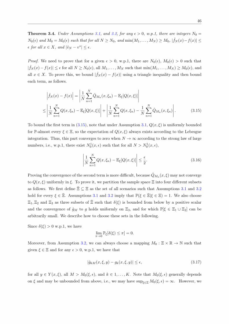
46

Theorem 3.4. Under Assumptions 3.1, and 3.2, for any ε > 0, w.p.1, there are integers N0 =

N0(ε) and M0 = M0(ε) such that for all N ≥ N0, and min(M1, . . . ,MN ) ≥M0, |fN (x)−f(x)| ≤ε for all x ∈ X, and |vN − v∗| ≤ ε.

Proof. We need to prove that for a given ε > 0, w.p.1, there are N0(ε), M0(ε) > 0 such that

|fN (x)−f(x)| ≤ ε for all N ≥ N0(ε), all M1, . . . ,MN such that min(M1, . . . ,MN ) ≥M0(ε), and

all x ∈ X. To prove this, we bound |fN (x) − f(x)| using a triangle inequality and then bound

each term, as follows.

∣∣∣fN (x)− f(x)∣∣∣ =

∣∣∣∣∣ 1

N

N∑n=1

QMn(x, ξn)− Eξ[Q(x, ξ)]

∣∣∣∣∣≤

∣∣∣∣∣ 1

N

N∑n=1

Q(x, ξn)− Eξ[Q(x, ξ)]

∣∣∣∣∣+

∣∣∣∣∣ 1

N

N∑n=1

Q(x, ξn)− 1

N

N∑n=1

QMn(x, ξn)

∣∣∣∣∣ . (3.15)

To bound the first term in (3.15), note that under Assumption 3.1, Q(x, ξ) is uniformly bounded

for P-almost every ξ ∈ Ξ, so the expectation of Q(x, ξ) always exists according to the Lebesgue

integration. Thus, this part converges to zero when N →∞ according to the strong law of large

numbers, i.e., w.p.1, there exist N10 (x, ε) such that for all N > N1

0 (x, ε),∣∣∣∣∣ 1

N

N∑n=1

Q(x, ξn)− Eξ[Q(x, ξ)]

∣∣∣∣∣ ≤ ε

2. (3.16)

Proving the convergence of the second term is more difficult, because QMn(x, ξ) may not converge

to Q(x, ξ) uniformly in ξ. To prove it, we partition the sample space Ξ into four different subsets

as follows. We first define Ξ ⊆ Ξ as the set of all scenarios such that Assumptions 3.1 and 3.2

hold for every ξ ∈ Ξ. Assumptions 3.1 and 3.2 imply that P(ξ ∈ Ξ|ξ ∈ Ξ) = 1. We also choose

Ξ1,Ξ2 and Ξ3 as three subsets of Ξ such that δ(ξ) is bounded from below by a positive scalar

and the convergence of gM to g holds uniformly on Ξ3, and for which P[ξ ∈ Ξ1 ∪ Ξ2] can be

arbitrarily small. We describe how to choose these sets in the following.

Since δ(ξ) > 0 w.p.1, we have

limπ→0

Pξ[δ(ξ) ≤ π] = 0.

Moreover, from Assumption 3.2, we can always choose a mapping M0 : Ξ × R → N such that

given ξ ∈ Ξ and for any ε > 0, w.p.1, we have that

|gkM (x, ξ, y)− gk(x, ξ, y)| ≤ ε, (3.17)

for all y ∈ Y (x, ξ), all M > M0(ξ, ε), and k ∈ 1, . . . ,K. Note that M0(ξ, ε) generally depends

on ξ and may be unbounded from above, i.e., we may have supξ∈ΞM0(ξ, ε) =∞. However, we

47

have

limM→∞

Pξ[M0(ξ, ε) ≥M ] = 0.

So, there exist π(ε) > 0 and M10 (ε) > 0 such that

P[δ(ξ) ≤ π(ε)] ≤ ε

6αand P[M0(ξ, π(ε)) ≥M1

0 (ε)] ≤ ε

6α,

where α is a constant chosen such that α > supx∈X,y∈Y, ξ∈Ξ\Ξ0|2f2(x, ξ, y)|. We can simply

choose α = supx∈X,y∈Y, ξ∈Ξ\Ξ0|2f2(x, ξ, y)|+1. Hence, we always have α > |QMn(x, ξ)−Q(x, ξ)|

for all x ∈ X, ξ ∈ Ξ and all n = 1, . . . , N . This α always exists and is finite because f2 is

bounded uniformly for every ξ ∈ Ξ. Let us define

Ξ1 = ξ ∈ Ξ | δ(ξ) ≤ π(ε),

Ξ2 = ξ ∈ Ξ |M0(ξ, π(ε)) ≥M10 (ε),

Ξ3 = Ξ\(Ξ1 ∪ Ξ2).

Suppose ξ1, . . . , ξN ∈ Ξ, which happens w.p.1. The second part of (3.15) can then be written as∣∣∣∣∣ 1

N

N∑n=1

Q(x, ξn)− 1

N

N∑n=1

QMn(x, ξn)

∣∣∣∣∣≤ 1

N

N∑n=1

∣∣∣Q(x, ξn)− QMn(x, ξn)∣∣∣

=1

N

∑ξn∈Ξ1∪Ξ2

∣∣∣Q(x, ξn)− QMn(x, ξn)∣∣∣+

1

N

∑ξn∈Ξ3

∣∣∣Q(x, ξn)− QMn(x, ξn)∣∣∣

≤ 1

N

N∑n=1

αI[ξn ∈ Ξ1 ∪ Ξ2] +1

N

∑ξn∈Ξ3

∣∣∣Q(x, ξn)− QMn(x, ξn)∣∣∣ . (3.18)

The term 1N

∑Nn=1 I[ξn ∈ Ξ1 ∪ Ξ2] is a sample average of P[ξn ∈ Ξ1 ∪ Ξ2]. Therefore, based on

the strong law of large numbers, w.p.1, there is N20 (x, ε) such that, for all N ≥ N2

0 (x, ε)

1

N

N∑n=1

I[ξn ∈ Ξ1 ∪ Ξ2] ≤ P[ξn ∈ Ξ1 ∪ Ξ2] +ε

6α

≤ P[ξn ∈ Ξ1] + P[ξn ∈ Ξ2] +ε

6α

≤ ε

6α+

ε

6α+

ε

6α=

ε

2α.

(3.19)

Moreover, as Ξ3 = ξ | δ(ξ) > π(ε), M0(ξ, π(ε)) < M10 (ε), then for any ξ ∈ Ξ3, w.p.1, we have

|gkM (x, ξ, y) − gk(x, ξ, y)| ≤ π(ε) < δ(ξ) for all y ∈ Y (x, ξ), all M > M10 (ε), and k = 1, . . . ,K.

So, for any ξ ∈ Ξ3, w.p.1, QM (x, ξ) = Q(x, ξ) for all M > M10 (ε) , or equivalently, w.p.1, for all

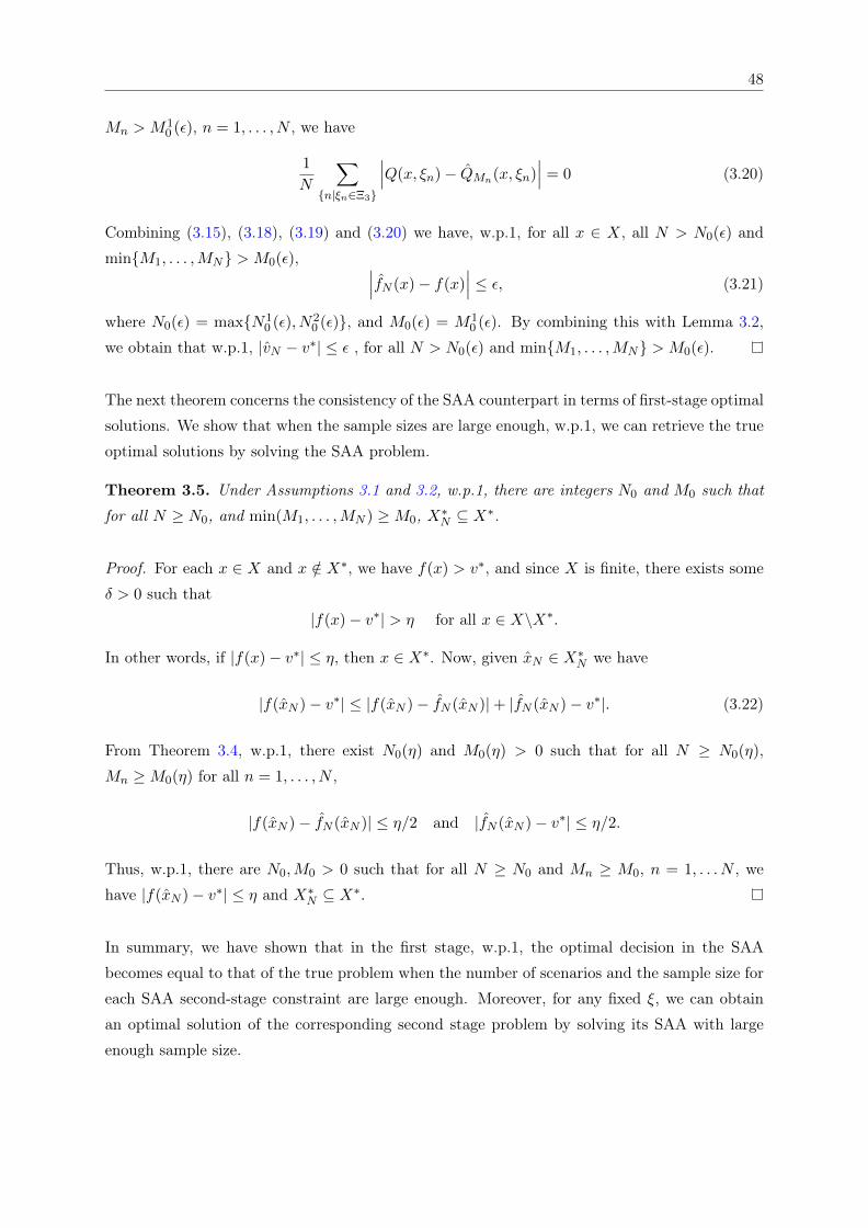
48

Mn > M10 (ε), n = 1, . . . , N , we have

1

N

∑n|ξn∈Ξ3

∣∣∣Q(x, ξn)− QMn(x, ξn)∣∣∣ = 0 (3.20)

Combining (3.15), (3.18), (3.19) and (3.20) we have, w.p.1, for all x ∈ X, all N > N0(ε) and

minM1, . . . ,MN > M0(ε), ∣∣∣fN (x)− f(x)∣∣∣ ≤ ε, (3.21)

where N0(ε) = maxN10 (ε), N2

0 (ε), and M0(ε) = M10 (ε). By combining this with Lemma 3.2,

we obtain that w.p.1, |vN − v∗| ≤ ε , for all N > N0(ε) and minM1, . . . ,MN > M0(ε).

The next theorem concerns the consistency of the SAA counterpart in terms of first-stage optimal

solutions. We show that when the sample sizes are large enough, w.p.1, we can retrieve the true

optimal solutions by solving the SAA problem.

Theorem 3.5. Under Assumptions 3.1 and 3.2, w.p.1, there are integers N0 and M0 such that

for all N ≥ N0, and min(M1, . . . ,MN ) ≥M0, X∗N ⊆ X∗.

Proof. For each x ∈ X and x /∈ X∗, we have f(x) > v∗, and since X is finite, there exists some

δ > 0 such that

|f(x)− v∗| > η for all x ∈ X\X∗.

In other words, if |f(x)− v∗| ≤ η, then x ∈ X∗. Now, given xN ∈ X∗N we have

|f(xN )− v∗| ≤ |f(xN )− fN (xN )|+ |fN (xN )− v∗|. (3.22)

From Theorem 3.4, w.p.1, there exist N0(η) and M0(η) > 0 such that for all N ≥ N0(η),

Mn ≥M0(η) for all n = 1, . . . , N ,

|f(xN )− fN (xN )| ≤ η/2 and |fN (xN )− v∗| ≤ η/2.

Thus, w.p.1, there are N0,M0 > 0 such that for all N ≥ N0 and Mn ≥ M0, n = 1, . . . N , we

have |f(xN )− v∗| ≤ η and X∗N ⊆ X∗.

In summary, we have shown that in the first stage, w.p.1, the optimal decision in the SAA

becomes equal to that of the true problem when the number of scenarios and the sample size for

each SAA second-stage constraint are large enough. Moreover, for any fixed ξ, we can obtain

an optimal solution of the corresponding second stage problem by solving its SAA with large

enough sample size.

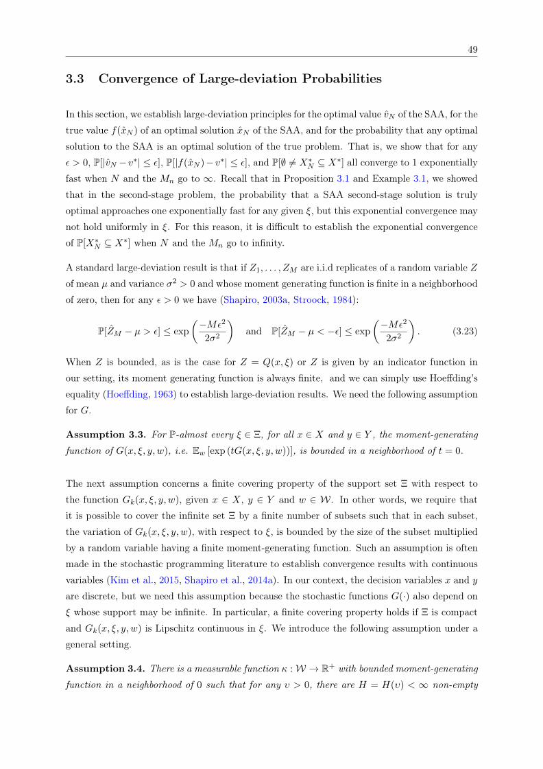
49

3.3 Convergence of Large-deviation Probabilities

In this section, we establish large-deviation principles for the optimal value vN of the SAA, for the

true value f(xN ) of an optimal solution xN of the SAA, and for the probability that any optimal

solution to the SAA is an optimal solution of the true problem. That is, we show that for any

ε > 0, P[|vN − v∗| ≤ ε], P[|f(xN )− v∗| ≤ ε], and P[∅ 6= X∗N ⊆ X∗] all converge to 1 exponentially

fast when N and the Mn go to ∞. Recall that in Proposition 3.1 and Example 3.1, we showed

that in the second-stage problem, the probability that a SAA second-stage solution is truly

optimal approaches one exponentially fast for any given ξ, but this exponential convergence may

not hold uniformly in ξ. For this reason, it is difficult to establish the exponential convergence

of P[X∗N ⊆ X∗] when N and the Mn go to infinity.

A standard large-deviation result is that if Z1, . . . , ZM are i.i.d replicates of a random variable Z

of mean µ and variance σ2 > 0 and whose moment generating function is finite in a neighborhood

of zero, then for any ε > 0 we have (Shapiro, 2003a, Stroock, 1984):

P[ZM − µ > ε] ≤ exp

(−Mε2

2σ2

)and P[ZM − µ < −ε] ≤ exp

(−Mε2

2σ2

). (3.23)

When Z is bounded, as is the case for Z = Q(x, ξ) or Z is given by an indicator function in

our setting, its moment generating function is always finite, and we can simply use Hoeffding’s

equality (Hoeffding, 1963) to establish large-deviation results. We need the following assumption

for G.

Assumption 3.3. For P-almost every ξ ∈ Ξ, for all x ∈ X and y ∈ Y , the moment-generating

function of G(x, ξ, y, w), i.e. Ew [exp (tG(x, ξ, y, w))], is bounded in a neighborhood of t = 0.

The next assumption concerns a finite covering property of the support set Ξ with respect to

the function Gk(x, ξ, y, w), given x ∈ X, y ∈ Y and w ∈ W. In other words, we require that

it is possible to cover the infinite set Ξ by a finite number of subsets such that in each subset,

the variation of Gk(x, ξ, y, w), with respect to ξ, is bounded by the size of the subset multiplied

by a random variable having a finite moment-generating function. Such an assumption is often

made in the stochastic programming literature to establish convergence results with continuous

variables (Kim et al., 2015, Shapiro et al., 2014a). In our context, the decision variables x and y

are discrete, but we need this assumption because the stochastic functions G(·) also depend on

ξ whose support may be infinite. In particular, a finite covering property holds if Ξ is compact

and Gk(x, ξ, y, w) is Lipschitz continuous in ξ. We introduce the following assumption under a

general setting.

Assumption 3.4. There is a measurable function κ :W → R+ with bounded moment-generating

function in a neighborhood of 0 such that for any υ > 0, there are H = H(υ) < ∞ non-empty

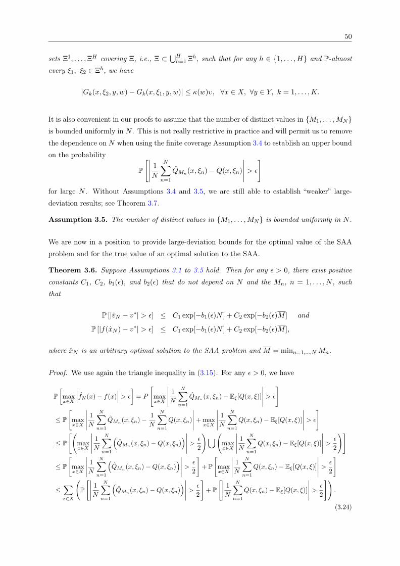
50

sets Ξ1, . . . ,ΞH covering Ξ, i.e., Ξ ⊂⋃Hh=1 Ξh, such that for any h ∈ 1, . . . ,H and P-almost

every ξ1, ξ2 ∈ Ξh, we have

|Gk(x, ξ2, y, w)−Gk(x, ξ1, y, w)| ≤ κ(w)υ, ∀x ∈ X, ∀y ∈ Y, k = 1, . . . ,K.

It is also convenient in our proofs to assume that the number of distinct values in M1, . . . ,MNis bounded uniformly in N . This is not really restrictive in practice and will permit us to remove

the dependence on N when using the finite coverage Assumption 3.4 to establish an upper bound

on the probability

P

[∣∣∣∣∣ 1

N

N∑n=1

QMn(x, ξn)−Q(x, ξn)

∣∣∣∣∣ > ε

]for large N . Without Assumptions 3.4 and 3.5, we are still able to establish “weaker” large-

deviation results; see Theorem 3.7.

Assumption 3.5. The number of distinct values in M1, . . . ,MN is bounded uniformly in N .

We are now in a position to provide large-deviation bounds for the optimal value of the SAA

problem and for the true value of an optimal solution to the SAA.

Theorem 3.6. Suppose Assumptions 3.1 to 3.5 hold. Then for any ε > 0, there exist positive

constants C1, C2, b1(ε), and b2(ε) that do not depend on N and the Mn, n = 1, . . . , N , such

that

P [|vN − v∗| > ε] ≤ C1 exp[−b1(ε)N ] + C2 exp[−b2(ε)M ] and

P [|f(xN )− v∗| > ε] ≤ C1 exp[−b1(ε)N ] + C2 exp[−b2(ε)M ],

where xN is an arbitrary optimal solution to the SAA problem and M = minn=1,...,N Mn.

Proof. We use again the triangle inequality in (3.15). For any ε > 0, we have

P[maxx∈X

∣∣∣fN (x)− f(x)∣∣∣ > ε

]= P

[maxx∈X

∣∣∣∣∣ 1

N

N∑n=1

QMn(x, ξn)− Eξ[Q(x, ξ)]

∣∣∣∣∣ > ε

]

≤ P

[maxx∈X

∣∣∣∣∣ 1

N

N∑n=1

QMn(x, ξn)− 1

N

N∑n=1

Q(x, ξn)

∣∣∣∣∣+ maxx∈X

∣∣∣∣∣ 1

N

N∑n=1

Q(x, ξn)− Eξ[Q(x, ξ)]

∣∣∣∣∣ > ε

]

≤ P

[(maxx∈X

∣∣∣∣∣ 1

N

N∑n=1

(QMn

(x, ξn)−Q(x, ξn))∣∣∣∣∣ > ε

2

)⋃(maxx∈X

∣∣∣∣∣ 1

N

N∑n=1

Q(x, ξn)− Eξ[Q(x, ξ)]

∣∣∣∣∣ > ε

2

)]

≤ P

[maxx∈X

∣∣∣∣∣ 1

N

N∑n=1

(QMn(x, ξn)−Q(x, ξn)

)∣∣∣∣∣ > ε

2

]+ P

[maxx∈X

∣∣∣∣∣ 1

N

N∑n=1

Q(x, ξn)− Eξ[Q(x, ξ)]

∣∣∣∣∣ > ε

2

]

≤∑x∈X

(P

[∣∣∣∣∣ 1

N

N∑n=1

(QMn

(x, ξn)−Q(x, ξn))∣∣∣∣∣ > ε

2

]+ P

[∣∣∣∣∣ 1

N

N∑n=1

Q(x, ξn)− Eξ[Q(x, ξ)]

∣∣∣∣∣ > ε

2

]).

(3.24)

51

Considering the second part of (3.24) and given the fact that Q(x, ξ) is bounded by the interval

[−α, α] for P-almost every ξ, where α is defined as in the proof of Theorem 3.4, we obtain the

following from Hoeffding’s inequality (Hoeffding, 1963):

P

[∣∣∣∣∣ 1

N

N∑n=1

Q(x, ξn)− Eξ[Q(x, ξ)]

∣∣∣∣∣ > ε

2

]≤ 2 exp

(−Nε2

8α2

). (3.25)

As discussed earlier, the convergence in probability of QM (x, ξ) → Q(x, ξ) does not hold uni-

formly on Ξ. To deal with this issue, similar to the proof of Theorem 3.4, we divide the support

set Ξ into smaller sub-sets. First, we define Ξ ⊆ Ξ as the set of all scenarios ξ ∈ Ξ for which

Assumptions 3.1, 3.2 and 3.3 hold. Note that P[ξ ∈ Ξ] = 1. We select π(ε) > 0 such that

Pξ[δ(ξ) ≤ π(ε)] ≤ ε

6α,

where δ(ξ) is defined in (3.14). Let also define Ξ1 = ξ ∈ Ξ|δ(ξ) ≤ π(ε), and Ξ2 = Ξ\Ξ1). We

write the first part of (3.24) as

P

[∣∣∣∣∣ 1

N

N∑n=1

QMn(x, ξn)− 1

N

N∑n=1

Q(x, ξn)

∣∣∣∣∣ > ε

2

]

≤ P

1

N

∑ξn∈Ξ1∪Ξ2

∣∣∣QMn(x, ξn)−Q(x, ξn)∣∣∣ > ε

2

≤ P

1

N

∑ξn∈Ξ1

∣∣∣QMn(x, ξn)−Q(x, ξn)∣∣∣ > ε

4

+ P

1

N

∑ξn∈Ξ2

∣∣∣QMn(x, ξn)−Q(x, ξn)∣∣∣ > ε

4

≤ P

[1

N

N∑n=1

αI[ξn ∈ Ξ1] >ε

4

]+ P

1

N

∑ξn∈Ξ2

∣∣∣QMn(x, ξn)−Q(x, ξn)∣∣∣ > ε

4

. (3.26)

The first term in (3.26) concerns a sample average approximation of αP[ξ ∈ Ξ1], and we have

αP[ξ ∈ Ξ1] ≤ ε/6 < ε/4. Moreover, I[ξ ∈ Ξ1] only takes values in 0, 1, so by Hoeffding’s

inequality we have

P

[1

N

N∑n=1

I[ξn ∈ Ξ1] >ε

4α

]≤ exp

(−Nε2

72α2

). (3.27)

For the second term of (3.26), we have

P

1

N

∑ξn∈Ξ2

∣∣∣QMn(x, ξn)−Q(x, ξn)∣∣∣ ≤ ε

4

≥ P

[∣∣∣QMn(x, ξn)−Q(x, ξn)∣∣∣ = 0, ∀ξn ∈ Ξ2, n = 1, . . . , N

]≥ P

[∣∣gkM(ξ)(x, ξ, y)− gk(x, ξ, y)∣∣ ≤ δ(ξ), ∀ξ ∈ Ξ2, ∀y ∈ Y, k = 1, . . . ,K

]≥ P

[∣∣gkM(ξ)(x, ξ, y)− gk(x, ξ, y)∣∣ ≤ π(ε), ∀ξ ∈ Ξ2, ∀y ∈ Y, k = 1, . . . ,K

],

52

where M(ξ) is a mapping from Ξ to N+ such that M(ξn) = Mn, n = 1, . . . , N , and we assume

that M(ξ) = M for all ξ 6= ξn, n = 1, . . . , N . Moreover, as the number of distinct values in

M1, . . . ,MN is bounded uniformly, there exists T ∈ N+ that is independent of N and T values

M1, . . . ,MT such that M(ξ) ∈ M1, . . . ,MT for all ξ ∈ Ξ. Hence, we have

P

1

N

∑ξn∈Ξ2

∣∣∣QMn(x, ξn)−Q(x, ξn)∣∣∣ > ε

4

≤ P

[∃(ξ, y, k)

∣∣∣ ξ ∈ Ξ2, y ∈ Y, k ∈ 1, . . . ,K,∣∣gkM(ξ)(x, ξ, y)− gk(x, ξ, y)

∣∣ > π(ε)]

≤∑y∈Y

K∑k=1

P

[supξ∈Ξ2

∣∣gkM(ξ)(x, ξ, y)− gk(x, ξ, y)∣∣ > π(ε)

]

≤∑y∈Y

K∑k=1

T∑t=1

P

[supξ∈Ξ2

|gkMt(x, ξ, y)− gk(x, ξ, y)| > π(ε)

]. (3.28)

Basically, given a scenario ξ ∈ Ξ2, we bound the probability P[|gkMt(x, ξ, y)−gk(x, ξ, y)| > π(ε)]

using LD theory. So, the probability P[supξ∈Ξ2|gkM(ξ)(x, ξ, y) − gk(x, ξ, y)| > π(ε)] can be

bounded using LD theory if |Ξ2| is finite. If |Ξ2| is infinite, we use a discretization technique

over set Ξ2 as in the following.

Under Assumption 3.4, if we define Ξh2 = Ξ2 ∩ Ξh, h = 1, . . . ,H, then for P-almost every

ξ, ξ1 ∈ Ξh2 and for all x ∈ X, y ∈ Y , k = 1 . . . ,K, we have

|Gk(x, ξ, y, w)−Gk(x, ξ1, y, w)| ≤ κ(w)υ.

For each set Ξh2 , h = 1, . . . ,H, we choose a representative point ξh ∈ Ξh2 such that for P-almost

every ξ ∈ Ξh2 and for all x ∈ X, y ∈ Y , k = 1 . . . ,K, we have

|Gk(x, ξ, y, w)−Gk(x, ξh, y, w)| ≤ κ(w)υ.

We also define the corresponding mapping h(ξ) = ξh if ξ ∈ Ξh2 . We have the following inequality

|gkM (x, ξ, y)− gk(x, ξ, y)| ≤ |gkM (x, ξ, y)− gkM (x, h(ξ), y)|

+ |gkM (x, h(ξ), y)− gk(x, h(ξ), y)|+ |gk(x, h(ξ), y)− gk(x, ξ, y)| .(3.29)

Here, we assume that gkM (x, ξ, y) and gkM (x, h(ξ), y) are computed by the same set of realiza-

tions of w. We also have gkM (x, ξ, y) − gkM (x, h(ξ), y) is a SAA of gk(x, ξ, y) − gk(x, h(ξ), y),

53

therefore, for P-almost every ξ ∈ Ξh2 we can write

|gkM (x, ξ, y)− gkM (x, h(ξ), y)| = 1

M

∣∣∣∣∣M∑m=1

(Gk(x, ξ, y, wm)−Gk(x, h(ξ), y, wm))

∣∣∣∣∣≤ 1

M

M∑m=1

|Gk(x, ξ, y, wm)−Gk(x, h(ξ), y, wm)|

≤ 1

M

M∑m=1

κ(wm)υ.

So, for P-almost every ξ ∈ Ξh2 ,

|gkM (x, ξ, y)− gkM (x, h(ξ), y)| ≤ κMυ, (3.30)

where κM = M−1∑M

m=1 κ(wm) is a sample average version of Ew[κ(w)]. We also have that, for

P-almost every ξ ∈ Ξh2 ,

|gk(x, ξ, y)− gk(x, h(ξ), y)| ≤ Ew[κ(w)]υ. (3.31)

From the assumption that the moment-generating function of κ(w) is finite valued in a neigh-

borhood of 0, we have Ew[κ(w)] is finite. We define Lκ = Ew[κ(w)]. From (3.31) we have

|gk(x, ξ, y) − gk(x, h(ξ), y)| ≤ Lκυ for P-almost every ξ ∈ Ξh2 . Thus, for P-almost every ξ ∈ Ξh2 ,

we have|gkM (x, ξ, y)− gk(x, ξ, y)|

≤ |gkM (x, ξ, y)− gkM (x, h(ξ), y)|+ |gkM (x, h(ξ), y)− gk(x, h(ξ), y)|

+ |gk(x, h(ξ), y)− gk(x, ξ, y)|

≤ κMv + |gkM (x, h(ξ), y)− gk(x, h(ξ), y)|+ Lkv.

Let us return to the evaluation of (3.28). If we set υ = π(ε)/(4Lκ), then from (3.29), (3.30) and

(3.31), we have

P

[supξ∈Ξ2

|gkMt(x, ξ, y)− E[Gk(x, ξ, y)]| > π(ε)

]

≤ P[

maxh=1,...,H

∣∣gkMt(x, ξh, y)− gk(x, ξh, y)∣∣ > π(ε)

3

]+ P

[max

h=1,...,HκMt >

π(ε)

3υ

]+ P

[Lκυ >

π(ε)

3

]≤

H∑h=1

(P[∣∣gkMt(x, ξh, y)− gk(x, ξh, y)

∣∣ > π(ε)

3

]+ P

[κMt >

4Lκ3

]). (3.32)

54

The first part of (3.32) can be handled using LD theory, i.e., under Assumption 3.3 and using

(3.23), we obtain

P[∣∣gkMt(x, ξh, y)− gk(x, ξh, y)

∣∣ > π(ε)

3

]≤ 2 exp

(−Mtπ

2(ε)

18σ2g

)≤ 2 exp

(−Mπ2(ε)

18σ2g

), (3.33)

where σ2g = supx,y,k,ξ Varw[Gk(x, ξ, y, w)]. For the second part of (3.32), using again LD theory

we obtain

P[κhMt >

4Lκ3

]≤ exp

(−ML2

κ

18σ2κ

), (3.34)

where σ2κ = Varw[κ(w)]. Combining (3.33) and (3.34), we have

P

[supξ∈Ξ2

|gkMt(x, ξ, y)− gk(x, ξ, y)| > π(ε)

]≤ H

(2 exp

(−Mπ2(ε)

18σ2g

)+ exp

(−ML2

κ

18σ2κ

)),

and, from (3.28),

P

1

N

∑ξn∈Ξ2

∣∣∣QMn(x, ξn)−Q(x, ξn)∣∣∣ > ε

4

≤ K|Y |HT (2 exp

(−Mπ2(ε)

18σ2g

)+ exp

(−ML2

κ

18σ2κ

)).

(3.35)

Combining (3.26), (3.27) and (3.35), we have

P

[∣∣∣∣∣ 1

N

N∑n=1

QMn(x, ξn)− 1

N

N∑n=1

Q(x, ξn)

∣∣∣∣∣ > ε

2

]

≤ exp

(−Nε2

72α2

)+ |Y |KHT

(2 exp

(−Mπ2(ε)

18σ2g

)+ exp

(−ML2

κ

18σ2κ

)).

Along with (3.24) and (3.25), this leads to

P[maxx∈X

∣∣∣fN (x)− f(x)∣∣∣ > ε

]≤ 2|X| exp

(−Nε2

8α2

)+ |X| exp

(−Nε2

72α2

)+ |X||Y |KHT

(2 exp

(−Mπ2(ε)

18σ2g

)+ exp

(−ML2

κ

18σ2κ

)).

So, in summary, there exist positive constants C1, C2, b1(ε), b2(ε), where b1, b2 depend on ε, and

C1, C2 depend on |X|, |Y |, K, H and T such that

P

[maxx∈X

∣∣∣fN (x)− f(x)∣∣∣ ≤ ε] ≥ 1− C1 exp(−Nb1(ε))− C2 exp(−Mb2(ε)). (3.36)

Combining this result with Lemma 3.2, we also have

P [|vN − v∗| ≤ ε] ≥ 1− C1 exp(−Nb1(ε))− C2 exp(−Mb2(ε))

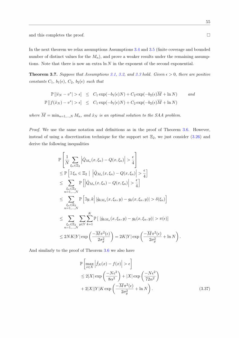
55

and this completes the proof.

In the next theorem we relax assumptions Assumptions 3.4 and 3.5 (finite coverage and bounded

number of distinct values for the Mn), and prove a weaker results under the remaining assump-

tions. Note that there is now an extra lnN in the exponent of the second exponential.

Theorem 3.7. Suppose that Assumptions 3.1, 3.2, and 3.3 hold. Given ε > 0, there are positive

constants C1, b1(ε), C2, b2(ε) such that

P [|vN − v∗| > ε] ≤ C1 exp(−b1(ε)N) + C2 exp(−b2(ε)M + lnN) and

P [|f(xN )− v∗| > ε] ≤ C1 exp(−b1(ε)N) + C2 exp(−b2(ε)M + lnN)

where M = minn=1,...,N Mn, and xN is an optimal solution to the SAA problem.

Proof. We use the same notation and definitions as in the proof of Theorem 3.6. However,

instead of using a discretization technique for the support set Ξ2, we just consider (3.26) and

derive the following inequalities

P

1

N

∑ξn∈Ξ2

∣∣∣QMn(x, ξn)−Q(x, ξn)∣∣∣ > ε

4

≤ P

[∃ ξn ∈ Ξ2

∣∣ ∣∣∣QMn(x, ξn)−Q(x, ξn)∣∣∣ > ε

4

]≤

∑ξn∈Ξ2n=1,...,N

P[∣∣∣QMn(x, ξn)−Q(x, ξn)

∣∣∣ > ε

4

]

≤∑ξn∈Ξ2n=1,...,N

P[∃y, k

∣∣∣ |gkMn(x, ξn, y)− gk(x, ξn, y)| > δ(ξn)]

≤∑ξn∈Ξ2n=1,...,N

∑y∈Y

K∑k=1

P [ |gkMn(x, ξn, y)− gk(x, ξn, y)| > π(ε)]

≤ 2NK|Y | exp

(−Mπ2(ε)

2σ2g

)= 2K|Y | exp

(−Mπ2(ε)

2σ2g

+ lnN

).

And similarly to the proof of Theorem 3.6 we also have

P[maxx∈X

∣∣∣fN (x)− f(x)∣∣∣ > ε

]≤ 2|X| exp

(−Nε2

8α2

)+ |X| exp

(−Nε2

72α2

)+ 2|X||Y |K exp

(−Mπ2(ε)

2σ2g

+ lnN

). (3.37)

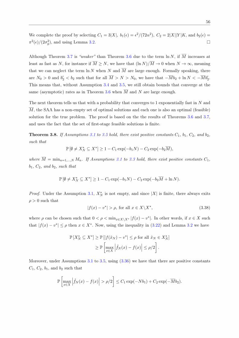
56

We complete the proof by selecting C1 = 3|X|, b1(ε) = ε2/(72α2), C2 = 2|X||Y |K, and b2(ε) =

π2(ε)/(2σ2g), and using Lemma 3.2.

Although Theorem 3.7 is “weaker” than Theorem 3.6 due to the term lnN , if M increases at

least as fast as N , for instance if M ≥ N , we have that (lnN)/M → 0 when N →∞, meaning

that we can neglect the term lnN when N and M are large enough. Formally speaking, there

are N0 > 0 and b′2 < b2 such that for all M > N > N0, we have that −Mb2 + lnN < −Mb′2.

This means that, without Assumption 3.4 and 3.5, we still obtain bounds that converge at the

same (asymptotic) rates as in Theorem 3.6 when M and N are large enough.

The next theorem tells us that with a probability that converges to 1 exponentially fast in N and

M , the SAA has a non-empty set of optimal solutions and each one is also an optimal (feasible)

solution for the true problem. The proof is based on the the results of Theorems 3.6 and 3.7,

and uses the fact that the set of first-stage feasible solutions is finite.

Theorem 3.8. If Assumptions 3.1 to 3.5 hold, there exist positive constants C1, b1, C2, and b2,

such that

P [∅ 6= X∗N ⊆ X∗] ≥ 1− C1 exp(−b1N)− C2 exp(−b2M),

where M = minn=1,...,N Mn. If Assumptions 3.1 to 3.3 hold, there exist positive constants C1,

b1, C2, and b2, such that

P [∅ 6= X∗N ⊆ X∗] ≥ 1− C1 exp(−b1N)− C2 exp(−b2M + lnN).

Proof. Under the Assumption 3.1, X∗N is not empty, and since |X| is finite, there always exits

ρ > 0 such that

|f(x)− v∗| > ρ, for all x ∈ X\X∗, (3.38)

where ρ can be chosen such that 0 < ρ < minx∈X\X∗ |f(x)− v∗|. In other words, if x ∈ X such

that |f(x)− v∗| ≤ ρ then x ∈ X∗. Now, using the inequality in (3.22) and Lemma 3.2 we have

P [X∗N ⊆ X∗] ≥ P [|f(xN )− v∗| ≤ ρ for all xN ∈ X∗N ]

≥ P[maxx∈X

∣∣∣fN (x)− f(x)∣∣∣ ≤ ρ/2] .

Moreover, under Assumptions 3.1 to 3.5, using (3.36) we have that there are positive constants

C1, C2, b1, and b2 such that

P[maxx∈X

∣∣∣fN (x)− f(x)∣∣∣ > ρ/2

]≤ C1 exp(−Nb1) + C2 exp(−Mb2).

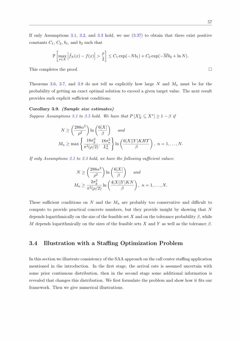
57

If only Assumptions 3.1, 3.2, and 3.3 hold, we use (3.37) to obtain that there exist positive

constants C1, C2, b1, and b2 such that

P[maxx∈X

∣∣∣fN (x)− f(x)∣∣∣ > ρ

2

]≤ C1 exp(−Nb1) + C2 exp(−Mb2 + lnN).

This completes the proof.

Theorems 3.6, 3.7, and 3.8 do not tell us explicitly how large N and Mn must be for the

probability of getting an exact optimal solution to exceed a given target value. The next result

provides such explicit sufficient conditions.

Corollary 3.9. (Sample size estimates)

Suppose Assumptions 3.1 to 3.5 hold. We have that P [X∗N ⊆ X∗] ≥ 1− β if

N ≥(

288α2

ρ2

)ln

(6|X|β

)and

Mn ≥ max

18σ2

g

π2(ρ/2),18σ2

κ

L2κ

ln

(6|X||Y |KHT

β

), n = 1, . . . , N.

If only Assumptions 3.1 to 3.3 hold, we have the following sufficient values:

N ≥(

288α2

ρ2

)ln

(6|X|β

)and

Mn ≥2σ2

g

π2(ρ/2)ln

(4|X||Y |KN

β

), n = 1, . . . , N.

These sufficient conditions on N and the Mn are probably too conservative and difficult to

compute to provide practical concrete numbers, but they provide insight by showing that N

depends logarithmically on the size of the feasible set X and on the tolerance probability β, while

M depends logarithmically on the sizes of the feasible sets X and Y as well as the tolerance β.

3.4 Illustration with a Staffing Optimization Problem

In this section we illustrate consistency of the SAA approach on the call center staffing application

mentioned in the introduction. In the first stage, the arrival rate is assumed uncertain with

some prior continuous distribution, then in the second stage some additional information is

revealed that changes this distribution. We first formulate the problem and show how it fits our

framework. Then we give numerical illustrations.

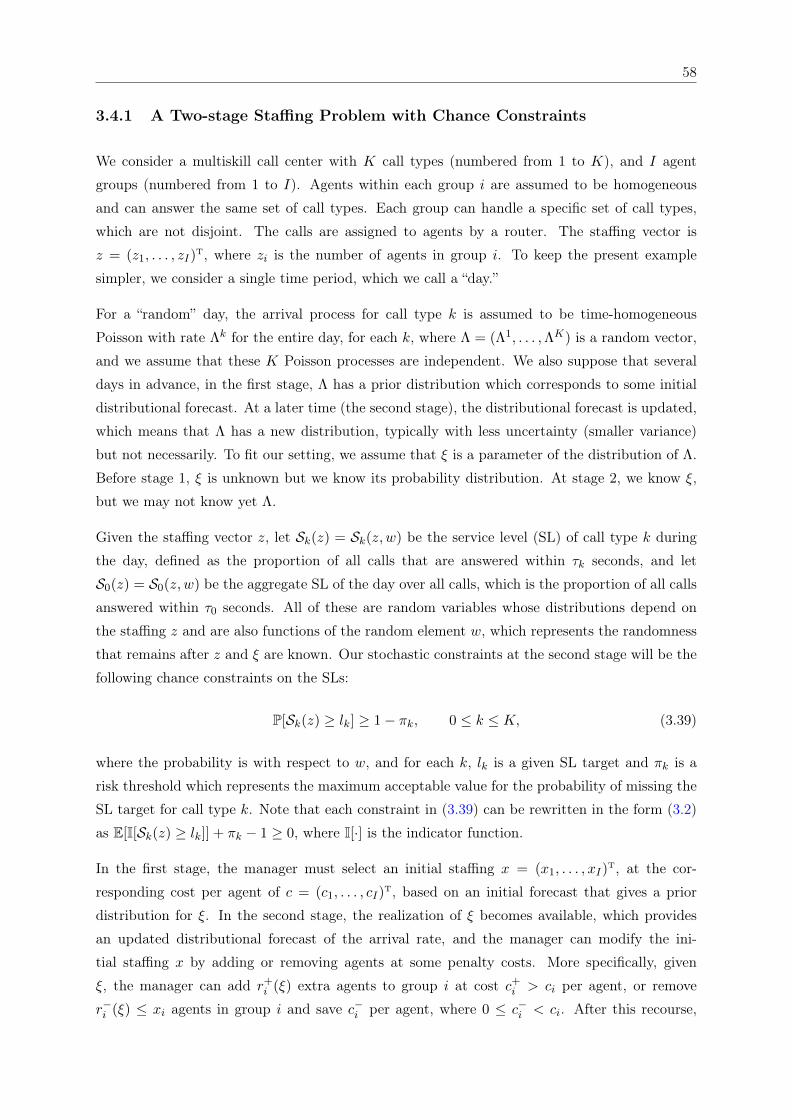
58

3.4.1 A Two-stage Staffing Problem with Chance Constraints

We consider a multiskill call center with K call types (numbered from 1 to K), and I agent

groups (numbered from 1 to I). Agents within each group i are assumed to be homogeneous

and can answer the same set of call types. Each group can handle a specific set of call types,

which are not disjoint. The calls are assigned to agents by a router. The staffing vector is

z = (z1, . . . , zI)T, where zi is the number of agents in group i. To keep the present example

simpler, we consider a single time period, which we call a “day.”

For a “random” day, the arrival process for call type k is assumed to be time-homogeneous

Poisson with rate Λk for the entire day, for each k, where Λ = (Λ1, . . . ,ΛK) is a random vector,

and we assume that these K Poisson processes are independent. We also suppose that several

days in advance, in the first stage, Λ has a prior distribution which corresponds to some initial

distributional forecast. At a later time (the second stage), the distributional forecast is updated,

which means that Λ has a new distribution, typically with less uncertainty (smaller variance)

but not necessarily. To fit our setting, we assume that ξ is a parameter of the distribution of Λ.

Before stage 1, ξ is unknown but we know its probability distribution. At stage 2, we know ξ,

but we may not know yet Λ.

Given the staffing vector z, let Sk(z) = Sk(z, w) be the service level (SL) of call type k during

the day, defined as the proportion of all calls that are answered within τk seconds, and let

S0(z) = S0(z, w) be the aggregate SL of the day over all calls, which is the proportion of all calls

answered within τ0 seconds. All of these are random variables whose distributions depend on

the staffing z and are also functions of the random element w, which represents the randomness

that remains after z and ξ are known. Our stochastic constraints at the second stage will be the

following chance constraints on the SLs:

P[Sk(z) ≥ lk] ≥ 1− πk, 0 ≤ k ≤ K, (3.39)

where the probability is with respect to w, and for each k, lk is a given SL target and πk is a

risk threshold which represents the maximum acceptable value for the probability of missing the

SL target for call type k. Note that each constraint in (3.39) can be rewritten in the form (3.2)

as E[I[Sk(z) ≥ lk]] + πk − 1 ≥ 0, where I[·] is the indicator function.

In the first stage, the manager must select an initial staffing x = (x1, . . . , xI)T, at the cor-

responding cost per agent of c = (c1, . . . , cI)T, based on an initial forecast that gives a prior

distribution for ξ. In the second stage, the realization of ξ becomes available, which provides

an updated distributional forecast of the arrival rate, and the manager can modify the ini-

tial staffing x by adding or removing agents at some penalty costs. More specifically, given

ξ, the manager can add r+i (ξ) extra agents to group i at cost c+

i > ci per agent, or remove

r−i (ξ) ≤ xi agents in group i and save c−i per agent, where 0 ≤ c−i < ci. After this recourse,

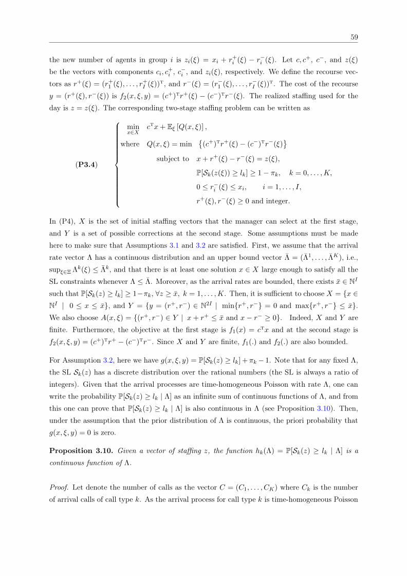
59

the new number of agents in group i is zi(ξ) = xi + r+i (ξ) − r−i (ξ). Let c, c+, c−, and z(ξ)

be the vectors with components ci, c+i , c

−i , and zi(ξ), respectively. We define the recourse vec-

tors as r+(ξ) = (r+1 (ξ), . . . , r+

I (ξ))T, and r−(ξ) = (r−1 (ξ), . . . , r−I (ξ))T. The cost of the recourse

y = (r+(ξ), r−(ξ)) is f2(x, ξ, y) = (c+)Tr+(ξ) − (c−)Tr−(ξ). The realized staffing used for the

day is z = z(ξ). The corresponding two-stage staffing problem can be written as

(P3.4)

minx∈X

cTx+ Eξ [Q(x, ξ)] ,

where Q(x, ξ) = min

(c+)Tr+(ξ)− (c−)Tr−(ξ)

subject to x+ r+(ξ)− r−(ξ) = z(ξ),

P[Sk(z(ξ)) ≥ lk] ≥ 1− πk, k = 0, . . . ,K,

0 ≤ r−i (ξ) ≤ xi, i = 1, . . . , I,

r+(ξ), r−(ξ) ≥ 0 and integer.

In (P4), X is the set of initial staffing vectors that the manager can select at the first stage,

and Y is a set of possible corrections at the second stage. Some assumptions must be made

here to make sure that Assumptions 3.1 and 3.2 are satisfied. First, we assume that the arrival

rate vector Λ has a continuous distribution and an upper bound vector Λ = (Λ1, . . . , ΛK), i.e.,

supξ∈Ξ Λk(ξ) ≤ Λk, and that there is at least one solution x ∈ X large enough to satisfy all the

SL constraints whenever Λ ≤ Λ. Moreover, as the arrival rates are bounded, there exists x ∈ NI

such that P[Sk(z) ≥ lk] ≥ 1−πk, ∀z ≥ x, k = 1, . . . ,K. Then, it is sufficient to choose X = x ∈NI | 0 ≤ x ≤ x, and Y = y = (r+, r−) ∈ N2I | minr+, r− = 0 and maxr+, r− ≤ x.We also choose A(x, ξ) = (r+, r−) ∈ Y | x+ r+ ≤ x and x− r− ≥ 0. Indeed, X and Y are

finite. Furthermore, the objective at the first stage is f1(x) = cTx and at the second stage is

f2(x, ξ, y) = (c+)Tr+ − (c−)Tr−. Since X and Y are finite, f1(.) and f2(.) are also bounded.

For Assumption 3.2, here we have g(x, ξ, y) = P[Sk(z) ≥ lk] + πk − 1. Note that for any fixed Λ,

the SL Sk(z) has a discrete distribution over the rational numbers (the SL is always a ratio of

integers). Given that the arrival processes are time-homogeneous Poisson with rate Λ, one can

write the probability P[Sk(z) ≥ lk | Λ] as an infinite sum of continuous functions of Λ, and from

this one can prove that P[Sk(z) ≥ lk | Λ] is also continuous in Λ (see Proposition 3.10). Then,

under the assumption that the prior distribution of Λ is continuous, the priori probability that

g(x, ξ, y) = 0 is zero.

Proposition 3.10. Given a vector of staffing z, the function hk(Λ) = P[Sk(z) ≥ lk | Λ] is a

continuous function of Λ.

Proof. Let denote the number of calls as the vector C = (C1, . . . , CK) where Ck is the number

of arrival calls of call type k. As the arrival process for call type k is time-homogeneous Poisson

60

with rate Λk, we can write the probability that the service level is at least some values as

hk(Λ) = P[Sk ≥ lk | Λ]

=∞∑r=0

∑c∈NK||c||1=r

P[Sk ≥ lk | C = c]P[C = c|Λ]

=

∞∑r=0

∑c∈NK||c||1=r

αcP[C = c |Λ]

=∞∑r=0

∑c∈NK||c||1=r

αc

K∏k=1

P[Ck = ck |Λk

],

(3.40)

where c = (c1, . . . , cK), ||c||1 =∑K

k=1 |ck|, and αc = P[Sk ≥ lk |C = c] ≤ 1. Moreover, each term

P[Ck = ck |Λk] is a continuous function with respect to Λk. So, P[C = c |Λ] is also a continuous

function with respect to Λ, and hk(Λ) can be written as an infinite sum of continuous functions.

From the definition of continuity, hk(Λ) is continuous if for any Λ0, and for any δ > 0, there

exists ε1 > 0 such that for all Λ satisfies ‖Λ− Λ0‖ ≤ ε1, we always have

|hk(Λ)− hk(Λ0)| ≤ δ, (3.41)

where ‖ · ‖ is the Euclidean norm.

To prove the continuity of hk(Λ), as limt→∞ P[Ck > t] = 0, we first have that, given any δ > 0,

there always exists t1 > 0 large enough such that

∑c∈NK

ck>t1,k=1,...,K

αcP[C = c | Λ] ≤∑c∈NK

ck>t1,k=1,...,K

P[C = c | Λ] =K∏k=1

P[Ck > t1|Λ

]≤ δ

4. (3.42)

Moreover, one can show that there exists t2 > 0 such that for all ck > t2, k = 1, . . . ,K, the

function P[Ck = ck |Λk] is monotonically increasing with respect to Λk. This can be verified by

considering the first-order derivative of P[Ck = ck |Λk] with respect to Λk

∂P[Ck = ck |Λk]∂Λk

=(Λk)ck−1

(ck − 1)!e−Λk − (Λk)ck

(ck)!e−Λk =

(Λk)ck−1

(ck − 1)!e−Λk

(1− Λk

ck

), (3.43)

which is positive if 1 − Λk/ck > 0. Since 1 − Λk/ck ≥ 1 − Λ/ck, it suffices to take t2 ≥ Λ.

Combine (3.42) and (3.43), and by choosing t0 = maxt1, t2 we obtain

∑c∈NK

ck>t0,k=1,...,K

αcP[C = c |Λ] ≤∑c∈NK

ck>t0,k=1,...,K

αcP[C = c | Λ] ≤ δ

4, for all Λ ≤ Λ. (3.44)

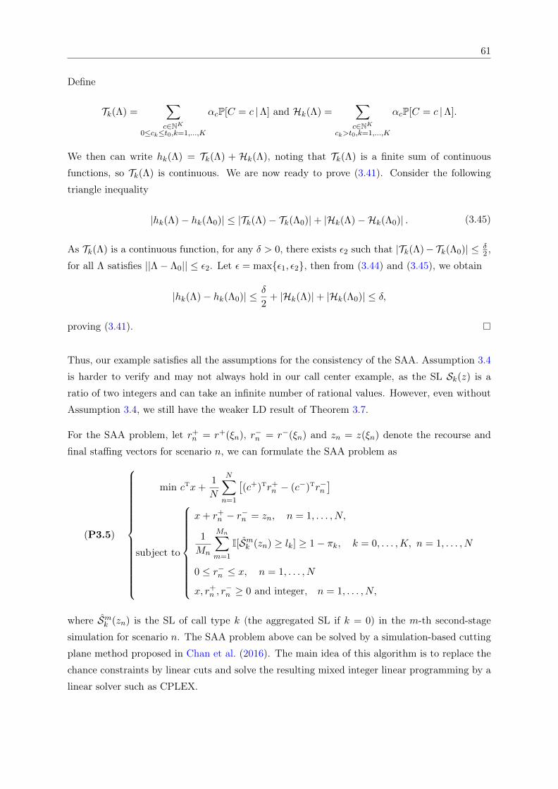
61

Define

Tk(Λ) =∑c∈NK

0≤ck≤t0,k=1,...,K

αcP[C = c |Λ] and Hk(Λ) =∑c∈NK

ck>t0,k=1,...,K

αcP[C = c |Λ].

We then can write hk(Λ) = Tk(Λ) + Hk(Λ), noting that Tk(Λ) is a finite sum of continuous

functions, so Tk(Λ) is continuous. We are now ready to prove (3.41). Consider the following

triangle inequality

|hk(Λ)− hk(Λ0)| ≤ |Tk(Λ)− Tk(Λ0)|+ |Hk(Λ)−Hk(Λ0)| . (3.45)

As Tk(Λ) is a continuous function, for any δ > 0, there exists ε2 such that |Tk(Λ)−Tk(Λ0)| ≤ δ2 ,

for all Λ satisfies ||Λ− Λ0|| ≤ ε2. Let ε = maxε1, ε2, then from (3.44) and (3.45), we obtain

|hk(Λ)− hk(Λ0)| ≤ δ

2+ |Hk(Λ)|+ |Hk(Λ0)| ≤ δ,

proving (3.41).

Thus, our example satisfies all the assumptions for the consistency of the SAA. Assumption 3.4

is harder to verify and may not always hold in our call center example, as the SL Sk(z) is a

ratio of two integers and can take an infinite number of rational values. However, even without

Assumption 3.4, we still have the weaker LD result of Theorem 3.7.

For the SAA problem, let r+n = r+(ξn), r−n = r−(ξn) and zn = z(ξn) denote the recourse and

final staffing vectors for scenario n, we can formulate the SAA problem as

(P3.5)

min cTx+1

N

N∑n=1

[(c+)Tr+

n − (c−)Tr−n]

subject to

x+ r+n − r−n = zn, n = 1, . . . , N,

1

Mn

Mn∑m=1

I[Smk (zn) ≥ lk] ≥ 1− πk, k = 0, . . . ,K, n = 1, . . . , N

0 ≤ r−n ≤ x, n = 1, . . . , N

x, r+n , r

−n ≥ 0 and integer, n = 1, . . . , N,

where Smk (zn) is the SL of call type k (the aggregated SL if k = 0) in the m-th second-stage

simulation for scenario n. The SAA problem above can be solved by a simulation-based cutting

plane method proposed in Chan et al. (2016). The main idea of this algorithm is to replace the

chance constraints by linear cuts and solve the resulting mixed integer linear programming by a

linear solver such as CPLEX.

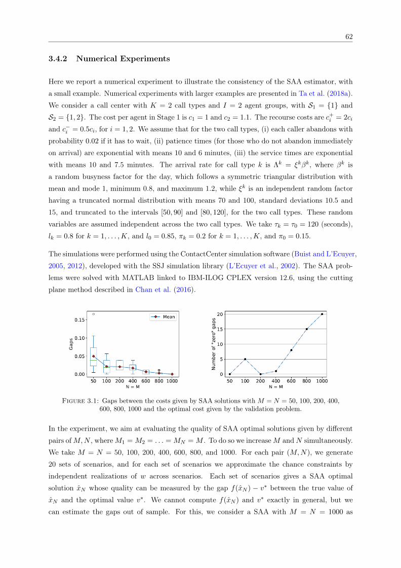
62

3.4.2 Numerical Experiments

Here we report a numerical experiment to illustrate the consistency of the SAA estimator, with

a small example. Numerical experiments with larger examples are presented in Ta et al. (2018a).

We consider a call center with K = 2 call types and I = 2 agent groups, with S1 = 1 and

S2 = 1, 2. The cost per agent in Stage 1 is c1 = 1 and c2 = 1.1. The recourse costs are c+i = 2ci

and c−i = 0.5ci, for i = 1, 2. We assume that for the two call types, (i) each caller abandons with

probability 0.02 if it has to wait, (ii) patience times (for those who do not abandon immediately

on arrival) are exponential with means 10 and 6 minutes, (iii) the service times are exponential

with means 10 and 7.5 minutes. The arrival rate for call type k is Λk = ξkβk, where βk is

a random busyness factor for the day, which follows a symmetric triangular distribution with

mean and mode 1, minimum 0.8, and maximum 1.2, while ξk is an independent random factor

having a truncated normal distribution with means 70 and 100, standard deviations 10.5 and

15, and truncated to the intervals [50, 90] and [80, 120], for the two call types. These random

variables are assumed independent across the two call types. We take τk = τ0 = 120 (seconds),

lk = 0.8 for k = 1, . . . ,K, and l0 = 0.85, πk = 0.2 for k = 1, . . . ,K, and π0 = 0.15.

The simulations were performed using the ContactCenter simulation software (Buist and L’Ecuyer,

2005, 2012), developed with the SSJ simulation library (L’Ecuyer et al., 2002). The SAA prob-

lems were solved with MATLAB linked to IBM-ILOG CPLEX version 12.6, using the cutting

plane method described in Chan et al. (2016).

Figure 3.1: Gaps between the costs given by SAA solutions with M = N = 50, 100, 200, 400,600, 800, 1000 and the optimal cost given by the validation problem.

In the experiment, we aim at evaluating the quality of SAA optimal solutions given by different

pairs ofM,N , whereM1 = M2 = . . . = MN = M . To do so we increaseM andN simultaneously.

We take M = N = 50, 100, 200, 400, 600, 800, and 1000. For each pair (M,N), we generate

20 sets of scenarios, and for each set of scenarios we approximate the chance constraints by

independent realizations of w across scenarios. Each set of scenarios gives a SAA optimal

solution xN whose quality can be measured by the gap f(xN ) − v∗ between the true value of

xN and the optimal value v∗. We cannot compute f(xN ) and v∗ exactly in general, but we

can estimate the gaps out of sample. For this, we consider a SAA with M = N = 1000 as

63

a validation problem, in which the set of scenarios is independent of those used to obtain xN .

We then compute the gaps between the costs given by these SAA solutions and the optimal

costs given by the validation problem. Let f and f∗ denote the first-stage cost function and

the optimal cost given by the SAA validation problem. We estimate the gap by f(xN )− f∗. InFigure 3.1, on the left side we show box plots of the estimated gaps and on the right side we

report the number of zero gaps, for the selected values of N = M . We see that when M = N

increase above 400, the number of SAA solutions that are also optimal for the validation problem

increases quickly with N . When M = N = 1000, the corresponding SAA solutions are all the

same, and identical to the optimal solution of the validation problem.

3.5 Conclusion

We have considered a two-stage stochastic programming problem with stochastic constraints in

the second stages. We have studied the consistency of the SAA method with nested sampling

to solve this problem, and we also proved exponential convergence of the probability of making

incorrect decisions. We used a call center staffing problem under arrival rate uncertainty to

illustrate our theoretical findings. For future work, it would be interesting to investigate methods

for choosing the sample size at the second stage adaptively, e.g., with larger sample sizes for the

more important scenarios. Another important aspect is to develop effective methods for solving

the SAA in large-scale settings.

Acknowledgment

This work has been supported by a Canada Research Chair, an Inria International Chair, and

a Hydro-Québec research grant to P. L’Ecuyer, by NSERC Discovery Grants to F. Bastin and

P. L’Ecuyer, by the SMART (Singapore-MIT Alliance for Research and Technology) scholar

program to Tien Mai, and by scholarships from the CIRRELT, DIRO and Université de Montréal

to T.A. Ta.

Chapter 4

Simulation-based Decomposition

Method for Two-stage Staffing

Optimization

In this chapter we consider the case that the arrival rates cannot be forecasted perfectly, leading

to a two-stage stochastic optimization problem. To solve the problem numerically, we formulate

its SAA version of which the consistency can be guaranteed through the results of Chapter 3. We

propose an algorithm that combines simulation, integer linear programming, cut generation and

the L-shaped method to solve the SAA problem. Numerical results based on three call center

examples show that our approach is practically efficient. This work has been presented at the

21st Conference of the International Federation of Operational Research Societies (Québec City,

Canada, July 2017) and the International Conference on Monte Carlo Methods and Applications

(MCM) (Montréal, Canada, July 2017).

Contents4.1 Introduction . . . . . . . . . . . . . . . . . . . . . . . . . . . . . . . . . 65

4.2 Literature Review . . . . . . . . . . . . . . . . . . . . . . . . . . . . . . 68

4.3 Problem Formulation and the Sample Average Approximation . . . 69

4.4 General Methodology . . . . . . . . . . . . . . . . . . . . . . . . . . . . 74

4.5 Numerical Experiments . . . . . . . . . . . . . . . . . . . . . . . . . . . 85

4.6 Conclusion . . . . . . . . . . . . . . . . . . . . . . . . . . . . . . . . . . 94

64

65

A Simulation-based Decomposition Approach forTwo-stage Staffing Optimization in Call Centers under

Arrival Rate Uncertainty

Thuy Anh Ta1, Wyean Chan1, Fabian Bastin1, and Pierre L’Ecuyer1

1Department of Computer Science and Operational Research, Université de Montréal and CIRRELT,

Canada

Abstract

This paper studies a common staffing problem in multiskill call centers. The objective is to

find a staffing solution with minimal cost while ensuring the desired level of quality of service

to customers. We consider the case where the arrival rates cannot be forecasted perfectly,

leading to a two-stage stochastic optimization problem. The arrival rates are modeled as random

variables with large variance (uncertainty) in the first stage, and smaller variance in the second

stage. The challenge lies in the complexity of the stochastic model, as the queuing system

needs to be simulated for a large number of scenarios and days. We propose a simulation-based

decomposition method, combined with sample average approximation (SAA), to solve this two-

stage staffing problem in reasonable computing time. We provide numerical studies based on

three call center examples to illustrate the practical efficiency of our decomposition approach.

Keywords: Two-stage stochastic program, multiskill call center, cutting plane, L-shaped, simu-

lation.

4.1 Introduction

The call center industry has been on a steady rise over the years. For instance, in the United

States, the number of call center agents rose from 2.1 million in 2004 to 2.7 million in 2016

with an estimated annual salary cost of US $95.2 billion (Bureau of Labor Statistics, 2007,

2016). Businesses use call centers to provide information and assistance to customers, to improve

customer satisfaction, or to increase revenue. Some call centers provide essential service, like the

911 emergency calls. Traditionally, call centers employ agents to interact with customers over

the telephone, but with today’s technology, they can also include emails and chat, and these are

often referred as contact centers.

In multiskill call centers, a call represents a customer and it is categorized by the type of requested

service (this is often determined when the customer travels through the interactive voice menu).

Each call type requires a specific skill, and an agent must have that particular skill in order to

66

answer it. Idle agents are assigned to calls by a router, following some skill-based routing policy,

see Chan et al. (2014a) for some examples. For easier management, agents are generally divided

into groups of similar skill sets. We refer the readers to Gans et al. (2003) for a more detailed

description.

The quality of service (QoS) of a call center is often measured according to the service level

(SL). The SL measures the fraction of calls that are answered within a given time, called the

acceptable wait threshold (AWT). The constraint on the SL is most commonly stated as s percent

of calls answered in τ seconds or less, where τ is a parameter, and is usually denoted by s/τ .

For instance, a SL constraint of 80/30 would mean 80% of calls answered within 30 seconds.

An important problem in call centers is the staffing problem, which deals with minimizing the

staffing cost under a set of constraints on the QoS. In this problem, a day is usually divided

into periods. Based on distributional forecast of the volume of calls and a stochastic model of

the entire call center, the task is to decide how many agents of each skill group to have at each

time period of the day. A more difficult problem is the scheduling problem (Avramidis et al.,

2010), in which a set of admissible shift schedules is first specified, and the decision variables

are the number of agents of each group in each shift. The number of decision variables in the

scheduling problem is typically much larger than in the staffing problem due to the numerous

combinations of work shifts, breaks, lunch breaks, training, etc. In that problem, the staffing is

determined indirectly by the selected shift schedules. Note that the routing policy can also be

optimized (Chan et al., 2014a, Koole et al., 2015), but such extensions are outside the scope of

this paper.

There are two important issues in the existing literature: (i) the arrival rates are often assumed to

be known perfectly, and (ii) the quality-of-service (QoS) targets (constraints) are usually defined

with respect to the long-term expected value, which is an average over an infinite number of

days. A perfect knowledge of the arrival rates can lead to simple optimization problems, but it

is well known that the arrival rates in call centers are often uncertain and depend on multiple

factors, such as the day of the week, time of the day, level of busyness, holidays and special

events (see for instance Channouf et al., 2007, Ibrahim et al., 2016b, Oreshkin et al., 2016).

Moreover, in practice, a call center is a (highly) transient queuing system where the arrival rates

and staffing level change often throughout the day. The QoS of a given day should then be

modeled as a random variable. A manager who desires to meet the QoS targets for a given

proportion of the days, or with a given probability, should impose some distributional or chance

constraints. The aim of this paper is to address the aforementioned issues by formulating and

solving the staffing problem under the uncertainty of the arrival rates and probability constraints

(i.e. chance constraints).

In this paper, we consider a chance-constrained two-stage staffing with recourse problem for

multiskill call centers. The first-stage problem consists of finding an initial staffing based on

67

some long-term forecast of the arrival rates, with large level of uncertainty. In the second-stage,

recourse actions may be applied to correct the initial staffing, by adding or removing agents at

the price of some penalty costs, upon the availability of an updated forecast. Chance constraints

are imposed on the staffing, such that the QoS of a day must meet its target with a minimum

probability threshold. To solve the problem, we use the sample average approximation (SAA)

method. The model is challenging due to the nonlinearity of the chance constraints and the

large number of integer variables. Previous studies suggest that the chance constraints can be

approximated by linear cuts and the resulting two-stage linear programs can be solved directly

by standard mixed-integer program (MIP) solvers, such as CPLEX. However, the computation

time quickly becomes too expensive for larger instances.

Our aim in this paper is to deal with challenges encountered with large-scale two-stage staffing

optimization problems, and develop novel methodologies that allow to solve such problems in

a practical way. More precisely, we propose a simulation-based decomposition method that

consists of two main steps. First, for each scenario, we use simulation to generate linear cuts

to remove infeasible solutions. Then, we iteratively solve the two-stage stochastic programming

problem in which the chance constraints are replaced by linear ones and add more cuts if there

are solutions that do not satisfy the chance constraints.

The first step allows us to create linear outer approximations of the probability functions and

linearize the chance constraints. This step is based on the cutting plane method (Atlason et al.,

2004), which is considered as the state-of-the-art approach to deal with “S-shaped” constraints.

The performance of the method, however, strongly depends on the determination of the con-

cave regions of the probability functions. In our context, these concave regions are difficult to

accurately identify. We propose a heuristic method to adjust the staffing to ensure that cuts

are generated from concave regions. Moreover, to efficiently solve the resulting two-stage linear

programs at the second step, we propose a way to strengthen the linear cuts by mixed-integer

rounding inequalities (Nemhauser and Wolsey, 1990) and decompose the mixed-integer linear

problems using the L-shaped method. The idea of the L-shaped is that, instead of solving the

complete mixed-integer program directly, we decompose it and iteratively solve a master program

that is enriched by linear cuts at each iteration.

We report numerical experiments for staffing problems over a single period, in which we assume

that the system is in steady state. We solve problems of different call-center sizes and numbers

of scenarios, from a toy example with 2 call types and 2 agent groups, to an example of moderate

size with 15 call types and 20 agent groups. Our experiments show that our simulation-based

decomposition approach is able to returns good staffing solutions in reasonably small computing

time and it performs better than the deterministic equivalence approach proposed in our previous

studies (Chan et al., 2016).

68

In the remainder of this paper, we review the relevant literature on the staffing and scheduling of

multiskill call centers in Section 4.2. In Section 4.3, we define the two-stage staffing optimization

problem, as well as its SAA formulation. We present our decomposition algorithm to solve

the stochastic problem in Section 4.4. In Section 4.5, we compare the performance of the

proposed algorithm and the deterministic equivalent approach in multiple numerical experiments.

Conclusions are given in Section 4.6.

4.2 Literature Review

Research studies have focused traditionally on single-skill call centers, see Green et al. (2003)

for example, but there exist a few studies on the optimization of multiskill call centers. One

reason is that multiskill queues are analytically more complex than single queues, and there are

no known accurate approximation formulas for the QoS for multiskill queues. One must rely on

time-costly simulation to estimate accurately the QoS. For the traditional staffing problem with

known arrival rates, Cezik and L’Ecuyer (2008) propose a simulation-based MIP optimization

method where the linear cuts are added iteratively using the subgradient of the SL function.

Avramidis et al. (2010) extend this algorithm to solve the shift scheduling problem with multiple

periods. These methods can be viewed as the adaption and generalization of the technique

presented in Atlason et al. (2004) for the scheduling of single-skill call centers with constraints

on the expected SL over an infinite time horizon. This method combines simulation with integer

programming and cut generation, based on the concavity property of the SL function in the

Erlang C model, when the queue is in steady state. However, the concavity property does not

necessarily hold in the multiskill context. These algorithms are therefore heuristics, but they

have been shown to work well empirically. Other algorithms (Avramidis et al., 2009, Pot et al.,

2008, Wallace and Whitt, 2005) have been proposed for the single period staffing problem that

use crude approximation formulas, search methods, and correction by simulation.

Forecasting call arrival rates is hard, so it is justified to include arrival rate uncertainty in the

optimization problems. Recently, a growing number of studies consider stochastic optimization.

Liao et al. (2013) and Liao et al. (2013) include the uncertainty of the arrival rate in the form of a

discrete probability distribution, Gurvich et al. (2010), Helber and Henken (2010) and Robbins

and Harrison (2010) discretize continuous probability distributions by random sampling, and

Gans et al. (2015) explore the Gaussian quadrature.

Robbins and Harrison (2010) consider a stochastic scheduling problem for a single-skill call

center, where a penalty cost is given for missing the SL target. A two-stage scheduling problem

with recourse for single-skill call centers is investigated in Gans et al. (2015). The forecast is

updated during the day, and the schedules can be corrected by adding or removing agents for the

latter part of the day. These papers use a MIP solver to deal with a MIP where a set of constraints

69

are generated beforehand by the linearization of the SL or abandonment, respectively, function

of a M/M/s single queue with abandonments. It is not clear how or even if this approach can

be generalized to the multiskill case.

For multiskill call centers with random arrival rates, Harrison and Zeevi (2005) and Bassamboo

et al. (2006) approximate the level of abandonments by a fluid system, and they solve a two-stage

scheduling problem. Their models seek to minimize the scheduling cost function with a penalty

cost on the abandonments. The first-stage variables are the schedules, and the second-stage

variables control the work assignment of each agent. A major drawback when optimizing a fluid

system is that it also changes the routing policy, which is often not possible in practice. Gurvich

et al. (2010) optimize a two-stage staffing problem with the chance constraints on the expectation

of the fraction of abandonments, for stochastic arrival rates. The requirement is that the QoS

can be violated on at most a fraction δ of the arrival rate realizations, where δ represents the

level of risk tolerance. Chan et al. (2016) propose an extension to Cezik and L’Ecuyer (2008)

to solve a two-stage staffing problem with scenario decomposition. The second-stage variables

are recourse actions to add or remove agents, and we consider chance constraints on the SL of

a day (not the expectation). In the present paper, we propose further improvements using a

decomposition approach.

4.3 Problem Formulation and the Sample Average Approxima-

tion

We now present a formulation of the multiskill staffing optimization problem under arrival rate

uncertainty. There are K call types, I agent groups, one period and N scenarios. We also

give a sample average approximation formulation in which the constraints are approximated by

simulation. Since this paper considers the same staffing optimization problem as in Chan et al.

(2016) and Ta et al. (2018b), we will use similar notations.

4.3.1 Call Center Model

Consider a call center with K call types, indexed from 1 to K, and I agent groups, numbered

from 1 to I. Agents in group i have the skill set Si ⊆ 1, . . . ,K, which defines the call types

they can serve. In practice, an agent can have more skills than his group’s skill set, but only the

skills in Si will be active. Conversely, we define Gk = i : k ∈ Si as the set of groups that can

answer calls of type k. Let z = (z1, . . . , zI)T be the staffing vector which defines the number of

agents in each of the I groups.

70

We assume that agents in the same group are homogeneous, and an agent in group i will serve a

call of type k with an average time of 1/µk,i. A customer will abandon the queue (and the call

center) when their waiting time exceeds their patience time. The patience time is modeled as a

random variable with mean 1/νk for calls of type k. Calls are assigned to agents by the router,

according to a routing policy. A major advantage of using simulation-based optimization is that

we do not need to impose any specific distribution family or routing policy in our model. The

service time can be exponential or lognormal for example. Like Wallace and Whitt (2005) and

Cezik and L’Ecuyer (2008), we optimize the staffing for only one period in order to simplify the

problem.

4.3.2 Random Arrival Rates

We assume that calls of type k arrive following a time-homogeneous Poisson process with rate

Λk that is constant throughout the entire period. In reality, the rate is not known in advance

(actually, it cannot even be observed), therefore Λk is a random variable, and it embeds the

uncertainty or errors of the forecast. The random variable Λk can follow any distribution.

In our two-stage staffing problem, we define Stage 1 as the time epoch where the call center

manager needs to provide an initial staffing for a future date, based on some initial (prior)

distribution forecast. Stage 1 can be days or weeks in advance of the targeted date. As the

targeted date draws near, the manager may have more actual information, like the trend of the

arrivals, and revise the forecast with a posterior distribution. In Stage 2, we assume that the

manager may correct the initial staffing by adding or removing agents from the schedule, using

the revised forecast. These resource actions may correspond to scheduling or canceling meetings

(or trainings) with agents. Note that, in general, the rate Λk is still a random variable in Stage

2.

As an example, in the numerical section, we consider that in Stage 1, the arrival rate Λk = ξkβk

follows a doubly stochastic distribution, where ξk represents a random mean rate and βk is a

random busyness factor of the day. In Stage 2, we assume that ξk can be estimated, and only βkremains random. In practice, we may relate ξk to the general trend of the call volume, and βkmay be some noise (although there can be correlation between call types). We chose arbitrarily

ξk to be normally distributed, and βk to have a triangular distribution in our numerical examples.

4.3.3 Service Level Constraint

In a service system, the quality of service experienced by the customers is an important measure.

A popular measure in the call center industry is the service level (SL) that was introduced in

Section 4.1. The SL is defined as the proportion of callers who waited less than an acceptable

71

waiting time (AWT) parameter τ . The constraint is to maintain a SL above a certain target

l ∈ [0, 1]. In practice, the formula of the SL may vary from one call center to another, because

it depends on how to include abandonments, how to count calls with over-lapping periods, etc.

In our work, we use one of the SL formulas implemented in the simulation library ContactCenters

(Buist and L’Ecuyer, 2005); alternative definitions of the SL can be found in Jouini et al. (2013).

In this study, instead of considering the expected value, we consider the distributions of SL in a

given time interval. Let T be the total number of calls that arrived in a day, A(z) be the number

of calls served after waiting at most τ , and L(z) be the number of calls that abandoned after

waiting more than τ . All of these variables are random, so that the SL over a given time period

is also a random variable which depends on the number of staffing z. The formula of SL is:

S(z) =A(z)

T − L(z). (4.1)

The SL of each call type can be measured with different values of the AWT parameter τ . In the

numerical experiment, we use the same τ for all call types.

Most studies in staffing in call centers consider the expected performance measures over an

infinite time horizon. A formula of service level defines a fraction of customers with good QoS

over an infinite number of independent and identically distributed (i.i.d.) days, that is:

S(z) =E[A(z)]

E[T − L(z)]. (4.2)

This formula was used in most previous articles on staffing and scheduling optimization (Atlason

et al., 2004, Avramidis et al., 2009, 2010, Cezik and L’Ecuyer, 2008). A typical constraint on

the SL is, for example, that S(z) = 80% with τ = 20 seconds, it means that 80% of calls are

answered within τ = 20 seconds. In multiskill call centers, there is no analytically formula to

compute the SLs in (4.1) and (4.2), but we can use simulation to estimate them.

4.3.4 Chance Constraints on the SL

We consider chance constraints using the random variable SL S(z) defined in (4.1). In fact, even

if we suppose that the arrival rate is constant, the variable S(z) may have significant stochastic

variance and the tail of its distribution (not only the average) is relevant. This means that even

if the staffing gives an expected SL over an infinite number of days above the target, the observed

SL of a day may still be well below the target. In case a manager wants to satisfy the SL target

most of the days, then chance constraints on S(z) can be applicable. They can be expressed

as: the SL targets (per call type, per period, global) on a random day must be satisfied with

probability at least 1− δ, for a given risk level δ selected by the manager.

72

Given the staffing vector z, let Sk(z) be the SL of call type k during the day, with AWT τk, and

let S0(z) be the aggregate SL of the day over all calls with AWT τ0. All of these are random

variables, whose distributions depend on the staffing z. The chance constraints are:

P[S0(z) ≥ l0] ≥ 1− δ0,

P[Sk(z) ≥ lk] ≥ 1− δk, k = 1, . . . ,K,

where lk and l0 are the SL targets, and δk and δ0 are the given risk thresholds in the interval

(0, 1), for each call type k and for the whole day. To give an example of chance constraints,

setting δk = δ0 = 0.05, lk = l0 = 0.8, and τk = τ0 = 20 seconds means that 80% of calls in a day

must be answered within 20 seconds, with at least 95% probability.

4.3.5 Staffing Problem with Recourse

We now describe our two-stage staffing problem with arrival rates uncertainty. In the first

stage, based on initial forecast that gives the prior distributions of arrival rates Λk for each call

type k, (parameterized by a random parameter ξk), the manager must select an initial staffing

x = (x1, . . . , xI)T at the corresponding cost per agent of c = (c1, . . . , cI)

T. In the second stage,

the manager obtains the realizations of ξ = (ξ1, . . . , ξK) ∈ Ξ, and based on the updated forecasts,

the initial staffing can be modified by adding or removing agents at some penalty costs. We

remark that even when ξk is known, in the second stage, the exact arrival rate may still be

random (the realization of Λk). Even in the case the arrival rate is known, we still do not know

the SL for the day, so there is still uncertainty. In our work, we suppose perfect forecast of

ξk in the second stage, meaning that ξk simply has a new distribution with only one possible

realization.

In the second stage, given the posterior distributions of the ξk’s, we can modify the initial

staffing by adding r+i (ξ) extra agents to group i at a greater cost of c+

i > ci per agent, or

removing r−i (ξ) ≤ xi agents in group i and save c−i per agent, where 0 ≤ c−i < ci. After the

recourse, the new number of agents in group i is zi(ξ) = xi + r+i (ξ)− r−i (ξ). Let c, c+, c−, and

z(ξ) be the vectors with components ci, c+i , c

−i , and zi(ξ), respectively. We define the recourse

vectors as r+(ξ) = (r+1 (ξ), . . . , r+

I (ξ))T, and r−(ξ) = (r−1 (ξ), . . . , r−I ξ))T.

Given a staffing z(ξ), the SL of call type k and the aggregate SL are random variables Sk(z(ξ))(k = 1, . . . ,K) and S0(z(ξ)). We require that the chance constraints are satisfied for every

scenario, i.e., P[Sk(z(ξ)) ≥ lk] ≥ 1− δk for all ξ and all k. A different requirement would be that

the chance constraints are only satisfied for a fraction of the scenarios, e.g., 95%. However, this

modeling assumption would be risky for the unsatisfied scenarios, as one would remove all the

agents for those scenarios to minimize the agent cost.

73

In summary, we consider the following chance-constrained staffing problem with recourse for

multiskill call centers with arrival rate uncertainty:

(P4.1)

minx∈NI

cTx+ Eξ [Q(x, ξ)] ,

where Q(x, ξ) = min

(c+)Tr+(ξ)− (c−)Tr−(ξ)

subject to x+ r+(ξ)− r−(ξ) = z(ξ),

P[Sk(z(ξ)) ≥ lk] ≥ 1− δk, k = 0, . . . ,K,

r+(ξ), r−(ξ) ≥ 0 and integer.

In the above problem formulation we only use SL but it can be extended with other quality of

services, e.g. waiting times, abandonment ratio.

4.3.6 The Sample Average Approximation Problem

Instead of solving the two-stage problem (P4.1), we solve a sample average approximation

(SAA) version, where we generate N scenarios of ξ by Monte Carlo which in turn defines the

distributions of the Λk’s in the second-stage problem. Let ξn = (ξ1n, . . . , ξ

Kn ) be the vector of K

distributions of the arrival rates of scenario n with probability pn > 0, and∑N

n=1 pn = 1. In our

numerical examples, we will assume, without loss of generality, the same probability pn = 1/N

for all n.

Moreover, we do not know how to compute exactly the probability functions in (P4.1), but we

can approximate their empirical values by simulation. Suppose we simulateM independent days

to get the estimators of these probabilities. We consider the distribution of the value of the SL

over the individual runs as in (4.1). The empirical service-level of a simulation run is a function

of the staffing level z. Since we have a finite number of scenarios in the second stage, we lighten

the notation by using indexed variables r+n = r+(ξn), r−n = r−(ξn) and zn = (z1,n, . . . , zI,n)T for

scenario n. We approximate (P4.1) by the following SAA problem

(P4.2)

minx,r+n ,r

−n

cTx+

N∑n=1

pn[(c+)Tr+

n − (c−)Tr−n],

subject to

x+ r+n − r−n = zn, n = 1, . . . , N,

1

M

M∑m=1

I[Smk (zn; ξn) ≥ lk] ≥ 1− δk, k = 0, . . . ,K, n = 1, . . . , N,

x, r+n , r

−n ≥ 0 and integer, n = 1, . . . , N,

where I is a 0-1 indicator function, and Smk (zn; ξn) (k = 1, . . . ,K) and Sm0 (zn; ξ0) are the SL of

call type k and aggregate SL respectively, for the m-th simulated day, given staffing vector zn

74

and ξn. For notational simplicity, we define the function g(z; ξ) : NI × Ξ→ RK+1 in which the

kth component of g(z; ξ) is defined as

gk(z; ξ) = P[Sk(z; ξ) ≥ lk]− (1− δk), k = 0, . . . ,K,

where Sk(z; ξ) is the SL given by staffing z, and lk, δk, k = 0, . . . ,K, are parameters of the

chance constraints. We also denote gM (z; ξn), gk,M (z; ξn) as a sample average approximation of

g(z; ξn) and gk(z; ξn), respectively, i.e., gM (z; ξn) and gk,M (z; ξn) are defined by the average over

M days

gk,M (z; ξn) =1

M

M∑m=1

I[Skm(z; ξn) ≥ lk]− (1− δk), k = 0, . . . ,K,

where Skm(z; ξ) is the SL for a simulated day m and gk,M (·) is the kth component of gM (·)corresponding to call type k.

Recently, Ta et al. (2018b) investigate the convergence properties of the SAA approach, i.e.,

they show that under some assumptions that hold in call center examples, the optimal value and

solutions to the SAA problem converge to the true ones when the sample sizes tend to infinite.

There are two main issues when solving (P4.2), namely, (i) the constraints gM (z; ξn) ≥ 0 are

non-linear and (ii) the problem (P4.2) becomes expensive to solve when N is large. According to

Chan et al. (2016), issue (i) can be dealt with using a cutting plane method, i.e., we can formulate

a deterministic equivalent of (P4.2), then replace the non-linear constraints by several linear

cuts, and solve the resulting problem by a linear programming solver. This approach can work

well in the case of deterministic arrival rates, but for the two-stage stochastic problem in (P4.2),

the deterministic equivalent would become too expensive to solve, due to the large number of

scenarios (i.e. issue (ii)). This is the main motivation for us to develop a decomposition method

to efficiently solve (P4.2), as described in the following section.

4.4 General Methodology

In this section we discuss a decomposition approach to solve the two-stage staffing optimization

problem. In order to deal with the SAA of the chance constraints, we use the cutting plane

method (Cezik and L’Ecuyer, 2008) to create outer linear approximations of the probability

functions. The cutting plane method results in two-stage stochastic integer linear programs that

could be expensive to solve. We propose a way to strengthen the linear cuts generated by the

cutting plane method, and a simulation-based decomposition algorithm that allows to efficiently

find good staffing solutions. In the following, we first describe some properties of the probability

functions, which are necessary for the use of the cutting plane.

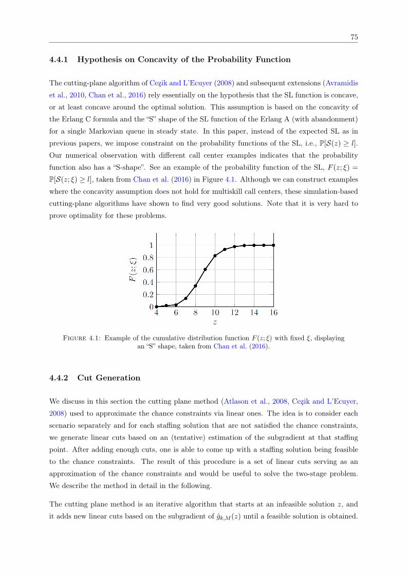
75

4.4.1 Hypothesis on Concavity of the Probability Function

The cutting-plane algorithm of Cezik and L’Ecuyer (2008) and subsequent extensions (Avramidis

et al., 2010, Chan et al., 2016) rely essentially on the hypothesis that the SL function is concave,

or at least concave around the optimal solution. This assumption is based on the concavity of

the Erlang C formula and the “S” shape of the SL function of the Erlang A (with abandonment)

for a single Markovian queue in steady state. In this paper, instead of the expected SL as in

previous papers, we impose constraint on the probability functions of the SL, i.e., P[S(z) ≥ l].

Our numerical observation with different call center examples indicates that the probability

function also has a “S-shape”. See an example of the probability function of the SL, F (z; ξ) =

P[S(z; ξ) ≥ l], taken from Chan et al. (2016) in Figure 4.1. Although we can construct examples

where the concavity assumption does not hold for multiskill call centers, these simulation-based

cutting-plane algorithms have shown to find very good solutions. Note that it is very hard to

prove optimality for these problems.

Figure 4.1: Example of the cumulative distribution function F (z; ξ) with fixed ξ, displayingan “S” shape, taken from Chan et al. (2016).

4.4.2 Cut Generation

We discuss in this section the cutting plane method (Atlason et al., 2008, Cezik and L’Ecuyer,

2008) used to approximate the chance constraints via linear ones. The idea is to consider each

scenario separately and for each staffing solution that are not satisfied the chance constraints,

we generate linear cuts based on an (tentative) estimation of the subgradient at that staffing

point. After adding enough cuts, one is able to come up with a staffing solution being feasible

to the chance constraints. The result of this procedure is a set of linear cuts serving as an

approximation of the chance constraints and would be useful to solve the two-stage problem.

We describe the method in detail in the following.

The cutting plane method is an iterative algorithm that starts at an infeasible solution z, and

it adds new linear cuts based on the subgradient of gk,M (z) until a feasible solution is obtained.

76

To avoid starting the algorithm at a null solution (all-zero solution) or in a non-concave region,

we add heuristic linear constraints to cover a fraction αk of the arrival rate of call type k, as

described in Chan (2013) and Chan et al. (2016). Such constraints are also used in the fluid

scheduling model of Bassamboo et al. (2006). These constraints require additional continuous

variables wk,i,n ≥ 0 which defines the (fractional) number of agents of group i working on calls

of type k for scenario n.

Before subgradient cuts are added, we construct some preliminary constraints for each scenario

n using the fluid scheduling model as following

∑i∈Gk

µk,iwk,i,n ≥ αkΛk,n, k = 1, . . . ,K

∑k∈Si

wk,i,n ≤ zi, i = 1, . . . , I

wk,i,n ≥ 0, k = 1, . . . ,K, i = 1, . . . , I,

where Λk,n is the arrival rate of call type k corresponding to scenario n and the parameters αkshould be selected such that the initial solution is hopefully in a concave region of gM .

Is is important to note that the parameter αk is generally chosen around 1 when we solve the

problem with the expected service level constraint. Once we consider probabilistic service level

constraints, it is more difficult to choose a good αk. The reason is that αk can depend on many

factors, for example, the distribution of the business factor of the arrival rate. Since it is usually

not easy to optimize αk, instead of optimizing αk, we propose a heuristic method to find the

initial solution. More precisely, we start with parameters αk of small values, e.g., usually around

1. We then iteratively use simulation to compute the probability values, and if there is a call

type k for which gk,M (z) is too small, i.e., less than a given threshold ρ (e.g., ρ can be chosen to

be equal to 0.5) then we add agents to the groups that serve that call type. We stop this step

when all the probability values are larger than ρ. We expect that after this step, the staffing

belongs to the concave region and the subgradient cut is valid.

The cutting plane method in our context is described as follows. We generate subgradient-based

linear cuts independently for each scenario. First, let consider scenario n with realization ξn and

a probability function gnk (z) = gk,M (z, ξn). Let also z∗ be the current solution and qnk(z∗) of

size I be the subgradient of gnk at point z∗. For a given staffing z∗, we estimate the i-th element

qink(z∗) by the forward finite difference, with step size d, using simulation:

qink(z∗) = [gnk (z∗ + dei)− gnk (z∗)]/d,

77

where ei is a unit vector with 1 at the i-th position and 0 elsewhere. Normally, we set d = 1,

but when the simulation has a lot of noise (e.g., the number of simulated days M is small), or

the subgradient is not computed as expected , e.g., qink(z∗) < 0 for some k, we may increase d

to 2 or 3. Assuming that qnk(z∗) is a subgradient of gnk at point z∗, we have the following valid

inequality gnk (z∗) + qnk(z∗)(z − z∗) ≥ gnk (z). Since we want to find z such that gnk (z) ≥ 1 − δk,

we have the following valid inequality

qnk(z∗)z ≥ 1− δk − gnk (z∗) + qnk(z

∗)z∗, (4.3)

which is a linear cut that can be added to the linear program to each scenario n:

min(z,w)∈NI×RK×I+

cTz | Anz ≤ bn, Hnz +Knw ≤ hn

, (4.4)

where Anz ≤ bn refers to the set of subgradient cuts and Hnz+Knw ≤ hn are constraints given

by the fluid model.

The cutting plane procedure allows to approximate (P4.2) by a mixed-integer linear program-

ming model. We can show that if we add sufficiently enough cuts to approximate the chance

constraints, one can obtain an optimal solution to (P4.2) by solving the corresponding linear

model. We discuss this in detail in the following.

We first let Q∧

(x) denote the value of the second stage of the SAA problem (P4.2) for a given

x, i.e., Q∧

(x) = 1N

∑Nn=1Q∧

M (x; ξn), where

Q∧

M (x; ξn) = min (c+)Tr+ − (c−)Tr−

subject to gk,M (x+ r+ − r−, ξn) ≥ 0 k = 0, . . . ,K

r+, r− ∈ NI .

For each scenario n, we denote by QM (x; ξn) the value of the second stage after replacing the

constraints gM (z; ξn) ≥ 0 by linear cuts, i.e.,

(P4.3)

QM (x; ξn) = min (c+)Tr+ − (c−)Tr−

subject to An(x+ r+ − r−) ≤ bn

Hn(x+ r+ − r−) +Knw ≤ hn

r+, r− ∈ NI

where An(x+r+−r−) ≤ bn are the linear cuts added to scenario n. When cuts are added to the

second-stage problem, we can get an approximate solution to (P4.2), obtained by the replacing

78

the chance constraints by linear cuts

(P4.4) minx∈X

f(x) = cTx+

1

N

N∑n=1

QM (x; ξn)

.

The following proposition indicates that if the linear cuts always form upper bounds of the

chance constraints and if we add sufficiently enough of them, then we can obtain an optimal

solution to (P4.2) by solving (P4.4).

Proposition 4.1. Assume that for each cut given by (4.3), z∗ is in the concave region of the

probability function and qnk(z∗) is a subgradient of the corresponding probability function, if

(x∗, f∗) is an optimal solution and the optimal value of (P4.4) and if (r∗+n , r∗−n ) is an optimal

solution to (P4.3) such that gk,M (x∗ + r∗+n − r∗−n ; ξn) ≥ 1 − δk, for all n, k, then (x∗, f∗) is

also an optimal solution and the optimal value to (P4.2).

Proof. Under the assumption that all cuts are subgradient ones in a concave region of the

probability functions, given a first-stage solution x we always have(r+, r−)

∣∣∣∣∣∣ gM (x+ r+ − r−; ξn) ≥ 0

r+, r− ∈ NI

⊆(r+, r−)

∣∣∣∣∣∣∣∣An(x+ r+ − r−) ≤ bn

Hn(x+ r+ − r−) +Knw ≤ hn

r+, r− ∈ NI , w ≥ 0

(4.5)

We denote by x∗1, r∗+1n , r

∗+1n , n = 1, . . . , N the optimal solution to (P4.2) and by x∗2, r

∗+2n , r

∗+2n , n =

1, . . . , N the optimal solution to (P4.4). According to (4.5) we have

cTx∗1 +1

N

N∑n=1

(c+)Tr∗+1n − (c−)Tr∗−1n ≥ cTx∗2 +

1

N

N∑n=1

(c+)Tr∗+2n − (c−)Tr∗−2n , (4.6)

Moreover, if gk,M (x∗2 + r∗+2n − r∗−2n ; ξn) ≥ 1− δk, ∀ n, k, then x∗2, r

∗+2n , r

∗+2n , n = 1, . . . , N is also

a feasible solution to (P4.2), so

cTx∗1 +1

N

N∑n=1

(c+)Tr∗+1n − (c−)Tr∗−1n ≤ cTx∗2 +

1

N

N∑n=1

(c+)Tr∗+2n − (c−)Tr∗−2n , (4.7)

From (4.6) and (4.7) we can deduce that x∗2, r∗+2n , r

∗+2n , n = 1, . . . , N is also an optimal solution

to (P4.2). This completes the proof.

So in theory, we can obtain an optimal solution to the SAA problem (P4.2) by adding enough

linear cuts to the second-stage problems and solve (P4.4). Indeed, (P4.4) is a mixed-integer

linear programming (MIP) model, which can be solved using a commercial solver as CPLEX.

However, in a large scale setting, (P4.4) would contain a large number of variables, making

it practically difficult to be solved in a direct way. The L-shaped algorithm presented in the

following provide a viable way to deal with this issue.

79

4.4.3 L-shaped Algorithm

The size of this MIP model (P4.4) depends proportionally on the number of scenarios, leading

to the fact that it would be expensive to directly solve if the number of scenarios is large.

However, the structure of (P4.4) suggests that a decomposition method (i.e., L-shaped) would

be an efficient alternative to solve the two-stage problem. Nevertheless, the problem involves

integer variables at both first and second stages, and therefore solving it exactly can be very

challenging whenN andM are large. The absence of general efficient methods for such a problem

reflects this difficulty (see Birge and Louveaux, 2011, Chapter 7 ). Several techniques have been

proposed over the years, but such techniques are developed under some specific restrictions

on the two-stage problem, e.g., the first-stage variables are integer or the recourse matrix has

integer coefficients. Thus, they generally do not apply in our context. In the following, we

present a simple integer L-shaped algorithm that can be combined with mixed-integer rounding

inequalities (Section 4.4.4) to efficiently find good integer solutions of the two-stage problem.

The general idea of the L-shaped method is a way to approximate the recourse function (or the

second-stage objective function) by a piece-wise linear and convex function. Since the non-linear

objective term involves a solution to all the second-stage programs, we want to avoid numerous

function evaluations for it. Therefore, we define a master linear model in x, but we only evaluate

the recourse function as a sub-problem. This can be done based on the duality properties of the

second-stage problem.

For any first-stage solution x, in order to get a feasible solution for the second stage, we just

need to add enough agents r+ and set r− = 0. It means that the problem (P4.1) has relatively

complete recourse, i.e., the second-stage problems always have feasible solutions given any first-

stage solution x (see Birge and Louveaux, 2011, Page 113 ). In addition, the linear cuts generated

from the cutting plane method (Section 4.4.2) represent upper bounds on the chance constraints.

In other terms, the linearized second-stage problem will be a relaxation of the true second-

stage problem, and consequently, any feasible solution of the true second-stage problem will be

feasible for the relaxed second-stage problem. Therefore, the problem (P4.4) remains relatively

complete. From this remark, we only need to add optimality cuts, i.e., linear cuts to build the

piece-wise linear function approximating the recourse function, to the master problem.

Now, let us consider the master problem of (P4.4) as follows

(MP1)

minx,θ

cTx+ θ

subject to Πx− 1θ ≤ π0

x ∈ X

(4.8)

80

where θ ∈ R is a variable serving as an underestimation of the second-stage objective function

and constraints (4.8) are optimality cuts. We now discuss how to add optimality cuts to the

master problem. To make the notations simpler, we assume that the constraints of the second-

stage problem of scenario n can be written as Tnx + Wny = rn, where y is the vector of the

second-stage variables. In our context, y contains r+, r− and w (from the fluid model). For

each solution x∗ and each scenario n = 1, . . . , N , we can rewrite the corresponding second-stage

problem using equality constraints as

miny

qTy∣∣∣ Tnx∗ +Wny = rn, y ≥ 0

.

We then solve the dual to obtain a dual optimal solution

σn = argmaxσ

(rn − Tnx∗)Tσ∣∣∣ (Wn)Tσ ≤ q

.

Due to duality properties we have

QM (x; ξn) = miny

qTy∣∣∣ Tnx+Wny = rn, y = (r+, r−, w) ≥ 0, r+ and r− are integer

≥ min

y

qTy∣∣∣ Tnx+Wny = rn, y ≥ 0

= max

σ

(rn − Tnx)Tσ

∣∣∣ (Wn)Tσ ≤ q

≥ σTn(rn − Tnx).

Since we want θ ≥ 1N

∑Nn=1QM (x; ξn), the following optimality cut can be added to the master

problem

θ ≥ 1

N

N∑n=1

σTn(rn − Tnx),

or equivalently,

−

(1

N

N∑n=1

σTnT

n

)x− θ ≤ − 1

N

N∑n=1

σTnr

n. (4.9)

It is also possible to add several cuts per each master iteration based on the idea of the multi-cut

L-shaped method (Birge and Louveaux, 2011, Page 198). More precisely, we can cluster the

set of all scenarios into L disjoint subsets N1, . . . , NL and we formulate the master problem of

(P4.4) as

(MP2)

minx,θl

cTx+

L∑l=1

θl

subject to Πlx− 1θl ≤ πl0, l = 1, . . . , L

x ∈ X,

(4.10)

81

where constraints (4.10) are optimality cuts given by L subsets of scenarios. For each subset Nl,

the following optimality cut can be added to the master problem.

− 1

N

( ∑n∈Nl

σTnT

n)x− θl ≤ −

1

N

∑n∈Nl

σTnr

n. (4.11)

Finally, we describe the L-shaped approach in Algorithm 4.1. If L = 1, then we have a single-cut

L-shaped algorithm in which only one cut is generated per iteration, and if L = N , then we

generate cuts for each scenario.

Algorithm 4.1: L-shaped algorithmrepeat

Select L clusters of scenarios, 1 ≤ L ≤ NSolve (MP2) to obtain a solution (x∗, θ∗1, . . . , θ

∗L)

Compute

Q(x∗) =N∑n=1

miny

qTy∣∣∣ Tnx∗ +Wny = rn, y ≥ 0

if∑L

l=1 θ∗l < Q(x∗) then

Add L optimality cuts to (MP2)

Until∑L

l=1 θ∗l ≥ Q(x∗);

Return x∗ as a first-stage solution

4.4.4 Strengthening the Cutting Plane

In this section we present a way to strengthen subgradient cuts generated by (4.3) using mixed-

integer rounding (MIR) inequalities. This approach plays a central role in the development of

strong cutting planes for mixed-integer programming. MIR inequalities can be derived from a

single mixed-integer constraint, and have been shown to be able to generate all facets inducing

valid inequalities for any mixed 0-1 integer program (Nemhauser and Wolsey, 1990). In this

paper, we derive MIR inequalities for our subgradient cuts, which are integer constraints. This

MIR inequalities allow to strengthen the cuts and improve the L-shaped algorithm described in

the previous section.

We consider a subgradient cut of the form∑I

i=1 aizi ≥ b. Since the subgradients are always

generated to be non-negative, we have ai ≥ 0 for all i = 1, . . . , I. Let define P = z ∈NI |

∑Ii=1 aizi ≥ b, i.e, the set of feasible solutions given by the subgradient cut. We have the

following proposition concerning the MIR inequalities that are valid for P.

Proposition 4.2. The following inequalities hold for all z ∈ P

∑t=1,...,It6=i

atzt + diaizi ≥⌈b

ai

⌉diai, ∀ i = 1, . . . , I, ai 6= 0, (4.12)

82

where di = b/ai − db/aie+ 1.

Proof. Given i ∈ 1, . . . , I such that ai > 0, we can write the inequality∑I

i=1 aizi ≥ b as∑t=1,...,It6=i

atztai

+ zi ≥b

ai,

which can be written as

∑t=1,...,It6=i

atztai≥ b

ai+ 1−

⌈b

ai

⌉+

⌈b

ai

⌉− zi − 1. (4.13)

Since zi ∈ N, we consider the two cases zi ≥ db/aie or zi ≤ db/aie − 1. If zi ≥ db/aie then the

following inequality holds

∑t=1,...,It6=i

atztai≥(

1 +b

ai−⌈b

ai

⌉)(⌈b

ai

⌉− zi

)= di

(⌈b

ai

⌉− zi

), (4.14)

as the left side of the inequality is non-negative and the right side is non-positive. Moreover, if

zi ≤ db/aie − 1, given that b/ai − db/aie+ 1 ≤ 1, from (4.13) we obtain

∑t=1,...,It6=i

atztai≥ di + di

(⌈b

ai

⌉− zi − 1

)= di

(⌈b

ai

⌉− zi

). (4.15)

Now, combine (4.14) and (4.15) we obtain (4.12).

In the following, we present a simple example to show how the inequalities given by (4.12) work.

We take a small call center example in which there are only two call types 1, 2 and two agent

groups 1, 2. We assume that call type 1 can be served by the two agent groups and call type 2

can be served by only group 2. Let x, y denote the number of agents in group 1, 2, respectively.

Now, suppose that we have added two subgradient cuts 0.13x+0.55y ≥ 1.2 and 1.3y ≥ 0.7. The

set of feasible staffing solutions given by these two cuts is illustrated on the left side of Figure

4.2. Using (4.12), we obtain the following inequalities0.23x+ 0.18y ≥ 0.55

y ≥ 1

0.23x+ 4.23y ≥ 2.31,

as illustrated on the right side of Figure 4.2. The hashed area corresponds to the set of points

that satisfy the basic constraints but violate the MIR inequalities above. We can see that the

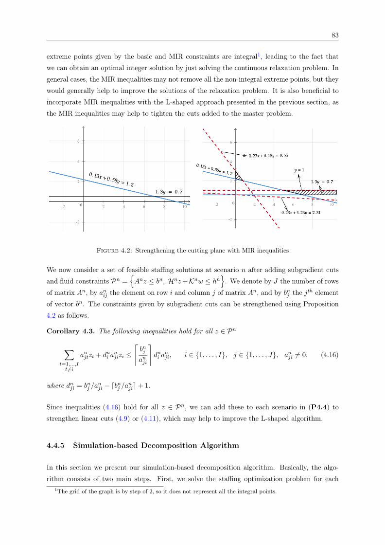
83

extreme points given by the basic and MIR constraints are integral1, leading to the fact that

we can obtain an optimal integer solution by just solving the continuous relaxation problem. In

general cases, the MIR inequalities may not remove all the non-integral extreme points, but they

would generally help to improve the solutions of the relaxation problem. It is also beneficial to

incorporate MIR inequalities with the L-shaped approach presented in the previous section, as

the MIR inequalities may help to tighten the cuts added to the master problem.

Figure 4.2: Strengthening the cutting plane with MIR inequalities

We now consider a set of feasible staffing solutions at scenario n after adding subgradient cuts

and fluid constraints Pn =Anz ≤ bn, Hnz+Knw ≤ hn

. We denote by J the number of rows

of matrix An, by anij the element on row i and column j of matrix An, and by bnj the jth element

of vector bn. The constraints given by subgradient cuts can be strengthened using Proposition

4.2 as follows.

Corollary 4.3. The following inequalities hold for all z ∈ Pn

∑t=1,...,It6=i

anjtzt + dni anjizi ≤

⌈bnjanji

⌉dni a

nji, i ∈ 1, . . . , I, j ∈ 1, . . . , J, anji 6= 0, (4.16)

where dnji = bnj /anji − dbnj /anjie+ 1.

Since inequalities (4.16) hold for all z ∈ Pn, we can add these to each scenario in (P4.4) to

strengthen linear cuts (4.9) or (4.11), which may help to improve the L-shaped algorithm.

4.4.5 Simulation-based Decomposition Algorithm

In this section we present our simulation-based decomposition algorithm. Basically, the algo-

rithm consists of two main steps. First, we solve the staffing optimization problem for each1The grid of the graph is by step of 2, so it does not represent all the integral points.

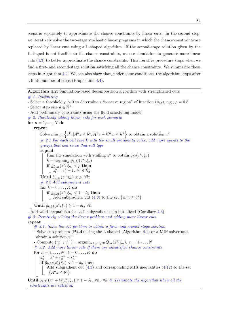
84

scenario separately to approximate the chance constraints by linear cuts. In the second step,

we iteratively solve the two-stage stochastic linear programs in which the chance constraints are

replaced by linear cuts using a L-shaped algorithm. If the second-stage solution given by the

L-shaped is not feasible to the chance constraints, we use simulation to generate more linear

cuts (4.3) to better approximate the chance constraints. This iterative procedure stops when we

find a first- and second-stage solution satisfying all the chance constraints. We summarize these

steps in Algorithm 4.2. We can also show that, under some conditions, the algorithm stops after

a finite number of steps (Proposition 4.4).

Algorithm 4.2: Simulation-based decomposition algorithm with strengthened cuts# 1. Initializing- Select a threshold ρ > 0 to determine a “concave region” of function (gM ), e.g., ρ = 0.5- Select step size d ∈ N+

- Add preliminary constraints using the fluid scheduling model# 2. Iteratively adding linear cuts for each scenariofor n = 1, . . . , N do

repeatSolve minz,w

cTz|Anz ≤ bn,Hnz +Knw ≤ hn

to obtain a solution z∗

# 2.1 For each call type k with too small probability value, add more agents to thegroups that can serve that call typerepeat

Run the simulation with staffing z∗ to obtain gM (z∗; ξn)k = argmink gk,M (z∗; ξn)if gk,M (z∗; ξn) < ρ then

z∗i = z∗i + 1, ∀i ∈ GkUntil gk,M (z∗; ξn) ≥ ρ, ∀k;# 2.2 Add subgradient cutsfor k = 0, . . . ,K do

if gk,M (z∗; ξn) < 1− δk thenAdd subgradient cut (4.3) to the set Anz ≤ bn

Until gk,M (z∗; ξn) ≥ 1− δk, ∀k;- Add valid inequalities for each subgradient cuts initialized (Corollary 4.3)# 3. Iteratively solving the linear problem and adding more linear cutsrepeat

# 3.1. Solve the sub-problem to obtain a first- and second-stage solution- Solve sub-problem (P4.4) using the L-shaped (Algorithm 4.1) or a MIP solver andobtain a solution x∗

- Compute (r∗+n , r∗−n ) = argminr+,r−∈NIQM (x∗; ξn), n = 1, . . . , N# 3.2. Add more linear cuts if there are unsatisfied chance constraintsfor n = 1, . . . , N ; k = 0, . . . ,K do

z∗n = x∗ + r∗+n − r∗−nif gk,M (z∗n; ξn) < 1− δk then

Add subgradient cut (4.3) and corresponding MIR inequalities (4.12) to the setAnz ≤ bn

Until gk,M (x∗ +Wy∗n; ξn) ≥ 1− δk, ∀n, ∀k # Terminate the algorithm when all theconstraints are satisfied;

85

Proposition 4.4. Assume that the arrival rates are always bounded from above and the set X

of feasible solutions at the first stage is finite. Then Algorithm 4.2 stops after a finite number of

iterations.

Proof. The L-shaped algorithm always stops after a finite number of steps. This is due to the

limited number of possible first-stage solutions (see Birge and Louveaux, 2011, Page 291). In

Step 1 and 3 of Algorithm 4.2, for each scenario, each time when a staffing solution is infeasible,

this solution is removed by subgradient cuts. Moreover, as the arrival rates are always bounded

from above, the number of infeasible solutions (r+, r−) at a second-stage problem is also finite,

so the number of added cuts for each scenario should also be finite. This remark leads to the

fact that Algorithm 4.2 converges after a finite number of iterations.

Note that if the the arrival rates are always bounded, we can always choose a staffing large

enough such that all the probability constraints are satisfied. So, without loss of generality we

can assume that the set of feasible staffing solutions at the first stage X is finite.

Steps 1 and 2 of Algorithm 4.2 are basically a procedure to separately solve the staffing op-

timization problem for each scenario, i.e., for each scenario we iteratively generate cuts and

solve the corresponding linear programs until getting a staffing solution satisfying all the chance

constraints. An important step of the algorithm is that when there is a call type of which the

corresponding probability value are too small, then we need to adjust the staffing, as the current

staffing may not belong to the concave region of the probability function and would result in

bad cuts. Moreover, since the linear cuts added after Step 1 and 2 of Algorithm 4.2 might be

insufficient to approximate the chance constraints, in Step 3 we need to solve the approximate

problem (P4.4) to get first- and second-stage solutions and add more cuts if these solutions do

not satisfy the chance constraints. In Step 3.1, we can either solve (P4.4) by a MIP solver (e.g.,

CPLEX) if it is not too large, or use the L-shaped in a large-scale setting.

4.5 Numerical Experiments

In this section, we evaluate the performance of the proposed simulation-based decomposition

algorithm using the data from three call centers of different sizes. We also compare our approach

with the algorithm presented in Chan et al. (2016), which solves (P4.4) directly by a mixed-

integer linear programming solver (e.g., CPLEX). The problem (P4.4) can be formulated as the

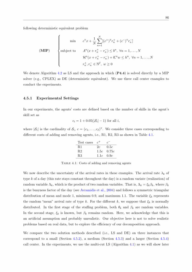
86

following deterministic equivalent problem

(MIP)

min cTx+1

N

N∑n=1

[(c+)Tr+n + (c−)Tr−n ]

subject to An(x+ r+n − r−n ) ≤ bn, ∀n = 1, . . . , N

Hn(x+ r+n − r−n ) +Knw ≤ hn, ∀n = 1, . . . , N

r+n , r

−n ∈ NI , w ≥ 0

We denote Algorithm 4.2 as LS and the approach in which (P4.4) is solved directly by a MIP

solver (e.g., CPLEX) as DE (deterministic equivalent). We use three call center examples to

conduct the experiments.

4.5.1 Experimental Settings

In our experiments, the agents’ costs are defined based on the number of skills in the agent’s

skill set as

ci = 1 + 0.05(|Si| − 1) for all i,

where |Si| is the cardinality of Si, c = (c1, . . . , cI)T. We consider three cases corresponding to

different costs of adding and removing agents, i.e., R1, R2, R3 as shown in Table 4.1.

Test cases c+ c−

R1 2c 0.5cR2 1.5c 0.75cR3 1.1c 0.9c

Table 4.1: Costs of adding and removing agents

We now describe the uncertainty of the arrival rates in these examples. The arrival rate λk of

type k of a day (this rate stays constant throughout the day) is a random variate (realization) of

random variable Λk, which is the product of two random variables. That is, Λk = ξkβk, where βkis the busyness factor of the day (see Avramidis et al., 2004) and follows a symmetric triangular

distribution of mean and mode 1, minimum 0.9, and maximum 1.1. The variable ξk represents

the random “mean” arrival rate of type k. For the different k, we suppose that ξk is normally

distributed. In the first stage of the staffing problem, both θk and βk are random variables.

In the second stage, ξk is known, but βk remains random. Here, we acknowledge that this is

an artificial assumption and probably unrealistic. Our objective here is not to solve realistic

problems based on real data, but to explore the efficiency of our decomposition approach.

We compare the two solution methods described (i.e., LS and DE) on three instances that

correspond to a small (Section 4.5.2), a medium (Section 4.5.3) and a larger (Section 4.5.4)

call center. In the experiments, we use the multi-cut LS (Algorithm 4.1) as we will show later

87

that the multi-cut version outperforms the single-cut one, especially for medium and large call

centers.

To perform the experiments, for each case (R1, R2 or R3), we independently generate some sets

of scenarios. Each set of scenarios corresponds to an instance to be solved. For each instance and

across the scenarios, we use the same sample size but independent random numbers to simulate

the probability functions.

To assess the solution quality, we also provide a study to validate the first-stage solutions returned

by the LS and DE on different sets of scenarios. More precisely, for the small, medium and large

call centers, we generate three sets of 1000, 100 and 100 scenarios, respectively. These sets are

independent of those used to obtain the first-stage solutions. Then, we compute the “out-of

sample” costs given by the first-stage solutions returned by the LS and DE approaches on the

new sets of scenarios.

The experiments were conducted on a machine running Debian 8 with Intel(R) Xeon(R) CPU

E5620 (2.40GHz). The computer has 8 physical CPUs and 98GB of memory. The simulations

were performed using the ContactCenters simulation library (Buist and L’Ecuyer, 2005), de-

veloped with the SSJ simulation package (L’Ecuyer et al., 2002). The algorithm was coded in

MATLAB and linked to IBM ILOG CPLEX 12.6 optimization routines under default settings.

To speed up the computation, the steps of performing simulation and adding subgradient cuts

for each scenario are parallelized using the 8 physical CPUs.

4.5.2 Case Study 1: A Small Call Center

We first consider a small call center with K = 2 call types and I = 2 agent groups, with S1 = 1and S2 = 1, 2. The motivation behind the use of this small example in our experiments is

that, with a large number of scenarios, the DE approach would become expensive and the use

of the decomposition method would be helpful to find good solutions in short computing time.

We assume that (i) each caller abandons with probability 2% if it has to wait, (ii) patience times

are exponential with means 10 and 6 minutes, (iii) for different k, we suppose that the “mean”

arrival rate ξk is normally distributed with mean 100 and 70 calls per hour and 15% standard

deviations from the means, and (iv) all service times are exponential distribution with means

10 and 7.5 minutes. In these experiments, we choose the parameters as follows: the acceptable

waiting times are τk = τ0 = 120 (seconds), the targets of SLs for all call types are lk = 80% for

k = 1, . . . ,K, and l0 = 85% for aggregated one. For each case (R1, R2 and R3), we generate

5 independent sets of 100, 200, 300, 400, 500 scenarios. The fluid parameters α are chosen as

αk = 1, for all k = 1, . . . ,K.

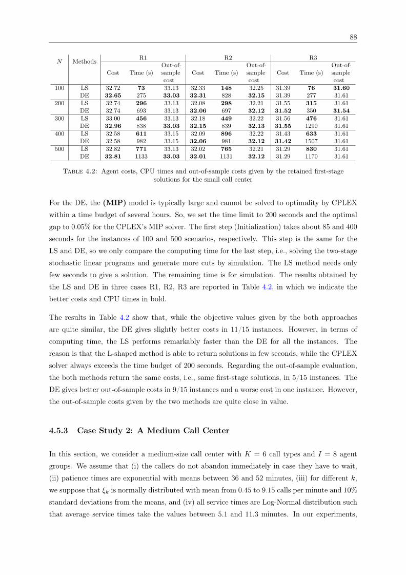
88

N Methods R1 R2 R3

Cost Time (s)Out-of-samplecost

Cost Time (s)Out-of-samplecost

Cost Time (s)Out-of-samplecost

100 LS 32.72 73 33.13 32.33 148 32.25 31.39 76 31.60DE 32.65 275 33.03 32.31 828 32.15 31.39 277 31.61

200 LS 32.74 296 33.13 32.08 298 32.21 31.55 315 31.61DE 32.74 693 33.13 32.06 697 32.12 31.52 350 31.54

300 LS 33.00 456 33.13 32.18 449 32.22 31.56 476 31.61DE 32.96 838 33.03 32.15 839 32.13 31.55 1290 31.61

400 LS 32.58 611 33.15 32.09 896 32.22 31.43 633 31.61DE 32.58 982 33.15 32.06 981 32.12 31.42 1507 31.61

500 LS 32.82 771 33.13 32.02 765 32.21 31.29 830 31.61DE 32.81 1133 33.03 32.01 1131 32.12 31.29 1170 31.61

Table 4.2: Agent costs, CPU times and out-of-sample costs given by the retained first-stagesolutions for the small call center

For the DE, the (MIP) model is typically large and cannot be solved to optimality by CPLEX

within a time budget of several hours. So, we set the time limit to 200 seconds and the optimal

gap to 0.05% for the CPLEX’s MIP solver. The first step (Initialization) takes about 85 and 400

seconds for the instances of 100 and 500 scenarios, respectively. This step is the same for the

LS and DE, so we only compare the computing time for the last step, i.e., solving the two-stage

stochastic linear programs and generate more cuts by simulation. The LS method needs only

few seconds to give a solution. The remaining time is for simulation. The results obtained by

the LS and DE in three cases R1, R2, R3 are reported in Table 4.2, in which we indicate the

better costs and CPU times in bold.

The results in Table 4.2 show that, while the objective values given by the both approaches

are quite similar, the DE gives slightly better costs in 11/15 instances. However, in terms of

computing time, the LS performs remarkably faster than the DE for all the instances. The

reason is that the L-shaped method is able to return solutions in few seconds, while the CPLEX

solver always exceeds the time budget of 200 seconds. Regarding the out-of-sample evaluation,

the both methods return the same costs, i.e., same first-stage solutions, in 5/15 instances. The

DE gives better out-of-sample costs in 9/15 instances and a worse cost in one instance. However,

the out-of-sample costs given by the two methods are quite close in value.

4.5.3 Case Study 2: A Medium Call Center

In this section, we consider a medium-size call center with K = 6 call types and I = 8 agent

groups. We assume that (i) the callers do not abandon immediately in case they have to wait,

(ii) patience times are exponential with means between 36 and 52 minutes, (iii) for different k,

we suppose that ξk is normally distributed with mean from 0.45 to 9.15 calls per minute and 10%

standard deviations from the means, and (iv) all service times are Log-Normal distribution such

that average service times take the values between 5.1 and 11.3 minutes. In our experiments,

89

we choose the parameters as follows: the acceptable waiting times are τk = τ0 = 120 (seconds)

and the targets for SLs are lk = 80% for all k = 0, . . . ,K. We test our approach with two sets

of targets for the chance constraints, namely, (i) 1− δ0 = 85% and 1− δk = 80%, k = 1, . . . ,K,

and (ii) 1 − δ0 = 95% and 1 − δk = 90% for k = 1, . . . ,K. We choose α = (1, 4, 1, 1.2, 1, 3).

These values are adjusted manually to ensure that the fluid scheduling model well identifies the

concave regions of the probability functions.

Given the fact that in this case, the simulation is more expensive as compared to the small-size

call center, we only consider instances of less than 100 scenarios. More precisely, for each case

R1, R2 or R3, we independently generate instances of 20, 50, 70 scenarios and we use the sample

size M = 1000 to approximate the chance constraints. We solve each instance and report the

corresponding first-stage solution. For the validation study, we generate a set 100 scenarios

that are independent of those used to obtain the first-stage solutions, acknowledging that 100

is rather small for a validation study, but we still keep this number due to the expensiveness of

the validation.

In Table 4.3, we report the results obtained by the LS and DE algorithms. We indicate in bold

the better costs and shorter CPU times and note that the common step (Step 1 in Algorithm 4.2)

takes about 0.14, 0.22 and 0.38 hour for the instances of 20, 50 and 70 scenarios, respectively.

In this experiment, while the L-shaped method always requires less than one minute to return a

solution, the CPLEX solver always exceeds the time budget of 10 minutes. The results show that

the total costs given by the two methods are quite similar. However, the LS gives slightly better

agent costs in 13/18 instances. It is also clear from the table that the LS requires remarkably

less CPU time as compared to the DE counterpart. The validation study also indicates that

the both approaches perform quite similarly in terms of first-stage solutions, as the validation

costs given by the LS and DE are quite close in value. However, the LS is able to return better

“out-of-sample” costs in 11/18 instances. Looking more closely to the validation study, we also

notice that, for the test cases R2 and R3, we obtained better first-stage solutions when increasing

the number of scenarios. It is not the case for the R1 instances when the differences between

c+ and c− are higher as compared to those in R2 and R3. For these instances, it seems that

increasing the number of scenarios from 20 to 70 does not really help to improve the first-stage

solutions.

In Table 4.4, we report the first-stage solutions, first-stage costs as well as the averages of the

numbers of adding/removing agents for the three cases with N = 70 scenarios. Similar to the

case of the small call center, we also see that the first-stage costs given by R1 and R2 are also

higher than the costs of R3, and the averaged r+ given by R1 and R2 are smaller than those

given by R3.

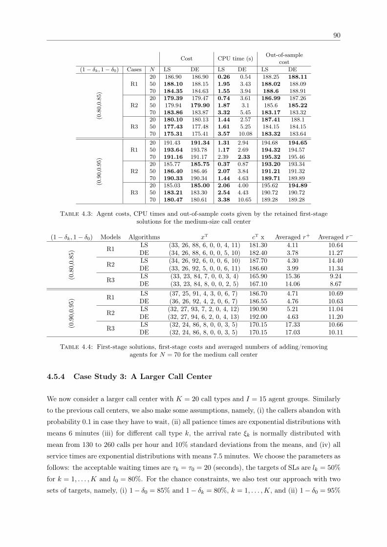
90

Cost CPU time (s) Out-of-samplecost

(1− δk, 1− δ0) Cases N LS DE LS DE LS DE

(0.8

0,0.

85)

R120 186.90 186.90 0.26 0.54 188.25 188.1150 188.10 188.15 1.95 3.43 188.02 188.0970 184.35 184.63 1.55 3.94 188.6 188.91

R220 179.39 179.47 0.74 3.61 186.99 187.2650 179.94 179.90 1.87 3.1 185.6 185.2270 183.86 183.87 3.32 5.45 183.17 183.32

R320 180.10 180.13 1.44 2.57 187.41 188.150 177.43 177.48 1.61 5.25 184.15 184.1570 175.31 175.41 3.57 10.08 183.32 183.64

(0.9

0,0.

95)

R120 191.43 191.34 1.31 2.94 194.68 194.6550 193.64 193.78 1.17 2.69 194.32 194.5770 191.16 191.17 2.39 2.33 195.32 195.46

R220 185.77 185.75 0.37 0.87 193.20 193.3450 186.40 186.46 2.07 3.84 191.21 191.3270 190.33 190.34 1.44 4.63 189.71 189.89

R320 185.03 185.00 2.06 4.00 195.62 194.8950 183.21 183.30 2.54 4.43 190.72 190.7270 180.47 180.61 3.38 10.65 189.28 189.28

Table 4.3: Agent costs, CPU times and out-of-sample costs given by the retained first-stagesolutions for the medium-size call center

(1− δk, 1− δ0) Models Algorithms xT cT x Averaged r+ Averaged r−

(0.80,0.85) R1 LS (33, 26, 88, 6, 0, 0, 4, 11) 181.30 4.11 10.64

DE (34, 26, 88, 6, 0, 0, 5, 10) 182.40 3.78 11.27

R2 LS (34, 26, 92, 6, 0, 0, 6, 10) 187.70 4.30 14.40DE (33, 26, 92, 5, 0, 0, 6, 11) 186.60 3.99 11.34

R3 LS (33, 23, 84, 7, 0, 0, 3, 4) 165.90 15.36 9.24DE (33, 23, 84, 8, 0, 0, 2, 5) 167.10 14.06 8.67

(0.90,0.95) R1 LS (37, 25, 91, 4, 3, 0, 6, 7) 186.70 4.71 10.69

DE (36, 26, 92, 4, 2, 0, 6, 7) 186.55 4.76 10.63

R2 LS (32, 27, 93, 7, 2, 0, 4, 12) 190.90 5.21 11.04DE (32, 27, 94, 6, 2, 0, 4, 13) 192.00 4.63 11.20

R3 LS (32, 24, 86, 8, 0, 0, 3, 5) 170.15 17.33 10.66DE (32, 24, 86, 8, 0, 0, 3, 5) 170.15 17.03 10.11

Table 4.4: First-stage solutions, first-stage costs and averaged numbers of adding/removingagents for N = 70 for the medium call center

4.5.4 Case Study 3: A Larger Call Center

We now consider a larger call center with K = 20 call types and I = 15 agent groups. Similarly

to the previous call centers, we also make some assumptions, namely, (i) the callers abandon with

probability 0.1 in case they have to wait, (ii) all patience times are exponential distributions with

means 6 minutes (iii) for different call type k, the arrival rate ξk is normally distributed with

mean from 130 to 260 calls per hour and 10% standard deviations from the means, and (iv) all

service times are exponential distributions with means 7.5 minutes. We choose the parameters as

follows: the acceptable waiting times are τk = τ0 = 20 (seconds), the targets of SLs are lk = 50%

for k = 1, . . . ,K and l0 = 80%. For the chance constraints, we also test our approach with two

sets of targets, namely, (i) 1− δ0 = 85% and 1− δk = 80%, k = 1, . . . ,K, and (ii) 1− δ0 = 95%

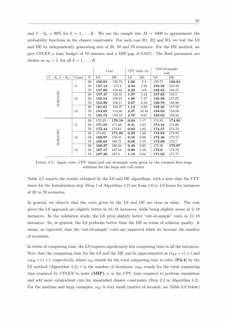
91

and 1 − δk = 90% for k = 1, . . . ,K. We use the sample size M = 1000 to approximate the

probability functions in the chance constraints. For each case R1, R2 and R3, we test the LS

and DE by independently generating sets of 20, 50 and 70 scenarios. For the DE method, we

give CPLEX a time budget of 10 minutes and a MIP-gap of 0.05%. The fluid parameter are

chosen as αk = 1, for all k = 1, . . . ,K.

Cost CPU time (s) Out-of-samplecost

(1− δk, 1− δ0) Cases N LS DE LS DE LS DE

(0.8

0,0.

85)

r120 156.62 156.75 1.08 5.2 159.77 158.6450 157.13 157.2 2.44 7.98 158.59 159.3970 157.66 158.65 2.29 9.9 158.52 158.75

r220 157.47 158.31 1.07 5.24 157.85 158.550 156.54 156.67 1.98 7.27 156.98 157.0770 154.86 156.11 2.67 6.34 156.78 156.96

r320 161.61 164.37 1.12 4.89 158.43 157.5850 154.65 154.86 2.37 10.48 158.03 158.0970 155.72 159.18 2.76 9.01 158.02 159.43

(0.9

0,0.

95)

r120 170.23 170.18 0.04 1.17 174.85 174.8350 171.55 171.68 0.41 1.93 174.44 174.6670 172.44 172.61 0.82 1.82 174.57 174.78

r220 172.02 171.95 0.29 1.28 173.82 173.9250 169.97 170.01 0.16 0.96 172.46 172.5770 169.63 169.77 0.58 1.19 172.68 172.7

r320 168.37 168.44 0.40 3.95 175.56 175.0750 167.17 167.64 0.96 5.19 173.6 174.7970 167.38 167.8 1.19 5.04 171.02 171.77

Table 4.5: Agent costs, CPU times and out-of-sample costs given by the retained first-stagesolutions for the large-size call center

Table 4.5 reports the results obtained by the LS and DE algorithms, with a note that the CPU

times for the Initialization step (Step 1 of Algorithm 4.2) are from 1.6 to 4.0 hours for instances

of 20 to 70 scenarios.

In general, we observe that the costs given by the LS and DE are close in value. The cost

given the LS approach are slightly better in 16/18 instances, while being slightly worse in 2/18

instances. In the validation study, the LS gives slightly better “out-of-sample” costs in 15/18

instances. So, in general, the LS performs better than the DE in terms of solution quality. It

seems, as expected, that the “out-of-sample” costs are improved when we increase the number

of scenarios.

In terms of computing time, the LS requires significantly less computing time in all the instances.

Note that the computing time for the LS and the DE can be approximated as (νLS + ν)× t and(νDE +ν)× t, respectively, where νLS stands for the total computing time to solve (P4.4) by the

LS method (Algorithm 4.2), t is the number of iterations, νDE stands for the total computing

time required by CPLEX to solve (MIP), ν is the CPU time required to perform simulation

and add more subgradient cuts for unsatisfied chance constraints (Step 2.2 in Algorithm 4.2).

For the medium and large examples, νLS is very small (matter of seconds, see Table 4.8 below)

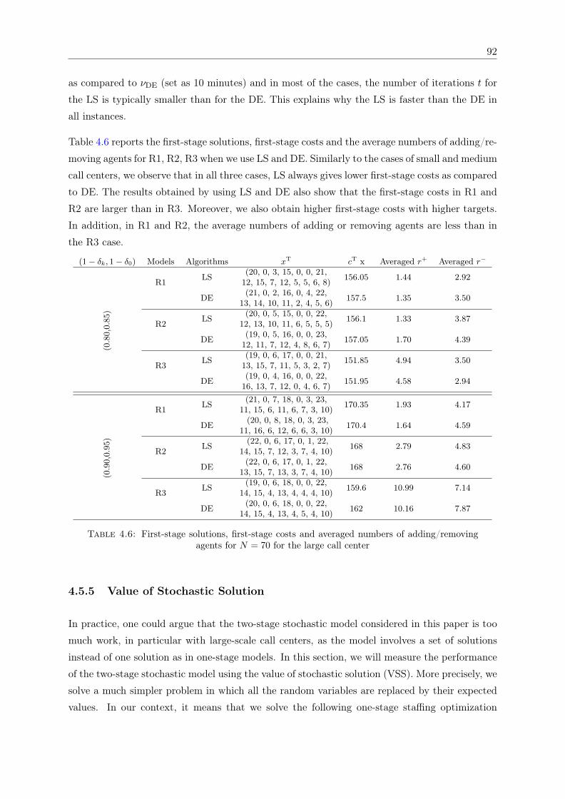
92

as compared to νDE (set as 10 minutes) and in most of the cases, the number of iterations t for

the LS is typically smaller than for the DE. This explains why the LS is faster than the DE in

all instances.

Table 4.6 reports the first-stage solutions, first-stage costs and the average numbers of adding/re-

moving agents for R1, R2, R3 when we use LS and DE. Similarly to the cases of small and medium

call centers, we observe that in all three cases, LS always gives lower first-stage costs as compared

to DE. The results obtained by using LS and DE also show that the first-stage costs in R1 and

R2 are larger than in R3. Moreover, we also obtain higher first-stage costs with higher targets.

In addition, in R1 and R2, the average numbers of adding or removing agents are less than in

the R3 case.

(1− δk, 1− δ0) Models Algorithms xT cT x Averaged r+ Averaged r−

(0.8

0,0.

85)

R1 LS (20, 0, 3, 15, 0, 0, 21,12, 15, 7, 12, 5, 5, 6, 8) 156.05 1.44 2.92

DE (21, 0, 2, 16, 0, 4, 22,13, 14, 10, 11, 2, 4, 5, 6) 157.5 1.35 3.50

R2 LS (20, 0, 5, 15, 0, 0, 22,12, 13, 10, 11, 6, 5, 5, 5) 156.1 1.33 3.87

DE (19, 0, 5, 16, 0, 0, 23,12, 11, 7, 12, 4, 8, 6, 7) 157.05 1.70 4.39

R3 LS (19, 0, 6, 17, 0, 0, 21,13, 15, 7, 11, 5, 3, 2, 7) 151.85 4.94 3.50

DE (19, 0, 4, 16, 0, 0, 22,16, 13, 7, 12, 0, 4, 6, 7) 151.95 4.58 2.94

(0.9

0,0.

95)

R1 LS (21, 0, 7, 18, 0, 3, 23,11, 15, 6, 11, 6, 7, 3, 10) 170.35 1.93 4.17

DE (20, 0, 8, 18, 0, 3, 23,11, 16, 6, 12, 6, 6, 3, 10) 170.4 1.64 4.59

R2 LS (22, 0, 6, 17, 0, 1, 22,14, 15, 7, 12, 3, 7, 4, 10) 168 2.79 4.83

DE (22, 0, 6, 17, 0, 1, 22,13, 15, 7, 13, 3, 7, 4, 10) 168 2.76 4.60

R3 LS (19, 0, 6, 18, 0, 0, 22,14, 15, 4, 13, 4, 4, 4, 10) 159.6 10.99 7.14

DE (20, 0, 6, 18, 0, 0, 22,14, 15, 4, 13, 4, 5, 4, 10) 162 10.16 7.87

Table 4.6: First-stage solutions, first-stage costs and averaged numbers of adding/removingagents for N = 70 for the large call center

4.5.5 Value of Stochastic Solution

In practice, one could argue that the two-stage stochastic model considered in this paper is too

much work, in particular with large-scale call centers, as the model involves a set of solutions

instead of one solution as in one-stage models. In this section, we will measure the performance

of the two-stage stochastic model using the value of stochastic solution (VSS). More precisely, we

solve a much simpler problem in which all the random variables are replaced by their expected

values. In our context, it means that we solve the following one-stage staffing optimization

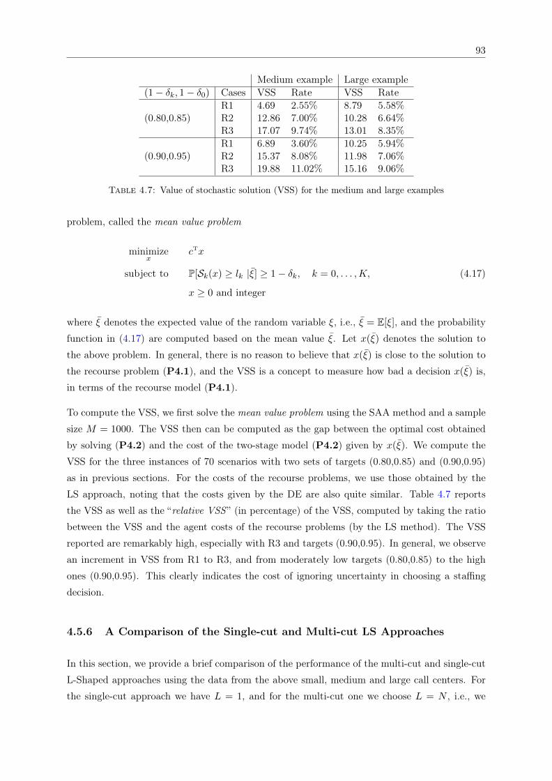
93

Medium example Large example(1− δk, 1− δ0) Cases VSS Rate VSS Rate

(0.80,0.85)R1 4.69 2.55% 8.79 5.58%R2 12.86 7.00% 10.28 6.64%R3 17.07 9.74% 13.01 8.35%

(0.90,0.95)R1 6.89 3.60% 10.25 5.94%R2 15.37 8.08% 11.98 7.06%R3 19.88 11.02% 15.16 9.06%

Table 4.7: Value of stochastic solution (VSS) for the medium and large examples

problem, called the mean value problem

minimizex

cTx

subject to P[Sk(x) ≥ lk |ξ] ≥ 1− δk, k = 0, . . . ,K, (4.17)

x ≥ 0 and integer

where ξ denotes the expected value of the random variable ξ, i.e., ξ = E[ξ], and the probability

function in (4.17) are computed based on the mean value ξ. Let x(ξ) denotes the solution to

the above problem. In general, there is no reason to believe that x(ξ) is close to the solution to

the recourse problem (P4.1), and the VSS is a concept to measure how bad a decision x(ξ) is,

in terms of the recourse model (P4.1).

To compute the VSS, we first solve the mean value problem using the SAA method and a sample

size M = 1000. The VSS then can be computed as the gap between the optimal cost obtained

by solving (P4.2) and the cost of the two-stage model (P4.2) given by x(ξ). We compute the

VSS for the three instances of 70 scenarios with two sets of targets (0.80,0.85) and (0.90,0.95)

as in previous sections. For the costs of the recourse problems, we use those obtained by the

LS approach, noting that the costs given by the DE are also quite similar. Table 4.7 reports

the VSS as well as the “relative VSS ” (in percentage) of the VSS, computed by taking the ratio

between the VSS and the agent costs of the recourse problems (by the LS method). The VSS

reported are remarkably high, especially with R3 and targets (0.90,0.95). In general, we observe

an increment in VSS from R1 to R3, and from moderately low targets (0.80,0.85) to the high

ones (0.90,0.95). This clearly indicates the cost of ignoring uncertainty in choosing a staffing

decision.

4.5.6 A Comparison of the Single-cut and Multi-cut LS Approaches

In this section, we provide a brief comparison of the performance of the multi-cut and single-cut

L-Shaped approaches using the data from the above small, medium and large call centers. For

the single-cut approach we have L = 1, and for the multi-cut one we choose L = N , i.e., we

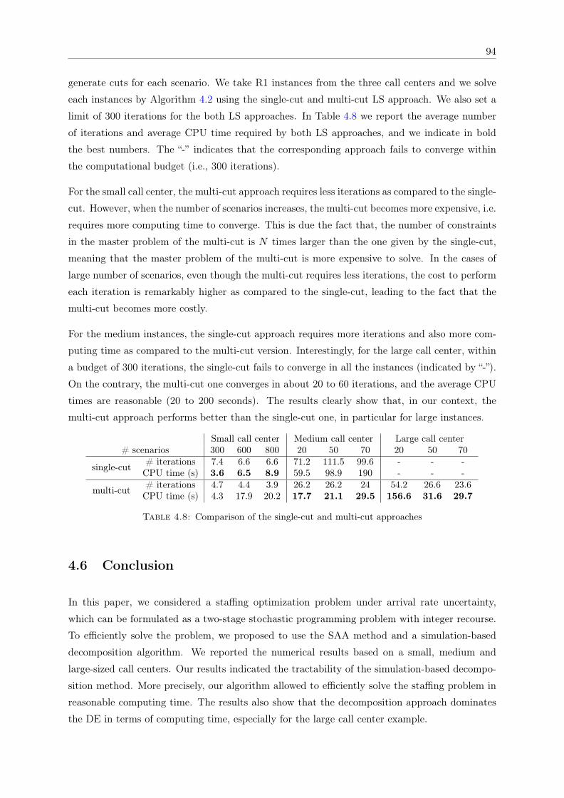
94

generate cuts for each scenario. We take R1 instances from the three call centers and we solve

each instances by Algorithm 4.2 using the single-cut and multi-cut LS approach. We also set a

limit of 300 iterations for the both LS approaches. In Table 4.8 we report the average number

of iterations and average CPU time required by both LS approaches, and we indicate in bold

the best numbers. The “-” indicates that the corresponding approach fails to converge within

the computational budget (i.e., 300 iterations).

For the small call center, the multi-cut approach requires less iterations as compared to the single-

cut. However, when the number of scenarios increases, the multi-cut becomes more expensive, i.e.

requires more computing time to converge. This is due the fact that, the number of constraints

in the master problem of the multi-cut is N times larger than the one given by the single-cut,

meaning that the master problem of the multi-cut is more expensive to solve. In the cases of

large number of scenarios, even though the multi-cut requires less iterations, the cost to perform

each iteration is remarkably higher as compared to the single-cut, leading to the fact that the

multi-cut becomes more costly.

For the medium instances, the single-cut approach requires more iterations and also more com-

puting time as compared to the multi-cut version. Interestingly, for the large call center, within

a budget of 300 iterations, the single-cut fails to converge in all the instances (indicated by “-”).

On the contrary, the multi-cut one converges in about 20 to 60 iterations, and the average CPU

times are reasonable (20 to 200 seconds). The results clearly show that, in our context, the

multi-cut approach performs better than the single-cut one, in particular for large instances.

Small call center Medium call center Large call center# scenarios 300 600 800 20 50 70 20 50 70

single-cut # iterations 7.4 6.6 6.6 71.2 111.5 99.6 - - -CPU time (s) 3.6 6.5 8.9 59.5 98.9 190 - - -

multi-cut # iterations 4.7 4.4 3.9 26.2 26.2 24 54.2 26.6 23.6CPU time (s) 4.3 17.9 20.2 17.7 21.1 29.5 156.6 31.6 29.7

Table 4.8: Comparison of the single-cut and multi-cut approaches

4.6 Conclusion

In this paper, we considered a staffing optimization problem under arrival rate uncertainty,

which can be formulated as a two-stage stochastic programming problem with integer recourse.

To efficiently solve the problem, we proposed to use the SAA method and a simulation-based

decomposition algorithm. We reported the numerical results based on a small, medium and

large-sized call centers. Our results indicated the tractability of the simulation-based decompo-

sition method. More precisely, our algorithm allowed to efficiently solve the staffing problem in

reasonable computing time. The results also show that the decomposition approach dominates

the DE in terms of computing time, especially for the large call center example.

95

The performance of the simulation-based decomposition method opens several directions for

future research, e.g., the application of the method to the scheduling problem under arrival rate

uncertainty. We are also interested in incorporating the decomposition method with several

clustering approaches to reduce the computational cost of the two-stage staffing problem.

Acknowledgment

This work has been supported by a Canada Research Chair, an Inria International Chair, and a

Hydro-Québec research grant to P. L’Ecuyer, by NSERC Discovery Grants to F. Bastin and P.

L’Ecuyer, and by scholarships from the CIRRELT, DIRO and Université de Montréal to T.A. Ta.

We have benefited from valuable discussions with Tien Mai from Singapore-MIT Alliance for

Research and Technology (SMART).

Chapter 5

Staffing Optimization via Nonlinear

Regression and Linear Programming

In this paper we consider a staffing problem under chance constraints on service level for multiskill

call centers. We propose a way to approximate the QoS via sigmoid functions and design a

method that combines nonlinear regression, cut generation and trust region local search to

efficiently solve the chance-constrained staffing optimization problem. We test our approach with

call center examples up to 65 call types and 89 agent groups. Numerical results show the practical

viability of our approach, in terms of solution quality and computing time. The algorithm

developed can be used to improve solutions to the two-stage problem considered in Chapter

4. The methodology is general, as it can be applied in other settings, e.g., staffing/scheduling

problems in other queuing systems. This work has been presented during the Optimization

Day (Montréal, Canada, June 2018) and the 23rd International Symposium on Mathematical

Programming (Bordeaux, France, June 2018).

Contents5.1 Introduction . . . . . . . . . . . . . . . . . . . . . . . . . . . . . . . . . 97

5.2 Literature Review . . . . . . . . . . . . . . . . . . . . . . . . . . . . . . 99

5.3 Chance-constrained Staffing Optimization in Multiskill Call Centers 100

5.4 General Methodology . . . . . . . . . . . . . . . . . . . . . . . . . . . . 103

5.5 Numerical Experiments . . . . . . . . . . . . . . . . . . . . . . . . . . . 117

5.6 Conclusion . . . . . . . . . . . . . . . . . . . . . . . . . . . . . . . . . . 123

96

97

A Nonlinear Regression and Linear ProgrammingApproach for Multiskill Staffing Optimization in Call

Centers

Thuy Anh Ta1, Tien Mai2, Fabian Bastin1, and Pierre L’Ecuyer1

1Department of Computer Science and Operational Research, Université de Montréal and CIRRELT,

Canada

2Singapore-MIT Alliance for Research and Technology (SMART), 1 Create Way, Singapore

Abstract

We study a staffing problem in multiskill call centers. The objective is to minimize the total cost

of agents under some quality of service (QoS) constraints. The key challenge when solving such a

problem lies in the fact that the QoS functions have no closed-form and need to be approximated

by simulation. In this paper we propose a new way to approximate the QoS functions by sigmoid

ones and design a new algorithm that combines nonlinear regression, cut generations and trust

region local search to efficiently find good staffing solutions. We report computational results

using examples up to 65 call types and 89 agent groups showing the practical viability of our

approach, in terms of solution quality and computing time.

Keywords: Staffing optimization, multiskill call center, nonlinear regression, linear program-

ming, trust region local search.

5.1 Introduction

In a call center, calls are served by agents of different skills. Each call type requires a specific

skill, and each agent group may have a number of skills to serve customers, also known as the

skill set. The calls arrive randomly according to arbitrary stochastic processes. An arriving call

can be served immediately if there is an available agent with the appropriate skill. Otherwise,

the call will be placed in a waiting queue. After a (random) patience time, waiting calls may

abandon. Skill-based routing strategies specify which agent group serves each call. A day is

usually divided into periods. The staffing and scheduling problems aim at minimizing the total

cost of agents while satisfying a set of constraints on the quality-of-service (QoS). To be more

detailed, the number of agents of each group at each time period will be decided based on

distributional forecasts of arrival calls and a stochastic model of the call center. In a staffing

problem, we do not consider constraints on agent work schedules and availability. On the other

hand, in a scheduling problem, we need to specify a set of admissible work schedules first and

then determine how many agents of each skill group to have in each work schedule. For a more

98

general background on the staffing and scheduling problems, we refer the readers to Gans and

Zhou (2003), Ingolfsson et al. (2003), Wallace and Whitt (2005), and Koole (2013).

Our aim of this paper is to develop new methodologies that allow to find good staffing solutions

in a practical way. We consider a staffing problem with chance constraints on service level

for multiskill call centers. To practically solve the problem, we consider its sample average

approximation version, which would be able to retain true optimal solutions when the sample size

is large enough. The main challenge is that the probability functions in the chance constraints are

nonlinear and non-concave, making the identification of optimal solutions (or even near-optimal

ones) difficult.

To deal with the issue, we propose a new way to approximate the QoS by sigmoid functions. The

advantage of the approach is that, even though the QoS functions are approximated by nonlinear

ones, the chance constraints can be well approximated by linear ones. This also allows us to

design an iterative procedure based on simulation, nonlinear regression and linear programming

to quickly find a staffing solution satisfying the chance constraints. Moreover, observing that the

sigmoidal approximations might be only good for some restricted regions, we design a local search

algorithm based on the approximation idea allowing to further polish feasible staffing solutions.

The idea is as follows. Inspired by the trust-region method in continuous optimization (Conn

et al., 2000), from a feasible candidate, we build model functions, which are sigmoidal, that

approximate the QoS functions and define a region around the current solution within which

we trust the model functions to be adequate representations of the QoS. Then, we can find a

next iterate by solving a sub-optimization problem in which the QoS are replaced by the model

functions and inside the region that we trust, in the hope of finding a new candidate solution

with better objective value. The good thing is that, with the sigmoidal approximations of the

QoS, the sub-optimization problems can be linearly formulated and efficiently solved.

Our approach combines nonlinear regression, the cutting plane method (Atlason et al., 2003,

Cezik and L’Ecuyer, 2008), and the aforementioned trust-region local search algorithm with

gradient estimation. The main algorithm consists of four main steps, namely, two steps to

collect QoS values and learn the shapes of the QoS functions via regression, one step to generate

linear cuts to approximate the concave regions of the QoS functions, and the final step to improve

a feasible solutions by a local search algorithm. Thus, the optimization procedure is basically

a sequence of steps of performing simulation to approximate the QoS and solving integer linear

programs. We test our approach with problems of various sizes, from a medium call center with

6 call types 8 agent groups, and a large real-size call center with 65 call types and 89 agent

groups. The numerical results clearly show the practical efficiency of our approach in finding

good staffing solutions in reasonable computational budgets.

The rest of the paper is organized as follows. We review some relevant studies in Section 5.2.

Section 5.3 presents a problem formulation and its sample average approximation version for

99

the staffing optimization in multiskill call centers. In Section 5.4, we present our new approach.

Section 5.5 provides numerical results using two call center examples, and Section 5.6 concludes.

5.2 Literature Review

The staffing problem strongly rely on the evaluation of the QoS with different staffing vectors.

In the case of single call type, single agent group, the Erlang queuing formula has usually been

used to evaluate the QoS. The simplest one is the Erlang C system (Cooper, 1981), also called

as M/M/s queue. The model does not consider the blocking and customer abandonment. The

inter-arrival times and the service times are assumed to be independent and follow exponential

distribution and the system is supposed to be stationary with s servers. This queuing formula is

convenient to use as it allows us to compute the SL quickly. However, it is not very realistic, and a

more accurate way to evaluate the QoS is using simulation. Various authors have used simulation

in order to solve a staffing and/or a scheduling problem. Atlason et al. (2008) considered a

staffing problem with single call type, single agent group and multi-period, under service level

(SL) constraints and proposed a combination of simulation, integer programming and the cutting

plane method of Kelley (1960). Cezik and L’Ecuyer (2008) extended this cutting plane method

to the staffing problem with multiskill call centers. In other works, Avramidis et al. (2009), Pot

et al. (2008), Wallace and Whitt (2005) proposed neighborhood search algorithms, guided by

simulation and approximation formula for a single-period, multiskill staffing problem.

The aforementioned papers all consider constraints on average performance measure in the long

run. It happens that in some cases, while the average QoS over an infinite number of days is

above the target, the observed QoS on a given day is a random variable that may have significant

stochastic variance and may be well below the target for a large proportion of the days. Therefore,

one may be interested in the probability that the realized QoS of the day meets the constraints.

Gurvich et al. (2010) proposed using chance constraints on the random abandonment ratios over

a given time period. More precisely, they required that the QoS constraint must be satisfied

on at least a fraction 1− δ of the arrival rate realizations, where δ is a risk level chosen by the

manager. They assume that the arrival rates are random but time-independent. More recently,

Excoffier et al. (2015a) and Excoffier et al. (2015b) also consider probabilistic constraints but

for a scheduling problem for single call type, single agent group, multi-period call centers, with

uncertain arrival rates. In Ta et al. (2016), the authors consider a multi-period staffing problem

with chance constraints on service level and average waiting time, for single-skill call centers. A

quick and simple method was designed for emergency call centers. In the other works, Chan et al.

(2016) and Ta et al. (2018a) study a two-stage staffing problem under arrival rates uncertainty

for multiskill call centers. The probabilistic constraints on service level are considered. In order

100

to solve this problem, Chan et al. (2016) extended the cutting plane method presented in Cezik

and L’Ecuyer (2008).

The cutting plane technique (Atlason et al., 2004) is a widely used method to deal with QoS

constraints. It is based on the observation that the QoS functions often have “S-shapes” and

the optimal solutions, in most of the cases, belong to the concave regions of the QoS functions.

This suggests an idea of generating linear cuts to approximate the concave regions of the QoS

functions. As being highlighted in several studies (Atlason et al., 2004, 2008, Cezik and L’Ecuyer,

2008, Ta et al., 2018a), there are two issues associated with the approach, namely, (i) the cuts

are based on simulation and may remove optimal solutions and (ii) the QoS functions are not

concave and determining the concave region of such functions is typically not easy, especially

with chance constraints. In many cases, they may lead to bad staffing solutions, i.e., far from the

optimal one. These issues have been highlighted in several studies (Atlason et al., 2004, 2008,

Cezik and L’Ecuyer, 2008, Ta et al., 2018a).

5.3 Chance-constrained Staffing Optimization in Multiskill Call

Centers

We now give a formulation for the chance-constrained staffing optimization in multiskill call

centers. There are K call types, I agent groups and one period. Each agent group may have

several skills and can serve different call types. To evaluate the quality of the services offered

by the call center, we use service level (SL). However, instead of imposing requirements for

the expected SL, we are interested in chance constraints on the SL associated with each call

type, i.e., we require that the SL target for every call type is satisfied for a large proportion of

the days. Finally, to practically solve the resulting chance-constrained problem, we present a

sample average approximation formulation in which the chance constraints are approximated by

simulation.

5.3.1 Call Center Models

We consider a call center with K call types, labeled from 1 to K and I agent groups, labeled from

1 to I. We assume that the calls arrive according to arbitrary stochastic processes that could be

non-stationary, and perhaps doubly stochastic (see for instance Avramidis et al., 2004). Arriving

calls that find all agents occupied line up in an infinite waiting queue. Arrivals are served in a

first-come first-serve order. We denote by λk the instantaneous arrival rate of calls of type k,

Si ⊆ 1, . . . ,K the set of call types that can be served by agent group i, Gk = i : k ∈ Si theset of agent groups that can serve call type k. For a call of type k, we define 1/µk,i as the mean

service time for an agent of group i to serve this call, and we define 1/νk as the mean patience

101

time of this call. In this study, we consider a day with only one period, similarly to Wallace

and Whitt (2005) and Cezik and L’Ecuyer (2008). The staffing vector is denoted by a vector

x = (x1, . . . , xI)T where xi is the number of agents in group i.

5.3.2 Service Level

Call centers are service systems where the quality of service offered is often measured by the so-

called service level (SL). The SL is defined as the proportion of calls that are answered within a

maximum wait time threshold. This threshold is often called the acceptable waiting time (AWT).

Service level can be defined as an expectation in a long run, or as a random variable in a given

time period.

In most of the studies in the literature (see Atlason et al., 2008, Avramidis et al., 2010, Cezik

and L’Ecuyer, 2008, for instance), the authors consider the expected service level in the long run

S(τ) =E[A(τ)]

E[N − L(τ)]. (5.1)

where A(τ) is the number of answered calls that waited at most the AWT τ , N is the number

of arrivals, and L(τ) is the number of calls having abandoned after a waiting time smaller than

or equal to τ . The SL defined in (5.1) is equal to the fraction of calls answered within τ over

an infinite number of independent and identically distributed (i.i.d) copies of a time interval.

A typical constraint on the expected SL is, for example, that 80% of calls are answered within

τ = 20 seconds (Cezik and L’Ecuyer, 2008). The SL S(τ) is usually approximated by simulation.

More recently, Ta et al. (2016), Chan et al. (2016) consider the SL in a given time period. Since

the arrival and service times of calls are not known but are random, the SL in a given time

period will be a random variable with a formula defined as

S(τ) =A(τ)

N − L(τ). (5.2)

This definition of service level (5.2) can be used in our formulation with chance constraints. For

any given fixed staffing of agents, no reliable formula or quick algorithm is available to estimate

the distribution of service level but it can be estimated with a long (stochastic) simulation. An

example of chance-constraint on the service level is, for example, the probability that at least

95% of calls are answered within τ = 2 seconds in a given time period is equal to or greater

than 85%. This constraint is used for the model of the Montreal’s emergency call center 911

presented in Ta et al. (2016).

102

5.3.3 Chance-constrained Staffing Optimization

We are interested in probabilistic constraints on the SLs. In practice, if the manager requires that

the SL target is satisfied most of the days then she may be interested in using a distributional

chance constraint on S(τ). She may also consider chance constraints on other performance

measures, i.e., average waiting time, abandonment ratio, occupancy ratio, etc. Such constraints

can be imposed per call type, per period and globally, with different thresholds.

Given a staffing vector x, let Sk(τk, x) be the fraction of calls of type k answered within τk seconds

(the SL for call type k) for k = 1, . . . ,K and S0(τ0, x) be the fraction of all calls answered within

τ0 seconds (the aggregated SL). All of these are random variables whose distributions depend

on the entire staffing. We consider the chance constraints of the form: the probabilities that

the service levels are satisfied are no smaller than some given thresholds. More precisely, the

constraints can be written as

gk(x) := P[Sk(τk, x) ≥ sk] ≥ lk, for all k = 0, . . . ,K,

where sk is the target of SL for call type k (k = 1, . . . ,K) and aggregated one (k = 0), lk ∈ [0, 1]

is the target for probabilistic constraint for call type k (k = 1, . . . ,K) and aggregated one

(k = 0). Our objective is to minimize the operating cost of the center while satisfying a set of

chance constraints on SL. The objective function is the sum of costs of all agents, where the cost

of an agent is a deterministic function of its set of skills. The problem can be formulated as

(P5.1)

minimize

xcTx =

I∑i=1

cixi

subject to gk(x) ≥ lk k = 0, . . . ,K

x ≥ 0 and integer

where c = (c1, . . . , cI)T is a cost vector, ci is the cost of an agent in group i. In our context, the

function gk(x), k = 0, . . . ,K cannot be easily computed and simulation could be the only viable

method for estimating gk(x).

5.3.4 Sample Average Approximation Formulation

In order to solve (P5.1), one can approximate gk(·) by simulation and solve the approximated

problem instead. Such an approach is often refereed to the sample average approximation.

Suppose we perform M simulation runs to get the estimates of probabilities. We denote the

empirical service level by the j-th replication by Sjk,M (τk, x) for each call type k = 1, . . . ,K and

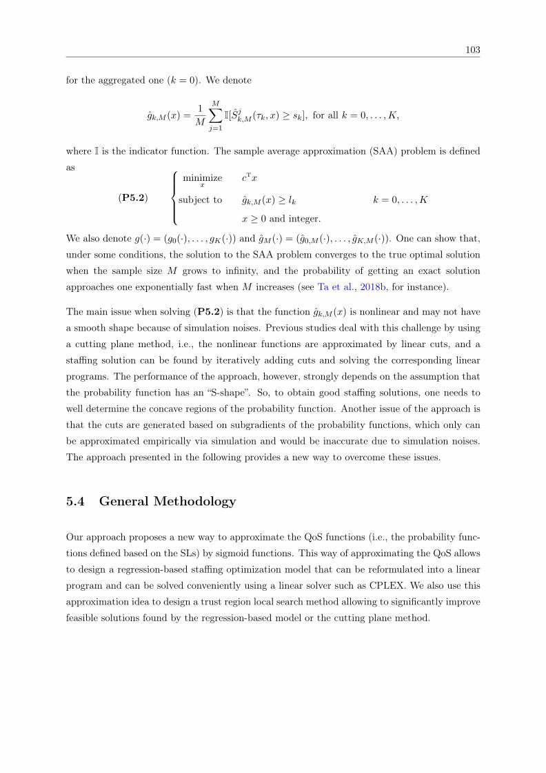
103

for the aggregated one (k = 0). We denote

gk,M (x) =1

M

M∑j=1

I[Sjk,M (τk, x) ≥ sk], for all k = 0, . . . ,K,

where I is the indicator function. The sample average approximation (SAA) problem is defined

as

(P5.2)

minimize

xcTx

subject to gk,M (x) ≥ lk k = 0, . . . ,K

x ≥ 0 and integer.

We also denote g(·) = (g0(·), . . . , gK(·)) and gM (·) = (g0,M (·), . . . , gK,M (·)). One can show that,

under some conditions, the solution to the SAA problem converges to the true optimal solution

when the sample size M grows to infinity, and the probability of getting an exact solution

approaches one exponentially fast when M increases (see Ta et al., 2018b, for instance).

The main issue when solving (P5.2) is that the function gk,M (x) is nonlinear and may not have

a smooth shape because of simulation noises. Previous studies deal with this challenge by using

a cutting plane method, i.e., the nonlinear functions are approximated by linear cuts, and a

staffing solution can be found by iteratively adding cuts and solving the corresponding linear

programs. The performance of the approach, however, strongly depends on the assumption that

the probability function has an “S-shape”. So, to obtain good staffing solutions, one needs to

well determine the concave regions of the probability function. Another issue of the approach is

that the cuts are generated based on subgradients of the probability functions, which only can

be approximated empirically via simulation and would be inaccurate due to simulation noises.

The approach presented in the following provides a new way to overcome these issues.

5.4 General Methodology

Our approach proposes a new way to approximate the QoS functions (i.e., the probability func-

tions defined based on the SLs) by sigmoid functions. This way of approximating the QoS allows

to design a regression-based staffing optimization model that can be reformulated into a linear

program and can be solved conveniently using a linear solver such as CPLEX. We also use this

approximation idea to design a trust region local search method allowing to significantly improve

feasible solutions found by the regression-based model or the cutting plane method.

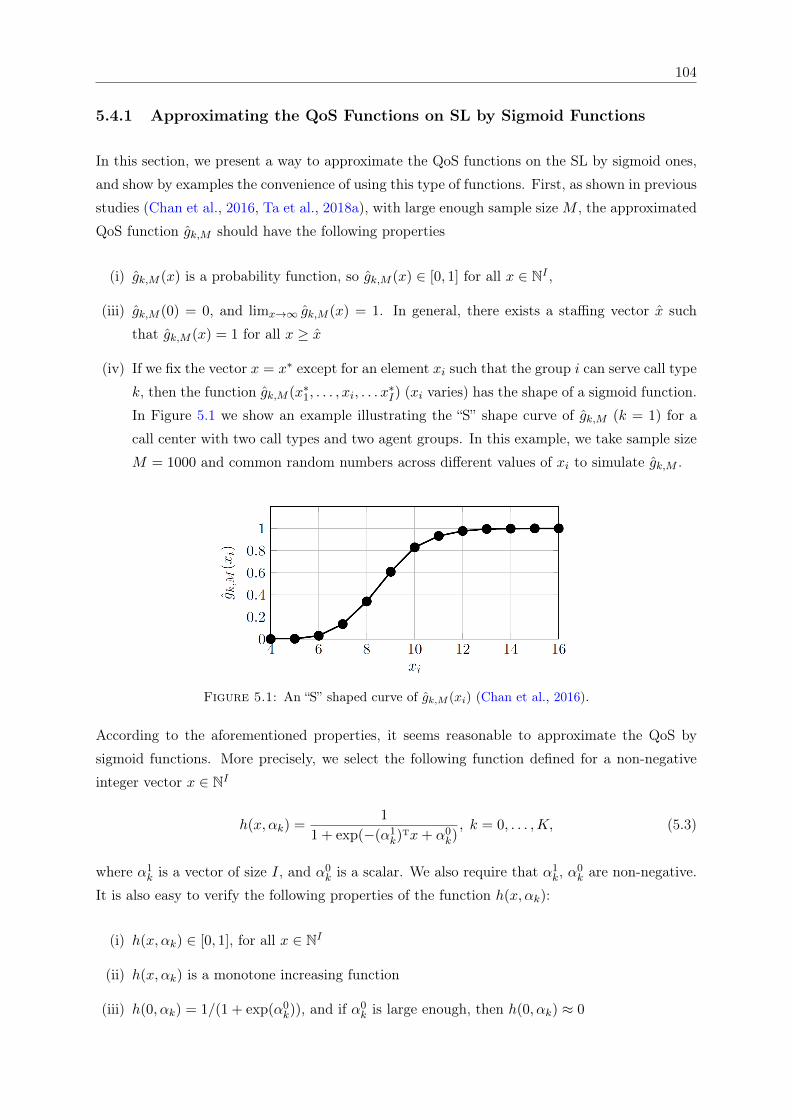
104

5.4.1 Approximating the QoS Functions on SL by Sigmoid Functions

In this section, we present a way to approximate the QoS functions on the SL by sigmoid ones,

and show by examples the convenience of using this type of functions. First, as shown in previous

studies (Chan et al., 2016, Ta et al., 2018a), with large enough sample sizeM , the approximated

QoS function gk,M should have the following properties

(i) gk,M (x) is a probability function, so gk,M (x) ∈ [0, 1] for all x ∈ NI ,

(iii) gk,M (0) = 0, and limx→∞ gk,M (x) = 1. In general, there exists a staffing vector x such

that gk,M (x) = 1 for all x ≥ x

(iv) If we fix the vector x = x∗ except for an element xi such that the group i can serve call type

k, then the function gk,M (x∗1, . . . , xi, . . . x∗I) (xi varies) has the shape of a sigmoid function.

In Figure 5.1 we show an example illustrating the “S” shape curve of gk,M (k = 1) for a

call center with two call types and two agent groups. In this example, we take sample size

M = 1000 and common random numbers across different values of xi to simulate gk,M .

Figure 5.1: An “S” shaped curve of gk,M (xi) (Chan et al., 2016).

According to the aforementioned properties, it seems reasonable to approximate the QoS by

sigmoid functions. More precisely, we select the following function defined for a non-negative

integer vector x ∈ NI

h(x, αk) =1

1 + exp(−(α1k)

Tx+ α0k), k = 0, . . . ,K, (5.3)

where α1k is a vector of size I, and α0

k is a scalar. We also require that α1k, α

0k are non-negative.

It is also easy to verify the following properties of the function h(x, αk):

(i) h(x, αk) ∈ [0, 1], for all x ∈ NI

(ii) h(x, αk) is a monotone increasing function

(iii) h(0, αk) = 1/(1 + exp(α0k)), and if α0

k is large enough, then h(0, αk) ≈ 0

105

(iv) limx→∞ h(x, αk) = 1

(v) If we fix the vector x = x∗ except an element xi, then the function h(x, αk) (xi varies)

displays an “S shaped” curve.

These properties suggest that h(x, αk) would be able to fit well with function gk,M (x). In other

words, we expect that a linear function can fit well with ln(1/gk,M (x)− 1).

The parameters α of the nonlinear function (5.3) can be generally estimated by fitting the QoS

function gk,M (x) with the sigmoid one h(x, αk). To be more precise, suppose that function

gk,M (x) is evaluated at T points (x1, . . . , xT ), then the parameters αk can be estimated solving

the following least-squares problem.

minimizeαk∈RI+1

1

T

T∑t=1

wk(xt)(h(xt, αk)− gk,M (xt)

)2(5.4)

subject to 0 ≤ α1k ≤ u

0 ≤ α0k ≤ u0,

where wk(xt) is a weight associated with point xt, u, u0 are upper bounds of the parameters

α1k, α

0k, respectively. These bounds are necessary in order to keep the values of αk reasonable

when the number of points T is small. Moreover, the use a weighted least-squares model is

motivated by the fact that some points may be more important than others. More precisely,

since we want to find staffing solutions as small as possible but still satisfy the QoS constraints,

the points with which the QoS values are close to the targets would be more important.

In order to illustrate how functions of the form (5.3) can fit the QoS ones, we present four

examples in the following. These examples are based on a small call center of 2 agent groups

and 2 call types. There is one group that can serve only one call type, and the other group can

serve both call types. We varied the staffing vector and use simulation to generate QoS values.

The parameters αk are estimated using the least-squares model (5.4) with equal weights and no

bound constraints, i.e., wk(xt) = 1, for all t.

Example 1: Fitting gk,M (x) and ln(1/gk,M (x) − 1) with different sigmoid and linear

functions. First, we use the example shown in Figure 5.1. In this example, gk,M (x) is a sample

average approximation of the probability function of the SL associated with call type k, where

k is the call type served by only one agent group and we use M = 1000. We evaluated the

function at a staffing xi ∈ 6, 7, . . . , 14, where i is the group that serves call type k. On

the left side of Figure 5.2, we plot gk,M and functions of the form 1/(1 + exp(−α1xi + α2)),

and on the right side we plot ln(1/gk,M (xi) − 1) and linear functions −α1xi + α2, where α ∈(1.14, 9.9), (1.14, 10.9), (1.24, 9.9)

. Clearly, with α = (1.14, 9.9), the corresponding sigmoid

and linear functions seem to fit very well with gk,M (xi) and ln(1/gk,M (xi) − 1), in particular

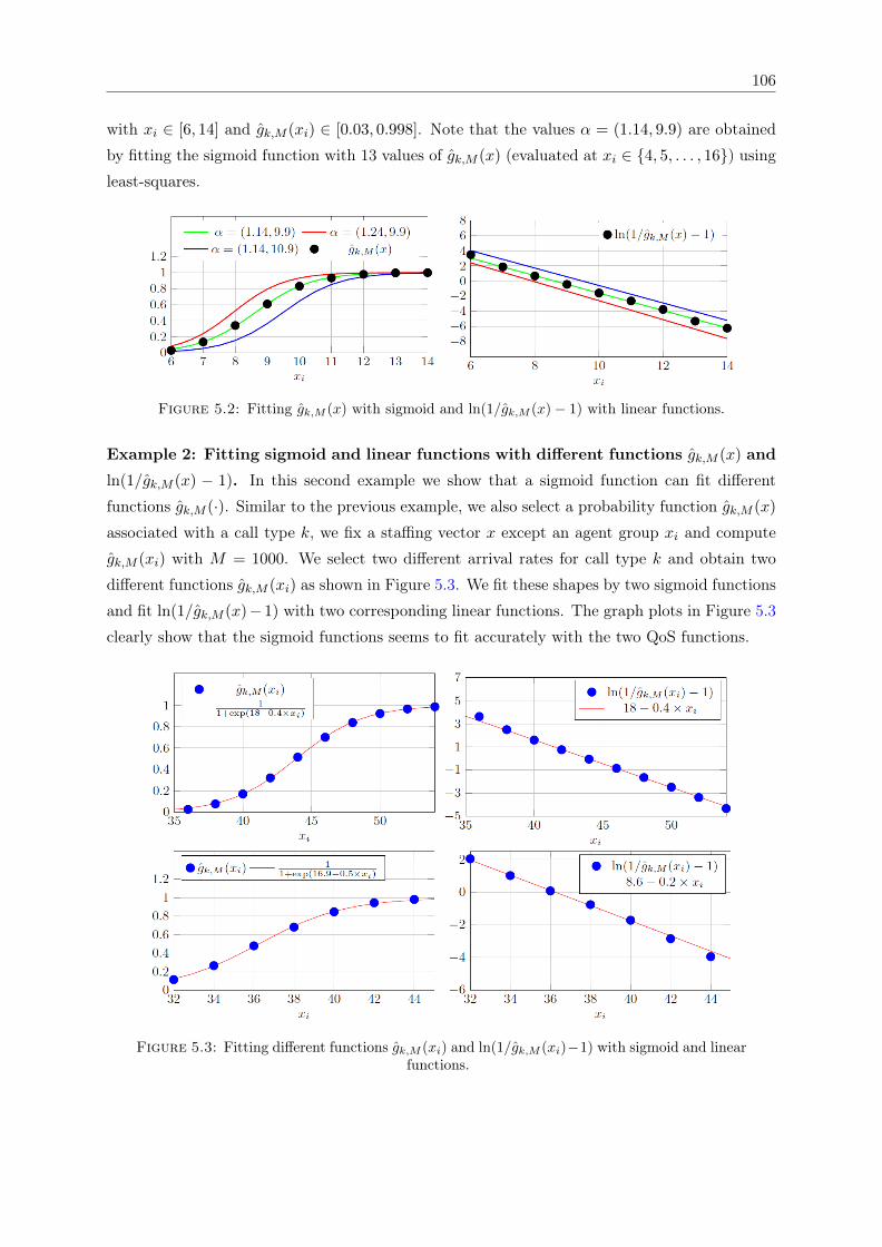
106

with xi ∈ [6, 14] and gk,M (xi) ∈ [0.03, 0.998]. Note that the values α = (1.14, 9.9) are obtained

by fitting the sigmoid function with 13 values of gk,M (x) (evaluated at xi ∈ 4, 5, . . . , 16) usingleast-squares.

Figure 5.2: Fitting gk,M (x) with sigmoid and ln(1/gk,M (x)− 1) with linear functions.

Example 2: Fitting sigmoid and linear functions with different functions gk,M (x) and

ln(1/gk,M (x) − 1). In this second example we show that a sigmoid function can fit different

functions gk,M (·). Similar to the previous example, we also select a probability function gk,M (x)

associated with a call type k, we fix a staffing vector x except an agent group xi and compute

gk,M (xi) with M = 1000. We select two different arrival rates for call type k and obtain two

different functions gk,M (xi) as shown in Figure 5.3. We fit these shapes by two sigmoid functions

and fit ln(1/gk,M (x)−1) with two corresponding linear functions. The graph plots in Figure 5.3

clearly show that the sigmoid functions seems to fit accurately with the two QoS functions.

Figure 5.3: Fitting different functions gk,M (xi) and ln(1/gk,M (xi)−1) with sigmoid and linearfunctions.

107

Example 3: The shapes of gk,M (x) and ln(1/gk,M (x) − 1) in 3D. The third example is to

illustrate how gk,M and ln(1/gk,M (xi)−1) look in 3D. Suppose that i, j are two agent groups that

can serve call type k. We vary both xi, xj , so function gk,M (x) becomes gk,M (xi, xj). We use

M = 1000 to compute 23×32 values of gk,M (xi, xj), where xi ∈ 1, . . . , 23 and xj ∈ 1, . . . , 32.We draw the 3D surface plots given by gk,M (xi, xj) and ln(1/gk,M (xi, xj)−1) in Figure 5.4, noting

that when plotting ln(1/gk,M (xi, xj)−1) we only select points for which gk,M (xi, xj) are greater

than 0.01 or less than 0.99 to avoid numerical issues. We see that gk,M (xi, xj) on the left hand

side seems to have a shape of a sigmoid function. On the other hand, ln(1/gk,M (xi, xj) − 1)

seems to have a linear shape

Figure 5.4: 3D surface plots of gk,M (xi, xj) and ln(1/gk,M (xi, xj)− 1)

Example 4: Fitting gk,M (x) and ln(1/gk,M (x) − 1) when the sample size is low. In

the last example, we show how sigmoid functions can fit gk,M when the number of samples

M is small. We also take a call type k that is served by group agent i, and we let xi varies,

other elements of staffing x are fixed. We use M = 20 to simulate the values of gk,M (xi)

for xi ∈ 4, 6, ..., 24. These values are also used to estimate the parameter α of function

h(xi, α) = 1/(1 + exp(−α1xi + α2)) and obtain parameters α = (0.5, 7.4). In Figure 5.5, we

plot the values of gk,M (xi) and ln(1/gk,M (xi)− 1) with M = 20 and M = 1000 on the left, and

the corresponding sigmoid and linear functions on the right side. It is interesting to remark that

even when α is estimated by values given by a low number of samples (M = 20), the shape

of h(xi, α) and its corresponding linear functions are close to the ones given by gk,M (xi) and

ln(1/gk,M (xi) − 1) with much larger number of samples (i.e., M = 1000). This observation

suggests that the sigmoid functions may well approximate the shapes of the QoS even if the

parameters are estimated through noisy observations.

It is also possible to estimate α by linear least-squares, as we remark that the function ln(1/h(x, αk)−1) is linear with respect to x. Thus, we can estimate the parameters α by fitting ln (1/gk,M (x)− 1)

with linear function (−(α1k)

Tx+α0k), noting that ln (1/gk,M (x)− 1) becomes undefined if gk,M (x)

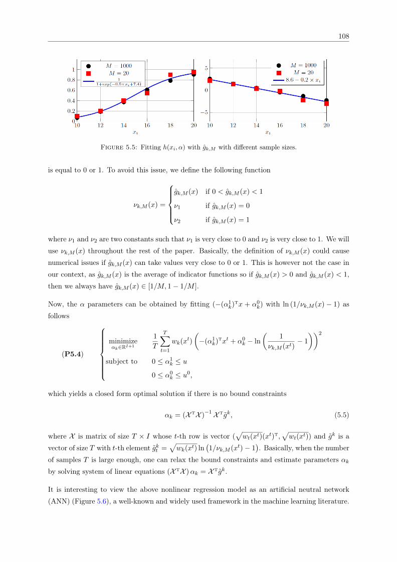
108

Figure 5.5: Fitting h(xi, α) with gk,M with different sample sizes.

is equal to 0 or 1. To avoid this issue, we define the following function

νk,M (x) =

gk,M (x) if 0 < gk,M (x) < 1

ν1 if gk,M (x) = 0

ν2 if gk,M (x) = 1

where ν1 and ν2 are two constants such that ν1 is very close to 0 and ν2 is very close to 1. We will

use νk,M (x) throughout the rest of the paper. Basically, the definition of νk,M (x) could cause

numerical issues if gk,M (x) can take values very close to 0 or 1. This is however not the case in

our context, as gk,M (x) is the average of indicator functions so if gk,M (x) > 0 and gk,M (x) < 1,

then we always have gk,M (x) ∈ [1/M, 1− 1/M ].

Now, the α parameters can be obtained by fitting (−(α1k)

Tx + α0k) with ln (1/νk,M (x)− 1) as

follows

(P5.4)

minimizeαk∈RI+1

1

T

T∑t=1

wk(xt)

(−(α1

k)Txt + α0

k − ln

(1

νk,M (xt)− 1

))2

subject to 0 ≤ α1k ≤ u

0 ≤ α0k ≤ u0,

which yields a closed form optimal solution if there is no bound constraints

αk = (X TX )−1X Tgk, (5.5)

where X is matrix of size T × I whose t-th row is vector (√wt(xt)(x

t)T,√wt(xt)) and gk is a

vector of size T with t-th element gkt =√wk(xt) ln

(1/νk,M (xt)− 1

). Basically, when the number

of samples T is large enough, one can relax the bound constraints and estimate parameters αkby solving system of linear equations (X TX )αk = X Tgk.

It is interesting to view the above nonlinear regression model as an artificial neutral network

(ANN) (Figure 5.6), a well-known and widely used framework in the machine learning literature.

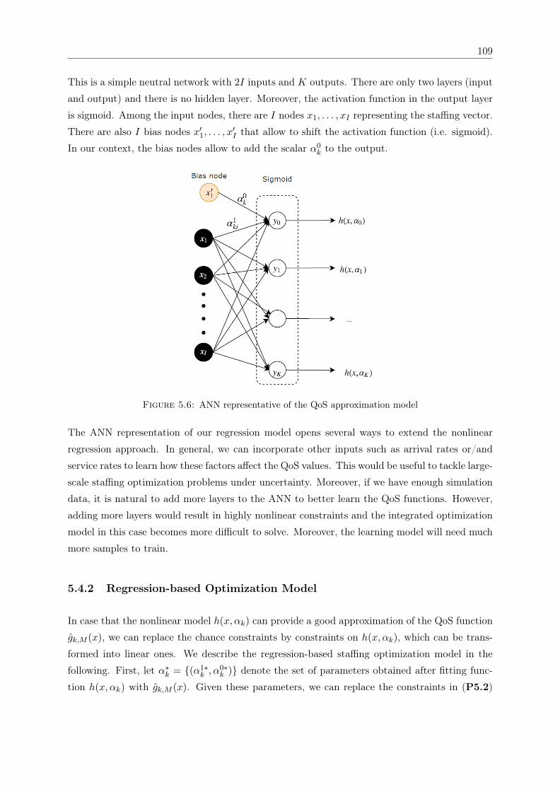
109

This is a simple neutral network with 2I inputs and K outputs. There are only two layers (input

and output) and there is no hidden layer. Moreover, the activation function in the output layer

is sigmoid. Among the input nodes, there are I nodes x1, . . . , xI representing the staffing vector.

There are also I bias nodes x′1, . . . , x′I that allow to shift the activation function (i.e. sigmoid).

In our context, the bias nodes allow to add the scalar α0k to the output.

Figure 5.6: ANN representative of the QoS approximation model

The ANN representation of our regression model opens several ways to extend the nonlinear

regression approach. In general, we can incorporate other inputs such as arrival rates or/and

service rates to learn how these factors affect the QoS values. This would be useful to tackle large-

scale staffing optimization problems under uncertainty. Moreover, if we have enough simulation

data, it is natural to add more layers to the ANN to better learn the QoS functions. However,

adding more layers would result in highly nonlinear constraints and the integrated optimization

model in this case becomes more difficult to solve. Moreover, the learning model will need much

more samples to train.

5.4.2 Regression-based Optimization Model

In case that the nonlinear model h(x, αk) can provide a good approximation of the QoS function

gk,M (x), we can replace the chance constraints by constraints on h(x, αk), which can be trans-

formed into linear ones. We describe the regression-based staffing optimization model in the

following. First, let α∗k = (α1∗k , α

0∗k ) denote the set of parameters obtained after fitting func-

tion h(x, αk) with gk,M (x). Given these parameters, we can replace the constraints in (P5.2)

110

by h(x, α∗k) ≥ lk, for all k = 0, . . . ,K, and obtain the following integer programming model

(P5.5)

minimize

xcTx

subject to1

1 + exp(−(α1∗k )Tx+ α0∗

k )≥ lk, k = 0, . . . ,K

x ≥ 0 and integer

The constraints in (P5.5) can be transformed into linear ones as

1

1 + exp(−(α1∗k )Tx+ α0∗

k )≥ lk

⇔ 1 + exp(−(α1∗k )Tx+ α0∗

k ) ≤ 1/lk

⇔ −(α1∗k )Tx+ α0∗

k ≤ ln(1/lk − 1).

So (P5.5) can be equivalently formulated as an integer linear programming model as

(P5.6)

minimize

xcTx

subject to (α1∗k )Tx ≥ α0∗

k − ln

(1

lk− 1

), k = 0, . . . ,K

x ≥ 0 and integer.

(5.6)

Basically, (P5.6) is an integer linear programming model that can be solved conveniently using a

commercial solver (e.g. CPLEX). The model in (P5.6) can be used to find good staffing solution

in an iterative manner as follows. We iteratively collect staffing solutions to estimate parameters

αk of the sigmoid functions h(x, αk) and solve (P5.6) to obtain new candidate solutions. This

approach would be efficient if h(x, αk) fit well with the QoS functions, as it would require small

number of QoS function evaluations.

In some cases, h(x, α∗k) may underestimate or overestimate gk,M (x). In order to (partially)

correct the errors in these situations, we define an approximation error associated with each

function gk,M (x) as follows

ζ(x, α∗k) =

gk,M (x)− h(x, α∗k), if |gk,M (x)− lk| ≤ τ

0 otherwise,(5.7)

where τ is a positive threshold. We impose the threshold τ in (5.7) to neglect the impact of

points that are far from the targets. In other words, we only correct the approximation errors for

points whose probability values are close to the targets. Given a solution x, if ζ(x, α∗k) > 0 then

h(x, α∗k) underestimates gk,M (x) and ζ(x, α∗k) < 0 means that h(x, α∗k) overestimates gk,M (x).

Now, assume that we obtain parameters α∗k, k ∈ 0, . . . ,K using a training set of T points.

Let x denote the solution given by the regression-based model (P5.6). We can use simulation

111

to measure the approximation error ζ(x, α∗k) at point x and adjust the linear constraints as

h(x, α∗k) + ζ(x, α∗k) ≥ lk, k = 0, . . . ,K.

Consequently, we can integrate the approximation error and adjust (P5.6) to have the following

model

(P5.7)

minimize

xcTx

subject to (α∗k)Tx ≥ α∗0,k − ln

(1

lk − ζ(x, α∗k)− 1

), k = 0, . . . ,K

x ∈ NI .

The regression-based optimization model can be incorporated with the fitting procedure in an it-

erative manner to find good staffing solutions. More precisely, at iteration t we add (xt, gk,M (xt))

to the training set of the regression model and update α∗k, k ∈ 0, . . . ,K. To obtain new so-

lutions, we replace gk,M (xt) by h(x, α∗k) and solve the approximate problem with constraints

h(x, α∗k) + ζ(xt, α∗k) ≥ lk, k = 0, . . . ,K, i.e., (P5.6). When the training set has enough points,

the parameter estimates α∗k, k ∈ 0, . . . ,K will become stable and we can stop the iterative

procedure and return the best solution found. In general, this approach does not require to

estimate the subgradients as in the conventional cutting plane method, so it is expected to take

less simulation time. However, it may not return good quality solutions in cases that the sigmoid

functions are not able to accurately approximate the QoS functions.

5.4.3 Cut Generation

We recall the cutting plan method, which is considered as the state-of-the-art approach to deal

with staffing optimization problems with constraints on “S-shaped” curve functions (Atlason

et al., 2003, Cezik and L’Ecuyer, 2008). This approach typically works well if the concave parts

of the QoS function are well determined and the QoS functions display “smooth” shapes.

Consider a QoS function gk,M (x) associated with k ∈ 0, . . . ,K. Let x∗ be a staffing solution

where we would like to generate cuts. We denote by qk(x∗) a (tentative) estimation of the

subgradient of gk,M (·) at point x∗. This vector has no closed-form and needs to be estimated by

simulation. More precisely, we estimate the i-th element qk,i(x∗) of qk(x∗) by the forward finite

difference, with step size d ∈ N∗ as

qk,i(x∗) =

gk,M (x∗ + dei)− gk,M (x∗)

d, (5.8)

where ei is a unit vector with 1 at the i-th position and zeroes elsewhere. Normally, we choose

d = 1, but when the function gk,M is not smooth enough (e.g., the number of simulated days

M is small) and (or) not concave, we need to increase d, e.g., d = 2 or 3. To use the cutting

112

plane, one need to assume that qk(x∗) is a good approximation of the subgradient of gk,M at

point x∗. Thus, under the assumption that gk,M (x) is “concave” at x, the following inequality

is valid gk,M (x∗) + qk(x∗)(x − x∗) ≥ gk,M (x), for all x ∈ X. Since we want to find x such that

gk,M (x) ≥ lk, the following inequality needs to hold

qk(x∗)x ≥ lk − gk,M (x∗) + qk(x

∗)x∗, k = 0, . . . ,K, (5.9)

which is a linear cut that can be used to create an outer approximation of the concave part

of gk,M (x). It is important to note that qk(x∗) computed as in (5.8) is not necessary a valid

subgradient cut of gk,M , especially when M is not large enough and x∗ does not belong to a

concave region of gk,M . This issue has been pointed out with examples in previous studies, for

instance, Atlason et al. (2008) and Chevalier and Van den Schrieck (2008).

An important issue of the cutting plane method is to determine the concave parts of the QoS.

Chan et al. (2016) suggested that one can add more constraints based on a fluid scheduling

model (Bassamboo et al., 2006) that may eliminate areas of non-concavity. These constraints

require additional continuous variables wki which defines the (fractional) number of agents of

group i working on calls of type k, as follows

∑i∈Gk

µk,iwk,i ≥ βkλk, k = 1, . . . ,K

∑k∈Si

wk,i ≤ xi, i = 1, . . . , I

wk,i ≥ 0, k = 1, . . . ,K, i = 1, . . . , I

(5.10)

where β = (β1, . . . , βK)T is a vector of parameters for the fluid model. The parameters βk should

be selected such that the initial solution is in a concave region of gM . So, with the constraints

in (5.10), at each iteration of the cutting plane algorithm, one needs to solve the following linear

programming model to obtain a staffing solution

(P5.8)

minimizex∈X

cTx =

I∑i=1

cixi

subject to Ax ≤ b

Hx+Kw ≤ q

x ∈ NI , w ≥ 0,

where Ax ≤ b are cuts given by (5.9), Hx + Kw ≤ q are constraints (5.10) given by the fluid

scheduling model presented above.

Here we need to emphasize that the selection of the parameters β is critical for the cutting plane

method, as it cannot return good staffing solutions if the convex regions of the QoS functions

113

are not well eliminated. For the expected SL constraints, β can be chosen around 1. However,

for the chance constraints, this way of selection may not work. We can deal with this issue by

manually adjusting the fluid scheduling parameters β such that the solutions given by the fluid

constraints belong to the concave regions of the QoS. One can show that, under the assumption

that the subgradient cuts are well generated from concave regions, we never remove feasible

solutions and will end up with an optimal one.

5.4.4 Trust Region Local Search

We design a local search algorithm that allows to improve a feasible solution given by the cutting

plane method or the regression-based optimization model described above. The algorithm is

inspired by the trust region method in continuous optimization (Conn et al., 2000). This is

an iterative approach in which, at each iteration, we build model functions approximating the

QoS functions and define a region around the current solution within which we trust the model

functions to be adequate representations of the QoS. Then, we find a next iterate by minimizing

an optimization problem in which the QoS are replaced by the model functions, and inside the

region that we trust, in the hope of finding a new candidate solution with better objective value.

The size of the region is reduced or enlarged according to the quality of the new solution found.

The difference between our approach and other conventional trust region algorithms in the lit-

erature is twofold. First, we apply the trust-region idea on the constraints while the standard

trust-region framework relies on the objective function. Second, we build the model functions

based on the idea of approximating the QoS functions by sigmoid ones described above. Techni-

cally speaking, we have shown previously that it might be a good idea to approximate the QoS

by the nonlinear functions of the form (5.3). So, as a natural consequence, we can approximate

ln (1/νk,M (x)− 1) by linear functions of x. This suggests an idea that, instead of using (esti-

mated) gradients of gk,M (x), we build the model functions based on the (estimated) gradients

of ln (1/νk,M (x)− 1). We describe our approach in detail in the following.

First, let us define

vk(x) = ln

(1

νk,M (x)− 1

), k = 0, . . . ,K.

Now, given a point x, let uk(x) denote a (tentative) estimation of the subgradient vk(.) at x.

The vector vk(x) has no closed-form and need to be approximated by simulation. Similar to the

cutting plane approach, the i-th element of uk(x) can be computed by finite difference as

uk,i(x) =vk(x+ dei)− vk(x)

d

=1

dln

((1− νkM (x+ dei))νkM (x)

(1− νkM (x))νkM (x+ dei)

), k = 0, . . . ,K,

(5.11)

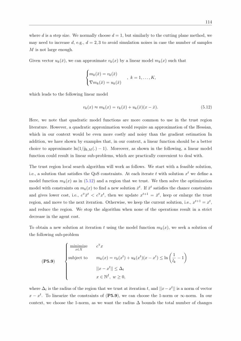
114

where d is a step size. We normally choose d = 1, but similarly to the cutting plane method, we

may need to increase d, e.g., d = 2, 3 to avoid simulation noises in case the number of samples

M is not large enough.

Given vector uk(x), we can approximate vk(x) by a linear model mk(x) such thatmk(x) = vk(x)

∇mk(x) = uk(x), k = 1, . . . ,K,

which leads to the following linear model

vk(x) ≈ mk(x) = vk(x) + uk(x)(x− x). (5.12)

Here, we note that quadratic model functions are more common to use in the trust region

literature. However, a quadratic approximation would require an approximation of the Hessian,

which in our context would be even more costly and noisy than the gradient estimation In

addition, we have shown by examples that, in our context, a linear function should be a better

choice to approximate ln(1/gk,M (.) − 1). Moreover, as shown in the following, a linear model

function could result in linear sub-problems, which are practically convenient to deal with.

The trust region local search algorithm will work as follows. We start with a feasible solution,

i.e., a solution that satisfies the QoS constraints. At each iterate t with solution xt we define a

model function mk(x) as in (5.12) and a region that we trust. We then solve the optimization

model with constraints on mk(x) to find a new solution xt. If xt satisfies the chance constraints

and gives lower cost, i.e., cTxt < cTxt, then we update xt+1 = xt, keep or enlarge the trust

region, and move to the next iteration. Otherwise, we keep the current solution, i.e., xt+1 = xt,

and reduce the region. We stop the algorithm when none of the operations result in a strict

decrease in the agent cost.

To obtain a new solution at iteration t using the model function mk(x), we seek a solution of

the following sub-problem

(P5.9)

minimizex∈X

cTx

subject to mk(x) = vk(xt) + uk(x

t)(x− xt) ≤ ln

(1

lk− 1

)||x− xt|| ≤ ∆t

x ∈ NI , w ≥ 0,

where ∆t is the radius of the region that we trust at iteration t, and ||x−xt|| is a norm of vector

x − xt. To linearize the constraints of (P5.9), we can choose the 1-norm or ∞-norm. In our

context, we choose the 1-norm, as we want the radius ∆ bounds the total number of changes

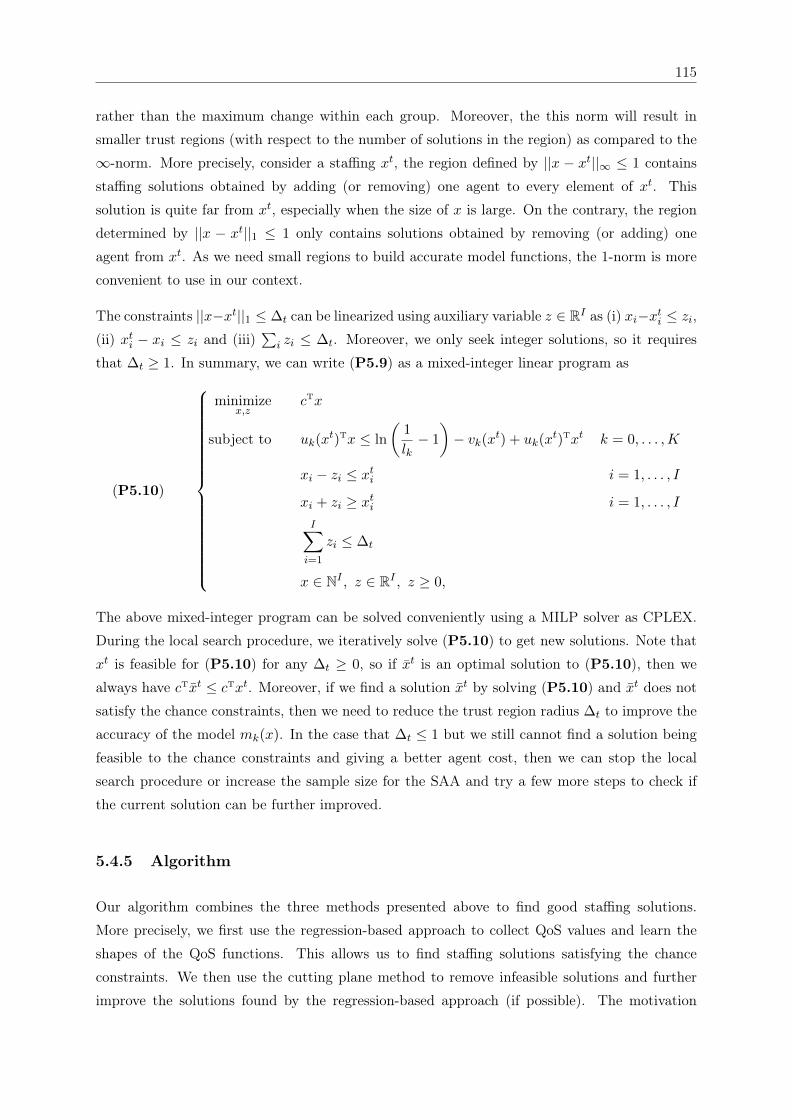
115

rather than the maximum change within each group. Moreover, the this norm will result in

smaller trust regions (with respect to the number of solutions in the region) as compared to the

∞-norm. More precisely, consider a staffing xt, the region defined by ||x − xt||∞ ≤ 1 contains

staffing solutions obtained by adding (or removing) one agent to every element of xt. This

solution is quite far from xt, especially when the size of x is large. On the contrary, the region

determined by ||x − xt||1 ≤ 1 only contains solutions obtained by removing (or adding) one

agent from xt. As we need small regions to build accurate model functions, the 1-norm is more

convenient to use in our context.

The constraints ||x−xt||1 ≤ ∆t can be linearized using auxiliary variable z ∈ RI as (i) xi−xti ≤ zi,(ii) xti − xi ≤ zi and (iii)

∑i zi ≤ ∆t. Moreover, we only seek integer solutions, so it requires

that ∆t ≥ 1. In summary, we can write (P5.9) as a mixed-integer linear program as

(P5.10)

minimizex,z

cTx

subject to uk(xt)Tx ≤ ln

(1

lk− 1

)− vk(xt) + uk(x

t)Txt k = 0, . . . ,K

xi − zi ≤ xti i = 1, . . . , I

xi + zi ≥ xti i = 1, . . . , I

I∑i=1

zi ≤ ∆t

x ∈ NI , z ∈ RI , z ≥ 0,

The above mixed-integer program can be solved conveniently using a MILP solver as CPLEX.

During the local search procedure, we iteratively solve (P5.10) to get new solutions. Note that

xt is feasible for (P5.10) for any ∆t ≥ 0, so if xt is an optimal solution to (P5.10), then we

always have cTxt ≤ cTxt. Moreover, if we find a solution xt by solving (P5.10) and xt does not

satisfy the chance constraints, then we need to reduce the trust region radius ∆t to improve the

accuracy of the model mk(x). In the case that ∆t ≤ 1 but we still cannot find a solution being

feasible to the chance constraints and giving a better agent cost, then we can stop the local

search procedure or increase the sample size for the SAA and try a few more steps to check if

the current solution can be further improved.

5.4.5 Algorithm

Our algorithm combines the three methods presented above to find good staffing solutions.

More precisely, we first use the regression-based approach to collect QoS values and learn the

shapes of the QoS functions. This allows us to find staffing solutions satisfying the chance

constraints. We then use the cutting plane method to remove infeasible solutions and further

improve the solutions found by the regression-based approach (if possible). The motivation

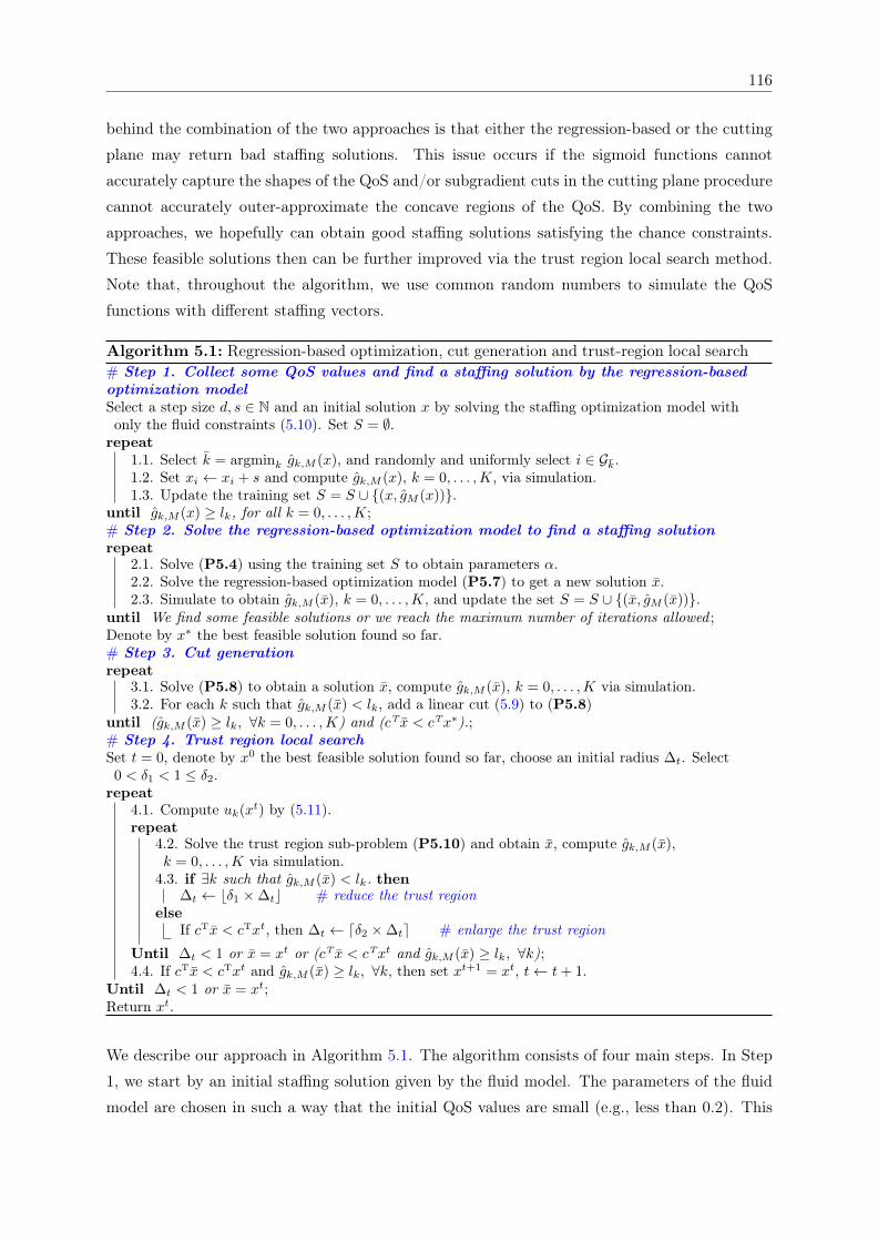
116

behind the combination of the two approaches is that either the regression-based or the cutting

plane may return bad staffing solutions. This issue occurs if the sigmoid functions cannot

accurately capture the shapes of the QoS and/or subgradient cuts in the cutting plane procedure

cannot accurately outer-approximate the concave regions of the QoS. By combining the two

approaches, we hopefully can obtain good staffing solutions satisfying the chance constraints.

These feasible solutions then can be further improved via the trust region local search method.

Note that, throughout the algorithm, we use common random numbers to simulate the QoS

functions with different staffing vectors.

Algorithm 5.1: Regression-based optimization, cut generation and trust-region local search# Step 1. Collect some QoS values and find a staffing solution by the regression-basedoptimization modelSelect a step size d, s ∈ N and an initial solution x by solving the staffing optimization model withonly the fluid constraints (5.10). Set S = ∅.repeat

1.1. Select k = argmink gk,M (x), and randomly and uniformly select i ∈ Gk.1.2. Set xi ← xi + s and compute gk,M (x), k = 0, . . . ,K, via simulation.1.3. Update the training set S = S ∪ (x, gM (x)).

until gk,M (x) ≥ lk, for all k = 0, . . . ,K;# Step 2. Solve the regression-based optimization model to find a staffing solutionrepeat

2.1. Solve (P5.4) using the training set S to obtain parameters α.2.2. Solve the regression-based optimization model (P5.7) to get a new solution x.2.3. Simulate to obtain gk,M (x), k = 0, . . . ,K, and update the set S = S ∪ (x, gM (x)).

until We find some feasible solutions or we reach the maximum number of iterations allowed ;Denote by x∗ the best feasible solution found so far.# Step 3. Cut generationrepeat

3.1. Solve (P5.8) to obtain a solution x, compute gk,M (x), k = 0, . . . ,K via simulation.3.2. For each k such that gk,M (x) < lk, add a linear cut (5.9) to (P5.8)

until (gk,M (x) ≥ lk, ∀k = 0, . . . ,K) and (cTx < cTx∗).;# Step 4. Trust region local searchSet t = 0, denote by x0 the best feasible solution found so far, choose an initial radius ∆t. Select0 < δ1 < 1 ≤ δ2.repeat

4.1. Compute uk(xt) by (5.11).repeat

4.2. Solve the trust region sub-problem (P5.10) and obtain x, compute gk,M (x),k = 0, . . . ,K via simulation.

4.3. if ∃k such that gk,M (x) < lk. then∆t ← bδ1 ×∆tc # reduce the trust region

elseIf cTx < cTxt, then ∆t ← dδ2 ×∆te # enlarge the trust region

Until ∆t < 1 or x = xt or (cTx < cTxt and gk,M (x) ≥ lk, ∀k);4.4. If cTx < cTxt and gk,M (x) ≥ lk, ∀k, then set xt+1 = xt, t← t+ 1.

Until ∆t < 1 or x = xt;Return xt.

We describe our approach in Algorithm 5.1. The algorithm consists of four main steps. In Step

1, we start by an initial staffing solution given by the fluid model. The parameters of the fluid

model are chosen in such a way that the initial QoS values are small (e.g., less than 0.2). This

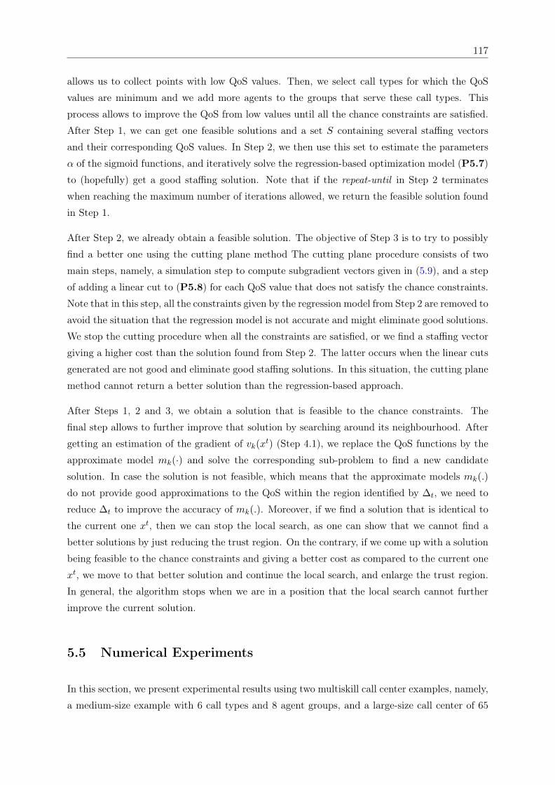
117

allows us to collect points with low QoS values. Then, we select call types for which the QoS

values are minimum and we add more agents to the groups that serve these call types. This

process allows to improve the QoS from low values until all the chance constraints are satisfied.

After Step 1, we can get one feasible solutions and a set S containing several staffing vectors

and their corresponding QoS values. In Step 2, we then use this set to estimate the parameters

α of the sigmoid functions, and iteratively solve the regression-based optimization model (P5.7)

to (hopefully) get a good staffing solution. Note that if the repeat-until in Step 2 terminates

when reaching the maximum number of iterations allowed, we return the feasible solution found

in Step 1.

After Step 2, we already obtain a feasible solution. The objective of Step 3 is to try to possibly

find a better one using the cutting plane method The cutting plane procedure consists of two

main steps, namely, a simulation step to compute subgradient vectors given in (5.9), and a step

of adding a linear cut to (P5.8) for each QoS value that does not satisfy the chance constraints.

Note that in this step, all the constraints given by the regression model from Step 2 are removed to

avoid the situation that the regression model is not accurate and might eliminate good solutions.

We stop the cutting procedure when all the constraints are satisfied, or we find a staffing vector

giving a higher cost than the solution found from Step 2. The latter occurs when the linear cuts

generated are not good and eliminate good staffing solutions. In this situation, the cutting plane

method cannot return a better solution than the regression-based approach.

After Steps 1, 2 and 3, we obtain a solution that is feasible to the chance constraints. The

final step allows to further improve that solution by searching around its neighbourhood. After

getting an estimation of the gradient of vk(xt) (Step 4.1), we replace the QoS functions by the

approximate model mk(·) and solve the corresponding sub-problem to find a new candidate

solution. In case the solution is not feasible, which means that the approximate models mk(.)

do not provide good approximations to the QoS within the region identified by ∆t, we need to

reduce ∆t to improve the accuracy of mk(.). Moreover, if we find a solution that is identical to

the current one xt, then we can stop the local search, as one can show that we cannot find a

better solutions by just reducing the trust region. On the contrary, if we come up with a solution

being feasible to the chance constraints and giving a better cost as compared to the current one

xt, we move to that better solution and continue the local search, and enlarge the trust region.

In general, the algorithm stops when we are in a position that the local search cannot further

improve the current solution.

5.5 Numerical Experiments

In this section, we present experimental results using two multiskill call center examples, namely,

a medium-size example with 6 call types and 8 agent groups, and a large-size call center of 65

118

call types and 89 agent groups. The latter is inspired by a large real-life call center operated

by Bell Canada. This example is also used in previous staffing optimization studies (Cezik and

L’Ecuyer, 2008).

5.5.1 Experimental Settings

We test our algorithm with three sets of targets, namely, (i) l0 = 75% and lk = 70%, k =

1, . . . ,K, (ii) l0 = 85% and lk = 80%, k = 1, . . . ,K and (iii) l0 = 95% and lk = 90%, k =

1, . . . ,K. For short, we denote the three sets of targets as (70%, 75%), (80%, 85%) and (90%,

95%), respectively. The agents costs are defined based on the number of skills in the agent’s

skill set as

ci = 1 + 0.1(|Si| − 1) for all group i,

where |Si| is the cardinality of Si.

We assume that calls arrive according to Poisson processes for all the call centers considered.

For each call center example, we generate different problem instances by varying the arrival

rates. That is, the arrival rate of call type k is modeled as a random variable Λk = ξkBkλk,where λk represents the mean of the arrival rate of call type k, Bk is the business factor of

the day and follows a symmetric triangular distribution of mean and mode 1, minimum 0.9 and

maximum 1.1, and ξk is used to capture the variation of the arrival rate of call type k in different

scenarios. For each call center example, we generate 10 vector values of ξ1, . . . , ξK around 1

and solve each one with the three sets of targets presented above. So, in total, for each call

center example, we have 30 problem instances to be solved. Note that this ways of generating

the problem instances is motivated by the fact that the arrival rates are often uncertain and

depend on may factor such as the day of the week, time of the day, level of business, holidays

and special events (see for instance Channouf et al., 2007, Ibrahim et al., 2016b, Oreshkin et al.,

2016).

We solve each instance by our approach (Algorithm 5.1, denoted by RCT, an abbreviation

for Regression, Cutting Plane and Trust Region Local Search), the conventional cutting plane

(presented in Section 5.4.3, denoted by CP) and the regression-based optimization approach

(Step 1 of Algorithm 5.1, denoted by RO). We will compare the three approaches in terms of

the agent costs returned and CPU time.

We select a sample size M = 1000 to approximate the QoS values. Moreover, a same set

of realizations used to approximate the QoS is reused during the optimization process. The

solutions obtained by different approaches are then evaluated via an out-of-sample study. More

precisely, for each solution x, we compute the corresponding QoS values with a larger sample

size M ′ = 2000 and 10 sets of realizations that are independent of those used to obtain the

119

solutions. Then, we report the average number of QoS values that violate the requirements, i.e.,

gk,M ′(x) ≤ lk − κ, k = 0, . . . ,K. Here, we use two values of κ, namely, κ = 0 and κ = 0.005.

The former refers to the exact chance constraints, while for the latter we relax a bit the QoS

requirements.

The CP is implemented as follows. We first solve the linear model with the fluid constraints

in (5.10) to obtain an initial solution x0. At each iteration, we compute an estimation of the

gradient of gk,M (x∗) using (5.8) with d = 1, where x∗ is the staffing solution chosen to generate

cuts. If mini=1,...,I qk,i(x∗) < 0 or maxi=1,...,I qk,i(x

∗) ≤ 0, i.e. qk(x∗) has a negative element or

there is no positive element in qk(x∗), then we increase the step side d← d+ 1 and re-compute

the subgradient. Otherwise, we generate linear cuts of the form linear model (P5.8). We also

require that the step size cannot exceed the maximum value allowed dmax, i.e., the cutting plane

stops if d ≥ dmax and in this situation the method fails to solve the staffing problem. We

choose dmax = 5. Moreover, since the subgradient cuts may be not accurate, we impose upper

bound constraints for the staffing x in (P5.3). In these experiments, we require xi ≤ 200 for all

i = 1, . . . I.

The RO method corresponds to Steps 1 and 2 of Algorithm 5.1. We use the the fluid scheduling

model with low fluid parameters, i.e. βk = 0.5 for all k = 1, . . . ,K, to obtain an initial staffing

vector to start collecting QoS values. The step size is chosen as s = 1 and we run Step 1

simultaneously on 8 physical CPUs to get as many points as possible. For estimating the α

parameters, we select the weight vector as wk(xt) = 4 if |gk,M (xt) − lk| < 0.05 and wk(xt) = 1

otherwise. The approximation errors defined in (5.7) are computed with τ = 0.05. For Step 4

of Algorithm 5.1, we select ∆0 = 8 as an initial trust region radius. The parameters to enlarge

and reduce the trust region are chosen as δ1 = 0.7 and δ1 = 1.3. These parameters are chosen

manually to achieve good performance for Algorithm 5.1. For the definition of νk,M (·), notethat with sample size M = 1000, if 0 < gk,M (xt) < 1, then gk,M (xt) ∈ [0.001, 0.999], so we

choose ν1, ν2 such that ν1 < 0.001 and ν2 > 0.999. In this experiment we choose ν1 = 0.0001

and ν2 = 0.9999. The subgradient uk(xt) are estimated with step size d = 1. The “repeat-until”

in Step 2 stops when we find 5 feasible solutions and we just return the best one found. In

general, since there are quite a lot of points generated after Step 1, Step 2 finishes after just a

few iterations.

We use solver cplexmilp from CPLEX to solve mixed-integer linear programming (MIP) models

under default settings. For the medium instances, because the corresponding MIPs are small,

we let CPLEX run to optimality. For the large instances, the relative optimality gap was set

to 0.05%. To solve (P5.4), we use the linear least-squares solver provided by MATLAB 2015a

(i.e., lsqlin).

The experiments were conducted on a machine running Debian 8 with Intel(R) Xeon(R) CPU

E5620 (2.40GHz). The computer has 8 physical CPUs and 98GB of memory. The computation

120

of the subgradients qk(·) and uk(·) is performed in parallel using the 8 physical CPUs. The

algorithms were coded in MATLAB and linked to IBM ILOG CPLEX 12.6 optimization routines

under default settings. The simulations were performed using the ContactCenters simulation

library (Buist and L’Ecuyer, 2005) developed with the SSJ simulation package (L’Ecuyer et al.,

2002).

5.5.2 Medium Call Center

In this section we report numerical results for the medium call center with 6 call types and 8 agent

groups. We assume that (i) the callers do not abandon immediately in case they have to wait, (ii)

patience times follow an exponential distribution with means between 36 and 52 minutes, and

(iii) all service times follow Log-Normal distributions with means between 5.1 and 11.3 minutes.

The acceptable waiting times are chosen as τk = τ0 = 120 (seconds) and the targets for SLs are

lk = l0 = 80%. For the fluid scheduling model, we choose β = (1, 4, 1, 1.2, 1, 3). These values

are adjusted manually to ensure that the first staffing solutions given by the fluid scheduling

constraints belong to concave regions of the QoS functions.

We report numerical results in Table 5.1 for the three approaches RO, CP and RCT with the

three sets of targets (70%,75%), (80%,85%) and (90%,95%). We indicate in bold the best costs

obtained by the three approaches. We also emphasize in red the costs that are remarkably higher

than the others for each instances.

In terms of agent cost, we generally see that the RO performs better than the CP in this experi-

ment, as it returns better costs than the CP in 19/30 instances. Moreover, in 8/30 instances, the

CP gives very high costs as compared to the two other approaches. This clearly indicates the

instability of the CP and can be explained by the issue that the fluid constraints are not be able

to eliminate all the non-concave points, leading to bad subgradient cuts. The RCT approach

basically takes the best costs given by the CP and RO and improves them by the local search

procedure. So, it is as expected that the RCT never gives worse costs than the RO and CP.

Moreover, the RCT improves the best costs given by the RO and CP by 0.4% on average and up

to 0.8%. An interesting observation to be noted here is that, to raise the targets from (70%,75%)

to (80%,85%), we need to increase the agent cost by about 1.6% on average, and to raise the

targets from (70%,75%) to (90%,95%) we need about 2.65% on average. These percentages are

computed using the costs given by the RCT. In terms of CPU time, the RO is the fastest one,

and the RCT requires remarkably higher CPU times as compared to the two other approaches.

Even so, the RCT requires only half an hour on average to solve one instance, which is indeed

viable in a practical point of view.

In the out-of-sample study with κ = 0, we observe some violated QoS constraints. It is interesting

to see that the average numbers of violated QoSs given by the CP are less than the other

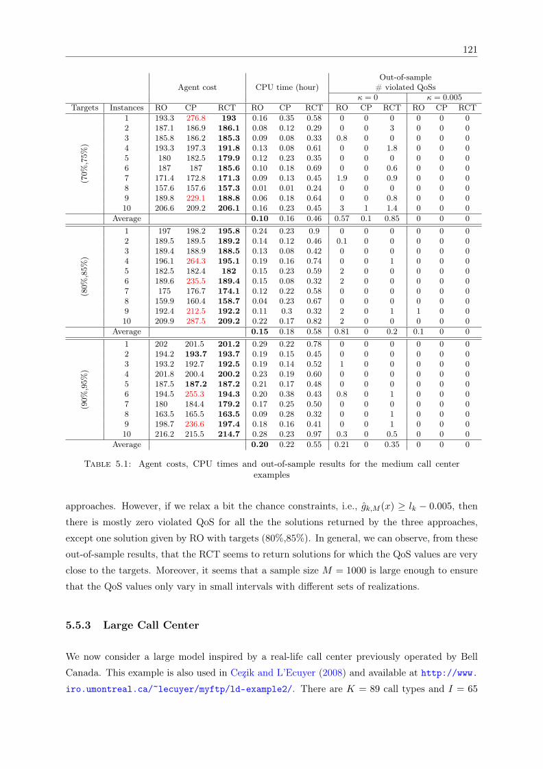
121

Agent cost CPU time (hour)Out-of-sample

# violated QoSsκ = 0 κ = 0.005

Targets Instances RO CP RCT RO CP RCT RO CP RCT RO CP RCT

(70%

,75%

)

1 193.3 276.8 193 0.16 0.35 0.58 0 0 0 0 0 02 187.1 186.9 186.1 0.08 0.12 0.29 0 0 3 0 0 03 185.8 186.2 185.3 0.09 0.08 0.33 0.8 0 0 0 0 04 193.3 197.3 191.8 0.13 0.08 0.61 0 0 1.8 0 0 05 180 182.5 179.9 0.12 0.23 0.35 0 0 0 0 0 06 187 187 185.6 0.10 0.18 0.69 0 0 0.6 0 0 07 171.4 172.8 171.3 0.09 0.13 0.45 1.9 0 0.9 0 0 08 157.6 157.6 157.3 0.01 0.01 0.24 0 0 0 0 0 09 189.8 229.1 188.8 0.06 0.18 0.64 0 0 0.8 0 0 010 206.6 209.2 206.1 0.16 0.23 0.45 3 1 1.4 0 0 0

Average 0.10 0.16 0.46 0.57 0.1 0.85 0 0 0

(80%

,85%

)

1 197 198.2 195.8 0.24 0.23 0.9 0 0 0 0 0 02 189.5 189.5 189.2 0.14 0.12 0.46 0.1 0 0 0 0 03 189.4 188.9 188.5 0.13 0.08 0.42 0 0 0 0 0 04 196.1 264.3 195.1 0.19 0.16 0.74 0 0 1 0 0 05 182.5 182.4 182 0.15 0.23 0.59 2 0 0 0 0 06 189.6 235.5 189.4 0.15 0.08 0.32 2 0 0 0 0 07 175 176.7 174.1 0.12 0.22 0.58 0 0 0 0 0 08 159.9 160.4 158.7 0.04 0.23 0.67 0 0 0 0 0 09 192.4 212.5 192.2 0.11 0.3 0.32 2 0 1 1 0 010 209.9 287.5 209.2 0.22 0.17 0.82 2 0 0 0 0 0

Average 0.15 0.18 0.58 0.81 0 0.2 0.1 0 0

(90%

,95%

)

1 202 201.5 201.2 0.29 0.22 0.78 0 0 0 0 0 02 194.2 193.7 193.7 0.19 0.15 0.45 0 0 0 0 0 03 193.2 192.7 192.5 0.19 0.14 0.52 1 0 0 0 0 04 201.8 200.4 200.2 0.23 0.19 0.60 0 0 0 0 0 05 187.5 187.2 187.2 0.21 0.17 0.48 0 0 0 0 0 06 194.5 255.3 194.3 0.20 0.38 0.43 0.8 0 1 0 0 07 180 184.4 179.2 0.17 0.25 0.50 0 0 0 0 0 08 163.5 165.5 163.5 0.09 0.28 0.32 0 0 1 0 0 09 198.7 236.6 197.4 0.18 0.16 0.41 0 0 1 0 0 010 216.2 215.5 214.7 0.28 0.23 0.97 0.3 0 0.5 0 0 0

Average 0.20 0.22 0.55 0.21 0 0.35 0 0 0

Table 5.1: Agent costs, CPU times and out-of-sample results for the medium call centerexamples

approaches. However, if we relax a bit the chance constraints, i.e., gk,M (x) ≥ lk − 0.005, then

there is mostly zero violated QoS for all the the solutions returned by the three approaches,

except one solution given by RO with targets (80%,85%). In general, we can observe, from these

out-of-sample results, that the RCT seems to return solutions for which the QoS values are very

close to the targets. Moreover, it seems that a sample size M = 1000 is large enough to ensure

that the QoS values only vary in small intervals with different sets of realizations.

5.5.3 Large Call Center

We now consider a large model inspired by a real-life call center previously operated by Bell

Canada. This example is also used in Cezik and L’Ecuyer (2008) and available at http://www.

iro.umontreal.ca/~lecuyer/myftp/ld-example2/. There are K = 89 call types and I = 65

122

agent groups. We assume that (i) immediate call abandonment does not occur, (ii) the patience

times follow exponential distributions with means 3 minutes for all call types, and (iii) the

service times follow exponential distributions with means varying from 4.32 to 12.79 minutes.

The acceptable waiting times for all call types are τk = τ0 = 20 seconds and the targets of SLs

are sk = 50% for all k = 1, . . . , 89 and s0 = 80%. For the fluid scheduling model, we choose

βk = 1 for all k = 1, . . . ,K.

For this large call center, both call types and the agent groups are split between two locations.

One location has 22 call types and 15 agent groups and the second location consists of 43 call

types and 74 agent groups. The number of skills per agent group varies from 1 to 24. The router

system operates a set of priority rules, named “local specialist routing policy”, i.e., any incoming

call is assigned primarily to an agent based in the location from where the call originates. The

reader can consult Cezik and L’Ecuyer (2008) for a more detailed description of call center.

Table 5.2 reports numerical results for the 30 instances of the large call center example with the

three set of targets. We also indicate the best costs given by the three approaches, i.e., RO, CP

and RCT. In this experiment, the CP is more stable and always gives better cost than the RO.

Moreover, as expected, the RCT always returns the best costs among the three approaches for

all the instances. Looking closely to the results, RCT improves the agent costs of the CP by

0.79%, 1.58% and 0.60%, on average, for the targets (70%, 75%), (80%, 85%) and (90%, 95%),

respectively. On average, the cost obtained by the RCT are about 0.99% smaller than those

given by the CP.

In terms of CPU time, it is clear that the RO is very fast as compared to the other approaches.

This is because the RO does not require to compute subgradients qk and uk, which are in need of

8 and 89 simulations for the medium and large examples, respectively. The CPU times required

by the RCT is about 43% higher than those required by the CP. Even so, the RCT needs a

maximum of 3.86 hours to solve one instance, which is viable in practice.

The out-of-sample results are not surprising for these large instances. Similarly to the medium

call center, we observe some violated QoS constraints with κ = 0, but these numbers are con-

siderably small, as there are about 66 chance constraints checked. When we relax a bit the

requirements with κ = 0.005, there is almost no violated QoS value, except for the CP and RCT

approaches with instance 5 and target (70%,75%). Moreover, we also observe that the average

number of violated QoS constraints given by the RCT is higher than for the CP, indicating that

the QoS values given by the solutions of the RCT seems to be closer to the targets, as compared

to the CP.

One important thing to note here is that, in terms the CPU time, the performance is achieved

using parallel computing with 8 physical CPUs. In general, the CPU times required by the CP

or RCT are proportional to the number of cores used in the computation, as we perform the

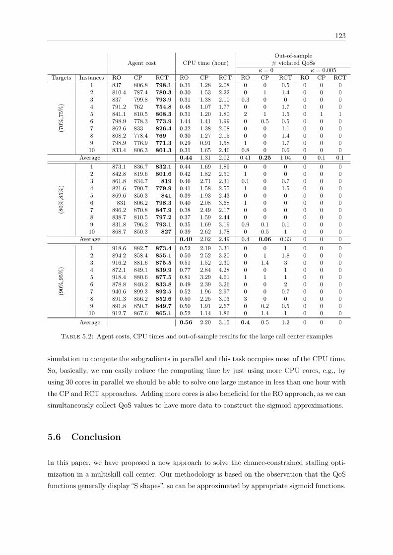
123

Agent cost CPU time (hour)Out-of-sample

# violated QoSsκ = 0 κ = 0.005

Targets Instances RO CP RCT RO CP RCT RO CP RCT RO CP RCT

(70%

,75%

)

1 837 806.8 798.1 0.31 1.28 2.08 0 0 0.5 0 0 02 810.4 787.4 780.3 0.30 1.53 2.22 0 1 1.4 0 0 03 837 799.8 793.9 0.31 1.38 2.10 0.3 0 0 0 0 04 791.2 762 754.8 0.48 1.07 1.77 0 0 1.7 0 0 05 841.1 810.5 808.3 0.31 1.20 1.80 2 1 1.5 0 1 16 798.9 778.3 773.9 1.44 1.41 1.99 0 0.5 0.5 0 0 07 862.6 833 826.4 0.32 1.38 2.08 0 0 1.1 0 0 08 808.2 778.4 769 0.30 1.27 2.15 0 0 1.4 0 0 09 798.9 776.9 771.3 0.29 0.91 1.58 1 0 1.7 0 0 010 833.4 806.3 801.3 0.31 1.65 2.46 0.8 0 0.6 0 0 0

Average 0.44 1.31 2.02 0.41 0.25 1.04 0 0.1 0.1

(80%

,85%

)

1 873.1 836.7 832.1 0.44 1.69 1.89 0 0 0 0 0 02 842.8 819.6 801.6 0.42 1.82 2.50 1 0 0 0 0 03 861.8 834.7 819 0.46 2.71 2.31 0.1 0 0.7 0 0 04 821.6 790.7 779.9 0.41 1.58 2.55 1 0 1.5 0 0 05 869.6 850.3 841 0.39 1.93 2.43 0 0 0 0 0 06 831 806.2 798.3 0.40 2.08 3.68 1 0 0 0 0 07 896.2 870.8 847.9 0.38 2.49 2.17 0 0 0 0 0 08 838.7 810.5 797.2 0.37 1.59 2.44 0 0 0 0 0 09 831.8 796.2 793.1 0.35 1.69 3.19 0.9 0.1 0.1 0 0 010 868.7 850.3 827 0.39 2.62 1.78 0 0.5 1 0 0 0

Average 0.40 2.02 2.49 0.4 0.06 0.33 0 0 0

(90%

,95%

)

1 918.6 882.7 873.4 0.52 2.19 3.31 0 0 1 0 0 02 894.2 858.4 855.1 0.50 2.52 3.20 0 1 1.8 0 0 03 916.2 881.6 875.5 0.51 1.52 2.30 0 1.4 3 0 0 04 872.1 849.1 839.9 0.77 2.84 4.28 0 0 1 0 0 05 918.4 880.6 877.5 0.81 3.29 4.61 1 1 1 0 0 06 878.8 840.2 833.8 0.49 2.39 3.26 0 0 2 0 0 07 940.6 899.3 892.5 0.52 1.96 2.97 0 0 0.7 0 0 08 891.3 856.2 852.6 0.50 2.25 3.03 3 0 0 0 0 09 891.8 850.7 849.7 0.50 1.91 2.67 0 0.2 0.5 0 0 010 912.7 867.6 865.1 0.52 1.14 1.86 0 1.4 1 0 0 0

Average 0.56 2.20 3.15 0.4 0.5 1.2 0 0 0

Table 5.2: Agent costs, CPU times and out-of-sample results for the large call center examples

simulation to compute the subgradients in parallel and this task occupies most of the CPU time.

So, basically, we can easily reduce the computing time by just using more CPU cores, e.g., by

using 30 cores in parallel we should be able to solve one large instance in less than one hour with

the CP and RCT approaches. Adding more cores is also beneficial for the RO approach, as we can

simultaneously collect QoS values to have more data to construct the sigmoid approximations.

5.6 Conclusion

In this paper, we have proposed a new approach to solve the chance-constrained staffing opti-

mization in a multiskill call center. Our methodology is based on the observation that the QoS

functions generally display “S shapes”, so can be approximated by appropriate sigmoid functions.

124

We have designed an algorithm combining a regression-based step to collect QoS values and ap-

proximate QoS functions by sigmoid ones, a step of generating linear cuts to approximate the

chance constraints, and a trust region local search to further improve feasible solutions given by

the regression-based and cutting plane approaches. We have tested on two call center examples,

one with medium and one with large numbers of agent groups and call types. The numeri-

cal results show the practical viability of our approach in finding good staffing optimization in

reasonable computing time.

Our methodology is general, in the sense that it can be applied in other settings, e.g., the staffing

problem with SL constraints considered in Cezik and L’Ecuyer (2008) or scheduling problem in

Avramidis et al. (2010). It might be also promising for more large-scale problems, e.g. a staffing

or scheduling optimization problem under uncertainty (Ta et al., 2018a). Future work could be

in that direction, or in a direction of incorporating more inputs to the regression model (or the

ANN representative), e.g. arrival rate and service rate, to have models being able to accurately

approximate the QoS functions in different settings.

Acknowledgment

This work has been supported by a Canada Research Chair, an Inria International Chair, and

a Hydro-Québec research grant to P. L’Ecuyer, by NSERC Discovery Grants to F. Bastin and

P. L’Ecuyer, by the SMART (Singapore-MIT Alliance for Research and Technology) scholar

program to Tien Mai, and by scholarships from the CIRRELT, DIRO and Université de Montréal

to T.A. Ta.

Chapter 6

Conclusions and Future Research

Perspectives

This thesis is based on a collection of three articles. One of them is currently under revision for

possible publication, and two of them will be submitted soon. In this chapter, we summarize

the main results and directions for future research.

6.1 Conclusion

In this thesis we have considered staffing optimization problems in different uncertainty settings.

The main challenge lies in the fact that the QoS constraints have no closed form and need to be

approximated by simulation. Moreover, the QoS functions, i.e., the probability functions defined

on the randomness of the SL, display nonlinear curves, making the optimization difficult with

large-size call centers. We have considered common one-stage staffing problems and two-stage

versions. For the latter, we assume that the arrival rates cannot be forecasted perfectly, leading

to two-stage stochastic programs. To solve the problems numerically, we have used the SAA

approach and study its consistency with respect to the sample sizes used to approximate the

QoS constraints and the second-stage objective function. We have shown, in Chapter 3, that the

optimal values and solutions of the SAA converge to those of the true problem with probability

one when the sample sizes go to infinity, and the probability of making incorrect decisions goes

to zero exponentially fast as the sample sizes grow. These results provide a theoretical basis for

the use of the SAA method throughout the thesis.

To solve the SAA problems in practical ways, we have developed several solution techniques.

The aim of this development is to deal with the nonlinearity of the QoS constraints and the large

size of the two-stage models under arrival rate uncertainty. While the former issue is considered

125

126

in Chapter 5, the latter is the main motivation for the development of the simulation-based

decomposition approach presented in Chapter 4. More precisely, Chapter 4 develops a solution

method for the SAA problem in a setting where the arrival rates are uncertain to the managers.

Motivated by the fact that the problem would become too large to solve in a direct way with

large-scale examples, we have developed a simulation-based decomposition algorithm. The idea

is to use simulation and cut generation to approximate the QoS constraints, and use the L-

shaped method to quickly solve the staffing problem in which the QoS constraints are replaced

by linear cuts. Numerical results have shown the practical efficiency of our approach.

In Chapter 5, we have proposed a way to approximate the QoS by sigmoid functions. The main

advantage of the approach is that we were able to reformulate the optimization procedure as

a sequence of QoS simulations and integer programs solutions. It is important to note that

the methodologies developed in this chapter are general and might be promising for other op-

timization problems such as optimization problems in queuing-based systems or problems with

separate chance constraints.

We have tested our theoretical findings and solution methods developed using call center ex-

amples of different sizes: from a toy example of 2 call types, 2 agent groups to a real-life one

of 65 call types and 89 agent groups. In general, our numerical experiments have (partially)

validated our theoretical findings in Chapter 3 and shown that our algorithms are more efficient

in a practical way, as compared to other state-of-the-art approaches.

We believe that the thesis makes significant contributions to the management of call centers and

stochastic programming, in both theoretical and practical aspects. The models and methods

developed may be useful for other problems in workforce management as well as stochastic opti-

mization. The work also raises several research questions that might be interesting to investigate

further. In the following we discuss some promising ideas for future research.

6.2 Future Research

In this section, we present some future research directions that are in line with the work presented

in the thesis. More precisely, we are interested in (i) a way to reduce the number of scenarios

in two-stage staffing problems using a clustering approach, (ii) other chance-constrained staffing

optimization problems, (iii) robust/distributionally robust optimization versions of the staffing

and scheduling problems to deal with data uncertainty, and (iv) a machine learning approach to

better approximate the QoS functions. We describe them in detail in the following.

Scenario selection for two-stage staffing optimization. One of the issues we have when

solving the two-stage stochastic staffing optimization problem in Chapter 4 is that one needs

a large number of scenarios to have good solutions. This makes the two-stage model difficult

127

to apply to large-scale call centers. So, a way to reduce the number of scenarios would be

beneficial in the context. Motivated by the fact that there are some scenarios that are very close

to others, we are interested in a clustering method (e.g., K-means) to better select scenarios for

the two-stage model. The idea is that we can generate a set of large number of scenarios and

use a clustering algorithm to separate that set into subsets, in the hope that scenarios belonging

to a subset are similar. Then, we can pick a representative from each subset to build smaller

two-stage stochastic model.

Chance-constrained staffing/scheduling optimization with VaR and CVaR. Consider

a staffing/scheduling problem under uncertainty and assume that we can well estimate the

distribution of the random components of the systems (e.g., arrival rates), we can construct an

optimization model requiring that the probability of meeting QoS constraints is above a certain

level. More precisely, we can formulate the following jointly chance-constrained staffing problem

(CC)

minx

cTx

subject to Pξ [gk(x, ξ) ≥ 1− δk, ∀k] ≥ 1− τ

x ≥ 0 and integer,

(6.1)

where τ, δ1, . . . , δK are constants and gk(·) is a QoS function associated with call type k. (CC)

might be interesting to use if the manager wants to make an one-time decision while being

uncertain about the arrival rates. Moreover, one advantage of (CC) is that it has less decision

variables as compared to the two-stage model considered in Chapter 4, so it might be easier to

solve.

Chance constraints (6.1) are often nonconvex. A popular approach to deal with the issue is to

construct a convex approximation of the probability function on the left of (6.1). In this context,

a possible approximation of the probability function is the Conditional Value-at-Risk. It is based

on the Value-at-Risk (VaR), which indicates the minimal loss such that the probability that the

loss is greater than or equal to this value is at least a certain level (see Kall and Mayer (2011)).

VaR is itself a risk measure and the Conditional Value-at-Risk (CVaR) represents the expected

value of loss, given that the loss is greater than or equal to the VaR. Nemirovski and Shapiro

(2006) show that the CVaR can construct a convex conservative approximation of the chance

constraints. Note that CVaR is known to have better properties than VaR (see for instance

Artzner et al., 2002) and many studies suggest moving from VaR to CVaR (e.g. Rockafellar and

Uryasev, 2000), we are interested in solving (CC) using CVaR. Another promising direction is

to use the idea of the convex approximation approach for joint chance constraints proposed by

Hong et al. (2011). It is also interesting to study the consistency of the SAA approach in the

context of (CC), as we have stochastic constraints and the constraints need to be approximated

by sampling over the distributions of the arrival rates and the SL.

128

Robust/Distributionally robust optimization. In many situations we do not have complete

information on the distribution of the random variables, e.g., arrival rates. For instance, if the

manager does not have any information other than the ranges of the values of random variables,

then it might be reasonable to optimize for the worst-case from a set of distributions which is

highly likely to contain the true distribution. This kind of decision making framework is known

as robust optimization (Ben-Tal et al., 2009), which has received a lot of attention over the past

decade. In our context, the framework would be an interesting direction to go, as the distribution

of the the arrival rates is typically difficult to estimate accurately. A robust staffing optimization

model can be formulated as

minx

cTx

subject to gk(x, ξ) ≥ 1− δk, ∀k = 1, . . . ,K, ξ ∈ Ξ

x ≥ 0 and integer,

where gk(x, ξ), k = 0, ...,K, are QoS functions (e.g., probability of SL functions), and Ξ is a

compact uncertainty set to which the random variables belong. There are several ways defining

the uncertainty set. For example, we can define a rectangular one as Ξ = ξ| ξ ≤ ξ ≤ ξ, whereξ and ξ are two constant vectors of appropriate size. One can also define an ellipsoidal set as

Ξ = ξ| ||ξ − ξ0|| ≤ α, where ξ0 and α are constants.

The above robust model might be too conservative in some situations. An alternative is to use the

distributionally robust optimization (DRO) framework, in which instead of considering the worst-

case defined on an uncertainty set of the random variables, one can construct an ambiguity set of

distributions with historical data. Over the past few years, DRO has been intensively studied and

has found many applications in operations research, finance and management sciences (Bertsimas

et al., 2010, Delage and Ye, 2010, Ghosh and Lam, 2019, Hong et al., 2017, Lam, 2018, Wiesemann

et al., 2014). In our context, a DRO version of the staffing optimization problem can be written

as

minx

cTx

subject to supP∈P

EP[gk(x, ξ)] ≥ 1− δk, ∀k = 1, . . . ,K

x ≥ 0 and integer,

where P is a set of probability distributions, which can be defined in different ways, e.g., am-

biguity sets defined through the mean and covariance of the random variables (Delage and Ye,

2010, Wiesemann et al., 2014), or based on Wasserstein metric (Esfahani and Kuhn, 2018). So,

in general, the DRO opens several interesting directions for the staffing/scheduling problems

under uncertainty.

129

Other research directions. For long term research, we are interested in investigating the use

of machine learning for chance-constrained programs, in both theoretical and practical aspects.

In particular, we would like to explore different artificial neutral network (ANN) (other activation

functions, or possibly deeper ANNs) to learn probability functions in general chance-constrained

programs. There are several open and interesting questions on this direction, for instance, how to

customize the ANNs in such a way that they not only give good approximations to the nonlinear

functions but also perform well even with limited observations. The trade-off between the use

of multi-layer ANNs and the complexity of the resulting integrated optimization model is also

interesting to investigate. In the theoretical point of view, we are curious about the consistency

of the approach in terms of optimal solutions. More precisely, we would like to study the issue

regarding the effect of the number of samples used to train the ANNs to the accuracy of the

outcomes, and the quality of the solutions found.

Bibliography

Ahmed, S. and Shapiro, A. Solving chance-constrained stochastic programs via sampling and

integer programming. In Tutorials in Operations Research, pages 261–269. INFORMS, 2008.

Artzner, P., Delbaen, F., Eber, J., and Heath, D. Coherent measures of risk1. Risk management:

value at risk and beyond, page 145, 2002.

Atlason, J., Epelman, M. A., and Henderson, S. G. Using simulation to approximate subgradi-

ents of convex performance measures in service systems. In Proceedings of the 2003 Winter

Simulation Conference, pages 1824–1832. IEEE Press, 2003.

Atlason, J., Epelman, M. A., and Henderson, S. G. Call center staffing with simulation and

cutting plane methods. Annals of Operations Research, 127:333–358, 2004.

Atlason, J., Epelman, M. A., and Henderson, S. G. Optimizing call center staffing using simu-

lation and analytic center cutting plane methods. Management Science, 54(2):295–309, 2008.

Avramidis, A. N., Deslauriers, A., and L’Ecuyer, P. Modeling daily arrivals to a telephone call

center. Management Science, 50(7):896–908, 2004.

Avramidis, A. N., Chan, W., and L’Ecuyer, P. Staffing multi-skill call centers via search methods

and a performance approximation. IIE Transactions, 41(6):483–497, 2009.

Avramidis, A. N., Chan, W., Gendreau, M., L’Ecuyer, P., and Pisacane, O. Optimizing daily

agent scheduling in a multiskill call centers. European Journal of Operational Research, 200

(3):822–832, 2010.

Bassamboo, A., Harrison, J. M., and Zeevi, A. Design and control of a large call center: Asymp-

totic analysis of an LP-based method. Operations Research, 54(3):419–435, 2006. ISSN 0030-

364X.

Bastin, F., Cirillo, C., and Toint, Ph. L. Convergence theory for nonconvex stochastic program-

ming with an application to mixed logit. Mathematical Programming, Series B, 108(2–3):

207–234, 2006.

Ben-Tal, A., El Ghaoui, L., and Nemirovski, A. Robust optimization, volume 28. Princeton

University Press, 2009.

130

Benders, J. F. Partitioning procedures for solving mixed-variables programming problems. Nu-

merische mathematik, 4(1):238–252, 1962.

Bertsekas, D. P., Bertsekas, D. P., Bertsekas, D. P., and Bertsekas, D. P. Dynamic programming

and optimal control, volume 1. Athena scientific Belmont, MA, 1995.

Bertsimas, D., Doan, X. V., Natarajan, K., and Teo, C.-P. Models for minimax stochastic linear

optimization problems with risk aversion. Mathematics of Operations Research, 35(3):580–602,

2010.

Bhulai, S., Koole, G., and Pot, G. Simple methods for shift scheduling in multi-skill call centers.

Technical report, WS 2005-10, Free University, Amsterdam, 2005.

Birge, J. R. and Louveaux, F. Introduction to Stochastic Programming. Springer-Verlag, New

York, NY, USA, 2nd edition, 2011.

Birge, J. R. and Louveaux, F. V. A multicut algorithm for two-stage stochastic linear programs.

European Journal of Operational Research, 34(3):384–392, 1988.

Brown, L., Gans, N., Mandelbaum, A., Sakov, A., Shen, H., Zeltyn, S., and Zhao, L. Statistical

analysis of a telephone call center: A queueing-science perspective. Journal of the American

Statistical Association, 100(469):36–50, 2005.

Buist, E. and L’Ecuyer, P. A Java library for simulating contact centers. In Kuhl, M. E., Steiger,

N. M., Armstrong, F. B., and Joines, J. A., editors, Proceedings of the 2005 Winter Simulation

Conference, pages 556–565. IEEE Press, 2005.

Buist, E. and L’Ecuyer, P. ContactCenters: A Java Library for Simulating Contact Centers,

2012. Software user’s guide, available at http://www.simul.umontreal.ca/contactcenters.

Bureau of Labor Statistics. Occupational Outlook Handbook, Customer Service Representatives,

2006-07 Edition. 2007. U.S. Department of Labor. Available online at http://www.bls.gov/

oco/ocos280.htm (last accessed February 14, 2007).

Bureau of Labor Statistics. An overview of U.S. occupational employment and wages in 2014.

March 2015. U.S. Department of Labor. Available online at http://www.bls.gov/news.

release/pdf/ocwage.pdf, (last accessed September, 2015).

Bureau of Labor Statistics. Occupational employment and wages, May 2016 - Customer Service

Representatives. May 2016. U.S. Department of Labor. Available online at //https://www.

bls.gov/Oes/current/oes434051.htm, (last accessed September, 2015).

Cezik, M. T. and L’Ecuyer, P. Staffing multiskill call centers via linear programming and

simulation. Management Science, 54(2):310–323, 2008.

Chan, W. Optimisation des horaires des agents et du routage des appels dans les centres d’appels.

PhD thesis, Département d’Informatique et de Recherche Opérationnelle, Université de Mon-

tréal, Canada, 2013.

Chan, W., Koole, G., and L’Ecuyer, P. Dynamic call center routing policies using call waiting

and agent idle times. Manufacturing & Service Operations Management, 16(4):544–560, 2014a.

Chan, W., Ta, T. A., L’Ecuyer, P., and Bastin, F. Chance-constrained staffing with recourse

for multi-skill call centers with arrival-rate uncertainty. In Proceedings of the 2014 Winter

Simulation Conference, pages 4103–4104. IEEE Press, 2014b.

Chan, W., Ta, T. A., L’Ecuyer, P., and Bastin, F. Two-stage chance-constrained staffing with

agent recourse for multi-skill call centers. In Proceedings of the 2016 Winter Simulation Con-

ference, pages 3189–3200, Piscataway, NJ, USA, 2016. IEEE Press.

Channouf, N., L’Ecuyer, P., Ingolfsson, A., and Avramidis, A. N. The application of forecasting

techniques to modeling emergency medical system calls in Calgary, Alberta. Health Care

Management Science, 10(1):25–45, 2007.

Chevalier, P. and Van den Schrieck, J. Approximating multiple class queueing models with loss

models, 2008. Preprint, CORE, Louvain.

Conn, A. R., Gould, N. I., and Toint, P. L. Trust region methods, volume 1. Siam, 2000.

Cooper, R. B. Introduction to Queueing Theory. North-Holland, New York, NY, second edition,

1981.

Dai, J. and He, S. Estimating customer patience-time density in large-scale call centers. In 7th

International Conference on Service Systems and Service Management, 2010.

Dai, L., Chen, C., and Birge, J. Convergence properties of two-stage stochastic programming.

Journal of Optimization Theory and Applications, 106(3):489–509, 2000.

Dantzig, G. B. and Wolfe, P. Decomposition principle for linear programs. Operations research,

8(1):101–111, 1960.

Delage, E. and Ye, Y. Distributionally robust optimization under moment uncertainty with

application to data-driven problems. Operations research, 58(3):595–612, 2010.

Dupacová, J. and Wets, R. Asymptotic behavior of statistical estimators and of optimal solutions

of stochastic optimization problems. The Annals of Statistics, pages 1517–1549, 1988.

Esfahani, P. M. and Kuhn, D. Data-driven distributionally robust optimization using the wasser-

stein metric: Performance guarantees and tractable reformulations. Mathematical Program-

ming, 171(1-2):115–166, 2018.

Excoffier, M., Gicquel, C., Jouini, O., and Lisser, A. A joint chance-constrained programming

approach for call center workforce scheduling under uncertain call arrival forecasts. manuscript,

2014.

Excoffier, M., Gicquel, C., and Jouini, O. Distributionally robust optimization for scheduling

problem in call centers with uncertain forecasts,. In Proceedings of the 4th International Con-

ference on Operations Research and Enterprise Systems, ICORES 2015, pages 3–20, 2015a.

Excoffier, M., Gicquel, C., Jouini, O., and Lisser, A. Comparison of stochastic programming

approaches for staffing and scheduling call centers with uncertain demand forecasts. In Pro-

ceedings of the 4th International Conference on Operations Research and Enterprise Systems,

ICORES 2014, pages 140–156, 2015b.

Gans, N. and Zhou, Y.-P. A call-routing problem with service-level constraints. Operations

Research, 51(2):255–271, 2003.

Gans, N., Koole, G., and Mandelbaum, A. Telephone call centers: Tutorial, review, and research

prospects. Manufacturing and Service Operations Management, 5:79–141, 2003.

Gans, N., Shen, H., Zhou, Y.-P., Korolev, N., McCord, A., and Ristock, H. Parametric forecast-

ing and stochastic programming models for call-center workforce scheduling. Manufacturing

& Service Operations Management, 17(4):571–588, 2015.

Ghosh, S. and Lam, H. Robust analysis in stochastic simulation: Computation and performance

guarantees. Operations Research, 67(1):232–249, 2019.

Green, L. V., Kolesar, P. J., and Soares, J. An improved heuristic for staffing telephone call

centers with limited operating hours. Production and Operations Management, 12:46–61, 2003.

Gurvich, I. and Whitt, W. Service-level differentiation in many-server service systems via queue-

ratio routing. Operations Research, 58(2):316–328, 2010. ISSN 0030-364X.

Gurvich, I., Luedtke, J., and Tezcan, T. Staffing call centers with uncertain demand forecasts:

A chance-constrained optimization approach. Management Science, 56(7):1093–1115, 2010.

Harrison, J. M. and Zeevi, A. A method for staffing large call centers based on stochastic fluid

models. Manufacturing and Service Operations Management, 7(1):20–36, 2005.

Helber, S. and Henken, K. Profit-oriented shift scheduling of inbound contact centers with

skills-based routing, impatient customers, and retrials. OR Spectrum, 32:109–134, 2010. ISSN

0171-6468. URL http://dx.doi.org/10.1007/s00291-008-0141-8.

Hoeffding, W. Probability inequalities for sums of bounded random variables. Journal of the

American statistical association, 58(301):13–30, 1963.

Hong, L. J., Yang, Y., and Zhang, L. Sequential convex approximations to joint chance con-

strained programs: A monte carlo approach. Operations Research, 59(3):617–630, 2011.

Hong, L. J., Huang, Z., and Lam, H. Learning-based robust optimization: Procedures and

statistical guarantees. arXiv preprint arXiv:1704.04342, 2017.

Ibrahim, R. and Whitt, W. Real-time delay estimation based on delay history. Manufacturing

and Services Operations Management, (11):397–415, 2009a.

Ibrahim, R. and Whitt, W. Real-time delay estimation in overloaded multiserver queues with

abandonments. Management Science, 55(10):1729–1742, 2009b.

Ibrahim, R. and Whitt, W. Wait-time predictors for customer service systems with time-varying

demand and capacity. Operations Research, 59(5):1106–1118, 2011.

Ibrahim, R., L’Ecuyer, P., Régnard, N., and Shen, H. On the modeling and forecasting of call

center arrivals. In Laroque, C., Himmelspach, J., Pasupathy, R., Rose, O., and Uhrmacher,

A. M., editors, Proceedings of the 2012 Winter Simulation Conference, pages 256–267. IEEE

Press, 2012.

Ibrahim, R., L’Ecuyer, P., Shen, H., and Thiongane, M. Inter-dependent, heterogeneous, and

time-varying service-time distributions in call centers. European Journal of Operational Re-

search, 250:480–492, 2016a.

Ibrahim, R., Ye, H., L’Ecuyer, P., and Shen, H. Modeling and forecasting call center arrivals: A

literature study and a case study. International Journal of Forecasting, 32(3):865–874, 2016b.

Ibrahim, R., Armony, M., and Bassamboo, A. Does the past predict the future? the case of

delay announcements in service systems. Management Science, 63(6):1762–1780, 2016c.

Ingolfsson, A., Cabral, E., and Wu, X. Combining integer programming and the randomization

method to schedule employees. Technical report, School of Business, University of Alberta,

Edmonton, Alberta, Canada, 2003. Preprint.

Jagers, A. A. and van Doorn, E. A. Convexity of functions which are generalizations of the

erlang loss function and the erlang delay function. SIAM Review, 32(2):301–302, 1990.

Jongbloed, G. and Koole, G. Managing uncertainty in call centers using Poisson mixtures.

Applied Stochastic Models in Business and Industry, 17(4):307–318, 2001.

Jouini, O., Koole, G., and Roubos, A. Performance indicators for call centers with impatient

customers. IIE Transactions, 45(3):341–354, 2013.

Kall, P. and Mayer, J. Stochastic Linear Programming. Springer, 2011.

Kaniovski, Y. M., King, A. J., and Wets, R. J. Probabilistic bounds (via large deviations) for the

solutions of stochastic programming problems. Annals of Operations Research, 56(1):189–208,

1995.

Kelley, J. The cutting-plane method for solving convex programs. Journal of the Society for

Industrial and Applied Mathematics, 8(4):703–712, 1960.

Kim, S., Pasupathy, R., and Henderson, S. G. A guide to sample average approximation. In

Fu, M. C., editor, Handbook of Simulation Optimization, pages 207–243. Springer, New York,

NY, USA, 2015.

Kleywegt, A. J., Shapiro, A., and Homem-de Mello, T. The sample average approximation

method for stochastic discrete optimization. SIAM Journal on Optimization, 12(2):479–502,

2002.

Koole, G. Call Center Optimization. MG books, Amsterdam, 2013.

Koole, G., Nielsen, B. F., and Nielsen, T. B. Optimization of overflow policies in call centers.

Probability in the Engineering and Informational Sciences, 29(3):461–471, 2015.

Lam, H. Recovering best statistical guarantees via the empirical divergence-based distribution-

ally robust optimization. forthcoming in Operations Research, 2018.

L’Ecuyer, P. SSJ: A Java Library for Stochastic Simulation, 2008. Software user’s guide, available

at http://www.iro.umontreal.ca/~lecuyer.

L’Ecuyer, P. and Buist, E. Simulation in Java with SSJ. In Kuhl, M. E., Steiger, N. M.,

Armstrong, F. B., and Joines, J. A., editors, Proceedings of the 2005 Winter Simulation

Conference, pages 611–620, Piscataway, NJ, 2005. IEEE Press.

L’Ecuyer, P., Meliani, L., and Vaucher, J. SSJ: A framework for stochastic simulation in Java.

In Yücesan, E., Chen, C.-H., Snowdon, J. L., and Charnes, J. M., editors, Proceedings of the

2002 Winter Simulation Conference, pages 234–242. IEEE Press, 2002.

Liao, S., Delft, C. V., Koole, G., and Jouini, O. Staffing a call center with uncertain non-

stationary arrival rate and flexibility. OR Spectrum, 34:691–721, 2012.

Liao, S., van Delft, C., and Vial, J.-P. Distributionally robust workforce scheduling in call centres

with uncertain arrival rates. Optimization Methods and Software, 28(3):501–522, 2013.

Mandelbaum, A. and Zeltyn, S. Service engineering in action: The Palm/Erlang-A queue, with

applications to call centers. In Advances in services innovations, pages 17–45. Springer, 2007.

Nemhauser, G. L. and Wolsey, L. A. A recursive procedure to generate all cuts for 0–1 mixed

integer programs. Mathematical Programming, 46(1-3):379–390, 1990.

Nemirovski, A. and Shapiro, A. Convex approximations of chance constrained programs. SIAM

J. on Optimization, 17(4):969–996, 2006.

Oreshkin, B., Régnard, N., and L’Ecuyer, P. Rate-based daily arrival process models with

application to call centers. Operations Research, 64(2):510–527, 2016. doi: 10.1287/opre.2016.

1484.

Palm, C. Research on telephone traffic carried by full availability groups. Tele, 1:107, 1957.

Pot, A., Bhulai, S., and Koole, G. A simple staffing method for multi-skill call centers. Manu-

facturing and Service Operations Management, 10:421–428, 2008.

Reynolds, P. Call center metrics: Best practices in performance measurement and management

to maximize quitline efficiency and quality. North American Quitline Consortium, 2010.

Robbins, T. R. and Harrison, T. P. A stochastic programming model for scheduling call centers

with global service level agreements. European Journal of Operational Research, 207(3):1608–

1619, 2010. http://dx.doi.org/10.1016/j.ejor.2010.06.013.

Robbins, T. R., Medeiros, D. J., and Harrison, T. Does the Erlang C model fit in real call

centers? In Proceedings of the 2010 Winter Simulation Conference, pages 2884–2889. IEEE

Press, 2010.

Robinson, S. M. Analysis of sample path optimization. Mathematics of Operations Research,

21:513–528, 1996.

Rockafellar, R. T. and Uryasev, S. Optimization of conditional value-at-risk. Journal of risk, 2:

21–42, 2000.

Roubos, A. and Jouini, O. Call centers with hyperexponential patience modeling. International

Journal of Production Economics, (141):307–315, 2012.

Rubinstein, R. Y. and Shapiro, A. Discrete Event Systems: Sensitivity Analysis and Stochastic

Optimization by the Score Function Method. Wiley, New York, 1993.

Ruszczyński, A. A regularized decomposition method for minimizing a sum of polyhedral func-

tions. Mathematical programming, 35(3):309–333, 1986.

Shapiro, A. Monte Carlo sampling methods. In Ruszczyński, A. and Shapiro, A., editors,

Stochastic Programming, Handbooks in Operations Research and Management Science, pages

353–425. Elsevier, Amsterdam, The Netherlands, 2003a. Chapter 6.

Shapiro, A. and de Mello, T. H. On rate of convergence of Monte Carlo approximations of

stochastic programs. SIAM Journal on Optimization, 11(1):70–86, 2000.

Shapiro, A., Dentcheva, D., and Ruszczyński, A. Lecture Notes on Stochastic Programming:

Modeling and Theory. SIAM, Philadelphia, second edition, 2014a.

Shapiro, A. Asymptotic behavior of optimal solutions in stochastic programming. Mathematics

of Operations Research, 18(4):829–845, 1993.

Shapiro, A. Monte Carlo sampling methods. Handbooks in operations research and management

science, 10:353–425, 2003b.

Shapiro, A. and Homem-de Mello, T. On rate of convergence of monte carlo approximations of

stochastic programs. SIAM Journal on Optimization, 11(1):70–86, 2000.

Shapiro, A. and Philpott, A. A tutorial on stochastic programming. Manuscript. Available at

www2. isye. gatech. edu/ashapiro/publications. html, 17, 2007.

Shapiro, A., Dentcheva, D., et al. Lectures on stochastic programming: modeling and theory,

volume 16. SIAM, 2014b.

Slyke, R. V. and Wets, R. L-shaped linear programs with applications to optimal control and

stochastic programming. SIAM Journal on Applied Mathematics, 17(4):638–663, 1969.

Stroock, D. W. An introduction to the theory of large deviations. Springer-Verlag New York,

1984.

Ta, A. Staffing optimization with chance constrained in call centers. Master’s thesis, Départe-

ment d’Informatique et de Recherche Opérationnelle, Université de Montréal, Canada, 2013.

Ta, T. A., Chan, W., L’Ecuyer, P., and Bastin, F. A simulation-based Benders decomposi-

tion method for the staffing problem in multiskill call centers under arrival rate uncertainty.

Working paper, 2018a.

Ta, T. A., Chan, W., L’Ecuyer, P., and Bastin, F. On a two-stage discrete stochastic optimization

problem with stochastic constraints and nested sampling. Technical report, 2018b.

Ta, T. A., L’Ecuyer, P., and Bastin, F. Staffing optimization with chance constraints for emer-

gency call centers. In MOSIM 2016–11th International Conference on Modeling, Optimiza-

tion and Simulation, 2016. See http://www.iro.umontreal.ca/~lecuyer/myftp/papers/

mosim16emergency.pdf.

Thiongane, M., Chan, W., and L’Ecuyer, P. Waiting time predictors for multiskill call centers.

In Proceedings of the 2015 Winter Simulation Conference. IEEE Press, 2015.

Vogel, S. A stochastic approach to stability in stochastic programming. Journal of Computational

and Applied Mathematics, 56:65–96, 1994.

Wallace, R. B. and Whitt, W. A staffing algorithm for call centers with skill-based routing.

Manufacturing and Service Operations Management, 7(4):276–294, 2005.

Whitt, W. Staffing a call center with uncertain arrival rate and absenteeism. Production and

Operations Management, 15:88–102, 2006.

Wiesemann, W., Kuhn, D., and Sim, M. Distributionally robust convex optimization. Operations

Research, 62(6):1358–1376, 2014.