arX

iv:1

404.

7786

v2 [

mat

h.PR

] 2

2 Se

p 20

14

STATIONARY COCYCLES FOR THE CORNER GROWTH MODEL

NICOS GEORGIOU, FIRAS RASSOUL-AGHA, AND TIMO SEPPALAINEN

Abstract. We study the directed last-passage percolation model on the planar integer

lattice with nearest-neighbor steps and general i.i.d. weights on the vertices, outside the

class of exactly solvable models. Stationary cocycles are constructed for this percolation

model from queueing fixed points. These cocycles serve as boundary conditions for sta-

tionary last-passage percolation, define solutions to variational formulas that characterize

limit shapes, and yield new results for Busemann functions, geodesics and the competition

interface.

Contents

1. Introduction 22. Main results 43. Convex duality 144. Stationary cocycles 175. Busemann functions 226. Directional geodesics 297. Competition interface 358. Exactly solvable models 39Appendix A. Cocycles from queuing fixed points 40Appendix B. Coalescence of directional geodesics 49Appendix C. Ergodic theorem for cocycles 54Appendix D. Percolation cone 55Appendix E. Shape theorem 63References 65

Date: September 22, 2014.

2000 Mathematics Subject Classification. 60K35, 65K37.

Key words and phrases. Busemann function, cocycle, competition interface, corrector, directed percola-

tion, geodesic, last-passage percolation, queueing fixed point, variational formula.

N. Georgiou was partially supported by a Wylie postdoctoral fellowship at the University of Utah.

F. Rassoul-Agha and N. Georgiou were partially supported by National Science Foundation grant DMS-

0747758.

T. Seppalainen was partially supported by National Science Foundation grant DMS-1306777 and by the

Wisconsin Alumni Research Foundation.

1

2 N. GEORGIOU, F. RASSOUL-AGHA, AND T. SEPPALAINEN

1. Introduction

We study nearest-neighbor directed last-passage percolation (LPP) on the lattice Z2,

also called the corner growth model. Random i.i.d. weights ωxx∈Z2 are used to definelast-passage times Gx,y between lattice points x ≤ y in Z

2 by

(1.1) Gx,y = maxx

n−1∑

k=0

ωxk

where the maximum is over paths x = x = x0, x1, . . . , xn = y that satisfy xk+1 − xk ∈e1, e2 (up-right paths).

When ωx ≥ 0 this defines a growth model in the first quadrant Z2+. Initially the growing

cluster is empty. The origin joins the cluster at time ω0. After both x − e1 and x − e2have joined the cluster, point x waits time ωx to join. (However, if x is on the boundaryof Z2

+, only one of x − e1 and x − e2 is required to have joined.) The cluster at time t is

At = x ∈ Z2+ : G0,x + ωx ≤ t. Our convention to exclude the last weight ωxn in (1.1)

forces the clumsy addition of ωx in the definition of At, but is convenient for other purposes.The interest is in the large-scale behavior of the model. This begins with the deterministic

limit gpp(ξ) = limn→∞ n−1G0,⌊nξ⌋ for ξ ∈ R2+, the fluctuations ofG0,⌊nξ⌋, and the behavior of

the maximizing paths in (1.1) called geodesics. Closely related are the Busemann functions

that are limits of gradients Gx,vn − Gy,vn as vn → ∞ in a particular direction and thecompetition interface between subtrees of the geodesic tree. To see how Busemann functionsconnect with geodesics, note that by (1.1) the following identity holds along any geodesicx from u to vn:

(1.2) ωxi = min(Gxi,vn −Gxi+e1,vn , Gxi,vn −Gxi+e2,vn

).

Busemann functions arise also in a limiting description of the Gx,y process locally arounda point vn → ∞. Take a finite subset V of Z2. A natural expectation is that the vectorG0,vn−u −G0,vn : u ∈ V converges in distribution as vn →∞ in a particular direction. Ashift by −vn and reflection ωx 7→ ω−x turn this vector into Gu,vn−G0,vn : u ∈ V. For thislast collection of random gradients we can expect almost sure convergence, in particularif the geodesics from 0 and u to vn coalesce eventually. These types of results will bedeveloped in the paper.

Here are some particulars of what follows, in relation to past work.In [14] we derived variational formulas for the point-to-point limit gpp(ξ) and its point-

to-line counterpart (introduced in Section 2) and developed a solution ansatz for thesevariational formulas in terms of stationary cocycles. In the present paper we constructthese cocycles for the planar corner growth model with general i.i.d. weights boundedfrom below, subject to a moment bound. This construction comes from the fixed pointsof the associated queueing operator. The existence of these fixed points was proved byMairesse and Prabhakar [23]. These cocycles are constructed on an extended space ofweights. The Markov process analogy is a simultaneous construction of processes for allinvariant distributions, coupled by common Poisson clocks that drive the evolution. Thei.i.d. weights ω are the analogue of the clocks and the cocycles the analogues of the initialstate variables. With the help of the cocycles we establish new results for Busemannfunctions and directional geodesics for the corner growth model.

CORNER GROWTH MODEL 3

A related recent result is Krishnan’s [20, Theorem 1.5] variational formula for the timeconstant of first passage bond percolation. His formula is analogous to our (2.15).

Under some moment assumptions on the weights, the corner growth model is expected tolie in the Kardar-Parisi-Zhang (KPZ) universality class. (For a review of KPZ universality

see [7].) The fluctuations of G0,⌊nξ⌋ are expected to have order of magnitude n1/3 andlimit distributions from random matrix theory. When the weights have exponential orgeometric distribution the model is exactly solvable. In these cases the cocycles mentionedabove have explicit product form distributions and last-passage values can be describedwith the Robinson-Schensted-Knuth correspondence and determinantal point processes.These techniques allow the derivation of exact fluctuation exponents and limit distributions[3, 18, 19]. The present paper can be seen as an attempt to begin development of techniquesfor studying the corner growth model beyond the exactly solvable cases.

On Busemann functions and geodesics, past milestones are the first-passage percolationresults of Newman et al. summarized in [26], the applications of his techniques to the exactlysolvable exponential corner growth model by Ferrari and Pimentel [13], and the recentimprovements to [26] by Damron and Hanson [9]. Coupier [8] further sharpened the resultsfor the exponential corner growth model. Stationary cocycles have not been developed forfirst-passage percolation. [26] utilized a global curvature assumption to derive propertiesof geodesics, and then the existence of Busemann functions. [9] began with a weak limit ofBusemann functions from which properties of geodesics follow.

In our setting everything flows from the cocycles, both almost sure existence of Busemannfunctions and properties of geodesics. With a cocycle appropriately coupled to the weightsω, geodesics can be defined locally in a constructive manner, simply by following minimalgradients of the cocycle.

The role of the regularity of the function gpp in our paper needs to be explained. Presentlyit is expected but not yet proved that under our assumptions (i.i.d. weights with some mo-ment hypothesis) gpp is differentiable and, if ω0 has a continuous distribution, strictlyconcave. Our development of the cocycles and their consequences for Busemann func-tions, geodesics and the competition interface by and large do not rely on any regularityassumptions. Instead the results are developed in a general manner so that points of nondif-ferentiability are allowed, as well as flat segments even if ω0 has a continuous distribution.After these fundamental but at times technical results are in place, we can invoke regularityassumptions to state cleaner corollaries where the underlying cocycles and their extendedspace do not appear. We put these tidy results at the front of the paper in Section 2.The real work begins after that. The point we wish to emphasize is that no unrealisticassumptions are made and we expect future work to verify the regularity assumptions thatappear in this paper.

Organization of the paper. Section 2 describes the corner growth model and the mainresults of the paper. These results are the cleanest ones stated under assumptions on theregularity of the limit function gpp(ξ). The properties we use as hypotheses are expectedto be true but they are not presently known. Later sections contain more general results,but at a price: (a) the statements are not as clean because they need to take corners andflat segments of gpp into consideration and (b) the results are valid on an extended spacethat supports additional edge weights (cocycles) in addition to vertex weights ω in (1.1).

4 N. GEORGIOU, F. RASSOUL-AGHA, AND T. SEPPALAINEN

Section 3 develops a convex duality between directions or velocities ξ and tilts or externalfields h that comes from the relationship of the point-to-point and point-to-line percolationmodels.

Section 4 states the existence and properties of the cocycles on which all the results ofthe paper are based. The cocycles define a stationary last-passage model. The variationalformulas for the percolation limits are first solved on the extended space of the cocycles.

Section 5 develops the existence of Busemann functions.Section 6 studies cocycle geodesics and with their help proves our results for geodesics.Section 7 proves results for the competition interface.Section 8 discusses examples with geometric and exponential weights ωx. These are

of course exactly solvable models, but it is useful to see the theory illustrated in its idealform.

Several appendixes come at the end. Appendix A proves the main theorem of Section 4by relying on queuing results from [23, 27]. Appendix B proves the coalescence of cocyclegeodesics by adapting the first-passage percolation proof of [21]. A short Appendix C statesan ergodic theorem for cocycles proved in [15]. Appendix D proves properties of the limitgpp in the case of a percolation cone, in particular differentiability at the edge. The proofsare adapted from the first-passage percolation work of [2, 24]. Appendix E states the almostsure shape theorem for the corner growth model from [25] and proves an L1 version.

Notation and conventions. R+ = [0,∞), Z+ = 0, 1, 2, 3, . . . , and N = 1, 2, 3, . . . .The standard basis vectors of R2 are e1 = (1, 0) and e2 = (0, 1) and the ℓ1-norm of x ∈ R

2

is |x|1 = |x · e1| + |x · e2|. For u, v ∈ R2 a closed line segment on R

2 is denoted by [u, v] =tu+ (1 − t)v : t ∈ [0, 1], and an open line segment by ]u, v[= tu + (1 − t)v : t ∈ (0, 1).Coordinatewise ordering x ≤ y means that x · ei ≤ y · ei for both i = 1 and 2. Its negationx 6≤ y means that x·e1 > y·e1 or x·e2 > y·e2. An admissible or up-right path x0,n = (xk)

nk=0

on Z2 satisfies xk − xk−1 ∈ e1, e2.

The basic environment space is Ω = RZ2

whose elements are denoted by ω. There is also

a larger product space Ω = Ω× Ω′ whose elements are denoted by ω = (ω, ω′) and ω.Parameter p > 2 appears in a moment hypothesis E[|ω0|p] <∞, while p1 is the probability

of an open site in an oriented site percolation process.A statement that contains ± or ∓ is a combination of two statements: one for the top

choice of the sign and another one for the bottom choice.

2. Main results

2.1. Assumptions. The two-dimensional corner growth model is the last-passage perco-

lation model on the planar square lattice Z2 with admissible steps R = e1, e2. Ω = R

Z2

is the space of environments or weight configurations ω = (ωx)x∈Z2 . The group of spatialtranslations Txx∈Z2 acts on Ω by (Txω)y = ωx+y for x, y ∈ Z

2. Let S denote the Borelσ-algebra of Ω. P is a Borel probability measure on Ω under which the weights ωx areindependent, identically distributed (i.i.d.) nondegenerate random variables with a 2 + εmoment. Expectation under P is denoted by E. For a technical reason we also assumeP(ω0 ≥ c) = 1 for some finite constant c.

CORNER GROWTH MODEL 5

For future reference we summarize our standing assumptions in this statement:

(2.1)P is i.i.d., E[|ω0|p] <∞ for some p > 2, σ2 = Var(ω0) > 0, and

P(ω0 ≥ c) = 1 for some c > −∞.

Assumption (2.1) is valid throughout the paper and will not be repeated in every statement.The constant

m0 = E(ω0)

will appear frequently. The symbol ω is reserved for these P-distributed i.i.d. weights, alsolater when they are embedded in a larger configuration ω = (ω, ω′).

Assumption P(ω0 ≥ c) = 1 is required in only one part of our proofs, namely in AppendixA where we rely on results from queueing theory. In that context ωx is a service time, andthe results we use have been proved only for ωx ≥ 0. (The extension to ωx ≥ c is immediate.)The point we wish to make is that once the queueing results have been extended to generalreal-valued i.i.d. weights ωx subject to the moment assumption in (2.1), everything in thispaper is true for these general real-valued weights.

2.2. Last-passage percolation. Given an environment ω and two points x, y ∈ Z2 with

x ≤ y coordinatewise, define the point-to-point last-passage time by

Gx,y = maxx0,n

n−1∑

k=0

ωxk.

The maximum is over paths x0,n = (xk)nk=0 that start at x0 = x, end at xn = y with

n = |y − x|1, and have increments xk+1 − xk ∈ e1, e2. We call such paths admissible orup-right.

Given a vector h ∈ R2, an environment ω, and an integer n ≥ 0, define the n-step

point-to-line last passage time with tilt (or external field) h by

Gn(h) = maxx0,n

n−1∑

k=0

ωxk+ h · xn

.

The maximum is over all admissible n-step paths that start at x0 = 0.It is standard (see for example [25] or [28]) that under assumption (2.1), for P-almost

every ω, simultaneously for every ξ ∈ R2+ and every h ∈ R

2, the following limits exist:

gpp(ξ) = limn→∞

n−1G0,⌊nξ⌋,(2.2)

gpl(h) = limn→∞

n−1Gn(h).(2.3)

In the definition above integer parts are taken coordinatewise: ⌊v⌋ = (⌊a⌋, ⌊b⌋) ∈ Z2 for

v = (a, b) ∈ R2.

Under assumption (2.1) the limits above are finite nonrandom continuous functions. Inparticular, gpp is continuous up to the boundary of R2

+. Furthermore, gpp is a symmetric,concave, 1-homogeneous function on R

2+ and gpl is a convex Lipschitz function on R

2.

Homogeneity means that gpp(cξ) = cgpp(ξ) for ξ ∈ R2+ and c ∈ R+. By homogeneity, for

most purposes it suffices to consider gpp as a function on the convex hull U = te1+(1−t)e2 :t ∈ [0, 1] ofR. The relative interior riU is the open line segment te1+(1−t)e2 : t ∈ (0, 1).

6 N. GEORGIOU, F. RASSOUL-AGHA, AND T. SEPPALAINEN

Decomposing according to the endpoint of the path and some estimation (Theorem 2.2in [28]) give

(2.4) gpl(h) = supξ∈Ugpp(ξ) + h · ξ.

By convex duality for ξ ∈ riUgpp(ξ) = inf

h∈R2gpl(h) − h · ξ.

Let us say ξ ∈ riU and h ∈ R2 are dual if

gpp(ξ) = gpl(h) − h · ξ.(2.5)

Very little is known in general about gpp beyond the soft properties mentioned above. Inthe exactly solvable case, with ωx either exponential or geometric, gpp(s, t) = (s + t)m0 +

2σ√st. The Durrett-Liggett flat edge result ([11], Theorem 2.10 below) tells us that this

formula is not true for all i.i.d. weights. It does hold for general weights asymptotically atthe boundary [25]: gpp(1, t) = m0 + 2σ

√t+ o(

√t ) as tց 0.

2.3. Gradients and convexity. Regularity properties of gpp play a role in our results, sowe introduce notation for that purpose. Let

D = ξ ∈ riU : gpp is differentiable at ξ.To be clear, ξ ∈ D means that the gradient ∇gpp(ξ) exists in the usual sense of differentia-bility of functions of several variables. At ξ ∈ riU this is equivalent to the differentiabilityof the single variable function s 7→ gpp(s, 1 − s) at s = ξ · e1/|ξ|1. By concavity the set(riU)rD is at most countable.

A point ξ ∈ riU is an exposed point if

(2.6) ∀ζ ∈ riU r ξ : gpp(ζ) < gpp(ξ) +∇gpp(ξ) · (ζ − ξ).The set of exposed points of differentiability of gpp is E = ξ ∈ D : (2.6) holds. The condi-tion for an exposed point is formulated entirely in terms of U because gpp is a homogeneousfunction and therefore cannot have exposed points as a function on R

2+.

It is expected that gpp is differentiable on all of riU . But since this is not known, ourdevelopment must handle possible points of nondifferentiability. For this purpose we takeleft and right limits on U . Our convention is that a left limit ξ → ζ on U means that ξ · e1increases to ζ · e1, while in a right limit ξ · e1 decreases to ζ · e1.

For ζ ∈ riU define one-sided gradient vectors ∇gpp(ζ±) by

∇gpp(ζ±) · e1 = limεց0

gpp(ζ ± εe1)− gpp(ζ)±ε

and ∇gpp(ζ±) · e2 = limεց0

gpp(ζ ∓ εe2)− gpp(ζ)∓ε .

Concavity of gpp ensures that the limits exist. ∇gpp(ξ±) coincide (and equal ∇gpp(ξ)) ifand only if ξ ∈ D. Furthermore, on riU ,

∇gpp(ζ−) = limξ·e1րζ·e1

∇gpp(ξ±) and ∇gpp(ζ+) = limξ·e1ցζ·e1

∇gpp(ξ±).(2.7)

CORNER GROWTH MODEL 7

For ξ ∈ riU define maximal line segments on which gpp is linear, Uξ− for the left gradientat ξ and Uξ+ for the right gradient at ξ, by

Uξ± = ζ ∈ riU : gpp(ζ)− gpp(ξ) = ∇g(ξ±) · (ζ − ξ).(2.8)

Either or both segments can degenerate to a point. Let

(2.9) Uξ = Uξ− ∪ Uξ+ = [ξ, ξ] with ξ · e1 ≤ ξ · e1.If ξ ∈ D then Uξ+ = Uξ− = Uξ, while if ξ /∈ D then Uξ+∩Uξ− = ξ. If ξ ∈ E then Uξ = ξ.Figure 1 illustrates.

For ζ · e1 < η · e1 in riU , [ζ, η] is a maximal linear segment for gpp if ∇gpp existsand is constant in ]ζ, η[ but not on any strictly larger open line segment in riU . Then[ζ, η] = Uζ+ = Uη− = Uξ for any ξ ∈ ]ζ, η[. If ζ, η ∈ D we say that gpp is differentiableat the endpoints of this maximal linear segment. This hypothesis will be invoked severaltimes.

Uξ = ξ ξ

Uξ+

ζ ζζ

Uζ+ = Uζ = Uζ−

Figure 1. A graph of a concave function over U to illustrate the definitions. ζ, ζ

and ζ are points of differentiability while ξ = ξ and ξ are not. Uζ = Uζ = Uζ = [ζ, ζ].The red lines represent supporting hyperplanes at ξ. The slope from the left at ξis zero, and the horizontal red line touches the graph only at ξ. Hence Uξ− = ξ.Points on the line segments [ζ, ζ] and ]ξ, ξ[ are not exposed. E = riUr

([ζ, ζ]∪[ξ, ξ]

).

2.4. Cocycles. The next definition is central to the paper.

Definition 2.1 (Cocycle). A measurable function B : Ω×Z2×Z

2 → R is a stationary L1(P)cocycle if it satisfies the following three conditions.

(a) Integrability: for each z ∈ e1, e2, E|B(0, z)| <∞.(b) Stationarity: for P-a.e. ω and all x, y, z ∈ Z

2, B(ω, z + x, z + y) = B(Tzω, x, y).(c) Cocycle property: P-a.s. and for all x, y, z ∈ Z

2, B(x, y) +B(y, z) = B(x, z).

The space of stationary L1(P) cocycles on (Ω,S,P) is denoted by C (Ω).A cocycle F (ω, x, y) is centered if E[F (x, y)] = 0 for all x, y ∈ Z

2. The space of centeredstationary L1(P) cocycles on (Ω,S,P) is denoted by C0(Ω).

8 N. GEORGIOU, F. RASSOUL-AGHA, AND T. SEPPALAINEN

The cocycle property (c) implies that B(x, x) = 0 for all x ∈ Z2 and the antisymmetry

property B(x, y) = −B(y, x). C0(Ω) is the L1(P) closure of gradients F (ω, x, y) = ϕ(Tyω)−

ϕ(Txω), ϕ ∈ L1(P) (see [29, Lemma C.3]). Our convention for centering a stationary L1

cocycle B is to let h(B) ∈ R2 denote the vector that satisfies

(2.10) E[B(0, ei)] = −h(B) · ei for i ∈ 1, 2and then define F ∈ C0(Ω) by

(2.11) F (x, y) = h(B) · (x− y)−B(x, y).

2.5. Busemann functions. We can now state the theorem on the existence of Busemannfunctions. This theorem is proved in Section 5.

Theorem 2.2. Let ξ ∈ riU with Uξ = [ξ, ξ] defined in (2.9). Assume that ξ, ξ, ξ are points

of differentiability of gpp. (The degenerate case ξ = ξ = ξ is also acceptable.) There exists

a stationary L1(P) cocycle B(x, y) : x, y ∈ Z2 and an event Ω0 with P(Ω0) = 1 such that

the following holds for each ω ∈ Ω0: for each sequence vn ∈ Z2+ such that

|vn|1 →∞ and ξ · e1 ≤ limn→∞

vn · e1|vn|1

≤ limn→∞

vn · e1|vn|1

≤ ξ · e1,(2.12)

we have the limit

(2.13) B(ω, x, y) = limn→∞

(Gx,vn(ω)−Gy,vn(ω)

)

for all x, y ∈ Z2. Furthermore,

(2.14) ∇gpp(ζ) =(E[B(x, x+ e1)] , E[B(x, x+ e2)]

)for all ζ ∈ Uξ.

To paraphrase the theorem, Busemann functions Bξ exist in directions ξ ∈ E , and further-more, if gpp is differentiable at the endpoints of a maximal linear segment, then Busemann

functions exist and agree in all directions on this line segment. (Note that if ξ 6= ξ, the

statement of the theorem is the same for any ξ ∈ ]ξ, ξ[ .) In particular, if gpp is differentiable

everywhere on riU , then (i) for each direction ξ ∈ riU there is a Busemann function Bξ

such that, almost surely, Bξ(ω, x, y) equals the limit in (2.13) for any sequence vn/|vn|1 → ξand (ii) the Bξ’s match on linear segments of gpp.

We shall not derive the cocycle property of Bξ from the limit (2.13). Instead in Section

4 and Appendix A we construct a family of cocycles on an extended space Ω = Ω×Ω′ andshow that one of these cocycles equals the limit on the right of (2.13).

The Busemann limits (2.13) can also be interpreted as convergence of the last-passageprocess to a stationary last-passage process, described in Section 4.2.

Equation (2.14) was anticipated in [16] (see paragraph after the proof of Theorem 1.13)

for Euclidean first passage percolation (FPP) where gpp(x, y) = c√x2 + y2. A version of

this formula appears also in Theorem 3.5 of [9] for lattice FPP.

2.6. Variational formulas. Cocycles arise in variational formulas that describe the lim-its of last-passage percolation models. In Theorems 3.2 and 4.3 in [14] we proved thesevariational formulas: for h ∈ R

2

gpl(h) = infF∈C0(Ω)

P- ess supω

maxi∈1,2

ω0 + h · ei + F (ω, 0, ei)(2.15)

CORNER GROWTH MODEL 9

and for ξ ∈ riU

gpp(ξ) = infB∈C (Ω)

P- ess supω

maxi∈1,2

ω0 −B(ω, 0, ei)− h(B) · ξ.(2.16)

The next theorem states that the Busemann functions found in Theorem 2.2 give minimizingcocycles.

Theorem 2.3. Let ξ ∈ riU with Uξ = [ξ, ξ] defined in (2.9). Assume that ξ, ξ, ξ ∈ D. Let

Bξ ∈ C (Ω) be given by (2.13). We have h(Bξ) = −∇gpp(ξ) by (2.14) and (2.10). Define

F (x, y) = h(Bξ) · (x− y)−Bξ(x, y) as in (2.11).

(i) Let h = h(Bξ) + (t, t) for some t ∈ R. Then for P-a.e. ω

(2.17) gpl(h) = maxi∈1,2

ω0 + h · ei + F (ω, 0, ei) = t.

In other words, F is a minimizer in (2.15) and the essential supremum vanishes.(ii) For P-a.e. ω

(2.18) gpp(ξ) = maxi∈1,2

ω0 −B(ω, 0, ei)− h(B) · ξ.

In other words, Bξ is a minimizer in (2.16) and the essential supremum vanishes.

The condition h = h(Bξ)+ (t, t) for some t ∈ R is equivalent to h dual to ξ. Every h hasa dual ξ ∈ riU as we show in Section 3. Consequently, if gpp is differentiable everywhereon riU , each h has a minimizing Busemann cocycle F that satisfies (2.17). Theorem 2.3 isproved in Section 5.

The choice of i ∈ 1, 2 in (2.17) and (2.18) must depend on ω. This choice is determinedif ξ is not the asymptotic direction of the competition interface (see Remark 2.8 below).

Borrowing from the homogenization literature (see e.g. page 468 of [1]), a minimizer of(2.15) or (2.16) that also removes the essential supremum, that is, a cocycle that satisfies(2.17) or (2.18), is called a corrector.

2.7. Geodesics. For u ≤ v in Z2 an admissible path x0,n from x0 = u to xn = v (with

n = |v − u|1) is a (finite) geodesic from u to v if

Gu,v =

n−1∑

k=0

ωxk.

An up-right path x0,∞ is an infinite geodesic emanating from u ∈ Z2 if x0 = u and for

any j > i ≥ 0, xi,j is a geodesic between xi and xj. Two infinite geodesics x0,∞ and y0,∞coalesce if there exist m,n ≥ 0 such that xn,∞ = ym,∞.

A geodesic x0,∞ is ξ-directed or a ξ-geodesic if xn/|xn|1 → ξ for ξ ∈ U , and simplydirected if it is ξ-directed for some ξ. Flat segments of gpp on U prevent us from assertingthat all geodesics are directed. Hence we say more generally for a subset V ⊂ U that ageodesic x0,∞ is V-directed if all the limit points of xn/|xn|1 lie in V.

Recall that gpp is strictly concave if there is no nondegenerate line segment on riU onwhich gpp is linear. Recall also the definition of Uξ± from (2.8) and Uξ = Uξ+ ∪ Uξ−.

10 N. GEORGIOU, F. RASSOUL-AGHA, AND T. SEPPALAINEN

Theorem 2.4. (i) The following statements hold for P-almost every ω. For every u ∈Z2 and ξ ∈ U there exist infinite Uξ+- and Uξ−-directed geodesics starting from u.

Every geodesic is Uξ-directed for some ξ ∈ U .(ii) If gpp is strictly concave then, with P-probability one, every geodesic is directed.(iii) Suppose Pω0 ≤ r is a continuous function of r ∈ R. Fix ξ ∈ U and assume

ξ, ξ, ξ ∈ D. Then P-almost surely there is a unique Uξ-geodesic out of every u ∈ Z2

and all these geodesics coalesce.

In the next theorem we repeat the assumptions of Theorem 2.2 to have a Busemannfunction and then show that in a direction that satisfies the differentiability assumptionthere can be no other geodesic except a Busemann geodesic.

Theorem 2.5. As in Theorem 2.2 let ξ ∈ riU with Uξ = [ξ, ξ] satisfy ξ, ξ, ξ ∈ D. Let B bethe limit from (2.13). The following events have P-probability one.

(i) Every up-right path x0,∞ such that ωxk= B(xk, xk+1) for all k ≥ 0 is an infinite

geodesic. We call such a path a Busemann geodesic.(ii) Every geodesic x0,∞ that satisfies

(2.19) ξ · e1 ≤ limn→∞

xn · e1n

≤ limn→∞

xn · e1n

≤ ξ · e1

is a Busemann geodesic.(iii) For each m ≥ 0, for any sequence vn as in (2.12), there exists n0 such that if n ≥ n0,

then for any geodesic x0,|vn|1 from x0 = 0 to vn we have B(ω, xi, xi+1) = ωxi for all0 ≤ i ≤ m.

When the distribution of ω0 is not continuous uniqueness of geodesics (Theorem 2.4(iii))cannot hold. Hence we consider leftmost and rightmost geodesics. The leftmost geodesicx

(between two given points or in a given direction) satisfies xk · e1 ≤ xk · e1 for any

geodesic x of the same category. The rightmost geodesic satisfies the opposite inequality.

Theorem 2.6. Let ξ ∈ riU with Uξ = [ξ, ξ] satisfying ξ, ξ, ξ ∈ D. The following statementshold P-almost surely.

(i) There exists a leftmost Uξ-geodesic from each u ∈ Z2 and all these leftmost geodesics

coalesce. Same statement for rightmost.(ii) For any u ∈ Z

2 and sequence vn as in (2.12), the leftmost geodesic from u to vnconverges to the leftmost Uξ-geodesic from u given in part (i). A similar statementholds for rightmost geodesics.

Theorems 2.4, 2.5, and 2.6 are proved at the end of Section 6.

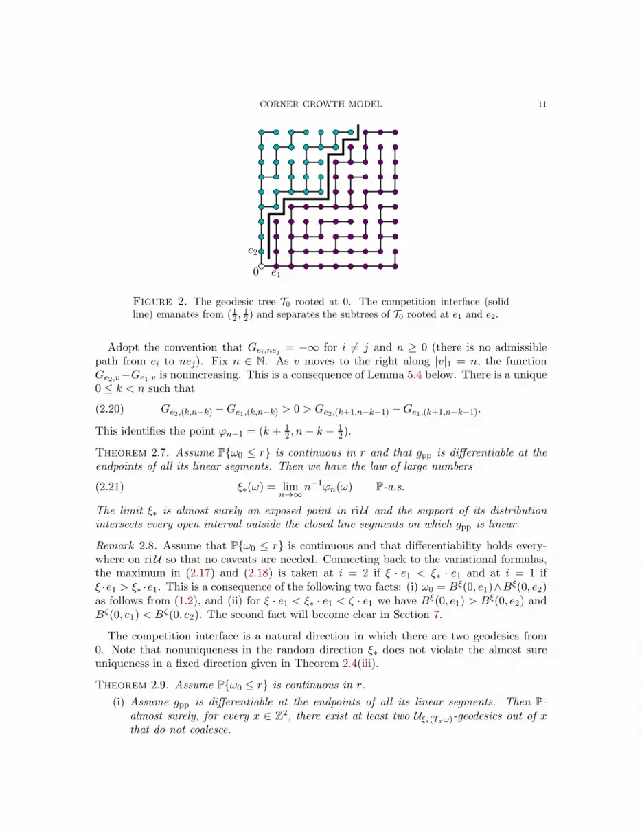
2.8. Competition interface. For this subsection assume that Pω0 ≤ r is a continuousfunction of r ∈ R. Then with probability one no two finite paths of any lengths have equalweight and consequently for any v ∈ Z

2+ there is a unique finite geodesic between 0 and v.

Together these finite geodesics form the geodesic tree T0 rooted at 0 that spans Z2+. The

two subtrees rooted at e1 and e2 are separated by an up-right path ϕ = (ϕk)k≥0 on thelattice (12 ,

12) + Z

2+ with ϕ0 = (12 ,

12). The path ϕ is called the competition interface. The

term comes from the interpretation that the subtrees are two competing infections on thelattice [12, 13]. See Figure 2.

CORNER GROWTH MODEL 11

0

e2

e1

Figure 2. The geodesic tree T0 rooted at 0. The competition interface (solidline) emanates from (1

2, 12) and separates the subtrees of T0 rooted at e1 and e2.

Adopt the convention that Gei,nej = −∞ for i 6= j and n ≥ 0 (there is no admissiblepath from ei to nej). Fix n ∈ N. As v moves to the right along |v|1 = n, the functionGe2,v−Ge1,v is nonincreasing. This is a consequence of Lemma 5.4 below. There is a unique0 ≤ k < n such that

(2.20) Ge2,(k,n−k) −Ge1,(k,n−k) > 0 > Ge2,(k+1,n−k−1) −Ge1,(k+1,n−k−1).

This identifies the point ϕn−1 = (k + 12 , n− k − 1

2).

Theorem 2.7. Assume Pω0 ≤ r is continuous in r and that gpp is differentiable at theendpoints of all its linear segments. Then we have the law of large numbers

ξ∗(ω) = limn→∞

n−1ϕn(ω) P-a.s.(2.21)

The limit ξ∗ is almost surely an exposed point in riU and the support of its distributionintersects every open interval outside the closed line segments on which gpp is linear.

Remark 2.8. Assume that Pω0 ≤ r is continuous and that differentiability holds every-where on riU so that no caveats are needed. Connecting back to the variational formulas,the maximum in (2.17) and (2.18) is taken at i = 2 if ξ · e1 < ξ∗ · e1 and at i = 1 ifξ ·e1 > ξ∗ ·e1. This is a consequence of the following two facts: (i) ω0 = Bξ(0, e1)∧Bξ(0, e2)as follows from (1.2), and (ii) for ξ · e1 < ξ∗ · e1 < ζ · e1 we have Bξ(0, e1) > Bξ(0, e2) andBζ(0, e1) < Bζ(0, e2). The second fact will become clear in Section 7.

The competition interface is a natural direction in which there are two geodesics from0. Note that nonuniqueness in the random direction ξ∗ does not violate the almost sureuniqueness in a fixed direction given in Theorem 2.4(iii).

Theorem 2.9. Assume Pω0 ≤ r is continuous in r.

(i) Assume gpp is differentiable at the endpoints of all its linear segments. Then P-almost surely, for every x ∈ Z

2, there exist at least two Uξ∗(Txω)-geodesics out of xthat do not coalesce.

12 N. GEORGIOU, F. RASSOUL-AGHA, AND T. SEPPALAINEN

(ii) Assume gpp is strictly concave. Then with P-probability one and for any x ∈ Z2,

there cannot be two distinct geodesics from x with a common direction other thanξ∗(Txω).

For the exactly solvable corner growth model with exponential weights Coupier [8] provedthat the set of directions with two non-coalescing geodesics in Z

2+ is countable and dense in

U . Here we have a partial result towards characterizing this set as ξ∗(Txω)x∈Z2+. Partial,

because we consider only pairs of geodesics from a common initial point.Point (i) of Theorem 2.9 is actually true without the differentiability assumption, but

at this stage of the paper we have no definition of ξ∗ without that assumption. This willchange in Theorem 7.2 in Section 7. In point (ii) above gpp has no linear segments and sothe differentiability of gpp at endpoints of linear segments is vacuously true.

Theorems 2.7 and 2.9 are proved in Section 7. An additional fact proved there is thatP(ξ∗ = ξ) > 0 is possible only if ξ /∈ D. In light of the expectation that gpp is differentiable,the expected result is that ξ∗ has a continuous distribution.

When weights ω0 do not have a continuous distribution, there are two competition in-terfaces: one for the tree of leftmost geodesics and one for the tree of rightmost geodesics.We compute the limit distributions of the two competition interfaces for geometric weightsin Sections 2.9 and 8.

2.9. Exactly solvable models. We illustrate our results in the two exactly solvable cases:the distribution of the mean m0 weights ωx is

(2.22)exponential: Pωx ≥ t = m−1

0 e−t/m0 for t ≥ 0 with σ2 = m20,

or geometric: Pωx = k = m−10 (1−m−1

0 )k−1 for k ∈ N with σ2 = m0(m0 − 1).

Calculations behind the claims below are sketched in Section 8.For both cases in (2.22) the point-to-point limit function is

gpp(ξ) = m0(ξ · e1 + ξ · e2) + 2σ√

(ξ · e1)(ξ · e2) .In the exponential case this formula was first derived by Rost [30] (though without the last-passage formulation) while early derivations of the geometric case appeared in [6, 17, 31].Convex duality (2.5) becomes

ξ ∈ riU is dual to h if and only if

h =(m0 + σ2

√ξ · e1/ξ · e2 + t, m0 +

√ξ · e2/ξ · e1 + t

), t ∈ R .

This in turn gives an explicit formula for gpl(h).Since the gpp above is differentiable and strictly concave, all points of riU are exposed

points of differentiability. Theorem 2.2 implies that Busemann functions (2.13) exist in alldirections ξ ∈ riU . They minimize formulas (2.15) and (2.16) as given in (2.17) and (2.18).For each ξ ∈ riU the processes Bξ(ke1, (k + 1)e1) : k ∈ Z+ and Bξ(ke2, (k + 1)e2) : k ∈Z+ are i.i.d. processes independent of each other, exponential or geometric depending onthe case, with means

(2.23)E[Bξ(ke1, (k + 1)e1)] = m0 + σ

√ξ · e2/ξ · e1

E[Bξ(ke2, (k + 1)e2)] = m0 + σ√ξ · e1/ξ · e2 .

CORNER GROWTH MODEL 13

Section 2.7 gives the following results on geodesics. Every infinite geodesic has a directionand for every fixed direction ξ ∈ riU there exists a ξ-geodesic. In the exponential case ξ-geodesics are unique and coalesce. In the geometric case uniqueness cannot hold, butthere exists a unique leftmost ξ-geodesic out of each lattice point and these leftmost ξ-geodesics coalesce. The same holds for rightmost ξ-geodesics. Finite (leftmost/rightmost)geodesics from u ∈ Z

2 to vn converge to infinite (leftmost/rightmost) ξ-geodesics out of u,as vn/|vn|1 → ξ with |vn|1 →∞.

In the exponential case the distribution of the asymptotic direction ξ∗ of the competitioninterface given by Theorem 2.7 can be computed explicitly. For the angle θ∗ = tan−1(ξ∗ ·e2/ξ∗ · e1) of the vector ξ∗,

Pθ∗ ≤ t =√sin t√

sin t+√cos t

, t ∈ [0, π/2].(2.24)

In the exponential case these results for geodesics and the competition interface wereshown in [13]. This paper utilized techniques for geodesics from [26] and the coupling ofthe exponential corner growth model with the totally asymmetric simple exclusion process(TASEP). For this case our approach provides new proofs.

The model with geometric weights has a tree of leftmost geodesics with competition

interface ϕ(l) = (ϕ(l)k )k≥0 and a tree of rightmost geodesics with competition interface

ϕ(r) = (ϕ(r)k )k≥0. Note that ϕ

(r) is to the left of ϕ(l) because in (2.20) there is now a middle

range Ge2,(k,n−k) −Ge1,(k,n−k) = 0 that is to the right (left) of ϕ(r) (ϕ(l)). Strict concavityof the limit gpp implies (with the arguments of Section 7) the almost sure limits

n−1ϕ(l)n → ξ

(l)∗ and n−1ϕ(r)

n → ξ(r)∗ .

The angles θ(a)∗ = tan−1(ξ

(a)∗ ·e2/ξ(a)∗ ·e1) (a ∈ l, r) have these distributions (with p0 = m−1

0denoting the success probability of the geometric): for t ∈ [0, π/2]

(2.25)

Pθ(r)∗ ≤ t =√

(1− p0) sin t√(1− p0) sin t+

√cos t

and Pθ(l)∗ ≤ t =√sin t√

sin t+√(1− p0) cos t

.

Taking p0 → 0 recovers (2.24) of the exponential case. For the details, see Section 8.

2.10. Flat edge in the percolation cone. We describe a known nontrivial example wherethe assumption of differentiable endpoints of a maximal linear segment is satisfied. A shortdetour into oriented percolation is needed.

In oriented site percolation vertices of Z2 are assigned i.i.d. 0, 1-valued random variablesσzz∈Z2 with p1 = Pσ0 = 1. For points u ≤ v in Z

2 we write u→ v (there is an open pathfrom u to v) if there exists an up-right path u = x0, x1, . . . , xm = v with xi−xi−1 ∈ e1, e2,m = |v − u|1, and such that σxi = 1 for i = 1, . . . ,m. (The openness of a path does notdepend on the weight at the initial point of the path.) The percolation event u →∞ isthe existence of an infinite open up-right path from point u. There exists a critical threshold~pc ∈ (0, 1) such that if p1 < ~pc then P0 → ∞ = 0 and if p1 > ~pc then P0 → ∞ > 0.

14 N. GEORGIOU, F. RASSOUL-AGHA, AND T. SEPPALAINEN

(The facts we need about oriented site percolation are proved in article [10] for orientededge percolation. The proofs apply to site percolation just as well.)

Let On = u ∈ Z2+ : |u|1 = n, 0 → u denote the set of vertices on level n that can be

reached from the origin along open paths. The right edge an = maxu∈Onu · e1 is definedon the event On 6= ∅. When p1 ∈ (~pc, 1) there exists a constant βp1 ∈ (1/2, 1) such that[10, eqn. (7) on p. 1005]

limn→∞

ann

10→∞ = βp110→∞ P-a.s.

Let η = (βp1 , 1 − βp1) and η = (1 − βp1 , βp1). The percolation cone is the set ξ ∈ R2+ :

ξ/|ξ|1 ∈ [η, η].The point of this for the corner growth model is that if the ω weights have a maximum

that percolates, gpp is linear on the percolation cone and differentiable on the edges. Thisis the content of the next theorem.

Theorem 2.10. Assume that ωxx∈Z2 are i.i.d., E|ω0|p <∞ for some p > 2 and ωx ≤ 1.Suppose ~pc < p1 = Pω0 = 1 < 1. Let ξ ∈ U . Then gpp(ξ) ≤ 1, and gpp(ξ) = 1 if and onlyif ξ ∈ [η, η]. The endpoints η and η are points of differentiability of gpp.

The theorem above summarizes a development that goes through papers [2, 11, 24]. Theproofs in the literature are for first-passage percolation. We give a proof of Theorem 2.10in Appendix D, by adapting and simplifying the first-passage percolation arguments for thedirected corner growth model.

As a corollary, our results that assume differentiable endpoints of a maximal linear seg-ment are valid for the percolation cone.

Theorem 2.11. Assume (2.1), ωx ≤ 1 and ~pc < p1 = Pω0 = 1 < 1. There exists astationary L1(P) cocycle B(x, y) : x, y ∈ Z

2 and an event Ω0 with P(Ω0) = 1 such thatthe following statements hold for each ω ∈ Ω0. Let vn ∈ Z

2+ be a sequence such that

|vn|1 →∞ and 1− βp1 ≤ limn→∞

vn · e1|vn|1

≤ limn→∞

vn · e1|vn|1

≤ βp1 .

Then

B(ω, x, y) = limn→∞

(Gx,vn(ω)−Gy,vn(ω)

)

for all x, y ∈ Z2. For each m ≥ 0 there exists n0 such that if n ≥ n0, then any geodesic

x0,|vn|1 from x0 = 0 to vn satisfies B(ω, xi, xi+1) = ωxi for all 0 ≤ i ≤ m.Furthermore,

E[B(x, x+ e1)] = E[B(x, x+ e2)] = 1.

This completes the presentation of results and we turn to developing the proofs.

3. Convex duality

By homogeneity we can represent gpp by a single variable function. A way of doing thisthat ties in naturally with the queuing theory arguments we use later is to define

γ(s) = gpp(1, s) = gpp(s, 1) for 0 ≤ s <∞.(3.1)

CORNER GROWTH MODEL 15

Function γ is real-valued, continuous and concave. Consequently one-sided derivativesγ′(s±) exist and are monotone: γ′(s0+) ≥ γ′(s1−) ≥ γ′(s1+) for 0 ≤ s0 < s1. Symmetryand homogeneity of gpp give γ(s) = sγ(s−1).

Lemma 3.1. The derivatives satisfy γ′(s±) > m0 for all s ∈ R+, γ′(0+) = ∞, and

γ′(∞−) ≡ lims→∞

γ′(s±) = γ(0) = m0.

Proof. The boundary shape universality of J. Martin [25, Theorem 2.4] says that

γ(s) = m0 + 2σ√s+ o(

√s ) as sց 0.(3.2)

This gives γ(0) = m0 and γ′(0+) =∞. Lastly,

γ′(∞−) = lims→∞

s−1γ(s) = lims→∞

γ(s−1) = γ(0) = m0.

Martin’s asymptotic (3.2) and γ(s) = sγ(s−1) give

γ(s) = sm0 + 2σ√s+ o(

√s ) as sր∞.(3.3)

This is incompatible with having γ′(s) = m0 for s ≥ s0 for any s0 <∞.

The lemma above has two important geometric consequences: (i) any subinterval of Uon which gpp is linear must lie in the interior riU and (ii) the boundary ξ : gpp(ξ) = 1 ofthe limit shape is asymptotic to the axes.

Define

f(α) = sups≥0γ(s)− sα for m0 < α <∞.(3.4)

Lemma 3.2. Function f is a strictly decreasing, continuous and convex involution of theinterval (m0,∞) onto itself, with limits f(m0+) = ∞ and f(∞−) = m0. That f is aninvolution means that f(f(α)) = α.

Proof. Asymptotics (3.2) and (3.3) imply that m0 < f(α) <∞ for all α > m0 and also thatthe supremum in (3.4) is attained at some s. Furthermore, α < β implies f(β) = γ(s0)−s0βwith s0 > 0 and f(β) < γ(s0)−s0α ≤ f(α). As a supremum of linear functions f is convex,and hence continuous on the open interval (m0,∞).

We show how the symmetry of gpp implies that f is an involution. By concavity of γ,

f(α) = γ(s)− sα if and only if α ∈ [γ′(s+), γ′(s−)](3.5)

and by Lemma 3.1 the intervals on the right cover (m0,∞). Since f is strictly decreasingthe above is the same as

α = γ(s−1)− s−1f(α) if and only if f(α) ∈ [f(γ′(s−)), f(γ′(s+))].(3.6)

Differentiating γ(s) = sγ(s−1) gives

γ′(s±) = γ(s−1)− s−1γ′(s−1∓).(3.7)

By (3.5) and (3.7) the condition in (3.6) can be rewritten as

f(α) ∈ [γ(s)− sγ′(s−), γ(s)− sγ′(s+)] = [γ′(s−1+), γ′(s−1−)].(3.8)

Combining this with (3.5) and (3.6) shows that α = f(f(α)). The claim about the limitsfollows from f being a decreasing involution.

16 N. GEORGIOU, F. RASSOUL-AGHA, AND T. SEPPALAINEN

Extend these functions to the entire real line by γ(s) = −∞ when s < 0 and f(α) =∞when α ≤ m0. Then convex duality gives

(3.9) γ(s) = infα>m0

f(α) + sα.

The natural bijection between s ∈ (0,∞) and ξ ∈ riU that goes together with (3.1) is

(3.10) s = ξ · e1/ξ · e2.Then direct differentiation, (3.5) and (3.7) give

∇gpp(ξ±) =(γ′(s±), γ′(s−1∓)

)=

(γ′(s±), f(γ′(s±))

).(3.11)

Since f is linear on [γ′(s+), γ′(s−)], we get the following connection between the gradientsof gpp and the graph of f :

(3.12) [∇gpp(ξ+),∇gpp(ξ−)] = (α, f(α)) : α ∈ [γ′(s+), γ′(s−)] for ξ ∈ riU .The next theorem details the duality between tilts h and velocities ξ.

Theorem 3.3. (i) Let h ∈ R2. There exists a unique t = t(h) ∈ R such that

(3.13) h− t(e1 + e2) ∈ −[∇gpp(ξ+),∇gpp(ξ−)]for some ξ ∈ riU . The set of ξ for which (3.13) holds is a nonempty (but possiblydegenerate) line segment [ξ(h), ξ(h)] ⊂ riU . If ξ(h) 6= ξ(h) then [ξ(h), ξ(h)] is amaximal line segment on which gpp is linear.

(ii) ξ ∈ riU and h ∈ R2 satisfy duality (2.5) if and only if (3.13) holds.

Proof. The graph (α, f(α)) : α > m0 is strictly decreasing with limits f(m0+) =∞ andf(∞−) = m0. Since every 45 degree diagonal intersects it at a unique point, the equation

h = −(α, f(α)) + t(e1 + e2)(3.14)

defines a bijection R2 ∋ h←→ (α, t) ∈ (m0,∞)×R illustrated in Figure 3. Combining this

with (3.12) shows that (3.13) happens for a unique t and for at least one ξ ∈ riU .Once h and t = t(h) are given, the geometry of the gradients ((3.11)–(3.12) and limits

(2.7)) can be used to argue the claims about the ξ that satisfy (3.13). This proves part (i).That h of the form (3.13) is dual to ξ follows readily from the fact that gradients are

dual and gpl(h+ t(e1 + e2)) = gpl(h) + t (this last from Definition (2.3)).Note the following general facts for any q ∈ [∇gpp(ζ+),∇gpp(ζ−)]. By concavity gpp(η) ≤

gpp(ζ)+ q · (η− ζ) for all η. Combining this with homogeneity gives gpp(ζ) = q ·ζ. Togetherwith duality (2.4) we have

gpl(−q) = 0 for q ∈⋃

ζ∈riU

[∇gpp(ζ+),∇gpp(ζ−)].(3.15)

It remains to show that if h is dual to ξ then it satisfies (3.13). Let (α, t) be determinedby (3.14). From the last two paragraphs

gpl(h) = gpl(−α,−f(α)) + t = t.

Let s = ξ · e1/ξ · e2 so that

gpp(ξ) + h · ξ = γ(s)

1 + s− αs+ f(α)

1 + s+ t.

CORNER GROWTH MODEL 17

αm0

m0

t(e1 + e2)

−h

(α, f(α))

Figure 3. The graph of f and bijection (3.14) between (α, t) and h.

Thus duality gpl(h) = gpp(ξ) + h · ξ implies γ(s) = αs + f(α) which happens if and only ifα ∈ [γ′(s+), γ′(s−)]. (3.12) now implies (3.13).

4. Stationary cocycles

In this section we begin with the stationary cocycles, then show how these define sta-tionary last-passage percolation processes and also solve the variational formulas for gpp(ξ)and gpl(h).

4.1. Existence and properties of stationary cocycles. We come to the technical cen-terpiece of the paper. By appeal to queueing fixed points, in Appendix A we construct a

family of cocycles Bξ±ξ∈riU on an extended space Ω = Ω×Ω′. The next theorem gives theexistence statement and summarizes the properties of these cocycles. Assumption (2.1) isin force. This is the only place where our proofs actually use the assumption P(ω0 ≥ c) = 1,and the only reason is that the queueing results we reference have been proved only forω0 ≥ 0.

The cocycles of interest are related to the last-passage weights in the manner described

in the next definition. A potential is simply a measurable function V : Ω → R. The case

relevant to us will be V (ω) = ω0 where ω = (ω, ω′) ∈ Ω is a configuration in the extendedspace and contains the original weights ω as a component.

Definition 4.1. A stationary L1 cocycle B on Ω recovers potential V if

(4.1) V (ω) = mini∈1,2

B(ω, 0, ei) for P-a.e. ω.

The extended space is the Polish space Ω = Ω×R1,2×A0×Z2where A0 is a certain count-

able subset of the interval (m0,∞). A precise description of A0 appears in the beginning

of the proof of Theorem 4.2 on page 46 in Appendix A. Let S denote the Borel σ-algebra

18 N. GEORGIOU, F. RASSOUL-AGHA, AND T. SEPPALAINEN

of Ω. Generic elements of Ω are denoted by ω = (ω, ω′) with ω = (ωx)x∈Z2 ∈ Ω = RZ2as

before and ω′ = (ωi,αx )i∈1,2, α∈A0, x∈Z2 . Spatial translations act on the x-index in the usual

manner: (Txω)y = ωx+y for x, y ∈ Z2 where ωx = (ωx, ω

′x) = (ωx, (ω

i,αx )i∈1,2, α∈A0

).

Theorem 4.2. There exist functions Bξ+(ω, x, y), Bξ−(ω, x, y) : x, y ∈ Z2, ξ ∈ riU on Ω

and a translation invariant Borel probability measure P on the space (Ω, S) such that thefollowing properties hold.

(i) For each ξ ∈ riU , x ∈ Z2, and i ∈ 1, 2, the function Bξ±(ω, x, x+ ei) is a function

only of (ωi,αx : α ∈ A0). Under P, the marginal distribution of the configuration ω is

the i.i.d. measure P specified in assumption (2.1). The R3-valued process ϕξ+

x x∈Z2

defined by

ϕξ+x (ω) = (ωx, B

ξ+(x, x+ e1), Bξ+(x, x+ e2))

is separately ergodic under both translations Te1 and Te2 . The same holds with ξ+replaced by ξ−. For each z ∈ Z

2, the variables (ωx, Bξ+(ω, x, x+ ei), B

ξ−(ω, x, x+ei)) : x 6≤ z, ξ ∈ riU , i ∈ 1, 2 are independent of ωx : x ≤ z.

(ii) Each process Bξ+ = Bξ+(x, y)x,y∈Z2 is a stationary L1(P) cocycle (Definition 2.1)

that recovers the potential V (ω) = ω0 (Definition 4.1), and the same is true of Bξ−.The associated tilt vectors h(ξ±) = h(Bξ±) defined by (2.10) satisfy

h(ξ±) = −∇gpp(ξ±)(4.2)

and are dual to velocity ξ as in (2.5).

(iii) No two distinct cocycles have a common tilt vector. That is, if h(ξ+) = h(ζ−)then Bξ+(ω, x, x + ei) = Bζ−(ω, x, x + ei), and similarly h(ξ+) = h(ζ+) impliesBξ+(ω, x, x+ ei) = Bζ+(ω, x, x+ ei). These equalities hold without any almost suremodifier because they come for each ω from the construction. In particular, if ξ is apoint of differentiability for gpp then

Bξ+(ω, x, x+ ei) = Bξ−(ω, x, x+ ei) = Bξ(ω, x, x+ ei)

where the second equality defines the cocycle Bξ.

(iv) The following inequalities hold P-almost surely, simultaneously for all x ∈ Z2 and

ξ, ζ ∈ riU : if ξ · e1 < ζ · e1 then

(4.3)Bξ−(x, x+ e1) ≥ Bξ+(x, x+ e1) ≥ Bζ−(x, x+ e1)

and Bξ−(x, x+ e2) ≤ Bξ+(x, x+ e2) ≤ Bζ−(x, x+ e2).

Fix ζ ∈ riU and let ξn → ζ in riU . If ξn · e1 ց ζ · e1 then for all x ∈ Z2 and

i = 1, 2

limn→∞

Bξn±(x, x+ ei) = Bζ+(x, x+ ei) P-a.s. and in L1(P).(4.4)

Similarly, if ξn · e1 ր ζ · e1 the limit holds P-a.s. and in L1(P) with ζ− on the right.

CORNER GROWTH MODEL 19

Remark 4.3. The construction of the cocycles has this property: there is a countable denseset U0 of U such that, for ξ ∈ U0, the cocycles are coordinate projections Bξ±(x, x + ei) =

ωi,γ(s±)x where s is defined by (3.10). A point ζ ∈ U r U0 will lie in D and we defineBζ through one-sided limits from Bξ±, ξ ∈ U0. We comment next on various technicalproperties of the cocycles that are important for the sequel.

(a) A natural question is whether Bξ±(ω, x, y) can be defined as a function of ω alone,or equivalently, whether it is S-measurable. This is important because we use the cocyclesto solve the variational formulas for the limits and to construct geodesics, and it would bedesirable to work on the original weight space Ω rather than on the artificially extended

space Ω = Ω × Ω′. We can make this S-measurability claim for those cocycles that ariseas Busemann functions or their limits. (see Remark 5.3 below).

(b) By part (iii), if gpp is linear on the line segment [ξ′, ξ′′] ⊂ riU with ξ′ · e1 < ξ′′ · e1,then

Bξ′+(ω, x, x+ ei) = Bξ(ω, x, x+ ei) = Bξ′′−(ω, x, x+ ei)

∀ ω ∈ Ω, ξ ∈ ]ξ′, ξ′′[ , i ∈ 1, 2.

The equalities in part (iii) do not extend to Bξ+(x, y) for all x, y without exceptional P-nullsets because the additivity Bξ+(x, z) = Bξ+(x, y) + Bξ+(y, z) cannot be valid for each ω,only almost surely.

(c) When we use these cocycles to construct geodesics in Section 6, it is convenientto have a single null set outside of which the ordering (4.3) is valid for all ξ, ζ. For the

countable family Bξ±ξ∈U0 we can arrange for (4.3) to hold outside a single P-null event.

By defining Bζζ∈UrU0 through limits from the left, we extend inequalities (4.3) to allξ, ζ ∈ riU outside a single null set. This is good enough for a definition of the entire familyBξ±ξ∈riU . But in order to claim that limits from left and right agree at a particular ζ,

we have to allow for an exceptional P-null event that is specific to ζ. Thus the limit (4.4)is not claimed outside a single null set for all ζ.

(d) When Pω0 ≤ r is a continuous function of r it is natural to ask whether Bξ(x, y)can be modified to be continuous in ξ. We do not know the answer.

4.2. Stationary last-passage percolation. Fix a cocycle B(ω, x, y) = Bξ±(ω, x, y) fromTheorem 4.2. Fix a point v ∈ Z

2 that will serve as an origin. By part (i) of Theorem4.2, the weights ωx : x ≤ v − e1 − e2 are independent of B(v − (k + 1)ei, v − kei) :k ∈ Z+, i ∈ 1, 2. These define a stationary last-passage percolation process in the thirdquadrant relative to the origin at v in the following sense. Define passage times GNE

u,v thatuse the cocycle as edge weights on the north and east boundaries and weights ωx in thebulk x ≤ v − e1 − e2:

GNEu,v = B(u, v) for u ∈ v − kei : k ∈ Z+, i ∈ 1, 2

and GNEu,v = ωu +GNE

u+e1,v ∨GNEu+e2,v for u ≤ v − e1 − e2 .

(4.5)

It is immediate from recovery ωx = B(x, x+ e1) ∧B(x, x+ e2) and additivity of B that

GNEu,v = B(u, v) for all u ≤ v.

20 N. GEORGIOU, F. RASSOUL-AGHA, AND T. SEPPALAINEN

Process GNEu,v : u ≤ v is stationary in the sense that the increments

(4.6) GNEx,v −GNE

x+ei,v = B(x, x+ ei)

are stationary under lattice translations and, as the equation above reveals, do not dependon the choice of the origin v (as long as we stay southwest of the origin).

Remark 4.4. In the exactly solvable cases where ωx is either exponential or geometric, moreis known. Given the stationary cocycle, define weights

Yx = B(x− e1, x) ∧B(x− e2, x).Then the weights Yx have the same i.i.d. distribution as the original weights ωx. Fur-thermore, Yx : x ≥ v+ e1 + e2 are independent of B(v+ kei, v+ (k+1)ei) : k ∈ Z+, i ∈1, 2. Hence a stationary last-passage percolation process can be defined in the firstquadrant with cocycles on the south and west boundaries:

GSWv,x = B(v, x) for x ∈ v + kei : k ∈ Z+, i ∈ 1, 2

and GSWv,x = Yx +GSW

v,x−e1 ∨GSWv,x−e2 for x ≥ v + e1 + e2 .

This feature appears in [3] as the “Burke property” of the exponential last-passage model.It also works for the log-gamma polymer in positive temperature [15, 32]. We do not knowpresently if this works in the general last-passage case. It would follow for example if weknew that the distributions of the cocycles of Theorem 4.2 satisfy this lattice symmetry:

B(x, y) : x, y ∈ Z2 d

= B(−y,−x) : x, y ∈ Z2.

4.3. Solution to the variational formulas. We solve variational formulas (2.15)–(2.16)

with the cocycles on the extended space (Ω, S, P). Once we have identified some cocyclesas Busemann functions in Section 5, we prove Theorem 2.3 as a corollary at the end ofSection 5.

Theorem 3.6 in [14] says that if a cocycle B recovers V (ω), h(B) is defined by (2.10),and centered cocycle F is defined by (2.11), then F is a minimizer in (2.15) for any h ∈ R

2

that satisfies (h−h(B)) · (e2 − e1) = 0. For such h, the essential supremum over ω in (2.15)disappears and we have

(4.7)gpl(h) = maxV (ω) + h · e1 + F (ω, 0, e1), V (ω) + h · e2 + F (ω, 0, e2)

= (h− h(B)) · z for P-a.e. ω and any z ∈ e1, e2.Recall from Theorem 3.3 that gpp is linear over each line segment [ξ(h), ξ(h)] and hence,

by part (iii) of Theorem 4.2, cocycles Bξ (and hence the tilts h(ξ) they define) coincide forall ξ ∈ ]ξ(h), ξ(h)[.Theorem 4.5. Let Bξ± be the cocycles given in Theorem 4.2. Fix h ∈ R

2. Let t(h),ξ(h), and ξ(h) be as in Theorem 3.3. One has the following three cases.

(i) ξ(h) 6= ξ(h): For any (and hence all) ξ ∈ ]ξ(h), ξ(h)[ let

F ξ(x, y) = h(ξ) · (x− y)−Bξ(x, y).(4.8)

Then F ξ solves (2.15): for P-almost every ω

gpl(h) = maxω0 + h · e1 + F ξ(ω, 0, e1), ω0 + h · e2 + F ξ(ω, 0, e2) = t(h).(4.9)

CORNER GROWTH MODEL 21

(ii) ξ(h) = ξ(h) = ξ ∈ D: (4.9) holds for F ξ defined as in (4.8).

(iii) ξ(h) = ξ(h) = ξ 6∈ D: Let θ ∈ [0, 1] be such that

h− t(h)(e1 + e2) = θh(ξ−) + (1− θ)h(ξ+)

and define

F ξ±(x, y) = h(ξ±) · (x− y)−Bξ±(x, y) and F (x, y) = θF ξ−(x, y) + (1− θ)F ξ+(x, y).

Then F solves (2.15): for P-almost every ω

gpl(h) = P- ess supω

maxω0 + h · e1 + F (ω, 0, e1), ω0 + h · e2 + F (ω, 0, e2) = t(h).(4.10)

If θ ∈ 0, 1, then the essential supremum is not needed in (4.10), i.e. (4.9) holdsalmost surely with F in place of F ξ.

Here is the qualitative descriptions of the cases above.(i) The graph of f has a corner at the point (α, f(α)) where it crosses the 45o diagonal

that contains −h. Correspondingly, γ is linear on the interval [s, s] and gpp is linear on

[ξ(h), ξ(h)] with gradient ∇gpp(ξ) = −(α, f(α)) at interior points ξ ∈ ]ξ(h), ξ(h)[.(ii) gpp is strictly concave and differentiable at ξ dual to tilt h.(iii) gpp is strictly concave but not differentiable at ξ dual to tilt h.

Proof of Theorem 4.5. By (ii) of Theorem 4.2 the cocycles Bξ and Bξ± that appear inclaims (i)–(iii) recover the potential as required by Definition 4.1 and hence conclusion(4.7) is in force.

In cases (i) and (ii) (4.7) implies

gpl(h) = maxω0 + h · e1 + F ξ(0, e1), ω0 + h · e2 + F ξ(0, e2) = (h− h(ξ)) · e1.The last term equals t(h), by combining (3.13) and (4.2). The same proof works for (iii)when θ ∈ 0, 1.

For the last case (iii), (4.2) and (3.15) imply gpl(h(ξ±)) = 0. Then Theorem 3.3 implies

gpl(h) = gpp(ξ) + h · ξ = t(h) + θ(gpp(ξ) + h(ξ−) · ξ) + (1− θ)(gpp(ξ) + h(ξ+) · ξ)= t(h) + θgpl(h(ξ−)) + (1− θ)gpl(h(ξ+))

= t(h).

Furthermore, we have for P-almost every ω

minθBξ−(0, e1) + (1− θ)Bξ+(0, e1), θBξ−(0, e2) + (1− θ)Bξ+(0, e2) ≥ ω0.

This translates into

P- ess supω

maxω0 + h · e1 + F (0, e1), ω0 + h · e2 + F (0, e2) ≤ t(h) = gpl(h).

Formula (2.15) implies then that the above inequality is in fact an equality and (4.10) isproved.

We state also the corresponding theorem for the point-to-point case, though there isnothing to prove.

22 N. GEORGIOU, F. RASSOUL-AGHA, AND T. SEPPALAINEN

Theorem 4.6. Let ξ ∈ riU . Cocycles Bξ± solve (2.16):

gpp(ξ) = maxω0 −Bξ±(ω, 0, e1)− h(ξ±) · ξ , ω0 −Bξ±(ω, 0, e2)− h(ξ±) · ξ= −h(ξ±) · ξ for P-a.e. ω.

(4.11)

If ξ 6∈ D and θ ∈ (0, 1), then cocycle B = θBξ− + (1− θ)Bξ+ also solves (2.16):

gpp(ξ) = P- ess supω

maxω0 −B(ω, 0, e1)− h(B) · ξ , ω0 −B(ω, 0, e2)− h(B) · ξ

= −h(B) · ξ.The above theorem follows directly from (2.5), Theorem 4.2(ii), (4.9), and the fact that

cocycles Bξ± recover V (ω) = ω0. The last claim follows similarly to (4.10).

5. Busemann functions

In this section we prove the existence of Busemann functions. As before (2.1) is a standingassumption. Recall the line segment Uξ = [ξ, ξ] with ξ · e1 ≤ ξ · e1 from (2.8)–(2.9) and the

cocycles Bξ± constructed on the extended space (Ω, S, P) in Theorem 4.2.

Theorem 5.1. Fix ξ ∈ riU . Then there exists an event Ω0 with P(Ω0) = 1 such that foreach ω ∈ Ω0 and for any sequence vn ∈ Z

2+ that satisfies

|vn|1 →∞ and ξ · e1 ≤ limn→∞

vn · e1|vn|1

≤ limn→∞

vn · e1|vn|1

≤ ξ · e1,(5.1)

we have

(5.2)Bξ+(ω, x, x+ e1) ≤ lim

n→∞

(Gx,vn(ω)−Gx+e1,vn(ω)

)

≤ limn→∞

(Gx,vn(ω)−Gx+e1,vn(ω)

)≤ Bξ−(ω, x, x+ e1)

and

(5.3)

Bξ−(ω, x, x+ e2) ≤ limn→∞

(Gx,vn(ω)−Gx+e2,vn(ω)

)

≤ limn→∞

(Gx,vn(ω)−Gx+e2,vn(ω)

)≤ Bξ+(ω, x, x+ e2).

The interesting cases are of course the ones where we have a limit. For the corollary note

that if ξ, ξ, ξ ∈ D then by Theorem 4.2(iii) Bξ± = Bξ = Bξ±.

Corollary 5.2. Assume that ξ, ξ and ξ are points of differentiability of gpp. Then there

exists an event Ω0 with P(Ω0) = 1 such that for each ω ∈ Ω0, for any sequence vn ∈ Z2+

that satisfies (5.1), and for all x, y ∈ Z2,

(5.4) Bξ(ω, x, y) = limn→∞

(Gx,vn(ω)−Gy,vn(ω)

).

In particular, if gpp is differentiable everywhere on riU , then for each direction ξ ∈ riUthere is an event of full P-probability on which limit (5.4) holds for any sequence vn/|vn|1 →ξ.

Before turning to proofs, let us derive the relevant results of Section 2 and address thequestion of measurability of cocycles raised in Remark 4.3(a).

CORNER GROWTH MODEL 23

Proof of Theorem 2.2. Immediate consequence of Corollary 5.2. Equation (2.14) followsfrom (4.2).

Proof of Theorem 2.3. The theorem follows from Theorems 4.5 and 4.6 because the Buse-mann function Bξ is the cocycle Bξ from Theorem 4.2.

Remark 5.3 (S-measurability of cocycles). A consequence of limit (5.4) is that the cocycleBξ(ω, x, y) is actually a function of ω alone, in other words, S-measurable. Furthermore,all cocycles Bζ± that can be obtained as limits, as these ξ-points converge to ζ± on riU ,are also S-measurable. In particular, if gpp is differentiable at the endpoints of its linear

segments (if any), all the cocycles Bζ± : ζ ∈ riU described in Theorem 4.2 are S-measurable. At points ζ /∈ D of strict concavity this follows because ζ can be approachedfrom both sides by points ξ ∈ E which satisfy (5.4).

The remainder of this section proves Theorem 5.1. We begin with a general comparison

lemma. With arbitrary real weights Yxx∈Z2 define last passage times

Gu,v = maxx0,n

n−1∑

k=0

Yxk.

The maximum is over up-right paths from x0 = u to xn = v with n = |v − u|1. The

convention is Gv,v = 0. For x ≤ v − e1 and y ≤ v − e2 denote the increments by

Ix,v = Gx,v − Gx+e1,v and Jy,v = Gy,v − Gy+e2,v .

Lemma 5.4. For x ≤ v − e1 and y ≤ v − e2(5.5) Ix,v+e2 ≥ Ix,v ≥ Ix,v+e1 and Jy,v+e2 ≤ Jy,v ≤ Jy,v+e1 .

Proof. Let v = (m,n). The proof goes by an induction argument. Suppose x = (k, n) forsome k < m. Then on the north boundary

I(k,n),(m,n+1) = G(k,n),(m,n+1) − G(k+1,n),(m,n+1)

= Yk,n + G(k+1,n),(m,n+1) ∨ G(k,n+1),(m,n+1) − G(k+1,n),(m,n+1)

≥ Yk,n = G(k,n),(m,n) − G(k+1,n),(m,n) = I(k,n),(m,n) .

On the east boundary, when y = (m, ℓ) for some ℓ < n

J(m,ℓ),(m,n+1) = G(m,ℓ),(m,n+1) − G(m,ℓ+1),(m,n+1)

= Ym,ℓ = G(m,ℓ),(m,n) − G(m,ℓ+1),(m,n) = J(m,ℓ),(m,n) .

These inequalities start the induction. Now let u ≤ v − e1 − e2. Assume by induction that(5.5) holds for x = u+ e2 and y = u+ e1.

Iu,v+e2 = Gu,v+e2 − Gu+e1,v+e2 = Yu + (Gu+e2,v+e2 − Gu+e1,v+e2)+

= Yu + (Iu+e2,v+e2 − Ju+e1,v+e2)+

≥ Yu + (Iu+e2,v − Ju+e1,v)+ = Iu,v .

24 N. GEORGIOU, F. RASSOUL-AGHA, AND T. SEPPALAINEN

For the last equality simply reverse the first three equalities with v instead of v + e2.

A similar argument works for Iu,v ≥ Iu,v+e1 and a symmetric argument works for the Jinequalities.

The estimates needed for the proof of Theorem 5.1 come from coupling Gu,v with thestationary LPP described in Section 4.2. For the next two lemmas fix a cocycle B(ω, x, y) =Bζ±(ω, x, y) from Theorem 4.2 and let r = ζ · e1/ζ · e2 so that α = γ′(r±) satisfies

(5.6) α = E[B(x, x+ e1)] and f(α) = E[B(x, x+ e2)].

As in (4.5) define

GNEu,v = B(u, v) for u ∈ v − kei : k ∈ Z+, i ∈ 1, 2

and GNEu,v = ωu +GNE

u+e1,v ∨GNEu+e2,v for u ≤ v − e1 − e2 .

(5.7)

Let GNEu,v(A) denote a maximum over paths restricted to the set A. In particular, below

we use

GNE0,vn(vn − ei ∈ x) = max

x: x|vn|1−1=vn−ei

|vn|1−1∑

k=0

Yxk

where the maximum is restricted to paths that go through the point vn−ei, and the weights

are from (5.7): Yx = ωx for x ≤ v − e1 − e2 while Yv−kei = B(v − kei, v − (k − 1)ei).Figure 4 makes the limits of the next lemma obvious. But a.s. convergence requires some

technicalities because the north-east boundaries themselves are translated as the limit istaken.

s

t

s− τ

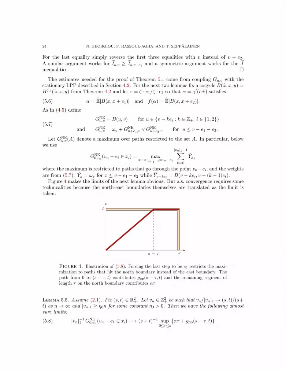
Figure 4. Illustration of (5.8). Forcing the last step to be e1 restricts the maxi-mization to paths that hit the north boundary instead of the east boundary. Thepath from 0 to (s − τ, t) contributes gpp(s − τ, t) and the remaining segment oflength τ on the north boundary contributes ατ .

Lemma 5.5. Assume (2.1). Fix (s, t) ∈ R2+. Let vn ∈ Z

2+ be such that vn/|vn|1 → (s, t)/(s+

t) as n→∞ and |vn|1 ≥ η0n for some constant η0 > 0. Then we have the following almostsure limits:

(5.8) |vn|−11 GNE

0,vn(vn − e1 ∈ x) −→ (s+ t)−1 sup0≤τ≤s

ατ + gpp(s− τ, t)

CORNER GROWTH MODEL 25

and

(5.9) |vn|−11 GNE

0,vn(vn − e2 ∈ x) −→ (s + t)−1 sup0≤τ≤t

f(α)τ + gpp(s, t− τ).

Proof. We prove (5.8). Fix ε > 0, let M = ⌊ε−1⌋, and

qnj = j⌊ε|vn|1ss+ t

⌋for 0 ≤ j ≤M − 1, and qnM = vn · e1.

For large enough n it is the case that qnM−1 < vn · e1.Suppose a maximal path for GNE

0,vn(vn−e1 ∈ x) enters the north boundary from the bulk

at the point vn − (ℓ, 0) with qnj < ℓ ≤ qnj+1. Then

GNE0,vn(vn − e1 ∈ x) = G0,vn−(ℓ,1) + ωvn−(ℓ,1) +B(vn − (ℓ, 0), vn)

≤ G0,vn−(qnj ,1)+ qnj α−

ℓ−1∑

k=qnj +1

(ωvn−(k,1) −m0

)+ (ℓ− 1− qnj )m0

+(B(vn − (ℓ, 0), vn)− ℓα

)+ (ℓ− qnj )α.

The two main terms come right after the inequality above and the rest are errors. Theinequality comes from

G0,vn−(ℓ,1) +

ℓ∑

k=qnj +1

ωvn−(k,1) ≤ G0,vn−(qnj ,1)

and algebraic rearrangement.Define the centered cocycle F (x, y) = h(B) · (x− y)−B(x, y) so that

B(vn − (ℓ, 0), vn)− ℓα = F (0, vn − (ℓ, 0)) − F (0, vn).The potential-recovery property (4.1) ω0 = B(0, e1) ∧B(0, e2) gives

F (0, ei) ≤ α ∨ f(α)− ω0 for i ∈ 1, 2.The i.i.d. distribution of ωx and E(|ω0|p) <∞ with p > 2 are strong enough to guaranteethat Lemma C.1 from Appendix C applies and gives

(5.10) limN→∞

1

Nmax

x≥0 : |x|1≤N|F (ω, 0, x)| = 0 for a.e. ω.

Collect the bounds for all the intervals (qnj , qnj+1] and let C denote a constant. Abbreviate

Snj,m =

∑qnj +m

k=qnj +1

(ωvn−(k,1) −m0

).

(5.11)

GNE0,vn(vn − e1 ∈ x) ≤ max

0≤j≤M−1

G0,vn−(qnj ,1)

+ qnj α+C(qnj+1 − qnj )

+ max0≤m<qnj+1−qnj

|Snj,m|+ max

qnj <ℓ≤qnj+1

F (0, vn − (ℓ, 0)) − F (0, vn).

Divide through by |vn|1 and let n→∞. Limit (E.1) gives convergence of the G-term on theright. We claim that the terms on the second line of (5.11) vanish. Limit (5.10) takes care

26 N. GEORGIOU, F. RASSOUL-AGHA, AND T. SEPPALAINEN

of the F -terms. Combine Doob’s maximal inequality for martingales with Burkholder’sinequality [4, Thm. 3.2] to obtain, for δ > 0,

P

max0≤m<qnj+1−qnj

|Snj,m| ≥ δ|vn|1

≤

E[|Sn

j,qnj+1−qnj|p]

δp|vn|p1

≤ C

δp|vn|p1E

[ ∣∣∣∣qnj+1−qnj∑

i=1

(ωi,0 −m0

)2∣∣∣∣p/2 ]

≤ C

|vn|p/21

.

Thus Borel-Cantelli takes care of the Snj,m-term on the second line of (5.11). (This is the

place where the assumption |vn|1 ≥ η0n is used.) We have the upper bound

limn→∞

|vn|−11 GNE

0,vn(vn − e1 ∈ x) ≤ (s+ t)−1 max0≤j≤M−1

[gpp(s − sjε, t) + sjεα+ Cεs

].

Let εց 0 to complete the proof of the upper bound.To get the matching lower bound let the supremum supτ∈[0,s]τα + gpp(s − τ, t) be

attained at τ∗ ∈ [0, s]. With mn = |vn|1/(s + t) we have

GNE0,vn(vn − e1 ∈ x) ≥ G0,vn−(⌊mnτ∗⌋∨1,1) + ωvn−(⌊mnτ∗⌋∨1,1)

+ B(vn − (⌊mnτ∗⌋ ∨ 1, 0), vn).

Use again the cocycle F from above, and let n→∞ to get

limn→∞

|vn|−11 GNE

0,vn(vn − e1 ∈ x) ≥ (s+ t)−1[gpp(s− τ∗, t) + τ∗α].

This completes the proof of (5.8).

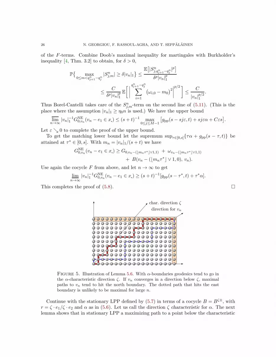
char. direction ζ

direction for vn

Figure 5. Illustration of Lemma 5.6. With α-boundaries geodesics tend to go inthe α-characteristic direction ζ. If vn converges in a direction below ζ, maximalpaths to vn tend to hit the north boundary. The dotted path that hits the eastboundary is unlikely to be maximal for large n.

Continue with the stationary LPP defined by (5.7) in terms of a cocycle B = Bζ±, withr = ζ · e1/ζ · e2 and α as in (5.6). Let us call the direction ζ characteristic for α. The nextlemma shows that in stationary LPP a maximizing path to a point below the characteristic

CORNER GROWTH MODEL 27

direction will eventually hit the north boundary before the east boundary. (Illustration inFigure 5.) We leave to the reader the analogous result to a point above the characteristicline.

Lemma 5.6. Let s ∈ (r,∞). Let vn ∈ Z2+ be such that vn/|vn|1 → (s, 1)/(1 + s) and

|vn|1 ≥ η0n for some constant η0 > 0. Assume that γ′(r+) > γ′(s−). Then P-a.s. thereexists a random n0 <∞ such that for all n ≥ n0,(5.12) GNE

0,vn = GNE0,vn(vn − e1 ∈ x).

Proof. The right derivative at τ = 0 of ατ + gpp(s − τ, 1) = ατ + γ(s− τ) equalsα− γ′(s−) > α− γ′(r+) ≥ 0.

The last inequality above follows from the assumption on r. Thus we can find τ∗ ∈ (0, r)such that

(5.13) ατ∗ + gpp(s− τ∗, 1) > gpp(s, 1).

To produce a contradiction let A be the event on which GNE0,vn = GNE

0,vn(vn − e2 ∈ x)

for infinitely many n and assume P(A) > 0. Let mn = |vn|1/(1 + s). On A we have forinfinitely many n

|vn|−1GNE0,vn(vn − e2 ∈ x) = |vn|−1GNE

0,vn

≥ |vn|−1B(vn − (⌊mnτ∗⌋+ 1)e1, vn) + |vn|−1G0,vn−(⌊mnτ∗⌋+1,1)

+ |vn|−1ωvn−(⌊mnτ∗⌋+1,1).

Apply (5.9) to the leftmost quantity. Apply limits (E.1) and (5.10) and stationarity andintegrability of ωx to the expression on the right. Both extremes of the above inequalityconverge almost surely. Hence on the event A the inequality is preserved to the limit andyields (after multiplication by 1 + s)

sup0≤τ≤1

f(α)τ + gpp(s, 1− τ) ≥ ατ∗ + gpp(s− τ∗, 1).

The supremum of the left-hand side is achieved at τ = 0 because the right derivative equals

f(α)− γ′(1−τs −) ≤ f(α)− γ

′(r−1−) ≤ 0

where the first inequality comes from s−1 < r−1 and the second from (3.8). Therefore

gpp(s, 1) ≥ ατ∗ + gpp(s− τ∗, 1)

which contradicts (5.13). Consequently P(A) = 0 and (5.12) holds for n large.

Proof of Theorem 5.1. The proof goes in two steps.

Step 1. First consider a fixed ξ = ( s1+s ,

11+s) ∈ riU and a sequence vn such that

vn/|vn|1 → ξ and |vn|1 ≥ η0n for some η0 > 0. We prove that the last inequality of (5.2)holds almost surely. Let ζ = ( r

1+r ,1

1+r ) satisfy ζ · e1 < ξ · e1 so that γ′(r+) > γ′(s−) andLemma 5.6 can be applied. Use cocycle Bζ+ from Theorem 4.2 to define last-passage times

28 N. GEORGIOU, F. RASSOUL-AGHA, AND T. SEPPALAINEN

GNEu,v as in (5.7). Furthermore, define last-passage times GN

u,v that use cocycles only on thenorth boundary and bulk weights elsewhere:

GNv−ke1,v = Bζ+(v − ke1, v) , GN

v−ℓe2,v =ℓ∑

j=1

ωv−je2 ,

and GNu,v = ωu +GN

u+e1,v ∨GNu+e2,v for u ≤ v − e1 − e2 .

For large n we have

Gx,vn −Gx+e1,vn ≤ GNx,vn+e2 −G

Nx+e1,vn+e2

= GNEx,vn+e1+e2(vn + e2 ∈ x)−GNE

x+e1,vn+e1+e2(vn + e2 ∈ x)= GNE

x,vn+e1+e2 −GNEx+e1,vn+e1+e2 = Bζ+(x, x+ e1).

The first inequality above is the first inequality of (5.5). The first equality above is obvious.The second equality is Lemma 5.6 and the last equality is (4.6). Thus

limn→∞

(Gx,vn −Gx+e1,vn

)≤ Bζ+(x, x+ e1).

Let ζ · e1 increase to ξ · e1. Theorem 4.2(iv) implies

limn→∞

(Gx,vn −Gx+e1,vn

)≤ Bξ−(x, x+ e1).

An analogous argument gives the matching lower bound (first inequality of (5.2)) bytaking ζ · e1 > ξ · e1 and by reworking Lemma 5.6 for the case where the direction ofvn is above the characteristic direction ζ. Similar reasoning works for vertical incrementsGx,vn −Gx+e2,vn .

Step 2. We prove the full statement of the theorem. Let ηℓ and ζℓ be two sequences

in riU such that ηℓ · e1 < ξ · e1, ξ · e1 < ζℓ · e1, ηℓ → ξ, and ζℓ → ξ. Let Ω0 be the event

on which limits (4.4) holds for directions ξ and ξ (with sequences ζℓ and ηℓ, respectively)and (5.2) holds for each direction ζℓ with sequence ⌊nζℓ⌋, and for each direction ηℓ with

sequence ⌊nηℓ⌋. P(Ω0) = 1 by Theorem 4.2(iv) and Step 1.Fix ℓ and a sequence vn as in (5.1). Abbreviate an = |vn|1. For large n

⌊anηℓ⌋ · e1 < vn · e1 < ⌊anζℓ⌋ · e1 and ⌊anηℓ⌋ · e2 > vn · e2 > ⌊anζℓ⌋ · e2.By repeated application of Lemma 5.4

Gx,⌊anζℓ⌋ −Gx+e1,⌊anζℓ⌋ ≤ Gx,vn −Gx+e1,vn ≤ Gx,⌊anηℓ⌋ −Gx+e1,⌊anηℓ⌋.

Take n → ∞ and apply (5.2) to the sequences ⌊anζℓ⌋ and ⌊anηℓ⌋. This works because

⌊anζℓ⌋ is a subset of ⌊nζℓ⌋ that escapes to infinity. Thus for ω ∈ Ω0

Bζℓ+(ω, x, x+ e1) ≤ limn→∞

(Gx,vn(ω)−Gx+e1,vn(ω))

≤ limn→∞

(Gx,vn(ω)−Gx+e1,vn(ω)) ≤ Bηℓ−(ω, x, x+ e1).

Take ℓ→∞ and apply (4.4) to arrive at (5.2) as stated. (5.3) follow similarly.

CORNER GROWTH MODEL 29

6. Directional geodesics

This section proves the results on geodesics. We work on the extended space Ω = Ω×Ω′

and define geodesics in terms of the cocycles Bξ± constructed in Theorem 4.2. The idea isin the next lemma, followed by the definition of cocycle geodesics.

Lemma 6.1. Let B be any stationary cocycle that recovers potential V (ω) = ω0, as inDefinitions 2.1 and 4.1. Fix ω so that properties (b)–(c) of Definition 2.1 and (4.1) holdfor all translations Txω.

(a) Let xm,n = (xk)nk=m be any up-right path that follows minimal gradients of B, that is,

ωxk= B(ω, xk, xk+1) for all m ≤ k < n.

Then xm,n is a geodesic from xm to xn:

(6.1) Gxm,xn(ω) =n−1∑

k=m

ωxk= B(ω, xm, xn).

(b) Let xm,n = (xk)nk=m be an up-right path such that for all m ≤ k < n

either ωxk= B(xk, xk+1) < B(xk, xk + e1) ∨B(xk, xk + e2)

or xk+1 = xk + e2 and B(xk, xk + e1) = B(xk, xk + e2).

In other words, path xm,n follows minimal gradients of B and takes an e2-step in atie. Then xm,n is the leftmost geodesic from xm to xn. Precisely, if xm,n is an up-right

path from xm = xm to xn = xn and Gxm,xn =∑n−1

k=m ωxk, then xk · e1 ≤ xk · e1 for all

m ≤ k ≤ n.If ties are broken by e1-steps the resulting geodesic is the rightmost geodesic between

xm and xn: xk · e1 ≥ xk · e1 for all m ≤ k < n.

Proof. Part (a). Any up-right path xm,n from xm = xm to xn = xn satisfies

n−1∑

k=m

ωxk≤

n−1∑

k=m

B(xk, xk+1) = B(xm, xn) =

n−1∑

k=m

B(xk, xk+1) =

n−1∑

k=m

ωxk.

Part (b). xm,n is a geodesic by part (a). To prove that it is the leftmost geodesic assumexk = xk and xk+1 = xk + e1. Then ωxk

= B(xk, xk + e1) < B(xk, xk + e2). Recovery of theweights gives Gx,y ≤ B(x, y) for all x ≤ y. Combined with (6.1),

ωxk+Gxk+e2,xn < B(xk, xk + e2) +B(xk + e2, xn) = B(xk, xn) = Gxk,xn .

Hence also xk+1 = xk + e1 and the claim about being the leftmost geodesic is proved. Theother claim is symmetric.

Next we define a cocycle geodesic, that is, a geodesic constructed by following minimalgradients of a cocycle Bξ± constructed in Theorem 4.2. Since our treatment allows discretedistributions, we introduce a function t on Z2 to resolve ties. For ξ ∈ riU , u ∈ Z2, and

t ∈ e1, e2Z2, let xu,t,ξ±0,∞ be the up-right path (one path for ξ+, one for ξ−) starting at

30 N. GEORGIOU, F. RASSOUL-AGHA, AND T. SEPPALAINEN

xu,t,ξ±0 = u and satisfying for all n ≥ 0

xu,t,ξ±n+1 =

xu,t,ξ±n + e1 if Bξ±(xu,t,ξ±n , xu,t,ξ±n + e1) < Bξ±(xu,t,ξ±n , xu,t,ξ±n + e2),

xu,t,ξ±n + e2 if Bξ±(xu,t,ξ±n , xu,t,ξ±n + e2) < Bξ±(xu,t,ξ±n , xu,t,ξ±n + e1),

xu,t,ξ±n + t(xu,t,ξ±n ) if Bξ±(xu,t,ξ±n , xu,t,ξ±n + e1) = Bξ±(xu,t,ξ±n , xu,t,ξ±n + e2).

Cocycles Bξ± satisfy ωx = Bξ±(ω, x, x+ e1)∧Bξ±(ω, x, x+ e2) (Theorem 4.2(ii)) and so by

Lemma 6.1(a), xu,t,ξ±0,∞ is an infinite geodesic. Since the cocycles are defined on the space Ω,

the geodesics are measurable functions on Ω. Recall from Remark 5.3 that under certain

conditions a cocycle Bξ± is S-measurable. When that happens, the geodesic xu,t,ξ±0,∞ can

be defined on Ω without the artificial extension to the space Ω = Ω × Ω′. In particular, if

gpp is differentiable at the endpoints of its linear segments (if any), all geodesics xu,t,ξ±0,∞ areS-measurable.

If we restrict ourselves to the event Ω0 of full P-measure on which monotonicity (4.3)holds for all ξ, ζ ∈ riU , we can order these geodesics in a natural way from left to right.

Define a partial ordering on e1, e2Z2by e2 e1 and then t t

′ coordinatewise. Then on

the event Ω0, for any u ∈ Z2, t t

′, ξ, ζ ∈ riU with ξ · e1 < ζ · e1, and for all n ≥ 0,

xu,t,ξ±n · e1 ≤ xu,t′,ξ±

n · e1, xu,t,ξ−n · e1 ≤ xu,t,ξ+n · e1, and xu,t,ξ+n · e1 ≤ xu,t,ζ−n · e1.(6.2)

The leftmost and rightmost tie-breaking rules are defined by tx = e2 and tx = e1 for allx ∈ Z

2. The cocycle limit (4.4) forces the cocycle geodesics to converge also, as the nextlemma shows.

Lemma 6.2. Fix ξ and let ζn → ξ in riU . If ζn · e1 > ξ · e1 ∀n then for all u ∈ Z2

P∀k ≥ 0 ∃n0 <∞ : n ≥ n0 ⇒ xu,t,ζn±0,k = xu,t,ξ+0,k = 1.(6.3)

Similarly, if ζn · e1 ր ξ · e1 the limit holds with ξ− on the right and t replaced by t.

Proof. It is enough to prove the statement for u = 0. By (4.4), for a given k and largeenough n, if x ≥ 0 with |x|1 ≤ k and Bξ+(x, x+e1) 6= Bξ+(x, x+e2), then B

ζn±(x, x+e1)−Bζn±(x, x+e2) does not vanish and has the same sign as Bξ+(x, x+e1)−Bξ+(x, x+e2). Fromsuch an x geodesics following the minimal gradient of Bζn± or the minimal gradient of Bξ+

stay together for their next step. On the other hand, when Bξ+(x, x+e1) = Bξ+(x, x+e2),monotonicity (4.3) implies

Bζn±(x, x+ e1) ≤ Bξ+(x, x+ e1) = Bξ+(x, x+ e2) ≤ Bζn±(x, x+ e2).

Once again, both the geodesic following the minimal gradient of Bζn± and rules t and theone following the minimal gradients of Bξ+ and rules t will next take the same e1-step.This proves (6.3). The other claim is similar.

Recall the line segments Uξ, Uξ± defined in (2.8)–(2.9). The endpoints of Uξ = [ξ, ξ] aregiven by

ξ · e1 = supα : (α, 1− α) ∈ Uξ+ and ξ · e1 = infα : (α, 1− α) ∈ Uξ−.By Lemma 3.1 both points are again in riU . When needed we extend this definition to theendpoints of U by Uei = Uei± = ei, i ∈ 1, 2.

The next theorem concerns the direction of the cocycle geodesics.

CORNER GROWTH MODEL 31

Theorem 6.3. We have these two statements:

(6.4) P

∀ξ ∈ riU ,∀t ∈ e1, e2Z

2,∀u ∈ Z

2 : xu,t,ξ±0,∞ is Uξ±-directed= 1.

If ξ ∈ D then the statement should be taken without the ±.

Proof. Fix ξ ∈ riU and abbreviate xn = xu,t,ξ+n . Since Bξ+ recovers weights ω, Lemma6.1(a) implies that Gu,xn = Bξ+(u, xn). Furthermore, Bξ+(x, y) + h(ξ+) · (y − x) is acentered cocycle, as in Definition 2.1. Theorem C.1 implies then

limn→∞

|xn|−11 (Gu,xn + h(ξ+) · xn) = 0 P-almost surely.

Define ζ(ω) ∈ U by ζ · e1 = lim xn·e1|xn|1

. If ζ · e1 > ξ · e1 then ζ 6∈ Uξ+ and hence

gpp(ζ) + h(ξ+) · ζ = gpp(ζ)−∇gpp(ξ+) · ζ < gpp(ξ)−∇gpp(ξ+) · ξ = 0.

(The first and last equalities come from (4.2) and (4.11).) Consequently, by the shapetheorem (limit (E.1)), on the event ζ · e1 > ξ · e1

limn→∞

|xn|−11 (Gu,xn + h(ξ+) · xn) < 0.

This proves that

P

limn→∞

xu,t,ξ+n · e1|xu,t,ξ+n |1

≤ ξ · e1= 1.

Repeat the same argument with t replaced by t and ξ by the other endpoint of Uξ+ (whichis either ξ or ξ). To capture all t use geodesics ordering (6.2). An analogous argumentworks for ξ−. We have, for a given ξ,

(6.5) P

∀t ∈ e1, e2Z

2,∀u ∈ Z

2 : xu,t,ξ±0,∞ is Uξ±-directed= 1.

Let Ω0 be an event of full P-probability on which all cocycle geodesics satisfy the ordering(6.2), and the event in (6.5) holds for ξ± in a countable set U0 that contains all points of

nondifferentiability of gpp and a countable dense subset of D. We argue that Ω0 is containedin the event in (6.4).

Let ζ /∈ U0 and let ζ denote the right endpoint of Uζ . We show that

(6.6) limn→∞

xu,t,ζn · e1|xu,t,ζn |1

≤ ζ · e1 on the event Ω0.

(Note that ζ ∈ D so there is no ζ± distinction in the cocycle geodesic.) The lim with t and≥ ζ · e1 comes of course with the same argument.

If ζ · e1 < ζ · e1 pick ξ ∈ D ∩ U0 so that ζ · e1 < ξ · e1 < ζ · e1. Then ξ = ζ and (6.6)follows from the ordering.

If ζ = ζ, let ε > 0 and pick ξ ∈ D ∩ U0 so that ζ · e1 < ξ · e1 ≤ ξ · e1 < ζ · e1 + ε. Thisis possible because ∇gpp(ξ) converges to but never equals ∇gpp(ζ) as ξ · e1 ց ζ · e1. Againby the ordering

limn→∞

xu,t,ζn · e1|xu,t,ζn |1

≤ limn→∞

xu,t,ξn · e1|xu,t,ξn |1

≤ ξ · e1 < ζ · e1 + ε.

32 N. GEORGIOU, F. RASSOUL-AGHA, AND T. SEPPALAINEN

This completes the proof of Theorem 6.3.

Lemma 6.4. (a) Fix ξ ∈ riU . Then the following statement holds P-almost surely. For anygeodesic x0,∞

limn→∞

xn · e1|xn|1

≥ ξ · e1 implies that xn · e1 ≥ xx0,t,ξ−n · e1 for all n ≥ 0(6.7)

and

limn→∞

xn · e1|xn|1

≤ ξ · e1 implies that xn · e1 ≤ xx0 ,t,ξ+n · e1 for all n ≥ 0.(6.8)

(b) Fix a maximal line segment [ζ, ζ] on which gpp is linear and such that ζ · e1 < ζ · e1.Assume ζ and ζ are both points of differentiability of gpp. Then the following statement

holds P-almost surely. Any geodesic x0,∞ such that a limit point of xn/|xn|1 lies in [ζ, ζ]satisfies

xx0,t,ζn · e1 ≤ xn · e1 ≤ xx0 ,t,ζ

n · e1 for all n ≥ 0.(6.9)

Proof. Part (a). We prove (6.7). (6.8) is proved similarly.Fix a sequence ζℓ ∈ D such that ζℓ · e1 ր ξ · e1 so that, in particular, ξ 6∈ Uζℓ . The good

event of full P-probability is the one on which xx0,t,ζℓ0,∞ is Uζℓ-directed (Theorem 6.3), x

x0,t,ζℓ0,∞

is the leftmost geodesic between any two of its points (Lemma 6.1(b) applied to cocycle

Bζℓ) and xx0,t,ζℓ0,∞ → x

x0,t,ξ−

0,∞ (Lemma 6.2).

By the leftmost property, if xx0,t,ζℓ0,∞ ever goes strictly to the right of x0,∞, these two

geodesics cannot touch again at any later time. But by virtue of the limit points, xx0,t,ζℓn ·e1 <

xn · e1 for infinitely many n. Hence xx0,t,ζℓ0,∞ stays weakly to the left of x0,∞. Let ℓ→∞.

Part (b) is proved similarly. The differentiability assumption implies that the geodesic

xx0,t,ζ

0,∞ can be approached from the left by geodesics xx0,t,ζℓ0,∞ such that ζ 6∈ Uζℓ .

Recall the set E of exposed points of differentiability defined below (2.6). Define sets E+and E− of their one-sided limit points by

E± = ζ ∈ riU : ∃ξn ∈ E such that ξn → ζ and ± ξn · e1 > ±ζ · e1.

Corollary 6.5. Fix ξ ∈ riU such that ξ ∈ E∪E−. Then P-almost surely and for all u ∈ Z2,

xu,t,ξ−

0,∞ is the leftmost Uξ−-geodesic out of u. Similarly, for a fixed ξ with ξ ∈ E ∪ E+, P-almost surely and for all u ∈ Z

2, xu,t,ξ+0,∞ is the rightmost Uξ+-geodesic out of u.

Proof. Theorem 6.3 implies that xu,t,ξ−

0,∞ is a Uξ−-geodesic. If ξ ∈ E ∪ E− then either Uξ− =

Uξ− or Uξ− = ξ ⊂ Uξ−. Thus, xu,t,ξ−

0,∞ is a Uξ−-geodesic. ξ ∈ E ∪ E− implies that there

cannot be a linear segment adjacent to ξ to the left, and consequently ξ = ξ. Lemma

6.4(a) implies that xu,t,ξ−

0,∞ is to the left of any other Uξ−-geodesic out of u. The claim aboutrightmost geodesics is proved similarly.

CORNER GROWTH MODEL 33

The next result concerns coalescence of geodesics xu,t,ξ±0,∞ : u ∈ Z2, for fixed t and

ξ ∈ riU .

Theorem 6.6. Fix t ∈ e1, e2Z2and ξ ∈ riU . Then P-almost surely, for all u, v ∈ Z

2,

there exist n,m ≥ 0 such that xu,t,ξ−n,∞ = xv,t,ξ−m,∞ , with a similar statement for ξ+.

Theorem 6.6 is proved by adapting the argument of [21], originally presented for firstpassage percolation and later ported by [13] to the exactly solvable corner growth modelwith exponential weights. Briefly, the idea is the following. Stationarity and two nonin-tersecting geodesics create three nonintersecting geodesics. A modification of the weightsturns the middle geodesic of the triple into a geodesic that stays disjoint from all geodesicsthat emanate from sufficiently far away. Stationarity again gives at least δL2 such disjointgeodesics emanating from an L × L square. This gives a contradiction because there areonly 2L boundary points for these geodesics to exit through. The details are in AppendixB.

To get to uniqueness of geodesics, we show that continuity of the distribution of ω0

prevents ties between cocycle weights. (The construction of the cocycles implies, througheqn. (A.6), that the variables Bξ±(x, y) have continuous marginal distributions, but here

we need a property of the joint distribution.) Consequently for a given ξ, P-almost surely

cocycle geodesics xu,t,ξ±0,∞ do not depend on t.

Lemma 6.7. Assume (2.1) and that Pω0 ≤ r is a continuous function of r ∈ R. Fixξ ∈ riU . Then for all u ∈ Z

2,

PBξ+(u, u + e1) = Bξ+(u, u+ e2) = PBξ−(u, u+ e1) = Bξ−(u, u+ e2) = 0.

Proof. Due to shift invariance it is enough to prove the claim for u = 0. We work with thecase ξ+, the other case being similar.

Assume by way of contradiction that the probability in question is positive. Pick an

arbitrary t ∈ e1, e2Z2. By Theorem 6.6, xe2,t,ξ+0,∞ and xe1,t,ξ+0,∞ coalesce with probability one.

Hence there exists v ∈ Z2 and n ≥ 1 such that

PBξ+(0, e1) = Bξ+(0, e2), x

e1,t,ξ+n = xe2,t,ξ+n = v

> 0.

Note that if Bξ+(0, e1) = Bξ+(0, e2) then both are equal to ω0. Furthermore, by Lemma6.1(a) we have

Bξ+(e1, v) =

n−1∑

k=0

ω(xe1,t,ξ+k ) and Bξ+(e2, v) =

n−1∑

k=0

ω(xe2,t,ξ+k ).

(For aesthetic reasons we wrote ω(x) instead of ωx.) Thus

ω0 +

n−1∑

k=0

ω(xe1,t,ξ+k ) = Bξ+(0, e1) +Bξ+(e1, v) = Bξ+(0, v)

= Bξ+(0, e2) +Bξ+(e2, v) = ω0 +n−1∑

k=0

ω(xe2,t,ξ+k ).

34 N. GEORGIOU, F. RASSOUL-AGHA, AND T. SEPPALAINEN

The fact that this happens with positive probability contradicts the assumption that ωx

are i.i.d. and have a continuous distribution. The lemma is proved.

It is known that, in general, uniqueness of geodesics cannot hold simultaneously for alldirections. In our development this is a consequence of Theorem 7.2 below.

Proof of Theorem 2.4. Part (i). The existence of Uξ±-directed geodesics for ξ ∈ riU follows

by fixing t and taking geodesics xu,t,ξ±0,∞ from Theorem 6.3. For ξ = ei geodesics are simply

x0,∞ = (nei)n≥0.

Let D0 be a dense countable subset of D. Let Ω0 be the event of full P-probability onwhich event (6.4) holds and Lemma 6.4(a) holds for each u ∈ Z

2 and ζ ∈ D0. We show

that on Ω0, every geodesic is Uξ-directed for some ξ ∈ U .Fix ω ∈ Ω0 and an arbitrary geodesic x0,∞. Define ξ′ ∈ U by

ξ′ · e1 = limn→∞

xn · e1|xn|1

.

Let ξ = ξ′ = the left endpoint of Uξ′ . We claim that x0,∞ is Uξ = [ξ, ξ]-directed. If ξ′ = e2then xn/|xn|1 → e2 and Uξ = e2 and the case is closed. Suppose ξ′ 6= e2.

The definition of ξ implies that ξ′ ∈ Uξ+ and so

limn→∞

xn · e1|xn|1

= ξ′ · e1 ≤ ξ · e1.

From the other direction, for any ζ ∈ D0 such that ζ · e1 < ξ′ · e1 we have

limn→∞

xn · e1|xn|1

> ζ · e1

which by (6.7) implies xn · e1 ≥ xx0,t,ζn · e1. Then by (6.4)

limn→∞

xn · e1|xn|1

≥ limn→∞

xx0,t,ζn · e1|xx0,t,ζ

n |1≥ ζ · e1

where ζ = the left endpoint of Uζ . It remains to observe that we can take ζ · e1 arbitrarily

close to ξ · e1. If ξ · e1 < ξ′ · e1 then we take ξ · e1 < ζ · e1 < ξ′ · e1 in which case ζ = ξ and

ζ = ξ. If ξ = ξ′ then also ξ = ξ′ = ξ. In this case, as D0 ∋ ζ ր ξ, ∇g(ζ) approaches but

never equals ∇g(ξ−) because there is no flat segment of gpp adjacent to ξ on the left. Thisforces both ζ and ζ to converge to ξ.

Part (ii) . If gpp is strictly concave then Uξ = ξ for all ξ ∈ riU and part (ii) followsfrom part (i).

Part (iii). By Theorem 4.2(iii) there is a single cocycle Bξ simultaneously for all ξ ∈ [ζ, ζ].

Consequently cocycle geodesics xx0,t,ζ

0,∞ and xx0,t,ζ0,∞ coincide for any given tie breaking function

t. By Corollary 5.2 this cocycle Bξ is S-measurable and hence so are the cocycle geodesics.On the event of full P-probability on which there are no ties between Bξ(x, x + e1) andBξ(x, x+ e2) the tie breaking function t makes no difference. Hence the left and right-handside of (6.9) coincide. Thus there is no room for two [ζ, ζ]-directed geodesics from anypoint. Coalescence comes from Theorem 6.6.

CORNER GROWTH MODEL 35

Proof of Theorem 2.5. Part (i) follows from Lemma 6.1.

Part (ii). Take sequences ηn, ζn ∈ riU with ηn · e1 < ξ · e1 ≤ ξ · e1 < ζn · e1 and ζn → ξ,ηn → ξ. Consider the full measure event on which Theorem 5.1 holds for each ζn and ηnwith sequences vm = ⌊mζn⌋ and ⌊mηn⌋, and on which continuity (4.4) holds as ζn → ξ,ηn → ξ. In the rest of the proof we drop the index n from ζn and ηn.

We prove the case of an infinite geodesic x0,∞ that satisfies x0 = 0 and (2.19). For largem, ⌊mη · e1⌋ < xm · e1 < ⌊mζ · e1⌋.

Consider first the case x1 = e1. If there exists a geodesic from 0 to ⌊mζ⌋ that goes throughe2, then this geodesic would intersect x0,∞ and thus there would exist another geodesic thatgoes from 0 to ⌊mζ⌋ passing through e1. In this case we would have Ge1,⌊mζ⌋ = Ge2,⌊mζ⌋.On the other hand, if there exists a geodesic from 0 to ⌊mζ⌋ that goes through e1, then wewould have Ge1,⌊mζ⌋ ≥ Ge2,⌊mζ⌋. Thus, in either case, we have

G0,⌊mζ⌋ −Ge1,⌊mζ⌋ ≤ G0,⌊mζ⌋ −Ge2,⌊mζ⌋.

Taking m → ∞ and applying Theorem 5.1 we have Bζ+(0, e1) ≤ Bζ+(0, e2). Taking

ζ → ξ and applying (4.4) we have Bξ+(0, e1) ≤ Bξ+(0, e2). Since ξ and ξ are points of

differentiability of gpp, we have Bξ+ = Bξ. Consequently, we have shown Bξ(0, e1) ≤Bξ(0, e2). Since Bξ recovers the potential (Definition 4.1), the first step satisfies ω0 =Bξ(0, e1) ∧Bξ(0, e2) = Bξ(0, x1).

When x1 = e2 repeat the same argument with η in place of ζ to get Bξ(0, e2) ≤ Bξ(0, e1).This proves the theorem for the first step of the geodesic and that is enough.

Part (iii). The statement holds if Bξ(0, e1) = Bξ(0, e2), since then both are equal to ω0

by potential recovery (4.1). If ω0 = Bξ(0, e1) < Bξ(0, e2) then convergence (2.13) impliesthat for n large enough Ge1,vn > Ge2,vn . In this case any maximizing path from 0 to vnwill have to start with an e1-step and the claim of the lemma is again true. The caseBξ(0, e1) > Bξ(0, e2) is similar.

Proof of Theorem 2.6. Part (i) follows from Corollary 6.5 and Theorem 6.6. Part (ii) followsfrom Theorem 2.5(iii) and the fact that the geodesics in Corollary 6.5 are the Busemanngeodesics from Theorem 2.5.

7. Competition interface

In this section we prove the results of Section 2.8. As before, we begin by studying the

situation on the extended space Ω with the help of the cocycles Bζ± of Theorem 4.2.

Lemma 7.1. Define Be1− as the monotone limit of Bζ± when ζ → e1. Then P-almostsurely Be1−(0, e1) = ω0 and Be1−(0, e2) = ∞. A symmetric statement holds for the limitas ζ → e2.

Proof. The limit in the claim exists due to monotonicity (4.3). Furthermore, by potentialrecovery we have almost surely Be1−(0, e1) ≥ ω0. On the other hand, dominated conver-gence, (3.11) and Lemma 3.1 give

E[Be1−(0, e1)] = limζ→e1

E[Bζ±(0, e1)] = limζ→e1

e1 · ∇gpp(ζ±) = m0 = E[ω0].

36 N. GEORGIOU, F. RASSOUL-AGHA, AND T. SEPPALAINEN

Thus, Be1−(0, e1) = ω0 almost surely.The cocycle property (Definition 2.1(c)) and recovery (Definition 4.1), both of which are

satisfied by Be1−, imply the relation

Be1−(ne1, ne1 + e2)

= ωne1 +(Be1−((n + 1)e1, (n + 1)e1 + e2)−Be1−(ne1 + e2, (n + 1)e1 + e2)

)+

= ωne1 +(Be1−((n + 1)e1, (n + 1)e1 + e2)− ωne1+e2

)+.

The second equality is from the just proved identity Be1−(x, x+ e1) = ωx.Repeatedly dropping the outer +-part and applying the same formula inductively leads

to

Be1−(0, e2) ≥ ω0 +n∑

i=1

(ωie1 − ω(i−1)e1+e2)

+(Be1−((n+ 1)e1, (n+ 1)e1 + e2)− ωne1+e2

)+.

Since the summands are i.i.d. with mean 0, taking n → ∞ gives Be1−(0, e2) = ∞ almostsurely.

Next we use the cocycles to define a random variable on Ω that represents the asymptoticdirection of the competition interface. Assume now that Pω0 ≤ r is continuous in r.

By Lemma 6.7, with P-probability one, Bξ±(0, e1) 6= Bξ±(0, e2) for all rational ξ ∈ riU .Furthermore, monotonicity (4.3) gives that

Bζ+(0, e1)−Bζ+(0, e2) ≤ Bζ−(0, e1)−Bζ−(0, e2) ≤ Bη+(0, e1)−Bη+(0, e2)

when ζ · e1 > η · e1. Lemma 7.1 implies that Bζ±(0, e1) − Bζ±(0, e2) converges to −∞ asζ → e1 and to ∞ as ζ → e2. Thus there exists a unique ξ∗(ω) ∈ riU such that for rationalζ ∈ riU ,

Bζ±(ω, 0, e1) < Bζ±(ω, 0, e2) if ζ · e1 > ξ∗(ω) · e1and Bζ±(ω, 0, e1) > Bζ±(ω, 0, e2) if ζ · e1 < ξ∗(ω) · e1.

(7.1)

Theorem 7.2. Assume Pω0 ≤ r is continuous in r. Then on the extended space (Ω, S, P)of Theorem 4.2 the random variable ξ∗(ω) ∈ riU defined by (7.1) has the following proper-ties.

(i) P-almost surely, for every x ∈ Z2, there exist at least two Uξ∗(Txω)-geodesics out of

x that do not coalesce.(ii) Recall Uξ∗(ω) = [ξ

∗(ω), ξ∗(ω)] from (2.9). Then the following holds P-almost surely.

Let x′0,∞ and x′′0,∞ be any geodesics with

limn→∞

x′n · e1n

< ξ∗(ω) and lim

n→∞

x′′n · e1n

> ξ∗(ω).

Then x′1 = e2 and x′′1 = e1.

(iii) Pω : ξ∗(ω) = ξ = 0 for any ξ ∈ D.(iv) Fix ζ, η ∈ riU such that ζ ·e1 < η ·e1 and ∇gpp(ζ+) 6= ∇gpp(η−), with Uζ = [ζ, ζ] and

Uη = [η, η]. Then for P-almost every ω there exists z ∈ Z2 such that ξ∗(Tzω) ∈ [ζ, η].

CORNER GROWTH MODEL 37

Proof. Define

B+∗ (ω, x, y) = lim

ζ·e1ցξ∗(ω)·e1Bζ±(ω, x, y)

and B−∗ (ω, x, y) = lim

ζ·e1րξ∗(ω)·e1Bζ±(ω, x, y) .

(7.2)

As pointed out in Remark 4.3(c), we have to keep the B±∗ distinction even if gpp is ev-

erywhere differentiable, because direction ξ∗ is random and continuity (4.4) has not been

shown simultaneously for all directions with a single P-null set.In any case, B±

∗ satisfy the cocycle property (Definition 2.1(c)) and recovery ωx =mini=1,2B

±∗ (ω, x, x + ei) (Definition 4.1). From (7.1) we have B+

∗ (0, e1) ≤ B+∗ (0, e2) and

B−∗ (0, e1) ≥ B−

∗ (0, e2). By Lemma 6.1 there exists a geodesic from 0 through e1 (by follow-ing minimal B+

∗ gradients) and another through e2 (by following minimal B−∗ gradients),

with an arbitrary tie breaking function t. These two geodesics cannot coalesce because ω0

has a continuous distribution.Let ζ · e1 < ξ∗ · e1 < η · e1. By the limits in (7.2) and monotonicity (4.3),

Bζ+(ω, x, x+ e1) ≥ B±∗ (ω, x, x+ e1) ≥ Bη−(ω, x, x+ e1)

and Bζ+(ω, x, x+ e2) ≤ B±∗ (ω, x, x+ e2) ≤ Bη−(ω, x, x+ e2).

These inequalities imply that the B±∗ -geodesics stay to the right of x0,ζ+0,∞ and to the left of

x0,η−0,∞ . By Theorem 6.3 these geodesics are Uζ+- and Uη−-directed, respectively. Hence the

B±∗ -geodesics are Uξ∗-directed. Part (i) is proved.In part (ii) we prove the first claim, the other claim being similar. The assumption allows

us to pick a rational η ∈ riU such that limx′n · e1/n < η · e1 ≤ η · e1 < ξ∗ · e1. Since ω0

has a continuous distribution and geodesic x0,η−0,∞ is Uη−-directed, geodesic x0,∞ has to stay

always to the left of it. (7.1) implies x0,η−1 = e2. Hence also x1 = e2. The claim is proved.

For part (iii) fix ξ ∈ riD, which implies Bξ± = Bξ. By Lemma 6.7, Bξ(0, e1) 6= Bξ(0, e2)almost surely. Let ζ · e1 ց ξ · e1 along rational points ζ ∈ riU . By (4.4), Bζ±(0, ei) →Bξ(0, ei) a.s. Then on the event Bξ(0, e1) > Bξ(0, e2) there almost surely exists a rational ζsuch that ζ ·e1 > ξ ·e1 and Bζ±(0, e1) > Bζ±(0, e2). By (7.1) this forces ξ∗ ·e1 ≥ ζ ·e1 > ξ ·e1.Similarly on the event Bξ(0, e1) < Bξ(0, e2) we have almost surely ξ∗ · e1 < ξ · e1. Theconclusion is that P(ξ∗ = ξ) = 0 and part (iii) is proved.

In part (iv), Uζ+ 6= Uη− and directedness (Theorem 6.3) force the cocycle geodesics x0,η−0,∞

and x0,ζ+0,∞ to separate. If n ≥ 0 is the time after which they separate, then by cocycle

geodesics ordering (6.2) there exists z ∈ Z2 such that x0,η−n = x0,ζ+n = z, x0,η−n+1 = z + e1,

and x0,ζ+n+1 = z + e2. Definition (7.1) implies that ζ · e1 ≤ ξ∗(Tzω) · e1 ≤ η · e1. For supposeη · e1 < ξ∗(Tzω) · e1. Pick a rational point strictly between η and ξ∗(Tzω). The second lineof (7.1) and ordering (4.3) imply that Bη−(ω, z, z + e1) > Bη−(ω, z, z + e2), contradicting

the choice x0,η−n+1 = z + e1.

Corollary 7.3. Assume Pω0 ≤ r is continuous in r and gpp is differentiable at theendpoints of all its linear segments. Then ξ∗ lies almost surely outside the union of theclosed linear segments of gpp. Equivalently, ξ∗ is almost surely an exposed point.

38 N. GEORGIOU, F. RASSOUL-AGHA, AND T. SEPPALAINEN

Proof. By Theorem 2.4(iii) each linear segment has a unique geodesic from 0 directed into it.Since there are at most countably many linear segments of gpp, Theorem 7.2(i) contradictsξ∗ lying on a flat segment. Under the differentiability assumption endpoints of flat segmentsare not exposed.

The next theorem identifies the asymptotic direction of the competition interface ϕ =(ϕk)0≤k<∞ defined in Section 2.8.

Theorem 7.4. Assume Pω0 ≤ r is continuous in r.

(i) All limit points of the asymptotic velocity of the competition interface are in Uξ∗(ω):for P-almost every ω

ξ∗(ω) · e1 ≤ lim

n→∞n−1ϕn(ω) · e1 ≤ lim

n→∞n−1ϕn(ω) · e1 ≤ ξ∗(ω) · e1.(7.3)

(ii) If gpp is differentiable at the endpoints of its linear segments then ξ∗ is S-measurable

and gives the asymptotic direction of the competition interface: P-almost surely

limn→∞

n−1ϕn(ω) = ξ∗(ω).(7.4)

Proof. Fix t ∈ e1, e2Z2. By (7.1), if ζ · e1 < ξ∗(ω) · e1 < η · e1, then x0,t,ζ±1 = e2 and

x0,t,η±1 = e1. Since the path ϕ separates the geodesics that go through e1 and e2, it has to

stay between x0,t,ζ+0,∞ and x0,t,η−0,∞ . By Theorem 6.3 these geodesics are Uζ+ and Uη− directed,and we have

ζ · e1 ≤ limn→∞

n−1ϕn · e1 ≤ limn→∞

n−1ϕn · e1 ≤ η · e1.

Claim (7.3) follows by taking ζ and η to ξ∗.If gpp is differentiable at the endpoints of its linear segments, then cocycles are S-

measurable and hence so is ξ∗. Furthermore, ξ∗ is an exposed point by Corollary 7.3. Inthis case, ξ

∗= ξ∗ and claim (7.4) is proved.

Proof of Theorem 2.7. Limit (2.21) is in (7.4). The fact that the limit lies in riU is in theconstruction in the paragraph that contains (7.1), and the properties of the limit are inTheorem 7.2(iv) and Corollary 7.3.

Proof of Theorem 2.9. Part (i) comes directly from Theorem 7.2(i). For part (ii) assumegpp strictly concave. Then Uξ = ξ and by Theorem 2.4(ii) every geodesic is directed. Inthis case, Theorem 7.2(ii) implies that with P-probability one, there cannot be two distinctgeodesics from 0 with a common direction other than ξ∗.

As mentioned at the end of Section 2.8, if Pω0 ≤ r is not continuous in r, we have

competition interfaces ϕ(l) and ϕ(r) for the trees of leftmost and rightmost geodesics. Their

limiting directions ξ(r)∗ (ω), ξ

(l)∗ (ω) ∈ riU are defined by

Bζ±(ω, 0, e1) > Bζ±(ω, 0, e2) if ζ · e1 < ξ(r)∗ (ω) · e1,

Bζ±(ω, 0, e1) = Bζ±(ω, 0, e2) if ξ(r)∗ (ω) · e1 < ζ · e1 < ξ

(l)∗ (ω) · e1

and Bζ±(ω, 0, e1) < Bζ±(ω, 0, e2) if ζ · e1 > ξ(l)∗ (ω) · e1.

(7.5)

CORNER GROWTH MODEL 39

With this definition limit (7.3) is valid also with superscripts (l) and (r). Consequently

n−1ϕ(a)n (ω)→ ξ

(a)∗ (ω) a.s. for a ∈ l, r under the assumption that gpp is strictly concave.

8. Exactly solvable models

We go through some details for the exactly solvable models discussed in Section 2.9.

8.1. Geometric weights. The weights ωx are i.i.d. with P(ωx = k) = (1−m0−1)k−1m0

−1

for k ∈ N, mean m0 = E(ω0) > 1 and variance σ2 = m0(m0 − 1).Begin by investigating the queueing fixed point. With Sn,0 i.i.d. geometric with mean

m0, let the initial arrival process An,0 be i.i.d. geometric with mean α. Let Jn = Sn,0 +Wn,0. Then equations (A.3) and (A.4) show that the process (An,1, Jn+1) : n ∈ Z is anirreducible aperiodic Markov chain with transition probability

(8.1)P (An,1 = b, Jn+1 = j |An−1,1 = a, Jn = i)

= P(An,0 − i)+ + Sn+1,0 = b, (i−An,0)

+ + Sn+1,0 = j.

Note that the equations also show that (An,0, Sn+1,0) are independent of (An−1,1, Jn). Sincethe process (An,1, Jn+1) : n ∈ Z is stationary, its marginal must be the unique invariantdistribution of transition (8.1), namely

P (An−1,1 = k, Jn = j) = (1− α−1)k−1α−1 · (1− f(α)−1)j−1f(α)−1 for k, j ∈ N.

with f(α) = m0α−1α−m0

. This shows that i.i.d. mean α geometric is a queuing fixed point.

Next solve for γ(s) = infα>m0αs + f(α). The unique minimizing α in terms of s =ξ · e1/ξ · e2 is

α = m0 + σ√ξ · e2/ξ · e1

which defines the bijection between ξ ∈ riU and α ∈ (m0,∞). From this

f(α) = m0α− 1

α−m0= m0 + σ

√ξ · e1/ξ · e2.

The terms in the sum Jn = Sn,0 +Wn,0 are independent, so we can also find the distri-bution of the waiting time:

P (Wn,0 = 0) =α−m0

α− 1, P (Wn,0 = k) =

m0 − 1

α− 1·(1− 1

f(α)

)k−1 1

f(α)(k ≥ 1).

The distributions of ξ(r)∗ and ξ

(l)∗ claimed in (2.25) come from (7.5), knowing that

B(a,1−a)(0, e1) and B(a,1−a)(0, e2) are independent geometrics with means (2.23). The cal-

culation for ξ(r)∗ goes

Pξ(r)∗ · e1 > a = PB(a,1−a)(0, e1) > B(a,1−a)(0, e2) =α−m0

α

=

√(m0 − 1)(1 − a)

√m0a+

√(m0 − 1)(1 − a)

from which the first formula of (2.25) follows. Similar computation for ξ(l)∗ .

40 N. GEORGIOU, F. RASSOUL-AGHA, AND T. SEPPALAINEN

8.2. Exponential weights. The weights ωx are i.i.d. exponential with mean m0 =E(ωx) > 0 and variance σ2 = m2

0, with marginal distribution

P(ωx > t) = m−10 e−t/m0 for t ≥ 0.

The queuing fixed point can be derived as in the geometric case. The distribution of ξ∗comes from knowing that B(a,1−a)(0, e1) and B(a,1−a)(0, e2) are independent exponentialswith parameters

√a/(√a+√1− a) and

√1− a/(√a+

√1− a). Hence

Pξ∗ · e1 > a = PB(a,1−a)(0, e1) > B(a,1−a)(0, e2) =√1− a√

a+√1− a

.

Equation (2.24) follows.

Appendix A. Cocycles from queuing fixed points

This section proves Theorem 4.2. By shifting the variables ωx, Bξ±(x, x+ ei) in The-

orem 4.2 if necessary, we can assume without loss of generality that Pω0 ≥ 0 = 1. Thenthe weights ωx can represent service times and we can tap into queueing theory. We switchnow to terminology and notation from queuing theory to enable the reader to relate thisappendix to the existing queueing literature.

Consider an infinite sequence of ·/G/1/∞/FIFO queues in tandem. That is, eachqueue or service station (these terms are used almost interchangeably) has a general servicetime distribution (the law of ωx under P), a single server, unbounded room for customerswaiting to be served, and customers obey first-in-first-out discipline. The service stations areindexed by k ∈ Z+ and a bi-infinite sequence of customers is indexed by n ∈ Z. Customersenter the system at station 0 and move from station to station in order. The server atstation k serves one customer at a time. Once the service of customer n is complete atstation k, customer n moves to the back of the queue at station k + 1 and customer n+ 1enters service at station k if he was already waiting in the queue. If the queue at station kis empty after the departure of customer n, then server k remains idle until customer n+1arrives. Each customer retains his integer label as he moves through the system.

Here is the mathematical apparatus. The system needs two ingredients: an initial inter-arrival process An,0 : n ∈ Z and the service times Sn,k : n ∈ Z, k ∈ Z+. An,0 ≥ 0 isthe time between the arrival of customer n and customer n+ 1 at queue 0. Sn,k ≥ 0 is theamount of time the service of customer n takes at station k. Let Sn,k : n ∈ Z, k ∈ Z+ bei.i.d. such that S0,0 has the distribution of ω0 under P. Assume An,0 : n ∈ Z is stationary,ergodic, and independent of Sn,k : k ∈ Z+, n ∈ Z. Assume

(A.1) E[S0,0] = m0 < E[A0,0] <∞.

This guarantees in particular a stable system where queues do not blow up. The servicetime distribution is taken to be fixed, while the input An,0 varies, by analogy with varyingthe initial distribution of a Markov process.

As a product of an ergodic process and an i.i.d. process (An,0, Sn,k)n∈Z,k∈Z+ is stationaryand ergodic under translations of the n-index. Consequently the entire queuing system isstationary and ergodic under translations of the n-index. The issue of interest is finding

CORNER GROWTH MODEL 41

input processes An,0 such that the system is also stationary under translations of the k-

index. Such a process or its distribution on RZ will be called a fixed point of the queueing

operator.Next we develop the iterative equations that describe the evolution of the system from

station to station, as k increases. These are the variables. An,k is the inter-arrival timebetween customers n and n+1 at queue k, or, equivalently, the inter-departure time betweencustomers n and n+ 1 from queue k − 1. Wn,k is the waiting time of customer n at queuek, that is, the time between the arrival of customer n at queue k and the beginning ofhis service at queue k. The total time customer n spends at station k is the sojourn timeWn,k + Sn,k.

The development begins with the waiting times. Define the stationary, ergodic processWn,0n∈Z by

Wn,0 =(

supj≤n−1

n−1∑

i=j

(Si,0 −Ai,0))+.(A.2)

By the ergodic theorem and (A.1)

Wn,0 <∞ for all n ∈ Z.

Process Wn,0 satisfies Lindley’s equation:Wn+1,0 = (Wn,0 + Sn,0 −An,0)

+.(A.3)

This equation agrees naturally with the queuing interpretation. If Wn,0 + Sn,0 < An,0

then customer n leaves station 0 before customer n+1 arrives, and consequently customern+ 1 has no wait and Wn+1,0 = 0. In the complementary case customer n + 1 waits timeWn+1,0 =Wn,0 + Sn,0 −An,0 before entering service at station 0.

With some additional work we prove the following.

Lemma A.1. n−1Wn,0 → 0 almost surely as n→∞.

Proof. Abbreviate Un = Sn,0 −An,0. For a ≥ 0 and ε > 0 define

W ε0 (a) = a

W εn+1(a) =

(W ε

n(a) + Un − E(U0) + ε)+

for n ≥ 0.

Check inductively that

W εn(0) =

(max

0≤m<n

n−1∑

k=m

[Uk − E(U0) + ε])+.

Consequently

W εn(a) ≥W ε

n(0) ≥n−1∑

k=0

[Uk − E(U0) + ε] −→∞ as n→∞.

Thus W εn(a) > 0 for large n which implies, from its definition, that for large n

W εn+1(a) =W ε

n(a) + Un −E(U0) + ε.

Another application of the ergodic theorem gives n−1W εn(a)→ ε P-a.s. as n→∞.

42 N. GEORGIOU, F. RASSOUL-AGHA, AND T. SEPPALAINEN

Now for the conclusion. Since W0,0 =W ε0 (W0,0), we can check inductively that

Wn+1,0 = (Wn,0 + Un)+ ≤

(W ε

n(W0,0) + Un

)+

≤(W ε

n(W0,0) + Un − E(U0) + ε)+

=W εn+1(W0,0).

From this, 0 ≤ n−1Wn,0 ≤ n−1W εn(W0,0)→ ε, and we let εց 0.

The stationary and ergodic process An,1 : n ∈ Z of inter-departure times from queue0 (equivalently, inter-arrival times at queue 1) is defined by

An,1 = (An,0 − Sn,0 −Wn,0)+ + Sn+1,0,(A.4)

again by considering the two cases: either customer n+1 arrives before customer n departs(An,0 < Sn,0 +Wn,0) and goes into service the moment customer n departs, or server 0 isempty waiting for customer n+1 for time (An,0−Sn,0−Wn,0)

+ before service of customern+ 1 begins. Process An,1 : n ∈ Z is independent of Sn,k : k ≥ 1, n ∈ Z.

Combining equations (A.3) and (A.4) and iterating gives

W1,0 + S1,0 +

n∑

i=1

Ai,1 =Wn+1,0 + Sn+1,0 +

n∑

i=1

Ai,0 for n ≥ 1.

This and Lemma A.1 imply E[A0,1] = E[A0,0]. (In the queueing literature, this has beenobserved in [22].)

These steps are repeated at each queue. At queue k we have the stationary, ergodicarrival process An,kn∈Z that is independent of the service times Sn,j : n ∈ Z, j ≥ k.Waiting times at queue k are defined by

Wn,k =(

supj≤n−1

n−1∑

i=j

(Si,k −Ai,k))+.(A.5)

Properties Wn,k < ∞, Lemma A.1, and E[An,k] = E[A0,0] are preserved along the way.This procedure constructs the process An,k, Sn,k,Wn,k : n ∈ Z, k ∈ Z+ that satisfies thefollowing system of equations:

Wn+1,k + Sn+1,k = Sn+1,k + (Wn,k + Sn,k −An,k)+,

An,k+1 = (An,k − Sn,k −Wn,k)+ + Sn+1,k,

Sn+1,k = (Sn+1,k +Wn+1,k) ∧An,k+1.

(A.6)

The third equation follows directly from the first two. A useful consequence of (A.6) is the“conservation law”

Wn+1,k + Sn+1,k +An,k =Wn,k + Sn,k +An,k+1.(A.7)

The next four statements summarize the situation with fixed points, quoted from articles[23, 27]. Given a stationary ergodic probability measure µ on R

Z consider random variables

An,0, Sn,0, Wn,0, An,1 : n ∈ Zwhere An,0 : n ∈ Z has distribution µ, Sn,0 : n ∈ Z are i.i.d. with distribution P, thetwo collections are independent of each other, Wn,0 are defined via (A.2), and An,1 aredefined via (A.4). Let Φ(µ) denote the distribution of An,1 : n ∈ Z. Φ is the queueing

operator whose fixed points are the focus now.

CORNER GROWTH MODEL 43

Let Mαe (R

Z) be the space of translation-ergodic probability measures µ on RZ with

marginal mean Eµ[A0,0] = α. We are mainly interested in ergodic fixed points, so we define

A = α > m0 : ∃µ ∈Mαe (R

Z) such that Φ(µ) = µ.Theorem A.2. [27, Thm. 1] Let α ∈ A. Then there exists a unique µα ∈ Mα

e (RZ) with

Φ(µα) = µα. Furthermore, let A0 = An,0 : n ∈ Z be ergodic with mean E[A0,0] = α and

Sn,k : n ∈ Z, k ∈ Z+ i.i.d. with distribution P and independent of A0. Let Ak = An,k :

n ∈ Z, k ∈ N, be defined via inductions (A.2) and (A.6). Then the distributions of Ak

converge weakly to µα.

Theorem A.3. [23, Thm. 5.1 and 6.4 and Lm. 6.3(a)] The set A is closed and nonempty,infA = m0, and supA = ∞. If α < β are both in A then µα ≤ µβ in the usual sense ofstochastic ordering.

Lemma A.4. [23, Lm. 6.3(b)] Let α ∈ A, A0 ∼ µα, and Sn,k ∼ P independent of A0.Define Wn,0 via (A.2). Then

(A.8) Eµα⊗P[W0,0 + S0,0] = f(α).

Suppose α ∈ (m0,∞) ∩ Ac. Let

α = sup(A ∩ (m0, α]

)∈ A and α = inf

(A ∩ [α,∞)

)∈ A,

t = (α− α)/(α− α) and µα = tµα + (1− t)µα. Now µα is a mean α fixed point of Φ. Thisfixed point is again attractive, in the following sense.

Theorem A.5. [23, Prop. 6.5] Let α > m0. Let An,0 : n ∈ Z be ergodic with meanE[A0,0] = α and Sn,k : n ∈ Z, k ∈ Z+ i.i.d. with distribution P and independent of theA-process. Let An,k : n ∈ Z, k ∈ N be defined via inductions (A.2) and (A.6). The Cesaromean of the distributions of An,k : n ∈ Z converges weakly to µα.

Lemma A.6. (a) Let α < α be points in A such that (α,α) ⊂ Ac. Then f is linear onthe interval [α,α].

(b) Let ξ ∈ D, s = ξ · e1/ξ · e2 and α = γ′(s). Then α ∈ A.Proof. Part (a). Let 0 < t < 1 and α = tα + (1 − t)α. In the notation of [23], consider asequence of tandem queues (Ak, Sk,W k, Ak+1)k∈Z+ where the initial arrival process A0 =

(An,0)n∈Z is ergodic with mean E(An,0) = α, the service times Skk∈Z+ = Sn,kn∈Z,k∈Z+

are independent of A0 and i.i.d. P-distributed, and the remaining variables are defined

iteratively. Let (A, S, W , D) denote a weak limit point of the Cesaro averages of the distri-butions of (Ak, Sk,W k, Ak+1). Then, as shown in [23, eqn. (29)] in the course of the proof

of their Theorem 5.1, W = Ψ(A, S) where the mapping Ψ encodes definition (A.2). By

Theorem A.5 [23, Prop. 6.5] the distribution of A is tµα + (1− t)µα. By [23, Theorem 4.1],

(A.9) n−1n−1∑

k=0

W0,k →M(α) ≡ f(α)−m0 almost surely.

Combine these facts as follows. First

E(W0) = E[Ψ(A, S)0] = tEµα⊗P[Ψ(A, S)0] + (1− t)Eµα⊗P[Ψ(A, S)0]

= tM(α) + (1− t)M(α)

44 N. GEORGIOU, F. RASSOUL-AGHA, AND T. SEPPALAINEN

where the last equality comes from [23, Lemma 6.3(b)] restated as Lemma A.4 above. Theweak limit, combined with the law of large numbers (A.9) and dominated convergence,gives, for any c <∞ and along a subsequence,

E(W0 ∧ c) = limn→∞

n−1n−1∑

k=0

E(W0,k ∧ c) ≤ limn→∞

E[ (n−1

n−1∑

k=0

W0,k

)∧ c

]=M(α) ∧ c

≤M(α).

Letting cր∞ givestM(α) + (1− t)M(α) ≤M(α).

SinceM is convex and f differs fromM by a constant, this implies f(α) = tf(α)+(1−t)f(α)and completes the proof of part (a).

Part (b). To get a contradiction, suppose α ∈ Ac. Then there exist α < α in A such thatα ∈ (α,α) ⊂ Ac. By part (a) f is linear on [α,α]. Basic convex analysis implies that γ hasmultiple tangent slopes at s and hence cannot be differentiable at s. Here is the argument.

By (3.5) the assumption γ′(s) = α implies that γ(s) = f(α) +αs. It follows that s mustbe the slope of f on (α,α). For suppose this slope is s1 and let α1 ∈ (α,α). Then by theduality (3.9)

γ(s) ≤ f(α1) + α1s = f(α) + s1(α1 − α) + α1s

= f(α) + αs + (α1 − α)(s1 − s)which contradicts γ(s) = f(α)+αs unless s1 = s because we can make α1−α both positiveand negative.

Since s is the slope of f on (α,α), we have f(α) + αs = f(α1) + α1s for all α1 ∈ [α,α].Hence for any t 6= s and any α1 ∈ [α,α]

γ(t)− γ(s) ≤(f(α1) + α1t

)−

(f(α1) + α1s

)= α1(t− s)

which contradicts γ′(s) = α because we can choose α1 smaller and larger than α.

To prepare for the proof of Theorem 4.2, fix α > m0. Let An,0 : n ∈ Z have theΦ-invariant distribution µα, let Sn,k : n ∈ Z, k ∈ Z+ be i.i.d. with distribution P, let thetwo collections be independent, and define Wn,k, An,k+1 : n ∈ Z, k ∈ Z+ using (A.2) and(A.6). Because Φ(µα) = µα, process An,k, Sn,k,Wn,k : n ∈ Z, k ∈ Z+ is stationary, bothin n and in k. This allows us to extend the process to entire lattice Z

2 and thereby definethe Z

2-indexed stationary process (A,S,W ) = An,k, Sn,k,Wn,k : n, k ∈ Z. Define also

another Z2-indexed stationary process (A, S, W ) by

(Ai,j , Si,j, Wi,j) = (Wj−1,i+1 + Sj−1,i+1, Sj,i, Aj−1,i+1 − Sj,i).Lemma A.7. Suppose α ∈ A. Then the process (A,S,W ) is ergodic under translation Te1 ,

and also ergodic under Te2. Furthermore, f(α) ∈ A. (A, S, W ) is a stationary queueing

system where An,0 : n ∈ Z has distribution µf(α), and is also ergodic under both Te1 andTe2.

Proof. Ergodicity under Te1 follows from the construction. Process (An,0, Sn,k)n∈Z,k∈Z+ isergodic under Te1 , as a product of an ergodic process and an i.i.d. process. The equations de-veloped above define (A0,k, S0,k,W0,k)k∈Z+ as a function of the process (An,0, Sn,k)n∈Z,k∈Z+ ,

CORNER GROWTH MODEL 45

and for each m ∈ Z, (Am,k, Sm,k,Wm,k)k∈Z+ is obtained by applying the same function tothe Tme1-shift of the process (An,0, Sn,k)n∈Z,k∈Z+. Thus (An,k, Sn,k,Wn,k)n∈Z,k∈Z+ is ergodicunder Te1 .

The same argument gives Te1-ergodicity of (An,k, Sn,k,Wn,k)n∈Z,k≥ℓ for any ℓ ∈ Z. Forthe final step, let B be a Te1-invariant event of the full process An,k, Sn,k,Wn,k : n, k ∈Z. Write Gℓ for the σ-algebra generated by (An,k, Sn,k,Wn,k)n∈Z,k≥ℓ. The conditionalexpectations E(1B |Gℓ) are Te1-invariant, hence a.s. constant by the ergodicity proved thusfar. E(1B |Gℓ)→ 1B almost surely as ℓ→ −∞, and consequently 1B is a.s. constant. Thiscompletes the proof of ergodicity under Te1 .

To get ergodicity under Te2 we transpose, and that leads us to look at (A, S, W ). To

see that (A, S, W ) is another queueing system with the same i.i.d. service time distribution

Si,j = Sj,i, we need to check three items.

(i) Independence of Ai,ℓi∈Z and Si,ji∈Z,j≥ℓ, for each ℓ ∈ Z. This follows from thestructure of equations (A.6) and the independence of the Si,j.

(ii) Ai,j+1 = (Aij − Sij − Wij)+ + Si+1,j. This follows from the top equation of (A.6).

(iii) The third point needed is

(A.10) Wk+1,j =(

supn:n≤k

k∑

i=n

(Sij − Aij))+.

This needs a short argument. Fix k, j. The middle equation of (A.6) gives

(A.11) Wij = (Wi−1,j + Si−1,j − Ai−1,j)+

which can be iterated to give

Wk+1,j =(Wℓj +

k∑

i=ℓ

(Sij − Aij)∨

max

n:ℓ<n≤k

k∑

i=n

(Sij − Aij))+

for ℓ ≤ k.

Thus (A.10) follows if Wℓj = 0 for some ℓ ≤ k. Suppose on the contrary that Wij > 0 for

all i ≤ k. Apply (A.11) to all Wij for n < i ≤ k and divide by |n| to get

Wkj

|n| =Wnj

|n| +1

|n|

k−1∑

i=n

(Sij − Aij)

which is the same as

(A.12)Aj−1,k+1

|n| − Sjk|n| =

Aj−1,n+1

|n| − Sjn|n| +

1

|n|

k−1∑

i=n

(Sji −Wj−1,i+1 − Sj−1,i+1).

Let n → −∞. The i.i.d. property of the Sij and Theorem 4.1 of [23], combined with(A.8) from above, give the a.s. limit

(A.13) limn→−∞

1

|n|

k−1∑

i=n

Aij = limn→−∞

1

|n|

k−1∑

i=n

(Wj−1,i+1 + Sj−1,i+1) = f(α).

46 N. GEORGIOU, F. RASSOUL-AGHA, AND T. SEPPALAINEN

The four leftmost terms of (A.12) vanish as n → −∞ (by stationarity and finite expecta-tions). Hence letting n → −∞ in (A.12) leads to 0 = m0 − f(α) < 0 (the last inequalityfrom Lemma 3.2). This contradiction verifies (A.10).

At this point we have shown that the stationary process An,0n∈Z is a fixed point for

Φ with the deterministic pathwise limit (A.13). By Prop. 4.4 of [23] the process An,0n∈Zmust be ergodic. We have shown that f(α) ∈ A. The part of the lemma already provedgives the ergodicity of the process

Aij , Sij , Wij = Wj−1,i+1 + Sj−1,i+1, Sj,i, Aj−1,i+1 − Sj,iunder translations of the index i. Since ergodicity is preserved by mappings that respecttranslations, a suitable mapping of the right-hand side above gives the Te2-ergodicity ofAnk, Snk,Wnk.

Proof of Theorem 4.2. We begin by constructing a convenient countable subset A0 of A.Let U0 be a dense countable subset of riU such that U0 contains all (at most countably many)points of nondifferentiability of gpp and a dense countable subset of points of differentiabilityof gpp. Then put A0 = γ′(s±) : ( s

1+s ,1

1+s) ∈ U0. A0 ⊂ A by virtue of Lemma A.6(b) andthe closedness of A.

We construct a measure µ on RA0×Z that couples together the distributions µα for α ∈ A0

so that the coordinates ηαnα∈A0,n∈Z satisfy ηαnn∈Z ∼ µα and ηαn ≤ ηβn µ-a.s. for α < β inA0. This measure µ comes from a weak limit of a coupled system of queues. For each α ∈ A0

let an initial inter-arrival process be the deterministic constant process Aαn,0 = α. As before

use the iterative equations to construct the variables (Aα,k, Sk,Wα,k) = Aαn,k, Sn,k,W

αn,k :

n ∈ Z for k ∈ Z+. Each process uses the same version of the service times Sn,k.According to Theorem A.2 [27, Thm. 1], each Aα,k converges weakly to µα. Let µ be anyweak limit point of the joint distributions of the systems Aα,k : α ∈ A0 as k →∞. Theinequalities

(A.14) Aαn,k ≤ Aβ

n,k and Wαn,k ≥W β

n,k for α < β

are true for the A-processes at k = 0 by construction. They are propagated for all k byequations (A.5) and (A.6). Consequently µ has the desired properties.

Next we construct a joint queueing process that couples together the stationary queuingprocesses for all α ∈ A0. Let the inputs (Aα,0 : α ∈ A0, Sk : k ∈ Z+) have distri-bution µ ⊗ P. Construct again the variables Aα

n,k, Sn,k,Wαn,k : n ∈ Z, k ∈ Z+, α ∈ A0

with the iterative equations. Use the stationarity under translations of k to extend thejoint distribution to a process indexed by Z

2, denoted by (Aα, S,Wα) : α ∈ A0 =Aα

n,k, Sn,k,Wαn,k : n, k ∈ Z, α ∈ A0. Then for each α ∈ A0, (A

α, S,Wα) is as described

in Lemma A.7: stationary and ergodic under both translations, Aαn,0 : n ∈ Z ∼ µα, and

S0,k +Wα0,k : k ∈ Z ∼ µf(α). Furthermore, inequalities (A.14) continue to hold almost

surely in this coupling.Define the following mapping from the coordinates (Aα, S,Wα) : α ∈ A0 to the coordi-

nates (ωx)x∈Z2 , (ωi,αx )i∈1,2, α∈A0, x∈Z2 of the space Ω = Ω×R

1,2×A0×Z2: for (n, k) ∈ Z

2

and α ∈ A0,

(ωn,k, ω1,αn,k, ω

2,αn,k) = (S−n,−k, A

α−n−1,−k+1, W

α−n,−k + S−n,−k).(A.15)

CORNER GROWTH MODEL 47

Let P be the distribution induced on Ω by this mapping, from the joint distribution of thecoupled stationary queueing processes.

The probability space (Ω, S, P) of Theorem 4.2 has now been constructed. For ξ ∈ U0and i = 1, 2 define the functions Bξ±(x, x+ ei) as the following coordinate projections:

(A.16) Bξ±(ω, x, x+ ei) = ωi,γ′(s±)x for s = ξ · e1/ξ · e2.

The set A0 was constructed to ensure γ′(s±) ∈ A0 for each ξ ∈ U0 so these functions arewell-defined.

The remainder of the proof consists of two steps: (a) verification that the processesBξ±(x, x + ei) defined in (A.16) for ξ ∈ U0 satisfy all the properties required by Theorem4.2 and (b) definition of Bξ±(x, x+ ei) for all ξ ∈ riU through monotone limits followed byanother verification of the required properties.

In part (i) of Theorem 4.2 the measurability claim comes from the construction. The sta-

tionarity and ergodicity of each process ϕξ±x (ω) = (ωx, B

ξ±(x, x+e1), Bξ±(x, x+e2)) under

both translations Te1 and Te2 are a consequence of Lemma A.7. The independence claim fol-lows from the fact that in the queuing construction the triple (Aα

−n−1,−k+1, S−n,−k,Wα−n,−k)

is a function of Aαi,m, Si,j : i ≤ −n,m ≤ j ≤ −k for any m < −k.

Part (ii) of Theorem 4.2 requires the cocycle properties. The conservation law (A.7) ofthe queueing construction implies that, almost surely, for all α ∈ A0

Wα−n,−k + S−n,−k +Aα

−n−1,−k = Aα−n−1,−k+1 +Wα

−n−1,−k + S−n−1,−k.

Via (A.15) and (A.16) this translates into the P-almost sure property

Bξ±(x, x+ e2) +Bξ±(x+ e2, x+ e1 + e2) = Bξ±(x, x+ e1) +Bξ±(x+ e1, x+ e1 + e2)

for x = (n, k) and all ξ ∈ U0. Thus each process Bξ±(x, x + ei) extends to a cocycleBξ±(x, y) : x, y ∈ Z

2. Stationarity came in the previous paragraph and integrabilitycomes form the next calculation.

The tilt vectors satisfy

h(ξ±) = −(E[Bξ±(0, e1)] , E[B

ξ±(0, e2)])= −

(E[A

γ′(s±)0,0 ], E[W

γ′(s±)0,0 + S0,0]

)

= −(γ′(s±), f(γ′(s±))

)= −∇gpp(ξ±).

The fact that one-sided gradients satisfy the duality (2.5) is basic convex analysis.Via (A.15) and (A.16) the bottom equation of (A.6) translates into the potential-recovery

property

ωx = Bξ±(x, x+ e1) ∧Bξ±(x, x+ e2) P-a.s.

Part (ii) of Theorem 4.2 has been verified for Bξ±(ω, x, x+ ei) for ξ ∈ U0.Part (iii) of Theorem 4.2 is the equality of cocycles that share the tilt vector. This is

clear from definition (A.16) because h(ξ±) determines γ′(s±).For the inequalities of part (iv), let s = ξ ·e1/ξ ·e2 and t = ζ ·e1/ζ ·e2 for ξ, ζ ∈ U0. Then

ξ · e1 < ζ · e1 implies s < t. By concavity γ′(s−) ≥ γ′(s+) ≥ γ′(t−) and the first inequality

of (A.14) gives Aγ′(s−)n,k ≥ Aγ′(s+)

n,k ≥ Aγ′(t−)n,k which translates into the first inequality of (4.3).

Assuming ξn · e1 ց ζ · e1, monotonicity gives a.s. existence of the limit and

(A.17) limn→∞

Bξn±(x, x+ e1) ≤ Bζ+(x, x+ e1) P-a.s.

48 N. GEORGIOU, F. RASSOUL-AGHA, AND T. SEPPALAINEN

Monotonicity of the family of cocycles gives a bound that justifies dominated convergence,and hence

E[limn→∞

Bξn±(x, x+ e1)]= lim

n→∞γ′(sn±) = γ′(t+) = E

[Bζ+(x, x+ e1)

].

Equality of expectations forces a.s. equality in (A.17). To complete part (iv) of Theorem4.2 replace e1 with e2, take limits from below, and adapt these arguments.

Theorem 4.2 has now been verified for Bξ±(x, x + ei) defined in (A.16) for ξ ∈ U0. Thenext step is to define Bζ(x, x + ei) = Bζ±(x, x + ei) for ζ ∈ (riU) r U0. Since all pointsof nondifferentiability of gpp were included in U0, ζ must be a point of differentiability in

which case we define Bζ±(x, x+ ei) as equal and denote the process by Bζ(x, x+ ei).In order to secure a single null set for all ξ, ζ ∈ riU for the monotonicity in (4.3), we

define the remaining cocycles as one-sided limits. Hence define

(A.18)

Bζ(ω, x, x+ e1) = Bζ±(ω, x, x+ e1) = infξ∈U0 : ξ·e1<ζ·e1

Bξ±(ω, x, x+ e1)

Bζ(ω, x, x+ e2) = Bζ±(ω, x, x+ e2) = supξ∈U0 : ξ·e1<ζ·e1

Bξ±(ω, x, x+ e2).

Fix an event Ω0 of full P-probability on which cocycles are finite and inequalities (4.3)hold for all ξ, ζ ∈ U0. Definition (A.18) extends (4.3) to all ξ, ζ.

Pick sequences ξ′n and ξ′′n in U0 such that ξ′n · e1 ր ζ · e1 and ξ′′n · e1 ց ζ · e1. Let

s′n = ξ′n · e1/ξ′n · e2 and similarly s′′n. Definition (A.18) implies that on the event Ω0

(A.19) Bζ(ω, x, x+ ei) = limn→∞

Bξ′n±(ω, x, x+ ei)

and by monotonicity and integrable bounds the limit also holds in L1(P).

Next we argue that for the price of a P-null set that is specific to ζ, we can also take thelimit in (A.19) from the right, as ξ′′n → ζ. Consider the edge (x, x+ e1) first. Monotonicitygives

Bζ(x, x+ e1) ≥ limn→∞

Bξ′′n±(ω, x, x+ e1) on the event Ω0.

Again monotonicity and integrability of the cocycles give both almost sure and L1(P) con-vergence. From differentiability of γ at t = ζ · e1/ζ · e2 follows

E[Bζ(x, x+ e1)] = limn→∞

E[Bξ′n±(x, x+ e1)] = limn→∞

γ′(s′n±) = γ′(t) = limn→∞

γ′(s′′n±)

= limn→∞

E[Bξ′′n±(x, x+ e1)] = E[ limn→∞

Bξ′′n±(x, x+ e1)].

Consequently Bζ(x, x + e1) = limn→∞Bξ′′n±(x, x + e1) P-a.s. The same argument withreversed inequalities works for e2. Now we have the limit

(A.20) Bζ(x, x+ ei) = limn→∞

Bξn±(x, x+ ei) for U0 ∋ ξn → ζ ∈ (riU)r U0

both P-a.s. and L1(P), but with a P-null set that can depend on ζ.We turn to verifying the remaining claims of Theorem 4.2 for the newly defined processes

Bζ(x, x+ ei).Part (i). The measurability claim again comes from the construction. Stationarity and

the independence claim are preserved by limits but ergodicity is not. To verify the ergodicity

CORNER GROWTH MODEL 49

of ϕζx(ω) = (ωx, B

ζ(x, x+ e1), Bζ(x, x+ e2)) under both translations Te1 and Te2 we return

to the queuing picture. The limit (A.18) can also be taken in the queueing processes. FirstA0 ∋ αn = γ′(s−n ) ր γ′(t) = β. Since A is closed, β ∈ A. Hence there is a stationaryqueueing process (Aβ , S,W β) that satisfies Lemma A.7 and that we can include in thecoupling with the queueing processes indexed by A0. The coordinatewise monotone a.s.limit limn→∞(Aαn , S,Wαn) must coincide with (Aβ, S,W β) by the same reasoning used

above: there are inequalities, namely limn→∞Aαnm,k ≤ Aβ

m,k and limn→∞Wαnm,k ≥ W β

m,k,

but the expectations agree and hence force agreement. The continuous mapping (A.15)

transports the distribution of (S−n,−k, Aβ−n−1,−k+1, W

β−n,−k + S−n,−k) : n, k ∈ Z to the

process (ωx, Bζ(x, x + e1), B

ζ(x, x + e2)) : x ∈ Z2, which thereby inherits from Lemma

A.7 the ergodicity claimed in part (i) of Theorem 4.2.The cocycle properties of part (ii) are preserved by pointwise limits. The identities of

part (iii) continue to hold without null sets if we refine the limit definition (A.20) by definingBζ(x, x+ ei) = Bξ(x, x+ ei) whenever ζ ∈ riU r U0, ξ ∈ U0 ∩ D, and ∇gpp(ζ) = ∇gpp(ξ).The inequalities and limits of part (iv) were discussed above.

Appendix B. Coalescence of directional geodesics

This section is dedicated to the proof of Theorem 6.6, namely, that two cocycle geodesicsdefined by the same cocycle and tie-breaking rule coalesce almost surely. The proof followsclosely the ideas in [21] for first passage percolation, ported later by [13] to last passagepercolation with exponential ω0. A key portion of the proof is a modification of the weightsto produce an event of positive probability that leads to a contradiction. We present themodification argument first.

Given V ⊂ Z2 let V∗ = ∩x∈Vy 6≤ x. Define two complementary projections on Ω by

φV(ω) =ωx, ω

i,αy : x 6∈ V, y ∈ V∗, i ∈ 1, 2, α ∈ A0

and ψV(ω) =ωx, ω

i,αy : x ∈ V, y 6∈ V∗, i ∈ 1, 2, α ∈ A0

.

Then ω = (φV(ω), ψV(ω)). Coordinates ψV(ω) are to be modified. For each finite subset

V ⊂ Z2 we are given a σ(ωx : x ∈ V)-measurable event RV ∈ S such that PRV > 0. This

means that RV = ω ∈ Ω : (ωx)x∈V ∈ HV for a Borel set HV ⊂ RV . Event RV represents

the desirable properties that the modified weights will have. For each ω ∈ Ω let W(ω) bea finite subset of Z2 that depends on ω in a S-measurable manner. This is the set of siteswhose weights will be modified to lie in HW(ω).

Let P( · |φV = ω) denote a regular conditional probability measure of P, given φV = ω.

For P-almost every ω it is supported on the event ω : φV(ω) = ω. For A ∈ S define

(B.1) Ψ(A) =⋃

V

[RV ∩

ω ∈ Ω : P

(A ∩ W = V

∣∣φV = ω)> 0

]∈ S.

The next lemma says that almost every ω ∈ Ψ(A) is a modification of an ω ∈ A whose

coordinates ωx : x 6∈ W(ω) and ωi,αy : y ∈ W(ω)∗, i ∈ 1, 2, α ∈ A0 were left unchanged

but whose weights ωx : x ∈ W(ω) were replaced by new weights ωx : x ∈ W(ω) inHW(ω). The association of ω to ω might not be measurable but that is not a problem.

50 N. GEORGIOU, F. RASSOUL-AGHA, AND T. SEPPALAINEN

Lemma B.1. [21, Lemma 3.1] P(A) > 0 implies P(Ψ(A)) > 0. For P-almost every ω ∈Ψ(A) there exists ω ∈ A and a finite V ∈ Z

2 such that ω ∈ RV , W(ω) = V, and φV(ω) =φV(ω).

Proof. To show that P(Ψ(A)) > 0, fix V so that P(A ∩ W = V) > 0. By Theorem 4.2(i),RV and φV are independent. Hence

P(Ψ(A)) ≥ P(RV) · P[P(A ∩ W = V

∣∣φV)> 0

]> 0.

Let ω ∈ Ψ(A) be such that P( · |φV = ω) is supported on the event ω : φV(ω) = ω.Pick a finite V ⊂ Z

2 such that ω ∈ RV and P(A∩W = V

∣∣φV = ω)> 0. A set of positive

measure cannot be empty so there exists ω ∈ A ∩ W = V ∩ φV = ω.

We turn to the proof of coalescence. Beginning with two geodesics that never intersect,stationarity and the modification argument show that with positive probability the followinghappens for some fixed rectangle: from the north boundary of the rectangle emanates ageodesic that intersects no geodesic that starts to the west or south of the rectangle. Bystationarity this gives at least cL2 disjoint geodesics that start inside an L×L square. Forlarge L this is a contradiction because there are only 2L north and east boundary pointsthrough which these geodesics can exit.

Fix ξ ∈ riU and t ∈ e1, e2Z2. We consider geodesics xu,t,ξ−0,∞ and drop ξ− and t from

the notation. Because these geodesics follow the same rule t and cocycle Bξ−, any two thatintersect stay together forever. Therefore, we need to prove only that geodesics eventuallyintersect. The proof is done by way of contradiction.

Suppose Pxa0,∞ ∩ xb0,∞ = ∅ > 0 for some a, b ∈ Z2. These geodesics are directed into

the interior of the first quadrant (Theorem 6.3 and Uξ− ⊂ riU) and hence must cross anyvertical line to the right of a and b. By restarting the geodesics and by stationarity wecan assume a = 0, b = me2 for some m ∈ N and x01 = e1. Thus we can take the followingassumption as the basis from which a contradiction will come.

(B.2) Px00,∞ ∩ xme2

0,∞ = ∅, x01 = e1> 0.

Again by shift invariance xie20,∞ ∩ x(i+m)e20,∞ = ∅ for infinitely many i ≥ 0, with positive

probability. Consequently, there exists i > m such that

Px00,∞ ∩ xme2

0,∞ = ∅, xie20,∞ ∩ x(i+m)e20,∞ = ∅, x01 = e1

> 0.

Let ℓ = i+m. If xme20,∞ ∩xℓe20,∞ 6= ∅ then by planarity xme2

0,∞ coalesces with xie20,∞, forcing xie20,∞

to intersect with xℓe20,∞. So we have 0 < m < ℓ such that

Px00,∞ ∩ xme2

0,∞ = ∅, xme20,∞ ∩ xℓe20,∞ = ∅, x01 = e1

> 0.

The remainder of the proof depends on whether the essential infimum of ω0 is taken withpositive probability.

Case 1. Suppose K = P-ess inf ω0 > −∞ and Pω0 = K > 0. Since n−1∑n−1

k=0 ωke2 →m0 > K a.s. we can follow the geodesic x00,∞ and fix large enough deterministic M1 > 0

CORNER GROWTH MODEL 51

and M2 > ℓ such that

(B.3)

P

ω : x00,∞ ∩ xme2

0,∞ = ∅, xme20,∞ ∩ xℓe20,∞ = ∅, x01 = e1,

x0M1+M2= (M1,M2),

M2−1∑

j=ℓ

ω0,j > K(M2 − ℓ)> 0.

Denote by A the intersection of the event above with the full probability event on whichcocycle Bξ− recovers potential V (ω) = ω0 (i.e. (4.1) holds for Txω for all x) and satisfies theadditivity condition (c) in Definition 2.1. Let u1, u2 and u3 be the points where geodesics

xℓe20,∞, xme20,∞ and x00,∞ (respectively) first intersect the line M2e2 + Re1. By definition u3 =

(M1,M2). (See Figure 6.)The geodesic xu2

0,∞ will be the one that does not intersect any geodesic that starts from

outside, and to the east and/or south of, the rectangle [0,M1]×[0,M2]. To make this happenwith positive probability, we apply the modification argument to the event A defined above.

LetR be the lattice region strictly between x00,∞(ω) and xℓe20,∞(ω), strictly east of Re2, and

strictly south ofM2e2+Re1 (shaded region in Figure 6). DefineW(ω) = x ∈ R : ωx > K.For a finite set V ⊂ Z

2 let RV = ω : ωx ≤ K ∀x ∈ V. Note that P(RV) > 0. Event

Ψ(A) is given in (B.1) and by Lemma B.1 P(A) > 0 implies P(Ψ(A)) > 0. The claim to beproved now is this:

Lemma B.2. In almost every environment ω ∈ Ψ(A), geodesic xu20,∞(ω) does not intersect

any geodesic that starts outside the rectangle [0,M1] × [0,M2] at a point (a, b) with eithera ≤ 0 or b ≤ 0.

Proof. From Lemma B.1 we read that almost every ω ∈ Ψ(A) is a modification of someω ∈ A so that the following items hold.

(i) If ωx > K for x ∈ R then the modified environment satisfies ωx = K.(ii) Weights ωx : x 6∈ R as well as the values Bξ−(y, y + ei) : y ≥ u1, i = 1, 2 remain

the same under both ω and ω. In particular, geodesics xu10,∞(ω), xu2

0,∞(ω), and xu30,∞(ω) are

the same as the ones under ω.Part of the reason that xu2

0,∞(ω) does not intersect any geodesic that starts from east or

south of the rectangle is that it is “shielded” by geodesics x00,∞(ω) and xℓe20,∞(ω). This isthe point of the next lemma.

Lemma B.3. Let ω ∈ A be the configuration associated to ω ∈ Ψ(A) by Lemma B.1. Then

for any v ∈ x00,∞(ω) and n ≥ 0, xvn(ω) · e2 ≤ xvn(ω) · e2. Similarly, for any v ∈ xℓe20,∞(ω) and

n ≥ 0, xvn(ω) · e2 ≥ xvn(ω) · e2.We defer the proof of this lemma to the end of the appendix. See Figure 6 for a summary

of the construction thus far.By Lemma B.3, any geodesic y0,∞(ω) that intersects geodesic xu2

0,∞(ω) in violation of

Lemma B.2 must (i) enter R through the vertical line segment ]0, ℓe2[ and (ii) exit Rthrough the line segment ]u1, u3[. The reason is that if y0,∞(ω) exits R through x00,∞(ω) or

xℓe20,∞(ω), Lemma B.3 prevents it from ever touching xu20,∞(ω).

To rule out this last possibility, we simply observe that in environment ω any path from]0, ℓe2[ to ]u1, u3[ through R is inferior to following the east and north boundaries of the

52 N. GEORGIOU, F. RASSOUL-AGHA, AND T. SEPPALAINEN

M1

M2

v

v

0

ℓ

u1

u2 u3

xℓe20,∞(ω) xℓe20,∞(ω)

x00,∞(ω)

x00,∞(ω)

xu20,∞

Figure 6. The shaded region is R where the weights are modified tobe small. Weights on the thick west and north boundaries are large. Thecurved lines represent the various geodesics. The middle geodesic startingat u2 is shielded by all the other ones around it: after the modification, thegeodesic starting at ℓ and going through u1 becomes the top geodesic in thepicture and the geodesic starting at 0 and going through u3 becomes thebottom one in the picture. Geodesics entering from [0, ℓe2] cannot exit thetop between u1 and u3 and hence cannot touch the middle geodesic startingat u2.

rectangle. This is because for x ∈ R each weight ωx = K, while along the east and northboundaries each weight ωx = ωx ≥ K and by (B.3) some weight on the line segment[ℓe2,M2e2] is > K. Thus no geodesic y0,∞(ω) from outside the rectangle can follow thisstrategy to intersect xu2

0,∞(ω). Lemma B.2 has been proved.

The Burton-Keane lack of space argument [5] gives a contradiction with Lemma B.2 and

P(Ψ(A)) > 0, and thereby contradicts assumption (B.2). By ergodicity and P(Ψ(A)) > 0,for all large enough L and a small enough fixed δ > 0, event Ψ(A) Tz occurs for at leastδL2 points z ∈ [0, L]2 such that the rectangles z+[0,M1]× [0,M2] are pairwise disjoint andlie inside [0, L]2. This gives δL2 pairwise disjoint geodesics that start inside [0, L]2. Each ofthese geodesics must exit through a boundary point of [0, L]2, but for large enough L thenumber of boundary points is < δL2. Theorem 6.6 has been proved in Case 1.

Case 2. Assume P-ess inf ω0 cannot be taken with positive P-probability. By taking Kclose enough but strictly above P-ess inf ω0 we can again find M1 and M2 such that

P

x00,∞ ∩ xme2

0,∞ = ∅, xme20,∞ ∩ xℓe20,∞ = ∅, x01 = e1, x

0M1+M2

= (M1,M2),

ωi,M2 ≥ K ∀i ∈ [0,M1], ω0,j > K ∀i ∈ [0,M2]> 0

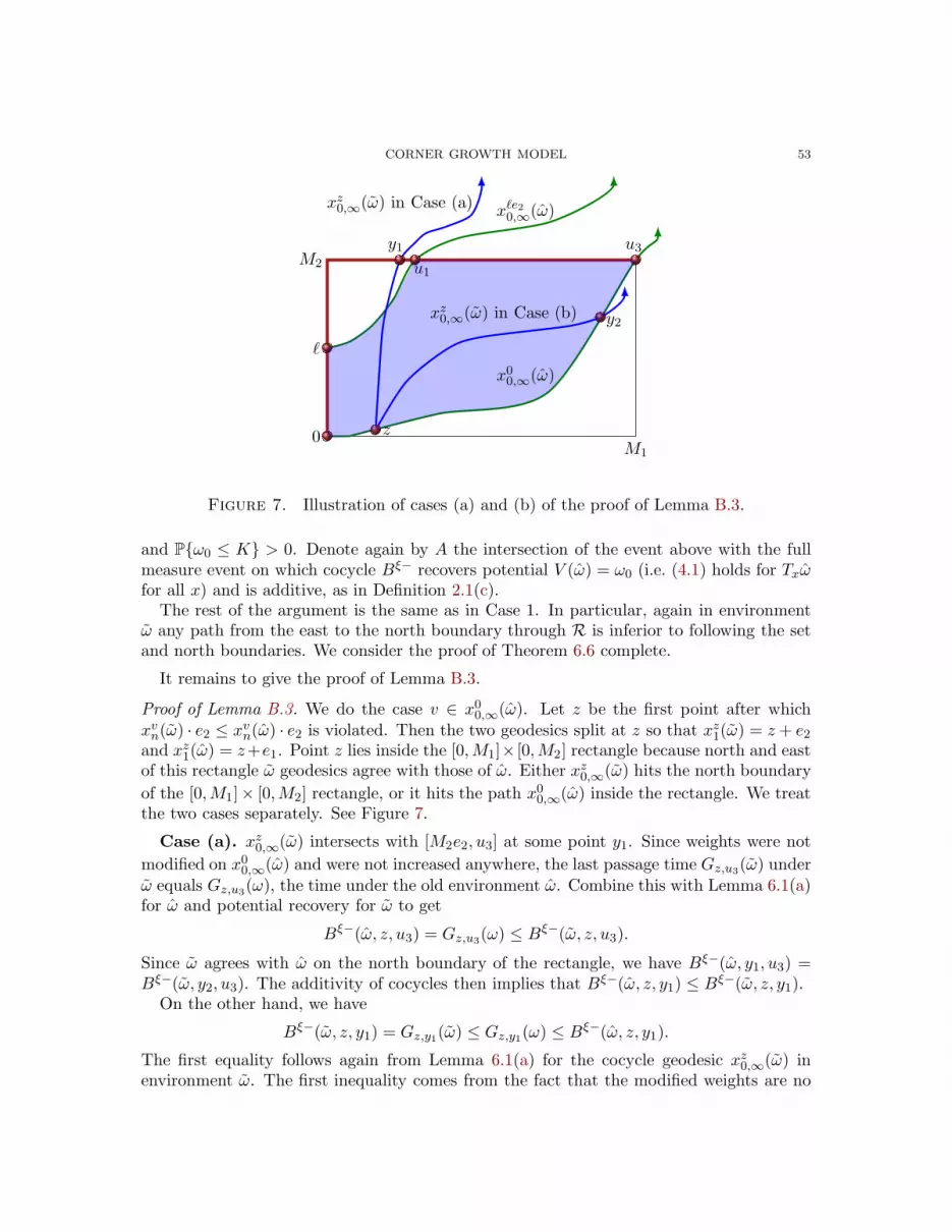
CORNER GROWTH MODEL 53

M1

M2

y2

y1

z0

ℓ

u1

u3

xℓe20,∞(ω)

x00,∞(ω)

xz0,∞(ω) in Case (b)

xz0,∞(ω) in Case (a)

Figure 7. Illustration of cases (a) and (b) of the proof of Lemma B.3.

and Pω0 ≤ K > 0. Denote again by A the intersection of the event above with the fullmeasure event on which cocycle Bξ− recovers potential V (ω) = ω0 (i.e. (4.1) holds for Txωfor all x) and is additive, as in Definition 2.1(c).

The rest of the argument is the same as in Case 1. In particular, again in environmentω any path from the east to the north boundary through R is inferior to following the setand north boundaries. We consider the proof of Theorem 6.6 complete.

It remains to give the proof of Lemma B.3.

Proof of Lemma B.3. We do the case v ∈ x00,∞(ω). Let z be the first point after whichxvn(ω) · e2 ≤ xvn(ω) · e2 is violated. Then the two geodesics split at z so that xz1(ω) = z + e2and xz1(ω) = z+e1. Point z lies inside the [0,M1]× [0,M2] rectangle because north and eastof this rectangle ω geodesics agree with those of ω. Either xz0,∞(ω) hits the north boundary

of the [0,M1]× [0,M2] rectangle, or it hits the path x00,∞(ω) inside the rectangle. We treat

the two cases separately. See Figure 7.

Case (a). xz0,∞(ω) intersects with [M2e2, u3] at some point y1. Since weights were not

modified on x00,∞(ω) and were not increased anywhere, the last passage time Gz,u3(ω) underω equals Gz,u3(ω), the time under the old environment ω. Combine this with Lemma 6.1(a)for ω and potential recovery for ω to get

Bξ−(ω, z, u3) = Gz,u3(ω) ≤ Bξ−(ω, z, u3).

Since ω agrees with ω on the north boundary of the rectangle, we have Bξ−(ω, y1, u3) =Bξ−(ω, y2, u3). The additivity of cocycles then implies that Bξ−(ω, z, y1) ≤ Bξ−(ω, z, y1).

On the other hand, we have

Bξ−(ω, z, y1) = Gz,y1(ω) ≤ Gz,y1(ω) ≤ Bξ−(ω, z, y1).

The first equality follows again from Lemma 6.1(a) for the cocycle geodesic xz0,∞(ω) inenvironment ω. The first inequality comes from the fact that the modified weights are no

54 N. GEORGIOU, F. RASSOUL-AGHA, AND T. SEPPALAINEN

larger than the original ones. The second inequality is again due to potential recovery.Combine all the inequalities above to conclude that

(B.4) Bξ−(ω, z, y1) = Bξ−(ω, z, y1)

and Bξ−(ω, z, u3) = Gz,u3(ω). Rewrite the last equality as

|u3−z|1−1∑

i=0

Bξ−(ω, xzi (ω), xzi+1(ω)) = Bξ−(ω, z, u3) = Gz,u3(ω) =

|u3−z|1−1∑

i=0

ωxzi (ω)

.

Potential recovery under ω and ω = ω on the path x00,∞(ω) now imply that the sums agreeterm by term. In particular,

(B.5) Bξ−(ω, z, xz1(ω)) = ωz.

In the same manner we deduce the statement

(B.6) Bξ−(ω, z, xz1(ω)) = ωz.

To see this last identity, consider this:

|y1−z|1−1∑

i=0

ωxzi (ω)≤

|y1−z|1−1∑

i=0

ωxzi (ω)≤

|y1−z|1−1∑

i=0

Bξ−(ω, xzi (ω), xzi+1(ω))

= Bξ−(ω, z, y1) = Bξ−(ω, z, y1) = Gz,y1(ω) =

|y1−z|1−1∑

i=0

ωxzi (ω)

.

The first two inequalities are valid term by term, by the modification and potential recovery.The third step is cocycle additivity, the fourth is (B.4) from above, and the last two aredue to xzi (ω) being a cocycle geodesic. The upshot is that the second and third sumsmust agree term by term. The equality of the first terms is (B.6) because ω = ω on thepath x00,∞(ω).

Equations (B.5)–(B.6) are incompatible with xz1(ω) 6= xz1(ω) since both geodesics followthe same tie-breaking rule t. Thus Case (a) led to a contradiction.

Case (b). xz0,∞(ω) intersects with x00,∞(ω) at some point y2 > z. Start by observing

that Gz,y2(ω) = Gz,y2(ω). Hence, Bξ−(ω, z, y2) = Bξ−(ω, z, y2) = Gz,y2(ω). An argumentsimilar to Case (a) shows that Case (b) cannot happen either.

We have proved the part of Lemma B.3 that claims xvn(ω) · e2 ≤ xvn(ω) · e2 for any

v ∈ x00,∞(ω). The claim for geodesics starting from v ∈ xℓe20,∞(ω) is proved similarly.

Appendix C. Ergodic theorem for cocycles

Cocycles satisfy a uniform ergodic theorem. The following is a special case of Theorem9.3 of [15]. Note that a one-sided bound suffices for a hypothesis. Recall Definition 2.1 forthe space C0 of centered cocycles.

Theorem C.1. Assume P is ergodic under the transformations Tei : i ∈ 1, 2. LetF ∈ C0. Assume there exists a function V such that for P-a.e. ω

(C.1) limεց0

limn→∞

maxx:|x|1≤n

1

n

∑

0≤k≤εn

|V (Tx+keiω)| = 0 for i ∈ 1, 2

CORNER GROWTH MODEL 55

and maxi∈1,2 F (ω, 0, ei) ≤ V (ω). Then

limn→∞

maxx=z1+···+znz1,n∈e1,e2n

|F (ω, 0, x)|n

= 0 for P-a.e. ω.

If the process V (Txω) : x ∈ Z2 is i.i.d., then a sufficient condition for (C.1) is E(|V |p) <

∞ for some p > 2 [29, Lemma A.4]

Appendix D. Percolation cone

In this appendix we prove Theorem 2.10. The proof is divided between two sections.Section D.1 proves that on U , gpp = 1 exactly on the percolation cone. Section D.2 provesthe differentiability of gpp at η = (βp1 , 1−βp1). Differentiability at η = (1−βp1 , βp1) comesby symmetry.

The standing assumptions are ωxx∈Z2 i.i.d., E|ω0|p < ∞ for some p > 2, ωx ≤ 1, andp1 = Pω0 = 1 > ~pc where ~pc is the critical probability of oriented site percolation. Theω-weights are assumed nondegenerate and so Pω0 < 1 > 0.

The oriented percolation weights are defined by σx = 1ωx = 1. The oriented perco-lation event u → v means that there exists an up-right path u = x0, x1, . . . , xm = v withxi−xi−1 ∈ e1, e2, m = |v−u|1, and such that σxi = 1 for i = 1, . . . ,m. (The initial pointu may be open or closed.) The percolation event u → ∞ means that there is an infiniteup-right path starting at u along which all weights σx = 1 except perhaps σu.

D.1. Flat edge. This section proves that on U the limiting time constant gpp is equal toone only on the percolation cone.

Theorem D.1. Let ξ ∈ U . Then gpp(ξ) = 1 if and only if 1− βp1 ≤ ξ · e1 ≤ βp1.

The rest of the section gives the proof.

Lemma D.2. Fix ρ ∈ (0, 1) and L > 0. Then there exists q0 = q0(ρ, L) ∈ (0, 1) such that thefollowing holds. If q ≥ q0 and τz : z ∈ Z

2 are stationary 0, 1-valued random variableswith Pτ0 = 1 = q and τ0 independent of τz : |z|1 > L, then there are positive constantsa and b such that, for all m ≥ 1,

P∃ up-right path z0,m : z0 = 0,

m∑

i=0

τzi ≤ ρ(m+ 1)≤ ae−bm.

Proof. First, fix m ≥ 1 and an up-right path z0,m such that z0 = 0. For k ≤ m + 1,on the event

∑mj=0(1 − τzj) = k, we can find, among the k indices with τzj = 0, indices

j1, . . . , j⌈k/(L+1)⌉ such that |zji − zjr |1 > L for all r, i ≤ ⌈k/(L+ 1)⌉. Given these indices,

the probability that τzjr = 0 for all r ≤ ⌈k/(L+ 1)⌉ is bounded above by (1 − q)k/(L+1).

There are at most( m+1⌈k/(L+1)⌉

)many choices of these indices. Consequently,

P m∑

j=0

(1− τzj) = k≤

(m+ 1

⌈k/(L + 1)⌉

)(1− q)k/(L+1).

56 N. GEORGIOU, F. RASSOUL-AGHA, AND T. SEPPALAINEN

This implies

P m∑

i=0

τzj ≤ ρ(m+ 1)≤

∑

(1−ρ)(m+1)≤k≤m+1

(m+ 1

⌈k/(L+ 1)⌉

)(1− q)k/(L+1).

Since there are 2m paths z0,m, the probability in the claim of the lemma is then boundedabove by

2m∑

(1−ρ)(m+1)≤k≤m+1

(m+ 1

⌈k/(L+ 1)⌉

)(1− q)k/(L+1)

≤ 2m(1− q)(1−ρ)(m+1)/(L+1) × (L+ 1)

m+1∑

i=0

(m+ 1

i

)

≤ 2(L+ 1)(1 − q)(1−ρ)/(L+1) exp[

log 4 +1− ρL+ 1

log(1− q)]m.

This decays exponentially fast as soon as q > 1− 4−(L+1)/(1−ρ).

The main work is in the next proposition.

Proposition D.3. Assume p1 = Pω0 = 1 > ~pc. Then for each ε ∈ (0, 1 − βp1) thereexist finite positive constants A, B, and δ such that for all ℓ, k ∈ N with ℓ/k ≤ (1 − βp1 −ε)/(βp1 + ε) we have

PG0,(k,ℓ) ≥ (1− δ)(k + ℓ) ≤ Ae−Bk.(D.1)

Proof. For N ∈ N and z ∈ Z2 define

CN (0) = x ≥ 0 : |x|1 < N, CN (z) = z + CN (0), and BN (z) = C2N (z) \ CN (z).

Fix ε1 ∈ (0, ε). Fix δ0 ∈ (0, 1) such that p0 = Pω0 ≥ 1−δ0 > ~pc and βp1 ≤ βp0 < βp1+ε.Here we used the continuity of βp as a function of p ∈ [~pc, 1) [10, (3) on p. 1031].

Abbreviate

λp1,ε1 =1− βp1 − ε1βp1 + ε1

.

Given N ∈ N and ω ∈ Ω, color z ∈ Z2 black if

Gu,v ≤ |v − u|1 − δ0(D.2)

for every Nz ≤ u ≤ v with |u−Nz|1 = N , |v − u|1 = N , and

(v − u) · e2(v − u) · e1

≤ λp1,ε1 .

See the left panel of Figure 9. Color z white if it is not black. Then

P0 is white ≤ (N + 1)P∃v ≥ 0 : |v|1 = N, v · e2/v · e1 ≤ λp1,ε1 , G0,v > |v|1 − δ0

= p−1(N + 1)P∃v ≥ 0 : |v|1 = N, v · e2/v · e1 ≤ λp1,ε1 , G0,v > |v|1 − δ0, ωv = 1

.

(For the equality we used the fact that G0,v is independent of ωv.) Define the oriented sitepercolation weights σx = 1ωx ≥ 1−δ0. Since ωx ≤ 1 for all x, ωv = 1 and G0,v > |v|1−δ0

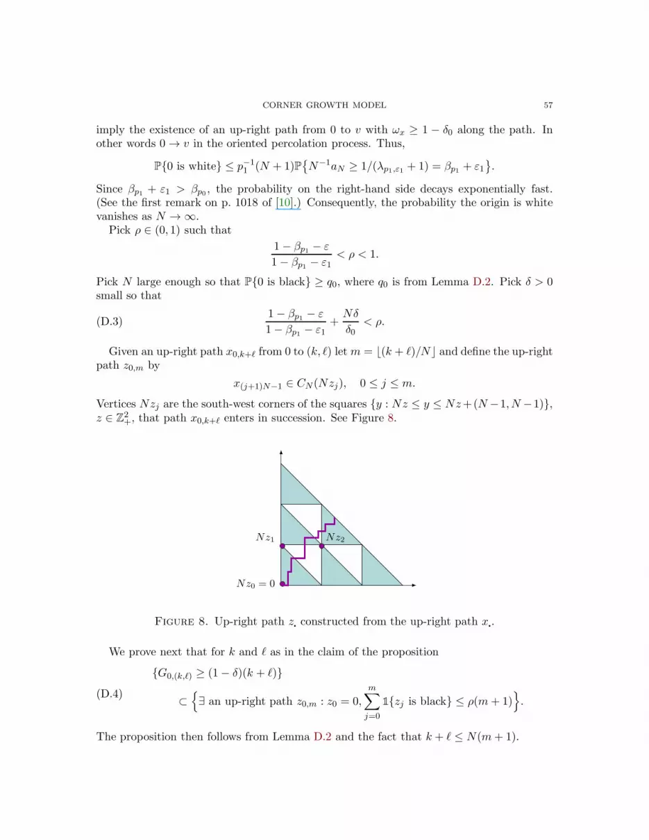
CORNER GROWTH MODEL 57

imply the existence of an up-right path from 0 to v with ωx ≥ 1 − δ0 along the path. Inother words 0→ v in the oriented percolation process. Thus,

P0 is white ≤ p−11 (N + 1)P

N−1aN ≥ 1/(λp1,ε1 + 1) = βp1 + ε1

.

Since βp1 + ε1 > βp0 , the probability on the right-hand side decays exponentially fast.(See the first remark on p. 1018 of [10].) Consequently, the probability the origin is whitevanishes as N →∞.

Pick ρ ∈ (0, 1) such that

1− βp1 − ε1− βp1 − ε1

< ρ < 1.

Pick N large enough so that P0 is black ≥ q0, where q0 is from Lemma D.2. Pick δ > 0small so that

1− βp1 − ε1− βp1 − ε1

+Nδ

δ0< ρ.(D.3)

Given an up-right path x0,k+ℓ from 0 to (k, ℓ) letm = ⌊(k + ℓ)/N⌋ and define the up-rightpath z0,m by

x(j+1)N−1 ∈ CN (Nzj), 0 ≤ j ≤ m.Vertices Nzj are the south-west corners of the squares y : Nz ≤ y ≤ Nz+(N−1, N −1),z ∈ Z

2+, that path x0,k+ℓ enters in succession. See Figure 8.

Nz0 = 0

Nz1 Nz2

Figure 8. Up-right path z constructed from the up-right path x.

We prove next that for k and ℓ as in the claim of the proposition

G0,(k,ℓ) ≥ (1− δ)(k + ℓ)

⊂∃ an up-right path z0,m : z0 = 0,

m∑

j=0

1zj is black ≤ ρ(m+ 1).

(D.4)

The proposition then follows from Lemma D.2 and the fact that k + ℓ ≤ N(m+ 1).

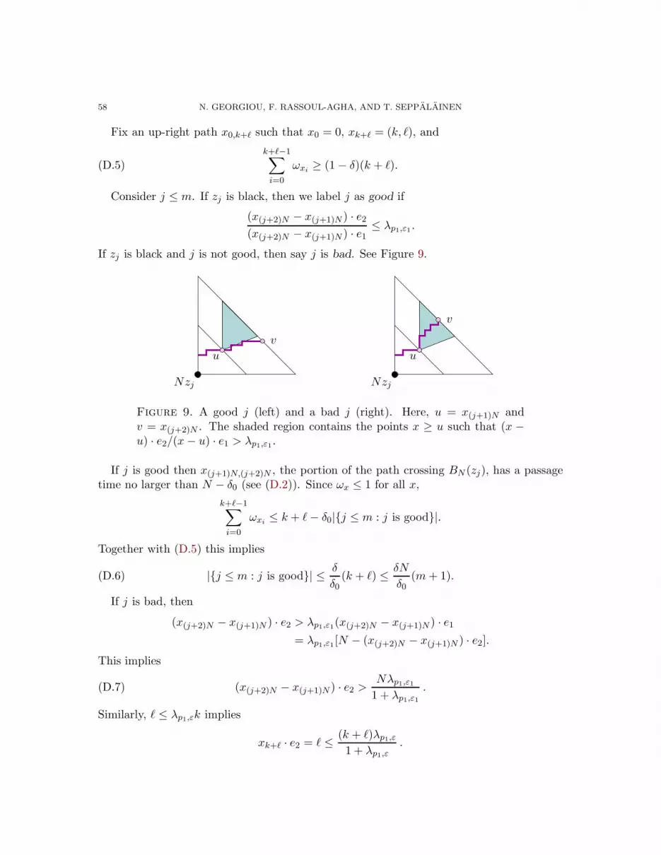
58 N. GEORGIOU, F. RASSOUL-AGHA, AND T. SEPPALAINEN

Fix an up-right path x0,k+ℓ such that x0 = 0, xk+ℓ = (k, ℓ), and

k+ℓ−1∑

i=0

ωxi ≥ (1− δ)(k + ℓ).(D.5)

Consider j ≤ m. If zj is black, then we label j as good if

(x(j+2)N − x(j+1)N ) · e2(x(j+2)N − x(j+1)N ) · e1

≤ λp1,ε1 .

If zj is black and j is not good, then say j is bad. See Figure 9.

v

u

Nzj

v

u

Nzj

Figure 9. A good j (left) and a bad j (right). Here, u = x(j+1)N andv = x(j+2)N . The shaded region contains the points x ≥ u such that (x −u) · e2/(x− u) · e1 > λp1,ε1 .

If j is good then x(j+1)N,(j+2)N , the portion of the path crossing BN (zj), has a passagetime no larger than N − δ0 (see (D.2)). Since ωx ≤ 1 for all x,

k+ℓ−1∑

i=0

ωxi ≤ k + ℓ− δ0|j ≤ m : j is good|.

Together with (D.5) this implies

|j ≤ m : j is good| ≤ δ

δ0(k + ℓ) ≤ δN

δ0(m+ 1).(D.6)

If j is bad, then

(x(j+2)N − x(j+1)N ) · e2 > λp1,ε1(x(j+2)N − x(j+1)N ) · e1= λp1,ε1 [N − (x(j+2)N − x(j+1)N ) · e2].

This implies

(x(j+2)N − x(j+1)N ) · e2 >Nλp1,ε11 + λp1,ε1

.(D.7)

Similarly, ℓ ≤ λp1,εk implies

xk+ℓ · e2 = ℓ ≤ (k + ℓ)λp1,ε1 + λp1,ε

.

CORNER GROWTH MODEL 59

Adding (D.7) over the bad j now leads to

Nλp1,ε11 + λp1,ε1

|j ≤ m : j is bad| ≤ (k + ℓ)λp1,ε1 + λp1,ε

.

Consequently,

|j ≤ m : j is bad| ≤ 1− βp1 − ε1− βp1 − ε1

· k + ℓ

N≤ 1− βp1 − ε

1− βp1 − ε1(m+ 1).(D.8)

By the choice of δ in (D.3), adding (D.6) and (D.8) we see that for a path satisfying(D.5) the proportion of zj colored black is no more than ρ(m+1). Inclusion (D.4) has beenverified and Proposition D.3 proved.

Proof of Theorem D.1. On the positive probability event 0 → ∞ in the oriented perco-lation with weights σx = 1ωx = 1 we have 0 → (an, n − an) and G0,(an,n−an) = n for alln. Since an/n → βp1 as n → ∞, the shape theorem (E.1) implies gpp(βp1 , 1 − βp1) = 1.By symmetry, we have gpp(1 − βp1 , βp1) = 1 as well. Concavity of gpp and the fact thatgpp(ξ) ≤ 1 for all ξ ∈ U imply that gpp(ξ) = 1 when 1− βp1 ≤ ξ · e1 ≤ βp1 .

For the other direction assume ξ ·e1 > βp1 and apply (D.1) to (k, ℓ) = ⌊nξ⌋ in conjunctionwith (2.2) to deduce that gpp(ξ) ≤ 1 − δ for some δ > 0. The result for ξ · e1 < 1 − βp1comes by symmetry.

D.2. Differentiability at the endpoints. In this section we prove that gpp is differ-entiable at η = (βp1 , 1 − βp1). It is convenient here to alter the definition (1.1) of thelast-passage time Gx,y so that ωx is excluded and ωy is included. This of course makes nodifference to the limit gpp.

We define the oriented percolation process more generally. The successive levels on whichthe process lives are denoted by Dn = (i, j) ∈ Z

2 : i + j = n. Let S ⊂ Dm be a giveninitial occupied set. Then at time n ∈ Z+ the occupied set is On(S) = v ∈ Dm+n : ∃u ∈S : u→ v. If S is bounded below (S has only finitely many points below the x-axis), thelowest point rn(S) of On(S) is well-defined and satisfies rn(S) = (an(S), bn(S)) where

an(S) = maxu∈On(S)

u · e1 and bn(S) = minu∈On(S)

u · e2.

A particular case of such an initial set is Z− = (−k, k) : k ∈ Z+, the antidiagonal copyof Z−. Occasionally we also use the notation b(On(S)) = bn(S). Let Fm = (k,−k) : k =1, . . . ,m.

Lemma D.4. For infinite sets A ⊆ B ⊆ Z−,

E[an(A ∪ Fm)− an(A)] ≥ E[an(B ∪ Fm)− an(B)] ≥ mwith equality in the last inequality if B = Z−.

Proof. Since On(A ∪ Fm) = On(A) ∪ On(Fm),

an(A ∪ Fm)− an(A) = an(A) ∨ an(Fm)− an(A) = 0 ∨ (an(Fm)− an(A))≥ 0 ∨ (an(Fm)− an(B)) = an(B ∪ Fm)− an(B).

By a shift of the underlying weights ω,

rn(Z− ∪ Fm)(ω) = rn(Z−)(Tm,−mω) + (m,−m).

60 N. GEORGIOU, F. RASSOUL-AGHA, AND T. SEPPALAINEN

By the shift-invariance of P

E[an(Z− ∪ Fm)]− E[an(Z−)] = m.

Let ℓ be an integer ≥ 2. Fix a constant c0 < 1 such that P(c0 ≤ ω0 < 1) > 0. Tohave an ℓ-triangle (configuration) at (a, b) ∈ Z

2 means that ωa,b+i < 1 for i = 1, . . . , ℓ,c0 ≤ ωa+1,b < 1, and except for (a + 1, b) all sites in the triangle (i, j) : i ≥ a + 1, j ≥b, i− (a+ 1) + j − b ≤ ℓ− 1 have weight ωi,j = 1. See Figure 10.

a

b

a+ ℓ

b+ ℓ

Figure 10. An ℓ-triangle at (a, b) with ℓ = 5. The weight ωa,b is unrestricted.The column above (a, b) has weights ωa,b+i < 1. Point (a + 1, b) has weight c0 ≤ωa+1,b < 1. In the region inside the dotted boundary all weights are equal to 1.

Let Vℓ = (ℓ − i, i) : 0 ≤ i ≤ ℓ − 1. Suppose there is an ℓ-triangle at (a, b). Then twothings happen that are relevant for the sequel.

(D.9)There is an up-right path of ω-weight ℓ+ ωa+1,b − 1 ≥ ℓ+ c0 − 1 from (a, b)

to each of the ℓ sites of (a, b) + Vℓ, without counting the weight at (a, b).

Furthermore, no open oriented percolation path can go through any of the sites (a +1, b), (a, b + i) : i = 1, . . . , ℓ.

Now let S be an infinite initial set that is bounded below. Set O0n = On(S), r

0n = rn(S) =

(a0n, b0n). Define the stopping time

τ1 = infn > 0 : ∃ ℓ-triangle at r0nℓ−ℓ.The natural filtration is Hm = σωi,j : i+ j ≤ m.

Since r0τ1ℓ−ℓ is the lowest point of the occupied set O0τ1ℓ−ℓ, no open oriented percolation

path can reach r0τ1ℓ−ℓ + Vℓ:

(r0τ1ℓ−ℓ + Vℓ) ∩ O0τ1ℓ = ∅.

To each point of the set V 0τ1ℓ

= r0τ1ℓ−ℓ + Vℓ ⊂ Dτ1ℓ there is an up-right path of ω-weight

τ1ℓ− 1 + ωr0τ1ℓ−ℓ+e1 ≥ τ1ℓ− 1 + c0

from some point on S.Start a new process O1

n at level τ1ℓ by joining V 0τ1ℓ

to the occupied set:

O1n =

O0

n, n ≤ τ1ℓ− 1

On−τ1ℓ(O0τ1ℓ∪ V 0

τ1ℓ), n ≥ τ1ℓ.

CORNER GROWTH MODEL 61

Let r1n = (a1n, b1n) be the lowest point of O1

n.Continue in this manner, with

τk+1 = infn > τk : ∃ ℓ-triangle at rknℓ−ℓ, V kτk+1ℓ

= rkτk+1ℓ−ℓ + Vℓ,

Ok+1n =

Ok

n, n ≤ τk+1ℓ− 1

On−τk+1ℓ(Okτk+1ℓ

∪ V kτk+1ℓ

), n ≥ τk+1ℓ,

with lowest point rk+1n = (ak+1

n , bk+1n ).

Let ρℓ > 0 be the probability of an ℓ-triangle and Kn = maxk : τk ≤ n ∼ Binom(n, ρℓ).

Lemma D.5. For any infinite initial occupied set that is bounded below,

E[aKnnℓ − a0nℓ] ≥ nℓρℓ and E[bKn

nℓ − b0nℓ] ≤ −nℓρℓ.

Proof. The two statements are equivalent since aKnnℓ +bKn

nℓ = nℓ = a0nℓ+b0nℓ. Since a

knℓ = aKn

nℓfor k > Kn, and by the strong Markov property and Lemma D.4,

E[aKnnℓ − a0nℓ] =

n∑

k=1

E[aknℓ − ak−1nℓ ] =

n∑

k=1

E[aknℓ − ak−1nℓ , τk ≤ n]

=

n∑

k=1

E[anℓ−τkℓ(Ok−1

τkℓ∪ V k−1

τkℓ)− anℓ−τkℓ(Ok−1

τkℓ), τk ≤ n

]

≥ ℓn∑

k=1

P(τk ≤ n) = ℓnρℓ.

For the remainder of the proof the initial set for oriented percolation is S = Z−.

Lemma D.6. With initial set S = Z−,

(D.10) limn→∞

(nℓ)−1E[ aKn

nℓ | 0→ Dnℓ] ≥ βp1 + ρℓ.

Proof. We prove the equivalent statement

(D.11) limn→∞

(nℓ)−1E[ bKn

nℓ | 0→ Dnℓ] ≤ 1− βp1 − ρℓ.

Let m < n. Since paths never go in the −e2 direction, bKnnℓ ≥ 0, and so

(D.12)E[ bKn

nℓ 10→ Dnℓ ] ≤ E[ bKnnℓ 10→ Dmℓ ]

= E[Eb(OKn

nℓ (Z−))∣∣Hmℓ

10→ Dmℓ

].

To bound the conditional expectation use the Markov property to restart the evolution

at OKmmℓ (Z−) and apply Lemma D.5. Note that OKm

mℓ (Z−) ⊃ O0mℓ(Z−). Hence if we replace

OKmmℓ (Z−) with O0

mℓ(Z−) as the initial set of an oriented percolation process, the lateroccupied set shrinks, which implies that the lowest e2-coordinate increases.

E[b(OKn

nℓ (Z−))∣∣Hmℓ

]= E

[b(OKn−m

(n−m)ℓ(OKmmℓ (Z−)))

∣∣Hmℓ

]

≤ E[b(O0

(n−m)ℓ(OKmmℓ (Z−)))

∣∣Hmℓ

]− (n−m)ℓρℓ

≤ E[b(O0

(n−m)ℓ(O0mℓ(Z−)))

∣∣Hmℓ

]− (n−m)ℓρℓ.

62 N. GEORGIOU, F. RASSOUL-AGHA, AND T. SEPPALAINEN

Substitute this back up in (D.12) to get the bound

(D.13)E[ bKn

nℓ 10→ Dnℓ ]≤ E

[b(O0

nℓ(Z−))10→ Dmℓ]− (n−m)ℓρℓP0→ Dmℓ.

For oriented percolation with p1 > ~pc we have the limits

n−1r(O0n(Z−))→ (βp1 , 1 − βp1) in L1 and P0→ Dn → P0→∞ > 0.

The L1 convergence of the lowest point is a consequence of the subadditive ergodic theoremand estimate (3) for oriented percolation on p. 1028 pf [10]. To get the conclusion (D.11)divide through (D.13) by nℓP0→ Dnℓ and let first n→∞ and then m→∞.

The final piece of preparation derives a bound on last-passage times.

Lemma D.7. Let the initial set for the construction of rkn be S = Z−. Then the orientedpercolation event 0→ Dn implies that G0, rkn

≥ n+ k(c0 − 1) for all n, k ≥ 0.

Proof. Induction on k. The case k = 0 is clear because 0 → Dn implies that there is anoriented percolation path from 0 to r0n, which is also an up-right path with ω-weight n.

Assume the claim is true for k. For n ≤ τk+1ℓ − 1 we have rk+1n = rkn and the claim

follows for k + 1 because c0 − 1 < 0.Suppose n ≥ τk+1ℓ. If r

k+1n and rkn do not coincide, rk+1

n must lie below rkn on level Dn.It follows that a path that links level Dτk+1ℓ to rk+1

n must originate from V kτk+1ℓ

. (If not,

such a path originates from Okτk+1ℓ

which forces rk+1n = rkn.) Now construct a path from 0

to rk+1n as follows. The induction assumption gives a path from 0 to rkτk+1ℓ−ℓ with ω-weight

≥ τk+1ℓ− ℓ+ k(c0 − 1). The oriented percolation path from V kτk+1ℓ

to rk+1n gives ω-weight

n− τk+1ℓ. Connect the two paths by taking (D.9) from rkτk+1ℓ−ℓ to a point on V kτk+1ℓ

with

ω-weight ≥ ℓ+c0−1. Adding up these pieces verifies that G0, rk+1n≥ n+(k+1)(c0−1).

Differentiability of gpp at η is equivalent to the differentiability of g(s) = gpp(s, 1− s) ats = βp1 . The left derivative g′(βp1−) = 0 because g(s) = 1 for 1− βp1 ≤ s ≤ βp1 . We showthat the right derivative equals zero also. Since g is concave and attains its maximum on[1− βp1 , βp1 ], it must be strictly decreasing on [βp1 , 1].

g(βp1 + ρℓ) ≥ g(

limn→∞

(nℓ)−1E[ aKn

nℓ | 0→ Dnℓ])

= limn→∞

g(E[(nℓ)−1aKn

nℓ

∣∣ 0→ Dnℓ

])

≥ limn→∞

E[g((nℓ)−1aKn

nℓ

) ∣∣ 0→ Dnℓ

]

= limn→∞

1

P0→ DnℓE[g((nℓ)−1aKn

nℓ

)10→ Dnℓ

]

= limn→∞

1

P0→ DnℓE[(nℓ)−1gpp

(rKnnℓ

)10→ Dnℓ

]

= limn→∞

1

P0→ DnℓE[(nℓ)−1G

0, rKnnℓ

10→ Dnℓ]

CORNER GROWTH MODEL 63

≥ limn→∞

1

P0→ DnℓE[ (

1 + (c0 − 1)(nℓ)−1Kn

)10→ Dnℓ

]

= 1 + (c0 − 1)ℓ−1ρℓ.

In the calculation above first use (D.10) and the monotonicity and continuity of g, thenconcavity to put g inside the conditional expectation. Homogeneity of gpp is used. Thesecond-last equality uses the L1 shape theorem (E.1) from Appendix E. The last inequalityuses Lemma D.7. The last equality is from the L1 limit Kn/n→ ρℓ.

From this and g(βp1) = 1 we write

0 ≥ g(βp1 + ρℓ)− g(βp1)ρℓ

≥ c0 − 1

ℓ.

Letting ℓր∞ takes ρℓ ց 0 and yields g′(βp1+) = 0. Differentiability of gpp at η has beenestablished. This concludes the proof of Theorem 2.10.

Appendix E. Shape theorem

Theorem E.1. Assume ωx are i.i.d. such that

∫ 0

−∞Pω0 ≤ r1/2 dr <∞ and

∫ ∞

0Pω0 > r1/2 dr <∞.

Then

limn→∞

n−1 maxx∈Z+

2 :|x|1=n|G0,x − gpp(x)| = 0 P-almost surely and in L1.(E.1)

Proof. The almost sure limit is in Theorem 5.1(i) of [25]. We prove the L1 limit.Fix an integer k ≥ 2. Let ξℓ = (ℓ/k, 1 − ℓ/k), ℓ ∈ 0, . . . , k. Given an integer n ≥ 2, let

m−n = ⌊n/(1 + 1/k)⌋ ∈ [1, n) and m+

n = ⌈n/(1 − 1/k)⌉ ≥ n.Given x ≥ 0 with |x|1 = n there exists ℓ−(x) ∈ 0, . . . , k such that m−

n ξℓ−(x) ≤ x. (Thisis because n−m−

n ≥ m−n /k.) Also, there exists ℓ+(x) ∈ 0, . . . , k such that x ≤ m+

n ξℓ+(x).

(This is because m+n − n ≥ m+

n /k.)A path from 0 to x can first go to ⌊m−

n ξℓ−(x)⌋ and then take at most n − m−n + 1 ≤

n/(k + 1) + 2 e1-steps followed by at most n/(k + 1) + 2 e2-steps. Hence,

G0,x ≥ G0,⌊m−n ξℓ−(x)⌋

−n/(k+1)+1∑

i=0

|ω⌊m−n ξℓ−(x)⌋+ie1

|

− max0≤i≤n/(k+1)+1

n/(k+1)+1∑

j=0

|ω⌊m−n ξℓ−(x)⌋+ie1+je2

|.

64 N. GEORGIOU, F. RASSOUL-AGHA, AND T. SEPPALAINEN

This gives

G0,x − gpp(x) ≥ gpp(⌊m−n ξℓ−(x)⌋)− gpp(x) +G0,⌊m−

n ξℓ−(x)⌋− gpp(⌊m−

n ξℓ−(x)⌋)

−n/(k+1)+1∑

i=0

|ω⌊m−n ξℓ−(x)⌋+ie1

|

− max0≤i≤n/(k+1)+1

n/(k+1)+1∑

j=0

|ω⌊m−n ξℓ−(x)⌋+ie1+je2

|.

Similarly,

G0,x − gpp(x) ≤ gpp(⌊m+n ξℓ+(x)⌋)− gpp(x) +G0,⌊m+

n ξℓ+(x)⌋− gpp(⌊m+

n ξℓ+(x)⌋)

+

n/(k−1)+1∑

i=0

|ω⌊m+n ξℓ+(x)⌋−ie1

|

+ max0≤i≤n/(k−1)+1

n/(k−1)+1∑

j=0

|ω⌊m+n ξℓ+(x)⌋−ie1−je2

|.

Note that |⌊m±n ξℓ±(x)⌋ − x|1 ≤ 1 + 2|n−m±

n | ≤ 1 + 2n/(1 ∓ k). By continuity of gpp

limk→∞

limn→∞

n−1 maxx∈nU

|gpp(⌊m±n ξℓ+(x)⌋)− gpp(x)|

= limk→∞

limn→∞

maxx∈nU

|gpp(n−1⌊m±n ξℓ+(x)⌋)− gpp(n−1x)| = 0.

By Proposition 2.1(i) of [25]

limn→∞

n−1E

[max0≤ℓ≤k

|G0,⌊m±n ξℓ⌋− gpp(⌊m±

n ξℓ⌋)|]= 0.

Next we put some distance between the sums to make them independent:

n−1E

[max0≤ℓ≤k

max0≤i≤n/(k−1)+1

n/(k−1)+1∑

j=0

|ω⌊m−n ξℓ⌋+ie1+je2

|]

≤ n−1E

[max

0≤ℓ≤k/2max

0≤i≤n/(k−1)+1

n/(k−1)+1∑

j=0

|ω⌊m−n ξ2ℓ⌋+ie1+je2

|]

+ n−1E

[max

0≤ℓ<k/2max

0≤i≤n/(k−1)+1

n/(k−1)+1∑

j=0

|ω⌊m−n ξ2ℓ+1⌋+ie1+je2

|].

The proof of the theorem is complete if we prove that the right-hand side vanishes as firstn→∞ and then k →∞. We show the first limit, the second being similar. Centering the|ωx| terms does not change the limit. Hence, we will show that

limk→∞

limn→∞

n−1E

[max

0≤ℓ≤k/2max

0≤i≤n/(k−1)+1

n/(k−1)+1∑

j=0

(|ω⌊m−n ξ2ℓ⌋+ie1+je2

| − E|ω0|)]= 0.

CORNER GROWTH MODEL 65

Abbreviate σ2 = E[|ω0|2]− (E|ω0|)2 and let

Si,ℓn,k =

n/(k−1)+1∑

j=0

(|ω⌊m−n ξ2ℓ⌋+ie1+je2

| − E|ω0|).

Note that Si,ℓn,k : 0 ≤ i ≤ n/(k − 1) + 1, 0 ≤ ℓ ≤ k/2 are i.i.d. By taking n and k

large enough and restricting to t ≥ k−1/4 Chebyshev’s inequality gives PS0,0n,k ≥ nt ≤

2σ2/(nkt2) < 1/2. Using (k2 + 1)( nk−1 + 2) ≤ 2n and (1 − δ)n ≥ 1 − nδ we bound the

expectation:

E[

max0≤ℓ≤k/2

max0≤i≤n/(k−1)+1

n−1Si,ℓn,k

]=

∫ ∞

0P

max

0≤ℓ≤k/2max

0≤i≤n/(k−1)+1Si,ℓn,k ≥ nt

dt

≤ k−1/4 +

∫ ∞

k−1/4

[1−

(1− 2σ2

nkt2

)2n ]dt

≤ k−1/4 +

∫ ∞

k−1/4

4σ2

kt2dt = k−1/4 + 4σ2k−3/4 −→ 0

as n→∞ and then k →∞. The argument can be repeated for the other sums.

References

[1] S. N. Armstrong and P. E. Souganidis. Stochastic homogenization of Hamilton-Jacobiand degenerate Bellman equations in unbounded environments. J. Math. Pures Appl.(9), 97(5):460–504, 2012.

[2] A. Auffinger and M. Damron. Differentiability at the edge of the percolation coneand related results in first-passage percolation. Probab. Theory Related Fields, 156(1-2):193–227, 2013.

[3] M. Balazs, E. Cator, and T. Seppalainen. Cube root fluctuations for the corner growthmodel associated to the exclusion process. Electron. J. Probab., 11:no. 42, 1094–1132(electronic), 2006.

[4] D. L. Burkholder. Distribution function inequalities for martingales. Ann. Probability,1:19–42, 1973.

[5] R. M. Burton and M. Keane. Density and uniqueness in percolation. Comm. Math.Phys., 121(3):501–505, 1989.

[6] H. Cohn, N. Elkies, and J. Propp. Local statistics for random domino tilings of theAztec diamond. Duke Math. J., 85(1):117–166, 1996.

[7] I. Corwin. The Kardar-Parisi-Zhang equation and universality class. Random MatricesTheory Appl., 1(1):1130001, 76, 2012.

[8] D. Coupier. Multiple geodesics with the same direction. Electron. Commun. Probab.,16:517–527, 2011.

[9] M. Damron and J. Hanson. Busemann functions and infinite geodesics in two-dimensional first-passage percolation. Comm. Math. Phys., 325(3):917–963, 2014.

[10] R. Durrett. Oriented percolation in two dimensions. Ann. Probab., 12(4):999–1040,1984.

[11] R. Durrett and T. M. Liggett. The shape of the limit set in Richardson’s growth model.Ann. Probab., 9(2):186–193, 1981.

66 N. GEORGIOU, F. RASSOUL-AGHA, AND T. SEPPALAINEN

[12] P. A. Ferrari, J. B. Martin, and L. P. R. Pimentel. A phase transition for competitioninterfaces. Ann. Appl. Probab., 19(1):281–317, 2009.

[13] P. A. Ferrari and L. P. R. Pimentel. Competition interfaces and second class particles.Ann. Probab., 33(4):1235–1254, 2005.

[14] N. Georgiou, F. Rassoul-Agha, and T. Seppalainen. Variational formulas and co-cycle solutions for directed polymer and percolation models. 2013. Submitted(arXiv:1311.0316).

[15] N. Georgiou, F. Rassoul-Agha, T. Seppalainen, and A. Yilmaz. Ratios of partition func-tions for the log-gamma polymer. Ann. Probab., 2013. To appear (arXiv:1303.1229).

[16] C. D. Howard and C. M. Newman. Geodesics and spanning trees for Euclidean first-passage percolation. Ann. Probab., 29(2):577–623, 2001.

[17] W. Jockusch, J. Propp, and P. Shor. Random domino tilings and the arctic circletheorem. 1998. arXiv:math/9801068.

[18] K. Johansson. Shape fluctuations and random matrices. Comm. Math. Phys.,209(2):437–476, 2000.

[19] K. Johansson. Random matrices and determinantal processes. In Mathematical statis-tical physics, pages 1–55. Elsevier B. V., Amsterdam, 2006.

[20] A. Krishnan. Variational formula for the time-constant of first-passage percolation I:Homogenization. 2013. arXiv:1311.0316.

[21] C. Licea and C. M. Newman. Geodesics in two-dimensional first-passage percolation.Ann. Probab., 24(1):399–410, 1996.

[22] R. M. Loynes. The stability of a queue with non-independent interarrival and servicetimes. Proc. Cambridge Philos. Soc., 58:497–520, 1962.

[23] J. Mairesse and B. Prabhakar. The existence of fixed points for the ·/GI/1 queue.Ann. Probab., 31(4):2216–2236, 2003.

[24] R. Marchand. Strict inequalities for the time constant in first passage percolation.Ann. Appl. Probab., 12(3):1001–1038, 2002.

[25] J. B. Martin. Limiting shape for directed percolation models. Ann. Probab.,32(4):2908–2937, 2004.

[26] C. M. Newman. A surface view of first-passage percolation. In Proceedings of theInternational Congress of Mathematicians, Vol. 1, 2 (Zurich, 1994), pages 1017–1023,Basel, 1995. Birkhauser.

[27] B. Prabharkar. The attractiveness of the fixed points of a ·/GI/1 queue. Ann. Probab.,31(4):2237–2269, 2003.

[28] F. Rassoul-Agha and T. Seppalainen. Quenched point-to-point free energy for randomwalks in random potentials. Probab. Theory Related Fields, 158(3-4):711–750, 2014.

[29] F. Rassoul-Agha, T. Seppalainen, and A. Yilmaz. Quenched free energy and large de-viations for random walks in random potentials. Comm. Pure Appl. Math., 66(2):202–244, 2013.

[30] H. Rost. Nonequilibrium behaviour of a many particle process: density profile andlocal equilibria. Z. Wahrsch. Verw. Gebiete, 58(1):41–53, 1981.

[31] T. Seppalainen. Hydrodynamic scaling, convex duality and asymptotic shapes ofgrowth models. Markov Process. Related Fields, 4(1):1–26, 1998.

[32] T. Seppalainen. Scaling for a one-dimensional directed polymer with boundary condi-tions. Ann. Probab., 40(1):19–73, 2012.

CORNER GROWTH MODEL 67

Nicos Georgiou, University of Sussex, School of Mathematical and Physical Sciences,

Department of Mathematics, Falmer Campus, Brighton BN1 9QH, UK.

E-mail address: n.georgiou@sussex.ac.uk

Firas Rassoul-Agha, University of Utah, Mathematics Department, 155S 1400E, Room 233.,

Salt Lake City, UT 84112, USA.

E-mail address: firas@math.utah.edu

URL: http://www.math.utah.edu/~firas

Timo Seppalainen, University of Wisconsin-Madison, Mathematics Department, Van Vleck

Hall, 480 Lincoln Dr., Madison WI 53706-1388, USA.

E-mail address: seppalai@math.wisc.edu

URL: http://www.math.wisc.edu/~seppalai