Embed Size (px)
Citation preview

STATA January 1993
TECHNICAL STB-11
BULLETINA publication to promote communication among Stata users
Editor Associate Editors
Joseph Hilbe J. Theodore Anagnoson, Cal. State Univ., LADepartment of Sociology Richard DeLeon, San Francisco State Univ.Arizona State University Paul Geiger, USC School of MedicineTempe, Arizona 85287 Lawrence C. Hamilton, Univ. of New Hampshire602-860-1446 FAX Stewart West, Baylor College of [email protected] EMAIL
Subscriptions are available from Stata Corporation, email [email protected], telephone 979-696-4600 or 800-STATAPC,fax 979-696-4601. Current subscription prices are posted at www.stata.com/bookstore/stb.html.
Previous Issues are available individually from StataCorp. See www.stata.com/bookstore/stbj.html for details.
Submissions to the STB, including submissions to the supporting files (programs, datasets, and help files), are ona nonexclusive, free-use basis. In particular, the author grants to StataCorp the nonexclusive right to copyright anddistribute the material in accordance with the Copyright Statement below. The author also grants to StataCorp the rightto freely use the ideas, including communication of the ideas to other parties, even if the material is never publishedin the STB. Submissions should be addressed to the Editor. Submission guidelines can be obtained from either theeditor or StataCorp.
Copyright Statement. The Stata Technical Bulletin (STB) and the contents of the supporting files (programs,datasets, and help files) are copyright c by StataCorp. The contents of the supporting files (programs, datasets, andhelp files), may be copied or reproduced by any means whatsoever, in whole or in part, as long as any copy orreproduction includes attribution to both (1) the author and (2) the STB.
The insertions appearing in the STB may be copied or reproduced as printed copies, in whole or in part, as longas any copy or reproduction includes attribution to both (1) the author and (2) the STB. Written permission must beobtained from Stata Corporation if you wish to make electronic copies of the insertions.
Users of any of the software, ideas, data, or other materials published in the STB or the supporting files understandthat such use is made without warranty of any kind, either by the STB, the author, or Stata Corporation. In particular,there is no warranty of fitness of purpose or merchantability, nor for special, incidental, or consequential damages suchas loss of profits. The purpose of the STB is to promote free communication among Stata users.
The Stata Technical Bulletin (ISSN 1097-8879) is published six times per year by Stata Corporation. Stata is a registeredtrademark of Stata Corporation.
Contents of this issue page
an1.1. STB categories and insert codes (Reprint) 2an27. Pagano and Gauvreau text available 2an28. Spanish analysis of biological data text published 3
crc24. Error in corc 4crc25. Problem with tobit 4crc26. Improvement to Poisson 4ip3.1. Stata programming 5os7.1. Stata and windowed interfaces 9os7.2. Response 10os7.3. CRC committed to Stata’s command language 10
sbe7.1. Hyperbolic regression correction 10sbe10. An improvement to Poisson 11sed7.2. Twice reroughing procedure for resistant nonlinear smoothing 14sg1.4. Standard nonlinear curve fits 17sg15. Sample size determination for means and proportions 17sg16. Generalized linear models 20
smv6. Identifying multivariate outliers 28

2 Stata Technical Bulletin STB-11
an1.1 STB categories and insert codes
Inserts in the STB are presently categorized as follows:
General Categories:an announcements ip instruction on programmingcc communications & letters os operating system, hardware, &dm data management interprogram communicationdt data sets qs questions and suggestionsgr graphics tt teachingin instruction zz not elsewhere classified
Statistical Categories:sbe biostatistics & epidemiology srd robust methods & statistical diagnosticssed exploratory data analysis ssa survival analysissg general statistics ssi simulation & random numberssmv multivariate analysis sss social science & psychometricssnp nonparametric methods sts time-series, econometricssqc quality control sxd experimental designsqv analysis of qualitative variables szz not elsewhere classified
In addition, we have granted one other prefix, crc, to the manufacturers of Stata for their exclusive use.
an27 Pagano and Gauvreau text available
Ted Anderson, CRC, FAX 310-393-7551
Principles of Biostatistics, 525 pp and 1 diskette, by Marcello Pagano and Kimberlee Gauvreau of the Harvard School ofPublic Health, and published by Duxbury Press (ISBN 0-534-14064-5), has just been released and is available from ComputingResource Center and other sources. The book was written for students of the health sciences and serves as an introduction tothe study of biostatistics.
Pagano and Gauvreau have minimized, but not eliminated, the use of mathematical notation in order to make the materialmore approachable. Moreover, this is a modern text, meaning some of the exercises require a computer. Throughout the textPagano and Gauvreau have used data drawn from published studies, rather than artificial data, to exemplify biostatistical concepts.The data sets are printed in an appendix, included in raw form on the accompanying diskette, and also included as Stata .dta
data sets.
The contents include
Data Presentation: Types of numerical data (nominal, ordinal, ranked, discrete, continuous); Tables (frequency distributions,relative frequency); Graphs (bar charts, histograms, frequency polygons, one-way scatterplots, box plots, two-wayscatterplots, line graphs).
Numerical Summary Measures: Measures of central tendency (mean, median, mode); Measures of dispersion (range, interquartilerange, variance and standard deviation, coefficient of variation); Grouped data; Chebychev’s inequality.
Rates and Standardization: Rates; Standardization of rates (direct method, indirect method, use).
Life Tables: Computation; Applications; Years of potential life lost.
Probability: Operations on events; Conditional probability; Bayes’ theorem; Diagnostic tests (sensitivity and specificity,applications of Bayes’ theorem, ROC curve); Calculation of prevalence; The relative risk and the odds ratio.
Theoretical Probability Distributions: Probability distributions; Binomial; Poisson, Normal.
Sampling Distribution of the Mean: Sampling distributions; Central limit theorem; Applications.
Confidence Intervals: Two-sided; One-sided; Student’s t distribution.
Hypothesis Testing: General concepts; Two-sided; One-sided; Types of error; Power; Sample size.
Comparison of Two Means: Paired samples; Independent samples (equal variances, unequal variances).
Analysis of Variance: One-way; Multiple comparisons procedures.
Nonparametric Methods: Sign test; Wilcoxon signed-rank test; Wilcoxon rank sum test; Advantages and disadvantages ofnonparametric methods.
Inference on Proportions: Normal approximation to the binomial distribution; Sampling distribution of a proportion; Confidenceintervals; Hypothesis testing; Sample size estimation; Comparison of two proportions.
Contingency Tables: Chi-square test; McNemar’s test; Odds ratio; Berkson’s fallacy.
Multiple 2 by 2 Tables: Simpson’s paradox; Mantel–Haenszel method (test of homogeneity, summary odds ratio, test ofassociation).
Correlation: Two-way scatterplot; Pearson’s correlation coefficient; Spearman’s rank correlation coefficient.
Stata Technical Bulletin 3
Simple Linear Regression: Regression concepts; Model (population regression line, method of least squares, inferencefor coefficients, inference for predicted values); Evaluation of model (coefficient of determination, residual plots,transformations).
Multiple Regression: Model (Least-squares regression equation, inference for regression coefficients, evaluation of the model,indicator variables, interaction terms); Model selection.
Logistic Regression: Model (Logistic function, fitted equation); Multiple logistic regression; Indicator variables.
Survival Analysis: Life table method; Product-limit method; Log-rank test.
Sampling Theory: Sampling schemes (simple random sampling, systematic sampling, stratified sampling, cluster sampling);Sources of bias.
Each chapter concludes with a section of further applications intended to serve as a laboratory session providing additionalexamples or different perspectives of the main material.
The text is available for $46 from CRC or may be obtained from your usual Duxbury source.
an28 Spanish analysis of biological data text published
Isaias Salgado-Ugarte, University of Tokyo, Japan, FAX (011)-81-3-3812-0529
I should like to announce the release of my text El Analisis Exploratorio de Datos Biologicos: Fundamentos y Aplicaciones,available from E.N.E.P. Zaragoza U.N.A.M., Departamento de Publicaciones, J.C. Bonilla 66, Ejercito de Oriente, Iztapalapa09230 A.P. 9-020, Mexico D.F. Mexico, Fax 52-5-744-1217, or from Marc Ediciones, S.A. de C.V., Gral. Antonio Leon No.305, C.P. 09100 Mexico D.F. Mexico. The cost in U.S. dollars is approximately $30.00.
The book is divided into three parts: the first part is composed of four chapters exposing univariate analytic methods;the second contains bivariate and multivariate analyses; the third presents an introduction to the use of several packages forexploratory data analysis (including Lotus 1-2-3, Statpackets, Statgraphics, Stata, and Minitab). This includes a 12-page chapterexplaining to the new user how to use Stata.
The book has two appendices with programs for nonlinear resistant smoothing adapted from Velleman and Hoaglin andinstructions for their use.
4 Stata Technical Bulletin STB-11
crc24 Error in corc
The answers produced by corc are incorrect; the problem is fixed. The problem was stated quite well by its discoverer,Richard Dickens of the Centre for Economic Performance, London School of Economics and Political Science, from whom wenow quote:
I have found what I believe to be a mistake in the method of corc (Cochrane–Orcutt regression) commandin Stata Release 3. The command ‘corc y x’ will first estimate yt = a+ bxt+ut and then ut = rut�1+et
to get an estimate of r. Subsequent iterations then estimate:
yt � ryt�1 = a(1� r) + b(xt � rxt�1) + vt (1)
and then reestimate r from vt = rvt�1+ut. This process will yield incorrect results and may not converge.
The correct way to proceed is to estimate equation (1) (as was done), take the estimates of a and b toproduce yt = a+ bxt and then estimate r from:
yt � yt = r(yt�1 � yt�1) + ut (2)
Then reestimate equation (1) using your new estimate of r. Continue to iterate between (1) and (2) until rconverges.
Mr. Dickens is, of course, correct and corc has been fixed.
crc25 Problem with tobit
A problem has been discovered with Stata’s built-in tobit routine in the presence of outliers. This “problem” (bug) cancause the likelihood function to be calculated incorrectly and thus the corresponding parameter estimates to be incorrect. Thisproblem will only occur in the presence of outliers more than six standard deviations from the regression line. The problem willbe corrected in the next release of Stata.
In the meantime, the new command safetob will allow you to estimate tobit models where there is not a problem.safetob has the same syntax as tobit. safetob executes tobit and then, at the calculated solution, recalculates the valueof the likelihood function. Both the internally calculated and recalculated results are presented. If they are the same, the bug inthe tobit code has not affected you. If they differ, the presented results are incorrect.
crc26 Improvement to poisson
The improvement to poisson’s iterative convergence procedure described in sbe10 (this issue) has been made and isofficially supported by CRC. From the user’s perspective, the change should not be apparent except that, in problems wherepoisson did not converge to a solution, it is more likely to converge now. Other problems may take fewer or more steps toobtain the answer.
The new zero option (type ‘help poisson’) causes poisson to use its original procedure. Specify zero if you haveconvergence problems and please call or fax technical support to alert them that the new procedure had difficulty.
Stata Technical Bulletin 5
ip3.1 Stata programming
William Gould, CRC, FAX 310-393-7551
In this, the first followup to ip3 (Gould 1992), I demonstrate how one proceeds to create a new Stata command to calculatea statistic not previously available. The statistic I have chosen is an influence measure for use with linear regression. It is, Ithink, an interesting statistic in its own right, but even if you are not interested in linear regression and influence measures,please continue reading. The focus of this insert is on programming, not on the particular statistic chosen. For those who areinterested in the particular statistic, the final version of the command is supplied on the STB diskette.
Hadi (1992) presents a measure of influence (see [5s] fit) in linear regression defined
H2
i =k
(1� hii)
d2
i
1� d2i
+hii
1� hii
where k is the number of estimated coefficients; d2i = e2
i =e0
e and ei is the ith residual; and hii is the ith diagonal elementof the hat matrix. The ingredients of this formula are all available through Stata and so, after estimating a regression, one caneasily calculate H2
i . For instance, one might type
. fit mpg weight displ
. fpredict hii, hat
. fpredict ei, resid
. gen eTe = sum(ei*ei)
. gen di2 = (ei*ei)/eTe[_N]
. gen Hi = (3/(1-hii))*(di2/(1-di2)) + hii/(1-hii)
The number 3 in the formula for Hi represents k, the number of estimated parameters (which is an intercept plus coefficientson weight and displ).
Aside: Do you understand why this works? Even if you have no interest in the statistic, it is worthunderstanding these lines. If you do understand Hadi’s formula, you know fpredict can create hii andei—otherwise, take our word for it. The only trick was in getting e
0
e—the sum of the squared ei’s. Stata’ssum() function creates a running sum. The first observation of eTe thus contains e2
1; the second, e2
1+ e
2
2;
the third e2
1+ e
2
2+ e
2
3; and so on. The last observation, then, contains
PN
i=1 e2
i , which is e0
e. We useStata’s explicit subscripting feature and then refer to eTe[ N], the last observation. (See [2] functions and[2] subscripts.) After that, we plug into the formula to obtain the result.
Assuming we often wanted this influence measure, it would be easier and less prone to error if we canned this calculationin a program. Our first draft of the program reflects exactly what we would have typed interactively:
-------------------------- File hinflu.ado, version 1 --------------------------
program define hinflu
version 3.0
fpredict hii, hat
fpredict ei, resid
gen eTe = sum(ei*ei)
gen di2 = (ei*ei)/eTe[_N]
gen Hi = (3/(1-hii))*(di2/(1-di2)) + hii/(1-hii)
drop hii ei eTe di2
end
--------------------------------- end of file ---------------------------------
All I have done is enter what we would have typed into a file, bracketing it with program define hinflu—meaning I decidedto call our new command hinflu—and end. Since our command is to be called hinflu, the file must be named hinflu.ado
and it must be stored in the c:\ado (DOS), ~/ado (Unix), or ~:ado (Macintosh) directory. That done, when we type ‘hinflu’,Stata will be able to find it, load it, and execute it. In addition to copying the interactive lines into a program, I have added theline ‘drop hii : : :’ to eliminate the working variables we had to create along the way.
So now we can interactively type
. fit mpg weight displ
. hinflu
and add the new variable Hi to our data.
Our program is not general. It is suitable for use only after estimating a regression model on two independent variablesbecause I coded a 3 in the formula for k. Stata statistical commands like fit store information about the problem and answer
6 Stata Technical Bulletin STB-11
in the built-in result() vector and/or the $S global macros. Looking under Saved Results in [5s] fit, I discover that “fitsaves the same things in result() as regress; see [5s] regress” and, looking under Saved Results in [5s] regress, I find thatresult(3) contains the model degrees of freedom, which is k � 1 assuming the model has an intercept (which fit requires
that it does). Thus, the second draft of our program reads:
-------------------------- File hinflu.ado, version 2 --------------------------
program define hinflu
version 3.0
fpredict hii, hat
fpredict ei, resid
gen eTe = sum(ei*ei)
gen di2 = (ei*ei)/eTe[_N]
quietly fit /* this line new, next line changed */
gen Hi = ((_result(3)+1)/(1-hii))*(di2/(1-di2)) + hii/(1-hii)
drop hii ei eTe di2
end
--------------------------------- end of file ---------------------------------
In the formula for Hi, I substituted ( result(3)+1) for the literal number 3. I also added a quietly fit just before doingthis. The saved results are reset by every statistical command in Stata, so they are available only immediately after the command.Since fit without arguments replays the previous results, it also resets the saved results. Since we do not want to see theregression on the screen again, I use quietly to suppress its output (see [5u] quietly).
fit also saves the residual sum of squares in result(4), so the calculation of eTe is not really necessary:
-------------------------- File hinflu.ado, version 3 --------------------------
program define hinflu
version 3.0
fpredict hii, hat
fpredict ei, resid
quietly fit
gen di2 = (ei*ei)/_result(4) /* changed this version */
gen Hi = ((_result(3)+1)/(1-hii))*(di2/(1-di2)) + hii/(1-hii)
drop hii ei di2
end
--------------------------------- end of file ---------------------------------
Our program is now shorter and faster and it is completely general. This program is probably good enough for most users; ifI were implementing this for just my own occasional use, I would probably stop right here. The program does, however, havethe following deficiencies:
1. When I use it with data with missing values, the answer is correct but I see messages about the number of missing valuesgenerated. (These messages appear when the program is generating the working variables.)
2. I cannot control the name of the variable being produced—it is always called Hi. Moreover, when Hi already exists (sayfrom a previous regression), I get an error message about Hi already existing. I then have to drop the old Hi and typehinflu again.
3. If I have created any variables named hii, ei, or di2, I also get an error about the variable already existing and theprogram refuses to run. (I like the name ei for residuals and now have to remember not to use it.)
Fixing these problems is not difficult. The fix for problem 1 is exceedingly easy; I merely embed the entire program in a quietlyblock:
-------------------------- File hinflu.ado, version 4 --------------------------
program define hinflu
version 3.0
quietly { /* new this version */
fpredict hii, hat
fpredict ei, resid
quietly fit
gen di2 = (ei*ei)/_result(4)
gen Hi = ((_result(3)+1)/(1-hii))*(di2/(1-di2)) + hii/(1-hii)
drop hii ei di2
} /* new this version */
end
--------------------------------- end of file ---------------------------------
The output for the commands between the ‘quietly {’ and ‘}’ is now suppressed—the result is the same as if I had putquietly in front of each command. (The quietly in front of fit is now superfluous, but it does not hurt.)
Stata Technical Bulletin 7
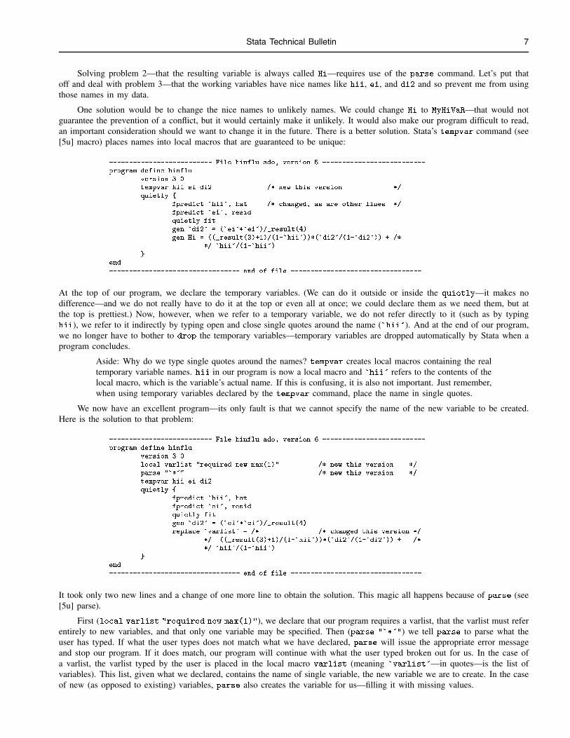
Solving problem 2—that the resulting variable is always called Hi—requires use of the parse command. Let’s put thatoff and deal with problem 3—that the working variables have nice names like hii, ei, and di2 and so prevent me from usingthose names in my data.
One solution would be to change the nice names to unlikely names. We could change Hi to MyHiVaR—that would notguarantee the prevention of a conflict, but it would certainly make it unlikely. It would also make our program difficult to read,an important consideration should we want to change it in the future. There is a better solution. Stata’s tempvar command (see[5u] macro) places names into local macros that are guaranteed to be unique:
-------------------------- File hinflu.ado, version 5 --------------------------
program define hinflu
version 3.0
tempvar hii ei di2 /* new this version */
quietly {
fpredict `hii', hat /* changed, as are other lines */
fpredict `ei', resid
quietly fit
gen `di2' = (`ei'*`ei')/_result(4)
gen Hi = ((_result(3)+1)/(1-`hii'))*(`di2'/(1-`di2')) + /*
*/ `hii'/(1-`hii')
}
end
--------------------------------- end of file ---------------------------------
At the top of our program, we declare the temporary variables. (We can do it outside or inside the quietly—it makes nodifference—and we do not really have to do it at the top or even all at once; we could declare them as we need them, but atthe top is prettiest.) Now, however, when we refer to a temporary variable, we do not refer directly to it (such as by typinghii), we refer to it indirectly by typing open and close single quotes around the name (`hii'). And at the end of our program,we no longer have to bother to drop the temporary variables—temporary variables are dropped automatically by Stata when aprogram concludes.
Aside: Why do we type single quotes around the names? tempvar creates local macros containing the realtemporary variable names. hii in our program is now a local macro and `hii' refers to the contents of thelocal macro, which is the variable’s actual name. If this is confusing, it is also not important. Just remember,when using temporary variables declared by the tempvar command, place the name in single quotes.
We now have an excellent program—its only fault is that we cannot specify the name of the new variable to be created.Here is the solution to that problem:
-------------------------- File hinflu.ado, version 6 --------------------------
program define hinflu
version 3.0
local varlist "required new max(1)" /* new this version */
parse "`*'" /* new this version */
tempvar hii ei di2
quietly {
fpredict `hii', hat
fpredict `ei', resid
quietly fit
gen `di2' = (`ei'*`ei')/_result(4)
replace `varlist' = /* /* changed this version */
*/ ((_result(3)+1)/(1-`hii'))*(`di2'/(1-`di2')) + /*
*/ `hii'/(1-`hii')
}
end
--------------------------------- end of file ---------------------------------
It took only two new lines and a change of one more line to obtain the solution. This magic all happens because of parse (see[5u] parse).
First (local varlist "required new max(1)"), we declare that our program requires a varlist, that the varlist must referentirely to new variables, and that only one variable may be specified. Then (parse "`*'") we tell parse to parse what theuser has typed. If what the user types does not match what we have declared, parse will issue the appropriate error messageand stop our program. If it does match, our program will continue with what the user typed broken out for us. In the case ofa varlist, the varlist typed by the user is placed in the local macro varlist (meaning `varlist'—in quotes—is the list ofvariables). This list, given what we declared, contains the name of single variable, the new variable we are to create. In the caseof new (as opposed to existing) variables, parse also creates the variable for us—filling it with missing values.
8 Stata Technical Bulletin STB-11
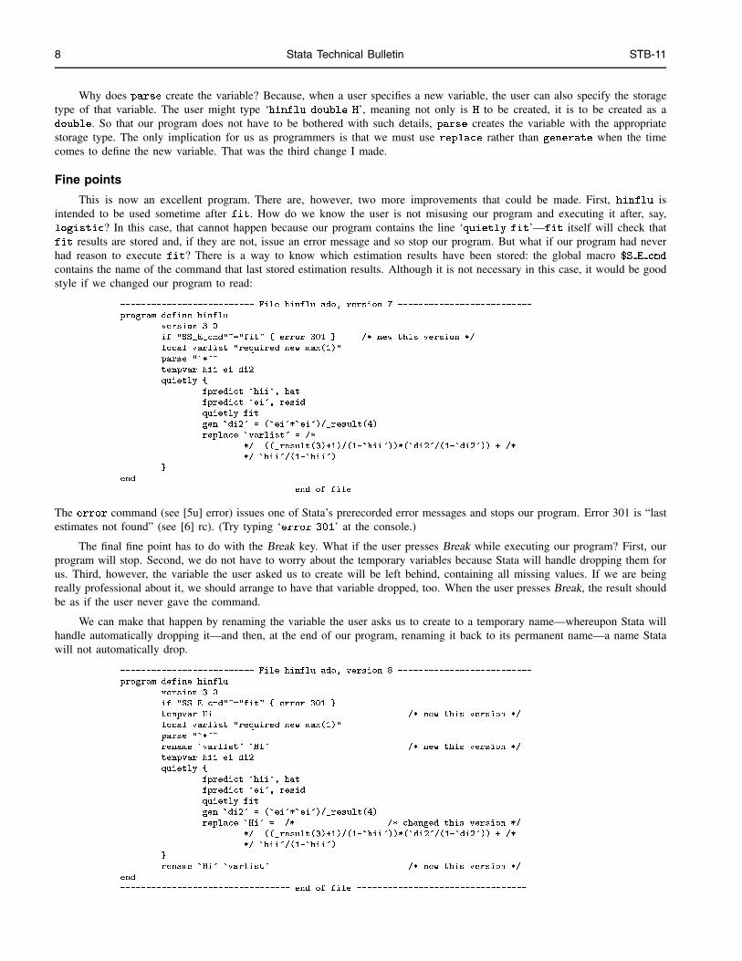
Why does parse create the variable? Because, when a user specifies a new variable, the user can also specify the storagetype of that variable. The user might type ‘hinflu double H’, meaning not only is H to be created, it is to be created as adouble. So that our program does not have to be bothered with such details, parse creates the variable with the appropriatestorage type. The only implication for us as programmers is that we must use replace rather than generate when the timecomes to define the new variable. That was the third change I made.
Fine points
This is now an excellent program. There are, however, two more improvements that could be made. First, hinflu isintended to be used sometime after fit. How do we know the user is not misusing our program and executing it after, say,logistic? In this case, that cannot happen because our program contains the line ‘quietly fit’—fit itself will check thatfit results are stored and, if they are not, issue an error message and so stop our program. But what if our program had neverhad reason to execute fit? There is a way to know which estimation results have been stored: the global macro $S E cmd
contains the name of the command that last stored estimation results. Although it is not necessary in this case, it would be goodstyle if we changed our program to read:
-------------------------- File hinflu.ado, version 7 --------------------------
program define hinflu
version 3.0
if "$S_E_cmd"~="fit" { error 301 } /* new this version */
local varlist "required new max(1)"
parse "`*'"
tempvar hii ei di2
quietly {
fpredict `hii', hat
fpredict `ei', resid
quietly fit
gen `di2' = (`ei'*`ei')/_result(4)
replace `varlist' = /*
*/ ((_result(3)+1)/(1-`hii'))*(`di2'/(1-`di2')) + /*
*/ `hii'/(1-`hii')
}
end
--------------------------------- end of file ---------------------------------
The error command (see [5u] error) issues one of Stata’s prerecorded error messages and stops our program. Error 301 is “lastestimates not found” (see [6] rc). (Try typing ‘error 301’ at the console.)
The final fine point has to do with the Break key. What if the user presses Break while executing our program? First, ourprogram will stop. Second, we do not have to worry about the temporary variables because Stata will handle dropping them forus. Third, however, the variable the user asked us to create will be left behind, containing all missing values. If we are beingreally professional about it, we should arrange to have that variable dropped, too. When the user presses Break, the result shouldbe as if the user never gave the command.
We can make that happen by renaming the variable the user asks us to create to a temporary name—whereupon Stata willhandle automatically dropping it—and then, at the end of our program, renaming it back to its permanent name—a name Statawill not automatically drop.
-------------------------- File hinflu.ado, version 8 --------------------------
program define hinflu
version 3.0
if "$S_E_cmd"~="fit" { error 301 }
tempvar Hi /* new this version */
local varlist "required new max(1)"
parse "`*'"
rename `varlist' `Hi' /* new this version */
tempvar hii ei di2
quietly {
fpredict `hii', hat
fpredict `ei', resid
quietly fit
gen `di2' = (`ei'*`ei')/_result(4)
replace `Hi' = /* /* changed this version */
*/ ((_result(3)+1)/(1-`hii'))*(`di2'/(1-`di2')) + /*
*/ `hii'/(1-`hii')
}
rename `Hi' `varlist' /* new this version */
end
--------------------------------- end of file ---------------------------------
Stata Technical Bulletin 9
This is a perfect program.
Comments
You do not have to go to all the trouble I have just gone to, to program the Hadi measure of influence or to program anyother statistic that appeals to you. Whereas version 1 was not really an acceptable solution—it was too specialized—version 2was acceptable. Version 3 was better, and version 4 better yet, but the improvements were of less and less importance.
Putting aside the details of Stata’s language, you should understand that final versions of programs do not just happen—they are the results of drafts that have been subject to refinement. How much refinement should depend on how often andwho will be using the program. In this sense, the ado-files written by CRC (which can be found in the c:\stata\ado
(DOS), /usr/local/stata/ado (Unix), or ~:Stata:ado (Macintosh) directory) are poor examples. They have been subject tosubstantial refinement because they will be used by strangers with no knowledge of how the code works. When writing programsfor yourself, you may want to stop refining at an earlier draft.
ReferencesGould, W. 1992. ip3: Stata programming. Stata Technical Bulletin 10: 3–18.
Hadi, A. S. 1992. A new measure of overall potential influence in linear regression. Computational Statistics and Data Analysis 14: 1–27.
os7.1 Stata and windowed interfaces
William Rising, Kentucky Medical Review Organization, 502-339-7442
The November 1992 issue of the Stata Technical Bulletin (STB-10) contains a brief article by Bill Gould giving his opinionsabout the requirements for a windowing interface for Stata. He invites comment (very dangerous, indeed); here are my $.02worth.
Stata gains its strength not from its command-line interface, but from its extensibility. Extensibility is present because Statahas its own programming language which allows the user to make customized functions which (when programmed correctly)are indistinguishable from “true” Stata functions. This is obviously something which should not be sacrificed. I am not so surethat all Stata graphics, data files, etc. need to be kept in exactly the same form on all platforms. This seems that it would be animpossible task, since it implicitly assumes that all future platforms will also be able to support the same types of files. Whetherthis will ever be true for graphics is doubtful.
If you people want a very good example of a nice mix of the two types of interface, look at the Mac (not the Sun orDOS) version of Mathematica. This interface (basically) keeps its own log, with several major differences. It allows scrolling (aswell as the usual cutting and pasting), so that the results of the old commands may be viewed without using a separate log file.Better still, new commands may be anywhere in the window, even after scrolling, (temporal order is preserved, of course), whichallows the commands to be put in presentable order as the work is done and new ideas come along. This has the advantage ifthe “log” is saved, then a do-file is automatically created with the steps in the saved order instead of the executed order. Whentesting ideas about a data set, this feature can be a big help. The best feature of all is the ability to put together notebooks ofcommands which can be executed similarly to a do-file or used similarly to an ado-file, and can be formatted with text and putin outline form. This is great for teaching, learning, and presentations. A similar interface would keep the flavor of the currentStata, while still allowing the advantages which are offered by windowing.
Since Stata has a very strict command syntax, one could imagine that the menubar could be used extensively when usingado-files or built-in files. This could be done as such: allow the user to type the name of something which has the syntax ofa typical Stata function (or an ado-file). If the user becomes lost, he/she could double-click on the name of the function. Thiswould alter the menubar to put up the “allowables”, namely varlist [if] [in] [w=exp], options. The varlist menuwould have the names of the currently defined variables (if “req” was specified), which could be checked. The w menu wouldgive the allowable weights; if a weight were selected, the user would then be prompted for the =exp. The options menuwould be the most useful, since it would allow the user to see which options could be used. The only problem could be the *
option, which could be implemented as an “other” item on the menu. When the user was finished (or had a change of heart)there could be a “run” menu which would signal that everything was ready to roll.
Another nice feature would be a HyperCard-like debugger. It allows the user to put a check point anywhere in a function,and allows the use of a variable watcher to look at the values of local and global variables from that point on. While I findStata very enjoyable to use, I am continually frustrated by the need to put in endless display statements to do any debugging.
10 Stata Technical Bulletin STB-11
os7.2 Response
William Gould, CRC, FAX 310-393-7551
You begin by stating, “Stata gains its strength not from its command-line interface but from its extensibility.” I could notagree more. The design issue is how to extend that extensibility, which comes so naturally in command-language environments,to a windowed environment. I think your suggestions are on target and are very much in line with my own inarticulated ideas.
We have not looked at Mathematica; we will take your advice and examine it on the Macintosh before designing anything.I think your suggestion of altering the menubar to display the “allowables” is excellent, although I also think that this willonly be sufficient for default behavior; there will be occasions when we or the user-programmer will want to do more with thewindows. We are currently thinking in terms of a design where filename.win is a standard text file that describes the dialogcorresponding to filename.ado. An important aspect of Stata’s extensibility is that the same Stata program can be used on allplatforms; similarly, the same dialog-description .win file must be usable not only on the Macintosh, but under Windows, OS/2,and X Windows.
I also like your Hypercard-like debugger, which I am tempted to immediately translate back to a command-languageinterface. Imagine the command watch. I could say “watch such-and-such” and then, after typing set watch on, those variableswould be tracked.
I will only take (minor) issue with your statement that “Stata graphics, data files, etc., need to be kept in exactly the sameform on all platforms [: : :] since it implicitly assumes that all future platforms will also be able to support the same types of files.”First, there is no assumption that these file formats are supported on all platforms and, in fact, they are really not supported onany platform. The Stata .gph format, for instance, is of our own devising and is translated, at the time of printing or redisplay,to the format appropriate for the given computer.
Second, Stata’s graphics and data files are not even now kept in the same form across all platforms; rather, the fact thatthey differ is invisible to the user. All Statas know how to read each others’ formats so, from the users point of view, it is asif all are stored in the same format. Moreover, the headers on all the files are the same and this header contains informationabout the release, byteorder, and format of the data that follows (see [6] gph and [6] dta), so it is relatively easy for us to ensurefuture compatibility.
Even if this were not an important feature for our users, since we ourselves work in a mixed environment of DOS, Macintosh,and Unix computers, we exploit this compatibility constantly. Stata itself, and the .dta data sets, are mostly developed onUnix computers. The on-line tutorials are (mostly) developed under DOS. The ado-files are developed on Unix and Macintoshcomputers. All releases except the Macintosh release are assembled on a Unix computer. We could not do this were it not forthe (apparent) file compatibility.
os7.3 CRC committed to Stata’s command language
William Gould, CRC, FAX 310-393-7551
Since the printing of os7, I have received numerous letters, faxes, and telephone calls requesting that we not abandon Stata’scommand language. As one user put it, “[I] would like to voice my support for keeping Stata command driven.”
I want to reassure these users: Stata’s command language will always be a part of Stata and, no matter what we do aboutwindowed operating systems in the future, you will be able to continue using the command language. This is not just a promise;there is no way it could be otherwise because many of Stata’s features are written in Stata’s command language via the ado-files.
This discussion about windowed operating systems is a discussion about additional features to be added to Stata—featureswhich some users want and others do not. Windowed operating systems—fortunately or unfortunately, depending on your pointof view—are the wave of the future. We are attempting to shift the focus of this interface from the standard icon-selection designto making these features usable in a language that is explicitly command driven.
sbe7.1 Hyperbolic regression correction
Paul Geiger, USC School of Medicine, [email protected]
The hbolic program described in sbe7 produces a syntax-error message due to a mistake introduced by CRC duringprocessing of the insert. The corrected version appears on the STB-11 media.
Stata Technical Bulletin 11
sbe10 An improvement to poisson
German Rodriguez, Princeton University, EMAIL [email protected]
Abstract: Stata’s poisson command fails with a numerical overflow in a simple example. The problem appears to be due to the choiceof starting values and can be easily corrected. [The correction has been adopted by CRC; see crc26—Ed.]
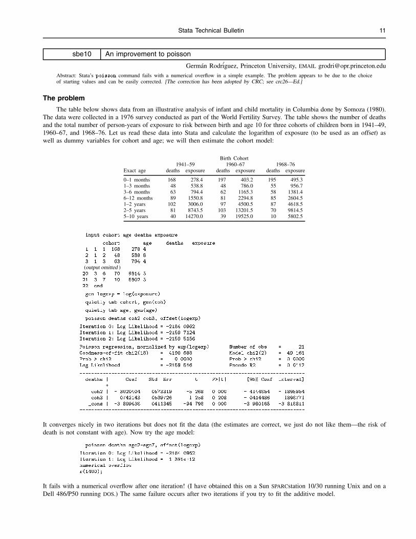
The problem
The table below shows data from an illustrative analysis of infant and child mortality in Columbia done by Somoza (1980).The data were collected in a 1976 survey conducted as part of the World Fertility Survey. The table shows the number of deathsand the total number of person-years of exposure to risk between birth and age 10 for three cohorts of children born in 1941–49,1960–67, and 1968–76. Let us read these data into Stata and calculate the logarithm of exposure (to be used as an offset) aswell as dummy variables for cohort and age; we will then estimate the cohort model:
Birth Cohort1941–59 1960–67 1968–76
Exact age deaths exposure deaths exposure deaths exposure
0–1 months 168 278.4 197 403.2 195 495.31–3 months 48 538.8 48 786.0 55 956.73–6 months 63 794.4 62 1165.3 58 1381.46–12 months 89 1550.8 81 2294.8 85 2604.51–2 years 102 3006.0 97 4500.5 87 4618.52–5 years 81 8743.5 103 13201.5 70 9814.55–10 years 40 14270.0 39 19525.0 10 5802.5
. input cohort age deaths exposure
cohort age deaths exposure
1. 1 1 168 278.4
2. 1 2 48 538.8
3. 1 3 63 794.4
(output omitted )20. 3 6 70 9814.5
21. 3 7 10 5802.5
22. end
. gen logexp = log(exposure)
. quietly tab cohort, gen(coh)
. quietly tab age, gen(age)
. poisson deaths coh2 coh3, offset(logexp)
Iteration 0: Log Likelihood = -2184.0962
Iteration 1: Log Likelihood = -2159.7124
Iteration 2: Log Likelihood = -2159.5156
Poisson regression, normalized by exp(logexp) Number of obs = 21
Goodness-of-fit chi2(18) = 4190.688 Model chi2(2) = 49.161
Prob > chi2 = 0.0000 Prob > chi2 = 0.0000
Log Likelihood = -2159.516 Pseudo R2 = 0.0112
------------------------------------------------------------------------------
deaths | Coef. Std. Err. t P>|t| [95% Conf. Interval]
---------+--------------------------------------------------------------------
coh2 | -.3020404 .0573319 -5.268 0.000 -.4144854 -.1895954
coh3 | .0742143 .0589726 1.258 0.208 -.0414486 .1898771
_cons | -3.899488 .0411345 -94.798 0.000 -3.980165 -3.818811
------------------------------------------------------------------------------
It converges nicely in two iterations but does not fit the data (the estimates are correct, we just do not like them—the risk ofdeath is not constant with age). Now try the age model:
. poisson deaths age2-age7, offset(logexp)
Iteration 0: Log Likelihood = -2184.0962
Iteration 1: Log Likelihood = -1.391e+12
numerical overflow
r(1400);
It fails with a numerical overflow after one iteration! (I have obtained this on a Sun SPARCstation 10/30 running Unix and on aDell 486/P50 running DOS.) The same failure occurs after two iterations if you try to fit the additive model.
12 Stata Technical Bulletin STB-11
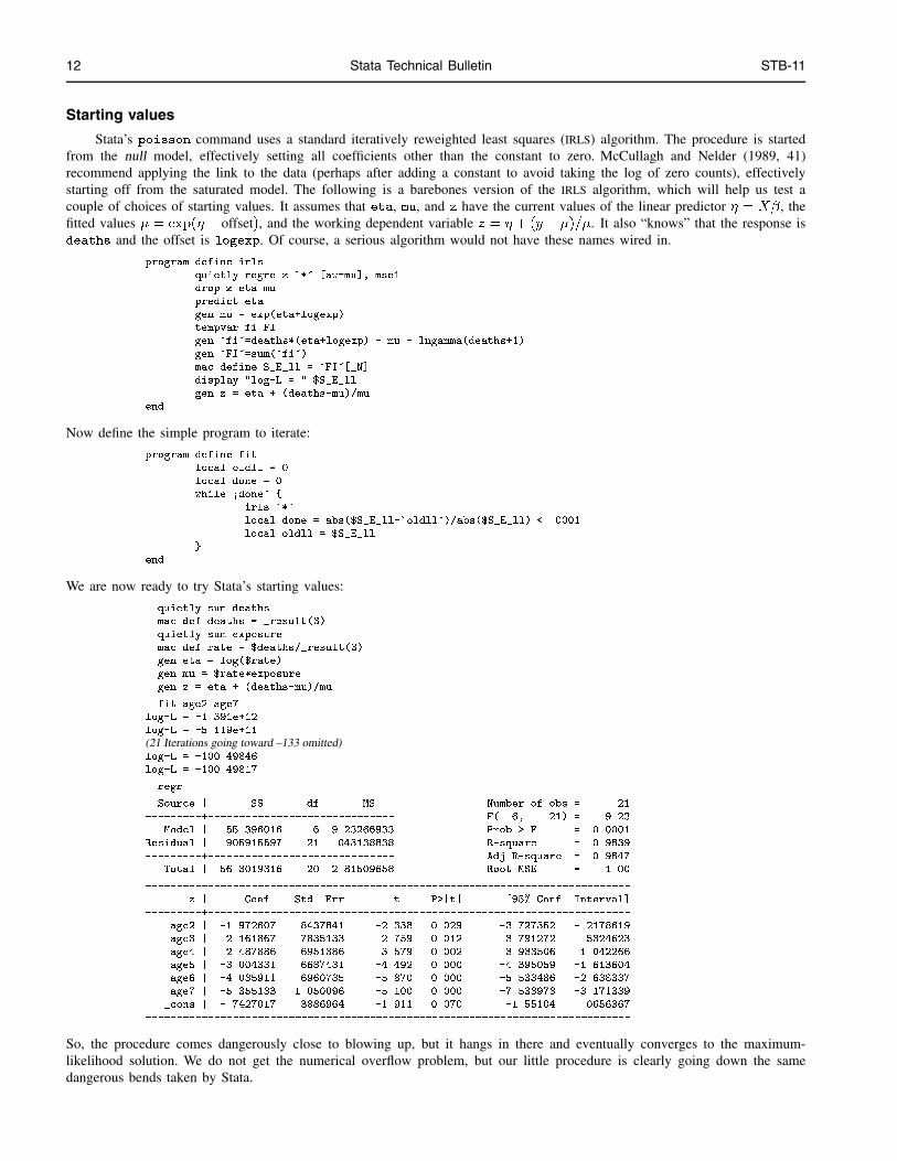
Starting values
Stata’s poisson command uses a standard iteratively reweighted least squares (IRLS) algorithm. The procedure is startedfrom the null model, effectively setting all coefficients other than the constant to zero. McCullagh and Nelder (1989, 41)recommend applying the link to the data (perhaps after adding a constant to avoid taking the log of zero counts), effectivelystarting off from the saturated model. The following is a barebones version of the IRLS algorithm, which will help us test acouple of choices of starting values. It assumes that eta, mu, and z have the current values of the linear predictor � = X�, thefitted values � = exp(�+ offset), and the working dependent variable z = � + (y� �)=�. It also “knows” that the response isdeaths and the offset is logexp. Of course, a serious algorithm would not have these names wired in.
program define irls
quietly regre z `*' [aw=mu], mse1
drop z eta mu
predict eta
gen mu = exp(eta+logexp)
tempvar fi FI
gen `fi'=deaths*(eta+logexp) - mu - lngamma(deaths+1)
gen `FI'=sum(`fi')
mac define S_E_ll = `FI'[_N]
display "log-L = " $S_E_ll
gen z = eta + (deaths-mu)/mu
end
Now define the simple program to iterate:
program define fit
local oldll = 0
local done = 0
while �done' {
irls `*'
local done = abs($S_E_ll-`oldll')/abs($S_E_ll) < .0001
local oldll = $S_E_ll
}
end
We are now ready to try Stata’s starting values:
. quietly sum deaths
. mac def deaths = _result(3)
. quietly sum exposure
. mac def rate = $deaths/_result(3)
. gen eta = log($rate)
. gen mu = $rate*exposure
. gen z = eta + (deaths-mu)/mu
. fit age2-age7
log-L = -1.391e+12
log-L = -5.119e+11
(21 Iterations going toward –133 omitted)log-L = -100.49846
log-L = -100.49817
. regr
Source | SS df MS Number of obs = 21
---------+------------------------------ F( 6, 21) = 9.23
Model | 55.396016 6 9.23266933 Prob > F = 0.0001
Residual | .905915597 21 .043138838 R-square = 0.9839
---------+------------------------------ Adj R-square = 0.9847
Total | 56.3019316 20 2.81509658 Root MSE = 1.00
------------------------------------------------------------------------------
z | Coef. Std. Err. t P>|t| [95% Conf. Interval]
---------+--------------------------------------------------------------------
age2 | -1.972607 .8437841 -2.338 0.029 -3.727352 -.2178619
age3 | -2.161867 .7835133 -2.759 0.012 -3.791272 -.5324623
age4 | -2.487886 .6951386 -3.579 0.002 -3.933506 -1.042266
age5 | -3.004331 .6687431 -4.492 0.000 -4.395059 -1.613604
age6 | -4.085911 .6960785 -5.870 0.000 -5.533486 -2.638337
age7 | -5.355183 1.050096 -5.100 0.000 -7.538978 -3.171389
_cons | -.7427017 .3886964 -1.911 0.070 -1.55104 .0656367
------------------------------------------------------------------------------
So, the procedure comes dangerously close to blowing up, but it hangs in there and eventually converges to the maximum-likelihood solution. We do not get the numerical overflow problem, but our little procedure is clearly going down the samedangerous bends taken by Stata.
Stata Technical Bulletin 13
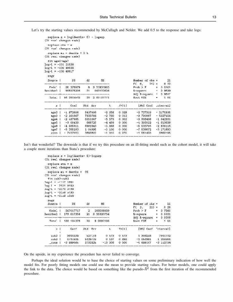
Let’s try the starting values recommended by McCullagh and Nelder. We add 0.5 to the response and take logs:
. replace z = log(deaths+.5) - logexp
(21 real changes made)
. replace eta = z
(21 real changes made)
. replace mu = deaths + 0.5
(21 real changes made)
. fit age2-age7
log-L = -101.21838
log-L = -100.49838
log-L = -100.49817
. regr
Source | SS df MS Number of obs = 21
---------+------------------------------ F( 6, 21) = 9.23
Model | 55.375979 6 9.22932983 Prob > F = 0.0001
Residual | .905575306 21 .043122634 R-square = 0.9839
---------+------------------------------ Adj R-square = 0.9847
Total | 56.2815543 20 2.81407771 Root MSE = 1.00
------------------------------------------------------------------------------
z | Coef. Std. Err. t P>|t| [95% Conf. Interval]
---------+--------------------------------------------------------------------
age2 | -1.972606 .8437686 -2.338 0.029 -3.727319 -.2178935
age3 | -2.161867 .7833766 -2.760 0.012 -3.790987 -.5327456
age4 | -2.487885 .6951067 -3.579 0.002 -3.933438 -1.042331
age5 | -3.00433 .668726 -4.493 0.000 -4.395022 -1.613638
age6 | -4.085911 .6961843 -5.869 0.000 -5.533705 -2.638116
age7 | -5.355183 1.04995 -5.100 0.000 -7.538672 -3.171693
_cons | -.7427022 .3888802 -1.910 0.070 -1.551423 .0660185
------------------------------------------------------------------------------
Isn’t that wonderful? The downside is that if we try this procedure on an ill-fitting model such as the cohort model, it will takea couple more iterations than Stata’s procedure:
. replace z = log(deaths+.5)-logexp
(21 real changes made)
. replace eta = z
(21 real changes made)
. replace mu = deaths + .05
(21 real changes made)
. fit coh2-coh3
log-L = -4117.1851
log-L = -2421.9153
log-L = -2170.3489
log-L = -2159.5493
log-L = -2159.5159
. regr
Source | SS df MS Number of obs = 21
---------+------------------------------ F( 2, 21) = 0.28
Model | .567017717 2 .283508859 Prob > F = 0.7560
Residual | 179.617358 21 8.55320754 R-square = 0.0031
---------+------------------------------ Adj R-square = 0.0506
Total | 180.184376 20 9.0092188 Root MSE = 1.00
------------------------------------------------------------------------------
z | Coef. Std. Err. t P>|t| [95% Conf. Interval]
---------+--------------------------------------------------------------------
coh2 | -.3020339 .527119 -0.573 0.573 -1.398238 .7941702
coh3 | .0741935 .5429732 0.137 0.893 -1.054981 1.203368
_cons | -3.899465 .3782825 -10.308 0.000 -4.686147 -3.112784
------------------------------------------------------------------------------
On the upside, in my experience the procedure has never failed to converge.
Perhaps the ideal solution would be to base the choice of starting values on some preliminary indication of how well themodel fits. For poorly fitting models one could use the mean to provide starting values. For better models, one could applythe link to the data. The choice would be based on something like the pseudo-R2 from the first iteration of the recommendedprocedure.
14 Stata Technical Bulletin STB-11
Code fixes
[In the submitted version of this insert, Rodriguez showed the changes one would make to poisson to implement the suggestedstarting values and then verified that the updated routine produced the desired results. Those changes will be made to your copyof poisson when you install the CRC updates (see crc26). The previously used initial values will still be used if you specifythe new zero option.—Ed.]
ReferencesMcCullagh, P. and J. A. Nelder. 1989. Generalized Linear Models. London: Chapman and Hall.
Somoza, J. 1980. Illustrative analysis: infant and child mortality in Columbia. World Fertility Survey Scientific Reports 10. Voorburg: Internal StatisticalInstitute.
sed7.2 Twice reroughing procedure for resistant nonlinear smoothing
I. Salgado-Ugarte, Univ. of Tokyo, Japan, FAX (011)-81-3-3812-0529, andJ. Curts-Garcia, U.N.A.M., Mexico City, Mexico
The smtwice ado-file for a nonlinear resistant smoother presented in sed7 (Salgado-Ugarte and Garcia 1992) is includedon the STB diskette. A new version of the ado-file sm4253eh for Stata 3.0 has been prepared and may be installed in place ofthe former, which was for Stata 2.1. This new version has a more efficient algorithm for carrying out running medians of span5 and permits the keeping of the original values of the sequence. In this way the results (generated as new variables by theprogram) are the smoothed values and a time index. It is now possible to build a graph with the original and smoothed valuesfor comparison after smoothing.
smtwice performs the reroughing adjust procedure applying the same compound smoother 4253eh to the rough valuescalculated from sm4253eh and adding the smoothed rough to the former smoothed values (a procedure that is usually called“twice”). smtwice automatically displays a graph with the original and smoothed values vs. the time index variable which makesit possible to see the effects of the smoother. The ado-file generates a variable that contains the final smooth and another withthe final rough to be used (if desired) to assess the smoother results. The implementation of smtwice makes it applicable onlyfor the results of sm4253eh.
The syntax of this new command is
smtwice datavar smthvar finsmth
where datavar is the same variable used in sm4253eh with the original sequence values, smthvar is the name of the variablegenerated by sm4253eh that contains the smoothed values, and finsmth is the name of the variable to keep the final “4253eh,twice”smoothed values.
Test and validation of the programs
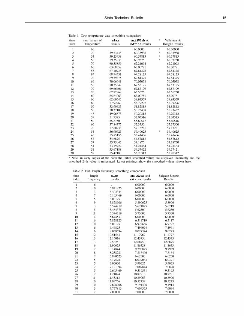
To test the programs we used the well-known cow temperature data set given by Velleman and Hoaglin (1981) and the fishlength frequency data (Salgado-Ugarte 1992). We compared our results with those obtained by the nlsm command of Gould(1992) and realized that both are similar but different. The differences found for smoothing the cow temperature data are asfollows:
Stata Technical Bulletin 15
Table 1. Cow temperature data smoothing comparison
time raw values of nlsm sm4253eh & * Velleman &index temperature results smtwice results Hoaglin results
1 60 . 60.0000 * 60.000002 70 59.23438 60.35938 * 60.359383 54 59.23438 60.57813 * 60.578134 56 59.35938 60.9375 * 60.937505 70 60.55859 62.21094 62.210936 66 63.68359 65.00781 65.007817 53 67.10938 67.84375 67.843758 95 68.94531 69.28125 69.281259 70 69.59375 69.84375 69.84375
10 69 70.06641 70.05078 70.0507811 56 70.35547 69.53125 69.5312512 70 69.66406 67.87109 67.8710913 70 67.92969 65.5625 65.5625014 60 65.64063 63.00781 63.0078115 60 62.60547 59.93359 59.9335916 60 57.92969 55.79297 55.7929617 50 52.90625 51.82813 51.8281218 50 50.37109 50.23438 50.2343719 48 49.96875 50.20313 50.2031220 59 51.9375 52.03516 52.0351521 50 55.8750 55.60547 55.6054622 60 57.84375 57.3750 57.3750023 70 57.60938 57.13281 57.1328124 54 56.90625 56.40625 * 56.4062525 46 55.85156 55.41406 55.4140626 57 54.6875 54.57813 54.5781227 57 53.73047 54.1875 54.1875028 51 53.19922 54.21484 54.2148429 51 53.67188 54.57422 54.5742130 59 55.42188 55.20313 55.20312
* Note: in early copies of the book the initial smoothed values are displayed incorrectly and thesmoothed 24th value is misprinted. Latest printings show the smoothed values shown here.
Table 2. Fish length frequency smoothing comparison
time length nlsm sm42535h and Salgado-Ugarteindex frequency results smtwice results Results
1 6 . 6.00000 6.00002 10 6.921875 6.00000 6.00003 3 6.402344 6.00000 6.00004 7 6.105469 6.00000 6.00005 5 6.03125 6.00000 6.00006 9 5.878906 5.890625 5.89067 3 5.574219 5.671875 5.67198 5 5.484375 5.62500 5.62509 11 5.574219 5.75000 5.750010 4 5.644531 6.00000 6.000011 6 5.828125 6.511719 6.511712 10 6.03125 6.972656 6.972713 6 6.46875 7.496094 7.496114 6 8.058594 9.027344 9.027315 12 10.51563 11.17969 11.179716 13 12.16016 12.43750 12.437517 13 12.5625 12.68750 12.687518 6 11.90625 11.86328 11.863319 12 10.14844 9.796875 9.796920 8 8.238281 7.816406 7.816421 7 6.890625 6.62500 6.625022 5 6.175781 6.039063 6.039123 5 6.00000 5.90625 5.906324 12 7.121094 7.089844 7.089825 5 9.605469 9.519531 9.519526 12 11.21094 10.82813 10.828127 11 11.45313 10.89063 10.890628 10 11.09766 10.52734 10.527329 10 9.628906 9.191406 9.191430 3 7.757813 7.609375 7.609431 7 7.00000 7.00000 7.0000

16 Stata Technical Bulletin STB-11
Comments on smoothing and programs’ performance
We would like to point out that the difference in the first value is due to the different implementation of nlsm and sm4253eh:our program follows the rules of copying (replicate) end values used by Velleman (1980, 1982) and Velleman and Hoaglin(1981), the step-down rule (Goodall 1990) and the Tukey’s endpoint rule (Tukey 1977, Velleman and Hoaglin 1981, Goodall1990) with even and uneven span smoothers. On the other hand, nlsm drops the initial value during the application of even spansmoothers (omit end-value rule; Goodall 1990). The choice of end-value rules is more important in short sequences in whichanalysis is concentrated to the middle and ends of the data sequence. It is true that there are few data points at the ends and thesmooth may behave erratically at these locations. However, there is no firm guidance in the election. Goodall (1990) commentsthat the replicate, the step-down, and Tukey’s extrapolation are commonplace in an exploratory data analysis setting.
This difference explains the discrepancies in the first few values occurring when sm4253eh and nlsm 4253eh are appliedto the same data sequence (see Gould 1992). However, when the twice part of the smoother is specified, the differences of thenlsm smooths are great as compared to the results of Velleman and Hoaglin (1981). The exact values are different in spite oftheir similarity, not only at the beginning but all along the sequence of values. It appears that nlsm begins to depart once thesmoothing of raw values finish and when it begins the twice part (smoothing of the residuals); but we have not yet explored thispossibility in detail.
As shown in Table 2, the analysis of fish length frequency data takes us to the same behavior when comparing nlsm
4253eh,twice with sm4253eh–smtwice combination (values similar but never equal each other).
The sm4253eh–smtwice combination for the temperature data gives the same results as those of Velleman and Hoaglin(1981); length frequency smoothing results are equal to those reported by Salgado-Ugarte (1992). Additionally, both smootheddata sets were compared to the results of other programs (Wallonick 1987; Salgado-Ugarte 1992). These programs produced thesame smooth values as our ado-files.
We have included two files on the STB diskette with the data sets used in this insert. The temperature data are in tempcow.dta
and the fish length frequency data are contained in fish.dta. The user can repeat all smoothing operations discussed.
ReferencesGoodall, C. 1990. A survey of smoothing techniques. In Modern Methods of Data Analysis, ed. J. Fox and J. S. Long, 126–176. Newbury Park, CA:
Sage Publications.
Gould, W. 1992. sed7.1: Resistant smoothing using Stata. Stata Technical Bulletin 8: 9–12.
Salgado-Ugarte, I. H. 1992. El Analisis Exploratorio de Datos Biologicos: Fundamentos y Aplicaciones. E.N.E.P. Zaragoza U.N.A.M. and MarcEdiciones, Mexico: 89–120; 213–233.
Salgado-Ugarte, I. H. and J. Curts-Garcia. 1992. sed7: Resistant smoothing using Stata. Stata Technical Bulletin 7: 8–11.
Tukey, J. W. 1977. Exploratory Data Analysis. Reading, MA: Addison–Wesley.
Velleman P. F. 1980. Definition and comparison of robust nonlinear smoothing algorithms. Journal of the American Statistical Association 75(371):609–615.
——. 1982. Applied nonlinear smoothing. In Sociological Methodology, ed. S. Leinhardt, 141–178. San Francisco: Jossey-Bass.
Velleman P. F. and D. C. Hoaglin. 1981. Applications, Basics, and Computing of Exploratory Data Analysis. Boston: Duxbury Press 159–199.
Wallonick, D. S. 1987. The Exploratory Analysis Program. Stat-Packets. Statistical Analysis Package for Lotus Worksheets. Version 1.0. Minneapolis,39 p.
Stata Technical Bulletin 17
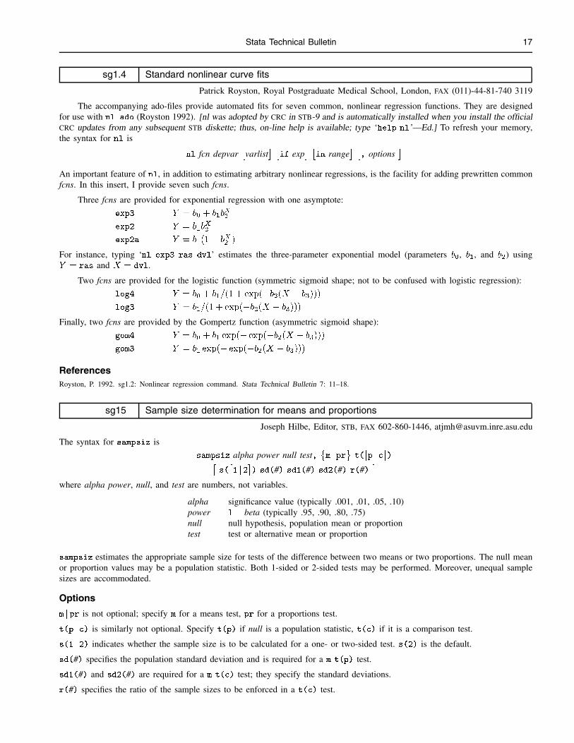
sg1.4 Standard nonlinear curve fits
Patrick Royston, Royal Postgraduate Medical School, London, FAX (011)-44-81-740 3119
The accompanying ado-files provide automated fits for seven common, nonlinear regression functions. They are designedfor use with nl.ado (Royston 1992). [nl was adopted by CRC in STB-9 and is automatically installed when you install the officialCRC updates from any subsequent STB diskette; thus, on-line help is available; type ‘help nl’—Ed.] To refresh your memory,the syntax for nl is
nl fcn depvar�varlist
� �if exp
� �in range
� �, options
�An important feature of nl, in addition to estimating arbitrary nonlinear regressions, is the facility for adding prewritten commonfcns. In this insert, I provide seven such fcns.
Three fcns are provided for exponential regression with one asymptote:
exp3 Y = b0 + b1bX2
exp2 Y = b1bX2
exp2a Y = b1(1� bX2)
For instance, typing ‘nl exp3 ras dvl’ estimates the three-parameter exponential model (parameters b0, b1, and b2) usingY = ras and X = dvl.
Two fcns are provided for the logistic function (symmetric sigmoid shape; not to be confused with logistic regression):
log4 Y = b0 + b1=(1 + exp(�b2(X � b3)))
log3 Y = b1=(1 + exp(�b2(X � b3)))
Finally, two fcns are provided by the Gompertz function (asymmetric sigmoid shape):
gom4 Y = b0 + b1 exp(� exp(�b2(X � b3)))
gom3 Y = b1 exp(� exp(�b2(X � b3)))
ReferencesRoyston, P. 1992. sg1.2: Nonlinear regression command. Stata Technical Bulletin 7: 11–18.
sg15 Sample size determination for means and proportions
Joseph Hilbe, Editor, STB, FAX 602-860-1446, [email protected]
The syntax for sampsiz is
sampsiz alpha power null test,�m j pr t(
�p j c�)�
s(�1 j 2�) sd(#) sd1(#) sd2(#) r(#)
�where alpha power, null, and test are numbers, not variables.
alpha significance value (typically .001, .01, .05, .10)power 1� beta (typically .95, .90, .80, .75)null null hypothesis, population mean or proportiontest test or alternative mean or proportion
sampsiz estimates the appropriate sample size for tests of the difference between two means or two proportions. The null meanor proportion values may be a population statistic. Both 1-sided or 2-sided tests may be performed. Moreover, unequal samplesizes are accommodated.
Options
m j pr is not optional; specify m for a means test, pr for a proportions test.
t(p j c) is similarly not optional. Specify t(p) if null is a population statistic, t(c) if it is a comparison test.
s(1 j 2) indicates whether the sample size is to be calculated for a one- or two-sided test. s(2) is the default.
sd(#) specifies the population standard deviation and is required for a m t(p) test.
sd1(#) and sd2(#) are required for a m t(c) test; they specify the standard deviations.
r(#) specifies the ratio of the sample sizes to be enforced in a t(c) test.
18 Stata Technical Bulletin STB-11
Discussion
The determination of test sample size provides a means to avoid making type I and type II errors. A type I error occurs whenthe null hypothesis is rejected when it is in fact true. The probability of making such an error is specified by the significancelevel of the test, referred to as �. For example, if we set � to .05, we would expect to mistakenly reject a true null hypothesis5% of the time. A type II error occurs if we fail to reject the null hypothesis when it is in fact false. The probability of makingsuch an error is called a � error. If we set � at .05, we would expect that a false null hypothesis is misdetermined as such 5%of the time.
Hypothesis testing, as well as sample size assessment, uses the notion of power rather than of �. Power, defined as 1� �,is the probability of correctly rejecting the null hypothesis; i.e., rejecting it as false when it is indeed false. In effect, it is theprobability of detecting a true deviation from the null hypothesis. We may also think of power as simply the probability ofavoiding a type II error. The balance of � and power represent the respective importance given to making or avoiding a type ofhypothesis error. There are no a priori guidelines as to the selection of values; it depends on the proposed type of study and itspurpose.
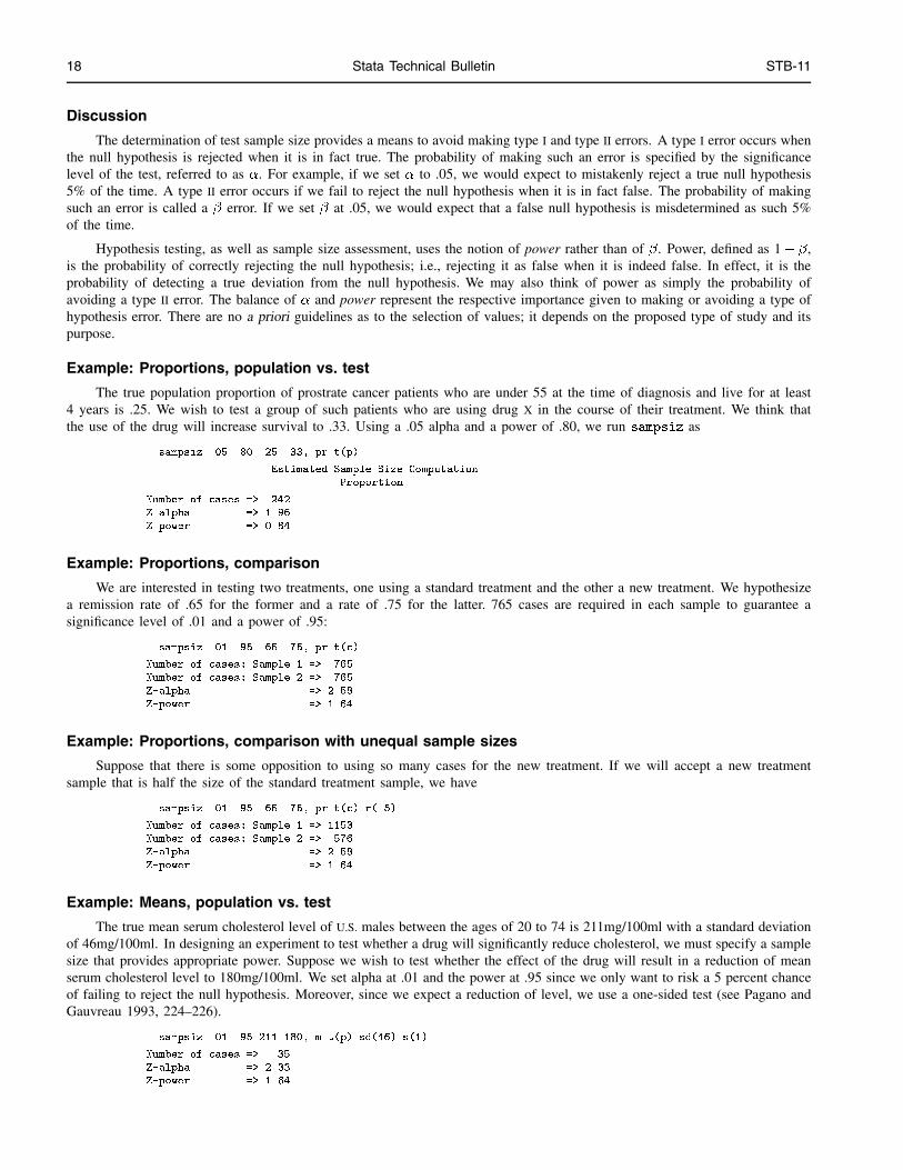
Example: Proportions, population vs. test
The true population proportion of prostrate cancer patients who are under 55 at the time of diagnosis and live for at least4 years is .25. We wish to test a group of such patients who are using drug X in the course of their treatment. We think thatthe use of the drug will increase survival to .33. Using a .05 alpha and a power of .80, we run sampsiz as
. sampsiz .05 .80 .25 .33, pr t(p)
Estimated Sample Size Computation
Proportion
Number of cases => 242
Z-alpha => 1.96
Z-power => 0.84
Example: Proportions, comparison
We are interested in testing two treatments, one using a standard treatment and the other a new treatment. We hypothesizea remission rate of .65 for the former and a rate of .75 for the latter. 765 cases are required in each sample to guarantee asignificance level of .01 and a power of .95:
. sampsiz .01 .95 .65 .75, pr t(c)
Number of cases: Sample 1 => 765
Number of cases: Sample 2 => 765
Z-alpha => 2.58
Z-power => 1.64
Example: Proportions, comparison with unequal sample sizes
Suppose that there is some opposition to using so many cases for the new treatment. If we will accept a new treatmentsample that is half the size of the standard treatment sample, we have
. sampsiz .01 .95 .65 .75, pr t(c) r(.5)
Number of cases: Sample 1 => 1153
Number of cases: Sample 2 => 576
Z-alpha => 2.58
Z-power => 1.64
Example: Means, population vs. test
The true mean serum cholesterol level of U.S. males between the ages of 20 to 74 is 211mg/100ml with a standard deviationof 46mg/100ml. In designing an experiment to test whether a drug will significantly reduce cholesterol, we must specify a samplesize that provides appropriate power. Suppose we wish to test whether the effect of the drug will result in a reduction of meanserum cholesterol level to 180mg/100ml. We set alpha at .01 and the power at .95 since we only want to risk a 5 percent chanceof failing to reject the null hypothesis. Moreover, since we expect a reduction of level, we use a one-sided test (see Pagano andGauvreau 1993, 224–226).
. sampsiz .01 .95 211 180, m t(p) sd(46) s(1)
Number of cases => 35
Z-alpha => 2.33
Z-power => 1.64
Stata Technical Bulletin 19
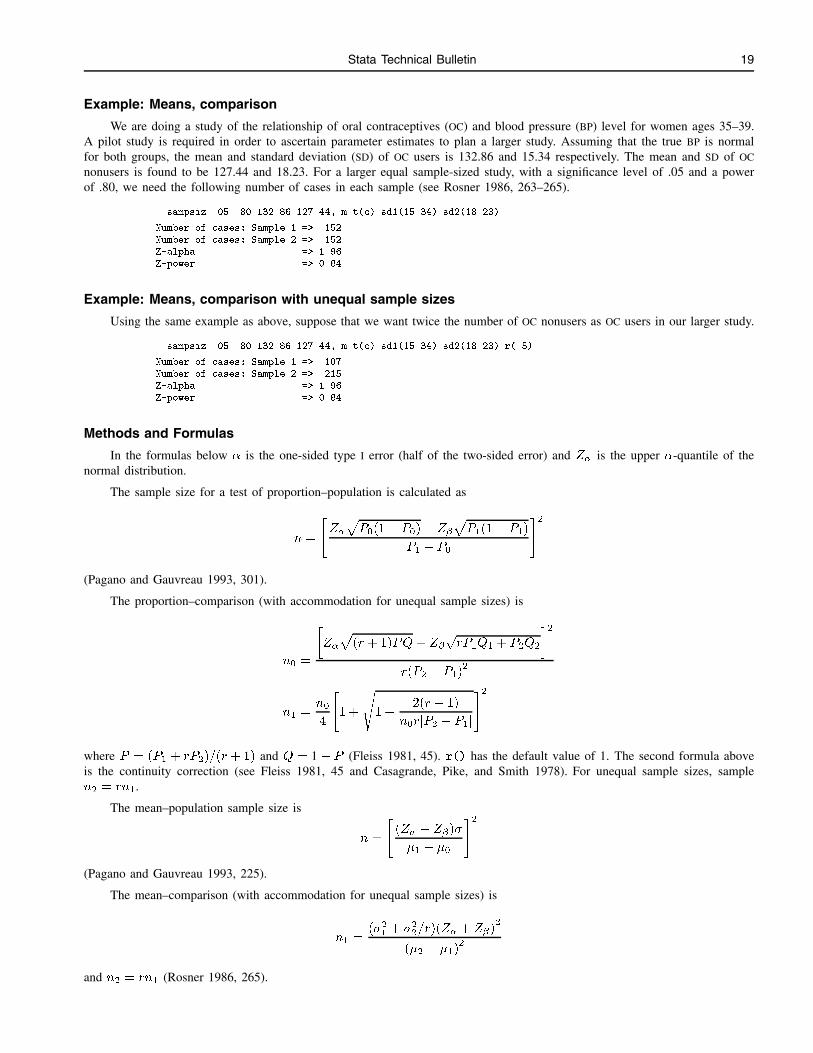
Example: Means, comparison
We are doing a study of the relationship of oral contraceptives (OC) and blood pressure (BP) level for women ages 35–39.A pilot study is required in order to ascertain parameter estimates to plan a larger study. Assuming that the true BP is normalfor both groups, the mean and standard deviation (SD) of OC users is 132.86 and 15.34 respectively. The mean and SD of OC
nonusers is found to be 127.44 and 18.23. For a larger equal sample-sized study, with a significance level of .05 and a powerof .80, we need the following number of cases in each sample (see Rosner 1986, 263–265).
. sampsiz .05 .80 132.86 127.44, m t(c) sd1(15.34) sd2(18.23)
Number of cases: Sample 1 => 152
Number of cases: Sample 2 => 152
Z-alpha => 1.96
Z-power => 0.84
Example: Means, comparison with unequal sample sizes
Using the same example as above, suppose that we want twice the number of OC nonusers as OC users in our larger study.
. sampsiz .05 .80 132.86 127.44, m t(c) sd1(15.34) sd2(18.23) r(.5)
Number of cases: Sample 1 => 107
Number of cases: Sample 2 => 215
Z-alpha => 1.96
Z-power => 0.84
Methods and Formulas
In the formulas below � is the one-sided type I error (half of the two-sided error) and Z� is the upper �-quantile of thenormal distribution.
The sample size for a test of proportion–population is calculated as
n =
"Z�
pP0(1� P0) + Z�
pP1(1� P1)
P1 � P0
#2
(Pagano and Gauvreau 1993, 301).
The proportion–comparison (with accommodation for unequal sample sizes) is
n0 =
�Z�
p(r + 1) �P �Q+ Z�
prP1Q1 + P2Q2
�2r(P2 � P1)
2
n1 =n0
4
"1 +
s1 +
2(r + 1)
n0rjP2 � P1j
#2
where �P = (P1 + rP2)=(r + 1) and �Q = 1 � �P (Fleiss 1981, 45). r() has the default value of 1. The second formula aboveis the continuity correction (see Fleiss 1981, 45 and Casagrande, Pike, and Smith 1978). For unequal sample sizes, samplen2 = rn1.
The mean–population sample size is
n =
"(Z� + Z�)�
�1 � �0
#2
(Pagano and Gauvreau 1993, 225).
The mean–comparison (with accommodation for unequal sample sizes) is
n1 =(�2
1+ �
2
2=r)(Z� + Z�)
2
(�2 � �1)2
and n2 = rn1 (Rosner 1986, 265).
20 Stata Technical Bulletin STB-11
ReferencesCasagrande, J. T., M. C. Pike, and P. G. Smith. 1978. The power function of the exact test for comparing two binomial distributions. Applied Statistics
27: 176–180.
Fleiss, J. L. 1981. Statistical Methods for Rates and Proportions. New York: John Wiley & Sons.
Pagano, M. and K. Gauvreau. 1993. Principles of Biostatistics. Belmont, CA: Duxbury Press.
Rosner, B. 1986. Fundamentals of Biostatistics. Boston: Duxbury Press.
sg16 Generalized linear models
Joseph Hilbe, Editor, STB, FAX 602-860-1446, [email protected]
Generalized linear models represent a method of extending standard linear regression to incorporate a variety of responsedistributions. The application of OLS regression to models having non-normal error terms, non-constant error variance, or tomodels where the response is non-continuous or must be constrained, yields statistically unacceptable results. Examples includeresponses that are binary, proportions, counts, or survival times. Regression models which effectively model such types ofresponse are, among others, logistic, probit, complementary loglog, Poisson, gamma, and inverse Gaussian. These constitutethe standard set of generalized linear models (GLM) as defined by McCullagh and Nelder (1989). Extensions to GLM havemainly taken the form of survival models; particularly the Cox proportional hazards model. However, several other survivaldistributions can rather easily be formatted into the GLM framework; e.g., exponential and Weibull regression. This article andits accompanying software address the complete standard GLM set, provide interesting additions, and offer suggestions for howthe user may extend the routines to satisfy various requirements.
I began working on the development of a glm command after writing a review for The American Statistician on generalizedadditive models software (Hilbe 1993). As nonparametric extensions to GLM models, I became increasingly impressed with thepower and flexibility of their GLM basis. In fact, GAM models, as they are called, can be placed within the GLM algorithm formost standard models. It is simply a matter of incorporating a backfitting algorithm within the GLM while-loop which iterativelysmooths the partial residuals from the GLM regression, adding the results back into a IRLS regression response variable. Thelpartr command developed and discussed in Hilbe (1992b) sets the stage for such a backfitting algorithm. The glm commandrepresents in part the combination of the various models into one. It is to be taken as a pedagogically useful tool by which tolearn more about GLM modeling and its capabilities. I should add that there are certain statistical features provided by glm whichare currently unavailable with other packages. I have added residual diagnostics which are rarely, if ever, found elsewhere, suchas likelihood and Anscombe’s residuals.
I have compared glm results with those few packages offering the ability to perform GLM modeling. In one case, forinstance, only S-Plus has an inverse Gaussian routine—whose deviance statistic is suspect I might add—although forthcomingversions of GLIM and XploRe plan to incorporate it. However, I have added log and identity link options to supplement itscanonical squared inverse link function. Since there are no other packages with which to compare results, these links should atpresent be taken as experimental; but their mathematical basis does seem appropriate. Moreover, no commercial GLM packagedirectly provides for exposure variables or significance and confidence interval levels—much less levels which may be changedby the user. These have been incorporated, together with the ability to designate an offset variable, across models, in the samemanner as is currently available for Stata’s poisson command. glm can also report exponentiated coefficients for binomial andPoisson models and it corrects the diagnostics for grouped binomial models as presently found in Stata.
This endeavor has assisted me in the evaluation of other GLM packages and, as an initially unexpected result, to developwhat I hope to be a useful program for others to use, modify, and expand. Refer to the Notes below for other considerations ofprogram development.
The syntax for glm is
glm depvar�cases
�varlist
�fweight
� �if exp
� �in range
�,
f(�gau j bin j poi j gam j invg) l(
�l j p j c j log j id)�
g s r ex(varname) o(varname) eform level(#) it(#) lt(#)�
where f() indicates the error or family distribution, and l() is the link. The user has a choice of the following distributionsand links:
Stata Technical Bulletin 21
f(gau) Gaussian; default if f() not specified. Identity link.
f(bin) binomial; either Bernoulli 0/1 or grouped; g option mustbe specified if grouped.
l(l) logit link (canonical)l(p) probit linkl(c) complementary log-log link (cloglog)
f(poi) Poisson; log link default (canonical)l(id) identity link
f(gam) gamma; inverse link default (canonical)l(log) log linkl(id) identity link
f(invg) inverse Gaussian; squared inverse link default (canonical)l(log) log linkl(id) identity link
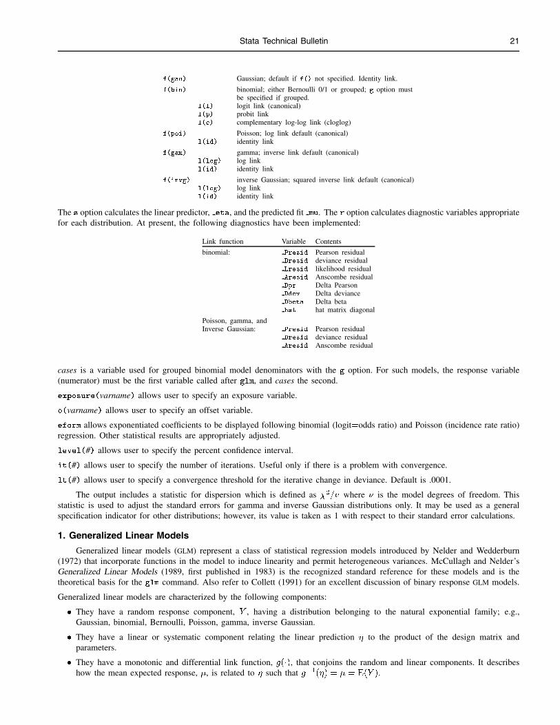
The s option calculates the linear predictor, eta, and the predicted fit mu. The r option calculates diagnostic variables appropriatefor each distribution. At present, the following diagnostics have been implemented:
Link function Variable Contents
binomial: Presid Pearson residualDresid deviance residualLresid likelihood residualAresid Anscombe residualDpr Delta PearsonDdev Delta devianceDbeta Delta betahat hat matrix diagonal
Poisson, gamma, andInverse Gaussian: Presid Pearson residual
Dresid deviance residualAresid Anscombe residual
cases is a variable used for grouped binomial model denominators with the g option. For such models, the response variable(numerator) must be the first variable called after glm, and cases the second.
exposure(varname) allows user to specify an exposure variable.
o(varname) allows user to specify an offset variable.
eform allows exponentiated coefficients to be displayed following binomial (logit=odds ratio) and Poisson (incidence rate ratio)regression. Other statistical results are appropriately adjusted.
level(#) allows user to specify the percent confidence interval.
it(#) allows user to specify the number of iterations. Useful only if there is a problem with convergence.
lt(#) allows user to specify a convergence threshold for the iterative change in deviance. Default is .0001.
The output includes a statistic for dispersion which is defined as �2=� where � is the model degrees of freedom. Thisstatistic is used to adjust the standard errors for gamma and inverse Gaussian distributions only. It may be used as a generalspecification indicator for other distributions; however, its value is taken as 1 with respect to their standard error calculations.
1. Generalized Linear Models
Generalized linear models (GLM) represent a class of statistical regression models introduced by Nelder and Wedderburn(1972) that incorporate functions in the model to induce linearity and permit heterogeneous variances. McCullagh and Nelder’sGeneralized Linear Models (1989, first published in 1983) is the recognized standard reference for these models and is thetheoretical basis for the glm command. Also refer to Collett (1991) for an excellent discussion of binary response GLM models.
Generalized linear models are characterized by the following components:
� They have a random response component, Y , having a distribution belonging to the natural exponential family; e.g.,Gaussian, binomial, Bernoulli, Poisson, gamma, inverse Gaussian.
� They have a linear or systematic component relating the linear prediction � to the product of the design matrix andparameters.
� They have a monotonic and differential link function, g(�), that conjoins the random and linear components. It describeshow the mean expected response, �, is related to � such that g�1(�) = � = E(Y ).
22 Stata Technical Bulletin STB-11
� They have a nonconstant variance, V , that changes with �. The inverse of V is typically used as the nonconstant regressionweight in the fitting algorithm.
� They are linear models that can be fit using an iteratively reweighted least squares algorithm (IRLS).
The fitting of a GLM model is a method of estimating a response variable Y with a vector of values, �. � is the expected mean ofY and is the result of the iterative transformation of a linear predictor, �, by means of a link function. Iteration converges withrespect to differential values of the residual deviance, which is initially determined by the model response probability (density)distribution.
a. The distribution of the random response component
Generalized linear models assume a relationship between the observations y of the random response variable Y and aprobability density function. All GLM response distributions are members of the exponential family defined, in canonical form,as
fY (y; �; �) = expf(y� � b(�))=a(�) + c(y; �)gwhere � is the natural parameter and � is the dispersion parameter. Each of the y observations is construed to be independent.The point, however, of our modeling is to determine model parameter values and hence values for �. Conveniently, the jointprobability density function may be reexpressed as a function of � on the basis of y. This is called the likelihood function,l(�; �; y). � is an ancillary parameter such as the standard deviation of a normal distribution. Typically the likelihood functionis transformed into log form since it is easier to work with sums than with multiplicative factors. The IRLS seeks to find themaximum-likelihood estimates.
The residual deviance of a model may be defined as the difference between a saturated or maximal log likelihood and thatof the log likelihood of the fitted model. Except for Gaussian-based models, the difference is actually twofold. Hence, for mostmodels, with � being substituted for �, D(y;�) = 2ls(�; y)� 2lf (�; y). The iterative maximization process is such that theresidual deviance will be the value displayed at the final iteration and is the value reported as the deviance on the output table.It is identical to the deviance value calculated as the sum of squared deviance residuals as discussed in Hilbe (1992a) and maybe interpreted as a goodness-of-fit statistic. However, see McCullagh and Nelder for arguments minimizing this interpretation.
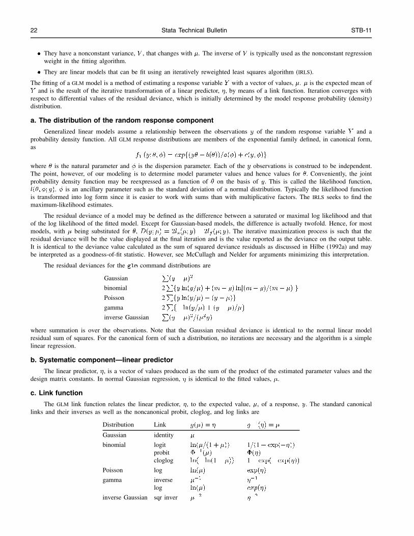
The residual deviances for the glm command distributions are
GaussianP
(y � �)2
binomial 2Pfy ln(y=�) + (m� y) ln[(m� y)=(m� �)]g
Poisson 2Pfy ln(y=�)� (y � �)g
gamma 2Pf� ln(y=�) + (y � �)=�g
inverse GaussianP
(y � �)2=(�2y)
where summation is over the observations. Note that the Gaussian residual deviance is identical to the normal linear modelresidual sum of squares. For the canonical form of such a distribution, no iterations are necessary and the algorithm is a simplelinear regression.
b. Systematic component—linear predictor
The linear predictor, �, is a vector of values produced as the sum of the product of the estimated parameter values and thedesign matrix constants. In normal Gaussian regression, � is identical to the fitted values, �.
c. Link function
The GLM link function relates the linear predictor, �, to the expected value, �, of a response, y. The standard canonicallinks and their inverses as well as the noncanonical probit, cloglog, and log links are
Distribution Link g(�) = � g�1(�) = �
Gaussian identity �
binomial logit ln(�=(1 + �)) 1=(1 + exp(��))probit ��1(�) �(�)cloglog ln(� ln(1 � �)) 1 � exp(� exp(�))
Poisson log ln(�) exp(�)
gamma inverse ��1
��1
log ln(�) exp(�)
inverse Gaussian sqr inver ��2
��2
Stata Technical Bulletin 23
where �(�) is calculated as normprob(�).
d. Variance and weighting
The variance functions for each of the canonical GLM distributions are
Gaussian identity link �
binomial: Bernoulli logit link �(1 � �)binomial: grouped logit link �(1 � �)=mPoisson log link �
gamma inverse link �2=�
inverse Gaussian sqr inverse link �3=�
Each of the above are used as weighting factors in the IRLS regression; but note that noncanonical links have a different weightingpattern. After a base weight is used to calculate IRLS response z (per discussion below), it is adjusted for use as a weightingfactor in the IRLS regression. For example, when the log link is used with the gamma distribution, the base weight is �, whilethe readjusted weight is given the value of 1. An adjustment, but more complicated one, occurs with the binomial probit andcomplementary log-log links. Regardless, an initial weighting factor is given to calculate z, whereupon a readjusted weight isspecified for the regression. Identity links are handled in quite a different manner.
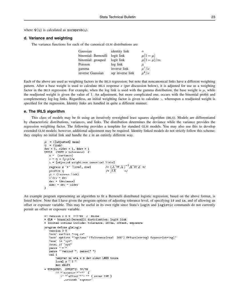
e. The IRLS algorithm
This class of models may be fit using an iteratively reweighted least squares algorithm (IRLS). Models are differentiatedby characteristic distributions, variances, and links. The distribution determines the deviance while the variance provides theregression weighting factor. The following provides a template for standard GLM models. You may also use this to developextended GLM models; however, additional adjustment may be required. Identity linked models do not strictly follow this scheme;they employ no initial link and handle the z in an entirely different way.
� = ([adjusted] mean)
� = (link)
dev = 0, oldev = 1, ddev = 1
WHILE (DDEV > tolerance) {
w = (variance)
z = � + (y-�)/w
w = [adjusted weight:non-canonical links]
regress z `*' [iw=w], mse1 /* (X 0
WX)�1X
0
WZ */
predict � /* �X */
� = (inverse link)
oldev = dev
dev = (deviance)
ddev = dev - oldev
}
An example program representing an algorithm to fit a Bernoulli distributed logistic regression, based on the above format, islisted below. Note that I have given the program options of adjusting tolerance level, of specifying if and in, and of allowing anoffset or exposure variable. This may be useful in its own right since Stata’s logit and logistic commands do not currentlypermit an offset or exposure variable.
*! version 1.0.0 7-7-92 J. Hilbe
* GLM - binomial:Bernoulli distribution; logit link
* limited options include: tolerance, if/in, offset, exposure
program define glmlogis
version 3.0
local varlist "req ex"
local options "`options' LTolerance(real .0001) Offset(string) Exposur(string)"
local in "opt"
local if "opt"
parse "`*'"
parse "`varlist'", parse(" ")
qui {
tempvar mu eta w z dev oldev LNEX touse
local y "`1'"
mac shift
* EXPOSURE: OFFSETS: IF/IN
if "`exposur'"~="" {
if "`offset'"~= "" { error 198 }
_crcunab `exposur'

24 Stata Technical Bulletin STB-11
local expostr "$S_1"
gen double `LNEX' = ln(`expostr')
local offset `LNEX'
local offmiss "| `offset'==."
}
else if "`offset'"~="" {
_crcunab `offset'
local offset "$S_1"
local offmiss "| `offset'==."
local expostr "exp($S_1)"
}
gen byte `touse'=1 `if' `in'
replace `touse'=0 if `y'==. | `touse'==. `offmiss'
if "`offset'"~="" {
local poffset "+`offset'"
local moffset "-`offset'"
local offopt "offset(`offset')"
}
* INITIALIZATION
sum `y' if `touse'
local nobs = _result(1)
gen `mu' = (`y' +.5)/2 if `touse' /* adj mean */
gen `eta' = log(`mu'/(1-`mu')) if `touse' /* link */
local i = 1
gen `w'=0 if `touse'
gen `z'=0 if `touse'
gen `dev'=1 if `touse'
gen `oldev'=1 if `touse'
local ddev = 1
* LOCAL SCORING ALGORITHM: IRLS : simple convergence procedure
while (abs(`ddev') > `ltolera') {
replace `w' = `mu'* (1-`mu') if `touse' /* variance weight */
replace `z' = `eta' + (`y'-`mu')/`w' `moffset' if `touse'
regress `z' `*' [iw=`w'], mse1 dof(100000) dep(`y')
drop `eta'
predict `eta' if `touse'
replace `eta' = `eta' `poffset'
replace `mu' = 1/(1+exp(-`eta')) /* inverse link */
replace `oldev' = `dev'
replace `dev' = cond(`y',log(`mu'),log(1-`mu'))
replace `dev' = sum(`dev')
replace `dev' = -2*`dev'[_N] /* deviance */
local ddev = `dev' - `oldev'
noi di in gr "Iter `i' : Dev = " in ye `dev'
local i = `i'+1
}
}
local df = `nobs'-_result(3)-1
* DISPLAY
di in gr _col(57) "No obs. = " in ye %9.0g `nobs'
di in gr _col(57) "Deviance = " in ye %9.4f `dev'
di in gr _col(57) "Prob>chi2 = " in ye %9.4f chiprob(`df',`dev')
di in gr _col(57) "Dispersion = " in ye %9.4f 1 /* not calculated */
di in gr "GLM - Binomial:Bernoulli (logit link)"
noi regress , noheader
end
glmlogis.ado has been placed on the STB diskette as an example for your use. It has been kept at a minimum so that thestructure of the algorithm is apparent.
2. Examples
The following is the log output of a Bernoulli response logistic regression model using the kyphosis data set (Hastie andTibshirani 1990, 200, and see Chambers and Hastie 1992, 301–303) and is included on the STB diskette. kyph is the 0/1 responseand indicates the presence of kyphosis following surgery on a group of 81 young children. age of child at surgery is given inmonths, start represents the disk at which kyphosis starts, and numb is the number of disks involved. The latter is modeled asan offset.
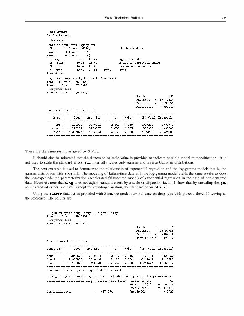
Stata Technical Bulletin 25
. use kyphsp
(Kyphosis data)
. describe
Contains data from kyphsp.dta
Obs: 81 (max= 166296) Kyphosis data
Vars: 4 (max= 99)
Width: 5 (max= 200)
1. age int %8.0g Age in months
2. start byte %8.0g Start of operation range
3. numb byte %8.0g Number of vertebrae
4. kyph byte %8.0g kyph kyph
Sorted by:
. glm kyph age start, f(bin) l(l) o(numb)
Iter 1 : Dev = 75.0809
Iter 2 : Dev = 67.4053
(output omitted )Iter 5 : Dev = 66.7913
No obs. = 81
Deviance = 66.79134
Prob>chi2 = .8133553
Dispersion = 4.089645
Bernoulli distribution: logit
---------------------------------------------------------------------------
kyph | Coef. Std. Err. t P>|t| [95% Conf. Interval]
---------+-----------------------------------------------------------------
age | .0165998 .0070802 2.345 0.019 .0027226 .0304769
start | -.213254 .0753637 -2.830 0.005 -.360966 -.065542
_cons | -5.247965 .8423953 -6.230 0.000 -6.89905 -3.596881
---------------------------------------------------------------------------
These are the same results as given by S-Plus.
It should also be reiterated that the dispersion or scale value is provided to indicate possible model misspecification—it isnot used to scale the standard errors. glm internally scales only gamma and inverse Gaussian distributions.
The next example is used to demonstrate the relationship of exponential regression and the log-gamma model; that is, thegamma distribution with a log link. The modeling of failure-time data with the log-gamma model yields the same results as doesthe log-expected-time parameterization (accelerated failure-time model) of exponential regression in the case of non-censoreddata. However, note that ereg does not adjust standard errors by a scale or dispersion factor. I show that by unscaling the glm
result standard errors, we have, except for rounding variation, the standard errors of ereg.
Using the cancer data set as provided with Stata, we model survival time on drug type with placebo (level 1) serving asthe reference. The results are
. glm studytim drug2 drug3 , f(gam) l(log)
Iter 1 : Dev = 19.4801
(output omitted )Iter 4 : Dev = 18.9079
No obs. = 48
Deviance = 18.90786
Prob>chi2 = .9997849
Dispersion = .3328512
Gamma distribution : log
---------------------------------------------------------------------------
studytim | Coef. Std.Err. t P>|t| [95% Conf. Interval]
---------------------------------------------------------------------------
drug2 | .5060523 .2010414 2.517 0.015 .1120184 .9000862
drug3 | 1.035836 .2010414 5.152 0.000 .6418019 1.42987
_cons | 2.197225 .129006 17.032 0.000 1.944377 2.450072
---------------------------------------------------------------------------
Standard errors adjusted by sqrt(dispersion)
. ereg studytim drug2 drug3 ,nolog /* Stata's exponential regression */
Exponential regression (log expected time form) Number of obs = 48
Model chi2(2) = 9.014
Prob > chi2 = 0.0110
Log Likelihood = -57.454 Pseudo R2 = 0.0727
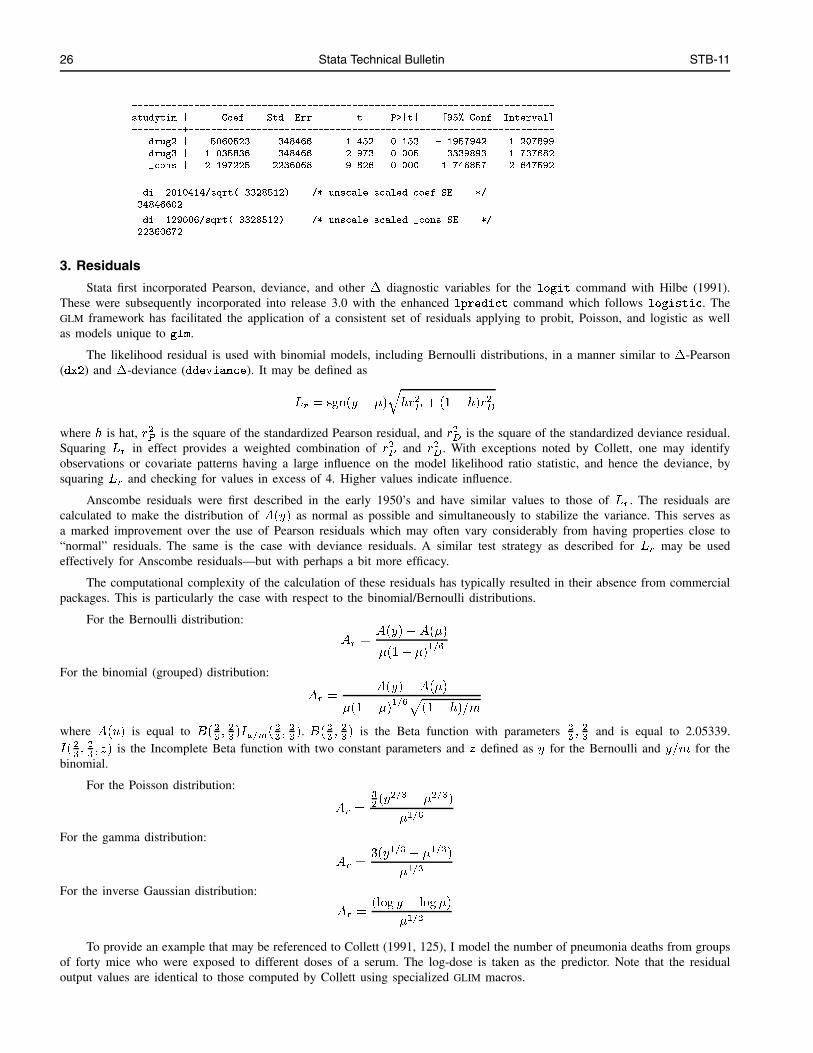
26 Stata Technical Bulletin STB-11
---------------------------------------------------------------------------
studytim | Coef. Std. Err. t P>|t| [95% Conf. Interval]
---------+-----------------------------------------------------------------
drug2 | .5060523 .348466 1.452 0.153 -.1957942 1.207899
drug3 | 1.035836 .348466 2.973 0.005 .3339893 1.737682
_cons | 2.197225 .2236068 9.826 0.000 1.746857 2.647592
---------------------------------------------------------------------------
. di .2010414/sqrt(.3328512) /* unscale scaled coef SE */
.34846602
. di .129006/sqrt(.3328512) /* unscale scaled _cons SE */
.22360672
3. Residuals
Stata first incorporated Pearson, deviance, and other � diagnostic variables for the logit command with Hilbe (1991).These were subsequently incorporated into release 3.0 with the enhanced lpredict command which follows logistic. TheGLM framework has facilitated the application of a consistent set of residuals applying to probit, Poisson, and logistic as wellas models unique to glm.
The likelihood residual is used with binomial models, including Bernoulli distributions, in a manner similar to �-Pearson(dx2) and �-deviance (ddeviance). It may be defined as
Lr = sgn(y � �)
qhr2P + (1� h)r2D
where h is hat, r2P is the square of the standardized Pearson residual, and r2D is the square of the standardized deviance residual.Squaring Lr in effect provides a weighted combination of r2P and r
2
D. With exceptions noted by Collett, one may identifyobservations or covariate patterns having a large influence on the model likelihood ratio statistic, and hence the deviance, bysquaring Lr and checking for values in excess of 4. Higher values indicate influence.
Anscombe residuals were first described in the early 1950’s and have similar values to those of Lr. The residuals arecalculated to make the distribution of A(y) as normal as possible and simultaneously to stabilize the variance. This serves asa marked improvement over the use of Pearson residuals which may often vary considerably from having properties close to“normal” residuals. The same is the case with deviance residuals. A similar test strategy as described for Lr may be usedeffectively for Anscombe residuals—but with perhaps a bit more efficacy.
The computational complexity of the calculation of these residuals has typically resulted in their absence from commercialpackages. This is particularly the case with respect to the binomial/Bernoulli distributions.
For the Bernoulli distribution:
Ar =A(y)�A(�)
�(1� �)1=6
For the binomial (grouped) distribution:
Ar =A(y)�A(�)
�(1� �)1=6p(1� h)=m
where A(u) is equal to B( 23;2
3)Iu=m(
2
3;2
3). B( 2
3;2
3) is the Beta function with parameters 2
3;2
3and is equal to 2.05339.
I( 23;2
3; z) is the Incomplete Beta function with two constant parameters and z defined as y for the Bernoulli and y=m for the
binomial.
For the Poisson distribution:
Ar =3
2(y2=3 � �
2=3)
�1=6
For the gamma distribution:
Ar =3(y1=3 � �
1=3)
�1=3
For the inverse Gaussian distribution:
Ar =(log y � log�)
�1=2
To provide an example that may be referenced to Collett (1991, 125), I model the number of pneumonia deaths from groupsof forty mice who were exposed to different doses of a serum. The log-dose is taken as the predictor. Note that the residualoutput values are identical to those computed by Collett using specialized GLIM macros.
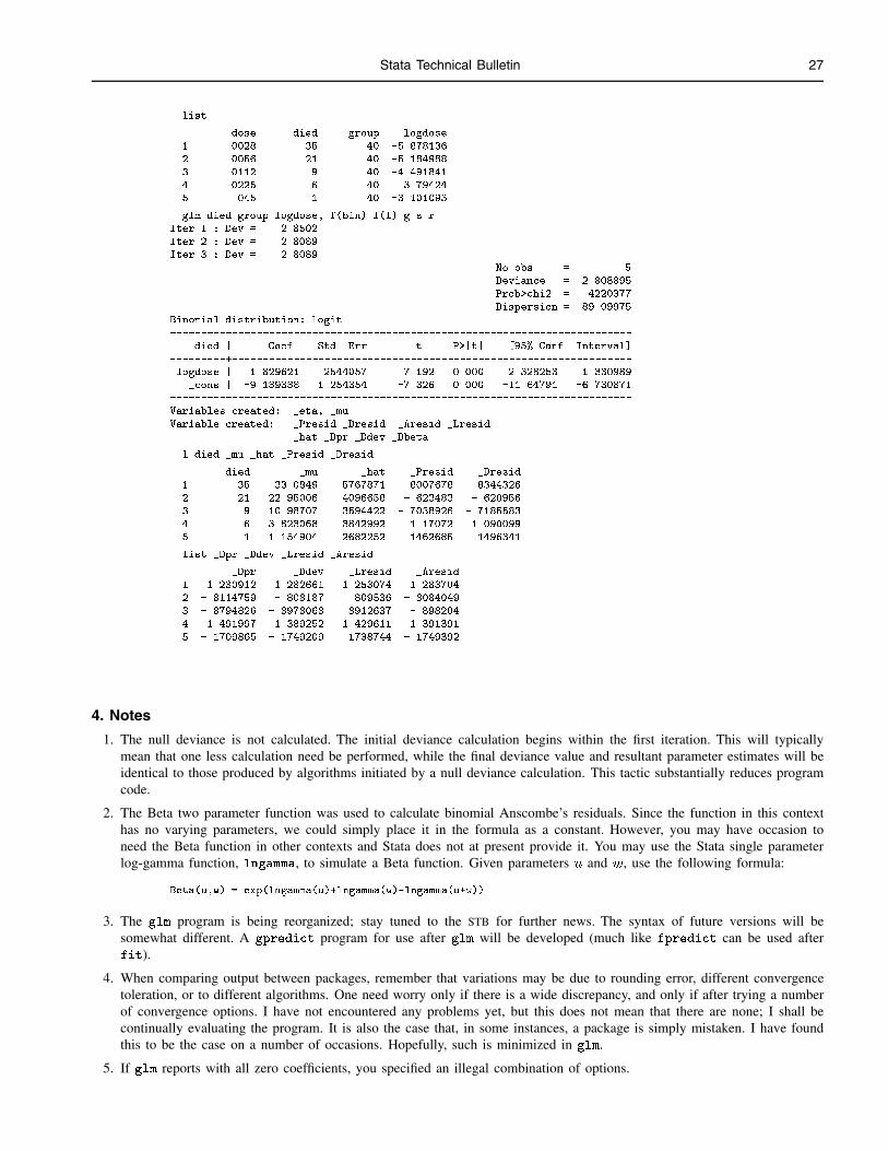
Stata Technical Bulletin 27
. list
dose died group logdose
1. .0028 35 40 -5.878136
2. .0056 21 40 -5.184988
3. .0112 9 40 -4.491841
4. .0225 6 40 -3.79424
5. .045 1 40 -3.101093
. glm died group logdose, f(bin) l(l) g s r
Iter 1 : Dev = 2.8502
Iter 2 : Dev = 2.8089
Iter 3 : Dev = 2.8089
No obs. = 5
Deviance = 2.808895
Prob>chi2 = .4220377
Dispersion = 89.09975
Binomial distribution: logit
---------------------------------------------------------------------------
died | Coef. Std. Err. t P>|t| [95% Conf. Interval]
---------+-----------------------------------------------------------------
logdose | -1.829621 .2544057 -7.192 0.000 -2.328253 -1.330989
_cons | -9.189388 1.254354 -7.326 0.000 -11.64791 -6.730871
---------------------------------------------------------------------------
Variables created: _eta, _mu
Variable created: _Presid _Dresid _Aresid _Lresid
_hat _Dpr _Ddev _Dbeta
. l died _mu _hat _Presid _Dresid
died _mu _hat _Presid _Dresid
1. 35 33.0849 .5767871 .8007678 .8344326
2. 21 22.95006 .4096658 -.623483 -.620956
3. 9 10.98707 .3594422 -.7038926 -.7185583
4. 6 3.823068 .3842992 1.17072 1.090099
5. 1 1.154904 .2682252 -.1462685 -.1496341
. list _Dpr _Ddev _Lresid _Aresid
_Dpr _Ddev _Lresid _Aresid
1. 1.230912 1.282661 1.253074 1.283704
2. -.8114759 -.808187 .809536 -.8084049
3. -.8794826 -.8978068 .8912637 -.898204
4. 1.491997 1.389252 1.429611 1.391391
5. -.1709865 -.1749209 .1738744 -.1749392
4. Notes
1. The null deviance is not calculated. The initial deviance calculation begins within the first iteration. This will typicallymean that one less calculation need be performed, while the final deviance value and resultant parameter estimates will beidentical to those produced by algorithms initiated by a null deviance calculation. This tactic substantially reduces programcode.
2. The Beta two parameter function was used to calculate binomial Anscombe’s residuals. Since the function in this contexthas no varying parameters, we could simply place it in the formula as a constant. However, you may have occasion toneed the Beta function in other contexts and Stata does not at present provide it. You may use the Stata single parameterlog-gamma function, lngamma, to simulate a Beta function. Given parameters u and w, use the following formula:
Beta(u,w) = exp(lngamma(u)+lngamma(w)-lngamma(u+w))
3. The glm program is being reorganized; stay tuned to the STB for further news. The syntax of future versions will besomewhat different. A gpredict program for use after glm will be developed (much like fpredict can be used afterfit).
4. When comparing output between packages, remember that variations may be due to rounding error, different convergencetoleration, or to different algorithms. One need worry only if there is a wide discrepancy, and only if after trying a numberof convergence options. I have not encountered any problems yet, but this does not mean that there are none; I shall becontinually evaluating the program. It is also the case that, in some instances, a package is simply mistaken. I have foundthis to be the case on a number of occasions. Hopefully, such is minimized in glm.
5. If glm reports with all zero coefficients, you specified an illegal combination of options.
28 Stata Technical Bulletin STB-11
6. Additional error trapping may be needed. It is always tedious attempting to ascertain in advance how multifaceted programsmay be misused or how they may respond to certain misspecified models. So far, priorities were made favoring modelingcapabilities over error trapping. If you run the program as designed on appropriate model data, you should not havedifficulties. Please let me know of any problems you discover.
ReferencesChambers, J. M. and T. J. Hastie (editors). 1992. Statistical models in S. Pacific Grove, CA: Wadsworth.
Collett, D. 1991. Modelling Binary Data. New York: Chapman & Hall.
Dobson, A. 1990. An Introduction to Generalized Linear Models. New York: Chapman & Hall.
Hastie, T. J. and R. J. Tibshirani. 1990. Generalized Additive Models. New York: Chapman & Hall.
Hilbe, J. 1991. sqv1: Additional logistic regression extensions. Stata Technical Bulletin 1: 21–23.
——. 1992a. sqv4: Calculation of the deviance goodness-of-fit statistic after logistic. Stata Technical Bulletin 8: 18–19.
——. 1992b. sqv6: Smoothed partial residual plots for logistic regression. Stata Technical Bulletin 10: 27.
——. 1993. Generalized additive models software. The American Statistician 47(1).
McCullagh, P. and J. A. Nelder. 1989. Generalized Linear Models. 2d ed. New York: Chapman & Hall.
Nelder, J. A. and R. Wedderburn. 1972. Generalized linear models. Journal of the Royal Statistical Society A. 135: 370–384.
smv6 Identifying multivariate outliers
William Gould, CRC, and Ali S. Hadi, Cornell University, FAX 310-393-7551
The syntax of hadimvo is
hadimvo varlist�if exp
� �in range
�, generate(newvar1
�newvar2
�)�p(#)
�hadimvo identifies multiple outliers in multivariate data using the method of Hadi (1992, 1993), creating newvar1 equal to 1 ifan observation is an “outlier” and 0 otherwise. Optionally, newvar2 can also be created containing the distances from the basicsubset. See Discussion below for general comments on the use of techniques such as hadimvo.
Options
generate(newvar1 [newvar2]) is not optional; it identifies the new variable(s) to be created. Whether you specify two variablesor one, however, is optional. newvar2, if specified, will contain the distances (not the distances squared) from the basicsubset. E.g., specifying gen(odd) creates odd containing 1 if the observation is an outlier in the Hadi sense and 0 otherwise.Specifying gen(odd dist) also creates dist containing the Hadi distances.
p(#) specifies the “significance” level for outlier cutoff; 0 < # < 1. The default is p(.05). Larger numbers identify a largerproportion of the sample as outliers. If # is specified greater than 1, it is interpreted as a percent. Thus, p(5) is the sameas p(.05).
Remarks
Multivariate analysis techniques (e.g., [5s] factor) are commonly used to analyze data from many fields of study. Thesedata often contain outliers. The search for subsets of the data which, if deleted, would change results markedly is known as thesearch for outliers. hadimvo provides one, computer intensive but practical method for identifying such observations.
Classical outlier detection methods (e.g., Mahalanobis distance and Wilks’ test) are powerful when the data contain onlyone outlier, but the power of these methods decreases drastically when more than one outlying observation is present. The lossof power is usually due to what are known as masking and swamping problems (false negative and false positive decisions) butin addition, these methods often fail simply because they are affected by the very observations they are supposed to identify.
Solutions to these problems often involve an unreasonable amount of calculation and therefore computer time. (Solutionsinvolving hundreds of millions of calculations even for samples of size 30 have been suggested.) The method developed by Hadi(1992, 1993) attempts to surmount these problems and produce an answer, albeit second best, in finite time.
A basic outline of the procedure is as follows: A measure of distance from an observation to a cluster of points is defined.A base cluster of r points is selected and then that cluster is continually redefined by taking the r + 1 points “closest” to thecluster as the new base cluster. This continues until some rule stops the redefinition of the cluster.
Stata Technical Bulletin 29
Ignoring many of the fine details, given k variables, the initial base cluster is defined as r = k + 1 points. The distancethat is minimized in selecting these k + 1 points is a covariance-matrix distance on the variables with their medians removed.(We will use the language loosely; if we were being more precise, we would have said the distance is based on a matrix ofsecond moments, but remember, the medians of the variables have been removed. We would also discuss how the k + 1 pointsmust be of full column rank and how they would be expanded to include additional points if they are not.)
Given the base cluster, a more standard mean-based center of the r-observation cluster is defined and the r+ 1 observationsclosest in the covariance-matrix sense are chosen as a new base cluster. This is then repeated until the base cluster hasr = int((n+ k + 1)=2) points.
At this point, the method continues in much the same way, except a stopping rule based on the distance of the additionalpoint, and the user specified p(), is introduced.
Simulation results are presented in Hadi (1993).
Examples. hadimvo price weight, gen(odd)
. list if odd /* list the outliers */
. summ price weight if ~odd /* summary stats for clean data */
. drop odd
. hadimvo price weight, gen(odd D)
. gen id=_n /* make an index variable */
. graph D id /* index plot of D */
. graph price weight [w=D] /* 2-way scatter, outliers big */
. graph price weight [w=1/D] /* same, outliers small */
. summarize D, detail
. sort D
. list make price weight D odd
. hadimvo price weight mpg, gen(odd2 D2) p(.01)
. fit : : : if ~odd2
Discussion
You have a theory about x1, x2, : : :, xk which we’ll write as F (x1; x2; : : : ; xk). Your theory might be that x1, x2, : : :,xk are jointly distributed normally, perhaps with a particular mean and covariance matrix; or your theory might be that
x1 = �1 + �2x2 + : : :+ �kxk + u
where u � N(0; �2); or your theory might be
x1 = �10 + �12x2 + �14x4 + u1
x2 = �20 + �21x1 + �23x3 + u2
or your theory might be anything else—it does not matter. You have some data on x1, x2, : : :, xk, which you will assume isgenerated by F (�), and from that data you plan to estimate the parameters (if any) of your theory and then test your theory inthe sense of how well it explains the observed data.
What if, however, some of your data is generated not by F (�) but by G(�), a different process? For example, you havea theory on how wages are assigned to employees in a firm and, for the bulk of employees, that theory is correct. There are,however, six employees at the top of the hierarchy for whom wages are set by a completely different process. Or, you have atheory on how individuals select different health insurance options except that, for a handful of individuals already diagnosedwith serious illness, a different process controls the selection process. Or, you are testing a drug that reduces trauma after surgeryexcept that, for a few patients with a high level of a particular protein, the drug has no effect. Or, in another drug experiment,some of the historical data is simply misrecorded.
The data generated by G(�) rather than F (�) are called contaminant observations. Of course, the analysis should be basedonly on the observations generated by F (�), but in practice we do not know which observations those are. In addition, if ithappened by chance that some of the observations are within a reasonable distance from the center of F (�), it becomes impossibleto determine whether they are contaminants. The following operational definition of outliers is, therefore, adopted: Outliersare observations that do not conform to the pattern suggested by the majority of the observations in a data set. Accordingly,observations generated by F (�) but located at the tail of F (�) are considered outliers. On the other hand, contaminants that arewithin a statistically reasonable distance from the center of F (�) are not considered outliers.
It is well worth noting that outliership is strongly related to the completeness of the theory—a grand unified theory wouldhave no outliers because it would explain all processes (including, one supposes, errors in recording the data). Grand unifiedtheories, however, are difficult to come by and are most often developed by synthesizing the results of many special theories.
30 Stata Technical Bulletin STB-11
Theoretical work has tended to focus on one special case: the data contain only one outlier. As mentioned above, thesingle-outlier techniques often fail to identify multiple outliers, even if applied recursively. One of the classic examples is thestar cluster data (a.k.a. Hertzsprung-Russell diagram) shown in Figure 1 (Rousseeuw and Leroy 1987, 27). For 47 stars, the datacontains the (log) light intensity and the (log) effective temperature at the star’s surface. (For the sake of illustration, we treatthe data here as a bivariate data—not as regression data—i.e., the two variables are treated similarly with no distinction betweenwhich variable is dependent and which is independent.)
Figure 1 presents a scatter of the data along with two ellipses expected to contain 95% of the data. The larger ellipse isbased on the mean and covariance matrix of the full data. All 47 stars are inside the larger ellipse, indicating that classicalsingle-case analysis fails to identify any outliers. The smaller ellipse is based on the mean and covariance matrix of the datawithout the five stars identified by hadimvo as outliers. These observations are located outside the smaller ellipse. The dramaticeffects of the outliers can be seen by comparing the two ellipses. The volume of the larger ellipse is much greater than that of thesmaller one and the two ellipses have completely different orientations. In fact, their major axes are nearly orthogonal to eachother; the larger ellipse indicates a negative correlation (r = �0.2) whereas the smaller ellipse indicates a positive correlation(r = 0.7). (Theory would suggest a positive correlation: hot things glow.)
The single-outlier techniques make calculations for each observation under the assumption that it is the only outlier—andthe remaining n� 1 observations are generated by F (�)—producing a statistic for each of the n observations. Thinking aboutmultiple outliers is no more difficult. In the case of two outliers, consider all possible pairs of observations (there are n(n�1)=2of them) and, for each pair, make a calculation assuming the remaining n � 2 observations are generated by F (�). For thethree-outlier case, consider all possible triples of observations (there are n(n� 1)(n� 2)=(3� 2) of them) and, for each triple,make a calculation assuming the remaining n� 3 observations are generated by F (�).
Conceptually, this is easy but practically, it is difficult because of the rapidly increasing number of calculations required(there are also theoretical problems in determining how many outliers to test simultaneously). Techniques designed for detectingmultiple outliers, therefore, make various simplifying assumptions to reduce the calculation burden and, along the way, losesome of the theoretical foundation. This loss, however, is no reason for ignoring the problem and the (admittedly second best)solutions available today. It is unreasonable to assume that outliers do not occur in real data.
If outliers exist in the data, they can distort parameter estimation, invalidate test statistics, and lead to incorrect statisticalinference. The search for outliers is not merely to improve the estimates of the current model but also to provide valuable insightinto the shortcomings of the current model. In addition, outliers themselves can sometimes provide valuable clues as to wheremore effort should be expended. In a drug experiment, for example, the patients excluded as outliers might well be furtherresearched to understand why they do not fit the theory.
Multivariate, multiple outliers
hadimvo is an example of a multivariate, multiple outlier technique. The multivariate aspect deserves some attention. In thesingle-equation regression techniques for identifying outliers, such as residuals and leverage, an important distinction is drawnbetween the dependent and independent variables—the y and the X’s in y = X�+ u. The notion that the y is a linear functionof X can be exploited and, moreover, the fact that some point (yi; Xi) is “far” from the bulk of the other points has differentmeanings if that “farness” is due to yi or Xi. A point that is far due to Xi but, despite that, still close in the yi given Xi metric,adds precision to the measurements of the coefficients and may not indicate a problem at all. In fact, if we have the luxury ofdesigning the experiment, which means choosing the values of X a priori, we attempt to maximize the distance between theX’s (within the bounds of X we believe are covered by our linear model) to maximize that precision. In that extreme case, thedistance of Xi carries no information as we set it prior to running the experiment. More recently, Hadi and Simonoff (1993)exploit the structure of the linear model and suggest two methods for identifying multiple outliers when the model is fitted tothe data (also see [5s] fit).
In the multivariate case, we do not know the structure of the model, so (yi; Xi) is just a point and the y is treated nodifferently than any of the X’s—a fact which we emphasize by writing the point as (x1i; x2i) or simply (Xi). The techniquedoes assume, however, that the X’s are multivariate normal or at least elliptically symmetric. This leads to a problem if some ofthe X’s are functionally related to the other X’s, such as the inclusion of x and x
2, interactions such as x1x2, or even dummyvariables for multiple categories (in which one of the dummies being 1 means the other dummies must be 0). There is no goodsolution to this problem. One idea, however, is to perform the analysis with and without the functionally related variables andto subject all observations identified for further study (see What to do with outliers below).
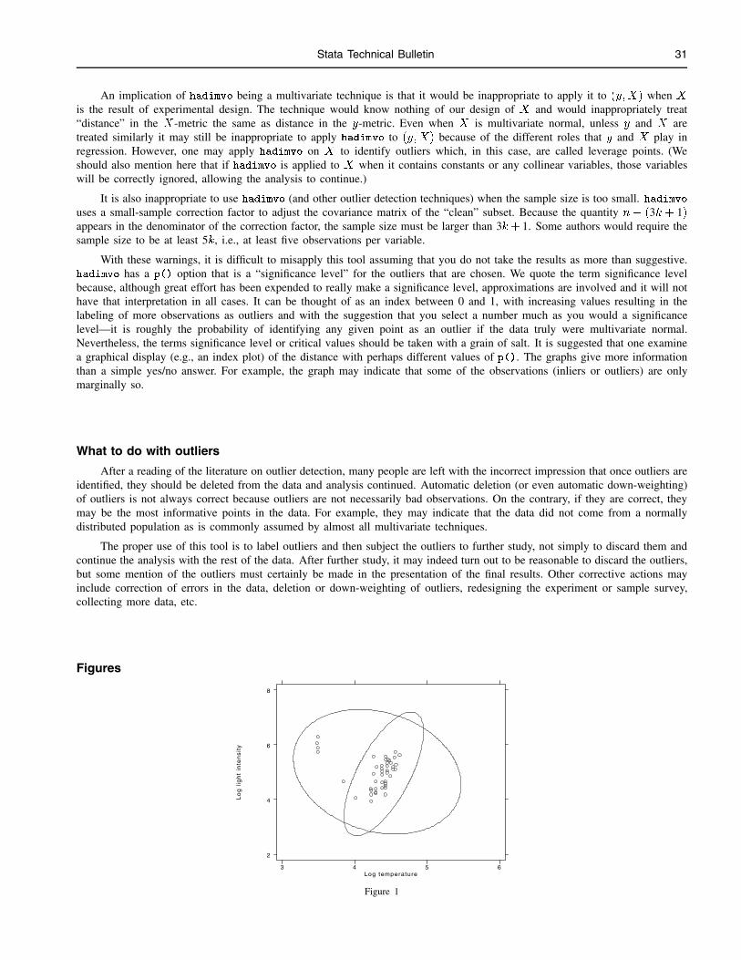
Stata Technical Bulletin 31
An implication of hadimvo being a multivariate technique is that it would be inappropriate to apply it to (y;X) when X
is the result of experimental design. The technique would know nothing of our design of X and would inappropriately treat“distance” in the X-metric the same as distance in the y-metric. Even when X is multivariate normal, unless y and X aretreated similarly it may still be inappropriate to apply hadimvo to (y;X) because of the different roles that y and X play inregression. However, one may apply hadimvo on X to identify outliers which, in this case, are called leverage points. (Weshould also mention here that if hadimvo is applied to X when it contains constants or any collinear variables, those variableswill be correctly ignored, allowing the analysis to continue.)
It is also inappropriate to use hadimvo (and other outlier detection techniques) when the sample size is too small. hadimvouses a small-sample correction factor to adjust the covariance matrix of the “clean” subset. Because the quantity n� (3k + 1)appears in the denominator of the correction factor, the sample size must be larger than 3k+ 1. Some authors would require thesample size to be at least 5k, i.e., at least five observations per variable.
With these warnings, it is difficult to misapply this tool assuming that you do not take the results as more than suggestive.hadimvo has a p() option that is a “significance level” for the outliers that are chosen. We quote the term significance levelbecause, although great effort has been expended to really make a significance level, approximations are involved and it will nothave that interpretation in all cases. It can be thought of as an index between 0 and 1, with increasing values resulting in thelabeling of more observations as outliers and with the suggestion that you select a number much as you would a significancelevel—it is roughly the probability of identifying any given point as an outlier if the data truly were multivariate normal.Nevertheless, the terms significance level or critical values should be taken with a grain of salt. It is suggested that one examinea graphical display (e.g., an index plot) of the distance with perhaps different values of p(). The graphs give more informationthan a simple yes/no answer. For example, the graph may indicate that some of the observations (inliers or outliers) are onlymarginally so.
What to do with outliers
After a reading of the literature on outlier detection, many people are left with the incorrect impression that once outliers areidentified, they should be deleted from the data and analysis continued. Automatic deletion (or even automatic down-weighting)of outliers is not always correct because outliers are not necessarily bad observations. On the contrary, if they are correct, theymay be the most informative points in the data. For example, they may indicate that the data did not come from a normallydistributed population as is commonly assumed by almost all multivariate techniques.
The proper use of this tool is to label outliers and then subject the outliers to further study, not simply to discard them andcontinue the analysis with the rest of the data. After further study, it may indeed turn out to be reasonable to discard the outliers,but some mention of the outliers must certainly be made in the presentation of the final results. Other corrective actions mayinclude correction of errors in the data, deletion or down-weighting of outliers, redesigning the experiment or sample survey,collecting more data, etc.
Figures
Lo
g l
igh
t in
ten
sity
Log temperature3 4 5 6
2
4
6
8
Figure 1

32 Stata Technical Bulletin STB-11
ReferencesHadi, A. S. 1992. Identifying multiple outliers in multivariate data. J. R. Statist. Soc. B 54(3): 761–771.
——. 1993. A modification of a method for the detection of outliers in multivariate samples. J. R. Statist. Soc. B (forthcoming).
Hadi, A. S. and J. S. Simonoff. 1993. Procedures for the identification of multiple outliers in linear models. Journal of the American StatisticalAssociation (forthcoming).
Rousseeuw, P. J. and A. M. Leroy. 1987. Robust Regression and Outlier Detection. New York: John Wiley & Sons.