Stability radii of positive discrete-time systems under a�neparameter perturbationsD. HinrichsenInstitut f�ur Dynamische SystemeUniversit�at BremenD-28334 BremenGermanydh@mathematik.uni-Bremen.deN. K. Son�Institute of MathematicsP.O. Box 631, Bo Ho10000 HanoiVietnamnkson@thevinh.ac.vnAbstractIn this paper we study stability radii of positive linear discrete-time systems under a�neparameter perturbations. It is shown that real and complex stability radii of positive systemscoincide for arbitrary perturbation structures, in particular for blockdiagonal disturbances asconsidered in �-analysis. Estimates and computable formulae are derived for these stabilityradii. The results are derived for arbitrary perturbation norms induced by monotonic vectornorms (e.g. p-norms, 1 � p � 1).Keywords : positive system, blockdiagonal perturbation, stability radius, �-analysis, structuredsingular value1 IntroductionA dynamical system is called positive if any trajectory of the system starting in the positiveorthant Rn+ = [0;1)n remains in Rn+ . In the time-invariant linear discrete-time case such systemsare described by equations of the formx(t+ 1) = Ax(t); t 2 N = f0; 1; 2; :::g (1)where A is a matrix with nonnegative entries. Positive dynamical systems play an important rolein the modeling of dynamical phenomena whose variables are restricted to be nonnegative. Areasof application are e.g. economics and population dynamics. The analysis of positive systems isbased on the theory of nonnegative matrices founded by Perron and Frobenius. As references wemention [6], [15], [2], [1].In this paper we study the asymptotic stability of uncertain positive systems of the form (1)where the system matrix A is subjected to a�ne parameter perturbations. We recall that thesystem (1) is asymptotically stable if and only if A is Schur stable, i.e. the spectrum of A iscontained in the open unit disk. The stability of positive linear systems is well studied and a�This author would like to thank the Alexander von Humboldt Foundation for its support during this work.1

number of useful stability criteria are available, see [2], [15].Over the past decade problems of model and parameter uncertainty have attracted a lot of atten-tion in control theory and this has motivated a renewed interest in robustness issues for positivesystems. Based on Kharitonov's results for interval polynomials [14] several authors analysed thequestion under which conditions all the linear systems x(t+1) = Ax(t) where A 2 [A;A] (a givenmatrix interval) are asymptotically stable. While this problem is a di�cult one for general linearsystems [3] it admits a simple solution for positive systems, see [18], [19].Another approach towards robust stability of positive systems is based on the concept ofstability radius, see [7], [8]. In its simplest form the problem is to determine the maximal � > 0for which the family of systemsx(t + 1) = (A+D�E)x(t); k�k < � (2)is asymptotically stable. D and E are given matrices specifying the structure of the pertubation,� is an unknown disturbance matrix and k � k a given operator norm. If complex perturbationsare allowed the maximal number � is called the complex stability radius and denoted by rC =rC (A;D;E). If only real perturbations are considered the real stability radius rR = rR(A;D;E)is obtained. For arbitrary linear discrete-time systems (without the positivity assumption) thesetwo stability radii are in general distinct. The complex stability radius is more easily analysed andcomputed than the real one. A detailed analysis of the complex stability radius of discrete-timesystems can be found in [11], an e�cient algorithm is described in [9] and the di�erence betweenthe two stability radii is discussed in [8], [10]. Only recently, a general formula for the real stabilityradius has been found by Qiu et al. [17]. The computation of rR(A;D;E) requires the solution ofa complicated global optimization problem.Fortunately, the situation is much simpler for positive systems. In this case we assume thatthe structure matrices are nonnegative. This assumption is quite natural for positive systemsand is not too restrictive since the disturbance matrix � is not restricted to be nonnegative. Inparticular, unstructured perturbations (for which D = E = In) can be represented in this wayand so can a�ne perturbations of single entries, rows or columns of A, see [7]. It has been shownin [12], [21] that if A;D;E are nonnegative and A is subjected to single perturbations of the formA; A+D�E, the real and complex stability radii coincide and can be determined via an easilycomputable formula. The results hold for arbitrary operator norms induced by monotonic vectornorms.In the present paper we go beyond the restricted class of single perturbations A; A+D�E.We consider perturbations of the formA; A+ NXi=1Di�iEi (3)or A; A + NXi=1 �iAi (4)where the matrices Ai; Di and Ei are given nonnegative matrices de�ning the structure of theperturbations and �i (resp. �i) are unknown matrices (resp. scalars) representing parameteruncertainties. Structured perturbations of these kinds are of great importance in control and formthe object of the so-called �-analysis, i.e. the theory of structured singular values as introducedin [5]. 2

The aim of this paper is to develop a �-analysis of positive systems and study the robustnessof stability of positive systems (1) subjected to a�ne perturbations of the forms (3), (4). Forarbitrary real matrices A;Ai; Di; Ei there exist no computable formulae for the stability radii of(1) with respect to perturbations of the form (3), (4). Only in the complex case reasonable boundscan be computed, very little is known for the real case, see [16], [8]. However, for nonnegativesystems and nonnegative structure matrices we will prove that real and complex stability radiicoincide and can be computed by formulae which extend the formula of [12] to a�ne perturbations(4). Throughout the paper the size of the disturbances �i is measured by operator norms inducedby arbitrary monotonic vector norms. This extends the applicability of the formulae beyond thelimits of usual �-analysis which only considers the spectral operator norm.The organization of this paper is as follows. In the next section we recall some theorems onnonnegative matrices and present preliminary results for later use. In Section 3 we study a generalclass of perturbations of blockdiagonal structure, which includes multi-perturbations of the form(3) and arbitrary a�ne perturbations (4) as particular cases. We show that for this perturbationclass, the stability radii of positive systems with respect to complex, real and nonnegative param-eter disturbances coincide. In this connection, a generalized notion of �-values is introduced andits properties for nonnegative matrices are analysed. In the �nal Section 4 a computable formulafor the stability radius of a positive system under arbitrary a�ne perturbations of the form (4) isderived. For multi-perturbations of the form (3) only bounds are obtained. The problem to �nda general computable formula for this type of perturbations still remains open.2 Preliminary resultsIn this section we present some properties of nonnegative matrices which will be used in the sequel.For more details and proofs we refer to [12].We �rst introduce some notations. Let n; l; q be positive integers. A matrix P = [pij] 2 Rl�qis said to be nonnegative (P � 0) if all its entries pij are nonnegative; it is said to be positive(P > 0) if all its entries are positive. For P;Q 2 Rl�q , P � Q means that P �Q � 0. The set ofall nonnegative l� q-matrices is denoted by Rl�q+ . A similar notation will be used for vectors. LetK = C or R, then for any x 2 K n and P 2 K l�q we de�ne jxj 2 Rn+ and jP j 2 Rl�q+ byjxj = (jxij) ; jP j = (jpijj) : (5)For any matrix A 2 K n�n the spectral radius of A is de�ned by�(A) = maxfj�j;� 2 �(A)g (6)where �(A) � C is the spectrum of A.A norm k � k on K n is said to be monotonic if it satis�esjxj � jyj ) kxk � kyk (7)for all x; y 2 K n : It can be shown that a vector norm k � k on K n is monotonic if and only ifkxk = k jxj k for all x 2 K n (see e.g. [13]). It follows that every p-norm on K n ; 1 � p � 1, ismonotonic. Recall that the p-norms on K n are de�ned bykxkp = ( (Pni=1 jxijp) 1p ; if 1 � p <1max1�i�n jxij; if p =1: (8)3

Throughout this section kPk denotes the operator norm of P 2 K l�q induced by a given pair ofnorms on K q and K l : kPk = maxkyk=1 kPyk:The following simple property of nonnegative matrices will be useful.Lemma 2.1 Suppose that P 2 Rl�q+ and k�k denotes the operator norm with respect to monotonicnorms on Rl , Rq . Then there exists e 2 Rq+ of norm kek = 1 such thatkPek = kPk: (9)Note that an operator norm induced by monotonic vector norms is not necessarily monotonic, i.e.for P;Q 2 K l�q ; the implication jP j � jQj ) kPk � kQk; (10)does not hold in general for such an operator norm. This implication holds, however, for nonneg-ative matrices. In fact, we haveLemma 2.2 Suppose that K l ; K q are provided with monotonic norms and k � k denotes the corre-sponding operator norm. If P 2 K l�q , Q 2 Rl�q+ and jP j � Q, thenkPk � k jP j k � kQk: (11)In particular, we obtain for arbitrary matrices P;Q 2 Rl�q ,0 � P � Q ) kPk � kQk (12)provided that Rl ;Rq are endowed with monotonic norms. Moreover, if the vector norms on K l ; K qare p-norms with p = 1 or 1 then the left inequality in (11) is an equality. This holds true forarbitrary monotonic norms if the matrix under consideration is of rank one.Lemma 2.3 Let K q ; K l be provided with monotonic norms and P 2 K l�q be of rank one. ThenkPk = k jP j k:The next two theorems state well known results from the literature on nonnegative matrices,see e.g. [6], [2], and [15].Theorem 2.4 (Perron - Frobenius) Suppose that A 2 Rn�n+ . Then(a) �(A) is an eigenvalue of A and there exists a nonnegative eigenvector x � 0; x 6= 0 such thatAx = �(A)x.(b) If � 2 �(A) and j�j = �(A) then the algebraic multiplicity of � is not greater than thealgebraic multiplicity of the eigenvalue �(A).Theorem 2.5 Let A;B 2 Rn�n+ ; t 2 R. Then(a) A � B implies �(A) � �(B);(b) Given � > 0, there exists a nonzero vector x � 0 such that Ax � �x if and only if �(A) � �;4

(c) (tI � A)�1 exists and is nonnegative if and only if t > �(A).As a corollary we obtain the following inequalities analogous to (11) for the spectral radius ofmatrices.Corollary 2.6 Let A 2 K n�n , B 2 Rn�n+ . If jAj � B then�(A) � �(jAj) � �(B): (13)We conclude this section with some comments concerning structured singular values or �-values.These were introduced by Doyle in [5] as a tool to analyze structured perturbations of controlsystems for which the available singular value based techniques only gave conservative results. Thefollowing de�nition extends Doyle's notion allowing for more general perturbation sets (includingsets of real perturbations only) and arbitrary perturbation norms.De�nition 2.7 Suppose M 2 C q�l , D � C l�q is non-empty and spanD is provided with a normk � kD. Then �D(M) = [ inffk�kD; � 2 D; det(Iq �M�) = 0g ]�1 (14)is called the �-value of M with respect to D and k � kD.In Doyle's original de�nition D was restricted to sets of blockdiagonal disturbances (see the nextsection) and k � kD to the spectral perturbation norm. The following two facts are easily veri�edfrom the de�nition. If D = C l�q then �D(M) = ��(M). If q = l, D = C Iq then �D(M) coincideswith the spectral radius �(M).If M is nonnegative, it is of interest to compare �D(M) with the �-values �DR(M); �D+(M)obtained by replacing the perturbation set D by the sets of real or nonnegative matrices in D:DR = D \ Rl�q ; D+ = D \ Rl�q+ : (15)Clearly, �D(M) � �DR(M) � �D+(M):The following lemma gives a technical criterion under which equalities hold.Lemma 2.8 Suppose M 2 Rq�l+ ;D � C l�q and k � kD is a norm on spanD such that the followingcondition is satis�ed:8� 2 D 8y 2 C q 9 ~� 2 C l�q : ~�y = �y; j ~�j 2 D; k j ~�j kD � k�kD: (16)If D+ is a cone, then �D(M) = �DR(M) = �D+(M):Proof: Since �D(M) � �DR(M) � �D+(M)it su�ces to show that for any � 2 D such that det(Iq�M�) = 0 there exists �+ 2 D+ satisfyingdet(Iq �M�+) = 0 and k�+kD � k�kD. Now suppose (Iq �M�)y = 0 where y 2 C q ; y 6= 0.Choose ~� as in (16). Then M ~�y = y and, by (13),~� := �(M j ~�j) � �(M ~�) � 1:Hence, by the Perron-Frobenius Theorem, �+ = ~��1j ~�j 2 D+ satis�esk�+kD � k�kD and det(Iq �M�+) = 0:5

3 Stability radii and �-valuesSince a dynamical model is never an exact portrait of the real process, it is important to determineto which extent the stability of a given nominal system is preserved under various classes ofperturbations. Before we analyse this question for positive systems we brie y outline a generalframework for the study of robust stability of discrete-time linear systems under arbitrary a�neparameter perturbations. The approach is based on the concept of stability radius introduced in[7] and extended in [8] and [10].Consider a dynamical system described by the following linear di�erence equationx(t + 1) = Ax(t); t 2 N (17)where A 2 C n�n . We assume that the system (17) is Schur stable, i.e. the spectrum �(A) of Alies in the open unit disk D = fs 2 C ; jsj < 1g.We consider a�ne parameter perturbations of the following typeA; A(�) = A+D�E; � 2 D: (18)Here D 2 C n�l and E 2 C q�n are given matrices and D � C l�q is a given subset of distur-bance matrices. The structure matrices D; E and the disturbance class D together determine thestructure of the additive perturbations D�E of A.De�nition 3.1 Given a subset D � C l�q and a norm k � kD on spanD � C l�q the stability radiusof the system (17) with respect to perturbations of the form (18) is de�ned byrD = rD(A;D;E) = inffk�kD; � 2 D; �(A+D�E) � 1g: (19)Throughout the paper we set inf ; =1, 1�1 = 0, and 0�1 =1. By continuity of the spectrumthe function � 7! �(A+D�E) is continuous, and hence the setU = f� 2 C l�q ; �(A +D�E) � 1gis closed. Therefore, if D is closed in C l�q and D \ U 6= ;, there always exists �0 2 D \ U suchthat k�0kD = rD(A;D;E). Such a matrix is called a minimum norm destabilizing perturbation ofclass D for (17). Clearly, if the perturbation class is restricted, the stability radius (with respectto the same perturbation norm) is increased:~D � D =) r ~D(A;D;E) � rD(A;D;E): (20)Of special interest are the sets of real and of nonnegative perturbations of class D.Throughout the paper spanDR and spanD+ will always be endowed with the norm inducedfrom spanD. As a consequence of (20) and the continuity of �(�),0 < rD(A;D;E) � rDR(A;D;E) � rD+(A;D;E): (21)In the following examples we illustrate the above de�nition by discussing stability radii for variousperturbation classes.Example 3.2 (Single perturbations) Suppose D = C l�q , i.e. we consider perturbations of theform A; A(�) = A +D�E; � 2 C l�q : (22)6

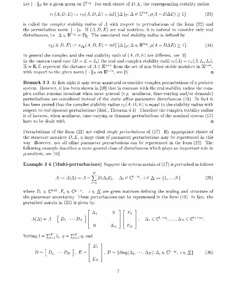
Let k � kD be a given norm on C l�q . For each choice of D;E, the corresponding stability radiusrC (A;D;E) := rD(A;D;E) = inffk�kD; � 2 C l�q ; �(A +D�E) � 1g (23)is called the complex stability radius of A with respect to perturbations of the form (22) andthe perturbation norm k � kD. If (A;D;E) are real matrices, it is natural to consider only realdisturbances, i.e. � 2 Rl�q = DR. The associated real stability radius is de�ned byrR(A;D;E) := rDR(A;D;E) = inffk�kD; � 2 Rl�q ; �(A+D�E) � 1g: (24)In general the complex and the real stability radii of (A;D;E) are di�erent, see [8].In the unstructured case (D = E = In) the real and complex stability radii rK (A) = rK (A; In; In),K = R; C represent the distance of A 2 K n�n from the set of non Schur stable matrices in K n�n ,with respect to the given norm k � kD on K n�n , see [8].Remark 3.3 At �rst sight it may seem unnatural to consider complex perturbations of a positivesystem. However, it has been shown in [10] that in contrast with the real stability radius the com-plex radius remains invariant when more general (e.g. nonlinear, time-varying and/or dynamic)perturbations are considered instead of the static a�ne parameter disturbances (18). In fact ithas been proved that the complex stability radius rC (A;D;E) is equal to the stability radius withrespect to real dynamic perturbations (ibid., Theorem 4.4). Therefore the complex stability radiusis of interest, when nonlinear, time-varying or dynamic perturbations of the nominal system (17)have to be dealt with.Perturbations of the form (22) are called single perturbations of (17). By appropriate choice ofthe structure matrices D;E, a large class of parameter perturbations may be represented in thisway. However, not all a�ne parameter perturbations can be represented in the form (22). Thefollowing example describes a more general class of disturbances which plays an important role in�-analysis, see [16].Example 3.4 (Multi-perturbations) Suppose the system matrix of (17) is perturbed as followsA; A(�) = A+ NXi=1Di�iEi; �i 2 C li�qi; i 2 N := f1; : : :Ng (25)where Di 2 C n�li ; Ei 2 C qi�n; i 2 N are given matrices de�ning the scaling and structure ofthe parameter uncertainty. These perturbations can be represented in the form (18). In fact, theperturbed matrix in (25) is given by:A(�) = A+ h D1 � � �DN i 2664 �1 0. . .0 �N 3775 2664 E1...EN 3775 ; �1 2 C l1�q1; : : : ;�N 2 C lN�qN :Setting l = PNi=1 li; q = PNi=1 qi andD = h D1 � � �DN i ; E = 2664 E1...EN 3775 ; D = fdiag(�1; � � � ;�N );�i 2 C li�qi; i 2 Ng (26)7

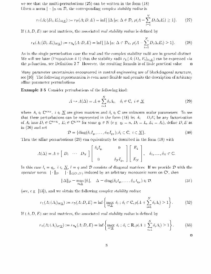
we see that the multi-perturbations (25) can be written in the form (18).Given a norm k � kD on D, the corresponding complex stability radius isrC (A; (Di; Ei)i2N) := rD(A;D;E) = inffk�kD; � 2 D; �(A + NXi=1Di�iEi) � 1g: (27)If (A;D;E) are real matrices, the associated real stability radius is de�ned byrR(A; (Di; Ei)i2N) := rDR(A;D;E) = inffk�kD; � 2 DR; �(A + NXi=1Di�iEi) � 1g: (28)As in the single perturbation case the real and the complex stability radii are in general distinct.We will see later (Proposition 4.1) that the stability radii rK (A; (Di; Ei)i2N ) can be expressed viathe �-function, see De�nition 2.7. However, the resulting formula is of little practical value.Many parameter uncertainties encountered in control engineering are of blockdiagonal structure,see [16]. The following representation is even more exible and permits the description of arbitrarya�ne parameter perturbations.Example 3.5 Consider perturbations of the following kind:A; A(�) = A + NXi=1 �iAi; �i 2 C ; i 2 N (29)where Ai 2 C n�n ; i 2 N are given matrices and �i 2 C are unknown scalar parameters. To seethat these perturbations can be represented in the form (18) let Ai = DiEi be any factorizationof Ai into Di 2 C n�qi ; Ei 2 C qi�n for some qi 2 N (e.g. qi = n, Di = In; Ei = Ai), de�ne D;E asin (26) and set D = fdiag(�1Iq1; : : : ; �NIqN ); �i 2 C ; i 2 Ng: (30)Then the a�ne perturbations (29) can equivalently be described in the form (18) withA(�) = A+ h D1 � � � DN i 2664 �1Iqi 0. . .0 �NIqN 3775 2664 E1...EN 3775 ; �1; : : : ; �N 2 C :In this case li = qi; i 2 N , l = q and D consists of diagonal matrices. If we provide D with theoperator norm k � kD = k � kL(C q ;C q ) induced by an arbitrary monotonic norm on C q , thenk�kD = maxi2N j�ij; � = diag(�1Iq1; : : : ; �NIqN ) 2 D: (31)(see, e.g. [13]), and we obtain the following complex stability radius:rC (A; (Ai)i2N) := rD(A;D;E) = inf (maxi2N j�ij; �i 2 C ; �(A + NXi=1 �iAi) � 1) : (32)If (A;D;E) are real matrices, the associated real stability radius is de�ned byrR(A; (Ai)i2N) := rDR(A;D;E) = inf (maxi2N j�ij; �i 2 R; �(A + NXi=1 �iAi) � 1) : (33)8

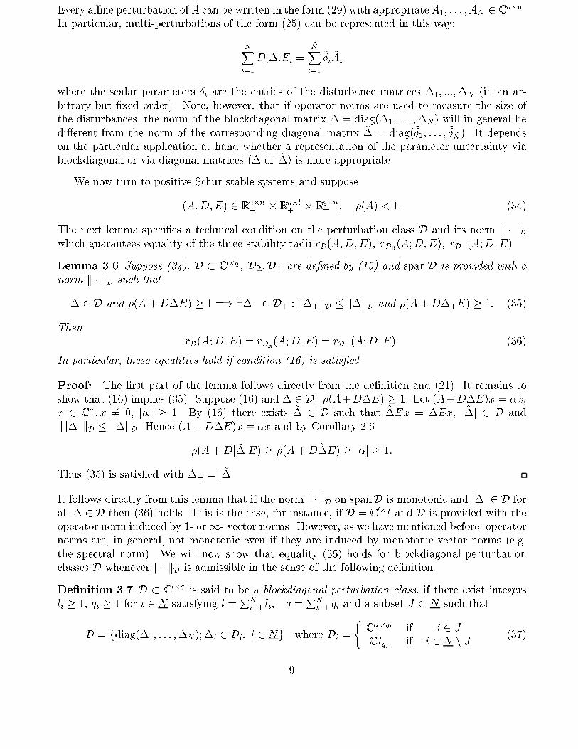
Every a�ne perturbation of A can be written in the form (29) with appropriateA1; : : : ; AN 2 C n�n .In particular, multi-perturbations of the form (25) can be represented in this way:NXi=1Di�iEi = ~NXi=1 ~�i ~Aiwhere the scalar parameters ~�i are the entries of the disturbance matrices �1; :::;�N (in an ar-bitrary but �xed order). Note, however, that if operator norms are used to measure the size ofthe disturbances, the norm of the blockdiagonal matrix � = diag(�1; : : : ;�N) will in general bedi�erent from the norm of the corresponding diagonal matrix ~� = diag(~�1; : : : ; ~� ~N ). It dependson the particular application at hand whether a representation of the parameter uncertainty viablockdiagonal or via diagonal matrices (� or ~�) is more appropriate.We now turn to positive Schur stable systems and suppose(A;D;E) 2 Rn�n+ � Rn�l+ � Rq�n+ ; �(A) < 1: (34)The next lemma speci�es a technical condition on the perturbation class D and its norm k � kDwhich guarantees equality of the three stability radii rD(A;D;E); rDR(A;D;E); rD+(A;D;E).Lemma 3.6 Suppose (34), D � C l�q , DR;D+ are de�ned by (15) and spanD is provided with anorm k � kD such that� 2 D and �(A +D�E) � 1 =) 9�+ 2 D+ : k�+kD � k�kD and �(A+D�+E) � 1: (35)Then rD(A;D;E) = rDR(A;D;E) = rD+(A;D;E): (36)In particular, these equalities hold if condition (16) is satis�ed.Proof: The �rst part of the lemma follows directly from the de�nition and (21). It remains toshow that (16) implies (35). Suppose (16) and � 2 D; �(A+D�E) � 1. Let (A+D�E)x = �x,x 2 C n ; x 6= 0, j�j � 1. By (16) there exists ~� 2 D such that ~�Ex = �Ex, j ~�j 2 D andk j ~�j kD � k�kD. Hence (A +D ~�E)x = �x and by Corollary 2.6�(A +Dj ~�jE) � �(A+D ~�E) � j�j � 1:Thus (35) is satis�ed with �+ = j ~�j.It follows directly from this lemma that if the norm k � kD on spanD is monotonic and j�j 2 D forall � 2 D then (36) holds. This is the case, for instance, if D = C l�q and D is provided with theoperator norm induced by 1- or1- vector norms. However, as we have mentioned before, operatornorms are, in general, not monotonic even if they are induced by monotonic vector norms (e.g.the spectral norm). We will now show that equality (36) holds for blockdiagonal perturbationclasses D whenever k � kD is admissible in the sense of the following de�nition.De�nition 3.7 D � C l�q is said to be a blockdiagonal perturbation class, if there exist integersli � 1; qi � 1 for i 2 N satisfying l = PNi=1 li; q = PNi=1 qi and a subset J � N such thatD = fdiag(�1; : : : ;�N);�i 2 Di; i 2 Ng where Di = ( C li�qi if i 2 JC Iqi if i 2 N n J: (37)9

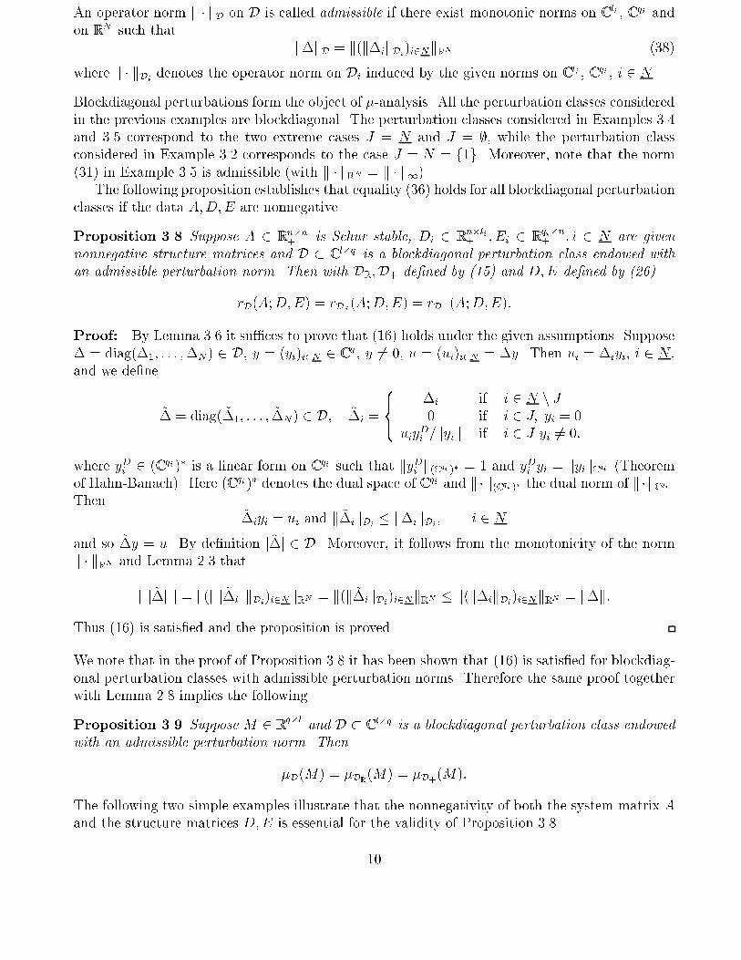
An operator norm k � kD on D is called admissible if there exist monotonic norms on C li ; C qi andon RN such that k�kD = k(k�ikDi)i2NkRN (38)where k � kDi denotes the operator norm on Di induced by the given norms on C li ; C qi , i 2 N .Blockdiagonal perturbations form the object of �-analysis. All the perturbation classes consideredin the previous examples are blockdiagonal. The perturbation classes considered in Examples 3.4and 3.5 correspond to the two extreme cases J = N and J = ;, while the perturbation classconsidered in Example 3.2 corresponds to the case J = N = f1g. Moreover, note that the norm(31) in Example 3.5 is admissible (with k � kRN = k � k1).The following proposition establishes that equality (36) holds for all blockdiagonal perturbationclasses if the data A;D;E are nonnegative.Proposition 3.8 Suppose A 2 Rn�n+ is Schur stable, Di 2 Rn�li+ ; Ei 2 Rqi�n+ ; i 2 N are givennonnegative structure matrices and D � C l�q is a blockdiagonal perturbation class endowed withan admissible perturbation norm. Then with DR;D+ de�ned by (15) and D;E de�ned by (26)rD(A;D;E) = rDR(A;D;E) = rD+(A;D;E):Proof: By Lemma 3.6 it su�ces to prove that (16) holds under the given assumptions. Suppose� = diag(�1; : : : ;�N) 2 D, y = (yi)i2N 2 C q , y 6= 0, u = (ui)i2N = �y. Then ui = �iyi; i 2 N ,and we de�ne ~� = diag( ~�1; : : : ; ~�N) 2 D; ~�i = 8><>: �i if i 2 N n J0 if i 2 J; yi = 0uiyDi =kyik if i 2 J yi 6= 0:where yDi 2 (C qi )� is a linear form on C qi such that kyDi k(C qi )� = 1 and yDi yi = kyikC qi (Theoremof Hahn-Banach). Here (C qi )� denotes the dual space of C qi and k �k(Cqi )� the dual norm of k �kCqi .Then ~�iyi = ui and k ~�ikDi � k�ikDi; i 2 Nand so ~�y = u. By de�nition j ~�j 2 D. Moreover, it follows from the monotonicity of the normk � kRN and Lemma 2.3 thatk j ~�j k = k(k j ~�ij kDi)i2NkRN = k(k ~�ikDi)i2NkRN � k(k�ikDi)i2NkRN = k�k:Thus (16) is satis�ed and the proposition is proved.We note that in the proof of Proposition 3.8 it has been shown that (16) is satis�ed for blockdiag-onal perturbation classes with admissible perturbation norms. Therefore the same proof togetherwith Lemma 2.8 implies the followingProposition 3.9 Suppose M 2 Rq�l+ and D � C l�q is a blockdiagonal perturbation class endowedwith an admissible perturbation norm. Then�D(M) = �DR(M) = �D+(M):The following two simple examples illustrate that the nonnegativity of both the system matrix Aand the structure matrices D;E is essential for the validity of Proposition 3.8.10

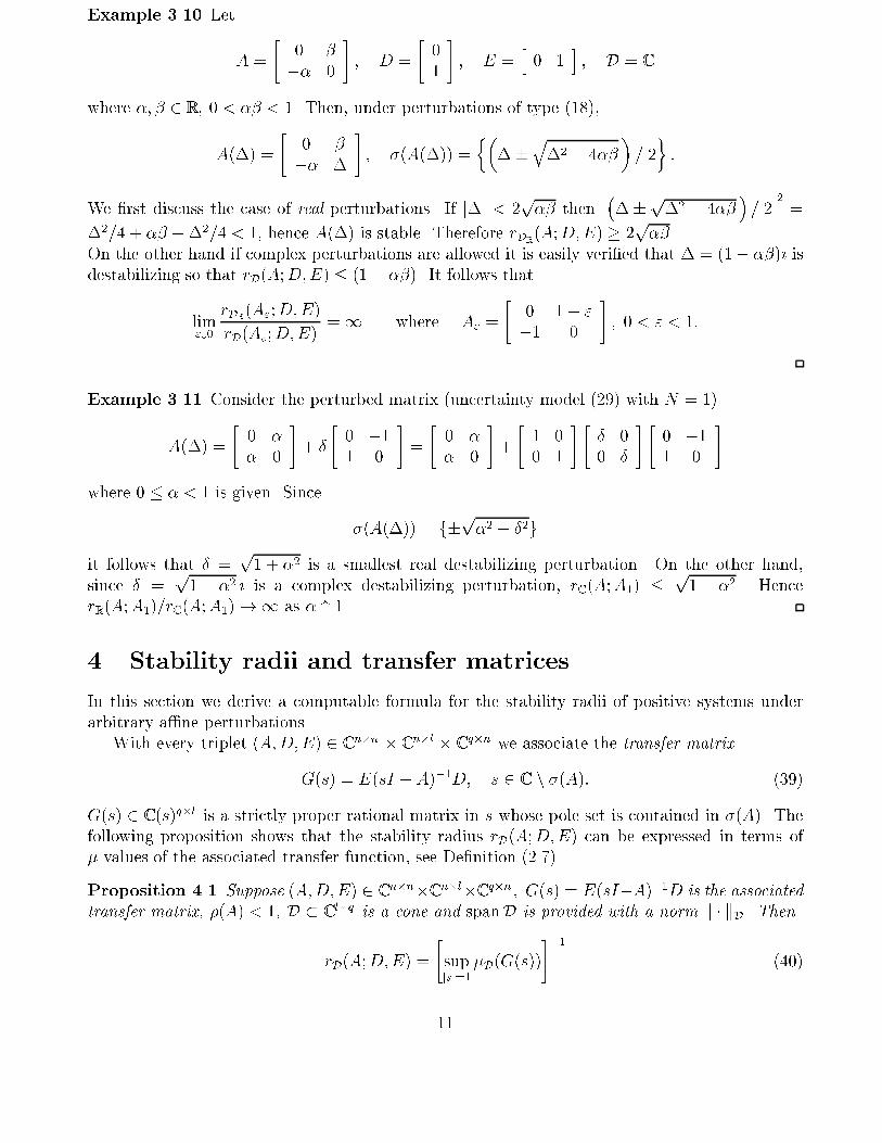
Example 3.10 LetA = " 0 ��� 0 # ; D = " 01 # ; E = h 0 1 i ; D = Cwhere �; � 2 R; 0 < �� < 1. Then, under perturbations of type (18),A(�) = " 0 ��� � # ; �(A(�)) = ����q�2 � 4�� � / 2� :We �rst discuss the case of real perturbations. If j�j < 2p�� then ������p�2 � 4�� � / 2���2 =�2=4 + �� ��2=4 < 1, hence A(�) is stable. Therefore rDR(A;D;E) � 2p��.On the other hand if complex perturbations are allowed it is easily veri�ed that � = (1� ��){ isdestabilizing so that rD(A;D;E) � (1� ��). It follows thatlim"#0 rDR(A";D;E)rD(A";D;E) =1 where A" = " 0 1� "�1 0 # ; 0 < " < 1:Example 3.11 Consider the perturbed matrix (uncertainty model (29) with N = 1)A(�) = " 0 �� 0 # + � " 0 �11 0 # = " 0 �� 0 # + " 1 00 1 # " � 00 � # " 0 �11 0 #where 0 � � < 1 is given. Since �(A(�)) = f�p�2 � �2git follows that � = p1 + �2 is a smallest real destabilizing perturbation. On the other hand,since � = p1� �2 { is a complex destabilizing perturbation, rC (A;A1) � p1� �2. HencerR(A;A1)=rC (A;A1)!1 as � " 1.4 Stability radii and transfer matricesIn this section we derive a computable formula for the stability radii of positive systems underarbitrary a�ne perturbations.With every triplet (A;D;E) 2 C n�n � C n�l � C q�n we associate the transfer matrixG(s) = E(sI � A)�1D; s 2 C n �(A): (39)G(s) 2 C (s)q�l is a strictly proper rational matrix in s whose pole set is contained in �(A). Thefollowing proposition shows that the stability radius rD(A;D;E) can be expressed in terms of�-values of the associated transfer function, see De�nition (2.7).Proposition 4.1 Suppose (A;D;E) 2 C n�n�C n�l�C q�n ; G(s) = E(sI�A)�1D is the associatedtransfer matrix, �(A) < 1, D � C l�q is a cone and spanD is provided with a norm k � kD. ThenrD(A;D;E) = "supjsj=1�D(G(s))#�1 (40)11

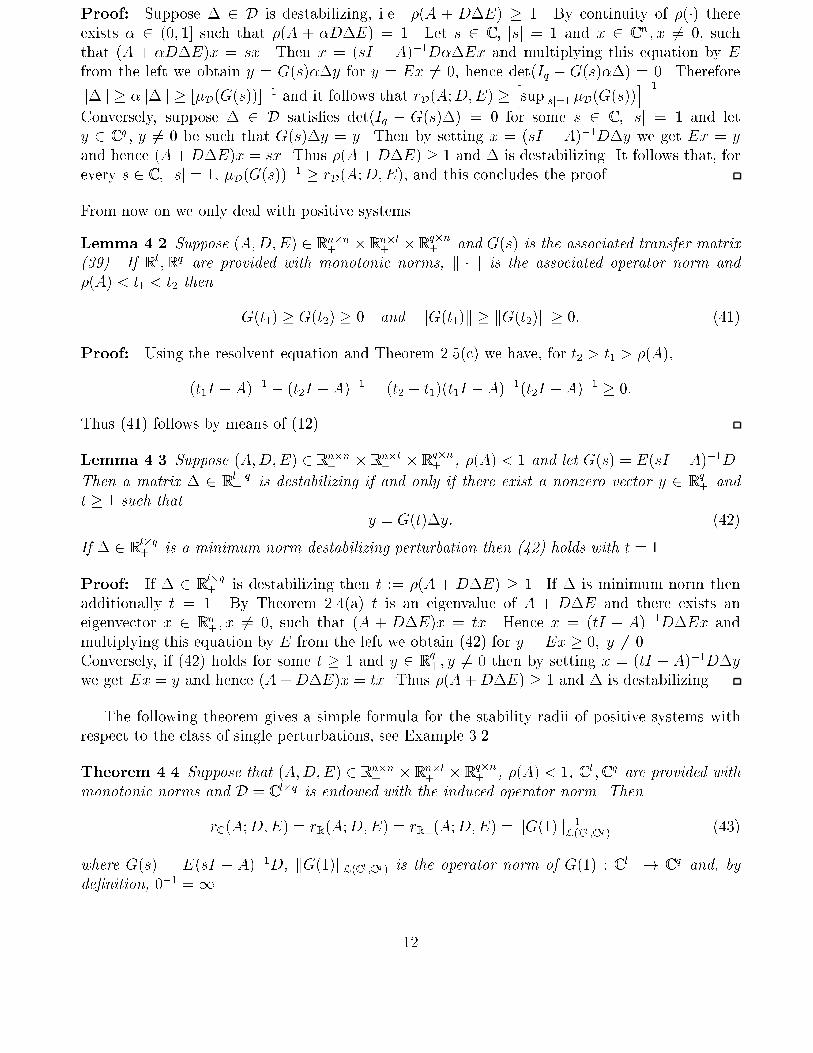
Proof: Suppose � 2 D is destabilizing, i.e. �(A + D�E) � 1. By continuity of �(�) thereexists � 2 (0; 1] such that �(A + �D�E) = 1. Let s 2 C ; jsj = 1 and x 2 C n ; x 6= 0; suchthat (A + �D�E)x = sx. Then x = (sI � A)�1D��Ex and multiplying this equation by Efrom the left we obtain y = G(s)��y for y = Ex 6= 0, hence det(Iq � G(s)��) = 0. Thereforek�k � �k�k � [�D(G(s))]�1 and it follows that rD(A;D;E) � hsupjsj=1 �D(G(s))i�1.Conversely, suppose � 2 D satis�es det(Iq � G(s)�) = 0 for some s 2 C ; jsj = 1 and lety 2 C q ; y 6= 0 be such that G(s)�y = y. Then by setting x = (sI � A)�1D�y we get Ex = yand hence (A+D�E)x = sx. Thus �(A+D�E) � 1 and � is destabilizing. It follows that, forevery s 2 C ; jsj = 1, �D(G(s))�1 � rD(A;D;E), and this concludes the proof.From now on we only deal with positive systems.Lemma 4.2 Suppose (A;D;E) 2 Rn�n+ � Rn�l+ �Rq�n+ and G(s) is the associated transfer matrix(39). If Rl ;Rq are provided with monotonic norms, k � k is the associated operator norm and�(A) < t1 < t2 then G(t1) � G(t2) � 0 and kG(t1)k � kG(t2)k � 0: (41)Proof: Using the resolvent equation and Theorem 2.5(c) we have, for t2 > t1 > �(A),(t1I � A)�1 � (t2I � A)�1 = (t2 � t1)(t1I � A)�1(t2I � A)�1 � 0:Thus (41) follows by means of (12).Lemma 4.3 Suppose (A;D;E) 2 Rn�n+ � Rn�l+ � Rq�n+ , �(A) < 1 and let G(s) = E(sI � A)�1D.Then a matrix � 2 Rl�q+ is destabilizing if and only if there exist a nonzero vector y 2 Rq+ andt � 1 such that y = G(t)�y: (42)If � 2 Rl�q+ is a minimum norm destabilizing perturbation then (42) holds with t = 1.Proof: If � 2 Rl�q+ is destabilizing then t := �(A + D�E) � 1. If � is minimum norm thenadditionally t = 1. By Theorem 2.4(a) t is an eigenvalue of A + D�E and there exists aneigenvector x 2 Rn+ ; x 6= 0; such that (A + D�E)x = tx. Hence x = (tI � A)�1D�Ex andmultiplying this equation by E from the left we obtain (42) for y = Ex � 0; y 6= 0.Conversely, if (42) holds for some t � 1 and y 2 Rq+ ; y 6= 0 then by setting x = (tI � A)�1D�ywe get Ex = y and hence (A+D�E)x = tx. Thus �(A+D�E) � 1 and � is destabilizing.The following theorem gives a simple formula for the stability radii of positive systems withrespect to the class of single perturbations, see Example 3.2.Theorem 4.4 Suppose that (A;D;E) 2 Rn�n+ � Rn�l+ � Rq�n+ , �(A) < 1, C l ; C q are provided withmonotonic norms and D = C l�q is endowed with the induced operator norm. ThenrC (A;D;E) = rR(A;D;E) = rR+(A;D;E) = kG(1)k�1L(C l ;C q ) (43)where G(s) = E(sI � A)�1D, kG(1)kL(C l ;C q ) is the operator norm of G(1) : C l ! C q and, byde�nition, 0�1 =1. 12

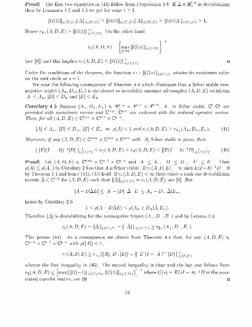
Proof: The �rst two equalities in (43) follow from Proposition 3.8. If � 2 Rl�q+ is destabilizingthen by Lemmata 4.2 and 4.3 we get for some t � 1kG(1)kL(C l ;Cq )k�kL(C q ;C l ) � kG(t)kL(C l ;Cq )k�kL(C q ;C l ) � kG(t)�kL(C q ;C q ) � 1:Hence rR+(A;D;E) � kG(1)k�1L(C l ;Cq ). On the other handrC (A;D;E) = "maxjsj=1 kG(s)kL(C l ;C q )#�1(see [8]) and this implies rC (A;D;E) � kG(1)k�1L(C l ;C q ).Under the conditions of the theorem, the function s 7! kG(s)kL(C l ;C q ) attains its maximum valueon the unit circle at s = 1.We note the following consequence of Theorem 4.4 which illustrates that a Schur stable non-negative triplet (A+; D+; E+) is the closest to instability amongst all complex (A;D;E) satisfyingjAj � A+, jDj � D+ and jEj � E+.Corollary 4.5 Suppose (A+; D+; E+) 2 Rn�n+ � Rn�l+ � Rq�n+ , A+ is Schur stable, C l ; C q areprovided with monotonic norms and C l�q , C q�l are endowed with the induced operator norms.Then, for all (A;D;E) 2 C n�n � C n�l � C q�n ,jAj � A+; jDj � D+; jEj � E+ ) �(A) < 1 and rC (A;D;E) � rR+(A+;D+; E+): (44)Moreover, if any (A;D;E) 2 C n�n � C n�l � C q�n with jAj Schur stable is given, thenk jEj(I � jAj)�1jDj k�1L(C l ;Cq ) � rC (A;D;E) � rR(A;D;E) � kE(I � A)�1Dk�1L(C l ;Cq ): (45)Proof: Let (A;D;E) 2 C n�n � C n�l � C q�n and jAj � A+; jDj � D+; jEj � E+. Then�(A) � �(A+) by Corollary 2.6 so that A is Schur stable. If rC (A;D;E) =1 then E(I�A)�1D = 0by Theorem 4.4 and hence (44), (45) hold. If rC (A;D;E) <1 there exists a rank one destabilizingmatrix ~� 2 C l�q for (A;D;E) such that k ~�kL(C q ;C l ) = rC (A;D;E), see [8]. ButjA+D ~�Ej � jAj+ jDj j ~�j jEj � A+ +D+j ~�jE+;hence by Corollary 2.6 1 � �(A+D ~�E) � �(A+ +D+j ~�jE+):Therefore j ~�j is destabilizing for the nonnegative triplet (A+; D+; E+) and by Lemma 2.3rC (A;D;E) = k ~�kL(C q ;C l ) = k j ~�j kL(Cq ;C l ) � rR+(A+;D+; E+):This proves (44). As a consequence we obtain from Theorem 4.4 that, for any (A;D;E) 2C n�n � C n�l � C q�n with �(jAj) < 1,rC (A;D;E) � rR+(jAj; jDj; jEj) = k jEj(I � jAj)�1jDj k�1L(C l ;C q )whence the �rst inequality in (45). The second inequality is clear and the last one follows fromrR(A;D;E) � hmaxfkG(�1)kL(C l ;C q ); kG(1)kL(C l ;Cq )gi�1 where G(s) = E(sI �A)�1D is the asso-ciated transfer matrix, see [9]. 13

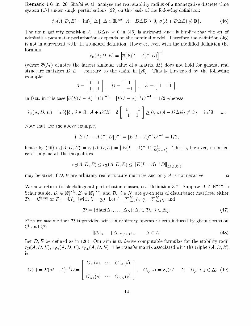
Remark 4.6 In [20] Shafai et al. analyse the real stability radius of a nonnegative discrete-timesystem (17) under single perturbations (22) on the basis of the following de�nition:~rR(A;D;E) = inffk�k; � 2 Rl�q ; A+D�E � 0; �(A+D�E) 6� D g: (46)The nonnegativity condition A + D�E � 0 in (46) is awkward since it implies that the set ofadmissible parameter perturbations depends on the nominal model. Therefore the de�nition (46)is not in agreement with the standard de�nition. However, even with the modi�ed de�nition theformula ~rR(A;D;E) = h�(E(I � A)�1D)i�1(where �(M) denotes the largest singular value of a matrix M) does not hold for general realstructure matrices D;E { contrary to the claim in [20]. This is illustrated by the followingexample: A = " 0 00 0 # ; D = " 1�1 # ; E = h 1 �1 i :In fact, in this case [�(E(I � A)�1D)]�1 = jE(I � A)�1Dj�1 = 1=2 whereas~rR(A;D;E) = inffj�j; � 2 R; A+D�E = � " 1 �1�1 1 # � 0; �(A+D�E) 6� D g = inf ; =1:Note that, for the above example,( jEj(I � jAj)�1jDj )�1 = jE(I � A)�1Dj�1 = 1=2;hence by (45) rR(A;D;E) = rC (A;D;E) = kE(I � A)�1Dk�1L(C l ;Cq ). This is, however, a specialcase. In general, the inequalitiesrC (A;D;E) � rR(A;D;E) � kE(I � A)�1Dk�1L(C l ;C q )may be strict if D;E are arbitrary real structure matrices and only A is nonnegative.We now return to blockdiagonal perturbation classes, see De�nition 3.7. Suppose A 2 Rn�n+ isSchur stable, Di 2 Rn�li+ ; Ei 2 Rqi�n+ , and Di, i 2 N , are given sets of disturbance matrices, eitherDi = C li�qi or Di = C Iqi (with li = qi). Let l = PNi=1 li; q = PNi=1 qi andD = fdiag(�1; : : : ;�N);�i 2 Di; i 2 Ng: (47)First we assume that D is provided with an arbitrary operator norm induced by given norms onC l and C q : k�kD = k�kL(C q ;C l ); � 2 D: (48)Let D;E be de�ned as in (26). Our aim is to derive computable formulae for the stability radiirD(A;D;E), rDR(A;D;E), rD+(A;D;E). The transfer matrix associated with the triplet (A;D;E)isG(s) = E(sI � A)�1D = 2664 G11(s) � � � G1N (s)... ...GN1(s) � � � GNN (s) 3775 ; Gij(s) = Ei(sI � A)�1Dj; i; j 2 N: (49)14

Proposition 4.7 Suppose A 2 Rn�n+ is Schur stable, Di 2 Rn�li+ ; Ei 2 Rqi�n+ , i 2 N , D;E arede�ned by (26) and G is the associated transfer matrix (49). If D is a class of blockdiagonalperturbations (47), provided with the operator norm (48) induced by a given pair of norms k �kC l ; k � kC q on C l and C q then" inf�>0 ��iGij(1)��1j �i;j2N L(C l ;Cq )#�1 � rD+(A;D;E): (50)where the in�mum is taken over all positive scaling vectors � = (�1; : : : ; �n) > 0.Proof: Suppose that � 2 D+ is a minimum norm destabilizing disturbance. By Lemma 4.3there exists a nonzero vector y 2 Rq+ such that y = G(1)�y. For any � = (�1; :::; �N) > 0, letL� = diag(�1Iq1; :::; �NIqN ); R� = diag(�1Il1; :::; �NIlN ):Then R�1� �L� = � whence L�y = L�G(1)R�1� �L�y 6= 0and so kL�G(1)R�1� kL(C l ;Cq )k�kL(C q ;C l ) � kL�G(1)R�1� �kL(C q ;Cq ) � 1:It follows thatk�k � � inf�>0 L�G(1)R�1� L(C l ;Cq )��1 = " inf�>0 ��iGij(1)��1j �i;j2N L(C l ;Cq )#�1 :This proves (50).Combining the preceding result with Proposition 3.8, we obtain the following general formula forthe stability radius of positive linear systems under arbitrary a�ne perturbations of the form (29)with nonnegative Ai = DiEi. Here rC (A; (Ai)i2N ), rR(A; (Ai)i2N) are de�ned by (32), (33), andrR+(A; (Ai)i2N ) is de�ned analogously. The underlying perturbation norm is given by (31):k�kD = maxi2N j�ij; � = diag(�1Iq1; : : : ; �NIqN ) 2 D:Theorem 4.8 Suppose A 2 Rn�n+ is Schur stable and subjected to perturbations of the formA; A(�) = A + NXi=1 �iAi; �i 2 C ; i 2 Nwhere Ai 2 Rn�n+ , i 2 N are given. If Di 2 Rn�qi+ ; Ei 2 Rqi�n+ (for some qi 2 N) are chosen suchthat Ai = DiEi, i 2 N , and G(s) is de�ned by (49) thenrC (A; (Ai)i2N) = rR(A; (Ai)i2N ) = rR+(A; (Ai)i2N) = [�(G(1))]�1 : (51)Proof: Proceeding as in Example 3.5 we de�ne D by (30) and endow D with the norm (31).Then rC (A; (Ai)i2N) = rD(A;D;E), rR(A; (Ai)i2N ) = rDR(A;D;E), and rR+(A; (Ai)i2N) =rD+(A;D;E). Since (31) is admissible, the �rst two equalities in (51) follow from Proposition3.8. Now let q = PNi=1 qi. By the Perron-Frobenius Theorem there exists an eigenvector u 2 Rq+of G(1) � 0 for the eigenvalue � = �(G(1)):G(1)u = �u:15

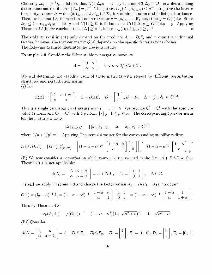
Choosing �0 = ��1Iq it follows that G(1)�0u = u. By Lemma 4.3 �0 2 D+ is a destabilizingdisturbance matrix of norm k�0k = ��1. This proves rR+(A; (Ai)i2N) � ��1. To prove the inverseinequality, assume � = diag(�1Iq1; : : : ; �NIqN ) 2 D+ is a minimum norm destabilizing disturbance.Then, by Lemma 4.3, there exists a nonzero vector y = (yi)i2N 2 Rq+ such that y = G(1)�y. Since�y � (maxi2N �i)y = k�ky and G(1) � 0, it follows that G(1)k�ky � G(1)�y = y. ApplyingTheorem 2.5(b) we conclude that k�k � ��1, hence rR+(A; (Ai)i2N ) � ��1.The stability radii in (51) only depend on the products Ai = DiEi and not on the individualfactors, however, the transfer matrix G(s) depends on the speci�c factorizations chosen.The following example illustrates the previous results.Example 4.9 Consider the Schur stable nonnegative matricesA = " 0 �� � # ; 0 < � < 2=(p5 + 1):We will determine the stability radii of these matrices with respect to di�erent perturbationstructures and perturbation norms.(i) Let A(�) = " �1 � + �2� � # = A +D�E; D = " 10 # ; E = I2; � = [�1 ; �2] 2 C 1�2 :This is a single perturbation structure with l = 1; q = 2. We provide C l = C 1 with the absolutevalue as norm and C q = C 2 with a p-norm k � kp ; 1 � p � 1. The corresponding operator normfor the perturbations is k�kL(C q ;C l ) = k[�1 ; �2]kp� ; � = [�1 ; �2] 2 C 1�2where 1=p+ 1=p� = 1. Applying Theorem 4.4 we get for the corresponding stability radius:rR(A;D;E) = kG(1)k�1L(C l ;C q ) = (1� �� �2)�1 " 1� � �� 1 # " 10 # �1p = (1� �� �2) " 1� �� # �1p(ii) We now consider a perturbation which cannot be represented in the form A +D�E so thatTheorem 4.4 is not applicable:A(�) = " � � +�� � +� # = A+�A1; A1 = " 1 10 1 # ; � 2 C :Instead we apply Theorem 4.8 and choose the factorization A1 = D1E1 = A1I2 to obtainG(1) = (I2 �A)�1A1 = (1� �� �2)�1 " 1� � �� 1 # " 1 10 1 # = (1� �� �2)�1 " 1� � 1� 1 + � # :Thus by Theorem 4.8rR(A;A1) = [�(G(1))]�1 = (1� �� �2)(1 +p�2 + �)�1 = 1�p�2 + �:(iii) ConsiderA(�)=" �1 �� � + �2 #= A+D1�1E1 +D2�2E2; D1 =" 10 # ; E1 = [1 ; 0] ; D2 =" 01 # ; E2 = [0 ; 1]16

where � = diag(�1 ; �2); �1; �2 2 C . Again the perturbation cannot be adequately representedin the form (22). In order to apply Theorem 4.8 we have to choose the perturbation normk diag(�1; �2)k = maxfj�1j; j�2jg. By (49) we haveG(1) = " E1(I2 � A)�1D1 E1(I2 � A)�1D2E2(I2 � A)�1D1 E2(I2 � A)�1D2 # = (I2 � A)�1 = (1� �� �2)�1 " 1� � �� 1 # :Hence, setting Ai = DiEi; i = 1; 2, we obtain from Theorem 4.8rC (A; (Ai)i=1;2) = [�(G(1))]�1 = (1� �� �2) �1 + �2 (p5� 1)��1 :As mentioned before, although arbitrary a�ne perturbations of the nominal system matrix A canbe represented in the form (29) it is often more convenient (see [16]) to represent parameter un-certainties by multi-perturbations, see Example 3.4. For these disturbance classes Proposition 4.7only yields a lower bound (50) (which may be tight) for the real stability radius. We conclude thepaper with the derivation of another lower bound, which is less sharp but more easily computablethan (50). For this we make use of the following balancing result due to Stoer and Witzgall, see[22].Lemma 4.10 Suppose that M 2 RN�N+ is positive and k � k is the operator norm induced by anyp-norm on RN , 1 � p � 1. Thenmin�>0 k diag(�i)M diag(��1i )k = �(M) (52)where the minimum is taken over all � = (�1; :::; �N) > 0.Remark 4.11 A counterexample in [22] shows that (52) does not hold for all operator normsinduced by monotonic vector norms.Proposition 4.12 Suppose A 2 Rn�n+ is Schur stable and subjected to perturbations of the formA; A(�) = A+ NXi=1Di�iEi; �i 2 C li�qi; i 2 Nwhere Di 2 Rn�li+ ; Ei 2 Rqi�n+ , i 2 N , are given. Suppose D is de�ned by (26) and is provided withthe norm k�kD = maxi2N k�ikL(C qi ;C li ) ; � = diag(�1; :::;�N) 2 D (53)where k � kL(C qi ;C li ) is the operator norm induced by given monotonic norms on C li ; C qi . Then theequalities (36) hold andrR(A; (Di ; Ei)i2N) � " inf�>0 ��iGij(1)��1j �i;j2N L(C l ;Cq )#�1 � [� (H(1)) ]�1 (54)where the Gij(s) are de�ned by (49) andH(s) = 2664 kG11(s)kL(C l1 ;C q1 ) � � � kG1N(s)kL(C lN ;C q1 )... ...kGN1(s)kL(C l1 ;C qN ) � � � kGNN(s)kL(C lN ;CqN ) 3775 : (55)17

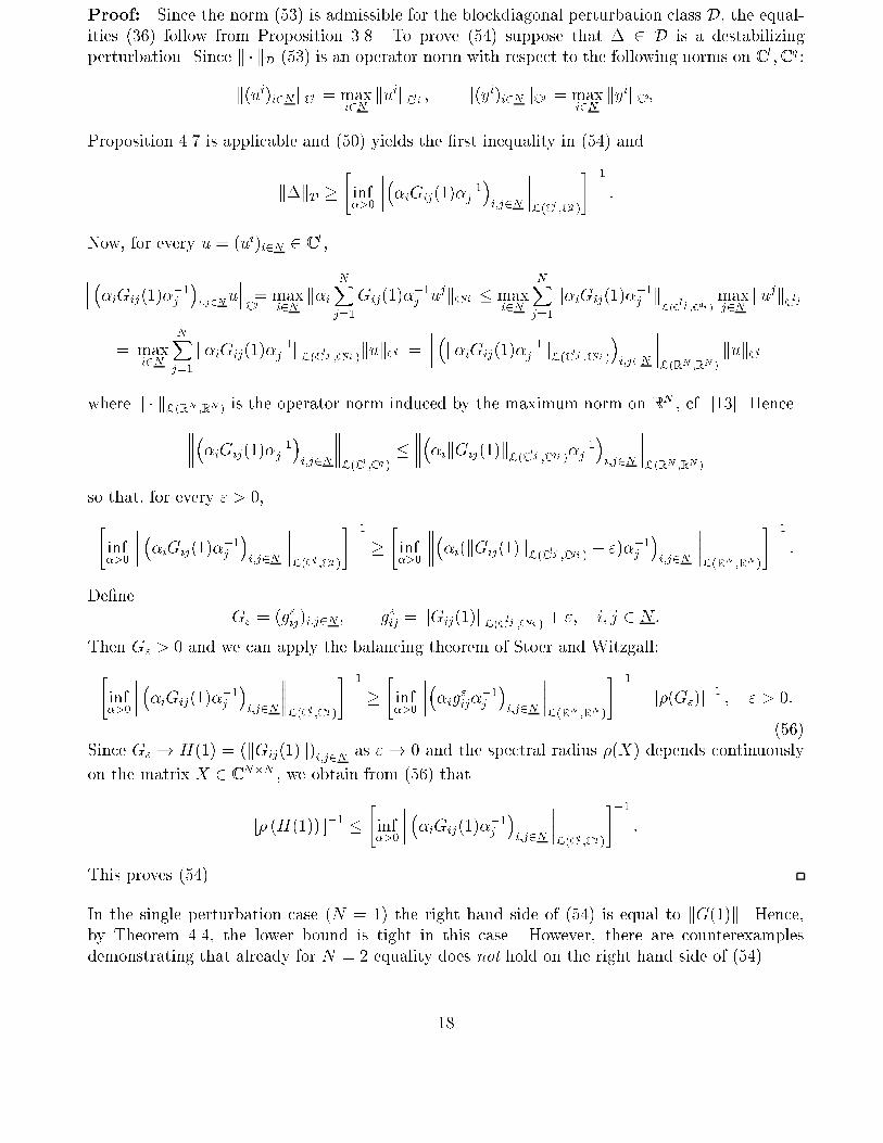
Proof: Since the norm (53) is admissible for the blockdiagonal perturbation class D, the equal-ities (36) follow from Proposition 3.8. To prove (54) suppose that � 2 D is a destabilizingperturbation. Since k � kD (53) is an operator norm with respect to the following norms on C l ; C q :k(ui)i2NkC l = maxi2N kuikC li ; k(yi)i2NkC q = maxi2N kyikC qiProposition 4.7 is applicable and (50) yields the �rst inequality in (54) andk�kD � " inf�>0 ��iGij(1)��1j �i;j2N L(C l ;C q )#�1 :Now, for every u = (ui)i2N 2 C l , ��iGij(1)��1j �i;j2Nu C q= maxi2N k�i NXj=1Gij(1)��1j ujkC qi � maxi2N NXj=1 k�iGij(1)��1j kL(Clj ;Cqi ) maxj2N kujkC lj= maxi2N NXj=1 k�iGij(1)��1j kL(C lj ;C qi )kukC l = �k�iGij(1)��1j kL(C lj ;Cqi )�i;j2N L(RN ;RN ) kukC lwhere k � kL(RN ;RN ) is the operator norm induced by the maximum norm on RN , cf. [13]. Hence ��iGij(1)��1j �i;j2N L(C l ;C q ) � ��ikGij(1)kL(C lj ;C qi )��1j �i;j2N L(RN ;RN )so that, for every " > 0," inf�>0 ��iGij(1)��1j �i;j2N L(C l ;Cq )#�1 � " inf�>0 ��i(kGij(1)kL(C lj ;Cqi ) + ")��1j �i;j2N L(RN ;RN )#�1 :De�ne G" = (g"ij)i;j2N ; g"ij = kGij(1)kL(C lj ;C qi ) + "; i; j 2 N:Then G" > 0 and we can apply the balancing theorem of Stoer and Witzgall:" inf�>0 ��iGij(1)��1j �i;j2N L(C l ;Cq )#�1 � " inf�>0 ��ig"ij��1j �i;j2N L(RN ;RN )#�1 = [�(G")]�1 ; " > 0:(56)Since G" ! H(1) = (kGij(1)k)i;j2N as "! 0 and the spectral radius �(X) depends continuouslyon the matrix X 2 C N�N , we obtain from (56) that[� (H(1)) ]�1 � " inf�>0 ��iGij(1)��1j �i;j2N L(C l ;Cq )#�1 :This proves (54).In the single perturbation case (N = 1) the right hand side of (54) is equal to kG(1)k. Hence,by Theorem 4.4, the lower bound is tight in this case. However, there are counterexamplesdemonstrating that already for N = 2 equality does not hold on the right hand side of (54).18

References[1] A. Berman, M. Neumann, and R. Stern, 1989, Nonnegative Matrices in Dynamic Systems.John Wiley & Sons, New York.[2] A. Berman and R. J. Plemmons, 1979, Nonnegative Matrices in Mathematical Sciences. Acad.Press, New York.[3] S.P. Bhattacharyya, H. Chapellat, L.H. Keel, 1995, Robust Control - The Parametric Ap-proach. Prentice Hall, Upper Saddle River.[4] S. Boyd and V. Balakrishnan, 1990, A regularity result for the singular values of a trans-fer function matrix and a quadratically convergent algorithm for computing the L1-norm.Systems & Control Letters, 15(1):1{7.[5] J. Doyle, 1982, Analysis of feedback systems with structured uncertainties. Proc. IEE,129:242{250.[6] F. R. Gantmacher, 1959, The Theory of Matrices, volume 1 and 2. Chelsea, New York.[7] D. Hinrichsen and A. J. Pritchard, 1986, Stability radius for structured perturbations andthe algebraic Riccati equation. Systems & Control Letters, 8:105{113.[8] D. Hinrichsen and A. J. Pritchard, 1990, Real and complex stability radii: a survey. InD. Hinrichsen and B. M�artensson, editors, Control of Uncertain Systems, volume 6 of Progressin System and Control Theory. Birkh�auser, Basel, 119-162.[9] D. Hinrichsen and A. J. Pritchard, 1991, On the robustness of stable discrete-time linearsystems. In G. Conte et al., editors, New Trends in Systems Theory, volume 7 of Progressin System and Control Theory Progress in System and Control Theory. Birkh�auser, Basel,393-400.[10] D. Hinrichsen and A. J. Pritchard, 1992, Destabilization by output feedback. Di�erentialand Integral Equations, 5:357{386.[11] D. Hinrichsen and N. K. Son, 1991, Stability radii of linear discrete-time systems and sym-plectic pencils. International Journal of Robust and Nonlinear Control, 1:79{97.[12] D. Hinrichsen and N. K. Son, 1995, Stability radii of positive discrete-time systems. ReportNr. 329, Inst. f. Dynamische Systeme, Universit�at Bremen, 1994. To appear in: Proc. 3rdCaribean Conf. Approximation and Optimization, Puebla, Mexico.[13] R. A. Horn and Ch. R. Johnson, 1985, Matrix Analysis. Cambridge University Press, Cam-bridge.[14] V. L. Kharitonov, 1979, Asymptotic stability of an equilibrium position of a family of systemsof linear di�erential equations. Di�. Uravn., 14:2086{2088.[15] D. G. Luenberger, 1979, Introduction to Dynamic Systems. Theory, Models and Applications.J. Wiley, New York. 19

[16] A. Packard and J. C. Doyle, 1993, The complex structured singular value. Automatica,29:71-109.[17] L. Qiu, B. Bernhardsson, A. Rantzer, E. J. Davison, P. M. Young, and J. C. Doyle, 1995, Aformula for computation of the real structured stability radius. Automatica, 31:879-890.[18] B. Shafai, K. Perev, D. Cowley and Y. Chehab, 1991, A necessary and su�cient condition forthe stability of nonnegative interval discrete-time systems. IEEE Trans. Automatic Control,36:743-746.[19] M. E. Sezer and D. Siljak, 1994, On stability of interval matrices. IEEE Trans. AutomaticControl, 39:368{371.[20] B. Shafai, J. Chen, H. H. Niemann and J. Stoustrup, 1994, Stability radius optimizationand loop transfer recovery for uncertain dynamical systems. Proc. 33rd Conf. Decision andControl, Lake Buena Vista, Florida, 2985-2987.[21] N. K. Son and D. Hinrichsen, 1995, Robust stability of positive linear systems. Proc. 34thConf. Decision and Control, New Orleans, 1423-24.[22] J. Stoer and C. Witzgall, 1962, Transformations by diagonal matrices in a normed space.Numer. Math., 4:158-171.

20