Speech enhancement by LSTM-based noise suppression

EURASIP Journal on Advancesin Signal Processing

Strake et al. EURASIP Journal on Advances in Signal Processing (2020) 2020:49 https://doi.org/10.1186/s13634-020-00707-1

RESEARCH Open Access

Speech enhancement by LSTM-basednoise suppression followed by CNN-basedspeech restorationMaximilian Strake1* , Bruno Defraene2, Kristoff Fluyt2, Wouter Tirry2 and Tim Fingscheidt1

*Correspondence:[email protected] for CommunicationsTechnology, Technische UniversitätBraunschweig, Schleinitzstr. 22,38106 Braunschweig, GermanyFull list of author information isavailable at the end of the article

AbstractSingle-channel speech enhancement in highly non-stationary noise conditions is a verychallenging task, especially when interfering speech is included in the noise. Deeplearning-based approaches have notably improved the performance of speechenhancement algorithms under such conditions, but still introduce speech distortionsif strong noise suppression shall be achieved. We propose to address this problem byusing a two-stage approach, first performing noise suppression and subsequentlyrestoring natural sounding speech, using specifically chosen neural network topologiesand loss functions for each task. A mask-based long short-term memory (LSTM)network is employed for noise suppression and speech restoration is performed viaspectral mapping with a convolutional encoder-decoder network (CED). The proposedmethod improves speech quality (PESQ) over state-of-the-art single-stage methods byabout 0.1 points for unseen highly non-stationary noise types including interferingspeech. Furthermore, it is able to increase intelligibility in low-SNR conditions andconsistently outperforms all reference methods.

Keywords: Speech enhancement, Noise suppression, Speech restoration, Two-stageprocessing, Long short-term memory, Convolutional neural networks

1 IntroductionSpeech enhancement is the task of removing interferences from a degraded speech signaland thereby improving the perceived quality and intelligibility of the signal. The researchinterest in speech enhancement has been consistently high, due to challenges arising withapplications such as mobile speech communication systems, hearing aids, and robustspeech recognition. This paper focuses on the challenging task of single-channel speechenhancement in non-stationary noise conditions including interfering speech, reflectingthe real-world conditions in many of the aforementioned applications.Classical speech enhancement algorithms typically operate in the short-time Fourier

transform (STFT) domain and use a frequency bin-wise gain function, also called weight-ing rule, which is derived using an optimality criterion under specific model assump-tions for the distributions of speech and/or noise [1–4]. Commonly, estimates of the a

© The Author(s). 2020 Open Access This article is licensed under a Creative Commons Attribution 4.0 International License,which permits use, sharing, adaptation, distribution and reproduction in any medium or format, as long as you give appropriatecredit to the original author(s) and the source, provide a link to the Creative Commons licence, and indicate if changes weremade. The images or other third party material in this article are included in the article’s Creative Commons licence, unlessindicated otherwise in a credit line to the material. If material is not included in the article’s Creative Commons licence and yourintended use is not permitted by statutory regulation or exceeds the permitted use, you will need to obtain permission directlyfrom the copyright holder. To view a copy of this licence, visit http://creativecommons.org/licenses/by/4.0/.

http://crossmark.crossref.org/dialog/?doi=10.1186/s13634-020-00707-1&domain=pdf

http://orcid.org/0000-0002-3393-8252

mailto: [email protected]

http://creativecommons.org/licenses/by/4.0/

Strake et al. EURASIP Journal on Advances in Signal Processing (2020) 2020:49 Page 2 of 26

priori signal-to-noise ratio (SNR) and in turn the noise power are needed for the weight-ing rule computation. Numerous algorithms exist for the estimation of a priori SNR[1, 5, 6] and noise power [7–9], where the latter ones are generally based on the assump-tion that noise in a given analysis segment is more stationary than speech [10, 11]. Thisassumption does not hold for highly non-stationary noise types such as speech babbleor restaurant noise and therefore classical speech enhancement algorithms often fail toprovide good performance in such conditions.With the advent of deep learning, an increasing number of studies using deep neu-

ral networks (DNNs) for speech enhancement have shown that these models are able tosignificantly outperform classical and other machine learning-based methods in termsof speech quality and intelligibility [12–21]. This is especially true for non-stationarynoise conditions, where deep learning-based methods have the advantage of making noassumptions on the stationarity of noise or the underlying distributions of speech andnoise. Important aspects of these methods are on the one hand the feature and targetrepresentations as well as the loss function used in training and on the other hand thetopology of the neural network. We focus on research addressing each of those aspects inthe next two paragraphs.In [13] and [14], the authors use a feedforward DNN to directly map from noisy

log-spectral features to the corresponding clean speech features and show that a goodgeneralization to unseen noise types can be achieved by multi-condition training with alarge amount of different noise types [14]. A comparison of various target representationsfor supervised DNN-based speech separation1 has been conducted in [15] and comes tothe result that estimating bounded time-frequency (T-F) ratio masks such as the idealratio mask (IRM) is advantageous compared to directly estimating the clean spectrogram.Various types of T-F masks have been further investigated in [16] and [22], where theauthors introduce a masked spectrum approximation (MSA) loss that optimizes the maskestimation task in the domain of speech spectra as opposed to using a mask approxima-tion (MA) loss with ideal masks as optimization targets. In addition, a phase-sensitivespectrum approximation (PSA) loss, that takes the phase difference between noisy andclean speech signals into account while still estimating real-valued masks, is introduced,showing advantages over other mask-based targets [22]. A way to fully integrate the jointestimation of clean speech spectral amplitude and phase into mask-based systems is theusage of complex ratio mask (cRM) targets, which perfectly reconstruct the clean signalunder ideal estimation conditions ([17], with early predecessors for speech quality testing[23, 24]). A potential drawback of this method is that it uses an MA loss and thereforedoes not leverage the advantages of optimization in the speech spectral domain.The models used in these early studies have mostly been feedforward DNNs [12–15,

17], although Weninger et al. [16] have shown that long short-term memory (LSTM)networks, with their ability to model temporal dynamics, have benefits in a speech sep-aration task. An important advantage of LSTMs in comparison to feedforward DNNs istheir ability to focus on a target speaker, taking into account long-term temporal depen-dencies, and therefore suppressing interfering speech better, as well as providing a betterspeaker generalization [25]. Recently, a third type of model, namely convolutional neu-ral networks (CNNs) have been subject to an increasing amount of studies in the field

1The term speech separation refers to the task of extracting one or more speech sources from a mixture signal and isoften used interchangeably with speech enhancement when only one source is to be extracted from a noise background.


of speech enhancement and separation [20, 26, 27]. Many of the successful CNN modelarchitectures are based on the convolutional encoder-decoder (CED) principle adoptedfrom computer vision research [28, 29]. As opposed to conventional CNN architecturesthat only compress the feature dimension by using pooling layers, the CED compressesin the encoder part and decompresses in the decoder part of the model by using upsam-pling layers or strided deconvolutions [30]. By adding skip connections from same-sizedlayers of the encoder to the decoder, high-resolution structural information can be pre-served, which is especially important for a regression task such as speech enhancement,where a mapping from the noisy speech spectrum to a same-sized target clean speechspectrum has to be learned. Park et al. [27] demonstrate the effectivity of different varia-tions of CEDs and Takahashi et al. [20] introduce densely connected convolutional layersand multi-band processing into the architecture. A CED network has also been used byZhao et al. to enhance encoded and subsequently decoded speech in a postprocessingstep, showing remarkable generalization capabilities even to unseen codecs [18].One way of leveraging the advantages of different network topologies is to combine

them into a single model and train this combined model on the task at hand. A combina-tion of CNN and bidirectional LSTM is shown to significantly outperform feedforwardDNNs and recurrent neural networks (RNNs) [31] for speech enhancement, with therestriction of the introducedmodel not being capable of real-time processing. Amodel forreal-time processing, which integrates LSTM layers in the bottleneck of a CED networkis introduced in [32].A second approach for the combination of models in speech enhancement is to employ

multi-stage processing, where either multiple identical models (cf. [33]) or most often dif-ferent models are used in succession to improve the enhancement performance. Appliedto classical speech enhancement, this principle is generally used to achieve a higher noiseattenuation, e.g., with the multi-stage Wiener filter approach [34], which in turn leadsto degradations of the speech quality. Different from that, some studies have focusedon first performing speech separation and subsequently enhancing the separated signalsusing nonnegative matrix factorization [35] or Gaussian mixture models [36]. In combi-nation with deep learning models, the multi-stage paradigm has been applied to musicsource separation using feedforward DNNs for the separation task as well as the subse-quent task of enhancing the separated signals [37]. A further possibility is proposed in[38], where denoising and dereverberation are addressed in subsequent stages using sep-arately trained feedforward DNNs and joint fine-tuning of the two-stage model is carriedout in a second step.Most of the described deep learning models aim at a high noise attenuation and there-

fore can still degrade speech quality, especially for low SNRs and non-stationary noisetypes, or when iterative processing is employed. We propose to address this problem byfirst performing noise suppression and subsequently restoring natural sounding speech. Dif-ferent to [37] and [38], we rely on specifically chosen DNN topologies with beneficialproperties for each of the two tasks. An LSTM-based model with its ability to use long-term temporal context to distinguish between noise and speech is used for noise suppres-sion. Inspired by its success for image restoration [28] and speech decoder postprocessing[18], we employ a CED network for speech restoration and residual noise suppression.Webelieve that this type of model is well-suited to perform amapping from the input domainto an only slightly different target domain, as is the case with slightly distorted speech and


undistorted clean speech. A further contribution is the reformulation of the MSA lossfunction for the joint estimation of real and imaginary parts of the clean speech spectrum,which is used with the LSTM-basedmodel to aim at a high noise attenuation after the firstprocessing stage. Finally, our work focuses on highly non-stationary noise types includ-ing interfering speech, which often have led to trouble in machine learning-based speechenhancement.2

The paper is structured as follows: in Section 2, we introduce the speech enhancementframework used for both baselines and our proposed approaches based on deep learning.Next, a detailed description of our two-stage approach and the utilized DNN topologiesis given in Section 3, followed by the experimental setup and network training details inSection 4. The evaluation results are presented in Section 5, and we conclude the work inSection 6.

2 Speech enhancement framework, classical and deep learning-basedapproaches

For the task of estimating the clean speech signal s(n) from a noisy microphone signaly(n), we employ a signal model of the form

y(n) = s(n) + d(n), (1)

where the noise signal d(n)with the discrete-time sample index n is assumed to additivelymix with s(n). The corresponding STFT domain representation, computed by applying aframe-wise window function with a frame length of L and a frame shift of R, followed bya K-point discrete Fourier transform (DFT), is given by

Y�(k) = S�(k) + D�(k), (2)

with frame index � and frequency bin index k ∈ K = {0, 1, . . . ,K−1}. Most of the classicalspeech enhancement approaches and also many deep learning-based approaches rely onestimating a frame- and frequency bin-wise gain functionG�(k) to subsequently computethe estimated clean speech following

S�(k) = G�(k) · Y�(k). (3)

2.1 Classical approaches

In classical speech enhancement approaches employing parametric statistical models ofspeech and noise, the computation of the gain function

G�(k) = g (ξ�(k), γ�(k)) (4)

typically depends on the a priori SNR ξ�(k) and the a posteriori SNR γ�(k). In thiswork, we consider g(·) to represent the well-known minimum mean-square error log-spectral amplitude (MMSE-LSA) estimator [2] or the super-Gaussian joint maximum aposteriori (SG-jMAP) estimator [4] and use the decision-directed (DD) approach [1] forthe estimation of ξ�(k). Additionally, an estimate of the noise power is required for the

2Note that a part of this work has been pre-published in a workshop paper [39]; however, in [39], a convolutional LSTMlayer has been employed and pooling and upsampling layers have been used in the CED architecture, resulting in acomputationally much more complex second stage. Furthermore, in this work, a much more thorough evaluation of thetwo-stage approach to learned speech enhancement including all relevant single-stage baselines is provided. In additionto that, an analysis of the benefits of the two-stage approach and its effects on the enhanced speech spectra, and ananalysis of the computational complexity are presented.


computation of ξ�(k) and γ�(k) and can be obtained utilizing the minimum statistics (MS)approach [7].

2.2 Deep learning-based approaches

Deep learning-based approaches use neural network (NN) models being trained before-hand on a set of training data to perform the speech enhancement task. In general,they can be described as a mapping from an input feature vector x� to the outputvector

u� = f (x�,h�−1;�) , (5)

based on the non-linear composite function f (·) defined by the network topology, andthe trainable parameters �. The additional input of network hidden states h�−1 for thepreceding frame is used to model temporal context in recurrent neural networks, e.g.,LSTMs.In the context of deep learning-based approaches, G�(k) from (3) is often referred to

as a T-F mask separating clean speech and noise. The NN model can be trained in asupervised fashion to estimate these masks by minimizing the mask approximation (MA)loss function

JMA� (�) = 1

K∑

k∈K

(G�(k) − Gideal

� (k))2

, (6)

where Gideal� (k) ∈ R are the ideal mask values representing the training targets and G�(k)

are the estimated mask values at the network output. In this case, the network outputvector is composed as u� =

(G�(0), G�(1), . . . , G�

(K2

))T, which can be obtained by

reducing the summation in (6) to the elements k ∈{0, 1, . . . , K2

}only, while halving the

contribution at k = 0 and k = K2 . A well-established choice for the ideal mask target is

the IRM

Gideal� (k) = GIRM

� (k) =( |S�(k)|β

|S�(k)|β + |D�(k)|β)1/β

(7)

with the common parameter choice of β = 2 [15, 25], making it formally comparable tothe square-root Wiener filter gain function.3

TheMA loss function does not directly optimize the objective of minimizing the differ-ence between estimated speech spectrum S�(k) and clean speech spectrum S�(k). In fact,the contribution of the estimates to the loss for each frequency bin is subject to a ratio ofS�(k) and D�(k) and not directly to the energy distribution of S�(k) and Y�(k). This canlead to, e.g., the MA loss taking on high values for bins k, where both S�(k) and Y�(k) areclose to zero and therefore no contribution to the loss should be considered regardlessof the estimated mask value G�(k). Direct optimization of the aforementioned objective,which also preserves the benefits of estimating a mask value that can be restricted to acertain value range, can be accomplished by using the masked spectrum approximation(MSA) loss function [16]

JMSA� (�) = 1

K∑

k∈K

(G�(k) · |Y�(k)| − |S�(k)|

)2. (8)

3Note that various ideal mask formulations and their loss functions have already been introduced to data-driven speechenhancement in 2006 and 2008 by Fingscheidt et al. [40, 41].


Up to this point, the loss functions presented in (6) and (8) only operate on spectralmagnitudes, which leads to G�(k) ∈ R and in turn, following (3), the usage of the noisyphase for the enhanced speech S�(k). One way of estimating the clean speech phase, thathas been proven beneficial for deep learning-based speech enhancement, is to use an idealcomplex mask GICM

� (k) = S�(k)/Y�(k) as target and separately estimate real and imagi-nary part of GICM

� (k) using an MA loss for training [17]. Different to that, we propose analternative loss function that combines the advantages of clean speech phase estimationand the MSA loss paradigm of optimizing in the speech spectral domain. Such a complexMSA (cMSA) loss can be formulated, e.g., as

JcMSA� (�) = 1

K

⎛

⎝K/2∑

k=0

(GR

� (k) · � {Y�(k)} − � {S�(k)})2

+K/2−1∑

k=1

(GI

�(k) · � {Y�(k)} − � {S�(k)})2

⎞

⎠ ,

(9)

where separate real-valued masks GR� (k) and GI

�(k) are used to estimate the real andimaginary part of S�(k), respectively. Here, �{·} delivers the real part, and �{·} theimaginary part of the argument. Applying the cMSA loss, the neural network output

becomes u� =(GR

� (0), . . . , GR�

(K2

), GI

�(1), . . . , GI�

(K2 −1

))T, and the enhanced signal is

computed according to

S�(k) = GR� (k) · �{Y�(k)} + jGI

�(k) · �{Y�(k)}. (10)

A third possibility, which we will call complex spectrum approximation (cSA), is todirectly estimate real and imaginary parts of the clean speech spectrum S�(k) following

JcSA� (�) = 1K

⎛

⎝K/2∑

k=0

(SR� (k) − � {S�(k)}

)2 +K/2−1∑

k=1

(SI�(k) − � {S�(k)}

)2⎞

⎠ , (11)

where SR� (k) and SI�(k) are the estimated real and imaginary parts, respectively.

3 New LSTM-based noise suppression followed by CNN-based speechrestoration

The underlying idea of our newly proposed system is to employ separate processing stagesfor speech denoising and restoration, both using deep NN topologies with advantageousproperties for the respective tasks. In the noise suppression stage, an LSTM-based net-work trained with the cMSA loss from (9) is employed to attain a strong noise attenuation,even at the cost of potentially introducing speech distortions. The subsequent restora-tion stage restores speech and further attenuates residual noise. For this second task aCED network is used, which has been found to be very well-suited for the restoration ofslightly corrupted structured signals, e.g., in image restoration [28] or enhancement ofcoded speech [18]. The CED network training employs the cSA loss function defined in(11) and therefore a direct spectral mapping is performed in the second stage. The cSAloss function is chosen over a mask-based loss for two reasons: On the one hand, the


restoration of missing T-F regions in the estimated signal can be quite difficult for a mask-based approach, requiring very large mask values. On the other hand, the CED networkis specifically designed to map to outputs of the same domain as the input, in this casespeech spectra rather than spectral masks. In the following, an overview of the system isgiven and the chosen network topologies for both stages are described in detail.

3.1 System description

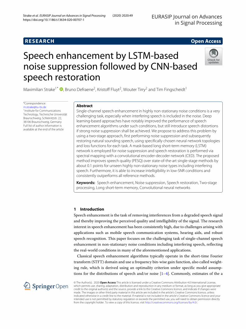
The overall processing scheme of our two-stage approach is depicted in Fig. 1. At first,the STFT representation of the noisy speech Y�(k) is input to the noise suppression stage.A feature extraction including mean and variance normalization (MVN) is performed toobtain the normalized feature vector x(1)

� , where the MVN is carried out using vectors ofmeans μ

(1)x and standard deviations σ

(1)x obtained during network training. The feature

extraction also includes concatenating L− frames of past and L+ frames of future contextto the features extracted for the current frame, but for more strict latency requirementsthe system can also work with L+ = 0, i.e., no lookahead at all. Based on the input featuresx(1)

� and the network parameters �(1) obtained during training, the noise suppressionnetwork estimates separate real-valued masks GR

� (k) and GI�(k) for the real and imagi-

nary part of the noisy speech spectrum Y�(k). In the subsequent masking block, thesemasks are applied following (10) and the estimated denoised speech spectrum S(1)

� (k) isobtained.The interpolation block in between the two stages is increasing the frequency resolution

for processing in the speech restoration stage to enable the employed CED network tofully leverage its potential of mapping to a high-resolution estimated spectrum and in turnrestoring spectral details of the clean speech signal. The interpolation is realized throughapplying a K-point inverse DFT (IDFT) followed by zero-padding in the time domain andsubsequent transformation back to the frequency domain via a K ′-point DFT

(K ′ > K

),

resulting in the interpolated denoised speech spectrum S(1)�

(k′).

In the speech restoration stage, a second feature extraction, including MVN usingthe vectors of means μ

(2)x and standard deviations σ

(2)x obtained during speech restora-

tion network training, is employed. The resulting feature representation x(2)� is input to

the speech restoration network, which directly maps to the enhanced speech spectrumS(2)�

(k′), using the trained network parameters �(2). Reconstruction of the correspond-

ing enhanced time-domain signal s(2)(n) is subsequently realized through IDFT, synthesiswindowing, and overlap-add (OLA).

Fig. 1 Block diagram of the proposed two-stage enhancement approach including the first-stage noisesuppression, followed by the second-stage speech restoration used to restore a natural sounding speechsignal. For details on the noise suppression network block and the speech restoration network block refer toFigs. 2 and 3, respectively


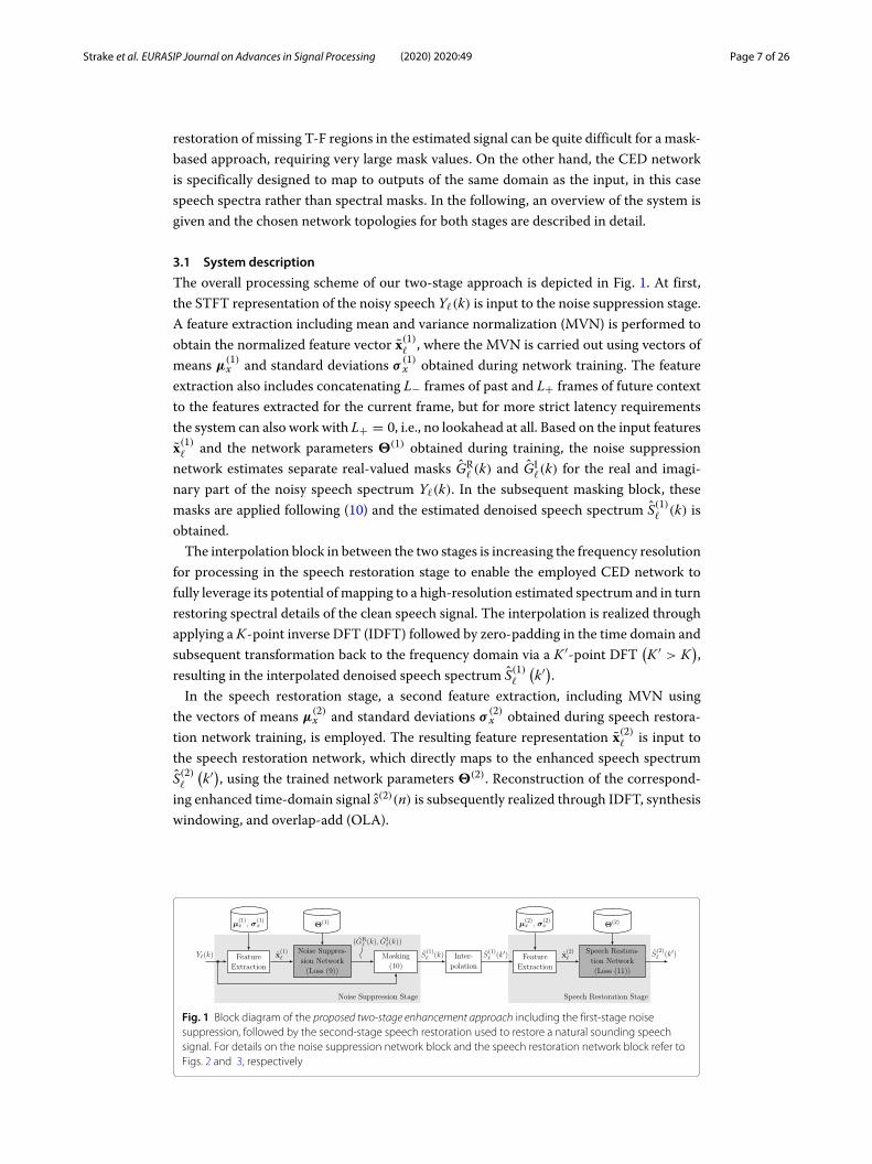
Fig. 2 Block diagram of the noise suppression network utilizing LSTM and fully connected feedforward (FF)layers. The sizes of the one-dimensional feature representations inside the network are shown at the inputand output of each layer. Except for the input features, these sizes are determined by the number of nodes inthe preceding layer

3.2 First-stage noise suppression network topology

The noise suppression network relies on the LSTM-based topology depicted in Fig. 2,where FF denotes fully connected feedforward layers and the sizes of the feature rep-resentations for each layer of the network are shown before and after the respectivelayers. The input feature vector x(1)

� is composed of MVN-normalized spectral magni-tudes4 using only the non-redundant DFT bins, which results in a feature vector size ofC = (L− + 1 + L+) ·

(K2 + 1

).

The employed network uses a single FF layer upfront, which can help to learn a goodfeature representation for the temporal modeling in the two following LSTM layers[25, 42]. Two additional FF layers lead to the output layer estimating the T-F masks fornoise suppression. All of the FF layers are composed of 425 nodes and use rectified linearunit (ReLU) activations [43] with the exception of the output layer, which has a number ofnodes corresponding to the DFT sizeK and uses a tanh activation to restrict the estimatedmasks to GR

� (k), GI�(k) ∈[−1, 1]. Such a restriction of mask values has been found to ease

optimization and to decrease the ideally achievable estimation accuracy only marginally[17, 22]. The LSTM layers use the standard implementation as introduced in [44] withoutpeephole connections, and also consist of 425 nodes.

3.3 Second-stage speech restoration network topology

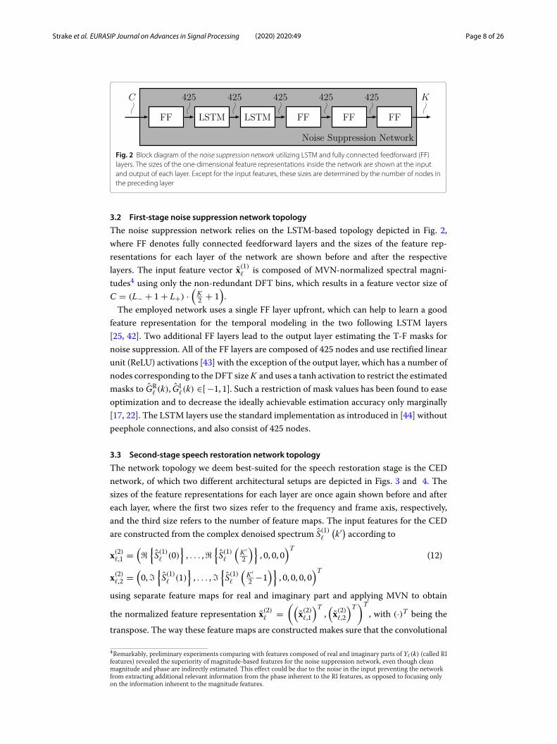
The network topology we deem best-suited for the speech restoration stage is the CEDnetwork, of which two different architectural setups are depicted in Figs. 3 and 4. Thesizes of the feature representations for each layer are once again shown before and aftereach layer, where the first two sizes refer to the frequency and frame axis, respectively,and the third size refers to the number of feature maps. The input features for the CEDare constructed from the complex denoised spectrum S(1)

�

(k′) according to

x(2)�,1 =

(�

{S(1)� (0)

}, . . . ,�

{S(1)�

(K ′2

)}, 0, 0, 0

)T(12)

x(2)�,2 =

(0,�

{S(1)� (1)

}, . . . ,�

{S(1)�

(K ′2 −1

)}, 0, 0, 0, 0

)T

using separate feature maps for real and imaginary part and applying MVN to obtain

the normalized feature representation x(2)� =

((x(2)

�,1

)T,(x(2)

�,2

)T)T, with (·)T being the

transpose. The way these feature maps are constructed makes sure that the convolutional

4Remarkably, preliminary experiments comparing with features composed of real and imaginary parts of Y�(k) (called RIfeatures) revealed the superiority of magnitude-based features for the noise suppression network, even though cleanmagnitude and phase are indirectly estimated. This effect could be due to the noise in the input preventing the networkfrom extracting additional relevant information from the phase inherent to the RI features, as opposed to focusing onlyon the information inherent to the magnitude features.


Fig. 3 Block diagram of the speech restoration network utilizing a CED network including encoder anddecoder sub-networks with maximum pooling and upsampling layers (du-setup). The sizes of the featurerepresentations inside the network regarding the frequency, frame, and feature map axis, respectively, areshown at the input and output of each layer

kernels in the first network layer always see matching bins of real and imaginary parts intheir receptive fields. The additional zero-padding in (12) is used to obtain a frequencyaxis sizeM that is a multiple of four, which is necessary for a total dimension reduction bya factor of four in the encoder and subsequent reconstruction of equally sized output fea-tures in the decoder. The output structure corresponds to that of the input features, whenreplacing S(1)

�

(k′) in (12) with the final clean speech spectrum estimates S(2)

�

(k′). The

features x(2)� do not use a frame lookahead or any other information from future frames,

which results in the speech restoration stage not adding any additional algorithmic delay.


Fig. 4 Block diagram of the speech restoration network utilizing a CED network including encoder anddecoder sub-networks with strided and transposed convolutions (tr-setup), where /2 indicates a stride of 2.The sizes of the feature representations inside the network regarding the frequency, frame, and feature mapaxis, respectively, are shown at the input and output of each layer

The actual network topology is inspired by the CED network from [18] and com-prises several building blocks. Convolutional layers are denoted by Conv(F ,N × 1), withF determining the number of filter kernels, N being the kernel size on the frequencyaxis and the kernel size on the frame axis being specified as one, resulting in one-dimensional convolutions. Transposed convolutions [45] are denoted correspondingly byConvT (F ,N × 1). All convolutional and transposed convolutional layers use the leakyReLU activation function [46], zero-padding to ensure a consistent size of the output fea-ture maps with respect to the input, and a stride of one, except where indicated by a /2besides the blocks, denoting a stride of two. The encoder part of the CED uses eithermaximum pooling (Fig. 3) or convolutions with a stride of two (Fig. 4), each reducing thesize of the features with respect to the frequency axis by a factor of two. As a counter-part in the decoder, either upsampling layers (Fig. 3) or transposed convolutions with a


stride of two (Fig. 4) are employed, leading to a doubling of the frequency axis size. Weindicate these different setups by du and tr, respectively, where the tr-setup can signifi-cantly reduce the computational complexity with respect to the number of multiplicationsneeded [47]. In the bottleneck between encoder and decoder, we also employ a convolu-tional layer and use a total number of two skip connections from encoder to decoder atpoints of matching feature map dimensions.

4 Databases, training, andmeasures4.1 Databases and preprocessing

For the training and evaluation of our proposed system, we use clean speech data fromthe TIMIT [48] and NTT super wideband [49] databases (British and American Englishonly for NTT), both downsampled to 8 kHz. We merge both databases to one large setcontaining a total amount of 7.5 h of speech and construct distinct training, development,and test sets by using 60%, 20%, and 20% of the total data, respectively. We make sure thatthere is no overlap in speakers between the distinct sets and the amount of female andmale speakers is balanced.The clean speech data is mixed with cuts of three different café noises (noise file

durations of 34:00, 39:23, and 42:02 minutes) from the QUT noise database [50] andthe babble and restaurant noise (with durations of 3:55 and 4:46 min, respectively)from the AURORA-2 database [51]. We deliberately choose only highly non-stationarynoise types including interfering speech to evaluate the performance of our systemunder challenging conditions. The noisy data is generated by defining three distinctparts of each noise file for training, development, and test (spanning 60%, 20% and20% of the noise file duration, respectively) and mixing random cuts of the respec-tive parts with the clean speech data. For the training set, each speech file is mixedwith a cut of each of the 5 noise files, applying SNRs of 0, 5 and 10 dB, resulting ina total of 5 · 3 = 15 training conditions, corresponding to a total amount of 67.5h of training material. The development and test data is constructed accordingly, butadditionally using SNRs of −5 and 15 dB unseen in training. Please note that theseadditional SNR conditions are only used for reporting of results and are removed fromthe development set for parameter optimization and loss monitoring during training.Furthermore, a separate test set employing the pub and office call center noises fromthe ETSI database [52] as unseen noise files is constructed and used to evaluate thegeneralization properties of the tested systems. Please note that the office call centernoise contains interfering speech as well as non-stationary non-speech sounds suchas clatter or typing, whereas pub noise mainly contains interfering speech. To furtherevaluate the generalization properties to non-stationary noise types without interferingspeech, we include an additional separate evaluation using the traffic noise from the ETSIdatabase [52].Input features and targets for both models are computed from the time domain signals

using a frame length of L = 256 and a frame shift of R = 128 samples in combination witha square-root Hann window function. For the first-stage training and the evaluation of thetwo-stage system, a DFT of size K = 256 is used to obtain the spectral representations,which results in a first-stage feature vector size of C = 645 for the chosen values ofL− = L+ = 2. The inputs and targets for the second-stage training are computed fromthe windowed time domain signals using zero-padding and a DFT of size K ′ = 2K =


512. Thus, the input signal representations for second-stage network training match theoutput of the interpolation block (see Fig. 1) during two-stage processing, resulting in asecond-stage feature size ofM = K ′

2 +4 = 260 on the frequency axis.

4.2 Training of the LSTM-based noise suppression

Training of the LSTM-based network for noise suppression is conducted using the back-propagation through time (BPTT) algorithm [53] in combination with the cMSA lossfunction (9) and the Adam optimizer [54]. We use an initial learning rate of μ = 0.001, abatch size of 25, and set the remaining parameters for Adam according to the recommen-dations in [54]. To prevent the network from overfitting, an L2 weight-decay of 0.0002is employed. The BPTT training is carried out in a truncated fashion with fixed-lengthsequences of size 100 being extracted from the training set utterances. Any remain-ing shorter sequences are zero-padded to match this size. The contributions of paddedsequence parts are set to zero for the computation of gradients in BPTT. During training,we monitor the development set loss and halve the learning rate once it does not decreasefor more than three epochs, restarting training using this new learning rate from theepoch with currently lowest development set loss. Training is stopped when a minimallearning rate of μmin = 0.0001 is reached.

4.3 Training of the CNN-based speech restoration

The CNN-based CED networks for both the du- and tr-setup are trained using stan-dard backpropagation [55] employing the cSA loss function (11). The Adam optimizerwith an initial learning rate of μ = 0.0001, a batch size of 16, and otherwise the sameparameter settings as in LSTM training is utilized. During CED training, the learningrate is multiplied by a factor of 0.6 and network training is resumed from the epochwith best development set loss, if the development set loss does not decrease for morethan two epochs. The training is once again stopped when a minimal learning rate ofμmin = 0.00001 is reached. The parameters defining the network topology in terms ofnumber of filter kernels and the kernel size on the frequency axis are chosen to F = 88and N = 24, respectively. These parameter values have been obtained from the optimalvalues found in [18] for a similar CED network by keeping proportions with regard to theinput feature size fixed.

4.4 Baseline and proposedmethods

We compare our new approach against several baseline methods, first considering theclassical MMSE-LSA and SG-jMAP weighting rules using the DD a priori SNR estimatorand theMS noise power estimator, as described in Section 2.1. These classical approachesuse optimal parameters adopted from [56]. Furthermore, LSTM-based baseline methodsusing an MA loss (6) with IRM targets (7) and β = 2, or alternatively the MSA loss func-tion (8) are considered and referred to as LSTM-IRM and LSTM-MSA, respectively. Bothuse LSTM topologies comparable to the proposed noise suppression network (LSTM-cMSA), with the only difference of employing a sigmoid output activation for the estima-tion of magnitude masks in the range [0, 1]. Note that the LSTM-IRM baseline is quitecomparable to the approach used in [25], with only slight changes to the employed LSTMtopology and the usage of spectral magnitude features for comparability to the proposedapproach. As a further baseline, the proposed second-stage CED network (du-setup) is


trained as a single-stage enhancement method using the cSA loss (11) and is referred to asCED-cSA-du.A first (novel) two-stage method dubbed LSTM-cMSA+DNN-cSA is investigated, con-

sisting of the proposed LSTM-cMSA network in the first stage, followed by a feedforwardDNN network trained with the cSA loss (11), the same training scheme as described inSection 4.3, and also the same features and targets used for training of the finally pro-posed second-stage network (CED-cSA). The DNN-cSA second-stage network uses fivehidden layers with 800 units each, resulting in a total amount of parameters comparableto the CED-cSA network. Furthermore, we report results of our proposed novel modelusing the du- and tr-setup described in Section 3.3 for the second-stage network architec-ture (called LSTM-cMSA+CED-cSA-du and LSTM-cMSA+CED-cSA-tr, respectively).We also experimented with an additional joint fine-tuning step after separate trainingof both stages, which did not obtain significantly improved results with respect to onlytraining separately. Furthermore, a joint training of both models from scratch has beenevaluated, but did not lead to converging trainings. Therefore, both fine-tuning variantswere not further considered for the experimental evaluation. As an additional reference,we include the two-stagemethod pre-published in [39], which uses a convolutional LSTMlayer [57] in between encoder and decoder of the second-stage network. A further dif-ference to our proposed model is the usage of maximum pooling and upsampling layersinstead of the computationally more efficient strided and transposed convolutions in theproposed CED-cSA-tr network.We call the method from [39] LSTM-cMSA+CLED-cSA-du and compare it to the proposed methods in terms of performance and computationalcomplexity.

4.5 Instrumental quality measures

We choose to only employ instrumental measures5 operating on the enhanced speechs(n), the noisy speech y(n), and the clean speech reference s(n). The signal-to-noiseratio improvement (SNRI) provided by the system under test is measured according toITU-T G.160 [58]. Note that the G.160 Recommendations [58] do not include highlynon-stationary noise conditions, but nonetheless, SNRI is regularly used for evaluationunder such conditions [59–61]. Thus, we employ SNRI only as an indicator for the noisesuppression capabilities of the respective system. Furthermore, we use perceptual evalu-ation of speech quality (PESQ) [62] to obtain a mean opinion score for listening qualityobjective (MOS-LQO), which is quite correlated with the overall speech quality percep-tion of human listeners, although not perfectly suited for speech with (residual) noise.To assess the intelligibility of the enhanced speech, the short-time objective intelligi-bility (STOI) measure [63] is utilized. The STOI measure is specifically designed for

5For quality evaluation of speech enhancement algorithms, it is often preferable to use a component-wise evaluationaccording to the so-called white-box [64] or black-box [23] approaches, to be able to investigate the effects on the speechcomponent and the noise component of the noisy mixture separately. These approaches rely on the multiplication of theclean speech spectrum S�(k) and the noise spectrum D�(k) with the estimated gain function G�(k) or an artificialcomplex-valued gain function computed from the enhanced speech S�(k) and the noisy speech Y�(k) to compute thefiltered speech component S�(k) and the filtered noise component D�(k). Unfortunately, those component-wiseapproaches can be problematic when using phase-aware processing with G�(k) = |G�(k)| · ej∠G�(k) ∈ C, where themultiplication with G�(k) includes applying the phase factor ej∠G�(k) to S�(k) and D�(k). This can lead to artifacts in thereconstructed filtered components s(n) and d(n) after IDFT and OLA, which would have been suppressed through thecombination of phase terms in S�(k) = G�(k)(S�(k) + D�(k)) and subsequent reconstruction of s(n) via IDFT and OLA.


the evaluation of noise reduction methods and provides values in the range [ 0, 1] withhigh values correlating strongly with high intelligibility.

5 Results and discussionIn the following, we discuss the results of the experiments conducted with seen andunseen noise types and subsequently analyze our proposed approach to give furtherexplanations for the performance improvements we observe compared to the baselinemethods.

5.1 Results on seen noise types

The results for the development set data using noise types that were seen during train-ing are presented in Table6 1. On average, but also for each single SNR condition, the deeplearning-based methods substantially outperform the classical MMSE-LSA and SG-jMAPin terms of PESQ, STOI, and SNRI. Most notably, the classical methods are not able toimprove the intelligibility in terms of STOI compared to the unprocessed noisy speech,which has an average STOI value of 0.75. In contrast, the deep learning-based methodsimprove on that value by up to 0.13 points (0.88) averaged over the SNR conditions. Thisobservation is in line with the results of earlier studies [14, 17], which also report higherintelligibility improvements for deep learning-basedmethods, especially in low-SNR con-ditions. Furthermore, MMSE-LSA and SG-jMAP only slightly improve the overall qualityin terms of PESQ over unprocessed noisy speech for the very challenging −5 dB condi-tion, whereas the deep learning-based methods are able to significantly improve PESQ,although not having seen a comparably low SNR during training.Comparing the single-stage baselines LSTM-IRM and LSTM-MSA, we observe consis-

tent superiority of LSTM-MSA in terms of PESQ and SNRI with average improvementsof 0.08 MOS points and 1.52 dB, respectively, confirming the advantage of optimization inthe speech spectral domain as opposed to the mask domain. The proposed LSTM-cMSAnoise suppression network, employed without second-stage processing, can furtherimprove PESQ by 0.02 MOS points and SNRI by an impressive 5.22 dB (23.11 dB) com-pared to LSTM-MSA (17.89 dB) and averaged over all SNR conditions. For the low-SNRconditions −5 and 0 dB though, LSTM-cMSA provides lower PESQ values than LSTM-MSA. This could be due to the fact that LSTM-cMSA is implicitly estimating the cleanphase or at least incorporates phase information by using real and imaginary part of theclean speech spectrum S�(k) as targets. Leveraging this information is potentially verydifficult for low SNRs where noise can be dominant in the mixture and therefore con-ceal relevant information on phase inherent to the magnitude features, e.g., the locationof harmonics. Nonetheless, LSTM-cMSA provides considerably higher noise suppressionthan all other single-stage methods in terms of SNRI, even in low-SNR conditions. This is inline with the original idea of aiming at a very high noise suppression in the first stage andallowing some speech distortions, which in turn can be restored by the second stage. Dueto this observation in combination with providing the best average performance on thedevelopment set, we choose to employ LSTM-cMSA as the first processing stage for allexperiments including second-stage processing. Employing CED-cSA-du as a single-stageenhancement network leads to a deterioration compared to LSTM-cMSA of PESQ by 0.04

6Note that no noise file portions have been seen both in training and development, only different portions of the same file.


Table 1 Instrumental measures for baseline and proposed approaches averaged over seen noisetypes of the development set data. Note that the SNR conditions of −5 and 15 dB are unseen duringtraining, whereas the remaining SNRs have been seen. Best two approaches are in boldface

SNR Method PESQ STOI SNRI

-5 Noisy 1.35 0.53 0.00

MMSE-LSA 1.39 0.50 3.51

SG-jMAP 1.38 0.49 4.13

LSTM-IRM 1.61 0.65 11.76

LSTM-MSA 1.65 0.66 12.61

LSTM-cMSA 1.60 0.64 15.83

CED-cSA-du 1.52 0.65 11.75

LSTM-cMSA + DNN-cSA 1.61 0.68 17.07

LSTM-cMSA + CED-cSA-du 1.63 0.69 17.12

LSTM-cMSA + CED-cSA-tr 1.63 0.69 17.27

0 Noisy 1.52 0.65 0.00

MMSE-LSA 1.64 0.63 4.37

SG-jMAP 1.63 0.63 5.19

LSTM-IRM 1.99 0.79 17.14

LSTM-MSA 2.08 0.80 19.21

LSTM-cMSA 2.03 0.80 24.59

CED-cSA-du 1.92 0.81 19.15




5 Noisy 1.77 0.76 0.00

MMSE-LSA 1.97 0.75 5.10

SG-jMAP 1.98 0.75 6.14

LSTM-IRM 2.42 0.87 18.39

LSTM-MSA 2.53 0.88 20.20

LSTM-cMSA 2.55 0.89 26.13

CED-cSA-du 2.43 0.90 21.98




10 Noisy 2.12 0.86 0.00

MMSE-LSA 2.36 0.84 5.54

SG-jMAP 2.41 0.85 6.88

LSTM-IRM 2.84 0.92 17.92

LSTM-MSA 2.93 0.93 19.22

LSTM-cMSA 3.01 0.93 25.51

CED-cSA-du 2.97 0.95 24.09




15 Noisy 2.54 0.92 0.00

MMSE-LSA 2.76 0.91 5.53

SG-jMAP 2.87 0.92 7.22

LSTM-IRM 3.24 0.96 16.64

LSTM-MSA 3.32 0.96 18.20

LSTM-cMSA 3.39 0.96 23.47

CED-cSA-du 3.42 0.97 25.58



Table 1 Instrumental measures for baseline and proposed approaches averaged over seen noise typesof the development set data. Note that the SNR conditions of−5 and 15 dB are unseen during training,whereas the remaining SNRs have been seen. Best two approaches are in boldface (continued)




Mean Noisy 1.86 0.75 0.00

MMSE-LSA 2.02 0.73 4.81

SG-jMAP 2.05 0.73 5.91

LSTM-IRM 2.42 0.84 16.37

LSTM-MSA 2.50 0.85 17.89

LSTM-cMSA 2.52 0.85 23.11

CED-cSA-du 2.45 0.85 20.51




points and SNRI by 2.60 dB averaged over all SNRs, while STOI remains comparable. Forthe 0 and 5 dB SNR conditions, CED-cSA-du performs worst of all deep learning-basedmethods in terms of PESQ and worse than LSTM-MSA and LSTM-cMSA in terms ofSNRI. However, the performance of CED-cSA-du compared to the LSTM-based methodsimproves for high-SNR conditions, even providing the best performance among single-stage methods in terms of all measures for 15 dB SNR. This shows that CED-cSA-du iswell-suited for high input SNRs, which supports its usage as a second-stage network,where noise suppression has already been applied in the first stage.The proposed two-stage method (for both du- and tr-setup of LSTM-cMSA+CED-cSA)

improves all employed instrumental measures for all SNR conditions compared to onlyusing LSTM-cMSA and all except SNRI for the 15 dB SNR condition compared to onlyusing CED-cSA, providing a notable average PESQ improvement of 0.11 MOS pointsover the best single-stage method. Even higher PESQ improvements of up to 0.18 MOSpoints with respect to the best performing single-stage methods can be obtained forthe 5 and 10 dB SNR conditions. Comparison with the other investigated two-stagemethod (LSTM-cMSA+DNN-cSA) shows significantly higher PESQ, when using theCED-cSA as second stage, while being comparable or even slightly worse in terms ofSNRI. Our interpretation of this observation is that the CED-cSA network, while pro-viding comparable additional noise suppression, is better suited to restore missing ordegraded parts of speech and therefore provides better overall speech quality in terms ofPESQ. Although yielding only second-best performance in terms of PESQ for the diffi-cult −5 dB SNR condition, the second-stage processing with CED-cSA can still slightlyimprove on using LSTM-cSA only. Concerning the intelligibility in terms of STOI, theLSTM-based single-stage methods roughly provide the same performance, but usingthe LSTM-cMSA+CED-cSA methods further improves STOI for all SNR conditions.It provides gains of up to 0.05 points for the lower SNR conditions, where improv-ing the intelligibility is very relevant. Direct comparison of the different second-stagesetups LSTM-cMSA+CED-cSA-du and LSTM-cMSA+CED-cSA-tr shows comparable orslightly better performance of PESQ and improved noise suppression in terms of SNRIfor the tr-setup.


Comparing the results on the development set with the results obtained on the test setdepicted in Table 2, the same conclusions on performance trends and model ranking forall three measures are obtained from the evaluation of both sets. The overall performanceon the test set is slightly worse for all models including the classical methods, which donot rely on the development set for parameter tuning. This shows that the test set is

Table 2 Instrumental measures for baseline and proposed approaches averaged over seen noisetypes of the test set data. Note that the SNR conditions of −5 and 15 dB are unseen during training,whereas the remaining SNRs have been seen. Best two approaches are in boldface,high-complexity reference LSTM-cMSA+CLED-cSA-du excluded


-5 Noisy 1.35 0.53 0.00

MMSE-LSA 1.38 0.49 3.34

SG-jMAP 1.37 0.49 3.92

LSTM-IRM 1.60 0.64 11.68

LSTM-MSA 1.64 0.65 12.51

LSTM-cMSA 1.58 0.64 15.56

CED-cSA-du 1.52 0.64 11.45




0 Noisy 1.52 0.65 0.00

MMSE-LSA 1.63 0.62 4.18

SG-jMAP 1.62 0.62 4.96

LSTM-IRM 1.98 0.78 17.02

LSTM-MSA 2.07 0.80 19.16

LSTM-cMSA 2.02 0.79 24.44

CED-cSA-du 1.92 0.80 18.74




5 Noisy 1.77 0.76 0.00

MMSE-LSA 1.96 0.74 4.90

SG-jMAP 1.97 0.75 5.91

LSTM-IRM 2.41 0.87 18.24

LSTM-MSA 2.52 0.88 20.11

LSTM-cMSA 2.54 0.88 26.04

CED-cSA-du 2.42 0.90 21.65




10 Noisy 2.11 0.86 0.00

MMSE-LSA 2.35 0.84 5.35

SG-jMAP 2.39 0.85 6.66

LSTM-IRM 2.83 0.92 17.83

LSTM-MSA 2.93 0.93 19.15

LSTM-cMSA 3.00 0.93 25.52

CED-cSA-du 2.96 0.94 23.91





Table 2 Instrumental measures for baseline and proposed approaches averaged over seen noisetypes of the test set data. Note that the SNR conditions of −5 and 15 dB are unseen during training,whereas the remaining SNRs have been seen. Best two approaches are in boldface,high-complexity reference LSTM-cMSA+CLED-cSA-du excluded (Continued)


15 Noisy 2.53 0.93 0.00

MMSE-LSA 2.75 0.90 5.38

SG-jMAP 2.85 0.91 7.04

LSTM-IRM 3.24 0.96 16.63

LSTM-MSA 3.32 0.96 18.17

LSTM-cMSA 3.39 0.96 23.50

CED-cSA-du 3.41 0.97 25.57




Mean Noisy 1.86 0.75 0.00

MMSE-LSA 2.01 0.72 4.63

SG-jMAP 2.04 0.72 5.70

LSTM-IRM 2.41 0.83 16.28

LSTM-MSA 2.50 0.84 17.82

LSTM-cMSA 2.51 0.84 23.01

CED-cSA-du 2.44 0.85 20.26




LSTM-cMSA + CLED-cSA-du [39] 2.66 0.88 25.13

slightly more difficult to process for different types of speech enhancement methods andthe deep learning-based approaches generalize well to the test set data. Average resultsof the best proposed method LSTM-cMSA+CED-cSA-tr are only very slightly worse interms of PESQ and STOI, but even slightly improved in terms of SNRI with respect to thehigh complexity reference LSTM-cMSA+CLED-cSA-du.

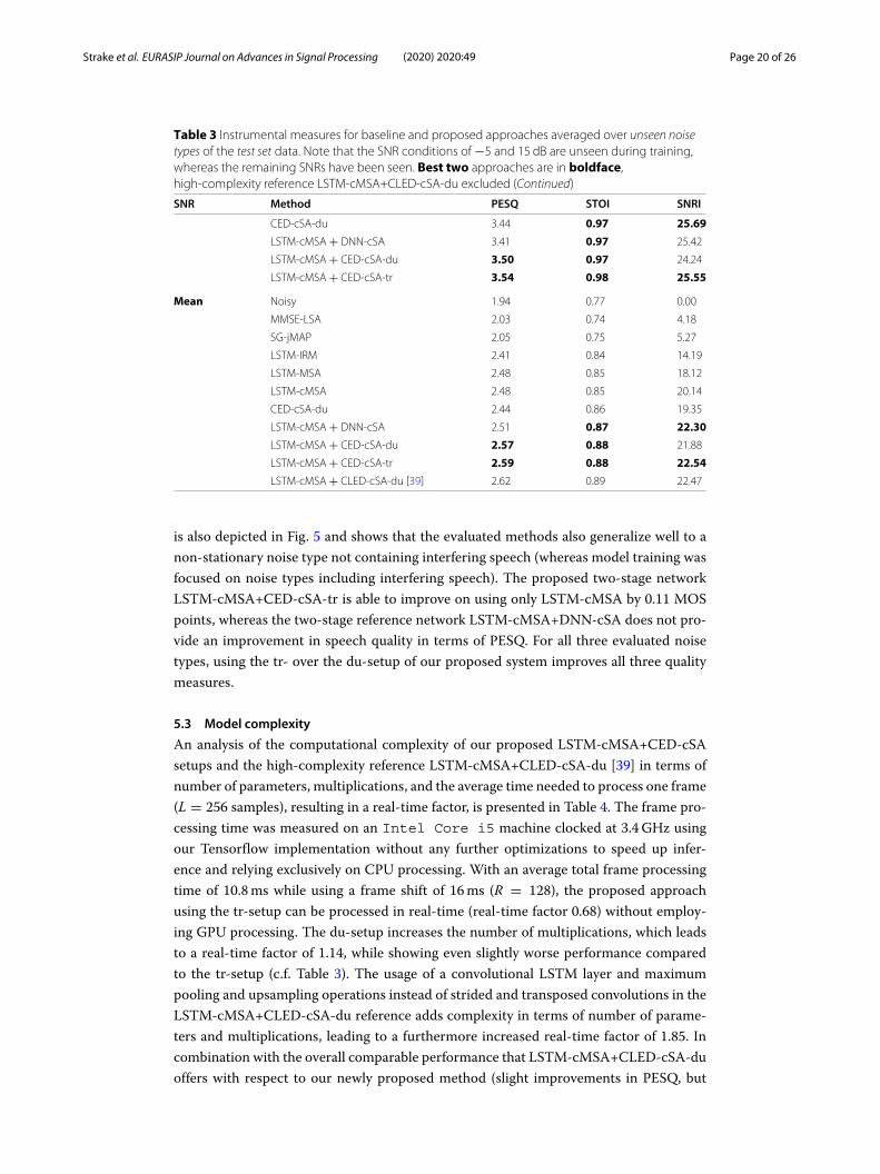
5.2 Results on unseen noise types

The results obtained from evaluating the unseen noise test dataset are presented inTable 3, where results are averaged over both noise types (pub and office noise). Onceagain, similar trends and model rankings compared to the evaluation with seen noisetypes can be observed, which shows a good generalization of the deep learning-basedmethods to these highly non-stationary unseen noise types in general. Especially, thetwo-stage LSTM-cMSA+CED-cSA-tr network is able to provide improvements overLSTM-cMSA comparable to the ones obtained with seen noise types (0.11 MOS points,0.03, and 2.40 dB in terms of PESQ, STOI, and SNRI, respectively).The comparison of deep learning-based methods for unseen pub and office noise in

5 dB SNR, depicted in Fig. 5, shows that all single-stage methods perform notably betterin office noise according to PESQ. However, pub noise, which contains mostly interferingspeech, seems to be quite difficult for the single-stage methods. This difference in over-all quality can be mitigated to some extent by the usage of the proposed second stage(LSTM-cMSA+CED-cSA-tr), which improves PESQ in pub noise by an impressive 0.17MOS points with regard to LSTM-cMSA. The additional analysis for unseen traffic noise


Table 3 Instrumental measures for baseline and proposed approaches averaged over unseen noisetypes of the test set data. Note that the SNR conditions of −5 and 15 dB are unseen during training,whereas the remaining SNRs have been seen. Best two approaches are in boldface,high-complexity reference LSTM-cMSA+CLED-cSA-du excluded


−5 Noisy 1.40 0.55 0.00

MMSE-LSA 1.39 0.51 3.01

SG-jMAP 1.38 0.51 4.13

LSTM-IRM 1.60 0.63 9.42

LSTM-MSA 1.62 0.65 11.05

LSTM-cMSA 1.57 0.64 13.65

CED-cSA-du 1.55 0.67 11.59




0 Noisy 1.59 0.68 0.00

MMSE-LSA 1.65 0.65 3.74

SG-jMAP 1.64 0.65 4.47

LSTM-IRM 1.95 0.78 13.44

LSTM-MSA 2.01 0.80 14.96

LSTM-cMSA 1.98 0.80 19.12

CED-cSA-du 1.89 0.82 16.33




5 Noisy 1.86 0.80 0.00

MMSE-LSA 1.98 0.77 4.41

SG-jMAP 1.98 0.78 5.35

LSTM-IRM 2.39 0.88 15.70

LSTM-MSA 2.48 0.89 17.35

LSTM-cMSA 2.49 0.89 22.07

CED-cSA-du 2.39 0.91 19.73




10 Noisy 2.22 0.89 0.00

MMSE-LSA 2.37 0.86 4.85

SG-jMAP 2.40 0.87 6.06

LSTM-IRM 2.84 0.93 16.58

LSTM-MSA 2.93 0.94 18.20

LSTM-cMSA 2.97 0.94 23.19

CED-cSA-du 2.96 0.95 23.40




15 Noisy 2.65 0.95 0.00

MMSE-LSA 2.77 0.92 4.88

SG-jMAP 2.86 0.93 6.36

LSTM-IRM 3.27 0.97 15.76

LSTM-MSA 3.35 0.97 17.92

LSTM-cMSA 3.39 0.97 22.66


Table 3 Instrumental measures for baseline and proposed approaches averaged over unseen noisetypes of the test set data. Note that the SNR conditions of −5 and 15 dB are unseen during training,whereas the remaining SNRs have been seen. Best two approaches are in boldface,high-complexity reference LSTM-cMSA+CLED-cSA-du excluded (Continued)


CED-cSA-du 3.44 0.97 25.69




Mean Noisy 1.94 0.77 0.00

MMSE-LSA 2.03 0.74 4.18

SG-jMAP 2.05 0.75 5.27

LSTM-IRM 2.41 0.84 14.19

LSTM-MSA 2.48 0.85 18.12

LSTM-cMSA 2.48 0.85 20.14

CED-cSA-du 2.44 0.86 19.35




LSTM-cMSA + CLED-cSA-du [39] 2.62 0.89 22.47

is also depicted in Fig. 5 and shows that the evaluated methods also generalize well to anon-stationary noise type not containing interfering speech (whereas model training wasfocused on noise types including interfering speech). The proposed two-stage networkLSTM-cMSA+CED-cSA-tr is able to improve on using only LSTM-cMSA by 0.11 MOSpoints, whereas the two-stage reference network LSTM-cMSA+DNN-cSA does not pro-vide an improvement in speech quality in terms of PESQ. For all three evaluated noisetypes, using the tr- over the du-setup of our proposed system improves all three qualitymeasures.

5.3 Model complexity

An analysis of the computational complexity of our proposed LSTM-cMSA+CED-cSAsetups and the high-complexity reference LSTM-cMSA+CLED-cSA-du [39] in terms ofnumber of parameters, multiplications, and the average time needed to process one frame(L = 256 samples), resulting in a real-time factor, is presented in Table 4. The frame pro-cessing time was measured on an Intel Core i5 machine clocked at 3.4GHz usingour Tensorflow implementation without any further optimizations to speed up infer-ence and relying exclusively on CPU processing. With an average total frame processingtime of 10.8ms while using a frame shift of 16ms (R = 128), the proposed approachusing the tr-setup can be processed in real-time (real-time factor 0.68) without employ-ing GPU processing. The du-setup increases the number of multiplications, which leadsto a real-time factor of 1.14, while showing even slightly worse performance comparedto the tr-setup (c.f. Table 3). The usage of a convolutional LSTM layer and maximumpooling and upsampling operations instead of strided and transposed convolutions in theLSTM-cMSA+CLED-cSA-du reference adds complexity in terms of number of parame-ters and multiplications, leading to a furthermore increased real-time factor of 1.85. Incombination with the overall comparable performance that LSTM-cMSA+CLED-cSA-duoffers with respect to our newly proposed method (slight improvements in PESQ, but


Fig. 5 Comparison of deep learning-based approaches for unseen noise types here also including traffic noise.Measures are PESQ, STOI, and SNRI, evaluated in the 5 dB SNR condition

lower SNRI, c.f. Table 3), we conclude that a recurrent model structure is not needed forthe second stage of our two-stage system and we therefore can drastically reduce modelcomplexity, while we are able to preserve performance.

5.4 Analysis of the two-stage approach

To further analyze the reasons for the observed quality improvements with our proposedtwo-stage approach, the enhanced speech spectrograms obtained with the deep learning-based methods are compared, using an exemplary test set utterance in pub noise at 5 dBSNR. The spectrograms of clean speech s(n), noisy speech y(n), and enhanced speech s(n)

for the different methods are shown in Fig. 6. Comparing the output of the two single-stage methods LSTM-MSA and LSTM-cMSA (third and fourth spectrogram from the

Table 4 Comparison of complexity in terms of number of trainable parameters, multiplications andreal-time factor (measured on an Intel Core i5machine clocked at 3.4 GHz) for our proposedmethods and the high-complexity reference pre-published in [39]. Comparisons are given for thesecond stage, for which the methods differ, and for the total two-stage system

MethodNumber ofparameters [ 106]

Number ofmultiplications [ 106] Real-time factor

Secondstage only

Total Secondstage only

Total Secondstage only

Total

LSTM-cMSA + CLED-cSA-du [39] 5.2 8.8 630.4 634.0 1.54 1.85

LSTM-cMSA + CED-cSA-du (new) 3.4 7.0 509.5 512.1 0.86 1.14

LSTM-cMSA + CED-cSA-tr (new) 3.4 7.0 364.6 369.2 0.45 0.68


Fig. 6 Spectrograms of reference and enhanced speech for a male speaker in unseen pub noise at 5 dB SNR.From top to bottom: clean speech, noisy speech, LSTM-MSA, LSTM-cMSA, new LSTM-cMSA+DNN-cSA,proposed LSTM-cMSA+CED-cSA-tr, and high-complexity reference LSTM-cMSA+CLED-cSA-du


top, respectively) shows the higher noise suppression that can be obtained with LSTM-cMSA. This comes at the cost of suppressing some parts of the speech signal as well,which can be examined in the highlighted areas in the respective spectrograms. Proceed-ing to the outputs after second-stage processing with DNN-cSA (third from bottom) andCED-cSA-tr (second from bottom), it can be observed that certain previously missing ordistorted parts are restored (again highlighted in the respective spectrograms). Further-more, CED-cSA-tr is able to more accurately restore the harmonic details of the originalclean speech compared to DNN-cSA, as can be seen, e.g., in the rightmost highlightedregion. We can credit this to the CED topology, which, as opposed to a fully connectedtopology, puts a focus on local dependencies over frequency through the use of convolu-tional kernels and is able to process different frequency regions with shared parameters,which we believe to be especially advantageous for the reconstruction of harmonic struc-tures. Moreover, the CED is able to use high-resolution information on the clean speechinherent to the noisy features directly via its skip connections, which can also aid amore detailed reconstruction. The comparison of the proposed LSTM-cMSA+CED-cSA-tr network with the high-complexity reference LSTM-cMSA+CLED-cSA-du furthermoreshows, that comparable speech restoration and noise suppression capabilities can beachieved with our newly proposed method, while employing significantly less modelparameters and computational resources.7

6 ConclusionIn this paper, we have proposed a new two-stage approach for speech enhancement, usingspecifically chosen network topologies for the subsequent tasks of noise suppression andrestoration of natural sounding speech. The first stage consists of an LSTM network esti-mating T-F masks for real and imaginary parts of the noisy speech spectrum, while thesecond stage performs spectral mapping using a convolutional encoder-decoder (CED)network. Employing only the noise suppression stage trained with the complex maskedspectrum approximation (cMSA) loss, we observe an impressive gain of more than 5 dBin SNR compared to the baselines, but only slight or no gains in terms of overall qual-ity (PESQ). When employing both stages, average improvements of PESQ by about 0.1MOS points can be obtained in unseen highly non-stationary noises including interferingspeech. Furthermore, our approach also improves STOI in low-SNR conditions comparedto the baselines.AbbreviationsBPTT: Backpropagation through time; CED: Convolutional encoder-decoder network; cMSA: Complex masked spectrumapproximation; CNN: Convolutional neural network; cRM: Complex ratio mask; cSA: complex spectrum approximation;DFT: Discrete Fourier transform; DNN: Deep neural network; IDFT: Inverse discrete Fourier transform; IRM: Ideal ratio mask;LSTM: Long short-term memory; MA: Mask approximation; MMSE-LSA: Minimummean-square error log-spectralamplitude; MOS-LQO: Mean opinion score for listening quality objective; MSA: Masked spectrum approximation; MVN:Mean and variance normalization; NN: Neural network; OLA: Overlap-add; PESQ: Perceptual evaluation of speech quality;PSA: Phase-sensitive spectrum approximation; RNN: Recurrent neural network; ReLU: Rectified linear unit; SG-jMAP:Super-Gaussian joint maximum a posteriori; SNR: Signal-to-noise ratio; SNRI: Signal-to-noise ratio improvement; STFT:Short-time Fourier transform; STOI: Short-time objective intelligibility; T-F: Time-frequency

AcknowledgementsNot applicable.

Authors’ contributionsAll authors contributed to the conception and design of the experiments and the interpretation of simulation results. MSwrote the software, performed the experiments and data analysis, and wrote the first draft of the manuscript. TF

7An audio demo of our proposed system including the example from Fig. 6 can be found under https://github.com/ifnspaml/Two-Stage-Speech-Enhancement

https://github.com/ifnspaml/Two-Stage-Speech-Enhancement

https://github.com/ifnspaml/Two-Stage-Speech-Enhancement


substantially revised the manuscript and BD and WT contributed additional revisions of the text. All authors read andapproved the final manuscript.

FundingThe project has been funded by NXP Semiconductors, Product Line Voice and Audio Solutions, Belgium. Open Accessfunding enabled and organized by Projekt DEAL.

Availability of data andmaterialsThe data supporting the findings of this study, namely the TIMIT [48], NTT super wideband [49], the QUT noise [50] andAURORA-2 [51] databases are available from the Linguistic Data Consortium (LDC), the NTT Advanced TechnologyCorporation, the SAIVT Research Labs, and the European Language Resources Association (ELRA), respectively.Restrictions apply to the availability of these data, which were used under license for the current study, and so are notpublicly available. Data are however available from the authors upon reasonable request and with permission of the LDC,the NTT Advanced Technology Corporation, the SAIVT Research Labs, and the ELRA.

Competing interestsThe authors would like to disclose that NXP Semiconductors has filed a patent comprising parts of this work. The authorsdeclare that this did not in any way affect the interpretation or presentation of results in this work and that they have noother competing interests.

Author details1Institute for Communications Technology, Technische Universität Braunschweig, Schleinitzstr. 22, 38106 Braunschweig,Germany. 2Goodix Technology Belgium BV, Arnould Nobelstraat 32, 3000 Leuven, Belgium.

Received: 10 January 2020 Accepted: 12 November 2020

References1. Y. Ephraim, D. Malah, Speech enhancement using a minimummean-square error short-time spectral amplitude

estimator. IEEE Trans. Acoust. Speech, Signal Process. 32(6), 1109–1121 (1984)2. Y. Ephraim, D. Malah, Speech enhancement using a minimummean-square error log-spectral amplitude estimator.

IEEE Trans. Acoust. Speech Sig. Process. 33(2), 443–445 (1985)3. P. Scalart, J. V. Filho, in Proc. of ICASSP, Speech enhancement based on a priori signal to noise estimation (IEEE,

Atlanta, 1996), pp. 629–6324. T. Lotter, P. Vary, Speech enhancement by map spectral amplitude estimation using a super-Gaussian speech

model. EURASIP J. Adv. Sig. Process. 2005(7), 1110–1126 (2005)5. C. Breithaupt, T. Gerkmann, R. Martin, in Proc. of ICASSP, A novel a priori SNR estimation approach based on selective

cepstro-temporal smoothing (IEEE, Las Vegas, 2008), pp. 4897–49006. S. Elshamy, N. Madhu, W. Tirry, T. Fingscheidt, Instantaneous a priori SNR estimation by cepstral excitation

manipulation. IEEE/ACM Trans. Audio, Speech, Lang. Process. 25(8), 1592–1605 (2017)7. R. Martin, Noise power spectral density estimation based on optimal smoothing and minimum statistics. IEEE Trans.

Speech Audio Process. 9(5), 504–512 (2001)8. I. Cohen, Noise spectrum estimation in adverse environments: improved minima controlled recursive averaging.

IEEE Trans. Speech Audio Process. 11(5), 466–475 (2003)9. T. Gerkmann, R. C. Hendriks, Unbiased MMSE-based noise power estimation with low complexity and low tracking

delay. IEEE/ACM Trans. Audio Speech Lang. Process. 20(4), 1383–1393 (2012)10. S. Rangachari, P. C. Loizou, A noise-estimation algorithm for highly non-stationary environments. Speech Commun.

48(2), 220–231 (2006)11. C. L.oizou. Philipos, Speech enhancement: theory and practice. (CRC Press, Boca Raton, 2007)12. Y. Wang, D. L. Wang, Towards scaling up classification-based speech separation. IEEE/ACM Trans. Audio Speech

Lang. Process. 21(7), 1381–1390 (2013)13. Y. Xu, J. Du, L. R. Dai, C. H. Lee, An experimental study on speech enhancement based on deep neural networks. IEEE

Sig. Process. Lett. 21(1), 65–68 (2014)14. Y. Xu, J. Du, L. R. Dai, C. H. Lee, A regression approach to speech enhancement based on deep neural networks.

IEEE/ACM Trans. Audio Speech Lang. Process. 23(1), 7–19 (2015)15. Y. Wang, A. Narayanan, D. L. Wang, On training targets for supervised speech separation. IEEE/ACM Trans. Audio

Speech Lang. Process. 22(12), 1849–1858 (2014)16. F. Weninger, J. R. Hershey, J. Le Roux, B. Schuller, in Proc. of GlobalSIP Machine Learning Applications in Speech

Processing Symposium, Discriminatively trained recurrent neural networks for single-channel speech separation (IEEE,Atlanta, 2014), pp. 577–581

17. D. S. Williamson, Y. Wang, D. L. Wang, Complex ratio masking for monaural speech separation. IEEE/ACM Trans.Audio Speech Lang. Process. 24(3), 483–492 (2016)

18. Z. Zhao, H. Liu, T. Fingscheidt, Convolutional neural networks to enhance coded speech. IEEE/ACM Trans. AudioSpeech Lang. Process. 27(4), 663–678 (2019)

19. S. Elshamy, N. Madhu, W. Tirry, T. Fingscheidt, DNN-supported speech enhancement with cepstral estimation ofboth excitation and envelope. IEEE/ACM Trans. Audio Speech Lang. Process. 26(12), 2460–2474 (2018)

20. N. Takahashi, N. Goswami, Y. Mitsufuji, in Proc. of IWAENC, MMdenseLSTM: an efficient combination of convolutionaland recurrent neural networks for audio source separation (IEEE, Tokyo, 2018), pp. 106–110

21. T. Gao, J. Du, L.-R. Dai, C.-H. Lee, in Proc. of ICASSP, Densely connected progressive learning for LSTM-based speechenhancement (IEEE, Calgary, 2018), pp. 5054–5058

22. H. Erdogan, J. R. Hershey, S. Watanabe, J. Le Roux, in Proc. of ICASSP, Phase-sensitive and recognition-boosted speechseparation using deep recurrent neural networks (IEEE, Brisbane, 2015), pp. 708–712


23. T. Fingscheidt, S. Suhadi, in Proc. of INTERSPEECH, Quality assessment of speech enhancement systems by separationof enhanced speech, noise, and echo (ISCA, Antwerpen, 2007)

24. ITU-T Rec P.1100, Narrow-band hands-free communication in motor vehicles (2015)25. J. Chen, D. L. Wang, Long short-term memory for speaker generalization in supervised speech separation. J. Acoust.

Soc. Am. 141(6), 4705–4714 (2017)26. S.-W. Fu, T. Hu, Y. Tsao, X. Lu, in Proc. of MLSP, Complex spectrogram enhancement by convolutional neural network

with multi-metrics learning (IEEE, Tokyo, 2017), pp. 1–627. S. R. Park, J. Lee, in Proc. of INTERSPEECH, A fully convolutional neural network for speech enhancement (ISCA,

Stockholm, 2017), pp. 1993–199728. X. Mao, C. Shen, Y.-B. Yang, in Proc. of NIPS, Image restoration using very deep convolutional encoder-decoder

networks with symmetric skip connections (Curran Associates, Inc., Barcelona, 2016), pp. 2802–281029. V. Badrinarayanan, A. Kendall, R. Cipolla, SegNet: a deep convolutional encoder-decoder architecture for image

segmentation. IEEE Trans. Pattern Anal. Mach. Intell. 39(12), 2481–2495 (2017)30. H. Noh, S. Hong, B. Han, in Proceedings of the IEEE International Conference on Computer Vision, Learning

deconvolution network for semantic segmentation (IEEE, Santiago, 2015), pp. 1520–152831. H. Zhao, S. Zarar, I. Tashev, C. Lee, in Proc. of ICASSP, Convolutional-recurrent neural networks for speech

enhancement (IEEE, Calgary, 2018), pp. 2401–240532. K. Tan, D. L. Wang, in Proc. of INTERSPEECH, A convolutional recurrent neural network for real-time speech

enhancement (ISCA, Hyderabad, 2018), pp. 3229–323333. Z. Xu, M. Strake, T. Fingscheidt, Concatenated identical DNN (CI-DNN) to reduce noise-type dependence in

DNN-based speech enhancement. arXiv:1810.11217 (2018)34. M. Tinston, Y. Ephraim, in Proc. of CISS, Speech enhancement using the multistage wiener filter (IEEE, Baltimore,

2009), pp. 55–6035. D. S. Williamson, Y. Wang, D. L. Wang, Reconstruction techniques for improving the perceptual quality of binary

masked speech. J. Acoust. Soc. Am. 136(2), 892–902 (2014)36. E. M. Grais, H. Erdogan, in Proc. of INTERSPEECH, Spectro-temporal post-enhancement using MMSE estimation in

NMF based single-channel source separation (ISCA, Lyon, 2013)37. E. M. Grais, G. Roma, A. J. R. Simpson, M. D. Plumbley, Two-stage single-channel audio source separation using deep

neural networks. IEEE/ACM Trans. Audio Speech Lang. Process. 25(9), 1773–1783 (2017)38. Z. Zhao, H. Liu, T. Fingscheidt, Convolutional neural networks to enhance coded speech. ACM Trans. Audio Speech

Lang. Process. 27(4), 663–678 (2019)39. M. Strake, B. Defraene, K. Fluyt, W. Tirry, T. Fingscheidt, in Proc. of WASPAA, Separated noise suppression and speech

restoration: LSTM-based speech enhancement in two stages (IEEE, New Paltz, 2019), pp. 234–23840. T. Fingscheidt, S. Suhadi, in ITG-Fachtagung Sprachkommunikation, Data-driven speech enhancement (ITG, Kiel, 2006)41. T. Fingscheidt, S. Suhadi, S. Stan, Environment-optimized speech enhancement. IEEE/ACM Trans. Audio Speech

Lang. Process. 16(4), 825–834 (2008)42. R. Pascanu, C. Gulcehre, K. Cho, Y. Bengio, How to construct deep recurrent neural networks. arXiv:1312.6026 (2013)43. V. Nair, G. E. Hinton, in Proc. of ICML, Rectified linear units improve restricted boltzmann machines (Omnipress, Haifa,

2010), pp. 807–81444. S. Hochreiter, J. Schmidhuber, Long short-term memory. Neural Comput. 9(8), 1735–1780 (1997)45. M. D. Zeiler, G. W. Taylor, R. Fergus, in Proc. of ICCV, Adaptive deconvolutional networks for mid and high level feature

learning (IEEE, Barcelona, 2011), pp. 2018–202546. A. L. Maas, A. Y. Hannun, A. Y. Ng, in Proc. of ICMLWorkshop on Deep Learning for Audio, Speech, and Language

Processing, Rectifier nonlinearities improve neural network acoustic models (Omnipress, Atlanta, 2013)47. V. Dumoulin, F. Visin, A guide to convolution arithmetic for deep learning. arXiv:1603.07285 (2016)48. J. S. Garofolo, L. F. Lamel, W. M. Fisher, J. G. Fiscus, D. S. Pallett, TIMIT acoustic-phonetic continuous speech corpus.

(Linguistic Data Consortium, Philadelpia, 1993). Linguistic Data Consortium49. NTT Advanced Technology Corporation, Super wideband stereo speech database. San Jose, CA, USA. NTT Advanced

Technology Corporation50. D. B. Dean, S. Sridharan, R. J. Vogt, M. W. Mason, in Proc. of INTERSPEECH, The QUT-NOISE-TIMIT corpus for the

evaluation of voice activity detection algorithms (ISCA, Makuhari, 2010), pp. 3110–311351. H.-G. Hirsch, D. Pearce, in Proc. of ASR2000-Automatic Speech Recognition: Challenges for the NewMillenium ISCA

Tutorial and ResearchWorkshop, The aurora experimental framework for the performance evaluation of speechrecognition systems under noisy conditions (ISCA, Paris, 2000), pp. 181–188

52. EG 202 396-1, Speech Processing, ETSI, Transmission and Quality Aspects (STQ); Speech Quality Performance in thePresence of Background Noise; Part 1: Background Noise Simulation Technique and Background Noise Database(2008)

53. P. J. Werbos, Generalization of backpropagation with application to a recurrent gas market model. Neural Netw. 1(4),339–356 (1988)

54. D. P. Kingma, J. Ba, Adam: a method for stochastic optimization. arXiv:1412.6980 (2014)55. D. E. Rumelhart, G. E. Hinton, R. J. Williams, Learning representations by back-propagating errors. Nature. 323(6088),

533–536 (1986)56. H. Yu, Post-filter optimization for multichannel automotive speech enhancement. PhD thesis, Technische Universität

Braunschweig (2013)57. X. Shi, Z. Chen, H. Wang, D. Y. Yeung, W. Wong, W. Woo, in Proc. of NIPS, Convolutional LSTM network: a machine

learning approach for precipitation nowcasting (Curran Associates, Inc., Montreal, 2015), pp. 802–81058. ITU-T Rec. G.160 Appendix II, Objective measures for the characterization of the basic functioning of noise reduction

algorithms (2012)59. V. Mai, D. Pastor, A. Aïssa-El-Bey, R. Le-Bidan, Robust estimation of non-stationary noise power spectrum for speech

enhancement. IEEE/ACM Trans. Audio Speech Lang. Process. 23(4), 670–682 (2015)60. M. Rahmani, A. Akbari, B. Ayad, B. Lithgow, Noise cross psd estimation using phase information in diffuse noise field.

Sig. Process. 89(5), 703–709 (2009)


61. A. Sugiyama, R. Miyahara, in Proc. of ICASSP, A directional noise suppressor with a specified beamwidth (IEEE,Brisbane, 2015), pp. 524–528

62. ITU-T Rec. P.862, Perceptual evaluation of speech quality (PESQ): an objective method for end-to-end speech qualityassessment of narrow-band telephone networks and speech codecs (2001)

63. C. H. Taal, R. C. Hendriks, R. Heusdens, J. Jensen, in Proc. of ICASSP, A short-time objective intelligibility measure fortime-frequency weighted noisy speech (IEEE, Dallas, 2010), pp. 4214–4217

64. S. Gustafsson, R. Martin, P. Vary, in Proc. of Workshop on Quality Assessment in Speech, Audio, and ImageCommunication, On the optimization of speech enhancement systems using instrumental measures (ITG/EURASIP,Darmstadt, 1996), pp. 36–40

Publisher’s NoteSpringer Nature remains neutral with regard to jurisdictional claims in published maps and institutional affiliations.

Documents

Speech enhancement by LSTM-based noise suppression