Spectral plots and the representation and

interpretation of biological data

Anirban Banerjee, Jurgen Jost

Max Planck Institute for Mathematics in the Sciences,

Inselstr.22, 04103 Leipzig, Germany,

banerjee@mis.mpg.de, jost@mis.mpg.de

February 13, 2013

Abstract

It is basic question in biology and other fields to identify the char-acteristic properties that on one hand are shared by structures from aparticular realm, like gene regulation, protein-protein interaction or neu-ral networks or foodwebs, and that on the other hand distinguish themfrom other structures. We introduce and apply a general method, basedon the spectrum of the normalized graph Laplacian, that yields repre-sentations, the spectral plots, that allow us to find and visualize suchproperties systematically. We present such visualizations for a wide rangeof biological networks and compare them with those for networks derivedfrom theoretical schemes. The differences that we find are quite strikingand suggest that the search for universal properties of biological networksshould be complemented by an understanding of more specific features ofbiological organization principles at different scales.

1 Introduction

The large volume of typical data sets produced in modern molecular, cell andneurobiology raises certain systematic questions, or, more precisely, brings newaspects to some old scientific issues. These, or at least the ones we wish toaddress in this note, are:

1. Given a particular biological structure, which of each features or qualitiesare universal, that is, shared by other structures within a certain class,and what is unique and special for the structure at hand?

2. Given a large and complex structure, should we focus on particular andspecific aspects and quantities in detail, or should we try to obtain, at least

1

arX

iv:0

706.

1198

v1 [

q-bi

o.Q

M]

8 J

un 2

007

at some coarse level, a simultaneous representation of all its qualitativefeatures?

Clearly, these questions can be posed, but not answered in such generality. Here,we look at those issues for a particular type of biological data, namely thosethat are presented as graphs or networks. For these, we introduce and discussa certain representation, a spectral plot, that allows for analyzing the questionsraised above, in both cases with an emphasis on the second alternative.

2 Graphs and their invariants

Many biological data sets are, or can be, represented as networks, that is, interms of the formal structure of a graph. The vertices of a graph stand forthe units in question, like genes, proteins, cells, neurons, and an edge betweenvertices expresses some correlation or interaction between the correspondingunits. These edges can be directed, to encode the direction of interaction, forexample via a synaptic connection between neurons, and weighted, to expressthe strength of interaction, like a synaptic weight. Here, for simplicity of pre-sentation, we only consider the simplest type of a graph, the undirected andunweighted one, although our methods apply and our considerations remainvalid in the general situation. Thus, an edge expresses the presence of someinteraction, connection or direct correlation between two vertices, regardless ofits direction or strength. Clearly, this abstraction may loose many importantdetails, but we are concerned here with what it preserves. Thus, we shall inves-tigate the two issues raised in the introduction for, possibly quite large, graphs.

An (unweighted, undirected) graph is given by a set V of vertices i, j, . . . anda set of edges E which are simply unordered pairs (i, j) of vertices.1 (Usually,one assumes that there can only be edges between different vertices, that is,there are no self-loops from a vertex to itself.) Thus, when the pair (i, j) isin E, then the vertices i and j are connected by an edge, and we call themneighbors and write this relation as i ∼ j. The degree ni of a vertex i is de-fined to be the number of its neighbors. Already for rather modest numbers ofvertices, say 20, the number of different graphs is bewilderingly high.2 Thus, itbecomes impractical, if not impossible, to list all different graphs with a givennumber of vertices, unless that number is rather small. Also, drawing a graphwith a large number of vertices is not helpful for visual analysis because thestructure will just look convoluted and complicated instead of transparent. Onthe other hand, graphs can be qualitatively quite different, and understandingthis is obviously crucial for the analysis of the represented biological structures.

1Some general references for graph theory are [9, 14].2As always in mathematics, there is a notion of isomorphism: Graphs Γ1 and Γ2 are called

isomorphic when there is a one-to-one map ρ between the vertices of Γ1 and Γ2 that preservesthe neighborhood relationship, that is i ∼ j precisely if ρ(i) ∼ ρ(j). Isomorphic graphs areconsidered to be the same because they cannot be distinguished by their properties. In otherwords, when we speak about different graphs, we mean non-isomorphic ones.

2

For example, the maximal distance (number of edges) between two vertices ina graph of size N can vary between 1 and N − 1, depending on the particulargraph. When the graph is complete, that is, every vertex is connected withevery other one, any two vertices have the distance 1, whereas for a chain wherevertex i1 is only connected to i2, i2 then also to i3, and so on, the first andthe last vertex have distance N − 1. For most graphs, of course, some interme-diate value will be realized, and one knows from the theory of random graphsthat for a typical graph this maximal distance is of the order logN . So, thismaximal distance is one graph invariant, but still, rather different graphs canhave the same value of this invariant. Adjoining a long sidechain to a completesubgraph can produce the same value as an everywhere loosely connected, butrather homogeneous graph. The question then emerges whether one should lookfor other, additional or more comprehensive, invariants, or whether one shouldadopt an entirely different strategy for capturing the essential properties of somegiven graph.In fact, there are many graph invariants that each capture certain importantqualitative aspects, and that have been extensively studied in graph theory (seee.g. [9, 14]). These range from rather simple and obvious ones, like maximal oraverage degree of vertices or distance between them, to ones that reflect moreglobal aspects, like how difficult it is to separate the graph into disjoint com-ponents (see e.g. [11]), commmunities (e.g.[24]) or classes, or to synchronizecoupled dynamics operating at the individual vertices (e.g. [19]). For the sakeof the subsequent discussion, we call these properties cohesion and coherence,resp. Recently, the degree distribution of the vertices received much attention.Here, for each n ∈ N, one lists the number kn vertices i in the graph withdegree ni = n and then looks at the behavior of kn as a function of n. Inrandom graphs as introduced by Erdos and Renyi (e.g. [10]), that is, graphswhere one starts with a given collection of, say N , vertices and to each pairi, j of vertices, one assigns an edge with some probability 0 < p < 1, typicallykn ∼ e−σn for some constant σ, that is the degree sequence decays exponen-tially.3 Barabasi-Albert [8] (and earlier Simon [27]) gave a different randomconstruction where the probability of a vertex i to receive an edge from someother vertex j is not uniform and fixed, but rather depends on how many edgesi already has. This was called preferential attachment, that is, the chance of avertex to receive an additional edge increases when it already possesses manyedges. For such a graph, the degree sequence behaves like kn ∼ n−κ for someexponent κ, typically between 2 and 3. Thus, the degree sequence decays likea power law, and the corresponding type of graph is called scale free. Theyalso gave empirical evidence of networks that follow such a power law degreedistribution rather than an exponential one. This produced a big fashion, andin its wake, many empirical studies appeared that demonstrated or claimed sucha power law behavior for large classes of biological or infrastructural networks.Thus, scalefreeness seemed a more or less universal feature among graphs com-

3In more precise terms, the degrees are Poisson distributed in the limit of an infinite graphsize.

3

ing from empirical data in a wide range of domains. While this does providesome insights (for some systematic discussion, see e.g. [1, 12, 28]), for examplea better understanding of the resilience of such graphs against random deletionof vertices, it also directly brings us to the two issues raised in the introduction:

1. A feature like scalefreeness that is essentially universal in empirical graphsby its very nature fails to identify what is specific for graphs coming froma particular domain. In other words, do there exist systematic structuraldifferents for example between gene regulation, protein-protein interactionor neural networks? Or, asked differently, given an empirical graph, with-out being told where it comes from, can one identify this domain on thebasis of certain unique qualitative features?

2. Graphs with the same degree sequence can be quite different with respectto other qualitative invariants like the coherence, as emphasized in [2,3]. Also, depending on the details of the preferential attachment rulechosen, invariants like the average or maximal distance can vary widely,as observed in [20]. Thus, is there some way to encode many, or evenessentially all, important graph invariants simultaneously in some compactmanner?

3 The spectrum of a graph

In order to provide a positive answer to these question, we shall now introduceand consider the spectrum of a (finite) graph Γ with N vertices. For functionsv from the vertices of Γ to R, we define the Laplacian as

∆v(i) := v(i)− 1ni

∑j,j∼i

v(j). (1)

(Note that in the graph theoretical literature (e.g.[9, 14, 21, 23]), it is morecustomary to put a factor ni in front of the right hand side in the definition ofthe Laplacian. The choice of convention adopted here is explained in [17, 18].It is equivalent to the one in [11].)The eigenvalue equation for ∆ is

∆u = λu. (2)

A nonzero solution u is called an eigenfunction for the eigenvalue λ. ∆ then hasN eigenvalues, perhaps occurring with multiplicity, that is, not necessarily alldistinct. (The multiplicity of the eigenvalue λ is the number of linearly indepen-dent solutions of (2).) The eigenvalues of ∆ are real and nonnegative (because∆ is a symmetric, nonnegative operator, see e.g. [17, 18] for details). The small-est eigenvalue is λ = 0. Its multiplicity equals the number of components of Γ.When Γ is connected, that is, has only one component (as we typically assumebecause one can simply study the different components as graphs in their own

4

right), this eigenvalue is simple. The other eigenvalues are positive, and weorder the eigenvalues as4

λ1 = 0 ≤ λ2 ≤ ... ≤ λN .

For the largest eigenvalue, we have

λN ≤ 2, (3)

with equality iff the graph is bipartite. Bipartiteness means that the graphconsists of two disjoint classes Γ′,Γ′′ with the property that there are no edgesbetween vertices in the same class. Thus, a single eigenvalue determines theglobal property of bipartiteness.The eigenvalue λ = 1 also plays a special role as it gives some indication of vertexor motif duplications underlying the evolution of the graph, as systematicallyexplored in [5, 7]. For a biological discussion, see [25, 29, 32]. For a generalmathematical discussion of the spectrum, see [11, 6] and the references giventhere.What we want to emphasize here is that the spectrum constitutes an essentiallycomplete set of graph invariants. At least without the qualification “essentially”,this is not literally true, in the following sense: there are examples of non-isomorphic graphs with the same spectrum – such graphs are called isospectral(see [33]). In other words, the spectrum of a graph does not determine the graphcompletely (see [15] for a graph reconstruction algorithm from the spectrum).Such isospectral graphs, while not necessarily isomorphic, are qualitatively verysimilar to each other, however. In particular, the spectrum of the graph encodesall the essential qualitative properties of a graph, like cohesion and coherence(e.g. [11, 19, 4]). Thus, for practical purposes, this is a good enough set ofgraph invariants.In conclusion, the spectrum of a graph yields a set of invariants that on one handcaptures what is specific about that graph and on the other hand simultaneouslyencodes all its important properties.

4 Visualization of a graph through its spectralplot

What is more, the spectral plot of a graph is much better amenable to visualinspection than a direct plot of the graph or any other method of representationthat we know of. In other words, with a little experience in graph theory, onecan quickly detect many important features of a graph through a simple lookat its spectral plot. We now display some examples.5

4Our convention here is different from [19, 17, 18, 6].5All networks are taken as undirected and unweighted. Thus, we suppress some potentially

important aspects of the underlying data, but as our plots will show, we can still detectdistinctive qualitative patterns. In fact, one can also compute the spectrum of directed andweighted networks, and doing that on our data will reveal further structures, but this is notexplored in the present paper.

5

First of all, the properties of the visualization will obviously depend on the dis-play style, and this will be described first, see Figure 1. That figure is basedon the metabolic network of C.elegans. The first diagram displays the binnedeigenvalues, that is, the range [0, 2] is divided here into 35 disjoint bins, andthe number of eigenvalues that fall within each such bin is displayed, normal-ized by the total number of eigenvalues (relative frequency plot). The nextfigure smoothes this out by using overlapping bins, see figure legend for param-eter values. The subsequent subfigures instead convolve the eigenvalues with aGaussian kernel, that is, we plot the function

f(x) =∑λj

1√2πσ2

exp(−|x− λj |2

2σ2)

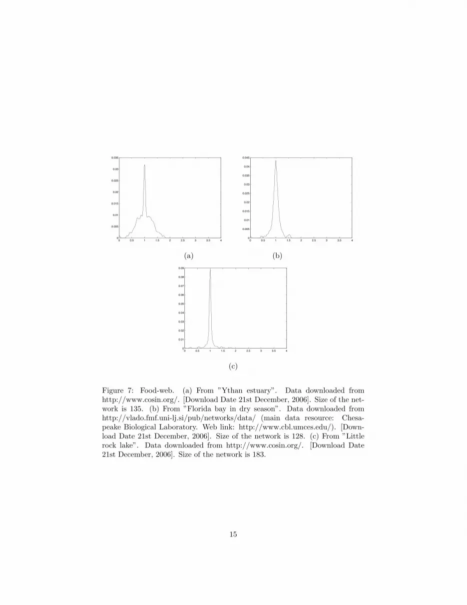
where the λj are the eigenvalues. Smaller values of the variance σ2 emphasizethe finer details whereas larger values bring out the global pattern more con-spicuously.So, this is a network constructed from biological data. We next exhibit spec-tral plots, henceforth always with the value σ = .03, of networks constructedby formal schemes that have been suggested to capture important features ofbiological networks, namely an Erdos-Renyi random network, a Watts-Strogatzsmall-world network and a Barabasi-Albert scale-free network (see Figure 2). Itis directly obvious that these spectral plots are very different from the metabolicnetwork. This suggests to us that any such generic network construction missesimportant features and properties of real biological networks. This will now bemade more evident by displaying further examples of biological networks. Weshall also see that biological networks from one given class typically have quitesimilarly looking spectral plots, which, however, are easily disitnguishable fromthose of networks from a different biological class. First, in Figure 3, we showsome further metabolic networks. Figures 4 and 5 display transcription andprotein-protein interaction networks. These still look somewhat similar to themetabolic networks, and this may reflect a common underlying principle. Byway of contrast, the neurobiological networks in Figure 6 and the food-webs inFigure 7 are entirely different – which is not at all surprising as they come fromdifferent biological scales.

In conclusion, we have presented a simple technique for visualizing the importantqualitative aspects of biological networks and for distinguishing networks fromdifferent origins. We expect that our method will further aid formal analysis ofbiological network data.

References

[1] R. Albert, A.-L. Barabasi, Statistical mechanics of complex networks, Re-views of Modern Physics 74, 2002, 47–97.

6

[2] F.M. Atay, T.Bıyıkoglu, J.Jost, Synchronization of networks with pre-scribed degree distributions, IEEE Trans. Circuits and Systems I 53 (1),2006, 92–98.

[3] F.M. Atay, T.Bıyıkoglu, J.Jost, Network synchronization: Spectral versusstatistical properties, Phys.D, to appear

[4] F.M. Atay, J. Jost, A. Wende, Delays, connection topology, and synchro-nization of coupled chaotic maps, Phys. Rev. Lett. 92 (14), 2004, 144101.

[5] A.Banerjee, J.Jost, Laplacian spectrum and protein-protein interactionnetworks, e-print: arXiv:0705.3373v1

[6] A.Banerjee, J.Jost, On the spectrum of the normalized graph Laplacian,e-print: arXiv:0705.3772v1

[7] A.Banerjee, J.Jost, Graph spectra as a systematic tool in computationalbiology, Discrete Appl.Math. to appear, e-print: arXiv:0706.0113v1

[8] A.-L. Barabasi, R. A. Albert, Emergence of scaling in random networks,Science 286, 1999, 509–512.

[9] B.Bolobas, Modern graph theory, Springer, 1998

[10] B.Bolobas, Random graphs, Cambridge Univ.Press, 22001

[11] F.Chung, Spectral graph theory, AMS, 1997

[12] S.N. Dorogovtsev, J.F.F. Mendes, Evolution of Networks, Oxford, 2003.

[13] P. Erdos, A. Renyi, On random graphs, Publicationes Mathematicae De-brecen, 6, 1959, 290-297

[14] C.Godsil, G.Royle, Algebraic graph theory, Springer, 2001

[15] M. Ipsen, A. S. Mikhailov, Evolutionary reconstruction of networks, Phys.Rev. E 66(4), 2002

[16] H. Jeong and B. Tombor and R. Albert and Z. N. Oltval and A. L.Barabasi, The Large-Scale Organization of Metabolic Networks, Nature,407(6804), 2000, 651-654

[17] J. Jost, Mathematical methods in biology and neurobiology, monograph,to appear

[18] J. Jost, Dynamical networks, in: J.F.Feng, J.Jost, M.P.Qian (eds.), Net-works: from biology to theory, Springer, 2007

[19] J. Jost, M. P. Joy, Spectral properties and synchronization in coupled maplattices, Phys.Rev.E 65(1), 16201-16209, 2001

7

[20] J.Jost, Joy, Evolving networks with distance preferences, Phys.Rev.E 66,36126-36132, 2002

[21] R. Merris, Laplacian matrices of graphs – a survey, Lin. Alg. Appl.198,1994, 143-176

[22] R. Milo and S. Shen-Orr and S. Itzkovitz and N. Kashtan and D.Chklovskii and U. Alon, Network Motifs: Simple Building Blocks of Com-plex Networks, Science, 298(5594), 2002, 824-827

[23] B. Mohar, Some applications of Laplace eigenvalues of graphs, in: G.Hahn,G.Sabidussi (eds.), Graph symmetry: Algebraic methods and applica-tions, pp. 227-277, Springer, 1997

[24] M. Newman, The structure and function of complex networks, SIAM Re-view 45, 2003, 167–256

[25] S.Ohno, Evolution by gene duplication, Springer, 1970

[26] S. S. Shen-Orr and R. Milo and S. Mangan and U. Alon, Network Motifsin the Transcriptional Regulation Network of Escherichia Coli, NatureGenetics, 31(1), 2002, 64-68

[27] H.Simon, On a class of skew distribution functions, Biometrika 42, 425-440, 1955

[28] A.Vazquez, Growing networks with local rules: Preferential attachment,clustering hierarchy and degree correlations, cond-mat/0211528, 2002

[29] A. Wagner, Evolution of gene networks by gene duplications - a math-ematical model and its implications on genome organization, Proc. Nat.Acad. Sciences USA 91(10), 1994, 4387-4391

[30] D. J. Watts, S. H. Strogatz, Collective Dynamics of ’Small-World’ Net-works, Nature, 393(6684), 1998, 440-442

[31] J. G. White and E. Southgate and J. N. Thomson and S. Brenner,The Structure of the Nervous-System of the Nematode Caenorhabditis-Elegans, Philosophical Transactions of the Royal Society of London SeriesB-Biological Sciences, 314(1165), 1986, 1-340

[32] K. H. Wolfe, D. C. Shields, Molecular evidence for an ancient duplicationof the entire yeast genome, Nature, 387(6634), 1997, 708-713

[33] P.Zhu, R.Wilson, A study of graph spectra for comparing graphs

8

0 0.2 0.4 0.6 0.8 1 1.2 1.4 1.6 1.8 20

0.05

0.1

0.15

0.2

0.25

0.3

0.35

0 0.2 0.4 0.6 0.8 1 1.2 1.4 1.6 1.8 20

0.02

0.04

0.06

0.08

0.1

0.12

0.14

0.16

(a) (b)

0 0.5 1 1.5 2 2.5 3 3.5 40

0.02

0.04

0.06

0.08

0.1

0.12

0.14

0 0.5 1 1.5 2 2.5 3 3.5 40

0.01

0.02

0.03

0.04

0.05

0.06

0.07

(c) (d)

0 0.5 1 1.5 2 2.5 3 3.5 40

0.005

0.01

0.015

0.02

0.025

0.03

0.035

0.04

0.045

0 0.5 1 1.5 2 2.5 3 3.5 40

0.005

0.01

0.015

0.02

0.025

0.03

(e) (f)

Figure 1: Spectral plots of metabolic network of Caenorhabditis el-egans. Size of the network is 1173. Nodes are substrates, en-zymes and intermediate complexes. Data used in [16]. Data Source:http://www.nd.edu/∼networks/resources.htm/. [Download date: 22nd Nov.2004]. (a) Relative frequency plot with number of bins = 35. (b) Relative fre-quency polygon with overlapping bins with bin width = 0.04 and number ofbins = 99 and bins are taken as [0, .04], [.02, .06], [.04, .08], . . . , [1.96, 2]. (c) withGaussian kernel with σ = 0.01. (d) with Gaussian kernel with σ = 0.02. (e)with Gaussian kernel with σ = 0.03. (f) with Gaussian kernel with σ = 0.05.

9

0 0.5 1 1.5 2 2.5 3 3.5 40

0.005

0.01

0.015

0.02

0.025

0 0.5 1 1.5 2 2.5 3 3.5 40

1

2

3

4

5

6

7

8x 10!3

(a) (b)

0 0.5 1 1.5 2 2.5 3 3.5 40

0.002

0.004

0.006

0.008

0.01

0.012

(c)

Figure 2: Specral plots of generic networks. (a) Random network by Erdosand Renyi’s model [13] with p = 0.05. (b) Small-world network by Watts andStogatz model [30] (rewiring a regular ring lattice of average degree 4 withrewiring probability 0.3). (d) Scale-free network by Albert and Barabasi model[8] (m0 = 5 and m = 3). Size of all networks is 1000. All figures are ploted with100 realization.

10

0 0.5 1 1.5 2 2.5 3 3.5 40

0.005

0.01

0.015

0.02

0.025

0.03

0.035

0.04

0.045

0.05

0 0.5 1 1.5 2 2.5 3 3.5 40

0.005

0.01

0.015

0.02

0.025

0.03

0.035

0.04

0.045

0.05

(a) (b)

0 0.5 1 1.5 2 2.5 3 3.5 40

0.005

0.01

0.015

0.02

0.025

0.03

0.035

0.04

0.045

0.05

(c)

Figure 3: Metabolic networks. Here nodes are substrates, enzymesand intermediate complexes. Data used in [16]. Data Source:http://www.nd.edu/∼networks/resources.htm/. [Download date: 22nd Nov.2004] (a) Pyrococcus furiosus. Network size is 746. (b) Aquifex aeolicus. Net-work size is 1052. (c) Saccharomyces cerevisiae. Network size is 1511.

11

0 0.5 1 1.5 2 2.5 3 3.5 40

0.01

0.02

0.03

0.04

0.05

0.06

0.07

0.08

0.09

0 0.5 1 1.5 2 2.5 3 3.5 40

0.01

0.02

0.03

0.04

0.05

0.06

0.07

0.08

0.09

(a) (b)

Figure 4: Transcription networks. Data source: Data published by Uri Alon(http://www.weizmann.ac.il/mcb/UriAlon/ ). [Download date: 13th Oct.2004]. Data used in [22, 26]. (a) Escherichia coli. Size of the network is 328.(b) Saccharomyces cerevisiae. Size of the network is 662.

12

0 0.5 1 1.5 2 2.5 3 3.5 40

0.01

0.02

0.03

0.04

0.05

0.06

0.07

0.08

0.09

0 0.5 1 1.5 2 2.5 3 3.5 40

0.01

0.02

0.03

0.04

0.05

0.06

0.07

0.08

0.09

(a) (b)

0 0.5 1 1.5 2 2.5 3 3.5 40

0.01

0.02

0.03

0.04

0.05

0.06

0.07

0.08

0.09

(c)

Figure 5: Protein-protein interaction networks. Data are collected fromhttp://www.cosin.org/ [download date: 25th September, 2005]. (a) Saccha-romyces cerevisiae. Size of the network is 3930. (b) Helicobacter pylori. Size ofthe network is 710. (c) Caenorhabditis elegans. Size of the network is 314.

13

0 0.5 1 1.5 2 2.5 3 3.5 40

0.005

0.01

0.015

0.02

0.025

0 0.5 1 1.5 2 2.5 3 3.5 40

0.002

0.004

0.006

0.008

0.01

0.012

0.014

0.016

(a) (b)

0 0.5 1 1.5 2 2.5 3 3.5 40

0.002

0.004

0.006

0.008

0.01

0.012

0.014

0.016

(c)

Figure 6: Neuronal connectivity. (a) Caenorhabditis elegans. Sizeof the network is 297. Data used in [30, 31]. Data Source:http://cdg.columbia.edu/cdg/datasets/ [Download date: 18th Dec. 2006]. (b)Caenorhabditis elegans (animal JSH, L4 male) in the nerve ring and RVG re-gions. Network size is 190. Data source: Data is assembled by J. G. White,E. Southgate, J. N. Thomson, S. Brenner [31] and was later revisited by R.M. Durbin (Ref. http://elegans.swmed.edu/parts/ ). [Download date: 27thSep. 2005]. (c) Caenorhabditis elegans (animal N2U, adult hermaphrodite) inthe nerve ring and RVG regions. Network size is 199. Data source: Data isassembled by J. G. White, E. Southgate, J. N. Thomson, S. Brenner [31] andwas later revisited by R. M. Durbin (Ref. http://elegans.swmed.edu/parts/ ).[Download date: 27th Sep. 2005].

14

0 0.5 1 1.5 2 2.5 3 3.5 40

0.005

0.01

0.015

0.02

0.025

0.03

0.035

0 0.5 1 1.5 2 2.5 3 3.5 40

0.005

0.01

0.015

0.02

0.025

0.03

0.035

0.04

0.045

(a) (b)

0 0.5 1 1.5 2 2.5 3 3.5 40

0.01

0.02

0.03

0.04

0.05

0.06

0.07

0.08

0.09

(c)

Figure 7: Food-web. (a) From ”Ythan estuary”. Data downloaded fromhttp://www.cosin.org/. [Download Date 21st December, 2006]. Size of the net-work is 135. (b) From ”Florida bay in dry season”. Data downloaded fromhttp://vlado.fmf.uni-lj.si/pub/networks/data/ (main data resource: Chesa-peake Biological Laboratory. Web link: http://www.cbl.umces.edu/). [Down-load Date 21st December, 2006]. Size of the network is 128. (c) From ”Littlerock lake”. Data downloaded from http://www.cosin.org/. [Download Date21st December, 2006]. Size of the network is 183.

15