Spatial discrimination

Regional Science and Urban Economics 19 (1989) 87-102. North-Holland

SPATIAL DISCRIMINATION

Bertrand vs. Cournot in a Model of Location Choice*

Jonathan H. HAMILTON

University of Florida, Gainesville, FL 32611, USA

Jacques-FranGois THISSE

CORE, Universitk Catholique de Louvain, Louvain-la-Neuve, Belgium

Anita WESKAMP

Universitiit Bonn, D-5300 Bonn 1, FRG

Received July 1987, final version received January 1988

A model with two firms competing in location and sales is analyzed for the case of spatial discrimination. Consumers are uniformly distributed along a line segment and have identical downward sloping demands. Two games are solved and results are compared. In one game, firms first choose locations and then quantity schedules; in the other, the final stage is choice of price schedules. Prices and transport costs are lower under Bertrand competition. Profits are higher under Cournot competition for low transport costs, but the reverse holds for larger values of these costs. Aggregate welfare is higher in the Bertrand competition case. In both games, firms locate in such a way as to minimize their own transport costs for the sales pattern arising in equilibrium, but the equilibrium configurations are quite different.

1. Introduction

Spatial discrimination has a long history of research, starting with the work of Robinson (1933) and Hoover (1937). However, study has long been confined to the monopoly case. It is only recently that spatial discrimination in oligopolistic environments has received increased attention. Two types of competition have been discussed - Bertrand and Cournot. In the first case, each competitor sets a location-specific delivered price schedule at which it is willing to supply consumers. In the second, each firm chooses a location-

*The authors thank S. Anderson and P. Lederer for their comments and suggestions on a first draft of this paper. The first author thanks the College of Business Administration, University of Florida and the National Science Foundation for financial support. This paper was completed while the second author was Visiting Research Professor at INSEAD, Fontainebleau, France.

016&0462/89/%3.50 0 1989, Elsevier Science Publishers B.V. (North-Holland)

88 J.H. Hamilton et al., Spatial discrimination

specific quantity schedule, letting the market-clearing condition determine price at each location. In both cases, the firms incur transport costs.

For monopoly firms undeterred by fear of entry, outcomes under price- and quantity-setting policies will be identical. In non-spatial markets, it is well known that Bertrand and Cournot competition yield different outcomes. Grossman (198 1) observes that, under Bertrand competition, a rival can cut price to capture all of one’s market, while under Cournot competition, a rival’s output expansion will capture none of one’s sales. This obviously carries over to the case of a spatial market. Surprisingly, no systematic attempt has been made to compare the specific characteristics of Bertrand and Cournot equilibria in models of spatial discrimination.

This paper provides a comparison of the two equilibria in the context of a spatial duopoly in which firms first choose locations and then price or quantity schedules. Before presenting our results, we briefly review the existing literature.

The case of price-setting firms has been treated by Lederer and Hurter (1986) who prove existence of a two-stage perfect Nash equilibrium with inelastic demands. MacLeod, Norman and Thisse (1988) have established the existence of free entry equilibria under a similar assumption. The shape of the equilibrium delivered price schedules for more general demands has been studied by Gee (1985). Finally, Hobbs (1986) has used the price discrimination model with consumers located on a network to analyze the impact of deregulating electricity distribution in the U.S.

Greenhut and Greenhut (1975) first discussed spatial discrimination by quantity-setting firms and derived the profile of the delivered price schedule. Anderson and Neven (1986) extend this to more general transport cost and demand functions. Weskamp (1985) establishes existence and characterizes equilibrium in a model with consumers located at the vertices of a network, while Dafermos and Nagurney (1987) look at the asymptotic behavior of the equilibrium. This model has been used to describe intra-industry trade by Brander (1981) and Neven and Philips (1985). It has also been employed in several empirical studies; see, e.g., Harker (1986).

We assume linear demand functions at all points of a linear bounded space, constant marginal production costs and transport costs which are linear in volume and distance. For transport costs low enough such that both firms always compete on the whole market, we solve the two games for the subgame perfect Nash equilibria. In addition to existence and uniqueness, we establish that: Cournot firms always agglomerate, while Bertrand firms locate at distinct locations inside the first and third quartiles; Bertrand delivered prices are lower than Cournot for all consumers; total transport costs are lower under Bertrand; welfare is higher under Bertrand; but profits are higher under Cournot.

The latter results confirm and extend previous results of Cheng (1985) and

J.H. Hamilton et al., Spatial discrimination 89

Vives (1985) who have obtained similar rankings for given differentiated products. Here, in contrast, the comparisons are made using equilibrium locations which differ under the two types of competition. However, for larger transport costs, Bertrand profits become greater than Cournot profits. This reversal of a standard result in industrial organization shows that spatial discrimination adds new facets to oligopoly problems.

The paper is organized as follows. Section 2 treats quantity-setting firms; section 3 analyzes price-setting firms. Section 4 compares equilibria of the two games, In section 5, we present conclusions and discuss some extensions.

2. Quantity competition

With the exception of dropping use of f.o.b. (mill) pricing by the firms, our framework is similar to that of Hotelling (1929). Two firms choose locations along a line segment of unit length and then sell a homogeneous product to consumers who are distributed uniformly along the line segment. Production involves constant marginal costs and transport costs are linear in distance and quantity. Each consumer has a linear demand function for the product. The standard inelastic demand assumption cannot be retained because the quantity-setting model would yield corner solutions.

We denote the firms as 1 and 2 and describe the firms locations a and b by their distance from the left and right endpoints of the market, respectively. Firm 1 is always assumed to lie to the left of firm 2. A consumer’s location is indexed by XE [0, 11. A consumer’s demand function is given by q(x) = 1 -p(x) where p(x) is the lower delivered price offered to consumers at x. For quantity-setting firms, it will be convenient to work with the inverse demand function since Cournot competition assumes prices at any location x to be determined by market clearing. The inverse demand function is p(x)= 1 -q(x) where q(x) is the total quantity offered to consumers at that point, q(x) = ql(x) + q2(x) with subscripts denoting firms.

As is common in location models, we restrict ourselves to subgame perfect Nash equilibria with locations chosen first and then quantities. This permits us to solve the game by backward induction, first solving for quantities given locations and then determining the equilibrium locations.

2.1. The quantity equilibrium

In the second stage, for fixed locations a and b, each firm chooses a quantity schedule qi(X) for XE [O, l] to maximize profit given its rival’s schedule q,(x). The contribution to profits of units sold by firm 1 is p(x)-& 1, h x w ere c is the unit transport cost and production costs are normalized to zero; for firm 2, this is p(x) -c/l -b-x/. Profits for each firm are:


and

Inspection of these expressions reveals that we can break down the problem into a subproblem at each location. Because of the assumption of constant marginal (production and transport) costs, a firm’s quantity decision at a particular location has no effect on actions at other locations. The possibility of arbitrage by consumers limits the slopes of delivered price schedules, but this constraint never binds in equilibrium. As a result, at each location, we seek a Cournot equilibrium between firms having non-identical transport costs.

Proposition 1. Let O<c_I$. Then there exists a unique Nash equilibrium in quantity schedules which is given byIs

q*(x’a 1 3 2

b)_l-2cJ~-x/+c~1-b-x~ 3

>

Furthermore, the resulting delivered price schedule is

p*(x.a b)J+cla-xl+c(l-b-~ 3 3

3

(1)

(2)

(3)

Proof. Direct computation of the Cournot equilibrium yields (1) and (2).

‘Uniqueness is true up to moditication of the equilibrium schedules on a zero measurement set. The same applies to Proposition 3.

2Existence and uniqueness can be established for larger values of c, but the resulting equilibrium schedules are no longer given by (1) and (2) [ see Anderson and Neven (1986)]. The reason for choosing c 5 $ will become clear later on and results for c > 4 are discussed in section 5. The same comment applies to Proposition 3.


Moreover, cs+ is the least stringent sufficient condition assuming that q: and q: exceed zero for all x E [0, 1) and all a, b such that a + b 5 1. 0

Inspection of (3) demonstrates that there are no arbitrage opportunities. When consumers are outside the two firms, delivered prices rise by two- thirds of the additional transport cost. When consumers are located between the two firms, they pay the same price,

p*_ 1 +c(l -b-a) __~ 3 .

The critical value c= 4 is easily interpreted. The monopoly price at a firm’s location is f, and the other firm finds it profitable to ship the product to its rival’s location as long as its transport costs are smaller than f. Thus cg+ insures that no firm serves a positive market segment monopolistically, even if the firms are at maximum distance, i.e., the endpoints.

2.2. The location equilibrium

Given the equilibrium quantity schedules, in the first stage each firm chooses a location to maximize profits given its rival’s location. Formally, a Nash location equilibrium is a pair (a&b,*) such that3

and

z:(a& b$) 2 $(a, b;) V a E [0, l] s.t. a+ b,* 5 1

~:(a& b,*) 2 n;( 1 -b& 1 -a) V a E [O, l] s.t. a + b; > 1,

and

@(a,*, b;) 1 ~:(a,*, b) V b E [0, l] s.t. a: + b 5 1

~r(ac*,bc*)~~:(l-b,l-ar) VbE[O,l] s.t. a,*+b>l,

where profits ~:(a, b) and ~;(a, b) are as follows:

7~:(u,b)=J[p*(x;a,b)-cla-x(]qT(x;a,b)dx

and

~;(a, b)=J[p*(x;a, b)-c(l- b-x(]q;(x;a, b) dx.

3The reversal of the subscripts is necessary because the functional forms of profits depend on firm 1 lying to the left of firm 2.


Clearly, if a 5 4 and b s _t, no firm prefers to locate on the other side of its rival.

Proposition 2. If O<c 5-3, then there exists a unique two-stuge perfect Nash equilibrium. The locations are

and q:(x;a,b) and qr(x;a,b) are given by (1) and (2).

Proof: See the appendix.

Thus, with spatial discrimination and quantity competition, agglomeration occurs [see also Anderson and Neven (1986)]. Since each firm’s sales are distributed symmetrically around the market center, each firm is located so as to minimize transportation costs associated with its sales pattern. No benefits from differentiated locations are therefore obtained.

3. Price competition

The standard model of price discrimination has a firm offering a price schedule to consumers at a set of locations where the firm is willing to deliver the product. For a monopolist, there will be no difference between choosing a quantity or a price schedule, but these differ for duopolists. Here we again analyze a two-stage perfect Nash equilibrium where duopolists first choose locations and then choose price schedules. As with quantity competition, the game is solved by backward induction. The assumptions are those of section 2. Of course, we now use the demand function q(x) = 1 -p(x), not the inverse demand function.

3.1. The price equilibrium

For fixed locations, each firm chooses a price schedule to maximize profits given its rival’s price schedule. Consumers at x buy from the firm charging the lower delivered price. When delivered prices are equal, the firm with lower transport costs provides the good to the consumers.4 Unless the firms locate at the same place, the set of consumers for whom transport costs are equal is of measure zero in equilibrium. Finally, it is assumed that the delivered price at x cannot be made smaller than the unit transport cost to X. 5

41f another assignment rule is used when firms charge identical prices (e.g., fifty-fifty), the nearer firm can reduce its price by E and secure the corresponding markets.

5Lederer and Hurter (1986) show how this assumption can be relaxed without aNecting the results.


As under quantity competition, the price problem can be solved at each location separately since there are no linkages between sales at different points. The problem is therefore to find the Bertrand equilibrium for firms having different costs.

Proposition 3. Let 0 < cs ). Then there exists a unique Nash equilibrium delivered price schedule which is given by

p:(x;a,b)=pt(x;a,b)=max{clx-al,cIl-b-x(}. (4)

Furthermore, the resulting quantity schedule is

q*(x;a,b)=l-cmax{lx-al,Il-b-xl>.

Proof: As cz+, the monopoly price is never less than transport cost from one firm to the other. The result then follows from a standard Bertrand argument at each point x. cl

Again, arbitrage cannot make consumers better off: the difference between delivered prices between any two points is always less than or equal to the cost of transport.

3.2. The location equilibrium

We now consider the location equilibrium when firms anticipate the equilibrium price schedule. Profits for firm 1 are

G(a, b) = j CpXx) - CIx - a11 Cl -PWI dx 0

=%[c(l-a-b)][l-c(l-b-x)]dx

+y[c(l+a-b-2x)][l-c(l-b-x)]dx,

where X = (1 + a - b)/2, and profits for firm 2 are

n:(a,b)=j[p:(x)-c/l-b-xl][l-p:(x)]dx X

R.S.U.E. D


l-b

= i [c(2x-l-a+6)][1-c(x-a)]dx

+ ,;, [c(l -a-b)][l-c(x-a),dx.

For these ~7 and rcf, the definition of a Nash location equilibrium (af, bg) is identical to that given in 2.2.

Proposition 4. If 0 <c =< 3, then there exists a unique perfect Nash equilibrium. The locations are

a*=6*_ 10c-8+~(10c-8)2+24(4-3c)c B B

24~

and p:(x; a, 6) and pf(x; a, 6) are given by (4).

Proof. See the appendix.

(5)

Thus, with spatial discrimination and price competition, agglomeration never occurs. This should not be surprising since, for a= l-6, the equilibrium price schedules are p:(x) = p;(x) = clu-x( and profits equal zero. Bertrand competitors must differentiate their location to earn positive profits. As a: > +, firms locate symmetrically inside the first and third quartiles, but very close to them.6 So there is not maximal differentiation. Furthermore, since the derivative of firm l(2)‘s profit function with respect to its location shows that, for X=), a,*(b,*) is the median of its sales distribution over the interval [O,+]([f, l]), ag(bf) is the location that minimizes the transport cost associated with the sales pattern of firm 1 (2) over CO,+] ([f, 11).

4. Comparison of equilibria

In the case of fixed product characteristics, Vives (1985) and Cheng (1985) have established that equilibrium prices for substitutes are higher in the Cournot case than in the Bertrand case. Here, in a spatial model, even though firms choose different locations, each consumer still pays a higher price in the Cournot equilibrium. Let p’(x) = p*(x; a& 63 and p”(x) = pt(x; a,*, bg).

Proposition 5. For afl x E [O, 11, we haue p”(x) > pB(x).

%‘HBpital’s rule establishes that lim _,, af = 4. Moreover, it can be shown that da,‘/dc z-0 for 0 i c 6 f. Finally, a simple computation yields a: = 0.2704 for c = f.


P”(x)

P’(x)

c pJ; -Xl

0 I/4 a; l/S b; a/1 I a:=b:

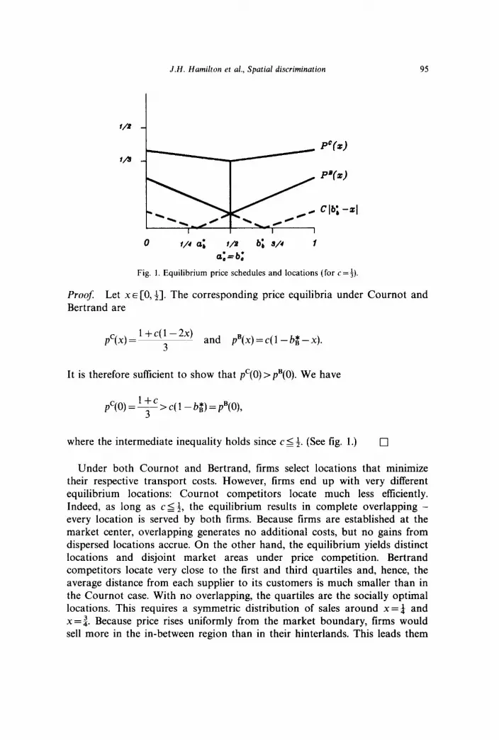
Fig. 1. Equilibrium price schedules and locations (for c = f).

Proof. Let x E [0,&l. The corresponding price equilibria under Cournot and Bertrand are

l+c(l-2x) PC(x)= 3 ~ and p”(x)=c(l-&-xX).

It is therefore sufficient to show that p’(O) > ~~(0). We have

l+c pC( 0) = ~ 3 >c(l -bB*)=pB(O),

where the intermediate inequality holds since c5f. (See fig. 1.) 0

Under both Cournot and Bertrand, firms select locations that minimize their respective transport costs. However, firms end up with very different equilibrium locations: Cournot competitors locate much less efficiently. Indeed, as long as csf, the equilibrium results in complete overlapping - every location is served by both firms. Because firms are established at the market center, overlapping generates no additional costs, but no gains from dispersed locations accrue. On the other hand, the equilibrium yields distinct locations and disjoint market areas under price competition. Bertrand competitors locate very close to the first and third quartiles and, hence, the average distance from each supplier to its customers is much smaller than in the Cournot case. With no overlapping, the quartiles are the socially optimal locations. This requires a symmetric distribution of sales around x=+ and x = 2. Because price rises uniformly from the market boundary, firms would sell more in the in-between region than in their hinterlands. This leads them


to locate closer to the center. (Recall that Bertrand competitors locate at precisely the points which minimize transport costs given their respective sales.)

In spite of the fact that Bertrand firms sell more at each point (price is lower), an even stronger result holds: the dispersed locations of the Bertrand firms make total transport costs lower under Bertrand than Cournot. Total transport costs for Cournot firms located identically at $ equal

- $.

Total transport costs for Bertrand firms located symmetrically at a = b are

TB(a,c)=2f+-xl[l-c(l-a-x)]dx 0

a2_3a2c+4a3c+I_a_c+ac 2 3 8 2 12 2’

These expressions are difficult to compare analytically when a is replaced by a;(c), as given by (5). A series of computations have therefore been undertaken for different values of c in CO,+]. They all indicate the T’(c) > TB(4c), 4.

As aggregate welfare is equal to total surplus minus total transport costs, Proposition 5 and the result above imply that aggregate welfare is higher under Bertrand than Cournot.

It remains to compare profits. Clearly, the local revenue function is concave in price. Since both p”(x) and p”(x) lie on the upward sloping part of this function, higher prices under Cournot are sufficient to establish higher revenues for the Cournot competitors. However, because they also incur higher costs, a direct calculation must be made to compare profits. Total revenue for both Cournot firms equals

For Bertrand firms, total revenue is

RB(a,c)=2fc(l-a-x)[l-c(l-a-x),dx 0


( 3 lc 3ac =c --_a--+--&. 4 12 2 >

Aggregate profits for Cournot and Bertrand firms are

7rC(C) = RC(c) - 7-C(c) =$ - g - g,

nB(a,c)=RB(a,c)-TB(a,c)=c 8a3c

;-$+7+2a’c-2a2-- 3

We defer the comparison of these expressions to the next section. However, observe that a change in transport costs has differing impacts on profits: Bertrand profits rise with c, but Cournot profits fall as c increases. Thus, for quantity-setting firms, distance does not act as a barrier to competition which allows firms to build up higher profits. Since the firms locate together, an increase in costs does not create more differentiation as it does in the Bertrand case.

5. Extensions

We have obtained the equilibrium configurations for 0 < c 5 3. For c > 3, at least some location pairs give rise to the nearer firm’s monopoly price being less than the more distant firm’s transport costs, which implies that the equilibrium schedule given in Propositions 1 and 3 do not remain valid. In the most extreme case, for ~24, firms locate at the first and third quartiles and sell at the monopoly price in their entire market areas. Price and quantity strategies yield identical outcomes.

For intermediate values of c, two types of difficulties in deriving equilibria arise: either the roots of the equations used in Propositions 2 and 4 are no longer relevant; or, for at least some location pairs, firms sell at monopoly prices and profit functions rc: and rcr are different from those used in the preceding analysis. In the Cournot case, for c> 1, the second-order condition for a maximum is violated at a= b =f, so that the agglomeration result no longer applies. For c> 1, Cournot firms prefer to move apart to lower the costs of serving their markets. In the Bertrand case, given a,*(c), monopoly price regions exist for c 20.9.’ Below this level, computation by grid search establishes that the solution in Proposition 4 remains the equilibrium.

Analytic comparison of n’(c) and nB[a~(c),c] proves difficult. Computation

‘At x=0, the monopoly price for firm 1 is (1 +ca#Z while the cost for firm 2 to deliver there is c( 1 - a;). Thus ( 1 + ~a;)/2 < c( 1 - 0;) and (5) imply

1-2c+3c (

10~-8+~(lOc-8)~+24~(4-3~) <o,

24c >

This holds only if - 8c2 - 64c + 64 < 0, i.e., c < 0.9.


of profits in both equilibria reveals that Cournot profits are greater than Bertrand profits for low levels of transport cost. However, for values of c between approximately 0.72 and 0.9, Bertrand profits exceed Cournot profits. Thus, there is no unambiguous ranking of profits for all levels of transport cost. The reason for the reversal in the ranking of profits is that Cournot firms, which agglomerate in the center, bear the higher transport costs, while, due to market segmentation, Bertrand firms choose locations which minimize transport costs given the distribution of demand. It remains true that welfare is higher under Bertrand competition in this range because prices to all consumers and transport costs are lower than under Cournot competition.

Singh and Vives (1984) find, with fixed products which are substitutes, that firms prefer quantity-setting to price-setting policies. If firms first choose price-setting or quantity-setting before choosing locations, this result will not hold for all levels of transport cost.

For c 24, only local monopolies are equilibria in the two-stage game. For these cost levels, Bertrand and Cournot profits are therefore equal. Thus, it cannot always be true that Bertrand profits always rise and Cournot profits always fall with increases in c. In other words, the process is not monotonic in c. For small c, Cournot profits exceed those in Bertrand equilibria. As c increases, the difference between the profit levels becomes negative. For c 2 4, the difference is zero. So it must be the case that the difference (in absolute value) decreases for c between 1 and 4. An analytic solution appears extremely cumbersome, if not impossible. Further computation should be undertaken to determine the behavior of the profit functions for intermediate levels of transport costs. In the Cournot case, for c> 1, the second-order condition for a maximum is violated at a= b=+, so that the agglomeration result no longer applies. For c> 1, Cournot firms prefer to move apart to lower the costs of serving their markets.

It is worthwhile noting that, in the Bertrand case, the general structure of the equilibrium price schedules is robust to changes in demand and transport costs, although the numerical solutions change. Duopolists will always charge the minimum of the monopoly price and the rival’s delivery cost at any location. Furthermore, the firms still locate so as to minimize their own transport costs (the derivative of the profit function 7~: with respect to location still equals minus the derivative of tirm i’s total transport costs). The equilibrium locations (if they exist!) lie away from the center, but inside the first and third quartiles because prices are lower between the firms. In the Cournot case, the existence of equilibrium quantity schedules can be established for varying demand and transport cost conditions [see Anderson and Neven (1986)]. If the whole market is served by both firms, then agglomeration still occurs provided that profits at each point are concave in quantity and transport costs are convex in distance.


Appendix

Proof of Proposition 2

We have

~:(a, b)=i [p*(x; a, 6) -cla-xl]q:(x;a, b) dx 0

=$ ~[(l-2c(u-x)+c(l-b-x)]2dx i

l-b

+ s [(l-2c(x-u)+c(l-b-x)12dx 0

1

+Ifb[(1-2c(x-u)+c(x+b-1)]2dx

Thus,

-a(l-2c(u+x)+c(l-b-x))dx

l-b

+ s (1-2c(x-u)+c(l -b-x))dx (1

1

+I!b(1-2c(x-u)+c(x+b-1))dx

4c =-( -2u+cu2-2cu(l -b)+c(l -by

9

+ 1- ;+2uc--c(l--b) 1

.

The solution to aZ7y(u, Q/au = 0 is the solution to the quadratic equation in brackets:

c(l-b)2+1-$+bc 1


l b+ =-- J (1+2b)+l+(l+B) -~__

C C 2 2

If b=+, then

1 =- -l+ J-1 , ( >

2 3 1 thatis --

c 2-c c 20’2’

Since c 54, only + lies in [0, l] and is therefore the relevant root. The second-order condition for a maximum is satisfied everywhere on the relevant domain since

aZ7cc:(a, b) - 8c aa2

=g[(l-C)+C(l-b-a)]

is strictly negative for cS+ and, a+ bS 1. Uniqueness is shown by an analysis of the positions of the reaction

functions: in the admissible regions of a, b, and c, both are strictly decreasing; and one is everywhere steeper than the other, hence they intersect at most once.

Proof of Proposition 4

We have

n;(a,b)=i[c(l-b-x)-c(a-x)][l-c(l-b-x)]dx 0

+i [c(l -b-x)-c(x-a),[1 -c(l -b-x)] dx. II

By Leibnitz’ Rule,

p=-cj(l-c(l-h)+cx)dx+cj(l-c(l-b)+cx)dx any aa o II

=c (1 -cY(l -b))(x-2a)-caZ+5 i I


and

a21c* &==c - ;+3I”_(l -b)-2ca+i.f ~0 since CSf.

For the symmetric equilibrium, X=4 and so &cf/&r=O requires aI: to be the solution of

[I-C(l-a)][_S-2a]-ca2+C=O 8

or

a,=10c-8+~(10c-8)2+24(4-3c)c B 24c

since only the positive root gives a solution in [0, 11. Finally, notice that uniqueness may be shown by proving that both

reactions functions are strictly increasing in the regions of a, b, and c and that one is everywhere steeper than the other, so that they intersect at most once.

References

Anderson, Simon and Damien Neven, 1986, Spatial competition a la Cournot,‘Working paper 86/13 (INSEAD, Fontainebleau).

Brander, James, 1981, Intra-industry trade in identical commodities, Journal of International Economics 11, 1-14.

Cheng, Leonard, 1985, Comparing Bertrand and Cournot equilibria: A geometric approach, Rand Journal of Economics 16, 146151.

Dafermos, Stella and Anna Nagurney, 1987, Oligopolistic and competitive behavior of spatially separated markets, Regional Science and Urban Economics 17, 245-254.

Gee, J.M.A., 1985, Competitive pricing for a spatial industry, Oxford Economic Papers 37, 466485. .

Greenhut, John and Melvin L. Greenhut, 1975, Spatial price discrimination, competition and location effects, Economica 42, 401419.

Grossman, Sanford, 1981, Nash equilibrium and the industrial organization of markets with large fixed costs, Econometrica 49, 1149-l 172.

Harker, Patrick, 1986, Alternative models of spatial competition, Operations Research 34, 41@425.

Hobbs, Benjamin, 1986, Network models of spatial oligopoly with an application to deregula- tion of electricity generation, Operations Research 34, 395409.

Hoover, Edgar, 1937, Spatial price discrimination, Review of Economic Studies 4, 182-191. Hotelling, Harold, 1929, Stability in competition, Economic Journal 39, 41-57. Lederer, Phillip and Arthur Hurter, 1986, Competition of firms: Discriminatory pricing and

location, Econometrica 54, 623-640. MacLeod, Bentley, George Norman and Jacques-Francois Thisse, 1988, Price discrimination and

equilibrium in monopolistic competition, International Journal of Industrial Organization 6, 429-446.

Neven, Damien and Louis Phlips, 1985, Discriminating oligopolists and common markets, Journal of Industrial Economics 34, 133-149.

102 J.H. ffamilton et al., Spatial discrimination

Robinson, Joan, 1933, The economics of imperfect competition (Macmillan, London). Singh, Nirvikar and Xavier Vives, 1984, Price and quantity competition in a differentiated

duopoly, Rand Journal of Economics 15, 546554. Vives, Xavier, 1985, On the efficiency of Bertrand and Cournot equilibria with product

differentiation, Journal of Economic Theory 36, 166-175. Weskamp, Anita, 1985, Existence of spatial Cournot equilibria, Regional Science and Urban

Economics 15, 219-228.

Documents

Spatial discrimination