Embed Size (px)
Citation preview
Ghent University
Faculty of Bioscience Engineering
Department of Soil Management
Space-time variability of soil salinity in irrigated vineyards of South Africa
Ruimte-tijd variabiliteit van bodemverzilting in geïrrigeerde wijngaarden van Zuid Afrika
ir. Willem de Clercq
Thesis submitted in fulfilment of the requirements for the degree of
Doctor (PhD) in Applied Biological Sciences: Land and Forest
Management
Academic Year 2008-2009
2
Examination committee:
Chairman: Prof. dr. ir. Norbert De Kimpe
Department of Organic Chemistry, Ghent University
Jury members:
Prof. dr. Tibor Tóth,
Research Institute for Soil Science and Agricultural
Chemistry of the Hungarian Academy of Sciences,
Hungary
Prof. dr. ir. Donald Gabriels
Department of Soil Management, Ghent University
Prof. dr. ir. Valentijn Pauwels,
Department of Forest and Water Management, Ghent
University
Promoters: Prof. dr. ir. Marc Van Meirvenne
Department of Soil Management Faculty of
Bioscience Engineering, Ghent University
Prof. dr. Martin V. Fey
Department of Soil Science, Faculty of AgriSciences,
University of Stellenbosch, South Africa
Dean: Prof. dr. ir. G. Van Huylenbroeck
Rector: Prof. dr. P. Van Cauwenberge
3
Cover:
Photograph of the farm Broodkraal close to the town Piketberg in the
Western Cape Province of South Africa.
Contact address:
Department of Soil Science, University of Stellenbosch, Private Bag X1,
Matieland, 7602, South Africa.
E-mail: [email protected]
Reference:
de Clercq W.P., 2009. Space-time variability of soil salinity in irrigated
vineyards of South Africa. PhD Thesis, Ghent University, 209p.
ISBN 978-90-5989-276-7
The author and promoters give the authorization to consult and copy
parts of this work for personal use only. Any other use is subject to the
copyright laws. Permission to reproduce any material contained in this
work should be obtained from the author.

4
ACKNOWLEDGEMENT
In April of 2000, Prof. Dr. Ir. M. Van Meirvenne and Prof. Dr. ir. D.
Gabriels visited the Department of Soil Science of the Stellenbosch
University as a part of a bilateral program between Flanders and South
Africa. During their visit, the idea to start a PhD at Ghent University took
shape. Consequently, in October 2001 my proposed project was accepted
for a PhD study. I continued the study in Stellenbosch with a number of
visits to Ghent University.
I need to express my gratitude first and foremost, to Prof. Dr. ir. M. Van
Meirvenne who encouraged me through the whole process.
And to a number of people, and organisations:
Prof. Dr. M.V. Fey and Dr. A. Rozanov, for always encouraging me and
reminding me of the urgency in completing the study.
The reading committee, Prof. Dr. D. Gabriels, Prof. Dr. ir. V. Pauwels,
Prof. Dr. Ir. T. Toth, whose comments ultimately contributed to a better
product.
Students from Ghent, Griet de Smet and Frederik Seghers, who handled
some of the fieldwork contained in this study.
Hendrik Engelbrecht (student at Stellenbosch), who also managed some
of the fieldwork in my absence.
My always loyal colleague, Kamilla Latief, for her assistance in lowering
my workload.
My Heavenly Father for His omnipresence.
The WRC of SA for funding most of this research.
Last but not least, my family, Maryke, Jaco and Jo-Anne.
5
ABSTRACT
Salts present in the soil and surface waters of the Western Cape Province
of South Africa represent a limitation to farming activities. Therefore the
management of salinity in the landscape, which includes measuring,
mapping and monitoring of its behaviour on a regional scale, is the
general subject of this investigation.
Four sites were actively investigated in this study. These are the
Robertson experimental farm, Goedemoed farm near Robertson,
Broodkraal farm near Piketberg and the Glenrosa farm near Paarl. At the
first two, regular point measurements were taken to study the behaviour
of salinity in irrigated soils over several irrigation seasons. Frequent
sampling of soil and soil water was done. The quality of the irrigation
water was recorded and at the Robertson site the quality of the irrigation
water was adjusted to six different levels of salinity, between 30 mS m-1
and 500 mS m-1
. At the Broodkraal and Glenrosa farms, large scale
investigations were conducted to estimate salinity over larger areas.
Broodkraal farm was a large newly established table grape enterprise
offering the opportunity to study the initial change in soil salinity when
irrigated with saline water. At the Glenrosa farm, there was an
opportunity to characterize the soil even before irrigated vineyards were
established.
Detailed point measurements were taken to investigate the salinity
distribution in these soil profiles and its dynamics. Suction cup
measurements were taken with self-designed and patented lysimeters and
used to follow the seasonal soil water salinity changes through the root
zone under different salinity regimes. These results were used to
characterize an average salt depth trend, which was found to be best

6
represented by a linear function, and its evolution over time. A method
was proposed to reduce the number of samples necessary to determine
this salt depth trend and to estimate the quality of the soil water that
drains below the rooting zone. One of the important findings was that an
ECe threshold for vines of 100 mS m-1
was more suitable than the
conventional 150 mS m-1
and that the sensitivity of the vines to levels
beyond this threshold increased with the number of years of exposure.
The detailed surveys at the Broodkraal and Glenrosa Farms helped the
modelling of the regional salinity behaviour. This study allowed to gain a
comprehensive understanding of the soil salinity dynamics in an irrigated
landscape using saline water.
7
SAMENVATTING
Zouten aanwezig in de bodems en oppervlaktewaters van de 'Westeren
Cape Province' van Zuid Afrika vertegenwoordigen een beperking van de
landbouwactiviteiten. Vandaar dat het landschappelijk beheer van
verzilting, inclusief het registreren, kartering en monitoren op een
regionale schaal, het algemeen onderwerp is van deze thesis.
Vier sites werden actief onderzocht in deze studie. Deze zijn de
Robertson experimentele boerderij, de Goedemoed boerderij nabij
Robertson, de Broodkraal boerderij nabij Piketberg en de Glenrosa
boerderij nabij Paarl. In de eerste twee werden op een regelmatige wijze
bodemstalen genomen om het gedrag van zouten in de geïrrigeerde
bodem te bestuderen doorheen meerdere irrigatieseizoenen. Regelmatig
werden stalen genomen van de bodem en het bodemwater. De kwaliteit
van het irrigatiewater werd opgemeten en in de Robertson boerderij werd
de kwaliteit van het irrigatiewater aangepast aan zes verschillende
zoutniveaus tussen 30 mS m-1 en 500 mS m-1
. In de Broodkraal en
Glenrosa boerderijen werden grootschalige onderzoeken uitgevoerd om
het zoutgehalte over grotere oppervlakten in te schatten. De Broodkraal
boerderij bestond hoofdzakelijk uit een nieuw opgericht bedrijf van
tafeldruiven, hetgeen de mogelijkheid bood om de initiële veranderingen
van bodemzouten te bestuderen tijdens irrigatie met zout water. Bij de
Glenrosa boerderij was er zelfs de mogelijkheid om de bodem te
karakteriseren voordat er geïrrigeerde wijngaarden werden aangelegd.
Gedetailleerde puntmetingen werden uitgevoerd om de verdeling en
veranderingen van zouten doorheen het bodemprofiel te onderzoeken.
Daarnaast werden met zelf ontworpen en gepatenteerde 'suction cup
lysimeters' de seizoensveranderingen van het zoutgehalte in het
8
bodemwater gevolgd onder verschillende zout regimes. Deze resultaten
werden gebruikt om gemiddelde zout-diepte trends te karakteriseren,
deze warden het best weergegeven door een lineaire functie, en hun
evolutie doorheen de tijd te volgen. Een methode werd voorgesteld om
het aantal stalen dat moet genomen worden om de zout-diepte trend te
bepalen, en zo de kwaliteit van het wegdrainerend bodemwater in te
schatten, te verminderen. Eén van de belangrijkste vaststelling was dat de
drempelwaarde voor de elektrische geleidbaarheid van de
verzadigingspasta van de bodem beter op 100 mS m-1
gesteld wordt dan
de gebruikelijke 150 mS m-1
, en dat de gevoeligheid van wijnstokken aan
hoge zoutdosissen toeneemt met het aantal jaren dat ze blootgesteld zijn
aan zout water irrigatie.
Aldus hielpen de gedetailleerde kartering van de Broodkraal en Glenrosa
boerderijen om het regionaal gedrag van verzilting te modelleren. Deze
studie liet toe om een alomvattend begrip te krijgen van de dynamiek in
bodemverzilting in een geïrrigeerd landschap waarbij verzilt
irrigatiewater gebruikt wordt.
9
LIST OF ACRONYMS
BRC Berg River Catchment
cdf Cumulative distribution function
Df Degrees of freedom
DWAF Department of Water Affairs and Forestry of SA
EC Electrical conductivity
ECa Apparent electrical conductivity
ECd Electrical conductivity of drainage water
ECe Electrical conductivity of a saturated soil paste extract
ECi Electrical conductivity of the irrigation water
ECih The half effect of ECi used in the calculation of yield
ECt Threshold EC value
ECsw Electrical conductivity of the soil water
ECswf Electrical conductivity of the soil water at field capacity
EM38 Proximal sensor for electromagnetic induction
measurements
Epan Class A-pan evaporation
ER Electrical resistance of a saturated soil paste
ET Evapotranspiration
icdf Inverse cumulative distribution function
LWP Leaf water potential
MAP Mean annual precipitation
masl Meters above sea level

10
PR Profile ratio defined as EM38hor / EM38vert
PTF Pedotransfer function
RSE Riviersonderend (Sub-catchment of the Breede River)
SAR Sodium adsorption ratio
SCL Suction cup lysimeter
SS Sum of squares
TC Trunk circumference
TMS Table Mountain sandstone
UBRC Upper Breede River Catchment
WC Western Cape Province
WRC Water Research Commission of SA
11
TABLE OF CONTENTS
1 GENERAL INTRODUCTION ............................................................................ 20
1.1 Background and problem description .......................................................... 21
1.1.1 Water requirements in the Berg and Breede River catchments ............... 22
1.1.2 Impact of irrigated agriculture on soil and surface water quality ............. 23
1.2 The general and specific aims of this study ................................................. 26
1.3 General structure of the thesis ...................................................................... 26
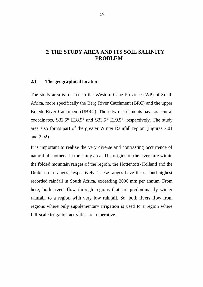
2 THE STUDY AREA AND ITS SOIL SALINITY PROBLEM .......................... 29
2.1 The geographical location ............................................................................ 29
2.2 A physical perspective of the study area ...................................................... 31
2.2.1 Geomorphology and geology ................................................................... 31
2.2.2 Climate ..................................................................................................... 36
2.2.3 Water Resources ...................................................................................... 40
2.2.3.1 Hydrology of the Berg River and the upper Breede River drainage
regions .................................................................................................. 40
2.2.3.2 Irrigation water quality ..................................................................... 41
2.2.3.3 Return flow as a water source .......................................................... 43
2.2.4 Soils.......................................................................................................... 45
2.2.5 Land use ................................................................................................... 51
2.3 Soil salinisation within the study area .......................................................... 52
2.3.2 Defining salinity hazard in irrigated vineyards of SA .............................. 56
3 IRRIGATION OF VINES WITH SALINE WATER .......................................... 58
3.1 Introduction .................................................................................................. 58
3.2 Materials and Method .................................................................................. 61
3.3 Results and discussion ................................................................................. 64
3.3.1 The soil and water .................................................................................... 64
3.3.2 The vine ................................................................................................... 70
3.3.3 Yield response .......................................................................................... 71
3.3.4 The wine ................................................................................................... 77
3.4 Conclusion ................................................................................................... 78
4 AN AUTOMATED SOIL WATER SAMPLE RETRIEVAL SYSTEM ............ 80
4.1 Introduction .................................................................................................. 80
4.2 Materials and method ................................................................................... 81
4.2.1 The SCL’s ................................................................................................ 81
4.2.2 Installation of a SCL ................................................................................ 84
4.2.3 Method of operation ................................................................................. 85
4.2.4 Measuring the relative matrix potential. .................................................. 86
4.3 Summary ...................................................................................................... 86
5 PREDICTION OF THE DEPTH TREND IN SOIL SALINITY OF A
VINEYARD AFTER SUSTAINED IRRIGATION WITH SALINE WATER. ......... 87
5.1 Introduction .................................................................................................. 88
12
5.2 Materials and methods ................................................................................. 93
5.2.1 Data analysis ............................................................................................ 94
5.3 Results and discussion ................................................................................. 97
5.4 Conclusions ................................................................................................ 107
6 EXPLORING THE VARIABILITY OF ECe BETWEEN VINE ROWS ......... 108
6.1 Introduction ................................................................................................ 108
6.2 Materials and methods ............................................................................... 109
6.3 Results and discussion ............................................................................... 110
6.4 Conclusions ................................................................................................ 112
7 EFFECT OF LONG TERM IRRIGATION APPLICATION ON THE
VARIATION OF SOIL ELECTRICAL CONDUCTIVITY IN VINEYARDS ........ 114
7.1 Introduction ................................................................................................ 115
7.2 Methods and materials. .............................................................................. 118
7.2.1 The experimental site ............................................................................. 118
7.2.2 Soil sampling ......................................................................................... 120
7.2.3 Statistical analysis .................................................................................. 121
7.2.4 Temporal modelling ............................................................................... 123
7.2.5 Variograms and kriging.......................................................................... 124
7.3 Results and discussion ............................................................................... 125
7.3.1 Modelling time ....................................................................................... 129
7.3.2 Modelling the variograms ...................................................................... 133
7.3.3 Time-space modelling ............................................................................ 135
7.4 Conclusions ................................................................................................ 137
8 REGIONAL SUSTAINABILITY IN TABLE GRAPE PRODUCTION ON
SALINE SOILS. ......................................................................................................... 138
8.1 Introduction ................................................................................................ 139
8.2 Materials and methods ............................................................................... 140
8.3 Results and discussion ............................................................................... 142
8.3.1 ECe and ER ........................................................................................... 142
8.3.2 Soil pH value .......................................................................................... 146
8.3.3 The vine ................................................................................................. 149
8.3.4 Soil clay percentage ............................................................................... 151
8.3.5 Parameters influencing TC ..................................................................... 151
8.4 Conclusions ................................................................................................ 155
9 SOIL SALINITY CHARACTERIZATION USING THE EM38 SOIL
PROXIMAL SOIL SENSOR. .................................................................................... 158
9.1 Introduction ................................................................................................ 159
9.2 Principles of EM38 operation .................................................................... 161
9.3 Method ....................................................................................................... 163
9.4 Results ........................................................................................................ 165
9.5 Conclusions ................................................................................................ 178
10 CONCLUSIONS AND RECOMMENDATIONS............................................. 180
10.1 Recapping the background to the study ..................................................... 180
10.2 Answers to the various research questions ................................................ 181

13
10.3 The impacts of the study ............................................................................ 190
10.4 Future perspectives .................................................................................... 192
11 REFERENCES .................................................................................................. 194
12 CURRICULUM-VITAE .................................................................................... 204
14
LIST OF FIGURES
Figure 2.01 Provinces of South Africa and the two catchments (Berg and Breede
River) representing the study area of this thesis located in the Western Cape. ... 30
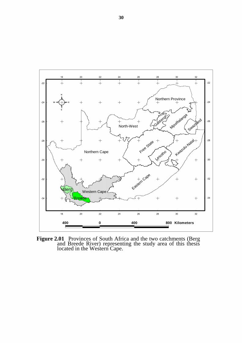
Figure 2.02 The study area with location of the experimental sites indicated by
squares. .............................................................................................................. 31
Figure 2.03 The morphology of the central part of the WC. ................................... 33
Figure 2.04 A Map of the Berg River catchment to show the geology and in
particular the shale formations of the region........................................................ 35
Figure 2.05 Map of the BRC showing the location of weather stations. ................. 38
Figure 2.06 Land type map of the study area providing a distribution of soils in the
WC based on the FAO (1998) classification (for codes see explanation in Table
2.05). .............................................................................................................. 46
Figure 2.07 Relationship between clay percentage, soil water content and volume
percent stone. ....................................................................................................... 48
Figure 2.08 Land use within the BRC and UBRC .................................................. 52
Figure 2.09 The EC in mS m-1 since 1983 of the Berg River water measured below
Wellington and Piketberg (see Figure 2.05 for the measuring positions). ........... 53
Figure 3.01 Schematic diagram of the experimental vineyard at Robertson showing
24 plots arranged according to a randomised block design consisting of four
blocks (replicates) and six treatments (the triangles indicate the centre of each
plot where the soil water content and soil solution was monitored). Treatments
are indicated as follows: 1 = 30, 2 = 75, 3 = 150, 4 = 250, 5= 350, .......................
6 = 500 mS m-1
. .................................................................................... 62
Figure 3.02 ECe – SAR relationship at Robertson based on all end of season
weighted mean ECe and SAR data over all treatments. ....................................... 70
Figure 3.03 Published grape yield – ECe relationships by Ayers & Westcot and
Moolman et al. (1999). ........................................................................................ 74
Figure 3.04 Yield – ECe (depth weighted mean ECe) relationships at Robertson
from 1992 to 1998 based on relative yield (relative to the fresh water treatment,
treatment 1). ......................................................................................................... 75
Figure 3.05 Yield and depth weighted mean SAR relationships at Robertson from
1992 to 1998 based on relative yield (relative to the fresh water treatment,
treatment 1). ......................................................................................................... 76
Figure 3.06 Relationship between the sodium content of must and wine of
Colombar grapes irrigated with saline water (Nawine = 0.976 Namust+2.961; .....
R2 = 0.988, n = 47). ............................................................................. 77
Figure 4.01 SCL with sample bottle that acts as a water trap. ................................ 82
Figure 4.02 The installation equipment for the SCL’s, including the Veihmeyer
type auger, hammer and hammer guide. .............................................................. 84
Figure 4.03 The positioning of 5 suction cup lysimeters (5 depth increments)
between two vines with a cartridge of empty bottles on the left. ......................... 85
Figure 5.01 Monthly means and standard deviations (vertical bars), calculated for
an eight year period, of soil water salinity developed in response to six irrigation
salinity treatments (mS m-1
). ................................................................................ 98
15
Figure 5.02 Trend surfaces represented by contours of soil water salinity (ECsw) in
relation to time in early summer and depth of soil in plots treated with six levels
of irrigated salinity over eight years. Graph columns from left to right are based
on the 1st , 2
nd and 3
rd order polynomials as applied to the time to depth ECsw
relationships. ...................................................................................................... 102
Figure 5.03 Migration of the regression lines for EC as a function of depth resulting
from irrigation treatment 5 (350 mS m-1
), revealing the dynamics of ECsw over
time. Numbers 1 to 12 represent months from October to September of the
following year. ................................................................................................... 106
Figure 5.04 A migration of the regression lines for EC as a function of depth
resulting from irrigation treatment 5 (350 mS m-1
), revealing the dynamics of
slopes (m) in ECsw trend lines over time (x = 1, offset = 0). Numbers 1 to 12
represent months from October to September of the following year. ................ 106
Figure 6.01 A vineyard row on the Robertson farm, indicating the vehicle tracks
and biomass on the soil surface. Salinity damage on the leaves is also visible. 109
Figure 6.02 Kriged soil ECe results taken perpendicular to vine rows to a depth of
1.2 m in the fresh water (~30 mS m-1
) treatment at the end of the irrigation
season. Sampling positions are indicated by all the X-axis tic marks. .............. 111
Figure 6.03 Kriged soil ECe results taken across vine rows to a depth of 1.2 m in
the 250 mS m-1
treatment at the end of the irrigation season. Sampling positions
are indicated by all the X-axis tic marks. ........................................................... 111
Figure 6.04 Kriged soil ECe results taken across vine rows to a depth of 1.2 m in
the 500 mS m-1
treatment at the end of the irrigation season. Sampling positions
are indicated by all the X-axis tic marks. ........................................................... 112
Figure 7.01 Area map and location map of the farm Broodkraal showing the
sampling site (approximate scales 1:1000000 and 1:5000 respectively). .......... 119
Figure 7.02 Soils map showing the prominent soil types according to the South
African classification system (Cf is Clovelly, Gs is Glenrosa, Oa is Oakleaf, Sw
is Swartland, Vf is Villafontes; Soil classification workgroup, 1991). .............. 120
Figure 7.03 Post map showing the sampling positions with indication of the ECe for
the 15-45 cm depth interval and year of planting............................................... 126
Figure 7.04 Histograms of ECe for the 15-45 cm depth interval with descriptive
statistics. ............................................................................................................ 126
Figure 7.05 Histograms of ECe for the 15-45 cm depth interval of the 4 year groups.
............................................................................................................ 127
Figure 7.06 The change in the standard deviation (a) and average (b) of ECe over
irrigation age of the vineyards.(Year refers to the time irrigation started and
sampling was done in the year 2000). ................................................................ 129
Figure 7.07 Lognormal cumulative distribution of ECe grouped per year of planting
(1996 to 1999). ................................................................................................... 131
Figure 7.08 Map of the sampling positions and the relative ECe values, with the
1996a and 1997a sampling positions. ................................................................ 131
Figure 7.09 The compared lognormal cumulative distribution functions of ECe for
the 4 consecutive years after irrigation started with 96a and 97a being the test
data. ............................................................................................................ 132
Figure 7.10 Compared measured ECe and predicted ECe developed for the 1996
data, i.e. for the oldest block, showing the ECe reconstruction through inverse
cumulative distribution functions. ..................................................................... 133
16
Figure 7.11 The change in predicted semi-variance for the 4 year groups 1996 to
1999 (original data). ........................................................................................... 133
Figure 7.12 Semi-variograms for the 1996 ECe data and its predicted data for 1997
(4 year old), 1998 (3 year old) and 1999 (2 year old). ....................................... 134
Figure 7.13 The combined ordinary point kriged maps of the original and predicted
data from the 1996 (age 5) segment. Age indicate years of irrigation. .............. 136
Figure 8.01 Histogram of ECe of the weighted average (0 to 40 cm soil depth). . 143
Figure 8.02 A location map of the depth-weighted averaged ECe values (0 to
40 cm soil depth). ............................................................................................... 143
Figure 8.03 (a) The experimental semivariogram and spherical variogram model of
the primary variable ECe (b) The experimental semivariogram and the spherical
variogram model of the second variable, electrical resistance. (c) The cross-
semivariogram and spherical variogram model of the primary variable ECe and
the secondary variable electrical resistance. ...................................................... 145
Figure 8.04 (a) Map of ECe after application of Ordinary Kriging . (b) Map of the
variable ECe resulting from Co-Kriging. ........................................................... 146
Figure 8.05 Histogram of depth-weighted average pH data (0 to 40 cm soil depth). .
............................................................................................................ 147
Figure 8.06 Location map of depth-weighted average pH (0 to 40 cm). ............... 148
Figure 8.07 An experimental semivariogram and variogram model of the variable
pH for soil depth 0 to 40 cm. ............................................................................. 148
Figure 8.08 Map of pH at Broodkraal generated using ordinary kriging. ............. 149
Figure 8.09 An experimental semivariogram of the residual trunk circumference
(TC) fitted to a spherical variogram-model. ...................................................... 150
Figure 8.10 A map of trunk circumference data on the Broodkraal farm, derived
from kriging with an overlay with the field boundaries and an indication of the
planting year of each vineyard. .......................................................................... 150
Figure 8.11 The positive correlation between [TC-averageTC] and a) the clay
percentage en b) the pH...................................................................................... 152
Figure 8.12 The negative correlation between [TC-averageTC] and the ECe. ...... 153
Figure 8.13 Prediction of TC of the vines after 4 years with the different
management blocks projected over the TC prediction. ...................................... 154
Figure 9.01 Operational principle of the EM38 (Lesch et al., 2005). ................... 162
Figure 9.02 Depth response curves for the two orientations of the EM8 (McNeill,
1980). ............................................................................................................ 163
Figure 9.03 EM38 measurement positions (crosses). The dots represent the soil
sampling positions. ............................................................................................ 164
Figure 9.04 Kriged maps of the (a) Slope angle, (b) elevation contours and (c) soil
depth (surface to hard rock). .............................................................................. 169
Figure 9.05 Semi-variogram of the EM38 measurements, (a) ECa-H, (b) ECa-V and
(c) the PR. The equations refer to a spherical model (Sph.) with the coefficients:
nugget, sill and range respectively and h = lag distance. ................................... 170
Figure 9.06 Kriged maps of the EM38, (a) ECa-H, (b) ECa-V measurements and (c)
PR. ............................................................................................................ 171
Figure 9.07 (a) Semi-variogram of depth weighted average ECe measurements
from soil samples, (b) the resultant Kriged map of ECe (mS m-1
). ................... 173
17
Figure 9.08 A comparison between (a) soil mapping (Soil Classification
Workgroup, 1991) and (b) the classified EM38 results of the Glenrosa study area.
............................................................................................................ 174
Figure 9.09 Regression between elevation and PR data obtained with the EM38
measurements. .................................................................................................... 175
Figure 9.10 The central values (Squares) for each soil group, based on Table 10.03.
............................................................................................................ 176
Figure 9.11 A soil map of the Glenrosa farm, based on the median PR values per
soil form. ............................................................................................................ 178
18
LIST OF TABLES
Table 1.01 Summary statistics of the total salt content in the Berg River, expressed
in terms of the 50 and 99 percentiles for the specific EC and total dissolved solid
content at various positions along the Berg River (Moolman and Lambrechts,
1996). .............................................................................................................. 25
Table 1.02 The experimental structure of the study ............................................... 28
Table 2.01 The geology of the BRC and UBRC with lithological classification and
stratigraphical units and related era...................................................................... 35
Table 2.02 Average monthly rainfall for selected stations in the Berg River
catchment (mm per day) and the mean annual precipitation (MAP in mm per
year). .............................................................................................................. 39
Table 2.03 Daily average temperature, per month in °C. ....................................... 39
Table 2.04 The average daily rainfall (per month) minus the average daily Epan (per
month) of selected weather stations of the Berg River catchment given in mm per
day and the yearly total in mm per year. .............................................................. 39
Table 2.05 A comparison between the FAO (1998) soil classification and the SA
soil classification for the WC, indicating also diagnostic characteristics. ........... 47
Table 2.06 Practical irrigation water guidelines for the irrigation of table and wine
grapes in SA based practical experience and on Ayers & Westcott, 1989. ......... 54
Table 2.07 A typical soil analysis of a Glenrosa soil of the Broodkraal farm in the
lower BRC (see Chapters 11 and 12). .................................................................. 56
Table 3.01 Soil water content from September 1995 to April 1996 for the
corresponding different treatments at Robertson, calculated as the weighted depth
mean . .............................................................................................................. 65
Table 3.02 Irrigation, rainfall and water balance data of the growing season
(September to April), summarised per season for the main Robertson experiment
(evaporation based on class A-pan or Penman-Monteith calculation where
indicated). ............................................................................................................. 66
Table 3.03 Treatment mean and standard deviation of the leaching fractions
according to the electrical conductivity of the irrigation water and the soil
solution at the 0.9 to 1.2 m depth layer (Treatment in mS m-1
). .......................... 67
Table 3.04 The descriptive statistics of the end of irrigation season soil ECe values
taken between 1992 and 1998 (n = 24 per treatment and soil depth). ................. 68
Table 3.05 The descriptive statistics of the start of irrigation season soil ECe
values taken between 1992 and 1998 (n = 24 per treatment and soil depth). ...... 69
Table 3.06 Mean grape yield in kg per vine per treatment of the saline irrigated
study at Robertson (Colombar grapes) for the 1992 to 1998 yield years, in
relation to ECe and ECi. ....................................................................................... 72
Table 3.07 Salinity effect on the treatment mean (the mean based in 4 replications)
expressed by the mineral composition of the must of Colombar grapes at harvest.
.............................................................................................................. 78
Table 5.01 : ANOVA table for a linear surface trend (n = number of observations)
(Davis, 1986). ....................................................................................................... 96
19
Table 5.02 ANOVA table for the significance of increase in order from p to p+1
where the trend surface of order p has k regression coefficients (without b0) and
surface of order p+1 have m regression coefficients (without b0). The number of
observations is n (Davis, 1986). ........................................................................... 96
Table 5.03 Summer month (October to March) statistics for ECsw (mS m-1
) as a
function of irrigation salinity treatments (n = 192 observations per treatment)... 99
Table 5.04 ANOVA table for a linear surface trend. ............................................. 99
Table 5.05 ANOVA table for the significance of an increase in order p to p+1
where the trend surface with order p has k regression coefficients (without b0)
and the trend surface with order p+1 has m regression coefficients (without b0).
The number of observations is n. ....................................................................... 100
Table 5.06 ANOVA table for the significance of an increase in order from p+1 to
p+2 where the trend surface with order p+1 has k regression coefficients (without
b0) and the trend surface with order p+2 has m regression coefficients (without
b0). The number of observations is n. ................................................................ 100
Table 5.07 R2 and the adjusted R
2* for the three trend orders. ............................. 103
Table 5.08 A regression between the gradient values of the 1st order polynomials
derived from ECsw at selected depth increments and from slope values derived
from ECsw at all 5 depth increments for situations 1 to 3. ................................. 104
Table 5.09 A regression analysis between predicted ECsw values for the 120 cm
depth (based on the 15-30 and 30-60 cm increments) and the measured 120 cm
depth ECsw values. ............................................................................................. 105
Table 7.01 Summary statistics of ECe (mS m-1
) for the whole data set in terms of
the two depth increments sampled. .................................................................... 128
Table 7.02 Statistics calculated on the difference between yearly modelled ECe to
derive the yearly average and median amount of salt lost from the 15-45cm depth
soil horizon of the Broodkraal farm. .................................................................. 135
Table 8.01 A multiple regression analysis done with a STEPWISE-method.
Exclusion of variables in a multiple regression equation. ................................. 151
Table 8.02 The multiple regression analysis done with stepwise outlier-rejection
method with TC the dependant variable. ........................................................... 153
Table 9.01 Descriptive statistics for the variables clay (%), pH, ECe stone content,
ER, Ca2+
, Mg2+
, Na+, K
+, ECa-V, ECa-H and PR from the Glenrosa farm. ...... 166
Table 9.02 Pearson correlation coefficient between ECa measurements, PR and
various analytical results derived from soil samples (values > |0.6| are given in
bold). ............................................................................................................ 167
Table 9.03 The soil class, form and PR values for Glenrosa farm. ...................... 176
20
1 GENERAL INTRODUCTION
The prime objective of sustainable agriculture, be it commercial or small
scale farming, should always be that the soil and water resources are
preserved and maintained for future generations. In order to meet this
objective, a sound knowledge of these two resources, as well as good
managerial skills, is required. Unfortunately, soil and water are the two
most misunderstood of all natural resources. This is well conveyed by
Hillel (1991): "All terrestrial life ultimately depends on soil and water.
So commonplace and seemingly abundant are these elements that we
tend to treat them contemptuously. The very manner in which we use
such terms as 'dirty', 'soiled', 'muddled', and 'watered down' betrays our
disdain. But in denigrating and degrading these precious resources, we
do ourselves and our descendants great - and perhaps irreparable-
harm, as shown by disastrous failures of past civilisations".
Mapping of soil salinity depicts the salinity state at a specific instant in
time. On the other hand, repeated mapping of soil, salinity will generate
information about its dynamics and provides a perspective to manage it.
This space–time modelling requires a consideration of area, depth,
salinity status and time intervals. The complexity of dealing with a 4-
dimensional process involves a specific sequence of steps (Heuvelink,
1998; Heuvelink & Pebesma, 1999; Heuvelink & Webster, 2001).
21
It is therefore of the utmost importance to understand soil salinity
behaviour in a one dimensional approach, i.e. soil depth, before one can
make predictions on a regional and temporal scale.
1.1 Background and problem description
During 1999 South Africa implemented a new water law that placed new
demands on all water users. The basic right of access to water was
constitutionalised. This brought about a reorganisation of water
management as a result of the larger number of rightful users. It also
created a need for research geared towards developing catchment
management strategies, providing researchers with an opportunity to
reorganise and reuse old data to serve this new goal. The incentive was
thus created to move from site-specific measurements to more regional
and GIS-based investigations that would provide a better basis for
decision making.
There is a need to extrapolate point information, gained from
measurements in detailed studies, to whole catchments. This study was
therefore aimed at expanding existing knowledge, using geostatistics and
GIS-applications, in order to establish the basis of a catchment
management system.
The effect of soil management is ultimately tested by the response of
crops cultivated on that soil. This is especially the case in agriculture
where saline irrigation water is used. Such information can be obtained
from remotely sensed images that involve the detection of various
canopy parameters, in addition to the more direct method of mapping
crop yield.
22
Since 1987, researchers of the Department of Soil Science at the
University of Stellenbosch have been assessing the salt tolerance of
grapevines in the Berg River Catchment (BRC), upper Breede River
Catchment (UBRC) and Stellenbosch regions of the Western Cape
Province (WC) (Figure 2.01). Wine grapes are the principal crop under
irrigation in the UBRC and it is on the increase in the BRC. This
expansion within the BRC, is becoming increasingly evident in its effect
on water quality. On the other hand, the Cape Town Metropolis is also
expanding rapidly. It has required supplementary water since 2006 and
since the Berg and Breede Rivers are the nearest alternative, urban water
use from these rivers has placed a large burden on local agriculture.
These two catchments are not the only amongst the most important food
producing areas in South Africa, but also the largest sources of
employment in the WC region. Concern exists that increased irrigation
water salinity may affect the sustainability of agricultural production of
this region. Even in Stellenbosch, where only supplementary irrigation is
applied, poorer water quality or the lack of water may also in future
hamper sustained grape production.
1.1.1 Water requirements in the Berg and Breede River
catchments
In the Berg River catchment, agriculture and specifically irrigation, is the
largest consumer of water. Recently, the whole water supply and
management system was brought in line with the new water laws of
South Africa (1999), the principles of which reflect fundamental
concepts contained in the constitution of South Africa.
A comparison of the estimated water requirement and the total storage
capacity of all the large dams listed by the Department of Water Affairs
23
in each of the three regions supporting the Larger Cape Town
metropolitan area (Anonymous, 1986), shows that the volume of water
stored in dams is insufficient to meet the requirements in those regions.
In 2006, the annual water requirement in the Berg River catchment
exceeded the existing storage capacity, even though this was only
expected to happen in 2008. Stringent water restrictions had to be put in
place (Shand et al., 1993; Berbel & Gomez-Limon, 2000).
A portion of the water used for irrigation will, however, always be
returned to the river system by drainage, albeit at a higher salt content
because of evapotranspiration losses and salt gains during leaching. In
the BRC, for example, Moolman and de Clercq (1992) illustrated that
drainage losses equivalent to as much as 40 % of the applied water can
occur under certain circumstances. However, very little quantitative data
are available regarding irrigation return flow in the different river
systems of the WC. If a river system is used both to convey water to
irrigated fields and to drain the landscape, some of the return flow will
inevitably be used by downstream irrigators, thereby increasing the
overall efficiency of water use (Cass, 1986; Moolman and Lambrechts,
1996).
More recently, Görgens and de Clercq (2001) indicated that for the BRC,
return flow and the quality thereof should be considered separately from
the dryland salinity problem.
1.1.2 Impact of irrigated agriculture on soil and surface water
quality
Irrigated agriculture has a large impact on the soil and surrounding
surface water conditions. Moolman and Lambrechts (1996) indicated that
a soil in its original state is in equilibrium with its environment. For
24
example, the chemical composition of a natural soil is a direct result of
soil forming factors such as climate, (particularly rainfall and
temperature), natural vegetation and parent material. With the
introduction of irrigation, especially in semi-arid and arid regions, this
equilibrium is disturbed and the weathering of soil minerals is
accelerated. This in turn releases soluble salt into the soil solution, which
leaches past the root zone and eventually finds its way to a river. As a
direct consequence, rivers flowing through regions with irrigation
schemes invariably experience an increase in salt concentration. The
degree of mineralisation in rivers is therefore a function of the underlying
geology, the amount and rate of irrigation return flow and the degree to
which dryland salinity has developed. Irrigation return flow is to a very
large extent determined by irrigation management and efficiency
(Moolman and Lambrechts, 1996).
In the WC, the main concern for the sustainability of the rivers and
environment is the increase in the salt content. Two examples serve to
justify this concern.
Firstly, in Table 1.01, some statistics on the progressive increase in the
salt content of the Berg River from Franschhoek downstream to
Misverstand are listed. These values are the summary statistics of
chemical data collected between 1985 and 1990 at various positions
along the Berg River. It shows the increasing trend in EC and total
dissolved solids (TDS) downstream as the water finds its way toward the
river mouth. Expansion of irrigated agriculture in the middle and lower
reaches of the Berg River, as well as the UBRC, is bound to mobilise
salts. Without the necessary precautions, such as artificial drainage and
proper on-farm irrigation management, the salt content of the Berg River
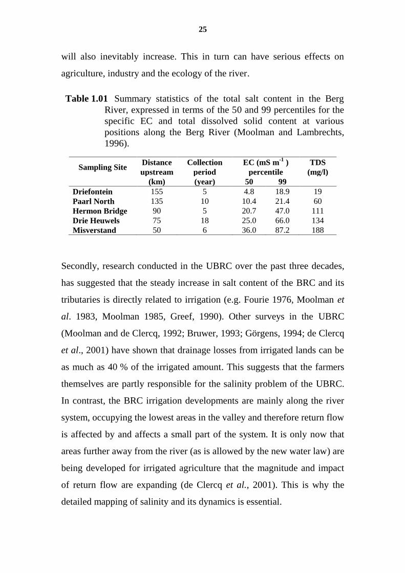
25
will also inevitably increase. This in turn can have serious effects on
agriculture, industry and the ecology of the river.
Table 1.01 Summary statistics of the total salt content in the Berg
River, expressed in terms of the 50 and 99 percentiles for the
specific EC and total dissolved solid content at various
positions along the Berg River (Moolman and Lambrechts,
1996).
Sampling Site Distance
upstream
Collection
period
EC (mS m-1
)
percentile
TDS
(mg/l)
(km) (year) 50 99
Driefontein
Paarl North
Hermon Bridge
Drie Heuwels
Misverstand
155
135
90
75
50
5
10
5
18
6
4.8
10.4
20.7
25.0
36.0
18.9
21.4
47.0
66.0
87.2
19
60
111
134
188
Secondly, research conducted in the UBRC over the past three decades,
has suggested that the steady increase in salt content of the BRC and its
tributaries is directly related to irrigation (e.g. Fourie 1976, Moolman et
al. 1983, Moolman 1985, Greef, 1990). Other surveys in the UBRC
(Moolman and de Clercq, 1992; Bruwer, 1993; Görgens, 1994; de Clercq
et al., 2001) have shown that drainage losses from irrigated lands can be
as much as 40 % of the irrigated amount. This suggests that the farmers
themselves are partly responsible for the salinity problem of the UBRC.
In contrast, the BRC irrigation developments are mainly along the river
system, occupying the lowest areas in the valley and therefore return flow
is affected by and affects a small part of the system. It is only now that
areas further away from the river (as is allowed by the new water law) are
being developed for irrigated agriculture that the magnitude and impact
of return flow are expanding (de Clercq et al., 2001). This is why the
detailed mapping of salinity and its dynamics is essential.
26
1.2 The general and specific aims of this study
The general aim of this thesis is to provide methodology through which
the time-space dynamics of soil salinity, within the framework of saline
irrigated viticulture, can be assessed more rapidly and accurately on a
regional scale.
The specific aims of the study were therefore as follows:
To investigate the sensitivity of grapevines (vitis vinifera, L), to
the quality of irrigation water it receives.
To establish soil water sampling (as opposed to laboratory
estimation using a saturated paste) as a preferred basis for
measuring the effect of saline irrigation on plants.
To analyze from the repetitive sampling of soil water, ways of
predicting soil salinity profiles over time, using polynomials of
the lowest possible order and to indicate the minimum amount of
information required to make such predictions.
To optimize soil sampling positions in view of the fact that partial
wetting of soil during irrigation is the norm within the study area.
To explore the positive management aspects of partial wetting in
terms of salt storage during the irrigation season.
To assess and model long-term irrigation and the change in soil
salinity on a regional scale and link this to regional sustainability
of table grape production.
To quantify the relationships between soil classification, soil
electromagnetic induction measurements and topography as an
improved basis for mapping soil salinity on a catchment scale.
1.3 General structure of the thesis
The thesis first reviews (Chapter 2) the state of knowledge on the salinity
problem in the Western Cape region that existed at the commencement of
the study. The study area is described with regard to features such as
27
geology, geomorphology, climate, available water resources, the soils
and their chemistry and land use.
In Chapter 3, an overview is presented of the saline irrigation
experiments that formed the basis for the research. Here the sensitivity of
vines to water quality was investigated. Because of the impact of water
quality on grape production, these studies prompted the investigations
that followed, aimed at discovering the level of water management
needed both on a farm scale and a regional scale.
An automated system for retrieving soil water samples was developed
and its operation and construction are presented in Chapter 4. This made
possible the measurement of depth trends in soil salinity in a vineyard
after prolonged irrigation with saline water.
An account is given in Chapter 5 of how the automated retrieval system
allowed data to be collected as the basis for predicting soil salinity
profiles over time, using first order polynomials, and then linking such
capability to remote sensing applications.
The seasonal change in soil salinity with depth, measured at a number of
points in the landscape is dealt with in Chapter 6. Chapter 7 explores the
profile distribution of salts between vine rows. The fact that most
irrigation systems are based on partial wetting of the soil surface raised
important considerations for regional salinity assessment.
In Chapter 8, the effect of long-term irrigation on the variation of soil
salinity in vineyards is considered on a regional scale, with particular
emphasis on predicting the response of vineyards to such variation. The
regional sustainability, of table grape production on saline soils, is
investigated in Chapter 9. These two chapters deal with the space-time
response of soils and vines to salinity of irrigation water in the region.
28
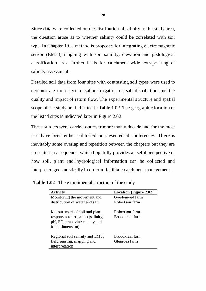
Since data were collected on the distribution of salinity in the study area,
the question arose as to whether salinity could be correlated with soil
type. In Chapter 10, a method is proposed for integrating electromagnetic
sensor (EM38) mapping with soil salinity, elevation and pedological
classification as a further basis for catchment wide extrapolating of
salinity assessment.
Detailed soil data from four sites with contrasting soil types were used to
demonstrate the effect of saline irrigation on salt distribution and the
quality and impact of return flow. The experimental structure and spatial
scope of the study are indicated in Table 1.02. The geographic location of
the listed sites is indicated later in Figure 2.02.
These studies were carried out over more than a decade and for the most
part have been either published or presented at conferences. There is
inevitably some overlap and repetition between the chapters but they are
presented in a sequence, which hopefully provides a useful perspective of
how soil, plant and hydrological information can be collected and
interpreted geostatistically in order to facilitate catchment management.
Table 1.02 The experimental structure of the study
Activity Location (Figure 2.02)
Monitoring the movement and
distribution of water and salt
Goedemoed farm
Robertson farm
Measurement of soil and plant
responses to irrigation (salinity,
pH, EC, grapevine canopy and
trunk dimension)
Robertson farm
Broodkraal farm
Regional soil salinity and EM38
field sensing, mapping and
interpretation
Broodkraal farm
Glenrosa farm
29
2 THE STUDY AREA AND ITS SOIL SALINITY
PROBLEM
2.1 The geographical location
The study area is located in the Western Cape Province (WP) of South
Africa, more specifically the Berg River Catchment (BRC) and the upper
Breede River Catchment (UBRC). These two catchments have as central
coordinates, S32.5° E18.5° and S33.5° E19.5°, respectively. The study
area also forms part of the greater Winter Rainfall region (Figures 2.01
and 2.02).
It is important to realize the very diverse and contrasting occurrence of
natural phenomena in the study area. The origins of the rivers are within
the folded mountain ranges of the region, the Hottentots-Holland and the
Drakenstein ranges, respectively. These ranges have the second highest
recorded rainfall in South Africa, exceeding 2000 mm per annum. From
here, both rivers flow through regions that are predominantly winter
rainfall, to a region with very low rainfall. So, both rivers flow from
regions where only supplementary irrigation is used to a region where
full-scale irrigation activities are imperative.
30
Northern Cape
Eastern
Cape
Free S
tate
North-West
Western Cape
Kwazulu
-Nat
al
Northern Province
Mpum
alanga
Lesotho
Gaute
ng
Swaziland
Breede
Berg
400 0 400 800 Kilometers
S
N
EW
18
18
20
20
22
22
24
24
26
26
28
28
30
30
32
32
-34 -34
-32 -32
-30 -30
-28 -28
-26 -26
-24 -24
-22 -22
Figure 2.01 Provinces of South Africa and the two catchments (Berg and Breede River) representing the study area of this thesis located in the Western Cape.
31
#
#
#
#
#
##
#
#
#
#
#
#
#
% %
%
%
CERES
CITRUSDAL
PIKETBERG
SALDANHA
MALMESBURY
PAARL
WORCESTER
STRAND
STELLENBOSCHCAPE TOWN
ROBERTSON
AGULHAS
HERMANUS
Expeimental Farm Goedemoed
Broodkraal
Glenrosa
70 0 70 140 Kilometers
S
N
EW
18
18
19
19
20
20
-34 -34
-33 -33
Figure 2.02 The study area with location of the experimental sites indicated by squares.
2.2 A physical perspective of the study area
2.2.1 Geomorphology and geology
The study area can be sub-divided into two broad physiographic regions,
each with its own distinct terrain morphology (Wellington, 1955). These
are broadly termed the Cape Fold Belt, consisting of mountains with a
north west to south east orientation, and the Coastal Foreland,
representing the extensive coastal plains cut by rivers that emerge from
32
the mountain ranges. The Cape Fold Belt is characterised by pronounced
folded mountain ranges consisting of resistant quartzitic rocks
(Trusswell, 1987; Kent, 1980). Generally, slopes are steep to very steep,
with exposed rock or with a thin soil cover. Except for some
afforestation, these mountain ranges are of negligible use for agricultural
activities.
The folded mountain ranges gave preference to the formation of rivers in
a north-westerly/south-easterly direction. This resulted from the impact
of the Gondwana break-up that was preceded by an apparent collision
(resulting in a zone of convergence) in a north-easterly direction
(Trusswell, 1987).
Prominent features of the folded mountain zone therefore are the
numerous downfold and fault valleys (e.g. Jonkershoek and Franschhoek
valleys). These valleys are usually underlain by easily weatherable rocks
with high clay forming potential. Most of the valley to the north opens up
through Karoo sediments (Karoo is the area bordering the Cape Folded
Belt to the north), which are predominantly saline with a high clay/silt
forming potential. In these cases locally derived sandy colluvial (gravity
transported) and fluvial (water transported) sediments from the mountain
slopes cover the clay forming rocks of the valley bottom.
In the lower BRC, the western Coastal Foreland is broken by a number of
igneous rock bodies (granite rocks), which also formed the high Paarl-
and Paardeberg or the lower Darling and Vredenburg hills. These
igneous intrusions are associated with moderate to fairly deep, red to
brown, clay loam to clay soils, with moderately steep to steep slopes
(usually 8 %).
33
In the UBRC the river runs through the Worcester-Robertson region to
the South Coastal Foreland, but this study will mainly focus on the
Worcester-Robertson region, which is cast in similar Table Mountain
sandstone mountain ranges as the BRC. This upper section of the valley
is mostly quite narrow (10 to 20 km) and the soil mainly developed from
Karoo sediments.
The morphological regions of the BRC and UBRC are given in Figure
2.03.
#
#
#
#
#
#
#
#
#
#
#
#
#
#
CERES
CITRUSDAL
PIKETBERGSALDANHA
MALMESBURY
PAARLWORCESTER
STRAND
STELLENBOSCH
SIMONS TOWN
CAPE TOWN
ROBERTSON
AGULHAS
HERMANUS
18
18
19
19
20
20
-34 -34
-33 -33
Morphology
High mountains
HillsLow mountains
Lowlands and parallel hills
Moderately undulating plainsPlains
Plains and pans
Slightly undulating plainsUndulating hills
UBRC
BRC
# Towns
20 0 20 40 Kilometers
S
N
EW
Figure 2.03 The morphology of the central part of the WC.
Both the BRC and UBRC have a terracing nature between the river and
the mountains. The terraces are usually quite old in the higher regions
and are generally considered part of the old African surface. The land
surfaces within the study area are in most cases very old and in balance
with the prevailing conditions. The old African land surfaces and the
34
African geology are considered the most stable and the oldest in the
world. Even the natural vegetation types that occur are genetically very
well adapted to their environment.
The Cape fold mountain ranges are dated 300 million year and similar in
age to the Gondwana episode and dates from the Carboniferous period
(Trusswell, 1987). Their positon can be seen in Figure 2.04, indicated as
Arenites and Luctaceous Arenites.
Most of the study area is underlain by granite (Figure 2.04) to a depth
varying between 0 and 120 m below the land surface. This deep contact,
with the more recent granite body, varies between a granite/phyllite,
granite/schist contact and a granite/sandstone contact (Trusswell, 1987;
Kent, 1980).
The Berg River itself flows from its origin in the Cape Super Group to
the older Klipheuwel Formation and Malmesbury shale Formation and
the Cape Granites (Table 2.01 and Figure 2.04). The river runs for the
last 50 km toward the coast, through a sand and limestone belt that lines
the west coast of the Cape. In terms of salinity, from Franschhoek to
Paarl the river runs through more recent sedimentary material that
originated from the Table Mountain Sandstones, which does not
contribute to the salt content of the water. From approximately
Wellington, the river runs through a region with more salts that
originated from the parent Malmesbury shale material itself (Trusswell,
1987; Kent, 1980). The latter statement is however not entirely true as de
Clercq et al. (in press) indicated the secondary origin of these salts.
Similarly, the UBRC has a stratigraphical sequence with the youngest
being the Table Mountain Sandstones, underlain by mostly Karoo
35
sediments in particular the Bokkeveld shale Formation and below that in
places, the Cape granites (Figure 2.04).
#
#
#
#
#
#
#
#
#
#
#
#
CERES
PIKETBERG
SALDANHA
MALMESBURY
PAARL
WORCESTER
STRAND
STELLENBOSCH
SIMONS TOWN
CAPE TOWN
ROBERTSON
HERMANUS
Lithology
ARENITE
CONGLOMERATE
GRANITEGREENSTONE
LIMESTONE
LUTACEOUS ARENITE
MUDSTONE
PHYLLITE
SCHISTSEDIMENTARY
SHALE
TILLITE
UBRC
BRC
# Towns
18
18
19
19
20
20
-34 -34
-33 -33
20 0 20 40 Kilometers
Figure 2.04 A Map of the Berg River catchment to show the geology and in particular the shale formations of the region.
Table 2.01 The geology of the BRC and UBRC with lithological
classification and stratigraphical units and related era.
Group and time Sub unit Lithology
Recent
Late Cenozoic
Recent Sediments Sedimentary
Recent Coastal Sediments Limestone
Karoo Super Group
Mesozoic
Mudstone
Dwaika Formation Tillite
Bokkeveld Formation Shale
Enon Formation Conglomerate
Cape Supergroup
Middle Palaeozoic
Pakhuis formation Tillite
Table Mountain Sandstone Arenites
Cape Ganite Suite
Early Palaeozoic Granite
Malmesbury Group
Namibian Malmesbury Shales
Greenstone
Luctaceous Arenites
Phyllite
Schist
36
2.2.2 Climate
Climate is to a large extent the driving force in the occurrence of salinity
in a landscape. Shalhevet (1994) reported that three elements of climate,
namely temperature, humidity and rainfall, might influence salt tolerance
and salinity response in plants, with temperature being the most crucial.
High temperatures increase the stress level to which a crop is exposed,
either because of increased transpiration rate or because of the effect of
temperature on the biochemical transformations in the leaf. High
atmospheric humidity tends to decrease the crop stress level to some
extent, thus reducing salinity damage, as has been demonstrated for
beans (Hoffman et al., 1978). Shalhevet (1994) concluded that under
environmental conditions of high temperature and low humidity, the salt
tolerance of plants might change so that the threshold salinity decreases
and the slope of the response function increases, making the crop more
sensitive to salinity. Prior et al. (1992b) in Australia found that
symptoms of leaf damage that appeared in December or January were
more related to climatic stress than to chloride or sodium levels.
In the BRC and UBRC it is possible to restrict the evaporative demand of
the atmosphere in harsh climatic conditions by using shade netting.
Under shade netting, the relative humidity rises, the leaf surface
temperature is lower and the soil surface temperature is lower. The result
is a lower transpiration rate and consequently less salt uptake. The plant
can consequently cope with much smaller osmotic potential differences.
An additional factor in causing salt-affected soils is the high potential
evapo-transpiration in these low rainfall areas, which increases the
concentration of salts in both soils and surface waters. It has been
estimated that evaporation losses can range from 50 to 90% in arid
37
regions, resulting in 2- to 20-fold increases in soluble salts (Yaalon,
1963).
The study area has a Mediterranean climate. Fey and de Clercq (2004)
indicated that, though the region is predominantly a winter rainfall
region, most precipitation takes place in the upper parts of the valleys
close to and on the mountains. Towards the coast, the rainfall is generally
lower, unpredictable and poorly distributed in time and space. Towards
the Piketberg, 30 km from the coast, a much higher rainfall is
experienced. From the coast the mean annual precipitation varies from
50 mm to more than 1000 mm in the combined apex of the Franschhoek,
Jonkershoek and Hottentots-Holland mountain ranges. More than 80 %
of this region has an annual rainfall between 200 mm and 500 mm.
Strong winds, especially during summer, are very common and lead to
severe wind erosion. Frost and snow are experienced in winter, mainly in
regions with elevation higher than 800 m. Both are uncommon in the
coastal zones.
Figure 2.05 shows the location of some weather stations in the BRC and
Tables 2.02 to 2.04 provide data from these weather stations. From these
measurements the effect of elevation and distance from the sea on the
climate is quite clear (de Clercq et al, 2008).
This gradual change between Franschhoek and Velddrif determines the
irrigation management approach from the South East to the North West,
ranging from no irrigation, to supplementary irrigation or full scale
irrigation. The amount of fresh water available, the electrical
conductivity of the irrigation water (ECi), and the electrical conductivity
of the soil water (ECsw) of the soils in general, all follows this sequence.
38
Berg River
Berg
Riv
er
Berg
Riv
er C
atc
hm
en
t
StellenboschCape Town
Atlantis
Malmesbury
Wellington
Paarl
Tulbach
Ceres
SaronMoorreesburg
Piketberg
Porterville
Hopefield
Langebaan
Saldanha
Vredenburg
Langbaanweg
VeldrifAurora
DarlingDassen Island
Robben Island
Franschhoek
Misverstand Dam
12
3
4
5
6
7
8
9 10 11
12
13
Weather Stations1. Langebaanweg2. Rooihoogte3. Eendekuil4. DeHoek/Saron5. Korinberg6. Vredenburg7. BienDonne8. HLSPaarl9. Vredehof10. LaMotte11. Franshoek12. LaPlaisante13. Heldervue
0 10 20 30 40 50 km
Scale
E18 E19S32
S33
Figure 2.05 Map of the BRC showing the location of weather stations.
Table 2.02 provides information on the distribution of the mean annual
precipitation (MAP) in the BRC. It is clear that the monthly means in
precipitation and the MAP are linked to elevation and distance from the
sea. The same cannot be said for the mean temperatures in the BRC
(Table 2.03). Table 2.04, however, where the mean pan-
evapotranspiration (Epan) values were subtracted from the MAP, shows a
precipitation deficit for the catchment on a monthly basis and a yearly
basis. It is clear that most of the farms shown in these tables, with the
exception of Heldervue, have a precipitation shortage mainly in the
39
summer months. This implies that for summer crops, water has to be
stored during winter for irrigation.
Table 2.02 Average monthly rainfall for selected stations in the Berg
River catchment (mm per day) and the mean annual
precipitation (MAP in mm per year).
Station Elevation Month MAP
masl J F M A M J J A S O N D
Langebaanweg 31 0.2 0.2 0.4 0.7 1.3 1.3 1.5 1.6 0.8 0.4 0.4 0.2 270
Rooihoogte 45 0.2 0.2 0.9 1.4 1.8 2 2.3 2 1.4 0.5 0.4 0.2 399
Eendekuil 114 0.1 0.3 0.5 1.2 0.7 1.9 1.2 1.8 0.8 0.5 0.2 0.1 279
DeHoek/Saron 115 0.3 0.5 1.4 1.7 1.8 3.2 2.9 3.9 2.3 0.7 0.7 0.3 591
Korinberg 128 0.2 0.2 0.4 0.9 1.8 2.1 1.6 1.8 0.8 0.9 0.5 0.2 342
Vredenburg 128 0.3 0.1 0.4 0.7 1.6 1.7 1.8 1.8 0.8 0.5 0.4 0.3 312
BienDonne 138 0.7 0.7 1 2.3 4.1 4.5 4.1 3.9 2.3 1.6 1 0.7 807
HLSPaarl 149 0.4 0.4 0.7 1.1 2.3 2.5 2.6 2.5 1.6 0.8 0.6 0.4 477
Vredehof 154 0.7 0.4 1.8 1.8 3 3.1 3.6 3.4 3 0.9 0.8 0.7 696
LaMotte 206 1.3 0.9 1.5 1.9 4.1 4.3 3.9 3.6 3 1.4 0.9 1.3 843
Franshoek 244 0.5 0.7 0.9 2.3 3.9 4.7 4.7 4.3 2.2 1.9 1.1 0.5 831
LaPlaisante 260 0.4 0.6 0.8 1.5 2.7 3.2 2.7 3 1.7 1.2 0.8 0.4 570
Heldervue 755 0.7 0.7 1.1 2.2 3.9 4.6 4.3 4.3 2.4 1.7 1.2 0.7 834
Table 2.03 Daily average temperature, per month in °C.
Station Elevation Month Yearly masl J F M A M J J A S O N D Average
Langebaanweg 31 21.9 22.6 20 20 15 13 12 13 15 15 19.1 20.2 17.2 Rooihoogte 45 23.8 24.5 22 19 16 13 11 13 15 18 21.4 22.5 18.3 Eendekuil 114 25.8 25.7 23 20 17 13 12 14 15 17 22.2 23.9 19.1 DeHoek/Saron 115 23.8 24.9 23 20 17 14 13 14 16 18 21 23 19.0 Korinberg 128 24.6 25.6 24 22 17 15 13 13 16 18 21 23.3 19.3 Vredenburg 128 20.2 20.6 20 19 16 14 13 14 15 16 18.1 19.4 17.1 BienDonne 138 22.3 22.6 21 18 15 12 12 12 14 17 19.4 20.9 17.1 HLSPaarl 149 22.7 23.7 22 19 16 13 12 13 14 17 20 21.6 17.9 Vredehof 154 22.7 23.5 21 19 16 13 12 14 15 17 20.8 21.5 18.0 LaMotte 206 22.1 22.8 21 19 16 13 12 13 15 17 19.5 21.2 17.6 Franshoek 244 22.2 23.5 22 19 15 13 12 12 13 17 20.2 20.7 17.4 LaPlaisante 260 22.9 23.1 22 18 15 13 12 12 14 17 19.9 21.6 17.5 Heldervue 755 19.1 19.3 18 15 13 11 11 11 12 14 16.7 18.3 14.7
Table 2.04 The average daily rainfall (per month) minus the average
daily Epan (per month) of selected weather stations of the Berg
River catchment given in mm per day and the yearly total in
mm per year.
Station Elevation Month Yearly
masl J F M A M J J A S O N D Total
Langebaanweg 31 -11 -9.6 -6.9 -4.6 -1.2 -0.3 0.1 -0.5 -4.2 -8.2 -10 -11 -1992
Rooihoogte 45 -9.8 -9.7 -5 -2 1 2.3 3.1 1.9 -0.6 -5.6 -8.2 -9.8 -1272
Eendekuil 114 -13 -12 -7.4 -3.5 -2.3 1.8 0.7 1.1 -2.5 -6.4 -11 -13 -2016
DeHoek/Saron 115 -9.5 -8.8 -4.2 -1.9 0.5 4.3 3.7 5.1 0.3 -5.2 -7.8 -9.5 -990
Korinberg 128 -11 -11 -8.8 -4.8 0.2 2 1 0.8 -2.7 -5 -8.7 -11 -1785
Vredenburg 128 -10 -9.8 -7 -4 -0.1 0.8 1.1 0.5 -3 -6.2 -8.4 -10 -1707
BienDonne 138 -8.3 -7.7 -5.1 0.1 5.7 7.4 6.3 5 0.6 -3.1 -6.6 -8.3 -420
HLSPaarl 149 -9.3 -8.9 -6 -2.6 1.7 3.1 3.2 2.3 -0.7 -4.8 -7.5 -9.3 -1164
Vredehof 154 -8.2 -8.5 -3.1 -0.7 3.1 4.4 5.2 4.1 1.9 -5.1 -8 -8.2 -693
LaMotte 206 -5.5 -6 -2.9 -0.1 5.5 6.8 5.8 4.3 2.4 -2.2 -4.9 -5.5 -69
Franshoek 244 -7.1 -6.5 -4 0.7 5.1 7.6 7.3 5.8 0.8 -1.2 -4.5 -7.1 -93
LaPlaisante 260 -9.1 -8 -5.5 -1.6 2.5 4.2 3.1 3.2 -0.6 -3.7 -7 -9.1 -948
Heldervue 755 -6.1 -5.5 -2.9 0.8 5.2 7.1 6.4 6.1 1.7 -1.4 -4.1 -6.1 36
40
2.2.3 Water Resources
2.2.3.1 Hydrology of the Berg River and the upper Breede River
drainage regions
The mean annual precipitation (MAP) for the BRC is 456 mm per year,
which is considerably less than the world mean for terrestrial surfaces,
i.e. 746 mm per year (Alexander, 1985; DWAF, 1986; Baumgartner &
Reichel, 1975; Bennie and Hensley, 2001).
The MAP of this region is also less than the MAP of South Africa
(501 mm, Bennie and Hensley, 2001), but the runoff coefficient of
16.8 % is well above the national mean of 9 %. A runoff coefficient of
9 % means that 91% of the MAP evaporates directly from the soil back to
the atmosphere and never reaches a river (Anonymous, 1986; Lipton et
al., 1996). However, it is still very low when compared to the runoff
coefficient of, for example, the Netherlands (57 %, DWAF, 1986). The
low runoff coefficients are the result of high evaporation rates and not
because of low rainfall. This is part of the mechanism in this region that
keeps salt on the land and, as in most cases, close to the soil surface. This
balance, however, is disturbed once the soils of the Berg River
Catchment are irrigated with direct consequences to the quality of the
water in the river system.
Flügel (1995) did a sub-catchment study in the BRC indicating the
distribution of salt in the landscape and the most affected areas. He found
that winter rainfall contributed for 23 % of the annual salt flux. He also
indicated that the topography has a large impact on the occurrence of salt
in the landscape. On hilltops the salinity was relatively low and salinity
increased downhill toward the river. In fact the occurrence of salt in the
landscape is very similar to that described in dryland salinity literature
41
from Australia. The Renosterveld vegetation (which is part of the Fynbos
biome and the natural veld type in the lower part of the BRC), although
comprising of smallish shrubs, has a deep rooting system aand replacing
it with winter wheat has changed the water balance with salts gradually
moving higher in the profile as a result (Fey and de Clercq, 2004).
The demand for fresh water in the BRC and UBRC caused the
government of SA to provide dams to meet this demand. Consequently,
dams have been built since 1950, including the Wemmershoek-,
Misverstand-, Voëlvlei- and (the youngest) the Franschhoek dam in the
BRC. In the UBRC there are the Brandvlei and Kwaggaskloof dams
close to Worcester, which supply the needs of irrigators. All of these
dams were also adapted to supply water to the major urban areas of the
WC (DWAF, 1986).
2.2.3.2 Irrigation water quality
An important factor affecting soil salinity is the quality of irrigation
water that farmers receive. If the irrigation water contains high levels of
soluble salts, Na, B, and trace elements, serious effects on plants and
animals can be the result (Ayers and Westcot, 1985). Salinity problems
are common in irrigated lands, with approximately one-third of the
irrigated land in the United States being seriously salt-affected (Rhoades,
1993). In other countries, Postel (1989) reported it to be as high as 50 %.
Areas affected include humid climate areas such as Holland, Sweden,
Hungary, and Russia, and arid and semiarid regions such as the south-
western United States, Australia, India, and the Middle East. Each year,
about 400,000 ha of irrigated land are no longer productive because of
salinity (Yaron, 1981).
42
The presence of selenium and other toxic elements (Cr, Hg) in subsurface
drainage waters is also a problem in irrigated areas. Selenium (resulting
from shale parent material) in drainage waters has caused massive death
and deformity to fish and waterfowl in the Kesterson Reservoir of
California (Schuler, 1990).
Poor quality water supply can be detrimental or hazardous to farmers and
other water users alike. Wrong actions by farmers and other water users
can in turn be detrimental to the environment. Therefore, sustainability
can be defined in terms of the intersection between the two.
Rhoades et al. (1990) summarized the situation as follows. Irrigated
agriculture cannot be sustained without adequate leaching and drainage
to prevent excessive salinisation of the soil. Yet these processes are the
very ones that contribute to the salt loading of the rivers and
groundwater. Several approaches are available to control and minimize
this hazard. Firstly, irrigation can be eliminated. This should be
undertaken where the detrimental effects of irrigation outweigh the
benefits. Secondly, the amount of water lost in seepage and deep
percolation can be reduced, lessening the amount of saline water that
passes through the soil and substrata. Thirdly, point sources of drainage
return-flow into streams or rivers can be intercepted and diverted to other
outlets and uses.
These concepts are quite crucial for water managers who have to supply
water of good quality to farming communities and towns in a catchment
such as the BRC and who do not have the ability to control drainage-
return. Here, the only feasible solution appears to be to avoid irrigated
agricultural expansion on unsuitable soils. Research into the exact origin
43
of salts in the landscape and methods to contain these salts should also be
continued until the problem is satisfactorily appreciated.
As an example of interpreting hazard, Moolman et al. (1999) and de
Clercq et al. (2001) have shown, with a study done at Robertson in the
Breede River valley that certain grapevine cultivars proved to be very
sensitive to salinity. Though the grapevines showed low tolerance for
saline irrigation water, sustainability was possible with irrigation water
quality of up to 100 mS m-1
. Irrigation water quality in this case implied
high risk for the farmer, but low risk for the environment (UBRC), which
was accustomed to higher salinity levels during the summer months prior
to the institution of water quality management in the Breede River
System. One major problem in these irrigated areas (including the BRC
and UBRC) is that salts accumulate unless they are leached. Saline
irrigation water, low soil permeability, inadequate drainage, low rainfall,
and poor irrigation management all cause salts to accumulate in soils.
The salts must be leached for sustained crop production. However, it is
leaching of these salts that result in saline drainage waters and that
causes pollution of waters, a major concern in saline environments.
2.2.3.3 Irrigation return flow as a water source
Van Schilfgaarde (1974, 1990) mentions that there are ways to minimise
effects of irrigation on downstream salinity. More precise irrigation
management to limit the leaching fraction to the amount needed to
maintain full crop growth can substantially reduce the amount of salt
discharge in the drainage water. The recent developments in irrigation
technology make the implementing of this concept more feasible. Drip
irrigation has definite advantages when used in a saline soil/water
environment. The main disadvantage is the much higher skill level it
44
demands of the farmer. Irrigated land in semi-arid regions must have
drainage. There must be a net downward flux of water in the soil to
prevent the concentration of solutes in the soil solution from rising to a
level that cannot be tolerated by the crop. Therefore when natural
drainage is not sufficient, drainage systems must be installed (Van
Schilfgaarde, 1990). The question that remains is how to dispose of
drainage water.
Wolters (1992) argues that it is virtually impossible to prevent drainage
losses. A 100 % crop-related irrigation efficiency, in theory implies that
no water, and consequently no salts, are conveyed out of the area.
Wolters (1992) also argues that a very high field application efficiency
that would lead to a build-up of salinity is only acceptable when rainfall,
or another source of water, at other times of the year (e.g. winter) leaches
salts supplied with the irrigation water.
Kutilek and Nielsen (1994) expressed their concern that point sampling
over a number of years has been done in numerous experiments around
the world, but with nothing to emerge other than a comparison of soil
status with crop production. These measurements did little for improving
our understanding of how agricultural practices impact on the quality of
water leaving the cultivated field or rangeland. They provided no direct
information regarding the subtle changes in soil quality occurring on a
farm or within an agricultural region.
The aim of this study is not to give an account of all previous attempts to
model return flow but rather to propose an alternative approach of
measuring the amounts of solutes lost from a landscape through the use
of geostatistical techniques. By modelling the variation of elements in the
45
irrigated soils, the total stock can be calculated and by repeating some
measurements, changes over time can be monitored.
Görgens and de Clercq (2006) indicated that most irrigators in the Berg
river valley currently make use of micro-irrigation. The order of
occurrence in type of irrigation is: micro (49 %), drip (30 %), sprinkler
and centre-pivot (18 %) and flood (3 %). Over-irrigation resulting in
large potential drainage losses was observed. The findings of this
research showed that the performance of the irrigation system depends in
practice far more on the management of the system than on the system
itself. The efficiency of water use by an irrigation system depends on
certain losses in the system, including those due to:
the irrigation system not having an application uniformity of
100%;
management decisions;
leakages in the distribution system;
a change in EC that can lower infiltration rate and enhance
runoff;
irrigation systems that ignores soil units;
stony soils or stony patches in irrigated lands.
It can thus be argued that irrigation return flow could also be regarded as
a water source in both the BRC and UBRC.
2.2.4 Soils
The soil properties of this region vary away from the mountain ranges. In
the BRC and UBRC, one often finds soils that format variance with
expectations based on the underlying geology as a result of it being river
transported material. For the BRC, one could distinguish between soils
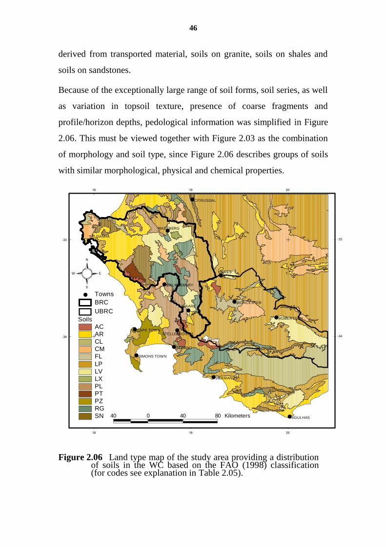
46
derived from transported material, soils on granite, soils on shales and
soils on sandstones.
Because of the exceptionally large range of soil forms, soil series, as well
as variation in topsoil texture, presence of coarse fragments and
profile/horizon depths, pedological information was simplified in Figure
2.06. This must be viewed together with Figure 2.03 as the combination
of morphology and soil type, since Figure 2.06 describes groups of soils
with similar morphological, physical and chemical properties.
#
#
#
#
#
#
#
#
#
#
#
#
#
#
CERES
CITRUSDAL
PIKETBERG
SALDANHA
MALMESBURY
PAARL
WORCESTER
STRAND
STELLENBOSCH
SIMONS TOWN
CAPE TOWN
ROBERTSON
AGULHAS
HERMANUS
CERES
CITRUSDAL
PIKETBERG
SALDANHA
MALMESBURY
PAARLWORCESTER
STRAND
STELLENBOSCH
SIMONS TOWN
CAPE TOWN
ROBERTSON
AGULHAS
HERMANUS
Soils
ACAR
CLCM
FL
LPLV
LXPL
PTPZ
RG
SN
UBRC
BRC
# Towns
S
N
EW
40 0 40 80 Kilometers
18
18
19
19
20
20
-34 -34
-33 -33
Figure 2.06 Land type map of the study area providing a distribution of soils in the WC based on the FAO (1998) classification (for codes see explanation in Table 2.05).
47
These can be considered as resource units, and all the soils in a resource
unit would require similar management practices (e.g. fertilisation,
cultivation, erosion protection methods), and the range of adapted crops
and the production potential would be similar under defined climate and
terrain conditions.
Table 2.05 A comparison between the FAO (1998) soil classification
and the SA soil classification for the WC, indicating also
diagnostic characteristics.
FAO
code
FAO
Soil
SA Soil Classes Diagnostic
horizon or material
AC Acrisols Shortlands Red structured B
AR Arenosols Clovelly/Hutton Red apedal B, yellow-brown
apedal B,
CL Calcisols Gamoep Soft or hardpan carbonate
CM Cambisols Cartref/Oakleaf/Glenrosa/Trawal/
Oudshoorn/Villafontes/Tukulu
Lithocutanic B or hard rock Plintic, Calcic, Hydromorphic
FL Fluvisols Dundee/Inhoek Regic sand, stratified alluvium
LP Leptosols Mispah/Glenrosa Inceptic, Lithocutanic B or hard
rock
LV Luvisols Swartland/Klapmuts (Duplex) Pedo- B or
prismacutanic B
LX Lixisols Mayo (Very rare)
PL Planosols Estcourt/Klapmuts (Duplex) Pedocutanic B or
prismacutanic B
PT Plinthosols Avalon/Longlands/Westleigh Soft plinthic B or hard plinthic
B
PZ Podzols Podzols/Fernwood Podzol B, E horizon
RG Regosols Namib/Mispah Regic sand, lithocutanic B or
hard rock
SN Solonetz Sterkspruit/Escourt Natric, Pedocutanic B or
prismacutanic B
The soil properties limiting land use include high clay content, swelling
clays, shallow soils, hardpans and fast weathering of most of the soils on
shale. Most of the BRC and UBRC have soils that are not deep with hard
rock at depths shallower than 50 cm. Most of these soils formed on the
Malmesbury and Bokkeveld shales. When these soils are prepared for
irrigation, they are deep ripped (to 1.2 m) and tilled and in many cases
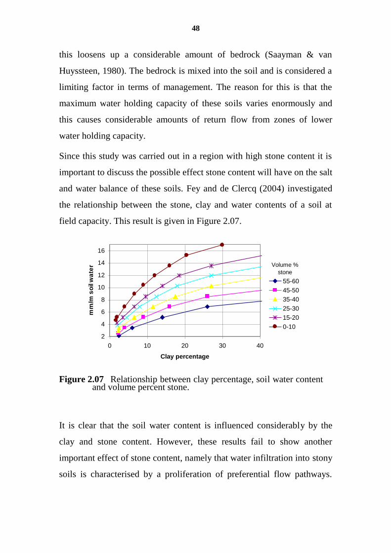
48
this loosens up a considerable amount of bedrock (Saayman & van
Huyssteen, 1980). The bedrock is mixed into the soil and is considered a
limiting factor in terms of management. The reason for this is that the
maximum water holding capacity of these soils varies enormously and
this causes considerable amounts of return flow from zones of lower
water holding capacity.
Since this study was carried out in a region with high stone content it is
important to discuss the possible effect stone content will have on the salt
and water balance of these soils. Fey and de Clercq (2004) investigated
the relationship between the stone, clay and water contents of a soil at
field capacity. This result is given in Figure 2.07.
2
4
6
8
10
12
14
16
0 10 20 30 40
Clay percentage
mm
/m s
oil
wa
ter
55-60
45-50
35-40
25-30
15-20
0-10
Volume %
stone
Figure 2.07 Relationship between clay percentage, soil water content and volume percent stone.
It is clear that the soil water content is influenced considerably by the
clay and stone content. However, these results fail to show another
important effect of stone content, namely that water infiltration into stony
soils is characterised by a proliferation of preferential flow pathways.
49
Moolman et al. (1992) have shown that drainage from stony soils
commences already about 15 minutes after irrigation has been initiated.
de Clercq et al. (2001) showed that clay content plays a major role in
determining the effect that salinity, and in particular Na+, has on a soil.
Tanji (1990) noted that structural degradation of soils, depends not only
on the levels of salinity and sodicity, but also on clay content and
mineralogy, and the presence of binding materials such as organic matter
and metal oxides. It is therefore impossible to predict a soil’s tolerance of
salinity and sodicity without taking these factors into account. It is
possible, however, to classify soils according to their stability under
saline irrigation, i.e., to distinguish soils that are prone to fast
degradation when subjected to saline irrigation, soils that are stable and
highly oxidised and do not deteriorate when irrigated with saline water,
and soils that are saline in their natural state. These are important
principles to bear in mind when modelling the effect of saline irrigation
on soils.
Tanji (1990) also reports that soils containing between 15 to 30% clay,
and less than 1.5% organic carbon, have a high potential for soil sealing
and crusting. Tanji (1990) further notes that this potential increases if the
ECi is low. This is a typical problem in irrigated agriculture where the
irrigation water quality varies during the season, resulting in poor
infiltration rates when water with low ECi is applied. It also becomes a
problem when the farmer exploits different sources of water with
different ECi values.
For the same evapotranspiration rate, a sandy soil will lose
proportionately more water than a clay soil, resulting in a more rapid
increase in the soil solution concentration (Shalhevet, 1994). However, if
50
sound irrigation practices are followed, the sandy soil will be irrigated
more frequently, thereby reducing the damage caused by increased
concentration.
The studies of Prior et al. (1992c) demonstrate the need to consider soil
properties, specifically texture, when predicting the effects of saline
water on grapevine productivity. In their study, irrigation with saline-
sodic water caused more damage to sultana grapes in heavier than in
lighter soils. Root zone depth and root density was lower in the heavier
soils. The textural effect on yield was the result of reduced leaching and
increased salinity in the more clayey soils with no effect in the yield
response to soil salinity (Prior et al., 1992c)
Soil properties that may alter the salt tolerance of plants and therefore
total leaf surface area, are fertility, texture and structure (Shalhevet,
1994). In a generalised statement, Shalhevet (1994) wrote that at high
fertility levels, there will be a larger yield reduction per unit increase in
salinity than in low fertility soils, meaning that plants are more sensitive
to salinity when conditions are conducive to high absolute yields. At
extremely low fertility levels, when yields are low, an increase in salinity
may have very little additional damaging effect on yield. Using this
approach as a management strategy should, however, be avoided. The
effects of soil texture and structure are manifested in their influence on
the infiltration capacity, water-holding capacity and the ratio of saturated
water content to field capacity. A combination of high salinity and low
soil oxygen results in greater uptake and transport of chloride and sodium
ions to shoots in grapevines, compared with high salinity and well
drained, aerated conditions (West and Taylor, 1984). If applied for long
51
enough, these combined factors can have a severe effect on the vine crop
(Shainberg and Letev, 1984).
Since the terms salinity and sodicity of soil are used in this research, they
are defined as follows (Verster & van Rooyen, 1990):
Soil salinity: The amount of soluble salts in a soil, expressed in
terms of conductivity of the saturation extract, mg kg-1
,
percentage, or other convenient units.
Soil sodicity: Soil with low soluble salt content but sufficient
adsorbed sodium to have caused significant deflocculation. The
exchangeable sodium percentage (ESP) is greater than 15.
2.2.5 Land use
The general land use pattern is driven by the availability of water and the
salinity of the soils (Figure 2.08). Irrigated soils are mostly found close to
the river systems. Further away from the river, most soils are used for
grazing and wheat production. Resulting from the occurrence of soils and
salinity in the study area, it is quite common to find that vineyards were
established on the higher grounds closer to the Berg River itself as these
soils are the older soils, which are well drained and not saline. These
soils are well prepared by deep ripping (1.2 m) of the soil. Where
necessary, drainage systems are installed (Saayman & Van Huyssteen,
1980).
Agricultural practices that increase the water holding capacity of the non-
irrigated soils and the removal of natural vegetation like the renosterbos,
contributes to increased saline seep toward the river. This extends further
into the summer season since winter wheat cannot utilize the excess
winter water. As a result of irrigation mainly around the river systems,
saline seeps also receive more water during summer and this contributes
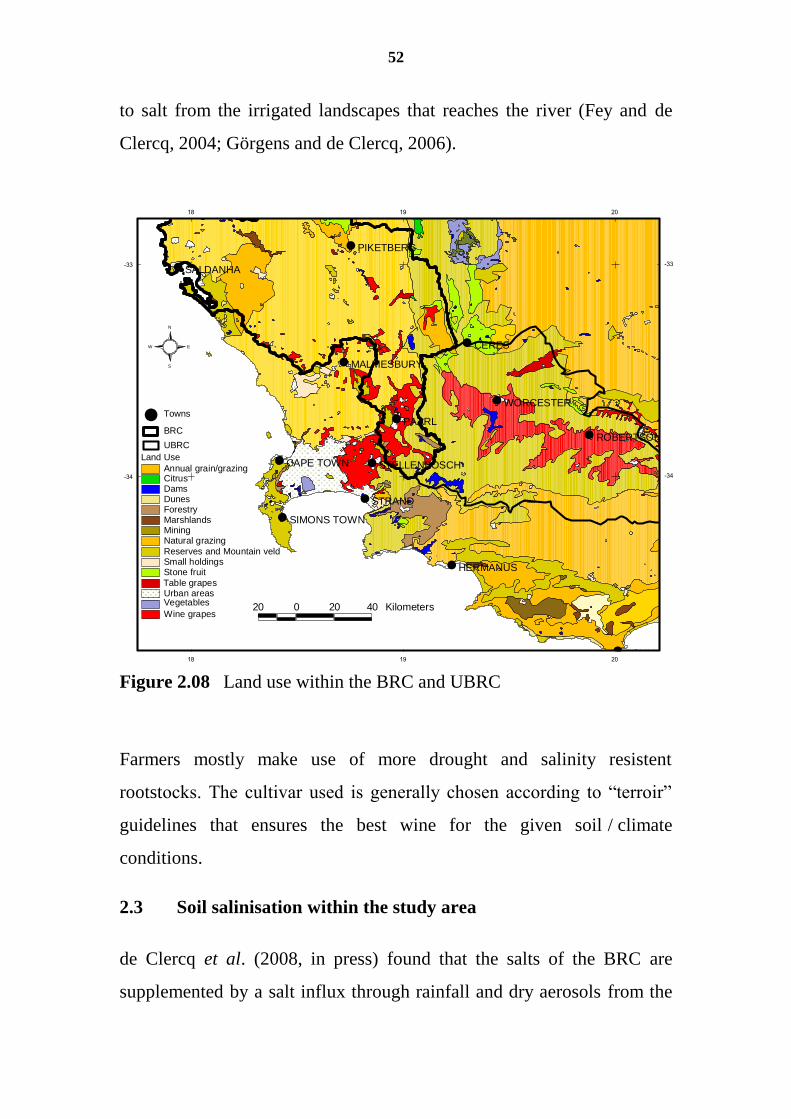
52
to salt from the irrigated landscapes that reaches the river (Fey and de
Clercq, 2004; Görgens and de Clercq, 2006).
#
#
#
#
#
#
#
#
#
#
#
#
#
CERES
PIKETBERG
SALDANHA
MALMESBURY
PAARL
WORCESTER
STRAND
STELLENBOSCH
SIMONS TOWN
CAPE TOWN
ROBERTSON
AGULHAS
HERMANUS
Land Use
Annual grain/grazingCitrusDamsDunesForestryMarshlandsMiningNatural grazing
Reserves and Mountain veldSmall holdingsStone fruit
Table grapesUrban areas
Wine grapes
UBRC
BRC
# Towns
Vegetables
18
18
19
19
20
20
-34 -34
-33 -33
S
N
EW
20 0 20 40 Kilometers
Figure 2.08 Land use within the BRC and UBRC
Farmers mostly make use of more drought and salinity resistent
rootstocks. The cultivar used is generally chosen according to ―terroir‖
guidelines that ensures the best wine for the given soil / climate
conditions.
2.3 Soil salinisation within the study area
de Clercq et al. (2008, in press) found that the salts of the BRC are
supplemented by a salt influx through rainfall and dry aerosols from the
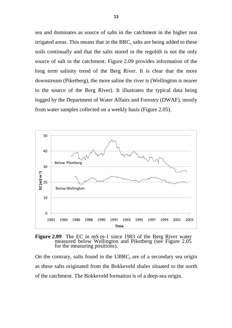
53
sea and dominates as source of salts in the catchment in the higher non
irrigated areas. This means that in the BRC, salts are being added to these
soils continually and that the salts stored in the regolith is not the only
source of salt in the catchment. Figure 2.09 provides information of the
long term salinity trend of the Berg River. It is clear that the more
downstream (Piketberg), the more saline the river is (Wellington is nearer
to the source of the Berg River). It illustrates the typical data being
logged by the Department of Water Affairs and Forestry (DWAF), mostly
from water samples collected on a weekly basis (Figure 2.05).
0
10
20
30
40
50
1982 1984 1986 1988 1990 1991 1993 1995 1997 1999 2001 2003
EC (m
S m
-1)
Time
Below Wellington
Below Piketberg
Figure 2.09 The EC in mS m-1 since 1983 of the Berg River water measured below Wellington and Piketberg (see Figure 2.05 for the measuring positions).
On the contrary, salts found in the UBRC, are of a secondary sea origin
as these salts originated from the Bokkeveld shales situated to the north
of the catchment. The Bokkeveld formation is of a deep-sea origin.
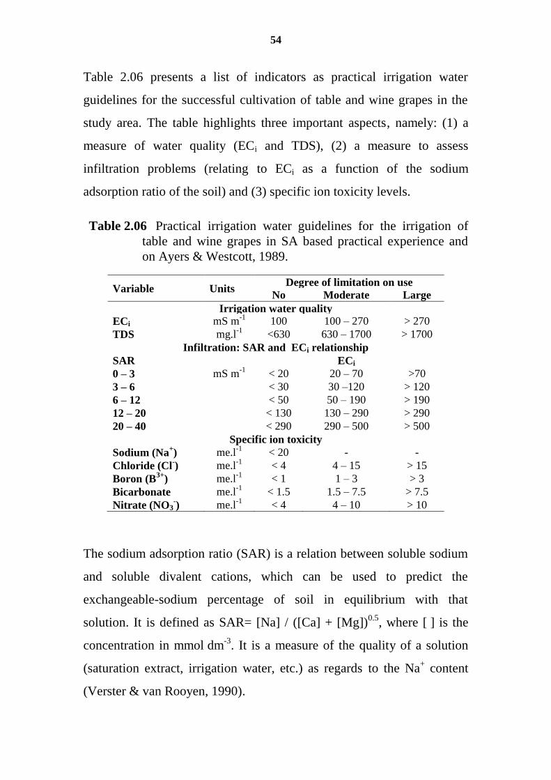
54
Table 2.06 presents a list of indicators as practical irrigation water
guidelines for the successful cultivation of table and wine grapes in the
study area. The table highlights three important aspects, namely: (1) a
measure of water quality (ECi and TDS), (2) a measure to assess
infiltration problems (relating to ECi as a function of the sodium
adsorption ratio of the soil) and (3) specific ion toxicity levels.
Table 2.06 Practical irrigation water guidelines for the irrigation of
table and wine grapes in SA based practical experience and
on Ayers & Westcott, 1989.
Variable Units Degree of limitation on use
No Moderate Large
Irrigation water quality
ECi
mS m-1
.m-1
100 100 – 270 > 270
TDS mg.l-1
<630 630 – 1700 > 1700
Infiltration: SAR and ECi relationship
SAR ECi
0 – 3 mS m-1
< 20 20 – 70 >70
3 – 6 < 30 30 –120 > 120
6 – 12 < 50 50 – 190 > 190
12 – 20 < 130 130 – 290 > 290
20 – 40 < 290 290 – 500 > 500
Specific ion toxicity
Sodium (Na+) me.l
-1 < 20 - -
Chloride (Cl-) me.l
-1 < 4 4 – 15 > 15
Boron (B3+
) me.l-1
< 1 1 – 3 > 3
Bicarbonate
(HCO3-)
me.l-1
< 1.5 1.5 – 7.5 > 7.5
Nitrate (NO3-) me.l
-1 < 4 4 – 10 > 10
The sodium adsorption ratio (SAR) is a relation between soluble sodium
and soluble divalent cations, which can be used to predict the
exchangeable-sodium percentage of soil in equilibrium with that
solution. It is defined as SAR= [Na] / ([Ca] + [Mg])0.5
, where [ ] is the
concentration in mmol dm-3
. It is a measure of the quality of a solution
(saturation extract, irrigation water, etc.) as regards to the Na+ content
(Verster & van Rooyen, 1990).
55
Table 2.06 indicates a distinctive relation between SAR of the soil and
the ECi. This implies that the higher the SAR of the soil the higher the
ECi must be to ensure continued good infiltration of the irrigation water.
In terms of specific ion toxicities, in this work attention will only be
given to the Cl- concentration of the water as it is the largest problem for
irrigation of vines. A chloride content exceeding 100 mg l-1
causes leaf
burn (Flowers and Yeo, 1986; de Clercq et al., 2001). Literature reveals
a sensitivity of grapevines to salinity with a salinity threshold value of
about 100 mS m-1
(Flowers and Yeo, 1986; Moolman et al., 1999; Prior
et al. 1992a,b,c).
To illustrate of the soil salinity of this region, an analysis of saline soils
from the Glenrosa farm is presented in Table 2.07. This result clearly
shows that the soil conditions in these irrigated soils exceed the known
limitations but after a three year preparation phase of these soils, one can
rid the soil of most of its salts. This is exactly what we should avoid in
catchment management since these salts simply contribute to the salt load
of the river. At least regional management of irrigation expansion could
be controlled using the information presented in this work.
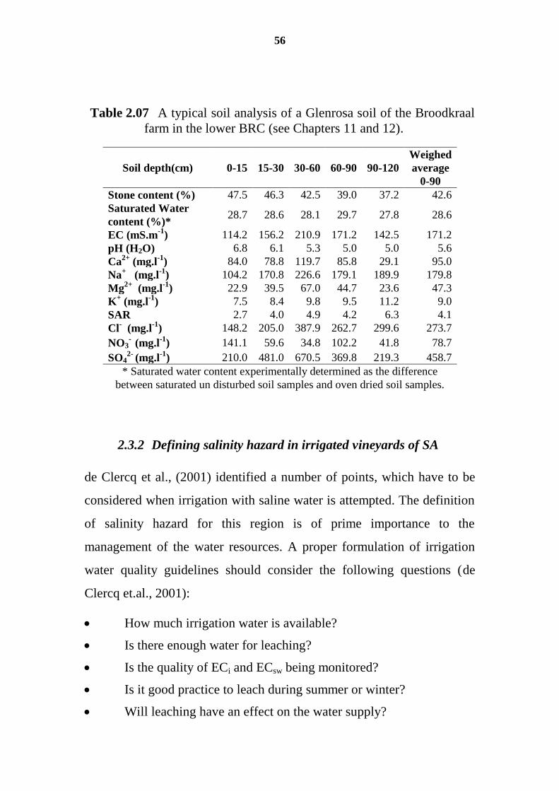
56
Table 2.07 A typical soil analysis of a Glenrosa soil of the Broodkraal
farm in the lower BRC (see Chapters 11 and 12).
Soil depth(cm) 0-15 15-30 30-60 60-90 90-120
Weighed
average
0-90
Stone content (%) 47.5 46.3 42.5 39.0 37.2 42.6
Saturated Water
content (%)* 28.7 28.6 28.1 29.7 27.8 28.6
EC (mS.m-1
) 114.2 156.2 210.9 171.2 142.5 171.2
pH (H2O) 6.8 6.1 5.3 5.0 5.0 5.6
Ca2+
(mg.l-1
) 84.0 78.8 119.7 85.8 29.1 95.0
Na+ (mg.l
-1) 104.2 170.8 226.6 179.1 189.9 179.8
Mg2+
(mg.l-1
) 22.9 39.5 67.0 44.7 23.6 47.3
K+ (mg.l
-1) 7.5 8.4 9.8 9.5 11.2 9.0
SAR 2.7 4.0 4.9 4.2 6.3 4.1
Cl- (mg.l
-1) 148.2 205.0 387.9 262.7 299.6 273.7
NO3- (mg.l
-1) 141.1 59.6 34.8 102.2 41.8 78.7
SO42-
(mg.l-1
) 210.0 481.0 670.5 369.8 219.3 458.7
* Saturated water content experimentally determined as the difference
between saturated un disturbed soil samples and oven dried soil samples.
2.3.2 Defining salinity hazard in irrigated vineyards of SA
de Clercq et al., (2001) identified a number of points, which have to be
considered when irrigation with saline water is attempted. The definition
of salinity hazard for this region is of prime importance to the
management of the water resources. A proper formulation of irrigation
water quality guidelines should consider the following questions (de
Clercq et.al., 2001):
How much irrigation water is available?
Is there enough water for leaching?
Is the quality of ECi and ECsw being monitored?
Is it good practice to leach during summer or winter?
Will leaching have an effect on the water supply?
57
Does the farmer use refined scheduling techniques?
Do the advantages of partial wetting of the soil apply?
What is the salt tolerance of the crop?
Does the salt content of the marketable product matter?
What is the length of season for the crop?
What is the typical rooting volume of the crop?
Under saline conditions, should crops be selected with the
smallest possible rooting volume?
The salinity hazard in South Africa stems from the large salt laden inland
surfaces and the fact that most inland sediments are from oceanic origin
(Trusswell, 1986). The South African land surface is extremely stable
and old. Most soils in the irrigated agricultural regions are old but in tune
with the current climatic conditions. Most soils are also quite shallow
and wherever soils are developed for irrigational purposes, a large
section of the underlying weathered zone in broken up. This result in a
new soil forming while under irrigation but as soon as this soil is
abandoned, it usually returns to previous condition with the exception of
the existence of more erodible material. Cultivation of land surfaces in
South Africa inevitably leads to a larger degree of soil erosion, and the
large changes in the water balance of these regions also means a large
change in the solute flux of the region. The combination of fine sediment
and solute that pollutes South Africa's river systems is therefore a great
source of concern (de Clercq et al., 2008, in press).
58
3 IRRIGATION OF VINES WITH SALINE WATER1
3.1 Introduction
The irrigation water guidelines in South Africa, regarding vines (Vitis
vinifera, L), had to be determined. The DWAF had broad management
principles regarding the quality of water in the BRC as well as in the
UBRC. Both these rivers act as drainage system and water supply system
for their catchments. The DWAF therefore managed the water during the
irrigation season to a level of about 30 mS m-1
and during the remainder
of the year to a level of 75 mS m-1
. As a result of the fact that vines are
the main agricultural crop of this region under irrigation, several studies
were conducted that focused on vines.
South Africa is not richly endowed with water. It follows that sustained
food production in many parts of South Africa is only possible through
irrigation.
1Published in:
Moolman, J.H., de Clercq, W.P., Wessels, W.P.J., Meiri, A., Moolman, C.G., 1999. The Use of Saline Water for Irrigation of Grapevines and The Development of Crop Salt Tolerance Indices. WRC Report:303/1/1999.
de Clercq, W.P., Fey, M.V., Moolman, J.H., Wessels, W.P.J., Eigenhuis, B., Hoffman, E., 2001. Experimental irrigation of vineyards with saline water. WRC Report; 522/1/01, (ISBN No. 1868457753).
de Clercq, W.P., Fey, M.V., Moolman, J.H., Wessels, W.P.J., Eigenhuis, B. Hoffman, E., 2001. Establishing the effects of saline irrigation water and managerial options on soil properties and plant performance. WRC Report; 695/1/01, (ISBN No. 1868457753).
59
In the Western Cape virtually the entire fruit and wine industries are
dependent on irrigation. Agriculture, and specifically irrigated
agriculture, is the largest consumer of water. In 1980 irrigated agriculture
accounted for 52% of the total water use in South Africa (DWAF, 1986).
According to various reports published since 1975, the quality of South
Africa's water resources, with specific emphasis on the total salt content,
is steadily deteriorating (Stander, 1987). Alexander (1980) stated that
"there is no doubt that mineralisation (salinisation) is a serious problem
in South Africa - and it can only get worse!"
Over the past 30 years, an awareness of salinity levels in the Breede
River during summer months has grown considerably. It plays an
important role in the economy of the Western Cape and contributes
significantly to South Africa’s agricultural output. It has a wide and
dynamic crop mix, but is primarily a wine-producing area, with 65% of
the area under wine grapes. Other crops produced in the valley are
peaches and apricots (13%), vegetables, mainly tomatoes (3%) and
irrigated pastures (7%). The perception of an increase in salinity over
time gave rise to concern about sustainability of using the water for the
irrigation of these high value salt sensitive crops Lipton et al, .
It is reasonable to assume that agriculture in future not only will have to
bring about substantial water savings but will also have to rely
increasingly on water of a poorer quality than at present. However,
international research has proved that salinity effects on the yield and
quality of agricultural crops are of primary importance (Frenkel and
Meiri, 1985; Shalhevet, 1994). Problems associated with salinity (yield
decrease, crop quality) have already been encountered in a number of
rivers and irrigation schemes in South Africa. A few examples are the
60
Fish/Sundays-River irrigation schemes in the Eastern Cape (Hall & Du
Plessis, 1979; Tylcoat, 1985), the Riet River scheme in the Orange Free
State, and the Breede River in the Western Cape.
Worsening of the salinity effect with time can result from important
metabolic processes that are weakened season after season. One such
process is a decrease in carbohydrate reserves in the perennial organs at
the end of the growing season, as shown for grapes by Prior et al.
(1992b). The most severe salinity effect on grapes was leaf damage that
almost killed vines after two, three and four years of irrigation with water
of ECi of 250 - 800 mS m-1
(Flowers and Yeo, 1986; Hoffman et al.
1989; Prior et al., 1992). In all these studies, the visual damage was
considered a specific ion effect, which showed up when Cl- reached toxic
levels in the leaves. Limited leaf damage showed up towards the end of
the first season in all treatments with ECi higher than 300 mS m-1
. The
leaf damage worsened in proportion to the water salinity and was visible
earlier in following seasons. Increased disorders in flowers with the
increase in salinity and number of seasons of saline irrigation were also
considered toxic effects. Since the soil was leached every winter the
increased salinity damage over time suggested a salt carry-over in the
perennial organs of the tree. It was previously documented that the build-
up to toxic levels of chloride and sodium in plant organs on soils with
relatively low salinity and sodicity can take several years (Bernstein et
al., 1958; Francois and Maas, 1994; Maas, 1984, 1990). The possibility
that winter irrigation lowers the nutrient status of soils was mentioned by
Moolman et al. (1999). This results in lower nutrient levels at bud break.
Initially, sodium was thought to be retained in the sapwood of the tree.
With the conversion of sapwood to heartwood, sodium is released and
61
then translocated to the leaves, causing leaf burn. This may partly explain
why grapes appear to be more sensitive to salinity as the plants grow
older (Francois and Maas, 1994).
This chapter reports on 10 years of applied research regarding irrigation
with saline water. It was not the intension to provide all the result but
rather the major findings that had a bearing on the investigation reported
in this thesis.
3.2 Materials and Method
The research was conducted at Robertson in an experimental vineyard
belonging to the Agricultural Research Council. Robertson (33o 46'S,
19o 46'E) are located in the south-western part of South Africa.
Robertson is situated in the BRC. The vineyard was established in 1974
with Colombar vines, grafted on Richter-99 rootstock and trained on a
factory roof trellising system (Saayman, 1988). Van Zyl (1984a&b)
described the soil as a Hutton fine sandy loam. In terms of the current
classification (Soil Classification Working Group, 1991) the soil belongs
to the Trawal 2210 family (Cambisol, under the FAO (1998) Soil
Taxonomy) and has a duripan at about 1.2 m. Soil preparation included
homogenising by deep cultivation to about 1 m.
The 1.2 ha block was divided into 24 plots to which were randomly
allocated 4 replications of six irrigation salinity treatments (Figure 3.01).
The six treatments had ECi levels of 30, 75, 150, 250, 350 and
500 mS m-1
(alternatively termed treatments 1 to 6), the first being normal
canal water and the others canal water to which CaCl2 and NaCl had been
added in a 1:1 molar ratio to achieve the desired salinity (Meiri, 1984;
62
Meiri et al., 1986; Wessels et al., 1995). Irrigation was applied with
microjet sprinklers, scheduled according to water use on the lowest
salinity plots (canal water), and included a 10 % leaching fraction which
is standard practice in the region (de Clercq et al., 2001). The
predominantly winter rainfall, which was supplemented with irrigation to
promote leaching of salts, ensured that there was minimal interference in
the water balance by rainfall during the summer months when most of the
irrigation was applied.
0
15
30
45
60
75
90
DIS
TA
NC
E (
m)
0 35 69 104 138
DISTANCE (m)
1 7 13 19
2 8 14 20
3 9 15 21
4 10 16 22
5 11 17 23
6 12 18 24
1 6 1 6
2 4 2 4
4 1 3 1
5 2 4 2
3 5 6 3
6 3 5 5
Experimental row Measuring point
MAP OF ROBERTSON VINEYARDNBL 4BL 3BL 2BL 1
Control CentrePlot Treatment
Figure 3.01 Schematic diagram of the experimental vineyard at Robertson showing 24 plots arranged according to a randomised block design consisting of four blocks (replicates) and six treatments (the triangles indicate the centre of each plot where the soil water content and soil solution was monitored). Treatments are indicated as follows: 1 = 30, 2 = 75, 3 = 150, 4 = 250, 5= 350, 6 = 500 mS m
-1.
Each plot consisted of five vine rows, 3 m apart, with 23 vines per row at
1 m spacing. Soil measurements were confined to the central ten vines in
the middle row of each plot. Suction cup lysimeters (SCL) (for a more
detailed description of these SCL’s it is referred to Chapter 4) were
63
installed between two vines at depths of 15, 30, 60, 90 and 120 cm and
linked to a central vacuum pump, which was synchronised with an
irrigation controller allowing remote control of soil water extraction (de
Clercq et al., 2001). Soil samples were taken twice per year (during
September and April) over 8 years, by augering between two
experimental vines and to the same depths as the suction cups. One set
consisted of 120 samples, i.e., 5 depths, 4 replicates and 6 treatments.
The experiment ran for eight years with prime function to test the salt
tolerance of Colombar grapevines and to investigate methods that will
allow the use of moderate to high salt content in irrigation waters. It was
also a prerequisite that the treatments should at least cover the range of
salinities defined by the EC-operational curve used by the Department of
Water Affairs for managing water releases from the Brandvlei dam.
Secondly, some of the treatments had to exceed the first threshold
estimate of the salinity value for Vitis vinifera L., i.e. 150 mS m-1
(Ayers
and Westcott, 1985).
Irrigation was scheduled according to the water use in the freshest water
treatment and measurements were done using a neutron probe. An
average of 17 irrigation events took place per year over the duration of
the project. An additional amount of 10 percent was usually applied as
over-irrigation to allow leaching. This was done, as it is standard practice
among farmers in this region. Irrigation was systematically applied in the
afternoon of each Wednesday and suction sampling was initiated 12
hours after irrigation had terminated, to ensure that the soil water status
was effectively at field capacity. Suction samples were withdrawn
simultaneously at all depths from all plots. Over the 8 year duration of
the experiment at least 12 annual sets (a set consisting of 120 samples,
64
ie., 5 depths, 6 treatments and 4 replicates) of suction cup data were
collected, with 7 to 9 of these being collected during the irrigation season
and the 3 to 5 during winter (Moolman et al., 1999 and de Clercq et al.,
2001).
Various vegetative growth parameters were recorded, which included
time of bud burst, shoot growth, shoot intermodal fresh and dry weights,
leaf fresh and dry weights, degree of leaf necrosis, leaf size and number,
canopy size and leaf density, leaf water potential, vacuole pressure,
stomatal resistance, trunk circumferences as well as yield and wine
quality. Of these, the intermodal lengths and weights, leaf water
potential, yield and wine quality produces the most noteworthy results.
The last two were focused on in more detail as these clearly provided the
means of expressing the influence of salinity in an economic sense. The
growth parameters were logged over the last 7 years and 5 growth stages
during each season, i.e., full bloom, pea size, veraison, harvest and post
harvest. The methods were fully described in Moolman et al. (1999) and
de Clercq et al, (2001). Leaf water potential was determined using a
pressure chamber technique.
3.3 Results and discussion
3.3.1 The soil and water
The seasonal mean soil water content measured before each irrigation
event (Table 3.01), did not increase in accordance with the range of
salinity treatments applied in any consistent way, as soil and irrigation
water salinity increased. This is probably due to the relatively high
frequency of irrigation (once per week) and the good internal drainage
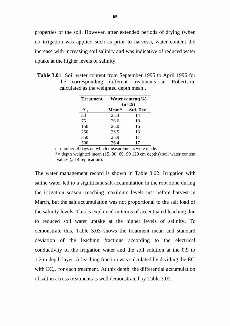
65
properties of the soil. However, after extended periods of drying (when
no irrigation was applied such as prior to harvest), water content did
increase with increasing soil salinity and was indicative of reduced water
uptake at the higher levels of salinity.
Table 3.01 Soil water content from September 1995 to April 1996 for
the corresponding different treatments at Robertson,
calculated as the weighted depth mean .
Treatment
Water content(%)
(n=19)
ECi Mean* Std. Dev
30 25.3 14
75 26.6 18
150 25.0 16
250 26.5 13
350 25.9 11
500 26.4 17
n=number of days on which measurements were made.
*= depth weighted mean (15, 30, 60, 90 120 cm depths) soil water content
values (all 4 replication).
The water management record is shown in Table 3.02. Irrigation with
saline water led to a significant salt accumulation in the root zone during
the irrigation season, reaching maximum levels just before harvest in
March, but the salt accumulation was not proportional to the salt load of
the salinity levels. This is explained in terms of accentuated leaching due
to reduced soil water uptake at the higher levels of salinity. To
demonstrate this, Table 3.03 shows the treatment mean and standard
deviation of the leaching fractions according to the electrical
conductivity of the irrigation water and the soil solution at the 0.9 to
1.2 m depth layer. A leaching fraction was calculated by dividing the ECi
with ECsw for each treatment. At this depth, the differential accumulation
of salt in across treatments is well demonstrated by Table 3.02.
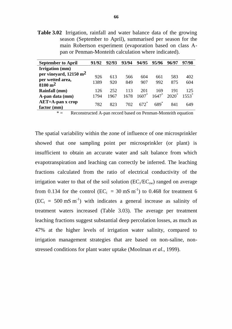
66
Table 3.02 Irrigation, rainfall and water balance data of the growing
season (September to April), summarised per season for the
main Robertson experiment (evaporation based on class A-
pan or Penman-Monteith calculation where indicated).
September to April 91/92 92/93 93/94 94/95 95/96 96/97 97/98
Irrigation (mm)
per vineyard, 12150 m2
per wetted area,
8100 m2
926
1389
613
920
566
849
604
907
661
992
583
875
402
604
Rainfall (mm) 126 252 113 201 169 191 125
A-pan data (mm) 1794 1967 1678 1607* 1647
* 2020
* 1553
*
AET=A-pan x crop
factor (mm) 782 823 702 672
* 689
* 841 649
* = Reconstructed A-pan record based on Penman-Monteith equation
The spatial variability within the zone of influence of one microsprinkler
showed that one sampling point per microsprinkler (or plant) is
insufficient to obtain an accurate water and salt balance from which
evapotranspiration and leaching can correctly be inferred. The leaching
fractions calculated from the ratio of electrical conductivity of the
irrigation water to that of the soil solution (ECi/ECsw) ranged on average
from 0.134 for the control (ECi = 30 mS m-1
) to 0.468 for treatment 6
(ECi = 500 mS m-1
) with indicates a general increase as salinity of
treatment waters increased (Table 3.03). The average per treatment
leaching fractions suggest substantial deep percolation losses, as much as
47% at the higher levels of irrigation water salinity, compared to
irrigation management strategies that are based on non-saline, non-
stressed conditions for plant water uptake (Moolman et al., 1999).
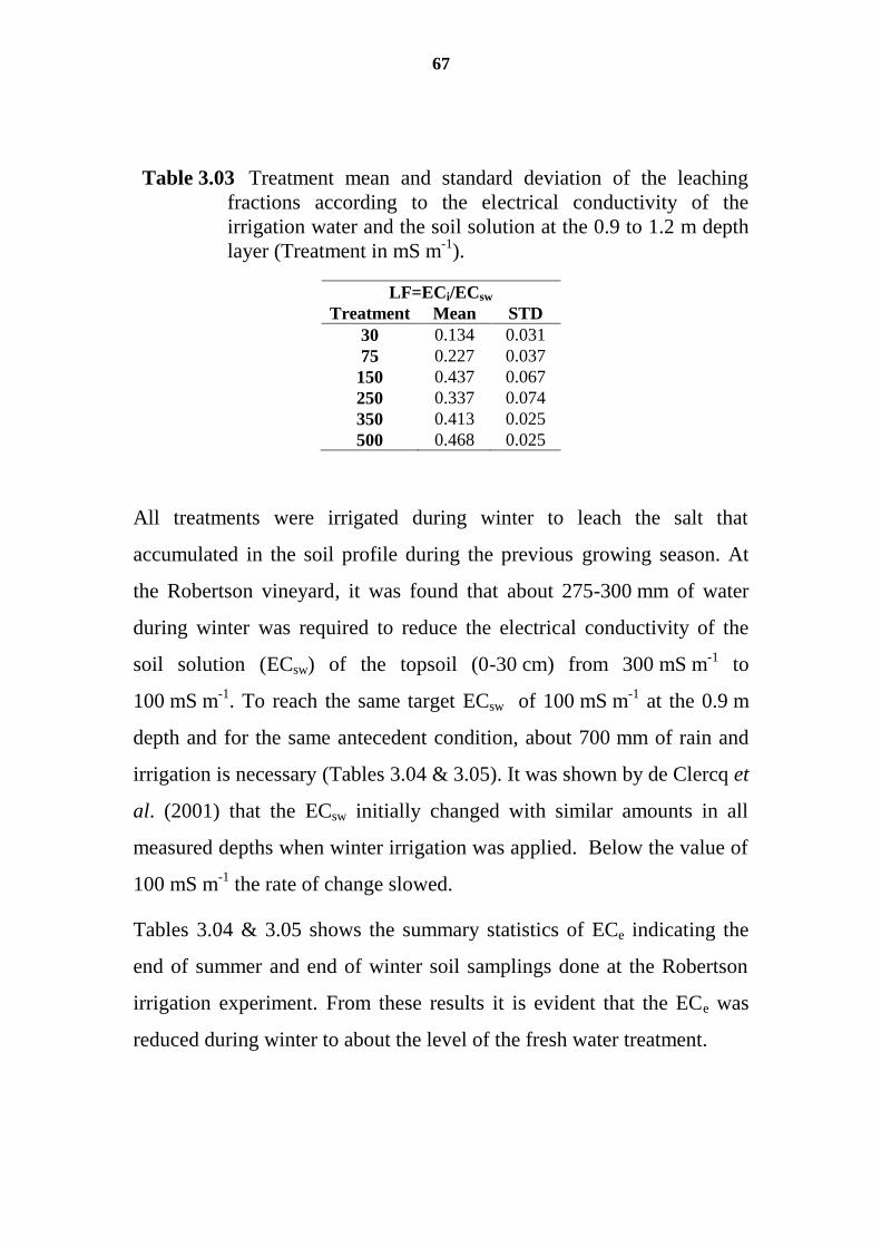
67
Table 3.03 Treatment mean and standard deviation of the leaching
fractions according to the electrical conductivity of the
irrigation water and the soil solution at the 0.9 to 1.2 m depth
layer (Treatment in mS m-1
).
LF=ECi/ECsw
Treatment Mean STD
30 0.134 0.031
75 0.227 0.037
150 0.437 0.067
250 0.337 0.074
350 0.413 0.025
500 0.468 0.025
All treatments were irrigated during winter to leach the salt that
accumulated in the soil profile during the previous growing season. At
the Robertson vineyard, it was found that about 275-300 mm of water
during winter was required to reduce the electrical conductivity of the
soil solution (ECsw) of the topsoil (0-30 cm) from 300 mS m-1
to
100 mS m-1
. To reach the same target ECsw of 100 mS m-1
at the 0.9 m
depth and for the same antecedent condition, about 700 mm of rain and
irrigation is necessary (Tables 3.04 & 3.05). It was shown by de Clercq et
al. (2001) that the ECsw initially changed with similar amounts in all
measured depths when winter irrigation was applied. Below the value of
100 mS m-1
the rate of change slowed.
Tables 3.04 & 3.05 shows the summary statistics of ECe indicating the
end of summer and end of winter soil samplings done at the Robertson
irrigation experiment. From these results it is evident that the ECe was
reduced during winter to about the level of the fresh water treatment.
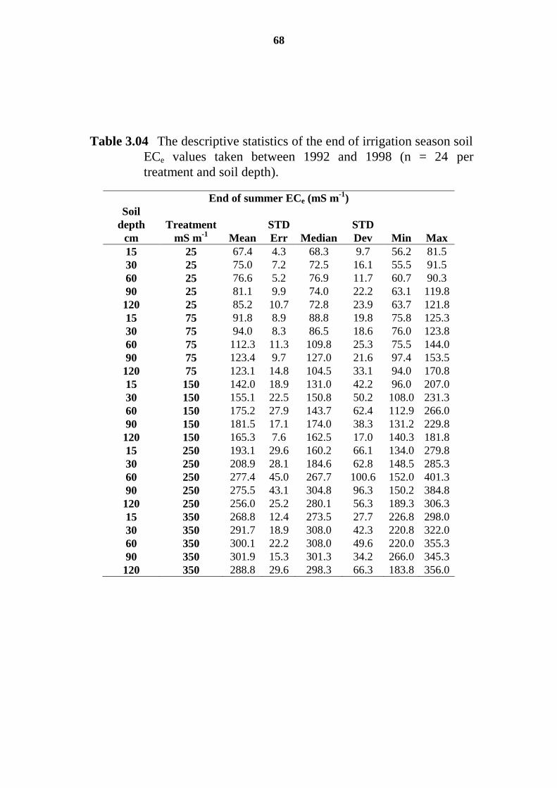
68
Table 3.04 The descriptive statistics of the end of irrigation season soil
ECe values taken between 1992 and 1998 (n = 24 per
treatment and soil depth).
End of summer ECe (mS m-1
)
Soil
depth
cm
Treatment
mS m-1
Mean
STD
Err Median
STD
Dev Min Max
15 25 67.4 4.3 68.3 9.7 56.2 81.5
30 25 75.0 7.2 72.5 16.1 55.5 91.5
60 25 76.6 5.2 76.9 11.7 60.7 90.3
90 25 81.1 9.9 74.0 22.2 63.1 119.8
120 25 85.2 10.7 72.8 23.9 63.7 121.8
15 75 91.8 8.9 88.8 19.8 75.8 125.3
30 75 94.0 8.3 86.5 18.6 76.0 123.8
60 75 112.3 11.3 109.8 25.3 75.5 144.0
90 75 123.4 9.7 127.0 21.6 97.4 153.5
120 75 123.1 14.8 104.5 33.1 94.0 170.8
15 150 142.0 18.9 131.0 42.2 96.0 207.0
30 150 155.1 22.5 150.8 50.2 108.0 231.3
60 150 175.2 27.9 143.7 62.4 112.9 266.0
90 150 181.5 17.1 174.0 38.3 131.2 229.8
120 150 165.3 7.6 162.5 17.0 140.3 181.8
15 250 193.1 29.6 160.2 66.1 134.0 279.8
30 250 208.9 28.1 184.6 62.8 148.5 285.3
60 250 277.4 45.0 267.7 100.6 152.0 401.3
90 250 275.5 43.1 304.8 96.3 150.2 384.8
120 250 256.0 25.2 280.1 56.3 189.3 306.3
15 350 268.8 12.4 273.5 27.7 226.8 298.0
30 350 291.7 18.9 308.0 42.3 220.8 322.0
60 350 300.1 22.2 308.0 49.6 220.0 355.3
90 350 301.9 15.3 301.3 34.2 266.0 345.3
120 350 288.8 29.6 298.3 66.3 183.8 356.0
69
Table 3.05 The descriptive statistics of the start of irrigation season
soil ECe values taken between 1992 and 1998 (n = 24 per
treatment and soil depth).
End of winter ECe (mS m-1
)
Soil
depth
cm
Treatment
mS m-1
Mean
STD
Err Median
STD
Dev Min Max
15 25 63.9 9.3 53.7 20.7 47.9 98.8
30 25 57.1 5.2 56.2 11.7 45.5 76.3
60 25 59.2 8.8 50.4 19.7 46.3 93.8
90 25 55.9 2.8 56.5 6.3 49.4 65.4
120 25 61.7 2.5 62.0 5.5 56.7 69.9
15 75 57.2 4.6 62.2 10.4 39.3 64.7
30 75 53.4 5.9 57.8 13.2 33.3 67.8
60 75 56.0 5.2 59.3 11.5 38.0 69.0
90 75 66.7 6.6 71.7 14.7 41.3 77.3
120 75 70.9 8.0 76.8 17.8 39.5 83.4
15 150 51.0 5.4 57.0 12.1 30.5 60.1
30 150 53.0 5.6 56.0 12.5 38.8 69.5
60 150 54.0 3.4 56.5 7.6 42.3 62.6
90 150 62.1 2.3 62.9 5.1 56.6 69.0
120 150 59.3 6.3 62.8 14.0 37.3 74.5
15 250 63.9 7.1 62.3 15.8 41.0 82.8
30 250 66.1 6.7 69.6 14.9 48.8 86.3
60 250 89.1 14.2 105.8 31.8 47.3 119.3
90 250 125.7 22.9 140.7 51.3 51.8 180.0
120 250 140.5 27.5 143.3 61.6 48.3 214.0
15 350 59.6 4.0 63.2 8.9 49.0 69.8
30 350 73.7 6.4 70.3 14.3 57.9 96.8
60 350 90.5 17.5 74.0 39.2 55.4 152.3
90 350 110.7 15.4 96.3 34.5 84.0 167.3
120 350 121.8 16.6 109.5 37.2 90.8 178.8
It should also be noted that the CaCl2-NaCl solution used for salinity
treatments was equimolar with respect to Na and Ca, which means that
SAR actually increases with increasing soil salinity (ECe) in all these
trials and consequently SAR also increased with increased ECi levels
(Figure 3.02).
70
y = 68.9x - 26.3R2 = 0.67
0
50
100
150
200
250
300
350
400
0 2 4 6 8
EC
e
SAR
Figure 3.02 ECe – SAR relationship at Robertson based on all end of season weighted mean ECe and SAR data over all treatments.
3.3.2 The vine
Despite thorough leaching with low salinity water every winter, the effect
of saline water treatments from the beginning of successive seasons
caused the first noticeable effect of salinity on expansive growth of
shoots and leaves to occur earlier every season. At Robertson this was on
day 35 of the 1992/93 season, and day 20 of the 1993/94 season and from
then on the higher salinity treatments continually started growing earlier
than the rest of the vines on the farm. This suggested that early in the
spring, expansive growth was sensitive even to low soil salinity and that
saline growth conditions in one season had a large influence on the
growth during the following season (Moolman et al., 1999).
Leaf specific fresh weights were not sensitive to salinity or leaf age while
the internodal fresh weights were smaller in the higher salinity levels.
The specific dry weight of leaves increased with age more in the low than
in the high salt treatments. From this it was inferred that salinity has a
71
larger effect on the mass than on the sizes of these leaves. Alternatively,
it indicated an increase in metabolite deposition in the leaves and
decreased metabolite transport to the internodes - a change that can be
the result of salinity interference to the metabolite export from the leaves.
The reduction in metabolite transport to the shoot under saline conditions
also implied a reduced build-up of metabolite storage in the perennial
plant organs of the vine (de Clercq et al., 2001).
Leaf water potential (LWP) and stomatal conductance measurements
showed that differences in LWP between salinity treatments were best
observed early in the day before the stomata start to control transpiration.
The results also showed that stomatal closure occurs earlier in the day in
the higher salinity levels than in non-saline treatments. This means that
the salinity treatment effects on LWP could only be detected with pre-
dawn measurements. The minimum recorded LWP at Robertson was
about -1100 kPa, which was much higher than the minimum potentials
reported from other irrigation studies. In spite of the relatively high leaf
water potentials, damage to growth and yield was significant. It was
therefore speculated that salinity damage to grapevine leaves may be the
result of accumulation of salts in the apoplast, which means that the
pressure chamber technique does not measure the total leaf water
potential and perhaps also not the hydrostatic component of the xylem
water potential of vines. Rather, it measures the difference between the
vacuole water potential and the apoplast osmotic potential (Moolman et
al., 1999; de Clercq et al., 2001).
3.3.3 Yield response
de Clercq et al. (2001) reported that salinity had a severe effect on yield
with an average decrease of 60 % at the ECi 500 mS m-1
salinity level
72
(Table 3.06). Yield (kg of grapes per vine) was negatively influenced
even at the intermediate ECi levels of 75 and 150 mS m-1
. However, a
better understanding of the effect of salinity on the yield and
reproductive growth of Colombar grapes is complicated by the fact that
during the first four years of this study an irrigation water salinity of
250 mS m-1
seemingly had less effect on the average kg of grapes per
vine yield (Table 3.06). Quantifying the effect of salinity on yield was
further hampered by the progressive decrease in the yield on the control
treatment. It seems that plant vigour and size are key determinants that
influence the response of Colombar grapes to salinity.
Table 3.06 Mean grape yield in kg per vine per treatment of the saline
irrigated study at Robertson (Colombar grapes) for the 1992
to 1998 yield years, in relation to ECe and ECi.
TREATMENT (mS m
-1)
YEARLY
AVERAGE
YEAR ECi 30 75 150 250 350 500 YIELD
ECe * 80 108 161 236 295 361 kg/vine
1992 13.28 10.95 11.65 12.90 10.19 9.72 11.45
1993 10.05 7.86 7.56 8.78 5.26 4.81 7.39
1994 7.83 5.49 5.73 7.50 3.54 2.68 5.46
1995 4.99 4.61 4.20 6.53 2.69 1.91 4.16
1996 6.80 6.06 4.98 5.95 1.16 1.50 4.41
1997 4.74 3.13 3.02 3.20 1.11 0.83 2.67
1998 4.56 3.25 2.30 3.07 0.79 1.03 2.50
AVG 7.46 5.91 5.63 6.85 3.53 3.21
* The 8 year average ECe per treatment, measured at harvest time.
Despite these two complicating factors, the results of this experiment
indicate that grapevines are more sensitive to salinity than previously
thought, and that the threshold soil salinity value of 150 mS m-1
as
reported by Ayers and Westcot (1985) is too high. These results are more
in line with a limiting value of ECe = 100 mS m-1
, as reported by Prior et
al. (1992 a, b, c).
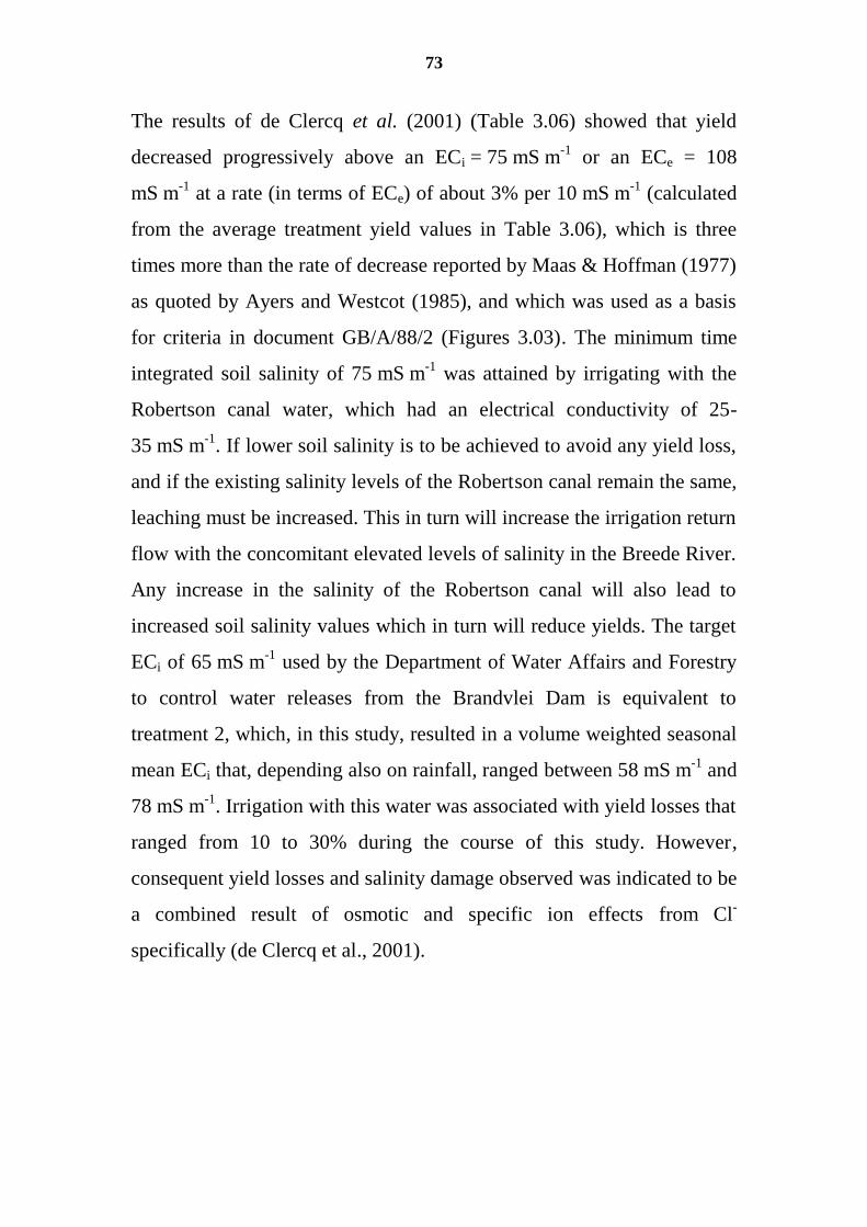
73
The results of de Clercq et al. (2001) (Table 3.06) showed that yield
decreased progressively above an ECi = 75 mS m-1
or an ECe = 108
mS m-1
at a rate (in terms of ECe) of about 3% per 10 mS m-1
(calculated
from the average treatment yield values in Table 3.06), which is three
times more than the rate of decrease reported by Maas & Hoffman (1977)
as quoted by Ayers and Westcot (1985), and which was used as a basis
for criteria in document GB/A/88/2 (Figures 3.03). The minimum time
integrated soil salinity of 75 mS m-1
was attained by irrigating with the
Robertson canal water, which had an electrical conductivity of 25-
35 mS m-1
. If lower soil salinity is to be achieved to avoid any yield loss,
and if the existing salinity levels of the Robertson canal remain the same,
leaching must be increased. This in turn will increase the irrigation return
flow with the concomitant elevated levels of salinity in the Breede River.
Any increase in the salinity of the Robertson canal will also lead to
increased soil salinity values which in turn will reduce yields. The target
ECi of 65 mS m-1
used by the Department of Water Affairs and Forestry
to control water releases from the Brandvlei Dam is equivalent to
treatment 2, which, in this study, resulted in a volume weighted seasonal
mean ECi that, depending also on rainfall, ranged between 58 mS m-1
and
78 mS m-1
. Irrigation with this water was associated with yield losses that
ranged from 10 to 30% during the course of this study. However,
consequent yield losses and salinity damage observed was indicated to be
a combined result of osmotic and specific ion effects from Cl-
specifically (de Clercq et al., 2001).
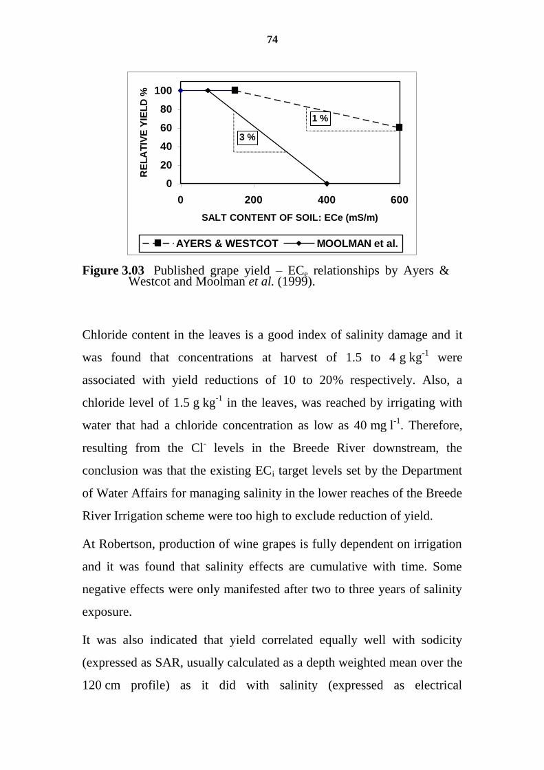
74
0
20
40
60
80
100
0 200 400 600
SALT CONTENT OF SOIL: ECe (mS/m)
RE
LA
TIV
E Y
IEL
D %
AYERS & WESTCOT MOOLMAN et al.
1 %
3 %
Figure 3.03 Published grape yield – ECe relationships by Ayers & Westcot and Moolman et al. (1999).
Chloride content in the leaves is a good index of salinity damage and it
was found that concentrations at harvest of 1.5 to 4 g kg-1
were
associated with yield reductions of 10 to 20% respectively. Also, a
chloride level of 1.5 g kg-1
in the leaves, was reached by irrigating with
water that had a chloride concentration as low as 40 mg l-1
. Therefore,
resulting from the Cl- levels in the Breede River downstream, the
conclusion was that the existing ECi target levels set by the Department
of Water Affairs for managing salinity in the lower reaches of the Breede
River Irrigation scheme were too high to exclude reduction of yield.
At Robertson, production of wine grapes is fully dependent on irrigation
and it was found that salinity effects are cumulative with time. Some
negative effects were only manifested after two to three years of salinity
exposure.
It was also indicated that yield correlated equally well with sodicity
(expressed as SAR, usually calculated as a depth weighted mean over the
120 cm profile) as it did with salinity (expressed as electrical
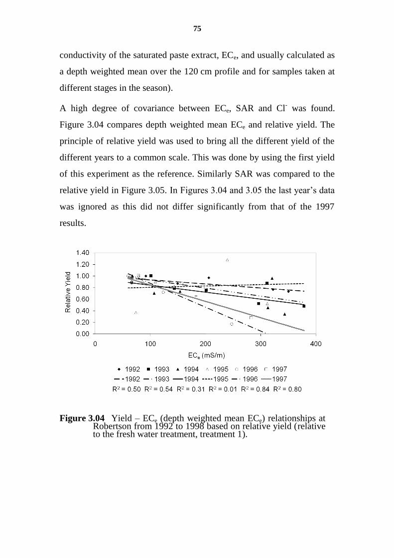
75
conductivity of the saturated paste extract, ECe, and usually calculated as
a depth weighted mean over the 120 cm profile and for samples taken at
different stages in the season).
A high degree of covariance between ECe, SAR and Cl- was found.
Figure 3.04 compares depth weighted mean ECe and relative yield. The
principle of relative yield was used to bring all the different yield of the
different years to a common scale. This was done by using the first yield
of this experiment as the reference. Similarly SAR was compared to the
relative yield in Figure 3.05. In Figures 3.04 and 3.05 the last year’s data
was ignored as this did not differ significantly from that of the 1997
results.
Figure 3.04 Yield – ECe (depth weighted mean ECe) relationships at Robertson from 1992 to 1998 based on relative yield (relative to the fresh water treatment, treatment 1).
76
Figure 3.05 Yield and depth weighted mean SAR relationships at Robertson from 1992 to 1998 based on relative yield (relative to the fresh water treatment, treatment 1).
A pattern emerged from these results, which could only be picked up as a
result of the duration of this experiment. The essence of the pattern is
that, irrespective of whether the inhibitory effect of the saline irrigation
treatments on yield is an osmotic one, a toxic one (Na+ and/or Cl
-), or
both, the threshold level remains the same over a number of seasons of
irrigation, but the sensitivity of the crop to levels beyond the threshold
increases with the number of seasons of exposure. This is reminiscent of
an allergic type of response which suggests that, instead of there being
one particular cultivar-specific response function, the response pattern
changes with time and the effect of the saline/sodic/chloridic water is
cumulative on the vines (i.e. not only through a build-up in the soil).
After all, vines are perennial plants. This might explain why the overall
yield of the main trial at Robertson showed a progressive decline, since
even the control treatment made use of slightly saline canal water on a
site that already was moderately saline. This result has important
management implications, because it suggests that even moderately
77
acceptable water may, in the longer-term, have a cumulative, debilitating
effect leading to premature failure of the vineyard.
3.3.4 The wine
Wine quality and in particular the concentration of NaCl in the wine, has
an influence on the market price of these wines as high NaCl content
affects the marketability of these wines negatively, which impacts on the
economy of the region. Consequently the wine quality at Robertson was
also subjected to a sensory evaluation (a panel of 20 wine experts tasting
the wine) and found to have a salty taste when made from the most saline
treatment but all wines (from all the treatments) lacked the typical
character of the cultivar. The best wine was produced from the 75 mS m-1
treatment. However, the result in Figure 3.06 showed that the chemical
analysis of must and wine in terms of Na+, produced the similar results.
0
100
200
300
400
500
600
CO
NC
EN
TR
AT
ION
IN
WIN
E (
mg
/L)
0 100 200 300 400 500 600
CONCENTRATION IN MUST (mg/L)
SODIUM IN MUST AND WINE
Figure 3.06 Relationship between the sodium content of must and wine of Colombar grapes irrigated with saline water (Nawine = 0.976 Namust+2.961; R2 = 0.988, n = 47).
78
When chemically analysed in 1997, the must (unfiltered grape juice in an
early stage of fermentation) showed a marked upturn in sodium content
in response to the two most saline treatments (Table 3.07).
Table 3.07 Salinity effect on the treatment mean (the mean based in 4
replications) expressed by the mineral composition of the
must of Colombar grapes at harvest.
Element in must Irrigation water quality (mS m-1
)
30 75 150 250 350 500
Cl- (mg l
-1) 25 30 64 108 228 560
Na+ (mg l
-1) 30 26 44 77 155 303
Ca2+
(mg l-1
) 90 99 118 105 132 140
3.4 Conclusions
It was shown that after irrigating vines for 8 consecutive years with 6
grades of saline water, that vines are influenced by saline irrigation
water, even by irrigation water with an ECi lower than 30 mS m-1
.
From this research a soil ECe threshold of 100 mS m-1
, instead of the
proposed 150 mS m-1
, was found to represent better the sensitivity of
vines to soil salinity. The yield response sensitivities were defined for
use by the DWAF and various aspects of plant and soil behaviour
regarding salinity were documented.
The influence of saline irrigation water on the economy could also be
established. Salinity had a major effect on the quality of wine and the
quantity of grapes that could be produced, which meant that elevated
levels of salinity could seriously hamper the economy of this region.
79
Saline water had a cumulative effect on the plants as the salts were found
to be stored in the perennial parts of the plant and therefore had an effect
on yield of the following years.
Perhaps the most important finding of this research was that the threshold
level of saline irrigation regarding sustainability remained the same over
a number of seasons of irrigation, but that the sensitivity of the crop to
levels beyond the threshold increased with the number of seasons of
exposure.
Wine quality was also found to be sensitive to saline irrigation water.
Irrigation water with an ECi = 75 mS m-1
caused lower yields than water
with a lower ECi, but slightly better wines. Above an ECi = 75 mS m-1
yield and wine quality dropped.
It was found that salinity could be adequately tested in the must and does
not need to be tested in the wine.
Irrigation with saline water, inevitable led to over irrigation of the more
saline plots as plants in treatments above the ECi = 75 mS m-1
level, used
less water.
80
4 AN AUTOMATED SOIL WATER SAMPLE
RETRIEVAL SYSTEM2
4.1 Introduction
The use of suction cup lysimeters (SCL’s) in a remote salt affected area,
made it imperative to redesign them. SCL’s were used extensively for
repetitive measurements in salinity research (Debyle et al. 1988;
Grossmann and Udluft, 1991; Wagner, 1962; Moolman et al. 1999; de
Clercq et al. 2001; de Clercq et al. 2006). With projects that ran over a
number of years, repeated soil sampling is impossible, as it is a
destructive way to evaluate soil salinity. Some instances necessitate
accurate time based response monitoring and by using SCL’s,
measurements could be repeated in the exact same soil matrix, over and
over. It is therefore of the utmost importance to explain their working as
some of the following chapters focus on these results.
The idea and the principles of sampling soil water with SCL’s is not new
and their usefulness in evaluating soil chemistry has aptly been described
(Debyle et al. 1988; Grossmann and Udluft, 1991; Wagner, 1962). All
authors also indicated the inertness of the ceramic material but also
warned for the possible change in chemical composition of the soil water
resulting from sampling over a pressure gradient (Debyle et al. 1988;
Grossmann and Udluft, 1991; Wagner, 1962). Most of these applications
2 This section formed the basis of a patent (Automated suction-cup-lysimeters),
registered by the University of Stellenbosch, in the name of WP de Clercq, 2003. The
patent is a direct product of this study.
81
of SCL’s indicated that the samplers were operated individually and this
is precisely the drawback of the method (Stanley et al., 2003). In such
circumstances they are time consuming to operate since the specific time
of sampling is mostly critical. In most agricultural soil water systems, the
soil water content and EC are dynamic over a day and by sampling at
different times during the day, the comparability between samples can be
lost. Therefore, the objective was to design a system that:
could be remotely operated;
had the ability of sampling a number of sites simultaneously or
separately;
minimizes time spent in the field;
minimizes contamination of samples;
could be used in non-destructive sampling of the soil solution at
any given time.
4.2 Materials and method
4.2.1 The SCL’s
The successful use of the SCL’s in the field is not always straight
forward. The easiest way to use them is between 0 and 20 kPa. Some
soils have swelling clays may cause a poor soil contact with the ceramic
cup. Generally, type of clay, the amount of clay and low water content is
limiting the use of these instruments. On the contrary, the best way to use
these instruments is when the soil is almost saturated and has therefore a
known water content. It is absolutely imperative that soil water content
and soil water samples be taken simultaneously (Grossmann and Udluft,
1991).
82
The SCL’s were made from 50 mm diameter ceramic cups with an air
entry value of 100 kPa and PVC tubes in lengths of 150, 300, 600, 900
and 1200 mm (Figure 4.01). A rubber stopper with an inlet for vacuum
was placed at the top of the PVC tube. The automated system contains a
25 ml bottle with a special cap that is placed inside the cup sampler. The
cap consists of a rubber grommet through which a thin capillary
polypropylene tube is fed. This capillary tube extends 10 mm outside and
50 mm to the inside of the bottle. The bottle is placed upside down in the
base of the cup sampler with the 10 mm capillary tube extension
touching the bottom of the ceramic cup. Any water that collects at the
base of the sampler will therefore be in contact with the small bottle.
Because the capillary tube on the inside of the bottle is at least 50 mm
long, it serves as a moisture trap.
Figure 4.01 SCL with sample bottle that acts as a water trap.
83
The entire assembly was installed in the soil by auguring a hole to the
required depth. The ceramic cup at the bottom end should be in contact
with the soil, while the rubber stopper and air inlet should protrude at
least 50 mm above the soil surface. When suction is applied to the
sampler, using an external device such as a vacuum pump, the applied
suction causes the soil water to move from the soil, through the porous
ceramic cup into the sampler where it collects at the base of the ceramic
cup (Figure 4.01).
When the suction is released the suction gradient reverses. In
conventional cups the collected sample must be removed quickly from
the soil water sampler otherwise it will permeate back into the soil.
However, in the present set-up, the bottle at the base of the SCL acts as a
liquid trap. The moment the vacuum is released, the soil water sample is
sucked up into the bottle since the pressure is now lower inside the bottle
than inside the cup.
Each sampler was connected through a thin flexible tube (diameter,
5 mm) to a central vacuum pump, which was operated via an irrigation
controller and telephone link. Suction could be applied in any number of
pulses to fill the sample bottles. The sample bottles containing the soil
solution could then be collected at any length of time after the suction
was applied. The soil water samples are safe in the SCL and the
temperature is fairly constant implying the sample is free of
contamination or degradation. Upon retrieval of the sample bottles, they
are capped and replaced with new ones and the system is set for another
run.
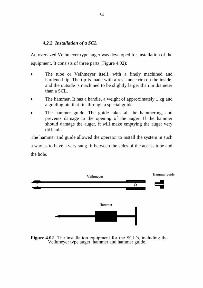
84
4.2.2 Installation of a SCL
An oversized Veihmeyer type auger was developed for installation of the
equipment. It consists of three parts (Figure 4.02):
The tube or Veihmeyer itself, with a finely machined and
hardened tip. The tip is made with a resistance rim on the inside,
and the outside is machined to be slightly larger than in diameter
than a SCL.
The hammer. It has a handle, a weight of approximately 1 kg and
a guiding pin that fits through a special guide
The hammer guide. The guide takes all the hammering, and
prevents damage to the opening of the auger. If the hammer
should damage the auger, it will make emptying the auger very
difficult.
The hammer and guide allowed the operator to install the system in such
a way as to have a very snug fit between the sides of the access tube and
the hole.
Figure 4.02 The installation equipment for the SCL’s, including the Veihmeyer type auger, hammer and hammer guide.
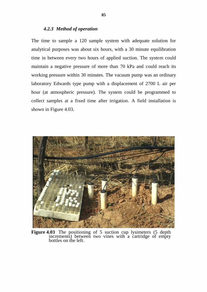
85
4.2.3 Method of operation
The time to sample a 120 sample system with adequate solution for
analytical purposes was about six hours, with a 30 minute equilibration
time in between every two hours of applied suction. The system could
maintain a negative pressure of more than 70 kPa and could reach its
working pressure within 30 minutes. The vacuum pump was an ordinary
laboratory Edwards type pump with a displacement of 2700 L air per
hour (at atmospheric pressure). The system could be programmed to
collect samples at a fixed time after irrigation. A field installation is
shown in Figure 4.03.
Figure 4.03 The positioning of 5 suction cup lysimeters (5 depth increments) between two vines with a cartridge of empty bottles on the left.
86
4.2.4 Measuring the relative matrix potential.
As a control measure, an extra SCL was connected to the system but not
installed in the soil. It is simply placed in a bottle half filled with water.
This SCL would not have any obstruction in sampling water and the
bottle would always be the fullest, indicating the physical upper limit of
this sampling event. The relative volumes of soil water sampled,
indicated the matrix potential at all sampling positions. Thus both the
volume and quality of all samples were important to be registered.
4.3 Summary
The new SCL was designed and successfully implemented during years
of field research. Our SCL had the advantage that it could be operated
remotely. This allowed sampling at precisely planned times and provided
added value in years of monitoring and managing soil salinity. Ease of
use is the main characteristic of this system. More details regarding the
results were given in Chapter 3.
The soil water samples could also supply information on the soil water
content by just recording the mass. This system is fairly inexpensive and
if one should choose between different management systems, this
research approach can supply more information than conventional SCL’s.
The system could always be left in a ready mode and could therefore
easily be activated whenever necessary. Since the system allows remote
operation, a lot of time was saved in acquiring data.
87
5 PREDICTION OF THE DEPTH TREND IN SOIL
SALINITY OF A VINEYARD AFTER SUSTAINED
IRRIGATION WITH SALINE WATER3.
ABSTRACT
Remote sensing combined with an ability to look deeper than the soil
surface is currently high in demand. This study was conducted through
scaling down on the amount of soil data from a saline irrigation water
experiment to see if one can still capture the essential soil salinity depth-
trends within the data, to a level that can enhance the ability of remote
methods. A saline irrigation experiment with 6 water qualities was
conducted for 8 years on 1.2 ha of vineyard land near Robertson in the
Western Cape Province of South Africa. Soil water was sampled at
regular intervals at 5 depths between 0.15 and 1.2 m with suction cup
lysimeters at a fixed time following each irrigation. Electrical
conductivity of the soil water (ECsw) was determined after sampling. Data
collected over the full 8 year period were investigated for depth trends in
ECsw, seeking trend lines with lowest polynomial order that were still
significantly predict the salinity profile. At all treatment levels a first
order polynomial equation, fitted to the salinity profiles, significantly
predicted the salinity trends.
3 Published in:
de Clercq, W.P., Van Meirvenne, M., Fey, M.V., 2008. Prediction of the depth trend
in soil salinity of a vineyard after sustained irrigation with saline water.
Agricultural Water Managment. In press, doi:10.1016/j.agwat.2008.09.002.
88
The ECsw value at only two depths could therefore be used to calculate
total salt accumulation and soil water quality below the root zone. The
implication is that considerable value can be obtained from minimal
measurements both in estimating salt accumulation in the soil profile and
predicting water quality in return flow from saline irrigation.
5.1 Introduction
There are scant reports on soil water salinity dynamics in response to
saline irrigation, especially concerning the seasonal variation in electrical
conductivity of the soil water (ECsw) as a function of depth. Amongst
others, Rhoades et al. (1997), Cetin (2003), de Clercq and Van
Meirvenne (2005) and Douaik et al. (2006) have all emphasised the
importance of spatial and temporal changes in soil salinity and the effect
on return-flow water-quality when use is made of low quality irrigation
water. In such studies, soil salinity is generally reported as an integrated
value for the whole profile.
In many countries sustained irrigation with poor quality water is
commonly practised and requires close monitoring and control of soil
salinity both at the regional and field scales to minimise the adverse
effects on production and impacts on downstream users (Odeh et al.,
1998; Kelleners and Chaudhry, 1998; Kotb et al., 2000; Görgens and de
Clercq, 2004). Rapid assessment of soil salinity is becoming increasingly
important for managerial purposes. Salinity depth trends were
investigated after sustained irrigation for sugar cane (Nelson and Ham,
2000), winter wheat (Sharma and Rao, 1998) and rice (Mondala et al.,
2001). For vineyards, de Clercq et al. (2001) reported on the effects of
89
poor quality irrigation and posed the following list of questions that
should be considered when considering irrigation quality:
Does the farmer use refined scheduling techniques?
Do the advantages of partial wetting of the soil apply?
What is the salt tolerance of the crop?
Does the salt content of the marketable product matter?
What is the length of season for the crop?
What is the typical rooting volume of the crop?
Under saline conditions, should crops be selected with the
smallest possible rooting volume?
What is the quality of the receiving waters?
Perssons and Uvo (2002) are amongst others, indicated that, the electrical
conductivity measured alone or where for instance time domain
reflectometry was used to measure to soil water content and bulk
electrical conductivity, a very complicated approach to link soil water EC
with other measured parameters. Perssons and Uvo (2002) is perhaps also
the most recent example of the complicated situation arising when soil
water EC is measured at a range of soil water content values for different
soils. These are all at non-saturated conditions. The ability to use these
values for any predictions depends on the accuracy of two infield-
measured parameters and the calibration of the individual sensors. These
measurements can be of great value when plant reaction to soil water EC
needs to be tested between irrigations but to compare results between
different locations and different instruments becomes quite a daunting
task. de Clercq et al. (2001) showed that the cumulative effect of bad
irrigation water quality on vines could be adequately described using a
single set of soil water measurements taken after each irrigation event,
90
when the soil water content was still at field water capacity. These soil
water samples, extracted from the soil using micro lysimetry, were then
analysed using a single laboratory EC probe. This method then allowed
for easier comparison between infield measurements done at different
depths and locations and different soil types. Using the extracted soil
water at field capacity also has the added advantage that it can be directly
related to the quality of the water that moved through the soil. Once
evaporation from the soil surface starts and the plant starts to utilise some
of the water, the downward movement of water stops and the ECsw starts
to change, as salts are concentrated in the remaining soil water.
Modern devices, such as the electromagnetic induction sensor EM38,
used for routine monitoring of soil salinity, are limited in their ability to
make measurements over the entire soil profile. Shi et al. (2006)
indicated that they could successfully map coastal sandy soils for
reclamation using hyperspectral remote sensing; however, their study
applied only to soil surface conditions. On the other hand, Zhu et al.
(2006) developed a knowledge based system for predicting grain yield
taking into account all possible conditions affecting wheat growth,
including soil type and soil depth parameters. If these two approaches
could be combined, the possibility of predicting subsoil conditions
remotely seems attainable. Farifteh and Farshad (2002) emphasized the
need to be able to detect and model soil properties from remotely sensed
sources. They listed some possibilities of how to be able to tell more
about subsoil conditions, in particular soil salinity, from remotely sensed
information. They indicated that imaging spectrometry provides large
volumes of high resolution spectral data, which can be useful to detect
soil properties. They further indicated that a next step would be to link
modelled soil processes using existing models (for example SWAP and
91
CropSyst) to this hyperspectral information base, to model subsoil
conditions and the fate of salinity in the landscape.
Metternicht and Zinck (2003) indicated some constraints on the use of
remote sensing data in a review article. They stated that monitoring soil
salinity cannot be achieved from remote sensing data alone, and requires
a solid synergy between remote sensing data, field observations and
laboratory determinations as sources of data, and GIS capabilities for
processing, transforming and displaying the data. They further concluded
that the best results are obtained when integrating remote sensing data
with field and laboratory data and that it is the researcher’s challenge to
identify the most adequate salinity indicators for a particular area, so that
appropriate ground and remote sensing techniques can be applied to
extract information in an accurate and cost-effective manner. Lesch et al.
(1995) attempted the link between satellite imagery and EM38
interpreted soil salinity information using multiple linear regression
models and found, after successful modelling, that they could reduce the
sampling density and still retain the prediction accuracy inherent in their
statistical calibration techniques, also facilitating assessment
methodology that can be applied in a rapid, practical, and cost-effective
manner.
This chapter strives to indicate means of revealing more about irrigated
subsoil conditions when using remotely sensed information. For that
purpose, it is important to indicate and define subsoil conditions that lend
itself to a higher degree of predictability and define a starting point for
modelling of this nature. Therefore, a basis needs to be established for
making the best use of relatively meagre information about the salinity
depth function. To achieve this goal, the approach posed by Davis (1986)
92
was used. This implied using a F-test (Tables 5.01 and 5.02) coupled
with trend surface theory (Davis 1986, pp. 405-422) to find trend lines
with the highest significance and with the lowest possible polynomial
order. The procedure aims to solve curvilinear regressions or trend
surfaces in the simplest possible way and the idea was developed before
computers became widely available. The choice of a polynomial
expression is normally governed by the goal of achieving the highest
degree of goodness-of-fit and higher order polynomials are more
successful at this, since they encompass the lower order forms (Mondala
et al., 2001). However, higher order polynomials require more parameters
to be fit and therefore they are more data demanding. Frequently by
making use of an adjusted R2-value, deviation from the trend surface and
the degrees of freedom, the decision for using a lower order polynomial
also becomes evident. Therefore, for small data sets, lower order
polynomials are usually more realistic (Lesch et al., 1995; Forsberg and
Nilsson, 2005).
The knowledge base for modelling soil salinity is however well
established and similarly the methodology for mapping features of the
topsoil from remote sources. The linkup between the two, that could
allow us to know more about the soil from the interpretation of remotely
sensed information, is currently fuzzy. The objective of this chapter
therefore is to examine soil-depth salinity-trends after prolonged
irrigation of a vineyard with different salt concentrations, and to find the
simplest basis for calculating salt accumulation and return flow water
quality from a limited number of measurements that could also be
detected remotely.
93
5.2 Materials and methods
This saline irrigation experiment was carried out for eight years (from
1991 till 1998) in a vineyard near Robertson in the Western Cape
Province, South Africa (Figure 2.02, central coordinates 33°49'29.03"S
and 19°52'44.77"E). The experimental layout was fully described in
Chapter 3 and will therefore not be repeated here.
This is a predominantly winter rainfall region, which ensured that there
was negligible interference in the water balance by rainfall during the
summer months when most of the irrigation was applied. The average
total amount of irrigation applied during summer was 600 mm and the
combined winter rainfall and winter irrigation was aimed at 600 mm.
During winter, rain was supplemented with irrigation to promote
leaching of salts and ensure the success of a cover crop (de Clercq et al.,
2001).
Irrigation was systematically applied in the afternoon of each Wednesday
and suction sampling was initiated 12 hours after irrigation had
terminated, to ensure that the soil water status was effectively at field
capacity. Over the 8 year duration of the experiment at least 12 annual
sets of suction cup data were successfully collected, with 7 to 9 of these
being collected during the irrigation season and the remainder during
winter (de Clercq et al., 2001).
94
5.2.1 Data analysis
Trend surface analysis, as described by Davis (1986), was used to
analyse the seasonal soil salinity distribution with depth. In this
procedure the order of the polynomial expressions, fitted to the ECsw
data (Z) plotted as a function of time (X) and depth (Y) for each
treatment, was raised successively to establish the polynomial with the
lowest order that was still significant.
To simplify the trend surface routine and to extend this as a statistical
decision base tool, an algorithm was developed in Basic programming
language, which determines the coefficients (b0, b1, b2) relating X, Y and
Z to each other for n observations and calculates the F-test results as
shown in Tables 5.01 and 5.02, up to a 3rd
order polynomial, based on the
following the three so-called normal equations (Davis, 1986):
5.01 .Eq YbXbnbZ 210
5.02 .Eq XYbXbXbXZ 2
2
10
5.03 .Eq 2
210 YbXYbYbYZ
Having derived these coefficients, the position of Z on a linear surface
trend (i.e. ECsw as a function of depth and time) can be predicted. The
goodness of fit of this surface trend can be calculated from the total sum
of squares (SSt) and the sums of squares resulting from the trend surface
(SSr), and the deviation from the trend surface (SSa), where
5.04 .Eq SSa = SSt – SSr
and the goodness of fit is then calculated as
95
5.05 .Eq SSt
SSrR 2
with R2 being a multiple synonym for the R
2 used in linear regression.
Using Eq. 5.04 in 5.05, R2 can be rewritten as:
5.06 .Eq SSt
SSa
SSt
SSrR 12
Because R2 is enhanced by increasing the order of the polynomial
describing the trend surface, it has doubtful value for decision making.
Therefore an adjusted R2*
was adopted, which is calculated in terms of
SSa in Eq. 5.06 and not SSr in Eq. 5.05, and then corrected for degrees of
freedom (df),
5.07 .Eq
1
1)1(1
1.
11 2
1
*2
kn
nR
n
SSt
kn
SSaR
where the numerator terms n-1 and n-k-1 are the df, in which n is the
number of observations and k is the number of regression coefficients
ignoring b0 (Davies, 1986).
The most important argument for using trend surface analysis in the
current context lies in the test for significance (F-test, Tables 5.01 and
5.02). The significance of the specific trend was tested through an
analysis of variance or ANOVA (Table 5.01). The degrees of freedom
used (df minus b0) were 2 for the 1st order polynomial, 5 for the 2
nd order
and 9 for the 3rd
order. The test for significance was then applied and
compared for surface trends of different order in an expanded ANOVA
(Table 5.02). For each increase in order the significance of the increase
was also tested. The expanded ANOVA in Table 5.02 consisted of three
variance analyses, each with its own F value.
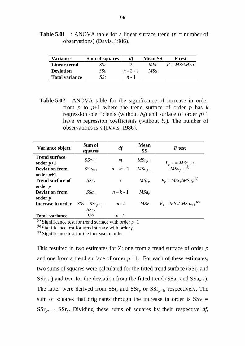
96
Table 5.01 : ANOVA table for a linear surface trend (n = number of
observations) (Davis, 1986).
Variance Sum of squares df Mean SS F test
Linear trend SSr 2 MSr F = MSr/MSa
Deviation SSa n - 2 - 1 MSa
Total variance SSt n - 1
Table 5.02 ANOVA table for the significance of increase in order
from p to p+1 where the trend surface of order p has k
regression coefficients (without b0) and surface of order p+1
have m regression coefficients (without b0). The number of
observations is n (Davis, 1986).
Variance object Sum of
squares df
Mean
SS F test
Trend surface
order p+1 SSrp+1 m MSrp+1
Fp+1 = MSrp+1/
MSap+1 (a)
Deviation from
order p+1
SSap+1 n – m - 1 MSap+1
Trend surface of
order p
SSrp k MSrp Fp = MSrp/MSap (b)
Deviation from
order p
SSap n – k - 1 MSap
Increase in order SSv = SSrp+1 -
SSrp
m - k MSv Fv = MSv/ MSap+1 (c)
Total variance SSt n - 1 (a)
Significance test for trend surface with order p+1 (b)
Significance test for trend surface with order p (c)
Significance test for the increase in order
This resulted in two estimates for Z: one from a trend surface of order p
and one from a trend surface of order p+ 1. For each of these estimates,
two sums of squares were calculated for the fitted trend surface (SSrp and
SSrp+1) and two for the deviation from the fitted trend (SSap and SSap+1).
The latter were derived from SSt, and SSrp or SSrp+1, respectively. The
sum of squares that originates through the increase in order is SSv =
SSrp+1 - SSrp. Dividing these sums of squares by their respective df,
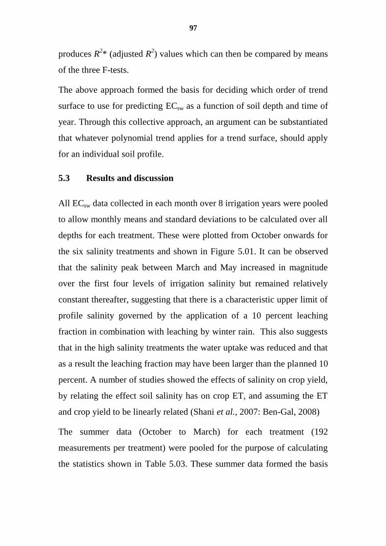
97
produces R2* (adjusted R
2) values which can then be compared by means
of the three F-tests.
The above approach formed the basis for deciding which order of trend
surface to use for predicting ECsw as a function of soil depth and time of
year. Through this collective approach, an argument can be substantiated
that whatever polynomial trend applies for a trend surface, should apply
for an individual soil profile.
5.3 Results and discussion
All ECsw data collected in each month over 8 irrigation years were pooled
to allow monthly means and standard deviations to be calculated over all
depths for each treatment. These were plotted from October onwards for
the six salinity treatments and shown in Figure 5.01. It can be observed
that the salinity peak between March and May increased in magnitude
over the first four levels of irrigation salinity but remained relatively
constant thereafter, suggesting that there is a characteristic upper limit of
profile salinity governed by the application of a 10 percent leaching
fraction in combination with leaching by winter rain. This also suggests
that in the high salinity treatments the water uptake was reduced and that
as a result the leaching fraction may have been larger than the planned 10
percent. A number of studies showed the effects of salinity on crop yield,
by relating the effect soil salinity has on crop ET, and assuming the ET
and crop yield to be linearly related (Shani et al., 2007: Ben-Gal, 2008)
The summer data (October to March) for each treatment (192
measurements per treatment) were pooled for the purpose of calculating
the statistics shown in Table 5.03. These summer data formed the basis
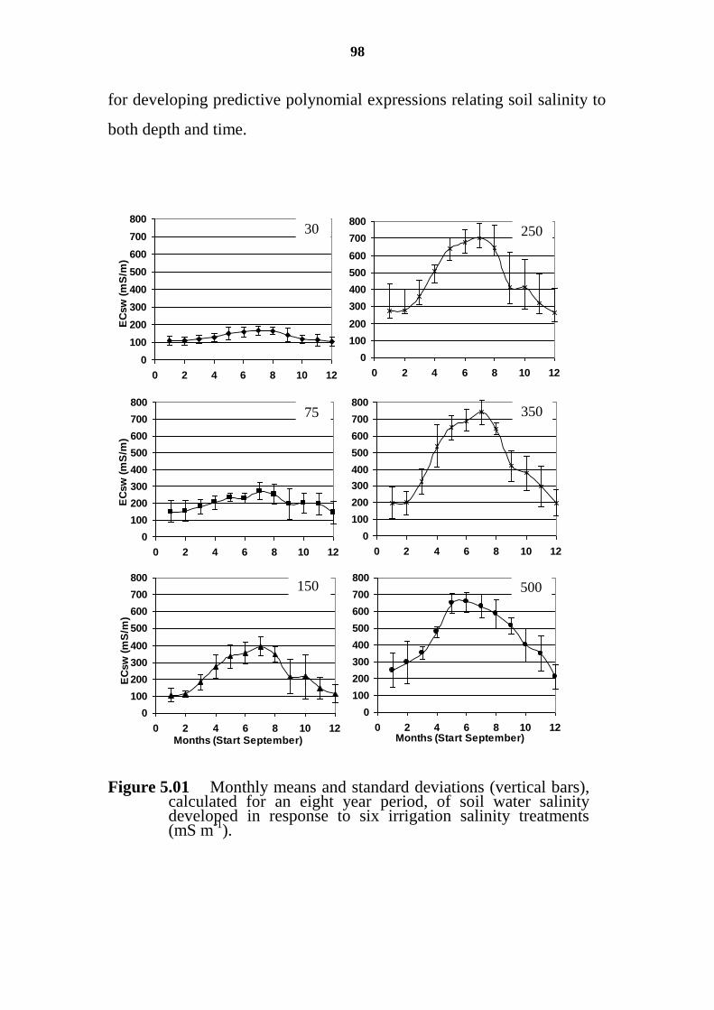
98
for developing predictive polynomial expressions relating soil salinity to
both depth and time.
1
0
100
200
300
400
500
600
700
800
0 2 4 6 8 10 12
EC
sw
(m
S/m
)
3
0
100
200
300
400
500
600
700
800
0 2 4 6 8 10 12Months (Start September)
EC
sw
(m
S/m
)
4
0
100
200
300
400
500
600
700
800
0 2 4 6 8 10 12
5
0
100
200
300
400
500
600
700
800
0 2 4 6 8 10 12
6
0
100
200
300
400
500
600
700
800
0 2 4 6 8 10 12Months (Start September)
2
0
100
200
300
400
500
600
700
800
0 2 4 6 8 10 12
EC
sw
(m
S/m
)
Figure 5.01 Monthly means and standard deviations (vertical bars), calculated for an eight year period, of soil water salinity developed in response to six irrigation salinity treatments (mS m
-1).
30
75
150
250
350
500
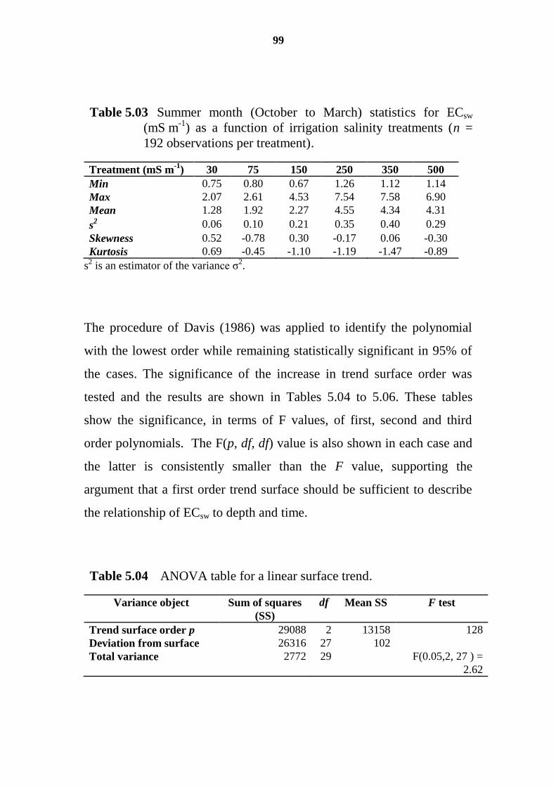
99
Table 5.03 Summer month (October to March) statistics for ECsw
(mS m-1
) as a function of irrigation salinity treatments (n =
192 observations per treatment).
Treatment (mS m-1
) 30 75 150 250 350 500
Min 0.75 0.80 0.67 1.26 1.12 1.14
Max 2.07 2.61 4.53 7.54 7.58 6.90
Mean 1.28 1.92 2.27 4.55 4.34 4.31
s2
0.06 0.10 0.21 0.35 0.40 0.29
Skewness 0.52 -0.78 0.30 -0.17 0.06 -0.30
Kurtosis 0.69 -0.45 -1.10 -1.19 -1.47 -0.89
s2 is an estimator of the variance σ
2.
The procedure of Davis (1986) was applied to identify the polynomial
with the lowest order while remaining statistically significant in 95% of
the cases. The significance of the increase in trend surface order was
tested and the results are shown in Tables 5.04 to 5.06. These tables
show the significance, in terms of F values, of first, second and third
order polynomials. The F(p, df, df) value is also shown in each case and
the latter is consistently smaller than the F value, supporting the
argument that a first order trend surface should be sufficient to describe
the relationship of ECsw to depth and time.
Table 5.04 ANOVA table for a linear surface trend.
Variance object Sum of squares
(SS)
df Mean SS F test
Trend surface order p 29088 2 13158 128
Deviation from surface 26316 27 102
Total variance 2772 29 F(0.05,2, 27 ) =
2.62
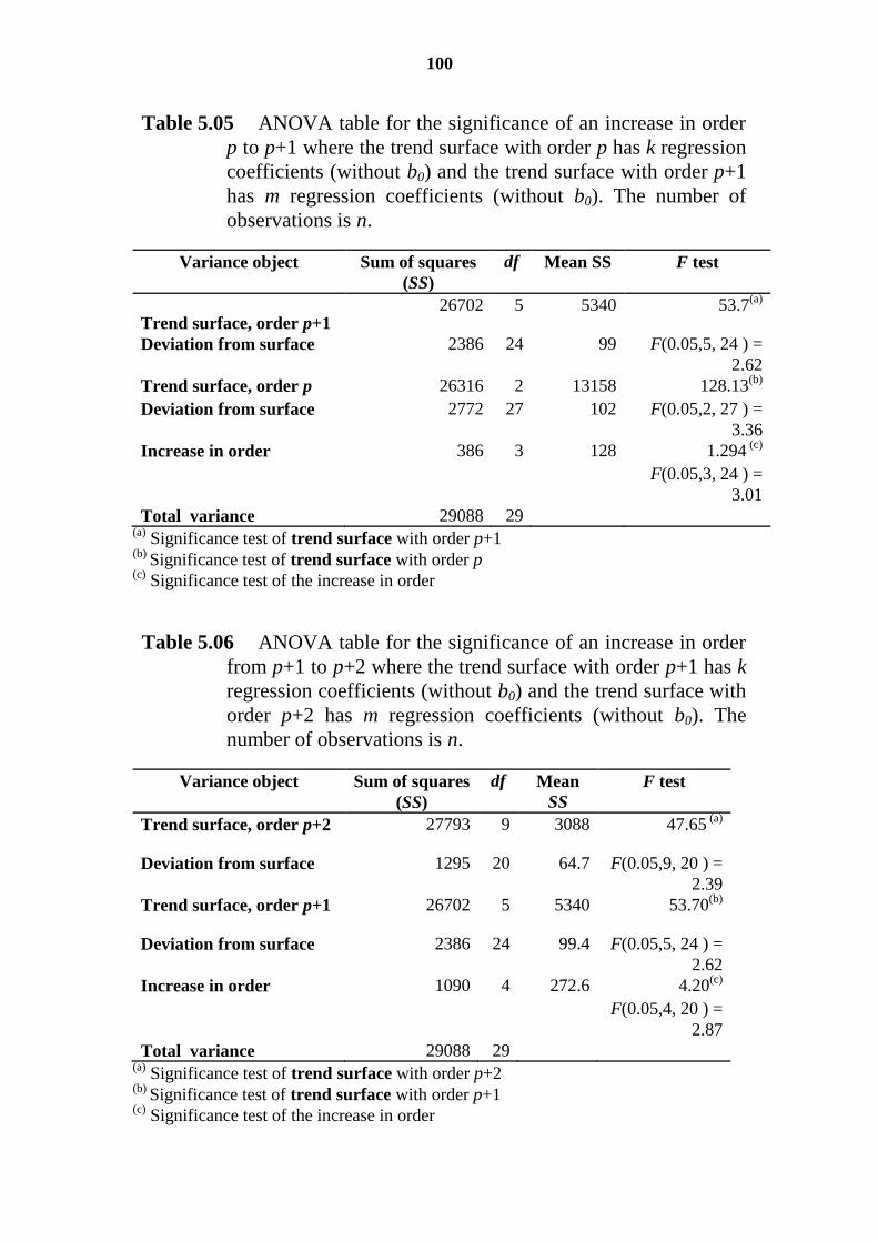
100
Table 5.05 ANOVA table for the significance of an increase in order
p to p+1 where the trend surface with order p has k regression
coefficients (without b0) and the trend surface with order p+1
has m regression coefficients (without b0). The number of
observations is n.
Variance object Sum of squares
(SS)
df Mean SS F test
Trend surface, order p+1 26702 5 5340 53.7
(a)
Deviation from surface 2386 24 99 F(0.05,5, 24 ) =
2.62
Trend surface, order p 26316 2 13158 128.13(b)
Deviation from surface 2772 27 102 F(0.05,2, 27 ) =
3.36
Increase in order 386 3 128 1.294 (c)
F(0.05,3, 24 ) =
3.01
Total variance 29088 29 (a)
Significance test of trend surface with order p+1 (b)
Significance test of trend surface with order p (c)
Significance test of the increase in order
Table 5.06 ANOVA table for the significance of an increase in order
from p+1 to p+2 where the trend surface with order p+1 has k
regression coefficients (without b0) and the trend surface with
order p+2 has m regression coefficients (without b0). The
number of observations is n.
Variance object Sum of squares
(SS)
df Mean
SS
F test
Trend surface, order p+2 27793 9 3088 47.65 (a)
Deviation from surface 1295 20 64.7 F(0.05,9, 20 ) =
2.39
Trend surface, order p+1 26702 5 5340 53.70(b)
Deviation from surface 2386 24 99.4 F(0.05,5, 24 ) =
2.62
Increase in order 1090 4 272.6 4.20(c)
F(0.05,4, 20 ) =
2.87
Total variance 29088 29 (a)
Significance test of trend surface with order p+2 (b)
Significance test of trend surface with order p+1 (c)
Significance test of the increase in order
101
The trend surfaces representing first, second and third order polynomials
were mapped for all six treatments in Figure 6.02 (the surfaces are
salinity contours, the shading intensity of which is proportional to the
salinity degree). Figure 5.02 indicates that the salinisation tendency as
summer progresses from October to March was strongest at depth in the
low salinity treatments but was more uniformly distributed through the
soil profile in response to more saline treatments. Since only five depth
intervals were sampled, fitting a polynomial higher than the first order
for a single sampling event would probably correspond to over-
interpretation. In Figure 5.02, treatments 150 and 350 mS m-1
showed
differences in the general trends compared with the other treatments.
These differences were associated with lower infiltration rates, as part of
these treatments were affected by ancient termite nests, causing different
soil water behavioural patterns. Regardless of the latter, the way in which
trend surface analysis was applied, combined the parameters of space and
time in the test. Therefore the different sampling points in the landscape
showed similar behaviour.
102
-12
-10
-8
-6
-4
-2
-12
-10
-8
-6
-4
-2
23
1 2 3
75
-12
-10
-8
-6
-4
-2
-12
-10
-8
-6
-4
-2
-12
-10
-8
-6
-4
-2
1 2 3 4 5 6-12
-10
-8
-6
-4
-2
1 2 3 4 5 61 2 3 4 5 6
150
250
350
500
Months: October(1) to March (6)
Treatment mS/m
Polynomial order
mS/m
100
200
300
400
500
600
700
800
Figure 5.02 Trend surfaces represented by contours of soil water salinity (ECsw) in relation to time in early summer and depth of soil in plots treated with six levels of irrigated salinity over eight years. Graph columns from left to right are based on the 1
st , 2
nd and 3
rd order polynomials as applied to the time to
depth ECsw relationships.
Table 5.07 shows the changes in both R2 and R
2* with increasing
polynomial order as was applied to the p, p+1 and p+2. It is clear that the
103
difference in R2 values has shrunk considerably by using the adjusted R
2
to such an extent that there is almost no difference between p and p+1.
Table 5.07 R2 and the adjusted R
2* for the three trend orders.
Order R2 R
2* R
2 - R
2*
p first 0.905 0.898 0.007
p+1 second 0.918 0.901 0.017
p+2 third 0.955 0.935 0.020
Due to the significance displayed in the first order polynomial above
(Table 5.04), it should be possible to describe salinisation of the soil
profile during an irrigation season on the basis of only two measurement
depths (preferably conveniently shallow). This could enable quick
estimation whether over- or under-irrigation has occurred and whether
salt accumulation has taken place below the root zone. This can be
indicated by knowing the gradient (m) of the first order polynomial. To
determine which two monitoring depths are most suitable, the data were
subjected to an analysis in which depth trend lines for each time interval
were calculated from ECsw measurements at two pairs of shallower
depths (either 15 and 60 cm or 30 and 60 cm). The gradients of these EC
depth trend lines were then compared with the gradients of EC lines
derived from EC measurements at all five depths in Table 5.08.
Therefore, the regression between the gradients derived from situation 1
(Table 5.08) and gradients derived from the 5 depth trend lines, produced
a R2 of 0.51 and a highly significant p0.005 value of 0.0034. But,
regressing the general soil ECsw-profile from situation 2 (Table 5.08),
with the 5 depth trend line gradients, produced a better R2 value of 0.89
and a p0.005 value of 0.0001. This shows that in about 9 out of 10 cases
tested, an increase or decrease of ECsw at a soil depth of 120 cm could be
104
predicted with confidence by looking at ECsw data from only two depth
increments in the upper soil. The reason that the 0-15 cm depth showed a
poorer result could possibly be related to the fact that ameliorants were
added shortly before sampling or salt accumulated on the soil surface as
an evaporite. The third depth increment, namely the 30-60 cm depth,
proved to be the region where the bulk of the roots were situated and
therefore where most soil water was taken up by the plant (de Clercq et
al., 2001). It is clear that the predictive accuracy increases when the soil
surface layer is avoided but the data for depth increment combination,
situation 3 in Table 5.08, show that inclusion of the A-horizon in the
prediction still produced a useful result. This demonstrates that the use of
an instrument such as the EM38 electromagnetic induction sensor could
be of great value in predicting salinity depth trends in irrigated
agriculture.
Table 5.08 A regression between the gradient values of the 1st order
polynomials derived from ECsw at selected depth increments
and from slope values derived from ECsw at all 5 depth
increments for situations 1 to 3.
Situation ECsw at
depths (cm)
Regression equation
(Y= ECsw, X=depth) R
2 p 0.005
1 0-15, 30-60 Y = 0.435X + 0.469 0.51 0.0034
2 15-30,30- 60 Y = 0.482X + 0.546 0.89 0.0001
3 0-30, 30-60 Y = 0.402X + 0.526 0.65 0.0001
A further step was to test the extent to which the ECsw below the root
zone could be predicted using information based on measurements at the
centre of the root zone. The resulting prediction is shown in Table 5.09,
where the ECsw at 120 cm depth was predicted using the ECsw values at
the 15-30cm and 30-60cm depth. The result as indicted in Table 5.09 is
highly significant in predicting the quality of the water that would drain
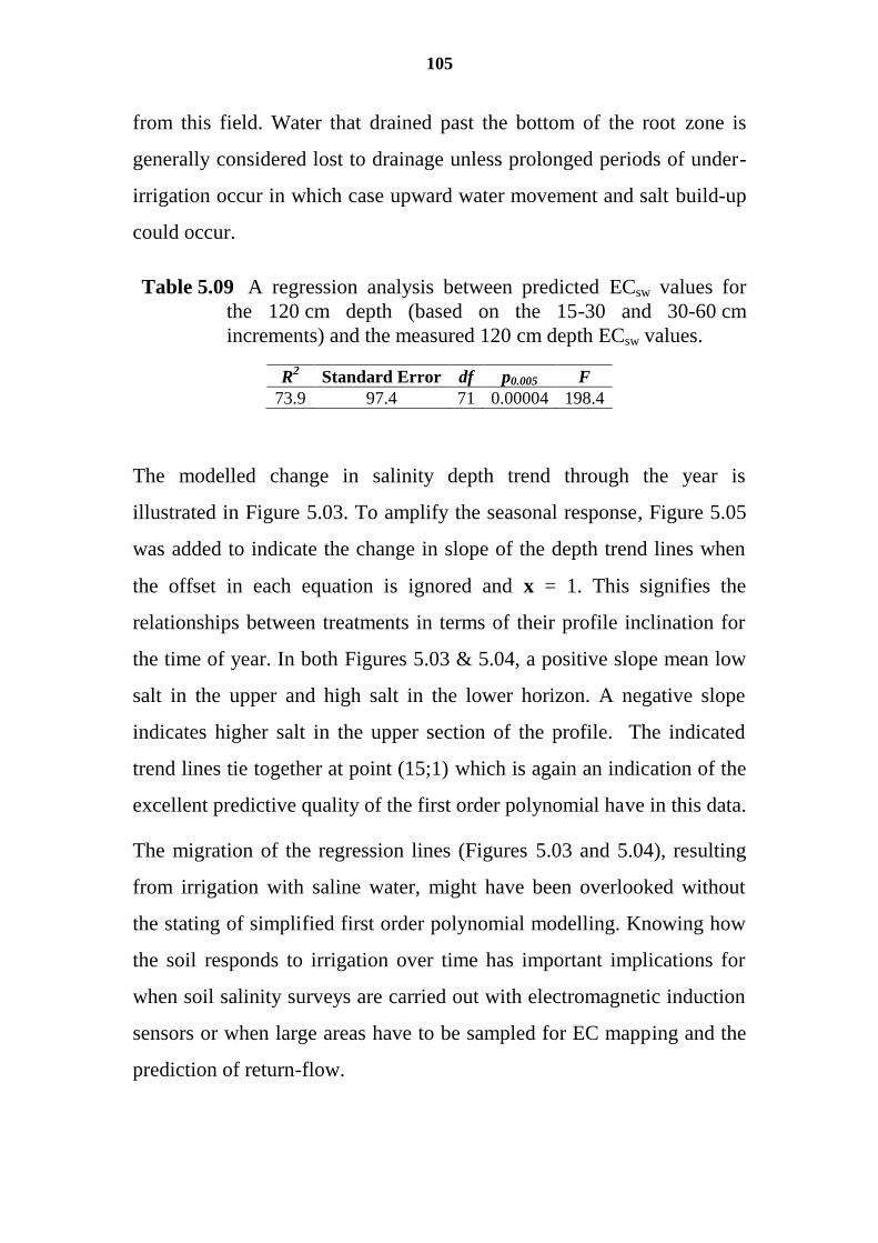
105
from this field. Water that drained past the bottom of the root zone is
generally considered lost to drainage unless prolonged periods of under-
irrigation occur in which case upward water movement and salt build-up
could occur.
Table 5.09 A regression analysis between predicted ECsw values for
the 120 cm depth (based on the 15-30 and 30-60 cm
increments) and the measured 120 cm depth ECsw values.
R2 Standard Error df p0.005 F
73.9 97.4 71 0.00004 198.4
The modelled change in salinity depth trend through the year is
illustrated in Figure 5.03. To amplify the seasonal response, Figure 5.05
was added to indicate the change in slope of the depth trend lines when
the offset in each equation is ignored and x = 1. This signifies the
relationships between treatments in terms of their profile inclination for
the time of year. In both Figures 5.03 & 5.04, a positive slope mean low
salt in the upper and high salt in the lower horizon. A negative slope
indicates higher salt in the upper section of the profile. The indicated
trend lines tie together at point (15;1) which is again an indication of the
excellent predictive quality of the first order polynomial have in this data.
The migration of the regression lines (Figures 5.03 and 5.04), resulting
from irrigation with saline water, might have been overlooked without
the stating of simplified first order polynomial modelling. Knowing how
the soil responds to irrigation over time has important implications for
when soil salinity surveys are carried out with electromagnetic induction
sensors or when large areas have to be sampled for EC mapping and the
prediction of return-flow.
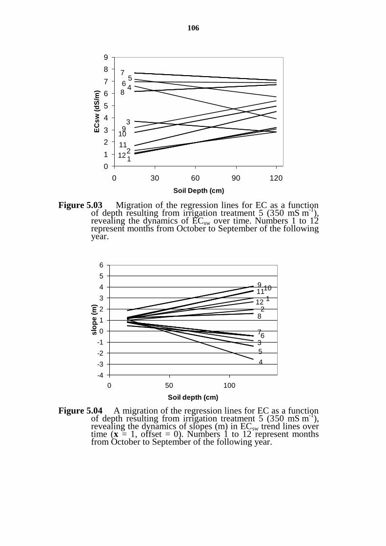
106
0
1
2
3
4
5
6
7
8
9
0 30 60 90 120
Soil Depth (cm)
EC
sw
(d
S/m
)
75
48
39
10
112
121
6
Figure 5.03 Migration of the regression lines for EC as a function of depth resulting from irrigation treatment 5 (350 mS m
-1),
revealing the dynamics of ECsw over time. Numbers 1 to 12 represent months from October to September of the following year.
-4
-3
-2
-1
0
1
2
3
4
5
6
0 50 100
Soil depth (cm)
slo
pe
(m
)
4
5
3
76
8
12
11109
2
1
Figure 5.04 A migration of the regression lines for EC as a function of depth resulting from irrigation treatment 5 (350 mS m
-1),
revealing the dynamics of slopes (m) in ECsw trend lines over time (x = 1, offset = 0). Numbers 1 to 12 represent months from October to September of the following year.
107
Apart from using electromagnetic induction sensors, by knowing the
date, irrigation water quality and being able to remotely measure the
topsoil EC, estimation of both the subsoil salinity conditions becomes
possible.
5.4 Conclusions
Soil scientists often focus on unnecessary detail regarding soils and their
behaviour. This study provided an opportunity to better understand the
temporal and spatial variation of ECsw by using a simplified approach.
The classical trend surface analysis procedure of Davis provided an
answer to the problem of finding a suitable depth relationship that could
be used as a norm for the soil studied. This simplified the management of
salt in the soil and the quantity and quality of return flow.
Prediction of the depth trend in ECsw with a first order polynomial has
distinct advantages. Over- or under-irrigation can easily be evaluated for
any irrigated land. Prediction of salt accumulation on the soil surface or
deep drainage can readily be assessed. The slope of the first order
polynomial indicates directly the general trend and whether an
accumulation or a depletion of salt can be expected in the soil. When
linked to remote sensing, the approach described here could be used in
evaluating extensive areas of land in terms of salinity and their suitability
for irrigated crops.
Lastly, this research further showed that by knowing the date and
irrigation water quality and being able to characterize the topsoil EC
remotely, one can estimate subsoil salinity conditions in irrigated lands
and further estimate the return-flow component from such irrigated lands.
108
6 EXPLORING THE VARIABILITY OF ECe
BETWEEN VINE ROWS
6.1 Introduction
Soil water samples could not be taken routinely with SCL’s between the
vine rows as this would have hampered traffic and soil tillage. Winter
wheat is normally sown and used as a cover crop for lowering
evapotranspiration from the soil surface during the summer, as the
stubble is left, acting as a soil blanket. The cover crop also has a large
influence on the distribution of salts in the inter-row region as it
minimises evaporation from the soil surface (Figure 6.01). The driving
force behind the accumulation of salt near and on the soil surface in the
inter-row region is therefore modified. It could be expected that in a
region where a cover crop was used, that more water would have been
available for leaching in comparison to a site where no cover crop was
used. Furthermore, the successful establishment of a following year’s
cover crop is dependent on the amount of salt in this top soil, implying
that less salt ensures more successful germination and better growth. This
concept therefore had a large influence on the amount of evaporation
from the soil surface. It thus also had a profound influence on the salt
gradient found between the row position and the inter-row position (Du
Toit, 1995).
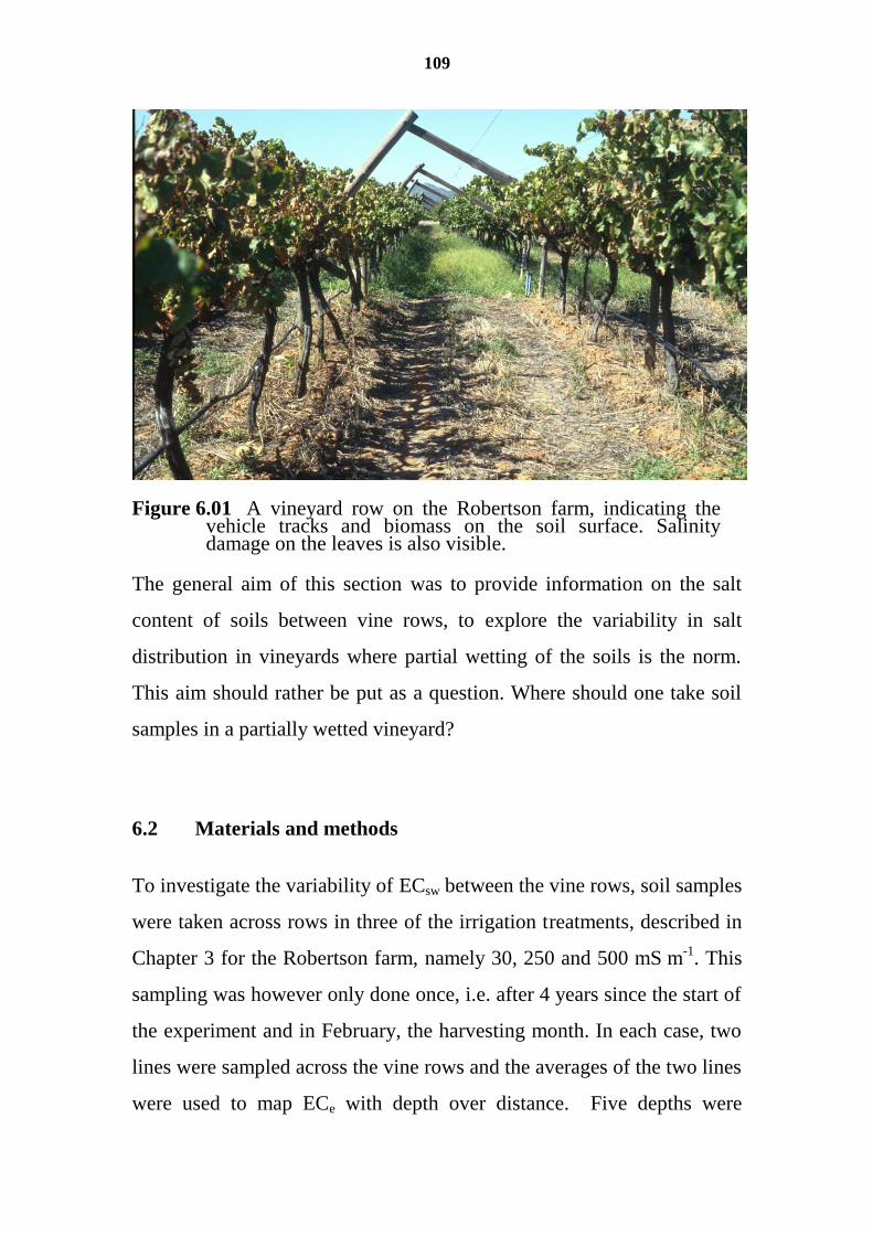
109
Figure 6.01 A vineyard row on the Robertson farm, indicating the vehicle tracks and biomass on the soil surface. Salinity damage on the leaves is also visible.
The general aim of this section was to provide information on the salt
content of soils between vine rows, to explore the variability in salt
distribution in vineyards where partial wetting of the soils is the norm.
This aim should rather be put as a question. Where should one take soil
samples in a partially wetted vineyard?
6.2 Materials and methods
To investigate the variability of ECsw between the vine rows, soil samples
were taken across rows in three of the irrigation treatments, described in
Chapter 3 for the Robertson farm, namely 30, 250 and 500 mS m-1
. This
sampling was however only done once, i.e. after 4 years since the start of
the experiment and in February, the harvesting month. In each case, two
lines were sampled across the vine rows and the averages of the two lines
were used to map ECe with depth over distance. Five depths were

110
sampled (15, 30, 60, 90 and 120 cm) in 9 positions across the vine rows
at a 0.5 m interval (Du Toit, 1996; Moolman et al., 1999).
To map the soil profile data, an omni-directional linear semi-variogram
model was used to interpret the ECe data using ordinary kriging of all the
observations (Webster and Oliver, 2007). Figures were generated with
the program Surfer™.
6.3 Results and discussion
The interpolated ECe is given in Figure 6.02 for the control treatment
(ECi = 30 mS m-1
) at harvest time (February 1996). A similar
presentation is given in Figure 6.03 for ECi = 250 mS m-1
and Figure
6.04 for the 500 mS m-1
.
As the treatment ECi increased over Figures 6.02 to 6.04, the hotspot in
the profile changed from deep (Figure 6.02) to the surface (Figure 6.04).
This shift is most likely due to the difference in surface cover and the
differential amount of water used by the vines between the treatments. It
is also apparent that the salt accumulation shown in Figures 6.03 and
7.04 is in the vicinity of the vehicle tracks. These tracks (Figure 6.03, at
the 1 and 2 m marks), being small furrows and more compacted than the
surrounding soil, possibly led to poorer growing conditions for the cover
crop and also created a larger capillary continuity to the lower soil layers
which aided evaporation and therefore deposition of salts. It was also
observed that the cover crop was less effective in the higher treatments as
a result of poorer growth.
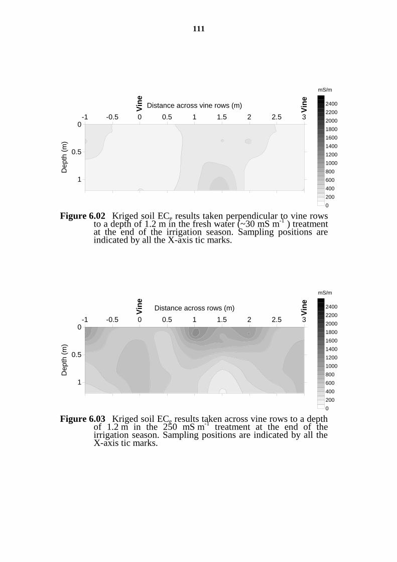
111
Vin
e
0
200
400
600
800
1000
1200
1400
1600
1800
2000
2200
2400
0
0.5
1
Depth
(m
)
-1 -0.5 0 0.5 1 1.5 2 2.5 3
Distance across vine rows (m)
mS/m
Vin
e
Figure 6.02 Kriged soil ECe results taken perpendicular to vine rows to a depth of 1.2 m in the fresh water (~30 mS m
-1 ) treatment
at the end of the irrigation season. Sampling positions are indicated by all the X-axis tic marks.
Vin
e
0
200
400
600
800
1000
1200
1400
1600
1800
2000
2200
2400
0
0.5
1
Depth
(m
)
-1 -0.5 0 0.5 1 1.5 2 2.5 3
Distance across rows (m)
mS/m
Vin
e
Figure 6.03 Kriged soil ECe results taken across vine rows to a depth of 1.2 m in the 250 mS m
-1 treatment at the end of the
irrigation season. Sampling positions are indicated by all the X-axis tic marks.
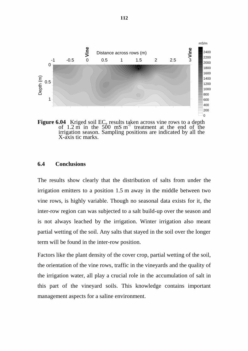
112
Vin
e
0
0.5
1
De
pth
(m
)
-1 -0.5 0 0.5 1 1.5 2 2.5 3
Distance across rows (m)
0
200
400
600
800
1000
1200
1400
1600
1800
2000
2200
2400
mS/m
Vin
e
Figure 6.04 Kriged soil ECe results taken across vine rows to a depth of 1.2 m in the 500 mS m
-1 treatment at the end of the
irrigation season. Sampling positions are indicated by all the X-axis tic marks.
6.4 Conclusions
The results show clearly that the distribution of salts from under the
irrigation emitters to a position 1.5 m away in the middle between two
vine rows, is highly variable. Though no seasonal data exists for it, the
inter-row region can was subjected to a salt build-up over the season and
is not always leached by the irrigation. Winter irrigation also meant
partial wetting of the soil. Any salts that stayed in the soil over the longer
term will be found in the inter-row position.
Factors like the plant density of the cover crop, partial wetting of the soil,
the orientation of the vine rows, traffic in the vineyards and the quality of
the irrigation water, all play a crucial role in the accumulation of salt in
this part of the vineyard soils. This knowledge contains important
management aspects for a saline environment.

113
The results shown here suggest various points to consider when research
is being conducted in saline soils as well as management options for
saline environments. These are as follows:
that salt could be stored during summer preventing the
contamination of river water,
during winter, when more fresh water is available, salts could be
leached gradually and
it is also important to know that where partial wetting of the soils
is the norm, the position where soil samples are taken, needs to be
very carefully considered as the variation across vine rows is
always more variable than along vine rows. Samples should be
taken both in between (max salinity) as well as in the vine rows
(minimal salinity).
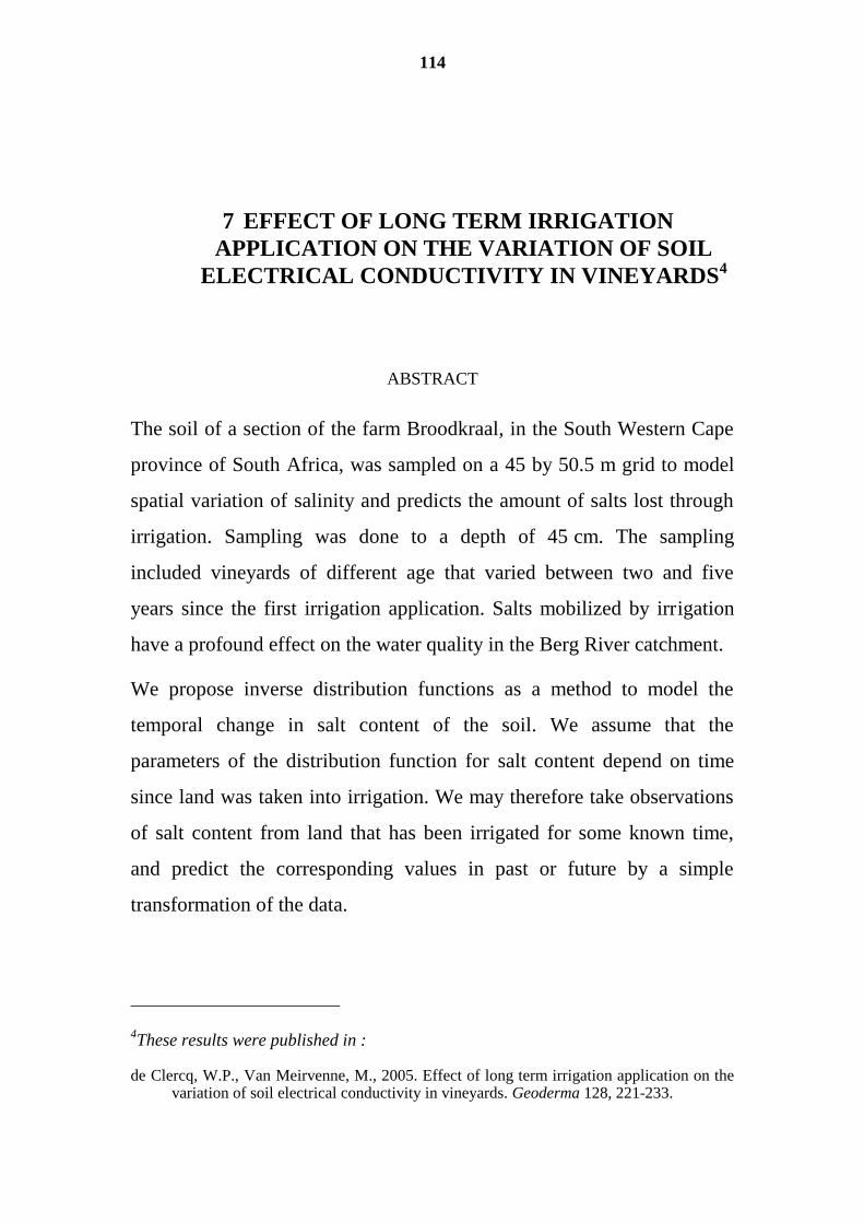
114
7 EFFECT OF LONG TERM IRRIGATION
APPLICATION ON THE VARIATION OF SOIL
ELECTRICAL CONDUCTIVITY IN VINEYARDS4
ABSTRACT
The soil of a section of the farm Broodkraal, in the South Western Cape
province of South Africa, was sampled on a 45 by 50.5 m grid to model
spatial variation of salinity and predicts the amount of salts lost through
irrigation. Sampling was done to a depth of 45 cm. The sampling
included vineyards of different age that varied between two and five
years since the first irrigation application. Salts mobilized by irrigation
have a profound effect on the water quality in the Berg River catchment.
We propose inverse distribution functions as a method to model the
temporal change in salt content of the soil. We assume that the
parameters of the distribution function for salt content depend on time
since land was taken into irrigation. We may therefore take observations
of salt content from land that has been irrigated for some known time,
and predict the corresponding values in past or future by a simple
transformation of the data.
4These results were published in :
de Clercq, W.P., Van Meirvenne, M., 2005. Effect of long term irrigation application on the variation of soil electrical conductivity in vineyards. Geoderma 128, 221-233.
115
To test this hypothesis we undertook a second sampling campaign on
sections of the farm irrigated for the same length of time as two of our
original data sets. We showed that temporal variability of the distribution
functions of all data was more substantial than the spatial variability
between data sets on land irrigated for the same period of time.
It is clear that the general lowering of ECe over time caused the variance
to reduce. The comparison of variograms showed that the use of only one
variogram model to krige the total landscape might result in an over
simplification of the young irrigated surfaces while it complicated the
older ones. Any mapping of ECe aimed over larger areas should therefore
take cognisance of the irrigation age and the sampling frequency should
be increased for younger or non-irrigated surfaces.
Finally, the results were used to estimate the yearly salt return to the Berg
River.
7.1 Introduction
The Berg River system supplies about 80 % of the water used by Cape
Town. This implies that water is being removed from this catchment
leaving less of the natural flow within the BRC. The BRC covers an area
of about 12000 km2 of which about 50 % can be considered as
potentially suitable for irrigation although only about 8 % of this land is
currently under irrigation. The Berg River is an open system implying
that both fresh water and all return flow runs in the same stream. Görgens
and de Clercq (2002) determined that a total of 30 % of the irrigation
116
water returns to the river as a combination of surface runoff and shallow
(below the root zone) subsurface return flow.
The quality of the return flow water is determined by the salinity status of
the soil being irrigated and the path length to the river. The river water is
still generally of good quality, having an ECe of below 50 mS m-1
.
Moolman et al. (1999) and de Clercq et al. (2001) found grapevines to be
totally sensitive to salinity even at irrigation water quality of below 30
mS m-1
. They also proposed an irrigation water quality upper limit of 75
mS m-1
, which means that the current irrigation water quality is
acceptable.
A variety of water supply expansion schemes are proposed to meet the
growing needs of users in the catchment, resulting in the extraction of
20% more water from the Berg River system. These developments may
exacerbate moderate salinity levels in the middle-lower Berg River as a
result of the utilization of more fresh water from the river during
summer, the saline return flow will increase and the capacity of the
system to dilute this increase for users downstream will be reduced. This
study aims to explain the influence of irrigated agriculture on salinization
of river water in the Berg River system. A better understanding of this
aspect of river water quality will allow improved management of the
system and more accurate prediction of the outcome of expanding
irrigation in the catchment. Due to the vastness of the area and the
restricted availability of good quality data, catchment-scale modelling is
usually done using sparse data with unreliable geographical positioning.
A vineyard was identified where differences in age since first irrigation
could be sampled in one large block. The problem is thus defined by a 60
ha piece of land, which consisted of one soil type mainly, that was
117
initially very saline and was irrigated with low salinity water for up to 4
years. The aim of this project was to use data from a single sampling
event, taken over an area that included irrigation blocks of different age
since development, to estimate the annual salt mass leached (de Clercq et
al., 2001). Usually when soil sampling is repeated often enough, repeated
detailed mapping of the soil electrical conductivity (saturated paste
extract, ECe), allows insight in soil EC change over time (or the salt
flux). Within this study, time is a variable and by using time in the
prediction, the amount of salt leached from this landscape could be
calculated.
As new land is being earmarked for irrigation development, one must be
able to calculate or predict the influence of irrigation return flow on the
quality of the river water. This meant modelling and predicting the
expected soil response as land-use changes from non-irrigated
wheatlands to irrigated vineyards (de Clercq et al., 2001). The problem
was how to use results with differences in age from neighbouring plots
and how to use the time relationship to quantify or predict the lowering
of salinity in the landscape as a result of irrigation. No literature could be
found that addressed this problem specifically. The effect time had on the
data (between the different blocks) will therefore be illustrated using
their cumulative distribution functions (cdf). By using the probability
(derived from the cdf) of all age groups and all ECe values, the expected
change in ECe of any specific point can be predicted using the inverse
cumulative distribution functions (icdf) for a specific year.
Characterizing the temporal variation in spatially adjacent vineyards that
occurred primarily as a result of irrigation then becomes possible. The
proposed method allows prediction of return flow salinity from the
decline in the landscape salinity without having to model runoff through
118
a conventional intricate 3 dimensional modelling routine. The hypothesis
is thus that temporal change can be expressed as a change in cdf
explicitly. The accuracy to which the method applies to plots outside of
this study area will render the hypothesis true or false.
Methodology of this nature can be beneficial in modelling seasonal
return flow over large areas or catchments since the method is based on
the variation in the landscape depending on ECe over time and differs
from others found in literature in that space-time research is usually
reported involving the same space but with time that varies (Bourgault et
al., 1998; Cetin and Kirda, 2003; Lesch et al., 1998; Rhoades et al.,
1997; Utset et al., 1999).
7.2 Methods and materials.
7.2.1 The experimental site
The study area is located in the Berg River catchment in the Western
Cape province of South Africa, close to the town of Piketberg (Figure
7.01). There is no infrastructure in terms of water supply to the farm
other than moderate quality control of the water in the Berg River itself.
Most soils are naturally saline and there is concern that large-scale
expansion of irrigation activities might adversely affect the water supply
in the river, triggering a situation where management of the quality of the
river water can soon drain the reserves from the supply dams. Most of
this area receives precipitation lower than 300 mm per year, most of
which falls in winter. Currently the quality of the water in the Berg River
is being manipulated from the three major fresh water dams in the
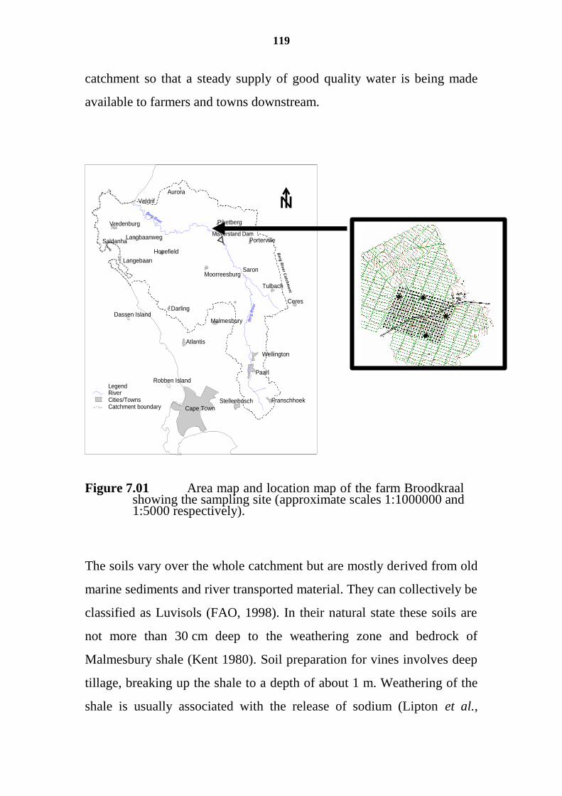
119
catchment so that a steady supply of good quality water is being made
available to farmers and towns downstream.
Berg River
Be
rg R
iver
Be
rg R
ive
r Ca
tch
me
nt
Stellenbosch
Cape Town
Atlantis
Malmesbury
Wellington
Paarl
Tulbach
Ceres
SaronMoorreesburg
Piketberg
Porterville
Hopefield
Langebaan
Saldanha
Vredenburg
Langbaanweg
Veldrif
Aurora
DarlingDassen Island
Robben Island
Franschhoek
Misverstand Dam
LegendRiverCities/TownsCatchment boundary
Figure 7.01 Area map and location map of the farm Broodkraal showing the sampling site (approximate scales 1:1000000 and 1:5000 respectively).
The soils vary over the whole catchment but are mostly derived from old
marine sediments and river transported material. They can collectively be
classified as Luvisols (FAO, 1998). In their natural state these soils are
not more than 30 cm deep to the weathering zone and bedrock of
Malmesbury shale (Kent 1980). Soil preparation for vines involves deep
tillage, breaking up the shale to a depth of about 1 m. Weathering of the
shale is usually associated with the release of sodium (Lipton et al.,
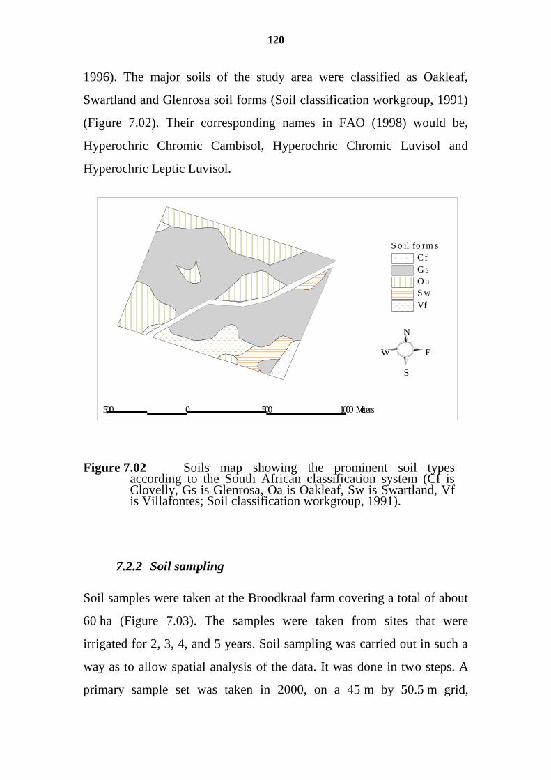
120
1996). The major soils of the study area were classified as Oakleaf,
Swartland and Glenrosa soil forms (Soil classification workgroup, 1991)
(Figure 7.02). Their corresponding names in FAO (1998) would be,
Hyperochric Chromic Cambisol, Hyperochric Chromic Luvisol and
Hyperochric Leptic Luvisol.
Figure 7.02 Soils map showing the prominent soil types according to the South African classification system (Cf is Clovelly, Gs is Glenrosa, Oa is Oakleaf, Sw is Swartland, Vf is Villafontes; Soil classification workgroup, 1991).
7.2.2 Soil sampling
Soil samples were taken at the Broodkraal farm covering a total of about
60 ha (Figure 7.03). The samples were taken from sites that were
irrigated for 2, 3, 4, and 5 years. Soil sampling was carried out in such a
way as to allow spatial analysis of the data. It was done in two steps. A
primary sample set was taken in 2000, on a 45 m by 50.5 m grid,
S o i l f o r m s
C f
G s
O a
S w
V f
5 0 0 0 5 0 0 1 0 0 0 M e t e r s
S
N
E W
121
generating 15 by 21 (315) sample positions. To enable the description of
the soil variability over a range of lag distances, 3 sets of 12 samples
were taken randomly within 4 of these grid units. Twenty six positions
that fell on roads and an old gypsum storage site were omitted, leaving a
total number of 325 points included in the analysis. A second sample set
was taken in 2001, to the south and west of the primary set, to allow
adequate room to test the method that was developed (Figure 7.08). The
latter was done on a 90 by 101 m grid. The two blocks were 4 year and 5
year old sites and provided the opportunity to test the methodology by
using the icdf of the original 4 year and 5 year old sites to predict the
values of the second set.
The soil sampling technique entailed a pooled sample of three micro-
positions within a vine row to minimise the effect of micro-irrigation
induced variation in salinity on a finer scale. Two depth increments were
sampled: 0 cm to15 cm and 15 cm to 45 cm. The reason for this was that
45 cm was generally considered to be the median depth of the root zone
and the 0 cm to 15 cm depth increment was seen as contaminated with
undissolved fertilizer or gypsum and needed to be separated. All soil
samples were air-dried, ground and passed through a 2-mm sieve. These
samples were analysed for ECe (Richards, 1954).
7.2.3 Statistical analysis
In analysing the data, one was confronted with the problem of how to
move from point support to block support in soil process modelling.
Heuvelink and Pebesma (1999) proposed a route from point support to
block support: first interpolate, then run the soil process model (in this
case statistical modelling of the ECe change with time) and lastly
aggregate the results. This approach is true in most circumstances where
122
only one site is under consideration that was resampled over a certain
time span. This dataset consisted of a single sampling event but with 4
subdivisions that has different ages in terms of its irrigation history.
Therefore, it was proposed to first perform the time modelling for the
different age blocks on the original data, i.e., on the original support, and
then do the interpolation on the time adjusted results. Temporal
modelling is in this case done through application of the collective
tendency in aging of the vineyards. Four new datasets could therefore be
derived for each of the different plots, representing 4 years in the life of
each plot individually, derived with a method that did not generate bias.
Variography was used to characterise the variance, and kriging was used
to map the original and derived datasets for each block. Lastly, through
aggregation, predictions regarding the amounts of salt lost from this 15 to
45 cm depth horizon were obtained (Chilès and Delfiner, 1999;
Goovaerts, 1997; Isaacs and Srivastava, 1989; Webster and Oliver,
2007).
The proposed process can be summarised as follows:
Deriving the time sequence for each plot.
Variography of the data for each year.
Interpolate the combined yearly data.
Derive the salt discharge over time.
Histograms and descriptive statistics were computed for the whole
dataset and for each of the four sectors in order to assess comparability of
the data despite not being equal in size. The use of cumulative
distribution functions (cdf’s) with a probability on the y-axis provided
the opportunity to compare the distribution differences irrespective of
sample size.
123
7.2.4 Temporal modelling
Cdf’s were developed for each year from the original support and their
resulting inverse cumulative distribution functions (icdf’s) were used to
generate the temporal data. The STATISTICA software was used for the
purpose of modelling cdf and icdf’s. Various types of cdf’s were tested in
search of the most suitable function. The lognormal function provided
the best fit for ECe data, which is in accordance with Lark (2000),
Rhoades et al. (1997) and Webster (2001). Cdf’s and its applications
were also described by amongst others Isaacs and Srivastava (1989) and
Rhoades et al. (1997) as a method to present ECe data. The method is
also used in comparing ECe data with apparent ECe data obtained from
electro-magnetic induction readings. Icdf’s and their predictive
capabilities were tested on the second dataset, sampled in 2001.
The lognormal cdf applied was of the form presented in Eq. 7.01 and its
inverse function in Eq. 7.03.
7.01 .Eq ft(x) = }22/2})log({e.
5.0)2(
1
x
x
= p
with 0 < x < ∞ , μ > 0, s > 0, and where t stands for time, is the scale
parameter and the mean of ln(x), is the shape parameter and the
standard deviation of ln(x), e is the base of the natural logarithm and
lastly, p is the probability as a frequency. In short Eq. 7.01 is expressed
as:
7.02 .Eq ft(x) = ILognorm(x,, )
The inverse lognormal function or icdf was used for this back-transform.
With this action the probability data are transformed back to original data
and is given as:
124
7.03 .Eq Loginverse (p,,) = e[+ x [Normal inverse (p)]]
In short, Eq. 7.03 is expressed as:
7.04 .Eq x = Loginverse (p,,) = Loginverse (ft(x),,)
For all data the ft(x) from Eq. 7.01 was calculated as a probability derived
from the actual data. To transform the data to another year, the icdf for
that year was used to transform the probability values. In other words, in
ft(x), t was replaced with (t + n), where n can be between – 3 and 3 as
follows:
7.05 .Eq xt = Loginv (p(t+n),,) = Loginv (f(t+n)(x),,)
Back transformation of data using Eq. 7.05 has no effect on the spatial
pattern of the data even if back transformation is done through an icdf of
another year. This is brought about by the fact that the dataset is
rearranged in an order of magnitude when the cdf is calculated. With
back transformation, a p-value is matched to an x-value that has the same
geographical position as the original x-value, but the size of x was
influenced. It is therefore only the magnitude of the original x-values that
change and not position.
7.2.5 Variograms and kriging
The variogram models for the raw and transformed data were generated
using Variowin software (Deutch and Journel, 1992). The theory applied
in terms of modelling the variance and the kriging used in this chapter
were extensively discussed in Chapter 3 and will therefore not be
repeated here. Variograms were calculated for the 1996 raw data and
only for the 3 sets of back transformed data based on the 1996 site.
125
Ordinary point kriging was used (Isaacs and Srivastava, 1989; Goovaerts,
1997; Chilès and Delfiner, 1999; Webster and Oliver, 2007) only to
demonstrate the reconstructed change based on the 1996 site for the three
years that followed since 1996. By converting the ECe values to a salt
mass per pixel, the total amount of salt lost per site could be estimated by
subtracting modelled values from one year from the other in a GIS. To
have this information as GIS maps is important as return flow and runoff
modelling is done within GIS. It also serves the purpose of sensitising the
farmer toward his irrigation management and the ripple effect this has on
the environment and local economy.
7.3 Results and discussion
Two depth increments were sampled but only the deeper increment was
used for analysis, since it is less influenced by management. Since the 0
to 15 cm data also showed a similar trend than the 15 to 45 cm data, it
was decided to focus the modelling on the 15 to 45 cm data. The reason
for removing the top layer was that visible undissolved fertilizer could
affect the soil surface data.
The post map presented in Figure 7.03 presents both the relative ECe
magnitude of each sampled point and its position. A cluster of points in
the area (50,550) was omitted from the data as it was found later that this
spot was used to store gypsum. Inclusion of this data led to a strong
disturbance of the sample distribution. Figure 7.04 shows a histogram
with descriptive statistics for the 15 to 45 cm depth interval and Figure
7.05 shows the age separation statistics of the data split according to the
year of planting. The distributions seem quite similar when comparing
the coefficients of variation and the standard deviation. From Figure 7.03
and 8.05 it is clear that the average ECe of this section on the farm (249
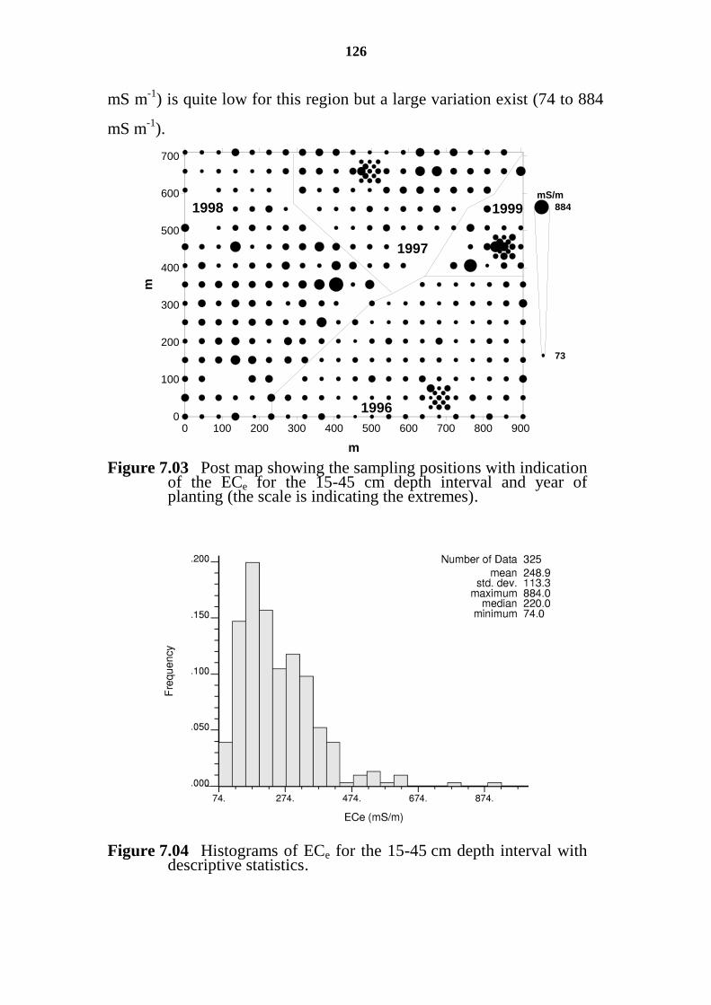
126
mS m-1
) is quite low for this region but a large variation exist (74 to 884
mS m-1
).
0 100 200 300 400 500 600 700 800 900
m
0
100
200
300
400
500
600
700m
1999
1996
1998
1997
884
73
mS/m
Figure 7.03 Post map showing the sampling positions with indication of the ECe for the 15-45 cm depth interval and year of planting (the scale is indicating the extremes).
Figure 7.04 Histograms of ECe for the 15-45 cm depth interval with descriptive statistics.
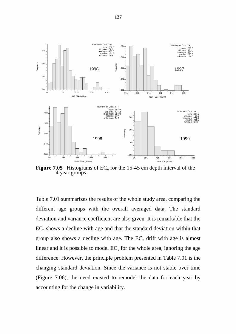
127
Figure 7.05 Histograms of ECe for the 15-45 cm depth interval of the 4 year groups.
Table 7.01 summarizes the results of the whole study area, comparing the
different age groups with the overall averaged data. The standard
deviation and variance coefficient are also given. It is remarkable that the
ECe shows a decline with age and that the standard deviation within that
group also shows a decline with age. The ECe drift with age is almost
linear and it is possible to model ECe for the whole area, ignoring the age
difference. However, the principle problem presented in Table 7.01 is the
changing standard deviation. Since the variance is not stable over time
(Figure 7.06), the need existed to remodel the data for each year by
accounting for the change in variability.
1996 1997
1998 1999
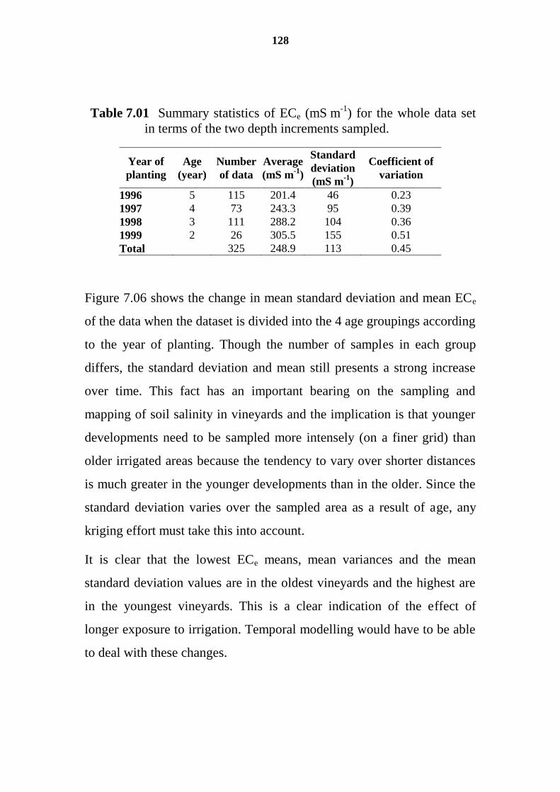
128
Table 7.01 Summary statistics of ECe (mS m-1
) for the whole data set
in terms of the two depth increments sampled.
Year of
planting
Age
(year)
Number
of data
Average
(mS m-1
)
Standard
deviation
(mS m-1
)
Coefficient of
variation
1996 5 115 201.4 46 0.23
1997 4 73 243.3 95 0.39
1998 3 111 288.2 104 0.36
1999 2 26 305.5 155 0.51
Total 325 248.9 113 0.45
Figure 7.06 shows the change in mean standard deviation and mean ECe
of the data when the dataset is divided into the 4 age groupings according
to the year of planting. Though the number of samples in each group
differs, the standard deviation and mean still presents a strong increase
over time. This fact has an important bearing on the sampling and
mapping of soil salinity in vineyards and the implication is that younger
developments need to be sampled more intensely (on a finer grid) than
older irrigated areas because the tendency to vary over shorter distances
is much greater in the younger developments than in the older. Since the
standard deviation varies over the sampled area as a result of age, any
kriging effort must take this into account.
It is clear that the lowest ECe means, mean variances and the mean
standard deviation values are in the oldest vineyards and the highest are
in the youngest vineyards. This is a clear indication of the effect of
longer exposure to irrigation. Temporal modelling would have to be able
to deal with these changes.
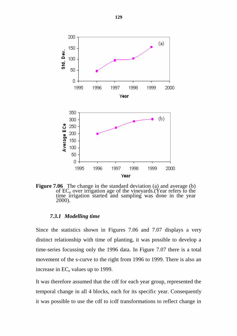
129
Figure 7.06 The change in the standard deviation (a) and average (b) of ECe over irrigation age of the vineyards.(Year refers to the time irrigation started and sampling was done in the year 2000).
7.3.1 Modelling time
Since the statistics shown in Figures 7.06 and 7.07 displays a very
distinct relationship with time of planting, it was possible to develop a
time-series focussing only the 1996 data. In Figure 7.07 there is a total
movement of the s-curve to the right from 1996 to 1999. There is also an
increase in ECe values up to 1999.
It was therefore assumed that the cdf for each year group, represented the
temporal change in all 4 blocks, each for its specific year. Consequently
it was possible to use the cdf to icdf transformations to reflect change in
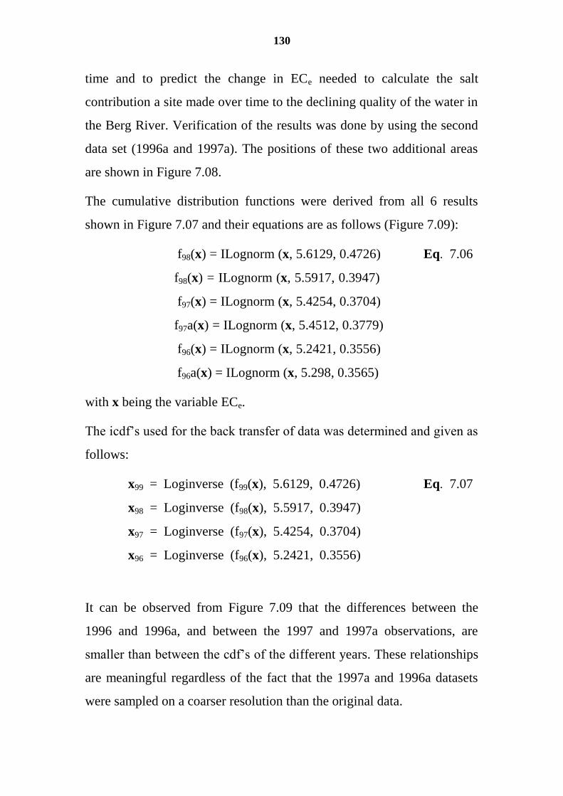
130
time and to predict the change in ECe needed to calculate the salt
contribution a site made over time to the declining quality of the water in
the Berg River. Verification of the results was done by using the second
data set (1996a and 1997a). The positions of these two additional areas
are shown in Figure 7.08.
The cumulative distribution functions were derived from all 6 results
shown in Figure 7.07 and their equations are as follows (Figure 7.09):
7.06 .Eq f98(x) = ILognorm (x, 5.6129, 0.4726)
f98(x) = ILognorm (x, 5.5917, 0.3947)
f97(x) = ILognorm (x, 5.4254, 0.3704)
f97a(x) = ILognorm (x, 5.4512, 0.3779)
f96(x) = ILognorm (x, 5.2421, 0.3556)
f96a(x) = ILognorm (x, 5.298, 0.3565)
with x being the variable ECe.
The icdf’s used for the back transfer of data was determined and given as
follows:
7.07 .Eq x99 = Loginverse (f99(x), 5.6129, 0.4726)
x98 = Loginverse (f98(x), 5.5917, 0.3947)
x97 = Loginverse (f97(x), 5.4254, 0.3704)
x96 = Loginverse (f96(x), 5.2421, 0.3556)
It can be observed from Figure 7.09 that the differences between the
1996 and 1996a, and between the 1997 and 1997a observations, are
smaller than between the cdf’s of the different years. These relationships
are meaningful regardless of the fact that the 1997a and 1996a datasets
were sampled on a coarser resolution than the original data.
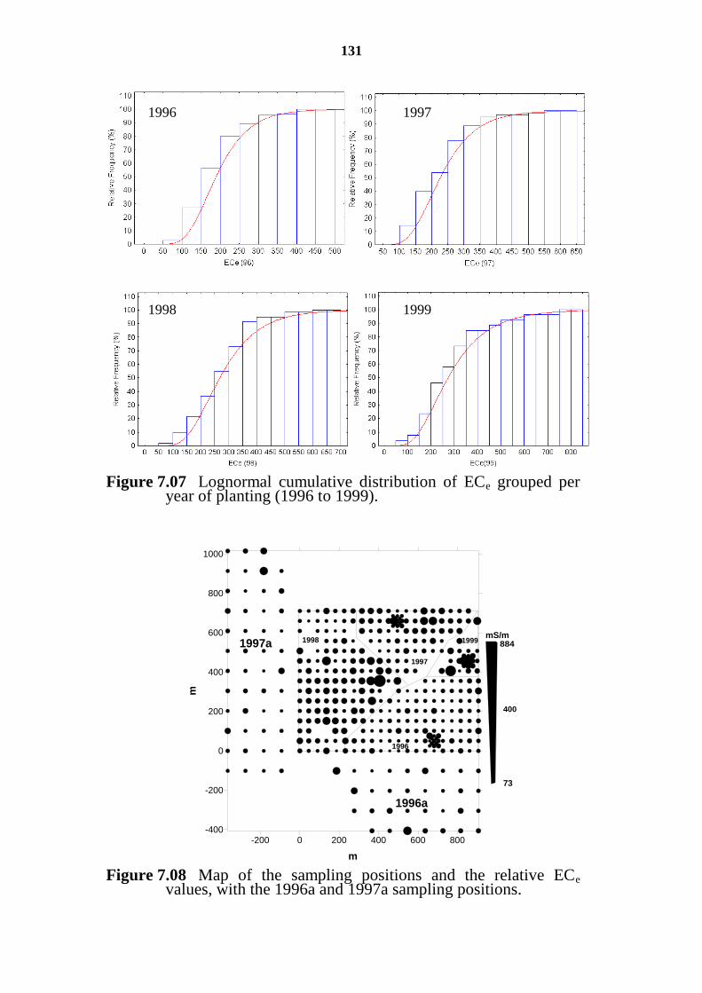
131
Figure 7.07 Lognormal cumulative distribution of ECe grouped per year of planting (1996 to 1999).
-200 0 200 400 600 800
m
-400
-200
0
200
400
600
800
1000
m
1997a
1996a
1999
1996
1998
1997
884
73
mS/m
400
Figure 7.08 Map of the sampling positions and the relative ECe values, with the 1996a and 1997a sampling positions.
1996 1997
1998 1999
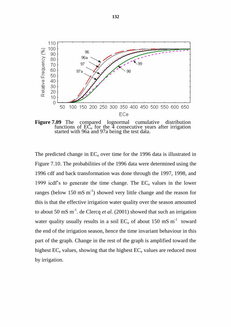
132
Figure 7.09 The compared lognormal cumulative distribution functions of ECe for the 4 consecutive years after irrigation started with 96a and 97a being the test data.
The predicted change in ECe over time for the 1996 data is illustrated in
Figure 7.10. The probabilities of the 1996 data were determined using the
1996 cdf and back transformation was done through the 1997, 1998, and
1999 icdf’s to generate the time change. The ECe values in the lower
ranges (below 150 mS m-1
) showed very little change and the reason for
this is that the effective irrigation water quality over the season amounted
to about 50 mS m-1
. de Clercq et al. (2001) showed that such an irrigation
water quality usually results in a soil ECe of about 150 mS m-1
toward
the end of the irrigation season, hence the time invariant behaviour in this
part of the graph. Change in the rest of the graph is amplified toward the
highest ECe values, showing that the highest ECe values are reduced most
by irrigation.
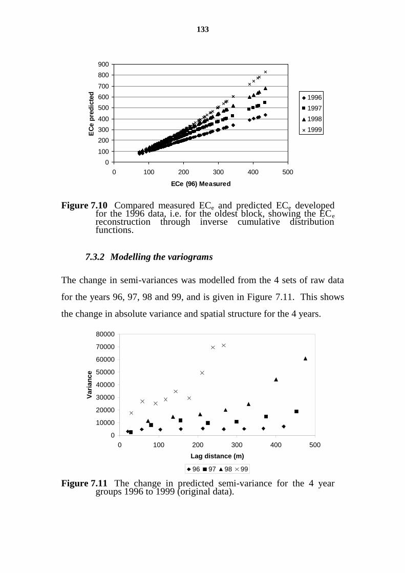
133
0
100
200
300
400
500
600
700
800
900
0 100 200 300 400 500
ECe (96) Measured
EC
e p
red
icte
d1996
1997
1998
1999
Figure 7.10 Compared measured ECe and predicted ECe developed for the 1996 data, i.e. for the oldest block, showing the ECe reconstruction through inverse cumulative distribution functions.
7.3.2 Modelling the variograms
The change in semi-variances was modelled from the 4 sets of raw data
for the years 96, 97, 98 and 99, and is given in Figure 7.11. This shows
the change in absolute variance and spatial structure for the 4 years.
0
10000
20000
30000
40000
50000
60000
70000
80000
0 100 200 300 400 500
Lag distance (m)
Va
ria
nc
e
96 97 98 99
Figure 7.11 The change in predicted semi-variance for the 4 year groups 1996 to 1999 (original data).
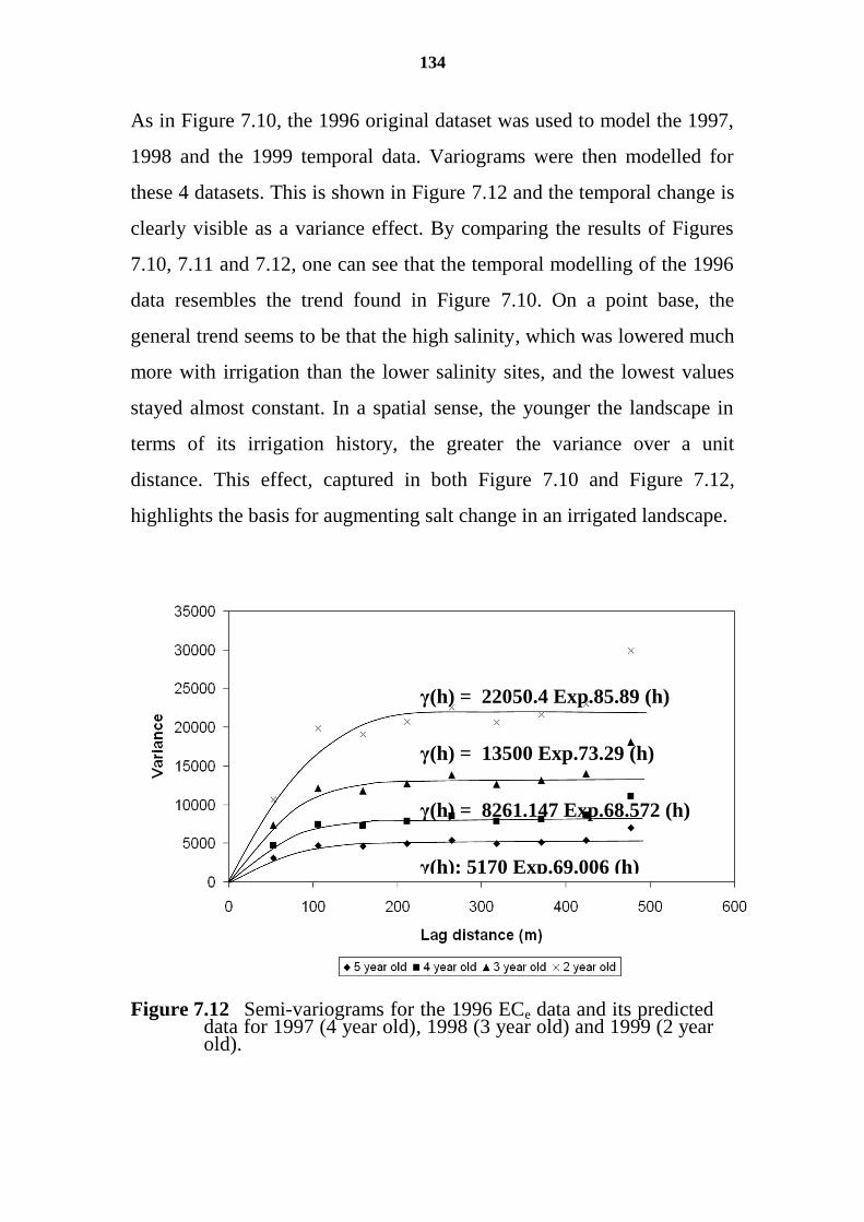
134
As in Figure 7.10, the 1996 original dataset was used to model the 1997,
1998 and the 1999 temporal data. Variograms were then modelled for
these 4 datasets. This is shown in Figure 7.12 and the temporal change is
clearly visible as a variance effect. By comparing the results of Figures
7.10, 7.11 and 7.12, one can see that the temporal modelling of the 1996
data resembles the trend found in Figure 7.10. On a point base, the
general trend seems to be that the high salinity, which was lowered much
more with irrigation than the lower salinity sites, and the lowest values
stayed almost constant. In a spatial sense, the younger the landscape in
terms of its irrigation history, the greater the variance over a unit
distance. This effect, captured in both Figure 7.10 and Figure 7.12,
highlights the basis for augmenting salt change in an irrigated landscape.
Figure 7.12 Semi-variograms for the 1996 ECe data and its predicted data for 1997 (4 year old), 1998 (3 year old) and 1999 (2 year old).
γ(h) = 22050.4 Exp.85.89 (h)
γ(h) = 13500 Exp.73.29 (h)
γ(h) = 8261.147 Exp.68.572 (h)
γ(h): 5170 Exp.69.006 (h)
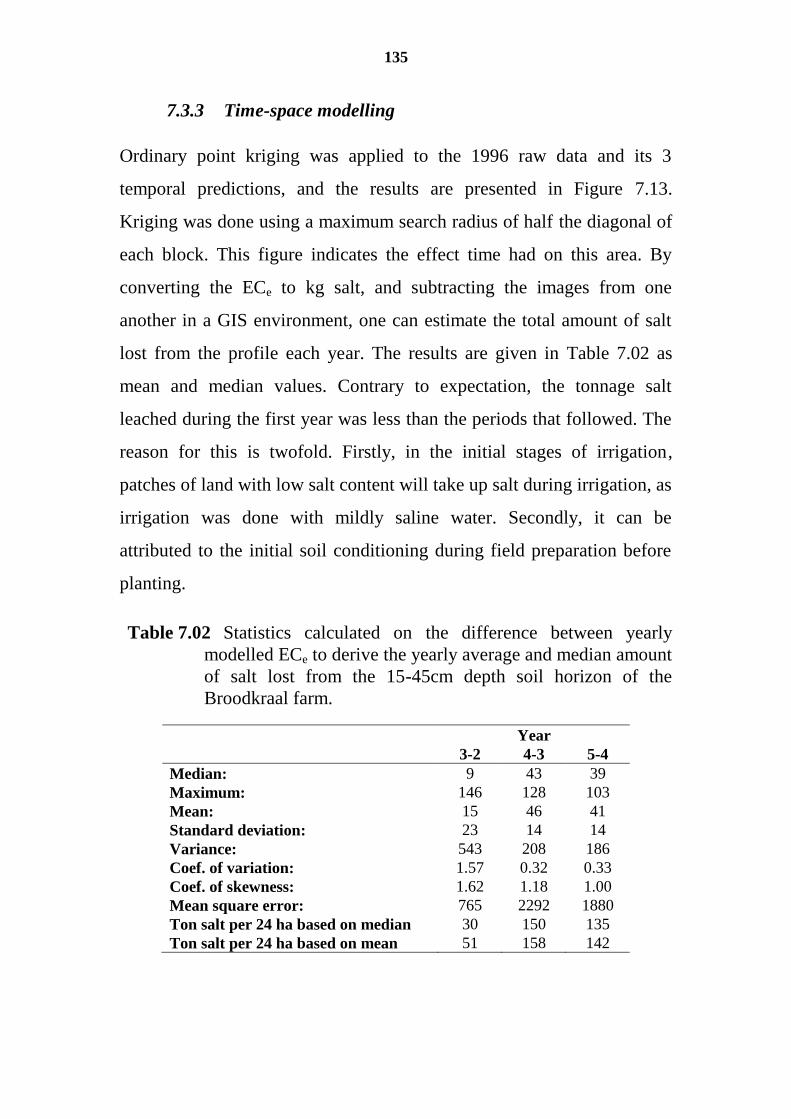
135
7.3.3 Time-space modelling
Ordinary point kriging was applied to the 1996 raw data and its 3
temporal predictions, and the results are presented in Figure 7.13.
Kriging was done using a maximum search radius of half the diagonal of
each block. This figure indicates the effect time had on this area. By
converting the ECe to kg salt, and subtracting the images from one
another in a GIS environment, one can estimate the total amount of salt
lost from the profile each year. The results are given in Table 7.02 as
mean and median values. Contrary to expectation, the tonnage salt
leached during the first year was less than the periods that followed. The
reason for this is twofold. Firstly, in the initial stages of irrigation,
patches of land with low salt content will take up salt during irrigation, as
irrigation was done with mildly saline water. Secondly, it can be
attributed to the initial soil conditioning during field preparation before
planting.
Table 7.02 Statistics calculated on the difference between yearly
modelled ECe to derive the yearly average and median amount
of salt lost from the 15-45cm depth soil horizon of the
Broodkraal farm.
Year
3-2 4-3 5-4
Median: 9 43 39
Maximum: 146 128 103
Mean: 15 46 41
Standard deviation: 23 14 14
Variance: 543 208 186
Coef. of variation: 1.57 0.32 0.33
Coef. of skewness: 1.62 1.18 1.00
Mean square error: 765 2292 1880
Ton salt per 24 ha based on median 30 150 135
Ton salt per 24 ha based on mean 51 158 142
136
300 400 500 600 700 800 900
Meter
0
100
200
300
2
0
100
200
300
Mete
r
3Age
0
100
200
300
4
0
100
200
300
5
100150200250300350400450500550600650700750
1999
1998
1997
1996
mS/m
Figure 7.13 The combined ordinary point kriged maps of the original and predicted data from the 1996 (age 5) segment. Age indicate years of irrigation.
137
7.4 Conclusions
The investigated areas were under table grapes and were subjected to a
rigorous irrigation program. The older sites had a lower salt content than
the younger sites but the relative variability remained almost constant.
So, the data showed proved that there is a general lowering of salinity in
the landscape resulting from irrigation practices.
By using the icdf method of predicting change with time, and by
sampling the irrigation history from the 2nd
year to the 5th
year, the period
of most dramatic change have been captured. After the 5th
year the soil
ECe tends to be subjected to the irrigation water quality of the past
season. It is therefore a suggestion to use the irrigation water quality
received as a correction factor.
The amount of salt removed from this profile over the study period has a
delayed effect in influencing the water quality of the river system.
However the amounts predicted is in line with the reaction that was
measured in the river system (de Clercq et al., 2001).
Two aspects can be highlighted. Time modelling was approached in a
unique manner that proved to be a good predictor, but rigorous proof will
however require resampling after a period of time. Secondly, predicting
the contribution of this site to the nearby river system in terms of the salt
load lost from the soil profile, proved to be a valuable way in bypassing
intricate soil process modelling in an era and area where funds, the total
land surface and skilled labour places a large burden in solving this
problems.
138
8 REGIONAL SUSTAINABILITY IN TABLE GRAPE
PRODUCTION ON SALINE SOILS5
ABSTRACT
A study was done in South Africa to investigate the state of the soil salt
content and its effect on plant growth on a regional rather than a point
basis. The study site went through a development phase since 1996 of
establishing new vineyards each year. This provided an excellent
opportunity to investigate soil characteristics, plant vigour and their
relationship since the start of development. Soil samples were taken and
trunk circumferences were measured. The soil properties included in the
investigation were soil clay percentage, ECe, soil pH value and time since
initial irrigation. Exploratory data analyses were done and variograms
were drawn for all data. Kriging was used to map the variables and
multiple regression analysis was used to investigate their relationships on
a regional basis.
5Published in:
de Clercq, W.P., Van Meirvenne, M., 2005. Regional sustainability in table grape production on saline soils. South African Journal of Plant and Soil, 23(2), 113-119.
This chapter was partly presented as:
de Clercq, W.P., De Smet, G., Van Meirvenne, M., 2001. Mapping of soil salinisation in an irrigated vineyard in South Africa. Workshop on Bilateral (Belgium/South Africa) Workshop on Cartographic modelling and land degradation. Gent, Belgium 2001.
139
A number of useful observations were made. Trunk circumference as an
index of growth showed a negative correlation with ECe and a positive
correlation with soil pH. Trunk circumference reflected a positive growth
cycle when compared with time since development. Regression analysis
showed that trunk circumference as an indicator of vigour could be
confidently predicted through knowledge of the vine age, soil pH and
ECe and reflected upon measurement and prediction of sustainability in
grape production.
This approach has widespread applications for agriculture in terms of
dealing with variation in a landscape and dealing with water supply
problems. Methodology that uses a regional approach rather than a point
approach in management could enhance the ability to increase
profitability and ultimately improve water management.
8.1 Introduction
The Berg River Catchment (BRC) irrigation system, as with many other
systems in South Africa, is experiencing increased pressure from a range
of water users. The quality of the water in the Berg River system is
largely determined by agriculture (as in most other water supply
systems). It is also reasonable to assume that agriculture in future will not
only have to bring about substantial water savings, but will also have to
be increasingly reliant on water of a poorer quality than at present as a
result of urban, industrial and agricultural pressure on this water
resource. Research has however indicated the role of salts in the
irrigation water on the yield and quality of agricultural crops and
indicated it to be crucial in terms of management and survival (Frenkel
140
and Meiri, 1985; Shalhevet, 1994; Finke et al., 1999; Moolman et al.,
1999; de Clercq et al., 2001).
It is for these reasons that a project was initiated with the aim to
contributing toward the creation of a methodology that will enable the
prediction of sustainability in agriculture systems and the minimisation
of over-development risk and the subsequent over pressure on water
resources.
8.2 Materials and methods
The test site was created on the farm Broodkraal near Piketberg (latitude
32 41' South, longitude 18 41' East) in the South Africa. This implied
that a history of saline irrigation in saline soils exists from 1995 and that
vineyards exist with increasing age of up to nine years.
Soil sampling was carried out following geostatistical methods (Webster
and Oliver, 2000). The sample set was taken on a 45 m by 50.5 m grid,
generating a grid of 15 by 21 samples. A total of 60 ha were covered
generating 264 samples. To be able to describe soil variability within
these points, four sets of 17 samples were taken randomly within four of
these grid units. One of these sets was later discarded as it was
accidentally taken on a location previously used for storage of gypsum.
The sampling technique entailed a pooled sample of three micro-
positions within a vine row to minimise the effect of the micro irrigation
induced pattern. Sampling positions close to roads or any visible
influence were omitted. Sampling was carried out at two depths, viz. 0-
15 cm and 15-45 cm. Throughout this chapter the weighted depth
average values were used in all calculations.
141
The samples were analysed for electrical resistance (ER), electrical
conductivity (ECe), pH and clay percentage (Görgens and de Clercq,
2005). The method for measuring ER involved the technique of
preparing saturated pastes and after a standing period of an hour, the
pastes were measured in a standardised cup using a Wheatstone bridge.
Chemical analyses were done, clay percentage and ECe were determined
on 60 % of the samples while ER and pH were determined on all
samples. Since there is a general good correlation between ER and ECe, it
was decided to use EC, but expand the ECe database using the ER values
in a co-kriging process (Webster and Oliver 2000). Chemical and
physical analytical methods used were reported in de Clercq et al. (2001)
and Görgens and de Clercq (2005).
Trunk circumferences (TC) of the 16 vines surrounding each soil sample
position were measured. The average TC of the 16 plants was used. The
age of each vineyard was also noted. Coordinates of all sampling points
were registered.
Digital maps of all variables were generated through kriging and used in
a GIS environment to correlate the results. Time was introduced as a
variable and a model generated making trunk circumference time
dependent (de Clercq and Van Meirvenne, 2005). This approach follows
the procedures used by Heuvelink and Pebesma (1999) in which
modelling first goes through a process of spatial modelling for each
variable (kriging) and then modelling of the relationships between digital
realisations.
The maximum distance over which a variogram could be calculated, was
restricted to half the largest dimension of the study area, i.e. half its
diagonal measurement. For ease of reading this distance was calculated
142
in Eq. 8.01. Therefore the maximum lag-distance that could be used in
calculation of the experimental variogram was 576 m. Generally, a
maximum lag distance of not greater than 500 m was used (Pannatier,
1996):
8.01 .Eq 2/5.710906 22 = 576 m
The theory applied in terms of modelling the variance and the kriging
used in this chapter were extensively discussed in Chapter 3 and will
therefore not be repeated here.
This procedure of generating digital pictures of salinity distribution and
the distribution of vigour allowed comparison to be done on a multitude
of points simultaneously instead of deriving answers from an individual
point basis (meaning a much poorer dataset). This procedure is therefore
better equipped to evaluate regional trends and therefore evaluate
sustainability on a regional basis rather than on a single point basis.
8.3 Results and discussion
8.3.1 ECe and ER
In the histogram of ECe (Figure 8.01), two definite extreme values were
identified that resulted in further investigation. The parameters of
centrality, spreading, skewness and kurtosis of the ECe histogram (Figure
8.01) are as follows: skewness is positive (0.94) and the histogram is
leptokurtic (3.91). The mean, maximum and minimum of the ECe data
are 195, 613 and 70 respectively. From Figure 8.02 it is also clear that
ECe, which was not measured at all the sampling points also shows three
clusters of higher density sampling and not four. One cluster was omitted
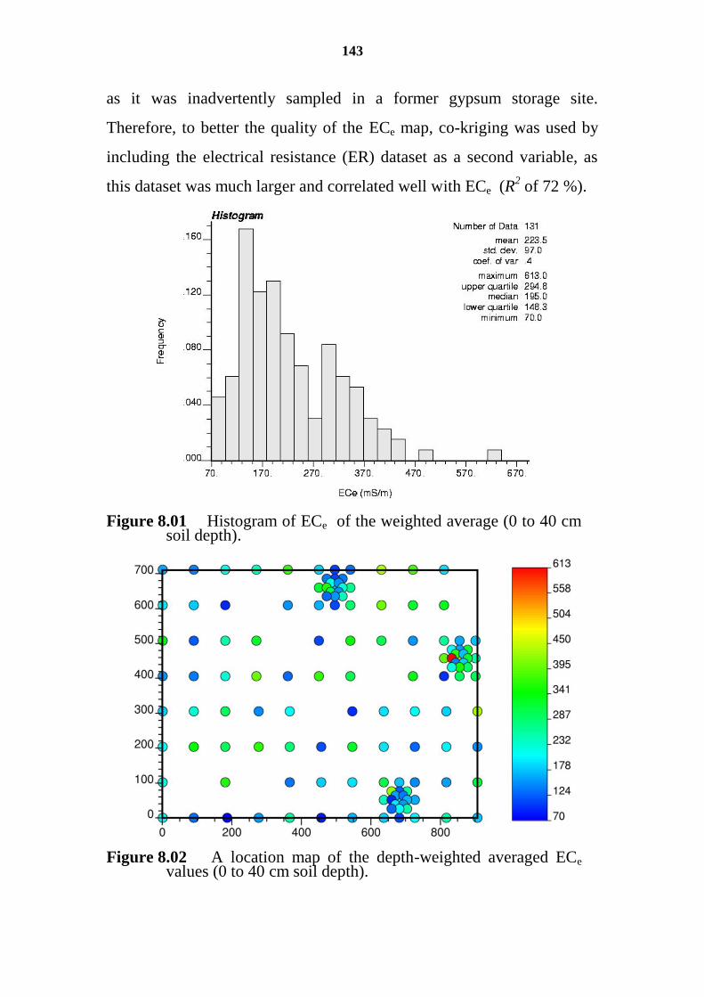
143
as it was inadvertently sampled in a former gypsum storage site.
Therefore, to better the quality of the ECe map, co-kriging was used by
including the electrical resistance (ER) dataset as a second variable, as
this dataset was much larger and correlated well with ECe (R2 of 72 %).
Figure 8.01 Histogram of ECe of the weighted average (0 to 40 cm soil depth).
Figure 8.02 A location map of the depth-weighted averaged ECe values (0 to 40 cm soil depth).
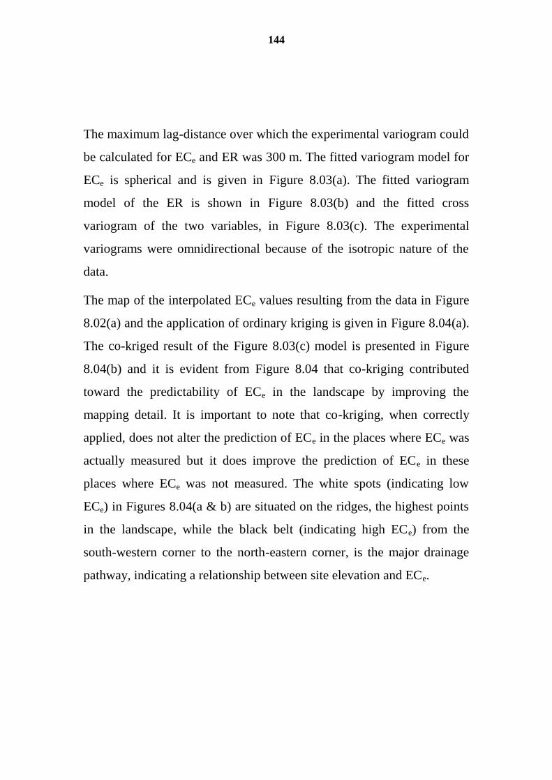
144
The maximum lag-distance over which the experimental variogram could
be calculated for ECe and ER was 300 m. The fitted variogram model for
ECe is spherical and is given in Figure 8.03(a). The fitted variogram
model of the ER is shown in Figure 8.03(b) and the fitted cross
variogram of the two variables, in Figure 8.03(c). The experimental
variograms were omnidirectional because of the isotropic nature of the
data.
The map of the interpolated ECe values resulting from the data in Figure
8.02(a) and the application of ordinary kriging is given in Figure 8.04(a).
The co-kriged result of the Figure 8.03(c) model is presented in Figure
8.04(b) and it is evident from Figure 8.04 that co-kriging contributed
toward the predictability of ECe in the landscape by improving the
mapping detail. It is important to note that co-kriging, when correctly
applied, does not alter the prediction of ECe in the places where ECe was
actually measured but it does improve the prediction of ECe in these
places where ECe was not measured. The white spots (indicating low
ECe) in Figures 8.04(a & b) are situated on the ridges, the highest points
in the landscape, while the black belt (indicating high ECe) from the
south-western corner to the north-eastern corner, is the major drainage
pathway, indicating a relationship between site elevation and ECe.
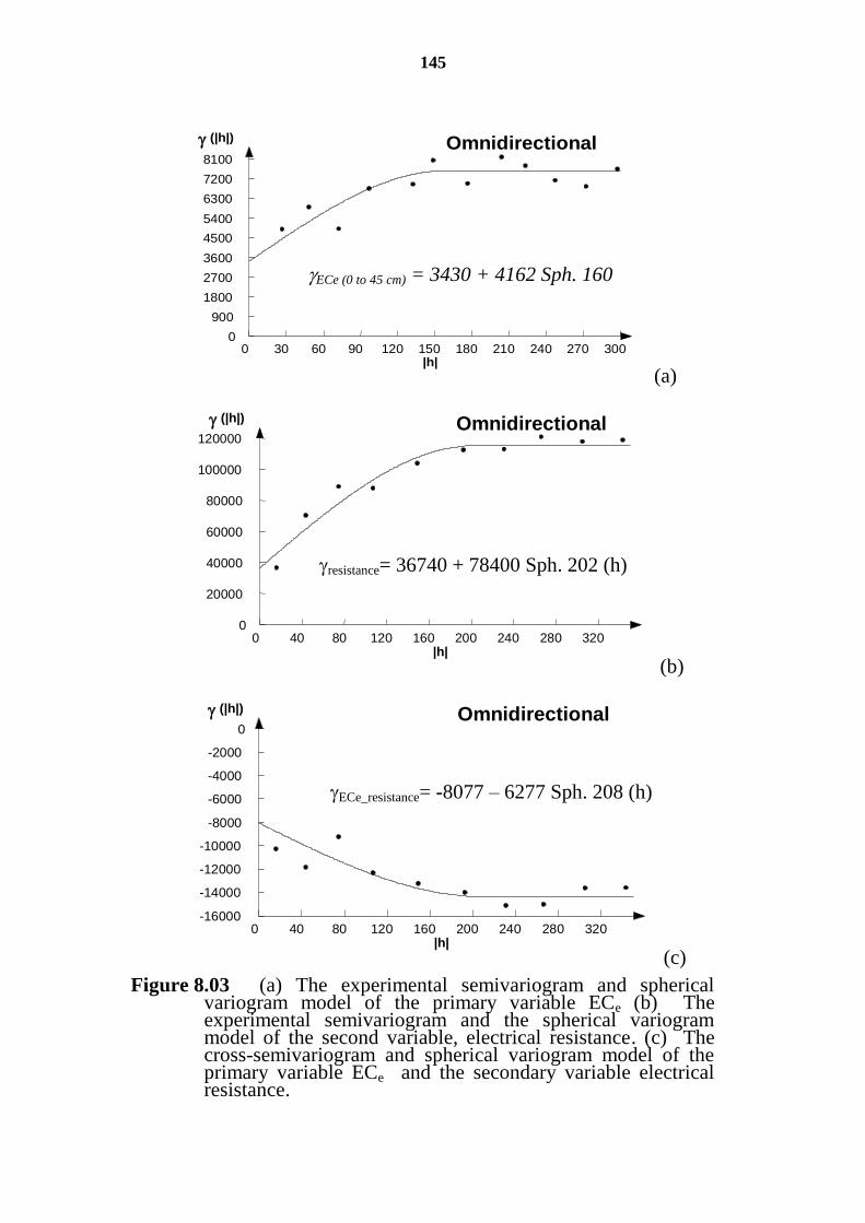
145
0 30 60 90 120 150 180 210 240 270 300 0
900 1800 2700 3600 4500 5400 6300 7200 8100
|h|
(|h|) Omnidirectional
(a)
0 40 80 120 160 200 240 280 320 0
20000
40000
60000
80000
100000
120000
|h|
(|h|) Omnidirectional
(b)
0 40 80 120 160 200 240 280 320
0
-2000
-4000
-6000
-8000
-10000
-12000
-14000
-16000
|h|
(|h|) Omnidirectional
(c)
Figure 8.03 (a) The experimental semivariogram and spherical variogram model of the primary variable ECe (b) The experimental semivariogram and the spherical variogram model of the second variable, electrical resistance. (c) The cross-semivariogram and spherical variogram model of the primary variable ECe and the secondary variable electrical resistance.
ECe (0 to 45 cm) = 3430 + 4162 Sph. 160
ECe_resistance= -8077 – 6277 Sph. 208 (h)
resistance= 36740 + 78400 Sph. 202 (h)
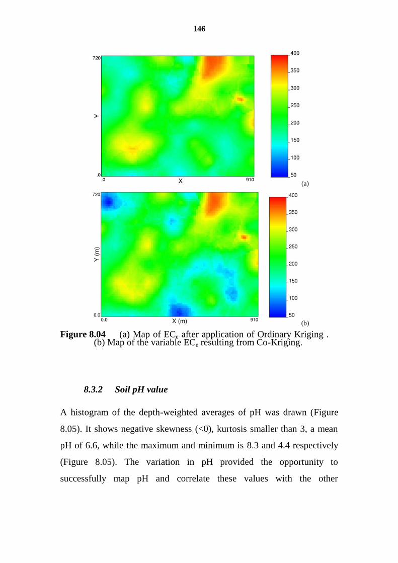
146
(a)
(b)
Figure 8.04 (a) Map of ECe after application of Ordinary Kriging . (b) Map of the variable ECe resulting from Co-Kriging.
8.3.2 Soil pH value
A histogram of the depth-weighted averages of pH was drawn (Figure
8.05). It shows negative skewness (<0), kurtosis smaller than 3, a mean
pH of 6.6, while the maximum and minimum is 8.3 and 4.4 respectively
(Figure 8.05). The variation in pH provided the opportunity to
successfully map pH and correlate these values with the other
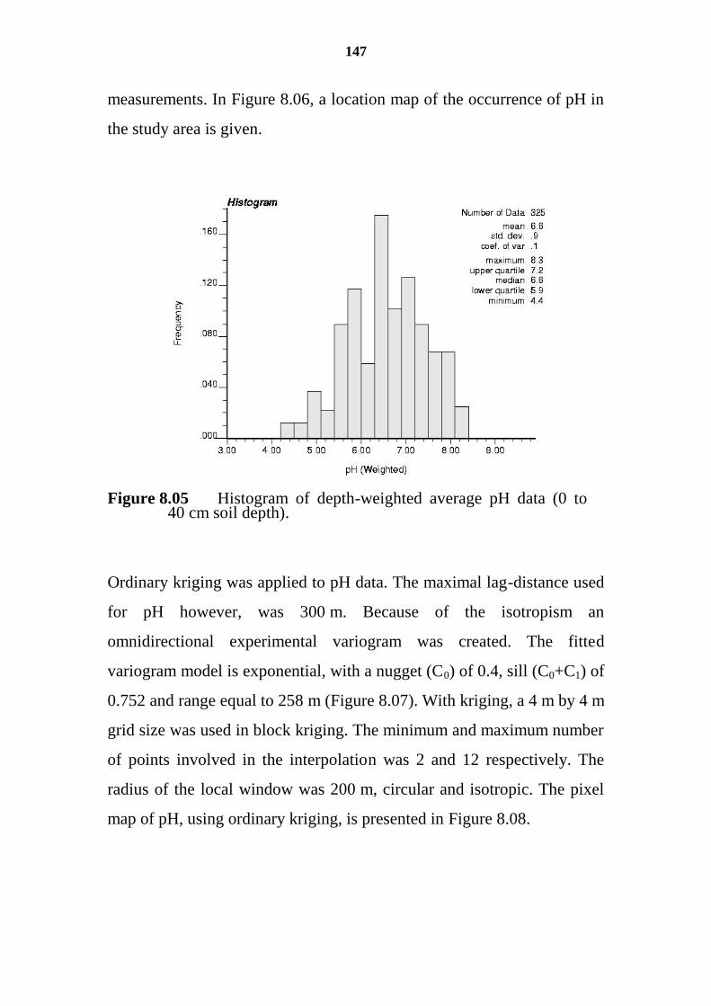
147
measurements. In Figure 8.06, a location map of the occurrence of pH in
the study area is given.
Figure 8.05 Histogram of depth-weighted average pH data (0 to 40 cm soil depth).
Ordinary kriging was applied to pH data. The maximal lag-distance used
for pH however, was 300 m. Because of the isotropism an
omnidirectional experimental variogram was created. The fitted
variogram model is exponential, with a nugget (C0) of 0.4, sill (C0+C1) of
0.752 and range equal to 258 m (Figure 8.07). With kriging, a 4 m by 4 m
grid size was used in block kriging. The minimum and maximum number
of points involved in the interpolation was 2 and 12 respectively. The
radius of the local window was 200 m, circular and isotropic. The pixel
map of pH, using ordinary kriging, is presented in Figure 8.08.
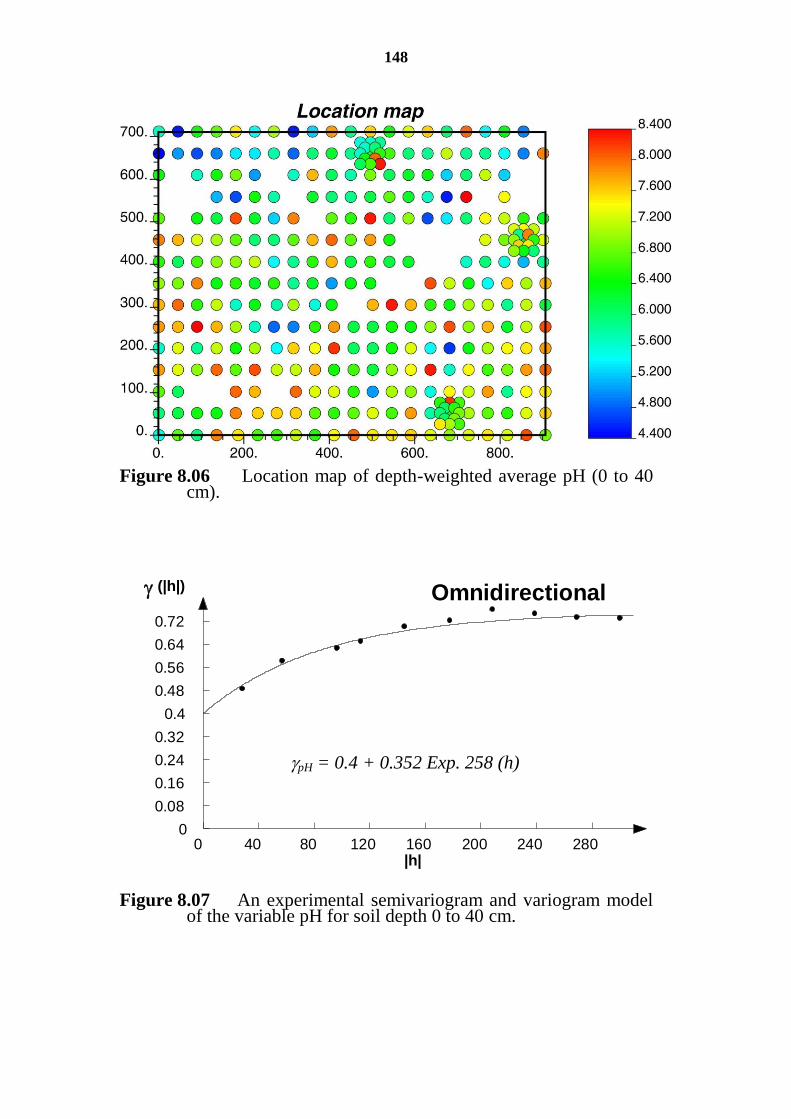
148
Figure 8.06 Location map of depth-weighted average pH (0 to 40 cm).
0 40 80 120 160 200 240 280 0
0.08 0.16 0.24 0.32
0.4 0.48 0.56 0.64 0.72
|h|
(|h|) Omnidirectional
Figure 8.07 An experimental semivariogram and variogram model of the variable pH for soil depth 0 to 40 cm.
pH = 0.4 + 0.352 Exp. 258 (h)
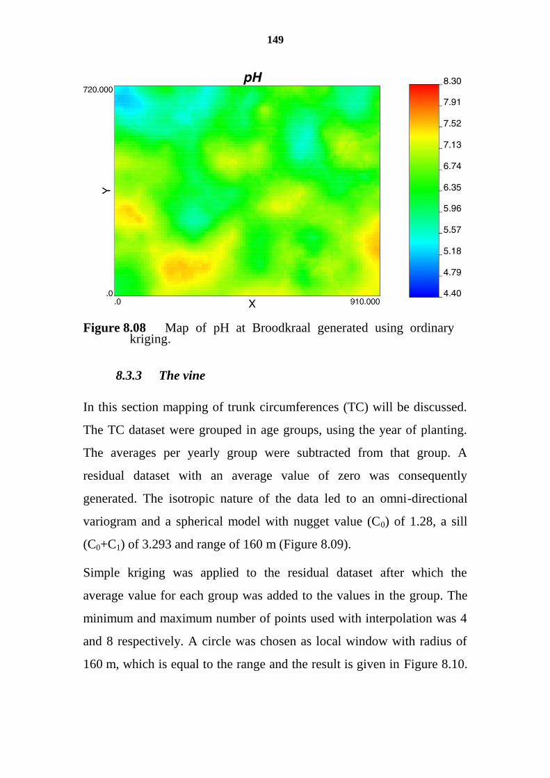
149
Figure 8.08 Map of pH at Broodkraal generated using ordinary kriging.
8.3.3 The vine
In this section mapping of trunk circumferences (TC) will be discussed.
The TC dataset were grouped in age groups, using the year of planting.
The averages per yearly group were subtracted from that group. A
residual dataset with an average value of zero was consequently
generated. The isotropic nature of the data led to an omni-directional
variogram and a spherical model with nugget value (C0) of 1.28, a sill
(C0+C1) of 3.293 and range of 160 m (Figure 8.09).
Simple kriging was applied to the residual dataset after which the
average value for each group was added to the values in the group. The
minimum and maximum number of points used with interpolation was 4
and 8 respectively. A circle was chosen as local window with radius of
160 m, which is equal to the range and the result is given in Figure 8.10.
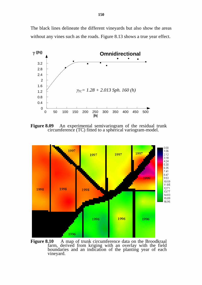
150
The black lines delineate the different vineyards but also show the areas
without any vines such as the roads. Figure 8.13 shows a true year effect.
0 50 100 150 200 250 300 350 400 450 500 0
0.4 0.8 1.2 1.6
2 2.4 2.8 3.2
|h|
(|h|) Omnidirectional
Figure 8.09 An experimental semivariogram of the residual trunk circumference (TC) fitted to a spherical variogram-model.
Figure 8.10 A map of trunk circumference data on the Broodkraal farm, derived from kriging with an overlay with the field boundaries and an indication of the planting year of each vineyard.
TC= 1.28 + 2.013 Sph. 160 (h)
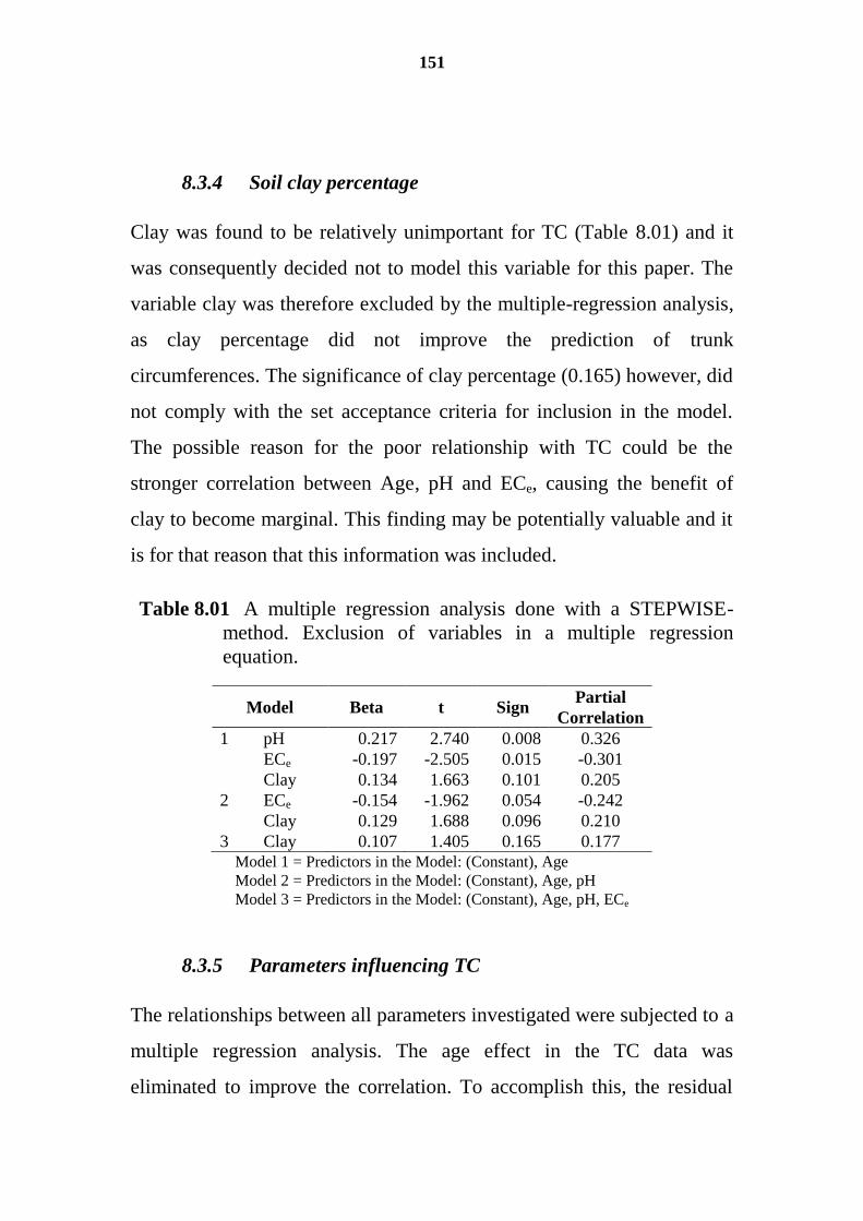
151
8.3.4 Soil clay percentage
Clay was found to be relatively unimportant for TC (Table 8.01) and it
was consequently decided not to model this variable for this paper. The
variable clay was therefore excluded by the multiple-regression analysis,
as clay percentage did not improve the prediction of trunk
circumferences. The significance of clay percentage (0.165) however, did
not comply with the set acceptance criteria for inclusion in the model.
The possible reason for the poor relationship with TC could be the
stronger correlation between Age, pH and ECe, causing the benefit of
clay to become marginal. This finding may be potentially valuable and it
is for that reason that this information was included.
Table 8.01 A multiple regression analysis done with a STEPWISE-
method. Exclusion of variables in a multiple regression
equation.
Model Beta t Sign Partial
Correlation
1 pH 0.217 2.740 0.008 0.326
ECe -0.197 -2.505 0.015 -0.301
Clay 0.134 1.663 0.101 0.205
2 ECe -0.154 -1.962 0.054 -0.242
Clay 0.129 1.688 0.096 0.210
3 Clay 0.107 1.405 0.165 0.177
Model 1 = Predictors in the Model: (Constant), Age
Model 2 = Predictors in the Model: (Constant), Age, pH
Model 3 = Predictors in the Model: (Constant), Age, pH, ECe
8.3.5 Parameters influencing TC
The relationships between all parameters investigated were subjected to a
multiple regression analysis. The age effect in the TC data was
eliminated to improve the correlation. To accomplish this, the residual
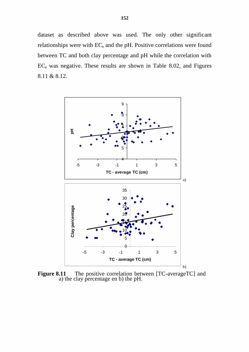
152
dataset as described above was used. The only other significant
relationships were with ECe and the pH. Positive correlations were found
between TC and both clay percentage and pH while the correlation with
ECe was negative. These results are shown in Table 8.02, and Figures
8.11 & 8.12.
4
5
6
7
8
9
-5 -3 -1 1 3 5
TC - average TC (cm)
pH
a)
0
5
10
15
20
25
30
35
-5 -3 -1 1 3 5
TC - average TC (cm)
Cla
y p
erc
en
tag
e
b)
Figure 8.11 The positive correlation between [TC-averageTC] and a) the clay percentage en b) the pH.
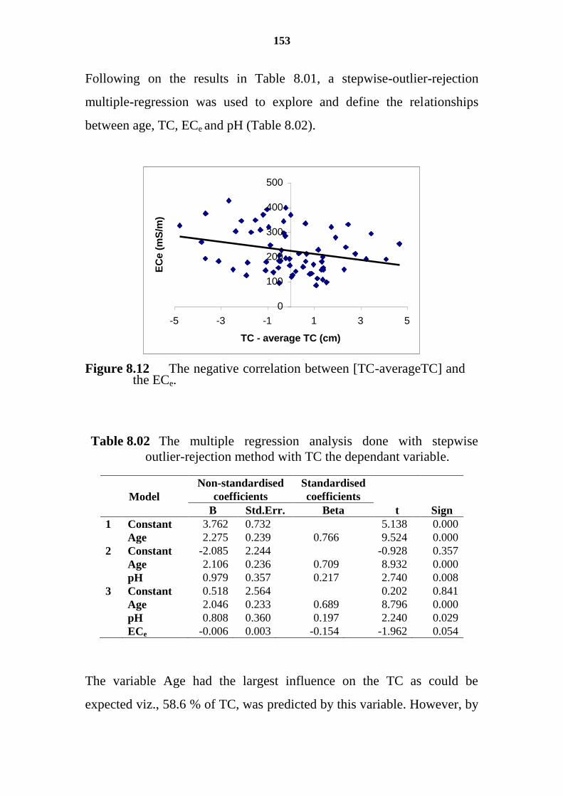
153
Following on the results in Table 8.01, a stepwise-outlier-rejection
multiple-regression was used to explore and define the relationships
between age, TC, ECe and pH (Table 8.02).
0
100
200
300
400
500
-5 -3 -1 1 3 5
TC - average TC (cm)
EC
e (
mS
/m)
Figure 8.12 The negative correlation between [TC-averageTC] and the ECe.
Table 8.02 The multiple regression analysis done with stepwise
outlier-rejection method with TC the dependant variable.
Model
Non-standardised
coefficients
Standardised
coefficients
t Sign B Std.Err. Beta
1 Constant
Age
3.762
2.275
0.732
0.239
0.766
5.138
9.524
0.000
0.000
2 Constant
Age
pH
-2.085
2.106
0.979
2.244
0.236
0.357
0.709
0.217
-0.928
8.932
2.740
0.357
0.000
0.008
3 Constant
Age
pH
ECe
0.518
2.046
0.808
-0.006
2.564
0.233
0.360
0.003
0.689
0.197
-0.154
0.202
8.796
2.240
-1.962
0.841
0.000
0.029
0.054
The variable Age had the largest influence on the TC as could be
expected viz., 58.6 % of TC, was predicted by this variable. However, by
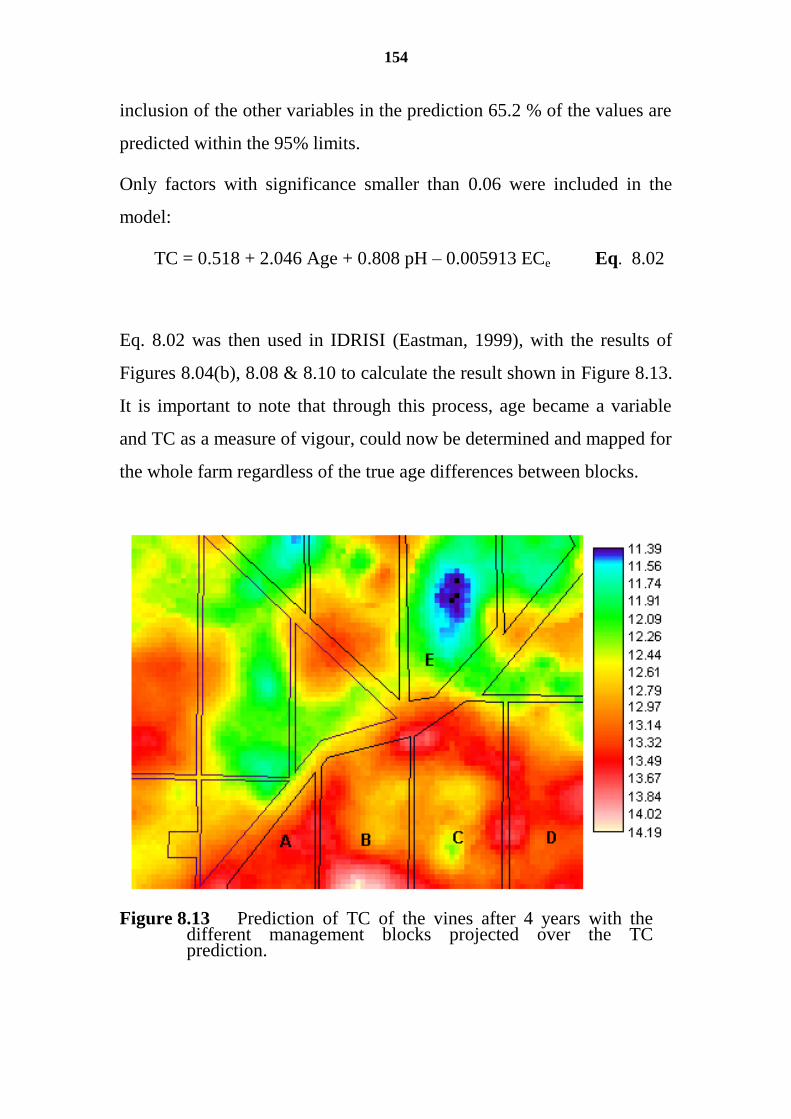
154
inclusion of the other variables in the prediction 65.2 % of the values are
predicted within the 95% limits.
Only factors with significance smaller than 0.06 were included in the
model:
8.02 .Eq TC = 0.518 + 2.046 Age + 0.808 pH – 0.005913 ECe
Eq. 8.02 was then used in IDRISI (Eastman, 1999), with the results of
Figures 8.04(b), 8.08 & 8.10 to calculate the result shown in Figure 8.13.
It is important to note that through this process, age became a variable
and TC as a measure of vigour, could now be determined and mapped for
the whole farm regardless of the true age differences between blocks.
Figure 8.13 Prediction of TC of the vines after 4 years with the different management blocks projected over the TC prediction.
155
Figure 8.13 shows the prediction of TC after four years of growth. It
must however be borne in mind that the prediction in Figure 8.13 was
done irrespective of the true age of the different segments on the farm. It
is simply an equal age prediction, predicting the TC of all vines after four
years of growth.
In Figure 8.13, A and D resemble the sections with the most stable
growth and yield, while, B and C are the sections with very large
variances. E and the similarly coloured sections to the left of E, show the
lowest potential. All of this was in fact confirmed by observation on the
farm.
Sustainable growth was however maintained in these saline conditions
mainly as a result of over-irrigation. Therefore the negative effect that
soil salinity and poor water quality could impose on growth was
overshadowed by water quantity.
8.4 Conclusions
By using kriging techniques, ECe, pH, age and vigour could be predicted
at a high resolution for this landscape generating a regional realization or
trend. It was shown that modelling of regional trends and comparing
these trends statistically produced good results and opened a window on
sustainability issues that could barely be possible using data on a point
basis. The shown predictable regional behaviour of ECe in relation to pH,
time and plant vigour could have widespread application for the
grape/wine industry of the Western Cape.
Resulting from over-irrigation as a means of dealing with salinity in the
landscape, no salt build-up occurred and the role clay could play in
156
affecting growth was also reduced. Gypsum was also used to better
infiltration and control sodium build-up in these soils and this led to the
reduced role clay played as a growth inhibitor.
The soil pH showed a significant influence on the long-term reaction
captured in the trunk circumference measurements. The ECe of the upper
part of the soil as being investigated here must be seen in the background
of a region with up to 10 mm evapotranspiration per day, very little
rainfall and thus totally dependent on irrigation. It can thus be expected
that the ECe will be lowest in over-irrigated segments. In segments that
received less irrigation than the evaporative demand, a build-up of salts
will occur. In parts that received no irrigation but are close to the
irrigated area, the ECe will soar. In sites where the soil pH is restricting
growth, transpiration is reduced and therefore over-irrigation usually
occurs, resulting in runoff and increased drainage.
From Figure 8.13 it is clear that areas with expected good or bad growth
can be delineated and could be predicted prior to planting. Though the
information presented in Figure 8.13 is mostly after the fact, this farmer
would surely have benefited from the ECe and pH maps, as the
information for sustained and correct development is contained in them.
The fact that this study was based on only the upper part of the soil
profile, and that such a good relationship could be defined between plant
growth and soil characteristics, implies that the vines reacted more to
what was happening in the upper part of the soil than the section below
the 45 cm sampling depth.
Perhaps the most important finding in this research was that, while vine
age, ECe and pH, when correlated with trunk circumference separately,
generated low R2-values. However, in combination (Eq. 9.02) their data
157
generated a R2-value of 66 % and consequently better levels of
significance. The fact then that 66 % of the variance (within the 95%
confidence limit) is explained by vine age, ECe and pH in combination
(Eq. 9.02), suggests very little else influenced growth negatively in these
circumstances.
The most important implications of these results are economic. This
research showed that the methods applied here could enhance current
knowledge in terms of the behaviour and sustainability of agricultural
crops on a regional basis through a process that deals with spatial
variation. This could increase profitability from these landscapes and it
deals with very important water issues.
158
9 SOIL SALINITY CHARACTERIZATION USING
THE EM38 SOIL PROXIMAL SOIL SENSOR6
ABSTRACT
Land used for wheat production since early 1900 in the Berg River
catchment of South Africa, was selected for grape production and
therefore the soil was characterized and mapped. Soil pits were dug on a
100 x 100 m grid and a large number of parameters were described.
EM38 vertical and horizontal scans were done over this 1.6 km2 area, and
at the soil pits. A digital terrain model was developed as part of the
detailed soil mapping. The aim was to characterize the EM38’s ability to
characterize and indicate the transition between soil classes. The
parameters that showed a good correlation with the EM38 observations
were mapped since the EM38 observations showed complex but
predictable relationships with a number of observations made. They also
showed an agreement with the soil types mapped in the conventional
manner. A typical soil toposequence could be established and linked to
the EM38 response.
6Published as part of:
Fey, M.V. and de Clercq, W.P., 2004. A pilot study investigating the role of dryland
salinity in the quality of the water of the Berg River. WRC Report, 1342/1/04
(ISBN No. 1770053059)
de Clercq, W.P., Van Meirvenne, M., Ellis, F., Lambrechts, J.J.N., 2008. Soil salinity
characterization using the EM38 soil proximal sensor (submitted to Soil Use
and Management).
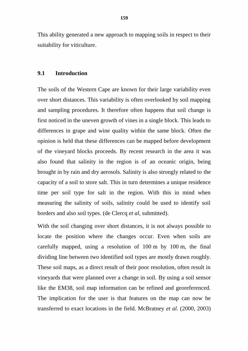
159
This ability generated a new approach to mapping soils in respect to their
suitability for viticulture.
9.1 Introduction
The soils of the Western Cape are known for their large variability even
over short distances. This variability is often overlooked by soil mapping
and sampling procedures. It therefore often happens that soil change is
first noticed in the uneven growth of vines in a single block. This leads to
differences in grape and wine quality within the same block. Often the
opinion is held that these differences can be mapped before development
of the vineyard blocks proceeds. By recent research in the area it was
also found that salinity in the region is of an oceanic origin, being
brought in by rain and dry aerosols. Salinity is also strongly related to the
capacity of a soil to store salt. This in turn determines a unique residence
time per soil type for salt in the region. With this in mind when
measuring the salinity of soils, salinity could be used to identify soil
borders and also soil types. (de Clercq et al, submitted).
With the soil changing over short distances, it is not always possible to
locate the position where the changes occur. Even when soils are
carefully mapped, using a resolution of 100 m by 100 m, the final
dividing line between two identified soil types are mostly drawn roughly.
These soil maps, as a direct result of their poor resolution, often result in
vineyards that were planned over a change in soil. By using a soil sensor
like the EM38, soil map information can be refined and georeferenced.
The implication for the user is that features on the map can now be
transferred to exact locations in the field. McBratney et al. (2000, 2003)
160
indicated that conventional soil survey is costly and time consuming
compared to soil mapping based on soil sensors. Burrough et al. (1997)
indicated that most soil maps had the inadequacy of no spatial variation
and that the taxonomy had a low level of geographical correctness.
Rhoades et al. (1997) indicated the importance of spatially referenced
information for the assessment of irrigation, drainage and salinity
management practises.
The use of electromagnetic induction was first developed as a field
survey technique in a geophysical sense and has been used as such since
as early as the 1920's. The first suggestion that EM sensors could be used
to measure soil salinity was in 1979 by de Jong et.al. (1979). The US
salinity lab tested the initial model EM31 and found that the instrument
readings were too responsive to the conductivity of material below the
rootzone (Rhoades and Corwin, 1981). Rhoades later developed the
model EM38 sensor that was sensitive to soil depths of less than 1.5 m.
Though the EM38 was initially built to measure salinity, the instrument
gained merit as being a good field surveying instrument. The mere fact
that the data can be linked and measured to the same and finer resolution
than satellite or remote imagery, has contributed to the use of the
instrument in prospecting soil variability.
The capacity of the soil to conduct an electromagnetic induction current
is synonymous to measuring the electrical conductivity of water. Both are
expressed in mS m-1
. As in the case with EC of water, the EM38 readings
are all inclusive. This means that everything in the soil that affects
electromagnetic induction needs to be taken into account, therefore the
readings are called apparent EC (ECa). McNeil (1980) indicated that the
EM38 readings are influenced mostly by the clay content in an ionised or
161
colloidal state, the ECsw, stone content as a negative influence and soil
water content. Since all of these also vary with soil type, the raw EM38
readings are also broadly sensitive to soil type (Dunn and Lilly, 2001.
The measurement resolution of the instrument is virtually limitless,
meaning the more measurements the better the detail presented on a map
(Fey and de Clercq, 2004).
9.2 Principles of EM38 operation
The EM38 comprises of a transmitter coil and a receiver coil (Figure
9.01), a battery and digital readout. The transmitter current generates
eddy-like loops in the ground. These currents also generate a secondary
magnetic field and the ratio between the secondary and primary fields are
proportional to the electrical conductivity of the ground material (Figure
9.01). The measurement is fast and ground penetration is immediate.
The instrument is always on, and data logging of ECa readings is
continuous. This allows speeding up measurements. The fact that the ECa
readings are continuous is therefore exploited by speeding up
measurement through dragging the instrument behind a vehicle on a sled.
Measurements from the EM38 are then logged at a constant rate on a
recorder.
The instrument can be used in a vertical or a horizontal mode resulting in
ECa-V and ECa-H measurements or in both simultaneously. The
differences in depth response curves (Figure 9.02), indicates that the
vertical mode is less effective at shallow depth. This response is then
characterised as the profile ratio (PR) (Cockx et al., 2007):
9.01 .Eq PR = ECa-H / ECa-V
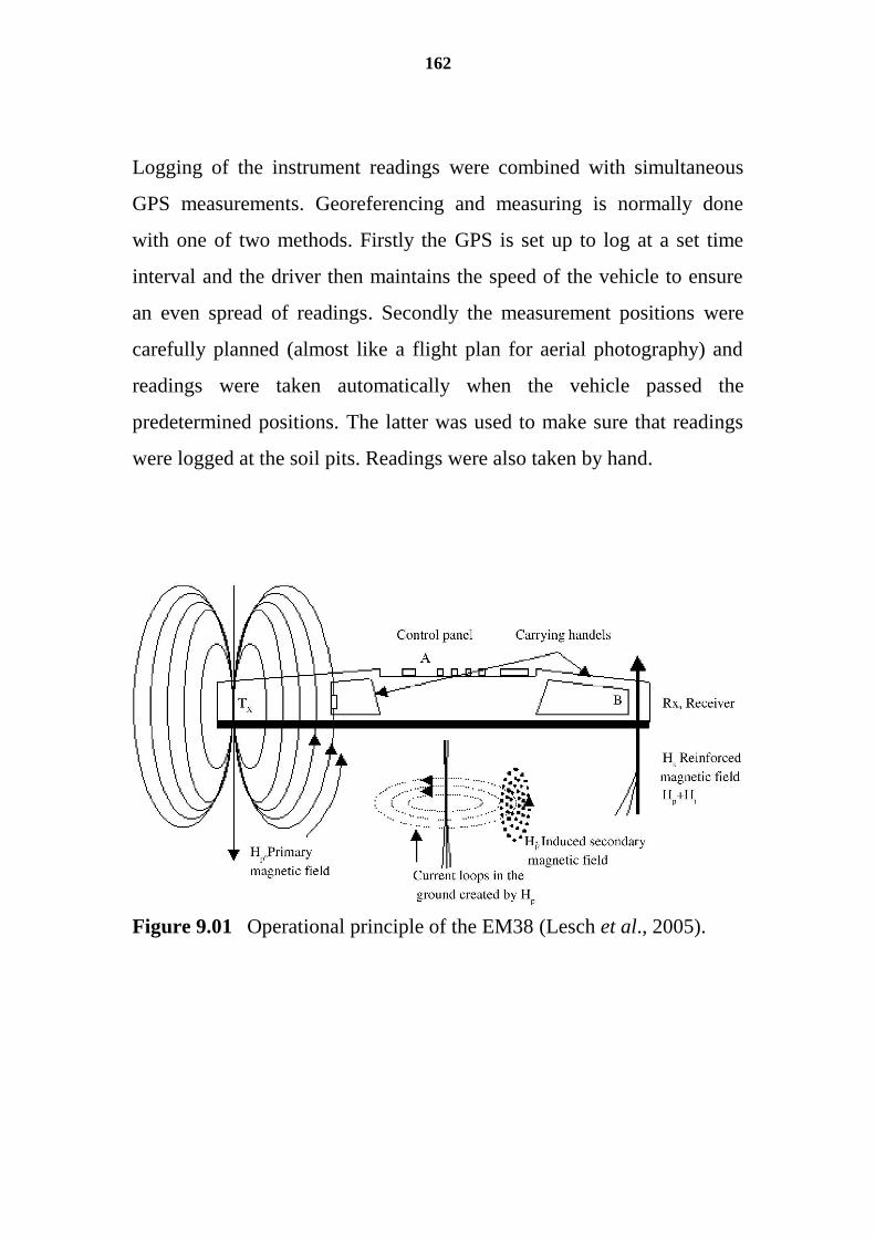
162
Logging of the instrument readings were combined with simultaneous
GPS measurements. Georeferencing and measuring is normally done
with one of two methods. Firstly the GPS is set up to log at a set time
interval and the driver then maintains the speed of the vehicle to ensure
an even spread of readings. Secondly the measurement positions were
carefully planned (almost like a flight plan for aerial photography) and
readings were taken automatically when the vehicle passed the
predetermined positions. The latter was used to make sure that readings
were logged at the soil pits. Readings were also taken by hand.
Figure 9.01 Operational principle of the EM38 (Lesch et al., 2005).
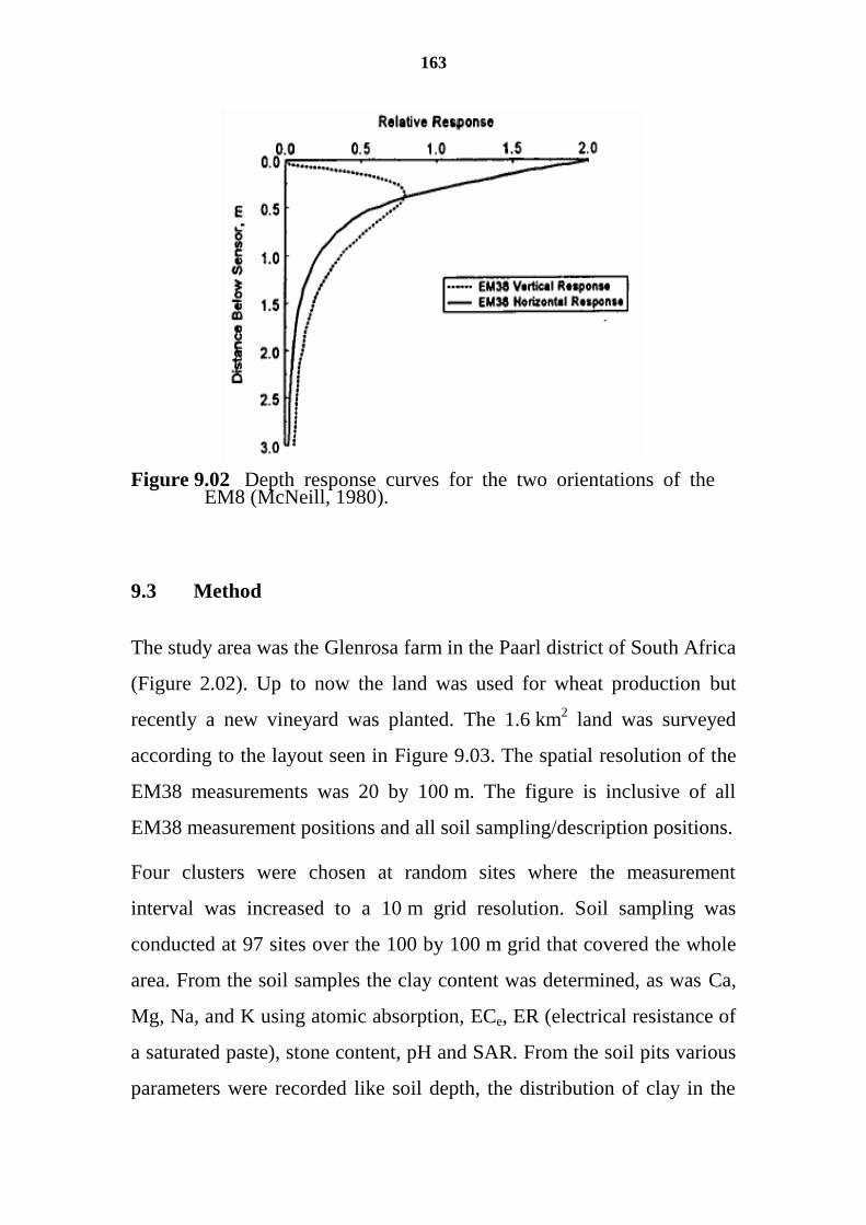
163
Figure 9.02 Depth response curves for the two orientations of the EM8 (McNeill, 1980).
9.3 Method
The study area was the Glenrosa farm in the Paarl district of South Africa
(Figure 2.02). Up to now the land was used for wheat production but
recently a new vineyard was planted. The 1.6 km2 land was surveyed
according to the layout seen in Figure 9.03. The spatial resolution of the
EM38 measurements was 20 by 100 m. The figure is inclusive of all
EM38 measurement positions and all soil sampling/description positions.
Four clusters were chosen at random sites where the measurement
interval was increased to a 10 m grid resolution. Soil sampling was
conducted at 97 sites over the 100 by 100 m grid that covered the whole
area. From the soil samples the clay content was determined, as was Ca,
Mg, Na, and K using atomic absorption, ECe, ER (electrical resistance of
a saturated paste), stone content, pH and SAR. From the soil pits various
parameters were recorded like soil depth, the distribution of clay in the
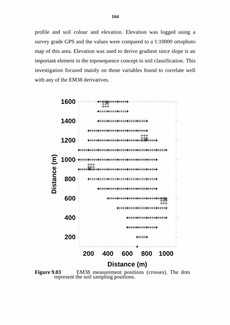
164
profile and soil colour and elevation. Elevation was logged using a
survey grade GPS and the values were compared to a 1:10000 ortophoto
map of this area. Elevation was used to derive gradient since slope is an
important element in the toposequence concept in soil classification. This
investigation focused mainly on those variables found to correlate well
with any of the EM38 derivatives.
200 400 600 800 1000
Distance (m)
200
400
600
800
1000
1200
1400
1600
Dis
tan
ce (
m)
Figure 9.03 EM38 measurement positions (crosses). The dots represent the soil sampling positions.
165
Since soil type and salt distribution is generally well correlated with
topography in the toposequence concept, the aim is to investigate this
link for the EM38 observations as well. Therefore the main aim was to
explore the sensitivity of the EM38 to a combination of soil variables,
variables also used in soil classification, and as such generates an EM38
to soil type relationship, that can be used for general soil mapping.
9.4 Results
Table 9.01 presents the descriptive statistics for the variables observed.
What is important in this table is the comparison between direct and
indirect measurements of salinity. Both the clay content and the stone
content of these soils are high but show similar distribution
characteristics (Table 9.01). Clay normally adds to the ECa readings
while stone content lowers the ECa (McNeil, 1980). All variables showed
a positive skewness except clay and stone content, but values were
generally small. Table 9.02 lists the correlation coefficients between the
variables listed in Table 9.01. This table shows a good correlation
between ECa and ECe. It also shows a good relationship between the ECa-
H and ECa-V measurements. Noteworthy as well is the good relationship
between ECa measurements and Na+, and to a lesser extent with SAR.
Stone content showed a poor correlation in general. Amongst all the
measurements, SAR, ECa-V, ECa-H, Na+, ECe and ER showed the
stronger interaction.
The elevation, slope and soil depth were mapped and are shown in Figure
9.04. Soil depth and slope angle showed similar spatial patterns. Both
maps on slope gradient and soil depth were produced by ordinary kriging
with a linear variogram model.
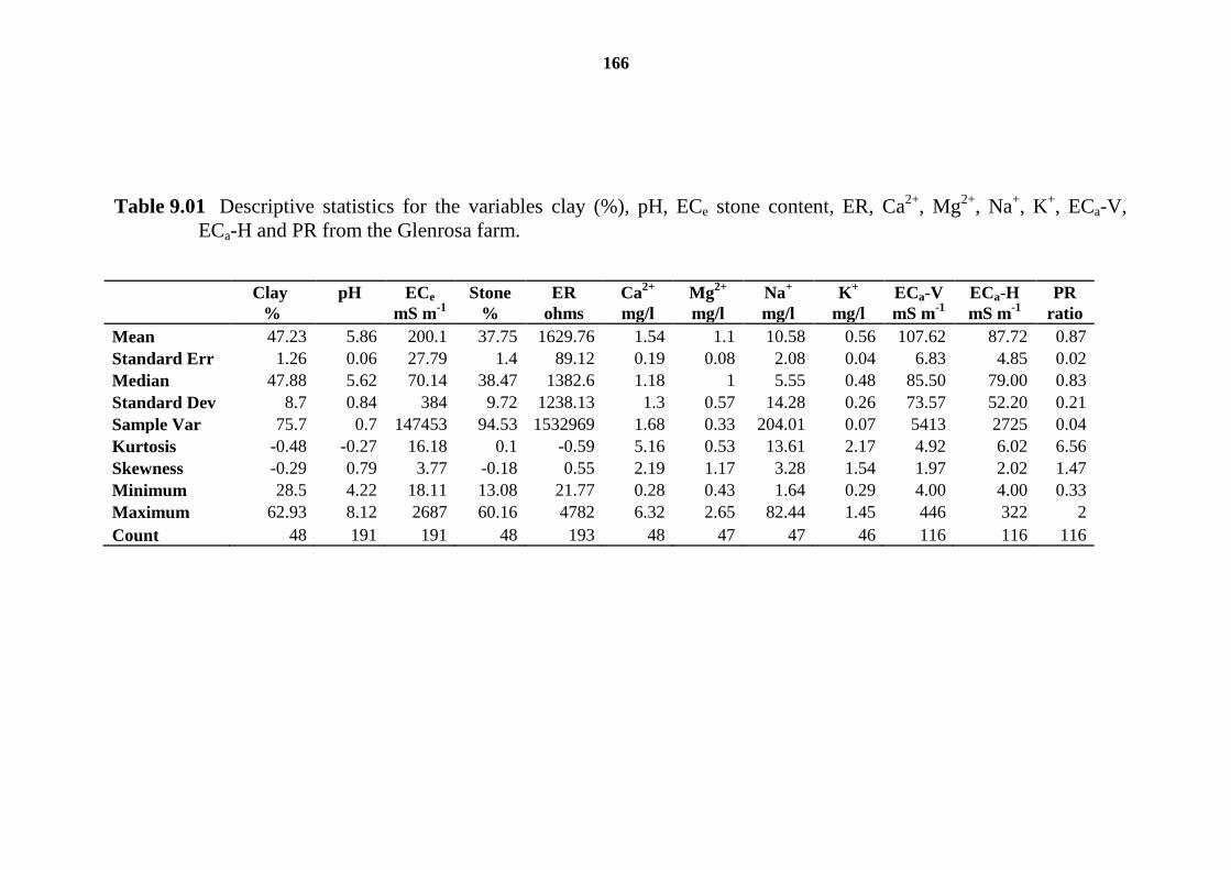
166
Table 9.01 Descriptive statistics for the variables clay (%), pH, ECe stone content, ER, Ca2+
, Mg2+
, Na+, K
+, ECa-V,
ECa-H and PR from the Glenrosa farm.
Clay
%
pH
ECe
mS m-1
Stone
%
ER
ohms
Ca2+
mg/l
Mg2+
mg/l
Na+
mg/l
K+
mg/l
ECa-V
mS m-1
ECa-H
mS m-1
PR
ratio
Mean 47.23 5.86 200.1 37.75 1629.76 1.54 1.1 10.58 0.56 107.62 87.72 0.87
Standard Err 1.26 0.06 27.79 1.4 89.12 0.19 0.08 2.08 0.04 6.83 4.85 0.02
Median 47.88 5.62 70.14 38.47 1382.6 1.18 1 5.55 0.48 85.50 79.00 0.83
Standard Dev 8.7 0.84 384 9.72 1238.13 1.3 0.57 14.28 0.26 73.57 52.20 0.21
Sample Var 75.7 0.7 147453 94.53 1532969 1.68 0.33 204.01 0.07 5413 2725 0.04
Kurtosis -0.48 -0.27 16.18 0.1 -0.59 5.16 0.53 13.61 2.17 4.92 6.02 6.56
Skewness -0.29 0.79 3.77 -0.18 0.55 2.19 1.17 3.28 1.54 1.97 2.02 1.47
Minimum 28.5 4.22 18.11 13.08 21.77 0.28 0.43 1.64 0.29 4.00 4.00 0.33
Maximum 62.93 8.12 2687 60.16 4782 6.32 2.65 82.44 1.45 446 322 2
Count 48 191 191 48 193 48 47 47 46 116 116 116
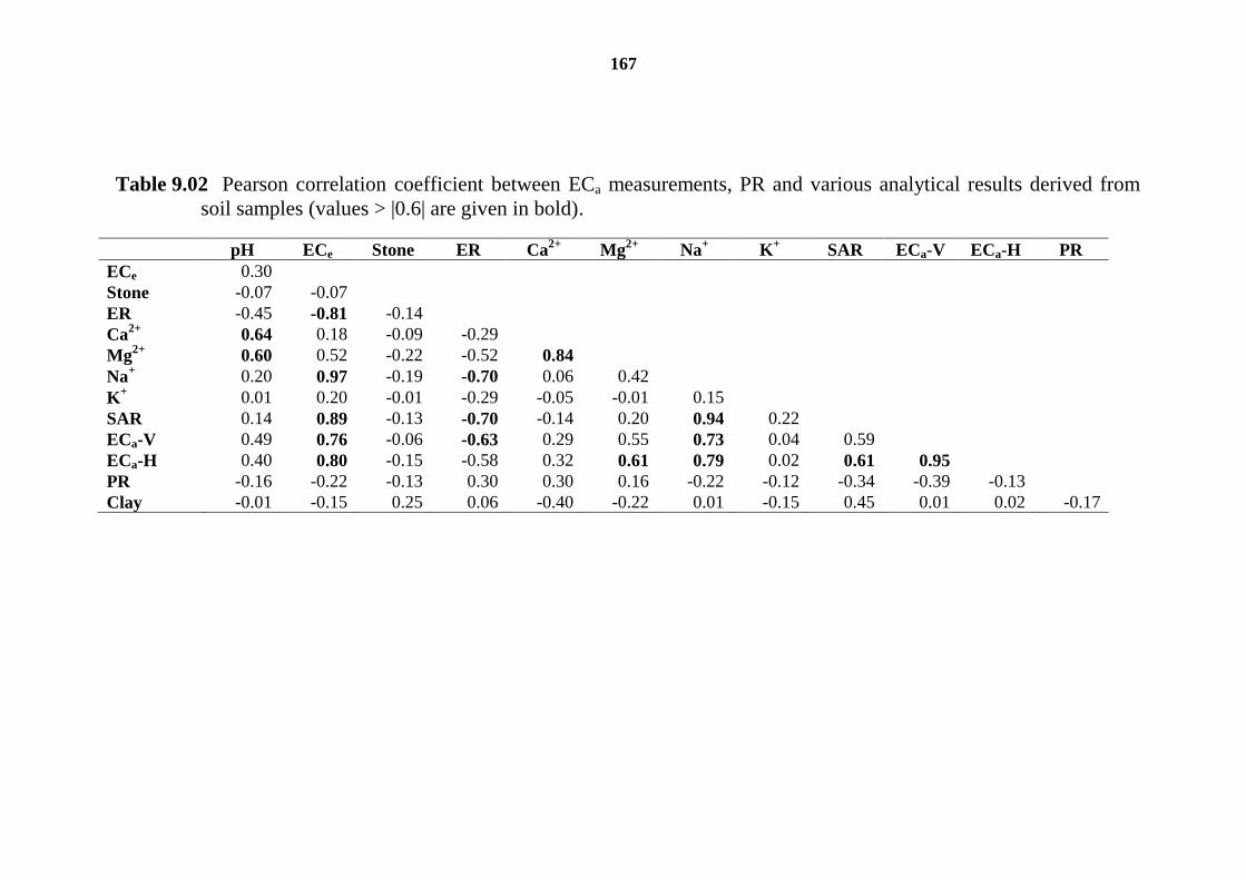
167
Table 9.02 Pearson correlation coefficient between ECa measurements, PR and various analytical results derived from
soil samples (values > |0.6| are given in bold).
pH ECe Stone ER Ca2+
Mg2+
Na+ K
+ SAR ECa-V ECa-H PR
ECe 0.30
Stone -0.07 -0.07
ER -0.45 -0.81 -0.14
Ca2+
0.64 0.18 -0.09 -0.29
Mg2+
0.60 0.52 -0.22 -0.52 0.84
Na+ 0.20 0.97 -0.19 -0.70 0.06 0.42
K+ 0.01 0.20 -0.01 -0.29 -0.05 -0.01 0.15
SAR 0.14 0.89 -0.13 -0.70 -0.14 0.20 0.94 0.22
ECa-V 0.49 0.76 -0.06 -0.63 0.29 0.55 0.73 0.04 0.59
ECa-H 0.40 0.80 -0.15 -0.58 0.32 0.61 0.79 0.02 0.61 0.95
PR -0.16 -0.22 -0.13 0.30 0.30 0.16 -0.22 -0.12 -0.34 -0.39 -0.13
Clay -0.01 -0.15 0.25 0.06 -0.40 -0.22 0.01 -0.15 0.45 0.01 0.02 -0.17
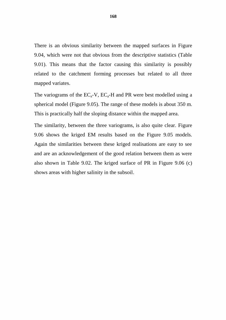
168
There is an obvious similarity between the mapped surfaces in Figure
9.04, which were not that obvious from the descriptive statistics (Table
9.01). This means that the factor causing this similarity is possibly
related to the catchment forming processes but related to all three
mapped variates.
The variograms of the ECa-V, ECa-H and PR were best modelled using a
spherical model (Figure 9.05). The range of these models is about 350 m.
This is practically half the sloping distance within the mapped area.
The similarity, between the three variograms, is also quite clear. Figure
9.06 shows the kriged EM results based on the Figure 9.05 models.
Again the similarities between these kriged realisations are easy to see
and are an acknowledgement of the good relation between them as were
also shown in Table 9.02. The kriged surface of PR in Figure 9.06 (c)
shows areas with higher salinity in the subsoil.
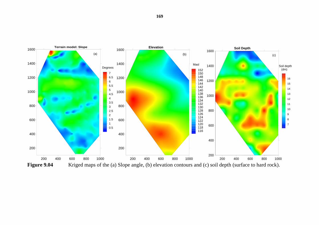
169
200 400 600 800 1000
200
400
600
800
1000
1200
1400
1600
0.5
1
1.5
2
2.5
3
3.5
4
4.5
5
5.5
6
6.5
7
Degrees
Terrain model: Slope
200 400 600 800 1000
200
400
600
800
1000
1200
1400
1600
116118120122124126128130132134136138140142144146148150152
Elevation
Masl
200 400 600 800 1000200
400
600
800
1000
1200
1400
1600
7
8
9
10
11
12
13
14
15
16
Soil depth (dm)
Soil Depth
(a) (b) (c)
Figure 9.04 Kriged maps of the (a) Slope angle, (b) elevation contours and (c) soil depth (surface to hard rock).
170
0 50 100 150 200 250 300 350 400 450 500 550
Lag Distance (m)
0
0.005
0.01
0.015
0.02
0.025
0.03
0.035
0.04
0.045
0.05
0.055
Vari
an
ce
0 50 100 150 200 250 300 350 400 450 500 550
Lag Distance (m)
0
10
20
30
40
50
Vari
an
ce
0 50 100 150 200 250 300 350 400 450 500 550
Lag Distance (m)
0
10
20
30
40
50
60
70
80
90
100
Vari
an
ce
Figure 9.05 Semi-variogram of the EM38 measurements, (a) ECa-H, (b) ECa-V and (c) the PR. The equations refer to a spherical model (Sph.) with the coefficients: nugget, sill and range respectively and h = lag distance.
(a)
(a)
(c) (b)
ECa-V= 11 + 39 Sph. 350 (h)
ECa-H= 0.015 + 0.038 Sph. 400 (h)
PR= 16 + 77 Sph. 350 (h)
171
600 800 1000 1200 14000
200
400
600
800
1000
1200
1400
0.8
0.85
0.9
0.95
1
1.05
1.1
1.15
1.2
1.25
1.3
1.35
1.4
1.45
1.5
1.55
1.6
200 400 600 800 1000
200
400
600
800
1000
1200
1400
1600
40
60
80
100
120
140
160
180
200
220
240
260
200 400 600 800 1000
200
400
600
800
1000
1200
1400
1600
406080100120140160180200220240260280300320340360380
mS/m mS/mPR
(c)(b)(a)
Figure 9.06 Kriged maps of the EM38, (a) ECa-H, (b) ECa-V measurements and (c) PR.
172
Figure 9.07 shows the mapped soil-sample derived ECe. The resemblance
with ECa of Figure 9.06 is also clear. Though a good correlation exists
between ECe and ECa, the images are not identical, primarily as a result
of the differences in sampling resolution and the subsequent
interpolation. The variogram of ECe shows no nugget effect and had a
shorter range, but is also similar in shape to the modelled variogram of
the ECa measurements (Figure 9.06).
Figure 9.08 shows the resemblance between the traditional soil map of
this section of land, and a map of ECa-V. In Figure 9.08(a) only the
dominant soil groups were presented. In Figure 9.08(b) only two ECa-V
contour values were chosen, namely that of 50 mS m-1
and 100 mS m-1
.
This compares to an ECe of 50 and 100 mS m-1
, respectively, when
compared to the ECa-V measurement. An ECe of 100 mS m-1
is generally
considered as the upper limit in soil salinity when soils for viticultural
purposes are demarcated. The area that shows less than 50 mS m-1
is
considered the region where low natural accumulation of salt occurs and
that the natural processes in the region could take care of any salt build-
up. The white area on this map is therefore the area indicated with low
natural EC and therefore the low risk area in terms of establishing
vineyards. The area between 50 and 100 as well as the area above 100
involves increased risk. The thick black line indicated on the soils map
was the surveyor’s indication of the soils to avoid in vineyard
development to the east of the line. A resemblance can be observed, but it
will be clear that the finer resolution of the EM38 observations allowed a
much finer localisation of the problem area.
173
0 50 100 150 200 250 300
Lag Distance (m)
0
1000
2000
3000
4000
5000
6000
7000
8000
9000
10000
11000
Vari
an
ce
(a)
0
50
100
150
200
250
300
350
400
450
500
550
600
650
700
200 400 600 800 1000
200
400
600
800
1000
1200
1400
1600
mS/m
(b)
Figure 9.07 (a) Semi-variogram of depth weighted average ECe measurements from soil samples, (b) the resultant Kriged map of ECe (mS m
-1).
ECe= 6000 Sph. 180 (h)
174
(a)
00
50
100
(b)
Figure 9.08 A comparison between (a) soil mapping (Soil Classification Workgroup, 1991) and (b) the classified EM38 results of the Glenrosa study area.
The PR and the elevation were also compared (Figure 9.09). Though the
R2 is moderate, it is still highly significant (p = 0.02). What is important
though, was that this result showed that PR is sensitive to elevation to the
same extent as soil classification is linked to the toposequence concept.
Though this is not a workable format, it was felt that with some
refinement to the classification procedure, or to allow the EM38 data to
be influenced by one of the other defining parameters, the prediction
could become better. The rich continuous variability so easily acquired
with the EM38 could be used as indication of soil changes which are not
detectable using only soil samples and inspection pits.
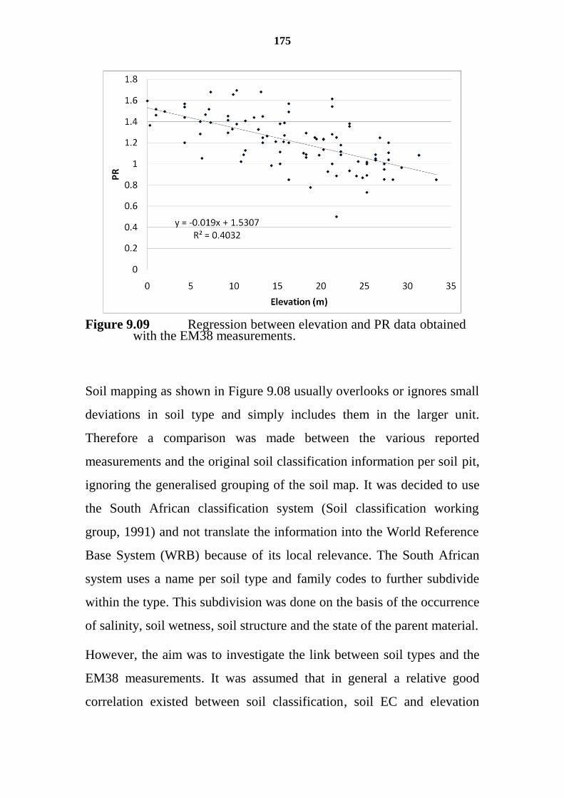
175
Figure 9.09 Regression between elevation and PR data obtained with the EM38 measurements.
Soil mapping as shown in Figure 9.08 usually overlooks or ignores small
deviations in soil type and simply includes them in the larger unit.
Therefore a comparison was made between the various reported
measurements and the original soil classification information per soil pit,
ignoring the generalised grouping of the soil map. It was decided to use
the South African classification system (Soil classification working
group, 1991) and not translate the information into the World Reference
Base System (WRB) because of its local relevance. The South African
system uses a name per soil type and family codes to further subdivide
within the type. This subdivision was done on the basis of the occurrence
of salinity, soil wetness, soil structure and the state of the parent material.
However, the aim was to investigate the link between soil types and the
EM38 measurements. It was assumed that in general a relative good
correlation existed between soil classification, soil EC and elevation
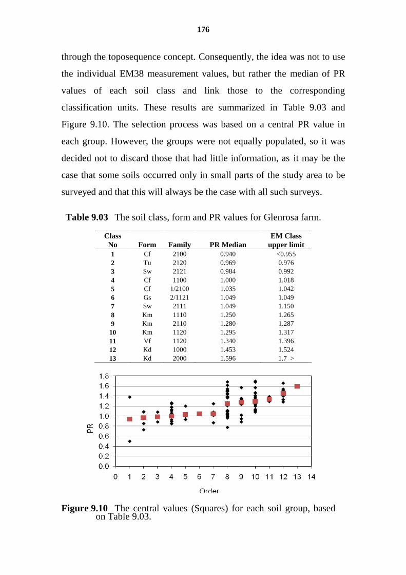
176
through the toposequence concept. Consequently, the idea was not to use
the individual EM38 measurement values, but rather the median of PR
values of each soil class and link those to the corresponding
classification units. These results are summarized in Table 9.03 and
Figure 9.10. The selection process was based on a central PR value in
each group. However, the groups were not equally populated, so it was
decided not to discard those that had little information, as it may be the
case that some soils occurred only in small parts of the study area to be
surveyed and that this will always be the case with all such surveys.
Table 9.03 The soil class, form and PR values for Glenrosa farm.
Class
No Form Family PR Median
EM Class
upper limit
1 Cf 2100 0.940 <0.955
2 Tu 2120 0.969 0.976
3 Sw 2121 0.984 0.992
4 Cf 1100 1.000 1.018
5 Cf 1/2100 1.035 1.042
6 Gs 2/1121 1.049 1.049
7 Sw 2111 1.049 1.150
8 Km 1110 1.250 1.265
9 Km 2110 1.280 1.287
10 Km 1120 1.295 1.317
11 Vf 1120 1.340 1.396
12 Kd 1000 1.453 1.524
13 Kd 2000 1.596 1.7 >
Figure 9.10 The central values (Squares) for each soil group, based on Table 9.03.
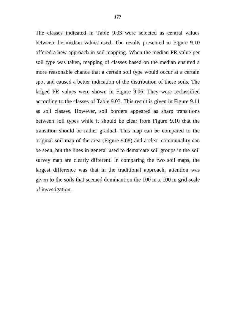
177
The classes indicated in Table 9.03 were selected as central values
between the median values used. The results presented in Figure 9.10
offered a new approach in soil mapping. When the median PR value per
soil type was taken, mapping of classes based on the median ensured a
more reasonable chance that a certain soil type would occur at a certain
spot and caused a better indication of the distribution of these soils. The
kriged PR values were shown in Figure 9.06. They were reclassified
according to the classes of Table 9.03. This result is given in Figure 9.11
as soil classes. However, soil borders appeared as sharp transitions
between soil types while it should be clear from Figure 9.10 that the
transition should be rather gradual. This map can be compared to the
original soil map of the area (Figure 9.08) and a clear communality can
be seen, but the lines in general used to demarcate soil groups in the soil
survey map are clearly different. In comparing the two soil maps, the
largest difference was that in the traditional approach, attention was
given to the soils that seemed dominant on the 100 m x 100 m grid scale
of investigation.
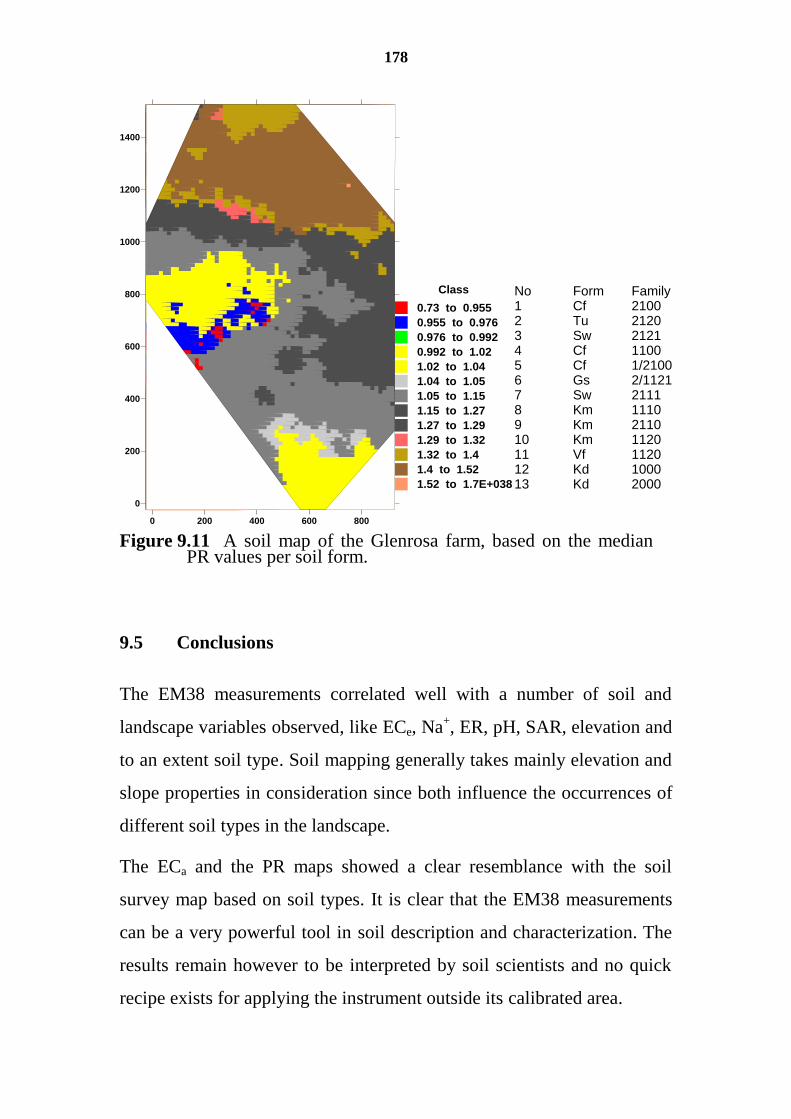
178
0 200 400 600 800
0
200
400
600
800
1000
1200
1400
Class
0.73 to 0.955
0.955 to 0.976
0.976 to 0.992
0.992 to 1.02
1.02 to 1.04
1.04 to 1.05
1.05 to 1.15
1.15 to 1.27
1.27 to 1.29
1.29 to 1.32
1.32 to 1.4
1.4 to 1.52
1.52 to 1.7E+038
No Form Family1 Cf 21002 Tu 21203 Sw 21214 Cf 11005 Cf 1/21006 Gs 2/11217 Sw 21118 Km 11109 Km 211010 Km 112011 Vf 112012 Kd 100013 Kd 2000
Figure 9.11 A soil map of the Glenrosa farm, based on the median PR values per soil form.
9.5 Conclusions
The EM38 measurements correlated well with a number of soil and
landscape variables observed, like ECe, Na+, ER, pH, SAR, elevation and
to an extent soil type. Soil mapping generally takes mainly elevation and
slope properties in consideration since both influence the occurrences of
different soil types in the landscape.
The ECa and the PR maps showed a clear resemblance with the soil
survey map based on soil types. It is clear that the EM38 measurements
can be a very powerful tool in soil description and characterization. The
results remain however to be interpreted by soil scientists and no quick
recipe exists for applying the instrument outside its calibrated area.

179
Not all three EM variables (ECa-V, ECa-H and PR) compared equally
well to various mapped realisations of soil properties, but all three can
provide a useful input to improve soil maps since the variation in a
number of soil variables are better presented in the higher resolution of
the EM38 maps.
The combination of EM38 information and soil classification information
can lead to better soil use maps at much lower survey effort.
180
10 CONCLUSIONS AND RECOMMENDATIONS
The objective of this final chapter is to highlight the main conclusions of
the study, to discuss the extent to which key research questions have
been answered and to consider the impact of the findings both in
determining future research directions and in affecting the welfare of
water users in the study area.
10.1 Recapping the background to the study
Salinity of soil and water in the Western Cape Province of South Africa
(WC) is having an increasing impact on the lives of people in the region.
A knowledge of how to manage salinity for the benefit of the whole
population and the environment is very important. This research was
initiated as a result of the foresight that prevailed prior to 1990 when
water supply was planned to match the population growth and the
expansion of industry and agriculture (Moolman et al., 1999).
Agricultural production in many parts of South Africa is not possible
without irrigation. In the WC virtually the entire fruit and wine industries
depend on irrigation. Agriculture is the largest consumer of water. In
1980 agriculture accounted for 52% of the total water use in South Africa
(Dept. Water Affairs, 1986). Although it is expected to decrease to less
than 50% in future, irrigated agriculture has remained to date the largest
user of water. According to various reports published since 1975, the
quality of South Africa's water resources, especially in relation to
181
salinity, is steadily deteriorating (Stander, 1987). Alexander (1980) stated
that "there is no doubt that mineralisation (salinisation) is a serious
problem in South Africa - and it can only get worse!". This is especially
true of rivers and storage dams situated in the WC (Fourie, 1976;
Stander, 1987).
This research was carried out over an extended period. The saline
irrigation experiments commenced in 1992. Most of the work has,
however, been published since 2001 in the form of reports, conference
proceedings and journal articles.
Based on the earlier indications of the salinity problem a number of
commitments were made by water authorities and research bodies to gain
and disseminate information that would facilitate water management in
the WC. First and foremost, water of adequate quantity and quality had to
be supplied to irrigation farmers. Secondly, information was needed
concerning the salt tolerance of crops and the economic viability of
products from saline environments. Thirdly, it became apparent that
managing water successfully required reliable measurements as well as
tools (appropriate methods and equipment, as well as models) to monitor,
predict and extrapolate salinity data on a regional basis. It was within this
framework that the study was carried out.
10.2 Answers to the various research questions
The research objectives of this dissertation were (Chapter 1):
To investigate the sensitivity of grapevine (vitis vinifera, L), to
the quality of irrigation water it receives.
To establish soil water sampling (as opposed to laboratory
estimation using a saturated paste) as a preferred basis for
measuring the effect of saline irrigation on plants.
182
To analyze, from the repetitive sampling of soil water, ways of
predicting soil salinity profiles over time, using polynomials of
the lowest possible order and to indicate the minimum amount
information required to make such predictions.
To optimize soil sampling positions in view of the fact that partial
wetting of soil during irrigation is the norm within the study area.
,
To explore the positive management aspects of partial wetting in
terms of salt storage during the irrigation season.
To assess and model long-term irrigation and the change in soil
salinity on a regional scale and link this to regional sustainability
of table grape production.
To quantify the relationships between soil classification, soil
electromagnetic induction measurements and topography as an
improved basis for mapping soil salinity on a catchment scale.
In the following a brief overview of the degree to which these aims were
met is provided:
It was shown that wine grapes are sensitive to saline irrigation, even
under moderate levels of salinity, with a threshold ECi of 100 mS m-1
.
It was indicated that taking soil water samples was beneficial over
analysing soil samples, as these allowed better the investigation of the
change in soil water salinity status over the growing season. The fact that
these measurements could be done repeatedly in the same soil matrix (i.e.
in an undisturbed way) proved to be very valuable.
By using polynomials in the prediction of ECsw, it was found that in the
study area the ECsw could be predicted satisfactorily using a first order
polynomial. Consequently, the minimum amount of information needed
to characterize this trend in the soil profile, are only two ECsw
measurements taken at two depths.
183
It was indicated that the partial wetting of the soil also implied that soil
sampling needs to focus on the wetting pattern of the soil. The sampling
carried out for the study at the Broodkraal farm, took this into
consideration and the result was that the local variation in soil salinity
could be accounted for by using combined samples from a specific
measuring point.
The partial wetting of soil caused the problem that salts tend to be
managed only in the wetted volume. But it was shown that also in the
non wetted zone the salinity rose during the irrigation season. This non-
wetted zone acted as a salt store and was to an extent also flushed during
winter by rain and winter irrigation. This situation opens the potential to
use the soil as a salt store in a region where leaching of salts poses a
problem.
The regional management and monitoring of salinity can be simplified by
predicting the contribution of a site to the nearby river system in terms of
the salt load lost from the soil profile. This allows to avoid the modelling
of complex soil processes in an era and area with limited resources.
Traditionally the mapping of soils, and the occurrence of soil types, is
linked to topography. Mobile non-invasive proximal soil sensors, like the
EM38, allow the rapid mapping of salinity. A relationship between the
degree of soil salinity and soil type in combination with topography
could be identified in the study area. The EM38 results could be used to
improve the soil map of this region, as the position of soil borders could
be much more clearly indicated.
Based on these objectives and observations, a number of specific
questions could be formulated, which are given below.
184
1. Has the problem area been adequately delineated?
The delineation of the soil salinity problem in the study area was
achieved with specific emphasis on geographic location, geomorphology,
geology, climate, water resources, soils, and land use. Consequently the
salinity hazard in irrigated vineyards of SA has also been defined.
2. Has the principal agricultural crop been adequately evaluated in
terms of its response to salinity?
After irrigating vines for 8 consecutive years with 6 grades of saline
water, it was found that vines were influenced by saline irrigation water,
even that with EC lower than 30 mS m-1
. A salinity tolerance threshold of
100 in place of the norm of 150 mS m-1
was recommended. The yield
response could be defined for use by water regulators, and various
aspects of plant and soil response to salinity were highlighted. A basis for
calculating the potential impact of saline irrigation water on the economy
was also established. Salinity was found to have a quantifiable effect on
the quality of wine and the quantity of grapes that could be produced.
Furthermore, saline water had a cumulative effect on the vines as the
salts were found to be stored in the perennial parts of the plant and
therefore had an effect on the following season’s yield.
Perhaps the most important finding of the research was that, while the
threshold level of saline irrigation required to ensure sustainability
remained the same over a number of years of irrigation, the sensitivity of
the crop to levels beyond the threshold increased with the number of
seasons of exposure.
185
As an economic indicator, wine quality was also found to be sensitive to
saline irrigation. Water quality below 100 mS m-1
caused lower yields but
slightly better wines. It was found that salinity could be adequately tested
in the must, and need not be tested in the wine. Irrigation with saline
water inevitably led to over-irrigation on the more saline plots because
the vines used less water.
3. Can the measurement of salinity be standardised?
A close relationship was found between the ECe and ECi and an equally
strong correlation was also found between ECsw and ECe that allowed the
interaction to be explained. A strong relationship was similarly found
between ECi and ECsw, explaining the ECsw reaction to a specific ECi.
The combination of the two forms a basis whereby the best possible
circumstances, when irrigating with saline water, can be predicted.
Though the ECsw results can be adequately converted to ECe, there is still
a hidden uncertainty in these results concerning the precise relationship
between available and unavailable forms of salt in the soil.
A new suction cup lysimeter (SCL) system was designed and
successfully implemented during years of field research. Our SCL had
the advantage that it could be operated remotely. This allowed sampling
at precisely planned times and provided added value in years of
monitoring and managing soil salinity. Ease of use is the main
characteristic of this system. The soil water samples could also supply
information on the soil water content by merely recording the mass of the
water sample. This system is fairly inexpensive and can supply more
information than conventional SCLs. Since the system allows remote
operation, a lot of time can be saved in acquiring soil water samples.
186
4. Was the salinity behaviour in soils adequately measured and to what
extent can salinity be predicted? Can the salinity behaviour in soil over a
landscape be predicted from a limited amount of point samples?
The focus was on the prediction of the depth trend in soil salinity within
a vineyard after sustained irrigation with saline water. This study
provided the opportunity to better understand the temporal and spatial
variation of ECsw. The classical trend surface analysis procedure of Davis
(1986) provided an answer to the problem of finding a suitable depth
relationship that could be used as a norm for the soil studied. This
simplified the management of salt in the soil and the quantity and quality
of return flow.
Prediction of the depth trend in ECsw with a first order polynomial has
distinct advantages. Over- or under-irrigation can easily be evaluated for
any irrigated land. Prediction of salt accumulation on the soil surface or
deep drainage can readily be assessed. The slope of the first order
polynomial indicates directly the general trend and whether an
accumulation or a depletion of salt can be expected in the soil. When
linked to remote sensing, this approach could be used in evaluating
extensive areas of land in terms of salinity and their suitability for
irrigated crops. This research further showed that by knowing the date
and irrigation water quality and being able to characterize the topsoil EC
remotely, one can estimate subsoil salinity conditions in irrigated lands
and further estimate the return-flow component from such irrigated lands.
In chapter 7, the variability of ECe between vine rows was explored. The
results clearly showed that the distribution of salts from under the
irrigation emitters to a position mid-way between two vine rows, can be
highly variable. The inter-row region was subjected to a salt build-up
187
over the growing season and is not always leached by the irrigation.
Factors such as density of the cover crop, partial wetting of the soil, the
orientation of the vine rows, traffic in the vineyards and the quality of the
irrigation water, all play a crucial role in the accumulation of salt in this
part of the vineyard soil. This knowledge has important management
implications for a saline environment.
5. Can the temporal effect of salinity in vineyards be captured and
modelled on a regional basis? Can the regional salinity behaviour be
predicted from less intensive data collection?
Both these questions were dealt with simultaneously. The effect of long
term irrigation application on the variation of soil electrical conductivity
in vineyards was investigated looking at soil sampling technique and
time-space modelling. The investigated areas were under table grapes
and were subjected to a rigorous irrigation program. The older sites had a
lower salt content than the younger sites but the relative variability
remained almost constant. So, the data proved that there is a general
lowering of salinity in the landscape resulting from irrigation practices.
By using a method of predicting change with time using icdf’s, and by
sampling the irrigation history from the 2nd
year to the 5th
year, the
periods of most dramatic change have been captured. After the 5th
year,
the soil ECe tends to be subjected to the irrigation water quality of the
past season. The amount of salt removed from the profile over the study
period showed a delayed effect in influencing the water quality of the
river system.
Two aspects can be highlighted. Firstly, modelling of the temporal
behaviour of soil salinity was approached in a unique manner that proved
to be a good predictor, but rigorous proof will, however, require re-
188
sampling after a period of time. Secondly, predicting the contribution of
the site to the nearby river system in terms of the salt load lost from the
soil profile, proved to be a valuable way of bypassing intricate soil
process modelling in a context for which funds, the total land area and
skilled labour shortages are limiting factors in addressing these problems.
The regional sustainability in table grape production on saline soils was
investigated looking at ECe and ER, soil pH, soil clay percentage and
vine response. By using kriging, soil ECe, pH, vine age and vigour could
be predicted at a high resolution, generating a regional realization or
trend. It was shown that modelling the regional trends, and their
statistical comparison, produced good results and opened opportunities
related to sustainability issues that were not afforded when using point
data only. The predictability of the regional variation of ECe in relation to
pH, time and plant vigour could have an impact on the grape/wine
industry of the Western Cape.
Over-irrigation, as a means of dealing with salinity in the landscape, did
not result in a salt build-up. Gypsum was also used to improve
infiltration and control the sodium build-up and this led to a reduced role
played by clay content as a growth inhibitor.
Soil pH showed a significant relationship to the long-term, measured
changes in trunk circumference of the vines. The ECe of the upper part of
the soil must be considered in the context of up to 10 mm
evapotranspiration per day and very little rainfall; hence the dependence
on irrigation. It can thus be expected that ECe will be lowest in over-
irrigated areas. In parts that receive less irrigation than the evaporative
demand a build-up of salts will occur. In parts that receive no irrigation
but that are near to the irrigated area the ECe will soar. In sites where the
189
soil pH is restricting growth, transpiration is reduced and therefore over-
irrigation usually occurs, resulting in runoff and increased drainage that
both augment return flow.
Perhaps the most important finding of the research was that vine age, ECe
and pH correlated weakly with trunk circumference. However, in
combination, these variables generated an R2 value of 66 %. The fact that
66 % of the variance was explained by vine age, ECe and pH in
combination, suggested that very little else influenced growth negatively
in this environment.
The most important implications of these results are economic. This
research showed that the methods applied here could enhance current
knowledge in terms of the behaviour and sustainability of agricultural
crops on a regional basis through a process that deals with spatial
variation. This could increase profitability from these landscapes and it
deals with very important water issues.
In Chapter 10, the soil salinity and soil type were characterized using the
EM38 proximal soil sensor. The EM38 measurements correlated well
with a number of soil and landscape variables. Soil survey generally
takes mainly elevation and slope properties into consideration since both
influence the occurrence of different soil types in the landscape. The data
presented here show a significant correlation with ECe, ER, pH, SAR,
Na+, elevation and to some extent soil type. From the maps presented,
elevation, the PR and soil depth showed a similar pattern. All three of
them, as well as the ECa-V and ECa-H maps, showed useful
comparability with the hand drawn soil map.
It is clear that the EM38-derived maps can be a powerful tool in soil
description and characterization. The results remain, however, to be
190
interpreted by soil scientists and no quick recipe exists for applying the
instrument outside its designed use. A fair knowledge of modelling semi-
variance using geostatistical procedures is also required.
Not all three EM variables compared equally well to various mapped
realisations of soil properties, but all three can provide a versatile input
to better soil maps since the variation in a number of soil variables are
better presented in the higher resolution of the EM38 maps.
The combination of EM38 information and soil classification information
can lead to better soil maps with much less survey effort.
10.3 The impacts of the study
This research has contributed in a number of ways:
A methodology for defining and dealing with salinity hazard has
been defined.
A methodology for prediction of salinity in the soil has been
established. This has the advantage of allowing better
management of salinity with fewer soil samples.
A methodology for the economic evaluation of salinity in the
study region has been established.
Various prescriptive aspects for water managers have been
described and defined.
The regional and temporal change in soil salinity has been
characterized and assessment methodology has been proposed.
Mapping salinity, i.e. profile salt distribution and regional distribution,
brought greater insight into the estimation of salt quantities in the
irrigated landscape. Various factors have been highlighted that
contributed to the attenuation capacity of a soil. It has also been shown
that soil salinity in irrigated landscapes is subject to the specific
191
irrigation practice. The capacity of the soil to retain salts was shown to
have a unique threshold value. Furthermore, the unique balance between
salt accumulation and salt leaching has been demonstrated.
Methods of measuring soil salinity were discussed and the investigation
revealed that measurements of the soil salinity status at field capacity
were the most accurate basis for evaluating the state of soil salinity. A
suction cup system was developed that allowed the simultaneous
sampling of soil water over a large area and numerous treatments.
The Davis (1986) approach provided an answer to the problem of finding
a suitable ECsw depth relationship that could be used as a norm for this
specific soil. This approach simplified management of salt in terms of
both quantity and quality of return flow. This approach will also help to
provide rapid assessment in regional soil salinity investigations in the
future.
This thesis connects the factors known to influence salinity with ways of
measuring salinity in the soil, the description of salinity changes over
time, and the assessment of salinity on a regional basis.
Our ability to predict soil salinity patterns on a regional scale is made
possible by adhering to simple rules developed in this study. A survey
can be done by taking soil samples at only two depths in the profile.
Alternatively, a survey can be conducted using an instrument such as the
EM38 which can estimate salinity in the soil profile at two depths.
It was also indicated that topography, the occurrence of soil types and the
occurrence of salinity in the Berg and Breede River landscapes are
closely related. This knowledge can be used in management, in the sense
that expansion of irrigated vineyards can be better controlled.
192
10.4 Future perspectives
This research indicated that irrigated land in the BRC and UBRC is
generally close to the river system and closely linked to the river system.
It focussed on a number of issues related to soil salinity and its apparent
effect on the rivers. These results showed that it was possible that the
irrigated areas originally had high salinity, but that after 3 years of
irrigation these soils maintained a salt content consistent with the salinity
of the irrigation water they received.
The need exists therefore to look wider in the region for situations and
conditions that could affect the quality of the water in these rivers. The
focus then shifts to dryland salinity as these changes in land use also
brings about changes in the behaviour of ground water and the resultant
migration of salt towards the river.
This research also indicated that a need exists to further map the irrigated
landscapes and bring everything into a hydrological modelling
perspective. Land use and soil type are important variables in
hydrological modelling and this type of modelling could broaden the
perspective and management principles for the region.
More effort needs to go into the detailed mapping of soil types. The
possibility of using remote sensing to accomplish this is currently being
debated among soil scientists. The study showed that using an instrument
such as the EM38 could help in generating better soil maps, containing
georeferenced information. This is one aspect of the research that will
need further attention.
Land use changes are causing differential changes in the production of
salinity that leads to a deterioration of the river systems. A study needs to

193
be conducted where different land uses are compared with respect to
their total effect on the environment. This should result in optimal
agricultural practices that will minimise the damaging effect of saline
seep and low quality return flow on both the rivers and the ecosystems
which they drain.
194
11 REFERENCES
Alexander, W.J.R., 1985. Hydrology of low latitude Southern Hemisphere land
masses. Hydrobiologia, 125,1.
Anon., 1989. Climate statistics for the Winter Rainfall Region up to 1989.
Agrometeorology Section, Elsenburg, Soil and Irrigation Research Institute,
Department of Agriculture and Water Supply.
Ayers, R.S., Westcott, D.W. 1985. Water Quality for Agriculture. FAO Irrigation and
Drainage Paper No 29, Rev. 1. FAO, Rome.
Baumgartner, A., Reichel, E., 1975. The world water balance. Elsevier Scientific
Publisching Company, Amsterdam.
Ben-Gal, A., Ityel, E., Dudley, L., Cohen, C., Yermiyahu, U., Presnov, E., Zigmond,
L., Shani, U., 2008. Effect of irrigation water salinity on transpiration and on
leaching requirements: A case study for bell peppers Agricultural Water
Management 95, 587–597.
Bennie, A.T.B., Hensley, M., 2001. Maximizing precipitation utilization in dryland
agriculture in South Africa — a review. Journal of Hydrology, 241,1-2, 124-
139.
Berbel, J., Gomez-Limon, J.A. 2000 The impact of water-pricing policy in Spain: an
analysis of three irrigated areas. Agricultural Water Management, 43,
219±238.
Bernstein, L., Hayward, H.E., 1958. Physiology of salt tolerance. Ann. Rev. Plant
Physiol. 9: 25-46.
Bourgault, G., Journel, A.G., Rhoades, J.D., Corwin, D.L., and Lesch, S.M., 1998.
Geostatistical analysis of a soil salinity data set. Advances in Agronomy, 58:
241-292.
195
Bruwer, L.H., 1993. Evaluation of the design and management of irrigation systems in
the Breede River Valley with the view to control potential drainage losses.
(In Afrikaans). WRC Report No 256/1/93, Water Research Commission,
Pretoria, South Africa.
Burrough, P.A., McDonnell, R.A., 1998. Principles of Geographic Information
Systems. Oxford University Press, New York.
Burrough, P.A., Van Gaans, P.F.M., Hootsmans, R., 1997. Continuous classification
in soil survey: Spatial correlation, confusion and boundaries. Geoderma, 77,
115-135.
Cass, A., 1979. Water quality and soil suitability for irrigation. SA Irrigation Aug/Sep
1979, Johannesburg, South Africa.
Cass, A., 1986. Irrigation return flow water quantity and quality modelling in South
Africa. Unpublished report to the WRC. Dept Soil Science, University of
Natal.
Cetin, M., Kirda, C., 2003. Spatial and temporal changes of soil salinity in a cotton
field irrigated with low-quality water. Journal of Hydrology, 272, 238-249.
Chilès, J.P., Delfiner, P., 1999. Geostatistics. John Wiley & Sons, New York.
Cockx, L., Van Meirvenne, M., De Vos, B., 2007. Using the EM38DD soil sensor to
delineate clay lenses in a sandy forest soil. Soil Science Society of America
Journal 71:1314-1322
Davis, J.C., 1986. Statistics and Data Analysis in Geology. Wiley, New York.
de Clercq, W.P., Fey, M.V., Moolman, J.H., Wessels, W.P.J., Eigenhuis, B., Hoffman,
E. 2001. Experimental irrigation of vineyards with saline water. WRC
Report, 522/1/01.
de Clercq, W.P., Fey, M.V., Moolman, J.H., Wessels, W.P.J., Eigenhuis, B., Hoffman,
E., 2001. Establishing the effects of saline irrigation water and managerial
options on soil properties and plant performance. WRC Report, 695/1/01.
de Clercq, W.P., Jovanovic, N., Fey, M., (Eds). 2008. Research on Berg River water
management. WRC Report, (in press).
de Clercq, W.P., Moolman, J.H., Wessels, W.P.J., 1994. An automated sample
retrieval system for soil water samples. p31-32 In: Proceedings of the 18th
Congress of the Soil Science Society of South Africa, 11-13 January 1994,
Potchefstroom, South Africa.
de Clercq, W.P., Van Meirvenne, M., 2005. Effect of long-term irrigation application
on the variation of soil electrical conductivity in vineyards. Geoderma 128,
221-233.

196
De Jong, E., Blantyre, A.K., Camaron, D.R., Read, D.W.L., 1979. Measurement of
apparent electrical conductivity of soils by an electromagnetic induction
probe to aid salinity surveys. Soil Science Society of America Journal, 43,
810-812.
Debyle, N.V., Hennes, R.W. Tanner, P.D., 1999. Evaluation of ceramic cups for
determining soil solution chemistry. Soil Science, 146, 30-36.
Deutch, C.V., Journel, A.G., 1992. GSLIB: Geostatistical software library and user’s
guide. Oxford university press, New York, p340.
Douaik, A., Van Meirvenne, M., Toth, T., 2006. Temporal stability of spatial patterns
of soil salinity determined from laboratory and field electrical conductivity.
Arid Land Research and Management, 20, 1-13.
Du Toit, S.F., 1995. Tyd- en ruimtelike veranderinge in die grondchemiese
samestelling van 'n wingerd wat met soutryke water besproei word.
(Afrikaans). Unpublished M.Sc. Thesis, University of Stellenbosch,
December, 1995.
Dunn, S.M., Lilly, A., 2001. Investigating the relationship between a soils
classification and the spatial parameters of a conceptual catchment-scale
hydrological model. Journal of Hydrology, 252, 1, 157-173.
DWAF, 1986. Management of the Water Resources of the Republic of South Africa.
Department of Water Affairs, Pretoria.
Eastman, J.R., 1999. IDRISI 32: Guide to GIS and Image Processing. Clark
University, Worcester MA.
FAO, 1998. World reference base for soils. World soil resources reports 84, FAO,
Rome.
Farifteh, J., Farshad, A., 2002. Remote sensing and modelling of topsoil properties, a
clue for assessing land degradation. 17th WCSS, Thailand, Paper 562.
Fey, M.V., de Clercq, W.P., 2004. A pilot study investigating the role of dryland salinity in the quality of the water of the Berg River. WRC Report 1342/1/04.
Finke, P.A., Wladis, D., Kros, J., Pebesma, E.J., Reinds, G.J., 1999. Quantification
and simulation of errors in categorical data for uncertainty analysis of soil
acidification modelling. Geoderma, 93, 177–194.
Flowers, T.J., Yeo, A.R., 1986. Ion relations of plants under drought and salinity.
Australian Journal of Plant Physiology, 13, 75-91.
Flügel, W.A., 1995. River salinity due to dryland agriculture in the Western Cape
Province, Republic of South Africa. Environmental Int., 21, 5, 679-686.
197
Forsberg, J., Nilsson, L., 2005. On polynomial response surfaces and kriging for use
in structural optimization of crashworthiness. Structural and
Multidisciplinary Optimization, 29, 3.
Fourie, J.M., 1976. Mineralization of Western Cape Rivers: An investigation into the
deteriorating water quality related to drainage from cultivated lands along
selected catchments, with special reference to the Great Berg River.
Ph.D.(Agric) Thesis, University of Stellenbosch, March 1976.
Francois, L.E., Maas. E.V., 1994. Crop response and management on salt affected
soils. In: "Handbook of Plant and Crop Stress". ed. M. Pessarakli. Marcel
Dekker, Inc.
Frenkel, H., Meiri, A., 1985. Crop response. In: Soil Salinity - Two decades of
research in irrigated agriculture. (Eds. Frenkel, H. & Meiri, A). Van Nostrand
Reinhold Company Inc., New York, pp 441.
Goovaerts, P., 1997. Geostatistics for natural resources evaluation. Oxford University
Press, New York.
Goovaerts, P., 1997. Geostatistics for Natural Resources Evaluation. Oxford
University Press, New York.
Goovaerts, P., 1999. Geostatistics in soil science: State-of-the-art and perspectives.
Geoderma, 89, 1-45.
Görgens, A., 1994. Breede River System: DISA salinity predictions for various
planning scenarios. NSI Report No. 1675/4747.
Görgens, A., de Clercq, W.P., (Eds), 2006. Water quality information systems for
integrated water resource management: The Riviersonderend-Berg River
system. WRC Report, TT262/06.
Greef, G.J., 1990. Detailed geohydrological investigations in the Poesjesnel River
catchment in the Breede River Valley with special reference to
mineralization. WRC Report No 120/1/90.
Grossmann, J., Udluft, P., 1991. The extraction of soil water by the suction cup
method: a review. J. Soil Sci. 42, 83-93.
Heuvelink, G. B. M., Webster, R., 2001, Modelling soil variation: past, present, and
future. Geoderma, 100, 3-4, 269-301.
Heuvelink, G.B.M., 1998. Uncertainty analysis in environmental modelling under a
change of spatial scale. Earth and Environmental Science, 50, 255-264.
Heuvelink, G.B.M., Pebesma, E.J., 1999. Spatial aggregation and soil process
modelling. Geoderma, 89 47–65.
Hillel, D., 1991. Out of the earth: Civilization and the life of the soil. The Free Press.
New York.
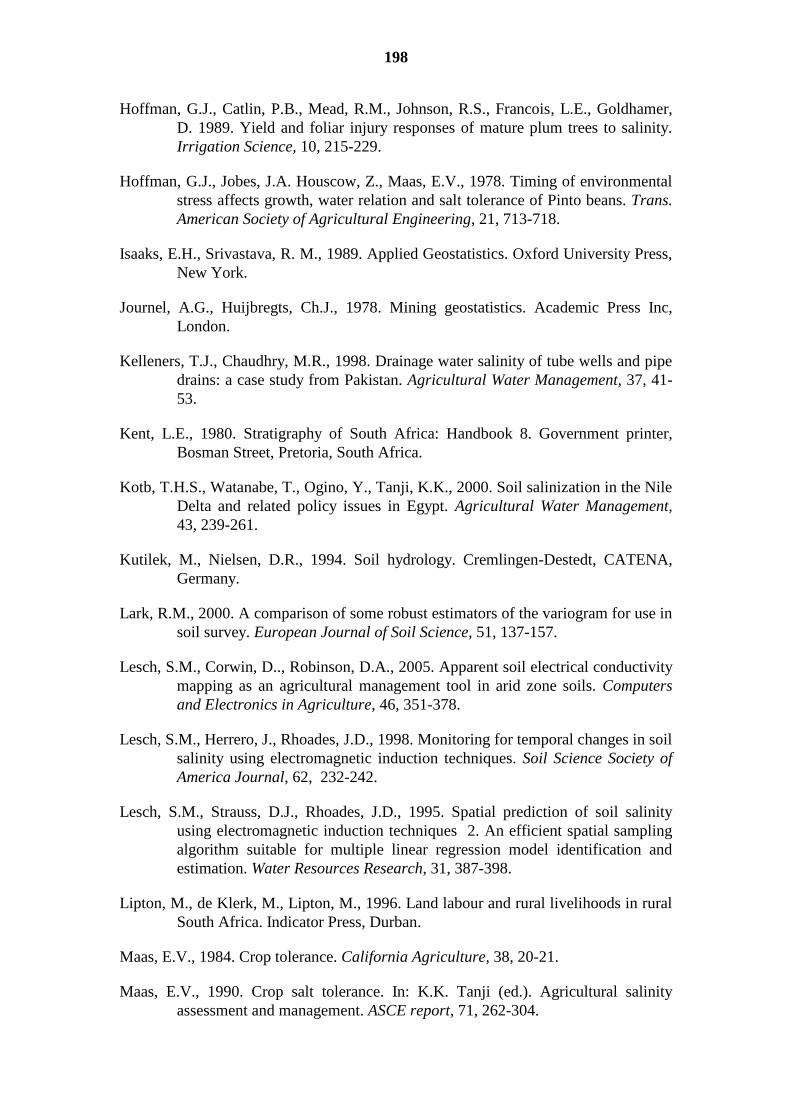
198
Hoffman, G.J., Catlin, P.B., Mead, R.M., Johnson, R.S., Francois, L.E., Goldhamer,
D. 1989. Yield and foliar injury responses of mature plum trees to salinity.
Irrigation Science, 10, 215-229.
Hoffman, G.J., Jobes, J.A. Houscow, Z., Maas, E.V., 1978. Timing of environmental
stress affects growth, water relation and salt tolerance of Pinto beans. Trans.
American Society of Agricultural Engineering, 21, 713-718.
Isaaks, E.H., Srivastava, R. M., 1989. Applied Geostatistics. Oxford University Press,
New York.
Journel, A.G., Huijbregts, Ch.J., 1978. Mining geostatistics. Academic Press Inc,
London.
Kelleners, T.J., Chaudhry, M.R., 1998. Drainage water salinity of tube wells and pipe
drains: a case study from Pakistan. Agricultural Water Management, 37, 41-
53.
Kent, L.E., 1980. Stratigraphy of South Africa: Handbook 8. Government printer,
Bosman Street, Pretoria, South Africa.
Kotb, T.H.S., Watanabe, T., Ogino, Y., Tanji, K.K., 2000. Soil salinization in the Nile
Delta and related policy issues in Egypt. Agricultural Water Management,
43, 239-261.
Kutilek, M., Nielsen, D.R., 1994. Soil hydrology. Cremlingen-Destedt, CATENA,
Germany.
Lark, R.M., 2000. A comparison of some robust estimators of the variogram for use in
soil survey. European Journal of Soil Science, 51, 137-157.
Lesch, S.M., Corwin, D.., Robinson, D.A., 2005. Apparent soil electrical conductivity
mapping as an agricultural management tool in arid zone soils. Computers
and Electronics in Agriculture, 46, 351-378.
Lesch, S.M., Herrero, J., Rhoades, J.D., 1998. Monitoring for temporal changes in soil
salinity using electromagnetic induction techniques. Soil Science Society of
America Journal, 62, 232-242.
Lesch, S.M., Strauss, D.J., Rhoades, J.D., 1995. Spatial prediction of soil salinity
using electromagnetic induction techniques 2. An efficient spatial sampling
algorithm suitable for multiple linear regression model identification and
estimation. Water Resources Research, 31, 387-398.
Lipton, M., de Klerk, M., Lipton, M., 1996. Land labour and rural livelihoods in rural
South Africa. Indicator Press, Durban.
Maas, E.V., 1984. Crop tolerance. California Agriculture, 38, 20-21.
Maas, E.V., 1990. Crop salt tolerance. In: K.K. Tanji (ed.). Agricultural salinity
assessment and management. ASCE report, 71, 262-304.
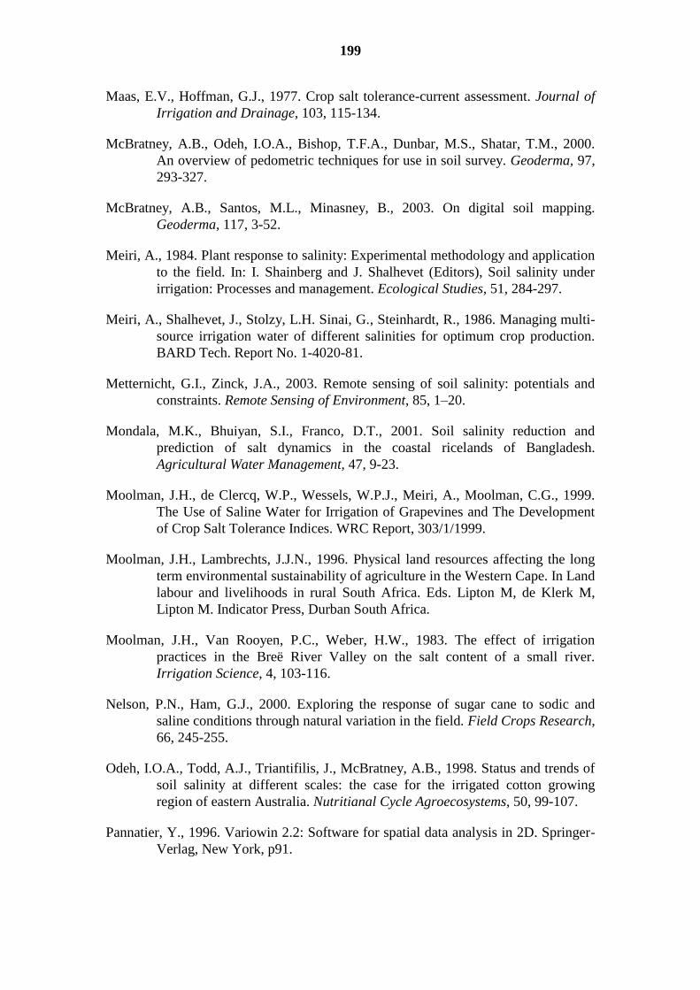
199
Maas, E.V., Hoffman, G.J., 1977. Crop salt tolerance-current assessment. Journal of
Irrigation and Drainage, 103, 115-134.
McBratney, A.B., Odeh, I.O.A., Bishop, T.F.A., Dunbar, M.S., Shatar, T.M., 2000.
An overview of pedometric techniques for use in soil survey. Geoderma, 97,
293-327.
McBratney, A.B., Santos, M.L., Minasney, B., 2003. On digital soil mapping.
Geoderma, 117, 3-52.
Meiri, A., 1984. Plant response to salinity: Experimental methodology and application
to the field. In: I. Shainberg and J. Shalhevet (Editors), Soil salinity under
irrigation: Processes and management. Ecological Studies, 51, 284-297.
Meiri, A., Shalhevet, J., Stolzy, L.H. Sinai, G., Steinhardt, R., 1986. Managing multi-
source irrigation water of different salinities for optimum crop production.
BARD Tech. Report No. 1-4020-81.
Metternicht, G.I., Zinck, J.A., 2003. Remote sensing of soil salinity: potentials and
constraints. Remote Sensing of Environment, 85, 1–20.
Mondala, M.K., Bhuiyan, S.I., Franco, D.T., 2001. Soil salinity reduction and
prediction of salt dynamics in the coastal ricelands of Bangladesh.
Agricultural Water Management, 47, 9-23.
Moolman, J.H., de Clercq, W.P., Wessels, W.P.J., Meiri, A., Moolman, C.G., 1999.
The Use of Saline Water for Irrigation of Grapevines and The Development
of Crop Salt Tolerance Indices. WRC Report, 303/1/1999.
Moolman, J.H., Lambrechts, J.J.N., 1996. Physical land resources affecting the long
term environmental sustainability of agriculture in the Western Cape. In Land
labour and livelihoods in rural South Africa. Eds. Lipton M, de Klerk M,
Lipton M. Indicator Press, Durban South Africa.
Moolman, J.H., Van Rooyen, P.C., Weber, H.W., 1983. The effect of irrigation
practices in the Breë River Valley on the salt content of a small river.
Irrigation Science, 4, 103-116.
Nelson, P.N., Ham, G.J., 2000. Exploring the response of sugar cane to sodic and
saline conditions through natural variation in the field. Field Crops Research,
66, 245-255.
Odeh, I.O.A., Todd, A.J., Triantifilis, J., McBratney, A.B., 1998. Status and trends of
soil salinity at different scales: the case for the irrigated cotton growing
region of eastern Australia. Nutritianal Cycle Agroecosystems, 50, 99-107.
Pannatier, Y., 1996. Variowin 2.2: Software for spatial data analysis in 2D. Springer-
Verlag, New York, p91.
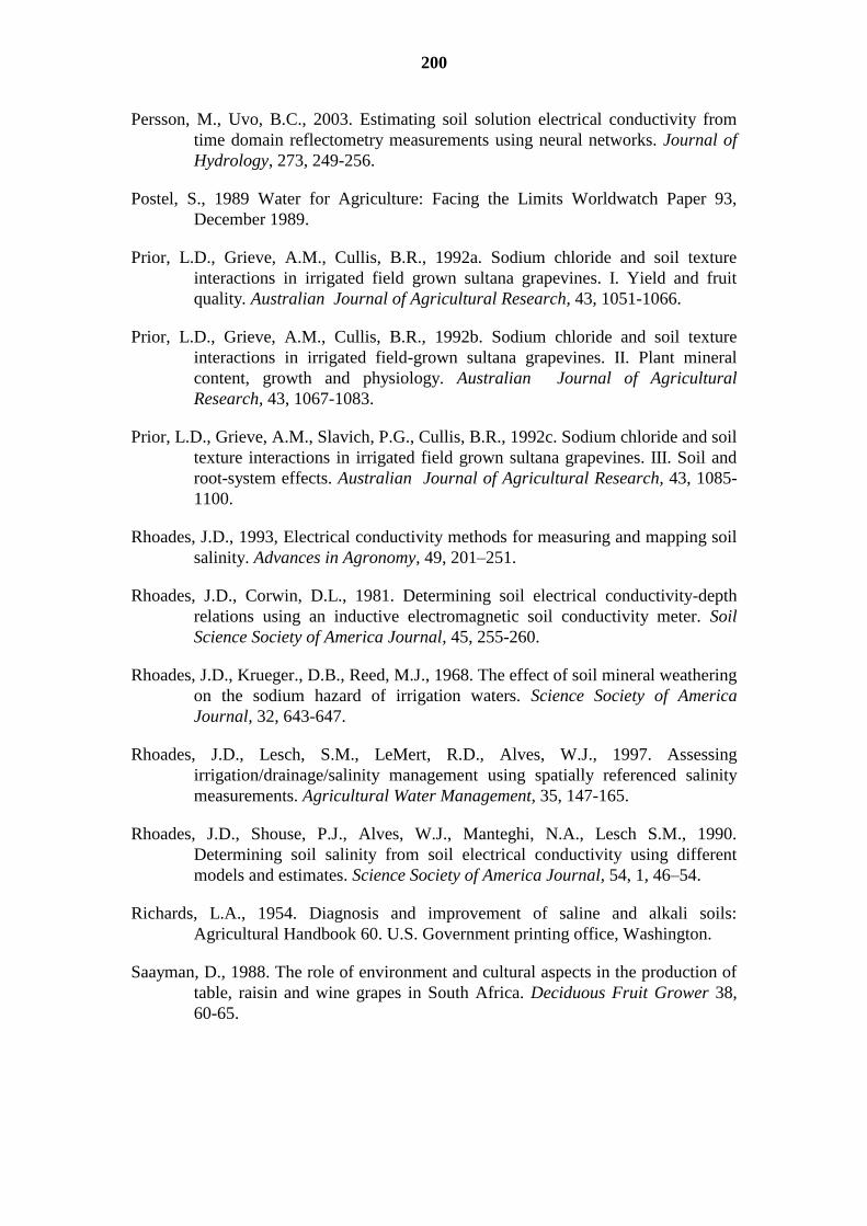
200
Persson, M., Uvo, B.C., 2003. Estimating soil solution electrical conductivity from
time domain reflectometry measurements using neural networks. Journal of
Hydrology, 273, 249-256.
Postel, S., 1989 Water for Agriculture: Facing the Limits Worldwatch Paper 93,
December 1989.
Prior, L.D., Grieve, A.M., Cullis, B.R., 1992a. Sodium chloride and soil texture
interactions in irrigated field grown sultana grapevines. I. Yield and fruit
quality. Australian Journal of Agricultural Research, 43, 1051-1066.
Prior, L.D., Grieve, A.M., Cullis, B.R., 1992b. Sodium chloride and soil texture
interactions in irrigated field-grown sultana grapevines. II. Plant mineral
content, growth and physiology. Australian Journal of Agricultural
Research, 43, 1067-1083.
Prior, L.D., Grieve, A.M., Slavich, P.G., Cullis, B.R., 1992c. Sodium chloride and soil
texture interactions in irrigated field grown sultana grapevines. III. Soil and
root-system effects. Australian Journal of Agricultural Research, 43, 1085-
1100.
Rhoades, J.D., 1993, Electrical conductivity methods for measuring and mapping soil
salinity. Advances in Agronomy, 49, 201–251.
Rhoades, J.D., Corwin, D.L., 1981. Determining soil electrical conductivity-depth
relations using an inductive electromagnetic soil conductivity meter. Soil
Science Society of America Journal, 45, 255-260.
Rhoades, J.D., Krueger., D.B., Reed, M.J., 1968. The effect of soil mineral weathering
on the sodium hazard of irrigation waters. Science Society of America
Journal, 32, 643-647.
Rhoades, J.D., Lesch, S.M., LeMert, R.D., Alves, W.J., 1997. Assessing
irrigation/drainage/salinity management using spatially referenced salinity
measurements. Agricultural Water Management, 35, 147-165.
Rhoades, J.D., Shouse, P.J., Alves, W.J., Manteghi, N.A., Lesch S.M., 1990.
Determining soil salinity from soil electrical conductivity using different
models and estimates. Science Society of America Journal, 54, 1, 46–54.
Richards, L.A., 1954. Diagnosis and improvement of saline and alkali soils:
Agricultural Handbook 60. U.S. Government printing office, Washington.
Saayman, D., 1988. The role of environment and cultural aspects in the production of
table, raisin and wine grapes in South Africa. Deciduous Fruit Grower 38,
60-65.
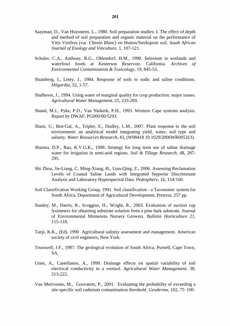
201
Saayman, D., Van Huyssteen, L., 1980. Soil preparation studies: I. The effect of depth
and method of soil preparation and organic material on the performance of
Vitis Vinifera (var. Chenin Blanc) on Hutton/Sterkspruit soil. South African
Journal of Enology and Viticulture, 1, 107-121.
Schuler, C.A., Anthony, R.G., Ohlendorf, H.M., 1990. Selenium in wetlands and
waterfowl foods at Kesterson Reservoir, California. Archives of
Environmental Contamination & Toxicology, 19, 845-53.
Shainberg, I., Letey, J., 1984. Response of soils to sodic and saline conditions.
Hilgardia, 52, 1-57.
Shalhevet, J., 1994. Using water of marginal quality for crop production: major issues.
Agricultural Water Management, 25, 233-269.
Shand, M.J., Pyke, P.D., Van Niekerk, P.H., 1993. Western Cape systems analysis.
Report by DWAF, PG000/00/5293.
Shani, U., Ben-Gal, A., Tripler, E., Dudley, L.M., 2007. Plant response to the soil
environment: an analytical model integrating yield, water, soil type and
salinity. Water Resources Research, 43, (W08418 10.1029/2006WR005313).
Sharma, D.P., Rao, K.V.G.K., 1998. Strategy for long term use of saline drainage
water for irrigation in semi-arid regions. Soil & Tillage Research, 48, 287-
295.
Shi Zhou, Jie-Liang, C, Ming-Xiang, H., Lian-Qing, Z., 2006. Assessing Reclamation
Levels of Coastal Saline Lands with Integrated Stepwise Discriminant
Analysis and Laboratory Hyperspectral Data. Pedosphere, 16, 154-160.
Soil Classification Working Group, 1991. Soil classification - a Taxonomic system for
South Africa. Department of Agricultural Development, Pretoria. 257 pp.
Stanley, M., Harris, R., Scoggins, H., Wright, R., 2003. Evaluation of suction cup
lysimeters for obtaining substrate solution from a pine bark substrate. Journal
of Environmental Minnesota Nursery Growers. Bulletin Horticulture 21,
115-118.
Tanji, K.K., (Ed). 1990 Agricultural salinity assessment and management. American
society of civil engineers, New York.
Trusswell, J.F., 1987. The geological evolution of South Africa. Purnell, Cape Town,
SA.
Utset, A., Castellanos, A., 1999. Drainage effects on spatial variability of soil
electrical conductivity in a vertisol. Agricultural Water Management, 38,
213-222.
Van Meirvenne, M., Goovaerts, P., 2001. Evaluating the probability of exceeding a
site-specific soil cadmium contamination threshold. Geoderma, 102, 75–100.

202
Van Schilfgaarde, J., 1970. Theory of flow to drains. In: Chow, V.T. (Ed.), Advances
in Hydroscience. Academic Press, London. pp. 6, 43-106.
Van Schilfgaarde, J., Bernstein, L., Rhoades, J.D., Rawlins, S.L., 1974. Irrigation
Management for Salt Control. Journal of the Irrigation and Drainage, 3,
321-338.
Van Schilfgaarde, J., 1994. Irrigation-a blessing or a curse. Agricultural Water
Management, 25, 203-219.
Van Zyl, J.L., 1984a. Interrelationships among soil water regime, irrigation and water
stress in the grapevine (Vitis vinifera L.). Unpublished Ph.D. (Agric.) thesis,
University of Stellenbosch, December 1984.
Van Zyl, J.L., 1984b. Response of colombar grapevine to irrigation as regards quality
aspects and growth. South African Journal of Enology and Viticultur, 5, 19-
28.
Verster, G., van Rooyen, F.C., 1990. Glossary of Soil Science. Soil Science Society of
South Africa, V&R Printing Pretoria.
Wagner, G.H., 1962. Use of porous ceramic cups to sample soil water within the
profile. Journal of Soil Science Series, 2402, 379-386.
Webster, R., 2001. Statistics to support soil research and their presentation. European
Journal of Soil Science, 52, 331-340.
Webster, R., Oliver, M., 2000. Geostatistics for environmental scientists. Statistics in
practice. John Wiley & Sons, Ltd., Baffins Lane, Chichester, West Sussex,
England.
Webster, R., Oliver, M.A., 2007. Geostatistics for Environmental Scientists. Second
Edition. John Wiley & Sons, Chichester.
Wellington, J.H., 1955. South Africa: A geographical study. Cambridge Univ. Press,
London.
Wessels, W.P.J., Steyn, W.H., Moolman, J.H., 1995. Automatic micro irrigation and
salt injection system for research and commercial applications. p116-122 In:
Proceedings of the Fifth International Micro irrigation Congress, Hyatt
Regency, Orlando Florida, U.S.A.
West, D.W., Taylor, J.A., 1984. Response of six grape cultivars to the combined
effects of high salinity and rootzone waterlogging. Journal of American
Society of Horticultural Science, 109, 844-851.
Wolters, W., 1992. Influences on the efficiency of irrigation water use. International
Institute for land reclamation and improvement. Wageningen, The
Netherlands.

203
Yaalon, D.H., 1963. On the origin and accumulation of salts in groundwater and soils
of Israel. Bulletin of the Research Council Israel, 11G, 105-131.
Yan Zhu, Wei-Xing Cao, Ting-Bo Dai, Yong-Chao Tian, Xia Yao, 2007. A
Knowledge Model System for Wheat Production Management. Pedosphere,
17, 172-181.
Yaron, B., Shalhevet, J., Shimshi, D., 1973. Pattern of salt distribution under trickle
irrigation. In:. A. Hadas, D. Swartzendruber, P.E. Rijtema, M. Fuchs, & B.
Yaron (eds.). Physical aspects of soil water and salts in ecosystems.
Ecological Studies Vol. IV. Springer-Verlag, Berlin, pp. 389-394.
204
12 CURRICULUM-VITAE
PERSONAL INFORMATION
Current employer Department of Soil Science
University of Stellenbosch
Private Bag X1
Matieland 7602
Stellenbosch
South Africa
Tel: +27-21-8084793
Fax: +27-21-8084791
E=mail: [email protected]
Place of Birth Bloemfontein, South Africa
Date of Birth 12 August 1957
List of previous employment
1984 to 1986 Department of Geography
University of Stellenbosch
Research assistant
1987 to 1990 Department of Soil Science
University of Stellenbosch
Junior researcher
1990 till now Department of Soil Science
University of Stellenbosch
Senior Researcher

205
Qualifications
B.Sc. in Natural Sciences.
Hons. B.Sc. Natural Sciences. Thesis: A water balance for vines
under salt stress.
M.Sc. Agricultural Sciences (Soil Science). Title: Leaf area
changes and transpiration in vineyards under salt stress.
As researcher at the Stellenbosch University, I was supervisor to a large
number of students from several departments.
My experience spans a range of field techniques and monitoring systems
regarding soils, plants, climate and water.
My position as researcher and my involvement in large research projects
taught me to work in a team. My dedication generated research funding
for the department of about an average of R400000 per year since 1987.
My experience as researcher is therefore best described by the general
topics of the research and training I have been involved in.
An evaluation of a range of computer models simulating the
transport of solutes and water in the root zone of irrigated soils.
An evaluation of the abilities of several root zone solute and
water transport models to adequately predict quantity and quality
of water leaving the root zone.
The use of saline water for irrigation of grapevines and the
development of crop salt tolerance indices.
A pilot study to investigate alternative management options to
enhance the use of saline water for vineyard irrigation purposes.
Establishing the effects of saline irrigation water and managerial
options on soil properties and plant performance.
Water quality information systems for integrated water resource
management: The Riviersonderend-Berg River system.
A pilot study investigating the role of dryland salinity in the
quality of the water of the Berg River.
206
Leaf area changes and transpiration of vines under salt stress.
Dryland salinity impacts on Western Cape Rivers.
Characterization, mapping and modelling dust around opencast
gypsum mines of the Northern Cape.
Mapping (3D) soil salinity in the Western Cape.
Experience and training in GIS (Idrisi, ArcView, ArcGIS, Surfer).
Experience and training in Geostatistics.
During the time of this study, I was working as a full time researcher at
the Stellenbosch University in South Africa, and a number of activities
from this research were logged below. They include a patent, some
published articles, reports and conference proceedings.
PUBLICATIONS.
Books
de Clercq, W.P., Ellis, F., Fey, M.V., Van Meirvenne, M., Engelbrecht, H., de Smet,
G., 2006. Water and soil quality information for integrated water resource
management: Berg River Catchment. WRC Report, TT252/06, (ISBN No.
1770053662)
de Clercq, W.P., Fey, M.V., Moolman, J.H., Wessels, W.P.J., Eigenhuis, B., Hoffman,
E., 2001. Experimental irrigation of vineyards with saline water. WRC
Reports, 522/1/01, (ISBN No. 1868457753)
de Clercq, W.P., Fey, M.V., Moolman, J.H., Wessels, W.P.J., Eigenhuis, B., Hoffman,
E., 2001. Establishing the effects of saline irrigation water and managerial
options on soil properties and plant performance. WRC Report, 695/1/01,
(ISBN No. 1868457753)
Fey, M.V. de Clercq, W.P., 2004. A pilot study investigating the role of dryland
salinity in the quality of the water of the Berg River. WRC Report, 1342/1/04
(ISBN No. 1770053059)
Görgens, A.H.M.; de Clercq, W.P., (eds), 2006. Summary of Water Quality
Information System and soil quality studies: Research on Berg River water
management. WRC Report: TT252/06, (ISBN No. 1770053670)
207
Jovanovic, N.Z., Bugan, R.D.H., Frantz, G., de Clercq, W. & Fey, M., 2008.
Hydrosalinity fluxes in a small scale catchment of the Berg River (South
Africa). In: D. Prats Rico, C.A. Brebbia, Y. Villacampa Esteve (eds.) Water
Pollution IX, 603-612. ISBN 978-1-84564-115-3, Wit Press, Southampton,
UK.
de Clercq, W.P., Jovanovic, N., Fey, M., (Eds). 2008. Research on Berg River water
management. WRC Report, (in press)
International journal articles – ISI-listed journals
de Clercq, W.P., Van Meirvenne, M., 2005. Effect of long term irrigation application
on the variation of soil electrical conductivity in vineyards. Geoderma 128,
221-233. IF=1.898
de Clercq, W.P., Van Meirvenne, M., Fey, M.V., 2008. Prediction of the depth trend
in soil salinity of a vineyard after sustained irrigation with saline water.
Agricultural Water Managment. In press, doi:10.1016/j.agwat.2008.09.002.
IF=1.388
International journal articles
de Clercq, W.P., Van Meirvenne, M., 2005. Regional sustainability in table grape
production on saline soils. South African Journal of Plant Soil, 23, 2, 113-
119.
National journal articles
de Clercq, W.P., 2004. The application of soil electromagnetic induction techniques in
aid of soil mapping. Winelands, South Africa
Fey, M.V., de Clercq, W.P., 2004: Die Bergrivier brak probleem. Landbouweekblad,
Januarie 2004.
de Clercq, W.P., Kunneke, A., 2007. A protocol for precise mapping of scientific
data. PositionIT, South Africa.
208
Contributions to conferences
de Clercq, W.P, De Smet, G., Van Meirvenne, M., 2001. Mapping of soil salinisation
in an irrigated vineyard in South Africa. Workshop on Bilateral
(Belgium/South Africa) Workshop on Cartographic modelling and land
degradation. Gent, Belgium 2001.
Mongwe, H.G., Rozanov, A., de Clercq, W.P., Fey, M.V. 2002. Methodological
aspects of soil organic carbon stock estimation in the Indigenous Forests,
Grasslands, Wetlands and Pine Plantations of the Woodbush forestry. In:
Proceedings of the 3rd Natural Forests and Woodlands Symposium, Berg-en-
Dal
de Clercq, W.P., Van Meirvenne, M., 2003. Effect of long-term irrigation application
on the variation of soil electrical conductivity in vineyards. Pedometrics
conference, Reading, England (September 2003)
Engelbrecht, H.N., de Clercq, W.P., 2003: A soil irrigation suitability study for the
lower Berg River catchment. SSSA Congess, Stellenbosch
de Clercq, W.P., 2004. Remote sensing and spatial description of landscape salinity.
WRC workshop. Riebeeck West. 31/8/2004
de Clercq, W.P., 2004. Remote sensing and spatial description of landscape salinity.
WRC workshop. Riebeeck West. 31/8/2004
de Clercq, W.P., 2004. Geostatistical Interpretation of point information. Precision
Forestry Workshop. Pietermaritzburg. June 2004.
Du Plessis, H.M., Annandale, J.G., de Clercq, W.P., & Fey, M.V., 2004. The Use of
Poor Quality Water for Irrigation – the South African Experience. Published
proceedings of the ICID, Moscow workshop. September 2004.
Fey, M. V., de Clercq, W. P., 2004. More effects of wheat farming on water quality in
a salty landscape: the Berg River basin in South Africa. Eurosoil 2004,
Freiburg, Germany. p. 134.
de Clercq, W.P., 2005. Seasonal soil salinity/sodicity dynamics in a vineyard that was
subjected to saline irrigation. water . SSSA Conference, Stellenbosch, 2003
de Clercq, W.P., Van Meirvenne, M., 2006. Predicting the change in soil electrical
conductivity related to irrigation. SSS of SA conference, Durban, 2006.
Kunneke, A., de Clercq, W.P., 2006. Advanced techniques of measuring and mapping
the impact of harvesting operations on forest soils. International Precision
forestry conference, Stellenbosch (2006).
209
de Clercq, W.P., Helmschrot, J., Fey, M.V., Flügel, W.A., Krause, P., 2007: A scale
integrated hydrological approach to redefine dryland salinity behaviour in
South Africa. Annual Meeting of the Africa group of German Geoscientists
(AdG), 6./7. July 2007, Potsdam, Germany.
Patents
A patent (Automated suction-cup-lysimeters) registered in South Africa
in my name by the University of Stellenbosch.
Awards
During the 1993 Soil Science Society of South Africa conference (Joint conference
with the Agronomy Society and Pomological Society), I received the joint
society's medal for best poster. The title was: An automated sample retrieval
system for soil water samplers.
Jointly won silver medal for best poster in the junior category at the 2003/01 joint
SSSA congress at Stellenbosch for: HN Engelbrecht, and WP de Clercq,
(2003): A soil irrigation suitability study for the lower Berg River catchment.
SSSA Congress, Stellenbosch.