Socially Responsible Investment Portfolios: Does the Optimization Process Matter?

Electronic copy available at: http://ssrn.com/abstract=2666661

1

Socially Responsible Investment Portfolios:

Does the Optimization Process Matter?

Ioannis Oikonomou

ICMA Centre, Henley Business School, University of Reading, UK

Emmanouil Platanakis


Charles Sutcliffe


This version: 24 September 2015

http://www.icmacentre.ac.uk/person/professor-charles-sutcliffe

Electronic copy available at: http://ssrn.com/abstract=2666661

2

ABSTRACT

This is the first study to investigate the impact of the choice of optimization technique when

constructing Socially Responsible Investing (SRI) portfolios, and to highlight the importance of

the selection of the optimization method within this specialized industry. Using data from MSCI

KLD on the social responsibility of US firms, we form SRI portfolios based on six different

approaches and compare their performance along the dimensions of risk, risk-return trade-off,

diversification and stability. Our results indicate that the more “formal” optimization approaches

(Black-Litterman, Markowitz and robust estimation) lead to portfolios that are both less risky

and have superior risk-return trade-offs; but at the cost of unstable asset allocations and lower

diversification. More simplistic approaches to asset allocation (naïve diversification, reward-to-

risk and risk-parity) are less effective in producing well-performing portfolios, but are associated

with greater diversification and asset stability. While the three formal approaches have higher

transactions costs, their net returns are appreciably larger than those of the three more simplistic

approaches. Our main conclusions are robust to a series of tests, including the use of different

estimation windows, stricter screening criteria, and 14 different metrics for evaluating portfolio

performance. While there are some differences in performance when individual aspects of

corporate social performance are used to select the sample companies, our conclusions are

broadly confirmed.

Keywords: corporate social responsibility; CSR; CSP; sustainability; portfolio optimization

JEL Classification: C61, G11, M14

Dr. Ioannis Oikonomou*

ICMA Centre, Henley Business School, University of Reading, PO Box 242

Whiteknights, Reading, RG6 6BA, UK.

E-mail: [email protected]

Mr. Emmanouil Platanakis




Professor Charles Sutcliffe




*Corresponding author. All remaining errors are the sole responsibility of the authors.

mailto:[email protected]


http://www.icmacentre.ac.uk/person/professor-charles-sutcliffe


3

1. Introduction

Corporate Social Responsibility (CSR) and Corporate Social Performance (CSP)1 have become

crucially important concepts in the modern business world. Broadly defined as “a management

concept whereby companies integrate social and environmental concerns in their business

operations and interactions with their stakeholders”2, it has gained traction over the past 20

years. A growing number of stakeholders have increased societal demands that corporations

perform well financially, while operating in a responsible and ethical manner.

This trend is noticeable in the latest surveys. Grant Thornton’s International Business Report3 in

2014 surveyed 2,500 firms in 34 countries and showed that more and more businesses are

adopting socially and environmentally sustainable practices and initiatives. These range from

charitable donations and active participation in local community causes to improving energy

efficiency and applying more effective waste management. The majority of these firms cite

client/consumer demand as one of the dominant driving forces behind their decision to move to

more sustainable business formats. Similarly, the Nielsen Global Survey on Corporate Social

Responsibility (2013) used a sample of 29,000 participants from 58 countries and found that at

least half of global consumers are willing to “walk the talk” and pay a premium for goods and

services produced by socially responsible firms.

In line with these developments, demand for CSP in financial markets, also known as Socially

Responsible Investing (SRI)4, has also been growing rapidly. According to the Global Sustainable

Investment Review 2012, which is a product of the collaboration of a variety of organizations

and sustainable investment forums across the world, approximately US$13.6 trillion of assets

under professional management incorporate environmental, social or governance considerations

into the investment selection process. This represents more than 20% of the total assets under

professional management in the areas covered in the report, and includes positive and negative

1 The two terms have been used interchangeably in relevant empirical research. In this paper, we use CSP.

2 United Nations Industrial Development Organization, retrieved October 2014 from

http://www.unido.org/en/what-we-do/trade/csr/what-is-csr.html

3 For additional information, the interested reader is directed at http://www.grant-

thornton.co.uk/en/Media-Centre/News/2014/Global-survey-finds-good-CSR-makes-good-business-

sense-British-businesses-reacting-to-stakeholders-demands/, retrieved October 2014.

4 Also referred to as Environmental, Social, and Governance Investing, Sustainable Investing and Impact

Investing, though there are some conceptual differences between these terms.

http://www.unido.org/en/what-we-do/trade/csr/what-is-csr.html

http://www.grant-thornton.co.uk/en/Media-Centre/News/2014/Global-survey-finds-good-CSR-makes-good-business-sense-British-businesses-reacting-to-stakeholders-demands/



4

screening, shareholder activism strategies, norm-based screening, best-in-class approaches and

other forms of SRI. While the criteria for an investment to be deemed socially responsible are

not strict, it is undeniable that SRI is nowadays a large and expanding segment of the financial

markets.

As a result, a significant amount of scholarly research has been dedicated to the investigation of

the nature of the relationship between CSP and firm financial performance. Meta-studies

focusing on this area (Margolis et al., 2009; Orlitzky et al., 2003) demonstrate both its depth and

breadth. Using data from hundreds of relevant papers going as far back as 1972, these studies

provide evidence of an overall positive link between the two concepts. At the portfolio level of

analysis, comparing SRI funds and indices with “conventional” funds and indices with otherwise

similar characteristics commonly points to statistically indistinguishable performance

(Renneboog et al., 2008; Schroder, 2007; Statman, 2000; Statman, 2006), although there are

indications of SRI outperformance in certain contexts (Derwall and Koedijk, 2009; Kempf and

Osthoff, 2007).

Despite the size of this literature, a very small number of studies has investigated optimal ways to

construct SRI portfolios, either in the sense of the screening criteria used to narrow the

investment universe, or the optimization process employed to determine the asset proportions.

Barnett and Salomon (2006) is one of the few papers that focuses on the effects of screening

intensity in SRI funds, and provides evidence of a U-shaped relationship between the number of

social/environmental screens used and fund performance. Similarly, there are only a handful of

papers (Ballestero et al. 2012; Drut, 2012; Utz et al. 2014) which explore the portfolio

optimization frameworks used in SRI. Although such studies contribute significantly to this

underdeveloped part of the literature, they are limited in that they do not go far beyond the

Markowitz (1952) mean-variance optimisation framework. They simply extend it by adding SRI

preferences as an additional constraint, or incorporate them in the objective function. Although

Markowitz optimization is the basis for the vast majority of modern portfolio optimization

methods, it suffers from significant estimation risk (Green and Hollofield, 1992; DeMiguel et al.,

2009a), and this leads to solutions that are very sensitive to the inputs, and the generation of

unstable and poorly diversified portfolios.

This omission of estimation risk is unfortunate as, compared to conventional portfolios, SRI

portfolios are characterised by a greater level of uncertainty in their inputs. This is due to the

inherent complexity in measuring CSP, and the largely discretionary nature of CSP reporting. So,

within the SRI framework it is important to consider alternative optimization techniques, and to

5

investigate the extent to which they lead to the construction of substantially different portfolios

in terms of risk, risk-return trade-off, diversification and the stability of the constituent assets.

Our study contributes to the literature by applying six different optimization methods5 to the

same SRI-screened investment universe, and comparing their out-of-sample performance as

captured by 14 different metrics indicative of various important portfolio characteristics. In this

way our study is the first to answer the question of whether the portfolio optimization process

matters in SRI, and to further contextualise this answer by indicating which methods tend to lead

to better results. The potential practical usefulness of this study is also significant. If different

optimization techniques lead to different SRI portfolio performance, this would indicate that,

apart from the social and environmental screening criteria, investors and fund managers also

need to carefully consider the choice of asset allocation method. Financially savvy investment

techniques and moral objectives need not be mutually exclusive. In fact, recognition of which

optimization methods yield better results within SRI may enhance the growth of the SRI sector,

leading to a larger share within the financial markets, and a lower cost of capital for the CSP

champions. This, in turn, will strengthen the pressure from the financial markets for the

adoption of sustainable practices by companies.

The remainder of the paper is structured as follows: Section 2 reviews previous studies of the

application of optimization techniques6 to forming SRI portfolios, and discusses the alternative

portfolio construction methods which we compare and contrast. Section 3 contains details of the

CSP database we use and the portfolio evaluation methods we employ. Section 4 presents our

empirical results, and Section 5 concludes.

2. Related literature and motivation of the study

The vast majority of scholarly research dedicated to SRI portfolios focuses on identifying the

ways in which they are different from (or similar to) conventional investments in terms of their

constituents, the performance they achieve and the risks they bear. A surprisingly small number

of academic papers have investigated ways in which the portfolio construction process, be it

5 Although all of these techniques are frequently referenced as optimization methods, the broader term

“portfolio construction” is more accurate in some cases. We follow the norm and hereafter refer to the

entire set of alternative methods as optimization methods.

6 We make use of the terms “technique”, “approach”, “model”, “process” and “method” interchangeably

in this regard.

6

through the use of alternative security selection criteria or different optimization techniques, can

lead to the generation of better performing, more efficient and stable SRI portfolios.

Barnett and Salomon (2006) shed some light on the optimal number and type of screening

criteria used by SRI funds. Their findings depict a non-linear link between screening intensity

and fund/portfolio performance. SRI portfolios where just a few or many social screens are

employed outperform portfolios with an intermediate number of such screens. In addition, the

authors also investigate the financial contribution of particular types of screening, and they find

that community relations screening increases financial performance, whereas environmental and

labour relations screens tend to decrease financial performance. Capelle-Blancard and Monjon

(2014) on the other hand, investigate French SRI funds and find that sectoral screens (i.e.

avoiding investing in the so-called ‘sin’ stocks) decrease financial performance, while other types

of CSP screen do not have a noticeable financial impact on fund performance.

In an effort to investigate the common claim that SRI funds are in reality nothing more than

conventional funds in disguise, Kempf and Osthoff (2008) compare the sustainability

characteristics of the portfolio holdings of SRI funds with those of conventional funds. Their

investigation focuses on US equity funds and demonstrates that the social and environmental

ratings of their constituent stocks are indeed higher than those of otherwise similar conventional

funds. Thus any outperformance of these funds can be attributed to the higher CSP levels of the

securities they include.

Complimentary to this line of academic research is the small, and fairly new, literature dedicated

to the use of alternative optimisation approaches to construct well-diversified and efficient SRI

portfolios. Hallerbach et al. (2004) were the first to point out that the SRI literature lacked

suggestions for combining the social characteristics of risky assets and the standard financial

information in the portfolio optimization process. They presented an interactive multiple goal

programming approach for managing an investment portfolio where the decision criteria include

social effects.

An alternative approach was suggested by Drut (2012), who investigated whether adding

restrictions regarding CSP when deriving optimal investment strategies leads to portfolios that

underperform otherwise similar conventional investments. He uses the classical mean-variance

model of Markowitz (1952), and imposed an extra constraint for the CSP rating. Drut concludes

that the effects of adding a CSP constraint depend “on the link between the returns and the

7

responsible ratings and on the strength of the constraint” (p. 28). Hence, including additional

CSP considerations may not necessarily lead to suboptimal portfolio performance.

Ballestero et al. (2012) used goal programming within the framework of classical Markowitz

mean-variance optimization to allow investors to take account of ethical issues, in addition to the

standard financial information. They considered both “green” and “conventional” assets, and

used a two-dimensional objective function (financial and environmental). Their numerical

analysis revealed that substantial green investment is generally outperformed by modest green

investment, a rare result within the core empirical literature, and hence discourage investors from

investing a large part their portfolio in green assets.

The most recent relevant work in the area comes from Utz et al. (2014) who extended the

Markowitz model by adding a social responsibility objective, in addition to the portfolio return

and variance, causing the traditional efficient frontier to become a three dimensional surface.

When applying their framework to both conventional and SRI mutual funds they did not find

any evidence that social responsibility, used as a third criterion and measured by CSP scores,

plays an important role in the financial outcome of asset allocation. The authors did, however,

find a modestly lower volatility associated with socially responsible compared to conventional

funds.

In short, the studies of the optimisation techniques for SRI portfolios tend to focus, not on the

effectiveness of the techniques themselves in creating well-performing, stable and diversified

portfolios, but rather on providing generic frameworks that integrate financial with social and

environmental considerations. They investigate whether there is a financial cost to including

these additional CSP considerations, and whether SRI portfolios tend to outperform or

underperform otherwise similar conventional portfolios. Contrary to the above, our study

explores whether different methodologies which are applied in the generic professional investing

arena lead to the construction of SRI portfolios with superior characteristics.

The current study attempts to answer questions of the following type. Are some approaches to

portfolio selection superior in creating the less volatile SRI portfolios sought by particularly risk

averse investors such as pension schemes and insurance funds? Which asset allocation

approaches lead to SRI portfolios which remain reasonably stable in terms of their constituent

assets, thereby minimizing transaction costs? Does optimizing a different measure of risk and

returns change the results? Or is performance of the various optimization methods broadly

similar when forming SRI portfolios?

8

A common denominator of previous studies is the use of the Markowitz framework (or

extensions of it) in the formation of SRI portfolios, and this has several important drawbacks.

The application of Markowitz mean-variance optimisation requires the estimation of the means,

variances and covariances of the asset returns for the investment universe under consideration.

In practice this means that, if the sample means and covariances are subject to estimation error,

optimal portfolios constructed via Markowitz optimization can be unstable, and characterised by

poor diversification and out-of-sample performance. This phenomenon has been well-

substantiated in the portfolio selection literature. For instance, Michaud (1999) states that,

although Markowitz theory provides a convenient framework for portfolio optimization, in

practice it is an “error-prone process” that often leads to the construction of portfolios with

problematic properties. Broadie (1993) has also studied the effects of estimation risk on the

construction of the Markowitz efficient frontier, while a more comprehensive review of the

influence of estimation errors on portfolio selection can be found in Ziemba and Mulvey (1998).

This is why it is important to study portfolios constructed using approaches that allow for

estimation risk, and to compare their characteristics and performance.

The above argument applies to both conventional and socially responsible investing, but a strong

case can be made that estimation errors in the input parameters are a more important issue when

constructing SRI portfolios.

There is a plethora of studies showing that CSP influences both asset returns (Brammer et al,

2006; Galema et al., 2008; Edmans, 2011; Hillman and Keim, 2001; Von Arx and Ziegler, 2014),

and financial risk (Bouslah et al., 2013; Lee and Faff, 2009; Oikonomou et al., 2012). Both

qualitative literature reviews (Margolis and Walsh 2003) and statistical meta-analyses (Margolis et

al., 2009; Orlitzky et al., 2003) broadly substantiate this conclusion. Hence, CSP contributes to

the estimation risk of the input parameters used in constructing portfolios. However CSP scores

are subject to considerable estimation error, and this is for four reasons.

First, CSP is a concept which has proved very hard to define. Many definitions have been vague

or too inclusive. In the words of Votaw (1973) ‘the term is a brilliant one; it means something,

but not always the same thing, to everybody’. The work of Carroll (1991) has been influential in

defining CSP, and makes reference to a variety of tiers or levels of firm responsibilities

(economic, legal, ethical and philanthropic) that taken together constitute CSP. The European

9

Commission on the other hand simply refers to CSP as a concept whereby “companies are

taking responsibility for their impact on society”1.

Second, CSP is characterised by a large amount of variability and heterogeneity in its various

dimensions making its accurate measurement a problematic task (Abbott and Monsen, 1979;

Griffin and Mahon, 1997). CSP may be related to, inter alia, issues involving a firm’s treatment

of the natural environment, employee welfare, philanthropic activity, engagement with local

societies and interaction with controversial industries.

Third, subjective judgements are involved, not only in assessing a company’s performance in all

of the above, but in measuring the relative importance of each CSP dimension for a firm

belonging to a particular industry and operating within a specific socio-cultural environment. For

example, it could be judged that oil and energy companies should put more emphasis on the

environmental aspects of their CSP due to their significant footprint, whereas firms in the

financial services sector should be more concerned about product quality and ethical business

practices. Hence, the quantification of CSP is a complex task which requires the collection and

assessment of information both internal and external to the firm by sophisticated, independent

assessors such as MSCI, Sustainalytics, Oekom and other agencies producing social ratings for

companies.

Finally, CSP disclosures remain a discretionary part of corporate reporting in most countries

(Orlitzky, 2013). Due to this, voluntary CSP reports are not subject to the same government

oversight and regulatory scrutiny which applies to compulsory company reporting. Hence,

erroneous or misleading CSP reporting may not lead to legal and financial sanctions, making

such disclosures more susceptible to unintentional errors and deliberate manipulation by

opportunistic firm managers (Edwards, 2008). This further complicates the issue of the accurate

measurement of CSP.

Overall, whether it is due to the inherent definitional complexity and heterogeneity of CSP, or

the subjectivity and misinformation surrounding CSP issues and a lack of regulatory scrutiny,

there is an additional degree of ambiguity when considering CSP as criterion in portfolio

creation. Orlitzky (2013) even goes as far as suggesting that CSP may increase the overall level of

1 http://europa.eu/rapid/press-release_MEMO-11-730_en.htm

http://europa.eu/rapid/press-release_MEMO-11-730_en.htm

10

“noise trading”2, with the noise associated with CSP scores leading to additional noise in the

pricing of assets in SRI portfolios. High (or low) reported CSP scores are likely to be subject to

greater estimation error than more average scores. If CSP scores are priced positively by financial

markets, such over (under) estimation of the CSP scores biases the company’s expected returns

upwards (downwards), and may also bias its estimated variance downwards (upwards). Therefore

companies with high (or low) CSP scores have higher estimation risk in their returns and risk.

Because SRI portfolios are characterised by a greater degree of estimation errors in the input

parameters, i.e. return and risk, an optimisation method which is less sensitive to these values

should be employed. However, the SRI literature is lacking in providing meaningful suggestions,

and this is the gap our study attempts to fill.

There are various alternative portfolio optimisation frameworks which could be used for the

construction of SRI portfolios with desirable properties. We apply six of these frameworks, all of

which are widely known and commonly considered by the professional portfolio management

community. Each framework has a different underlying rationale, and may lead to the

construction of portfolios with different characteristics. Though dozens of different optimization

techniques are available, we believe the six we use are an appropriate representation of the broad

alternative rationales behind asset allocation mechanisms. In addition, previous research has been

conducted on each of them which allows us to compare and contrast the findings of this study

(within the SRI framework) with those of general portfolio optimization studies. The first three

of the approaches below (Markowitz, robust estimation, and Black-Litterman) are “classical”,

quantitatively sophisticated models, whereas the other three (naïve diversification, risk parity, and

reward-to-risk) are more recent approaches with a less solid mathematical basis, and draw largely

on basic investing intuition. Below, we provide an explanation of the rationale behind these

approaches and a broad outline of their implementation. The technical details of each framework

are in Appendix A.

i) Markowitz portfolio optimization

In spite of the various problems we have outlined, the Markowitz (1952) portfolio optimization

technique is the forefather of the vast majority of modern portfolio construction methods, and

usually serves as the basis for the comparison of the performance of different models.

Markowitz was the first to formally recognise the importance of diversification, and to create a

method whose principal premise is that only the first two moments (mean and variance) of the

2 Noise trades are based on false signals, not on the underlying economic fundamentals.

11

return distribution are important to investors. Hence the ultimate goal is to create a portfolio by

optimizing the risk-return trade-off. As self-evident as this may seem for today’s investment

professionals, Markowitz’s work provided the foundation on which the mathematical modelling

of portfolio construction was established. Furthermore, there have recently been calls for a

return to Markowitz’s model of portfolio construction (Kaplan, 2014), with explicit risk and

expected return assumptions, instead of the implicit assumptions made by many of the

alternative methods.

ii) Robust estimation

A sophisticated set of portfolio construction practices, which has been used when considering

“conventional” (i.e. non-SRI) assets, involves imposing norm constraints on the portfolio

weights to obtain the desired characteristics (see, for instance, Ledoit and Wolf, 2003 and 2004;

Fan et al., 2008). We elect to use a technique that falls within this category, and adopt a robust

portfolio technique, inspired by Xing et al. (2014) among others, to construct superior portfolios

in the presence of estimation risk which, as we noted above, is higher when creating SRI

portfolios. This approach encourages the creation of sparse portfolios with relatively few active

positions and significantly reduced associated transaction costs. It is also particularly well suited

to the preferences of the SRI investing community as it tends to generate cautious, low risk

portfolios. It has been documented that long-term institutional investment is greater in

companies with high CSP scores (Johnson and Greening, 1999; Cox et al., 2004). This demand

arises principally from pension funds and life assurance companies, who are characterized by

high levels of risk aversion, and who consider worst-case scenarios to ensure their investment

decisions are guided by prudence and safety. Insurance companies in many countries must

comply with prudential regulations, such as Solvency II for countries in the European Union,

while defined benefit pension schemes must satisfy their regulators that they will meet their

pensions promise. So both these large groups of institutional investor have a low tolerance for

risk.

iii) Black-Litterman

The Black-Litterman (1992) asset allocation model is another approach commonly employed by

a variety of financial institutions. It is particularly popular among active money managers “who

believe they hold information superior to that of other market participants, but wish to update

their beliefs using market prices” (Gofman and Manela, 2012). The main advantage of this model

is that it allows the investor to combine the market equilibrium with the views of the investor. In

the words of He and Litterman (1999), the intuition underlying this approach can be summed up

12

as: “the user inputs any number of views, which are statements about the expected returns of

arbitrary portfolios, and the model combines the views with equilibrium, producing both the set

of expected returns of assets as well as the optimal portfolio weights”. In this way, optimal

portfolios start from a set of “neutral” weights which are then tilted in the direction of investor

views.

iv) Naive diversification

The naive diversification approach is based on the very simple rule whereby 1/N of the

investor’s wealth is allocated to each of the N assets available in the investment universe being

considered. In other words, it leads to the construction of an equally weighted portfolio of the

available set, or screened subset, of assets. Unlike the mean–variance framework of portfolio

optimization, it does not attempt to assign asset weights to optimize the risk-return trade-off.

Instead, the most appealing feature of the naive approach lies in its simplicity, as it does not

require the estimation of expected returns, covariances, or higher moments of asset returns. In

addition, the previous literature provides evidence that the naive diversification (1/N) approach

is not inferior to sample-based mean-variance models (Bloomfield, Leftwich, and Long , 1977),

or even to most of the extensions of the Markowitz optimization framework (DeMiguel et al.,

2009b). Therefore, it is considered a reasonable approach to portfolio formation.

v) Risk-parity portfolios

In recent years the risk-parity portfolio approach has attracted significant interest from

academics and practitioners, and is widely applied by long term institutional investors such as

pension funds, and insurance companies, as well as mutual funds (Anderson, Bianchi and

Goldberg, 2012). In its simplest form, it leads to a portfolio of risky assets where the weights are

anti-proportional to each asset’s variance of returns (i.e. total risk). The emphasis the approach

places on risk increased its popularity in the post-crisis period, as models related to the

Markowitz framework were accused of not providing effective risk controls when they were

most needed. In addition, the risk-parity approach benefits from the fact that assets with high

volatility usually earn a lower premium per volatility unit that those with lower volatility (Baker et

al., 2011; and Frazzini and Pederson, 2014).

vi) Reward-to-risk timing portfolios

The reward-to-risk timing portfolio strategy has been proposed by Kirby and Ostdiek (2012). Its

development was motivated by the finding that naive diversification portfolios tend to

outperform mean-variance optimization approaches. Kirby and Ostdiek (2012) argue that the

main reason behind this is the greater instability of the portfolios created by Markowitz-style

13

methods. Hence, they created an alternative method which keeps the essential rationale of the

importance of the risk-return trade-off intact, but leads to more stable portfolios with lower

transaction costs. The reward-to-risk timing strategy allocates asset weights in proportion to the

contribution of each asset’s mean-variance ratio to the mean-variance ratio of the entire universe

of assets.

Further techniques for deriving optimal portfolio strategies which might have been considered

include: stochastic programming, e.g. Geyer and Ziemba (2008); dynamic programming, e.g.

Rudolf and Ziemba (2004); and stochastic simulation, e.g. Boender (1997). However, they are

computationally challenging, making them inappropriate for use in practice for the sizeable

portfolios we consider. For instance, Platanakis and Sutcliffe (forthcoming) mention that the

number of scenarios required by stochastic programming exceeds 24 billion for a portfolio with

just 14 assets, four non-overlapping investment periods and five independent outcomes for each

uncertain parameter per estimation period. With 100 assets this figure rises to 3.1554×1070. As a

result these techniques are not used in our study due to the computational load they would

entail. Goal programming (Hallerbach et al., 2004; Ballestero et al. 2012) includes SRI

preferences in the objective function so that the investor optimizes some combination of both

financial and social performance. Our study investigates the impact of financial optimization on

an investment universe screened according to CSP criteria, and so goal programming lies beyond

the scope of this study.

To summarise, we consider a variety of widely applied modern portfolio construction

approaches with different points of emphases and supporting rationales, and conduct a horse

race between them using a socially responsibly screened universe of stocks. The next section

discusses the portfolio evaluation measures we use, and then describes the CSP data which

allows us to identify sustainable/responsible equity investments.

3. Model and dataset

3.1 Portfolio evaluation metrics

We compare the impact of the different portfolio construction techniques on socially responsible

investments along the following dimensions: risk, risk-adjusted returns, level of diversification

and stability of asset weights. We use different metrics to capture alternative aspects of the first

14

two of these dimensions and to ensure the convergent validity of these comparisons. The

performance evaluation metrics we use will now be explained.

i) Risk

We use the annualized mean standard deviation of portfolio returns as it is the most common

measure of total risk. However, although the standard deviation is an appropriate measure of risk

for normal (or at least symmetric around the mean) distributions of returns, it may lead to

erroneous conclusions in skewed distributions. This is because it treats deviations above and

below the mean in the same way, although only the latter should be a source of concern for

investors. Hence, we use the annualised mean standard deviation only for negative returns,

which is the semi-standard deviation that Markowitz (1991) identified as a “more plausible

measure of risk”.

We also use the Value at Risk (VaR) measure which is commonly used for financial risk

management purposes. VaR captures the maximum monetary (or percentage) loss for a given

investment horizon and a specified probability level, indicting the loss for outcomes in the

extreme left tail of the distribution, i.e. the worst outcomes. We use a 99% probability level (i.e.

focusing on the worst 1% scenarios) and an investment horizon equal to our out-of-sample

period (2001 until 2011). Along similar lines we use the 99th percentile conditional value-at-risk,

which is defined as the expected value of the portfolio’s returns that do not exceed the possible

losses, as indicated by the standard VaR.

Finally, drawdown measures are popular in the asset management industry, and are often used by

commodity and hedge fund traders (Eling and Schuhmacher, 2007), as well as by institutional

investors such as pension funds (Berkelaar and Kouwenberg, 2010) to assess the magnitude of

large potential drops in portfolio returns. The maximum drawdown rate measures the drop from

the highest point in cumulative portfolio returns over a certain time horizon (we use the entire

out-of-sample period of twelve years), and is a measure that does not depend on distributional

assumptions.

ii) Risk-adjusted performance

Optimization methods maximise the portfolio’s risk-adjusted performance. However, since there

is no consensus on the most appropriate way to measure returns or risk, or how to combine the

two in order to measure their trade-off, many different metrics have been proposed and used.

The simplest ratio to calculate is the ratio of mean portfolio returns divided by their standard

15

deviation - effectively a Sharpe ratio with a zero risk-free rate (Sharpe, 1994). A more advanced

metric, which is an extension of the Sharpe ratio, has been proposed by Dowd (2000). This

measure is calculated by dividing the mean return by the VaR of the portfolio, and Dowd (2000)

provides several numeric examples which demonstrate its superiority over the Sharpe ratio.

Another version of the Sharpe ratio is the Sortino ratio which uses only downside risk (as

captured by the semi-standard deviation) instead of total risk (Rollinger and Hoffman, 2014).

This modification avoids the paradoxical investment choices brought about by non-normality of

the distribution of asset returns. We also calculate the Omega ratio (Shadwick and Keating

(2002) which is defined as the probability weighted ratio of gains versus losses for some

threshold return target (we use zero, as is common practice). One of the main benefits of this

metric over the alternatives is that, by construction, it considers all the moments of the empirical

distribution of returns.

In a final set of portfolio performance metrics we divide portfolio returns by the average

drawdown to capture significant price falls from previous peaks. A few similar, but distinct,

measures have been used for this purpose. The standard metric is the Sterling ratio, which

measures the average return divided by the average drawdown for an investment period, Bacon

(2008). We also make use of the Calmar ratio, which is the average annual return divided by the

maximum drawdown for the entire out of sample period. Young (1991) concludes that the

Calmar ratio is superior because it changes gradually, leading to a smoothing of the portfolio’s

risk-adjusted performance, especially when compared to the Sterling and Sharpe ratios. As a final

variation, we use the Burke ratio by taking the difference between the portfolio return and the

risk free rate, and dividing it by the square root of the sum of the square of the drawdowns

(Burke, 1994). Although these three measures are positively correlated, they are distinct, and can

lead to moderately different empirical evaluations of portfolios produced via different

approaches.

iii) Diversification and stability

SRI requires additional screening of the universe of investable assets using non-financial criteria

(positive, negative, and best-in-class screening are indicative approaches), and the ambiguity in

companies’ CSP scores makes it more likely that this process will lead to greater estimation risk

in their inputs to portfolio models. Therefore it may be harder to create SRI portfolios which

effectively reduce idiosyncratic risks through diversification than it is for non-SRI portfolios. So

examining the way in which the portfolio optimization process influences this characteristic is

https://en.wikipedia.org/wiki/Drawdown_%28economics%29

16

important for our analysis. We measure the diversification of the portfolios by summing up the

squared portfolio weights for each constituent and each estimation period, following Blume and

Friend (1975).

In addition, a portfolio construction approach which results in substantial rebalancing each

period leads to significant transaction costs that reduce returns. So the stability of the resulting

portfolio also needs to be examined. Following Goldfarb and Iyengar (2003), the portfolio

stability between two successive investment periods is measured by summing the squares of the

differences between each asset’s portfolio weights in adjacent investment periods.

3.2 Dataset

To create SRI portfolios we use CSP metrics constructed using the MSCI ESG STATS

database7. In the relevant research this dataset is the most frequently used, and has been

characterised as “the best-researched and most comprehensive” (Wood and Jones, 1995) in this field, as

well as “the de facto research standard at the moment” for measuring CSP (Waddock, 2003, p. 369). It is

a multi-dimensional CSP database rich in both the cross section of firms analysed (currently

about 3,000 US firms) and the timespan covered (23 years), and has been shown to be

characterised by reliability, consistency and construct validity (Sharfman, 1996).

The MSCI ESG STATS data contains annual assessments of the societal and environmental

policies and practices of US corporations since 1991. Firms from every sector and industry are

assessed on a plethora of indicators relevant to distinct aspects of CSP, which are referred to as

“qualitative issue areas”. These are: community relations, diversity in the workplace, treatment of

employees, environmental issues, product (or services) level of safety and quality, corporate

governance framework, and respect for human rights. The relevant assessment is done separately

on positive aspects (“strengths”) and controversial aspects (“concerns”) for each qualitative issue

area. Sources both internal to the companies (e.g. proxy statements, quarterly reports and other

firm documentation) and external to them (e.g. articles in the business and financial press,

periodicals, and general media) are used to conduct the assessments of their social performance.

In 1991 the dataset covered 650 firms, including all the firms listed in the S&P 500 Composite

Index and the Domini 400 Social Index (now the MSCI KLD 400 Social Index). In 2001 this

number grew as the relevant universe incorporated the largest 1,000 US companies in terms of

market value. Expansion continued in 2003 with the inclusion of the 3,000 largest US firms.

7 Known as KLD STATS before the acquisition of KLD (as part of RiskMetrics) by MSCI in 2010.

17

Since 2003 the number of firms in the dataset has remained stable at approximately 3,000, and

this dataset is available to us until 2011.

We follow the relevant empirical work which uses the MSCI ESG STATS database (Hillman and

Keim 2001; Oikonomou et al., 2012) and focus solely on those qualitative business issues that

can be directly connected with primary stakeholder groups. This is based on the stakeholder

theory framework developed by Clarkson (1995) which broadly posits that strong collaborative

links with those stakeholder groups that are essential to the firm’s viability and operational well-

being (i.e. the primary stakeholders) are the only ones that will produce tangible financial benefits

to the firm. Hence, the CSP measures used to create SRI portfolios are based on those

qualitative issue areas considered important for effective stakeholder management with local

communities, employees (including diversity issues), customers and environmental

groups/activists (Hillman and Keim, 2001). An outline of the five indicators used in the

assessment of each CSP issue area we are interested in can be found in Appendix B.

For the core part of our analysis we construct aggregate measures of CSP for each firm-year

observation in the MSCI ESG STATS universe between 1991 and 2011. For each of the five

issue areas of interest we sum all the indications for social strengths and deduct the sum of the

respective indications for social concerns for a given firm in a given year. Then we calculate the

arithmetic average of all five of these scores in order to create a single, multidimensional CSP

rating indicative of the firm’s overall social and environmental profile8. Our approach follows

previous scholarly work in the area of CSP and finance (Jo and Harjoto, 2012 and Deng, Kang

and Low, 2013 being two notable examples). Finally, based on these aggregated CSP scores, we

estimate the ranking of each firm across the entire universe covered by MSCI (formerly, KLD) in

a given year, and average this relative ranking across the years when the firm is included in the

database. We exclude firms for which we cannot construct aggregate scores for at least 10 years

out of the 22 in our sample, which helps to ensure the robustness and consistency of the CSP

standing of each company. This process results in the estimation of average, aggregate, CSP

rankings for 1,362 US firms. We identified the 100 firms with the highest CSP scores as the sub-

set of CSP screened firms. This ensures that we have a large enough number of stocks to benefit

from the risk reducing effects of diversification when we form portfolios which consist entirely

8 Creating such a multidimensional CSP measure raises questions about the appropriate way to weight

each dimension (i.e. the relative importance of each dimension). The common practice in the literature is

to use equal weighting (Deng et al., 2013; Oikonomou et al, 2012) which is what we do. In addition, as a

robustness check in subsection 4.3 we look at robust SRI portfolios based on individual CSP dimensions

to investigate whether our results can be replicated using each of the five individual CSP measures.

18

of the top CSP performers. We match this dataset with total returns (i.e. returns that include

dividends) for these firms from Thomson Reuters DataStream.

4. Results

4.1 Main results

Due to the smaller coverage of firms by KLD during its earlier stages, as well as missing

observations for quite a few firms over that period, it is not feasible to include years prior to

1993 in the data. Furthermore, KLD data is available to us up to 2011 (inclusive). Tables 1 and 2

depict the details of the estimation and investment periods (in months) we use to evaluate the

SRI portfolios. Each three year out-of-sample period is preceded by its six year estimation

period.

Periods(t) Start End Length

Estimation Period 1 1994M1 1999M12 72




Table 1: Six-Year Estimation Periods


Investment Period 1 2000M1 2002M12 36




Table 2: Non-Overlapping Three-Year Investment Periods

In the literature, the length of the estimation period varies, but five to ten years is generally

considered to be appropriate. For instance, Xing et al. (2014) use rolling windows of five years

(60 months), ten years (120 months) and 15 years (180 months) to evaluate out-of-sample

performance; DeMiguel et al. (2009a) use ten years (120 months); DeMiguel et al. (2009b) use

ten years (120 months), 30 years (360 months) and 500 years (6,000 months) to evaluate the out-

of-sample performance of simulated data, while Platanakis and Sutcliffe (forthcoming) use a six

year (72 months) rolling window. The choice of a six year estimation window which starts in

1994M1 and ends in 1999M12 for the first estimation period lies within the range used by

previous studies. We use out-of-sample investment periods of three years. We believe this to be a

reasonable investment span within the area of SRI for two reasons. First, we know that a

significant part of the demand for SRI comes from long term institutional investors (pension

19

funds and insurance funds, as noted by Cox et al., 2004). These investors have long investment

horizons, and generally apply buy-and-hold strategies for long periods (Ryan and Schneider,

2002). Second, the extant literature argues that CSP leads to the creation of comparative

advantages that become economically valuable in the long run (Cox et al, 2004; Hillman and

Keim, 2001; Waddock and Graves, 1997); while in the short run it may not yield any tangible

financial benefits to the firm and investor.

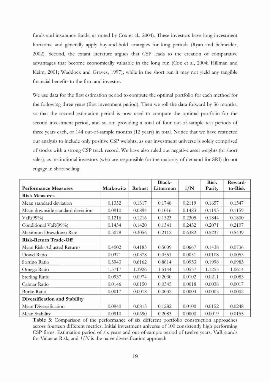
We use data for the first estimation period to compute the optimal portfolio for each method for

the following three years (first investment period). Then we roll the data forward by 36 months,

so that the second estimation period is now used to compute the optimal portfolio for the

second investment period, and so on; providing a total of four out-of-sample test periods of

three years each, or 144 out-of-sample months (12 years) in total. Notice that we have restricted

our analysis to include only positive CSP weights, as our investment universe is solely comprised

of stocks with a strong CSP track record. We have also ruled out negative asset weights (or short

sales), as institutional investors (who are responsible for the majority of demand for SRI) do not

engage in short selling.

Performance Measures Markowitz Robust Black-

Litterman 1/N Risk

Parity Reward-to-Risk

Risk Measures

Mean standard deviation 0.1352 0.1317 0.1748 0.2119 0.1657 0.1547

Mean downside standard deviation 0.0910 0.0894 0.1016 0.1483 0.1193 0.1159

VaR(99%) 0.1216 0.1216 0.1323 0.2305 0.1844 0.1800

Conditional VaR(99%) 0.1434 0.1420 0.1341 0.2432 0.2071 0.2107

Maximum Drawdown Rate 0.3078 0.3056 0.2112 0.6382 0.5237 0.5439

Risk-Return Trade-Off

Mean Risk-Adjusted Returns 0.4002 0.4183 0.5009 0.0667 0.1438 0.0736

Dowd Ratio 0.0371 0.0378 0.0551 0.0051 0.0108 0.0053

Sortino Ratio 0.5943 0.6162 0.8614 0.0953 0.1998 0.0983

Omega Ratio 1.3717 1.3926 1.5144 1.0557 1.1253 1.0614

Sterling Ratio 0.0937 0.0974 0.2030 0.0102 0.0211 0.0083

Calmar Ratio 0.0146 0.0150 0.0345 0.0018 0.0038 0.0017

Burke Ratio 0.0017 0.0018 0.0032 0.0003 0.0005 0.0002

Diversification and Stability

Mean Diversification 0.0940 0.0813 0.1282 0.0100 0.0152 0.0248

Mean Stability 0.0910 0.0690 0.2083 0.0000 0.0019 0.0155

Table 3: Comparison of the performance of six different portfolio construction approaches across fourteen different metrics. Initial investment universe of 100 consistently high performing CSP firms. Estimation period of six years and out-of-sample period of twelve years. VaR stands for Value at Risk, and 1/N is the naive diversification approach

20

Table 3 contains the core of our empirical results, and compares the performance of the six

portfolio construction methods we employ (Markowitz, robust estimation, Black-Litterman,

naïve diversification (1/N), risk parity, and reward-to-risk) on the universe of the best 100 CSP

performers. We restrict the universe to 100 firms as a reasonable compromise between having

firms which do not really constitute the “cream of the crop” in terms of CSP, and having

insufficient firms to effectively study the difference in the impact of the optimization methods

on the performance of the SRI portfolios. The performance of these portfolios, formed in six

different ways, is compared using 14 criteria which examine risk (five measures), risk-adjusted

returns (seven measures), diversification, and portfolio stability. The comparisons are made over

the 144 out-of-sample months (12 years) which include four investment periods (4×36 months),

with different optimal portfolios applying for each three year period (36 months). The results are

adjusted to present annualized figures (where applicable), as is the norm in the asset management

industry.

Focusing on risk, the robust estimation approach produces the least risky SRI portfolios in terms

of total risk (mean standard deviation), total downside risk (mean downside standard deviation)

and VaR, while it comes second to the Black-Litterman approach in terms of conditional VaR

and maximum drawdown. The Markowitz model also performs well, finishing second or third in

almost all of the risk metrics, and ties first on VaR. On the other hand, the naïve diversification

(1/N) approach consistently produces the riskiest portfolios across all the measures, with the risk

parity and reward-to-risk approaches also producing high risk portfolios. The differences

between the scores of the most and least risky portfolios are substantial. In terms of total risk,

the robust estimation approach leads to an SRI portfolio with an average annualised standard

deviation of returns of 13.17%, whereas the equivalent number for the naive diversification

approach is 21.19%, i.e. over 60% higher; while the VaR score for the 1/N portfolios is 90%

higher than for robust estimation. The maximum drawdown for the “risky” naive diversification

SRI portfolio is over 100% larger than for the “safe” Black-Litterman SRI portfolio. These

observations are particularly important for the risk-averse, long-term institutional investors who

form a significant portion of the demand for SRI.

Focusing on the risk-return trade-off, analysis of the extensive array of metrics we have used

produces a very clear picture. It terms of portfolio risk-adjusted returns (Dowd ratio, Sortino

ratio, Omega ratio, Sterling ratio, Calmar ratio and Burke ratio), the Black-Litterman model leads

to the best out-of-sample performance, with robust estimation ranking second. At the other end

of the spectrum, the naive diversification and reward-to-risk methods produce the worst risk-

21

return ratios. Once more, the differences in the extremes are quantitatively large. For example,

the value of the Dowd ratio for the portfolio produced using the Black-Litterman method is

0.0551, while for the “naive” portfolio it is just 0.0051 (i.e. less than one tenth of the value of the

former). Similarly, looking at the Sterling ratio, the Black-Litterman approach again produces the

best result with a value of 0.2030, which is more than 20 times larger than the corresponding

result of 0.0083 for the reward-to-risk method. Comparisons across the other risk-return metrics

corroborate this conclusion.

The picture changes when looking at the diversification and stability of portfolio constituents. By

construction, the naive approach leads to an equal weighting of all the assets in the investment

universe (a 1% investment in all 100 stocks in our case), and this remains stable in every period.

Hence it leads to the optimal diversification and stability scores for the metrics we utilize. What

is interesting is that the second best approach with regard to these aspects is risk parity, whereas

Black-Litterman (which led all the other models in terms of riskiness and risk-return tradeoff)

performs the worst, and the Markowitz model is the second worst. So, although the more

quantitative portfolio optimization techniques (Black-Litterman, robust estimation and

Markowitz) lead to less risky portfolios which provide higher returns per unit of risk taken, they

are also associated with less diversification and require more significant rebalancing of their

constituent assets. The exact opposite is true for the more simplistic portfolio construction

techniques which are based on fundamental investment intuition (naive diversification, risk parity

and reward-to-risk).

We now examine some key characteristics the 144 month time series of returns for the different

approaches. We focus first on risk, and look at drawdown rates. As can be seen in Figure 1, for

the majority of the 12 year evaluation period, all the approaches lead to portfolios with

reasonably similar drawdown rates. However, from the start of the global financial crisis (late

2007), the drawdown rates of the different models diverge significantly. The Black-Litterman

approach is consistently associated with the lowest drawdown, followed by the Markowitz and

robust estimation approaches (with almost identical drawdown), whereas naive diversification,

risk parity and reward-to-risk have much higher drawdown rates during this period.

22

Figure 1: Comparison of the drawdown rate of SRI portfolios constructed using the six different portfolio construction approaches over the 12 years of the out-of-sample period.

23

Figure 2 shows the cumulative wealth associated with the different strategies. The Black-

Litterman approach dominates all the other strategies in terms of cumulative wealth throughout

the entire 12 years (2000-2011). After the first two years the Black-Litterman portfolio clearly

moves ahead of its rivals, and over time gains a significant advantage which it maintains

irrespectively of the overall direction of the market. Once more, the naive diversification, risk

parity and reward-to-risk approaches perform worst, while the robust estimation and Markowitz

models are somewhere in between the best and worst performing strategies (and trend so closely

together that are nearly indistinguishable as in Figure 1). Given that all these portfolios are “long

only” (i.e. no short-selling of assets, or negative weights), it is to be expected that the cumulative

wealth for all strategies falls in 2008 and 2009 when the financial markets were collapsing, before

it starts climbing again.

24

Figure 2: Comparison of the cumulative wealth of SRI portfolios constructed using the six different portfolio construction approaches over the 12 years of the out-of-sample period.

0.5

0.6

0.7

0.8

0.9

1

1.1

1.2

1.3

1.4

1.5

1.6

1.7

1.8

1.9

2

2.11

2/1

99

9

3/2

00

0

6/2

00

0

9/2

00

0

12

/20

00

3/2

00

1

6/2

00

1

9/2

00

1

12

/20

01

3/2

00

2

6/2

00

2

9/2

00

2

12

/20

02

3/2

00

3

6/2

00

3

9/2

00

3

12

/20

03

3/2

00

4

6/2

00

4

9/2

00

4

12

/20

04

3/2

00

5

6/2

00

5

9/2

00

5

12

/20

05

3/2

00

6

6/2

00

6

9/2

00

6

12

/20

06

3/2

00

7

6/2

00

7

9/2

00

7

12

/20

07

3/2

00

8

6/2

00

8

9/2

00

8

12

/20

08

3/2

00

9

6/2

00

9

9/2

00

9

12

/20

09

3/2

01

0

6/2

01

0

9/2

01

0

12

/20

10

3/2

01

1

6/2

01

1

9/2

01

1

12

/20

11

Out-of-Sample Evaluation Period

Cumulative Wealth

Robust Markowitz Black-Litterman 1/N Risk-Parity Reward-to-Risk Timing

25

Finally, in Figure 3 we provide a comparison of the distribution of asset weights for the SRI

portfolios constructed using five different portfolio approaches (we do not include the assets of

the 1/N approach as they are all assigned a 1% weight). Only weights of 1% or more are

presented in Figure 3, as this is a rule-of-thumb cutoff point for professional asset managers.

The weights are average values across the four investment periods. The Markowitz, robust

estimation and Black-Litterman models all lead to portfolios with exactly 26 assets. However, the

identity of these assets is not the same across these three approaches, and the size distribution of

asset weights is also different. The distribution of asset weights is very similar for the Markowitz

and robust estimation approaches, with comparable maxima (10.88% and 11.13% respectively),

and six assets with weights of 4% or more in each portfolio. On the other hand, the Black-

Litterman portfolio has a lower maximum weight (8.79%), and eight assets with weights of

approximately 4% or more. The risk parity and reward-to-risk techniques lead to portfolios with

more assets and lower average weights. The risk parity portfolio comprises 42 assets with a

weight of 1% or more, and a maximum weight of just 3.56%; while the reward-to-risk portfolio

contains 39 assets with a maximum weight of 3.95%. So, although the three less formal

optimization models create portfolios which are more stable and require less rebalancing across

investment periods, they also contain a greater number of assets compared to the more formal

optimization methods. Hence, no clear conclusion can be drawn about the overall impact that

transaction costs would have from this analysis.

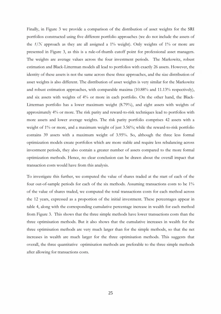
To investigate this further, we computed the value of shares traded at the start of each of the

four out-of-sample periods for each of the six methods. Assuming transactions costs to be 1%

of the value of shares traded, we computed the total transactions costs for each method across

the 12 years, expressed as a proportion of the initial investment. These percentages appear in

table 4, along with the corresponding cumulative percentage increase in wealth for each method

from Figure 3. This shows that the three simple methods have lower transactions costs than the

three optimisation methods. But it also shows that the cumulative increases in wealth for the

three optimisation methods are very much larger than for the simple methods, so that the net

increases in wealth are much larger for the three optimisation methods. This suggests that

overall, the three quantitative optimisation methods are preferable to the three simple methods

after allowing for transactions costs.

26

Total Transactions Costs as a % of Initial Wealth

Cumulative % Increase in Initial Wealth

Differences

Markowitz 5.51% 64.92% 59.41%

Robust 5.22% 66.13% 60.91%

Black-Litterman 8.82% 105.03% 96.21%

1/N 2.40% 16.95% 14.55%

Risk Parity 2.35% 28.61% 26.26%

Reward-to-Risk 3.10% 13.66% 10.56%

Table 4: Comparison of the cumulative transactions costs and cumulative increases in wealth.

Initial investment universe of 100 consistently high performing CSP firms. Estimation period of

six years and out-of-sample period of twelve years. 1/N is the naive diversification approach.

27

Figure 3: Comparison of the asset weight distributions of SRI portfolios constructed using five different portfolio construction approaches. Only weights of assets which are allocated 1% or more are presented.

Before continuing with the robustness tests and additional analyses, we will compare our key

findings with the main conclusions from the general literature on asset allocation. In a nutshell,

while contradictory results exist regarding the relative effectiveness of different optimization

techniques, there is considerable evidence which supports simple portfolio selection methods

such as 1/N. When comparing the performance of a range of different methods, including 1/N,

Markowitz, risk parity and minimum variance; Board and Sutcliffe (1995), Zhu (2015) and Jacobs

et. al. (2014) found mixed results with no clear winner. However, there is more positive evidence.

28

Bloomfield, Leftwich and Long (1977) found that naive portfolio allocation methods are

superior to more sophisticated methods, and that 1/N performs well; while Jorion (1991)

demonstrated that, for NYSE stocks, 1/N is superior to the sophisticated techniques of

Markowitz, Bayes-Stein and minimum variance. More recently, Jagannathan and Ma (2003) show

that 1/N is superior to Markowitz for US stocks. DeMiguel et al. (2009b) compare 14 different

methods using US equity data sets, and show that none of them consistently outperforms the

1/N approach in terms of risk-adjusted returns. Tu and Zhou (2011) reach similar conclusions.

Brown et al. (2013) show that this outperformance is compensation for the increased tail risk (i.e.

extreme loss risk) that the naïve diversification portfolio bears. Kirby and Ostdiek (2012) also

point out that the stability of naïve diversification is one of the main causes behind its strong

performance, and that the reward-to-risk approach can yield stronger results, even in the

presence of high transaction costs. Finally, Chaves et. al. (2011) find that the simple methods of

1/N and risk parity are superior to Markowitz and minimum variance, while Ang (2014) shows

that 1/N is preferable to minimum variance and Markowitz. Therefore, the literature for general

portfolios tends to support the use of simple, rather than sophisticated portfolio selection

techniques.

Our results show that, within the SRI framework, the Black-Litterman approach produces

portfolios with the strongest out-of-sample risk-adjusted returns. The robust estimation

approach generally produces good results, and the reward-to-risk approach beats the naïve

diversification method, as Kirby and Ostdiek (2012) have shown. Our results conflict with those

of the general asset allocation literature surveyed above. For an investment universe screened for

CSP, the simple methods (1/N, risk parity and reward-to-risk) consistently yield the poorest

results in terms of risk, maximum possible losses and risk-adjusted returns; while the

sophisticated methods (Black-Litterman, robust estimation and Markowitz) yield the best results.

This is an important and interesting finding for the SRI community.

4.2 Robustness tests

To test the robustness of our results, we narrow our investment universe to the top 80 firms (a

significant shrinkage of 20% in the number of assets) in terms of aggregate CSP score.

According to traditional finance theory, further restricting the investment universe should lead to

inferior portfolio performance. On the other hand, given the strong empirical link between

higher CSP and lower financial risk (Orlitzky and Benjamin, 2001; Godfrey et al., 2009;

29

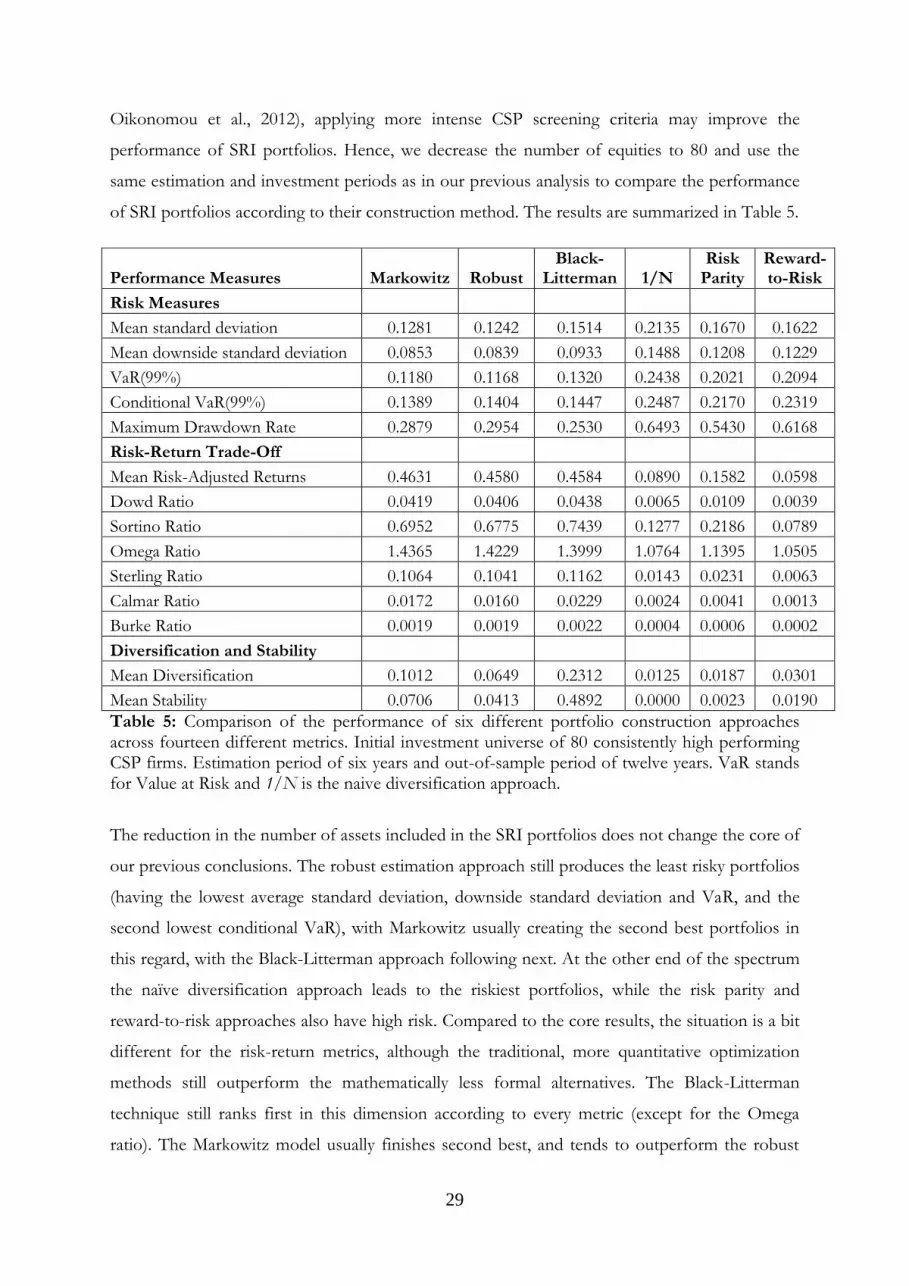
Oikonomou et al., 2012), applying more intense CSP screening criteria may improve the

performance of SRI portfolios. Hence, we decrease the number of equities to 80 and use the

same estimation and investment periods as in our previous analysis to compare the performance

of SRI portfolios according to their construction method. The results are summarized in Table 5.


Litterman 1/N Risk


Risk Measures



VaR(99%) 0.1180 0.1168 0.1320 0.2438 0.2021 0.2094

Conditional VaR(99%) 0.1389 0.1404 0.1447 0.2487 0.2170 0.2319




Dowd Ratio 0.0419 0.0406 0.0438 0.0065 0.0109 0.0039

Sortino Ratio 0.6952 0.6775 0.7439 0.1277 0.2186 0.0789

Omega Ratio 1.4365 1.4229 1.3999 1.0764 1.1395 1.0505

Sterling Ratio 0.1064 0.1041 0.1162 0.0143 0.0231 0.0063

Calmar Ratio 0.0172 0.0160 0.0229 0.0024 0.0041 0.0013

Burke Ratio 0.0019 0.0019 0.0022 0.0004 0.0006 0.0002



Mean Stability 0.0706 0.0413 0.4892 0.0000 0.0023 0.0190

Table 5: Comparison of the performance of six different portfolio construction approaches across fourteen different metrics. Initial investment universe of 80 consistently high performing CSP firms. Estimation period of six years and out-of-sample period of twelve years. VaR stands for Value at Risk and 1/N is the naive diversification approach.

The reduction in the number of assets included in the SRI portfolios does not change the core of

our previous conclusions. The robust estimation approach still produces the least risky portfolios

(having the lowest average standard deviation, downside standard deviation and VaR, and the

second lowest conditional VaR), with Markowitz usually creating the second best portfolios in

this regard, with the Black-Litterman approach following next. At the other end of the spectrum

the naïve diversification approach leads to the riskiest portfolios, while the risk parity and

reward-to-risk approaches also have high risk. Compared to the core results, the situation is a bit

different for the risk-return metrics, although the traditional, more quantitative optimization

methods still outperform the mathematically less formal alternatives. The Black-Litterman

technique still ranks first in this dimension according to every metric (except for the Omega

ratio). The Markowitz model usually finishes second best, and tends to outperform the robust

30

portfolio. The naïve diversification and reward-to-risk portfolios still have the lowest risk-

adjusted returns on every relevant metric. As previously, the rank order is reversed when looking

at the diversification and stability measures, with the 1/N approach producing the best results,

followed by risk parity. The Black-Litterman model finishes last, with Markowitz as second

worst. Overall, even when significantly reducing the investment universe, the rank order of the

different approaches remains largely unchanged. The sophisticated approaches have lower risk

and a superior risk-return trade-off than the unsophisticated approaches, but the simpler

techniques are more diversified and stable.

As a second robustness test we keep the number of assets at 100, but change the length of the

estimation periods to nine years (108 months) instead of six years (72 months). Tables 6 and 7

provide the relevant details of the new estimation and investment periods. We now have only

three estimation periods and three investment periods.





Table 6: Nine-Year Estimation Periods





Table 7: Non-Overlapping Three-Year Investment Periods


Litterman 1/N Risk


Risk Measures



VaR(99%) 0.1354 0.1363 0.1346 0.2559 0.2255 0.2318

Conditional VaR(99%) 0.1354 0.1363 0.1346 0.2559 0.2255 0.2318




Dowd Ratio 0.0369 0.0366 0.0374 0.0048 0.0075 0.0074

Sortino Ratio 0.7288 0.7253 0.7365 0.0923 0.1511 0.1655

Omega Ratio 1.4492 1.4484 1.4536 1.0565 1.0971 1.1121

Sterling Ratio 0.1223 0.1204 0.1258 0.0093 0.0144 0.0140

Calmar Ratio 0.0196 0.0194 0.0200 0.0019 0.0030 0.0031

Burke Ratio 0.0024 0.0024 0.0024 0.0003 0.0005 0.0005

31

Table 8: Comparison of the performance of six different portfolio construction approaches

across fourteen different metrics. Initial investment universe of 100 consistently high performing

CSP firms. Estimation period of nine years.

The results are summarized in Table 8. All our previous conclusions remain valid, and in some

cases are even stronger than those drawn from the original results. The Black-Litterman model

dominates all the alternative SRI portfolios according to every metric of risk and risk-adjusted

performance. The Markowitz and robust approaches are second and third best respectively

according to the same criteria. The naïve diversification technique produces the riskiest

portfolios with the worst risk-return ratios, while the risk-parity and reward-to-risk portfolios do

not fare much better. Once more, the 1/N approach leads to the most stable and well-diversified

portfolios, followed by the risk-parity portfolios; whereas the Markowitz and Black-Litterman

portfolios perform worst on both these dimensions.

4.3 Additional analyses

It has been documented that different measures of CSP based on different aspects or dimensions

of corporate sustainability relate to distinct stakeholder groups (Griffin and Mahon, 1997;

Mattingly and Berman, 2006) and may have different impacts on financial performance. This is

especially relevant when looking at samples of firms from different industries, where the social

and environmental issues and key performance indicators can be significantly different. So far in

our analysis we avoided this issue by using an aggregate, multidimensional measure of CSP to

construct SRI portfolios. In this subsection, we create five different SRI investment data sets,

each based on one of the CSP qualitative issue areas from which the aggregate CSP measure was

constructed; i.e. relationships with local communities, diversity in the workplace, employee

relations, environmental considerations, and product safety and quality.

To construct these SRI portfolios we follow the principles outlined in subsection 4.1. Thus, we

use the top 100 firms for each of the qualitative issue areas, and the estimation and investment

periods described in Tables 1 and 2. The performance metrics and the optimization approaches

employed also remain the same. The results appear in Table 9 which contains five different

panels, each of which focuses on one of the five CSP dimensions.



Mean Stability 0.0605 0.0542 0.0600 0.0000 0.0009 0.0107

32

Community relations Markowitz Robust Black-

Litterman 1/N Risk




VaR(99%) 0.1939 0.1962 0.2031 0.2387 0.2032 0.1869

Conditional VaR(99%) 0.1994 0.2008 0.2132 0.2513 0.2298 0.2168



Dowd Ratio 0.0234 0.0208 0.0267 0.0115 0.0104 0.0071

Sortino Ratio 0.5219 0.4615 0.5579 0.2182 0.1899 0.1294

Omega Ratio 1.3680 1.3203 1.3840 1.1368 1.1259 1.0860

Sterling Ratio 0.0766 0.0617 0.0815 0.0277 0.0200 0.0116

Calmar Ratio 0.0119 0.0102 0.0145 0.0046 0.0036 0.0023

Burke Ratio 0.0016 0.0013 0.0018 0.0007 0.0005 0.0003


Mean Stability 0.0741 0.0731 0.2710 0.0000 0.0026 0.0154

Diversity Markowitz Robust Black-

Litterman 1/N Risk




VaR(99%) 0.1326 0.1428 0.1487 0.2314 0.2116 0.2293

Conditional VaR(99%) 0.1491 0.1542 0.1593 0.2453 0.2122 0.2299


Mean Risk-Adjusted Returns 0.1519 0.1501 0.2319 -0.0074 0.0257 -0.1238

Dowd Ratio 0.0136 0.0126 0.0211 -0.0006 0.0017 -0.0074

Sortino Ratio 0.2123 0.2100 0.3517 -0.0104 0.0347 -0.1560

Omega Ratio 1.1272 1.1257 1.2043 0.9939 1.0217 0.9003

Sterling Ratio 0.0169 0.0166 0.0363 -0.0009 0.0027 -0.0086

Calmar Ratio 0.0037 0.0036 0.0080 -0.0002 0.0005 -0.0021

Burke Ratio 0.0005 0.0005 0.0009 0.0000 0.0001 -0.0003


Mean Stability 0.0562 0.0478 0.0999 0.0000 0.0016 0.0149

Employee relations Markowitz Robust Black-

Litterman 1/N Risk




VaR(99%) 0.1371 0.1376 0.1414 0.2141 0.1763 0.2005

Conditional VaR(99%) 0.1952 0.1933 0.1877 0.2434 0.2215 0.2475



Dowd Ratio 0.0322 0.0313 0.0332 0.0103 0.0170 0.0100

Sortino Ratio 0.4710 0.4756 0.5319 0.1812 0.2813 0.1809

Omega Ratio 1.3214 1.3296 1.3568 1.1113 1.1851 1.1223

Sterling Ratio 0.0576 0.0577 0.0683 0.0205 0.0311 0.0166

Calmar Ratio 0.0120 0.0116 0.0136 0.0041 0.0063 0.0038

Burke Ratio 0.0013 0.0013 0.0015 0.0006 0.0008 0.0005

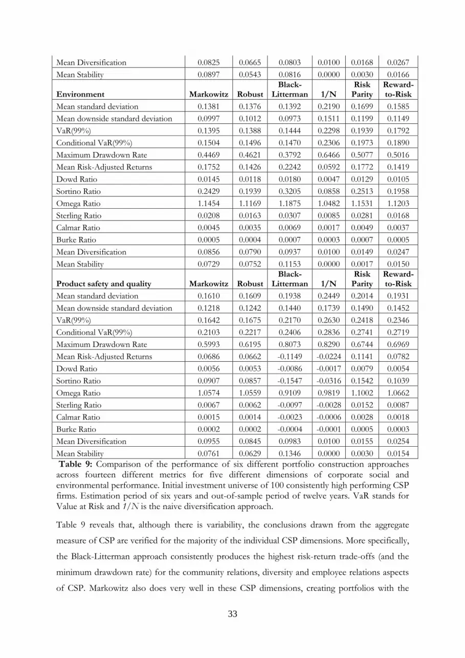
33


Mean Stability 0.0897 0.0543 0.0816 0.0000 0.0030 0.0166

Environment Markowitz Robust Black-

Litterman 1/N Risk




VaR(99%) 0.1395 0.1388 0.1444 0.2298 0.1939 0.1792

Conditional VaR(99%) 0.1504 0.1496 0.1470 0.2306 0.1973 0.1890



Dowd Ratio 0.0145 0.0118 0.0180 0.0047 0.0129 0.0105

Sortino Ratio 0.2429 0.1939 0.3205 0.0858 0.2513 0.1958

Omega Ratio 1.1454 1.1169 1.1875 1.0482 1.1531 1.1203

Sterling Ratio 0.0208 0.0163 0.0307 0.0085 0.0281 0.0168

Calmar Ratio 0.0045 0.0035 0.0069 0.0017 0.0049 0.0037

Burke Ratio 0.0005 0.0004 0.0007 0.0003 0.0007 0.0005


Mean Stability 0.0729 0.0752 0.1153 0.0000 0.0017 0.0150

Product safety and quality Markowitz Robust Black-

Litterman 1/N Risk




VaR(99%) 0.1642 0.1675 0.2170 0.2630 0.2418 0.2346

Conditional VaR(99%) 0.2103 0.2217 0.2406 0.2836 0.2741 0.2719


Mean Risk-Adjusted Returns 0.0686 0.0662 -0.1149 -0.0224 0.1141 0.0782

Dowd Ratio 0.0056 0.0053 -0.0086 -0.0017 0.0079 0.0054

Sortino Ratio 0.0907 0.0857 -0.1547 -0.0316 0.1542 0.1039

Omega Ratio 1.0574 1.0559 0.9109 0.9819 1.1002 1.0662

Sterling Ratio 0.0067 0.0062 -0.0097 -0.0028 0.0152 0.0087

Calmar Ratio 0.0015 0.0014 -0.0023 -0.0006 0.0028 0.0018

Burke Ratio 0.0002 0.0002 -0.0004 -0.0001 0.0005 0.0003


Mean Stability 0.0761 0.0629 0.1346 0.0000 0.0030 0.0154

Table 9: Comparison of the performance of six different portfolio construction approaches across fourteen different metrics for five different dimensions of corporate social and environmental performance. Initial investment universe of 100 consistently high performing CSP firms. Estimation period of six years and out-of-sample period of twelve years. VaR stands for Value at Risk and 1/N is the naive diversification approach.

Table 9 reveals that, although there is variability, the conclusions drawn from the aggregate

measure of CSP are verified for the majority of the individual CSP dimensions. More specifically,

the Black-Litterman approach consistently produces the highest risk-return trade-offs (and the

minimum drawdown rate) for the community relations, diversity and employee relations aspects

of CSP. Markowitz also does very well in these CSP dimensions, creating portfolios with the

34

lowest volatility, downside risk and VaR, while also usually finishing second in terms of risk-

adjusted returns. The robust approach ranks second or third in terms of both riskiness and risk-

return trade-offs, whereas the naïve diversification and reward-to-risk approaches invariably lead

to portfolios with the worst values on these measures. So once again the formal optimization

models outperform the less strict portfolio construction approaches. However, in line with the

core findings of this study, the 1/N approach still produces the most well-diversified and stable

portfolios, while the Black-Litterman and Markowitz models finish last on these criteria.

The picture is qualitatively similar, although not identical, when focusing on corporate

environmental performance. The key differences are that the robust portfolio performs less well,

finishing next to last on most of the risk-adjusted return ratios, while the risk-parity portfolio

does better, being ranked second best on most risk-return metrics. Black-Litterman is still the

model of choice according to most criteria, while 1/N is last.

Things are quite different when using product safety and quality as the CSP feature guiding

portfolio construction. This is the only CSP dimension where the Black-Litterman approach

leads to poorly performing portfolios with the worst risk-adjusted returns, diversification and

stability characteristics. On the other hand, the risk parity and reward-to-risk techniques are the

methods with the best and second best risk-return trade-offs respectively, something that has not

been the case in any of our previous analysis.

The distinctiveness of CSP dimensions and the variability of the financial impacts of each has

been well documented in the empirical CSP literature (Hillman and Keim, 2001; Mattingly and

Berman, 2006; Oikonomou et al., 2012). Hence, our results are compatible with previous

findings. Overall, Table 9 shows that the results from the solo use of the CSP measures produces

only slightly different conclusions. This suggests that our results are not highly sensitive to the

weighting scheme involved in computing the aggregate CSP.

5. Conclusions

We expand the SRI literature by moving beyond the question of whether portfolios comprising

“sustainable equities” outperform conventional investments, and focus on finding optimal ways

to construct SRI portfolios. We have found that the optimization process for forming SRI

portfolios matters. There are large, economically significant differences in the risk, risk-adjusted

returns, diversification and intertemporal stability of the SRI portfolios, depending on which

35

optimization technique is used. Formal optimization techniques (Markowitz, Black-Litterman

and robust estimation) tend to produce less risky SRI portfolios with higher risk-adjusted returns

and a smaller total number of constituent assets compared to less formal techniques (naïve

diversification, risk parity and reward-to-risk). The Black-Litterman model is usually the best

technique, while naïve diversification is usually the worst on these criteria. These conclusions are

robust to different lengths of the estimation and investment periods, and to the use of more

stringent CSP screening criteria. Our conclusions using CSP-screened assets are in contrast to

studies of unscreened assets, which have found that naive diversification is one of the best

techniques.

When implementing the various portfolio construction approaches for single CSP dimensions,

we have found that our key findings for aggregate CSP scores also hold for the community,

diversity and employee relations dimensions of CSP. But they are less applicable for

environmental performance and product safety and quality. This is in line with previous work in

the wider literature on the financial effects of CSP, and demonstrates the contextualization

required for an analysis to be complete.

Overall, our study shows that just applying stringent SRI criteria to restrict the investment

universe to the best socially and environmentally performing companies is insufficient. The

optimization process is also very important. It further demonstrates to fund managers,

institutional and retail investors (especially those who are more risk-averse and have longer-term

investment horizons) that the more quantitative approaches to portfolio construction typically

lead to better results. The appropriate selection of an optimization technique is an issue which

needs to be taken into serious consideration for anyone placing their funds in SRI. Choosing the

correct optimization method for the creation of SRI portfolios will lead to stronger financial

performance, which in turn will generate greater demand for this kind of investment. Through

this mechanism, the cost of equity for any corporation that applies sustainable/

responsible/ethical practices will be reduced, incentivising them to engage in such behaviour;

while penalizing companies involved in various social or environmental controversies by

increasing their cost of capital. In short, the selection of the most suitable optimization method

for SRI portfolios will have an effect on the bottom line of companies and, through this, on the

promotion of societal well-being and environmental conservation. Hence, the results of this

study are of interest and importance to a variety of constituents including investors, fund

managers, corporate executives, social and environmental activists and overall concerned

citizens.

36

Although our study is innovative within the SRI field, it is limited by considering only one asset

class (equities) and the geographic coverage of the markets considered (US). Future studies can

extend our analysis in either of these directions. Furthermore, the selection of the CSP criteria

and dataset used is always an important issue within the literature (Griffin and Mahon, 1997).

Using different social and environmental sources of data and alternative CSP metrics would

provide a useful test for the reliability of different optimization methods for SRI.

References

Abbott, W. F. and Monsen R. J. (1979). On the measurement of corporate social responsibility: Self-reported disclosures as a method of measuring corporate social involvement. Academy of Management Journal: vol. 22, pp. 501-515. Anderson, R.M., Bianchi, S.W. and Goldberg, L.R. (2012). Will My Risk Parity Strategy Outperform?, Financial Analysts Journal, vol. 68, no. 6, pp. 75-93. Ang, A. (2014) Asset Management – A Systematic Approach to Factor Investing, Oxford University Press. Bacon, C., Practical portfolio performance measurement and attribution, 2nd edition, Wiley 2008. Baker, M., Bradley B. and Wurgler, J. (2011). Benchmarks as Limits to Arbitrage: Understanding the Low Volatility Anomaly, Financial Analysts Journal, vol. 67, pp. 40-54. Ballestero, E., Bravo, M., Pérez-Gladish, B., Arenas-Parra, M., and Plà-Santamaria, D. (2012) Socially Responsible Investment: A Multicriteria Approach to Portfolio Selection Combining Ethical and Financial Objectives. European Journal of Operational Research, vol. 216, pp. 487–494. Barnett, M. L. and Salomon, R. M. (2006). Beyond dichotomy: The Curvilinear Relationship between Social Responsibility and Financial Performance, Strategic Management Journal vol. 27, pp. 1101-1122. Berkelaar, A. and Kouwenberg, R (2010). A Liability-Relative Drawdown Approach to Pension Asset Liability Management. Journal of Asset Management, vol. 11, pp. 194-217. Bessler, W., Opfer, H. and Wolff, D., (forthcoming) Multi-Asset Portfolio Optimization and Out-of-Sample Performance: An Evaluation of Black–Litterman, Mean-Variance, and Naïve Diversification Approaches. The European Journal of Finance. Bloomfield, T., Leftwich, R. and Long, J.B. (1977). Portfolio Strategies and Performance. Journal of Financial Ecoonomics vol. 5, pp.201-218. Blume, M.E. and Friend, I. (1975) The Asset Structure of Individual Portfolios and Some Implications for Utility Functions, Journal of Finance, vol. 30, pp. 585-603. Bloomfield, T., Leftwich, R. and Long, J.B. (1977) Portfolio Strategies and Performance, Journal of Financial Economics, vol. 5, no. 2, November, pp. 201-218.

37

Board, J.L.G. and Sutcliffe, C.M.S. (1995) Estimation Methods in Portfolio Selection and the Effectiveness of Short Sales Restrictions: UK Evidence, Management Science, Vol. 40, No. 4, April, pp. 516-534. Boender, C.G.E. (1997) A Hybrid Simulation-Optimization Scenario Model for Asset-Liability Management, European Journal of Operations Research, vol. 99, pp. 126-135. Bondell, H.D. and Reich, B.J. (2008) Simultaneous regression shrinkage, variable selection, and supervised clustering of predictors with OSCAR, Biometrics, vol. 64, pp. 115-123. Bouslah, K., Kryzanowski, L. amd M’Zali, B. (2013), The impact of the dimensions of social performance on firm risk, Journal of Banking & Finance, vol. 37, pp. 1258-1273. Brammer, S., C. Brooks and S. Pavelin (2006). Corporate social performance and stock returns: UK evidence from disaggregate measures. Financial Management, vol. 35, pp. 97-116. Broadie, M. (1993) Computing Efficient Frontiers Using Estimated Parameters, Annals of Operations Research, vol. 45, pp. 21-58. Brodie, J.I., Daubechies, C.D., Giannone, M.D. and Loris, I. (2008) Sparse and Stable Markowitz Portfolios, European Central Bank Working Paper Series, no. 936. Brown, S. J., Hwang, I. and In, F. H. (2013), Why Optimal Diversification Cannot Outperform Naive Diversification: Evidence from Tail Risk Exposure. Available at SSRN: http://ssrn.com/abstract=2242694 Burke. G. (1994). A sharper Sharpe ratio. Futures, vol. 23, no. 3, p. 56. Candelon, B., Hurlin, C. and Tokpavi, S. (2012) Sampling Error and Double Shrinkage Estimation of Minimum Variance Portfolios, Journal of Empirical Finance, vol. 19, September, pp. 511–527. Capelle-Blancard, G. and Monjon, S. (2014), The Performance of Socially Responsible Funds: Does the Screening Process Matter?. European Financial Management, vol. 20, pp. 494–520. Carroll, A. B. (1991). The pyramid of corporate social responsibility: Toward the moral management of organizational stakeholders. Business Horizons vol. 34, pp. 39-48. Chaves, D., Hsu, J., Li, F. and Shakernia, O. (2011) Risk Parity Portfolio vs. Other Asset Allocation Heuristic Portfolios, Journal of Investing, vol. 20, no. 1, Spring, pp. 108-118.

Clarkson, M. B. E. (1995). A stakeholder framework for analyzing and evaluating corporate social performance. Academy of Management Review, vol. 20, pp. 92-117. Cox, P., Brammer, S. and Millington, A. (2004). An empirical examination of institutional investor preferences for corporate social performance. Journal of Business Ethics, vol. 52, pp. 27-43. Deng, X., Kang, J. K. & Low, B. S. (2013). Corporate social responsibility and stakeholder value maximization: Evidence from mergers. Journal of Financial Economics, vol. 110, pp. 87-109.

http://ssrn.com/abstract=2242694

38

DeMiguel, V., Garlappi, L., Nogales, F.J. and Uppal, R. (2009a) A Generalized Approach to Portfolio Optimization: Improving Performance by Constraining Portfolio Norms, Management Science, vol. 22, no. 5, pp. 1915–1953. DeMiguel, V., Garlappi, L. and Uppal, R. (2009b) Optimal Versus Naive diversification: How Inefficient is the 1/N Portfolio Strategy? The Review of Financial Studies, vol. 22, no. 5, pp. 1915–1953. Derwall, J. and K. Koedijk (2009). Socially Responsible Fixed Income Funds. Journal of Business Finance & Accounting, vol. 36, pp. 210-229. Dowd, K. (2000). Adjusting for Risk: An Improved Sharpe Ratio. International Review of Economics and Finance, vol. 9, pp.209-222. Drut, B. (2012) Social Responsibility and Mean-Variance Portfolio Selection, Amundi Working Paper. Edmans, A. (2011). Does the stock market fully value intangibles? Employee satisfaction and equity prices. Journal of Financial Economics vol. 101, pp. 621-640. Edwards, M. (2008). Small change: Why business won’t save the world. San Francisco: Berrett-Koehler. Eling, M. and Schuhmacher, F. (2007). Does the Choice of Performance Measure Influence the Evaluation of Hedge Funds?, Journal of Banking and Finance, vol. 31, no. 9, pp. 2632-2647. Fan, J., Zhang, J. and Yu, K. (2008) Asset allocation and risk assessment with gross exposure constraints for vast portfolios, The Annals of Statistics, vol. 25, pp. 1425–1432. Fan, J., Zhang, J. and Yu, K. (2012) Vast Portfolio Selection with Gross-Exposure Constraints, Journal of the American Statistical Association, vol. 107, pp. 592-606. Frazzini, A. and Pedersen, L.H. (2014). Betting Against Beta, Journal of Financial Economics, vol. 111, no. 1, pp. 1–25. Galema, R., A. Plantinga and B. Scholtens (2008). The stocks at stake: Return and risk in socially responsible investment. Journal of Banking & Finance, vol. 32, pp. 2646-2654. Geyer, A. and Ziemba, W.T. (2008) The Innovest Austrian Pension Fund Financial Planning Model InnoALM, Operations Research, vol. 56, pp. 797-810. Godfrey, P. C., Merrill, C. B. and Hansen, J.M. (2009). The relationship between corporate social responsibility and shareholder value: an empirical test of the risk management hypothesis. Strategic Management Journal, vol. 30, pp. 425-445. Gofman, M. and Manela, A. (2012). An Empirical Evaluation of the Black-Litterman Approach to Portfolio Choice. Available at SSRN: http://ssrn.com/abstract=1782033 Goldfarb, D. and Iyengar, G. (2003) Robust Portfolio Selection Problems, Mathematics of Operations Research, vol. 28, no. 1, pp. 1-38.

http://ssrn.com/abstract=1782033

39

Green, R. and Hollifield, B. (1992) When will Mean–Variance Efficient Portfolios be well Diversified?, Journal of Finance, vol. 47, no. 5, pp. 1785–1809. Griffin, J. J. and. Mahon, J. F (1997). The corporate social performance and corporate financial performance debate. Business & Society, vol. 36, pp. 5-31. Grossman, S. and Zhou, Z. (1993) Optimal investment strategies for controlling drawdowns, Mathematical Finance, vol. 3, pp. 241–276.

Hallerbach, W., Ning, H., Soppe, A., and Spronk, J. (2004) A framework for managing a portfolio of socially responsible investments. European Journal of Operational Research, vol. 153, pp. 517–529. Jacobs, H., Muller, S. and Weber, M. (2014) How Should Individual Investors Diversify? An Empirical Evaluation of Alternative Asset Allocation Policies, Journal of Financial Markets, vol. 19, June, pp. 62-86.

Jagannathan, R. and Ma, T. (2003) Risk Reduction in Large Portfolios: Why Imposing the Wrong Constraints Helps, Journal of Finance, vol. 58, no. 4, August, pp. 1651-1683.

Jo, H., and M. Harjoto. (2012). The causal effect of corporate governance on corporate social responsibility. Journal of Business Ethics, vol. 106, pp. 53-72.

Jorion, P. (1991) Bayesian and CAPM Estimators of the Means: Implications for Portfolio Selection, Journal of Banking and Finance, vol. 15, no. 3, June, pp. 717-727.

Hillman, A. J. and G. D. Keim (2001). Shareholder value, stakeholder management, and social issues: what's the bottom line? Strategic Management Journal, vol. 22, pp. 125-139. Johnson, R. D. and D. W. Greening (1999), The Effects of Corporate Governance and Institutional Ownership Types on Corporate Social Performance, Academy of Management Journal, vol. 42, pp. 564-576. Kaplan, P.D. (2014), Back to Markowitz. Morningstar Indexes 2014/15 Yearbook. Available at: http://corporate.morningstar.com/us/asp/detail.aspx?xmlfile=8383.xml Kempf, A. and P. Osthoff (2007). The effect of socially responsible investing on portfolio performance. European Financial Management, vol. 13, pp. 908-922.

Kempf, A. and Osthoff, P. (2008), SRI Funds: Nomen est Omen. Journal of Business Finance & Accounting, vol. 35, pp. 1276-1294.

Kirby, C. and Ostdiek B. (2012). It’s All in the Timing: Simple Active Portfolio Strategies that Outperform Naive Diversification, Journal of Financial and Quantitative Analysis, vol. 47, no. 2, pp. 437-467.

Kourtis, A., Dotsis, G. and Markellos, R.N. (2012) Parameter uncertainty in portfolio selection: Shrinking the inverse covariance matrix, Journal of Banking and Finance, vol. 36, pp. 2522-2531. Ledoit, O. and Wolf, M. (2003) Improved Estimation of the Covariance Matrix of Stock Returns with an Application to Portfolio Selection, Journal of Empirical Finance, vol. 10, December, pp. 603–621.

http://corporate.morningstar.com/us/asp/detail.aspx?xmlfile=8383.xml

40

Ledoit, O., Wolf, M. (2004) A Well-Conditioned Estimator for Large-Dimensional Covariance Matrices. Journal of Multivariate Analysis, vol. 88, February, pp. 365–411. Lee, D. D. and Faff, R. W. (2009), Corporate Sustainability Performance and Idiosyncratic Risk: A Global Perspective. Financial Review, vol. 44, pp. 213–237. Margolis, J. D. and J. P. Walsh (2003). Misery loves companies: Rethinking social initiatives by business. Administrative Science Quarterly, vol. 48, pp. 268-305. Margolis, J., Elfenbein, H., & Walsh, J. P. (2009). Does it pay to be good and does it matter? A meta-analysis of the relationship between corporate social and financial performance. Harvard Business School Working Paper No. 229. Markowitz, H. (1952). Portfolio Selection, Journal of Finance, vol. 7, no. 1, pp. 77-91. Markowitz, H. (1991). Portfolio selection: Efficient diversification of investment (2e). Malden, MA: Blackwell Publishers Inc. Mattingly, J. E. and Berman, S. L. (2006). Measurement of corporate social action. Business & Society, vol. 45, pp. 20-46. Michaud, R. (1999) Efficient Asset Management: A Practical Guide to Stock Portfolio Optimization and Asset Allocation, Harvard Business School Press. Oikonomou, I., Brooks, C., & Pavelin, S. (2012). The impact of corporate social performance on financial risk and utility: A longitudinal analysis. Financial Management, vol. 41, pp. 483–515. Orlitzky, M. and J. D. Benjamin (2001). Corporate social performance and firm risk: A meta-analytic review. Business & Society, vol. 40, pp. 369-396. Orlitzky, M., F. L. Schmidt and S.L. Rynes (2003). Corporate social and financial performance: A meta-analysis. Organization Studies, vol. 24, pp. 403-441. Orlitzky, M. (2013). Corporate social responsibility, noise and stock market volatility, The Academy of Management Perspectives, vol. 27, pp. 238-254. Platanakis, E and Sutcliffe, C. (forthcoming) Asset Liability Modelling and Pension Schemes: The Application of Robust Optimization to USS, The European Journal of Finance. Renneboog, L., J. Ter Horst, and C. Zhang (2008). The Price of Ethics and Stakeholder Governance: The Performance of Socially Responsible Mutual Funds, Journal of Corporate Finance 14, 302-322. Rollinger, T. and Hoffman, S (2014). Sortino: A “Sharper” Ratio. Red Rock Capital. http://www.redrockcapital.com/Sortino__A__Sharper__Ratio_Red_Rock_Capital.pdf Rudolf, M. and Ziemba, W.T. (2004) Intertemporal Surplus Management, Journal of Economic Dynamics and Control, vol. 28, pp. 975 990. Ryan, L. V. and M. Schneider: 2002, 'The Antecedents of Institutional Investor Activism', Academy of Management Review vol. 27(4), pp. 554-573.

http://www.redrockcapital.com/Sortino__A__Sharper__Ratio_Red_Rock_Capital.pdf

41

Schroder, M. (2007). Is there a difference? The performance characteristics of SRI equity indices. Journal of Business Finance and Accounting, vol. 34, pp. 331–348. Shadwick, W. and Keating, C. (2002). A universal performance measure Journal of Performance Measurement, vol. 6, no. 3, pp. 59–84. Sharfman, M. (1996). The construct validity of the Kinder, Lydenberg & Domini social performance ratings data. Journal of Business Ethics, vol. 15, pp. 287-296. Sharpe, W. (1994). The Sharpe Ratio. Journal of Portfolio Management 21, no. 1, pp. 49-59. Statman, M. (2000). Socially responsible mutual funds. Financial Analysts Journal, vol. 56, pp.: 30-39. Statman, M. (2006). Socially responsible indexes. Journal of portfolio Management, vol. 32, pp.: 100-109. Tu, J. and Zhou, G. (2011) Markowitz Meets Talmud: A Combination of Sophisticated and Naive Diversification Strategies, Journal of Financial Economics, vol. 99, no. 1, pp. 204-215. Utz, S., Wimmer, M., Hirschberger, M. and Steuer, R.E. (2014) Tri-Criterion Inverse Portfolio Optimization with Application to Socially Responsible Mutual Funds, European Journal of Operational Research, vol. 234, pp. 491-498. Von Arx, U., & Ziegler, A. (2014). The effect of corporate social responsibility on stock performance: New evidence for the USA and Europe. Quantitative Finance, vol. 14, pp. 977-991. Votaw, D. (1973). Genius becomes rare. The Corporate Dilemma-Traditional Values versus Contemporary Problems. Prentice Hall, Englewood Clifs, NJ. Waddock, S.A. (2003). Myths and Realities of Social Investing, Organization and Environment, vol. 16, pp. 369-380. Waddock, S. A. and S. B. Graves: 1997, 'The Corporate Social Performance-Financial Performance Link', Strategic Management Journal vol. 18(4), 303—319. Wood, D. J. and Jones, R. E. (1995). Stakeholder mismatching: A theoretical problem in empirical research on corporate social performance. International Journal of Organizational Analysis vol. 3, pp. 229-267. Xing, X., Hu, J. and Yang, Y. (2014) Robust Minimum Variance with L-Infinity Constraints, Journal of Banking and Finance, vol. 46, pp. 107-117.

Young, T. W. (1991). "Calmar Ratio: A Smoother Tool", Futures, vol.20, p.40.

Zhu, L.L. (2015) The Performance of Asset Allocation Strategies Across Datasets and Over Time, Working paper, University of Edinburgh Business School, August, 42 pages.

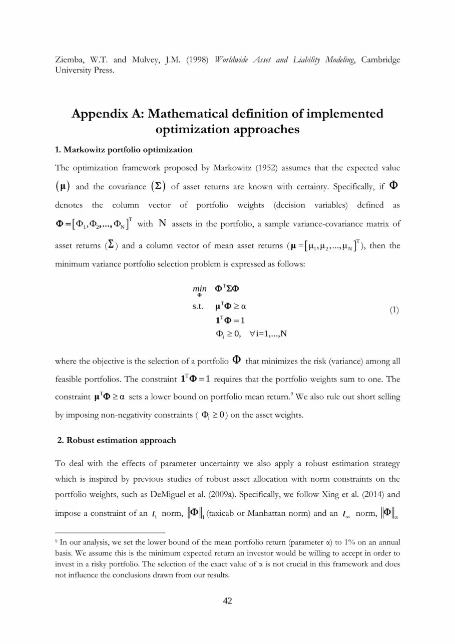
42

Ziemba, W.T. and Mulvey, J.M. (1998) Worldwide Asset and Liability Modeling, Cambridge University Press.

Appendix A: Mathematical definition of implemented optimization approaches

1. Markowitz portfolio optimization

The optimization framework proposed by Markowitz (1952) assumes that the expected value

μ and the covariance of asset returns are known with certainty. Specifically, if

denotes the column vector of portfolio weights (decision variables) defined as

T

1 2 N, with N assets in the portfolio, a sample variance-covariance matrix of

asset returns ( ) and a column vector of mean asset returns ( T

1 2 N= μ ,μ ,...,μμ ), then the

minimum variance portfolio selection problem is expressed as follows:

T

T

T

i

s.t. α

1

0, i=1,...,N

min

μ

1

(1)

where the objective is the selection of a portfolio that minimizes the risk (variance) among all

feasible portfolios. The constraint T 11 requires that the portfolio weights sum to one. The

constraint T α μ sets a lower bound on portfolio mean return.9 We also rule out short selling

by imposing non-negativity constraints ( i 0 ) on the asset weights.

2. Robust estimation approach

To deal with the effects of parameter uncertainty we also apply a robust estimation strategy

which is inspired by previous studies of robust asset allocation with norm constraints on the

portfolio weights, such as DeMiguel et al. (2009a). Specifically, we follow Xing et al. (2014) and

impose a constraint of an 1l norm,

1 (taxicab or Manhattan norm) and an l norm,

9 In our analysis, we set the lower bound of the mean portfolio return (parameter α) to 1% on an annual

basis. We assume this is the minimum expected return an investor would be willing to accept in order to

invest in a risky portfolio. The selection of the exact value of α is not crucial in this framework and does

not influence the conclusions drawn from our results.

43

(maximum norm) on the portfolio weights. The taxicab norm (l1) is the sum of the absolute

values of a vector, and setting an upper bound on l1 encourages sparse solutions, i.e. portfolios

with active positions in only a few assets (sparse portfolios), see for instance Brodie et al. (2008).

Having active positions in only a few assets leads to the significant practical benefit of lower

transaction costs. However, after applying the 1l norm constraint, some of the positions may be

very large. The additional use of the l norm addresses this issue, see for instance Brondell and

Reich (2008). The maximum norm (l∞) of a vector is the largest absolute value of the elements in

the vector, and an upper bound on l∞ prevents large positions in any asset. Therefore a

combination of the 1l and l upper bounds tends to produce sparse portfolios without very

large individual weights.

By additionally employing the three optimization constraints of problem (1), the optimization

problem can be written as follows:

T

1

T

T

i

s.t. c

α

1

0, i=1,...,N

min

μ

1

(2)

where

N

i1i 1

Φ

denotes the 1l norm, i

1 i NΦmax

represents the l norm ( i

denotes the absolute value of i ), while 1 is a column vector of ones. Furthermore,

1c 1

N

denotes the upper bound10 of the constraint that involves the 1l and l norms. We run the

robust estimation strategy using time varying values for c. For the first period we set c = 1.1, but

for subsequent periods we set c equal to the value in the range 1.1 to 9.0 that gave the best out-

of-sample performance during the previous period, Fan et al. (2008), Fan et al. (2012) and Xing

et al. (2014). The conclusions are unaltered when different values of c are used in the first period.

10 The lowest feasible value of c occurs when it is equal to 1+ 1/N and all the asset weights are equal to 1/N. Simulations of robust portfolio models usually start with a value of c just above 1. Setting c some way above 1 permits the optimization process to make a trade-off between preventing short sales and allowing large asset weights.

44

3. Black-Litterman approach

The Black-Litterman portfolio framework combines the subjective views of the investor, in

terms of returns and risk, with those of a benchmark portfolio (e.g. the equilibrium market

portfolio), and is an alternative way of dealing with estimation risk in the input parameters (Black

and Litterman, 1992). The posterior estimates of expected returns and covariances are then used

in the portfolio optimization process. We use the portfolio optimization model described in

problem (1), which minimizes the portfolio risk (variance), subject to three linear constraints on

asset weights.

The column vector of implied excess returns Π for the benchmark portfolio is expressed as

follows:

benchmarkΠ (3)

where denotes the risk aversion coefficient11 and benchmark is a column vector of the asset

weights of the benchmark portfolio12. The column vector of the posterior asset returns BLμ is

given by:

1

1 1T 1 T 1

BL

μ P P P Q (4)

where represents the overall level of confidence in the column vector .Π We set this

parameter to 0.1625, which is the mean of the values used in the literature (see for instance

Bessler, Opfer and Wolff, forthcoming; and Platanakis and Sutcliffe, forthcoming).

Bessler, Opfer and Wolff (forthcoming) experimented with different values of the parameter ,

and showed that the Black-Litterman results are robust to the choice of in the range between

0.025 to 1.00. In addition, P denotes a binary matrix defining the assets involved in each view,

Q is a column vector that contains the views (subjective returns), and is a diagonal matrix

that quantifies the reliability of each view. The latter is estimated following Meucci (2010), as

follows:

11 The investor’s risk aversion parameter disappears in the optimization process, since we use just the portfolio variance in the objective function.

12 We have used the equally-weighted portfolio (1/N) as the benchmark portfolio. Bessler, Opfer and Wolff (forthcoming) show that the effect of the choice of benchmark portfolio on the Black-Litterman results is minimal.

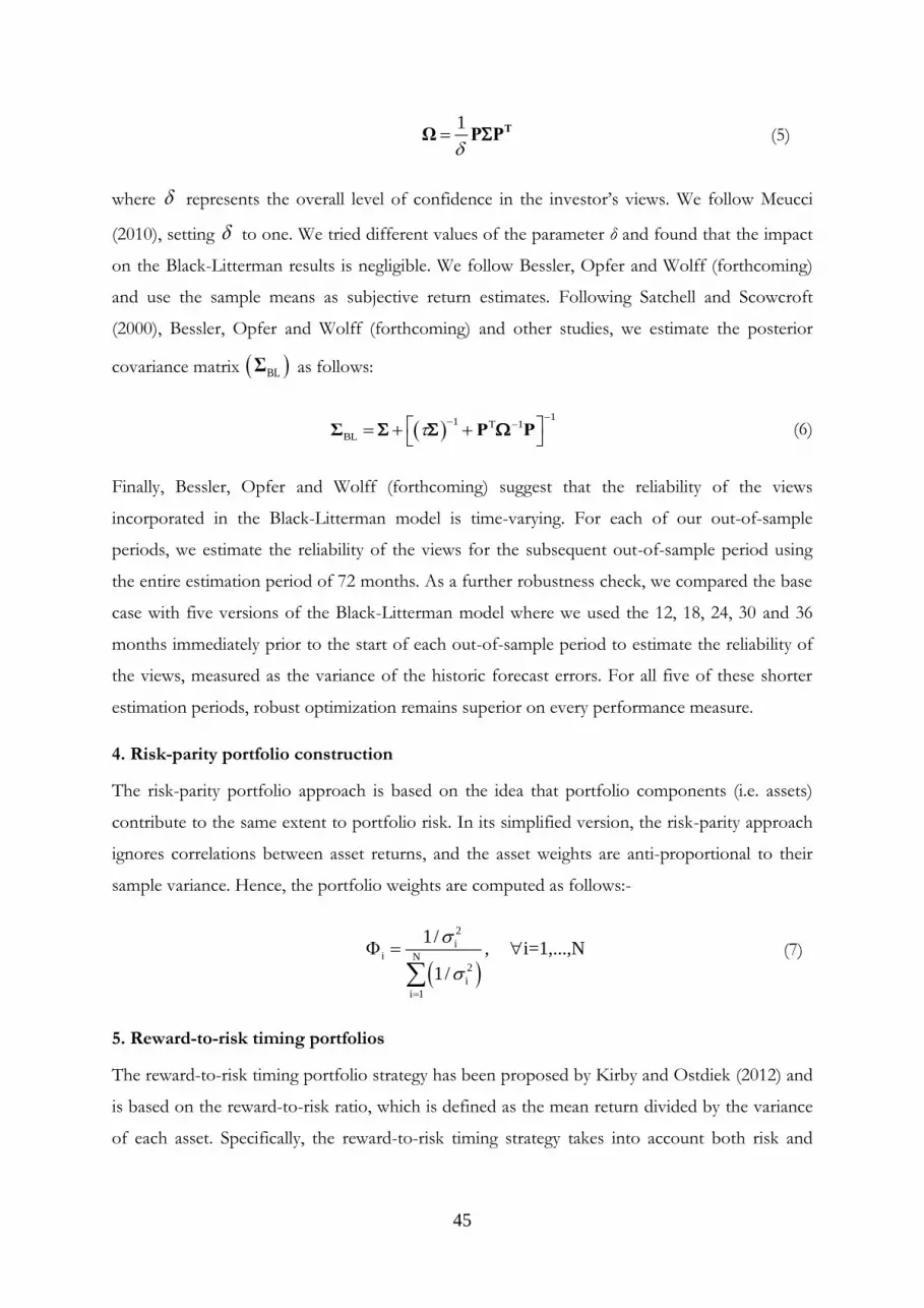
45

1

TΩ P P (5)

where represents the overall level of confidence in the investor’s views. We follow Meucci

(2010), setting to one. We tried different values of the parameter δ and found that the impact

on the Black-Litterman results is negligible. We follow Bessler, Opfer and Wolff (forthcoming)

and use the sample means as subjective return estimates. Following Satchell and Scowcroft

(2000), Bessler, Opfer and Wolff (forthcoming) and other studies, we estimate the posterior

covariance matrix BLΣ as follows:

1

1 T 1

BL

Σ P P (6)

Finally, Bessler, Opfer and Wolff (forthcoming) suggest that the reliability of the views

incorporated in the Black-Litterman model is time-varying. For each of our out-of-sample

periods, we estimate the reliability of the views for the subsequent out-of-sample period using

the entire estimation period of 72 months. As a further robustness check, we compared the base

case with five versions of the Black-Litterman model where we used the 12, 18, 24, 30 and 36

months immediately prior to the start of each out-of-sample period to estimate the reliability of

the views, measured as the variance of the historic forecast errors. For all five of these shorter

estimation periods, robust optimization remains superior on every performance measure.

4. Risk-parity portfolio construction

The risk-parity portfolio approach is based on the idea that portfolio components (i.e. assets)

contribute to the same extent to portfolio risk. In its simplified version, the risk-parity approach

ignores correlations between asset returns, and the asset weights are anti-proportional to their

sample variance. Hence, the portfolio weights are computed as follows:-

2

ii N

2

i

i 1

1/, i=1,...,N

1/

(7)

5. Reward-to-risk timing portfolios

The reward-to-risk timing portfolio strategy has been proposed by Kirby and Ostdiek (2012) and

is based on the reward-to-risk ratio, which is defined as the mean return divided by the variance

of each asset. Specifically, the reward-to-risk timing strategy takes into account both risk and

46

return, and allocates more weight to assets with higher risk-adjusted returns. The portfolio

weights are given by:

2

i ii N

2

i i

i 1

μ /, i=1,...,N,

μ /

(8)

where i iμ μ ,0max to prevent short selling. In the very rare case when all asset returns are

negative, an equally-weighted portfolio (1/N) is considered.

47

Appendix B: Indicators for each CSP dimension

MSCI KLD

Qualitative Issue

Areas of Interest

Strengths Concerns

Community - Charitable Giving - Investment Controversies

- Innovative Giving - Negative Economic Impact

- Non-US Charitable Giving - Indigenous Peoples Relations

- Support for Housing - Tax Disputes

- Support for Education - Other Concern

- Indigenous Peoples Relations

- Volunteer Programs

- Other Strength

Diversity - CEO’s identity - Controversies

- Promotion - Non-Representation

- Board of Directors - Other Concern

- Work/Life Benefits

- Women & Minority Contracting

- Employment of the Disabled

- Gay & Lesbian Policies

- Other Strength

Employee Relations - Union Relations - Union Relations

- No-Layoff Policy - Health and Safety Concern

- Cash Profit Sharing - Workforce Reductions

- Employee Involvement - Retirement Benefits Concern

- Retirement Benefits Strength - Other Concern

- Health and Safety Strength

- Other Strength

Environment - Beneficial Products and Services - Hazardous waste

- Pollution Prevention - Regulatory Problems

- Recycling - Ozone Depleting Chemicals

- Clean Energy - Substantial Emissions

- Communications - Agricultural Chemicals

- Property, Plant, and Equipment - Climate Change

- Management Systems - Other Concern

- Other Strength

Product Safety &

Quality

- Quality - Product Safety

- R&D/Innovation - Marketing/Contracting

Concern - Benefits to Economically

Disadvantaged

- Antitrust

- Other Strength - Other Concern

Documents

Socially Responsible Investment Portfolios: Does the Optimization Process Matter?