Social Incidence of Indirect Taxation in Pakistan (1990 - CORE

I

Social Incidence of Indirect Taxation in Pakistan

(1990 – 2001)

Saadia Refaqat

A thesis submitted for the degree of Doctor of Philosophy

University of Bath

Department of Economics and International Development

April 2008

COPYRIGHT

Attention is drawn to the fact that copyright of this thesis rests with its author. This copy of the thesis has been supplied on condition that anyone who

consults it is understood to recognise that its copyright rests with its author and that no quotation from the thesis and no information derived from it may

be published without the prior written consent of the author.

This thesis may be made available for consultation within the University Library and may be photocopied or lent to other libraries for the purposes of

consultation.

Singature: ______________________________________________________

brought to you by COREView metadata, citation and similar papers at core.ac.uk

provided by OpenGrey Repository

https://core.ac.uk/display/40042068?utm_source=pdf&utm_medium=banner&utm_campaign=pdf-decoration-v1

II

Table of Contents

Table of Contents .......................................................................................... II List of Tables ........................................................................................... VI List of Figures .........................................................................................VIII Dedication ........................................................................................... IX Acknowledgments.........................................................................................X Abstract ..........................................................................................XII List of Abbreviations.................................................................................XIII CHAPTER I: Introduction ......................................................................... 1

1.1 Aims of the study ...................................................................... 1 1.2 Methodology ............................................................................. 4 1.3 The plan of the study................................................................. 6

CHAPTER II: Taxation in Pakistan (1985 – 2001) .................................... 9 2 Introduction ............................................................................... 9 2.1 Why Reform? .......................................................................... 13

2.1.1 Internal factors................................................................... 13 2.1.1.1 Economic Factors.......................................................... 13 2.1.1.2 Political Factors............................................................. 16

2.1.2 External Factors................................................................. 17 2.1.2.1 Gulf War........................................................................ 18 2.1.2.2 International Monetary Fund......................................... 18

2.2 Nature and Direction of Tax Reforms..................................... 20 2.3 Trends in Pakistan’s Public Finance: Before and After the Tax

Reform process........................................................................ 23 2.3.1 Direct Taxes ...................................................................... 24 2.3.2 Indirect Taxes.................................................................... 29

2.3.2.1 Custom Duties .............................................................. 30 2.3.2.2 Sales Tax ....................................................................... 39 2.3.2.3 Excise Duties................................................................. 45

2.4 Conclusion............................................................................... 47 CHAPTER III: Literature Review.............................................................. 50

3 Introduction ............................................................................. 50 3.1 SECTION I: Partial Equilibrium Tax Incidence Analysis ..... 52

3.1.1 Tax Incidence approach but which one? ........................... 52 3.1.2 Conventional Models of Partial Equilibrium Tax Incidence

........................................................................................... 55 3.1.2.1 Representative or typical household approach.............. 55 3.1.2.2 Differential incidence approach .................................... 55 3.1.2.3 Numerical Tax Incidence Approach ............................. 56

3.1.3 Tax incidence analysis: other issues.................................. 58 3.1.3.1 Annual or lifetime Perspective on Incidence?............... 58

III

3.1.3.2 Tax shifting Assumptions ............................................. 59 3.2 SECTION II: Tax Progression and Evidence ......................... 63

3.2.1 What can be learned from evidence on tax progression and distribution: some general conclusions ............................. 63

3.2.2 Pakistan Tax Incidence Studies......................................... 73 3.3 SECTION III: Normative Analysis ........................................ 77

3.3.1 Optimal Taxation............................................................... 77 3.4 SECTION IV: Marginal Theory of Tax Reform: A Bridge

between Positive and Normative Analysis.............................. 82 3.5 SECTION V: Conclusion........................................................ 88

CHAPTER IV: Data Issues and Methodology ........................................... 91 4 Introduction ............................................................................ 91 4.1 Data and related issues ............................................................ 92

4.1.1 HIES (1990-91) and (2001-02): Developments over time 94 4.2 Issues in Constructing Household Welfare Aggregate using

HIES data ................................................................................ 98 4.2.1 Unit of Analysis ............................................................... 98 4.2.2 Per Capita or Adult Equivalent ......................................... 98 4.2.3 Measurement of Household Welfare................................. 98 4.2.4 Measurement of Household Consumption aggregate?.... 100

4.2.4.1 What is included in Household Consumption aggregate?...................................................................................... 101

4.2.4.2 Dealing with Household durable expenses ................. 101 4.2.4.3 Cost of living adjustment ............................................ 102 4.2.4.4 Inflation adjustment between Surveys ........................ 106 4.2.4.5 Total Sample Size........................................................ 106

4.3 Household Expenditure Analysis (1990-91 & 2001-02)....... 107 4.3.1 National Expenditure Comparison .................................. 107 4.3.2 Rural and Urban Expenditure Comparison ..................... 111

4.4 Selected Commodity Expenditure Analysis (1990 – 91) & (2001 – 02) ............................................................................ 114

4.5 Conclusion............................................................................. 118 CHAPTER V: Social Incidence of General Sales Tax (GST) in Pakistan

(1990-91) & (2001-02).................................................... 119 5 Introduction ........................................................................... 119 5.1 GST Incidence....................................................................... 120

5.1.1 Description of GST ......................................................... 120 5.1.2 Estimation of GST/VAT amounts................................... 122 5.1.3 Progressivity, Regressivity or Proportionality of tax ...... 123 5.1.4 National GST Incidence .................................................. 123 5.1.5 GST Incidence: Urban and Rural Areas.......................... 127

5.2 Selected Commodity Incidence Analysis.............................. 130 5.3 Analysis of GST exemptions using Distributional

Characteristics of a good approach ....................................... 139 5.4 Conclusion............................................................................. 146

IV

Chapter VI: Overall Indirect Tax Incidence in Pakistan (1990 – 2001)......................................................................................... 149

6 Introduction ........................................................................... 149 6.1 Custom Duty Incidence (1990-91) to (2001-02)................... 150

6.1.1 Measuring Imports Content (IMPCON) within Domestic Consumption ................................................................... 150

6.1.2 Additional data sources used for calculating IMPCON.. 151 6.1.3 Additional assumptions ................................................... 152 6.1.4 Custom duty rates............................................................ 153 6.1.5 Estimating Custom duty amounts and incidence ............ 154 6.1.6 Empirical Results ............................................................ 155

6.1.6.1 Custom Duty Incidence (1990-2001) at national level 155 6.2 Central Excise Duty (CED) Incidence (1990-91) to (2001-02)

............................................................................................... 158 6.2.1 Description of Central Excise Duty ................................ 158 6.2.2 Further Assumptions ....................................................... 160 6.2.3 Calculating payable excise duty and incidence............... 162 6.2.4 National CED Incidence (1990-91) & (2001-02) ........... 163 6.2.5 Selected Excise Duty Commodity Incidence .................. 166

6.3 Total Indirect Tax Incidence for Pakistan (1990-91) to (2001-02).......................................................................................... 172

6.3.1 National level results ....................................................... 172 6.4 Conclusion............................................................................. 178

CHAPTER VII: Using Demand Analysis to Evaluate Price and Tax Reforms in Pakistan (2001-02) ....................................... 180

7 Introduction ........................................................................... 180 7.1 Basic approach ...................................................................... 181 7.2 Why Unit Values? ................................................................. 181 7.3 Deaton’s Methodology.......................................................... 182

7.3.1 First Stage........................................................................ 186 7.3.2 Second Stage ................................................................... 187

7.4 The DATA............................................................................. 191 7.5 Estimation.............................................................................. 199

7.5.1 First-stage estimates ........................................................ 199 7.5.2 Price response: Second-stage estimates .......................... 202

7.6 Demand Responses and Our Incidence Findings.................. 207 7.7 Tax and Price Reform ........................................................... 209

7.7.1 The Analysis of Tax and Price Reform........................... 214 7.7.2 Efficiency Effect ............................................................. 217 7.7.3 Equity Effect and cost-benefit ratio for price increase in

Pakistan ........................................................................... 218 7.8 Conclusion............................................................................. 220

CHAPTER VIII: Conclusions ............................................................ 223 8.1 Main Findings ....................................................................... 223

V

8.2 Qualifications to the Study and Future Directions of Research............................................................................................... 227

APPENDICES ......................................................................................... 230 Appendix 3.1 : Pakistan Tax Incidence Studies (1970 – 2007) ........ 231 Appendix 3.2 : Main Findings Pakistan Incidence Studies (1970 –

2007)................................................................................ 233 Appendix 3.3: Measurement of Progressivity................................... 236 Appendix 4.1: HIES Survey Design and Sampling Methods ........... 241 Appendix 4.2: HIES (1990-91) and (2001-02) Item by item

comparison and coding.................................................... 243 Appendix 4.3: Household Expenditures (as a % of total expenditures)

Urban and Rural Pakistan (1990-2001)........................... 250 Appendix 5.1: Distributional Characteristics of Goods (HIES 2001-02)

......................................................................................... 252 Appendix 6.1: Import Content within Domestic Consumption

(IMPCON) estimates....................................................... 255 Appendix 6.2: Custom Duty Rates for 2001-02 & 1990-91 ............. 257 Appendix 7.1: Price Elasticities: Estimates from First Stage (Unit

Value and Share Equations) ............................................ 260 Appendix 7.2: Estimates of Own- and Cross- Price Elasticities: Rural

Pakistan (2001-02) .......................................................... 263 REFERENCES ......................................................................................... 264

VI

List of Tables

Table 2.1: Fiscal Indicators of Consolidated Federal and Provincial

Governments (as Percent of GDP) ................................................ 11 Table 2.2: Structure of Federal Tax Revenue ................................................. 12 Table 2.3: Total Federal Transfers to Provinces (under various revenue sharing

NFC awards) ................................................................................. 15 Table 2.4: Elasticity and Buoyancy of Major Federal Taxes, 1972-73 to 1989-

90................................................................................................... 16 Table 2.5: Components of Income Tax (as % of total income tax) ................ 27 Table 2.6: Para-tariffs (in percentage): A Brief Overview.............................. 34 Table 3.1: Tax shifting assumptions ............................................................... 62 Table 3.2: Results of welfare dominance for African countries ..................... 67 Table 4.1: Household Distribution (both Survey’s) ........................................ 93 Table 4.2: Distribution of Population (as % of total Population).................... 93 Table 4.3: Expenditure questionnaire of HIES (1990-91) and (2001-02)....... 97 Table 4.4: Paasche Price Index at Primary Sampling Unit (PSU) level ....... 106 Table 4.5 : Household Expenditure Comparison (1990-91) & (2001-02) .... 110 Table 4.6 : Household Expenditure (as % age of total expenditure)............. 117 Table 5.1: Summary of General Sales Tax evolution overtime .................... 121 Table 5.2: Household per capita annual expenditure and GST Incidence (1990-

2001)............................................................................................ 125 Table 5.3: Share of Exempt goods and services............................................ 127 Table 5.4: Regional Expenditure and GST Incidence (2001-02) & (1990-91)

..................................................................................................... 129 Table 5.5: Incidence shares (i.e. % of total GST incidence) for GST (1990-91)

..................................................................................................... 133 Table 5.6: Incidence Shares (i.e. % of total GST incidence) for GST/VAT

(2001-02)..................................................................................... 137 Table 5.7: GST incidence with Sugar & Vegetable ghee exemption............ 138 Table 5.8: Distributional characteristics of items consumed in Pakistan (2001-

02)................................................................................................ 148 Table 6.1: Pakistan and Urban/Rural Custom Duties Incidence (1990-91).. 157 Table 6.2: Central Excise Duty Evolution Over time ................................... 159 Table 6.3: All Pakistan and Urban/Rural CED Incidence (1990-2001)........ 165 Table 6.4a: Selected Excise Duty Incidence Shares in (1990-91) as

(percentage of total CED incidence) ........................................... 170 Table 6.4b: Selected Excise Duty Incidence Shares in (2001-02) as

(percentage of total CED incidence) ........................................... 171 Table 6.5: All Pakistan and Urban/Rural Indirect Tax Incidence (1990-2001)

..................................................................................................... 174 Table 7.1: Cluster level Information of HIES (2001-02) Survey................. 192

VII

Table 7.2: Summary Statistics: Dependent Variable Budget Shares ............ 193 Table 7.3: Summary Statistics: Explanatory Variables................................. 194 Table 7.4: Summary Statistics: Unit Values for food items.......................... 195 Table 7.5: Price variation by Province and Quarters: Pakistan (2001-02).... 198 Table 7.6: Income and Household Size Coefficients in Share and Unit Value

Regression (within Cluster estimates)......................................... 201 Table 7.7: Estimates of Own- and Cross- Price Elasticities (2001-02)......... 203 Table 7.8: Comparison of Own Price Elasticities Results ............................ 206 Table 7.9: Nominal Rate of price distortions in Pakistan’s Agriculture ....... 216 Table 7.10 a: Efficiency aspects of price reform in Pakistan (2001-02)....... 218 Table 7.10 b: Equity effect and cost-benefit ratios for price increase in

Pakistan (2001-01) ................................................................... 220

VIII

List of Figures

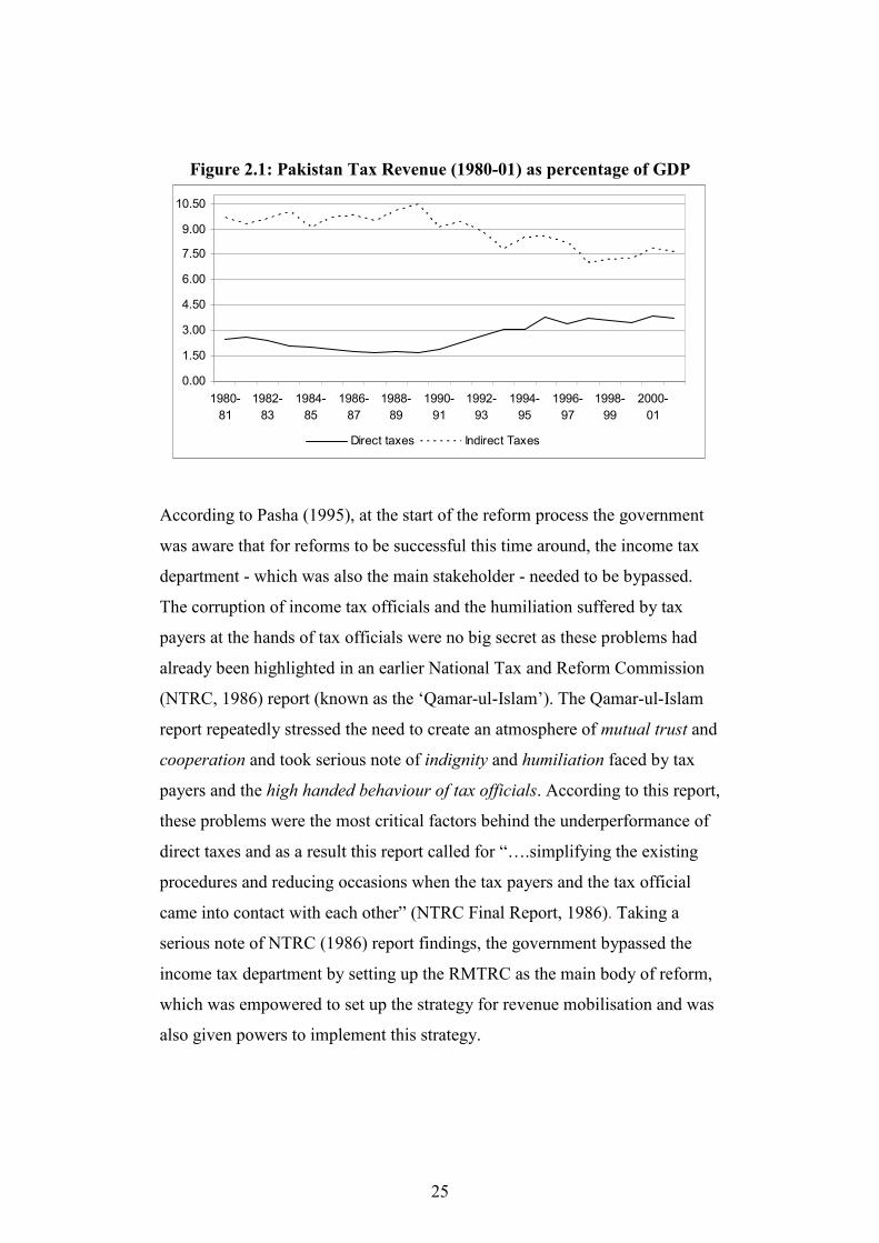
Figure 2.1: Pakistan Tax Revenue (1980-01) as percentage of GDP.............. 25 Figure 2.2: Pakistan Major Tax Components (1980-01) as percentage of GDP......................................................................................................................... 32 Figure 2.3: Tariff Trend (1980-2001) ............................................................. 37 Figure 2.4: Distribution of MFN Tariff rate, 1996-97 – 2001-2 ..................... 38 Figure 4.1: Welfare Comparison (1990-2001).............................................. 109 Figure 6.1: Share of Sugar incidence in total indirect tax incidence (2001-02)....................................................................................................................... 175 Figure 6.2: Share of Sugar, Kerosene-oil and vegetable ghee incidence in total

indirect tax incidence (2001-02) ................................................. 176 Figure 6.3: Percentage change in tax liabilities: National and Regional Results

(1990-2001)................................................................................. 177

IX

Dedication

For my mother, Tallat, and my father, Refaqat

X

Acknowledgments

First of all, I would like to thank Allah Almighty for giving me the

opportunity to pursue my dream for a Doctorate Degree. I offer my deep

gratitude to Him for having bestowed upon me the strength, dedication and

perseverance to undertake such an ambitious project and to complete it. I feel

greatly humbled by His blessings and favours upon me.

These acknowledgements would not be complete without the mention of my

parents; my mother, Tallat and my father, Refaqat who have been the source

of constant support and encouragement throughout my life. It is very rare for

someone from my part of the world, especially a woman, to undertake such an

ambitious journey. This would not have been possible without their persistent

struggles and sacrifices in life which created for me an opportunity to pursue

my dreams. I owe a great debt of gratitude to you ammi and abbu for being

such inspiring role models and for being so generous and loving.

I would like to take this opportunity to thank Commonwealth Scholarship that

provided generous funding for this study. Such funding sources open unique

opportunities for students from third world countries to enter such world class

institutes of learning and for this I will always be grateful. I would also like to

acknowledge and thank Mr. David Constable (Mountbatten Memorial Grant)

and Mr. William Crawley (Charles Wallace Pakistan Trust) for providing

timely and generous funding during the last year of this project.

I would also like to take this opportunity to thank both my supervisors,

Professor Andy Mckay and Professor Philip Jones for their constant

XI

encouragement and support and for reposing confidence in me This work

could not have been completed without your constant guidance, professional

and personal input, so thank you once again.

I must also add and extend a deep appreciation to my mentors, Dr. Abid Aman

Burki (Quaidi-i-Azam University, Islamabad, Pakistan) and Professor Peter J.

Montiel (Williams College, USA), whose immense love and passion for

Economics touched me deeply and made me interested in this field. All this

would not have happened without your encouragement and support during my

Master’s degree, so thank you to you both.

I would also like to extend a special thanks to my friend Saima. Thank you for

adding so much colour, laughter and fun in these last few years and for giving

me such a refreshing perspective on life and friendship. Furthermore, I would

also like to thank my friends, Hari and Ipshita, for our daily coffee and

luncheon breaks that made so much difference to the daily routine. Lastly, I

would also like to thank Mrs. Samina Bokhari for not only accepting the

mammoth task of editing this work at such a short notice but also for

completing it seemingly effortlessly and gracefully.

XII

Abstract

This study aims at measuring the social incidence of indirect taxes in Pakistan

as a result of the tax reform process specifically carried out in the area of

indirect taxes (1990-2001). The intention is to analyze how indirect tax reform

reflects the policy objectives particularly in the light of equity and

distributional considerations envisaged in the tax reform strategy. Whilst one

aim is to reflect on the aggregate indirect tax incidence overtime at the

national as well as the urban/rural level, the second objective is to provide a

high level of disaggregation of incidence picture in order to explore the

sensitivity of tax incidence in terms of key commodities. Additionally, this

study attempts to illustrate the sensitivity of estimated tax incidence results to

the assumption of zero demand responses and to identify welfare enhancing

directions of tax reform for Pakistan at the margin by using the marginal

theory of tax reform.

The findings of this study seem to indicate that a move from dependence on

trade tax revenues to GST/VAT revenues for Pakistan has made the overall

indirect tax system a little more progressive. It appears post- reform indirect

tax incidence is sensitive to taxation of key commodities including sugar,

edible oils and basic fuel/utilities. Incidentally, taxation of these commodities

also appears to have strong distributional effects on the poor. Whilst exploring

the sensitivity of estimated tax incidence results to the incorporation of

behaviour responses, our estimated results do not appear to be very sensitive

to this incorporation. Furthermore, directions of welfare enhancing tax reform

(at the margin) for Pakistan reveal that a reduction in the price of basic food

(including beef, wheat, milk and pulses) should be welfare enhancing; taxation

of sugar maybe efficient but not equitable, while only taxation of vegetable

ghee simultaneously fits both criterion.

XIII

List of Abbreviations

CBR: Central Board of Revenue

FATA: Federally Administered Tribal Area

FBS: Federal Bureau of Statistics

GDP: Gross Domestic Product

GNP: Gross National Product

GoP: Government of Pakistan

GST: General Sales Tax

HIES: Household Integrated Economic Survey

IEO: Independent Evaluation Office

IJI: Islami Jamhoori Ittehad

IMF: International Monetary Fund

ITO: Income Tax Ordinance

NFC: National Finance Commission

NTRC: National Tax Reform Commission

NWFP: North Western Frontier Province

PIHS: Pakistan Integrated Economic Survey

PPP: Pakistan People’s Party

PSU: Primary Sampling Unit

PTCL: Pakistan Telecommunication Company Limited

RMTRC: Resource Mobilization and Tax Reform Commission

SAF: Structural Adjustment Facility

SAP: Social Action Program

SBA: Stand by Agreement

SBP: State Bank of Pakistan

SIZ: Special Industrial Zones

TRC: Tax Reform Commission

VAT: Value Added Tax

WAPDA: Water and Power Development Authority

XIV

WB: World Bank

WHT: With-holding Tax

WTO: World Trade Organization

1

CHAPTER I: Introduction

1.1 Aims of the study

This study aims at measuring the social incidence of indirect taxes in Pakistan

as a result of the tax reform process1 during 1990-2001, focusing on the area

of indirect taxes. The intention is to analyze whether indirect tax reform

achieved the policy objectives, particularly in the light of equity and

distributional considerations envisaged in the tax reform strategy. Whilst one

aim is to reflect on the aggregate indirect tax incidence overtime at the

national as well as the urban/rural level, the second objective is to provide a

highly disaggregated picture of this incidence in order to explore the

sensitivity of tax incidence in terms of key commodities and to isolate their

impact on the poor.

The third aim of this study is to illustrate the sensitivity of estimated tax

incidence results (summarized in terms of tax progression) to the assumption

of zero demand responses (a special case of partial equilibrium tax incidence

analysis assumed in some tax incidence studies. For instance see Chen et al.,

2001; Munoz et al., 2003; and Sahn and Younger, 2003, to name but a few).

The fourth aim of this study is to attempt to move beyond the tax incidence

analysis by identifying welfare enhancing directions of tax reform for Pakistan

at the margin by using the marginal theory of tax reform.

This study focuses on the indirect taxes only (which include sales tax, excise

duties and custom duties) because the focus of this research is the tax reforms

1 Also known as the first generation of tax reform process in Pakistan.

2

(1990-2001) specifically carried out in the area of indirect taxes. Furthermore,

this focus should not be a surprise as a substantial amount of total federal tax

revenue in Pakistan is raised solely via indirect taxes. For instance, almost 83

percent and 67 percent respectively of total federal tax2 came from indirect

taxes in 1990-91 and 2001-02 respectively. Thus in the case of Pakistan,

indirect taxes occupy a central place in the federal tax structure and any

serious evaluation of Pakistan tax structure must begin by looking at indirect

taxes.

As mentioned earlier Pakistan, like many other developing countries, also

embarked on significant tax reforms within the area of indirect taxes, mainly

focusing on replacing trade tax revenues with GST/VAT revenues. While

revenue mobilization was the key factor behind this reform, ‘equity’ and

‘distributional’ considerations were the central focus when the overall reform

strategy was envisaged. This raises an important question of what has

happened in terms of these policy aspirations or in other words, what was the

social incidence of this tax reform process. This study will attempt to answer

this important question by using the partial equilibrium tax incidence approach

while analyzing tax incidence in terms of tax progression using the average

progressivity rate.

The analysis holds immense interest for the tax policy and tax reform in

Pakistan, as the efficiency and distributional impact of this policy reform has

never been systematically studied. But it can also fit a broader perspective as a

case study illustrative of the type of reforms carried out in many other

developing countries as well. Thus, this study will attempt to add to a growing

but limited research on whether a move from dependence on trade tax

revenues to GST/VAT revenues for developing countries has made the tax

2 Total federal tax figure here excludes surcharges which averaged around 1.6 and 1.2 percent of GDP in 1990-91 and 2001-02 respectively.

3

system (indirect taxes in our case) more progressive (Gemmell and Morrissey,

2003) or regressive (Emran and Stiglitz, 2005).

It is important to stress that the strength of partial equilibrium tax incidence

analysis lies in its ability to disaggregate the incidence picture. This is decisive

because such a high level of disaggregation allows us to explore the sensitivity

of tax incidence to key commodities and to isolate commodities that may have

strong distributional effect on the poor. As a result, this could be extremely

useful information for the policymakers and can add to the growing literature

on how evidence from tax incidence (in terms of tax progression) can be more

informative regarding possible impact on the poor (see for instance Bird and

Zolt, 2005).

One of the core concerns regarding evidence emerging from partial

equilibrium tax incidence analysis relates to the underlying assumption used to

constrain demand responses. This approach assumes that tax levied on a

particular commodity is fully borne by those who consume that item. In other

words, consumers of the commodity cannot avoid paying the tax on that

commodity by changing their behaviour. Although this is a simplifying

assumption nevertheless it is a restrictive one. Thus this study will attempt to

illustrate the sensitivity of the estimated results to incorporation of demand

responses. We will do this by estimating own- and cross-price elasticities (for

a sample of key commodities) for Pakistan using spatial price variations in the

(HIES 2001-02) survey data. By doing so, this study will attempt to inform the

literature on tax incidence and price elasticities as well.

This study will also attempt to move beyond tax incidence. We aim to do this

by trying to identify welfare enhancing directions of tax reform for Pakistan at

the margin. For a developing country like Pakistan where one third of the

population lives below the poverty line, improving the welfare of the

4

population in general and of poor in particular is one of the key policy issues.

This means a core concern of tax policy in such a country (with respect to the

poor) should be “not to make them even poorer” (Bird, 1974; and Mclure Jr.,

1977) or to focus on “un-taxing the poor” (Bird and Zolt, 2005). We aim to

identify directions of welfare enhancing reforms for Pakistan at the margin

using the theory of marginal tax reform (MTR). The practical appeal of this

approach for a developing country like Pakistan cannot be exaggerated as

policymakers in such countries are keenly interested in empirically robust and

theoretically consistent suggestions for improvements in the status quo

(Ahmad and Stern, 1987).

1.2 Methodology

The methodological approach followed in this study for the analysis of

distributional burden of indirect taxes is a variant of numerical tax incidence

approach which was first introduced by Nicholson (1964) for the United

Kingdom and Pechman and Okner (1974) for the United States. According to

this approach total tax liability for a household is determined by allocating

total tax revenue collected on a good to household expenditure shares on that

good, until all revenue is fully exhausted. Although this study also calculates

tax liabilities based on household (observed) consumption patterns, we make

no assumption of proportionality between tax burden and tax revenues as

assumed by the earlier studies. In this sense, this is an improvement on the

earlier approach as it allows for excess burden and tax evasion.

The data set used for analysis is the Household Integrated Economic Survey

(HIES) for (1990-91) and (2001-02) which is a cross-sectional data set

collected by the Federal Bureau of Statistics (FBS) Pakistan. This data set is

the main source for poverty and inequality estimates for the country. It is a

5

nationally representative good quality cross sectional data set that has been

used extensively (Ahmad and Stern (1987; 1991), Deaton (1987; 1997),

Deaton and Grimard (1992), Alderman and Garcia (1993); Malik (1988);

Aamjad, et al. (1997); Jafri (1999); Anwar et al. (2005); Kamal et al. (2003);

World Bank (1995; 2002); ADB (2006); CRPRID (2003; 2005; 2006).

Availability of cross-sectional surveys ten years apart allows us to see how the

distributional incidence of these taxes has changed over time. This study will

use the most recent survey and will attempt to show information presented in

the (HIES) is as relevant for tax policy analysis as it is for carrying out poverty

and inequality estimates. Furthermore, it will show how this information can

be used for estimating price elasticities and for carrying out tax reform and tax

planning analysis.

The advantages of such a micro-analysis are well established. It relies on rich

micro information encompassing several thousand households in order to

ascertain consumption patterns, demographic characteristics and other

household characteristics at the national or more local geographic levels. As a

result, even a complicated indirect tax structure like that of Pakistan can be

modeled in detail and across various segments of the population. This allows

us not only to build an incidence picture at the aggregate level but also to

disaggregate the picture in order to see how this incidence is being generated.

Such information may be very relevant for the likely impact of key taxes on

the poor (e.g. taxes on basic fuels, processed food items etc.).

We do accept that the tractability and intuition of partial equilibrium models

must be balanced against the ‘static’ and ‘closed’ nature of the approach.

There is no ideal or unique approach to tax incidence analysis (Martinez-

Vazquez, 1991). The superiority of one approach over the other crucially

depends on what is being asked. Thus, if the aim of the study is to measure the

distributional effect of taxes, partial equilibrium tax incidence approach is

6

sufficient. More importantly, the partial equilibrium tax incidence approach

allows us to clearly disaggregate the incidence picture which as mentioned

earlier is the key to analyzing sensitivity of tax incidence for key commodities,

and to isolate the effects of commodities that may be having a powerful

distributional impact on the poor. All this information is very relevant for the

policy makers and key for identifying impact on the poor.

This study also aims at estimating price elasticities using spatial price

variation in the survey data (i.e. HIES 2001-02) to estimate demand functions

by taking unit values (dividing expenditure by quantities) as proxies for prices.

The basic assumption of this methodology hinges on assuming that households

belonging to the same cluster face the same prices. Since typically the number

of households belonging to the same cluster are in single digits and these

households will be interviewed more or less at the same time (in order to

minimize time and travel cost), this assumption is quite realistic particularly

for rural areas. Nevertheless, unit values are not the same as ‘prices’ and

cannot be directly treated as market prices. But if the appropriate adjustment

in unit values can be made, the usefulness of information contained in unit

values cannot be denied, particularly for developing countries where price data

is so scarce (Deaton, 1988). Thus, this study will attempt to use spatial price

variation in HIES 2001-02 data set to estimate price elasticities for Pakistan.

This information will in turn be used to illustrate the sensitivity of partial

equilibrium tax incidence estimates (for a selected sample of key

commodities), to incorporation of demand responses as well as to propose

directions of welfare enhancing reforms at the margin for Pakistan.

1.3 The plan of the study

7

This study is organized into eight chapters, each of which is discussed briefly

below to provide an outline of discussion. The following chapter begins with

a detailed description of factors (both internal and external) responsible for the

initiation of the tax reform process in Pakistan. It goes on to give details of the

nature and direction of tax reform followed in Pakistan and provides an

overview of how the structure of direct and indirect taxes has changed

overtime due to this reform process.

Chapter three presents an analytical framework for evaluating the

distributional aspects of an indirect tax system. Given the extensive literature

on tax incidence for developed and developing countries, this chapter will

focus on approaches that are important for developing countries. Furthermore,

this chapter will attempt to summarize this evidence of tax incidence in terms

of tax progression. Chapter four discusses the data and methodology issues

related to the measurement of household welfare aggregate and the analysis of

tax incidence.

Chapter five makes up the main body of this study. It establishes the social

incidence of the GST/VAT in Pakistan in the pre- and post- reform era (at the

national as well as the urban/rural level). The welfare impact of GST/VAT is

looked at independently due to the post- reform and future significance of

GST/VAT revenue in total federal tax revenues of Pakistan. We also look at

the issue of GST/VAT exemptions in order to evaluate if these exemptions are

really safeguarding the poor. We use the distributional characteristics of the

goods approach to determine goods/services that are relatively more important

for the poor and recommend exemptions that are in line with the government’s

pro-poor agenda.

Chapter six completes the discussion on the indirect tax incidence in Pakistan

by evaluating the incidence of overall indirect taxes both pre- and post- reform

8

(1990 – 2001) (at the national as well as the urban/rural levels). We first look

at the methodology and assumptions, then at the social incidence of custom

duties and excise taxes respectively. The discussion on the social incidence is

completed by bringing all of these components together.

Chapter seven broadens the analysis of tax incidence for Pakistan. This

chapter relies on spatial price variation in the survey data to determine price

elasticities for 2001-02 along with a detailed discussion of the underlying

methodology and data used. Estimates of elasticities are pivotal for moving the

discussion forward towards the analysis of tax reform and planning. This

chapter also uses this information to evaluate the future direction of welfare-

improving tax reforms for Pakistan at the margin using marginal theory of tax

reform. Furthermore, this chapter will also try to illustrate if our partial

equilibrium tax incidence results from the earlier chapters are sensitive to the

incorporation of demand responses.

The final chapter concludes the study. Along with summarizing the major

findings, the intention is to broadly talk about the importance and main

contributions of this research. Furthermore the chapter also provide a brief

discussion on the qualifications to this work and highlights areas of possible

future research.

9

CHAPTER II: Taxation in Pakistan (1985 – 2001)

2 Introduction

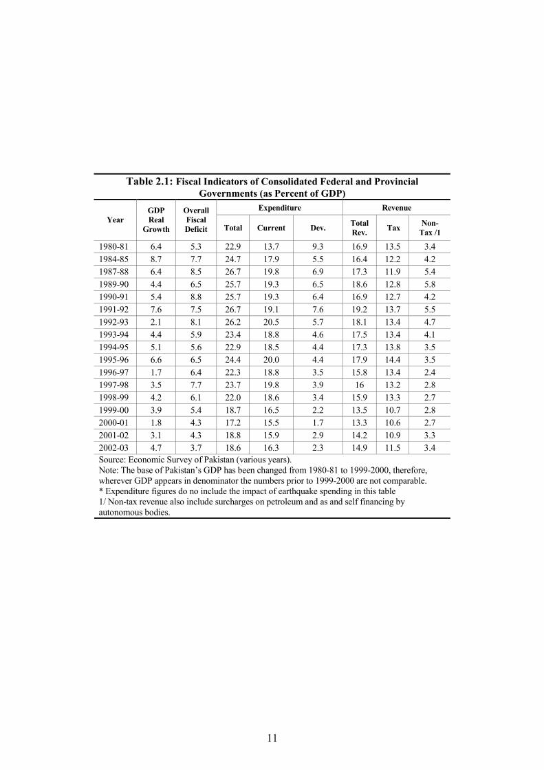
Pakistan’s tax system has undergone profound changes since the nineties, but

despite these changes tax revenue in relation to GDP has remained remarkably

stable over the last two decades (see Table 2.1). Federal tax revenue as a

percent of GDP during the last two decades averaged around 13 percent never

falling below 10 percent of GDP (International Monetary Fund, 2001). The

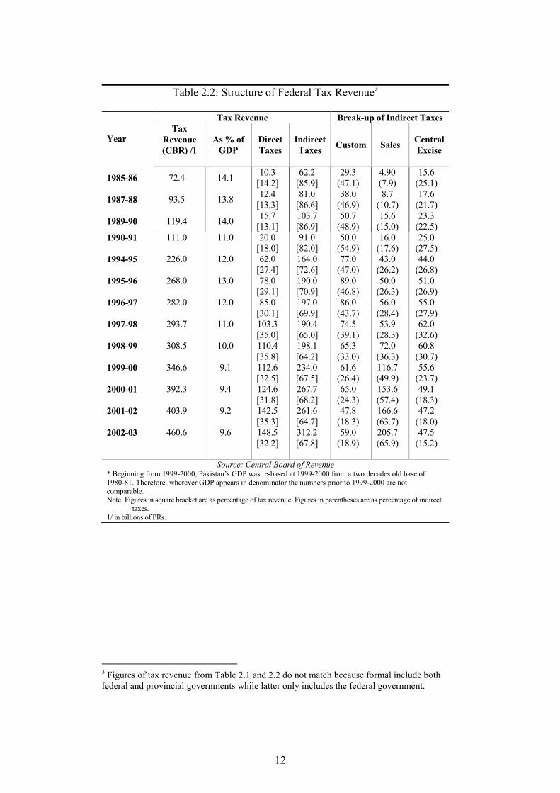
overall revenues still appear to be dominated by revenues collected by the

federal government (see Table 2.2) and these mainly comprise direct taxes

(income and corporation tax) and indirect taxes (custom duties, sales tax and

excise duties).

The purpose of this chapter is to analyse the structure of the country’s federal

taxation in conjunction with the reform process, also called the first generation

of tax reforms, that took place during the 90s in Pakistan. The main focus of

this reform process was to impose direct taxes as well as replace trade

revenues with GST/VAT revenues. This process approximately ended in 2001.

And shortly after, Pakistan initiated the second generation of tax reforms

which are purely administrative in nature and are not the focus of this study.

This chapter will try to address the following questions:

(a) What were the internal and external factors that impelled the tax

reform process in Pakistan?

10

(b) What was initially envisaged regarding the nature, shape and scope of

these reforms, and more importantly, whether this vision translated

into policy actions or not?

(c) Who envisaged these reforms?

(d) How have the overall federal tax structure and its components changed

during the reform process and what were the major reform steps?

(e) Were equity concerns considered under the overall reform strategy and

within its components? And did these concerns translate into

respective policy actions?

For this purpose, this chapter is divided into four main sections. The first

section addresses the question of why tax reforms were initiated in the first

place in Pakistan during the decade of the 90s. The second section talks

about the overall nature and direction of the tax reform process as foreseen

by the Resource Mobilization and Tax Reform Commission (RMTRC).

The third section is divided into several subsections; each analyzing major

changes that took place in each component of the federal taxation (namely

income tax, custom duties, sales tax and excise duties) due to this reform

process and the last section concludes the discussion.

11

Table 2.1: Fiscal Indicators of Consolidated Federal and Provincial Governments (as Percent of GDP)

Expenditure Revenue

Year

GDP

Real

Growth

Overall

Fiscal

Deficit Total Current Dev. Total

Rev. Tax

Non-

Tax /1

1980-81 6.4 5.3 22.9 13.7 9.3 16.9 13.5 3.4

1984-85 8.7 7.7 24.7 17.9 5.5 16.4 12.2 4.2

1987-88 6.4 8.5 26.7 19.8 6.9 17.3 11.9 5.4

1989-90 4.4 6.5 25.7 19.3 6.5 18.6 12.8 5.8

1990-91 5.4 8.8 25.7 19.3 6.4 16.9 12.7 4.2

1991-92 7.6 7.5 26.7 19.1 7.6 19.2 13.7 5.5

1992-93 2.1 8.1 26.2 20.5 5.7 18.1 13.4 4.7

1993-94 4.4 5.9 23.4 18.8 4.6 17.5 13.4 4.1

1994-95 5.1 5.6 22.9 18.5 4.4 17.3 13.8 3.5

1995-96 6.6 6.5 24.4 20.0 4.4 17.9 14.4 3.5

1996-97 1.7 6.4 22.3 18.8 3.5 15.8 13.4 2.4

1997-98 3.5 7.7 23.7 19.8 3.9 16 13.2 2.8

1998-99 4.2 6.1 22.0 18.6 3.4 15.9 13.3 2.7

1999-00 3.9 5.4 18.7 16.5 2.2 13.5 10.7 2.8

2000-01 1.8 4.3 17.2 15.5 1.7 13.3 10.6 2.7

2001-02 3.1 4.3 18.8 15.9 2.9 14.2 10.9 3.3

2002-03 4.7 3.7 18.6 16.3 2.3 14.9 11.5 3.4

Source: Economic Survey of Pakistan (various years). Note: The base of Pakistan’s GDP has been changed from 1980-81 to 1999-2000, therefore, wherever GDP appears in denominator the numbers prior to 1999-2000 are not comparable. * Expenditure figures do no include the impact of earthquake spending in this table 1/ Non-tax revenue also include surcharges on petroleum and as and self financing by autonomous bodies.

12

3 Figures of tax revenue from Table 2.1 and 2.2 do not match because formal include both federal and provincial governments while latter only includes the federal government.

Table 2.2: Structure of Federal Tax Revenue3

Tax Revenue Break-up of Indirect Taxes

Year Tax

Revenue

(CBR) /1

As % of

GDP

Direct

Taxes

Indirect

Taxes Custom Sales

Central

Excise

1985-86 72.4 14.1 10.3

[14.2] 62.2

[85.9] 29.3

(47.1) 4.90 (7.9)

15.6 (25.1)

1987-88 93.5 13.8 12.4

[13.3] 81.0

[86.6] 38.0

(46.9) 8.7

(10.7) 17.6

(21.7)

1989-90 119.4 14.0 15.7

[13.1] 103.7 [86.9]

50.7 (48.9)

15.6 (15.0)

23.3 (22.5)

1990-91

1994-95

1995-96

1996-97

1997-98

1998-99

1999-00

2000-01

2001-02

2002-03

111.0

226.0

268.0

282.0

293.7

308.5

346.6

392.3

403.9

460.6

11.0

12.0

13.0

12.0

11.0

10.0

9.1

9.4

9.2

9.6

20.0 [18.0] 62.0

[27.4] 78.0

[29.1] 85.0

[30.1] 103.3 [35.0] 110.4 [35.8] 112.6 [32.5] 124.6 [31.8] 142.5 [35.3] 148.5 [32.2]

91.0 [82.0] 164.0 [72.6] 190.0 [70.9] 197.0 [69.9] 190.4 [65.0] 198.1 [64.2] 234.0 [67.5] 267.7 [68.2] 261.6 [64.7] 312.2 [67.8]

50.0 (54.9) 77.0

(47.0) 89.0

(46.8) 86.0

(43.7) 74.5

(39.1) 65.3

(33.0) 61.6

(26.4) 65.0

(24.3) 47.8

(18.3) 59.0

(18.9)

16.0 (17.6) 43.0

(26.2) 50.0

(26.3) 56.0

(28.4) 53.9

(28.3) 72.0

(36.3) 116.7 (49.9) 153.6 (57.4) 166.6 (63.7) 205.7 (65.9)

25.0 (27.5) 44.0

(26.8) 51.0

(26.9) 55.0

(27.9) 62.0

(32.6) 60.8

(30.7) 55.6

(23.7) 49.1

(18.3) 47.2

(18.0) 47.5

(15.2)

Source: Central Board of Revenue * Beginning from 1999-2000, Pakistan’s GDP was re-based at 1999-2000 from a two decades old base of 1980-81. Therefore, wherever GDP appears in denominator the numbers prior to 1999-2000 are not comparable. Note: Figures in square bracket are as percentage of tax revenue. Figures in parentheses are as percentage of indirect

taxes. 1/ in billions of PRs.

13

2.1 Why Reform?

The main forces behind the tax reform process - also known as the first

generation of tax reforms - can be analysed in terms of internal factors (e.g.

the economy and politics) as well as external factors (e.g. the Gulf war,

International Monetary Fund programmes etc) and these are discussed in

detail below.

2.1.1 Internal factors

2.1.1.1 Economic Factors

At the time of the initiation of the tax reform process, several economic factors

dictated the need for serious tax reforms in Pakistan. In order to understand

this phenomenon the country’s economic history over the last 30 years needs

to be taken into account, Pakistan’s economic history can be broadly

categorized into two periods. During the first period which started in 1970 and

lasted until the middle of the 1980s, Pakistan enjoyed an impressive growth

performance six-seven percent per annum). Although fiscal and external

imbalances were not significant at the beginning of this period by the end of

this period significant imbalances appeared to emerge.

The second stage can be marked from the middle of 1980s till the end of 2000

during which the growth process started to fade away and ballooning of fiscal

and current account deficits led to serious deterioration of the debt situation of

the country (Independent Evaluation Office, 2002). For instance, in (1977-78)

14

debt servicing payments (as a percentage of net revenue receipts) were only 19

percent but by the end of 1980s these had ballooned to 42 percent. Much of

the problem according to Pasha et al. (1992) arose from the mounting share of

current expenditures, which remained in excess of 19 percent of GDP between

1985-93 as a result of dramatic increase in debt service payments. Together

with military expenditure, these accounted for 80 percent of current

expenditures.

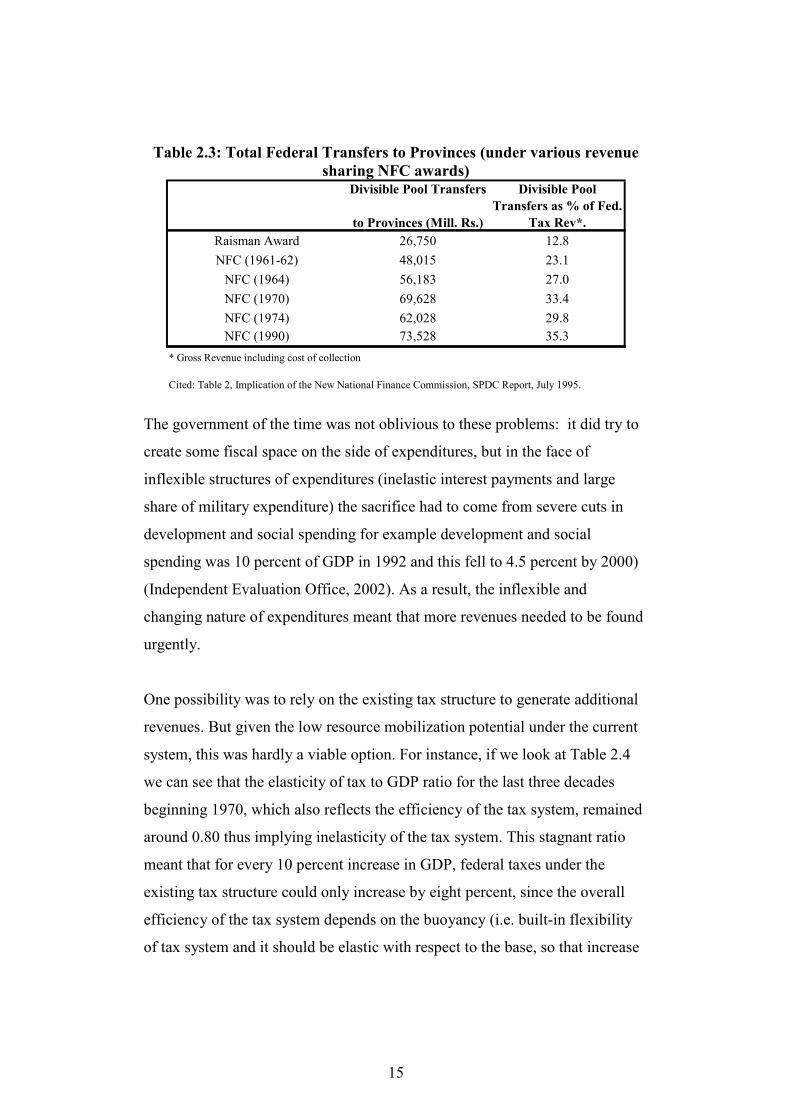
Another important economic change which took place during the second

period were the changes in revenue sharing transfers from federal government

to provincial governments through the National Finance Commission (NFC)

Awards4 (see Table 2.3). In May 1991, the sixth NFC award took place after a

span of 12 years. The May 1991 NFC award significantly increased revenue-

sharing transfers to the provinces. This was made possible by including excise

duties on tobacco and tobacco manufacturers and sugar in the divisible pool of

taxes. On the whole, the 1990 NFC award increased the total federal transfers

to the provinces in (1991-92) by PRs. 25 billion,- an increase of 2.1 percentage

point in terms of GDP. This put significant additional pressure on an already

dwindling fiscal stance.

4 The National Finance Commission is a constitutional body which is required to meet every five years to make recommendations on the distribution of financial resources between provinces by the federal government.

15

Table 2.3: Total Federal Transfers to Provinces (under various revenue

sharing NFC awards) Divisible Pool Transfers

to Provinces (Mill. Rs.)

Divisible Pool

Transfers as % of Fed.

Tax Rev*.

Raisman Award 26,750 12.8

NFC (1961-62) 48,015 23.1

NFC (1964) 56,183 27.0

NFC (1970) 69,628 33.4

NFC (1974) 62,028 29.8

NFC (1990) 73,528 35.3

* Gross Revenue including cost of collection

Cited: Table 2, Implication of the New National Finance Commission, SPDC Report, July 1995.

The government of the time was not oblivious to these problems: it did try to

create some fiscal space on the side of expenditures, but in the face of

inflexible structures of expenditures (inelastic interest payments and large

share of military expenditure) the sacrifice had to come from severe cuts in

development and social spending for example development and social

spending was 10 percent of GDP in 1992 and this fell to 4.5 percent by 2000)

(Independent Evaluation Office, 2002). As a result, the inflexible and

changing nature of expenditures meant that more revenues needed to be found

urgently.

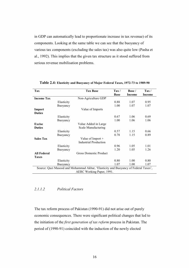
One possibility was to rely on the existing tax structure to generate additional

revenues. But given the low resource mobilization potential under the current

system, this was hardly a viable option. For instance, if we look at Table 2.4

we can see that the elasticity of tax to GDP ratio for the last three decades

beginning 1970, which also reflects the efficiency of the tax system, remained

around 0.80 thus implying inelasticity of the tax system. This stagnant ratio

meant that for every 10 percent increase in GDP, federal taxes under the

existing tax structure could only increase by eight percent, since the overall

efficiency of the tax system depends on the buoyancy (i.e. built-in flexibility

of tax system and it should be elastic with respect to the base, so that increase

16

in GDP can automatically lead to proportionate increase in tax revenue) of its

components. Looking at the same table we can see that the buoyancy of

various tax components (excluding the sales tax) was also quite low (Pasha et

al., 1992). This implies that the given tax structure as it stood suffered from

serious revenue mobilisation problems.

Table 2.4: Elasticity and Buoyancy of Major Federal Taxes, 1972-73 to 1989-90

Tax Tax Base Tax /

Base

Base /

Income

Tax /

Income

Income Tax Non-Agriculture GDP

Elasticity 0.88 1.07 0.95

Buoyancy 1.00 1.07 1.07

Import

Duties

Value of Imports


Buoyancy 1.00 1.06 1.06

Excise

Duties

Value Added in Large Scale Manufacturing


Buoyancy 0.78 1.15 0.89

Sales Tax Value of Import + Industrial Production


Buoyancy 1.20 1.05 1.26

All Federal

Taxes

Gross Domestic Product

Elasticity 0.80 1.00 0.80 Buoyancy 1.07 1.00 1.07

Source: Qazi Masood and Mohammad Akbar, ‘Elasticity and Buoyancy of Federal Taxes’, AERC Working Paper, 1991.

2.1.1.2 Political Factors

The tax reform process of Pakistan (1990-91) did not arise out of purely

economic consequences. There were significant political changes that led to

the initiation of the first generation of tax reform process in Pakistan. The

period of (1990-91) coincided with the induction of the newly elected

17

Government of Islami Jamhoori Ittehad (IJI) led by Mian Nawaz Sharif in

November 1990. This event was a catalyst for reform process as Nawaz Sharif

(contrary to his predecessor Benazir Bhutto5) was a capitalist, a political

moderate and member of a leading industrial family. The IJI had a strong

industrialist hold and enjoyed thriving urban support. And the party was

elected with the specific goal of strengthening the economy which included

reforms in areas of privatisation, deregulation, denationalization, foreign

exchange and payment, taxation, administration and law. All this made the IJI

government more forward looking and responsive to the needs of the private

sector.

This, coupled with the macroeconomic pressure created by the Gulf War,

(which will be discussed later) made Nawaz Sharif’s government more eager

to pursue reforms. The seriousness of the commitment to reforms, particularly

in the area of taxation, can be seen from the fact that within a few months of

the formation of the new government, the IJI government created a high

profile Tax Reform Committee (TRC) which was followed by the

establishment of the Resource Mobilization and Tax Reform Commission

(RMTRC) in February 1991. This commission was created with the purpose of

outlining a revenue mobilization strategy as well as improving tax laws and

procedures6. It would be no exaggeration to add that role of RMTRC in

formulating the direction and nature of tax reform process in Pakistan was

pivotal.

2.1.2 External Factors

5 Benazir Bhutto is the lifetime chairperson of the Pakistan People’s Party (PPP). The previous government was held by PPP with Benazir as prime minister. The PPP enjoys support in the rural areas of Pakistan. 6 RMTRC’s terms of reference as suggested by an open letter to Prime Minister (August 28, 1994) by the RMTRC.

18

It will be too naïve to say that Pakistan’s first generation of tax reform process

was initiated only due to internal pressures. There were some significant

external forces as well that helped initiate the reform process.

2.1.2.1 Gulf War

The Gulf war started in August 1990. Although Pakistan was not a direct

stakeholder in this war, it indirectly put a lot of stress on government finances

particularly on the budget and the balance of payments. According to Pasha et

al. (1992) the cost of the Gulf war to the Government of Pakistan (GoP) is

estimated at around PRs. 3 billion. This cost was incurred because of: (a) a

higher oil import bill (over $600 million): (b) a decline in home remittances

from Kuwait and Iraq (approximately $180 million); and (c) a decline in

custom duties due to an export decline (PRs. 2 billion). These factors caused

the budget deficit for (1990-91) to swell up to a historic high level of 8.8

percent of the GDP and also resulted in a jump in inflation from six to 13

percent. This resulted in a severe macroeconomic shock for the government

(Pasha et al., 1992).

2.1.2.2 International Monetary Fund

From (1988-2001) Pakistan has been involved with seven different

International Monetary Fund (IMF) programmes, four of which were short

term and three multi-year arrangements (Independent Evaluation Office,

19

2002). The balance of payment crisis triggered by the Gulf war (as mentioned

earlier) forced the government to borrow again from the IMF, initially under a

one-year Stand-by Arrangement (SBA) that started in September 19937.

There is no doubt about the fact that various IMF programmes brought

significant structural adjustment reforms in the areas of tariff liberalization,

and GST broad-basing that were similar in features to IMF reform

programmes in other developing countries. As a result, these programmes

were important to the interlocking tax reforms agenda within the economic

agenda of various Pakistani governments during the decade of the 90s.

However, it must be added that the IMF support role in the design and

implementation of reform process was particularly significant in the design of

GST/VAT taxation. This is also noted by the (Task Force on Tax

Administration, 2001) according to which “(like) many developing countries

the technology of VAT was transferred to Pakistan as a part of IMF

stabilisation programme. It was exported and implemented in light of its

advantages, i.e. in terms of “revenue buoyancy, a broad base consisting of

most goods and services, neutrality as concerns both domestic and

international trade and difficulties of evasion”.

What is most noteworthy about the decade of the 90s is that it was the most

politically unsettling decade, or the decade of institutional decay (Hussain,

2004). Between 1988-2001, nine different governments came to power. Thus,

what is remarkable and must be acknowledged is that despite political

upheavals and government shuffling, the tax reform agenda managed to stay

and run its course. The only plausible explanation for sustaining the reforms at

such a time (in a country where these reforms have been aborted many times

7 Immediately before this, Pakistan had had two unsuccessful programs with the IMF. The first was a three-year Structural Adjustment Facility (SAF) signed on Dec. 1988. The second was a year-long SBA arrangement which started in Dec. 1988. The first programme was completely aborted with zero funds withdrawn, while only 29 percent of total disbursement was withdrawn in the second arrangement.

20

for lesser reasons) appears to be the balance of payment crisis, the acute need

for revenue mobilization and the IMF push factor.

2.2 Nature and Direction of Tax Reforms

After having discussed the factors (both internal and external) that forced

Pakistan to undertake the tax reform process, it is equally important to

understand why these reforms took this particular form and shape and what

was responsible for this. In this regard, the role of the Resource Mobilisation

and Tax Reform Commission (RMTRC) is pivotal and will now be discussed

in detail.

The Tax Reform Committee (TRC) (as mentioned earlier) was formulated

early in 1990 by the government of Nawaz Sharif. However, while the TRC

was mandated to undertake a comprehensive look at the current situation and

identify bottlenecks, it lacked the powers to implement the identified reform

process. The issue of dealing with the tax reform process was taken a step

further with the establishment of the Resource Mobilization and Tax Reform

Commission (RMTRC) in February 1991. The RMTRC was created with the

purpose of not only outlining a revenue mobilization strategy and

recommending improvements in tax laws but also for implementing these

improvements.

The commission was different from earlier committees and commissions of a

similar nature, since it was mandated to work as an advisory group in close

liaison with the Central Board of Revenue and the Ministry of Finance8. And

8 The Resource Mobilisation and Tax Reforms Commission Report, Government of Pakistan, August 1994.

21

by creating the RMTRC, the government had effectively bypassed the tax

department by giving the responsibility for development of proposals and

implementation of strategies (via provisions in the Finance Bills) to the

RMTRC. The actual collection responsibilities were also shifted to the large

public sector and corporate entities (Pasha, 1995).

The RMTRC term of reference include 9the following objectives:

a. To assist with the implementation of the recommendations of the Tax

Reform Committee

b. To bring structural reforms in the following area(s):

i. Excise Taxation by developing a workable capacity.

ii. (to) Establish a fixed, or presumptive, tax system in direct taxes.

iii. (to) Restructure the Custom Duties Collection system.

iv. (to) Broaden and increase the tax base.

c. To improve the overall tax system with the view of minimising

discretion and simplifying procedures etc.

d. To formulate other steps that can improve the federal and provincial

finances.

According to the RMTRC final report (1994) the basic objective of the tax

reform process was to generate bigger tax resources while the motivation for

the proposed reform was the acknowledgement from the government that it

was facing a serious budgetary problem and that there was an urgent need to

finance that burden. The RMTRC was of the opinion that the government was

also aware that the best way forward was to increase revenues via domestic

taxation as other sources of financing (such as seignorage revenue, internal

and external borrowing) at this time were of limited use or had already been

utilized to the maximum possible.

9 Ibid.

22

Although, revenue mobilisation was at the core of the tax reform agenda, there

was an understanding that the resultant tax structure must be efficient,

administratively feasible as well as equitable. And this was mentioned in

numerous places in the Commission’s main report i.e. RMTRC (1994). For

instance:

• “…..above all it is also sought to provide a long-term vision of an

efficient and just taxation system”10.

• “….while giving due weight to the difficult problem of

implementability, the Report does not lose sight of the central

objectives of public policy, i.e. economic efficiency, equity and

macroeconomic stability—and of the fact that the ultimate purpose of

any meaningful tax reform is to raise the economic well being of the

people, especially that of the least privileged in the society”.

• “The central objective of the tax reforms is to raise bigger resources

than the pre-reform situation so that the large budgetary deficits can be

reduced in such a manner that the maxims of efficiency and equity are

met…”

• “While recognizing multiplicity of the sources of financing for public

expenditure…the report regards taxation to be the basic instrument of

public policy which alone is consistent with efficiency and equity”.

• “In the field of indirect taxation, the basic objective is to move away

from trade taxes to domestic taxes in an offsetting manner to prevent a

10 This one is taken from the open letter to the prime minister by RMTRC, Aug. 28, 1994.

23

reduction in public revenue while greater efficiency is achieved….The

pursuit of these objectives will involve carrying out tariff reform,

which aims to reduce the dispersion of the rates of nominal tariffs and

to lower the nominal and effective rates of import tariffs, partly to

simplify the tax laws and partly to discourage smuggling activity.

Furthermore, a broad based value added tax imposed at the

consumption stage should be introduced. And, an effort should be

made to make indirect taxation relatively more equitable by a highly

selective exemption of basic necessities, which are mainly consumed

by the poor, and by taxing luxuries at a higher rate. However, it should

be understood that indirect taxation is basically inequitable; it is no

substitute for a properly designed system of direct taxation”

• However, in several other places in the Commission report, there is

also confusion and doubt about whether equity and efficiency goals

can be met simultaneously. For instance:

“….(although) there is an inevitable trade-off between objectives; but

in Pakistan’s present situation, what is equitable is also efficient”

Thus, it is not an exaggeration to imply that the RMTRC vision of tax reform

for Pakistan included delivering a tax structure that would not only be revenue

enhancing but one which would also encompass equity as a central pillar of

reform process along with efficiency and administrative ease.

2.3 Trends in Pakistan’s Public Finance: Before and After the Tax Reform

process

24

2.3.1 Direct Taxes11

Pakistan’s direct tax regime mainly comprises income and corporation tax12,

which together constitute 90 percent of the total direct taxes. This discussion

therefore will only focus on these two components.

If we look at Figure 2.1, we can see that the contribution of direct taxes within

total revenues over the years has been minuscule when compared to the share

of indirect taxes within federal revenues. For instance, between 1980 to 1990

direct tax shares averaged no more than two percent of GDP. According to the

IMF (2004), this was primarily due to a narrow base, non-compliance and

abundant use of tax concessions13. If we look at Figure 2.1 we can clearly see

that the most significant increase in the share of direct taxes share came during

the initial period of tax reform i.e. (1990-95) when direct tax share as a

percentage of GDP increased to a historic high of 3.8 percent and by the time

reforms ended, it had more or less steadied around this level. Thus on the

surface it appears that a significant increase in direct tax revenues took place.

But the real question is, how this increase was made possible.

11 The discussion on direct taxes has been purposely kept brief since the focus of this research is indirect taxes. 12 For the purpose of income taxation, income is classified into six broad categories including salary, interest on securities, income (from house or business or profession), capital gains and income from other sources. 13 Pakistan’s economy has a large informal sector estimated to be around at least a quarter of GDP. Additionally, service and agriculture sector representing 52 and 23 percent of GDP are taxed nominally (International Monetary Fund, 2004).

25

Figure 2.1: Pakistan Tax Revenue (1980-01) as percentage of GDP

0.00

1.50

3.00

4.50

6.00

7.50

9.00

10.50

1980-

81

1982-

83

1984-

85

1986-

87

1988-

89

1990-

91

1992-

93

1994-

95

1996-

97

1998-

99

2000-

01

Direct taxes Indirect Taxes

According to Pasha (1995), at the start of the reform process the government

was aware that for reforms to be successful this time around, the income tax

department - which was also the main stakeholder - needed to be bypassed.

The corruption of income tax officials and the humiliation suffered by tax

payers at the hands of tax officials were no big secret as these problems had

already been highlighted in an earlier National Tax and Reform Commission

(NTRC, 1986) report (known as the ‘Qamar-ul-Islam’). The Qamar-ul-Islam

report repeatedly stressed the need to create an atmosphere of mutual trust and

cooperation and took serious note of indignity and humiliation faced by tax

payers and the high handed behaviour of tax officials. According to this report,

these problems were the most critical factors behind the underperformance of

direct taxes and as a result this report called for “….simplifying the existing

procedures and reducing occasions when the tax payers and the tax official

came into contact with each other” (NTRC Final Report, 1986). Taking a

serious note of NTRC (1986) report findings, the government bypassed the

income tax department by setting up the RMTRC as the main body of reform,

which was empowered to set up the strategy for revenue mobilisation and was

also given powers to implement this strategy.

26

The direct tax reform process came in two phases: the first phase (1990-95)

and the second one (1995-2000). The first phase included:

a. Development of Withholding Taxes (WHT)14 or presumptive tax

regime.

b. Reduction in tax rates.

As a consequence, the first stage facilitated the reform agenda by immediately

incorporating steps that were revenue enhancing (i.e. WHT) and also

effectively bypassed the income tax department as the collecting agent. The

commission was aware that increasing the direct tax revenue in this manner

was not the best way possible. But given the serious administrative

bottlenecks, this was perhaps the only way to move forward at this time.

Thus, if we look at Figure 2.1 we can see clearly that much of the increase in

direct tax share during the reform process came during the first phase of

reforms. According to the (International Monetary Fund, 2001; Pasha, 1995;

Khan, 1997) the factor responsible for almost the entire increase in the direct

tax collection over the decade of 1990 has been the steady expansion of the

WHT collection regime. And this can be more easily identified if we look at

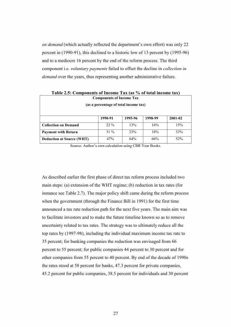
Table 2.5 which classifies income tax revenues into its three components15.

The contribution of WHT in the total income tax revenue in (1990-91) was

only 47 percent; by (1995-96) this had jumped to a staggering 64 percent and

by the end of the reform process had dropped to 53 percent. While collection

14 Section 50 of Income Ordinance of Pakistan, 1979, contains the provisions for payment of tax before assessment. It is called deduction at source and commonly known as withholding

tax (WHT), (Choudhry, 2001). 15 Income tax components include: (a) Collection on demand refers to collection made through audit; (b) Voluntary payments are made on five different dates i.e. each quarter of the income year on the basis of anticipated annual income and final payment at the time of annual return of income; (c) Withholding Taxes (WHT) are essentially in the nature of advance tax payments (or essentially deduction at source) and very similar to the indirect taxes (since their payment constitutes a final discharge of tax liability).

27

on demand (which actually reflected the department’s own effort) was only 22

percent in (1990-91), this declined to a historic low of 13 percent by (1995-96)

and to a mediocre 16 percent by the end of the reform process. The third

component i.e. voluntary payments failed to offset the decline in collection in

demand over the years, thus representing another administrative failure.

Table 2.5: Components of Income Tax (as % of total income tax) Components of Income Tax

(as a percentage of total income tax)

1990-91 1995-96 1998-99 2001-02

Collection on Demand 22 % 13% 16% 15%

Payment with Return 31 % 23% 18% 33%

Deduction at Source (WHT) 47% 64% 66% 52%

Source: Author’s own calculation using CBR Year Books.

As described earlier the first phase of direct tax reform process included two

main steps: (a) extension of the WHT regime; (b) reduction in tax rates (for

instance see Table 2.7). The major policy shift came during the reform process

when the government (through the Finance Bill in 1991) for the first time

announced a tax rate reduction path for the next five years. The main aim was

to facilitate investors and to make the future timeline known so as to remove

uncertainty related to tax rates. The strategy was to ultimately reduce all the

top rates by (1997-98), including the individual maximum income tax rate to

35 percent; for banking companies the reduction was envisaged from 66

percent to 55 percent; for public companies 44 percent to 30 percent and for

other companies from 55 percent to 40 percent. By end of the decade of 1990s

the rates stood at 58 percent for banks, 47.3 percent for private companies,

45.2 percent for public companies, 38.5 percent for individuals and 30 percent

28

for individuals with salary-based incomes (International Monetary Fund,

2001; Pasha, 1995).

The second phase of direct tax reform started in the middle of 1990s and was

aimed at addressing serious structural weaknesses in the direct tax system.

According to the RMTRC (1994) the main reform components included:

1. Expanding the tax net by including other activities particularly agriculture,

capital gains, services, and informal sector.

2. Eliminating all or most of the tax expenditure and tax holidays.

3. Moving away from the presumptive taxes to more adequate and systematic

taxation of personal and corporate incomes.

It has to be admitted that the agenda for the second phase of income tax

reform was much more complicated as it tried to address issues of reform in

order to have a long-term impact on revenues rather than the short-term

revenue mobilisation achieved under the first phase. But reforms during the

second phase at best remained partial. For instance, although the commission

did highlight the imperative to extend and broaden the income tax base by

bringing in agriculture income and corporate gains within the tax net, the

government found it very hard to carry this through due to political reasons.

In conclusion, direct tax reforms were able to bring an immediate increase in

tax revenues but most of the increased tax revenue came from the expansion

of the withholding taxes. For instance, in 1990-91, direct taxes were

contributing around 1.9 percentage of GDP, this increased to 3.8 percent in

1995-96 and settled down to 3.7 percent towards the end of decade. Since

29

revenues by WHT are not progressive, this did not add much needed

progressivity to direct taxes.

Also the envisaged progressivity of the direct tax system failed to materialize

as the broadening of direct taxes and the expansion supposed to address the

structural features of the direct tax regime (such as agriculture tax and

corporate profits etc.) failed to materialize. Thus, even though revenues

increased in the short run, the direct taxes performance in the long run

remained lacklustre at best. We can say that the resultant direct tax structure

failed to adequately address the concerns envisaged by the commission

regarding enhancing the progressivity of direct tax system. This makes

distributional concerns related to the incidence of indirect taxation even more

important because in the case of Pakistan we can no longer rely on the

conventional wisdom of addressing progressivity issues via direct taxes only.

2.3.2 Indirect Taxes

Pakistan’s taxation policy over the years can be marked with excessive

reliance on indirect taxes. For instance if we look at Table 2.2 we can see that

in (1990-91) almost 82 percent of total federal tax revenues came from

indirect taxes. By the mid-1990s, indirect taxes contribution to total federal

taxes slightly reduced to 73 percent and by the end of reform process, indirect

taxes were contributing around 65 percent of total federal taxes. Not only has

the contribution of indirect taxes to the overall federal taxes been changing,

but a significant change has taken place in terms of how this revenue is being

generated. For instance, in 1990-91 almost 55 percent of total indirect taxes

were coming from custom revenues followed by excise and sales tax at 28 and

18 percent respectively. During the middle of the reform process (1995-96),

30

even though custom duties still remained the dominant source of indirect tax

revenues, this contribution had declined to 47 percent while excises and sales

tax were both contributing around 26 percent respectively. However, by the

end of the reform process, revenues from GST had surpassed all the other

sources. For instance, in 2001-02 GST was contributing an unprecedented 64

percent of total indirect tax revenues followed by both customs and excises at

18 percent each. Thus, we can see a remarkable change in how the indirect tax

revenues were being generated over time and this is discussed in the following

sections.

2.3.2.1 Custom Duties 16

It would not be wrong to say that Pakistan’s tariff and trade reform process

started much earlier than the 1990s and it can be divided into two main phases.

The first phase of import liberalization was initiated in the middle of the 1980s

with recommendation from National Tax Reform Commission (NTRC),

(1986) which lasted about ten years and the second phase of reform process

started in the middle of 1990s with the establishment of Tariff Reform

Commission (TRC) in 1996 which lasted until 2001-02.

Historically, import taxes in Pakistan were primarily raised for revenue

generation and to promote industrialization based on import substitution

policy. As expected, this policy resulted in a large-scale diversion of resources

and created a strong anti-export bias by creating extremely high and distorted

16 Since import tariff and non-tariff barriers are the prime source of custom duties, discussion here only focuses on these taxes.

31

tariff structure that led to rampant smuggling and inefficient resource

allocation17 (Pasha, 1995).

After 1990, there was a major policy shift in trade policy toward trade

liberalization and tariff reform was deemed essential for reducing protection in

the import-substituting industries, as well as for encouraging export promotion

and reducing smuggling (RMTRC, 1994). Furthermore, compared to the first

phase of reform, this phase was not envisaged to be revenue neutral as it was

seen as a part of the overall tax reform strategy where revenue loss from the

declining importance of trade taxes would be compensated by the increasing

importance of domestic tax; GST/VAT (RMTRC, 1994). Thus, as a result of

this reform process, tariff revenue contribution as a proportion of indirect

taxes exhibited a steep decline during the decade of 1990s (World Bank,

2004). For instance, tariff revenue as a percentage of indirect tax declined

from around 46 percent in 1990-91 to only 15 percent in 2001-02. However,

these tariff cuts were not offset by an increase in the share of imports to GDP

which maintained more or less the same trend (World Bank, 2004). As a

result, tariff revenue as a share of GDP also fell from around 5 percentage of

GDP in 1990-91 to 1.7 percent in 2001-02 (also see, Figure 2.2).

17 These issues have been discussed in preceding paragraphs.

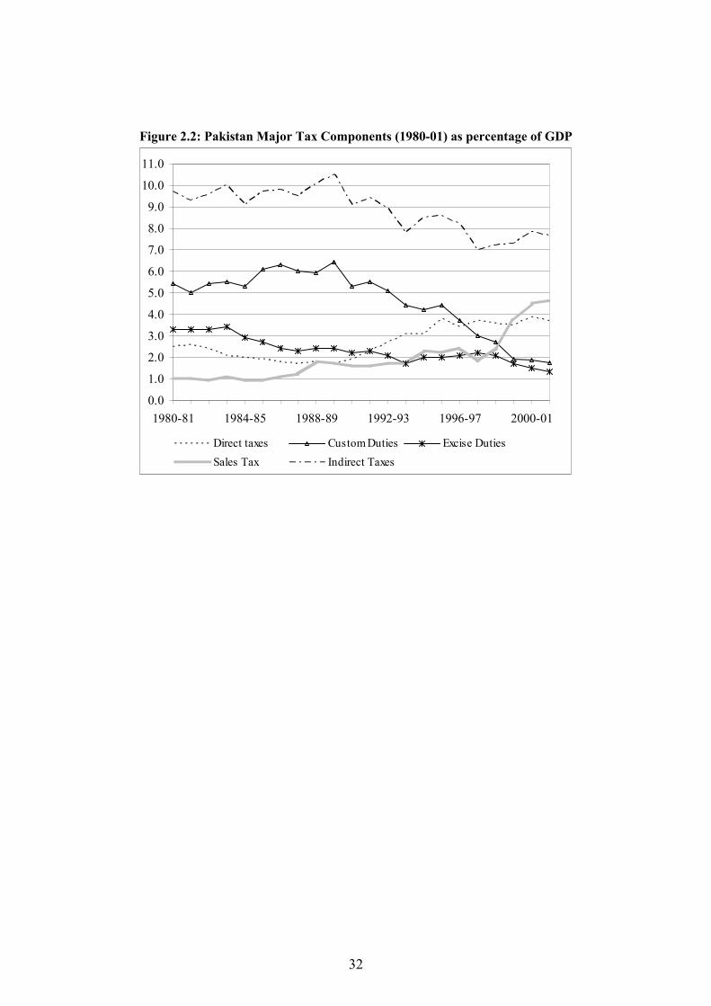
32

Figure 2.2: Pakistan Major Tax Components (1980-01) as percentage of GDP

0.0

1.0

2.0

3.0

4.0

5.0

6.0

7.0

8.0

9.0

10.0

11.0

1980-81 1984-85 1988-89 1992-93 1996-97 2000-01

Direct taxes Custom Duties Excise Duties

Sales Tax Indirect Taxes

33

a. First phase of custom duty reform (1986-1995)

Pakistan pre-reform custom duty structure suffered from very high rates and a

narrow base. The tariff structure was highly dispersed. For instance, in the

middle of the 1980s, the structure of ad valorem tariff rate ranged from 10 to

350 percent. There were 17 different duty slabs; almost 40 percent of imports

were facing 0-10 percent, 32 percent import under 10-50, 22 percent import

under 50-100, and 0.6 percent import under 100 plus percent tariff slab

(NTRC, 1986).

A large number of imported items were also under quantitative restrictions

(QR) with an equally large number of items placed on an exhaustive negative

list (i.e. items subject to import ban/quantitative restrictions). For instance, in

1984-85, there were almost 1,000 items on the negative list: 22 percent items

classified as totally prohibited; 16 percent as partially prohibited and 10

percent as restricted items (NTRC, 1986).

The underlying tax base was very narrow due to a plethora of

exemptions/concessions that existed on the basis of type of end use,

geographical location or nature of importer. For instance, in 1984-85 despite

high rates, duty free imports made up almost 45 percent of total imports in the

country!

Thus, high tariff rates with a narrow tax base meant that tax rates had to be

further raised in order to meet the revenue requirements. This was done by the

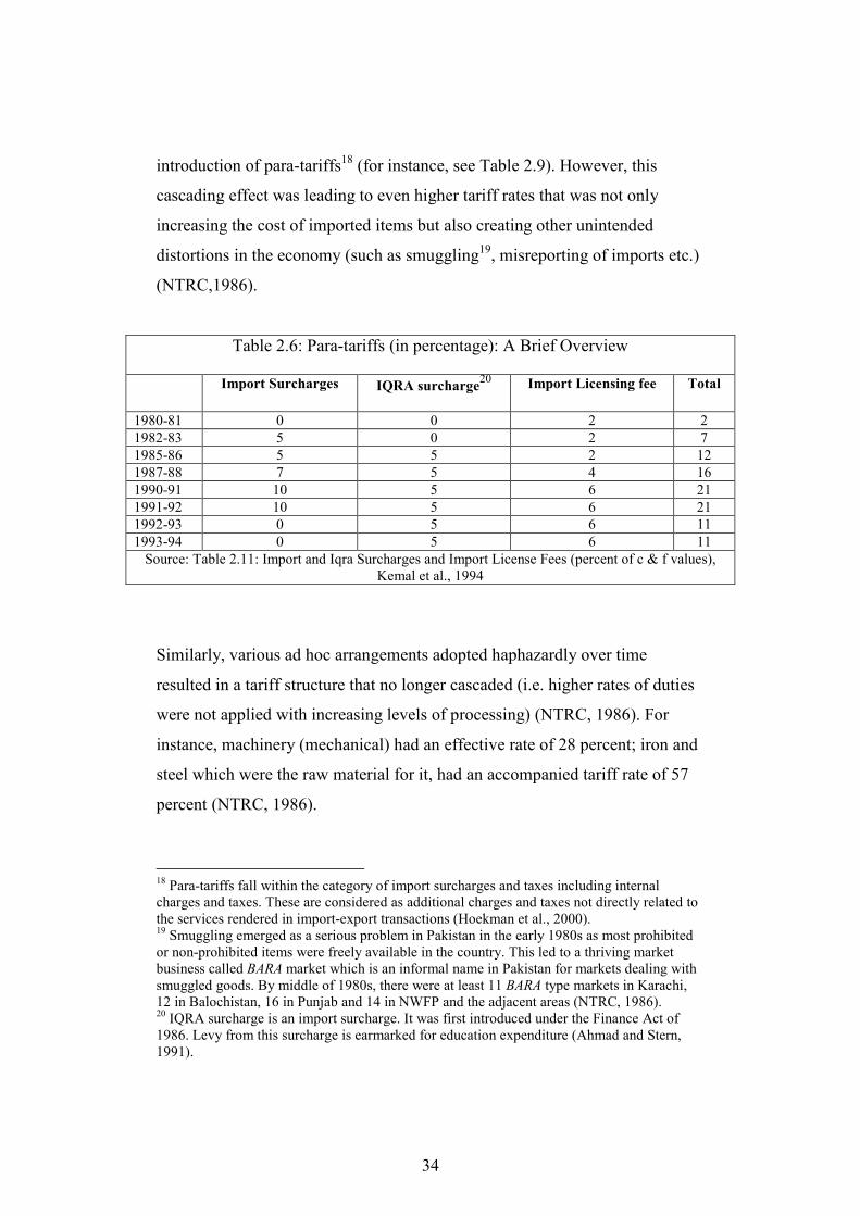
34

introduction of para-tariffs18 (for instance, see Table 2.9). However, this

cascading effect was leading to even higher tariff rates that was not only

increasing the cost of imported items but also creating other unintended

distortions in the economy (such as smuggling19, misreporting of imports etc.)

(NTRC,1986).

Table 2.6: Para-tariffs (in percentage): A Brief Overview

Import Surcharges IQRA surcharge20

Import Licensing fee

Total

1980-81 0 0 2 2

1982-83 5 0 2 7

1985-86 5 5 2 12

1987-88 7 5 4 16

1990-91 10 5 6 21

1991-92 10 5 6 21

1992-93 0 5 6 11

1993-94 0 5 6 11

Source: Table 2.11: Import and Iqra Surcharges and Import License Fees (percent of c & f values), Kemal et al., 1994

Similarly, various ad hoc arrangements adopted haphazardly over time

resulted in a tariff structure that no longer cascaded (i.e. higher rates of duties

were not applied with increasing levels of processing) (NTRC, 1986). For

instance, machinery (mechanical) had an effective rate of 28 percent; iron and

steel which were the raw material for it, had an accompanied tariff rate of 57

percent (NTRC, 1986).

18 Para-tariffs fall within the category of import surcharges and taxes including internal charges and taxes. These are considered as additional charges and taxes not directly related to the services rendered in import-export transactions (Hoekman et al., 2000). 19 Smuggling emerged as a serious problem in Pakistan in the early 1980s as most prohibited or non-prohibited items were freely available in the country. This led to a thriving market business called BARA market which is an informal name in Pakistan for markets dealing with smuggled goods. By middle of 1980s, there were at least 11 BARA type markets in Karachi, 12 in Balochistan, 16 in Punjab and 14 in NWFP and the adjacent areas (NTRC, 1986). 20 IQRA surcharge is an import surcharge. It was first introduced under the Finance Act of 1986. Levy from this surcharge is earmarked for education expenditure (Ahmad and Stern, 1991).

35

Thus, NTRC (1986) considered it an opportune time to “redefine” the tax

policy objectives in the area of trade taxes and underlined a comprehensive

reform strategy 21 mainly focused on the rationalization of the existing

structure. Some of the salient recommendations of the Commission are given

below:

• Removal of all exemptions (except charitable exemptions).

• Reduction in the rates of duty.

• A shift should be made from specific to Ad Valorem duty rates

particularly for those items that are not prone to smuggling and under-

reporting.

• Tariff structure must be cascaded.

• All imports and importers must be treated similarly.

• Duty slabs over time must be reduced to 5 applicable slabs (10, 20, 40,

80 and 100 percent) with basic rate not exceeding; 20 percent for duty

on plant, machinery, basic raw materials for capital and consumer

goods; 40 percent for consumer goods; 100 percent for luxury

consumer goods; and 40-80 percent for consumer durable items.

• Custom duty surcharge must be abolished and maybe merged into the

proposed tariff structure.

However, while trying to achieve these objectives, the process of tariff

rationalization was somewhat constrained by concerns over limiting the

revenue impact of tariff changes (ADB, 1999). This was due to the fact that

tariff reforms after 1990 were simultaneously undertaken with ongoing

reforms to broaden domestic taxation (GST) and income taxes. As a result

pace of trade tax reforms largely depended on how quickly these other

21 A large part of first phase of reform was of administrative nature as it dealt with custom valuation concepts, procedures and their application to Pakistan. Since administrative reforms are not the focus of this study, these are not discussed here.

36

resources could be mobilized (however, by looking at Figure 2.2 we can see

that income tax mobilization did not happen until middle of 1990s while

GST/VAT mobilization happened even later than that). As a result during

early years of 1990 tariff reforms process were mostly put on a hold.

However, some tariff rationalization steps were taken. These included: (a) the

negative list was drastically reduced to 75 items, as 724 items were removed

from the negative list from 1983-84 to 1993-94 (Kemal and Siddiqui, 2002);

(b) removal of most QR by 1993 (Kemal and Siddiqui, 2002); (c) import

licensing scheme was gradually eliminated by 1993 (World Trade

Organization, 1995); and (d) by 1992-93 the maximum rate of protection was

brought down to 80 percent. But on the other side, revenue considerations

sometimes reversed this process. For instance, during the time when tariff

rationalization was being undertaken, Paratariffs reached a historic high of 21

percent in order to mitigate loss of revenues (see for instance Table 2.9).

Thus, tariff reforms during this period made very limited or no headway on

some critical areas flagged in the NTRC (1986) reform strategy; these

included exemptions, cascading of tariff structure, smuggling etc. For

instance, the share of exempted import items within total imports between

1986 to1991 rose from 45 to 48 percent. Only one SRO relating to public

transport (the yellow cab scheme) is estimated to cost the exchequer almost

PRs. 12 billion (Pasha and Iqbal, 1994). Additionally, smuggling still

remained a massive problem due to high tariff and paratariff structure,

according to one estimate it was around PRs. 100 billion in 1992-93 (PIDE,

1993).

b. Second phase of reforms

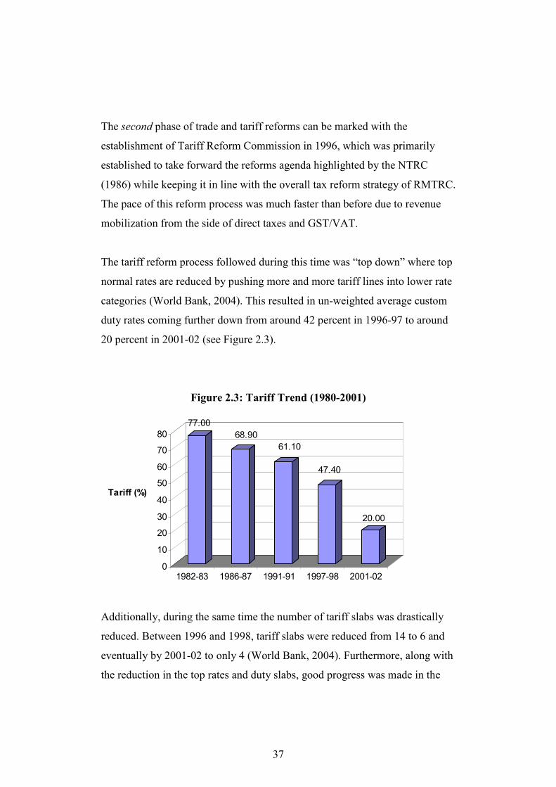
37

The second phase of trade and tariff reforms can be marked with the

establishment of Tariff Reform Commission in 1996, which was primarily

established to take forward the reforms agenda highlighted by the NTRC

(1986) while keeping it in line with the overall tax reform strategy of RMTRC.

The pace of this reform process was much faster than before due to revenue

mobilization from the side of direct taxes and GST/VAT.

The tariff reform process followed during this time was “top down” where top

normal rates are reduced by pushing more and more tariff lines into lower rate

categories (World Bank, 2004). This resulted in un-weighted average custom

duty rates coming further down from around 42 percent in 1996-97 to around

20 percent in 2001-02 (see Figure 2.3).

Figure 2.3: Tariff Trend (1980-2001)

77.00

68.90

61.10

47.40

20.00

0

10

20

30

40

50

60

70

80

Tariff (%)

1982-83 1986-87 1991-91 1997-98 2001-02

Additionally, during the same time the number of tariff slabs was drastically

reduced. Between 1996 and 1998, tariff slabs were reduced from 14 to 6 and

eventually by 2001-02 to only 4 (World Bank, 2004). Furthermore, along with

the reduction in the top rates and duty slabs, good progress was made in the

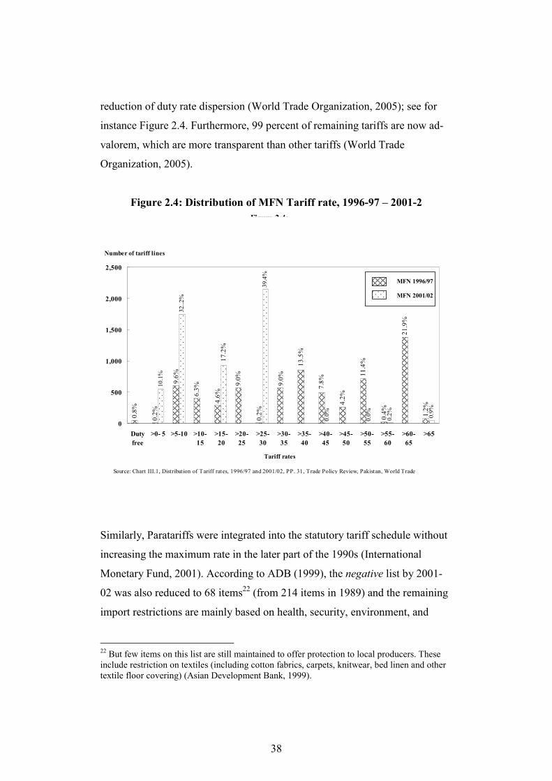
38

reduction of duty rate dispersion (World Trade Organization, 2005); see for

instance Figure 2.4. Furthermore, 99 percent of remaining tariffs are now ad-

valorem, which are more transparent than other tariffs (World Trade

Organization, 2005).

Figure 2.4: Distribution of MFN Tariff rate, 1996-97 – 2001-2

Similarly, Paratariffs were integrated into the statutory tariff schedule without

increasing the maximum rate in the later part of the 1990s (International

Monetary Fund, 2001). According to ADB (1999), the negative list by 2001-

02 was also reduced to 68 items22 (from 214 items in 1989) and the remaining

import restrictions are mainly based on health, security, environment, and

22 But few items on this list are still maintained to offer protection to local producers. These include restriction on textiles (including cotton fabrics, carpets, knitwear, bed linen and other textile floor covering) (Asian Development Bank, 1999).

7.8

%

9.0

%

4.6

%6.3

%

9.6

%

0.8

%

0.2

%

0.2

%

9.0

%

13

.5%

4.2

%

11

.4%

0.4

%

21

.9%

1.2

%

17

.2%

32

..2

%

10

.1%

39

.4%

0.0

%

0.0

%

0.2

%

0.9

%0

500

1,000

1,500

2,000

2,500

Duty

free

>0- 5 >5-10 >10-

15

>15-

20

>20-

25

>25-

30

>30-

35

>35-

40

>40-

45

>45-

50

>50-

55

>55-

60

>60-

65

>65

MFN 1996/97

MFN 2001/02

Number of tariff lines

Figure 2.4:

Distribution of MFN tariff rates, 1996/97 and 2001/02

Tariff rates

Source: Chart III.1, Distribution of Tariff rates, 1996/97 and 2001/02, PP. 31, T rade Policy Review, Pakistan, World Trade

39

religious reasons23. A significant headway has been made in the reduction of

duty free imports. For instance, from 2001/02 no tariff lines are duty free and

the lowest tariff rate has been raised to 5 percent (World Trade Organization,

2005). This is a clear break from the past as prior to this change, in 1996-97, 4

percent of the tariff lines were duty free and five times more in 1996-97

(World Trade Organization, 2005).

Thus, at the end we can say that the commission envisaged the declining

importance of trade taxes within the indirect taxes because these taxes were

deemed smuggling prone, leading to misallocation of resources and causing

substantial revenue losses. As a result, substantial reform process that has

taken place is primarily aimed reducing the role of trade taxes within the

overall tax revenue of Pakistan.

2.3.2.2 Sales Tax

Sales tax in Pakistan was introduced in pre-partition time. In the Punjab

province, it was introduced in 1941 while in the province of Sindh in 1947.

Initially, it was a provincial tax in accordance with the provisions of the

Government of India Act, 1935. However, in 1951 sales tax on goods was

permanently shifted to the federal list. The Sales Tax Act of 1951 which

replaced the Sales Tax Act of 1948, introduced a single stage manufacturer tax

imposed on imports and on domestic production with a standard rate of 12.5

percent (CBR Yearbook, various years).

23 According to Asian Development Bank (1999) there are still at least 28 non-trade barriers aimed at protecting local producers.

40

During the years before the reform, the sales tax was a minor tax. For instance,

in 1986-87 sales tax was responsible for less than 10 percent of total federal

taxes or less than one percent of GDP. The reason for this lacklustre

performance was that the sales tax regime was riddled with numerous

exemptions which resulted in a very narrow tax base. For example, according

to Ahmad and Stern (1991), the number of sales tax exemptions in the mid-80s

was fairly large as it included around 300 tariff headings and 19 broad

categories of domestically produced goods. Additionally, the sales tax regime

was operated much like a surcharge on excise duties or a trade tax with a large

proportion of sales tax collection coming from the import side. According to

the International Monetary Fund (2001) this tax was highly distortionary,

difficult to administer, and unsuccessful in raising much revenue.

The motivation for Sales Tax reform, according to Commission’s (1994)

report came from:

(a) Need to maintain revenue neutrality as a result of trade and tariff reforms

(as mentioned in the earlier section).

(b) Distributional concerns

(c) VAT superiority over Sales tax

(d) Export promotion

(e) Documentation of the economy24

As according to the Commission (1994) report:

• “…furthermore, contrary to popular perceptions, a move away from

Custom Duties and Excise duties towards a General Sales Tax (GST)

24 Here it means creating more incentive to either keep activities in the formal sector or increasing benefit of bringing activities within the formal sector of the economy.

41

or a VAT can contribute to making the tax system less regressive”, (pp.

31).

• “It has been shown that a VAT imposed at low rates and with

exemptions accorded to the goods consumed by the poor – and when

combined with excise duties on luxury goods—will make the tax

system mildly progressive”, (pp. 47).

• “Tax system in Pakistan is by and large inequitable and violates the

dictates of horizontal and vertical equity…….furthermore, import

taxes and excise duties (which are mostly regressive) occupy the centre

stage in indirect taxation as opposed to sales tax (which are essentially

neutral with respect of incidence)”, (pp. 37).

• “…in this connection, one of the maxims of optimal taxation may be

kept in view – given the acceptable level of efficiency cost, taxes

imposed on income-inelastic items of expenditure produce more

revenue than those levied on income-elastic items, of course on the

understanding that the income-inelastic commodities consumed by the

poor will be exempted from tax. As for the rate structure, the reformed

tax system will, by definition, carry much lower and undifferentiated

rates than is the case now”, (pp. 42).

However, some confusion can be seen from commission reports regarding the

distributional impact of GST. For instance:

• “Introducing a consumption based VAT, its adverse effects on equity

should be offset by corrective reforms in direct and indirect taxes”,

(pp. 41).

42

• “VAT of whatever kind is primarily a revenue-raising device, and is

administratively effective only when its rate structure is by and large

simple and differentiated. The equity objective will, therefore, be

mainly achieved by raising a share of genuine direct tax”, (pp. 48).

A major change in the sales tax regime came in 1990-91, with the passage of

Sales Tax Act of 1990 by the Parliament. This led to the imposition of a

variant of Value Added Tax (VAT) known as the General Sales Tax (GST)25.

GST was initially levied at the import and manufacturing stages. The Sales

Tax Act of 1990 imposed a sales tax at the rate of 12.5 percent on imported

goods and on the value added at each stage of production, from production

through retail level and on goods manufactured or sold in Pakistan. Although

the federal government could only charge sales tax on goods26, this regime

was extended to incorporate several services. And in some case revenue from

services subject to central excise duty is collected as it were sales tax27 (State

Bank of Pakistan, 2005).

The GST regime at the start, like its predecessors (trade and tariff regime) was

riddled with exemptions28. Thus, even when between 1991-93 GST was levied

25 This included replacement of the traditional administrative structures by separate functions of audit, assessment, enforcement, arbitration and monitoring. In addition to this, domestic sales tax collection was transferred from central excise collectorates to the newly established collectorates for sales tax (Refaqat, 2003). 26 The Federal Legislative list (item no. 49 of the Fourth Schedule) of the constitution provides for levy of tax on sales and purchase of goods, but not on services. The Sales tax act, 1990 accordingly is applicable only to supply of goods. Services are, therefore, considered to be a provincial subject. In the case of eleven services (hotels; caterers; clubs, agents; radio and televisions advertisement; custom agents; ship chandlers; stevedores; courier services; beauty parlours; laundries, and dry cleaners; Provincial ordinance have been promulgated authorizing the Federal Government to collect tax on services as if under the Sales tax Act, 1990 (State Bank of Pakistan, 2005). 27 These include telephone/telegraph/telex/fax; advertisement on TV; travel by air/train; shipping agents. 28 The GST revenues in the early years of reform also did not increase because of a system of geographical (i.e. granted on the basis of promotion of selective industries) and developmental exemptions (i.e. granted to the backward areas of the country). Geographical exemptions included areas such as Special Industrialized Zones (SIZ) encompassing areas such as Gadoon

43

on 59 additional industries the revenue impact of this inclusion and also of

shifting to the GST regime (for the first three years) was almost negligible

(Pasha, 1995). The main reason for this was that, at the same time, the

government exempted 120 additional locally produced goods, including

agriculture products, raw products, semi-manufactured goods, petroleum,

electricity, pharmaceuticals, fertilizers, motor vehicles, toys, etc. (International

Monetary Fund, 2001). A significant step in the right direction was made in

the budget of 1994-95 when the government eliminated 266 exemptions.

Further broadening occurred when in August 1999 GST was extended to

lucrative sectors such as petroleum products, natural gas, and electricity

(International Monetary Fund, 2001).

It must be added that the initial years GST expansion into the retail sector met

with fierce resistance (International Monetary Fund, 2001). According to

International Monetary Fund (2001) during the initial years GST was

deliberately kept restricted to the manufacturing and import stage for

administrative and collection ease. Although its extension to the retail sector

was being contemplated by the middle of the 1990s in order to bring the GST

in line with the true essence of VAT, the government opted to introduce small

changes at a time29. In 1996-97, the government announced that the retail

sector will be brought into the GST net but this announcement was met by

fierce tax payer resistance. As a result, the government imposed a turnover tax

and Amazai, and a large part of (province) NWFP and (province) Balochistan. Most of these geographical exemptions persisted until the middle of 1990’s but automatically expired by the end of the decade of 1990s. But exemptions granted to backward areas such as Provincial and Federal Administered Tribal Areas as well as Northern Areas still exist. Thus, the impact of gradual elimination of standard, geographical and developmental exemptions along with broad basing has been felt within the GST regime over time as GST revenues in the later part of the 1990s increased sharply. For example, sales tax as a percent of total federal taxes was around 15 percent in (1990-91). This steadily increased to 19 percent by (1995-96). The real jump came in (1998-99) when sales tax revenue as a percent of total federal taxes increased to 23 percent. 29 For instance, GST broadening in (1994-95) was not without its consequences as inclusion of 266 additional items within GST net met with strikes by the business community. This forced the government to temporarily suspend GST collection from additional items (Ahmed, 1997)

44

of three percent on the retail sector instead. Unyielding tax payer resistance

and implementation problems forced the government to replace this turnover

tax in April 1998, with a system of fixed fees, called enrolment certificates,

which were to be monitored by the retail association themselves. However,

this move was not effective from a revenue point of view: the government

abandoned this scheme and again took up the issue of extending GST on the

retail sector. The second time around ( July 1998), the government legally

imposed GST on the retail sector, but as a result of massive and expected

nationwide strikes, postponed enforcement till May 2000. In May 2000

retailers were granted an option to pay a two percent turnover tax in lieu of

GST up to (end) June 2001 and this time the government stood its ground.

There is no question that Pakistan has carried successful General Sales Tax

reform in the past decade or so as at the end of reform process in 2001-02

revenues from GST as a percentage of federal taxes stood at 41 percent

compared to 15 percent at the start of the reform process. Thus, as far as the

issue of maintaining revenue neutrality (due to trade taxes reform) is

concerned, the sales tax reform filled this gap.

But perhaps a more relevant question here is whether these reforms were

implemented in keeping with the RMTRC reform agenda or resulted in

something quite different. There is no question that something close to the

spirit of VAT was envisaged by RMTRC; a tax that was broad based but fair

and where fairness issues was explicitly dealt by exempting those goods that

are predominantly consumed by the poor and by maintaining a low tax rate.

These questions can not be answered alone by reviewing the policy documents

or the overall revenue patterns. Thus, one chapter of this study will try to

answer all these questions related to GST: (a) Distributional affect of GST in

post and pre-reform time; (b) What is being consumed by the poor in Pakistan;

45

and (c) How well placed are GST exemptions? And are these really benefiting

the poor?

2.3.2.3 Excise Duties

Excise duties have historically been the second largest source of revenue for

Pakistan after custom duties. In 1985-86, excise revenue was equivalent to 2.5

percent of GDP and before the start of the reform process excises were

yielding around 2.2 percent of GDP (see for example Figure 2.2). Excises

have always been levied on only a limited number of goods and as a result

revenue pattern has been highly skewed (Iqbal and Pasha, 1994).

According to the RMTRC (1994) report, excise tax reforms attempted to

broaden the base30 and in some cases increase the tax rates31 32. The reform

agenda has attempted to introduce capacity taxation in key industries. This

was done via formulation of a special Capacity Taxation Committee (CTC).

The move to capacity taxation was expected to stimulate production activities

in industries33 and to reduce corruption and harassment of tax payers at the

hands of tax officials (RMTRC, 1994). However, CTC committee found it

extremely hard to arrive at a consistent formula for fixing the tax base for

individual units in various industries (Iqbal and Pasha, 1994). As a result, this

measure was only carried out in the cement industry due to relative

30 Excise duties broad-basing over the years has led to targeting of service utilities (telephone), bank advances, unprocessed fiber, sugar and petroleum (RMTRC, 1994; International Monetary Fund, 2004). 31 In 1991-92, specific rate was increased on bank cheques while ad valorem rates were raised on hotels and television adds (RMTRC, 1994). 32 Excise duty rate of 25 percent was levied on telephone bills for this first time in the Finance Act of 1991. In 1992, this rate was increased to 60 percent which led to massive loss of revenue from this head due to leakage as a result of such high rates. Thus, in 1993 rates were again brought down to 35 percent. 33 As the marginal tax rate in this system with respect to output is zero.

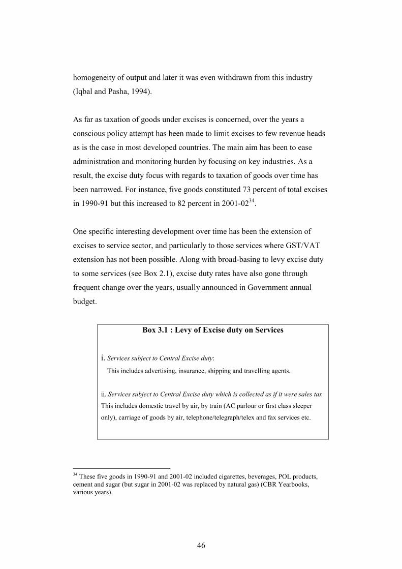
46

homogeneity of output and later it was even withdrawn from this industry

(Iqbal and Pasha, 1994).

As far as taxation of goods under excises is concerned, over the years a

conscious policy attempt has been made to limit excises to few revenue heads

as is the case in most developed countries. The main aim has been to ease

administration and monitoring burden by focusing on key industries. As a

result, the excise duty focus with regards to taxation of goods over time has

been narrowed. For instance, five goods constituted 73 percent of total excises

in 1990-91 but this increased to 82 percent in 2001-0234.

One specific interesting development over time has been the extension of

excises to service sector, and particularly to those services where GST/VAT

extension has not been possible. Along with broad-basing to levy excise duty

to some services (see Box 2.1), excise duty rates have also gone through

frequent change over the years, usually announced in Government annual

budget.

Box 3.1 : Levy of Excise duty on Services

i. Services subject to Central Excise duty:

This includes advertising, insurance, shipping and travelling agents.

ii. Services subject to Central Excise duty which is collected as if it were sales tax

This includes domestic travel by air, by train (AC parlour or first class sleeper

only), carriage of goods by air, telephone/telegraph/telex and fax services etc.

34 These five goods in 1990-91 and 2001-02 included cigarettes, beverages, POL products, cement and sugar (but sugar in 2001-02 was replaced by natural gas) (CBR Yearbooks, various years).

47

It would not be wrong to say that the role of central excise duty (CED) under

the current taxation structure of Pakistan is envisaged to be one that aids sales

tax extension to service sector (which is not directly possible without

constitutional amendment). A conscious policy effort over time has been made

to restrict excise duties to few selected items in order to ease administrative

burden. These policies have led to a sharp decline in the collection of excise

duties over time from around 2.2 percent of GDP prior to reform process to

only 1.7 percent of GDP at the end of reform process.

2.4 Conclusion

The main aim of this chapter has been to provide a summary of what has

happened to the federal taxation structure of Pakistan due to the tax reform of

the 1990s and also to point out various factors that initiated and helped the

reform process stay its course along with providing an overview of reform

agenda particularly with regards to equity and distributional concerns.

Although, Pakistan’s tax system has undergone profound changes during the

decade of the nineties, despite these changes tax revenue in relation to GDP

has remained fairly stagnant. For instance, federal tax revenue as percentage

of GDP in 1990-91 (i.e. also the start of first generation of tax reform process)

was 12.6 percent and by the end of the reform process in 2001-02, the ratio

remained almost unchanged.

The type of tax reform followed in Pakistan largely followed from trade

liberalization and focused on replacing dependence on trade tax revenues with

domestic taxation such as GST/VAT. It would not be wrong to say that the

government was able to successfully reduce and replace revenues from trade

48

taxes with GST/VAT revenues, but this led to several problems. First, the pace

of these reforms led to inherent sequencing problem, as trade and tariff

reforms were carried out at a faster pace compared to GST reforms. The

resultant gap was haphazardly filled by (a) increasing reliance on the WHT

regime of direct taxes35 and (b) by a uniform expansion of GST on all goods

without undertaking any careful analysis of extension in some cases (such as

sugar, edible oils, kerosene oil etc.) met with the Commission’s intention of

introducing an equitable and just reform process. Thus, perhaps Pakistan’s tax

reform experience highlights the fact that issues related to equity did occupy a

central place in the stated reform strategy but this concern could not be

translated into specific actions/measures when policy was actually being

implemented. Furthermore, it is also highlighted that as far as direct taxes

were concerned, it appeared that government agenda largely focused on issues

that addressed short-term revenue needs while more fundamental, structural

and perhaps painful reforms were largely put off.

Although discussion in this chapter has tried to highlight (where possible)

where tax reform steps or the resultant changes may not be in line with the

equity and fairness vision of the tax reform Commission, most of these

questions cannot be answered only by reviewing the official documents or the

overall revenue patterns. Although discussion in this chapter has helped set out

the overall picture, yet a detailed and careful empirical analysis is required to

answer these questions, which this study intends to do. Moreover, since a

similar type of reform process was also followed in many other developing

countries, this study should be considered as a case study of the type of

reforms carried out in several developing countries.

35 According to the Independent Evaluation Office (2002) “while the reduction of tariffs and other taxes on international trade was relatively fast, it took much longer for the GST instituted in 1990 to yield a comparable revenue” (pp.125).

49

The next chapter will provide an overview of approaches and models that have

been used to carry out tax incidence analysis particularly in the context of

developing countries. And it will also try to establish the best possible

approach that can be used given the question in hand and data availability for

Pakistan.

50

CHAPTER III: Literature Review

3 Introduction

One of the essential goals of government policy is to address inequalities in

the distribution of income and to make an attempt to improve the welfare of

the poor. Thus, an important part of theory and practice of public finance is

dedicated to better understanding and measuring of how revenue and

expenditure side of Government policy affects the distribution of income and

welfare of households (Martinez-Vazquez, 2007). This is the area of tax

incidence, which deals with impact of taxes on the distribution of welfare

within a society, of critical importance within the field of public economics.

It has to be accepted from the start that the analysis of tax incidence is far from

simple. The diversity and the richness of the problem comes from the fact that

although tax incidence appears to be a deceptively simple question, as soon as

we realize that the person who is legally obligated to pay the taxes may not be

the one who ultimately ends up bearing the burden of the tax complexity

arises. Because this means in order to ascertain the correct tax incidence we

need to know how private markets respond to taxes but this knowledge

requires a vast amount of information on consumers preferences, technology,

etc. which is not available (Martinez-Vazquez, 2007).

As a result, every tax incidence study varies in complexity depending on what

is being asked and the set of assumptions used to drive out the key element of

that study (Martinez-Vazquez, 2007). Even where there is similarity between

studies in terms of country being assessed the answers tend to vary a great deal

because of the time at which such analysis was undertaken, data used, tax

51

instruments covered etc. Hence, it can be admitted that generally no two tax

incidence studies are the same and this makes the job of inferring a conclusive

theme from such studies in this chapter quite difficult.

The purpose of this chapter is to provide a brief overview of methodological

view of approaches/measures/other issues related to tax incidence analysis at

household level in developing countries. The first section will discuss the

partial equilibrium tax incidence approach, its limitations and how some of the

fundamental concerns with this approach have been addressed by researchers.

The second section of this chapter will try to summarize the evidence from tax

incidence studies. The third and fourth sections of this chapter will attempt to

highlight how tax incidence analysis has tried to inform policy concerned with

normative issue of how social welfare should be maximised. The last section

concludes.

52

3.1 SECTION I: Partial Equilibrium Tax Incidence Analysis

The purpose of this section is to highlight that the choice of the tax incidence

approach used for analysis fundamentally depends on the question being

asked. If the question is distributional analysis, partial equilibrium tax

incidence analysis is adequate. However, this does not mean such is free from

limitations. Thus, the aim of this section is to show relative difficulty of

estimating partial equilibrium tax incidence analysis and to show how these

difficulties have been mitigated (in the light of literature survey) by

researchers in order to get around some of the fundamental problem of

difficulties attached to this approach.

3.1.1 Tax Incidence approach but which one?

The broad methodology used in the tax incidence analysis can generally be

divided into three basic approaches; first, partial-equilibrium or micro-data

based incidence analysis (such as Pechman and Okner, 1974; Musgrave, Case

and Leonard, 1974), static computable general equilibrium (CGE) models36

(such as Harberger, 1962; Shoven and Whalley, 1984) and quite recently

dynamic computable general equilibrium models following either the

overlapping generation life cycle approach or the neoclassical growth model

(such as Kotlikoff and Summers, 1987; Kotlikoff, 2001).

36 For examples of tax incidence studies using CGE modelling for developing countries see for instance, Deverajan and Hossein, (1998) and Hossein, (1995) for Bangladesh; Shah and Whalley, (1991) for Pakistan; Dahl and Mitra, (1991) for Bangladesh, China and India; Coady and Harris, (2004) for Mexico; to name but a few.

53

It should not be surprising to know that most frequently used approach for tax

incidence analysis for developing countries is partial equilibrium incidence

analysis. This approach examines the incidence of tax within the context of a

single market and assumes tax imposed in one market does not affect other

markets in terms of either price changes, factor shares or income (Alleyne,

2007). Since tax shifting within one market depends on elasticities of demand

and supply, this issue in partial equilibrium tax incidence models is addressed

by assuming constant returns to scale; as a result, production in these models

is pushed into the background. Thus, these models assume producer prices are

fixed; which in this context means that increase in taxes correspond to an

equal increase in consumer prices which is a fairly standard assumption also

adopted in the literature of optimal taxation (see for instance Atkinson and

Stiglitz, 1980; or Myles, 1995).

As a consequence, tax incidence in partial equilibrium models depend entirely

on assumption of how consumers will react to the imposition of a tax;

something which in the context of a perfectly competitive market is dealt by

assuming different tax shifting assumptions for various types of tax.

There is no hard and fast rule to say whether partial equilibrium or a general

equilibrium tax incidence approach would be preferable. The superiority of

one approach over the other crucially depends on what is being asked.

Partial equilibrium modelling of tax incidence is preferable because of its

tractability and intuition. These models also provide a unique opportunity to

disaggregate the incidence picture since they are based on rich micro-data and

this ability to disaggregate is a strength as it can provide very useful analysis

as far as welfare and equity impact of a particular tax policy or a particular

feature is concerned. However, such an approach is not free from criticism.

The most noteworthy criticism of micro-simulation tax incidence approach has

54

come from Shah and Whalley (1991) who have fundamentally criticised this

approach for not making any sort of attempt to incorporate tax and non-tax

institutional features of developing countries37 38.

On the other hand, even though institutional features can be better

accommodated in a general equilibrium type of modelling of tax incidence

(Fullerton and Metcalf, 2002) these models are also not without serious

limitations. Whalley (1984) pointed out that the results from computable

general equilibrium models (particularly within the area of public finance) to a

large extent appear to be driven by the value of elasticities and other

parameters used in the model. Thus, it is quite possible in many cases the

arbitrariness of shifting assumptions used in the partial equilibrium tax

incidence models is being replaced by the arbitrariness of both the model form

and its parameter values (Shah and Whalley, 1991). And it is also quite

possible that in cases where second round effects are not that significant, the

findings of both type of approaches are quite close (Devarajan et al, 1980).

Thus, there is no ideal or unique approach to tax incidence analysis

((Martinez-Vazquez, 2007). All approaches have their advantages and

disadvantages (Fullerton and Rogers, 1991; Devarjan et. al., 1980). However,

if the aim of the study is to measure the distributional affect of taxes, partial

equilibrium approach is sufficient (Fullerton and Metcalf, 2002; Alleyene,

2007) As a result, partial equilibrium tax incidence approach, despite its

37 According to Shah and Whalley (1991), the incidence of import duties may be progressive compared to regressive incidence commonly reported by conventional studies if it is assumed that incidence is borne by the recipient of higher incomes who are also the main beneficiaries of quotas and licences ( see for instance Table 11-10, pp.183). 38 Shah and Whalley (1991) mentioned that the presence of widespread tax evasion in many developing countries can make the assumption of full-forward shifting of direct taxes among some workers quite susceptible and the presence of large the informal sectors creates opportunities for some workers to reduce the tax burden by either fully or partially shifting to this sector.

55

shortcomings, has been quite resilient (Alleyne, 2007). This is the approach

that will be followed in this study.

3.1.2 Conventional Models of Partial Equilibrium Tax Incidence

3.1.2.1 Representative or typical household approach

This is perhaps one of the oldest approaches used for tax incidence analysis39.

This approach relies on tax burden computation relying on a relatively small

number of artificial households, and their composition, expenditure and

income sources are assumed to be representative of the entire population. It

would not be wrong to call this approach more or less a version of the

statutory or legal incidence than economic incidence. As a result, this type of

analysis has been completely abandoned40 in favour of approaches that do not

ignore individual variations (Bird and De Wulf, 1973, pp. 647).

3.1.2.2 Differential incidence approach

One possible way to determine tax incidence is by comparing the distribution

of income resulting from the presence of tax with some initial benchmark or

counterfactual (Martinez-Vazquez, 2007). In this approach the result of

income distribution due to taxes is compared with some initial benchmark

39 This approach follows from report of the Committee on National Debt and Taxation, minutes of evidence, Vol. 1, 1927 (quoted in Prest (1955), p. 244) and Shoup (1939) for developed countries. 40 Early examples include Adler and Wallich (1951) for El Salvador, Adler et al. (1952) for Guatemala, Shoup et al (1959) for Venezuela, and Wasylenko (1986) for Jamaica.

56

distribution of income such as comparison with distribution of tax burden that

would have taken place if the same amount of taxes were collected from a

proportional income tax (thus assuming that proportional income tax is the

most neutral way to collect revenue). However, this approach has not been

very popular in developing countries41 perhaps because of small role of

income taxes in the economy and because determining a true counterfactual is

a tall task (Martinez-Vazquez, 2007)42.

3.1.2.3 Numerical Tax Incidence Approach

The most frequently used approach for tax incidence analysis is the numerical

tax incidence approach. This approach is directly adopted from the seminal

work of Pechman and Okner (1974)43. The objective is to allocate tax burden

by income groups. The term numerical tax incidence refers to the procedure of

imputing tax incidence where the total amount of tax revenue collected by the

Government is allocated to the households grouped by income classes. As a

41 For application, see Sahota (1968) for Brazil, and Sjoquist and Green (1992). 42 Determining a true counterfactual will require observing an economy without taxes, which is not possible (Martinez-Vazquez, 2007). 43 The origin of large majority of work on tax incidence analysis for developing countries is Pechman and Okner, (1974). This study was based on 87,000 income tax return and 30,000 households from 1966 U.S survey of economic opportunity file. The novelty of the analysis was that the incidence analysis was carried out using eight different set of shifting assumptions. P&O, for all classes assumed that the burden of personal tax is borne by the households and the burden of sales and excise taxes falls on households according to their consumption patterns. The employee part of payroll tax remains with the worker. The property tax is analysed for cases when it affects either the return to landowners or all capital owners while for corporate taxes they assume four different scenarios; where it is shifted to shareholders, capital owners, wage earners or consumers. Total tax incidence is calculated using effective tax rate (i.e. total tax burden as a proportion of economic income) for each household. Interestingly they found US tax system to be “proportional” irrespective to whether they use the most-progressive set of assumptions or the least-progressive set of assumptions. This analysis has also come to be known as the “proportionality hypothesis” and the main conclusion that emerged from this analysis was that the U.S. tax system does not redistribute income and this conclusion sparked intensive policy debate within U.S. tax policy for many decades to come.

57

result this approach assumes no excess burden or deadweight loss44. Thus, at

the end the total burden allocated for each tax is equal to the total revenue

collected45.

Over the years although the gist of analysis is still based on micro-data, there

have been many additions and changes to this methodology to better fit such

approaches to the data availability, tax instruments and the country context,

although it must be admitted that not much has changed in terms of tax

shifting assumptions46. For instance, in many cases the recent studies using

this methodology have dropped the proportionality assumption between tax

burden and tax revenues; thus calculating tax liabilities only in cases where

actual consumption of the taxed item takes place within the households47. This

is a much better approach as it allows for both excess burden as well as tax

evasion. In some cases the tax incidence analysis has focused on calculating

effective taxes that involves the use of input-output tables for the economy.

The general idea is to trace taxes on intermediate goods through input output

table to estimate the implied tax on the final product (Rajemison and Younger,

1999)48. This allows one to take account of cascading effect of taxes which

can be important for taxes that fall heavily on the intermediate goods49.

44However, this is an acceptable approach as long as we differentiate between the equity impact (tax incidence) and efficiency impact (excess burden) (Martinez-Vazquez, 2007). 45 For application, see Ghandi (1966) for India, Bird (1970); and Mclure (1971) for Columbia, Yukon (1976) for Tanzania, Foxley (1979) for Chile, Lovejoy (1963); Bird and Miller (1989) for Jamaica, Azfar (1974); Jeetun (1978); Kazi (1984); Malik and Saqib (1985); Khalilzadeh-Shirazi et al. (2001) for Pakistan, Chen et al. (2001) for Uganda and Sonia et al. (2003) for Ethiopia. 46 Issues related to tax shifting assumption are discussed separately. 47 For application see, Engle, Galetovic and Raddatz (1998) for Chile, Refaqat (2003 ); SPDC (2004) for Pakistan, and Martinez-Vanquez (2001) for Mexico, to name a few. 48 According to Ahmed and Stern (1991), difference between nominal and effective tax rates may be quite significant. For instance, for India and Pakistan they found that even when nominal tax rates on goods primarily consumed by the poor were zero or negative (i.e. a subsidy), many of such goods had positive effective rates. 49 For application see, Heller (1981) for Korea, Ahmad and Stern (1991) for India and Pakistan, SPDC (2004) for Pakistan, Engle, Galetovic and Raddatz (1997) for Chile, Rajemison and Younger (2001) for Madagascar, and Cho et al. (2003) for Ethiopia.

58

However, this approach is not free from problems even if input-output tables

are available and readily updated. Estimation of effective tax rates requires

considerable aggregation across goods as a result reducing the accuracy of

progressivity comparison (Gemmell and Morrissey, 2003). For instance, in the

case of Madagascar, use of input-output table reduced the number of goods

examined from 222 to 30 (Rajemison and Younger, 2001), which is a serious

loss of information.

3.1.3 Tax incidence analysis: other issues

3.1.3.1 Annual or lifetime50

Perspective on Incidence?

The question of looking at the incidence from lifetime versus annual

perspective is an interesting one. Theoretically, one would expect annual and

lifetime tax incidence calculation to vary for several reasons51. For instance, it

is quite possible that the annual measure of income reflects transitory

components (such as sickness and unemployment) which are bound to have a

smaller effect on consumption than when permanent change in income is

considered. This can be credited to the permanent income hypothesis

(Friedman, 1957). Second, income measured in a single period differs from

lifetime income due to age related differences in earnings52 (Lyon and

Schwab, 1995). Third, consumption of certain items follows life cycle pattern

which is independent of changes in income (Modigliani and Brumberg, 1954).

50 lifetime income concept can be defined as present discounted value of earnings plus gifts and inheritance received. 51 For theoretical distinction between annual and lifetime incidence approach see Levhari and Sheshinski (1972) and Driffill and Rosen (1983). 52 Mincer argues that about half of the log variation of earning is attributable to transitory components and age related differences (pp. 119).

59

A very few studies have taken a more rigorous approach of trying to estimate

the lifetime earning capacity of the household and not surprisingly most of

these are on developed countries (Fullerton and Rogers 1991; 1993, Davies et

al, 1984). Perhaps surprisingly, the main result of such a carefully done work

was not much different from results reported by Pechman (1985). Perhaps

more importantly, the refinement between lifetime and annual perspective may

carry very little weight as far as developing countries are concerned as life

expectancies in these countries tend to be relatively short and the level of

poverty is stark (Bird and Zolt, 2005).

3.1.3.2 Tax shifting Assumptions

It may not be wrong to say that the role of incidence assumptions is to aid the

allocation of the tax burden between different income groups (Vazquez, 2007).

Most of the studies on tax incidence for developing and developed countries

use the 100 percent tax shifting assumption particularly where indirect taxes

incidence is concerned; although lesser consensus appears to hold where pass

through effect of direct taxes is concerned (see for instance Table 3.1). This

assumption simplifies the analysis since it allows the tax component of the

retail price of an item to be easily identified on the basis of statutory

legislation.

In a perfect competitive market under a partial equilibrium tax incidence

analysis this assumption implies taxes will always be shifted from 0 to 100

percent while the exact burden lying within this range depends on the relative

elasticities of demand and supply of an item. Things get slightly complicated

when market structure other than perfect competition is considered (Besley,

1989; Delipalla and Keen, 1992; Katz and Rosen, 1985; and Stern, 1987).

60

What has been emerging from this work is that under an imperfectly

competitive market structure, a variable degree of tax shifting possibilities

exist and even over shifting becomes a real possibility: see for instance

Lockwood, (1988) and Stern, (1987a). According to Stern (1987) “100 percent

shifting is a reasonable intermediate assumption and not a polar case that the

simple theory makes it appear”.

There are very few studies that have tried to answer the question of tax

shifting assumptions but most of those studies are limited to analysis of a few

goods. Sidhu (1971) found evidence of overshifting of sales tax; the same is

found by Besley and Rosen (1994; 1996)53. Poterba (1996) on the other hand

found evidence supporting the perfect competition assumption.

There is very limited research within this empirical area for Pakistan and

where some evidence does exist it is quite simplistic in its methodology and

often the time period covered is quite limited. Few studies for Pakistan have

focused on the effect of price shifting due to import taxes. These have

compared the c.i.f. prices of import with their corresponding wholesale price,

(Pal, 1964; Alamgir, 1968). This approach concluded that given profit margins

are so high, small changes in import duties are unlikely to be passed on to the

consumer. Radhu (1965), on the other hand, related changes in taxes (sales

and excises taxes) to changes in prices and found taxes are not shifted to

53 Sidhu (1971) analyzed relationship between CPI and sales tax rate in a sample of seven cities during (1954-66) and found evidence of over shifting for four out of five categories under consideration. Besley and Rosen (1994) examined the impact of state and local sales tax on the price of a particular item. Their study also yielded evidence of overshifting. Poterba (1996) study is an empirical analyses that examined city specific price indices for eight cities for fifty year period (1947-1977) and fourteen cities during (1925-39). He examined quarterly data on tax rates and prices and confirmed evidence of 100 percent tax shifting assumption. Besley and Rosen (1996) extended Poterba’s type of analysis using panel of quarterly data to 12 commodities and 155 cities over the period of (1982-1990). They found for half commodities tax shifting occurred almost one to one but for rest of these commodities, there was clear and robust evidence of overshifting.

61

consumers. However, subsequent studies that extended Radhu’s work report

differently. Irfan (1974) and Naqvi (1975) found evidence that taxes are

shifted to consumers and in some cases evidence of overshifting54.

Given the lack of empirical research in the area of tax shifting assumptions

even for developed countries let alone Pakistan and other developing

countries, it may be adequate to assume a full tax shifting assumption for

(indirect) taxes (Besley and Rosen, 1996) but a cautious interpretation of

results is necessary (for instance see Table 3.1 to see LDC factors that may

impact these assumptions more)55. Although incidence results can be sensitive

to the shifting assumptions, nevertheless there has been wide agreement on the

assumptions used (Vazquez, 2007). More importantly, in practice these

assumptions have been justified because the incidence results obtained from

conventional studies have come out to be quite similar to results obtained with

more realistic and laborious assumptions (Vazquez, 2007). As a result, this

study will also follow the assumption that indirect taxes are passed on fully to

the consumers.

54 The methodology used by Irfan (1974) and Naqvi (1975) is quite simplistic. They directly relate changes in prices with changes in taxes making no effort to control for other variables such as production cost etc. Irfan (1974) focused on only tobacco and petroleum products annual prices during (1953-72) and found evidence of tax shifting. Naqvi (1975) extended this work to 12 groups of commodities. She finds that in 50 percent cases taxes are shifted to consumers and in some of these cases there is over-shifting. She finds taxes on cigarettes and petroleum products resulted into one to one increase in prices while for food products, cotton fabrics and misc. products exhibited fifty percent shifting; and taxes on chemicals revealed a pattern of over shifting. 55 The use of full tax shifting assumption in the case of indirect cases goes back to work by Samuel (1919). This assumption is used not only in vast majority of incidence work related to indirect taxes in developing countries but also developed countries, for instance see Musgrave (1964) and Pechman and Okner (1974).

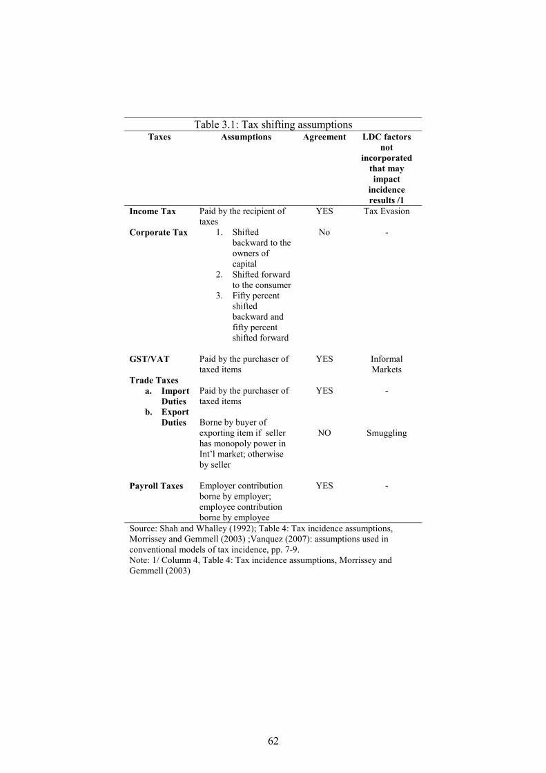
62

Table 3.1: Tax shifting assumptions Taxes Assumptions Agreement LDC factors

not

incorporated

that may

impact

incidence

results /1

Income Tax Paid by the recipient of taxes

YES Tax Evasion

Corporate Tax 1. Shifted backward to the owners of capital

2. Shifted forward to the consumer

3. Fifty percent shifted backward and fifty percent shifted forward

No -

GST/VAT Paid by the purchaser of taxed items

YES Informal Markets

Trade Taxes

a. Import Duties

b. Export Duties

Paid by the purchaser of taxed items Borne by buyer of exporting item if seller has monopoly power in Int’l market; otherwise by seller

YES

NO

-

Smuggling

Payroll Taxes Employer contribution borne by employer; employee contribution borne by employee

YES -

Source: Shah and Whalley (1992); Table 4: Tax incidence assumptions, Morrissey and Gemmell (2003) ;Vanquez (2007): assumptions used in conventional models of tax incidence, pp. 7-9. Note: 1/ Column 4, Table 4: Tax incidence assumptions, Morrissey and Gemmell (2003)

63

3.2 SECTION II: Tax Progression and Evidence56

This section summarizes the evidence of tax incidence analysis in terms of tax

progression. Whilst there may be different ways of considering insight from

tax incidence studies, it is reasonable to focus on the results that they offer in

terms of tax progression. Since there are different ways of measuring tax

progressivity, the first section starts with describing how tax progressivity has

been measured in tax incidence analysis for developing countries before

embarking on what can be learned from incidence studies.

3.2.1 What can be learned from evidence on tax progression and

distribution: some general conclusions57

It is hard to infer one common conclusion from the tax progression literature

as far as progressivity, regressivity or neutrality of overall tax system or its

components is concerned as these conclusions are often country specific

(Gemmell and Morrissey, 2003). This is perhaps one reason why tax

progression studies have received a lot of criticism from tax incidence surveys

such as Bird and De wulf (1973) and De Wulf (1975), as results appear to vary

not only across countries but also within the same country. Nevertheless, both

partial equilibrium tax incidence models of tax progression and distribution

56 For a brief discussion on measures of tax progression commonly used in tax incidence studies, please see Appendix 3.3. . 57 This section is not a survey of tax incidence studies. For surveys see Bird and De Wulf (1973), De Wulf (1975), Mclure (1977), Jimenez (1986), Shah and Whalley (1991) and more recently, Chu ke-young et al. (2000).

64

reveal some interesting general conclusions/themes and some of these are

summarized below.

The recent evidence on incidence of taxes on consumption reveals this to be

much less regressive than suggested earlier (Chu et al., 2000; Gemmell and

Morrissey, 2005). Trade liberalization motivated tax reforms, that have

replaced import taxes in most developing countries with domestic taxes such

as sales taxes, have appeared to make the underlying tax incidence a little

more progressive (Gemmell and Morrissey, 2005). Thus, recent literature has

underlined the importance of not to pre-judge the incidence, particularly of

indirect taxes on a priori belief. According to Bird and Zolt (2005), the

distributional impact of indirect taxes in any particular developing country

depends on a question of relative quantitative importance of different taxes

and underlying income distribution patterns in that society. As a result, such

matters cannot be decided on a priori grounds.

Another important aspect that has emerged from this literature is the

importance of asking the right questions which such methodology can

accommodate. One reason why findings of most of tax progression studies are

at best mixed is because most of these studies have only focused on the

progressivity, regressivity or neutrality of this or that tax (Bird and Zolt,

2005). And this is bound to run into inherent problem of identifying a

distribution of income that is considered to be acceptable to everyone in the

society. Thus, focusing on the right questions will not only make this research

more interesting but also meaningful from a policy perspective. For instance,

recently some studies have started to focus on particular issues such as how

progressivity of underlying tax system is affected by: (a) replacement of

general sales tax with excises; (b) reforms that have replaced trade revenues

with domestic taxes such as GST/VAT or ; (c) focusing on a particular change

65

in the design of indirect taxes that may be more relevant for its potential

impact on the poor (Bird and Zolt, 2005).

The last point warrants more attention. Although, it is agreed that indirect

taxes can play a very limited role in redistribution of income that does not

mean that they do not impact the lives of the poor in a limited but powerful

way (Bird and Zolt, 2005). Thus, even though the overall incidence of fiscal

policy is what really matters for redistribution, the policy makers in

developing countries need to pay close attention to even minor features of

consumption tax design and implementation as they can have important

distributive effects (Bird and Zolt, 2005).

One thing that has become evident over the years is that such features can

easily remain hidden in an aggregate analysis. Thus, detailed micro-analysis of

expenditure data with close attention to details of tax structure is necessary for

such conclusions (Bird and Zolt, 2005). Thus, even though most partial

equilibrium tax incidence literature has been based on rich micro-data, minute

policy analysis of particular features has not been explored.

For instance, excise duties, like other indirect tax components have been

analysed in terms of whether these are collectively progressive, regressive or

proportional. This focus has ended up revealing at best a mixed bag of results.

Thus, such research has been largely uninformative for policymakers who

have resorted to levying excises based on conventional wisdom i.e. taxing

luxuries or taxing those items that have explicit negative externalities attached

to their consumption. Most studies have not focused on individual excises

even though excise levies on petroleum, tobacco and alcoholic beverages for

most developing countries make up almost the entire revenue from this

heading. As a result, their individual redistributive effects can often be as large

as any single component of tax system.

66

This issue i.e. determining the incidence of individual excises due to their

possible effect on the poor has, however received much more attention in

recent literature using distribution measures such as concentration curve and

associated welfare dominance technique and some thought provoking results

for policy makers have been revealed (for instance look at Table 3.2).

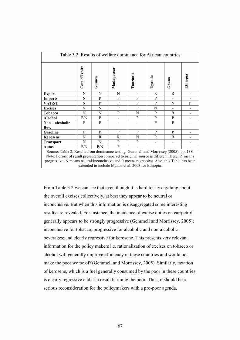
67

Table 3.2: Results of welfare dominance for African countries

Cote d’Ivoire

Guinea

Madagascar

Tanzania

Uganda

Ghana

Ethiopia

Export N N N - R R -

Imports N P P P P - -

VAT/ST N P P P P N P

Excises N N P P N - -

Tobacco N N P N P R -

Alcohol P/N P - P P P -

Non – alcoholic

Bev.

P P - - P P -

Gasoline P P P P P P -

Kerosene N R R N R R -

Transport N N P P - - -

Autos P/N P/N P - - - -

Source: Table 2: Results from dominance testing, Gemmell and Morrissey (2005), pp. 138. Note: Format of result presentation compared to original source is different. Here, P means

progressive; N means neutral/inconclusive and R means regressive. Also, this Table has been extended to include Munoz et al. 2003 for Ethiopia.

From Table 3.2 we can see that even though it is hard to say anything about

the overall excises collectively, at best they appear to be neutral or

inconclusive. But when this information is disaggregated some interesting

results are revealed. For instance, the incidence of excise duties on car/petrol

generally appears to be strongly progressive (Gemmell and Morrissey, 2005);

inconclusive for tobacco, progressive for alcoholic and non-alcoholic

beverages; and clearly regressive for kerosene. This presents very relevant

information for the policy makers i.e. rationalization of excises on tobacco or

alcohol will generally improve efficiency in these countries and would not

make the poor worse off (Gemmell and Morrissey, 2005). Similarly, taxation

of kerosene, which is a fuel generally consumed by the poor in these countries

is clearly regressive and as a result harming the poor. Thus, it should be a

serious reconsideration for the policymakers with a pro-poor agenda,

68

particularly when it is possible to exempt this tax to help the poor without

encouraging inefficient substitution between fuel types (Gemmell and

Morrissey, 2005).

However, despite the voluminous nature of research in the area of tax

progression, very few tax progression studies have focused on the

distributional impact of individual excises in developing countries. Issues of

tobacco taxation and alcohol taxation have received very little attention.

Exceptions include McLure (1977a), who found the tobacco tax in Jamaica to

be far the most regressive indirect tax. This is also supported by Cnossen

(1977) who found tobacco tax to be the most regressive tax in a number of

countries. In some cases these excises have appeared to be progressive but

progressivity was mainly due to higher tax on imported cigarettes (DeWulf,

1974 for Lebanon and Asher and Booth, 1983 for Philippines and India and

Indonesia). High taxation of alcohol has been supported on social grounds in

some countries. For instance Bird (1983) and Bird and Wallace (2005) note

that higher taxation of alcohol in some cases may not be regressive. But

research in this area is not sufficient and further research in the selective role

of excises based on detailed micro data is necessary in order to formulate and

guide tax policy analysis in this area in developing countries (Bird and Zolt,

2005).

Recent literature on the incidence of GST/VAT appears to indicate that VAT

in some countries may be more progressive than trade taxes and excise duties

and in some cases it may be as progressive as income tax (Shah and Whalley,

1991). This is despite the fact that tax incidence studies using distributional

measures have generally put VAT on low progressivity ranking compared to

other taxes (Gemmell and Morrissey, 2005), but generally these are not found

to be regressive (see Table 3.2). Evidence on this coming from tax progression

studies is mixed; for instance GST/VAT neutrality is reported for Ghana

69

(Younger, 1996) and Pakistan (Refaqat, 2003) and regressivity of VAT is

reported for Korea (Heller, 1981) and Pakistan (SPDC, 2004).

Very few studies have explored the explicit issue of replacing GST with VAT

(which is a very relevant tax reform issue as many developing countries are

undergoing this transition). This issue is explored for Ethiopia (Munoz et al.,

2003), and Uganda (Chen et al., 2001). Findings so far are mixed since results

for Uganda shows that although the effective tax after reform is higher,

perhaps due to better coverage, post- reform tax system appears to be neutral.

Only results for Ethiopia indicate this reform process having an adverse

impact on the bottom forty percent of the population. Few studies have also

indicated that GST/VAT neutrality or slight progressivity conclusion is likely

to emerge when expenditure is used as a base rather than annual income. But

on the other hand, this study reveals an interesting point that disaggregated

incidence picture is not that sensitive to change in base. Thus, a disaggregated

conclusion regarding particular policy features is important (Refaqat, 2003).

Due to the emerging prominent position of GST/VAT revenues in many

developing countries, many issues related to this type of taxation have

received more attention. For instance, the issue of GST/VAT taxation at a

uniform or differentiated rate is an important issue and has received some

attention. Ahmad and Stern (1983) noted for India that a shift to a uniform

taxation would reduce the expenditures of the poorest segment of rural and

urban households by almost 7 and 5 percent due to increase in the prices of

many essential items. Similarly, Bird and Miller (1986) using basic micro data

for Jamaica show that if the current highly differentiated tax system is

replaced by a uniform General Consumption tax (GCT), it would increase

taxes on all income groups and also increase the regressivity of the indirect tax

system.

70

Interestingly, recent research has also pointed out several reasons why

conventional incidence studies may be overestimating the burden of

GST/VAT. For instance, Fedeli (1998) pointed out that VAT may make the

tax system less allocatively distorted as it reduces the pressure on market-

based activities to move into the informal sector. Gemmell and Morrissey

(2005) have pointed out that VAT may be beneficial for the poor as it

improves upon serious price distortions as a result of ad hoc array of excises.

However, more research is required to quantify these issues but they do put an

interesting contrast to the traditional “regressive” label pre-assigned to these

taxes.

Some studies on GST/VAT incidence have gone beyond the question of

progression, regression or neutrality. For instance, some research has focused

on the possibility of differential taxation58 under GST/VAT due to very

substantial differences in consumption patterns between income groups in

developing countries (Bird and Zolt, 2005). Although this issue has not

received much attention in most conventional progression and distributional

studies in developing countries, this is a very important issue particularly in

the context of the poor. For instance, in most developing countries it is a

common practice to exempt unprocessed food items from the GST/VAT net.

This practice is based on the age old a-priori belief that only un-processed

food items consumption is important for the poor. But recent research has

challenged this policy stance particularly in some developing countries where

GST/VAT has been extended to unprocessed food items. For instance,

disaggregated results for Pakistan, India and Jamaica have revealed GST/VAT

taxation of sugar has very important implication for the poor (Ahmad, Leung,

and Stern, 1984 for India and Pakistan; Bird and Miller, 1986 for Jamaica). In

fact results from the Bird and Miller (1986) study show that that exemption of

58 Differential taxation in the case of GST/VAT may not necessarily mean thinking about different standard rates for GST/VAT but may also mean thinking about commodities that should face standard VAT rate and those that should be exempted.

71

few processed food items can eliminate almost all of the regressivity of GCT.

They also found that GST on sugar appeared to be the most regressive tax

within all taxes.

Thus, it is no surprise to find that these issues have recently received more

attention in the context of GST/VAT exemptions and in some recent studies

this issue has been explicitly addressed using the “distributional

characteristics” measure59 of each good. This measure estimates how heavily

consumption of a particular item is concentrated on the poor (Sahn and

Younger, 2003). In this approach the welfare effect of a price change is given

by the weighted sum of each household’s consumption of the taxed item(s),

where the weights reflect the social marginal value of consumption by each

household with higher weights given to the poor households (Sahn and

Younger, 2003). This has revealed some very strong tax policy results from

micro-data analysis that are very significant for tax policy reforms of

GST/VAT in developing countries. For instance, in the case of Papua New

Guinea, Gibson (1998) noted that exemptions of rice and tinned fish from

GST is desirable on both “merit good” criterion as well as from poverty

alleviation objectives. Also, Alderman et al. (1999), found that GST

exemption of beans, sugar and kerosene in South Africa is desired from equity

point of view. This type of research has raised a question regarding carrying

out GST/VAT exemptions under “a-priori” belief particularly as far as

Government’s pro-poor policy agenda is concerned.

Tax progression evidence on trade taxes has largely focused on import taxes.

Most tax progression literature finds custom duties as slightly regressive

(Jeetun, 1978; SPDC, 2004 for Pakistan; Heller, 1981 for Korea to name a

few, but since import tax incidence estimation from survey data is not straight

59 For application see Gibson (1998) for Papua New Guinea, and Alderman and del Ninno (1999) for South Africa59 and Sonia et al. (2003) for Ethiopia

72

forward, tax progression studies have been cautious about these findings). The

literature using distribution measures has given attention to both import and

export taxes (primarily due to importance of latter type of tax in Africa) and

overall results for this study find import duties to be progressive (see Table

3.2) which is contrast to evidence from tax progression studies. Incidence of

overall export taxes appears to be neutral/ inconclusive or regressive (see

Table 3.2). However, where regressivity is reported this is due to one specific

item (for instance, cocoa export tax for Ghana and coffee tax in Uganda).

Another important point highlighted in recent research is the definition of the

“poor” used in most of these studies. This is an important point since it

involves understanding the extent and nature of variation among those

classified as the “poor” (Bird and Zolt, 2005) as these differences can be very

important for policy decision as far as the poor are concerned. However, this

issue has received considerably less attention due to lack of availability of

surveys that explicitly focus on the poor. However, there are some notable

exceptions. For instance, Adler, et al., (1952) reports considerable variation in

families between the same income classes in Guatemala. They find that heavy

drinkers and smokers probably paid 3 percent of their income in taxes

compared to 1 percent for moderate consumers and 0 percent for abstainers.

Bird and Miller (1989) used micro-data from a special survey in Jamaica on

the poor. They report that effect of taxation may vary more due to

characteristics of the poor households then to income or expenditure. Perhaps

more importantly, the gain in vertical equity may offset increased horizontal

inequities if such issues are not analysed carefully. Thus, a more detailed focus

on the characteristics of the poor is essential in order to rightly estimate the

effect of indirect taxes on the poor as well.

73

In summarizing, this evidence has revealed that generalization regarding

progressivity, regressivity or neutrality of this or that tax is not helpful (Bird

and Zolt, 2005). If research in this area is to be more revealing and interesting

from policy perspective, the right questions need to be asked. Even though

indirect taxes may have a very little redistribution role, such impact can be

very powerful as far as the poor are concerned. Thus, detailed micro-data

analysis along with information on tax structure is required to fine tune

particular policy features that may be very important for the poor (such as

taxes on kerosene, basic fuels, sugar, tobacco, cocoa etc.). Thus, even though

the incidence of any single tax is less important than the incidence of the fiscal

system as a whole, nonetheless there is good reason for those concerned with

distributive issue to pay close attention to the details of indirect tax design and

administration (Bird, 1987).

3.2.2 Pakistan Tax Incidence Studies

Most of the literature on incidence of taxation in Pakistan has focused on tax

progression of overall tax system. Results and overall findings of these studies

are summarized in Appendix Table 3.1 and 3.2.

One of the earliest studies of tax incidence for Pakistan is Jeetun (1978)60.

This study was done following the Pechman and Okner (P&O) (1974)

methodology and almost following the same set of assumptions for allocation

of taxes. Jeetun’s (1978) results showed that total tax incidence and total

indirect tax burden exhibited either slight progressivity or a U-curve pattern

(i.e. implying redistribution taking place from the very poor and the rich

60 One of the earliest study for Pakistan tax incidence is by Jawaid Afzar “Theory and Practice of Tax Incidence in

Pakistan” (1974) is a PhD dissertation but was not available to us.

74

classes towards the middle income classes). He also found urban classes

bearing a higher proportion of tax incidence than rural classes. The novelty of

this study was that it was one of the first studies that covered the issue of tax

incidence in Pakistan and also provided detailed disaggregated results based

on incidence of components of tax system.

Kazi (1984) aimed at analysing inter-sectoral tax burden for Pakistan. For this

reason, although the analysis is similar to conventional P&O type of

methodology, the expenditure and taxes allocation takes place on the basis of

sectoral expenditure shares and sectoral population. Their results showed over-

taxation of agriculture when compared with the relative capacity of taxation in

each sector. They also found that rich farmers in agriculture sector are under-

taxed.

Malik and Saqib (1989), also employ P&O (1974) type of methodology to

allocate the tax burden. However, tax burden allocation is further refined to

take account of cascading effect of taxes by using the input output tables for

(1975-76). They also explicitly address the question of redistribution of

income due to taxes using the Suite index. Although they report the entire tax

system to be regressive (pp.18), the results at best appear to be U-shaped

particularly at national level.

Shirazi et al., (2001) is perhaps the only study that attempts to ascertain the

fiscal incidence for Pakistan. They also use P&O methodology to allocate tax

burdens and expenditure benefits. The shortcoming of this analysis is the

arbitrary way the expenditure and tax burden is distributed across the

population. As a result the findings for the poorest cohort look particularly

dubious.

75

Kemal (2001) reports the tax incidence results for the overall tax system for 13

years (1987-88 to 1999-00). However, this analysis can be only indicative

because this study explicitly says nothing about the data, methodology and

assumptions used in this tax incidence study.

The novelty of Refaqat’s (2003) VAT analysis is that although it uses the

conventional methodology it drops the assumption of proportionality between

tax burden and tax revenues. This study shows that GST/VAT appears to be

slightly regressive when income is used as a base but this regressivity

disappears when expenditure is used as incidence base. The other important

aspect of this study is that it provides a comprehensive breakdown of VAT

incidence on main commodities including important items such as cooking

oils, kerosene oils, electricity etc. It appears that disaggregated findings are not

particularly sensitive to the choice of base. It appears tobacco tax, kerosene

oil, gas-pipe and electricity consumption taxation under GST are highly

regressive.

SPDC (2004) is another comprehensive look at federal taxation in Pakistan.

This study also uses the conventional incidence approach but like Refaqat

(2003) drops the proportionality assumption. This study finds all components

of indirect tax system along with the overall tax system clearly regressive. The

study finds if fertilizers and pesticides are exempted from GST net, it will

make GST incidence slightly progressive. The novelty of the study is to

attempt to measure effective taxation; however, this study uses 1989-90 input-

output tables for Pakistan and provides no information on how these tables

were updated for 2001-02, which makes this study quite susceptible.

Thus, it will not be wrong to say that most of the research in Pakistan has

remained preoccupied with the tax progression issue and as a result most of

the issues highlighted in the earlier section have very little attention in

76

Pakistan. And this gives current study an opportunity to undertake some of the

issues mentioned earlier.

77

3.3 SECTION III: Normative Analysis 61

In the previous sections we talked about partial equilibrium approach and

compared results of studies on tax incidence in developing countries on the

basis of tax progression. The focus on this section and following section is

how tax incidence studies might inform policy concerned with the normative62

question of how social welfare is to be maximised. However, much of the

normative tax incidence literature encompassing the theory of optimal taxation

and the theory of marginal tax reform (MTR) (discussed in next section) is

sensitive to the underlying assumptions regarding tax incidence (such as cross

price elasticities assumption, Ramsey rule etc.). Some of these assumptions

may or may not be true. This further highlights the importance of partial

equilibrium tax incidence analysis discussed in the first two sections.

However, the current and the following section discuss some general lessons

emerging from this literature that may be very useful for policymakers in

developing countries along with there limitations.

3.3.1 Optimal Taxation

61 Since the focus of current study is not normative analysis of taxation we do not claim to review studies in this area. Our intuition behind this section is to draw upon some reliable tax policy recommendations rather than to focus on individual studies. For a comprehensive review of normative studies, see the seminal collection in Newbery and Stern (1988). 62 According to Gemmell, (1987) normative analysis raises the question of which taxes should

be preferred. In addition to the knowledge of how taxes affect the economy and income distribution, they also require knowledge of specific policy objectives such as economic growth, fair distribution of resources etc.

78

One of the most prominent theories within this area is the theory of optimal

taxation. The theory of optimal taxation is based on the principle of Pareto

optimality63 and it uses the tool of welfare economics to pinpoint an allocation

of resources that will maximize the social welfare function (Gemmell, 1987).

It is true that the starting point of the theory of optimal taxation is the

breakdown of the basic theorems of welfare economics. The first theorem

states a competitive equilibrium is Pareto efficient and the second theorem

states that any prescribed Pareto efficient allocation can be achieved as a

competitive equilibrium if prices are set appropriately and if individual lump-

sum taxes64 or transfers are possible. Since it is not possible to create

individual specific lumpsum taxes (Mirrlees, 1976) we move into the second

best world and the need to develop the theory of optimal taxation.

The concept of optimal taxation is not intuitive. However, it is nicely

summarised by Sandmo (1976) who suggests three criteria to explain optimal

taxation:

i. A tax system which minimizes the resource cost of assessing,

collecting and paying taxes.

ii. Alternate tax system can be ranked following some criteria of

fairness.

iii. It is possible to evaluate tax system in terms of economic

efficiency.

Given individual specific lump-sum transfers are not possible; we move into a

world of commodity and factor taxes. In its early stages the theory of optimal

63 One allocation is said to be Pareto dominate than other if it makes every consumer at least as well off and at least one better off (Fuente, 2000:369) 64 Lump-sum tax on an individual is a payment that the individual cannot alter by action (Newbery and Stern, 1988: 25).

79

taxation was completely preoccupied by efficiency concerns as summarized

by Ramsey (1927) who was the first one to provide the solution of raising

revenue by indirect taxes only in a one person economy when lumpsum

transfers are ruled out. Assuming a one person economy (or identical

consumers who can be treated identically) is equivalent to assuming

distributional concerns that do not matter. Thus, according to the Ramsey rule,

a given amount of taxes can be raised at minimum cost if taxes as a proportion

of commodity prices are set inversely proportional to the elasticity of demand

(Newbery and Stern, 1988). However, this makes this rule rather in-egalitarian

as it appears to direct commodity taxation towards necessities (Newbery and

Stern, 1988). Although the Ramsey rule provides general intuition behind the

optimal taxation framework, it does not give any explicit formula for the

calculation of optimal taxes.

Much of the extension and development of this theory came during the decade

of 1970s with seminal contribution by Diamond and Mirrlees (1971a, 1971b)

who extended Ramsey rule to a many person rule, proved the production

efficiency theorem65

, and brought forward a discussion regarding optimum. In

cases where all cross price effects are assumed to be zero, this leads us to

derive a well known result known as the inverse elasticity rule. Other

significant contributions that have moved this theory forward come from

Atkinson and Stiglitz (1972), Deaton (1977), Ray (1986), and Kaiser and

Spahn (1989). However, the mathematics of optimal tax theory is complex;

results are often not intuitive and governed by many restrictive assumptions

regarding the structure of preferences and the set of tax instrument allowed

(Gemmell, 1987).

65 Production efficiency theorem asserts that goods that enter into production processes as inputs and intermediate

goods must not be taxed.

80

One of the empirical studies that has done away with much of restrictive

assumptions is by Ebrahimi and Heady (1988) who allow for non-uniform

preference, non-separability between goods and leisure, and other tax

instruments. The result emerging from their study is that the cost in terms of

social welfare of ignoring optimal tax theory recommendations and imposing

uniformity in the indirect tax structure is fairly small in terms of GNP.

Other important studies that have exposed a vast array of problems in this area

include Murty and Ray (1987), who show extreme sensitivity of optimal tax

rates calculations to deviations from leisure and good assumption; Ray (1986)

who show calculations to be very sensitive to alternate functional form; and

Deaton and Stern (1986) who shows that incorporating equity considerations

moves optimal tax rates further from uniformity. Baumol and Bradford (1970)

and Atkinson and Stiglitiz (1980) criticise the assumption of zero cross price

effects which according to them translates the general equilibrium analysis

into a partial one equivalent to the problem of minimising excess burden in

such a framework.

As a result of difficulties with methodological and practical differences as well

as problems with restrictive set of assumptions led to the development of

theory of marginal tax reform (MTR) developed by Ahmad and Stern (1984;

1987).

However, despite these problems the optimal taxation literature does offer

some general lessons to tax policy. Newbery and Stern (1988:49) summarized

these as three general principles which might be very useful for tax policy

formulation in either developed or developing countries.

i. ‘Tax revenue is raised most efficiently by taxing goods and factors with

inelastic demand or supply’. This follows from the earlier discussion on

81

the deadweight loss and because effects external to the good or factor

being taxed are minimized (Gemmell, 1987). Thus, ‘Care should be taken

with the pattern of complement and substitutes’.

ii. ‘Taxation concerned with distribution and with externalities or market

failure should as much possible go to the root of the problem’.

iii. ‘We must recognize that it will be impossible to deal perfectly with the

questions of distribution and market failure directly’. As a result we need

to carefully ascertain ‘how any particular policy affects all of our

objectives-including distribution’ since ‘optimal policy for any one tax

will often by very sensitive to assumptions concerning the availability and

levels of other taxes’.

82

3.4 SECTION IV: Marginal Theory of Tax Reform: A Bridge

between Positive and Normative Analysis

The theory of “tax reform” is interested in marginal changes from the status

quo that can be welfare enhancing (Newbery and Stern, 1988). The practical

appeal of the theory of marginal tax reform (MTR), particularly in developing

countries, is that the policy makers rarely have the privilege of designing tax

structure from scratch or of introducing extreme changes in tax structure.

Thus, in many cases policy makers are interested in knowing empirically

robust and theoretically consistent suggestions for improvement over the

status quo. And in this lies the practical appeal of the theory of marginal tax

reform. The theory of marginal tax reform was developed by Ahmad and Stern

(1984); it is based on the optimal taxation framework and presents a structure

for considering beneficial reforms to an existing tax system (Gemmell, 1984).

Ahmad and Stern (1984; 1987) developed the methodology for finding

desirable welfare-improving directions of marginal tax reform from a status-

quo, which need not be optimal. The theory assuming that a government

maximising a social welfare function W (i.e. Bergson-Samuelson type), under

perfect competition and constant return to scale in production, ensures that

indirect taxes are fully passed on in the market price. Consequently, an

increase in the tax of a commodity, ti, will raise consumer price by an equal

amount leaving producer prices pi constant. Given that government wants to

raise one rupee in revenue at a rate ∂R/∂ti; the effect on social welfare will be

∂W/∂ti. This effect, λi or the marginal social cost (MSC) can be written as

83

λi = -(∂W/∂ti)/(∂R/∂ti), R = t·X 3.1

where t is the vector of taxes and X is the aggregate demand vector. Equation

3.1 shows that a tax reform ∆t will be beneficial as long as it fulfils ∆W>0 and

∆R ≥0 i.e. welfare increases without decline in revenue. As long as the present

taxes are not-optimal (i.e. λi’s or the marginal social cost (MSC) are not

equal), there must be at least one welfare improving tax change (Gemmell,

1987). The general idea is that tax on the good with a higher MSC should be

lowered while that on a good which has lower MSC should be raised

(Madden, 1995). In general we should not expect uniqueness from the whole

collection of beneficial reforms (Newbery and Stern, 1988). However, if we

define optimum as a state no beneficial reform can be identified then this

would mean that all λ’s are the same. Thus, the theories of optimality and the

theory of marginal tax reform are very close (Newbery and Stern, 1988).

According to Ahmad and Stern (1984), it is possible to show that (∂R/∂ti) is a

function of responses of aggregate demand to changes in ti and the vector of

tax rates. It was shown by Ahmad and Stern (1984) that aggregate demand

changes responses must be considered as long as price effects are significant

and different from zero. Having defined a social welfare function (SWF),

∂W/∂ti can be estimated using household consumption patterns and welfare

weights attached to household’s utility in SWF and ∂W/∂ti will be sensitive to

what is being consumed by the ‘poor’ and the ‘rich’ and value judgements

related to preferences of equality in the society (Gemmell, 1987).

According to Madden (1995) this approach has considerable advantage over

the theory of optimal taxation as it does not require the choice of explicit

utility functions or explicit model of distribution of income. What it requires is

84

information on the actual position of the economy at that time, using actual

aggregate consumptions rather than individual demand responses.

Ahmad and Stern (1984), using data on household consumption for nine

consumption goods and taxes for India 1979-80, estimated λi’s for these nine

groups. They found ranking of λi’s to be very sensitive to the inequality

aversion parameter used. Under no inequality aversion, they found the existing

tax structure to be optimal; however when a higher inequality aversion was

used there was always at least one welfare improving reform.

Ahmad and Stern (1987; 1991) in addition to identifying welfare improving

direction of reform also provide a methodology for solving the ‘inverse

optimum problem’66 and this detailed empirical study is extended to Pakistan

in addition to India. The concept of MTR theory is extended to incorporate

effective taxes and shadow prices67; which they illustrate by calculating

effective taxes and shadow prices for 87 sub-sectors for Pakistan and 90 sub-

sectors for India. They calculate marginal social cost (MSC) for nine

commodity aggregation for India (based on demand system estimates taken

from the Radhakrishna and Murty (1981) study) and thirteen commodity

groups for Pakistan (taken from Ahmad, Ludlow and Stern (1988) estimates

based on food and clothing items categories and other estimates from earlier

work of Ahmad and Stern (1986), Ahmad, Coady and Stern (1988) and

Ahmad, Ludlow and Stern (1988)). The demand systems for Pakistan and

India were both estimated using the linear expenditure system using cross

sectional data. The main results from the studies are as follows:

66 Inverse optimum problem can be defined as computing the set of social welfare weights for which the existing tax system would be optimal. 67 The shadow prices represent the element of tax (or subsidy) in percentage term that each good is subject to. Ideally, this price should be set by taking into account tariffs, taxes, subsidies and other transfers; all of which contribute to the determination of domestic price of a good (Deaton, 1997).

85

• Taxes on fuel, sugar and other food appear to result in consistently

high social cost.

• Taxes on milk and milk products, meat, fish and edible oils appear to

entail low social cost.

• The author finds λ’s to be very sensitive to the level of inequality

aversion used.

• When only efficiency considerations are given prominence results

appear to support inverse elasticity rule.

• Solving for inverse optimum problem reveals that Pareto-welfare

improving reforms are possible and the authors identify two such

reforms. They also show that marginal tax reform theory results are

much less sensitive to model specification and parameters estimates

compared with non-marginal reform68.

Even though the marginal theory of reform provides a unique opportunity of

ex-ante tax policy planning and reform analysis, its application due to data

problems has been largely limited to developed countries69. The sensitivity of

MSC ranking to elasticity parameters like Ahmad and Stern (1984; 1987;

1991) is also supported by Madden (1989). Cragg, 1991 reports the MSC

ranking of 10 commodity groups in Canada. He reports that if the Government

gave more importance to equity; it would be desirable to increase taxation of

recreation, electricity, tobacco and communication while lowering taxation of

alcohol, food, fuel, gas and reading materials. The explicit issue of modelling

externalities in such model is undertaken by Irvine and Sims (1993) for

Canada. The novelty of the study is calculation of MSC ranking of 19

alcoholic beverages for different values of the externality corrective charge.

68 Due to its appeal and relatively small informational requirement the theory of MTR has been used extensively for instance see Decoster and Schokkaert (1989) for Belgiam, Madden (1989, 1995 and 1997) for Ireland, and Cragg (1991) and Irvine and Sims (1993) for Canada. 69 For application in developed countries see Madden (1989;1995;1997), Cragg (1991), Irvine and Sims (1993), and Kaplaoglou and Newbery (2003a; 2003b).

86

Madden (1995;1997) extends the Ahmad and Stern (1984) model of indirect

tax reform for Ireland to a corresponding concept of marginal revenue cost

(MRC) (i.e. reciprocal of MSC). The novelty of this analysis is the inclusion

of labour supply in the original model so that the underlying consumer

demand and labour supply responses have to be jointly determined using a

commodity demand-labour supply model. The important finding is that author

provides empirical support for Deaton’s (1987) theoretical conjecture, as his

results show that the recommendation of marginal tax reform theory are less

sensitive to the assumption of separability compared with those that are

derived from optimal tax rates70. An important issue of separability of

consumption patterns between income groups is also assessed by Kaplaoglou

and Newbery (2003a; 2003b). Estimation is carried out for 12 commodity

aggregation level. Their findings reveal that consumption patterns in Greece

are not sufficiently differentiated to allow for an important distributive role to

the indirect taxes.

We can see from the discussion above that, except for Ahmad and Stern’s

seminal work, most of the work on marginal tax reform has largely focused on

the developed countries. Estimation of consumer behaviour requires accurate

and robust price information based on historical time series data on prices but

this information has been generally unavailable for most of the developing

countries. As a result, some researchers in developing countries have resorted

to using unit values, ratio of expenditure to quantities, directly for estimation

of price elasticities (for instance see Deaton, 1988; Timmer and Alderman,

1979; Timmer, 1981; and Pitt, 1983), while others have relied on using fairly

restrictive systems such as linear expenditure system (for example Ahmad and

Stern’s own seminal work). However, both methods are not free from serious

70 Though Madden 1997 reports results do not appear to be sensitive to the inclusion of

conditioning variable but results do appear to be sensitive to the choice of the conditioning variable used.

87

problems. For instance, unit values cannot be directly treated as market prices

because unit value reflects quality choices as well as the effects of price and

income of consumers (Deaton, 1988). And using a restrictive demand system

which assumes preferences to be additive, tax reform prescription tends to be

quite simple and in most cases “under these assumptions, empirical analysis is

unnecessary, since the answer is predetermined” (Deaton, 1987).

Although, application of marginal theory of tax reform particularly for

developing countries is at very elementary stage of development (as

mentioned above) use of survey data does provide a unique opportunity to

move discussion further in the area of ex-ante analysis of price and tax

reforms in developing countries. Also, marginal theory of tax reforms provides

some useful theoretical underpinning of this rather than ad hoc tax reforms

that have been carried out in many developing countries which have solely

focused on revenue and administrative aspect while completely neglecting the

social welfare aspect of these reforms (Gemmell, 1987).

88

3.5 SECTION V: Conclusion

The aim of this chapter has been to review range of literature that is important

for my research. The first section discussed partial equilibrium tax incidence

approach, its limitations and how some of fundamental concerns associated

with this approach have been mitigated by researchers. The second section of

this chapter has tried to show that despite the fact that no two tax incidence

studies are the same, some inference from partial equilibrium tax incidence

literature is possible, if evidence is summarized in terms of tax progression.

The third and fourth sections of this chapter have tried to highlight how tax

incidence analysis can inform policy concerned with normative issue of how

social welfare should be maximised. These sections have also tried to show

sensitivity of normative tax incidence analysis to its underlying assumptions,

which may or may not be true. And this, we believe further highlights the

importance of undertaking partial equilibrium tax incidence analysis.

Since the aim of this study is social incidence of indirect taxation in Pakistan,

given the data availability and our research question, we believe the literature

survey has highlighted that partial equilibrium tax incidence approach is

adequate. However, there are some limitations, particularly relating to inability

of this approach to incorporate certain features of developing countries such as

informal markets, corruption etc., thus cautious interpretations of the results is

warranted.

This literature survey has highlighted another important aspect that pre-

occupation with the progressivity, regressivity or neutrality of this or that tax

has failed to make use of the very feature of partial equilibrium tax incidence

approach that is also its strength i.e. ability to disaggregate. We believe this

89

survey has highlighted the importance of asking the right questions for

research, such as impact of particular type of reform process on progressivity

of the underlying tax structure overtime etc., along with the importance of

further disaggregating the tax incidence results in order to better inform the tax

policy decisions. A large literature on tax progression has shied away such

minute and explicit focus on taxation of particular commodities that may be

more important for the poor. We believe this further disaggregation is vital

and must be explored; as a result, this study will follow this approach.

The discussion on normative analysis of tax incidence analysis by

incorporating the theory of optimal taxation as well as the marginal theory of

tax reform, has tried to highlight that despite the wider appeal of this

approach, results are sensitive to the underlying tax incidence assumptions

which may or may not be true. The prescriptions in optimal tax theory are

sensitive to assumption about own- and cross- price elasticities, e.g. the

Ramsey rule is premised on the assumption that cross- price effects are zero.

We believe this is a critical assumption and more research particularly in the

developing countries needs to go into the estimation of own- and cross- price

elasticities, given these estimates are critical for ex-ante tax policy reforms

analysis. This estimation may also be very important given partial equilibrium

tax incidence analysis is often criticised for the way demand responses are

treated i.e. via ad-hoc tax shifting assumptions. We believe estimation of price

elasticities can really help show how sensitive results from these models really

are and shed light on further credibility of this approach. Thus, this study will

attempt to estimate own- and cross- price elasticities to contribute to this

discussion.

Additionally, although it is evident from the literature on the theory of

marginal tax reforms in developing countries, that this literature is at its early

stage of empirical development but literature review has also shown that this

90

area (despite its limitations) provides a unique opportunity for ex-ante tax

reform analysis and planning. The operational and data requirements of this

approach are much less intensive than the theory of optimal taxation and

results may be much more relevant for the policy makers in developing

countries. As a result, we believe estimation of demand responses is also

necessary to take debate further from tax progression to analysis of tax reform

and planning analysis. This study will attempt to do that for Pakistan.

Given that partial equilibrium tax incidence analysis is deemed adequate in the

light of literature survey for our research question, the next chapter deals in

detail with the micro-data set that will be used in this study.

91

CHAPTER IV: Data Issues and Methodology

4 Introduction

The aim of this chapter is to discuss the data and methodological issues pertaining to

this study. The primary data source that will be used in this study is the Household

Integrated Economic Survey (HIES) for 1990-91 and 2001-02 both of which are

micro cross-sectional data sets collected by the Federal Bureau of Statistics (FBS)

Pakistan. These data sets provide extensive information on household income and

expenditure patterns in Pakistan. As already discussed (in the previous chapter) given

the aim of this study, partial equilibrium tax incidence approach appears to be

adequate. Thus, this study will proceed with tax incidence analysis at micro level and

issues related to data set are discussed in this chapter.

This chapter is divided into three main sections. The first section presents an overview

of the underlying data source. The second section talks about how information present

in the HIES data set is used to construct a household expenditure aggregate and

discusses other methodological issues related to this calculation. Section three

presents the estimates of household welfare in the pre- and post-reform era followed

by, section four which presents a disaggregated view of household expenditures in

(1990-91) and (2001-02). The aim is to show how expenditures have changed over

time and identify various expenditure categories (based on expenditure patterns) as

necessities or luxuries. Section five concludes the discussion.

92

4.1 Data and related issues71

The Household Integrated Economics Survey (HIES) has been conducted by the

Federal Bureau of Statistics (FBS) Pakistan, with some breaks from time to time since

July 1963. It is the main data source for: (a) providing data on household income and

expenditure; and (b) for estimating household saving and liabilities (Asian

Development Bank, 2006). HIES survey prior to 1998-99 used to be an independent

survey but in 1998-99 it was merged with Pakistan Integrated Economic Survey

(PIHS)72 and as a result the last two HIES surveys- 1998-99 and 2001-02- were

collected together with PIHS survey.

The HIES 1990-91 and PIHS/HIES 2001-02 sample consists of 6,516 and 14,713

households respectively and this ample is considered to be sufficient to give estimates

of key variable at national and provincial level at 95% level of confidence interval

with 5-7 percent margin of error (FBS, HIES 01-02, pp. 21 and FBS, HIES 90-91, pp.

15) 73. Further information on sample size and allocation is given in Table 4.1 below.

71 For detailed information on the HIES design and sampling methodology, please see Appendix 4.1. 72 The PIHS was first started in (1995-96) with an intention of providing estimates to monitor Government social action program (SAP). 73 For HIES (1990-91) and (2001-02), 123 and 90 households respectively could not be enumerated for various reasons (FBS, HIES 1990-91, pp. 16; FBS, HIES 2001-02).

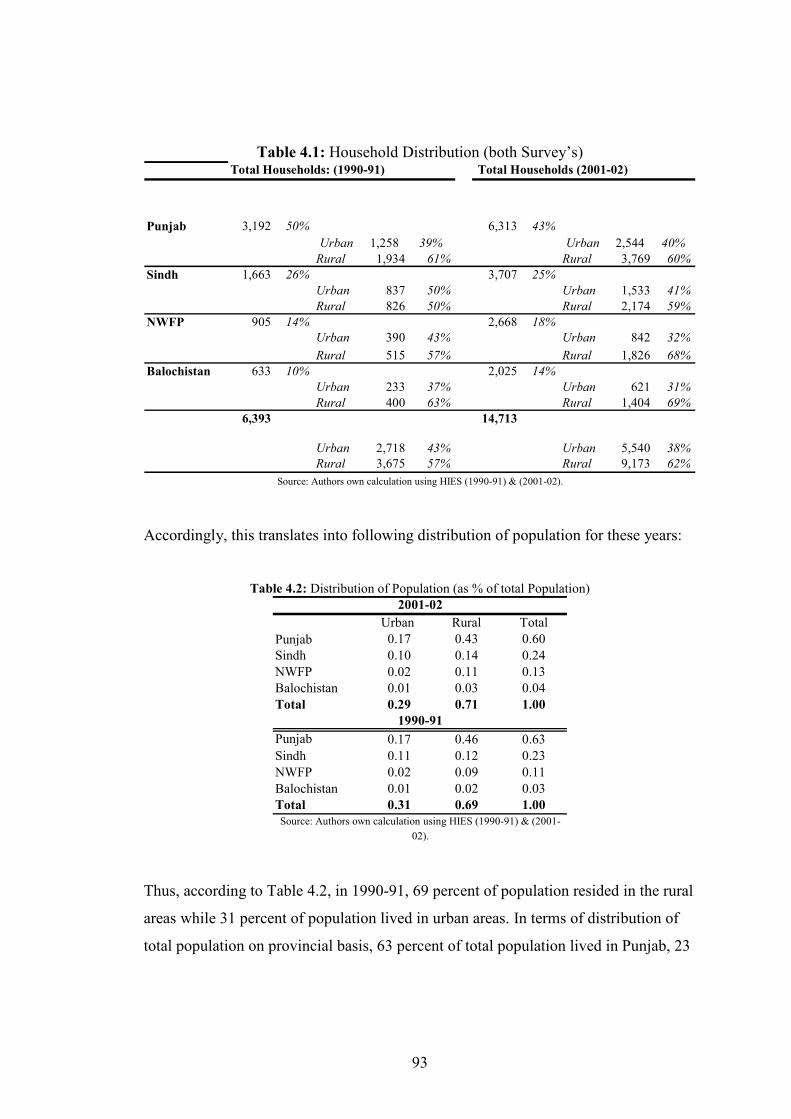
93

Table 4.1: Household Distribution (both Survey’s) Total Households: (1990-91) Total Households (2001-02)

Punjab 3,192 50% 6,313 43%

Urban 1,258 39% Urban 2,544 40%

Rural 1,934 61% Rural 3,769 60%

Sindh 1,663 26% 3,707 25%

Urban 837 50% Urban 1,533 41%

Rural 826 50% Rural 2,174 59%

NWFP 905 14% 2,668 18%

Urban 390 43% Urban 842 32%

Rural 515 57% Rural 1,826 68%

Balochistan 633 10% 2,025 14%

Urban 233 37% Urban 621 31%

Rural 400 63% Rural 1,404 69%

6,393 14,713

Urban 2,718 43% Urban 5,540 38%

Rural 3,675 57% Rural 9,173 62%

Source: Authors own calculation using HIES (1990-91) & (2001-02).

Accordingly, this translates into following distribution of population for these years:

Table 4.2: Distribution of Population (as % of total Population)

Urban Rural Total

Punjab 0.17 0.43 0.60

Sindh 0.10 0.14 0.24

NWFP 0.02 0.11 0.13

Balochistan 0.01 0.03 0.04

Total 0.29 0.71 1.00

Punjab 0.17 0.46 0.63

Sindh 0.11 0.12 0.23

NWFP 0.02 0.09 0.11

Balochistan 0.01 0.02 0.03

Total 0.31 0.69 1.00

2001-02

1990-91

Source: Authors own calculation using HIES (1990-91) & (2001-

02).

Thus, according to Table 4.2, in 1990-91, 69 percent of population resided in the rural

areas while 31 percent of population lived in urban areas. In terms of distribution of

total population on provincial basis, 63 percent of total population lived in Punjab, 23

94

percent in Sindh, 11 percent in NWFP and around 3 percent in Balochistan.

According to HIES (2001-02) estimates, surprisingly the rural share of population

slightly increased to 71 percent while urban share declined to 29 percent. On

provincial basis, population slightly declined in Punjab while it slightly increased in

all other provinces.

If we compare this with Population Census for Pakistan (1981; 1998), according to

the census estimates the share of urban population in Pakistan increased from 31

percent to 33.6 percent while rural population on the other hand decreased from 69

percent to 66.4 percent respectively. Thus, although, 1990-91 HIES survey population

distribution estimates are quite accurate, it appears 2001-02 HIES survey is slightly

over-estimating rural population and under-estimating urban population overtime74.

This is quite surprising given the migration and urbanization that has been taking

place in Pakistan. This anomaly according to ADB (2006) is related to the urban

sampling frame of HIES (2001-02) survey. The problem is that although the rural

sampling frame (as mentioned earlier) has been updated but the urban sampling frame

has not been updated since 1995. As a consequence HIES (2001-02) survey appears to

overestimate the rural population (World Bank 2002; ADB 2006).

4.1.1 HIES (1990-91) and (2001-02): Developments over time

Although various HIES surveys are collected by the same organization intended to

capture the same information yet over the years there have been some changes in data

collection methods and questionnaire design. These include:

74 Arif (2003) also reports a slight decline in percentage of households or individuals in urban areas based on the results of HIES and PIHS for (1995-96) and (2001-02).

95

(a) HIES (1990-91) survey like its predecessors was collected by a single male

enumerator interviewing only the male members of the households but after the

PIHS/HIES merge75, subsequent HIES surveys have been collected by a mobile team

of male and female enumerators under day to day management of a team supervisor

which allowed the team to interview both the male and the female members of the

households. This has definitely improved the quality of data collection overtime since

in Pakistan, females members are at the centre of day to day household management.

(b) After PIHS/HIES merge, minor expenditure categories that were considered

obsolete were either removed or merged with other categories. It is generally agreed

that such minor changes should not effect the direct comparability between both the

HIES survey (FBS 2001 and World Bank 2002).

(c) There has been a change in the recall period of some categories (see for instance

Table 4.3). In HIES (1990-91) all food expenditure items were recalled on monthly

basis while in HIES (2001-02) most of these are recalled on fortnightly basis.

Although this can possibly have some affect on comparison of both surveys it is not

likely to be too dramatic. For instance, according to Deaton (1997, pp26) “we should

perhaps not be too concerned with the discrepancies that are attributable to differences

in reporting periods, at least over the practical range”.

(d) It is also argued by Kemal (2003) that HIES and PIHS surveys understate the

income accruing to the highest income group. In some cases it is also reported that

poorest households are also inadequately represented or systematically excluded

particularly those that are homeless and illiterate (Zaidi, 1992; Gazdar, 2000); while

some have pointed towards possible underreporting at both tails (Jehle, 1990).

However, this issue is not just an issue pertaining to HIES but it is often argued that

this is a common observation about large surveys in general (ADB, 2006).

75 i.e. HIES (1998-99) and (2001-02).

96

Thus, it must be mentioned here that most of the issues mentioned above are not that

serious particularly in the context of this study, which is interested in measurement of

tax incidence not poverty or inequality since data comparability requirements for

latter types of analysis are much more stringent.

Additionally, it needs to be mentioned that HIES survey overall is very good quality

cross sectional data source. Over the years this survey has been used intensively by

domestic and foreign scholars, and government and multilateral agencies. For instance

see, (Ahmad and Stern (1987; 1991), Deaton (1987; 1997), Deaton and Grimard

(1992), Alderman and Garcia (1993); Malik (1988); Aamjad, et al. (1997); Jafri

(1999); Anwar et al. (2005); Kamal et al. (2003); World Bank (1995; 2002); ADB

(2006); CRPRID (2003; 2005; 2006), to name but a few.

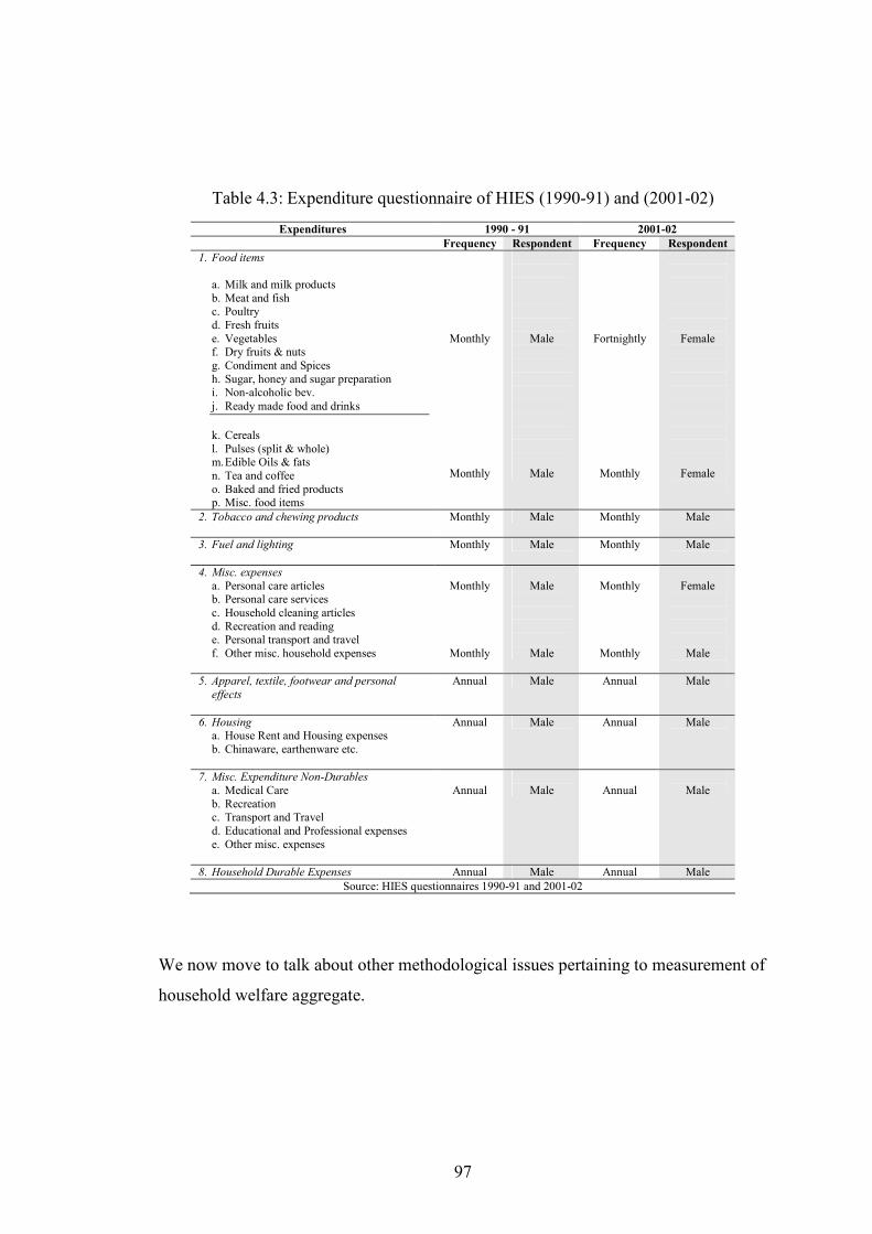
97

Table 4.3: Expenditure questionnaire of HIES (1990-91) and (2001-02)

Expenditures 1990 - 91 2001-02

Frequency Respondent Frequency Respondent

1. Food items

a. Milk and milk products b. Meat and fish c. Poultry d. Fresh fruits e. Vegetables f. Dry fruits & nuts g. Condiment and Spices h. Sugar, honey and sugar preparation i. Non-alcoholic bev.

j. Ready made food and drinks

k. Cereals l. Pulses (split & whole) m. Edible Oils & fats n. Tea and coffee o. Baked and fried products p. Misc. food items

Monthly

Monthly

Male

Male

Fortnightly

Monthly

Female

Female

2. Tobacco and chewing products

Monthly Male Monthly Male

3. Fuel and lighting

Monthly Male Monthly Male

4. Misc. expenses

a. Personal care articles b. Personal care services c. Household cleaning articles d. Recreation and reading e. Personal transport and travel f. Other misc. household expenses

Monthly

Monthly

Male

Male

Monthly

Monthly

Female

Male

5. Apparel, textile, footwear and personal

effects

Annual Male Annual Male

6. Housing a. House Rent and Housing expenses b. Chinaware, earthenware etc.

Annual Male Annual Male

7. Misc. Expenditure Non-Durables

a. Medical Care b. Recreation c. Transport and Travel d. Educational and Professional expenses e. Other misc. expenses

Annual

Male

Annual

Male

8. Household Durable Expenses Annual Male Annual Male

Source: HIES questionnaires 1990-91 and 2001-02

We now move to talk about other methodological issues pertaining to measurement of

household welfare aggregate.

98

4.2 Issues in Constructing Household Welfare Aggregate using HIES data

4.2.1 Unit of Analysis

The term unit of analysis refers to the unit with reference to which the welfare and

tax analysis will be undertaken. This study takes household as the basis of

measurement76. Thus, by doing so we are implicitly assuming that all household

resources are pooled and shared equally among all household members. This is a

simplistic assumption not necessarily a realistic one (Blundell et al., 1994; Creedy

1998; Hoddinott and Haddad, 1995).

4.2.2 Per Capita or Adult Equivalent

It is important to point out that the welfare as well as tax incidence analysis in this

study uses the ‘per capita’ (i.e. dividing by family size) basis insread of the ‘adult

equivalent’ basis. This is because, in the case of Pakistan, there is no single official

definition of adult equivalent which makes such analysis difficult.

4.2.3 Measurement of Household Welfare

76 According to the FBS, a ‘household’ is defined as either a single person household or a multi-person household. A single person household is one where the individual makes provisions for his/her own food and other essentials of living, without combining these resources with any other person and has no usual place of residence elsewhere. A multi-person household on the other hand is defined as a group of two or more person who make some common provision for food or other essentials of living and which has no usual place of residence elsewhere. Thus, the persons constituting the group may pool their incomes and have a common budget to a greater or lesser extent; they may be related or unrelated or a combination of both...

99

Since the aim of the present research is to evaluate the indirect tax system, its

progressivity, etc. the issue of measurement of welfare is required for ranking

households in terms of welfare. Thus, even though measurement of welfare is not

central to this research, adequate approximation of welfare is required to carry out tax

incidence analysis in this study. However, it may not be wrong to say that our concern

regarding welfare is primarily concerned with measuring the economic component of

standard of living Deaton and Grosh, 2000). Thus in doing so we do not claim to

cover any non-economic components of living standards, such as health, education,

political freedom etc., which can be equally important but cannot be adequately

captured by any simple monetary measure (Deaton and Zaidi, 2002). Our discussion

here will mainly focus on two most prominent and commonly used indicators of well-

being; income and consumption77.

The choice between annual income and consumption as an indicator of welfare is a

frequently debated and discussed issue. It would not be wrong to say that both are two

different concepts not just two different ways of measuring income (Deaton and

Grosh, 2000). For instance, income together with assets measures a person’s or

household’s potential claims on the economy while consumption measures what

people actually acquired (Deaton and Grosh, 2000). However, both can be defended

as approximation to utility; and as a result has been extensively used for analysis.

There is no doubt that average income in the long-run is the most appropriate

indicator of living standard (Anand and Harris, 1990). In longer term, such as

lifetime, the average level of consumption (including bequests) must be equal to the

average level of income (including inheritance); thus the choice between the two,

does not matter (Deaton and Zaidi, 2002). However, over a shorter reference period

such as one year, there is reason to believe that short-run income may be a poor proxy

of long term income. The main problem with using annual income data is that on a

77 The aim of this section is not to provide exhaustive survey of this argument but only to highlight some of the main points. For an exhaustive survey, see e.g. Anand and Harris (1990), McGregor and Borooah (1992).

100

short term it can suffer from high fluctuation and sometimes this variability is present

even across years. (Deaton, 1997).

In the view of such criticism current consumption has received much attention as a

better indicator of welfare particularly for developing countries: (a) there is

substantial evidence that even where income fluctuates a great deal in short term,

consumption is relatively smoother and less variable than income (Chaudhuri and

Ravallion, 1994); (b) there is empirical evidence supporting income smoothing in

poor agricultural societies with limited ability to borrow (Paxson, 1992;1993; Deaton,

1997) ; (c) in countries with substantial agriculture sector, self-employment and

informal sector, it is impossible to get a credible income measure without multiple

seasonal visits to the households; something that is rarely done (Deaton and Zaidi,

2002;; Havinga et al, 1989; Malik 1991; and Younger, 1999); (d) consumption of

certain items follows life cycle pattern which is independent of changes in income

(Modigliani and Brumberg, 1954) and ; (e) for evaluating the impact of price, subsidy

and taxation policies where the main concern is the price changes caused by policy

changes; consumption data is invaluable (Deaton and Grosh, 2000). Since all these

issues are very important particularly for developing countries, this study like many

others has opted to using current consumption as a measure of welfare.

4.2.4 Measurement of Household Consumption aggregate?

After having decided (based on discussion in the preceding section) that this study

will use consumption as measure of household welfare, we are now in a position to

move this discussion forward on how this study will construct the real value of total

household consumption that will be used as the indicator of households standard of

living.

101

4.2.4.1 What is included in Household Consumption aggregate?

Since this study uses expenditure as an indicator of household welfare it is important

to explicitly address the question what this indicator includes. The HIES survey

consists of expenditure on food, non-food, durable and non-durable items (for

example see Table 4.3 for further detail). Essentially total household expenditure

must contain all types of expenditure brought to a common frequency (annual in our

case) with a few exceptions78. Another important aspect is the types of expenditures.

HIES survey contains information on two broad types of expenditures; namely paid &

consumed and unpaid & consumed 79. Such distinction in consumption type can be of

importance for developing countries. Thus, although both types of expenditure are

included while calculating the household welfare indicator, tax liabilities are

calculated only with reference to the market purchased expenditures.

4.2.4.2 Dealing with Household durable expenses

78 Exceptions normally followed are: (a) Expenditure on levies and taxes (such as house and property tax, annual license fee for arms, fines, birth/marriage taxes and annual registration fees) are not included in the welfare indicator since these are essentially not part of consumption but rather a deduction from income (Deaton and Zaidi, 2002). (b) Certain type of health expenses (such as medical fees paid to doctor/specialist and hospitalisation charges) are also excluded from the welfare indicator given if included they will appear to increase the welfare of the household where as in reality opposite has happened (Deaton and Zaidi, 2002). (c) Lumpy expenditures (such as expenditure on food and drinks on birth/marriage/death ceremonies are excluded) because these are “lumpy” and “infrequent expenditures” and ideally should be “smoothed” out but since such information is not available it would be better to leave them out (Deaton and Zaidi, 2002). For instance, Howes and Zaidi (1994) report for PIHS (1991) that less than 8 percent households reported making a dowry payment during the past 12 months but these expenses made up almost 20 percent of their total annual consumption. All of the above expense categories are also not included in our household welfare indicator. 79 paid & consumed refers to a formal market transaction where an item is directly purchased from the market by paying for it and unpaid & consumed refers to informal transaction where an item is consumed either via own production, barter exchange, or gift/assistance.

102

The issue of dealing with household durables expenditures while constructing a

household welfare indicator based on consumption is an important and problematic

one. It is problematic because for major durable items in short run, consumption and

expenditure are not closely related to each other; as a result, expenditure is a very

poor guide to their consumption as consumption of durable items must be linked to

their stock not to purchases (Deaton and Grosh, 2000).

Empirically, this issue has been treated broadly in three different ways. (a)

Expenditure on durable items is treated no differently from other expenditure as a

result no adjustment is made (Goodman and Webb, 1995); (b) expenditure on the

lumpiest items such as cars, home repair is excluded, while other durables are

included (Deaton et al, 1989; World Bank 2002); and (c) only expenditure on non-

durable items is included (Prais and Houthakker, 1971).

However, for studies explicitly interested in tax incidence analysis, this issue is more

complicated because taxation of durable items such as TV, cars, electric fans etc. may

constitute a very important part of consumption taxes such as VAT. As a result some

proxy of durable good consumption needs to be imputed in order to get the correct tax

incidence picture. As a consequence, some studies explicitly dealing with tax

incidence analysis have made a specific attempt of imputing flow of durable good

consumption from their stock. These studies have made a simplifying assumption that

households in a given year only consume ten percent of the current value of the stock

of durable items (e.g. Johnson et al., 1989; Younger et al., 1999; Refaqat, 2003) we

also follow this procedure80.

4.2.4.3 Cost of living adjustment

80 Though it must be admitted that use of such a depreciation/proxy measure is fairly arbitrary.

103

This brings us to another important issue of cost of living adjustment across

household survey. In developing countries the main issue pertaining to the use of

household survey data appears to be spatial price variation i.e. people in different

parts of the country pay different prices for consuming the same goods which also

depends on inflation and seasonality. In many cases spatial price variation tend to be

quite large in both the relative and absolute price differences and must be accounted

for (Deaton and Zaidi, 2002). In comparison this issue tends to be much less

pronounced in household surveys of developed countries because well developed and

inexpensive transportation and distribution systems (for most consumer goods) appear

to minimize the spatial price variation (Deaton and Zaidi, 2002).

In order to make nominal consumption aggregates comparable across time and space

one can use Paasche index (i.e. current weighted), and Laspeyres price index (i.e. base

weighted)81. We use the Paasche price index because even though both indexes are

weighted average of price ratios, the former is weighted by expenditure in the current

period while the latter index is weighted by expenditure at the base period. As a

result, Paasche index is a preferable price index to adjust cost of living differences

(Deaton and Zaidi, 2002).

Following Deaton and Zaidi (2002) we can write the household money metric utility

function as:

h

P

h

h

p

hhh

mP

x

p

qpu =≈

. 4.1

Where h

mu represent the minimum cost of reaching utility level hu at prices 0p

81 Recently a superlative price index i.e. the Fisher Ideal index (which is a geometric mean of Laspeyres and the Paasche index) has also been used for deflation of nominal aggregate but such refinement may make more sense in poverty analysis.

104

Where Paasche index, h

hhh

pqp

qpP

.

.0

= 4.2

Or we can rewrite equation (4.2) intuitively in terms of how actually it will be

calculated using household survey data

11

01

−−

=

= ∑

k

ikn

k

ik

P

ip

pwP 4.3

where ikw is the average budget share of item k in the primary sampling unit i;

ikp is the median price of item k in the primary sampling unit i;

kp0 is the national median price of item k.

The Paasche price index using equation 4.3 is constructed at the level of primary

sampling unit (PSU) compared to the household level. According to the World Bank

(2002), this is a preferable method because it helps avoid the effect of outliers in some

households and also of cases in which household consumes most of its budget by

eating outside. Furthermore, the price ratio is constructed using median prices, this

according to Deaton and Tarozzi (2000), preferable to using average prices because

they avoid the effect of outliers.

Additionally, some extra qualifications are required to understand how equation 4.3 is

estimated. Although, estimating ikw (i.e. is the budget share of item k in the PSU i), is

fairly straight forward from survey data but the calculation of price ratio is not.

According to Deaton and Grosh (2000), LSMS and other surveys contain three

possible sources of prices: (a) survey itself, since household survey in many cases

report both quantities and expenditures for most food items. Thus, we can estimate

unit values i.e. dividing expenditures by quantities; (b) prices collected along with the

105

household survey) and; (c) other official sources for price data such as Government

price surveys.

For our estimation, price ratio in equation 4.3, is estimated using unit value (i.e.

dividing expenditure by quantities) for food items from survey data which is a widely

acceptable and followed method82. However, it is important to keep in mind that unit

value is not the same as ‘actual prices’, without adjustment for quality differences in

purchases across household and measurement error correction (Deaton, 1997).

However, spatial variation of unit value has been found to be closely related to the

actual price variation especially when averaged over households in a cluster/PSU

(Deaton and Zaidi, 2002).

Additionally, it must be mentioned that Paasche index is calculated from unit values

for food items only. Thus, this procedure makes an implicit and simplifying

assumption that the household cost of living is exactly proportional to standard of

living, it is adequate in the presence of unavailability of information on quantities for

non-food items (World Bank, 2002).

Finally, we calculate Paasche price index at primary sampling unit (PSU) level in

order to remove price differences between urban and rural areas and between

provinces. These indexes are given in Table 4.4.

82 Additionally, other price sources mentioned above were of limited or no use. For instance price data from community questionnaire was not available for Pakistan. And using price data from government price survey according to Deaton and Zaidi (2002; 40), should be a last resort because such data is often thin on ground and for many households the nearest observed price is so far away that it is irrelevant.

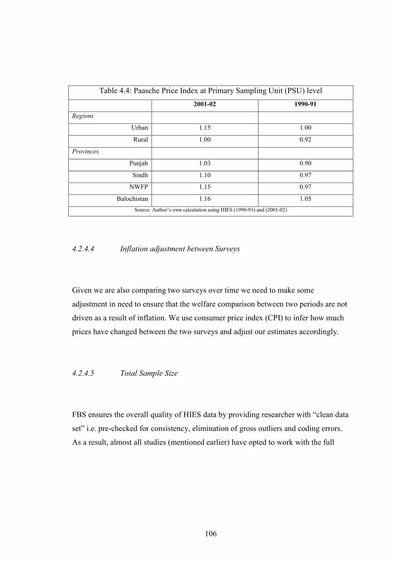
106

Table 4.4: Paasche Price Index at Primary Sampling Unit (PSU) level

2001-02 1990-91

Regions

Urban 1.15 1.00

Rural 1.00 0.92

Provinces

Punjab 1.03 0.90

Sindh 1.10 0.97

NWFP 1.15 0.97

Balochistan 1.16 1.05

Source: Author’s own calculation using HIES (1990-91) and (2001-02)

4.2.4.4 Inflation adjustment between Surveys

Given we are also comparing two surveys over time we need to make some

adjustment in need to ensure that the welfare comparison between two periods are not

driven as a result of inflation. We use consumer price index (CPI) to infer how much

prices have changed between the two surveys and adjust our estimates accordingly.

4.2.4.5 Total Sample Size

FBS ensures the overall quality of HIES data by providing researcher with “clean data

set” i.e. pre-checked for consistency, elimination of gross outliers and coding errors.

As a result, almost all studies (mentioned earlier) have opted to work with the full

107

sample83. However, nine households were removed from HIES (2001-02) sample

since there was no reported expenditure on any fortnightly items which is the most

basic category dealing with food necessities.

4.3 Household Expenditure Analysis (1990-91 & 2001-02) 84

4.3.1 National Expenditure Comparison85

Table 4.5 and Figure 4.1 present estimates for household welfare (measured in terms

of annualized total household per capita expenditure as discussed in the previous

chapter) at national level. Perhaps a relevant point before embarking on welfare

analysis is to determine what proportion of population in both years can be designated

as ‘poor’. It appears in 1990-91 almost thirty percent of national population was

below the official poverty line86 and consequently can be termed as the poor, while

the incidence of poverty for Pakistan significantly increased over the decade of 1990s

as by 2001-02 almost 40 percent of the total national population was below the

official poverty line.

This is in line with the national poverty trends during the decade of 1990 for Pakistan.

For instance, Jafri (1999) and World Bank (2004) estimate head count poverty ratio

for Pakistan for 1990-91 to be 27 percent and 34 percent respectively while for 2000-

01, World Bank (2004), DFID (2003) and CRPRID (2003) estimate head count

83 Only exception is Cheema (2005), who provides official poverty line estimates for Pakistan. After carrying out minute and careful analysis of HIES (2001-02) data set, this study removed only 16 households or 0.1 percent of sample size. 84 ‘Expenditure’ or ‘consumption’ referred to anywhere in the chapter refers to household annual per capita (pc) expenditures unless mentioned otherwise. 85 Deciles here are based on household ranking in terms of annual pc expenditures. 86 The Government of Pakistan official poverty line estimates for (2000-01) is PRs. 725 per month. This line (adjusted for inflation rate) is used in this study to identify households falling below poverty line for (1990-91) and (2001-02).

108

poverty ratio for Pakistan to be 37 percent, 34 percent and 38.5 percent respectively.

According to World Bank (2002) growth and consumption poverty appear to be

strongly linked. For instance according to the same source, between (1990-94) the

average annual per capita GDP growth was around 2 percent while poverty declined

by 5 percentage point. In contrast, during (1993-99) when per capita GDP grew only

at an average annual rate of 1.4 percent, poverty increased by 4 percentage point.

Furthermore the largest increase in poverty took place between (1996-99), when per

capita GDP grew at a rate of less than 1 percent. However, slow per capita GDP

growth was not the only reason for increase in poverty in Pakistan during the 1990s.

For instance, according to World Bank (2002) skewed pattern of landownership, poor

access to education and health facilities, lack of critical infrastructure and restrictive

social grouping, all exacerbated poverty during this period.

If we look at household welfare, during 1990-9187 it is estimated that Pakistani

household on average (at per capita and annual level) was consuming around PRs88.

13,140 while the average consumption of the poorest and the richest ten percent of

population was PRs. 5,243 and PRs. 37,628 respectively. By 2001-02 it appears that a

Pakistani household on average was consuming (at per capita and annual level)

around PRs. 11,218 while the poorest and richest ten percent of population during this

year were consuming PRs. 4,367 and PRs. 32,782 respectively.

A quick look at household welfare comparison over time reveals that household

welfare in 2001-02 relative to 1990-91 at national level (for instance see Figure 4.1)

fell across all segments of population!89 It appears a Pakistani household at national

level on average experienced almost 16 percent decline in welfare compared to 1990-

91 level. Furthermore, estimates reveal that over time the highest decline in welfare in

2001-02 relative to 1990-91 was experienced by the poorest segment of the

87 All 1990-91 estimates are presented in 2001-02 prices. 88 PRs.: Pakistan rupee. 89 ‘Welfare’ is being measured in terms of household total annualized per capita consumption. Please see Chapter 3; Data Issues and Methodology for a detailed discussion.

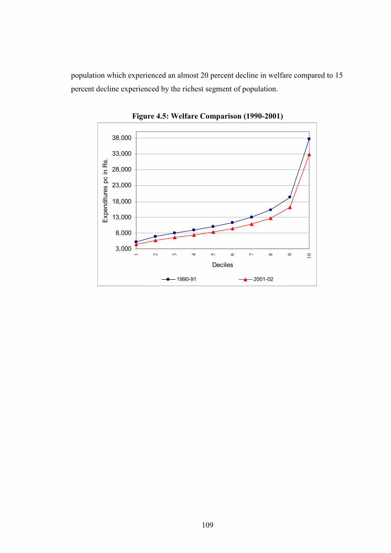
109

population which experienced an almost 20 percent decline in welfare compared to 15

percent decline experienced by the richest segment of population.

Figure 4.5: Welfare Comparison (1990-2001)

3,000

8,000

13,000

18,000

23,000

28,000

33,000

38,0001 2 3 4 5 6 7 8 9

10

Deciles

Expenditure

s p

c in R

s.

1990-91 2001-02

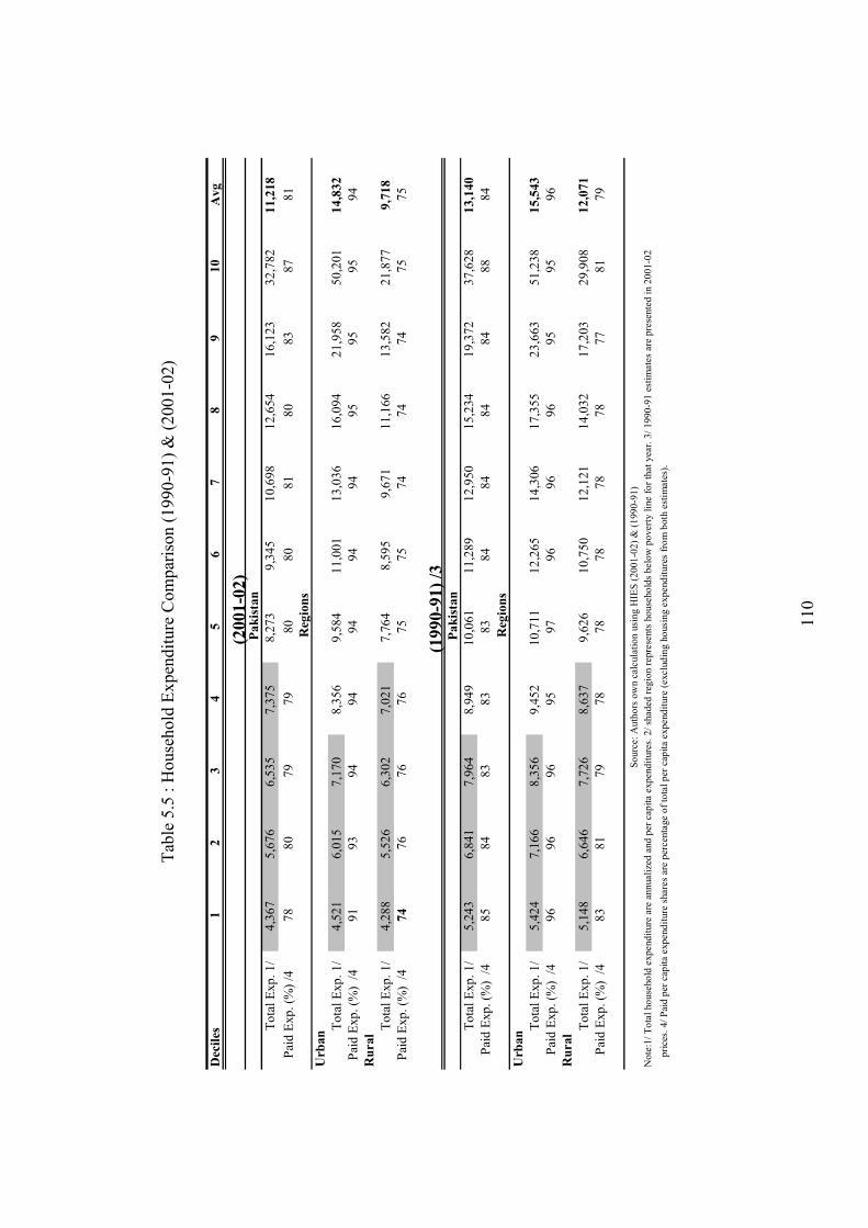
110

Tab

le 5

.5 :

House

hold

Ex

pen

dit

ure

Com

par

ison (

1990-9

1)

& (

2001-0

2)

Deciles

1

2

34

5

67

8

910

Avg

To

tal

Exp

. 1

/4

,36

75

,67

66

,53

57

,37

58

,27

39

,34

51

0,6

98

12

,654

16

,123

32

,782

11,218

Pai

d E

xp

. (%

) /4

78

80

79

79

80

80

81

80

83

87

81

Urban T

ota

l E

xp

. 1

/4

,52

16

,01

57

,17

08

,35

69

,58

41

1,0

01

13

,036

16

,094

21

,958

50

,201

14,832

Pai

d E

xp

. (%

) /

49

19

39

49

49

49

49

49

59

59

59

4

Rural T

ota

l E

xp

. 1

/4

,28

85

,52

66

,30

27

,02

17

,76

48

,59

59

,67

11

1,1

66

13

,582

21

,877

9,718

Pai

d E

xp

. (%

) /

474

76

76

76

75

75

74

74

74

75

75

To

tal

Exp

. 1

/5

,24

36

,84

17

,96

48

,94

91

0,0

61

11

,289

12

,950

15

,234

19

,372

37

,628

13,140

Pai

d E

xp

. (%

) /

48

58

48

38

38

38

48

48

48

48

88

4

Urban T

ota

l E

xp

. 1

/5

,42

47

,16

68

,35

69

,45

21

0,7

11

12

,265

14

,306

17

,355

23

,663

51

,238

15,543

Pai

d E

xp

. (%

) /

49

69

69

69

59

79

69

69

69

59

59

6

Rural T

ota

l E

xp

. 1

/5

,14

86

,64

67

,72

68

,63

79

,62

61

0,7

50

12

,121

14

,032

17

,203

29

,908

12,071

Pai

d E

xp

. (%

) /

48

38

17

97

87

87

87

87

87

78

17

9

S

ourc

e: A

uth

ors

ow

n c

alcu

lati

on u

sing H

IES

(2001

-02)

& (

1990-9

1)

Note

:1/

To

tal

ho

use

ho

ld e

xp

end

iture

are

annual

ized

and p

er c

apit

a ex

pen

dit

ure

s. 2

/ sh

aded

reg

ion r

epre

sents

ho

use

ho

lds

bel

ow

po

ver

ty l

ine

for

that

yea

r. 3

/ 1990-9

1 e

stim

ates

are

pre

sente

d i

n 2

001-0

2

pri

ces.

4/

Pai

d p

er c

apit

a ex

pen

dit

ure

shar

es a

re p

erce

nta

ge

of

tota

l p

er c

apit

a ex

pen

dit

ure

(ex

clud

ing h

ousi

ng e

xp

end

iture

s fr

om

both

est

imat

es).

(1990-91) /3

Pakistan

Regions

(2001-02)

Pakistan

Regions

111

Table 4.5 also presents the share of market and non-market90 transactions within total

household expenditures. This estimate is very important given it is the transaction

carried out in the formal market that are consequently taxable. It appears in 1990-91

the share of informal market transactions (as percentage of total household

expenditure) for an average Pakistani household was around 16 percent; by 2001-02

this had increased to 19 percent. It appears in 1990-91 the poorest ten percent of

households on average carried out 15 percent of their total household transactions in

the informal market, this significantly increased to 22 percent by 2001-02. In

comparison in 1990-91 the richest ten percent of population carried out 12 percent of

transactions in the informal market. This, however, more or less remained at the same

level over time. Thus it appears over time there was a significant increase in the share

of informal expenditure for the poorest segment of population but same is not true for

the most affluent segment of population. Although it is difficult to gauge why this has

happened, one possible contributing factor could be GST broad-basing over time.

4.3.2 Rural and Urban Expenditure Comparison

Table 4.5 also presents welfare estimates for rural/urban households over time. It

appears in 1990-91 a urban household on average (in terms of annual per capita

expenditure) was consuming around PRs. 15,543 while in comparison household in

the rural areas on average was consuming PRs. 12,07191. This meant rural households

on average were consuming 33 percent less than their urban counterparts. In 1990-91

almost thirty percent of urban population and forty percent of rural population was

below the poverty line for that year92.

90 ‘Non-market’ here implies to household consumption made possible through barter exchange, gift or assistance. 91 Urban deciles here are based on urban household ranking in terms of annual per capita expenditures while rural deciles are based on rural households ranking in terms of annual per capita expenditures. 92 This is supported by urban and rural poverty estimates for Pakistan. For instance, the urban poverty estimates place incidence of urban poverty at the beginning of 1990s to be around 20 percent (for

112

In 1990-91 the poorest ten percent of households in the rural and urban area on

average were consuming PRs. 5,148 and PRs. 5,424 respectively while the richest ten

percent households in rural and urban area respectively were consuming around PRs.

29,908 and PRs. 51,238 respectively. According to these estimates there was a clear

welfare gap existing between the poorest and the richest segment of population. For

example, in rural areas the poorest decile households’ proportionate consumption was

only 18 percent of the richest decile in the same region. This was even worse for

urban areas at 11 percent only.

Another interesting piece of information is to compare welfare levels of the same

decile households in the urban and rural areas which gives an idea of how well similar

segments of population are doing when compared against each other. By doing this

we find poor to middle decile households in urban/rural areas fairing better when

compared to each other (as compared to how the affluent decile households were

doing). For instance, rural poorest ten percent of population in terms of their urban

counterparts was almost 94 percent; this fell to 89 percent for the middle decile

households but to only 58 percent for the most affluent decile.

In 2001-02, a rural and urban household on average was consuming (per annum per

capita basis) around PRs. 9,718 and PRs. 14,832 respectively. During the same time

the poorest ten percent of population in the rural and the urban areas was consuming

PRs. 4,288 and PRs. 4,521 respectively while the richest ten percent of population in

the rural and the urban area was consuming PRs. 21,877 and PRs. 50,201

respectively. We can see from the shaded region in Table 5.1 that in 2001-02 almost

30 percent of urban and forty percent of rural population was below the official

poverty line or ‘poor’.

instance see Amjad and Kemal, 1997 and Ali and Tahir, 1999) and 22-25 percent for the end of 1990s (see for instance FBS ,2001; and World Bank, 2002). Similarly, rural poverty incidence at the beginning of 1990s is estimated to be around 19-26 percent (see for example Amjad and Kemal, 1997; Ali and Tahir, 1999; and Jafri, 1999) while that for end of 1990’s is estimated to be around 35-40 percent (see for example FBS, 2001; World Bank, 2002; Arif et al, 2001).

113

During this time, the poorest ten percent of population in the rural area was enjoying

only 20 percent of consumption level being enjoyed by the richest ten percent of

population in this region. However, situation was much worse in the urban areas

where the urban poorest ten percent of population enjoyed only 9% of consumption

level being enjoyed by their richest counterparts. Thus, it appears that although this

gap had slightly decreased for the rural population but increased for the urban

population.

If we compare same segments of population in both regions, we find trends similar to

that for 1990-91. For instance, the rural poorest ten percent proportionate

consumption in terms of same segment of population in the urban areas was around

95 percent (almost the same level as in 1990-91). This, however, fell to 78 percent for

the fifth decile households (compared to 89 percent in 1990-91) and to only 65

percent (against 58 percent for 1990-91) for the richest ten percent households. Thus,

it appeared that in 2001-02 middle decile households in the rural areas fell further

behind their urban counterparts compared to 1990-91.

Table 4.5 also presents the share of market and non-market transactions carried out by

the rural and the urban areas over time. In 1990-91, 96 percent of the total

transactions of an average urban household were carried out in the formal market

compared to 79 percent by the rural households. By 2001-02, little had changed for

the urban areas as an urban household on average still carried out 94 percent of total

transactions in the formal market compared to 75 percent for the rural area.

However, this difference was more apparent for the poorest and richest ten percent of

population in the urban/rural areas. For instance, in 1990-91 the poorest ten percent of

households in the urban (rural) areas carried out 96 (83) percent of total transactions

in the formal market while by 2001-02 this changed to 91 (74) percent respectively.

Similarly the richest ten percent of population in the urban (rural) areas in 1990-91

114

were carrying 95 (81) percent of total transactions in the formal market but by 2001-

02 this changed to 95 (and only 75) percent. Thus, although share of formal market

transactions in the urban areas did not change much, things changed considerably for

the rural areas.

4.4 Selected Commodity Expenditure Analysis (1990 – 91) & (2001 – 02)

This section will briefly look at the main expenditure categories emerging from the

HIES (1990-91) and (2001-02) survey. This will enable us to look at household

expenditure patterns at a disaggregated level and allow us to characterize various

expenditure patterns as necessities or luxuries based on the overall population

expenditure patterns. This information is important because this analysis will not only

help us identify categories that are more important for the poor, but this information

will come handy when attempting to disaggregate the GST incidence picture in the

later section.

If we look at Table 4.6 we can see household disaggregated expenditure patterns at

national level both for (1990-91) and (2001-02) [please see Appendix 4.3 for

disaggregated expenditure patterns for the urban and the rural areas]. If we look at

Table 4.6 we can see that in 1990-91 the most important expenditure category for a

Pakistani household on average was food items on which households on average were

spending around 53 percent of total household expenditure. The second important

expenditure category for households on average appeared to be housing expenditures

(15 percent), this was followed by clothing items (8.5 percent), fuels/utilities (6.0

percent), transport and travelling group (4.0 percent), health (3.1 percent), tobacco

(2.2 percent), education (1.7 percent), and durable expenses (0.52 percent). It is quite

important to note that three particular food items namely milk, sugar and cereals

individually were as significant (in terms of expenditure shares) for households as

115

many other non-food expenditure items as households on average were spending 10.8

percent on milk, 10.1 percent on cereals, and 4.8 percent on edible oils.

Another interesting piece of information is the general trend of these expenditure

categories. For instance, we find expenditure on food, clothing and (surprisingly) fuel

/utilities as a percentage of total household expenditure decrease as households

become affluent, thus these appear to be necessities. On the other hand, proportionate

expenditures (as a proportion of total household expenditure) on transport and travel

group, education, and housing increase as population becomes more affluent. As a

result these appear to be luxuries. However, expenditure share on Tobacco group

appears to be inverted U-shaped (it is relatively more important for the middle classes

compared to the tails). Lastly, it was not possible to make any clear cut expenditure

pattern across population on health and durable goods.

If we look at Table 4.6 we can also see significant differences in expenditure shares

on important expenditure categories for the poorest ten percent and the richest ten

percent of population. For instance, in 1990-91 if we rank top three important

categories for the poorest ten percent of population, these are food expenditures (61

percent), clothing (9.5 percent) and housing (9.2 percent), while the top three

expenditure categories for the richest ten percent of population are also food

expenditures (40 percent), housing (21 percent), and transport and travel group (8.08

percent). Thus, even though the top two expenditure categories are the same across

both segments of population the poor are spending almost fifty percent more on the

food items while the richest ten percent of the population is spending almost double

on housing expenses.

By 2001-02, food expenditure still remained as the most important expenditure

category with a Pakistani household on average spending around 48 percent of total

household expenditure on food. This is followed by housing which retains its position

as the second most important expenditure category (on which households on average

116

are spending around 13 percent of total household expenditure). This is followed by

fuels/utilities (8 percent), clothing (7 percent), education and travel group (both

around 4 percent), health (2 percent), tobacco (1.6 percent) and durable items (1.4

percent).

If we look at the overall trend of expenditures across population on these

commodities, as earlier, categories such as education, housing, travelling group and

additionally durable items appeared to be luxuries (as expenditures on these

categories as a percentage of total household expenditure increases as household

become affluent) while expenditure on food, fuels/utilities and clothing still appear to

be necessities (as expenditures on these categories as a percentage of total household

expenditure fall as household become affluent). Surprisingly now tobacco also

appears to be a necessity!

In addition to this if we look at the average level of expenditures over time we find

that the average expenditure on a food category has slightly fallen from 53 percent in

1990-91 to 48 percent in 2001-02. It appears overtime average expenditure on major

food items like milk has slightly declined, but increased for sugar and cereals. Among

non-food expenditure categories, average expenditure shares on clothing, travelling,

house rent, tobacco and health have slightly declined, while expenditure on durable

items, fuels/utilities and education has slightly increased over time.

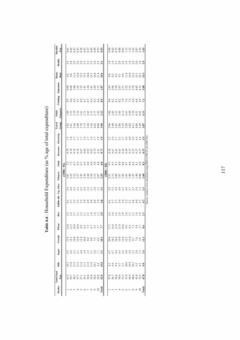
117

Table 6.6 : H

ouse

hold

Expen

dit

ure

(as

% a

ge

of

tota

l ex

pen

dit

ure

)

Deciles

Total Food

Exp

Milk

Sugar

Cereals

Whea

tRice

Edible oils

Veg

. Ghee

Tobacco

Fuels

Kerosene

Electricity

Travel

Group

Public

Tra

nsp

ort

Clothing

Education

House

Rent

Health

Durable

Exp

16

1.3

10

.54

.517

.51

4.6

2.4

6.1

5.4

2.0

17

.20

.70

1.5

1.8

31.6

09.5

0.9

49

.23

.30.6

1

25

9.7

11

.04

.615

.11

2.2

2.4

5.7

4.9

2.2

37

.20

.76

1.6

2.4

12.2

29.6

0.9

89

.82

.80.4

2

35

8.7

11

.94

.214

.01

0.9

2.7

5.5

4.5

2.1

26

.70

.76

1.7

2.4

42.1

99.5

1.0

811

.42

.90.4

7

45

7.7

11

.44

.112

.81

0.0

2.2

5.3

4.2

2.3

76

.50

.76

1.7

2.4

02.1

09.1

1.4

212

.03

.00.4

7

55

7.1

11

.84

.011

.88

.92

.35

.54.3

2.4

36

.70

.87

1.7

2.7

62.4

18.9

1.2

212

.23

.00.3

8

65

5.1

11

.53

.810

.98

.32

.15

.03.8

2.3

66

.40

.84

1.8

3.1

52.7

18.7

1.4

113

.23

.50.4

7

75

4.4

11

.83

.39

.87

.32

.14

.93.4

2.4

46

.00

.92

1.7

3.3

62.6

18.7

1.3

414

.43

.30.3

7

85

3.8

11

.93

.19

.06

.71

.94

.83.1

2.3

96

.00

.92

1.8

3.4

22.5

18.4

1.6

115

.13

.50.4

5

95

0.2

10

.52

.87

.55

.51

.64

.62.8

2.1

35

.80

.74

1.7

4.4

52.7

18.3

1.6

916

.83

.60.4

9

10

39

.98

.01

.74

.32

.71

.32

.91.3

2.0

74

.00

.31

1.9

8.0

81.9

36.6

3.1

521

.42

.50.5

3

Total

52.9

10.8

3.3

10.1

7.7

2.0

4.8

3.4

2.25

6.0

0.73

1.8

3.96

2.32

8.5

1.67

14.6

3.1

0.52

15

7.4

8.2

4.5

20

.81

7.2

3.4

6.1

5.8

2.2

19

.30

.38

3.2

2.0

41.8

68.6

1.6

38

.01

.80.4

9

25

6.7

8.9

4.7

18

.21

4.4

3.6

5.7

5.3

2.1

39

.10

.47

3.4

2.4

02.6

38.2

2.0

68

.21

.90.6

2

35

6.0

9.4

4.6

16

.61

2.9

3.4

5.7

4.9

2.0

89

.10

.41

3.7

2.6

53.2

28.1

2.3

48

.22

.10.7

2

45

4.9

9.7

4.4

15

.01

1.8

2.8

5.4

4.6

1.8

78

.80

.41

3.5

2.8

63.4

48.2

2.6

79

.12

.00.8

8

55

3.3

9.7

4.3

13

.81

0.6

2.9

5.4

4.3

1.9

58

.80

.38

3.7

3.3

24.1

37.9

2.7

19

.92

.00.9

3

65

1.9

10

.04

.012

.59

.62

.65

.24.0

1.8

38

.70

.39

3.8

3.2

84.4

17.6

3.2

211

.41

.91.1

5

75

0.5

10

.03

.611

.08

.42

.35

.13.7

1.8

08

.60

.35

4.0

3.8

24.8

87.4

3.1

312

.01

.81.3

2

84

8.6

10

.23

.29

.77

.32

.24

.83.2

1.4

78

.20

.32

3.9

4.1

35.5

86.9

3.7

813

.22

.01.6

1

94

3.8

9.5

2.6

7.4

5.6

1.6

4.4

2.6

1.4

08

.10

.27

4.4

4.9

46.3

16.8

4.4

215

.12

.02.0

7

10

32

.56

.51

.53

.92

.71

.02

.71.2

0.8

06

.90

.27

4.4

5.4

86.9

54.9

6.1

322

.11

.82.3

6

Total

47.8

9.0

3.4

11.1

8.6

2.3

4.7

3.5

1.60

8.3

0.35

3.9

3.87

4.33

7.1

3.68

13.3

1.9

1.43

(1990 - 91)

(2001 - 02)

So

urc

e: A

uth

ors

ow

n c

alcu

lati

on

usi

ng

HIE

S (

199

0-9

1)

& (

20

01

-02

)

118

4.5 Conclusion

This study will use the HIES (1990-91) and (2001-02) survey for carrying out partial

equilibrium indirect tax incidence analysis of Pakistan. This chapter has tried to

present an overview of the underlying data source, its methodology, data collection

procedures along with household welfare estimates for 1990-91 and 2001-02. We

have tried to show in this chapter that HIES survey is a carefully collected survey; it

provides very relevant information to what is needed in this study and it is a good

quality household cross section survey which has been utilised intensively over time

for Pakistan.

Thus, in the following chapters we are in a position of carrying out the main empirical

analysis of this study. In next chapter we move to determining the social incidence of

GST/VAT in Pakistan while using (1990-91) and (2001-02) HIES survey.

119

CHAPTER V: Social Incidence of General Sales Tax (GST)

in Pakistan (1990-91) & (2001-02)

5 Introduction

This chapter attempts to measure the social incidence of GST in Pakistan in the pre-

and post- reform era. We start with GST/VAT incidence because GST/VAT reforms

were at the centre stage of the reform process embarked by Pakistan in the 1990s, and

by the end of the reform process GST/VAT revenues emerged as the most significant

component of Pakistan’s federal tax structure. Thus, any serious attempt at estimating

indirect tax incidence must start with the GST/VAT incidence, which this chapter

intends to do.

Furthermore, this chapter also aims to present GST/VAT incidence picture at

disaggregated level. The intention is to clearly show how the underlying GST/VAT

incidence at pre- and post- reform era for the national as well as the urban/rural areas

is being generated. We believe such discussion is important not only for

understanding the elements that may make the overall GST/VAT incidence pattern

progressive/regressive/proportional but also for isolating effects that may be

distributively more important for the poor. Furthermore, the last section of this

chapter also focuses on the explicit issue of GST/VAT exemptions. We believe this is

fundamentally an important issue for safeguarding the poor from GST/VAT net by

maintaining well-targeted exemptions.

This Chapter is divided into four main sections. The first section begins with the main

aim of this chapter that is determining the GST/VAT social incidence at pre- and post-

120

reform time for national as well as for the urban/rural areas. The second section

presents the disaggregated view of GST incidence over time at national level as well

as for the urban/rural areas. The third section of this chapter moves to address the

question of GST/VAT exemptions. We use distributional characteristics of a good

approach to show expenditure items in HIES (2001-02) that are proportionally more

important for the poor, and use this information to evaluate current and propose future

GST/VAT exemptions to safeguard the poor. The fourth section concludes.

5.1 GST Incidence

5.1.1 Description of GST

As mentioned in Chapter two in detail, GST in VAT mode was introduced in Pakistan

by the Sales Tax Act of 1990. Initially it was levied at the import and manufacturing

stage only at a rate of 12.5 percent. During the initial years the revenue impact of GST

was almost negligible because the GST regime was riddled with standard,

geographical and development exemptions. It was not until late 1990s when GST

structure came close to the true spirit of VAT; with its extension to the retail sector,

elimination of most of exemptions, and introduction of a single rate at 15 percent93.

These summary differences are presented in Table 5.1.

93 This discussion has been kept brief purposely since most of these issues have been covered in detail in Chapter 2; Taxation in Pakistan (1985-2001).

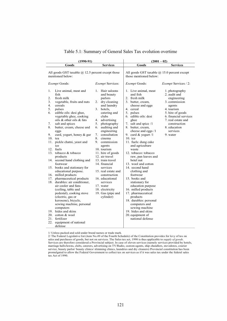
121

Table 5.1: Summary of General Sales Tax evolution overtime

(1990-91) (2001 – 02)

Goods Services Goods Services

All goods GST taxable @ 12.5 percent except those

mentioned below:

All goods GST taxable @ 15.0 percent except

those mentioned below: Exempt Goods: 1. Live animal, meat and

fish 2. fresh milk

3. vegetable, fruits and nuts 4. cereals 5. pulses 6. edible oils: desi ghee,

vegetable ghee, cooking oils & other oils & fats

7. salt and spices 8. butter, cream, cheese and

eggs

9. curd, yogurt, honey & gur 10. tea 11. pickle chatni, yeast and

ice 12. fuels 13. tobacco & tobacco

products 14. second hand clothing and

footwear 15. books and stationary for

educational purpose. 16. milled products 17. pharmaceutical products 18. durables: air conditioner,

air cooler and fans (ceiling, table and

pedestal), cooking stove (electric, gas or kerosene), bicycle, sewing machine, personal computers

19. hides and skins 20. cotton & wool 21. fertilizer 22. equipment of national

defense

Exempt Services: 1. Hair saloons

and beauty parlors

2. dry cleaning and laundry

3. hotels, catering and clubs

4. advertising 5. photography 6. auditing and

engineering

7. consultation 8. cinema 9. commission

agents 10. tourism 11. hire of goods 12. air travel 13. train travel 14. financial

services 15. real estate and

construction 16. educational

services 17. water 18. electricity

19. Gas (pipe and cylinder)

Exempt Goods: 1. Live animal, meat

and fish 2. fresh milk

3. butter, cream, cheese and eggs

4. cereal 5. pulses 6. edible oils: desi

ghee 7. salt and spice /1 8. butter, cream,

cheese and eggs /1

9. curd & yogurt /1 10. ice 11. fuels: dung cake

and agriculture waste

12. tobacco: tobacco raw, pan leaves and betel nut

13. wool and cotton 14. second hand

clothing and footwear

15. books and stationary for education purpose

16. milled products

17. pharmaceutical products

18. durables: personal computers and sewing machine

19. hides and skins 20. equipment of

national defense

Exempt Services / 2:

1. photography 2. audit and

engineering

3. commission agents

4. tourism 5. hire of goods 6. financial services 7. real estate and

construction 8. education

services

9. water

1/ Unless packed and sold under brand names or trade mark. 2/ The Federal Legislative list (item No.49 of the Fourth Schedule) of the Constitution provides for levy of tax on

sales and purchases of goods, but not on services. The Sales tax act, 1990 is thus applicable to supply of goods. Services are therefore considered a Provincial subject. In case of eleven services (namely services provided by hotels, marriage halls/lawns, clubs, caterers, advertising on TV/Radio, custom agents, ship chandlers, stevedores, courier

service, beauty parlor/ beauty clinics/ slimming clinics, laundries and dry cleaners) Provincial constitution has been promulgated to allow the Federal Government to collect tax on services as if it was sales tax under the federal sales tax Act of 1990.

122

5.1.2 Estimation of GST/VAT amounts94

Since GST/VAT can be charged from market transactions only, the starting point of

this calculation is HIES reported paid or formal market transactions. The tax

information is provided by the Central Board of Revenue, Pakistan which is used to

identify taxable items from the HIES survey for each year. Once a good/ service is

identified as taxable, the statutory GST/VAT rate is used to calculate the taxable

liability.

We use the same formula used by Cho et al., (2003), Sahn and Younger (2003), and

Edmiston and Bird (2006) (to name but a few) to determine the tax paid on each item:

ji

j

j

ji et

tT ,,

1+= 5.1

Where

jiT , = household i’'s per capita VAT/GST payment on good j

jt = statutory VAT/GST rate

jie , = observed expenses or post tax per capita expenditures on good j

Equation 5.1 is used to determine amount of taxes paid on each item, (on per capita

basis) for each household for a span of a year. However, we present results on the

basis of deciles. Households ranking in deciles are based on ascending order of

94 Given that household welfare estimates for 1990-91 and 2001-02 have already been discussed in

detail in Chapter 4, this section only focuses on how that information is used to calculate GST liabilities and incidence.

123

annualized per capita household total expenditures, also a proxy of household welfare

(for instance see Chapter four). This enables us to determine average tax payments per

decile at annual level. The incidence or the effective GST/VAT rate per decile is

determined by dividing this by the average total household annual per capita

expenditure (paid & un-paid) per decile.

5.1.3 Progressivity, Regressivity or Proportionality of tax

This study uses average progressivity rate (APR) to judge progressivity, regressivity

or proportionality of an underlying tax/tax system. As already discussed above (and in

chapter 4) that this study uses household total expenditure (per capita) as a measure of

household welfare and this measure is used to rank households in decile in ascending

order; from poorest (1st) decile to richest (10th) decile. Thus, when effective tax rate

per decile (i.e. average per capita tax liability as a percentage of average per capita

total household expenditures for each decile) rises as we move up the deciles; the

tax/tax system will be considered progressive; it is regressive if effective tax rate falls

as we move up the deciles and proportional when effective tax rates remain

constant95.

5.1.4 National GST Incidence

Results for GST incidence at the national level for (1990-91) and (2001-02) are

presented in Table 5.2. If we look at Table 5.2 and the GST incidence figures for

(1990-91) two things are quite obvious. (a) GST incidence for (1990-91) appears to be

95 This may not be the only definition of progressivity/regressivity; for other definitions/measures see Chapter 3. However, this definition is considered adequate for this analysis.

124

clearly progressive. (b) The magnitude of incidence is quite small. For instance, the

average GST/VAT tax incidence in (1990-91) was around 1.30 percent while for the

poorest and richest ten percent population of Pakistan it was only 1.08 and 1.52

percent respectively. However, this should not be a surprise given information in

Table 5.1 and discussion in the earlier chapter, chapter two.

Table 5.2 also presents GST/VAT incidence for (2001-02) which in other words also

shows the impact of tax reform process and shows GST incidence at post- reform

time. Looking at (2001-02) results makes two things apparent. (a) The magnitude of

GST/VAT in (2001-02) is quite different from GST/VAT incidence at pre-reform era.

(b) Despite exemptions of basic food items, GST/VAT incidence appears to be at best

proportional over majority of the population. Our results show that the average

GST/VAT incidence in 2001-02 for a Pakistani household was 4.7 percent, whereas it

was 4.58 percent for the bottom ten percent of the population and only 4.65 percent

for the richest ten percent of the population!

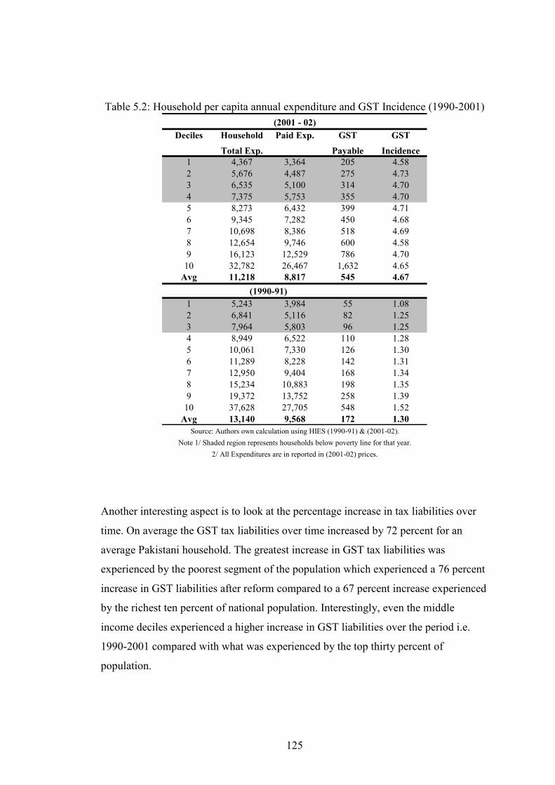
125

Table 5.2: Household per capita annual expenditure and GST Incidence (1990-2001)

Deciles Household

Total Exp.

Paid Exp. GST

Payable

GST

Incidence

1 4,367 3,364 205 4.58

2 5,676 4,487 275 4.73

3 6,535 5,100 314 4.70

4 7,375 5,753 355 4.70

5 8,273 6,432 399 4.71

6 9,345 7,282 450 4.68

7 10,698 8,386 518 4.69

8 12,654 9,746 600 4.58

9 16,123 12,529 786 4.70

10 32,782 26,467 1,632 4.65

Avg 11,218 8,817 545 4.67

1 5,243 3,984 55 1.08

2 6,841 5,116 82 1.25

3 7,964 5,803 96 1.25

4 8,949 6,522 110 1.28

5 10,061 7,330 126 1.30

6 11,289 8,228 142 1.31

7 12,950 9,404 168 1.34

8 15,234 10,883 198 1.35

9 19,372 13,752 258 1.39

10 37,628 27,705 548 1.52

Avg 13,140 9,568 172 1.30

Note 1/ Shaded region represents households below poverty line for that year.

2/ All Expenditures are in reported in (2001-02) prices.

(1990-91)


(2001 - 02)

Another interesting aspect is to look at the percentage increase in tax liabilities over

time. On average the GST tax liabilities over time increased by 72 percent for an

average Pakistani household. The greatest increase in GST tax liabilities was

experienced by the poorest segment of the population which experienced a 76 percent

increase in GST liabilities after reform compared to a 67 percent increase experienced

by the richest ten percent of national population. Interestingly, even the middle

income deciles experienced a higher increase in GST liabilities over the period i.e.

1990-2001 compared with what was experienced by the top thirty percent of

population.

126

One plausible explanation of this (other than changing expenditure patterns overtime)

could be that during the reform process the pattern of GST/VAT broad-basing has

affected the poor households more than the rich. For instance, if we look at Table 5.3

we get some feel of how GST broad basing over time has affected different segments

of population over time. In 1990-91, 84 percent of the total goods/services consumed

by a Pakistani household on average were GST/VAT exempt. Furthermore, almost 87

percent of total goods/services consumed by a Pakistani household on average were

exempted; this fell to 84 percent for the middle decile households and to 82 percent

for the richest ten percent of population. Thus, the pattern of GST/VAT exemption at

pre- reform era appear to benefit the relatively poor segments of populations more and

could be one of the reasons behind GST/VAT progressivity in 1990-91.

By 2001-02 due to the removal of GST/VAT exemptions or GST/VAT broad basing,

GST/VAT exemption shares for an average Pakistani household fell from 88 percent

to only 52 percent! Additionally, compared to the pre-reform era, it appears that the

pattern of GST/VAT exemptions is benefiting all segments of population almost

equally (this issue in detail is discussed in the last section of this chapter). Thus, this is

also one of the reasons (other than changes in expenditure patterns overtime)

responsible for almost proportional GST/VAT incidence in 2001-02.

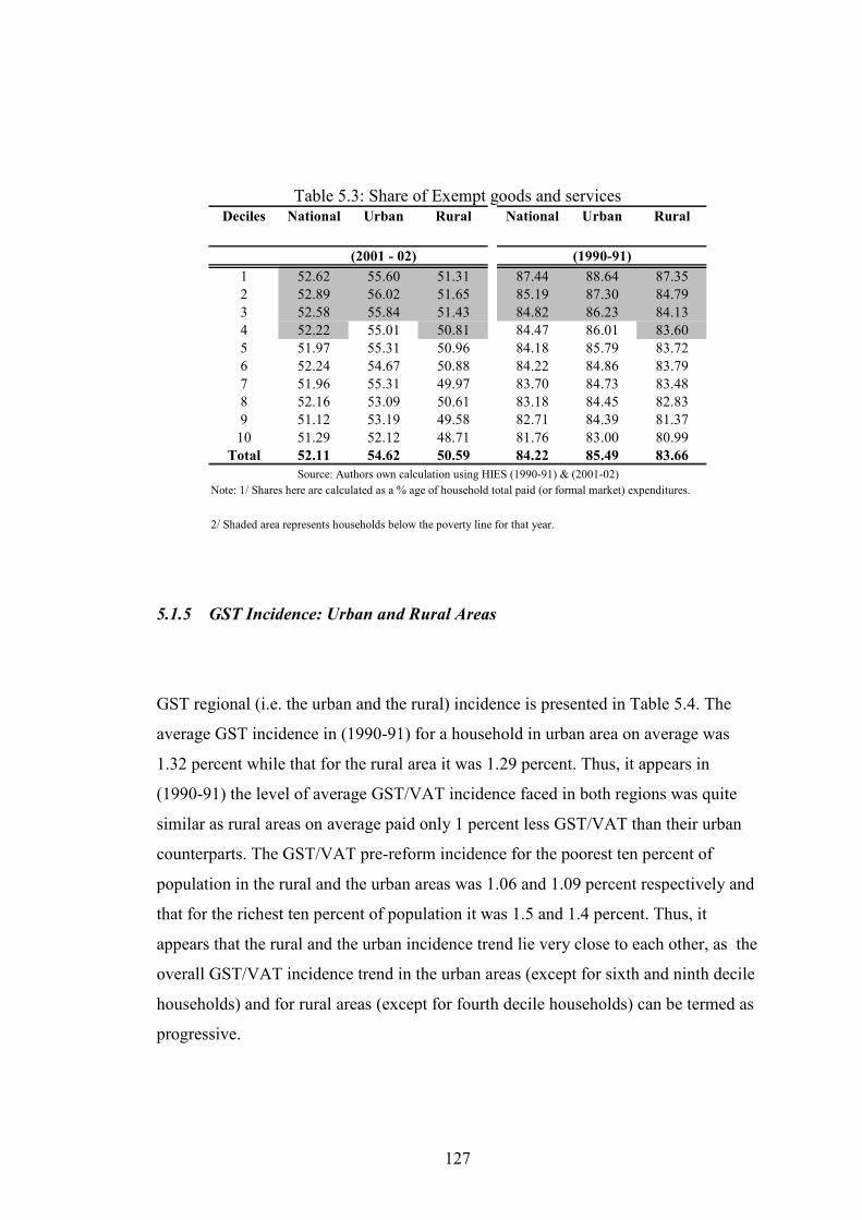
127

Table 5.3: Share of Exempt goods and services Deciles National Urban Rural National Urban Rural

1 52.62 55.60 51.31 87.44 88.64 87.35

2 52.89 56.02 51.65 85.19 87.30 84.79

3 52.58 55.84 51.43 84.82 86.23 84.13

4 52.22 55.01 50.81 84.47 86.01 83.60

5 51.97 55.31 50.96 84.18 85.79 83.72

6 52.24 54.67 50.88 84.22 84.86 83.79

7 51.96 55.31 49.97 83.70 84.73 83.48

8 52.16 53.09 50.61 83.18 84.45 82.83

9 51.12 53.19 49.58 82.71 84.39 81.37

10 51.29 52.12 48.71 81.76 83.00 80.99

Total 52.11 54.62 50.59 84.22 85.49 83.66

Source: Authors own calculation using HIES (1990-91) & (2001-02)

Note: 1/ Shares here are calculated as a % age of household total paid (or formal market) expenditures.

2/ Shaded area represents households below the poverty line for that year.

(2001 - 02) (1990-91)

5.1.5 GST Incidence: Urban and Rural Areas

GST regional (i.e. the urban and the rural) incidence is presented in Table 5.4. The

average GST incidence in (1990-91) for a household in urban area on average was

1.32 percent while that for the rural area it was 1.29 percent. Thus, it appears in

(1990-91) the level of average GST/VAT incidence faced in both regions was quite

similar as rural areas on average paid only 1 percent less GST/VAT than their urban

counterparts. The GST/VAT pre-reform incidence for the poorest ten percent of

population in the rural and the urban areas was 1.06 and 1.09 percent respectively and

that for the richest ten percent of population it was 1.5 and 1.4 percent. Thus, it

appears that the rural and the urban incidence trend lie very close to each other, as the

overall GST/VAT incidence trend in the urban areas (except for sixth and ninth decile

households) and for rural areas (except for fourth decile households) can be termed as

progressive.

128

If we look at the average GST/VAT incidence in 2001-02 i.e. the post reform era for

the rural and urban households, it averaged around 4.62 percent for the rural areas

compared with 4.80 percent for the urban areas. In (2001-02) the poorest ten percent

of the rural and the urban households were facing an incidence of 4.50 and 4.84

percent respectively while the richest ten percent of population in the rural and the

urban areas faced an incidence of 4.66 and 4.60 percent respectively. It appears the

incidence faced by the poorest ten percent of population in the rural areas was lowest

GST/VAT incidence on average faced by any rural decile in the post- reform era but

in the urban areas incidence faced by the poorest ten percent of population was the

highest incidence faced by any decile (except the fourth and sixth decile households).

As for the overall incidence trend for the regional population, it appeared to be

progressive for both the urban areas (at least over the bottom six deciles) and the rural

areas.

If we look at the proportionate increase in tax liabilities over time we can see that both

rural/urban areas on average experienced a 72 percent increase in tax liabilities.

However, the poorest ten percent of population in both the rural/urban areas

experienced a 77 percent increase in tax liabilities compared to 69 and 67 percent

increase in tax liabilities experienced by the urban and rural richest ten percent

respectively. Thus, it appeared GST reforms on average increased the tax liabilities

for the poorest segment of urban/rural population more than that for the richest

segment of population.

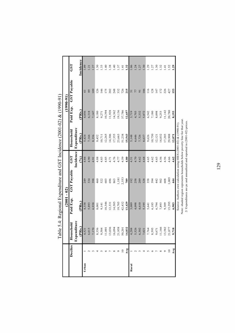
129

Tab

le 5

.4:

Reg

ional

Ex

pen

dit

ure

and G

ST

Inci

den

ce (

2001-0

2)

& (

1990-9

1)

Deciles

Household

Expenditure

(PRs.)

Paid Exp.

(PRs.)

GST Payable

GST

Incidence

(%)

Household

Expenditure

(PRs.)

Paid Exp.

(PRs.)

GST Payable

GST

Incidence

Urban

14

,52

14

,33

82

49

4.8

45

,42

44

,85

66

11

.09

26

,01

55

,89

33

34

4.9

07

,16

66

,31

88

91

.21

37

,17

06

,93

83

98

4.9

18

,35

67

,14

71

09

1.2

7

48

,35

68

,00

14

60

4.8

89

,45

28

,18

01

26

1.3

0

59

,58

49

,14

15

22

4.8

31

0,7

11

9,2

71

14

61

.33

61

1,0

01

10

,34

66

03

4.8

51

2,2

65

10

,39

41

75

1.4

0

71

3,0

36

12

,33

16

96

4.7

11

4,3

06

11

,92

82

02

1.3

8

81

6,0

94

14

,58

58

63

4.7

61

7,3

55

14

,36

22

48

1.4

0

92

1,9

58

19

,78

51

,18

14

.77

23

,66

31

9,1

36

33

21

.37

10

50

,20

14

2,4

32

2,5

53

4.5

95

1,2

38

37

,78

67

26

1.4

1

Avg

14,832

13,429

789

4.80

15,543

12,657

215

1.32

Rural

14

,28

83

,08

91

92

4.5

15

,14

83

,71

95

11

.06

25

,52

64

,09

82

58

4.7

06

,64

64

,70

37

71

.24

36

,30

24

,61

02

89

4.6

27

,72

65

,33

29

11

.27

47

,02

15

,19

53

28

4.6

88

,63

75

,87

21

06

1.3

0

57

,76

45

,64

13

58

4.6

59

,62

66

,54

21

16

1.2

9

68

,59

56

,18

53

94

4.6

21

0,7

50

7,1

80

12

81

.27

79

,67

16

,79

44

42

4.6

31

2,1

21

8,0

98

14

71

.30

81

1,1

66

7,8

93

50

24

.56

14

,03

29

,25

31

72

1.3

2

91

3,5

82

9,3

09

60

84

.56

17

,20

31

1,1

42

22

61

.41

10

21

,87

71

5,2

95

1,0

05

4.6

62

9,9

08

20

,78

04

27

1.5

2

Avg

9,718

6,903

444

4.62

12,071

8,193

153

1.29

Note

: sh

ad

ed

regio

n r

ep

rese

nts

hou

seh

old

s b

elo

w p

overt

y l

ine f

or

that

year.

2/

Exp

en

dit

ure

s a

re p

c a

nd

an

nu

ali

zed

an

d r

ep

ort

ed

in

(2

00

1-0

2)

pri

ces.

(2001 - 02)

(1990-91)

Sou

rce:

Au

thors

ow

n c

alc

ula

tion

usi

ng H

IES

(2

00

1-0

2)

& (

19

90

-91

).

130

5.2 Selected Commodity Incidence Analysis

The main reason for disaggregating GST/VAT incidence is to highlight the important

facts that remain hidden when we only look at the overall incidence picture only. For

instance, by disaggregating the incidence picture we can clearly see how this

incidence picture is being generated and also identify taxable commodities that may

be having powerful distributional impact on the poor. This we believe is a very

important information as far as the Government pro-poor policy agenda is concerned.

Table 5.5 presents GST/VAT disaggregated incidence picture for 1990-91 at national

as well as for the rural and the urban areas. It is perhaps no surprise to find a very few

items on the list as taxation under GST at this time was quite limited (due to plethora

of existing exemptions as discussed earlier). During 1990-91 the highest average GST

incidence share (as a percentage of total GST incidence) for a average Pakistani

household at national level came from food items (0.28 percent with almost 85

percent of this due to the taxation of sugar!). This was followed by petroleum, oil and

lubricant products (POL) taxation which was responsible for (0.27 percent of total

GST incidence), tobacco (0.15 percent), clothing (0.14 percent) and personal effects

(0.13 percent) respectively.

As perhaps expected, the overall incidence of the food category (also sugar) and

clothing items were clearly regressive. In addition to this we find that the GST

incidence on POL products appears to be strongly progressive. Furthermore, GST

incidence on tobacco also appears to be progressive but only for the first fifty percent

of population and slightly regressive afterwards (this ties well with our discussion of

selected commodities disaggregated expenditure analysis in section 4.4 of previous

chapter). According to our earlier discussion based on the pattern of expenditures on

131

major expenditure categories (as percentage of total household expenditure); food

items, clothing appeared to be necessities while POL products appeared to be a luxury

item. Thus if necessities are taxed they are likely to create a negative distributional

effect on the welfare of people.

The bottom part of Table 5.5 also presents the rural and the urban GST disaggregated

incidence shares (i.e. as a percentage of the total GST incidence) for 1990-91. This

analysis is important since it can help us figure out why average GST incidence and

the overall GST trend for both the urban and the rural areas in the pre- reform era

appeared to lie so close. Interestingly, the top GST incidence share for an urban

household on average was coming from POL product (0.30 percent). This was

followed by food items (0.25 percent share), tobacco (0.15 percent), personal effects

(0.14 percent) and clothing (0.13 percent). While for rural households on average the

most significant incidence share was coming from food items (0.30 percent), followed

by POL products (0.25 percent), tobacco and clothing (each at 0.15 percent), and

personal effect at 0.12 percent. Thus, it appeared as a result of underlying similar

patterns of expenditures on these taxable items in the rural/urban areas on average, the

respective incidence picture was also quite similar.

In terms of the overall GST incidence trend of these categories, in the urban areas

only POL product incidence appeared to be progressive while the incidence on food

items and clothing was significantly regressive. Additionally, the GST incidence on

tobacco group appeared to be of inverted U-shaped showing middle classes bearing

larger burden of tax compared to tails. Thus, one reason for the clear progressivity of

GST incidence in the urban areas appeared to be strong progressivity of GST

incidence on POL products. Furthermore, this to some extent was aided by the fact

that even though GST incidence on food fell across population as households became

more affluent but for the top fifty percent of population this fall in the GST incidence

on food was comparatively less sharp than increase in POL incidence on the other

side.

132

On the other side, for the rural areas, we also find GST incidence on POL products

progressive but regressive for food items. Furthermore, clothing incidence appears to

be regressive, while GST incidence on tobacco and personal effects to a large extent

appear to be proportional. However, compared to the urban population, GST

incidence on food appears to fall much slowly over deciles as population becomes

affluent (because of the underlying expenditure patterns). Thus, it appears GST

incidence progressivity in the rural areas appears to be largely driven by POL

incidence particularly due to strong progressivity of GST incidence on POL products

over the top fifty percent of population.

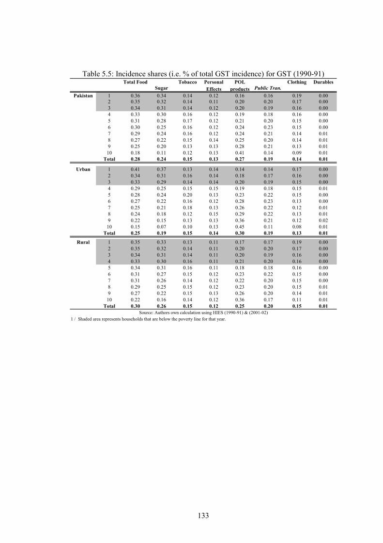
133

Table 5.5: Incidence shares (i.e. % of total GST incidence) for GST (1990-91) Total Food

Sugar

Tobacco Personal

Effects

POL

products Public Tran.

Clothing Durables

Pakistan 1 0.36 0.34 0.14 0.12 0.16 0.16 0.19 0.002 0.35 0.32 0.14 0.11 0.20 0.20 0.17 0.00

3 0.34 0.31 0.14 0.12 0.20 0.19 0.16 0.00

4 0.33 0.30 0.16 0.12 0.19 0.18 0.16 0.00

5 0.31 0.28 0.17 0.12 0.21 0.20 0.15 0.00

6 0.30 0.25 0.16 0.12 0.24 0.23 0.15 0.00

7 0.29 0.24 0.16 0.12 0.24 0.21 0.14 0.01

8 0.27 0.22 0.15 0.14 0.25 0.20 0.14 0.01

9 0.25 0.20 0.13 0.13 0.28 0.21 0.13 0.01

10 0.18 0.11 0.12 0.13 0.41 0.14 0.09 0.01

Total 0.28 0.24 0.15 0.13 0.27 0.19 0.14 0.01

Urban 1 0.41 0.37 0.13 0.14 0.14 0.14 0.17 0.00

2 0.34 0.31 0.16 0.14 0.18 0.17 0.16 0.00

3 0.33 0.29 0.14 0.14 0.20 0.19 0.15 0.00

4 0.29 0.25 0.15 0.15 0.19 0.18 0.15 0.01

5 0.28 0.24 0.20 0.13 0.23 0.22 0.15 0.00

6 0.27 0.22 0.16 0.12 0.28 0.23 0.13 0.00

7 0.25 0.21 0.18 0.13 0.26 0.22 0.12 0.01

8 0.24 0.18 0.12 0.15 0.29 0.22 0.13 0.01

9 0.22 0.15 0.13 0.13 0.36 0.21 0.12 0.02

10 0.15 0.07 0.10 0.13 0.45 0.11 0.08 0.01

Total 0.25 0.19 0.15 0.14 0.30 0.19 0.13 0.01

Rural 1 0.35 0.33 0.13 0.11 0.17 0.17 0.19 0.00

2 0.35 0.32 0.14 0.11 0.20 0.20 0.17 0.00

3 0.34 0.31 0.14 0.11 0.20 0.19 0.16 0.00

4 0.33 0.30 0.16 0.11 0.21 0.20 0.16 0.00

5 0.34 0.31 0.16 0.11 0.18 0.18 0.16 0.00

6 0.31 0.27 0.15 0.12 0.23 0.22 0.15 0.00

7 0.31 0.26 0.14 0.12 0.22 0.20 0.15 0.00

8 0.29 0.25 0.15 0.12 0.23 0.20 0.15 0.01

9 0.27 0.22 0.15 0.13 0.26 0.20 0.14 0.01

10 0.22 0.16 0.14 0.12 0.36 0.17 0.11 0.01

Total 0.30 0.26 0.15 0.12 0.25 0.20 0.15 0.01

Source: Authors own calculation using HIES (1990-91) & (2001-02)

1 / Shaded area represents households that are below the poverty line for that year.

134

The disaggregated incidence of GST/VAT for 2001-02 is presented in Table 5.6.

From this Table we can easily see the appearance of many new GST/VAT incidence

categories that were not there in 1990-91 (for instance, edible oils, and fuels/utilities).

At the national level we can see that the highest average GST/VAT incidence share

(in terms of total GST/VAT incidence) is coming from food items averaging around

0.34 percent, followed by incidence share on fuels/utilities (0.28 percent), clothing

and footwear (0.19 percent), POL products (0.15 percent), durables (0.08 percent),

personal care (0.07 percent), and tobacco (0.04 percent). We can also clearly see that

the GST/VAT incidence on food items, clothing (for the top fifty percent of

population) and fuel/utilities appears to be regressive. This should not be a surprise

given their underlying expenditure patterns show these to be necessities (for instance,

see section 4.4 of previous chapter). On the other hand, GST/VAT incidence for

durable items, and POL products, appears to be progressive (as these are also luxuries

according to our discussion in section 4.4). Furthermore, the incidence trend for

tobacco and personal care articles appears to be proportional for a large segment of

population.

If we look at the urban GST/VAT incidence in 2001-02 we can see that food items on

average appear to be the most significant incidence category (compared to POL

products in 1990-91) responsible for almost 24 percent of total GST/VAT incidence.

This is closely followed by an average incidence share of fuels/utilities at (0.20

percent), clothing (0.13 percent), POL products (0.11 percent), durables (0.05

percent), personal care (0.05 percent), and tobacco (0.03 percent) respectively.

A look at the GST/VAT disaggregated incidence trend for these categories reveals

that for urban areas only GST/VAT incidence on durables items and POL products is

progressive while GST/VAT incidence on clothing, tobacco and (all) food items

appears to be regressive. Furthermore, the GST/VAT incidence for personal care

items and fuels/utilities appears to be at best proportional (for a large segment of

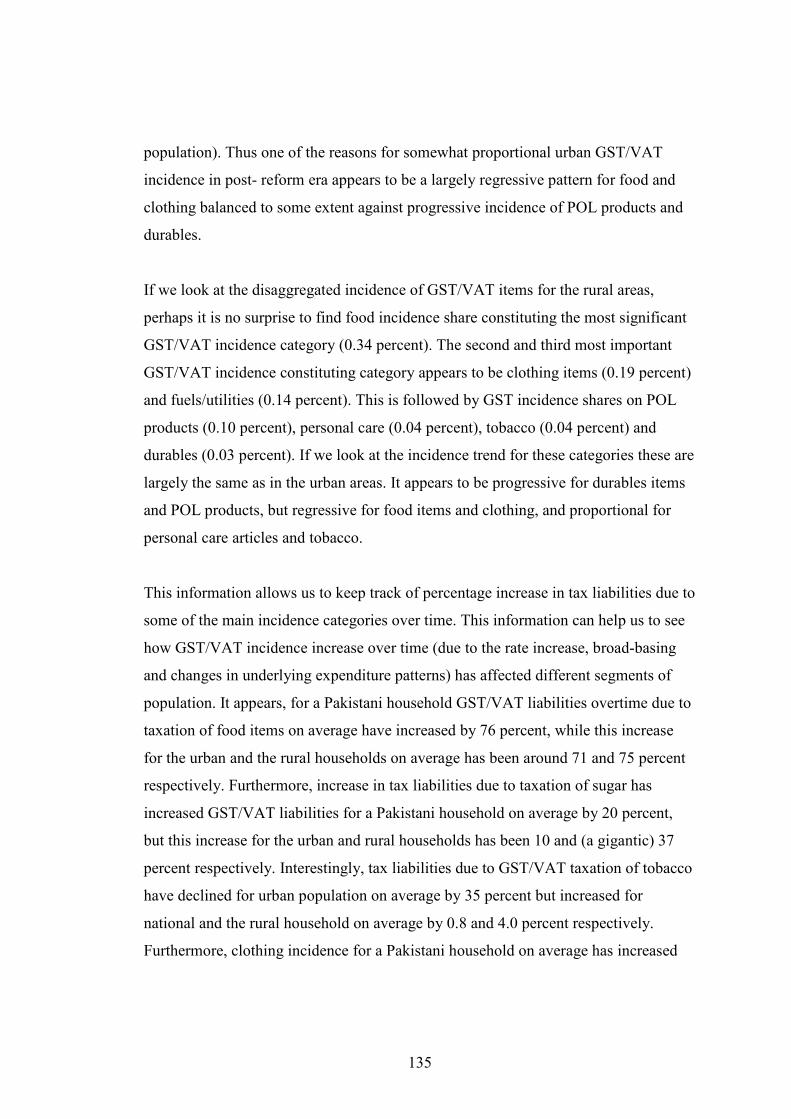
135

population). Thus one of the reasons for somewhat proportional urban GST/VAT

incidence in post- reform era appears to be a largely regressive pattern for food and

clothing balanced to some extent against progressive incidence of POL products and

durables.

If we look at the disaggregated incidence of GST/VAT items for the rural areas,

perhaps it is no surprise to find food incidence share constituting the most significant

GST/VAT incidence category (0.34 percent). The second and third most important

GST/VAT incidence constituting category appears to be clothing items (0.19 percent)

and fuels/utilities (0.14 percent). This is followed by GST incidence shares on POL

products (0.10 percent), personal care (0.04 percent), tobacco (0.04 percent) and

durables (0.03 percent). If we look at the incidence trend for these categories these are

largely the same as in the urban areas. It appears to be progressive for durables items

and POL products, but regressive for food items and clothing, and proportional for

personal care articles and tobacco.

This information allows us to keep track of percentage increase in tax liabilities due to

some of the main incidence categories over time. This information can help us to see

how GST/VAT incidence increase over time (due to the rate increase, broad-basing

and changes in underlying expenditure patterns) has affected different segments of

population. It appears, for a Pakistani household GST/VAT liabilities overtime due to

taxation of food items on average have increased by 76 percent, while this increase

for the urban and the rural households on average has been around 71 and 75 percent

respectively. Furthermore, increase in tax liabilities due to taxation of sugar has

increased GST/VAT liabilities for a Pakistani household on average by 20 percent,

but this increase for the urban and rural households has been 10 and (a gigantic) 37

percent respectively. Interestingly, tax liabilities due to GST/VAT taxation of tobacco

have declined for urban population on average by 35 percent but increased for

national and the rural household on average by 0.8 and 4.0 percent respectively.

Furthermore, clothing incidence for a Pakistani household on average has increased

136

by 79 percent, while this increase for the urban and the rural areas on average has

been around 74 and 78 percent respectively.

Thus, it appears GST broad-basing (and also change in rate and changes in underlying

expenditure patterns) to include un-processed food items, vegetable ghee on top of

sugar consumption that is already taxable, has relatively increased the GST incidence

burden for the poor more as compared to other segments of population. This change,

we believe, has been responsible for emergence of (largely) proportional GST

incidence at national as well as the urban/rural areas over time.

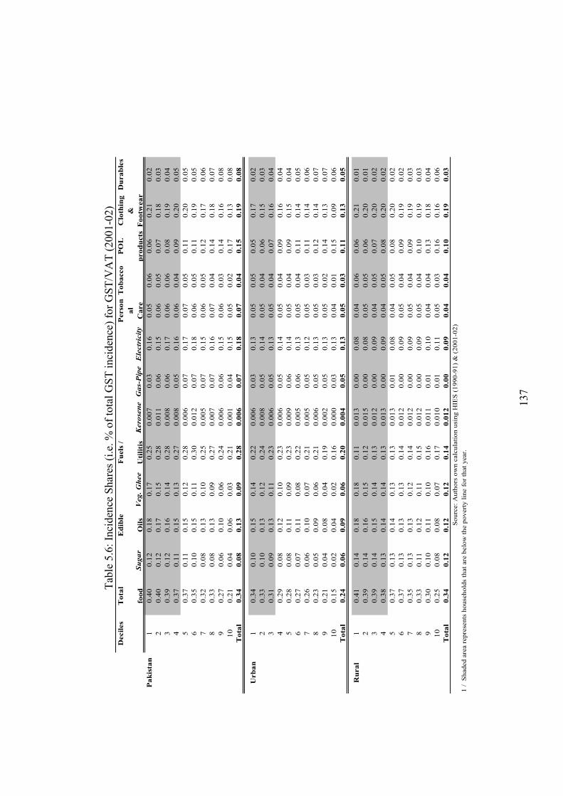
137

Tab

le 5

.6:

Inci

den

ce S

har

es (

i.e.

% o

f to

tal

GS

T i

nci

den

ce)

for

GS

T/V

AT

(2001-0

2)

Deciles

Total

food

Sugar

Edible

Oils

Veg. Ghee

Fuels /

Utilitis

Kero

sene

Gas-Pipe

Electricity

Person

al

Care

Tobacco

POL

products

Clothing

&

Footwear

Durables

Pakistan

10

.40

0.1

20

.18

0.1

70

.25

0.0

07

0.0

30

.16

0.0

50

.06

0.0

60

.21

0.0

2

20

.40

0.1

20

.17

0.1

50

.28

0.0

11

0.0

60

.15

0.0

60

.05

0.0

70

.18

0.0

3

30

.39

0.1

20

.16

0.1

40

.28

0.0

08

0.0

60

.17

0.0

60

.06

0.0

80

.19

0.0

4

40

.37

0.1

10

.15

0.1

30

.27

0.0

08

0.0

50

.16

0.0

60

.04

0.0

90

.20

0.0

5

50

.37

0.1

10

.15

0.1

20

.28

0.0

06

0.0

70

.17

0.0

70

.05

0.1

10

.20

0.0

5

60

.35

0.1

00

.15

0.1

10

.30

0.0

12

0.0

70

.18

0.0

60

.05

0.1

10

.19

0.0

5

70

.32

0.0

80

.13

0.1

00

.25

0.0

05

0.0

70

.15

0.0

60

.05

0.1

20

.17

0.0

6

80

.33

0.0

80

.13

0.0

90

.27

0.0

07

0.0

70

.16

0.0

70

.04

0.1

40

.18

0.0

7

90

.27

0.0

60

.10

0.0

60

.24

0.0

06

0.0

60

.15

0.0

60

.03

0.1

40

.16

0.0

8

10

0.2

10

.04

0.0

60

.03

0.2

10

.00

10

.04

0.1

50

.05

0.0

20

.17

0.1

30

.08

Total

0.34

0.08

0.13

0.09

0.28

0.006

0.07

0.18

0.07

0.04

0.15

0.19

0.08

Urban

10

.34

0.1

00

.15

0.1

40

.22

0.0

06

0.0

30

.13

0.0

50

.05

0.0

50

.17

0.0

2

20

.33

0.1

00

.13

0.1

20

.24

0.0

08

0.0

50

.14

0.0

50

.04

0.0

60

.15

0.0

3

30

.31

0.0

90

.13

0.1

10

.23

0.0

06

0.0

50

.13

0.0

50

.04

0.0

70

.16

0.0

4

40

.29

0.0

80

.12

0.1

00

.23

0.0

06

0.0

50

.14

0.0

50

.04

0.0

90

.16

0.0

4

50

.28

0.0

80

.11

0.0

90

.23

0.0

09

0.0

60

.14

0.0

50

.04

0.0

90

.15

0.0

4

60

.27

0.0

70

.11

0.0

80

.22

0.0

05

0.0

60

.13

0.0

50

.04

0.1

10

.14

0.0

5

70

.26

0.0

60

.10

0.0

70

.21

0.0

05

0.0

50

.12

0.0

50

.03

0.1

10

.14

0.0

6

80

.23

0.0

50

.09

0.0

60

.21

0.0

06

0.0

50

.13

0.0

50

.03

0.1

20

.14

0.0

7

90

.21

0.0

40

.08

0.0

40

.19

0.0

02

0.0

50

.13

0.0

50

.02

0.1

40

.13

0.0

7

10

0.1

50

.02

0.0

40

.02

0.1

60

.00

00

.03

0.1

30

.04

0.0

10

.15

0.0

90

.06

Total

0.24

0.06

0.09

0.06

0.20

0.004

0.05

0.13

0.05

0.03

0.11

0.13

0.05

Rural

10

.41

0.1

40

.18

0.1

80

.11

0.0

13

0.0

00

.08

0.0

40

.06

0.0

60

.21

0.0

1

20

.39

0.1

40

.16

0.1

50

.12

0.0

15

0.0

00

.08

0.0

50

.05

0.0

60

.20

0.0

1

30

.39

0.1

40

.15

0.1

40

.13

0.0

12

0.0

00

.09

0.0

40

.05

0.0

70

.20

0.0

2

40

.38

0.1

30

.14

0.1

40

.13

0.0

13

0.0

00

.09

0.0

40

.05

0.0

80

.20

0.0

2

50

.37

0.1

30

.14

0.1

30

.13

0.0

13

0.0

10

.08

0.0

40

.05

0.0

80

.20

0.0

2

60

.37

0.1

30

.13

0.1

30

.14

0.0

12

0.0

00

.09

0.0

50

.04

0.0

90

.19

0.0

2

70

.35

0.1

30

.13

0.1

20

.14

0.0

12

0.0

00

.09

0.0

50

.04

0.0

90

.19

0.0

3

80

.33

0.1

10

.12

0.1

10

.15

0.0

12

0.0

00

.09

0.0

50

.04

0.1

00

.19

0.0

3

90

.30

0.1

00

.11

0.1

00

.16

0.0

11

0.0

10

.10

0.0

40

.04

0.1

30

.18

0.0

4

10

0.2

50

.08

0.0

80

.07

0.1

70

.01

00

.01

0.1

10

.05

0.0

30

.16

0.1

60

.06

Total

0.34

0.12

0.12

0.12

0.14

0.012

0.00

0.09

0.04

0.04

0.10

0.19

0.03

So

urc

e:

Au

tho

rs o

wn

calc

ula

tio

n u

sin

g H

IES

(1

99

0-9

1)

& (

20

01

-02

)

1 /

S

had

ed

are

a r

ep

rese

nts

ho

use

ho

lds

that

are

belo

w t

he p

ov

ert

y l

ine f

or

that

year.

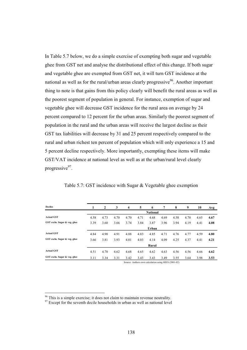
138

In Table 5.7 below, we do a simple exercise of exempting both sugar and vegetable

ghee from GST net and analyse the distributional effect of this change. If both sugar

and vegetable ghee are exempted from GST net, it will turn GST incidence at the

national as well as for the rural/urban areas clearly progressive96. Another important

thing to note is that gains from this policy clearly will benefit the rural areas as well as

the poorest segment of population in general. For instance, exemption of sugar and

vegetable ghee will decrease GST incidence for the rural area on average by 24

percent compared to 12 percent for the urban areas. Similarly the poorest segment of

population in the rural and the urban areas will receive the largest decline as their

GST tax liabilities will decrease by 31 and 25 percent respectively compared to the

rural and urban richest ten percent of population which will only experience a 15 and

5 percent decline respectively. More importantly, exempting these items will make

GST/VAT incidence at national level as well as at the urban/rural level clearly

progressive97.

Table 5.7: GST incidence with Sugar & Vegetable ghee exemption

96 This is a simple exercise; it does not claim to maintain revenue neutrality. 97 Except for the seventh decile households in urban as well as national level

Deciles 1 2 3 4 5 6 7 8 9 10 Avg

Actual GST 4.58 4.73 4.70 4.70 4.71 4.68 4.69 4.58 4.70 4.65 4.67

GST exclu. Sugar & veg. ghee 3.39 3.60 3.66 3.74 3.84 3.87 3.96 3.94 4.19 4.41 4.08

Actual GST 4.84 4.90 4.91 4.88 4.83 4.85 4.71 4.76 4.77 4.59 4.80


Actual GST 4.51 4.70 4.62 4.68 4.65 4.62 4.63 4.56 4.56 4.66 4.62


Source: Authors own calculation using HIES (2001-02)

National

Urban

Rural

139

However, the question of what must be exempt from GST/VAT in Pakistan is a

critical policy question particularly as far as Governments pro-poor agenda is

concerned. In the next section, we explicitly address the question of GST/VAT

exemptions in order to determine how GST/VAT exemptions can be better targeted to

provide relief to the poor.

5.3 Analysis of GST exemptions using Distributional Characteristics of a good

approach

In the earlier section we have seen that the GST incidence for 2001-02 appears to be

regressive. With that we have also seen that increase in GST incidence over time has

been proportionally much higher for the poor segment of the population and for those

in the rural areas. This is quite interesting since, on the one hand, policymakers in

Pakistan claim to have adequately sheltered the poor against GST (by exempting basic

items consumed by the poor) on the other hand our GST incidence results do not

match with the policymaker’s claims. Thus it is quite possible that GST exemptions

are not working the way they are supposed to. Although in the earlier section we have

briefly talked about GST exemption, in this section we will probe this issue

empirically and attempt to evaluate how well placed GST exemptions in Pakistan

really are by first addressing the issue of what is really being consumed by the poor in

Pakistan98.

The question of what the poor really consume in Pakistan has never been really

addressed. Are only basic (un-processed) food items (namely, cereals, vegetables,

pulses and fruits) more important to the poor as far as their budget is concerned? How

98 For instance according to Ahmad and Stern (1987) a uniform VAT in India would reduce the expenditures of the poorest segment of population in the rural areas by almost 7 percent compared to 5 percent for the urban poorest. These estimates suggest a strong distributional case for exemptions in general and that such exemptions may play an important role in poverty reduction in developing countries (Bird and Zolt, 2005).

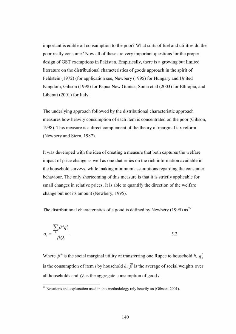
140

important is edible oil consumption to the poor? What sorts of fuel and utilities do the

poor really consume? Now all of these are very important questions for the proper

design of GST exemptions in Pakistan. Empirically, there is a growing but limited

literature on the distributional characteristics of goods approach in the spirit of

Feldstein (1972) (for application see, Newbery (1995) for Hungary and United

Kingdom, Gibson (1998) for Papua New Guinea, Sonia et al (2003) for Ethiopia, and

Liberati (2001) for Italy.

The underlying approach followed by the distributional characteristic approach

measures how heavily consumption of each item is concentrated on the poor (Gibson,

1998). This measure is a direct complement of the theory of marginal tax reform

(Newbery and Stern, 1987).

It was developed with the idea of creating a measure that both captures the welfare

impact of price change as well as one that relies on the rich information available in

the household surveys, while making minimum assumptions regarding the consumer

behaviour. The only shortcoming of this measure is that it is strictly applicable for

small changes in relative prices. It is able to quantify the direction of the welfare

change but not its amount (Newbery, 1995).

The distributional characteristics of a good is defined by Newbery (1995) as99

i

h

i

h

h

iQ

q

dβ

β∑≡ 5.2

Where hβ is the social marginal utility of transferring one Rupee to household h, i

hq

is the consumption of item i by household h, β is the average of social weights over

all households and iQ is the aggregate consumption of good i.

99 Notations and explanation used in this methodology rely heavily on (Gibson, 2001).

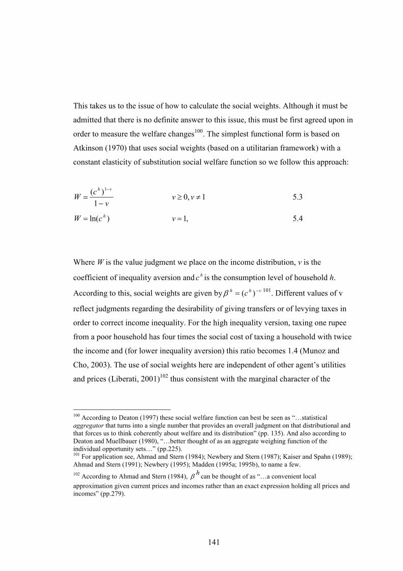
141

This takes us to the issue of how to calculate the social weights. Although it must be

admitted that there is no definite answer to this issue, this must be first agreed upon in

order to measure the welfare changes100. The simplest functional form is based on

Atkinson (1970) that uses social weights (based on a utilitarian framework) with a

constant elasticity of substitution social welfare function so we follow this approach:

v

cW

vh

−=

−

1

)( 1

1,0 ≠≥ vv 5.3

)ln( hcW = ,1=v 5.4

Where W is the value judgment we place on the income distribution, v is the

coefficient of inequality aversion and hc is the consumption level of household h.

According to this, social weights are given by vhh c −= )(β 101. Different values of v

reflect judgments regarding the desirability of giving transfers or of levying taxes in

order to correct income inequality. For the high inequality version, taxing one rupee

from a poor household has four times the social cost of taxing a household with twice

the income and (for lower inequality aversion) this ratio becomes 1.4 (Munoz and

Cho, 2003). The use of social weights here are independent of other agent’s utilities

and prices (Liberati, 2001)102 thus consistent with the marginal character of the

100 According to Deaton (1997) these social welfare function can best be seen as “…statistical aggregator that turns into a single number that provides an overall judgment on that distributional and that forces us to think coherently about welfare and its distribution” (pp. 135). And also according to Deaton and Muellbauer (1980), “…better thought of as an aggregate weighing function of the individual opportunity sets…” (pp.225). 101 For application see, Ahmad and Stern (1984); Newbery and Stern (1987); Kaiser and Spahn (1989); Ahmad and Stern (1991); Newbery (1995); Madden (1995a; 1995b), to name a few.

102 According to Ahmad and Stern (1984), hβ can be thought of as “…a convenient local

approximation given current prices and incomes rather than an exact expression holding all prices and incomes” (pp.279).

142

approach that identifies direction of reforms but not their amounts (Ahmad and Stern,

1984).

The distributional characteristics ranking for 165 items in the HIES (2001-02) is

reported in Appendix 5.1 corresponding to relatively little, and higher inequality

aversion (v = 0.5, 2.0). By looking at Appendix 5.1 we can see clearly that two out of

the first four items are own produced and consumed items (namely beg gasses , and

dung-cake). It is perhaps little surprise to find various food items ranked at the very

start of the list (implying these are disproportionately more consumed by the poor).

We find cereals ranked at the start of the list (for instance wheat is ranked 7,

maize/barley ranked 17 and rice is ranked 19). Similarly some spices such as salt at 10

and chillies at 12, are proportionally more consumed by the poor. Additionally, some

vegetables are ranked as quite important for the poor (for instance potato is ranked 18,

onion at 25, karaila, lady finger, brinjal and cucumber ranked at 26 and tinda,

pumpkin and bottle gourd are ranked 27). Pulses are also quite early on the list as

expected (for example other pulses are ranked at 15, dal channa is ranked 21, moong

at 23, and masoor at 38).

Perhaps it is a bit surprising to find some tobacco based items ranked so early (for

instance biri is ranked at 3, raw tobacco at 16 and cigarettes at 24). Another surprise is

to find some of home fuel items ranked so early (reflecting that these are

disproportionately more consumed by the poor). For example, we find firewood

ranked 11, coal ranked 14, charcoal ranked 31 and kerosene oil is ranked at 34. It is

also a surprise to find items from the edible oil group ranked so early (for example,

other oils and fats at 6, and vegetable ghee ranked at 13). We also find sugar and

clothing items being disproportionately more important for the poor, for instance

sugar is ranked 20 while clothing items are ranked 50.

Even under lower inequality aversion, using distributional characteristic ranking, we

can find a clear difference in goods that are important for the poor and for the rich.

143

For instance, the first fruit to appear on the list is mango and it is ranked 70. Utilities

such as electricity is ranked 82, gas pipe ranked 109 and gas cylinder 110, appear to

be more important for the rich. Travelling expenditures such as travelling by train is

ranked 107, petrol/diesel charges ranked 151, and air-travel ranked 154 appear to be

highly skewed toward the richer segments of population. Within edible oil group it

appears cooking oil is disproportionately more consumed by the rich as it is ranked at

130. Similarly, items related to educational expenses, health expense and housing also

appear to be disproportionately more important for the rich.

If we use a higher inequality aversion, i.e. v = 2.0, we find some changes in the list

but nothing too drastic103. Within the cereal group, we find wheat becoming more

important for the poor as it moves from 7 to 6, while there is no change for rice flour

(ranked 19) but maize, barley and jawar fall in rank from 17 to 37. If we look at fuel

items that were important for the poor under low inequality aversion, we find

firewood slightly falling down in ranking from 11 to 16, coal becoming very

important as it moves to 2 from 14, while both charcoal and kerosene oil slightly fall

in ranking (charcoal from 31 to 41 and kerosene 34 to 36). If we look at the edible

oils, both other oils and fat (previously ranked 6 now 3) and vegetable ghee

(previously ranked 13 now 11) become proportionally more important for the poor

when higher inequality aversion is used.

Similarly, biri falls in ranking from 3 to 7, both cigarettes and raw-tobacco move up

in the ranking (cigarettes move from 24 to 20 while raw-tobacco moves from 16 to

13). Utilities still remain important for the rich with electricity slightly falling down in

ranking from 82 to 74, while gas pipe and gas cylinder appears to be even more

skewed toward the richer segment of population. Similarly, travelling expenditures

such as travelling by train, by-air and petrol/diesel charges appear to become more

important for the richer segment of population. Also, edible oil items previously

103 The fact that such listing do not appear to be too sensitive to the middle ranges of inequality aversion (i.e. 0.5 and 2.0) is also reported by Gibson, (1998) for Papua New Guinea, Sonia et al (2003) for Ethiopia, and Liberati (2001) for Italy.

144

important for the richer segment of population, namely cooking oil and desi-ghee

become more skewed toward the richer segment of population.

Thus, this ranking is immensely important in the case of Pakistan because for certain

categories it clearly shows exemptions that would be beneficial for improving

distributional burden of GST as well for meeting Government‘s poverty alleviation

initiatives. For instance, sometimes it is asserted that VAT exemptions cannot be

better targeted than generally exempting basic food items since consumption patterns

are not sufficiently separable to provide low-income household necessary protection.

However, in the case of ranking for Pakistan (at such disaggregated level) we saw

clear separable consumption patterns in key commodities that can be targeted to

provide relief for the poor.

For instance information in Appendix 5.1 is summarized in Table 5.8 for key

elements along with information on whether these are taxed or not. We can clearly see

that within the edible oil group; other oils and fats (ranked 6 under low inequality

aversion), vegetable ghee (ranked 13 under low inequality aversion) are important for

the poor compared to cooking oil that is ranked 130 but all three are taxed. Similarly,

within the fuel and utilities group basic fuels are disproportionately more consumed

by the poor (even under low inequality aversion firewood is ranked 11, coal at 14,

charcoal at 31 and kerosene oil is ranked at 34) while utilities such as electricity and

gas-pipe are ranked at 82 and 109 (under low inequality aversion) but both categories

are being taxed. Similarly, sugar ranked at 20 (under low inequality aversion) is taxed.

Some food items such as chicken meat, mutton and particularly fruits are very high up

in the ranking (thus benefiting the rich more) but these are exempt.

Thus looking at this list, if distributional issues and poverty alleviation issue are at the

heart of Government policy agenda, it has an option to fine- tune exemptions that can

help alleviate the burden of GST from the poor segment of population particularly

within categories such as edible oils, basic fuels and sugar where there is a clear

145

difference between the types of commodities consumed by the poor and the rich and

where revenue loss may not be significant.

Does this mean that distributional characteristics ranking of expenditure items in

Pakistan is very different from other countries which requires a different pattern of

exemptions? This question can be answered in the light of existing evidence of

distributional characteristic ranking for Papua New Guinea (PNG), and Italy (former

developing countries and latter a developed country) with prime exemptions

candidates mentioned in the case of Pakistan (see previous discussion)104. In the case

of Papua New Guinea (PNG), Gibson (1998) ranks 87 goods in the PNG survey. In

the PNG case (under low inequality aversion), goods disproportionately more

important for the poor are firewood (ranked 3), leaf tobacco (7), sugar cane (9),

children clothing (16), adult clothing (23), sugar (26), kerosene (29) and cigarettes

(37) while goods that were disproportionately more important for the rich included

health, housing, travel expenses and expenses on electricity etc.

While in the case of Italy, Liberati (2001) provides ranking of 68 goods in the Italian

HES survey and the main findings are as following. Under low inequality aversion,

sugar is ranked 1, electricity (3), other meat (7), Pasta (8), beef (12), telephone (14),

oil (15), gas (17), vegetables (16), other cereals (19), tobacco (21), medicine (24),

coal (34), cloths (53), and kerosene (63).

Thus, it appears the distributional characteristic ranking in the case of Pakistan is

more similar to PNG as compared to Italy. For instance, if we look at the Italian

ranking, it appears, clothing items, kerosene and coal (under low inequality aversion)

is being disproportionately more consumed by the rich! That is quite opposite to PNG

and Pakistan. Additionally for Italy, it appears utilities such as gas and electricity are

better candidates for exemptions compared to basic fuels. Also, we see other items

104 Here a comparison with Ethiopia was not possible because the author did not include a complete listing with her work.

146

such as education, health expenses, telephone charges, appear quite early in the list

which is not the case for either PNG or Pakistan. Thus, it appears that the

distributional characteristics ranking in the case of a developing and a developed

country can be different; as a result what is more important for the poor is also

different. However, since GST/VAT reforms in most of the developing countries are

designed and dictated by IFI’s, it is perhaps no surprise to find that VAT/GST

harmonization over the years has failed to take this difference into account (that can

be very important for the poor).

5.4 Conclusion

GST/VAT is the most pervasive feature of tax reforms in many developing countries

including Pakistan. This highlights the importance of evaluating GST/VAT incidence

in Pakistan in both pre- and post- reform era to see how GST incidence at the national

as well as the urban/rural levels has changed over time. And given, the current and

future importance of this tax in many countries, it is also important to evaluate how

this tax can be better structured (particularly via exemptions) to address the

distributional issues. Thus, this chapter has tried to present the overall GST incidence

picture along with the disaggregated incidence picture in order to clearly show how

the underlying incidence is generated and how it has impacted various segments of

population at both the national level and the urban/rural areas over time.

We have tried to highlight that certain steps in the reform strategy (such as GST/VAT

broad basing to include processed food items such as sugar, vegetable ghee etc.)

appear to be having strong distributional impact particularly as far as the poorest and

most vulnerable segments of the population are concerned. Similarly extension of

GST/VAT to basic fuels such as kerosene, firewood, coal etc. in order to maintain

147

GST/VAT uniformity appear to be creating significant burden for the poor and for

those in the rural areas.

We also believe that the issue of GST/VAT exemptions in developing countries needs

to be looked at more carefully if GST/VAT development over time has to keep in line

with the Government pro-poor agenda. It appears at the moment policymakers in

Pakistan are not paying sufficient attention to the fact that consumption patterns for

key commodities are clearly separable. This separation should provide a very good

opportunity to the policymakers to fine- tune GST/VAT exemptions to safeguard the

poor (and not necessary at too much cost to the exchequer). And this chapter has tried

to answer how GST/VAT exemptions can be better tailored to safeguard the poor in

Pakistan.

Although analysis of the incidence of a single tax (in this case GST/VAT) over time is

important on its own we do need to look at the overall indirect tax incidence over

time for Pakistan in order to see how social incidence of indirect taxes in Pakistan has

changed due to the type of reform process followed in Pakistan. This is undertaken in

the next chapter which completes the discussion on the social incidence of indirect

taxes at pre- and post- reform era in Pakistan by first looking at custom duty and

excise duty incidence (in that order) and than completing the picture by bringing all

components together.

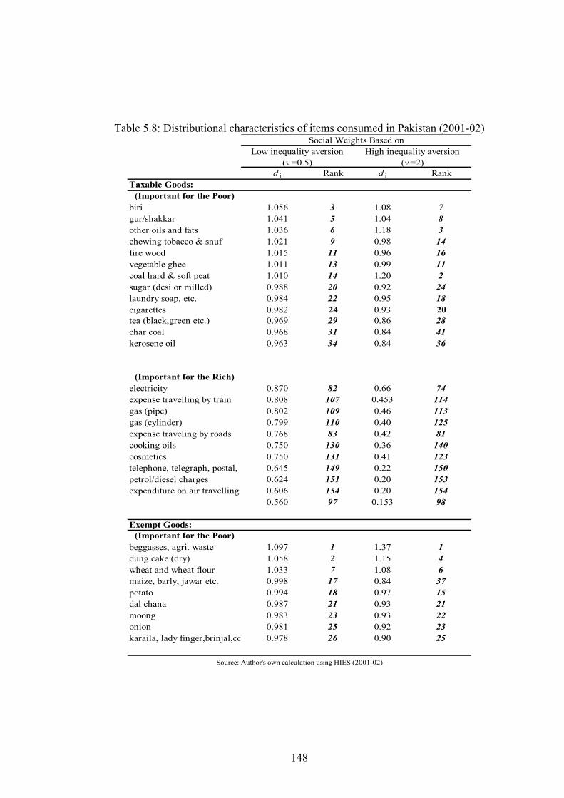
148

Table 5.8: Distributional characteristics of items consumed in Pakistan (2001-02)

d i Rank d i Rank

Taxable Goods:

(Important for the Poor)

biri 1.056 3 1.08 7

gur/shakkar 1.041 5 1.04 8

other oils and fats 1.036 6 1.18 3

chewing tobacco & snuf 1.021 9 0.98 14

fire wood 1.015 11 0.96 16

vegetable ghee 1.011 13 0.99 11

coal hard & soft peat 1.010 14 1.20 2

sugar (desi or milled) 0.988 20 0.92 24

laundry soap, etc. 0.984 22 0.95 18

cigarettes 0.982 24 0.93 20

tea (black,green etc.) 0.969 29 0.86 28

char coal 0.968 31 0.84 41

kerosene oil 0.963 34 0.84 36

(Important for the Rich)

electricity 0.870 82 0.66 74

expense travelling by train 0.808 107 0.453 114

gas (pipe) 0.802 109 0.46 113

gas (cylinder) 0.799 110 0.40 125

expense traveling by roads 0.768 83 0.42 81

cooking oils 0.750 130 0.36 140

cosmetics 0.750 131 0.41 123

telephone, telegraph, postal, etc 0.645 149 0.22 150

petrol/diesel charges 0.624 151 0.20 153

expenditure on air travelling etc. 0.606 154 0.20 154

0.560 97 0.153 98

Exempt Goods:

(Important for the Poor)

beggasses, agri. waste 1.097 1 1.37 1

dung cake (dry) 1.058 2 1.15 4

wheat and wheat flour 1.033 7 1.08 6

maize, barly, jawar etc. 0.998 17 0.84 37

potato 0.994 18 0.97 15

dal chana 0.987 21 0.93 21

moong 0.983 23 0.93 22

onion 0.981 25 0.92 23

karaila, lady finger,brinjal,cocumber0.978 26 0.90 25

Source: Author's own calculation using HIES (2001-02)

Social Weights Based on

Low inequality aversion

(v =0.5)

High inequality aversion

(v =2)

149

Chapter VI: Overall Indirect Tax Incidence in

Pakistan (1990 – 2001)

6 Introduction

Our incidence analysis started in the previous section with determining the

social incidence of GST during the pre- and post- reform time. Our analysis in

the previous chapter showed that as a result of reform process the incidence of

GST has increased substantially over time and the overall incidence looks

proportional for most of the population. Although, it is meaningful to ascertain

the incidence of a single component of tax system particularly GST/VAT

(which in the case of Pakistan has emerged as the single most important tax

component), what really matters is the collective tax incidence picture not its

individual components. Thus, the main aim of this chapter is to determine the

overall indirect tax incidence for Pakistan at the pre- and post- reform time.

This is an extremely important issue because it will allow us to determine

whether equity envisaged (as a part of reform process) was really translated

into policy actions (that made the overall indirect tax system progressive).

For this purpose this Chapter is divided into four sections. We start with

determining the incidence of remaining components of indirect tax system at

the pre- and post- reform time before we put them together. This is important

because it gives a clear and transparent picture of how the overall indirect tax

incidence is being put together. Thus, the first section begins with determining

the custom duties incidence at the pre- and post- reform time at national as

well as for the urban/ rural areas, along with discussion on the underlying

150

methodology and assumptions used for incidence determination. The second

section estimates the social incidence of excise duties at the pre- and post--

reform time and provides a description of methodology used for incidence

calculation. The third section moves to the main aim of this study, that is to

determine the social incidence of overall indirect taxes in Pakistan at the pre-

and post-- reform time. This section enables us to ascertain if the indirect tax

system has really changed in line with the vision of RMTRC at least where

equity is concerned, which is also the central question of this study. The last

section concludes.

6.1 Custom Duty Incidence (1990-91) to (2001-02)

6.1.1 Measuring Imports Content (IMPCON) within Domestic

Consumption

Since trade taxes are levied on the imported items, the base for determining

payable custom duties is consumption of imported items not consumption of

domestically produced goods. Thus, this section will try to establish how this

study measures proportionate consumption of the imported goods within total

domestic consumption of these goods, which is a clear improvement in the

methodology used for estimation for trade tax incidence.

It is not an exaggeration to admit that determining custom duties incidence is

not straightforward. The complication arises from the fact that in order to

accurately assess the custom duties incidence we need to know the content of

imported goods consumption within total domestic consumption (IMPCON)

for each good (at respective level of unit of analysis which in our case is the

151

household). Since information in HIES survey does not distinguish between

imported and domestically consumed goods we have no way of directly

ascertaining this information from the survey. As a result, we have to rely on

other data sources such as aggregate data on domestic production and

aggregate import/export data in order to get some sense of this estimate.

However, since data on domestic production and trade is available at an

aggregated level we can only calculate the IMPCON ratio for a few broad

categories of goods and henceforth use the same ratio for all items within that

category.

The IMPCON ratio is calculated in the following way.

IMPCONA = IMA / (IMA + DPA – EXA) 6.1

Where, IMPCONA is the imported content of good A within the domestic

consumption of good A. IMA is the import value, DPA is the domestic

production and EXA is the export value of good A (all in PRs.). This

relationship enables us to estimate proportionate imported content

(IMPCONA) for 19 categories of goods (see for instance Appendix 6.1).

6.1.2 Additional data sources used for calculating IMPCON

The additional data sources used for calculating IMPCON are as follows:

i. Production data105:

105 Production data for Pakistan does not include data on other sectors such as services.

152

a. Agriculture production data is taken from the Agriculture

Statistical Year Books for Pakistan (various years).

b. Manufacturing production data is taken from the Census of

Manufacturing Industries (CMI) (1990-91) and (2000-01)106.

ii. Import and export data:

a. Data on imports and export of agriculture goods is taken from

the Agriculture Year Books of Pakistan (various years)107.

b. Remaining import and export data is taken from the Statistical

Yearbooks of Pakistan (various years)108.

6.1.3 Additional assumptions

This section like the previous chapter uses the assumption that custom duties

are fully borne by the consumers of tradable items and this assumption is

made by a large number of studies for developed as well as developing

countries. But this has been severely criticised by Shah and Whalley (1991)

according to whom, the presence of binding quotas and tariff licensing scheme

on trade taxes may result in tax shifting of less than a hundred percent since

106 The (2000-01) manufacturing data is updated using (2001-02) sectoral growth rates as reported in Economic Survey of Pakistan (2001-02) which reports 5 percent growth rate for manufacturing sector. Thus, all categories covered in the CMI (2000-01) are updated using this rate except dairy products for which a 3.7% rate of growth of livestock GNP for (2001-02) is used. 107 However, data on fruits, vegetables and condiment is taken from Fruit, Vegetables and Condiment Statistics for Pakistan (various years). 108 With exception of trade data on pulses, edible oil, tea/coffee/green tea, and bakery products that is provided directly on request by Pakistan Custom House Karachi.

153

these taxes may more or less operate like lump-sum taxes; borne by the

recipients of rents.

Although, this may be true in some cases, in the case of Pakistan, we believe

using a hundred percent tax shifting assumption makes more sense because

although earlier empirical evidence on shifting of trade taxes in Pakistan

supports Shah and Whalley (1991) criticism (for instance see Pal, 1964; and

Alamgir, 1968), later evidence on trade tax shifting supports a full or even

higher tax shifting possibility (for example see Irfan, 1974; and Naqvi,

1975)109.

Also, since most of the binding restrictions on quotas and import licensing

scheme in Pakistan were largely removed by the early 1990’s (for instance see

World Trade Organization, 1995)110, this makes trade tax structure in the

decade of 1990 less relevant for the structure described by Shah and Whalley

(1991). As a result, we feel that a hundred percent tax shifting assumption is

the right assumption to use in this analysis.

6.1.4 Custom duty rates111

Custom duty rates for (1990-91) and (2001-02) are directly provided by the

Central Board of Revenue (CBR), Pakistan on request. These rates were used

as statutory rates for incidence calculation with two exceptions; (a) In cases

where HIES expenditure category included more than one statutory rate, the

weighted average duty rate was used, (b) in cases where duty rates were levied

109 Tax shifting assumptions are discussed in detail in Chapter 3: Literature Review (pp.21-23). 110 For instance see custom duty discussion in Chapter 2: Taxation in Pakistan (1985-2001), pp. 28-36. 111 See Appendix 6.2 (pp. 270) for Custom duty rates for (2001-02) & (1990-91).

154

by weight (for instance edible oils and fats group and pharmaceutical

products), effective duty rates were used.

6.1.5 Estimating Custom duty amounts and incidence

Now we are in the position to determine the calculation of custom duty

incidence. This is calculated using the following equations:

jji

j

j

ji IMPCONec

cD ..

1,, +

= 6.2

where

jiD , = household i’s per capita custom duty payment on good j

jc = statutory custom duty rate on good j

jie , = observed expenses or post- tax per capita expenditures on good j

Similar to GST incidence, custom duty payable is also calculated with

reference to only paid or formal market transactions. Payable custom duties on

various dutiable items is summed across the relevant households and

calculated on per capita basis. Additionally, average payable dutiable amount

per decile is calculated by aggregating this amount over each decile and

incidence is calculated with reference to average (net) total household per

capita expenditure112 for each decile.

112 The progressivity, regressivity or proportionality definition used in this chapter is

discussed in section 5.3.3. The same definition is used for all taxes.

155

6.1.6 Empirical Results

6.1.6.1 Custom Duty Incidence (1990-2001) at national level

The apparent difference in the importance of trade taxes within total federal

structure of Pakistan over time is also evident in custom duty incidence.

Custom duty incidence results are presented in Table 6.1. The custom duty

incidence for an average Pakistani household in 1990-91 stood at 2.89 percent.

The incidence for the poorest and richest ten percent of population on average

stood at 3.26 and 2.22 percent respectively. This meant that the incidence

faced by the richest ten percent of population was 32 percent less than the duty

incidence borne by the poorest segment of population. If we look at the overall

trend of custom duties incidence in (1990-91) at pre-reform era, it appeared to

be clearly regressive. The results appeared to be largely driven by import

duties on edible oils, sugar/sugar preparations, spice and condiment group and

also wheat, which were important imported consumption commodities for the

poor.

By (2001-02), the customs duty incidence for an average Pakistani household

stood at 1.35 percent. The average custom duty incidence for the poorest and

the richest ten percent of population in (2001-02) stood at 1.23 and 1.54

percent respectively. This meant that at the post--reform era the gap between

what the poorest and the richest segment of population was paying narrowed

to 25 percent. The incidence trend for (2001-02) except for sixth decile

households appeared to be clearly progressive. Thus it appeared, as a result of

the trade tax reform carried out during the decade of 1990s two things

happened: (a) overall the level of incidence at national level was reduced by

156

fifty percent for most deciles; (b) the overall incidence in the post- reform era

appears to have become progressive. This was mainly due to the combination

of three different things over time; changing consumption patterns, change in

dutiable rates and changes in IMPCON ratios. But, it is difficult to disentangle

change in incidence over time due to these factors individually. However, it

appears the progressivity of custom duties at the post-- reform time was

largely driven by importance of POL product and miscellaneous expenditure

items (such as bath soap, shampoo etc) within the budget of affluent

households.

It appears over time, due to the tax reform process, custom duty tax liabilities

for an average Pakistani household have been reduced by 53 percent. The

highest reduction in tax liabilities over time is experienced by the poorest ten

percent households which is equal to 62 percent, while the richest ten percent

households have experienced only 31 percent decline in tax liabilities due to

custom duty reforms over time. Thus we can say that the highest relief of

scaling down of custom duties taxation is experienced by most deserving part

of the population. This has been a fundamental change in the incidence of

custom duties over time along with a clear change in the trend of underlying

incidence of custom duties from a clearly regressive to a progressive pattern.

The rural/urban results are also presented in Table 6.1, which are quite similar

to the overall national results.

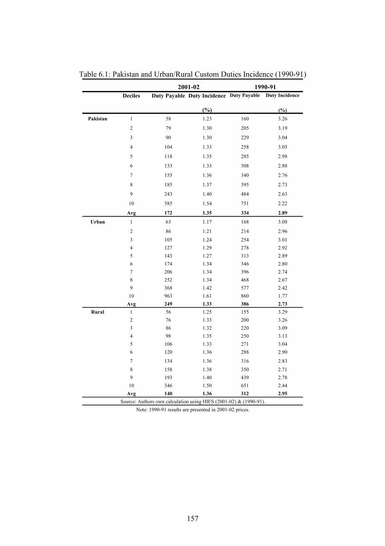
157

Table 6.1: Pakistan and Urban/Rural Custom Duties Incidence (1990-91)

Deciles Duty Payable Duty Incidence

(%)

Duty Payable Duty Incidence

(%)

Pakistan 1 58 1.23 160 3.26

2 79 1.30 205 3.19

3 90 1.30 229 3.04

4 104 1.33 258 3.05

5 118 1.35 285 2.98

6 133 1.33 308 2.88

7 155 1.36 340 2.76

8 185 1.37 395 2.73

9 243 1.40 484 2.63

10 585 1.54 751 2.22

Avg 172 1.35 334 2.89

Urban 1 63 1.17 168 3.08

2 86 1.21 214 2.96

3 105 1.24 254 3.01

4 127 1.29 278 2.92

5 143 1.27 313 2.89

6 174 1.34 346 2.80

7 206 1.34 396 2.74

8 252 1.34 468 2.67

9 368 1.42 577 2.42

10 963 1.61 860 1.77

Avg 249 1.33 386 2.73

Rural 1 56 1.25 155 3.29

2 76 1.33 200 3.26

3 86 1.32 220 3.09

4 98 1.35 250 3.13

5 106 1.33 271 3.04

6 120 1.36 288 2.90

7 134 1.36 316 2.83

8 158 1.38 350 2.71

9 193 1.40 439 2.78

10 346 1.50 651 2.44

Avg 140 1.36 312 2.95

Note: 1990-91 results are presented in 2001-02 prices.


2001-02 1990-91

158

6.2 Central Excise Duty (CED) Incidence (1990-91) to (2001-02)

Excise duty revenue was the second largest revenue source for Pakistan in the

past but over time its relative importance has significantly declined. This

change (as discussed in Chapter two) was a part of the overall indirect tax

reform strategy where CED role was envisaged as being complementary to

GST/VAT in taxation of luxuries. However, the scope of excise duties over

time has remained quite narrow. For instance in 1990-91 five items were

responsible for almost 75 percent of total CED revenue, this included

cigarettes (33 percent), sugar (15 percent), cement (12.5 percent), petroleum

products (8.7 percent) and beverages (4.4 percent) while in 2001-02, five

items constituted almost 82 percent of total CED revenue; cigarettes (35

percent), cement (21 percent), petroleum products (11 percent), natural gas (9

percent) and sugar (6 percent).

6.2.1 Description of Central Excise Duty

Excise duty description (in cases where they apply to HIES items) is taken

from the Effective Tariff of Central Excises Duty (1990-91) and (2001-02)

and reported in Table 6.2.

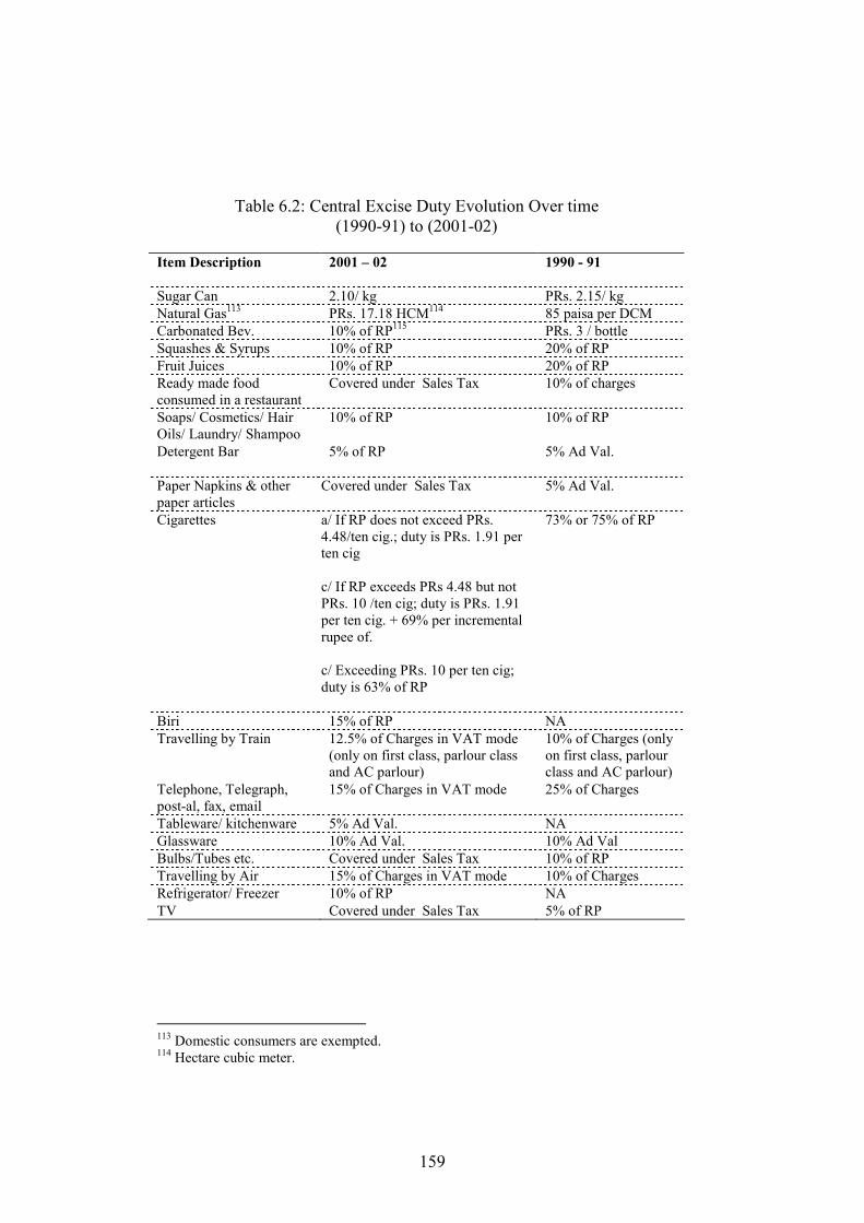
159

113 Domestic consumers are exempted. 114 Hectare cubic meter.

Table 6.2: Central Excise Duty Evolution Over time (1990-91) to (2001-02)

Item Description 2001 – 02

1990 - 91

Sugar Can 2.10/ kg PRs. 2.15/ kg

Natural Gas113 PRs. 17.18 HCM114 85 paisa per DCM

Carbonated Bev. 10% of RP115 PRs. 3 / bottle

Squashes & Syrups 10% of RP 20% of RP

Fruit Juices 10% of RP 20% of RP

Ready made food consumed in a restaurant

Covered under Sales Tax 10% of charges

Soaps/ Cosmetics/ Hair Oils/ Laundry/ Shampoo

10% of RP

10% of RP

Detergent Bar 5% of RP

5% Ad Val.

Paper Napkins & other paper articles

Covered under Sales Tax 5% Ad Val.

Cigarettes a/ If RP does not exceed PRs. 4.48/ten cig.; duty is PRs. 1.91 per ten cig c/ If RP exceeds PRs 4.48 but not PRs. 10 /ten cig; duty is PRs. 1.91 per ten cig. + 69% per incremental rupee of. c/ Exceeding PRs. 10 per ten cig; duty is 63% of RP

73% or 75% of RP

Biri 15% of RP NA

Travelling by Train 12.5% of Charges in VAT mode (only on first class, parlour class and AC parlour)

10% of Charges (only on first class, parlour class and AC parlour)

Telephone, Telegraph, post-al, fax, email

15% of Charges in VAT mode 25% of Charges

Tableware/ kitchenware 5% Ad Val. NA

Glassware 10% Ad Val. 10% Ad Val

Bulbs/Tubes etc. Covered under Sales Tax 10% of RP

Travelling by Air 15% of Charges in VAT mode 10% of Charges

Refrigerator/ Freezer 10% of RP NA

TV Covered under Sales Tax 5% of RP

160

6.2.2 Further Assumptions

We have assumed that excise duty is fully borne by consumers of goods and

services in terms of higher prices of these items. This simplifies incidence

calculation in most cases except for cigarettes.

a. Cigarettes (2001-02)

The case of calculating excise duty on cigarettes for (2001-02) warrants more

explanation since excise duty on cigarettes is levied according to three

different tariff slabs. We can simplify the information presented in Table 6.2

as following:

a. If retail price per cigarette is no more than 0.448 paisa, excise duty is

0.191 paisa per cig.

b. If retail price per cigarettes is more than 0.448 paisa but no more than

1 rupee, excise duty is 0.191 paisa per cig plus 69 percent of

incremental rupee or part of.

c. If retail price per cigarette is more than 1 rupeee excise duty is 63

percent of retail price.

Since there is no price information in HIES survey (and even if we get price

information on cigarettes from some other source, it will be impossible to

match this with HIES survey since consumers are not asked about the type of

cigarettes they consume) we instead rely on unit values i.e. expenditure

115 RP is retail price.

161

divided by quantities, information from within the HIES survey data.

Although, it needs to be mentioned that unit values are not actual prices, they

have been used as implicit prices (for instance see Deaton and Grosh, 1988;

and Deaton 1995) in cases where price information is hard to come by or

where it is hard to match this information with information presented in the

survey data.

Although, it has been shown that unit values can be affected by quality choices

i.e. someone buying better meat quality will pay more for that, spatial price

variations of unit values have been found to be closely related to price

variations especially when averaged over clusters (Deaton and Zaidi, 2002)116.

Thus, we assume unit values for cigarettes are equal to the retail prices of

cigarettes and this allows us to determine applicable duty slab for cigarettes.

For example if a household consumed 100 cigarettes while spending PRs. 110

in total than according to our calculation the unit value or the implicit price of

cigarette in this case will be 1.1, which according to our estimation falls within

duty slab c. Although, it must be admitted that by doing this we are assuming

that all 100 cigarettes consumed by the household are of the same type and

purchased at the same price, which is quite a restrictive assumption but in the

light of available information the only option. Once we know the respective

duty slab applicable for household cigarette consumption we can use the

information given above to determine the duty slab and duty paid117.

b. Travelling by Train (1990-91) & (2001-02)

116 For detailed discussion on using unit values as proxy for prices, see chapter 7. 117 If unit value falls within slab b, excise duty is determined in two parts. Unit value is separated into two portions; that falls below 0.448 and the remaining unit value portion. These are then taken as weights to determine expenditure falling under a particular type of duty slab and duty is applied accordingly.

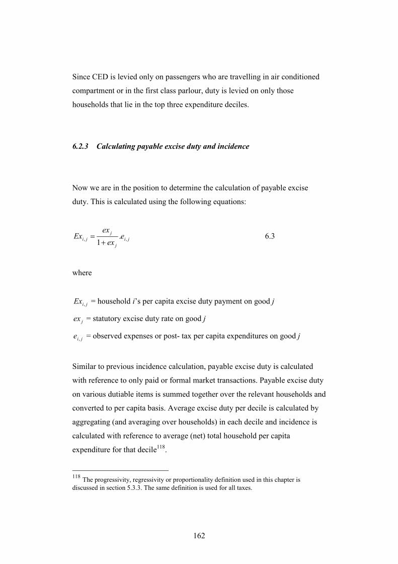
162

Since CED is levied only on passengers who are travelling in air conditioned

compartment or in the first class parlour, duty is levied on only those

households that lie in the top three expenditure deciles.

6.2.3 Calculating payable excise duty and incidence

Now we are in the position to determine the calculation of payable excise

duty. This is calculated using the following equations:

ji

j

j

ji eex

exEx ,, .

1+= 6.3

where

jiEx , = household i’s per capita excise duty payment on good j

jex = statutory excise duty rate on good j

jie , = observed expenses or post- tax per capita expenditures on good j

Similar to previous incidence calculation, payable excise duty is calculated

with reference to only paid or formal market transactions. Payable excise duty

on various dutiable items is summed together over the relevant households and

converted to per capita basis. Average excise duty per decile is calculated by

aggregating (and averaging over households) in each decile and incidence is

calculated with reference to average (net) total household per capita

expenditure for that decile118.

118 The progressivity, regressivity or proportionality definition used in this chapter is

discussed in section 5.3.3. The same definition is used for all taxes.

163

6.2.4 National CED Incidence (1990-91) & (2001-02)

The CED incidence results for (1990-91) and (2001-02) are reported in Table

6.3. If we look at the 1990-91 results we can see that the CED incidence for an

average Pakistani household stood at 1.88 percent. The average CED

incidence for the poorest and the richest ten percent of population at pre-

reform time stood at 1.55 and 2.15 percent respectively. If we look at the

overall trend of CED incidence, at pre-reform time the overall incidence

pattern for CED clearly appears to be progressive.

By (2001-02), the CED incidence at national level appears to be slightly

reduced. This mainly appeared to be due to reduction in rates (see for instance

Table 6.2) as well as changes in the underlying consumption patterns over

time (for instance see chapter five). The post- reform CED incidence for

average Pakistani household stood at only 1.02 percent while incidence for the

poorest and the richest ten percent of households stood at 1.06 and 1.05

percent respectively. If we look at the overall trend of CED incidence during

the post- reform time it appeared to be more or less proportional. Interestingly

in (1990-91), CED incidence for the richest ten percent of households was

almost 28 percent higher than their poorest counterparts but over time this

difference was completely removed as by the end of the reform process,

richest ten percent households were in fact paying on average 1 percent less

than their poorest counterpart.

This picture is also reflected in the proportionate change in CED tax liabilities

over time which reflects how CED scaling down gains are distributed across

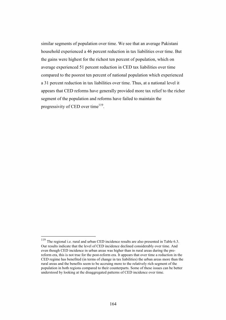
164

similar segments of population over time. We see that an average Pakistani

household experienced a 46 percent reduction in tax liabilities over time. But

the gains were highest for the richest ten percent of population, which on

average experienced 51 percent reduction in CED tax liabilities over time

compared to the poorest ten percent of national population which experienced

a 31 percent reduction in tax liabilities over time. Thus, at a national level it

appears that CED reforms have generally provided more tax relief to the richer

segment of the population and reforms have failed to maintain the

progressivity of CED over time119.

119 The regional i.e. rural and urban CED incidence results are also presented in Table 6.3.

Our results indicate that the level of CED incidence declined considerably over time. And even though CED incidence in urban areas was higher than in rural areas during the pre-reform era, this is not true for the post-reform era. It appears that over time a reduction in the CED regime has benefited (in terms of change in tax liabilities) the urban areas more than the rural areas and the benefits seem to be accruing more to the relatively rich segment of the population in both regions compared to their counterparts. Some of these issues can be better understood by looking at the disaggregated patterns of CED incidence over time.

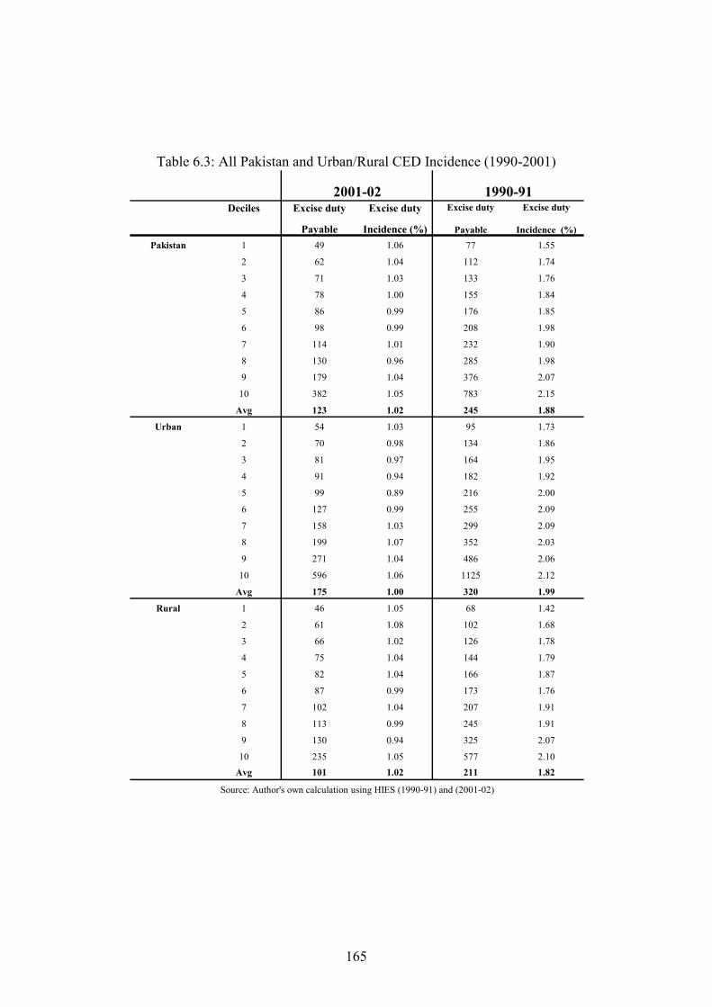
165

Table 6.3: All Pakistan and Urban/Rural CED Incidence (1990-2001)

Deciles Excise duty

Payable

Excise duty

Incidence (%)

Excise duty

Payable

Excise duty

Incidence (%)

Pakistan 1 49 1.06 77 1.55

2 62 1.04 112 1.74

3 71 1.03 133 1.76

4 78 1.00 155 1.84

5 86 0.99 176 1.85

6 98 0.99 208 1.98

7 114 1.01 232 1.90

8 130 0.96 285 1.98

9 179 1.04 376 2.07

10 382 1.05 783 2.15

Avg 123 1.02 245 1.88

Urban 1 54 1.03 95 1.73

2 70 0.98 134 1.86

3 81 0.97 164 1.95

4 91 0.94 182 1.92

5 99 0.89 216 2.00

6 127 0.99 255 2.09

7 158 1.03 299 2.09

8 199 1.07 352 2.03

9 271 1.04 486 2.06

10 596 1.06 1125 2.12

Avg 175 1.00 320 1.99

Rural 1 46 1.05 68 1.42

2 61 1.08 102 1.68

3 66 1.02 126 1.78

4 75 1.04 144 1.79

5 82 1.04 166 1.87

6 87 0.99 173 1.76

7 102 1.04 207 1.91

8 113 0.99 245 1.91

9 130 0.94 325 2.07

10 235 1.05 577 2.10

Avg 101 1.02 211 1.82

Source: Author's own calculation using HIES (1990-91) and (2001-02)

2001-02 1990-91

166

6.2.5 Selected Excise Duty Commodity Incidence

One thing (as mentioned) earlier that remained constant during the pre and

post- reform time was the narrow focus of excise duties. For instance in 1990-

91 five goods were responsible for almost 70 percent of excise revenue and

these included cigarettes, sugar, petroleum or POL products and beverages

and these, more or less were also responsible in 2001-02 for around 80 percent

of total excise duty collection. This narrow focus makes incidence analysis of

excise duties quite interesting and makes it possible to see the impact of main

component of excise duties at pre- and post-- reform time.

Table 6.4a presents five categories that made up almost 80 percent of total

CED incidence in (1990-91)120. On average, cigarettes were the highest

incidence creating category responsible for almost 37 percent of total excise

duty incidence. This was followed by sugar (31 percent), beverages (12

percent), detergent (4.2 percent), and telephone/fax (1.6 percent) respectively.

It appears the top three CED incidence creating categories for the poorest ten

percent of households were sugar (40 percent share of total excise duty

incidence), cigarettes (34 percent), and beverages (6.2 percent). While these

for the richest ten percent of households were also cigarettes (contributing a

share of 41 percent), beverages (18 percent) and sugar (16 percent).

If we look at the incidence trend of these components it appears CED

incidence for sugar and detergent is clearly regressive, while cigarette

incidence appears to be progressive for the bottom fifty percent of population

and proportional afterwards. Furthermore, telephone/fax and beverages CED

120 We were not able to measure CED incidence on POL products and cement because of difficulty of identifying relevant expenditure item in HIES survey as well as complicated CED slab structure in the case of formal.

167

incidence generally appeared to be progressive. Thus, it appears that CED

progressivity at national level was largely driven by progressivity of

telephone/fax charges as well as beverages. This was significantly supported

by the progressive cigarettes incidence over the first half of the population and

proportionality for rest of the population. And these factors, more than offset

the regressivity of sugar CED incidence.

The combined incidence of these five categories in 2001-02 still appeared to

be around 80 percent of total CED incidence. Table 6.4b shows disaggregated

CED incidence at the post--reform era. In 2001-02, sugar became the top CED

incidence category contributing around 31 percent of the total CED incidence.

This was followed by cigarettes at 29, telephone/fax and detergents both at 7.5

percent and beverages at 3.2 percent.

In 2001-02, the top three CED incidence generating categories for the poorest

ten percent of population were cigarettes, sugar and detergents, each

contributing around 38, 34 and 10 percent of total CED incidence respectively.

while for the richest ten percent of households the top three incidence

generating categories were telephone/fax, cigarettes and sugar, each

responsible for 31, 18 and 15 percent of total CED incidence respectively.

If we look at the individual incidence trends, it appears to be progressive for

beverages and telephone/fax; regressive for cigarettes, sugar and detergents.

Thus, over time regressivity of cigarettes (due to change in CED duty slabs as

well as of changes in underlying consumption patterns) on top of regressivity

of sugar (that also existed in the pre- reform era) has significantly affected the

post- reform CED incidence. The overall CED incidence at post- reform time

at best appears to be proportional as regressivity of sugar and cigarettes is

balanced against the progressivity of beverages and telephone/fax charges.

168

These concerns are further highlighted when we look at urban/rural results

particularly at the top and bottom ten percent of population and for top three

incidence creating categories. For instance, in 1990-91, the top three incidence

creating categories for the bottom ten percent of population in the urban areas

were sugar (40 percent), cigarettes (30 percent) and detergents (11 percent).

For the richest ten percent of population, the top three incidence creating

categories included cigarettes contributing 37 percent of total CED incidence,

24 percent for beverages and 13 percent for telephone/fax.

As for incidence trend, sugar appeared to be clearly regressive, cigarettes

progressive over first half of the population and regressive afterwards,

telephone and fax charges and detergent remained generally progressive.

Thus, again progressivity of CED incidence at pre- reform time for urban

areas was generally driven by cigarettes incidence which was progressive over

first half of the population and its regressivity for the top fifty percent of the

population was more than offset by progressivity of telephone/fax charges and

beverages over that segment of population.

During the same time in the rural areas the top three incidence generating

categories for the poorest ten percent of population were sugar (34 percent),

cigarettes (26 percent) and detergent (5.4 percent). while for the richest ten

percent of population the top three CED incidence categories were cigarettes

(41 percent), sugar (22 percent) and beverages (15 percent). However, the

progressivity of CED incidence for rural areas was largely driven by cigarette

incidence that appeared to be generally progressive over most of rural

population and it was strongly supported by beverage incidence that was

clearly progressive.

In 2001-02 in the urban areas the top three incidence creating categories for

the poorest ten percent of population were cigarettes (38 percent), sugar (31

169

percent) and detergent (9 percent) while for the richest ten percent households

these were telephone/fax (43 percent), cigarettes (14 percent) and sugar (7.6

percent). Thus, in urban areas similar to 1990-91 there were significant

variation in terms of which goods were mainly responsible for CED share for

the urban poorest and the richest ten percent of the population. The incidence

trend for sugar, detergent and cigarettes again appeared to be clearly

regressive, while CED incidence for telephone/fax and beverages was

progressive.

For the poorest ten percent of households in the rural areas, the most

significant CED incidence share came from cigarettes (38 percent), followed

by sugar (36 percent) and detergents (11 percent) while for the richest ten

percent households the most significant category this time was sugar (23

percent), cigarettes (22.8 percent) and telephone/fax (17 percent). Thus, for

rural households in all deciles compared with the urban population sugar

remained the most significant incidence category.

As for incidence trend in post- reform era for both the urban and rural areas,

results were largely driven by a clear regressive pattern of CED incidence on

cigarettes (both due to change in rate and due to changes in the underlying

consumption patterns). This along with regressive sugar incidence created a

strong regressive CED setup that to some extent was neutralized by the

progressivity of telephone/fax charges but this was not enough to create

progressivity in the overall urban/rural CED incidence.

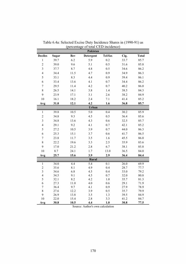
170

Table 6.4a: Selected Excise Duty Incidence Shares in (1990-91) as (percentage of total CED incidence)

Deciles Sugar Bev Detergent Tel/fax Cig. Total

1 39.7 6.2 5.9 0.2 33.7 85.7

2 39.0 9.6 5.1 0.5 31.6 85.8

3 37.7 8.7 4.8 0.5 34.6 86.2

4 34.4 11.5 4.7 0.9 34.9 86.3

5 33.1 8.3 4.4 0.9 39.4 86.1

6 33.4 13.6 4.1 0.7 34.4 86.2

7 29.5 11.4 4.2 0.7 40.2 86.0

8 26.5 14.1 3.8 1.4 38.5 84.3

9 23.9 17.1 3.1 2.6 38.2 84.9

10 16.1 18.2 2.4 7.1 41.4 85.2

Avg 31.0 12.1 4.2 1.6 36.8 85.7

1 39.8 10.5 5.0 0.4 30.2 85.9

2 34.8 9.3 4.5 0.5 36.4 85.6

3 34.8 13.6 4.3 0.6 32.5 85.7

4 29.1 9.2 4.1 0.7 42.1 85.2

5 27.2 10.5 3.9 0.7 44.0 86.3

6 25.3 15.1 3.7 0.6 41.7 86.5

7 23.8 11.7 3.5 1.6 45.5 86.0

8 22.2 19.6 3.3 2.5 35.9 83.6

9 17.0 21.2 2.8 6.7 38.1 85.8

10 8.7 24.1 1.7 13.0 36.5 84.0

Avg 25.7 15.6 3.9 2.9 36.4 84.4

1 34.0 4.4 5.4 0.1 26.0 69.9

2 35.6 8.1 4.9 0.4 28.7 77.7

3 34.6 6.8 4.5 0.4 33.0 79.2

4 34.5 9.1 4.5 0.7 32.0 80.8

5 32.1 8.2 4.2 1.0 35.7 81.3

6 27.3 11.0 4.0 0.6 29.1 71.9

7 36.4 9.7 4.1 0.9 27.9 78.9

8 27.6 12.2 3.9 0.5 35.7 79.9

9 26.9 13.8 3.5 1.3 39.5 84.9

10 22.0 15.4 2.8 3.3 41.2 84.7

Avg 30.8 10.5 4.4 1.0 30.8 77.5

Source: Author's own calculation

Urban

Rural

Pakistan

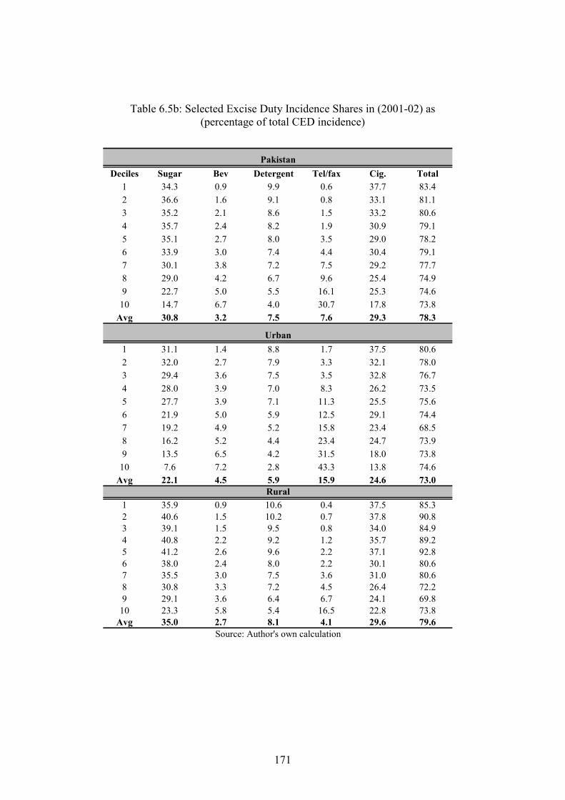
171

Table 6.5b: Selected Excise Duty Incidence Shares in (2001-02) as (percentage of total CED incidence)

Deciles Sugar Bev Detergent Tel/fax Cig. Total

1 34.3 0.9 9.9 0.6 37.7 83.4

2 36.6 1.6 9.1 0.8 33.1 81.1

3 35.2 2.1 8.6 1.5 33.2 80.6

4 35.7 2.4 8.2 1.9 30.9 79.1

5 35.1 2.7 8.0 3.5 29.0 78.2

6 33.9 3.0 7.4 4.4 30.4 79.1

7 30.1 3.8 7.2 7.5 29.2 77.7

8 29.0 4.2 6.7 9.6 25.4 74.9

9 22.7 5.0 5.5 16.1 25.3 74.6

10 14.7 6.7 4.0 30.7 17.8 73.8

Avg 30.8 3.2 7.5 7.6 29.3 78.3

1 31.1 1.4 8.8 1.7 37.5 80.6

2 32.0 2.7 7.9 3.3 32.1 78.0

3 29.4 3.6 7.5 3.5 32.8 76.7

4 28.0 3.9 7.0 8.3 26.2 73.5

5 27.7 3.9 7.1 11.3 25.5 75.6

6 21.9 5.0 5.9 12.5 29.1 74.4

7 19.2 4.9 5.2 15.8 23.4 68.5

8 16.2 5.2 4.4 23.4 24.7 73.9

9 13.5 6.5 4.2 31.5 18.0 73.8

10 7.6 7.2 2.8 43.3 13.8 74.6

Avg 22.1 4.5 5.9 15.9 24.6 73.0

1 35.9 0.9 10.6 0.4 37.5 85.3

2 40.6 1.5 10.2 0.7 37.8 90.8

3 39.1 1.5 9.5 0.8 34.0 84.9

4 40.8 2.2 9.2 1.2 35.7 89.2

5 41.2 2.6 9.6 2.2 37.1 92.8

6 38.0 2.4 8.0 2.2 30.1 80.6

7 35.5 3.0 7.5 3.6 31.0 80.6

8 30.8 3.3 7.2 4.5 26.4 72.2

9 29.1 3.6 6.4 6.7 24.1 69.8

10 23.3 5.8 5.4 16.5 22.8 73.8

Avg 35.0 2.7 8.1 4.1 29.6 79.6

Source: Author's own calculation

Rural

Pakistan

Urban

172

6.3 Total Indirect Tax Incidence for Pakistan (1990-91) to (2001-02)121

After having examined the pre- and post- reform incidence for GST (Chapter

five) and incidence for custom duties and excise duty in this chapter we are

now in a position to address one of the core questions of this study i.e. the

overall incidence of indirect taxes in Pakistan at pre- and post- reform times.

This will allow us to see how the indirect tax incidence over time has changed

due to the tax reform process embarked in the 1990s and to ascertain if the

equity concerns envisaged in the pre- reform strategy really got translated into

positive policy actions aimed at making the overall indirect tax incidence pro-

poor or not.

6.3.1 National level results122

The total indirect tax system incidence results for (1990-91) and (2001-02) are

presented in Tables 6.5. The results for the pre-reform era i.e. (1990-91) show

that the total indirect tax incidence for an average Pakistani household stood at

6.32 percent. The overall incidence for the poorest ten percent of households

stood at 6.11 percent while the incidence for the richest ten percent of

households stood at 6.16 percent. If we look at the overall incidence trend at

the pre-reform time it appears to be of inverted U-shaped with higher indirect

tax incidence faced by the middle portion of population compared to the

population at the tails. If we look at how total indirect tax incidence is being

constituted for an average household at national level, almost 47 percent of

121 Incidence is this section is calculated by accumulating tax liabilities over net paid expenditures for three taxes, namely custom duties, excise duty and sales tax. 122 Although the overall indirect tax incidence results at the regional level i.e. urban and rural are also presented in Table 6.5, there are no major differences.

173

total indirect tax incidence is coming from custom duties, while 30 and 21

percent incidence is coming from CED and sales tax respectively. Thus it

appears that the inverted U-shaped incidence trend was mainly due to the

regressivity of custom duty incidence which more than counterbalanced

progressive patterns for CED and GST tax at the pre-reform time.

In (2001-02) i.e. also the post- reform time an average Pakistani household

faced an overall indirect tax incidence of 7.31 percent. The indirect tax

incidence for the poorest and the richest ten percent of the population stood at

7.14 and 7.56 percent respectively. If we look at the overall trend of indirect

tax incidence at the post- reform era it appears to be progressive (excluding

the second, sixth and eight decile households). However, one important thing

to note is that the poorest ten percent of population now bear lowest indirect

tax incidence while the top ten percent of population bear the highest indirect

tax incidence, which is a positive development over time.

If we look at the constitution of total indirect tax incidence at the post-reform

era, for an average Pakistani household almost the lion’s share i.e. 65 percent

of total indirect tax incidence came from GST/VAT, while remaining 19 and

15 percent of indirect tax incidence came from custom duties and CED. Thus,

it appeared shifting reliance from trade taxes to GST/VAT revenues over time

was mainly responsible for making the overall indirect tax incidence

progressive, although we believe that progressivity of the current system at

lower deciles has been limited (also evident from the national incidence

pattern) because of taxation of processed food items such as sugar and

vegetable ghee and basic fuel such as kerosene (also highlighted in chapter

five).

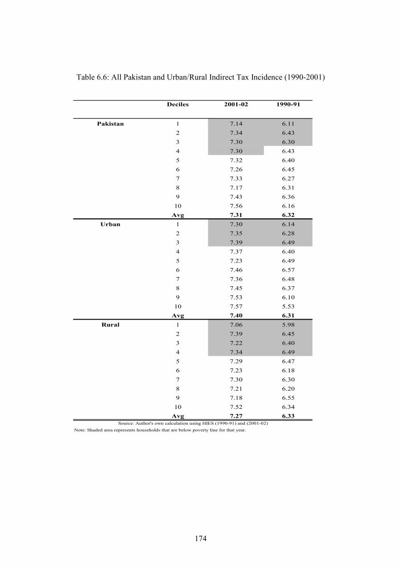
174

Table 6.6: All Pakistan and Urban/Rural Indirect Tax Incidence (1990-2001)

Deciles

Pakistan 1 7.14 6.11

2 7.34 6.43

3 7.30 6.30

4 7.30 6.43

5 7.32 6.40

6 7.26 6.45

7 7.33 6.27

8 7.17 6.31

9 7.43 6.36

10 7.56 6.16

Avg 7.31 6.32

Urban 1 7.30 6.14

2 7.35 6.28

3 7.39 6.49

4 7.37 6.40

5 7.23 6.49

6 7.46 6.57

7 7.36 6.48

8 7.45 6.37

9 7.53 6.10

10 7.57 5.53

Avg 7.40 6.31

Rural 1 7.06 5.98

2 7.39 6.45

3 7.22 6.40

4 7.34 6.49

5 7.29 6.47

6 7.23 6.18

7 7.30 6.30

8 7.21 6.20

9 7.18 6.55

10 7.52 6.34

Avg 7.27 6.33

Note: Shaded area represents households that are below poverty line for that year.

2001-02 1990-91

Source: Author's own calculation using HIES (1990-91) and (2001-02)

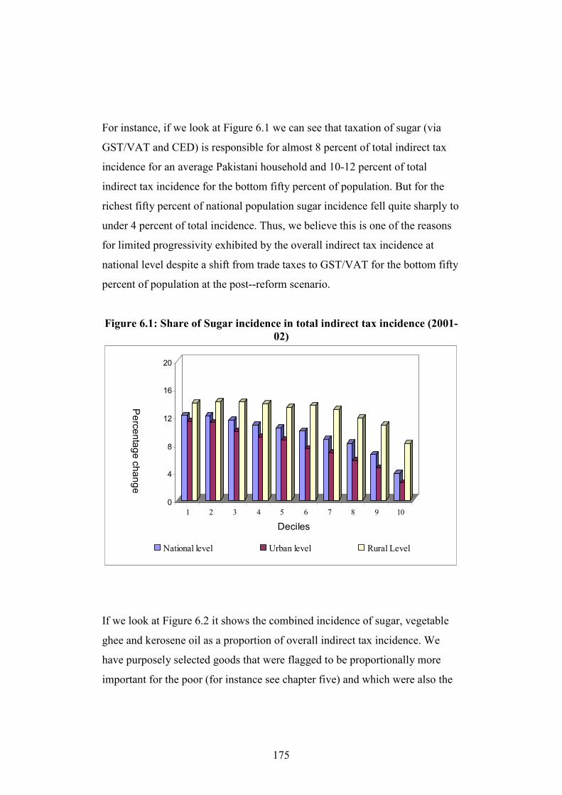
175

For instance, if we look at Figure 6.1 we can see that taxation of sugar (via

GST/VAT and CED) is responsible for almost 8 percent of total indirect tax

incidence for an average Pakistani household and 10-12 percent of total

indirect tax incidence for the bottom fifty percent of population. But for the

richest fifty percent of national population sugar incidence fell quite sharply to

under 4 percent of total incidence. Thus, we believe this is one of the reasons

for limited progressivity exhibited by the overall indirect tax incidence at

national level despite a shift from trade taxes to GST/VAT for the bottom fifty

percent of population at the post--reform scenario.

Figure 6.1: Share of Sugar incidence in total indirect tax incidence (2001-

02)

0

4

8

12

16

20

Pe

rce

nta

ge

ch

an

ge

1 2 3 4 5 6 7 8 9 10

Deciles

National level Urban level Rural Level

If we look at Figure 6.2 it shows the combined incidence of sugar, vegetable

ghee and kerosene oil as a proportion of overall indirect tax incidence. We

have purposely selected goods that were flagged to be proportionally more

important for the poor (for instance see chapter five) and which were also the

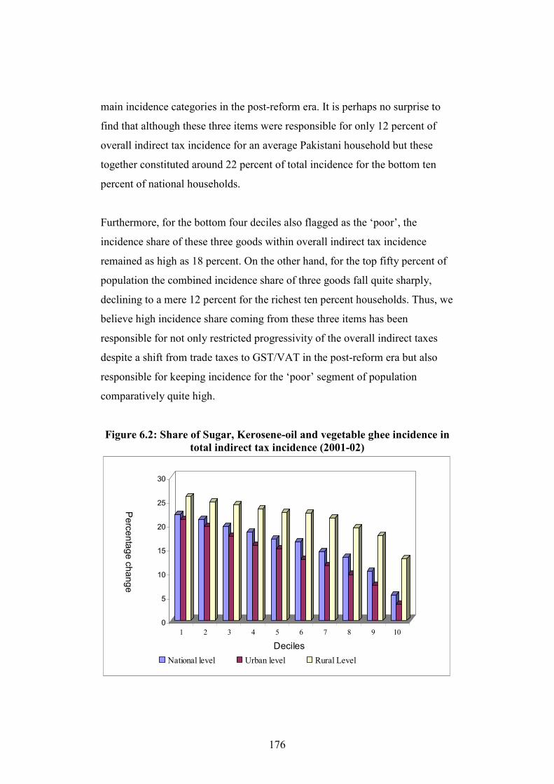
176

main incidence categories in the post-reform era. It is perhaps no surprise to

find that although these three items were responsible for only 12 percent of

overall indirect tax incidence for an average Pakistani household but these

together constituted around 22 percent of total incidence for the bottom ten

percent of national households.

Furthermore, for the bottom four deciles also flagged as the ‘poor’, the

incidence share of these three goods within overall indirect tax incidence

remained as high as 18 percent. On the other hand, for the top fifty percent of

population the combined incidence share of three goods fall quite sharply,

declining to a mere 12 percent for the richest ten percent households. Thus, we

believe high incidence share coming from these three items has been

responsible for not only restricted progressivity of the overall indirect taxes

despite a shift from trade taxes to GST/VAT in the post-reform era but also

responsible for keeping incidence for the ‘poor’ segment of population

comparatively quite high.

Figure 6.2: Share of Sugar, Kerosene-oil and vegetable ghee incidence in

total indirect tax incidence (2001-02)

0

5

10

15

20

25

30

Pe

rce

nta

ge

ch

an

ge

1 2 3 4 5 6 7 8 9 10

Deciles


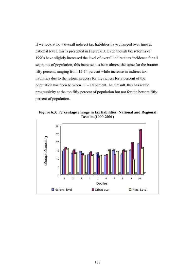
177

If we look at how overall indirect tax liabilities have changed over time at

national level, this is presented in Figure 6.3. Even though tax reforms of

1990s have slightly increased the level of overall indirect tax incidence for all

segments of population, this increase has been almost the same for the bottom

fifty percent; ranging from 12-14 percent while increase in indirect tax

liabilities due to the reform process for the richest forty percent of the

population has been between 11 – 18 percent. As a result, this has added

progressivity at the top fifty percent of population but not for the bottom fifty

percent of population.

Figure 6.3: Percentage change in tax liabilities: National and Regional

Results (1990-2001)

0

5

10

15

20

25

30

Pe

rce

nta

ge

ch

an

ge

1 2 3 4 5 6 7 8 9 10

Deciles


178

6.4 Conclusion

The Pakistan federal tax structure relies heavily on indirect taxes as the prime

source of revenue. Like many developing countries, Pakistan also embarked

upon a substantial tax reform process during the decade of 1990s with the

main aim of revenue mobilization. But this reform strategy also gave

substantial importance to equity considerations and envisaged addressing both

issues via revitalizing direct taxes (that later did not materialize) as well as the

replacement of trade taxes with GST/VAT revenues, with latter expected to be

“pro-poor” as a result of well targeted GST/VAT exemptions.

It would not be wrong to say that even though tax reforms of the 1990s have

increased the tax liabilities for an average Pakistani household at the national

level by 15 percent, reforms have been generally progressive for national as

well as for the urban areas. This is a clear break from the pre-reform era in

which the overall indirect tax incidence at national as well as the urban/rural

levels at best appeared to be of inverted U-shaped. Thus, we do believe that

our overall indirect tax incidence results at national as well as for the urban

areas support Gemmel and Morrissey (2003) finding that for most developing

countries a move away from import taxes to sales taxes has generally been

progressive.

Although this result is not apparent in the rural areas, we believe one of the

main reasons for this is the existing taxation of sugar, vegetable ghee and

kerosene oil, which are responsible for almost a quarter of total indirect tax

incidence for the poorest ten percent of households. These items have been

flagged (in the previous chapter) to be proportionally more important for the

poor, thus best candidate for GST/VAT exemptions on distributional grounds.

179

And our incidence results clearly support our previous findings. And results

show that post reform progressivity of the overall indirect tax system for

urban/rural poor and for rural areas in general have been marginalized by

taxation of sugar, vegetable ghee and kerosene oil.

We have found sufficient differences in the consumption patterns of the poor

in Pakistan that allows for better targeting of exemptions particularly where

basic fuels, sugar and vegetable ghee consumption is concerned (for instance

see chapter five). These consumption patterns are found to be quite different

from developed countries. Thus, if poverty alleviation and distributional

concerns are important for the policy makers in developing countries, general

rule of thumb for GST/VAT exemptions may not work. And policy making

has to be more sensitive to the indigenous factors.

In this chapter, our incidence results still hinge on the no-behavioural response

assumption. In the next chapter we try to evaluate how incorporation of

behaviour responses will change our results and also try to propose direction

of reforms that can be welfare improving at margin.

180

CHAPTER VII: Using Demand Analysis to Evaluate

Price and Tax Reforms in Pakistan (2001-02)

7 Introduction

The aim of this chapter is to go beyond the distributional analysis of tax

incidence by estimating own- and cross- price elasticities using spatial price

variation in the survey data. The intentions are multiple: (a) to provide useful

discussion on why estimates of elasticities are important for ex-ante tax policy

planning and tax reform analysis; (b) to illustrate how or if tax incidence

estimates from earlier chapters are sensitive to demand responses; and (c) to

recommend the future directions of welfare enhancing reforms for Pakistan at

margin.

For this purpose this chapter is divided into eight sections. The first section

provides a brief description of the general approach. The second section talks

about unit values and how they can be used to estimate implicit or proxy

prices from survey data and problems and issues related to this conjecture.

Section three talks in depth about Deaton’s (1988;1990;1997) methodology

that can be used to estimate spatial price variation from survey data. Section

four talks about basic data information i.e. cluster structure of HIES (2001-02)

for Pakistan, basic summary information on dependent and independent

variables that will be used in this analysis as well as providing important

information on how unit values vary across clusters as well as over time. The

fifth section provides the results of the first stage of estimation as well as final

own- and cross- price elasticity estimates for Pakistan for (2001-02). The sixth

181

section will try to illustrate if partial equilibrium tax incidence estimates from

earlier chapters are sensitive to incorporation of demand responses. The

seventh section starts with a brief explanation of theory and methodology of

marginal theory of tax and price reform and concludes with providing

recommendations on the future direction of tax reforms particularly for VAT

for Pakistan that can be welfare enhancing (and are in line with efficiency and

equity criteria). The last section concludes.

7.1 Basic approach

This chapter aims at estimating price elasticities using spatial price variation in

the survey data to estimate demand functions, by taking unit values as proxies

for prices. The survey data that used for this estimation is the Household

Integrated Economic Survey (HIES) 2001-02 for Pakistan. The following

sections provide detailed description of various issues related to this

methodology as well as our results.

7.2 Why Unit Values?

In order to determine the welfare price effect of a tax change we must begin

with understanding how households will respond to price changes. Such

information is also critical for design of effective tax or subsidy policy.

However, modelling consumer behaviour is not easy because it requires

accurate and robust price information (that requires historical time series data

on prices). According to Deaton (1988) availability of such data is a rarity

even for developed countries let alone developing countries123. Although in

123 For instance see [Barton, 1969] for classic attempt using data on Holland and [Deaton, 1974a] using time series data on UK.

182

many cases some price data is collected by the statistical offices, in many

developing countries such data is available only at: (a) a geographically

aggregated level and (b) for a few years only. This, therefore rules out a

possibility of using this price data source for constructing robust price

elasticity estimates.

However, many developing countries do have cross-sectional survey data of

very good quality collected for a reasonable span of time. Such surveys report

data on both expenditures and quantities consumed by households for a wide

variety of goods. Dividing expenditures by quantity gives us unit values for

each items purchased by the households, ratio of expenditure to quantities,

which can be used as proxies for prices (Disney et. al, 2004).

However, unit values are not the same as ‘prices’ and can not be directly

treated as market prices without adjustment in quality differences in purchases

across households (Houthakker, 1952; Theil 1952; and Deaton, 1988),

adjustment for units of measurement (Prais and Houthakker, 1955), as well as

other sources of measurement error (Timmer and Alderman, 1979; Strauss,

1982; .Prais and Houthakker, 1955). Although, unit value has been used

directly for estimation of price elasticities (Deaton, 1988; Timmer and

Alderman, 1979; Timmer, 1981; and Pitt, 1983), failure to address quality

effects within prices can lead to parameters being different from what would

have been otherwise (Cox and Wohlgenant, 1986). But if the appropriate

adjustment in unit values can be made, the usefulness of information contained

in unit values cannot be denied particularly for developing countries where

price data is so scarce (Deaton, 1988).

7.3 Deaton’s Methodology124

124 This section relies heavily on Deaton (1988; 1992; 1997) for notations and explanations.

183

Deaton (1988; 1990; 1997) proposes a methodology aimed at estimated spatial

price variation from unit values in order to estimate price elasticities using

survey data. The basic assumption of this methodology is that households

belonging to the same cluster face the same prices. Since households

belonging to the same cluster in a survey are more or less interviewed at the

same time (in order to minimize travel cost) this assumption is quite realistic

particularly for rural areas where a single market exists. Once this assumption

is made the idea is to use cluster information on expenditures and unit values

to estimate the effects of household income and demographics characteristics

on quantities and qualities. The demand system can then be estimated on the

basis of inter-cluster variation in corrected quantities and unit values.

Before we start with Deaton’s methodology we need to understand how he

models quality. According to Deaton (1997) the most suitable way of thinking

about quality is to define quality as a property of commodity aggregates.

According to this definition if icq denotes the household’s vector of

consumption levels of good i within the group consumed by household in

cluster c, than the group quantity index icQ can be written as:

iciic qkQ .= 7.1

where ik is used to add quantities of items in the group. Corresponding to the

quantity vector is a price vector, icp , which contains no price variation since

each commodity that makes up commodity vector is perfectly homogenous.

Thus, we can write icp as:

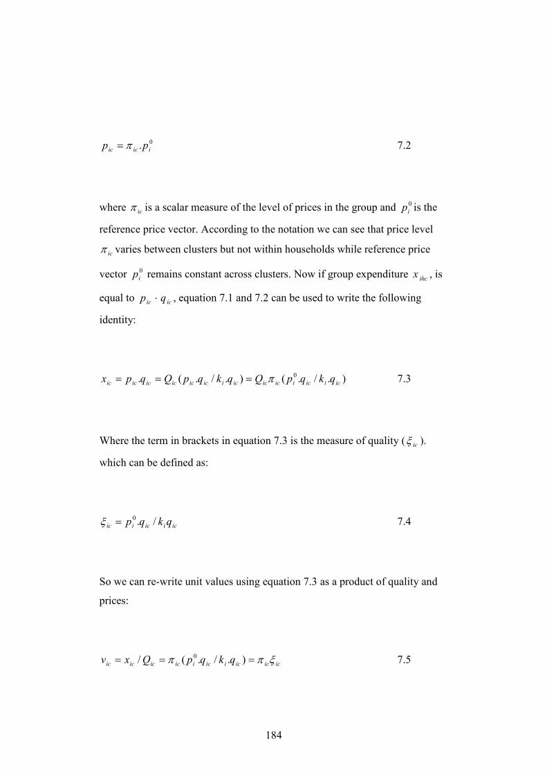
184

0. iicic pp π= 7.2

where icπ is a scalar measure of the level of prices in the group and 0

ip is the

reference price vector. According to the notation we can see that price level

icπ varies between clusters but not within households while reference price

vector 0

ip remains constant across clusters. Now if group expenditure ihc

x , is

equal to icic qp ⋅ , equation 7.1 and 7.2 can be used to write the following

identity:

)./.()./.(. 0

iciiciiciciciicicicicicic qkqpQqkqpQqpx π=== 7.3

Where the term in brackets in equation 7.3 is the measure of quality ( icξ ).

which can be defined as:

iciiciic qkqp /.0=ξ 7.4

So we can re-write unit values using equation 7.3 as a product of quality and

prices:

iciciciiciicicicic qkqpQxv ξππ === )./.(/ 0 7.5

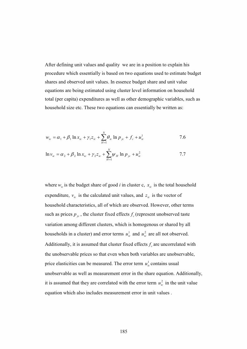
185

After defining unit values and quality we are in a position to explain his

procedure which essentially is based on two equations used to estimate budget

shares and observed unit values. In essence budget share and unit value

equations are being estimated using cluster level information on household

total (per capita) expenditures as well as other demographic variables, such as

household size etc. These two equations can essentially be written as:

1

1

111 lnln iccjc

N

H

icicicic ufpzxw +++++= ∑=

θγβα 7.6

2

1

222 lnlnln icjc

N

H

Hicicic upzxv ++++= ∑=

ψγβα 7.7

where icw is the budget share of good i in cluster c, icx is the total household

expenditure, icv is the calculated unit values, and icz is the vector of

household characteristics, all of which are observed. However, other terms

such as prices jcp , the cluster fixed effects cf (represent unobserved taste

variation among different clusters, which is homogenous or shared by all

households in a cluster) and error terms 1

icu and 2

icu are all not observed.

Additionally, it is assumed that cluster fixed effects cf are uncorrelated with

the unobservable prices so that even when both variables are unobservable,

price elasticities can be measured. The error term 1

icu contains usual

unobservable as well as measurement error in the share equation. Additionally,

it is assumed that they are correlated with the error term 2

icu in the unit value

equation which also includes measurement error in unit values .

186

We can see that equations 7.6 and 7.7 contain different dependent variables.

The unit value equation i.e. equation 7.7 is kept slightly different because unit

values unlike unobservable prices vary from household to household within

the same commodity group. These are linked with prices through 2β (i.e.

elasticity of quality with respect to total expenditure) in the unit value

equation. If there was no measurement error or unit values were equal to

prices, the matrix Hψ would be an identity. Also it is important to mention

that the cluster fixed effect term because of identification issues only appears

in the share equation but not in the unit value equation because if it did it

would break the direct link between prices and unit value.

Now we are in a position to explain Deaton’s estimation procedure given

underlying assumption and structure as has been mentioned above.

7.3.1 First Stage

Once we have assumed that there is no price variation within the same cluster

we can use within cluster information on expenditures and unit values to

estimate the effects of household income and demographics characteristics on

quantities and qualities using Ordinary Least Squares (OLS). However, if we

look at equation 7.6 we can see that this equation is being estimated with

cluster fixed effects by allowing dummy variables for each cluster. But the

possibility of a very large number of clusters in survey data can make this very

time consuming if not impossible task. One shortcut according to Firsch-

Waugh (1993) theorem is to carry out estimation of equations after removing

cluster means from each of the variables. Consequently, all variables in both

equations can be first demeaned by their cluster means and then OLS can be

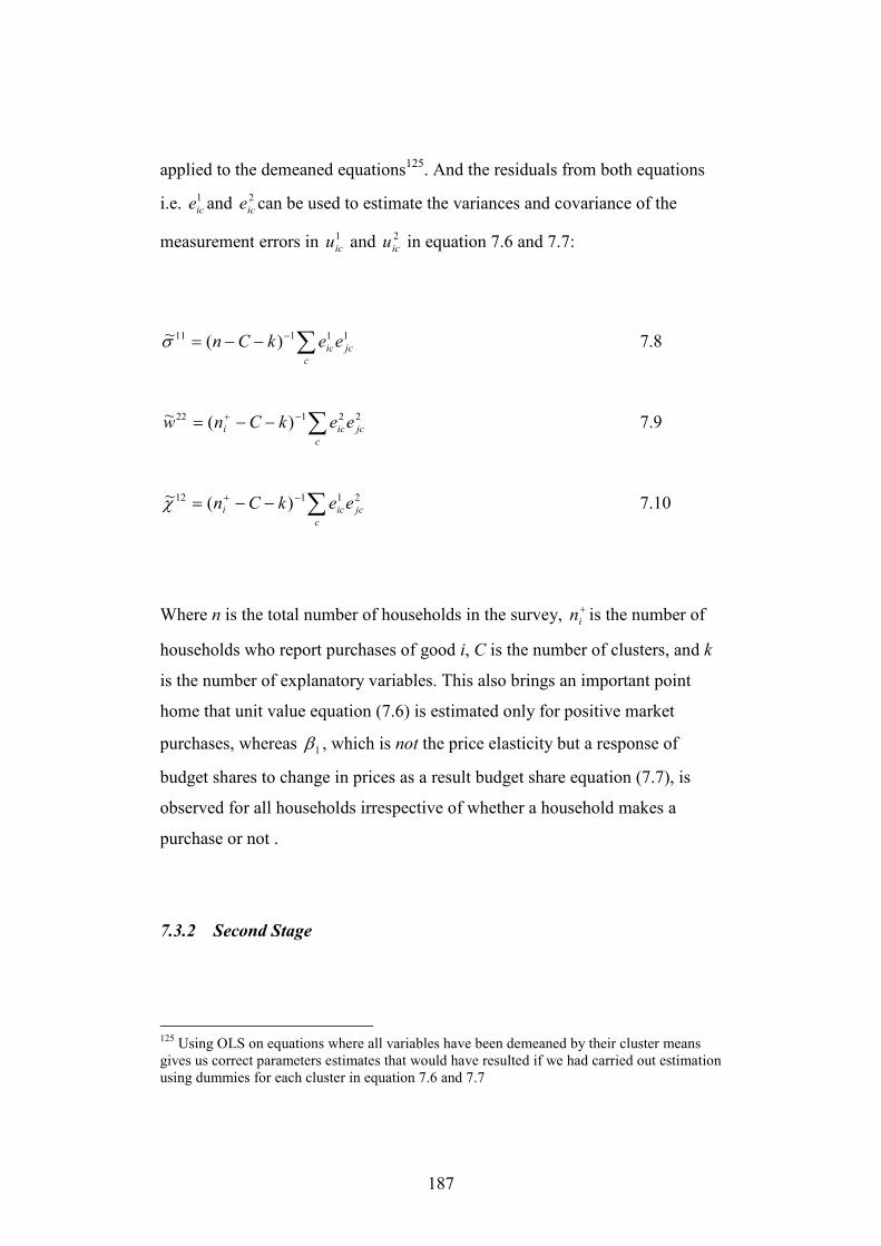
187

applied to the demeaned equations125. And the residuals from both equations

i.e. 1

ice and 2

ice can be used to estimate the variances and covariance of the

measurement errors in 1

icu and 2

icu in equation 7.6 and 7.7:

11111 )(~jc

c

iceekCn ∑−−−=σ 7.8

22122 )(~jc

c

ici eekCnw ∑−+ −−= 7.9

21112 )(~jc

c

ici eekCn ∑−+ −−=χ 7.10

Where n is the total number of households in the survey, +in is the number of

households who report purchases of good i, C is the number of clusters, and k

is the number of explanatory variables. This also brings an important point

home that unit value equation (7.6) is estimated only for positive market

purchases, whereas 1β , which is not the price elasticity but a response of

budget shares to change in prices as a result budget share equation (7.7), is

observed for all households irrespective of whether a household makes a

purchase or not .

7.3.2 Second Stage

125 Using OLS on equations where all variables have been demeaned by their cluster means gives us correct parameters estimates that would have resulted if we had carried out estimation using dummies for each cluster in equation 7.6 and 7.7

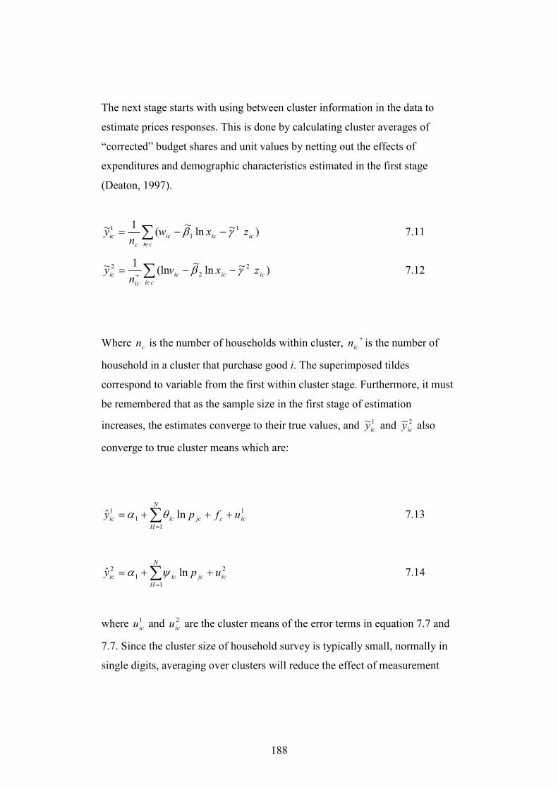
188

The next stage starts with using between cluster information in the data to

estimate prices responses. This is done by calculating cluster averages of

“corrected” budget shares and unit values by netting out the effects of

expenditures and demographic characteristics estimated in the first stage

(Deaton, 1997).

)~ln~

(1~ 1

1

1

icicic

cic

ic zxwn

y γβ −−= ∑∈

7.11

)~ln~

(ln1~ 2

2

2

icicic

ciic

ic zxvn

y γβ −−= ∑∈

+ 7.12

Where cn is the number of households within cluster, +

icn is the number of

household in a cluster that purchase good i. The superimposed tildes

correspond to variable from the first within cluster stage. Furthermore, it must

be remembered that as the sample size in the first stage of estimation

increases, the estimates converge to their true values, and 1~icy and 2~

icy also

converge to true cluster means which are:

1

1

1

1 lnîccjc

N

H

icic ufpy +++= ∑=

θα 7.13

2

1

1

2 lnîcjc

N

H

icic upy ++= ∑=

ψα 7.14

where 1

icu and 2

icu are the cluster means of the error terms in equation 7.7 and

7.7. Since the cluster size of household survey is typically small, normally in

single digits, averaging over clusters will reduce the effect of measurement

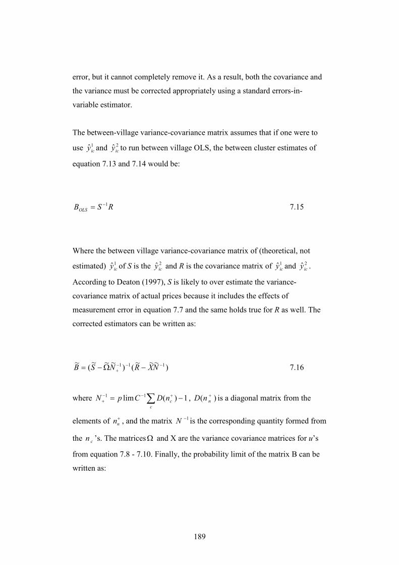
189

error, but it cannot completely remove it. As a result, both the covariance and

the variance must be corrected appropriately using a standard errors-in-

variable estimator.

The between-village variance-covariance matrix assumes that if one were to

use 1îcy and 2ˆ

icy to run between village OLS, the between cluster estimates of

equation 7.13 and 7.14 would be:

RSBOLS

1−= 7.15

Where the between village variance-covariance matrix of (theoretical, not

estimated) 1îcy of S is the 2ˆ

icy and R is the covariance matrix of 1îcy and 2ˆ

icy .

According to Deaton (1997), S is likely to over estimate the variance-

covariance matrix of actual prices because it includes the effects of

measurement error in equation 7.7 and the same holds true for R as well. The

corrected estimators can be written as:

)~~~

()~~~

(~ 111 −−−

+ −Ω−= NXRNSB 7.16

where 1)(lim 11 −= ∑ +−−+

c

cnDCpN , )( +nnD is a diagonal matrix from the

elements of +nn , and the matrix 1−N is the corresponding quantity formed from

the cn ’s. The matricesΩ and X are the variance covariance matrices for u’s

from equation 7.8 - 7.10. Finally, the probability limit of the matrix B can be

written as:

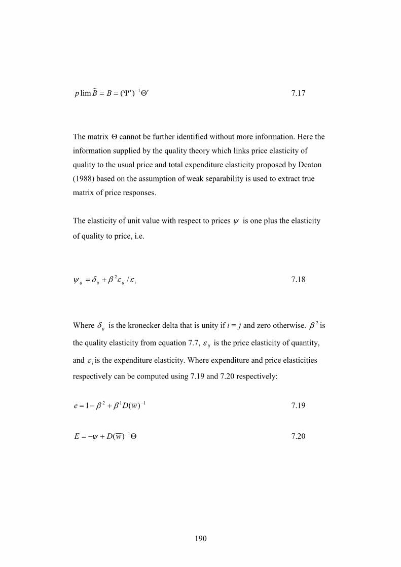
190

Θ′Ψ′== −1)(~

lim BBp 7.17

The matrix Θ cannot be further identified without more information. Here the

information supplied by the quality theory which links price elasticity of

quality to the usual price and total expenditure elasticity proposed by Deaton

(1988) based on the assumption of weak separability is used to extract true

matrix of price responses.

The elasticity of unit value with respect to prices ψ is one plus the elasticity

of quality to price, i.e.

iijijij εεβδψ /2+= 7.18

Where ijδ is the kronecker delta that is unity if i = j and zero otherwise. 2β is

the quality elasticity from equation 7.7, ijε is the price elasticity of quantity,

and iε is the expenditure elasticity. Where expenditure and price elasticities

respectively can be computed using 7.19 and 7.20 respectively:

112 )(1 −+−= wDe ββ 7.19

Θ+−= −1)(wDE ψ 7.20

191

Where e is the vector of total expenditure elasticity and E is the matrix of price

elasticities. The diagonalization operator D(.) converts its vector argument into

a diagonal matrix.

7.4 The DATA

The data set that is being used for carrying out demand responses is the

Household Integrated Economic Survey (HIES) (2001-02) which is also

discussed in Chapter three of this study. Thus in this section only information

relevant to estimation for this chapter will be discussed. As already explained

HIES (2001-02) is a nationally representative survey which like other

household surveys tries to minimize travel cost by selecting and interviewing

households belonging to the same cluster almost at the same time. This is

made possible because the size of cluster tends to be quite small; around 10-16

households in each cluster.

As a result, Deaton’s (1992;1997) assumption about households facing the

same set of prices within a cluster is a plausible example for households in the

cluster particularly in villages where a single market exists. However, we have

decided to use both urban/rural clusters for estimation of price elasticities

because we believe tax policy recommendations cannot be disaggregated on

the basis of urban/rural areas, thus we want to estimate elasticities that are

representative of a national scenario.

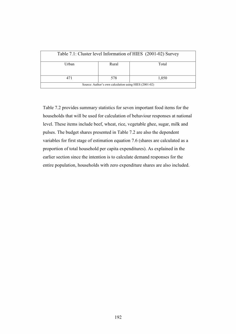
192

Table 7.1: Cluster level Information of HIES (2001-02) Survey

Urban Rural Total

471 578 1,050

Source: Author’s own calculation using HIES (2001-02)

Table 7.2 provides summary statistics for seven important food items for the

households that will be used for calculation of behaviour responses at national

level. These items include beef, wheat, rice, vegetable ghee, sugar, milk and

pulses. The budget shares presented in Table 7.2 are also the dependent

variables for first stage of estimation equation 7.6 (shares are calculated as a

proportion of total household per capita expenditures). As explained in the

earlier section since the intention is to calculate demand responses for the

entire population, households with zero expenditure shares are also included.

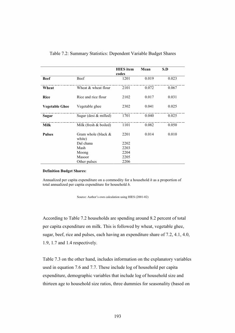
193

Table 7.2: Summary Statistics: Dependent Variable Budget Shares

HIES item

codes

Mean S.D

Beef Beef

1201 0.019 0.023

Wheat Wheat & wheat flour 2101 0.072

0.067

Rice Rice and rice flour 2102 0.017

0.031

Vegetable Ghee Vegetable ghee 2302 0.041

0.025

Sugar Sugar (desi & milled) 1701 0.040

0.025

Milk Milk (fresh & boiled) 1101 0.082

0.050

Pulses Gram whole (black & white) Dal chana Mash Moong Masoor Other pulses

2201

2202 2203 2204 2205 2206

0.014 0.010

Definition Budget Shares:

Annualized per capita expenditure on a commodity for a household h as a proportion of total annualized per capita expenditure for household h.


According to Table 7.2 households are spending around 8.2 percent of total

per capita expenditure on milk. This is followed by wheat, vegetable ghee,

sugar, beef, rice and pulses, each having an expenditure share of 7.2, 4.1, 4.0,

1.9, 1.7 and 1.4 respectively.

Table 7.3 on the other hand, includes information on the explanatory variables

used in equation 7.6 and 7.7. These include log of household per capita

expenditure, demographic variables that include log of household size and

thirteen age to household size ratios, three dummies for seasonality (based on

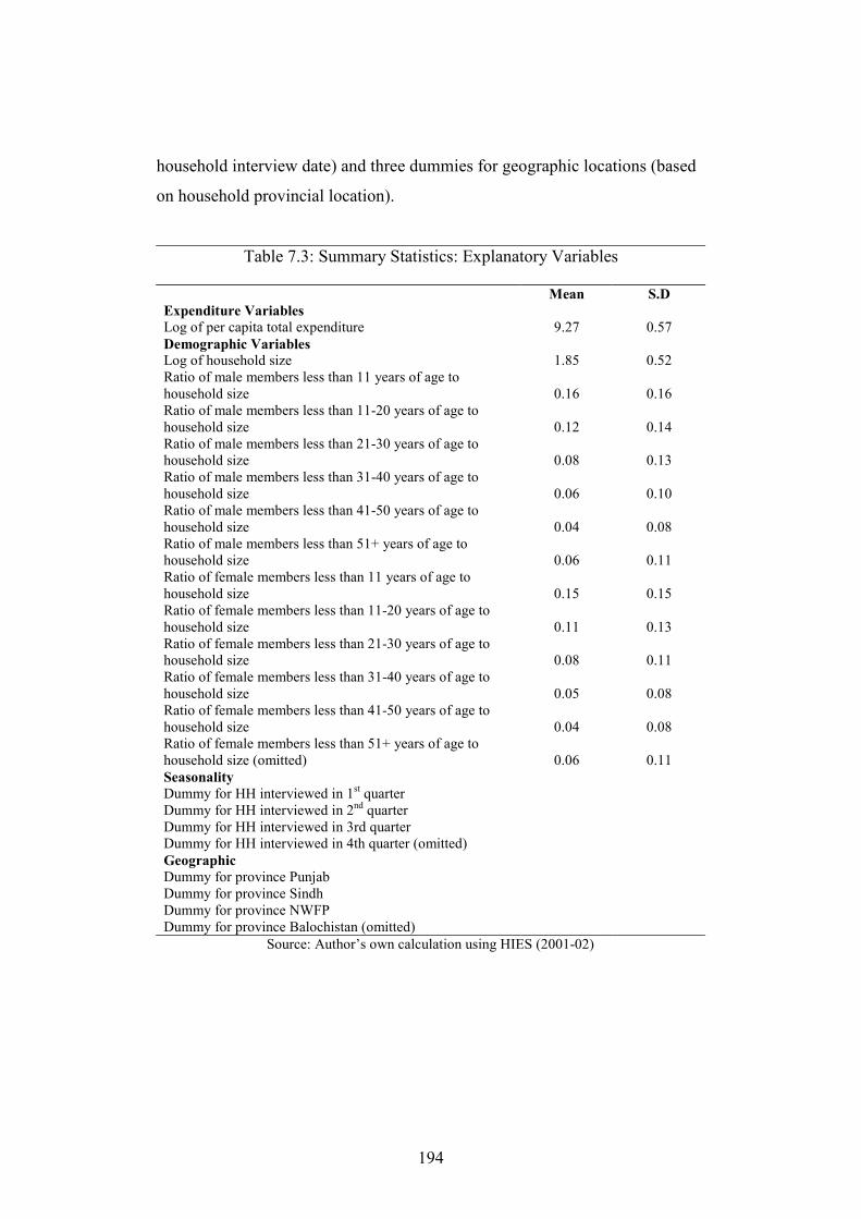
194

household interview date) and three dummies for geographic locations (based

on household provincial location).

Table 7.3: Summary Statistics: Explanatory Variables

Mean S.D

Expenditure Variables

Log of per capita total expenditure 9.27 0.57

Demographic Variables

Log of household size Ratio of male members less than 11 years of age to household size Ratio of male members less than 11-20 years of age to household size Ratio of male members less than 21-30 years of age to household size Ratio of male members less than 31-40 years of age to household size Ratio of male members less than 41-50 years of age to household size Ratio of male members less than 51+ years of age to household size Ratio of female members less than 11 years of age to household size Ratio of female members less than 11-20 years of age to household size Ratio of female members less than 21-30 years of age to household size Ratio of female members less than 31-40 years of age to household size Ratio of female members less than 41-50 years of age to household size Ratio of female members less than 51+ years of age to household size (omitted)

1.85

0.16

0.12

0.08

0.06

0.04

0.06

0.15

0.11

0.08

0.05

0.04

0.06

0.52

0.16

0.14

0.13

0.10

0.08

0.11

0.15

0.13

0.11

0.08

0.08

0.11

Seasonality

Dummy for HH interviewed in 1st quarter Dummy for HH interviewed in 2nd quarter Dummy for HH interviewed in 3rd quarter Dummy for HH interviewed in 4th quarter (omitted)

Geographic

Dummy for province Punjab Dummy for province Sindh Dummy for province NWFP Dummy for province Balochistan (omitted)


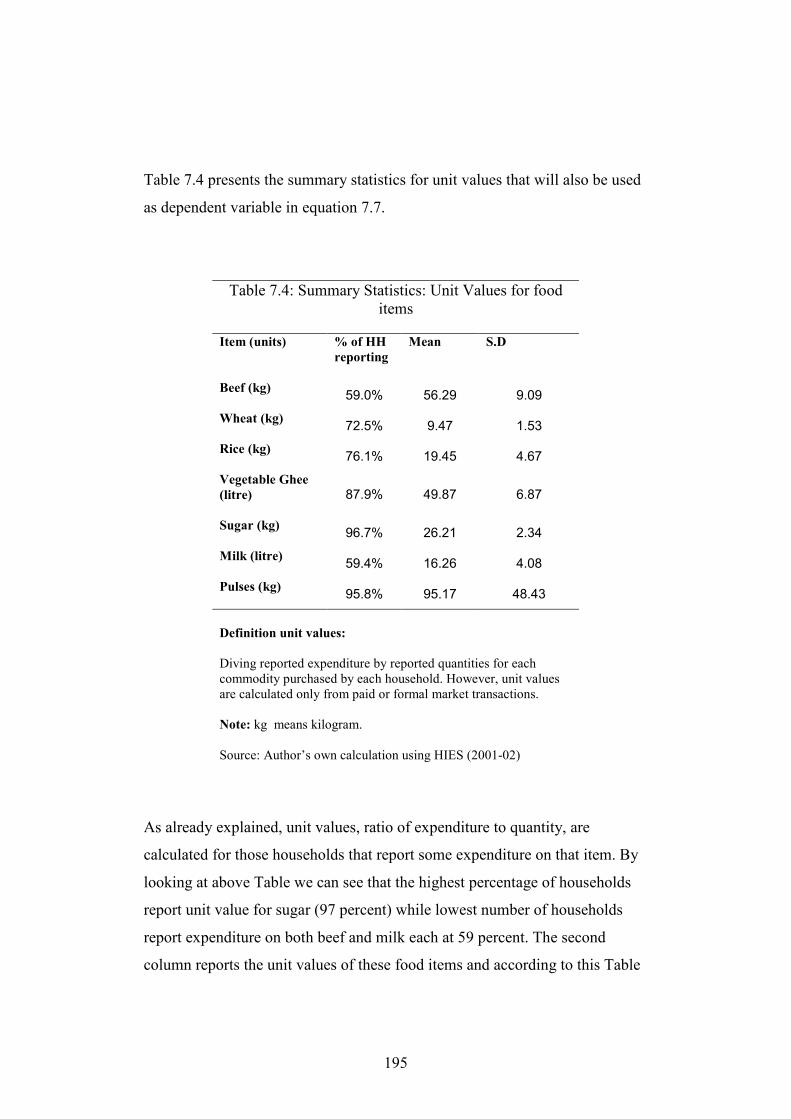
195

Table 7.4 presents the summary statistics for unit values that will also be used

as dependent variable in equation 7.7.

Table 7.4: Summary Statistics: Unit Values for food items

Item (units) % of HH

reporting

Mean S.D

Beef (kg)

59.0% 56.29 9.09

Wheat (kg)

72.5% 9.47 1.53

Rice (kg)

76.1% 19.45 4.67

Vegetable Ghee

(litre)

87.9% 49.87 6.87

Sugar (kg)

96.7% 26.21 2.34

Milk (litre)

59.4% 16.26 4.08

Pulses (kg)

95.8% 95.17 48.43

Definition unit values:

Diving reported expenditure by reported quantities for each commodity purchased by each household. However, unit values are calculated only from paid or formal market transactions.

Note: kg means kilogram.


As already explained, unit values, ratio of expenditure to quantity, are

calculated for those households that report some expenditure on that item. By

looking at above Table we can see that the highest percentage of households

report unit value for sugar (97 percent) while lowest number of households

report expenditure on both beef and milk each at 59 percent. The second

column reports the unit values of these food items and according to this Table

196

on average households paid PRs. 56 for each kg of beef while per kg wheat

cost was around PRs. 10.

Since demand analysis is primarily concerned with spatial price variation in

the unit values, it is a worthy exercise to look at the behaviour of unit values in

a bit of detail before we embark on our formal analysis (and result of this is

presented in Table 7.5). Table 7.5 provides a way of looking at the spatial

price variation in the unit values. It reports two different sets of calculation for

Pakistani data. The top panel represents the logarithm of unit values regressed

against a set of dummies for each of the four provinces; Punjab, Sindh and

NWFP, (Balochistan is the omitted category) and for each of the four quarters

(omitting the fourth) of the calendar year during which the survey was

conducted. The intention is to capture broad provincial and seasonal patterns.

The bottom portion of the table looks at variation from cluster to cluster within

each province, and uses analysis of variation to decompose price variation into

its within- cluster and between cluster components.

The top panel of Table 7.5 shows that in most cases (except wheat and sugar)

inter-provincial price variations are much larger than the seasonal differences

(although none appear to be statistically significant). We can see that in 2001-

02 among provinces, wheat was relatively cheaper in Punjab, while rice

appeared to be relatively cheaper in Sindh (this is in line with the fact that

most of the production of wheat takes place in Punjab while most of

production of rice takes place in Sindh). Sugar appears to be cheapest in

Balochistan (the omitted province), while milk appears to be cheapest in

Punjab. There appears to be a great deal of price variation across provinces for

all commodities (except for wheat and sugar).

The bottom part of Table 7.5 reports not parameter estimates but the F-test and

R2- statistics for a regression of the logarithm of unit value on dummies for

197

clusters, of which there are 458 in Punjab, 264 in Sindh, 188 in NWFP and

140 in Balochistan. However, it must be kept in mind that not all clusters will

appear in each regression since if no household in a cluster reports that type of

expenditure, that cluster is not selected. What we are aiming to look for from

this regression is how informative unit values are about prices. Since prices

are assumed not to vary by much within-cluster over a short period of time, F-

statistics should be significant for cluster effects at conventional level of

significance, or in other words the cluster effects should explain around a half

of the total variance.

According to our results, all F-Statistics appear to be quite large and

significant by conventional standard. However, given that the sample size is

quite large, a better indication of the strength of inter-cluster variation in unit

values is typically whether the F-Statistics are larger than the logarithm of the

sample sizes (Schwarz, 1978). Most of F-Statistics (identified as bold figures)

meet even this stringent requirement. Thus, this should justify the assumption

that there is spatial price variation and that the variation in unit values

provides a (noisy) guide to it.

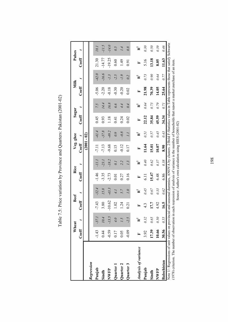
198

Tab

le 7

.5:

Pri

ce v

aria

tion b

y P

rovin

ce a

nd Q

uar

ters

: P

akis

tan (

2001-0

2)

Coeff

tCoeff

t

Coeff

t

Coeff

t

Coeff

t

Coeff

t

Coeff

t

Reg

ression

Punjab

-1.4

3-3

7.1

-7.4

3-3

2.4

-1.4

6-1

1.1

-7.1

1-4

1.4

0.4

57

.5-5

.06

-42

.021

.30

18

.1

Sindh

0.4

41

0.4

3.8

01

5.8

-3.3

5-2

3.1

-7.1

3-3

7.8

0.9

31

4.4

-2.2

0-1

6.6

-14

.77

-11

.5

NWFP

-0.5

9-1

3.5

-10

.62

-43

.3-2

.73

-18

.2-9

.68

-49

.21

.18

16

.8-0

.18

-1.3

-19

.25

-14

.0

Quarter 1

0.1

74

.01

.02

4.1

0.0

10

.10.1

50

.90

.41

6.6

-0.3

0-2

.50

.60

0.5

Quarter 2

0.0

51

.51

.24

5.7

0.2

72

.2-0

.12

-0.8

0.2

44

.4-0

.20

-1.9

1.4

91

.4

Quarter 3

-0.0

9-2

.50

.21

1.0

0.1

61

.30.1

71

.10

.02

0.4

0.0

20

.20

.91

0.8

Analysis of va

riance

FR2

FR2

FR2

FR2

FR2

FR2

FR2

Punjab

3.9

20

.32

4.3

0.4

56.1

10

.40

11.64

0.5

122.12

0.6

421.98

0.7

35

.16

0.3

0

Sindh

17.39

0.6

517.7

0.6

715.47

0.6

215.01

0.5

735.84

0.7

370.39

0.9

013.18

0.5

0

NWFP

10.66

0.5

04

.92

0.3

36.4

80

.37

10.07

0.4

545.59

0.7

914.05

0.6

48.05

0.3

9

Balochistan

30.56

0.5

516.5

0.6

26.8

60

.38

8.90

0.4

334.34

0.7

125.64

0.7

711.63

0.4

6

So

urc

e: A

uth

or'

s o

wn c

alcu

lati

on

usi

ng H

IES

(2

00

1-0

2)

No

te 1

/: R

egre

ssio

ns

of

unit

val

ues

on p

rovin

cial

and

sea

sonal

dum

mie

s, A

NO

VA

by c

lust

ers.

2/B

old

F-S

tati

stic

s val

ues

in T

able

rep

rese

nts

tho

se t

hat

sat

isfy

Sch

war

tz

(19

78

) cr

iter

ion.

The

num

ber

of

ob

serv

atio

n i

n e

ach r

egre

ssio

n o

f an

alysi

s o

f var

iance

is

the

num

ber

of

ho

use

ho

lds

that

rep

ort

a m

arket

purc

has

e o

f an

ite

m.

Milk

Pulses

Wheat

(2001 - 02)

Beef

Rice

Veg. ghee

Sugar

199

7.5 Estimation

7.5.1 First-stage estimates

After a detailed basic discussion regarding variables that will be used in this

estimation and after confirming that the unit values (at least in the case of

seven goods above) are providing significant inter-cluster variation

(significant enough in most cases to meet stringent (Schwarz, 1978) criteria);

as a result, we are in a good position to start discussion of our estimation.

Table 7.6 presents within cluster estimates of regression for (log) unit values

and expenditure shares i.e. equation 7.6 and 7.7. As explained before, all

variables in both equations were first demeaned by their cluster means and

then OLS was applied to the demeaned equations. OLS regressions at this

stage are run using demeaned values of each variable in the regression and

result of key variables is presented in Table 7.6 (for complete estimation

results please see Appendix 7.1 attached at the end of this chapter)

Note that the estimates in Table 7.6 are final estimates for the effects of total

expenditure and demographic variables derived completely from within cluster

information. The first and fourth line represent our 1β and 2β coefficient

respectively from equation 7.6 and 7.7. According to our estimates, all

coefficients of total (per capita) household expenditures (w:lnx) appear to be

statistically significant and with right sign (except milk). The total expenditure

elasticity for wheat appears to be 0.157, for rice it is 0.518, vegetable ghee

0.41, sugar 0.64, milk 1.01, pulses 0.28 and beef 0.77. Since only milk appears

to have expenditure elasticity greater than unity, it appears to be a luxury item

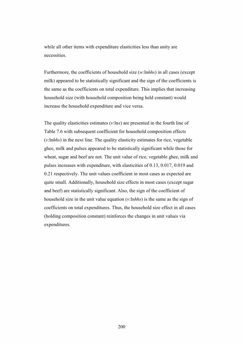
200

while all other items with expenditure elasticities less than unity are

necessities.

Furthermore, the coefficients of household size (w:lnhhs) in all cases (except

milk) appeared to be statistically significant and the sign of the coefficients is

the same as the coefficients on total expenditure. This implies that increasing

household size (with household composition being held constant) would

increase the household expenditure and vice versa.

The quality elasticities estimates (v:lnx) are presented in the fourth line of

Table 7.6 with subsequent coefficient for household composition effects

(v:lnhhs) in the next line. The quality elasticity estimates for rice, vegetable

ghee, milk and pulses appeared to be statistically significant while those for

wheat, sugar and beef are not. The unit value of rice, vegetable ghee, milk and

pulses increases with expenditure, with elasticities of 0.13, 0.017, 0.019 and

0.21 respectively. The unit values coefficient in most cases as expected are

quite small. Additionally, household size effects in most cases (except sugar

and beef) are statistically significant. Also, the sign of the coefficient of

household size in the unit value equation (v:lnhhs) is the same as the sign of

coefficients on total expenditures. Thus, the household size effect in all cases

(holding composition constant) reinforces the changes in unit values via

expenditures.

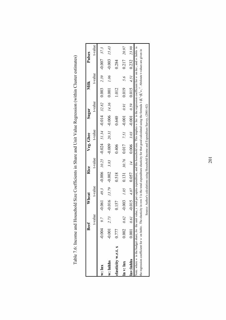
201

Tab

le 7

.6:

Inco

me

and H

ouse

hold

Siz

e C

oef

fici

ents

in S

har

e an

d U

nit

Val

ue

Reg

ress

ion (

wit

hin

Clu

ster

est

imat

es)

t-val

ue

t-val

ue

t-val

ue

t-val

ue

t-val

ue

t-val

ue

t-val

ue

w: lnx

-0.0

04

9.7

-0.0

61

49

.3-0

.006

10

.25

-0.0

24

51

.34

-0.0

14

32

.82

0.0

03

2.3

9-0

.007

37

.3

w: lnhhs

-0.0

01

2.7

3-0

.016

13

.79

-0.0

02

3.8

3-0

.009

20

.31

-0.0

06

14

.36

0.0

01

1.0

6-0

.003

15

.43

elasticity w.r.t. x

0.7

77

0.1

57

0.5

18

0.4

06

0.6

40

1.0

12

0.2

84

ln v: lnx

0.0

02

0.6

2-0

.003

1.0

50.1

31

30

.76

0.0

17

7.5

1-0

.001

0.9

10.0

19

5.6

0.2

17

20

.97

lnv:lnhhs

0.0

01

0.6

1-0

.015

4.8

70.0

57

14

0.0

06

3.0

3-0

.001

0.5

90.0

15

4.5

10.2

32

23

.99

Sou

rce:

Au

thor'

s ca

lcu

lati

on

s u

sin

g H

ou

seh

old

In

com

e an

d E

xp

end

itu

re S

urv

ey,

(20

01

-02

)

Note

: w

her

e w

is

the

bu

dget

sh

are,

ln

v t

he

un

it v

alu

e, x

tota

l p

er c

apit

a ex

pen

dit

ure

, an

d h

hs

hou

seh

old

siz

e. T

his

im

pli

es w

:ln

x i

s th

e re

gre

ssio

n c

oef

fici

ent

for

w o

n l

nx

, an

d w

:ln

hh

s i

s

the

regre

ssio

n c

oef

fici

ent

for

w o

n l

nh

hs

. T

he

elas

tici

ty i

n r

ow

3 i

s th

e to

tal

exp

end

itu

re e

last

icit

y f

or

that

good

cal

cula

ted

usi

ng t

he

form

ula

1-β

i1+

βi2

wi-1

. A

bsl

ou

te t

-val

ues

are

giv

en i

n

colu

mn

t-v

alu

es.

Sugar

Milk

Pulses

Beef

Wheat

Rice

Veg. Ghee

202

7.5.2 Price response: Second-stage estimates

Table 7.7 present own- and cross-price elasticities results for Pakistan along

with the bootstrapped estimates for “standard errors”. The numbers are

presented such that the elasticity estimate in row i and column j is the response

of consumption of good i to the price of good j . These estimates include the

provincial and quarter effects in demands as these are allowed for by

regressing the corrected cluster averages of budget shares and unit values on

quarterly and provincial dummies.

According to our results in Table 7.7 we can see that all own- price elasticity

estimates are negative (except for wheat) and significant126. The own- price

elasticity for beef, rice and milk is less than -1. This means milk, rice and beef

are price elastic goods while demand for vegetable ghee, sugar, and pulses is

fairly inelastic. This provides very useful information from the tax policy

planning perspective. For instance, additional price increase of milk, rice and

beef (due to imposition of tax for instance) is going to be not that successful

because demand for these products is quite elastic. Thus, it is unlikely that

much revenue is going to be raised from such a policy. On the other hand,

vegetable ghee, sugar and pulses are an attractive candidate for further price

increase (due to a tax) since their demand is fairly inelastic. Thus, these

elasticities estimates are fundamental for tax policy planning as they make ex-

ante tax policy analysis possible.

126 It is hard to explain a positive own-price elasticity case, such as wheat, in our case. One possibility is that the estimation is severely affected by aggregation across various qualities of wheat in the survey..

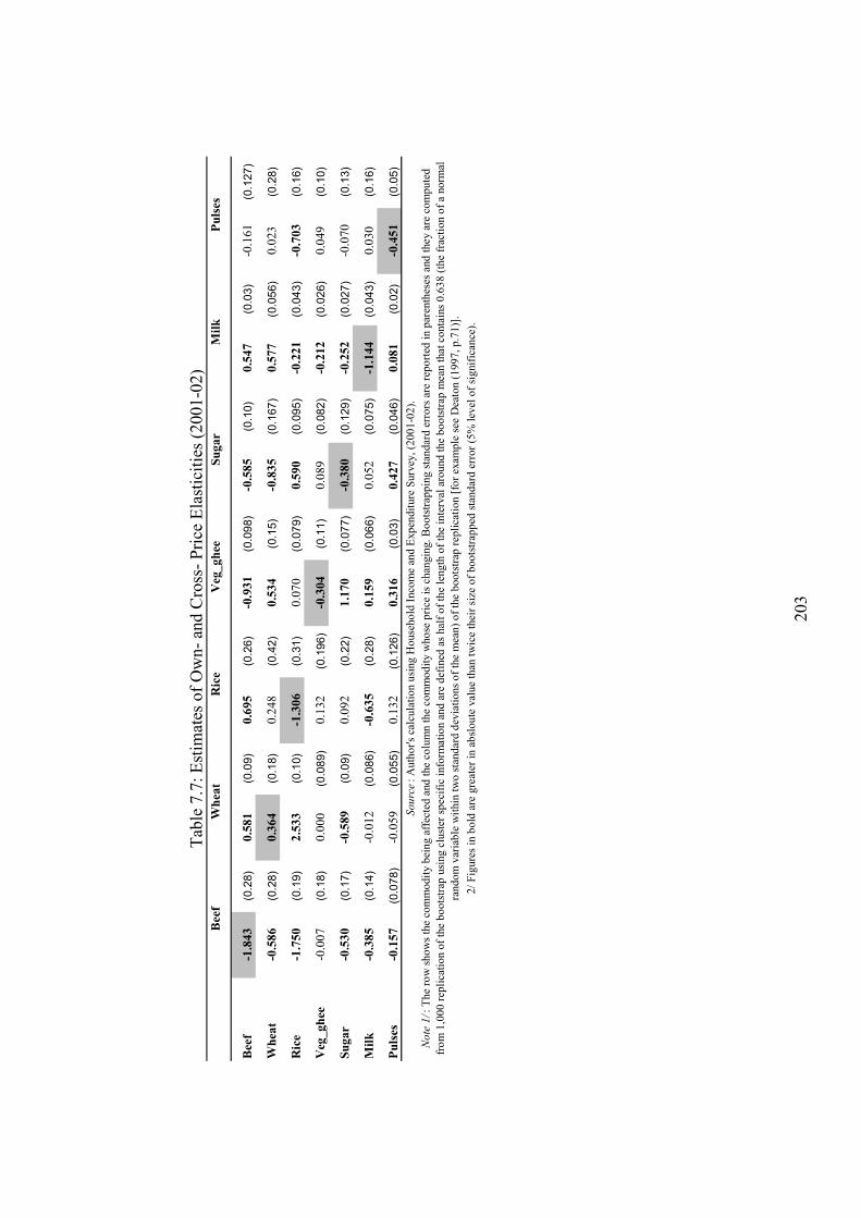
203

Tab

le 7

.7:

Est

imat

es o

f O

wn-

and C

ross

- P

rice

Ela

stic

itie

s (2

001-0

2)

Beef

-1.843

(0.2

8)

0.581

(0.0

9)

0.695

(0.2

6)

-0.931

(0.0

98)

-0.585

(0.1

0)

0.547

(0.0

3)

-0.1

61

(0.1

27

)

Wheat

-0.586

(0.2

8)

0.364

(0.1

8)

0.2

48

(0.4

2)

0.534

(0.1

5)

-0.835

(0.1

67

)0.577

(0.0

56)

0.0

23

(0.2

8)

Rice

-1.750

(0.1

9)

2.533

(0.1

0)

-1.306

(0.3

1)

0.0

70

(0.0

79)

0.590

(0.0

95

)-0.221

(0.0

43)

-0.703

(0.1

6)

Veg_ghee

-0.0

07

(0.1

8)

0.0

00

(0.0

89)

0.1

32

(0.1

96

)-0.304

(0.1

1)

0.0

89

(0.0

82

)-0.212

(0.0

26)

0.0

49

(0.1

0)

Sugar

-0.530

(0.1

7)

-0.589

(0.0

9)

0.0

92

(0.2

2)

1.170

(0.0

77)

-0.380

(0.1

29

)-0.252

(0.0

27)

-0.0

70

(0.1

3)

Milk

-0.385

(0.1

4)

-0.0

12

(0.0

86)

-0.635

(0.2

8)

0.159

(0.0

66)

0.0

52

(0.0

75

)-1.144

(0.0

43)

0.0

30

(0.1

6)

Pulses

-0.157

(0.0

78

)-0

.059

(0.0

55)

0.1

32

(0.1

26

)0.316

(0.0

3)

0.427

(0.0

46

)0.081

(0.0

2)

-0.451

(0.0

5)

So

urc

e:

Auth

or'

s ca

lcula

tio

n u

sing

Ho

use

ho

ld I

nco

me

and

Exp

end

itu

re S

urv

ey,

(20

01

-02

).

No

te 1

/: T

he

row

sh

ow

s th

e co

mm

od

ity b

ein

g a

ffec

ted

and

the

colu

mn t

he

com

mo

dit

y w

ho

se p

rice

is

chan

gin

g.

Bo

ots

trap

pin

g s

tan

dar

d e

rro

rs a

re r

epo

rted

in p

aren

thes

es a

nd

they

are

co

mp

ute

d

fro

m 1

,00

0 r

epli

cati

on o

f th

e b

oo

tstr

ap u

sin

g c

lust

er s

pec

ific

info

rmat

ion

an

d a

re d

efin

ed a

s h

alf

of

the

leng

th o

f th

e in

terv

al a

rou

nd

the

bo

ots

trap

mea

n t

hat

co

nta

ins

0.6

38

(th

e fr

acti

on o

f a

no

rmal

ran

do

m v

aria

ble

wit

hin

tw

o s

tand

ard

dev

iati

on

s o

f th

e m

ean

) o

f th

e b

oo

tstr

ap r

epli

cati

on [

for

exam

ple

see

Dea

ton (

19

97

, p

.71

)].

2/

Fig

ure

s in

bo

ld a

re g

reat

er i

n a

bsl

ou

te v

alu

e th

an t

wic

e th

eir

size

of

bo

ots

trap

ped

sta

nd

ard

err

or

(5%

lev

el o

f si

gnif

ican

ce).

Beef

Wheat

Rice

Veg_ghee

Sugar

Milk

Pulses

204

Table 7.7 also presents cross- price elasticity results for all seven goods.

Almost around half of our cross- price elasticity estimates appear to be

significant and in some cases the cross- price elasticities estimates are not too

small to ignore. For instance, one percent increase in the price of beef

decreases the demand for rice by 1.7 percent. In quite a few cases we are able

to make out a clear relationship pattern between goods but very few of these

are also statistically significant. For instance, beef appears to be a complement

to vegetable ghee, sugar and pulses (but only in the case of sugar is this

relationship statistically significant). The complement relationship between

beef and sugar warrant extra comment. One possibility is that given beef is an

expansive meat type, it is normally cooked by average Pakistani households

on special occasions and a dessert is also part of the menu of such events. This

can explain a positive relationship between beef and sugar. Wheat, on the

other hand, appears to be a substitute for rice and vegetable ghee but a

complement to sugar (but only in the case of sugar is this relationship also

statistically significant). Similarly, rice appears to be a substitute of vegetable

ghee and sugar but a complement to milk while vegetable ghee appears to be a

substitute to sugar and pulses (but none of these relationships are significant).

Lastly, milk and pulses appear to be complements (but this relationship is not

statistically significant). Thus, these results show important differences from

results obtained by imposing symmetry.

The results presented in Table 7.7 highlight an important point. In the case of

developing countries where data availability is limited to one year cross-

sectional data, model based on additive preferences such as linear expenditure

system (LES) that restricts cross- price elasticities to be small and enforces

approximate proportionality, are generously used (for instance see Ahmad and

Stern (1986) for Pakistan). According to Deaton (1987) models that assume

additive preferences (such as LES system), tax reform prescriptions tend to be

205

quite simple and he concludes “under these assumptions, empirical analysis is

unnecessary, since the answer is predetermined” (pp.6). This is supported by

our findings since we do not find any such proportionality between

expenditure elasticities and price elasticities127. For instance, first we do not

find cross-price elasticities to be too small to be negligible (i.e. fundamental

assumption underlying most of optimal taxation literature) and second, if we

look at Table 7.6 expenditure elasticities show all items except milk to be

necessities while according to own- price elasticities estimates in Table 7.7,

demand for beef, rice and milk appears to be quite price elastic while demand

for wheat, vegetable ghee, sugar, and pulses appears to be price inelastic.

Thus, this really questions whether predictions of a system such as LES are

really meaningful for tax and price reform analysis.

Table 7.8 presents our own price elasticity results with Deaton and Grimard

results using the same methodology but for a different time period. We do not

expect results to completely match with Deaton & Grimard (1992) own-price

elasticities for three reasons: (a) Difference in time period (almost 15 years);

(b) The definition (see third column) of only sugar, rice and wheat is directly

comparable to ours otherwise Deaton and Grimard (1992) use broader

aggregation of commodities; (c) Our results are for national level (as flagged

earlier)128.

127 This finding is supported by Deaton and Grimard (1992) and Deaton (1997).

128 Please see Appendix 7.2 for rural elasticities estimates for (2001-02).

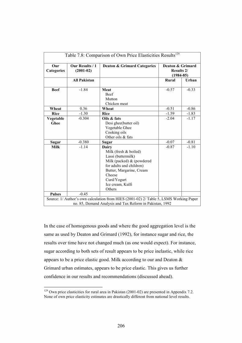
206

Table 7.8: Comparison of Own Price Elasticities Results129

Our

Categories

Our Results / 1

(2001-02)

Deaton & Grimard Categories Deaton & Grimard

Results 2/

(1984-85)

All Pakistan

Rural Urban

Beef -1.84 Meat

Beef Mutton Chicken meat

-0.57 -0.33

Wheat 0.36 Wheat -0.51 -0.86

Rice -1.30 Rice -1.59 -1.83

Vegetable

Ghee

-0.304 Oils & fats

Desi ghee(butter oil) Vegetable Ghee Cooking oils Other oils & fats

-2.04 -1.17

Sugar -0.380 Sugar -0.07 -0.81

Milk -1.14 Dairy

Milk (fresh & boiled) Lassi (buttermilk) Milk (packed) & (powdered for adults and children) Butter, Margarine, Cream Cheese Curd/Yogurt Ice cream, Kulfi Others

-0.87 -1.10

Pulses -0.45

Source: 1/ Author’s own calculation from HIES (2001-02) 2/ Table 5, LSMS Working Paper no. 85, Demand Analysis and Tax Reform in Pakistan, 1992

In the case of homogenous goods and where the good aggregation level is the

same as used by Deaton and Grimard (1992), for instance sugar and rice, the

results over time have not changed much (as one would expect). For instance,

sugar according to both sets of result appears to be price inelastic, while rice

appears to be a price elastic good. Milk according to our and Deaton &

Grimard urban estimates, appears to be price elastic. This gives us further

confidence in our results and recommendations (discussed ahead).

129 Own price elasticities for rural area in Pakistan (2001-02) are presented in Appendix 7.2. None of own price elasticity estimates are drastically different from national level results.

207

7.6 Demand Responses and Our Incidence Findings

In this section we will try to illustrate how price elasticities estimated in the

previous section are likely to impact our incidence findings reported in the

earlier chapters. This is quite important as it is one of the fundamental

criticisms faced by partial equilibrium tax incidence model.

Let’s assume there is an x percentage point increase in the price of sugar (for

instance GST on sugar is increased). This means according to our elasticity

estimates, demand for sugar will fall by 0.38x percent. As demand for sugar is

fairly price inelastic, Government revenue should increase from this policy. As

sugar is consumed more by the poor in both the rural and urban areas, this is

likely to impact the poor more. However, due to fairly inelastic demand

patterns incidence is likely to remain very close to the one predicted earlier

(because partial equilibrium tax incidence analysis already assumes no

demand response).

However, an x percentage increase in the price of sugar due to GST does not

only affect sugar consumption, but also affects demand for other commodities

via significant cross- price effects. Thus, demand for beef and wheat will fall,

while the demand for rice, vegetable ghee, milk and pulses will increase. As a

result Government revenue will fall on account of decrease in demand for

beef, and wheat but increase due to increase in demand for other goods

(assuming all these goods were already being taxed). However, it appears a

fall in demand on aggregate will slightly dominate the increase in demand,

given our cross- price elasticities estimates. Thus on this account, overall

Government revenue will fall. Since large cross price effects are for beef

(demand falls), wheat (demand falls) and rice (demand increases), poor who

208

largely consume wheat will experience some relief but this to some extent will

be offset by increase in demand for rice. Thus, at the end the overall incidence

picture may not change much. More importantly, price of sugar that was

mainly increased to raise additional revenue, may not result in much additional

revenues.

Let’s consider another example, vegetable ghee. For an x percentage point

increase in price of vegetable ghee given its demand is fairly inelastic (with

own- price elasticity similar to that of sugar) demand for vegetable ghee will

not fall by that much. Thus, Government should be able to raise revenue from

this policy but it is likely to impact the poor more as they spend relatively

more on this item. However, in this case if we look at cross- price effects

things appear to be quite different compared to our earlier illustration. For

instance, demand for sugar and wheat will increase (and also milk and pulses

but to a lesser extent) while demand for beef declines quite sharply. However,

in this case the cross- price effects do not balance out neatly as before. Thus,

as a result of this policy Government will be able to raise revenue but likely

large distributional effects will be borne by the poor who are spending more

on vegetable ghee, sugar and wheat.

Thus it appears for our selected sample of commodities, incidence patterns

while allowing for the own- price elasticities do not alter dramatically.

However, effect of incorporation of cross- price elasticities varies from case to

case basis depending on the magnitude and sign of the elasticity and the

importance of the other commodities in the consumption basket; sometimes

(as per our illustration) it makes little difference, in other cases it might matter

more. However, generally it appears that incorporation of own- and cross-

price effects while making possibly bigger impact on incidence, may still not

alter our results that dramatically. Nevertheless, we cannot generalize these

results to commodities outside our sample or for other countries or for a

209

different time period. As in other cases inclusion of cross-price effects may

prove more important for policy purposes.

7.7 Tax and Price Reform

Now we are in a position to begin with the last section of our chapter, that is

carrying out microsimulation analysis using elasticities estimates calculated in

the previous section. We feel it is necessary to incorporate this section because

in chapters five and six, we were able to show the social incidence of indirect

taxation at pre- and post reform scenarios but we were not able to give any

specific recommendation that at the margin can improve the welfare of

households particularly from the point of view of post-reform position. This

section gives us an opportunity to point out future reforms that will be

welfare-enhancing at margin (as a consequence completing our discussion in

earlier chapters).

This section will use the theory of marginal tax reform (MTR) (as explained

earlier in chapter three) developed by the seminal work of Ahmad and Stern

(1984). The aim of this theory is to measure welfare gains due to small

changes in tax rates of every good. Essential to this approach is that the

current system must be taken as given and the aim is to identify directions of

tax reform that at the margin are welfare enhancing (Madden, 1995). The

importance of MTR theory lies in the fact that this approach attempts to

calculate the directions of welfare improving reform at margin from the

existing position of the economy, which according to Madden (1995) and

Deaton (1995), is not only more appealing for the policy makers but also a

more practical approach.

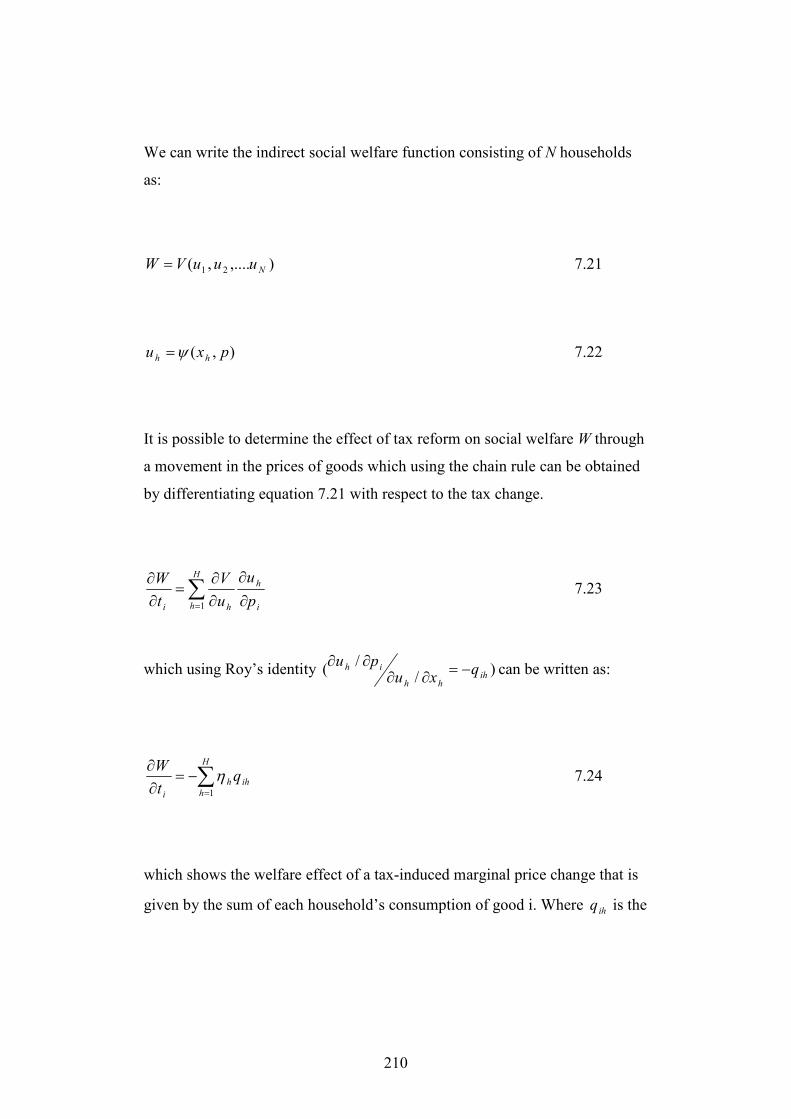
210

We can write the indirect social welfare function consisting of N households

as:

),....,( 21 NuuuVW = 7.21

),( pxu hh ψ= 7.22

It is possible to determine the effect of tax reform on social welfare W through

a movement in the prices of goods which using the chain rule can be obtained

by differentiating equation 7.21 with respect to the tax change.

i

hH

h hi p

u

u

V

t

W

∂

∂

∂

∂=

∂

∂∑=1

7.23

which using Roy’s identity )/

/( ih

hh

ih qxu

pu −=∂∂∂∂

can be written as:

∑=

−=∂

∂ H

h

ihh

i

qt

W

1

η 7.24

which shows the welfare effect of a tax-induced marginal price change that is

given by the sum of each household’s consumption of good i. Where ihq is the

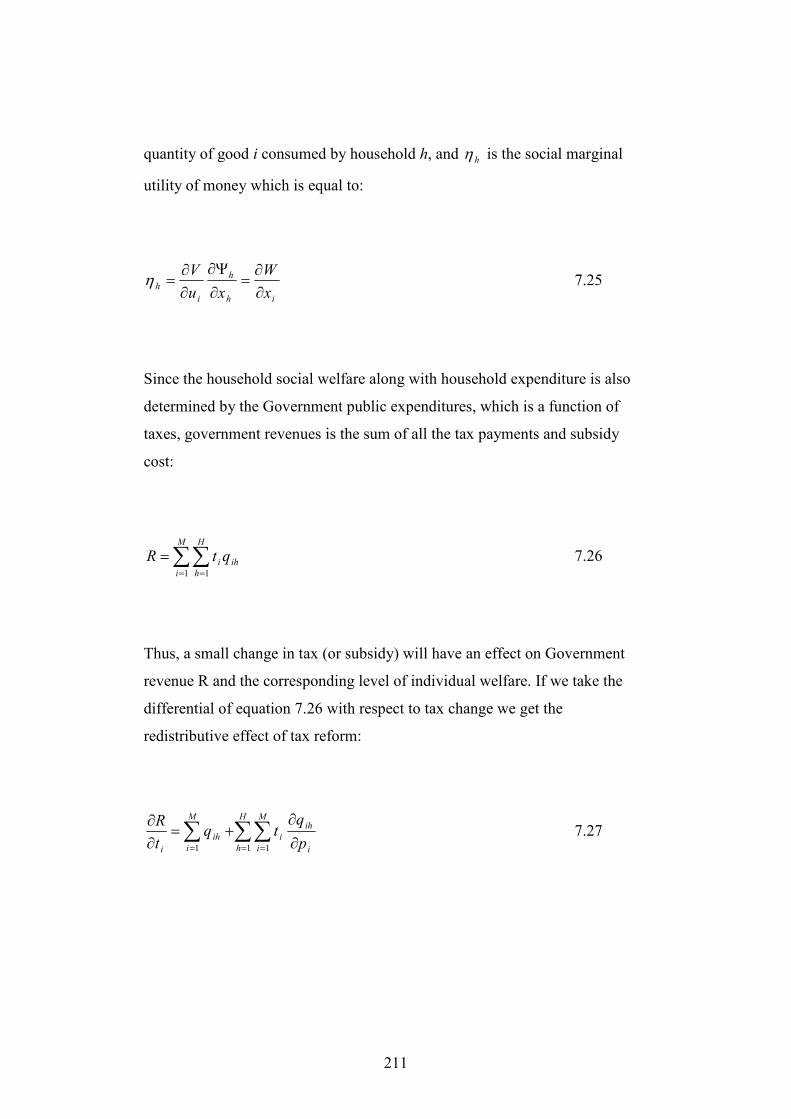
211

quantity of good i consumed by household h, and hη is the social marginal

utility of money which is equal to:

ih

h

i

hx

W

xu

V

∂

∂=

∂

Ψ∂

∂

∂=η 7.25

Since the household social welfare along with household expenditure is also

determined by the Government public expenditures, which is a function of

taxes, government revenues is the sum of all the tax payments and subsidy

cost:

∑∑= =

=M

i

H

h

ihi qtR1 1

7.26

Thus, a small change in tax (or subsidy) will have an effect on Government

revenue R and the corresponding level of individual welfare. If we take the

differential of equation 7.26 with respect to tax change we get the

redistributive effect of tax reform:

i

ihH

h

M

i

i

M

i

ih

i p

qtq

t

R

∂

∂+=

∂

∂∑∑∑= == 1 11

7.27

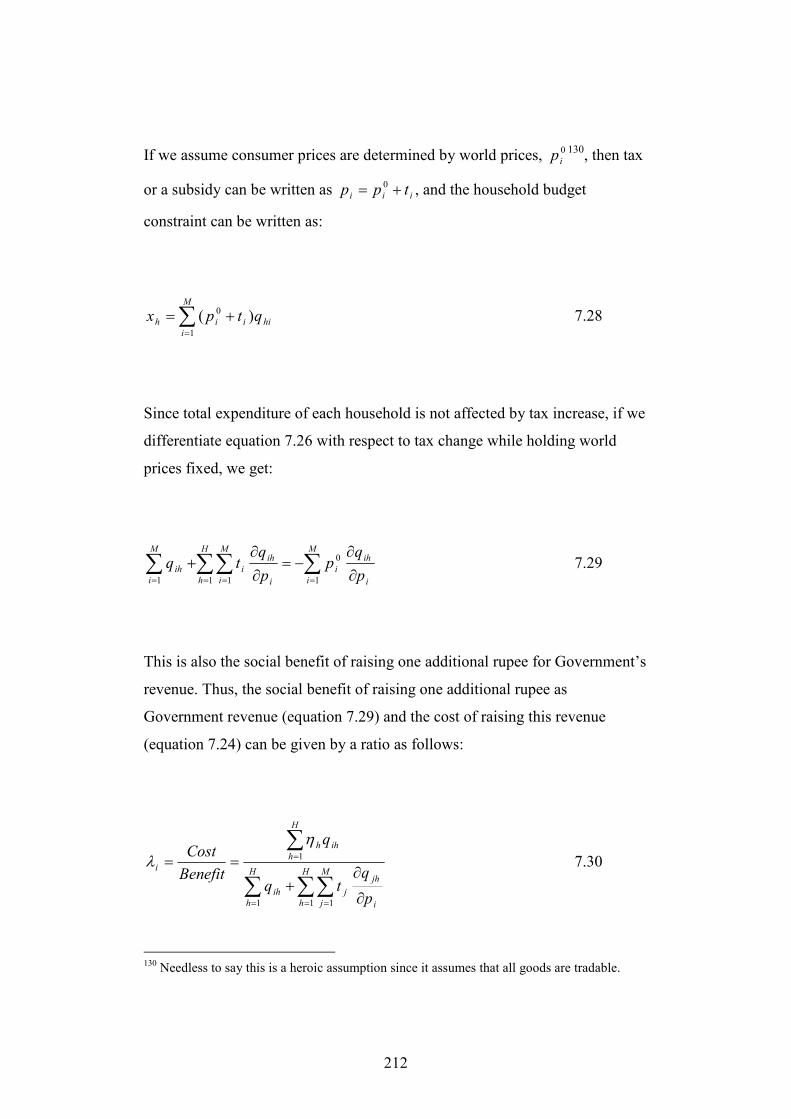
212

If we assume consumer prices are determined by world prices, 0

ip130, then tax

or a subsidy can be written as iii tpp += 0 , and the household budget

constraint can be written as:

hii

M

i

ih qtpx )(1

0 +=∑=

7.28

Since total expenditure of each household is not affected by tax increase, if we

differentiate equation 7.26 with respect to tax change while holding world

prices fixed, we get:

i

ihM

i

i

i

ihH

h

M

i

i

M

i

ihp

qp

p

qtq

∂

∂−=

∂

∂+ ∑∑∑∑

== == 1

0

1 11

7.29

This is also the social benefit of raising one additional rupee for Government’s

revenue. Thus, the social benefit of raising one additional rupee as

Government revenue (equation 7.29) and the cost of raising this revenue

(equation 7.24) can be given by a ratio as follows:

∑ ∑∑

∑

= = =

=

∂

∂+

==H

h

H

h

M

j i

jh

jih

H

h

ihh

i

p

qtq

q

Benefit

Cost

1 1 1

1

ηλ 7.30

130 Needless to say this is a heroic assumption since it assumes that all goods are tradable.

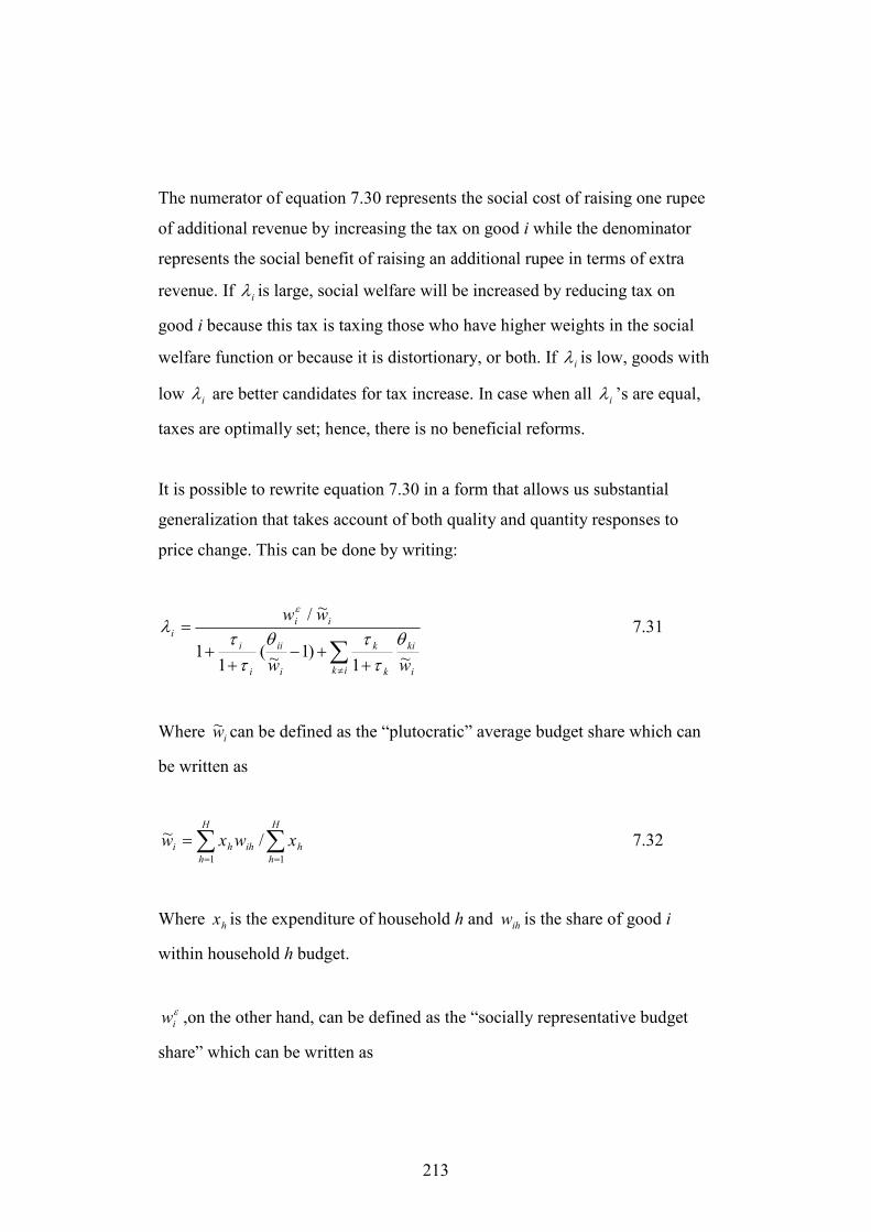
213

The numerator of equation 7.30 represents the social cost of raising one rupee

of additional revenue by increasing the tax on good i while the denominator

represents the social benefit of raising an additional rupee in terms of extra

revenue. If iλ is large, social welfare will be increased by reducing tax on

good i because this tax is taxing those who have higher weights in the social

welfare function or because it is distortionary, or both. If iλ is low, goods with

low iλ are better candidates for tax increase. In case when all iλ ’s are equal,

taxes are optimally set; hence, there is no beneficial reforms.

It is possible to rewrite equation 7.30 in a form that allows us substantial

generalization that takes account of both quality and quantity responses to

price change. This can be done by writing:

∑≠ +

+−+

+=

ik i

ki

k

k

i

ii

i

i

ii

i

ww

ww

~1)1~(

11

~/

θτ

τθτ

τλ

ε

7.31

Where iw~ can be defined as the “plutocratic” average budget share which can

be written as

∑∑==

=H

h

hih

H

h

hi xwxw11

/~ 7.32

Where hx is the expenditure of household h and ihw is the share of good i

within household h budget.

εiw ,on the other hand, can be defined as the “socially representative budget

share” which can be written as

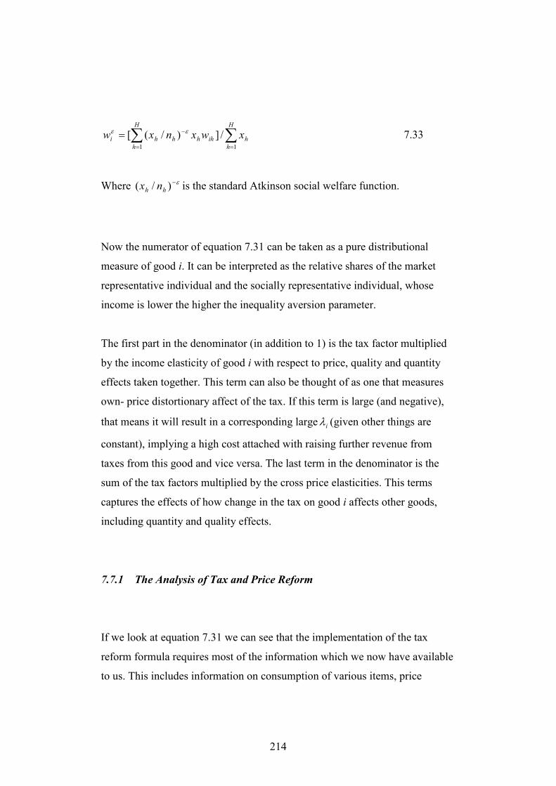
214

∑∑=

−

=

=H

h

hihh

H

h

hhi xwxnxw11

/])/([ εε 7.33

Where ε−)/( hh nx is the standard Atkinson social welfare function.

Now the numerator of equation 7.31 can be taken as a pure distributional

measure of good i. It can be interpreted as the relative shares of the market

representative individual and the socially representative individual, whose

income is lower the higher the inequality aversion parameter.

The first part in the denominator (in addition to 1) is the tax factor multiplied

by the income elasticity of good i with respect to price, quality and quantity

effects taken together. This term can also be thought of as one that measures

own- price distortionary affect of the tax. If this term is large (and negative),

that means it will result in a corresponding large iλ (given other things are

constant), implying a high cost attached with raising further revenue from

taxes from this good and vice versa. The last term in the denominator is the

sum of the tax factors multiplied by the cross price elasticities. This terms

captures the effects of how change in the tax on good i affects other goods,

including quantity and quality effects.

7.7.1 The Analysis of Tax and Price Reform

If we look at equation 7.31 we can see that the implementation of the tax

reform formula requires most of the information which we now have available

to us. This includes information on consumption of various items, price

215

derivates, social weights and shadow prices. We have just estimated price

derivates (own and cross). Assigning social weights is a fairly common

practice; as a result we are left with the issue of clarifying how shadow prices

or shadow tax (subsidy) rate iτ can be determined. The shadow prices

represent the element of tax (or subsidy) in percentage terms that each good is

subject to. Ideally, this price should be set by taking into account tariffs, taxes,

subsidies and other transfers; all of which contribute to the determination of

domestic price of a good (Deaton, 1997). However, like Deaton (1997), we

work with an illustrative set of shadow prices in order to keep this discussion

simple. This price set is termed illustrative since it does not claim to

incorporate all the ingredients that should ideally be included for a shadow

price but nevertheless it is simple, transparent and comprehensive enough to

include Pakistan’s actual post reform situation, that should be enough to

ascertain direction of welfare improving reforms131 132.

Most of the information required for the calculation of an illustrative set of

shadow prices (tax or subsidy) is taken from World Bank (2007). According to

this report most of major agriculture commodities during the 1980s were

heavily implicitly taxed through negative indirect effects of trade and

exchange rate policies. However, by the end of the 1980’s there was a

significant decline in the distortion of agriculture prices as a result of major

trade and agriculture price reform policies undertaken by the Government

(World Bank, 2007). This information is presented in Table 7.9 which shows

131 The experiment that is being considered here is an increase or decrease in the consumer price of a good as a result of a consumption tax like VAT or tariff. This experiment would not correspond well with analysis of export taxes because such a tax according to our model will increase consumer welfare as well as Government revenue at the same time, which according to our specification requires this tax to be increased indefinitely. Additionally, since export taxes can alter both the consumer as well as producer prices, it can not be fully analyzed without bring supply responses in the picture (Deaton, 1997). 132 Also, this experiment only looks at the demand side of analysis where its assumed producer and consumer prices are separated (Deaton, 1997).

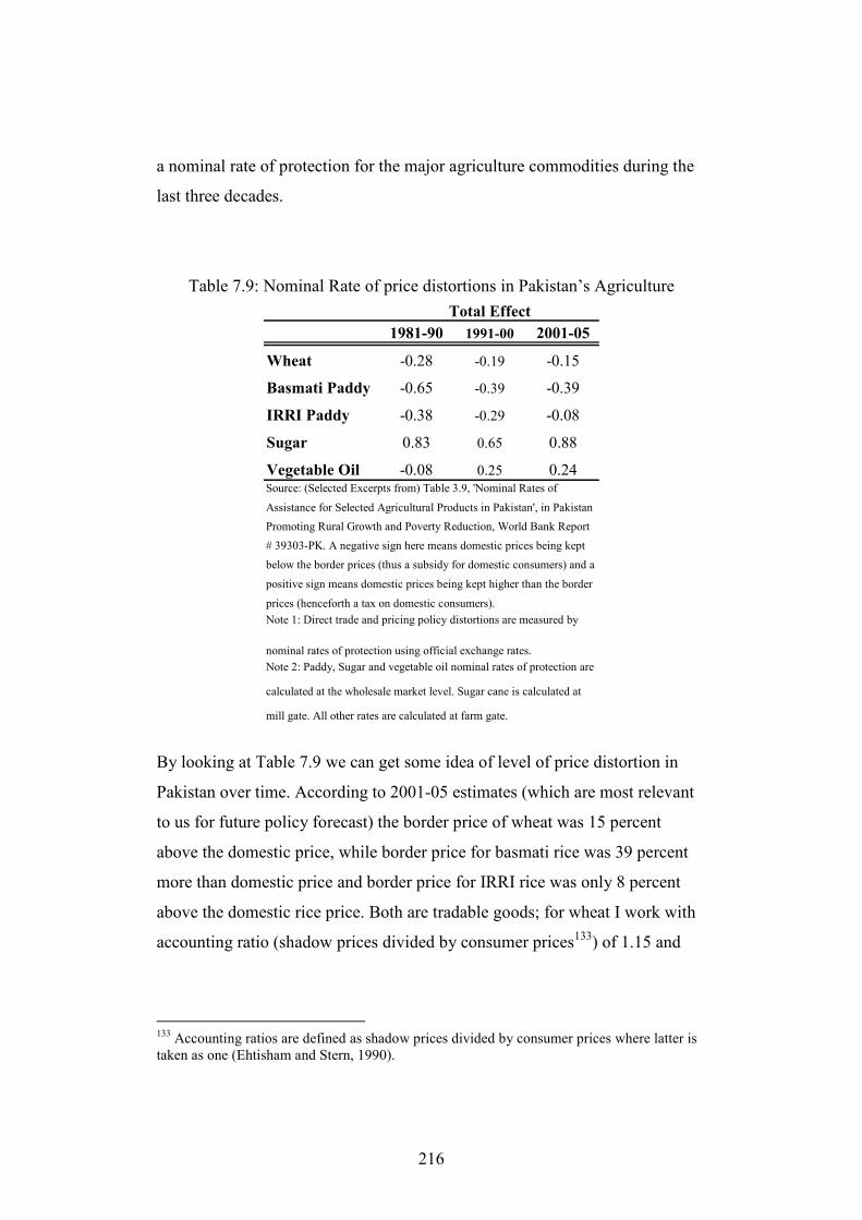
216

a nominal rate of protection for the major agriculture commodities during the

last three decades.

Table 7.9: Nominal Rate of price distortions in Pakistan’s Agriculture

1981-90 1991-00 2001-05

Wheat -0.28 -0.19 -0.15

Basmati Paddy -0.65 -0.39 -0.39

IRRI Paddy -0.38 -0.29 -0.08

Sugar 0.83 0.65 0.88

Vegetable Oil -0.08 0.25 0.24

Note 2: Paddy, Sugar and vegetable oil nominal rates of protection are

calculated at the wholesale market level. Sugar cane is calculated at

mill gate. All other rates are calculated at farm gate.

Source: (Selected Excerpts from) Table 3.9, 'Nominal Rates of

Assistance for Selected Agricultural Products in Pakistan', in Pakistan

Promoting Rural Growth and Poverty Reduction, World Bank Report

# 39303-PK. A negative sign here means domestic prices being kept

below the border prices (thus a subsidy for domestic consumers) and a

positive sign means domestic prices being kept higher than the border

prices (henceforth a tax on domestic consumers).

Total Effect

Note 1: Direct trade and pricing policy distortions are measured by

nominal rates of protection using official exchange rates.

By looking at Table 7.9 we can get some idea of level of price distortion in

Pakistan over time. According to 2001-05 estimates (which are most relevant

to us for future policy forecast) the border price of wheat was 15 percent

above the domestic price, while border price for basmati rice was 39 percent

more than domestic price and border price for IRRI rice was only 8 percent

above the domestic rice price. Both are tradable goods; for wheat I work with

accounting ratio (shadow prices divided by consumer prices133) of 1.15 and

133 Accounting ratios are defined as shadow prices divided by consumer prices where latter is taken as one (Ehtisham and Stern, 1990).

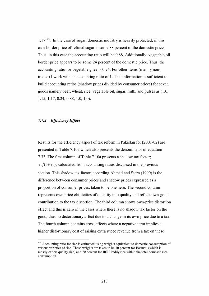
217

1.17134. In the case of sugar, domestic industry is heavily protected; in this

case border price of refined sugar is some 88 percent of the domestic price.

Thus, in this case the accounting ratio will be 0.88. Additionally, vegetable oil

border price appears to be some 24 percent of the domestic price. Thus, the

accounting ratio for vegetable ghee is 0.24. For other items (mainly non-

traded) I work with an accounting ratio of 1. This information is sufficient to

build accounting ratios (shadow prices divided by consumer prices) for seven

goods namely beef, wheat, rice, vegetable oil, sugar, milk, and pulses as (1.0,

1.15, 1.17, 0.24, 0.88, 1.0, 1.0).

7.7.2 Efficiency Effect

Results for the efficiency aspect of tax reform in Pakistan for (2001-02) are

presented in Table 7.10a which also presents the denominator of equation

7.33. The first column of Table 7.10a presents a shadow tax factor;

)1( ii ττ + , calculated from accounting ratios discussed in the previous

section. This shadow tax factor, according Ahmad and Stern (1990) is the

difference between consumer prices and shadow prices expressed as a

proportion of consumer prices, taken to be one here. The second column

represents own price elasticities of quantity into quality and reflect own-good

contribution to the tax distortion. The third column shows own-price distortion

effect and this is zero in the cases where there is no shadow tax factor on the

good, thus no distortionary affect due to a change in its own price due to a tax.

The fourth column contains cross effects where a negative term implies a

higher distortionary cost of raising extra rupee revenue from a tax on these

134 Accounting ratio for rice is estimated using weights equivalent to domestic consumption of various varieties of rice. These weights are taken to be 30 percent for Basmati (which is mostly export quality rice) and 70 percent for IRRI Paddy rice within the total domestic rice consumption.

218

goods. The last column reflects the total effect or the denominator of equation

7.30.

According to our estimates for total effect, as far as efficiency is concerned,

rice is one prime candidate for price increase; its subsidy is distortionary and

should be removed. Moreover, vegetable ghee and sugar are also prime

candidates for further price increase. By contrast wheat, beef and milk appear

to be prime candidates for price decrease.

Table 7.10 a: Efficiency aspects of price reform in Pakistan (2001-02)

Own

effect

Cross

effect

Total

Beef 0.00 -1.95 0.00 -0.41 0.59

Wheat -0.15 0.84 -0.13 -0.53 0.35

Rice -0.17 -1.37 0.23 0.17 1.41

Veg_ghee 0.76 -0.69 -0.02 1.13 2.11

Sugar 0.12 -0.22 -0.20 0.25 1.05

Milk 0.00 -1.16 0.00 -0.22 0.78

Pulses 0.00 -0.34 0.00 -0.03 0.97

(2001-02)

Note: This estimation is based on Equation 7.33. The own effect column is the product of

column 1 and column 2; cross effect column is the last term in denominator of Equation

7.33 ; column total is 1 plus own effect and cross effect column.

Source: Author's own calculation using HIES (2001-02).

i

i

ττ+1

1−i

i

w

θ

7.7.3 Equity Effect and cost-benefit ratio for price increase in Pakistan

The equity effects of price and tax reform in Pakistan are presented in Table

7.10b along with the cost benefit ratio of raising an extra rupee by increasing

the price of a good. The first two columns of Table 7.10b shows the equity

effect of price reform when there are no distributional concerns (i.e. 0=ε ) and

219

the equity effect here is simply the reciprocal of total effects in Table 7.10a as

a result the outcome is also same as described in Table 7.10a.

The results show that when there are no distributional concerns that rice,

vegetable ghee and sugar are prime candidates for price increase while beef,

wheat, milk and pulses are not. Under low inequality aversion, ε =0.5, goods

whose price should not be increased, now also include sugar. For the medium

level of inequality aversion, ε =1.0, results do not change from the previous

level while only in the case of a higher inequality aversion, ε =2.0, rice joins

the ranks of goods whose price should not be increased for equity reasons.

Thus, as we move across different equality aversion levels in Table 7.10 we

can see that results in particular are not very sensitive to the level of inequality

aversion used which is the usual strength of this procedure.

Thus, if we compare the efficiency and equity recommendation for inequality

aversion (ε =0.5 andε =1.0) we can see that efficiency requires price of goods

such as sugar, vegetable ghee and rice should be increased. When relatively

more inequality aversion is introduced i.e. using either,ε =0.5 andε =1.0,

equity still requires that not only price of wheat, meat, milk and pulses but also

of sugar should not be raised. However, rice joins the rank of commodities

whose price should not be increased on distributional grounds when higher

(i.e. ε =2.0) inequality aversion is used.

Thus, our finding suggest that raising revenue from an increase in the price of

rice and vegetable ghee would be desirable from both an efficiency and equity

considerations (except for higher inequality aversion i.e. ε =2.0 for rice).

However, raising revenue by increasing price of sugar is desirable on

efficiency grounds but undesirable on equity grounds (even with low

inequality aversion). We can further extrapolate these results to VAT future

recommendation since such experiment of price increase is clearly in line with

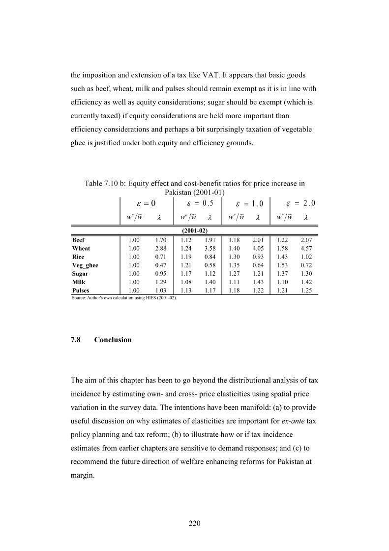
220

the imposition and extension of a tax like VAT. It appears that basic goods

such as beef, wheat, milk and pulses should remain exempt as it is in line with

efficiency as well as equity considerations; sugar should be exempt (which is

currently taxed) if equity considerations are held more important than

efficiency considerations and perhaps a bit surprisingly taxation of vegetable

ghee is justified under both equity and efficiency grounds.

Table 7.10 b: Equity effect and cost-benefit ratios for price increase in Pakistan (2001-01)

Beef 1.00 1.70 1.12 1.91 1.18 2.01 1.22 2.07

Wheat 1.00 2.88 1.24 3.58 1.40 4.05 1.58 4.57

Rice 1.00 0.71 1.19 0.84 1.30 0.93 1.43 1.02

Veg_ghee 1.00 0.47 1.21 0.58 1.35 0.64 1.53 0.72

Sugar 1.00 0.95 1.17 1.12 1.27 1.21 1.37 1.30

Milk 1.00 1.29 1.08 1.40 1.11 1.43 1.10 1.42

Pulses 1.00 1.03 1.13 1.17 1.18 1.22 1.21 1.25

(2001-02)

Source: Author's own calculation using HIES (2001-02).

0=ε 5.0=ε 0.1=ε 0.2=ε

ww ~ε ww ~ε ww ~ε ww ~ελ λ λ λ

7.8 Conclusion

The aim of this chapter has been to go beyond the distributional analysis of tax

incidence by estimating own- and cross- price elasticities using spatial price

variation in the survey data. The intentions have been manifold: (a) to provide

useful discussion on why estimates of elasticities are important for ex-ante tax

policy planning and tax reform; (b) to illustrate how or if tax incidence

estimates from earlier chapters are sensitive to demand responses; and (c) to

recommend the future direction of welfare enhancing reforms for Pakistan at

margin.

221

There is overwhelming support for the fact that robust estimation of price

elasticities is pivotal for tax policy planning and reform analysis. However,

empirical research in this area, particularly for developing countries to date,

has been limited. This shortcoming appears to be rooted in difficulty involved

with estimating price elasticities given data availability in these countries.

However, this is very relevant and critical information for policy makers for

carrying out successful and welfare enhancing reforms (at margin or

otherwise). Thus, this is one area where despite all the problems debate needs

to be taken further and here we believe this study has made a valuable attempt

by estimating elasticities.

We have also tried to illustrate that at least in the case of Pakistan

incorporating demand responses into partial equilibrium tax incidence analysis

may not change results that much. However, this in our case largely hinges on

the fact that for our illustrative case cross- price effects appear to cancel out.

This should give some credibility to the earlier estimates in the previous

chapters. However, it is worth nothing that in other studies the inclusion of

cross- price effects may prove more important for policy purposes.

The practical appeal of the theory of marginal tax reform (MTR) in developing

countries can not be exaggerated. In these countries policy makers rarely have

the privilege of designing tax structure from scratch or of introducing changes

in tax structure that may be too extreme. Thus, in many cases policy makers

are interested in knowing empirically robust and theoretically consistent

suggestions to improvement over the status quo. Our estimates show that

raising further revenue (from VAT) by increasing the price of basic goods

such beef, wheat, milk and pulses will not be welfare enhancing, as it is

neither efficient nor equitable. On the other hand raising further revenue from

taxation of sugar (which is currently being taxed) is efficient but not equitable.

222

Similarly, increasing price of rice is efficient but not equitable (for all cases of

inequality aversion). Lastly, it appears only in the case of vegetable ghee there

is a case of further price increase that is both equitable and efficient. This

offers some lessons for future direction of VAT reforms. It appears

policymakers seriously need to think about taxation of sugar (as also flagged

in earlier chapters). Also, exemptions of wheat, pulses, beef, milk and rice

(last under high inequality aversion) should continue. Furthermore, taxation of

vegetable ghee is justified and it is an ideal candidate for future price

increases.

Interestingly, the results for MTR also show that policy makers in these

countries in reality face a dilemma in trying to balance equity and efficiency

considerations. For instance, in many cases additional revenue can be raised

from reforms that may be efficient but not necessary equitable. Thus, finding

the right combination of reforms that are both efficient and equitable may

leave policymakers with very few policy options. Thus, this perhaps highlight

real problem and issues faced by policymakers when designing reforms or

policy options.

In next chapter, which is also the conclusion of this study we will attempt to

highlight what this study has brought in terms of its overall contribution and

innovation to this research area.

223

CHAPTER VIII: Conclusions

8.1 Main Findings

This study aimed at measuring the social incidence of indirect taxes in

Pakistan as a result of the tax reform process135 during 1990-2001, focusing on

the area of indirect taxes. In this regard, our results show that a move from

dependence on trade tax revenues to GST/VAT revenues has made the overall

indirect tax system of Pakistan a little more progressive136. This study also

carried out a high level of disaggregation of the incidence to reveal its

sensitivity to key commodities. It appears post- reform indirect tax incidence

is sensitive to taxation of key commodities which include sugar, edible oils

and basic fuel/utilities. Incidentally, taxation of these commodities also

appears to have strong distributional effect on the poor and our results show

that the indirect tax system can be made strongly progressive by exempting

these commodities137.

We also explored the sensitivity of estimated tax incidence results to a special

case of partial equilibrium tax incidence analysis that assumes zero demand

responses. Estimations illustrate that incidence results (for the selected sample

of commodities) do not appear to be very sensitive to incorporation of own-

and cross- price responses. We also used these estimates to identify directions

of welfare enhancing reform for Pakistan at margin. We find that a reduction

135 Also known as the first generation of tax reform process in Pakistan 136 This statement is borrowed from Gemmell and Morrissey (2003) excluding the country reference. 137 These are not necessarily revenue-neutral recommendations.

224

in the price of basic items such as beef, wheat, milk and pulses should be

welfare enhancing at the margin. Furthermore, taxation of sugar maybe

justified on efficiency grounds but not from the equity perspective while

taxation of vegetable ghee is justified on both revenue efficiency as well as on

equity grounds.

This study has made a significant contribution to tax policy analysis in

Pakistan as well as to the literature of tax incidence in general. For instance,

this study has not only attempted to disaggregate indirect tax incidence over its

major components (namely, GST/VAT, custom duties and excise duty) but

further disaggregation of incidence in each case (except custom duties) was

undertaken to reveal sensitivity of incidence to key commodities. Needless to

say, both of these aims themselves were extremely ambitious given the

difficulty of estimating aggregate custom duties and excise duty incidence as

well as attempting to further disaggregate this. However, we believe herein

lies the strength of this study.

We carried out a separate GST/VAT incidence evaluation pre- and post-

reform given the importance of this tax within Pakistan federal taxation

structure. Results have revealed that progressivity of GST pre-reform

incidence was mainly due to the limited scope of GST/VAT at that time and

due to the patterns of exemptions that clearly favored the poor. However, post-

reform GST/VAT incidence, despite focus on ‘equity’ and ‘distributional’

considerations in the reform agenda, appears at best to be proportional. Our

disaggregated incidence results here reveal that taxation of some basic

processed food items and basic fuels has undermined the progressivity of

GST/VAT. Given this is also the most pervasive component of indirect tax

system in the post- reform era, this proportionality has restricted the

progressivity of the overall indirect taxation to being slightly so (or

progressive over a limited range).

225

This issue was probed further by exploring how GST/VAT exemptions can be

better targeted to safeguard the poor. This was done using the distributional

characteristics of a good approach in order to identify goods/services that are

relatively more important to the poor. This issue has been explicitly addressed

for Pakistan for the first time. Our findings reveal that consumption patterns of

key commodity groups such as basic fuels, sugar and edible oils, are

sufficiently separable to provide poor households with necessary relief via

well targeted exemptions (and not necessarily at too much cost to the

exchequer138). This is extremely relevant information for the policymakers in

Pakistan for safeguarding the poor from the GST/VAT net and for carrying out

future GST/VAT reforms.

This study has also attempted to evaluate the pre- and post- reform incidence

of custom duties as well as excise duties. Since pre-reform incidence was

largely dependent on trade taxes this disaggregation was crucial. The

innovation in attempting to measure the incidence of custom duties came from

attempting to measure the import content of domestic consumption of major

product categories (rather than treating all consumption identically as is done

in most other studies). We believe this was a crucial and ambitious

undertaking as these estimates had to be generated from relying on many other

data sources necessary for carrying out informative analysis. Our results reveal

that the inverted U-shaped incidence of pre-reform indirect tax incidence was

largely driven by regressivity of custom duties incidence while disaggregated

analysis revealed that this regressivity was mainly due to significantly large

import share that year (within domestic consumption) for some basic food

commodities which included sugar, edible oils, spices and even wheat.

138 Though this line of argument was not formally investigated

226

One of the aims of this study was to illustrate the sensitivity of estimated tax

incidence results (summarized in terms of tax progression) to the assumption

of zero demand responses (a special case of partial equilibrium tax incidence

analysis assumed in some tax incidence studies. For instance see Chen et al.,

2001; Munoz et al., 2003; and Sahn and Younger, 2003, to name but a few).

Our illustration suggests that in most cases (for a selected sample of

commodities) our estimated incidence results are not affected much by

incorporation of own-price elasticities although not allowing for behavioural

responses may appear to overestimate the incidence results slightly. In the case

of cross-elasticities, overall impact appears to vary from case to case as it

depends on the magnitude and sign of the elasticity and the importance of the

other commodities in the consumption basket. Sometimes it makes little

difference, in other cases, it matters more. However, generally, incorporation

of own-price elasticities plus cross-price elasticities (which could make the

impact bigger) is still quite small to impact our results significnatly. We

believe by doing this we have made a contribution to the literature on price

elasticities and to tax incidence (given any attempt to test the robustness of tax

incidence estimates is important rather than ignoring this issue altogether).

We also used our estimates of elasticities (for a selected sample of

commodities) to identify the directions of welfare enhancing reform at the

margin for Pakistan using the marginal theory of tax reform. Our results show

that a reduction in the prices of basic items such as wheat, pulses, milk, and

beef should be welfare-enhancing. Results also reveal that further revenue can

be raised by raising the price of sugar; this may be efficient but it is not

equitable whereas vegetable ghee appears to be an ideal candidate for a price

increase on both grounds.

This perhaps also reflects that, in reality, policymakers are faced with a very

delicate act of juggling equity, efficiency and administrative convenience.

227

What is efficient may not necessarily be equitable; thus achieving both goals

simultaneously to raise revenue may leave policymakers with very limited

options. Thus, this research informs the literature of ex-ante tax policy

planning and tax reform (in margin) for Pakistan and for this literature in

general.

With regards to Pakistan’s future tax policy we believe getting the GST/VAT

exemptions right is a critical policy step for safeguarding the poor because of

current and future importance of this tax within the overall federal tax

structure. Furthermore, powerful distributional effects created due to taxation

of (some) processed food items and basic fuels needs serious reconsideration.

8.2 Qualifications to the Study and Future Directions of Research

Although this study has tried to be ambitious, innovative and comprehensive

in meeting its objectives, like all research, its findings are limited to what was

achievable within the given the timeframe, availability of data, existing

literature and the scope of this study.

This research looks at the welfare effect of a specific type of indirect tax

reform process that largely focused on replacement of trade tax revenues with

GST/VAT revenues. Thus, this study does not claim to be reflective of

distributional incidence of a wider reform process that may encompass the

whole tax system139 or overall fiscal policy i.e. tax and expenditure policy.

Though these are interesting areas of research they are not the explicit focus of

this research.

139 This may include direct taxes, local and provincial tax and non-tax revenues, implicit taxation issues and surcharges.

228

It is also worth mentioning that the findings of this study are specific to the

particular definition of progressivity used in this study i.e. average

productivity rate and also to a particular method of measuring household

welfare. The main aim of this research was not to find the ideal definition of

progressivity or welfare in Pakistan though these can be future areas of

research.

Likewise, we have made a simple underlying assumption regarding tastes,

preferences and technology. Going beyond this was not possible given the

non- availability of data, and time constraints.

Most of the studies on tax incidence for developing and developed countries

use the 100 percent tax shifting assumptions particularly where indirect taxes

incidence is concerned, although little consensus emerges where pass- through

effects of direct taxes are concerned. Given the lack of empirical research in

the area of tax shifting, even for developed countries let alone Pakistan and

other developing countries, it may be adequate to assume a full tax shifting

assumption for indirect taxes. But a cautious interpretation of the results is

necessary. Similarly particular features of developing countries such as tax

evasion and smuggling can have an important impact on incidence results

(though the former may be a more significant problem for direct tax

incidence). However, incorporation of these features within our analysis was

not possible due to non-availability of necessary data. These however pose

interesting questions which should be investigated in the future.

All these factors/issues point towards the fact that ascertaining tax incidence

for any country, especially a developing country is a difficult empirical

question and there are no easy answers. Future research in the case of Pakistan

should focus on incorporating direct taxes into the tax incidence analysis but

229

realistically hinges on the availability of tax return data which, at present, is

not available. Also, given the structure of Household Integrated Economic

Survey (HIES) it is not possible to get estimates of services consumption in

Pakistan. Since GST/VAT is the most fundamental tax component of

Pakistan’s tax system we believe these estimates and analysis are necessary to

analyze how GST/VAT can be broadened to the services sector and who it is

likely to be affected.

Lastly, we would like to add (for various reasons mentioned above) that this

study should be taken as more than just a study on Pakistan. On the whole, we

believe, this study has been ambitious, methodologically innovative and

comprehensive which should further strengthen the relevance, uniqueness and

innovativeness of this dissertation.

230

APPENDICES

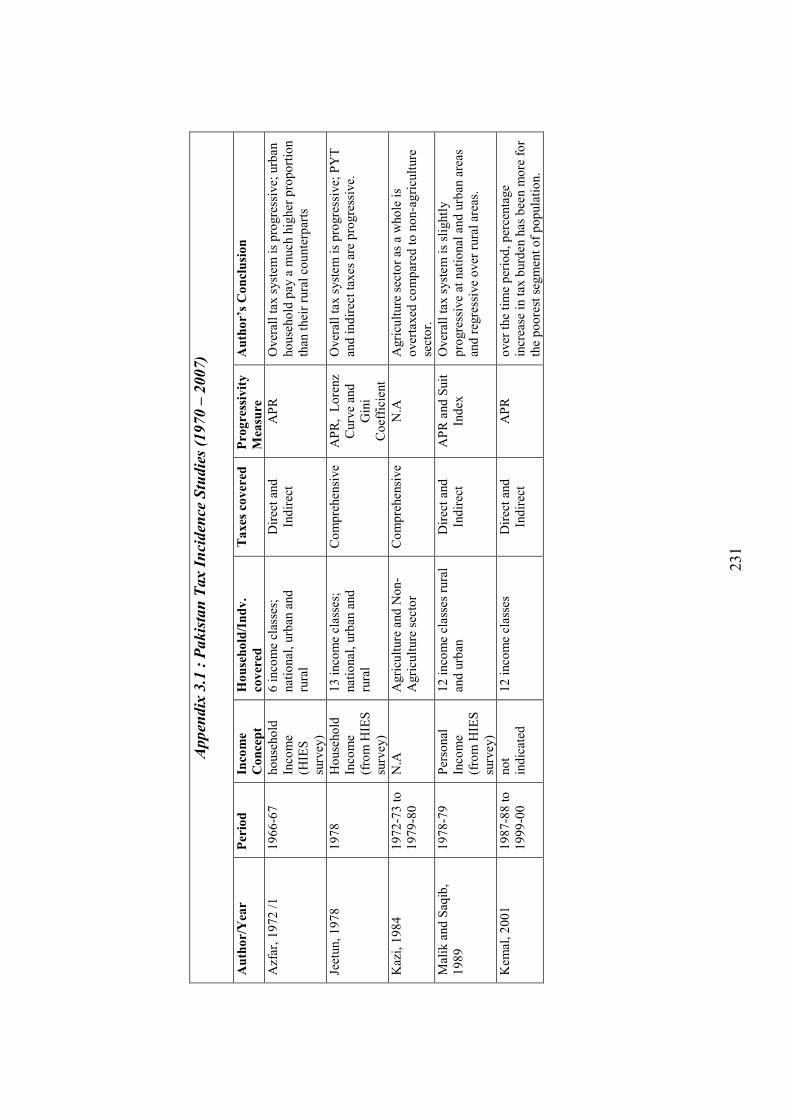
231

Appen

dix 3.1 : Pakistan Tax Inciden

ce Studies (1970 – 2007)

Author/Year

Period

Income

Concept

Household/Indv.

covered

Taxes covered Progressivity

Measure

Author’s Conclusion

Azf

ar,

19

72

/1

1

96

6-6

7

ho

use

ho

ld

Inco

me

(HIE

S

surv

ey)

6 i

nco

me

clas

ses;

nat

ional

, urb

an a

nd

ru

ral

Dir

ect

and

In

dir

ect

AP

R

Over

all

tax s

yst

em i

s p

rogre

ssiv

e; u

rban

ho

use

ho

ld p

ay a

much

hig

her

pro

po

rtio

n

than

thei

r ru

ral

cou

nte

rpar

ts

Jeet

un,

19

78

1

97

8

Ho

use

ho

ld

Inco

me

(fro

m H

IES

su

rvey

)

13

inco

me

clas

ses;

nat

ional

, urb

an a

nd

ru

ral

Co

mp

rehen

sive

AP

R,

Lo

renz

Curv

e an

d

Gin

i C

oef

fici

ent

Over

all

tax s

yst

em i

s p

rogre

ssiv

e; P

YT

an

d i

nd

irec

t ta

xes

are

pro

gre

ssiv

e.

Kaz

i, 1

98

4

19

72

-73

to

1

97

9-8

0

N.A

A

gri

cult

ure

and

No

n-

Agri

cult

ure

sec

tor

Co

mp

rehen

sive

N.A

A

gri

cult

ure

sec

tor

as a

who

le i

s o

ver

taxed

co

mp

ared

to

no

n-a

gri

cult

ure

se

cto

r.

Mal

ik a

nd

Saq

ib,

19

89

1

97

8-7

9

Per

sonal

In

com

e (f

rom

HIE

S

surv

ey)

12

inco

me

clas

ses

rura

l an

d u

rban

D

irec

t an

d

Ind

irec

t A

PR

and

Suit

In

dex

O

ver

all

tax s

yst

em i

s sl

ightl

y

pro

gre

ssiv

e at

nat

ional

and

urb

an a

reas

an

d r

egre

ssiv

e o

ver

rura

l ar

eas.

Kem

al,

20

01

1

98

7-8

8 t

o

19

99

-00

no

t in

dic

ated

1

2 i

nco

me

clas

ses

Dir

ect

and

In

dir

ect

AP

R

over

the

tim

e p

erio

d,

per

centa

ge

incr

ease

in t

ax b

urd

en h

as b

een m

ore

fo

r th

e p

oo

rest

seg

men

t o

f p

op

ula

tio

n.

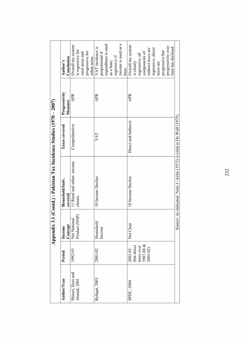
232

Appendix 3.1 (Contd.) : Pakistan Tax Incidence Studies (1970 – 2007)

Author/Year

Period

Income

Concept

Household/Indv.

covered

Taxes covered

Progressivity

Measure

Author’s

Conclusion

Shir

azi,

Ily

as a

nd

A

hm

ad,

20

01

1

99

2-9

3

Net

Nat

ional

P

rod

uct

(N

NP

) 1

1 R

ura

l an

d u

rban

in

com

e cl

asse

s C

om

pre

hen

sive

AP

R

Over

all

tax s

yst

em

is r

egre

ssiv

e fo

r ru

ral

area

s an

d

pro

gre

ssiv

e fo

r urb

an a

reas

.

Ref

aqat

, 2

00

3

20

01

-02

H

ouse

ho

ld

Inco

me

10

Inco

me

Dec

iles

V

AT

A

PR

V

AT

inci

den

ce i

s p

ropo

rtio

nal

if

exp

end

iture

is

use

d

as a

bas

e;

regre

ssiv

e if

in

com

e is

use

d a

s a

bas

e.

SP

DC

, 2

00

4

20

01

-02

(b

ut

dir

ect

taxes

over

1

98

7-8

8 &

2

00

1-0

2)

No

t C

lear

1

0 I

nco

me

Dec

iles

D

irec

t an

d I

nd

irec

t)

AP

R

Over

all

tax s

yst

em

is c

lear

ly

regre

ssiv

e; a

ll

com

po

nen

ts o

f in

dir

ect

taxes

are

re

gre

ssiv

e; d

irec

t ta

xes

are

p

rogre

ssiv

e b

ut

pro

gre

ssiv

ity o

ver

ti

me

has

dec

lined

.

So

urc

e: A

s in

dic

ated

. N

ote

:1/

Azf

ar (

19

72

) is

cit

ed i

n D

e W

ulf

(1

97

5).

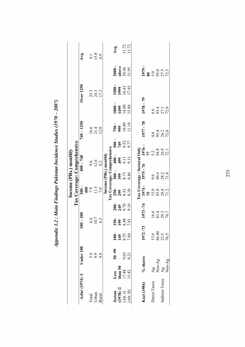
233

Appen

dix 3.2 : M

ain F

indings Pakistan Inciden

ce Studies (1970 – 2007)

Income (PRs.) monthly

Tax Coverage: Comprehensive

Azfar (1974) /1

Under 100

100 – 200

200 –

400

400 – 740

740 – 1250

Over 1250

Avg.

To

tal

5

.0

6.4

7

.9

9.6

1

6.6

2

5.3

9

.1

Urb

an

9.9

1

0.7

1

1.5

1

2.6

2

1.4

2

4.3

1

5.8

R

ura

l 4

.8

6.3

7

.0

8.2

1

2.0

1

7.3

6

.9


Tax Coverage: Comprehensive

Jeetun

(1978) /2

Less

than 50

50 -99

100-

149

150-

199

200-

249

250-

299

300 –

399

400 –

499

500 –

749

750 -

999

1000 –

1499

1500 -

1999

2000 -

above

Avg.

(Alt

. I)

1

7.4

8

9.0

3

8.5

5

8.4

8

9.7

0

8.5

2

8.7

3

9.1

1

9.5

2

10

.49

1

4.8

0

16

.43

3

0.4

6

11

.72

(Alt

. II

) 1

5.4

2

8.2

1

7.8

4

7.8

1

9.1

0

8.1

0

8.4

6

9.1

1

9.7

7

11

.19

1

5.8

4

17

.45

3

1.9

5

11

.72

Tax Coverage : Sectoral Only

Kazi (1984)

% shares

1972 -73

1973 -74

1974 -

75

1975 - 76

1976 –

77

1977 - 78

1978 – 79

1979 -

80

Dir

ect

Tax

es

Ag.

13

.6

16

.6

15

.0

9.6

5

.2

4.6

6

.6

5.0

N

on-A

g

86

.40

8

3.4

8

5.0

9

0.4

9

4.8

9

5.4

9

3.4

9

5.0

Ind

irec

t T

axes

A

g.

23

.5

29

.3

28

.8

28

.2

26

.9

26

.2

27

.1

27

.5

No

n-A

g

76

.5

70

.7

71

.2

71

.8

72

.1

72

.8

72

.9

72

.5

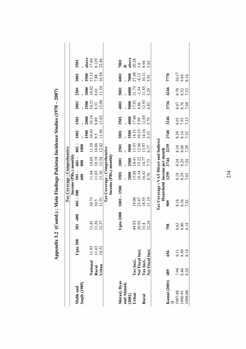
234

Appendix 3.2 (Contd.) : Main Findings Pakistan Incidence Studies (1970 – 2007)

Tax Coverage : Comprehensive


Malik and

Saqib (1989)

Upto 300

301 -400

401 – 500

501 –

600

601 –

800

801 –

1000

1001

–

1500

1501

–

2000

2001

–

2500

2501

–

3000

3001

–

3500

3501

- above

National

11

.93

1

1.4

1

10

.75

1

1.4

4

10

.69

11

.30

10

.43

10

.14

1

0.2

1

10

.02

13

.15

17

.60

Rural

11

.63

1

1.2

6

10

.5

11

.03

10

.19

10

.86

9.5

8

.89

8

.33

8

.01

7

.88

8

.12

9

Urban

14

.32

1

2.3

7

11

.91

1

3.3

6

12

.54

12

.42

11

.96

11

.62

1

2.0

0

11

.34

16

.54

22

.86

Tax Coverage : Comprehensive


Shirazi, Ilyas

and Ahmad,

(2001)

Upto 1000 1001 – 1500 1501

–

2000

2001

–

2500

2501

–

3000

3001

–

3500

3501

–

4000

4001

–

5000

5001

–

6000

6001

–

7000

7001

&

above

Urban

Tax Inci..

44

.93

1

8.0

0

15

.88

14

.41

13

.93

14

.51

17

.46

1

7.0

1

21

.73

27

.48

20

.28

Net Fiscal Inci.

20

.93

2

3.6

7

18

.14

15

.22

12

.96

10

.33

5.9

9

4.8

6

-1.3

4

-8.1

3

3.6

Rural

Tax Inci..

33

.4

18

.55

1

6.4

1

14

.77

13

.97

14

.16

12

.85

1

2.9

3

11

.85

10

.31

8.9

4

Net Fiscal Inci.

12

.24

1

1.1

9

8.7

0

7.7

3

6.7

7

5.3

3

5.7

9

4.8

3

5.2

9

5.9

1

5.8

2

Tax Coverage : VAT Direct and Indirect

Household income per month

Kamal (2001)

/3

489

656

758

909

1259 1744 2239 2748 3246

3736 4246 7770

19

87

-88

7

.94

8

.11

8

.63

8

.18

8

.18

8

.24

8

.10

8

.29

8

.03

8

.87

8

.70

1

0.1

7

19

90

-91

8

.40

8

.49

8

.80

8

.36

8

.29

8

.29

8

.08

8

.14

7

.93

8

.76

8

.52

9

.84

1

99

9-0

0

8.2

4

8.1

8

8.1

8

7.8

1

7.6

5

7.5

4

7.2

9

7.3

3

7.1

3

7.6

9

7.3

3

8.1

4

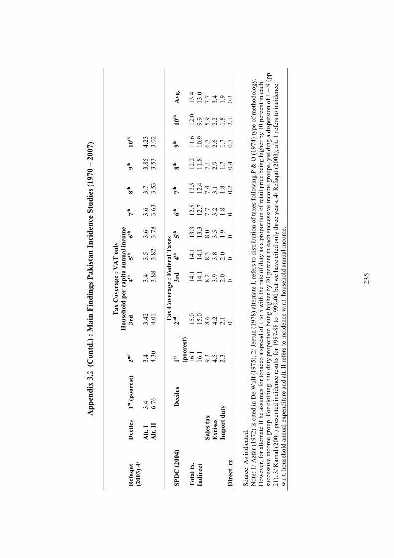
235

Appendix 3.2 (Contd.) : Main Findings Pakistan Incidence Studies (1970 – 2007)

Tax Coverage : VAT only

Household per capita annual income

Refaqat

(2003) 4/

Deciles

1st (poorest)

2nd

3rd

4th

5th

6th

7th

8th

9th

10th

Alt. I

3.4

3

.4

3.4

2

3.4

3

.5

3.6

3

.6

3.7

3

.85

4

.23

Alt. II

6.7

6

4.3

0

4.0

1

3.8

8

3.8

2

3.7

8

3.6

3

3.5

3

3.5

3

3.0

2

Tax Coverage : Federal Taxes

SPDC (2004)

Deciles

1st

(poorest)

2nd

3rd

4th

5th

6th

7th

8th

9th

10th

Avg.

Total tx.

1

6.1

1

5.0

1

4.1

1

4.1

1

3.3

1

2.8

1

2.5

1

2.2

1

1.6

1

2.0

1

3.4

Indirect

1

6.1

1

5.0

1

4.1

1

4.1

1

3.3

1

2.7

1

2.4

1

1.8

1

0.9

9

.9

13

.0

Sales tax

9.3

8

.6

8.2

8

.3

8.0

7

.7

7.4

7

.1

6.7

5

.9

7.7

Excises

4.5

4

.2

3.9

3

.8

3.5

3

.2

3.1

2

.9

2.6

2

.2

3.4

Import duty

2.3

2

.1

2.0

2

.0

1.9

1

.8

1.8

1

.7

1.7

1

.8

1.9

Direct tx

0

0

0

0

0

0.2

0

.4

0.7

2

.1

0.3

So

urc

e: A

s in

dic

ated

. N

ote

: 1

/ A

zfar

(1

97

2)

is c

ited

in D

e W

ulf

(1

97

5).

2/

Jeet

un (

19

78)

alte

rnat

e I,

ref

ers

to d

istr

ibuti

on o

f ta

xes

fo

llo

win

g P

& O

(1

97

4)

typ

e o

f m

etho

do

log

y.

Ho

wev

er,

for

alte

rnat

e II

he

assu

mes

fo

r to

bac

co a

sp

read

of

1 t

o 5

wit

h t

he

rate

of

duty

as

a p

ropo

rtio

n o

f re

tail

pri

ce b

eing h

igher

by 1

0 p

erce

nt

in e

ach

succ

essi

ve

inco

me

gro

up

. F

or

clo

thin

g,

this

du

ty p

rop

ort

ion b

eing h

igher

by 2

0 p

erce

nt

in e

ach s

ucc

essi

ve

inco

me

gro

up

s, y

ield

ing a

dis

per

sio

n o

f 1

– 9

(p

p.

21

). 3

/ K

amal

(2

00

1)

pre

sente

d i

nci

den

ce r

esu

lts

for

19

87

-88

to

199

9-0

0 b

ut

we

hav

e ci

ted

only

thre

e yea

rs.

4/

Ref

aqat

(2

003

), a

lt. 1

ref

ers

to i

nci

den

ce

w.r

.t.

ho

use

ho

ld a

nn

ual

exp

end

iture

and

alt

. II

ref

ers

to i

nci

den

ce w

.r.t

. ho

use

ho

ld a

nnual

inco

me.

236

Appendix 3.3: Measurement of Progressivity

1. Average Progressivity Rate (APR)

It may not be wrong to say that progressivity is one of the key concepts in

incidence analysis. Statistical progressivity measures like APR record changes

in income distribution compared to an alternative such as proportionality

(Gemmell and Morrissey, 2005). It is generally agreed that a tax structure is

progressive where effective tax rate (i.e. tax liability as a percentage of

income) rises when we move up the income scale; regressive when effective

tax rates falls as we move up the income distribution; and proportional when

effective tax rates remain constant (Musgrave and Thin, 1948). According to

Gemmell and Morrissey (2005), average rate of progression is the most

common measure used to determine tax progressivity for developing

countries. Although this measure provides useful information on the extent to

which the tax system departs from proportionality, it cannot quantify the

amount of redistribution that takes place through a tax system140.

2. Distribution Measures

Distributional measure on the other hand, assess if the tax in question

increases or reduces a measure of inequality of incomes, poverty etc., of the

overall population or some other grouping (Gemmell and Morrissey, 2005).

One can generally distinguish between purely statistical measures and

normative measures (that use explicit value judgements to ascertain adequacy,

rightness and desirability of a tax).

140 For a comprehensive discussion regarding numerous structural and distributional measures of progressivity, see Musgrave and Thin (1948) and Kiefer (1984).

237

2.1 Lorenz Curve and Gini Coefficient 141

One approach specifically focuses on the use of Lorenz curve or Gini

coefficient. Lorenz curve shows the relationship between cumulative

percentage of population ranked from lowest to highest on the vertical axis

and cumulative percentage of income, placed on the horizontal axis. The

Lorenz curve in other words maps the cumulative share of income received by

bottom X percentage of population (Martinez-Vazquez, 2001). The more

Lorenz curve slopes down; the more unequal is the underlying distribution of

income. In terms of tax incidence analysis, the comparison of pre- and post-

tax income distribution, where one curve wholly lies under the other, equality

is said to be greater for the income distribution with a Lorenz curve that lies

inside (Gemmell and Morrissey, 2005).

However, the comparison of Lorenz curve may not always work if Lorenz

curves cross; thus a simpler way to summarize this information is to use Gini

coefficient that summarizes the same information. In this case the “before” and

“after” comparison of Gini coefficient allows one to analyze whether the

resultant tax will positively or negatively affect the distribution of income,

henceforth its progressivity. These have been readily used for tax incidence

analysis for developing countries142.

141 Where coefficient of equality or Gini coefficient (G) can be written as: G=1+1/n – (y1 + 2y2+…+nyn)*2/(n2*µ), where n is the number of individuals, yi is the income of the ith individual, µ is the average income, and subscript 1 to n run from highest to lowest income. 142 For application see Engel, Galetovic and Raddatz (1998) for Chile, El-Edel (1970) for Egypt, Jeetun (1978) for Pakistan, Chen et al. (2001) for Uganda, Munoz et al. (2003) for Ethiopia and Prasada et al. (2005) for Sri Lanka.

238

However, indexes based on Gini coefficient have been criticised for two main

reasons. First, these indexes attach highest weight to income transfers from

income brackets close to the mode of income distribution compared to either

evenly distributing these weights or giving more weight to the tail of the

distribution (Atkinson, 1973; Dasgupta, Sen and Starrett, 1973; and Sen,

1973). Second, it is desirable for an index to attach most weight to improving

the income distribution of the poor particularly when income distribution is

very unequal but treat the improvements near the mean more symmetrically.

But Gini has the same symmetric weighting irrespective of how equal or

unequal the income distribution is (Blackorby and Donaldson, 1978).

2.2 Concentration Curves

A concentration curve is an idea similar to Lorenz curve. It depicts a

relationship between the cumulative tax payment on the vertical axis and

cumulative population ranked by pre-tax income on the horizontal axis. If a

concentration curve of tax payment lies wholly outside the concentration curve

of expenditures; the tax is clearly progressive. Application of this curve for tax

incidence analysis is also frequent143.

2.3 Indexes based on explicit value judgment: Atkinson index

Even a basic descriptive index such as Gini coefficient can be shown to make

use of an implicit set of weights or giving relative importance to individuals at

different income levels. For instance, Gini coefficient implicitly gives higher

143 For application see, Sahn and Younger (1998) for Cote d’Ivoire, Munoz et al. (2003) for Ethiopia, Prasada et al (2005) for Sri Lanka, and Chen et al. (2001) for Uganda.

239

importance to changes in income of individual is closer to the mode of the

distribution. One way to get rid of this accidental choice of weights is by

explicitly choosing these weights (Vazquez, 2001). Such an index is the

Atkinson index, which uses explicit weights derived from an explicit social

welfare function. The Atkinson index uses an “inequality aversion parameter”

with the intention of capturing social aversion to inequality in the distribution

of income (Atkinson, 1983)144. This can be written as A=1-ye/µ, where ye is

the “equally distributed income” i.e. income if distributed equally will produce

the same level of social welfare, µ is average actual income and e is inequality

aversion parameter145. The definition of ye uses an inequality aversion

parameter z which is less or equal to one, as follows: ye = [( y1)ε + ( y2)

ε +

………+ ( yn)ε ]/n1/ε (Vazquez, 2001).

2.4 Welfare Dominance146

The comparisons of Lorenz or concentration curves have given rise to the

notion of dominance (Gemmell and Morrissey, 2005) which is another

criterion that is used to determine tax progressivity. In this case when a curve

dominates another curve definitely; this represents a more equal distribution of

income or more dominant or progressive tax (Gemmell and Morrissey, 2005;

Sahn and Younger, 1999). The statistical test used to measure this dominance

is known as welfare dominance and this methodology is developed by

Yitzhaki and Slemrod (1991).

Intuitively, the term welfare dominance means that for any social welfare

function that favours an equitable distribution of income, a revenue neutral tax

change that reduces taxes on one good x but increases taxes on good y will

144 Atkinson index is a normative index. 145 For application see Murty (1989) for India. 146 Welfare dominance is a normative measure.

240

improve social welfare as long as the concentration curve for the tax on x lies

above the concentration curve of y. Thus, the theory of welfare dominance for

a broad class of social welfare functions, provides a general criterion to

ascertain if one distribution of welfare is better than another (Saposnik, 1981;

Shorrocks, 1983; Foster and Shorrocks, 1988; Yitzhaki and Slemrod, 1991;

Lambert, 1993). In practice, the attraction of the welfare dominance criterion

is that statistical tests can be used to determine dominance of one curve over

the other (Younger et al., 1999). In many cases crossing of Lorenz curve

makes it impossible to determine dominance; in such cases a more

sophisticated approach such as generalized Lorenz curves can be used.147

However, use of welfare dominance approach in tax incidence analysis for

developing countries has largely focused African countries148.

147 The generalized Lorenz curve can be defined as:

)(*)(

1

1 w

w

w

iNn

k

k

i

k

k

µ

=

∑

∑

=

=

Where N(i) is the generalized Lorenz ordinate and µ(w) is the mean of the distribution of W. The generalized Lorenz curve plots the cumulative share of individuals in the sample (indexed by i) on the x-axis against cumulative share of the welfare variable multiplied by its mean on the y-axis. The Lorenz curve is identical but not scaled by the mean (Sahn and Younger, 2003). 148 For application see Younger (1996), Younger et al. (1999), Sahn and Younger (1998), Munoz et al. (2003) for Ethiopia, and Chen et al. (2001) for Uganda.

241

Appendix 4.1: HIES Survey Design and Sampling Methods

4.1 Sampling Frame

The HIES 1990-91 and 2001-02 cover all urban and rural areas of the four

provinces of Pakistan except some parts of northern areas and FATA149. The

FBS uses separate sampling frames for urban and rural areas of Pakistan. For

urban areas, FBS has developed a sample frame using quick count listing

methods for households in major cities and town. Each area is subdivided into

enumeration blocks based on 200 to 250 households. The list of enumeration

blocks is updated using Census of Establishments conducted during 1988. For

rural areas the list of village/mouzas/dehs published in population and housing

census of 1981 and 1998 is used as a frame for HIES 1990-91 and 2001-02

respectively (FBS, HIES 90-91, pp. 15; FBS, HIES 01-02, pp. 21;

International Monetary Fund, 2004).

4.2 Stratification Plan

The FBS uses two stage sample design for HIES survey. In urban areas each

large size city is treated as an independent stratum and further divided into

low, middle, and high income sub-strata in the light of information from

enumeration blocks. The remaining urban areas in all provinces are grouped

together and treated as an independent stratum. In rural areas, the population

of each district in Punjab, Sindh and NWFP province have been grouped

together to make a stratum while for Balochistan province each of defunct

administrative division is taken as a stratum (FBS, HIES 01-02, pp. 22).

149 FATA refers to Federal Administrated Tribal Area and this area constitutes around 3 percent of total population.

242

4.3 Sample Design

Enumeration blocks in the urban areas and mouzas/dehs/village in the rural

areas were the primary sampling units (PSUs). The sample of PSUs was

selected by probability to size (PPS) based on the number of households in the

PSU. The households within PSU were taken as secondary sampling units

(SSUs) and chosen using systematic sampling scheme with a random start.

Sixteen and 13 households respectively are chosen from each rural PSU and

12 and 10 households from each urban PSU are selected for HIES 1990-91

and 2001-02 survey respectively. This sampling procedure implies that

households living in different parts of the country have been selected for the

PIHS surveys with differing probabilities of selection. In order to derive

representative statistics for each of the provinces, as well as for the country as

a whole, raising factors (i.e. sampling weights) are applied. These raising

factors take into account the sampling strategy adopted in the survey and

weight each household by a factor that is inversely proportional to its

probability of selection

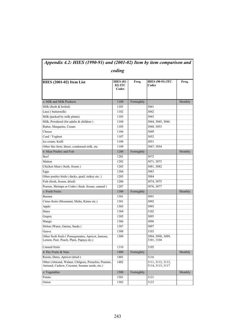
243

Appendix 4.2: HIES (1990-91) and (2001-02) Item by item comparison and

coding

HIES (2001-02) Item List

HIES (01-

02) ITC

Codes

Freq. HIES (90-91) ITC

Codes

Freq.

a: Milk and Milk Products 1100 Fortnightly Monthly

Milk (fresh & boiled) 1101 3041

Lassi ( buttermilk) 1102 3042

Milk (packed by milk plants) 1103 3043

Milk, Powdered (for adults & children ) 1104 3044, 3045, 3046

Butter, Margarine, Cream 1105 3048, 3053

Cheese 1106 3049

Curd / Yoghurt 1107 3052

Ice cream, Kulfi 1108 3051

Other like ferni, kheer, condensed milk, etc. 1109 3047, 3054

b: Meat Poultry and Fish 1200 Fortnightly Monthly

Beef 1201 3072

Mutton 1202 3071, 3073

Chicken Meat ( fresh, frozen ) 1203 3081, 3082

Eggs 1204 3083

Other poultry birds ( ducks, quail, turkey etc. ) 1205 3084

Fish (fresh, frozen, dried) 1206 3074, 3075

Prawns, Shrimps or Crabs ( fresh, frozen, canned ) 1207 3076, 3077

c: Fresh Fruits: 1300 Fortnightly Monthly

Banana 1301 3091

Citrus fruits (Mosummi, Malta, Kinno etc.) 1301 3092

Apple 1303 3093

Dates 1304 3102

Grapes 1305 3095

Mango 1306 3096

Melon (Water, Garma, Sarda ) 1307 3097

Guava 1308 3103

Other fresh fruits ( Pomegranates, Apricot, Jamons, Lemon, Peer, Peach, Plum, Papaya etc.)

1309 3094, 3098, 3099, 3101, 3104

Canned fruits 1310 3105

d: Dry Fruits & Nuts 1400 Fortnightly Monthly

Raisin, Dates, Apricot (dried ) 1401 3116

Other (Almond, Walnut, Chilgoza, Pistachio, Peanuts, Aniseed, Cashew, Coconut, Sesame seeds, etc.)

1402 3111, 3112, 3113, 3114, 3115, 3117

e: Vegetables 1500 Fortnightly Monthly

Potato 1501 3121

Onion 1502 3123

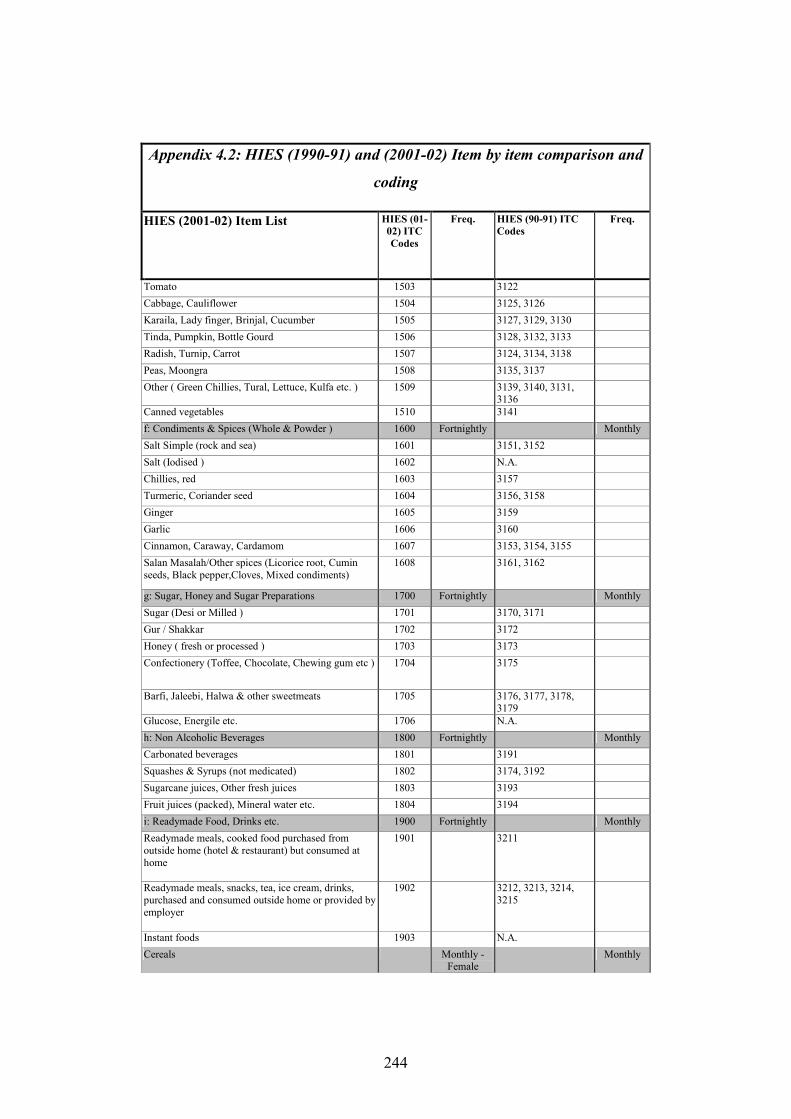
244


coding


HIES (01-

02) ITC

Codes


Codes

Freq.

Tomato 1503 3122

Cabbage, Cauliflower 1504 3125, 3126

Karaila, Lady finger, Brinjal, Cucumber 1505 3127, 3129, 3130

Tinda, Pumpkin, Bottle Gourd 1506 3128, 3132, 3133

Radish, Turnip, Carrot 1507 3124, 3134, 3138

Peas, Moongra 1508 3135, 3137

Other ( Green Chillies, Tural, Lettuce, Kulfa etc. ) 1509 3139, 3140, 3131, 3136

Canned vegetables 1510 3141

f: Condiments & Spices (Whole & Powder ) 1600 Fortnightly Monthly

Salt Simple (rock and sea) 1601 3151, 3152

Salt (Iodised ) 1602 N.A.

Chillies, red 1603 3157

Turmeric, Coriander seed 1604 3156, 3158

Ginger 1605 3159

Garlic 1606 3160

Cinnamon, Caraway, Cardamom 1607 3153, 3154, 3155

Salan Masalah/Other spices (Licorice root, Cumin seeds, Black pepper,Cloves, Mixed condiments)

1608 3161, 3162

g: Sugar, Honey and Sugar Preparations 1700 Fortnightly Monthly

Sugar (Desi or Milled ) 1701 3170, 3171

Gur / Shakkar 1702 3172

Honey ( fresh or processed ) 1703 3173

Confectionery (Toffee, Chocolate, Chewing gum etc ) 1704 3175

Barfi, Jaleebi, Halwa & other sweetmeats 1705 3176, 3177, 3178, 3179

Glucose, Energile etc. 1706 N.A.

h: Non Alcoholic Beverages 1800 Fortnightly Monthly

Carbonated beverages 1801 3191

Squashes & Syrups (not medicated) 1802 3174, 3192

Sugarcane juices, Other fresh juices 1803 3193

Fruit juices (packed), Mineral water etc. 1804 3194

i: Readymade Food, Drinks etc. 1900 Fortnightly Monthly

Readymade meals, cooked food purchased from outside home (hotel & restaurant) but consumed at home

1901 3211

Readymade meals, snacks, tea, ice cream, drinks, purchased and consumed outside home or provided by employer

1902 3212, 3213, 3214, 3215

Instant foods 1903 N.A.

Cereals Monthly - Female

Monthly

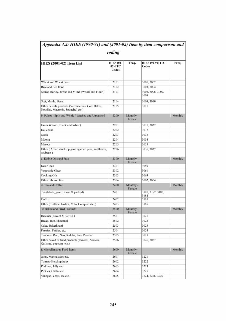
245


coding


HIES (01-

02) ITC

Codes


Codes

Freq.

Wheat and Wheat flour 2101 3001, 3002

Rice and rice flour 2102 3003, 3004

Maize, Barley, Jawar and Millet (Whole and Flour ) 2103 3005, 3006, 3007, 3008

Suji, Maida, Besan 2104 3009, 3010

Other cereals products (Vermicellies, Corn flakes, Noodles, Macronis, Spageite) etc.)

2105 3011

b. Pulses - Split and Whole / Washed and Unwashed 2200 Monthly - Female

Monthly

Gram Whole ( Black and White) 2201 3031, 3032

Dal chana 2202 3037

Mash 2203 3033

Moong 2204 3034

Masoor 2205 3035

Other ( Arhar, chick / pigeon /garden peas, sunflower, soybean )

2206 3036, 3037

c. Edible Oils and Fats 2300 Monthly - Female

Monthly

Desi Ghee 2301 3050

Vegetable Ghee 2302 3061

Cooking Oils 2303 3063

Other oils and fats 2304 3062, 3064

d. Tea and Coffee 2400 Monthly - Female

Monthly

Tea (black, green loose & packed) 2401 3181, 3182, 3183, 3184

Coffee 2402 3185

Other (ovaltine, harlics, Milo, Complan etc. ) 2403 3185

e: Baked and Fried Products 2500 Monthly - Female

Monthly

Biscuits ( Sweet & Saltish ) 2501 3021

Bread, Bun, Sheermal 2502 3022

Cake, Bakerkhani 2503 3023

Pastries, Patties, etc. 2504 3024

Tandoori Roti, Nan, Kulcha, Puri, Paratha 2505 3025

Other baked or fried products (Pakoras, Samosa, Qatlama, popcorn etc.)

2506 3026, 3027

f. Miscellaneous Food Items 2600 Monthly - Female

Monthly

Jams, Marmalades etc. 2601 3221

Tomato Ketchup/pulp 2602 3222

Pudding, Jelly etc. 2603 3223

Pickles, Chatni etc. 2604 3225

Vinegar, Yeast, Ice etc. 2605 3224, 3226, 3227

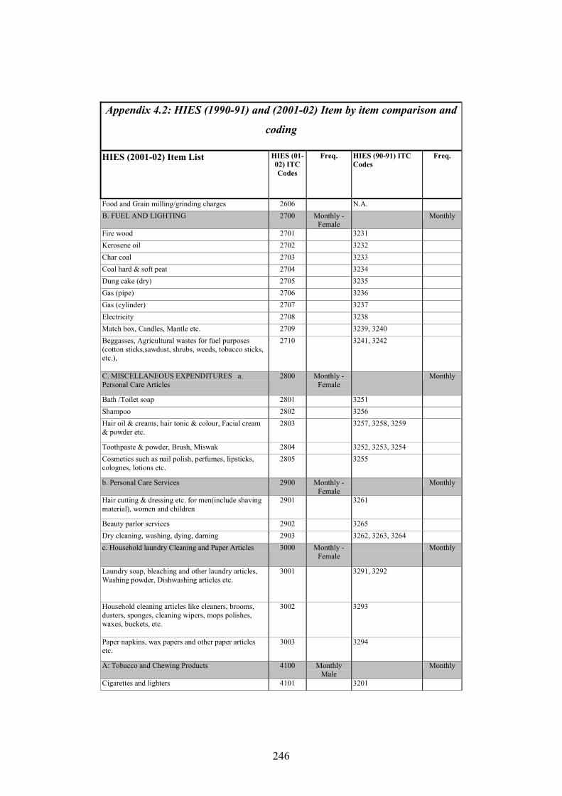
246


coding


HIES (01-

02) ITC

Codes


Codes

Freq.

Food and Grain milling/grinding charges 2606 N.A.

B. FUEL AND LIGHTING 2700 Monthly - Female

Monthly

Fire wood 2701 3231

Kerosene oil 2702 3232

Char coal 2703 3233

Coal hard & soft peat 2704 3234

Dung cake (dry) 2705 3235

Gas (pipe) 2706 3236

Gas (cylinder) 2707 3237

Electricity 2708 3238

Match box, Candles, Mantle etc. 2709 3239, 3240

Beggasses, Agricultural wastes for fuel purposes (cotton sticks,sawdust, shrubs, weeds, tobacco sticks, etc.),

2710 3241, 3242

C. MISCELLANEOUS EXPENDITURES a. Personal Care Articles

2800 Monthly - Female

Monthly

Bath /Toilet soap 2801 3251

Shampoo 2802 3256

Hair oil & creams, hair tonic & colour, Facial cream & powder etc.

2803 3257, 3258, 3259

Toothpaste & powder, Brush, Miswak 2804 3252, 3253, 3254

Cosmetics such as nail polish, perfumes, lipsticks, colognes, lotions etc.

2805 3255

b. Personal Care Services 2900 Monthly - Female

Monthly

Hair cutting & dressing etc. for men(include shaving material), women and children

2901 3261

Beauty parlor services 2902 3265

Dry cleaning, washing, dying, darning 2903 3262, 3263, 3264

c. Household laundry Cleaning and Paper Articles 3000 Monthly - Female

Monthly

Laundry soap, bleaching and other laundry articles, Washing powder, Dishwashing articles etc.

3001 3291, 3292

Household cleaning articles like cleaners, brooms, dusters, sponges, cleaning wipers, mops polishes, waxes, buckets, etc.

3002 3293

Paper napkins, wax papers and other paper articles etc.

3003 3294

A: Tobacco and Chewing Products 4100 Monthly Male

Monthly

Cigarettes and lighters 4101 3201

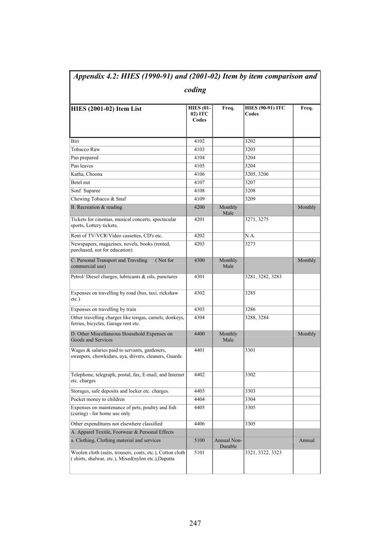
247


coding


HIES (01-

02) ITC

Codes


Codes

Freq.

Biri 4102 3202

Tobacco Raw 4103 3203

Pan prepared 4104 3204

Pan leaves 4105 3204

Katha, Choona 4106 3205, 3206

Betel nut 4107 3207

Sonf Suparee 4108 3208

Chewing Tobacco & Snuf 4109 3209

B. Recreation & reading 4200 Monthly Male

Monthly

Tickets for cinemas, musical concerts, spectacular sports, Lottery tickets,

4201 3271, 3275

Rent of TV/VCR/Video cassettes, CD's etc. 4202 N.A.

Newspapers, magazines, novels, books (rented, purchased, not for education)

4203 3273

C. Personal Transport and Traveling ( Not for commercial use)

4300 Monthly Male

Monthly

Petrol/ Diesel charges, lubricants & oils, punctures 4301 3281, 3282, 3283

Expenses on travelling by road (bus, taxi, rickshaw etc.)

4302 3285

Expenses on travelling by train 4303 3286

Other travelling charges like tongas, camels, donkeys, ferries, bicycles, Garage rent etc.

4304 3288, 3284

D. Other Miscellaneous Household Expenses on Goods and Services

4400 Monthly Male

Monthly

Wages & salaries paid to servants, gardeners, sweepers, chowkidars, aya, drivers, cleaners, Guards

4401 3301

Telephone, telegraph, postal, fax, E-mail, and Internet etc. charges

4402 3302

Storages, safe deposits and locker etc. charges. 4403 3303

Pocket money to children 4404 3304

Expenses on maintenance of pets, poultry and fish (curing) - for home use only

4405 3305

Other expenditures not elsewhere classified 4406 3305

A. Apparel Textile, Footwear & Personal Effects

a. Clothing, Clothing material and services 5100 Annual Non-Durable

Annual

Woolen cloth (suits, trousers, coats, etc.), Cotton cloth ( shirts, shalwar, etc.), Mixed(nylon etc.),Dupatta

5101 3321, 3322, 3323

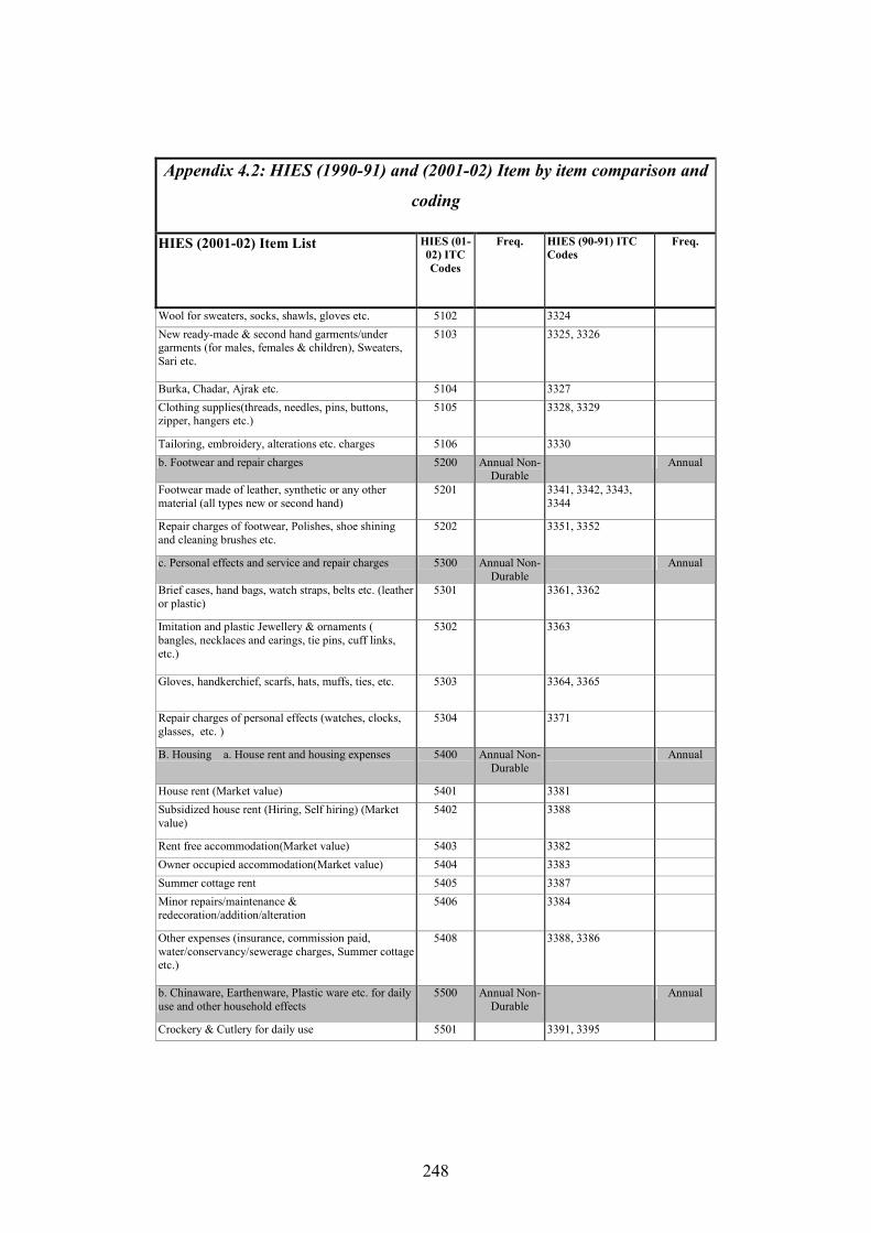
248


coding


HIES (01-

02) ITC

Codes


Codes

Freq.

Wool for sweaters, socks, shawls, gloves etc. 5102 3324

New ready-made & second hand garments/under garments (for males, females & children), Sweaters, Sari etc.

5103 3325, 3326

Burka, Chadar, Ajrak etc. 5104 3327

Clothing supplies(threads, needles, pins, buttons, zipper, hangers etc.)

5105 3328, 3329

Tailoring, embroidery, alterations etc. charges 5106 3330

b. Footwear and repair charges 5200 Annual Non-Durable

Annual

Footwear made of leather, synthetic or any other material (all types new or second hand)

5201 3341, 3342, 3343, 3344

Repair charges of footwear, Polishes, shoe shining and cleaning brushes etc.

5202 3351, 3352

c. Personal effects and service and repair charges 5300 Annual Non-Durable

Annual

Brief cases, hand bags, watch straps, belts etc. (leather or plastic)

5301 3361, 3362

Imitation and plastic Jewellery & ornaments ( bangles, necklaces and earings, tie pins, cuff links, etc.)

5302 3363

Gloves, handkerchief, scarfs, hats, muffs, ties, etc. 5303 3364, 3365

Repair charges of personal effects (watches, clocks, glasses, etc. )

5304 3371

B. Housing a. House rent and housing expenses 5400 Annual Non-Durable

Annual

House rent (Market value) 5401 3381

Subsidized house rent (Hiring, Self hiring) (Market value)

5402 3388

Rent free accommodation(Market value) 5403 3382

Owner occupied accommodation(Market value) 5404 3383

Summer cottage rent 5405 3387

Minor repairs/maintenance & redecoration/addition/alteration

5406 3384

Other expenses (insurance, commission paid, water/conservancy/sewerage charges, Summer cottage etc.)

5408 3388, 3386

b. Chinaware, Earthenware, Plastic ware etc. for daily use and other household effects

5500 Annual Non-Durable

Annual

Crockery & Cutlery for daily use 5501 3391, 3395

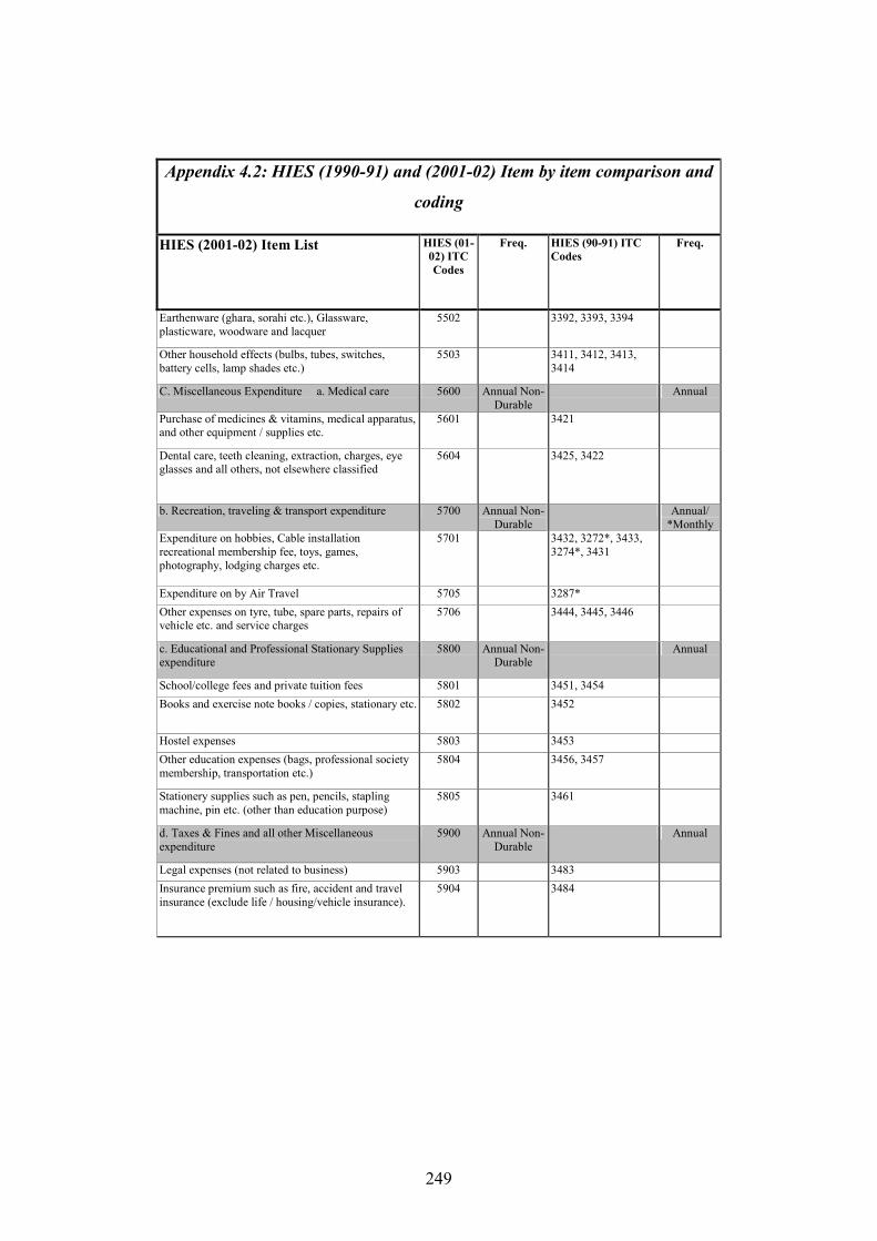
249


coding


HIES (01-

02) ITC

Codes


Codes

Freq.

Earthenware (ghara, sorahi etc.), Glassware, plasticware, woodware and lacquer

5502 3392, 3393, 3394

Other household effects (bulbs, tubes, switches, battery cells, lamp shades etc.)

5503 3411, 3412, 3413, 3414

C. Miscellaneous Expenditure a. Medical care 5600 Annual Non-Durable

Annual

Purchase of medicines & vitamins, medical apparatus, and other equipment / supplies etc.

5601 3421

Dental care, teeth cleaning, extraction, charges, eye glasses and all others, not elsewhere classified

5604 3425, 3422

b. Recreation, traveling & transport expenditure 5700 Annual Non-Durable

Annual/ *Monthly

Expenditure on hobbies, Cable installation recreational membership fee, toys, games, photography, lodging charges etc.

5701 3432, 3272*, 3433, 3274*, 3431

Expenditure on by Air Travel 5705 3287*

Other expenses on tyre, tube, spare parts, repairs of vehicle etc. and service charges

5706 3444, 3445, 3446

c. Educational and Professional Stationary Supplies expenditure


Annual

School/college fees and private tuition fees 5801 3451, 3454

Books and exercise note books / copies, stationary etc. 5802 3452

Hostel expenses 5803 3453

Other education expenses (bags, professional society membership, transportation etc.)

5804 3456, 3457

Stationery supplies such as pen, pencils, stapling machine, pin etc. (other than education purpose)

5805 3461

d. Taxes & Fines and all other Miscellaneous expenditure


Annual

Legal expenses (not related to business) 5903 3483

Insurance premium such as fire, accident and travel insurance (exclude life / housing/vehicle insurance).

5904 3484

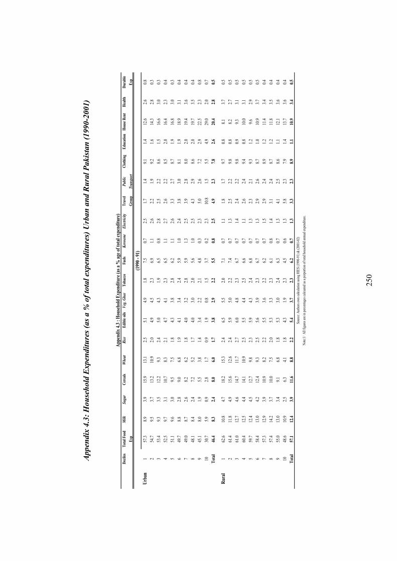
250

Appen

dix 4.3: Household E

xpen

ditures (as a %

of total ex

pen

ditures) U

rban and R

ural Pakistan (1990-2001)

Deciles

Total Food

Exp

Milk

Suga

rCereals

Whe

atRice

Edible oils

Veg

. Ghee

Tobacco

Fuels

Kerosen

eElectricity

Travel

Group

Pub

lic

Tra

nsport

Clothing

Education

House Rent

Health

Durable

Exp

Urban

157

.38.

93.

915

.913

.12.

55.

14.

91.

87.

50.

72.

51.

71.

49.

11.

412

.62.

60.

8

254

.79.

53.

713

.210

.92.

04.

94.

52.

36.

91.

12.

62.

21.

99.

21.

614

.32.

80.

3

353

.49.

33.

512

.29.

32.

45.

04.

31.

96.

50.

82.

82.

52.

28.

61.

516

.63.

00.

3

452

.59.

73.

110

.78.

32.

14.

74.

12.

36.

51.

12.

72.

62.

28.

52.

016

.42.

30.

4

551

.19.

63.

09.

57.

51.

84.

33.

82.

86.

21.

12.

63.

32.

78.

71.

916

.83.

00.

3

649

.78.

82.

89.

06.

81.

94.

13.

42.

45.

91.

02.

43.

83.

08.

11.

918

.93.

10.

4

749

.08.

72.

68.

26.

21.

84.

03.

22.

85.

91.

32.

53.

92.

88.

02.

019

.43.

60.

4

848

.18.

42.

47.

25.

21.

74.

03.

02.

05.

61.

02.

54.

32.

98.

62.

019

.73.

50.

4

945

.18.

01.

95.

53.

81.

43.

42.

22.

14.

80.

32.

35.

02.

67.

22.

922

.52.

30.

8

1030

.75.

90.

92.

81.

70.

91.

90.

81.

53.

70.

22.

310

.81.

55.

54.

929

.02.

00.

7

Total

46.4

8.3

2.4

8.0

6.0

1.7

3.8

2.9

2.2

5.5

0.8

2.5

4.9

2.3

7.8

2.6

20.4

2.8

0.5

Rural

162

.610

.84.

718

.215

.32.

46.

55.

52.

07.

10.

71.

11.

81.

79.

70.

88.

13.

70.

5

261

.411

.84.

915

.612

.62.

45.

95.

02.

27.

40.

71.

32.

52.

29.

80.

88.

22.

70.

5

361

.012

.74.

614

.711

.72.

76.

04.

82.

36.

70.

71.

42.

42.

29.

80.

99.

33.

10.

5

460

.412

.54.

414

.110

.92.

55.

54.

42.

56.

60.

71.

12.

62.

49.

40.

810

.03.

10.

5

559

.712

.44.

512

.79.

82.

35.

94.

32.

46.

80.

71.

32.

32.

19.

31.

29.

62.

90.

5

658

.413

.04.

212

.49.

32.

55.

63.

92.

36.

70.

71.

32.

92.

68.

71.

010

.93.

70.

5

757

.312

.93.

910

.98.

22.

25.

53.

62.

26.

20.

71.

52.

92.

48.

91.

211

.43.

40.

4

857

.414

.23.

710

.07.

52.

05.

33.

32.

36.

10.

81.

43.

12.

48.

71.

211

.83.

50.

4

955

.013

.03.

49.

16.

81.

85.

33.

02.

46.

30.

71.

34.

12.

58.

61.

112

.13.

60.

4

1048

.610

.92.

56.

34.

11.

84.

31.

92.

34.

50.

61.

35.

82.

37.

91.

413

.73.

60.

4

Total

57.1

12.4

3.9

11.6

8.8

2.2

5.4

3.7

2.3

6.2

0.7

1.3

3.3

2.3

8.9

1.1

10.9

3.4

0.5

Appendix 4.3 : Household Expenditure (as a % age of total expenditure)

(1990 - 91)

Sour

ce: A

utho

rs o

wn

calc

ulat

ion

usin

g H

IES

(199

0-91

) & (2

001-

02)

Not

e:1/

All

figu

res

are

in p

erce

ntag

es c

alcu

ated

as

a po

rpor

tion

of to

tal h

ouse

hold

ann

ual e

xpen

ditu

re.

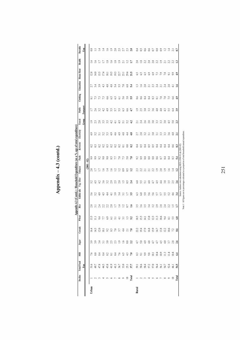
251

Appendix – 4.3 (contd.)

Deciles

Total Food

Exp

Milk

Suga

rCereals

Whe

atRice

Edible oils

Veg

. Ghee

Tobacco

Fuels

Kerosen

eElectricity

Travel

Group

Pub

lic

Tra

nsport

Clothing

Education

House Rent

Health

Durable

Exp

Urban

151

.67.

63.

916

.413

.52.

85.

65.

22.

09.

90.

24.

91.

91.

78.

12.

712

.81.

60.

8

249

.78.

03.

914

.311

.13.

15.

24.

51.

79.

90.

35.

22.

32.

67.

33.

414

.01.

61.

1

347

.88.

43.

412

.09.

42.

44.

94.

21.

79.

20.

25.

12.

83.

27.

33.

915

.51.

71.

4

444

.58.

43.

110

.17.

72.

24.

53.

61.

69.

00.

25.

23.

54.

27.

34.

317

.41.

71.

4

543

.88.

23.

09.

26.

92.

24.

43.

21.

49.

00.

35.

33.

54.

96.

64.

818

.11.

81.

6

641

.98.

12.

58.

36.

12.

04.

12.

91.

68.

50.

24.

94.

25.

56.

54.

819

.51.

61.

9

741

.38.

42.

37.

05.

11.

73.

92.

51.

27.

70.

24.

64.

15.

76.

35.

419

.31.

82.

0

836

.77.

61.

95.

74.

11.

43.

42.

01.

27.

80.

24.

94.

55.

56.

15.

522

.71.

92.

5

933

.06.

51.

64.

43.

11.

23.

11.

50.

97.

30.

14.

85.

16.

35.

67.

023

.12.

12.

7

1025

.14.

30.

82.

11.

30.

71.

70.

50.

55.

80.

04.

45.

26.

63.

86.

829

.41.

22.

3

Total

37.7

7.0

2.2

7.0

5.2

1.6

3.5

2.4

1.2

7.8

0.2

4.8

4.2

4.7

5.9

5.4

21.5

1.7

2.0

Rural

159

.18.

34.

722

.218

.53.

56.

36.

02.

39.

20.

42.

72.

11.

98.

61.

36.

52.

00.

4

258

.69.

15.

019

.415

.53.

66.

05.

52.

28.

90.

52.

82.

42.

58.

61.

66.

51.

80.

5

358

.49.

94.

917

.914

.13.

55.

95.

12.

18.

80.

43.

22.

63.

08.

42.

06.

52.

20.

6

457

.29.

84.

816

.813

.03.

45.

64.

82.

18.

80.

53.

12.

83.

38.

42.

16.

92.

00.

6

557

.010

.14.

715

.912

.33.

25.

64.

72.

28.

80.

53.

03.

03.

68.

32.

36.

92.

00.

7

656

.410

.44.

714

.711

.32.

95.

74.

51.

98.

60.

43.

13.

34.

08.

12.

47.

32.

20.

8

756

.110

.94.

513

.810

.62.

85.

74.

42.

08.

70.

43.

33.

34.

07.

82.

17.

91.

90.

9

854

.711

.34.

012

.29.

42.

45.

53.

81.

98.

40.

43.

33.

84.

37.

82.

47.

82.

11.

2

952

.411

.43.

710

.68.

12.

25.

23.

51.

68.

40.

43.

64.

55.

57.

52.

89.

12.

21.

4

1046

.110

.42.

87.

25.

51.

54.

62.

51.

48.

30.

64.

05.

86.

46.

64.

19.

92.

22.

1

Total

54.5

6.4

2.6

8.6

6.8

1.7

3.4

2.6

1.2

5.4

0.3

2.1

2.3

3.9

4.9

1.6

4.9

1.3

0.7

Sour

ce: A

utho

rs o

wn

calc

ulat

ion

usin

g H

IES

(199

0-91

) &

(20

01-0

2)

Not

e:1/

All

figu

res

are

in p

erce

ntag

es c

alcu

ated

as

a po

rpor

tion

of

tota

l hou

seho

ld a

nnua

l exp

endi

ture

.

(2001 - 02)

Appendix 4.3 (Contd.) : Household Expenditure (as a % age of total expenditure)

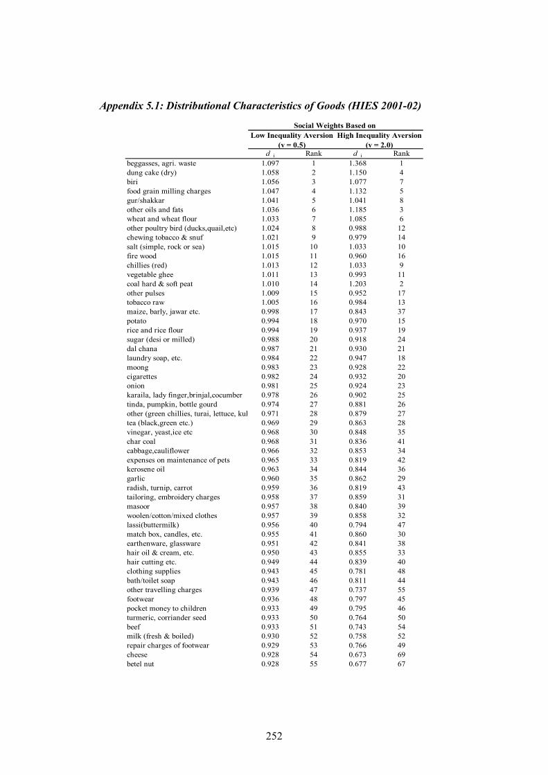
252

Appendix 5.1: Distributional Characteristics of Goods (HIES 2001-02)

d i Rank d i Rank

beggasses, agri. waste 1.097 1 1.368 1

dung cake (dry) 1.058 2 1.150 4

biri 1.056 3 1.077 7

food grain milling charges 1.047 4 1.132 5

gur/shakkar 1.041 5 1.041 8

other oils and fats 1.036 6 1.185 3

wheat and wheat flour 1.033 7 1.085 6

other poultry bird (ducks,quail,etc) 1.024 8 0.988 12

chewing tobacco & snuf 1.021 9 0.979 14

salt (simple, rock or sea) 1.015 10 1.033 10

fire wood 1.015 11 0.960 16

chillies (red) 1.013 12 1.033 9

vegetable ghee 1.011 13 0.993 11

coal hard & soft peat 1.010 14 1.203 2

other pulses 1.009 15 0.952 17

tobacco raw 1.005 16 0.984 13

maize, barly, jawar etc. 0.998 17 0.843 37

potato 0.994 18 0.970 15

rice and rice flour 0.994 19 0.937 19

sugar (desi or milled) 0.988 20 0.918 24

dal chana 0.987 21 0.930 21

laundry soap, etc. 0.984 22 0.947 18

moong 0.983 23 0.928 22

cigarettes 0.982 24 0.932 20

onion 0.981 25 0.924 23

karaila, lady finger,brinjal,cocumber 0.978 26 0.902 25

tinda, pumpkin, bottle gourd 0.974 27 0.881 26

other (green chillies, turai, lettuce, kulfa 0.971 28 0.879 27

tea (black,green etc.) 0.969 29 0.863 28

vinegar, yeast,ice etc 0.968 30 0.848 35

char coal 0.968 31 0.836 41

cabbage,cauliflower 0.966 32 0.853 34

expenses on maintenance of pets 0.965 33 0.819 42

kerosene oil 0.963 34 0.844 36

garlic 0.960 35 0.862 29

radish, turnip, carrot 0.959 36 0.819 43

tailoring, embroidery charges 0.958 37 0.859 31

masoor 0.957 38 0.840 39

woolen/cotton/mixed clothes 0.957 39 0.858 32

lassi(buttermilk) 0.956 40 0.794 47

match box, candles, etc. 0.955 41 0.860 30

earthenware, glassware 0.951 42 0.841 38

hair oil & cream, etc. 0.950 43 0.855 33

hair cutting etc. 0.949 44 0.839 40

clothing supplies 0.943 45 0.781 48

bath/toilet soap 0.943 46 0.811 44

other travelling charges 0.939 47 0.737 55

footwear 0.936 48 0.797 45

pocket money to children 0.933 49 0.795 46

turmeric, corriander seed 0.933 50 0.764 50

beef 0.933 51 0.743 54

milk (fresh & boiled) 0.930 52 0.758 52

repair charges of footwear 0.929 53 0.766 49

cheese 0.928 54 0.673 69

betel nut 0.928 55 0.677 67


Low Inequality Aversion

(v = 0.5)

High Inequality Aversion

(v = 2.0)

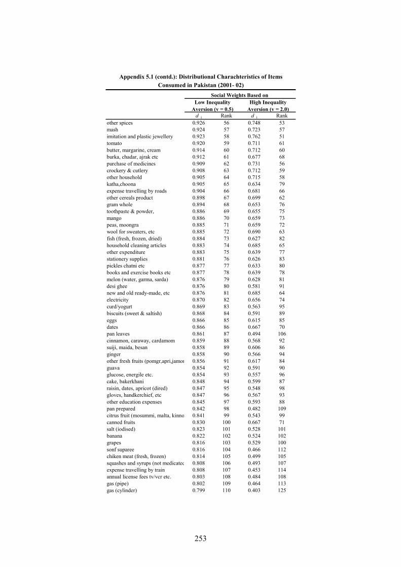
253

d i Rank d i Rank

other spices 0.926 56 0.748 53

mash 0.924 57 0.723 57

imitation and plastic jewellery 0.923 58 0.762 51

tomato 0.920 59 0.711 61

butter, margarine, cream 0.914 60 0.712 60

burka, chadar, ajrak etc 0.912 61 0.677 68

purchase of medicines 0.909 62 0.731 56

crockery & cutlery 0.908 63 0.712 59

other household 0.905 64 0.715 58

katha,choona 0.905 65 0.634 79

expense travelling by roads 0.904 66 0.681 66

other cereals product 0.898 67 0.699 62

gram whole 0.894 68 0.653 76

toothpaste & powder, 0.886 69 0.655 75

mango 0.886 70 0.659 73

peas, moongra 0.885 71 0.659 72

wool for sweaters, etc 0.885 72 0.690 63

fish (fresh, frozen, dried) 0.884 73 0.627 82

household cleaning articles 0.883 74 0.685 65

other expenditure 0.883 75 0.639 77

stationery supplies 0.881 76 0.626 83

pickles chatni etc 0.877 77 0.633 80

books and exercise books etc 0.877 78 0.639 78

melon (water, garma, sarda) 0.876 79 0.628 81

desi ghee 0.876 80 0.581 91

new and old ready-made, etc 0.876 81 0.685 64

electricity 0.870 82 0.656 74

curd/yogurt 0.869 83 0.563 95

biscuits (sweet & saltish) 0.868 84 0.591 89

eggs 0.866 85 0.615 85

dates 0.866 86 0.667 70

pan leaves 0.861 87 0.494 106

cinnamon, caraway, cardamom 0.859 88 0.568 92

suiji, maida, besan 0.858 89 0.606 86

ginger 0.858 90 0.566 94

other fresh fruits (pomgr,apri,jamon,lemon etc.)0.856 91 0.617 84

guava 0.854 92 0.591 90

glucose, energile etc. 0.854 93 0.557 96

cake, bakerkhani 0.848 94 0.599 87

raisin, dates, apricot (dired) 0.847 95 0.548 98

gloves, handkerchief, etc 0.847 96 0.567 93

other education expenses 0.845 97 0.593 88

pan prepared 0.842 98 0.482 109

citrus fruit (mosummi, malta, kinno) 0.841 99 0.543 99

canned fruits 0.830 100 0.667 71

salt (iodised) 0.823 101 0.528 101

banana 0.822 102 0.524 102

grapes 0.816 103 0.529 100

sonf suparee 0.816 104 0.466 112

chiken meat (fresh, frozen) 0.814 105 0.499 105

squashes and syrups (not medicated) 0.808 106 0.493 107

expense travelling by train 0.808 107 0.453 114

annual license fees tv/vcr etc. 0.803 108 0.484 108

gas (pipe) 0.802 109 0.464 113

gas (cylinder) 0.799 110 0.403 125

Appendix 5.1 (contd.): Distributional Charachteristics of Items

Consumed in Pakistan (2001- 02)


Low Inequality

Aversion (v = 0.5)

High Inequality

Aversion (v = 2.0)

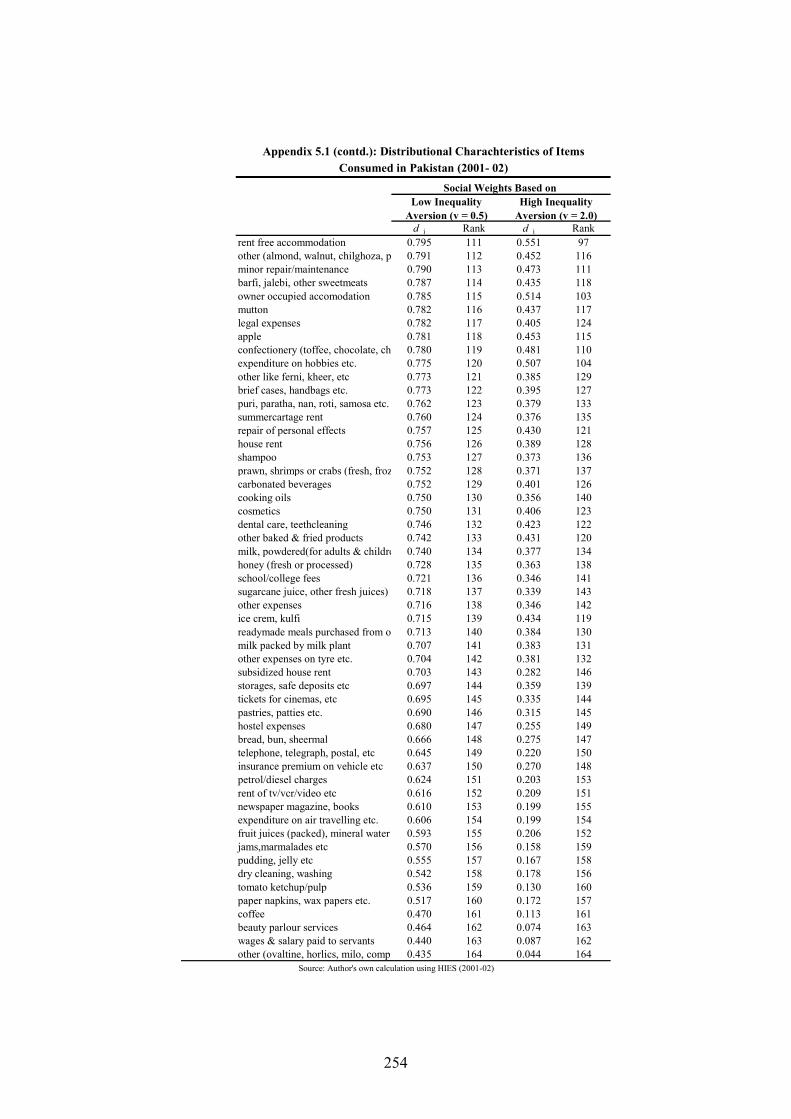
254

d i Rank d i Rank

rent free accommodation 0.795 111 0.551 97

other (almond, walnut, chilghoza, pistacho etc.)0.791 112 0.452 116

minor repair/maintenance 0.790 113 0.473 111

barfi, jalebi, other sweetmeats 0.787 114 0.435 118

owner occupied accomodation 0.785 115 0.514 103

mutton 0.782 116 0.437 117

legal expenses 0.782 117 0.405 124

apple 0.781 118 0.453 115

confectionery (toffee, chocolate, chewing gum etc.)0.780 119 0.481 110

expenditure on hobbies etc. 0.775 120 0.507 104

other like ferni, kheer, etc 0.773 121 0.385 129

brief cases, handbags etc. 0.773 122 0.395 127

puri, paratha, nan, roti, samosa etc. 0.762 123 0.379 133

summercartage rent 0.760 124 0.376 135

repair of personal effects 0.757 125 0.430 121

house rent 0.756 126 0.389 128

shampoo 0.753 127 0.373 136

prawn, shrimps or crabs (fresh, frozen, canned)0.752 128 0.371 137

carbonated beverages 0.752 129 0.401 126

cooking oils 0.750 130 0.356 140

cosmetics 0.750 131 0.406 123

dental care, teethcleaning 0.746 132 0.423 122

other baked & fried products 0.742 133 0.431 120

milk, powdered(for adults & children) 0.740 134 0.377 134

honey (fresh or processed) 0.728 135 0.363 138

school/college fees 0.721 136 0.346 141

sugarcane juice, other fresh juices) 0.718 137 0.339 143

other expenses 0.716 138 0.346 142

ice crem, kulfi 0.715 139 0.434 119

readymade meals purchased from outside0.713 140 0.384 130

milk packed by milk plant 0.707 141 0.383 131

other expenses on tyre etc. 0.704 142 0.381 132

subsidized house rent 0.703 143 0.282 146

storages, safe deposits etc 0.697 144 0.359 139

tickets for cinemas, etc 0.695 145 0.335 144

pastries, patties etc. 0.690 146 0.315 145

hostel expenses 0.680 147 0.255 149

bread, bun, sheermal 0.666 148 0.275 147

telephone, telegraph, postal, etc 0.645 149 0.220 150

insurance premium on vehicle etc 0.637 150 0.270 148

petrol/diesel charges 0.624 151 0.203 153

rent of tv/vcr/video etc 0.616 152 0.209 151

newspaper magazine, books 0.610 153 0.199 155

expenditure on air travelling etc. 0.606 154 0.199 154

fruit juices (packed), mineral water etc.0.593 155 0.206 152

jams,marmalades etc 0.570 156 0.158 159

pudding, jelly etc 0.555 157 0.167 158

dry cleaning, washing 0.542 158 0.178 156

tomato ketchup/pulp 0.536 159 0.130 160

paper napkins, wax papers etc. 0.517 160 0.172 157

coffee 0.470 161 0.113 161

beauty parlour services 0.464 162 0.074 163

wages & salary paid to servants 0.440 163 0.087 162

other (ovaltine, horlics, milo, complan etc.)0.435 164 0.044 164

Source: Author's own calculation using HIES (2001-02)

Appendix 5.1 (contd.): Distributional Charachteristics of Items

Consumed in Pakistan (2001- 02)


Low Inequality

Aversion (v = 0.5)

High Inequality

Aversion (v = 2.0)

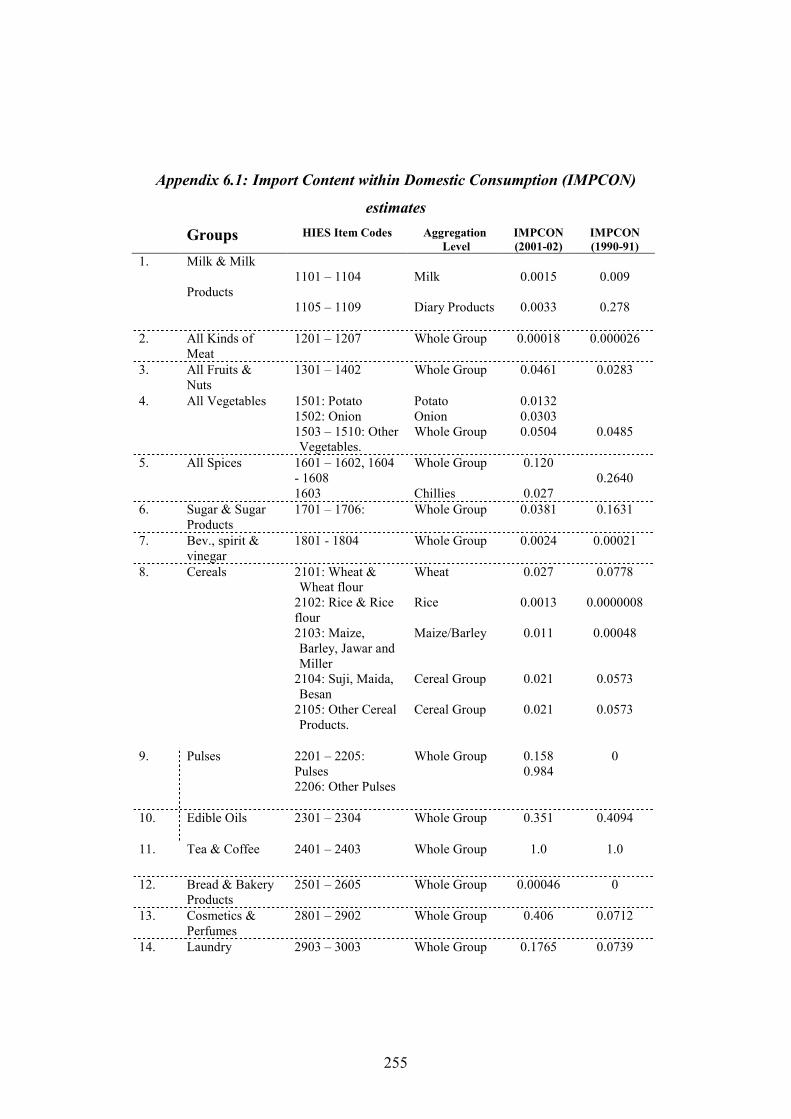
255

Appendix 6.1: Import Content within Domestic Consumption (IMPCON)

estimates

Groups HIES Item Codes Aggregation

Level

IMPCON

(2001-02)

IMPCON

(1990-91)

1. Milk & Milk

Products

1101 – 1104 1105 – 1109

Milk Diary Products

0.0015

0.0033

0.009

0.278

2. All Kinds of Meat

1201 – 1207

Whole Group 0.00018 0.000026

3. All Fruits & Nuts

1301 – 1402

Whole Group

0.0461 0.0283

4. All Vegetables 1501: Potato 1502: Onion 1503 – 1510: Other Vegetables.

Potato Onion Whole Group

0.0132 0.0303 0.0504

0.0485

5. All Spices 1601 – 1602, 1604 - 1608 1603

Whole Group Chillies

0.120

0.027

0.2640

6. Sugar & Sugar Products

1701 – 1706:

Whole Group 0.0381 0.1631

7. Bev., spirit & vinegar

1801 - 1804

Whole Group

0.0024

0.00021

8. Cereals 2101: Wheat & Wheat flour

2102: Rice & Rice flour 2103: Maize, Barley, Jawar and Miller

2104: Suji, Maida, Besan

2105: Other Cereal Products.

Wheat Rice Maize/Barley Cereal Group Cereal Group

0.027

0.0013

0.011

0.021

0.021

0.0778

0.0000008

0.00048

0.0573

0.0573

9. Pulses 2201 – 2205: Pulses 2206: Other Pulses

Whole Group

0.158 0.984

0

10. Edible Oils 2301 – 2304

Whole Group

0.351 0.4094

11. Tea & Coffee 2401 – 2403 Whole Group

1.0 1.0

12. Bread & Bakery Products

2501 – 2605

Whole Group 0.00046 0

13. Cosmetics & Perfumes

2801 – 2902


14. Laundry 2903 – 3003

Whole Group

0.1765 0.0739

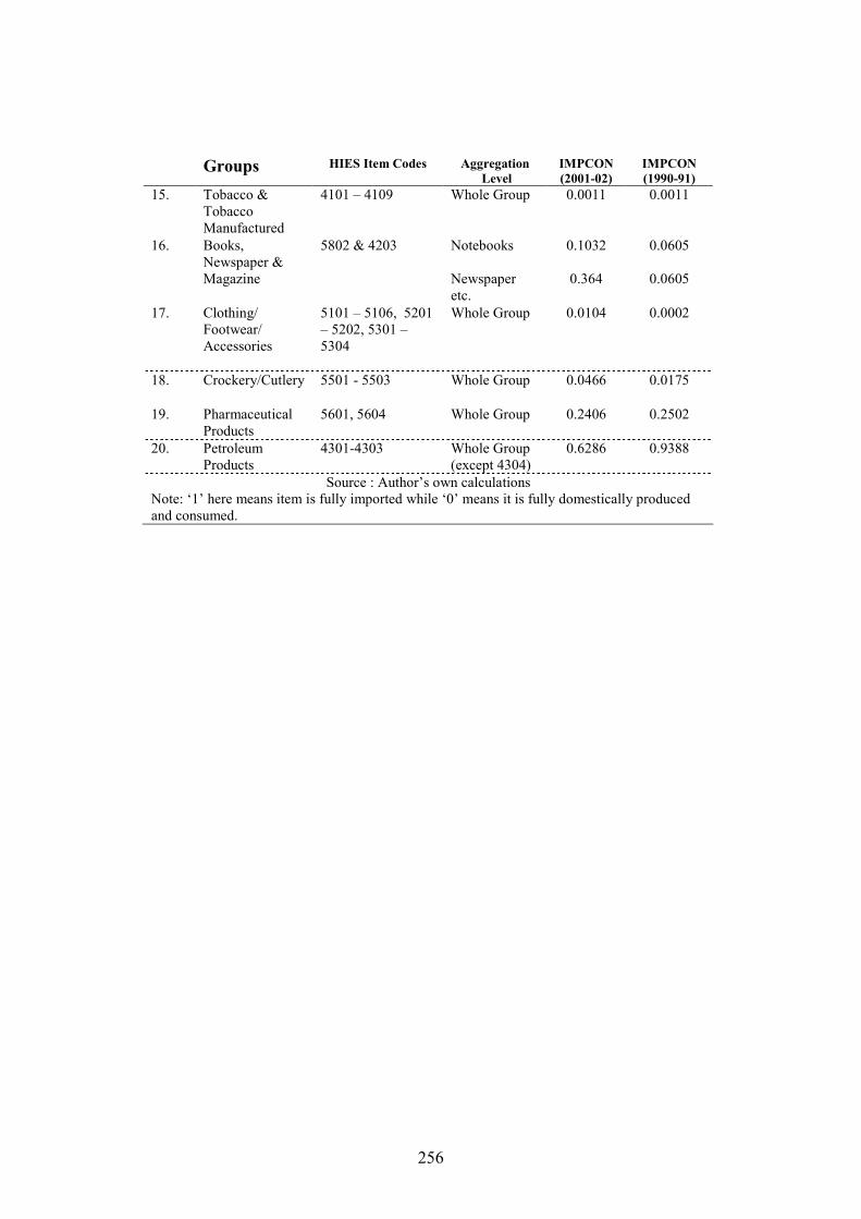
256

Groups HIES Item Codes Aggregation

Level

IMPCON

(2001-02)

IMPCON

(1990-91)

15. Tobacco & Tobacco Manufactured

4101 – 4109


16. Books, Newspaper & Magazine

5802 & 4203

Notebooks Newspaper etc.

0.1032

0.364

0.0605

0.0605

17. Clothing/ Footwear/ Accessories

5101 – 5106, 5201 – 5202, 5301 – 5304


18. Crockery/Cutlery 5501 - 5503


19. Pharmaceutical Products

5601, 5604


20. Petroleum Products

4301-4303 Whole Group (except 4304)

0.6286 0.9388

Source : Author’s own calculations Note: ‘1’ here means item is fully imported while ‘0’ means it is fully domestically produced and consumed.

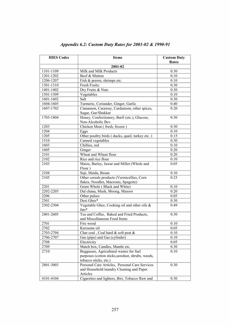
257

Appendix 6.2: Custom Duty Rates for 2001-02 & 1990-91

HIES Codes

Items Custom Duty

Rates

2001-02

1101-1109 Milk and Milk Products 0.30

1201-1202 Beef & Mutton 0.10

1206-1207 Fish & prawn, shrimps etc. 0.10

1301-1310 Fresh Fruits: 0.30

1401-1402 Dry Fruits & Nuts 0.30

1501-1509 Vegetables 0.10

1601-1602 Salt 0.30

1604-1605 Turmeric, Coriander, Ginger, Garlic 0.40

1607-1702 Cinnamon, Caraway, Cardamom, other spices, Sugar, Gur/Shakkar

0.20

1703-1804 Honey, Confectionery, Barfi (etc.), Glucose, Non-Alcoholic Bev.

0.30

1203 Chicken Meat ( fresh, frozen ) 0.30

1204 Eggs 0.10

1205 Other poultry birds ( ducks, quail, turkey etc. ) 0.15

1510 Canned vegetables 0.30

1603 Chillies, red 0.10

1605 Ginger 0.20

2101 Wheat and Wheat flour 0.20

2102 Rice and rice flour 0.10

2103 Maize, Barley, Jawar and Millet (Whole and Flour )

0.05

2104 Suji, Maida, Besan 0.10

2105 Other cereals products (Vermicellies, Corn flakes, Noodles, Macronis, Spageite)

0.25

2201 Gram Whole ( Black and White) 0.10

2202-2205 Dal chana, Mash, Moong, Masoor 0.20

2206 Other pulses 0.05

2301 Desi Ghee* 0.30

2302-2304 Vegetable Ghee, Cooking oil and other oils & fats*

0.49

2401-2605 Tea and Coffee, Baked and Fried Products, and Miscellaneous Food Items

0.30

2701 Fire wood 0.10

2702 Kerosene oil 0.05

2703-2704 Char coal , Coal hard & soft peat & 0.10

2706-2707 Gas (pipe) and Gas (cylinder) 0.10

2708 Electricity 0.05

2709 Match box, Candles, Mantle etc. 0.30

2710 Beggasses, Agricultural wastes for fuel purposes (cotton sticks,sawdust, shrubs, weeds, tobacco sticks, etc.)

0.10

2801-3003 Personal Care Articles, Personal Care Services and Household laundry Cleaning and Paper Articles

0.30

4101-4104 Cigarettes and lighters, Biri, Tobacco Raw and 0.30

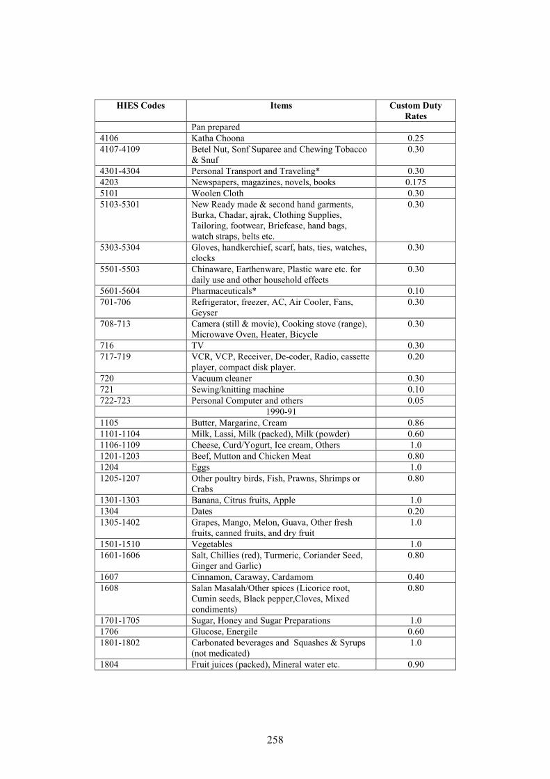
258

HIES Codes

Items Custom Duty

Rates

Pan prepared

4106 Katha Choona 0.25

4107-4109 Betel Nut, Sonf Suparee and Chewing Tobacco & Snuf

0.30

4301-4304 Personal Transport and Traveling* 0.30

4203 Newspapers, magazines, novels, books 0.175

5101 Woolen Cloth 0.30

5103-5301 New Ready made & second hand garments, Burka, Chadar, ajrak, Clothing Supplies, Tailoring, footwear, Briefcase, hand bags, watch straps, belts etc.

0.30

5303-5304 Gloves, handkerchief, scarf, hats, ties, watches, clocks

0.30

5501-5503 Chinaware, Earthenware, Plastic ware etc. for daily use and other household effects

0.30

5601-5604 Pharmaceuticals* 0.10

701-706 Refrigerator, freezer, AC, Air Cooler, Fans, Geyser

0.30

708-713 Camera (still & movie), Cooking stove (range), Microwave Oven, Heater, Bicycle

0.30

716 TV 0.30

717-719 VCR, VCP, Receiver, De-coder, Radio, cassette player, compact disk player.

0.20

720 Vacuum cleaner 0.30

721 Sewing/knitting machine 0.10

722-723 Personal Computer and others 0.05

1990-91

1105 Butter, Margarine, Cream 0.86

1101-1104 Milk, Lassi, Milk (packed), Milk (powder) 0.60

1106-1109 Cheese, Curd/Yogurt, Ice cream, Others 1.0

1201-1203 Beef, Mutton and Chicken Meat 0.80

1204 Eggs 1.0

1205-1207 Other poultry birds, Fish, Prawns, Shrimps or Crabs

0.80

1301-1303 Banana, Citrus fruits, Apple 1.0

1304 Dates 0.20

1305-1402 Grapes, Mango, Melon, Guava, Other fresh fruits, canned fruits, and dry fruit

1.0

1501-1510 Vegetables 1.0

1601-1606 Salt, Chillies (red), Turmeric, Coriander Seed, Ginger and Garlic)

0.80

1607 Cinnamon, Caraway, Cardamom 0.40

1608 Salan Masalah/Other spices (Licorice root, Cumin seeds, Black pepper,Cloves, Mixed condiments)

0.80

1701-1705 Sugar, Honey and Sugar Preparations 1.0

1706 Glucose, Energile 0.60

1801-1802 Carbonated beverages and Squashes & Syrups (not medicated)

1.0

1804 Fruit juices (packed), Mineral water etc. 0.90

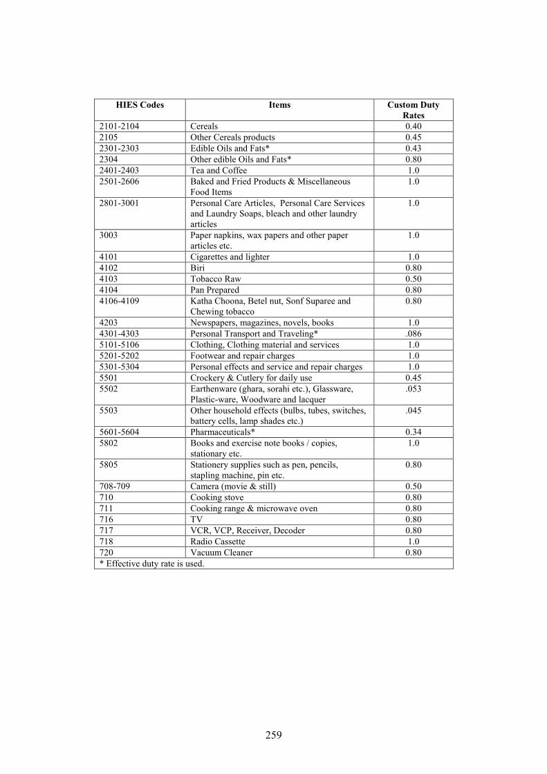
259

HIES Codes

Items Custom Duty

Rates

2101-2104 Cereals 0.40

2105 Other Cereals products 0.45

2301-2303 Edible Oils and Fats* 0.43

2304 Other edible Oils and Fats* 0.80

2401-2403 Tea and Coffee 1.0

2501-2606 Baked and Fried Products & Miscellaneous Food Items

1.0

2801-3001 Personal Care Articles, Personal Care Services and Laundry Soaps, bleach and other laundry articles

1.0

3003 Paper napkins, wax papers and other paper articles etc.

1.0

4101 Cigarettes and lighter 1.0

4102 Biri 0.80

4103 Tobacco Raw 0.50

4104 Pan Prepared 0.80

4106-4109 Katha Choona, Betel nut, Sonf Suparee and Chewing tobacco

0.80

4203 Newspapers, magazines, novels, books 1.0

4301-4303 Personal Transport and Traveling* .086

5101-5106 Clothing, Clothing material and services 1.0

5201-5202 Footwear and repair charges 1.0

5301-5304 Personal effects and service and repair charges 1.0

5501 Crockery & Cutlery for daily use 0.45

5502 Earthenware (ghara, sorahi etc.), Glassware, Plastic-ware, Woodware and lacquer

.053

5503 Other household effects (bulbs, tubes, switches, battery cells, lamp shades etc.)

.045

5601-5604 Pharmaceuticals* 0.34

5802 Books and exercise note books / copies, stationary etc.

1.0

5805 Stationery supplies such as pen, pencils, stapling machine, pin etc.

0.80

708-709 Camera (movie & still) 0.50

710 Cooking stove 0.80

711 Cooking range & microwave oven 0.80

716 TV 0.80

717 VCR, VCP, Receiver, Decoder 0.80

718 Radio Cassette 1.0

720 Vacuum Cleaner 0.80

* Effective duty rate is used.

260

Appendix 7.1: Price Elasticities: Estimates from First Stage (Unit Value and

Share Equations)

Notations

Dependent Variables

Log of unit values Budget Shares

iv

iw

Independent Variables

Log of per capita total expenditure

iβ

Log of household size

hhz

Ratio of male members less than 11 years of age to household size

Mz1

Ratio of male members less than 11-20 years of age to household size

Mz2


Mz3


Mz4


Mz5

Ratio of male members less than 51+ years of age to household size

Mz6

Ratio of female members less than 11 years of age to household size

Fz1

Ratio of female members less than 11-20 years of age to household size

Fz2


Fz3


Fz4


Fz5

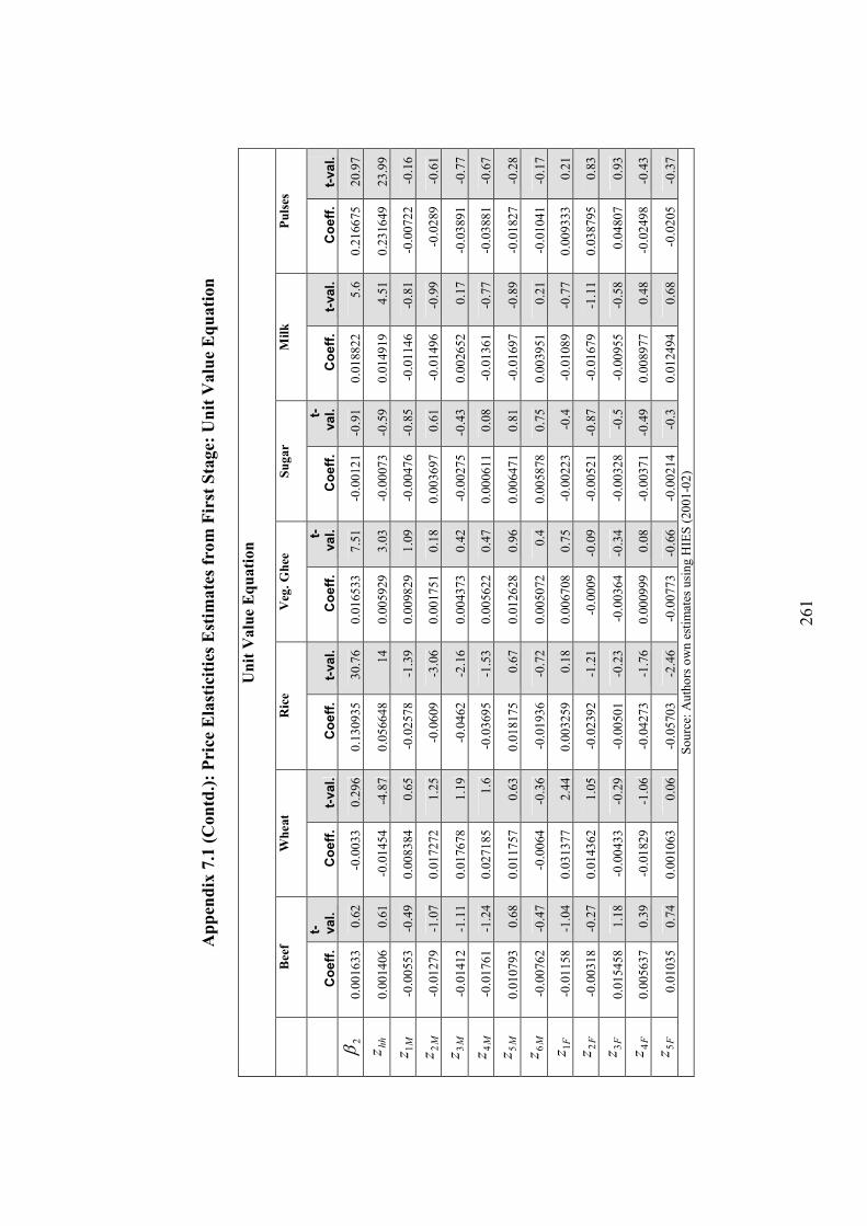
261

Appendix 7.1 (Contd.): Price Elasticities Estimates from First Stage: Unit Value Equation

Unit Value Equation

Beef

Wheat

Rice

Veg. Ghee

Sugar

Milk

Pulses

Coeff. t- val.

Coeff.

t-val.

Coeff.

t-val.

Coeff.

t-val.

Coeff.

t-val.

Coeff.

t-val.

Coeff.

t-val.

2β

0.0

016

33

0

.62

-0

.00

33

0

.29

6

0.1

309

35

3

0.7

6

0.0

165

33

7

.51

-0

.00

12

1

-0.9

1

0.0

188

22

5

.6

0.2

166

75

2

0.9

7

hh

z

0.0

014

06

0

.61

-0

.01

45

4

-4.8

7

0.0

566

48

1

4

0.0

059

29

3

.03

-0

.00

07

3

-0.5

9

0.0

149

19

4

.51

0

.23

16

49

2

3.9

9

Mz 1

-0

.00

55

3

-0.4

9

0.0

083

84

0

.65

-0

.02

57

8

-1.3

9

0.0

098

29

1

.09

-0

.00

47

6

-0.8

5

-0.0

114

6

-0.8

1

-0.0

072

2

-0.1

6

Mz 2

-0

.01

27

9

-1.0

7

0.0

172

72

1

.25

-0

.06

09

-3

.06

0

.00

17

51

0

.18

0

.00

36

97

0

.61

-0

.01

49

6

-0.9

9

-0.0

289

-0

.61

Mz 3

-0

.01

41

2

-1.1

1

0.0

176

78

1

.19

-0

.04

62

-2

.16

0

.00

43

73

0

.42

-0

.00

27

5

-0.4

3

0.0

026

52

0

.17

-0

.03

89

1

-0.7

7

Mz 4

-0

.01

76

1

-1.2

4

0.0

271

85

1

.6

-0.0

369

5

-1.5

3

0.0

056

22

0

.47

0

.00

06

11

0

.08

-0

.01

36

1

-0.7

7

-0.0

388

1

-0.6

7

Mz 5

0

.01

07

93

0

.68

0

.01

17

57

0

.63

0

.01

81

75

0

.67

0

.01

26

28

0

.96

0

.00

64

71

0

.81

-0

.01

69

7

-0.8

9

-0.0

182

7

-0.2

8

Mz 6

-0

.00

76

2

-0.4

7

-0.0

064

-0

.36

-0

.01

93

6

-0.7

2

0.0

050

72

0

.4

0.0

058

78

0

.75

0

.00

39

51

0

.21

-0

.01

04

1

-0.1

7

Fz 1

-0

.01

15

8

-1.0

4

0.0

313

77

2

.44

0

.00

32

59

0

.18

0

.00

67

08

0

.75

-0

.00

22

3

-0.4

-0

.01

08

9

-0.7

7

0.0

093

33

0

.21

Fz 2

-0

.00

31

8

-0.2

7

0.0

143

62

1

.05

-0

.02

39

2

-1.2

1

-0.0

009

-0

.09

-0

.00

52

1

-0.8

7

-0.0

167

9

-1.1

1

0.0

387

95

0

.83

Fz 3

0

.01

54

58

1

.18

-0

.00

43

3

-0.2

9

-0.0

050

1

-0.2

3

-0.0

036

4

-0.3

4

-0.0

032

8

-0.5

-0

.00

95

5

-0.5

8

0.0

480

7

0.9

3

Fz 4

0

.00

56

37

0

.39

-0

.01

82

9

-1.0

6

-0.0

427

3

-1.7

6

0.0

009

99

0

.08

-0

.00

37

1

-0.4

9

0.0

089

77

0

.48

-0

.02

49

8

-0.4

3

Fz 5

0

.01

03

5

0.7

4

0.0

010

63

0

.06

-0

.05

70

3

-2.4

6

-0.0

077

3

-0.6

6

-0.0

021

4

-0.3

0

.01

24

94

0

.68

-0

.02

05

-0

.37

So

urc

e: A

uth

ors

ow

n e

stim

ates

usi

ng H

IES

(20

01

-02

)

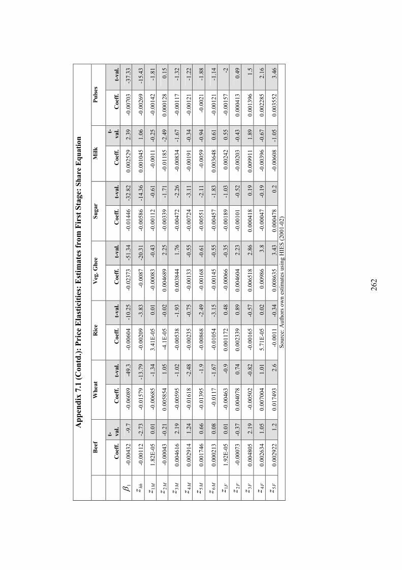
262

Appendix 7.1 (Contd.): Price Elasticities: Estimates from First Stage: Share Equation

Beef

Wheat

Rice

Veg. Ghee

Sugar

Milk

Pulses

Coeff.

t- val.

Coeff.

t-val.

Coeff.

t-val.

Coeff.

t-val.

Coeff.

t-val.

Coeff.

t-

val.

Coeff.

t-val.

1β

-0.0

043

2

-9.7

-0

.06

08

9

-49

.3

-0.0

060

4

-10

.25

-0

.02

37

3

-51

.34

-0

.01

44

6

-32

.82

0

.00

25

29

2

.39

-0

.00

70

3

-37

.33

hh

z

-0.0

011

2

-2.7

3

-0.0

157

9

-13

.79

-0

.00

20

9

-3.8

3

-0.0

087

-2

0.3

1

-0.0

058

6

-14

.36

0

.00

10

45

1

.06

-0

.00

26

9

-15

.43

Mz 1

1

.82

E-0

5

0.0

1

-0.0

068

5

-1.3

4

3.4

1E

-05

0

.01

-0

.00

08

3

-0.4

3

-0.0

011

2

-0.6

1

-0.0

011

-0

.25

-0

.00

14

2

-1.8

1

Mz 2

-0

.00

04

3

-0.2

1

0.0

058

54

1

.05

-4

.1E

-05

-0

.02

0

.00

46

89

2

.25

-0

.00

33

9

-1.7

1

-0.0

118

5

-2.4

9

0.0

001

28

0

.15

Mz 3

0

.00

46

16

2

.19

-0

.00

59

5

-1.0

2

-0.0

053

8

-1.9

3

0.0

038

44

1

.76

-0

.00

47

2

-2.2

6

-0.0

083

4

-1.6

7

-0.0

011

7

-1.3

2

Mz 4

0

.00

29

14

1

.24

-0

.01

61

8

-2.4

8

-0.0

023

5

-0.7

5

-0.0

013

3

-0.5

5

-0.0

072

4

-3.1

1

-0.0

019

1

-0.3

4

-0.0

012

1

-1.2

2

Mz 5

0

.00

17

46

0

.66

-0

.01

39

5

-1.9

-0

.00

86

8

-2.4

9

-0.0

016

8

-0.6

1

-0.0

055

1

-2.1

1

-0.0

059

-0

.94

-0

.00

21

-1

.88

Mz 6

0

.00

02

13

0

.08

-0

.01

17

-1

.67

-0

.01

05

4

-3.1

5

-0.0

014

5

-0.5

5

-0.0

045

7

-1.8

3

0.0

036

48

0

.61

-0

.00

12

1

-1.1

4

Fz 1

1

.92

E-0

5

0.0

1

-0.0

046

3

-0.9

0

.00

11

72

0

.48

-0

.00

06

6

-0.3

5

-0.0

018

9

-1.0

3

0.0

024

2

0.5

5

-0.0

015

7

-2

Fz 2

-0

.00

07

3

-0.3

7

0.0

040

78

0

.74

0

.00

23

39

0

.89

0

.00

46

04

2

.23

-0

.00

10

1

-0.5

2

-0.0

020

3

-0.4

3

0.0

004

13

0

.49

Fz 3

0

.00

48

05

2

.19

-0

.00

50

2

-0.8

2

-0.0

016

5

-0.5

7

0.0

065

18

2

.86

0

.00

04

18

0

.19

0

.00

99

11

1

.89

0

.00

13

96

1

.5

Fz 4

0

.00

26

34

1

.05

0

.00

70

04

1

.01

5

.71

E-0

5

0.0

2

0.0

098

6

3.8

-0

.00

04

7

-0.1

9

-0.0

039

6

-0.6

7

0.0

022

85

2

.16

Fz 5

0

.00

29

22

1

.2

0.0

174

93

2

.6

-0.0

011

-0

.34

0

.00

86

35

3

.43

0

.00

04

78

0

.2

-0.0

060

8

-1.0

5

0.0

035

52

3

.46

So

urc

e: A

uth

ors

ow

n e

stim

ates

usi

ng H

IES

(20

01

-02

)

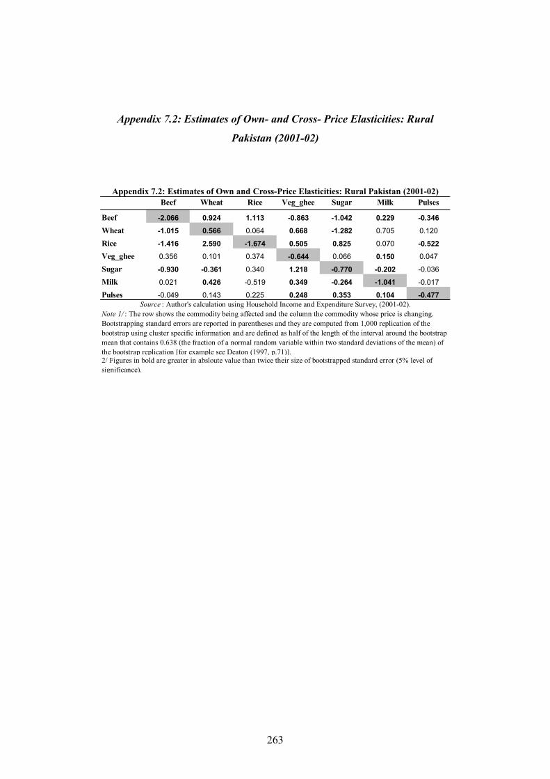
263

Appendix 7.2: Estimates of Own- and Cross- Price Elasticities: Rural

Pakistan (2001-02)

Beef Wheat Rice Veg_ghee Sugar Milk Pulses

Beef -2.066 0.924 1.113 -0.863 -1.042 0.229 -0.346

Wheat -1.015 0.566 0.064 0.668 -1.282 0.705 0.120

Rice -1.416 2.590 -1.674 0.505 0.825 0.070 -0.522

Veg_ghee 0.356 0.101 0.374 -0.644 0.066 0.150 0.047

Sugar -0.930 -0.361 0.340 1.218 -0.770 -0.202 -0.036

Milk 0.021 0.426 -0.519 0.349 -0.264 -1.041 -0.017

Pulses -0.049 0.143 0.225 0.248 0.353 0.104 -0.477

Source : Author's calculation using Household Income and Expenditure Survey, (2001-02).

Note 1/ : The row shows the commodity being affected and the column the commodity whose price is changing.

Bootstrapping standard errors are reported in parentheses and they are computed from 1,000 replication of the

bootstrap using cluster specific information and are defined as half of the length of the interval around the bootstrap

mean that contains 0.638 (the fraction of a normal random variable within two standard deviations of the mean) of

the bootstrap replication [for example see Deaton (1997, p.71)].2/ Figures in bold are greater in absloute value than twice their size of bootstrapped standard error (5% level of

significance).

Appendix 7.2: Estimates of Own and Cross-Price Elasticities: Rural Pakistan (2001-02)

264

REFERENCES

Aamjad, R. and A.R. Kemal. "Macroeconomic Policy and Their Impact on Poverty Alleviation in Pakistan." Pakistan Development Review, 1997, 36(1), pp. 39-68. Adler, J., Eugene R. Schlesinger, and Ernest C. Olson. Public Finance and

Economic Development in Guatemala. Stanford University Press, 1952. Adler, John H., and Henry C. Wallich. Public Finance in a Developing

Country: El Salvador - a Case Study. Harvard University Press, 1951. Ahmad, E., and Nicholas Stern. "Tax Reform and Shadow Prices for Pakistan." Oxford Economic Papers, 1990, 42(1), pp. 135-59. ____. "Tax Reform for Pakistan: Overview and Effective Taxes for 1975/76." Pakistan Development Review, 1986, (Spring), pp. 43-72. Ahmad, E., Coady D., and Nicholas Stern. "A Complete Set of Shadow Prices for Pakistan: Illustrations for 1975-76." Pakistan Development Review, 1988, (Spring), pp. 7-43. Ahmad, E., H.-M. Leung, and N. Stern. "Demand Response and the Reform of Indirect Taxes in Pakistan," Discussion Paper. Development Economics Research Centre, University of Warwick, 1984. Ahmad, Etisham and Nicholas Stern. "Alternative Sources of Government Revenue: Illustrations from India, 1979-80," D. M. Newbery and N. Stern, The

Theory of Taxation for Developing Countries. Cambridge: Oxford University Press, 1987. ____. "Effective Taxes and Tax Reform in India," Discussion Paper 25.

Development Economic Research Centre, University of Warwick, 1983. ____. Tax Reform and Development: An Economic Analysis of the Indian

Fiscal System. Cambridge: Cambridge University Press, 1989. ____. The Theory and Practice of Tax Reform in Developing Countries. Cambridge: Cambridge University Press, 1991.

265

Ahmad, Mushtaq. "Fiscal Adjustment: Trade-Offs of Macro-Economic Goals and Recent Policy Reforms in Pakistan." Pakistan Development Review, 1998, 37(4), pp. 1123-42. Ahmad, S.E., Ludlow, S. and Stern, N.H. "Demand Responses in Pakistan: A Modification of the Linear Expenditure System for 1976." Pakistan

Development Review, 1988, (Autumn), pp. 293-308. Ahmed, Khawaja Tanveer. "Value Added Tax: A Case Study," Custom House, Karachi, 1997. Alamgir, I'Viohiuddin. "The Domestic Prices of Imported Commodities in Pakistan: A Further Study." Pakistan Development Review, 1968, (Spring), pp. 35-73. Alderman, H. and Carlo Del Ninno. "Poverty Issues for Zero Rating VAT in South Africa." Journal of African Economics, 1999, 8(2), pp. 182-208. Alderman, H. and M. Garcia. "Poverty, Household Food Security, Nutrition in Pakistan " Research Report. Washington D.C.: International Food Policy Research Institute, 1993. Ali, Salman S. and Sayyid Tahir. "Dynamics, Poverty and Inequality in Pakistan." Pakistan Development Review, 1999, 38(4), pp. 337-58. Alleyne, D. "The Evolution of Jamaica's Tax Burden." Public Finance

Review, 2007, 35(1), pp. 150-71. Amjad, Rashid and Kamal, A.R. "Macro-Economic Policies and Their Impact on Poverty Alleviation in Pakistan." Pakistan Development Review, 1997a, 36(1), pp. 39-68. ____. "Macroeconomic Policies and Their Impact on Poverty Alleviation in Pakistan." Pakistan Development Review, 1997b, 36(1), pp. 39-68. Anand, S. and Harris, C. "Food and Standard of Living: An Analysis Based on Sri Lankan Data," J. a. A. S. Dreze, The Political Economy of Hunger (Vol.

1). Oxford: Oxford University Press, 1990, Anwar, Talat. "Prevalence of Relative Poverty in Pakistan." Pakistan

Development Review, 2005, 44(4), pp. 1111-31. Arif, G.M. "Measuring Poverty in Pakistan: A Critical Review of Recent Poverty Lines," Human Condition Report 2002. Islamabad: Centre for Research on Poverty Reduction and Income Distribution, 2003,

266

____. "Urbanization in Pakistan: Trends, Growth and Evaluation of the 1998 Census," Kemal A.R., M. Irfan, and Naushin Mahmood, An Evaluation of the

1998 Population and Housing Census. Islamabad: PIDE and UNFPA, 1998. Asher, M.G. and A. Booth. Indirect Taxation in Asean. Singapore: Singapore University Press, 1983. Asian Development Bank. "The Reliability and Credibility of Poverty Analysis in Pakistan," Background paper series. Poverty Group, Country Policy Operations Unit, Asian Development Bank, 2006. ____. "Rising to the Challenge in Asia: A Study of Financial Markets: Vol. 9 - Pakistan," 1999. Atkinson, A.B. "More on the Measurement of Inequality," 1973.

____. "On the Measurement of Inequality." Journal of Economic Theory, 1970, 2, pp. 244-63. ____. Social Justice and Public Policy. Cambridge: MIT Press, 1983. Atkinson, A.B. and J.E. Stiglitz. Lectures on Public Economics. New York: McGraw-Hill, 1980. ____. "The Structure of Indirect Taxation and Economic Efficiency." Journal

of Public Economics, 1972, 1(1), pp. 97-119. Azfar, Jawaid. "The Income Distribution in Pakistan, before and after Taxes, 1966-67," Harvard University, 1972. Bahl, Roy. ed. The Jamaican Tax Reform. Cambridge, MA: Lincoln Institute of Land Policy, 1991. Ballard, Charles, Don Fullerton, John Shoven, and John Whalley. A

General Equilibrium Model for Tax Policy Evaluation. Chicago: University of Chicago Press, 1985. Barten, Anton P. . "Family Composition, Prices, and Expenditure Patterns," G. M. Peter E. Hart, and John K. Whitaker, Economic Analysis for National

Economic Planning. London: Butterworth, 1964, Baumol, W.J. and Bradford, D.F. "Optimal Departures from Marginal Cost Pricing." American Economic Review, 1970, 60, pp. 265-83.

267

Bernard M. Hoekman, and Hanaa Kheir-El-Din ed. Trade Policy

Developments in the Middle East and North Africa

Washington D.C: World Bank Publication, 2000. Besley, Timothy. "Commodity Taxation and Imperfect Competition: A Note on the Effects of Entry." Journal of Public Economics, 1989, 40(3), pp. 359-67. Besley, Timothy and Harvey Rosen. "Sales Tax and Prices: An Empirical Analysis," Princeton University Economics Department, 1994. ____. "Sales Taxes and Prices: An Empirical Analysis." National Tax Journal, 1996, 52, pp. 157-78. Besley, Timothy., and Harvey Rosen. Sales Tax and Prices: An Empirical

Analysis. National Bureau of Economic Research, 1998. Bird, Richard. "The Allocation of Taxing Power in Papua New Guinea," Port Moresby: Institute of National Affairs, 1983. ____. "Income Distribution and Tax Policy in Colombia." Economic

Development and Cultural Change, 1970, 18(1), pp. 519-35. Bird, Richard "A New Look at Indirect Taxation in Developing Countries." World Development, 1987, 15(9), pp. 1151-61. Bird, Richard and B.D. Miller. "The Incidence of Indirect Taxes on Low-Income Households in Jamaica," Jamaican Tax Structure Examination Project

Staff Paper. Metropolitan Studies Program, Maxwell School, Syracuse University, 1986. Bird, Richard and Barbara D. Miller. "The Incidence of Indirect Taxes on Low-Income Households in Jamaica." Economic Development and Cultural

Change, 1989, 37(2), pp. 393-409. Bird, Richard. Taxing Agricultural Land in Developing Countries. Cambridge: Harvard University Press, 1974. Bird, Richard., and Luc H. De Wulf. "Taxation and Income Distribution in Latin America: A Critical Review of Empirical Studies." IMF Staff Papers, 1973, 20(3), pp. 639-82. Bird, Richard. "The Allocation of Taxing Power in Papua New Guinea," Port Moresby: Institute of National Affairs, 1983.

268

Bird, Richard "A New Look at Indirect Taxation in Developing Countries." World Development, 1987, 15(9), pp. 1151-61. Bird, Richard and B.D. Miller. "The Incidence of Indirect Taxes on Low-Income Households in Jamaica," Jamaican Tax Structure Examination Project

Staff Paper. Metropolitan Studies Program, Maxwell School, Syracuse University, 1986. Bird, Richard and Barbara D. Miller. "The Incidence of Indirect Taxes on Low-Income Households in Jamaica." Economic Development and Cultural

Change, 1989, 37(2), pp. 393-409. Bird, Richard and Eric. M. Zolt. "The Limited Role of the Personal Income Tax in Developing Countries." Journal of Asian Economics, 2005, 16(6), pp. 928-46. Bird, Richard and S. Wallace. "Taxing Alcohol in Africa: Reflections from International Experience," S. Cnossen, Excise Taxation in Africa. Pretoria: UNISA Press, 2005, Bird, Richard. Taxing Agricultural Land in Developing Countries. Cambridge: Harvard University Press, 1974. Blackorby, C. and D. Donaldson. "Measures of Relative Equality and Their Meaning in Terms of Social Welfare." Journal of Economic Theory, 1978, 18(59-80). Blundell, R.W. and Preston, I.P. "Income or Consumption in the Measurement of Inequality and Poverty?," Working Paper Series. London: The Institute of Fiscal Studies, 1994. Bovenberg, A.L. "Indirect Taxation in Developing Countries: A General Equilibrium Approach." IMF Staff Papers, 1987, 34(2), pp. 333-73. Ceedy, J. The Dynamics of Inequality and Poverty. Edward Elgar Publishing Limited, UK, 1998.

Centre for Research on Poverty Reduction and Income Distribution. "Pakistan Human Condition Report," Islamabad: Planning Commission, 2003. ____. "A Profile of Poverty in Pakistan," Islamabad: Planning Commission 2005.

269

Centre for Research on Poverty Reduction and Income Distribution

Planning Commission Islamabad. "Poverty, Risk and Vulnerability in Pakistan," 2006. Chaudhry, M.G. "The Problems of Agriculture Taxation and an Alternative Solution." Pakistan Development Review, 1973, 12(2). Chaudhuri, S. and M. Ravallion. "How Well Do Static Indicator Identify the Chronically Poor?" Journal of Public Economics, 1994, 53(3), pp. 367-94. Cheema, Iftikhar Ahmed. "Revisiting the Poverty Line (2000-2001)," Discussion Papers. Centre for Research on Poverty Reduction and Income Distribution Planning Commission Islamabad, 2005. Chen, Duanjie, John M. Matovu, and Rita Reinikka,. "A Quest for Revenue and Tax Incidence in Uganda," IMF Working Paper 01/24.

Washington D.C.: International Monetary Fund, 2001. Choudhry, Tariq Najib. Withholding Income Tax. Lahore: Maktaba Jadeed Press, 2001. Chu, Ke-young, Hamid Davoodi and Sanjeev Gupta. "Income Distribution and Tax and Government Social Spending Policies in Developing Countries," IMF Working Paper. Washington, DC: International Monetary Fund, 2000. Clarete, R., and John Whalley. "Equilibrium in the Presence of Foreign Exchange Premia," London, Ontario: Centre for the Study of International Economic Relations, University of Western Ontario, 1986. Cnossen, S. Excise Systems: A Global Study of the Selective Taxation of

Goods and Services. Baltimore: The Johns Hopkins Press, 1977. Coady, David. P. and Rebecca Lee Harris. "Evaluating Targeted Cash Transfer Programs: A General Equilibrium Framework with an Application to Mexico," Research Report. Washington D.C.: International Food Policy Research Institute, 2004. Cox, T.L. and M.K. Wohlgenant. "Prices and Quality Effects in Cross-Sectional Demand Analysis." American Journal of Agricultural Economics, 1986, 68, pp. 908-19. Cragg, M. "Do We Care? A Study of Canada's Indirect Tax System." Canadian Journal of Economics, 1991, 24(1), pp. 124-43.

270

Creedy, John. "Indirect Tax Reform and the Role of Exemptions." Fiscal

Studies, 2001, 22(457-486). ____. "Marginal Indirect Tax Reform in Australia." Economic Analysis and

Policy, 1999, 29, pp. 1-14. Dahl, Henrik and Pradeep Mitra. "Applying Tax Policy Models in Country Economic Work: Bangladesh, China and India." World Bank Economic

Review, 1991, 5(3), pp. 553-72. Dasgupta, P., A. Sen and D. Starrett. "Notes on Measurement of Inequality." Journal of Economic Theory, 1973, 6, pp. 180-87. Davies, James B., St-Hilaire, France, John Whalley. "Some Calculations of Lifetime Tax Incidence." American Economic Review, 1984, 74, pp. 633-49. De Wulf, Luc. "Fiscal Incidence Studies in Developing Countries: Survey and Critique." IMF Staff Papers, 1975, 22(2), pp. 61-131. ____. "Taxation and Income Distribution in Lebanon." Bulletin for

International Fiscal Documentation, 1974, 28, pp. 151-54. Deaton, A. "The Analysis of Consumer Demand in the United Kingdom 1900-1970." Econometrica, 1974, 42, pp. 341-67. ____. "Data and Econometric Tools for Development Analysis," J. Behrman and T.N.Srinivasan, Handbook of Development Economics, 3a. Amsterdam: Elsevier, 1995, ____. "The Measurement of Welfare," LSMS Working Paper. Washington DC: World Bank, 1985. ____. "Price Elasticities from Survey Data: Extension and Indonesian Results." Journal of Econometrics, 1990, 44, pp. 281-309. ____. "Quality, Quantity, and Spatial Variation of Price: Estimating Price Elasticities from Cross-Sectional Data," LSMS Working Papers. Washington DC: World Bank, 1987. Deaton, A., and Alessandro Tarzzi. "Prices and Poverty in India," Research Program in Development Studies, Princeton University, 2000. Deaton, A. and John Muellbauer. "An Almost Ideal Demand System." American Economic Review, 1980, 70(312-26).

271

Deaton, A. and Serena Ng. "Parametric and Non-Parametric Approaches to Tax Reform," Princeton University Research Program in Development Studies, 1996. Deaton, A., Ruiz-Castillo, J. and Thomas, D. "The Influence of Household Composition on Household Expenditure Patterns: Theory and Spanish Evidence." Journal of Political Economy, 1989, 97(1), pp. 179-200. Deaton, Angus. "Equity, Efficiency and the Structure of Indirect Taxation." Journal of Public Economics, 1977, 8, pp. 299-312. ____. A Microeconometric Approach to Development Policy. London: The John Hopkins University Press, 1997. ____. "Quality, Quantity and Spatial Price Variation of Prices." American

Economic Review, 1988, 78(3), pp. 418-30. Deaton, Angus., and Anne Case. "Analysis of Household Expenditures," Washington D.C.: World Bank, 1987. Deaton, Angus., and Grimard, F. "Demand Analysis and Tax Reform in Pakistan," LSMS Papers. Living Standard Measurement, World Bank, 1992. Deaton, Angus. and Grosh, M. "Consumption," M. Grosh and P. Glewwe, Designing Household Questionnaires for Developing Countries: Lessons from

Fifteen Years of the Living Standard Measurement Study. Washington DC: The World Bank, 2000, 91-133. Deaton, Angus. and N.H. Stern. "Optimally Uniform Commodity Taxes, Taste Differences and Lump-Sum Grants." Economics Letters, 1986, 20, pp. 263-66. Deaton, Angus., and Salman Zaidi. "Guidelines for Constructing Consumption Aggregates for Welfare Analysis," Washington D.C.: World Bank, 2002. Decoster, A. and Schokkaert, F. "Equity and Efficiency of a Reform of Belgian Indirect Taxes." Journal of Public Economics, 1989, 41(3), pp. 277-96. Delipalla, S. and M. Keen "The Comparison between Ad Valorem and Specific Taxation under Imperfect Competition." Journal of Public

Economics, 1992, 49, pp. 351-67.

272

Deverajan, Shantayanan and Shaikh I. Hussain. "The Combined Incidence of Taxes and Public Expenditure in the Philippines." World Development, 1998, 26(2), pp. 963-77.

Deverajan, Shantayanan, Don Fullerton and Richard A. Musgrave. "Estimating the Distribution of Tax Burdens: A Comparison of Different Approaches." Journal of Public Economics, 1980, 13, pp. 155-82. Diamond, P.A. and Mirrlees, J.A. "Optimal Taxation and Public Production: Part I - Production Efficiency." American Economic Review, 1971a, 61(1), pp. 8-27. Diamond, P.A. and Mirrlees J.A. "Optimal Taxation and Public Production: Part II - Tax Rules." American Economic Review, 1971b, 61(3), pp. 261-78. Disney, R., A. Kedir and A. Mckay. "Price Deflators and Food Poverty in Urban Ethiopia," School of Economics, University of Nottingham, 2004. Driffill, E.J. and Harvey S. Rosen. "Taxation and Excess Burden: A Life Cycle Perspective." International Economic Review, 1983, 24(3), pp. 671-83. Duanjie, Chen., John M. Matovu, and Ritva Reinikka. "A Quest for Revenue and Tax Incidence in Uganda," International Monetary Fund, 2001. Ebrahimi, A. and Heady, C. "Tax Design and Household Composition." The

Economic Journal Conference Papers, 1988, 98(390), pp. 83-96. Ebrill, Liam., Michael Keen, Jean-Paul Bodin, Victoria Summers ed. The

Modern VAT. Washington DC: International Monetary Fund, 2001. Edmiston, Kelly D. and Richard M. Bird. "Taxing Consumption in Jamaica," Community Affairs Research Working Paper. Kansas: Federal Reserve Bank of Kansas City, 2006. El-Edel, M. Reda A. "Impact of Taxation on Income Distribution: An Exploratory Attempt to Estimate Tax Incidence in Egypt," Princeton-Egypt

Income Distribution Project Conference Paper. 1979.

Engel, Eduardo M.R.A, Alexander Galetovic and Claudio E. Raddatz. "Taxation and Income Distribution in Chile: Some Unpleasant Redistributive Arithmetic," NBER Working Paper. Cambridge, Mass.: National Bureau of Economic Research, 1998. Etisham, Ahmad., and Nicholas Stern. "The Theory of Tax Reform and Indian Indirect Taxes." Journal of Public Economics, 1984, 25, pp. 259-98.

273

Fedeli, S. . "The Effects of Interaction between the Direct and Indirect Tax Evasion: The Cases of Value Added Tax and Retail Sales Tax." Public

Finance, 1998, 53, pp. 385-418. Federal Board of Revenue, Government of Pakistan. "CBR Yearbook," various years. Federal Bureau of Statistics., Government of Pakistan. "Census of Manufacturing Industries," Islamabad, Pakistan, 1990-91a. ____. "Census of Manufacturing Industries," Islamabad, Pakistan, 2000-2001.

____. "Household Integrated Economic Survey," Islamabad, Pakistan, 1990-91b. ____. "Household Integrated Economic Survey," Federal Bureau of Statistics, Islamabad, Pakistan, 2001-02. ____. "Pakistan Integrated Household Survey: Poverty in the 1990s," Islamabad: Statistics Division, 2001. ____. "Statistical Yearbook of Pakistan." various years. Feldstein, M.S. "Distributional Equity and the Optimal Structure of Public Prices." American Economic Review, 1972, 62, pp. 32-36. ____. "On the Theory of Tax Reform." Journal of Public Economics, 1976, 6, pp. 77-104. Foster, James E., and Shorrocks, A.F. "Poverty Ordering." Econometrica, 1988, 56, pp. 173-77. Foxley, A., E. Aninat, and J. Arellano. Redistributive Effects of Government

Programms. New York: Pergamon Press, 1987. Foxley, Alejandro. Redistributive Effects of Government Programs: The

Chilean Case. Oxford: Pergamon Press, 1979. Friedman, M. A Theory of the Consumption Function. New York: Princeton University Press, 1957. Frisch, Ragnar and F.V. Waugh. "Partial Time Regressions as Compared with Individual Trends." Econometrica, 1933, 1(387-401).

274

Fuente, Angel D.L. Mathematical Method and Models for Economist. Cambridge University Pres, 2000. Fullerton, D., A.T. King, J.B. Shoven and J Whalley. "Corporate and Personal Tax Integration in the U.S.: Some Preliminary Findings from a General Equilibrium Analysis:." 1979. Fullerton, D., and D. Rogers. "Lifetime Versus Annual Perspectives of Tax Incidence." National Tax Journal, 1991, 47, pp. 731-46. Fullerton, D. and Diane Lim Rogers. "Who Bears the Lifetime Tax Burden?," Washington D.C.: Brookings Institution, 1993. Fullerton, D. and Gilbert E. Metcalf. "The Distribution of Tax Burdens: An Introduction " Working Papers. National Bureau of Economic Research, 2002. Fullerton, D., J.B. Shoven and J Whalley. "A General Equilibrium Analysis of U.S Taxation Policy, 1978 Compendium of Tax Research," Washington D.C.: U.S. Treasury Department, Office of Tax Analysis, U.S. Government Printing Office., 1978. Gazdar, Harris. "Poverty in Pakistan: A Review," A.R. Kemal, M.Irfan and N. Mahmood, Population in Pakistan: An Analysis of 1998 Population and

Housing Census. Islamabad: PIDE and UNFPA, 2000, Gemmell, N. and Oliver Morrissey. "Tax Structure and the Incidence on the Poor in Developing Countries," CREDIT Research Paper. Centre for Research in Economic Development and International Trade, University of Nottingham, 2003. Gemmell, Norman "Taxation and Development," N. Gemmell, Surveys in

Development Economics. Oxford: Basil Blackwell, 1987, Gemmell, Norman and Oliver Morrissey. "Distribution and Poverty Impact of Tax Structure Reform in Developing Countries: How Little We Know." Development Policy Review, 2005, 23(2), pp. 131-44. Ghandi, Ved P. "Tax Burden on Indian Agriculture," Cambridge, Mass.: Harvard Law School International Tax Program, Harvard University Law School, 1966. Ghaus, Aisha. "Implication of New National Finance Commission," Karachi: Social Development and Development Centre, 1995.

275

Gibson, John. "Indirect Tax Reform and the Poor in Papua New Guinea." Pacific Economic Bulletin (Australia), 1998, 13(2), pp. 29-39. Gillespie, W. Irwin. The Redistribution of Income in Canada. Ottawa: Cage Publishing Ltd., 1980. Goodman, A. and Webb, S. "The Distribution of UK Household Expenditure." Fiscal Studies, 1995, 16(3), pp. 55-80.

Government of Pakistan., Food, Agriculture and Livestock Division, . "Agricultural Statistics of Pakistan," various years. Government of Pakistan., Food division. "Fruit, Vegetables and Condiments Statistics of Pakistan," various years. Haddinott, J. and Haddad, L. "Does Female Income Share Influence Household Expenditure? Evidence from Cote D'ivoire." Oxford Bulletin of

Economics and Statistics, 1995, 57(1), pp. 77-96. Hafiz A. Pasha and M.A.Iqbal. "Taxation Reforms in Pakistan." Journal of

Applied Economics, 1994, 10(1&2), pp. 47-75. Hamid, J. "Suggested Approach to Agriculture Taxation Policy." Pakistan

Development Review, 1970, 10(4). Harberger, A.C. "The Incidence of Corporate Income Tax." Journal of

Political Economy, 1962, 70, pp. 215-40. Haveman, R. and K. Hollebeck ed. Microeconomic Simulations. Madison, Wisconsin: Institute for Research on Poverty, 1979.

Havinga, I.C., F. W. Haanappel, A.S. Louter and W.A. van den Andel. "Poverty in Pakistan 1984-85." Pakistan Development Review, 1989, 36(1), pp. 851-69. Heady, Christopher. "Optimal Taxation as a Guide to Tax Policy: A Survey." Fiscal Studies, 1993, 14(1), pp. 15-41. Heller, Peter S. "Testing the Impact of Value-Added and Global Income Tax Reforms on Korean Tax Incidence in 1976: An Input-Output and Sensitivity Analysis." IMF Staff Papers, 1981, 28(June), pp. 375-410. Hossain, S.M. "The Equity Impact of Value-Added Tax in Bangladesh." IMF

Staff Papers, 1995, 42(2), pp. 411-30.

276

Houthakker, H.S. "Compensated Changes in Quantities and Qualities Consumed." Review of Economic Studies, 1952, 19, pp. 155-64. Howes, Stephan and Salman Zaidi. "Notes on Some Household Surveys from Pakistan in the Eighties and Nineties," London: STICERD, London School of Economics, 1994. Hussain, Ishrat. Economic Management in Pakistan 1999-2002. New Delhi: Oxford University Press, 2004. Independent Evaluation Office. "Evaluation of Prolonged Use of Fund Resources," IMF Surveillance Report. International Monetary Fund, 2002. International Monetary Fund. "Pakistan: Selected Issues and Statistical Appendix," IMF Staff Country Reports. 2001. ____. "Pakistan: Selected Issues and Statistical Appendix," IMF Country

Report. Washington D.C., 2004. Irfan, Mohammad. "Shifting and Incidence of Indirect Taxes on Tobacco and Petroleum Products in Pakistan." Pakistan Development Review, 1974, 13(1), pp. 66-87. Irvine, I.J. and Sims, W.A. "The Welfare Effects of Alcohol Taxation." Journal of Public Economics, 1993, 52, pp. 83-100. Jafri, S.M. Younis. "Assessing Poverty in Pakistan," In a Profile of Poverty

in Pakistan. Islamabad: Mahbub ul Haq Centre for Human Development, 1999, Jeetun, A. "Incidence of Taxes in Pakistan," Applied Economic Research

Report. University of Karachi, 1978a. ____. "Tax Shifting in Pakistan: A Case Study of Excise Duties, Sales Tax and Import Duties," Applied Economic Research Centre Discussion Report.

University of Karachi, 1978b. Jhele, A. Geoffrey. "Inequality in Pakistan: A Sectoral Welfare Approach." Pakistan Journal of Applied Economics, 1990, 2, pp. 165-93. Jimenez, E. "The Public Subsidization of Education and Health in Developing Countries: A Review of Equity and Efficiency." World Bank Research

Observer, 1986, 1, pp. 111-30.

277

Johnson, Martin., Andrew Mckay, and Jeffery Round. "Household Income and Expenditure Sub-Aggregate from Ghana Living Standard Survey," Warwick: University of Warwick: Development Research Centre, 1989.

Jose Manuel Roig Cotanda, Amparo Sanchis Llopisy, Juan Alberto

Sanchis Llopis. "The Effects of the Spanish 1999 Income Tax Reform on Progressivity," 2002. Kaiser, H. and Spahn, P.B. "On Efficiency and Redistributive Justice of Consumption Taxes: A Study on VAT in Germany." Journal of Economics, 1989, 49(2), pp. 199-218. Kaplanoglou, Georgia., and David M. Newbery. "The Distributional Impact of the Proposed Tax Reform on Greek Households," Athens: Centre of Planning and Economic Research, 2003b. ____. "Indirect Taxation in Greece: Evaluation and Possible Reform." International Tax and Public Finance, 2003a, 10, pp. 511-33. ____. "Redistributive Impact of Indirect Tax Reforms: Greece, 1988 - 2002." Fiscal Studies, 2004, 25, pp. 225-47. Katz, Micheal L. and Harvey S. Rosen. "Tax Analysis in an Oligopoly Model," NBER Working Paper. National Bureau of Economic Research, Inc., 1985. Kazi, S. "Inter-Sectoral Tax Burdens in Pakistan: A Critical Review of Existing Evidence and Some New Evidence." Pakistan Development Review, 1984, 23(4). Kedir, Abbi M. "Estimation of Own- and Cross- Price Elasticities Using Unit Value: Econometric Issues and Evidence from Urban Ethiopia." Journal of

African Economics, 2005, 14(1), pp. 1-20. Kemal, A.R. "Income Distribution Studies in Pakistan and an Agenda for Future Direction of Research," Pakistan Human Condition Report. Islamabad: UNDP/UNOPS/CRPRID, 2003, Kemal, A.R. . "Structural Adjustment, Macroeconomics Policies and Poverty Trends in Pakistan," Pakistan Institute of Development Economics, 2001. Kemal A.R. and Rizwana Siddiqui. "Remittances, Trade Liberalization, and Poverty in Pakistan: The Role of Excluded Variables in Poverty Change Analysis." Pakistan Development Review, 2002, 45(3), pp. 383-415.

278

Kemal A.R., Zafar Mahmood., and Ather Maqsood Ahmed,. "Structure of Protection, Efficiency, and Profitability (Vol. 1)," Pakistan Institute of Development Economics, 1994. Khalilzadeh-Shirazi J. and Anwar Shah. Tax Policy in Developing

Countries. Washington D.C.: World Bank, 1991. Khan, Ashfaque. "What Is Wrong with Pakistan's Public Finance?," Research

Report. Islamabad: Pakistan Institute of Development Economics, 1997. Kotlikoff, L.J. . "Generational Policy," Auerbach A.J. and M. Feldstein, Handbook of Public Economics, Vol. 3. Amsterdam: Elsevier, 2001, Kotlikoff, L.J. and L.H.Summers. "Tax Incidence," Auerbach. A.J. and M. Feldstein, Handbook of Public Economics, Vol. 2. Amsterdam: Elsevier Science, 1987, 1043-92. Lambert, P.J. The Distribution and Redistribution of Income: A

Mathematical Analysis. Manchester: Manchester University Press, 1993. Levhari, David and E. Sheshinski. "Lifetime Excess Burden of a Tax." Journal of Political Economy, 1972, 80(1), pp. 139-47. Liberati, Paolo. "The Distributional Effects of Indirect Tax Changes in Italy." International Tax and Public Finance, 2001, 8, pp. 27-51. Lockwood, B. "Tax Incidence, Market Power and Bargaining Structure," London: Birbeck College, 1988. Lovejoy, Robert M. "The Burden of Jamaican Taxation, 1959." Social and

Economic Studies, 1963, 12, pp. 442-58. Lyon, Andrew B. and Robert M. Schwab. "Consumption Taxes in a Life-Cycle Framework: Are Sin Taxes Regressive?" The Review of Economics and

Statistics, 1995, 77(3), pp. 389-406. Madden, D. "Conditional Demands and Marginal Tax Reform." Oxford

Bulletin of Economics and Statistics, 1997, 59(2), pp. 237-55. ____. "Indirect Tax Reform in Ireland." Economic and Social Review, 1989, 21, pp. 27-47. ____. "Labour Supply, Commodity Demand and Marginal Tax Reform." Economic Journal, 1995, 105, pp. 485-97.

279

____. "Marginal Tax Reform and the Specifications of Consumer Demand Systems." Oxford Economic Papers, 1996, 48(4), pp. 556-67. Malik, M.H. "Some New Evidence on the Incidence of Poverty in Pakistan." Pakistan Development Review, 1988, 27(4). Malik, M.H., and Najam-us-Saqib. "Tax Incidence by Income Classes in Pakistan." Pakistan Development Review, 1989, 28(1), pp. 13-26. Malik, Sohail J. "Poverty in Pakistan: 1984-85 to 1987-88," Washington DC: International Food Policy Research Institute, 1991. Martinez-Vazquez, Jorge. "Budget Policy and Income Distribution," Working Paper. International Studies Program, Andrew Young, School of Policy Studies, Georgia State University, 2007. ____. "The Impact of Budgets on the Poor: Tax and Benefit Incidence," International Studies Program, Andrew Young School of Policy Studies, Georgia State University., 2001. McGregor, P.P.L. and Borooah, V.K. "Is Low Spending or Low Income a Better Indicator of Whether or Not a Household Is Poor: Some Results from the 1985 Family Expenditure Survey." Journal of Social Policy, 1992, 21(1), pp. 53-69. McLure, Charles E., Jr. "General Equilibrium Incidence Analysis: The Harberger Model after Ten Years." Journal of Public Economics, 1975, 4, pp. 125-61. ____. "The Incidence of Jamaican Taxes, 1971-72," Working Paper. Mona, Jamaica: Institute of Social and Economic Research, University of the West Indies, 1977a. ____. "The Incidence of Taxation in Colombia," M. Gillis, Fiscal Reform for

Colombia: Final Report and Staff Papers of the Colombian Commission on

Tax Reform. Cambridge, Mass.: 1971, 239-66. ____. "Taxation and the Urban Poor in Developing Countries." World

Development, 1977, 5(3), pp. 169-88. Metcalf, Gilbert E. "The Lifetime Incidence of State and Local Taxes: Measuring Changes During the 1980s," NBER Working Paper Series.

Cambridge: National Bureau of Economic Research, 1993.

280

Mieszkowski, Petr M. "Tax Incidence Theory: The Effect of Taxes on the Distribution of Income." Journal of Economic Literature, 1969, 7, pp. 1103-24. Ministry of Finance. "Economic Survey of Pakistan," Islamabad, Pakistan, various years. Mirrlees, J.A. "Optimal Tax Theory: A Synthesis." Journal of Public

Economics, 1976, 6, pp. 327-58. Modigliani, F. and Brumberg R. "Utility Analysis and the Consumption Function: An Interpretation of Cross-Section Data," K. Kurihara, Post-

Keynsian Economics. New Brunswick: Rutgers University Press, 1954, Morrissey, Norman Gemmell and Oliver. "Tax Structure and the Incidence on the Poor in Developing Countries," CREDIT Research Paper. Centre for Research in Economic Development and International Trade, University of Nottingham, 2003. Munoz, Sonia., Sang-Wook Cho, Stanley. "Social Impact of a Tax Reform: The Case of Ethiopia," IMF Working Paper 03/232. Washington D.C.: International Monetary Fund, 2003. Murty, M.N. and Ray, R. "Sensitivity of Optimal Commodity Taxes to Relaxing Leisure/Goods Separability and to the Wage Rate." Economics

Letters, 1987, 24, pp. 273-7. Musgrave, Richard. "Estimating the Distribution of the Tax Burden," Income

and Wealth , Series 10. Income redistribution and statistical foundations of economic policy 1964, 186-219. Musgrave, Richard and Thin, T. "Income-Tax Progression 1929-1948." Journal of Political Economy, 1948, 56, pp. 498-514. Musgrave, Richard. The Theory of Public Finance. New York: McGraw Hill, 1959. Musgrave, Richard., Karl E. Case and Herman Leonard. "The Distribution of Fiscal Burdens and Benefits." Public Finance Quarterly, 1974, 2, pp. 259-311. Myles, G.D. Public Economics. Cambridge University Press, 1995. Naqvi, Bilquees. "Forward Shifting of Indirect Taxes: A Further Study." Pakistan Development Review, 1975, 14(2), pp. 174-84.

281

National Taxation Reform Commission. "Final Report," Islamabad, Pakistan, 1986. Nellor, David. "The Effect of Value Added Tax on the Tax Ratio," IMF

Working Paper 87/47. Washington D.C.: International Monetary Fund, 1987. Newbery, David M. "The Distributional Impact of Price Changes in Hungry and United Kingdom." The Economic Journal, 1995, (105), pp. 847-63. Newbery, David M., and Stern, N.H. ed. The Theory of Taxation for

Developing Countries. New York: Oxford University Press, 1987. Nicholson, J.L. Redistribution of Income in the United Kingdom in 1959,

1957 and 1953. Cambridge: Bowes and Bowes, 1964. Nicholson, J.L. and Britton, A.J.C. "The Redistribution of Income," A. B. Atkinson, The Personal Distribution of Income. London: Allen and Unwin, 1976, Nicita, Alessandro. "Efficiency and Equity of a Marginal Tax Reform: Income, Quality and Price Elasticities for Mexico," World Bank Policy

Research Working Papers. Washington D.C.: World Bank, 2004. OECD. "The Impact of Consumption Taxes at Different Income Levels," OECD Studies in Taxation. Paris, 1981. ____. "Tax Burdens: Alternatives Measures," OECD Tax Policy Studies.

Paris: Organization of Economic Co-operation and Development, 2000. Pakistan Institute of Development Economics. "Impact of Smuggling," 1993. Pal, Mati L. "The Determinants of the Domestic Prices of Imports." Pakistan

Development Review, 1964, 4(4), pp. 597-622. Pasha, H.A. "Political Economy of Tax Reforms: The Pakistan Experience." Pakistan Journal of Applied Economics, 1995, 11(1&2), pp. 129-54. Pasha, H.A. and M.A. Iqbal. "Taxation Reforms in Pakistan." Pakistan

Journal of Applied Economics, 1994, 10(1&2), pp. 47-75. Pasha, H.A., G.A., G.R. and Khan Rizwanullah. "Fiscal Policy in Pakistan," Research Report. Social Development and Policy Centre, 1992.

282

Paxson, Christina H. "Consumption and Income Seasonality in Thailand." Journal of Political Economy, 1993, 101. ____. "Using Weather Variability to Estimate the Response of Savings to Transitory Income in Thailand." American Economic Review, 1992, 82. Pechman, J. "Who Paid the Taxes 1966-85?," Washington D.C.: Brookings Institution, 1985. Pechman, J.A. and Benjamin Okner. "Who Bears the Tax Burden?," Washington D.C.: Brooking Institute, 1974. Pitt, Mark M. "Food Preferences and Nutrition in Rural Bangladesh." The

Review of Economics and Statistics, 1983, 65(1), pp. 105-14. Poterba, James M. "Retail Price Reactions to Changes in State and Local Taxes." National Tax Journal, 1996, 49(2), pp. 165-76. Prais, S.J. and houthakker, H.S. The Analysis of Family Budgets. Cambridge: Cambridge University Press, 1955. ____. The Analysis of Family Budgets. Cambridge: Cambridge University Press, 1971. Prasada, P., R de Silva and J. Weerahewa. "Incidence of Commodity Taxation on Income Distribution in Sri Lanka," 4th Poverty Economic Policy

Research Network General Meeting. Colombo, Sri Lanka, 2005. Prest, A.R. "The Statistical Calculation of Tax Burdens." Economica, 1955, 22, pp. 234-45. Provopoulos, G.A. "The Distribution of Fiscal Burdens and Benefits by Income Groups in Greece." Greece Economic Review, 1979, 1, pp. 77-99. Qazi, Masood and Mohammad Akbar. "Elasticity and Buoyancy of Federal Taxes," Working Papers. Karachi: Applied Economic Research Centre, 1991. Radhakrishna, R. and Murty, K.N. "Agricultural Prices, Income Distribution and Demand Patterns in a Low Income Country," Symposium on

economic theory and planning. Indian Statistical Institute, Bangalore, 1981. Radhu, Ghulam M. "The Relation of Indirect Tax Changes to Price Changes in Pakistan." Pakistan Development Review, 1965, 5(1), pp. 54-63.

283

Rajemison, H. and Younger, S.D. "Indirect Tax Incidence in Madagascar: Estimations Using Input-Output Table," Ithaca, NY: Cornell University Food and Nutrition Program, 2001. Ramsey, F.P. "A Contribution to the Theory of Taxation." The Economic

Journal, 1927, 37(1), pp. 47-61. Ray, R. "Sensitivity of 'Optimal' Tax Rates to Alternative Demand Functional Forms: An Econometric Case Study of India." Journal of Public Economics, 1986, 31(2), pp. 253-68. Refaqat, Saadia. "Social Incidence of the General Sales Tax in Pakistan," IMF Working Paper 03/216. Washington D.C.: International Monetary Fund, 2003. Resource Mobilization and Tax Reforms Commission. Final Report. Government of Pakistan, 1994. Sahn, David E. ed. Economic Reform and the Poor in Africa. Oxford: Clarendon Press, 1996. Sahn, David E. and Stephen Younger. "Estimating the Incidence of Indirect Taxes in Developing Countries," Pereira da Silva, L. A. and Bourguignon F., Evaluating the Poverty and Distributional Impact of Economic Policies: A

Compendium of Existing Techniques. Washington D.C.: Oxford University Press, 2003, ____. "Poverty and Fiscal Policy: Microeconomic Evidence," Cornell University, 1998. Sahn, David E. and Younger, S.D. "Dominance Testing of Social Expenditures and Taxes in Africa," IMF Working Papers. Washington, DC: International Monetary Fund, 1999. Sahota, Gian S. "The Distribution of Tax Burden in Brazil," Sao Paulo, 1968. Samuel, H. "The Taxation of the Various Classes of the Poor." Journal of the

Royal Statistical Society, 1919, 82(2), pp. 143-82. Sandamo, A. "Optimal Taxation - an Introduction to the Literature " Journal

of Public Economics, 1976, 6, pp. 37-54. Saposnik, Rubin. "Rank-Dominance in Income Distributions." Public

Choice, 1981, 36, pp. 147-51.

284

Schwarz, Gideon. "Estimating the Dimensions of a Model." Annals of

Statistics, 1978, 6, pp. 461-64. Sen, A. On Economic Inequality. Oxford: Clarendon Press, 1973. Shah, Anwar and John Whalley. "Tax Incidence Analysis of Developing Countries: An Alternative View." World Bank Economic Review, 1991, 5(3), pp. 535-52. Shirazi, Nasim S., M. Ilyas and Mehboob Ahmad. "Redistributive Effects of Fiscal Policy across the Income Groups in the Urban-Rural Areas of Pakistan." Pakistan Development Review, 2001, 40(4), pp. 519-33. Shorrocks, Anthony F. "Ranking Income Distributions." Economica, 1983, 50, pp. 3-17. Shoup, Carl S. and others. The Fiscal System of Venezuela: A Report. Baltimore: Johns Hopkins Press, 1959. Shoven, J.B. and Whalley, J. "Applied General-Equilibrium Models of Taxation and International Trade: An Introduction and Survey." Journal of

Economic Literature, 1984, 22(3), pp. 1007-51. Sidhu, N. "The Effects of Change in Sales Tax on Retail Prices," Proceedings

of the Sixty-Fourth Annual Conference on Taxation. 1971, 720-33. Sjoquist, David L. and D. Green. "Distribution of Tax Burdens," Jamaica

Tax Review Project. Atlanta: Policy Research Centre, College of Business Administration, Georgia State University, 1992. Social Policy Development Centre. "Social Development in Pakistan," Karachi, 2004. Sonia Munoz and Stanley Sang-Wook Cho. "Social Impact of a Tax Reform: The Case of Ethiopia," International Monetary Fund, 2003. State Bank of Pakistan. "Annual Report 2004-2005," Annual Reports.

Karachi, 2005. Stern, N. "Aspects of the General Theory of Tax Reform," D. M. N. a. N.Stern, The Theory of Taxation for Developing Countries. New York: Oxford University Press, 1987, Stern, Nicholas H. "The Effects of Taxation, Price Control and Government Contracts in Oligopoly." Journal of Public Economics, 1987a, 32, pp. 133-58.

285

Stiglitz, Emran M. Shahe and J. "On Selective Indirect Tax Reform in Developing Countries." Journal of Public Economics, 2005, 89(4), pp. 599-623. Straus, J. "Determinant of Food Consumption in Rural Sierra Leone." Journal of Development Economics, 1982, 11, pp. 327-53. Task Force on Tax Administration. "Reform of Tax Administration in Pakistan," Islamabad: Central Board of Revenue, 2001. Theil, H. "Qualities, Prices and Budget Enquiries." Review of Economic

Studies, 1952, 19, pp. 129-47. Timmer, Peter C. . "Is There 'Curvature' in the Slutsky Matrix?" Review of

Economic Statistics, 1981, 63(August), pp. 395-402. Timmer, Peter C. and Harold Alderman. "Estimating Consumption Parameters for Food Policy Analysis." American Journal of Agricultural

Economics, 1979, 61(5), pp. 982-87. Verbist, G. "Taxes and Redistribution an International Comparison Using Euromod, the European Microsimulation Model," International Conference on

Policy Modelling of ECOMODNET. Paris, France, 2004. Wasylenko, Micheal. "The Distribution of Tax Burden in Jamaica: Pre-1985 Reform," Jamaica Tax Structure Examination Project Staff Paper. Syracuse, N.Y.: Syracuse University, Metropolitan Studies Program, Maxwell School, 1986. Whalley, John. "Regression or Progression: The Taxing Question of Incidence Analysis." Canadian Journal of Economics, 1984, 17(4), pp. 654-82. World Bank. "Pakistan Poverty Assessment," Country Operations Divisions, Country Department 1, South Asia Region, World Bank, 1995. ____. "Pakistan Poverty Assessment - Poverty in Pakistan: Vulnerabilities, Social Gaps and Rural Dynamics," Poverty Reduction and Economic Management Sector Unit, South Asia Region, World Bank, 2002. ____. "Promoting Rural Growth and Poverty Reduction," Washington DC, 2007.

286

____. "Trade Policies in South Asia (Volume Iii): An Overview," Poverty Reduction and Economic Management Sector Unit, South Asia Region, World Bank, 2004. World Trade Organization. "Pakistan," Trade Policy Reviews. 1995.

____. "Pakistan," Trade Policy Reviews. 2001. Yitzhaki, Shlomo, and Slemrod, J. "Welfare Dominance: An Application to Commodity Taxation." American Economic Review, 1991, 81, pp. 480-96. Younger, Stephen D. "Estimating Tax Incidence in Ghana: An Exercise Using Household Data," D.Sahn, Economic Reform and the Poor in Africa.

Oxford: Clarendon Press, 1996, ____. "Estimating Tax Incidence in Ghana: An Exercise Using Household Data," Research Paper. Cornell Food and Nutrition Policy Program, Cornell University, 1993, 1-45.

Younger, Stephen D., David E. Sahn, Steven Haggblade, and Paul A.

Dorosh. "Tax Incidence in Madagascar: An Analysis Using Household Data." World Bank Economic Review, 1999, 13, pp. 303-31. Yukon, Huang. "Distribution of the Tax Burden in Tanzania." Economic

Journal, 1976, 86(March), pp. 73-86. Zaidi, M. Ashghar. "Relative Poverty in Pakistan: An Estimation from the Household Income and Expenditure Survey." Pakistan Development Review, 1992, 31(4), pp. 955-74. Zolt, Richard M. Bird and Eric M. "Redistribution Via Taxation: The Limited Role of the Personal Income Tax in Developing Countries," International Tax Program, Joseph L. Rotman School of Management, University of Toronto, Working Papers. 2005.

Documents

Social Incidence of Indirect Taxation in Pakistan (1990 - CORE