Shaping Interference Towards Optimality of Modern

Wireless Communication Transceivers

Guido Ferrante

To cite this version:

Guido Ferrante. Shaping Interference Towards Optimality of Modern Wireless CommunicationTransceivers. Other. Supelec, 2015. English. <NNT : 2015SUPL0008>. <tel-01349297>

HAL Id: tel-01349297

https://tel.archives-ouvertes.fr/tel-01349297

Submitted on 27 Jul 2016

HAL is a multi-disciplinary open accessarchive for the deposit and dissemination of sci-entific research documents, whether they are pub-lished or not. The documents may come fromteaching and research institutions in France orabroad, or from public or private research centers.

L’archive ouverte pluridisciplinaire HAL, estdestinee au depot et a la diffusion de documentsscientifiques de niveau recherche, publies ou non,emanant des etablissements d’enseignement et derecherche francais ou etrangers, des laboratoirespublics ou prives.

N d’ordre : 2015-08-TH

CentraleSupélec

ECOLE DOCTORALE STITS“Sciences et Technologies de l’Information, des

Télécommunications et des Systémes”

THÈSE DE DOCTORAT

DOMAINE : Sciences et Technologies de l’Information et de laCommunication (STIC)

Spécialité : Télécommunications

Soutenue le 10 avril 2015

par :

Guido Carlo FERRANTE

Façonnement de l’Interférence en vue d’une Optimisation Globale d’un SystèmeModerne de Communication

(Shaping Interference Towards Optimality of Modern WirelessCommunication Transceivers)

Directrice de thèse : Maria-Gabriella DI BENEDETTO Professeur, SapienzaCodirecteur de thèse : Jocelyn FIORINA Professeur, CentraleSupélec

Composition du jury :

Président du jury : Pierre DUHAMEL Directeur de recherche,CNRS/CentraleSupélec

Rapporteurs : Laurent CLAVIER Professeur,Université de Lille

Michel TERRÉ Professeur, CNAMExaminateur : Andrea GIORGETTI Professeur agrégé,

Université de Bologne

Sagomatura dell’InterferenzaVerso un’Ottimizzazione dei Moderni

Sistemi di RicetrasmissioneShaping Interference Towards Optimality

in Modern Wireless Communication Transceivers

Guido Carlo Ferrante

Dottorato di Ricercain Ingegneria dell’Informazione e della Comunicazione

Doctor of Philosophyin Information and Communication Engineering

Sapienza Università di RomaSapienza University of Rome

2015XXVII Ciclo27 th Course

AutoreAuthor . . . . . . . . . . . . . . . . . . . . . . . . . . . . . . . . . . . . . . . . . . . . . . . . . . . . . . . . . . . . . . . . . . .

Dipartimento di Ingegneria dell’Informazione, Elettronica eTelecomunicazioni

Department of Information Engineering, Electronics and TelecommunicationsVistoCertified by . . . . . . . . . . . . . . . . . . . . . . . . . . . . . . . . . . . . . . . . . . . . . . . . . . . . . . . . . . . . . . .

Prof. Maria-Gabriella Di BenedettoTutore di Dottorato (Thesis Supervisor)

VistoCertified by . . . . . . . . . . . . . . . . . . . . . . . . . . . . . . . . . . . . . . . . . . . . . . . . . . . . . . . . . . . . . . .

Prof. Jocelyn FiorinaCo-tutore di Dottorato (Thesis Co-supervisor)

.

.

Shaping Interference TowardsOptimality of Modern Wireless

Communication Transceivers

by

Guido Carlo Ferrante

A Thesis Submitted to theDepartment of Information Engineering, Electronics and

Telecommunicationsat

Sapienza University of Romeand to the

Department of Telecommunicationsat

CentraleSupélecin Partial Fulfillment

of the Requirements for the Degree ofDoctor of Philosophy

in Information and Communication Engineering

April 2015

Supervisors:Prof. Maria-Gabriella Di Benedetto

andProf. Jocelyn Fiorina

This thesis was typeset using the LATEX typesettingsystem originally developed by Leslie Lamport,based on TEX created by Donald Knuth.

The body text is set in the 10pt size fromDonald Knuth’s Concrete Roman font.Other fonts include Sans and Typewriter fromDonald Knuth’s Computer Modern family.

Most figures were typeset in TikZ.

.

Acknowledgements

I would like to thank everyone who supported me during the years of my PhD.Support is a somewhat vague word, and this implies that I feel indebted to too manypeople to remember. My gratitude is doubled for those whom I don’t remember atthe time of writing.

I am of course indebted to both my advisors, Prof. Di Benedetto and Prof.Fiorina. I spent many hours with them, and I realize how much their time is worth.They encouraged me to pursue the double degree, and I will always be grateful fortheir help. I hope I have been and continue to be at the level of their expectations.

I want to thank Luca De Nardis: he is a dear friend and in many ways a modelfor me. Also, not only did I unduly share his office space for a year, but he wasalways funny and positive. And thoughtful, when needed.

I want to thank my lab mates, in particular Stefano and Giuseppe: we had longdiscussions about research, career, and life. And Luca Lipa, who has been a closefriend of mine since we met, many years ago, in the ACTS lab.

I would like to thank my dear friend Valeria, who was always there for me whenI needed her, and never stepped back from saying the truth, which is the way shecared for me; and my dear friend Elira, who is always close despite any distance. Iwant to thank Nick, who was always keen on coffee breaks, sharing thoughts, andhelping me friendly.

I lived one year with my long friend Matt, and I thank him for putting up withme.

Words cannot express the gratitude to my brother: he was a guidance, a friend,a mentor. I know that I can rely on him. I know that I can discuss any matter, andI can grasp some new perspective every time.

Finally, thanks Rome, because you are the only place where I felt at home:Rome sweet Rome.

This thesis is dedicated to the old generations, my grandparents and parents,who valued education above all else, and to the new one, the little Isabel, who isstarting her most adventurous trip in this world: the one in the knowledge.

vi

.

viii

Contents

Synopsis 1

Résumé 5

1 Spectral Efficiency of Random Time-Hopping CDMA 91.1 Reference Model . . . . . . . . . . . . . . . . . . . . . . . . . . . . . 111.2 Spectral Efficiency of TH-CDMA . . . . . . . . . . . . . . . . . . . . 14

1.2.1 Optimum decoding . . . . . . . . . . . . . . . . . . . . . . . . 141.2.2 Single-User Matched Filter . . . . . . . . . . . . . . . . . . . 251.2.3 Decorrelator and MMSE . . . . . . . . . . . . . . . . . . . . . 311.2.4 Synopsis of the TH-CDMA case . . . . . . . . . . . . . . . . 35

1.3 Conclusions . . . . . . . . . . . . . . . . . . . . . . . . . . . . . . . . 381.4 Asynchronous channel . . . . . . . . . . . . . . . . . . . . . . . . . . 40

1.4.1 Model . . . . . . . . . . . . . . . . . . . . . . . . . . . . . . . 401.4.2 Impulsiveness . . . . . . . . . . . . . . . . . . . . . . . . . . . 441.4.3 Impulsiveness vs. Peakedness . . . . . . . . . . . . . . . . . . 461.4.4 First results . . . . . . . . . . . . . . . . . . . . . . . . . . . . 47

1.5 Future work . . . . . . . . . . . . . . . . . . . . . . . . . . . . . . . . 511.6 Conclusion . . . . . . . . . . . . . . . . . . . . . . . . . . . . . . . . 54

Appendices 571.A Proof of opt opt . . . . . . . . . . . . . . . . . . . . . . . 571.B Proof of Theorem 2 . . . . . . . . . . . . . . . . . . . . . . . . . . . . 581.C Relationship between Rank and high-SNR slope . . . . . . . . . . . 601.D Asymptotics in the wideband regime for s . . . . . . . . . . . . 611.E Mutual Information of SUMF when single-user decoders have knowl-

edge on cross-correlations. . . . . . . . . . . . . . . . . . . . . . . . . 621.F Proof of Theorem 6 . . . . . . . . . . . . . . . . . . . . . . . . . . . 641.G Proof of Eq. (1.43) . . . . . . . . . . . . . . . . . . . . . . . . . . . . 641.H Spectral Efficiency of SUMF for s , , As . . . 661.I Closed form expression of eq. (1.53) for a General Class of Linear

Receivers. . . . . . . . . . . . . . . . . . . . . . . . . . . . . . . . . 68

ix

2 Is A Large Bandwidth Mandatory to Maximally Exploit the Trans-mit Matched-Filter Structure? 712.1 System Model and Performance Measure . . . . . . . . . . . . . . . . 722.2 System Analysis Based on Gain . . . . . . . . . . . . . . . . . . . 74

2.2.1 Gain Limit Values . . . . . . . . . . . . . . . . . . . . . . . 742.2.2 Slope of vs. . . . . . . . . . . . . . . . . . . . . . . . . . 75

2.3 Future work . . . . . . . . . . . . . . . . . . . . . . . . . . . . . . . . 772.4 Conclusion . . . . . . . . . . . . . . . . . . . . . . . . . . . . . . . . 81

Appendices 832.A Derivation of the case of eq. (2.11). . . . . . . . . . . . . . . . 83

3 Some results on Time Reversal vs. All-Rake Transceivers in Mul-tiple Access Channels 873.1 Reference Model . . . . . . . . . . . . . . . . . . . . . . . . . . . . . 89

3.1.1 Network Model . . . . . . . . . . . . . . . . . . . . . . . . . . 893.1.2 Single User Channel . . . . . . . . . . . . . . . . . . . . . . . 913.1.3 Multiuser Channel . . . . . . . . . . . . . . . . . . . . . . . . 933.1.4 Channel Estimation and Data Transmission . . . . . . . . . . 953.1.5 Performance measures . . . . . . . . . . . . . . . . . . . . . . 99

3.2 Probability of Error . . . . . . . . . . . . . . . . . . . . . . . . . . . 1003.2.1 Single User . . . . . . . . . . . . . . . . . . . . . . . . . . . . 1003.2.2 Multiuser . . . . . . . . . . . . . . . . . . . . . . . . . . . . . 104

3.3 Mutual information, Sum-Rate, and Spectral Efficiency . . . . . . . 1083.3.1 Derivation of Mutual Information . . . . . . . . . . . . . . . . 108

3.4 Future work . . . . . . . . . . . . . . . . . . . . . . . . . . . . . . . . 1163.5 Conclusions . . . . . . . . . . . . . . . . . . . . . . . . . . . . . . . . 117

Appendices 1193.A Derivation of the PDF of and . . . . . . . . . . . . . . . . . . . 119

4 Some results on MISO Time Reversal 1234.1 Introduction . . . . . . . . . . . . . . . . . . . . . . . . . . . . . . . . 1234.2 System model . . . . . . . . . . . . . . . . . . . . . . . . . . . . . . . 124

4.2.1 Channel Model: Continuous-Time . . . . . . . . . . . . . . . 1264.2.2 Simplified Discrete-Time Channel Model . . . . . . . . . . . . 1264.2.3 Performance measure . . . . . . . . . . . . . . . . . . . . . . 130

4.3 Results . . . . . . . . . . . . . . . . . . . . . . . . . . . . . . . . . . . 1304.3.1 Analytical Derivations . . . . . . . . . . . . . . . . . . . . . . 130

x

4.3.2 Simulation Results . . . . . . . . . . . . . . . . . . . . . . . . 1324.4 Conclusion and Future work . . . . . . . . . . . . . . . . . . . . . . . 134

5 Some results on SISO Time Reversal 1375.1 Introduction . . . . . . . . . . . . . . . . . . . . . . . . . . . . . . . . 1385.2 System model . . . . . . . . . . . . . . . . . . . . . . . . . . . . . . . 1395.3 Time Reversal SNR in SISO Frequency-Selective Channels . . . . . . 1405.4 Optimum SNR in SISO Frequency-Selective Channels . . . . . . . . 1425.5 The Case of IR-UWB Channels . . . . . . . . . . . . . . . . . . . . . 1455.6 Conclusion . . . . . . . . . . . . . . . . . . . . . . . . . . . . . . . . 150

Appendices 1515.A Time Reversal is Optimum if the Receiver is 1-Rake . . . . . . . . . 1515.B Proof of Time Reversal Gain. . . . . . . . . . . . . . . . . . . . . . . 1515.C Proof of Lemma 3: Channel Process Intensity Function. . . . . . . . 1525.D Statistical Description of IEEE 802.15.3a Channel Path Amplitudes 1535.E Proof of Proposition 3: TR Gain Lower Bound. . . . . . . . . . . . . 155

6 Closed Form Asymptotic Expression of a Random-Access Interfer-ence Measure 1596.1 System Model . . . . . . . . . . . . . . . . . . . . . . . . . . . . . . . 1596.2 Main Result . . . . . . . . . . . . . . . . . . . . . . . . . . . . . . . . 1626.3 Future work and Conclusion . . . . . . . . . . . . . . . . . . . . . . . 166

Appendices 1676.A Basics on Analytic Combinatorics of Lattice Paths . . . . . . . . . . 167

7 Conclusion and Future works 1697.1 Conclusion . . . . . . . . . . . . . . . . . . . . . . . . . . . . . . . . 1697.2 Future works . . . . . . . . . . . . . . . . . . . . . . . . . . . . . . . 170

Bibliography 172

xi

.

Synopsis

A communication is impulsive whenever the information-bearing signal is burst-like in time. Examples of the impulsive concept are: impulse-radio signals, that is,wireless signals occurring within short intervals of time; optical signals conveyedby photons; speech signals represented by sound pressure variations; pulse-positionmodulated electrical signals; a sequence of arrival/departure events in a queue;neural spike trains in the brain. Understanding impulsive communications requiresto identify what is peculiar to this transmission paradigm, i.e., different fromtraditional continuous communications.

In order to address the problem of understanding impulsive vs. non-impulsivecommunications, the framework of investigation must include the following aspects:the different interference statistics directly following from the impulsive signalstructure; the different interaction of the impulsive signal with the physical medium;the actual possibility for impulsive communications of coding information into thetime structure, relaxing the implicit assumption made in continuous transmissionsthat time is a mere support.

This thesis partially addresses a few of the above issues, and draws future linesof investigation.

The starting point of our analysis (Chapter 1) is a multiple access schemewhere users adopt time-hopping spread-spectrum signals to communicate towardsa common receiver. In time-hopping spread-spectrum, a symbol period is dividedinto chips, and just a subset of chips is actually used to transmit the radiosignal; in other words, the spreading sequence is modeled with a sparse vector,with s nonzero entries. Different degrees of sparsity imply different degrees ofimpulsiveness. In particular, two regimes may be studied as grows to infinity,corresponding s finite or s . When s , we obtain direct-sequence spread-spectrum. The energy concentration in time-hopping is, therefore,achieved by the uneven use of the degrees of freedom in time. The analysis isconducted in terms of mutual information (with Gaussian inputs) or, wheneverfeasible, spectral efficiency, in the so-called “large-system limit,” where the num-ber of users is proportional to the number of dimensions of the spreadingsequence, i.e., with fixed load as both and . In orderto understand the role of multiuser interference, different receiver structures areconsidered, namely optimum and linear receivers. The key outcome of the analysisis the following. Spectral efficiency with optimum decoding is higher with direct-sequence than with time-hopping. We show that, in the large-system limit, spectralefficiency increases as s increases, even when s remains finite, and thus s .It does not matter that, as s increases, interference tends to be Gaussian, and,

1

therefore, more detrimental—optimum multiuser detection shall cope with that.This is no longer true if we adopt a far simpler receiver, e.g. a bank of single-user matched-filters or MMSE filters. In this case, the interference distributionplays a key role, and the case s (maximum energy concentration) shows theadvantages of impulsive modulation formats: in particular, in a low load, high

0 setting, sparsity allows to achieve a spectral efficiency that is strictly higherthan that achievable with direct-sequence.

In the above scheme, transmitted energy is concentrated in bursts, that isthe basic idea of impulse-radio communications. Although this characteristic canbe attained irrespectively of bandwidth, that defines the “effective duration” ofthe transmitted pulse, impulse-radio signals have been extensively applied withultrawide bandwidths. In the opposite case, that is, with narrow bandwidths,the transmission rate would be, indeed, severely affected. The ultra-widebandcharacteristic of the transmitted signal makes the multipath components of thewireless channel resolvable, whereas the impulse-radio characteristic permits touse simple receiver structures since the signal format avoids intersymbol inter-ference. To further simplify reception, without any performance loss, one mustuse prefiltering at the transmitter, and specifically a transmit matched filter, alsoknown as time reversal in the ultra-wideband literature. Although prefiltering,and in general precoding, can be used with signals of any bandwidth, transmitmatched filter was traditionally used in connection with ultrawide bandwidth. InChapter 2, the main reason for this is traced back in the statistical behavior ofwireless channels. Indeed, the energy of the effective channel, i.e., the channelformed by the cascade of the prefilter and the multipath channel, is monotonicallyincreasing with the bandwidth with usual multipath channels. Since the prefilteringstructure requires the knowledge of the multipath channel, Chapter 3 addresses theimportant issue of the impact of imperfect channel state information on rate anderror probability with simple receiver structures, where each user is detected anddecoded independently. The investigation links the accuracy needed for the channelestimation with the maximum mutual information achievable with Gaussian inputs.Extension to multiple antennas at the transmitter is considered in Chapter 4, whereit is shown that the signal-to-noise ratio achieved with time reversal is not affectedby the lack of correlation between channels relative to different antennas, and thatmultiple antennas increase the energy focusing of time reversal. Chapter 5 comparestime reversal with other prefiltering schemes, as a function of the number of fingersof the Rake receiver.

Finally, Chapter 6 discusses interference patterns typically arising with impul-sive signals. In particular, two interference distributions seen in Chapter 1 and 3are shown to belong to a more general family, and a novel interference model arisingfrom binary-valued signals is discussed.

As presented above, the general framework of our analysis permits to addressseveral issues connected with, and implied by, the impulsiveness of transmittedsignals. In particular, we are able to markedly separate two characteristics ofimpulsive signals, namely the time and amplitude statistics, and the bandwidth.On the one hand, the statistics may be measured in several ways; however, the key

2

feature is the sparsity of the signal into the degrees of freedom occupied in time,i.e., impulsiveness. This peculiar statistics has several implications on fundamentallimits of impulsive communications. Under this perspective, we address this issuefor a flat-fading multiple access channel with random time-hopping, which impliessparsity of the single-user signal. Simple modifications of the model serve towardsthe analysis of interesting extensions: fading and multipath channels, non-uniformpower constraint over users, frequency-hopping (time-hopping dual), and partialchannel knowledge at receiver. On the other hand, the bandwidth has implicationon the interaction with the medium where the signal propagates: for example, inthe wireless communications setting analyzed, the more the bandwidth, the morethe number of resolvable paths—up to the number of multipath components of thechannel. We traced back to this interaction the reason for the traditional choice ofthe time reversal prefilter in connection with ultra-wideband communications. Weset the basis for a thorough study of the interplay between the bandwidth of thesignal, the multipath channel, the sparsity in time, and the transceiver structure,in both the coded and uncoded regimes, as well as for the robustness analysis of thecommunication system, that could also be regarded in the bigger picture where thenet-ergodic rate of the network and the analog and digital feedback for the channelknowledge acquisition are optimized.

There are several topics that could be envisioned by, but are not specificallyaddressed in this thesis. In particular, two of the most promising areas of investiga-tion comprises the role of compressive sampling, and in particular super-resolutiontheory, in the recovery of the sparse signal, and the possibility to encode informationdirectly in time, for example in the interarrival time between pulses, or in their rate.We believe that both investigations may have considerable impact, in particular inthe communication and neuroscience communities.

3

4

Résumé (français)

Une communication est impulsive chaque fois que le signal portant des informa-tions est intermittent dans le temps et que la transmission se produit à rafales.Des exemples du concept impulsife sont : les signaux radio impulsifs, c’est-à-dire des signaux très courts dans le temps; les signaux optiques utilisé dans lessystèmes de télécommunications; certains signaux acoustiques et, en particulier, lesimpulsions produites par le système glottale; les signaux électriques modulés enposition d’impulsions; une séquence d’événements dans une file d’attente; les trainsde potentiels neuronaux dans le système neuronal. Ce paradigme de transmissionest différent des communications continues traditionnelles et la compréhension descommunications impulsives est donc essentielle.

Afin d’affronter le problème des communications impulsives, le cadre de larecherche doit inclure les aspects suivants : la statistique d’interférence qui suitdirectement la structure des signaux impulsifs; l’interaction du signal impulsif avecle milieu physique; la possibilité pour les communications impulsives de coderl’information dans la structure temporelle. Cette thèse adresse une partie desquestions précédentes et trace des lignes indicatives pour de futures recherches.

Chapitre 1Le point de départ de notre analyse est un système d’accès multiple où les

utilisateurs adoptent des signaux avec étalement de spectre par saut temporel(time-hopping spread spectrum) pour communiquer vers un récepteur commun.Dans l’étalement de spectre par saut de temps, une période de symbole est diviséeen chips, et seulement un sous-ensemble des chips est effectivement utilisépour transmettre le signal radio; en d’autres termes, la séquence d’étalement estmodélisée avec un vecteur , avec s entrées non nulles. Deux régimes de faibledensité sont étudiés quand tend vers l’infini, correspondant à s

ou s finis. Lorsque s , nous avons un étalement du spectre à séquence directe.La concentration d’énergie dans le temps est donc obtenue par l’utilisation inégaledes degrés de liberté disponibles. L’analyse est effectuée en termes d’informationmutuelle avec entrées gaussiennes ou, lorsque cela est possible, l’efficacité spectrale,dans la dénommée limite de grand système, où le nombre d’utilisateurs estproportionnel au nombre de dimensions de la séquence d’étalement, c’est-à-dire avec fixée avec et . Afin de comprendre le rôlede l’interférence, plusieurs structures de récepteur sont considérées, à savoir lastructure optimale et les structures linéaires. Les principaux résultats de l’analysesont les suivants: l’efficacité spectrale avec décodage optimal est supérieure avec

5

séquence directe qu’avec saut temporel, en particulier pour 0 et . Peuimporte que, quand s croît, l’interférence tend à être gaussienne et, par conséquent,plus nuisible : la détection optimale doit faire face à cela. Cela n’est plus vrai siles récepteurs sont linéaires. Dans ce cas, la distribution de l’interférence joue unrôle clé, et le cas s (concentration maximale d’énergie) montre pleinementles avantages des formats de modulation impulsive. En particulier, avec ethaut 0, la sparsité temporelle permet d’atteindre une efficacité spectrale quiest strictement supérieure à celle obtenue avec séquence directe.

Les résultats de cette section ont été publiés dans les articles suivants :

G. C. Ferrante, M.-G. Di Benedetto, “Spectral efficiency of Random Time-Hopping CDMA,” IEEE Trans. Inf. Theory, soumis en Nov. 2013; réviséen Nov. 2014.

Chapitres 2–5Dans les étalements de spectre par saut temporelle ci-dessus, l’énergie trans-

mise est concentrée en intervalles de courte durée, ce qui forme l’idée de base decommunications radio impulsionnelle. Bien que cette propriété peut être vérifiéeindépendamment de la bande, qui définit la “durée effective” de l’impulsion trans-mise, les communications radio d’impulsion ont été largement appliquées dans labande ultra large. Dans le cas contraire, c’est-à-dire avec des bandes passantesétroites, le taux de transmission serait, en effet, fortement affectée. L’ultra largebande caractéristique du signal transmis permet la résolution de trajets multiplesqui caractérise le canal, cette caractéristique impulsive permet l’utilisation desstructures de réception simples car le format de signal évite l’interférence entresymboles. Pour simplifier la réception, sans perte de performance, un préfiltreà l’émetteur peut être utilisé, et plus précisément un transmit matched filter,également connu comme retournement temporel (time reversal) dans la littératurede systèmes à bande ultra large. Bien que le préfiltrage peut être appliqué àdes signaux avec largeur de bande quelconque, le transmit matched filter a ététraditionnellement utilisé dans le cadre de la bande ultra large. Dans le Chapitre 2,la principale raison de l’utilisation de ce filtre pour bande ultra large est reconduità certaines propriéts statistiques du canal. En effet, l’énergie du canal indiquécomme efficace, c’est-à-dire le canal formé par la cascade du préfiltre et du canal àtrajets multiples, est croissante de manière monotone avec la largeur de bandepour les canaux à trajets multiples ordinaires. Puisque le préfiltrage à besoinde connaître le canal à trajets multiples à l’émetteur, le Chapitre 3 aborde laquestion importante de l’impact de l’information imparfaite du canal sur le taux etla probabilité d’erreur avec des structures de réception simples, où chaque utilisateurest détecté et décodé indépendamment. Nous avons également étudié l’impact dela précision de l’estimation du canal sur l’information mutuelle maximale réalisableavec des entrées gaussiennes. L’extension à plusieurs antennes à l’émetteur estconsidérée dans le Chapitre 4, où il est montré que le rapport signal-sur-bruit obtenuavec time reversal n’est pas affecté par l’absence de corrélation entre les canaux dedifférentes antennes, et que les antennes multiples augmentent l’énergie concentrée

6

par time reversal au récepteur. Le Chapitre 5 compare le time reversal avecd’autres préfiltres, en fonction du nombre de fingers du récepteur Rake.

Les résultats de cette section ont été publiés dans les articles suivants :

G. C. Ferrante, “Is a large bandwidth mandatory to maximally exploit thetransmit matched-filter structure?” IEEE Commun. Lett., vol. 18, no. 9,pp. 1555-1558, 2014.

G. C. Ferrante, J. Fiorina, M.-G. Di Benedetto, “Statistical analysis of theSNR loss due to imperfect time reversal,” in Proc. IEEE Int. Conf. Ultra-Wideband (ICUWB), Paris, France, Sep. 1-3, 2014, pp. 36-40.

G. C. Ferrante, J. Fiorina, M.-G. Di Benedetto, “Time Reversal beamformingin MISO-UWB channels,” in Proc. IEEE Int. Conf. Ultra-Wideband(ICUWB), Sydney, Australia, Sep. 15-18, 2013, pp. 261-266.

G. C. Ferrante, M.-G. Di Benedetto , “Optimum IR-UWB coding under powerspectral constraints,” in Proc. ISIVC 2012, Valenciennes, France, Jul. 4-6,2012, pp. 192-195.

G. C. Ferrante, “Time Reversal against optimum precoder over frequency-selective channels,” in Proc. 18th European Wireless Conf., Poznan,Poland, Apr. 18-20, 2012, pp. 1-8.

G. C. Ferrante, J. Fiorina, M.-G. Di Benedetto, “Complexity reduction bycombining Time Reversal and IR-UWB,” in Proc. IEEE Wireless Commun.and Networking Conf. (WCNC), Paris, France, Apr. 1-4, 2012, pp. 28-31.

S. Boldrini, G. C. Ferrante, M.-G. Di Benedetto, “UWB network recognitionbased on impulsiveness of energy profiles,” in Proc. IEEE Int. Conf. Ultra-Wideband (ICUWB), Bologna, Italy, Sep. 14-16, 2011, pp. 327-330.

Chapitre 6Le Chapitre 6 analyse les modèles d’interférence pour des signaux impulsifs. En

particulier, nous montrons que deux distributions d’interférence, dejà obtenues auxchapitres 1 et 2, appartiennent à une famille plus générale, et nous trouvons unenouvelle distribution pour l’interférence produit par accès aléatoire à une ressourcecommune, quand les signaux des utilisateurs sont de forme binaires antipodaux.

Les résultats de cette section ont été publiés dans les articles suivants :

G. C. Ferrante, M.-G. Di Benedetto, “Closed form asymptotic expression of arandom-access interference measure,” IEEE Commun. Lett., vol. 18, no. 7,pp. 1107-1110, 2014.

Discussion et travaux futurs

7

Le cadre général de notre analyse permet de traiter plusieurs problèmes liésà l’impulsivité de signaux. En particulier, nous sommes maintenant en mesurede séparer nettement les deux caractéristiques principales des signaux impulsifs,à savoir faible densité dans le temps et largeur de bande. Nous avons modéliséla faible densité avec le codes des time-hopping, ce qui a plusieurs implicationssur les limites fondamentales de communications impulsives. Grâce à de simplesmodifications, le modèle proposé peut être utilisé pour analyser certaines extensionsintéressantes : fading et canaux à trajets multiples, contrainte de puissance nonuniforme sur les utilisateurs, frequency-hopping, et connaissance partielle du canalau récepteur. La largeur de bande a des implications sur l’action réciproque avecle milieu dans laquelle le signal se propage : par exemple, dans le cadre analysé descommunications sans fil, plus grande sera la bande, plus nombreux seront le cheminsrésolubles—jusqu’au nombre de chemins multiples composants le canal. Nous avonsainsi expliqué la raison du choix traditionnel du préfiltre time reversal dans lecadre de communications ultra large bande. Nous avons posé la base d’une étudeapprofondie de l’interaction entre la largeur de bande du signal, le canal à trajetsmultiples, la faible densité dans le temps, et la structure d’émetteur-récepteur, dansles deux régimes codés et non codés, ainsi que pour l’analyse de la robustesse dusystème de communication. Il y a plusieurs sujets qui pourraient être envisagées àla suite de notre étude, et ne sont pas abordées dans cette thèse. En particulier,deux des domaines les plus prometteurs sont : le rôle de la théorie de l’acquisitioncomprimée (compressed sensing) et la possibilité de coder l’information directementdans le temps, par exemple dans l’intervalle temporel entre deux impulsions. Cesdeux enquêtes pourraient avoir un impact considérable, en particulier dans lacompréhension des problèmes de base et la génération de modèles de phénomènesphysiques qui sont typiques des domaines des communications et des neurosciences.

8

CHAPTER 1Spectral Efficiency of Random

Time-Hopping CDMA

Traditionally paired with impulsive communications, Time-Hopping CDMA (TH-CDMA) is a multiple access technique that separates users in time by codingtheir transmissions into pulses occupying a subset of s chips out of the totalincluded in a symbol period, in contrast with traditional Direct-Sequence CDMA(DS-CDMA) where s . The object of this work was to analyze TH-CDMA withrandom coding, by determining whether peculiar theoretical limits were identifiable,with both optimal and sub-optimal receiver structures. Results indicate that TH-CDMA has a fundamentally different behavior than DS-CDMA, where the crucialrole played by energy concentration, typical of time-hopping, directly relates withits intrinsic “uneven” use of degrees of freedom.

While Direct-Sequence CDMA (DS-CDMA) is widely adopted and thoroughlyanalyzed in the literature, Time-Hopping CDMA (TH-CDMA) remains a nichesubject, often associated with impulsive ultra-wideband communications; as such,it has been poorly investigated in its information-theoretical limits. This paperattempts to fill the gap, by addressing a reference basic case of synchronous, power-controlled systems, with random hopping.

Time-hopping systems transmit pulses over a subset of chips of cardinality s

out of the chips composing a symbol period. In contrast to common DS-CDMA,where each chip carries one pulse, and therefore the number of transmitted pulsesper symbol is equal to the number of chips, i.e., s , time-hopping signalsmay contain much fewer chips in which pulses are effectively used, i.e., s .Asymptotically, if the number of used chips is fixed, as the number of chips in asymbol period grows, the fraction of filled-in chips in TH vanishes, i.e., s ,making TH intrinsically different, the performance of which cannot be derived fromthat of DS. TH vs. DS reflect “sparse” vs. “dense” spreading, where degrees offreedom, that is, dimensions of the signal space, are “unevenly” vs. “evenly”used [1–5]. In our setting, as further explored in the paper, degrees of freedomcoincide with chips; while DS “evenly” uses chips, TH adopts the opposite strategy.In this regard, it is evident that DS and TH represent two contrasting approaches,

9

that will be compared, under the assumption of same bandwidth and same per-symbol energy, in terms of spectral efficiency.

Although we will show that there exist peculiar theoretical limits for TH-CDMA,their derivation can be carried out within the framework developed by Verdúand Shamai [6] and Shamai and Verdú [7], providing a methodology that is validfor investigating general CDMA with random spreading in the so-called large-system limit (LSL), where , , while finite; in particular,[6] provides expressions of spectral efficiency for DS power-controlled systems usingoptimum as well as linear receivers, while [7] removes the power-control assumptionand introduces fading. Other seminal contributions towards the understandingof random DS-CDMA, although limited to linear receivers, are those of Tse andHanly [8], and Tse and Zeitouni [9]. Aside from DS-CDMA, the same framework isaptly used for analyzing other CDMA channels, such as multi-carrier CDMA [10].

The analysis of optimum decoders relies, in general, on the study of the eigen-value distribution of random matrices describing random spreading. Consolidatedresults on the statistical distribution of such eigenvalues of DS matrices [11] formthe basis for a tractable analysis of theoretical limits in terms of spectral efficiency.In particular, it is shown in [6] that a fixed loss, that depends upon the load, i.e.,the ratio between the number of users and chips , is incurred with DS vs.orthogonal multiple-access. This loss becomes negligible with optimum decodingwhen while, for , even a linear receiver such as MMSE is sufficientfor achieving this negligible loss; however, this is no longer the case for simplerlinear receivers, such as the single-user matched filter (SUMF), that is shown to belimited in spectral efficiency at high SNR. As a matter of fact, the above findingson spectral efficiency of DS-CDMA strongly depend on the statistical propertiesof the eigenvalue distribution, and as such on the cross-correlation properties ofthe spreading sequences. By changing the spreading strategy from DS to TH, itcan be predicted that different theoretical limits will hold, as will be investigatedbelow. In particular, TH matrices, as rigorously defined in this paper, are aspecial subset of sparse matrices, where the number of nonzero entries is smallcompared to the total number of elements. Previous work on sparse CDMA relieson non-rigorous derivations based on replica methods, which are analytical toolsborrowed from statistical physics, as pioneered by Tanaka [12], who provides anexpression of capacity when inputs are binary. Montanari and Tse [13] proposea rigorous argument for s , proving Tanaka’s formula, that is valid up to amaximum load, called spinodal . Above the spinodal load, Tanaka’sformula remains unproved. Binary sparse CDMA is also analyzed in terms ofdetection algorithms, in particular in the so-called belief propagation [13–15]. Morerecently, capacity bounds for binary sparse CDMA are derived in [16, 17]. Stillrelying on replica methods, [18] and [19] analyze two different regimes, where s iseither finite or random with fixed mean.

The main contribution of the present work is to provide rigorous information-theoretical limits of time-hopping communications, by inscribing this particulartime-domain sparse multiple access scheme into the random matrix frameworkdeveloped by Verdú and Shamai in [6], for analyzing random spreading. The

10

present analysis allows comparing TH vs. DS with same energy per symbol andsame bandwidth constraints, and, therefore, highlights the effect of the energy“concentration,” that is typical of TH. A first contribution consists in providing aclosed form expression for spectral efficiency of TH with optimum decoding when

s . A second contribution is to prove that the spectral efficiency formula fora bank of single-user matched filter obtained by Verdú and Shamai in [6] for DSsystems s remains valid if s , , and s . A thirdcontribution is to provide understanding of when TH performs better than DS.

Based on the above contributions, we are able to present a novel interpretationof TH-CDMA against DS-CDMA, that offers a better understanding of the effectof sparsity in time.

The chapter is organized as follows: in Section 1.1 we describe the model of thesynchronous CDMA channel adopted throughout the chapter, and particularizedto the special case of time-hopping. Section 1.2 contains the derivation of spectralefficiency of TH-CDMA for different receiver structures, in particular optimumdecoding as well as sub-optimal linear receivers, and a comparison with traditionalDS-CDMA limits [6]. Conclusions are drawn in Section 4.4.

1.1 Reference Model

We consider the traditional complex-valued multiple access channel model with“no-fading” where the received signal y is:

y A b s n (1.1)

where is the number of users, b is the set of transmitted symbols,n the complex Additive White Gaussian Noise process with real and imaginaryparts modeled as independent white Gaussian processes both characterized bydouble-side power spectral density 0 , and s is the unit-energy spreadingwaveform of user . Based on the “no-fading” hypothesis, coefficient A in(1.1) is common to all users and for simplicity normalized to one. Under thesynchronous hypothesis, the above model that considers only one symbol b peruser, is sufficient, that is, it can provide a sufficient statistic for optimum detectionof b [20].

Each spreading waveform, s , can be written as the superposition oforthonormal functions , that is:

s s

Typically, a single unit-energy function generates the whole set of orthonormalfunctions by translation; In this case, denoting with s the symbol period, anywaveform with autocorrelation function satisfying the Nyquist criterion for a time

11

1pN

� 1pN

User k

0

Ts = NTc

Tc

(a) DS-CDMA: .1pNs

� 1pNs

User k

0

Ts = NsNhTc

Tc

NhTc

(b) TH-CDMA: , s , h .

Figure 1.1: DS-CDMA vs. TH-CDMA time-axis structure. The symbol period is dividedinto chips in both figures. In DS-CDMA (Fig. 1.1a), each chip is used fortransmitting one pulse, hence eight pulses are transmitted per symbol period.The signature sequence shown on figure is T. InTH-CDMA (Fig. 1.1b) the symbol period is divided into s subgroupsof h contiguous chips: one pulse only per subgroup is transmitted,that is four pulses in total. The signature sequence shown on figure is

T. Total energy per symbol is identical in both cases,and equal to one.

shift c s , i.e..any waveform that is orthogonal to its translated versionby multiples of c, may generate this set, meanwhile producing ISI-free symbolsequences at the receiver. A typical generating function set is thus:

c

where c is called chip time, chip waveform, and is the number of chips.In the present analysis, is, for the sake of simplicity, the minimum band-

width, that is, zero-excess bandwidth waveform, with unit-energy, and bandlimitedto W W with W c. This choice is common although specific, sincethere may be infinite possible bandlimited waveforms exceeding the minimum band-width and still appropriate, vs. infinite possible unlimited bandwidth waveforms,time-limited with duration lower than c (see for example Pursley [21] in particularfor DS-CDMA with time-limited chip waveforms). The choice of a minimumbandwidth waveform implies in our case that is not time-limited.

12

By projecting the received signal y onto the set of orthonormal functions, a sufficient statistic for optimum detection is obtained:

(1.2)

where C , and R is the spreading matrix,

s s s

s s s

......

. . ....

s s s

In addition, b b T C , and C is a circularly symmetric Gaussianvector with zero mean and covariance 0 . Since the spreading waveforms haveunit-energy, the signature sequences have unit norm: .

Matrix structure is appropriate for describing spread-spectrum systems ingeneral.

In DS-CDMA, the spreading sequences are typically modeled as binary, where:

s

is drawn with uniform probability, or spherical, where is a Gaussian randomvector with unit norm [6].

In order to cast TH-CDMA in the model described by eq. (1.2), let s h,that is the chips are divided into s subgroups, and each of these s subgroupsis made of h contiguous chips. In this case, elements of the signature sequencecan take the following values:

s s s

and the structure of the sequence is such that there is one and only one non-zeros within each of the s subgroups. Therefore, the number of non-zero elementsof each signature sequence is fixed to s. Note that, for s , TH-CDMA reducesto DS-CDMA.

We formally introduce the new structure of spreading sequences by the twofollowing definitions.

Definition 1 (Sparse vector). A vector T C is -sparse if thesubset of its nonzero elements has cardinality , i.e., .

Definition 2 ( s h -sequence, TH and DS sequences and matrices). A vectorT C is a s h -sequence when:

1. s h, with s N and h N;

2. for all s, the vector h hT is -sparse, where the

nonzero element is either s or s with equal probability.

13

A s h -sequence with s is a Time-Hopping (TH) sequence; the specialcase s , i.e., -sequences corresponds to binary DS sequences, that willbe referred to below simply as DS sequences. A matrix is called TH vs. DSmatrix when its columns correspond to TH vs. DS sequences. The set of allpossible TH vs. DS matrices is indicated as TH vs. DS ensemble.

Figure 1.1 shows the organization of the time axis for DS-CDMA (Fig. 1.1a)and compares this time pattern against TH-CDMA (Fig. 1.1b).

The unit-norm assumption on spreading sequences implies that comparisonof TH-CDMA vs. DS-CDMA is drawn under the constraint of same energyper sequence. Note that the s case models a strategy of maximum energyconcentration in time, while maximum energy spreading in time corresponds tomaking s , as in DS. Also note that, the two systems operate under samebandwidth constraint given the hypothesis on .

1.2 Spectral Efficiency of TH-CDMA

In this section, spectral efficiency of TH-CDMA is derived for different receiverstructures, and compared against consolidated results for DS-CDMA [6].

The section is organized as follows: we first analyze the case of optimum decod-ing (Section 1.2.1), then proceed to linear receivers in sections 1.2.2 and 1.2.3 forsingle-user matched filters (SUMF), and decorrelator/MMSE receivers, respectively.Finally, Section 1.2.4 contains a synposis.

1.2.1 Optimum decoding

Theoretical framework

In general terms, a key performance measure in the coded regime is spectral effi-ciency opt (b/s/Hz) as a function of either signal-to-noise ratio or energy per bit

-to-noise- 0, 0.Referring to model of eq. (1.2), where the dimension of the observed process is ,

spectral efficiency is indicated as opt and is the maximum mutual informationbetween and knowing over distributions of , normalized to . opt

(b/s/Hz) is achieved with Gaussian distributed , and it is expressed by [6,22–24]:

opt T (1.3)

where noise has covariance 0 and is given by [25]:

E

E 0

E

0

opt (1.4)

where is the load, 0, is the number of bits encoded in fora capacity-achieving system, and therefore coincides with spectral efficiency

14

opt of eq. (1.3). Since is equal to the number of possible complex dimensions,spectral efficiency can, therefore, be interpreted as the maximum number of bits pereach complex dimension. Note that the number of complex dimensions coincides inour setting with the degrees of freedom of the system, that is, with the dimensionof the observed signal space.

Eq. (1.3) can be equivalently rewritten in terms of the set of eigenvaluesT of the Gram matrix T as follows:

opt FT

(1.5)

where FT

is the so called empirical spectral distribution (ESD) defined as [22]:

FT

1 T (1.6)

that counts the fraction of eigenvalues of T not larger than . Being random,so is the function F

T, though the limit distribution F of the sequence F

T

, called limiting spectral distribution (LSD), is usually nonrandom [26]. Inparticular, the regime of interest, referred to as large-system limit (LSL), is thatof both and while keeping finite. Spectral efficiency inthe LSL is:

opt F (1.7)

Therefore, finding the spectral efficiency of CDMA systems with random spread-ing in the LSL regime reduces to finding the LSD F , that depends on thespreading sequence family only; hence, in the rest of this section, we find the LSDof TH-CDMA with s , which corresponds to a maximum energy concentrationin time, as well as asymptotic behaviors of TH-CDMA systems with generic s.

LSD and spectral efficiency of TH-CDMA systems with s

While for DS-CDMA, spectral efficiency can be computed directly from Marcenkoand Pastur result on the ESD of matrices with i.i.d. elements [11], it appearsthat no analog result is available for neither TH-CDMA matrices nor dual matricesdescribing frequency-hopping.

We hereby derive the LSD and properties of the ESD of synchronous TH-CDMAwhen s .

Theorem 1. Suppose that R is a time-hopping matrix, as specifiedin Definition 2, with s . Then, the ESD of T converges in

15

probability to the distribution function F of a Poisson law with mean :

FT

F 1 (1.8)

Proof. Denote by the nonzero element of the th column of . Then:

T T T

where , being the Kronecker symbol. Hence, T is diagonal, and theth element on the diagonal, denoted T , is equal to:

The set of eigenvalues is equal to , and, therefore,eigenvalues belong to non-negative integers. The ESD F

Tcan be written as

follows:

FT

1 1 T

(1.9)where it is intended that the upper bound of the last summation is . In general,when the th diagonal element of T is equal to , we say that users are in chip. Therefore, the last equality indicates that F

Tis the fraction of chips with at

most users. We will find the generating function (GF) of:

A T (1.10)

and we will show that E FT

F and FT

, which in particular implies FT

in the LSL, therefore provingconvergence in probability of F

Tto F .

In order to find the GF of A , we use the symbolic method of analyticcombinatorics [27, 28]. In our setting, atoms are users, and we define the followingcombinatorial class:

Seq Set Set

where is the class containing a single atom, Seq and Set are two basic construc-tions in analytic combinatorics, and marks the number of chips with at mostusers, i.e., A . is mapped to the following bivariate GF:

(1.11)

16

where . From , we can derive E A and E A ,as follows [27]:

E A (1.12)

E A E A (1.13)

Hence, from eqs. (1.11) and (1.12), one has:

E FT

(1.14)

while from eqs. (1.11) and (1.13), one has:

E FT

E FT

(1.15)

and, therefore, FT

is:

FT

The quantity in brackets is since:

Hence:

FT

uniformly in .

In Theorem 2 we derive properties of the th moment of the ESD FTwith

s , denoted by:

Tr T FT

17

in particular a closed form expression of E for TH matrices with s forfinite and , and we prove convergence in probability to moments of a Poissondistribution with mean in the LSL.

Theorem 2. Suppose that R is a time-hopping matrix with s .Then, the expectation of the th moment is:

E ETr T (1.16)

where denotes a Stirling number of the second kind. In the LSL,converges in probability to the th moment of a Poisson distribution withmean , i.e.:

that is .

Proof. See Appendix 1.B.

Lemma 1 (Verifying the Carleman condition). The sequence of momentsverifies the Carleman condition, i.e.,

Proof. We upper bound as follows:

(a)

(b)

(c)

(d)

where: (a) follows from the elementary inequality; (b) from the inequality ; (c)

from upper bounding the term with ; (d) from extending thesummation over .

18

From elementary relations between -norms, one has, thus , and therefore:

which verifies the Carleman condition.

In terms of measures, TH-CDMA is thus characterized by the purely atomicmeasure given by:

TH f (1.17)

being f , and the point mass distribution, i.e., if ,and otherwise. Whence, F TH TH . The aboveimplies peculiar properties of TH-CDMA when compared against DS-CDMA. Forconvenience, we report here the Marcenko-Pastur law, that is the LSD of eigenvaluesof DS-CDMA matrices (see Definition 2), which has measure:

DS DSac (1.18)

where , and DSac is the absolute continuous part of DS with

density (Radon-Nikodym derivative with respect to the Lebesgue measure ):

DSac 1 fMP (1.19)

where .Fig. 1.2 shows Marcenko-Pastur and Poisson laws for . The Marcenko-

Pastur law has, in general, an absolute continuous part with probability densityfunction showed in solid line and an atomic part formed by a point mass at theorigin showed with a cross at height . The Poisson law has a purely atomic (alsoknown as discrete, or counting) measure with point masses at nonnegative integersshowed by dots with heights given by f (envelope showed in dashed line).

We use the Poisson LSD to find the spectral efficiency of TH-CDMA with s

in the LSL, i.e. (see eq. (1.5)):

FT

F (1.20)

It is important to remark that the above convergence in probability does not followimmediately; in fact, convergence in law does only imply convergence of boundedfunctionals, but is not bounded on the support of F . We proveeq. (1.20) in Appendix 1.A, and thus:

opt opt (1.21)

19

1 2 3 4 5

0.1

0.2

0.3

0.4

0.5

0.6

Density of DS-CDMA

Infinitesimal mass of DS-CDMA

Infinitesimal masses of TH-CDMA (Ns = 1)

�

Figure 1.2: Density function of the LSD for DS-CDMA in solide line, and infinitesimalmasses of atomic measures of DS-CDMA and TH-CDMA (Poisson law) for

in cross and dots, respectively. DS-CDMA and TH-CDMA with s

are governed by Marcenko-Pastur and Poisson laws, respectively.

The capacity of a TH-CDMA system with s can be interpreted as follows.Rewrite eq. (1.21) as follows:

opt f (1.22)

where . Hence, opt is a sum of channel capacities ,N, weighted by probabilities f . Since is the capacity of a complex

AWGN channel with signal-to-noise ratio , N, opt is equal to the capacityof an infinite set of complex AWGN channels with increasing signal-to-noise ratio

paired with decreasing probability of being used f . Therefore, TH-CDMAhas the same behavior of an access scheme that splits the multiaccess channel intoindependent channels, each corrupted by noise only, with power gain equal to , andexcited with probability f . Since f is also the probability that signatureshave their nonzero element in the same dimension, that is for TH-CDMA associatedwith the event of waveforms having their pulse over the same chip, for small , thatis, , channels with high capacity (for a fixed ), that is, with , are lessfrequently used than channels with low capacity; in general, channels with in aneighborhood of are used most frequently.

One noticeable difference between DS and TH matrices is that in the formerthe maximum eigenvalue max

a.s. [29], and thus also max ,while in the latter max .

Moreover, there exists a nonzero probability f such that, also for, the zero-capacity channel ( ) is excited. This probability, that is the

20

amplitude of the Dirac mass at , is equal to F ; it equals the probabilitythat a chip is not chosen by any user or, equivalently, the average fraction of unusedchips; and, finally, it equals the high-SNR slope penalty, as we will detail below.

It is interesting to analyze the behavior of , that is a randomvariable for finite . Figure 1.3 shows with marks E for TH-CDMA with

s and s , and for DS-CDMA, when : Monte-Carlo simulationsprovide point data, represented by marks, with error bars showing one standarddeviation of . Solid lines represent the limiting value of as . Wewill show in the below Theorem 3 that, for s , . Almost sureconvergence does hold for the Marcenko-Pastur law, hence for DS-CDMA one has

a.s. . For TH-CDMA with increasing s, one might expect of TH-CDMA to tend to that of DS-CDMA, also suggested by the behavior of the s

case shown on figure. In the general s case, we were able to find the upperbound s only, holding in probability, that is derived in the belowTheorem 4, and shown with the dashed line.

Theorem 3. Suppose that R is a time-hopping matrix with s .Then: .

Proof. When s , each column of is nonzero in one dimension only, hence,by indicating with T, one has . Inwords, is equal to the number of nonempty raws of . Therefore,

FT

, hence, by Theorem 1.8, F .

Theorem 4. Let s . An upper bound to is given by:

s (1.23)

which holds in probability.

Proof. Rewrite as follows: T Ts

T, where s are h matri-ces, h s. Using the inequality , we can upperbound as follows: s . Since s are independent,by Theorem 3 one has s in probability. Moreover, since

surely, we also have , and therefore eq. (1.23).

Asymptotics

In the following, spectral efficiency, when expressed as a function of 0,will be indicated by1 C (b/s/Hz), as suggested in [25], rather than (b/s/Hz),that denotes spectral efficiency as a function of . While an expression of canbe found in terms of the LSD, the same is more difficult for C, given the nonlinearrelation between and C: C C (c.f. eq. (1.4)).

In order to understand the asymptotic behavior of Cin the low-SNR and high-SNR regimes, i.e., as min C C and , respectively, Shamai andVerdú [7] and Verdú [25] introduced the following four relevant parameters:

1In this subsection, we drop the superscript “opt” for ease of notation.

21

0.5 1 1.5 2 2.5 3

0.2

0.4

0.6

0.8

1

TH-CDMANs = 2

Upper bound

TH-CDMANs = 1

DS-CDMA

�

r

Figure 1.3: Normalized rank (solid lines) vs. load . The dashed line represents anupper bound of for TH-CDMA with s . Crosses, circles, and squares(generally referred to as marks), are obtained by evaluating E byMonte-Carlo simulations of a finite-dimensional system with , for TH-CDMA with s , TH-CDMA with s , and DS-CDMA, respectively.Error bars represent one standard deviation of .

min: the minimum energy per bit over noise level required for reliable com-munication;

: the wideband slope (b/s/Hz/(3 dB));

: the high-SNR slope (b/s/Hz/(3 dB));

: the high-SNR decibel offset.

In our setting, the low-SNR and high-SNR regimes also correspond to C (socalled wideband regime [25]) and C .

The minimum energy-per-bit min and the wideband slope (b/s/Hz/(3 dB))characterize the affine approximation of C vs. dB as C :

dB dBmin C C C (1.24)

From eq.s (1.24) and (1.4), one can find min and as follows:

minE

(1.25)

E

E(1.26)

22

�1.6 2 4 6 8 10 12 14 16 18

1

2

3

4

Eb/N0 (dB)

Copt (b/s/Hz)

TH-CDMA Ns = 1 (theo.)TH-CDMA Ns = 1 (sim.)TH-CDMA Ns = 2 (sim.)

OrthogonalDS-CDMA

�1.6 2 4 6 8 10 12 14 16 18

1

2

3

4

Eb/N0 (dB)

Copt (b/s/Hz)

TH-CDMA Ns = 1 (theo.)TH-CDMA Ns = 1 (sim.)TH-CDMA Ns = 2 (sim.)

OrthogonalDS-CDMA

�1.6 2 4 6 8 10 12 14 16 18

1

2

3

4

Eb/N0 (dB)

Copt (b/s/Hz)

TH-CDMA Ns = 1 (theo.)TH-CDMA Ns = 1 (sim.)TH-CDMA Ns = 2 (sim.)

OrthogonalDS-CDMA

Figure 1.4: Spectral efficiency Copt (b/s/Hz) of TH-CDMA vs. DS-CDMA with optimumdecoding as a function of 0 (dB) with load . Orthogonal multipleaccess is reported for comparison (gray solid line). Analytical expression vs.simulation are plotted for the s TH-CDMA case in blue solid line andblue triangles, respectively. Blue dots represent the s TH-CDMA caseobtained by simulation only. DS-CDMA is shown with red solid line. Note onfigure that TH-CDMA with s and s have both similar performanceas DS in the wideband regime ( 0 ), while departing from it for highSNR when s . Note on figure that the loss incurred with TH drops to avery small value with as early as s .

where the expression in the last equality of both eqs. (1.25) and (1.26) is obtainedby differentiating with respect to under the integral sign.

The high-SNR slope (b/s/Hz/(3 dB)) and high-SNR decibel offsetcharacterize the affine approximation of C vs. as C :

dB C C C

Equivalently, the following relation holds in terms of vs. :

from which and are derived as:

CC F (1.27)

23

Orth

ogon

al

No spreading

CoptDS

CoptTH with Ns = 1

CoptTH with Ns = 2

1 2 3 4 5 6

1

2

3

4

5

6

�

Copt (b/s/Hz)

Copt (theo.)Copt (sim.)

Figure 1.5: Spectral efficiency Copt (b/s/Hz) as a function of , for 0 dB. DSand TH with s are shown in solid lines, indicating that curves derivefrom closed form expressions, while values for TH with s are shown indots, indicating that they derive from simulations. Orthogonal access is alsoreported for reference (gray solid line).

(1.28)

where the last equality in eq. (1.27) is obtained by differentiatingwith respect to and applying the dominated convergence theorem to pass thelimit under the integral sign. As a remark, in Appendix 1.C it is shown thatF

T, hence one should be able to prove that

in some mode of convergence. We can verify this result in the s case, whereF and , as shown by the above Theorem 3.

For TH-CDMA with s , it can be shown by direct computations that thefour above parameters are given by:

min (1.29)

(1.30)

(1.31)

(1.32)

For the generic case s , one can show that asymptotics in the widebandregime are the same as above (see eq. (1.29) and (1.30)). More precisely, we showin Appendix 1.D that E surely for any matrix ensemble where columns of

24

are normalized, and that . Therefore, from eqs. (1.25) and(1.26), one has min surely for any s and in probability as in eq. (1.30),respectively.

Comparison with DS-CDMA results ( [6]), eqs. (1.29)-(1.32) show that TH-CDMA has same wideband asymptotic parameters, min and , as DS-CDMA,while different high-SNR parameters, and . In particular, in the high-SNR regime, DS-CDMA achieves [6] while TH-CDMA achieves

, that is, TH-CDMA incurs in a slope penalty given by . At veryhigh loads, , this penalty becomes negligible, and TH-CDMA high-SNR slopetends to that of DS-CDMA.

Figure 3.6 shows spectral efficiency C (b/s/Hz) of TH-CDMA with s (bluesolid line) vs. DS-CDMA (red solid line) as a function of 0 (dB) with load

; simulation for TH with s are also represented on figure (blue triangles)to highlight agreement with theoretical values. Orthogonal multiple access is alsoreported for comparison (gray solid line) and represents an upper bound on thesum-rate of a multiuser communication scheme. In the wideband regime, whereC , both TH-CDMA and DS-CDMA achieve min and same widebandslope . At the high-SNR regime, where 0 , DS achieves larger high-SNR slope than TH. A simulated case of s was also considered in order tounderstand the effect on C of increased s for TH-CDMA (see blue dots on figure).While for any finite s the spectral efficiency gap between DS-CDMA and TH-CDMA grows as 0 increases, figure shows that for common values of 0,e.g. 0 dB, s pulses only are sufficient to reduce the gap to very smallvalues. Figure 1.5 shows spectral efficiency Copt (b/s/Hz) for TH with s (bluesolid line) and s (dotted line), and for DS (red solid line), for 0 dB.It is shown that TH achieves lower spectral efficiency with respect to DS. However,the loss is negligible for both and . The gap between the two spectralefficiencies can be almost closed with increased, yet finite, s. Simulations suggestthat s is sufficient to significantly reduce the gap.

1.2.2 Single-User Matched Filter

The output of a bank of SUMF is given by eq. (1.2), that is, . Focusingon user , one has:

y T

b b (1.33)

b

where T . As shown in [6], spectral efficiency for binary or spherical DS-CDMA when each SUMF is followed by an independent single-user decoder knowing

is [6, 7]:sumfDS (b/s/Hz) (1.34)

25

�15 �10 �5 5 10 15

0.05

0.1

0.15

0.2

z

P

sumfZ

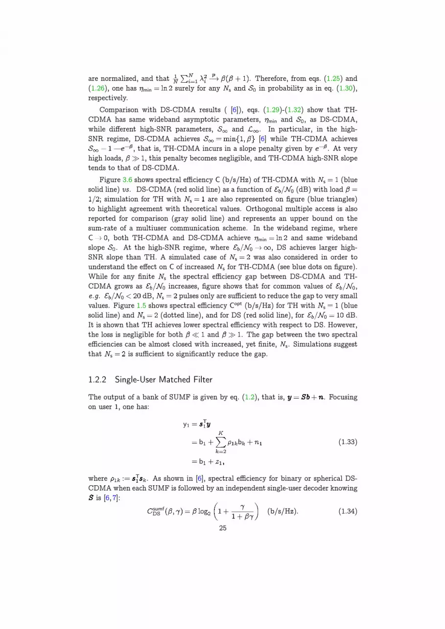
Figure 1.6: Probability density function of the real or imaginary part of the noise-plus-interference term of eq. (1.33) for TH sequences with dB, , and

s (blue solid line), and comparison against a Gaussian PDF with samemean and variance (red dashed line). This example shows that, contrary toDS-CDMA, sumf as given in eq. (1.42) may be far from Gaussian.

This result is general, and in particular it does not assume that the PDF of neitherinputs nor interference term is Gaussian. Note, however, that, in this case, Gaussianinputs are optimal. In fact, for long spreading sequences, by virtue of the strong lawsof large numbers, one has a.s. , and therefore the mutual informationper user in bits per channel use is:

y b y b

Ea.s. (1.35)

A similar result does hold for y b as well.

When interference is not Gaussian, we may expect spectral efficiency to assumea very different form than above. This will prove to be the case for the mutualinformation of TH-CDMA assuming Gaussian inputs, when s remains finite while

, as investigated below.

Theorem 5. Suppose that R is a time-hopping matrix with generics , and that the receiver is a bank of single-user matched filters followed

by independent decoders, each knowing . Assuming Gaussian inputs, mutualinformation sumf

TH (b/s/Hz) is given by:

sumfTH s y b s s

s

(1.36)

26

Proof. See Appendix 1.E.In particular, for the s case, mutual information is:

sumfTH (1.37)

that can be compared to, and interpreted as, eq. (1.21).Note that eq. (1.37) provides the mutual information of TH-CDMA with

s , and not the spectral efficiency, since Gaussian inputs, rather than optimalones, are assumed. Hence, we know that spectral efficiency will be larger than orequal to sumf

TH . This mutual information expression is, however, sufficient tocatch a significant difference between DS-CDMA and TH-CDMA. By comparingeqs. (1.34) and (1.37), we can claim that, while spectral efficiency for DS is boundedat high , being:

sumfDS (1.38)

spectral efficiency for TH is unbounded. We can indeed derive the below strongerresult:

Corollary 1. Under the hypotheses of Theorem 5, the high-SNR slope of themutual information (1.36) of TH is:

sumfTH

s (1.39)

The maximum slope as a function of is achieved at s , for whichsumf

TH s . Since s , the global maximum is , and the optimum loadis . This behavior directly provides an insight from a design standpoint: athigh-SNR, the number of chips such that an increase in 0 yields a maximumincrease in terms of mutual information is equal to the number of users. As acomparison, for optimum decoding, increases monotonically with , and itssupremum is .

Differently from DS, when decoders have no knowledge about cross-correlationsof signature sequences of other users, mutual information assumes a very differentform, as derived in the following theorem.

Theorem 6. Suppose that R is a time-hopping matrix with generics , and that the receiver is a bank of single-user matched filters followed

by independent decoders, each knowing the signature sequence of the user todecode only. Assuming Gaussian inputs, mutual information sumf

TH s

(bits/s/Hz) is given by:

sumfTH s y b sumf sumf (1.40)

27

where sumf and sumf are the two following Poisson-weighted linear combina-tions of Gaussian distributions:

sumf s s CN s (1.41)

sumf s s CN s (1.42)

Proof. See Appendix 1.F.Despite decoders’ lack of knowledge on , a same high-SNR slope as that

achieved when decoders have knowledge of is verified in the s case, asderived in the following corollary.

Corollary 2. Under the hypotheses of Theorem 6, and when s , the high-SNR slope of the mutual information (1.40) of TH is:

sumfTH (1.43)

Based on eq. (1.42), it can be checked that the kurtosis of the interference-plus-noise , that we denote since it is independent of the user, is:

E

E s(1.44)

that is always greater than , hence showing non-Gaussianity of for any ,and s. This non-Gaussian nature is represented on Fig. 1.6, that shows the

interference-plus-noise PDF sumf (solid blue line on figure), as given by eq. (1.42)when , dB and s , vs. a Gaussian distribution with same meanand variance (red dashed line on figure). As shown by figure, sumf , that is alinear combination, or “mixture,” of Gaussian distributions with Poisson weights,cannot be reasonably approximated with a single Gaussian distribution; hence, theStandard Gaussian Approximation does not hold in general. This is the reason forthe spectral efficiency gap between DS and TH.

The wideband regime is not affected by decoders’ knowledge about crosscorre-lations between signature sequences, as summarized by the below corollary, whichproof is omitted for brevity.

Corollary 3. The wideband regime parameters derived from either eq. (1.37) oreq. (1.40) are min and:

sumfTH (1.45)

Differently from above, where s is finite and does not depend on , we nowinvestigate the case s with , while . We show, using anapproach similar to that developed in [6], that spectral efficiency of a TH channelwith s , , is equal to that of a DS system, irrespectively of .

28

Orth

ogon

al

Ns = 1

Ns = 2

Ns = 1

Ns = 2

Ns/N ! ↵ 2 (0, 1]

�1.6 2 4 6 8 10 12 14 16 18 20 22 24 26 28

0.5

1

1.5

2

2.5

3

3.5

Eb/N0 (dB)

Csumf vs. Isumf

(b/s/Hz) Corth

IsumfTH?

IsumfTH

Csumf

Figure 1.7: Spectral efficiency Csumf vs. Isumf (b/s/Hz) as a function of 0 (dB)with load . Closed form expressions of spectral efficiency vs. mutualinformation are plotted in solid vs. dashed lines. Simulated mutualinformation is represented by dotted lines. On figure: SUMF, TH-CDMA,

s , s and s , blue dashed lines; SUMF, TH-CDMA , s ,blue dashed line; DS-CDMA, red solid line; TH-CDMA with s when

, blue solid line, coinciding with red solid line; TH-CDMA with s

and s , blue dotted lines. Note on figure the crossover of SUMF, TH-CDMA, s and SUMF, TH-CDMA , s , that shows an example ofmutual information becoming greater than conditional mutual information.For reference, orthogonal multiple-access in gray line.

Theorem 7. Suppose that R is a time-hopping matrix with s ,, and that the receiver is a bank of single-user matched filters followed

by independent decoders knowing cross-correlations and input distributions ofinterfering users. Capacity sumf

b b of the single-userchannel of eq. (1.33), expressed in bits per user per channel use, convergesalmost surely to:

sumfb b

a.s. (1.46)

irrespective of .

Proof. See Appendix 1.H.

29

Orth

ogon

al

No spreading

Ns = 1

Ns = 2

Ns = 1

Ns = 2

Ns/N ! ↵ 2 (0, 1]

1 2 3 4 5 6

1

2

3

4

5

6

�

Csumf vs. Isumf

(b/s/Hz)Corth/ns

IsumfTH?

IsumfTH

Csumf

Figure 1.8: Spectral efficiency Csumf vs. mutual information Isumf as a function of forfixed 0 dB. DS and TH with s are shown in red solidline, and represent the worst performance on figure. Dashed lines correponds toeither TH knowing (large dashing) or TH where decoders know the spreadingsequence of the user to decode only (small dashing). Orthogonal access isreported for reference (gray solid line).

Based on eq. (1.46), spectral efficiency coincides with that of DS sequences, asgiven by eq. (1.34). As a matter of fact, Theorem 7 is a generalization of the resultof Verdú and Shamai [6], for TH matrices where the fraction of nonzero entries is, to which it reduces for .

Figure 1.7 shows spectral efficiency Csumf vs. mutual information Isumf (b/s/Hz)as a function of 0 (dB) for DS-CDMA (eq. (1.34), red solid line on figure), TH-CDMA knowning cross-correlations between users (eq. (1.37), blue large-dashedlines) and TH-CDMA without knowing cross-correlations between users, indicatedas TH-CDMA (eq. (1.40), blue small-dashed line), with unit load . Spectralefficiency of TH-CDMA when s , , as , is equal to that ofDS (c.f. eq. (1.46), red solid line). As previously, the orthogonal case (gray solidline) is shown for reference. Note that spectral efficiency is bounded in DS-CDMAand in TH-CDMA when s , , as ; the value of the limit is

on figure (c.f. eq. (1.38)). On the contrary, mutual information is not boundedfor both TH-CDMA and TH-CDMA ; in particular, when s , both TH-CDMAand TH-CDMA grow with similar slope as 0 increases. Mutual informationof systems using multiple pulses per symbol is shown for TH-CDMA with s

(small-dashed line) and for TH-CDMA with s (eq. (1.36), large-dashed line).These s cases show that mutual information decreases with respect to theone pulse per symbol case. Figure 1.8 shows spectral efficiency Csumf (b/s/Hz) asa function of for fixed 0 dB. Similarly as on fig. 1.7, TH with s

outperforms other schemes, with and without complete knowledge of . As ,

30

interference becomes increasingly Gaussian, and mutual information of TH reducesto that of DS, tending to the same limit .

1.2.3 Decorrelator and MMSE

The output of a bank of decorrelators, following the discrete channel(c.f. eq. (1.2)), is given by:

(1.47)

where denotes the Moore-Penrose pseudoinverse; if T is invertible, thenT T, otherwise , according to the Tikhonov regularization, exists

and can be computed as the limit T T as .In DS-CDMA, for any fixed , is almost surely full rank as ,

and therefore, is almost surely invertible, in which case eq. (1.47) becomes:

(1.48)

where CN 0 . Assuming independent single-user decoders, spectralefficiency is [6]:

decoDS (1.49)

The output of a bank of MMSE filters observing (c.f. eq. (1.2)) is:

T T T

(1.50)

where T is defined as follows:

T T T T T (1.51)

Note that, as well known, MMSE and decorrelator coincide as .In DS-CDMA, for any fixed , it was shown in [6] that:

mmseDS (1.52)

where:

being as in eq. (1.19).We can treat both decorrelator and MMSE as special cases of the linear operator:

T T T T T

31

for and , respectively. Similarly as eq. (1.50), one has:

T (1.53)

where dependence on is now made explicit, and the output for user is:

b b (1.54)

For s , a closed form expression for the generic element of is derived inAppendix 1.I, and reads as:

(1.55)

where is:

1 (1.56)

Denote with J the following set: J . Hence, J is thecardinality of J . Denote with J J . Since J , one has J .We can rewrite eq. (1.119) as follows:

bJ

b (1.57)

Note that b for is distributed as b , and given is complex Gaussianwith zero mean and conditional variance:

0

Known , and given b are both complex Gaussian, hence mutual informationexpressed in bits per user per channel use is:

b b E0

E

Since , in the LSL one has P . Therefore, we proved thefollowing:

Theorem 8. Suppose that R is a time-hopping matrix with s , andthat the receiver is a bank of either decorrelators or MMSE filters

followed by independent decoders, each knowing . Assuming Gaussian

32

Orth

ogon

al ImmseTH = Ideco

TH

CdecoDS

CmmseDS

�1.6 2 4 6 8 10 12 14 16 18 20 22 24 26 28

0.5

1

1.5

2

2.5

3

3.5

Eb/N0 (dB)

Cmmse vs. Immse

Cdeco vs. Ideco

(b/s/Hz)ITH

C

Figure 1.9: Spectral efficiency Cmmse vs. mutual information Immse and Cdeco vs. Ideco

(b/s/Hz) as a function of 0 (dB) with load . Mutual informationof TH-CDMA with s (blue dashed line) vs. spectral efficiency of DS-CDMA (red solid lines), for decorrelator and MMSE receivers, is shown. It isalso shown orthogonal access (gray line) for reference.

inputs, mutual information TH (b/s/Hz) is given by:

TH b (1.58)

Since eq. (1.58) does not depend on and is equal to eq. (1.37) for SUMF, oneexplicitly has TH

sumfTH

mmseTH

decoTH , thus we will write the above quantities

interchangeably. With minor modifications of the above argument, it is possible toshow that a similar result does hold for any linear receiver T , , under theassumption s . Therefore, results for SUMF can be extended verbatim to bothdecorrelator and MMSE receivers, when s . This result suggests a strikingdifference with respect to DS, where spectral efficiency depends on the adoptedlinear receiver: In TH with s , SUMF, decorrelator and MMSE all result in thesame mutual information.

In order to compare DS and TH for decorrelator and MMSE, we separate theanalysis for systems with and , to which we refer as underloaded andoverloaded, respectively.

33

Underloaded system .Decorrelation in DS allows to achieve the maximum high-SNR slope, deco

DS ,that is equal to that of orthogonal multiple access. On the contrary, TH does notfully exploit the capabilities of CDMA in the high-SNR regime, since deco

THsumf

TH . This behavior follows directly from cross-correlation propertiesof signature sequences of DS vs. TH: In DS, the almost sure linear independenceof signature sequences, that holds for any , makes T almost sureinvertible, and thus interference can be mostly removed, which is not the case ofTH (c.f. Fig. 1.3 and Theorem 3). However, the optimal high-SNR slope in DScomes at the expense of a minimum 0 equal to , that can bemuch larger than that achieved by TH, namely ; in particular, as , theminimum energy-per-bit for DS with decorrelator grows without bound. Therefore,decorrelation with DS should to be considered in a very low load, high-SNR regimeonly: in this region, it outperforms TH. It can be shown, by comparing eqs. (1.52)and (1.49), that in DS spectral efficiency of MMSE is always larger than that ofdecorrelator. In particular, it achieves a minimum energy-per-bit equal to ,which is optimal, and also an optimal high-SNR slope.

Overloaded system .Spectral efficiency of TH and DS with MMSE is similar in the low-SNR regime,

with same minimum energy-per-bit and wideband slope. At high-SNR, mutualinformation of TH is unbounded, while spectral efficiency of DS is bounded, asin the SUMF case. In particular, while the high-SNR slope of TH is equal to

sumfTH for any , the high-SNR slope of DS with MMSE is:

mmseDS 1 1 1

which implies that, as 0 , CmmseDS is infinite for , while it is finite for

, and equal to (c.f. eq. (1.52)) [6]:

mmseDS (1.59)

By comparing this result with eq. (1.38), that refers to SUMF, one also notes thatthe two limits are different, although as both tend to .

Figure 1.9 shows spectral efficiency Cmmse and Cdeco vs. mutual informationImmse and Ideco (b/s/Hz) as a function of 0 (dB) for DS (red solid lines) andTH (blue dashed line), when . Orthogonal access is also shown for reference(gray solid line). The choice of represents a scenario with high interferencewhere eq. (1.49) is still valid, and DS with decorrelation still comparable. MMSEand decorrelator receivers achieve a same mutual information for TH: in the low-SNR regime, Immse

TH IdecoTH and Cmmse

DS have similar behavior, that departs as 0

increases. Decorrelator with DS achieves the maximum high-SNR slope, which isequal to that of the orthogonal access: note that the two curves on figure are,in fact, translated. This is not the case for TH, for is not full rank with highprobability, and the high-SNR slope is indeed lower. It is shown on figure that

34

Orth

ogon

al

No spreading

Ns = 1

CmmseDSCdeco

DS

1 2 3 4 5 6

1

2

3

4

5

6

�

C vs. I (b/s/Hz)

Corth/ns

IsumfTH

CDS

Figure 1.10: Spectral efficiency CmmseDS and Cdeco

DS vs. mutual information Immse decoTH (b/s/Hz)

as a function of for DS-CDMA (red solid lines) and TH-CDMA (blue dashedline), when 0 dB. Orthogonal access is reported for reference (graysolid line).

DS with MMSE outperforms linear receivers with TH: this is due to the particularchoice of . Figure 1.10 shows spectral efficiency Cmmse

DS and CdecoDS (red solid lines)

vs. mutual information IsumfTH Ideco

TH ImmseTH (blue dashed line) as a function of ,

when 0 dB. This figure shows that MMSE with DS is outperformed byTH for large : in particular, there exists a minimum value of , say , in generaldepending on 0, beyond which the mutual information of TH is higher than thespectral efficiency of DS, although both tending to a same limit as , that is,

. While it is difficult to study as a function of 0, the above discussionon the high-SNR slope of DS suggest that marks a transition in DS behavior as

0 . Figure 1.11 shows CmmseDS (red solid lines) and Isumf

TH IdecoTH Immse

TH (bluedashed line) as a function of , for different values of dB

0 . Figureshows that, as dB increases, spectral efficiency of DS grows linearly for , andat about quickly drops towards the limit value given by eq. (1.59), whilespectral efficiency of TH remains smooth for any load in the neighborhood ofand increases monotonically with dB.

1.2.4 Synopsis of the TH-CDMA case

Figure 1.12 shows spectral efficiency C or mutual information I (b/s/Hz) vs.0 (dB) for the two extreme cases of optimum decoding and SUMF receivers,

when . Curves derived from closed form expressions of spectral efficiencyare shown for optimum decoding when s (top blue solid line), and SUMFwhen s as and (bottom blue solid line). Curves derived

35

⌘dB= 10 dB

⌘dB= 20 dB ⌘dB

= 40 dB

⌘dB= 10 dB

⌘dB= 20 dB

⌘dB= 40 dB⌘dB

= 1

1 2 3 4 5 6

2

4

6

8

10

12

14

�

C vs. I (b/s/Hz)IsumfTH

CmmseDS

Figure 1.11: Spectral efficiency CmmseDS vs. mutual information Isumf

TH (b/s/Hz) as a functionof for DS-CDMA (red solid lines) and TH-CDMA (blue dashed lines), forvalues of dB

0 dB. Asymptotic value of CmmseDS for dB

is also shown for reference (thin solid black line).

from closed form expressions of mutual information assuming Gaussian inputs areshown for SUMF, TH-CDMA (blue dashed line, see label on figure) and SUMF, TH-CDMA (blue dashed line, see label on figure), when s and s . Findingclosed form expressions of spectral efficiency of optimum decoding with generic

s finite remains an open problem. Simulations provide, however, insights intothe behavior of spectral efficiency for this particular case, as shown by Copt

TH withs (blue dotted line). TH behavior is delimited by DS curves, with optimum

decoding vs. SUMF (top and bottom red lines). Both upper and lower curvesare approached by TH as s increases; in particular, we showed that the lowercurve describes, in fact, TH when s , , as . In betweenthese two extremes lie TH curves with optimum vs. linear receivers. In particular,for s (maximum energy concentration), mutual information of a receiver assimple as SUMF is not bounded, and also close to optimum decoding with s .Furthermore, a lack of knowledge in cross-correlations of spreading codes provokes adrop of performance that is, however, not sufficient to degrade mutual informationto DS spectral efficiency, with any finite s.

Figure 1.13 compares either spectral efficiency C or mutual information I

(b/s/Hz), as a function of , for DS and TH, when 0 dB. Both DSand TH have similar behaviors when , for linear and optimum receivers.Irrespective of , spectral efficiency of DS with optimum decoding is larger thanthat achieved by TH, the gap being almost closed when s finite. Conversely,among linear receivers and access schemes, it is shown that DS with SUMF hasthe lowest spectral efficiency, which is equal to that of TH when the number of

36

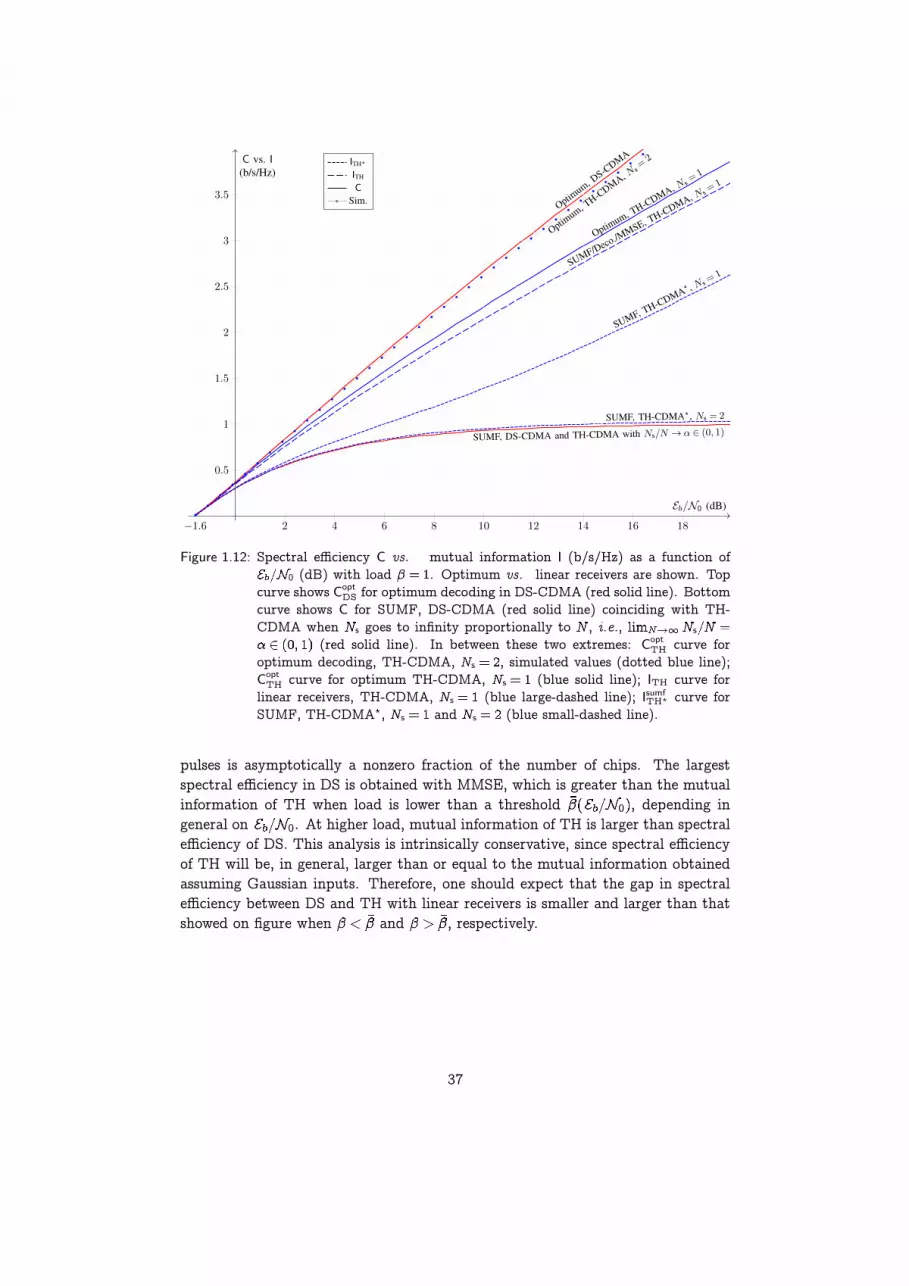
SUMF, TH-CDMA? , Ns =

1

SUMF/Deco./MMSE, TH-CDMA, Ns

=

1

Optimum, TH-CDMA, Ns

=

1

Optimum, TH-CDMA, N s

=

2

SUMF, DS-CDMA and TH-CDMA with Ns/N ! ↵ 2 (0

, 1)

Optimum, DS-CDMA

SUMF, TH-CDMA?, Ns =

2

�1.6 2 4 6 8 10 12 14 16 18

0.5

1

1.5

2

2.5

3

3.5

Eb/N0 (dB)

C vs. I(b/s/Hz)

ITH?

ITH

CSim.

Figure 1.12: Spectral efficiency C vs. mutual information I (b/s/Hz) as a function of0 (dB) with load . Optimum vs. linear receivers are shown. Top

curve shows CoptDS for optimum decoding in DS-CDMA (red solid line). Bottom

curve shows C for SUMF, DS-CDMA (red solid line) coinciding with TH-CDMA when s goes to infinity proportionally to , i.e., s

(red solid line). In between these two extremes: CoptTH curve for

optimum decoding, TH-CDMA, s , simulated values (dotted blue line);Copt

TH curve for optimum TH-CDMA, s (blue solid line); ITH curve forlinear receivers, TH-CDMA, s (blue large-dashed line); Isumf

TH curve forSUMF, TH-CDMA , s and s (blue small-dashed line).

pulses is asymptotically a nonzero fraction of the number of chips. The largestspectral efficiency in DS is obtained with MMSE, which is greater than the mutualinformation of TH when load is lower than a threshold 0 , depending ingeneral on 0. At higher load, mutual information of TH is larger than spectralefficiency of DS. This analysis is intrinsically conservative, since spectral efficiencyof TH will be, in general, larger than or equal to the mutual information obtainedassuming Gaussian inputs. Therefore, one should expect that the gap in spectralefficiency between DS and TH with linear receivers is smaller and larger than thatshowed on figure when and , respectively.

37

Orth

ogon

al

No spreading

CsumfTH , Ns/N ! ↵ 2 (0, 1]

CoptDS

CoptTH with Ns = 1

CoptTH with Ns = 2

IsumfTH , Ns = 1

CmmseDS

1 2 3 4 5 6

1

2

3

4

5

6

�

C vs. I (b/s/Hz)

C (theo.)C (sim.)

IsumfTH

Figure 1.13: Spectral efficiency C or mutual information I (b/s/Hz) as a function offor DS and TH, when 0 dB, with optimum and SUMF receivers.Orthogonal access and DS with MMSE receiver are reported for reference.

1.3 Conclusions

Verdú and Shamai showed in [6] that optimum decoding provides a substantialgain over linear decoding in DS-CDMA, with random spreading. In particular, abank of single-user matched filters followed by independent decoders is bounded inspectral efficiency at high-SNR, and linear multiuser detectors are needed in orderto recover a nonzero spectral efficiency high-SNR slope. This behavior is partly dueto the “even” use of degrees of freedom—coinciding in our setting with chips—thatis intrisic of DS-CDMA [1].

The object of this paper was to analyze TH-CDMA with random hopping, andcompare its behavior against DS-CDMA; we interpreted time-hopping in the generalframework developed in [6, 7]. The present analysis allowed comparison of THvs. DS with same energy per symbol and same bandwidth constraints, and,therefore, showed the effect of the energy “concentration,” that is typical of TH. Thedegree of “unevenness” in TH-CDMA is directly related to the number of pulses s

representing each symbol. At one extreme, one has maximum “unevenness,” whereall energy is concentrated in one pulse ( s ), while the other extreme correspondsto maximum “evenness,” s , where TH coincides with DS. Particular emphasishas been put on the archetypal case of “unevennes,” that is s , and partialresults showing the general behavior when s have been derived.

A first result of our analysis was to derive a closed form expression for spectralefficiency of TH-CDMA with optimum decoding when s , showing that, in thiscase, DS-CDMA outperforms TH-CDMA, in particular in the high-SNR regime.Same wideband behavior, but lower high-SNR slope, was observed for TH-CDMA

38

vs. DS-CDMA, that is DS TH . A closed formexpression for generic s remains an open problem; results based on simulationssuggested, however, that the spectral efficiency loss at high-SNR may be consid-erably reduced while maintaining the number of pulses finite, and we providedevidences that the gap is reduced to a very small value with as low as two pulsesper symbol ( s ). This result indicates that the spectral efficiency gap may besubstantially reduced while only using a fraction s of degrees of freedom peruser, that asymptotically vanishes as grows.

A different behavior of TH-CDMA with respect to DS-CDMA was observedwith linear receivers. Contrarily to DS, spectral efficiency of SUMF for TH with

s was unbounded. As suggested, this asymptotic behavior may be traced backto the non-Gaussian distribution of the interference-plus-noise variable observed byeach independent single-user decoder, that, in turn, depends on cross-correlationproperties of spreading sequences. The same high-SNR slope sumf

TH wasachieved by TH irrespectively of the knowledge that each single-user decoder hadabout spreading sequences of all other users. It was interesting to note that themaximum slope for TH, providing a hint on greatest energy efficiency, was reachedwhen the number of users was equal to the number of chips , i.e., , leadingto sumf

TH . On the contrary, for s , , same spectralefficiency as DS-CDMA ( ) was obtained irrespectively of for .

The bounded nature of spectral efficiency with a SUMF bank in DS-CDMA isovercome, as well known, by using more complex linear receivers, that also accountfor interference, such as MMSE and decorrelator. Conversely, we showed that, inTH-CDMA, mutual information assuming Gaussian inputs has the same expression,irrespective of the linear receiver used, due to the peculiar structure of TH spreadingsequences. TH sequences are indeed “more” likely to be linearly dependent thanDS ones, in agreement with the intuition based on the cardinality of binary DS vs.TH codes, that is vs. . This lack of independence led to the impossibilityof removing interference, which is instead almost surely feasible for DS, e.g. witheither decorrelator or MMSE receivers, as long as the load . Therefore, in alow load, high-SNR scenario, DS outperforms TH. The opposite is true when .In fact, while spectral efficiency in DS with MMSE rapidly drops, in particular withlarge 0, as soon as becomes larger than one, mutual information of TH decayssoftly when one keeps overloading the system, and tends to the same MMSE DSlimit. The absence of a spectral efficiency “transition” in the neighborhood of theunit load, that is typical of DS, allows TH to outperform DS with any load largerthan for sufficiently high 0.

Beyond the natural extension of the present work to channels with fading,where the effect of an “uneven” use of degrees of freedom typical of TH shouldbe investigated, we do stress that, from the single-user perspective, TH is a par-ticular instance of impulsive signal. As such, the present theoretical setting, ifappropriately adapted to asynchronous links, may serve as a basis for refining theunderstanding of the limits of impulsive communications.

39

.

User 1

User 2

⌧2

User K⌧K

mT (m + 1)TNhTcTc

. . .

1 2 · · · Ns

Figure 1.14: Signal model: in picture, s , h , therefore s h . Delaysare considered with respect to the first User, therefore .

1.4 Asynchronous channel

1.4.1 Model

As for the asynchronous channel model, we adopt the model proposed in [20] forCDMA systems, where the received signal is:

y A b s n (1.60)

in which we introduce the possibility for the signature waveform to change fromone symbol to the next, and propose the following straightforward generalization:

y A b s n (1.61)

where the codeword of length is considered for each user, the spreadingwaveform s of user in the th epoch may depend on , that is:

s s

is the th symbol of user , and indicates its delay. Users areordered according to increasing , that is, , and is set to .As previously, A .

Note that in this case, the anaylis focuses on set of symbols per user vs.of the synchronous case since this has proved to be necessary in order to derive asufficient statistic for b [20].

A procedure similar to the one adopted in [30] allows to derive a discrete channelmodel equivalent to the continuous-time channel of eq. (1.61); the equivalence isdefined in terms of channel capacity, and also in terms of capability of producingsufficient statistics leading to optimum inference of .

40

To this end, define the th symbol vector C as:

b b T

and form vector by stacking the above vectors:

T T T (1.62)

This vector can be compactly written using the Kronecker product as follows:

(1.63)

where . Explicitly, the ( )-th component of is b . Notethat, according to the above notation, the asynchronous channel with users andcodewords length is equivalent to a synchronous channel with users andcodeword length one.

Now consider projecting the continuous-time process y onto the set of allspreading waveforms:

s

(1.64)

that is, consider the inner product between y and the generic :

y

This is the output of a filter that is matched to the signature sequence of user atsymbol sampled at the corresponding epoch, that is, at time .

Stacking these projections as for , one has:

(1.65)

that is, a vector C providing a sufficient statistic for the optimum detectionof .

Based on eqs. (1.62) and (1.65), the equivalent discrete channel model cantherefore be expressed by:

(1.66)

where components of matrix R are given by:

R

41

s s

s s

c c

T (1.67)

with: c

c

showing that is symmetric.Since symbols are transmitted for each user and given eqs. (1.62), (1.65) and

(1.66), has the following block-matrix structure:

T (1.68)

where each block is with components:

Since is symmetric, one also has T. Given (1.68), the follow-ing relation holds for :

(1.69)

Compared to CDMA systems where signatures do not change across symbolperiods, note that, as previously indicated, the proposed model releases this con-straint, as reflected in the general block structure of . Note that the proposedmodel reduces to its traditional form [20] when signatures do not vary across symbolperiods, for which one has:

T

having defined . In this case, is also block-Toeplitz.

Note that if the channel were synchronous, one would have T , withis a block-diagonal matrix with the generic th diagonal block has the following

42

block-diagonal structure:

......

. . ....

(1.70)

Therefore, is:

T

T T

We may express in terms of chip-matched filter output sampled at epochs for user and symbol . To this end, note that the generic element of

can be written in terms of matrices:

R

as defined in eq. (1.67). Note that is Toeplitz and only dependson difference rather than on and . Therefore, denoting bythe block matrix obtained by grouping the blocks

, that is:

T

it results that is block-Toeplitz. Finally, consider the matrix obtained bygrouping the blocks as follows:

T

By construction, is block-Toeplitz with respect to blocksand also with respect to smaller blocks

.The generic element of can be expressed by:

R

having defined:c

which also shows that is symmetric.

43

We can express in terms of spreading sequences and matrix as follows:

T

This model duly reduces to the synchronous model when delays are null, as canbe derived in a straightforward way.

Note that a linear time-invariant, frequency-selective channel with impulse re-sponse might be taken into account by substituting with . In thiscase, would account for both asynchronicity and frequency-selectivity.

Note that the assumption of zero-excess bandwidth pulses was, as initiallyindicated, introduced for mere simplification, and any orthonormal family of pulses,as in particular time-limited waveforms, fit the model; UWB impulse-radio com-munications are appropriately modeled.

1.4.2 Impulsiveness

A non-impulsive system occupying frequency band W W (Hertz) and usinga channel for (seconds) may transmit at most W orthogonal waveforms bytransmitting a waveform that occupies a bandwidth W every W seconds forseconds. Symbol period is therefore W, and effective duration is W as well,that is in non-impulsive systems these two quantities coincide.

Conversely, in impulsive systems, that is, systems using pulses with bandwidthW W, while keeping fixed the symbol period, the channel may still used every

W seconds but transmission occurs over bandwidth W ; effective duration is thusW . Impulsiveness can, therefore, be measured by ratio W W, that is, the ratio

of transmission bandwidth over minimum Nyquist bandwidth. We call this ratioimpulsiveness index ˚i�.

While spread-spectrum systems use a bandwidth larger than what is the min-imum required to transmit at a given symbol rate, impulsive systems use a largerbandwidth than the minimum required to transmit at a given chip rate. There-fore, impulsiveness can be viewed as another way for spreading bandwidth. Innon-impulsive spread-spectrum systems, bandwidth spreading is described by thenumber of chips in one symbol period, named spreading factor c N.Similarly, impulsiveness index ˚i� specifies spreading as system bandwidth vs. chiprate; impulsive systems may use bandwidth W c, i.e., e↵ c, thereforetransmitting pulses that are much shorter than the chip interval. The condition˚i� N guarantees the Nyquist criterion to be satisfied.

In general, we propose to define impulsiveness resorting to the concept of effec-tive duration akin to that of effective bandwidth as described in [31]:

˚i� c

e↵(1.71)

44

mTs (m + 1)Ts

Tc =

1

W

(a) Non-impulsive

mTs (m + 1)Ts

Tc =

ıW

1

W

(b) Impulsive

Figure 1.15: Illustration of the impulsiveness index concept. A non-impulsive system,where ˚i� , and therefore c W, is shown in Fig. (a), while an impulsivesystem, where ˚i� , and therefore c W, is shown in Fig. (b).

where effective duration is defined as to satisfy:

e↵R

(1.72)

Note that for zero-excess bandwidth pulses occupying frequency bandW W , as used throughout this chapter for the sake of simplicity, one

has e↵ W, and therefore ˚i� cW. However, the impulsiveness index is welldefined also for the opposite case of strictly time-limited pulses; for example,for rectangular pulses with duration (seconds), eq. (1.72) yields e↵ , asintuitive.

Figure 1.15 shows an example of a spreading waveform for non-impulsive com-munications (Fig. 1.15a), where pulse bandwidth is directly related to chip rate,vs. impulsive communications (Fig. 1.15b), where pulse effective duration is shorterthan the chip interval, and thus bandwidth is larger than chip rate, specifically ˚i�times c.

In the literature of the last fifteen years, the concept of peaky signaling arose(e.g. [1,5,25,32]). Although related, the concepts of impulsiveness and peakdenessare complementary, as we explain in the next section.

45

1.4.3 Impulsiveness vs. Peakedness

The notion of peakedness of a random variable is strictly related to the limitednessof its maximum absolute value or, in a relaxed sense, to the limitedness of itsfourth moment and kurtosis [1,5,32]. In general, a distribution with large kurtosisis indicated as “peaky” [1].

As example of non-peaky distribution, consider a discrete binary r.v. uni-formly distributed, A A; has kurtosis . On thecontrary, as example of “peaky” distribution, consider A

A; has kurtosis , that is increasingly “peaky” as . Ingeneral, a “peaky” distribution has the zero value, or nearly zero values comparedto the standard deviation, with high probability with respect to the probabilityunder the tails, that is, for values greater than the standard deviation; therefore,leptokurtic distributions are “peaky”. A r.v. drawn from a “peaky” distribution ischaracterized by rare large and frequent mild deviations.

A communication system that transmits over bandwidth W W forseconds is characterized by W degrees of freedom indicating that the channelmay carry W input symbols towards output; the capacity of the channel is themaximum number of bits, that can be encoded in these W symbols, with avanishing error probability. Under fixed power constraint, the distribution of inputsover these degrees of freedom determines peakedness. In particular, if the kurtosisof inputs is “relatively” high, then the input distribution is “peaky”.

Increasingly “peaky” inputs lead to reaching the wideband capacity, i.e.capacityfor spectral efficiency tending to zero, for transmissions over fading channels whenthe receiver has no a priori knowledge on fading coefficients [33–35]. Conversely,in the same context, Gallager and Médard [1, 2] show that non-peaky inputs leadto zero mutual information. In particular, these authors highlight a “bandwidthscaling” property for multipath fading channels, that can be described as follows: as-suming an infinite number of path scattering model, mutual information of spread-spectrum signals tends to zero as bandwidth grows if energy and fourth momentof inputs scale with W and W , respectively, that is, if degrees of freedom areused “evenly”, in a typical non-peaky fashion. Finally, Verdú [25] defines the familyof input distributions, called flash, achieving capacity at the wideband regime. Thisfamily encompasses inputs that are distributed as the mixture of two probabilitydistributions, the first tending to a Dirac mass in the origin, and the second thatvanishes as the signal-to-noise ratio per degree of freedom tends to zero.

Degrees of freedom can be exploited in time only, in frequency only, or in bothtime and frequency.

As example of a system that is non-peaky neither in time nor in frequency,consider DS-CDMA as in [1,2]. As example of a system that is “peaky” in frequency,but not in time, consider -FSK with symbol duration and bandwidth W dividedinto equal slices of width , hence W . For transmitting a messagewith , one frequency slice only is used. Inputs present thus out of

nonzero value occurences, and therefore are distributed as, with kurtosis . As example of a system that is “peaky” in both

46

time and frequency, consider FSK with duty cycle, as in [3, 5]. As example of asystem that is “peaky” in time, but not in frequency, consider -PPM with symboleffective-duration W, hence W . Inputs are distributed as above as in thecase of -FSK.

The last example is particularly significant to draw an analogy between peakyinputs in time, that are those that present “many” occurrences of the zero value,and impulsiveness.

Impulsive systems are intrinsically “peaky” since a subset only of the availabledegrees of freedom is used; this is particularly evident in the time domain sincemany occurrences of the zero value can be observed. Impulsiveness reshapes indeedthe input distribution of a non-impulsive signal with ˚i� by adding a Diracmass at the origin as follows: ˚i� ˚i� . Therefore, the intuitionmay be that impulsiveness provides a mean that is complementary to duty-cycle inorder to achieve capacity at the wideband regime; as impulsiveness grows, inputsbecome increasingly “peaky”, and may flash at the limit ˚i� .

Moreover, TH-CDMA signals, as opposed to DS-CDMA, are “peaky”; also, forany fixed s, as grows, these signals are increasingly “peaky”, while tending toflash at the limit .

Impulsive CDMA signals in general have increased peakedness with respect tonon-impulsive CDMA signals; therefore, for DS-CDMA, impulsiveness is a meantowards peakedness, while for TH-CDMA signals it is a mean towards increasedpeakedness.

1.4.4 First results

Spectral efficiency of the asynchronous channel can be derived, similarly to thesynchronous case, from the equivalent discrete channel model (c.f.eq. (1.66)) as:

(b/s/Hz)

Since the covariance of and the conditional covariance of given are, respec-tively:

0

ET

0

being E , then:

(b/s/Hz) (1.73)

having denoted with 0 as previous.

47

�20 �15 �10 �5 5 10 15 20

0.5

1

1.5

2

2.5

3

3.5

� (dB)

C(�) (b/s/Hz)ı = 1, � = 1/2, symb. asynch. (sim.)ı = 2, � = 1/2, discr. chip asynch. (sim.)ı = 2, � = 1/2, discr. chip asynch. (th.)ı = 2, � = 1, discr. chip asynch. (sim.)ı = 2, � = 1, discr. chip asynch. (th.)

Figure 1.16: Spectral efficiency as function of (dB) for the asynchronous channel withs .

When an impulsive communication is employed, then the bandwidth used is ˚i�times larger than the minimum required, therefore eq. (1.73) generalizes to:

˚i� (b/s/Hz) (1.74)

Investigation of when either or for special families ofrandom spreading signatures in an asynchronous setting is the major challange.

For non-varying signatures across symbol periods, a prior work of Verdú [30]reports the expression of capacity for asynchronous DS-CDMA channel withand finite, once signature sequences are fixed and nonrandom. For random DS-CDMA, Cottatellucci et al. [36] find the expression of the SINR achieved by anMMSE receiver using the REFORM method proposed by Girko [37] and exploitthe celebrated relation between mutual information and mmse [38] in order to findcapacity with the optimum receiver.

Cottatellucci’s analysis of the DS-CDMA asynchronous channel in [36] proceedsin two steps. In the first step, it is assumed that the maximum delay between usersis limited to a chip interval, that is c: the so obtained channel is calledchip asynchronous, symbol quasi-synchronous channel. In the second step, itis shown that results obtained in the previous step continue to be valid also when

s: this is called symbol asynchonous channel.In what follows, we limit our attention to the chip-asynchronous, symbol quasi-

synchronous TH-CDMA channel.

48

Chip asynchronous, symbol quasi-synchronous channel

As in [36], the assumption of limitedness of to c implies that, in the largesystem limit, ISI becomes negligible.

Therefore, we can study a channel where one symbol only is transmitted.We further assume discrete delays, i.e., delays that are multiples of W:W with ˚i� . This kind of “discrete-asynchronism” effectively turns

the channel into a set of ˚i� parallel channels, each populated by a number of usersequal to the number of users with same delay: therefore, capacity of the discrete-asynchronous channel is the sum of capacities of these parallel channels.

Intuition behind this result lies on orthogonality of users with different delays.When two users have indeed different delays, their waveforms are orthogonal irre-spective of the signature sequences: this follows from the property of bandlimitedpulses to be orthogonal if delayed by multiples of W. Therefore, dividing theset of users into equivalent classes where the equivalence is defined by havingthe same delay and calling the number of users with delay W, the originalchannel is decomposed into at most ˚i� orthogonal channels, since there are at most˚i� delays, each channel having symbols of chips, using a bandwidth W, and beingpopulated by users, hence having load equal to . This construction impliesthat ˚i� .

Now let prove these intuitions in light of the asynchronous channel modeldeveloped in Section 1.4.1 and the general spectral efficiency expression given byeq. (1.74), both specialized to the case .

Consider a composition of into ˚i� parts, that is, ˚i�, where. If two users and have different delays, i.e., , then:

c c

Therefore, when , and is a block-diagonalmatrix with at most ˚i� diagonal blocks of dimensions , , ˚i� ˚i� .

As defined in eq. (1.66), inherits this block-diagonal structure, with diagonalblocks of dimensions , , ˚i� ˚i�. Call these diagonal blocks , . . . , ˚i� .From eq. (1.74), we have:

˚i�

˚i�˚i�

˚i�˚i�

(b/s/Hz)

where each describes a multiple access channel with synchronous users andchips having capacity (b/s/chip) as found in Section 1.2. Ensemble average

49

of is therefore:

E ˚i�˚i�

˚i�˚i�E

where the expectation is on , that is the number of users with delay equal toW. Assuming uniform i.i.d. delays, Binom with ˚i�, irrespective

of , hence:

(b/s/Hz)

Assuming as previous spectral efficiency to be self-averaging, the large-system limityields spectral efficiency :

F (b/s/Hz) (1.75)

where:

F F (1.76)

having denoted with F the e.s.d. of a synchronous CDMA channel with loadaveraged over the spreading sequences, and with F the large-system limit

e.s.d. that is found by averaging F with respect to and let .In general ˚i� is function of . There are, therefore, different ways we can

approach the large-system limit depending on the behavior of as .

Case 1) ˚i�This is case when , and ˚i� is constant, and thus

also the bandwidth is constant. The load of the system is:

usersDoF ˚i� (1.77)

Case 2) ˚i�When ˚i� grows as , the number of DoFs grows as ; therefore, also the number

of users has to grow as in order to keep spectral efficiency nonzero.This is the case when ˚i� . For the sake of simplicity, consider:

˚i�50

Note that in this case, as the impulsiveness index, also the bandwidth tends toinfinity in the large-system limit. The load of the system is:

usersDoF ˚i� (1.78)

Therefore we can actually call the constant factor .

TH-CDMA with s .We find closed form expression of (1.75) for TH-CDMA with s in the two

cases specified above.In general, spectral efficiency of TH-CDMA with s is given by:

E Ex x (b/s/Hz)

where the inner expectation is over x Pois and the outer expectation isover Binom ˚i� .Case 1) Quite surprisingly, although in this case the Binomial distribution doesnot tend to a Poisson distribution, we can anyway regard the (unconditioned)distribution of x as Poissonian:

fx f fx

hence, asymptotically, x Pois .

Case 2) In this case, the Binomial distribution tends to a Poisson distribution asfollows: Pois , x Pois and x Pois .

Therefore, in both cases, spectral efficiency is given by:

E x (b/s/Hz) (1.79)

as in a synchronous channel with load given respectively by eqs. (1.77) and (1.78).

1.5 Future work

In this section, several proposal for extending the analysis of previous sections arepresented in order to account:

51

(E1) non-uniform power constraints over users;

(E2) fading channels;

(E3) multipath channels;

(E4) frequency-hopping;

(E5) asynchronism.

E1. We call non-uniform power constraint a constraint E b that dependson , i.e.,

E b

that, when symbols of different users are independent, leads to:

E (1.80)

where is diagonal. Spectral efficiency is, therefore, given by:

0

T (1.81)

E2. The extension of model (1.2) to account channels with fading is straight-forward. Denote with the diagonal matrix of the fading coefficientsA A . The flat-fading channel model reads as:

(1.82)

For the sake of simplicity, it is common to assume (e.g. [39]) that A

are i.i.d. with unit variance, E A . This corresponds to channels having, onaverage, unit gain, that may be assumed w.l.o.g. (in the opposite case, the differentgains may be included in a non-uniform power constraint, such as in E1 ). Spectralefficiency, when receiver has knowledge of the fading coefficients, is:

(1.83)

and, therefore, the analysis reduces to that of finding the eigenvalue distributionof T, or equivalently T . In case a non-uniform powerconstraint is set, one has, similarly to eq. (1.85):

0

T (1.84)

Suppose to set the maximum power consumption of the network, i.e., Tr

. If each transmitter has knowledge of , one can find the spectral efficiency as

52

follows:

Tr

Tr 0

T (1.85)

where the optimum is expected to be non-diagonal, thus requiring cooperatingusers, and follow a water-filling argument. It would be interesting to find a closedform expression of eq. (1.85) and compare the resulting spectral efficiency vs. asuboptimum uniform power constraint, as given by eq. (1.84) with diagonal .

E3. The multipath channel between user and the receiver may be modeledwith a convolution matrix of dimensions , where is the length of thechannel expressed in number of taps, corresponding to the delay spread W

seconds. The channel model becomes:

b b (1.86)

where:T

Spectral efficiency is given again by eqs. (1.84) and (1.85) by formally replacingwith . In the present case, however, we may exploit the convolutional structureof in order to attempt finding a closed form solution.

E4. Frequency-hopping may be regarded as the time-hopping dual modulation.We present in the following the basic time-hopping signaling scheme, and analogiesand differences with frequency-hopping. Investigation of a further generalizationis proposed. Strictly speaking, several expressions below are valid asymptoticallyonly, as degrees of freedom in time and/or frequency tend to infinity; we do notaccount this specific issue here.

In time-hopping, a waveform strictly bandlimited to is transmittedwith period for . By projecting onto the set ,one has:

(1.87)

where is the vector symbol transmitted (or the set of transmitted symbols withtime-hopping), CN 0 , and assumes a different form depending on thechannel that is experienced. In particular, when the channel is time-selective, then

A A , with typically i.i.d. diagonal elements [39]; when thechannel is frequency-selective, is a convolution matrix, such that

, which is asymptotically circulant, and there-

fore diagonalizable with a Fourier basis, i.e., , where is diagonal

53

with diagonal elements equal to the DFT of the first column of . In case whereboth time- and frequency-selective fading are present, one has: .

On the contrary, in frequency-hopping (e.g. [3]), transmitted signals belong tothe orthonormal family

1

The presence of the term implies that . In presenceof a frequency-selective channel, the signal projected onto the above family is:

, where is diagonal. On the other hand, in case of time-selectivefading, is circulant, in a dual fashion with respect to frequency-selective fadingin time. The relationship between signaling expressed in time or frequency domainis given by the Fourier matrix and its inverse .

A further generalization is not to divide the degrees of freedomavailable in “slices” that occupies the whole frequency resource for a short time(time-hopping) or the whole time resource in a narrow frequency band (frequency-hopping). For the sake of clarity, consider time and frequency as two coordinateaxis on a plane: the time-frequency (TF) plane. Time vs. frequency resourcesare not independent—there exist a coupling expressed by an uncertainty principle.Indeed, one can divide the TF plane in rectangles with dimensions and

, such that . This partition can be obtained, for example, bythe Weyl-Heisenberg (WH) family. A suitable choice of and alongsideWH signaling is able to diagonalize a given channel—under the rather technicalassumption of being underspread, which is largely verified by most indoor andoutdoor channels. Several investigations of TF signals in connection with wirelesscommunications can be found in [40]. Future analyses may find closed-formexpressions of spectral efficiency, by starting from relations similar to eq. (1.85),under the general perspective of a TF discretization, by further consider the effectof pratical impairments due to imperfect channel knowledge and correlations inchannels coefficients.

E5. In symbol-asynchronous systems, where users may experience delay, the general formula for the spectral efficiency is given by eq. (1.73). Find a

closed form as both and seems to be a formidable task in general;on the other hand, a success in this direction, that could maybe rely on Girko’smethods [37], would probably uncover a way to address several issues related toasynchronism in spread-spectrum systems, as well as systems which can be formallyreconducted to a spread-spectrum description.

1.6 Conclusion

Verdú and Shamai showed in [6] that optimum decoding provides a substantial gainover linear decoding in DS-CDMA, with random spreading. In particular, a bank ofsingle-user matched-filters followed by independent decoders is limited in spectralefficiency at high SNR, and linear multiuser detectors are needed in order to recover

54

a nonzero spectral efficiency high-SNR slope. This behavior is partly due to the“even” use of degrees of freedom — coinciding in our setting with chips — that isintrisic of DS-CDMA [1].

The object of this chapter was to analyze TH-CDMA with random hopping,and compare its behavior against DS-CDMA; we interpreted time-hopping in thegeneral framework developed in [6, 7]. The present analysis allowed comparison ofTH vs. DS with same energy per symbol and same bandwidth constraints, and,therefore, showed the effect of the energy “concentration”, that is typical of TH. Thedegree of “unevenness” in TH-CDMA is directly related to the number of pulses s

representing each symbol. At one extreme, one has maximum “unevenness”, whereall energy is concentrated in one pulse ( s ); the other extreme corresponds tomaximum “evenness”, s , where TH coincides with DS.

A first result of our analysis was to derive a closed form expression for spectral ef-ficiency of TH-CDMA with optimum decoding in the archetypal case of “unevennes”,that is s , showing that, in this case, DS-CDMA outperforms TH-CDMA; samewideband behavior, but lower high-SNR slope, was observed for TH-CDMA vs.DS-CDMA, that is DS TH . A closed form expressionfor generic s remains an open problem; results based on simulations suggested,however, that the spectral efficiency loss may become negligible with as low astwo pulses per symbol ( s ). This result indicates that the spectral efficiencygap between TH-CDMA and DS-CDMA may be substantially reduced to a verysmall value, although only using a fraction s of degrees of freedom per user,that asymptotically vanishes as grows. With respect to the non-asymptotic

s generic case with finite, we developed a systematic method for findingapproximations of spectral efficiency at the wideband regime (C ). In particular,for small values of (example ), 0 (dB) vs. C was independent of s,up to a second order approximation.

A different behavior of TH-CDMA with respect to DS-CDMA was observedwith a SUMF linear receiver. Contrarily to DS, TH-CDMA spectral efficiency with

s was unbounded for increasing SNR. As suggested, this asymptotic behaviormay be traced back to the non-Gaussian distribution nature of the interference-plus-noise variable observed by each independent single-user decoder, that, in turn,depends on cross-correlation properties of spreading sequences. The same high-SNR slope sumf

TH was achieved by TH irrespectively of the knowledge thateach single-user decoder had about spreading sequences of all other users. Forgeneric s, we were able to show that, when s obeys the rule s , ,same spectral efficiency as DS-CDMA ( ) was obtained irrespectively of for

. The unstructured generic s case, where each single-user decoder had noknowledge on spreading sequences of other users, was analyzed by simulation, andresults showed that, for increased s, the high-SNR slope decreased although neverreaching zero (spectral efficiency tending but not reaching a horizontal asymptote).It was interesting to note that the maximum slope for TH, providing a hint ongreatest energy efficiency, was reached when the number of users was equal tothe number of chips , i.e., , leading to sumf

TH .

55

The bounded nature of spectral efficiency with a SUMF bank in DS-CDMA isovercome, as well known, by using more complex linear receivers, that also accountfor interference, such as MMSE and decorrelator. Conversely, we showed that,in TH-CDMA, the introduction of complexity in the linear receiver led to onlysmall gains over SUMF, due to the structure of spreading sequences; TH spreadingsequences are “more” likely to be linearly dependent than DS ones, in agreementwith the intuition based on the cardinality of binary DS vs. TH codes, that is

vs. . Reinforcing this argument, note that, for TH with generic finite s,we proved that same spectral efficiency was achieved with SUMF, decorrelator andMMSE, when decoders had knowledge on cross-correlations of spreading sequences.

Beyond natural extensions of the present work to channels with fading, multi-path, and asynchronism, where the effect of an “uneven” use of degrees of freedomtypical of TH should be investigated, we do stress that, from the single-user per-spective, TH is a particular instance of impulsive signals. As such, the presenttheoretical setting, if appropriately adapted to asynchronous links, may serve as abasis for refining the understanding of impulsive communications bound laws.

56

Appendix

1.A Proof of opt opt

In order to prove eq. (1.20), we have to show that P opt opt

for all , that is:

P FT

F

(1.88)It is useful to rewrite integrals with respect to measures. In particular, let TH bea measure such that F

T TH , and denote by TH its expectation.Also, recall that TH is given by eq. (1.17). As already pointed out in the proofof Theorem 1, eigenvalues of T belong to non-negative integers, therefore bothmeasures are discrete (i.e., purely atomic), and one has:

TH TH

TH TH

TH TH

TH TH

TH (1.89)

where (c.f. eq. (1.14)):

TH TH

and, for ease of notation, we write TH and TH for TH and TH ,respectively. It can be shown by elementary methods that, in the LSL, the last twoterms in eq. (1.89) both tend to zero. Since:

57

TH TH

FT

eq. (1.88) holds.

1.B Proof of Theorem 2

This appendix is split in two parts. In the first part, we will find average momentsE for finite dimensional systems, where both and are finite. In the secondpart, we will prove convergence in probability of to the th moment of a Poissondistribution in the LSL, by showing that .

Part 1: Average Moments of TH-CDMA matrices with s .

The th moment of the ESD can be written as follows:

Tr T Tr T T T T

T T T (1.90)

where summations span over . By taking the expectation of eq. (1.90),the following expression for the th average moment is derived:

E E T T T

P

P

1 (1.91)

Sums in eq. (1.91) span over all possible -uple and. In order to derive a closed form expression, we partition the set as

follows. Consider nonempty subsets of indeces ; hence, .Stirling numbers of the second kind enumerates the number of partitions of a setof elements into nonempty subsets, therefore there are possible partitions.Assign a (different) value in to each subset in the partition; the number ofpossible assignments is . For any fixed , there arefree summations, hence each partition with parts is counted times.

58

Therefore, eq. (1.91) can be rewritten as:

E 1

(1.92)

In the LSL, one has:

E (1.93)

that is exactly the Bell polynomial B providing the th moment of a Poissondistribution with mean .

Remark 1. Interestingly, the th moment of the Marcenko-Pastur law (c.f.eq. (1.19)) can be expressed as follows (see e.g. [22, 29]):

MP (1.94)

where is the number of non-crossing partitions of the set into blocks,also known as Narayana number. As a remark, the sum of Narayana numbers over

is the th Catalan number, that has many combinatorial interpretations (seee.g. [41, 42]).

On the other hand, eq. (1.93) is formally similar to eq. (1.94), with Stirlingnumber of the second kind in place of Narayana numbers. While the latter enumer-ate non-crossing partitions only, the former enumerate all partitions, both crossingand non-crossing ones. As a remark, the sum of Stirling numbers over , or,equivalently, the value of E with unit load, is equal to the th Bell number.

Part 2: .

We will find E , from which E E . Proceeding asfor eq. (1.90) and (1.91), we have:

E E T T T T T T

P (1.95)

P (1.96)

59

P (1.97)

where sums in eq. (1.96) and in eq. (1.97) are over indeces such thatand , respectively.

Suppose that . Hence:

P

P P

(1.98)

where, akin to the previous section, and are the number of parts of a partitionof and , respectively. Therefore, for disjoint subsets ofindeces, eq. (1.96) reduces to:

P

(1.99)

which remains finite in the LSL. Suppose now that:

In this case, at least for one it happens that , and therefore thereis only one long chain of equalities in eq. (1.95), i.e.,

P

where there are at most different RVs. Hence, for any fixed partition ofinto parts, the above probability is , and

we can assign to each part a (different) value in in ways,similarly as in the previous section. Therefore, each part accounts for , andsince the number of partitions remains finite, the overall sum in eq. (1.97) is .Since eq. (1.99) is equal to E up to an term, we havein the LSL.

1.C Relationship between Rank and high-SNR slope

From the definition of ESD, one has:

FT

1

60

and the number of zero eigenvalues is the geometric multiplicity of , that isequal to the dimension of the associated eigenspace, which is the nullity subspaceof T. In general, from the Rank-Nullity Theorem, it results:

T T

T

and, therefore:F

T

F

from which can be obtained as F .

1.D Asymptotics in the wideband regime for s

1) Minimum energy-per-bit.

We will show that:

surely. In fact, while are RVs, is not, for any . This follows from:

Tr T Tr T T

and therefore E since E . Hence, the minimum energy-per-bit is:

minE

2) Wideband slope .

We will show that:

Denoting with T , since:

Tr T Tr T

(1.100)

61

one has:E E

Denote with:T

s

T

where T Ts

T is an s h -sequence (see Definition 2). Indicate withT . The moment generating function (MGF) of is:

E E s E ss

where:

h s h h s

Hence:

h h s

s

(1.101)

and E , and also:

E

We will now show that , proving convergence in probability ofto . From eq. (1.100), one has:

E E

E E

hence .

1.E Mutual Information of SUMF when single-user decodershave knowledge on cross-correlations.

The SUMF channel for user , as given by eq. (1.33), is:

y b b

62

Assuming Gaussian inputs, b CN , the conditional mutual information onexpressed in bits per channel use per user is:

y b E (1.102)

where expectation is over , and . We find below thePDF of in the LSL.

From eq. (1.101), the characteristic function (CF) of the generic RV is:

Es

s

s

ss s

s

s

s(1.103)

and the CF of is:E E (1.104)

The last expectation can be computed as:

ER R

R

s s

In the LSL, eq. (1.104) becomes:

ss

which is the CF of a Poisson RV with measure:

s ss

Therefore, from eq. (1.102), mutual information converges to:

y b s s

s

63

1.F Proof of Theorem 6

Consider the output of the SUMF of user , that is given by eq. (1.33), divided by0:

where CN and we assume CN . The goal is to find mutualinformation , that reduces to find and , both of which easily followfrom .

From eq. (1.103), one can write the CF of each term as:

E ss

and, therefore, the CF of in the LSL is:

s ss s s

which is the CF of:

s s CN s

Therefore, and are distributed as:

s s CN s (1.105)

and:s s CN s (1.106)

Mutual information can be obtained as .

1.G Proof of Eq. (1.43)

The goal is to find the quantity sumfTH , where (nats/s/Hz) is

given in Theorem 6. Assuming that a limit does exist, we will upper and lowerbound with bounds having the same first derivative as . Hereis a generic linear combination of Gaussian distributions with possibly differentmoments and weighted by a real sequence w , that is,

w CN

64

Upper bound. Apply the elementary inequality x x x x x x

x x with x and x , aptly generalized to a denumerable number ofsummands, to the entropy of , that is:

C

w CN w CN

C

w CN w CN

w w w CN P G

where CN CN , irrespective of ; P isconstant in , while G , that is a weighted sum of entropies CN ,may depend on via .Lower bound. It is easy to show via variational calculus that the solution of thefollowing problem:

R

s.t.R

for sufficiently well-behaved functions R is , this resultbeing a generalization of the Gibbs’ inequality to continuous functions. We canapply the above result for CN , from which is bounded frombelow as follows:

wC

CN w CN

w CN G

Bounds. From above bounds, it follows that G G P , andsince P is constant in , one has:

G (1.107)

provided that the limit on the LHS does exist. By specifying upper and lowerbounds to Poisson weights, w , and equal to either or asgiven by eqs. (1.41) and (1.42), respectively, it results:

sumfTH

G G (1.108)

65

and, by direct computations, it follows that:

G (1.109)

G (1.110)

hence sumfTH .

1.H Spectral Efficiency of SUMF for s , , As.

In this appendix we will show that spectral efficiency of the single-user SUMFchannel:

y b b (1.33)

b

for TH-CDMA with s , , is same as that of DS-CDMA, thereforegeneralizing a previous result of Verdú and Shamai [6] to which we reduce when

. The argument below follows closely that developed in [6].

Part 1: Non-Gaussian capacity bounds.Spectral efficiency of channel of eq. (1.33) is obtained by knowing cross-

correlations R and input distributions F fb . In general,is non-Gaussian, and depends on both R and F , i.e., R F . We denotewith a Gaussian r.v. with same mean and variance as , and, for simplicity,

R F by . A classic result [43] allows to bound as follows:

D (1.111)

where is the spectral efficiency of a Gaussian channel with noise variance givenby:

R 0

that is,

R(1.112)

and where D is the Kullback-Leibler divergence between the distribution ofthe interference-plus-noise term and a Gaussian distribution with same variance;we recall that the divergence D between two distributions and with

66

densities and , respectively, is defined as follows:

D

and D with equality when .We will prove below that D

a.s. when s with byshowing that is asymptotically Gaussian distributed.

We proceed by verifying the Lindeberg-Feller condition as proposed in [6]:

E b 1 b

for our purposes, it is sufficient to show that:

E b 1 b

E b 1 b 1 (1.113)

where the inequality is true .

Part 2: Verification of the Lindeberg-Feller condition. The first term in theright-hand side of eq. (1.113) tends to zero, irrespective of s, since b isfinite while for any and .

The second term, thanks to the law of large numbers, tends a.s. to:

1 a.s.E 1

therefore it is sufficient to show that:

E 1 (1.114)

Call ; the c.f. of is:

Ch h

s s

s

(1.115)

When s with fixed , we have s h h, hence h ;as , eq. (1.115) becomes:

C h (1.116)

67

therefore is asymptotically Gaussian distributed with zero mean and unit vari-ance. Applying the Markov inequality:

E 1

eq. (1.114) is satisfied as .

1.I Closed form expression of eq. (1.53) for a General Class ofLinear Receivers.

The discrete synchronous multiple-access channel considered is (c.f. eq. (1.2)):

The output of a generic linear receiver T is as follows:

T T T

(1.117)

where T and CN 0T . We consider the following linear

receiver structure parametrized by and :

T T T (1.118)

by setting , decorrelator and MMSE receivers are obtained as special cases forand , respectively; by setting and , one obtains SUMF.

By focusing on user , the output of channel of (1.117) can be written aseq. (1.119), which is reported here for reference:

b b (1.119)

As in the proof of Theorem 1, we say that users are in chip when the thdiagonal element of T is equal to . Since T is diagonal, one can write:

T

where is the number of users in chip ; since , one hasa for some a and , and therefore can be formally ex-

pressed as . The generic element in eq. (1.119) is ex-plicitly given by:

T T

a T T a

68

a a

where we denoted by , that is also equal to the number of spreadingsequences equal to either or , i.e.:

With similar computations, the generic element of the conditional covariance matrixof the noise vector in eq. (1.117) given , and, therefore, given , is:

E T0

T0

69

70

CHAPTER 2Is A Large Bandwidth Mandatory to

Maximally Exploit the TransmitMatched-Filter Structure?

Transmitted signals can be focused in time or space, i.e., at a particular receiverlocation, by introducing a prefilter in the transmitter. Prefiltering also allows tocontain inter-symbol and multiuser interference. Performance bounds in terms ofsignal-to-noise ratio gain, achievable by prefiltering, depend on both transmittedsignal bandwidth and channel characteristics. This chapter analyzes the abovedependence for transmit matched-filters, also known as time-reversal prefilters, andchannels with multipath.

Theoretical results show that single-cluster channels verify a condition by whichthe gain is monotonic non-decreasing with bandwidth. Multi-cluster channels, suchas those described by the Saleh-Valenzuela model, seem to follow a similar behavior,as suggested by simulation of the IEEE 802.15.3a channel model. As such, thetransmit matched-filter is particularly suitable for signals with large bandwidths,as in acoustics and ultra-wideband communications.

The interplay between transmitted signals, that are under designer’s control,and channel, that is set by Nature, has an impact on system performance bounds.For systems with prefiltering, the dependence of performance bounds in terms ofsignal-to-noise ratio (SNR) on both bandwidth and channel has not been specificallyaddressed. For particular contexts, such as ultra-wideband (UWB) communica-tions, the general claim is that the larger the bandwidth the higher the SNR. Theintuition is that, while bandwidth grows, the prefilter can take advantage of anincreased fraction of the channel; this intuition, however, has not been thoroughlyinvestigated.

The goal of this paper is to address the above issue by investigating whetherincreased bandwidth implies increased SNR, when the channel is affected by multi-path. To this end, two different transceiver structures are considered in the analysis.In the first structure, a simple pulse, i.e., a zero-excess bandwidth pulse as willbe further defined, is transmitted. In the second structure, the same zero-excess

71

bandwidth pulse is filtered by a transmit matched-filter [44–46], that has an impulseresponse proportional to the time-reversed version of the channel impulse response.In acoustics [47,48], and UWB [49], this prefilter is known as time-reversal, althoughits first appearence may go back to [50, 51], where it was introduced as pre-Rake.These two structures are compared based on the SNR gain , that is achievable byintroducing prefiltering.

The paper is organized as follows: Section 4.2 contains the two reference systemmodels and defines the system performance measure. Results are presented anddiscussed in Section 2.2. Section 6.3 contains the conclusion.

2.1 System Model and Performance Measure

The two transceiver structures under analysis are shown in Fig. 2.1. No Inter-Symbol Interference (ISI) is assumed, e.g. either one symbol only, or symbolsequences with symbols modulating waveforms with vanishing crosscorrelations atthe receiver, are transmitted.

In Structure 1, the transmitted signal is , where has unitenergy and is the symbol to be transmitted, with E . The noiselessreceived signal is, as a function of frequency, , where isthe channel transfer function.

In Structure 2, the transmitted signal is . As a function of frequency, onehas , where is a constant such thatand have same energy . Structure 2 requires a perfect knowledge of thechannel at the transmitter. The noiseless received signal is as a function offrequency: .

In the two structures, is a White Gaussian Noise process with spectrumheight 0 , and the receiver is a matched-filter followed by a sampler. Basedon the no-ISI hypothesis, the channel can be modeled as Additive White GaussianNoise (AWGN). In the first structure, the received signal isprojected onto a waveform proportional to . In the second structure,

is projected onto a waveform proportional to . The projection ofthe generic received signal onto , , is:

R

(2.1)

where is a real Gaussian random variable (r.v.) with. The SNR at the receiver, after the sampler, is:

SNRE

(2.2)

With reference to Fig. 2.1, one has SNR and SNR

.

72

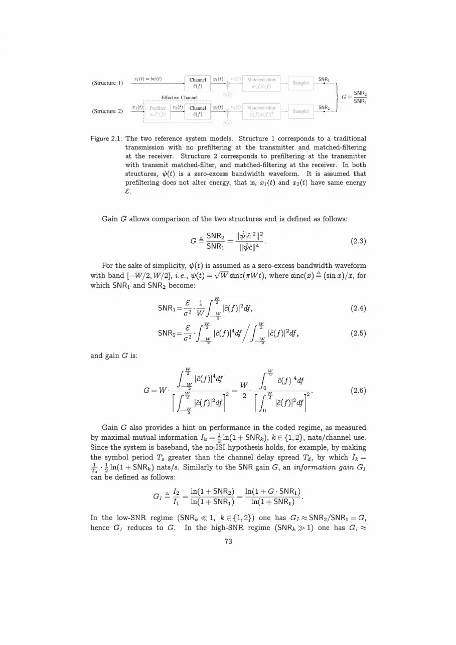
Prefilter/ c

⇤(f)Channel

c(f)+

n(t)

Matched-filter (f)|c(f)|2 Sampler

x

1

(t) x

2

(t) y

2

(t) r

2

(t) SNR2

Channelc(f)

+

n(t)

Matched-filter (f)c(f)

Samplerx

1

(t) = b (t) y

1

(t) r

1

(t) SNR1 )

G =SNR2

SNR1

(Structure 1)

(Structure 2)

Effective Channel

Figure 2.1: The two reference system models. Structure 1 corresponds to a traditionaltransmission with no prefiltering at the transmitter and matched-filteringat the receiver. Structure 2 corresponds to prefiltering at the transmitterwith transmit matched-filter, and matched-filtering at the receiver. In bothstructures, is a zero-excess bandwidth waveform. It is assumed thatprefiltering does not alter energy, that is, and have same energy.

Gain allows comparison of the two structures and is defined as follows:

SNR

SNR(2.3)

For the sake of simplicity, is assumed as a zero-excess bandwidth waveformwith band , i.e., , where , forwhich SNR and SNR become:

SNR (2.4)

SNR (2.5)

and gain is:

(2.6)

Gain also provides a hint on performance in the coded regime, as measuredby maximal mutual information SNR , , nats/channel use.Since the system is baseband, the no-ISI hypothesis holds, for example, by makingthe symbol period greater than the channel delay spread , by which

SNR nats/s. Similarly to the SNR gain , an information gaincan be defined as follows:

SNR

SNR

SNR

SNR

In the low-SNR regime (SNR , ) one has SNR SNR ,hence reduces to . In the high-SNR regime (SNR ) one has

73

SNR SNR SNR , and for channels with bounded , e.g.multipath channels, reduces to unity as SNR . is, therefore, the mostimportant parameter to be analyzed to determine performance of systems in bothuncoded and coded regimes, under the no-ISI hypothesis.

2.2 System Analysis Based on Gain

In this section, we find the lower bound of and the asymptotic value of asfor multipath channels (section 2.2.1), and derive a necessary and sufficient

condition for to be a monotonic non-decreasing function of , also showingexamples and counterexamples of channels verifying the condition (section 2.2.2).

2.2.1 Gain Limit Values

1) Lower bound of .By applying the Cauchy-Schwarz inequality to the denominator of eq. (2.3), one

has . Therefore, , implying that Structure2 in Fig. 2.1 cannot underperform Structure 1. Equality is achieved iff ,i.e. iff is constant for R , as can also be di-rectly shown by methods of variational calculus. The minimum gain is thusobtained when the magnitude of the channel transfer function is nonzero and flat,for frequency intervals where the amplitude of the spectrum of transmitted signalsis nonzero. Typically, this is true when the channel is perfect (channel transferfunction with constant amplitude) at least within the transmitted signal bandwidth.This condition easily holds for narrowband communications.

2) Asymptotic value of as .Consider the following multipath channel:

(2.7)

where and R are delay and amplitude of ray . Eq. (2.7) also modelsrealizations of channels with clusters. Supposing that a same interarrival timebetween two consecutive rays is not possible,1 it can be shown that [52], as ,the gain is:

(2.8)

and, therefore, irrespective of channel amplitudes.

1This hypothesis often holds with probability one for random channels, since interarrival times

are usually independent.

74

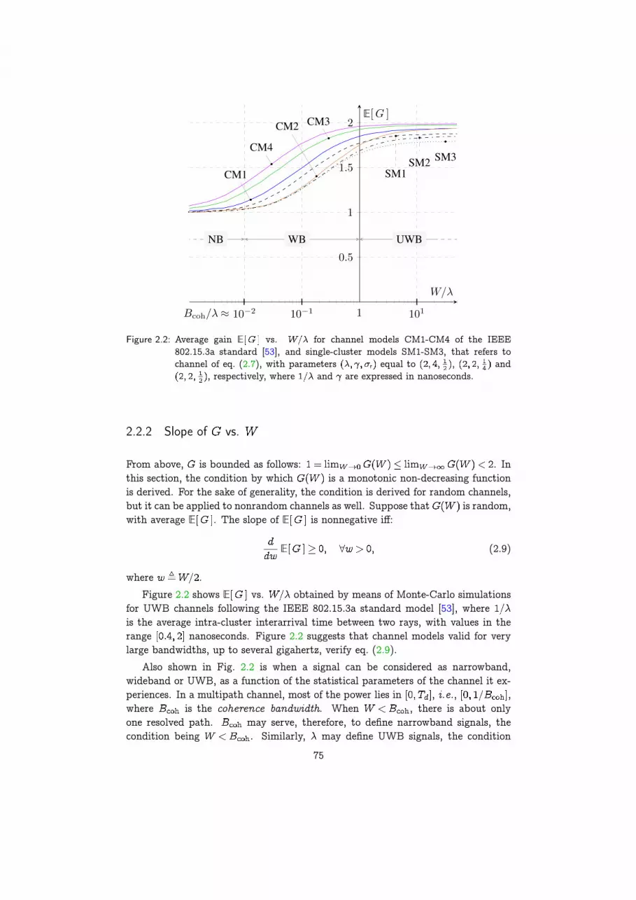
10�2 10�1 101

0.5

1

1.5

2

CM1

CM2 CM3

CM4

SM1SM2 SM3

WBNB UWB

1

W/�

E[ G ]

B

coh

/� ⇡

Figure 2.2: Average gain E vs. for channel models CM1-CM4 of the IEEE802.15.3a standard [53], and single-cluster models SM1-SM3, that refers tochannel of eq. (2.7), with parameters r equal to , and

, respectively, where and are expressed in nanoseconds.

2.2.2 Slope of vs.

From above, is bounded as follows: . Inthis section, the condition by which is a monotonic non-decreasing functionis derived. For the sake of generality, the condition is derived for random channels,but it can be applied to nonrandom channels as well. Suppose that is random,with average E . The slope of E is nonnegative iff:

E (2.9)

where .Figure 2.2 shows E vs. obtained by means of Monte-Carlo simulations

for UWB channels following the IEEE 802.15.3a standard model [53], whereis the average intra-cluster interarrival time between two rays, with values in therange nanoseconds. Figure 2.2 suggests that channel models valid for verylarge bandwidths, up to several gigahertz, verify eq. (2.9).

Also shown in Fig. 2.2 is when a signal can be considered as narrowband,wideband or UWB, as a function of the statistical parameters of the channel it ex-periences. In a multipath channel, most of the power lies in , i.e., ,where is the coherence bandwidth. When , there is about onlyone resolved path. may serve, therefore, to define narrowband signals, thecondition being . Similarly, may define UWB signals, the condition

75

being , for which a significant fraction of the multipath components can beresolved. For , the signal may be considered as wideband.

In general, a direct computation of E is a formidable task, even for simplemodels that do not account for clustering. Therefore, a condition, that does notrequire the explicit knowledge of E , for eq. (2.9) to hold, is derived below.

Proposition 1. Let be the frequency response of a realization of a randommultipath channel, and denote by its squared magnitude. ThenE is a monotonic non-decreasing function, i.e., condition of eq. (2.9) holds,iff:

E

E (2.10)

Proof. Interchange differentiation and expectation operators in eq. (2.9), and com-pute ; then discard the denominator, since it is always positive, and inter-change the order of expectations and integrations.

Note on eq. (2.10) that is the derivative of E up to a positive factordepending on .

An example of a channel model that verifies eq. (2.10) is the “Single-clusterModel” (SM). This model is similar to the IEEE 802.15.3a-CM1 [53] when re-stricted to the first cluster. In particular, the SM channel impulse response isgiven by eq. (2.7), where and are random variables. Interarrivaltimes are independent and exponentially distributed with averageE . Conditioned on , the distribution of the path amplitude

is an even function, and follows a log-normal distribution. Evenconditional moments are E r for , where

is the ray decay factor, r is the standard deviation of the Gaussian r.v.generating the log-normal r.v., and is the variance of . Odd conditionalmoments are nil. In order to compute E , the approach proposedin [54] for E is generalized here:

E E E

(2.11)

that, for and , provides E . In the right-hand side ofeq. (2.11), the inner expectation is over amplitudes conditioned on delays ,and the outer expectation is over delays only. Inner expectations are nonzero iffthe set can be partitioned into subsets with even cardinal-ity. With probability one, the set of indices can be equivalentlypartitioned. Logical conditions ensuring the partition can be derived. In the

76

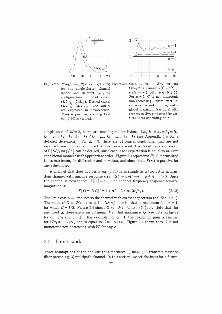
�20 �10 10 20

0.5

1

0

10 log

10

w�

F (w)

max

uF (u)

Figure 2.3: vs. (dB)for the single-cluster channelmodel and di� erent r

configurations. Solid curve:, . Dashed curve:, . and

are expressed in nanoseconds.is positive, showing that

eq. (2.10) is verified.

2 4 6 8 10

1

2

↵ = 1/4

↵ = 1

↵ = 0

0

W ⌧1

G

Figure 2.4: Gain vs. for thetwo-paths channel

with .For , is not monotonicnon-decreasing: there exist lo-cal maxima and minima, and aglobal maximum (see dots) withrespect to (indicated by ver-tical lines) depending on .

simple case of , there are four logical conditions, i.e., ;; ; (see Appendix 2.A for a

detailed derivation). For , there are logical conditions, that are notreported here for brevity. Once the conditions are set, the closed form expressionof E can be derived, since each inner expectation is equal to an evenconditional moment with appropriate order. Figure 2.3 represents , normalizedto its maximum, for different and r values, and shows that is positive forany relevant .

A channel that does not verify eq. (2.10) is as simple as a two-paths nonran-dom channel with impulse response , R, . Sincethe channel is nonrandom, E . The channel frequency response squaredmagnitude is:

(2.12)

The limit case reduces to the channel with constant spectrum (c.f. Sec. 2.2.1).The value of as is , that is maximum for ,for which . Figure 2.4 shows vs. for . Note that, forany fixed , there exists an optimum that maximizes (see dots on figurefor and ). For example, for , the maximum gain is reachedfor , and is equal to . Figure 2.4 shows that is notmonotonic non-decreasing with for any .

2.3 Future work

Three assumptions of the analysis thus far were: 1) no-ISI; 2) transmit matchedfilter precoding; 3) multipath channel. In this section, we set the basis for a future,

77

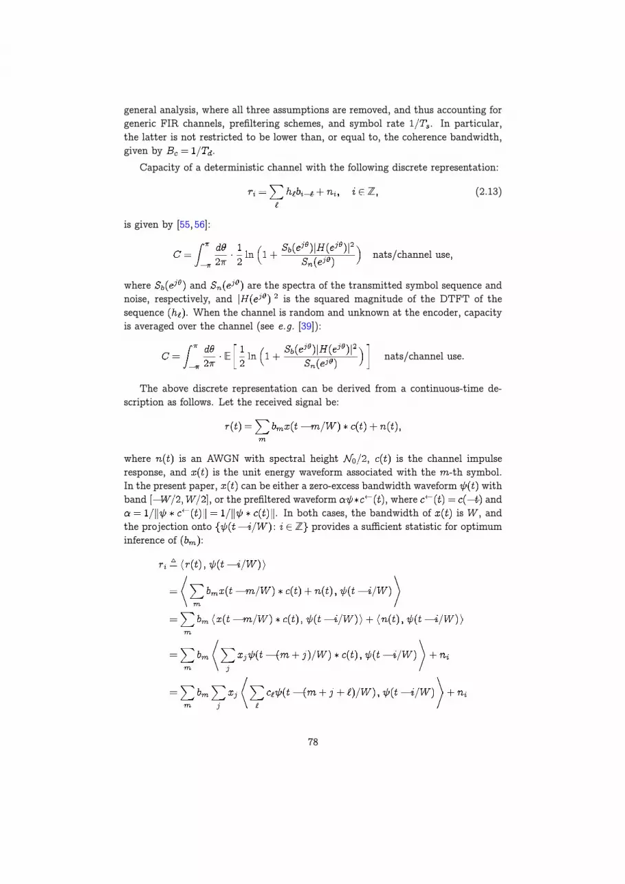
general analysis, where all three assumptions are removed, and thus accounting forgeneric FIR channels, prefiltering schemes, and symbol rate . In particular,the latter is not restricted to be lower than, or equal to, the coherence bandwidth,given by .

Capacity of a deterministic channel with the following discrete representation:

Z (2.13)

is given by [55, 56]:

nats/channel use

where and are the spectra of the transmitted symbol sequence andnoise, respectively, and is the squared magnitude of the DTFT of thesequence . When the channel is random and unknown at the encoder, capacityis averaged over the channel (see e.g. [39]):

E nats/channel use

The above discrete representation can be derived from a continuous-time de-scription as follows. Let the received signal be:

where is an AWGN with spectral height 0 , is the channel impulseresponse, and is the unit energy waveform associated with the -th symbol.In the present paper, can be either a zero-excess bandwidth waveform withband , or the prefiltered waveform , where and

. In both cases, the bandwidth of is , andthe projection onto Z provides a sufficient statistic for optimuminference of :

78

that has the form (2.13) as , hence:

E0

nats/channel use

where the expectation is taken over the channel spectrum, and 0 sinceN 0 . The channel is used every seconds, therefore the capacity in

nats/s is:

E0

nats/s (2.14)

For Structure 1, one has , E , and the capacity is given by:

E0

nats/channel use

For Structure 2, one has , and the capacity is given by:

E0

nats/channel use

It can be shown that:

A capacity gain can be defined as follows:

A careful analysis of the capacity gain in terms of (prefiltering) and(channel), which also depends on the two parameters and , represents a futureline of investigation.

Let see how this reduces to the previous analysis in absence of ISI. Underthe hypothesis of vanishing crosscorrelation of waveforms modulating symbols, thechannel becomes an AWGN channel with multipath. This assumption holds, forexample, by transmitting symbols farther apart than the channel delay spread ,i.e., the symbol period is such that , i.e., such that:

79

There is, indeed, no ISI, and the channel can be represented (for ) by:

Hereinafter, we will write instead of for notation simplicity.Equivalently, optimum inference of is based on:

N 0

For Structure 1, one has:

N 0

and the maximum mutual information is achieved with Gaussianinputs and assumes the well-known AWGN capacity expression:

SNR nats/channel use (2.15)

where here the channel is used every seconds, and:

SNR0

is that analyzed in the Letter, being .Similarly, for Structure 2, one has:

SNR nats/channel use (2.16)

where:SNR

0SNR

being SNR SNR the SNR gain analyzed in the Letter.Expressed in terms of nats/s, we have:

SNR nats/s

We adopted the notation and in place of and , respectively, to stressthat the above are mutual informations rather than capacities, that are derivedunder the constraint of a symbol period larger than the minimum, i.e., .

Similarly to the capacity gain defined above, we can define the following (mu-tual) information gain :

SNR

SNR

SNR

SNR

80

In the low-SNR regime, that is, when SNR , , one has:

SNR

SNR

and therefore the information gain is equal to the SNR gain studied in the paper.In the high-SNR regime, that is, when SNR , one has:

SNR

SNR SNR

In particular, for those channels (e.g. multipath channels) having bounded ,for large SNR.

2.4 Conclusion

This chapter investigated whether a large bandwidth is mandatory to maximallyexploit the potential benefits of the transmit matched-filter, in the absence ofISI. To this end, two transceiver structures, with and without prefiltering, werecompared based on a parameter indicating the SNR gain achieved by introducingthe prefilter. Performance depended on both transmitted signal bandwidth andchannel frequency response squared magnitude. Limit values of when the channelis affected by multipath were derived, for and , and it was proventhat for reaches the minimum, and is equal to one. A condition for

to be a monotonic non-decreasing function of was also derived for genericrandom channels. This condition was then specified for single-cluster multipathchannel models, and verified in the particular case of exponentially distributedinterarrival times and absolute path amplitudes following a log-normal distribution.Simulation experiments of channels following the IEEE 802.15.3a standard channelmodel showed a monotonic non-decreasing gain in for the four models of thestandard, suggesting that may also be monotonic non-decreasing for channelswith clusters. However, the analysis of a channel with two paths only was shown tobe a very simple counterexample, for which the gain was not a monotonic functionof .

In conclusion, a large bandwidth is not mandatory to achieve a maximumgain with transmit matched filter, although this seems to be the case for modelsdescribing realistic channels, such as the IEEE 802.15.3a model.

Results were obtained in terms of SNR gain . As discussed in Section II, aninformation gain can be defined, similarly to , as the ratio between the mutualinformation achieved with and without prefiltering. It was proven that, under theno-ISI hypothesis, essentially reduces to . This would be no longer true if theno-ISI hypothesis were removed, in which case an achievable “capacity gain” shouldbe analyzed. This will be the goal of future work together with two generalization:1) channel models that expand beyond multipath; 2) prefilter structures that ex-pand beyond transmit matched-filters. The former can be analyzed by specifyingfairly general channel models and studying when eq. (2.10) holds with respect to

81

the parameters specified in the channel model. The latter can be investigated byspecifying a prefilter that is proportional to , that encompassesboth transmit zero-forcing and transmit MMSE, for particular values of .

The setting used in this chapter, therefore, may serve towards a deeper under-standing of prefiltering effects beyond the transmit matched-filter case in multipathchannels.

82

Appendix

2.A Derivation of the case of eq. (2.11).

The goal is to evaluate E when the channel is:

Therefore:

Note that, in the previous expression, both and are random. Then:

Since the expectation E is on both and , but conditionalmoments of amplitudes are provided for fixed delays, we may split the expectationin the previous expression by conditioning first on delays :

E E E

(2.17)

Since amplitudes for different delays are uncorrelated, the inner expectation isnonzero when with both andeven numbers, and . For the case under analysis, the conditionsare:

;

, , and ;

, , and ;

, , and .

83

Therefore, explicitly, eq. (2.17) becomes:

E E E

E E

E E

E E

(2.18)

Since, in the Letter, we assumed that:

E r

inner expectations are:

E r

and:

E E E

Therefore, eq. (2.18) becomes:

E (2.19)

E r

E

E

E

(2.20)

84

Now expectations are only over delays. Assuming, as in the Letter, Poisson arrivals,i.e., E , , and the possible presence of a line-of-sight (LOS)component, it results:

E (2.21)

r LOS

LOS LOS

LOS LOS

LOS LOS (2.22)

when LOS when the line-of-sight component is present, and LOS otherwise.These integrals can be solved in closed form, providing the following result:

E r LOS

LOS

LOS LOS

LOS LOS (2.23)

85

86

CHAPTER 3Some results on Time Reversal vs.All-Rake Transceivers in Multiple

Access Channels

Time reversal, that is prefiltering of transmitted signals with time reversed channelimpulse responses, may be used in single user communications in order to movecomplexity from the receiver to the transmitter, and in multiuser communicationsto also modify statistical properties of multiuser interference. Imperfect channelestimation may, however, affect pre- vs. post- filtering schemes in a differentway. This issue is the object of this chapter; Robustness of time reversal (TR)vs. All-Rake (AR) transceivers, in multiple access communications, with respectto channel estimation errors, is investigated. Results of performance analysesin terms of symbol error probability and spectral efficiency when the receiver isstructured either by a bank of matched filters or by 1Rake, followed by independentdecoders, indicate that AR is slightly more robust than time reversal but requiresin practice more complex channel estimation procedures since all channels must besimultaneously inferred in the multiuser communication setting.

Field equivalence principles [57–60] state that the radiated field within a volume, with boundary , enclosing a source, can be computed by considering, in place

of actual source, an infinity of equivalent virtual sources placed on .Suppose the source is pointwise, impulsive, and located in a point .

The electromagnetic problem of finding radiated field in can be solved based onthe Green function.

From a communication perspective, knowing the channel at all points ofwould allow, in principle, to understand the nature of a source , that is, thelocation of a pointwise source within volume , that radiated the field observed on

. Sensing the channel on would require a multiantenna system and a perfectknowledge of impulse responses of channels between and all points on .

Time reversal is a technique that takes advantage of the above physical phe-nomenon and that was also proposed in acoustics [47, 48, 61]. By prefilteringtransmissions with a scaled version of the channel impulse response, reversed in

87

time, allows simplification of receiver design, since the channel is compensated byprecoding. Time reversal also focuses signals in space, given that there is onlyone “correct” location of the receiver that experiences the specific “time reversed”channel impulse response.

Pioneering work on single-antenna time reversal spread-spectrum communica-tions dates back to the nineties, where the time reversal pre-filter was named pre-Rake [50,51]. The basic idea was to pre-filter the transmitted pulse with the channelimpulse response reversed in time, therefore matching the transmitted signal withthe subsequent channel.

Precoding techniques for multiuser spread-spectrum systems were developedalong similar lines of receive filters: transmit Zero-Forcing (ZF) [62], that attemptsto pre-equalize the channel by flattening the effective channel formed by the cascadeof the pre-filter and the actual channel, is optimum in the high-SNR regime; transmitmatched-filter (MF), that has been recognized to be equivalent to the pre-Rake filterin [44], that conversely is optimum in the low-SNR regime; and finally, transmitMMSE (Wiener) filter minimizing the SINR was derived in [46] following previousattempts [63,64].

In recent years, along with the fast developing of narrowband MIMO systems,pre-coding techniques using multiple antennas at the transmitter were thoroughlystudied (for a complete overview on MIMO precoding see [65]). Since the math-ematical formulation of multiuser spread-spectrum is very close to that of MIMOcommunications (see [66] for an overview of this analogy), MIMO linear precoderscan be derived along similar techniques.

Time reversal was proposed in connection to UWB communications in [49], thatalso addressed equalization through an MMSE receiver. In [67], early experimentaldata, showing the feasibility of time reversal, were collected. Following, experi-mental investigations on multiple-antenna systems with time reversal [68–70], andperformance analyses [71], were also pursued. In [72, 73], compensation for pulsedistortion in connection to time reversal was investigated. In [74], the trade-offbetween the complexity of transmitter vs. receiver in terms of number of pathswas analyzed. In [75], the insensitivity of time reversal to the lack of correlationbetween channels in a MISO system was investigated. Finally, in [76], the effect oftime reversal on statistical properties of multiuser interference in communicationvs. positioning was explored.

The above investigations were all carried out based on the hypothesis of perfectchannel estimation. This hypothesis, however, is strong, since it is unrealistic,irrespectively of whether channel estimation is performed at the transmitter or atthe receiver. While previous works addressed the comparison of pre- and post-channel filtering, the problem remains of realistic imperfect channel estimationand of how this affects performance for time reversed vs. receiver-based channelestimation schemes.

This chapter addresses the above problem, by comparing single-antenna sys-tems using time reversal, against receiver-based equalization schemes such as theexemplary case of an AR receiver.

88

The adopted network model considers multiple access by user terminals (UTs)communicating to one basestation (BS), where both UTs and the BS have oneantenna only, and communication between each UT and BS adopts ultra-wideband,impulse-radio signaling.

Performance comparison of TR vs. AR transceivers will be carried out in termsof effect of imperfect channel state information (CSI) on symbol error probabilityof a generic information-bearing symbol for a given UT (see [77] for a work on aclose topic regarding CDMA systems). The analysis will further explore robustnessof TR vs. AR, by finding the maximum achievable rate for the uplink channel.Finally, the maximum information rate, that takes into account channel estimationoverhead, will be explored.

The chapter is organized as follows: Section 3.1 contains the system model; Sec-tion 3.2 is devoted to the performance analysis in terms of symbol error probability;Section 3.3 contains results of comparison in terms of uplink rate of the network;Section 3.4 suggests future works, and conclusions are drawn in Section 4.4.

3.1 Reference Model

3.1.1 Network Model

A multiple access channel where independent sources transmit information-bearing symbols to a common sink is considered (uplink communication channel).Borrowing the terminology from the cellular network field, sources of informationare called user terminals (UTs) and the sink is called basestation (BS). However,UTs and BS are intendend to designate more than what the name implies. Forexample, in a typical WLAN, a BS is a fixed (e.g. desktop) or mobile receiver (e.g.tablet, laptop, mobile phone) and UTs are peripherals or other fixed vs. mobiledevices. Figure 3.1 shows the adopted network model.

A generic UT transmits data, that is encoded into a sequence of information-bearing symbols Z . This set of symbols is partitioned into blocksof symbols each, Z where T. TheSUBMITTED TO THE IEEE TRANSACTIONS ON WIRELESS COMMUNICATIONS 3

BS

UTk

UTKUT1

FIG. 1: Network model: several user terminals (UTs) transmit information-bearing symbols to a common sink, i.e.,

basestation (BS).

comparison in terms of uplink rate of the network. Section V contains the conclusions.

II. REFERENCE MODEL

This section is organized as follows: II-A. Network model; II-B. Single User Channel; Multiuser

Channel; II-D. Channel Estimation and Data Transmission.

A. Network Model

A multiple access channel where K independent sources transmit information-bearing symbols

to a common sink is considered (uplink communication channel). Borrowing the terminology

from the cellular network field, sources of information are called user terminals (UTs) and the

sink is called basestation (BS). However, UTs and BS are intendend to designate more than what

the name implies. For example, in a typical WLAN, a BS is a fixed (e.g. desktop) or mobile

receiver (e.g. tablet, laptop, mobile phone) and UTs are peripherals or other fixed vs. mobile

devices. Figure 1 shows the adopted network model.

A generic UTk transmits data, that is encoded into a sequence of information-bearing symbols

{bk[m] : m � Z}. This set of symbols is partitioned into blocks of n symbols each, {bk[i] : i � Z}

where bk[i] = (bk[in], . . . , bk[(i + 1)n � 1])T. The length n of the block in terms of symbols will

be linked below with the coherence time Tcoh of the channel. Each block is transmitted by the

following signal:

sk,i(t; bk[i]) =(i+1)n�1�

m=in

bk[m]gk,m(t � mTs), (1)

May 17, 2014 DRAFT

Figure 3.1: Network model: several user terminals (UTs) transmit information-bearingsymbols to a common sink, i.e., basestation (BS).

89

Modulator 1 Channel 1 +

n(t)

b

1

s

1

(t) x

1

(t)Demodulator 1

y(t)b

1

Modulator 2 Channel 2b

2

s

2

(t) x

2

(t)

......

Modulator K Channel K

bK sK(t) xK(t)

Figure 3.2: System model. The transmitter is formed by modulators. Radiated signalsare a� eted by di� erent channels and white gaussian noise at the receiver.Receveir consists in one demodulator shown on figure for the example case ofuser .

length of the block in terms of symbols will be linked below with the coherencetime of the channel. Each block is transmitted by the following signal:

s (3.1)

where s (sec) is the symbol period and is the unit energy waveformassociated with the -th symbol of user . In general, is a spread-spectrumsignal at user prefilter output, and has band W W , that is, its spectrum isnonzero for W . Assuming that s areorthonormal, or very mildly crosscorrelated, the energy of in eq. (3.1)is E ; Since the block has duration s, the average power is P

E s.In the adopted model, demodulation at BS is performed on a block-by-block

basis. Index , that specifies the block number, is thus dropped. Consider for thesake of simplicity in eq. (3.1):

(3.2)

Figure 4.1 shows the system model, including modulators producing transmit-ted signals, , , affected by propagation within different channelsand corrupted at the receiver by white gaussian noise . The receiver consists inone demodulator.

90

Transmitted signal of each user propagates over a multipath channelwith impulse response and is distorted into :

(3.3)

where and are amplitudes and delays of the paths of ,respectively.

The received signal is:

(3.4)

where is a white Gaussian noise with flat power spectral density 0 (W/Hz).Throughout the chapter, the receiver estimates transmitted symbols of user ,

, on a symbol-by-symbol basis, by consider-ing users as unknown interference over user ; for example, Fig. 4.1 shows thedemodulation of user . As detailed below, transmissions are symbol-synchronousbut not necessarily chip-synchronous, therefore the symbol-by-symbol demodula-tion does not imply any performance loss. In the adopted model, the receiver isa single user detector, and as such suboptimal, since it does not take into accountthe possibility of joint multiuser detection. How channel is estimated and howerror affected estimated channels play a role in the model will be explained furtherdown in this section in association with the different modulation and demodulationstructures. Expliciting signals for the symbol at time epoch , and denotingby , eqs. (3.2), (3.3) and (3.4) become:

(3.5)

(3.6)

(3.7)

3.1.2 Single User Channel

Since the system symbol-synchronous, analysis may refer to transmission of onegeneric symbol, that is chosen as symbol , , denoted by . If transmissiondoes not foresee prefiltering, that is, a zero-excess bandwidth pulse withbandwidth W and unit energy is transmitted to modulate , the received signalis:

(a)s c

(b)s

˚i�W c

91

(c)s

˚i�˚i� W (3.8)

where in (a) the spreading sequence s s T and the chip periodc are made explicit; (b) follows from , and therefore also , being

bandlimited to W ; and (c) follows from assuming c ˚i� W, being ˚i� a positiveinteger called impulsiveness index, that introduces a model to account for a pulseduration shorter than chip duration, as common in UWB communications. In thefollowing, time-hopping is considered, for which all s are zero, but one.

By projecting eq. (3.8) onto W ˚i� , thefollowing discrete model is obtained:

˚i� (3.9)

where ˚i� T˚i� T is the first vector of the canonical basis of R ˚i�, is ˚i� ,and is Toeplitz with dimensions ˚i� ˚i� and elements .Since is causal, it is assumed that for , and since has finitedelay spread , it is assumed that for ˚i�, being c ˚i� W;therefore, is banded Toeplitz.

In general, for a system with prefiltering, with prefiltering impulse response ,eq. (3.9) generalizes to (see e.g. [66]):

(3.10)

where is a Toeplitz matrix with dimensions ˚i� ˚i� andelements W .

Prefiltering is introduced in order to compensate channel effects; in particular,prefiltering is based on an estimated version of the channel impulse response. Inother words, imperfect prefiltering may be matched to channel estimation errorpatterns. If prefiltering is imperfect, as will be justified in Subsection 3.1.4, theerror due to the estimation process can be modeled as a white Gaussian process

, that is added to as follows:

(3.11)

where N , where accounts for estimation accuracy, andis such that .

No prefiltering, All-Rake receiver.The traditional (or conventional) receiver is a matched-filter, i.e., an AR receiver

in the case of a multipath channel. Knowing the time-hopping spreading sequenceand the resolved channel , a sufficient statistic for is obtained by projecting

the received signal onto , or, equivalently, onto :

T

92

where N 0 .As occurs in the prefiltering, also the AR receiver is affected by possible channel

estimation errors. If the AR is provided with imperfect channel state information(CSI), that is, operates using an estimation of channel that is impaired by anerror N ˚i� , then the AR combines paths through instead of

, and inference of is based on:

T T T T

(3.12)

where T T T ˚i� T, being the nonzero dimension of .

Time Reversal prefiltering, 1Rake receiver.The time reversal prefilter is represented by ˚i� , where

guarantees that prefiltered and non prefiltered transmitted waveforms have sameenergy. Time-hopping implies , and ˚i� ˚i� . A1Rake receiver is given by ˚i� . Denoting by the time-reversal prefilter matrix,one has:

T ˚i� T ˚i� T ˚i� T ˚i� ˚i� (3.13)

being ˚i� N 0 .If the transmitter is provided with imperfect CSI, then model of eq. (3.11) holds,

and eq. (3.13) becomes:

T ˚i� T ˚i� T ˚i� ˚i� (3.14)

AR vs. TR.As well-known [76], TR is equivalent to a system without prefiltering and AR

in terms of the signal-to-noise ratio. From a single user perspective, there is noperformance difference in both uncoded (symbol error probability) and coded (chan-nel capacity) regimes between the two transceiver structures. Moreover, previouswork [74] suggested that sets of equivalent systems can be obtained with partialRakes compensating for partial time reversal transmitter structures. In the caseof imperfect CSI, the comparison of the different structures is the object of thischapter.

3.1.3 Multiuser Channel

A straightforward extension of eq. (3.9) to users is as follows:

(3.15)

93

where ˚i� and ˚i� models the chip-asynchronism by making i.i.d.according to a uniform distribution. This extension holds based on the hypothesisthat all UTs are symbol-synchronous. This hypothesis is reasonable since, as furtherdiscussed in Subsection 3.1.4, the BS broadcasts in a link setup phase a knownsequence to the UTs. Denoting by the spreading sequence aftertransition in the multipath channel, and by:

T

the spreading matrix, eq. (3.9) can also be rewritten as follows:

(3.16)

where T. For systems with prefiltering, eq. (3.15) generalizes to:

(3.17)

where matrices and have same dimensions as and of eq. (3.10), respec-tively, and eq. (3.16) holds with . In the presence of imperfect CSI,

in eq. (3.17) is substituted by , as defined in eq. (3.11), where estimationerrors are independent with respect to .

No prefiltering, All-Rake receiver.The decision variable following the matched filter of user is:

T T

(3.18)

where , represents the MUI, andT

N 0 .

If the AR is provided with imperfect CSI, then signal is projected ontoinstead of , hence:

T T T

(3.19)

whereT

N 0 .

Time Reversal prefiltering, 1Rake receiver.

94

Preamble

Postamble0 T 2T

bk[0] bk[1]

· · ·· · ·

Figure 3.3: Data transmission structured into blocks for UT .

With time reversal, the decision variable for user becomes:

T T T (3.20)

where ˚i� is the delay (in samples) to which the 1Rake is synchronized.In the presence of imperfect CSI, the decision variable is:

T T T (3.21)

AR vs. TR.As well-known [76, 78], time reversal usually increases the kurtosis of the inter-

ference at the output of Rake receivers. This follows from the fact that the effectivechannel impulse response formed by the combination of prefilter and multipathchannel has a peaked behavior, whereas without time reversal the behavior isnon-peaked. While in the single user case the two schemes are equivalent, thisequivalence does not hold in the multiuser case. The impact of estimation errorswill be investigated below.

3.1.4 Channel Estimation and Data Transmission

For both AR and TR, the channel impulse response estimation takes place, at leastpartially, both in the transmitter and in the receiver.

Actual transmission of the set of information-bearing symbols requires, there-fore, additional symbols to be sent either in a preamble or in a postamble of theblock [79], as shown in Fig. 3.3.

Training is the simplest estimation process to evaluate the necessary channelstate information. Time-Division Duplexing (TDD) is assumed as commonly wit-nessed in impulse-radio as well as common WLAN transmissions. Since precodingof UT does not depend on channels experienced by users , feedback is not anecessary feature, given that channel is reciprocal. Note that there is no dedicatedtraining since precoding is supposed to be disjoint, that is, the precoding vector ofeach UT does uniquely depend on the channel between its transmitter and the BS

95

and is in particular independent of channels and precoding vectors of other UTs(see [80] for a thorough discussion).

Transmission follows a scheme that is shown at a glance in Fig. 3.4a and inmore detail in Fig. 3.4b. Figure 3.4 summarizes the organization of the differentlinks (downlink, i.e., broadcast, vs. uplinks) over time, where durations of data,preamble and postamble are indicated in terms of number of chips ( , , d,

). In particular, Fig. 3.4b shows an information exchange between the BS andeach UT consisting in four phases:

1. Downlink Channel Training: the BS broadcasts a training sequence oflength ˚i� samples, known by the set of UTs, followed by a zero-paddingsequence of ˚i� samples (idle period), that allows each UT to receive thetraining sequence smeared by the channel; each UT estimates the channelbased on the received samples and the knowledge of the transmitted trainingsequence, as further detailed in the remaining part of this section. Thistraining sequence may be also used for network synchronization at symbollevel.

2. Uplink Channel Training: each UT transmits a training sequence of length˚i� samples, known by the BS, followed by a zero-padding sequence of

length ˚i� samples; these training sequences are assumed pseudo-noise (PN)sequences rather than orthogonal given that each UT chooses its sequenceindependently from the others. The BS estimates channels through the ob-servation of the superposition of training sequences, that have been distortedby respective channels.

3. Data Transmission: each UT sends information-bearing symbols of ablock, corresponding to d ˚i� ˚i� samples;

4. Idle: each UT sends a zero-padded postamble of duration ˚i� samples.

During the downlink training, the BS broadcasts its training sequence to theUTs. With reference to model of Section 3.1, and in particular to eq. (3.9) andimpulsiveness index ˚i�, the received signal at UT is:

˚i� (3.22)

where is the ˚i� ˚i� vector of received samples, is the ˚i�˚i� ˚i� Toeplitz channel matrix, is the training sequence,

is the ˚i� training sequence accounting for impulsiveness, and is the˚i� ˚i� white Gaussian noise vector.

Eq. (3.22) can be rewritten as follows:

(3.23)

where now is a ˚i� ˚i� ˚i� Toeplitz matrix and is the ˚i� channelvector.

96

BSPre 1Pre 2

...Pre K

BroadcastUplink 1Uplink 2

...Uplink K

Data 1Data 2

...Data K

Post 1Post 2

...PostK

Time0 NDL

t NUL

t Nd NUL

g

(a) Transmission scheme: at a glance..

BS UT

Preamble Data Postamble

Time

0

T

NDL

t

L

NUL

t

L

Nd

L 0

L

(b) Detailed transmission scheme.

Figure 3.4: Transmission schemes. In (a): transmission scheme at a glance. In (b):detailed transmission scheme. Phase 1 : the BS broadcasts a training sequenceof length ˚i� samples (corresponding to ˚i� W seconds) that is receivedby each UT starting at time . Each multipath channel spreads the sequencefor ˚i� samples, hence each UT listens from time to time ˚i� ˚i� samples.This training sequence may be also used for network synchronization at symbollevel. Phase 2 : Once the training sequence is received, each UT transmits itsown training sequence of length ˚i� samples to the BS (preamble). Byreciprocity, channels spread these sequences for ˚i� samples, therefore eachUT remains idle for ˚i� samples. Phase 3 : Each UT transmits a sequenceof information-bearing symbols for d ˚i� ˚i� samples. Phase 4 : Each UTtransmits a sequence of null symbols denoted with (postamble).

97

In order to minimize the signal-plus-interference-to-noise ratio, UT may usean MMSE estimation of , where the cause of interference is due to multipath.However, the use of PN sequences as training sequences is very common, due totheir good autocorrelation properties. In fact, PN sequences have periodic ACF ofthe following form [81,82]:

that is asymptotically impulse-like, as .Asymptotically then, and dropping the superscript to unclutter notation,

T , and MMSE reduces to a matched-filter, and estimation isas follows:

T T N N (3.24)

Dividing by the previous expression yields:

(3.25)

where N N . Note that, as well-known (e.g. [83]), the estimationcan be made as accurate as desired by increasing . For antipodal sequences,say A A with A , the energy of the training sequence is A ;therefore, can be increased either by increasing power spent on training, thatis, by increasing A , or by increasing time spent for training, that is, by increasing

, or both.

In the uplink training, the BS receives the superposition of the sequences ofusers each filtered by the corresponding channel, that is:

(3.26)

having defined:

T (3.27)

As previously, the superscript is dropped to unclutter notation.The goal of the BS is to linearly estimate by observing , knowing :

T T T (3.28)

where is the ˚i� vector of channel estimations, being the ˚i� vectorrepresenting estimate, and T is the ˚i� ˚i� matrix representing the esti-mator. All common linear estimators, that is ZF (Zero-Forcing), RZF (RegularizedZero-Forcing), MMSE (Minimum Mean Square Error) and MF (Matched Filter),

98

can be described by the following expression, parametrized by and :

T T T (3.29)

Indeed, MMSE is obtained with N ; ZF with ; MF with; RZF with .

In the simple case of ZF, the form assumed by eq. (3.28) is as follows:

T T N NT (3.30)

and, therefore, the -th tap of the channel of generic user is:

Here, is a correlated Gaussian random variable with variance coinciding withthe ˚i� -th diagonal element of N

T .Assuming all UTs are transmitting the same power, i.e., is the same for

each , the approximation T allows to assume uncorrelatedestimation errors, since T , and thus:

N N (3.31)

3.1.5 Performance measures

In both system structures, the statistic for inferring the transmitted symbol ofuser can be written in the following form:

where is a r.v. representing noise, and are r.vs. dependingon multipath channels, random time-hopping codes, random delays, and estimationerrors.

Two performance measures are considered.In the uncoded regime, the probability of error as defined by:

P P

is considered.In the coded regime, mutual information with Gaussian inputs and a bank of

matched-filters followed by independent decoders is considered; for the generic user, this is given by:

nats/channel use (3.32)

where is the mutual information between the transmitted symbol andthe decision variable . Since a channel use corresponds to c ˚i� seconds,

99

the sum-rate achieved by the set of users is:

˚i� nats/s (3.33)

having indicated with the mutual information (3.32) for a generic user.Finally, a spectral efficiency equal to

R ˚i� (nats/s)/Hz (3.34)

is obtained.

3.2 Probability of Error

3.2.1 Single User

The main contribution of this subsection is to show that imperfect TR and ARachieves the same probability of error, and, therefore, that the same accuracy isneeded for channel estimation at transmitter and receiver in order to achieve agiven error probability.

With reference to decision variables of eq. (3.14) and of eq. (3.12), theprobability of error, in both cases, is:

P A P A P A (3.35)

where the first equality follows from belonging to A A with equal probability,and the second equality follows from the distribution of being an even function.For the power constraint, it results A . Equivalence of for the two cases isderived by showing that and have the same distribution.

To this end, rewrite the decision variable conditioned on A. Withoutloss of generality, and for the sake of simplicity, consider . Then:

A T A T A T A T

Similarly, the decision variable conditioned on A is:

A T

where N N . By comparing the two expressions, is equivalent to ,the equivalence being defined as producing the same , iff term T in isdistributed as in . This is, indeed, the case; by choosing an orthogonalmatrix such that , one has:

T T T T

where N N , hence the equivalence in terms of distributions, and, therefore,probability of error is verified.

100

Based on the described training algorithm, samples of the channel estimated byare:

R (3.36)

where is the channel length in terms of samples ( , being the delayspread of the channel); T is the vector of samples of the channelimpulse response, where:

N is a Gaussian random vector modeling the uncertainty of estimation,being N

r where r is the energy of the training sequence received byduring the Training Phase I [83].

Focus on transmission of one symbol only, that for the sake of simplicity isassumed binary, . Assume that the symbol period is formed of chips ofduration ; therefore, the symbol period has duration . The sampledreceived signal is:

where is the trasmitted energy per symbol, is the convolutionmatrix describing the channel, is the transmitted waveform, and

N N . In particular, for , and otherwise,where are the elements of as in eq. (3.36). A 1Rake yields to the followingdecision variable, upon which depends the decision on :

T (3.37)

and N N . Define:T

(3.38)

then eq. (3.37) becomes:(3.39)

The two performance measures analyzed are the signal-to-noise ratio SNR:

SNRN

(3.40)

where is the SNR loss, that is a r.v. since is a random vector, and the symbolerror probability:

P (3.41)

As derived in Appendix 3.A, the PDF of is:

f fT

(3.42)

101

where fT is the Student T-distribution with degrees of freedom and non-central parameter . Figure 3.5 shows simulated histograms vs. f fordifferent values of and . Values of corresponds, for example, to a channelwith delay spread of ns, and a signal with a bandwidth of GHz.Values of depends on r , and, therefore, on the training sequence powerand the duration of the training. By comparing Fig. 3.5(a) vs. (b), it is shown,as can be expected, that approaches when the estimation improves. It canbe shown that, as , i.e., for vanishing estimation errors, the PDF tends to

, and no loss in eq. (3.39) occurs. By comparing Fig. 3.5(a) vs. (c), itis shown that departs from as increases. This can be intuitively justifiedas follows: for a given accuracy, the total uncertainty on the channel increaseswith the number of resolved paths , and, therefore, as increases, thevariance of the estimation error on each path must decrease to avoid reduced, oreven worse, performance. Moreover, physical multipath channels become more andmore sparse as bandwidth increases: the number of multipath components, that is,the number of resolvable paths, is indeed limited, and so is the energy gain thatcan be carried by the whole channel. Hence, as bandwidth increases, there areno multipath components in an increasing fraction of the taps composing theresolved channel, that, therefore, become a mere source of nuisance.

Note that, in eq. (3.42), is regarded as nonrandom since during each coherencetime the channel remains constant. This allows to derive, for example, the symbolerror probability that affects the system during a particular coherence time, asstudied below. However, if average performance over multiple coherence time isof interest, then the PDF of must be regarded as the conditional pdf given .Nonetheless, although depends upon , f depends upon only via . Not theentire channel realization affects , but just its energy . Therefore, although inthe following is regarded as nonrandom, it is just to be nonrandom, that is afading coefficient.

There are two main detrimental effects that imperfect estimation implies onSNR and .

The first effect is a reduction in the SNR. The variance of the useful termin eq. (3.39) is, indeed, equal to : with perfect CSIT, ,

while with imperfect CSIT, , and therefore measures the lossof variance in the useful term, and thus in SNR (see eq. (3.40)), due to the imperfectknowledge of the channel.

The second effect is the presence of a symbol error probability floor dependingon , irrespective of the amount of power spent in transmission (Data TransmissionPhase), and only depending on the energy spent during the Training Phase I.Accuracy of estimation can bound, therefore, the achievability of low (uncoded)symbol error probability. The symbol error probability floor appears as N ;in this asymptotic case, the decision variable tends to:

T

102

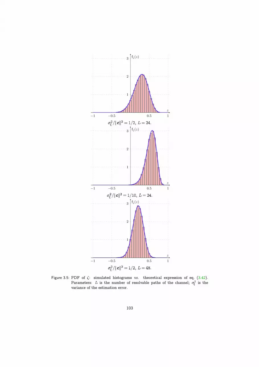
�1 �0.5 0.5 1

1

2

3

z

f⇣(z)

, .

�1 �0.5 0.5 1

1

2

3

z

f⇣(z)

, .

�1 �0.5 0.5 1

1

2

3

z

f⇣(z)

, .

Figure 3.5: PDF of : simulated histograms vs. theoretical expression of eq. (3.42).Parameters: is the number of resolvable paths of the channel; is thevariance of the estimation error.

103

and decision on is made based on the sign of , hence:

floor P

P T

The exact symbol error probability is (see eqs. (3.41) and (3.39)):

P

P

Nf (3.43)

where the dependence on and (see eq. (3.42)) is explicited in f .Figure 3.6 shows vs. N for different values of and , and compares

the symbol error rate obtained through Monte-Carlo simulations (points with errorbars on figure) with the analytical expression of (solid lines) given by eq. (3.43).Observe that, as expected, increased accuracy of the estimation yields to decreased

floor. Furthermore, for fixed and N, increased yields to increased :increasing by a factor of two implies a loss of approximately dB for floor

(see N dB on figure), while the floor does not depend on ,hence same performance is reached for high SNR irrespective of the bandwidth.

3.2.2 Multiuser

In the multiuser setting, although the expression for the probability of error remainsas in eq. (3.35), there are three sources of errors: thermal noise, imperfect CSI, andmultiuser interference (MUI). In particular, as N increases, the last two factorsboth lead to a probability error floor, i.e., floor as N ,being the load of the system.

Figures 3.7 and 3.8 show the probability of error vs. N (dB) for systemswith ˚i� vs. ˚i� , respectively, and for different values of and ,

. In particular, in both figures, the left-hand side plot(Fig. 3.7a and 3.8a) refers to TR, while the r.h.s. plot (Fig. 3.7b and 3.8b) refers toAR. Figures show that floors depend on a combination of both imperfect CSI andMUI. For low-SNR, i.e., N, is not very sensitive to estimation errors: onfigures, systems with same load have similar at low-SNR, and leads to different

floor at high-SNR, N. On the contrary, for fixed estimation error variance, increased implies increased for any SNR, and contributes to a higher error

floor. All figures are obtained by Monte-Carlo simulations of finite-dimensionalsystems with chips. By comparing Figs. 3.7 (a) and (b), that both refer tosystems with ˚i� , AR is shown to outperform TR when imperfect CSI is the maincause of error, and vice versa when the load is the main cause of error: compare, forexample, the two cases and . A similar behavior can be observedwith impulsive systems (Fig. 3.8) with even more emphasis. Figure 3.8 (a) and

104

�2

⇠

kck2

=

1

2

, L = 24

�2

⇠

kck2

=

1

10

, L = 24

�2

⇠

kck2

=

1

10

, L = 48

�5 0 5 10 15 20 25 30 35 40

10�3

10�2

10�1

E/�

2

N

(dB)

Pe

Figure 3.6: Symbol error probability vs. N for di� erent values of the number ofresolved paths and the estimation error variance .

(b) shows performance of systems with ˚i� , and indicates that performance ofTR is strongly limited by the presence of estimation errors, while when MUI is thelimiting cause TR and AR have similar performance (see for example curves with

and ).

105

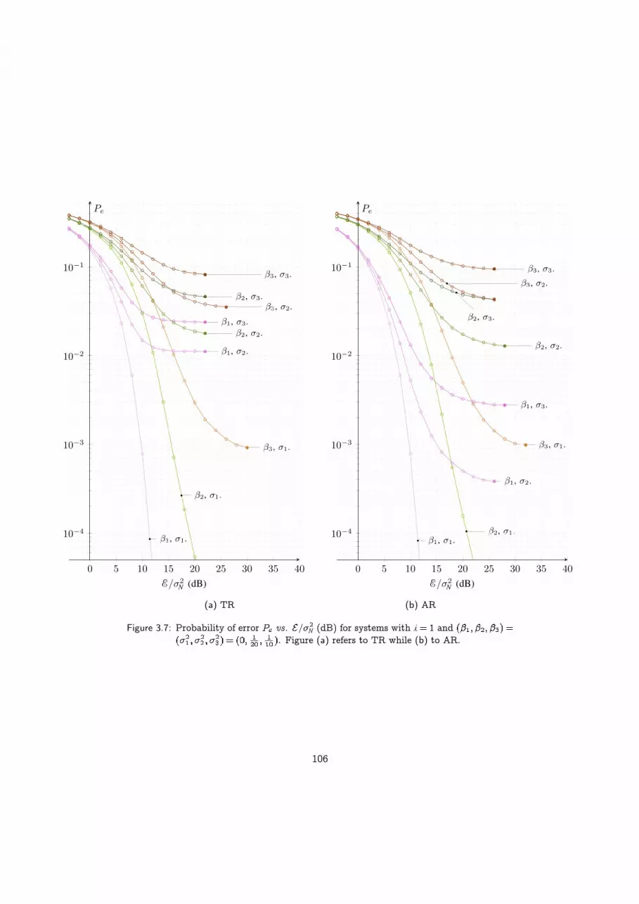
�1

, �1

.

�1

, �2

.

�1

, �3

.

�2

, �1

.

�2

, �2

.

�2

, �3

.

�3

, �1

.

�3

, �2

.

�3

, �3

.

0 5 10 15 20 25 30 35 40

10�4

10�3

10�2

10�1

E/�

2

N (dB)

Pe

(a) TR

�1

, �1

.

�1

, �2

.

�1

, �3

.

�2

, �1

.

�2

, �2

.

�2

, �3

.

�3

, �1

.

�3

, �2

.�3

, �3

.

0 5 10 15 20 25 30 35 40

10�4

10�3

10�2

10�1

E/�

2

N (dB)

Pe

(b) AR

Figure 3.7: Probability of error vs. N (dB) for systems with ˚i� and. Figure (a) refers to TR while (b) to AR.

106

�1

, �1

.

�1

, �2

.

�1

, �3

.

�2

, �1

.

�2

, �2

.

�2

, �3

.

�3

, �1

.

�3

, �2

.

�3

, �3

.

0 5 10 15 20 25 30 35 40

10�4

10�3

10�2

10�1

E/�

2

N (dB)

Pe

(a) TR

�1

, �1

.

�1

, �2

.

�1

, �3

.

�2

, �1

.

�2

, �2

.

�2

, �3

.

�3

, �1

.

�3

, �2

.

�3

, �3

.

0 5 10 15 20 25 30 35 40

10�4

10�3

10�2

10�1

E/�

2

N (dB)

Pe

(b) AR

Figure 3.8: Probability of error vs. N (dB) for impulsive (˚i� ) systems with. Figure (a) refers to TR while (b) to

AR.

107

3.3 Mutual information, Sum-Rate, and Spectral Efficiency

In this section, mutual information (3.32) is derived for AR and TR. The other meritfigures (3.33) and (3.34) follows directly, although all the elements for a comparisonare already included in (3.32).

3.3.1 Derivation of Mutual Information

The decision variable for both the imperfect TR (c.f. eq. (3.21)) and AR (c.f.eq. (3.19)) can be cast in the following form:

(3.44)

where N 0 .Let specify and give an interpretation of the terms , , for both

TR and AR.

TR coupling coefficients.For TR, the term is given by:

T T T

where R denotes a vector with same components of vector in reversedorder, i.e., , . The term , , is:

T T T

(3.45)

where T T T ˚i� T being the ˚i� autocorrela-tion sequence of ˚i� , and, similarly, T T T ˚i� T with aGaussian random vector with non-identity correlation.

In order to provide an interpretation of the above expressions, it is useful tostart with the case of no estimation error. In general, the decision variable at theoutput of the matched filter of user is given by the -th sample of the sum of bothintended and interference signals, plus noise. In the special case of no estimationerrors, is the square root energy of channel , i.e., the maximum tapof the effective channel, while is either equal to zero if the effective channel ofuser , that occupies ˚i� out of ˚i� degrees of freedom in a symbol period,is not present at delay , or to a random resolved path of the effective channel ofuser , the randomness owing to random hopping and asynchronism. In presence ofestimation errors, is smaller than, although in general in the neighbourhood of,the square root energy of channel due to the mismatch between and , and

108

is either equal to zero if the perturbed effective channel of user , that occupies˚i� out of ˚i� degrees of freedom in a symbol period, is not present at

delay , or equal to a random path of the perturbed effective channel of user ,the perturbation owing to the imperfect channel estimation of user .

AR coupling coefficients.For AR, the set of coupling coefficients are:

TT (3.46)

T

(3.47)

where , , and . We can think of asthe perturbed direction along which the received signal is projected in order todecode user ; represents, therefore, the “mismatch” between the perturbedand unperturbed channels of user ; represents the coupling between user, that is perturbed, and another user . As in the TR case, a channel impulse

response occupies a fraction, that is approximately equal to , of theavailable degrees of freedom in a symbol period; Opposite of the TR case, wherethe perturbation affects user in , user is perturbed in the AR case (through

), user appearing with the true channel impulse response .

Derivation.Being each term in the r.h.s. of eq. (3.44) independent from the other terms,

mutual information can be derived once the distributions of andare known. The former depends on both the random channel impulse responseand estimation errors of user , and the latter on the random channel impulseresponses and estimation errors, and the random delays with respect to user .Hence, the final form assumed by strongly depends on the channel model;however, in the following, the effect of the time-hopping and random asynchronismwill be enucleated, without enter in the computation of a mutual information whena particular channel model is adopted; this last task is addressed by simulations,where the IEEE 802.15.3a model [53], that is valid for bandwidths up to severalgigahertz, is selected.

As for TR, since the effective channel of user occupies a fraction˚i� ˚i� , and user , due to the assumptions on independence and uniformity of

hopping codes and asynchronism, selects uniformly at random one of the ˚i� samplesavailable per symbol period, then , , is equal to zero with probability ,and is distributed as the generic path of the effective channel with probability, that is:

(3.48)

where indicates the distribution of the generic path of the effective channelof user (that is independent of ). In presence of estimation errors, the aboveargument holds, that is, , , is equal to zero with probability , and is

109

�1 �0.5 0 0.5 1

5

10

15P

AR

(a)

�1 �0.5 0 0.5 1

5

10

15P

TR

�1 �0.5 0 0.5 1

5

10

15P

TR

(b)

�1 �0.5 0 0.5 1

5

10

15P

AR

(c)

�1 �0.5 0 0.5 1

5

10

15P

TR

�1 �0.5 0 0.5 1

5

10

15P

TR

(d)

�1 �0.5 0 0.5 1

5

10Pa

(e)

Figure 3.9: PDFs and of the variables , , and , respectively. Distributionsdo not depend on the particular user . Figs. (a) and (b) correspond to avariable , , in systems without estimation errors; Figs. (c) and (d)correspond to a variable , , in systems with estimation errors withvariance ; Fig. (e) corresponds to a variable in systems with asame error variance.

110

distributed as the generic path of the perturbed effective channel with probability:

(3.49)

where indicates the distribution of the generic path of the perturbed effectivechannel of user (that is independent of ).

As for AR, let start by finding the distribution of , , i.e., the couplingcoefficient between two users in absence of estimation error. Each channel spansa subspace of dimension ˚i� in a space with ˚i� dimensions1;in other words, just ˚i� entries of are nonzero. From the hypotheses ofindependence and uniformity of delays due to asynchronism between users andtime-hopping codes, there exists a probability such that the inner product T

is nonzero, and the remaining probability that the inner product is zero. Wemay think of the “nonzero event” as the partial overlapping between two channels.As , it results ˚i� ˚i� , where the assumption allowsto neglect border effects. Indicating with the distribution of conditionedon the nonzero event, one has:

(3.50)

In presence of estimation errors, the above discussion remains valid, since an errorchanges, in general, the direction of vector with respect to , i.e., andare, in general, not collinear, but it does not change the subspace spanned by

the two channels, i.e., the subspace spanned by the true channel is equal to thesubspace spanned by the perturbed channel. Indicating with the distributionof conditioned on the nonzero event, one has:

(3.51)

reduces to when the estimation error is nil.Figure 3.9 shows the distributions , , and in eqs. (3.48),

(3.49), (3.50) and (3.51), respectively, and the distribution of the term ,assuming the Channel Model 1 (CM1) specified in the IEEE 802.15.3a standard.All simulations refer to a system with fixed chip duration c ns and bandwidthW c. Power control is assumed; in particular, for all users,

. The delay spread of each channel impulse response is fixed at a valuens that includes most of the energy of typical CM1 channels. For a given

bandwidth W, the length of the channel expressed in number of samples per channelis W, i.e., is a W vector.

Figures 3.9 (a) vs. (b) show the distributions of the coupling coefficient ,, in case of no estimation errors, for AR and TR, respectively. As may be expected,

the variance of the latter is larger than the variance of the former, as follows fromthe property of time reversal to increase the total energy of the effective channel;In the specific case, the while . In Fig. 3.9 (b)

1The number of degrees of freedom in a symbol period is ˚i�; in the large system limit, as

, the difference between ˚i� and ˚i� due to the convolution is negligible.

111

it is highlighted the presence of a strong interference ( ) that is not presentin the AR case; in the TR case, there is, indeed, among the ˚i� paths ofthe effective channel, one path with amplitude equal to the square-root energy ofthe channel, , that is, therefore, selected with probability ˚i� .

is also more leptokurtic than , showing a kurtosis approximately equal tovs. reached by the AR variable. Figures 3.9 (c) vs. (d) show the distributions

of the coupling coefficient , , in case of estimation error with per samplevariance , for AR and TR, respectively. Both variance and kurtosis ofTR are still larger than those of AR; in particular, it results vs.

, and vs. . Figure 3.9 (e) showsthe distribution of the term , that is the same for both TR and AR, and isrepresented for . Note that all variables can be regarded as normalizedcross-correlations, hence .

In terms of c.fs., eqs. (3.51) and (3.49) becomes:

ER

being equal to either or in eqs. (3.51) and (3.49), respectively. Ingeneral, given two independent r.vs. and and their product , it results

E E ; therefore, the r.v. has c.f.:

E E

where the expectation is with respect N , and is independent of .Since with are independent, then has c.f.:

˚i�˚i�

that, in the large system limit, where , , , converges to:

(3.52)

where ˚i� ˚i� is the effective load; without multipath ( ) andone pulse per chip (˚i� ), reduces to the usual load as given by . Theinterference-plus-noise variable has thus c.f. given by:

N

Figure 3.10 shows distributions , , , and , that correspond to c.fs., , , and defined above, for different values of and SNR N,

and fixed value of load . Figures 3.10 (a) and (b) show a noise-limitedscenario, where SNR dB, without and with estimation errors, respectively: sim-ulations show that the interference-plus-noise variable is not significantly affectedby estimation errors (c.f. and curves), although , as well as ,

112

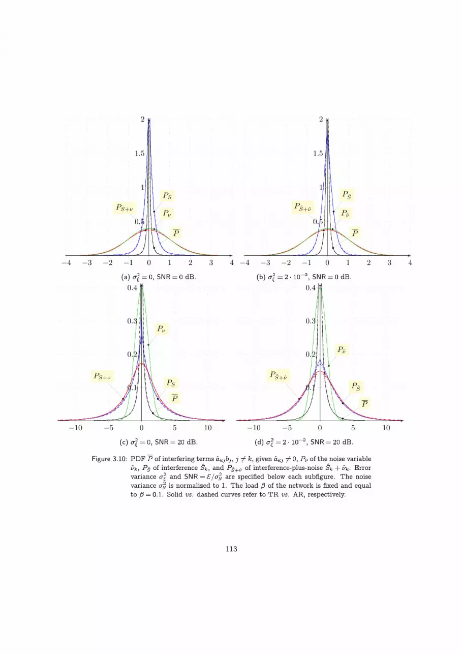
P

PS

P⌫PS+⌫

�4 �3 �2 �1 0 1 2 3 4

0.5

1

1.5

2

(a) , SNR dB.

P

P

ˆS

P⌫

P

ˆS+⌫

�4 �3 �2 �1 0 1 2 3 4

0.5

1

1.5

2

(b) , SNR dB.

P

PS

P⌫

PS+⌫

�10 �5 0 5 10

0.1

0.2

0.3

0.4

(c) , SNR dB.

P

P

ˆS

P⌫

P

ˆS+⌫

�10 �5 0 5 10

0.1

0.2

0.3

0.4

(d) , SNR dB.

Figure 3.10: PDF of interfering terms , , given , of the noise variable, of interference , and of interference-plus-noise . Error

variance and SNR N are specified below each subfigure. The noisevariance N is normalized to . The load of the network is fixed and equalto . Solid vs. dashed curves refer to TR vs. AR, respectively.

113

AR.AR (LB).

TR.TR (LB).

�20 �10 0 10 20 30 40

0.05

0.10

0.15

0.20

E/�

2

N (dB)

R (nats/s/Hz)

(a) ˚i� , ,

�20 �10 0 10 20 30 40

0.05

0.10

0.15

0.20

AR.AR (LB).

TR.

TR (LB).

E/�

2

N (dB)

R (nats/s/Hz)

(b) ˚i� , ,

�20 �10 0 10 20 30 40

0.05

0.10

0.15

0.20

AR.AR (LB).

TR.TR (LB).

E/�

2

N (dB)

R (nats/s/Hz)

(c) ˚i� , ,

�20 �10 0 10 20 30 40

0.05

0.10

0.15

0.20

AR.AR (LB).

TR.TR (LB).

E/�

2

N (dB)

R (nats/s/Hz)

(d) ˚i� , ,

�20 �10 0 10 20 30 40

0.02

0.04

0.06

0.08

AR.AR (LB).

TR.

TR (LB).

E/�

2

N (dB)

R (nats/s/Hz)

(e) ˚i� , ,

�20 �10 0 10 20 30 40

0.02

0.04

0.06

0.08

AR.AR (LB).

TR.

TR (LB).

E/�

2

N (dB)

R (nats/s/Hz)

(f) ˚i� , ,

Figure 3.11: Spectral efficiency R (solid curve) and lower bound assuming Gaussianinterference (dashed curve) vs. SNR N (dB) for di� erent values of load

and error variance . Impulsiveness index is fixed to ˚i� in Figs. from(a) to (d), and to ˚i� in Figs. (e) and (f).

114

becomes less leptokurtic in presence of estimation errors. Figures 3.10 (a) and (b)show an interference-limited scenario, where SNR dB: in this case is farfrom Gaussian, and so is the interference-plus-noise PDF ; the effect of theestimation error is to decrease the kurtosis of , and so that of .

Knowing the distribution of conditioned on , or equivalently its c.f., mutualinformation follows directly. Hence, the c.f. of given

is:

hence, the c.f. of is:

E E

where the expectation is over N . Explicitly, one has:

R R

and:

R R R

where denotes a Gaussian distribution with zero mean and variance , and:

R

The above derivation allows to find as a functionof the distribution of , , and the distribution accounting for theloss of correlation incurred by the user to be decoded because of the estimationerror. Both and accounts for the channel model and the estimation error,in particular its variance.

As baseline comparison, we also provide the following lower bound for, that is achieved when the interference is Gaussian:

E

where the expectation is over . The corresponding spectral efficiency lowerbound is R ˚i� (c.f. eq. (3.34)).

Results are shown on Fig. 3.11, where R (solid curve) and R (dashed curve)are presented as a function of N, for different values of and . The receiverstructure shows a mutual information floor at high SNR. By comparing Figs. 3.11(a) and (b), one observes that R increases sublinearly as increases, while bycomparing Figs. 3.11 (a) and (c), or Figs. 3.11 (b) and (d), a reduction in spectralefficiency due to the presence of an estimation error is observed. R scales with ˚i� asshown on Figs. 3.11 (e) and (f).

115

In each of these simulations, AR outperforms TR. However, note that the gapR R may be viewed as a measure of the non-Gaussianity of and , and isindeed higher in the TR case with respect to the AR case, because of the differentdistribution of the interference term, that is more leptokurtic in the TR case. Therecould be, therefore, a room for TR to outperform AR.

3.4 Future work

In order to generalize the analysis developed in this chapter, the following twoassumptions may be relaxed:

1. single user detection: different receiver structures that use multiuser detectionmay be considered, in first place linear multiuser detection (RZF, MMSE),that can be obtained by leaving eq. (3.29) in the general form;

2. unit gain of channel impulse responses: a complete characterization of thewireless channel should include fading/shadowing.

The first generalization can proceed by projecting eq. (3.17) onto a filter asspecified by eq. (3.29) in the general form. Results are envisioned to be very differentwith linear receivers that account for the interference, such as RZF and MMSE, inconstrast to the simple MF bank that is used above.

The second generalization can be obtained by removing the constraintfor each and every , that also implies that power transmitted by all users is

identical. In this case, performance is not envisioned to differ qualitatively fromthe present analysis.

For both generalizations, a comparison of transceiver structures and fadingstatistics with different degrees of sparsity of the signal transmitted by each user,e.g. selecting DS-CDMA vs. TH-CDMA, will complete the above analysis.

Furthermore, the mutual information analysis can be extended by consideringthe maximum net ergodic rate,

netDL

DL

where the factor in paretheses, namelyDL

, accounts for the data trans-mission fraction of time, and is the rate achievable during that period. Sincethe latter depends on the former, i.e., , a maximum with respect tois expected, as also suggested in [80] and confirmed by preliminary investigations.The analysis of net is important from a practical viewpoint since it suggests theoptimal duration of training phases that maximize the data rate.

116

3.5 Conclusions

In this chapter, the problem of characterizing system performance for single an-tenna systems using time reversal in the case of imperfect channel estimation wasaddressed. The analyzed setting included one BS and several UTs, and the uplinkcommunication channel was considered in the investigation. Each UT adoptedimpulse-radio ultra-wideband communication with prefiltering, and the receivingBS adopted a 1Rake; degrees of impulsiveness were reflected by an impulsivenessindex that ranges from ˚i� to ˚i� for ideal impulsiveness. In order to eval-uate time reversal behavior, this communication scheme was compared against areference configuration with no prefiltering and AR at the receiver. The effectof imperfect channel estimation on both transceiver configurations was analyzed.Channel estimation error was modeled as an additive Gaussian noise based onthe output of a training phase that was used to tune transmitter and receiverstructures. The comparison was performed for both the single user channel andthe multiuser channel with power control. Modeling of the channels was obtainedbased on the 802.15.3a CM1 model. The two communication schemes, TR and AR,were compared based on two different performance parameters: probability of errorand mutual information as a function of signal-to-noise ratio.

Results highlighted that, for the single user channel, probability of error for TRand AR coincided, while for the multiuser channel, AR outperformed TR whenimperfect CSI was the main cause of error, and the two schemes had similarperformance when the load, as measured by the ratio between the number ofterminals and the number of chips in a symbol period, , was themain cause of error, irrespectively of the degree of impulsiveness.

In terms of spectral efficiency, we provided lower and upper bound expressions,and analyzed the two structures with different impulsiveness index ˚i� and load .Results expressed by spectral efficiency R (nats/s/Hz) as a function of signal-to-noise ratio indicated that, for low-SNR, R was similar for the two systems, whilefor higher SNR values, AR outperforms TR. However, remind that, in practicalscenarios, it would be simpler for a TR system to acquire a better estimation ofthe channel with respect to an AR system, since the estimation error variancedepends on the energy of the training sequence only, and in the TR case the trainingsequence is transmitted by a basestation rather than a device, and may requireweaker energy consumption constraints. Furthermore, in the presence of estimationerrors, a reduction in R was observed, due to both a mismatch with the user todecode, and a reduced kurtosis of the interference term.

Both generalizations and extensions of the analysis developed in this chapterare presented.

117

118

Appendix

3.A Derivation of the PDF of and

1) PDF of .

An orthogonal transformation on greatly simplifies the expression of . Wecan think of as the -tuple of coordinates of a vector in R with respectto the canonical basis . A different orthonormal basis such that only the firstcoordinate of the vector is non-zero can be found, for example via the Gram-Schmidtorthogonalization. By denoting with the coordinates of the vector with respectto , it results T. For convenience, we choose the first vector ofas , hence .

Call the matrix that changes coordinates from to ; then . It isa well-known result that , that is the matrix that changes coordinates of vectorsbetween two orthogonal bases, is an orthogonal matrix, i.e., T. As aconsequence, is also an isometry, that is, vectors transformed under the actionof do not change their norm: .

We can rewrite as follows:

T T T T

Since T, one has:

where T, being a set of i.i.d. Gaussianr.vs. Define:

N

and:

hence is as follows:

(3.53)

119

therefore depends only on the ratio . It is useful to define the followingvariable:

(3.54)

in fact, is distributed according to a known distribution, that is the non-centralStudent T-distribution with degrees of freedom and non-central parameter

[84], that we denote by T and has the following canonicalform:

fT

where is the Hermite polynomial [84]. Then, since from eqs. (3.53) and(3.54), it results:

the pdf of is obtained by a change of variables2 as follows:

f fT

2) PDF of .

Write as follows:

having defined . The pdf of can be traced back to a known distribution.In fact, since and , depends on the ratio of two indepen-dent chi-square distributions. It is known as (non-central) F (ratio) distributionthe pdf that describes the ratio of two independent chi-square distributions [84].Precisely, if , , then has a doubly non-central F

ratio distribution of orders and non-centrality parameters ,

F

2The pdf of can be obtained from that of by guaranteeing that fT f .

120

In the present case, , , and , hence:

F

Since:

the pdf can be derived from that of by a change of variables from to , andassumes the following form:

f 1

where is the Beta function and is the Kummer confluent hyperge-ometric function [84].

121

122

CHAPTER 4Some results on MISO Time Reversal

In this chapter, we investigate Multiple-Input Single-Output (MISO) UWB com-munications over a multipath channel. After introducing a tractable discrete-time multipath MISO channel model accounting for correlation between multiplechannels, analytical results for single-user transmissions are drawn in the followingtwo cases: no precoding at transmitter with All-Rake receiver vs. time reversal (TR)at transmitter with 1-Rake receiver. Channel state information at both transmitter(CSIT) and receiver (CSIR) is assumed. Optimality of TR conditioned on 1-Rakereceiver structure is proved. Robustness brought by TR combined with 1-Rakewith respect to lack of correlation between channels vs. no precoding is shown.Simulations with realistic reference channels show that combining time reversalwith multiple transmit antennas amplifies the performance improvement due toeach technique when used alone.

4.1 Introduction

Time reversal is a signaling scheme that focuses a signal in both time and space.When transmitted signals have impulsive nature, as in Impulse Radio Ultra WideBand (IR-UWB), time reversal further increases impulsiveness thanks to the manyresolvable paths of UWB channels, even in the single-antenna setting [78,85]. Whenmultiple antennas at transmitter side are used, time reversal is a beamformerfocusing the wideband signal at receiver. Early experimental results for MISOand MIMO time reversal are collected, respectively, in [67] and in [68–70]. MISObeamforming with antennas in flat-fading channels provides SNR gain of [79].On the other hand, in Single-Input Single-Output (SISO) multipath channels, aprefilter, i.e., a filter at transmitter side, matched to the realization of the channelimpulse response (CIR), which corresponds to time reversal, can focus in timethe signal received: a transceiver using time reversal and 1-Rake achieves sameperformance in terms of SNR as that obtained without time reversal and with All-Rake [76]. This is useful when transmitter cost and complexity are not crucial asopposed to receiver simplicity. However, time reversal can also provide SNR gainwhen more complex receiver is used, that is when more than one finger is employedin Rake.

123

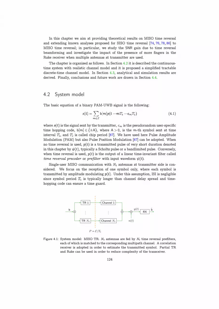
In this chapter we aim at providing theoretical results on MISO time reversaland extending known analyses proposed for SISO time reversal [74, 76, 78, 86] toMISO time reversal; in particular, we study the SNR gain due to time reversalbeamforming and investigate the impact of the presence of more fingers in theRake receiver when multiple antennas at transmitter are used.

The chapter is organized as follows. In Section 4.2 it is described the continuous-time system with realistic channel model and it is proposed a simplified tractablediscrete-time channel model. In Section 4.3, analytical and simulation results arederived. Finally, conclusions and future work are drawn in Section 4.4.

4.2 System model

The basic equation of a binary PAM-UWB signal is the following:

Z

b s (4.1)

where is the signal sent by the transmitter, is the pseudorandom user-specifictime hopping code, b A , where A , is the -th symbol sent at timeinterval s, and is called chip period [87]. We have used here Pulse AmplitudeModulation (PAM) but also Pulse Position Modulation [87] can be adopted. Whenno time reversal is used, is a transmitted pulse of very short duration denotedin this chapter by , typically a Scholtz pulse or a bandlimited pulse. Conversely,when time reversal is used, is the output of a linear time-invariant filter calledtime reversal precoder or prefilter with input waveform .

Single-user MISO communication with antennas at transmitter side is con-sidered. We focus on the reception of one symbol only, where each symbol istransmitted by amplitude modulating . Under this assumption, ISI is negligiblesince symbol period s is typically longer than channel delay spread and time-hopping code can ensure a time guard.

� ...

TR 1

TR Nt

...

Channel 1

Channel Nt

+ + RXb

n(t)

y(t) ˆb

P = E/Ts

FIG. 1: System model: MISO-TR. Nt antennas are fed by Nt

time reversal prefilters, each of which is matched to thecorresponding multipath channel. A correlation receiver isadopted in order to estimate the transmitted symbol. PartialTR and Rake can be used in order to reduce complexity ofthe transceiver.

symbol period Ts is typically longer than channel delay spreadand time-hopping code can ensure a time guard.

Received signal y(t) can be written as follows, where weomitted the time-hopping code because of the one-symbolassumption:

y(t) = b

�

R

hT(t � �) p(�)d� + n(t), (2)

where h(t) and p(t) are the Nt � 1 channel impulse response(CIR) and transmitted signal real-valued vectors, n(t) is anAdditive White Gaussian Noise (AWGN) with power spectraldensity �

2

N , and b is the transmitted symbol. Note that allantennas transmit the same symbol during a symbol period.The i-th component of h(t) and p(t) is denoted by hi(t) andpi(t). Power constraint is intended as follows:

1

Ts

�

R

A2�p(t)�2

dt =1

Ts

Nt�

i=1

�

R

A2

p

2

i (t)dt � P,

where Ts is the symbol period and P is the power spent bythe Nt antennas, and, therefore, by the transmitter.

Given the large bandwidth of UWB systems, the propa-gation channel is resolved into multiple paths. In general,knowledge of CIR realizations at transmitter side can beexploited for prefilter design; MISO-TR design adopts a bankof Nt prefilters, where each antenna element is fed by theoutput of a prefilter modulated by b and matched to the CIRbetween that antenna element and the receiver, hence:

pn(t) =

�

R

(�)hn(� � t)d� = ( � h

rn)(t), (3)

where h

rn(t) = hn(�t); denoting by E the maximum energy

spent by the transmitter during a symbol period, powerconstraint reads as:

A2

Nt�

n=1

�

R

�� � h

rn(t)

��2dt � PTs � E .

Since the multipath channel hi(t) can be written as:

hi(t) =�

k�0

a

ik �(t � �

ik),

partial time reversal prefilters can be also designed, where justa subset of paths is considered [5].

Finally, receiver is assumed to be a matched filter thatprojects y(t) onto the following template:

�

R

hT(t � �) p(�)d� ��

k�0

ak (t � tk).

where {ak, tk : k � 0} represents the set of amplitudes anddelays of fingers in the Rake. However, we can also consider apartial Rake receiver where only a subset of {ak, tk : k � 0} isknown and used: when the strongest paths only are considered,the receiver is known as Selective-Rake, whereas when allpaths are considered, it is known as All-Rake.

A. Channel Model: Continuous-Time

We consider for simulation results the channel proposed in[8] that combines the standard SISO channel IEEE 802.15.3a[7] with the Kronecker channel correlation model for MIMO.We briefly summarize below this model in the special case ofMISO and uniform linear array.

Channel impulse response between the i-th transmit antennaand the receiver is as follows:

hi(t) =�

�,k�0

a

ik,��(t�T� ��k,� ��i)�(�t ��

tk,�)�(�

r ��

rk,�) ,

where a

ik,� is the signed amplitude of ray k in cluster �,

T� is cluster � delay, �k,� is the delay of ray k in cluster �with respect to T�, �i = (i � 1)d/c is the incremental delaydue to antenna i position where d is the distance betweentwo antennas and c is the speed of light, and �

tk,� and

�

rk,� are the angle-of-departure and angle-of-arrival of ray k

in cluster �, respectively. Amplitude of ray k in cluster �for CIR i has the form: a

ik,� = zk,����

ik,�, where zk,� is the

equiprobable ±1 amplitude sign due to random reflections,and �� and �

ik,� are lognormal distributed cluster and ray

fading, respectively. Amplitudes and delays statistics are inaccordance with the standard IEEE 802.15.3a SISO channel.Multiple transmit antennas correlation is taken into accountby assigning a correlation structure to aT

k,� = (a1

k,�, . . . , aNtk,�),

that is by requiring that E[ak,�aTk,�] = �a

k,�. Since only �ik,� =

10(µk,�+⌫ik,�)/20 in a

ik,� depends on the antenna, we just need

to assign a correlation structure to (�ik,�)

Nti=1

, and, in turn, to�k,� = (�1

k,�, . . . , �Ntk,�)

T. Since �

ik,� is Gaussian, then �k,� is

a zero mean multivariate normal distribution with covariancematrix ��

k,� that can be derived once fixed �ak,�. For further

details refer to [8].

B. Simplified Discrete-Time Channel Model

A more tractable channel model for analytical derivationsis described below under the assumption of unit-energy, idealbaseband W-bandlimited pulse (t) with band [�W/2, W/2].

Figure 4.1: System model: MISO TR. antennas are fed by time reversal prefilters,each of which is matched to the corresponding multipath channel. A correlationreceiver is adopted in order to estimate the transmitted symbol. Partial TRand Rake can be used in order to reduce complexity of the transceiver.

124

Received signal can be written as follows, where we omitted the time-hopping code because of the one-symbol assumption:

bR

T (4.2)

where and are the channel impulse response (CIR) and transmittedsignal real-valued vectors, is an Additive White Gaussian Noise (AWGN) withpower spectral density N, and b is the transmitted symbol. Note that all antennastransmit the same symbol during a symbol period. The -th component of and

is denoted by and . Power constraint is intended as follows:

s R

As R

A

where s is the symbol period and is the power spent by the antennas, and,therefore, by the transmitter.

Given the large bandwidth of UWB systems, the propagation channel is resolvedinto multiple paths. In general, knowledge of CIR realizations at transmitter sidecan be exploited for prefilter design; MISO TR design adopts a bank of prefilters,where each antenna element is fed by the output of a prefilter modulated by b andmatched to the CIR between that antenna element and the receiver, hence:

R

r (4.3)

where r ; denoting by the maximum energy spent by the transmitterduring a symbol period, power constraint reads as:

AR

rs

Since the multipath channel can be written as:

partial time reversal prefilters can be also designed, where just a subset of paths isconsidered [74].

Finally, receiver is assumed to be a matched filter that projects onto thefollowing template:

R

T

where represents the set of amplitudes and delays of fingers in theRake. However, we can also consider a partial Rake receiver where only a subset of

is known and used: when the strongest paths only are considered,

125

the receiver is known as Selective-Rake, whereas when all paths are considered, itis known as All-Rake.

4.2.1 Channel Model: Continuous-Time

We consider for simulation results the channel proposed in [88] that combines thestandard SISO channel IEEE 802.15.3a [53] with the Kronecker channel correlationmodel for MIMO. We briefly summarize below this model in the special case ofMISO and uniform linear array.

Channel impulse response between the -th transmit antenna and the receiveris as follows:

t t r r

where is the signed amplitude of ray in cluster , is cluster delay, isthe delay of ray in cluster with respect to , is the incrementaldelay due to antenna position where is the distance between two antennas and

is the speed of light, and t and r are the angle-of-departure and angle-of-arrival of ray in cluster , respectively. Amplitude of ray in cluster for CIR

has the form: , where is the equiprobable amplitude signdue to random reflections, and and are lognormal distributed cluster andray fading, respectively. Amplitudes and delays statistics are in accordance withthe standard IEEE 802.15.3a SISO channel. Multiple transmit antennas correlationis taken into account by assigning a correlation structure to T ,that is by requiring that E T . Since only independs on the antenna, we just need to assign a correlation structure to ,and, in turn, to T. Since is Gaussian, then is a zeromean multivariate normal distribution with covariance matrix that can bederived once fixed . For further details refer to [88].

4.2.2 Simplified Discrete-Time Channel Model

A more tractable channel model for analytical derivations is described below underthe assumption of unit-energy, ideal baseband W-bandlimited pulse with band

W W .

SISO model

Single-Input Single-Output frequency-selective continuous-time AWGN channelscan be described by the relation:

b s

126

where b is the set of transmitted symbols, is the ban-dlimited waveform, s is the symbol period, is the channel impulse response,and is a realization of the continuous-time AWGN process with power spectraldensity N.

In impulse-radio ultra-wideband communications, adjacent symbols are sepa-rated in time by an interval much longer than W: in fact, W is shorter thanthe chip period and each symbol period counts usually tens of chips. Therefore,called sW, previous relation can be written as follows:

b W

where b b for , and b when is not a multiple of .Since one symbol only is considered, the channel model is as follows:

b W

At receiver, projecting this signal onto W Z yields the followingdiscrete-time channel:

Z

where b , Z is a set of i.i.d. Gaussian random variables withvariance N, and

W R

W

Typically, most of the energy is included in the first paths, say . Withoutloss of generality, since can be made as large as needed. Sincefor and , then

and this relation can be written in vector form as follows:

where is a Toeplitz matrix with first column equal toT, and . One-shot communication

implies that b , therefore b , where is the vector withall zero entries but -th element equal to . Note that b is equal to b of eq. (4.2),therefore hereinafter we will denote it with b. Power constraint is expressed asE A .

Note that we can consider as the concatenation of two vectors, and , such

that T T T, where is and is . Similarly,T T T and

127

T T T, where is and is . Since , we can neglect .Prefiltering can be accounted by a matrix as follows: . Withprefiltering, transmitted vector is , therefore power constraint is E

A , being the first column of . Since the prefilter is a linear time-invariant system, is Toeplitz and is the vector containing projections of theprefilter impulse response onto W .

In order to provide a tractable model for the MISO channel, we propose firsta simplified channel model for the SISO channel, which helps in illustrating thebehavior of the system with and without TR. For SISO NLOS channels, it seemsreasonable to consider independent, zero-mean Gaussian randomvariables with variance profile , i.e., . Therefore, thesimplest model we propose is: , where are i.i.d.unit variance Gaussian random variables. Furthermore, when the channel has alsoa LOS component, we propose a generalization that reads as follows:

where , similarly to the “Ricean factor” in flat-fading channels, accounts for thefraction of energy in the LOS component with respect to the NLOS componentin the first path, and accounts for the fraction of energy of the first path withrespect to the sum of the energy of all paths, namely G, where G

is the total channel gain.

MISO model

The discrete-time model is as follows:

T

where is a vector where the -th element is the channel impulse responsebetween the -th transmit antenna and the receiver projected onto W W,and b , where is a vector of ‘ ’. Stackingin a vector, , the previous relation can be written as:

with b (4.4)

where is a vector of symbols and is a block-Toeplitz channelmatrix structured as follows:

T T (4.5)

where is a matrix with ones on the -th subdiagonal. Power constraintis: E A . Prefiltering can be accounted by a block-

128

Toeplitz matrix structured as follows:

(4.6)

Thus, the channel assumes the following form: ; from eq. (4.4), wehave:

b (4.7)

where:

having denoted . In general, jointly precodes symbols forall antennas; in MISO TR prefilters are decoupled, that is, each antenna is fed by theoutput of a prefilter knowing the channel impulse response between that antennaand the receiver only. This structure implies that is diagonal, therefore alsouniquely defined by a vector that we call , that is consistent with previousnotation:

Power constraint reads:E A (4.8)

In order to derive analytical results, we propose the following tractable simplifiedchannel model for MISO channel, that similarly to SISO channels is defined as:

T hT T

where matrix is introduced as in the Kronecker model in order to accountcorrelation between channels of different antennas, h is a deterministic compo-nent that account for the line-of-sight path, and N . We want thatE , therefore we set Tr and h . In this way,correlation matrix of is as follows:

E T h hT (4.9)

A generalization to MIMO would be straightforward, taking into account alsocorrelations at receiver antennas with a matrix . However, since in this chapterwe investigate MISO channels, we denote hereinafter by , being the subscriptredundant.

129

4.2.3 Performance measure

The key performance measure that we are interested in is SNR. The problem isto estimate b from eq. (4.7) through a linear receiver, that is a vectoronto which is projected. We want to compute the SNR of the decision variable

T , that is:T b T

where T b and T . Therefore, SNR of is as follows:

SNRE

E

A

N

T

where expectations are taken conditioned on the channel realization. This quantityis, therefore, still a random variable, since the channel is a random process. We areprimary interested in its mean value, E SNR .

4.3 Results

4.3.1 Analytical Derivations

We derive expressions of SNR in terms of channel correlation, receiver number offingers and transmitter number of antennas. In particular, we compute the twoopposed cases of strongly correlated and independent channels, characterized by

T and , respectively.

All-Rake ( ), General Precoder

SNRA

N

A

N

T

intending that the sum is extended over .

All-Rake ( ), No Precoding

With no precoding, , therefore . According to the powerconstraint, it is sufficient to specialize the general relation for SNR to:

A

130

that yields:

SNRN

T (4.10)

Note that, in the SISO case, this reduces to the well-known result SNR

N .Using the tractable proposed channel model, the average SNR is:

E SNRN

TE T

that, using eq. (4.9), is:

E SNRN

hT T

G

NH (4.11)

having set H hT , T and G .Let analyze particular cases. Assume deterministic LOS component equal for

all antennas, that is h , then H . For strongly correlated channels, namelyfor T, we have . In this case:

E SNRG

N

For independent channels, that is , we have , and therefore:

E SNRG

N

1-Rake, time reversal

A 1-Rake is , where in the case of time reversal . Time reversal isthe use of the precoder:

A rr

where r and is the -th row of . We can prove that thisprecoder maximizes the SNR when 1-Rake is used.

In fact, consider 1-Rake , . Since T T , where is the-th row of , the problem is that of finding the precoding vector:

SNR T

subject to power constraint A . This problem is solved, using for instancethe Cauchy-Schwarz inequality, by , that is time reversal. Each

131

Table 4.1: Parameters used in simulations.

Channel Model IEEE 802.15.3a-CH1Pulse Scholtz, psAntenna distance ( ) mAngle spread ( )

is sufficient for taking into account the whole delay spread of channels, thereforeexploiting the whole gain offered. For the sake of simplicity, we choose .

With the time reversal precoder, achieved SNR is:

SNRN

r

N(4.12)

A well-known result in SISO channels is that this SNR is equal to that obtainedwith All-Rake receiver and no precoding. This is no longer true with MISO, sinceeq. (4.12) is not equivalent to eq. (4.10).

Using the tractable proposed channel model, the average value of (4.12) is:

E SNRG

N(4.13)

The meaning of this relation is that time reversal is insensitive, on average andin terms of SNR, to many parameters characterizing the channel as in (4.11). Inparticular, time reversal is robust to the lack of correlation as opposed to All-Rakewithout precoding: in fact, 1-Rake, time reversal systems average SNR is larger thanthat achieved by systems with All-Rake receiver and without precoding, beiungequal only when channels between different transmit antennas and receiver areidentical.

4.3.2 Simulation Results

In addition to analytical derivations and comparison of performance (in terms ofSNR) of systems using time reversal with 1-Rake vs. All-Rake without prefiltering,we investigate through simulations performance dependence on number of antennas,type of receiver (1-Rake vs. All-Rake) and number of taps in the time reversalprefilter. In fact, transmitter may also select a subset of channel paths to form TR:when one tap only is employed, we have no prefiltering; when the whole channelimpulse response is taken into account, we have full TR; between this two extrema,when the number of taps in the precoder is limited, we have in general partial TR,and paths are selected with decreasing amplitude. Simulations are performed withthe realistic channel described in Subsection 4.2.1. Parameters used in simulationsare reported in Table 4.1.

In Figs. 4.2a and 4.2b it is shown the energy collected by an All-Rake and by a 1-Rake, respectively, normalized to the average energy collected without time reversal

132

100 101 1020

5

10

15

20

25

30

35

40

Number of taps

Ener

gy (n

orm

aliz

ed)

All−Rake receiver

124820

(a) Energy collected by an All-Rake

100 101 1020

5

10

15

20

25

30

35

40

Number of tapsEn

ergy

(nor

mal

ized

)

1−finger Rake receiver

124820

(b) Energy collected by a -Rake.

Figure 4.2: Energy collected with two di� erent receivers normalized to the average energycollected without time reversal, with single antenna, as a function of thenumber of taps of precoder.

with single antenna, as function of the number of paths considered in time reversal.In both cases, time reversal can be used for reducing the number of antennas whilemaintaining fixed the energy collected by the receiver. For instance, in Fig. 4.2a, asystem with antennas without time reversal collects the same energy of a systemwith antennas employing time reversal with taps. Note that, moreover, energygain due to time reversal remains roughly constant as function of the number ofantennas, therefore the total gain due to multiple antennas and time reversal isroughly the product of each gain. A relative increase of focusing, although of smallentity, is observed on Figs. 4.3 showing the percentage of collected energy as functionof the number of fingers in the Rake receiver with time reversal. We confirmed bysimulations the better performance of time reversal with 1-Rake with respect to notime reversal with All-Rake, as expected from the analyical derivation.

133

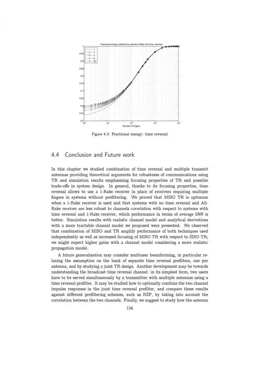
100 101 102 103 1040.5

0.55

0.6

0.65

0.7

0.75

0.8

0.85

0.9

0.95

1

Number of fingers

Ener

gy (n

orm

aliz

ed)

Fractional energy collected by selective Rake with time−reversal

124820

Figure 4.3: Fractional energy: time reversal

4.4 Conclusion and Future work

In this chapter we studied combination of time reversal and multiple transmitantennas providing theoretical arguments for robustness of communications usingTR and simulation results emphasizing focusing properties of TR and possibletrade-offs in system design. In general, thanks to its focusing properties, timereversal allows to use a 1-Rake receiver in place of receivers requiring multiplefingers in systems without prefiltering. We proved that MISO TR is optimumwhen a 1-Rake receiver is used and that systems with no time reversal and All-Rake receiver are less robust to channels correlation with respect to systems withtime reversal and 1-Rake receiver, which performance in terms of average SNR isbetter. Simulation results with realistic channel model and analytical derivationswith a more tractable channel model we proposed were presented. We observedthat combination of MISO and TR amplify performance of both techniques usedindependently as well as increased focusing of MISO TR with respect to SISO TR;we might expect higher gains with a channel model considering a more realisticpropagation model.

A future generalization may consider multiuser beamforming, in particular re-laxing the assumption on the bank of separate time reversal prefilters, one perantenna, and by studying a joint TR design. Another development may be towardsunderstanding the broadcast time reversal channel: in its simplest form, two usershave to be served simultaneously by a transmitter with multiple antennas using atime reversal prefilter. It may be studied how to optimally combine the two channelimpulse responses in the joint time reversal prefilter, and compare these resultsagainst different prefiltering schemes, such as RZF, by taking into account thecorrelation between the two channels. Finally, we suggest to study how the antenna

134

configuration, i.e., geometry, impacts the performance of TR-based transmitters,which may be relevant in distributed antenna setups.

135

136

CHAPTER 5Some results on SISO Time Reversal

In this chapter, a comparison between two optimum prefilters for frequency-selectiveSISO channels under different assumptions on the receiver is drawn. The first designforesees a jointly optimized transceiver (optimum prefilter and all-Rake receiver)while the second constrains the receiver to be minimum complex (1-Rake) andconsequently uses the optimized prefilter, that is, time reversal. Assuming an802.15.3a channel model, analytical results based on the description of the channelas a doubly stochastic point process are proposed for the latter case. Simulationsprovide performance comparison with the former design showing the maximumprefiltering gain gap and the minimum Rake complexity required by the optimumprefilter for a performance improvement.

Notation

absolute value (element-wise if is a vector)-norm where is a vector ( if not specified)

N set of natural numbers ( , , )N set of non-negative integers (N N )

Heaviside theta (or unit-step) functionD is distributed according to the probability

density functionE expectation of where is a function

of random variable (r.v.)

For notation simplicity, the expectation takes no precedence over any other operator.For example, the following holds:

E E

E E E E

137

Pulse

ShaperPrecoder

Channel

Rake

correlator

Decision

operator

Noise

Binary

digit

Pulse Tx signal

Rx signalmetric

Correlation

digit

Binary

Figure 5.1: System model: block diagram.

5.1 Introduction

Communications over frequency-selective channels benefit from pre-equalization oftransmitted waveforms. The optimum receiver in absence of interference is theRake receiver, but its complexity grows with the required number of fingers –that is ideally equal to the number of paths– and the performance gain providedby adding a new finger is always below a prediction based on a linear improve-ment. Furthermore, prefiltering optimality is conditioned on the structure of thereceiver. Therefore, much work [66] has focused on finding sub-optimal receiverand transceiver joint optimum design.

When the receiver is constrained to one finger only, time reversal is the optimumprefilter (see Appendix 5.A for a simple proof). We compare the design composed oftime reversal and 1-Rake with the joint optimum transceiver, assuming an 802.15.3achannel model. The channel is described as a doubly stochastic one-dimensionalpoint process, that is a simplification of previous works on the topic [89–91]. Wefind the average prefiltering gain brought by time reversal, and compare it withthe maximum gain reached with the optimum prefilter. Driven by the underlyingmotivation of simplifying the receiver, we compute the minimum number of fingersrequired by the Rake receiver to guarantee an average performance improvementwith respect to time reversal.

The chapter is organized as follows: Section 5.2 is devoted to the description ofthe system model; Sections 5.3 and 5.4 present time reversal vs. Optimum Prefiltertheoretical performance; Section 5.5 introduces the channel model and analyzes theperformance of time reversal for this specific case. Finally, simulation results andconclusions are presented in Section 5.6.

For clarity of presentation, complex analytical derivations and descriptions areincluded in Appendices. In particular, Appendix 5.A provides a proof of theoptimality of time reversal when the receiver is constrained to one finger only.Appendix 5.B contains the derivation of an expression for the time reversal pre-filtering gain. In Appendix 5.C and 5.D we describe the point process model ofthe channel and in Appendix 5.E we specialize the time reversal prefiltering gainto this channel family.

138

Precoder

p(t)

Channel

h(t)+

Rake

w(t)Sampler

n(t)

g(t; x) s(t) y(t) r(t)x

Figure 5.2: System model (continuous-time): is the useful signal andthe received signal corrupted by the AWGN with variance N . The receiveris implemented by a filter with impulse response followed by asampler at .

5.2 System model

We consider a point-to-point communication through a frequency-selective channel.The system is represented in block diagram form in Fig. 5.1. We model each blockas a linear time-invariant system with impulse response shown in Fig. 5.2. Weassume:

(a1) a signaling scheme based on the two normalized waveforms , beingthe information-bearing symbol;

(a2) a power constraint at the transmitter, that is, independent of the prefilter,the power of the transmitted signal is constant and equal to (w.l.o.g. wecan set );

(a3) independent inter-arrival times between paths in the multipath channel.

For the sake of simplicity we consider PAM as the modulation technique, that is, where is the unit-energy pulse and is the information-

bearing symbol, being the bit of information.The optimum demodulator is the filter matched to the whole useful received

signal . In the case of a multipath channel, it is known as Rake correlator [92,93].This is depicted in Fig. 5.2 that shows the continuous-time model of the system.We can derive an equivalent discrete-time model (see Fig. 5.3): the optimal decoder

is the one that maximizes, having fixed , the SNR of the correlation metric, andit is the matched filter to the effective channel :

SNRE H

E H H

H

N

The resulting SNR H HN E N depends only on the energy of

the useful received signal.

139

p H + wH

n

x

1

snt

ynr

rnr

x

1

Figure 5.3: System model (discrete-time): represents the symbol to be transmitted,R the prefilter sampled impulse response, the transmitted signal,R the linear convolution channel matrix, the received signalwith useful component and AWGN R , and R the correlator.

5.3 Time Reversal SNR in SISO Frequency-Selective Channels

We describe the SISO frequency-selective channel as

where and are amplitude and delay of the th path, respectively.

Note 1. Delays are taken in ascending order, .

Note 2. In practice, we would take only a finite number of paths, say .Given a channel realization, we can design the prefilter according to different

criteria. One criterion is the maximization of the at the 1-Rake receiver. Underthis assumption, the optimum filter is time reversal, represented by a special choiceof , that is

Proof. See Appendix 5.A.

Note 3. We do not address the issue of the causality of this filter; however, it isevident that in order to model a real system we need to introduce a delay of at least

.

Remark 2. Normalization is required by the power constraint assumption (a2).

Definition 3. We call prefiltering gain the quantity .

Remark 3. The prefiltering gain is absent without prefiltering, that is when.

Proposition 2 (Prefiltering gain of time reversal). Assume that (a3) holds.Then, having fixed the continuous-time channel impulse response , it re-sults almost surely (that is, with probability ) that

(5.1)

where .

Proof. See Appendix 5.B.

140

Remark 4. This result is no longer true in the discrete-time model. However,it is an excellent approximation if the discrete-time channel impulse response isrepresented by a sparse vector. In the case of multipath channel, the higher thebandwidth of the receiver, the better is the approximation.Remark 5. This result is a property of the continuous-time channel impulse re-sponse (CIR) and it remains valid if and only if the temporal duration of thepulse is lower than the minimum distance between two paths, that is,

. Conversely, due to the presence of inter-pulse interference(IPI), the wider the pulse, the worse is the approximation.

Now, the aim is to bound . Since , a trivial upper bound ofis given by . A lower bound follows from the Cauchy-Schwarz inequality once

we accept a rather technical assumption verified numerically by simulations (seeFig. 5.3 for more details):

Lemma 2. Assume thatE

E

E

then the following inequality holds:

E EE

E

E

E

141

Number of realizations N

Tim

e-Rev

ersa

lPre

codi

ngG

ain

Est

imat

ion

±��

2 � E�h�4

4

/�h�4

2

2 � E�h�4

4

/E�h�4

2

2 � E�h�4

4

/(E�h�2

2

)2

�(N)�a(N)

0 0.5 1 1.5 2�105

1.87

1.88

1.89

1.9

1.91

1.92

1.93

1.94

1.95

1.96

1

Figure 5.3: This plot suggests that assumption of Lemma 2 is verified with IEEE 802.15.3a(CM1). Here we denote with a discrete-time CIR sampled at GHz.Furthermore, is the ensemble average of (see Def. 3) over a setof channel realizations, , and the accuracy of the meanestimator within , that is one standard deviation, is represented by thefilled region. As , tends to the expectation of (computed overdiscrete-time channels). Since Prop. 2 is valid only in continuous-time, weshow a di� erent curve for the average of the RHS of eq. (5.1), that is, a .The dashed curve shows the asymptotic value of a . This value is below theasymptotic value of , that means that, in discrete-time, the estimation of

with a is conservative, at least asymptotically. The dot-dashed curve showsthat it is conservative to replace the expectation of the ratio with the ratio ofexpectations, verifying the assumption of Lemma 2. Finally, the thick solidcurve show the lower bound that derives from the Cauchy-Schwarz inequality.

5.4 Optimum SNR in SISO Frequency-Selective Channels

The optimum prefilter is designed to maximize SNR under the power constraint:

R

H H

Tr H

having set . This is also optimum from an information theoretic point ofview as it maximizes the capacity of the link.

The solution of this optimization problem is given by the eigenvector of matrixH corresponding to the maximum eigenvalue , or equivalently by the right

singular vector of matrix corresponding to the maximum singular value. In turn, it results that .

142

Remark 6. The optimum prefilter tries to focus the power at the neighbourhood ofthe channel spectrum peak frequency. We can justify informally this behavior not-ing that is a convolutional matrix, thus it is at least asymptotically diagonalizedby a Fourier matrix (like a Toeplitz matrix):

HH

H H HH H

HH

where H H H , being H the th sample of the -points DFT of , say H H , and emphasizing the asymptotic natureof the equality. The last diagonal matrix is intended to be generated fromH H H with the absolute value on the matrix actingelement-wise. With this diagonalization, we can simply read the eigenvaluespectrum of H as the power spectrum of , H . Therefore, themaximum eigenvalue occurs at the discrete-frequency that maximizes thediscrete power spectrum of the channel. Conversely, the optimum prefilter triesto focus the energy where the channel attenuation is the least, that is in theneighbourhood of . This behavior is shown in Fig. 5.4(d).

143

Time (ns)

Precoder Impulse Response

Optimum precoder (All-Rake)

Time-ReversalNo-precoding

0 5 10 15 20 25-0.5

0

0.5

1

1

(a) Prefilter impulse response (samplingtime: [ns]).

PSfrag

Time (ns)

Received Signal: Time Domain

Opt. precoder (All-Rake)

Time-ReversalNo-precoding

0 10 20 30 40 50-1

-0.5

0

0.5

1

1.5

2

2.5

1

(b) Received signal in time domain (sam-pling time: [ns]).

PSfrag Transmitted Signal: Frequency Domain

Frequency (GHz)

Sin

gle-

Sid

edAm

plitud

eSpe

ctru

m(V

/Hz)

Opt. prec. (All-Rake)Time-Reversal

0 1 2 3 4 50

0.5

1

1.5

2

2.5

3

3.5

1

(c) Transmitted signal: amplitude spec-trum.

Frequency (GHz)

Sin

gle-

Sid

edAm

plitud

eSpe

ctru

m(V

/Hz)

Received Signal: Frequency Domain

Opt. precoder (All-Rake)Time-ReversalNo-precoding

0 1 2 3 4 50

2

4

6

8

10

12

14

16

18

1

(d) Received signal: amplitude spectrum.

Figure 5.4: Example of (a) prefilter impulse response, and transmit and received signals(b)–(d) with a fixed channel realization drawn from the IEEE 802.15.3astandard.

144

5.5 The Case of IR-UWB Channels

In line with previous works on the topic [89–91], we use point process theory tomodel the channel impulse response. Hence, the channel is described as a doublystochastic point process, that is formally derived from a Cox process (doublystochastic Poisson point process).

The starting point is the channel model proposed by Saleh and Valenzuela in [94]and further adapted to UWB by Foerster et al. in [53]. The expression for thechannel impulse response is

where is the th cluster start time and is the delay of the th path in the th

cluster relative to . According to the model in [53]

C N is a Poisson process of intensity , and

N is another independent Poisson process of intensity .

Therefore, defining R N, we have that R is a Poisson processof intensity R . The idea is now to model the (deterministic)presence of the first path of each cluster at the cluster start time using generalizedfunctions in the intensity function. Thus, in order to model that (in LOSenvironment) and almost surely, we define:

C N that is a point process of intensity C , and

R that is a point process of intensity R .

By the independence of the latter processes, also their superimposition

R C R

is a point process with intensity function given by

R C R

Remark 7. In NLOS environments it results that C .Thus, regarding N as random, this intensity function becomes a random

field

C

This means that R conditioned on is a point process with intensity function ,therefore it is a doubly stochastic process with random intensity measure and

145

intensity function:

R E

Lemma 3. The intensity function of the point process representing the channelis

R

Proof. See Appendix 5.C.

The statistical properties of the channel amplitudes N are describedin [53]. We recall them in Appendix 5.D and use them in Appendix 5.E in order tofind the following result:

Proposition 3 (Bounds to prefiltering gain of TR). Assume that the channelis described as previously, then

E (5.2)

Proof. See Appendix 5.E.

146

Precoder Impulse Response (All-Rake)Precoder Impulse Response (50-Rake)

Precoder Impulse Response (20-Rake)Precoder Impulse Response (10-Rake)

Precoder Impulse Response (5-Rake)Precoder Impulse Response (1-Rake)

0 10

20

0 10 20

0 10 20 0 10 20

0 10 20 0 10 20

-0.4

-0.2

0

0.2

0.4

0.6

-0.4

-0.2

0

0.2

0.4

0.6

-0.4

-0.2

0

0.2

0.4

0.6

-0.4

-0.2

0

0.2

0.4

0.6

-0.4

-0.2

0

0.2

0.4

0.6

-0.4

-0.2

0

0.2

0.4

0.6

1

Figure 5.5: Prefilter impulse responses optimized with respect to the number of fingers ofRake receivers. The impulse responses are obtained by maximizing numericallythe SNR at the receiver. This is an empirical study, since there is no proof thateach of these impulse responses actually maximize the SNR, but the prefilteroptimized for the All-Rake receiver matches the theory.

147

Number of Fingers

Average Precoding Gain (IEEE 802.15.3a CM1)

Optimum precoderOpt. prec. (All-Rake)

Time-ReversalNo precoding

1-Rake 10 100 All-Rake10�2

10�1

1

10

1

Figure 5.6: Prefiltering gain as a function of the number of fingers of the Rake receiver. Theasymptotically optimum precoder (crosses) is optimum under the conditionthat the receiver is an All-Rake. The optimum precoder (diamonds) is obtainedempirically by using prefilters as shown in Fig. 5.5. Performance of systemswith no precoding (pluses) and time reversal (circles) at the transmitter sideis shown for comparison. The receiver bandwidth is GHz; however, thequalitative behavior of the curves is loosely dependent from the bandwidth.

148

PDF of the Equivalent Number of Fingers for Di�erent Precoders

Number of Fingers

No-precoding

Time-Reversal

0 20 40 60 80 1000

0.005

0.01

0.015

0.02

0.025

0.03

0.035

0.04

0.045

0.05

1

Figure 5.7: Estimation of the PDF of that number of fingers such that di� erent prefiltershave same performance (see also Fig. 5.6). The histogram on the left (with thelighter background) refers to Optimum Prefilter (All-Rake) and No-prefiltering;the histogram on the right (with the darker background) refers to OptimumPrefilter (All-Rake) and time reversal.

149

5.6 Conclusion

In this chapter we compared optimum prefilters operating in SISO frequency-selective channels. The SISO channels are characterized by a complexity featurethat we define in association with the number of fingers of the Rake receiver.The analysis is carried out in the absence of MUI. Figures 5.4(a)–(d) showed thebehavior in time and frequency of different prefilters. It is shown that the optimumprefilter focuses the energy in a neighbourhood of the frequency corresponding tothe maximum channel gain (see Fig. 5.4(d)). A drawback is the spreading in timeof both the impulse response of this filter (see Fig. 5.4(a)) and the received signal(see Fig. 5.4(b)), implying that a larger number of fingers is required in order tocollect the same energy that would be collected with other prefilters. Eventually,further analysis is required in order to verify compliance with UWB masks.

A comparison of the gain of different prefiltering schemes is shown on Fig. 5.6.The prefiltering gain is the value that the curves tend to asymptotically, as thenumber of fingers grows to infinity. Other points on the curves show the energynormalized to the channel gain as a function of the number of fingers of theRake receiver. For the simplest Rake receiver (one finger only), time reversal isoptimum: it allows to collect the maximum energy with a -Rake, that is equalto . At the other extreme, the optimum prefilter, that is joint-optimized withthe optimum receiver (All-Rake), allows to collect the maximum energy. Figure 5.6further shows that the asymptotically optimum prefilter, i.e., optimum only whenthe receiver is an All-Rake, outperforms time reversal only if the receiver has anumber of fingers larger than a threshold, that is a random variable whose pdf isestimated in Fig. 5.7. Conversely, this analysis suggests that it is mandatory torequire receiver complexity if a prefilter that is optimum when the receiver is anAll-Rake is employed.

Future work may investigate analytically optimum prefilters as a function ofthe number of fingers of the Rake receiver. In general, a deeper investigation ofprefiltering techniques with multipath channels is of interest. Moreover, extensionto multiuser communications is possible and may reveal peculiar properties ofprefilters operating in time over multipath channels.

150

Appendix

5.A Time Reversal is Optimum if the Receiver is 1-Rake

This appendix aims at providing a quick proof of the optimality of time reversalwhen the receiver is constrained to one finger only. The problem can be stated incontinuous-time as follows: Given the channel impulse response (CIR) , findthe function solution of the problem:

We can constrain w.l.o.g. the solution to provide the maximum at ; theproblem becomes

R

Defining , the last integral is the inner product and the solutionderives from the Cauchy-Schwarz inequality: , that implies , thatis, time reversal.

5.B Proof of Time Reversal Gain.

The received useful signal is as follows:

The assumption (a3) implies that with and , one has; therefore, almost surely, all previous are located at

different times. The energy of considering only the firsts paths tends

151

asymptotically (as ) to:

where . It follows that

5.C Proof of Lemma 3: Channel Process Intensity Function.

The aim is to compute E . This can be accomplished by applying the Campbell’sformula that allows to determine expectations of functions evaluated on the pointprocess. Precisely, given a point process R with measure , mean measure

E and intensity , and a function R, it holds that:

E E

where the integral is extended over the domain of .We recall that

C

and that C . Therefore

E E

152

5.D Statistical Description of IEEE 802.15.3a Channel PathAmplitudes

Let us summarize the statistical properties of the channel amplitudes proposedin [53] as the following three constraints:

(c1) exponential decay : E

being and the intra-cluster and cluster decay factors, respectively;

(c2) independent cluster fading : each cluster is affected by a Log-Normal fading(cluster fading) independently from other clusters, that is, the paths withinthe th cluster, say N, are scaled by (the same) log-normal r.v.statistically independent from ;

(c3) independent ray fading : each path is affected by a Log-Normal fading (rayfading) independently from other paths, that is, the generic path is scaledby a r.v. statistically independent from

Remark 8. The generic , C, R can beviewed as the mark of the point located in .

In line with [53], the generic channel amplitude can be decomposed as follows:

where D takes into account the path sign due to reflections andand follows from the natural extension of Remark 8 to and ,

respectively. We further decompose the term in a deterministic part, say, and a random part, say :

and call .

Remark 9. In this way and are i.i.d. while dealing with leads justto independence. Furthermore, if we were dealing with , we would only haveconditional independence of with respect to , that is, the amplitudes areindepedent only once conditioned to the cluster.

Constraints (c1)–(c3) uniquely define the channel process. Nevertheless, itremains a freedom in the formal description and we use it to slightly simplify theanalytical formulation found in [53]. We recap the latter in A and propose theformer in B . Hereinafter, we use the following notation:

stands for a Normal process such that D ,

is the standard variation of the Normal r.v. associated with the clusterfading,

153

is the standard variation of the Normal r.v. associated with the ray fading,

is the conversion factor from dB to Np, thus [dB] [Np].

A In [53] it is assumed that

D

D

and is such that it is satisfied (c1). Therefore, having defined, they impose that

E

thus

In this formulation, we have

E E

E

From a pragmatic point of view, the paths within a cluster, prior to be affectedby cluster fading, are thought with a (conditional) second moment lower than thesecond moment that they have to exhibit to be compliant with (c1), that is, afterthe cluster fading. Therefore, the cluster fading has the effect to rise the conditionalsecond moment.

In general, we can write the moments as follows:

E

E

E E

B We define differently and introducing a gauge parameter such thatE and E :

D

D

154

With the same of , we find that

thus:

In this formulation, we have

E E

E

From a pragmatic point of view, the paths within a cluster, prior to be affected bycluster fading, are thought with a (conditional) second moment equal to the secondmoment that they have to exhibit to be compliant with (c1). Therefore, the clusterfading has no effect on the second moment.

In general, we can write the moments as follows:

E

E

E E

Note that the last equality holds either in A and B .

5.E Proof of Proposition 3: TR Gain Lower Bound.

Notation. For a given realization of C, we write and similarlyfor R. All summations over or are understood to be over C or R ,respectively.

We want to compute

E E

with and , where is the amplitude of the path occurred at thetime belonging to the cluster begun in . Let us start reducing the expectationsonly over the point process:

155

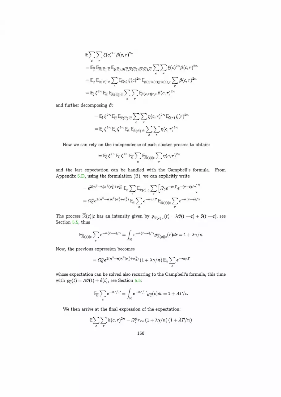
E

EC ER C C E C C R C R C C

EC ER C C E E R R

E EC ER C C E

and further decomposing :

E EC ER C C E

E E EC ER C C

Now we can rely on the independence of each cluster process to obtain:

E E EC ER

and the last expectation can be handled with the Campbell’s formula. FromAppendix 5.D, using the formulation B , we can explicitly write

EC ER

EC ER

The process R has an intensity given by R , seeSection 5.5, thus

ERR

R

Now, the previous expression becomes

EC

whose expectation can be solved also recurring to the Campbell’s formula, this timewith C , see Section 5.5:

ECR

C

We then arrive at the final expression of the expectation:

E

156

having set .Specializing this formula to and respectively we obtain

E

E

that are the required formulas to compute the ratio.

157

158

CHAPTER 6Closed Form Asymptotic Expression

of a Random-Access InterferenceMeasure

A model describing the cumulative effect of the independent access of users toa shared resource, formed by elements, is proposed, based on which an integerinterference measure is defined. While traditional cases can be reconducted toreference well-known results, for which is either Gaussian or Poissonian (see,for example, Appendix 1.H and eq. (1.37), respectively, and also eq. (3.52) for aPoisson-mixture distribution), the proposed model provides a framework that offersthe tool for understanding the different nature of . In particular, an asymptoticclosed form expression ( , , ) for distribution isprovided for systems presenting constructive vs. destructive interference, and assuch is applicable to characterizing statistical properties of interference in a widerange of random multiple access channels.

6.1 System Model

When many users access a common resource independently, they may interfere witheach other. A resource can be viewed, in general, as a set of elements that are usedto transmit information. For example, at the physical layer, the resource is theset of degrees of freedom that carry the information-bearing signal: a system usingbandwidth for time with antennas can access degrees of freedombelonging to time, frequency and space domains; at the medium access layer, theresource is usually time supporting either continuous or slotted packet transmission.

In the proposed model, the resource is a discrete set of elements1 ,i.e., slots. This description holds when the resource is discrete, or can be aptlydiscretized. Resource is shared independently by users: user chooses a subset

1In this chapter, two common notations in combinatorics are used: the set

is denoted by , and, when , it is simply written as .

159

K users

Resource···

1 2 3 N· · ·

Slots

1

2

K

Figure 6.1: Abstract setting: a resource composed on parts (slots) is randomly accessedby users. Each user assigns to the accessed slot a numerical value (label),randomly and independently from other users.

of (irrespective of ) slots, ignoring the other users choice, and assigns a labelto each accessed slot .

Figure 6.1 illustrates the abstract setting, where a resource is made up ofslots and users access randomly to a subset of slots, which is shown for .

Let for , and otherwise, that is, is zero for thenon-accessed slots of user , while it is equal to the assigned labels for the accessedslots. Therefore, , where is the set of possible values that the label mayassume, and , where and may or may not be equal.

Let be the sum of labels assigned to slot by all users but user , that is:

(6.1)

By specifying and , the proposed model encompasses the problem of statis-tically describing multiple access interference for communication systems in whichinterference has a quantal nature, or can be reconducted to the model of eq. (6.1).Let present four examples: the first three address well-known problems, and areintended to clarify concepts and notations defined above, while the last addressesa novel problem, that is solved thanks to results proved in this chapter.Example 1. This example may refer to throughput of Slotted Aloha at the mediumaccess layer [95]. Assume that resource is time, that is slotted in equal parts,and that users, each willing to transmit a single packet, independently chooseone of the slots. In this setting, and can be interpreted as the binaryvariable indicating the presence or absence of packet of user

within slot . The goal is to find the number of colliding packets with userpacket, i.e., the number of packets in the slot selected by user . Given , itresults . Moreover, and . in eq. (6.1) indicatesthe number of packets in slot that are transmitted by all users but user , and,therefore, the goal is to find . In the large-system limit, that is, as ,

160

, and , both and are distributed according toa Poisson distribution with mean .Example 2. This example may describe demodulation of direct-sequence spread-spectrum (DSSS) signals with a single-user matched filter bank. Assume thatresource is time, that is slotted in chips of duration , and supports transmissionof synchronous random DSSS signals [6]. Let the received signal be

(6.2)

where is the number of users, is the set of unit energy transmittedspreading waveforms, is the set of transmitted antipodal symbols, and

is a white Gaussian noise process with power spectrum N. Direct-sequenceimplies , whereare i.i.d. r.v.s assuming values in with equal probability (seee.g. [6]). In this scenario, , , , ,and is the signal interfering with that of user , within chip , at the outputof a chip-matched filter. The goal is to find the distribution of , that can beused, for example, in order to find the capacity of the system. In the large-systemlimit, is Gaussian distributed with zero mean and unit variance. Generally,a Lindeberg condition suggests that if a fixed fraction, however small, of degreesof freedom is “uniformly” used, then is Gaussian distributed; otherwise, if fewdegrees of freedom are used in the large-system limit, e.g. a finite number, thenthe asymptotic distribution may be not Gaussian, as is usually the case.Example 3. This example may describe demodulation of binary PPM time-hoppingspread-spectrum (THSS) signals with a single-user matched filter bank, whereinterference is at physical rather than medium access layer compared to Example1, and can only be constructive. Assume that resource is time, that is divided in

chips of duration , and supports transmission of synchronous binary PPMTHSS signals (see e.g. [96]). Let the received signal be

(6.3)

where is the number of users, is uniformly distributed overassuming an integer, is the set of binary transmitted symbols, and,for the sake of simplicity, is a zero-excess bandwidth waveform with band

, and . In this model, there are slots of duration, , , and may be regarded as the interference of the

output of a filter slot-matched to slot . In the large-system limit, is distributedaccording to a Poisson distribution with mean , as in the first example.Example 4. Example 4 is similar to Example 2, except for the random spreadingsequences that now belong to the time-hopping family (see e.g. [97,98]), i.e., for anyfixed , , with equal probability, for only one chip .In this case, is the interference, to which contribute both constructive and

161

distructive terms for , at the output of a filter chip-matched to chip ,, and . Moreover, is the interference at the output

of the single-user matched filter of user . The distribution of is unknown,and can be found thanks to the result presented in this chapter.

As hinted by Example 4, this chapter finds, in the large-system limit, the closedform distribution of:

(6.4)

The chapter is organized as follows: in Section 6.2 the main result is presentedand proved; essential analytic combinatorics are recapped in Appendix 6.A. Con-clusions are drawn in Section 6.3.

6.2 Main Result

Theorem 9. Let be the number of slots of a resource, that is shared byusers. The generic user selects one slot only , and

assigns to this slot a label that is a r.v. taking value in with equalprobability. Then, , as defined in eq. (6.4), is distributed in the large-systemlimit, that is, for , , and , as:

Z

(6.5)

irrespective of , where is the modified Bessel function of the first kind.

Proof. We provide two proofs. The first proof is probabilistic: is regarded asa r.v. and the pdf of is derived straightforwardly via algebraic manipulations.The second proof is based on results of analytic combinatorics: the probabilityP is derived by considering all the ways, and the associated probability, aparticular value of can be obtained; the law of large numbers guarantees thatthe so obtained result holds with probability one in the large-system limit.

First Proof.For fixed , is the sum of i.i.d. random variables , each

of which is distributed according to:

(6.6)

Denoting by , one has:

162

1 2 3 4 5 6 7 8 9 10 11

�2

�1

1

2

3

1� 1

N

1

2N

1

2N

k

Pki=1

si

Figure 6.2: Two simple lattice walks are shown. In the two cases, , and thereforethe walk length is , and steps are , as shown in the box atthe north-east corner. Both walks start from and end at : thedarker corresponds to the sequence , while the lightercorresponds to .

In order to obtain the asymptotic pdf, rewrite the previous relation as follows:

where this time the contribution to the amplitude of each Dirac mass is isolatedin the term in parentheses, that is defined as . In thelarge-system limit, the Binomial distribution tends to a Poisson distribution withmean , , and the term in parentheses reduces to

, being:

Finally, becomes:

Z

irrespective of . The theorem follows since when Z.Second Proof.As expressed by eq. (6.4), is a sum of the form:

where subscript is discarded. In order to find P , the number of wayscan be obtained as sum of elements of a sequence is counted, and let

163

the probability each that sequence appears be:

(6.7)

Sequence can be regarded as an unconstrained, simple walk of lengthin the lattice Z Z (refer to Appendix 6.A for definitions and theorems of

analytic combinatorics that are used in this chapter). Figure 6.2 shows two suchwalks with possible steps, , where notation for simple walksis adopted. Associated with these steps are weights and (see boxat north-east corner of Fig. 6.2) such that the characteristic polynomial of is:

Thanks to weights, the probability a particular point in Z Z is reached can becomputed. In order to find P , summation in eq. (6.7) is over walks startingfrom and ending at , and the probability within the sum is thatassociated to each walk, that is the product of probabilities associated to stepscomposing the walk. The generating function of these walks is:

the coefficient giving the probability to reach :

In the large-system limit, the quantity in brackets converges to:

with . In order to find andtherefore , Cauchy’s integral formula can be used as follows:

Therefore, assumes the integer value with probability , hence thetheorem.

164

�5 �4 �3 �2 �1 1 2 3 4 5

0.2

0.4

0.6

Simulation

Th. envelope

Gaussian Approx.

z

P⇣(z)

(a)

�5 �4 �3 �2 �1 1 2 3 4 5

0.2

0.4

0.6

Simulation

Th. envelope

Gaussian Approx.

z

P⇣(z)

(b)

Figure 6.3: Theoretical envelope (red dashed line) vs. simulated histogram (filled circles)of for (subfig. (a)) and (subfig. (b)). A Gaussian PDF withsame mean and variance is shown for reference.

Figure 6.3 shows simulations (filled circles at integer values) vs. theoreticalenvelope , R (red solid line) of , for (Fig. 6.3(a)) and(Fig. 6.3(b)). Simulated values are drawn from Monte-Carlo simulations offinite dimensional systems with . A Gaussian r.v. with same mean andvariance (black dashed line) is reported for reference. As hinted by figures, theenvelope of the distribution is increasingly Gaussian as increases. In particular,odd moments of are null, while the two first even moments are E andE , hence the kurtosis is . Since , is alwaysleptokurtic, and as , suggesting that a Gaussian approximation mayhold for .

165

6.3 Future work and Conclusion

In this chapter, a model describing systems where users access a resource inde-pendently was proposed. Each user assigns labels to accessed slots: the label is anumerical value with sign, i.e. accounting for polarity. Based on this model, aninterference measure called for the generic user that considers the cumulativevalue of other users labels in terms of their sum was considered. In particular, thecase where each user accesses one slot only and assigns a label or with equalprobability to the accessed slot was addressed. A closed form expression of thedistribution of this cumulative value was found in the large-system limit: it wasshown that, if the cardinality of the population of users is a fraction of the numberof available slots, then the distribution converges to a novel expression that is ingeneral far from Gaussian, and may be approximated by a Gaussian distribution for

. Two proofs, one probabilistic and the other based on analytic combinatorics,were provided.

The second proof presents a potentially fruitful framework that can be used toderive several generalizations. Firstly, the labels are restricted to be binary in thiswork: by removing this constraint, conditions under which the interference does notfollow neither a Gaussian nor a Poisson distribution can be studied. Secondly, thenumber of slots accessed by each user is here constrained to one, as both the totalnumber of slots and the population grows at the same rate . Thisconstraint also can be removed, and the maximum number of slots, as a functionof , that each user may access without reducing the interference to behave asa Gaussian random variable can be studied. Lastly, as a third generalization, therelation with so-called “stable distributions,” that represent distributions describingthe sum of an infinite number of properly scaled i.i.d. random variables, can beinvestigated.

166

Appendix

6.A Basics on Analytic Combinatorics of Lattice Paths

We refer mostly to the seminal work of Banderier and Flajolet [99].

Definition 4 (Lattice Path or Walk). A lattice path (or walk) is a sequencewhere is the length of the path and

Z Z

is the set of steps. A path is:

directed if ;

simple if (in this case the set of steps is written as );

unconstrained (resp. constrained) if Z Z (resp. Z Z ).

We can assign a weight to each allowed step, that is R. Thefollowing definition is the starting point of the analytic approach:

Definition 5 (Characteristic Polynomial). Let be the set of steps of a simplewalk and the weight associated to . The characteristic polynomial of is:

The ending point of a walk is that, for simple walks, assumes the form, where is called final altitude. Denote by the class of walks with

length and final altitude , and let .

Definition 6 (Generating Function). The generating function of is definedas:

where C is a mark for the length and C is a mark for the final altitude.

The following theorem links with :

Theorem 10. The generating function of a simple walk is:

(6.8)

167

Proof (sketch). Rewrite as follows:

where is a Laurent polynomial in where is the(possibly weighted) number of ways to reach the final altitude in steps. Sincethe only altitude reachable in steps is , then ; at step , the reachablealtitudes are described by . In general , and therefore asummation over yields to eq. (6.8).

168

CHAPTER 7Conclusion and Future works

Impulsive communications belong to the subset of communications that are sparsein time. Impulsiveness is, therefore, strictly related to both sparsity in time of thetransmitted signal and properties of the physical medium that the signal passesthrough. Impulsive communications are those where the received signal occupies afraction of the received signal space. The typical example in the wireless commu-nication field is represented by impulse-radio ultra-wideband, where transmissionsoccur at bursts and the transmitted signal occupies a small fraction of the symbolperiod.

In this thesis we addressed several issues concerning impulsive communicationsand the effect of interference on their performance. In particular, we formalized es-sential characteristics of multiuser impulsive communications, namely sparsity andrandom hopping, and we identified their information-theoretical limits in multipleaccess channels with power-control. We then investigated the interplay between thetransmitted signal bandwidth and the statistical properties of a multipath channel,when transmitter uses a prefiltering scheme called transmit matched-filter (alsoknown as time reversal in ultra-wideband and speech communities). Several workson the analysis of performance of systems using time reversal is then presented,for both SISO and MISO systems, and in presence of imperfect knowledge of thechannel. Finally, the interference of a general multiple access model accounting forconstructive vs. destructive events is investigated: we showed that several systemscan be described with this model, and a new asymptotic distribution formula forthe interference is derived.

7.1 Conclusion

We summarize below the main conclusions that can be drawn from each chapter ofthis thesis.

In Chapter 1, information-theoretical limits are derived for impulsive vs.non-impulsive multiuser communications, represented by time-hopping vs. direct-sequence CDMA, that are prototypes of sparse vs. dense multiple access formats.We compared spectral efficiency of random time-hopping with consolidated results

169

regarding direct-sequence. We found that there is a regime where time-hoppingallows to achieve spectral efficiency higher than that achievable by direct-sequence,namely when the system is overloaded and the receiver is linear. This resultprovides a hint for and a partial justification to designing networks with nodesthat transmit bursty signals in time: this signaling scheme is appropriate wheneverthe network load is high, , while keeping the receiver design simple, e.g.owing to very large bandwidths: the performance gain with respect to traditionaldirect-sequence networks is increasingly relevant as 0 increases.

In Chapter 2, we investigated the interplay between transmitted signal band-width and statistical properties of a multipath channel, when transmitter uses aprefiltering scheme called transmit matched-filter (also known as time reversal inultra-wideband and speech communities). We derived a necessary and sufficientcondition for the performance of the system to increase as bandwidth increases.We showed that multipath channels that are described by or strictly related to theSaleh-Valenzuela model, satisfy the condition, therefore suggesting a theoretical jus-tification for the wide adoption of time reversal in ultra-wideband communications.

Chapters 3–5 are dedicated to detailed study of time reversal in various settings.In Chapter 3, we analyzed performance of two different transceiver structures,namely transceivers with time reversal prefiltering and -Rake receiver vs. no pre-filtering and All-Rake receiver. Performance is analyzed in terms of error probabilityin both single-user and multiuser settings; preliminary mutual information analyseshas been also conducted. It was shown that in the single-user setting the two systemdesigns are equivalent in terms of error probability and sensitivity to perturbations,while behaving differently in the multiuser setting, where the system using timereversal shows higher error probability. Partial results on mutual information donot change qualitatively the conclusion drawn from the comparison based on theerror probability metric. In Chapter 4, we analyzed MISO ultra-wideband withtime reversal, in particular showing that performance is not affected by the the lackof correlation between channels from each transmitting antenna to the receiver. InChapter 5, we compared SISO time reversal with other prefilters, as a functionof the number of fingers of a Rake receiver, and we showed the gain that can beobtained by the different transceiver structures.

Finally, in Chapter 6 we analyzed a general multiple access model where userscan interfere with each other antipodally in either a constructive or destructivefashion. We detailed few settings of practical relevance that are described by thismodel, but several others, including queues in particular regimes, may be aptlydescribed as well. We found the asymptotic distribution of the interference inclosed form, that cannot be reduced to any known probability distribution.

7.2 Future works

In several chapters of this thesis, we already detailed future works that are relatedto the content of the chapter. The kind of detailed works aims at extending resultsobtained under certain sets of assumptions, and can form the basis for investigations

170

that either complete or extend the scope of the works that are presented in thethesis. We hope also that several other works, different from the ones that weexplicitly proposed, will be inspired by this thesis.

In this section we briefly discuss future works that necessitate models that areeither more general or intrinsically different with respect to those presented in thisthesis. Firstly, although this thesis is focused on impulsive communications, thatare sparse in time, it is interesting to investigate more general cases of sparsityacross dimensions of the signal space. Secondly, it is interesting to investigate thesum-rate of a random ad hoc network where each node uses sparse spreading, andcompare results with those achieved with dense spreading. Different scaling lawsare envisioned in the sparse case. Finally, we believe that the most ambitious futurework lies in embracing a different perspective, namely the possibility to formalizeimpulsive communications as those that regard time not as a mere support of thecommunications, but as the resource within which coding information through inter-arrival times between events, such as signal receptions. In this regard, [100–102]are seminal contributions that may form the basis for this ambitious project.

171

172

Bibliography

[1] M. Medard and R. G. Gallager, “Bandwidth scaling for fading multipathchannels,” IEEE Trans. Inf. Theory, vol. 48, no. 4, pp. 840–852, 2002.

[2] R. Gallager and M. Medard, “Bandwidth scaling for fading channels,” in Proc.IEEE Int. Symp. Inf. Theory, 1997, p. 471.

[3] E. Telatar and D. Tse, “Capacity and mutual information of widebandmultipath fading channels,” IEEE Trans. Inf. Theory, vol. 46, no. 4, pp.1384–1400, 2000.

[4] D. Porrat, D. Tse, and S. Nacu, “Channel uncertainty in ultra-widebandcommunication systems,” IEEE Trans. Inf. Theory, vol. 53, no. 1, pp. 194–208, 2007.

[5] E. Biglieri, J. Proakis, and S. Shamai, “Fading channels: information-theoreticand communications aspects,” IEEE Trans. Inf. Theory, vol. 44, no. 6, pp.2619–2692, 1998.

[6] S. Verdù and S. Shamai, “Spectral efficiency of CDMA with random spread-ing,” IEEE Trans. Inf. Theory, vol. 45, no. 2, pp. 622–640, 1999.

[7] S. Shamai and S. Verdù, “The impact of frequency-flat fading on the spectralefficiency of CDMA,” IEEE Trans. Inf. Theory, vol. 47, no. 4, pp. 1302–1327,2001.

[8] D. Tse and S. Hanly, “Linear multiuser receivers: effective interference,effective bandwidth and user capacity,” IEEE Trans. Inf. Theory, vol. 45,no. 2, pp. 641–657, 1999.

[9] D. Tse and O. Zeitouni, “Linear multiuser receivers in random environments,”IEEE Trans. Inf. Theory, vol. 46, no. 1, pp. 171–188, 2000.

[10] A. M. Tulino, L. Li, and S. Verdu, “Spectral efficiency of multicarrier CDMA,”IEEE Trans. Inf. Theory, vol. 51, no. 2, pp. 479–505, 2005.

[11] V. A. Marcenko and L. A. Pastur, “Distribution of eigenvalues for some setsof random matrices,” Mathematics of the USSR-Sbornik, vol. 1, no. 4, pp.457–483, 1967.

[12] T. Tanaka, “A statistical-mechanics approach to large-system analysis ofCDMA multiuser detectors,” IEEE Trans. Inf. Theory, vol. 48, no. 11, pp.2888–2910, 2002.

173

[13] A. Montanari and D. Tse, “Analysis of belief propagation for non-linearproblems: The example of CDMA (or: How to prove tanaka’s formula),”in Proc. IEEE Inf. Theory Workshop (ITW), Punta del Este, 2006, pp.160–164.

[14] D. Guo and C.-C. Wang, “Multiuser detection of sparsely spread CDMA,”IEEE J. Sel. Areas Commun., vol. 26, no. 3, pp. 421–431, 2008.

[15] T. Tanaka and M. Okada, “Approximate belief propagation, density evolution,and statistical neurodynamics for CDMA multiuser detection,” IEEE Trans.Inf. Theory, vol. 51, no. 2, pp. 700–706, 2005.

[16] K. Alishahi, F. Marvasti, V. Aref, and P. Pad, “Bounds on the sum capacityof synchronous binary CDMA channels,” IEEE Trans. Inf. Theory, vol. 55,no. 8, pp. 3577–3593, 2009.

[17] S. Korada and N. Macris, “Tight bounds on the capacity of binary inputrandom CDMA systems,” IEEE Trans. Inf. Theory, vol. 56, no. 11, pp.5590–5613, 2010.

[18] J. Raymond and D. Saad, “Sparsely spread CDMA—a statistical mechanics-based analysis,” J. Phys. A: Math. Theor., vol. 40, no. 41, pp. 12 315–12 333,2007.

[19] M. Yoshida and T. Tanaka, “Analysis of sparsely-spread CDMA via statisticalmechanics,” in Proc. IEEE Int. Symp. Inf. Theory, 2006, pp. 2378–2382.

[20] S. Verdù, Multiuser Detection, 1st ed. New York: Cambridge UniversityPress, 1998.

[21] M. B. Pursley, “Performance evaluation for phase-coded spread-spectrummultiple-access communication–Part I: System analysis,” Communications,IEEE Transactions on, vol. 25, no. 8, pp. 795–799, 1977.

[22] A. M. Tulino and S. Verdú, “Random matrix theory and wireless communi-cations,” Foundations and Trends in Communications and InformationTheory, vol. 1, no. 1, pp. 1–182, 2004.

[23] A. M. Tulino, The Eta and Shannon transforms: a bridge between randommatrices and wireless communications, ser. Lecture notes. World ScientificPublishing, 2009, vol. 18, ch. 4, pp. 95–138.

[24] R. Couillet and M. Debbah, Random matrix methods for wireless commu-nications. Cambridge University Press, 2011.

[25] S. Verdú, “Spectral efficiency in the wideband regime,” IEEE Trans. Inf.Theory, vol. 48, no. 6, pp. 1319–1343, 2002.

[26] Z. Bai and J. Silverstein, Spectral Analysis of Large Dimensional RandomMatrices, 2nd ed., ser. Springer Series in Statistics. New York: Springer,2010.

174

[27] P. Flajolet and R. Sedgewick, Analytic Combinatorics. CambridgeUniversity Press, 2009.

[28] R. Sedgewick and P. Flajolet, An Introduction to the Analysis of Algo-rithms. Boston, MA, USA: Pearson Education, 2013.

[29] Z. D. Bai and J. W. Silverstein, “No eigenvalues outside the support ofthe limiting spectral distribution of large dimensional sample covariancematrices,” Ann. Probab., vol. 26, pp. 316–345, 1998.

[30] S. Verdu, “The capacity region of the symbol-asynchronous gaussian multiple-access channel,” IEEE Trans. Inf. Theory, vol. 35, no. 4, pp. 733–751, 1989.

[31] S. Benedetto and E. Biglieri, Principles of Digital Transmission: WithWireless Applications. Norwell, MA, USA: Kluwer Academic Publishers,1999.

[32] A. Lozano and D. Porrat, “Non-peaky signals in wideband fading channels:Achievable bit rates and optimal bandwidth,” IEEE Trans. WirelessCommun., vol. 11, no. 1, pp. 246–257, 2012.

[33] J. Richters, Communication over fading dispersive channels, ser. Technicalreport. MIT, RLE, 1967.

[34] I. Abou-Faycal, M. Trott, and S. Shamai, “The capacity of discrete-timememoryless rayleigh-fading channels,” IEEE Trans. Inf. Theory, vol. 47,no. 4, pp. 1290–1301, 2001.

[35] R. S. Kennedy, Fading dispersive communication channels. Wiley-Interscience, 1969.

[36] L. Cottatellucci, R. Muller, and M. Debbah, “Asynchronous CDMA systemswith random spreading: Part i: Fundamental limits,” IEEE Trans. Inf.Theory, vol. 56, no. 4, pp. 1477–1497, 2010.

[37] V. Girko, Theory of Stochastic Canonical Equations: Volumes I and II,ser. Mathematics and Its Applications. Springer Netherlands, 2001.

[38] D. Guo, S. Shamai, and S. Verdu, “Mutual information and minimum mean-square error in gaussian channels,” IEEE Trans. Inf. Theory, vol. 51, no. 4,pp. 1261–1282, 2005.

[39] A. Tulino, G. Caire, S. Shamai, and S. Verdú, “Capacity of channels withfrequency-selective and time-selective fading,” IEEE Trans. Inf. Theory,vol. 56, no. 3, pp. 1187–1215, 2010.

[40] F. Hlawatsch and G. Matz, Wireless communications over rapidly time-varying channels. Academic Press, 2011.

[41] R. P. Stanley, Enumerative combinatorics. Cambridge University Press,2011, vol. 1.

175

[42] ——, Enumerative combinatorics. Cambridge University Press, 2011,vol. 2.

[43] I. S., “On the capacity of channels with additive non-gaussian noise,”Information and Control, vol. 37, no. 1, pp. 34–39, 1978.

[44] M. Joham, W. Utschick, and J. Nossek, “On the equivalence of prerakeand transmit matched filter,” in Proc. 10th Aachen Symp. Signal Theory,Aachen, Germany, 2001, pp. 313–318.

[45] ——, “Linear transmit processing in MIMO communications systems,” IEEETrans. on Signal Process., vol. 53, no. 8, pp. 2700–2712, 2005.

[46] M. Joham, K. Kusume, M. H. Gzara, W. Utschick, and J. A. Nossek,“Transmit Wiener filter for the downlink of TDD DS-CDMA systems,” inProc. IEEE 7th Int. Symp. Spread Spectr. Techn. and Appl. (ISSSTA),Prague, Czech Republic, 2002, pp. 9–13.

[47] A. Derode, P. Roux, and M. Fink, “Robust acoustic time reversal with high-order multiple scattering,” Phys. Rev. Lett., vol. 75, pp. 4206–4209, 1995.

[48] M. Fink, G. Montaldo, and M. Tanter, “Time reversal acoustics,” in Proc.IEEE Ultrason. Symp., vol. 2, Montreal, Canada, 2004, pp. 850–859.

[49] T. Strohmer, M. Emami, J. Hansen, G. Papanicolaou, and A. Paulraj, “Ap-plication of time-reversal with MMSE equalizer to UWB communications,”in Proc. IEEE Global Telecommun. Conf. (GLOBECOM), vol. 5, Dallas,TX, USA, 2004, pp. 3123–3127.

[50] R. Esmailzadeh and M. Nakagawa, “Pre-rake diversity combination for directsequence spread spectrum communications systems,” in Proc. IEEE Int.Conf. Commun. (ICC), vol. 1, Geneva, Switzerland, 1993, pp. 463–467.

[51] ——, “Pre-rake diversity combination for direct sequence spread spectrummobile communications systems,” IEICE Trans. Commun., vol. 76, no. 8,pp. 1008–1015, 1993.

[52] G. C. Ferrante, “Time-reversal against optimum precoder over frequency-selective channels,” in Proc. 18th European Wireless Conf., Poznan, Poland,2012, pp. 1–8.

[53] J. Foerster, “Channel modeling sub-committee report final,” IEEE, Tech. Rep.Doc. P802.15-02/490r1-SG3a, 2003.

[54] W.-D. Wu, C.-C. Lee, C.-H. Wang, and C.-C. Chao, “Signal-to-interference-plus-noise ratio analysis for direct-sequence ultra-wideband systems in gen-eralized saleh-valenzuela channels,” IEEE J. Sel. Topics Signal Process.,vol. 1, no. 3, pp. 483–497, 2007.

[55] T. M. Cover and J. A. Thomas, Elements of Information Theory, 2nd ed.Wiley, 2006.

176

[56] Y.-H. Kim, “Feedback capacity of stationary gaussian channels,” IEEE Trans.Inf. Theory, vol. 56, no. 1, pp. 57–85, 2010.

[57] S. A. Schelkunoff, “Some equivalence theorems of electromagnetics and theirapplication to radiation problems,” Bell System Technical Journal, vol. 15,no. 1, pp. 92–112, 1936.

[58] ——, “On diffraction and radiation of electromagnetic waves,” Phys. Rev.,vol. 56, pp. 308–316, 1939.

[59] J. A. Stratton and L. J. Chu, “Diffraction theory of electromagnetic waves,”Phys. Rev., vol. 56, pp. 99–107, 1939.

[60] Y. F. Chen, “A mathematical formulation of the equivalence principle,” IEEETran. Microw. Theory Techn., vol. 37, no. 10, pp. 1576–1581, 1989.

[61] M. Fink, “Time reversal of ultrasonic fields. i. basic principles,” IEEE Trans.Ultrason., Ferroelectr., Freq. Control, vol. 39, no. 5, pp. 555–566, 1992.

[62] Z. Tang and S. Cheng, “Interference cancellation for DS-CDMA systems overflat fading channels through pre-decorrelating,” in Proc. IEEE Int. Symp.Personal, Indoor and Mobile Radio Commun., vol. 2, 1994, pp. 435–438.

[63] B. R. Vojcic and W. M. Jang, “Transmitter precoding in synchronousmultiuser communications,” IEEE Trans. Commun., vol. 46, no. 10, pp.1346–1355, 1998.

[64] A. N. Barreto and G. Fettweis, “Capacity increase in the downlink of spreadspectrum systems through joint signal precoding,” in Proc. IEEE Int. Conf.Commun. (ICC), vol. 4, 2001, pp. 1142–1146.

[65] M. Vu and A. Paulraj, “Mimo wireless linear precoding,” IEEE SignalProcess. Mag., vol. 24, no. 5, pp. 86–105, 2007.

[66] D. P. Palomar and Y. Jiang, “MIMO transceiver design via majorizationtheory,” Found. Trends Commun. Inf. Theory, vol. 3, no. 4, pp. 331–551,2006.

[67] A. E. Akogun, R. C. Qiu, and N. Guo, “Demonstrating time reversal inultra-wideband communications using time domain measurements,” in Int.Instrumentation Symp., Knoxville, TN, USA, 2005, pp. 8–12.

[68] N. H. T., J. B. Andersen, G. F. Pedersen, P. Kyritsi, and P. C. F.Eggers, “Time reversal in wireless communications: a measurement-basedinvestigation,” IEEE Trans. Wireless Commun., vol. 5, no. 8, pp. 2242–2252, 2006.

[69] R. C. Qiu, C. Zhou, N. Guo, and J. Q. Zhang, “Time reversal with MISOfor ultrawideband communications: Experimental results,” IEEE AntennasWireless Propag. Lett., vol. 5, no. 1, pp. 269–273, 2006.

177

[70] C. Zhou, N. Guo, and R. C. Qiu, “Time-reversed ultra-wideband (UWB)multiple input multiple output (MIMO) based on measured spatial channels,”IEEE Trans. Veh. Technol., vol. 58, no. 6, pp. 2884–2898, 2009.

[71] N. Guo, B. M. Sadler, and R. C. Qiu, “Reduced-complexity uwb time-reversaltechniques and experimental results,” IEEE Trans. Wireless Commun.,vol. 6, no. 12, pp. 4221–4226, 2007.

[72] R. Qiu, J. Zhang, and N. Guo, “Detection of physics-based ultra-widebandsignals using generalized rake with multiuser detection (MUD) and time-reversal mirror,” IEEE J. Sel. Areas Commun., vol. 24, no. 4, pp. 724–730,2006.

[73] R. C. Qiu, “Generalized time domain multipath channel and its applicationin ultra-wideband (UWB) wireless optimal receiver—Part III: system per-formance analysis,” IEEE Trans. Wireless Commun., vol. 5, no. 10, pp.2685–2695, 2006.

[74] G. C. Ferrante, J. Fiorina, and M.-G. Di Benedetto, “Complexity reduction bycombining time reversal and IR-UWB,” in Proc. IEEE Wireless Commun.and Networking Conf. (WCNC), Paris, France, 2012, pp. 28–31.

[75] ——, “Time reversal beamforming in MISO-UWB channels,” in Proc. IEEEInt. Conf. Ultra-Wideband (ICUWB), Sydney, Australia, 2013, pp. 261–266.

[76] L. De Nardis, J. Fiorina, D. Panaitopol, and M.-G. Di Benedetto, “CombiningUWB with time reversal for improved communication and positioning,”Telecommunication Systems, vol. 52, no. 2, pp. 1145–1158, 2013.

[77] X. Wang and J. Wang, “Effect of imperfect channel estimation on transmitdiversity in CDMA systems,” IEEE Trans. Veh. Technol., vol. 53, no. 5, pp.1400–1412, 2004.

[78] J. Fiorina, G. Capodanno, and M.-G. Di Benedetto, “Impact of time reversalon multi-user interference in IR-UWB,” in Proc. IEEE Int. Conf. Ultra-Wideband (ICUWB), 2011, pp. 415–419.

[79] E. G. Larsson and P. Stoica, Space-Time Block Coding for WirelessCommunications. New York: Cambridge University Press, 2008.

[80] G. Caire, N. Jindal, M. Kobayashi, and N. Ravindran, “Multiuser MIMOachievable rates with downlink training and channel state feedback,” IEEETrans. Inf. Theory, vol. 56, no. 6, pp. 2845–2866, 2010.

[81] D. Sarwate and M. Pursley, “Crosscorrelation properties of pseudorandom andrelated sequences,” Proc. IEEE, vol. 68, no. 5, pp. 593–619, 1980.

[82] M. A., “On pseudo-random and orthogonal binary spreading sequences,” Int.J. Information Techn., vol. 2, no. 12, pp. 543–550, 2008.

178

[83] E. Biglieri, Coding for Wireless Channels. New York: Springer-Verlag,2005.

[84] M. Abramowitz and I. A. Stegun, Handbook of mathematical functions:with formulas, graphs, and mathematical tables. New York: DoverPublications, 1964.

[85] H. Saghir, M. Heddebaut, F. Elbahhar, A. Rivenq, and J. Rouvaen, “Time-reversal UWB wireless communication-based train control in tunnel,” Journalof Communications, vol. 4, no. 4, pp. 248–256, 2009.

[86] D. Panaitopol, J. Fiorina, and M. Di Benedetto, “Trade-off between thenumber of fingers in the prefilter and in the rake receiver in time reversalir-uwb,” in Proc. IEEE Int. Conf. Ultra-Wideband (ICUWB), 2009, pp.819–823.

[87] M.-G. Di Benedetto and G. Giancola, Understanding Ultra Wide Bandradio fundamentals. Prentice Hall, 2004.

[88] X. Hong, C.-X. Wang, B. Allen, and W. Q. Malik, “Correlation-based double-directional stochastic channel model for multiple-antenna ultra-widebandsystems,” IET microw., antennas and propag., vol. 1, no. 6, pp. 1182–1191,2007.

[89] M. L. Jakobsen, T. Pedersen, and B. H. Fleury, “Analysis of the stochasticchannel model by saleh & valenzuela via the theory of point processes,” inInternational Zurich Seminar on Communications, 2012, pp. 115–118.

[90] J. A. Gubner and K. Hao, “A computable formula for the average bit errorprobability as a function of window size for the ieee 802.15.3a uwb channelmodel,” IEEE Tran. Microw. Theory Techn., vol. 54, no. 4, pp. 1762–1768,2006.

[91] K. Hao and J. A. Gubner, “The distribution of sums of path gains in the ieee802.15.3a uwb channel model,” IEEE Trans. Wireless Commun., vol. 6,no. 3, pp. 811–816, 2007.

[92] R. Price and P. Green, “A communication technique for multipath channels,”Proc. IRE, vol. 46, no. 3, pp. 555–570, 1958.

[93] J. G. Proakis and M. Salehi, Digital Communications. McGraw-Hill HigherEducation, 2008.

[94] A. A. M. Saleh and R. A. Valenzuela, “A statistical model for indoor multipathpropagation,” IEEE J. Sel. Areas Commun., vol. 5, no. 2, pp. 128–137, 1987.

[95] N. Abramson, “The throughput of packet broadcasting channels,” IEEETrans. Commun., vol. 25, no. 1, pp. 117–128, 1977.

[96] G. Giancola and M.-G. Di Benedetto, “A novel approach for estimating multi-user interference in impulse radio UWB networks: The pulse collision model,”Signal Processing, vol. 86, no. 9, pp. 2185 – 2197, 2006.

179

[97] G. C. Ferrante and M.-G. Di Benedetto, “Spectral efficiency of random time-hopping CDMA,” submitted to the IEEE Trans. Inf. Theory, 2013. Revisedon Nov. 2014, [Online]. Available: http://arxiv.org/abs/1311.4830.

[98] J. Fiorina and W. Hachem, “On the asymptotic distribution of the correlationreceiver output for time-hopped uwb signals,” IEEE Trans. on SignalProcess., vol. 54, no. 7, pp. 2529–2545, 2006.

[99] B. C. and F. P., “Basic analytic combinatorics of directed lattice paths,”Theoretical Computer Science, vol. 281, no. 1–2, pp. 37–80, 2002.

[100] V. Anantharam and S. Verdú, “Bits through queues,” IEEE Trans. Inf.Theory, vol. 42, no. 1, pp. 4–18, 1996.

[101] R. Sundaresan and S. Verdu, “Robust decoding for timing channels,” IEEETrans. Inf. Theory, vol. 46, no. 2, pp. 405–419, 2000.

[102] R. Sundaresan and S. Verdú, “Capacity of queues via point-process channels,”IEEE Trans. Inf. Theory, vol. 52, no. 6, pp. 2697–2709, 2006.

180