Embed Size (px)
Citation preview

Optimality and Robustness of the English Auction
Giuseppe Lopomo1
Fuqua School of Business, Duke University
email: [email protected]
Games and Economic Behavior, Vol. 36, 219-240 (2000).
1Helpful comments and suggestions by Jeremy Bulow, Jose Campa, Faruk Gul, Paul Klemperer, Vijay
Krishna, Roy Radner, Ennio Stacchetti and Chuck Wilson are gratefully acknowledged.

Abstract
In Milgrom and Weber’s (1982) “general symmetric model,” under few additional regularity con-
ditions, the English auction maximizes the seller’s expected profit within the class of all posterior-
implementable trading procedures, and fails to do so among all interim incentive-compatible proce-
dures in which ‘losers do not pay.’ These results suggest that appropriate notions of robustness and
simplicity which imply the optimality of the English auction for a risk neutral seller must impose
“bargaining-like” features to the set of feasible trading mechanisms. Journal of Economic Literature
Classification Numbers: D44, D82.
Direct correspondence to: Giuseppe Lopomo, Fuqua School of Business, Duke University, Durham
NC27708-0120.

1 Introduction
Under what conditions is the English auction optimal for a seller who aims at maximizing her
expected profit? Is there an appealing characterization of the feasible set of trading mechanisms
which implies the optimality of the English auction for a risk neutral seller?
The motivation for this type of inquiry is two-fold: on one hand the English auction is often the
chosen trading procedure by the owner of an indivisible object facing a number of potential buyers;
on the other hand, it is known from the theory of mechanism design that, under generic assumptions
on the buyers’ preferences and information structure, one can construct incentive-compatible and
individually rational trading procedures which dominate the English auction in terms of seller’s
expected revenue. In particular, if the buyers are risk averse, the seller earns more on average with
mechanisms in which risk is used as a screening device than with any of the “standard” auctions –
i.e. Dutch, English, first-price and second-price;1 and, if all buyers are risk neutral, then any nonzero
degree of correlation, no matter how small, among their private information enables the seller to
extract all expected gains from trade.2
This discrepancy between theory and common practice has led researches to argue that a seller’s
set of feasible trading mechanisms should be restricted according to a set of simplicity and robustness
criteria in order to rule out mechanisms which, like the “full extraction” mechanisms mentioned
above, rely heavily on the common knowledge of fine details of the model, e.g. the buyers’ beliefs
conditional on their private information, or the curvature of their utility functions. Indeed, in all
“standard” auctions, the terms of trade are determined by a small set of simple rules. 3
In this paper we consider two nested classes of equilibrium outcomes of trading mechanisms,
which correspond to alternative sets of simplicity and robustness. First, attention is restricted to
the class of all equilibrium outcomes of selling procedures which satisfy a no-regret condition: each
buyer has no incentive to revise his decisions after observing his opponents’ behavior. This no-
regret property is implied by the traders’ inability to commit to their actions before observing their
opponents’ choices, and results in outcome functions – i.e. functions which specify how the object
1For a description of the rules of these four auction formats see for example McAfee and McMillan (1987). A classic
reference documenting the widespread use of auctions is Cassady (1967).
2The optimality of the all standard auctions has been established by Myerson (1981) and Riley and Samuelson (1981).
Optimal selling mechanisms with risk averse buyers and independent values have been characterized by Matthews (1983)
and Maskin and Riley (1984). ‘Full extraction’ results with risk neutral buyers have been established by Cremer and
McLean (1988) for the case of discrete probability distributions. With continuous distributions McAfee and Reny
(1992) have provided a nearly-full extraction result.
3Here is a representative quote: “A reasonable question for the mechanism design literature is how to capture the
importance of robustness. Specifically, we think the answer to questions like ‘under what circumstances are English
auctions used?’ has to do with the need for an institution perform well in a variety of circumstances.” [McAfee and
McMillan (1987).] See also Milgrom (1985) and (1987).
1

is allocated, and how much each buyer pays to the seller, for each realization of the buyers’ private
information – that are posterior-implementable, as defined by Green and Laffont (1987). We show
that, in Milgrom and Weber’s (1982) “general symmetric model”, the symmetric equilibrium4 of an
English auction in which the reserve price is set after all but one buyers have dropped out maximizes
the seller’s expected profit among all posterior-implementable outcome functions.
It is worth noting that this optimality result does not generalize to environments with asymmetric
distributions. To see this, consider the case with private and independent values. As shown by Bulow
and Roberts (1989), the optimal auction in this case, which entails awarding the object to the buyer
with the highest “virtual utility”, can be implemented in dominant strategies: the winner pays the
lowest value that he could have reported without losing the object. With asymmetric distributions, it
can happen that the buyer with the highest virtual utility does not have the highest value. Thus the
object may not always be awarded to the buyer with the highest value, as in the English auction. By
Myerson’s Revenue Equivalence Theorem, this implies that the optimal auction generates a higher
seller’s expected revenue than the English auction.
The second subset of equilibrium outcomes of selling procedures considered in this paper is
identified by the sole additional restriction that “losers do not pay” (LDNP), i.e. only the buyer who
is awarded the object makes a payment to the seller. This class of outcome functions includes all
equilibrium outcomes of the four standard auctions, as well as all posterior-implementable outcome
functions.
In light of the following two observations, one may conjecture that, in a symmetric model with
risk neutral buyers, no LDNP outcome function generates more seller’s expected revenue than the
symmetric equilibrium outcome of the English auction: first, in any ‘full extraction’ mechanism the
losers must make payments to the seller for some realizations of their opponents’ signals; second, in
an English auction the seller can set an optimal reserve price for the last active bidder based on all
losers’ private signals which are revealed by their quitting times.
Proposition 2 of this paper establishes however that the set of all LDNP selling mechanisms
includes a large class of sealed-bid auction, named b-composite auctions, which dominate the English
auction in terms of seller’s expected revenue. This result demonstrates that, to improve upon the
English auction, the seller does not have to resort to procedures in which the losers pay, such as
“all-pay” auctions or mechanisms with entry fees.5
A third interesting class of trading procedures among which the English auction maximizes the
4In the common value case, Bikhchandani and J. Riley (1991) have shown that the “irrevocable exit” English auction
also has many asymmetric equilibria.
5Krishna and Morgan (1996) have shown that, under conditions which guarantee the existence of a symmetric
equilibrium, the “second-price all-pay auction” generates dominates the standard second-price auction in terms of
seller’s expected profit.
2
seller’s expected profit has been considered in Lopomo (1998). The seller’s feasible set in that paper
consists of a large family of dynamic bidding procedures called “Simple Sequential Auctions,” whose
essential feature is that each buyer chooses his actual payment conditional on being awarded the
object from a given set. The ability for each buyer to determine his payment conditional on receiv-
ing the object is a “bargaining-like” property that also characterizes the posterior-implementable
outcome functions considered in this paper. The buyer who receives the object is guaranteed an
amount of information rent which cannot be lower than the difference between his value and the
highest among his opponents’ values.
The rest of this paper is organized as follows. Section 2 reviews the assumptions of Milgrom
and Weber’s general symmetric model (1982) and states a few additional regularity conditions under
which the optimality of the English auction among all posterior-implementable mechanisms will be
established. In Section 3 the optimality of the English auction among all posterior-implementable
mechanisms is established. Section 4 shows that the b-composite auctions dominate the English auc-
tion in terms of seller’s expected revenue, and sheds light on the key idea underlying the construction
of any mechanisms which does better than the English auction in terms of seller’s expected revenue.
Section 5 provides some conclusive remarks.
2 The Model
This section reviews the assumptions of Milgrom and Weber’s “general symmetric model”, and
introduces some additional regularity conditions that will be used to establish the optimality of the
English auction among all posterior-implementable outcome functions.
The owner of an indivisible object faces n risk-neutral potential buyers. Let N := {1, . . . , n}denote the set of buyers. Each buyer i ∈ N observes privately the realization of a random variable
θi, i.e. his ‘signal’, drawn jointly with the other n− 1 signals θ−i := (θ1, . . . , θi−1, θi+1, . . . , θn) froma symmetric distribution with density f , which is strictly positive on its support Θ := [0, 1]n . The
signals (θ1, . . . , θn) are affiliated, i.e.
f¡θ ∨ θ0¢ · f ¡θ ∧ θ0¢ ≥ f (θ) · f ¡θ0¢ for all θ, θ0 ∈ Θ,
where θ∨θ0 and θ∧θ0 denote the component-wise maximum and minimum of θ and θ0. The affiliationproperty has the following two useful implications. First, for any decomposition of the vector θ into
a k-dimensional vector θK and the vector θ−K containing its remaining n− k elements, the ratio ofthe conditional densities
f|−K (θK |θ−K)f|−K
¡θ0K |θ−K
¢is nondecreasing in θ−K whenever θK > θ0K . Second, the function
h (a1, ..., an, b1, ..., bn) ≡ E [g (θ) |ai ≤ θi ≤ bi; i ∈ N ]
3

is nondecreasing for any nondecreasing function g : Θ→ R.The amount that each buyer i ∈ N is willing to pay for the object is determined by a function ui
of the realization of his signal θi, and possibly of the other n− 1 signals θ−i. Moreover, there existsa ‘valuation function’ u,
u : Θi ×Θ−i → R,
where Θi := [0, 1] and Θ−i := [0, 1]n−1 , strictly increasing in its first argument, and weakly increasingand symmetric in its last n− 1 arguments, such that
u (θi, θ−i) ≡ ui (θ1, ..., θn) for each i ∈ N.
The overall payoff function of buyer i is
u (θi, θ−i) Qi −M i
where Qi denotes the probability that he is awarded the object andM i denotes his expected payment
to the seller.
This general symmetric model includes as special cases both the “private values” case, where
u (θi, θ−i) ≡ u (θi) for some function u : [0, 1] → R; and the “common value” case, in whichu (θi, θ−i) = u (θj , θ−j) for any two permutations (θi, θ−i) and (θj, θ−j) of any given realizationθ ∈ Θ.
To establish the optimality result in Section 3, we will use the following additional assumptions.
On the valuation function u:
A1: Fix any (θ1, ..., θn) ∈ Θ, pick two elements θi and θj , and let θ−ij ∈ [0, 1]n−2 denote thevector containing the remaining n− 2 signals. Then, θi > θj implies u (θi, θj, θ−ij) ≥ u (θj, θi, θ−ij) ;
A2: u11 ≤ 0, (where the subscripts denote partial derivatives in the usual way);A3: u1j ≥ 0, j = 2, ..., n;and on the signals’ distribution F :
A4: all conditional hazard ratiosf|−i (θi | θ−i)
1− F|−i (θi | θ−i), where F|−i and f|−i denote the c.d.f. and
the density of θi conditional on θ−i ∈ Θ−i, are nondecreasing in θi;A5: The derivative ∂
∂θif|i (θ−i|θi) , where f|i (·) denotes the density of θ−i conditional on θi, exists
for all θ ∈ Θ;Assumption A1 is made to guarantee that buyers with higher signals have higher values. As-
sumptions A2 and A3 imply that buyers with higher signals have a lower sensitivity of their value
to their own signal. Assumption A4 extends the standard ‘monotone hazard ratio’ condition to the
distribution of each signal conditional on all other signals. Finally, A5 is a smoothness assumption
made to simply the proof of Lemma 1 in Section 3.
4

3 The English Auction is Optimal among Posterior Implementable
Mechanisms
Any trading mechanism can be represented as a set of 2n functions
pi : B1 × ...×Bn → R, i ∈ N,
and
xi : B1 × ...×Bn → [0, 1] , i ∈ N,such that X
i∈Nxi (b1, .., bn) ≤ 1, for each (b1, .., bn) ∈ B1 × ...×Bn,
where, Bi denotes the set of feasible actions, i.e. “messages,” for buyer i, the function pi determines
his payment to the seller6 and the function xi determines the probability that he is awarded the
object, for any n-tuple of messages (b1, ..., bn) ∈ B1 × ...×Bn.Any trading mechanism (p, x) :=
¡p1, ..., pn, x1, ..., xn
¢induces an incomplete information game
with payoff functions
U i (b1, ..., bi, ..., bn; θi, θ−i) := u (θi, θ−i) · xi (b1, ..., bi, ..., bn)− pi (b1, ..., bi, ..., bn) , i ∈ N,
and (mixed) strategy sets
Σi :=©σi (·|θi) ∈ ∆ (Bi) : θi ∈ Θi
ª, i ∈ N.
Any strategy profile σ :=¡σ1, ...,σn
¢ ∈ Σ1 × ... × Σn determines a probability distribution µσover the set B1 × ... × Bn × Θni , and implements an outcome function, i.e. a set of 2n functions(q,m) =
¡q1, ..., qn,m1, ...,mn
¢which assign a probability vector
qi (θ1, ..., θi, ..., θn) :=
ZBxi (b1, ..., bi, ..., bn) · σ1 (db1|θ1) · ... · σn (dbn|θn) , i ∈ N,
and an expected payment vector
mi (θ1, ..., θi, ..., θn) :=
ZBpi (b1, ..., bi, ..., bn) · σ1 (db1|θ1) · ... · σn (dbn|θn) , i ∈ N,
to each type profile θ ∈ Θ.In this section attention is restricted to outcome functions which are posterior-implementable,
i.e., which can be implemented by a profile σ such that, for µσ -almost every (b1, ..., bn , θ1, ..., θn) ,
bi ∈ arg maxb0i∈Bi
wi (θi, b−i) · xi¡b1, ..., b
0i, ..., bn
¢− pi ¡b1, ..., b0i, ..., bn¢ all i ∈ N,
6Since the buyers are risk neutral attention can be restricted to deterministic payment functions without loss of
generality.
5

where
wi (θi, b−i) :=ZΘ−i
u (θi, θ−i)σ−i (b−i|θ−i) f|i (θ−i|θi)R
Θ−i σ−i (b−i|τ−i) f|i (τ−i|θi) dτ−i
dθ−i
denotes bidder i’s willingness to pay for the object, conditional on his type θi and the information
revealed by his opponents’ actions b−i.We are now ready to state and prove the main result of this section.
Proposition 1 Define the “ex-post virtual utility function” v : [0, 1]× [0, 1]n−1 → R by
v (θi, θ−i) ≡ u (θi, θ−i) −1− F|−i (θi|θ−i)f|−i (θi|θ−i)
u1 (θi, θ−i) . (1)
In Milgrom and Weber’s general symmetric model, and under assumptions A1-A5, the seller’s ex-
pected revenue is maximized, among all posterior-implementable and individually rational outcome
functions, by the symmetric equilibrium outcome of the irrevocable-exit English auction in which,
after n− 1 buyers drop out, the auctioneer sets the reserve price atr (θ−i) ≡ u (t0 (θ−i) , θ−i) ,
where the function t0 (θ−i) is defined by the equation v (t0 (θ−i) , θ−i) = 0.
Proof: The proof is broken in four Lemmas. Lemma 1 establishes a revenue equivalence result
for posterior-implementable outcome functions with affiliated types’ distributions, similar to Myer-
son’s (1981) Revenue Equivalence Theorem: it derives an ‘envelope condition’ (equation (2) below)
akin to the standard ‘interim’ envelope condition in mechanism design, which determines the payment
of each type of buyer i once the strategies used by his opponents, the assignment function qi, and the
expected surplus of the lowest type are given. Lemma 2 shows that the seller’s expected revenue is
maximized, among all posterior-implementable outcome functions which have the same assignment
functions q1, ..., qn, by the function in which the buyer who wins the object learns his opponents’
type perfectly. Lemma 3 finds a revenue maximizing outcome function among all the functions that
are ‘fully revealing’ for the winner. Finally, Lemma 4 shows that the equilibrium outcome of the
English auction with optimal ex-post reserve prices coincides almost everywhere with the optimal
function found in Lemma 3, hence is optimal for the seller among all posterior-implementable and
individually rational outcome functions.
Lemma 1. If the outcome function (q,m) is posterior-implementable, then, for all i ∈ N, all(θ1, ..., θi, ..., θn) ∈ Θ, and all b−i ∈ B−i, we have
mi (θ1, ..., θi, ..., θn) = wi (θi, b−i) qi (θ1, ..., θi, ..., θn)−Z θi
0qi (θ1, ..., τ, ..., θn) w
i1 (τ, b−i) dτ
6
(2)
−U i (0, b−i) ,
where U i (0, b−i) denotes the surplus of buyer i’s lowest type, given his opponents messages.Proof. Fix a posterior equilibrium profile σ of a selling mechanisms (p, x) and a buyer i ∈ N.
Take any selection βi (·) from the correspondence which assigns the support of σi (·|θi) to each typeθi ∈ Θi, i.e. βi (θi) ∈ Suppσi (·|θi) for all θi ∈ Θi. Define
χi³bθi, b−i´ := xi ³b1, ...,βi ³bθi´ , ..., bn´ ,
πi³bθi, b−i´ := pi ³b1, ...,βi ³bθi´ , ..., bn´ ,
and
U i (θi, b−i) := maxbθinwi (θi, b−i) χi
³bθi, b−i´− πi ³bθi, b−i´o .By posterior implementability, we have, for µσ -almost all b−i,
U i (θi, b−i) ≥ wi (θi, b−i) χi³bθi, b−i´− πi ³bθi, b−i´
= wi³bθi, b−i´ χi ³bθi, b−i´− πi ³bθi, b−i´
(3)
+hwi (θi, b−i)−wi
³bθi, b−i´i χi ³bθi, b−i´= U i
³bθi, b−i´+ hwi (θi, b−i)−wi ³bθi, b−i´i χi ³bθi, b−i´ ,and interchanging bθi with θi we obtain
U i³bθi, b−i´ ≥ U i (θi, b−i) + hwi ³bθi, b−i´−wi (θi, b−i) iχi (θi, b−i) . (4)
Combining (3) and (4) yieldshwi (θi, b−i)−wi
³bθi, b−i´iχi (θi, b−i) ≥ U i (θi, b−i)− U i³bθi, b−i´
(5)
≥hwi (θi, b−i)−wi
³bθi, b−i´i χi ³bθi, b−i´ .Since by assumption A5 the derivative wi1 (θi, b−i) exists everywhere and χi (·, b−i) ∈ [0, 1] , (5)
implies that U i (·, b−i) is Lipschitz continuous, hence absolutely continuous. Therefore U i (·, b−i) can
7
be written as the integral of its derivative (which exists almost everywhere7), i.e.
U i (θi, b−i) = U i¡θ0i, b−i
¢+
Z θi
θ0iU i1 (τ, b−i) dτ for any θi, θ
0i ∈ Θi.
Moreover, by affiliation wi (·, b−i) is nondecreasing, thus (5) also implies that χi (·, b−i) is nonde-creasing, hence continuous almost everywhere. Therefore, choosing θi > bθi, dividing through (5) byθi − bθi, and taking the limit as bθi → θi yields
U i1 (θi, b−i) = wi1 (θi, b−i) χi (θi, b−i) almost everywhere. (6)
By (6), for each bidder i ∈ N, the probability χi (θi, b−i) of being assigned the object is uniquefor almost all types θi ∈ Θi. Thus we can define
qi (θ1, ..., θi, ..., θn) ≡ χi¡β1 (θ1) , ...,β
i (θi) , ...,βn (θn)
¢for almost all θ ∈ Θ,
where each βj is any selection from the support of σj , all j ∈ N. Integrating both sides of (6) yields
U i (θi, b−i) = U i (0, b−i) +Z θi
0wi1 (τ, b−i) q
i (θ1, ..., τ, ..., θn) dτ,
which is equivalent to (2). 2
Equation (2) shows that, in any posterior-implementable outcome function, the payment of type
θi of bidder i conditional on his opponents’ actions b−i depends on two things: i) the probabilityqi (θ1, ..., τ, ..., θn) that his and each of his lower types τ ≤ θi receives the object, and ii) how muchinformation about his opponents’ signals θ−i their actions b−i reveal. The next Lemma shows that,among all posterior-implementable outcome functions with the same qi, i ∈ N, the seller’s expectedrevenue is maximized by the outcome function in which the winner learns all his opponents’ private
information.
Lemma 2. If an outcome function©qi,mi; i ∈ Nª is posterior-implementable, then the outcome
function©qi,mi∗ (·|q) ; i ∈ N
ª, where mi∗ (·|q) is defined by
mi∗ (θ1, ..., θi, ..., θn|q) ≡ u (θi, θ−i) qi (θ1, ..., θi, ..., θn)−Z θi
0qi (θ1, ..., τ, ..., θn) u1 (τ, θ−i) dτ
(7)
−U i (0, b−i)
for each i ∈ N, is also posterior-implementable. Moreover ©qi,mi∗ (·|q) ; i ∈ Nª generates at least asmuch seller’s expected revenue as (q,m) .
7For a proof of this, see, for example, Kolmogorov and Fomin (1970), Theorem 6, p. 340.
8

Proof. The proof of the first claim is standard, and is reported here for completeness. Define
U i∗ (θi, b−i|q) := u (θi, θ−i) qi (θ1, ..., θi, ..., θn)−mi∗ (θ1, ..., θi, ..., θn|q) ,
and take θi, bθi ∈ Θi, assuming θi > bθi without loss of generality. Then, by the definition of mi∗ (·|q)and since qi is nondecreasing in θi, we have
U i∗ (θi, b−i|q)− U i∗³bθi, b−i|q´ =
Z θi
bθi u1 (τ, θ−i) qi (θ1, ..., τ, ..., θn) dτ
≥Z θi
bθi u1 (τ, θ−i) qi³θ1, ..., bθi, ..., θn´ dτ
=hu (θi, θ−i)− u
³bθi, θ−i´i qi ³θ1, ..., bθi, ..., θn´or equivalently
U i∗ (θi, b−i|q) ≥ U i∗³bθi, b−i|q´+ hu (θi, θ−i)− u³bθi, θ−i´i qi ³θ1, ..., bθi, ..., θn´
= u (θi, θ−i) qi³θ1, ..., bθi, ..., θn´−mi∗ ³θ1, ..., bθi, ..., θn|q´
Similarly, we have
U i∗ (θi, b−i|q)− U i∗³bθi, b−i|q´ ≤ hu (θi, θ−i)− u³bθi, θ−i´i qi (θ1, ..., θi, ..., θn) ,
i.e.
U i∗³bθi, b−i|q´ ≥ u³bθi, θ−i´ qi (θ1, ..., θi, ..., θn)−mi∗ (θ1, ..., θi, ..., θn|q) .
To establish the revenue inequality, it is sufficient to show thatZΘ−i
mi (θ1, ..., θi, ..., θn) f|i (θ−i|θi)dθ−i ≤ZΘ−i
mi∗ (θ1, ..., θi, ..., θn|q) f|i (θ−i|θi) dθ−i (8)
for each θi ∈ Θi. Integrating (2) and (7) by parts yields
mi (θ1, ..., θi, ..., θn) =
Z θi
0wi (τ, b−i) χi1 (τ, b−i) dτ − U i (0, b−i) , (9)
and
mi∗ (θ1, ..., θi, ..., θn|q) =Z θi
0u (τ, θ−i) χi1 (τ, b−i) dτ −U i∗ (0, b−i) ,
9

where as usual χi1 (·) denotes the partial derivative of χi with respect to the first variable, andintegrating both expressions over the set
T−i (b−i) :=©θ−i ∈ Θ−i|β−i (θ−i) = b−i
ª,
with respect to the density f|i (θ−i|θi) yieldsZT−i(b−i)
mi (θ1, ..., θi, ..., θn) f|i (θ−i|θi) dθ−i =Z θi
0wi (τ, b−i) χi1 (τ, b−i) dτ ·
ZT−i(b−i)
f|i (θ−i|θi) dθ−i
andZT−i(b−i)
mi∗ (θ1, ..., θi, ..., θn|q) f|i (θ−i|θi) dθ−i =
Z θi
0
ZT−i(b−i)
u (τ, θ−i) f|i (θ−i|θi) dθ−i χi1 (τ, b−i) dτ
=
Z θi
0E [u (τ, θ−i) |θi, b−i] χi1 (τ, b−i) dτ
·ZT−i(b−i)
f|i (θ−i|θi) dθ−i.
By affiliation we have wi (τ, b−i) = E [u (τ, θ−i) |τ, b−i] ≤ E [u (τ, θ−i) |θi, b−i] , hence the inequal-ity in (8) holds. 2
In light of Lemma 2, we can restrict the search for an optimal posterior-implementable outcome
function without loss of generality to the class of functions in which the winner learns his opponent’s
types perfectly. That is, we can restrict attention to outcome functions in which the payments satisfy
(7).
Taking the expected value with respect to the distribution of θi conditional on θ−i in both sidesin (7), and integrating the right-hand side by parts, yields the following expression for the expected
payment by bidder i, conditional on his opponents’ types θ−i,Z 1
0mi∗ (θ|q) dF|−i (θi|θ−i) =
Z 1
0v (θi, θ−i) qi (θ) dF|−i (θi|θ−i)
−U i (0, b−i) ,
where the “ex-post virtual utility” function v is defined in (1). Integrating over Θ−i, and summingover all buyers i ∈ N, yieldsZ
Θ
Xi∈N
mi (θ|q) dF (θ) =ZΘ
"Xi∈N
v (θi, θ−i) qi (θ)
#dF (θ)−
Xi∈N
Ui(0) , (10)
10
where Ui(0) denotes the expected surplus of the lowest type of bidder i. By individual rationality,
each Ui(0) i ∈ N, cannot be negative, and it is optimally set equal to zero.
Next, Lemma 3 shows that, under the assumptions A1-A4 , it is optimal for the seller to assign
the object to a buyer with the highest ex-post virtual utility, if this is positive.
Lemma 3. Under assumptions A1-A4, the first term in the objective function (10) is maximized,
subject to the feasibility constraintPi∈N q
i (θ) ≤ 1 all θ ∈ Θ, by the following assignment function
qi∗ (θ1, ..., θi, ..., θn) := 1[θi>max{ θ1,...,θi−1,t0(θ−i),θi+1,...,θn}], i ∈ N, (11)
where 1[·] denotes the indicator function i.e. 1[A] = 1 if and only if A is true.Proof. As in the statement of Assumption A1, fix an arbitrary (θ1, ..., θn) ∈ Θ, pick two elements
θi and θj such that θi > θj , and let θ−ij denote the vector containing the remaining n − 2 signals.Assumption A1 immediately implies u (θi, θj , θ−ij) ≥ u (θj , θi, θ−ij) . Moreover we have
u1 (θi, θj , θ−ij) ≤ u1 (θj, θj , θ−ij) (by A2)
≤ u1 (θj, θi, θ−ij) , (by A3)
and
1− F|−i (θi|θj, θ−ij)f|−i (θi|θj , θ−ij)
≤ 1− F|−i (θj|θj , θ−ij)f|−i (θj |θj, θ−ij)
(by A4)
≤ 1− F|−i (θj|θi, θ−ij)f|−i (θj |θi, θ−ij)
. (by affiliation)
These inequalities immediately imply
v (θi, θj, θ−ij) ≥ v (θj, θi, θ−ij) , (12)
hence the statement in the lemma is immediate. 2
By the envelope condition (7) in Lemma 1, the payment function corresponding to the optimal
assignment function qi∗ is
mi∗ (θ1, ..., θi, ..., θn|q∗) ≡ u (θi, θ−i) qi∗ (θ1, ..., θi, ..., θn)−Z θi
0qi∗ (θ1, ..., τ, ..., θn) u1 (τ, θ−i) dτ
(13)
= maxnu³θ(1)−i , θ
(1)−i , θ
(2)−i , ..., θ
(n−1)−i
´, u³t0 (θ−i) , θ
(1)−i , θ
(2)−i , ..., θ
(n−1)−i
´o
11

where the last equality is obtained by integrating by parts, and θ(j)−i denotes the j-th order statistic
among the components of θ−i.
Lemma 4. The optimal outcome function defined in (11) and (13) coincides almost everywhere
with the symmetric equilibrium outcome of the irrevocable exit English auction in which, after
n− 1 buyers drop out, the auctioneer sets the reserve price at r (θ−i) as defined in the statement ofProposition 1.
Proof. The key step of the proof consists in verifying that the introduction of the seller’s reserve
price strategy does not alter each bidder’s equilibrium strategy until all other bidders have dropped
out. As shown in Milgrom and Weber (1982) (Theorem 10), the symmetric equilibrium in the English
auction without any reserve price is s ≡ ¡s0, ..., sn−2¢ defined recursively as followss0 (θi) = u (θi, θi, ..., θi) ,
sj (θi|p1, ..., pj) = u³θi, θi, ..., θi,
¡sj−1
¢−1(θi|p1, ..., pj−1) , ...,
¡s0¢−1
(p1)´, j = 1, ..., n− 2,
where pj denotes the price at which the j-th buyer has dropped out. The auctioneer acts a buyer
who, when the price reaches pn−1, drops out if pn−1 > r0 (θ−i), and remains active until the pricereaches r0 (θ−i) otherwise. If his opponents use strategy s, buyer i’s payoff is
u³θi, θ
(1)−i , θ
(2)−i , ..., θ
(n−1)−i
´−max
nu³θ(1)−i , θ
(1)−i , θ
(2)−i , ..., θ
(n−1)−i
´, u³t0 (θ−i) , θ
(1)−i , θ
(2)−i , ..., θ
(n−1)−i
´o,
if he wins the auction, and zero otherwise. By assumption A1, this is nonnegative if
θi ≥ maxnθ(1)−i , t0 (θ−i)
o,
hence it is optimal for buyer i to use s and buy the object if and only if θi ≥ t0 (θ−i) . 2
4 “Losers Do not Pay” and the “b-composite” Auctions
The main objective of this section is to show that the English auction fails to maximize the seller’s
expected revenue among all selling mechanisms in which the losers do not pay.
For simplicity, assume that there are only two bidders with private values: u (θi, θ−i) ≡ θi,
i = 1, 2. Consider the following family of direct revelation mechanisms, parametrized by b ∈ (0, 1]:for any pair of reports
³bθi, bθ−i´ , bidder i is awarded the object with probabilityqi³bθi, bθ−i´ = 1[bθi>bθ−i], (14)
and pays
12
mi³bθi, bθ−i; b´ =
bθi, if b ≤ bθ−i < bθi;bθ−i −B ³bθi; b´ , if bθ−i < b < bθi;bθ−i, if bθ−i < bθi ≤ b;0, if bθi ≤ bθ−i;
(15)
where
B³bθi; b´ := Z bθi
b
µG (τ | τ)G (b | τ) − 1
¶dτ,
and G denotes the c.d.f. of the type of buyer i’s opponent θ−i conditional on his own type θi. Tocomplete the specification of the mechanism, we stipulate that in the (zero-probability) event of a
tie, i.e. θ1 = θ2, no bidder is awarded the object and each pays zero.
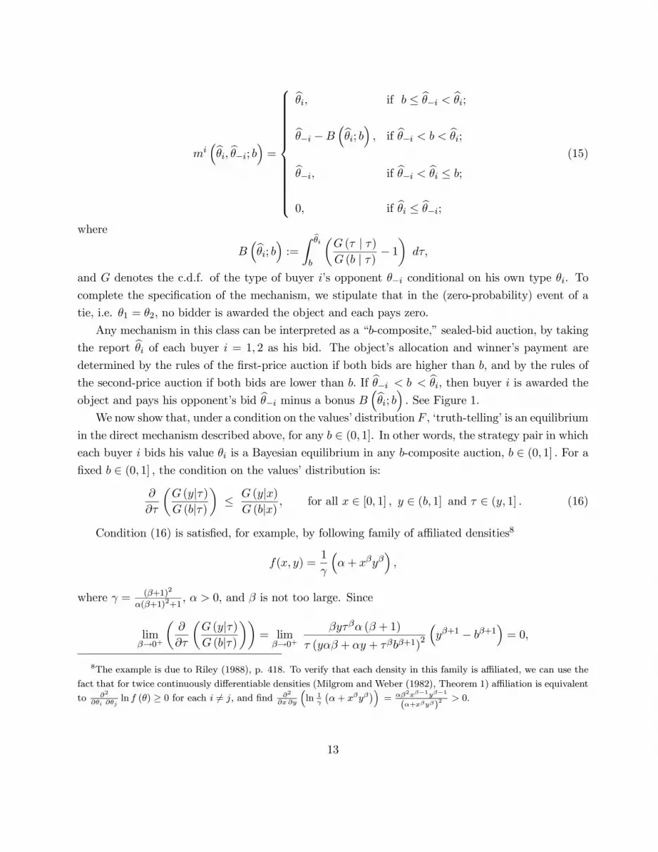
Any mechanism in this class can be interpreted as a “b-composite,” sealed-bid auction, by taking
the report bθi of each buyer i = 1, 2 as his bid. The object’s allocation and winner’s payment are
determined by the rules of the first-price auction if both bids are higher than b, and by the rules of
the second-price auction if both bids are lower than b. If bθ−i < b < bθi, then buyer i is awarded theobject and pays his opponent’s bid bθ−i minus a bonus B ³bθi; b´ . See Figure 1.
We now show that, under a condition on the values’ distribution F , ‘truth-telling’ is an equilibrium
in the direct mechanism described above, for any b ∈ (0, 1]. In other words, the strategy pair in whicheach buyer i bids his value θi is a Bayesian equilibrium in any b-composite auction, b ∈ (0, 1] . For afixed b ∈ (0, 1] , the condition on the values’ distribution is:
∂
∂τ
µG (y|τ)G (b|τ)
¶≤ G (y|x)G (b|x) , for all x ∈ [0, 1] , y ∈ (b, 1] and τ ∈ (y, 1] . (16)
Condition (16) is satisfied, for example, by following family of affiliated densities8
f(x, y) =1
γ
³α+ xβyβ
´,
where γ = (β+1)2
α(β+1)2+1, α > 0, and β is not too large. Since
limβ→0+
µ∂
∂τ
µG (y|τ)G (b|τ)
¶¶= limβ→0+
βyτβα (β + 1)
τ (yαβ + αy + τβbβ+1)2
³yβ+1 − bβ+1
´= 0,
8The example is due to Riley (1988), p. 418. To verify that each density in this family is affiliated, we can use the
fact that for twice continuously differentiable densities (Milgrom and Weber (1982), Theorem 1) affiliation is equivalent
to ∂2
∂θi ∂θjln f (θ) ≥ 0 for each i 6= j, and find ∂2
∂x ∂y
³ln 1
γ
¡α+ xβyβ
¢´= αβ2xβ−1yβ−1
(α+xβyβ)2> 0.
13

b
b
0 1
1
θ1
θ2
Second-Price - B(θ1; b)
Second-
Price
-
B(θ2; b)
First-Price
Second-Price
Figure 1: A b-composite auction
and
limβ→0+
µG (y|x)G (b|x)
¶= limβ→0+
µα (β + 1) y + xβyβ+1
α (β + 1) y + xβbβ+1
¶=(α+ 1) y
αy + b> 0, for all y ∈ (b, 1] ,
there must exist a β∗ such that condition (16) holds for all densities with β ∈ (0,β∗).
Lemma 1 For any b ∈ (0, 1] , if condition (16) holds, the direct mechanism described in (14) and
(15) is incentive compatible.
Proof. To verify that truth-telling is a best reply to itself, suppose that buyer 2 reports his true
type. There are two cases.
Case 1: Buyer 1’s type is at least as high as b, i.e. θ1 ∈ [b, 1] . Bidding above b, i.e. biddingbθ1 ∈ (b, 1] , yieldsS³bθ1, θ1; b´ ≡
hθ1 −E [θ2 | θ2 < b] +B
³bθ1; b´i Pr [θ2 < b | θ1] + (θ1 − bθ1) Pr hb < θ2 < bθ1 | θ1i=
hθ1 −E [θ2 | θ2 < b] +B
³bθ1; b´i G (b|θ1) + (θ1 − bθ1) hG³bθ1|θ1´−G (b|θ1)i .
14

The first derivative with respect to bθ1 is∂S³bθ1, θ1; b´∂bθ1 = G (b|θ1)
∂B³bθ1; b´∂bθ1 −
hG(bθ1|θ1)−G(b|θ1)i+ ³θ1 − bθ1´ g ³bθ1|θ1´
= G(b|θ1)ÃG(bθ1|bθ1)G(b|bθ1) − 1
!−hG(bθ1|θ1)−G(b|θ1)i+ ³θ1 − bθ1´ g ³bθ1|θ1´
=³θ1 − bθ1´ g ³bθ1|θ1´−G(bθ1|θ1) +G(b|θ1)G(bθ1|bθ1)
G(b|bθ1)= (θ1 − bθ1) g(bθ1|θ1)−G(b|θ1)ÃG(bθ1|θ1)
G(b|θ1) −G(bθ1|bθ1)G(b|bθ1)
!
=
Z θ1
bθ1"g(bθ1|θ1)−G(b|θ1) ∂
∂τ
ÃG(bθ1|τ)G(b|τ)
!#dτ,
where g0 denotes the density corresponding to g. By condition (16), the last expression is nonnegative,for bθ1 < θ1, and nonpositive for bθ1 > θ1. Thus S (·, θ1; b) is weakly increasing in the interval (b, θ1) ,and weakly decreasing in the interval (θ1, 1] . Since S (·, θ1; b) is also continuous, we have that biddingθ1 maximizes S(·, θ1; b) in the interval (b, 1] .
Bidding b or less, i.e. bθ1 ∈ [0, b] , yieldsS³bθ1, θ1´ ≡ Z bθ1
0(θ1 − y) dG (y|θ1) .
Since Z bθ10(θ1 − y) dG (y|θ1) ≤
Z b
0(θ1 − y) dG(y|θ1)
≤Z b
0(θ1 − y) dG(y|θ1) +G(b|θ1)B(θ1; b)
= S (θ1, θ1; b) ,
buyer 1 has no incentive to bid below b either. Thus bidding θ1 is optimal for buyer 1 whenever his
type is in the interval [b, 1].
Case 2: Buyer 1’s type is lower than b, i.e. θ1 ∈ [0, b) . Bidding bθ1 ∈ [0, b] yields S ³bθ1, θ1´ =Z bθ10(θ1 − y) dG (y|θ1) . Since the derivative
∂S³bθ1, θ1´∂bθ1 =
³θ1 − bθ1´ g ³bθ1|θ1´15

has the same sign of θ1− bθ1, the payoff is increasing for bθ1 < θ1 and decreasing for θ1 < bθ1. As in thefirst half of Case 1 above, by continuity S, we have that S (·, θ1) is maximized by θ1 in the interval[0, b] , i.e.
S³bθ1, θ1´ ≤ S (θ1, θ1) , for all bθ1 ∈ [0, b] . (17)
Finally, reporting bθ1 ∈ (b, 1] yieldsS³bθ1, θ1; b´ =
hθ1 −E [θ2 | θ2 < b] +B
³bθ1; b´i G (b|θ1) + (θ1 − bθ1) hG³bθ1|θ1´−G (b|θ1)i≤ (θ1 −E [θ2 | θ2 < b]) G (b|θ1)
= S (b, θ1)
≤ S (θ1, θ1)
where the last inequality is implied by (17) above. 2
We are now ready to show that, if the buyers’ values are strictly affiliated and condition (16)
holds, the b-composite auctions can be ranked strictly in terms of seller’s expected revenue: the lower
the parameter b, the higher the seller’s expected revenue. Therefore the English auction, which is
equivalent to the “1-composite” auction (we are assuming private values), generates a strictly lower
expected revenue for the seller than any b-composite auction, for b ∈ (0, 1) .
Proposition 2 Let Π (b) , b ∈ (0, 1] , denote the seller’s expected revenue generated by the b-compositeauction. If the signals’ distribution satisfies both strict affiliation and condition (16), then Π is strictly
decreasing in b.
Proof. Each buyer’s ex ante equilibrium payoff in a b-composite auction is:
S(b) =
Z b
0
µZ x
0(x− y) g (y|x) dy
¶dFi(x)
+
Z 1
b
µZ b
0[x− y +B (x; b)] g (y|x) dy
¶dFi (x) ,
where Fi denotes the marginal c.d.f. of buyer i’s type. It is sufficient to show that S (b) is strictly
increasing in b, because in any b-composite auction the object is always sold to a buyer with the
highest value, hence the same (maximum) expected social surplus is realized. Differentiating yields:
dS(b)
db=
Z 1
b
µ[x− b+B (x; b)] g (b|x) +
Z b
0
∂B (x; b)
∂bg (y|x) dy
¶dFi (x)
16

=
Z 1
b
·(x− b) g (b|x) +B (x; b) g (b|x) + ∂B (x; b)
∂bG (b|x)
¸dFi(x)
=
Z 1
b
·(x− b) g (b|x) + g (b|x)
Z x
b
µG (τ |τ)G (b|τ) − 1
¶dτ
−G (b|x)Z x
b
µG (τ |τ)[G (b|τ)]2 g (b|τ)
¶dτ
¸dFi (x)
=
Z 1
b
·g (b|x)
Z x
b
G (τ |τ)G (b|τ) dτ −G (b|x)
Z x
b
G (τ |τ)G (b|τ)
g (b|τ)G (b|τ) dτ
¸dFi (x)
=
Z 1
b
·G (b|x)
Z x
b
G (τ |τ)G (b|τ)
µg (b|x)G (b|x) −
g (b|τ)G (b|τ)
¶dτ
¸dFi(x).
Strict affiliation implies g(y|τ)g(b|τ) >g(y|x)g(b|x) for all τ, x, y and b such that τ < x and y < b. Thus we haveR b
0 g(y|τ)dyg(b|τ) >
R b0 g(y|x)dyg(b|x) , hence g(b|τ)
G(b|τ) <g(b|x)G(b|x) whenever τ < x, for any b. Since the inside integral in
the last line of the expression above is taken for τ ∈ [b, x], the derivative dS(b)db is strictly positive. 2
Corollary 1 Any b-composite auction, b ∈ (0, 1) (with two bidders), generates a strictly higher
seller’s expected revenue than the English auction.
Proof. The result follows from proposition 2 and the fact that S (1) =
Z 1
0
Z x
0(x− τ) g(τ |x)dτ is
also each buyer’s ex ante expected surplus in the English auction. 2
The rest of this section is devoted to illustrate the key idea behind the results of Proposition 2
and Corollary 1 and clarify the role of condition (16).9 Consider a model in which the two buyers’
signals have a discrete distribution. The table in Figure 2 (last page) represents the payoffs of buyer
1 when his signal (i.e., his ‘type’) is θ1 and he reports the row’s type, in a mechanism that mimics
the symmetric equilibrium of the English auction10, except when (θ1, θ2) ∈ {(3, 1) , (3, 2) , (4, 1)}. Ifθ1 = 3, the buyer’s expected payoff is as in the English auction, but he pays ε more if θ2 = 2, and
ε p (2|3) /p (1|3) less if θ2 = 1, where p (j|i) denotes the probability that θ2 = j conditional on θ1 = i.This difference from the English auction relaxes type 4’s “downward-adjacent” incentive constraint:
9The idea is the same that allows the construction of full extraction mechanisms. A brief explanation can be found
in Myerson (1981) p. 71.
10Ties are resolved in favor of bidder 1.
17

if he reports bθ1 = 3, his expected payoff isµu (4, 1)− u (1, 1) + ε p (2|3)
p (1|3)¶p (1|4) + (u (4, 2)− u (2, 2)− ε) p (2|4) + (u (4, 3)− u (3, 3)) p(3|4),
while his payoff in the English auction would be
(u(4, 1)− u(1, 1)) p(1|4) + (u(4, 2)− u(2, 2)) p(2|4) + (u(4, 3)− u(3, 3) ) p(3|4).
The difference
δ(ε) =
µp (2|3)p (1|3)p (1|4)− p (2|4)
¶ε
is negative for any ε > 0 , since p (2|3) /p (1|3) < p (2|4) /p (1|4) , by the monotone likelihood ratioproperty, which is implied by the affiliation hypothesis. Thus type 4’s expected payment can be
made higher than the English auction’s
4Xj=1
u (j, j) p (j|4)
by δ (ε) ; and so can the expected payments of all types above 4. To summarize the above discussion
in one sentence, the difference in preferences over lotteries among the various types of each buyer
can be exploited to increase their expected payments.
In any b-composite auction the bonus function B changes each type’s equilibrium payment func-
tion in the same way: it induces a higher payment when his opponent’s type is above b, and a lower
payment otherwise. To see why condition (16) is needed, note that in the example of Figure 2 the
expected payoff of type 2 from reporting bθ1 = 3,µu(2, 1)− u(1, 1) + p (2|3)
p (1|3)ε¶p (1|2) + (u(2, 2)− u(2, 2)− ε) p(2|2) + (u(2, 3)− u(3, 3) ) p(3|2),
is increasing in ε, since p(2|3)p(1|3) >p(1|2)p(2|2) by affiliation. Thus, for any ε, his “upward-adjacent” constraint
will be violated if the degree of affiliation is high enough. Condition (16) limits the degree of
affiliation, so that no ‘upward’ incentive constraint is violated by the changes in the payment functions
that the bonus function B induces. It should be clear however that condition (16) is not crucial for
the results of this section: even if it does not hold, it is still possible to construct LDNP selling
mechanisms which generate a higher seller’s expected revenue that the EA.
5 Conclusive Remarks
The comparison between the widespread use of the English auction in reality, and the fact that
optimal selling mechanisms, as engineered by the theory of mechanism design, are never observed in
18
practice, poses a puzzle to which the results of this paper provide partial answers. The main insight,
which also emerges from the results established in Lopomo (1998), appears to be that the English
auction can only maximize the seller’s expected profit if the rules of all feasible trading mechanisms
allow each buyer to determine his actual payment conditional on the allocation of the object. The
central role played by this “bargaining-like” feature deserves further investigation. The reward could
be a significant step toward a unified theory of auctions and bargaining.
19

References
[1] Bikhchandani, S. and J. Riley (1991): “Equilibria in Open Common Value Auctions,” Journal
of Economic Theory 53: 101—30.
[2] Bulow, J. and J. Roberts (1989): “The Simple Economics of Optimal Auctions,” Journal of
Political Economy 92: 1060-90.
[3] Cremer, J. and R. McLean (1988): “Full Extraction of the Surplus in Bayesian and Dominant
Strategy Auctions,” Econometrica 56: 1247—57.
[4] Cassady, R. (1967): Auctions and Auctioneering, Berkeley, University of California Press.
[5] Green, J. R., and J. Laffont (1987): “Posterior Implementability in a Two-Person Decision
Problem,” Econometrica 55: 69—94.
[6] Kolgomorov A. N., and S. V. Fomin (1970): Introductory Real Analysis, Dover.
[7] Krishna, V. and J. Morgan, (1996): “An Analysis of the War of Attrition and All-Pay Auction,”
Journal of Economic Theory 72: 343—362.
[8] Lopomo G. (1998): “The English Auction is Optimal among Simple Sequential Auctions,”
Journal of Economic Theory 82: 144—166.
[9] Maskin, E. and J. Riley (1984): “Optimal Auctions with Risk Averse Buyers,” Econometrica
52: 1473—518.
[10] Matthews, S. (1983): “Selling to Risk Averse Buyers with Unobservable Tastes,” Journal of
Economic Theory 30: 370—400.
[11] McAfee, R.P. and J. McMillan (1987): “Auctions and Bidding,” Journal of Economic Literature
25: 699—738.
[12] McAfee, R.P. and P. Reny (1992): “Correlated Information and Mechanism Design,” Econo-
metrica 60: 395—421.
[13] Milgrom, P. (1985): “The Economics of Competitive Bidding: A Selective Survey,” in Social
Goals and Social Organization. Essays in Memory of Elisha Pazner, L. Hurwicz et al. (eds.),
Cambridge UK: Cambridge University Press.
20

[14] Milgrom, P. (1987): “Auction Theory,” in Advances in Economic Theory: Fifth World Congress,
T.F. Bewley (ed.), Cambridge UK: Cambridge University Press.
[15] Milgrom, P. and R. Weber (1982): “A Theory of Auctions and Competitive Bidding,” Econo-
metrica 50: 1089—122.
[16] Myerson, R. (1981): “Optimal Auction Design,” Mathematics of Operations Research 6: 58—73.
[17] Riley, J. (1988): “Ex Post information in Auctions,” Review of Economic Studies LV, 409-30.
[18] Riley, J. and W. Samuelson (1981): “Optimal Auctions,” American Economic Review 71:
381—92.
21

1 2 3 4
1
2
3
4
u(θ1, 1)− u(1, 1)
u(θ1, 2)− u(2, 2)
0 00
0 0
0
0
u(θ1, 3)− u(3, 3)
0
0
u(θ1, 4)− u(4, 4)
u(θ1, 1)− u(1, 1)
u(θ1, 1)− u(1, 1)
+p(2|3)p(1|3)ε
u(θ1, 2)− u(2, 2)
− ε
u(θ1, 1)− u(1, 1)
− δ(ε)
u(θ1, 2)− u(2, 2) u(θ1, 3)− u(3, 3)
Figure 2: An LDNP mechanism generating more seller’s expected profit than the English auction
22


