Embed Size (px)
Citation preview
SYSTEMS MODELING FOR ELECTRIC SHIP DESIGN
By
Charalambos Soultatis
Hellenic Naval Academy (Mechanical Eng.), 1995National Technical University of Athens (Department of Naval Architecture)
Submitted to the Department of Ocean Engineering in partial fulfillment of the requirements for thedegrees of
Naval Engineer in Naval Architecture and Marine EngineeringAnd
Master of Science in Ocean Systems ManagementAt the
MASSACHUSETTS INSTITUTE OF TECHNOLOGY
June 2004
C 2004 Charalambos SoultatisThe author hereby grants to MIT and the US Government permission to reproduce and distribute
publicly paper and electronic copies of this document in whole or in part.
Signature of Authorfffment of Ocean Engineering
07 May 2004
Certified By
Michael TriantafyllouProfessor of Ocean Engineering
Thesis Supervisor
Certified By
Henry S. MarcusProfessor of Ocean Engineering
- -Thesis Sunervisor
Accepted By
Timothy J. McCoyAsociate Professor of Ocean Engineering
Accepted By
Michael TriantafyllouProfessor of Ocean Engineering
Chairperson, Department Committee on Graduate Studies
MASSACHUSET1S INS SE,
BARKER OF TECHNOLOGY
SEP 0 12005
LIBRARIES
SYSTEMS MODELING FOR ELECTRIC SHIP DESIGN
by
Charalambos Soultatis
Submitted to the Department of Ocean Engineering on May 7, 2004 in partial fulfillment of
the requirements for the degrees of Naval Engineer in Naval Architecture and Marine
Engineering
And
Master of Science in Ocean Systems Management
Abstract
Diesel and gas turbine electric ship propulsion are of current interest for several
types of vessels that are important for commercial shipping and for the next generation of
war ships. During the design process of a platform, a choice has to be made between two
different fundamental concepts regarding propulsion; a conventional arrangement, and a
diesel or gas turbine electric propulsion. For both concepts, the electrical installation is
present and the demand for additional electric energy becomes a dominant parameter.
In both cases, the selection of the prime mover significantly influences the
effectiveness of the design. In this thesis, the simulation modeling of a complete
propulsion system will be attempted, with overall emphasis on the prime movers.
In the first part a diesel engine is considered. The time delay between changing a
set point for the revolutions of the engine and the change of the real revolutions is often
modeled as a first order system. However, this modeling is too simple to describe the real
behavior of the diesel engine. More complex models exist, but in general they are too
complex, describing the full thermodynamic behavior of diesels. So there is a need for a
model that is more advanced than a first order system and less complex than complete
thermodynamic models. Such a model has been derived, based on the Seiliger
1
(thermodynamic) process. The results of the model show that the diesel engine behaves
like a second order system when operating in the governor area and more like a first order
system in the constant torque (overload) area. The simulation model of a diesel engine
can be regarded as an explanation of the real engine operation, which combines the
mathematical relationship between the relative components and can be used to simulate
dynamic loading of the diesel engine.
In the second part, a development of a nonlinear gas turbine model for loop-
shaping control purposes is presented. The nonlinear dynamic equations of the gas
turbine are based on first engineering principles. In order to complete the model,
constitutive algebraic equations are also needed. These equations describe the static
behavior of the gas turbine at various operating points. The complete, substituted
nonlinear model is presented along with its model verification results based on a
simulator and measured data.
A mathematical description for the electric part of the propulsion and energy
generation system with respect to numbers of components such as generators and
thruster drives is attempted. Other electrical loads may be represented with an aggregate
load. Based on the control functions focus on power production, advanced dynamic
models shall be used for the generators and simplified static models shall be used for
thruster drives and other loads. The final model shall be in a state-space vector form,
suitable for control design.
As a conclusion, a reliability analysis on the decision for the electric propulsion
system is utilized based on market data, speed and electric energy requirements studies.
The purpose of this study is to justify the employment of innovative and efficient electric
propulsion systems for the future needs of the commercial and naval ship industries.
Thesis Supervisor: Professor Michael TriantafyllouProfessor Henry S. Marcus
2

AKNOLDGEMENT
Ga iilOOa Va acLplpG(O alYI7I1 Tfi OfrcTIi K(XtapXag (YTCL 610 M1O CXyaiapitSVa
npOMIT7Ua fqq (O)1g p01, 7101) iapa Ttq (YUVe6jTEg 6KoadOktCg pIC Gflp 1V C K(LO6
pcyako Pfqpta poo. Kai noto DYxKCKplIva TIJv pryupa pWO AXFaV6pa, q OnOW cyXt
KcXVCt (17FIpEg Oucntc yta va 66t Tct ovstpa p1O'U Va ytvovTaIt 7[PUYpXtlKOT1jTa Kat TTOV
na2rpa ptoD Ayycko, (ptko Kat ap oi)po go' 7roi) ps ptyakocyc pt 7cpt(n aya7n.
Acv Oa r1OEa otog va RapaklUWo Kalt okoog auOUg RoD 'wr1p0av apoyol okiq
a1)Tflg Trwg RpoolMcOclc ptol). Akka Oa MLo E2tlypaptpKXa c76 6o ptkoog MRL a66ppoDg
RO [tS CYT1'qltaV Kal pic POI1Orqcav Eo Y'nv A~tspl . Tog oo 0 sopyit68 nO 1rjav
KOVTa gOD. IiattEpa Oa 1106cl va 1)XaptYT1GO To Flopyo II. Y7W All TTV P01O61t08 rKt
But it would be faire if I did not dedicate this Thesis to my valuable assistants and
supporters, my professors. I want to express my gratitude especially to Pr. Michel
Tryantafyllou for his guidance and his understanding, to Pr. T. J. McCoy for his
unlimited help for all this thesis preparation period and of course the so kind person Pr. H.
S. Marcus for his knowledge that openly shared with me.
To dedicate such a work to your lovely person may be it is not so important or
does not make sense. But to characterize this person as your inspiration and your hope I
believe that is the real meaning of love. And this is what I want to declare for my small
angel. Because everything that it took place in this period that we are together was full of
success and this I want to keep inside me forever. So .... to the person that I really love.
To Tomoko
Inspiration and meaning of my success
3
Table of Contents
Chapter 1..............................................................................................................................9Introduction ......................................................................................................................... 9
1.2 Objectives ..................................................................................................... 111.3 Thesis Outline................................................................................................. 12
Chapter 2............................................................................................................................14Gas Turbine ................................................................................................................... 142.1 Gas Turbine Com ponents Description .......................................................... 142.2 Com pressor.................................................................................................... 16
2.2.1 M ethodology of approach...................................................................... 162.2.2 Transient com pressor characteristics........................................................ 22
2.3 Turbine...................................................................................................... 242.3.1 M ethodology of approach...................................................................... 242.3.2 Transient turbine characteristics.............................................................27
2.4 Com bustion cham ber.................................................................................... 272.4.1 M ethodology of approach...................................................................... 27
2.4.2 Transient com bustion cham ber characteristics...........................................302.5 Power Turbine .............................................................................................. 312.6 Turbomachinery Theory-Model Development............................................. 32
2.6.1 Governing Equations ............................................................................ 322.6.2 Therm odynam ic approach ........................................................................ 352.6.3 Fluid Dynam ics Approach........................................................................ 35
a. Conservation of m ass...................................................................................... 35b. Conservation of m om entum .......................................................................... 37c. Conservation of energy.................................................................................. 39
2.7 N onlinear M odel.............................................................................................442.8 Constitutive Relations.................................................................................... 472.9 General Com ponents equations......................................................................492.10 Engine Param eter Interrelationships M atlab Chart ........................................ 532.11 Gas Turbine Operation- Control Considerations........................................... 56
Chapter 3............................................................................................................................603 Diesel Engine.............................................................................................................60
3.1 D iesel Utility................................................................................................. 603.2 Prim e m over m odel developm ent................................................................. 613.2.1 Introduction .............................................................................................. 623.2.2 Engine inlet............................................................................................... 633.2.3 Engine outlet............................................................................................... 663.2.4 Therm odynam ic approach - approxim ation ............................................... 683.2.5 Fuel M odel................................................................................................. 733.2.6 Ideal first-order dynamic model of a turbine-compressor system..............813.2.7 Exhaust system .......................................................................................... 853.2.8 A ir flow through Cylinders............................................................................873.2.9 M odel sum m ary........................................................................................ 883.3 D iesel Engine Sim ulation Transients ............................................................ 89
Chapter 4............................................................................................................................94
4
4 Electric Propulsion Components .................................................................. 94
4.1 Approach ..............................................................................- 94
4.1.1 Synchronous Generator .................................................................. 94
4.2 Electric Load..................................................................... ...... 105
4.4.3 Converters...........................................................................1224.4.3.1 PWM Converter............................................................ . ...... 1224.4.3.2 Cycloconverter.......................................................... ........ 123
4.5 State space model .................................................................. 124
C hapter 5............................................................--.--.-.--.. ... ------------------......................... 128
5. Life Cycle Cost Estimation and Reliability Analysis..................................................1285.1 Functional and Reliability Analysis ............................... 128
5.1.1 Fuel Problem Description...............................................................1295.2 Value of Speed Study .......................................................................... .... 131
5.3 Manning Reduction .............................................................. 143
5.4 Area and Volume Challenge........................................................ ... 146
5.5 Some additional considerations..............................................................1485.6 Systems Reliability Models...................................1505.6.1 The basic series reliability m odel..............................................................150
5.6.2.1 A ctive redundancy...................................................................................1515.6.2.2 m -out-of-n Redundancy...........................................................................1535.6.2.3 Standby Redundancy ................................................. ........ ... 157
5.6.3 Availability of Repairable Systems ............................................................. 158
5.6.4 Modification example............................................................1605.6.5 Modular Design ........................................................................ 164
5.7 Market Option........................................................... ......... 170
REFERENCES ......................................................................... .. ..... .... 172
APPENDIX 1 ..................................................................... 175
APPENDIX 2 ...................................................................... 177
APPENDIX 3 .....................................................................--......... 178
APPENDIX 4 ............................................................... ..... 180
APPENDIX 5 ................................................ 183
5
List of fiEures
Figure 1: Gas turbine single shaft (or Gas generator of a Twin shaft GT) representation 15Figure 2: Simplified compressor representation.............................................................16Figure 3: Stator and rotor components Figure 4: Operating principle of an ..... 19Figure 5: Simplified Centrifugal Pump ........................................................................ 20Figure 6: Two stage compressor....................................................................................20Figure 7: Typical axial flow compressor characteristics...................................................21Figure 8: Typical centrifugal flow compressor characteristics ..................................... 22Figure 9: Simplified Turbine representation ................................................................. 24Figure 10: Combustion Chamber representation.......................................................... 28Figure 11: Energy/ power transfer diagram....................................................................32Figure 12: Change of the output HP with respect to the change in the fuel mass flow.....55Figure 13: Turbine speed (RPM) variations with respect to the change in the fuel mass
flow and compression ratio (P3/P2)........ ................... ....... 56Figure 14: Diesel engine nomenclature ........................................................................ 63Figure 15: Diesel engine schematic representation ...................................................... 63Figure 16: Typical Silinger cycle ................................................................................. 68Figure 17: Simplified Silinger cycle............................................................................. 68Figure 18: x-t m odel...................................................................................................... 74Figure 19: Curve fit of x-t model to engine transient ................................................... 77Figure 20: Concept flow-chart...................................................................................... 80Figure 21: Fuel input ..................................................................................................... 91Figure 22: Revolutions respond....................................................................................91Figure 23: Output Torque response...............................................................................92Figure 24: Air Intake response ..................................................................................... 92Figure 25: Diagram of current transformation to d-q frame....................107Figure 26: Propeller - shaft m odel .................................................................................. 112Figure 27: Pow er Loss diagram ....................................................................................... 113Figure 28: Per- unit induction motor equivalent circuit .................................................. 114Figure 29: d- and q-axes equivalent circuits....................................................................120Figure 30: Phasor diagram of PM synchronous motor....................................................120Figure 31: Electric vs. traditional propulsion configuration............................................129Figure 32- Speed Profiles for various missions...............................................................132Figure 33- Operational value of speed and Derivative of the value of speed ................. 132Figure 34- Speed Profiles for various missions...............................................................134Figure 35: Installed electric power in USN Destroyers vs. years....................................136Figure 36: Power distribution vs. gross tonnage for large cruise ships...........................137Figure 37: Power loss flow & Electric propulsion system representation .......... 138Figure 38: Engine Output Power vs. efficiency chart ..................................................... 139Figure 39: Diesel engine fuel consumption vs. % Output Power Graph...........140
6
CP & FP Propeller characteristic data............................................................143Manning vs. cost analysis .............................................................................. 145Three comparative concepts of a Ropax vessel showing how space can beutilized with electric propulsion and podded propulsion. ............................. 147Conversional propulsion system....................................................................150serial system Reliability Block diagram ........................................................ 151Traditional Redundant Propulsion System .................................................... 152Dual redundant diagram.................................................................................152Electric propulsion parallel reduction configuration ..................................... 153Reliability block diagram...............................................................................158
7
Figure 40:Figure 41:Figure 42:
betterFigure 43:Figure 44:Figure 45:Figure 46:Figure 47:Figure 48:
List of tables
Table 1: Comparison of the given values with the simulated for a given steady statecondition .................................................................................................................... 89
Table 2: Conversional system components ..................................................................... 161Table 3: Electric system components .............................................................................. 161Table 4: Main engines and Diesel generators characteristics..........................................162Table 5: Reliability analysis ............................................................................................ 163Table 6: For modules MTBR and replacement costs ...................................................... 164Table 7: For modules MTBR and total costs...................................................................165Table 8: Podded propulsors Data.....................................................................................167Table 9: Capital and Operational Expenditures...............................................................171
8
Chapter 1
Introduction
1.1 Motivation
Diesel or turbine electric propulsion of ships is of current interest for several types
of ships that are important for commercial and military shipping. When designing a
vessel a choice has to be made between two different fundamental concepts regarding
propulsion; a conventional, straight diesel drive or gas turbine or even a combination and
diesel electric propulsion. For both concepts, the electrical installations are very compact
with short distances from generators to consumers. This gives several consequences that
are particular for these installations.
Common to most modem vessels is the high generating power, often about 6 - 7
MW, due to large electric loads that the modem life and the huge and different types of
power electronics demand. This also implies high load currents and large fault currents.
The basic idea with such systems is to replace the main diesel or gas turbines
propulsion engines with electric motors, and split the power production into several
smaller diesel-generators. Electrical motors can be designed with a very high efficiency
throughout the whole range of operation with respect to both speed and power output, in
9
contrast to the diesel engine which has a clear peak in efficiency around its nominal
working point. A ship which varies its velocity will be able to operate with a high
efficiency for the whole range of operation by selecting the optimal number of diesel
generators to supply the desired power demand. For a conventional system with diesel
propulsion the efficiency would decrease noticeably for operation outside nominal
operation. In addition there are several other advantages which are discussed later in this
thesis.
The choice of a diesel or GT electric system as the power source for a propulsion
system of a vessel has nothing to do with hydro-dynamic efficiency. A propulsion system
of a vessel i.e. that which is providing thrust to move the vessel is still chosen by the
designer based on its merits for the vessel's application. Conventional propellers, CP
propellers, azimuthing Z drives, transverse tunnel thrusters and low speed water jet
systems can all be driven with equal effectiveness by a diesel electric system. Diesel
electric systems become viable when the installed KW for propulsion approaches or is
exceeded by the installed KW for other purposes. The convenience of electric power
distribution makes it possible to locate the primary power source i.e. diesel generators
exclusive of consideration for where the power is to be applied, whether it be propulsion,
thrusters, HVAC or cargo handling purposes. A large variation in propulsion power
requirements i.e. long periods of low speed or a necessity to shift power from main
propulsion to thrusters for dynamic positioning purposes can also justify diesel electric.
Modem turbo charged diesel and GT engines are efficient over a relatively narrow
operating load and RPM range. They are not suitable for long periods of low speed, low
load, or low RPM high torque requirements for reversing large propellers. Modem
generator systems with load sharing, auto start, and load shedding features make it
possible to more efficiently utilize the installed H.P. of a diesel or GT electric system.
It is obvious from the above that there is a large number of factors that make the
use of the electric propulsion of substantial importance. But the thing that carries such an
innovation to the next stage is the ability to control such a system, a controller that can
achieve the maximum power production efficiency in any power demand scenario.
The main motivation for modeling a Diesel or GT Electric Propulsion system is
for simulation of different scenarios to check the performance and the stability of the
10
prime movers, in the electrical network and to improve the power management with more
advanced control theory.
1.2 Objectives
The present thesis is divided into four major parts. The Gas Turbine (GT) prime
mover model development, Diesel Engine model development, the state space
representation of the electric machinery systems and propulsion thrusters and last a
reliability and efficiency analysis based on the market data. The goals of this thesis are:
* The development of a Gas Turbine math model appropriate for control
implementation using the state space model approach and a simulation transient
response program.
* The formulation of a computer simulation of the transient characteristics of marine
Diesel Engines based on the so called Quasi Steady State Method.
* The developing of a state space representation in the matrix form appropriate for
control implementation of the electric systems (generators, motors, converters) and
main thrusters.
* The presentation of a full reliability analysis of the Electric Ship implementation, and
an evaluation of all the factors that are increasing the efficiency of such a system.
11
1.3 Thesis Outline
Chapter 1. Intoduction to the thesis
Chapter 2. In the second chapter an illustration for the development of the Gas Turbine
model is taking place. The analytic part of the model is based on the turbomachinery
theory. Since the GT are energetic systems any attempt to describe their operation must
start from energy consideration. The power transfer associated with various GT may be
classified into three major groups: the mechanical power transfer, pure thermal power
transfer and the fluid power transfer. The equations are describing the main Gas turbine
components. For the computer model that it will be formulated for the calculations of the
steady state condition and transient responses a non dimensional analysis will be
presented. Also the developing of the gas turbine interrelationships and a series of
thermodynamic based equations used to couple the equations that actually represent the
gas turbine model is taking place. These equations are the constitutive equations that are
needed to complete the nonlinear gas model. We will describe two deferent types of
constitutive equations. The fist type describes the total temperature after the compressor
Ttot_3 and the total temperature after the turbine Ttot_5 .
The analysis also includes estimations for the time constants for each GT component
and considerations about the control concepts on the gas turbine plant.
Chapter 3. The third chapter is dedicated to the development of a diesel engine quasi
static model. The classic dynamic behavior is also implemented which includes inertia of
the diesel engine and turbine-compressor system as the main parts. For other subsystems
the dynamic behavior is mainly based on the thermodynamic theory. With the charge air
condition parameters it is possible to ignore the sub-systems like, air-filter, inter-cooler,
inter-receiver and outlet-receiver in a simple model.
Chapter 4. A mathematical description for the electric part of the propulsion and
energy generation system with respect to numbers of components such as generators and
thruster drives is attempted in this chapter. The mathematical description should be
12

general with respect to numbers of components as generators and thruster drives. Other
consumers may be represented with an aggregate load. The model is presented in matrix
form.
Chapter 5. A functional and reliability analysis with extensions to the efficiency of
the system considering fuel consumption, manning and maintenance cost is been
illustrated in this chapter.
13
Chapter 2
Gas Turbine
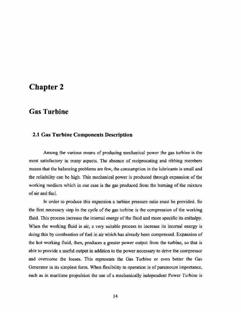
2.1 Gas Turbine Components Description
Among the various means of producing mechanical power the gas turbine is the
most satisfactory in many aspects. The absence of reciprocating and ribbing members
means that the balancing problems are few, the consumption in the lubricants is small and
the reliability can be high. This mechanical power is produced through expansion of the
working medium which in our case is the gas produced from the burning of the mixture
of air and fuel.
In order to produce this expansion a turbine pressure ratio must be provided. So
the first necessary step in the cycle of the gas turbine is the compression of the working
fluid. This process increase the internal energy of the fluid and more specific its enthalpy.
When the working fluid is air, a very suitable process to increase its internal energy is
doing this by combustion of fuel in air which has already been compressed. Expansion of
the hot working fluid, then, produces a greater power output from the turbine, so that is
able to provide a useful output in addition to the power necessary to drive the compressor
and overcome the losses. This represents the Gas Turbine or even better the Gas
Generator in its simplest form. When flexibility in operation is of paramount importance,
such as in maritime propulsion the use of a mechanically independent Power Turbine is
14
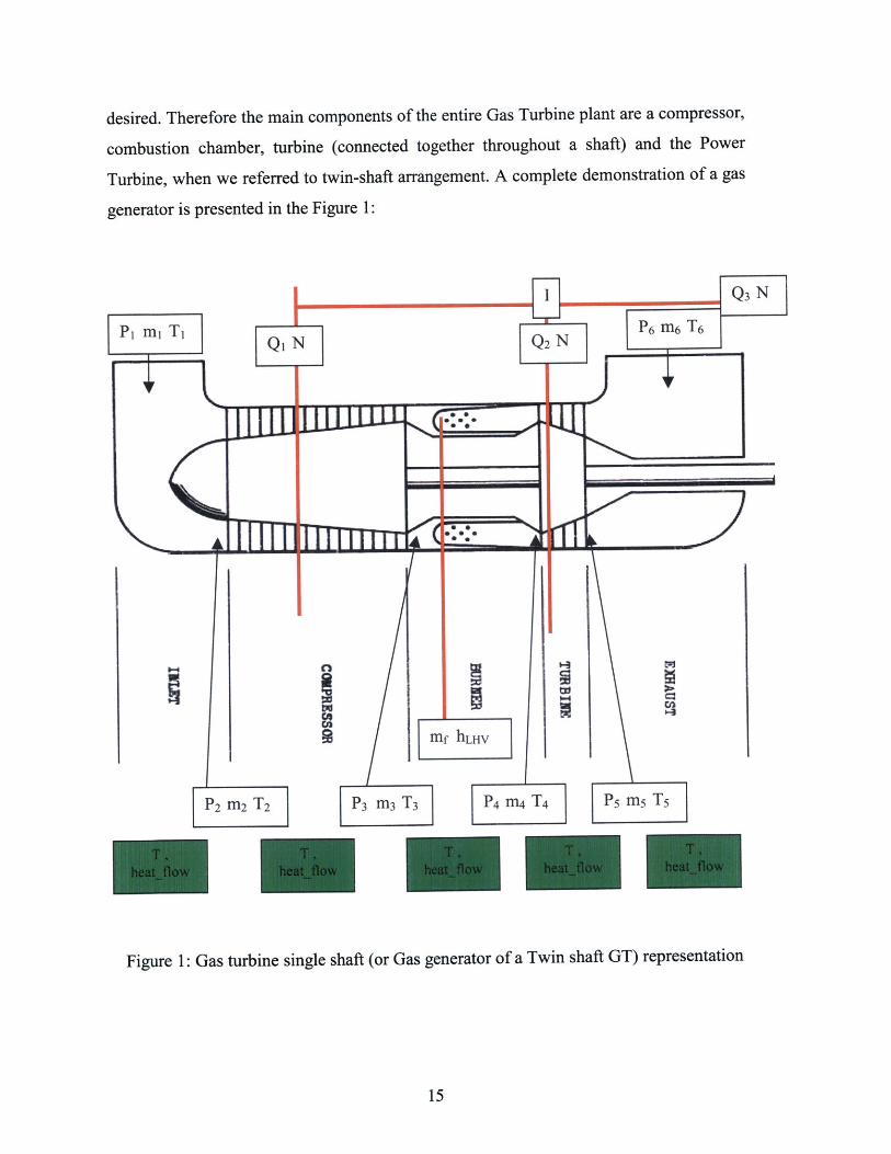
desired. Therefore the main components of the entire Gas Turbine plant are a compressor,
combustion chamber, turbine (connected together throughout a shaft) and the Power
Turbine, when we referred to twin-shaft arrangement. A complete demonstration of a gas
generator is presented in the Figure 1:
Q1 N
C ~EE. * *
=1- ~ U _____________________ U U urn mm
0
Ieqeq
P 2 m 2 T2
e~s
mf hLHV
P3 m 3 T3 P4 m4 T4 P5 m5 T5
Figure 1: Gas turbine single shaft (or Gas generator of a Twin shaft GT) representation
15
PI m, Ti
Q3 N
P6 M6 T6Q2 N
I
2.2Compressor
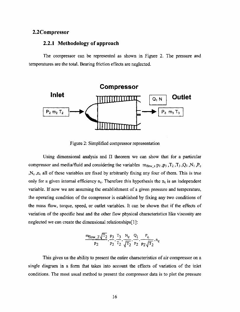
2.2.1 Methodology of approach
The compressor can be represented as shown in Figure 2. The pressure and
temperatures are the total. Bearing friction effects are neglected.
CompressorInlet j1 Outlet
P2 M2 T2 P3 m3 T3
Figure 2: Simplified compressor representation
Using dimensional analysis and H theorem we can show that for a particular
compressor and media/fluid and considering the variables mflowc P2 ,p3 ,T2 ,T3 ,Qi ,Nj ,Pc
,Nc ,nc all of these variables are fixed by arbitrarily fixing any four of them. This is true
only for a given internal efficiency n. Therefore this hypothesis the n_ is an independent
variable. If now we are assuming the establishment of a given pressure and temperature,
the operating condition of the compressor is established by fixing any two conditions of
the mass flow, torque, speed, or outlet variables. It can be shown that if the effects of
variation of the specific heat and the other flow physical characteristics like viscosity are
neglected we can create the dimensional relationships[ 1]:
nflow_2T2 P3 T3 NC Q, Pc
P 2 P 2 T2 2 P2 P2'j2,n
This gives us the ability to present the entire characteristics of air compressor on a
single diagram in a form that takes into account the effects of variation of the inlet
conditions. The most usual method to present the compressor data is to plot the pressure
16
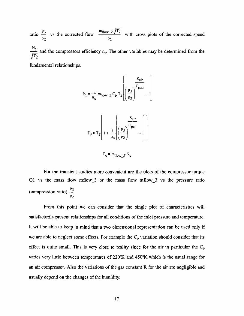
ratio P vs the corrected flow inflOW I22 with cross plots of the corrected speedP2 P2
C and the compressors efficiency n. The other variables may be determined from the
fundamental relationships.
Rair
1C I ( 2[P3) CpairInc P2)
Rair
Cpair
T3 T2. + P3
PC~~P = ---fnfow_-3 NC
For the transient studies more convenient are the plots of the compressor torque
Q I vs the mass flow inflow_3 or the mass flow inflow_3 vs the pressure ratio
P2
From this point we can consider that the single plot of characteristics will
satisfactorily present relationships for all conditions of the inlet pressure and temperature.
It will be able to keep in mind that a two dimensional representation can be used only if
we are able to neglect some effects. For example the CP, variation should consider that its
effect is quite small. This is very close to reality since for the air in particular the CP,
varies very little between temperatures of 220'K and 450'K which is the usual range for
an air compressor. Also the variations of the gas constant R for the air are negligible and
usually depend on the changes of the humidity.
17

Another effect that actually is related directly with the compressor losses are the
effects from the variation of the gas viscosity .The viscosity changes can be related to
the Reynolds's number (Re) variation, are normally neglected as unimportant in the usual
rage of operation and for marine propulsors1 .We will neglect also the heat transfer
through casing and the bearing friction. For the latter we should notice that the effect
becomes noticeable only if we are referred for torqueses that are small compared to the
design torque. The clearance inside the compressor is a factor that can affect leakage and
consequently efficiency, as temperature and pressure changes alter compressor
component dimensional relationships.
At the present time there are two important types of air compressors having high
rate flow and high efficiency characteristics needed in use in gas turbines. These are the
axial flow compressors and the centrifugal compressors.
In the axial-flow engine, the air is compressed while continuing its original
direction of flow parallel to the axis of the compressor rotor. The compressor is located
at the very front of the engine. The purpose of the axial compressor is to take in
ambient air, increase the speed and pressure, and discharge the air through the
diffuser into the combustion chamber.
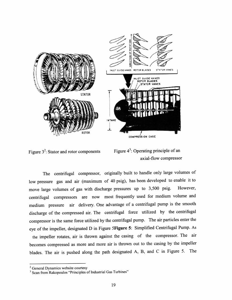
The two main elements of an axial-flow compressor are the rotor and stator
(Figure 3). The rotor is the rotating element of the compressor. The stator is the
fixed element of the compressor. The rotor and stator are enclosed in the compressor
case. The rotor has fixed blades that force the air rearward much like an aircraft propeller.
In front of the first rotor stage are the inlet guide vanes (IGVs). These vanes direct the
intake air toward the first set of rotor blades. Directly behind each rotor stage is a
stator. The stat or directs the air rearward to the next rotor stage (Figure 4). Each
consecutive pair of rotor and stator blades constitutes a pressure stage.
Ponomareff: for operations in high altitude the effects are more noticeable. So our hypothesis stands betterfor the maritime GTs
18
'%LET GuIDE VANES ROTOR tLADES STATOR VANES
T GUIDE VANES
STATOR VANES
STATOR
ROTOR
Figure 3 2: Stator and rotor components
COMPRE( sON CASE
INTAKE
Figure 43: Operating principle of an
axial-flow compressor
The centrifugal compressor, originally built to handle only large volumes of
low pressure gas and air (maximum of 40 psig), has been developed to enable it to
move large volumes of gas with discharge pressures up to 3,500 psig. However,
centrifugal compressors are now most frequently used for medium volume and
medium pressure air delivery. One advantage of a centrifugal pump is the smooth
discharge of the compressed air. The centrifugal force utilized by the centrifugal
compressor is the same force utilized by the centrifugal pump. The air particles enter the
eye of the impeller, designated D in Figure 5Figure 5: Simplified Centrifugal Pump. As
the impeller rotates, air is thrown against the casing of the compressor. The air
becomes compressed as more and more air is thrown out to the casing by the impeller
blades. The air is pushed along the path designated A, B, and C in Figure 5. The
2 General Dynamics website courtesy3 Scan from Rakopoulos "Principles of Industrial Gas Turbines"
19
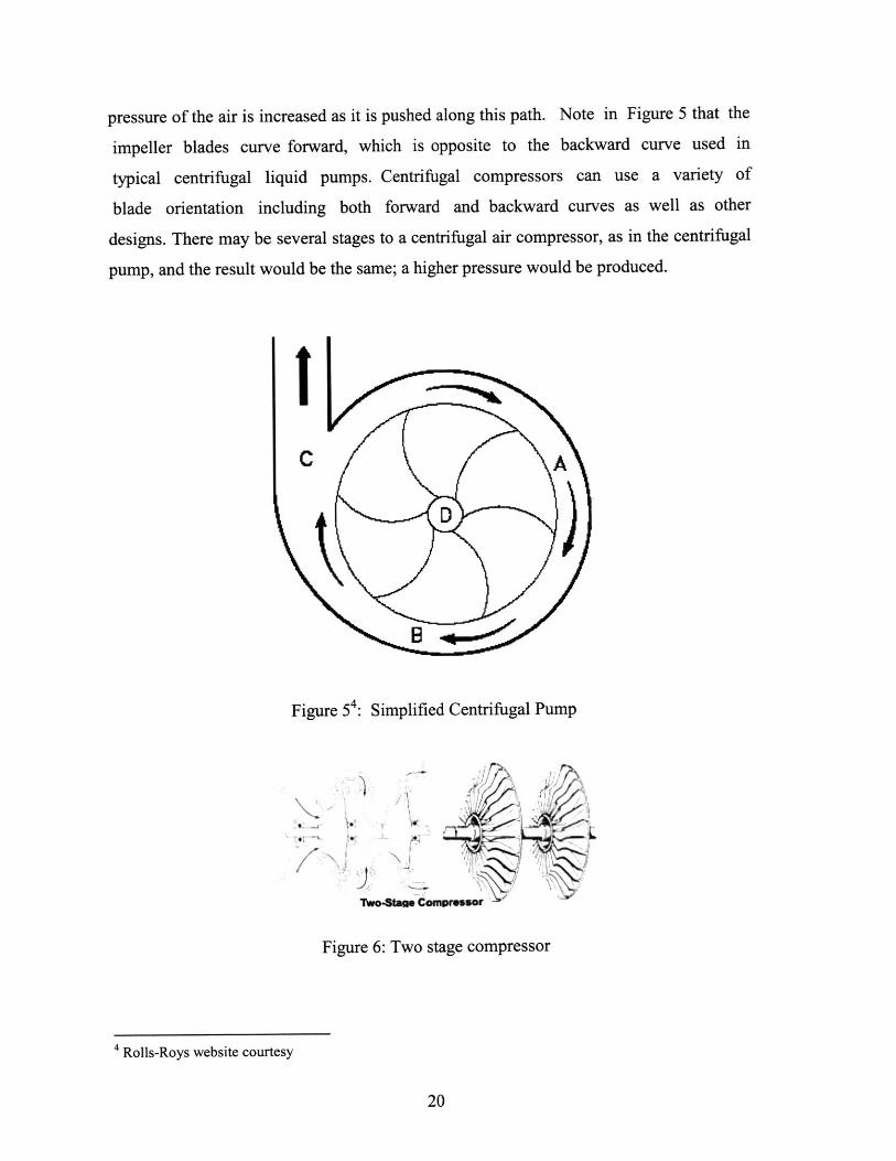
pressure of the air is increased as it is pushed along this path. Note in Figure 5 that the
impeller blades curve forward, which is opposite to the backward curve used in
typical centrifugal liquid pumps. Centrifugal compressors can use a variety of
blade orientation including both forward and backward curves as well as other
designs. There may be several stages to a centrifugal air compressor, as in the centrifugal
pump, and the result would be the same; a higher pressure would be produced.
CA
Figure 54: Simplified Centrifugal Pump
Two-stae Comormor
Figure 6: Two stage compressor
20
4 Rolls-Roys website courtesy
The numerical calculations in this study are made largely using a compressor with axial
flow characteristics.
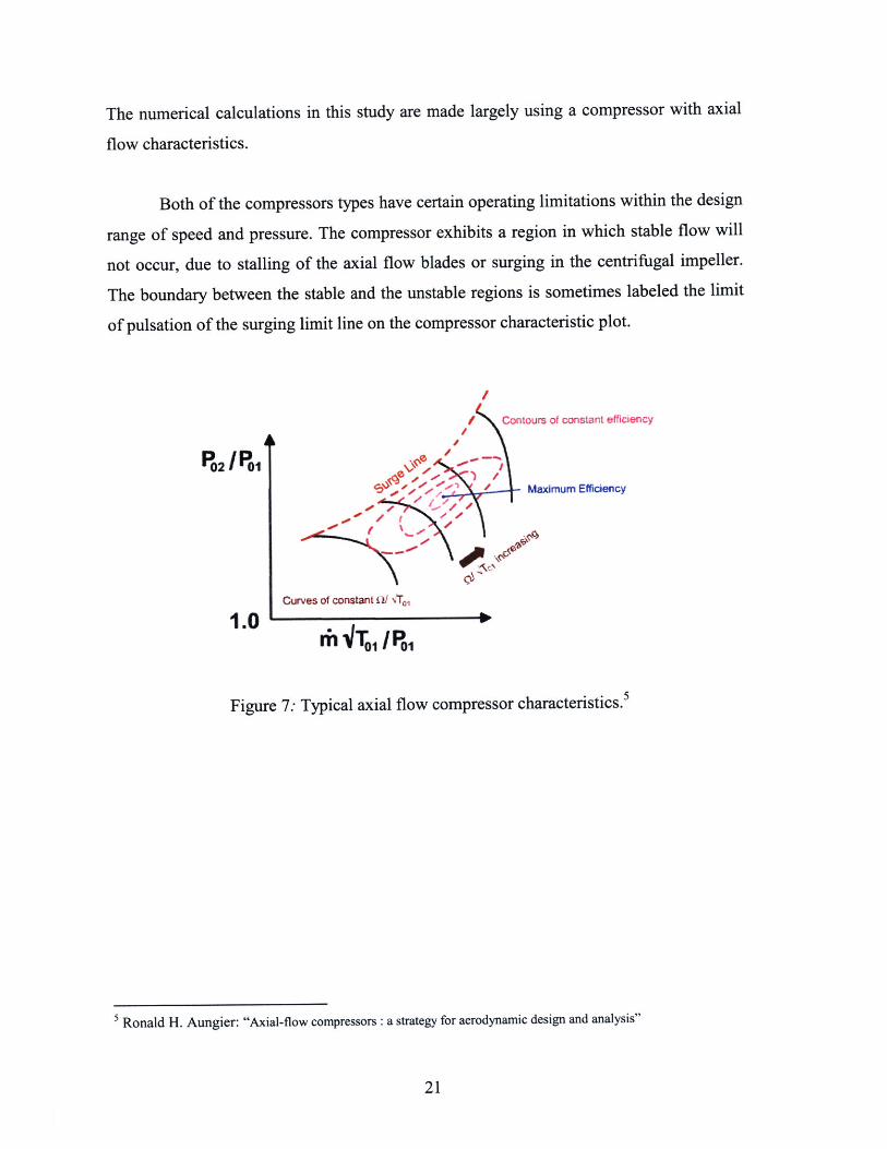
Both of the compressors types have certain operating limitations within the design
range of speed and pressure. The compressor exhibits a region in which stable flow will
not occur, due to stalling of the axial flow blades or surging in the centrifugal impeller.
The boundary between the stable and the unstable regions is sometimes labeled the limit
of pulsation of the surging limit line on the compressor characteristic plot.
02 1POI
1.0
I Contours of constant efficiency
e I~
00 /e Maximum Efficiency
Curves of constant L9 -N6.
Figure 7: Typical axial flow compressor characteristics. 5
5 Ronald H. Aungier: "Axial-flow compressors: a strategy for aerodynamic design and analysis"
21
4 n
Lines ofConstantRotational
peed
s-d
nstant~ U'1JOCurves of co
S4T 1 /P.,
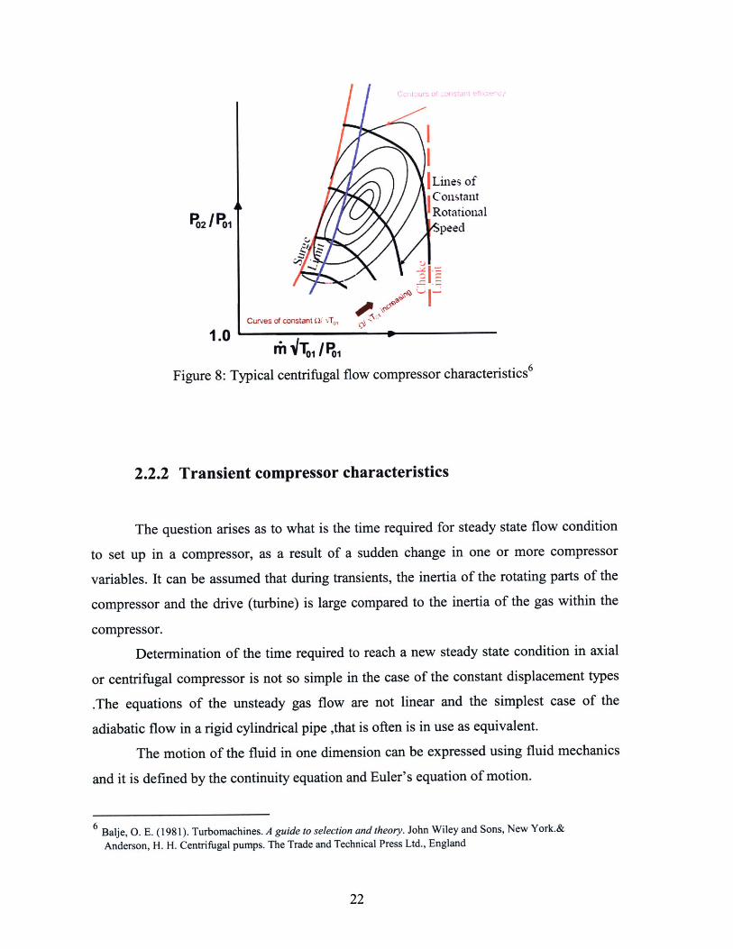
Figure 8: Typical centrifugal flow compressor characteristics 6
2.2.2 Transient compressor characteristics
The question arises as to what is the time required for steady state flow condition
to set up in a compressor, as a result of a sudden change in one or more compressor
variables. It can be assumed that during transients, the inertia of the rotating parts of the
compressor and the drive (turbine) is large compared to the inertia of the gas within the
compressor.
Determination of the time required to reach a new steady state condition in axial
or centrifugal compressor is not so simple in the case of the constant displacement types
.The equations of the unsteady gas flow are not linear and the simplest case of the
adiabatic flow in a rigid cylindrical pipe ,that is often is in use as equivalent.
The motion of the fluid in one dimension can be expressed using fluid mechanics
and it is defined by the continuity equation and Euler's equation of motion.
6 Baije, 0. E. (1981). Turbomachines. A guide to selection and theory. John Wiley and Sons, New York.&
Anderson, H. H. Centrifugal pumps. The Trade and Technical Press Ltd., England
22
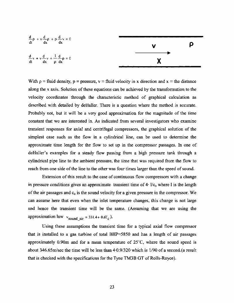
d d AP+P d =C-p +v-.-p+p--v=Cdt dx dx
-v + v--v + I--p = 0dt dx p dx
V
X
With p = fluid density, p = pressure, v = fluid velocity in x direction and x = the distance
along the x axis. Solution of these equations can be achieved by the transformation to the
velocity coordinates through the characteristic method of graphical calculation as
described with detailed by deHaller. There is a question where the method is accurate.
Probably not, but it will be a very good approximation for the magnitude of the time
constant that we are interested in. As indicated from several investigators who examine
transient responses for axial and centrifugal compressors, the graphical solution of the
simplest case such as the flow in a cylindrical line, can be used to determine the
approximate time length for the flow to set up in the compressor passages. In one of
deHaller's examples for a steady flow passing from a high pressure tank through a
cylindrical pipe line to the ambient pressure, the time that was required from the flow to
reach from one side of the line to the other was four times larger than the speed of sound.
Extension of this result to the case of continuous flow compressors with a change
in pressure conditions gives an approximate transient time of 4- 1/c0 where 1 is the length
of the air passages and c. is the sound velocity for a given pressure in the compressor. We
can assume here that even when the inlet temperature changes, this change is not large
and hence the transient time will be the same. (Assuming that we are using the
approximation law vsoundair = 331.4+ 0.6Te ).
Using these assumptions the transient time for a typical axial flow compressor
that is installed to a gas turbine of total BHP=5850 and has a length of air passages
approximately 0.90m and for a mean temperature of 25*C, where the sound speed is
about 346.65m/sec the time will be less than 4-0.9/320 which is 1/90 of a second.(a result
that is checked with the specifications for the Tyne TM3B GT of Rolls-Royce).
23
It is concluded that unless periods of few hundreds of a second are important in
the gas turbine transient operation, the steady state compressor characteristics may be
used.
2.3Turbine
2.3.1 Methodology of approach
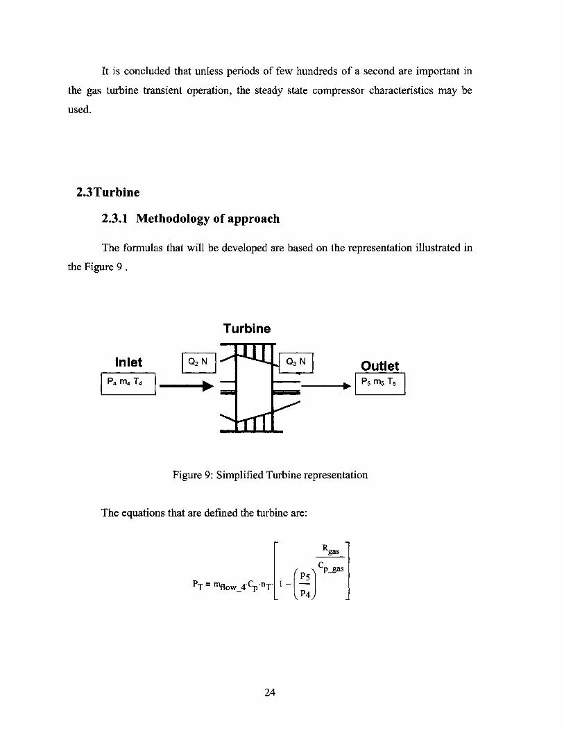
The formulas that will be developed are based on the representation illustrated in
the Figure 9 .
Turbine
Inlet Q2 N IP4 M4 T4
Q3 Outlet-P5 ME T
Figure 9: Simplified Turbine representation
The equations that are defined the turbine are:
Rgas
PT = mflow 4CP-nT 1 P Cpga
P4
24
RgaCpgas
T5 =T4 . 1-nT - P[ P4
PT = Q3. NT
with Q3 = turbine output torque ,NT= turbine rotate speed ,mflow4 = gas mass flow rate ,
PT = turbine output power and n=T turbine internal efficiency. As in the compressor case ,
the selection of the four turbine particulars can be made among any of the following
variables:
flowi_ 4 P4,P 5 Q 3 , NT,nT
Similar dimensionless relations as that derived for the axial flow compressor may be used
for the turbine, and it would be quite reasonable to question whether a turbine
characteristics chart similar to the commonly used for a compressor might be used. The
answer is positive under certain conditions.
The variation of the flow and the turbine efficiency can be calculated with more
certainty than for the compressor. The reason is that for the turbine design we use heated
gasses under pressure, a method that was highly developed and tested in the steam
turbines.
The flow in the compressor varies greatly with the change in speed as we saw
earlier while the response of the turbine flow under the same input differs only slightly.
The variation of the inlet pressure and temperature in the turbine are much higher
than these for a compressor. Also a very important consideration here will be the impact
of the changes in Reynolds number and the one of the specific heat.
F Rgas
C ]
PT = nflow__4-Cp-nT I _I P4) _
25
A more general expression of the fundamental equation will be:
PT nflow_4-nT-Ah
where Ah is the isentropic change of the enthalpy of the gas when expanding from the
state T4 and p4 to p5.The most simple expression of the functions can be represented as
following 7:
P4 P4 NTnmflow_4 ~ ~~fl 2(NT
Sp4 NT
PT - 3
P5 4AI
and since the expression of the isentropic change of the enthalpy is
P4Ah= T4,C
and the Cp can be expressed as a function of:
P4C, T4,--
P5it can be seen that the following variables are only needed:
PT mflow 4 P4
P5 P4 P5
The present approach is guided by the methods of the turbine characteristics provide by
the manufacturers. This will give us the ability for developing a simpler simulation
model: the set of tables each with a different value of T4 (turbine inlet temperature) is
obtained for transient studies and to determine single shaft plant characteristics (as is our
model gas turbine); a set of plots with constant rotational speed NT is particularly useful
26
7 Horlock "Axial flow turbines", 1966
[1]. Also we can employ sets of plots such as torque vs. gas flow, and the expansion
pressure ratio vs. gas flow.
2.3.2 Transient turbine characteristics
A similar reasoning as used for the axial flow compressor can be applied for the
turbines. Because the turbine has fewer stages than the compressor, and because the
temperature is higher, the actual transient time is expected to be shorter for the turbine
than the associated compressor. So for a turbine of 0.70m length which operates at the
meaning temperature of 2000*C - then the velocity of the sound for this temperature will
be 1551 m/sec - and could be expected to reach the steady state condition in a time period
of less than 1/550 of a second. So for transients that take long time compared with that
required for adjustment of the internal turbine flow, the turbine steady state
characteristics may be used.
2.4 Combustion chamber
2.4.1 Methodology of approach
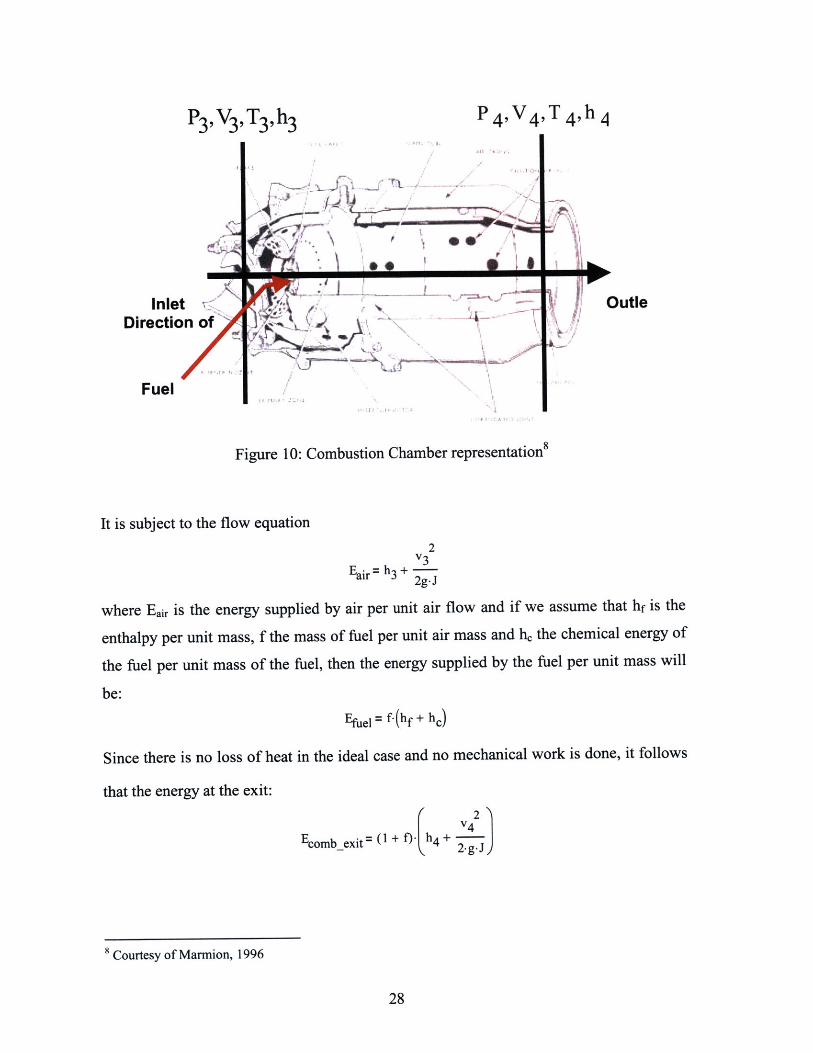
The air leaving the compressor flows to the combustion chamber where fuel is
added and combustion proceeds. The ideal combustion chamber will be the one in which
the chemical energy of the fuel was completely released in the form of an increase of the
internal energy without loss of pressure due to friction or any other effect, and no heat
loss due to the conduction, radiation, ect., occurred. Such a combustion chamber can be
represented by Figure 10.
27
P3,V3,T3,h3
InletDirection of
Fuel
e i
L W4c,% ----
mm
Outle
Figure 10: Combustion Chamber representation8
It is subject to the flow equation
2V3
Eair= h3 + --2g-J
where Eair is the energy supplied by air per unit air flow and if we assume that hf is the
enthalpy per unit mass, f the mass of fuel per unit air mass and he the chemical energy of
the fuel per unit mass of the fuel, then the energy supplied by the fuel per unit mass will
be:
Efuel = f.(hf + hJ)
Since there is no loss of heat in the ideal case and no mechanical work is done, it follows
that the energy at the exit:
2
Ecomb exit= ('+ f)- h4+ +2-g-J)
28
Courtesy of Marmion, 1996
Alli
must be equal to the energy input. Thus:
2 2V 3 v 4I
h3 +---+ f(hf+hc)=(1+ f). h4+ V42g.J 2.g-J)
Now hf can be approximated by9:
h f = 0.5 -T - 375
it is follows that the above equation can be written as:
2 2
h3 + --- + f-(0.5-T - 375) = (1 + f)- h4+2g-J 2-g.J,
It is known, that the maximum gas temperature is limited by the materials of
construction of the turbine blades; thus the materials selection will provide a basis on
which the exit temperature T4 and thus h4 should be fixed' 0 .The magnitude of the v4 can
be varied considerably by variation of the cross sectional area of the exit duct. However,
the maximum velocity that can be reached by heat addition only is that of the local
velocity of sound.1 Such a velocity would be excessive and involves high frictional losses
and thus pressure losses, which would adversely effect the performance of the
turbomachine; in general the velocity at the exit from the combustion chamber will be of
the order of 140-200 m/sec, or a Mach number of 0.185-0.31 [2].
The combustion chamber velocity at the point where the fuel is injected will be
governed by that at which combustion can be started and maintained under all operated
conditions. At the present time it is true that low velocities at the zone of combustion
provide improved combustion efficiency, and velocities of 0.06-0.15 can be employed at
the combustion chamber inlet.
9 Keenan and J.Kaye "Thermodynamic Properties of Air",John Wiley & Sons Inc.,N.Y.10 E.T.Vincent "Theory and Design of Gas Turbines and Jet Engines" ,Chap. XVIII,McGraw-Hill ,1950"1 E.T.Vincent "Theory and Design of Gas Turbines and Jet Engines" ,Chap. II, pp 48-53 ,McGraw-Hill,1950
29
In the actual combustion chamber there are of necessity various losses; these can
be summarized as follows:
1. Pressure drop necessary to provide the acceleration of the gas resulting from heat
addition.
2. Loss due to skin friction.
3. Loss due to the type of flame tubes and holders employed. This loss is mainly due
to the turbulence created to provide flame maintenance.
4. Losses due to radiation
5. Losses due to incomplete combustion and poor mixing of fuel and air.
2.4.2 Transient combustion chamber characteristics
Tests have established the degree of combustion that can be expected, and this
depends on the gas velocity in the combustion chamber at the inlet and the end. If the
velocity is low, let's says approximately 50m/sec, and does not accelerate to high values
in the combustion chamber, an efficiency of 0.95-0.97 is expected. The higher value will
be reached where large sizes chambers are employed. If the inlet velocity increases to as12much as 60-100m/sec, the efficiency will fall perhaps as low as 0.88-0.92
So for a combustion chamber of 0.40m gas pass way which operates at the maximum
efficiency - then the velocity of the inlet air will be limited to 50m/sec theoretically -
could be expected to reach the steady state condition in a period less than 8/1000 of a
second. So for transients that take long time compared with that required for adjustment
of the internal combustion chamber flow, the turbine steady state characteristics may be
used.
12 E.T.Vincent "Theory and Design of Gas Turbines and Jet Engines" ,Chap. V,McGraw-Hill ,1950
30
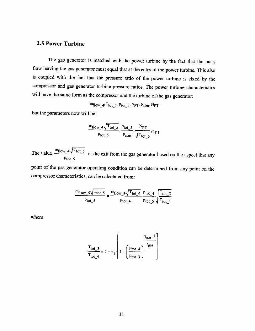
2.5 Power Turbine
The gas generator is matched with the power turbine by the fact that the massflow leaving the gas generator must equal that at the entry of the power turbine. This alsois coupled with the fact that the pressure ratio of the power turbine is fixed by thecompressor and gas generator turbine pressure ratios. The power turbine characteristicswill have the same form as the compressor and the turbine of the gas generator:
inflow_4, Ttot_5' Ptot_5,nPT' Patm, NPT
but the parameters now will be:
"'flow_4jFtoT5 Ptot 5 NPT
Ptot_5 Patm tTo5
The value -flow4\U7 at the exit from the gas generator based on the aspect that anytot_5
point of the gas generator operating condition can be determined from any point on thecompressor characteristics, can be calculated from:
"'flow_4-4 Ttot_ _ "flow_4ftot_4 Ptot 4 Ttot 5
tot_5 Ptot_4 Ptot_5 Ttot_4
where
Ygs-
tot_5 ot 4 gas
Ttot_4 Ptot_3) j
31
2.6 Turbomachinery Theory-Model Development
2.6.1 Governing Equations
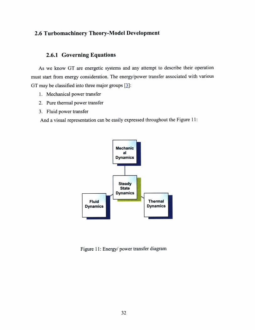
As we know GT are energetic systems and any attempt to describe their operation
must start from energy consideration. The energy/power transfer associated with various
GT may be classified into three major groups [3]:
1. Mechanical power transfer
2. Pure thermal power transfer
3. Fluid power transfer
And a visual representation can be easily expressed throughout the Figure 11:
Mechanical
Dynamics
SteadyState
ADynamics
Fluid ThermalDynamics Dynamics
Figure 11: Energy/ power transfer diagram
32
1. The mechanical power transfer is associated with the shaft connection to various
rotating components and the inputs and outputs that may be present. Therefore the
mechanical power transfer will has the form:
PM = 3-Q-NN (G-1)
where
PM = mechanical power transfer in [m-N/sec]
Q = torque carried by shaft in [m-N]
N = rotation speed of the shaft in [rpm]
2. Pure thermal power transfer is simply the heat flow into and out of the various fluid
streams and any metal parts present.
(Heat flow)PT= T .T = (Heatflow) (G-2)
with
PT = thermal power transfer in [m-N /sec]
Heatflow = heat flow in [m-N /sec]
T = temperature in [K*]
3. Fluid power transfer is associated with the main gas stream, the fuel flow and any
secondary present fluid flow.
2
PF = mflow U + - + VI+ z-g ho + z- (G-3)pb 2
with the following parameters corresponded to:
ho - total enthalpy in [m-N /Kg]
u= internal energy in [m-N /Kg]
33
p = static density in [-K]3
m
p = static pressure in [ N3
m
v = mean velocity in [m/sec]
z = height measure from a reference point in [m]
g= gravity acceleration in [MI sec]
Pi Mi TC
P2 m 2 T2
QI N
1~iU~W~K~,
Trrrrr rrrrrr
P3 m3 T3
mf hLHVI
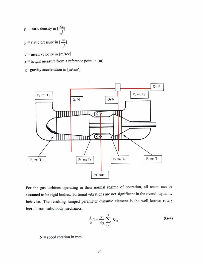
For the gas turbines operating in their normal regime of operation, all rotors can be
assumed to be rigid bodies. Tortional vibrations are not significant in the overall dynamic
behavior. The resulting lumped parameter dynamic element is the well known rotary
inertia from solid body mechanics.
3N = 3 Q (G4)
dt nIR
N = speed rotation in rpm
34
P5 M T5P4 m 4 T4
TflT - ii;
Q3 N
P6 M6 T6
ig-rotary inertia of the rotor
Q0,= torque input
2.6.2 Thermodynamic approach
The pure thermal lumped parameter dynamic elements are the lumped metal parts
in contact with one or more of the fluid streams. Negligible internal temperature gradients
are assumed in this approach.
3Td i (G-5)
dt CT
T = temperature of lumped element
cT = thermal capacitance with the expression13:
n Pstatic o.CV-VCT=n - I R-To
9qi= heat flow into the elements
2.6.3 Fluid Dynamics Approach
a. Conservation of mass
The only interesting dynamics in the gas turbine are the fluid dynamics. To
analyze the dynamics now of the fluid subsystem we must consider the three basic
conservation equations and the boundary conditions present [4]. Here in my approach the
fluid dynamics are assumed to be those of a duct the equivalent area and length of the
actual component passage. The one dimensional assumption is carried throughout.
13 Cochen: Gas turbine Theory, Longman Ltd, 1974
35
dt dx G6
x = axial distance along the duct
p = density of the fluid
V,= mean axial velocity of the fluid
Integrating the (G-6) over the area assuming that the fluid properties are constant
with area and assuming that the area is constant with the time results in:
dpA + (p-v A)dt dx
However I A) = C
which can be written as
therefore:
= p-v--d-AjJ
pA + .-(p.v A) = Cdt dx
A-d-p + 4 -(p .vA) = Cdt dx
Integrating the (G-8) over a given length of the duct with the length constant with time
results:
dt Jp -A dx + 2-(p -A-v dx= C (G-9)
but the integral I p -A dx= rr is the mass of the fluid in the given segment therefore,
In the equation (G-9) the A.p -A dx= p av is also the mass of the fluid in the given
segment therefore the portion p -A-v, is nothing more than the mass flow. Set:
m~flow = p .A, v,.
and using the average value of the density we can write the (G-9) as:
36
(G-7)
(G-8)
(G-6)
P av = I*mlowI - nlow_2)dt V
(G-10)
b. Conservation of momentum
The single dimensional equation of the momentum conservation neglecting shear stresses
and body forces is:
2
d(p.V + d P.dt dx, 2
+ Pstaticj = C (G- 11)
hence
(G-12)2
p -A-v + A- P-VX 2 Pstatic =Cdt dx 2
Integrate over the given length:
dp -A-v = - pstaticd(P L ~
2P. xv
2 2d A-g
dt "HOW L . Pstatic+
Using the assumption of the perfect gas and introducing this approximation in our
equation and the Mach number we will have:
We call as y the ratio of the specific heat: CP
CV
and as a the local sonic velocity:
37
2. i
2 X 12
so the Mach number can be defined as:V
M=
Also c is the specific heat at a constant pressure and
c, is the specific heat at a constant Volume
Using now the perfect gas approximation we will have:
d 2fl 1.mflow pstatic-(i + Y-M2
But:
( y-Ptot = Pstatic. (1 + 2 M
substitute this into the (G- 13) equation and:
dmA Ptot I + Y-M 2- M flowdt L y
1+ y21- M 2) 1
(G-13)
(G- 14)
If we set for example in the equation (G-14) the values: M=O.5 and y = 1.4 close to the air
value we will have:
d A -g Ptot l1 + 140.52)... ow 4
dt L 1.4
S1.4 4-1I1
2
38

This is equal to
d A
1" -low =L 2[8.24'IPtot_1 - Ptot 2)]
If the M<0.5 which actually implied to low throttle or even unload conditions then the
simplified form that can be used is :
d A
dtiow -L(Ptot 1 Ptot_2)
c. Conservation of energy
Apply now the energy conservation in one dimension and neglecting viscous work and
external work
2
r- p- U+ + - pV3 hdtL 2). dx. s
U = internal energy of the fluid and
h = enthalpy of the fluid
carry out the lumped parameter development
2
d- P.- U+ = - nflow- h +dt -- 2 /-av V s
2
+ = C2 )._
(G-15)
2
2 )j 2
The total enthalpy can be expressed as: htot = Cp-Ttot
2
using thermodynamics we have: htot = h + h + V2
39
and with the same manner as before: Ttot =
2
which guide as to the expression: U + = C-T- 1 + -. M22 2
If now we substitute the (G- 16) in to energy conservation equation (G- 15):
- (p -C-Ttot)dt av
1+ -
1+
M2~2
2
2 j
(G-16)
- -(nflOWCp.TtOt). I
(G-17)
Set again the same values for M=0.5 and y-1.4 then the equation takes the form:
1.019[ (p .CvTtot)av] = .- (njpowi.Ttot_1 - nflow_ 2-Ttot_2)
With the same assumption that the Mach number drops bellow the limit of 0.5 then the
results will be simplified to:
d(p -TtOt) -1 ~ITtot 1 - nflow_2 'Ttot_2)
In the industry the exit temperature is generally taken to be the average temperature of
the element. The equation of state may be written:
1
ptot = p -R-Ttot- I + Y .M2 J
Set again the values M=0.5 and y=-.4 and the equation yields to:
Ptot = 1.13p -R- Ttot
40
(G- 18)
T. I + - M2
And for low Mach numbers the equation may be simplified to:
ptot = p .R-Ttot (G-19)
Since the fluid power has been expressed as a function of ptot ,n"ifo , Ttot it might proven
useful to express the simplified fluid dynamic elements in terms of the same three
variables. This can be accomplished by the concept of polytropic process.
n
Ttot n- = const .ptot (G-20)
where n = polytropic constant
Introducing the approximate equation ptot = p -R.Ttot into the state given above (G- 19)
nPtot = R const -p and n-1
Ttot = R- const -p
If now we differentiate the above equations with respect to time results in:
dn-ptot = - R-const p
dt dtor even better d n-i d
-ptot = R.const -p -n.-pdt dt
Since we know that Ttot = R-const -pn- as we show before then we can write:
dptot = n-R-Ttoti-pdt dt
From the equation (G-2 1) now we have that:
n
d Ttot n-1 = !-(const -ptot)dt dt
but if we apply the gas law
I
or simpler -Ttot -Ttot=n - dt
n
n-IT tot = const *Po
const- d ptotdt
can turned the equations in the form:
1
n -Ttot n-d Ttot const .I(p -R- Ttot)n-i dt dt
-+ .n - tot -Ttot = R dconst (p -Ttot)n -I dt dt
41
(G-2 1)
with the final expression:
d(p Ttt) =1 1 *Ttot n-dTtotdt n - I) R const dt
n
Using the expression n- iT tot = const and solve for the constant we get:
n
const = t
Ptotwhich implies that 1 Ptot
const n
The equation (G-22) now can be formed as:
I
d = (NT Ptot Tttn-I .d Todt ( o) (n-1) R n dt
and yields into the equation:
d n I _IPtot dTdt n 1 R Ttot dt (G-23)
* By substitute this into the previous simplified dynamic element equations an even
more simplified form results (assuming from 1-+2):
Pav = I("lowI - "flow_2)dt V
using the equation Iptot = n.R.Ttotd -Pdt dt
we will turn it into the form:
d n-TR- Ttt
dtot V t "low_ I -nlow_2)
42
(G-22)
(G-24)
d g.A
dt"Iow L(PtotI - Ptot_2)
4-(p -TtO = -n1
1 Ptot
R TtotLtotdt
But as we proved:
dt(P'tot)av (m w i-'Itot _1 - " flow_2 Ttot_2)
Substitute this into the equation (G-26) and:
(Inn R Ttot ) .iTtot = -- (mlowF'Ttot_1 - nifow 2ITtot 2)
The (G-27) yields finally to:
d T no -(1' CP'.R*Ttotd to n .('mfl- Ttot_-1 - m~flow 2.Ttot 2)
In this point we should highlight that the polytropic constant n, equals 1.0 for an
isothermal process and equals y for isentropic process.
43
0
a
(G-25)
(G-26)
(G-27)
(G-28)
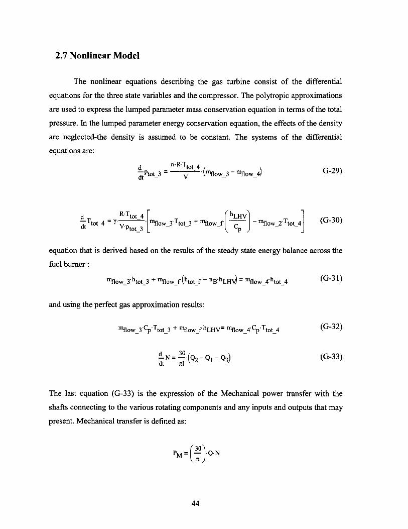
2.7 Nonlinear Model
The nonlinear equations describing the gas turbine consist of the differential
equations for the three state variables and the compressor. The polytropic approximations
are used to express the lumped parameter mass conservation equation in terms of the total
pressure. In the lumped parameter energy conservation equation, the effects of the density
are neglected-the density is assumed to be constant. The systems of the differential
equations are:
d n -R. Ttt4 (ml_ m _) G-29)Pt tot 3 = n --Tt4 *-(nflow_3 - nflow_4)G-9
T R-Ttot_4 'hLHVdTtot4 :' VPtot_3 _n fo _3 -Ttot_3 + nflowf C nflow 2-Ttot 4 (G30)
equation that is derived based on the results of the steady state energy balance across the
fuel burner :
nflow_3*htot_3 + n1 low1 f (totf + nB-hLH)= nlow_4.htot_4 (G-31)
and using the perfect gas approximation results:
nflow_3CP-TtOt_3 + nflow_f hLHV= nflow_4Cp- Ttot_4(G-32)
N = -(Q2 -1 - Q3) (G-33)dt 7d
The last equation (G-33) is the expression of the Mechanical power transfer with the
shafts connecting to the various rotating components and any inputs and outputs that may
present. Mechanical transfer is defined as:
PM --- -Q.N
44
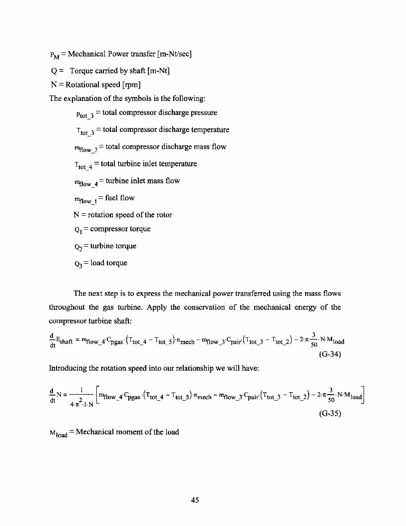
PM = Mechanical Power transfer [m-Nt/sec]
Q = Torque carried by shaft [m-Nt]
N = Rotational speed [rpm]
The explanation of the symbols is the following:
ptot_3 = total compressor discharge pressure
Ttot_3 = total compressor discharge temperature
mt lo3= total compressor discharge mass flow
Ttot_4 = total turbine inlet temperature
mnl - = turbine inlet mass flow
myfl - = fuel flow
N = rotation speed of the rotor
Q,= compressor torque
Q2= turbine torque
Q3= load torque
The next step is to express the mechanical power transferred using the mass flows
throughout the gas turbine. Apply the conservation of the mechanical energy of the
compressor turbine shaft:
-Eshaft = mflow_4.Cpgas -(Ttot_4 - Ttot_5)-nmech - mflow_3- Cpair-(Ttot_3 - Ttot_2) - 2x -- N. Mloaddt shf nwpa e 3artt50 a
(G-34)
Introducing the rotation speed into our relationship we will have:
o1 3d-N = 2 -[nflow_4. Cpgas -(Ttot_4 - Ttot_5)nmech - Now_3.Cpair.(Ttot_3 - Ttot_2) - 2.n -- N-Mloaddt 2*r** 50j
4-7E .I.N -(G-35)
Mload = Mechanical moment of the load
45

Note: as we can see the compressor and turbine torques were determined from the steady
state energy balance:
= 4 -n- N-nlOW_3(TtOt_3 - Ttot_2)
2 4- Nflow_4(Ttot_4 - Ttot_5)
And as Q3 the load torque is designated.
46
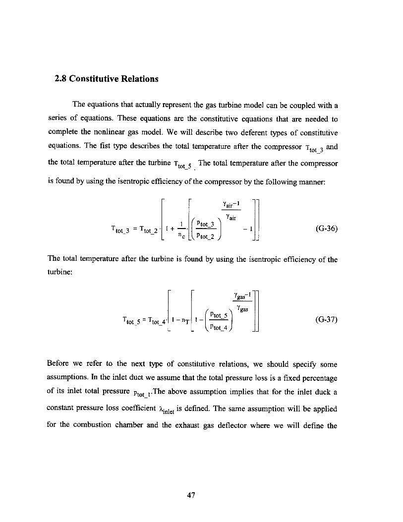
2.8 Constitutive Relations
The equations that actually represent the gas turbine model can be coupled with a
series of equations. These equations are the constitutive equations that are needed to
complete the nonlinear gas model. We will describe two deferent types of constitutive
equations. The fist type describes the total temperature after the compressor Ttot_3 and
the total temperature after the turbine Ttot_5 . The total temperature after the compressor
is found by using the isentropic efficiency of the compressor by the following manner:
Yair~
1air_ Tt~t .1 LrtOt_2Ttot_3 = Ttot_2 1 + - J ijj (G-36)_ nc _ P tot_2)
The total temperature after the turbine is found by using the isentropic efficiency of the
turbine:
Ygas-r ~ Ygas1
Ttot_5 = Ttot_4. I - nT' I ~ (G-37)_ Ptot_4 _
Before we refer to the next type of constitutive relations, we should specify some
assumptions. In the inlet duct we assume that the total pressure loss is a fixed percentage
of its inlet total pressure ptot_1.The above assumption implies that for the inlet duck a
constant pressure loss coefficient nilel is defined. The same assumption will be applied
for the combustion chamber and the exhaust gas deflector where we will define the
47

constant pressure loss coefficients Xcomb and ?def respectively 4 '. Therefore the equations
that illustrate those modeling assumption will be:
Ptot 4Xcomb = -
Ptot_3
Xinlet Xdef : Ptot_2Ptot_5
(G-38)
(G-39)
14 J.H Horlock "Axial flow turbines",London, 1966
48
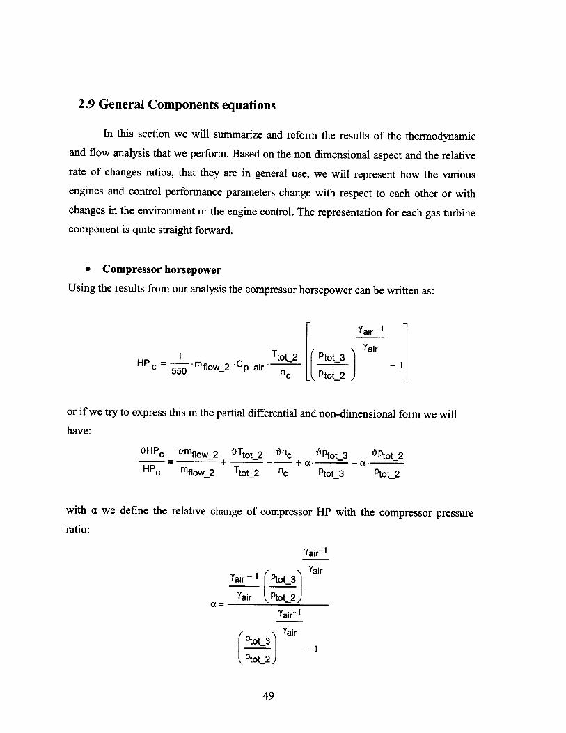
2.9 General Components equations
In this section we will summarize and reform the results of the thermodynamic
and flow analysis that we perform. Based on the non dimensional aspect and the relative
rate of changes ratios, that they are in general use, we will represent how the various
engines and control performance parameters change with respect to each other or with
changes in the environment or the engine control. The representation for each gas turbine
component is quite straight forward.
9 Compressor horsepower
Using the results from our analysis the compressor horsepower can be written as:
[air1
C 'o2 aiTtot 2 Ptot 3 airHP c - rnmflOW_2 COpair nc n
550 ric Ptot_2 _
or if we try to express this in the partial differential and non-dimensional form we will
have:
HPC 5rnflow 2 'Ttot 2 Onc 6ptot 3 6Ptot 2:+ = -7- -HPC inflow_2 Ttot_2 nc Ptot_3 Ptot_2
with a we define the relative change of compressor HP with the compressor pressure
ratio:
Yair~1
Tair 1 Ptot3 Yair
Yair Ptot_2
Yair-I
YairPtot 3
Ptot_2J
49
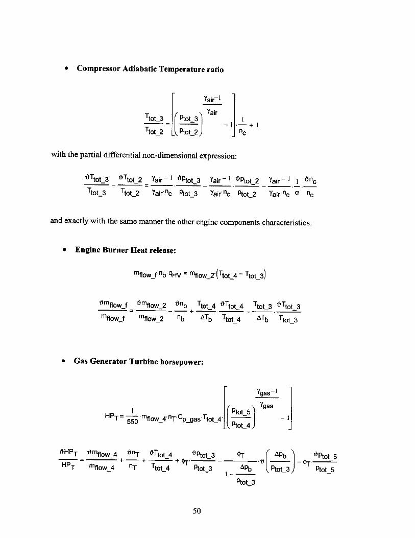
* Compressor Adiabatic Temperature ratio
Yair~-Ir ~ ~air1
Ttot 3 _ Ptot_3 air
Ttot_2 K Ptot_2)
with the partial differential non-dimensional expression:
t'Ttot_3 t*Ttot 2 7air -1 Ptot_3
Ttot_3 Ttot_2 7air-nc Ptot_3
Tair 1 Ptot 2 'air - I 1 *nc
Yair-nc Ptot_2 Yair.nc a nc
and exactly with the same manner the other engine components characteristics:
* Engine Burner Heat release:
inflow f.nb'HV = inflow 2-(Ttot_4 - Ttot_3)
*mflow 2 1nb
mflow_2 nb
Ttot 4 15Ttot 4
ATb Ttot_4
Ttot 3 15Ttot 3
ATb Ttot_3
* Gas Generator Turbine horsepower:
Ygas- 1Ygas
HPT = -mflow_4- nT- Cpgas.Ttot_4 ~t~t4 - 1]550 _- Ptot_4)
15nT '5Ttot 4++ I
'ptot 3 OT APb
Ptot_3 APb Ptot_3)1 -
ptot_3
50
1+ I
nc
t5mflow f
mflow_f
1 HPT
HPT
t5mflow 4
"flow_4 "T 'tot_4'5ptot 5
Ptot_5
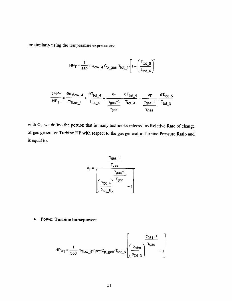
or similarly using the temperature expressions:
HPT = Imflow_4'cp_gas.Ttot_4 - Ttot_5
550 Ttot_4
I HPT t6mflow 4 *Ttot_4 r 15Ttot 4 0r 15Ttot 5HPT mflow_4 Ttot_4 Ygas- 1 Ttot_4 Ygas 1 Ttot_5
Ygas Ygas
with (DT we define the portion that in many textbooks referred as Relative Rate of change
of gas generator Turbine HP with respect to the gas generator Turbine Pressure Ratio and
is equal to:
Ygas 1
Ygas
Ptot 4
_ Ptot_s5
Ygas~
Ygas
- 1
* Power Turbine horsepower:
Ygas 1
I ~~~atm gaHPPT -mflow_4.nPT Cp_gas Ttot_5L P-t Y55_0 Ptot_5 )
51
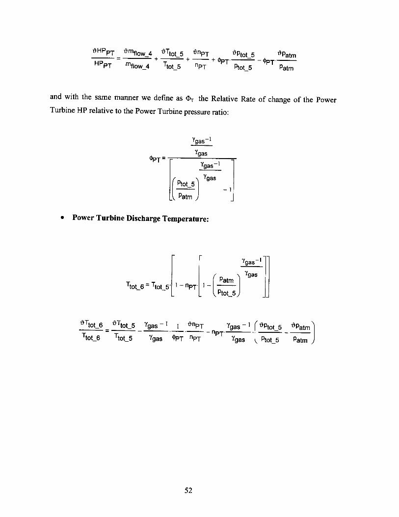
t HPPT *mflow 4 'Ttot 5 fnPT *Ptot 5 'patmH P + -+A PT'~t
HPpT mflow_4 Ttot_5 nPT Ptot_5 Patm
and with the same manner we define as ,DT the Relative Rate of change of the Power
Turbine HP relative to the Power Turbine pressure ratio:
Ygas 1
Ygas
O Ygas - jPtot 5 Ygas
_Patm )
* Power Turbine Discharge Temperature:
Ygas-
Pam YgasPatm 1Ttot 6 - Ttot5- 1nPT' 7 s -
ptot_5 j
*Ttot 6 _ Ttot_ 5 Ygas - 1 I nPT 7gas - 1 (1Ptot 5 *patm
Ttot_6 Ttot_5 Ygas OPT nPT Ygas Ptot_5 Patm
52
2.10 Engine Parameter Interrelationships Matlab Chart
When dealing with gas turbine engines, the engineer often finds it necessary to
know how the various engine and control performance parameters change with respect to
each other or with changes in the environment or the engine control. The simplified
technique presented herein will provide answers to most questions that will arise. It is
applicable to all currently known types of gas turbine engines and requires that the
engineer know only the engine compressor pressure ratio and the turbine inlet
temperature. In some cases, superficial information about the type of engine and the
control will be helpful. The preciseness of the answer obtained will depend primarily
upon the precision exercised by the engineer in stating his problem.
Basic to the system is an engine parameter interrelationship chart that can be
developed based on the above interrelationships. These are the fundamental equations
from which this chart has been derived, using evaluation methods in both their absolute
and differential forms. The evaluations of the general cases are for three typical values.
Pot 3 Ttot 4 P ~ tot 3 T tot 4 (1) a relatively low t and _ with values -1-t_ = 5.0 and _ 2000 RPtot_2 OT2 P tot_2 6T 2
where the portion 0T2 = - is a conversion to the relative absolute Temperature ratio,
P tot 3 T tot 4(2) a medium with values -t 10.0 t_ = 2160 R andP tot_2 0T 2
P tot 3 Ttot 4(3) a relatively high with values z_ = 20.0 and 4 =2600 RP tot_2 0T 2
In many instances, it will be sufficient to determine which of the three given cases best
approximates the specific case of interest and to use the appropriate numerical chart in
the problem solution.
Most of the major engine parameters that might be of interest are listed vertically
on the left side of the chart; those not listed may be obtained readily as combinations of
listed parameters {e.g., the change in specific fuel consumption [SFC] is simply the
change in fuel flow minus the change in thrust). Independent variables head each vertical
column. The cells within each column contain either parameters immediately obtainable
53
from knowledge of the compressor pressure ratio and turbine inlet temperature, fixed
physical constants, or combinations of these items. They indicate those parameters
assumed to be constant and also show how each of the other parameters varies with the
independent variable. To illustrate, the first column shows how all engine parameters
vary with turbine Inlet temperature Ttot_4 at constant engine speed, N, when Ttot_2 , Ptot_2,
Pa, nc, APtotb/Pto3, nb, nt and n are constant and when there is no air bleed or shaft power
extraction from the engine; these second column shows how the parameters vary with
engine speed at constant turbine inlet temperature; and so on. Note that the change in all
variables is expressed as a relative fractional, or percentage, change of the initial value,
which o. SHP is an absolute change and has units of horsepower per pound of air permflowair
second, and for e. which is the absolute change in the relative burner pressure drop.Ptot_3
Also note that an increase in any quantity is positive.
The following general rules may be stated:
1. For a steady-state problems, as a minimum use the first and second columns
unless Ttot 4 or speed obviously are constant in the statement of the problem.
2. For all transient problems, as a minimum use the first second and third columns
unless Ttot_4 or speed obviously are constant. The third column is necessary since
transient compressor-turbine horsepower imbalance is thermodynamically equivalent 'to
turbine shaft horsepower extraction.
3. For steady state or transient problems, use any additional column that may be
relevant in the statement of the problem or to the desired degree of answer precision. In
respect to precision, any steady-state problem solved using only the first and second
columns automatically assumes that component efficiencies are constant and that
compressor inlet air flow at constant speed is independent of compressor pressure ratio. If
the user cares to and seeks greater precision in his answer, he may do so by proper use of
the appropriate additional columns.
4. For all problems, use those horizontal rows that deal with able, or parameter, of
interest in the problem statement. The intersection of the application rows and columns
54
define the coefficients of the partial differential equation that shows how the dependent
variable varies with one or more independent.
5. When Rule 4 results in an equation having more than one independent variable,
an additional equation must be written for each additional independent variable- on the
basis of what is known about the engine or control-to permit simultaneous solution of
equations and reduction to an expression of the dependent variable in terms of one
independent variable. The additional equations mayor may not be in terms of the prime
independent variable of interest.
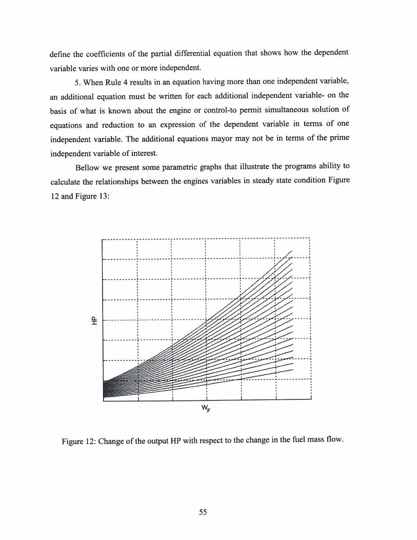
Bellow we present some parametric graphs that illustrate the programs ability to
calculate the relationships between the engines variables in steady state condition Figure
12 and Figure 13:
WF
Figure 12: Change of the output HP with respect to the change in the fuel mass flow.
55
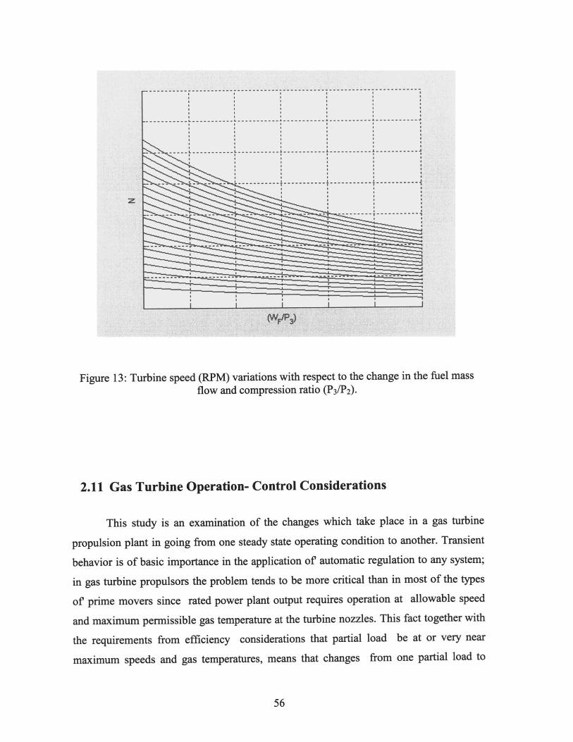
Figure 13: Turbine speed (RPM) variations with respect to the change in the fuel massflow and compression ratio (P3/lP2).
2.11 Gas Turbine Operation- Control Considerations
This study is an examination of the changes which take place in a gas turbine
propulsion plant in going from one steady state operating condition to another. Transient
behavior is of basic importance in the application of automatic regulation to any system;
in gas turbine propulsors the problem tends to be more critical than in most of the types
of prime movers since rated power plant output requires operation at allowable speed
and maximum permissible gas temperature at the turbine nozzles. This fact together with
the requirements from efficiency considerations that partial load be at or very near
maximum speeds and gas temperatures, means that changes from one partial load to
56

another must be accomplished under relatively rigid requirements of allowable speed and
temperature overshoot.
The method of attack is to consider first the individual steady state and transient
characteristics of the many different components which actually form a gas turbine
propulsor. Among these are included compressors, intercoolers, regenerators, combustion
chambers, turbines and the ducting from one component to the next, plus the transmission
and control system. Then certain particular types of transients are studied for typical plant
arrangements. The method of handling is somewhat akin to that used for transients of
electrical and mechanical systems with pressures temperatures, shaft speeds, torques and
gas and fuel flows as important variables. In order to handling by mathematics,
simplified assumptions are made wherever the errors so introduced are not expected to
alter the general trends to be examined.
For example, fuel injection and combustion effects are actually represented by an
equivalent heat transfer across the boundaries of the combustion chamber. Lumped
constants are used for combustion chamber and heat energy storage elements.
Furthermore, though the plots of characteristics of gas turbines and individual
components frequently show marked non-linearities, it is usually possible to make linear
approximations of relationships over important range of values in a specific problem. As
in transient calculations for other similarly liberalized systems the use of operational
methods of analysis is virtually indispensable.
The analyses in this study, together wlth the calculated examples, show that the
transient effects of interest in gas- turblne operation and control may be separated into
several relatively independent groups depending on the time lags involved. Such a listing
together with a short discussion of the importance of the trans lent effects in each group,
is as follows:
a) Transient effects which are over in a few hundredths of a second at most. The
time required for internal readjustment of compressor and turbine flow after changes in
inlet or exhaust conditions appears to be of this order, and may be roughly approximated
to be three or four times that required for a sound wave to travel the length of the turbine
or compressor. The importance of these transients does not seem to be very great, except
57
in their possible contribution to certain ducting and combustion chamber resonance
effects reportedly observed on jet aircraft.
b) Those transients involve readjustments times of between one-tenth of a second
and one second, namely, certain combustion chamber and ducting pressure and
temperature lag effects. A quick approximation of the characteristic time lags in
combustion chamber and ducting can apparently be obtained by using that length of time
required for the mass of air in the combustion chamber and ducting involved to be
replaced by the incoming gas flow. For the pressure lag the entire volume between
compressor and turbine should be used for temperature lag following a change in fuel
rate, that volume between the fuel nozzles and the inlet to the turbine is apparently the
applicable one. The duration of combustion chamber transients may be of importance in
certain cases where rapid emergency shutoff is required. Also, since these lags may cause
temperatures or pressures to over- shoot equilibrium values following a sudden
disturbance in fuel rate, they may affect flame stability adversely under some
circumstances.
c) The third group includes the transient effects that most directly influence
operation and control. The characteristics time lags in changing from one equilibrium
operating condition to another vary from few seconds to many seconds, and are a results
of the presence of such energy storage elements in the gas-turbine plant as the inertia or
rotating parts and the heat capacity or heat exchange tubes and walls of combustion
chambers, ducting, ash removers anti-icing valves. Other time lags may be present in the
plant transmission characteristics. All in all the presence of these lags, together with the
strict limitation on temperature and speed overshoot during transient changes in operating
conditions, makes necessary carefully designed and often quit complicated control
components if reasonably fast rates of response are to be obtained. The Characteristic
time for a turbine-compressor, turbine-load., or turbine-compressor-load unit on a single
shaft is calculated by dividing the total shaft rotational inertia by the variation at constant
fuel of net shaft torque with speed, The characteristic time lag of a regenerator appears to
be between a third and a half of the time required for a mass of air with a total heat
capacity equal to the heat capacity of the heat exchanger tubes to pass a give station in
the heat exchanger circuit. For intercoolers and precoolers characteristic time lags are a
58
somewhat smaller fraction of that time, depending on the ratio of coolant flow to gas
flow.
A complete transient picture must of course include the effects of control
components and control component lags. This is particularly evident when controls of the
regulatory type are used, as will be the case where minimum response time control
changes is required (e.g. propeller gas- turbine installations) or where the operator's
duties must be simplified. For the more elementary turbine arrangements and the simpler
types of control systems, mathematical computation of operating and control transients
appears quite feasible, but for control systems - involving two or more automatic
regulators of any degree of complexity, an experimental method of analysis using models
or analogs may be the only satisfactory way. The later method has the farther advantage
of allowing nonlinearities to be taken into account.
59
Chapter 3
3 Diesel Engine
3.1 Diesel Utility
Propulsion of the vast majority of contemporary merchant ships (especially
containerships and VLCCs) utilizes the marine Diesel engine as prime mover. Typical
marine propulsion plants include a single, long-stroke, slow-speed turbocharged, two
stroke Diesel engine directly coupled to the vessel's single large-diameter, fixed-pitch
screw propeller. Most often a variable-speed AC generator is also attached to the engine-
propeller shaft for efficient electric power generation. This typical configuration has been
adopted because it is characterized by quite large propulsion power outputs (typically
more than 30-40 MW from a single unit) and yet by operational robustness and increased
efficiency due to its conceptual simplicity.
The Diesel engines used in such marine propulsion power plants are designed for
steady-state operation and they are selected, during the ship design stage, so that they can
cover the vessel's propulsion power requirements at an rpm.
The Diesel (compression ignition) engine has shown to be a reliable, energy
efficient and cost effective power source for road vehicles, mobile machinery and
60
especially as marine propulsion. The internal combustion engine running on diesel fuel
still shows sufficient technical potential to meet future NOx and particulate emission
requirements. The diesel engine is energy efficient, resulting in relatively low CO2
emissions as long as automotive fuels are predominantly made from fossil oil. Also,
when in the long term the palette of energy carriers gets more diverse than it is today, the
diesel engine can be adapted to many of those new energy carriers. For any fuel, the
energy efficiency this engine is a plus.
The diesel engine is a reliable and durable power source with relatively low costs.
Therefore it is chosen in commercial heavy-duty applications like maritime propulsion
and earth moving equipment. Today, this heavy-duty industry sees no alternative power
source. For this automotive market, the diesel engine is expected to remain the
predominant power source for the next two decades.
3.2 Prime mover model development
The simulation model of a diesel engine can be regarded as an explanation of the
real engine operation, which combines the mathematical relationship between the relative
components and can be used to simulate the dynamic process of the diesel engine. A clear
overview of engine operations is helpful to understand the modeling of the real diesel
engine.
In an internal combustion engine, air is induced into the cylinders. The airflow
first passes through an air filter or air purifier to get the qualified fresh air in density and
dryness. Then it flows into the compressor, during which the air pressure is increased to
be higher than the atmospheric pressure. The charge air then flows through an inter
cooler to decrease the intake air temperature. Hence the air density is increased again
prior to the cylinder. Finally, it flows through a manifold and inlet valve into the cylinder.
61

3.2.1 Introduction
The classic dynamic behavior includes inertia of the diesel engine and turbine-
compressor system as the main parts. For other subsystems the dynamic behavior is
mainly based on the thermodynamic theory. With the charge of air condition parameters
it is possible to ignore sub-systems such as, air-filter, inter-cooler, inter-receiver and
outlet-receiver in a simple model. The cylinder model is the most important part. It
explains the combustion process inside the cylinder and calculates important operating
Compressor Turbine parameters such as the output work; mean effective pressure, brake
torque, revolution speed.
To model the combustion process, the subsystem used to explain the heat release
is necessary. There are several assumptions about parameters and processes in this
subsystem with which the simulation results are nearby the realistic situation. The
dynamic behavior of the turbine and the compressor systems are very complicated. The
performance map of the turbine and the compressor system is a common tool used in the
modeling. A general assumption is used to explain its dynamic action. Load control is
achieved by varying the amount of fuel injected each cycle while the airflow at a given
engine speed is essentially unchanged. So the governor and the fuel pump system are a
necessary part. Our model will be based on the following schematic representation
(Figure 14and Figure 15)
62
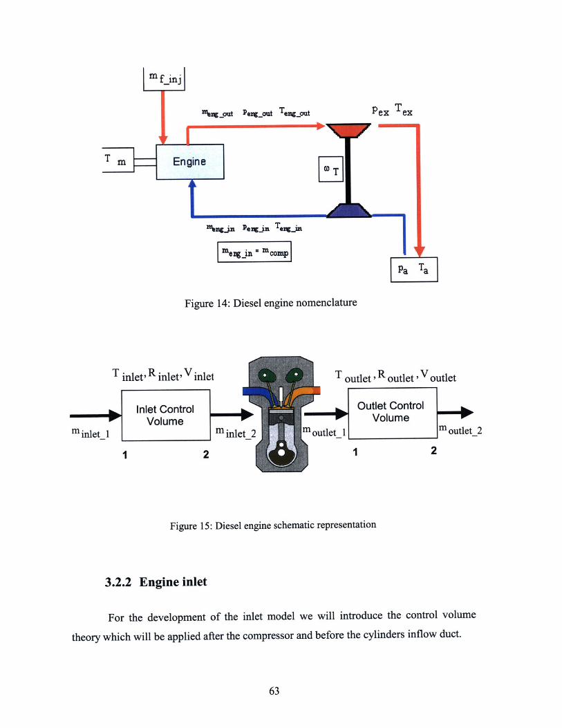
Ut PaiW outom-put
m f inj
T MI Engine
L -U
1%riCjU POeACJ TenM-
IMerg in' .MCOMPI
Pex Tex
Pa Ta
Figure 14: Diesel engine nomenclature
T inlet, R inletV inlet
Inlet ControlP- Volume
m inlet_1 minlet_2
1 2 1
T outlet , R outlet, ,V outlet
Outlet ControlP" Volume
moutlet_ IMoutlet_2
1I 2
Figure 15: Diesel engine schematic representation
3.2.2 Engine inlet
For the development of the inlet model we will introduce the control volume
theory which will be applied after the compressor and before the cylinders inflow duct.
63
ElT
We can assume that the gas at the inlet process is considered ideal in terms of
pressure and temperature. Apply this assumption and use the ideal gas law we will have:
D- Ii nl inlet-Tinlet
Pinlet Vinlet
Differentiate with respect to time:
d Rinlet-Tinlet d m-Rinlet d~Pinlet = -m + -Tinletdt Vinlet dt Vinlet dt D- 2
At the inlet control volume we can assume that the temperature varies slowly throughout
the inlet line from the compressor until the cylinder entrance. The assumption is based on
the consideration that the temperature exchange from the engine to the inlet air is not
significant at this point. Therefore we can approximate that:
d T -Odt inlet - D-3
Therefore
d Rinlet-Tinlet d-pinlet = -- i
dt Vinlet dt
dnti. - niinlet_1 - ninlet_2
D- 4
D- 5
where the position 1 and 2 are the boundaries of the control volume after the compressor
and before the engine's air intake respectively. The equation can take the form:
64
with
d Riniet-Tinietd~Pinlet - -iit (niet_1 - minlet_2) D- 6dt Vinlet
where:
"inlet_1 = mass flow before the cylinder input
ninlet_2 = mass flow in the cylinders
From the application of mass conservation theorem, the mass flow that enters the
engine is equal to the mass flow from the compressor and the mass that enters in the
engine will be the same with the mass that exit from the control volume.
d Rinlet'Tiniet~~Pinlet * (mcomp - mengin)dt Vinlet
with
'mcomp = mass flow from the compressor
M engin = air mass flow entering the engine and with
mengin = niinlet_2
The mass flow into the cylinder can be modeled as:
cyl =: * N* Pinlet' displ60 NRev Rinlet Tinlet
and the formula that expresses the mass flow for the entire engine will be:
= = Zfvol N Pinlet-VdisplD8n'engin = z-mcyl = z-nVOI-N- 60- N D- 8
6GRev-Rinlet' inlet
with:
nvol = volumetric efficiency
65
N = engine speed in RPMs
2 = number of cylinders
Vdispl = displacement volume of each cylinder
NRev = number of revolutions per cycle
Rinlet = gas constant at the inlet
We should remind here that the values of the mass flow through the control volume at the
boundaries are equal to:
inlet_2 = Meng-in and 1Tnlet_1 = n'omp D- 9
3.2.3 Engine outlet
For the study of the engine outlet characteristics we will consider an outlet control
volume like the one that we use for the inlet part study (figure 15). Based on the same
assumption that the ideal gas law can be applied on the gas at the outlet of the cylinder -
with other words that has the characteristics of that of an ideal one we will have:
Poutlet = mRoutiet Toutlet D- 10Voutlet
Following the same steps as before, we differentiate with respect to time the D-10expression,
d Routlet Toutlet d m iRoutlet d-L -Poutlet) = '11 + -- Toutlet D- 11
dt Voutlet dt Voutlet dt
and based on the same assumption that the temperature varies slowly throughout the
entire length of the control volume:
dToutlet = C D- 12dt
hence:
d Routlet.Toutlet d-Poutlet = D- 13
dt Voutlet dt
66
from the mass conservation in the control volume:
"= %OutletI - OUtet_2 D- 14
with moutiet_1 and moutlet_2 the mass flows at the boundaries of the outlet control volume
(figure 2). The mass flow that enters into the outlet control volume is actually the mass
flow that exits from the engine manifold and the mass flow that exits from the above
control volume is the gas mass that enters in the turbine manifold of the turbocharger. We
assume in this point that the heat exchange with the wall of the entire exhaust system is
negligible. This assumption holds under the consideration that the engine is running after
the transient period of the ignition and 'warm up' and already the temperatures in all the
engines parts reach the equilibrium temperature point. Therefore the expression will be:
di Routiet-ToutietD-5-Poutlet = ou utl (nng_out nturb) D- 15
dt Voulet
The next step is to consider that the engine is actually a third control volume. Based on
that, the mass flows moutet_1 and moutlet_2 can be calculated if we apply the mass
conservation of the engine manifold. Let us assume that mfinj is the mass of the injected
fuel per stroke then:
_ _ f.injN D- 166 G NRev
mengout meng_in + mffuel D- 17
Substitute the two previous equations into D- 15 and we will have the final expression:
- RouteToutlet * (meng in + mfuel - mturb) D 18dt Voulet
67
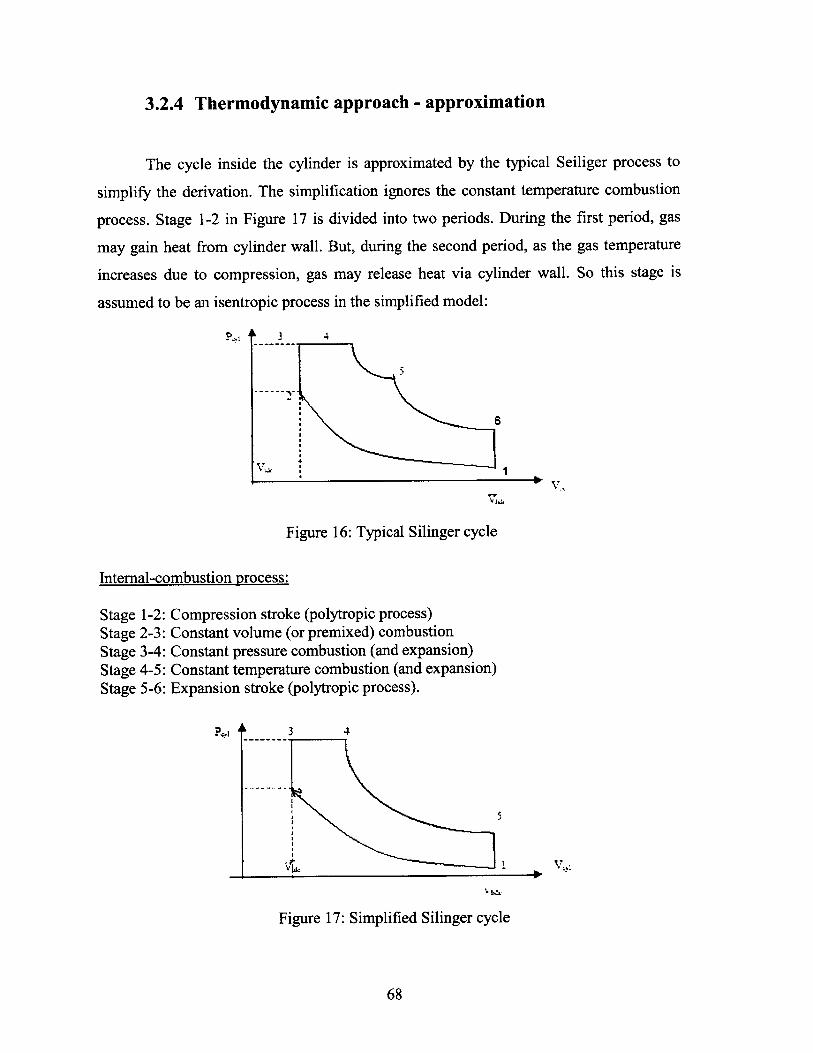
3.2.4 Thermodynamic approach - approximation
The cycle inside the cylinder is approximated by the typical Seiliger process to
simplify the derivation. The simplification ignores the constant temperature combustion
process. Stage 1-2 in Figure 17 is divided into two periods. During the first period, gas
may gain heat from cylinder wall. But, during the second period, as the gas temperature
increases due to compression, gas may release heat via cylinder wall. So this stage is
assumed to be an isentropic process in the simplified model:
V4.
V,
Figure 16: Typical Silinger cycle
Internal-combustion process:
Stage 1-2: Compression stroke (polytropic process)Stage 2-3: Constant volume (or premixed) combustionStage 3-4: Constant pressure combustion (and expansion)Stage 4-5: Constant temperature combustion (and expansion)Stage 5-6: Expansion stroke (polytropic process).
Figure 17: Simplified Silinger cycle
68
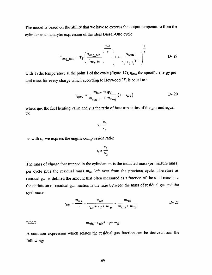
The model is based on the ability that we have to express the output temperature from the
cylinder as an analytic expression of the ideal Diesel-Otto cycle:
T = T F Pengout 1 + qspec D- 19g Peng in cv T i -rc )
with T1 the temperature at the point 1 of the cycle (figure 17), qspec the specific energy per
unit mass for every charge which according to Heywood [7] is equal to:
_ mbum 'qHV . 1 - \ D- 209spec -egn fKn ( res)}
"Mengjin + ifinj
where qHv the fuel heating value and y is the ratio of heat capacities of the gas and equalto:
cPcv
as with rc we express the engine compression ratio:
Vi
V2
The mass of charge that trapped in the cylinders m is the inducted mass (or mixture mass)
per cycle plus the residual mass mres left over from the previous cycle. Therefore as
residual gas is defined the amount that often measured as a fraction of the total mass and
the definition of residual gas fraction is the ratio between the mass of residual gas and the
total mass:
"'res m res _ "res D- 21m mair + mf + nres mmix+ "1res
where mmix= mair + nf= maf
A common expression which relates the residual gas fraction can be derived from the
following:
69
imep _ q spec 1
P i c-T i y - 1
with
imep = mean effective pressure and
qspec the specific internal energy
and the dimensionless numbers rc , y , Cspec are sufficient to describe the characteristics
of the constant volume ideal gas standard cycle, relative to its initial conditions Pi , T , For
the constant volume adiabatic combustion process:
m-cv-(T3 - T2) = lyqLH\ D- 23
Note that the heating values at constant volume and constant pressure are the same for
this working fluid. And for convenience we will define:
qLHVqspec - m m
D-24
where qLHv the lower heating value of the fuel
The way that the specific internal energy is defined is that the enthalpy decrease during
the isothermal combustion per unit mass of working fluid. Hence:
my mairqspec ~ ~~ ~= LHV
m1air mD- 25
mf r - 1A simple approximation for -- is e : i.e fresh air fills the displaced volume
mair rc
and the residual gas fills the clearance volume at the same density. Then for isooctane
r - 1fuel, for stoichiometric mixture the Aspec is given by 2.92 106 C [J/Kg]. For y--1.3 and
70
D- 22rc C
rc ~ rc
an average molecular weight of 29.3 cv= 9 4 6 [J/KgK].For T,=333 [K] the ratio qspeccv-Ti
r -1becomes equal to 9.3 .For this value the cycle will be burning a stoichiometric
re
mixture with an appropriate residual gas fraction.' 5
It is useful to compare the imep - a measure of effectiveness with witch the
displaced volume of the engine is used to produce work - and the maximum pressure in
the cycle P3. The ratio - can be determined from the ideal gas law applied at points 2 andPi
3 and the relation
= spec D- 26
T2 cv-Tiv 1-
is obtained from the combination of the equations (D-23) and (D-24) and with theapplication to the equation (D-22) is giving:
11 -
imep _ 1 c Y-1
P3 rc.(Y - ) rc - I cv-T 1q spec rc Y 1 D- 27
The indicate fuel convention efficiency and the ratios .mep and imep for this ideal cycleP1 P3
model do not depend on whether the cycle is throttled or supercharged. However the
working fluid properties at the point 1 to 5 do depend on the degree of throttling or
supercharging. For the throttled engine operation, the residual gas mass fraction xres can
be determined as follows:
15 Indicated values as can be obtained from Heywood
71
From the equation (Heywood p-168) [7]
1) 4
Xres== D-28m rc 'U5
and since the state 5 corresponds to an isentropic expansion from state 4 p Pengout
1 1 1
Pengout Peng-out P1
- P4 P eng in P4 D- 29rc rc
apply simple thermodynamic laws:
P I PI P2 P3 I T2 q spec- =-re = - D- 30P4 P2 P3 P4 r Y T3 C}rcY 1 -D
It follows that:
1 - 1
e = n Peng_out 1 + qspec D- 31 rc Pengin cV-T
1 -rC7 1 J
It is more difficult to determine the fluid temperature at intake valve closing
compared to the pressure, since it is influenced by heat transfer and residual gases that are
difficult to measure and determine. The air in the intake manifold is heated from Tengin to
Tres by the hot valves and the locally high heat transfer coefficients in the cylinder. Fuel is
added in the ports and undergoes an evaporation which also influences the temperature.
In the cylinder the residual gases the fresh charge is mixed with the residual gases and the
mixture temperature is:
Ti = maf-Cp.af-Taf - frescpxres -Tres D- 32nfaf-Cp.af - mres-cp.res
72
As Heywood in his book indicates that the outlined model for heating,
evaporation, and mixing processes are complex and contain several variables that have to
be determined. The central question here is to see how well a simple model can capture
the process and therefore some simplifications are made. First it is assumed that the
specific heats c, are the same for the residual gas and the fresh air and fuel mixture
yields:
Ti - maf-Cp-Taf - mres-cp-Tres _ mafTaf - mres-Tres D- 33nafcp -rescp mafr -res
apply the equation for xres (D-21) and we will have:
Ti = xres-Tengout + (1 - xres)-Tengin D- 34
3.2.5 Fuel Model
The fuel injection model that it will be used it is developed in the Mater of
Science Thesis with the title "Fuel Targeting and Thermal Environment Effects on Spark
Ignition Engine Mixture Separation Process" and it was modified for the demands of the
present thesis [5].
A very simple fuel transport model, which provides a reasonably good prediction
of these excursions, is the x-T model [1, 2, 3, and 4]. This model is based on the
phenomenological description illustrated in figure5. The governing equations are the
following:
res = x-ff.inj~ D- 35
73
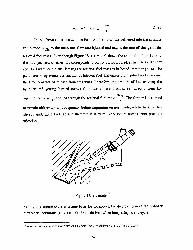
mru x)nyinj D- 36
In the above equations burn is the mass fuel flow rate delivered into the cylinder
and burned, nfli is the mass fuel flow rate injected and mres is the rate of change of the
residual fuel mass. Even though Figure 18: x-r model shows the residual fuel in the port,
it is not specified whether mre corresponds to port or cylinder residual fuel. Also, it is not
specified whether the fuel leaving the residual fuel mass is in liquid or vapor phase. The
parameter x represents the fraction of injected fuel that enters the residual fuel mass and
the time constant of release from this mass. Therefore, the amount of fuel entering the
cylinder and getting burned comes from two different paths: (a) directly from the
m'resinjector: (1 - x)mnyj. and (b) through the residual fuel mass:---. The former is assumed
to remain airborne, i.e. it evaporates before impinging on port walls, while the latter has
already undergone fuel lag and therefore it is very likely that it comes from previous
injections.
Figure 18: x-u model' 6
Setting one engine cycle as a time basis for the model, the discrete form of the ordinary
differential equations (D-35) and (D-36) is derived when integrating over a cycle:
16Figure from Thesis in MASTER OF SCIENCE IN MECHANICAL ENGINEERING-loannis Kitsopanidis
74
'Wes =es + X mnf.inj - es D- 37
(1bur - x)ny.inj + nWes .A D- 38
A. is the time duration of a cycle, which is a constant at constant speeds. Under steady
state conditions the residual fuel mass is constant, i.e. mr1 = mrinI, so equation (D-36)
yields:
i-Ies x-m .t D- 39
Substituting back to equation (D-37):
i i"'bum =nf.inj D- 40
Therefore, for steady state conditions the amount of fuel entering into the cylinder
and getting burned equals to the amount of fuel injected. Even though fuel lag exists,
there is no net effect because the amounts of fuel entering and leaving the residual fuel
mass are the same.
However, under transient operating conditions this is not true due to the fuel lag
effect. The amount of fuel that remains airborne and enters into the cylinder directly from
the injector responds to transients in one cycle, while the amount that passes through the
residual fuel mass has a finite response time because the residual fuel mass increases
during the transients. This increase is due to the fact that the mass of residual fuel scales
with the mass of fuel injected as equation (D-38) implies (if x and T remain constant) and
therefore, the residual fuel mass tries to reach a new steady state. Physically, the increase
is attributed to residual fuel mass inertia as more fuel enters and less fuel can leave that
mass during a transient. Since the residual fuel mass increases, equation (D-36) reads:
n'es x fles I- D- 41At
Substituting back to equation (D-37):
nbum I mf.inj
75
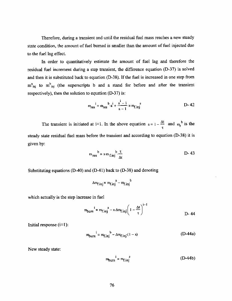
Therefore, during a transient and until the residual fuel mass reaches a new steady
state condition, the amount of fuel burned is smaller than the amount of fuel injected due
to the fuel lag effect.
In order to quantitatively estimate the amount of fuel lag and therefore the
residual fuel increment during a step transient, the difference equation (D-37) is solved
and then it is substituted back to equation (D-38). If the fuel is increased in one step from
mainj to m inj (the superscripts b and a stand for before and after the transient
respectively), then the solution to equation (D-37) is:
1 res ~ " res b*a + -xmf.inja D- 4
The transient is initiated at i=1. In the above equation a= 1 - At and nrb is the
steady state residual fuel mass before the transient and according to equation (D-38) it is
given by:
M -= -b bt- D- 43 res f.inj At
Substituting equations (D-40) and (D-41) back to (D-38) and denoting
An~~ = a bAmf.inj = m.inj a- nf.inj
which actually is the step increase in fuel
m burn = nf.inja - Aninj{ I D
T D- 44
Initial response (i=1):
fur = mf.injb - Anfy.inj'(1 - x) (D-44a)
New steady state:
%ur ="f.inja (D-44b)
76
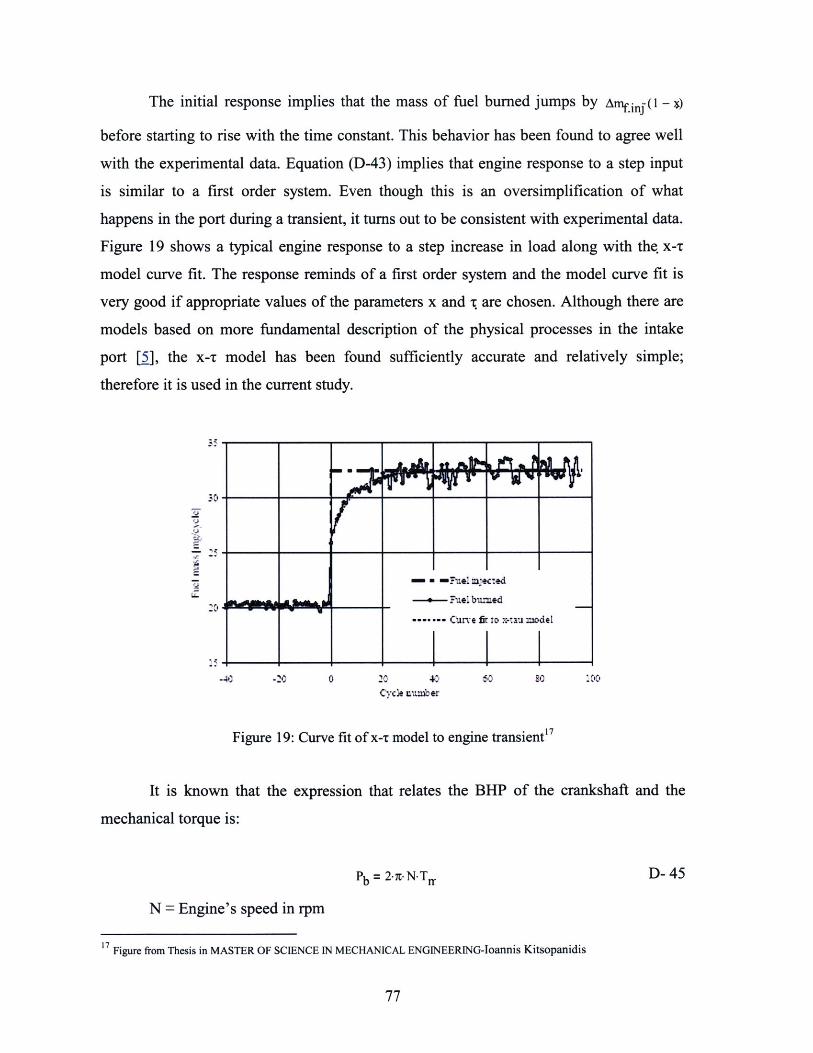
The initial response implies that the mass of fuel burned jumps by Any (1 -i)
before starting to rise with the time constant. This behavior has been found to agree well
with the experimental data. Equation (D-43) implies that engine response to a step input
is similar to a first order system. Even though this is an oversimplification of what
happens in the port during a transient, it turns out to be consistent with experimental data.
Figure 19 shows a typical engine response to a step increase in load along with the. x-T
model curve fit. The response reminds of a first order system and the model curve fit is
very good if appropriate values of the parameters x and T are chosen. Although there are
models based on more fundamental description of the physical processes in the intake
port [5], the x-t model has been found sufficiently accurate and relatively simple;
therefore it is used in the current study.
Iz
-40 -20 0 20 40Cycle umber
60 so
Figure 19: Curve fit of x-T model to engine transient1
It is known that the expression that relates
mechanical torque is:
Pb = 2.N.Trr
the BHP of the crankshaft and the
D- 45
N = Engine's speed in rpm
17 Figure from Thesis in MASTER OF SCIENCE IN MECHANICAL ENGINEERING-loannis Kitsopanidis
77
-. 1 -?.=jtcted
_______t - &bu.rned
.... C~inve fir to x-:au nwdol
The thermodynamic relation that connects the BHP with the fuel mass the
efficiencies and the fuel characteristics can expressed as follow:
b qLHV C air-nv)-(nc.nth.i -nm){ -$1'tum air pst t 2n R t
We will use a simpler expression that actually covers the needs of this thesis
Pb [ LHV C a $ D (mair).(nc-nth.i .nm)
L mair )St
D- 46
The parameter D represents a ratio that express the burned mass of the fuel with the18injected one and it is known as fuel/air equivalence ratio
mif.burn
C air
Sair )st
Cmf-In*mburn = mf.burn - m* air
"air St D- 47
Plug the (D-47) into the (D-45):
D- 48
Therefore the expression of the mechanical torque becomes:
1 bTm= --
2 r-N
1nthi = 1 --
..y--1
T 1 [qLHVn um(ncnth.i.n ]2 n-N
and Yc= vc V
Heywood "Internal Combustion Engine Fundamentals "McGraw Hill, 1988, (P-7 1)
78
with:
D- 49
Typical values for a diesel engine are y 1.4 which with no harm of the generality can be
assumed that is very close to the air y=1.4 and with a compression ratio rc=20 for a
engine of our characteristics. This can give as a nth.ij0.6 9 8 19. The typical value for the
qLH\ and for the type of the light fuel diesel that we are using will be approximately
qLHV= 43.2 Mkg 20
As ne we express the combustion efficiency which is very close to 98-99%21. For
the mechanical efficiency nr. and with respect the sector of our engine rpm its value will
be around 98%2.From the equation (D-48) became obvious that the crankshaft torque of
the diesel engine can be expressed as a function of the n .
Tm = nburn)
since the number of the rpm for a diesel engines that it is designed for electric generator
service set are constant and vary from 1200-1800 [rpm].In this sector all the values of
the parameters that we referred can be determined from graphs and tables as we notice
previously. Therefore we can approximate our expression as:
I [qLHV(nc-nth.i-nm).-
T_= 2 [ Nmbum = kflmbum with mbum-f(mf inj) D- 50
In conclusion we can say that if we do know the mass of the injected fuel and according
to the x-T model we can calculate the mass of the burned fuel which actually illustrates
the BHP of the engine's crankshaft and as a final result the output mechanical torque of
the engine. The Figure 20 bellow shows the concept flow of our hypothesis.
19 Heywood "Internal Combustion Engine Fundamentals "McGraw Hill, 1988,( P-170 formula 5.31)20 Heywood "Internal Combustion Engine Fundamentals "McGraw Hill, 1988,( P-915 Table D.4)21 Heywood "Internal Combustion Engine Fundamentals "McGraw Hill,1988,( P-82 Figure 3-9)22 Heywood "Internal Combustion Engine Fundamentals "McGraw Hill, 1988,( P-825 figure 15-1)
79
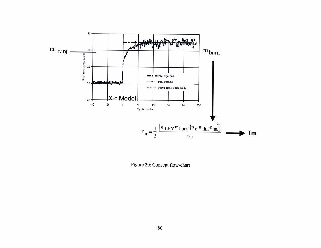
m f.inj
-.m in==ii. njected
_ Fuel burned
-..... Curvt fit to riau model
40 -20 0 20 40 60 80 i0oCycle zumbtr
1 [q LHVmburn-(n c-n th.i- n)]
2 t-n-**Tm
Figure 20: Concept flow-chart
80
mbum
Tm
3.2.6 Ideal first-order dynamic model of a turbine-compressorsystem
The exhaust flows through the outlet valve and manifold ant then flows into
turbine. It drives the turbine, which powers the compressor. The turbocharger, a
compressor-turbine combination, uses the energy available in the engine exhaust stream
to achieve compression of the intake flow. The function of the turbine and the
compressor is to increase the maximum power that can be obtained from a given
displacement engine. The work transfer to the piston per cycle, in each cylinder, which
controls the power the engine can deliver, depends on the amount of fuel burned per
cylinder per cycle. This depends on the amount of fresh air that is induced each cycle.
The airflow at a given engine speed is essentially unchanged. But for the turbocharged
engine, the inlet air is compressed by this exhaust driven turbine-compressor
combination. With the compression function of the compressor, the intake air pressure is
increased, and hence the air density. Increasing the air density prior to entry into the
engine thus makes the increasing in fuel flow allowed. Then it increases the maximum
power that an engine can offer.
The turbine and compressor are assumed to be of the centrifugal type. The
power used to drive the turbine comes from heat transfer released from the cylinder,
which is the so called exhaust-driven turbine. This power is transferred to the compressor
to compress the intake air. With a certain value of power input, the air can be conditioned
to a certain density level and velocity. This system can be modeled as a first order classic
dynamic system.
The work-transfer rate of power that is required to drive the compressor is calculated
from the equations:2 3
P 02Wc= ncompcp.i-(T02-TOl) with T02 = TOl P02
2 Heywood "Internal Combustion Engine Fundamentals "McGraw Hill, 1 988,(Eq.(6.42) and (6.58))
81
The ratio - is the compression ratio of the turbocharger which is equivalent for ourPOI
model with the ratio:
P02 Pinlet
POI Pa
The work done by the compressor is equal to:
mcomp cPi-Tex
nc
P inlet
P a
Yin-1
inJ - Ij = C(t
W mComp -Cn -TaC nc
or
"comp = W C*
Cp.i-T a
Yin
D-52
The torque produced by the compressor is:
Yin- 1~,- ~ in
c= Mccp.i.Ta Pinlet -1
nC'*OtC _ Pa )
The power delivered by the turbine is given by the equation:
-W = nturb.(ho.out - ho.i
82
therefore
D-51
Yin-IKP inlet
PaIi
nc
(Yin~)
YinI P inlet
P a
D-53
D- 54
We
The total to total turbine efficiency is given by:
n = h03 h04 D- 551TTT h ho4h03~ h04s
where 03 stage is the inlet stagnation state 4 and 04 are the exit static and stagnation
states respectively. States 4s and 04s define the static and stagnation exit states of the
equivalent reversible adiabatic turbine. If the exhausted gas is modeled as an ideal gas
with constant specific heats the previous equation (D-54) can be written as:
T04
T03 - T04 T03 D- 56TT =T03 - T04s' (D- )
P041 - -
P03
Note that for exhaust gas over the temperature range of interest, cp, may vary significantly
with respect to temperature. The power delivered by the turbine is given by:
WT = mengout - h0 4) = 'meng-out Cp ex(T03 - T0 4)
Yex-1
Yex
WT = mengout *cpP0nTTT-T33 (P-4- D- 57
04For our model again the equivalent pressure ratio -- will be:
P03
P04 Poutlet
P03 Pex
Therefore the equation (D-56) will transformed to:
Yex-
W T = n T -mturb -cp.T } T 1 ule- P= TT*tc WTPex e
83
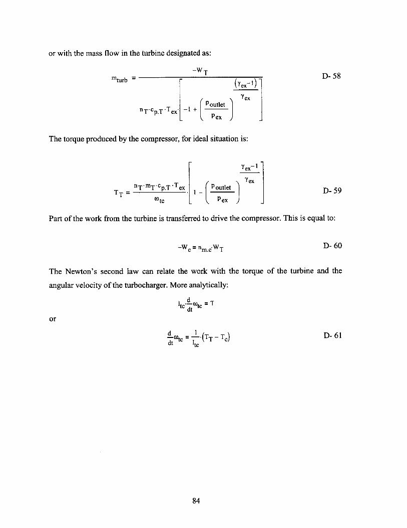
or with the mass flow in the turbine designated as:
mturb -
nT'cp.T *Tex*
--W
[P outlet-l +Pex
D- 58Yex-1)
" ex
The torque produced by the compressor, for ideal situation is:
nT-nT mcp.T -rTeTT t
)e I
Yex-
j 7exP outlet
ex jx
Part of the work from the turbine is transferred to drive the compressor. This is equal to:
-WC = m.cWT D- 60
The Newton's second law can relate the work with the torque of the turbine and the
angular velocity of the turbocharger. More analytically:
dItc-(otc = I
dt
or
d tc = -(TT - T)dt Itc
D- 61
84
D- 59
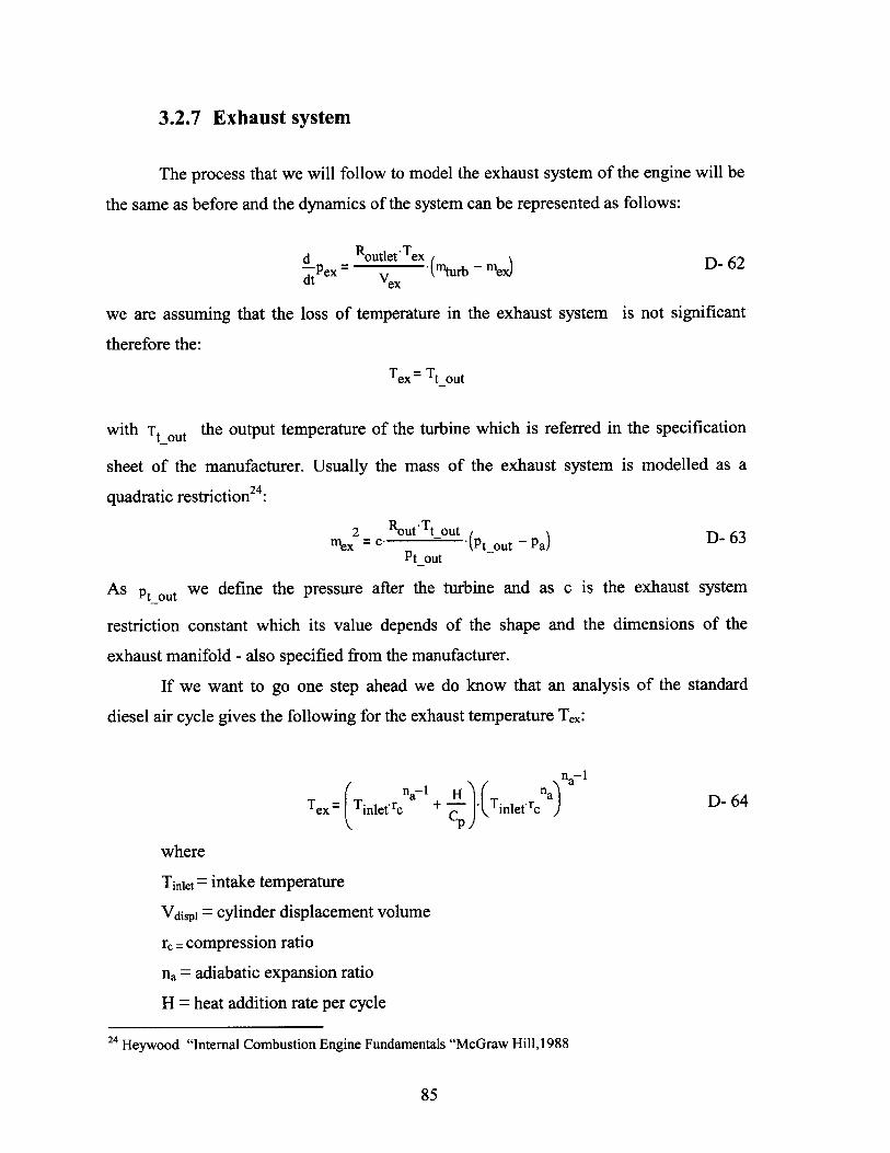
3.2.7 Exhaust system
The process that we will follow to model the exhaust system of the engine will be
the same as before and the dynamics of the system can be represented as follows:
d Routlet-Tex -_ex. D-62dt Vex
we are assuming that the loss of temperature in the exhaust system is not significant
therefore the:
Tex = Ttout
with Ttout the output temperature of the turbine which is referred in the specification
sheet of the manufacturer. Usually the mass of the exhaust system is modelled as a
quadratic restriction24 :
2 Rout-Tt outmex = C Pt-out -(Pt_out Pa) D-63
As pt_out we define the pressure after the turbine and as c is the exhaust system
restriction constant which its value depends of the shape and the dimensions of the
exhaust manifold - also specified from the manufacturer.
If we want to go one step ahead we do know that an analysis of the standard
diesel air cycle gives the following for the exhaust temperature Tex:
Tex = (Tinlet-rcna-I + H -(Tinletrena i D- 64CP
where
Tiniet= intake temperature
Vdispl = cylinder displacement volume
r_= compression ratio
na = adiabatic expansion ratio
H = heat addition rate per cycle
24 Heywood "Internal Combustion Engine Fundamentals "McGraw Hill, 1988
85

The heat added per cycle can be described as:
H = finj. HVz.n
2 ntrapMengin D- 65
fij= fuel mass injected
HV = fuel heating value
n = engine speed
ntrap = fraction of the air flow which is trapped
meng5 in = total air mass flow rate entering the engine
(the 2 in the denominator is for four stroke engine)
86
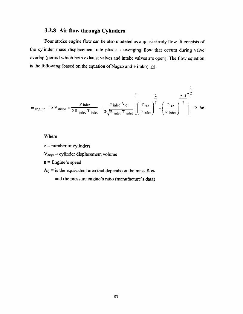
3.2.8 Air flow through Cylinders
Four stroke engine flow can be also modeled as a quasi steady flow .It consists of
the cylinder mass displacement rate plus a scavenging flow that occurs during valve
overlap (period which both exhaust valves and intake valves are open). The flow equation
is the following (based on the equation of Nagao and Hirako) [6].
2
P inlet P inlet-Ac K P exm e__n= z-V disp +-n -engin dispi 2-R inlet* T inlet 2. R inletT inlet _ P inlet)
7+1 - 2
P ex
SP inlet) _
Where
z = number of cylinders
Vdispl = cylinder displacement volume
n = Engine's speed
Ac = is the equivalent area that depends on the mass flow
and the pressure engine's ratio (manufacture's data)
87
D- 66
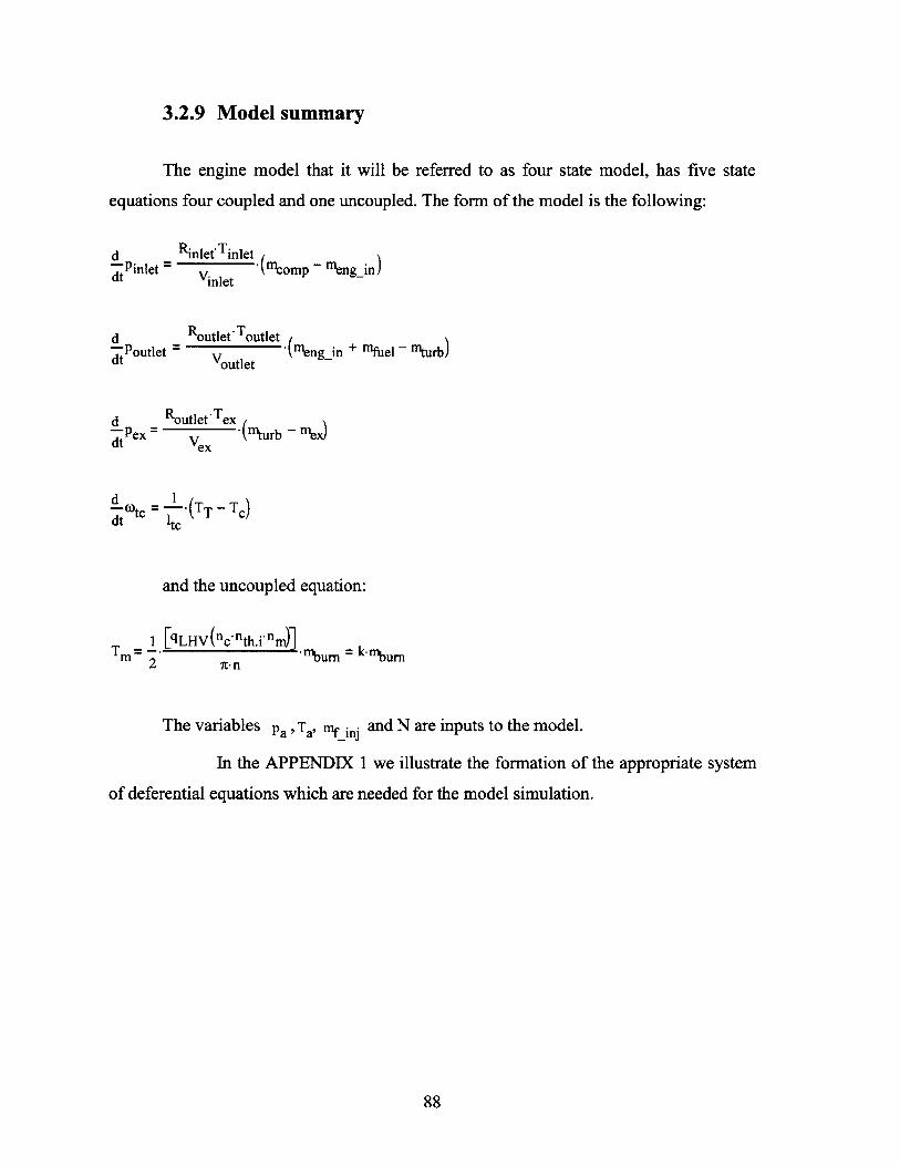
3.2.9 Model summary
The engine model that it will be referred to as four state model, has five state
equations four coupled and one uncoupled. The form of the model is the following:
d RnletTinletd - (minlet * (mcomp - meng in)y lt Vinlet
~Poutlet RoutetToutiet (ngin + nmfuel ~ "'turb)dt Voutlet
d Routlet-Tex -dt Vex
-Otc = .(TT - TC)dt itc
and the uncoupled equation:
1 [qLHV(nc-nth.i-nn)]TM= ~'mbn nur = k-nburn2 IC-n
The variables pa , Ta' "'_ninj and N are inputs to the model.
In the APPENDIX 1 we illustrate the formation of the appropriate system
of deferential equations which are needed for the model simulation.
88
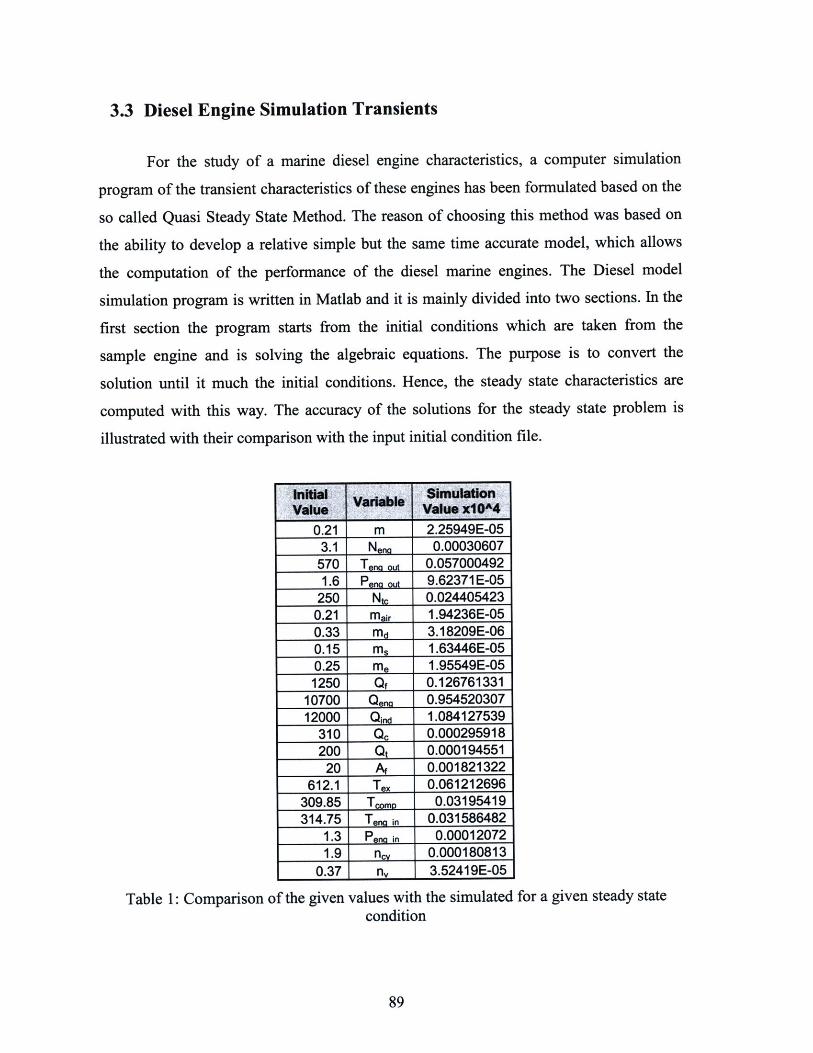
3.3 Diesel Engine Simulation Transients
For the study of a marine diesel engine characteristics, a computer simulation
program of the transient characteristics of these engines has been formulated based on the
so called Quasi Steady State Method. The reason of choosing this method was based on
the ability to develop a relative simple but the same time accurate model, which allows
the computation of the performance of the diesel marine engines. The Diesel model
simulation program is written in Matlab and it is mainly divided into two sections. In the
first section the program starts from the initial conditions which are taken from the
sample engine and is solving the algebraic equations. The purpose is to convert the
solution until it much the initial conditions. Hence, the steady state characteristics are
computed with this way. The accuracy of the solutions for the steady state problem is
illustrated with their comparison with the input initial condition file.
Initial SimulationValue Variable ValUO xO^4
0.21 m 2.25949E-053.1 Neng 0.00030607
570 Teng out 0.0570004921.6 Peng Ow 9.62371E-05
250 Ntc 0.0244054230.21 Mair 1.94236E-050.33 Md 3.18209E-060.15 m, 1.63446E-050.25 me 1.95549E-051250 Qf 0.126761331
10700 Qena 0.95452030712000 Qinc 1.084127539
310 Qc 0.000295918200 Qt 0.000194551
20 A, 0.001821322612.1 Tex 0.061212696
309.85 T omp 0.03195419314.75 Tena in 0.031586482
1.3 Penn in 0.000120721.9 ncy 0.000180813
0.37 n, 3.52419E-05
Table 1: Comparison of the given values with the simulated for a given steady state
condition
89

For a wide range of operating conditions that the model was tested although there
was an error of the values for the air flow and exhaust temperature of 10% in the case of
the speed and output torque that we are more interested this error margin was decreased
within 3-4%.25
In the next step the developed algorithm is using the full problem formulation
(complete set of differential and algebraic equations) and with the already calculated
steady state problem evaluates the transient characteristics.
The engine that was used for the evaluation of our model is a Marine type
Mitsubishi 3 cylinder, 420 [rpm], and maximum output power of 385 [PS] 26. The engine
characteristics data are presented in APPENDIX 2.
For the transient test response we initiate the case of a strong fuel flow change.
The engine we assume that was running under a certain condition and more specific at
the 2/3 of the max power and the fuel supply was decreased for amount of time equal to
1.5 sec and then it was released to the original position. The change in the mass flow that
is presented with the following function is steep but it was chosen to illustrate the
program's ability.
The simulation results that we are interesting are the engine's rpms, the output
torque and the changes in the air intake. These characteristics are presented in the
following figures:
25 According to the data that were available26 Courtesy of Mitsubishi Motors, Japan
90
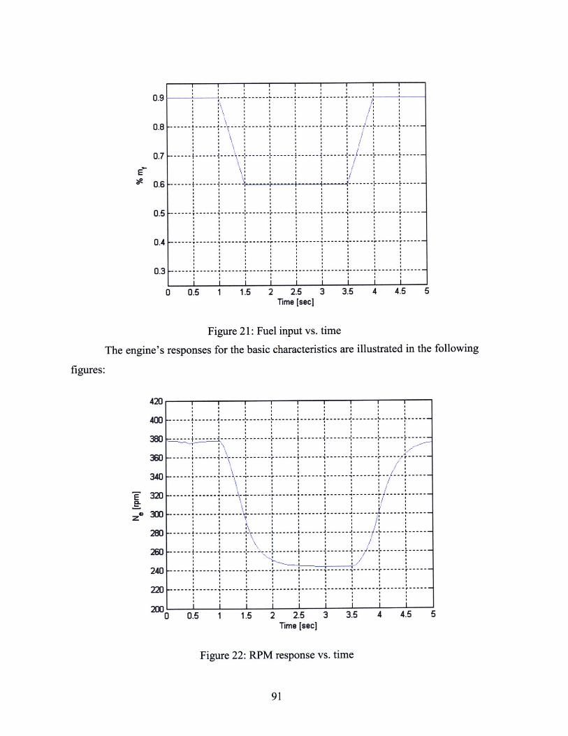
1 1.5 2 2.5Time [seci
3 3.5 4 4.5 5
Figure 2 1: Fuel input vs. time
The engine's responses for the basic characteristics are illustrated in the following
figures:
0.5 1 1.5 2 2.5Time [seci
3 3.5 4 4.5 5
Figure 22: RPM response vs. time
91
0.9
0.8
0.7
0.6
0.5
0.4
0.310 0.5
-- -- --------------------
-J - - - - -a -
k___-___-__-___-__-___ .-- L-- - - ---
-- -- - - - --
I t a a a a a aa a a a a a a
a a a a a a a a aa a a a a a a a
a................-a a a a a a a a aa a a a a a a a aa a a a a a a a aa a a a a a a a aa a a a a a a a aa a a a a a a a aa a a a a a a a a
S-a------------------a a a a a a a a aa a a a a a a a aa a a a a a a a aa a a a a a a a aa a a a a a a a aa a a a a a a a aa a a a a a a a a
.--a---------------a.--a a a a a a a aa a a a a a a aI I I ififfi
420
400
380
360
340
320
280
260
240
220
200
z
I I I I a a
a a a a a a a a aa a a a a a a a aa a a a a a a a a
a I.----.1- .~- a..- a.a a a a a a a a aa a a a a a a a aa a a a a a a a aa a a a a a a a aa a a a a a a a a
a a a a a a aa a a a a a a a
a a a a a a aa a a a a aa a a a a a
-~. ---------a a a a a aa a a a a aa a a a a aa a a a a a a
---------------------a a a a a aa a a a a a aa a a a a aa a a a a a a
-I. -a-a a a a a aa a a a a aa a a a a aa a a a a a I-
-- A----a a a a a aa a a a a aa a d a a a aa a a a a aA- .1 .L- A- .1--.J.. JL La a a a a a (a a a a a a a aa a a a a aa a a a a aa a a a a a -a a a a a aa a a a a aa a ~ a a aa a a~-J a a
--S1
a a a a a aa a a a a aa a a a a a
a a a a a---------
a a a a a aa a a a a a aa a a a a aI I I I I I I ~
F
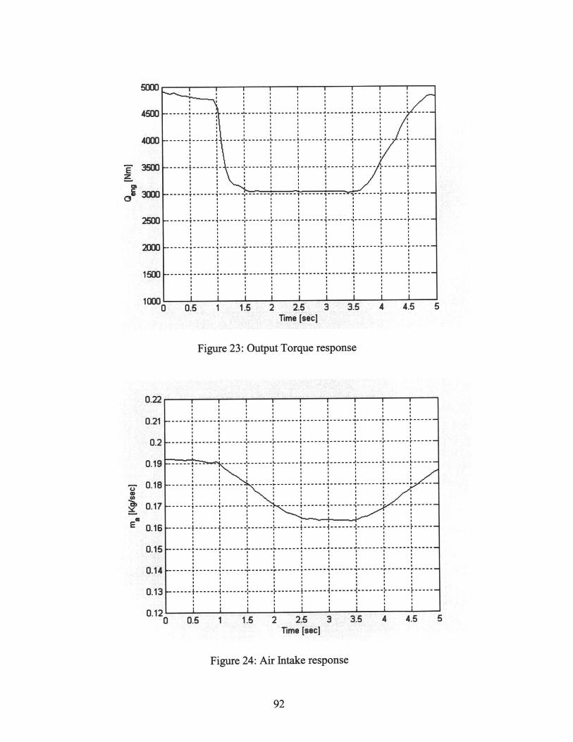
92
Figure 24: Air Intake response
I3 0.5 1 1.6 2 2.5 3 3.5 4 4.5 5
Time [Secl
Figure 23: Output Torque response
3 3.5 4 4.5 5Ia 0.6 1 1.5 2 2.5
rime [Secl
------------- ------ ------ L ------ 1 ------ 1 ---------------- L ------
---
r . . . . . . T - - - - - - - - - - - - . . . . . . .. r - - - - - - -r ------
---------------- 4 ------ I -------- I -------- ------
SM
46M
M
3SOO
30M
2500
20M
ism
1000
0.21
0.2
0.19
0.18
0.17
0.16
0.15
0.14
0 * 13
0.12
I - - - - - - - -- - - - - - - - - - - - r - - - - - -
- - - - - - -1 - - - - - - ---- - - - - - -o- - - - - - - -- -- - - - ---------------
- - - - - - - - - - - -0 -- -- - - - - - - - - - - - - - - - -4 - - - - - - -0 -- - - -- - 0-
or# - - - - - - - - - - - - T - - - - - - I - - - - - - I - - - - - - - - - - - - r
- - - - - -- - - - - - -I L - - - - - - - - - - - - - - - - - - j 1- - - - - - -- I L - - - - - - - - - - - -
- - - - - - . . . . . . - - - - - - -a - - -- - - - L - - - - - - A . . . . . . - - - - - - -& - - - - - - - 16 - - - - - - 6 - - - - - -
- - - - - - - - - - - - - - - - - - - - - - - -I -- -- - - - I - - - - - - I - - - - -- - - - - - - - -- - - - - - - Or - - - - - -
. . . . . . .. . . . . . . - - - - - - - - - - - - -- - - - - . . . . . . ... L - - - - - - - - - - - -
II
As we can see the transient responses of the engine for the above particulars are
following fairly well the mathematic representation of the input. From the output torque
response it became obvious that the impact of the fuel flow change has immediate
response in the reduction phase but during the recovery phase the correction is obviously
slower. Comparing this with the results on the engine's speed we can say that both of the
curves are presenting the same overall features. Small differences appear only during the
recovery phase when actually the rpms of the engine presents a steeper curve. Which is in
accordance with our expectations since the diesel engine reduces the torque for a gain in
speed.
In the case of the airflow, the transient response follows the input but more
smoothly since a time delay is added.
Of great importance is the simulation time and the time step used. By increasing
the final time a better resolution can be achieved, but the computational process
implemented in the present code did not allow for such options. (For the present time
frame the simulation time exceeded 75 min)
For future work, parallel computational routines can be incorporated in the code.
These routines are able to accelerate the computational processes and give better
resolution to the results.
There are few things that we should take into consideration about the diesel
engines and their control. In general the diesel engine system comprises of the diesel
engine and the hydro-mechanical governor. The control of the diesel engine system is
characterized by the following aspects: First the dynamics of the diesel engine which as
we saw is affected not only by its input but also by the speed and the torque conditions in
which is running. Therefore the input - output relationships should be non linear. In
addition we should conceder that there is a pure time delay between fuel flow and actual
injection of fuel, as was presented also previously in this chapter. The transients with
exceptional illustration that of the air flow can show the time delays that appear to the
responses. These should be the main considerations that should be taken into account for
the design of a Diesel engine controller.
93
Chapter 4
4 Electric Propulsion Components
4.1Approach
R.H. Park was the first to incorporate a change of variables in the analysis of
synchronous machines .He transformed the stator variables to the rotor reference frame
which eliminates the time-varying inductances in the voltage equations 27 by setting the
speed of the arbitrary reference frame equal to rotor speed (co = cor).
The general idea is that we start with a commonly accepted picture of the
synchronous machine, assuming that the rotor can be fairly represented by three
equivalent windings: one is the field and the other two, the d- and q- axis "damper"
windings, representing the effects of the rotor body, wedge chain, amortisseur and other
current currying paths.
4.1.1 Synchronous Generator
The employment of the dq-model is used for the synchronous Generators
representation. Differential equations describing the electrical stator, rotor and damper-
2 Paul C. Krauser "Analysis of Electric Machinery", McGraw Hill, 1986, (equations 5.4-1 and 5.4-3)
94
windings dynamics are included. The model will be completed with the addition of the
mechanical differential equations for the shaft speed and power angle. For the
simplification of the model effects like the magnetic saturation, hysteresis, and eddy-
currents are neglected. These are assumed to have minor impact on the dynamic
performance of interest in this particular model.
We should define here the way that we will normalize the electric machine system
or as it called "per unit "system28 . The reason for this step is that, when the measured
quantities like voltage, current, power, and impendence are referred to normal operating
parameters the behavior characteristics of all type of all types of machines become quite
similar, giving us the a better way of relating hoe the particular machine works to some
reasonable standards. Normalized, or "per unit" quantities are derived by dividing the
ordinary variable (with units) by the corresponding base. Therefore, "per unit" flux, if we
assume that the flux is symbolized with the letter X and the base flux with the XB, will be:
XB
The voltage equations, including speed voltage terms may be augmented to reflect
armature resistance:
Vd ~d - Aq + Rs.Id E- 1
V = Xd + o-kd + Rs'lq E- 2qdtq OdRq
Per unit equivalence:
I d (0vd - -Vd - 'Vq + rslId E- 3
coo dt (0
vd + Vq+0Vd+rsl E- 4JC e coo dt imut Mds 1995-2002
28 J.L. Kirtley Jr. Class Notes "Synchronous Machines Simulation Models", 1995-2002
95
where the per unit resistance is is -~RZB
Note that none of the other circuits in this model have speed voltage terms, so their
voltage are exactly as we might expect:
Vf= d-Nf+ rfif E- 5100 dt
vkd = kd + rkd'ikd E- 6co dt
vkq - dt'Vkg + rkqikq E- 7
It should be noted that the damper winding circuits represent closed conducting paths on
the rotor, so their voltages vkd and vkq are always zero.
We can notice that the portions have the dimensions of 1/time and actually
represent the time constants for d-axis damper winding, q-axis damper winding, and field
winding respectively.
1O(-rkd ~
tkd
IOmo-rkq ~~rk
1(00-rf =--
tf
since the portions rkd ,rkq and rf are dimensionless resistances. Therefore for each
winding the voltage balance will be:
dd ( - id-rs + vd) E- 8
d E-9d =V Coo (- (0 '4 d - iq -rs + v q ) E
96
d -1 E-1-... Vkd kdE-lOdt t kd
d kg E- 11dt W Tkq
--vf = .(i+ Uf) E- 12dt Tf
and the fluxes for each winding as expressed in a lot of text books with the introductions
of the "Leakage factors" akd damper/stator-winding, d-axis, Tkq damper/stator-winding,
q-axis and 7f field/stator-winding:
Vd = -xd'id + ikd +i E- 13
Vq = -xqlq + i E- 14
Vkd= -(i - akd) xdid + 'kd + gkdif E- 15
Wkq = -( ) -qiq + i E- 16
Vf = -(I Of) xid + gf'kd + if E- 17
Per unit torque simply we can write:
Te Vdiq ~ Wqid E- 18
Often we need to represent the dynamic behavior of the machine, including
electromechanical dynamics and involving rotor inertia. If we note with I as the rotational
inertia, which actually is constant for the particular machine system, the rotor dynamics
are described by the two ordinary differential equations:
do = Tm - Te) E- 19dt Ta
97

- (d-1) E- 20dt
where Tm and Te represent electrical and mechanical torques respectively. The angle 8
represents rotor phase angle with respect to some synchronous reference. In our system
the assumption is that the same time more than one generators, synchronous engines, will
be "on line". Therefore on of them should be the synchronous reference. With respect to
the generality we name this generator as G-I (with rotational speed CO).
A direct axis flux current relationship becomes:
98
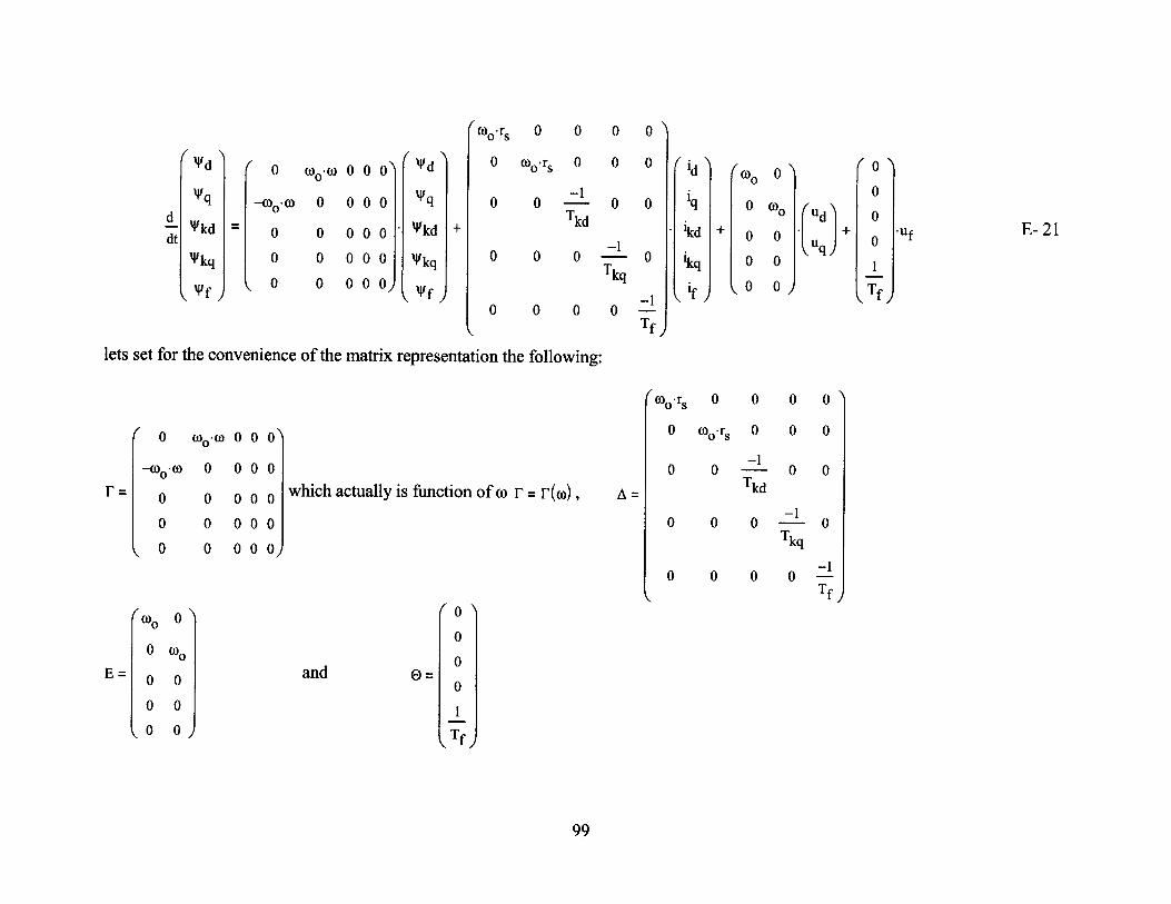
+
rOors 0 0 0
0
0 0 -
Tkd
0 0 0Tkq
Wd
V1 q
Wkd
Vkq
lets set for the convenience of the matrix representation the following:
which actually is function of o r = r(O),
and
0
0
0
0
Tf
I- 0 0 0 0
0 0 0 0
0 0Tkd
0 0
0 0 0 -1Tkq
0
0 0 0 0 -
Tf
99
I-'d ( 0 0- 0) 0 0
0 0 0d
dt
-(- 0)
0
0
0
'kd
'kq
Wf
0
0
0100)
0 0 0 0 --Tf
0
0
0
0 0
0 0
0
0
0
0
0
0
'id
'q
'kd
ikq
Yf
+
O)
0
0
0
0
0
0
0 ~Uq0
0
+
0
0
0
0
1
Tf
Uf
I/
-o
E-21
0 0' CO
0
I/
0 0 0
0 0 0
0
0
0
0
0
0
0
0
0
01010)
V
0
0
0
W 0
0
0
00
0
O0
0
0
0
0 0 0
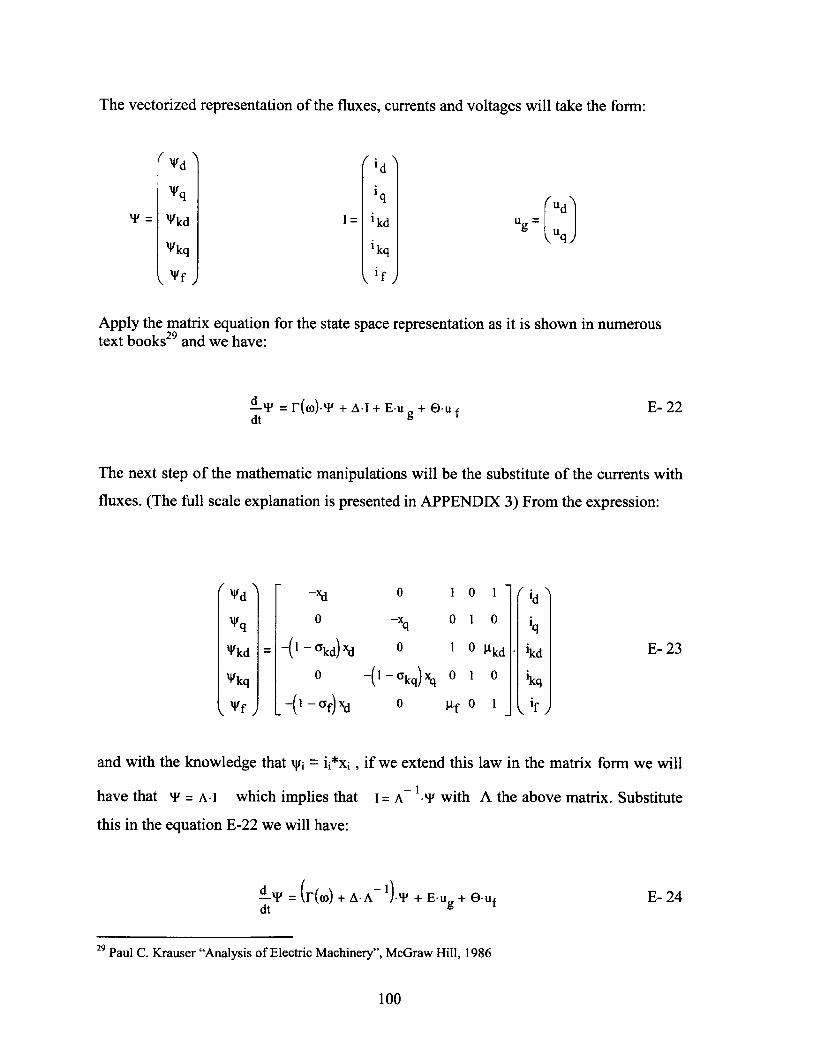
The vectorized representation of the fluxes, currents and voltages will take the form:
T =
'd
Vq
Vkd
'Vkq
If
1= kd
Skq
if
udu9 uq
Apply the matrix equation for the state space representation as it is shown in numeroustext books 29 and we have:
1 = F(O)-P + A.I + E-u + fdtE- 22
The next step of the mathematic manipulations will be the substitute of the currents with
fluxes. (The full scale explanation is presented in APPENDIX 3) From the expression:
-xd
0
( kd) xd
0
-( f) xd
0
-xq
0
-(i -akq) Xq
0
and with the knowledge that % = ii*xi , if we extend this law in the matrix form we will
have that T = A. I which implies that
this in the equation E-22 we will have:
1= A~ I.p with A the above matrix. Substitute
dt = r(o) + A-A 1-. + E-u + e-ufdt
29 Paul C. Krauser "Analysis of Electric Machinery", McGraw Hill, 1986
100
'd
Vq
Vkd
"k
0
1
0
1
0
1
0
9kd
0
1
0
0
1
0
9f
' d
'q
1kd
'kq
Y
E- 23
E- 24
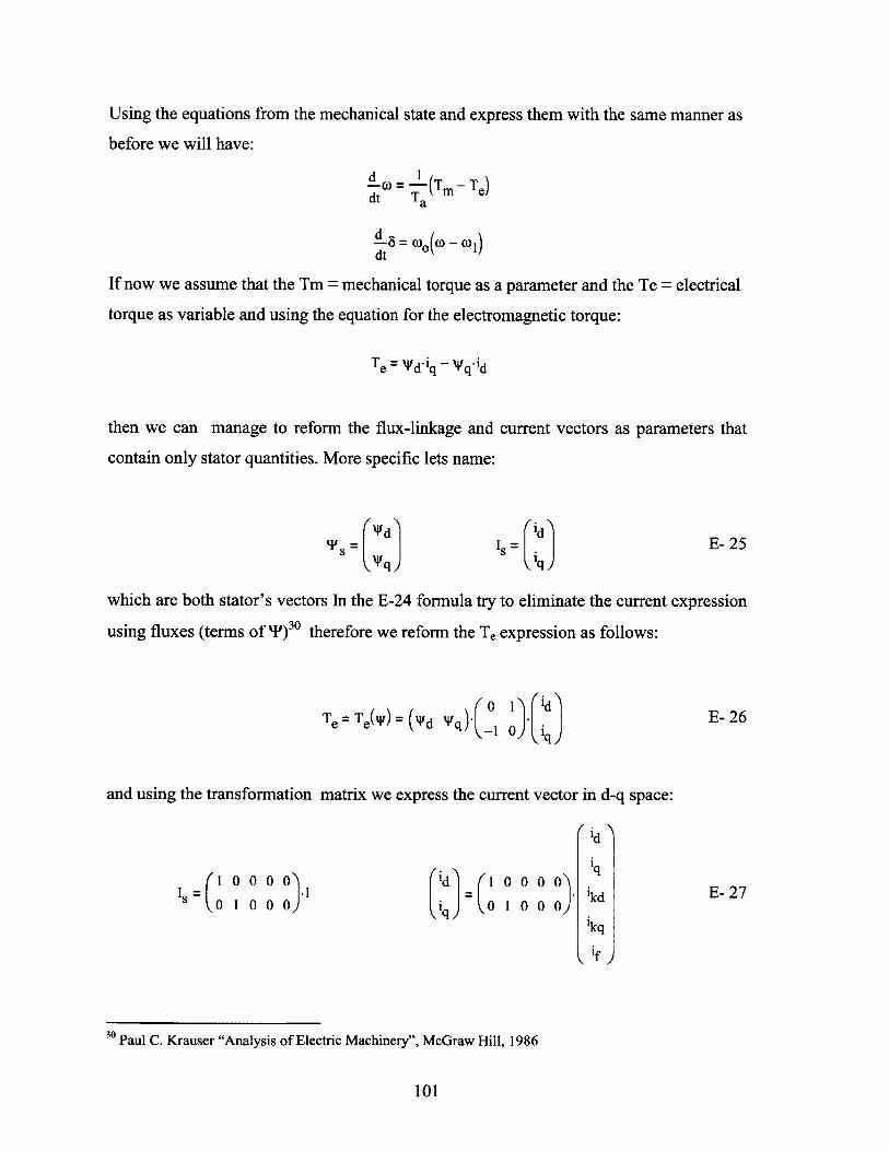
Using the equations from the mechanical state and express them with the same manner as
before we will have:
o= (Tm - Te)dt Ta
dt
If now we assume that the Tm = mechanical torque as a parameter and the Te = electrical
torque as variable and using the equation for the electromagnetic torque:
Te = Vd'iq ~ lqid
then we can manage to reform the flux-linkage and current vectors as parameters that
contain only stator quantities. More specific lets name:
d dVs = Is = E- 25
Nfq iq
which are both stator's vectors In the E-24 formula try to eliminate the current expression
using fluxes (terms of 'P) 30 therefore we reform the Te expression as follows:
T =T 0 1 ).idE-2Te =Te( ) = ( d W).{ _ : E- 26
and using the transformation matrix we express the current vector in d-q space:
id
I =S oo iqd E- 27s 0 1 000 i 0 1 0 0 0q'kq
ikf
30 Paul C. Krauser "Analysis of Electric Machinery", McGraw Hill, 1986
101
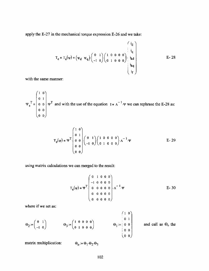
apply the E-27 in the mechanical torque expression E-26 and we take:
Te = Te(XV) = (Vd W 01 1( 1( --1 0 0
0 0 0
1 0 0
00
N
1kd
ikq
if
E- 28
with the same manner:
('1
0
0
0
0
0 -T Tand with the use of the equation I = A- 1. we can rephrase the E-28 as:00)
(1 0"
0 1Te T 0 1 1 0 0 0 0 -A
0 -1 0 0 1 0 0 0
\0 0/
1A E-29
using matrix calculations we can merged to the result:
(0
-1
Te() = T-. 0
0
0
1 0 0 0"
0 0 0 0
0 0 00 .A IF'
0 0 0 0
0 0 0 0)
where if we set as:
0 192=(- 0 1
00
00
0o)
and call as 0 the01
matrix multiplication:
102
E-30
(1 00 1
E),:= 0 0
0 0
o 0)
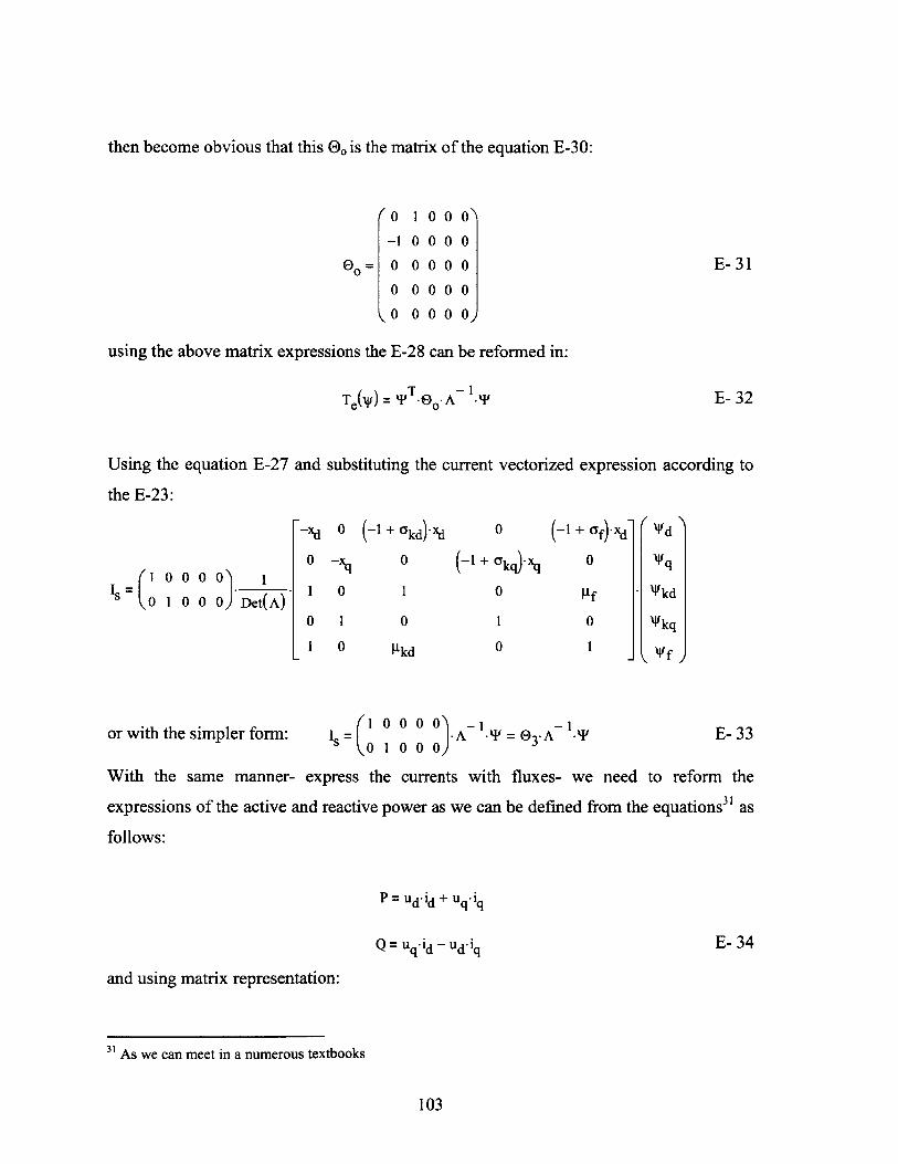
then become obvious that this 0 is the matrix of the equation E-30:
0 1 0 0 0"-1 0 0 0 0
GE= 0 0 0 0 0
0 0 0 0 0
0 0 0 0 0)
using the above matrix expressions the E-28 can be reformed in:
TeM TT -0.*A~ 1.y P
Using the equation E-27
the E-23:
and substituting the current vectorized expression according to
1=1 0 0 0 0 I0 1 0 0 0 Det(A)
-xd
0
1
0
1
0
-Xq
0
1
0
(-i + akd)'xd
0
1
0
pkd
0
(-i + Okq)-Xq
0
1
0
or with the simpler form: is '=1 0 0 0 A- = 03.A~ . E- 330 1 0 0 0
With the same manner- express the currents with fluxes- we need to reform the
expressions of the active and reactive power as we can be defined from the equations3' as
follows:
P= ud'1d + uq-q
Q Uq*-d - Ud\q
and using matrix representation:
31 As we can meet in a numerous textbooks
103
E- 34
E-31
E- 32
(-i + f).xd'
0
p9f
0
1
Vd
Vq
Vkd
Vkq
"If
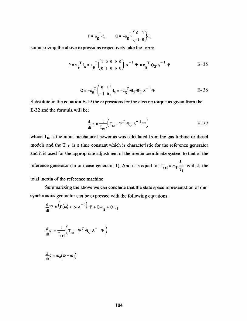
T T( 0 >P = u -Is = -U 1s
summarizing the above expressions respectively take the form:
P = UTis = UT- 1 A -1 = U -. E- 35
Q = -UgT.{ 0 = -ugT.e2 e3.A '. E- 36
Substitute in the equation E- 19 the expressions for the electric torque as given from the
E-32 and the formula will be:
(TO = T T- T. 0 A 1-I E- 37dt Tref
where Tm is the input mechanical power as was calculated from the gas turbine or diesel
models and the Tref is a time constant which is characteristic for the reference generator
and it is used for the appropriate adjustment of the inertia coordinate system to that of the
reference generator (In our case generator 1). And it is equal to: Tref= O1- with J1 theT I
total inertia of the reference machine
Summarizing the above we can conclude that the state space representation of our
synchronous generator can be expressed with the following equations:
d = (()+A-A-A)-T+E-u +O-u0
dt g
I= T T -d(1) =L(TM - I .TOA 1qTdt Tref
dt = ( - (0)dt
104
4.2 Electric Load
The term load can have several meanings in power and system engineering
including: a device connected to a power system that consumes energy, or the total power
(active or reactive) consumed by all devices connected to a power system. Sometimes
position of the system that is not explicitly represented in the system model, but rather is
treated as if it were a single power consuming device connected to a bus in the system
model and often the power output of a generator or generating plant.
There are various types of load models that commonly describe appropriate the
characteristic performance of the one of the above attributes. And we when we say model
we imply a mathematic representation of the relationship between a bus voltage
(magnitude or frequency) and the power (active or reactive) or current flowing into the
bus load. The term load model as become clear according to [2] may refer to equations
themselves or the equations plus specific values for the parameters (coefficients,
exponents) of the equations.
The choice of which model can be used, depends on the fact if this model can
represent with the appropriate way the device or devices that we want to implement
inside our model. In the present model the loads that we want to represent for simplicity
can be limited in two main categories. An aggregate load will be used for each type.
Both the models that will be used are static load models. Such models express the
active and reactive powers at any instant of time as functions of the bus voltage
magnitude and frequency at the same instant.
The secondary loads like small motors distribution and hotel loads that very often
described as "no preference loads" can be easily represented with a constant impendence
load [3]. The constant impedance load is a static load model where the power varies
directly with the square of the voltage magnitude. It may also be called a constant
admittance load model and its impedance is independent of the voltage and is constant for
constant power demand. This impedance has a value of:
zci= ~ . E- 38Pci + N-Ci)
105
A very good representation for the main propulsion motors can be achieved with
the use of constant power load model. This is a static load model where the power does
not vary with the changes in the voltage magnitude. It may also be called constant MVA
load model. Because constant MVA devices, such as the motors and electronic devices,
do not maintain this characteristic below some voltage (typically 80-90%), many load
models provide for changing constant MVA (and other static models) to constant
impedance.
= [ udi + juqjj 2 E-39L CP + i*QCP
where: udi: d-axis terminal voltage of the ith generator.
Uqi: q-axis terminal voltage of the ith generator.
PCP: Active power demand, const. power.
QcP: Reactive power demand, const. power.
Pci: Active power demand, const. impedance.
Qcj: Reactive power demand, const. impedance
The voltage that each generator is producing is related with the load and its
characteristics. The purpose of this approach is to express the vector ug as a function of
the current. To achieve this, an equivalent load should be assigned. Based on the way that
the electric distribution is designed in a electric ship and under the legacy that numerous
papers refer as modeling based on equivalent load methods, we will assume that this
equivalent load is a parallel connection of two impedances. Therefore:
Zeq = (req + ixeq) = zp-zi E- 40ZCP + Zci
All the currents from each generator are expressed in the d-q frame of the same generator.
But we need to express everything with respect to a common frame. This frame will be
the frame of the reference generator which as we specified from the beginning is the
Generator-1. So if we assume the ith generator then the total current that this generator
produces is:
106
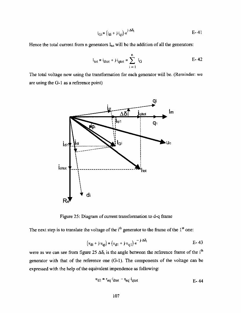
iGi: (di + jiq)je i E- 41
Hence the total current from n generators Itot will be the addition of all the generators:
n
Itot = tdtot + jiqtot = G E- 42
The total voltage now using the transformation for each generator will be. (Reminder: we
are using the G- 1 as a reference point)
qj
Ai Iqltot
- qq1
Id1 di _ _ _ _ Gi UC
iditot --------------------------- Itot
diRe
Figure 25: Diagram of current transformation to d-q frame
The next step is to translate the voltage of the ith generator to the frame of the 1" one:
(udi + J-uqi) = (udl + j-uql).-~ j-A E- 43
were as we can see from figure 25 A6j is the angle between the reference frame of the ith
generator with that of the reference one (G-1). The components of the voltage can be
expressed with the help of the equivalent impendence as following:
udl = req.idtot - xeqlqtot E- 44
107
uqi - req.iqtot + xeq-dtot
To maintain the matrix expression we will define the itt which referred to the dq axis of
the reference generator as:
idtottot I
i qtot j
The transformation from the n frames of the same number generators to that of the
reference one will take place with the use of the 2D transformation matrix E-46 since the
coordinate systems are orthogonal (Re - Im plane)32.
( cos ($) -sin($)ET($) =1E 4
sin ($) Cos ($)
nUsing again the expression for the total current itot = G and analyze that to the Re-
Im reference system: itot = idtot + j-iqtot and using the vectorized form:
dtot E di + j-ii)-e T(ABi)- d E- 47S ZqtOt ( qe
And more analytically:
idtot = id1 + cos (A82) -sin(A&2) id2 (cos(Aln) -sin(An dn
iqtot ) (ql sin(A82) Cos (A2) )Yiq2) sin(A~n) COS (A~n) q in
The transformation matrix can be written as:
32 Not: oc os (AS ) -sin (A8)
sin(Asi) cos(ASi)
32 Note: our transformation system is clockwise according to the figure
108
E- 45
using matrix algebra:
T(A~i) I =
(cos(A ))2+ (sin(Ai))2]
which is equals to:
and the current expression is:
E- 48cos(ASi) sin(A8,)
-sin(Ai) COS(S)
htot = i i+ T(A82) - 2+ -- + T(,&8,) -in
If we apply the above concept to all the generators from 1 to n we will have:
* for i= I
(udl + jiuqi) = (udG1 + j-uqGl)-e jA
But we do know that ud I= req-dtot - Xeq'qtot
= Udl + j-uqI
and uqi = req-iqtot + xeqldtot
Ugi = Zitot
* for i = 2 with the same aspect:
(ud2 + j-Uq2) = (UdGI + j-UqGl).e jA 2
where in matrix form will be
fud2) ( cos(A&2)
Uq2 j -sin(A&2)
sin(A82) r udl
cos(A&2 ))* uqi)
and the final formulation:
ug2 = (TT)(A 2)-ugi =
* for i= n and with the same manner we will have:
Ugn = (TT)(A8n)-z-itot
109
hence:
E- 49
E- 50
E- 51
cos(A~i) sin(ASi) cos(A&i) sin(ASi)
-sin (A~i) Cos (Asi) -_sin(ai) cos(ai))
(T) (,&82) -- itot
Summarizing the voltage for each generator expressed in the reference generator
coordinate system, which actually is the expression of the busbar we have:
Ugi = ZQot I Ug2 = (TT)(A2).z-tot ... Ugn = (T(ASn)-z-qot
4.3 Propeller
One of the big advantages, of the electric propulsion system, is the ability to use a
fixed pitch propeller. This gives as the ability to alleviate the need of all the hydraulic and
hydro-mechanical apparatus which are imperative for the operation and control of a
controllable pitch propeller system.
For a fixed propeller the propeller thrust Q and torque T are formulated accordingto:
T = p .D4 .KTnp. InpI E- 52
Q= pD .D5.KQ.np. InpI E- 53
The expression for the power of the above propeller will be:
Pp = -p D5.KQ.np .In pI
which can be reformed as follows:
P2 = np-Qp E- 54
with TP : Propeller thrust in [N]
Q, : Propeller torque in [Nm]
np: Shaft RPMs
KT : Thrust coefficient
Kg: Torque coefficient
and from the propeller theory we know that the non-dimensional thrust and torque
coefficients are given as:
110
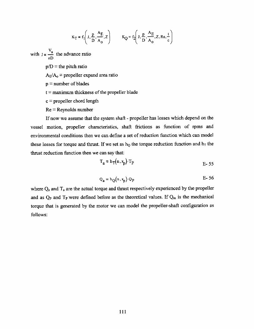
pAE'Z pQ AE tKT = J, 2 , K2 J, , ,Z,Re,-
(D'AO D AO C)
with j = - the advance rationD
p/D = the pitch ratio
AE/A. = propeller expand area ratio
p number of blades
t = maximum thickness of the propeller blade
c propeller chord length
Re = Reynolds number
If now we assume that the system shaft - propeller has losses which depend on the
vessel motion, propeller characteristics, shaft frictions as function of rpms and
environmental conditions then we can define a set of reduction function which can model
these losses for torque and thrust. If we set as hQ the torque reduction function and hT the
thrust reduction function then we can say that:
Ta = hT(n,xp).Tp E- 55
Qa = hQ(n,xp)-Qp E- 56
where Qa and Ta are the actual torque and thrust respectively experienced by the propeller
and as Qp and Tp were defined before as the theoretical values. If Qm is the mechanical
torque that is generated by the motor we can model the propeller-shaft configuration as
follows:
III
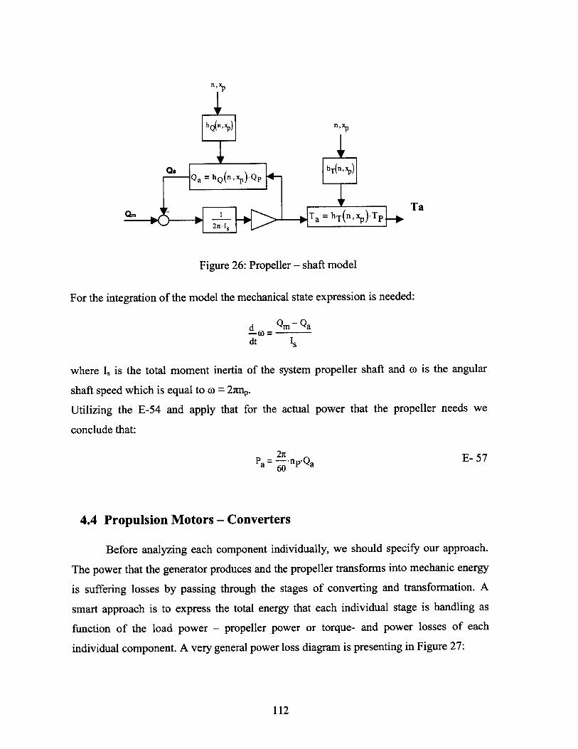
n,xp
h Q(n,xP) nxP
Oa Qa =Q(n,xp)-Qp hT(n, xP)
Ta = hT(fx)Tp Ta
Figure 26: Propeller - shaft model
For the integration of the model the mechanical state expression is needed:
d Qm~-Qa
dt Is
where I is the total moment inertia of the system propeller shaft and o is the angular
shaft speed which is equal to o = 2np.
Utilizing the E-54 and apply that for the actual power that the propeller needs we
conclude that:
Pa = 2n*np-Q. E- 5760
4.4 Propulsion Motors - Converters
Before analyzing each component individually, we should specify our approach.
The power that the generator produces and the propeller transforms into mechanic energy
is suffering losses by passing through the stages of converting and transformation. A
smart approach is to express the total energy that each individual stage is handling as
function of the load power - propeller power or torque- and power losses of each
individual component. A very general power loss diagram is presenting in Figure 27:
112
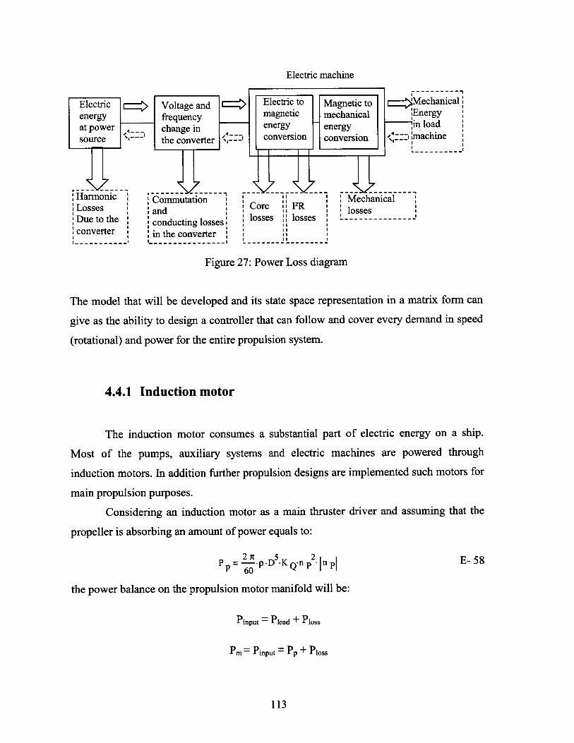
Electric machine
Electric c=> Voltage and E=:energy frequencyat power _0 _._ change in .0
source -- ' the converter
Harmonic j ~CommutationLosses andDue to the conducting losses'converter | in the converter
Figure 27
Core PRlosses losses
Power Loss diagra
gnetic to =:Mechanical|hanical Energy
rgy !in loadversion machine
Mechanicallosses---------------
The model that will be developed and its state space representation in a matrix form can
give as the ability to design a controller that can follow and cover every demand in speed
(rotational) and power for the entire propulsion system.
4.4.1 Induction motor
The induction motor consumes a substantial part of electric energy on a ship.
Most of the pumps, auxiliary systems and electric machines are powered through
induction motors. In addition further propulsion designs are implemented such motors for
main propulsion purposes.
Considering an induction motor as a main thruster driver and assuming that the
propeller is absorbing an amount of power equals to:
P P = 2-.p -D 5.K -n p_ -In pI E- 58
the power balance on the propulsion motor manifold will be:
Pinput = Pload + Ploss
Pm = Pinput P~ Pp + Ploss
113
Electric to Mamagnetic mecenergy eneconversion con
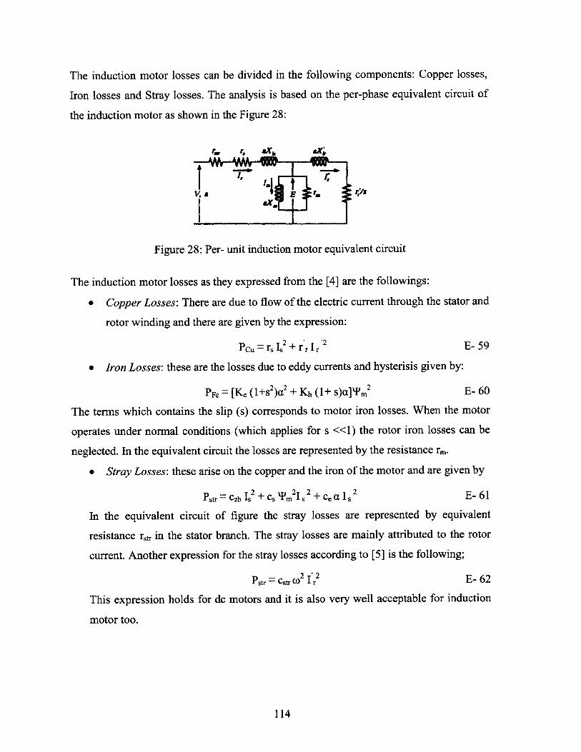
The induction motor losses can be divided in the following components: Copper losses,
Iron losses and Stray losses. The analysis is based on the per-phase equivalent circuit of
the induction motor as shown in the Figure 28:
r., ', 841 4
Figure 28: Per- unit induction motor equivalent circuit
The induction motor losses as they expressed from the [4] are the followings:
* Copper Losses: There are due to flow of the electric current through the stator and
rotor winding and there are given by the expression:
Pcu = rs Is2 + r'r Ir '2 E- 59
" Iron Losses: these are the losses due to eddy currents and hysterisis given by:
PFe = [K, (1+s 2 )a2 +h s(1+ m)a]m2 E- 60
The terms which contains the slip (s) corresponds to motor iron losses. When the motor
operates under normal conditions (which applies for s <<1) the rotor iron losses can be
neglected. In the equivalent circuit the losses are represented by the resistance rm.
e Stray Losses: these arise on the copper and the iron of the motor and are given by
Pstr z C s2 + cs Tm 2 + Ce a I,2 E- 61
In the equivalent circuit of figure the stray losses are represented by equivalent
resistance rstr in the stator branch. The stray losses are mainly attributed to the rotor
current. Another expression for the stray losses according to [5] is the following;
Pstr = Cstr 0)2 f r2 E- 62
This expression holds for dc motors and it is also very well acceptable for induction
motor too.
114
Since the rotor iron losses are not a significant portion of the total losses under
normal operating condition for the purpose of this thesis we will neglect them. Then
sequentially the total losses included the friction losses are given by:
Ploss= rs Is2 + r r Ir '2 + (Ke 2 +Kh 0)rm2 + Cstr 2 'r2 + cfw C2 E- 63
From Faraday's law we know that:
eag= ns dT" dt
with the air gap flux linking the stator phase winding to be 'm(t) = Tnm sin (wt) and the
above equation results in:
eag = nsa),m cos(ar)
which has an rms value of
Eag = k3f Tm
Eliminating the stator current we obtain:
1 2 22+K )+r m 2+CPloss (cL rs + r r + Cstr )) I r 2 (Ke 2+Kho rsm2 2 + w 2 E- 64
If now we apply the loss minimization conditions with respect to air gap flux (since we
are interesting in the better motor and propulsion system efficiency), at steady state,
which is given by:
d Ploss = c E- 65d'Pm
From the equation that gives the per unit frequency- according the equivalent circuit of
the induction motor Figure 28:
115
a (0 E-661- s
the magnetizing and rotor currents are given respectively by:
E
a TmI = = mm Xm Xm
and
'=m E- 672
+ Xlr2
s 4
from the E-67 we obtain the air gap flux:
T m 2 1r 2 rr2 + Xir2s 2a 2) E-68
2 2a
The electromagnetic torque is given by:
Te = Ir2 rr E- 69s -a
Combining E-67 and E-69 we obtain:
rr
Te= sa -- 2 E- 70
rr )2+Xr2-- + Xi~7s -a_
Usually the induction motor operates with a small slip and the condition r r >> a X I
holds. In this case the equations E-68 and E-70 become respectively:
r Ir
S - a
116
Te - PmrrE- 71= W m Ir
Also according the analysis presented by [10]
is2 2 + CL'Ir2
XirCL= 1+ 2---
Xm
Since the electromagnetic torque is constant (a Te / a 'm = 0) from the E-71 we obtain
that:
d
dym m
And the loss minimization condition is determined:
( cL rs+ r r + Cstr 2) I r 2 (K 2 +Kh O +rsXm 2)TM 2 E- 72
We know that the I r is proportional to the load [5]:
Ir= ci Qp E- 73
Therefore I m and Tm are proportional to motor load which is equal with the load of the
propeller. This sequentially is translated to the propeller torque Qp. Therefore the above
expression depends only on the load torque which is the propeller torque Q, and the
corresponding angular velocity o = 27mp. Therefore
2 2)Q2+C2(
Pioss=c2 (cLrs+rr+CstrO)Qp 2 +c1 2 (eo2 + Kh CO +rs/Xm 2) Qp 2 + Cf ) 2 E- 74
And sequentially:
Pm = Pp + Pioss
Pm= Pp+c 2 ( cL rs+ rr + cstr 2)Qp 2 + C1 2 Ke 2 +Kh +rs/Xm 2) Qp 2 + Cfw 2
117
The terms in parenthesis contain constants which are characteristics of each individual
electric machine. The same will be the conclusion with the analysis as it is introduced in
[9] where the approach implements the total power which is flowing in the motor.
4.4.2 Permanent magnet synchronous motors
The development and availability of very high energy permanent magnet materials
has contributed to an increased use of the permanent magnet synchronous motor (PMSM)
in high performance Naval and underwater applications. The PMSM offers advantages
such as increased efficiency, superior torque to volume and power to volume ratios, and
quiet operation. These advantages have resulted in the Navy considering a switch from its
present induction motor technology to the PMSM.
Another characteristic example is the compact Azipods from ABB. Compact
Azipods contain an electric motor and propeller in a pod-type structure suspended from
the vessel's hull. An entire unit rotates a full 3600, which makes a ship considerably more
agile than one equipped with traditional propellers. No separate steering propellers,
rudder, or propeller shaft are required. The motor providing the power is located
immediately behind the propeller. Compact Azipods are rated at 0.5 - 10 MW output, and
sufficient torque is provided even though the propeller usually only runs at 10 - 300 rpm.
The permanent magnet motor is a synchronous motor, which, as there is no rotor
slip, provides better accuracy than standard, asynchronous motors. In an asynchronous
motor, the slip varies according to speed and load. With a synchronous motor, it is
simpler to optimize the speed, while the elimination of slip compensation improves the
dynamic motor control. The construction of the traditional synchronous motor is more
complicated than that of the asynchronous motor, so it requires more maintenance.
However, the permanent magnets simplify its construction by creating a constant flux in
the air gap, thereby eliminating the need for the rotor windings and the brushes normally
used for excitation in synchronous motors. This has resulted in a motor that combines the
118
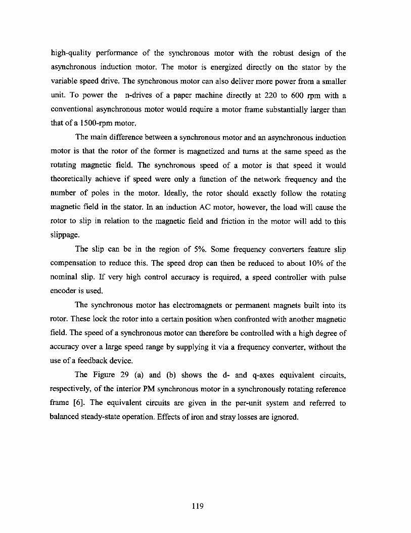
high-quality performance of the synchronous motor with the robust design of the
asynchronous induction motor. The motor is energized directly on the stator by the
variable speed drive. The synchronous motor can also deliver more power from a smaller
unit. To power the n-drives of a paper machine directly at 220 to 600 rpm with a
conventional asynchronous motor would require a motor frame substantially larger than
that of a 1500-rpm motor.
The main difference between a synchronous motor and an asynchronous induction
motor is that the rotor of the former is magnetized and turns at the same speed as the
rotating magnetic field. The synchronous speed of a motor is that speed it would
theoretically achieve if speed were only a function of the network frequency and the
number of poles in the motor. Ideally, the rotor should exactly follow the rotating
magnetic field in the stator. In an induction AC motor, however, the load will cause the
rotor to slip in relation to the magnetic field and friction in the motor will add to this
slippage.
The slip can be in the region of 5%. Some frequency converters feature slip
compensation to reduce this. The speed drop can then be reduced to about 10% of the
nominal slip. If very high control accuracy is required, a speed controller with pulse
encoder is used.
The synchronous motor has electromagnets or permanent magnets built into its
rotor. These lock the rotor into a certain position when confronted with another magnetic
field. The speed of a synchronous motor can therefore be controlled with a high degree of
accuracy over a large speed range by supplying it via a frequency converter, without the
use of a feedback device.
The Figure 29 (a) and (b) shows the d- and q-axes equivalent circuits,
respectively, of the interior PM synchronous motor in a synchronously rotating reference
frame [6]. The equivalent circuits are given in the per-unit system and referred to
balanced steady-state operation. Effects of iron and stray losses are ignored.
119
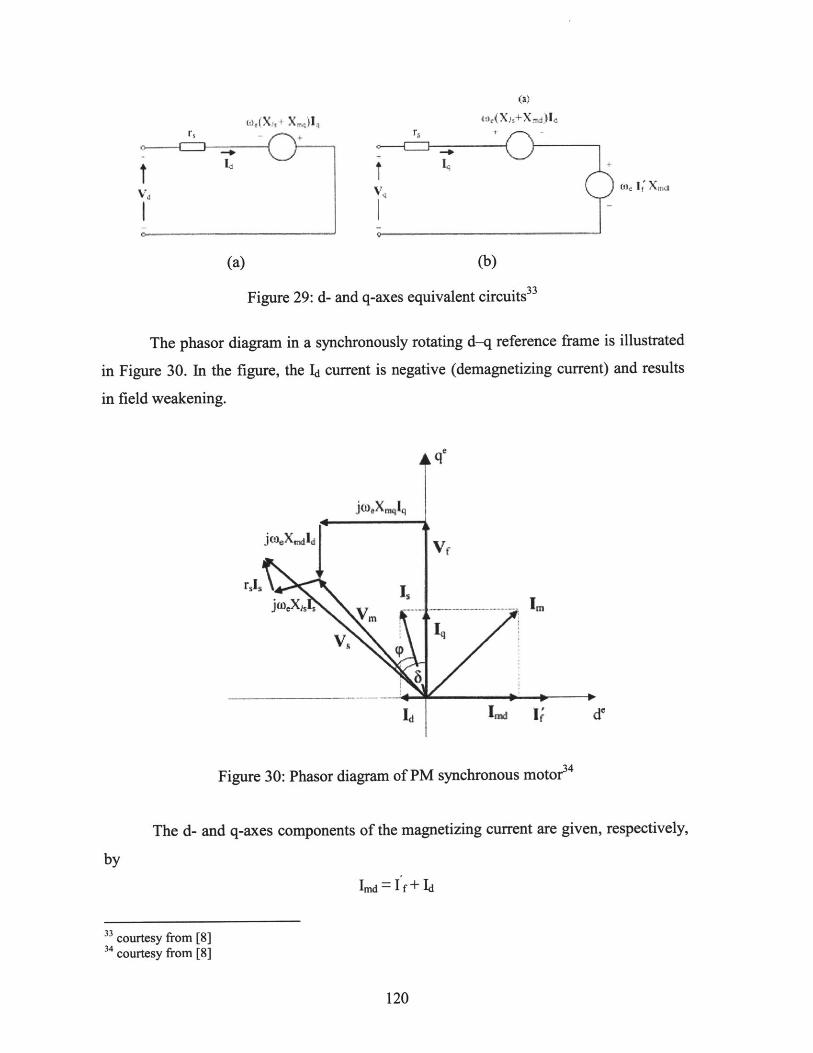
r Id
(a)
r(-
(b)
Figure 29: d- and q-axes equivalent circuits3 3
The phasor diagram in a synchronously rotating d-q reference frame is illustrated
in Figure 30. In the figure, the 1L current is negative (demagnetizing current) and results
in field weakening.
j(OXmqlq 1
Vjm.Xa(P
idf
q*
Vf
In)~j If C
Figure 30: Phasor diagram of PM synchronous motor3 4
The d- and q-axes components of the magnetizing current are given, respectively,
by
Imd = I f+ I
120
3 courtesy from [8]3 courtesy from [8]
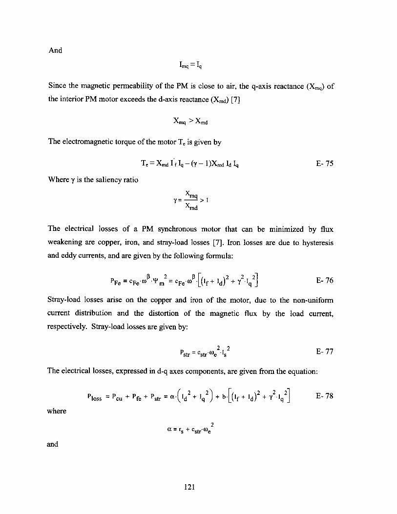
And
Imq = Iq
Since the magnetic permeability of the PM is close to air, the q-axis reactance (Xmq) Of
the interior PM motor exceeds the d-axis reactance (Xmd) [7]
Xmq > Xmd
The electromagnetic torque of the motor Te is given by
Te = Xmd I fIq (Y )Xm L Iq E- 75
Where y is the saliency ratio
Y= Xmq >Xmd
The electrical losses of a PM synchronous motor that can be minimized by flux
weakening are copper, iron, and stray-load losses [7]. Iron losses are due to hysteresis
and eddy currents, and are given by the following formula:
PFe = CFe . M2 = cFe*o*[(If + Id)2 + y2q 2] E- 76
Stray-load losses arise on the copper and iron of the motor, due to the non-uniform
current distribution and the distortion of the magnetic flux by the load current,
respectively. Stray-load losses are given by:
Pstr = Cstr*o)e2is E- 77
The electrical losses, expressed in d-q axes components, are given from the equation:
Ploss = Pcu + Pfe + Pstr = a -(d2 + Iq2 + b [(If + Id) 2 Y2Iq2] E- 78
where
2a = rs + Cstr'e
and
121
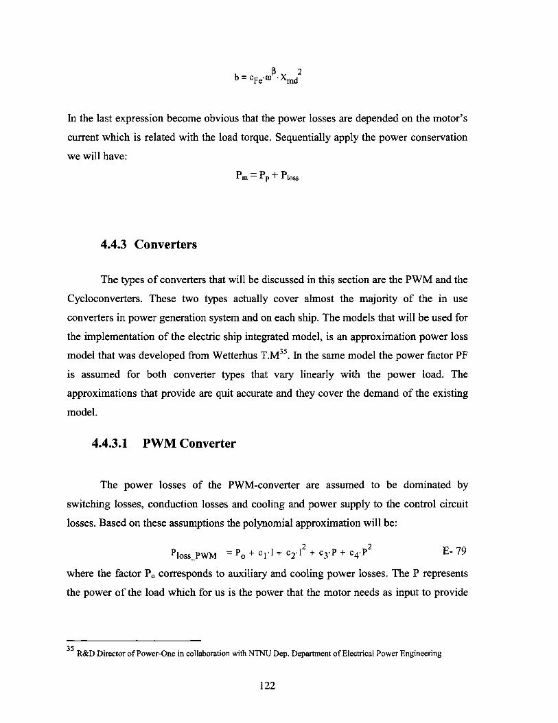
f~ 2b = cFeP Xmd
In the last expression become obvious that the power losses are depended on the motor's
current which is related with the load torque. Sequentially apply the power conservation
we will have:
Pm= PP + Pioss
4.4.3 Converters
The types of converters that will be discussed in this section are the PWM and the
Cycloconverters. These two types actually cover almost the majority of the in use
converters in power generation system and on each ship. The models that will be used for
the implementation of the electric ship integrated model, is an approximation power loss
model that was developed from Wetterhus T.M3 5 . In the same model the power factor PF
is assumed for both converter types that vary linearly with the power load. The
approximations that provide are quit accurate and they cover the demand of the existing
model.
4.4.3.1 PWM Converter
The power losses of the PWM-converter are assumed to be dominated by
switching losses, conduction losses and cooling and power supply to the control circuit
losses. Based on these assumptions the polynomial approximation will be:
PlossPWM = Po + c I + c 2 -I2 + c3-P + c 4 .P 2 E- 79
where the factor Po corresponds to auxiliary and cooling power losses. The P represents
the power of the load which for us is the power that the motor needs as input to provide
35 R&D Director of Power-One in collaboration with NTNU Dep. Department of Electrical Power Engineering
122
the appropriate power for the propeller, and I is the current that actually the converter
provide to the motor. Therefore we can rewrite the above expression as:
Ploss_PWM ~ PO + CI+ 2 C3Pm + C4-Pm2 E- 80
Switching losses are included in ci, inverter conducting losses are included in ci and c2
and rectifier conducting losses are included in c3 and c4.Apply the power conservation
and we will have:
i =m + Ploss_PWM E- 81
The first factor there is the total power that the i-generators provide to the system. Here
we assume that the losses on the system such as bus losses can be neglected.
4.4.3.2 Cycloconverter
For the cycloconverters the power losses can be modeled as:
P=OSS-CYCO PO + ci + C2-12 E- 82
where I is the motor current, and PO is a term representing possible reverse recovery
losses, cooling losses etc. and ci and c2 are constants representing conduction losses. The
cycloconverter is usually combined with a synchronous motor in the thruster drives.
Apply the energy conservation under the same considerations like above and we will
have:
i M+ Ploss-cycIo E- 83
123
4.5 State space model
For the integration of the model we need to implement a simple equation than can
connect the prime movers model with that of the power production and the load. A
simple expression for transient response of such a system will be:
d 1Tml = -(-TmI + fl(my)
dt TI
where T, is the dynamic time constant which is characteristic for each individual prime
mover as we mention before. The fi(mf) is a dimensionless function of the fuel mass flow
which in the existing prime mover model is the one of the factors that control the output
power Tm. The values of this function are expressed per unit.
Therefore in case of the n-prime movers that turn n generators the above
expression becomes:
4 Tml=I (~Tmi + f1 (mf))dt T
T = - (-Tm2 + f2(ghdt T2
Tm3 = (-Tm3+ f3(m(T)dt T3
d 1-Tm .(-Tmn + f3 (mf)) E- 84dt Tn
Using the expression as were developed in the generator section and generalized for n
generator sets can be expressed as:
d ~ (( .) + A 1.A ,- 1 - I + E-ugi + -u ni
d 2 (r-2)+ A-.-A2- 2+ E-ug2 + -u2dt ~ 2 j 2 f
124
d T3 = (v( 3) + A 3 A 3 3 + E-Ug3 + O-uf3
d Tn = (r'(on) + An.An n + E-ugn + O.ufn
Generalized the mechanical state equations for rotational speed and relative power angle
we will have:
d WI (dt Tal
dt Ta2
TTmi '{iF* 2 O3
d I T - 1-W3 = --- (Tm 3 - 3 .023 A 3 3dt Ta3
On = Tfi(Tmn - Tn . 2 0 3 .An n)an
dA82 = (ON(C03 - CO )
dt
d
dtA = ON(Wn - WI)
dt
from the previous sections we saw that
Ugi = -Ot
125
E- 85
-1
E- 86
E- 87
Tm2- Y2 T. 2'03- A2 1 2)
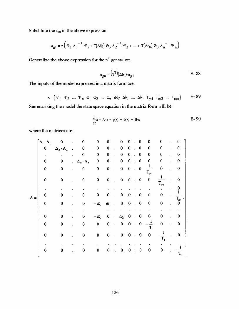
Substitute the itot in the above expression:
Ugi = Z.( 3. A 1 1. i + T(A&2)-03- A2 2 + .... + T(AQn)-E 3.An- ln1
Generalize the above expression for the nth generator:
U gn = (TT)(An)-ugi E- 88
The inputs of the model expressed in a matrix form are:
x= (T 1 ' 2 ---- n c1 *2 ---. cn A62 A83 -... A8 n TmI Tm2 .... Tmn) E- 89
Summarizing the model the state space equation in the matrix form will be:
-x = Ax+ y(x) + 8(x) + Bu E- 90dt
where the matrices are:
Al-A1 0 . 0 0 0. 0 0 .0 0 0 .00 A 2 -A 2 - 0 0 0. 0 0 .0 0 0 . 0
. . . 0 0 0. 0 0. 0 0 0 . 0
0 0 . A-An 0 0. 0 0 .0 0 0 . 0
S0 0 . 0 0 0 0 0 . 0Tai
0 0 . 0 0 0.0 0.0 0 0
Ta2. . . 0
10 0 . 0 0 0. 0 0. 0 0 0 .
A= T, -0 0 . 0 -O 0 . 0 0 .0 0 0 . 0
0 0 . 0 -, 0 . 0 0 0 0 . 0
0 0 . 0 0 0. 0 0. 0 0 --. 0T2
10 0 . 0 0 0. 0 0. 0 0 0
Tn
126
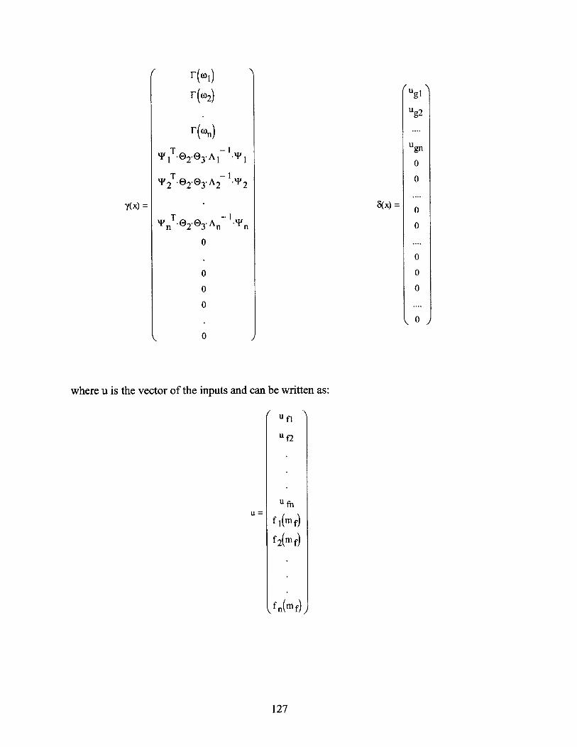
(
F(02)
1con)
T -1P1 T. 2.e 3 .A '-P 1
T -T'P2 .02.e 3 -A2 'P2
Tn* 9 23-An
0
- IJ
0
0
0
0
where u is the vector of the inputs and can be written as:
(
Y(x) =
n
Ugi
Ug2
Ugn
0
0
0
0
0
0
0
y 0 J
/U fi
U f2
u fn
f 1 ( mf)
f 2 (mf)
f n(m f) I
127

Chapter 5
5. Life Cycle Cost Estimation and Reliability Analysis
5.1 Functional and Reliability Analysis
The main consideration in this point is whether the decision of driving an entire
aspect of the ship design in the electric integration field is profitable in any sense and not
only an innovation technology that is not ready to be applied. To distinguish and issue the
measures that we will use to validate such a project we should first indicate the targets
that are expected to be accomplished and the solutions that may be able to be applied in
various problems and restrictions that the compatible form of propulsion and energy
distribution cannot achieve. The first will be the fuel efficiency that can be achieved with
the use of the electric propulsion compared to that of the conversional Diesel or Gas
turbine. The second point will be the area and volume issue that stands as the biggest
milestone for the designs of the Naval and commercial ships and is actually this that most
of the time drives the design concept. In the next step a reliability analysis for both of the
propulsion categories will be performed. A schematic representation of the two
propulsion systems is presented below (Figure 31).
128
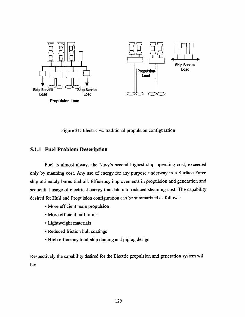
Ship ServicePropulsion Load
Load
(= (=Ship Service hip Service
Load Load
Propulsion Load
Figure 31: Electric vs. traditional propulsion configuration
5.1.1 Fuel Problem Description
Fuel is almost always the Navy's second highest ship operating cost, exceeded
only by manning cost. Any use of energy for any purpose underway in a Surface Force
ship ultimately bums fuel oil. Efficiency improvements in propulsion and generation and
sequential usage of electrical energy translate into reduced steaming cost. The capability
desired for Hull and Propulsion configuration can be summarized as follows:
" More efficient main propulsion
" More efficient hull forms
" Lightweight materials
" Reduced friction hull coatings
" High efficiency total-ship ducting and piping design
Respectively the capability desired for the Electric propulsion and generation system will
be:
129
* High efficiency electrical generation regardless of load. Will probably require
more numerous, smaller generators brought on and off line automatically in
response to demand to keep generators operating in high efficiency load range.
" High efficiency, pumps, motors
" High reliability electrical distribution components
" Automatic-start on-demand and casualty recovery replacing always-on standby
machinery wherever possible (e.g. fire pumps, backup generators)
From the above we can see that all the factors that actually affect the fuel consumption in
a ship are present in both the propulsion configurations. The factor that can make the
difference between the two competitors is the appropriate analysis of speed and the
electric energy demands.
The decision about a ship's propulsion system is directly related to the speed that
is designed to achieve. Referring to speed we include all the characteristic values that this
parameter can take such as sustained speed ,maximum continuous speed, cruising speed
or even sprint or as usually met as maximum speed. Even the variable of speed is multi-
attribute for the function of the propulsion system choice; the last will be optimized for
one and only speed with the ability to achieve the demand of a maximum value. It is very
common for the Naval ship design that these two values maximum speed and optimum
speed coincide. Therefore, the ship and as sequence the propulsion system has its best
performance for a given speed or speed sector.
But in general the ships are not performing in one and only speed. The type of
their mission, the sea conditions even the geographical position of their route can
alternate the speed values. The more the ship is performing away from its optimum
speed, the worst the consumption becomes. To understand how spread this "speed field"
can be, a trade off speed study will be presented.
130
5.2 Value of Speed Study
The decision process for the selection of the propulsion system started with an
"operational value of speed" study to determine the benefit of speed as it relates to
mission effectiveness. For the Naval ships the study is more complex compared with the
commercial ones since the dispersion of the speeds is very big due to the demands of the
multi-phase missions. For the commercial fleets it is easy to make the decision for the
propulsion system since the sector of the speed versus mission is very limited. The results
of this study are presented below with specific details provided in APPENDIX 4
The method used to assess the operational value of speed was as follows:
1. For each mission area, the desirable speed ranges were determined based on
assumptions and information contained in sources such as Jane's Fighting Ships.
Assumptions for each mission area and Appendices are attached where
appropriate.
2. For each mission area, it was assumed that each increment in speed adds linearly
to the value for that mission.
3. Each mission area was weighted equally against the other mission areas.
4. The contribution from each mission was added together at each speed increment
to quantify the value of speed between a value of 0 and 1 for the speed ranges
included in the analysis.
131
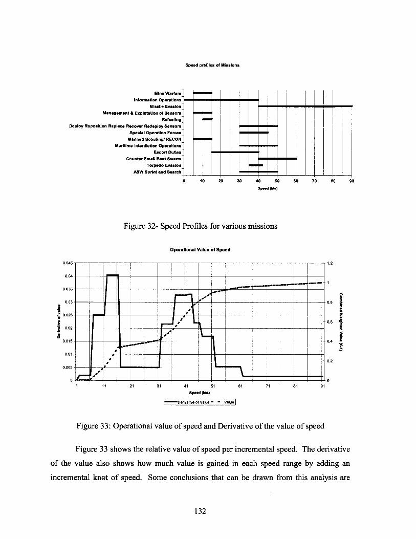
Speed profiles of Missions
Mine Warfareinformation Operations
Missile EvasionManagement & Explotation of Sensors
Refueling_Deploy Reposition Replace Recover Redeploy Sensors
Special Operation ForcesManned Scouting) RECON
Maritime Interdiction OperationsEscort Duties-
Counter Small Boat SwarmTorpedo Evasion
ASW Sprint and Search
0 10 20 30 40 50
speed (kta)
Figure 32- Speed Profiles for various missions
Operational Value of Speed
0.045-
0.04
0.035
0.03-
0.025
0.02
0.015 -
0.01 -
0.005
0-
__ __- I I~ L ~NON__ _ _ I 2 1 __ _ __ _ __ __ _ __sop_
__ _ 1 _ _ __ __2 _ __ __ _ __ __ IN_
INI. ___
___I __ ___ g __ __polo_
___ _ __ __ I__ _ __ _ I _ _ _go
___ __ ___ _ _ 2 __ ___ __
__________ _______________ _____________.___ 4____011001_________
0 0__ __ _ _ _ _ _ _ _ _ _ _ _ _ _ _ _ _ _ _ _ _ _ _ _ _ _ _ _ _ _ _ _ _ _ _ _ _ _ _ _ _ _ _ _ _ .11 21 31 41 51 61 71 81
Speed (kts)
IDerivative of Value - - Value
91
Figure 33: Operational value of speed and Derivative of the value of speed
Figure 33 shows the relative value of speed per incremental speed. The derivative
of the value also shows how much value is gained in each speed range by adding an
incremental knot of speed. Some conclusions that can be drawn from this analysis are
132
60 70 80 90
1.2
1
0.8 cr5.
-0.6
OA0.4 a
0.2
0
7-77 1 1 1 .
====...
mm.p.msim.
1I

that a ship with the capability to exceed 60 knots is excessive, while a ship that achieves
45 knots utilizes most of the attainable "value of speed". More generally there is the
option to eliminate some areas. But even this kind of elimination cannot improve
substantially the efficiency of the design since the speeds values remained wide spread.
The utility in the above method is that the assumptions can be corrected for
specific threats or intelligence available. It can also be updated as the world threats and
missions change. One drawback of this method is that it assumes that each knot of speed
in a particular mission area varies linearly. For example, mission areas conducting MIO
or SAR may vary quadratically with speed for searching circular areas in the open ocean.
Another simplification of this method is that each mission area is weighted equally.
However, this could be refined further with the right set of intelligence as mentioned
previously. But with enough mission areas included, no one mission has an undue
influence over the overall results.
Similar are the results of the same study for a commercial ship as shown in Figure
34. The differences that appeared based on the mission characteristics are not so
demanded. Specifically for the needs of this study we assume that the ship has three main
areas of speed interest: seaport approach and maneuvering, cruising speed which includes
also the maximum speed and casualty or damage situation. Secondary areas will also be
taken into account.
133
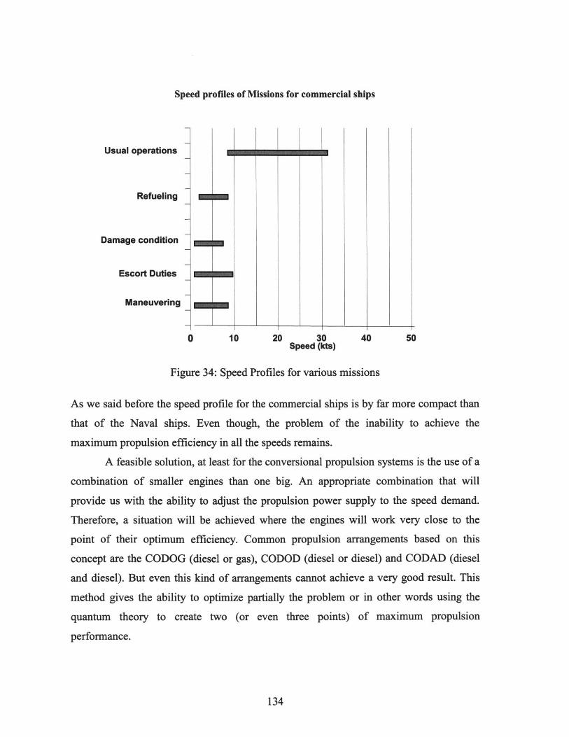
Speed profiles of Missions for commercial ships
perations
Refueling
condition
ort Duties
neuvering
0
El-I-I-I-'.
10 20 30Speed (kts)
Figure 34: Speed Profiles for various missions
As we said before the speed profile for the commercial ships is by far more compact than
that of the Naval ships. Even though, the problem of the inability to achieve the
maximum propulsion efficiency in all the speeds remains.
A feasible solution, at least for the conversional propulsion systems is the use of a
combination of smaller engines than one big. An appropriate combination that will
provide us with the ability to adjust the propulsion power supply to the speed demand.
Therefore, a situation will be achieved where the engines will work very close to the
point of their optimum efficiency. Common propulsion arrangements based on this
concept are the CODOG (diesel or gas), CODOD (diesel or diesel) and CODAD (diesel
and diesel). But even this kind of arrangements cannot achieve a very good result. This
method gives the ability to optimize partially the problem or in other words using the
quantum theory to create two (or even three points) of maximum propulsion
performance.
134
Usual c
Damage
Esc
40 50
Mg

An easy solution will be the increase of the number of propulsion engines and the
decrease at the same time of their individual output horsepower keeping the total
horsepower constant. By this way, theoretically it is possible to achieve more points of
optimum propulsion efficiency and as a result reduction of the fuel consumption. At this
point, design limitations which are driving from the weights, space factors and of course
the cost will prove that this solution is not feasible. It is very characteristic that the
increase of the line inputs on a gearbox from 1 to 2 has as a result the increase of its
dimensions with a factor of 1.35 and its weight with a factor of 1.736 (With the
assumptions that both the gear boxes have the same output power). An analog will be the
increment of the fabrication cost. In addition, all the auxiliary support systems will be
increased substantially, increasing as a result the total cost of the propulsion plant.
On the other hand the need for electric energy, which actually is the main form of
energy for all the other ship's activities except propulsion, exists. In addition, this
demand becomes bigger with the use of the recent technology achievements such as:
computer networks, phase array radars, power electronics, pulse guns, laser guns and
numerous other technological commodities that can be met in any of the modem ship
designs from the super size aircraft carriers to the luxurious commercial cruisers. It is
certain that tomorrow's technology and innovation is the today's design and
implementation. The historical data are the proof of this aspect and can be illustrated in
the Figure 3537: The data for the graph were from the [1] and [2].
36 From Blohm + Voss research data3 McCoy, T.J. "Powering the 21 st-Century Fleet." U.S.Naval Institute Proceedings. Vol. 126/5/1,167.Pp. 54-58. May 2000.
135
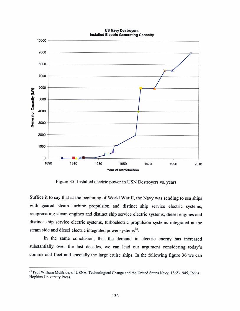
US Navy DestroyersInstalled Electric Generating Capacity
10000
9000 4M
8000
7000
6000
5000
4000-0.
3000-
2000
1000
0 3001890 1910 1930 1950 1970 1990 2010
Year of Introduction
Figure 35: Installed electric power in USN Destroyers vs. years
Suffice it to say that at the beginning of World War II, the Navy was sending to sea shipswith geared steam turbine propulsion and distinct ship service electric systems,
reciprocating steam engines and distinct ship service electric systems, diesel engines anddistinct ship service electric systems, turboelectric propulsion systems integrated at thesteam side and diesel electric integrated power systems.
In the same conclusion, that the demand in electric energy has increased
substantially over the last decades, we can lead our argument considering today's
commercial fleet and specially the large cruise ships. In the following figure 36 we can
38 Prof William McBride, of USNA, Technological Change and the United States Navy, 1865-1945, JohnsHopkins University Press.
136
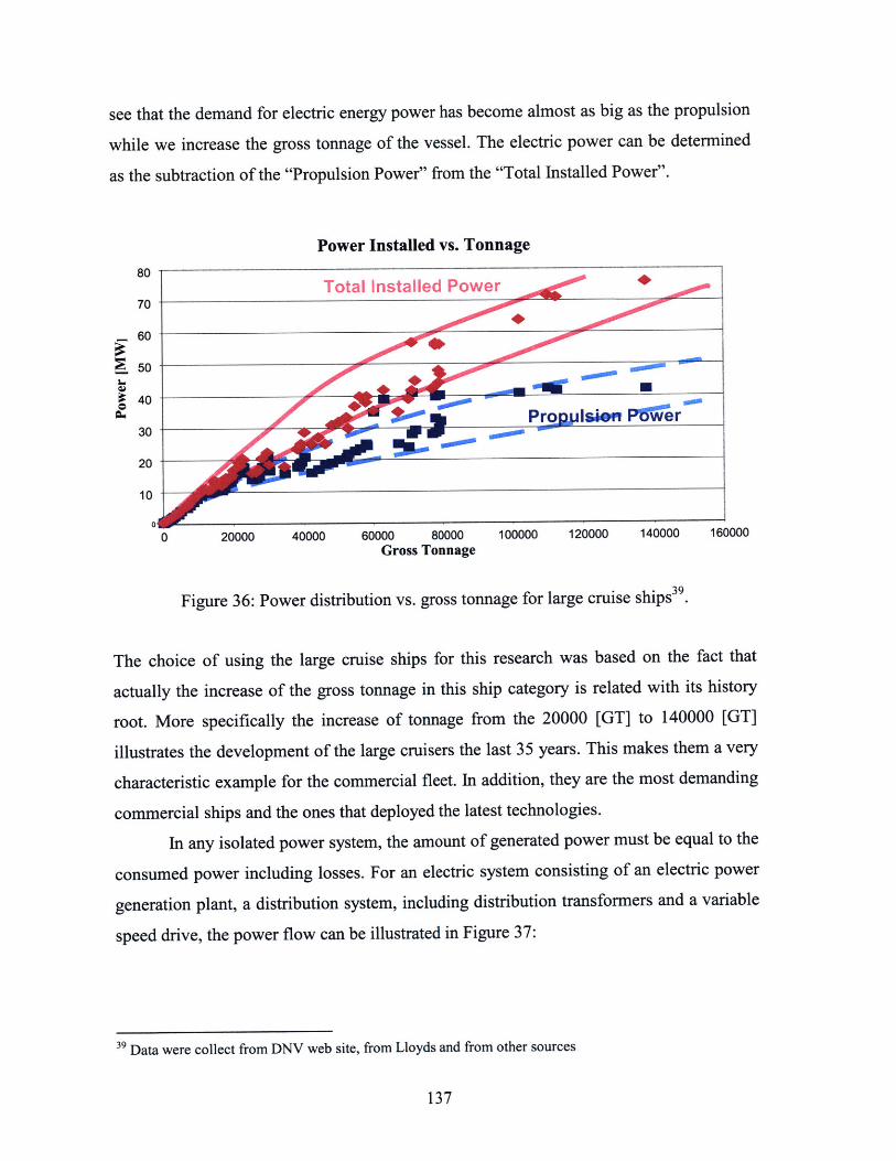
see that the demand for electric energy power has become almost as big as the propulsion
while we increase the gross tonnage of the vessel. The electric power can be determined
as the subtraction of the "Propulsion Power" from the "Total Installed Power".
Power Installed vs. Tonnage
C
80
70
60
50
40
30
20
10
20000 40000 60000 80000Gross Tonnage
100000 120000 140000 160000
Figure 36: Power distribution vs. gross tonnage for large cruise ships 3 9.
The choice of using the large cruise ships for this research was based on the fact that
actually the increase of the gross tonnage in this ship category is related with its history
root. More specifically the increase of tonnage from the 20000 [GT] to 140000 [GT]
illustrates the development of the large cruisers the last 35 years. This makes them a very
characteristic example for the commercial fleet. In addition, they are the most demanding
commercial ships and the ones that deployed the latest technologies.
In any isolated power system, the amount of generated power must be equal to the
consumed power including losses. For an electric system consisting of an electric power
generation plant, a distribution system, including distribution transformers and a variable
speed drive, the power flow can be illustrated in Figure 37:
39 Data were collect from DNV web site, from Lloyds and from other sources
137
Total Installed Power
Pro Isie P'ow'er
0
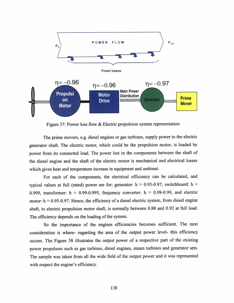
POWER FLOW Pau~
Power losses
F= ~1.6 = ~0.96 11= ~0-97
on ~ Moo DistributionPrm
Moto Moer
Figure 37: Power loss flow & Electric propulsion system representation
The prime movers, e.g. diesel engines or gas turbines, supply power to the electric
generator shaft. The electric motor, which could be the propulsion motor, is loaded by
power from its connected load. The power lost in the components between the shaft of
the diesel engine and the shaft of the electric motor is mechanical and electrical losses
which gives heat and temperature increase in equipment and ambient.
For each of the components, the electrical efficiency can be calculated, and
typical values at full (rated) power are for; generator: h = 0.95-0.97, switchboard: h =
0.999, transformer: h = 0.99-0.995, frequency converter: h = 0.98-0.99, and electric
motor: h = 0.95-0.97. Hence, the efficiency of a diesel electric system, from diesel engine
shaft, to electric propulsion motor shaft, is normally between 0.88 and 0.92 at full load.
The efficiency depends on the loading of the system.
So the importance of the engines efficiencies becomes sufficient. The next
consideration is where- regarding the area of the output power level- this efficiency
occurs. The Figure 38 illustrates the output power of a respective part of the existing
power propulsors such as gas turbines, diesel engines, steam turbines and generator sets.
The sample was taken from all the wide field of the output power and it was represented
with respect the engine's efficiency.
138
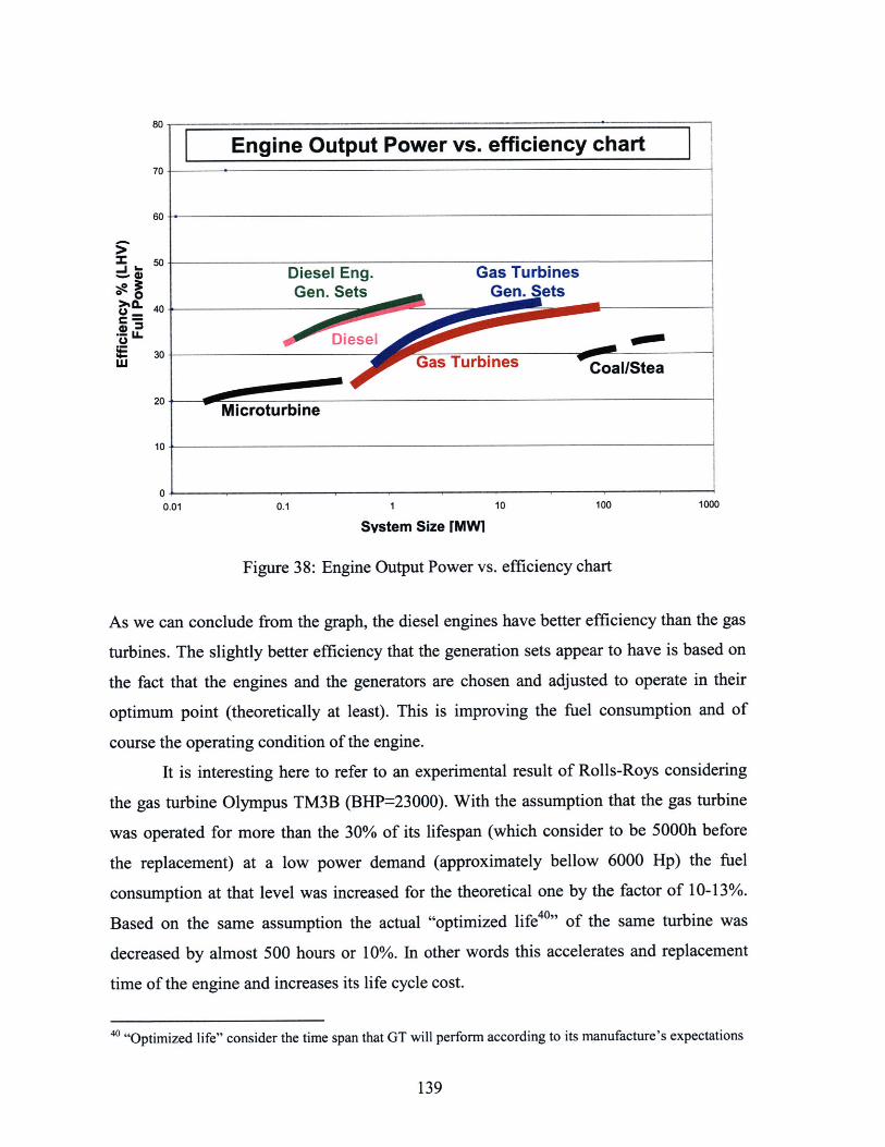
80
70 1
60-
Z 50-00 Diesel Eng. Gas Turbines
0 Gen. Sets Gen. Sets
0
'CL- 40
1 30-j-GsTriewo
20- Microturbine
10
00.01 0.1 1 10 100 1000
System Size iMWi
Figure 38: Engine Output Power vs. efficiency chart
As we can conclude from the graph, the diesel engines have better efficiency than the gas
turbines. The slightly better efficiency that the generation sets appear to have is based on
the fact that the engines and the generators are chosen and adjusted to operate in their
optimum point (theoretically at least). This is improving the fuel consumption and of
course the operating condition of the engine.
It is interesting here to refer to an experimental result of Rolls-Roys considering
the gas turbine Olympus TM3B (BHP=23000). With the assumption that the gas turbine
was operated for more than the 30% of its lifespan (which consider to be 5000h before
the replacement) at a low power demand (approximately bellow 6000 Hp) the fuel
consumption at that level was increased for the theoretical one by the factor of 10-13%.
Based on the same assumption the actual "optimized life40 " of the same turbine was
decreased by almost 500 hours or 10%. In other words this accelerates and replacement
time of the engine and increases its life cycle cost.
40 "Optimized life" consider the time span that GT will perform according to its manufacture's expectations
139
I Engine Output Power vs. efficiency chart
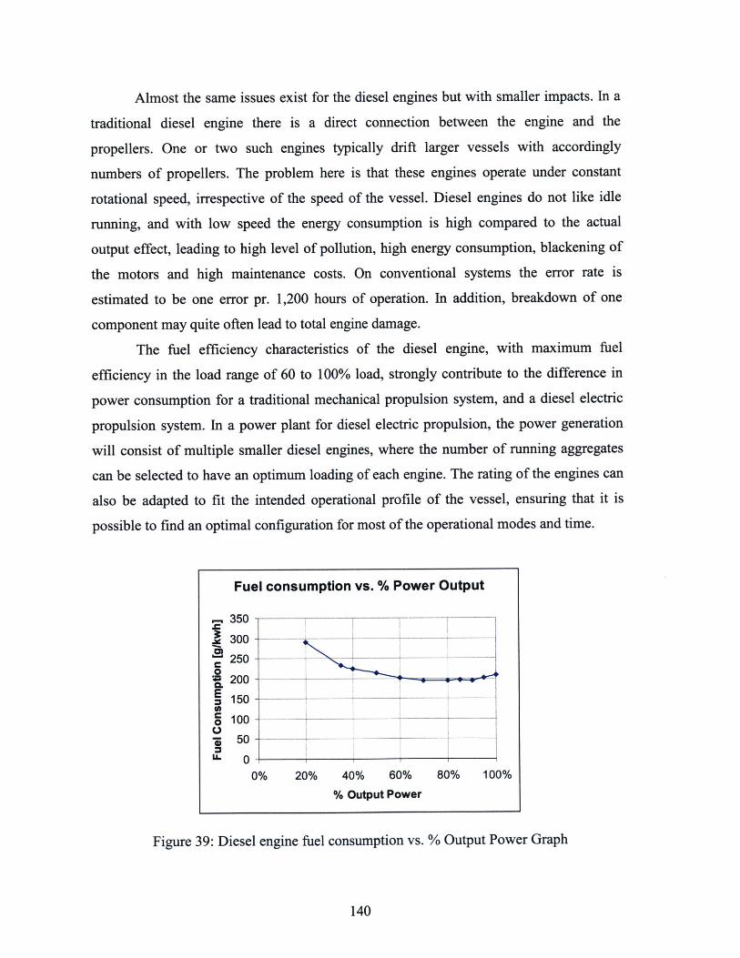
Almost the same issues exist for the diesel engines but with smaller impacts. In a
traditional diesel engine there is a direct connection between the engine and the
propellers. One or two such engines typically drift larger vessels with accordingly
numbers of propellers. The problem here is that these engines operate under constant
rotational speed, irrespective of the speed of the vessel. Diesel engines do not like idle
running, and with low speed the energy consumption is high compared to the actual
output effect, leading to high level of pollution, high energy consumption, blackening of
the motors and high maintenance costs. On conventional systems the error rate is
estimated to be one error pr. 1,200 hours of operation. In addition, breakdown of one
component may quite often lead to total engine damage.
The fuel efficiency characteristics of the diesel engine, with maximum fuel
efficiency in the load range of 60 to 100% load, strongly contribute to the difference in
power consumption for a traditional mechanical propulsion system, and a diesel electric
propulsion system. In a power plant for diesel electric propulsion, the power generation
will consist of multiple smaller diesel engines, where the number of running aggregates
can be selected to have an optimum loading of each engine. The rating of the engines can
also be adapted to fit the intended operational profile of the vessel, ensuring that it is
possible to find an optimal configuration for most of the operational modes and time.
Fuel consumption vs. % Power Output
,350 --
300
2500 0
200
50
00% 20% 40% 60% 80% 100%
% Output Power
Figure 39: Diesel engine fuel consumption vs. % Output Power Graph
140

Therefore the already installed number of engines which provide the electric
power, the high ratio of the electric power installed over the total power in collaboration
with the better efficiency of the diesel or gas turbine generator sets indicates that the
efficient and cost effective solution can be achieved with only one kind of energy. The
use of different type of engines - main, secondary generator sets and emergency
generator sets- creates additional problems in various processes like logistics,
maintenance and manning. Hence, they demand different type of spare parts, different
maintenance process and as a result more personnel that can maintain and operate the
above engines efficiently.
In addition the optimized operation that the generator sets provide can be
combined with the flexibility to handle only one type of energy (electric) and to exchange
and arrange the energy supply in every time step according to the demand. The
controllability can be achieved with the implementation of an integrated power plant
design which can satisfies the electric and propulsion power needs at all circumstances.
And this can vary from high power demands with maximum speed to the situation of
minimum lighting inside the harbor. The correct choice of the generator sets type- diesel
generator set, gas turbine generator set or combination of both- should based on the
mission need statement for the ship and this leads to a speed vs. electric energy demand
trade of study.
The flexibility will be integrated with the existence of an auto control system
which will evaluate the energy demand for both propulsion and arbitrary loads and will
act respectively. It will start and stop the power generators considering the size of the
loads and that of the engine. At the same time a prediction program with a number of
load demand scenarios will improve the response times.
An electric propulsion system is designed differently. One or two large main
engines may be substituted by more and smaller diesel engines, each of them being
connected to an electrical generator delivering the electricity to one or more frequency
converters, independently of the numbers of propellers. The electricity goes into the
converter on a fixed frequency and moves out with a variable frequency, drifting an
electric motor with direct connection to the propeller. This is functional power electronics
in practice, a growing and highly interesting business area.
141
The great advantage of such a system is the use of sufficient numbers of auxiliary
diesel engines, i.e., the usage of all engines at all times is avoided. If the engine is
working idle or the vessel is moving with reduced speed, it may be sufficient to connect
only one auxiliary generator which in return may be operated on optimum capacity and
efficiency. On the other side, to reach the vessel's field of operation quickly may demand
high speed and running of the entire vessel's auxiliary generator. This flexibility gives
substantial energy-savings and at the same time securing optimal output effect.
On a standard supply vessel operating out from Aberdeen4 to platforms in the
North Sea, it is estimated that the energy savings may be as high as 30% on an annual
basis, giving cost advantages of app. EUR 350,000 p.a.. The investment level of a diesel-
electric system compared to a conventional system is typically around EUR 1.3 million
higher, which implies a pay-back time of 3 - 4 years. With an estimated economical life
of 20 - 30 years for a supply vessel, such an investment is by all means favorable.
Furthermore, an added economical advantage is the cost savings from reduced
maintenance.
Another significant factor that contributes to the fuel efficiency improvement is
the use of the fixed pitch propeller (FPP). Since the additional components between the
prime mover and the propeller shaft in a diesel electric propulsion system contributes to a
total of approximately 10% losses, the fuel savings potential is not only due to the
electrical component. One must regard the hydrodynamic efficiency of a speed controlled
propeller compared to a fixed speed controllable pitch propeller (CPP), and the fuel
efficiency of the prime mover when installed in a diesel electric system with constant
speed and high loading, compared to in a mechanical propulsion system with strongly
varying load. The differences may be significant, especially on low thrust operations as
DP and maneuvering. The Figure 40 shows the power vs. thrust comparison of a variable
speed and a controllable pitch propeller (CPP).
The hydrodynamic losses will vary significantly dependent on the operational
condition for a CPP used in direct driven diesel solutions compared to variable speed
fixed pitch propellers (FPP), which normally are used in electrical propulsion. In low
load condition it is a rule of thumb that the zero-load hydrodynamic losses for a CPP is
142
41 From Aberdeen statistic reaserch
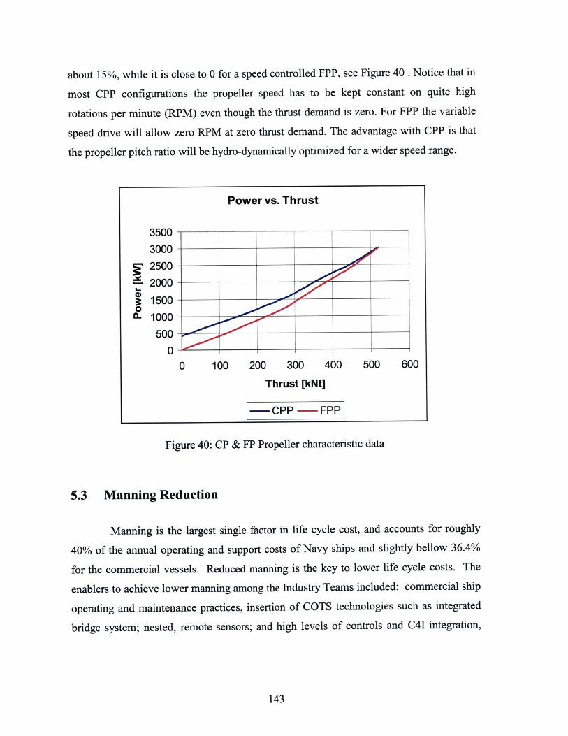
about 15%, while it is close to 0 for a speed controlled FPP, see Figure 40 . Notice that in
most CPP configurations the propeller speed has to be kept constant on quite high
rotations per minute (RPM) even though the thrust demand is zero. For FPP the variable
speed drive will allow zero RPM at zero thrust demand. The advantage with CPP is that
the propeller pitch ratio will be hydro-dynamically optimized for a wider speed range.
0I0
Power vs. Thrust
3500
3000
2500
2000
1500
1000500
0500 600100 200 300 400
Thrust [kNt]
-- CPP - FPP
0
Figure 40: CP & FP Propeller characteristic data
5.3 Manning Reduction
Manning is the largest single factor in life cycle cost, and accounts for roughly
40% of the annual operating and support costs of Navy ships and slightly bellow 36.4%
for the commercial vessels. Reduced manning is the key to lower life cycle costs. The
enablers to achieve lower manning among the Industry Teams included: commercial ship
operating and maintenance practices, insertion of COTS technologies such as integrated
bridge system; nested, remote sensors; and high levels of controls and C41 integration,
143
,-

with ultimate solution the full electric integrated propulsion system. The Arsenal Ship
study is highlighting these words.42
The most demanding ship's positions in manning are the shipboard engineering
and damage control. For these positions the support systems can be divided into three
tiers. The centrally located global or supervisory control system is composed of software
that monitors the operation of the entire ship network. The second, intermediate tier
control systems coordinate with the supervisory controller and can independently direct
the operation of a specified system or zone of operation. The third tier consists of local
controllers that integrate the ship's hardware with the software based network centric
command and control infrastructure.
These systems must be extremely dependable and survivable despite scenarios
induced disruptions to normal operating mode or even to war-fighting operations. Should
an individual system fail, the goal is that a zonal or supervisory controller could take over
effective operation of the system without causing further disruption in controller
activities. For the success of such a design, integrated communications networks are
essential. Because of commercial and military technological advances in communications
and controls, the ship control model must evolve. Incorporation of electric ship
technologies results in a fundamental change in shipboard operation that must be
accounted for.
Because control systems integration and automation have been the dynamic
impetus for a modification of the shipboard concept of operations, interdisciplinary
research is the only recourse for examining how ships will operate in the future and
presently, with the incorporation of new automation and sensing technologies.
All of this leads to the concept of optimized manning. The total cost to meet a
mission has two components: manning costs and automation costs. The manning cost
function is essentially linear with slope being the capitalized cost of a single sailor. The
automation cost function is intuitively not linear. The cost of completely automating the
ship is not the same as the sum of automating each task.
42 Arsenal Ship Joint Program Office + DARPA: For the Arsenal study the goal of less than a crew of 50 was
easily achieved by the Industry Teams (who averaged crew of 22). Preliminary Navy estimates for Arsenal Ship were
crew of 269.
144
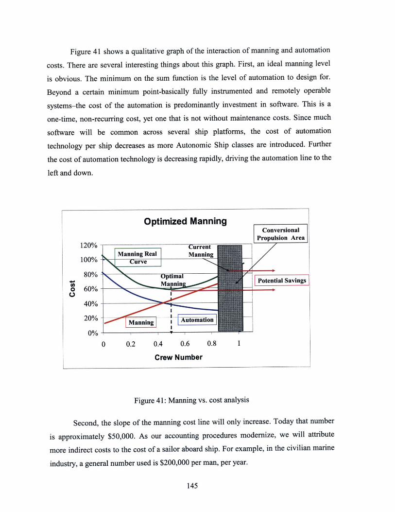
Figure 41 shows a qualitative graph of the interaction of manning and automation
costs. There are several interesting things about this graph. First, an ideal manning level
is obvious. The minimum on the sum function is the level of automation to design for.
Beyond a certain minimum point-basically fully instrumented and remotely operable
systems-the cost of the automation is predominantly investment in software. This is a
one-time, non-recurring cost, yet one that is not without maintenance costs. Since much
software will be common across several ship platforms, the cost of automation
technology per ship decreases as more Autonomic Ship classes are introduced. Further
the cost of automation technology is decreasing rapidly, driving the automation line to the
left and down.
Optimized Manning
120%
100%
80%
o 60%0
ConversionalPropulsion Area
Potential Savings
'tU 70
20% Automat on20% Mnning
0%
0 0.2 0.4 0.6 0.8 1
Crew Number
Figure 41: Manning vs. cost analysis
Second, the slope of the manning cost line will only increase. Today that number
is approximately $50,000. As our accounting procedures modernize, we will attribute
more indirect costs to the cost of a sailor aboard ship. For example, in the civilian marine
industry, a general number used is $200,000 per man, per year.
145
CurrentManning Real Manning
Curve
0ptImalMannin
Finally, funding for two cost elements is provided by different sources. Manning
is paid for by military salary funds after initial acquisition. The cost of automation is paid
for with acquisition and R&D funds. It is not surprising then that there is a push to
minimize acquisition cost of the ship by reducing the cost of the technology and
automated equipment going onto ships even if it means paying people to do things that
can be done more cheaply by machines! For example, it costs over $25,000 per year to
pay a person to read one gage, once an hour and write the value on a piece of paper. It
costs perhaps $1000 to collect that data automatically. Therefore the capital cost of this
reading is recovered in the first 3 days of operation.43
Obviously over the life of a ship the cost of manning greatly overshadows the
cost of purchasing that ship, yet we place an inordinate value on the purchase price of the
ship. Ironically the purchase price of a fully automated ship is decreasing at a
phenomenal rate while the cost of manpower is increasing. There is some hope, however.
Recently the U.S. Navy has begun to consider the total cost of ownership as a metric for
awarding ship building programs. The Total Ownership Cost includes the cost of
building, staffing, maintaining and operating the ship. Although, no program has yet been
awarded on this basis, at least the thinking is moving in this direction.
5.4 Area and Volume Challenge
Even in modem ships, propulsion systems are so large and heavy that in many
applications they force the rest of the ship to be constructed around them. Machine sizes
and their locations also reduce the space available for cargo and passengers and interfere
with efficient loading and unloading. Shafts can extend considerable lengths, further
compromising efficient space utilization. Additionally, the propulsion systems, both
43 Data by Scott B. Hoyle Lockheed Martin, Naval Electronics & Surveillance Systems
146
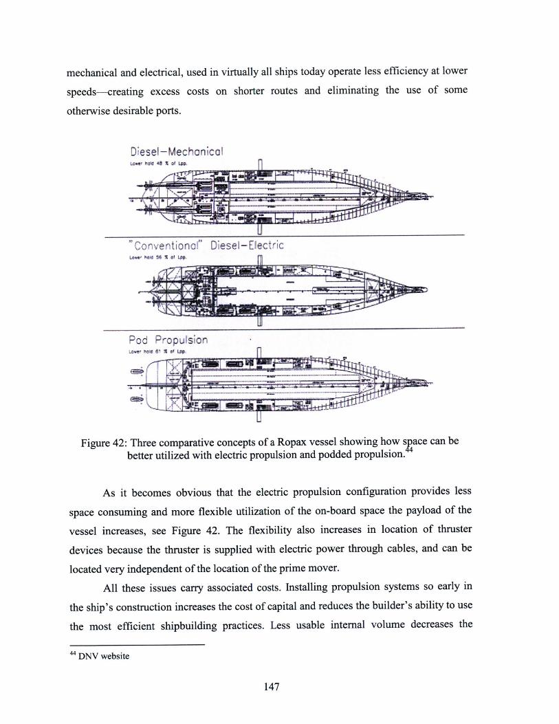
mechanical and electrical, used in virtually all ships today operate less efficiency at lower
speeds-creating excess costs on shorter routes and eliminating the use of some
otherwise desirable ports.
Diesel- Mechanical
Conventionad Diesel-Electric
Pod Propulsion
Figure 42: Three comparative concepts of a Ropax vessel showing how space can be
better utilized with electric propulsion and podded propulsion.
As it becomes obvious that the electric propulsion configuration provides less
space consuming and more flexible utilization of the on-board space the payload of the
vessel increases, see Figure 42. The flexibility also increases in location of thruster
devices because the thruster is supplied with electric power through cables, and can be
located very independent of the location of the prime mover.
All these issues carry associated costs. Installing propulsion systems so early in
the ship's construction increases the cost of capital and reduces the builder's ability to use
the most efficient shipbuilding practices. Less usable internal volume decreases the
147
44DNV website
revenue generation potential for commercial vessels as well as the war-fighting capability
for military ships. Inefficient loading and unloading create longer cycle times, increase
port costs, and jeopardize schedules. Prolonged and low speed operation of diesel direct-
drive and geared propulsion systems increases maintenance costs. Reduced efficiency at
low ship speeds may make certain shipping routes unprofitable compared with other
transportation alternatives
5.5 Some additional considerations
Conventional diesel propulsion needs an extensive engine room ventilation
system, due to the fact that the prime movers cannot be installed in airtight and air/water
cooled sound enclosures. In addition any conventional system consists of two flexible
mounted marine duct axial flow fans with a total capacity of 40.000 m3/hr complete with
fire damper assemblies, mist eliminators, sound dampers, grills and ducting. An engine
room with diesel electric propulsion, due to the fact that the heat rejection of all engines
is absorbed by air/water coolers, needs a ventilation system of only 4000 m3/hr like one
that exists even in medium size yachts of 30 meter. This results in much less noise on
deck.
For the compatible propulsion the engine room needs an extensive sound
insulation, due to uninsulated prime movers. Even with an extensive sound insulation
system, it is difficult to achieve a sound level of less than 58-60 dB where with diesel
electric propulsion a sound level of 50-55 dB easily can be achieved. The level noise
becomes critical if we refer to gas turbines. Especially for the engines with horsepower
above 20000HP the noise level climbs at 92-95 dB. The ability to use small engines in
the electric drive configuration decreases the noise level to 89-91dB45 .
For the manning now, the conventional system needs more man hours for engine
beds, installation of shaft drives, and the more extensive hydraulic installation. And this
because controllable pitch propeller configuration is usually used. The electric propulsion
as described needs less man hours for installation since it has not so extended supporting
4 Data from manufactures MAN,MTU and Rolls-Royce respectively
148

and auxiliary systems. The arrangements are easy to be configured and the accessibility
for construction and maintenance is more than satisfactory. This also is another factor
that decreases the construction cost.
It is impossible to give exact prices for the man hours in a preliminary design
stage and it is also depending on which yard the ship will built and their experience. At
this moment there are few shipyards that can implement an intergraded diesel or gas
turbine-electric design. And since the market is under development, the prices will vary
at the beginning until the point that the system will prove its ability and satisfy most of
the expectations.
149
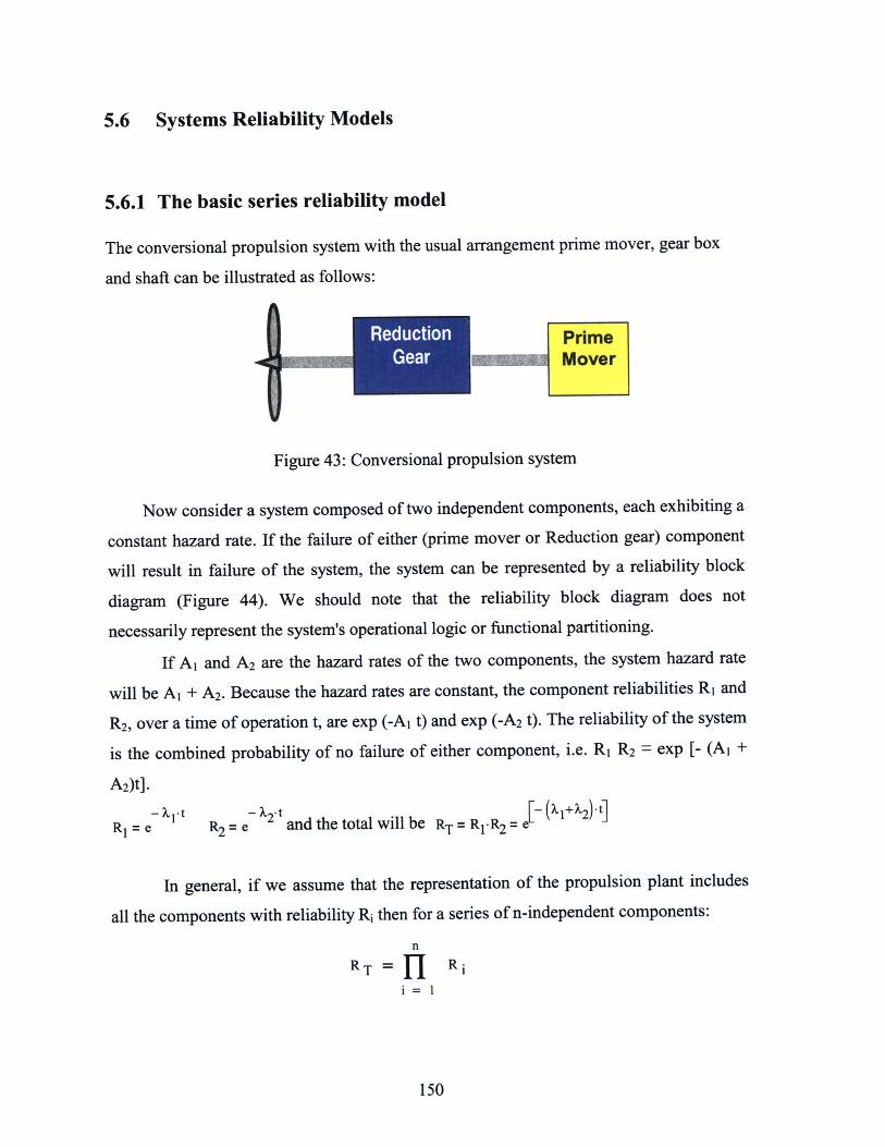
5.6 Systems Reliability Models
5.6.1 The basic series reliability model
The conversional propulsion system with the usual arrangement prime mover, gear box
and shaft can be illustrated as follows:
Geal -T Mover
Figure 43: Conversional propulsion system
Now consider a system composed of two independent components, each exhibiting a
constant hazard rate. If the failure of either (prime mover or Reduction gear) component
will result in failure of the system, the system can be represented by a reliability block
diagram (Figure 44). We should note that the reliability block diagram does not
necessarily represent the system's operational logic or functional partitioning.
If A1 and A2 are the hazard rates of the two components, the system hazard rate
will be A1 + A2. Because the hazard rates are constant, the component reliabilities R1 and
R2, over a time of operation t, are exp (-A1 t) and exp (-A 2 t). The reliability of the system
is the combined probability of no failure of either component, i.e. R1 R2 = exp [- (A1 +
A2)t].
R, = e _?-t R2= e -2-t and the total will be RT = R-R2 1+X 2).t]
In general, if we assume that the representation of the propulsion plant includes
all the components with reliability Ri then for a series of n-independent components:
n
RT = R1= 1
150
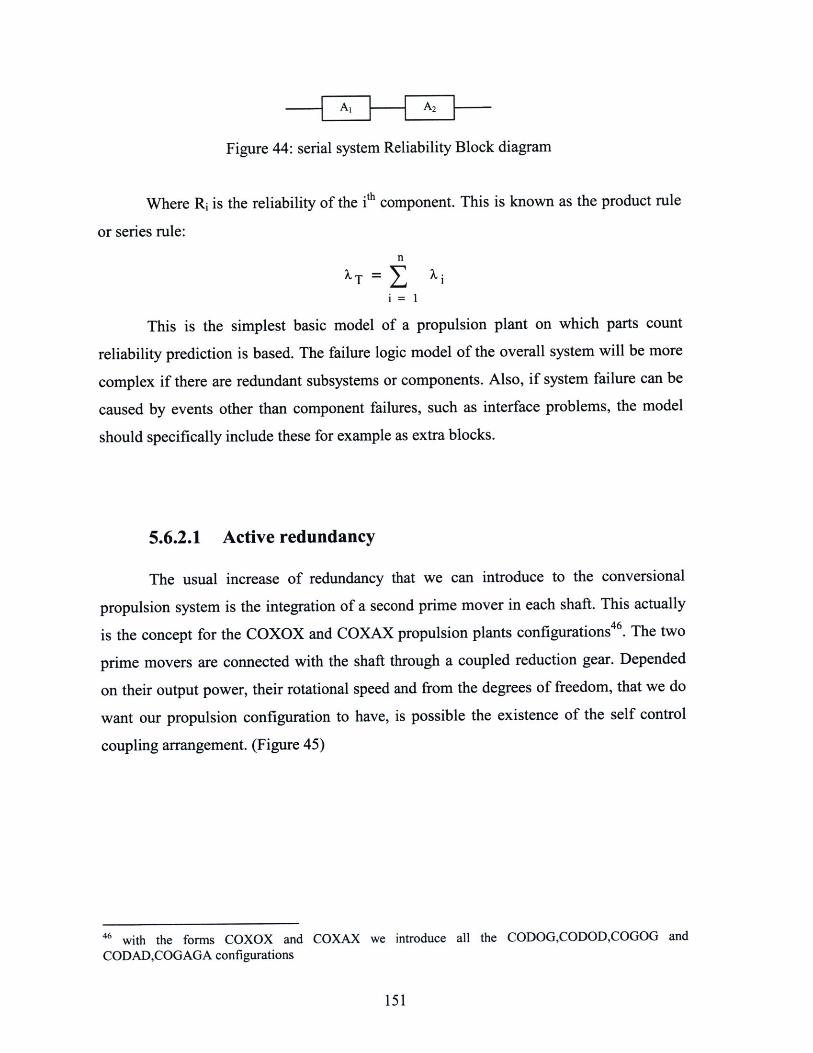
Figure 44: serial system Reliability Block diagram
Where Ri is the reliability of the ith component. This is known as the product rule
or series rule:
nXT.. X
i = 1
This is the simplest basic model of a propulsion plant on which parts count
reliability prediction is based. The failure logic model of the overall system will be more
complex if there are redundant subsystems or components. Also, if system failure can be
caused by events other than component failures, such as interface problems, the model
should specifically include these for example as extra blocks.
5.6.2.1 Active redundancy
The usual increase of redundancy that we can introduce to the conversional
propulsion system is the integration of a second prime mover in each shaft. This actually
is the concept for the COXOX and COXAX propulsion plants configurations46. The two
prime movers are connected with the shaft through a coupled reduction gear. Depended
on their output power, their rotational speed and from the degrees of freedom, that we do
want our propulsion configuration to have, is possible the existence of the self control
coupling arrangement. (Figure 45)
46 with the forms COXOX and COXAX we introduce all the CODOG,CODOD,COGOG and
CODAD,COGAGA configurations
151
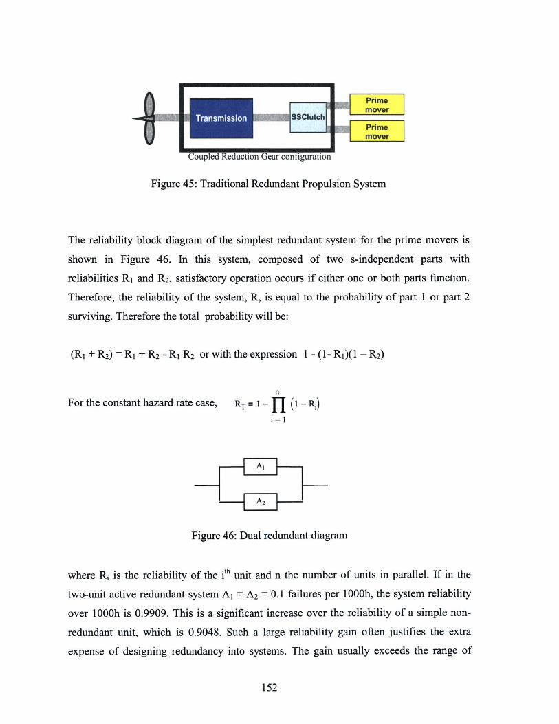
Coupled Reduction Gear configuration
Figure 45: Traditional Redundant Propulsion System
The reliability block diagram of the simplest redundant system for the prime movers is
shown in Figure 46. In this system, composed of two s-independent parts with
reliabilities R1 and R2, satisfactory operation occurs if either one or both parts function.
Therefore, the reliability of the system, R, is equal to the probability of part 1 or part 2
surviving. Therefore the total probability will be:
(Ri + R2) = R1 + R2 - R1 R2 or with the expression 1 - (1- R1)(1 - R2)
nFor the constant hazard rate case, RT = 1 - (1 - Rj)
i=1
A2
Figure 46: Dual redundant diagram
where Ri is the reliability of the ith unit and n the number of units in parallel. If in the
two-unit active redundant system AI = A2 = 0.1 failures per 1000h, the system reliability
over 1000h is 0.9909. This is a significant increase over the reliability of a simple non-
redundant unit, which is 0.9048. Such a large reliability gain often justifies the extra
expense of designing redundancy into systems. The gain usually exceeds the range of
152
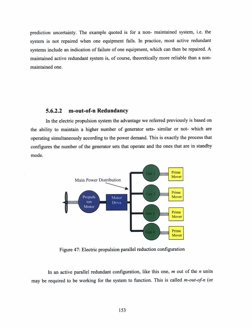
prediction uncertainty. The example quoted is for a non- maintained system, i.e. the
system is not repaired when one equipment fails. In practice, most active redundant
systems include an indication of failure of one equipment, which can then be repaired. A
maintained active redundant system is, of course, theoretically more reliable than a non-
maintained one.
5.6.2.2 m-out-of-n Redundancy
In the electric propulsion system the advantage we referred previously is based on
the ability to maintain a higher number of generator sets- similar or not- which are
operating simultaneously according to the power demand. This is exactly the process that
configures the number of the generator sets that operate and the ones that are in standby
mode.
PrimeMover
Main Power Distribution
PrimeMover
PrimeMover
Figure 47: Electric propulsion parallel reduction configuration
In an active parallel redundant configuration, like this one, m out of the n units
may be required to be working for the system to function. This is called m-out-of-n (or
153
m/n) parallel redundancy. The reliability of an m/n system, with n, s-independent
components in which all the unit reliabilities are equal, is the binomial reliability function
rn-IR -, n! i n-i
RT=i!-(n - .(I -R)
i=O
or, for the constant hazard rate case:
rn-iRT = I - 1 n! .(,t)n-i
RT-t1 + 1)n Z= i!.(n - i)!
It is general practice in technological systems design to employ redundancy to
enhance Systems reliability. However, an assumption of independence between
redundant components or systems is often implicitly made in such designs that may not
always be valid. In fact, the possibility of 'common cause' failures (i.e. dependent
failures) can defeat system redundancy and significantly reduce system availability. Thus,
it is important to include a quantitative assessment of common cause failures when
analyzing the reliability of redundant systems.
The beta factor method has been most often recently applied to common cause
analyses safety systems. However, the beta factor method requires that a number of
simplifying assumptions often be applied, particularly for systems that involve a multiple
number of redundant trains. The beta factor is defined as:
XC XC
Where
= system common cause failure rate,
X = system random failure rate and
XT - total system failure rate.
Generally, in electric system applications, values for p range from 0.001 to 0.1 and
sometimes can be as high as 0.2 based on the analysis of historical failure rate data and
analyst expert opinions
154
In general, for a m-out-of-n system, which can be defined as a redundant, parallel system
that is available if m-out-of-n components perform satisfactorily, the system reliability
Rk can be expressed as:
Rm n n! [- ( R: r.r) - R)n-r]] .R2_ r!-(n - r)!
where the effect of common cause failures can be included in this expression by notingthat:
R, = e
and
R2 = e- e-X-t
Thus we can define the reliability, Rmn, for m=1 and n=2,3and 4 respectively, as:
R12= -exp(-X-t)-[-2 + exp(-1 + $)-.x-t]]
R13= exp(-X-t).[3 - 3-exp{(-1 + p).x.t] + exp2-(-1 + P).Xt]]
R14 = -exp(-A.t).[-4 + 6.exp{(-1 + ) .. t] - 4.exp2.(-1 + p).).t] + exp[3.(-1 + X.f]
with the inequality to be satisfied straight forward: R14 R13 R12.
Similar expressions for the unavailability Q. of the m-out-of-n can be derived from the
previous equations using the relation Qmn = I-Rmn.
In most common cause analysis models of redundant systems, no distinction is
made between different possible levels of failure due to a single common cause; little
effort has been made to obtain estimates for the probability of failing three, four or more
identical trains. Instead, the failure contribution due to different levels of component
multiplicity is aggregated into a single value (the beta factor). Reasons for this include
previous studies have focused mostly on two-unit redundant systems, and few experience
data are available on common cause failures so that consideration of different levels of
system redundancy is not easy. But for the configuration of the electric propulsion this
does not cover all the scenarios. However, to treat the partial failure cases in an electric
propulsion system, a reliability equation incorporating the multiple dependent failure
155
fraction has previously been derived for a 1 -out-of-3 redundant system but which does
not treat failures on demand.
Following the same treatment of the beta factor as was described before, we can
define the failure rate X as a consisting of a random failure component X, and a common
cause component L. We can extend our definition for the term ), and assume that this is a
part of a fraction of the common cause failure of the entire system. If we name this
fraction as fi with n belongs to the set [2.. .N] with N the total of components, then this
fraction represents the nth component fraction of failure. Therefore:
N
f= I fn
n =2
so the final expression for the X will be:
N
X= r+X-c=r+XnZ fn
n =2
Now provided that average unit failure rates can be assumed constant (that is negative
exponential distribution of time to failure) and the same applies to average unit repair
rates (that is negative exponential distribution of time to repair) we can use the Markov
Chain Theory to evaluate the average availabilities. Even with the use of the
simplification that the fraction ratio is introducing to the Markov Theory, the full-scale
analysis cannot be achieved since there is lack of data that can buck up our hypothesis.
The new design was never been tested and the data that exist are very limited.
The simplification that we suggest is based on the idea to incorporate in the
system common cause failure rate the partial failure rates of each individual component.
This will give us the ability knowing the subsystem that we examine to prevent the
unexpected casualties. With simpler words if we do know their partial rate of failure, we
can design the systems more efficiently using aspects as redundancy and standby
redundancy minimizing with this way the mean repair time and increase the system
availability. In addition, the modularity that can be introduced in the design can improve
further the system's reliability. Since the modules include almost the same units, their
156
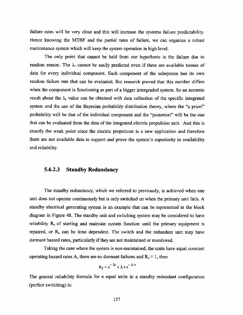
failure rates will be very close and this will increase the systems failure predictability.
Hence knowing the MTBF and the partial rates of failure, we can organize a robust
maintenance system which will keep the system operation in high level.
The only point that cannot be held from our hypothesis is the failure due to
random reason. The X, cannot be easily predicted even if there are available tonnes of
data for every individual component. Each component of the subsystem has its own
random failure rate that can be evaluated. But research proved that this number differs
when the component is functioning as part of a bigger intergraded system. So an accurate
result about the Xr value can be obtained with data collection of the specific integrated
system and the use of the Bayesian probability distribution theory, where the "a priori"
probability will be that of the individual component and the "posteriori" will be the one
that can be evaluated from the data of the integrated electric propulsion unit. And this is
exactly the weak point since the electric propulsion is a new application and therefore
there are not available data to support and prove the system's superiority in availability
and reliability.
5.6.2.3 Standby Redundancy
The standby redundancy, which we referred to previously, is achieved when one
unit does not operate continuously but is only switched on when the primary unit fails. A
standby electrical generating system is an example that can be represented in the block
diagram in Figure 48. The standby unit and switching system may be considered to have
reliability R, of starting and maintain system function until the primary equipment is
repaired, or R. can be time dependent. The switch and the redundant unit may have
dormant hazard rates, particularly if they are not maintained or monitored.
Taking the case where the system is non-maintained, the units have equal constant
operating hazard rates A, there are no dormant failures and R, = 1, then
RT = e + X-t-e X.t
The general reliability formula for n equal units in a standby redundant configuration
(perfect switching) is:
157
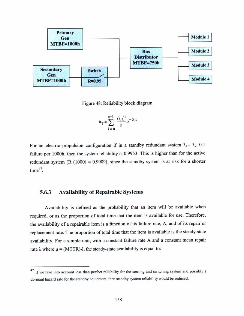
PrimaryGen
MTBF=1000h
Secondary SwitchGen
MTBF=1000h R=0.95
BusDistributor
MTBF=75Oh
-- Module I
Module 2
Module 3
Module 4
Figure 48: Reliability block diagram
RT - X-t
i=0
For an electric propulsion configuration if in a standby redundant system X 1= X2=0. 1
failure per 1000h, then the system reliability is 0.9953. This is higher than for the active
redundant system [R (1000) = 0.9909], since the standby system is at risk for a shorter
time4 7.
5.6.3 Availability of Repairable Systems
Availability is defined as the probability that an item will be available when
required, or as the proportion of total time that the item is available for use. Therefore,
the availability of a repairable item is a function of its failure rate, A, and of its repair or
replacement rate. The proportion of total time that the item is available is the steady-state
availability. For a simple unit, with a constant failure rate A and a constant mean repair
rate X where p = (MTTR)-l, the steady-state availability is equal to:
47 If we take into account less than perfect reliability for the sensing and switching system and possibly a
dormant hazard rate for the standby equipment, then standby system reliability would be reduced.
158
A= 9 MTBF
X + MTBF + MTTR
The instantaneous availability or probability that the item will be available at time t is
equal to
A= + -(X+p).tX+pi X+p
which approaches the steady-state availability as t becomes large.
It is often more revealing, particularly when comparing design options, to
consider system unavailability:
Steady-state unavailability = 1 - A, but:
I - A=X+ p
and instantaneousunavailability = - -+X)t
X+p X+p
If scheduled maintenance is necessary and involves taking the system out of action, this
must be included in the availability formula. The availability of spare units for repair by
replacement is often a further consideration, dependent upon the previous spares usage
and the repair rate of replacement units.
Availability is an important consideration in the propulsion systems and more
specifically to the electric propulsion ones which are relatively complex. In such systems,
high reliability by itself is sufficient to ensure that the system will be available when
needed. It is also necessary to ensure that it can be repaired in a short time and that
essential scheduled maintenance tasks can be performed quickly, if possible, without
shutting down the system. This is not sufficient for the conversional propulsion system
since the repair time should be limit to zero otherwise the availability is dropping
substantially.
Therefore, maintainability is an important aspect of design for maximum
availability, and trade-offs are often necessary between reliability and maintainability
features. For the electric propulsion systems a very common application to improve
maintainability is the incorporation of built-in test equipments. This added complexity
can degrade slightly the reliability and can also result in spurious failure indications.
159
However, these systems can greatly reduce maintenance times, by providing an
instantaneous indication of fault location, and therefore availability can be increased.
Availability is also affected by redundancy. If standby systems can be repaired or
overhauled while the primary system provides the required service, overall availability
can be greatly increased. The electric propulsion system's ability to use and interchange a
numerous generator sets under different scenarios allows the increase of the standby
times. This increase to the optimum operation life span of each unit provides the ability
for better and more organized maintenance system improving sequentially the total
system availability.
5.6.4 Modification example
With the implementation of this example we will illustrate the improvement of the
Reliability that we can achieve with the conversion from a conversional propulsion
system to an electric one. For the purpose of this model and to include a more general
arrangement configuration we will divide the ship units according to the demand for
support for each propulsion plant. So we can generalize the problem with the assumption
that the ship has n self sustained units. Any unit of this ship can provide electric power
and propulsion integrity. The configuration that each unit of the starting ship has
(conversional design) can be seen in the Table 2:
160
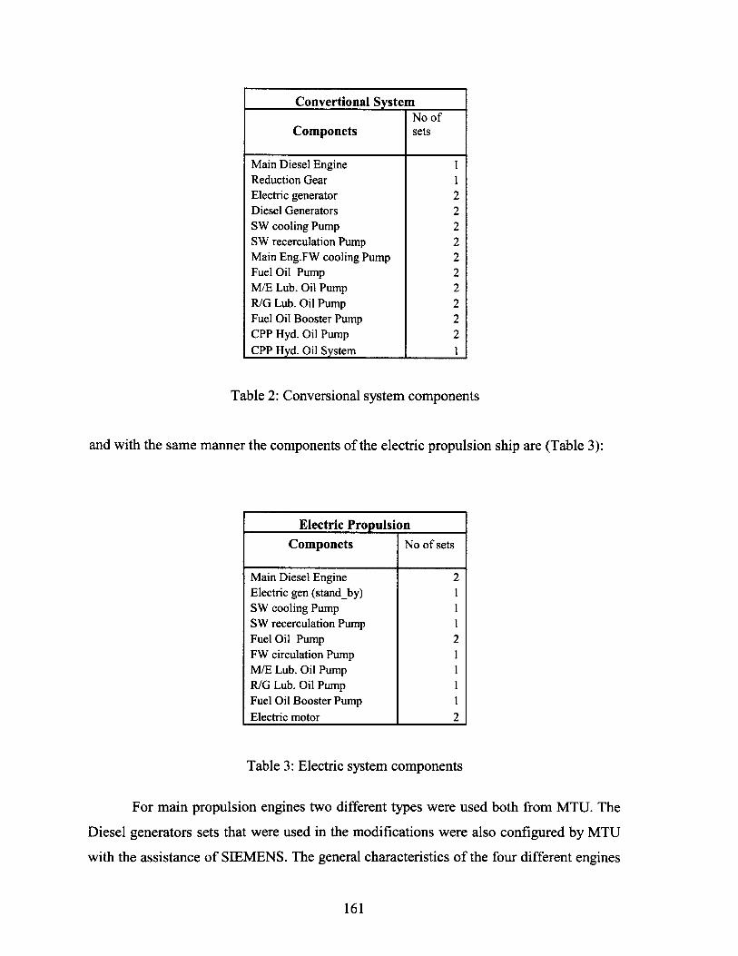
Table 2: Conversional system components
and with the same manner the components of the electric propulsion ship are (Table 3):
Table 3: Electric system components
For main propulsion engines two different types were used both from MTU. The
Diesel generators sets that were used in the modifications were also configured by MTU
with the assistance of SIEMENS. The general characteristics of the four different engines
161
Convertional SystemNo of
Componets sets
Main Diesel Engine 1Reduction Gear 1Electric generator 2Diesel Generators 2SW cooling Pump 2SW recerculation Pump 2Main Eng.FW cooling Pump 2Fuel Oil Pump 2M/E Lub. Oil Pump 2R/G Lub. Oil Pump 2Fuel Oil Booster Pump 2CPP Hyd. Oil Pump 2CPP Hyd. Oil System 1
Electric Propulsion
Componets No of sets
Main Diesel Engine 2Electric gen (stand-by) 1SW cooling Pump 1SW recerculation Pump 1Fuel Oil Pump 2FW circulation Pump 1M/E Lub. Oil Pump IR/G Lub. Oil Pump 1Fuel Oil Booster Pump 1Electric motor 2
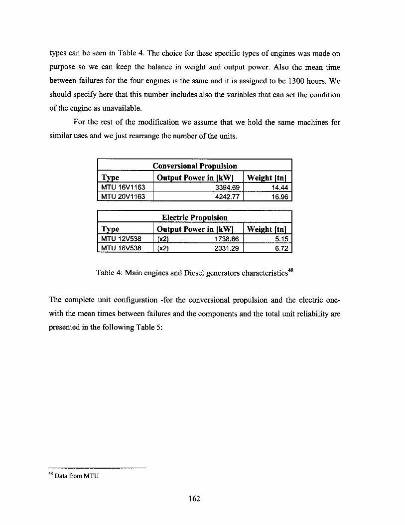
types can be seen in Table 4. The choice for these specific types of engines was made on
purpose so we can keep the balance in weight and output power. Also the mean time
between failures for the four engines is the same and it is assigned to be 1300 hours. We
should specify here that this number includes also the variables that can set the condition
of the engine as unavailable.
For the rest of the modification we assume that we hold the same machines for
similar uses and we just rearrange the number of the units.
Conversional Propulsion
Type Output Power in [kW] Weight [tn]MTU 16V1163 3394.69 14.44MTU 20V1163 4242.77 16.96
Electric Propulsion
Type Output Power in [kW] Weight [tn]MTU 12V538 (x2) 1738.66 5.15MTU 16V538 (x2) 2331.29 6.72
Table 4: Main engines and Diesel generators characteristics 48
The complete unit configuration -for the conversional propulsion and the electric one-
with the mean times between failures and the components and the total unit reliability are
presented in the following Table 5:
162
48 Data from MTU
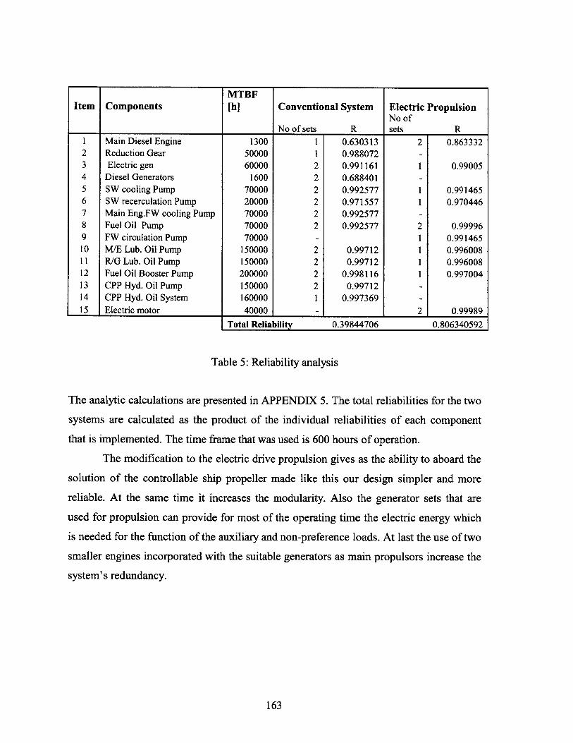
Total Reliability 0.39844706 0.806340592
Table 5: Reliability analysis
The analytic calculations are presented in APPENDIX 5. The total reliabilities for the two
systems are calculated as the product of the individual reliabilities of each component
that is implemented. The time frame that was used is 600 hours of operation.
The modification to the electric drive propulsion gives as the ability to aboard the
solution of the controllable ship propeller made like this our design simpler and more
reliable. At the same time it increases the modularity. Also the generator sets that are
used for propulsion can provide for most of the operating time the electric energy which
is needed for the function of the auxiliary and non-preference loads. At last the use of two
smaller engines incorporated with the suitable generators as main propulsors increase the
system's redundancy.
163
MTBFItem Components [h] Conventional System Electric Propulsion
No ofNo of sets R sets R
1 Main Diesel Engine 1300 1 0.630313 2 0.8633322 Reduction Gear 50000 1 0.988072 -3 Electric gen 60000 2 0.991161 1 0.990054 Diesel Generators 1600 2 0.688401 -5 SW cooling Pump 70000 2 0.992577 1 0.9914656 SW recerculation Pump 20000 2 0.971557 1 0.9704467 Main Eng.FW cooling Pump 70000 2 0.992577 -8 Fuel Oil Pump 70000 2 0.992577 2 0.999969 FW circulation Pump 70000 - 1 0.99146510 M/E Lub. Oil Pump 150000 2 0.99712 1 0.99600811 R/G Lub. Oil Pump 150000 2 0.99712 1 0.99600812 Fuel Oil Booster Pump 200000 2 0.998116 1 0.99700413 CPP Hyd. Oil Pump 150000 2 0.99712 -14 CPP Hyd. Oil System 160000 1 0.997369 -15 Electric motor 40000 - 1 2 0.99989
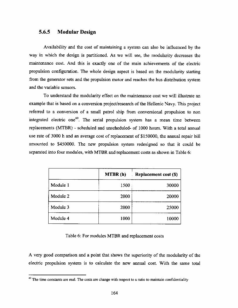
5.6.5 Modular Design
Availability and the cost of maintaining a system can also be influenced by the
way in which the design is partitioned. As we will see, the modularity decreases the
maintenance cost. And this is exactly one of the main achievements of the electric
propulsion configuration. The whole design aspect is based on the modularity starting
from the generator sets and the propulsion motor and reaches the bus distribution system
and the variable sensors.
To understand the modularity effect on the maintenance cost we will illustrate an
example that is based on a conversion project/research of the Hellenic Navy. This project
referred to a conversion of a small patrol ship from conversional propulsion to non
integrated electric one4 9. The serial propulsion system has a mean time between
replacements (MTBR) - scheduled and unscheduled- of 1000 hours. With a total annual
use rate of 3000 h and an average cost of replacement of $150000, the annual repair bill
amounted to $450000. The new propulsion system redesigned so that it could be
separated into four modules, with MTBR and replacement costs as shown in Table 6:
Table 6: For modules MTBR and replacement costs
A very good comparison and a point that shows the superiority of the modularity of the
electric propulsion system is to calculate the new annual cost. With the same total
49 The time constants are real. The costs are change with respect to a ratio to maintain confidentiality
164
MTBR (h) Replacement cost ($)
Module 1 1500 30000
Module 2 2000 20000
Module 3 2000 25000
Module 4 1000 10000
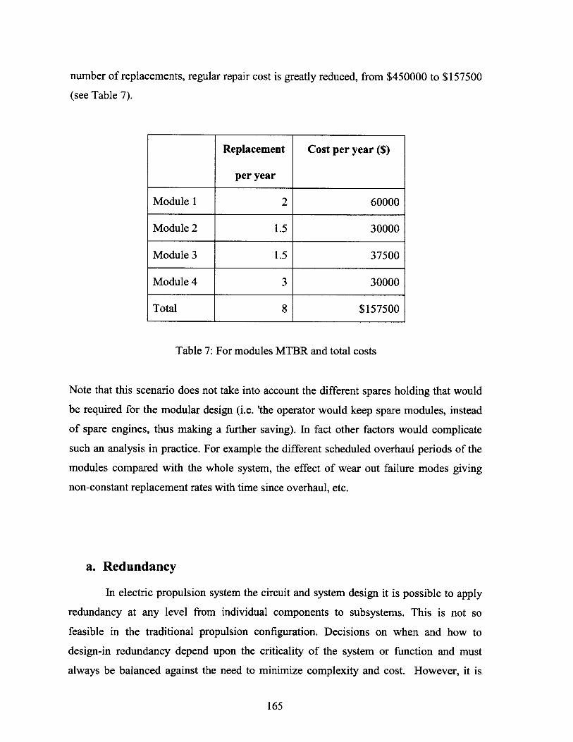
number of replacements, regular repair cost is greatly reduced, from $450000 to $157500
(see Table 7).
Table 7: For modules MTBR and total costs
Note that this scenario does not take into account the different spares holding that would
be required for the modular design (i.e. 'the operator would keep spare modules, instead
of spare engines, thus making a further saving). In fact other factors would complicate
such an analysis in practice. For example the different scheduled overhaul periods of the
modules compared with the whole system, the effect of wear out failure modes giving
non-constant replacement rates with time since overhaul, etc.
a. Redundancy
In electric propulsion system the circuit and system design it is possible to apply
redundancy at any level from individual components to subsystems. This is not so
feasible in the traditional propulsion configuration. Decisions on when and how to
design-in redundancy depend upon the criticality of the system or function and must
always be balanced against the need to minimize complexity and cost. However, it is
165
Replacement Cost per year ($)
per year
Module 1 2 60000
Module 2 1.5 30000
Module 3 1.5 37500
Module 4 3 30000
Total 8 $157500
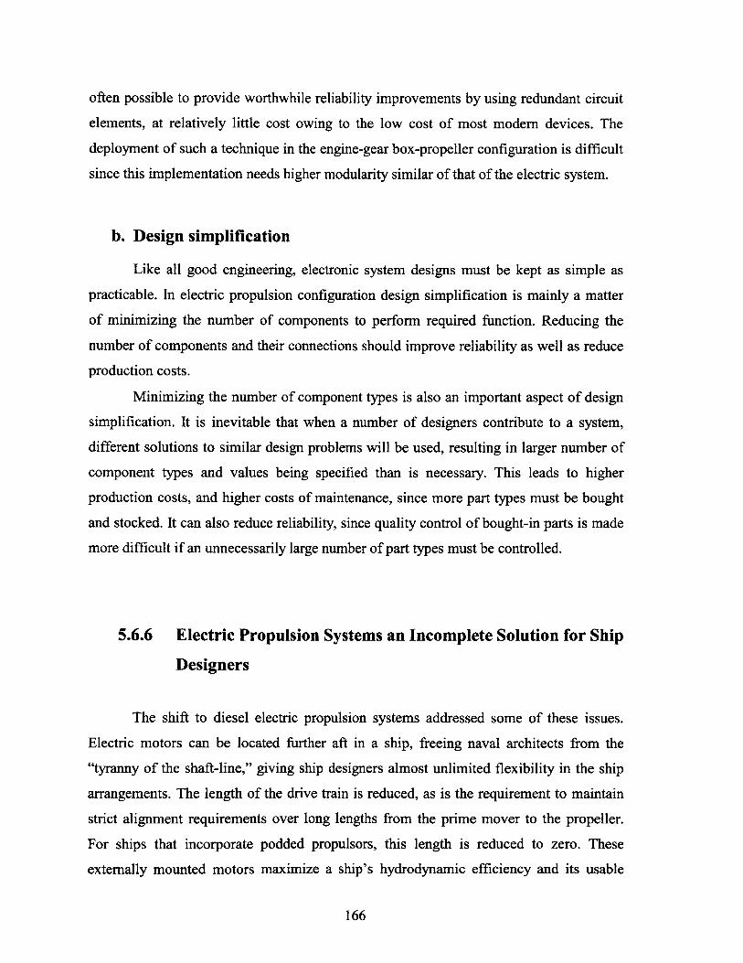
often possible to provide worthwhile reliability improvements by using redundant circuit
elements, at relatively little cost owing to the low cost of most modem devices. The
deployment of such a technique in the engine-gear box-propeller configuration is difficult
since this implementation needs higher modularity similar of that of the electric system.
b. Design simplification
Like all good engineering, electronic system designs must be kept as simple as
practicable. In electric propulsion configuration design simplification is mainly a matter
of minimizing the number of components to perform required function. Reducing the
number of components and their connections should improve reliability as well as reduce
production costs.
Minimizing the number of component types is also an important aspect of design
simplification. It is inevitable that when a number of designers contribute to a system,
different solutions to similar design problems will be used, resulting in larger number of
component types and values being specified than is necessary. This leads to higher
production costs, and higher costs of maintenance, since more part types must be bought
and stocked. It can also reduce reliability, since quality control of bought-in parts is made
more difficult if an unnecessarily large number of part types must be controlled.
5.6.6 Electric Propulsion Systems an Incomplete Solution for Ship
Designers
The shift to diesel electric propulsion systems addressed some of these issues.
Electric motors can be located further aft in a ship, freeing naval architects from the
"tyranny of the shaft-line," giving ship designers almost unlimited flexibility in the ship
arrangements. The length of the drive train is reduced, as is the requirement to maintain
strict alignment requirements over long lengths from the prime mover to the propeller.
For ships that incorporate podded propulsors, this length is reduced to zero. These
externally mounted motors maximize a ship's hydrodynamic efficiency and its usable
166
internal volume for revenue generation. Podded propulsors also reduce shipbuilding costs
through increased modularity during construction. Ships today tend to consume more
electricity than did their predecessors. Integrated electric propulsion systems optimize
ship operators' flexibility through the ability to only use the minimum amount of
electricity generation equipment for a given operational scenario.
Table 8: Podded propulsors Data
The generators may therefore be operated closer to their full outputs and
unneeded machines shut down, which increases the overall system efficiency and
minimizes maintenance requirements. It is because of advantages like these that nearly all
cruise ships and many other ship types including shuttle tankers, product carriers, ferries,
icebreakers, and offshore oil exploration platforms have made the transition to integrated
electric propulsion systems, in both in-hull and podded propulsion variants. Data for the
Podded propulsor are presented in Table 8. In addition, 13 navies of the world have either
modem electrically propelled ships, are already designing/constructing electrically
propelled ships, or have announced plans to initiate such programs. Prominent among
these is the U.S. Navy, which in 2000, announced that its next generation of surface
combatant ships will have electric propulsion systems.
Although they are an improvement over their predecessors, modem electric drives
still have not presented an ideal propulsion solution for shipbuilders across a wide range
of applications. Electric propulsion motors at higher power levels can be large and heavy,
which limits their flexibility in placement within the ship. In propulsion pod applications,
this large size and weight provide an upper bound to the pod's applicability, apparently
167
Manufacturer Product Largest in ServiceABB - KMY Azipod 19.5 MWAlstom - Kamewa Mermaid 21.5 MWSiemens-Schottel SSP 25 MW (design)
11 MW builtLIPS STN Atlas Marine Dolphin 19 MW (design)/ John Crane 7 MW built
around 20 MW. In addition, today's electric propulsion motors have significantly reduced
efficiencies at lower ship speeds, thereby failing to take best advantage of one of their
primary attributes - reduced fuel consumption when compared to low speed diesel
engines operated at low power levels.
5.6.7 Electric Propulsion Systems a Robust Solution for Ship
Designers
The advantages of diesel-electric systems are several. The reliability is superior.
The components in such systems are anticipated to work faultlessly in ten years. If one
diesel engine should be damaged, other engines will be used. In addition, the whole
machinery package is less space demanding, and may be placed on deck in such a way
that repairs and maintenance could be performed most easily. For some small vessels like
fishing boats this will increase the loading capacity substantially. All this adds up to
significant cost savings in addition to the savings in energy and environmental damages.
Improved maneuvering capabilities, more quiet operation and less vibration may also be
listed as operational advantages.
Summarizing the benefits we can say that the diesel electric system can be
distinguished from the followings:
* Survivability. The elimination of gear trains and propeller shafts, together with
the flexibility and modularity of electric systems will enable graceful degradation
and rapid reconfiguration of vital systems, thus enhancing survivability.
* Signature reduction and quieting. By eliminating the mechanical link between the
power plant and the propulsor (i.e., propeller), electric drive will enable reduction
of noise and vibration by allowing acoustic isolation of the engine generators.
* Improved operational flexibility and reliability. With the power station concept,
all power will be supplied by a set of prime movers that provide power to
propulsion, ship service, and other designated loads. This approach will provide
the flexibility to shift power between propulsion, ship service, and other electrical
loads, which cannot be done with a mechanical drive ship, and can enable
improved speed control.
168

* Increased flexibility and adaptability. Integrating electric power and propulsion
systems will provide flexibility in servicing other loads such as environmental
controls (air conditioning) and launch and recovery systems, electric armor, high-
power advanced electronics, and electric weapons.
* More space available. Eliminating gears and shafts from the propulsion system
will make more space available for other uses. Also, the prime mover will no
longer be tied to the propeller shaft line, and the power sources can be distributed
throughout the ship as necessary.
* Reduced manning. Digital control and automation, which will be an integral part
of ship electrification, will reduce the requirements for human operators (in
machinery spaces, for example).
* Reduced logistics. Common power and propulsion modules can be used across
the fleet.
* Reduced costs. Commercial technology appears likely to be available for many of
the system elements.
* Life-cycle cost and fuel-consumption savings. Overall fuel efficiency can be
improved if a ship is able to operate at varying speeds over a substantial part of its
operational profile, and variable speed propulsion will be enabled by electric
drive.
169
5.7 Market Option
As described, with an electric propulsion system electrical motors turn the ship
propellers. Diesel or Gas Turbine electric systems are considered to represent a huge and
substantial growth potential. The diesel-electric systems offered today have several
advantages compared to conventional systems. The diesel-electric systems add value to
the customers by energy saving and flexibility, higher reliability, increased safety,
decrease in stress level on motors and grid, reduced emission, quiet operation, soft starts
on heavy machinery and better utilization of space.
The target market consists of specialist vessels where propulsion and positioning
are complex and critical to operation. Offshore supply vessels, standby vessels, anchor
handling vessels, ferries, smaller cruise ships, fishing vessels and seismic vessels are
typical examples where the energy savings from diesel electric propulsion systems are
substantial. Annual energy savings of 10% (less positioning and maneuvering) up to 30%
(much positioning and maneuvering) gives, in addition to the operational advantages of
diesel-electric systems, a favorable pay-back time, i.e. on average 2-4 years, for the
customers.
From a customer's point of view, the economical advantage in energy saving from
a diesel electric system may be converted to an increase in the customer's overall
investment capacity. For instance, assuming a rate of return of say 10% in perpetuity, the
"economical value" of an energy savings of say USD 350,000 will be USD 3.5 million (USD 350,000/0.10 = USD 3.5 million)
An accurate comparison of the different concepts should be accomplished by use
of a Life Cycle Cost assessment. There are several ways to do this, and Norsok [3] has
suggested a method, intended for use in offshore industry, but it can also be applied for
ships. The main elements of the LCC are divided in CAPEX (Capital Expenditures) and
OPEX (Operation Expenditures), and are listed in Table 9.
Although a life cycle cost of the complete vessel and its operations ought to be
done for a fair and precise comparison of different concepts, this is not feasible mainly
because of lack of competence, lack of reliable data or lack of time and resources at this
170
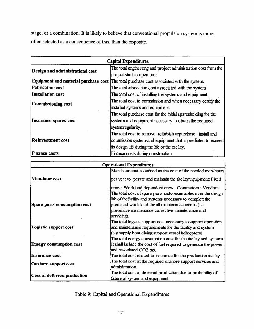
stage, or a combination. It is likely to believe that conventional propulsion system is more
often selected as a consequence of this, than the opposite.
Capital Expenditures
Design and administrationd cost
Equipment and material purchase costFabrication costInstallation cost
Commissioning cost
Insurance spares cost
Reinvestment cost
Finance costs
Man-hour cost
Spare parts consumption cost
Logistic support cost
Energy consumption cost
Insurance cost
Onshore support cost
Cost of deferred production
The total engineering and project administration cost from theproject start to operation.The total purchase cost associated with the system.The total fabrication cost associated with the systemThe total cost of installing the systems and equipment.The total cost to commission and when necessary certify theinstalled systems and equipment.The total purchase cost for the initial sparesholding for thesystems and equipment necessary to obtain the requiredsystemregularity.The total cost to remove refurbish orpurchase install andcommission systemsand equipment that is predicted to exceedits design life during the life ofthe facility.Finance costs during construction
Man-hour cost is defined as the cost of the needed man-hours
per year to perate and maintain the facility/equipment: Fixed
crew.- Workload dependent crew.- Contractors.- Vendors.The total cost of spare parts andconsumables over the designlife of thefacility and systems necessary to completethepredicted work load for all maintenanceactions (ie.preventive maintenance corrective maintenance andservicing).The total logistic support cost necessary tosupport operationand maintenance requirements for the facility and system(e.g.supply boat diving support vessel helicopters)The total energy consumption cost for the facility and systems.It shall include the cost of fuel required to generate the powerand associated C02 tax.The total cost related to insurance for the production facility.The total cost of the required onshore support services andadministration.The total cost of deferred production due to probability offailure of system and equipment.
Table 9: Capital and Operational Expenditures
171
Operational Expenditures
REFERENCES
Chapter 2
[1] H. Gohen, G.F.C. Rogers, H.I.H. Saravanamutto, "Gas Turbine Theory", 2nd edition,
Longman
[2] E.T.Vincent "Theory and Design of Gas Turbines and Jet Engines", Chap. XVIII,
McGraw-Hill, 1950
[3] Hawthorne W.R. "Elements of turbine and compressor theory"
[4] H.I.H. Saravanamutto and A.J. Fawke "Simulation of the Gas Turbine dynamic
performance" ASME 70-GT-23, 1970.
Chapter 3
[1] Shayler, P.J., Davies, M.T., Colechin, M.J.F., "Intake Port Fuel Transport and
Emissions: The Influence of Injector Type and Fuel Composition," SAE Paper
961996(1996).
[2] Bossert, J.C., Shin, Y., Cheng, W.K., "Fuel Effects on Throttle Transients in PFI
Spark Ignition Engines," SAE Paper 971613 (1997).
[3] Shayler, P.J., Teo, Y.C., Scarisbrick, A., "Fuel Transport Characteristics of Spark
Ignition Engines for Transient Fuel Compensation," SAE Paper 950067 (1995).
[4] Russ, S., Stevens, J., Aquino, C.F., Curtis, E.W., Fry, J., "The Effects of Injector
Targeting and Fuel Volatility on Fuel Dynamics in PFI Engine During Warm-UP:
Part I-Experimental Results," SAE Paper 982518 (1998).
172
[5] I. Kitsopanidis "Fuel Targeting and Thermal Environment Effects on Spark Ignition
Engine Mixture Separation Process" Master Thesis, MIT, MECHANICAL
ENGINEERING Dept.
[6] Nagao F. and Hirako Y." Estimation of the Operating Characteristics of a
Turbocharged Four-cycle Diesel Engine",Buletting of JSME ,vol. 2, No 7,1959 ,pp 41-62
[7] John B. Heywood, "Internal Combustion Engines Fundamentals" McGraw Hill,
London, 1988
Chapter 4
[1] Fitagerald, Kingsley, and Umans, Electric Machinery, 5th Edition, McGraw-Hill
[2] Price, W.W., Chiang, H.D., Clark, H.K., Concordia, C., Lee, D.C., Hsu, J.C., Ihara,
S.,King, C.A., Lin, C.J., Mansour, Y., Srinivasan, K., Taylor, C.W. and Vaahedi, E.:Load
Representation for Dynamic Performance Analysis. IEEE Task Force Report. IEEE
Trans.Power Sys 8(2) (1993), pp.4 7 2 -4 82 .
[3] C. Concordia, S. Ihara, "Load Representation in Power System Stability Studies",
IEEE Trans. PAS-101 pp.969-977, 1982
[4] I. Kioskeridis, N. Margaris:"Loss Minimization in Induction Motor Adjustable-Speed
Drives", IEEE Trans. Ind. Elec. vol. 43 No 1, 1996.
[5]Ordys, A.W. Pike, A.W. Johnson, M.A. Katebi, R.M and Grimble, M.J.: Modelling
and Simulation of Power Generation Plants. Advances in Industrial Control, Springer-
Verlag, 1994
173

[6] S. D. Umans and H. L. Hess: "Modeling and analysis of the Wanlass three-phase
induction motor configuration", IEEE Trans. Power Apparatus, vol. PAS-102, no-9,
pp.2912-2926, 1983.
[7] P. C. Krause: "Analysis of Electric Machinery", New York, McGraw-Hill, 1986.
[8] Ch. Mademlis, N. Margaris:"Loss minimization in Vector Controlled Interior
permanent-Magnet Synchronous Motor drives. ", IEEE Trans. Ind. Elec., vol. 42, 2002.
[9] Hashem Oraee: "Three-Phase Induction Motors", Worcester Polytechnic Institute
[10] A.Abbodanti "Method of Flux Control in Induction Motor Driven by Variable
Frequency, Variable Voltage supplies," Adjustable speed AC Drive systems, B. K. Bose
Ed., Piscataway, NJ: IEEE Press.
Chapter 5
[1] Friedman, N., US Destroyers, An Illustrated Design History, Naval Institute Press,
Annapolis, MD, 1982
[2] Moore, J., Jane's Fighting Ships 1984-1985, Jane's Publishing, London, England,
1984
[3] Norsok NORSOK STANDARDS http://www.nts.no/norsok
174
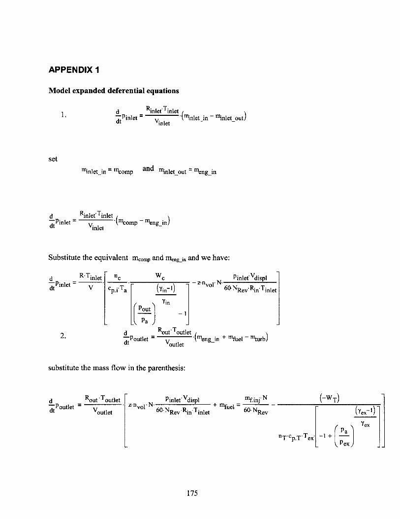
APPENDIX 1
Model expanded deferential equations
1. d riniet R inlet.T inlet in - * out).- pinlet = v -(niet_i- niinlet_ut
dt Vinlet
set
Iinlet-in = mcomp and minletout = nengin
d RinletTinietdrinlet - V* -*(mcomp - mfeng-in)et Vinlet
Substitute the equivalent mcomp and meng in and we have:
d R-Tinlet
dt net V
2.
nc Wc Pinlet-Vdisplc -*a(y~i - z-n -01 N-
c, -T1 6nvo 6NReVRin-TinletYin
Pa
d RoutToutlet .mni-put - To= '(eng_in + n"fuel - " rb)dt Voutlet
substitute the mass flow in the parenthesis:
d Rout -Toutlet
doutlet Voutlet
Pinlet Vdispl nf. inj.Nz-nvol.N. 60.NRevRnTinlet + fuel = 60- NRev
(-WT)
nT.cp.T-Tex - +
(Yex~
YexPa
SPex)
175
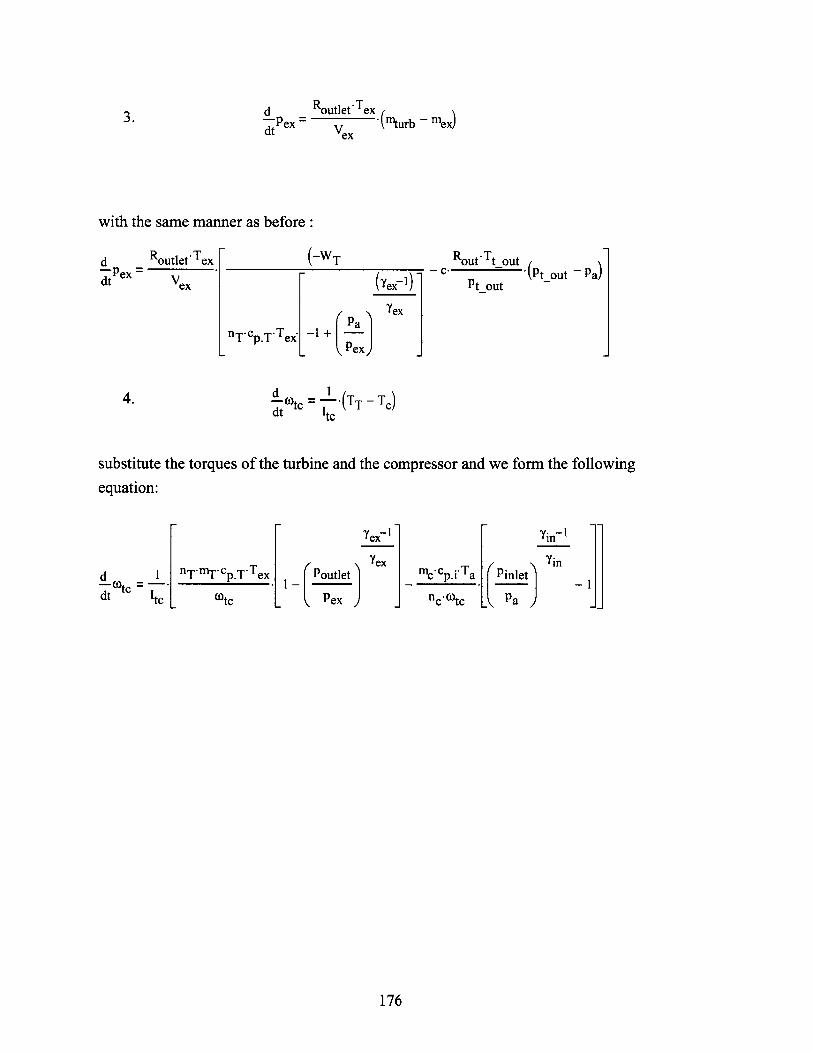
3 . d Routet-Tex3-pex= v '("\urb~-mex)
dt Vex
with the same manner as before:
d Routlet Tex-- Pex = Vedt Vex
(-WT
n TCp.T-Tex-
(ye,-l) -
texPa
-1+ -Pex)
Rout-Tt out (Pt out
Pt_out
dtc .(TT - TC)dt Itc
substitute the torques of the turbine and the compressor and we form the following
equation:
d 1nT.m.cp.TTex- t = *j lOtdt L "c _
Yex- 1
YexPoutlet
Pex )
flcp.i-Ta Pinlet
nc.*tc K Pa
176
Pa)
4.
Yin- 1
Yin
- i
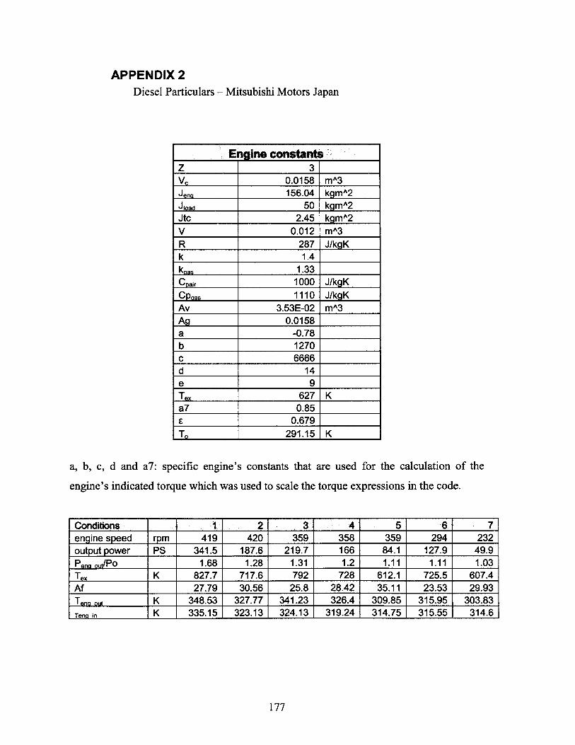
APPENDIX 2Diesel Particulars - Mitsubishi Motors Japan
E gine constantZ 3
V_ 0.0158 mA3
Jena 156.04 kgmA2JIoad 50 kgmA2Jtc 2.45 kgmA2V 0.012 mA3
R 287 J/kgKk 1.4kaps 1.33
Cpair 1000 J/kgK
Cpaas 1110 J/kgKAv 3.53E-02 mA3
Ag 0.0158a -0.78b 1270c 6666d 14e 9Tex 627 K
a7 0.85
E 0.679
To 291.15 K
a, b, c, d and a7: specific engine's constants that are used for the calculation of the
engine's indicated torque which was used to scale the torque expressions in the code.
Conditions 1 2 3 4 5 6 7engine speed rpm 419 420 359 358 359 294 232output power PS 341.5 187.6 219.7 166 84.1 127.9 49.9Pen out/PO 1.68 1.28 1.31 1.2 1.11 1.11 1.03Tex K 827.7 717.6 792 728 612.1 725.5 607.4Af 27.79 30.56 25.8 28.42 35.11 23.53 29.93Tena out K 348.53 327.77 341.23 326.4 309.85 315.95 303.83-Teng in K 335.15 323.13 324.13 319.24 314.75 315.55 314.6
177

APPENDIX 3
The matrix form of the state space equation will be:
dtdt ' = IF()T + A-I + E-ug9 + .Uf
Using the equations the following equations in the matrix form we will have:
Wd = -xd- id + ikd + if
Wq = -xq-iq + iq
'Vkd = - Gkd) Xdid + ikd + 9kd'if
'Vkq = - Gkq) Xqdq + iq
Vf= -(i ~f) Xdd + 9f'kd+ if
matrix form
-xd
0
-( -kd) xd
( -(1
-- of) xd
0 1 0 1
-xq 0 1 0
0 1 0 kd
Gkq)Xq 0 1 0
0 gf 0 1
if we call the matrix in the middle A then :
-xd
0
-(1-akd) Xd
0 -(1
-(1 - fa) Xd
0 1 0 1
-Xq 1 0
0 1 0 kd
-kq) Xq 0 1 0
0 g 0 1
As we know T = A A this means that
(
Vkd
Vkq
'Vf
/
iq'q
'kd
tkq
iy
A
1= A- 1.
178
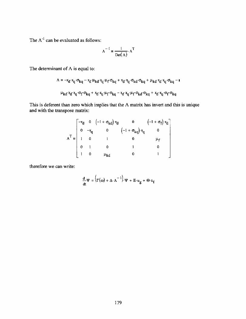
The A 1 can be evaluated as follows:
A-1 1 TA AT
Det(A)
The determinant of A is equal to:
A = -xd'xq'akq - xd*'kd'xq*9f akq + xd'xq*akd*akq + gkd'Xd'Xq*Gkq -
gkd'xd'xq*Of Gkq + xd'Xq4fGkq - xd'xq*9f Ukd'5kq + xd'Xq*Gf Okq
This is deferent than zero which implies that the A matrix has invert and this is uniqueand with the transpose matrix:
-xd 0 (-1 + Ckd)-Xd 0 (-i + Gf).xd
0 -Xq 0 (-1 + Gkq).xiq
1 0 1
0 1
1 0
0
pkd
0
1
0
0
9 f
0
1
therefore we can write:
d'P - (F(o) + A.A~ -t + E-ug + e.ufdt
179
A =
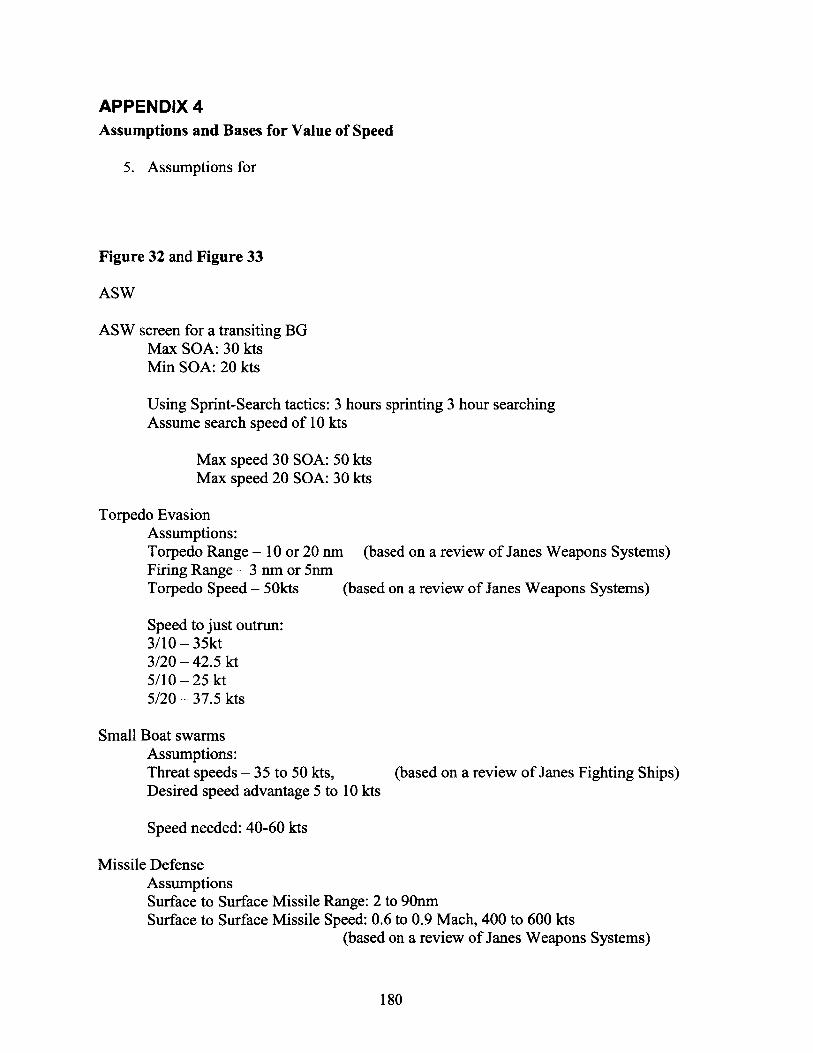
APPENDIX 4Assumptions and Bases for Value of Speed
5. Assumptions for
Figure 32 and Figure 33
ASW
ASW screen for a transiting BGMax SOA: 30 ktsMin SOA: 20 kts
Using Sprint-Search tactics: 3 hours sprinting 3 hour searchingAssume search speed of 10 kts
Max speed 30 SOA: 50 ktsMax speed 20 SOA: 30 kts
Torpedo EvasionAssumptions:Torpedo Range - 10 or 20 nm (based on a review of Janes Weapons Systems)Firing Range - 3 nm or 5nmTorpedo Speed - 50kts (based on a review of Janes Weapons Systems)
Speed to just outrun:3/10 - 35kt3/20 - 42.5 kt5/10 - 25 kt5/20 - 37.5 kts
Small Boat swarmsAssumptions:Threat speeds - 35 to 50 kts, (based on a review of Janes Fighting Ships)Desired speed advantage 5 to 10 kts
Speed needed: 40-60 kts
Missile DefenseAssumptionsSurface to Surface Missile Range: 2 to 90nmSurface to Surface Missile Speed: 0.6 to 0.9 Mach, 400 to 600 kts
(based on a review of Janes Weapons Systems)
180
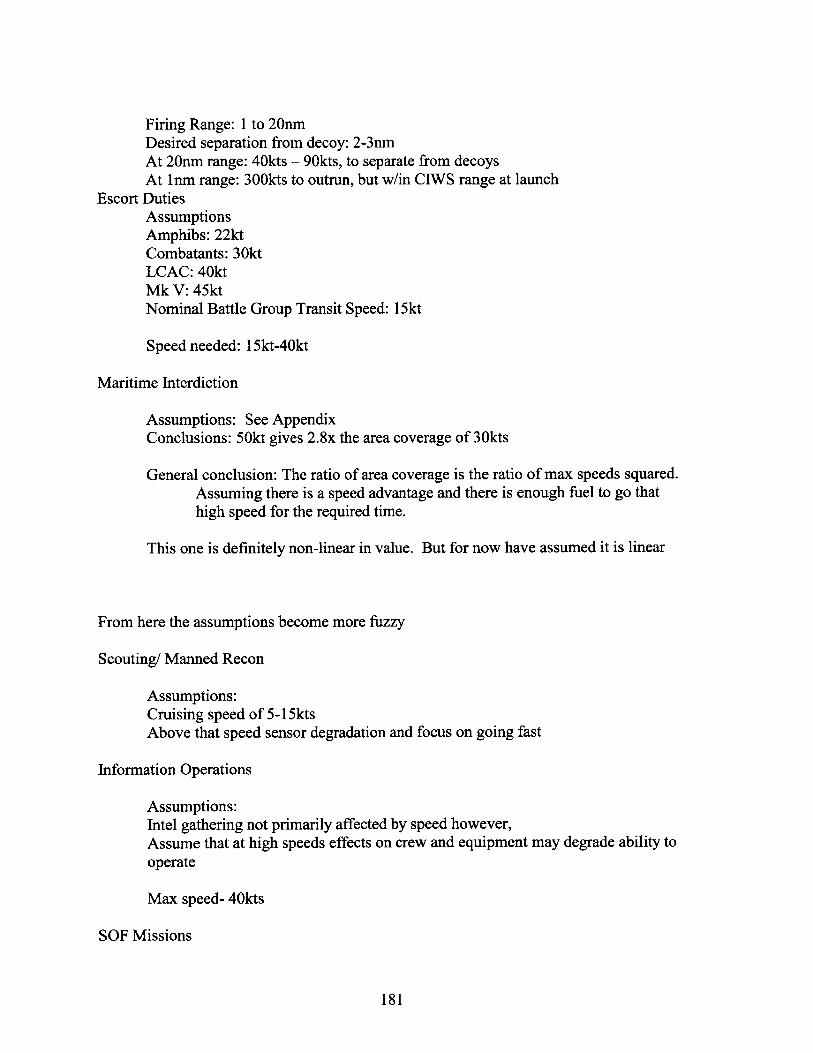
Firing Range: 1 to 20nmDesired separation from decoy: 2-3nmAt 20nm range: 40kts - 90kts, to separate from decoysAt lnm range: 300kts to outrun, but w/in CIWS range at launch
Escort DutiesAssumptionsAmphibs: 22ktCombatants: 30ktLCAC: 40ktMk V: 45ktNominal Battle Group Transit Speed: 15kt
Speed needed: 15kt-40kt
Maritime Interdiction
Assumptions: See AppendixConclusions: 50kt gives 2.8x the area coverage of 30kts
General conclusion: The ratio of area coverage is the ratio of max speeds squared.Assuming there is a speed advantage and there is enough fuel to go thathigh speed for the required time.
This one is definitely non-linear in value. But for now have assumed it is linear
From here the assumptions become more fuzzy
Scouting/ Manned Recon
Assumptions:Cruising speed of 5-15ktsAbove that speed sensor degradation and focus on going fast
Information Operations
Assumptions:Intel gathering not primarily affected by speed however,Assume that at high speeds effects on crew and equipment may degrade ability tooperate
Max speed- 40kts
SOF Missions
181
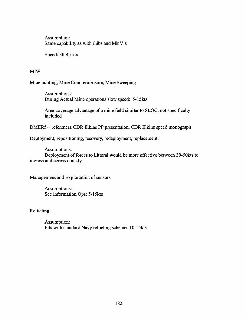
Assumption:Same capability as with rhibs and Mk V's
Speed: 30-45 kts
MIW
Mine hunting, Mine Countermeasure, Mine Sweeping
Assumptions:During Actual Mine operations slow speed: 5-15kts
Area coverage advantage of a mine field similar to SLOC, not specificallyincluded
DMER5-references CDR Elkins PP presentation, CDR Elkins speed monograph
Deployment, repositioning, recovery, redeployment, replacement:
Assumptions:Deployment of forces to Littoral would be more effective between 30-50kts to
ingress and egress quickly
Management and Exploitation of sensors
Assumptions:See information Ops: 5-15kts
Refueling
Assumption:Fits with standard Navy refueling schemes 10-1 5kts
182
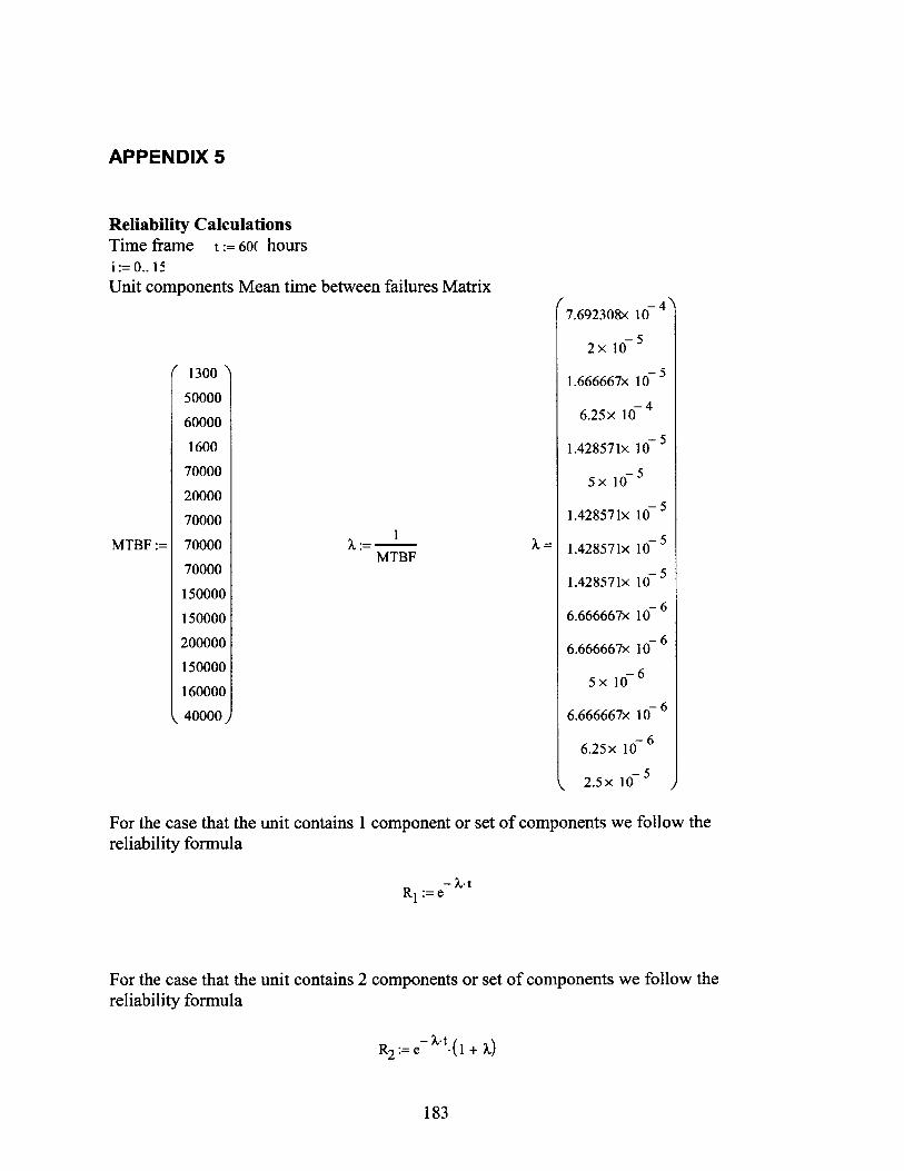
APPENDIX 5
Reliability CalculationsTime frame t:= 60( hoursi:= 0.. 15Unit components Mean time between failures Matrix
1300
50000
60000
1600
70000
20000
70000
MTBF:= 70000 :MTBF
70000
150000
150000
200000
150000
160000
(40000)
7.692308x 16-
2x 10⁵
1.666667x 10⁻⁵
6.25x 10
- 51.428571x 10-
5x 10⁵
1.428571x 10 5
1.428571x 10-
1.428571x 10
6.666667x 10 6
6.666667x 1O 6
-65x 10
6.666667x I-6
6.25x 1- 6
- 52.5x 10
For the case that the unit contains 1 component or set of components we follow thereliability formula
Rl:= e -)-t
For the case that the unit contains 2 components or set of components we follow thereliability formula
R2 :=e- +-t
183
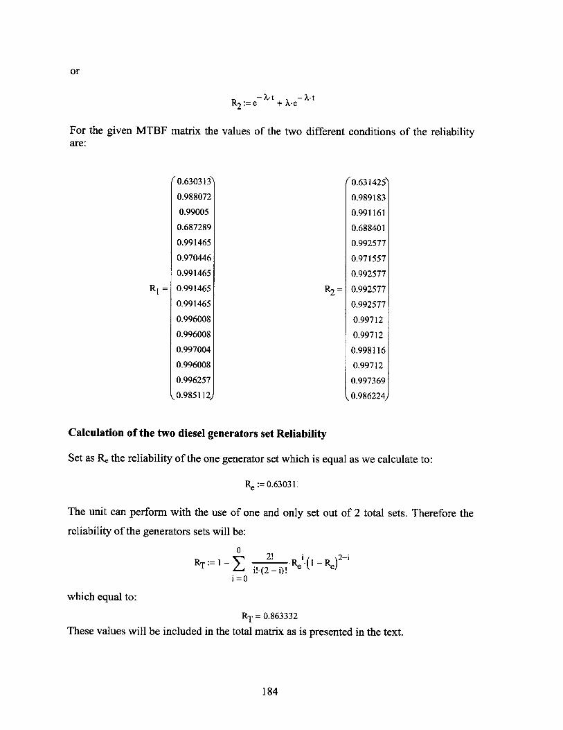
or
- X-t + X-tR2 :=e + X-e
For the given MTBFare:
R, =
matrix the values of the two different conditions of the reliability
0.630313'
0.988072
0.99005
0.687289
0.991465
0.970446
0.991465
0.991465
0.991465
0.996008
0.996008
0.997004
0.996008
0.996257
(0.985112)
0.631425
0.989183
0.991161
0.688401
0.992577
0.971557
0.992577
0.992577
0.992577
0.99712
0.99712
0.998116
0.99712
0.997369
0.986224)
Calculation of the two diesel generators set Reliability
Set as R the reliability of the one generator set which is equal as we calculate to:
Re:= 0.6303 1
The unit can perform with the use of one and only set out of 2 total sets. Therefore the
reliability of the generators sets will be:
0RTi= I - 2! R."O - Re)2-iEiP-(2 - i)!
i = 0
which equal to:
RT = 0.863332
These values will be included in the total matrix as is presented in the text.
184
R2 =

185


![arXiv:2109.09979v1 [cs.SI] 21 Sep 2021](https://img.dokumen.tips/doc/110x75/6333e926a6138719eb0ad5d8/arxiv210909979v1-cssi-21-sep-2021.jpg)


![arXiv:2103.13885v3 [cs.LG] 15 Sep 2021](https://img.dokumen.tips/doc/110x75/63342ebe62e2e08d49028405/arxiv210313885v3-cslg-15-sep-2021.jpg)
![arXiv:2011.12631v3 [cs.CL] 27 Sep 2021](https://img.dokumen.tips/doc/110x75/633dcfa01fccc5e0f302d212/arxiv201112631v3-cscl-27-sep-2021.jpg)


![arXiv:2109.14097v1 [cs.SE] 28 Sep 2021](https://img.dokumen.tips/doc/110x75/6327791acedd78c2b50d9764/arxiv210914097v1-csse-28-sep-2021.jpg)

![arXiv:2009.02429v2 [cs.CV] 14 Sep 2020](https://img.dokumen.tips/doc/110x75/633626cc62e2e08d49035eb0/arxiv200902429v2-cscv-14-sep-2020.jpg)


![arXiv:2109.10037v1 [math.AG] 21 Sep 2021](https://img.dokumen.tips/doc/110x75/63338f933108fad7760f1c1a/arxiv210910037v1-mathag-21-sep-2021.jpg)


