Sensitivity Analysis of the Greedy Heuristic forBinary Knapsack Problems

Diptesh Ghosh∗ Nilotpal Chakravarti† Gerard Sierksma‡

SOM-theme A Primary Processes within Firms

Abstract

Greedy heuristics are a popular choice of heuristics when we have to solvea large variety ofNP-hard combinatorial problems. In particular for binaryknapsack problems, these heuristics generate good results. If some uncertaintyexists beforehand regarding the value of any one element in the problem data,sensitivity analysis procedures can be used to know the tolerance limits withinwhich the value may vary will not cause changes in the output. In this paper weprovide a polynomial time characterization of such limits for greedy heuristicson two classes of binary knapsack problems, namely the 0-1 knapsack problemand the subset sum problem.

We also study the relation between algorithms to solve knapsack problems andalgorithms to solve their sensitivity analysis problems, the conditions underwhich the sensitivity analysis of the heuristic generates bounds for the toler-ance limits for the optimal solutions, and the empirical behavior of the greedyoutput when there is a change in the problem data.

Keywords:Sensitivity Analysis, Heuristics, Knapsack ProblemsAMS Subject Classification: 90C31

∗ Corresponding author, Faculty of Economic Sciences, University of Groningen, The Netherlands (onleave from the Indian Institute of Management Lucknow, India)

† Singapore Airlines, Singapore

‡ Faculty of Economic Sciences, University of Groningen, The Netherlands

1

1. Introduction

Binary knapsack problems are among some of the most widely studied problems incombinatorial optimization (see, for example, Martello and Toth [6]). Algorithms tosolve a large variety of combinatorial problems, such as capital budgeting, cargo load-ing, and vehicle routing, either reduce to solving knapsack problems, or solve a largenumber of such problems en route to their solutions. Since the optimization versions ofthese problems areNP-hard, practical solution techniques do not ask for optimality,but are heuristics that generate feasible, suboptimal solutions.ε-optimal heuristics forma special class of heuristics for which, in case of maximization problems, the objectivefunction values of the solutions output are greater than(1−ε) times those of the optimalsolution.

Heuristics are usually compared on their execution speeds and quality of solutions (ei-ther empirically, or probabilistically, or using their worst case performance results), butrecently some work has been done on the effect of perturbations in problem data on theperformance of the heuristics (see, for example, Chakravarti and Wagelmans [2], andKolen et al. [5]). This body of work is referred to as the sensitivity analysis of heuris-tics. Although sensitivity analysis of optimal solutions to combinatorial optimizationproblems is an established problem (see, for example, Gal and Greenberg [3]), sensitiv-ity analysis ofε-optimal heuristics is not. In Wagelmans [8] the following definition forsensitivity analysis of heuristics is suggested.

Problem SA-WagelmansInput An instanceI of a combinatorial optimization problem, anε-optimal

heuristicH and a solutionS to I underH.Output For each problem parameterp the following values

• βWp = sup{δ|S remainsε-optimal underH whenp → p + δ}

• αWp = sup{δ|S remainsε-optimal underH whenp → p − δ}

In Wagelmans [8] it is shown that this problem isNP-hard when the underlying com-binatorial optimization problem isNP-hard, even when the heuristic is of polynomialcomplexity. In this paper, we study the following related problem.

Problem SA-HeuristicInput An instanceI of a combinatorial optimization problem, a heuristicH and a

solutionS to I underH.Output For each problem parameterp the following values

• βHp = sup{δ|S remains the heuristic output whenp → p + δ}

• αHp = sup{δ|S remains the heuristic output whenp → p − δ}

We refer toβp andαp respectively as the upper and lower tolerance limits of the pa-rameterp. We agree with Wagelmans [8] that this is indeed not the sensitivity analysis

2

of the heuristic solution, but rather of the heuristic method. However, it is easy to seethatβW

p ≥ βHp andαW

p ≥ αHp .

In this paper we consider two types of binary knapsack problems, the 0-1 knapsackproblem and the subset sum problem.

The 0-1 knapsack problem can be described as follows.

Problem KP{[ej ]|c}Instance : An integern ≥ 2, a setE of n elementsej =< pj,wj >, j = 1, . . . , n

wherepj,wj are positive integers. A positive integerc.Output : A subsetE1 of E such that

∑ej∈E1

wj ≤ c, and∀E2 ⊆ E with

∑ej∈E2

wj ≤ c,∑

ej∈E1pj ≥ ∑

ej∈E2pj.

An integer programming formulation of the problem is the following.

Maximize∑n

j=1 pjxj subject to∑n

j=1 wjxj ≤ c, xj ∈ {0, 1} for j = 1, . . . , n. (KP)

We assume that allpj’s, wj’s and c are positive integers,wj ≤ c for j = 1, · · · , n;∑nj=1 wj ≥ c; and thatp1

w1≥ p2

w2≥ · · · ≥ pn

wn.

The subset sum problem is a special case of KP in whichpj = wj for j = 1, . . . , n. Thisproblem has various practical applications, for example in the analysis of coalitions invoting games (see Chakravartiet al. [1]). This problem can be stated in the followingmanner.

Problem SS{[ej ]|c}Instance : An integern ≥ 2, a setE of n elementsej, each associated with a positive

integerwj, j = 1, . . . , n. A positive integerc.Output : A subsetE1 of E such that

∑wj∈E1

wj ≤ c, and∀E2 ⊆ E with

∑wj∈E2

wj ≤ c,∑

wj∈E1wj ≥ ∑

wj∈E2wj.

The integer programming formulation for this problem is as follows.

Maximize∑n

j=1 wjxj subject to∑n

j=1 wjxj ≤ c, xj ∈ {0, 1} for j = 1, . . . , n. (SS)

We assume that allwj’s and c are positive integers,wj ≤ c for j = 1, · · · , n;∑n

j=1 wj ≥c; and thatw1 ≥ w2 ≥ · · · ≥ wn.

An interesting fact may be noted here. SS is a special case of KP, and any algorithmfor solving KP instances can be easily modified to solve SS instances (by providingwj values instead of thepj values as input). However the sensitivity analysis problemsfor KP and SS are not similarly related, and it is not easy to modify an algorithm forcalculating the tolerance limits for KP instances to output the tolerance limits for SAinstances (or vice versa). The reason for this is the following. When a particularwj

value changes in a SS instance, it affects both the constraint and the objective function.In case of KP instances, such a change would only affect the constraint. Again, when

3

a particularpj value changes in a KP instance, only the objective function is affected.This has no parallel in SS instances. Suppose we have an algorithm designed to outputtolerance limits for KP instances. For this algorithm, calculating tolerance limits forwj

values in SS instances would amount to handling simultaneous changes in two problemparameters (thewj valueand the correspondingpj value) — something the algorithm isnot designed to do. If we have an algorithm for calculating tolerances for SS instances,and if we want to use it to calculate the tolerance limit for apj value in a KP instance,the algorithm would be expected to handle a situation where the objective functionchanges but not the constraint. An algorithm to calculate tolerances for SS instances isnot designed to handle such cases.

In this paper, we will concentrate on the greedy heuristic. The greedy heuristic worksin the following manner. It assumes a prior ordering of the elements inE. (We willrefer to this ordering as theinput orderingin the remainder of the paper.) The heuristicconsiders the elements (ej’s) one at a time and decides whether it can be added toE1

without violating the constraint. If it can, the heuristic addsej to E1. The heuristic stopswhen there are no more elements to consider. We will refer to the output of the greedyheuristic as thegreedy solution. In this paper we will assume the input ordering of theelements ofE to be a non-increasing order ofpj

wjratios for KP instances and a non-

increasing order ofwj values for SS instances.

We will now explain some notations that we use in this paper.X = {xj} denotes asolution to an instance of KP or SS.XH = {xH

j } refers to the greedy solution andX∗ = {x∗

j} to the optimal solution for the instance. The objective function value of a

solutionX is denoted byzX. We useZH andZ∗ to denote the objective functions of thegreedy heuristic and any exact algorithm. Notice thatzX, ZH andZ∗ are all functions ofthe problem parameters (pj, wj andc for KP instances, andwj andc for SS instances).We also need to differentiate betweenzXH

andzX∗on one hand andZH andZ∗ on the

other.zXHandzX∗

are in a sense,tied to the solutionsXH andX∗ respectively. If the datain the instance changes sufficiently,XH may cease to remain the solution output by thegreedy heuristic and the previously optimalX∗ may become sub-optimal butzXH

andzX∗

will still reflect the objective function values of these solutions.ZH andZ∗ howeverwill change and store the objective function values of thenewgreedy solution, and thenewoptimal solution respectively. We will use the superscript∗ to denote the tolerancelimits of optimal solutions. For instanceβ∗

c denotes the maximum amount by which theparameterc can vary without affecting the optimality ofX∗.

The remainder of the paper is organized as follows. In Section 2 we characterize thetolerance limits output by SA-Heuristic for KP and SS, i.e. theβH andαH values. InSection 3 we analyze the characteristics ofZH andZ∗, and illustrate their behaviourwith as a function of changes in the values of certain problem parameters. It may appear

4

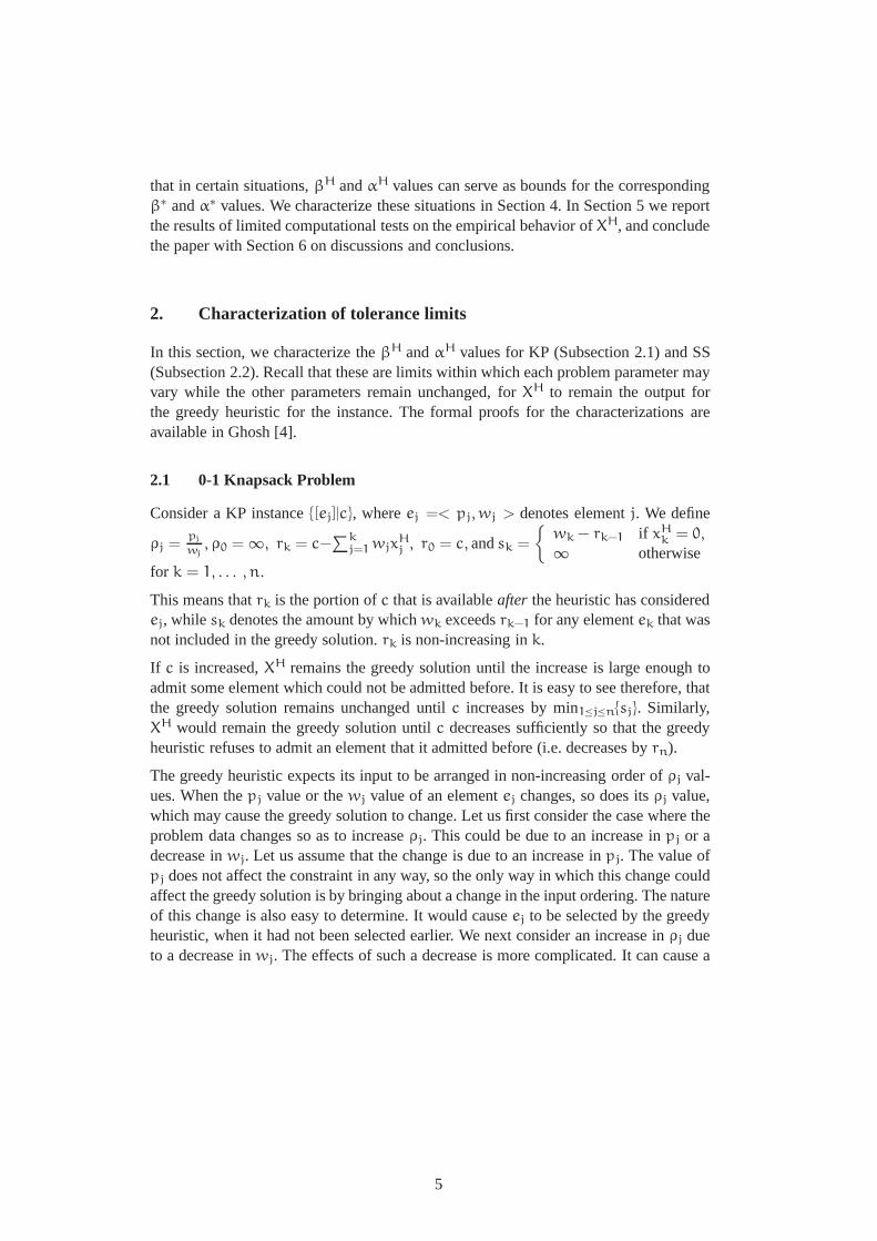
that in certain situations,βH andαH values can serve as bounds for the correspondingβ∗ andα∗ values. We characterize these situations in Section 4. In Section 5 we reportthe results of limited computational tests on the empirical behavior ofXH, and concludethe paper with Section 6 on discussions and conclusions.

2. Characterization of tolerance limits

In this section, we characterize theβH andαH values for KP (Subsection 2.1) and SS(Subsection 2.2). Recall that these are limits within which each problem parameter mayvary while the other parameters remain unchanged, forXH to remain the output forthe greedy heuristic for the instance. The formal proofs for the characterizations areavailable in Ghosh [4].

2.1 0-1 Knapsack Problem

Consider a KP instance{[ej]|c}, whereej =< pj,wj > denotes elementj. We define

ρj =pj

wj, ρ0 = ∞, rk = c−

∑kj=1 wjx

Hj , r0 = c, andsk =

{wk − rk−1 if xH

k = 0,∞ otherwisefor k = 1, . . . , n.

This means thatrk is the portion ofc that is availableafter the heuristic has consideredej, while sk denotes the amount by whichwk exceedsrk−1 for any elementek that wasnot included in the greedy solution.rk is non-increasing ink.

If c is increased,XH remains the greedy solution until the increase is large enough toadmit some element which could not be admitted before. It is easy to see therefore, thatthe greedy solution remains unchanged untilc increases by min1≤j≤n{sj}. Similarly,XH would remain the greedy solution untilc decreases sufficiently so that the greedyheuristic refuses to admit an element that it admitted before (i.e. decreases byrn).

The greedy heuristic expects its input to be arranged in non-increasing order ofρj val-ues. When thepj value or thewj value of an elementej changes, so does itsρj value,which may cause the greedy solution to change. Let us first consider the case where theproblem data changes so as to increaseρj. This could be due to an increase inpj or adecrease inwj. Let us assume that the change is due to an increase inpj. The value ofpj does not affect the constraint in any way, so the only way in which this change couldaffect the greedy solution is by bringing about a change in the input ordering. The natureof this change is also easy to determine. It would causeej to be selected by the greedyheuristic, when it had not been selected earlier. We next consider an increase inρj dueto a decrease inwj. The effects of such a decrease is more complicated. It can cause a

5

change in the input ordering. Even if it does not, it will increaserk values for allk ≥ j

and decreasesk values for allk ≥ j if xHj = 1. If xH

j = 0, only sj will decrease. These

changes may affect the greedy solution in a variety of ways. IfxHj = 1, the decrease

could cause thesk value of some elementek, k ≥ j to reduce to 0, thus including it inthe greedy solution. IfxH

j = 0, the decrease insj or the new position ofej in the input

ordering could setxHj to 1 after the change.

Next let us consider a decrease inρj due to a decrease inpj or an increase inwj. Sincea change in thepj value cannot affect the feasibility of any solution, the only way inwhich such a change can affect the greedy solution is by causing a change the inputordering so that the greedy heuristic, which may have setxH

j = 1 before the changewould set it to0 after the change. If the decrease inρj is due to an increase inwj, thenagain we have several effects. IfxH

j = 1 originally, then this change would causerk to

decrease for allk ≥ j andsk to increase for allk > j with xHk = 0. If xH

j was initiallyset to 0, then a change inwj would causesj to increase by a corresponding amount. Ifthe increase is sufficient,XH could cease to be the output of the greedy heuristic. Thiscould be due torn decreasing to0, or due to a change in the input ordering.

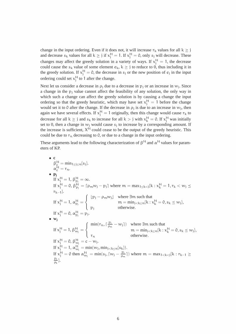
These arguments lead to the following characterization ofβH andαH values for param-eters of KP.

• cβH

c = min1≤j≤n{sj}.αH

c = rn.• pj

If xHj = 1, βH

pj= ∞.

If xHj = 0, βH

pj= dρmwj − pje wherem = max1≤k<j{k : xH

k = 1, rk < wj ≤rk−1}.

If xHj = 1, αH

pj=

bpj − ρmwjc where∃m such thatm = minj<k≤n{k : xH

k = 0, sk ≤ wj},

pj otherwise.If xH

j = 0, αHpj

= pj.• wj

If xHj = 1, βH

wj=

min(rn, d pj

ρm− wje) where∃m such that

m = minj<k≤n{k : xHk = 0, sk ≤ wj},

rn otherwise.If xH

j = 0, βHwj

= c − wj.

If xHj = 1, αH

wj= min(wj, minj<k≤n{sk}).

If xHj = 0 thenαH

wj= min(sj, dwj −

pj

ρme) wherem = max1<k<j{k : rk−1 ≥

pj

ρk}.

6

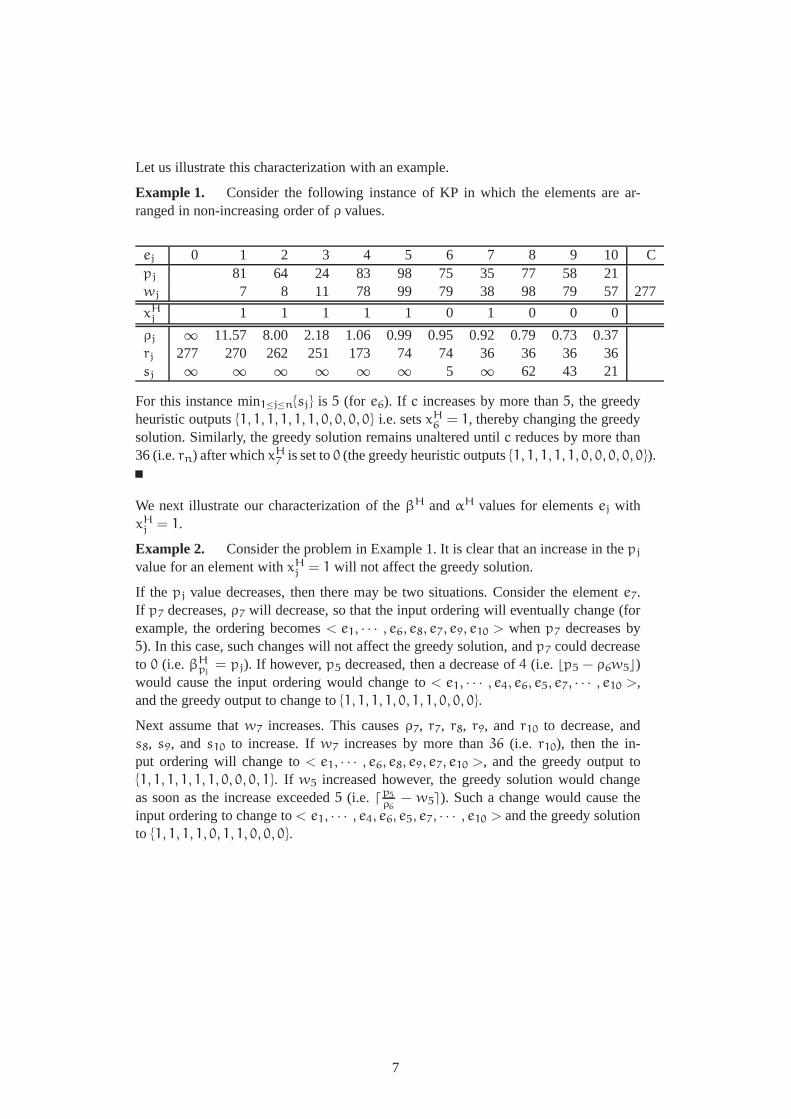
Let us illustrate this characterization with an example.

Example 1. Consider the following instance of KP in which the elements are ar-ranged in non-increasing order ofρ values.

ej 0 1 2 3 4 5 6 7 8 9 10 Cpj 81 64 24 83 98 75 35 77 58 21wj 7 8 11 78 99 79 38 98 79 57277

xHj 1 1 1 1 1 0 1 0 0 0

ρj ∞ 11.57 8.00 2.18 1.06 0.99 0.95 0.92 0.79 0.73 0.37rj 277 270 262 251 173 74 74 36 36 36 36sj ∞ ∞ ∞ ∞ ∞ ∞ 5 ∞ 62 43 21

For this instance min1≤j≤n{sj} is 5 (for e6). If c increases by more than5, the greedyheuristic outputs{1, 1, 1, 1, 1, 1, 0, 0, 0, 0} i.e. setsxH

6 = 1, thereby changing the greedysolution. Similarly, the greedy solution remains unaltered untilc reduces by more than36 (i.e.rn) after whichxH

7 is set to0 (the greedy heuristic outputs{1, 1, 1, 1, 1, 0, 0, 0, 0, 0}).

We next illustrate our characterization of theβH andαH values for elementsej withxH

j = 1.

Example 2. Consider the problem in Example 1. It is clear that an increase in thepj

value for an element withxHj = 1 will not affect the greedy solution.

If the pj value decreases, then there may be two situations. Consider the elemente7.If p7 decreases,ρ7 will decrease, so that the input ordering will eventually change (forexample, the ordering becomes< e1, · · · , e6, e8, e7, e9, e10 > whenp7 decreases by5). In this case, such changes will not affect the greedy solution, andp7 could decreaseto 0 (i.e. βH

pj= pj). If however,p5 decreased, then a decrease of4 (i.e. bp5 − ρ6w5c)

would cause the input ordering would change to< e1, · · · , e4, e6, e5, e7, · · · , e10 >,and the greedy output to change to{1, 1, 1, 1, 0, 1, 1, 0, 0, 0}.

Next assume thatw7 increases. This causesρ7, r7, r8, r9, and r10 to decrease, ands8, s9, and s10 to increase. Ifw7 increases by more than36 (i.e. r10), then the in-put ordering will change to< e1, · · · , e6, e8, e9, e7, e10 >, and the greedy output to{1, 1, 1, 1, 1, 1, 0, 0, 0, 1}. If w5 increased however, the greedy solution would changeas soon as the increase exceeded5 (i.e. dp5

ρ6− w5e). Such a change would cause the

input ordering to change to< e1, · · · , e4, e6, e5, e7, · · · , e10 > and the greedy solutionto {1, 1, 1, 1, 0, 1, 1, 0, 0, 0}.

7

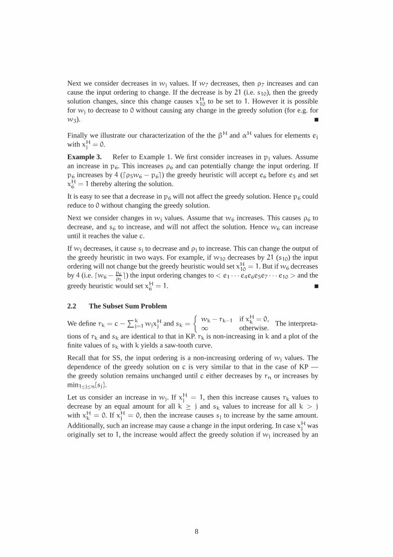
Next we consider decreases inwj values. Ifw7 decreases, thenρ7 increases and cancause the input ordering to change. If the decrease is by21 (i.e. s10), then the greedysolution changes, since this change causesxH

10 to be set to1. However it is possiblefor wj to decrease to0 without causing any change in the greedy solution (for e.g. forw3).

Finally we illustrate our characterization of the theβH andαH values for elementsej

with xHj = 0.

Example 3. Refer to Example 1. We first consider increases inpj values. Assumean increase inp6. This increasesρ6 and can potentially change the input ordering. Ifp6 increases by4 (dρ5w6 − p6e) the greedy heuristic will accepte6 beforee5 and setxH

6 = 1 thereby altering the solution.

It is easy to see that a decrease inp6 will not affect the greedy solution. Hencep6 couldreduce to0 without changing the greedy solution.

Next we consider changes inwj values. Assume thatw6 increases. This causesρ6 todecrease, ands6 to increase, and will not affect the solution. Hencew6 can increaseuntil it reaches the valuec.

If wj decreases, it causesj to decrease andρj to increase. This can change the output ofthe greedy heuristic in two ways. For example, ifw10 decreases by21 (s10) the inputordering will not change but the greedy heuristic would setxH

10 = 1. But if w6 decreasesby 4 (i.e.dw6 − p6

ρ5e) the input ordering changes to< e1 · · · e4e6e5e7 · · · e10 > and the

greedy heuristic would setxH6 = 1.

2.2 The Subset Sum Problem

We definerk = c −∑k

j=1 wjxHj andsk =

{wk − rk−1 if xH

k = 0,∞ otherwise.The interpreta-

tions ofrk andsk are identical to that in KP.rk is non-increasing ink and a plot of thefinite values ofsk with k yields a saw-tooth curve.

Recall that for SS, the input ordering is a non-increasing ordering ofwj values. Thedependence of the greedy solution onc is very similar to that in the case of KP —the greedy solution remains unchanged untilc either decreases byrn or increases bymin1≤j≤n{sj}.

Let us consider an increase inwj. If xHj = 1, then this increase causesrk values to

decrease by an equal amount for allk ≥ j and sk values to increase for allk > j

with xHk = 0. If xH

j = 0, then the increase causessj to increase by the same amount.

Additionally, such an increase may cause a change in the input ordering. In casexHj was

originally set to1, the increase would affect the greedy solution ifwj increased by an

8

amount greater thanrn. If xHj was originally set to0, the greedy solution can change

only if the input ordering becomes such thatwj is input to the greedy heuristic earlyenough forxH

j to be set to1.

If wj decreases, the effects are the reverse of the effects mentioned above, i.e. ifxHj = 1

originally, thenrk values will increase by an equal amount for allk ≥ j andsk valuesdecrease for allk > j with xH

k = 0. If xHj = 0, then sj registers a corresponding

decrease. Ifwj decreases sufficiently, then if originallyxHj = 0, thensj would become

0 thus changing the greedy solution. If originallyxHj = 1, the greedy solution changes

when the value ofwj decreases tillsp for somep > j decreases to0, or the inputordering changes appropriately.

This discussion leads to the following characterization ofβH andαH values for param-eters of SS.

• cβH

c = min1≤j≤n{sj}.αH

c = rn.• wj

If xHj = 1, βH

wj= rn.

If xHj = 0, βH

wj= max1≤k<j{wk : xH

k = 1, rk > 0} − wj.

If xHj = 1 αH

wj=

min(sp,wj − wt) if ∃t, andk > j such thatxHk = 0,

sp if ∃k > j such thatxHk = 0,

wj otherwise.

wherep = minj<m≤n{m : sm = minj<k≤n{sk}}, andt = minj<m≤n{m : xm =

0}.If xH

j = 0, αHwj

= sj.

As in the case of KP, let us illustrate these tolerance limits with an example.

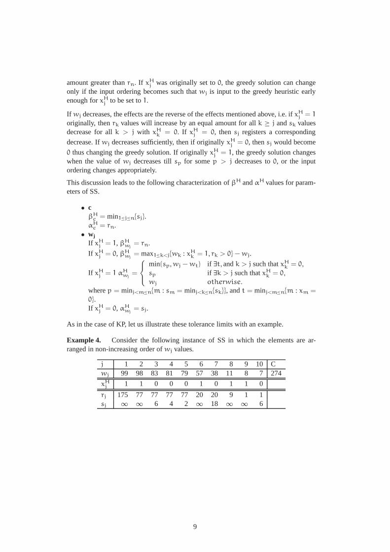
Example 4. Consider the following instance of SS in which the elements are ar-ranged in non-increasing order ofwj values.

j 1 2 3 4 5 6 7 8 9 10 Cwj 99 98 83 81 79 57 38 11 8 7274

xHj 1 1 0 0 0 1 0 1 1 0

rj 175 77 77 77 77 20 20 9 1 1sj ∞ ∞ 6 4 2 ∞ 18 ∞ ∞ 6

9

If c increases by2 (i.e. s5), then the greedy heuristic setsxH5 = 1, thus changing the

greedy solution. Again, ifc decreases by more than1 (i.e.r10), the greedy heuristic setsxH

9 = 0, thereby changing the greedy solution.

We now examine the effect of changes inwj onβH andαH values for elementsej withxH

j = 1.

Example 5. Considere8 in Example 4. Ifw8 increases, thenr8, r9, andr10 decreasesands10 increases. Ifw8 increases by more than1 (i.e.r10), it causes the greedy heuristicto setxH

9 = 0, thereby changing the greedy solution. Notice that we do not considerchanges in input ordering since, if there existsej, ej+1 such thatwj > wj+1, xH

j =

0, xHj+1 = 1, thenwj − wj+1 > rj+1 ≥ rn.

If w8 decreases, thenr8, r9, andr10 increases ands10 decreases. If the decrease is bymore than4 (i.e. w8 − w10, since in this caset = 10), the initial ordering changesto < e1, · · · , e7, e9, e10, e8 >. The greedy heuristic now setsxH

10 = 1, i.e. the greedysolution changes. If there was no elementej such thatwj ≤ w8 and xH

j = 0, thena decrease inw8 would never affect the greedy solution, and sow8 could reduce to0.

We finally examine the effect of changes inwj on βH andαH values for elementsej

with xHj = 0.

Example 6. Considere7 in Example 4. Ifw7 increases,s7 increases by an equalamount. If the increase is by more than19 (i.e. w6 − w7), then the initial orderingchanges to< e1, · · · , e5, e7, e6, e8, · · · , e10 > and the greedy heuristic setsxH

7 = 1.

If w7 decreases, thens7 decreases by the same amount. Ifw7 decreases by more than18 (i.e. s7), it causes the greedy heuristic to out put a different solution withxH

7 = 1.Note that here also we do not consider changes in input ordering since, if there existsej, ej+1 such thatwj > wj+1, xH

j = 0, xHj+1 = 1, thenwj − wj+1 ≥ sj.

One more interesting result is clear from the characterizations presented in Subsec-tions 2.1 and 2.2. Notice that the tolerance limits of all the problem parameters for KPare polynomial functions ofρk, rk andsk values while those of SS are polynomial func-tions ofrk andsk values. These values can be calculated by careful book-keeping whenthe greedy heuristic is generating the greedy solution. Hence we have the followingtheorem.

Theorem 1 The complexity of calculatingβH and αH values of any parameter ofKP or SS is polynomial in the size of the problem.

10

3. The objective functionsZH and Z∗

In this section, we studyZH andZ∗ as functions of the problem parameters. We willassume that the value of exactly one parameter of the instance at hand varies. If thisparameter isc for either a KP instance or a SS instance, orwj for a KP instance,ZH

(andZ∗) are piecewise linear discontinuous functions with the linear sections having aslope of0. This is because neitherc for KP or SS instances, norwj for KP instancesappear in the objective function, and hence a change in their values cannot cause alinear change in the objective function. If the parameter ispj for a KP instance orwj fora SS instance, thenZH (andZ∗) are piecewise linear functions with the linear sectionshaving slopes of+1 or 0 depending on whether or notej ∈ E1 in the greedy (andoptimal) solution. We will now illustrate this with examples.

Example 7. Let us consider the KP instance whereE = {< 65, 50 >,< 6, 5 >

,< 25, 25 >} andc = 65. We first assume thatc changes from0 to∑3

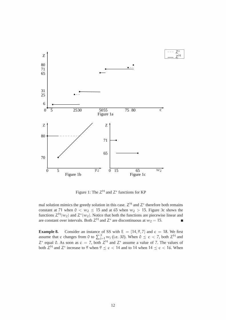
j=1 wj (i.e.80). When0 ≤ c < 5, bothZH andZ∗ equal0. As soon asc = 5, bothZH andZ∗assume a value of6. Whenc increases to25, a new optimal solution is reached andZ∗ equals25. ZH however remains at6. Both ZH andZ∗ assume values of31 when30 ≤ c < 50, of 65 when50 ≤ c < 55, and of71 when55 ≤ c < 75. Whenc reaches75, Z∗ assumes a value of90, (ZH remains at71,) and when it touches80, bothZH andZ∗ assume values of96. Figure 3a shows the functionsZH(c) andZ∗(c). Notice thatboth are piecewise linear and are constant over intervals.ZH(c) is discontinuous atc =

5, 30, 50, 55, and80, while Z∗(c) is discontinuous atc = 5, 25, 30, 50, 55, 75, and80.

Next we assume thatp2 changes in the problem instance. When0 ≤ p2 < 5, the inputordering for the greedy heuristic is< e1, e3, e2 >. Both the greedy and the optimalsolution to this instance is{1, 0, 1} and hence bothZH andZ∗ equal80. Whenp2 crosses5 the input ordering for the greedy heuristic changes to< e1, e2, e3 > which causes thegreedy solution to become{1, 1, 0} and theZH value decreases to70. Whenp2 ≥ 7

the input ordering for the greedy heuristic again changes (this time to< e2, e1, e3 >)but the greedy solution remains{1, 1, 0}. So whenp2 ≥ 5, ZH increases linearly withp2 and the function has a slope of+1. Z∗ remains constant at80 when5 ≤ p2 ≤ 15

but whenp2 > 15 the optimal solution becomes{1, 1, 0}, Z∗ increases linearly withp2.Figure 3b shows the functionsZH(p2) andZ∗(p2). Notice that both the functions arepiecewise linear, and have regions where the slope is+1 as well as regions where thefunctions are constant.ZH has a discontinuity atp2 = 5 while Z∗ is continuous.

Next we assume thatw2 changes. Note thatw2 can only vary in the interval(0, c].The input ordering for the greedy heuristic is< e2, e1, e3 > when 0 < w2 < 5,< e1, e2, e3 > when5 ≤ w2 ≤ 6, and< e1, e3, e2 > whenw2 < 6. Hence the greedysolution is{1, 1, 0} for 0 < w2 ≤ 15 and changes to{1, 0, 0} whenw2 > 15. The opti-

11

Z∗ZH

-

6

p2

Z

-

6

w2

Z

80

70

5

Figure 1a

Figure 1b Figure 1c15 6500

71

65

-

6

c80

80

255 30 5055 750

6

2531

6571

Z

Figure 1: TheZH andZ∗ functions for KP

mal solution mimics the greedy solution in this case.ZH andZ∗ therefore both remainsconstant at71 when0 < w2 ≤ 15 and at65 whenw2 > 15. Figure 3c shows thefunctionsZH(w2) andZ∗(w2). Notice that both the functions are piecewise linear andare constant over intervals. BothZH andZ∗ are discontinuous atw2 = 15.

Example 8. Consider an instance of SS withE = {14, 9, 7} andc = 18. We firstassume thatc changes from0 to

∑3j=1 wj (i.e. 30). When0 ≤ c < 7, both ZH and

Z∗ equal0. As soon asc = 7, both ZH andZ∗ assume a value of7. The values ofbothZH andZ∗ increase to9 when9 ≤ c < 14 and to14 when14 ≤ c < 16. When

12

c increases to16, a new optimal solution is reached ({0, 1, 1}), andZ∗ equals16. ZH

however remains at14. BothZH andZ∗ assume values of21 when21 ≤ c < 23, of 23

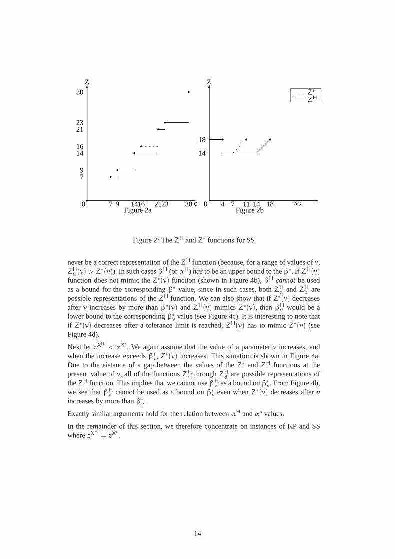
when23 ≤ c < 30, and of30 whenc = 30. Figure 3a shows the functionsZH(c) andZ∗(c). Notice that both the functions are piecewise linear, continuous and have regionswhere the slope is+1 as well as regions where the functions are constant.

Finally we assume thatw2 changes. As in case of the KP instance,w2 can vary inthe interval(0, c]. When0 < w2 ≤ 7, the input ordering for the greedy heuristicis < e1, e3, e2 >. Both the greedy output and the optimal solution are{1, 0, 1} when0 < w2 ≤ 4 and{1, 0, 0} when4 < w2 ≤ 7. So bothZH andZ∗ remain constant at18 when0 < w2 ≤ 4 and at14 when4 < w2 ≤ 7. When7 < w2 ≤ 14, the inputordering for the greedy heuristic changes to< e1, e2, e3 >. In this whole range, thegreedy solution remains{1, 0, 0} andZH remains constant at14. The optimal solutionhowever becomes{0, 1, 1} when7 < c ≤ 11 andZ∗ increases linearly withw2 in thisrange. When11 < c ≤ 14, the optimal solution again becomes{1, 0, 0} andZ∗ remainsconstant at14. The input ordering for the greedy heuristic again changes whenw2 >

14 and becomes< e2, e1, e3 >. So when14 < c ≤ 18, the greedy heuristic outputs{0, 1, 0} andZH increases linearly withw2. The optimal solution is also{0, 1, 0} whenw2 is in this interval and soZ∗ also increases linearly withw2. Figure 3b shows thefunctionsZH(w2) andZ∗(w2). Notice that here too, both the functions are piecewiselinear and have regions where the slope is+1 as well as regions where the slope is0.ZH is discontinuous atw2 = 4 while Z∗ is discontinuous atw2 = 4 and11.

4. βH and αH as bounds forβ∗ and α∗

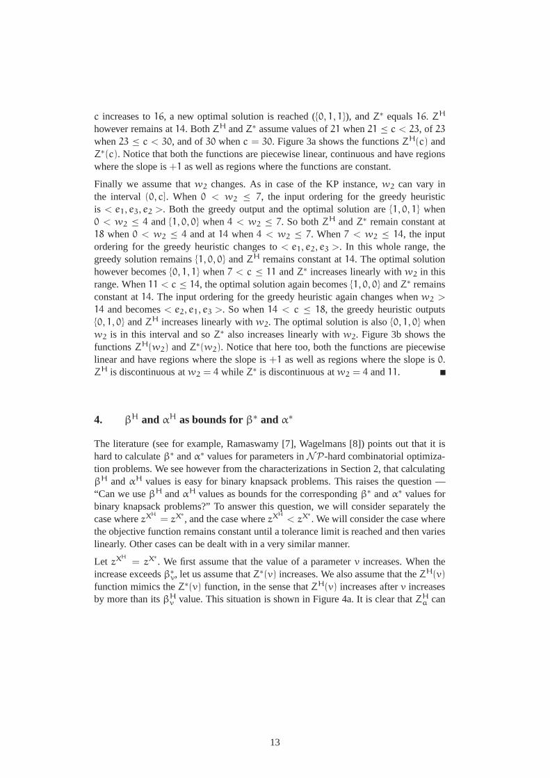
The literature (see for example, Ramaswamy [7], Wagelmans [8]) points out that it ishard to calculateβ∗ andα∗ values for parameters inNP-hard combinatorial optimiza-tion problems. We see however from the characterizations in Section 2, that calculatingβH andαH values is easy for binary knapsack problems. This raises the question —“Can we useβH andαH values as bounds for the correspondingβ∗ andα∗ values forbinary knapsack problems?” To answer this question, we will consider separately thecase wherezXH

= zX∗, and the case wherezXH

< zX∗. We will consider the case where

the objective function remains constant until a tolerance limit is reached and then varieslinearly. Other cases can be dealt with in a very similar manner.

Let zXH= zX∗

. We first assume that the value of a parameterv increases. When theincrease exceedsβ∗

v, let us assume thatZ∗(v) increases. We also assume that theZH(v)

function mimics theZ∗(v) function, in the sense thatZH(v) increases afterv increasesby more than itsβH

v value. This situation is shown in Figure 4a. It is clear thatZHa can

13

-

6

0 7 9 1416 2123 30c

Z

30

2321

1614

79

Figure 2a

Z∗ZH

-

6

0 4 7 11 14 18 w2

14

18

Z

Figure 2b

Figure 2: TheZH andZ∗ functions for SS

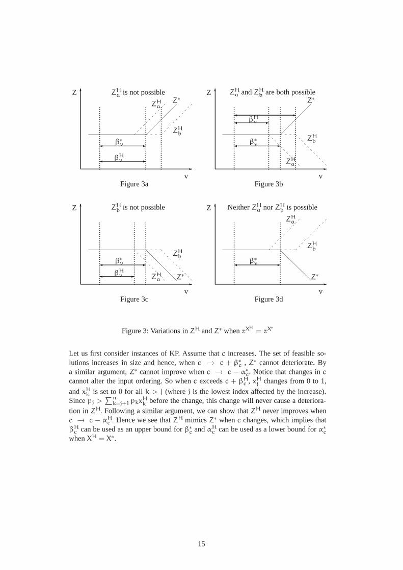
never be a correct representation of theZH function (because, for a range of values ofv,ZH

a(v) > Z∗(v)). In such casesβH (or αH) hasto be an upper bound to theβ∗. If ZH(v)

function does not mimic theZ∗(v) function (shown in Figure 4b),βH cannotbe usedas a bound for the correspondingβ∗ value, since in such cases, bothZH

a andZHb are

possible representations of theZH function. We can also show that ifZ∗(v) decreasesafter v increases by more thanβ∗(v) andZH(v) mimics Z∗(v), thenβH

v would be alower bound to the correspondingβ∗

v value (see Figure 4c). It is interesting to note thatif Z∗(v) decreases after a tolerance limit is reached,ZH(v) has to mimicZ∗(v) (seeFigure 4d).

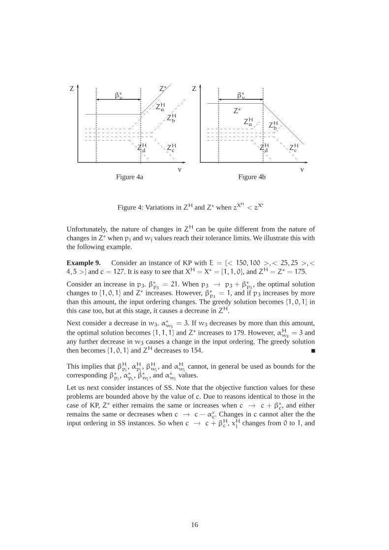
Next let zXH< zX∗

. We again assume that the value of a parameterv increases, andwhen the increase exceedsβ∗

v, Z∗(v) increases. This situation is shown in Figure 4a.Due to the eistance of a gap between the values of theZ∗ and ZH functions at thepresent value ofv, all of the functionsZH

a throughZHd are possible representations of

theZH function. This implies that we cannot useβHv as a bound onβ∗

v. From Figure 4b,we see thatβH

v cannot be used as a bound onβ∗v even whenZ∗(v) decreases afterv

increases by more thanβ∗v.

Exactly similar arguments hold for the relation betweenαH andα∗ values.

In the remainder of this section, we therefore concentrate on instances of KP and SSwherezXH

= zX∗.

14

-

6

.................................v

ZZ∗

ZHa

ZHb

ZHa is not possible

Figure 3a

-

6

.................................v

ZZ∗

ZHa

ZHb

ZHa andZH

b are both possible

Figure 3b

-

6

.................................v

Z

Z∗ZHa

ZHb

ZHb is not possible

Figure 3c

-

6

.................................v

Z NeitherZHa norZH

b is possible

Z∗

ZHa

ZHb

Figure 3d

β∗v

.................................

.................................

.................................

.................................

-� β∗v -�

β∗v -� β∗

v -�

.................................

.................................

.................................

.................................βH

v

βHv

βHv�

��

-

-

--

�

Figure 3: Variations inZH andZ∗ whenzXH= zX∗

Let us first consider instances of KP. Assume thatc increases. The set of feasible so-lutions increases in size and hence, whenc → c + β∗

c , Z∗ cannot deteriorate. Bya similar argument,Z∗ cannot improve whenc → c − α∗

c. Notice that changes inccannot alter the input ordering. So whenc exceedsc + βH

c , xHj changes from 0 to 1,

andxHk is set to 0 for allk > j (wherej is the lowest index affected by the increase).

Sincepj >∑n

k=j+1 pkxHk before the change, this change will never cause a deteriora-

tion in ZH. Following a similar argument, we can show thatZH never improves whenc → c − αH

c . Hence we see thatZH mimicsZ∗ whenc changes, which implies thatβH

c can be used as an upper bound forβ∗c andαH

c can be used as a lower bound forα∗c

whenXH = X∗.

15

-

6 .........................................v

Z Z∗

ZHa

ZHb

ZHd ZH

c

Figure 4a

-

6 .........................................v

Z

Z∗

ZHa ZH

b

ZHd ZH

c

Figure 4b

...........................................

.........................................

-� -�β∗v β∗

v

Figure 4: Variations inZH andZ∗ whenzXH< zX∗

Unfortunately, the nature of changes inZH can be quite different from the nature ofchanges inZ∗ whenpj andwj values reach their tolerance limits. We illustrate this withthe following example.

Example 9. Consider an instance of KP withE = {< 150, 100 >,< 25, 25 >,<

4, 5 >} andc = 127. It is easy to see thatXH = X∗ = {1, 1, 0}, andZH = Z∗ = 175.

Consider an increase inp3. β∗p3

= 21. Whenp3 → p3 + β∗p3

, the optimal solutionchanges to{1, 0, 1} andZ∗ increases. However,β∗

p3= 1, and if p3 increases by more

than this amount, the input ordering changes. The greedy solution becomes{1, 0, 1} inthis case too, but at this stage, it causes a decrease inZH.

Next consider a decrease inw3. α∗w3

= 3. If w3 decreases by more than this amount,the optimal solution becomes{1, 1, 1} andZ∗ increases to 179. However,αH

w3= 3 and

any further decrease inw3 causes a change in the input ordering. The greedy solutionthen becomes{1, 0, 1} andZH decreases to154.

This implies thatβHpj

, αHpj

, βHwj

, andαHwj

cannot, in general be used as bounds for thecorrespondingβ∗

pj, α∗

pj, β∗

wj, andα∗

wjvalues.

Let us next consider instances of SS. Note that the objective function values for theseproblems are bounded above by the value ofc. Due to reasons identical to those in thecase of KP,Z∗ either remains the same or increases whenc → c + β∗

c, and eitherremains the same or decreases whenc → c − α∗

c. Changes inc cannot alter the theinput ordering in SS instances. So whenc → c + βH

c , xHj changes from0 to 1, and

16

xHk is set to0 for all k > j (wherej is the lowest index affected by the increase). Since

wj < rj−1 ≥ ∑nk=j+1 wkx

Hk before the change, this change will never causeZH to

deteriorate. Similarly whenc → c − αHc , xH

m changes from1 to 0, (wherem was thelargest index such thatxH

m was set to1 before the change) and somexHk , k > m may be

set to1. Following an argument similar to the one above, we can infer thatZH cannotimprove at this point. ThereforeβH

c can be used as an upper bound forβ∗c andαH

c canbe used as a lower bound forα∗

c whenXH = X∗ whenXH = X∗.

Consider changes inwj for elementsej with xHj = x∗

j = 1. Assume thatwj increases.

X∗ remains the optimal solution untilzX∗reachesc, after which this solution becomes

infeasible. Hence whenwj → wj + β∗wj

, Z∗ cannot improve. In case of the greedy

heuristic,ZH increases untilwj → wj + βHwj

. βHwj

is reached due to one of two

reasons. EitherzXHreaches a value ofc (which causes a further increase inwj to render

theXH infeasible), or any further increase inwj causes a change in the input ordering,and movesej to a position just ahead ofek such thatxH

j−1 = · · · = xHk+1 = 1 and

xHk = 0 before the change. In the former situation,ZH clearly cannot improve. The

latter situation is impossible to reach. Next assume thatwj decreases. This causeszX ofall solutionsX with xj = 1 to decrease. HenceX∗ ceases to be the optimal solution whenzX∗

< zXnewfor some other solutionXnew with xnew

j = 0. So whenwj → wj − α∗wj

,

Z∗ does not decrease.αHwj

can be reached in several ways. It is possible that the decrease

in wj would cause somexHk , k > j to be changed from0 to 1. This would cause

an increase inZH. It is also possible that the decrease inwj would change the inputordering and placeej after someek such thatxH

j+1 = · · · = xHk−1 = 1 andxH

k = 0

before the change. This would cause the greedy heuristic to setxHk = 1 which will

keepZH from reducing further. A third possibility is thatwj would reduce to0. Clearly,ZH cannot decrease at this stage. From the nature of changes in the objective functionvalues, we can conclude that in such cases,βH

wjis a lower bound onβ∗

c andαHc is an

upper bound forα∗c.

Finally we consider changes inwj for elementsej with xHj = x∗

j = 0. Assume that

wj increases.Z∗ remains equal tozX∗until zX for some other solutionX with xj = 1

exceeds this value. HenceZ∗ increases whenwj → wj + β∗wj

. In case of the greedy

heuristic,ZH does not change until the increase inwj causes a change in the inputordering, and setsej in a position just ahead ofek such thatxH

j−1 = · · · = xHk+1 = 0 and

xHk = 1 before the change. Ifwj increases further, it is clear thatZH would increase.

Next assume thatwj decreases.zX∗remains unchanged, andzX values of all solutions

X (feasible and otherwise) withxj = 1 decrease. When the decrease inwj is largeenough, a previously infeasible solution becomes feasible andZ∗ = c. HenceZ∗ doesnot deteriorate whenwj → wj − α∗

wj. Consider the greedy heuristic. Ifwj decreases,

17

ZH remains unchanged untilwj decreases enough to be able to be incorporated into thecurrent greedy solution thus settingZH to c, i.e. it does not deteriorate. Hence in thesecasesβH

wjandαH

wjact as upper bounds onβ∗

wjandα∗

wjrespectively.

Hence, ifzXH< zX∗

, in general we cannot useβH andαH as bounds for the corre-spondingβ∗ andα∗ values. Even whenXH = X∗, βH andαH values can respectivelybe used as upper and lower bounds for the correspondingβ∗ andα∗ values for varia-tions inwj andc in SS instances and inc for KP instances, but not for variations inpj

andwj values in KP instances.

5. Empirical behaviour of xH

In this section we report the results of certain preliminary computations we carried outto test the empirical behavior ofxH. The computations were carried out with an aim toanswer the following two questions.

1. How does the performance ratio of the greedy heuristic vary when a particularproblem parameter is altered?

2. How often are theβW andαW values reached in randomly generated probleminstances?

The second question is interesting for binary knapsack problems since the empiricalperformance of the greedy heuristic is very different from its worst-case performance.

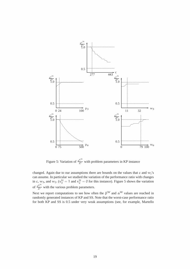
We used the KP instance of Example 1 to see how the performance ratio of the greedyheuristic varied when various problem parameters are changed. In particular we studiedthe variation of the performance ratio with changes inc, p3, w3, p6, andw6. (Recallthat xH

3 = 1 andxH6 = 0 for that instance). The performance ratio is the ratio of the

objective function value ofzXHto Z∗.

Due to our assumptions that none of thewj values can exceedc and thatc ≤ ∑nj=1 wj,

and the fact that the original greedy solution has to be feasible in the changed probleminstance, most of the problem parameters can only vary within certain ranges. For ex-ample, the value ofc can vary between241 and554, that ofw3 between0 and32 andthat ofw6 between0 and100. p3 andp6 can take on any non-negative value. Figure 5

shows the variation ofzXH

Z∗ with the various problem parameters. It is interesting to seethat for this instance, the performance ratio of0.5 is reached only in the case wherep6

increases to443.

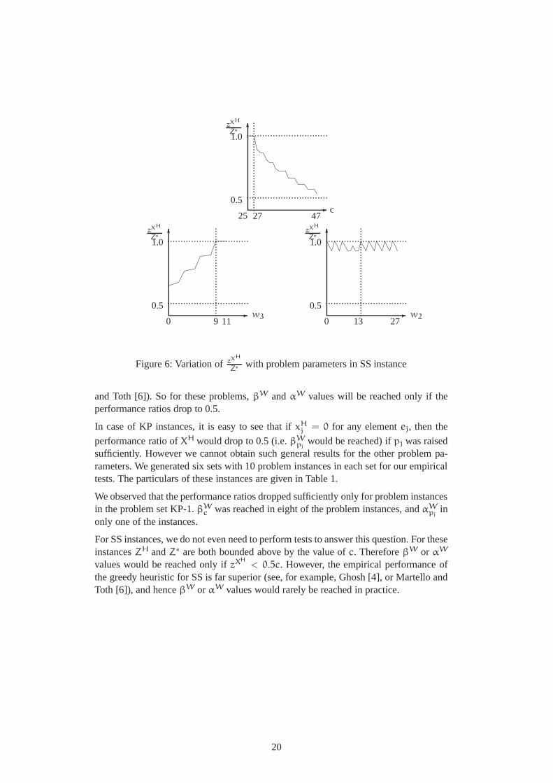
We used the SS instanceE = {16, 13, 9, 6, 3}, c = 27 to see the variation of the per-formance ratio of the greedy heuristic varied when various problem parameters are

18

-

6...............................

..

..

..

..

..

..

..

..

..

..

..

..

..

..

..

..

..

...............................

-

6...............................

..

..

..

..

..

..

..

..

..

..

..

..

..

..

..

..

..

...............................-

6...............................

..

..

..

..

..

..

..

..

..

..

..

..

..

..

..

..

..

...............................

-

6...............................

..

..

..

..

..

..

..

..

..

..

..

..

..

..

..

..

..

...............................-

6...............................

..

..

..

..

..

..

..

..

..

..

..

..

..

..

..

..

..

...............................

0.5

0.5 0.5

0.5 0.5

1.0

1.0 1.0

1.0 1.0

zxH

Z∗

zxH

Z∗

zxH

Z∗

zxH

Z∗

zxH

Z∗

c277

p324

p679

w675

32w3

443

0

0 0

100

500 100

11

Figure 5: Variation ofzXH

Z∗ with problem parameters in KP instance

changed. Again due to our assumptions there are bounds on the values thatc andwj’scan assume. In particular we studied the variation of the performance ratio with changesin c, w3, andw2. (xH

3 = 1 andxH2 = 0 for this instance). Figure 5 shows the variation

of zXH

Z∗ with the various problem parameters.

Next we report computations to see how often theβW andαW values are reached inrandomly generated instances of KP and SS. Note that the worst-case performance ratiofor both KP and SS is 0.5 under very weak assumptions (see, for example, Martello

19

-

6

...............................

...............................

..

..

..

..

..

..

..

..

..

..

..

..

..

..

..

..

..

-

6

...............................

...............................

..

..

..

..

..

..

..

..

..

..

..

..

..

..

..

..

..

-

6

...............................

...............................

..

..

..

..

..

..

..

..

..

..

..

..

..

..

..

..

..

zXH

Z∗

zXH

Z∗ zXH

Z∗

0.5

0.5 0.5

1.0

1.0 1.0

c

w3 w2

25 4727

0 9 11 0 13 27

Figure 6: Variation ofzXH

Z∗ with problem parameters in SS instance

and Toth [6]). So for these problems,βW andαW values will be reached only if theperformance ratios drop to 0.5.

In case of KP instances, it is easy to see that ifxHj = 0 for any elementej, then the

performance ratio ofXH would drop to 0.5 (i.e.βWpj

would be reached) ifpj was raisedsufficiently. However we cannot obtain such general results for the other problem pa-rameters. We generated six sets with 10 problem instances in each set for our empiricaltests. The particulars of these instances are given in Table 1.

We observed that the performance ratios dropped sufficiently only for problem instancesin the problem set KP-1.βW

c was reached in eight of the problem instances, andαWpj

inonly one of the instances.

For SS instances, we do not even need to perform tests to answer this question. For theseinstancesZH andZ∗ are both bounded above by the value ofc. ThereforeβW or αW

values would be reached only ifzXH< 0.5c. However, the empirical performance of

the greedy heuristic for SS is far superior (see, for example, Ghosh [4], or Martello andToth [6]), and henceβW or αW values would rarely be reached in practice.

20

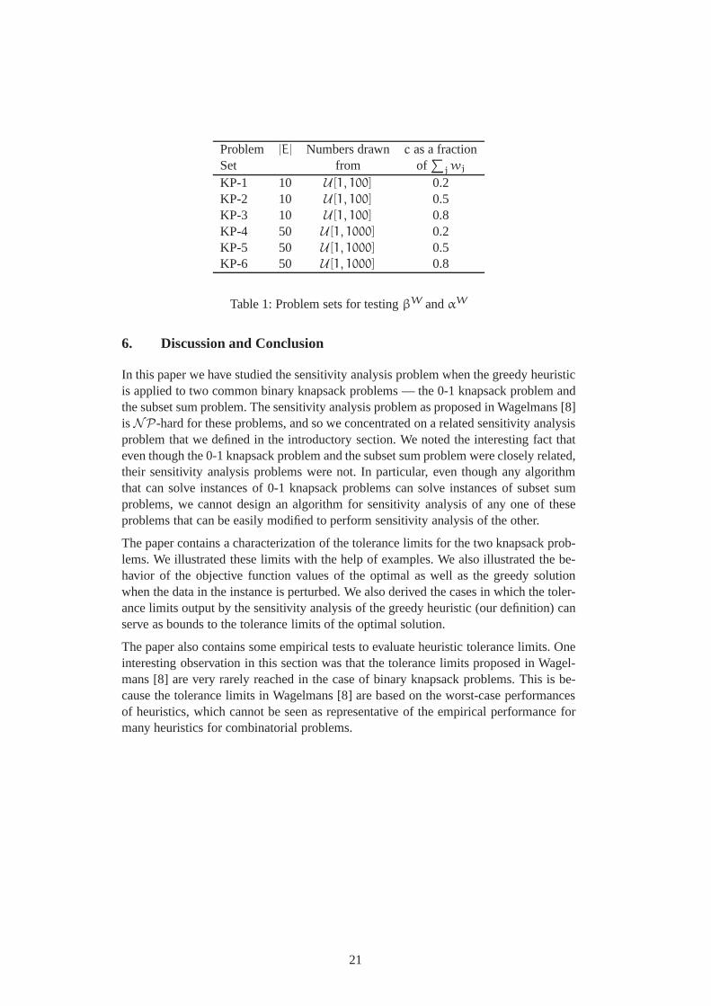
Problem |E| Numbers drawn c as a fractionSet from of

∑j wj

KP-1 10 U [1, 100] 0.2KP-2 10 U [1, 100] 0.5KP-3 10 U [1, 100] 0.8KP-4 50 U [1, 1000] 0.2KP-5 50 U [1, 1000] 0.5KP-6 50 U [1, 1000] 0.8

Table 1: Problem sets for testingβW andαW

6. Discussion and Conclusion

In this paper we have studied the sensitivity analysis problem when the greedy heuristicis applied to two common binary knapsack problems — the 0-1 knapsack problem andthe subset sum problem. The sensitivity analysis problem as proposed in Wagelmans [8]isNP-hard for these problems, and so we concentrated on a related sensitivity analysisproblem that we defined in the introductory section. We noted the interesting fact thateven though the 0-1 knapsack problem and the subset sum problem were closely related,their sensitivity analysis problems were not. In particular, even though any algorithmthat can solve instances of 0-1 knapsack problems can solve instances of subset sumproblems, we cannot design an algorithm for sensitivity analysis of any one of theseproblems that can be easily modified to perform sensitivity analysis of the other.

The paper contains a characterization of the tolerance limits for the two knapsack prob-lems. We illustrated these limits with the help of examples. We also illustrated the be-havior of the objective function values of the optimal as well as the greedy solutionwhen the data in the instance is perturbed. We also derived the cases in which the toler-ance limits output by the sensitivity analysis of the greedy heuristic (our definition) canserve as bounds to the tolerance limits of the optimal solution.

The paper also contains some empirical tests to evaluate heuristic tolerance limits. Oneinteresting observation in this section was that the tolerance limits proposed in Wagel-mans [8] are very rarely reached in the case of binary knapsack problems. This is be-cause the tolerance limits in Wagelmans [8] are based on the worst-case performancesof heuristics, which cannot be seen as representative of the empirical performance formany heuristics for combinatorial problems.

21

References

[1] N. Chakravarti, A.M. Goel, T. Sastry, Easy Weighted Majority Games,WorkingPaper WPS-287/97, Indian Institute of Management, Calcutta(To appear inMath-ematical Social Sciences) (1997)

[2] N. Chakravarti, A.P.M. Wagelmans, Calculation of stability radii for combinatorialoptimization problems,Operations Research Letters 23(1998) pp. 1-7

[3] T. Gal, H.J. Greenberg (Eds.), Advances in Sensitivity Analysis and ParametricProgramming, Kluwer Academic Publishers, Boston (1997)

[4] D. Ghosh,Heuristics for Knapsack Problems: Comparative Survey and SensitivityAnalysis, Fellowship dissertation, IIM Calcutta, Calcutta (1997)

[5] A.W.J. Kolen, A.H.G. Rinnooy Kan, C.P.M. van Hoesel and A.P.M. Wagelmans,Sensitivity analysis of list scheduling heuristics,Discrete Applied Mathematics 55(1994) pp. 145-162

[6] S. Martello, P. Toth,Knapsack problems: Algorithms and Computer Implementa-tions, John Wiley & Sons, Singapore (1989)

[7] R. Ramaswamy,Sensitivity Analysis in Combinatorial Optimization, Fellowshipdissertation, IIM Calcutta, Calcutta (1994)

[8] A.P.M. Wagelmans,Sensitivity Analysis in Combinatorial Optimization, Ph. D.dissertation, Erasmus University, Rotterdam (1990)

22