Sensing the ionosphere with the Spire radio occultation

constellation

Matthew J. Angling* , Oleguer Nogués-Correig, Vu Nguyen, Sanita Vetra-Carvalho ,Francois-Xavier Bocquet , Karl Nordstrom, Stacey E. Melville, Giorgio Savastano,Shradha Mohanty, and Dallas Masters

Earth Intelligence Department, Spire Global, Skypark 6, 64–72 Finnieston Square, Glasgow G3 8ET, UK

Received 15 July 2021 / Accepted 13 October 2021

Abstract –Radio occultation (RO) provides a cost-effective component of the overall sensor mix requiredto characterise the ionosphere over wide areas and in areas where it is not possible to deploy groundsensors. The paper describes the RO constellation that has been developed and deployed by Spire Global.This constellation and its associated ground infrastructure are now producing data that can be used tocharacterise the bulk ionosphere, lower ionosphere perturbations, and ionospheric scintillation.

Keywords: Ionosphere / radio occultation

1 Introduction

The ionosphere is a dynamic environment that varies overscale lengths ranging from metres to thousands of kilometres,and on scale times of fractions of seconds to decades. Further-more, many radio systems operate through or via the ionospherewhose performance can be affected by changing ionosphericconditions. Ionospheric impacts are generally limited to systemsoperating at L band (1–2 GHz) and below but cover a wide rangeof applications, including high frequency (HF, 3–30 MHz)communications and radar, very high frequency (VHF, 30–300 MHz) satellite communications, and ultra-high frequency(UHF, 300–3000 MHz) space track radar and space-based radar(Angling et al., 2012).

Although many ground-based techniques have been devel-oped to monitor the ionosphere, space-based methods are beingincreasingly used since they can measure the ionosphere overregions where ground-based sensors cannot easily be located,such as the oceans. This paper is concerned with a particularspace-based method known as Global Navigation SatelliteSystem (GNSS) radio occultation (RO) (Jakowski et al.,2009). This is a form of atmospheric limb sounding that usestransmissions from GNSS satellites in medium Earth orbit(MEO) and corresponding receivers on low Earth Orbit (LEO)satellites. GNSS RO was first demonstrated for remote sensingthe Earth’s ionosphere (and the neutral atmosphere) by theGPS/MET instrument (e.g., Hajj et al., 1994; Kursinski et al.,

1996). Further individual missions such as CHAMP (Jakowskiet al., 2002) and SAC-C (Hajj et al., 2004) provided opportuni-ties to improve data processing methods. However, the ability toprovide global ionospheric monitoring has come about throughthe use of constellations of RO satellites such as the Constella-tion Observing System for Meteorology, Ionosphere andClimate (COSMIC) (Hajj et al., 2000) and COSMIC2 (Hsuet al., 2018). Furthermore, commercial operators are now flyingconstellations of RO satellites. One such operator is Spire Global(https://spire.com), and this paper describes how Spire collects,processes, and uses ionospheric RO data.

The following parts of this section provide brief descriptionsof how GNSS can measure the ionosphere (Sect. 1.1) and theRO method (Sect. 1.2). Then Section 2 describes the Spiremeasurement system (constellation, satellite platform, GNSSreceiver, etc.), and Section 3 describes three example uses ofthe data global ionospheric data assimilation, high-resolutionE region perturbation detection, and ionospheric scintillationdetection. Finally, Section 4 describes future developments.

1.1 GNSS measurements of the ionosphere

Dual-frequency GNSS signals can be used to determine thetotal electron content (TEC) between a GNSS transmitter (Tx)and a GNSS receiver (Rx) (Jin et al., 2014). The TEC is theline integral of electron density on a path (l) between the Txand the Rx. It is related to the frequency (f in Hz), excess phase(S in metres), phase refractive index (n) and electron density(Ne in electrons/m3) by Gorbunov & Kornblueh (2001):*Correspondingauthor: matthew.angling@spire.com

J. Space Weather Space Clim. 2021, 11, 56�M.J. Angling et al., Published by EDP Sciences 2021https://doi.org/10.1051/swsc/2021040

Available online at:www.swsc-journal.org

OPEN ACCESSTECHNICAL ARTICLE

This is an Open Access article distributed under the terms of the Creative Commons Attribution License (https://creativecommons.org/licenses/by/4.0),which permits unrestricted use, distribution, and reproduction in any medium, provided the original work is properly cited.

TEC ¼Z

N edl ¼ � f 2

40:3

Zn� 1ð Þdl ¼ � f 2S

40:3ð1Þ

TEC is often expressed in TEC units (TECu), where 1 TECuequals 1016 electrons/m2.

A dual-frequency (f1, f2) GNSS receiver can record pseudo-range (P1, P2, the distance measured by the GNSS codebetween Tx and Rx, assuming propagation at the velocity oflight in a vacuum) and phase (L1, L2) for both frequencies.The path separation between the two signals is usually small,and the assumption is often made that they both travel alongthe same straight line. The TEC can be estimated by formingthe geometry-free combination (Teunissen & Montenbruck,2017). This is advantageous as the combination cancels errorsin the satellite position and clock.

The TEC estimated from the pseudorange is noisy due tomultipath and to limitations of the receiver front end bandwidth.It is, however, an absolute measurement except for a bias:

STECP ¼ � f 21 f

22

40:3 f 21 � f 2

2ð Þ P 1 � P 2ð Þ þ DCB ð2Þ

where DCB is the differential code bias. In contrast, the TECestimate from the phase measurements has less noise butincludes an unknown phase ambiguity (b):

STECL ¼ f 21 f

22

40:3 f 21 � f 2

2ð Þ L1 � L2ð Þ þ b: ð3Þ

Since L1 and L2 signals can suffer from cycle slips, these needto be detected and corrected (Blewitt, 1990; Savastano et al.,2017).

One approach to obtain calibrated TEC is to level the phaseTEC to the pseudorange TEC, either by simply modifying themean value or by weighting each point in the TEC arc accord-ing to the impact of multipath as measured by the divergencebetween code and phase (Pedatella, 2011). The final step is toestimate the Tx and Rx DCBs. For the GNSS transmittersand a network of ground receivers, these can be solved for aspart of a thin shell ionosphere mapping process, and valuesare published by the International GNSS Service (IGS; Beutleret al., 1999) and other institutions such as the Chinese Academyof Science (CAS) (Wang et al., 2020). For space-based recei-vers, other methods are required for DCB estimation (e.g.Yue et al., 2011; Zhong et al., 2016).

1.2 Radio occultation

Radio occultation (RO) methods are a form of atmosphericlimb sounding that was originally developed at Stanford Univer-sity and the Jet Propulsion Laboratory (JPL) to sense planetaryatmospheres (Fjeldbo et al., 1971). GNSS-RO can be applied tothe Earth’s atmosphere by monitoring transmissions fromGNSS with a receiver on an LEO satellite. As the LEO satellitemoves in its orbit, the GNSS satellites rise above or set belowthe horizon. Thus, the GNSS signals traverse the atmosphereat a range of heights. Currently, there are over a hundred activeGNSS satellites transmitting radio-navigation signals, therebyoffering a great opportunity to collect RO atmospheric sound-ings from LEO.

Comprehensive descriptions of GNSS-RO techniques canbe found in Hardy et al. (1994), Kursinski et al. (1997), and

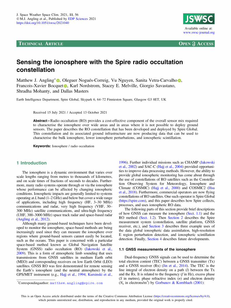
Hajj et al., (2002). In summary, when electromagnetic radiationpasses through the atmosphere, it is refracted. The magnitude ofthe refraction (bending angle a in Fig. 1) depends on the gradi-ent of the atmosphere refractivity normal to the path, whichdepends on the composition of the atmosphere (see Eq. (6)).The bending angle cannot be measured directly; rather, thebending can be estimated using the Doppler shift of the signal,given precise knowledge of the satellites’ positions andvelocities.

An Abel Transform is often then used to invert the GNSS-RO measurements. Given an assumption of spherical symmetry,the bending angle (a) of the ray between the GNSS satellite anda LEO is (e.g., Hajj et al., 2002):

a að Þ ¼ �aZ GNSS

aþZ LEO

a

� �1ffiffiffiffiffiffiffiffiffiffiffiffiffiffi

x2 � a2p d ln n

dxdx; ð4Þ

where a is the impact parameter (= nrsin(/) = const); n is therefractive index; x is the refractional radius (= rn(r)). Then therefractive index can be expressed as:

n xð Þ ¼ exp1p

Z 1

x

aðaÞffiffiffiffiffiffiffiffiffiffiffiffiffiffia2 � x2

p� �

da: ð5Þ

Formally, this requires the extension of the bending angleprofile to infinite values of impact parameter. In practice, thebending angles above the LEO height are extrapolated fromlower heights or derived from a model.

The atmospheric refractivity (N) comprises terms depen-dent on the neutral atmosphere and the ionospheric electrondensity (ne):

N ¼ n� 1ð Þ � 106 ¼ a1PTþ a2

Pw

T 2 � knef 2

þ O1f 3

� �ð6Þ

where a1 = 77.6 (K/mbar), a2 = 3.73 � 105 (K2/mbar), P (mbar)is the total pressure, Pw (mbar) is the water vapour partial pres-sure, T (K) is the temperature, ne (m

�3) is the electron density,f (Hz) is the operating frequency, k = 40.3 � 106 (m3 s�2) andthe final terms represent higher-order terms related to propaga-tion in a magnetised medium which are often neglected (Hoque& Jakowski, 2008). At ionospheric altitudes, the terms in pres-sure and temperature can also be dropped so that the refractivityis only related to the electron density and the frequency. Conse-quently, the refractive index profile derived from the AbelTransform can be converted to electron density.

Figure 1. Radio occultation geometry.

M.J. Angling et al.: J. Space Weather Space Clim. 2021, 11, 56

Page 2 of 13

An alternative approach is to estimate the TEC using themethod described in Section 1.1. Then, by assuming sphericalsymmetry, it is possible to relate the TEC to the electron densityprofile (e.g., Schreiner et al., 1999):

TEC r0ð Þ ¼Z rGNSS

r0

þZ rLEO

r0

� �r � N eðrÞffiffiffiffiffiffiffiffiffiffiffiffiffiffir2 � r20

p dr ð7Þ

where r0 is the straight-line impact parameter (i.e., it is theshortest distance from the assumed straight-line ray to the cen-tre of the Earth). This expression can be inverted thus:

N e rð Þ ¼ � 1p

Z 1

r

dðTECÞdr0ffiffiffiffiffiffiffiffiffiffiffiffiffiffir20 � r2

p dr0: ð8Þ

Both these approaches provide vertical electron density profileswith the high vertical resolution (on the order of the width ofthe first Fresnel zone) but with poor horizontal resolution sincethe geometry of the measurement results in the measuredbending angles or TECs containing information from a large

region of the ionosphere. Furthermore, the presence of horizon-tal structures will limit the performance of methods thatassume spherical symmetry. Many methods have been devel-oped to attempt to overcome this (e.g. Hernández-Pajareset al., 2000; Wu et al., 2009; Mannucci et al., 2011; Pedatellaet al., 2015).

A further alternative is to dispense with the Abel Transformaltogether and assimilate the slant TEC (or potentially excessphase) directly into an ionospheric model (e.g. Angling,2008). This will be discussed in Section 3.1.

2 The Spire ionospheric measurementsystem

2.1 Overview

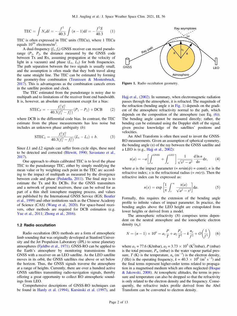
Figure 2 illustrates Spire’s GNSS-RO observing systemarchitecture. Spire owns the entire stack of the observing

Figure 2. Schematic representation of the Spire ionospheric observing system.

M.J. Angling et al.: J. Space Weather Space Clim. 2021, 11, 56

Page 3 of 13

system, including the design of the GNSS payload hardwareand software, the ground station network, mission operations,and ground-side processing (Cappaert, 2018; Bryce & Cappaert,2019). This gives Spire the ability to modify one or more of thecomponents of the observing system to optimise for ionosphericmeasurement quality, quantity, and latency.

2.2 The LEMUR satellite platform

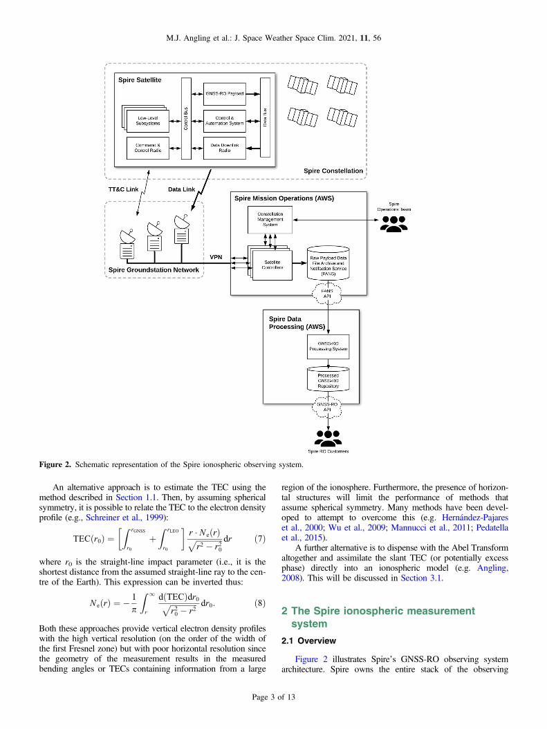
Spire Low Earth Multi-Use Receiver (LEMUR) second-generation satellites (LEMUR2) use the 3U CubeSat form factor(Johnstone, 2020). An overview of the platform capability isgiven in Table 1. From flight model 91 (FM91) onwards,LEMUR2 v3.4 has a third stowable solar panel to increasethe power generating surface (Fig. 3). Due to the increase inthe available power that this bus provides, the GNSS-RO pay-load can be operated at high duty cycles; 98% duty cycle hasbeen tested, though in practice lower duty cycles are usuallyused.

A new major revision of the LEMUR2 bus (v 4.0) has beendesigned to incorporate internal architectural changes and addi-tional features such as an X-band downlink and S-band uplinkcapability to improve data quantity and latency. The LEMUR2v4.X will become the standard Spire satellite platform in thefuture.

2.3 The STRATOS GNSS payload

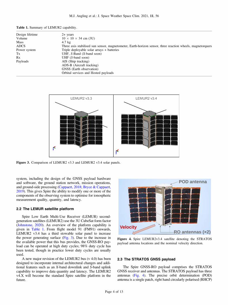
The Spire GNSS-RO payload comprises the STRATOSGNSS receiver and antennas. The STRATOS payload has threeantennas (Fig. 4). The precise orbit determination (POD)antenna is a single patch, right hand circularly polarised (RHCP)

Figure 3. Comparison of LEMUR2 v3.3 and LEMUR2 v3.4 solar panels.

Table 1. Summary of LEMUR2 capability.

Design lifetime 2+ yearsVolume 10 � 10 � 34 cm (3U)Mass 4.7 kgADCS Three axis stabilised sun sensor, magnetometer, Earth-horizon sensor, three reaction wheels, magnetorquersPower system Triple deployable solar arrays + batteriesTx UHF, S-Band (X-band soon)Rx UHF (S-band soon)Payloads AIS (Ship tracking)

ADS-B (Aircraft tracking)GNSS (Earth observation)Orbital services and Hosted payloads

Figure 4. Spire LEMUR2v3.4 satellite denoting the STRATOSpayload antenna locations and the nominal velocity direction.

M.J. Angling et al.: J. Space Weather Space Clim. 2021, 11, 56

Page 4 of 13

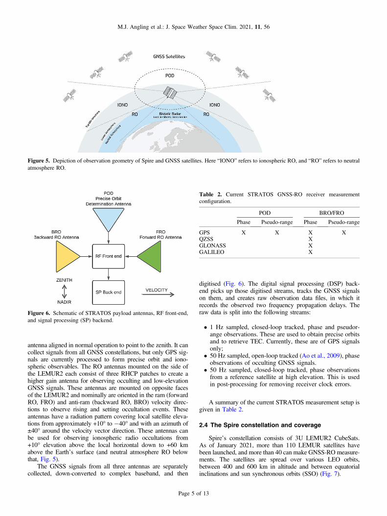
antenna aligned in normal operation to point to the zenith. It cancollect signals from all GNSS constellations, but only GPS sig-nals are currently processed to form precise orbit and iono-spheric observables. The RO antennas mounted on the side ofthe LEMUR2 each consist of three RHCP patches to create ahigher gain antenna for observing occulting and low-elevationGNSS signals. These antennas are mounted on opposite facesof the LEMUR2 and nominally are oriented in the ram (forwardRO, FRO) and anti-ram (backward RO, BRO) velocity direc-tions to observe rising and setting occultation events. Theseantennas have a radiation pattern covering local satellite eleva-tions from approximately +10� to �40� and with an azimuth of±40� around the velocity vector direction. These antennas canbe used for observing ionospheric radio occultations from+10� elevation above the local horizontal down to +60 kmabove the Earth’s surface (and neutral atmosphere RO belowthat, Fig. 5).

The GNSS signals from all three antennas are separatelycollected, down-converted to complex baseband, and then

digitised (Fig. 6). The digital signal processing (DSP) back-end picks up those digitised streams, tracks the GNSS signalson them, and creates raw observation data files, in which itrecords the observed two frequency propagation delays. Theraw data is split into the following streams:

� 1 Hz sampled, closed-loop tracked, phase and pseudor-ange observations. These are used to obtain precise orbitsand to retrieve TEC. Currently, these are of GPS signalsonly;

� 50 Hz sampled, open-loop tracked (Ao et al., 2009), phaseobservations of occulting GNSS signals.

� 50 Hz sampled, closed-loop tracked, phase observationsfrom a reference satellite at high elevation. This is usedin post-processing for removing receiver clock errors.

A summary of the current STRATOS measurement setup isgiven in Table 2.

2.4 The Spire constellation and coverage

Spire’s constellation consists of 3U LEMUR2 CubeSats.As of January 2021, more than 110 LEMUR satellites havebeen launched, and more than 40 can make GNSS-RO measure-ments. The satellites are spread over various LEO orbits,between 400 and 600 km in altitude and between equatorialinclinations and sun synchronous orbits (SSO) (Fig. 7).

Figure 5. Depiction of observation geometry of Spire and GNSS satellites. Here “IONO” refers to ionospheric RO, and “RO” refers to neutralatmosphere RO.

Figure 6. Schematic of STRATOS payload antennas, RF front-end,and signal processing (SP) backend.

Table 2. Current STRATOS GNSS-RO receiver measurementconfiguration.

POD BRO/FRO

Phase Pseudo-range Phase Pseudo-range

GPS X X X XQZSS XGLONASS XGALILEO X

M.J. Angling et al.: J. Space Weather Space Clim. 2021, 11, 56

Page 5 of 13

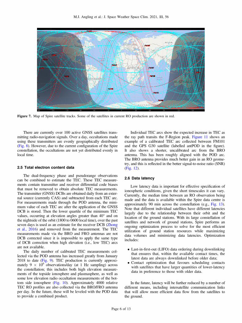
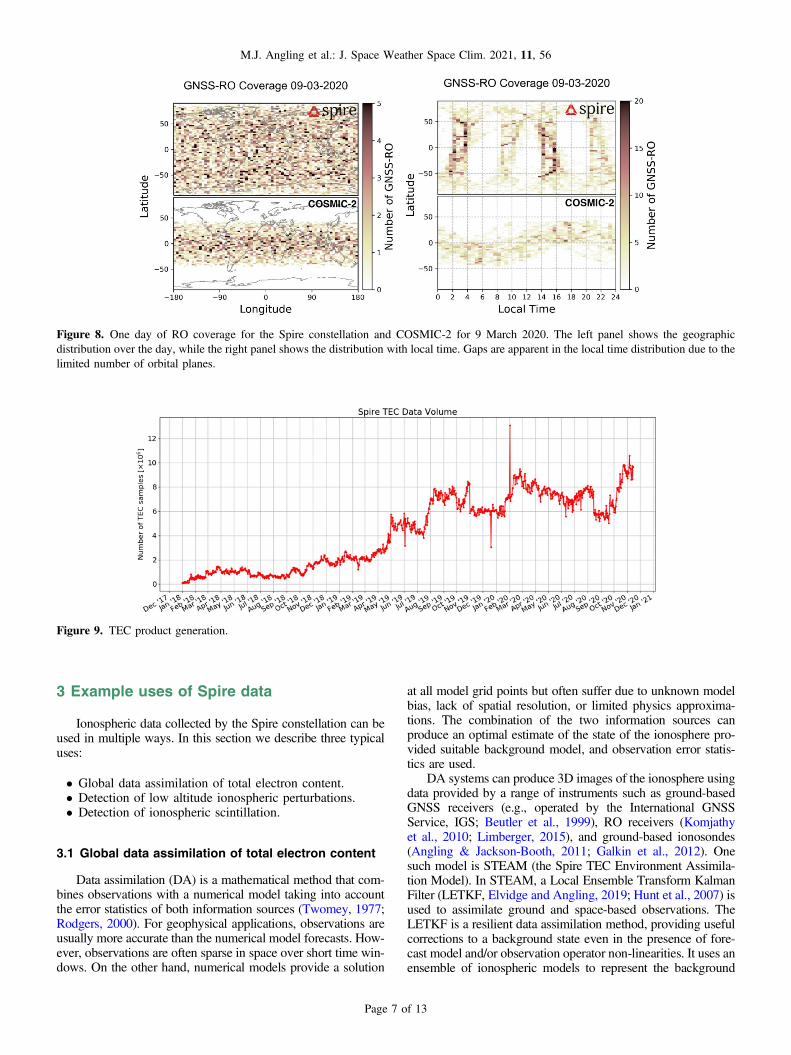
There are currently over 100 active GNSS satellites trans-mitting radio-navigation signals. Over a day, occultations madeusing these transmitters are evenly geographically distributed(Fig. 8). However, due to the current configuration of the Spireconstellation, the occultations are not yet distributed evenly inlocal time.

2.5 Total electron content data

The dual-frequency phase and pseudorange observationscan be combined to estimate the TEC. These TEC measure-ments contain transmitter and receiver differential code biasesthat must be removed to obtain absolute TEC measurements.The transmitter (GNSS) DCBs are obtained daily from an exter-nal source (currently CAS) and subtracted from each TEC arc.For measurements made through the POD antenna, the mini-mum value of each TEC arc after the application of the GNSSDCB is stored. Then the lower quartile of the minimum TECvalues, occurring at elevation angles greater than 40� and onthe nightside of the orbit (1800 to 0600 local time), over the pastseven days is used as an estimate for the receiver DCB (Zhonget al., 2016) and removed from the measurement. The TECmeasurements made via the BRO and FRO antennas are notDCB corrected since it is impossible to apply the same typeof DCB correction when high elevation (i.e., low TEC) arcsare not available.

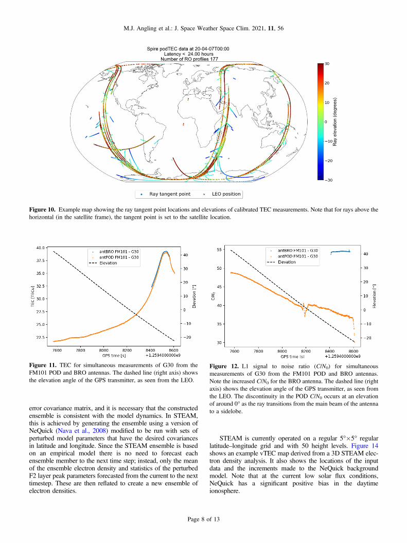
The daily number of calibrated TEC measurements col-lected via the POD antenna has increased greatly from January2018 to date (Fig. 9). TEC production is currently approxi-mately 9 � 106 observations/day (at 1 Hz sampling) acrossthe constellation; this includes both high elevation measure-ments of the topside ionosphere and plasmasphere, as well assome low elevation radio occultation measurements of the bot-tom side ionosphere (Fig. 10). Approximately 4000 relativeTEC RO profiles are also collected via the BRO/FRO antennaper day. In the future, these will be leveled with the POD datato provide a combined product.

Individual TEC arcs show the expected increase in TEC asthe ray path transits the F-Region peak. Figure 11 shows anexample of a calibrated TEC arc collected between FM101and the GPS G30 satellite (labelled antPOD in the figure).It also shows a shorter, uncalibrated arc from the BROantenna. This has been roughly aligned with the POD arc.The BRO antenna provides much better gain in an RO geome-try, and this is reflected in the better signal-to-noise ratio (SNR)(Fig. 12).

2.6 Data latency

Low latency data is important for effective specification ofionospheric conditions, given the short timescales it can vary.Currently, the median time between an RO observation beingmade and the data is available within the Spire data centre isapproximately 90 min across the constellation (e.g., Fig. 13).Note that different individual satellites have different latencieslargely due to the relationship between their orbit and thelocation of the ground stations. With its large constellation ofsatellites and network of ground stations, Spire performs anongoing optimization process to solve for the most efficientutilization of ground station resources while maximizingdata volumes and minimizing data latencies. Optimizationincludes:

� Last-in-first-out (LIFO) data ordering during downlinkingthat ensures that, within the available contact times, thelatest data are always downlinked before older data;

� Contact optimization that favours scheduling contactswith satellites that have larger quantities of lower-latencydata in preference to those with older data.

In the future, latency will be further reduced by a number ofdifferent means, including intersatellite communication linksthat will allow more efficient data flow from the satellites tothe ground.

Figure 7. Map of Spire satellite tracks. Some of the satellites in current RO production are shown in red.

M.J. Angling et al.: J. Space Weather Space Clim. 2021, 11, 56

Page 6 of 13

3 Example uses of Spire data

Ionospheric data collected by the Spire constellation can beused in multiple ways. In this section we describe three typicaluses:

� Global data assimilation of total electron content.� Detection of low altitude ionospheric perturbations.� Detection of ionospheric scintillation.

3.1 Global data assimilation of total electron content

Data assimilation (DA) is a mathematical method that com-bines observations with a numerical model taking into accountthe error statistics of both information sources (Twomey, 1977;Rodgers, 2000). For geophysical applications, observations areusually more accurate than the numerical model forecasts. How-ever, observations are often sparse in space over short time win-dows. On the other hand, numerical models provide a solution

at all model grid points but often suffer due to unknown modelbias, lack of spatial resolution, or limited physics approxima-tions. The combination of the two information sources canproduce an optimal estimate of the state of the ionosphere pro-vided suitable background model, and observation error statis-tics are used.

DA systems can produce 3D images of the ionosphere usingdata provided by a range of instruments such as ground-basedGNSS receivers (e.g., operated by the International GNSSService, IGS; Beutler et al., 1999), RO receivers (Komjathyet al., 2010; Limberger, 2015), and ground-based ionosondes(Angling & Jackson-Booth, 2011; Galkin et al., 2012). Onesuch model is STEAM (the Spire TEC Environment Assimila-tion Model). In STEAM, a Local Ensemble Transform KalmanFilter (LETKF, Elvidge and Angling, 2019; Hunt et al., 2007) isused to assimilate ground and space-based observations. TheLETKF is a resilient data assimilation method, providing usefulcorrections to a background state even in the presence of fore-cast model and/or observation operator non-linearities. It uses anensemble of ionospheric models to represent the background

Figure 8. One day of RO coverage for the Spire constellation and COSMIC-2 for 9 March 2020. The left panel shows the geographicdistribution over the day, while the right panel shows the distribution with local time. Gaps are apparent in the local time distribution due to thelimited number of orbital planes.

Figure 9. TEC product generation.

M.J. Angling et al.: J. Space Weather Space Clim. 2021, 11, 56

Page 7 of 13

error covariance matrix, and it is necessary that the constructedensemble is consistent with the model dynamics. In STEAM,this is achieved by generating the ensemble using a version ofNeQuick (Nava et al., 2008) modified to be run with sets ofperturbed model parameters that have the desired covariancesin latitude and longitude. Since the STEAM ensemble is basedon an empirical model there is no need to forecast eachensemble member to the next time step; instead, only the meanof the ensemble electron density and statistics of the perturbedF2 layer peak parameters forecasted from the current to the nexttimestep. These are then reflated to create a new ensemble ofelectron densities.

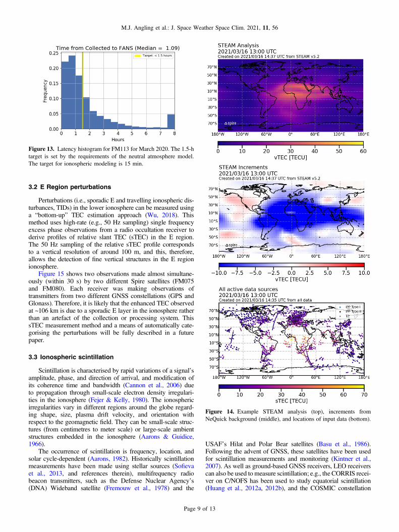
STEAM is currently operated on a regular 5��5� regularlatitude–longitude grid and with 50 height levels. Figure 14shows an example vTEC map derived from a 3D STEAM elec-tron density analysis. It also shows the locations of the inputdata and the increments made to the NeQuick backgroundmodel. Note that at the current low solar flux conditions,NeQuick has a significant positive bias in the daytimeionosphere.

Figure 10. Example map showing the ray tangent point locations and elevations of calibrated TEC measurements. Note that for rays above thehorizontal (in the satellite frame), the tangent point is set to the satellite location.

Figure 11. TEC for simultaneous measurements of G30 from theFM101 POD and BRO antennas. The dashed line (right axis) showsthe elevation angle of the GPS transmitter, as seen from the LEO.

Figure 12. L1 signal to noise ratio (C/N0) for simultaneousmeasurements of G30 from the FM101 POD and BRO antennas.Note the increased C/N0 for the BRO antenna. The dashed line (rightaxis) shows the elevation angle of the GPS transmitter, as seen fromthe LEO. The discontinuity in the POD C/N0 occurs at an elevationof around 0� as the ray transitions from the main beam of the antennato a sidelobe.

M.J. Angling et al.: J. Space Weather Space Clim. 2021, 11, 56

Page 8 of 13

3.2 E Region perturbations

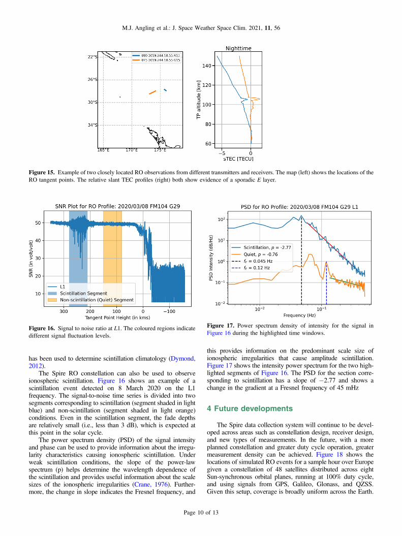
Perturbations (i.e., sporadic E and travelling ionospheric dis-turbances, TIDs) in the lower ionosphere can be measured usinga “bottom-up” TEC estimation approach (Wu, 2018). Thismethod uses high-rate (e.g., 50 Hz sampling) single frequencyexcess phase observations from a radio occultation receiver toderive profiles of relative slant TEC (sTEC) in the E region.The 50 Hz sampling of the relative sTEC profile correspondsto a vertical resolution of around 100 m, and this, therefore,allows the detection of fine vertical structures in the E regionionosphere.

Figure 15 shows two observations made almost simultane-ously (within 30 s) by two different Spire satellites (FM075and FM080). Each receiver was making observations oftransmitters from two different GNSS constellations (GPS andGlonass). Therefore, it is likely that the enhanced TEC observedat ~106 km is due to a sporadic E layer in the ionosphere ratherthan an artefact of the collection or processing system. ThissTEC measurement method and a means of automatically cate-gorising the perturbations will be fully described in a futurepaper.

3.3 Ionospheric scintillation

Scintillation is characterised by rapid variations of a signal’samplitude, phase, and direction of arrival, and modification ofits coherence time and bandwidth (Cannon et al., 2006) dueto propagation through small-scale electron density irregulari-ties in the ionosphere (Fejer & Kelly, 1980). The ionosphericirregularities vary in different regions around the globe regard-ing shape, size, plasma drift velocity, and orientation withrespect to the geomagnetic field. They can be small-scale struc-tures (from centimetres to meter scale) or large-scale ambientstructures embedded in the ionosphere (Aarons & Guidice,1966).

The occurrence of scintillation is frequency, location, andsolar cycle-dependent (Aarons, 1982). Historically scintillationmeasurements have been made using stellar sources (Sofievaet al., 2013, and references therein), multifrequency radiobeacon transmitters, such as the Defense Nuclear Agency’s(DNA) Wideband satellite (Fremouw et al., 1978) and the

USAF’s Hilat and Polar Bear satellites (Basu et al., 1986).Following the advent of GNSS, these satellites have been usedfor scintillation measurements and monitoring (Kintner et al.,2007). As well as ground-based GNSS receivers, LEO receiverscan also be used to measure scintillation; e.g., the CORRIS recei-ver on C/NOFS has been used to study equatorial scintillation(Huang et al., 2012a, 2012b), and the COSMIC constellation

Figure 13. Latency histogram for FM113 for March 2020. The 1.5-htarget is set by the requirements of the neutral atmosphere model.The target for ionospheric modeling is 15 min.

Figure 14. Example STEAM analysis (top), increments fromNeQuick background (middle), and locations of input data (bottom).

M.J. Angling et al.: J. Space Weather Space Clim. 2021, 11, 56

Page 9 of 13

has been used to determine scintillation climatology (Dymond,2012).

The Spire RO constellation can also be used to observeionospheric scintillation. Figure 16 shows an example of ascintillation event detected on 8 March 2020 on the L1frequency. The signal-to-noise time series is divided into twosegments corresponding to scintillation (segment shaded in lightblue) and non-scintillation (segment shaded in light orange)conditions. Even in the scintillation segment, the fade depthsare relatively small (i.e., less than 3 dB), which is expected atthis point in the solar cycle.

The power spectrum density (PSD) of the signal intensityand phase can be used to provide information about the irregu-larity characteristics causing ionospheric scintillation. Underweak scintillation conditions, the slope of the power-lawspectrum (p) helps determine the wavelength dependence ofthe scintillation and provides useful information about the scalesizes of the ionospheric irregularities (Crane, 1976). Further-more, the change in slope indicates the Fresnel frequency, and

this provides information on the predominant scale size ofionospheric irregularities that cause amplitude scintillation.Figure 17 shows the intensity power spectrum for the two high-lighted segments of Figure 16. The PSD for the section corre-sponding to scintillation has a slope of �2.77 and shows achange in the gradient at a Fresnel frequency of 45 mHz

4 Future developments

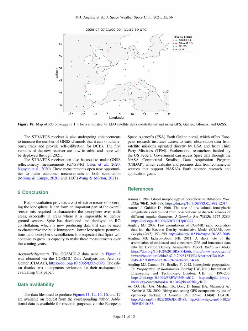
The Spire data collection system will continue to be devel-oped across areas such as constellation design, receiver design,and new types of measurements. In the future, with a moreplanned constellation and greater duty cycle operation, greatermeasurement density can be achieved. Figure 18 shows thelocations of simulated RO events for a sample hour over Europegiven a constellation of 48 satellites distributed across eightSun-synchronous orbital planes, running at 100% duty cycle,and using signals from GPS, Galileo, Glonass, and QZSS.Given this setup, coverage is broadly uniform across the Earth.

Figure 16. Signal to noise ratio at L1. The coloured regions indicatedifferent signal fluctuation levels.

Figure 17. Power spectrum density of intensity for the signal inFigure 16 during the highlighted time windows.

Figure 15. Example of two closely located RO observations from different transmitters and receivers. The map (left) shows the locations of theRO tangent points. The relative slant TEC profiles (right) both show evidence of a sporadic E layer.

M.J. Angling et al.: J. Space Weather Space Clim. 2021, 11, 56

Page 10 of 13

The STRATOS receiver is also undergoing enhancementsto increase the number of GNSS channels that it can simultane-ously track and provide self-calibration for DCBs. The firstversions of the new receiver are now in orbit, and more willbe deployed through 2021.

The STRATOS receiver can also be used to make GNSSreflectometry measurements (GNSS-R) (Jales et al., 2020;Nguyen et al., 2020). These measurements open new opportuni-ties to make additional measurements of both scintillation(Molina & Camps, 2020) and TEC (Wang & Morton, 2021).

5 Conclusion

Radio occultation provides a cost-effective means of observ-ing the ionosphere. It can form an important part of the overallsensor mix required to characterise the ionosphere over wideareas, especially in areas where it is impossible to deployground sensors. Spire has developed and deployed an ROconstellation, which is now producing data that can be usedto characterise the bulk ionosphere, lower ionosphere perturba-tions, and ionospheric scintillation. It is expected that Spire willcontinue to grow its capacity to make these measurements overthe coming years.

Acknowledgements. The COSMIC-2 data used in Figure 8was obtained via the COSMIC Data Analysis and ArchiveCenter (CDAAC), https://doi.org/10.5065/t353-c093. The edi-tor thanks two anonymous reviewers for their assistance inevaluating this paper.

Data availability

The data files used to produce Figures 11, 12, 15, 16, and 17are available on request from the corresponding author. Addi-tional data is available for research purposes via the European

Space Agency’s (ESA) Earth Online portal, which offers Euro-pean research institutes access to earth observation data fromsatellite missions operated directly by ESA and from ThirdParty Missions (TPM). Furthermore, researchers funded bythe US Federal Government can access Spire data through theNASA Commercial Smallsat Data Acquisition Program(CSDAP), which evaluates and procures data from commercialsources that support NASA’s Earth science research andapplication goals.

References

Aarons J. 1982. Global morphology of ionospheric scintillations. Proc.IEEE 70(4): 360–378. https://doi.org/10.1109/PROC.1982.12314.

Aarons J, Guidice D. 1966. The size of low-latitude ionosphericirregularities determined from observations of discrete sources ofdifferent angular diameters. J Geophys Res 71(13): 3277–3280.https://doi.org/10.1029/JZ071i013p03277.

Angling MJ. 2008. First assimilations of COSMIC radio occultationdata into the Electron Density Assimilative Model (EDAM). AnnGeophys 26(2): 353–359. https://doi.org/10.5194/angeo-26-353-2008.

Angling MJ, Jackson-Booth NK. 2011. A short note on theassimilation of collocated and concurrent GPS and ionosonde datainto the Electron Density Assimilative Model. Radio Sci 46(4):https://doi.org/10.1029/2010RS004566. http://www.scopus.com/inward/record.url?eid=2-s2.0-79961243531&partnerID=40&md5=b77f3095bba218c9c9ed4c0edd36466b.

Angling MJ, Cannon PS, Bradley P. 2012. Ionospheric propagation.In: Propagation of Radiowaves. Barclay LW, (Ed.) Institution ofEngineering and Technology, London, UK. pp. 199–233.https://doi.org/10.1049/PBEW056E_ch12. https://digital-library.theiet.org/content/books/10.1049/pbew056e_ch12

Ao CO, Hajj GA, Meehan TK, Dong D, Iijima BA, Mannucci AJ,Kursinski ER. 2009. Rising and setting GPS occupations by use ofopen-loop tracking. J Geophys Res Atmos 114(4): D04101.https://doi.org/10.1029/2008JD010483. http://doi.wiley.com/10.1029/2008JD010483.

Figure 18. Map of RO coverage in 1 h for a simulated 48 LEO satellite delta constellation and using GPS, Galileo, Glonass, and QZSS.

M.J. Angling et al.: J. Space Weather Space Clim. 2021, 11, 56

Page 11 of 13

Basu S, Basu S, Senior C, Weimer D, Nielsen E, Fougere PF. 1986.Velocity Shears and Sub-KM scale Irregularities in the nighttimeauroral F-region. Geophys Res Lett 13(1): 101–104. https://doi.org/10.1029/GL013i002p00101.

Beutler G, Rothacher M, Schaer S, Springer TA, Kouba J, NeilanRE. 1999. The International GPS Service (IGS): An interdisci-plinary service in support of earth sciences. Adv Space Res 23(4):631–653. https://doi.org/10.1016/S0273-1177(99)00160-X.

Blewitt G. 1990. An automatic editing algorithm for GPS data.Geophys Res Lett 17(3): 199–202. https://doi.org/10.1029/GL017i003p00199.

Bryce D, Cappaert J. 2019. Smallsat Manufacturing: The Spire “ConstantNPI” Model, SSC19-I-01. In: Proceedings of the AIAA/USU Confer-ence on Small Satellite Production – Driving a Revolution. https://digitalcommons.usu.edu/smallsat/2019/all2019/267/.

Cannon PS, Groves K, Fraser DJ, Donnelly WJ, Perrier K. 2006.Signal distortion on VHF/UHF transionospheric paths: First resultsfrom the Wideband Ionospheric Distortion Experiment. Radio Sci41(5): RS5S40. https://doi.org/10.1029/2005RS003369. http://doi.wiley.com/10.1029/2005RS003369.

Cappaert J. 2018. Building, deploying and operating a cubesatconstellation – exploring the less obvious reasons space is hard,SSC18-IV-03. In: Proceedings of the AIAA/USU Conference onSmall Satellites – Delivering Mission Success. https://digitalcommons.usu.edu/smallsat/2018/all2018/274/.

Crane RK. 1976. Spectra of ionospheric scintillation. J Geophys Res81(13): 2041–2050. https://doi.org/10.1029/ja081i013p02041.http://doi.wiley.com/10.1029/JA081i013p02041.

Dymond KF. 2012. Global observations of L band scintillation atsolar minimum made by COSMIC. Radio Sci 47(3): 1–10.https://doi.org/10.1029/2011RS004931.

Elvidge S, Angling MJ. 2019. Using the local ensemble TransformKalman Filter for upper atmospheric modelling. J. Space WeatherSpace Clim 9: A30. https://doi.org/10.1051/swsc/2019018.

Fejer BG, Kelly M. 1980. Ionospheric irregularities. Rev Geophys18(2):401–454. https://doi.org/10.1029/RG018i002p00401.

Fjeldbo G, Kliore AJ, Eshleman VR. 1971. The neutral atmosphereof venus as studied with the Mariner V Radio OccultationExperiments. Astron J 76: 123. https://doi.org/10.1086/111096.

Fremouw EJ, Leadabrand RL, Livingston RC, Cousins MD, Rino CL,Fair BC, Long RA. 1978. Early results from the DNA Widebandsatellite experiment – Complex-signal scintillation. Radio Sci 13(1):167–187. https://doi.org/10.1029/RS013i001p00167.

Galkin IA, Reinisch BW, Huang X, Bilitza D. 2012. Assimilation ofGIRO data into a real-time IRI. Radio Sci 47(4): https://doi.org/10.1029/2011RS004952.

Gorbunov ME, Kornblueh L. 2001. Analysis and validation of GPS/MET radio occultation data. J Geophys Res Atmos 106(D15):17161–17169. https://doi.org/10.1029/2000JD900816.

Hajj GA, Ibañez-Meier R, Kursinski ER, Romans LJ. 1994. Imagingthe ionosphere with the global positioning system. Int J ImagingSyst Technol 5(2): 174–187. https://doi.org/10.1002/ima.1850050214. http://doi.wiley.com/10.1002/ima.1850050214.

Hajj GA, Lee LC, Pi X, Romans LJ, Schreiner WS, Straus PR, WangC. 2000. COSMIC GPS ionospheric sensing and space weather.Terr Atmos Ocean Sci 11(1): 235–272. https://doi.org/10.3319/TAO.2000.11.1.235(COSMIC).

Hajj GA, Kursinski ER, Romans LJ, Bertiger WI, Leroy SS. 2002. Atechnical description at atmospheric sounding by GPS occultation.J Atmos Sol-Terr Phys 64(4): 451–469. https://doi.org/10.1016/S1364-6826(01)00114-6.

Hajj GA, Ao CO, Iijima BA, Kuang D, Kursinski ER, Mannucci AJ,Meehan TK, Romans LJ, de la Torre Juarez M, Yunck TP. 2004.

CHAMP and SAC-C atmospheric occultation results and inter-comparisons. J Geophys Res Atmos 109(6): https://doi.org/10.1029/2003jd003909.

Hardy KR, Hajj GA, Kursinski ER. 1994. Accuracies of atmosphericprofiles obtained from GPS occultations. Int J Satell Commun 12(5):463–473. https://doi.org/10.1002/sat.4600120508. http://doi.wiley.com/10.1002/sat.4600120508.

Hernández-Pajares M, Juan JM, Sanz J. 2000. Improving the Abelinversion by adding ground GPS data to LEO radio occultations inionospheric sounding. Geophys Res Lett 27(16): 2473–2476. https://doi.org/10.1029/2000GL000032. http://doi.wiley.com/10.1029/2000GL000032.

Hoque MM, Jakowski N. 2008. Estimate of higher order ionosphericerrors in GNSS positioning. Radio Sci 43(5): https://doi.org/10.1029/2007RS003817. http://doi.wiley.com/10.1029/2007RS003817.

Hsu C-T, Matsuo T, Yue X, Fang T-W, Fuller-Rowell T, Ide K, LiuJ-Y. 2018. Assessment of the impact of FORMOSAT-7/COSMIC-2GNSS RO observations on midlatitude and low-latitude ionospherespecification: Observing system simulation experiments usingensemble square root filter. J Geophys Res Space Phys 123(3):2296–2314. https://doi.org/10.1002/2017JA025109. http://doi.wiley.com/10.1002/2017JA025109.

Huang CS, De La Beaujardiere O, Roddy PA, Hunton DE,Ballenthin JO, Hairston MR. 2012a. Generation and characteristicsof equatorial plasma bubbles detected by the C/NOFS satellite nearthe sunset terminator. J Geophys Res Space Phys 117(11): 1–11.https://doi.org/10.1029/2012JA018163.

Huang CS, Retterer JM, De La Beaujardiere O, Roddy PA, HuntonDE, Ballenthin JO, Pfaff RF. 2012b. Observations and simulationsof formation of broad plasma depletions through merging process.J Geophys Res Space Phys 117(2): 1–11. https://doi.org/10.1029/2011JA017084.

Hunt BR, Kostelich EJ, Szunyogh I. 2007. Efficient data assimilationfor spatiotemporal chaos: A local ensemble transform Kalmanfilter. Phys D Nonlinear Phenom 230(1–2): 112–126. https://doi.org/10.1016/j.physd.2006.11.008.

Jakowski N, Wehrenpfennig A, Heise S, Reigber C, Lühr H,Grunwaldt L, Meehan TK. 2002. GPS radio occultation measure-ments of the ionosphere from CHAMP: Early results. Geophys ResLett 29(10): 95-1–95-4. https://doi.org/10.1029/2001GL014364.http://doi.wiley.com/10.1029/2001GL014364.

Jakowski N, Leitinger R, Angling MJ. 2009. Radio occultationtechniques for probing the ionosphere. Ann Geophys 47(2–3 Sup.):1049–1066. https://doi.org/10.4401/ag-3285. http://www.scopus.com/inward/record.url?eid=2-s2.0-8844263125&partnerID=40&md5=325faf47b4c45fb685e88828202790b2.

Jales P, Esterhuizen S, Masters D, Nguyen V, Nogués-Correig O,Yuasa T, Cartwright J. 2020. The new Spire GNSS-R satellitemissions and products. In: Image and Signal Processing forRemote Sensing XXVI, Vol. 11533. Notarnicola C, Bovenga F,Bruzzone L, Bovolo F, Benediktsson JA, Santi E, Pierdicca N,(Eds.), SPIE. pp. 41. https://doi.org/10.1117/12.2574127. https://www.spiedigitallibrary.org/conference-proceedings-of-spie/11533/2574127/The-new-Spire-GNSS-R-satellite-missions-and-products/10.1117/12.2574127.full

Jin S, Cardellach E, Xie F. 2014. GNSS Remote Sensing: Theory,Methods and Applications. Springer. https://doi.org/10.1007/978-94-007-7482-7. http://link.springer.com/10.1007/978-94-007-7482-7_1.

Johnstone A. 2020. Cubesat Design Specification. CP-CDS-R14,Cal. Poly. https://www.cubesat.org/s/CDS-REV14-2020-07-31-DRAFT.pdf.

M.J. Angling et al.: J. Space Weather Space Clim. 2021, 11, 56

Page 12 of 13

Kintner PM, Ledvina BM, de Paula ER. 2007. GPS and ionosphericscintillations. Space Weather 5(9): https://doi.org/10.1029/2006SW000260.

Komjathy A, Wilson B, Pi X, Akopian V, Dumett M, Iijima B,Verkhoglyadova O, Mannucci AJ. 2010. JPL/USC GAIM: On theimpact of using COSMIC and ground-based GPS measurements toestimate ionospheric parameters. J Geophys Res Space Phys115(2): 1–10. https://doi.org/10.1029/2009JA014420.

Kursinski ER, Hajj GA, Bertiger WI, Leroy SS, Meehan TK, et al.1996. Initial results of radio occultation observations of Earth’satmosphere using the global positioning system. Science 271(5252):1107–1110. https://doi.org/10.1126/science.271.5252.1107.

Kursinski ER, Hajj GA, Schofield JT, Linfield RP, Hardy KR. 1997.Observing Earth’s atmosphere with radio occultation measure-ments using the global positioning system. J Geophys Res Atmos102(19): 23429–23465. https://doi.org/10.1029/97jd01569.

Limberger M. 2015. Ionosphere modeling from GPS radio occulta-tions and complementary data based on B-splines, PhD Thesis,Technische Universität München. https://mediatum.ub.tum.de/doc/1254715/1254715.pdf.

Mannucci AJ, Ao CO, Pi X, Iijima BA. 2011. The impact of largescale ionospheric structure on radio occultation retrievals. AtmosMeas Tech 4(12): 2837–2850. https://doi.org/10.5194/amt-4-2837-2011. http://www.atmos-meas-tech.net/4/2837/2011/.

Molina C, Camps A. 2020. First evidences of ionospheric plasmadepletions observations using GNSS-R data from CYGNSS.Remote Sens 12(22): 1–21. https://doi.org/10.3390/rs12223782.https://www.mdpi.com/2072-4292/12/22/3782.

Nava B, Coisson P, Radicella S. 2008. A new version of the neQuickionosphere electron density model. J Atmos Sol-Terr Phys 70:1856–1862. https://doi.org/10.1016/j.jatsp.2008.01.015.

Nguyen VA, Nogués-Correig O, Yuasa T, Masters D, Irisov V. 2020.Initial GNSS phase altimetry measurements from the spire satelliteconstellation. Geophys Res Lett 47(15): e2020GL088308.https://doi.org/10.1029/2020GL088308. https://onlinelibrary.wi-ley.com/doi/10.1029/2020GL088308.

Pedatella NM. 2011. Response of the ionosphere-plasmasphere systemto periodic forcing. University of Colorado, Boulder. https://scholar.colorado.edu/concern/graduate_thesis_or_dissertations/cj82k760d.

Pedatella NM, Yue X, Schreiner WS. 2015. An improved inversionfor FORMOSAT-3/COSMIC ionosphere electron density profiles.J Geophys Res A Space Phys 120(10): 8942–8953. https://doi.org/10.1002/2015JA021704. http://doi.wiley.com/10.1002/2015JA021704.

Rodgers CD. 2000. Inverse methods for atmospheric sounding:Theory and practice, Vol. 2 of Series on Atmospheric, Oceanic and

Planetary Physics. World Scientific Publishing, Singapore.https://doi.org/10.1142/3171.

Savastano G, Komjathy A, Verkhoglyadova O, Mazzoni A, Crespi M,Wei Y, Mannucci AJ. 2017. Real-time detection of Tsunamiionospheric disturbances with a stand-alone GNSS receiver: Apreliminary feasibility demonstration. Sci Rep 7: 46607. https://doi.org/10.1038/srep46607. https://github.com/giorgiosavastano/VARION.

Schreiner WS, Sokolovskiy SV, Rocken C, Hunt DC. 1999. Analysisand validation of GPS/MET radio occultation data in theionosphere. Radio Sci 34(4): 949–966. https://doi.org/10.1029/1999RS900034. http://doi.wiley.com/10.1029/1999RS900034.

Sofieva VF, Dalaudier F, Vernin J. 2013. Using stellar scintillationfor studies of turbulence in the Earth’s atmosphere. Philos Trans RSoc A Math Phys Eng Sci 371(1982): 20120174. https://doi.org/10.1098/rsta.2012.0174.

Teunissen PJG, Montenbruck O. 2017. Springer Handbook ofGlobal Navigation Satellite Systems. Springer InternationalPublishing. https://doi.org/10.1007/978-3-319-42928-1.

Twomey S. 1977. Introduction to the mathematics of inversion inremote sensing and indirect measurement. Dover Publications,New York. 978-0-444-41547-9

Wang Q, Jin S, Yuan L, Hu Y, Chen J, Guo J. 2020. Estimation andanalysis of BDS-3 differential code biases from MGEX observa-tions. Remote Sens 12(1): 68. https://doi.org/10.3390/RS12010068.

Wang Y, Morton YJ. 2021. Ionospheric total electron content anddisturbance observations from space borne coherent GNSS-Rmeasurements. Submitted to IEEE Trans Geosci Remote Sens.https://doi.org/10.1109/TGRS.2021.3093328

Wu DL. 2018. New global electron density observations from GPS-RO in the D- and E-Region ionosphere. J Atmos Sol Terr Phys171: 36–59. https://doi.org/10.1016/j.jastp.2017.07.013. https://www.sciencedirect.com/science/article/pii/S1364682617301050?via%3Dihub.

Wu X, Hu X, Gong X, Zhang X, Wang X. 2009. An asymmetrycorrection method for ionospheric radio occultation. J GeophysRes Space Phys 114(A3): n/a–n/a, https://doi.org/10.1029/2008JA013025. http://doi.wiley.com/10.1029/2008JA013025.

Yue X, Schreiner WS, Hunt DC, Rocken C, Kuo YH. 2011.Quantitative evaluation of the low Earth orbit satellite based slanttotal electron content determination. Space Weather 9(9): 09001.https://doi.org/10.1029/2011SW000687.

Zhong J, Lei J, Yue X, Dou X. 2016. Determination of DifferentialCode Bias of GNSS Receiver Onboard Low Earth Orbit Satellite.IEEE Trans Geosci Remote Sens 54(8): 4896–4905. https://doi.org/10.1109/TGRS.2016.2552542.

Cite this article as: Angling M, Nogués-Correig O, Nguyen V, Vetra-Carvalho S, Bocquet F, et al. 2021. Sensing the ionosphere with theSpire radio occultation constellation. J. Space Weather Space Clim. 11, 56. https://doi.org/10.1051/swsc/2021040.

M.J. Angling et al.: J. Space Weather Space Clim. 2021, 11, 56

Page 13 of 13