Seismic Performance of Steel Framed Water Tower Structures

Seismic Performance of Steel Framed Water Tower

Structures

by

Vianney Ntibaziyaremye

Thesis presented in fulfilment of the requirements for the degree of

Master of Engineering in the Faculty of Civil Engineering at

Stellenbosch University

Supervisor: Dr JAvB Strasheim

December 2016

ii

Declaration

By submitting this thesis electronically, I declare that the entirety of the work contained therein is

my own, original work, that I am the sole author thereof (save to the extent explicitly otherwise

stated), that reproduction and publication thereof by Stellenbosch University will not infringe any

third party rights and that I have not previously in its entirety or in part submitted it for obtaining

any qualification.

December 2016

Copyright © 2016 Stellenbosch University

All rights reserved

Stellenbosch University https://scholar.sun.ac.za

iii

Abstract

From the year 1620 until June, 2008, more than 27000 earthquakes of magnitude ranging from 0.2

to 6.3 have been recorded by the South African National Seismological Database (SANSD). The

most affected regions are Cape Town, Ceres, Koffiefontein, Lesotho and the Witwatersrand Basin.

The historical record showed that the earthquake with the longest time duration was felt in South

Africa on 4 December 1809. It caused small damages to buildings in Cape Town and caused

liquefaction and cracks in the soil in the region of Blauwberg. However, the 29 September 1969

earthquake was the strongest and the most damaging in South African earthquake history. It was

felt across Western Cape as far as Ceres, Tulbagh and Wolseley. It was of magnitude 6.3 on the

Richter scale. Many building structures were seriously damaged, a few people were killed and

others were injured. Old and poorly constructed buildings were completely destroyed. The total

cost of the damaged infrastructure was estimated at U.S. $24million. Given this history, South

African is classified as being at risk of moderate intensity earthquakes.

The first version of seismic design code was released in 1980. It was updated in 1989 and 2010,

but the updated code does not include all factors influencing the seismic response of the structures

(e.g. soil foundation interaction). In addition, structures like dams, water towers, bridges, silos,

pipelines, masts and chimneys were not covered. The new code limited its consideration to

building structures. The concern is to know whether old structures or newer structures which are

not covered by the new seismic designed code will be susceptible to damage by the seismic

intensity assigned to the region of their location. Therefore, a methodology for seismic

performance assessment of steel framed structures was presented from various publications and

was applied to a typical water tower located in a high risk seismic zone of South Africa. The

Winelands Engen 1-Stop water tower met the above criteria and was checked for its susceptibility

to a seismic event. The results showed that the Engen 1-Stop water tower is vulnerable to the

seismic risk attributed to its location. The seismic demand on the tower far exceeds its seismic

capacity, which causes concern over whether the Engen 1-Stop water tower was designed to meet

any seismic hazard.


iv

Opsomming

Vanaf die jaar 1620 tot en met Junie 2008, het die Suid-Arikaanse Nasionale Seismologiese

Databasis (SANSD) meer as 27000 aardbewings, wat tussen 0.2 en 6.3 op die Richter skaal meet,

opgeneem. Kaapstad, Ceres, Koiffiefontein, Lesotho en die Witwatersrand Kom is onder meer die

areas wat die meeste geteister word deur aardbewings. Historiese opnames toon dat die langste

aardbewing in Suid-Afrika plaasgevind het op 04 Desember 1809. Daar was minimale skade

aangerig aan geboue in die Kaapstad-omgewing, alhoewel vervloeiing en klein krake waargeneem

was op die grond in die Blauwberg-area. Inteendeel het die sterkste aardbewing, wat die meeste

verwoesting gesaai het, plaasgevind op 29 September 1969. Dié aardbewing het 6.3 gemeet op die

Richter skaal en was gevoel regoor die Wes-Kaap provinsie. Die aardbewing was veral gevoel in

areas soos Ceres, Tulbagh en Wolseley. Die aardbewing het gelei tot die ernstige skade aan geboue,

lewensverlies en die besering van tale mense. As gevolg van die sterkte van die aardbewing het

tale ou geboue, sowel as die wat nie ontwerp is vir aardbewings nie, ineengestort. Die beraamde

skade as gevolg van die aardbewing was ongeveer U.S. $24 miljoen. Suid-Afrika word

geklassifiseer as ‘n area met ‘n risiko van middelmatige intensiteit aardbewings.

Die eerste weergawe van die seismiese ontwerp kode was gepubliseer in 1980. Hersiene

weergawes is beskikbaar gestel in 1989 en 2010, maar die nuutste weergawes sluit nie alle faktore

met betrekking tot die invloed van seismiese reaksie van strukture soos byvoorbeeld die grond-

fondasie interaksie in nie. Strukture soos damme, watertorings, brûe, silos, pyplyne, maste en

skoorstene word ook nie gedek deur die nuutste kodes nie. Die ontwerpstappe en riglyne van die

nuutste weergawe is beperk tot die ontwerp van geboue. Die vraag ontstaan dan of die ouer sowel

as toekomstige nuwe strukture wat nie ingesluit is onder die nuwe ontwerp kode nie, nie dalk

vatbaar is vir skade wat nie onder die nuwe seismiese intensiteit waaronder dit ge geklassifiseer

word nie. Verskeie publikasies is geraadpleeg om ‘n metode vir die bepaal van die seismiese

gedrag van staalraam strukture daar te stel. Hierna was die informasie gebruik en toegepas op ‘n

watertoring in ‘n area met n hoë seismiese risiko in Suid-Afrika. Die Engen 1-Stop watertoring,

geleë in die Wynland, is gekies vir die studie aangesien dit aan die vereiste kriteria voldoen het en

is gebruik om die vatbaarheid daarvan te bepaal in die geval van seismiese gebeure. Die resultate

het getoon dat die Engen 1-Stop water toring kwesbaar vir die seismiese risiko wat daaraan

toegewys is aan die area waar dit is. Die studie het gevind dat die seismiese aanvraag op die toring


v

veel meer is as die seismiese kapasiteit waarvoor dit ontwerp is. Die vraag kan dus gestel word of

die Engen 1-Stop onder bespreking ontwerp is vir enige seismiese gebeure en die gepaardgaande

strukturele impak daarop.


vi

Acknowledgements

I would like to express my sincere gratitude to the people and institutions below for contributing

to the successful completion of my master’s studies.

My supervisor Dr JAvB Strasheim for being actively involved in every stage of this

dissertation. His generous wise advice and guidance have contributed to the accuracy of

this dissertation.

Dr Trevor Neville Haas for his role in identifying the research topic.

The lab manager Mr Stephan Zeranka. His technical assistance during laboratory testing is

acknowledged.

Laboratory and workshop personnel Mr. Charlton Ramat, Mr. Peter Cupido, Mr. Johan

Van der Merwe and Mr. Deon Viljoen. Their assistance in different ways is highly

appreciated.

My classmates, particularly B. Le Roux, A. Bauer, A. Vital, L. Oliver and E. Nuraan. Their

friendships and academic discussions are priceless. They made me feel at home in South

Africa. To them, deeply, thank you. I owe very much to them.

My family for their love, prayers and support throughout my life.

The government of Rwanda for funding the first two years of my studies.

Institute of Structural Engineering (ISE) at Stellenbosch University for funding the

extension of my studies. Special thanks to Prof. Billy Boshoff; the ISE staff and head of

Structural Engineering Division. I am really speechless at his wise advice, suggestions, and

advocacy on different problems I faced on the route to this achievement. May God bless

him.

Rwanda High Commission in South Africa for administrative assistance.

Stellenbosch University, particularly the entire staff of the civil engineering department

and the engineering librarians. The realization of this work is a result of your combined

efforts in one way or another.

“Glory to God.”


vii

Dedications

To

Niyomungeri A.

Irankunda B.


viii

Table of contents

Declaration ...................................................................................................................................... ii

Abstract .......................................................................................................................................... iii

Opsomming .................................................................................................................................... iv

Acknowledgements ........................................................................................................................ vi

Dedications ................................................................................................................................... vii

Table of contents .......................................................................................................................... viii

List of figures ................................................................................................................................ xii

List of tables ................................................................................................................................. xvi

List of symbols ............................................................................................................................ xvii

List of acronyms ......................................................................................................................... xxv

Chapter 1 Introduction .................................................................................................................. 26

1.1 Background to the research question ...................................................................................... 26

1.2 Problem statement ................................................................................................................... 27

1.3 Research objectives ................................................................................................................. 28

1.4 Scope and limitation ............................................................................................................... 28

1.5 Assumptions ............................................................................................................................ 29

1.6 Overview of research conducted ............................................................................................. 29

Chapter 2 Literature Review ......................................................................................................... 31

2.1 Introduction ............................................................................................................................. 31

2.2 Dynamic modelling of water tanks ......................................................................................... 32

2.3 Seismic analysis with consideration of Soil Structure Interaction (SSI) ................................ 34

2.3.1 Introduction .......................................................................................................................... 34

2.3.2 Research done on Soil Structure Interaction ........................................................................ 36

2.3.2.1 Review of soil structure inertia interaction effects ........................................................... 38


ix

2.3.2.2 A review on kinematic interaction .................................................................................... 50

2.3.2.3 A review on foundation flexibility .................................................................................... 55

2.3.3 A review on standards and code provisions ......................................................................... 56

2.3.3.1 Building codes and standards............................................................................................ 56

2.3.3.2 Codes and standards for water storage tanks .................................................................... 61

2.4 Seismic performance assessment methods ............................................................................. 61

2.4.1 Nonlinear time history ......................................................................................................... 62

2.4.2 Nonlinear pushover approach .............................................................................................. 62

2.4.2.1 Transformation of a MDOF system to a SDOF system .................................................... 63

2.4.2.2 Horizontal load distribution .............................................................................................. 65

2.4.2.3 A review of pushover analysis methods ........................................................................... 66

Chapter 3 Methodology ................................................................................................................ 83

3.1 Introduction ............................................................................................................................. 83

3.2 Numerical method for structural performance assessment of a steel frame water tower ....... 84

3.2.1 Dynamic modelling of water tank........................................................................................ 84

3.2.2 Dynamic modelling of soil foundation interaction .............................................................. 85

A. Direct method.......................................................................................................... 85

B. Substructure approach ............................................................................................. 86

3.2.3 Estimation of the seismic demand of the structure ............................................................ 101

A. Nonlinear dynamic approach ................................................................................ 101

B. Code design approach ........................................................................................... 101

3.2.4 Estimation of the seismic capacity of the structure ........................................................... 102

3.3 Design criteria of frame members......................................................................................... 103

3.4 Case study layout .................................................................................................................. 103

3.4.1 Structural characteristics .................................................................................................... 103


x

3.4.1.1 Description of the water tower ........................................................................................ 103

3.4.1.2 Description of the foundation ......................................................................................... 104

3.4.1.3 Mechanical characteristics of structural materials .......................................................... 105

3.4.2 Site soil Characteristics ...................................................................................................... 106

3.4.3 Seismic characteristics of the site ...................................................................................... 107

3.4.3.1 Peak ground acceleration ................................................................................................ 107

3.4.3.2 Ground motion ................................................................................................................ 108

Chapter 4 Analysis and testing of the structure .......................................................................... 110

4.1 Analysis of test structure ....................................................................................................... 111

4.1.1 Experimental testing of the test structure ........................................................................... 111

4.1.2 Numerical analysis of the test structure ............................................................................. 117

4.1.3 Analysis of test structure by the code design approach ..................................................... 120

A. Determination of the lateral stiffness of the test structure .................................... 121

B. Determination of the natural period of the test structure ...................................... 123

C. Determination of the total base shear force .......................................................... 123

4.1.4 Summary and discussion of results .................................................................................... 124

4.2 Seismic assessment of the water tower ................................................................................. 125

4.2.1 Investigation of the behaviour of the tower for the fixed base condition .......................... 125

4.2.1.1 Development of the analysis model ................................................................................ 125

4.2.1.2 Estimation of the seismic demand of the tower .............................................................. 127

4.2.1.3 Estimation of seismic capacity of the water tower ......................................................... 131

4.2.2 Investigation of the tower by consideration of flexible base condition ............................. 134

4.2.2.1 Development of the analysis model ................................................................................ 134

4.2.2.2 Estimation of the seismic demand .................................................................................. 140

4.2.2.3 Estimation of seismic capacity of the tower ................................................................... 142


xi

4.3 Stability of the water tower ................................................................................................... 144

4.3.1 Local stability..................................................................................................................... 144

4.3.2 Global stability ................................................................................................................... 144

4.3.2.1 Global stability requirement ........................................................................................... 145

Chapter 5 Results summary and discussions .............................................................................. 147

5.1 Summary of the results ......................................................................................................... 147

5.2 Discussions ........................................................................................................................... 150

5.2.1 Seismic capacity of the tower ............................................................................................ 150

5.2.2 Seismic demand of the tower ............................................................................................. 150

5.2.3 The soil structure interaction effect ................................................................................... 150

Chapter 6 Conclusion and recommendation .......................................................................... 152

6.1 General conclusion................................................................................................................ 152

6.2 Recommendations ................................................................................................................. 157

References ................................................................................................................................... 159

Appendices .................................................................................................................................. 171


xii

List of figures

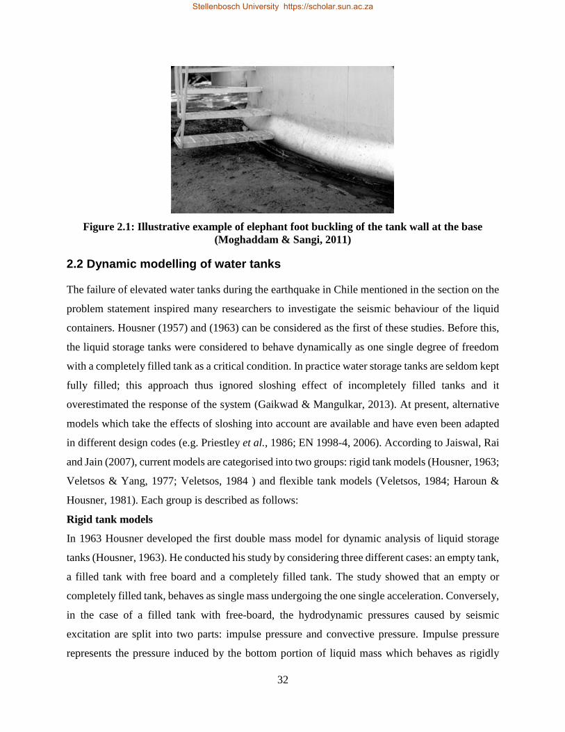
Figure 2.1: Illustrative example of elephant foot buckling of the tank wall at the base

(Moghaddam & Sangi, 2011) ....................................................................................................... 32

Figure 2.2: Housner’s dynamic model .......................................................................................... 33

Figure 2.3: Mechanical model for flexible tank walls .................................................................. 34

Figure 2.4: Force transfer to the base of structure (adapted from Stewart, 2004) ........................ 34

Figure 2.5: Failure example due to soil flexibility (adapted from Kotronis, Tamagnini & Grange,

2013) ............................................................................................................................................. 35

Figure 2.6: Radiation of energy at foundation base (adapted from Stewart, 2004) ...................... 37

Figure 2.7: Total displacement of flexibly supported SDOF (adapted from Kotronis et al., 2013)

....................................................................................................................................................... 37

Figure 2.8:Effective pressure(modified from Richart et al. 1970) ............................................... 38

Figure 2.9: Simplified analogical model of SSI analysis (Veletsos & Wei, 1971) .................... 41

Figure 2.10: Single degree of freedom replacement oscillator (adapted from Veletsos & Meek,

1974) ............................................................................................................................................. 43

Figure 2.11: Replacement oscillator of hysteretic soil structure analysis (Veletsos & Nair 1975).

....................................................................................................................................................... 46

Figure 2.12: Illustrative example of the embedded foundations considered by Avilés and Pérez-

Rocha ............................................................................................................................................ 48

Figure 2.13: Illustrative example of seismic waves transmitted at inclined angle ....................... 50

Figure 2.14: Transfer function amplitude or impedance function amplitude for vertically incident

incoherent waves (from Kramer & Stewart, 2004) ....................................................................... 52

Figure 2.15: Model considered by Iguchi and Luco for investigation of foundation effect for the

response of the structure (based on Iguchi & Luco, 1982) ........................................................... 55

Figure 2.16: Foundation damping factor (adapted from ASCE, 2010) ........................................ 59

Figure 2.17: Illustrative example of displacement based approach for SSI

(NEHRP Consultants Joint Venture, 2012) .................................................................................. 61

Figure 2.18: The basic concept of POA( adapted from Themelis, 2008) ..................................... 63

Figure 2.19: (a) Base shear force-top displacement relationship of MDOF; (b) bilinearised force-

displacement relationship of equivalent SDOF (modified from Themelis, 2008)........................ 64

Figure 2.20: An illustrative example of capacity curve for a MDOF system ............................... 67


xiii

Figure 2.21: Conversion of elastic demand spectrum to ADRS (adapted from Themelis, 2008) 68

Figure 2.22: Estimation of initial performance point.................................................................... 69

Figure 2.23: Bilinearised capacity spectrum in ADRS format (adapted from ATC, 1996) ......... 70

Figure 2.24: Estimation of hysteretic damping associated with ................................................... 71

Figure 2.25: Determination of performance point (modified from ATC-40, 1996) ..................... 72

Figure 2.26: Illustrative example of capacity spectrum demand with various ductility factors ... 73

Figure 2.27: Illustrative example of demand spectrum of constant ductility factors in ADRS

format (adapted from Fajfar, 2000) .............................................................................................. 75

Figure 2.28: Illustrative example of response spectrum components ........................................... 76

Figure 2.29: A graph combining the demand spectrum and the capacity spectrum in ADRS

format (adapted from Fajfar, 2000) .............................................................................................. 77

Figure 2.30: Bilinearisation of capacity curve (extracted from ASCE, 2000) .............................. 79

Figure 2.31: Dynamic characteristics of equivalent SDOF system obtained from capacity curve

(extracted from Chopra & Goel, 2002) ......................................................................................... 81

Figure 3.1: Dynamic model for flexible wall tank (adapted from Malhotra et al., 2000) ............ 84

Figure 3.2: Direct approach for SSI modelling of bridge column supported on two different

layers of soil (modified from Kotronis et al., 2013) ..................................................................... 86

Figure 3.3: Substructure approach for SSI analysis (modified from PEER, 2010) ...................... 86

Figure 3.4: Modelling approach (modified from PEER 2010) ..................................................... 98

Figure 3.5:Allocation of vertical spring and dashpot forces to the foundation base .................... 99

Figure 3.6: Typical example of soil reaction (stiffness) distribution (modified from NEHRP

Consultants Joint Venture, 2012) ................................................................................................ 100

Figure 3.7: Engen Winelands 1-Stop elevated water tower ........................................................ 104

Figure 3.8: (a) Connection of the columns to foundation; (a) Connection of frame elements to the

column......................................................................................................................................... 105

Figure 3.9: Seismic hazard map of South Africa (adapted from SANS 10160-4, 2011) ........... 107

Figure 3.10: Selected ground motion characteristics .................................................................. 109

Figure 4.1: Typical test structure ................................................................................................ 111

Figure 4.2 : Column to beam and bracing connection ................................................................ 112

Figure 4.3:Footplates of the columns.......................................................................................... 113

Figure 4.4:Shaking table testing machine ................................................................................... 113


xiv

Figure 4.5:Typical connection of the test structure to the shaking table .................................... 114

Figure 4.6: Loaded steel frame on shaking table ........................................................................ 115

Figure 4.7: Experimental earthquake characteristics .................................................................. 115

Figure 4.8: Connection of LVDTs to the apex of the test structure ............................................ 116

Figure 4.9: Top displacement for the test structure .................................................................... 117

Figure 4.10: Base shear force for the test structure .................................................................... 117

Figure 4.11: 3D numerical model of the test structure ............................................................... 118

Figure 4.12: Test structure horizontally fixed............................................................................. 121

Figure 4.13: Test structure loaded at tip ..................................................................................... 121

Figure 4.14: Typical connection of test structure to the rigid support beam .............................. 122

Figure 4.15:Displacement measurement setup for test structure ................................................ 122

Figure 4.16: Force displacement relationship curve of the test structure ................................... 123

Figure 4.17: Fixed base model .................................................................................................... 126

Figure 4.18: Allocation of dynamics characteristics into analysis model .................................. 127

Figure 4.19: Displacement time history for perfectly fixed base condition ............................... 128

Figure 4.20: Collapse point of the water tower........................................................................... 129

Figure 4.21: Top mass centre of the water tower........................................................................ 131

Figure 4.22: Base shear force-top displacement relationship (capacity curve) .......................... 132

Figure 4.23: Bilinearised capacity curve .................................................................................... 132

Figure 4.24: Capacity spectrum of the tower .............................................................................. 133

Figure 4.25: Combined capacity spectrum and seismic elastic demand ..................................... 134

Figure 4.26: Assignment of vertical springs and dashpots to the footprint of foundation.......... 138

Figure 4.27: Assignment of springs and dashpots to the base of the water tower ...................... 139

Figure 4.28: Numerical analysis model for flexible base condition ........................................... 140

Figure 4.29: Top displacement time history ............................................................................... 141

Figure 4.30: Bilinearized capacity curve .................................................................................... 142

Figure 4.31: Capacity spectrum of the tower .............................................................................. 143

Figure 4.32: Combined capacity spectrum and seismic elastic demand ..................................... 144

Figure 4.33: Tension force induced by the base shear V at point A ........................................... 146

Figure B.1: (a) SDOF system excited by any given earthquake, (b) Generated forces at the mass

of the system during the earthquake excitation........................................................................... 173


xv

Figure B.2: Force-displacement relationship of the elastoplastic system (Chopra, 2007) ......... 174

Figure B.3: Elastoplastic system and its equivalent elastic system (Chopra, 2007) ................... 174


xvi

List of tables

Table 3.1: Values of impulse and convective modes for different sizes of water tanks ............... 85

Table 3.2: Frequency dependent coefficients for horizontal translation and rotation .................. 91

Table 3.3: Static stiffnesses of surface and embedded rectangular foundations (adapted from Pais

& Kausel; 1988) ............................................................................................................................ 93

Table 3.4:Dynamic stiffnesses of surface and embedded rectangular foundations (adapted from

Pais & Kausel; 1988) .................................................................................................................... 94

Table 3.5: Radiation damping values of surface rectangular foundations (adapted from Pais &

Kausel; 1988) ................................................................................................................................ 95

Table 3.6: Radiation damping values for embedded rectangular foundations (Tabulated from Pais

& Kausel; 1988) ............................................................................................................................ 96

Table 3.7: Lattice steel frame characteristics .............................................................................. 105

Table 3.8: Mechanical properties of the system ......................................................................... 105

Table 3.9 : South African soil categories for seismic analysis and design ................................. 106

Table 3.10: Available earthquake records corresponding to the specifications of the site

(magnitude and the class of the soil) ........................................................................................... 108

Table 4.1: Mechanical properties of test structure elements ....................................................... 112

Table 4.2: Selected earthquake for test structure simulation ...................................................... 114

Table 4.3: Numerical analysis results for test structure .............................................................. 119

Table 4.4: Based shear force for the test structure ...................................................................... 124

Table 4.5: Analysis results of the test structure .......................................................................... 124

Table 4.6: Dynamic characteristics of water tank ....................................................................... 126

Table 4.7: NLDA results for perfectly fixed base condition ...................................................... 128

Table 4.8: Mass components of the water tower ........................................................................ 129

Table 4.9: Input parameters for stiffness and dashpot calculation.............................................. 136

Table 4.10 : Foundation stiffness and damping values for the Engen 1-stop water tower ......... 137

Table 4.11: Soil foundation stiffness and dashpot intensities ..................................................... 138

Table 4.12: NLDA results for flexible base condition ................................................................ 140

Table 5.1: Analysis results summary .......................................................................................... 149

Table 5.2: Increase/decrease from fixed to flexible base conditions .......................................... 151


xvii

List of symbols

(Kj)B, (Kjj)B modified static stiffnesses Kj and Kjj for bedrock effect

(Kj)E, (Kjj)E modified static stiffnesses Kj and Kjj for embedment effect

[C] damping matrix of MDOF

[M] mass matrix of MDOF

{1} influence vector

{F} storey force vector of MDOF

{U} relative displacement vector of MDOF

{ϕ} mode shape of MDOF

µ ductility factor

a half width of the footprint dimension of the rectangular foundation

A1, A2 areas

a1, a2 dimensionless coefficients dependent on the translation and rotation radius of the

foundation, and effective height h of the structure

Af area of the foundation

ag maximum ground acceleration

ao dimensionless frequency parameter

oa~ adjusted dimensionless frequency parameter

api initial performance acceleration of ESDOF in CSM

apl plastic acceleration of MDOF

ay yield acceleration of SDOF in CSM

r

oa reduced dimensionless frequency parameter

b half length of the footprint dimension of the rectangular foundation

B, L half width and length of a rectangular foundation

be effective dimension of the foundation

C* damping of ESDOF

C2 modification factor representing the increased displacement due to second-order

effects

Cc convective period factor

Ci dimensionless coefficient for impulse period


xviii

Ci modification factor relating the expected maximum inelastic displacement to the

displacement calculated from linear elastic response

cj dashpot coefficient modifier for the degree of freedom j

Co modification factor relating spectral displacement to equivalent SDOF to the

top/roof displacement of MDOF

Cs seismic coefficient calculated based on fundamental natural period T of fixed base

condition of the structure

i

zc soil dashpot intensity

sC seismic coefficient of the flexibly supported structure calculated based on

effective/fundamental natural period T~

of the flexibly supported structure

jC dashpot value for the degree of freedom j

dA attributed area to one spring and dashpot of the foundation

Dj maximum displacement for mode j

Djy yield deformation for the jth mode of the inelastic SDOF

dpi initial performance displacement of ESDOF for CSM

dpl plastic displacement of MDOF

ds depth of the stratum or bedrock

dy yield displacement of SDOF in CSM

D~

rigidity of the foundation base

e foundation depth

E Young’s modulus of the steel

Ed energy dissipated by damping

ES Young’s modulus of the soil

Eso maximum strain energy

Et Young’s modulus of the tank material

F force

f frequency corresponding to the dominant response of the structure, mostly taken

as fundamentals frequency of the flexibly supported structure

F* storey force of ESDOF

fe frequency/dominant frequency of excitation


xix

Fi horizontal load applied at ith level

Fsjy force of the equivalent SDOF for mode j

f~

fundamental/effective natural frequency of the flexibly supported structure

*

yF yield storey force of ESDOF

g gravitational acceleration

G shear modulus of the soil at large strain level

Go shear modulus of the soil at small strain level

H overall depth of the water in the tank

h height/effective height of the structure from the base to the centroid of the inertia

forces

hc height of the convective mass

hf height of the mass mf

hi height of the impulse mass, unless otherwise stated

Ht total height of the structure

Hu(ω) transfer function amplitude

'

ih , '

ch height of the impulse and convective masses for moment calculation

Iyy moment of inertia of the foundation about y-axis

j index which represents the degree of freedom, translation or rotation; unless

otherwise stated

K lateral static stiffness of the structure supported on undeformable ground level

K* elastic stiffness of ESDOF

Kc spring for the convective mass

Ke effective stiffness of MDOF

Kf rotation and translation dynamic stiffness of the foundation

Ki spring assigned to the impulse mass

Ki initial stiffness of MDOF

kj dynamic stiffness modifier for the degree of freedom j

Kj, jK static and dynamic stiffnesses of the foundation for translation in the j-direction

Kjj, jjK static and dynamic stiffnesses of the foundation for rotation about the j-axis


xx

Ks hardening stiffness of MDOF

i

zk soil spring intensity

l length of the steel frame element

m(t) exciting dynamic moment

M* mass of ESDOF

M, m total mass of the superstructure

mc convective mass

mf mass of the steel frame

mf mass representing the flexibility of the tank walls

mi impulse mass

mi storey mass at ith floor

ml total mass of the water contained in the tank

mrb mass of the roof and the base of the tank

ms mass of the empty tank and one third of the mass of the steel frame

mw mass of the tank walls

*

jM effective mass of the mode j

PF1 modal participation factor in CSM

r radius of the water tank

Rµ strength reduction factor

Re foundation length ratio

rf radius of the foundation

rg radius of gyration

Rj maximum modal response for mode j

rj translation radius of the foundation in the j-direction

rjj rotation radius of the foundation about the j-axis

Rkj, Rcj stiffness and dashpot modifier for rocking effect about j-axis

RMPA total seismic demand

S spacing of the columns of the tower

Sa acceleration response of inelastic ESDOF

Sae pseudo-acceleration ordinate obtained from response spectrum


xxi

Say yield acceleration obtained from capacity spectrum

Sd displacement response of inelastic ESDOF

Sde elastic displacement ordinate obtained from response spectrum

Sds design spectral acceleration at short periods

Se elastic design acceleration

Se(Tcon) convective spectral acceleration

Se(Timp) impulse spectral acceleration

Sg free field ground motion

Sj distribution of lateral force for mode j

t equivalent uniform thickness of the tank

Tc characteristic period of the ground motion i.e. transition period where constant

acceleration comes to constant velocity

Tcon natural period of convective mass

Te effective period of MDOF

Teq elastic fundamental period of ESDOF

Ti initial fundamental period of MDOF

Timp, Tcon natural periods of the impulse and convective masses

Tn,/T fundamental natural period of the rigidly supported structure

Tr tension capacity of the bolt

Tu ultimate tension force which could be applied to the bolt

T~

fundamental /effective natural period of the flexibly supported structure

T

T~

period lengthening ratio due to SSI

mod

~

T

T modified period lengthening ratio

T

T~

u top/roof displacement of MDOF

u(t) top lateral displacement of SDOF structure

u* reference displacement of ESDOF

uFIM foundation input motion

ug time history ground displacement

um maximum peak displacement of an inelastic system


xxii

ut target top/roof displacement of MDOF

utj maximum displacement of MDOF

utjy jth mode top/roof displacement of MDOF

uy yield displacement of MDOF

gu ground acceleration

U relative acceleration vector of MDOF

U relative velocity vector of MDOF

*u reference velocity of ESDOF

*u reference acceleration of ESDOF

*

yu yield displacement of ESDOF

V seismic base shear force calculated based on fixed base condition of the structure

Vb base shear force of MDOF

Vbjy base shear force of MDOF for mode j

Vr shear capacity of the bolt

Vs shear wave velocity

Vs,r reduced shear waves velocity

Vu ultimate shear force which could be applied to the bolt

Vy yield base shear force of MDOF

V~

base shear force of the flexibly supported structure

Wi portion of the total gravity load of the structure at level i

W effective seismic weight of the structure

natural frequency

y(t) exciting dynamic load

α strain hardening ratio

αj dynamic stiffness and radiation damping modifier for the degree of freedom j

αm modal mass coefficient

αv incidence angle of the seismic waves

β damping ratio of the structure supported on a ground level that can’t be deformed

βeq equivalent damping coefficient of inelastic ESDOF


xxiii

βf translation and rotation damping ratio of the foundation, hysteretic damping of the

soil and radiation damping of foundation both included

βf,j damping ratio of the foundation (respectively, soil and foundation damping) for

the degree of freedom j

βf,r translation and rotation radiation damping of the foundation

βfr,j radiation damping of the foundation for the degree of freedom j

βo hysteretic damping of ESDOF

βs hysteretic damping of the soil

~

damping/effective damping ratio of the flexibly supported structure

γ1 Rayleigh stiffness damping coefficient

γI importance factor of the structure

γo Rayleigh mass damping coefficient

Δ top lateral displacement of the superstructure

Δv induced vertical displacement of the foundation

ΔV reduction in base shear force V due to SSI

Δϕ induced rotation angle of the foundation

η damping correction factor

ηj static stiffness or modified static stiffness (for embedment effect and or bedrock

effect) for the j mode of vibration

κ ground motion incoherence parameter

ν Poisson’s ratio of the steel

νs Poisson’s ratio of the soil

π PI, ratio of a circle perimeter to its diameter

ρ mass density of the steel

ρs soil density

ρw mass density of the water

σ wave parameter

σax allowable axial stress in the frame elements

σu ultimate tensile strength

σy yield stress

Φ relative rigidity of the foundation


xxiv

ϕi1 fundamental mode displacement magnitude at the ith level of the structure

ϕij mode shape vector of ith floor for mode j

ϕj mode shape of vibration for mode j

ϕn magnitude of mode shape at roof level of MDOF

ϕnj jth mode top shape value

ψ velocity ratio


xxv

List of acronyms

2D Two-Dimension

3D Three-Dimension

ASCE American Society of Civil Engineers

ATC Applied Technology Council

BSSC Building Seismic Safety Council

CDA Code Design Approach

CSM Capacity Spectrum Method

DCM Displacement Coefficient Method

EC Eurocode

EMDOF Equivalent Multi-Degree of Freedom

EN European Standard

ESDOF Equivalent Single Degree of Freedom

FEMA Federal Emergency Management Agency

FEM Finite Element Method

LVDTs Linear Variable Displacement Transducers

MDOF Multi-Degree of Freedom

MPA Modal Pushover Analysis

MVM Modified Veletsos Method

NEHRP National Earthquake Hazards Reduction Program

NLDA Nonlinear Dynamic Analysis/Approach

PEER Pacific Earthquake Engineering Research

PGA Peak Ground Acceleration

POA Pushover Analysis/Approach

SAISC Southern African Institute of Steel Construction

SANS South African National Standards

SDOF Single Degree of Freedom

SRSS Square Root Sum of Squares

SSI Soil Structure Interaction

ADRS Acceleration Displacement Response Spectrum


26

Chapter 1

Introduction

1.1 Background to the research question

A water tower is a vertical structural system supporting a water tank. The tank is situated on top

at a height specified for sufficient water pressure, with the purpose of storing and distributing

water. The stored water can be used for various purposes, including chemical manufacturing,

farming, firefighting, industrial raw water treatment, irrigation services and the distribution of

potable water. These structures have the advantage, inter alia, of supplying water at the desired

pressure and can keep water from freezing during cold weather due to the filling up and emptying

out movements of the water inside of the tank. In addition, the stored water in the tower can also

help to supply peak demand as well as provide backup when supply is interrupted.

Water towers operate in cycles: the water tank is filled with water by a pumping system, generally

during night-time, and the water is frequently supplied to the consumer during the daytime. The

standard height of a water tower specified in the literature is 40 meters, but, as mentioned, it varies

depending on the desired output water pressure. The materials used for the construction of water

towers depend on various parameters such as shape, site limitations and aesthetics, but steel and

concrete (or prestressed concrete) are mostly used.

Water towers have been constructed since ancient times. In the middle of the 19th century, it was

even mandatory in America for a building of more than six storeys to have a rooftop water tower.

During this period, water towers improved significantly. Presently, the country with the largest

number of water towers is India. These towers are required to cope with widespread power outages.

In South Africa, water towers have been used intensively in water supply since 1990. As a result,

accessibility to potable water has increased from 66% to 79% in a period of twenty years from

1990 to 2010. However, due to lack of maintenance, some water towers are susceptible to failure;

adequate rehabilitation measures are thus required. With regard to the structural performance and

reliability requirements, it was found that water towers are vulnerable to seismic excitation due to

their low ductility (Birtharia & Jain, 2015). Nevertheless, despite the vulnerability of water towers,

the seismic code of South Africa does not cover seismic design and evaluation of the water towers.


27

This study is therefore concerned with presenting a methodology for seismic performance

assessment of steel framed water towers. The reviewed methodology was applied to a typical water

tower located in a high seismic risk zone in South Africa. Based on the seismic risk map of South

Africa (available from SANS 10160-4: 2011), the Engen Winelands 1-Stop water tower was

selected for the purpose of this study.

1.2 Problem statement

In the past, the seismic design of a water tower was done by considering the total weight of the

water reacting as a mass rigidly attached to the centre of gravity of the tank. Later, this method

was proven to result in underestimation of the water pressure on the tank walls as well as

overestimation of the base shear force and base moment when the structure is exposed to seismic

action (Gaikwad & Mangulkar, 2013; Algreane, Osman, Karim & Kasa, 2011). This approach, as

referred to in the literature, is based on the concepts of “static structural analysis”.

Following the catastrophic failure of water tanks during an earthquake in Chile in 1960, research

was conducted to assess the realistic seismic behaviour of water contained in the tanks (e.g.

Housner, 1963). Consequently, a more accurate approach based on dynamic analysis techniques

used for structures was developed, namely “dynamic analysis”. It has been shown that under

seismic action, the mass of the water contained in a tank with a freeboard can be modelled as two

parts namely an impulse mass and a convective mass. The impulse mass represents the portion of

the mass of water which reacts dynamically, as if is rigidly attached to the tank, and thus translates

in unison with the tank. The convective mass represents the top part of the water that sloshes as

the tank is excited by the dynamic load at the base. The latter is known as “sloshing effect’’ and,

apart from static pressure induced by water, it induces an additional dynamic pressure which

results in a higher water pressure than that obtained from static analysis. This approach has been

proven to provide a smaller base shear force and base moment than the static analysis approach.

This leads to a more economical design for the structure.

Moreover, the introduction of soil structure/foundation interaction modelling into the seismic

design procedures (displacement based procedure) showed that seismic soil structure interaction

(SSI) analysis had been wrongly implemented into design codes and standards because SSI

procedures available from the design codes and standards give reduced internal design forces


28

compared to the fixed base condition of the structure (refer to 2.3.3). The reason for this was that

SSI analysis procedures adopted into the design codes and standards did not consider excessive

lateral displacement induced by soil flexibility, which was found to result in increased internal

forces. Later on, improved SSI analysis methods were developed which are now available (e.g.

non-linear time history and displacement based analysis). Thus, a methodology including all of

the above developments is need.

1.3 Research objectives

The main objective of this research is to review and present from the literature a numerical method

for seismic performance assessment of steel framed water towers with consideration of the effect

of soil foundation interaction as well as the sloshing effect of contained water, and to apply it to a

typical existing water tower. More specifically, this research seeks to assess the seismic state of

the Engen Winelands 1-Stop water tower, with consideration of the local yield and buckling of the

frame elements (bracings and columns) as well as the global stability of the tower (i.e. overturning

capacity). The global stability was checked at the column base, specifically the connection between

the bottom column and the foundation (refer to 4.3.2). The local yield and buckling of both

bracings and columns were taken into account at the stage of defining the section properties as

well as analysis configurations i.e. defining and consideration of nonlinearity of material and

geometry into analysis process (refer to 4.2.1.1 and 4.2.2.1).

1.4 Scope and limitation

The research will be applied to a case study for the evaluation of an existing water tower, namely,

the steel water tower located at the Engen Winelands 1-Stop in South Africa. Furthermore, the

research is limited in considering only a few of the relevant factors influencing the seismic

response of the mentioned structure. Only the dynamic behaviour (convective and impulse

responses) of the water in the tower and the soil flexibility will be considered. Various other

parameters which might also contribute to the failure of the structure, such as wind load, blast load,

etc., however, were not included. The structure was checked to consider: (i)local section yielding,

(ii)local section buckling, and (iii) global structure stability.


29

1.5 Assumptions

The research was oriented towards its application to the analysis and evaluation of an existing

structure, therefore, a reduction in overall strength of the structure could occur due to the

deterioration (e.g. rusting) of materials as well as various other external and internal (e.g. fatigue)

parameters. During the analysis process, all parameters which could result in reduced strength

relative to the same newly built structure were ignored. Moreover, the walls of the water tank, the

connection of the frame elements (bracings) to the vertical columns, as well as the connection of

the tank to the top of the steel frame were assumed to be designed well enough to withstand any

resultant applied force.

1.6 Overview of research conducted

The research conducted for this thesis is documented in six chapters:

Chapter 1: Introduction

In the first chapter, the objectives and scope of the research, background to the research question,

and the assumptions used in analysis are discussed.

Chapter 2: Literature Review

Firstly, a summary on the dynamic modelling of water tanks is presented in chapter two. Secondly,

a review of the effects of soil structure interaction (SSI) on the seismic response of structures and

the implementation of SSI into seismic design code is discussed. Lastly, different methods of

seismic performance assessment of structures are presented.

Chapter 3: Methodology

The methodology for assessing the structural performance of a steel frame water tower is

discussed. All of the information which is necessary to achieve the main objective of assessing the

seismic performance of a typical water tower is presented. This includes the size of the structural

components and the mechanical properties of the materials used to build the water tower, the

seismic and soil characteristics of the site where the water tower was built and the overall size of

the tower. Moreover, a step-by-step methodology for assessing the performance of the water tower

is described. Lastly, the allowable maximum stress in the lattice steel frame members is defined.


30

Chapter 4: Analysis and testing of the structure

This chapter contains two different parts. The first part presents the analysis of the test structure

using laboratory procedures, code design procedures and numerical procedures. Based on these

results, the design parameters (e.g. damping factor) for numerical analysis of the water tower under

assessment are presented.

The second part of this chapter consists of the seismic assessment of the previously mentioned

structure. Its seismic capacity obtained from modal pushover analysis, and its seismic demand

obtained from code design analysis and nonlinear dynamic analysis are presented. In addition, this

chapter also contains the requirements for maintaining the global stability of the water tower under

assessment.

Chapter 5: Summary and discussion of results

In chapter 5, a summary of all the results obtained from chapter 4 is presented. The discussions on

seismic capacity and seismic demand of the investigated water tower are included. The effect of

the soil flexibility on the seismic response of the mentioned tower is also discussed.

Chapter 6: Conclusions and Recommendations

In the last chapter a general conclusion is drawn from the results discussed in chapter 5, providing

recommendations for further research.


31

Chapter 2

Literature Review

2.1 Introduction

Water towers are widely known as elevated water storage tanks with the main objectives of safely

maintaining and supplying water to the consumers with sufficient pressure. They should be big

enough to satisfy the daily demand of the community, stable, durable and capable of maintaining

the chemical properties of the stored water. Many water towers have a height of about 40 meters;

however, the specified minimum size of water towers is a height of 6 meters and a diameter of 4

meters. Water towers can be categorised based on construction materials, e.g. steel, concrete or

composite water towers.

The seismic collapse of a water system has led to catastrophic losses of property and human lives

since it causes a lack of water for firefighting and consumption (Chen, 2010). The failure of water

reticulation system that carried water from the San Andreas Lake to San Francisco during the San

Francisco earthquake in 1906 is the case referred to most in literature This earthquake destroyed

San Francisco city due to a lack of water for firefighting. Hosseinzadeh (2008) and Mehrpouya

(2012), indicate that the seismic collapse of water tanks can result from: (i) damage to the roof of

the tank due to sloshing of the contained liquid, (ii) elephant foot buckling of the shell of the tank

due to excess axial force and overturning (see Figure 2.1), (iii) sliding of the tank due to excessive

stress in the base anchors, (iv) differential settlement of the foundation which can cause global

instability of the tank system, and (v) uplifting of the tank which can damage the pipes connected

to it.

Some of the aforementioned failure modes can be taken into account at the analysis stage, e.g.

settlement of the foundation and sloshing of the contained liquid; others such as elephant foot

buckling and failure of the base anchors can be dealt with at the design stage. In section 2.2 of this

chapter different approaches on dynamic analysis of water tanks with consideration of sloshing

effects of the contained water are presented. Section 2.3 discusses a review of the analysis of the

structure with consideration of the flexibility of the soil. The last section, section 2.4, contains the

different methods of seismic assessment of the structure.


32

Figure 2.1: Illustrative example of elephant foot buckling of the tank wall at the base

(Moghaddam & Sangi, 2011)

2.2 Dynamic modelling of water tanks

The failure of elevated water tanks during the earthquake in Chile mentioned in the section on the

problem statement inspired many researchers to investigate the seismic behaviour of the liquid

containers. Housner (1957) and (1963) can be considered as the first of these studies. Before this,

the liquid storage tanks were considered to behave dynamically as one single degree of freedom

with a completely filled tank as a critical condition. In practice water storage tanks are seldom kept

fully filled; this approach thus ignored sloshing effect of incompletely filled tanks and it

overestimated the response of the system (Gaikwad & Mangulkar, 2013). At present, alternative

models which take the effects of sloshing into account are available and have even been adapted

in different design codes (e.g. Priestley et al., 1986; EN 1998-4, 2006). According to Jaiswal, Rai

and Jain (2007), current models are categorised into two groups: rigid tank models (Housner, 1963;

Veletsos & Yang, 1977; Veletsos, 1984 ) and flexible tank models (Veletsos, 1984; Haroun &

Housner, 1981). Each group is described as follows:

Rigid tank models

In 1963 Housner developed the first double mass model for dynamic analysis of liquid storage

tanks (Housner, 1963). He conducted his study by considering three different cases: an empty tank,

a filled tank with free board and a completely filled tank. The study showed that an empty or

completely filled tank, behaves as single mass undergoing the one single acceleration. Conversely,

in the case of a filled tank with free-board, the hydrodynamic pressures caused by seismic

excitation are split into two parts: impulse pressure and convective pressure. Impulse pressure

represents the pressure induced by the bottom portion of liquid mass which behaves as rigidly


33

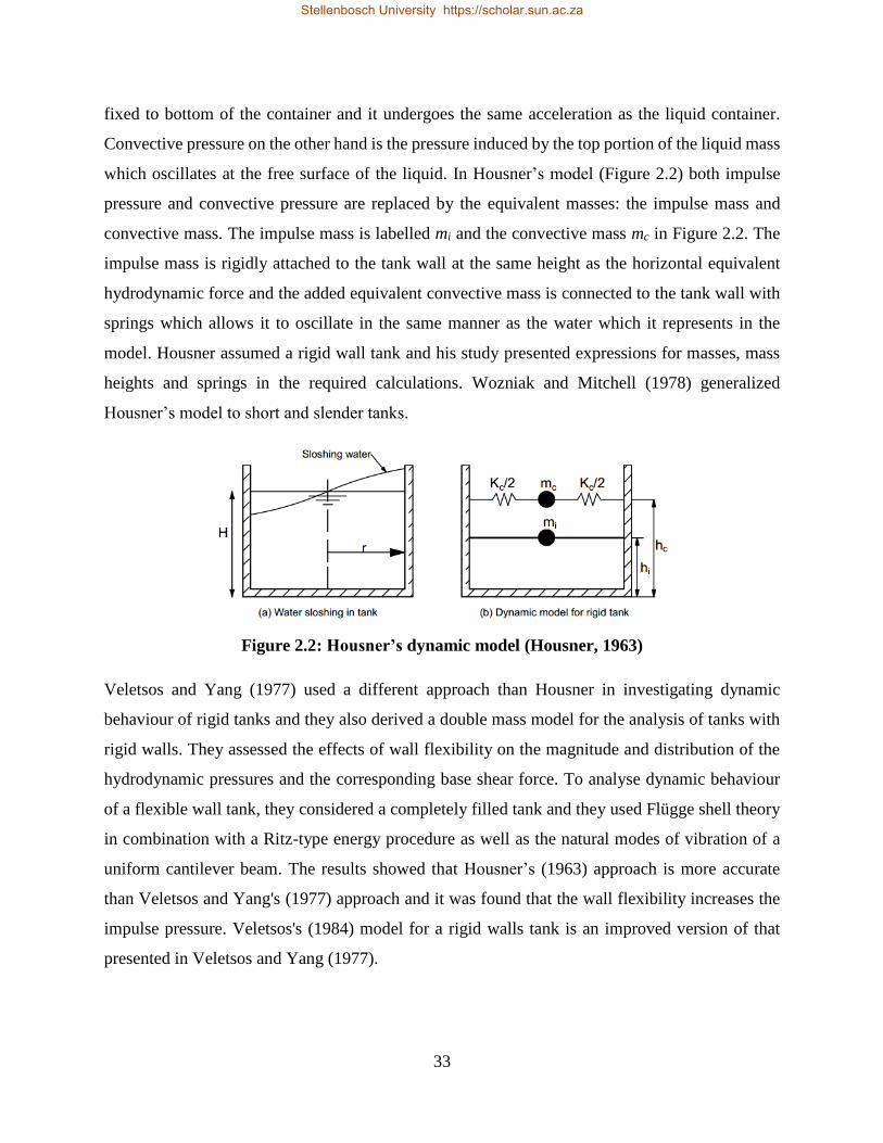
fixed to bottom of the container and it undergoes the same acceleration as the liquid container.

Convective pressure on the other hand is the pressure induced by the top portion of the liquid mass

which oscillates at the free surface of the liquid. In Housner’s model (Figure 2.2) both impulse

pressure and convective pressure are replaced by the equivalent masses: the impulse mass and

convective mass. The impulse mass is labelled mi and the convective mass mc in Figure 2.2. The

impulse mass is rigidly attached to the tank wall at the same height as the horizontal equivalent

hydrodynamic force and the added equivalent convective mass is connected to the tank wall with

springs which allows it to oscillate in the same manner as the water which it represents in the

model. Housner assumed a rigid wall tank and his study presented expressions for masses, mass

heights and springs in the required calculations. Wozniak and Mitchell (1978) generalized

Housner’s model to short and slender tanks.

Figure 2.2: Housner’s dynamic model (Housner, 1963)

Veletsos and Yang (1977) used a different approach than Housner in investigating dynamic

behaviour of rigid tanks and they also derived a double mass model for the analysis of tanks with

rigid walls. They assessed the effects of wall flexibility on the magnitude and distribution of the

hydrodynamic pressures and the corresponding base shear force. To analyse dynamic behaviour

of a flexible wall tank, they considered a completely filled tank and they used Flügge shell theory

in combination with a Ritz-type energy procedure as well as the natural modes of vibration of a

uniform cantilever beam. The results showed that Housner’s (1963) approach is more accurate

than Veletsos and Yang's (1977) approach and it was found that the wall flexibility increases the

impulse pressure. Veletsos's (1984) model for a rigid walls tank is an improved version of that

presented in Veletsos and Yang (1977).


34

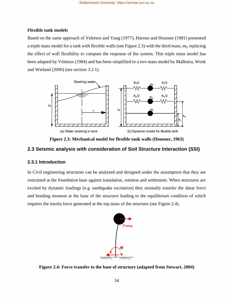
Flexible tank models

Based on the same approach of Veletsos and Yang (1977), Haroun and Housner (1981) presented

a triple mass model for a tank with flexible walls (see Figure 2.3) with the third mass, mf, replacing

the effect of wall flexibility to compute the response of the system. This triple mass model has

been adapted by Veletsos (1984) and has been simplified to a two mass model by Malhotra, Wenk

and Wieland (2000) (see section 3.2.1).

Figure 2.3: Mechanical model for flexible tank walls (Housner, 1963)

2.3 Seismic analysis with consideration of Soil Structure Interaction (SSI)

2.3.1 Introduction

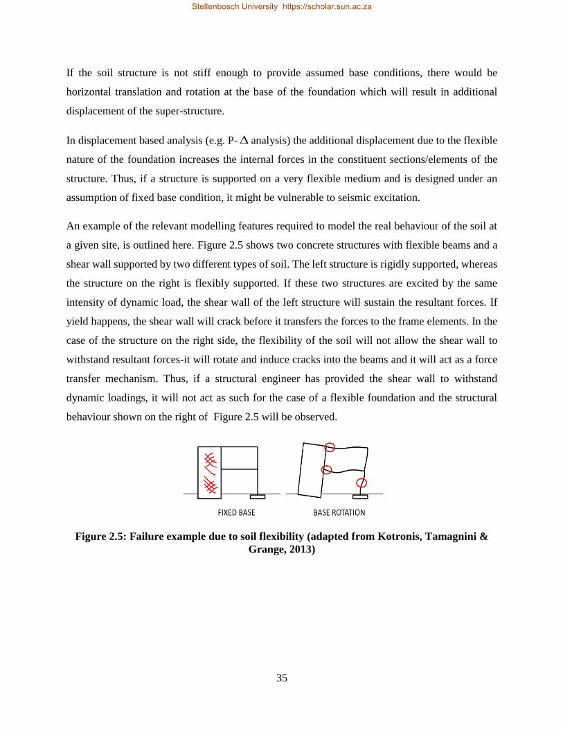
In Civil engineering structures can be analysed and designed under the assumption that they are

restrained at the foundation base against translation, rotation and settlement. When structures are

excited by dynamic loadings (e.g. earthquake excitation) they normally transfer the shear force

and bending moment at the base of the structure leading to the equilibrium condition of which

requires the inertia force generated at the top mass of the structure (see Figure 2.4).

Figure 2.4: Force transfer to the base of structure (adapted from Stewart, 2004)


35

If the soil structure is not stiff enough to provide assumed base conditions, there would be

horizontal translation and rotation at the base of the foundation which will result in additional

displacement of the super-structure.

In displacement based analysis (e.g. P- analysis) the additional displacement due to the flexible

nature of the foundation increases the internal forces in the constituent sections/elements of the

structure. Thus, if a structure is supported on a very flexible medium and is designed under an

assumption of fixed base condition, it might be vulnerable to seismic excitation.

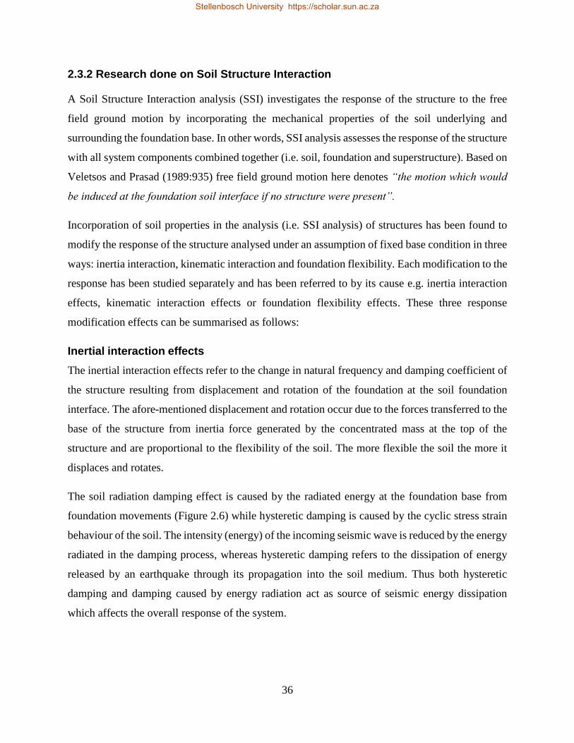
An example of the relevant modelling features required to model the real behaviour of the soil at

a given site, is outlined here. Figure 2.5 shows two concrete structures with flexible beams and a

shear wall supported by two different types of soil. The left structure is rigidly supported, whereas

the structure on the right is flexibly supported. If these two structures are excited by the same

intensity of dynamic load, the shear wall of the left structure will sustain the resultant forces. If

yield happens, the shear wall will crack before it transfers the forces to the frame elements. In the

case of the structure on the right side, the flexibility of the soil will not allow the shear wall to

withstand resultant forces-it will rotate and induce cracks into the beams and it will act as a force

transfer mechanism. Thus, if a structural engineer has provided the shear wall to withstand

dynamic loadings, it will not act as such for the case of a flexible foundation and the structural

behaviour shown on the right of Figure 2.5 will be observed.

Figure 2.5: Failure example due to soil flexibility (adapted from Kotronis, Tamagnini &

Grange, 2013)


36

2.3.2 Research done on Soil Structure Interaction

A Soil Structure Interaction analysis (SSI) investigates the response of the structure to the free

field ground motion by incorporating the mechanical properties of the soil underlying and

surrounding the foundation base. In other words, SSI analysis assesses the response of the structure

with all system components combined together (i.e. soil, foundation and superstructure). Based on

Veletsos and Prasad (1989:935) free field ground motion here denotes “the motion which would

be induced at the foundation soil interface if no structure were present”.

Incorporation of soil properties in the analysis (i.e. SSI analysis) of structures has been found to

modify the response of the structure analysed under an assumption of fixed base condition in three

ways: inertia interaction, kinematic interaction and foundation flexibility. Each modification to the

response has been studied separately and has been referred to by its cause e.g. inertia interaction

effects, kinematic interaction effects or foundation flexibility effects. These three response

modification effects can be summarised as follows:

Inertial interaction effects

The inertial interaction effects refer to the change in natural frequency and damping coefficient of

the structure resulting from displacement and rotation of the foundation at the soil foundation

interface. The afore-mentioned displacement and rotation occur due to the forces transferred to the

base of the structure from inertia force generated by the concentrated mass at the top of the

structure and are proportional to the flexibility of the soil. The more flexible the soil the more it

displaces and rotates.

The soil radiation damping effect is caused by the radiated energy at the foundation base from

foundation movements (Figure 2.6) while hysteretic damping is caused by the cyclic stress strain

behaviour of the soil. The intensity (energy) of the incoming seismic wave is reduced by the energy

radiated in the damping process, whereas hysteretic damping refers to the dissipation of energy

released by an earthquake through its propagation into the soil medium. Thus both hysteretic

damping and damping caused by energy radiation act as source of seismic energy dissipation

which affects the overall response of the system.


37

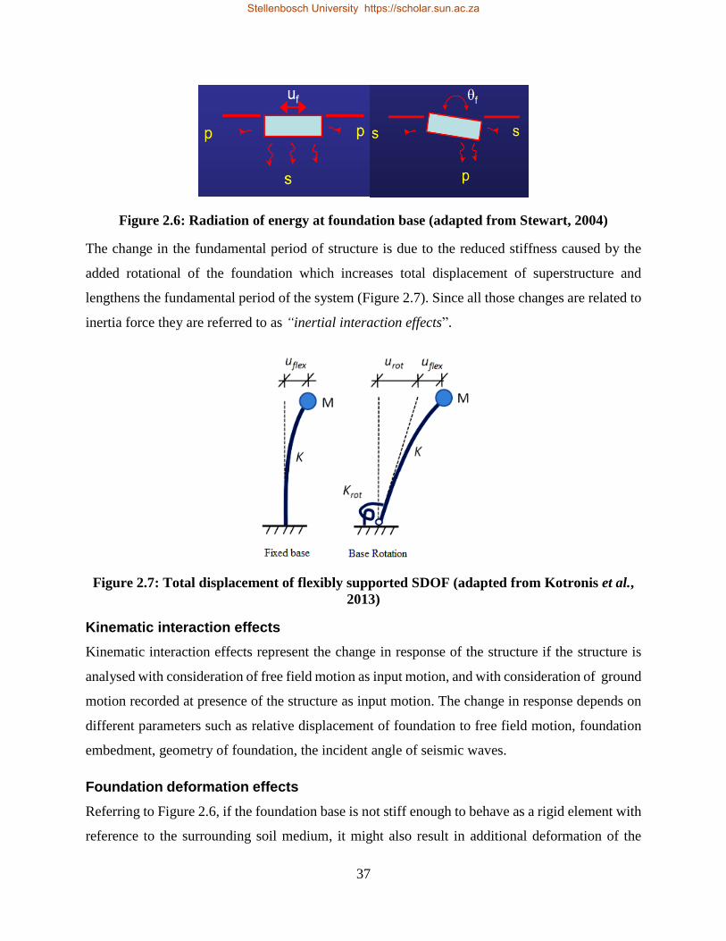
Figure 2.6: Radiation of energy at foundation base (adapted from Stewart, 2004)

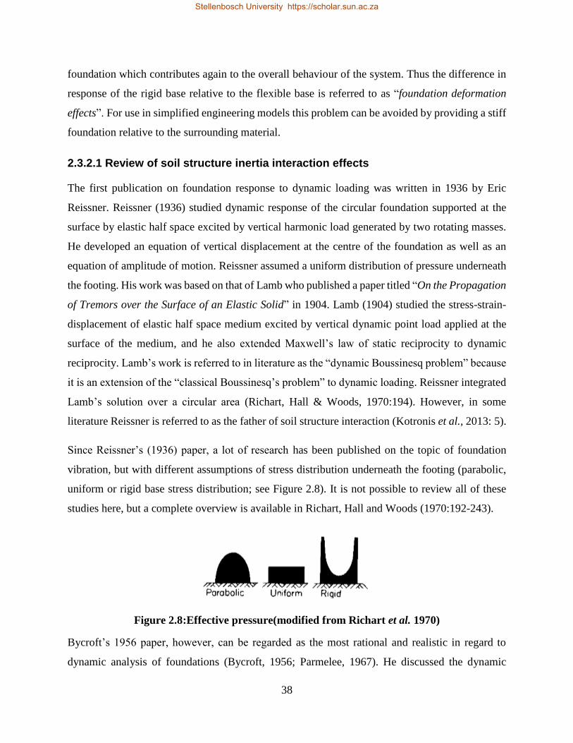
The change in the fundamental period of structure is due to the reduced stiffness caused by the

added rotational of the foundation which increases total displacement of superstructure and

lengthens the fundamental period of the system (Figure 2.7). Since all those changes are related to

inertia force they are referred to as “inertial interaction effects”.

Figure 2.7: Total displacement of flexibly supported SDOF (adapted from Kotronis et al.,

2013)

Kinematic interaction effects

Kinematic interaction effects represent the change in response of the structure if the structure is

analysed with consideration of free field motion as input motion, and with consideration of ground

motion recorded at presence of the structure as input motion. The change in response depends on

different parameters such as relative displacement of foundation to free field motion, foundation

embedment, geometry of foundation, the incident angle of seismic waves.

Foundation deformation effects

Referring to Figure 2.6, if the foundation base is not stiff enough to behave as a rigid element with

reference to the surrounding soil medium, it might also result in additional deformation of the


38

foundation which contributes again to the overall behaviour of the system. Thus the difference in

response of the rigid base relative to the flexible base is referred to as “foundation deformation

effects”. For use in simplified engineering models this problem can be avoided by providing a stiff

foundation relative to the surrounding material.

2.3.2.1 Review of soil structure inertia interaction effects

The first publication on foundation response to dynamic loading was written in 1936 by Eric

Reissner. Reissner (1936) studied dynamic response of the circular foundation supported at the

surface by elastic half space excited by vertical harmonic load generated by two rotating masses.

He developed an equation of vertical displacement at the centre of the foundation as well as an

equation of amplitude of motion. Reissner assumed a uniform distribution of pressure underneath

the footing. His work was based on that of Lamb who published a paper titled “On the Propagation

of Tremors over the Surface of an Elastic Solid” in 1904. Lamb (1904) studied the stress-strain-

displacement of elastic half space medium excited by vertical dynamic point load applied at the

surface of the medium, and he also extended Maxwell’s law of static reciprocity to dynamic

reciprocity. Lamb’s work is referred to in literature as the “dynamic Boussinesq problem” because

it is an extension of the “classical Boussinesq’s problem” to dynamic loading. Reissner integrated

Lamb’s solution over a circular area (Richart, Hall & Woods, 1970:194). However, in some

literature Reissner is referred to as the father of soil structure interaction (Kotronis et al., 2013: 5).

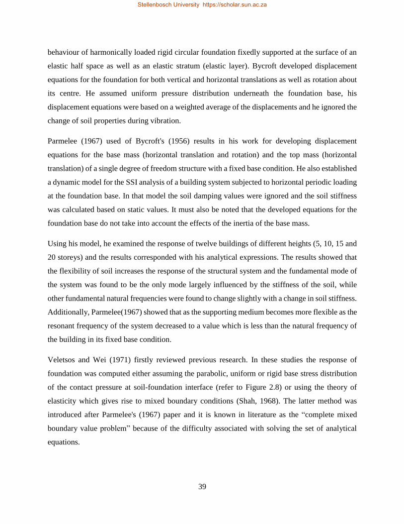
Since Reissner’s (1936) paper, a lot of research has been published on the topic of foundation

vibration, but with different assumptions of stress distribution underneath the footing (parabolic,

uniform or rigid base stress distribution; see Figure 2.8). It is not possible to review all of these

studies here, but a complete overview is available in Richart, Hall and Woods (1970:192-243).

Figure 2.8:Effective pressure(modified from Richart et al. 1970)

Bycroft’s 1956 paper, however, can be regarded as the most rational and realistic in regard to

dynamic analysis of foundations (Bycroft, 1956; Parmelee, 1967). He discussed the dynamic


39

behaviour of harmonically loaded rigid circular foundation fixedly supported at the surface of an

elastic half space as well as an elastic stratum (elastic layer). Bycroft developed displacement

equations for the foundation for both vertical and horizontal translations as well as rotation about

its centre. He assumed uniform pressure distribution underneath the foundation base, his

displacement equations were based on a weighted average of the displacements and he ignored the

change of soil properties during vibration.

Parmelee (1967) used of Bycroft's (1956) results in his work for developing displacement

equations for the base mass (horizontal translation and rotation) and the top mass (horizontal

translation) of a single degree of freedom structure with a fixed base condition. He also established

a dynamic model for the SSI analysis of a building system subjected to horizontal periodic loading

at the foundation base. In that model the soil damping values were ignored and the soil stiffness

was calculated based on static values. It must also be noted that the developed equations for the

foundation base do not take into account the effects of the inertia of the base mass.

Using his model, he examined the response of twelve buildings of different heights (5, 10, 15 and

20 storeys) and the results corresponded with his analytical expressions. The results showed that

the flexibility of soil increases the response of the structural system and the fundamental mode of

the system was found to be the only mode largely influenced by the stiffness of the soil, while

other fundamental natural frequencies were found to change slightly with a change in soil stiffness.

Additionally, Parmelee(1967) showed that as the supporting medium becomes more flexible as the

resonant frequency of the system decreased to a value which is less than the natural frequency of

the building in its fixed base condition.

Veletsos and Wei (1971) firstly reviewed previous research. In these studies the response of

foundation was computed either assuming the parabolic, uniform or rigid base stress distribution

of the contact pressure at soil-foundation interface (refer to Figure 2.8) or using the theory of

elasticity which gives rise to mixed boundary conditions (Shah, 1968). The latter method was

introduced after Parmelee's (1967) paper and it is known in literature as the “complete mixed

boundary value problem” because of the difficulty associated with solving the set of analytical

equations.


40

Moreover, in their previous studies there was also no provision for both foundation rotation

induced by horizontal force and the lateral displacement of the foundation induced by overturning

moment (this is referred to in the literature as “coupling effects”). In other words, the displacement

equations have been established in the direction of the exciting forces only.

Secondly Veletsos and Wei (1971) also studied a steady state response of a massless rigid circular

disk supported on the surface of an elastic half space, excited by both a harmonic horizontal load

and a harmonic overturning moment. They developed displacement equation for the disk,

equations for the stress distribution underneath the disk and established an equivalent analogical

model for SSI analysis (see Figure 2.9). During the development of all the mentioned equations

both the rotation amplitude induced by horizontal force and the lateral displacement induced by

overturning moment were considered and each force effect was evaluated independently. In other

words, the response of horizontal force was evaluated by considering zero normal contact stress

and the response of overturning moment was provided by assuming zero horizontal contact stress.

It is also essential to recognise that the soil medium which was on the sides of the disc was

considered as stress free. Moreover, the rotation amplitude induced by horizontal force and the

lateral displacement induced by overturning moment, i.e. “coupling effects”, were not taken into

consideration in the damping and stiffness equations (equation 2.1 to 2.4) of Veletsos and Wei’s

model presented in Figure 2.9 (see page 41). All these assumptions used by these researchers are

referred to in literature as the “relaxed mixed boundary value problem”.

According to Bielak (1971) for the complete mixed boundary value problem all the components

of displacements underneath the footing have to be provided whereas in the relaxed mixed

boundary value problem, at least one component of surface stress is zero.

The writers (Veletsos & Wei, 1971) compared their solutions with those of previous researchers

and both results were in good agreement with low range of frequency of vibration (their previous

results were limited to low frequency of vibration applications). Veletsos and Wei's (1971)

solutions appeared to be the most realistic SSI analysis results because they were in good

agreement with the previous results and they extended to high frequency of oscillation.


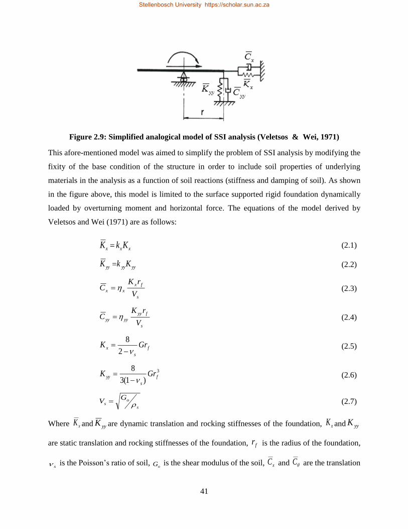
41

Figure 2.9: Simplified analogical model of SSI analysis (Veletsos & Wei, 1971)

This afore-mentioned model was aimed to simplify the problem of SSI analysis by modifying the

fixity of the base condition of the structure in order to include soil properties of underlying

materials in the analysis as a function of soil reactions (stiffness and damping of soil). As shown

in the figure above, this model is limited to the surface supported rigid foundation dynamically

loaded by overturning moment and horizontal force. The equations of the model derived by

Veletsos and Wei (1971) are as follows:

xxx KkK (2.1)

yyyyyy KkK (2.2)

s

fx

xxV

rKC (2.3)

s

fyy

yyyyV

rKC (2.4)

f

s

x GrK

2

8 (2.5)

3

)1(3

8f

s

yy GrK

(2.6)

s

os

GV

(2.7)

Where xK and yyK are dynamic translation and rocking stiffnesses of the foundation, xK and yyK

are static translation and rocking stiffnesses of the foundation, fr is the radius of the foundation,

s is the Poisson’s ratio of soil, oG is the shear modulus of the soil, xC and C are the translation


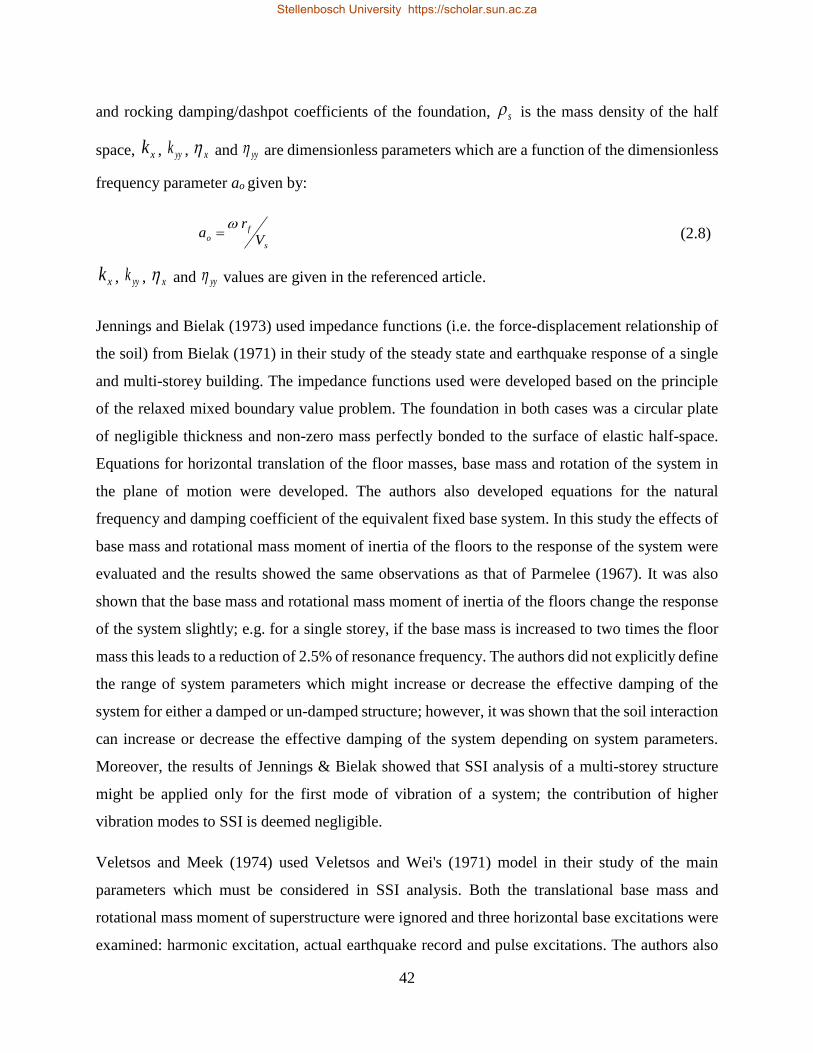
42

and rocking damping/dashpot coefficients of the foundation, s is the mass density of the half

space, xk , yyk , x and yy are dimensionless parameters which are a function of the dimensionless

frequency parameter ao given by:

s

fo V

ra

(2.8)

xk , yyk , x and yy values are given in the referenced article.

Jennings and Bielak (1973) used impedance functions (i.e. the force-displacement relationship of

the soil) from Bielak (1971) in their study of the steady state and earthquake response of a single

and multi-storey building. The impedance functions used were developed based on the principle

of the relaxed mixed boundary value problem. The foundation in both cases was a circular plate

of negligible thickness and non-zero mass perfectly bonded to the surface of elastic half-space.

Equations for horizontal translation of the floor masses, base mass and rotation of the system in

the plane of motion were developed. The authors also developed equations for the natural

frequency and damping coefficient of the equivalent fixed base system. In this study the effects of

base mass and rotational mass moment of inertia of the floors to the response of the system were

evaluated and the results showed the same observations as that of Parmelee (1967). It was also

shown that the base mass and rotational mass moment of inertia of the floors change the response

of the system slightly; e.g. for a single storey, if the base mass is increased to two times the floor

mass this leads to a reduction of 2.5% of resonance frequency. The authors did not explicitly define

the range of system parameters which might increase or decrease the effective damping of the

system for either a damped or un-damped structure; however, it was shown that the soil interaction

can increase or decrease the effective damping of the system depending on system parameters.

Moreover, the results of Jennings & Bielak showed that SSI analysis of a multi-storey structure

might be applied only for the first mode of vibration of a system; the contribution of higher

vibration modes to SSI is deemed negligible.

Veletsos and Meek (1974) used Veletsos and Wei's (1971) model in their study of the main

parameters which must be considered in SSI analysis. Both the translational base mass and

rotational mass moment of superstructure were ignored and three horizontal base excitations were

examined: harmonic excitation, actual earthquake record and pulse excitations. The authors also


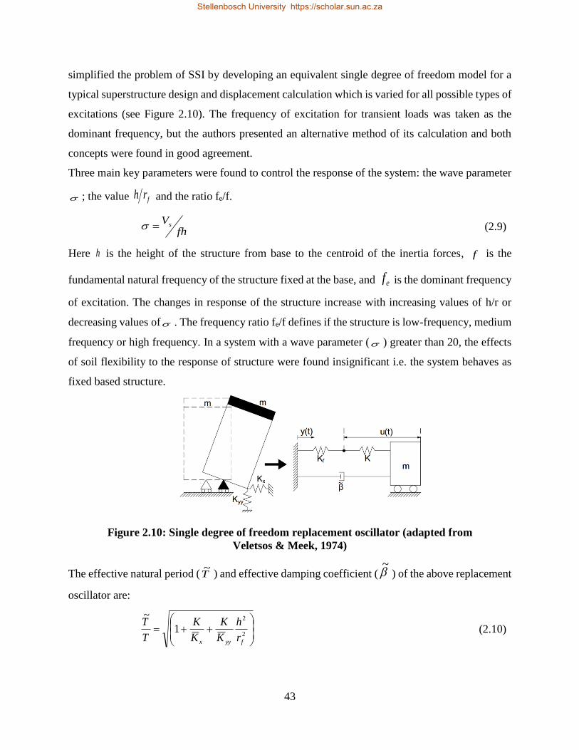
43

simplified the problem of SSI by developing an equivalent single degree of freedom model for a

typical superstructure design and displacement calculation which is varied for all possible types of

excitations (see Figure 2.10). The frequency of excitation for transient loads was taken as the

dominant frequency, but the authors presented an alternative method of its calculation and both

concepts were found in good agreement.

Three main key parameters were found to control the response of the system: the wave parameter

; the value frh and the ratio fe/f.

fhVs (2.9)

Here h is the height of the structure from base to the centroid of the inertia forces, f is the

fundamental natural frequency of the structure fixed at the base, and ef is the dominant frequency

of excitation. The changes in response of the structure increase with increasing values of h/r or

decreasing values of . The frequency ratio fe/f defines if the structure is low-frequency, medium

frequency or high frequency. In a system with a wave parameter ( ) greater than 20, the effects

of soil flexibility to the response of structure were found insignificant i.e. the system behaves as

fixed based structure.

Figure 2.10: Single degree of freedom replacement oscillator (adapted from

Veletsos & Meek, 1974)

The effective natural period (T~

) and effective damping coefficient ( ~

) of the above replacement

oscillator are:

2

2

1

~

fyyx r

h

K

K

K

K

T

T (2.10)


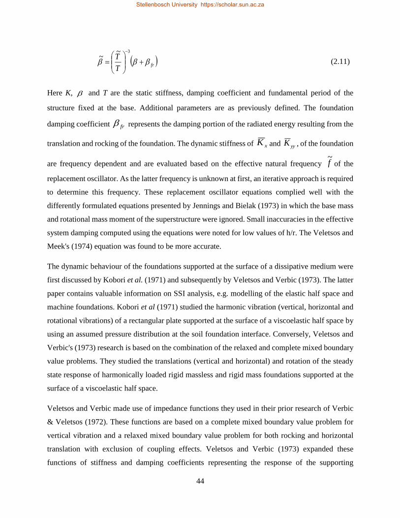
44

frT

T

3~~

(2.11)

Here K, and T are the static stiffness, damping coefficient and fundamental period of the

structure fixed at the base. Additional parameters are as previously defined. The foundation

damping coefficient fr represents the damping portion of the radiated energy resulting from the

translation and rocking of the foundation. The dynamic stiffness of xK and yyK , of the foundation

are frequency dependent and are evaluated based on the effective natural frequency f~

of the

replacement oscillator. As the latter frequency is unknown at first, an iterative approach is required

to determine this frequency. These replacement oscillator equations complied well with the

differently formulated equations presented by Jennings and Bielak (1973) in which the base mass

and rotational mass moment of the superstructure were ignored. Small inaccuracies in the effective

system damping computed using the equations were noted for low values of h/r. The Veletsos and

Meek's (1974) equation was found to be more accurate.

The dynamic behaviour of the foundations supported at the surface of a dissipative medium were

first discussed by Kobori et al. (1971) and subsequently by Veletsos and Verbic (1973). The latter

paper contains valuable information on SSI analysis, e.g. modelling of the elastic half space and

machine foundations. Kobori et al (1971) studied the harmonic vibration (vertical, horizontal and

rotational vibrations) of a rectangular plate supported at the surface of a viscoelastic half space by

using an assumed pressure distribution at the soil foundation interface. Conversely, Veletsos and

Verbic's (1973) research is based on the combination of the relaxed and complete mixed boundary

value problems. They studied the translations (vertical and horizontal) and rotation of the steady

state response of harmonically loaded rigid massless and rigid mass foundations supported at the

surface of a viscoelastic half space.

Veletsos and Verbic made use of impedance functions they used in their prior research of Verbic

& Veletsos (1972). These functions are based on a complete mixed boundary value problem for

vertical vibration and a relaxed mixed boundary value problem for both rocking and horizontal

translation with exclusion of coupling effects. Veletsos and Verbic (1973) expanded these

functions of stiffness and damping coefficients representing the response of the supporting


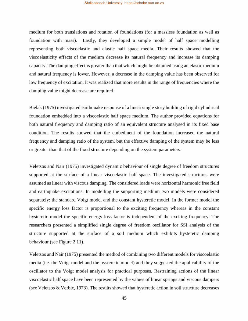
45

medium for both translations and rotation of foundations (for a massless foundation as well as

foundation with mass). Lastly, they developed a simple model of half space modelling

representing both viscoelastic and elastic half space media. Their results showed that the

viscoelasticity effects of the medium decrease its natural frequency and increase its damping

capacity. The damping effect is greater than that which might be obtained using an elastic medium

and natural frequency is lower. However, a decrease in the damping value has been observed for

low frequency of excitation. It was realized that more results in the range of frequencies where the

damping value might decrease are required.

Bielak (1975) investigated earthquake response of a linear single story building of rigid cylindrical

foundation embedded into a viscoelastic half space medium. The author provided equations for

both natural frequency and damping ratio of an equivalent structure analysed in its fixed base

condition. The results showed that the embedment of the foundation increased the natural

frequency and damping ratio of the system, but the effective damping of the system may be less

or greater than that of the fixed structure depending on the system parameters.

Veletsos and Nair (1975) investigated dynamic behaviour of single degree of freedom structures

supported at the surface of a linear viscoelastic half space. The investigated structures were

assumed as linear with viscous damping. The considered loads were horizontal harmonic free field

and earthquake excitations. In modelling the supporting medium two models were considered

separately: the standard Voigt model and the constant hysteretic model. In the former model the

specific energy loss factor is proportional to the exciting frequency whereas in the constant

hysteretic model the specific energy loss factor is independent of the exciting frequency. The

researchers presented a simplified single degree of freedom oscillator for SSI analysis of the

structure supported at the surface of a soil medium which exhibits hysteretic damping

behaviour (see Figure 2.11).

Veletsos and Nair (1975) presented the method of combining two different models for viscoelastic

media (i.e. the Voigt model and the hysteretic model) and they suggested the applicability of the

oscillator to the Voigt model analysis for practical purposes. Restraining actions of the linear

viscoelastic half space have been represented by the values of linear springs and viscous dampers

(see Veletsos & Verbic, 1973). The results showed that hysteretic action in soil structure decreases


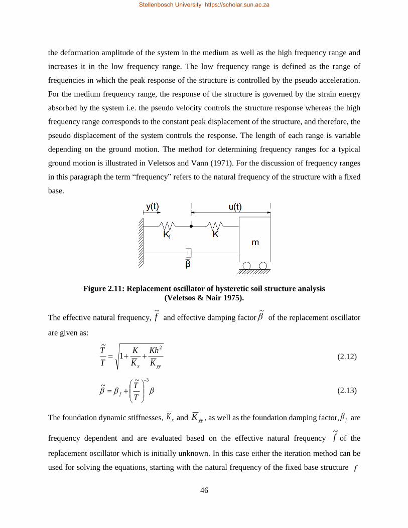
46

the deformation amplitude of the system in the medium as well as the high frequency range and

increases it in the low frequency range. The low frequency range is defined as the range of

frequencies in which the peak response of the structure is controlled by the pseudo acceleration.

For the medium frequency range, the response of the structure is governed by the strain energy

absorbed by the system i.e. the pseudo velocity controls the structure response whereas the high

frequency range corresponds to the constant peak displacement of the structure, and therefore, the

pseudo displacement of the system controls the response. The length of each range is variable

depending on the ground motion. The method for determining frequency ranges for a typical

ground motion is illustrated in Veletsos and Vann (1971). For the discussion of frequency ranges

in this paragraph the term “frequency” refers to the natural frequency of the structure with a fixed

base.

Figure 2.11: Replacement oscillator of hysteretic soil structure analysis

(Veletsos & Nair 1975).

The effective natural frequency, f~

and effective damping factor ~

of the replacement oscillator

are given as:

yyx K

Kh

K

K

T

T 2

1

~

(2.12)

3~~

T

Tf (2.13)

The foundation dynamic stiffnesses, xK and yyK , as well as the foundation damping factor, f are

frequency dependent and are evaluated based on the effective natural frequency f~

of the

replacement oscillator which is initially unknown. In this case either the iteration method can be

used for solving the equations, starting with the natural frequency of the fixed base structure f


47

as effective natural frequency of the replacement oscillator or a graphic method as presented by

Veletsos (1977) can be used. These equations are different from those presented by Veletsos and

Meek (1974) in that the foundation damping factor f includes both hysteretic damping of the soil

and radiation damping of the foundation. The above equations of Veletsos and Nair (1975) are of

a particular case in which the effects of the foundation mass on the response of the system are not

considered. See Veletsos and Nair (1975) for the same equations with consideration of the

foundation mass.

Bielak (1976) extended modal superposition of classical modes damping to non-classical modes

damping. Consequently, he developed equations for the effective frequency and damping ratio of

the structure in its fixed base condition as well as for both horizontal translation and rotational

equations of the foundation mass and superstructure. Bielak considered a linear multi-storey

structure with a circular rigid mass foundation perfectly bonded to the surface of a viscoelastic half

space and free to rotate and translate in the horizontal direction. The foundation thickness was

taken as negligible and the contribution of foundation stiffness to the overall stiffness of the system

was taken as constant and evaluated at the fundamental natural frequency of the system whereas

that of the damping ratio was evaluated as frequency dependent for the corresponding system

mode.

Luco (1980) studied the effect of inertia interaction on the response of the multi-degree of freedom

structures by considering a planar elastic structure with a rigid foundation supported at the surface

of viscoelastic half space. The author ignored the mass of the foundation and the rotational inertia

of the superstructure as well as the coupling effects of the foundation.

Luco developed displacement equations for both the foundation and superstructure in which the

equivalent natural frequency and equivalent damping ratio of the structure in its fixed base

condition were derived. The research concentrated on the fundamental mode of the system seeing

that Parmelee (1967) and Jennings and Bielak (1973) proved that the other mode shapes are not

influenced by soil flexibility. Luco’s equations correlated well with those of Jennings and Bielak

(1973) for the structure of one single degree of freedom. However, for the multi-storey structure,

both displacement and rotation equations of the foundation did not correlate well.


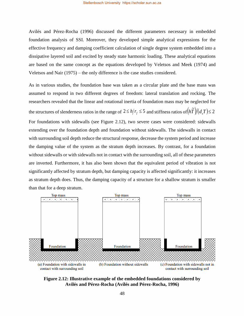
48

Avilés and Pérez-Rocha (1996) discussed the different parameters necessary in embedded

foundation analysis of SSI. Moreover, they developed simple analytical expressions for the

effective frequency and damping coefficient calculation of single degree system embedded into a

dissipative layered soil and excited by steady state harmonic loading. These analytical equations

are based on the same concept as the equations developed by Veletsos and Meek (1974) and

Veletsos and Nair (1975) – the only difference is the case studies considered.

As in various studies, the foundation base was taken as a circular plate and the base mass was

assumed to respond in two different degrees of freedom: lateral translation and rocking. The

researchers revealed that the linear and rotational inertia of foundation mass may be neglected for

the structures of slenderness ratios in the range of 52 frh and stiffness ratios of 2~

TdTh s

For foundations with sidewalls (see Figure 2.12), two severe cases were considered: sidewalls

extending over the foundation depth and foundation without sidewalls. The sidewalls in contact

with surrounding soil depth reduce the structural response, decrease the system period and increase

the damping value of the system as the stratum depth increases. By contrast, for a foundation

without sidewalls or with sidewalls not in contact with the surrounding soil, all of these parameters

are inverted. Furthermore, it has also been shown that the equivalent period of vibration is not

significantly affected by stratum depth, but damping capacity is affected significantly: it increases

as stratum depth does. Thus, the damping capacity of a structure for a shallow stratum is smaller

than that for a deep stratum.

Figure 2.12: Illustrative example of the embedded foundations considered by

Avilés and Pérez-Rocha (Avilés and Pérez-Rocha, 1996)


49

Summary:

A lot of scholarly work has been done on soil structure interaction, as can be gathered from Mason

(2011) and Jones (2013). For this reason not all publications on this subject could be reviewed

herein, but a complete review is available in, inter alia, Kausel (2010), Roesset (2013) and Lou et

al. (2011). The papers reviewed here mostly focused on linear structures and some on material

nonlinearity of the superstructure, e.g. Moghaddasi et al. (2012) and Avilés and Pérez-Rocha

(2003) and (2005). They were treated as a group in this section seeing that they indicate that Soil

Structure Interaction analysis (SSI) of structures with consideration of material nonlinearity of the

superstructure reduces the seismic demand of the structure.

Based on all the mentioned references, the problem of inertia interaction has been made clear and

understandable. Despite various approaches used for assessing this problem, the same observations

have been revealed. The principal effects of inertia interaction are to increase fundamental period

of the fixed base structure and to change (increase or decrease depending on system parameters)

its corresponding damping coefficient. The subsequent fundamental natural period and damping

coefficient were referred to equivalent fundamental natural period and damping coefficient. The

total effect may increase or decrease maximum displacement of the structure depending on system

parameters. These changes are observed for the fundamental mode and other modes are not

practically affected. Moreover, different parameters which control inertia interaction were defined

(Veletsos & Meek, 1974). The studies of Stewart, Fenves and Seed (1999) and Stewart, Seed and

Fenves (1999) showed that for a system with 1.0TVh s inertia interaction effects are negligible.

In general, the solutions to the problem of inertia interaction has been provided by modifying the

fundamental natural period and damping coefficient of the fixed base structure in order to make it

easy to be implemented in seismic design codes utilizing spectrum analysis. Additional studies

(e.g. Worku , 2014; Stewart et al. , 1999; Mylonakis & Gazetas, 2000) have demonstrated this

concept as an economical method because it gives a reduced resultant seismic design force

compared to that of the fixed based condition. On the other hand, Mylonakis et al (2006) and

Mylonakis and Gazetas (2000) have demonstrated different cases where even if the resultant

seismic design force may be reduced, it is not conservative due to additional horizontal

displacement of the superstructure caused by the rotation of the foundation base which causes

increased internal forces in secondary seismic elements. To account for that additional


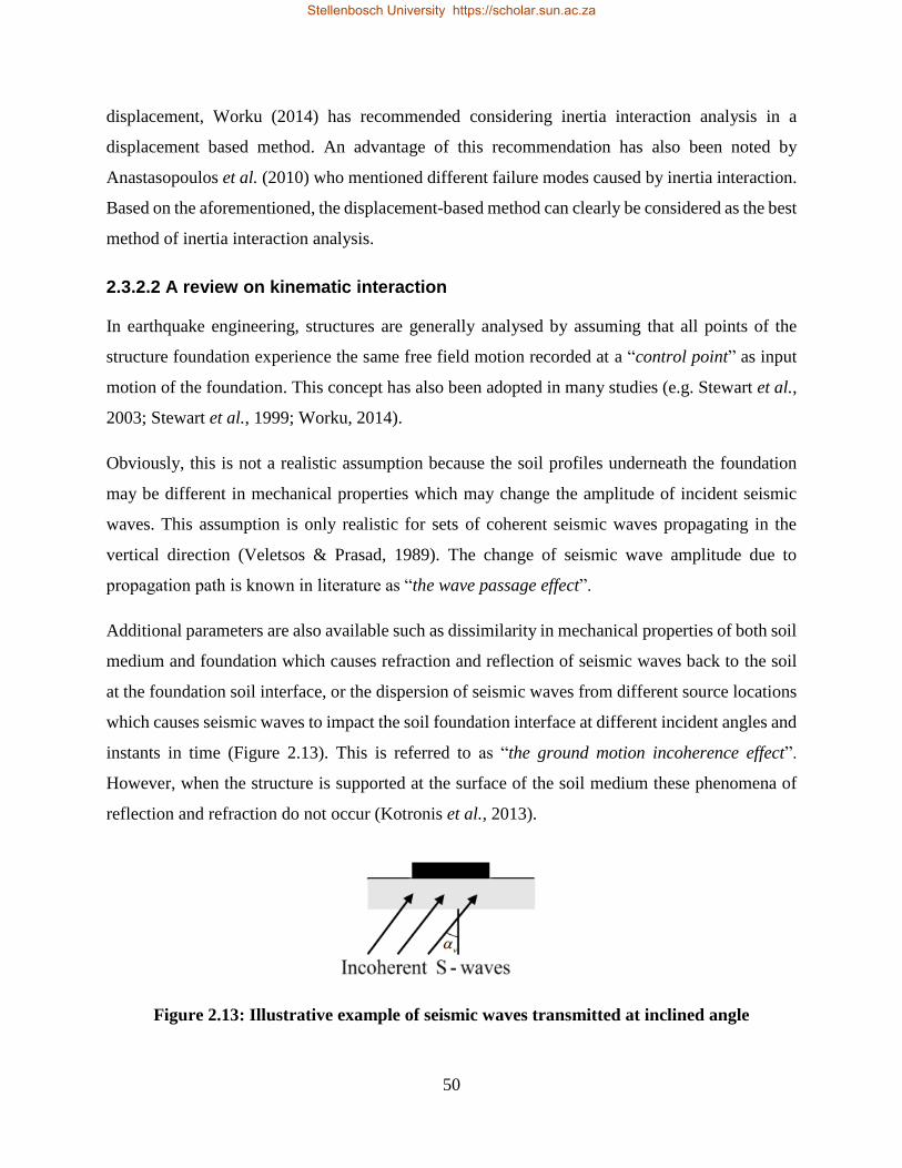
50

displacement, Worku (2014) has recommended considering inertia interaction analysis in a

displacement based method. An advantage of this recommendation has also been noted by

Anastasopoulos et al. (2010) who mentioned different failure modes caused by inertia interaction.

Based on the aforementioned, the displacement-based method can clearly be considered as the best

method of inertia interaction analysis.

2.3.2.2 A review on kinematic interaction

In earthquake engineering, structures are generally analysed by assuming that all points of the

structure foundation experience the same free field motion recorded at a “control point” as input

motion of the foundation. This concept has also been adopted in many studies (e.g. Stewart et al.,

2003; Stewart et al., 1999; Worku, 2014).

Obviously, this is not a realistic assumption because the soil profiles underneath the foundation

may be different in mechanical properties which may change the amplitude of incident seismic

waves. This assumption is only realistic for sets of coherent seismic waves propagating in the

vertical direction (Veletsos & Prasad, 1989). The change of seismic wave amplitude due to

propagation path is known in literature as “the wave passage effect”.

Additional parameters are also available such as dissimilarity in mechanical properties of both soil

medium and foundation which causes refraction and reflection of seismic waves back to the soil

at the foundation soil interface, or the dispersion of seismic waves from different source locations

which causes seismic waves to impact the soil foundation interface at different incident angles and

instants in time (Figure 2.13). This is referred to as “the ground motion incoherence effect”.

However, when the structure is supported at the surface of the soil medium these phenomena of

reflection and refraction do not occur (Kotronis et al., 2013).

Figure 2.13: Illustrative example of seismic waves transmitted at inclined angle


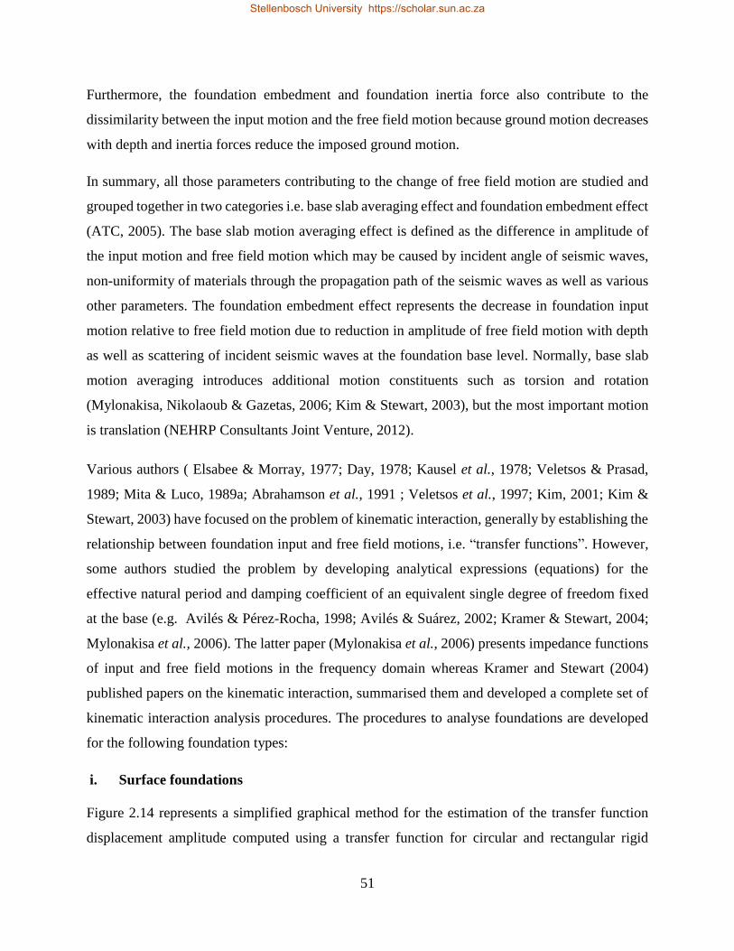
51

Furthermore, the foundation embedment and foundation inertia force also contribute to the

dissimilarity between the input motion and the free field motion because ground motion decreases

with depth and inertia forces reduce the imposed ground motion.

In summary, all those parameters contributing to the change of free field motion are studied and

grouped together in two categories i.e. base slab averaging effect and foundation embedment effect

(ATC, 2005). The base slab motion averaging effect is defined as the difference in amplitude of

the input motion and free field motion which may be caused by incident angle of seismic waves,

non-uniformity of materials through the propagation path of the seismic waves as well as various

other parameters. The foundation embedment effect represents the decrease in foundation input

motion relative to free field motion due to reduction in amplitude of free field motion with depth

as well as scattering of incident seismic waves at the foundation base level. Normally, base slab

motion averaging introduces additional motion constituents such as torsion and rotation

(Mylonakisa, Nikolaoub & Gazetas, 2006; Kim & Stewart, 2003), but the most important motion

is translation (NEHRP Consultants Joint Venture, 2012).

Various authors ( Elsabee & Morray, 1977; Day, 1978; Kausel et al., 1978; Veletsos & Prasad,

1989; Mita & Luco, 1989a; Abrahamson et al., 1991 ; Veletsos et al., 1997; Kim, 2001; Kim &

Stewart, 2003) have focused on the problem of kinematic interaction, generally by establishing the

relationship between foundation input and free field motions, i.e. “transfer functions”. However,

some authors studied the problem by developing analytical expressions (equations) for the

effective natural period and damping coefficient of an equivalent single degree of freedom fixed

at the base (e.g. Avilés & Pérez-Rocha, 1998; Avilés & Suárez, 2002; Kramer & Stewart, 2004;

Mylonakisa et al., 2006). The latter paper (Mylonakisa et al., 2006) presents impedance functions

of input and free field motions in the frequency domain whereas Kramer and Stewart (2004)

published papers on the kinematic interaction, summarised them and developed a complete set of

kinematic interaction analysis procedures. The procedures to analyse foundations are developed

for the following foundation types:

i. Surface foundations

Figure 2.14 represents a simplified graphical method for the estimation of the transfer function

displacement amplitude computed using a transfer function for circular and rectangular rigid


52

massless foundations supported at the surface of homogeneous elastic medium and excited by

incoherent waves at an angle v to the vertical plane. The transfer function amplitude is a function

of adjusted dimensionless frequency parameter oa~ .

Figure 2.14: Transfer function amplitude or impedance function amplitude for vertically

incident incoherent waves (from Kramer & Stewart, 2004)

In Figure 2.14, the curve labelled “disk” represents a rigid circular foundation whereas the

parameters a and b represent one half of the smaller and greater footprint dimensions of a

rectangular foundation (with b being taken perpendicular to the incidence direction of the seismic

waves). The adjusted dimensionless frequency parameter oa~ is evaluated as:

foundationcircular afor sin~ 22

v

r

oo aa (2.14)

foundationr rectangula afor sin2

~2

22

,

e

v

rs

eo

b

b

V

ba

(2.15)

Where rsf

r

o Vra , , abbe , foundation radius ff Ar ( fA = foundation area) and rsV ,

is the reduced shear wave velocity. The ground motion incoherence parameter was obtained

from Kim and Stewart (2003) and is written as:

m/s )50(10*4.7 4

sV (2.16)


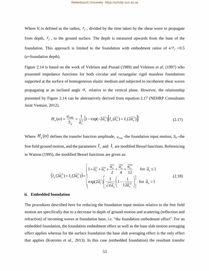
53

Where Vs is defined as the radius, fr , divided by the time taken by the shear wave to propagate

from depth, fr , to the ground surface. The depth is measured upwards from the base of the

foundation. This approach is limited to the foundation with embedment ratios of e/ fr <0.5

(e=foundation depth).

Figure 2.14 is based on the work of Veletsos and Prasad (1989) and Veletsos et al. (1997) who

presented impedance functions for both circular and rectangular rigid massless foundations

supported at the surface of homogeneous elastic medium and subjected to incoherent shear waves

propagating at an inclined angle v relative to the vertical plane. However, the relationship

presented by Figure 2.14 can be alternatively derived from equation 2.17 (NEHRP Consultants

Joint Venture, 2012).

)~2()~()~2exp(1~1

)( 2

1

22

2 oooo

og

FIMu aIaIa

aS

uH (2.17)

Where )(uH defines the transfer function amplitude, FIMu -the foundation input motion, Sg –the

free field ground motion, and the parameters oI and 1

I are modified Bessel functions. Referencing

to Watson (1995), the modified Bessel functions are given as:

1~for ~12

11~

1)~2exp(

1~for 12

~

4

~

2

~~~1

)~2()~2(

12

2

108642

2

1

2

o

oo

o

oooo

oo

ooo

aaa

a

aaaa

aa

aIaI

(2.18)

ii. Embedded foundation

The procedures described here for reducing the foundation input motion relative to the free field

motion are specifically due to a decrease in depth of ground motion and scattering (reflection and

refraction) of incoming waves at foundation base, i.e. “the foundation embedment effect”. For an

embedded foundation, the foundation embedment effect as well as the base slab motion averaging

effect applies whereas for the surface foundation the base slab averaging effect is the only effect

that applies (Kotronis et al., 2013). In this case (embedded foundation) the resultant transfer


54

function is a product of both the two transfer functions calculated separately. The transfer function

amplitude for an embedded foundation in horizontal translation is estimated as:

0.454 coscos

s

ouV

ea

r

eH

(2.19)

All parameters in this equation are as previously defined. It is essential to note that applicability

of this equation is limited to embedment quotient 1fre .

The numerical solutions of Mylonakisa et al. (2006) are the same results as the ones discussed

above (Kramer & Stewart, 2004) except that they are applicable in the frequency domain.

Moreover, all mentioned procedures for kinematic interaction effects estimation are in agreement

with the field (on site) results as well as the finite element results of Stewart and Tileylioglu

(2007). These procedures were adopted by the Applied Technology Council (ATC 2005).

Basically, the kinematic interaction is important for a structure with short fundamental periods

(<0.5s), or with larger plan dimensions compared to the length of the dominant seismic waves or

a structure with a deep foundation i.e. depth mfeet 310 (ATC, 2005).

Application of transfer function

Studies on the seismic response spectrum analysis method (e.g. ATC 2005) have showed that the

transfer function solutions are evaluated as discussed previously (equations 2.17 and 2.19), for

vibration frequencies of 5Hz and higher, the solution at 5Hz can be used. In the case of free field

ground motion given in time history format, calculation procedures are available from the

mentioned references (e.g. ATC, 2005, Kramer & Stewart, 2004). These procedures make use of

the Fourier transformation of the free field ground motion. Considering the solution to the problem

of kinematic interaction which is available, and the studies mentioned in this section, which have

revealed that neglecting kinematic interaction effects is conservative because it increases the

seismic demand (Kramer & Stewart, 2004:4-34), the kinematic effect will be ignored in the next

sections.


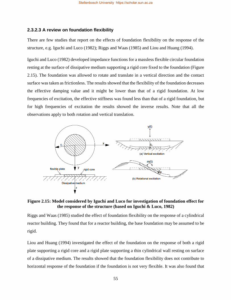
55

2.3.2.3 A review on foundation flexibility

There are few studies that report on the effects of foundation flexibility on the response of the

structure, e.g. Iguchi and Luco (1982); Riggs and Waas (1985) and Liou and Huang (1994).

Iguchi and Luco (1982) developed impedance functions for a massless flexible circular foundation

resting at the surface of dissipative medium supporting a rigid core fixed to the foundation (Figure

2.15). The foundation was allowed to rotate and translate in a vertical direction and the contact

surface was taken as frictionless. The results showed that the flexibility of the foundation decreases

the effective damping value and it might be lower than that of a rigid foundation. At low

frequencies of excitation, the effective stiffness was found less than that of a rigid foundation, but

for high frequencies of excitation the results showed the inverse results. Note that all the

observations apply to both rotation and vertical translation.

Figure 2.15: Model considered by Iguchi and Luco for investigation of foundation effect for

the response of the structure (based on Iguchi & Luco, 1982)

Riggs and Waas (1985) studied the effect of foundation flexibility on the response of a cylindrical

reactor building. They found that for a reactor building, the base foundation may be assumed to be

rigid.

Liou and Huang (1994) investigated the effect of the foundation on the response of both a rigid

plate supporting a rigid core and a rigid plate supporting a thin cylindrical wall resting on surface

of a dissipative medium. The results showed that the foundation flexibility does not contribute to

horizontal response of the foundation if the foundation is not very flexible. It was also found that


56

the mechanical properties of the supported structure influence the response of the system, i.e. the

response of a rigid plate with a rigid core was different to that of a rigid plate with a thin cylindrical

wall. Moreover, the authors showed that a foundation with parameter 10 (see equation 2.20)

can be considered as a rigid foundation and the contribution of the foundation to the horizontal

response of the system needs to be considered for values of Phi ( ) less than 0.01( 01.0 ). The

values of Phi are computed as follows:

3

forG

D (2.20)

Where oG is the shear modulus of elasticity of the soil at small strain level, D is the rigidity of

the foundation base. Other parameters are as previously defined.

The criteria for defining a rigid foundation have also been discussed by Todorovska et al. (2001).

They demonstrated that if the shear modulus of the foundation is less than 16 times that of the soil,

then the foundation must be recognised as a flexible foundation. Currently, there is no numerical

method of implementing the foundation effects into an analysis (Stewart & Tileylioglu, 2007),

however, in various studies the assumption of a rigid foundation have been made (Arefi, 2008;

Stewart et al., 1999; Worku, 2014). Stewart & Tileylioglu (2007). NEHRP Consultants Joint

Venture (2012) have integrated the effects of foundation into an analysis model by distributing the

soil reactions (damping and stiffness values) along the sides and underneath the foundation. The

concept of the distribution of the soil reactions along the sides and underneath the foundation

developed by NEHRP Consultants Joint Venture (2012) is discussed in chapter three.

2.3.3 A review on standards and code provisions

2.3.3.1 Building codes and standards

SSI were implemented in various American design codes and standards many years ago. It was

suggested by the Applied Technology Council in 1978 and it was implemented in National

Earthquake Hazard Reduction Program (NEHRP) in 1986 (Veletsos, 1993). The latest versions of

the applicable codes and standards are ASCE (2013); ASCE (2014); ASCE (2010); ATC (2005);

BSSC (2004a) and BSSC (2004b). European standards do not mention soil flexibility (Arefi,

2008). However, in EN 1998-5: 2004 section 6 a number of structural configuration cases are listed


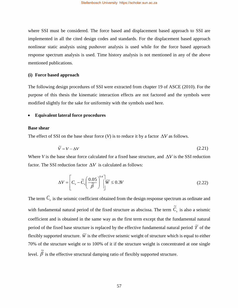
57

where SSI must be considered. The force based and displacement based approach to SSI are

implemented in all the cited design codes and standards. For the displacement based approach

nonlinear static analysis using pushover analysis is used while for the force based approach

response spectrum analysis is used. Time history analysis is not mentioned in any of the above

mentioned publications.

(i) Force based approach

The following design procedures of SSI were extracted from chapter 19 of ASCE (2010). For the

purpose of this thesis the kinematic interaction effects are not factored and the symbols were

modified slightly for the sake for uniformity with the symbols used here.

Equivalent lateral force procedures

Base shear

The effect of SSI on the base shear force (V) is to reduce it by a factor V as follows.

VVV ~

(2.21)

Where V is the base shear force calculated for a fixed base structure, and V is the SSI reduction

factor. The SSI reduction factor V is calculated as follows:

VWCCV ss 3.0~05.0~

4.0

(2.22)

The term sC is the seismic coefficient obtained from the design response spectrum as ordinate and

with fundamental natural period of the fixed structure as abscissa. The term sC~

is also a seismic

coefficient and is obtained in the same way as the first term except that the fundamental natural

period of the fixed base structure is replaced by the effective fundamental natural period T~

of the

flexibly supported structure. W is the effective seismic weight of structure which is equal to either

70% of the structure weight or to 100% of it if the structure weight is concentrated at one single

level. ~

is the effective structural damping ratio of flexibly supported structure.


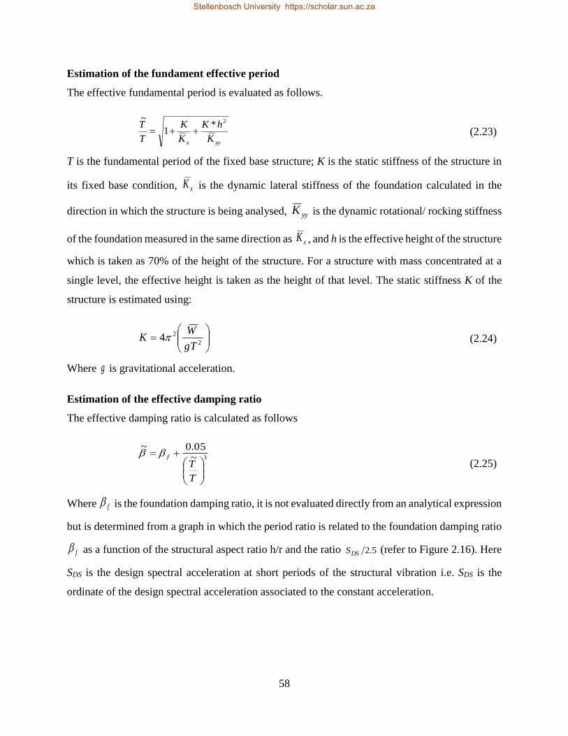
58

Estimation of the fundament effective period

The effective fundamental period is evaluated as follows.

yyx K

hK

K

K

T

T 2*1

~

(2.23)

T is the fundamental period of the fixed base structure; K is the static stiffness of the structure in

its fixed base condition, xK is the dynamic lateral stiffness of the foundation calculated in the

direction in which the structure is being analysed, yyK is the dynamic rotational/ rocking stiffness

of the foundation measured in the same direction as xK , and h is the effective height of the structure

which is taken as 70% of the height of the structure. For a structure with mass concentrated at a

single level, the effective height is taken as the height of that level. The static stiffness K of the

structure is estimated using:

2

24gT

WK (2.24)

Where g is gravitational acceleration.

Estimation of the effective damping ratio

The effective damping ratio is calculated as follows

3~

05.0~

T

Tf

(2.25)

Where f is the foundation damping ratio, it is not evaluated directly from an analytical expression

but is determined from a graph in which the period ratio is related to the foundation damping ratio

f as a function of the structural aspect ratio h/r and the ratio 5.2DSS (refer to Figure 2.16). Here

SDS is the design spectral acceleration at short periods of the structural vibration i.e. SDS is the

ordinate of the design spectral acceleration associated to the constant acceleration.


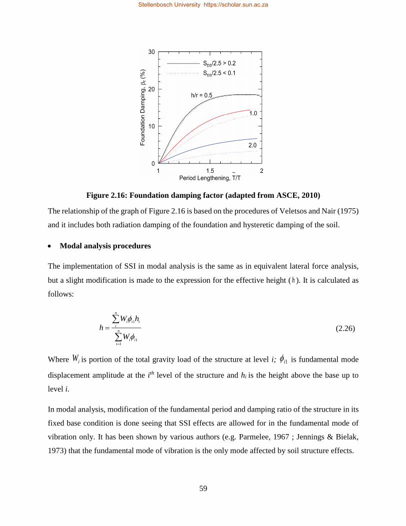
59

Figure 2.16: Foundation damping factor (adapted from ASCE, 2010)

The relationship of the graph of Figure 2.16 is based on the procedures of Veletsos and Nair (1975)

and it includes both radiation damping of the foundation and hysteretic damping of the soil.

Modal analysis procedures

The implementation of SSI in modal analysis is the same as in equivalent lateral force analysis,

but a slight modification is made to the expression for the effective height ( h ). It is calculated as

follows:

n

iii

n

iiii

W

hW

h

11

1

(2.26)

Where iW is portion of the total gravity load of the structure at level i; 1i is fundamental mode

displacement amplitude at the ith level of the structure and hi is the height above the base up to

level i.

In modal analysis, modification of the fundamental period and damping ratio of the structure in its

fixed base condition is done seeing that SSI effects are allowed for in the fundamental mode of

vibration only. It has been shown by various authors (e.g. Parmelee, 1967 ; Jennings & Bielak,

1973) that the fundamental mode of vibration is the only mode affected by soil structure effects.


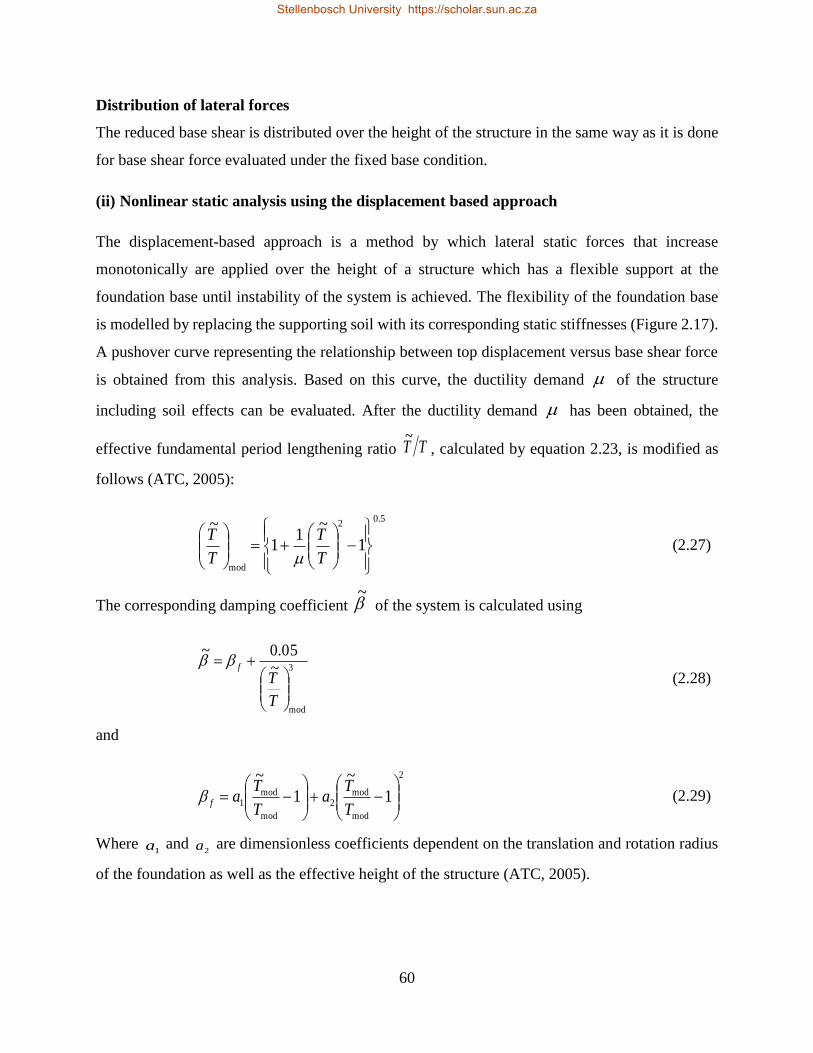
60

Distribution of lateral forces

The reduced base shear is distributed over the height of the structure in the same way as it is done

for base shear force evaluated under the fixed base condition.

(ii) Nonlinear static analysis using the displacement based approach

The displacement-based approach is a method by which lateral static forces that increase

monotonically are applied over the height of a structure which has a flexible support at the

foundation base until instability of the system is achieved. The flexibility of the foundation base

is modelled by replacing the supporting soil with its corresponding static stiffnesses (Figure 2.17).

A pushover curve representing the relationship between top displacement versus base shear force

is obtained from this analysis. Based on this curve, the ductility demand of the structure

including soil effects can be evaluated. After the ductility demand has been obtained, the

effective fundamental period lengthening ratio TT~

, calculated by equation 2.23, is modified as

follows (ATC, 2005):

5.02

mod

1

~1

1

~

T

T

T

T

(2.27)

The corresponding damping coefficient ~

of the system is calculated using

3

mod

~05.0~

T

Tf

(2.28)

and

2

mod

mod2

mod

mod1 1

~

1

~

T

Ta

T

Taf (2.29)

Where 1a and

2a are dimensionless coefficients dependent on the translation and rotation radius

of the foundation as well as the effective height of the structure (ATC, 2005).


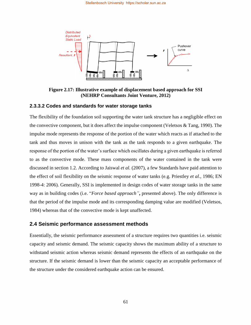
61

Figure 2.17: Illustrative example of displacement based approach for SSI

(NEHRP Consultants Joint Venture, 2012)

2.3.3.2 Codes and standards for water storage tanks

The flexibility of the foundation soil supporting the water tank structure has a negligible effect on

the convective component, but it does affect the impulse component (Veletsos & Tang, 1990). The

impulse mode represents the response of the portion of the water which reacts as if attached to the

tank and thus moves in unison with the tank as the tank responds to a given earthquake. The

response of the portion of the water’s surface which oscillates during a given earthquake is referred

to as the convective mode. These mass components of the water contained in the tank were

discussed in section 1.2. According to Jaiswal et al. (2007), a few Standards have paid attention to

the effect of soil flexibility on the seismic response of water tanks (e.g. Priestley et al., 1986; EN

1998-4: 2006). Generally, SSI is implemented in design codes of water storage tanks in the same

way as in building codes (i.e. “Force based approach”, presented above). The only difference is

that the period of the impulse mode and its corresponding damping value are modified (Veletsos,

1984) whereas that of the convective mode is kept unaffected.

2.4 Seismic performance assessment methods

Essentially, the seismic performance assessment of a structure requires two quantities i.e. seismic

capacity and seismic demand. The seismic capacity shows the maximum ability of a structure to

withstand seismic action whereas seismic demand represents the effects of an earthquake on the

structure. If the seismic demand is lower than the seismic capacity an acceptable performance of

the structure under the considered earthquake action can be ensured.


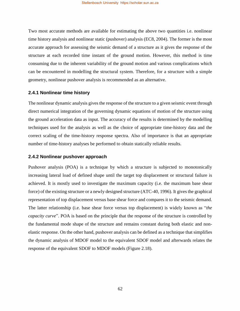
62

Two most accurate methods are available for estimating the above two quantities i.e. nonlinear

time history analysis and nonlinear static (pushover) analysis (EC8, 2004). The former is the most

accurate approach for assessing the seismic demand of a structure as it gives the response of the

structure at each recorded time instant of the ground motion. However, this method is time

consuming due to the inherent variability of the ground motion and various complications which

can be encountered in modelling the structural system. Therefore, for a structure with a simple

geometry, nonlinear pushover analysis is recommended as an alternative.

2.4.1 Nonlinear time history

The nonlinear dynamic analysis gives the response of the structure to a given seismic event through

direct numerical integration of the governing dynamic equations of motion of the structure using

the ground acceleration data as input. The accuracy of the results is determined by the modelling

techniques used for the analysis as well as the choice of appropriate time-history data and the

correct scaling of the time-history response spectra. Also of importance is that an appropriate

number of time-history analyses be performed to obtain statically reliable results.

2.4.2 Nonlinear pushover approach

Pushover analysis (POA) is a technique by which a structure is subjected to monotonically

increasing lateral load of defined shape until the target top displacement or structural failure is

achieved. It is mostly used to investigate the maximum capacity (i.e. the maximum base shear

force) of the existing structure or a newly designed structure (ATC-40, 1996). It gives the graphical

representation of top displacement versus base shear force and compares it to the seismic demand.

The latter relationship (i.e. base shear force versus top displacement) is widely known as “the

capacity curve”. POA is based on the principle that the response of the structure is controlled by

the fundamental mode shape of the structure and remains constant during both elastic and non-

elastic response. On the other hand, pushover analysis can be defined as a technique that simplifies

the dynamic analysis of MDOF model to the equivalent SDOF model and afterwards relates the

response of the equivalent SDOF to MDOF models (Figure 2.18).


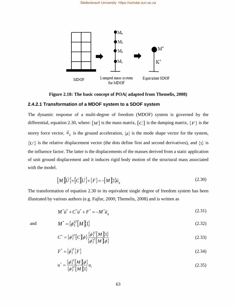
63

Figure 2.18: The basic concept of POA( adapted from Themelis, 2008)

2.4.2.1 Transformation of a MDOF system to a SDOF system

The dynamic response of a multi-degree of freedom (MDOF) system is governed by the

differential, equation 2.30, where: M is the mass matrix, C is the damping matrix, F is the

storey force vector, gu is the ground acceleration, is the mode shape vector for the system,

U is the relative displacement vector (the dots define first and second derivatives), and 1 is

the influence factor. The latter is the displacements of the masses derived from a static application

of unit ground displacement and it induces rigid body motion of the structural mass associated

with the model.

guMFUCUM 1 (2.30)

The transformation of equation 2.30 to its equivalent single degree of freedom system has been

illustrated by various authors (e.g. Fajfar, 2000; Themelis, 2008) and is written as

guMFuCuM ****** (2.31)

and 1* MMT

(2.32)

M

MCC

T

TT 1* (2.33)

FFT

* (2.34)

tT

T

uM

Mu

1

*

(2.35)


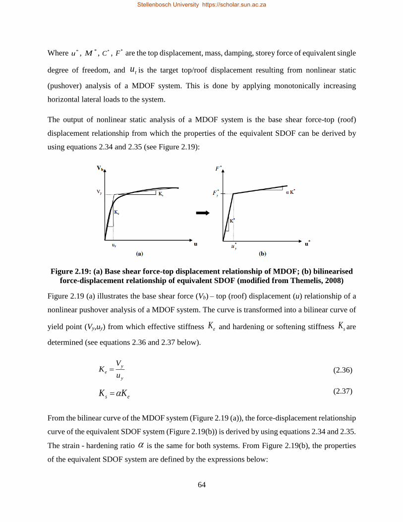
64

Where *u , *M , *C , *F are the top displacement, mass, damping, storey force of equivalent single

degree of freedom, and tu is the target top/roof displacement resulting from nonlinear static

(pushover) analysis of a MDOF system. This is done by applying monotonically increasing

horizontal lateral loads to the system.

The output of nonlinear static analysis of a MDOF system is the base shear force-top (roof)

displacement relationship from which the properties of the equivalent SDOF can be derived by

using equations 2.34 and 2.35 (see Figure 2.19):

Figure 2.19: (a) Base shear force-top displacement relationship of MDOF; (b) bilinearised

force-displacement relationship of equivalent SDOF (modified from Themelis, 2008)

Figure 2.19 (a) illustrates the base shear force (Vb) – top (roof) displacement (u) relationship of a

nonlinear pushover analysis of a MDOF system. The curve is transformed into a bilinear curve of

yield point (Vy,uy) from which effective stiffness eK and hardening or softening stiffness sK are

determined (see equations 2.36 and 2.37 below).

y

y

eu

VK (2.36)

es KK (2.37)

From the bilinear curve of the MDOF system (Figure 2.19 (a)), the force-displacement relationship

curve of the equivalent SDOF system (Figure 2.19(b)) is derived by using equations 2.34 and 2.35.

The strain - hardening ratio is the same for both systems. From Figure 2.19(b), the properties

of the equivalent SDOF system are defined by the expressions below:


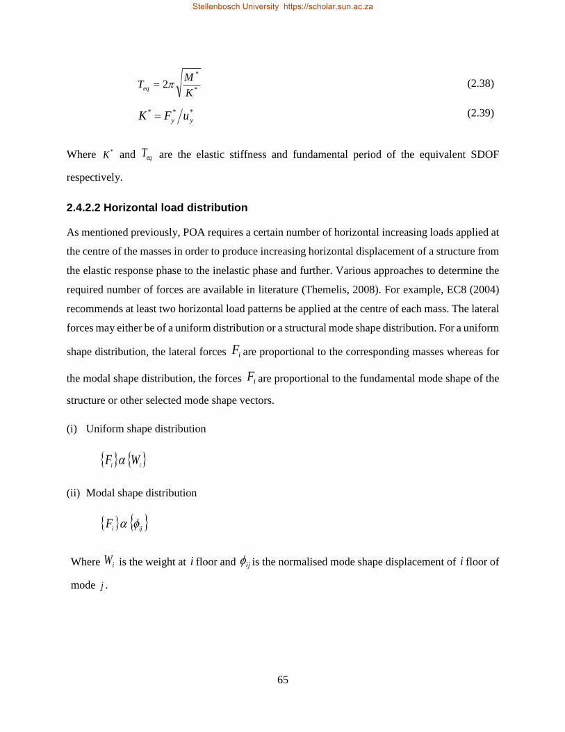
65

*

*

2K

MTeq (2.38)

***

yy uFK (2.39)

Where *K and eqT are the elastic stiffness and fundamental period of the equivalent SDOF

respectively.

2.4.2.2 Horizontal load distribution

As mentioned previously, POA requires a certain number of horizontal increasing loads applied at

the centre of the masses in order to produce increasing horizontal displacement of a structure from

the elastic response phase to the inelastic phase and further. Various approaches to determine the

required number of forces are available in literature (Themelis, 2008). For example, EC8 (2004)

recommends at least two horizontal load patterns be applied at the centre of each mass. The lateral

forces may either be of a uniform distribution or a structural mode shape distribution. For a uniform

shape distribution, the lateral forces iF are proportional to the corresponding masses whereas for

the modal shape distribution, the forces iF are proportional to the fundamental mode shape of the

structure or other selected mode shape vectors.

(i) Uniform shape distribution

ii

WF

(ii) Modal shape distribution

iji

F

Where iW is the weight at i floor and ij is the normalised mode shape displacement of i floor of

mode j .


66

2.4.2.3 A review of pushover analysis methods

Based on Themelis (2008), there are five main methods of pushover analysis:

1. Capacity spectrum method

2. Improved capacity spectrum method

3. N2 method

4. Displacement coefficient method

5. Modal pushover analysis

1. Capacity spectrum method (CSM)

CSM is a nonlinear static analysis method introduced by Freeman, Nicoletti and Tyrell (1975) and

it has been adapted extensively in design codes. The description herein of this method is mainly

based on information collected from ATC-40 (1996). It involves several steps which can be

summarised as follows:

i. Nonlinear static (Pushover) Analysis of a MDOF System

The horizontal lateral loads of modal shape are distributed vertically on the system as described in

section 2.4.2.2, and the POA is performed. Based on analysis, the base shear force-top (roof)

displacement curve is derived (Figure 2.19(a)). This is widely known as capacity curve for the

MDOF system.

ii. Derivation of equivalent SDOF

The capacity curve of MDOF (Figure 2.20) is bilinearised so that the area A1 is equal to area A2.

From the bilinearised curve, the properties of the equivalent single degree of freedom system can

be determined by using equations 2.38 and 2.39 as discussed in section 2.4.2.1.


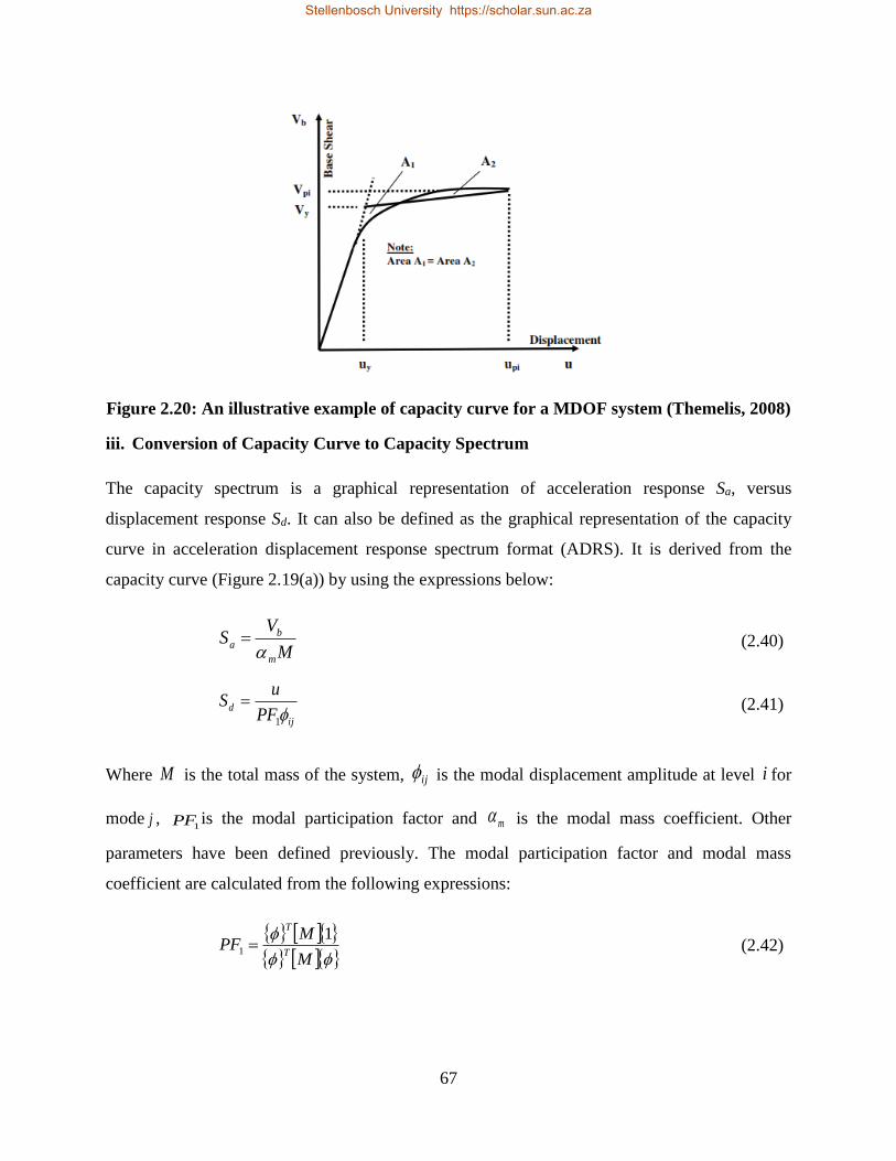
67

Figure 2.20: An illustrative example of capacity curve for a MDOF system (Themelis, 2008)

iii. Conversion of Capacity Curve to Capacity Spectrum

The capacity spectrum is a graphical representation of acceleration response Sa, versus

displacement response Sd. It can also be defined as the graphical representation of the capacity

curve in acceleration displacement response spectrum format (ADRS). It is derived from the

capacity curve (Figure 2.19(a)) by using the expressions below:

M

VS

m

ba

(2.40)

ij

dPF

uS

1 (2.41)

Where M is the total mass of the system, ij is the modal displacement amplitude at level i for

mode j , 1PF is the modal participation factor and m is the modal mass coefficient. Other

parameters have been defined previously. The modal participation factor and modal mass

coefficient are calculated from the following expressions:

M

MPF

T

T1

1 (2.42)


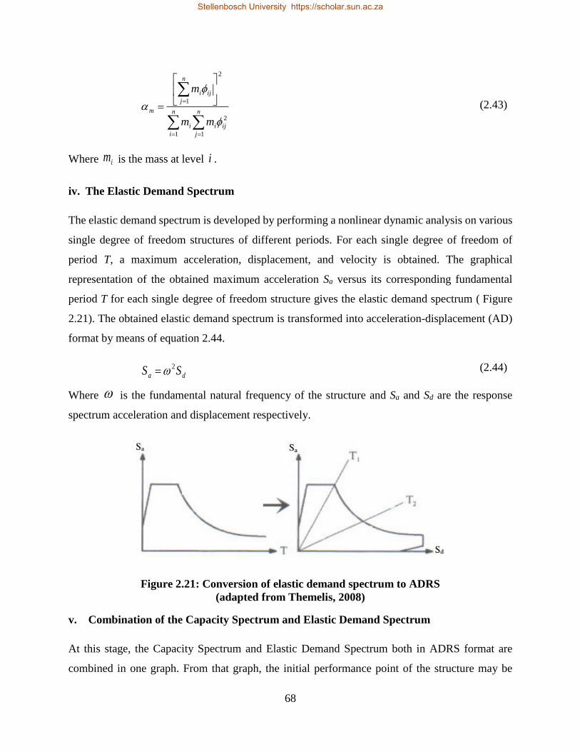
68

(2.43)

Where im is the mass at level i .

iv. The Elastic Demand Spectrum

The elastic demand spectrum is developed by performing a nonlinear dynamic analysis on various

single degree of freedom structures of different periods. For each single degree of freedom of

period T, a maximum acceleration, displacement, and velocity is obtained. The graphical

representation of the obtained maximum acceleration Sa versus its corresponding fundamental

period T for each single degree of freedom structure gives the elastic demand spectrum ( Figure

2.21). The obtained elastic demand spectrum is transformed into acceleration-displacement (AD)

format by means of equation 2.44.

da SS 2 (2.44)

Where is the fundamental natural frequency of the structure and Sa and Sd are the response

spectrum acceleration and displacement respectively.

Figure 2.21: Conversion of elastic demand spectrum to ADRS

(adapted from Themelis, 2008)

v. Combination of the Capacity Spectrum and Elastic Demand Spectrum

At this stage, the Capacity Spectrum and Elastic Demand Spectrum both in ADRS format are

combined in one graph. From that graph, the initial performance point of the structure may be

n

i

n

j

ijii

n

j

iji

m

mm

m

1 1

2

2

1


69

estimated. The performance point defines the point at which the seismic demand is equal to the

seismic capacity of the structure for a given earthquake. This point is estimated based on the

principle of equal displacement, i.e. the inelastic displacement of the structure is equal to elastic

displacement of the same structure which will take place if it remains perfectly elastic (ATC-40,

1996). It is obtained by drawing a line upwards of the same slope as the initial stiffness of the

structure until it intersects Elastic Demand Spectrum; the vertical line passing through that

intersection point is drawn. The intersection point of the vertical line and Capacity Spectrum

represents the initial performance point (Figure 2.22).

Figure 2.22: Estimation of initial performance point (modified from Themelis, 2008)

vi. Bilinearisation of the Capacity curve (ADRS format)

The Capacity Spectrum in ADRS format developed from step (iii) is bilinearised by chosing a

yield point yy da , such that area A1 is equal to A2 (Figure 2.23).


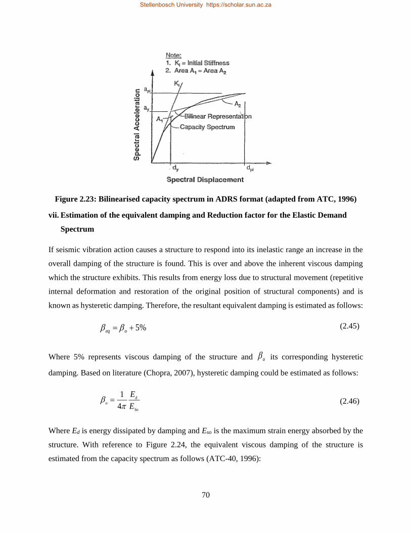
70

Figure 2.23: Bilinearised capacity spectrum in ADRS format (adapted from ATC, 1996)

vii. Estimation of the equivalent damping and Reduction factor for the Elastic Demand

Spectrum

If seismic vibration action causes a structure to respond into its inelastic range an increase in the

overall damping of the structure is found. This is over and above the inherent viscous damping

which the structure exhibits. This results from energy loss due to structural movement (repetitive

internal deformation and restoration of the original position of structural components) and is

known as hysteretic damping. Therefore, the resultant equivalent damping is estimated as follows:

%5 oeq (2.45)

Where 5% represents viscous damping of the structure and o its corresponding hysteretic

damping. Based on literature (Chopra, 2007), hysteretic damping could be estimated as follows:

So

d

oE

E

4

1 (2.46)

Where Ed is energy dissipated by damping and Eso is the maximum strain energy absorbed by the

structure. With reference to Figure 2.24, the equivalent viscous damping of the structure is

estimated from the capacity spectrum as follows (ATC-40, 1996):


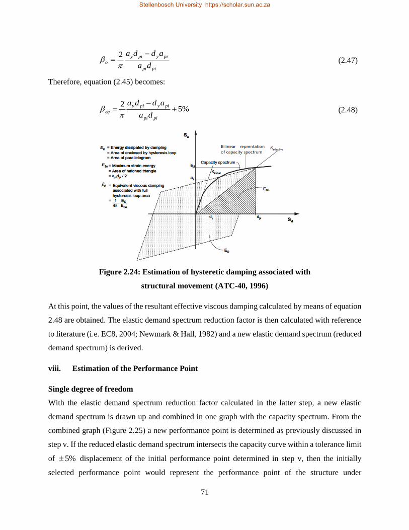
71

pipi

piypiy

oda

adda

2

(2.47)

Therefore, equation (2.45) becomes:

%52

pipi

piypiy

eqda

adda

(2.48)

Figure 2.24: Estimation of hysteretic damping associated with

structural movement (ATC-40, 1996)

At this point, the values of the resultant effective viscous damping calculated by means of equation

2.48 are obtained. The elastic demand spectrum reduction factor is then calculated with reference

to literature (i.e. EC8, 2004; Newmark & Hall, 1982) and a new elastic demand spectrum (reduced

demand spectrum) is derived.

viii. Estimation of the Performance Point

Single degree of freedom

With the elastic demand spectrum reduction factor calculated in the latter step, a new elastic

demand spectrum is drawn up and combined in one graph with the capacity spectrum. From the

combined graph (Figure 2.25) a new performance point is determined as previously discussed in

step v. If the reduced elastic demand spectrum intersects the capacity curve within a tolerance limit

of %5 displacement of the initial performance point determined in step v, then the initially

selected performance point would represent the performance point of the structure under


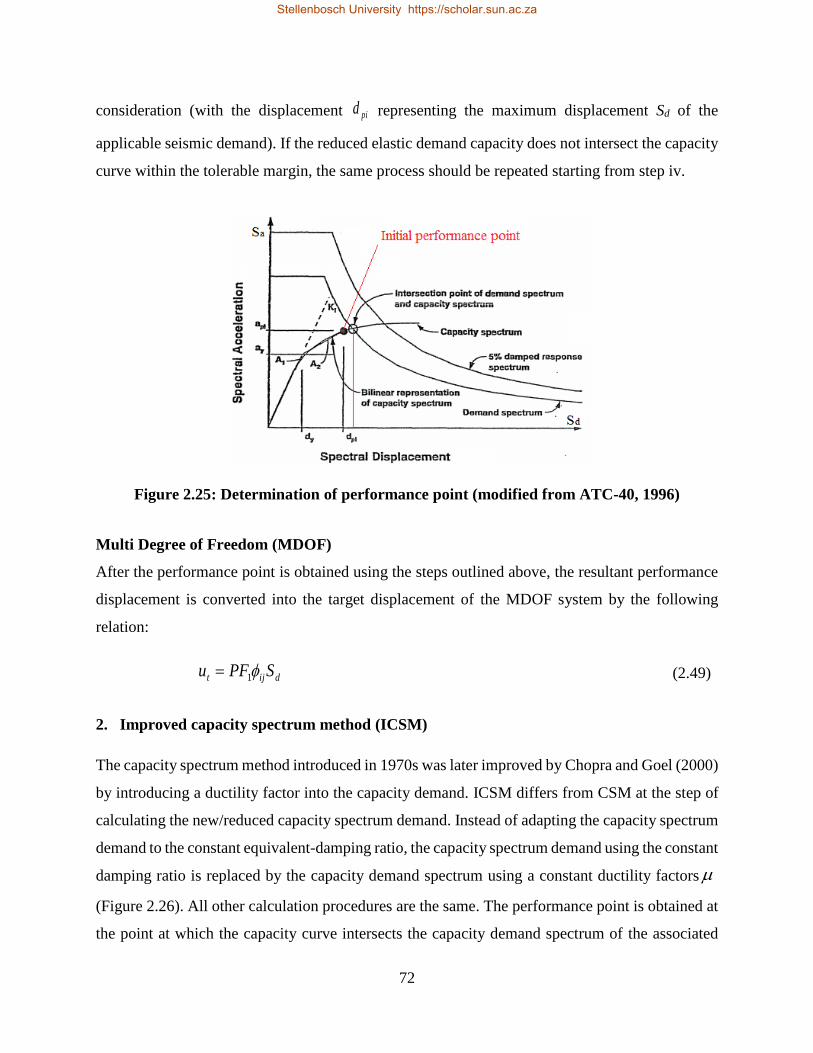
72

consideration (with the displacement pid representing the maximum displacement Sd of the

applicable seismic demand). If the reduced elastic demand capacity does not intersect the capacity

curve within the tolerable margin, the same process should be repeated starting from step iv.

Figure 2.25: Determination of performance point (modified from ATC-40, 1996)

Multi Degree of Freedom (MDOF)

After the performance point is obtained using the steps outlined above, the resultant performance

displacement is converted into the target displacement of the MDOF system by the following

relation:

dijt SPFu 1 (2.49)

2. Improved capacity spectrum method (ICSM)

The capacity spectrum method introduced in 1970s was later improved by Chopra and Goel (2000)

by introducing a ductility factor into the capacity demand. ICSM differs from CSM at the step of

calculating the new/reduced capacity spectrum demand. Instead of adapting the capacity spectrum

demand to the constant equivalent-damping ratio, the capacity spectrum demand using the constant

damping ratio is replaced by the capacity demand spectrum using a constant ductility factors

(Figure 2.26). All other calculation procedures are the same. The performance point is obtained at

the point at which the capacity curve intersects the capacity demand spectrum of the associated


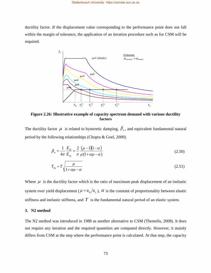
73

ductility factor. If the displacement value corresponding to the performance point does not fall

within the margin of tolerance, the application of an iteration procedure such as for CSM will be

required.

Figure 2.26: Illustrative example of capacity spectrum demand with various ductility

factors

The ductility factor is related to hysteretic damping, o , and equivalent fundamental natural

period by the following relationships (Chopra & Goel, 2000).

)1(

112

4

1

so

Do

E

E (2.50)

1TTeq

(2.51)

Where is the ductility factor which is the ratio of maximum peak displacement of an inelastic

system over yield displacement ( ym uu ), is the constant of proportionality between elastic

stiffness and inelastic stiffness, and T is the fundamental natural period of an elastic system.

3. N2 method

The N2 method was introduced in 1988 as another alternative to CSM (Themelis, 2008). It does

not require any iteration and the required quantities are computed directly. However, it mainly

differs from CSM at the step where the performance point is calculated. At that step, the capacity


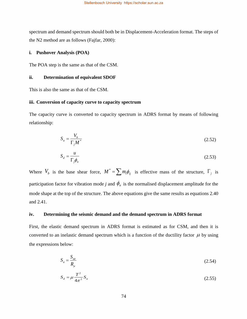
74

spectrum and demand spectrum should both be in Displacement-Acceleration format. The steps of

the N2 method are as follows (Fajfar, 2000):

i. Pushover Analysis (POA)

The POA step is the same as that of the CSM.

ii. Determination of equivalent SDOF

This is also the same as that of the CSM.

iii. Conversion of capacity curve to capacity spectrum

The capacity curve is converted to capacity spectrum in ADRS format by means of following

relationship:

*M

VS

j

ba

(2.52)

nj

d

uS

(2.53)

Where bV is the base shear force, ijimM * is effective mass of the structure, j is

participation factor for vibration mode j and n is the normalised displacement amplitude for the

mode shape at the top of the structure. The above equations give the same results as equations 2.40

and 2.41.

iv. Determining the seismic demand and the demand spectrum in ADRS format

First, the elastic demand spectrum in ADRS format is estimated as for CSM, and then it is

converted to an inelastic demand spectrum which is a function of the ductility factor by using

the expressions below:

R

SS ae

a (2.54)

ad S

TS

2

2

4 (2.55)


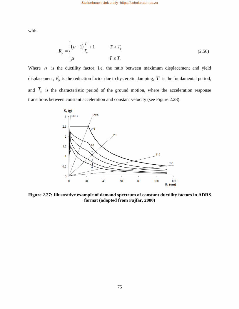
75

with

c

c

c

TT

TTT

T

R

11

(2.56)

Where is the ductility factor, i.e. the ratio between maximum displacement and yield

displacement, R is the reduction factor due to hysteretic damping, T is the fundamental period,

and cT is the characteristic period of the ground motion, where the acceleration response

transitions between constant acceleration and constant velocity (see Figure 2.28).

Figure 2.27: Illustrative example of demand spectrum of constant ductility factors in ADRS

format (adapted from Fajfar, 2000)


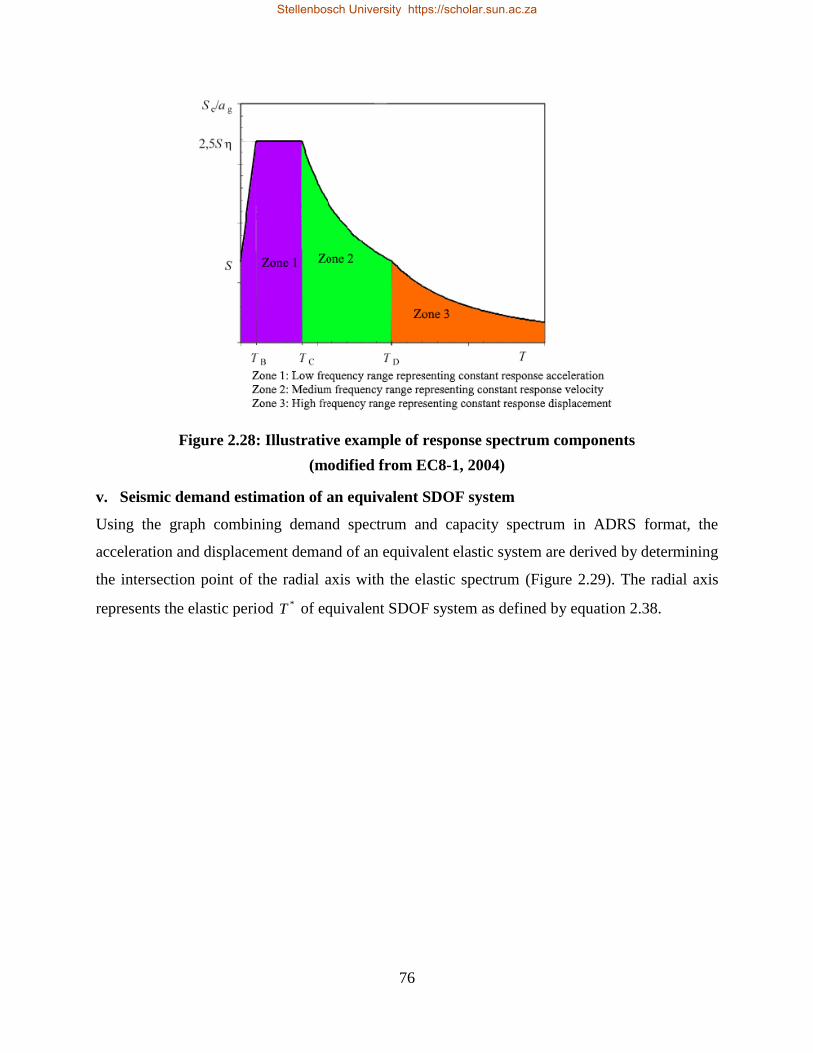
76

Figure 2.28: Illustrative example of response spectrum components

(modified from EC8-1, 2004)

v. Seismic demand estimation of an equivalent SDOF system

Using the graph combining demand spectrum and capacity spectrum in ADRS format, the

acceleration and displacement demand of an equivalent elastic system are derived by determining

the intersection point of the radial axis with the elastic spectrum (Figure 2.29). The radial axis

represents the elastic period *T of equivalent SDOF system as defined by equation 2.38.


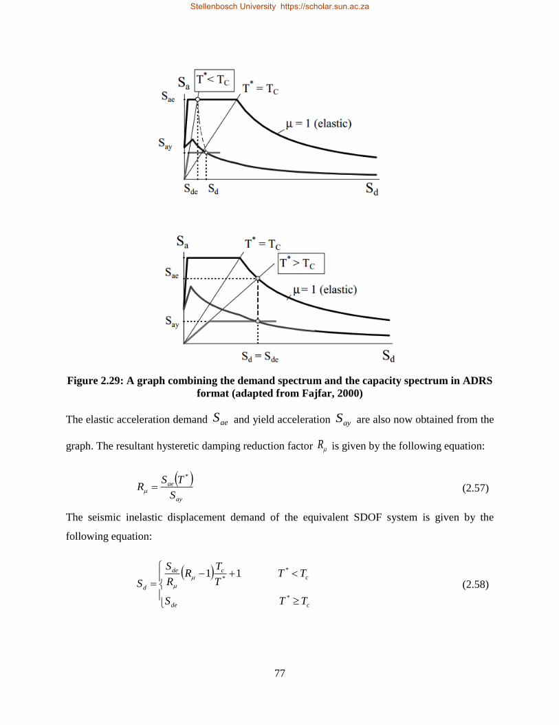
77

Figure 2.29: A graph combining the demand spectrum and the capacity spectrum in ADRS

format (adapted from Fajfar, 2000)

The elastic acceleration demand aeS and yield acceleration ayS are also now obtained from the

graph. The resultant hysteretic damping reduction factor R is given by the following equation:

ay

ae

S

TSR

*

(2.57)

The seismic inelastic displacement demand of the equivalent SDOF system is given by the

following equation:

cde

ccde

d

TTS

TTT

TR

R

S

S

*

*

*

11

(2.58)


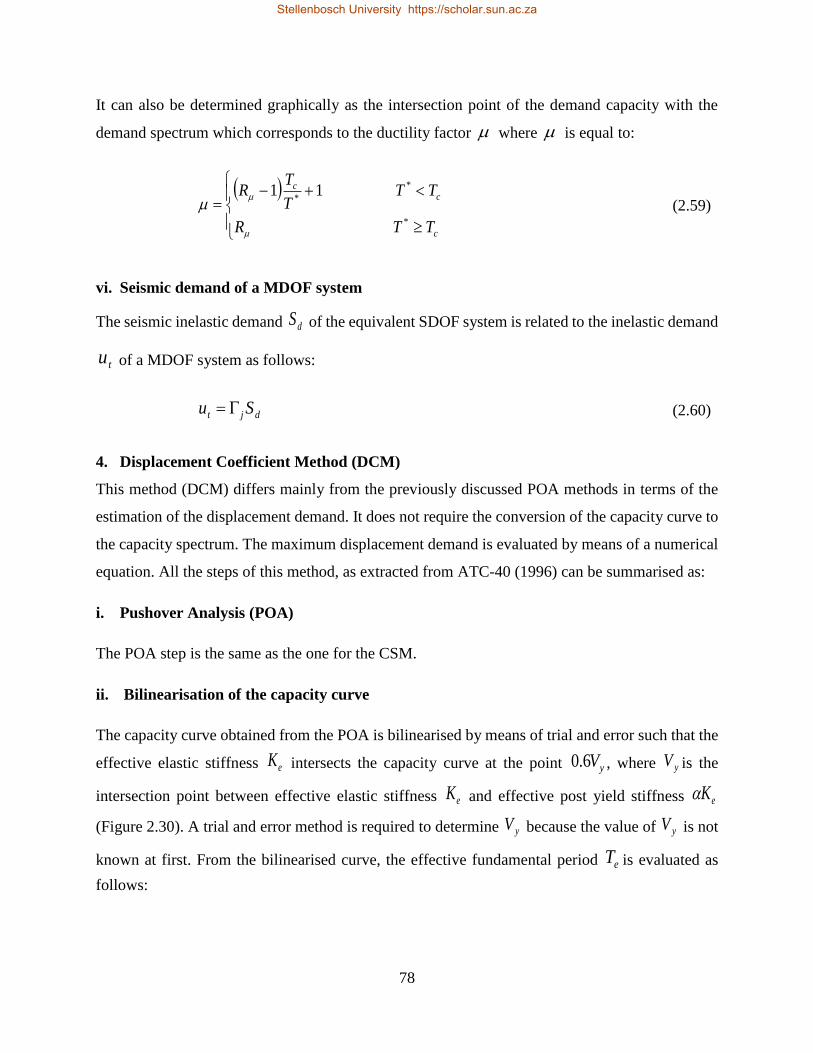
78

It can also be determined graphically as the intersection point of the demand capacity with the

demand spectrum which corresponds to the ductility factor where is equal to:

c

cc

TTR

TTT

TR

*

*

*

11

(2.59)

vi. Seismic demand of a MDOF system

The seismic inelastic demand dS of the equivalent SDOF system is related to the inelastic demand

tu of a MDOF system as follows:

djt Su (2.60)

4. Displacement Coefficient Method (DCM)

This method (DCM) differs mainly from the previously discussed POA methods in terms of the

estimation of the displacement demand. It does not require the conversion of the capacity curve to

the capacity spectrum. The maximum displacement demand is evaluated by means of a numerical

equation. All the steps of this method, as extracted from ATC-40 (1996) can be summarised as:

i. Pushover Analysis (POA)

The POA step is the same as the one for the CSM.

ii. Bilinearisation of the capacity curve

The capacity curve obtained from the POA is bilinearised by means of trial and error such that the

effective elastic stiffness eK intersects the capacity curve at the point yV6.0 , where yV is the

intersection point between effective elastic stiffness eK and effective post yield stiffness eK

(Figure 2.30). A trial and error method is required to determine yV because the value of yV is not

known at first. From the bilinearised curve, the effective fundamental period eT is evaluated as

follows:


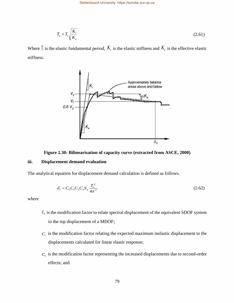
79

e

iie

K

KTT (2.61)

Where iT is the elastic fundamental period, iK is the elastic stiffness and eK is the effective elastic

stiffness.

Figure 2.30: Bilinearisation of capacity curve (extracted from ASCE, 2000)

iii. Displacement demand evaluation

The analytical equation for displacement demand calculation is defined as follows.

2

2

32104

eat

TSCCCC (2.62)

where

0c is the modification factor to relate spectral displacement of the equivalent SDOF system

to the top displacement of a MDOF;

1C is the modification factor relating the expected maximum inelastic displacement to the

displacements calculated for linear elastic response;

2C is the modification factor representing the increased displacements due to second-order

effects; and


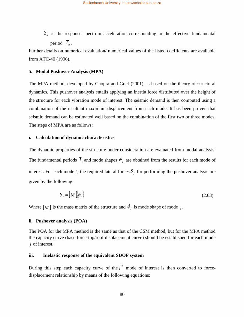
80

aS is the response spectrum acceleration corresponding to the effective fundamental

period eT .

Further details on numerical evaluation/ numerical values of the listed coefficients are available

from ATC-40 (1996).

5. Modal Pushover Analysis (MPA)

The MPA method, developed by Chopra and Goel (2001), is based on the theory of structural

dynamics. This pushover analysis entails applying an inertia force distributed over the height of

the structure for each vibration mode of interest. The seismic demand is then computed using a

combination of the resultant maximum displacement from each mode. It has been proven that

seismic demand can be estimated well based on the combination of the first two or three modes.

The steps of MPA are as follows:

i. Calculation of dynamic characteristics

The dynamic properties of the structure under consideration are evaluated from modal analysis.

The fundamental periods nT and mode shapes j are obtained from the results for each mode of

interest. For each mode j , the required lateral forces jS for performing the pushover analysis are

given by the following:

jj

MS (2.63)

Where M is the mass matrix of the structure and j is mode shape of mode j .

ii. Pushover analysis (POA)

The POA for the MPA method is the same as that of the CSM method, but for the MPA method

the capacity curve (base force-top/roof displacement curve) should be established for each mode

j of interest.

iii. Inelastic response of the equivalent SDOF system

During this step each capacity curve of thethj mode of interest is then converted to force-

displacement relationship by means of the following equations:


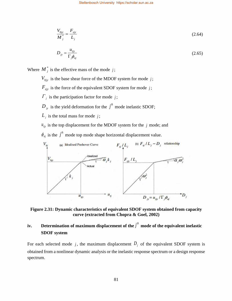
81

j

sjy

j

bjy

L

F

M

V

* (2.64)

njj

tjy

jy

uD

(2.65)

Where *

jM is the effective mass of the mode j ;

bjyV is the base shear force of the MDOF system for mode j ;

sjyF is the force of the equivalent SDOF system for mode j ;

jΓ is the participation factor for mode j ;

jyD is the yield deformation for the

thj mode inelastic SDOF;

jL is the total mass for mode j ;

tjyu is the top displacement for the MDOF system for the j mode; and

nj is the thj mode top mode shape horizontal displacement value.

Figure 2.31: Dynamic characteristics of equivalent SDOF system obtained from capacity

curve (extracted from Chopra & Goel, 2002)

iv. Determination of maximum displacement of thethj mode of the equivalent inelastic

SDOF system

For each selected mode j , the maximum displacement jD of the equivalent SDOF system is

obtained from a nonlinear dynamic analysis or the inelastic response spectrum or a design response

spectrum.


82

v. Calculation of maximum displacement of MDOF

The maximum displacement jD of the equivalent inelastic SDOF is related to the maximum

displacement tju of the MDOF system by

jnjjtj Du (2.66)

vi. Total seismic response demand

The total seismic displacement demand MPAR is obtained from the combination of the maximum

modal responses jR . For example, if the square root of the sum of squares (SRSS) rule is selected

as combination rule, the total response demand will be given by

2/1

1

2

n

j

jMPA RR (2.67)

Where n represents the number of modes of interest.

Conclusion

As reported by Themelis (2008), extensive research has been conducted on pushover analysis

methods to evaluate seismic response of structures. The latest studies conducted on the accuracy

of different pushover procedures/methods have shown that Modal Pushover Analysis (MPA) is

the most accurate method.


83

Chapter 3

Methodology

3.1 Introduction

The main objective of this research was to identify a methodology for assessing the structural

performance of a steel frame water tower and apply this to evaluate whether the elevated steel

water tank at the Engen Winelands 1-Stop in South Africa can withstand the seismic demand at its

location. In this investigation the seismic demand of a typical elevated steel water tower supported

by a steel frame was estimated from nonlinear dynamic analysis and the response spectrum

approach prescribed by the Eurocode seismic design code. Afterwards, the results of both

approaches (nonlinear dynamic and response spectrum) were compared to the seismic capacity

estimated from Modal Pushover Analysis (MPA). Thereafter, the overall stability of the system

was checked. During this analysis process, the structure was subjected to earthquake excitation

corresponding to its site location as specified by the South African National Standard for the basis

of structural design and actions for buildings and industrial structures /Part 4: Seismic actions and

general requirements for buildings (SANS 10160-4:2011), and the finite element software package

ABAQUS (SIMULIA, 2012) was used to perform the nonlinear dynamic analysis and MPA

analyses.

The first step in the process was the analysis of the structure by considering it as perfectly fixed at

the ground level. The second step was to analyse it by modifying its fixed base condition to flexible

foundation by incorporating the flexibility of site soil at the foundation level. This was done by

introducing dashpots and springs of equivalent soil properties as discussed in chapter two. For the

purpose of checking the effects of soil flexibility to the general response of the system, the results

of both foundation formulations were compared.

In order to validate the ABAQUS Finite Element Analysis (FEA), a steel frame structure was

constructed and tested in the laboratory. This was done to ensure that suitable applicable analysis

techniques were selected for the ABAQUS modelling of the structure. This chapter describes the

numerical analysis methodology and parameters used to achieve the stated objective. A description

of laboratory tests and results and the FEA analysis procedures and results are provided in

Chapter 4.


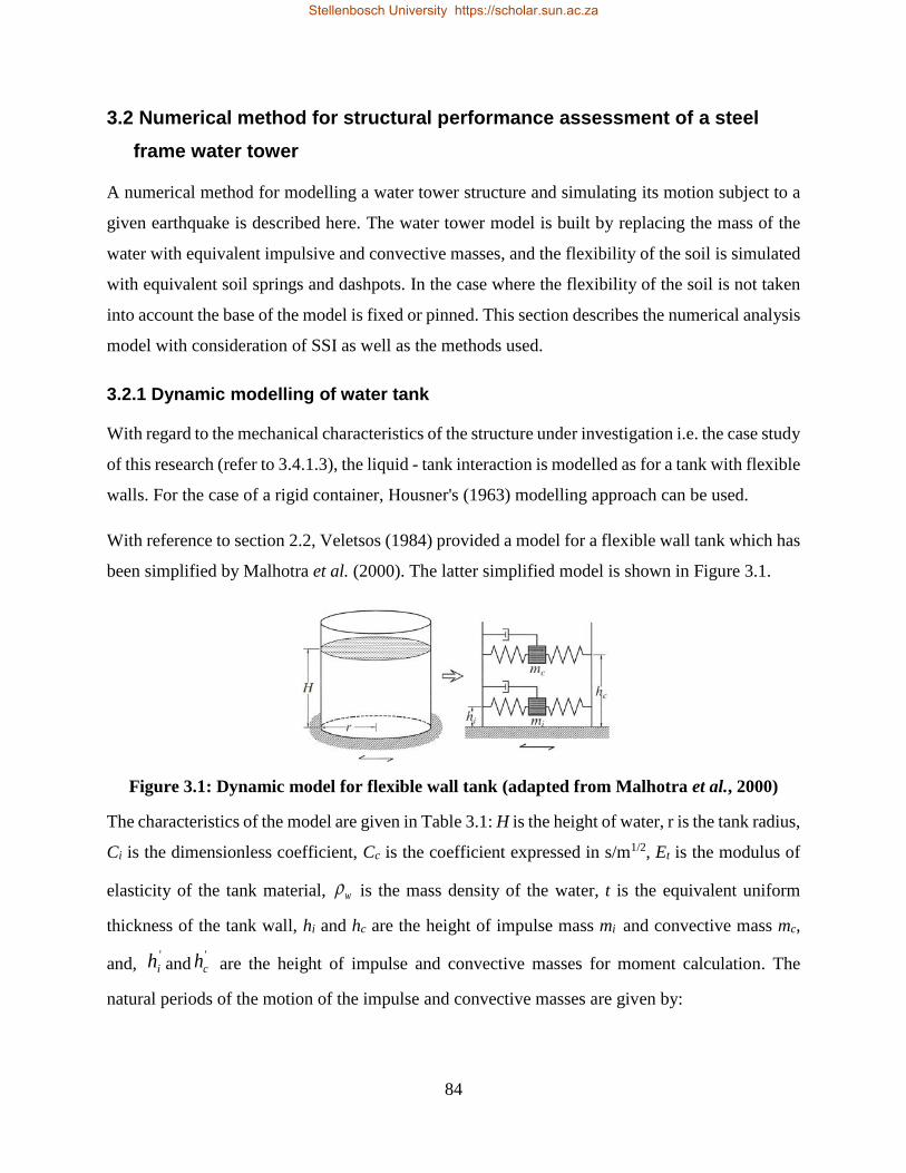
84

3.2 Numerical method for structural performance assessment of a steel

frame water tower

A numerical method for modelling a water tower structure and simulating its motion subject to a

given earthquake is described here. The water tower model is built by replacing the mass of the

water with equivalent impulsive and convective masses, and the flexibility of the soil is simulated

with equivalent soil springs and dashpots. In the case where the flexibility of the soil is not taken

into account the base of the model is fixed or pinned. This section describes the numerical analysis

model with consideration of SSI as well as the methods used.

3.2.1 Dynamic modelling of water tank

With regard to the mechanical characteristics of the structure under investigation i.e. the case study

of this research (refer to 3.4.1.3), the liquid - tank interaction is modelled as for a tank with flexible

walls. For the case of a rigid container, Housner's (1963) modelling approach can be used.

With reference to section 2.2, Veletsos (1984) provided a model for a flexible wall tank which has

been simplified by Malhotra et al. (2000). The latter simplified model is shown in Figure 3.1.

Figure 3.1: Dynamic model for flexible wall tank (adapted from Malhotra et al., 2000)

The characteristics of the model are given in Table 3.1: H is the height of water, r is the tank radius,

Ci is the dimensionless coefficient, Cc is the coefficient expressed in s/m1/2, Et is the modulus of

elasticity of the tank material, w is the mass density of the water, t is the equivalent uniform

thickness of the tank wall, hi and hc are the height of impulse mass mi and convective mass mc,

and, '

ih and'

ch are the height of impulse and convective masses for moment calculation. The

natural periods of the motion of the impulse and convective masses are given by:


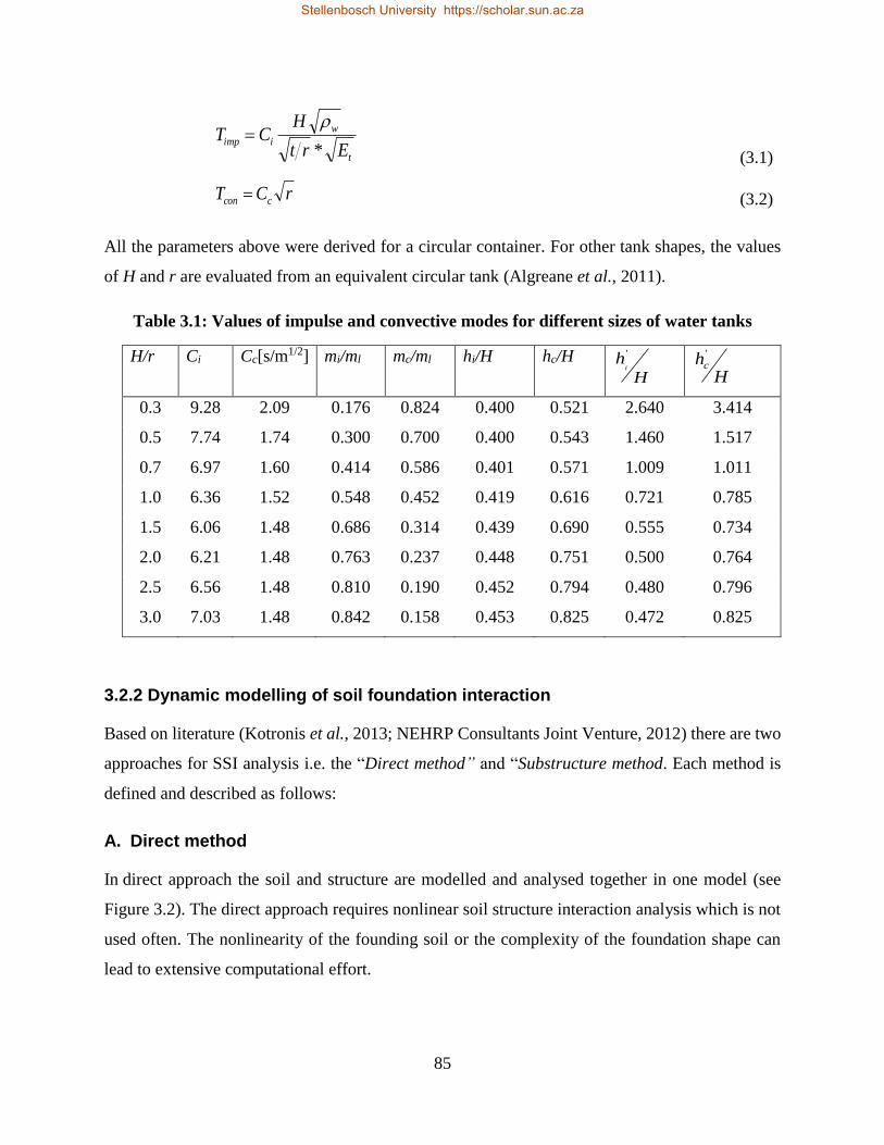
85

t

w

iimpErt

HCT

*

(3.1)

rCT ccon (3.2)

All the parameters above were derived for a circular container. For other tank shapes, the values

of H and r are evaluated from an equivalent circular tank (Algreane et al., 2011).

Table 3.1: Values of impulse and convective modes for different sizes of water tanks

H/r Ci Cc[s/m1/2] mi/ml mc/ml hi/H hc/H

H

hi

'

H

hc

'

0.3 9.28 2.09 0.176 0.824 0.400 0.521 2.640 3.414

0.5 7.74 1.74 0.300 0.700 0.400 0.543 1.460 1.517

0.7 6.97 1.60 0.414 0.586 0.401 0.571 1.009 1.011

1.0 6.36 1.52 0.548 0.452 0.419 0.616 0.721 0.785

1.5 6.06 1.48 0.686 0.314 0.439 0.690 0.555 0.734

2.0 6.21 1.48 0.763 0.237 0.448 0.751 0.500 0.764

2.5 6.56 1.48 0.810 0.190 0.452 0.794 0.480 0.796

3.0 7.03 1.48 0.842 0.158 0.453 0.825 0.472 0.825

3.2.2 Dynamic modelling of soil foundation interaction

Based on literature (Kotronis et al., 2013; NEHRP Consultants Joint Venture, 2012) there are two

approaches for SSI analysis i.e. the “Direct method” and “Substructure method. Each method is

defined and described as follows:

A. Direct method

In direct approach the soil and structure are modelled and analysed together in one model (see

Figure 3.2). The direct approach requires nonlinear soil structure interaction analysis which is not

used often. The nonlinearity of the founding soil or the complexity of the foundation shape can

lead to extensive computational effort.


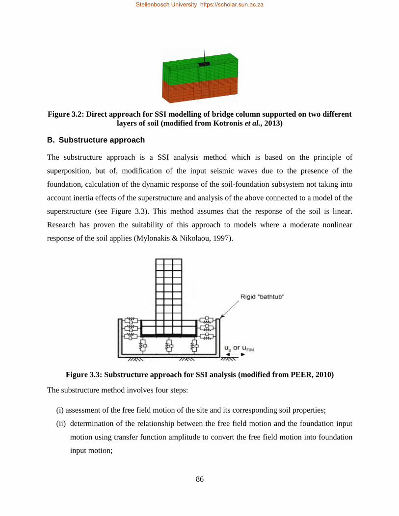
86

Figure 3.2: Direct approach for SSI modelling of bridge column supported on two different

layers of soil (modified from Kotronis et al., 2013)

B. Substructure approach

The substructure approach is a SSI analysis method which is based on the principle of

superposition, but of, modification of the input seismic waves due to the presence of the

foundation, calculation of the dynamic response of the soil-foundation subsystem not taking into

account inertia effects of the superstructure and analysis of the above connected to a model of the

superstructure (see Figure 3.3). This method assumes that the response of the soil is linear.

Research has proven the suitability of this approach to models where a moderate nonlinear

response of the soil applies (Mylonakis & Nikolaou, 1997).

Figure 3.3: Substructure approach for SSI analysis (modified from PEER, 2010)

The substructure method involves four steps:

(i) assessment of the free field motion of the site and its corresponding soil properties;

(ii) determination of the relationship between the free field motion and the foundation input

motion using transfer function amplitude to convert the free field motion into foundation

input motion;


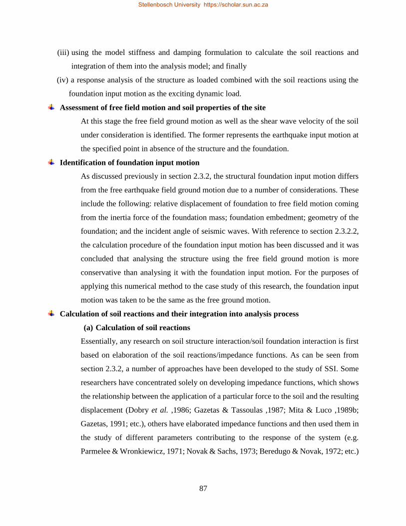
87

(iii) using the model stiffness and damping formulation to calculate the soil reactions and

integration of them into the analysis model; and finally

(iv) a response analysis of the structure as loaded combined with the soil reactions using the

foundation input motion as the exciting dynamic load.

Assessment of free field motion and soil properties of the site

At this stage the free field ground motion as well as the shear wave velocity of the soil

under consideration is identified. The former represents the earthquake input motion at

the specified point in absence of the structure and the foundation.

Identification of foundation input motion

As discussed previously in section 2.3.2, the structural foundation input motion differs

from the free earthquake field ground motion due to a number of considerations. These

include the following: relative displacement of foundation to free field motion coming

from the inertia force of the foundation mass; foundation embedment; geometry of the

foundation; and the incident angle of seismic waves. With reference to section 2.3.2.2,

the calculation procedure of the foundation input motion has been discussed and it was

concluded that analysing the structure using the free field ground motion is more

conservative than analysing it with the foundation input motion. For the purposes of

applying this numerical method to the case study of this research, the foundation input

motion was taken to be the same as the free ground motion.

Calculation of soil reactions and their integration into analysis process

(a) Calculation of soil reactions

Essentially, any research on soil structure interaction/soil foundation interaction is first

based on elaboration of the soil reactions/impedance functions. As can be seen from

section 2.3.2, a number of approaches have been developed to the study of SSI. Some

researchers have concentrated solely on developing impedance functions, which shows

the relationship between the application of a particular force to the soil and the resulting

displacement (Dobry et al. ,1986; Gazetas & Tassoulas ,1987; Mita & Luco ,1989b;

Gazetas, 1991; etc.), others have elaborated impedance functions and then used them in

the study of different parameters contributing to the response of the system (e.g.

Parmelee & Wronkiewicz, 1971; Novak & Sachs, 1973; Beredugo & Novak, 1972; etc.)


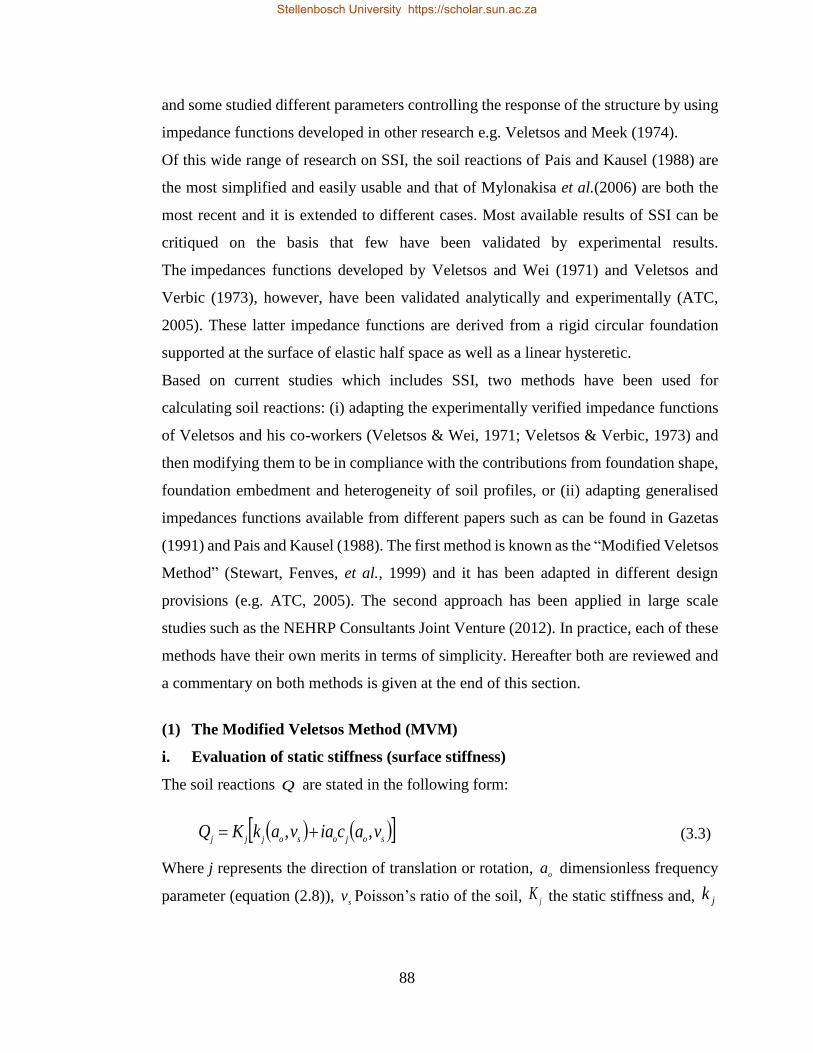
88

and some studied different parameters controlling the response of the structure by using

impedance functions developed in other research e.g. Veletsos and Meek (1974).

Of this wide range of research on SSI, the soil reactions of Pais and Kausel (1988) are

the most simplified and easily usable and that of Mylonakisa et al.(2006) are both the

most recent and it is extended to different cases. Most available results of SSI can be

critiqued on the basis that few have been validated by experimental results.

The impedances functions developed by Veletsos and Wei (1971) and Veletsos and

Verbic (1973), however, have been validated analytically and experimentally (ATC,

2005). These latter impedance functions are derived from a rigid circular foundation

supported at the surface of elastic half space as well as a linear hysteretic.

Based on current studies which includes SSI, two methods have been used for

calculating soil reactions: (i) adapting the experimentally verified impedance functions

of Veletsos and his co-workers (Veletsos & Wei, 1971; Veletsos & Verbic, 1973) and

then modifying them to be in compliance with the contributions from foundation shape,

foundation embedment and heterogeneity of soil profiles, or (ii) adapting generalised

impedances functions available from different papers such as can be found in Gazetas

(1991) and Pais and Kausel (1988). The first method is known as the “Modified Veletsos

Method” (Stewart, Fenves, et al., 1999) and it has been adapted in different design

provisions (e.g. ATC, 2005). The second approach has been applied in large scale

studies such as the NEHRP Consultants Joint Venture (2012). In practice, each of these

methods have their own merits in terms of simplicity. Hereafter both are reviewed and

a commentary on both methods is given at the end of this section.

(1) The Modified Veletsos Method (MVM)

i. Evaluation of static stiffness (surface stiffness)

The soil reactions Q are stated in the following form:

sojosojjj

vaciavakKQ ,, (3.3)

Where j represents the direction of translation or rotation, o

a dimensionless frequency

parameter (equation (2.8)), s

v Poisson’s ratio of the soil, jK the static stiffness and, jk


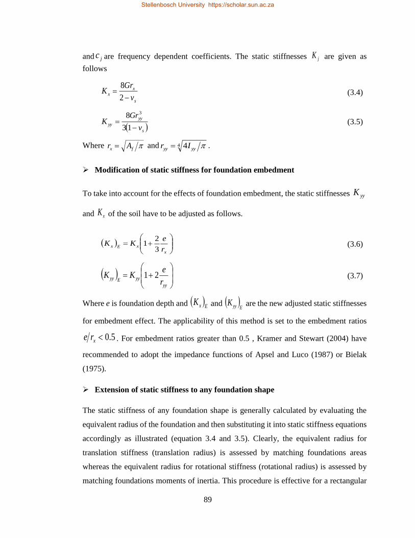
89

and jc are frequency dependent coefficients. The static stiffnesses jK are given as

follows

s

xx

v

GrK

2

8 (3.4)

s

yy

yyv

GrK

13

8 3

(3.5)

Where fx Ar and 4 4 yyyy Ir .

Modification of static stiffness for foundation embedment

To take into account for the effects of foundation embedment, the static stiffnesses yyK

and xK of the soil have to be adjusted as follows.

x

xExr

eKK

3

21 (3.6)

yy

yyEyyr

eKK 21 (3.7)

Where e is foundation depth and ExK and

EyyK are the new adjusted static stiffnesses

for embedment effect. The applicability of this method is set to the embedment ratios

5.0xre . For embedment ratios greater than 0.5 , Kramer and Stewart (2004) have

recommended to adopt the impedance functions of Apsel and Luco (1987) or Bielak

(1975).

Extension of static stiffness to any foundation shape

The static stiffness of any foundation shape is generally calculated by evaluating the

equivalent radius of the foundation and then substituting it into static stiffness equations

accordingly as illustrated (equation 3.4 and 3.5). Clearly, the equivalent radius for

translation stiffness (translation radius) is assessed by matching foundations areas

whereas the equivalent radius for rotational stiffness (rotational radius) is assessed by

matching foundations moments of inertia. This procedure is effective for a rectangular


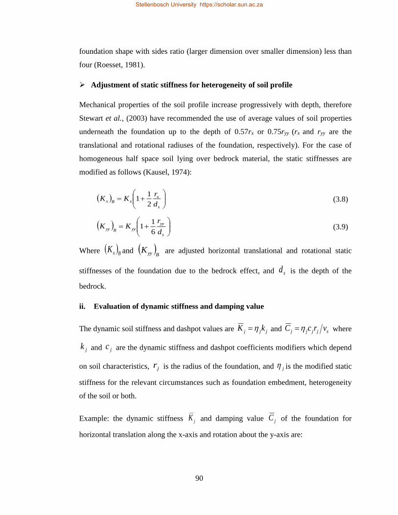
90

foundation shape with sides ratio (larger dimension over smaller dimension) less than

four (Roesset, 1981).

Adjustment of static stiffness for heterogeneity of soil profile

Mechanical properties of the soil profile increase progressively with depth, therefore

Stewart et al., (2003) have recommended the use of average values of soil properties

underneath the foundation up to the depth of 0.57rx or 0.75ryy (rx and ryy are the

translational and rotational radiuses of the foundation, respectively). For the case of

homogeneous half space soil lying over bedrock material, the static stiffnesses are

modified as follows (Kausel, 1974):

s

xxBx

d

rKK

2

11 (3.8)

s

yy

yyByyd

rKK

6

11 (3.9)

Where BxK and

ByyK are adjusted horizontal translational and rotational static

stiffnesses of the foundation due to the bedrock effect, and sd is the depth of the

bedrock.

ii. Evaluation of dynamic stiffness and damping value

The dynamic soil stiffness and dashpot values are jjj kK and sjjjj vrcC where

jk and jc are the dynamic stiffness and dashpot coefficients modifiers which depend

on soil characteristics, jr is the radius of the foundation, and j is the modified static

stiffness for the relevant circumstances such as foundation embedment, heterogeneity

of the soil or both.

Example: the dynamic stiffness jK and damping value jC of the foundation for

horizontal translation along the x-axis and rotation about the y-axis are:


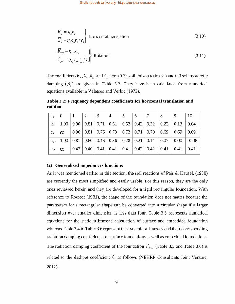
91

sxxxx

xxx

vrcC

kK

Horizontal translation (3.10)

syyyyyyyy

yyyyyy

vrcC

kK

Rotation (3.11)

The coefficients xk , xc , yyk and yyc for a 0.33 soil Poison ratio (s

) and 0.3 soil hysteretic

damping (s

) are given in Table 3.2. They have been calculated from numerical

equations available in Veletsos and Verbic (1973).

Table 3.2: Frequency dependent coefficients for horizontal translation and

rotation

ao 0 1 2 3 4 5 6 7 8 9 10

kx 1.00 0.90 0.81 0.71 0.61 0.52 0.42 0.32 0.23 0.13 0.04

cx ꝏ 0.96 0.81 0.76 0.73 0.72 0.71 0.70 0.69 0.69 0.69

kyy 1.00 0.81 0.60 0.46 0.36 0.28 0.21 0.14 0.07 0.00 -0.06

cyy ꝏ 0.43 0.40 0.41 0.41 0.41 0.42 0.42 0.41 0.41 0.41

(2) Generalized impedances functions

As it was mentioned earlier in this section, the soil reactions of Pais & Kausel, (1988)

are currently the most simplified and easily usable. For this reason, they are the only

ones reviewed herein and they are developed for a rigid rectangular foundation. With

reference to Roesset (1981), the shape of the foundation does not matter because the

parameters for a rectangular shape can be converted into a circular shape if a larger

dimension over smaller dimension is less than four. Table 3.3 represents numerical

equations for the static stiffnesses calculation of surface and embedded foundation

whereas Table 3.4 to Table 3.6 represent the dynamic stiffnesses and their corresponding

radiation damping coefficients for surface foundations as well as embedded foundations.

The radiation damping coefficient of the foundation jfr , (Table 3.5 and Table 3.6) is

related to the dashpot coefficient jC as follows (NEHRP Consultants Joint Venture,

2012):


92

jf

j

sjfr

jj

K

KC

,

,

2

2

(3.12)

Where jK is dynamic stiffness and s is the soil hysteretic damping coefficient. The

indices j denotes excitation direction of interest.


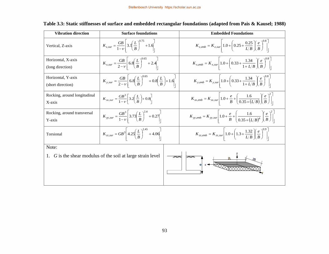
93

Table 3.3: Static stiffnesses of surface and embedded rectangular foundations (adapted from Pais & Kausel; 1988)

Vibration direction Surface foundations Embedded Foundations

Vertical, Z-axis

6.11.3

1

75.0

,B

LGBK surz

8.0

,,

25.025.00.1

B

e

BLKK surzembz

Horizontal, X-axis

(long direction)

4.28.6

2

65.0

,B

LGBK surx

8.0

,,1

34.133.00.1

B

e

BLKK surxembx

Horizontal, Y-axis

(short direction)

6.18.08.6

2

65.0

,B

L

B

LGBK sury

8.0

,,1

34.133.00.1

B

e

BLKK suryemby

Rocking, around longitudinal

X-axis

8.02.3

1

3

,B

LGBK surxx

2

,,35.0

6.10.1

B

e

BLB

eKK surxxembxx

Rocking, around transversal

Y-axis

27.073.3

1

4.23

,B

LGBK suryy

2

4,,35.0

6.10.1

B

e

BLB

eKK suryyembyy

Torsional

06.425.4

45.23

,B

LGBK surzz

9.0

,,

32.13.10.1

B

e

BLKK surzzembzz

Note:

1. G is the shear modulus of the soil at large strain level



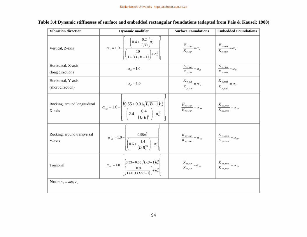
94

Table 3.4:Dynamic stiffnesses of surface and embedded rectangular foundations (adapted from Pais & Kausel; 1988)

Vibration direction Dynamic modifier Surface Foundations Embedded Foundations

Vertical, Z-axis

2

2

131

10

2.04.0

0.1

o

o

z

aBL

aBL

zsurz

surz

K

K

,

, z

embz

embz

K

K

,

,

Horizontal, X-axis

(long direction) 0.1x x

surx

surx

K

K

,

, x

embx

embx

K

K

,

,

Horizontal, Y-axis

(short direction) 0.1y

xsury

sury

K

K

,

, x

emby

emby

K

K

,

,

Rocking, around longitudinal

X-axis

2

3

2

4.04.2

101.055.00.1

o

o

xx

aBL

aBL

xxsurxx

surxx

K

K

,

, xx

embxx

embxx

K

K

,

,

Rocking, around transversal

Y-axis

2

3

2

4.16.0

55.00.1

o

oyy

aBL

a yy

suryy

suryy

K

K

,

, yy

embyy

embyy

K

K

,

,

Torsional

2

2

133.01

8.0

103.033.00.1

o

ozz

aBL

aBL

zzsurzz

surzz

K

K

,

, zz

embzz

embzz

K

K

,

,

Note: sVBa 0



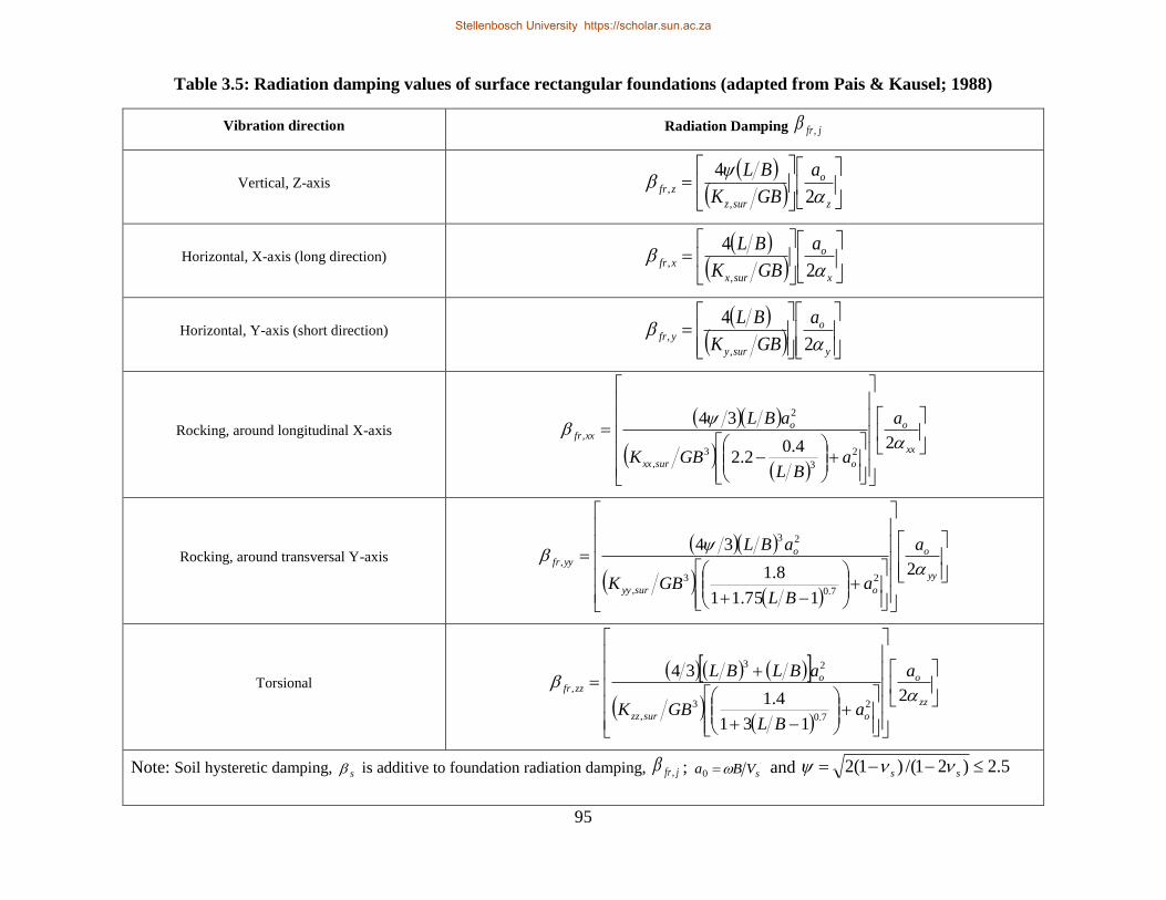
95

Table 3.5: Radiation damping values of surface rectangular foundations (adapted from Pais & Kausel; 1988)

Vibration direction Radiation Damping jfr ,

Vertical, Z-axis

z

o

surz

zfr

a

GBK

BL

2

4

,

,

Horizontal, X-axis (long direction)

x

o

surx

xfr

a

GBK

BL

2

4

,

,

Horizontal, Y-axis (short direction)

y

o

sury

yfr

a

GBK

BL

2

4

,

,

Rocking, around longitudinal X-axis

xx

o

osurxx

oxxfr

a

aBL

GBK

aBL

24.02.2

34

2

3

3

,

2

,

Rocking, around transversal Y-axis

yy

o

osuryy

oyyfr

a

aBL

GBK

aBL

2

175.11

8.1

34

2

7.0

3

,

23

,

Torsional

zz

o

osurzz

ozzfr

a

aBL

GBK

aBLBL

2

131

4.1

34

2

7.0

3

,

23

,

Note: Soil hysteretic damping, s is additive to foundation radiation damping, jfr , ; sVBa 0 and 5.2)21/()1(2 ss



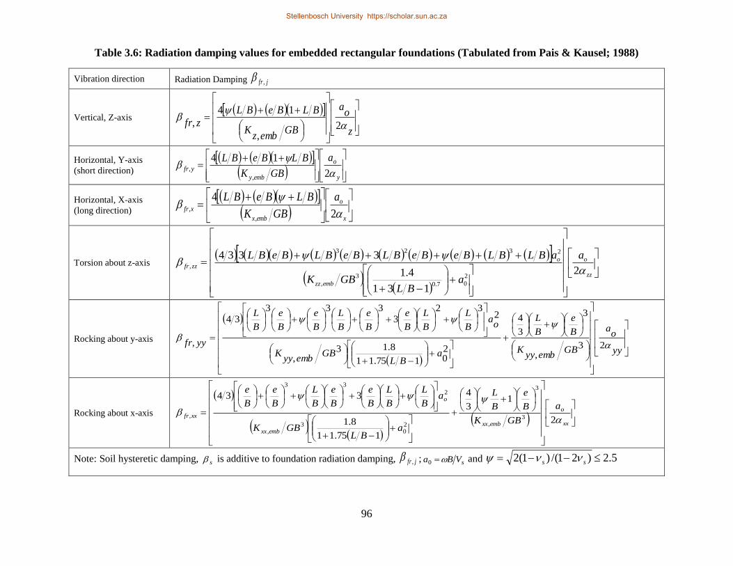
96

Table 3.6: Radiation damping values for embedded rectangular foundations (Tabulated from Pais & Kausel; 1988)

Vibration direction Radiation Damping jfr ,

Vertical, Z-axis

z

oa

GBembz

K

BLBeBL

zfr

2,

14

,

Horizontal, Y-axis

(short direction)

y

o

emby

yfr

a

GBK

BLBeBL

2

14

,

,

Horizontal, X-axis

(long direction)

x

o

embx

xfr

a

GBK

BLBeBL

2

4

,

,

Torsion about z-axis

zz

o

embzz

ozzfr

a

aBL

GBK

aBLBLBeBeBLBeBLBeBL

2

131

4.1

3334

2

07.0

3

,

2323

,

Rocking about y-axis

yy

oa

GBembyy

K

B

e

B

L

aBL

GBembyy

K

oa

B

L

B

L

B

e

B

e

B

L

B

e

B

e

B

L

yyfr

23

,

3

3

4

20175.11

8.13,

232

3333

34

,

Rocking about x-axis

xx

o

embxx

embxx

o

xxfr

a

GBK

B

e

B

L

aBL

GBK

aB

L

B

L

B

e

B

e

B

L

B

e

B

e

2

13

4

175.11

8.1

334

3,

3

20

3,

2

33

,

Note: Soil hysteretic damping, s is additive to foundation radiation damping, jfr , ; sVBa 0 and 5.2)21/()1(2 ss



97

Commentary: The Modified Veletsos method (MVM) was developed for the purpose

of incorporating the effects of SSI into the seismic design codes and standards using the

response spectrum approach. The equations represent the soil reactions for horizontal

translation and rocking only and do not represent vertical soil reactions. The latter are

required for estimating the updated fundamental frequency as well as the updated

damping ratio (see section 2.3.3).

Pais and Kausel's (1988) expressions of soil reactions are available for any degree of

freedom. Therefore, they are suitable either for response spectrum analysis or nonlinear

static or dynamic analysis. Thus, for the purpose of comparing the results of different

analysis methods the equations of Pais and Kausel (1988) are suitable.

(b) Integration of soil reactions into analysis process

In this section dynamic modelling using SSI is discussed. Response spectrum analysis

is dealt with in section 3.2.3(B).

i. SSI analysis model

With reference to PEER (2010), the recommended model for SSI analysis is shown in

Figure 3.4. It was first introduced by Stewart & Tileylioglu (2007) and later Naeim,

Tileylioglu, Alimoradi & Stewart (2008) proved that the model agrees with recorded

results from the field. It was developed for buildings with levels below the ground, but

it can be modified for meeting different levels of foundation embedment (NEHRP

Consultants Joint Venture, 2012). There is also the classical model of Veletsos and Wei

(1971) (see Figure 2.9) which is based on the principle of modifying the fixity of the

foundation base. Currently, this latter model is not used. One reason for this might be

the fact that it is limited to 2D analysis of surface foundations.


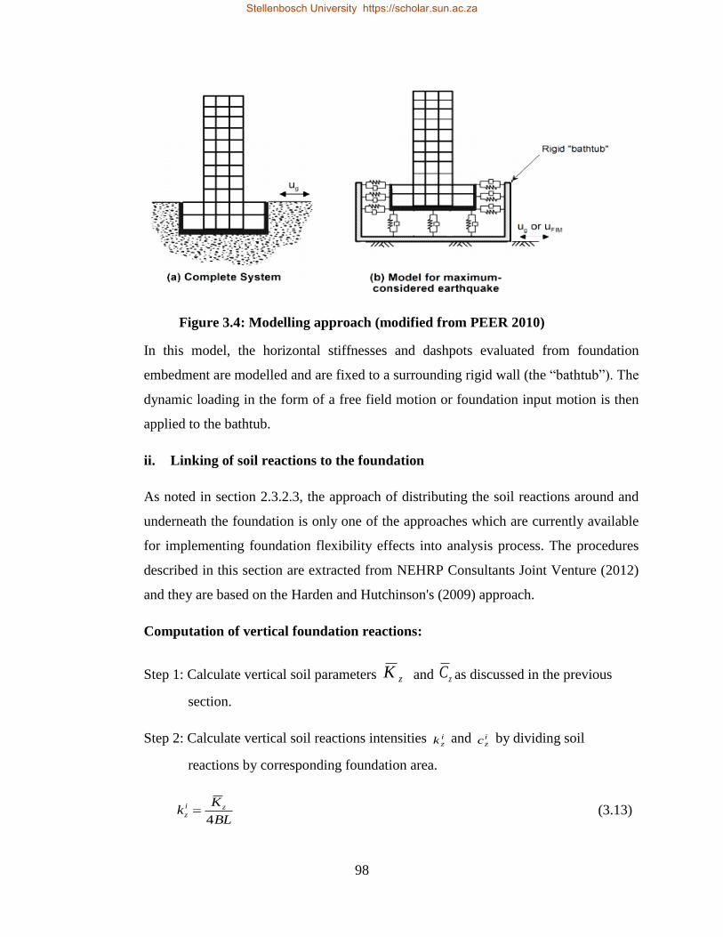
98

Figure 3.4: Modelling approach (modified from PEER 2010)

In this model, the horizontal stiffnesses and dashpots evaluated from foundation

embedment are modelled and are fixed to a surrounding rigid wall (the “bathtub”). The

dynamic loading in the form of a free field motion or foundation input motion is then

applied to the bathtub.

ii. Linking of soil reactions to the foundation

As noted in section 2.3.2.3, the approach of distributing the soil reactions around and

underneath the foundation is only one of the approaches which are currently available

for implementing foundation flexibility effects into analysis process. The procedures

described in this section are extracted from NEHRP Consultants Joint Venture (2012)

and they are based on the Harden and Hutchinson's (2009) approach.

Computation of vertical foundation reactions:

Step 1: Calculate vertical soil parameters zK and zC as discussed in the previous

section.

Step 2: Calculate vertical soil reactions intensities izk and i

zc by dividing soil

reactions by corresponding foundation area.

BL

Kk zi

z4

(3.13)


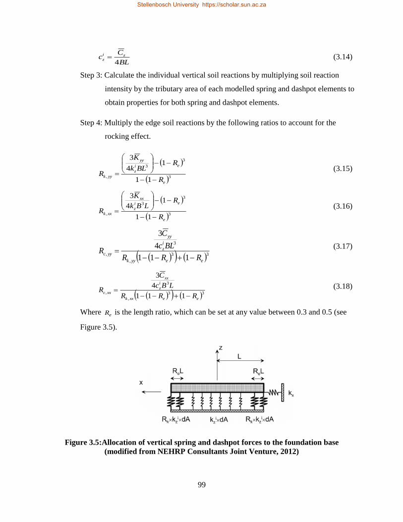
99

BL

Cc zi

z4

(3.14)

Step 3: Calculate the individual vertical soil reactions by multiplying soil reaction

intensity by the tributary area of each modelled spring and dashpot elements to

obtain properties for both spring and dashpot elements.

Step 4: Multiply the edge soil reactions by the following ratios to account for the

rocking effect.

3

3

3

,11

14

3

e

ei

z

yy

yykR

RBLk

K

R

(3.15)

3

3

3

,11

14

3

e

ei

z

xx

xxkR

RLBk

K

R

(3.16)

33

,

3

,111

4

3

eeyyk

i

z

yy

yycRRR

BLc

C

R

(3.17)

33

,

3

,111

4

3

eexxk

i

z

xx

xxcRRR

LBc

C

R

(3.18)

Where eR is the length ratio, which can be set at any value between 0.3 and 0.5 (see

Figure 3.5).

Figure 3.5:Allocation of vertical spring and dashpot forces to the foundation base

(modified from NEHRP Consultants Joint Venture, 2012)


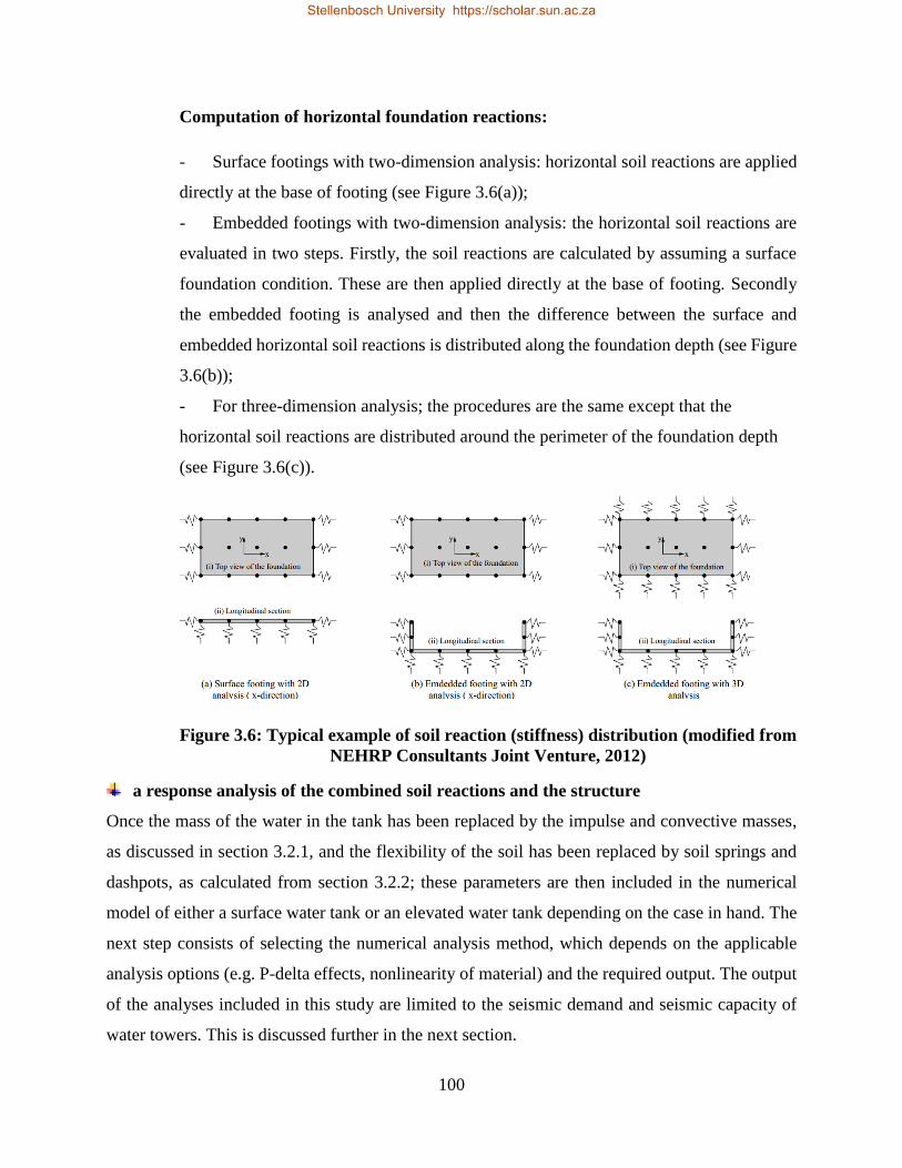
100

Computation of horizontal foundation reactions:

- Surface footings with two-dimension analysis: horizontal soil reactions are applied

directly at the base of footing (see Figure 3.6(a));

- Embedded footings with two-dimension analysis: the horizontal soil reactions are

evaluated in two steps. Firstly, the soil reactions are calculated by assuming a surface

foundation condition. These are then applied directly at the base of footing. Secondly

the embedded footing is analysed and then the difference between the surface and

embedded horizontal soil reactions is distributed along the foundation depth (see Figure

3.6(b));

- For three-dimension analysis; the procedures are the same except that the

horizontal soil reactions are distributed around the perimeter of the foundation depth

(see Figure 3.6(c)).

Figure 3.6: Typical example of soil reaction (stiffness) distribution (modified from

NEHRP Consultants Joint Venture, 2012)

a response analysis of the combined soil reactions and the structure

Once the mass of the water in the tank has been replaced by the impulse and convective masses,

as discussed in section 3.2.1, and the flexibility of the soil has been replaced by soil springs and

dashpots, as calculated from section 3.2.2; these parameters are then included in the numerical

model of either a surface water tank or an elevated water tank depending on the case in hand. The

next step consists of selecting the numerical analysis method, which depends on the applicable

analysis options (e.g. P-delta effects, nonlinearity of material) and the required output. The output

of the analyses included in this study are limited to the seismic demand and seismic capacity of

water towers. This is discussed further in the next section.


101

3.2.3 Estimation of the seismic demand of the structure

A. Nonlinear dynamic approach

After implementing the sloshing and soil structure interaction effects into the analysis process, as

discussed in sections 3.2.1 and 3.2.2, the seismic demand on the steel framed water tower is

estimated from a nonlinear dynamic analysis. This analysis approach requires numerical

integration of the governing dynamic equations of the structure at each time history point of the

input ground motion. The advantage of the nonlinear dynamic approach is that it takes excessive

lateral displacement resulting from SSI and the local yield and buckling of the frame elements into

account. This is highly likely to affect the overall stability of the steel frame even before it is

disturbed by seismic activity.

To estimate the maximum base shear force which can be induced by an earthquake on the structure,

a code design approach could also be used.

B. Code design approach

A review of seismic designs for water tanks with consideration of SSI was presented in

section 2.3.3.2. Most standards do not contain analysis procedures for elevated tanks. Since the

analysis recommendations of the European standard EN 1998-4 (EC8-4, 2006) do not contain

enough information on elevated water tanks, it was decided to use them in conjunction with the

guidelines of Sudhir and Jaiswal (2007). The EN 1998-4 (EC8-4, 2006) contains various

approaches to be used for the SSI analysis of water tanks; since Malhotra et al.'s (2000) approach

is among those approaches, is presented herein. It was also discussed briefly in section 3.2.1.

(1) Water tanks founded on soil

With reference to Malhotra et al. (2000), the maximum seismic base shear force V which can

be induced on the base of this type of water tank is given by

)(*)(*)( conecimpeemi TSmTSmmV (3.19)

where )( impe TS is the impulse spectral acceleration, )( cone TS is the convective spectral

acceleration and emm is the mass of the container (i.e. empty tank). Other parameters were


102

previously defined. The impulse and convective spectral accelerations are dependent on damping

and the natural period of the structure as well as the maximum ground acceleration and soil type

(refer to section 3.2.2.2 of EC8, 2004). The damping ratios for the impulse mass and convective

mass are 2% and 0.5%, respectively. The natural periods of the impulse and convective masses,

impT and conT , are obtained from equations 3.1 and 3.2.

(2) Elevated water tanks

The height of the water tank only influences the impulse mode and not the convective mode. With

reference to Sudhir and Jaiswal (2007), the impulse period impT for elevated water tanks is given

by

K

mmT si

imp

2 (3.20)

where mi is the impulse mass, ms is the mass of the container and one third of the mass of the steel

frame, and K is the lateral static stiffness of the steel frame. The total base shear force is obtained

from the same equation as equation 3.19, by replacing cm with sm .

The above analysis procedures for both ground supported and elevated water tanks, the effect of

SSI is not implemented in. In order to implement the SSI effect into the above procedures, the

impulse period impT should be modified, as stated in equation 2.23. For elevated water tanks, the

SSI effect can be alternatively included into the analysis process by modifying the lateral stiffness

K for the fixed base condition of the tower to the flexible base condition.

3.2.4 Estimation of the seismic capacity of the structure

Generally, the seismic capacity of the structure is estimated by a pushover analysis. With reference

to the summary of section 2.4.2.3, the modal pushover analysis was shown to be more accurate

than others. Therefore, it better to use the modal pushover approach for estimating the seismic

capacity of steel framed water towers. However, any other pushover method could be used,

depending on the accuracy required and the analysis tool used.


103

3.3 Design criteria of frame members

According to Haroun and Temraz (1992) the maximum axial stress ax in any frame element is

limited as follows:

103

180001

180002

MPa

rl gax (3.21)

The local buckling of frame members is limited as stated by equation 3.22. Here l defines the

length of the frame member and gr is its radius of gyration.

175gr

l (3.22)

3.4 Case study layout

The numerical method for the seismic assessment of a steel framed water tower, illustrated in the

above sections, was applied to the case study of this research, the Engen Winelands 1-Stop water

tower, in order to evaluate its seismic performance. This section describes in detail the structural

characteristics, site soil characteristics and site seismic characteristics used for the case study.

3.4.1 Structural characteristics

3.4.1.1 Description of the water tower

The system is composed of a steel tank container supported by a steel frame (see Figure 3.7). The

steel tank is a square tank made of square steel plates 1.22m in length and 3.0mm thick which are

connected to each other in order to achieve the total volume of the tank. The tank is 2.44m high

and 6.1m wide with a total capacity of 90,793 litres of water.


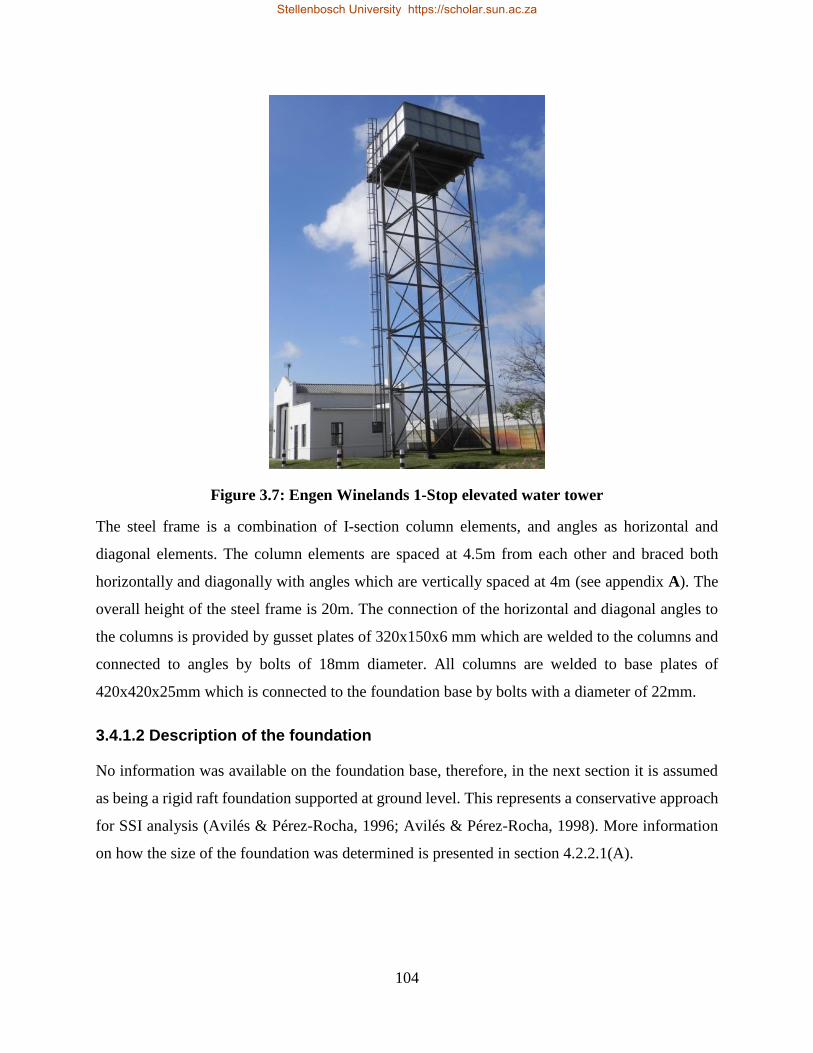
104

Figure 3.7: Engen Winelands 1-Stop elevated water tower

The steel frame is a combination of I-section column elements, and angles as horizontal and

diagonal elements. The column elements are spaced at 4.5m from each other and braced both

horizontally and diagonally with angles which are vertically spaced at 4m (see appendix A). The

overall height of the steel frame is 20m. The connection of the horizontal and diagonal angles to

the columns is provided by gusset plates of 320x150x6 mm which are welded to the columns and

connected to angles by bolts of 18mm diameter. All columns are welded to base plates of

420x420x25mm which is connected to the foundation base by bolts with a diameter of 22mm.

3.4.1.2 Description of the foundation

No information was available on the foundation base, therefore, in the next section it is assumed

as being a rigid raft foundation supported at ground level. This represents a conservative approach

for SSI analysis (Avilés & Pérez-Rocha, 1996; Avilés & Pérez-Rocha, 1998). More information

on how the size of the foundation was determined is presented in section 4.2.2.1(A).


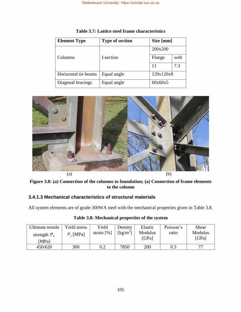
105

Table 3.7: Lattice steel frame characteristics

Element Type Type of section Size [mm]

Columns I-section

200x200

Flange web

11 7.3

Horizontal tie beams Equal angle 120x120x8

Diagonal bracings Equal angle 60x60x5

Figure 3.8: (a) Connection of the columns to foundation; (a) Connection of frame elements

to the column

3.4.1.3 Mechanical characteristics of structural materials

All system elements are of grade 300WA steel with the mechanical properties given in Table 3.8.

Table 3.8: Mechanical properties of the system

Ultimate tensile

strength u

[MPa]

Yield stress

y [MPa]

Yield

strain [%]

Density

[kg/m3]

Elastic

Modulus

[GPa]

Poisson’s

ratio

Shear

Modulus

[GPa]

450/620 300 0.2 7850 200 0.3 77

(a) (b)


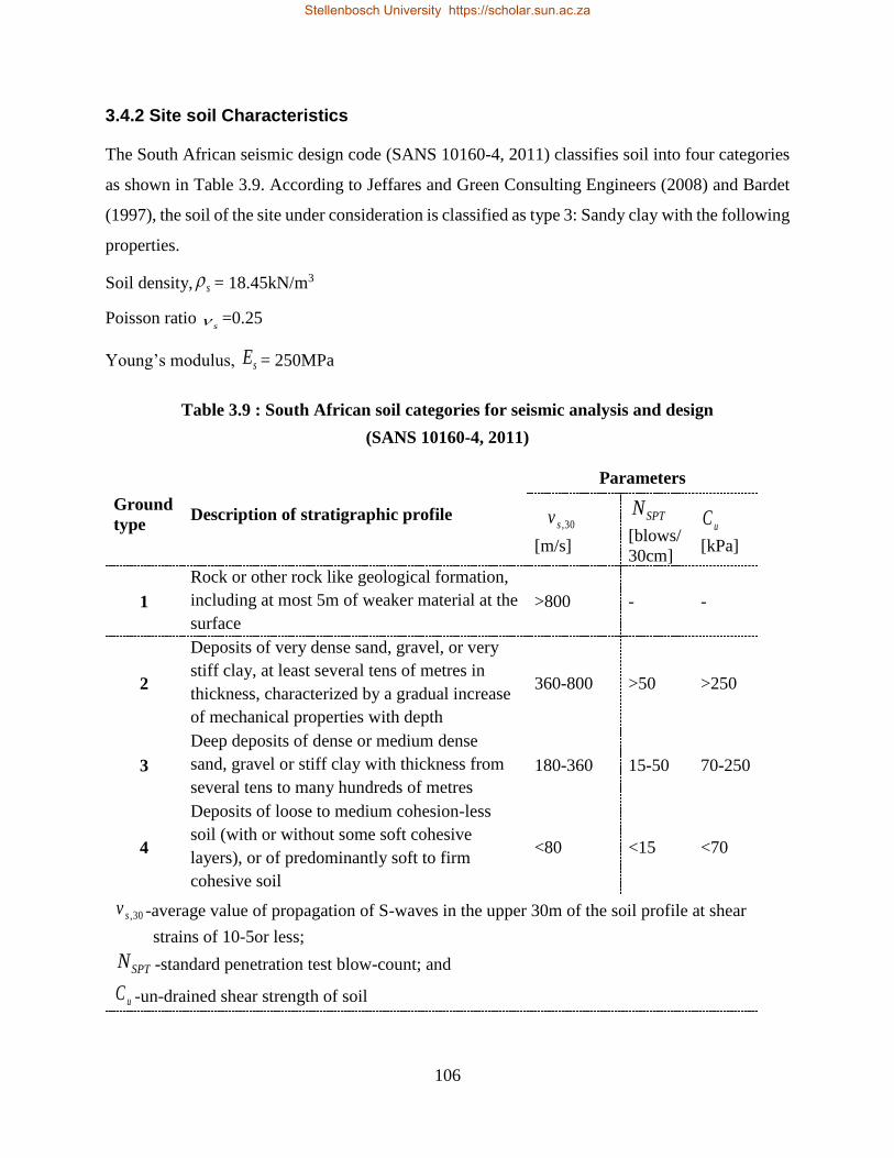
106

3.4.2 Site soil Characteristics

The South African seismic design code (SANS 10160-4, 2011) classifies soil into four categories

as shown in Table 3.9. According to Jeffares and Green Consulting Engineers (2008) and Bardet

(1997), the soil of the site under consideration is classified as type 3: Sandy clay with the following

properties.

Soil density, s = 18.45kN/m3

Poisson ratio s =0.25

Young’s modulus, sE = 250MPa

Table 3.9 : South African soil categories for seismic analysis and design

(SANS 10160-4, 2011)

Ground

type Description of stratigraphic profile

Parameters

30,sv

[m/s]

SPTN

[blows/

30cm]

uC

[kPa]

1

Rock or other rock like geological formation,

including at most 5m of weaker material at the

surface

>800 - -

2

Deposits of very dense sand, gravel, or very

stiff clay, at least several tens of metres in

thickness, characterized by a gradual increase

of mechanical properties with depth

360-800 >50 >250

3

Deep deposits of dense or medium dense

sand, gravel or stiff clay with thickness from

several tens to many hundreds of metres

180-360 15-50 70-250

4

Deposits of loose to medium cohesion-less

soil (with or without some soft cohesive

layers), or of predominantly soft to firm

cohesive soil

<80 <15 <70

30,sv -average value of propagation of S-waves in the upper 30m of the soil profile at shear

strains of 10-5or less;

SPTN -standard penetration test blow-count; and

uC -un-drained shear strength of soil


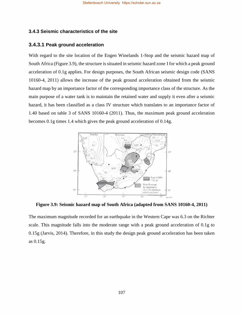
107

3.4.3 Seismic characteristics of the site

3.4.3.1 Peak ground acceleration

With regard to the site location of the Engen Winelands 1-Stop and the seismic hazard map of

South Africa (Figure 3.9), the structure is situated in seismic hazard zone I for which a peak ground

acceleration of 0.1g applies. For design purposes, the South African seismic design code (SANS

10160-4, 2011) allows the increase of the peak ground acceleration obtained from the seismic

hazard map by an importance factor of the corresponding importance class of the structure. As the

main purpose of a water tank is to maintain the retained water and supply it even after a seismic

hazard, it has been classified as a class IV structure which translates to an importance factor of

1.40 based on table 3 of SANS 10160-4 (2011). Thus, the maximum peak ground acceleration

becomes 0.1g times 1.4 which gives the peak ground acceleration of 0.14g.

Figure 3.9: Seismic hazard map of South Africa (adapted from SANS 10160-4, 2011)

The maximum magnitude recorded for an earthquake in the Western Cape was 6.3 on the Richter

scale. This magnitude falls into the moderate range with a peak ground acceleration of 0.1g to

0.15g (Jarvis, 2014). Therefore, in this study the design peak ground acceleration has been taken

as 0.15g.


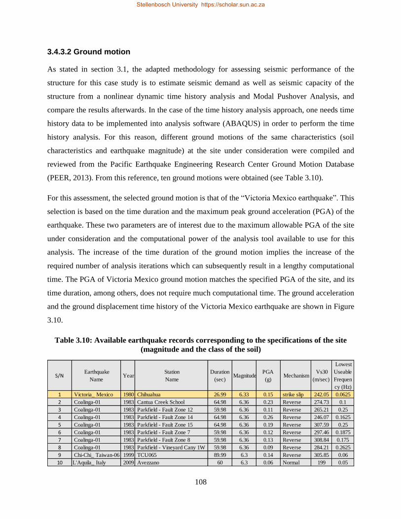
108

3.4.3.2 Ground motion

As stated in section 3.1, the adapted methodology for assessing seismic performance of the

structure for this case study is to estimate seismic demand as well as seismic capacity of the

structure from a nonlinear dynamic time history analysis and Modal Pushover Analysis, and

compare the results afterwards. In the case of the time history analysis approach, one needs time

history data to be implemented into analysis software (ABAQUS) in order to perform the time

history analysis. For this reason, different ground motions of the same characteristics (soil

characteristics and earthquake magnitude) at the site under consideration were compiled and

reviewed from the Pacific Earthquake Engineering Research Center Ground Motion Database

(PEER, 2013). From this reference, ten ground motions were obtained (see Table 3.10).

For this assessment, the selected ground motion is that of the “Victoria Mexico earthquake”. This

selection is based on the time duration and the maximum peak ground acceleration (PGA) of the

earthquake. These two parameters are of interest due to the maximum allowable PGA of the site

under consideration and the computational power of the analysis tool available to use for this

analysis. The increase of the time duration of the ground motion implies the increase of the

required number of analysis iterations which can subsequently result in a lengthy computational

time. The PGA of Victoria Mexico ground motion matches the specified PGA of the site, and its

time duration, among others, does not require much computational time. The ground acceleration

and the ground displacement time history of the Victoria Mexico earthquake are shown in Figure

3.10.

Table 3.10: Available earthquake records corresponding to the specifications of the site

(magnitude and the class of the soil)

S/N Earthquake

Name Year

Station

Name

Duration

(sec) Magnitude

PGA

(g) Mechanism

Vs30

(m/sec)

Lowest

Useable

Frequen

cy (Hz)

1 Victoria_ Mexico 1980 Chihuahua 26.99 6.33 0.15 strike slip 242.05 0.0625

2 Coalinga-01 1983 Cantua Creek School 64.98 6.36 0.23 Reverse 274.73 0.1

3 Coalinga-01 1983 Parkfield - Fault Zone 12 59.98 6.36 0.11 Reverse 265.21 0.25





8 Coalinga-01 1983 Parkfield - Vineyard Cany 1W 59.98 6.36 0.09 Reverse 284.21 0.2625

9 Chi-Chi_ Taiwan-06 1999 TCU065 89.99 6.3 0.14 Reverse 305.85 0.06

10 L'Aquila_ Italy 2009 Avezzano 60 6.3 0.06 Normal 199 0.05


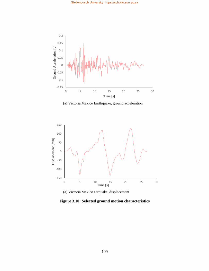
109

Figure 3.10: Selected ground motion characteristics

-0.15

-0.1

-0.05

0

0.05

0.1

0.15

0.2

0 5 10 15 20 25 30

Gro

und

Acc

eler

atio

n [

g]

Time [s]

(a) Victoria Mexico Earthquake, ground acceleration

-150

-100

-50

0

50

100

150

0 5 10 15 20 25 30

Dis

pla

cem

ent

[mm

]

Time [s]

(a) Victoria Mexico earquake, displacement


110

Chapter 4

Analysis and testing of the structure

This chapter contains two main sections i.e. the analysis and results of the test structure as well as

the analysis and results of the existing water tower. The test structure was a lattice steel frame with

the same characteristics as the existing water tower under investigation. It was built in the

laboratory for the main purpose of obtaining the damping ratio of the tower as well as validating

the numerical analysis model of the tower.

The test structure was subjected to the same seismic excitation in both laboratory and ABAQUS

finite element software. From a comparison of the two, the damping ratio was obtained. The

analysis model of the existing water tower was validated through the use of the damping coefficient

determined from the test structure inserted into the analysis software data.

After the analysis model was validated, the seismic behaviour of the water tower was assessed.

Two boundary conditions were considered i.e. whether the water tower was perfectly fixed at

ground level and whether it was flexibly supported at ground level. With respect to the boundary

conditions, the seismic assessment of the tower was divided into two parts. For the first part the

seismic behaviour of the tower with a fixed base condition was considered while for the second

part a flexible base condition was considered. In each part, the assessment was conducted by

estimating the seismic demand of the tower using the nonlinear dynamic approach, the code design

approach as presented in the previous chapter and estimating the seismic capacity of the tower

using the pushover approach. Later on, the seismic performance of the tower was found by

comparing the seismic demand to the seismic capacity. In addition, the global stability of the tower

was also checked.


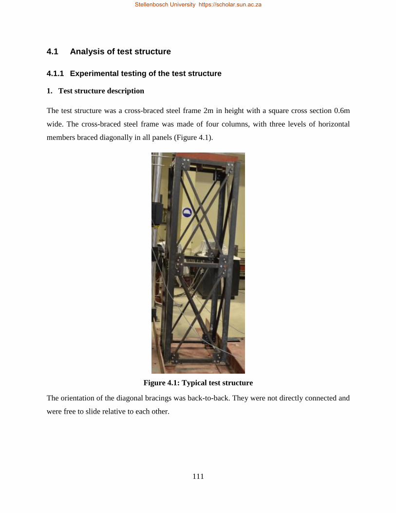
111

4.1 Analysis of test structure

4.1.1 Experimental testing of the test structure

1. Test structure description

The test structure was a cross-braced steel frame 2m in height with a square cross section 0.6m

wide. The cross-braced steel frame was made of four columns, with three levels of horizontal

members braced diagonally in all panels (Figure 4.1).

Figure 4.1: Typical test structure

The orientation of the diagonal bracings was back-to-back. They were not directly connected and

were free to slide relative to each other.


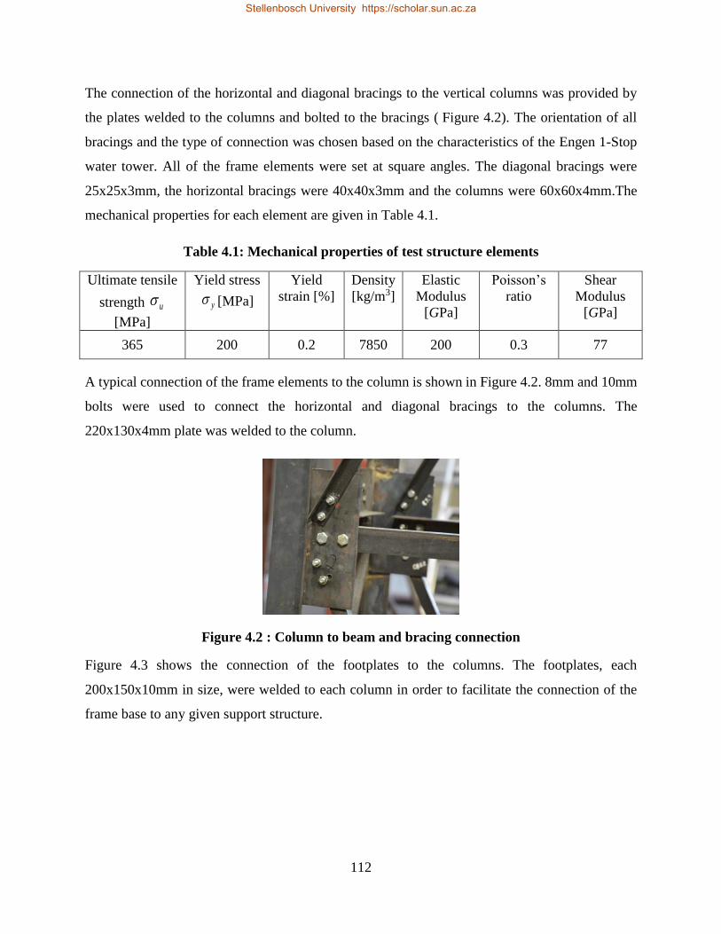
112

The connection of the horizontal and diagonal bracings to the vertical columns was provided by

the plates welded to the columns and bolted to the bracings ( Figure 4.2). The orientation of all

bracings and the type of connection was chosen based on the characteristics of the Engen 1-Stop

water tower. All of the frame elements were set at square angles. The diagonal bracings were

25x25x3mm, the horizontal bracings were 40x40x3mm and the columns were 60x60x4mm.The

mechanical properties for each element are given in Table 4.1.

Table 4.1: Mechanical properties of test structure elements

Ultimate tensile

strength u

[MPa]

Yield stress

y [MPa]

Yield

strain [%]

Density

[kg/m3]

Elastic

Modulus

[GPa]

Poisson’s

ratio

Shear

Modulus

[GPa]

365 200 0.2 7850 200 0.3 77

A typical connection of the frame elements to the column is shown in Figure 4.2. 8mm and 10mm

bolts were used to connect the horizontal and diagonal bracings to the columns. The

220x130x4mm plate was welded to the column.

Figure 4.2 : Column to beam and bracing connection

Figure 4.3 shows the connection of the footplates to the columns. The footplates, each

200x150x10mm in size, were welded to each column in order to facilitate the connection of the

frame base to any given support structure.


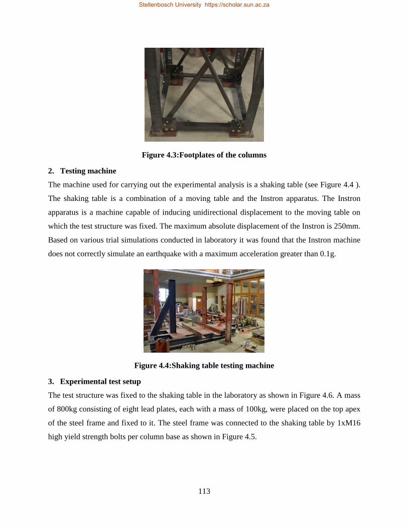
113

Figure 4.3:Footplates of the columns

2. Testing machine

The machine used for carrying out the experimental analysis is a shaking table (see Figure 4.4 ).

The shaking table is a combination of a moving table and the Instron apparatus. The Instron

apparatus is a machine capable of inducing unidirectional displacement to the moving table on

which the test structure was fixed. The maximum absolute displacement of the Instron is 250mm.

Based on various trial simulations conducted in laboratory it was found that the Instron machine

does not correctly simulate an earthquake with a maximum acceleration greater than 0.1g.

Figure 4.4:Shaking table testing machine

3. Experimental test setup

The test structure was fixed to the shaking table in the laboratory as shown in Figure 4.6. A mass

of 800kg consisting of eight lead plates, each with a mass of 100kg, were placed on the top apex

of the steel frame and fixed to it. The steel frame was connected to the shaking table by 1xM16

high yield strength bolts per column base as shown in Figure 4.5.


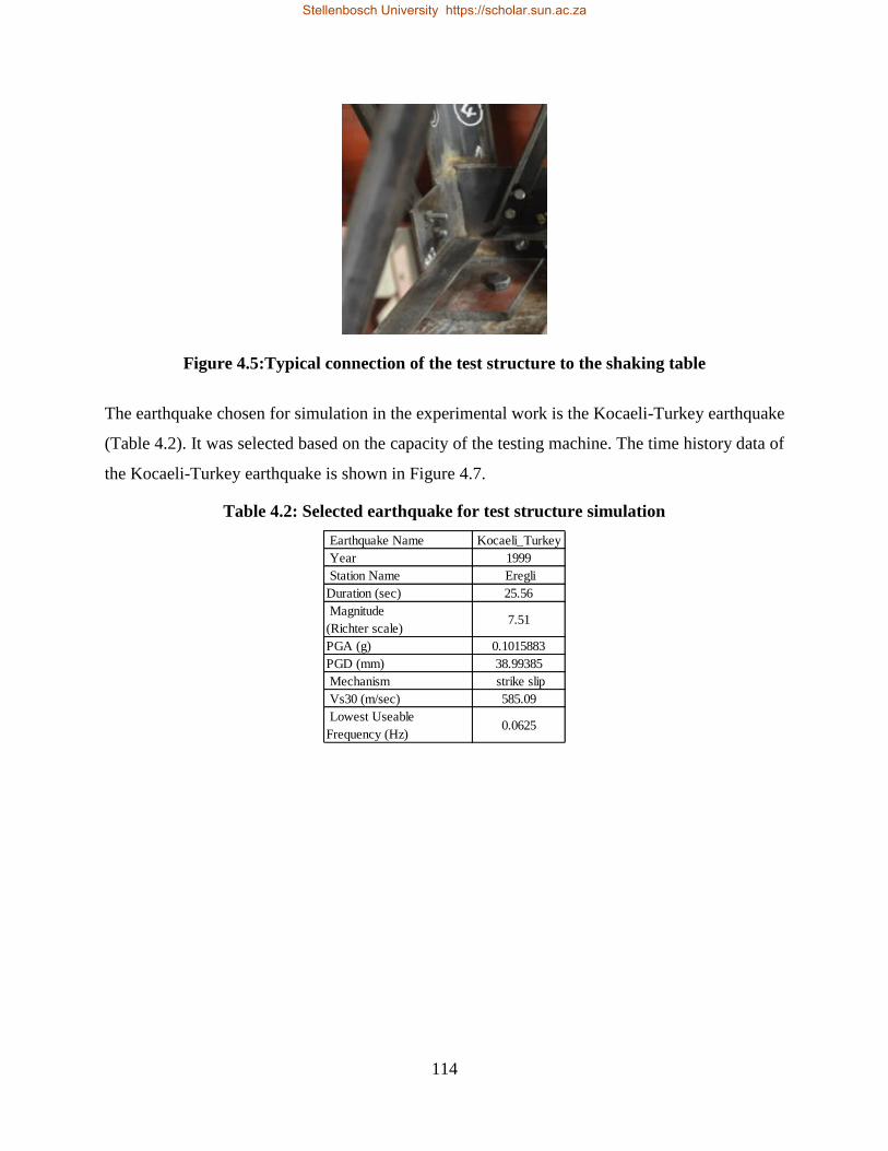
114

Figure 4.5:Typical connection of the test structure to the shaking table

The earthquake chosen for simulation in the experimental work is the Kocaeli-Turkey earthquake

(Table 4.2). It was selected based on the capacity of the testing machine. The time history data of

the Kocaeli-Turkey earthquake is shown in Figure 4.7.

Table 4.2: Selected earthquake for test structure simulation

Earthquake Name Kocaeli_Turkey

Year 1999

Station Name Eregli

Duration (sec) 25.56

Magnitude

(Richter scale)7.51

PGA (g) 0.1015883

PGD (mm) 38.99385

Mechanism strike slip

Vs30 (m/sec) 585.09

Lowest Useable

Frequency (Hz)0.0625


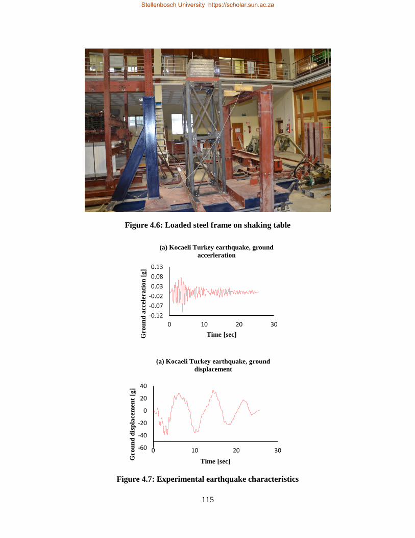
115

Figure 4.6: Loaded steel frame on shaking table

Figure 4.7: Experimental earthquake characteristics

-0.12

-0.07

-0.02

0.03

0.08

0.13

0 10 20 30

Gro

un

d a

ccel

era

tio

n [

g]

Time [sec]

(a) Kocaeli Turkey earthquake, ground

accerleration

-60

-40

-20

0

20

40

0 10 20 30

Gro

un

d d

isp

lace

men

t [g

]

Time [sec]

(a) Kocaeli Turkey earthquake, ground

displacement


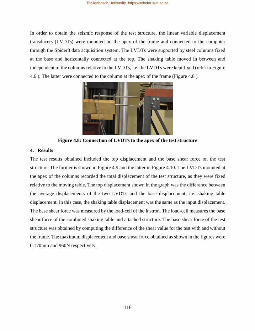
116

In order to obtain the seismic response of the test structure, the linear variable displacement

transducers (LVDTs) were mounted on the apex of the frame and connected to the computer

through the Spider8 data acquisition system. The LVDTs were supported by steel columns fixed

at the base and horizontally connected at the top. The shaking table moved in between and

independent of the columns relative to the LVDTs, i.e. the LVDTs were kept fixed (refer to Figure

4.6 ). The latter were connected to the column at the apex of the frame (Figure 4.8 ).

Figure 4.8: Connection of LVDTs to the apex of the test structure

4. Results

The test results obtained included the top displacement and the base shear force on the test

structure. The former is shown in Figure 4.9 and the latter in Figure 4.10. The LVDTs mounted at

the apex of the columns recorded the total displacement of the test structure, as they were fixed

relative to the moving table. The top displacement shown in the graph was the difference between

the average displacements of the two LVDTs and the base displacement, i.e. shaking table

displacement. In this case, the shaking table displacement was the same as the input displacement.

The base shear force was measured by the load-cell of the Instron. The load-cell measures the base

shear force of the combined shaking table and attached structure. The base shear force of the test

structure was obtained by computing the difference of the shear value for the test with and without

the frame. The maximum displacement and base shear force obtained as shown in the figures were

0.170mm and 960N respectively.


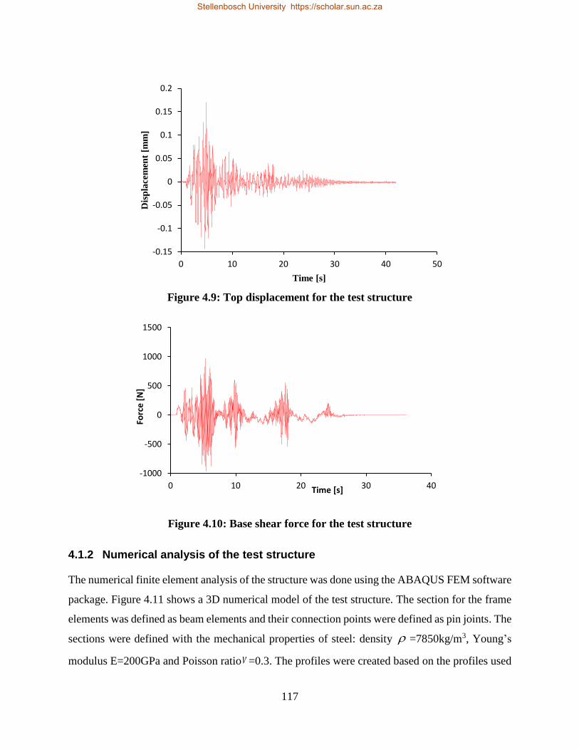
117

Figure 4.9: Top displacement for the test structure

Figure 4.10: Base shear force for the test structure

4.1.2 Numerical analysis of the test structure

The numerical finite element analysis of the structure was done using the ABAQUS FEM software

package. Figure 4.11 shows a 3D numerical model of the test structure. The section for the frame

elements was defined as beam elements and their connection points were defined as pin joints. The

sections were defined with the mechanical properties of steel: density =7850kg/m3, Young’s

modulus E=200GPa and Poisson ratio =0.3. The profiles were created based on the profiles used

-0.15

-0.1

-0.05

0

0.05

0.1

0.15

0.2

0 10 20 30 40 50

Dis

pla

cem

ent

[mm

]

Time [s]

-1000

-500

0

500

1000

1500

0 10 20 30 40

Forc

e [

N]

Time [s]


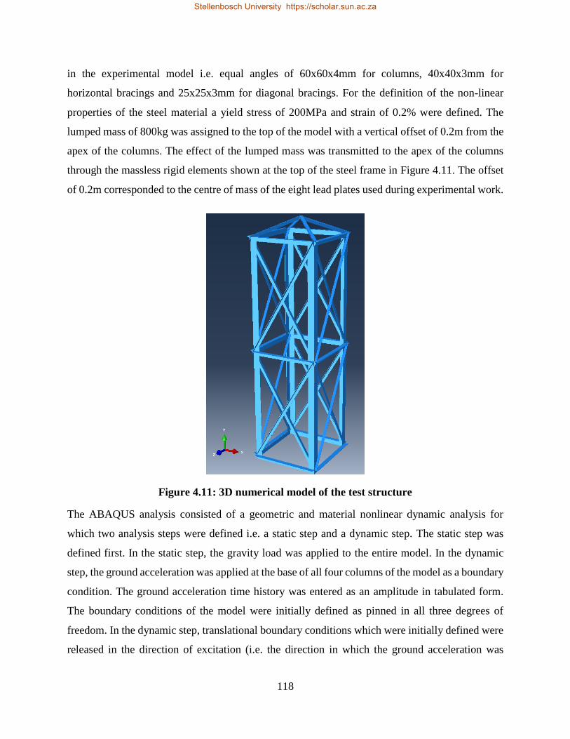
118

in the experimental model i.e. equal angles of 60x60x4mm for columns, 40x40x3mm for

horizontal bracings and 25x25x3mm for diagonal bracings. For the definition of the non-linear

properties of the steel material a yield stress of 200MPa and strain of 0.2% were defined. The

lumped mass of 800kg was assigned to the top of the model with a vertical offset of 0.2m from the

apex of the columns. The effect of the lumped mass was transmitted to the apex of the columns

through the massless rigid elements shown at the top of the steel frame in Figure 4.11. The offset

of 0.2m corresponded to the centre of mass of the eight lead plates used during experimental work.

Figure 4.11: 3D numerical model of the test structure

The ABAQUS analysis consisted of a geometric and material nonlinear dynamic analysis for

which two analysis steps were defined i.e. a static step and a dynamic step. The static step was

defined first. In the static step, the gravity load was applied to the entire model. In the dynamic

step, the ground acceleration was applied at the base of all four columns of the model as a boundary

condition. The ground acceleration time history was entered as an amplitude in tabulated form.

The boundary conditions of the model were initially defined as pinned in all three degrees of

freedom. In the dynamic step, translational boundary conditions which were initially defined were

released in the direction of excitation (i.e. the direction in which the ground acceleration was


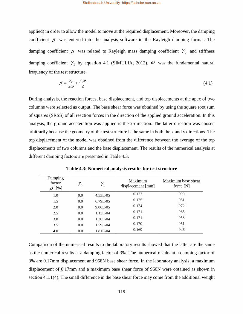
119

applied) in order to allow the model to move at the required displacement. Moreover, the damping

coefficient was entered into the analysis software in the Rayleigh damping format. The

damping coefficient was related to Rayleigh mass damping coefficient o and stiffness

damping coefficient 1 by equation 4.1 (SIMULIA, 2012). was the fundamental natural

frequency of the test structure.

22

1

o (4.1)

During analysis, the reaction forces, base displacement, and top displacements at the apex of two

columns were selected as output. The base shear force was obtained by using the square root sum

of squares (SRSS) of all reaction forces in the direction of the applied ground acceleration. In this

analysis, the ground acceleration was applied is the x-direction. The latter direction was chosen

arbitrarily because the geometry of the test structure is the same in both the x and y directions. The

top displacement of the model was obtained from the difference between the average of the top

displacements of two columns and the base displacement. The results of the numerical analysis at

different damping factors are presented in Table 4.3.

Table 4.3: Numerical analysis results for test structure

Damping

factor

[%] o 1

Maximum

displacement [mm]

Maximum base shear

force [N]

1.0 0.0 4.53E-05 0.177 990

1.5 0.0 6.79E-05 0.175 981

2.0 0.0 9.06E-05 0.174 972

2.5 0.0 1.13E-04 0.171 965

3.0 0.0 1.36E-04 0.171 958

3.5 0.0 1.59E-04 0.170 951

4.0 0.0 1.81E-04 0.169 946

Comparison of the numerical results to the laboratory results showed that the latter are the same

as the numerical results at a damping factor of 3%. The numerical results at a damping factor of

3% are 0.17mm displacement and 958N base shear force. In the laboratory analysis, a maximum

displacement of 0.17mm and a maximum base shear force of 960N were obtained as shown in

section 4.1.1(4). The small difference in the base shear force may come from the additional weight


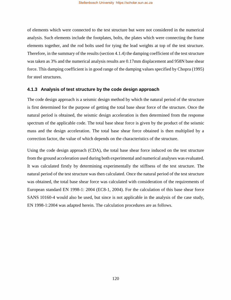
120

of elements which were connected to the test structure but were not considered in the numerical

analysis. Such elements include the footplates, bolts, the plates which were connecting the frame

elements together, and the rod bolts used for tying the lead weights at top of the test structure.

Therefore, in the summary of the results (section 4.1.4) the damping coefficient of the test structure

was taken as 3% and the numerical analysis results are 0.17mm displacement and 958N base shear

force. This damping coefficient is in good range of the damping values specified by Chopra (1995)

for steel structures.

4.1.3 Analysis of test structure by the code design approach

The code design approach is a seismic design method by which the natural period of the structure

is first determined for the purpose of getting the total base shear force of the structure. Once the

natural period is obtained, the seismic design acceleration is then determined from the response

spectrum of the applicable code. The total base shear force is given by the product of the seismic

mass and the design acceleration. The total base shear force obtained is then multiplied by a

correction factor, the value of which depends on the characteristics of the structure.

Using the code design approach (CDA), the total base shear force induced on the test structure

from the ground acceleration used during both experimental and numerical analyses was evaluated.

It was calculated firstly by determining experimentally the stiffness of the test structure. The

natural period of the test structure was then calculated. Once the natural period of the test structure

was obtained, the total base shear force was calculated with consideration of the requirements of

European standard EN 1998-1: 2004 (EC8-1, 2004). For the calculation of this base shear force

SANS 10160-4 would also be used, but since is not applicable in the analysis of the case study,

EN 1998-1:2004 was adapted herein. The calculation procedures are as follows.


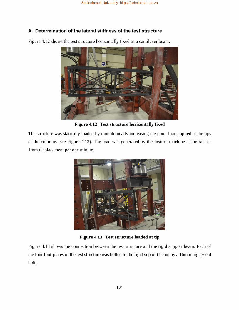
121

A. Determination of the lateral stiffness of the test structure

Figure 4.12 shows the test structure horizontally fixed as a cantilever beam.

Figure 4.12: Test structure horizontally fixed

The structure was statically loaded by monotonically increasing the point load applied at the tips

of the columns (see Figure 4.13). The load was generated by the Instron machine at the rate of

1mm displacement per one minute.

Figure 4.13: Test structure loaded at tip

Figure 4.14 shows the connection between the test structure and the rigid support beam. Each of

the four foot-plates of the test structure was bolted to the rigid support beam by a 16mm high yield

bolt.


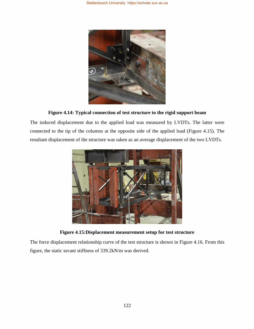
122

Figure 4.14: Typical connection of test structure to the rigid support beam

The induced displacement due to the applied load was measured by LVDTs. The latter were

connected to the tip of the columns at the opposite side of the applied load (Figure 4.15). The

resultant displacement of the structure was taken as an average displacement of the two LVDTs.

Figure 4.15:Displacement measurement setup for test structure

The force displacement relationship curve of the test structure is shown in Figure 4.16. From this

figure, the static secant stiffness of 339.2kN/m was derived.


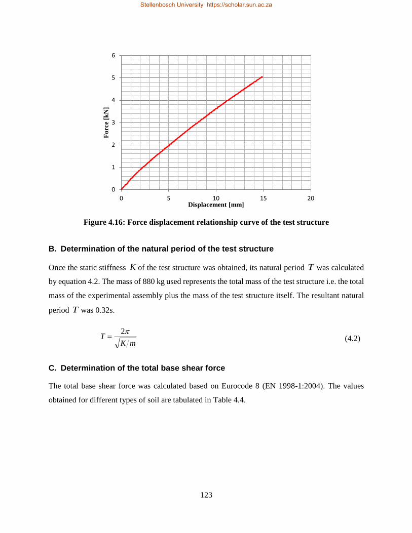
123

Figure 4.16: Force displacement relationship curve of the test structure

B. Determination of the natural period of the test structure

Once the static stiffness K of the test structure was obtained, its natural period T was calculated

by equation 4.2. The mass of 880 kg used represents the total mass of the test structure i.e. the total

mass of the experimental assembly plus the mass of the test structure itself. The resultant natural

period T was 0.32s.

mK

T2

(4.2)

C. Determination of the total base shear force

The total base shear force was calculated based on Eurocode 8 (EN 1998-1:2004). The values

obtained for different types of soil are tabulated in Table 4.4.

0

1

2

3

4

5

6

0 5 10 15 20

Fo

rce

[kN

]

Displacement [mm]


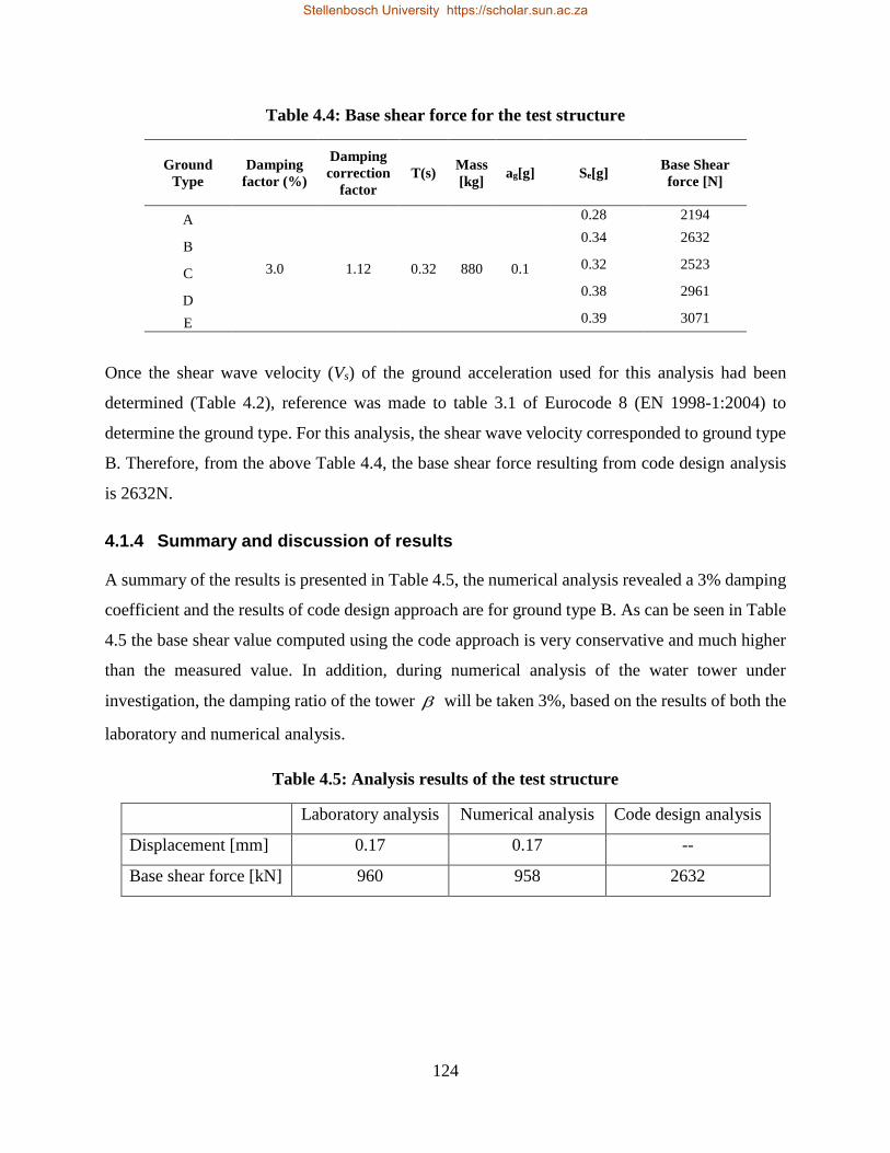
124

Table 4.4: Base shear force for the test structure

Ground

Type

Damping

factor (%)

Damping

correction

factor

T(s) Mass

[kg] ag[g] Se[g]

Base Shear

force [N]

A

3.0 1.12 0.32 880 0.1

0.28 2194

B 0.34 2632

C 0.32 2523

D 0.38 2961

E 0.39 3071

Once the shear wave velocity (Vs) of the ground acceleration used for this analysis had been

determined (Table 4.2), reference was made to table 3.1 of Eurocode 8 (EN 1998-1:2004) to

determine the ground type. For this analysis, the shear wave velocity corresponded to ground type

B. Therefore, from the above Table 4.4, the base shear force resulting from code design analysis

is 2632N.

4.1.4 Summary and discussion of results

A summary of the results is presented in Table 4.5, the numerical analysis revealed a 3% damping

coefficient and the results of code design approach are for ground type B. As can be seen in Table

4.5 the base shear value computed using the code approach is very conservative and much higher

than the measured value. In addition, during numerical analysis of the water tower under

investigation, the damping ratio of the tower will be taken 3%, based on the results of both the

laboratory and numerical analysis.

Table 4.5: Analysis results of the test structure

Laboratory analysis Numerical analysis Code design analysis

Displacement [mm] 0.17 0.17 --

Base shear force [kN] 960 958 2632


125

4.2 Seismic assessment of the water tower

As addressed in section 3.1, the seismic assessment of the Engen Winelands 1-Stop water tower

was done firstly by considering the foundation of the tower as a rigid foundation supported on the

undeformable soil medium. This was referred to as the fixed base condition. Later on, the fixity of

the base foundation was modified in order to incorporate the flexibility of the underlying soil to

apply SSI analysis. This was referred to as the flexible base condition. Moreover, with reference

to appendix A, the geometry of the columns supporting the water tower implies that the tower is

better able to resist force from the x-direction than the y-direction. Because the columns are I-

shaped, the column is sturdier when force is applied in the direction running from the top of the

“I” to the bottom, rather than across the “I”. The direction running across the “I” will be referred

to as the weak direction of the water tower. Therefore, this study assessed the tower in its weak

direction with respect to the geometry of the columns. Thus, the next section contains the

assessment steps as well as the assessment results for both the fixed and the flexible base

conditions.

4.2.1 Investigation of the behaviour of the tower for the fixed base condition

4.2.1.1 Development of the analysis model

1. Dynamic characteristics of the water tank

Various methods of dynamic modelling of water tanks have been discussed in section 2.2. They

vary in terms of the mechanical characteristics of the tank. The water tank of the tower under

investigation is made of a combination of steel plates, which allows it to be classified as a flexible

container. The method used for this model was for a flexible container as has been discussed in

section 3.2.1. Based on sections 3.2.1and 3.4.1.1, the dynamic characteristics of the water

container were evaluated and are given in Table 4.6. As was mentioned in section 3.2.1, the values

shown in the latter table are computed based on an equivalent circular tank of 2.3m in height and

7.1m in diameter.


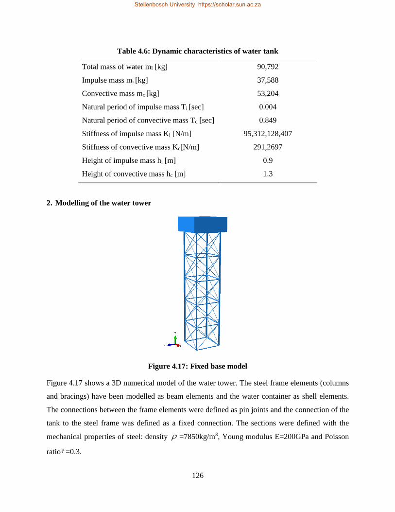
126

Table 4.6: Dynamic characteristics of water tank

Total mass of water ml [kg] 90,792

Impulse mass mi [kg] 37,588

Convective mass mc [kg] 53,204

Natural period of impulse mass Ti [sec] 0.004

Natural period of convective mass Tc [sec] 0.849

Stiffness of impulse mass Ki [N/m] 95,312,128,407

Stiffness of convective mass Kc[N/m] 291,2697

Height of impulse mass hi [m] 0.9

Height of convective mass hc [m] 1.3

2. Modelling of the water tower

Figure 4.17: Fixed base model

Figure 4.17 shows a 3D numerical model of the water tower. The steel frame elements (columns

and bracings) have been modelled as beam elements and the water container as shell elements.

The connections between the frame elements were defined as pin joints and the connection of the

tank to the steel frame was defined as a fixed connection. The sections were defined with the

mechanical properties of steel: density =7850kg/m3, Young modulus E=200GPa and Poisson

ratio =0.3.


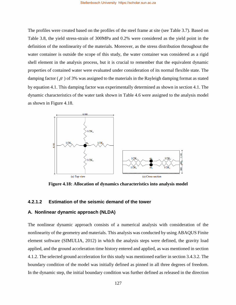
127

The profiles were created based on the profiles of the steel frame at site (see Table 3.7). Based on

Table 3.8, the yield stress-strain of 300MPa and 0.2% were considered as the yield point in the

definition of the nonlinearity of the materials. Moreover, as the stress distribution throughout the

water container is outside the scope of this study, the water container was considered as a rigid

shell element in the analysis process, but it is crucial to remember that the equivalent dynamic

properties of contained water were evaluated under consideration of its normal flexible state. The

damping factor ( ) of 3% was assigned to the materials in the Rayleigh damping format as stated

by equation 4.1. This damping factor was experimentally determined as shown in section 4.1. The

dynamic characteristics of the water tank shown in Table 4.6 were assigned to the analysis model

as shown in Figure 4.18.

Figure 4.18: Allocation of dynamics characteristics into analysis model

4.2.1.2 Estimation of the seismic demand of the tower

A. Nonlinear dynamic approach (NLDA)

The nonlinear dynamic approach consists of a numerical analysis with consideration of the

nonlinearity of the geometry and materials. This analysis was conducted by using ABAQUS Finite

element software (SIMULIA, 2012) in which the analysis steps were defined, the gravity load

applied, and the ground acceleration time history entered and applied, as was mentioned in section

4.1.2. The selected ground acceleration for this study was mentioned earlier in section 3.4.3.2. The

boundary condition of the model was initially defined as pinned in all three degrees of freedom.

In the dynamic step, the initial boundary condition was further defined as released in the direction


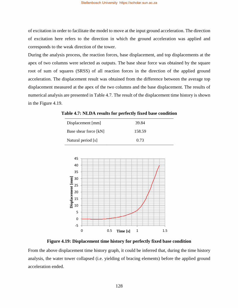
128

of excitation in order to facilitate the model to move at the input ground acceleration. The direction

of excitation here refers to the direction in which the ground acceleration was applied and

corresponds to the weak direction of the tower.

During the analysis process, the reaction forces, base displacement, and top displacements at the

apex of two columns were selected as outputs. The base shear force was obtained by the square

root of sum of squares (SRSS) of all reaction forces in the direction of the applied ground

acceleration. The displacement result was obtained from the difference between the average top

displacement measured at the apex of the two columns and the base displacement. The results of

numerical analysis are presented in Table 4.7. The result of the displacement time history is shown

in the Figure 4.19.

Table 4.7: NLDA results for perfectly fixed base condition

Displacement [mm] 39.84

Base shear force [kN] 158.59

Natural period [s] 0.73

Figure 4.19: Displacement time history for perfectly fixed base condition

From the above displacement time history graph, it could be inferred that, during the time history

analysis, the water tower collapsed (i.e. yielding of bracing elements) before the applied ground

acceleration ended.

-5

0

5

10

15

20

25

30

35

40

45

0 0.5 1 1.5

Dis

pla

cem

ent

[mm

]

Time [s]


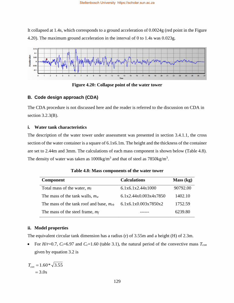
129

It collapsed at 1.4s, which corresponds to a ground acceleration of 0.0024g (red point in the Figure

4.20). The maximum ground acceleration in the interval of 0 to 1.4s was 0.023g.

Figure 4.20: Collapse point of the water tower

B. Code design approach (CDA)

The CDA procedure is not discussed here and the reader is referred to the discussion on CDA in

section 3.2.3(B).

i. Water tank characteristics

The description of the water tower under assessment was presented in section 3.4.1.1, the cross

section of the water container is a square of 6.1x6.1m. The height and the thickness of the container

are set to 2.44m and 3mm. The calculations of each mass component is shown below (Table 4.8).

The density of water was taken as 1000kg/m3 and that of steel as 7850kg/m3.

Table 4.8: Mass components of the water tower

Component Calculations Mass (kg)

Total mass of the water, ml 6.1x6.1x2.44x1000 90792.00

The mass of the tank walls, mw 6.1x2.44x0.003x4x7850 1402.10

The mass of the tank roof and base, mrb 6.1x6.1x0.003x7850x2 1752.59

The mass of the steel frame, mf ------ 6239.80

ii. Model properties

The equivalent circular tank dimension has a radius (r) of 3.55m and a height (H) of 2.3m.

For H/r=0.7, Ci=6.97 and Cc=1.60 (table 3.1), the natural period of the convective mass Tcon

given by equation 3.2 is

3.0s

55.3*60.1

conT


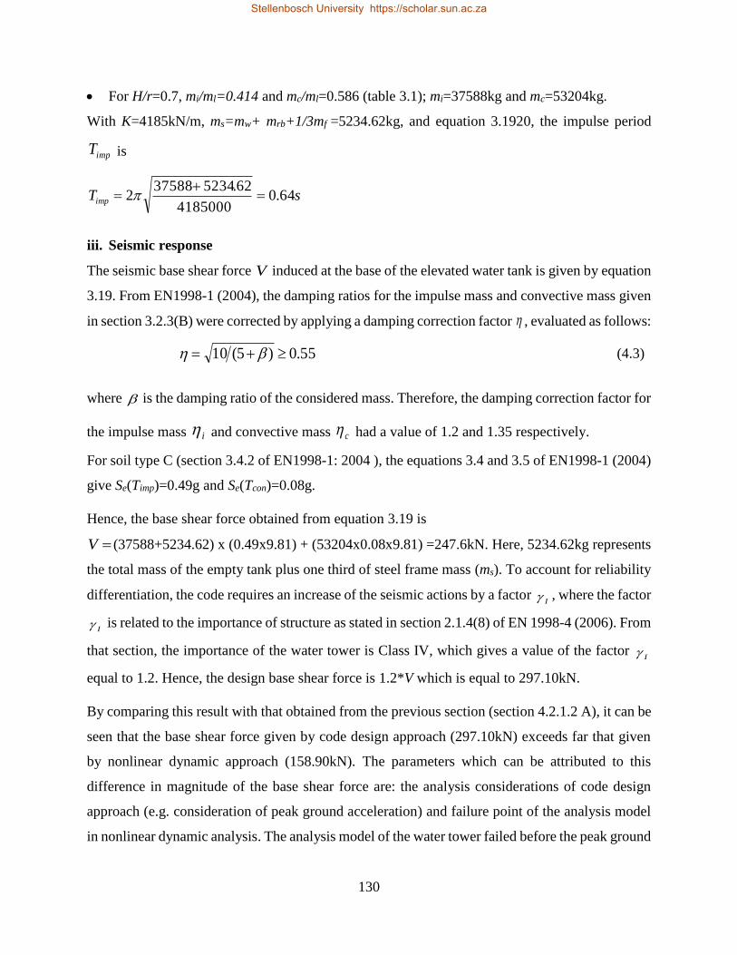
130

For H/r=0.7, mi/ml=0.414 and mc/ml=0.586 (table 3.1); mi=37588kg and mc=53204kg.

With K=4185kN/m, ms=mw+ mrb+1/3mf =5234.62kg, and equation 3.1920, the impulse period

impT is

sTimp 64.04185000

62.5234375882

iii. Seismic response

The seismic base shear force V induced at the base of the elevated water tank is given by equation

3.19. From EN1998-1 (2004), the damping ratios for the impulse mass and convective mass given

in section 3.2.3(B) were corrected by applying a damping correction factor , evaluated as follows:

55.0)5(10 (4.3)

where is the damping ratio of the considered mass. Therefore, the damping correction factor for

the impulse mass i and convective mass c had a value of 1.2 and 1.35 respectively.

For soil type C (section 3.4.2 of EN1998-1: 2004 ), the equations 3.4 and 3.5 of EN1998-1 (2004)

give Se(Timp)=0.49g and Se(Tcon)=0.08g.

Hence, the base shear force obtained from equation 3.19 is

V (37588+5234.62) x (0.49x9.81) + (53204x0.08x9.81) =247.6kN. Here, 5234.62kg represents

the total mass of the empty tank plus one third of steel frame mass (ms). To account for reliability

differentiation, the code requires an increase of the seismic actions by a factor I , where the factor

I is related to the importance of structure as stated in section 2.1.4(8) of EN 1998-4 (2006). From

that section, the importance of the water tower is Class IV, which gives a value of the factor I

equal to 1.2. Hence, the design base shear force is 1.2*V which is equal to 297.10kN.

By comparing this result with that obtained from the previous section (section 4.2.1.2 A), it can be

seen that the base shear force given by code design approach (297.10kN) exceeds far that given

by nonlinear dynamic approach (158.90kN). The parameters which can be attributed to this

difference in magnitude of the base shear force are: the analysis considerations of code design

approach (e.g. consideration of peak ground acceleration) and failure point of the analysis model

in nonlinear dynamic analysis. The analysis model of the water tower failed before the peak ground


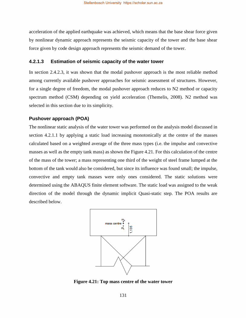
131

acceleration of the applied earthquake was achieved, which means that the base shear force given

by nonlinear dynamic approach represents the seismic capacity of the tower and the base shear

force given by code design approach represents the seismic demand of the tower.

4.2.1.3 Estimation of seismic capacity of the water tower

In section 2.4.2.3, it was shown that the modal pushover approach is the most reliable method

among currently available pushover approaches for seismic assessment of structures. However,

for a single degree of freedom, the modal pushover approach reduces to N2 method or capacity

spectrum method (CSM) depending on yield acceleration (Themelis, 2008). N2 method was

selected in this section due to its simplicity.

Pushover approach (POA)

The nonlinear static analysis of the water tower was performed on the analysis model discussed in

section 4.2.1.1 by applying a static load increasing monotonically at the centre of the masses

calculated based on a weighted average of the three mass types (i.e. the impulse and convective

masses as well as the empty tank mass) as shown the Figure 4.21. For this calculation of the centre

of the mass of the tower; a mass representing one third of the weight of steel frame lumped at the

bottom of the tank would also be considered, but since its influence was found small; the impulse,

convective and empty tank masses were only ones considered. The static solutions were

determined using the ABAQUS finite element software. The static load was assigned to the weak

direction of the model through the dynamic implicit Quasi-static step. The POA results are

described below.

Figure 4.21: Top mass centre of the water tower


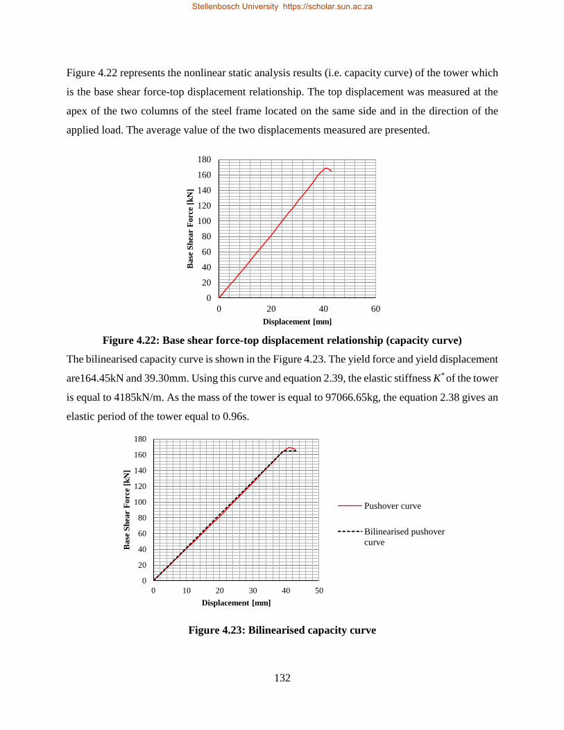
132

Figure 4.22 represents the nonlinear static analysis results (i.e. capacity curve) of the tower which

is the base shear force-top displacement relationship. The top displacement was measured at the

apex of the two columns of the steel frame located on the same side and in the direction of the

applied load. The average value of the two displacements measured are presented.

Figure 4.22: Base shear force-top displacement relationship (capacity curve)

The bilinearised capacity curve is shown in the Figure 4.23. The yield force and yield displacement

are164.45kN and 39.30mm. Using this curve and equation 2.39, the elastic stiffness K* of the tower

is equal to 4185kN/m. As the mass of the tower is equal to 97066.65kg, the equation 2.38 gives an

elastic period of the tower equal to 0.96s.

Figure 4.23: Bilinearised capacity curve

0

20

40

60

80

100

120

140

160

180

0 20 40 60

Base

Sh

ear

Forc

e [k

N]

Displacement [mm]

0

20

40

60

80

100

120

140

160

180

0 10 20 30 40 50

Base

Sh

ear

Forc

e [k

N]

Displacement [mm]

Pushover curve

Bilinearised pushover

curve


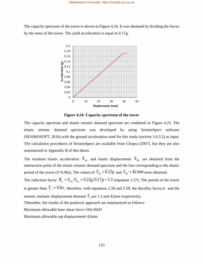
133

The capacity spectrum of the tower is shown in Figure 4.24. It was obtained by dividing the forces

by the mass of the tower. The yield acceleration is equal to 0.17g.

Figure 4.24: Capacity spectrum of the tower

The capacity spectrum and elastic seismic demand spectrum are combined in Figure 4.25. The

elastic seismic demand spectrum was developed by using SeismoSpect software

(SEiSMOSOFT, 2016) with the ground acceleration used for this study (section 3.4.3.2) as input.

The calculation procedures of SeismoSpect are available from Chopra (2007), but they are also

summarised in Appendix B of this thesis.

The resultant elastic acceleration aeS and elastic displacement deS are obtained from the

intersection point of the elastic seismic demand spectrum and the line corresponding to the elastic

period of the tower (T=0.96s). The values of gSae 22.0 and mm 42deS were obtained.

The reduction factor 3.117.022.0 ggSSR ayae (equation 2.57). The period of the tower

is greater than sTc 6.0 ; therefore; with equations 2.58 and 2.59, the ductility factor and the

seismic inelastic displacement demand aS are 1.3 and 42mm respectively.

Thereafter, the results of the pushover approach are summarized as follows:

Maximum allowable base shear force=164.45kN

Maximum allowable top displacement=42mm

0

0.02

0.04

0.06

0.08

0.1

0.12

0.14

0.16

0.18

0.2

0 10 20 30 40 50

Acc

eler

ati

on

[g

]

Displacement [mm]


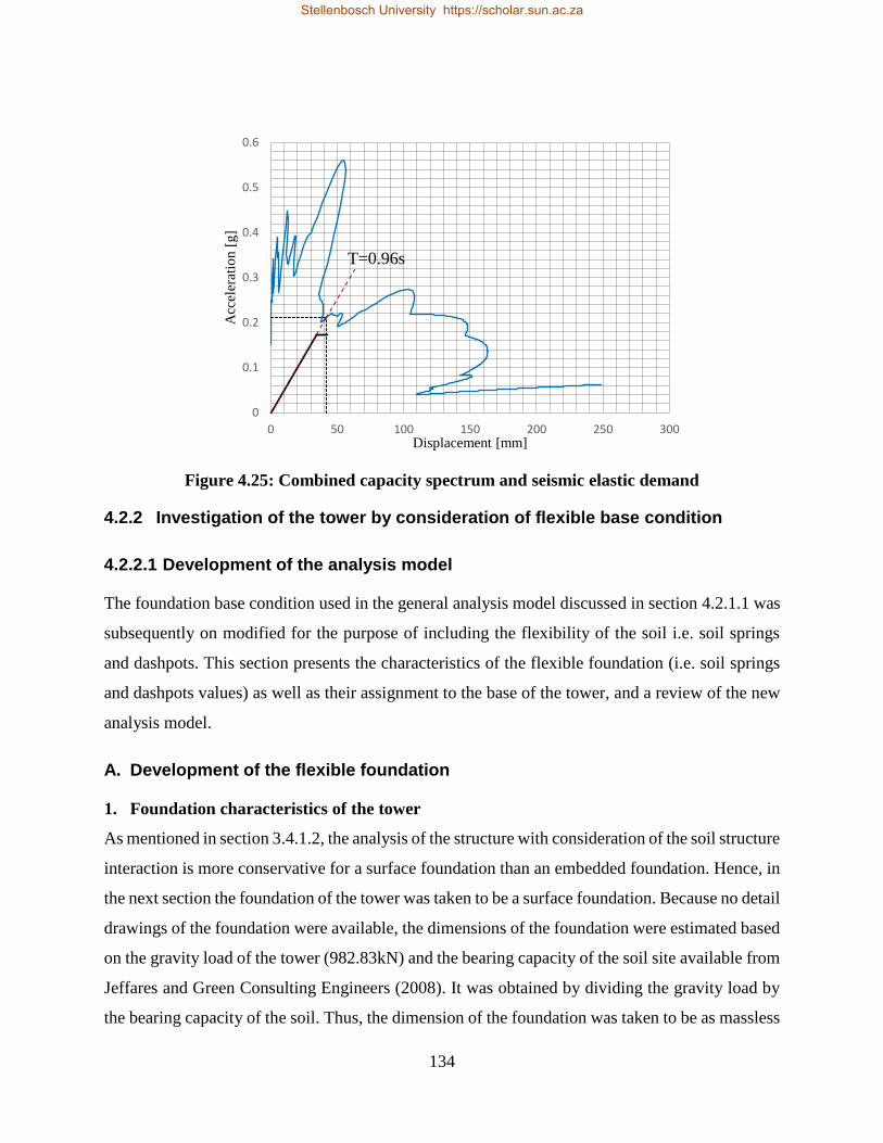
134

Figure 4.25: Combined capacity spectrum and seismic elastic demand

4.2.2 Investigation of the tower by consideration of flexible base condition

4.2.2.1 Development of the analysis model

The foundation base condition used in the general analysis model discussed in section 4.2.1.1 was

subsequently on modified for the purpose of including the flexibility of the soil i.e. soil springs

and dashpots. This section presents the characteristics of the flexible foundation (i.e. soil springs

and dashpots values) as well as their assignment to the base of the tower, and a review of the new

analysis model.

A. Development of the flexible foundation

1. Foundation characteristics of the tower

As mentioned in section 3.4.1.2, the analysis of the structure with consideration of the soil structure

interaction is more conservative for a surface foundation than an embedded foundation. Hence, in

the next section the foundation of the tower was taken to be a surface foundation. Because no detail

drawings of the foundation were available, the dimensions of the foundation were estimated based

on the gravity load of the tower (982.83kN) and the bearing capacity of the soil site available from

Jeffares and Green Consulting Engineers (2008). It was obtained by dividing the gravity load by

the bearing capacity of the soil. Thus, the dimension of the foundation was taken to be as massless

0

0.1

0.2

0.3

0.4

0.5

0.6

0 50 100 150 200 250 300

Acc

eler

atio

n [

g]

Displacement [mm]

T=0.96s


135

square mat foundation of 6.5x6.5 meters. The choice of mat foundation was based on the spacing

of the columns of the tower, which is not sufficient to ensure that the stress bulbs underneath the

pad foundation do not overlap at a certain depth. Therefore, since the stress bulbs overlap, the pad

foundations behave as if they were a mat foundation.

2. Foundation springs and dashpots

The appropriate approach for calculating the foundation springs and dashpots of the tower was

discussed in chapter 3. The calculation expressions of those foundation springs and dashpots are

shown in Table 3.3 to Table 3.6 of the aforementioned chapter.

i. Shear waves velocity Vs

As stated in Table 3.9, the shear waves velocity of the site under consideration ranges from 180 to

360m/s. The shear waves velocity selected for this assessment is one corresponding to the used

ground motion, which is equal to 242.05m/s (see section 3.4.3.2).

ii. Fundamental natural period of the tower T

The modal analysis of the tower was carried out and the results showed that the fundamental period

of the tower T =0.73s. As was stated early in section 4.2.1.2; the selected mode shape corresponds

to the weak direction of the tower. Moreover, the mass of the water was replaced by the equivalent

impulse and convective masses as shown in Figure 4.18 and the analysis model was pinned at the

base (see section 4.2.1.1).

iii. Structure-to-soil stiffness ratio h/(VsT)

The ratio h/(VsT) for the water tower being assessed is 0.12 which is slightly greater than 0.1. This

implies that the SSI influences the response of the tower (see summary of section 2.3.2.1). The

height h was taken to be the height of the tower from base to the centre of the top mass (see Figure

4.21) and is equal to 21.135m. As the ratio h/(VsT) is close to 0.1, the effect of soil structure

interaction might not be significant.

iv. Stiffness and dashpot coefficient calculation

The calculated stiffness and damping coefficient for the foundation of the water tower are given

in Table 4.10. The shear modulus oG of the soil was calculated based on equation 2.7, but it was

later modified with a modification ratio of 6825.0oGG (EN 1998-5, 2004) in order to consider


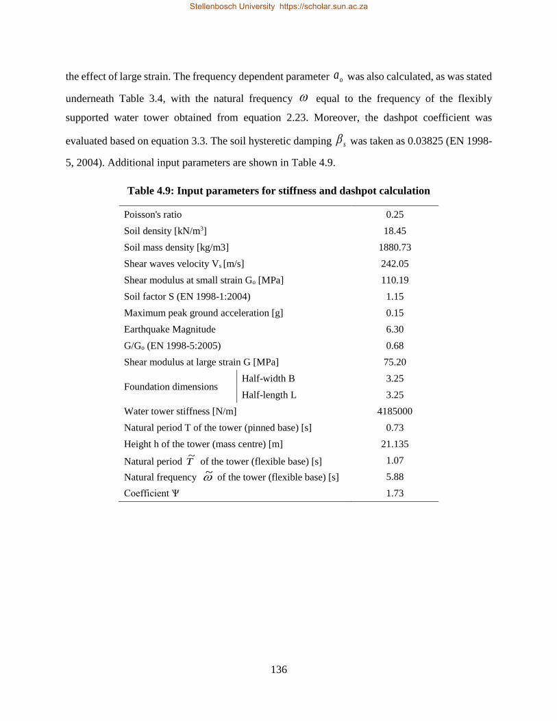
136

the effect of large strain. The frequency dependent parameter oa was also calculated, as was stated

underneath Table 3.4, with the natural frequency equal to the frequency of the flexibly

supported water tower obtained from equation 2.23. Moreover, the dashpot coefficient was

evaluated based on equation 3.3. The soil hysteretic damping s was taken as 0.03825 (EN 1998-

5, 2004). Additional input parameters are shown in Table 4.9.

Table 4.9: Input parameters for stiffness and dashpot calculation

Poisson's ratio 0.25

Soil density [kN/m3] 18.45

Soil mass density [kg/m3] 1880.73

Shear waves velocity Vs [m/s] 242.05

Shear modulus at small strain Go [MPa] 110.19

Soil factor S (EN 1998-1:2004) 1.15

Maximum peak ground acceleration [g] 0.15

Earthquake Magnitude 6.30

G/Go (EN 1998-5:2005) 0.68

Shear modulus at large strain G [MPa] 75.20

Foundation dimensions Half-width B 3.25

Half-length L 3.25

Water tower stiffness [N/m] 4185000

Natural period T of the tower (pinned base) [s] 0.73

Height h of the tower (mass centre) [m] 21.135

Natural period T~

of the tower (flexible base) [s] 1.07

Natural frequency ~ of the tower (flexible base) [s] 5.88

Coefficient Ѱ 1.73


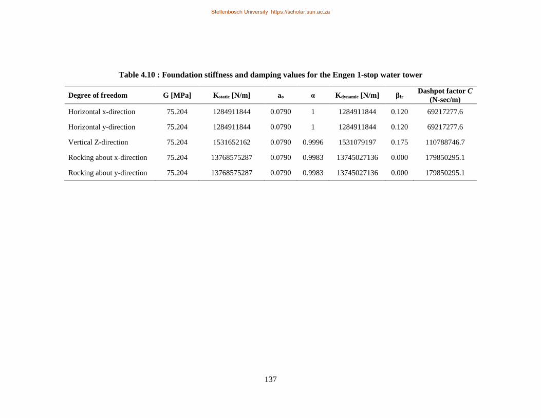
137

Table 4.10 : Foundation stiffness and damping values for the Engen 1-stop water tower

Degree of freedom G [MPa] Kstatic [N/m] ao α Kdynamic [N/m] βfr Dashpot factor C

(N-sec/m)

Horizontal x-direction 75.204 1284911844 0.0790 1 1284911844 0.120 69217277.6

Horizontal y-direction 75.204 1284911844 0.0790 1 1284911844 0.120 69217277.6

Vertical Z-direction 75.204 1531652162 0.0790 0.9996 1531079197 0.175 110788746.7

Rocking about x-direction 75.204 13768575287 0.0790 0.9983 13745027136 0.000 179850295.1

Rocking about y-direction 75.204 13768575287 0.0790 0.9983 13745027136 0.000 179850295.1



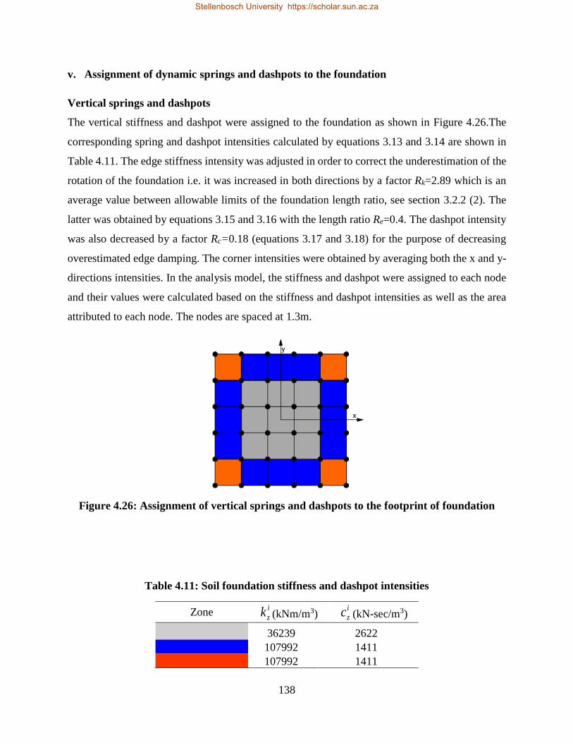
138

v. Assignment of dynamic springs and dashpots to the foundation

Vertical springs and dashpots

The vertical stiffness and dashpot were assigned to the foundation as shown in Figure 4.26.The

corresponding spring and dashpot intensities calculated by equations 3.13 and 3.14 are shown in

Table 4.11. The edge stiffness intensity was adjusted in order to correct the underestimation of the

rotation of the foundation i.e. it was increased in both directions by a factor Rk=2.89 which is an

average value between allowable limits of the foundation length ratio, see section 3.2.2 (2). The

latter was obtained by equations 3.15 and 3.16 with the length ratio Re=0.4. The dashpot intensity

was also decreased by a factor Rc=0.18 (equations 3.17 and 3.18) for the purpose of decreasing

overestimated edge damping. The corner intensities were obtained by averaging both the x and y-

directions intensities. In the analysis model, the stiffness and dashpot were assigned to each node

and their values were calculated based on the stiffness and dashpot intensities as well as the area

attributed to each node. The nodes are spaced at 1.3m.

Figure 4.26: Assignment of vertical springs and dashpots to the footprint of foundation

Table 4.11: Soil foundation stiffness and dashpot intensities

Zone i

zk (kNm/m3) i

zc (kN-sec/m3)

36239 2622

107992 1411

107992 1411


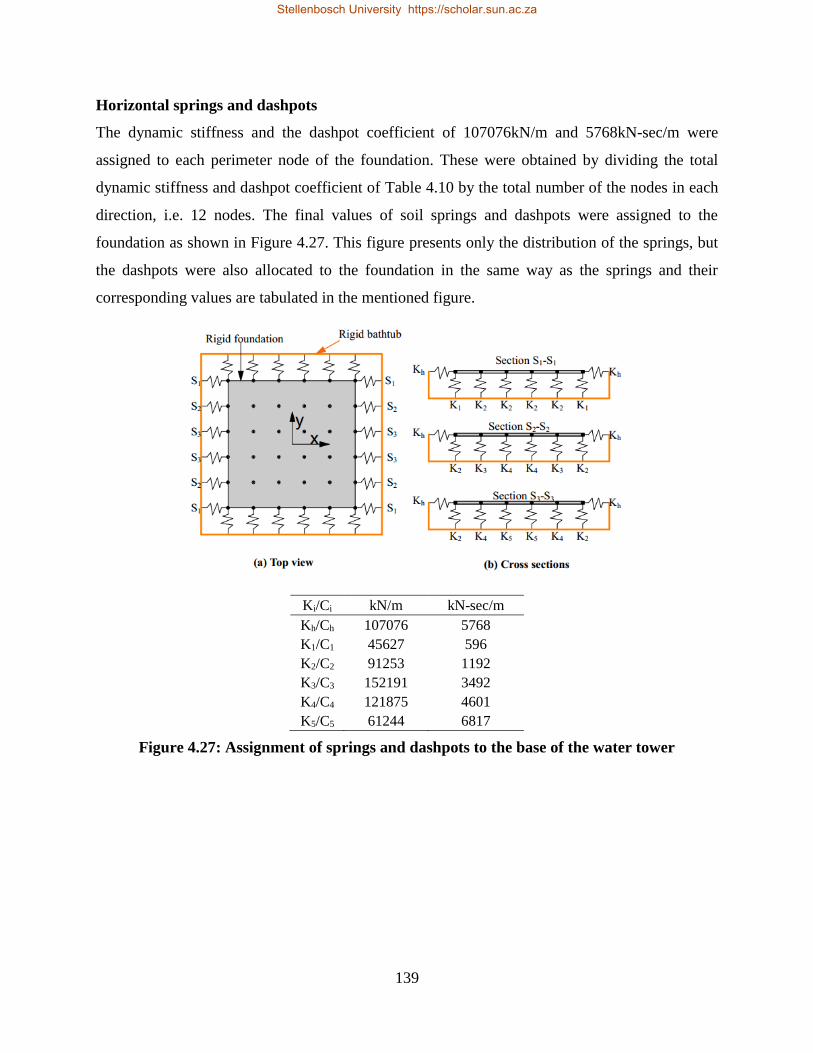
139

Horizontal springs and dashpots

The dynamic stiffness and the dashpot coefficient of 107076kN/m and 5768kN-sec/m were

assigned to each perimeter node of the foundation. These were obtained by dividing the total

dynamic stiffness and dashpot coefficient of Table 4.10 by the total number of the nodes in each

direction, i.e. 12 nodes. The final values of soil springs and dashpots were assigned to the

foundation as shown in Figure 4.27. This figure presents only the distribution of the springs, but

the dashpots were also allocated to the foundation in the same way as the springs and their

corresponding values are tabulated in the mentioned figure.

Ki/Ci kN/m kN-sec/m

Kh/Ch 107076 5768

K1/C1 45627 596

K2/C2 91253 1192

K3/C3 152191 3492

K4/C4 121875 4601

K5/C5 61244 6817

Figure 4.27: Assignment of springs and dashpots to the base of the water tower


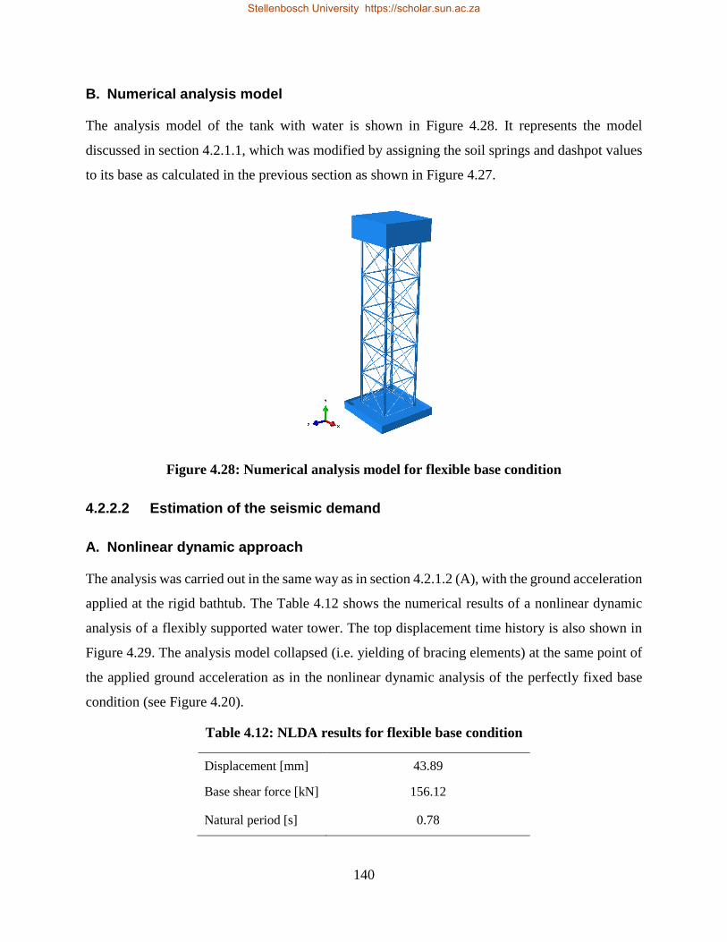
140

B. Numerical analysis model

The analysis model of the tank with water is shown in Figure 4.28. It represents the model

discussed in section 4.2.1.1, which was modified by assigning the soil springs and dashpot values

to its base as calculated in the previous section as shown in Figure 4.27.

Figure 4.28: Numerical analysis model for flexible base condition

4.2.2.2 Estimation of the seismic demand

A. Nonlinear dynamic approach

The analysis was carried out in the same way as in section 4.2.1.2 (A), with the ground acceleration

applied at the rigid bathtub. The Table 4.12 shows the numerical results of a nonlinear dynamic

analysis of a flexibly supported water tower. The top displacement time history is also shown in

Figure 4.29. The analysis model collapsed (i.e. yielding of bracing elements) at the same point of

the applied ground acceleration as in the nonlinear dynamic analysis of the perfectly fixed base

condition (see Figure 4.20).

Table 4.12: NLDA results for flexible base condition

Displacement [mm] 43.89

Base shear force [kN] 156.12

Natural period [s] 0.78


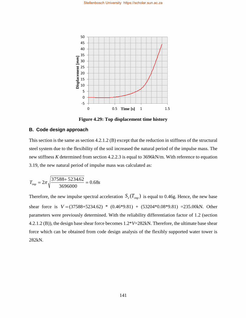
141

Figure 4.29: Top displacement time history

B. Code design approach

This section is the same as section 4.2.1.2 (B) except that the reduction in stiffness of the structural

steel system due to the flexibility of the soil increased the natural period of the impulse mass. The

new stiffness K determined from section 4.2.2.3 is equal to 3696kN/m. With reference to equation

3.19, the new natural period of impulse mass was calculated as:

sTimp 68.03696000

62.5234375882

Therefore, the new impulse spectral acceleration )( impe TS is equal to 0.46g. Hence, the new base

shear force is V (37588+5234.62) * (0.46*9.81) + (53204*0.08*9.81) =235.00kN. Other

parameters were previously determined. With the reliability differentiation factor of 1.2 (section

4.2.1.2 (B)), the design base shear force becomes 1.2*V=282kN. Therefore, the ultimate base shear

force which can be obtained from code design analysis of the flexibly supported water tower is

282kN.

-5

0

5

10

15

20

25

30

35

40

45

50

0 0.5 1 1.5

Dis

pla

cem

ent

[mm

]

Time [s]


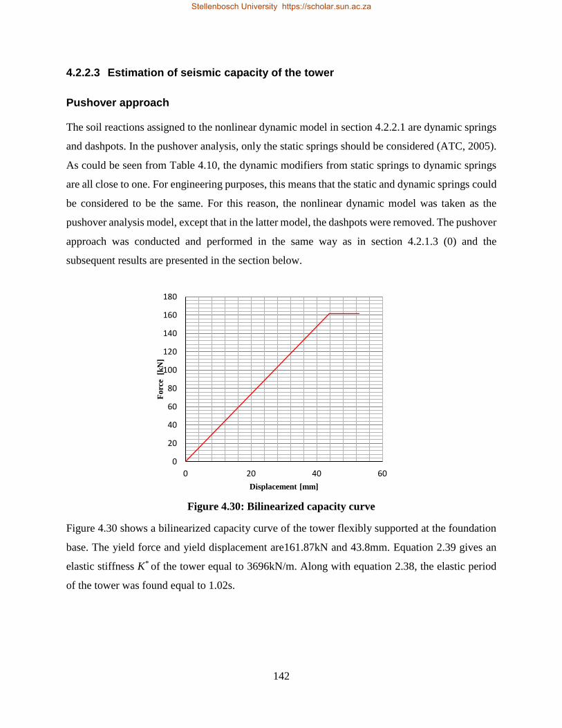
142

4.2.2.3 Estimation of seismic capacity of the tower

Pushover approach

The soil reactions assigned to the nonlinear dynamic model in section 4.2.2.1 are dynamic springs

and dashpots. In the pushover analysis, only the static springs should be considered (ATC, 2005).

As could be seen from Table 4.10, the dynamic modifiers from static springs to dynamic springs

are all close to one. For engineering purposes, this means that the static and dynamic springs could

be considered to be the same. For this reason, the nonlinear dynamic model was taken as the

pushover analysis model, except that in the latter model, the dashpots were removed. The pushover

approach was conducted and performed in the same way as in section 4.2.1.3 (0) and the

subsequent results are presented in the section below.

Figure 4.30: Bilinearized capacity curve

Figure 4.30 shows a bilinearized capacity curve of the tower flexibly supported at the foundation

base. The yield force and yield displacement are161.87kN and 43.8mm. Equation 2.39 gives an

elastic stiffness K* of the tower equal to 3696kN/m. Along with equation 2.38, the elastic period

of the tower was found equal to 1.02s.

0

20

40

60

80

100

120

140

160

180

0 20 40 60

Forc

e [

kN

]

Displacement [mm]


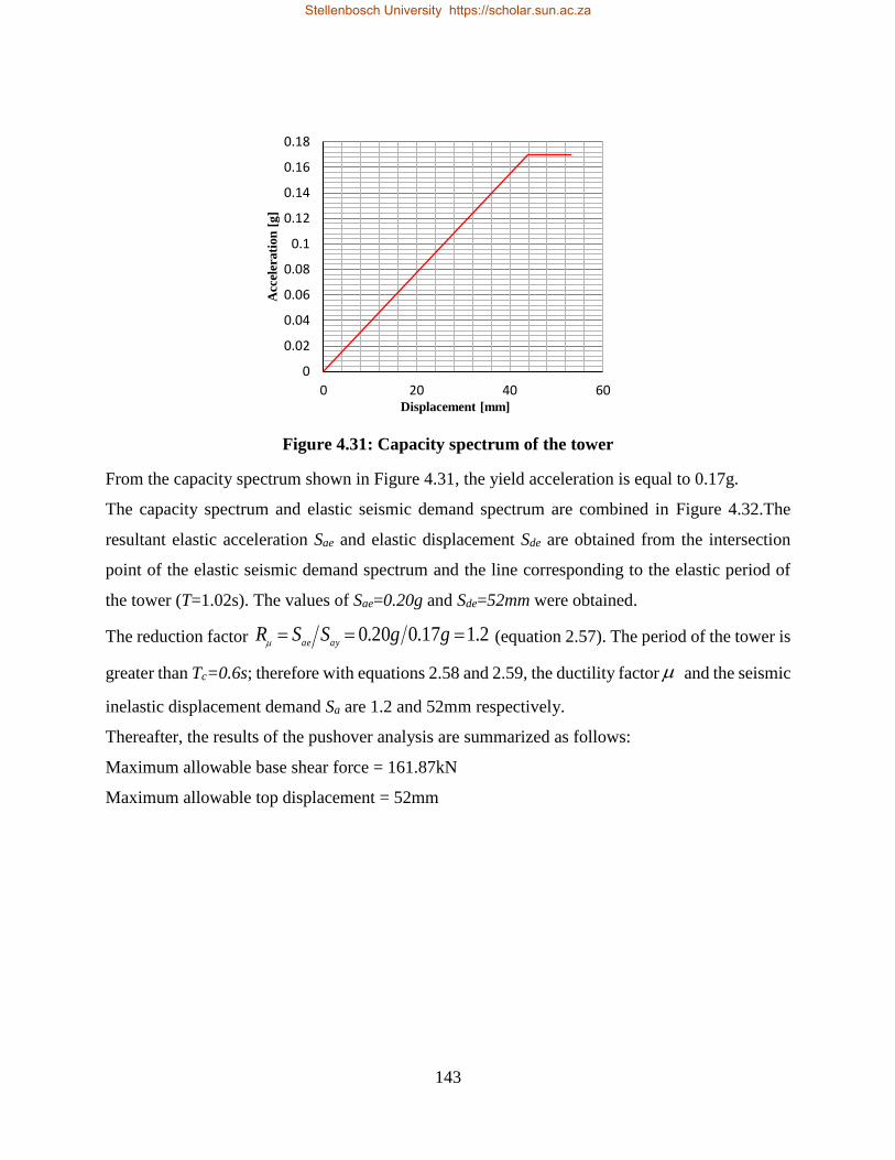
143

Figure 4.31: Capacity spectrum of the tower

From the capacity spectrum shown in Figure 4.31, the yield acceleration is equal to 0.17g.

The capacity spectrum and elastic seismic demand spectrum are combined in Figure 4.32.The

resultant elastic acceleration Sae and elastic displacement Sde are obtained from the intersection

point of the elastic seismic demand spectrum and the line corresponding to the elastic period of

the tower (T=1.02s). The values of Sae=0.20g and Sde=52mm were obtained.

The reduction factor 2.117.020.0 ggSSRayae (equation 2.57). The period of the tower is

greater than Tc=0.6s; therefore with equations 2.58 and 2.59, the ductility factor and the seismic

inelastic displacement demand Sa are 1.2 and 52mm respectively.

Thereafter, the results of the pushover analysis are summarized as follows:

Maximum allowable base shear force = 161.87kN

Maximum allowable top displacement = 52mm

0

0.02

0.04

0.06

0.08

0.1

0.12

0.14

0.16

0.18

0 20 40 60

Acc

eler

ati

on

[g

]

Displacement [mm]


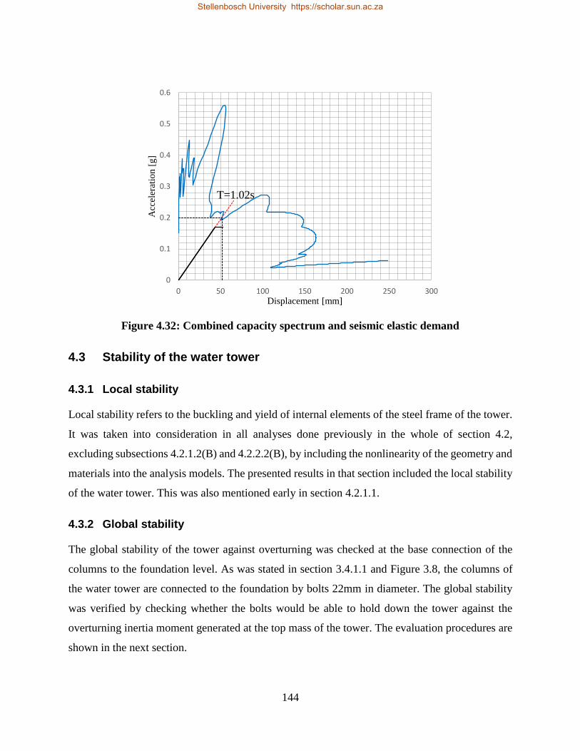
144

Figure 4.32: Combined capacity spectrum and seismic elastic demand

4.3 Stability of the water tower

4.3.1 Local stability

Local stability refers to the buckling and yield of internal elements of the steel frame of the tower.

It was taken into consideration in all analyses done previously in the whole of section 4.2,

excluding subsections 4.2.1.2(B) and 4.2.2.2(B), by including the nonlinearity of the geometry and

materials into the analysis models. The presented results in that section included the local stability

of the water tower. This was also mentioned early in section 4.2.1.1.

4.3.2 Global stability

The global stability of the tower against overturning was checked at the base connection of the

columns to the foundation level. As was stated in section 3.4.1.1 and Figure 3.8, the columns of

the water tower are connected to the foundation by bolts 22mm in diameter. The global stability

was verified by checking whether the bolts would be able to hold down the tower against the

overturning inertia moment generated at the top mass of the tower. The evaluation procedures are

shown in the next section.

0

0.1

0.2

0.3

0.4

0.5

0.6

0 50 100 150 200 250 300

Acc

eler

atio

n [

g]

Displacement [mm]

T=1.02s


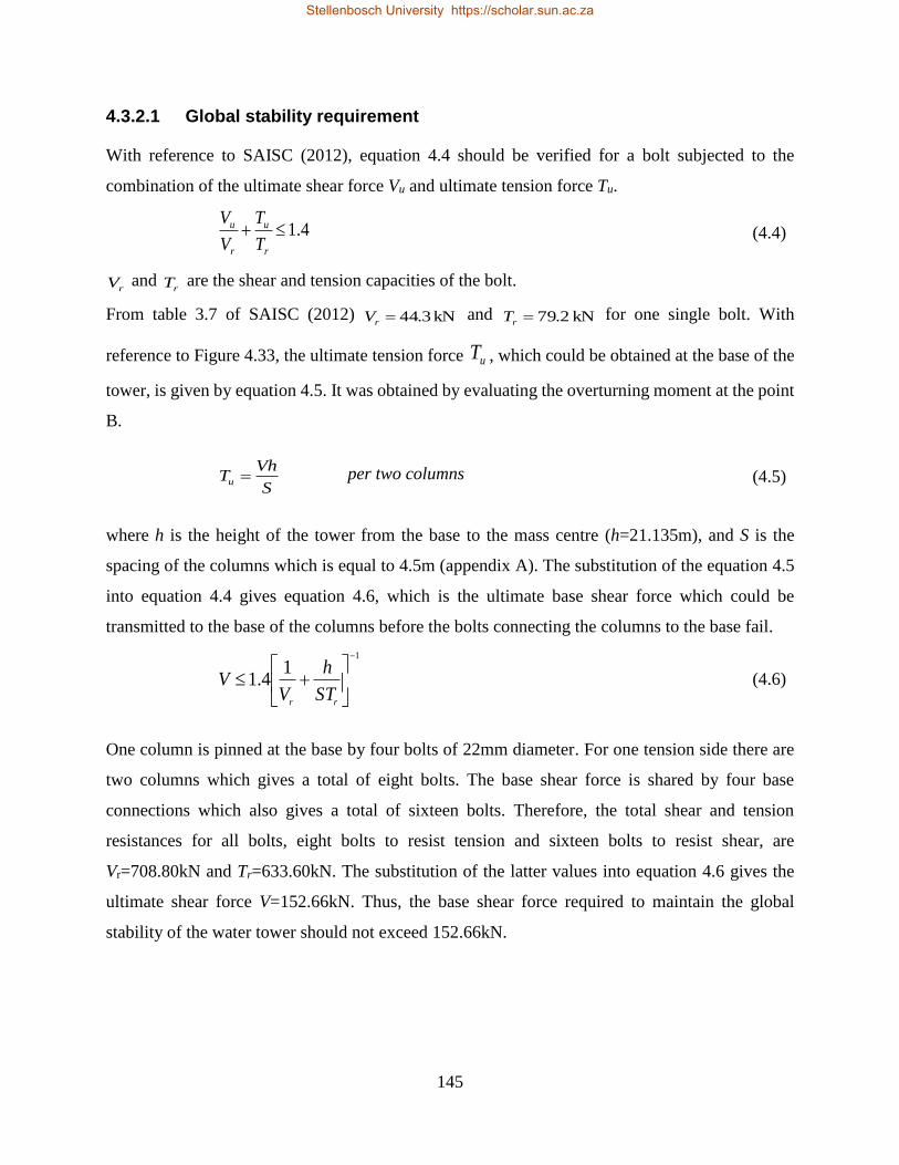
145

4.3.2.1 Global stability requirement

With reference to SAISC (2012), equation 4.4 should be verified for a bolt subjected to the

combination of the ultimate shear force Vu and ultimate tension force Tu.

4.1r

u

r

u

T

T

V

V (4.4)

rV and rT are the shear and tension capacities of the bolt.

From table 3.7 of SAISC (2012) kN 3.44rV and kN 2.79rT for one single bolt. With

reference to Figure 4.33, the ultimate tension force uT , which could be obtained at the base of the

tower, is given by equation 4.5. It was obtained by evaluating the overturning moment at the point

B.

S

VhTu per two columns (4.5)

where h is the height of the tower from the base to the mass centre (h=21.135m), and S is the

spacing of the columns which is equal to 4.5m (appendix A). The substitution of the equation 4.5

into equation 4.4 gives equation 4.6, which is the ultimate base shear force which could be

transmitted to the base of the columns before the bolts connecting the columns to the base fail.

1

14.1

rrST

h

VV (4.6)

One column is pinned at the base by four bolts of 22mm diameter. For one tension side there are

two columns which gives a total of eight bolts. The base shear force is shared by four base

connections which also gives a total of sixteen bolts. Therefore, the total shear and tension

resistances for all bolts, eight bolts to resist tension and sixteen bolts to resist shear, are

Vr=708.80kN and Tr=633.60kN. The substitution of the latter values into equation 4.6 gives the

ultimate shear force V=152.66kN. Thus, the base shear force required to maintain the global

stability of the water tower should not exceed 152.66kN.


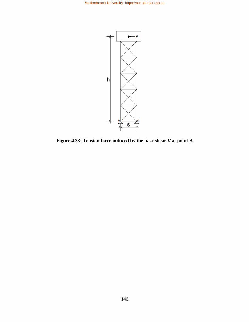
146

Figure 4.33: Tension force induced by the base shear V at point A


147

Chapter 5

Results summary and discussions

5.1 Summary of the results

The aim of this thesis was to study and document techniques to assess the dynamic structural

performance of typical water tower structures and apply this to investigate whether the Engen 1-

Stop water tower would be able to withstand an earthquake of a magnitude appropriate to its site

location. In overview, the seismic assessment was conducted by estimating the seismic demand

and seismic capacity of the structure and comparing both these results. The state of the structure

under dynamic seismic loading is assessed by comparing whether the base shear force of the

seismic demand is greater than the base shear force of the seismic capacity. A greater seismic

demand relative to the seismic capacity implies a high probability that the structure will fail during

seismic activity; a greater seismic capacity relative to seismic demand implies that the structure is

less likely to fail and will be able to resist the earthquake.

Three approaches were used for achieving the objectives of the study: the nonlinear dynamic

approach (NLDA), the code design approach (CDA) and the pushover approach (POA). The

NLDA and CDA were used for estimating the seismic demand of the tower, and the POA was used

for evaluating the seismic capacity of the water tower. Two boundary conditions were considered:

one in which the water tower was flexibly supported at ground level and one in which the water

tower was perfectly fixed at ground level. The former was referred to as the flexible base condition

and the latter as the perfectly fixed base condition. The flexible base condition was analysed by

considering the soil structure interaction (SSI). Consequently, there is no SSI for the perfectly

fixed base condition. The analysis steps and the results for each approach were presented in chapter

four. In addition, the global stability requirement (GSR) of the tower was checked and the resultant

seismic demand from the GSR was also presented.

Chapter 4 concluded that, during the NLDA for both perfectly and flexibly fixed base conditions,

the analysis models of the water tower failed before the applied earthquake ended. In both cases,

the tower failed after 1.4s, whereas the ground acceleration used has a time duration of 27s (see

Figure 4.20 ). This implies that the water tower cannot withstand an earthquake of a magnitude

expected at its site location. Consequently, the NLDA results represent the seismic capacity of the


148

tower and not the seismic demand under the seismic activity of the location of the water tower.

The seismic demand is therefore only given by CDA. Since the tower failed in both models and

the NLDA represents the seismic capacity of the structure, the results between the NLDA and the

POA should be similar because the POA also represents the seismic capacity of the structure. It is

important to remember that the principle of the POA is to apply a constantly increasing static load

until the failure point of the structure is achieved. Based on these results, the seismic capacity is

evaluated. The summary of results is presented in Table 5.1 and a discussion of the results in

follows section 5.2.


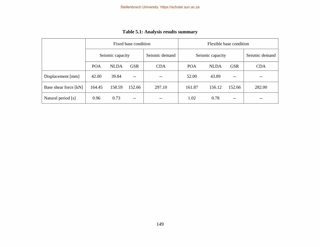
149

Table 5.1: Analysis results summary

Fixed base condition Flexible base condition

Seismic capacity Seismic demand Seismic capacity Seismic demand

POA NLDA GSR CDA POA NLDA GSR CDA

Displacement [mm] 42.00 39.84 -- -- 52.00 43.89 -- --

Base shear force [kN] 164.45 158.59 152.66 297.10 161.87 156.12 152.66 282.00

Natural period [s] 0.96 0.73 -- -- 1.02 0.78 -- --



150

5.2 Discussions

5.2.1 Seismic capacity of the tower

The POA was carried out on the water tower structure to determine the capacity of the tower under

seismic loading in addition to the GSR, which also gave values for the base shear force capacity

of the water tower. However, the values from the NLDA also represent the base shear force

capacity of the tower since the water tower failed during the analysis. Since both the POA and

NLDA gave values for the seismic capacity of the tower, the values were expected to be the similar.

From Table 5.1 it can be seen that the values are indeed similar, with the POA giving a base shear

force capacity of 164.45 kN compared to the 158.59 kN provided by the NLDA. The small

difference in these values could be attributed to the inertia force and the effect of sloshing that was

considered in the NLDA, but ignored in the POA. In conclusion, the controlling base shear force

which represents the capacity of the water tower structure model is the minimum from among the

POA, NLDA and GSR. From the results in Table 5.1, it can be seen that the GSR provided the

lowest value at 152.66 kN.

5.2.2 Seismic demand of the tower

At the start of this study, the seismic demand of the tower was expected to be given by the NLDA

as well as the CDA. However, during the NLDA, the maximum resistance of the tower was

achieved, which implied that the NLDA results represented the seismic capacity of the tower

instead. Therefore, the seismic demand was only given by the CDA. From Table 5.1 it is shown

that the seismic demand for the structure for the perfectly fixed and flexible base conditions is

297.1 and 282 kN, respectively.

5.2.3 The soil structure interaction effect

For the purpose of assessing the effect of Soil Structure Interaction (SSI) on the seismic response

of the tower, Table 5.2 was developed from the results of the Non-Linear Dynamic Analysis

(NLDA) presented in Table 5.1. The effect of the SSI on the CDA results was also evaluated and

is equal to -5.1%, i.e. the base shear force in the perfectly fixed base condition was 5.1% less that

the base shear force obtained when SSI was considered.


151

Table 5.2: Increase/decrease from fixed to flexible base conditions

Perfectly fixed

base condition

Flexible base

condition

Percentage

increase/decrease

Displacement 39.84 mm 43.89 mm 9.2

Base shear force 158.59 kN 156.12 kN -1.6

Natural period 0.73 s 0.78 s 6.4

From the above results, it could be concluded that the effects of SSI did not significantly influence

the response of the tower. This corresponds to the predicted result in section 4.2.2.1(2)iii, since the

calculated ratio h/(VsT) was close to 0.1.


152

Chapter 6

Conclusion and recommendation

6.1 General conclusion

Elevated water tanks are classified as important structures. There are different reasons for this

classification, such as the importance of water tanks in lifeline and industrial area, the vulnerability

of elevated tanks to horizontal lateral loads and the negative consequences associated with the

failure of the water supply system. In the past, the value of the lateral seismic load which could be

induced on a particular elevated water tank was estimated based on the static approach, which was

carried out by taking the mass of the structure as the total mass of the tank filled by water.

The report on the catastrophic failure of water tanks during the Chilean earthquake of May, 1960

(Steinbrugge & Flores, 1963) caused uncertainty about the accuracy of this approach.

Subsequently, much research on seismic behaviour of water tanks has been conducted. As a result,

it has been shown that the static approach does not represent the realistic response of water tanks

to a given earthquake excitation. Housner’s (1963) research was among the first to show that the

static approach is reliable only for the case in which the water tank is full of water, which is not

practically useful as water tanks are rarely kept full. For a rigid wall tank full of water with a

freeboard, it has been shown that the seismic excitation of water tanks is best represented if one

understands the mass of the tank as made up of two components, the impulsive mass and the

convective mass.

The impulsive mass represents the portion of the water tank which responds as a solid mass

attached to the bottom of the tank. The convective mass represents the portion of the water which

contributes to the sloshing of the surface water during a given excitation. The seismic responses

of these masses are obtained based on standard structural dynamic procedures, and their natural

periods should be separated so that the seismic response of each mass can be modelled separately,

each with its respective stiffness. The total seismic response of the tank is then obtained by the

combination (e.g. absolute sum) of each mass’s response. This analysis concept is known as

“dynamic analysis” and correlates to laboratory results (Sonobe & Nishikawa, 1969). Dynamic

analysis gives a lower base shear force and higher hydrodynamic pressure on the wall of the tank

when compared to the static approach (Gaikwad & Mangulkar, 2013).


153

Later on, Haroun & Housner (1981) found that the flexibility of the walls of the tank influences

the response of the impulse mass. Consequently, Malhotra et al. (2000) updated Housner’s

analytical equations in order to consider the flexibility of the wall of the tank. At present, the

dynamic analysis for water tanks has been adopted in various design codes and standards (e.g. EN

1998-4, 2006, Priestley et al., 1986). However, standards such as SANS 10160-4:2011 have not

yet been implemented in any design provisions for water tanks.

Another factor which contributes to the seismic response of the structure is the mechanical

properties of the soil. The literature showed that when a structure is analysed with consideration

of the soil properties of the medium under the foundation, the resultant seismic base shear force is

reduced and the resultant internal forces are increased compared to that obtained from the same

structure analysed with a perfectly fixed foundation. These changes are attributed to the Soil

Structure Interaction (SSI) effect. Three forms of SSI occur when the seismic waves strike the

foundation of the structure. The first is associated with the difference between the foundation input

motion and the free field ground motion, which is caused by the dissimilarity between the

mechanic properties of the foundation unit and the soil. This dissimilarity causes reflection and

refraction of the incident seismic waves at the soil-foundation interface back to the soil medium,

and the resultant foundation input motion is reduced compared to the free field ground motion.

This mechanism is known as kinematic interaction and its effect is small enough so that it can be

practically ignored (Kramer & Stewart, 2004:4-34).

The second form of SSI occurs when the structure starts oscillating as a result of the inertial force

generated over the height of the superstructure, which in turn induces the shear force and

overturning moment at the foundation base resulting in translation and rotation of the foundation.

The translation and rotation of the foundation induce the deformation of the soil and radiate energy

into the soil medium. The radiated energy dissipates part of the incoming seismic waves, and, as a

result, the incoming seismic waves are reduced. This mechanism is considered to be an additional

source of energy dissipation to the inherent damping of the system. In addition, the rotation of the

foundation base induces excessive lateral displacement on the superstructure compared to the

displacement estimated based on a perfectly fixed foundation, which results in lengthening of the

fundamental natural period of the structure. All mechanisms associated with the modification of

the damping and lengthening of the fundamental natural period of the system are referred to as


154

inertia interaction. The inertia interaction has been implemented into design codes and standards

(e.g. ASCE, 2014; ATC,2005) by modifying the fundamental natural period and the damping

coefficient of the structure calculated based on the fixed foundation. However, the displacement

based approach has been critiqued on the basis that during the evaluation of the internal forces, it

does not take into account the effect of the lateral displacement induced by the rotation of the

foundation on the superstructure, which was proven to increase the internal forces in the

superstructure elements. Therefore, updated codes and standards containing the design

considerations for the evaluation of the internal forces with consideration of this lateral

displacement are needed.

The third form of SSI is associated with the flexibility of the foundation unit. Iguchi and Luco

(1982) have demonstrated that the flexibility of the foundation decreases the damping value of the

system compared to a rigid foundation. For low frequencies of excitation, the effective stiffness of

the system is lower than that obtained with consideration of a rigid foundation, and higher for high

frequencies of excitation. However, the literature shows that there are no analytical equations for

design of the structures with consideration of the foundation flexibility.

The concern of this research was to illustrate a numerical method for seismic design and

performance assessment of steel framed water tower structures which could take into account all

of the aforementioned factors influencing the seismic response. This method was applied to

investigate a particular case study, the Engen 1-Stop water tower. A review of relevant publications

for achieving these objectives were presented in chapter 2, and the numerical method developed

in this study was described in section 3.2. In addition, the general characteristics of the water tower

were also discussed in section 3.4 and an explanation of the application of the method to the

assessment of the tower was given in section 4.2.

From sections 4.1 and 4.2, the first step before assessment of the mentioned structure was to

validate the analysis model. This was done by building in a laboratory a steel frame structure,

which was referred to as the test structure. The test structure had the same characteristics as the

steel frame of the tower, scaled down by a factor of 12. Once the test structure was built, it was

then subjected to a simulation of ground acceleration in the laboratory and in ABAQUS finite

element software. The analysis model for the water tower was calibrated by comparing both the

numerical and laboratory results of the test structure. Furthermore, this analysis model was


155

modified in order to conform to the boundary conditions used to implement SSI in the assessment

process.

The seismic performance assessment of the tower was conducted by evaluating and comparing the

seismic capacity of the tower to its seismic demand. The seismic performance of the tower was

determined by whether or not demand exceeded capacity. If not, this implies that the structure is

less likely to fail under a given ground motion. If demand exceeds capacity, however, the structure

has a higher probability of failure during an earthquake. To achieve this, following approach was

followed: the developed numerical method and the code design approach. The developed

numerical method in this section refers to the documented method which considers all the

discussed analysis considerations (i.e. the sloshing of the surface water, the SSI, etc.) for the

seismic design of the water tower. The latter method consisted of the nonlinear dynamic and static

analyses in which the soil medium characteristics were included into the analysis models through

springs and dashpots. The code design approach is a response spectrum analysis which was

performed based on the design provisions of EN 1998-4:2006.

The seismic demand was given by the nonlinear dynamic analysis and the code design analysis

while the seismic capacity was obtained from the static pseudo-dynamic analysis (pushover

analysis). The code design analysis was considered for the purpose of checking its accuracy in

estimating the base shear force induced on the structure. It is important to remember that the

current design codes and standards do not consider the effect of the flexibility of the foundation

on the response of the structure, nor the influence of the lateral displacement on the internal forces

induced in the superstructure. Two boundary conditions were considered: the water tower perfectly

fixed at the base of the foundation and the water tower flexibly supported at the ground level. The

latter was used in order to be able to include the properties of the soil medium on which the tower

is supported into the analysis process, i.e. the SSI analysis. The former was considered in order to

illustrate the effect of the SSI on the base shear force imposed on the tower. Additionally, the

seismic capacity of the tower against overturning was checked.

With reference to sections 5.1 and 5.2, the results showed that during the nonlinear dynamic

analysis for both perfectly fixed and flexibly supported base conditions, the analysis models of the

water tower failed before the applied ground acceleration time history ended. This implied that the

water tower on the site is not able to survive under the seismic activity expected for its site location.


156

Consequently, the resultant nonlinear dynamic results represented the seismic capacity instead of

the expected seismic demand on the tower. Therefore, the seismic capacity was given by both the

nonlinear dynamic analysis and pushover analysis while the seismic demand was only given by

the code design approach. Subsequently, the accuracy of the code design analysis on the base shear

force was not identified. This is due to the fact that, since the code design analysis (i.e. the response

spectrum analysis) peaks only at the maximum value for a given ground acceleration and the

nonlinear dynamic analysis models failed before that point, it was not reasonable to compare both

results.

Moreover, the nonlinear dynamic and pushover analyses results were expecting to be the same

because the maximum capacity of the tower was achieved during both analyses. The small

difference in results can be attributed to the inertia force and sloshing effect which are basically

not considered in the pushover analysis. By comparing the seismic capacity results given by both

methods (the nonlinear dynamic and pushover analyses) against the global stability requirement,

it was concluded that the global stability requirement controlled the seismic capacity. In other

words, the seismic capacity of the water tower was considered as that given by the global stability

requirement of the tower, as it gave the lowest value.

Therefore, the seismic demand and seismic capacity of the tower were taken as the values given

by the code design analysis and global stability requirement, respectively. The comparison of these

results causes serious uncertainty over whether the Engen 1-Stop water tower could withstand any

seismic hazard. The effect of Soil Structure Interaction (SSI) on the response of the tower was

interpreted by comparing the nonlinear dynamic results of the perfectly fixed and flexible base

conditions. From these results, it was shown that the effect of SSI was not significant. The reason

attributed to these observations are the system parameters, as the ratio h/(VsT) was close to 0.1.

As a final point, the Engen 1-Stop water tower would not be able to survive during seismic activity,

therefore, retrofitting of the structure is required in order to ensure the safety of the tower. In

addition, the computed effect of Soil Structure Interaction on the dynamic response of the structure

appeared insignificant, but this does preclude further investigation, especially for the purpose of

assessing the stress distribution throughout the steel frame elements, because the induced

additional lateral displacement from SSI increases the internal forces.


157

6.2 Recommendations

Considered assumptions and analysis data

During the study, a number of assumptions were made, as presented in Chapter 1. Some of the

data used was obtained from literature, as discussed in Chapter 3. For a more accurate analysis,

further on-site investigation should be conducted to obtain specific data for the existing water

tower. This could be achieved by evaluating the shear waves velocity of the soil at the site as

well as the foundation characteristics of the tower. Although the member sizes and structure

dimensions of the model are the same as the existing structure, the structural integrity of the

two may differ. The existing water tower has been there for a number of years, whereas the

water tower analysis model is made up of new elements. In order to consider the stiffness

degradation of the steel frame which results from rusting and the weathering of elements on

site, further study should introduce the imperfections of the elements into the analysis process.

Design seismic response

The earthquake ground motions used in this study were selected based on the soil

characteristics of the site and the expected earthquake magnitude. These were considered as

preliminary factors for the investigation of the tower. Factors such as the source mechanisms

of the earthquakes, the epicenter distances relative to the site location of the water tower and

the epicenter distances with respect to the recording station of the ground motions should be

taken into account for better results. With reference to NEHRP Consultants Joint Venture

(2011), this can be achieved by considering and grouping at least six different appropriate

ground accelerations into three groups. The ground accelerations of each group should be

scaled so that their average value, the square root sum of the squares, does not drop below 1.3

times the associated ordinate of the design response spectrum assigned to the site location of

the structure for the periods in the range of 0.2T to 1.5T. Here, T defines the fundamental

natural period of the structure in the direction of interest. Next, if the analyses will be

performed with consideration of more than seven ground accelerations, the seismic response

of the structure will be obtained from an analysis giving the maximum values. In the other way

around, the seismic response will be given by the average value of all analyses.


158

Seismic assessment methods

The literature showed that current pushover approaches were developed based on building

structures. Since the behaviour of building structures is dynamically different than water

retaining structures, further study is needed to determine whether these pushover approaches

are applicable to water retaining structures. This is due to the fact that in the modelling of the

water retaining structures, two mass components, solid mass and active mass, are considered

because of the sloshing effect, while in building structures all masses are considered as a solid

mass.

Soil Structure Interaction, SSI

More research is required in order to investigate the magnitude of the influence of foundation

flexibility on the response of structures, as a review of the literature revealed little. Stewart and

Tileylioglu (2007) also stated that analytical equations for the evaluation of this influence on

the response of the structures are needed. It was also drawn from literature that the updated

design codes and standards which are based on a “displacement-based approach” are required

for accurate SSI analysis results. Since the presented numerical method requires high

performance analysis tools, these will be helpful to design engineers who do not have access

to those analysis tools.


159

References

Abrahamson, N.A., Schneider, J.F. & Stepp, J.C. 1991. Empirical Spatial Coherency Functions

for Application to Soil Structure Interaction Analyses. Earthquake Spectra. 7(1):1–27.

Algreane, G.A.I., Osman, S.A., Karim, O.A. & Kasa, A. 2011. Behavior of Elevated Concrete

Water Tank Subjected to Artificial Ground Motion. Electronic Journal of Geotechnical

Engineering. 16:387–406.

Anastasopoulos, I., Gazetas, G., Loli, M., Apostolou, M. & Gerolymos, N. 2010. Soil failure can

be used for seismic protection of structures. Bulletin of Earthquake Engineering. 8(2):309–326.

Apsel, R.J. & Luco, J.E. 1987. Impedance Functions for Foundations Embedded in A Layered

Medium: An Integral Equation Approach. Earthquake Engineering & Structural Dynamics.

15(2):213–231.

Arefi, M.J. 2008. Effects of Soil-Structure Interaction on the Seismic Response of Existing R . C

. Frame Buildings, Master’s Thesis. Istituto Universitario di Studi Superiori di Pavia.

ASCE. 2000. FEMA 356 Prestandard and Commentary for the Seismic Rehabilitation of

Building. Reston, Virginia: Prepared by American Society of Civil Engineers for Federal

Emergency Management Agency.

ASCE. 2010. Minimum Design Loads for Buildings and Other Structures, ASCE/SEI 7-10.

Reston, Virginia: American Society of Civil Engineers.

ASCE. 2013. Seismic Analysis of Safety-Related Nuclear Structures and Commentary, ASCE 4-

98. Reston, Virginia: American Society of Civil Engineers.

ASCE. 2014. Seismic Evaluation and Retrofit of Existing Buildings, ASCE/SEI 41-13. Reston,

Virginia: American Society of Civil Engineers.

ATC. 2005. Improvement of Nonlinear Static Seismic Analysis Procedures, FEMA 440.

Redwood City, California: Prepared by the Applied Technology Council (ATC-55 Project) for

the Federal Emergency Management Agency.


160

ATC-40. 1996. ATC-40 report,Seismic Evaluation and Retrofit of Concrete Buildings. Redwood

City/ Califonia: Applied Technology Council.

Avilés, J. & Pérez-Rocha, L.E. 1996. Evaluation of Interaction Effects On the System Period and

The System Damping Due to Foundation Embedment and Layer Depth. Soil Dynamics and

Earthquake Engineering. 15(1):11–27.

Avilés, J. & Pérez-Rocha, L.E. 1998. Effects of Foundation Embedment During Building-Soil

Interaction. Earthquake Engineering and Structural Dynamics. 27(12):1523–1540.

Avilés, J. & Pérez-Rocha, L.E. 2003. Soil-Structure Interaction in Yielding Systems. Earthquake

Engineering and Structural Dynamics. 32(11):1749–1771.

Avilés, J. & Pérez-Rocha, L.E. 2005. Design Concepts for Yielding Structures On Flexible

Foundation. Engineering Structures. 27(3):443–454.

Avilés, J. & Suárez, M. 2002. Effective Periods and Dampings of Building-Foundation Systems

Including Seismic Wave Effects. Engineering Structures. 24(5):553–562.

Bardet, J. 1997. Experimental Soil Mechanics. Upper Saddle River, New Jersey 07458: Prentice

Hall.

Beredugo, Y.O. & Novak, M. 1972. Coupled Horizontal and Rocking Vibration of Embedded

Footings. Canadian Geotechnical Journal. 9(4):477–497.

Bielak, J. 1971. Earhquake Response of Building Foundation System. Califonia Institude of

Technology.

Bielak, J. 1975. Dynamic Behaviour of Structures with Embedded Foundations. Earthquake

Engineering & Structural Dynamics. 3(3):259–274.

Bielak, J. 1976. Modal Analysis for Building-Soil Interaction. Journal of the Engineering

Mechanics Division. 102(5):771–786.

Birtharia, A. & Jain, S.K. 2015. Seismic Response of Elevated Water Tanks: an overview.

International Research Journal of Engineering and Technology (IRJET). 2(4):964–968.


161

BSSC. 2004a. NEHRP Reccomended Provisions For Seismic Regulations for New Buildings and

Other Structures, Part 1: Provisions, FEMA 450/2003 Edition. Washington, D.C.: Prepared by

the Building Seismic Safety Council for the Federal Emergency Management Agency.

BSSC. 2004b. NEHRP Reccomended Provisions For Seismic Regulations for New Buildings and

Other Structures, Part 2: Commentary, FEMA 450/2003 Edition. Washington, D.C: Prepared by

the Building Seismic Safety Council for the Federal Emergency Management Agency.

Bycroft, G.N. 1956. Forced Vibrations of a Rigid Circular Plate on a Semi-Infinite Elastic Space

and on an Elastic Stratum. Philosophical Transactions of the Royal Society A: Mathematical,

Physical and Engineering Sciences. 248(948):327–368.

Chen, J.Z. 2010. Generalized SDOF System for Dynamic Analysis of Concrete Rectangular

Liquid Storage Tanks. Ryerson University.

Chopra, A.K. 2007. Dynamics of Structures Theory and Applications to Earthquake

Engineering. Third Edit ed. Upper Saddle River, New Jersey: Prentice-Hall.

Chopra, A.K. & Goel, R.K. 2000. Evaluation of NSP to Estimate Seismic Deformation: SDF

Systems. Journal of Structural Engineering. 126(4):482–490.

Chopra, A.K. & Goel, R.K. 2001. A Modal Pushover Analysis Procedure for Estimating Seismic

Demands for Buildings: Theory and Preliminary Evaluation. PEER Report 2001/2003, Pacific

Earthquake Engineering Research Center, College of Engineering, University of California,

Berkeley.

Chopra, A.K. & Goel, R.K. 2002. A Modal Pushover Analysis Procedure for Estimating Seismic

Demands for Buildings. Earthquake Engineering and Structural Dynamics. 31(3):561–582.

Day, S.M. 1978. Seismic Response of Embedded Foundations. Volume 3450 of Preprint / ASCE

National Convention. (Preprint / ASCE National Convention). New York: American Society of

Civil Engineers.

Dobry, R., Gazetas, G. & Stokoe, K.H. 1986. Dynamic Response of Arbitrarily Shaped

Foundations. Journal of Geotechnical Engineering. 112(2):136–154.


162

EC8-1. 2004. EN 1998-1: Design of structures for earthquake resistance - Part 1: General rules,

seismic actions and rules for buildings. London: British Stantard Institution.

EC8-4. 2006. EN 1998-4: Design of Structures for Earthquake Resistance: Silos, Tanks and

Pipelines. Brussels: European Committee for Standardization.

Elsabee, F. & Morray, J.P. 1977. Dynamic Behavior of Embedded Foundations. Issue 33 of

Publication. (Publication). Massachusetts: Massachusetts Institute of Technology, Department of

Civil Engineering, Constructed Facilities Division.

EN 1998-5. 2004. Design of structures for earthquake resistance Part 5: Foundations, retaining

structures and geotechnical aspects. Brussels: European Committee for Standardization.

Fajfar, P. 2000. A Nonlinear Analysis Method for Performance-Based Seismic Design.

Earthquake Spectra. 16(3):573–592.

Freeman S.A., Nicoletti J.P. & Tyrell J.V. 1975. ‘Evaluations of Existing Buildings for Seismic

Risk - A Case Study of Puget Sound Naval Shipyard, Bremerton, Washington. Proceedings of

U.S. National Conference on Earthquake Engineering. 113–122.

Gaikwad, M. V & Mangulkar, M.N. 2013. Comparison between Static and Dynamic Analysis of

Elevated Water Tank. International Journal of Scientific & Engineering Research. 4(6):2043–

2052.

Gazetas, G. 1991. Foundation Vibrations. In Foundation Engineering Handbook, Second

Edition. H.-Y. Fang, Ed. New York: Chapman & Hall. 553–593.

Gazetas, G. & Tassoulas, J.L. 1987. Horizontal Stiffness of Arbitrarily Shaped Foundations.

Journal of Geotechnical Engineering. 113(5):440–457.

Harden, C.W. & Hutchinson, T.C. 2009. Beam-on-Nonlinear-Winkler-Foundation Modeling of

Shallow, Rocking-Dominated Footings. Earthquake Spectra. 25(2):277–300.

Haroun, M.A. & Housner, G.W. 1981. Seismic Design of Liquid Storage Tanks. Journal of the

Technical Councils of ASCE. 107(1):191–207.


163

Haroun, M.A. & Temraz, M.K. 1992. Effects of Soil-Structure Interaction on Seismic Response

of Elevated Tanks. Soil Dynamics and Earthquake Engineering. 11(2):73–86.

Hosseinzadeh, N. 2008. Seismic Vulnerability Analyses of Steel Storage Tanks in an Oil

Refinery Complex Using Dynamic Analyses.

Housner, G.W. 1957. Dynamic Pressures on Accelerated Fluid Containers. Bulletin of the

Seismological Society of America. 47(1):15–35.

Housner, G.W. 1963. The Dynamic Behavior of Water Tanks. Bulletin of the Seismological

Society of America. 53(2):381–387.

Iguchi, M. & Luco, J.E. 1982. Vibration of Flexible Plate on Viscoelastic Medium. Journal of

the Engineering Mechanics Division. 108(6):1103–1120.

Jaiswal, O.R., Rai, D.C. & Jain, S.K. 2007. Review of Seismic Codes On Liquid-Containing

Tanks. Earthquake Spectra. 23(1):239–260.

Jarvis, W.J. 2014. The Effect of Seismic Activity on Reinforced Concrete Frame Structures with

Infill Masonry Panels. Stellenbosch University.

Jeffares and Green Consulting Engineers. 2008. Getechnical Report On Refuse Transfer Station,

Winelands. Camps Bay.

Jennings, P.C. & Bielak, J. 1973. Dynamics of building-Soil Interaction. Bulletin of the

Seismological Society of America. 63(1):9–48.

Jones, K.C. 2013. Dynamic Soil-Structure-Interaction Analysis of Structures in Dense Urban

Environments, Ph.D. Dissertation. University of Califonia, Berkely.

Kausel, E. 1974. Forced Vibrations of Circular Foundations On Layered Media, Research

Report No R74-11. Cambridge, MA.

Kausel, E. 2010. Early History of Soil–Structure Interaction. Soil Dynamics and Earthquake

Engineering. 30(9):822–832.


164

Kausel, E., Whitman, R. V., Morray, J.P. & Elsabee, F. 1978. The Spring Method for Embedded

Foundations. Nuclear Engineering and Design. 48(2–3):377–392.

Kim, S. 2001. Calibration of Simple Models for Seismic Soil-Structure Interaction from Field

Performance Data, Ph.D. Dissertation. University of Califonia, Los Angeles.

Kim, S. & Stewart, J.P. 2003. Kinematic Soil-Structure Interaction from Strong Motion

Recordings. Journal of Geotechnical and Geoenvironmental Engineering. 129(4):323–335.

Kobori, T., Minai, R. & Suzuki, T. 1971. The Dynamical Ground Compliance of a Rectangular

Foundation on a Viscoelastic Stratum. Bulletin of the Disaster Prevention Research Institute.

20(4):289–329.

Kotronis, P., Tamagnini, C. & Grange, S. 2013. ALERT Doctoral School 2013: Soil-Structure

Interaction. Unpublished Class Notes. Germany: Technische Universitat Dresden.

Kramer, S.L. & Stewart, J.P. 2004. Geotechnical Aspects of Seismic Hazards. In Earthquake

Engineering: From Engineering Seismology to Performance-Based Engineering. Y. Bozorgnia

& V. V.Bertero, Eds. Boca Raton: CRC Press. 1–85 of chapter 4.

Lamb, H. 1904. On the Propagation of Tremors over the Surface of an Elastic Solid. Proceedings

of the Royal Society of London, Philosophical Transactions of the Royal Society. 203:1–42.

Liou, G. & Huang, P. 1994. Effect of Flexibility on Impedance Functions for Circular

Foundation. Journal of Engineering Mechanics. 120(7):1429–1446.

Lou, M., Wang, H., Chen, X. & Zhai, Y. 2011. Structure–Soil–Structure Interaction: Literature

review. Soil Dynamics and Earthquake Engineering. 31(12):1724–1731.

Luco, J.E. 1980. Soil-Structure Interaction and Identification of Structural Models. In Civil

Engineering and Nuclear Power. Knoxville, Tennessee: ASCE. 1–31.

Mahin, S.A. & Lin, J. 1983. Construction of Inelastic Response spectra for SDOF Systems.

Computer program and applications. Report No UCB/EERC-83/17,University of California,

Berkeley.


165

Malhotra, P.K., Wenk, T. & Wieland, M. 2000. Simple Procedure for Seismic Analysis of

Liquid-Storage Tanks. Structural Engineering International: Journal of the International

Association for Bridge and Structural Engineering (IABSE). 10(3):197–201.

Mason, H.B. 2011. Seismic Performance Assessment in Dense Urban Environments, Ph.D.

Dissertation. University of Califonia, Berkely.

Mehani, Youcef. 2012. Inelastic Response and Ductility Demand of Structures. 15th World

Conference on Earthquake Engineering (15WCEE). (1991).

Mehrpouya, Siavash. 2012. Seismic Vulnerability of Cylindrical Steel Tanks Using Static and

Dynamic Analysis and Fluid Wave Height Control. 15th World Conference on Earthquake

Engineering (15WCEE).

Mita, A. & Luco, J.E. 1989a. Dynamic Response of a Square Foundation Embedded in an Elastic

Half-Space. Soil Dynamics and Earthquake Engineering. 8(2):54–67.

Mita, A. & Luco, J.E. 1989b. Impedance Functions and Input Motions for Embedded Square

Foundations. Journal of Geotechnical Engineering. 115(4):491–503.

Moghaddam, H. & Sangi, S. 2011. Elephant’s Foot Buckling of Cylindrical Steel Storage Tanks

Subjected to Earthquake Excitation. Semnan University, Semnan, Iran: 6th National Congress on

Civil Engineering.

Moghaddasi, M., Carr, A., Cubrinovski, M., Pampanin, S. & Chase, J.G. 2012. The Effects of

Soil-Foundation Interface Nonlinearity On Seismic Soil-Structure Interaction Analysis. 2012

NZSEE Conference. (Xxx).

Mylonakis, G. & Gazetas, G. 2000. Seismic Soil-Structure Interaction: Beneficial or

Detrimental? Journal of Earthquake Engineering. 4(3):277–301.

Mylonakis, G. & Nikolaou, A. 1997. Soil--Plie--Bridge Seismic Interaction: Kinematic and

Inertial Effects. Part I: Soft Soil. Earthquake Engineering & Structural Dynamics. 26:337–359.


166

Mylonakis, G., Syngros, C., Gazetas, G. & Tazoh, T. 2006. The Role of Soil in The Collapse of

18 Piers of Hanshin Expressway in The Kobe Earthquake. Earthquake Engineering and

Structural Dynamics. 35(5):547–575.

Mylonakisa, G., Nikolaoub, S. & Gazetas, G. 2006. Footings under seismic loading: Analysis

and design issues with emphasis on bridge foundations. Soil Dynamics and Earthquake


Naeim, F., Tileylioglu, S., Alimoradi, A. & Stewart, J.P. 2008. Impact of foundation modeling

on the accuracy of response history analysis of a tall building. Proceedings, SMIP 2008 Seminar

on Utilization of Strong Motion Data, Califonia Strong Motion Instrumentation Program,

Sacramento, Califonia. 19–56.

NEHRP Consultants Joint Venture. 2011. Selecting and Scaling Earthquake Ground Motions for

Performing Analyses, NIST GCR 11-917-15.

NEHRP Consultants Joint Venture. 2012. Soil-Structure Interaction for Building Structures,

NIST GCR 12-917-21. Prepared by NEHRP Consultants Joint Venture. A partnership of the

Applied Technology Council and the Consortium of Universities for Research in Earthquake

Engineering for U.S. Department of Commerce. National Institute of Standards and Technology.

Enginee.

Newmark, N.M. & Hall, W.J. 1982. Earthquake Spectra and Design. Oakland, California.:

Earthquake Engineering Research Institute.

Novak, M. & Sachs, K. 1973. Torsional and Coupled Vibrations of Embedded Footings.

Earthquake Engineering & Structural Dynamics. 2(1):11–33.

Pais, A. & Kausel, E. 1988. Approximate formulas for dynamic stiffnesses of rigid foundations.

Soil Dynamics and Earthquake Engineering. 7(4):213–227.

Parmelee, R.A. 1967. Building-Foundation Interaction Effects. Engineering Mechanics Division.

93(2):131–152.

Parmelee, R.A. & Wronkiewicz, J.H. 1971. Seismic Design of Soil Structure Interaction

Systems. Journal of the Structural Division. 97(ST10):8437–2517.


167

PEER. 2010. PEER Report No. 2010/05 Guidelines for Performance-Based Seismic Design of

Tall Buildings. University of California, Berkeley: Pacific Earthquake Engineering Research

Center (PEER).

PEER. 2013. Pacific Earthquake Engineering Research Center Ground Motion Database.

[Online], available from URL:http://ngawest2.berkeley.edu.

Priestley, M.J.N., Davidson, B.J., Honey, G.D., Hopkins, D.C., Martin, R.J., Ramsay, G.,

Vessey, J.. & Wood, J.H. 1986. Seismic Design of Storage Tanks, Recommendations of a Study

Group of the New Zealand National Society for Earthquake Engineering.

Reissner, E. 1936. Stationäre, axialsymmetrische, durch eine schüttelnde Masse erregte

Schwingung eines homogenen elastischen Halbraum. Ingenieur Archiv. VII(6):381–396.

Richart, F.E., Hall, J.R. & Woods, R.D. 1970. Vibration of soils and foundations. Englewood

Cliffs, New Jersey: Prentice-Hall, Inc.

Riggs, H.R. & Waas, G. 1985. Influence of Foundation Flexibility On Soil-Structure Interaction.

Earthquake Engineering & Structural Dynamics. 13(5):597–615.

Roesset, J.M. 1981. A Review of Soil-Structure Interaction. In Soil-Structure Interaction: The

Status of Current Analysis Methods and Research, Report No NUREG/CR-1780 and UCRL-

53011. J.J. Johnson, Ed. Livermore CA: Prepared by Lawrence Livermore Laboratory for Office

of Nuclear Regulatory Research, Washington DC.

Roesset, J.M. 2013. Soil Structure Interaction the Early Stages. Journal of Applied Science and


SABS. 2011. Basis of structural design and actions for buildings and industrial structures. Part

4: Seismic actions and general requirements for buildings (SANS 10160-4: 2011). 1.1 ed. South

Africa Bureau of Standard (SABS).

SAISC. 2012. Structural Steel Connections The Green Book. Johannesburg: Southern African

Institute of Steel Construction (SAISC).


168

SEiSMOSOFT. 2016. SeismoSpect 2016 [Online].Available at:

http://www.seismosoft.com/downloads [ 2016, April].

Shah, P.M. 1968. On The Dynamic Response of Foundation Systems. Rice University.

SIMULIA. 2012. Abaqus Analysis User’s Manual. V. 4. SIMULIA.

Sonobe, Y. & Nishikawa, T. 1969. Study on the Earthquake Proof Design of Elevated Water

tanks. Proceedings of the 4th World Conference on Earthquake Engineering, 3(B-4), Santiago.

11–24.

Steinbrugge, K. V. & Flores, A.R. 1963. The Chilean earthquakes of May, 1960: A structural

engineering viewpoint. Bulletin of the Seismological Society of America. 53(2):225–307.

Stewart, J.P. 2004. Overview of Soil-Structure Interaction Principles. University of Califonia,

Los Angels. [online].

Available:https://www.eeri.org/site/images/free_pubs/sem_Jon_Stewart.pdf [2015, April 6].

Stewart, J.P. & Tileylioglu, S. 2007. Input Ground Motions for Tall Buildings with Subterranean

Levels. Structural Design of Tall and Special Buildings. 16(5):543–557.

Stewart, J.P., Fenves, G.L. & Seed, R.B. 1999. Seismic Soil-Structure Interaction in Buildings. I:

Analytical Methods. Journal of Geotechnical and Geoenvironmental Engineering. 125(1):26–37.

Stewart, J.P., Seed, R.B. & Fenves, G.L. 1999. Seismic Soil-Structure Interaction in Buildings II:

Empirical Findings. Journal of Geotechnical and Geoenvironmental Engineering. 125(1):38–48.

Stewart, J.P., Kim, S., Bielak, J., Dobry, R. & Power, M.S. 2003. Revisions to Soil-Structure

Interaction Procedures in NEHRP Design Provisions. Earthquake Spectra. 19(3):677–696.

Sudhir, K.J. & Jaiswal, O.R. 2007. Guidelines for Seismic Design of Liquid Storage Tanks,

Report No. IITK-GSDMA-EQ08. Kanpur: Indian Institute of Technology Kanpur.

Themelis, S. 2008. Pushover Analysis for Seismic Assessment and Design of Structures. Hariot-

watt University.


169

Todorovska, M.I., Hayir, A. & Trifunac, M.D. 2001. Antiplane Response of a Dike On Flexible

Embedded Foundation to Incident SH-Waves. Soil Dynamics and Earthquake Engineering.

21(7):593–601.

Veletsos, A.S. 1977. Dynamics Of Structure Foundation Systems. In Structural and

Geotechnical Mechanics. W.J. Hall, Ed. Englewood Cliffs, New Jersey: Prentice-Hall, Inc. 333–

361.

Veletsos, A.S. 1984. Seismic Response and Design of Liquid Storage Tanks. In Guidelines for

the Seismic Design of Oil and Gas Pipeline Systems. New York: American Society of Civil

Engineers. 255–370.

Veletsos, A.S. 1993. Design Concepts for Dynamics of Soil-Structure Interaction. In

Developments in Dynamic Soil-Structure Interaction. P. Gülkan & R.W. Clough, Eds. The

Netherlands: Springer Netherlands. 307–325.

Veletsos, A. & Meek, J. 1974. Dynamic Behaviour of Building-Foundation Systems. Earthquake

Engineering & Structural Dynamics. 3(January):121–138.

Veletsos, A.S. & Nair, V.V.D. 1975. Seismic Interaction of Structures on Hysteretic

Foundations. Journal of the Structural Division. 101(1):109–129.

Veletsos, A.S. & Prasad, A.M.. 1989. Seismic Interaction of Structures and Soils: Stochastic

Approach. Journal of Structural Engineering. 115(4):935–956.

Veletsos, A.S. & Tang, Y. 1990. Soil-Structure Interaction Effects for Laterally Excited Liquid

Storage Tanks. Earthquake Engineering & Structural Dynamics. 19(4):473–496.

Veletsos, A.S. & Vann, W.P. 1971. Response of Ground-Excited Elastoplastic Systems. Journal

of the Structural Division. 97(4):1257–1281.

Veletsos, A.S. & Wei, Y.T. 1971. Lateral and Rocking Vibration of Footings. ASCE Journal of

Soil Mechanics and Foundations Division. 97(SM9):1227–1248.

Veletsos, A.S. & Yang, J.Y. 1977. Earthquake Response of Liquid-Storage Tanks. In Advances

in Civil Engineering Through Engineering Mechanics. 1–24.


170

Veletsos, a. S. & Verbic, B. 1973. Vibration of Viscoelastic Foundations. Earthquake

Engineering and Structural Dynamics. 2(April):87–102.

Veletsos, A.S., Prasad, A.M. & Wu, W.H. 1997. Transfer Functions for Rigid Rectangular

Foundations. Earthquake Engineering and Structural Dynamics. 26(1):5–17.

Verbic, B. & Veletsos, A. 1972. Impulse Response Functions for Elastic Foundations. Issue 15

of Structural Research at Rice, Report, Rice University Dept. of Civil Engineering. Houston,

Texas.

Watson, G.N. 1995. A Treatise on theTheory Of Bessel Functions. Second Edi ed. Cambridge:

Cambridge University Press.

Worku, A. 2014. Soil-structure- interaction provisions. A potential tool to consider for

economical seismic design of buildings ? Journal of South African Institution of Civil


Wozniak, R.S. & Mitchell, W.W. 1978. Basis of Seismic Design Provisions for Welded Steel Oil

Storage Tanks. Advances in Storage Tank Design API, Refining 43rd Midyear Meeting.


171

Appendices


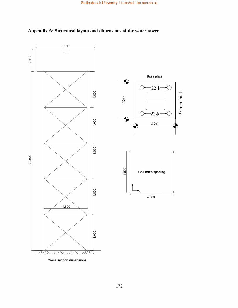
172

Appendix A: Structural layout and dimensions of the water tower

4,500

6,100

Cross section dimensions

420

22 Φ

22 Φ

Base plate

4,500

Column's spacing

y

x


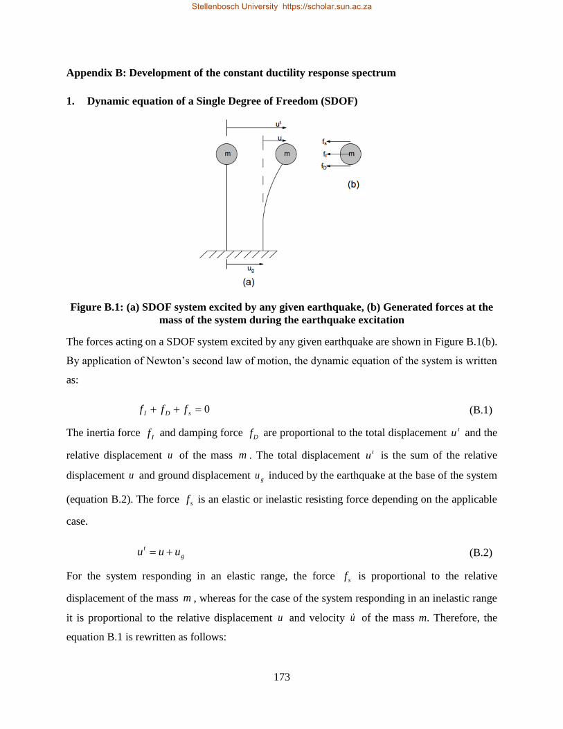
173

Appendix B: Development of the constant ductility response spectrum

1. Dynamic equation of a Single Degree of Freedom (SDOF)

Figure B.1: (a) SDOF system excited by any given earthquake, (b) Generated forces at the

mass of the system during the earthquake excitation

The forces acting on a SDOF system excited by any given earthquake are shown in Figure B.1(b).

By application of Newton’s second law of motion, the dynamic equation of the system is written

as:

0 sDI fff (B.1)

The inertia force If and damping force Df are proportional to the total displacement tu and the

relative displacement u of the mass m . The total displacement tu is the sum of the relative

displacement u and ground displacement gu induced by the earthquake at the base of the system

(equation B.2). The force sf is an elastic or inelastic resisting force depending on the applicable

case.

g

t uuu (B.2)

For the system responding in an elastic range, the force sf is proportional to the relative

displacement of the mass m , whereas for the case of the system responding in an inelastic range

it is proportional to the relative displacement u and velocity u of the mass m. Therefore, the

equation B.1 is rewritten as follows:


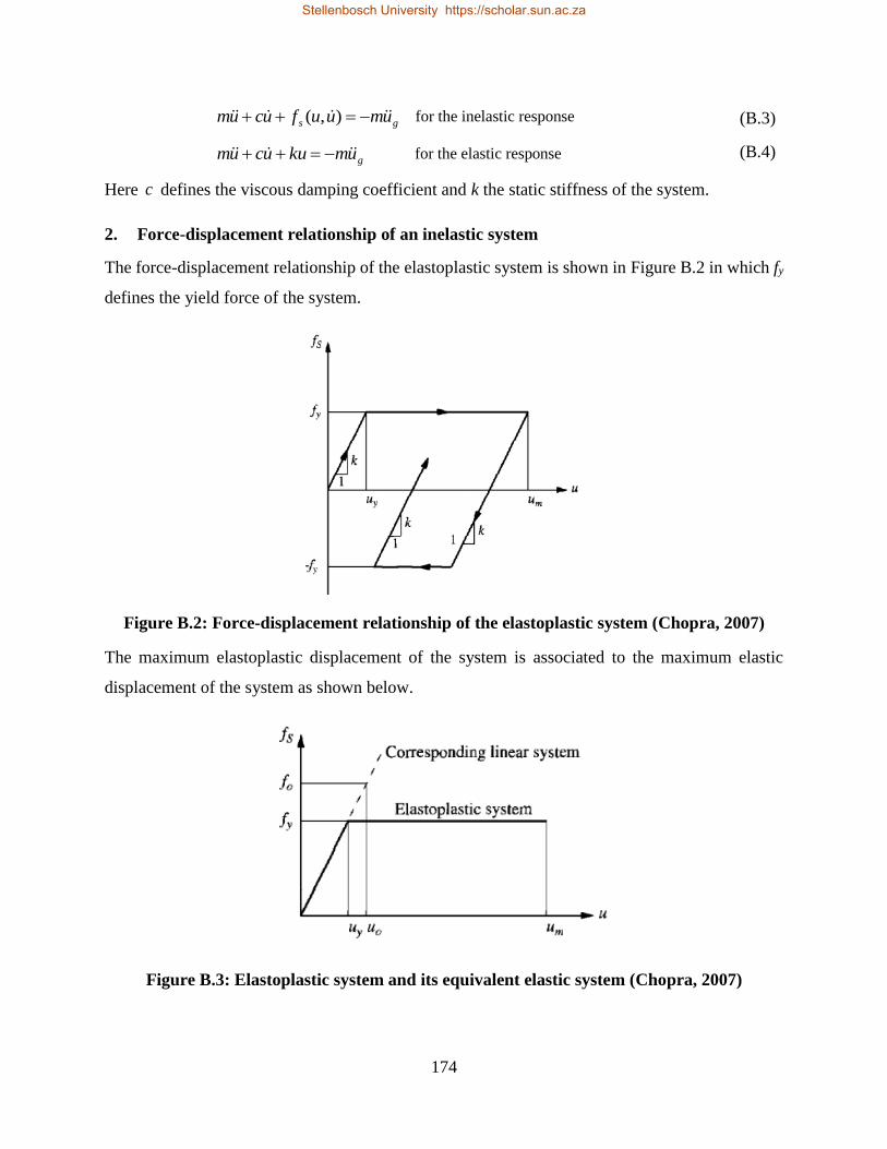
174

gs umuufucum ),( for the inelastic response (B.3)

gumkuucum for the elastic response (B.4)

Here c defines the viscous damping coefficient and k the static stiffness of the system.

2. Force-displacement relationship of an inelastic system

The force-displacement relationship of the elastoplastic system is shown in Figure B.2 in which fy

defines the yield force of the system.

Figure B.2: Force-displacement relationship of the elastoplastic system (Chopra, 2007)

The maximum elastoplastic displacement of the system is associated to the maximum elastic

displacement of the system as shown below.

Figure B.3: Elastoplastic system and its equivalent elastic system (Chopra, 2007)


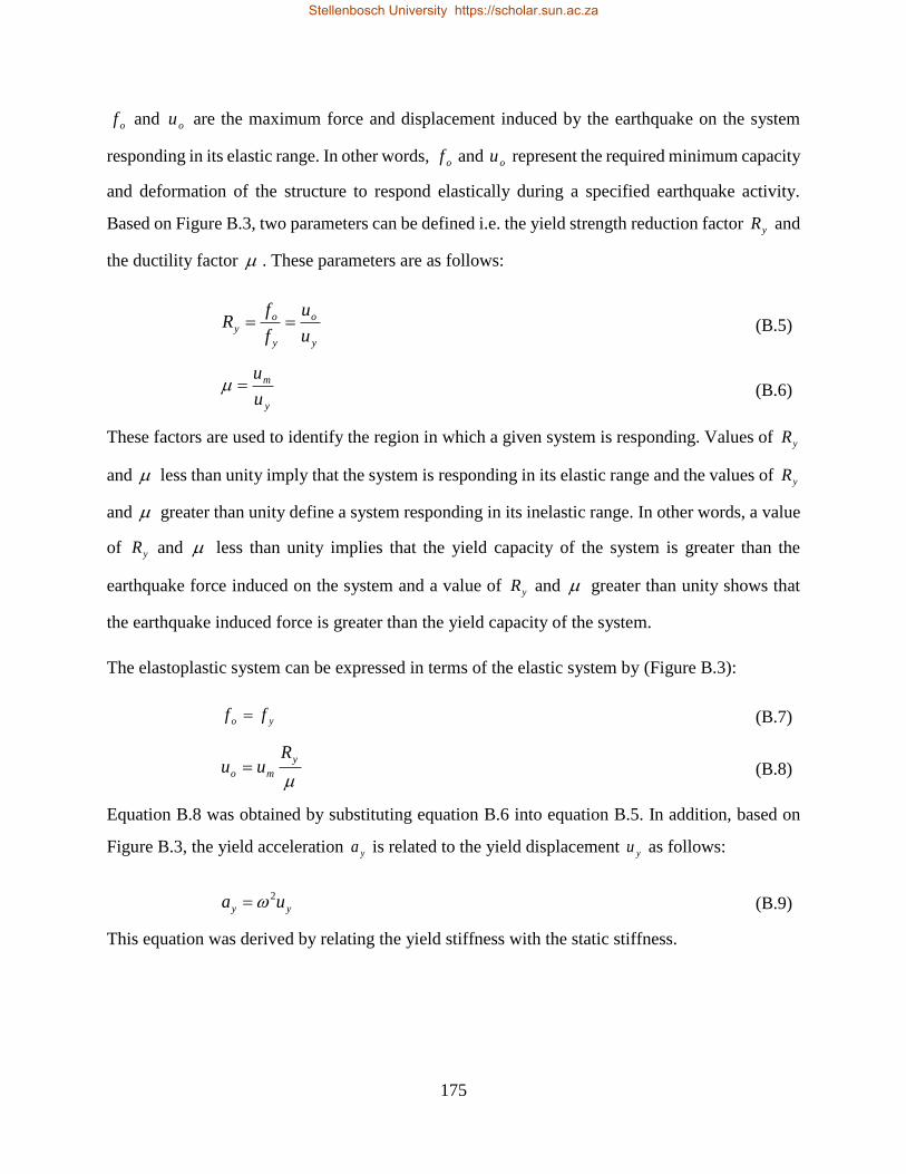
175

of and ou are the maximum force and displacement induced by the earthquake on the system

responding in its elastic range. In other words, of and ou represent the required minimum capacity

and deformation of the structure to respond elastically during a specified earthquake activity.

Based on Figure B.3, two parameters can be defined i.e. the yield strength reduction factor yR and

the ductility factor . These parameters are as follows:

y

o

y

oy

u

u

f

fR (B.5)

y

m

u

u (B.6)

These factors are used to identify the region in which a given system is responding. Values of yR

and less than unity imply that the system is responding in its elastic range and the values of yR

and greater than unity define a system responding in its inelastic range. In other words, a value

of yR and less than unity implies that the yield capacity of the system is greater than the

earthquake force induced on the system and a value of yR and greater than unity shows that

the earthquake induced force is greater than the yield capacity of the system.

The elastoplastic system can be expressed in terms of the elastic system by (Figure B.3):

yo ff (B.7)

y

mo

Ruu (B.8)

Equation B.8 was obtained by substituting equation B.6 into equation B.5. In addition, based on

Figure B.3, the yield acceleration ya is related to the yield displacement yu as follows:

yy ua 2 (B.9)

This equation was derived by relating the yield stiffness with the static stiffness.


176

3. The constant ductility response spectrum equation

Dividing equation B.3 by the mass m of the system, gives

gsynn uuufuuu ),(~

2 2 (B.10)

where

m

Kn

nm

Cξ

2 and

y

s

sf

uufuuf

),(),(

~ (B.11)

For an instant of time t , the ductility factor (equation B.6) is equal to yutut )()( . Therefore,

)()( tutu y , )()( tutu y , and )()( tutu y . By substituting these parameters into equation

B.10 and dividing by yu , it gives the constant ductility response spectrum equation (equation

B.12).

y

g

nsnna

tuf

)(),(

~2 22

(B.12)

Here mfa yy which represents the required acceleration to induce the yield force fy. With

reference to Mahin & Lin (1983), the equation B.12 is rewritten in terms of normalised yield

strength as follows:

)(

),(~

2 22tu

fg

nsnn

(B.13)

Where

PGA

ay (B.14)

PGA

tutu

g

g

)()(

(B.15)

Substitution of equation B.9 into equation B.14 gives

2

PGA

u y (B.16)

Here PGA represents the peak ground acceleration.


177

4. Development of the constant ductility response spectra

The procedures for developing the constant ductility response spectra are defined as follows

(Chopra, 2007; Mehani, 2012):

i. Identify the ground acceleration time history )(tu g of the earthquake of interest

ii. Identify and fix the damping ratio of the system for which the response spectra are going

to be plotted

iii. Identify a value for the normalised yield strength ;

iv. Determine the fundamental natural period nT of the system;

v. Evaluate the ductility response )(t of the system associated to the selected values of the

natural period nT and damping ratio of the system by numerical solution of equation

B.13. From the results, determine max , maxmax yuu , maxmax yuu , and maxmax

yuu .

The yield displacement yu is given by equation B.16;

vi. Repeat steps iv and v for a set of the natural frequency nT . From the results, various plots

can be obtained such as:

(a) ductility demand response spectrum, max against nT

(b) acceleration-displacement response spectrum, maxu against maxu ;

vii. Repeat steps iii to vi for various values of .


Documents

Seismic Performance of Steel Framed Water Tower Structures