Sea-swell interaction as a mechanism for the generation of freak waves

Sea-swell interaction as a mechanism for the generation of freak wavesA. Regev,1 Y. Agnon,1,a� M. Stiassnie,1 and O. Gramstad2

1Faculty of Civil and Environmental Engineering, Technion, Haifa 32000, Israel2Department of Mathematics, University of Oslo, P.O. Box 1053, Blindern, NO-0316 Oslo, Norway

�Received 2 January 2008; accepted 18 September 2008; published online 18 November 2008�

The probability of freak waves in an inhomogeneous ocean is studied by integration of Alber’sequation. The special phase structure of the inhomogeneous disturbance, required for instability, isprovided by bound waves, generated by the quadratic interaction of the stochastic sea with adeterministic, long swell. The probability of freak waves higher than twice the significant waveheight increases by a factor of up to 20 compared to the classical value given by Rayleigh’sdistribution. The probability of exceptionally high freak waves, with height larger than three timesthe significant wave height, is shown to increase some 30 000-fold compared to that given by theRayleigh distribution, which renders their encounter feasible. © 2008 American Institute of Physics.�DOI: 10.1063/1.3012542�

I. INTRODUCTION

Longuet–Higgins1 showed that the wave heights in awave field with a narrow spectrum, within the theory of lin-ear waves, are Rayleigh distributed. From the Rayleigh dis-tribution one can calculate that the probabilities for wavesthat are higher than twice or three times the significant waveheight are 3�10−4 and 10−8, respectively. The latter is suchan extremely rare event that it would require an unrealisticstay in a stormy area for 30 years or so to encounter theseexceptional freak waves. To encounter the former, a 10 h staymay suffice.

In recent years a few authors have used the nonlinearSchrödinger equation and its extensions, in combination withMonte Carlo simulations, to show that nonlinear interactionscan increase the frequency of freak-wave occurrence bymore than tenfold provided that the sea is very long crestedor basically unidirectional; see Ref. 2 and the referencestherein. Extensive literature surveys on freak waves can befound in Refs. 3–5.

Freak waves may be an essentially inhomogeneous phe-nomenon. They occur at isolated places and times. Thus it isof interest to study their statistics using a model for inhomo-geneous seas, namely, Alber’s6 equation. Alber’s6 equationdesigned for treating inhomogeneous wave fields, albeit withnarrow spectra, was used by him and others to study theinstability of homogeneous wave fields to inhomogeneousdisturbances. Alber’s6 findings are actually the stochasticcounterpart of the well-known deterministic Benjamin–Feirinstability obtained for the cubic Schrödinger equation. Thegrowth rates of the inhomogeneous instabilities are propor-tional to �2 �where � is the wave steepness�, reflecting thefact that the time scale of Alber’s6 equation is proportional to�−2. Although Abler6 did not state it specifically, the choiceof his initial small inhomogeneous disturbances discloses a

certain correlation between their phases and those of the ho-mogeneous base state.

Stiassnie et al.7 found long-time recurrent evolution ofAlber’s6 equation. They found that the instability whichleads to subsequent recurrent evolution requires specific re-lations between the phases of the inhomogeneous perturba-tion and the primary homogeneous wave field. Here we showthat such relations exist when a long, deterministic swellinteracts with a short, stochastic sea.

The theoretical background is given in Sec. II, the casesstudied are specified in Sec. III, and the stability diagram andthe recurrent solution are presented in Sec. IV. Section Vanalyzes the probability density function of wave energies,and the probability of freak waves is derived and discussedin Sec. VI. The findings are assessed and discussed in Sec.VII. The calculation of the initial disturbance and some de-tails about the numerical approach are given in AppendixesA and B.

II. THEORETICAL BACKGROUND

Alber’s6 equation for narrow-banded random surfacewaves on infinitely deep water written for one spatial dimen-sion reads

i� ��

�t+

1

2� g

k0

��

�x� −

1

4� g

k03

�2�

�r � x

= �gk05��x,r,t��x +

r

2,0,t� − ��x −

r

2,0,t� . �1�

The definition of the two-point spatial correlation ��x ,r , t� is

��x,r,t� = A�x +r

2,t�A��x −

r

2,t�� , �2�

where the angular brackets � stand for the ensemble aver-age. A�x , t� is the complex envelope of the narrow-bandedsea, related to the random free-surface elevation ��x , t� by

a�Author to whom correspondence should be addressed. Telephone:�972-4-8292489. FAX: �972-4-8228898. Electronic mail:[email protected].

PHYSICS OF FLUIDS 20, 112102 �2008�

1070-6631/2008/20�11�/112102/8/$23.00 © 2008 American Institute of Physics20, 112102-1

Downloaded 09 Feb 2010 to 132.68.226.21. Redistribution subject to AIP license or copyright; see http://pof.aip.org/pof/copyright.jsp

http://dx.doi.org/10.1063/1.3012542

http://dx.doi.org/10.1063/1.3012542

2��x,t� = A�x,t�ei�k0x−�gk0t� + � . �3�

The correlation for a homogeneous ocean at r=0 is given bythe integral of the energy spectrum

�h�r = 0� = �−�

�

S�k�dk �4�

and, thus,

�h�r = 0� � Hrms02 , �5�

where Hrms0 is the root mean square wave height of the ho-mogeneous ocean. In a similar way, based on Eq. �3.2� ofRef. 7 one can assume that for an inhomogeneous ocean,

��x,r = 0,t� � Hrms2 , �6�

where Hrms2 is a measure of the average energy density at the

point �x , t�.From Eqs. �5� and �6� one has

Hrms02

Hrms2 =

�h�r = 0��x,r = 0,t�

. �7�

The Rayleigh distribution

P�H � H� = e−�H/Hrms�2

�8�

can be rewritten as

P�H/Hrms0 � H/Hrms0� = e−��H/Hrms0��Hrms0/Hrms��2. �8��

Substituting Eq. �7� into Eq. �8�� gives that for a chosenvalue of �,

P�H/Hrms0 H/Hrms0� = exp�− � H

Hrms0�2

�h

�� . �8��

However, the probability to obtain values of � in the range�� ,�+�� is given by pdf��, which stands for the probabil-ity density function of ��x ,r=0, t�. Thus, the probability to

obtain H H throughout the spatial and temporal evolutionsof � is given by

P�H/Hrms0 � H/Hrms0� =� pdf��e−�H/Hrms0�2��h/��d� . �9�

The probability density function of ��x ,0 , t� is discussed andcalculated in Sec. V.

III. SEVEN CASE STUDIES

In the present article seven different oceanic combina-tions of sea and swell conditions are considered. The initialcondition of the sea is assumed to have a Gaussian spectrum,and the swell is assumed to be monochromatic.

The period of the long swell is Tl=18 s for all sevencases �which corresponds to the wavelength �s=505 m�, andthe amplitude of the swell, al, is taken to be 1 or 2 m.

The peak period of the shorter sea is denoted by Ts andvaries from 8 to 10 and to 12 s. The initial Gaussian spectraof the sea are given by

S�k� = 1.45soe−1.64��k − k0�/W�2, �10�

where k0 is the peak wave number of the sea, 2W is thespectral width, and 2s0 W is the total energy density. Thevalues of k0, W, s0, and a few other characteristic quantitiesare given in Table I. Note that all seven initial seas have thesame significant wave height Hs=11.3 m.

TABLE I. Different input parameters for seven case studies.

Case A1 A2 B C D E F

Swell conditions

Tl �s� Period 18 18 18 18 18 18 18

al �m� Amplitude 1 2 1 1 1 1 1

�l �m� Length 505 505 505 505 505 505 505

K �m−1� Wave number 0.0124 0.0124 0.0124 0.0124 0.0124 0.0124 0.0124

Initial sea conditions

Ts �s� Peak period 10 10 10 10 10 8 12

as �m� Amplitude 4 4 4 4 4 4 4

Hs �m� Significant height 11.3 11.3 11.3 11.3 11.3 11.3 11.3

�s �m� Length 156 156 156 156 156 100 225

k0 �m−1� Wave number 0.04 0.04 0.04 0.04 0.04 0.063 0.028

W �m−1� Spectral width 0.0032 0.0032 0.0065 0.0097 0.013 0.0158 0.0031

s0 �m3� Eq. �17� 1234 1234 617 411 309 253 1280

Nondimensional parameters

� Wave steepness 0.16 0.16 0.16 0.16 0.16 0.25 0.11

W Eq. �18� 0.5 0.5 1 1.5 2 1 1

BFI Benjamin–Feir index 1.4 1.4 0.7 0.47 0.35 0.7 0.7

K Eq. �18� 1.9 1.9 1.9 1.9 1.9 0.8 4

�I Growth rate 0.46 0.46 0.41 0.3 0.14 0.22 0

Eq. �15� 0.08 0.16 0.08 0.08 0.08 0.126 0.056

112102-2 Regev et al. Phys. Fluids 20, 112102 �2008�


IV. STABILITY DIAGRAM AND RECURRENTSOLUTIONS

The evolution of the solution of Eq. �1� has been calcu-lated numerically in Ref. 7 using the following nondimen-sional variables

� =k0

2

�2�, = �k0�x −1

2� g

k0t� ,

� = ��2�gk0�t, r = �k0r ,

where � is the steepness of the sea.In these variables Eq. �1� reduces to

i� �

� �−

1

4

�2�

� � r− �� + r/2,0� − �� − r/2,0�� = 0. �11�

The values of �� , r , �� are calculated for different initialconditions, defined as

��x,r,t = 0� = �h�r� + �1�x,r,t = 0� , �12�

where

�h�r� = �−�

�

ei�k−ko�rS�k�dk �13�

and

�1�x,r,t� = R�r�cos�Kx� . �14�

For a sea-swell interaction �see details in Appendix A�, Eq.�A7� reads

R�r� = �h� K

k0cos�Kr/2� + i sin�Kr/2�� and = 2alk0. �15�

K and k0 are the swell and sea wave numbers, respectively,and the initial homogeneous correlation is

�h�r� =1.133��

4e−��rW�2/6.45�. �16�

The governing nondimensional parameters as defined inRef. 7 are

� = ask0 = �4s0Wk0 = o�1� , �17�

�I = �I/�2�gk0, K = K/�k0, and W = W/�k0, �18�

where �I is the nondimensional growth rate.All seven cases of Table I are marked on the stability

diagram given in Fig. 1.

Cases E, B, and F are all for W=1 but for different K.Case F falls in the stable zone and no freak waves, whichresult from the swell-sea interaction, are expected for thiscase. Cases E and B are in the unstable zone, where freak-waves will emerge from the evolution. However, Stiassnieet al.7 found that unstable cases outside the shaded zone willproduce simple recurrence, whereas those in the shaded zoneproduce complex recurrence. The statistical treatment ofcases within the shaded zone is more complicated and is notconsidered in this paper.

Cases A1, B, C, and D of Table I and Fig. 1 have beenchosen in order to assess the influence of the spectral widthon the probability of freak waves. These four cases have all

the same K and . A comparison between cases A1 and A2

will enable us to assess the influence of , i.e., of the ampli-tude of the swell, see Eq. �15�. One should note the simple

relation between our W and the Benjamin–Feir index �BFI�of Janssen:8 BFI=1 /�2W.

The numerical results for the values of �m��, i.e., of the

maximum value of �� ,0 , ��, taken for a chosen � and for all

possible , are shown in Fig. 2. Note that only one typicalcycle of the recurring evolution is drawn. The numerical ap-proach is outlined in Appendix B.

Comparing case A2 to case A1, one can see that as theswell amplitude becomes larger, the recurrence period short-ens but the maximum value of � remains similar. One canalso see that as the initial spectral width becomes smaller�that is, larger growth rate and larger BFI� the maximumvalues of � get larger and the recurrence period shortens. Thenondimensional periods of the cycles drawn in Fig. 2 are 14,17.5, 19.5, 26, and 52 for A2, A1, B, C, and D, respectively.

V. THE PROBABILITY DENSITY FUNCTIONOF �„� ,0 , �…

In order to find pdf�� the following steps were taken:

First, 100 locations evenly distributed along the axis from 0

FIG. 1. Stability diagram: Isolines of the nondimensional growth rate �I fora Gaussian spectrum. Ts=8 s �triangle�, Ts=10 s �circles�, and Ts=12 s�square�.

FIG. 2. A typical cycle of the long-time recurring evolution of �m�� / �h�0�for A2 ��, A1 ��, B ��, C ��, and D ��.

112102-3 Sea-swell interaction as a mechanism Phys. Fluids 20, 112102 �2008�


to 2� / K were taken. During one recurrence cycle, � wassampled at 100 evenly distributed sampling times, so that 104

�� ,0 , �� values were used to establish pdf��. The isolinesof � / �h are plotted in Fig. 3 for the above mentioned fivedifferent cases. In these plots the values were shifted on

the axis so that the maximum values are at =0 and

=2� / K. The curves were also slightly smoothed.Second, the 10 000 values were arranged from the low-

est to the highest and divided into 100 evenly spaced incre-ments in �. The probability of each increment was calculatedas the number of elements within the increment divided by10 000. Figure 4 presents the probability density function of� / �h by a bar diagram �to ease comparison, the widths of thebins in all bar diagrams are equal� and the probability func-tion �the probability to obtain a value smaller or equal to� / �h� by the solid line for the five different cases. From Figs.3 and 4 one can see that for cases A1 and A2 many bins areactivated and that the number of active bins reduces whenthe spectral width grows.

VI. THE PROBABILITY OF FREAK WAVES

The probability function of the wave height, Eq. �9�, iscalculated on the basis of the known values of pdf�� shownin Fig. 4.

The values of the wave-height probabilities for an inho-mogeneous ocean are compared with those of the homoge-neous case given by Eq. �8�. In Fig. 5 one can see the freak-wave probability values, i.e., the probability for waves with

H�2.85Hrms0�2Hs. The inset shows the probability func-tion for the Rayleigh distribution, which corresponds to ahomogeneous sea, and the probability obtained from the cal-culation made using Alber’s6 equation for case A2. As one

can see from Fig. 5 the probability up to H�1.4Hrms0 isgreater for the Rayleigh distribution, but after the intersec-tion point the probability is greater for the results obtainedfrom Alber’s6 equation, the intersection values for cases A1,

B, C, and D are in the range H /Hrms0� �1.4,1.7�.From the results given by Fig. 5 one can draw the fol-

lowing conclusions:

FIG. 3. Isolines of �� ,0 , �� / �h�0�.



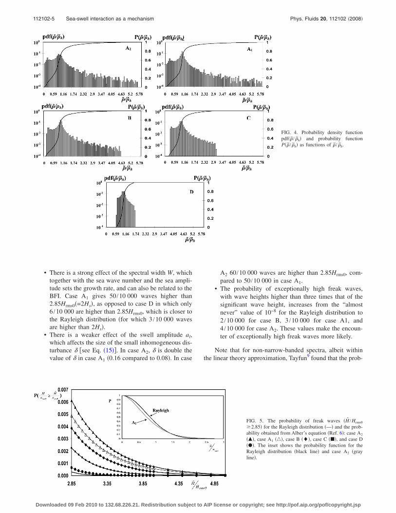
• There is a strong effect of the spectral width W, whichtogether with the sea wave number and the sea ampli-tude sets the growth rate, and can also be related to theBFI. Case A1 gives 50 /10 000 waves higher than2.85Hrms0�=2Hs�, as opposed to case D in which only6 /10 000 are higher than 2.85Hrms0, which is closer tothe Rayleigh distribution �for which 3 /10 000 wavesare higher than 2Hs�.

• There is a weaker effect of the swell amplitude al,which affects the size of the small inhomogeneous dis-turbance �see Eq. �15��. In case A2, is double thevalue of in case A1 �0.16 compared to 0.08�. In case

A2 60 /10 000 waves are higher than 2.85Hrms0, com-pared to 50 /10 000 in case A1.

• The probability of exceptionally high freak waves,with wave heights higher than three times that of thesignificant wave height, increases from the “almostnever” value of 10−8 for the Rayleigh distribution to2 /10 000 for case B, 3 /10 000 for case A1, and4 /10 000 for case A2. These values make the encoun-ter of exceptionally high freak waves more likely.

Note that for non-narrow-banded spectra, albeit withinthe linear theory approximation, Tayfun9 found that the prob-

FIG. 4. Probability density functionpdf�� / �h� and probability functionP�� / �h� as functions of � / �h.

FIG. 5. The probability of freak waves �H /Hrms0

�2.85� for the Rayleigh distribution �—� and the prob-ability obtained from Alber’s equation �Ref. 6�: case A2

��, case A1 ��, case B ��, case C ��, and case D��. The inset shows the probability function for theRayleigh distribution �black line� and case A2 �grayline�.



ability for the very high waves is overpredicted by the Ray-leigh distribution.

VII. DIRECT SIMULATION AND SUMMARY

In order to confirm the results for the probability of freakwaves, described in Sec. VI, we carried out “Monte Carlo”simulations with solutions of the nonlinear Schrödingerequations; for As, the complex wave envelopes of the sea �Ais defined in Eq. �3��:

i� �As

�t+

1

2� g

k0

�As

�x� −

g1/2

8k03/2

�2As

�x2 =g1/2k0

5/2

2�As�2As. �19�

The numerical solution of Eq. �19� was carried out using thesplit-step Fourier method used by Shemer et al.10 and by Loand Mei.11 The computation domain consisted of 512�s, andan average over 2000 realizations was taken.

Case A2 of Table I was chosen for comparison. Theprobability of freak waves, as well as the probability forexceptionally high freak waves, as a function of time is pre-sented in Fig. 6. The asymptotic probabilities for large timesof H�2Hs and H�3Hs from Fig. 6 are 120 /10 000 and4 /10 000, compared to 60 /10 000 and 5 /10 000, which wereobtained from Alber’s6 equation, respectively. We considerthis to be a fair agreement in view of the difference describedbelow.

The initial sea that we have substituted into Alber’s6

equation is strictly homogeneous, and an additional inhomo-geneous disturbance is required in order to obtain nontrivialsolutions. One could think about different physical mecha-nisms that can induce the required inhomogeneity.

In the solution that used Alber’s6 equation, the activatinginhomogeneous disturbances are provided by bound waves,which are generated through quadratic interaction of the sto-chastic sea with a deterministic swell, as explained in Appen-dix A. This is just one possible source of inhomogeneity. Analternative source is the inevitably limited number of realiza-tions in a Monte Carlo simulation.

Thus, it is not necessary to have long waves for theinhomogeneity to arise. Indeed, the swell, as such, is notinvolved in the 2000 solutions of the nonlinear Schrödingerequation �19�, which were used for the Monte Carlo simula-tion. However, using the 2000 random sets of initial

condition, one can calculate the two-point spatial correlation��x ,r , t� at t=0, see Fig. 7. From Fig. 7, it is quite clear thatthe ensemble of 2000 realizations fails to produce a homo-geneous sea, for which � must be independent of x. Thematter of fact is that a closer observation of the fine structureof the lines ��x ,r ,0��=const reveals length scales in x of the

order of about 10�s, which correspond to K�0.6. On thestability diagram, see Fig. 1, these length scales would belocated on the horizontal line w=0.5 �dashed line in the fig-ure�, well within the shaded complex recurrence zone.

Thus, it seems that the difference in the nature of theinitial inhomogeneous disturbances is the main reason for thesomewhat different results of both models.

To summarize we have the following:

• Alber’s6 equation was used to study the statistics offreak waves in a unidirectional inhomogeneous sea.The inhomogeneity arises due to the interaction of adeterministic, long swell with a stochastic, short sea.

FIG. 6. Probability of freak waves as afunction of time from Monte Carlosimulations with the nonlinearSchrödinger equation for �a� H�2Hs

and �b� exceptionally freak waves H�3Hs.

FIG. 7. Isolines of the modulus of the two-point spatial correlation of thesea at t=0 and for case A2. The ensemble average was taken over 2000realizations



• The probability of freak waves increased up to 20times �compared to the reference, Rayleigh distribu-tion� as the spectral width of the sea decreases and theamplitude of the swell increases. The probability forexceptionally high freak waves was increased by a fac-tor of about 30 000.

• The results were compared to those obtained by MonteCarlo simulations with the nonlinear Schrödingerequations.

• The more general and more common case, where thewind-wave system and the swell propagate in differentdirections, requires a much heavier numerical effortand is left for a future study.

ACKNOWLEDGMENTS

This research was supported by the Israel Science Foun-dation �Grant No. 695/04� and by the U.S.–Israel BinationalScience Foundation �Grant No. 2004-205�.

APPENDIX A: THE INITIAL DISTURBANCE

Using the notation of Secs. 14.2 and 14.3 in Ref. 12 and

assuming the coexistence of a swell with a single mode B0l

and a sea which consists of many modes Bns :

�B�k,t� = �n

Bns�k − kn

s� + B0l �k − kl�; �A1�

One can use their Eqs. �14.3.1�, �14.3.3�, and �14.2.15� to obtain the following expression for the free-surface elevation:

��x,t� =1

2��kl�

2g�B0

l ei�klx−��kl�t� + c.c� +1

2��

n��kn

s�2g

Bnsei�kn

sx−��kns �t�

+1

4�� kn

s + kl��kl��kn

s��1/2��kl��kns�

g2 ��kn

s + kl��kl��kn

s�Bn

s B0l ei��kn

s+kl�x−��kns �+��kl��t�

− ��kns�

��kl� 1/2��kns − kl��kl�

g2 1

��kl�ei��kn

s−kl�x−��kns �−��kl��t�Bn

s�B0l �� + c.c� . �A2�

The above expression includes the free modes of the swell and the sea, as well as the bound modes of their mutual interaction.

Substituting Eq. �A2� into Eqs. �2� and �3�, in Sec. II, and assuming that the sea modes Bns have random phases leads to

��x,r,0� = �n

��kns�

2g�2 �Bns �2ei�kn

s−ks�r�1 +1

2��kl�

2g�1/2

�kns + kl�B0

l eikl�x+r/2� −1

2��kl�

2g�1/2

�kns − kl��B0

l ��e−ikl�x+r/2�

+1

2��kl�

2g�1/2

�kns + kl��B0

l ��e−ikl�x−r/2� −1

2��kl�

2g�1/2

�kns − kl�B0

l eikl�x−r/2� . �A3�

From Eq. �14.5.5� in Ref. 12,

an =1

��Bn��n

2g�1/2

, al =1

��Bl�� l

2g�1/2

, �A4�

and substituting Eq. �A4� and B0l = �B0

l �ei�l into Eq. �A3� gives

��x,r,0� = �n

an2

2ei�kn

s−ks�r�1 +al

2�ei�l�kn

seikl�x+r/2� + kleikl�x+r/2�

− knseikl�x−r/2� + kleikl�x−r/2�� + e−i�l�kn

se−ikl�x−r/2�

+ kle−ikl�x−r/2� − knse−ikl�x+r/2� + kle−ikl�x+r/2�� . �A5�

Using Eq. �4� and recalling the narrowness of the sea spec-trum, which justifies replacing kn

s by ks in the curly bracketsof Eq. �A5�, gives

��x,r,0�

= �h�1 + 2alks cos�klx + �l�� kl

kscos�klr/2� + i sin�klr/2��.

�A6�

Comparing Eq. �A6� with Eqs. �12� and �14� and recognizingthat kl=K, ks=k0 results in

R�r� = �h� K

k0cos�Kr/2� + i sin�Kr/2�� ,

�A7�

= 2alk0 = 2�lk0

K.

Equation �A7� is the final result of this appendix and it isidentical to Eq. �15�, in Sec. IV, of this paper.



APPENDIX B: THE NUMERICAL APPROACH

Equation �11� was formulated as a finite differencescheme, approximating the time derivative by a forward dif-

ference and the and r derivatives by central differences:

i� ��n,j,�+1� − ��n,j,��

�� −

1

16� �r��n+1,j+1,�� − ��n−1,j+1,��

− ��n+1,j−1,�� − ��n−1,j−1,��

− ��n,j,��n+j�r/�2� �,0,�� − ��n−j�r/�2� �,0,�� = 0, �B1�

where the index n represents points along the axis, =n� ,n=0,1 ,2 , . . . ,N, and N+1 is the number of points along thisaxis. The subscript j represents points along the r axis, wherer= j�r, j=0,1 ,2 , . . . ,M, and M +1 is the number of pointsalong the r axis. � represents time steps where �=��,�=0,1 ,2 , . . ..

The numerical time stepping scheme is formulated asfollows:

��n,j,�+1� = ��n,j,�� −i��

16� �r��n+1,j+1,�� − ��n−1,j+1,��

− ��n+1,j−1,�� − ��n−1,j−1,�� − i��n,j,��

��n+j�r/�2� �,0,�� − ��n−j�r/�2� �,0,�� . �B2�

We restrict ourselves to periodic solutions in so that on the

boundary = end, ��N,j,��= ��0,j,��.The last term on the right-hand side of Eq. �B2� depends

on values of � at =n� + j�r /2 which can be larger than

end=N� . Again, the periodicity condition is used:

�� +2p� , r , ��= �� , r , ��, where p=1,2 , . . ., or ��n+pN,j,��= ��n,j,��.

The values of � along r=0 depend on points outside thedomain 0� r� rend. Specifically, the second term on theright-hand side of Eq. �B2� depends on ��n,−1,��. From the

definition of �, Eq. �2�, we see that �� ,−r , ��= �� , r , ��, soone can calculate the value of � along r=0 from the condi-tion ��n,−1,��= ��n,1,l�

� .Theoretically, the r axis extends to infinity: however, for

practical reasons, the axis must be truncated. The boundarycondition that was used for large r is given by

�� , r, �� = �� + r/2,0, �� − r/2,0, ��sin�wr�

wr. �B3�

For more details see Sec. 4.3 in Ref. 7.

1M. S. Longuet-Higgins, “On the statistical distribution of the heights ofsea waves,” J. Mar. Res. 11, 1245 �1952�.

2O. Gramstad and K. Trulsen, “Influence of crest and group length on theoccurrence of freak-waves,” J. Fluid Mech. 582, 463 �2007�.

3C. Kharif and E. Pelinovsky, “Physical mechanism of the rogue wavephenomenon,” Eur. J. Mech. B/Fluids 22, 603 �2003�.

4M. Onorato, A. R. Osborne, M. Serio, L. Cavaleri, C. Brandini, and C. T.Stansberg, “Observation of strongly non-Gaussian statistics for randomsea surface gravity waves in wave flume experiments,” Phys. Rev. E 70,067302 �2004�.

5N. Mori, M. Onorato, P. A. Janssen, A. R. Osborne, and M. Serio, “On theextreme statistics of long-crested deep water waves: Theory and experi-ments,” J. Geophys. Res. 112, C09011, DOI: 10.1029/2006JC004024�2007�.

6I. E. Alber, “The effects of randomness on the stability of two-dimensionalsurface wavetrains,” Proc. R. Soc. London, Ser. A 363, 525 �1978�.

7M. Stiassnie, A. Regev, and Y. Agnon, “Recurrent solutions of Alber’sequation for random water-wave fields,” J. Fluid Mech. 598, 245 �2008�.

8P. A. E. M. Janssen, “Nonlinear four-wave interactions and freak-waves,”J. Phys. Oceanogr. 33, 863 �2003�.

9M. A. Tayfun, “Distribution of crest-to-trough wave height,” J. Waterway,Port, Coastal, Ocean Eng. 107, 149 �1981�.

10L. Shemer, E. Kit, and H.-Y. Jiao, “An experimental and numerical studyof the spatial evolution of unidirectional nonlinear water-wave groups,”Phys. Fluids 14, 3380 �2002�.

11E. Lo and C. C. Mei, “A numerical study of water-wave modulation basedon a higher-order nonlinear Schrödinger equation,” J. Fluid Mech. 150,395 �1985�.

12C. C. Mei, M. Stiassnie, and D. K.-P. Yue, Theory and Applications ofOcean Surface Waves, Advanced Series on Ocean Engineering Vol. 23�World Scientific, Singapore, 2005�.



http://dx.doi.org/10.1017/S0022112007006507

http://dx.doi.org/10.1016/j.euromechflu.2003.09.002

http://dx.doi.org/10.1103/PhysRevE.70.067302

http://dx.doi.org/10.1029/2006JC004024

http://dx.doi.org/10.1175/1520-0485(2003)33<863:NFIAFW>2.0.CO;2

http://dx.doi.org/10.1063/1.1501908

http://dx.doi.org/10.1017/S0022112085000180

Documents

Sea-swell interaction as a mechanism for the generation of freak waves