Embed Size (px)
Citation preview

Screenkhorn: Screening Sinkhorn Algorithm forRegularized Optimal Transport
Mokhtar Z. AlayaSummer School on Applied Harmonic Analysis and Machine Learning
Genoa, September 9-13, 2019
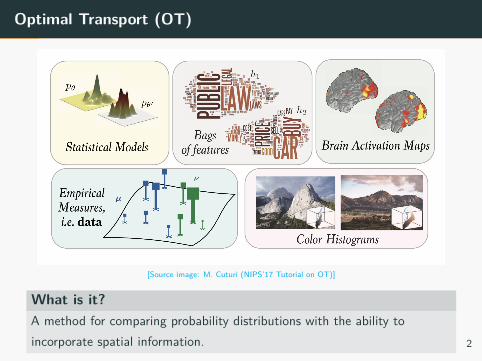
Optimal Transport (OT)
[Source image: M. Cuturi (NIPS’17 Tutorial on OT)]
What is it?A method for comparing probability distributions with the ability toincorporate spatial information. 2

Outline
1 Regularized Discrete-Discrete OT
2 Screenkhorn: Screened Dual of Sinkhorn Divergence
3 Theoretical Analysis and Guarantees
4 Integrating Screenkhorn into a ML pipeline
3

Regularized Discrete-Discrete OT
Regularized Discrete OT Framework: Kantorovitch’s Formula
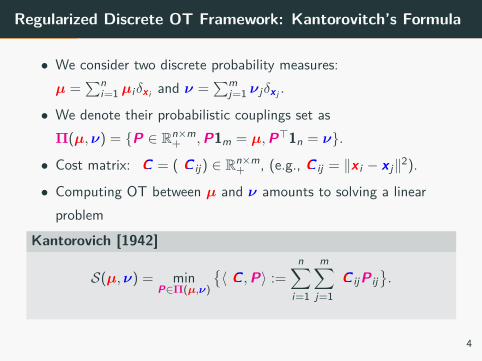
• We consider two discrete probability measures:µ =
∑ni=1 µiδx i and ν =
∑mj=1 ν jδx j .
• We denote their probabilistic couplings set asΠ(µ,ν) = {P ∈ Rn×m
+ ,P1m = µ,P⊤1n = ν}.
• Cost matrix: CC = ( CC ij) ∈ Rn×m+ , (e.g., CC ij = ∥x i − x j∥2).
• Computing OT between µ and ν amounts to solving a linearproblem
Kantorovich [1942]
S(µ,ν) = minP∈Π(µ,ν)
{⟨ CC ,P⟩ :=
n∑i=1
m∑j=1
CC ijP ij}.
4
Regularized Discrete OT Framework: Sinkhorn Divergence
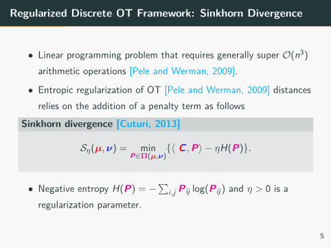
• Linear programming problem that requires generally super O(n3)
arithmetic operations [Pele and Werman, 2009].
• Entropic regularization of OT [Pele and Werman, 2009] distancesrelies on the addition of a penalty term as follows
Sinkhorn divergence [Cuturi, 2013]
Sη(µ,ν) = minP∈Π(µ,ν)
{⟨ CC ,P⟩ − ηH(P)}.
• Negative entropy H(P) = −∑
i ,j P ij log(P ij) and η > 0 is aregularization parameter.
5
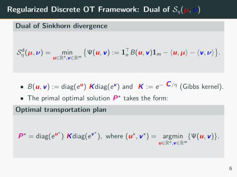
Regularized Discrete OT Framework: Dual of Sη(µ,ν)
Dual of Sinkhorn divergence
Sdη (µ,ν) = min
u∈Rn,v∈Rm
{Ψ(u, v) := 1⊤
n B(u, v)1m − ⟨u,µ⟩ − ⟨v ,ν⟩}.
• B(u, v) := diag(eu) KKdiag(ev) and KK := e− CC/η (Gibbs kernel).• The primal optimal solution P⋆ takes the form:
Optimal transportation plan
P⋆ = diag(eu⋆) KKdiag(ev⋆
), where (u⋆, v⋆) = argminu∈Rn,v∈Rm
{Ψ(u, v)}.
6
Regularized Discrete OT Framework: Sinkhorn Algorithm
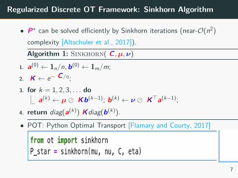
• P⋆ can be solved efficiently by Sinkhorn iterations (near-O(n2)
complexity [Altschuler et al., 2017]).Algorithm 1: Sinkhorn( CC ,µ,ν)
1. a(0) ← 1n/n,b(0) ← 1m/m;
2. KK ← e− CC/η;
3. for k = 1, 2, 3, . . . doa(k) ← µ⊘ KKb(k−1); b(k) ← ν ⊘ KK⊤a(k−1);
4. return diag(a(k)) KKdiag(b(k)).
• POT: Python Optimal Transport [Flamary and Courty, 2017]
7

Screenkhorn: Screened Dual ofSinkhorn Divergence
Screened Dual of Sinkhorn Divergence: Motivation
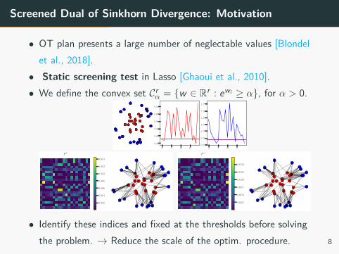
• OT plan presents a large number of neglectable values [Blondelet al., 2018].• Static screening test in Lasso [Ghaoui et al., 2010].• We define the convex set Cr
α = {w ∈ Rr : ewi ≥ α}, for α > 0.
0 5 10 15
0.02
0.04
0.06
0.08
0.10
0.12
0 5 10 150.25
0.50
0.75
1.00
1.25
1.50
1.75
P ?
0.002
0.004
0.006
0.008
0.010
0.012
0.014
P sc
0.0025
0.0050
0.0075
0.0100
0.0125
0.0150
• Identify these indices and fixed at the thresholds before solvingthe problem. → Reduce the scale of the optim. procedure. 8

Static Screening Test: Approximate Dual of Sη(µ,ν)
• Based on this idea, we define a so-called approximate dual ofSinkhorn divergence
Approximate dual of Sinkhorn divergence
Sadη (µ,ν) = min
u∈Cnεκ,v∈Cm
εκ
{Ψκ(u, v) := 1⊤
n B(u, v)1m−⟨κu,µ⟩−⟨vκ,ν⟩
}.
• This is a simply dual Sinkhorn with lower-bounded variables,where the bounds are αu = ε
κ and αv = εκ with ε > 0 and κ > 0being fixed numeric constants.
9

Static Screening Test: Definition
• The κ-parameter plays a role of scaling factor→ closed order of the potential components eu and ev .• Without κ, the components eu and ev can have inversely related
scale that may lead in, for instance, eu being too large and ev
being too small.• The static screening test aims at locating two subsets of indices(I, J) in {1, . . . , n} × {1, . . . ,m} satisfying:
Static screening test T (I, J)
(u, v) ∈ Cnαu × C
mαv ≡
eui > αu and ev j > αv , ∀(i , j) ∈ I × J ,
eui′ = αu and ev j′ = αv , ∀(i ′, j ′) ∈ I∁ × J∁.
10

Static Screening Test T (Iε,κ, Jε,κ)
PropositionLet (u∗, v∗) be an optimal solution of Sad
η (µ,ν). DefineIε,κ =
{i = 1, . . . , n : µi ≥ ε2
κ ri( KK)}
andJε,κ =
{j = 1, . . . ,m : ν j ≥ κε2cj( KK)
}. Then one has eu∗i = ε
κ andev∗j = εκ for all i ∈ I∁ε,κ and j ∈ J∁
ε,κ.
• The parameters ε and κ are difficult to interpret, we exhibit theirrelations with a fixed number budget of points from the supportsof µ and ν.
11

Screening with a Fixed Number Budget of Points
• We denote by nb ∈ {1, . . . , n} and mb ∈ {1, . . . ,m} the numberof points that are going to be optimized in Sad
η (µ,ν).
• Let ξ ∈ Rn and ζ ∈ Rm to be the ordered decreasing vectors ofµ⊘ r( KK) and ν ⊘ c( KK) respectively.
• To keep only nb-budget and mb-budget of points, the parametersκ and ε satisfy ε2
κ = ξnb and ε2κ = ζmb . Then
ε = (ξnbζmb)1/4 and κ =
√ζmb
ξnb
.
• This guarantees that |Iε,κ| = nb and |Jε,κ| = mb.
12

Screening with a Fixed Number Budget of Points
• Any solution (u∗, v∗) of Sadη (µ,ν) satisfies T (Iε,κ, Jε,κ) with
αu∗ =εκ and αv∗ = εκ.
• We can restrict the variables in Sadη (µ,ν) to variables in Iε,κ and
Jε,κ.
• This boils down to restricting the constraints feasibility Cnεκ∩ Cm
εκ
to the screened domain defined by U sc ∩ Vsc, where
Screened feasibility domain
U sc = {u ∈ Rnb : eui ≥ ε
κ} and Vsc = {v ∈ Rmb : ev j ≥ εκ}.
13

Screening with a Fixed Number Budget of Points
• By replacing in Sadη (µ,ν), the variables belonging to (I∁ε,κ × J∁
ε,κ)
by εκ and εκ, we derive the screened dual of Sinkhorn divergence
problem asScreened dual of Sinkhorn divergence
Sscdη (µ,ν) = min
u∈U sc,v∈Vsc{Ψε,κ(u, v)}
where
Ψε,κ(u, v) := (euIε,κ )⊤ KK (Iε,κ,Jε,κ)evJε,κ + εκ(euIε,κ )⊤ KK (Iε,κ,J∁
ε,κ)1mb +
εκ1⊤
nbKK (I∁ε,κ,Jε,κ)
evJε,κ − κµ⊤Iε,κuIε,κ − κ−1ν⊤
Jε,κvJε,κ
+ Ξ
with Ξ =
ε2 ∑i∈I∁ε,κ,j∈J∁
ε,κKK ij − κ log(εκ−1)
∑i∈I∁ε,κ
µi − κ−1 log(εκ)∑
j∈J∁ε,κ
ν j . 14

L-BFGS-B: Box Constraints on (usc, v sc)
Sscdη (µ,ν) uses only the restricted parts KK (Iε,κ,Jε,κ), KK (Iε,κ,J∁
ε,κ), and
KK (I∁ε,κ,Jε,κ)of the Gibbs kernel KK for calculating the objective
function Ψε,κ.
Proposition 1Let (usc, v sc) be an optimal pair solution of the screened dual Sscd
η (µ,ν)
and KKmin = mini∈Iε,κ,j∈Jε,κ KK ij . Then, one has
ε
κ∨
mini∈Iε,κ µi
ε(m −mb) + ε ∨ maxj∈Jε,κ ν j
nεκ KKminmb≤ eusc
i ≤ ε
κ∨
maxi∈Iε,κ µi
mε KKmin,
εκ ∨minj∈Jε,κ ν j
ε(n − nb) + ε ∨ κmaxi∈Iε,κ µi
mε KKminnb≤ ev sc
j ≤ εκ ∨maxj∈Jε,κ ν j
nε KKmin
for all i ∈ Iε,κ and j ∈ Jε,κ.
15

Screenkhorn
Algorithm 2: Screenkhorn( CC , η,µ,ν, nb,mb)
1. KK ← e− CC/η ;2. ξ← sort(µ⊘ r( KK)), ζ ← sort(ν ⊘ c( KK)); //(decreasing order)3. ε← (ξnb ζmb )
1/4, κ←√
ζmb /ξnb ;
4. Iε,κ ← {i = 1, . . . , n : µi ≥ ε2κ−1ri ( KK)};5. Jε,κ ← {j = 1, . . . , m : ν j ≥ ε2κcj ( KK)};6. KKmin = minIε,κ,Jε,κ KK ij ;7. µ← mini∈Iε,κ µi , µ← maxi∈Iε,κ µi ; ν ← minj∈Jε,κ µi , ν ← maxj∈Jε,κ µi ;8. u ← log
( εκ∨
µ
ε(m−mb )+ε∨ νnεκ KKmin
mb
), u ← log
( εκ∨ µ
mε KKmin
);
9. v ← log(εκ ∨ ν
ε(n−nb )+ε∨ κµmε KKmin
nb
), v ← log
(εκ ∨ ν
nε KKmin
);
10. θθ ← stack(u1nb , v1mb ), θθ ← stack(u1nb , v1mb );
Step 1: Screening
11. u(0) ← log(εκ−1)1nb , v(0) ← log(εκ)1mb ;
12. θθ(0) ← stack(u(0), v(0));
13. θθ ← L-BFGS-B( θθ(0), θθ, θθ);
14. θθu ← ( θθ1, . . . , θθnb )⊤;
15. θθv ← ( θθnb+1, . . . , θθnb+mb )⊤;
Step 2: L-BFGS-B (SciPy Library)
16. usci ← ( θθu)i if i ∈ Iε,κ and usc
i ← log(εκ−1) if i ∈ I∁ε,κ;
17. vscj ← ( θθv )j if j ∈ Jε,κ and vsc
j ← log(εκ) if j ∈ J∁ε,κ;
18. return B(usc, vsc).
16

Theoretical Guarantees
Theoretical Analysis and Guarantees
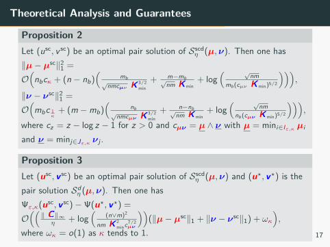
Proposition 2Let (usc, v sc) be an optimal pair solution of Sscd
η (µ,ν). Then one has∥µ− µsc∥2
1 =
O(
nbcκ + (n − nb)(
mb√nmcµν KK 3/2
min
+ m−mb√nm KKmin
+ log( √
nmmb(cµν KKmin)5/2
))),
∥ν − νsc∥21 =
O(
mbc 1κ+ (m −mb)
(nb
√nmcµν KK 3/2min
+ n−nb√nm KKmin
+ log( √
nmnb(cµν KKmin)5/2
))),
where cz = z − log z − 1 for z > 0 and cµν = µ ∧ ν with µ = mini∈Iε,κ µi
and ν = minj∈Jε,κν j .
Proposition 3Let (usc, v sc) be an optimal pair solution of Sscd
η (µ,ν) and (u⋆, v⋆) is thepair solution Sd
η (µ,ν). Then one hasΨε,κ(usc, v sc)−Ψ(u⋆, v⋆) =
O((
∥ CC∥∞η + log
((n∨m)2
nm KK 2minc7/2
µν
))(∥µ− µsc∥1 + ∥ν − νsc∥1) + ωκ
),
where ωκ = o(1) as κ tends to 1. 17
Theoretical Analysis and Guarantees: Simulation on Toy Data
1.1
1.25 2 5 10 20 50 10
0
Decimation factor n/nb
10−3
10−2
10−1
100
‖µ−µsc‖ 1
n = m =1000
η =0.1
η =0.5
η =1
η =10
1.1
1.25 2 5 10 20 50 10
0
Decimation factor mb/m
10−3
10−2
10−1
100
‖ν−νsc‖ 1
n = m =1000
η =0.1
η =0.5
η =1
η =10
1.1
1.25 2 5 10 20 50 10
0
Decimation factor n/nb
0.5
1.0
1.5
2.0
Run
ning
Tim
eG
ain
n = m =1000
η =0.1
η =0.5
η =1
η =10
1.1
1.25 2 5 10 20 50 10
0
Decimation factor n/nb
10−3
10−2
10−1
100
Rel
ativ
eD
iver
genc
eV
aria
tion
n = m =1000
η =0.1
η =0.5
η =1
η =10
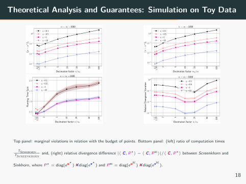
Top panel: marginal violations in relation with the budget of points. Bottom panel: (left) ratio of computation times
TSinkhornTScreenkhorn
and, (right) relative divergence difference |⟨ CC, P⋆⟩ − ⟨ CC, Psc⟩|/⟨ CC, P⋆⟩ between Screenkhorn and
Sinkhorn, where P⋆ = diag(eu⋆ ) KKdiag(ev⋆ ) and Psc = diag(eusc) KKdiag(evsc
).
18

Integrating Screenkhorn into MLPipeline: Unsupervised DomainAdaptation

Domain Adaptation Problem
[Credit image: N. Courty]
Traditional machine learning hypothesis:
• We have access to training data. Probability distribution of the training set and the testing are the same.• We want to learn a classifier that generalizes to new data. 19
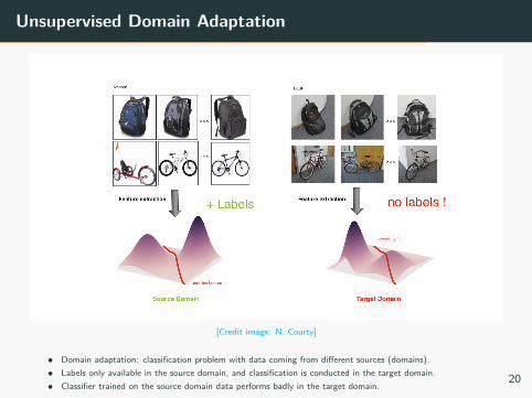
Unsupervised Domain Adaptation
[Credit image: N. Courty]
• Domain adaptation: classification problem with data coming from different sources (domains).• Labels only available in the source domain, and classification is conducted in the target domain.• Classifier trained on the source domain data performs badly in the target domain.
20

Optimal Transport Domain Adaptation [Courty et al., 2017]
Source image: [Courty et al., 2017]
Assumptions• There exist a transport T in the feature space between the two domains.• The transport preserves the conditional distributions: Ps [y|xs ] = Pt [y|T (xs )].
3-step strategy1. Estimate optimal transport between distributions.2. Transport the training samples onto the target distribution using barycentric mapping [Ferradans et al., 2013].3. Learn a classifier on the transported training samples.
21
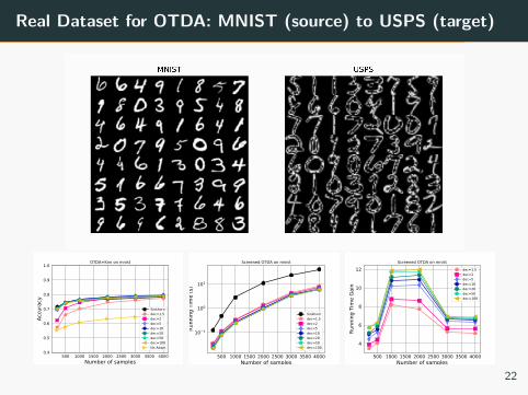
Real Dataset for OTDA: MNIST (source) to USPS (target)
500 1000 1500 2000 2500 3000 3500 4000Number of samples
0.4
0.5
0.6
0.7
0.8
0.9
1.0
Accu
racy
OTDA+Knn on mnist
Sinkhorndec=1.5dec=2dec=5dec=10dec=20dec=50dec=100No Adapt
500 1000 1500 2000 2500 3000 3500 4000Number of samples
10 1
100
101
Runn
ing
Tim
e (s
)
Screened OTDA on mnist
Sinkhorndec=1.5dec=2dec=5dec=10dec=20dec=50dec=100
500 1000 1500 2000 2500 3000 3500 4000Number of samples
4
6
8
10
12
Runn
ing
Tim
e Ga
in
Screened OTDA on mnistdec=1.5dec=2dec=5dec=10dec=20dec=50dec=100
22

Take Home Message
• We introudce a novel approach for approximating the Sinkhorndivergence based on a screening strategy with a carefullyanalyzing its optimality conditions.
• Integrated in some complex machine learning pipelines, ourScreenkhorn algorithm achieves strong gain in efficiency while notcompromising on accuracy.
23
References
References
Alaya, M. Z., M. Bérar, G. Gasso, and A. Rakotomamonjy (2019). Screening Sinkhorn algorithm for regularized optimaltransport. accepted in NeurIPS2019 .
Altschuler, J., J. Weed, and P. Rigollet (2017). Near-linear time approximation algorithms for optimal transport viasinkhorn iteration. In I. Guyon, U. V. Luxburg, S. Bengio, H. Wallach, R. Fergus, S. Vishwanathan, and R. Garnett(Eds.), Advances in Neural Information Processing Systems 30, pp. 1964–1974. Curran Associates, Inc.
Blondel, M., V. Seguy, and A. Rolet (2018, 09–11 Apr). Smooth and sparse optimal transport. In A. Storkey andF. Perez-Cruz (Eds.), Proceedings of the Twenty-First International Conference on Artificial Intelligence andStatistics, Volume 84 of Proceedings of Machine Learning Research, Playa Blanca, Lanzarote, Canary Islands, pp.880–889. PMLR.
Courty, N., R. Flamary, D. Tuia, and A. Rakotomamonjy (2017). Optimal transport for domain adaptation. IEEEtransactions on pattern analysis and machine intelligence 39(9), 1853–1865.
Cuturi, M. (2013). Sinkhorn distances: Lightspeed computation of optimal transport. In C. J. C. Burges, L. Bottou,M. Welling, Z. Ghahramani, and K. Q. Weinberger (Eds.), Advances in Neural Information Processing Systems 26,pp. 2292–2300. Curran Associates, Inc.
Ferradans, S., N. Papadakis, J. Rabin, G. Peyré, and J.-F. Aujol (2013). Regularized discrete optimal transport. InA. Kuijper, K. Bredies, T. Pock, and H. Bischof (Eds.), Scale Space and Variational Methods in Computer Vision,Berlin, Heidelberg, pp. 428–439. Springer Berlin Heidelberg.
Flamary, R. and N. Courty (2017). Pot python optimal transport library.Ghaoui, L. E., V. Viallon, and T. Rabbani (2010). Safe feature elimination in sparse supervised learning.
CoRR abs/1009.4219.Pele, O. and M. Werman (2009). Fast and robust earth mover’s distances. In 2009 IEEE 12th International Conference
on Computer Vision, pp. 460–467.24

25
Op˚tˇi‹m`a˜l T˚r`a‹n¯sfi¯p`o˘r˚t, S”w˘i¯sfi¯s A˚r‹m‹y K”n˚i˜f´e ˜f´o˘rffl D`a˚t´affl Scˇi`e›n`c´e!
Thank You!


