A shorter version of this paper appeared as: Kuhn, G..M. and K. Ojamaa, “Scores for

Connected Recognition of Words Differing in Distinctive Quantity”, IEEE Transactions

on Acoustics, Speech and Signal Processing, Vol 37, No. 7, Pgs. 1009-1019, July 1989.*

Scores for Connected Recognition of Words Differing In Distinctive Quantity

Gary M. Kuhn, Member, IEEE, and Koit Ojamaa

ABSTRACT

We report the results of experiments on talker-dependent, connected recognition of 10

Estonian words that differ in distinctive quantity. These are consonant-vowel-consonant-

vowel (CVCV) words. The words were spoken, and recognized, in sentence pairs of the

form "Did you say (word 1, word 2, word 3)? No, I said (word 4, word 5, word 6)." The

test sentences were spoken either at the same rate as the training sentences, or at a much

faster rate. Corresponding to their CVCV structure, each of the 10 words was modeled

with four, variable-duration states. Word models were trained on the slow speech, either

by averaging dynamic programming alignments to hand-marked phonetic states, or by

averaging forward-backward (hidden Markov model) alignments to gamma-weighted

states. In the first set of experiments, the likelihood of the spectral match was the only

type of factor in the recognition score; average word recognition performance at the

slower (faster) rate of speech was only 62% (52%). In the second set of experiments, the

likelihood of the spectral match was multiplied by probabilities or likelihoods of state

durations; average word recognition climbed as high as 86% (68%). In the third set of

experiments, the likelihood of the spectral match was multiplied by likelihoods of state

duration ratios; average word recognition climbed as high as 85% (77%). We conclude

that speech rate can be a major problem for automatic recognition of these words, and our

most successful attack on the problem used the product of the likelihood of the spectral

match and the likelihood of the state duration ratios as the recognition score. In these

experiments the problem was not completely overcome, even using the likelihoods of the

state duration ratios.

1. INTRODUCTION

In the field of automatic speech recognition, there is new interest in implicit [1] and

explicit [2,3] modeling of speech state durations. However, unless there is a correction

for speech rate, expected state durations may be inappropriate. In languages like Estonian

or Finnish, duration is the major acoustic correlate of the “distinctive quantity” of

consonants and vowels. In these languages, inappropriate state durations could lead to

misrecognition of a large number of words.

In this paper, we report the results of experiments on automatic recognition of 10

Estonian consonant-vowel-consonant-vowel (CVCV) words that differ in distinctive

quantity. Estonian is described as having three consonant quantities and three vowel

quantities: short, long and overlong [4,5,6,7]. Within our vocabulary of 10 Estonian

words to be recognized, 4 words participated in 2 two-way quantity contrasts: tee:de-

2

teete and kude-kuu:de; and 6 words participated in 2 three-way contrasts: toode-toote-

too:te and kade-kate-katte. We use the colon “:” to indicate extra length where the

orthography is ambiguous. The meaning of each word is listed in Appendix 1.

The organization of the paper is as follows. Section 2 explains the database and the

speech parameters. Section 3 presents modeling with variable-duration states, under both

Dynamic Programming (DP) and hidden Markov model Forward-Backward (F-B)

training. Sections 4-6 describe our expanded durations, tied spectral shapes and restricted

word order, respectively. Section 7 presents the vocabulary subsets that we call quantity

“contrast groups”. Section 8 gives a spectral match likelihood ratio that is less biased than

the spectral match probability. Section 9 gives the results for the experimental conditions

in which variable-duration states were used with a recognition score that included only

the likelihood of the spectral match.

Section 10 introduces the probabilities of state durations as a possible second factor in

the recognition score. Section 11 uses contrast groups to define likelihoods of the state

durations given the contrast groups.

Section 12 shows that the probabilities of state duration ratios should work better than

the probabilities of state durations as a second factor in the recognition score. Section 13

defines likelihoods of state duration ratios given the contrast groups.

Section 14 shows that the log of either the duration or duration ratio likelihoods is small

compared to the log of the spectral match likelihoods.

Section 15 gives the results for the experimental conditions in which the product of the

spectral match likelihood and either the probability or the likelihood, of the duration or of

the duration ratios, is used as the recognition score. Section 16 discusses the results,

Section 17 is a summary of results, and Section 18 gives our conclusions.

2. DATABASE AND SPEECH PARAMETERS

Speech was recorded while one of the authors (KO) read a prepared text. The text

consisted of a randomization of 36 occurrences of each of the 10 words, embedded in 50

repetitions of the sentence pair “Kas sa ütlesid (Did you say) ‘word 1, word 2, word 3’?

Ei, ma ütlesin (No I said) ‘word 4, word 5, word 6.’ ” The randomization was constrained

so that each word occurred 6 times in each of the 6 positions in the sentence pair.

The text was recorded 3 times. In the first two recordings, one sentence pair was spoken

every 6 seconds. In the third recording, one sentence pair was spoken every 4 seconds.

The first recording was used to train the word models, while the second and third

recordings were used for the recognition tests.

Each recording was digitized at 10000 samples/s. The digitized recordings were

parameterized in centisecond frames using a 10-channel, filter-bank spectrum analyzer

[8]. Filter center frequencies were spaced uniformly from 300 to 3000 Hz. Filter

3

bandwidths were 300 Hz for center frequencies up to 900 Hz, increasing linearly to 1000

Hz at a center frequency of 3000 Hz.

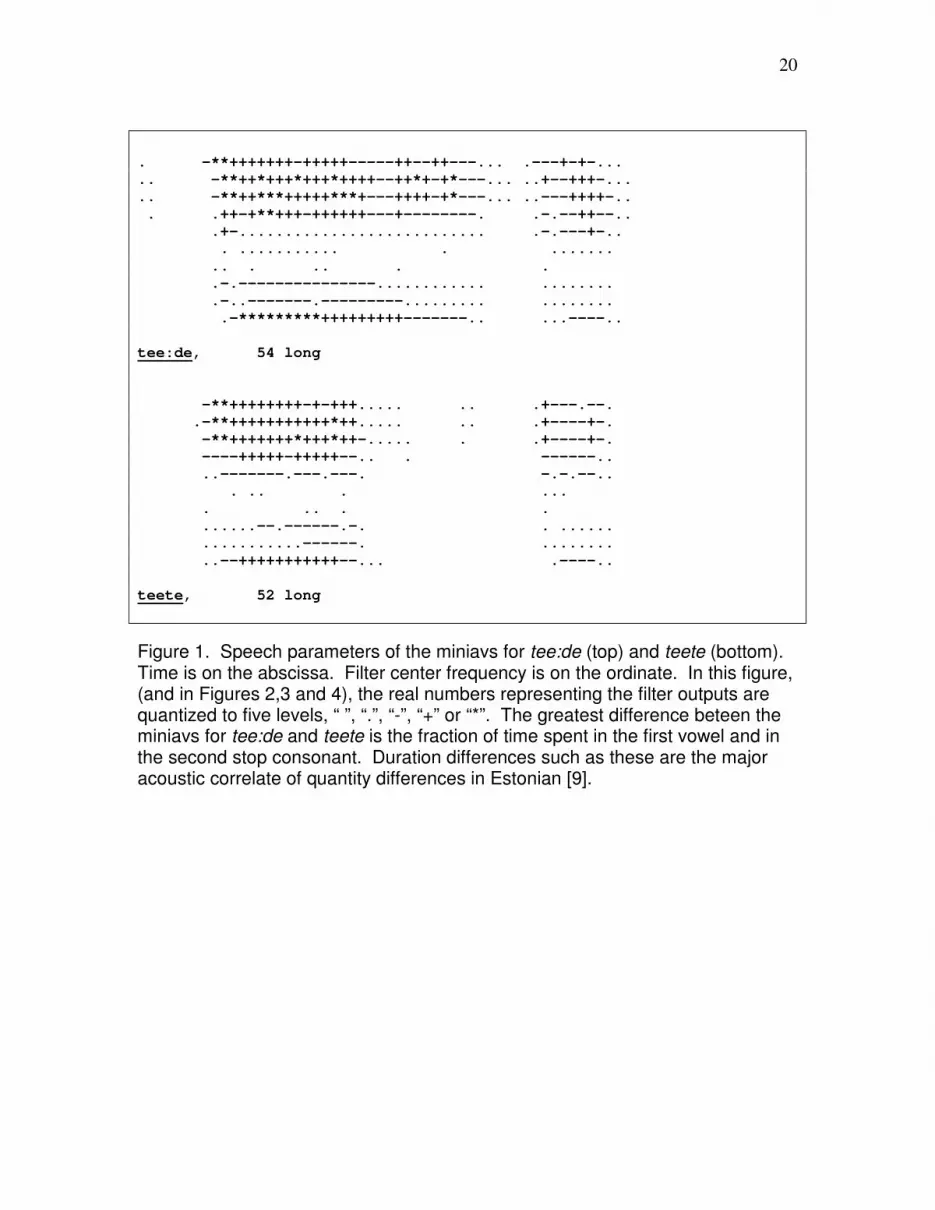
Figure 1 shows the speech parameters of the “miniavs” for tee:de (top) and teete

(bottom). The “miniav” for a word is that training production of the word which has

minimum average distance to all other training productions of the word. Time is on the

abscissa. Filter center frequency is on the ordinate. In this figure, the real numbers

representing the filter outputs are quantized to five levels, “ ”, “.”, “-”, “+” or “*”. The

greatest difference between the miniavs for tee:de and teete is the fraction of time spent

in the first vowel and in the second stop consonant. Duration differences such as these are

the major acoustic correlate of quantity differences in Estonian [9].

3. MODELING WITH VARIABLE-DURATION STATES

Our modeling used variable-duration states. We used 15 “word” models, one each for

Kas sa, ütlesid, Ei ma, ütlesin, (pause), and the 10 CVCV words. The models for ütlesid

and ütlesin had six variable-duration states. The models for (pause) and the 10 CVCV

words words had four variable-duration states.

Each variable-duration state was modeled as a sequence of three constant segments: an

initial segment of fixed duration, a center segment of variable (possibly 0) duration, and a

final segment, again of fixed duration. Our tripartite structure for a speech state was

inspired by that used in speech synthesis by rule [13], but non-constant initial and final

segments were not permitted.

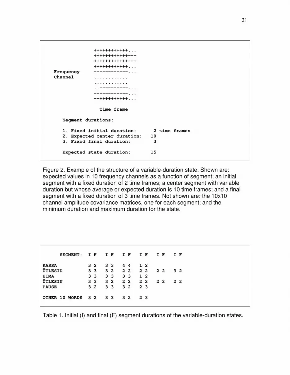
Shown in Figure 2 are: expected values in 10 frequency channels as a function of the

speech state segment; a fixed duration of 2 time frames for the initial segment; a variable

duration averaging 10 time frames for the center segment; and a fixed duration of 3 time

frames for the final segment. Not shown are the 10x10 channel amplitude covariance

matrices, one for each segment; and the minimum duration and maximum duration for

the state.

The minimum duration of a state was the sum of the durations of its initial and final

segments. Table 1 gives the duration used for the initial and final segment of each state of

each word model. An analysis of the training productions of the CVCV words indicated

that C1, V1, C2 and V2 were never shorter than 5, 6, 5 and 5 cs, respectively. Also, the

stop consonant burst was about 2 time frames long, on average. Therefore, the minimum

duration of the four states in the 10 CVCV words was set to 5, 6, 5, and 5 cs; and the

duration of the final segment of states 1 and 3 was set to 2 cs. The maximum duration of

all states was initialized to 40 time frames (40 cs).

The word models were trained using either Dynamic Programming (DP) training or

hidden Markov model “Forward-Backward” (F-B) training.

DP training used two passes through the training productions. Pass 1 started with DP

alignments [14] to the hand-marked miniav. Pass 1 alignments minimized the Euclidean

4

distance between each training production and the miniav. A mean vector and a

covariance matrix were computed over the spectra aligned to each segment of each hand-

marked state of the miniav. Pass 2 alignments maximized the probability of the training

productions given the Pass 1 segment means and covariances. Duration estimates

(minimum, average, maximum) for each state were produced from the Pass 2 alignments.

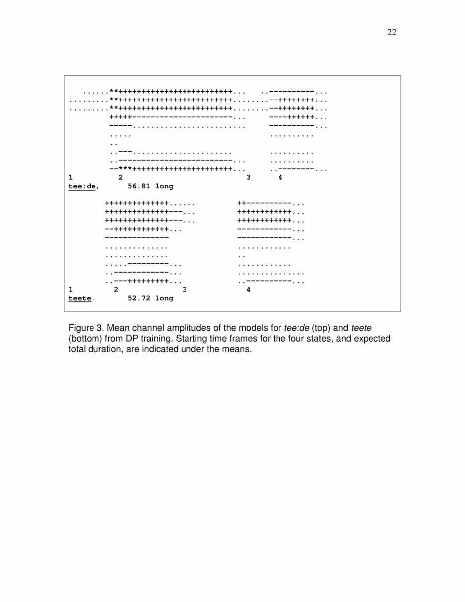
Figure 3 shows the means for the models of tee:de (top) and teete (bottom) as trained by

the two-pass DP technique. State 1 of tee:de has a three-long initial segment, a variable-

duration center segment and a two-long final segment. State 2 of tee:de has a three-long

initial segment, a variable-duration center segment, and a three-long final segment, and

so on. The states of teete also have an initial, middle and final segment structure. State 1

in both of these DP trained models is the first stop consonant, including the burst. State 2

in both cases is the first vowel. State 3 is the second stop consonant, including the burst,

and state 4 is the second vowel.

F-B training [15, 16] started by setting the mean and covariance for each segment of each

state to the overall mean and covariance of the miniav. The expected duration of each

state was set to the length of the miniav divided by S, the number of states in the word.

F-B training was allowed to continue for 10 iterations. For each training occurrence of a

word, on each iteration, the forward pass summed the probability of observations 1

through t and state i ending at time t, over all possible durations d of state i, from

αt(i) = Σd αt-d(i-1) P(d|i) P(Ot-d+1 … Ot | i) ,

and the backward pass summed the probability of the observations from time T back to

time t+1, given state i ending at time t, over all possible durations d of state i+1, from

βt(i) = Σd P(d|i+1) P(Ot+1 … Ot+d | i+1) βt+d(i+1).

Each word model transited only from state i to state i+1, so all transition probabilities

ai,i+1 were 1, and are not shown in the above equations.

βT(s) was set to 1/αT(s) at the beginning of the backward pass. P(d|i) was a duration

distribution parameterized by a discrete binomial probability density function (“pdf”).

See Section 10 below for details. P(Ot-d+1 … Ot | i) and P(Ot+1 … Ot+d | i+1) were

evaluated as the product of the probabilities of a fixed number of initial observations

under the multivariate gaussian model for the initial segment of the state, times the

product of the probabilities of the next 0 or more observations under the multivariate

gaussian model for the middle segment of the state, times the product of the probabilities

of the last fixed number of observations under the multivariate gaussian model for the

final segment of the state. A partial gamma, or posterior probability that state i occurred

with duration d at time t was computed from

γt(i,d) = αt-1(i-1) Σd P(d|i) P(Ot … Ot+d-1 | i ) βt+d-1(i) .

5

The complete gamma, or posterior probability of being in segment j of state i at time t,

was computed by summing those γt(i,d)'s for which state i was in segment j at time t. The

mean for each segment of each state was re-estimated from the normalized sum of the

gamma-weighted training vectors, and the covariance for each segment was re-estimated

from the normalized sum of the gamma-weighted training vector outer-products. Except

for the factoring of the output probabilities into three parts, one for each segment of the

state, this training is an example of the variable-duration hidden Markov model training

described in [15], or the hidden semi-Markov model training of [16].

Minimum, average and maximum state-durations were recorded on each iteration, by

tracking the last time frame in each training production for which the sum of the gammas

over the last two segments of each state was the maximum over states. We summed the

gammas over the last two segments of the state because gamma for the short final

segment by itself often was not the maximum over segments.

On successive iterations, only the new average durations were used to re-compute the

P(d|i): the minimum and maximum state-durations were kept at the sum of the durations

of the initial and final segments, and at 40 cs, respectively.

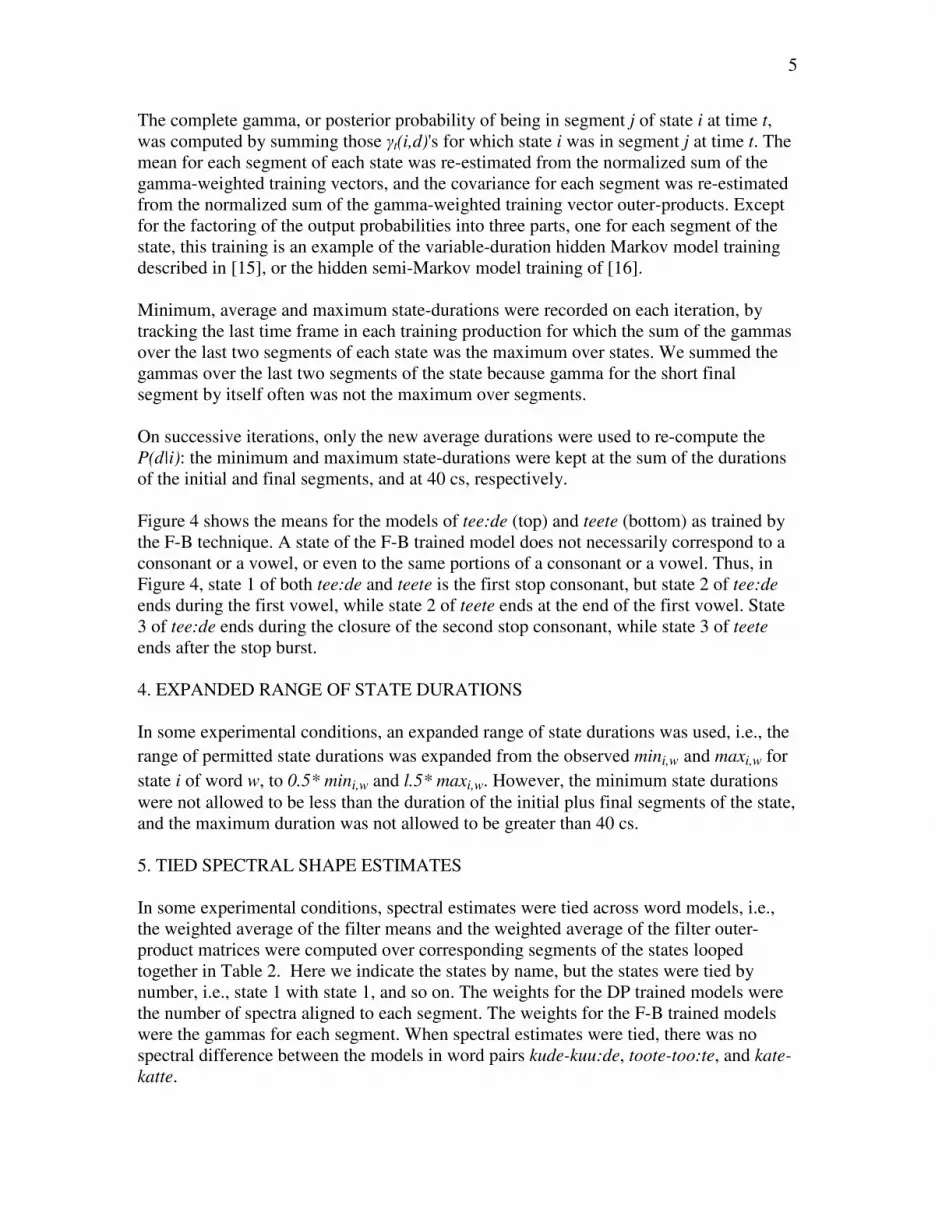
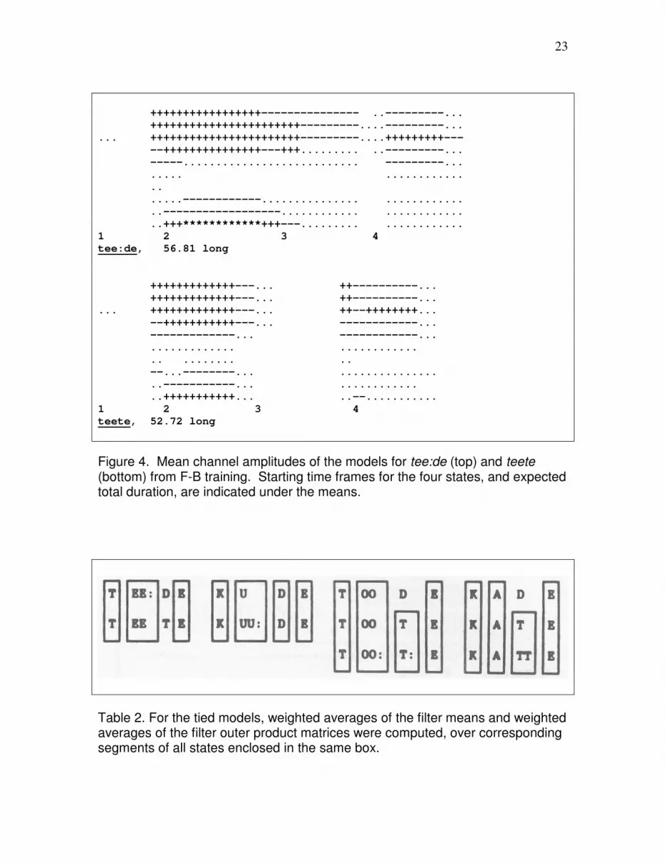
Figure 4 shows the means for the models of tee:de (top) and teete (bottom) as trained by

the F-B technique. A state of the F-B trained model does not necessarily correspond to a

consonant or a vowel, or even to the same portions of a consonant or a vowel. Thus, in

Figure 4, state 1 of both tee:de and teete is the first stop consonant, but state 2 of tee:de

ends during the first vowel, while state 2 of teete ends at the end of the first vowel. State

3 of tee:de ends during the closure of the second stop consonant, while state 3 of teete

ends after the stop burst.

4. EXPANDED RANGE OF STATE DURATIONS

In some experimental conditions, an expanded range of state durations was used, i.e., the

range of permitted state durations was expanded from the observed mini,w and maxi,w for

state i of word w, to 0.5* mini,w and l.5* maxi,w. However, the minimum state durations

were not allowed to be less than the duration of the initial plus final segments of the state,

and the maximum duration was not allowed to be greater than 40 cs.

5. TIED SPECTRAL SHAPE ESTIMATES

In some experimental conditions, spectral estimates were tied across word models, i.e.,

the weighted average of the filter means and the weighted average of the filter outer-

product matrices were computed over corresponding segments of the states looped

together in Table 2. Here we indicate the states by name, but the states were tied by

number, i.e., state 1 with state 1, and so on. The weights for the DP trained models were

the number of spectra aligned to each segment. The weights for the F-B trained models

were the gammas for each segment. When spectral estimates were tied, there was no

spectral difference between the models in word pairs kude-kuu:de, toote-too:te, and kate-

katte.

6

6. RESTRICTED WORD ORDER

In some experimental conditions, word order was restricted. With restricted word order,

Kas sa could only follow (pause); ütlesid could only follow Kas sa; Ei ma could only

follow (pause), ütlesin could only follow Ei ma; while the other 10 words and (pause)

could follow one another any number of times.

7. CONTRAST GROUPS

In some experimental conditions the recognition routines used the notion of a quantity

"contrast group". Let G(w) be the contrast group for word w, i.e., the group of words

including word w that we expected to be confusable under a pure spectral match score.

Kas sa, Ei ma and (pause) were each assigned to a one-word group. ütlesid and ütlesin

were assigned to a two-word group. The 10 CVCV words were assigned to four contrast

groups, one for each V1: /e/, /u/, /o/ or /a/.

8. LIKELIHOOD OF SPECTRAL MATCH GIVEN ALL SEGMENTS IN THE

VOCABULARY

Let P(Ot | j,i,w) be the probability of spectrum Ot under a continuous multivariate-

gaussian pdf for spectral shape in segment j of state i of word w. We wanted to know

whether a dynamic programming spectral match score of the type

max Σt log10 P(Ot | j,i,w)

is biased toward short or long words. So we used this score to find the best alignment of

each word model to each of its training productions, and for each word, recorded both the

average duration, and the average spectral match score normalized by the average

duration, i.e. the average score per unit time.

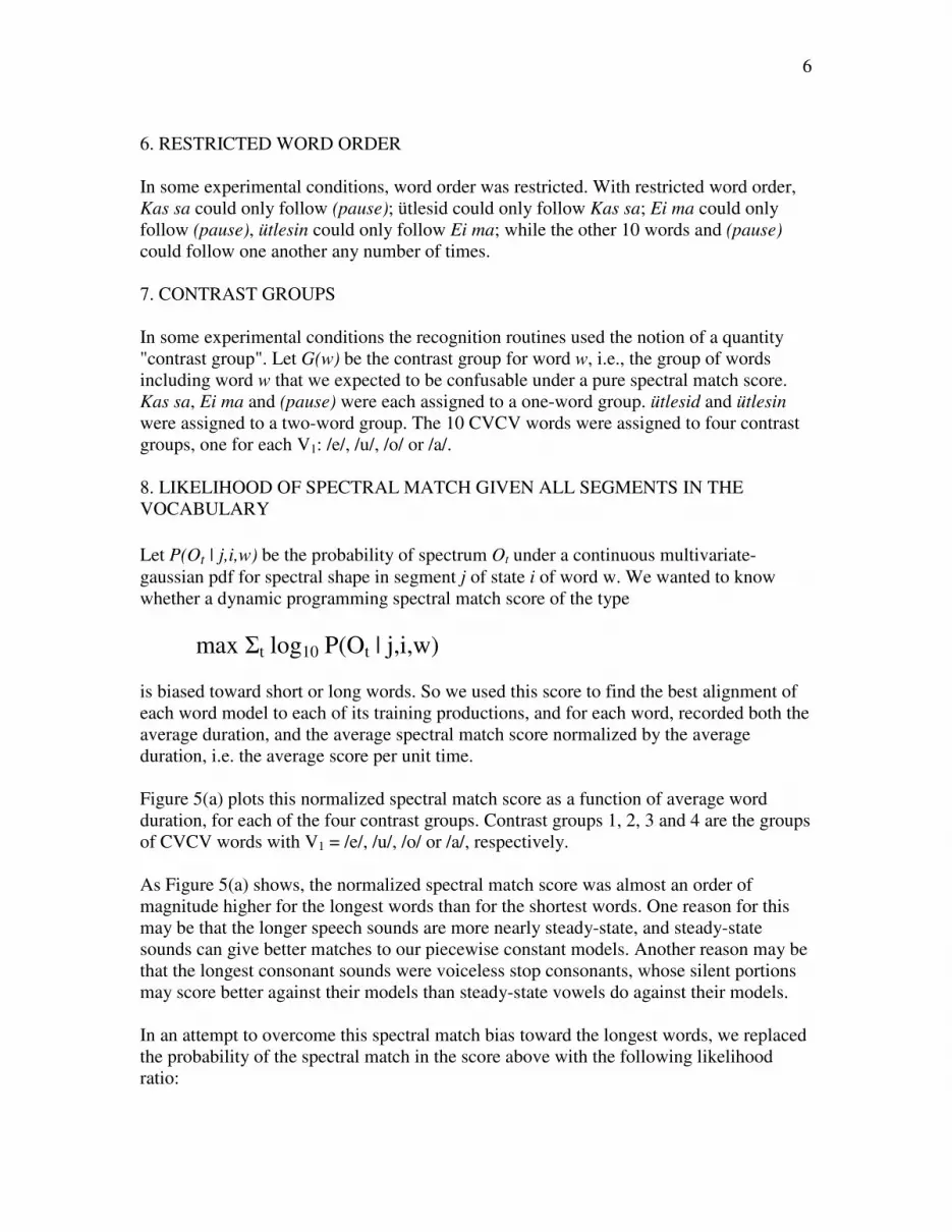
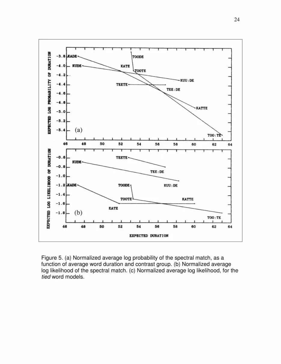
Figure 5(a) plots this normalized spectral match score as a function of average word

duration, for each of the four contrast groups. Contrast groups 1, 2, 3 and 4 are the groups

of CVCV words with V1 = /e/, /u/, /o/ or /a/, respectively.

As Figure 5(a) shows, the normalized spectral match score was almost an order of

magnitude higher for the longest words than for the shortest words. One reason for this

may be that the longer speech sounds are more nearly steady-state, and steady-state

sounds can give better matches to our piecewise constant models. Another reason may be

that the longest consonant sounds were voiceless stop consonants, whose silent portions

may score better against their models than steady-state vowels do against their models.

In an attempt to overcome this spectral match bias toward the longest words, we replaced

the probability of the spectral match in the score above with the following likelihood

ratio:

7

L(Ot | j,i,w) = P(Ot | j,i,w) / P(Ot) ,

where P(Ot) = ΣjΣiΣw P(Ot | j,i,w) . Then we used the maximum sum of the log of this

likelihood ratio to align each word model to its training productions. Now the plot of

normalized spectral match as a function of average duration showed less bias toward the

long words, as indicated in Figure 5(b). And when the spectral match likelihood ratio was

used to align each tied model to its training productions, the difference in normalized

spectral match score across contrast groups was reduced even further, as shown in Figure

5(c).

9. RESULTS WITH THE LIKELIHOOD OF THE SPECTRAL MATCH

We attempted connected recognition on the 6s/pair test recording, with a baseline system

that was limited to using the observed range of state durations, spectral models that were

not tied, unrestricted word order, and a recognition score based on the likelihood of the

spectral match. The spectral match score was computed for the DP best alignment path

through the entire recording [10,11].

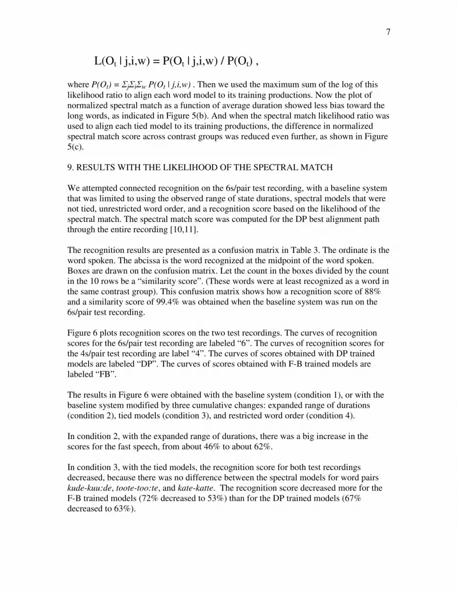
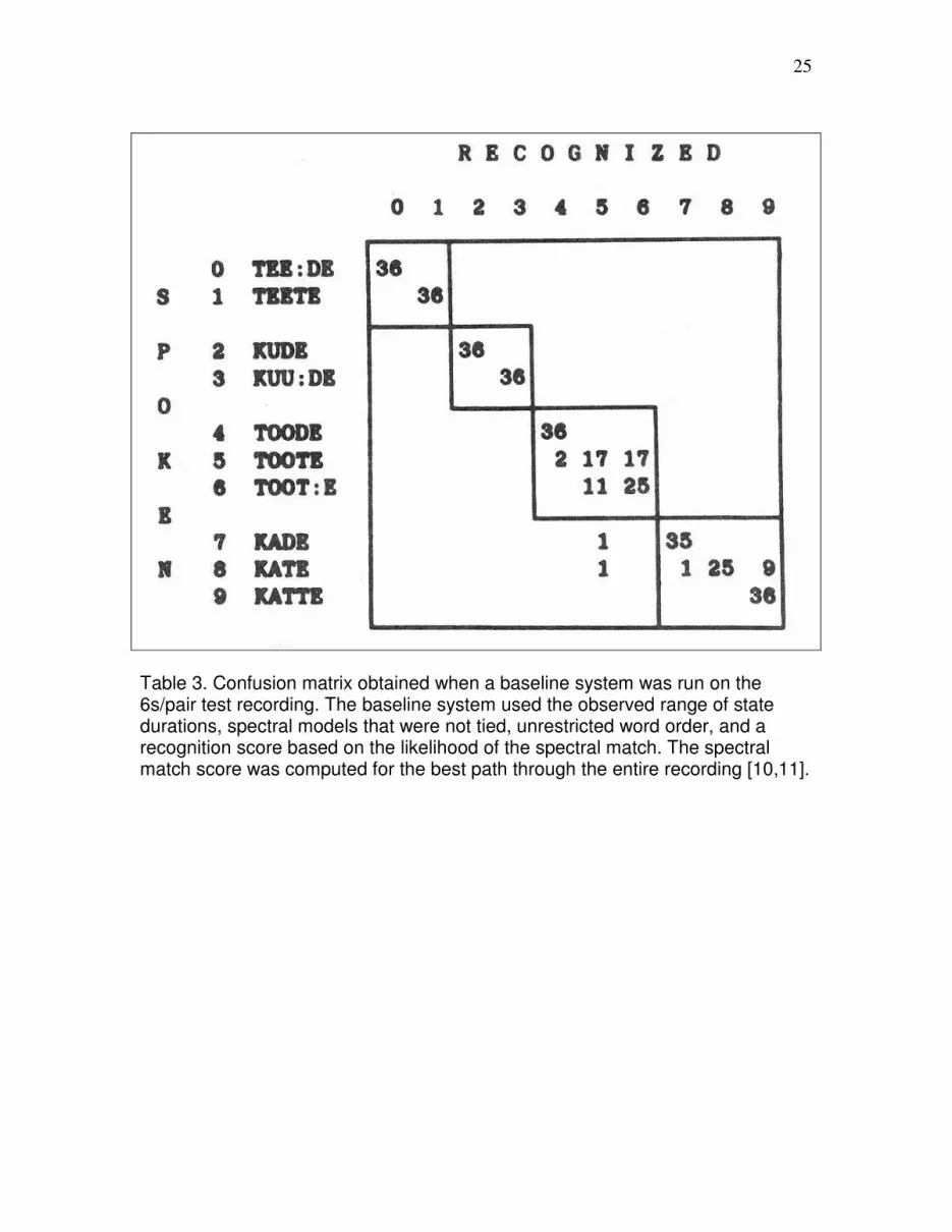
The recognition results are presented as a confusion matrix in Table 3. The ordinate is the

word spoken. The abcissa is the word recognized at the midpoint of the word spoken.

Boxes are drawn on the confusion matrix. Let the count in the boxes divided by the count

in the 10 rows be a “similarity score”. (These words were at least recognized as a word in

the same contrast group). This confusion matrix shows how a recognition score of 88%

and a similarity score of 99.4% was obtained when the baseline system was run on the

6s/pair test recording. [0]

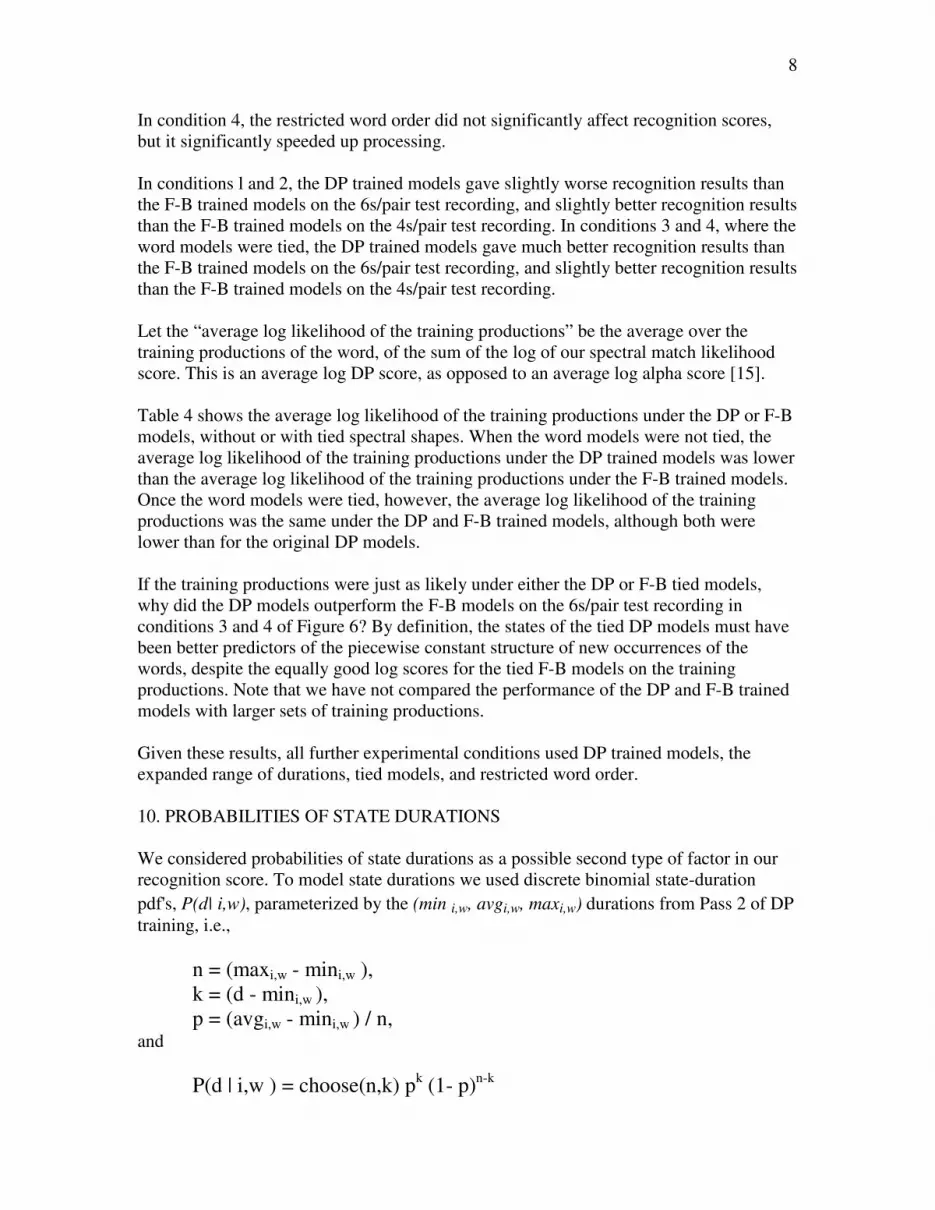
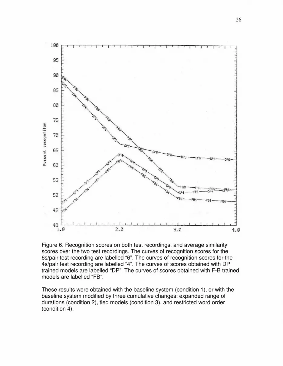
Figure 6 plots recognition scores on the two test recordings. The curves of recognition

scores for the 6s/pair test recording are labeled “6”. The curves of recognition scores for

the 4s/pair test recording are label “4”. The curves of scores obtained with DP trained

models are labeled “DP”. The curves of scores obtained with F-B trained models are

labeled “FB”. [1]

The results in Figure 6 were obtained with the baseline system (condition 1), or with the

baseline system modified by three cumulative changes: expanded range of durations

(condition 2), tied models (condition 3), and restricted word order (condition 4).

In condition 2, with the expanded range of durations, there was a big increase in the

scores for the fast speech, from about 46% to about 62%.

In condition 3, with the tied models, the recognition score for both test recordings

decreased, because there was no difference between the spectral models for word pairs

kude-kuu:de, toote-too:te, and kate-katte. The recognition score decreased more for the

F-B trained models (72% decreased to 53%) than for the DP trained models (67%

decreased to 63%).

8

In condition 4, the restricted word order did not significantly affect recognition scores,

but it significantly speeded up processing.

In conditions l and 2, the DP trained models gave slightly worse recognition results than

the F-B trained models on the 6s/pair test recording, and slightly better recognition results

than the F-B trained models on the 4s/pair test recording. In conditions 3 and 4, where the

word models were tied, the DP trained models gave much better recognition results than

the F-B trained models on the 6s/pair test recording, and slightly better recognition results

than the F-B trained models on the 4s/pair test recording.

Let the “average log likelihood of the training productions” be the average over the

training productions of the word, of the sum of the log of our spectral match likelihood

score. This is an average log DP score, as opposed to an average log alpha score [15].

Table 4 shows the average log likelihood of the training productions under the DP or F-B

models, without or with tied spectral shapes. When the word models were not tied, the

average log likelihood of the training productions under the DP trained models was lower

than the average log likelihood of the training productions under the F-B trained models.

Once the word models were tied, however, the average log likelihood of the training

productions was the same under the DP and F-B trained models, although both were

lower than for the original DP models. [2]

If the training productions were just as likely under either the DP or F-B tied models,

why did the DP models outperform the F-B models on the 6s/pair test recording in

conditions 3 and 4 of Figure 6? By definition, the states of the tied DP models must have

been better predictors of the piecewise constant structure of new occurrences of the

words, despite the equally good log scores for the tied F-B models on the training

productions. Note that we have not compared the performance of the DP and F-B trained

models with larger sets of training productions.

Given these results, all further experimental conditions used DP trained models, the

expanded range of durations, tied models, and restricted word order.

10. PROBABILITIES OF STATE DURATIONS

We considered probabilities of state durations as a possible second type of factor in our

recognition score. To model state durations we used discrete binomial state-duration

pdf's, P(d| i,w), parameterized by the (min i,w, avgi,w, maxi,w) durations from Pass 2 of DP

training, i.e.,

n = (maxi,w - mini,w ),

k = (d - mini,w ),

p = (avgi,w - mini,w ) / n, and

P(d | i,w ) = choose(n,k) pk (1- p)

n-k

9

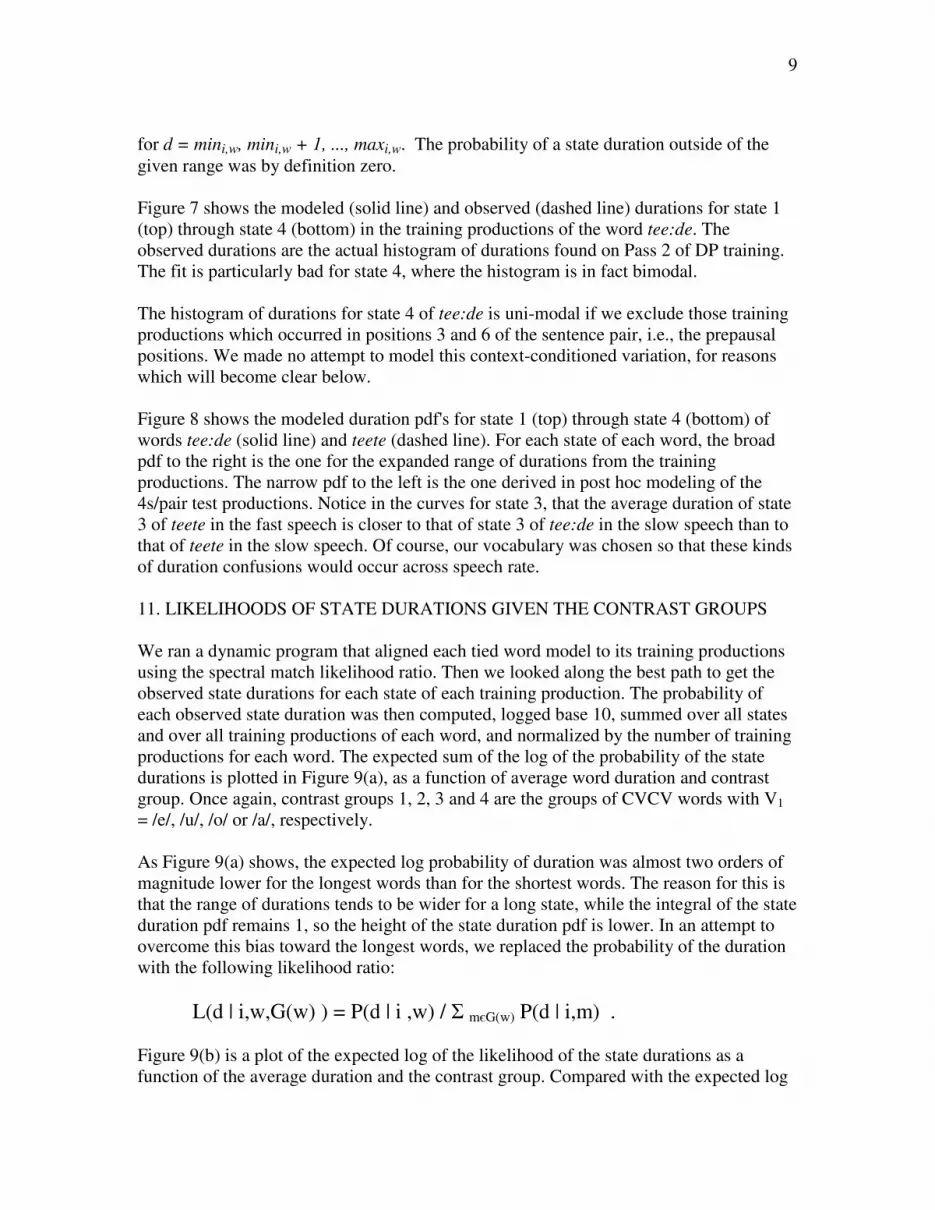
for d = mini,w, mini,w + 1, ..., maxi,w. The probability of a state duration outside of the

given range was by definition zero.

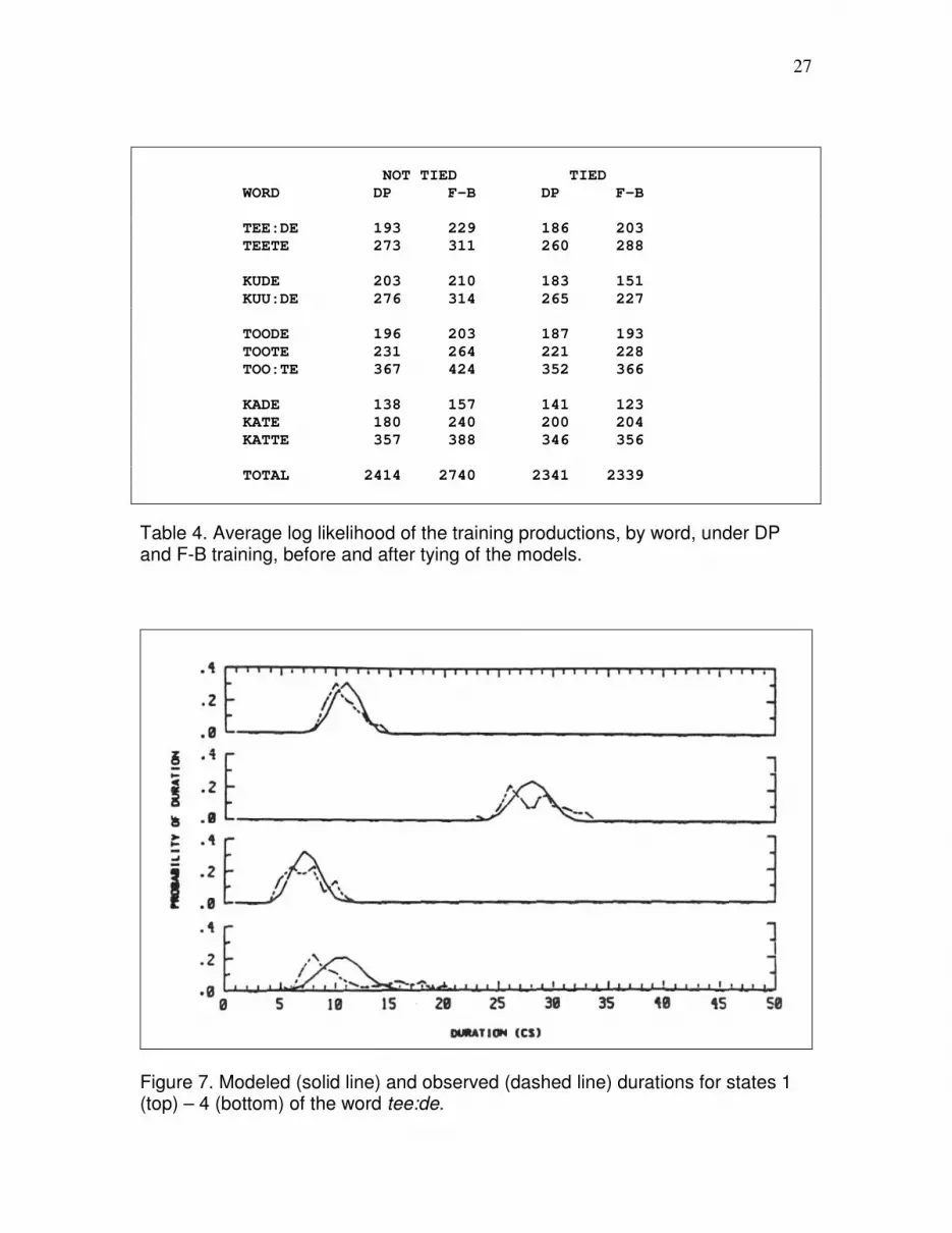
Figure 7 shows the modeled (solid line) and observed (dashed line) durations for state 1

(top) through state 4 (bottom) in the training productions of the word tee:de. The

observed durations are the actual histogram of durations found on Pass 2 of DP training.

The fit is particularly bad for state 4, where the histogram is in fact bimodal.

The histogram of durations for state 4 of tee:de is uni-modal if we exclude those training

productions which occurred in positions 3 and 6 of the sentence pair, i.e., the prepausal

positions. We made no attempt to model this context-conditioned variation, for reasons

which will become clear below.

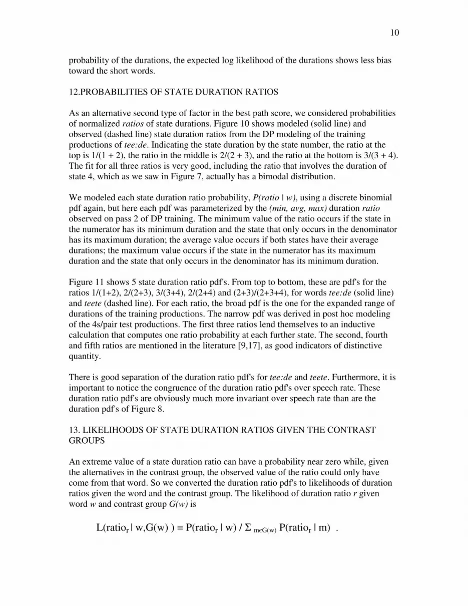
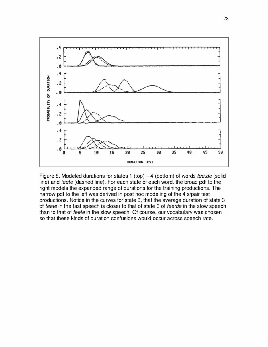
Figure 8 shows the modeled duration pdf's for state 1 (top) through state 4 (bottom) of

words tee:de (solid line) and teete (dashed line). For each state of each word, the broad

pdf to the right is the one for the expanded range of durations from the training

productions. The narrow pdf to the left is the one derived in post hoc modeling of the

4s/pair test productions. Notice in the curves for state 3, that the average duration of state

3 of teete in the fast speech is closer to that of state 3 of tee:de in the slow speech than to

that of teete in the slow speech. Of course, our vocabulary was chosen so that these kinds

of duration confusions would occur across speech rate.

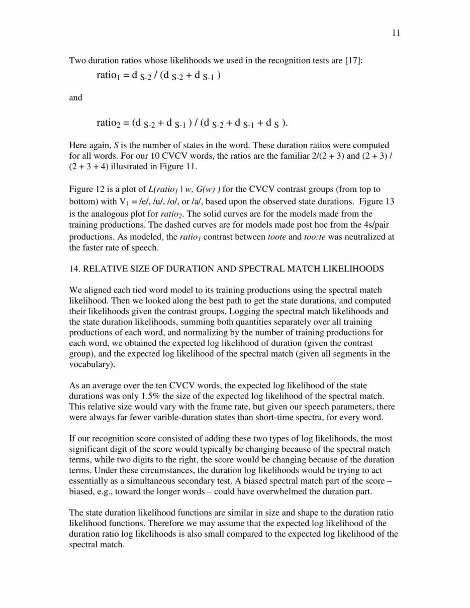
11. LIKELIHOODS OF STATE DURATIONS GIVEN THE CONTRAST GROUPS

We ran a dynamic program that aligned each tied word model to its training productions

using the spectral match likelihood ratio. Then we looked along the best path to get the

observed state durations for each state of each training production. The probability of

each observed state duration was then computed, logged base 10, summed over all states

and over all training productions of each word, and normalized by the number of training

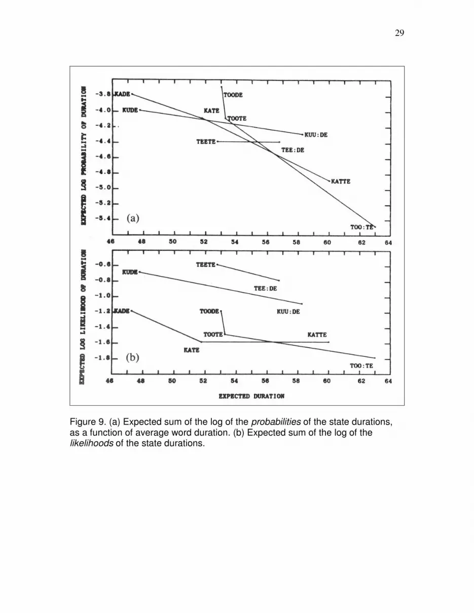
productions for each word. The expected sum of the log of the probability of the state

durations is plotted in Figure 9(a), as a function of average word duration and contrast

group. Once again, contrast groups 1, 2, 3 and 4 are the groups of CVCV words with V1

= /e/, /u/, /o/ or /a/, respectively.

As Figure 9(a) shows, the expected log probability of duration was almost two orders of

magnitude lower for the longest words than for the shortest words. The reason for this is

that the range of durations tends to be wider for a long state, while the integral of the state

duration pdf remains 1, so the height of the state duration pdf is lower. In an attempt to

overcome this bias toward the longest words, we replaced the probability of the duration

with the following likelihood ratio:

L(d | i,w,G(w) ) = P(d | i ,w) / Σ mєG(w) P(d | i,m) .

Figure 9(b) is a plot of the expected log of the likelihood of the state durations as a

function of the average duration and the contrast group. Compared with the expected log

10

probability of the durations, the expected log likelihood of the durations shows less bias

toward the short words.

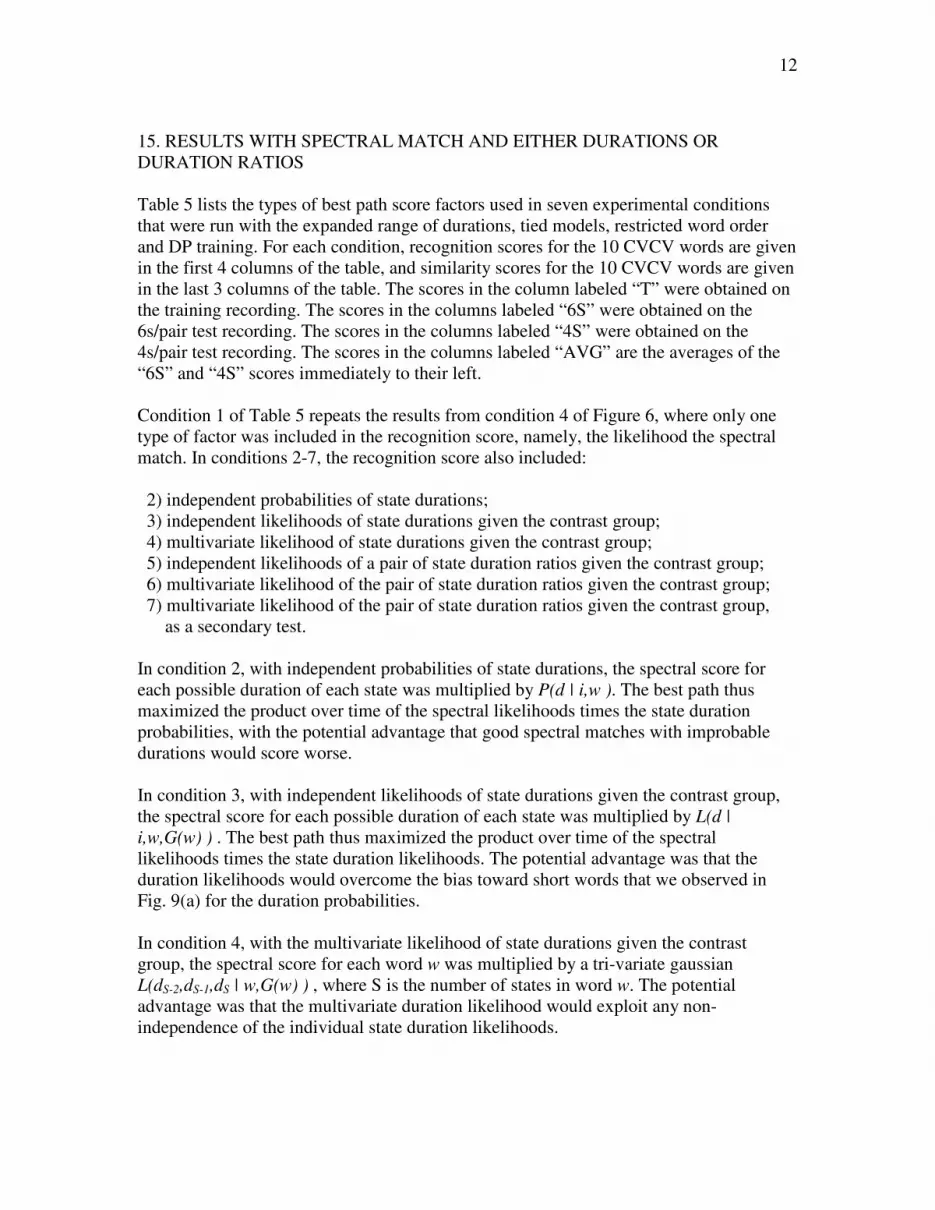
12.PROBABILITIES OF STATE DURATION RATIOS

As an alternative second type of factor in the best path score, we considered probabilities

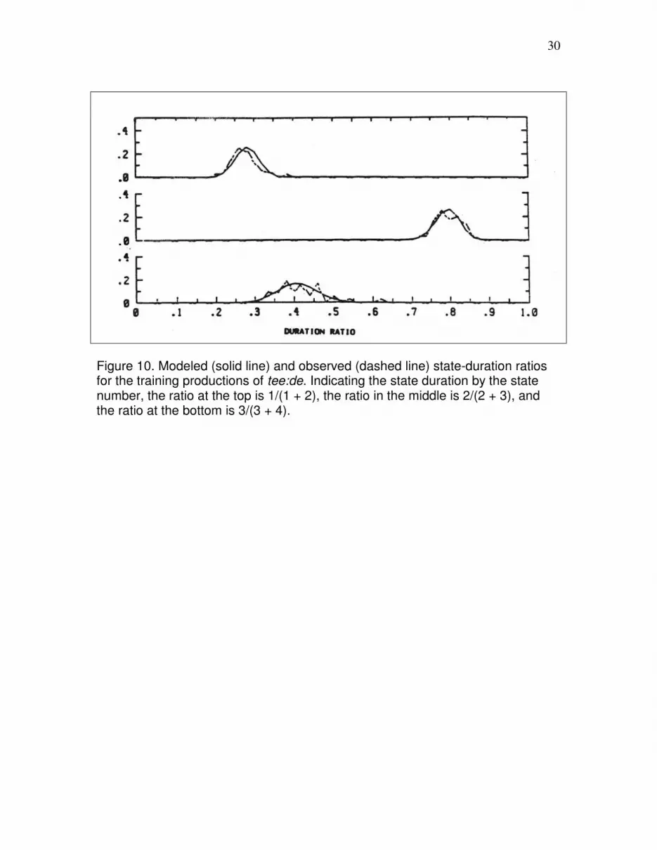
of normalized ratios of state durations. Figure 10 shows modeled (solid line) and

observed (dashed line) state duration ratios from the DP modeling of the training

productions of tee:de. Indicating the state duration by the state number, the ratio at the

top is 1/(1 + 2), the ratio in the middle is 2/(2 + 3), and the ratio at the bottom is 3/(3 + 4).

The fit for all three ratios is very good, including the ratio that involves the duration of

state 4, which as we saw in Figure 7, actually has a bimodal distribution.

We modeled each state duration ratio probability, P(ratio | w), using a discrete binomial

pdf again, but here each pdf was parameterized by the (min, avg, max) duration ratio

observed on pass 2 of DP training. The minimum value of the ratio occurs if the state in

the numerator has its minimum duration and the state that only occurs in the denominator

has its maximum duration; the average value occurs if both states have their average

durations; the maximum value occurs if the state in the numerator has its maximum

duration and the state that only occurs in the denominator has its minimum duration.

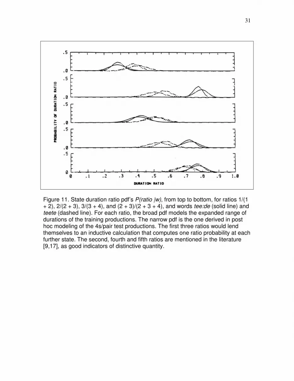
Figure 11 shows 5 state duration ratio pdf's. From top to bottom, these are pdf's for the

ratios 1/(1+2), 2/(2+3), 3/(3+4), 2/(2+4) and (2+3)/(2+3+4), for words tee:de (solid line)

and teete (dashed line). For each ratio, the broad pdf is the one for the expanded range of

durations of the training productions. The narrow pdf was derived in post hoc modeling

of the 4s/pair test productions. The first three ratios lend themselves to an inductive

calculation that computes one ratio probability at each further state. The second, fourth

and fifth ratios are mentioned in the literature [9,17], as good indicators of distinctive

quantity.

There is good separation of the duration ratio pdf's for tee:de and teete. Furthermore, it is

important to notice the congruence of the duration ratio pdf's over speech rate. These

duration ratio pdf's are obviously much more invariant over speech rate than are the

duration pdf's of Figure 8.

13. LIKELIHOODS OF STATE DURATION RATIOS GIVEN THE CONTRAST

GROUPS

An extreme value of a state duration ratio can have a probability near zero while, given

the alternatives in the contrast group, the observed value of the ratio could only have

come from that word. So we converted the duration ratio pdf's to likelihoods of duration

ratios given the word and the contrast group. The likelihood of duration ratio r given

word w and contrast group G(w) is

L(ratior | w,G(w) ) = P(ratior | w) / Σ mєG(w) P(ratior | m) .

11

Two duration ratios whose likelihoods we used in the recognition tests are [17]:

ratio1 = d S-2 / (d S-2 + d S-1 )

and

ratio2 = (d S-2 + d S-1 ) / (d S-2 + d S-1 + d S ).

Here again, S is the number of states in the word. These duration ratios were computed

for all words. For our 10 CVCV words, the ratios are the familiar 2/(2 + 3) and (2 + 3) /

(2 + 3 + 4) illustrated in Figure 11.

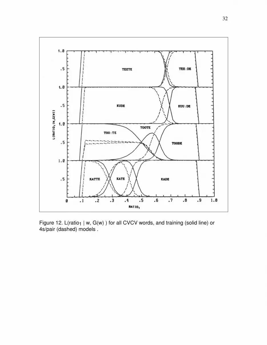
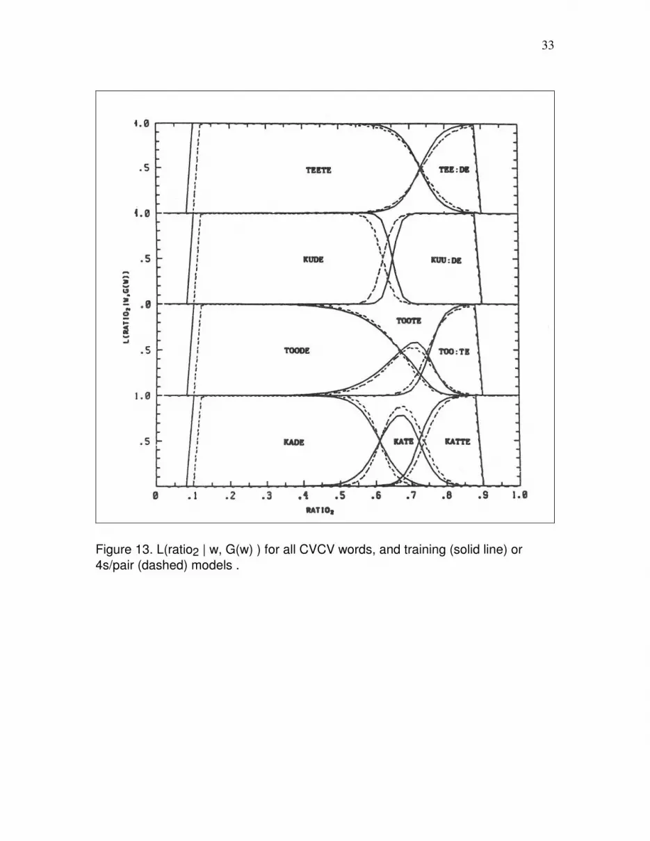
Figure 12 is a plot of L(ratio1 | w, G(w) ) for the CVCV contrast groups (from top to

bottom) with V1 = /e/, /u/, /o/, or /a/, based upon the observed state durations. Figure 13

is the analogous plot for ratio2. The solid curves are for the models made from the

training productions. The dashed curves are for models made post hoc from the 4s/pair

productions. As modeled, the ratio1 contrast between toote and too:te was neutralized at

the faster rate of speech.

14. RELATIVE SIZE OF DURATION AND SPECTRAL MATCH LIKELIHOODS

We aligned each tied word model to its training productions using the spectral match

likelihood. Then we looked along the best path to get the state durations, and computed

their likelihoods given the contrast groups. Logging the spectral match likelihoods and

the state duration likelihoods, summing both quantities separately over all training

productions of each word, and normalizing by the number of training productions for

each word, we obtained the expected log likelihood of duration (given the contrast

group), and the expected log likelihood of the spectral match (given all segments in the

vocabulary).

As an average over the ten CVCV words, the expected log likelihood of the state

durations was only 1.5% the size of the expected log likelihood of the spectral match.

This relative size would vary with the frame rate, but given our speech parameters, there

were always far fewer varible-duration states than short-time spectra, for every word.

If our recognition score consisted of adding these two types of log likelihoods, the most

significant digit of the score would typically be changing because of the spectral match

terms, while two digits to the right, the score would be changing because of the duration

terms. Under these circumstances, the duration log likelihoods would be trying to act

essentially as a simultaneous secondary test. A biased spectral match part of the score –

biased, e.g., toward the longer words – could have overwhelmed the duration part.

The state duration likelihood functions are similar in size and shape to the duration ratio

likelihood functions. Therefore we may assume that the expected log likelihood of the

duration ratio log likelihoods is also small compared to the expected log likelihood of the

spectral match.

12

15. RESULTS WITH SPECTRAL MATCH AND EITHER DURATIONS OR

DURATION RATIOS

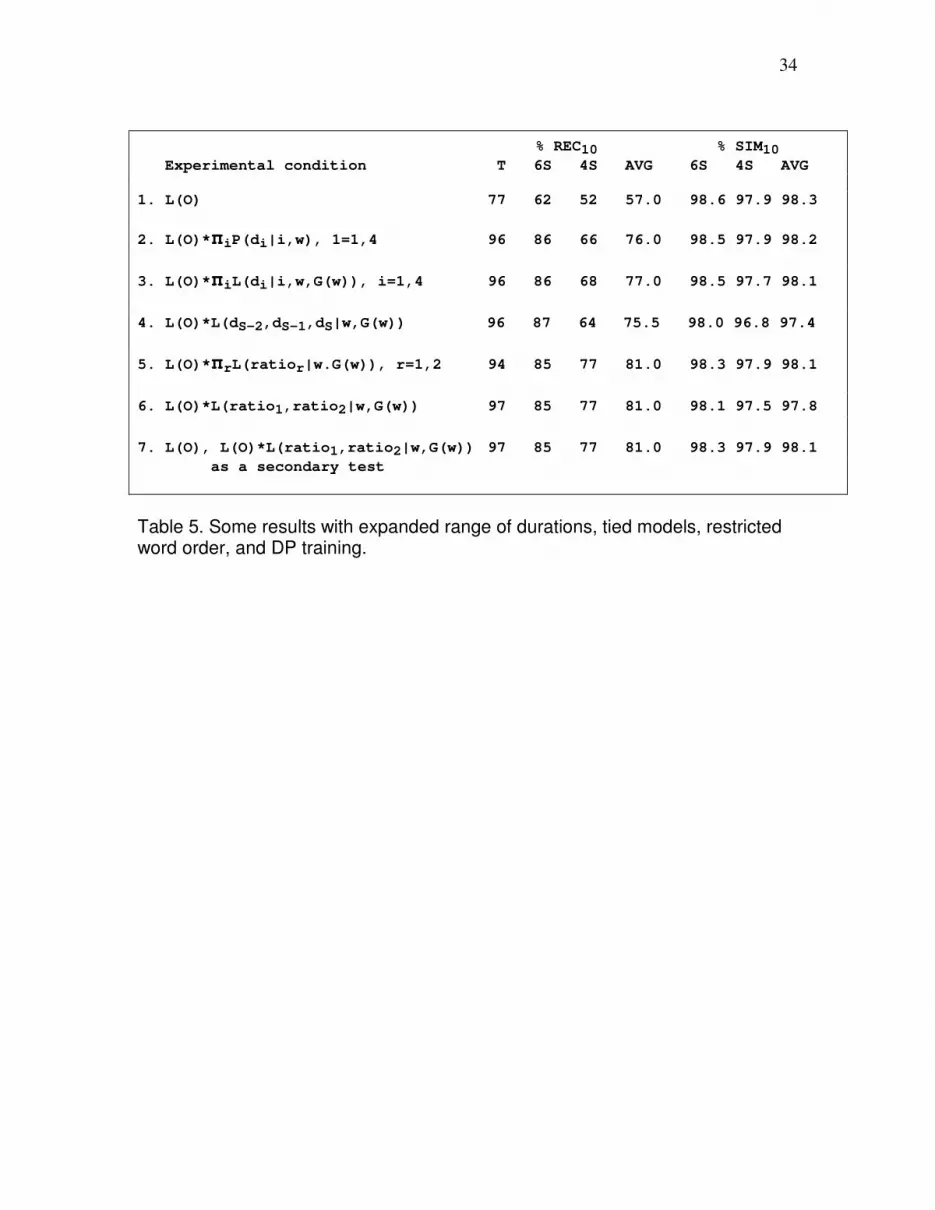
Table 5 lists the types of best path score factors used in seven experimental conditions

that were run with the expanded range of durations, tied models, restricted word order

and DP training. For each condition, recognition scores for the 10 CVCV words are given

in the first 4 columns of the table, and similarity scores for the 10 CVCV words are given

in the last 3 columns of the table. The scores in the column labeled “T” were obtained on

the training recording. The scores in the columns labeled “6S” were obtained on the

6s/pair test recording. The scores in the columns labeled “4S” were obtained on the

4s/pair test recording. The scores in the columns labeled “AVG” are the averages of the

“6S” and “4S” scores immediately to their left.

Condition 1 of Table 5 repeats the results from condition 4 of Figure 6, where only one

type of factor was included in the recognition score, namely, the likelihood the spectral

match. In conditions 2-7, the recognition score also included:

2) independent probabilities of state durations;

3) independent likelihoods of state durations given the contrast group;

4) multivariate likelihood of state durations given the contrast group;

5) independent likelihoods of a pair of state duration ratios given the contrast group;

6) multivariate likelihood of the pair of state duration ratios given the contrast group;

7) multivariate likelihood of the pair of state duration ratios given the contrast group,

as a secondary test.

In condition 2, with independent probabilities of state durations, the spectral score for

each possible duration of each state was multiplied by P(d | i,w ). The best path thus

maximized the product over time of the spectral likelihoods times the state duration

probabilities, with the potential advantage that good spectral matches with improbable

durations would score worse.

In condition 3, with independent likelihoods of state durations given the contrast group,

the spectral score for each possible duration of each state was multiplied by L(d |

i,w,G(w) ) . The best path thus maximized the product over time of the spectral

likelihoods times the state duration likelihoods. The potential advantage was that the

duration likelihoods would overcome the bias toward short words that we observed in

Fig. 9(a) for the duration probabilities.

In condition 4, with the multivariate likelihood of state durations given the contrast

group, the spectral score for each word w was multiplied by a tri-variate gaussian

L(dS-2,dS-1,dS | w,G(w) ) , where S is the number of states in word w. The potential

advantage was that the multivariate duration likelihood would exploit any non-

independence of the individual state duration likelihoods.

13

In condition 5, with independent likelihoods of a pair of state duration ratios, the spectral

score for each word w was multiplied by Πr L(ratior | w, G(w) ) , r = 1,2. The pair of

duration ratios tested [17] was

ratio1 = dS-2 / (dS-2 + dS-1 )

ratio2 = (d S-2 + d S-1) / (d S-2 + d S-1 + d S) .

These duration ratios were computed for all words. For our 10 CVCV words, these

ratios are the familiar 2/(2+3) and (2+3)/(2+3+4) illustrated in Figures 11, 12 and 13.

Remember that the expanded range of durations forced the use of the broad duration

probability pdf’s, so the slopes of the (dependent) duration ratio likelihood functions

were shallower than in Figures 12 and 13.

The best path was not guaranteed to maximize the product over time of the spectral

likelihoods times the state duration ratio likelihoods, because the best spectral path for the

last word was chosen before the two duration ratio factors were multiplied in. We

expected this to make little difference because, as we argued in Section 14, the size and

the shape of the state duration ratio likelihoods are similar to those of the state duration

likelihoods, and log of the state duration likelihoods for one of our words is on average

almost two orders of magnitude smaller than the log of its spectral likelihoods.

The potential advantage was that the state duration ratios appear to be more invariant

over speech rate than the state durations.

In condition 6, with the multivariate likelihood of the pair of state duration ratios given

the contrast group, the spectral score for each word was multiplied by a bi-variate

gaussian L(ratio1, ratio2 | w, G(w) ).

The covariance of a transformation of the state duration ratios was also computed during

pass 2 of DP training. The transformation consisted of treating the duration ratios as polar

coordinates, as follows.

We let ratio2 be the radius and ratio1 * π/2 be the angle, for reasons that are given in

Section 16 below, and then we computed the covariance of the Cartesian coordinates for

the transformed duration ratios. During recognition, the best path score through the end

of each word final state was multiplied by L(ratio1,ratio2 | w,G(w) ), i.e., by the bivariate

Gaussian probability of the transformed duration ratios normalized by the sum of these

same probabilities over the contrast group, with no modification for the expanded range

of durations. The best path was not guaranteed to maximize the product of its factors,

with the same caveats as above.

The potential advantage was the ability to model non-independence of the state duration

ratios.

14

In condition 7, with the multivariate likelihood of the pair of state duration ratios given

the contrast group as a secondary test, the spectral match score determined a word w on

the best path; the word w in turn determined the contrast group G(w); and the multivariate

likelihood of the pair of state duration ratios times the spectral match likelihood

determined the best word mєG(w) on the path.

The covariance of the transformed state duration ratios was once again available for each

word, from pass 2 of DP training. During recognition, best paths were computed using

the likelihood of the spectral match, but the choice for best path-final word at each time

frame t was modified as follows.

First, the best path-final word w determined the best contrast group G(w), and the state

durations for w were used to compute L(ratio1,ratio2|w,G(w) ) for every word mєG(w).

This is the same likelihood function of transformed duration ratios as in condition 6.

Then, in a second step, the maximum of the best path score through the end of each word

m times L(ratio1,ratio2|w,G(w) ) determined the best word m to be reported as having

terminated with w’s total duration at time frame t. The assumption was that w’s state

durations along the best path were the same as those for every word mєG(w). The best

path actually maximized just the product over time of the likelihoods of the spectral

match.

Two potential advantages were, first, that only one pair of duration ratios had to be

computed at each time frame, and second, the duration ratio factor could not knock

recognition out of the contrast group of the word with the best spectral score.

The recognition results in Table 5 form three distinct groups. The worst average result on

the test sentences, 57%, was obtained in condition 1 where the only type of factor in the

best path score was the likelihood of the spectral match.

Better average results, as high as 77%, were obtained in conditions 2, 3 and 4, where the

second type of factor in the recognition score was either the probability or the likelihood

of the state durations.

The best average results, 81%, were obtained in conditions 5, 6 and 7, where the second

type of factor was the likelihood of the state duration ratios.

Comparing the conditions with the duration factors to those with the duration ratio

factors, the results on the 6 s/pair test sentences declined only 1%, while the results on the

4 s/pair sentences improved anywhere from 9% to 11%. There were only very small

differences in results within conditions 2, 3 and 4, and within conditions 5, 6 and 7.

16. DISCUSSION

As Figure 6 and Table 5 show, the best recognition results obtained on the test words

spoken at the training (faster) rate, were 88% (64%) without probabilities or likelihoods

15

of durations or duration ratios, 87% (68%) with likelihoods of durations, and 85% (77%)

with likelihoods of duration ratios.

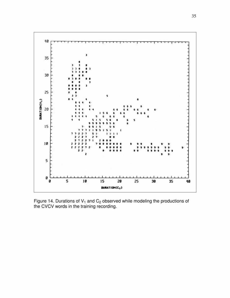
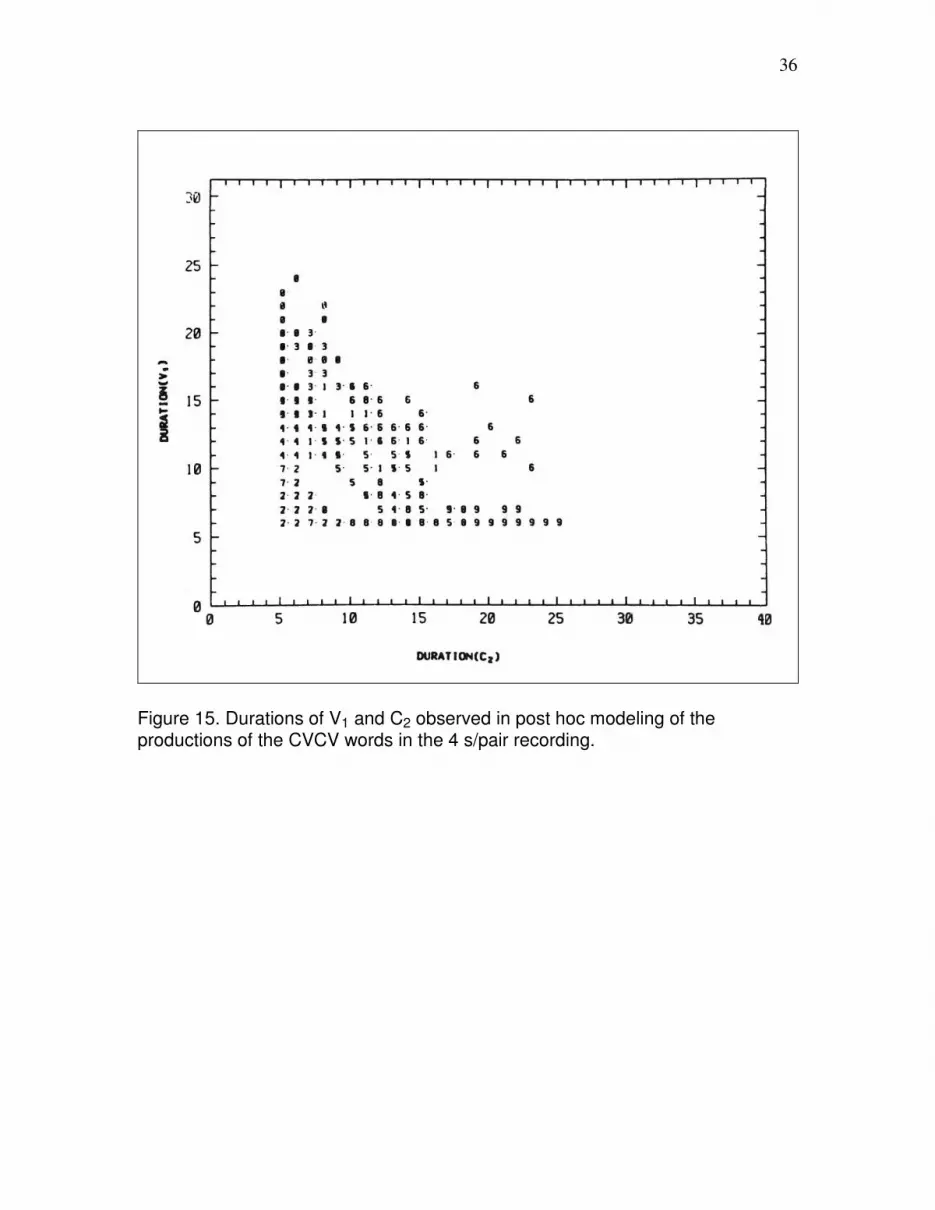
Figure 14 is a scatter plot of the values of the durations of V1 and C2 observed while

modeling the CVCV words of the training recording. Figure 15 is the analogous plot for

the 4s/pair test recording. The numbering for the CVCV words is the same as in Table 3

above. Figure 15 reveals that the minimum permitted state durations were apparently

somewhat too long for the 4s/pair recording.

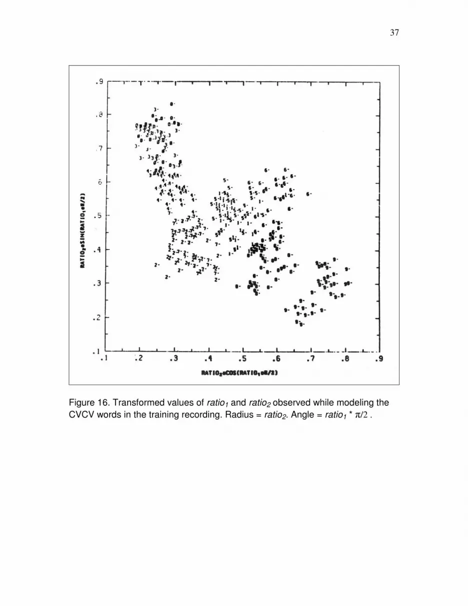
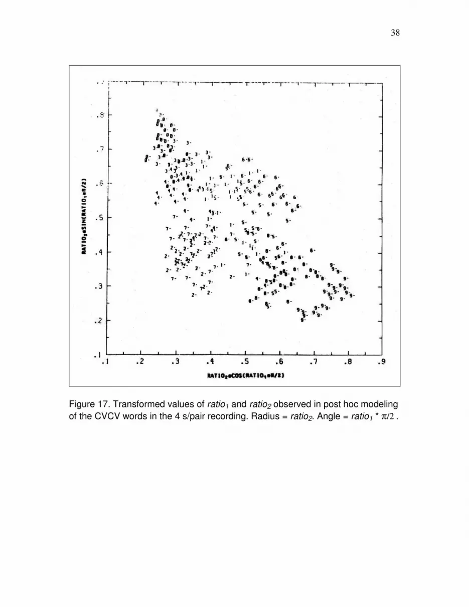
Figure 16 is a scatter plot of the values of ratio1 and ratio2 observed while modeling the

CVCV words in the training recording. Figure 17 is the analogous plot for the 4s/pair test

recording. Polar coordinates were used for these plots, i.e., the radius is ratio2, and the

angle is ratio1* π/2. Assuming independence, quantity contrast boundaries lie along radii

or along rays.

The reason for using the polar coordinates is now clear: the arrangement of the CVCV

words in duration ratio polar coordinates is so similar to their arrangement in the

traditional (and phonological) V1 and C2 duration coordinates, that the greater invariance

of the duration ratios over speech rate is easily seen.

The advantage of the state duration ratios is evident. However, the likelihoods of the state

duration ratios would have been of no use if there had been no multiword contrast groups.

There may not be any multiword contrast groups in connected recognition of a small,

phonetically dissimilar vocabulary, or in recognition of selected words from connected

speech.

Still, in these cases, state durations may help to discriminate within- from across-word

patterns, or to discriminate selected words from background speech. Probabilities of state

durations have been used as a second factor in speech recognition [16, 17, 18], but our

probabilities of state duration ratios appears to be more invariant over speech rate.

Therefore, we suspect that in the absence of multiword contrast groups, a better

alternative as a second factor in the best path score would be the probabilities of specific

state duration ratios.

With our vocabulary, we could use the likelihoods of the state duration ratios as a second

type of factor in the best path score. Nevertheless, the results on the faster speech did not

recover to the level of the results on the speech spoken at the training rate. Reasons for

this may include the fact the the shortest possible state durations were somewhat long for

the faster speech.

We emphasize that we have used a segmentation of the training productions of our

words, based on a priori knowledge, to test the discriminative power of temporal aspects

of distinctive quantity, at different speech rates.

16

17. SUMMARY

We now summarize these experiments and the most important results.

We are reporting on experiments on talker-dependent, connected recognition of 10

Estonian words that differ in distinctive quantity. The words were spoken, and

recognized, in sentence pairs of the form "Did you say (word 1, word 2, word 3)? No, I

said (word 4, word 5, word 6)." The test sentences were spoken either at the same rate as

the training sentences, or at a much faster rate.

These 10 words are consonant-vowel-consonant-vowel (CVCV) words. Four words

participate in 2 two-way quantity contrasts: tee:de-teete and kude-kuu:de; and six words

participate in 2 three-way contrasts: toode-toote-too:te and kade-kate-katte. The colon

":" indicates extra length where the orthography is ambiguous. There are 4 contrast

groups, with V1 either /e/, /u/, /o/ or /a/.

Corresponding to their CVCV structure, each word was modeled with four, variable-

duration states. To accommodate the two rates of speech, an expanded range of state

durations was used. The 4 contrast groups were used to tie spectral estimates across

states for words with identical C1, V1, C2 or V2. When spectral estimates were tied, there

was no spectral difference between the models for word pairs kude-kuu:de, toote-too:te,

and kate-katte.

The word models were trained on the slow speech, either by averaging dynamic

programming alignments to hand-marked phonetic states, or by averaging forward-

backward (hidden Markov model) alignments to gamma-weighted states. With the

expanded range of state durations and tied spectral models, the likelihood of the training

data given the word models was the same for the phonetic states and the gamma-

weighted states. But, on test data at the slow rate of speech, recognition performance was

better for the phonetic states (63%) than for the gamma-weighted states (53%). So, our

second and third sets of experiments only used modeling by dynamic programming

alignments of hand-marked phonetic states.

In the first set of experiments, the likelihood of the spectral match was the only type of

factor in the recognition score. Without probabilities or likelihoods of durations or

duration ratios in our recognition score, the wide range of durations and the tied word

models held our average recognition result over the two rates of speech down to 57%

(condition 1 of Table 5).

In the second set of experiments, the likelihood of the spectral match was multiplied by

probabilities or likelihoods of state durations. With probabilities or likelihoods of state

durations, the average recognition result climbed as high as 77% (condition 3 of Table 5).

In the third set of experiments, the likelihood of the spectral match was multiplied by

likelihoods of state duration ratios. With likelihoods of duration ratios, the average

recognition result climbed to 81% (conditions 5-7 of Table 5).

17

18. CONCLUSION

For good recognition results over the two speech rates, we allowed a ride range of state

durations. Without probabilities or likelihoods of durations or duration ratios in our

recognition score, the wide range of durations and tied word models held our average

recognition result over the two speech rates down to 57% (condition 1 of Table 5). With

probabilities or likelihoods of absolute durations, the average recognition result climbed

as high as 77% (condition 3 of Table 5). With likelihoods of duration ratios, the average

recognition result climbed to 81% (conditions 5-7 of Table 5).

Speech rate can be a major problem for automatic recognition of these words, and our

most successful attack on the problem used the product of the likelihood of the spectral

match and the likelihood of the state duration ratios as the recognition score. In these

experiments the problem was not completely overcome, even using the likelihoods of the

state duration ratios.

Looking toward future work, four topics that deserve more attention are: 1) to what

extent the discriminative power of the duration ratios can be tapped by automatic and

probabilistic training [19], including hidden Markov model training [20] that did not

work as well with our small data sample here; 2) to what extent other aspects of

distinctive quantity, e.g., spectral shape and pitch contour differences [11], can provide

additional discriminative power; 3) whether an expanded range of state durations is the

best way to accommodate an unknown speech rate; and 4) what an optimal constant of

proportionality between our spectral and temporal factors might be.

ACKNOWLEDGMENTS

The authors thank T. Crystal, J. Delucia, A. House, I. Lehiste and A. Poritz for many

helpful discussions.

NOTE

* IEEE received a shorter version of this manuscript on November 19, 1987; IEEE

received a revised version on October 19, 1988 and published it in IEEE Transactions on

Acoustics, Speech and Signal Processing, Vol 37, No. 7, pages 1009-1019, in July 1989.

The manuscript first submitted was a revised version of Paper Se 86.1, presented at the

11th International Congress of Phonetic Sciences, Tallinn, Estonia, August 1-7, 1987, and

printed in the proceedings of that Congress at pages 251-254. G. M. Kuhn was with

IDA-CRD, Thanet Road, Princeton, NJ 08540. K. Ojamaa was with the Library of

Congress, Washington, DC 20540. The IEEE Log Number of the revised submitted paper

is 8928120.

18

REFERENCES

[1] R.K. Moore, M.J. Russell and M.J. Tomlinson, “Locally constrained dynamic

programming in automatic speech recognition”, Proc. IEEE Intl. Conf. Acoustics,

Speech and Signal Processing, 1982, pp. 1270-1273.

[2] T.H. Crystal and A.S. House, “Characterization and modeling of speech-segment

durations”, Proc. IEEE Intl. Conf. Acoustics, Speech and Signal Processing, 1986, pp.

2791-2794.

[3] M.J. Russell and A.E. Cook, “Experimental evaluation of duration modeling

techniques for automatic speech recognition”, to appear in Proc. IEEE Intl. Conf.

Acoustics, Speech and Signal Processing, 1987.

[4] P. Ariste, “A quantitative language”, Proc. Third Intl. Cong. Phonetic Sciences, 1938,

pp. 276-280.

[5] G. Liiv, “On the quantity and quality of Estonian vowels of three phonological

degrees of length”, Proc. Fourth Intl. Cong. Phonetic Sciences, 1962, pp. 682-687.

[6] I. Lehiste, “Temporal Compensation in a quantity language”, Ohio State

University Working Papers in Linguistics, 12, 1972, pp. 53-67.

[7] A. Eek, “Estonian quantity: notes on the perception of duration”, Estonian

Papers in Phonetics, 1979, pp. 5-29.

[8] C.A. Olano, “An investigation of spectral match statistics using a phonemically

marked data base”, Proc. IEEE Conf. Acoustics, Speech and Signal Processing,

1983, pp. 773-776.

[9] U. Lippus, “Prosody analysis and speech recognition strategies: some

implications concerning Estonian”, Estonian Papers in Phonetics, 1978, pp.

56-62.

[10] T.K. Vintsyuk, “Element-wise recognition of continuous speech consisting

of words of a given vocabulary”, Kibernetika, 7, 1971, pp. 133-143.

[11] J.S. Bridle, M.D. Brown and R.M. Chamberlain, “Continuous connected word

recognition using whole word templates”, Radio & Electronic Engineer, 53, 1983,

pp. 167-173.

[12] M.J. Russell, R.K. Moore and M.J. Tomlinson, “Some techniques for incorporating

local timescale variability information into a dynamic time-warping algorithm for

automatic speech recognition”, Proc. IEEE Intl. Conf. Acoustics, Speech and Signal

Processing, 1983, pp. 1037-1040.

19

[13] J.N. Holmes, I.G. Mattingly and J.N. Shearme, “Speech synthesis by rule”,

Language and Speech, 7, 1964, pp. 127-143.

[14] H. Sakoe and S. Chiba, “Dynamic programming algorithm optimisation for

spoken word recognition”, IEEE Trans. ASSP-26, February 1978, pp. 43-49.

[15] S. Levinson, “Continuously variable duration hidden Markov models for speech

analysis”, in Proc, IEEE-IECEJ-ASJ Intl. Conf. Acoustics, Speech and Signal

Processing, 1986, pp. 1341-1344.

[16] M.J. Russell, R.K. Moore, Explicit modeling of state occupancy in hidden

Markov models for automatic speech recognition, in Proc. IEEE Intl. Conf.

Acoustics, Speech and Signal Processing, 1985, pp. 5-8.

[17] K. Ojamaa, “Temporal aspects of phonological quantity in Estonian”, Ph.D.

Thesis, Univ. of Connecticut, 1976.

APPENDIX 1.

Here is the meaning of each of the 10 Estonian words:

teede roads' (genitive plural)

teete you (plural) do

kude web, fabric, tissue (nominative singular)

kuude moons', months' (genitive plural)

toode product (nominative singular)

toote you (plural) bring

too:te product's (genitive singular)

kade envious (nominative singular)

kate cover (nominative singular)

katte cover's (genitive singular)

20

. -**+++++++-+++++-----++--++---... .---+-+-... .. -**++*+++*+++*++++--++*+-+*---... ..+--+++-... .. -**++***+++++***+---++++-+*---... ..---++++-.. . .++-+**+++-++++++---+--------. .-.--++--.. .+-........................... .-.---+-.. . ........... . ....... .. . .. . . .-.---------------............ ........ .-..-------.---------......... ........ .-*********+++++++++-------.. ...----.. tee:de, 54 long -**++++++++-+-+++..... .. .+---.--. .-**+++++++++++*++..... .. .+----+-. -**+++++++*+++*++-..... . .+----+-. ----+++++-+++++--.. . ------.. ..-------.---.---. -.-.--.. . .. . ... . .. . . ......--.------.-. . ...... ...........------. ........ ..--+++++++++++--... .----.. teete, 52 long

Figure 1. Speech parameters of the miniavs for tee:de (top) and teete (bottom). Time is on the abscissa. Filter center frequency is on the ordinate. In this figure, (and in Figures 2,3 and 4), the real numbers representing the filter outputs are quantized to five levels, “ ”, “.”, “-”, “+” or “*”. The greatest difference beteen the miniavs for tee:de and teete is the fraction of time spent in the first vowel and in the second stop consonant. Duration differences such as these are the major acoustic correlate of quantity differences in Estonian [9].

21

++++++++++++... ++++++++++++--- ++++++++++++--- ++++++++++++... Frequency ------------... Channel ............ ............ ..----------... ------------... --++++++++++... Time frame Segment durations: 1. Fixed initial duration: 2 time frames 2. Expected center duration: 10 3. Fixed final duration: 3 Expected state duration: 15

Figure 2. Example of the structure of a variable-duration state. Shown are: expected values in 10 frequency channels as a function of segment; an initial segment with a fixed duration of 2 time frames; a center segment with variable duration but whose average or expected duration is 10 time frames; and a final segment with a fixed duration of 3 time frames. Not shown are: the 10x10 channel amplitude covariance matrices, one for each segment; and the minimum duration and maximum duration for the state.

SEGMENT: I F I F I F I F I F I F KASSA 3 2 3 3 4 4 1 2 ÜTLESID 3 3 3 2 2 2 2 2 2 2 3 2 EIMA 3 3 3 3 3 3 1 2 ÜTLESIN 3 3 3 2 2 2 2 2 2 2 2 2 PAUSE 3 2 3 3 3 2 2 3 OTHER 10 WORDS 3 2 3 3 3 2 2 3

Table 1. Initial (I) and final (F) segment durations of the variable-duration states.

22

......**+++++++++++++++++++++++++... ..----------... .........**+++++++++++++++++++++++++........--++++++++... .........**+++++++++++++++++++++++++........--++++++++... +++++----------------------... ----++++++... -----......................... ----------... ..... .......... .. ..---...................... .......... ..-------------------------... .......... --***++++++++++++++++++++++... ..--------... 1 2 3 4 tee:de, 56.81 long ++++++++++++++...... ++----------... ++++++++++++++---... ++++++++++++... ++++++++++++++---... ++++++++++++... --++++++++++++... ------------... -------------- ------------... .............. ............ .............. .. .....---------... ............ ..------------... ............... ..---+++++++++... ..----------... 1 2 3 4 teete, 52.72 long

Figure 3. Mean channel amplitudes of the models for tee:de (top) and teete (bottom) from DP training. Starting time frames for the four states, and expected total duration, are indicated under the means.

23

+++++++++++++++++--------------- ..---------... +++++++++++++++++++++++---------....---------... ... +++++++++++++++++++++++---------....+++++++++--- --+++++++++++++++---+++......... ..---------... -----........................... ---------... ..... ............ .. .....------------............... ............ ..------------------............ ............ ..+++************+++---......... ............ 1 2 3 4 tee:de, 56.81 long +++++++++++++---... ++----------... +++++++++++++---... ++----------... ... +++++++++++++---... ++--++++++++... --+++++++++++---... ------------... -------------... ------------... ............. ............ .. ........ .. --...--------... ............... ..-----------... ............ ..+++++++++++... ..--........... 1 2 3 4 teete, 52.72 long

Figure 4. Mean channel amplitudes of the models for tee:de (top) and teete (bottom) from F-B training. Starting time frames for the four states, and expected total duration, are indicated under the means.

Table 2. For the tied models, weighted averages of the filter means and weighted averages of the filter outer product matrices were computed, over corresponding segments of all states enclosed in the same box.

24

Figure 5. (a) Normalized average log probability of the spectral match, as a function of average word duration and contrast group. (b) Normalized average log likelihood of the spectral match. (c) Normalized average log likelihood, for the tied word models.

25

Table 3. Confusion matrix obtained when a baseline system was run on the 6s/pair test recording. The baseline system used the observed range of state durations, spectral models that were not tied, unrestricted word order, and a recognition score based on the likelihood of the spectral match. The spectral match score was computed for the best path through the entire recording [10,11].

26

Figure 6. Recognition scores on both test recordings, and average similarity scores over the two test recordings. The curves of recognition scores for the 6s/pair test recording are labelled “6”. The curves of recognition scores for the 4s/pair test recording are labelled “4”. The curves of scores obtained with DP trained models are labelled “DP”. The curves of scores obtained with F-B trained models are labelled “FB”. These results were obtained with the baseline system (condition 1), or with the baseline system modified by three cumulative changes: expanded range of durations (condition 2), tied models (condition 3), and restricted word order (condition 4).

27

NOT TIED TIED WORD DP F-B DP F-B TEE:DE 193 229 186 203 TEETE 273 311 260 288 KUDE 203 210 183 151 KUU:DE 276 314 265 227 TOODE 196 203 187 193 TOOTE 231 264 221 228 TOO:TE 367 424 352 366 KADE 138 157 141 123 KATE 180 240 200 204 KATTE 357 388 346 356 TOTAL 2414 2740 2341 2339

Table 4. Average log likelihood of the training productions, by word, under DP and F-B training, before and after tying of the models.

Figure 7. Modeled (solid line) and observed (dashed line) durations for states 1 (top) – 4 (bottom) of the word tee:de.

28

Figure 8. Modeled durations for states 1 (top) – 4 (bottom) of words tee:de (solid line) and teete (dashed line). For each state of each word, the broad pdf to the right models the expanded range of durations for the training productions. The narrow pdf to the left was derived in post hoc modeling of the 4 s/pair test productions. Notice in the curves for state 3, that the average duration of state 3 of teete in the fast speech is closer to that of state 3 of tee:de in the slow speech than to that of teete in the slow speech. Of course, our vocabulary was chosen so that these kinds of duration confusions would occur across speech rate.

29

Figure 9. (a) Expected sum of the log of the probabilities of the state durations, as a function of average word duration. (b) Expected sum of the log of the likelihoods of the state durations.

30

Figure 10. Modeled (solid line) and observed (dashed line) state-duration ratios for the training productions of tee:de. Indicating the state duration by the state number, the ratio at the top is 1/(1 + 2), the ratio in the middle is 2/(2 + 3), and the ratio at the bottom is 3/(3 + 4).

31

Figure 11. State duration ratio pdf’s P(ratio |w), from top to bottom, for ratios 1/(1 + 2), 2/(2 + 3), 3/(3 + 4), and (2 + 3)/(2 + 3 + 4), and words tee:de (solid line) and teete (dashed line). For each ratio, the broad pdf models the expanded range of durations of the training productions. The narrow pdf is the one derived in post hoc modeling of the 4s/pair test productions. The first three ratios would lend themselves to an inductive calculation that computes one ratio probability at each further state. The second, fourth and fifth ratios are mentioned in the literature [9,17], as good indicators of distinctive quantity.

32

Figure 12. L(ratio1 | w, G(w) ) for all CVCV words, and training (solid line) or

4s/pair (dashed) models .

33

Figure 13. L(ratio2 | w, G(w) ) for all CVCV words, and training (solid line) or

4s/pair (dashed) models .

34

% REC10 % SIM10 Experimental condition T 6S 4S AVG 6S 4S AVG 1. L(O) 77 62 52 57.0 98.6 97.9 98.3

2. L(O)*πiP(di|i,w), 1=1,4 96 86 66 76.0 98.5 97.9 98.2

3. L(O)*πiL(di|i,w,G(w)), i=1,4 96 86 68 77.0 98.5 97.7 98.1

4. L(O)*L(dS-2,dS-1,dS|w,G(w)) 96 87 64 75.5 98.0 96.8 97.4

5. L(O)*πrL(ratior|w.G(w)), r=1,2 94 85 77 81.0 98.3 97.9 98.1

6. L(O)*L(ratio1,ratio2|w,G(w)) 97 85 77 81.0 98.1 97.5 97.8

7. L(O), L(O)*L(ratio1,ratio2|w,G(w)) 97 85 77 81.0 98.3 97.9 98.1 as a secondary test

Table 5. Some results with expanded range of durations, tied models, restricted word order, and DP training.

35

Figure 14. Durations of V1 and C2 observed while modeling the productions of the CVCV words in the training recording.

36

Figure 15. Durations of V1 and C2 observed in post hoc modeling of the productions of the CVCV words in the 4 s/pair recording.

37

Figure 16. Transformed values of ratio1 and ratio2 observed while modeling the

CVCV words in the training recording. Radius = ratio2. Angle = ratio1 * π/2 .

38

Figure 17. Transformed values of ratio1 and ratio2 observed in post hoc modeling

of the CVCV words in the 4 s/pair recording. Radius = ratio2. Angle = ratio1 * π/2 .