Embed Size (px)
Citation preview
MANAGEMENT SCIENCEVol. 54, No. 4, April 2008, pp. 777–792issn 0025-1909 �eissn 1526-5501 �08 �5404 �0777
informs ®
doi 10.1287/mnsc.1070.0829©2008 INFORMS
Quantity Discounts Under Demand Uncertainty
Nihat AltintasEnterprise Valuation Group, Lehman Brothers, New York, New York 10019, [email protected]
Feryal ErhunDepartment of Management Science and Engineering, Stanford University, Stanford, California 94305,
Sridhar TayurTepper School of Business, Carnegie Mellon University, Pittsburgh, Pennsylvania 15213, [email protected]
To motivate buyers to increase their order quantity, suppliers often rely on a well-established and widely usedapproach—they offer quantity discounts. This practice is in large part driven to obtain improved economiesin transportation through higher truckload utilization. Recently, transportation rates, which are increasing fasterthan other costs, have become a larger portion of total net landed cost, placing the traditional quantity-discountpractices under scrutiny. Many suppliers are left perplexed as to why their approach is not effective anymore,and some are even concerned that their overall profits may have actually decreased due to their discountparameters. In this paper, we study a multiperiod model, with a buyer facing stochastic end-item demand anda supplier offering an all-units quantity discount to him, to understand better the dynamics of such systems.We provide guidelines and insights on how to set effective discount parameters, and when not to expect muchfrom them. We derive the optimal policy of the buyer, develop insights as to why the policy is complex, studythe supplier’s profit as a function of her offered quantity-discount scheme (accommodating the buyer’s optimalpolicy), and discover a new phenomenon that is distinct and structurally different from the well-known bullwhipeffect.
Key words : all-unit quantity discounts; inventory management; stochastic demand; periodic review policies;minimum-order quantity
History : Accepted by Paul H. Zipkin, operations and supply chain management; received June 15, 2005. Thispaper was with the authors 1 year and 2 12 months for 3 revisions.
1. IntroductionRecent years have witnessed an average annualincrease of 6% in transportation costs that stemsfrom increasing fuel prices and capacity shortages(Banta Publications Group 2004). A survey of over60 corporate executives from a wide range of indus-tries shows that 98% of the participants have alreadybeen impacted by the changing cost structure and77% state that their executives are more focusedon supply chain operations because of it (IndustryDirections Inc. 2005). In this new environment, com-panies who manage their transportation networkseffectively gain considerable competitive advantage.One way of achieving this goal is minimizing the inef-ficient use of transportation capacity by administer-ing (near-) full truckload shipments because truckloadoperations are simpler to manage and are lower incosts compared to their less-than-truckload counter-parts. This approach, however, has a possible setback:larger shipments decrease transportation costs at theexpense of inventory-related costs. When these twocosts are incurred by different parties, such as sup-pliers and buyers, a common practice by suppliers is
to provide their customers with an all-unit quantitydiscount.Although very common in industry, quantity dis-
counts as a tactic have had inconsistent performance.Less than 10% of suppliers who participated in arecent Adesso study feel that they are managing theirdiscount and promotion schemes effectively (AdessoSolutions 2005). From a supplier’s perspective, poorlymanaged discount schedules not only fail to providethe expected returns but also create additional opera-tional burdens, such as inflating the uncertainty in thesystem, a phenomenon known as the bullwhip effect inthe literature (Lee et al. 1997). If a supplier enforcesquantity discounts without considering these effects,quantity discounts are likely to create chaotic ordersand eventually increase the cost to the supplier. Froma buyer’s perspective, a poorly managed discountschedule also increases the total cost, possibly by cre-ating excess inventory in the system. Surprisingly, theavailable academic literature on quantity discounts instochastic environments does not provide the neces-sary insights to see how best to operate under and
777
Copyright:
INF
OR
MS
hold
sco
pyrig
htto
this
Articlesin
Adv
ance
vers
ion,
whi
chis
mad
eav
aila
ble
toin
stitu
tiona
lsub
scrib
ers.
The
file
may
notb
epo
sted
onan
yot
her
web
site
,inc
ludi
ngth
eau
thor
’ssi
te.
Ple
ase
send
any
ques
tions
rega
rdin
gth
ispo
licy
tope
rmis
sion
s@in
form
s.or
g.

Altintas, Erhun, and Tayur: Quantity Discounts Under Demand Uncertainty778 Management Science 54(4), pp. 777–792, © 2008 INFORMS
design quantity discounts. That is the main goal ofthis paper.Additionally, the authors are motivated to study
quantity discounts in a stochastic environment due totheir practical experiences at grocery retailers, suchas Shaw’s Supermarkets (Erhun and Tayur 2003), andtheir projects to design quantity discounts, such as atH. J. Heinz Company. Heinz, typical of many sup-pliers, manages its own transportation network andprovides all-unit quantity discounts to its customers:when a customer orders a near-full truckload (morethan 42,000 pounds on a truck with a capacity of45,000 pounds), he receives a discount. We thus studytwo problems: (1) the effects of discounts on optimalbuyer behavior under stochastic demand, and (2) thecharacteristics of effective discount schemes from asupplier’s perspective.We do so by considering a single-item, two-stage
quantity-discount model where the buyer faces sta-tionary and stochastic demand from his customers.We consider an all-unit quantity discount providedby the supplier to the buyer with a single price break.The supplier sets a quantity-discount scheme and thebuyer determines his optimal ordering policy. Boththe supplier and the buyer maximize their own prof-its. That is, achieving supply chain coordination is notour goal.Our main results are as follows: (i) We ana-
lyze a fundamental model that captures the buyer’sbehavior under stochastic demand when the sup-plier provides an all-unit quantity discount. We showthat for a single-period problem, a three-index pol-icy is optimal. We also show that for N -periodand infinite-horizon problems, a higher-index pol-icy may be required due to the buyer’s wait-and-seeand buy-and-hold strategies. (ii) Based on the opti-mal response of the buyer, we analyze the opti-mal discount schemes using a cost function for thesupplier to capture transportation-related issues. Weshow that when fixed costs are high, the suppliershould design discount schemes that essentially act asminimum-order quantity schemes to eliminate less-than-truckload orders. Hence, our results raise ques-tions on the value of quantity discounts, especially inthe times of high transportation costs. (iii) We alsodiscover a new phenomenon. Contrary to the well-documented bullwhip-effect problem, in this settingthe order variability may decrease as the demandvariability increases (and vice versa). Therefore, well-designed quantity discounts may actually help sup-pliers to minimize their order variability under somecircumstances, or create amplified variability—that isfundamentally different from the bullwhip effect—under others.The rest of this paper is organized as follows. We
introduce our model and notation and discuss the lit-erature on quantity discounts in §2. We then study
the buyer’s problem under quantity discounts in §3.We characterize the optimal policy for a single-periodproblem (§3.1.1) and identify the complicating charac-teristics of an infinite-horizon problem (§3.1.2) in §3.1.With a numerical analysis, we study the infinite-horizon setting in depth in §3.2. We analyze designof discounts from the supplier’s perspective in §4.A summary of our results and future research are dis-cussed in §5.
2. Model Definition andLiterature Review
We consider a situation in which a buyer replenisheshis inventory for a single item from a supplier whohas no capacity restrictions. We analyze an all-unitquantity discount with a single price break Q. Ifthe quantity ordered for the item reaches Q, then aunit price of c1 (discounted price) is paid for eachitem. Otherwise, the unit price is c0 (original price).The quantity-discount scheme satisfies c0 > c1 > 0 andQ> 0.The buyer’s demand comes from a stationary dis-
tribution and demands in different periods are inde-pendent. We represent the cumulative distributionfunction of demand in a period by F ���, which is inde-pendent of the quantity-discount scheme. Lead time isassumed to be zero. Inventory position, which deter-mines the buyer’s order quantity, is reviewed anddecisions are made periodically. We present resultsfor the single-period and finite- and infinite-horizonproblems. The sequence of the events is as follows:1. At the beginning of the first period n = 1, the
supplier announces the discount scheme (Qc0 c1).2. In each period 1 ≤ n < N : (i) The buyer checks
his initial inventory position xn and may place anorder of qn to increase his inventory position up toyn = xn + qn. (ii) The supplier delivers qn and chargesthe appropriate price to the buyer. (iii) The buyer firstsatisfies the backorders from the previous period andthen observes demand un. (iv) The buyer incurs aholding cost of h for each unit of excess inventory.If there is unmet customer demand, the buyer incursa unit penalty cost p. The inventory position for thenext period is then equal to xn+1 = xn+ qn−un.3. In period N , steps (i)–(iii) are the same as above.
However, at the end of period N , any unmet demandmust be satisfied from an alternative source with ahigher price and any unused inventory must be dis-posed. We modify the penalty and holding costs ofthe last period with the cost of replenishment from thealternative source and disposal cost, respectively. Wecall these updated values, p and h, the terminal costs.To eliminate trivial cases, we assume that p > c0, i.e.,the buyer is better off eliminating all his backordersat the beginning of the last period of the planninghorizon.
Copyright:
INF
OR
MS
hold
sco
pyrig
htto
this
Articlesin
Adv
ance
vers
ion,
whi
chis
mad
eav
aila
ble
toin
stitu
tiona
lsub
scrib
ers.
The
file
may
notb
epo
sted
onan
yot
her
web
site
,inc
ludi
ngth
eau
thor
’ssi
te.
Ple
ase
send
any
ques
tions
rega
rdin
gth
ispo
licy
tope
rmis
sion
s@in
form
s.or
g.

Altintas, Erhun, and Tayur: Quantity Discounts Under Demand UncertaintyManagement Science 54(4), pp. 777–792, © 2008 INFORMS 779
2.1. Buyer’s ProblemThe buyer minimizes his average operating cost,which includes procurement, inventory holding, andpenalty costs. As the supplier processes and ships theorder, the buyer does not incur any fixed orderingcosts. In each period, the buyer decides how muchto order in that particular period. While doing that,he has to balance inventory-related costs (i.e., inven-tory holding and penalty costs) with the discountopportunity. For any period n, if the buyer orders upto yn with a unit price of cj , j = 0, 1, his total costLjn�xnyn� is
Ljn�xnyn�= cj �yn− xn�+Hn�yn��
For n= 1 � � � N ,
Hn�yn�=
p∫ �
yn
�un−yn�dF �un�+h∫ yn
0�yn−un�dF �un�
+E�Ln+1�yn−un�� n= 1 � � � N − 1
p∫ �
yn
�un− yn�dF �un�+ h∫ yn
0�yn−un�dF �un�
n=Nwhere E�Ln+1�yn − un�� =
∫ �0 Ln+1�yn − un�dF �un� and
N is the problem horizon. The first two componentsof Hn�yn� are the expected penalty cost and inventoryholding cost for period n. Ln+1�xn+1� is the optimalcost-to-go function for period n+ 1 given state xn+1.Hence, Hn�yn� is the sum of all costs in the remainingperiods plus the holding and penalty costs in the cur-rent period. Note that the buyer can order with thediscounted price only if qn = yn− xn ≥Q.For n = 1 � � � N , Ln�xn� must satisfy the Bellman
equation
Ln�xn�
= mindn∈�01� yn≥xn+dnQ
��c0+ �c1− c0�dn��yn− xn�+Hn�yn���
For any given xn, the only decision variable is yn. Thebuyer’s objective is to minimize his average cost, i.e.,�1/N�L1�x1�. For the infinite-horizon problem, we usepolicy iteration for stochastic dynamic programmingrecursion; we refer the reader to Bertsekas (1995) forthe details.
Table 1 A Sample of Literature That Studies the Quantity-Discount Problem
Early results Buyer’s problem Supplier’s problem Channel coordination Survey papers
Buchanan (1953), Porteus (1971),∗ Sethi (1984), Monahan (1984), Lal and Staelin Jeuland and Shugan (1983), Munson and Rosenblatt (1998),Garbor (1955) Jucker and Rosenblatt (1985)† (1984), Lee and Rosenblatt (1986) Weng (1995), Chen et al. Benton and Park (1996),
(2001), Corbett and Dolan (1987)de Groote (2000)
Note. Unless otherwise stated, papers study all-unit discounts under a deterministic demand setting.∗Incremental discounts under stochastic demand.†All-unit discounts under stochastic demand.
2.2. Supplier’s ProblemThe supplier pays for the fixed cost, which is to beinterpreted as the trucking and order processing costs,of each order placed by the buyer. We assume thatthe supplier has sufficient trucking and productioncapacity, and inventory-related costs and other costsare not a significant part of her total cost in the contextof quantity-discount design.Each truck has a capacity C and any number of
trucks can be sent in a given period. Therefore, thesupplier ships �qn/C� trucks in period n, by incur-ring a cost of K per truck. The total fixed cost ofthe supplier can then be calculated as K
∑Nn=1�qn/C�.
The supplier uses quantity discounts to decrease thecost of transportation. In period n, the supplier losesqn�c0− c1� in terms of revenue if the buyer chooses toorder with the discount. Hence, the supplier’s profit is
B�Qc0 c1�= E[ N∑n=1
(qnc0−K
⌈qnC
⌉− qn�c0− c1�I�qn≥Q�
)]
where I�·� is the indicator function. The trade-off forthe supplier is between the fixed cost and the discountthat is provided to the buyer. The decision for the sup-plier is to find the discount scheme �Q c = c0− c1�,which maximizes her average profit
maxQ>0 c>0
1NB�Qc0 c1��
2.3. Literature ReviewDespite their widespread use in practice, research ondiscount schedules under uncertainty and multipleperiods is still in its infancy. In fact, the majority ofthe studies in the literature analyze quantity discountswith deterministic demand, or study a single-periodsetting (Table 1). We refer readers to Benton and Park(1996) and Munson and Rosenblatt (1998) for exten-sive reviews, and to Dolan (1987) for a detailed surveyof different variants of the problem from a market-ing research standpoint. From a historical perspective,interest in the quantity-discount problem started withthe research of Buchanan (1953) and Garbor (1955),where the authors discuss the motivations for quan-tity discounts. Porteus (1971) studies an incremen-tal discount problem with a concave increasing cost
Copyright:
INF
OR
MS
hold
sco
pyrig
htto
this
Articlesin
Adv
ance
vers
ion,
whi
chis
mad
eav
aila
ble
toin
stitu
tiona
lsub
scrib
ers.
The
file
may
notb
epo
sted
onan
yot
her
web
site
,inc
ludi
ngth
eau
thor
’ssi
te.
Ple
ase
send
any
ques
tions
rega
rdin
gth
ispo
licy
tope
rmis
sion
s@in
form
s.or
g.

Altintas, Erhun, and Tayur: Quantity Discounts Under Demand Uncertainty780 Management Science 54(4), pp. 777–792, © 2008 INFORMS
function. He shows that a generalized (s S) policyis optimal in a finite-horizon problem under certainconditions, including one in which the probabilitydensities of demand in each period are Polyá den-sities. Sethi (1984) and Jucker and Rosenblatt (1985)provide solutions from the buyer’s perspective. Witha model similar to ours, Jucker and Rosenblatt (1985)study a single-period problem with many discountbreaks and develop an algorithm to calculate the opti-mal order quantities. Sethi (1984) models disposaloptions as a nonlinear pricing scheme under deter-ministic demand. He provides a method of obtainingoptimal lot sizes for an entire range of disposal costs.Monahan (1984), Lal and Staelin (1984), and Lee andRosenblatt (1986) study the economic implications forthe supplier and focus on deriving pricing schemesthat maximize the supplier’s profit. To the best of ourknowledge, there are no results on a buyer’s opti-mal behavior for an all-unit quantity-discount prob-lem under stochastic demand for multiple periods.One of our objectives in this paper is to close this gapin the literature.A limitation of the existing literature from a sup-
plier’s perspective is that it does not consider theimpact of quantity discounts in a multiperiod setting.1
This is ironic because by offering quantity discounts,companies are likely to create artificial spikes in theirdemands in one period, followed by periods of can-nibalized demand, which would impact the futurerevenues and profits. We focus on effective design ofdiscount schemes in a multiperiod setting from a sup-plier’s perspective under stochastic demand, an areathat has been overlooked in the literature.A stream of research related to quantity discounts
considers minimum-purchase commitment contracts. Werefer readers to Anupindi and Bassok (1998) for asummary of results for quantity-commitment con-tracts, and Tsay et al. (1998) for a review of supplychain contracts. Anupindi and Akella (1993) con-sider a periodic-review, finite-horizon model in whichthe buyer commits to purchase at least Q units ineach period. Additional units can be purchased for ahigher price but may not be delivered immediately.Moinzadeh and Nahmias (2000) study a similar prob-lem, but with a two-part tariff for adjustments, andover an infinite rather than a finite horizon. Bassokand Anupindi (1997) study a total minimum-purchase
1 Multiple-period effects are characterized in other contexts.Cheung and Lee (2002) model forced shipment coordination tohave full truckload shipments. Cachon (1999) studies scheduledordering policies as a way to decrease supply chain demand vari-ability in a model with one supplier and M retailers that facestochastic demand. The retailers in his model order at fixed inter-vals and their order quantities are equal to some multiple of afixed-batch size. Note that in our work, we are not making anysimplifying policy assumptions for the buyer’s ordering behavior.
commitment where the buyer commits to purchaseat least QN units over a planning horizon of N peri-ods. In all three models, discounts increase with thecommitted quantity. Different from this stream, in ourpaper the buyer does not make any constraining com-mitments on the quantities to be purchased; he simplyfollows his optimal strategy.Another stream of quantity-discount research
emphasizes channel coordination under determinis-tic demand. Jeuland and Shugan (1983) show thatprofit-sharing mechanisms with quantity discountscan coordinate the supply chain. Weng (1995) andChen et al. (2001) show that centralized channelwideprofits can be achieved in a decentralized system bydifferent quantity-discount schemes. Corbett and deGroote (2000) consider coordinating the supply chainwhen the buyer has some private information. In thispaper, we do not consider quantity discounts (or theirvariants and enhancements) as a tool to coordinatethe channel; rather, we treat quantity discounts as areality of doing business and study them as such.
3. Analysis of the Buyer’s ProblemWe provide a structural analysis of the buyer’s opti-mal response in §3.1. In §3.2, we present a numericalanalysis for the optimal policy of the buyer in the infi-nite horizon.
3.1. Structural Analysis of the Buyer’sOptimal Response
We first analyze the buyer’s optimal response to all-unit quantity discounts for the single-period problem.We then extend our analysis to an infinite-horizonsetting.
3.1.1. Single-Period Problem. In this section, wedefine the single-period problem and present the ex-pected cost-minimizing solution.2 The buyer choosesan order quantity before realizing demand. Because itis a single-period problem, there is no need to use thesubscript n:
Lj�xy�= cj �y− x�+H�y� j = 01�The penalty and holding cost function is
H�y�= p∫ �
y�u− y�dF �u�+ h
∫ y
0�y−u�dF �u�
which is convex. Hence, there are unique S0 and S1that minimize the functions L0�xy� and L1�xy�,
2 Our single-period model is a special case of Jucker andRosenblatt’s (1985) because we analyze a model with only one dis-count break. However, Jucker and Rosenblatt do not derive a pol-icy but instead derive an algorithm to calculate the optimal orderquantities. Therefore, the policy that we introduce in this section isoriginal.
Copyright:
INF
OR
MS
hold
sco
pyrig
htto
this
Articlesin
Adv
ance
vers
ion,
whi
chis
mad
eav
aila
ble
toin
stitu
tiona
lsub
scrib
ers.
The
file
may
notb
epo
sted
onan
yot
her
web
site
,inc
ludi
ngth
eau
thor
’ssi
te.
Ple
ase
send
any
ques
tions
rega
rdin
gth
ispo
licy
tope
rmis
sion
s@in
form
s.or
g.

Altintas, Erhun, and Tayur: Quantity Discounts Under Demand UncertaintyManagement Science 54(4), pp. 777–792, © 2008 INFORMS 781
Figure 1 The Cost Functions of Different Ordering Strategies and Cost of the Optimal Policy for Poisson(5), c0 = 1�0, c1 = 0�7, p= 2�0, h= 0�3, andQ= 10 for Various Initial Inventory Positions, Where �a+ =max0� a�
CostH(x)
14
12
10
8
6
4
2
20–1–2–4–5–6–8–10 4 5 6 8 10 12 14
Do not orderOrder w/o discountOrder with discountOrder QMIN
Initial inventory position (x )
S1–Q
c1(S1–x )++H(max{S1, x})
c0(S0–x )++H(max{S0, x})
c1Q +H(x +Q)
S01 S0 S1
respectively, such that S0 ≤ S1. To calculate S0 and S1,we take the derivatives of L0�xy� and L1�xy� withrespect to y, and we achieve the newsvendor solution
Sj = F −1(p− cjh+ p
) j = 01� (1)
Figure 1 displays the cost functions of different order-ing strategies for a given parameter set.3 As can beseen from the figure, the optimal policy is a func-tion of the initial inventory position. The buyer ordersmore than Q units when his initial inventory positionis less than −5. By ordering up to 5, he gets the dis-count and avoids backorders in the selling period. Theorder-up-to levels are the same for all initial inven-tory positions less than −5. We call this order-up-tolevel S1 = 5, which can also be derived from Equa-tion (1). To get the discount, the buyer should orderat least Q = 10. Therefore, S1 = 5 is a feasible order-up-to level when the initial inventory position is nogreater than S1 −Q =−5. When the initial inventoryposition is −4, the buyer faces a trade-off betweenusing the discount opportunity by ordering exactlyQ units versus incurring less holding cost by orderingwithout the discount. He prefers to get the discount
3 In our examples and numerical analysis, we use demand distri-butions with integral nonnegative values; however, we continue torepresent the costs with continuous functions.
by ordering exactly Q= 10 units for initial inventorypositions between −4 and −2. When the initial inven-tory is −1, the marginal return from the discount canno longer compensate the higher holding and dis-posal cost, and the buyer stops ordering with the dis-count. We call the maximum inventory position wherethe buyer still orders with the discounted price c1,S01. In this example, S01 =−2. For inventory positionsgreater than S01 and less than 4, the buyer orders upto S0 = 4, which is the order-up-to level for price c0in Equation (1). When the initial inventory position islarger than S0 = 4, he prefers not to order. The outerenvelope of the feasible cost curves at a given ini-tial inventory position determines the optimal policy.Even for a single-period problem, the optimal costfunction is not pseudoconvex in the initial inventoryposition and not differentiable everywhere.Next, we prove the structural properties of the cost
functions, L0�xy� and L1�xy�, and determine theoptimal policy using a case-by-case analysis. We showthat the optimal policy depends on the inventoryposition, the discount break Q, and the minimizers ofthe functions L0�xy� and L1�xy�.
Proposition 1. For x < S1 −Q, the optimal policy isto order up to S1.
Proof. The buyer can get the discount in two ways:he can either order up to S1 or he can order Q. How-ever, L1�xx+Q�≥ L1�x S1� because S1 is the optimal
Copyright:
INF
OR
MS
hold
sco
pyrig
htto
this
Articlesin
Adv
ance
vers
ion,
whi
chis
mad
eav
aila
ble
toin
stitu
tiona
lsub
scrib
ers.
The
file
may
notb
epo
sted
onan
yot
her
web
site
,inc
ludi
ngth
eau
thor
’ssi
te.
Ple
ase
send
any
ques
tions
rega
rdin
gth
ispo
licy
tope
rmis
sion
s@in
form
s.or
g.

Altintas, Erhun, and Tayur: Quantity Discounts Under Demand Uncertainty782 Management Science 54(4), pp. 777–792, © 2008 INFORMS
order-up-to level for L1�xy� and x < S1 −Q. There-fore, for x < S1 −Q, it is optimal to get the quantitydiscount by ordering an amount larger than Q. Theproof must consider two cases:Case 1: x < min�S0 S1 −Q�. In this case, the func-
tions L0�xy� and L1�xy� are convex with minima atpoints y = S0 and y = S1, respectively. Then,L0�x S0� >
�as c0>c1�L1�x S0� >
�as S1 = argminy≥x L1�xy��L1�x S1�
⇒ L0�x S0� > L1�x S1��
Case 2: S0 ≤ x < S1 − Q. In this case, if the buyerdoes not get the discount, he does not order and thetotal cost is L0�xx�. As L0�xx�= L1�xx� > L1�x S1�,the optimal policy is to place an order with the quan-tity discount. �
Next, we consider all possible subcases when x ≥S1−Q. In this range, ordering with the original pricemay turn out to be nonoptimal and the problem mayreduce to a single-price problem with a minimumorder quantity Q.
Proposition 2. For x ≥ S1 −Q, there exists a criticallevel S01, such that(i) When S1−Q≤ x≤ S01, it is optimal to order exactly
Q units.(ii) When x > S01, it is optimal to order without the
quantity discount if necessary, i.e., the order quantity is�S0− x�+.Proof. We consider two cases based on the evalu-
ation of the total cost function when the initial inven-tory position is equal to S0. In the first case, when thebuyer has S0 units to start with, he does not preferto order Q units to get the discount, i.e., H�S0+Q�>H�S0�− c1Q. In the second case, he has a motivationto do so, i.e., H�S0+Q�≤H�S0�− c1Q.Case 1: H�S0 +Q� > H�S0�− c1Q. The cost function
L1�xy� is convex, and for any y ≥ S1, it is increasing.Hence, the buyer’s optimal policy is to order exactlyQ units (but no more) in case he would like to get thediscount. The total cost is
L1�xx+Q�= c1Q+H�x+Q��For x ≤ S0, it is optimal to order up to S0 if the buyerdoes not get the discount. The total cost is
L0�x S0�= c0�S0− x�+H�S0��Ordering with the quantity discount is optimal if
L1�xx+Q�≤ L0�x S0�⇒ c1Q+H�x+Q�≤ c0�S0− x�+H�S0�⇒ H�x+Q�− c0�S0− x�≤H�S0�− c1Q� (2)
The right-hand side of inequality (2) is constant. Theleft-hand side, on the other hand, is convex withrespect to x. For x = S1 − Q, the inequality is strictas L1�S1 −QS1� < L1�S1 −QS0� < L0�S1 −QS0�. Thefirst inequality follows from the fact that S1 is theoptimal order-up-to level for c1, therefore ordering upto S0 will be costlier. The second inequality followsfrom the fact that c1 < c0. At point x= S0, H�S0+Q�>H�S0�− c1Q by assumption. Therefore, there exists acritical level S01 such that S1 −Q< S01 ≤ S0 that satis-fies (2) as an equality.For x > S0, the buyer will not order at all if he
chooses not to use the discounted price. Then, thetotal cost is
L0�xx�=H�x��Ordering with the quantity discount is optimal if
L1�xx+Q�≤ L0�xx� ⇒ c1Q+H�x+Q�≤H�x�⇒ c1Q≤H�x�−H�x+Q�� (3)
At x = S0, c1Q > H�S0� − H�S0 + Q� by assump-tion. Because H�x� is convex and H�x�−H�x+Q�is decreasing in x, for all x > S0 we havec1Q>H�x�−H�x+Q�. Therefore, there does not existany x that satisfies inequality (3), i.e., the buyer doesnot order at all when x > S0.To summarize, when H�S0 +Q� > H�S0�− c1Q, we
have shown the following: (a) There exists a criticallevel S01 such that S1−Q≤ S01 ≤ S0. (b) When S1−Q<x ≤ S01, the buyer orders exactly Q units. When x >S01, the buyer orders �S0− x�+ units.Case 2: H�S0+Q�≤H�S0�− c1Q. For x≥ S0, we use
inequality (3). When x= S0, the inequality is satisfiedby the assumption of Case 2. However, as x goes toinfinity, the right-hand side of the inequality becomesnegative; hence, c1Q > H�x� − H�x + Q�. Therefore,there exists a critical level S01 such that S01 ∈ �S0��that satisfies inequality (3) as an equality.For x < S0, from the analysis of Case 1 we know that
inequality (2) is convex with respect to x and strictfor x = S1 −Q. Due to the assumption of Case 2, theinequality continues to hold at x = S0. Therefore, forx ∈ �S1−QS0�, the buyer orders exactly Q units.To summarize, when H�S0 +Q� ≤ H�S0�− c1Q, we
have shown the following: (a) There exists a criticallevel S01 such that S0 ≤ S01. (b) When S1−Q< x ≤ S01,the buyer orders exactly Q units. When x > S01, thebuyer does not order at all. �
Our first theorem combines the observations for dif-ferent inventory positions and presents the optimalordering policy for the single-period problem.
Theorem 1 (Three-Index Policy). The optimal orderquantity (q∗�x�) for the single-period all-unit quantity-
Copyright:
INF
OR
MS
hold
sco
pyrig
htto
this
Articlesin
Adv
ance
vers
ion,
whi
chis
mad
eav
aila
ble
toin
stitu
tiona
lsub
scrib
ers.
The
file
may
notb
epo
sted
onan
yot
her
web
site
,inc
ludi
ngth
eau
thor
’ssi
te.
Ple
ase
send
any
ques
tions
rega
rdin
gth
ispo
licy
tope
rmis
sion
s@in
form
s.or
g.

Altintas, Erhun, and Tayur: Quantity Discounts Under Demand UncertaintyManagement Science 54(4), pp. 777–792, © 2008 INFORMS 783
discount problem with one price break is given by the fol-lowing rule:
q∗�x�=max�S1− xQ� when x≤ S01max�S0− x0� when x > S01
where Si = F −1��p − ci�/�h + p��. We call this policy athree-index policy with indices (S0 S1 S01).
Proof. Directly follows from Propositions 1and 2. �
The order quantity is monotonic in initial inven-tory position. When x ≤ S01, the buyer orders at leastQ units and gets the discount. Otherwise, he eitherorders up to S0 or does not order at all. The opti-mal policy depends on the problem parameters. Itis straightforward from the newsvendor formula thatthe order-up-to level Si depends only on p, h, and ci.However, the critical level S01 depends on all param-eters. We have shown that it is possible to have S01larger than S0. When this is the case, the buyer exer-cises only the discounted price, S0 is not utilized, andthe optimal policy is a two-index policy with indices(S1 S01). Ordering with the original price is nonopti-mal for all initial inventory positions. This problem isequivalent to a minimum-order quantity problem, wherean order cannot be less than Q units and there is onlyone price available. (Also see Appendix B.)
3.1.2. Infinite-Horizon Problem. In this section,we study the structural properties of the infinite-horizon problem. Our objective is to minimize thelong-run average total cost. While a three-index policycontinues to be optimal in many parameter settings,we observe examples where this may no longer be thecase.4 5 6
4 Similar examples can be created for a finite-horizon problem, withas few as two periods. Interested readers may contact the authorsfor the details.5 One can argue that all-unit quantity discounts have irrationalcharacteristics: the buyer may be better off buying and disposing ofa few units at the beginning of the period without incurring hold-ing cost on these items. Including the disposal option, however,does not eliminate any of the cases that we discuss in this section.Interested readers may contact the authors for the details of theanalysis with disposal.6 Along the same lines with the existing literature, we assume“practical” discounts, i.e., the holding cost is independent of thevalues of c0 and c1. When the holding cost depends on the pur-chase price (“theoretical” discounts), the buyer’s decisions dependnot only on the initial inventory, but also on the individual levelsof items in the inventory ordered with and without discount. Thebuyer has an incentive to sell the high-inventory-cost items first andkeep the ones with the lower cost. In this case, the policy gets com-plicated and becomes a function of two states: the number of unitsin the inventory purchased with and without discount. Accordingto Monahan (1984, p. 722), “numerical differences in the [‘practi-cal discount’ and ‘theoretical discount’] tend to be minor.” When
Example 1. For Poisson�6�, with c0 = 1�3, c1 = 0�7,p = 0�75, h= 0�55, and Q = 30, the optimal policy forthe infinite-horizon problem is as follows:
initial inventory≤ −19% order up to 11 Region (I)−18 ≤ initial inventory≤ − 7% order Q= 30 Region (II)−6 ≤ initial inventory≤ −3% order 0 Region (III)−2 ≤ initial inventory≤ 6% order up to 6 Region (IV)7 ≤ initial inventory % order 0 Region (V)�
Definition 1. An ordering interval s is a minimalconvex set of initial inventory positions [xsl x
su] at
which the order quantity is larger than zero.When a three-index policy is optimal, there is only
one ordering interval, hence, we drop superscripts% �xl xu� = �−� S0� if S0 > S01 or �xl xu� = �−� S01�otherwise. In Example 1, there are two ordering inter-vals with �x1l x
1u� = �−�−7� and �x2l x
2u� = �−26�.
Therefore, three indices will not be sufficient todescribe the optimal policy. Next, we provide the def-inition for a k-index policy.Definition 2. A k-index policy is an ordering policy
that cannot be specified using less than k indices.In Example 1, the optimal policy turns out to be a
four-index policy: (S11 = 11, S101 =−7, x2l =−2, S20 = 6).Note that the order quantities are not monotonic inthe initial inventory position. In region (III), it is opti-mal not to order, while in region (IV), the buyerstarts ordering again, but this time with the originalprice. This can be explained as follows: in region (III),the buyer cannot afford to order with the discountedprice any longer due to high inventory carrying costs.Ordering with the original price is not in his bestinterest either. If he orders, he would lose the dis-count opportunity due to two reasons. First, the dis-count opportunity for the items being ordered in thisperiod would be lost. Second, the inventory positionwould increase and ordering with the discount wouldbecome difficult in the upcoming period. Hence, thebuyer chooses to wait until the next period to uti-lize the advantages of the quantity discount. In region(IV), however, the initial inventory position is highenough to prevent ordering with the discounted pricein the next period. Therefore, the buyer starts order-ing again to prevent paying penalties for stock-outs.Note that region (III) divides the strategy space intotwo ordering intervals. In the first ordering interval,the objective is to decrease the procurement costs, andin the second one, it is to decrease the penalty costs.We call this strategy of the buyer’s a wait-and-see strat-egy, i.e., the buyer holds on to an order (not orderor order few units) to receive discounts in a futureperiod.7
the holding cost depends on the purchase price, the buyer prefersusing the discounted price more often. The supplier should keepthis positive enforcement in mind while offering discount schemes.7 To provide additional insights about the wait-and-see strategy, werepeat the same example for different values of c0. As c0 increases,
Copyright:
INF
OR
MS
hold
sco
pyrig
htto
this
Articlesin
Adv
ance
vers
ion,
whi
chis
mad
eav
aila
ble
toin
stitu
tiona
lsub
scrib
ers.
The
file
may
notb
epo
sted
onan
yot
her
web
site
,inc
ludi
ngth
eau
thor
’ssi
te.
Ple
ase
send
any
ques
tions
rega
rdin
gth
ispo
licy
tope
rmis
sion
s@in
form
s.or
g.

Altintas, Erhun, and Tayur: Quantity Discounts Under Demand Uncertainty784 Management Science 54(4), pp. 777–792, © 2008 INFORMS
In Example 1, within each ordering interval, theorder quantities are monotonic. Our next exampleshows that this does not have to be the case ingeneral.Example 2. For Discrete Normal(30( = 3),8 with
�) = 30, �( = 3�01, c0 = 1�0, c1 = 0�7, p = 0�45, h = 0�15,and Q= 40, the optimal policy for the infinite-horizonproblem is as follows:
initial inventory ≤ −10% order up to 30−9 ≤ initial inventory ≤ 5% order Q= 406 ≤ initial inventory ≤ 17% order up to 5718 ≤ initial inventory ≤ 19% order Q= 4020 ≤ initial inventory ≤ 24% order up to 2425 ≤ initial inventory % order 0�
In Example 2, order quantities are no longer mono-tonic within the ordering interval. This leads to ournext definition:Definition 3. In an ordering interval s, a mono-
tone ordering interval r is a minimal convex set of ini-tial inventory positions [ms%r
l ms%ru ], at which the order
quantities are larger than zero and monotonic in theinitial inventory position.An ordering interval can be divided into monotone
ordering intervals. If all ordering intervals are mono-tone for a policy, then superscript r is dropped. InExample 1, both ordering intervals are also mono-tone ordering intervals. In Example 2, there is onlyone ordering interval with (x1l x
1u�= �−�24), which
consists of two monotone ordering intervals with�m1%1l m
1%1u � = �−�5� and �m1%2l m
1%2u � = �624�. The
optimal policy turns out to be a five-index policy:(S1%11 = 30m1%1u = 5 S1%21 = 57 S1%201 = 19 S1%20 = 24). Touse the discount opportunity, the buyer may orderinventory for several periods in advance. When theinitial inventory position is less than −10, the buyerorders up to S1%11 = 30. With a mean demand of 30,
the buyer’s behavior changes. Initially, when c0 = 1�2, the discountis not high enough to tempt the buyer to wait for additional peri-ods: he orders with the discounted price whenever he can and theoptimal policy is a three-index policy. As the discount increases,c0 ∈ �1�251�31�351�4�, the buyer starts using the wait-and-seestrategy and the optimal policy is a four-index policy: the buyer stilluses the original price from time to time to prevent paying penal-ties for stock-outs. As c0 increases further, the trade-offs changecompletely and the quantity discount dominates the penalty cost.It is at this point where the buyer orders with the discounted pricec1 all the time and the optimal policy becomes a two-index policy.8 To have integral nonnegative demand, we first discretize thedemand function by approximating the probability of an integraldemand pY �y�, where y is an integer (pY �y�= F �y+0�5�−F �y−0�5�).We then truncate this distribution and consider only the positiveobservations. The probability function for demand pY �y� is equalto (pY �y�/�1−
∑x∈�− pY �x��= �F �y+0�5�− F �y−0�5��/�1− F �−0�5�)).
Because of discretization and truncation, the observed �) and �( val-ues differ from the original values.
this can be considered as ordering a one-period sup-ply with the discounted price. When the initial inven-tory position is between −10 and 5, the buyer ordersexactly Q = 40 units to get the discount. As the ini-tial inventory position increases further, it is no longeroptimal for the buyer to order Q units to get the dis-count. In this case, the buyer orders up to S1%21 = 57,i.e., the buyer procures around two periods’ worth ofinventory. We call this strategy of the buyer’s a buy-and-hold strategy, i.e., the buyer can buy more thanwhat he actually needs and keep it for future use.The examples we provide show that a three-index
policy is not necessarily optimal for the infinite-horizon problem. However, we can still prove basicresults that show important patterns.
Theorem 2. In any ordering interval s, there exists atmost one initial inventory position Ss01, such that in anoptimal policy,• when xsl ≤ x≤ Ss01, the buyer places an order with the
discount;• when Ss01 < x≤ xsu, the buyer places an order with the
original price.
Proof. Available in the e-companion; see §EC.1.9 �
Theorem 2 shows that within an ordering interval,there exists a sequence from lower to higher price.This result helps us limit the search space in thedynamic programming solution. Note that the theo-rem does not make any claims about the order quan-tity. Within an ordering interval, the order quantitiescan be nonmonotonic in the initial inventory positionas seen in Example 2.
3.2. Numerical Analysis of the Buyer’s ProblemAs we have shown in §3.1.1, a three-index policy isoptimal for the single-period problem. However, thisresult cannot be extended to a finite horizon problemwith N ≥ 2 or an infinite-horizon.10 Next, we considerdifferent numerical settings to better understand thecharacteristics of the optimal policy for the infinite-horizon problem. We analyze the effect of demandvariability and discount scheme on the buyer’s opti-mal policy and the orders that the supplier faces as aresult.
9 An electronic companion to this paper is available as part ofthe online version that can be found at http://mansci.journal.informs.org/.10 We carry out a detailed numerical analysis on the performanceof a three-index policy as a possible heuristic solution for themultiperiod quantity-discount problem. Appendix A provides ourresults for 4,800 instances with different problem parameters. Ouranalysis shows that even though a three-index policy is no longeroptimal for the infinite-horizon problem, it performs exceptionallywell under a wide range of problem parameters.
Copyright:
INF
OR
MS
hold
sco
pyrig
htto
this
Articlesin
Adv
ance
vers
ion,
whi
chis
mad
eav
aila
ble
toin
stitu
tiona
lsub
scrib
ers.
The
file
may
notb
epo
sted
onan
yot
her
web
site
,inc
ludi
ngth
eau
thor
’ssi
te.
Ple
ase
send
any
ques
tions
rega
rdin
gth
ispo
licy
tope
rmis
sion
s@in
form
s.or
g.

Altintas, Erhun, and Tayur: Quantity Discounts Under Demand UncertaintyManagement Science 54(4), pp. 777–792, © 2008 INFORMS 785
3.2.1. The Effect of Demand Variability on theBuyer’s Orders. One of the major factors in thebuyer’s decision is demand uncertainty. When uncer-tainty is high, the future looks blurry. When uncer-tainty is low, he can make refined long-term decisionsconsidering the delicate interactions between the peri-ods. Therefore, we can anticipate that the optimal pol-icy has a higher number of indices when demanduncertainty is low.To discuss the impact of demand variability on
the buyer’s optimal policy, we provide Example 3,in which we use a discrete normal distribution withdifferent standard deviation values keeping the meandemand the same. When ( ≤ 5 (the buy-and-holdregion), we observe two monotone ordering inter-vals. When the buyer buys and holds, he wants tohave some visibility into the future. Therefore, whendemand is close to deterministic, the buyer can lookfurther along the horizon and order inventory for(around) two periods. As we further increase thestandard deviation (( ≥ 5�5), the buyer no longerobserves multiple order-up-to levels for the dis-counted price. The uncertainty in the system makesordering arrangements for a longer period of time lessattractive and the buyer orders for a single period.Example 3. Monotone ordering intervals and opti-
mal order-up-to levels for Discrete Normal(30, (),with c0 = 1�0, c1 = 0�7, p = 0�45, h= 0�15, and Q = 40.(Bold values define the optimal policy.)
Ordering interval (O.I.) 1
Observed Monotone O.I. I Monotone O.I. IIOptimal
( �) �( S1%10 S1%11 S1%101 m1%1l m1%1u S1%20 S1%21 S1%201 m1%2l m1%2u policy
0.5 30 0�57 — 30 — −� 2 — 60 19 3 19 Four-index
1 30 1�04 — 30 — −� 3 21 59 19 4 21 Five-index���
���
���
���
���
���
���
���
���
���
���
���
���
���
3 30 3�01 — 30 — −� 5 24 57 19 6 24���
���
���
���
���
���
���
���
���
���
���
���
���
���
���
5 30 5�01 — 30 — −� 9 23 55 18 10 23 Five-index
5.5 30 5�51 23 31 18 −� 23 — — — — — Three-index���
���
���
���
���
���
���
���
���
���
���
���
���
���
11 30.09 10�87 21 35 19 −� 21 — — — — — Three-index
11.5 30.13 11�32 — 35 20 −� 20 — — — — — Two-index���
���
���
���
���
���
���
���
���
���
���
���
���
���
In Example 3, within the buy-and-hold region,the buyer orders only with the discounted price for( ≤ 0�5. The buyer has nearly perfect visibility intothe future and can avoid paying penalty cost with-out having to pay the original price. However, for1≤ ( ≤ 5, the buyer ends up having backorders andneeds to adjust his inventory by placing small orderswith the original price. Outside the buy-and-hold
region, the buyer follows a three-index policy for5�5 ≤ ( ≤ 11. As we further increase the standarddeviation (( ≥ 11�5), the demand distribution haslarger spread and the buyer does not have an incen-tive to wait additional periods to use the discountedprice. Therefore, the buyer always orders with thediscounted price and a two-index policy becomesoptimal.As the demand variance increases above a thresh-
old, the buyer follows policies with fewer indices.Next, we investigate the impact of these policieson the buyer’s order variability. There are differ-ent components of variability within a supplier-buyerrelationship: demand variance (DV), actual ordervariance (AV), and order quantity variance (OV). Wedefine AV as the variance of orders placed by thebuyer including orders of size 0, and OV as the vari-ance of orders placed by the buyer not includingorders of size 0.Figure 2 plots the effect of DV on average order
size - (Figure 2(a)) and AV and OV (Figure 2(b)). Bygiving discounts, the supplier increases - (because thebuyer batches the orders), and decreases the probabil-ity of receiving an order in a period. Therefore, thereare many periods where the buyer does not place anorder, which inflates AV. This is known as the bull-whip effect (Lee et al. 1997) and is well documentedin the literature. Interestingly, AV is quite insensi-tive to changes in the demand variance. The impacton OV, however, is not that clear. OV is always lessthan AV, it may even be less than DV, and OV andDV may move in opposite directions. This phenomenon,which has not been previously studied, is significantlydifferent from the bullwhip effect11 and is closelyrelated to our previous observation: as DV increases(i.e., “a” decreases), the buyer follows policies withfewer indices. That is, the buyer consistently placeslarger orders (note that the mean order size - is muchhigher than demand mean for lower values of “a”).This decreases the OV. For larger values of “a,” thebuyer follows policies with more indices, hence placessmaller orders more frequently (note that the meanorder size - is lower for higher values of “a”). In thisregion, the OV increases—possibly beyond DV. Alsonote that OV is not monotone as a function of DV.
3.2.2. The Effect of the Discount Scheme onthe Optimal Policy. We study the effect of thebasic parameters (Q and c0) on the buyer’s order-
11 There are studies in the literature that question if decreasing thebullwhip effect is always the best alternative for the supply chain.For example, Chen and Samroengraja (2004) consider a problemwhere a single product is sold through multiple retailers. In theirmodel, the retailers replenish their inventory from a supplier withfinite production capacity. The authors compare two different poli-cies (staggered and (RT ) policies) and show that a replenishmentstrategy that dampens actual variance does not necessarily reducethe supply chain costs.
Copyright:
INF
OR
MS
hold
sco
pyrig
htto
this
Articlesin
Adv
ance
vers
ion,
whi
chis
mad
eav
aila
ble
toin
stitu
tiona
lsub
scrib
ers.
The
file
may
notb
epo
sted
onan
yot
her
web
site
,inc
ludi
ngth
eau
thor
’ssi
te.
Ple
ase
send
any
ques
tions
rega
rdin
gth
ispo
licy
tope
rmis
sion
s@in
form
s.or
g.
Altintas, Erhun, and Tayur: Quantity Discounts Under Demand Uncertainty786 Management Science 54(4), pp. 777–792, © 2008 INFORMS
Figure 2 Demand is Discrete Uniform �a�40− a, c0 = 1�0, c1 = 0�7,p= 0�4, h= 0�15, and Q= 50
60
50
40
30
20
10
00 5 10 15 19
0 5 10 15 19
600
500
400
300
200
100
0
Ord
er s
ize
Var
iabi
lity
Lower bound (a)
Lower bound (a)
Upper limit
Lower limit
Mean
Five-indexis optimal
Five-indexis optimal
Three-indexis optimal
Three-indexis optimal
Two-indexis optimal
Two-indexis optimal
AV
OV
DV
(a) The effect of DV on order size
(b) The effect of DV on AV and OV
Note. Bounds are provided for 95% confidence level based on 10,000experiments for each a.
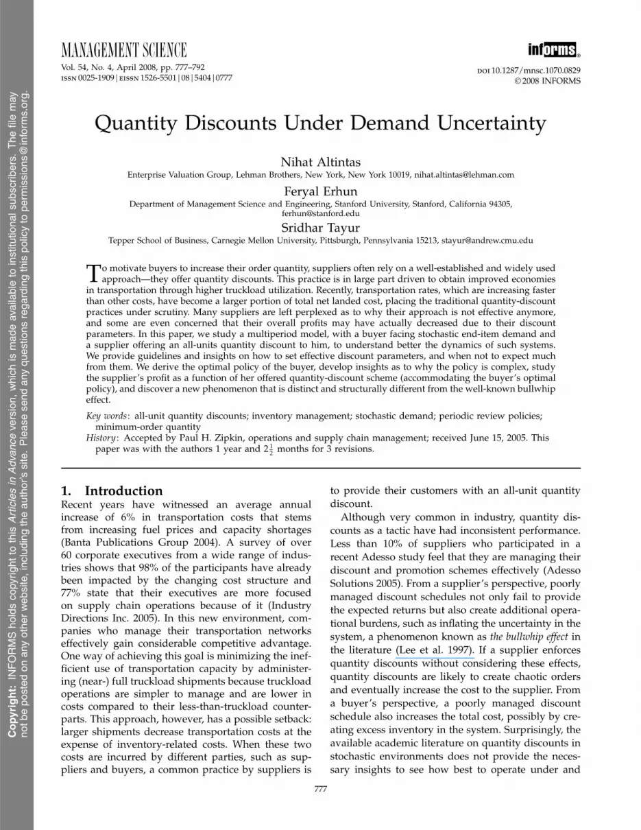
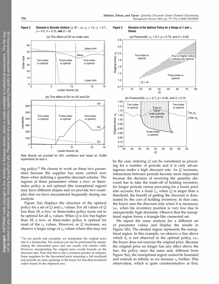
ing policy.12 We choose to work on these two param-eters because the supplier has more control overthese when defining a quantity-discount scheme. Theregions of these parameters where a two- or three-index policy is not optimal (the nonoptimal region)may have different shapes and we provide two exam-ples that we have encountered frequently during ouranalysis.Figure 3(a) displays the structure of the optimal
policy for a set of Q and c0 values. For all values of Qless than 18, a two- or three-index policy turns out tobe optimal for all c0 values. When Q is low but higherthan 18, a two- or three-index policy is optimal formost of the c0 values. However, as Q increases, weobserve a larger range of c0 values where this may not
12 In our proofs and examples, we manipulate the original pricedue to a technicality. The analysis can also be performed by manip-ulating the discounted price and our results will remain valid.However, manipulating the original price avoids bounds on thediscount ratio. Note that this is also a common practice in industry.Some suppliers fix the discounted price assuming a full truckloadand provide an extra upcharge to the buyer for less-than-truckloadorders based on the shipment size.
Figure 3 Structure of the Optimal Policy for a Range of Q and c0Values
0.7
1.0
1.3
1.6
1.9
2.2
2.5
2.8
0 10 20 30 40 50 60 70 80Q
Orig
inal
pric
e, c
0O
rigin
al p
rice,
c0
Two-index isoptimal
Three-index isoptimal
Four or higher indexpolicies are optimal
Q = 18
0.70
0.75
0.80
0.85
0.90
0.95
1.00
1.05
1.10
1.15
1.20
25 30 35 40 45 50 55 60 65Q
No S0
With S0
Two-indexis optimal
Two-indexis optimal
Three-indexis optimal
Four orhigher
index policiesare optimal
(a) Poisson(6), c1 = 0.7, p = 0.75, and h = 0.55
(b) Poisson(20), c1 = 0.7, p = 0.45, and h = 0.15
be the case: ordering Q can be considered as procur-ing for a number of periods and it is only advan-tageous under a high discount rate. As Q increases,interactions between periods become more importantbecause the decision of receiving the quantity dis-count has to take the trade-off of holding inventoryfor longer periods versus procuring for a lower priceinto account. For a fixed c0, when Q is larger than athreshold, the benefit of getting the discount is dom-inated by the cost of holding inventory. In that case,the buyer uses the discount only when it is necessary,i.e., when his inventory position is very low due tounexpectedly high demands. Observe that the nonop-timal region forms a triangle-like connected set.We repeat the same analysis for a different set
of parameter values and display the results inFigure 3(b). The shaded region represents the nonop-timal region. In this example, we observe a line abovewhich S0 is not observed in the optimal policy, i.e.,the buyer does not exercise the original price. Becausethe original price no longer has any effect above theline, the policy stays the same and, different fromFigure 3(a), the nonoptimal region cannot be boundedand extends to infinity as we increase c0 further. Thisobservation, which is quite counterintuitive at first,
Copyright:
INF
OR
MS
hold
sco
pyrig
htto
this
Articlesin
Adv
ance
vers
ion,
whi
chis
mad
eav
aila
ble
toin
stitu
tiona
lsub
scrib
ers.
The
file
may
notb
epo
sted
onan
yot
her
web
site
,inc
ludi
ngth
eau
thor
’ssi
te.
Ple
ase
send
any
ques
tions
rega
rdin
gth
ispo
licy
tope
rmis
sion
s@in
form
s.or
g.
Altintas, Erhun, and Tayur: Quantity Discounts Under Demand UncertaintyManagement Science 54(4), pp. 777–792, © 2008 INFORMS 787
shows that even the minimum-order quantity prob-lem may not have a well defined optimal policy. Thatis, even when a minimum-order quantity is enforcedupon the buyer by the supplier, a two-index policyis not necessarily optimal because the anomalies dueto buy-and-hold continue to occur. There are caseswhere the buyer orders up to different base-stock lev-els for different inventory positions. The first row ofExample 3 highlights this phenomenon.In summary, operational difficulties in a quantity-
discount setting are often self-created by suppliers: ifthe supplier does not pay due attention to the designof effective quantity-discount schemes, these schemesmay create chaotic orders, which eventually increasethe cost to the supplier. Such problems become evenmore prominent at times when there are changes inthe operating conditions, such as the recent increasein transportation rates.
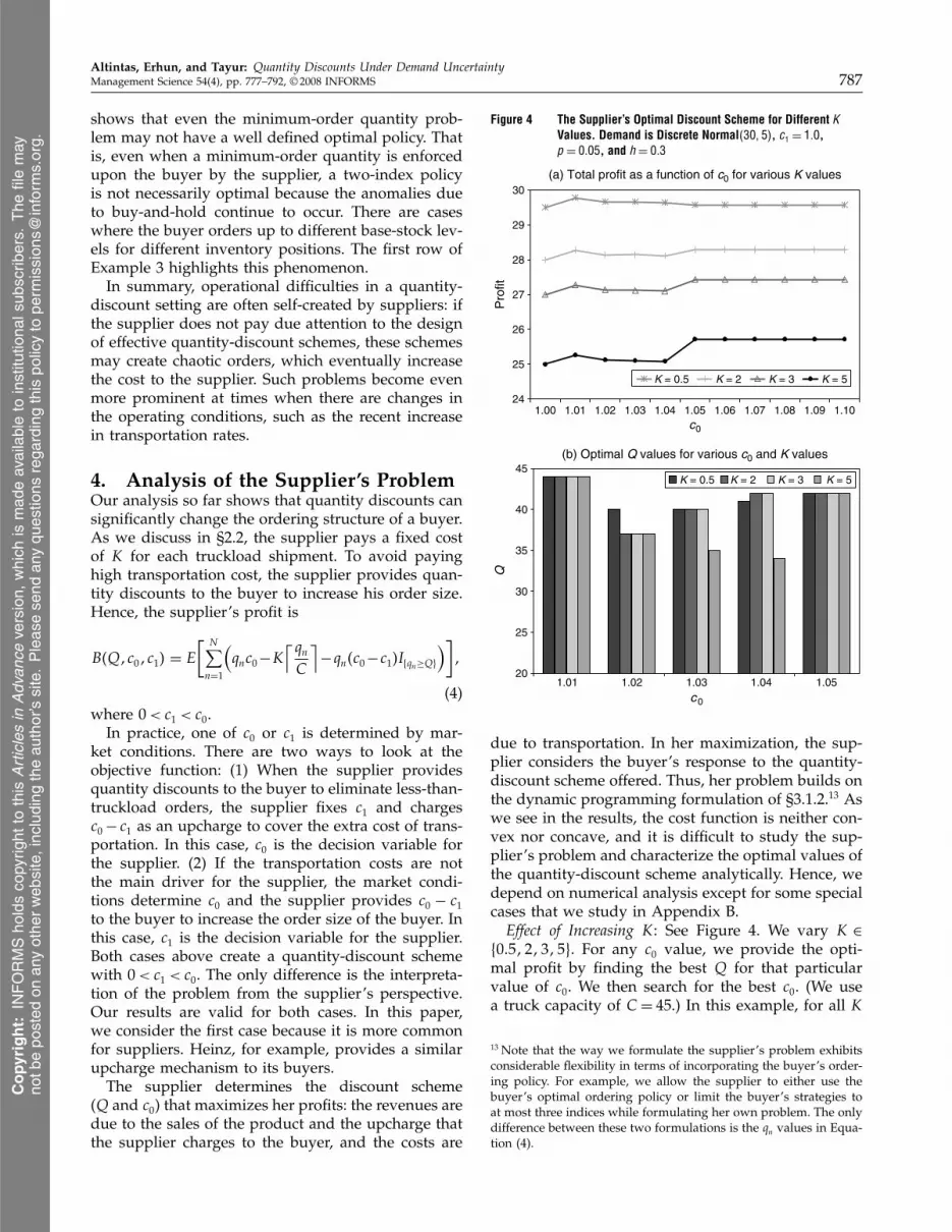
4. Analysis of the Supplier’s ProblemOur analysis so far shows that quantity discounts cansignificantly change the ordering structure of a buyer.As we discuss in §2.2, the supplier pays a fixed costof K for each truckload shipment. To avoid payinghigh transportation cost, the supplier provides quan-tity discounts to the buyer to increase his order size.Hence, the supplier’s profit is
B�Qc0c1� = E
[ N∑n=1
(qnc0−K
⌈qnC
⌉−qn�c0−c1�I�qn≥Q�
)]
(4)where 0< c1 < c0.In practice, one of c0 or c1 is determined by mar-
ket conditions. There are two ways to look at theobjective function: (1) When the supplier providesquantity discounts to the buyer to eliminate less-than-truckload orders, the supplier fixes c1 and chargesc0− c1 as an upcharge to cover the extra cost of trans-portation. In this case, c0 is the decision variable forthe supplier. (2) If the transportation costs are notthe main driver for the supplier, the market condi-tions determine c0 and the supplier provides c0 − c1to the buyer to increase the order size of the buyer. Inthis case, c1 is the decision variable for the supplier.Both cases above create a quantity-discount schemewith 0< c1 < c0. The only difference is the interpreta-tion of the problem from the supplier’s perspective.Our results are valid for both cases. In this paper,we consider the first case because it is more commonfor suppliers. Heinz, for example, provides a similarupcharge mechanism to its buyers.The supplier determines the discount scheme
(Q and c0) that maximizes her profits: the revenues aredue to the sales of the product and the upcharge thatthe supplier charges to the buyer, and the costs are
Figure 4 The Supplier’s Optimal Discount Scheme for Different KValues. Demand is Discrete Normal�30�5, c1 = 1�0,p= 0�05, and h= 0�3
24
25
26
27
28
29
30
1.00 1.01 1.02 1.03 1.04 1.05 1.06 1.07 1.08 1.09 1.10c0
c0
Pro
fit
K = 0.5
K = 0.5
K = 2
K = 2
K = 3
K = 3
K = 5
K = 5
20
25
30
35
40
45
1.01 1.02 1.03 1.04 1.05
Q
(a) Total profit as a function of c0 for various K values
(b) Optimal Q values for various c0 and K values
due to transportation. In her maximization, the sup-plier considers the buyer’s response to the quantity-discount scheme offered. Thus, her problem builds onthe dynamic programming formulation of §3.1.2.13 Aswe see in the results, the cost function is neither con-vex nor concave, and it is difficult to study the sup-plier’s problem and characterize the optimal values ofthe quantity-discount scheme analytically. Hence, wedepend on numerical analysis except for some specialcases that we study in Appendix B.Effect of Increasing K% See Figure 4. We vary K ∈
�0�5235�. For any c0 value, we provide the opti-mal profit by finding the best Q for that particularvalue of c0. We then search for the best c0. (We usea truck capacity of C = 45.) In this example, for all K
13 Note that the way we formulate the supplier’s problem exhibitsconsiderable flexibility in terms of incorporating the buyer’s order-ing policy. For example, we allow the supplier to either use thebuyer’s optimal ordering policy or limit the buyer’s strategies toat most three indices while formulating her own problem. The onlydifference between these two formulations is the qn values in Equa-tion (4).
Copyright:
INF
OR
MS
hold
sco
pyrig
htto
this
Articlesin
Adv
ance
vers
ion,
whi
chis
mad
eav
aila
ble
toin
stitu
tiona
lsub
scrib
ers.
The
file
may
notb
epo
sted
onan
yot
her
web
site
,inc
ludi
ngth
eau
thor
’ssi
te.
Ple
ase
send
any
ques
tions
rega
rdin
gth
ispo
licy
tope
rmis
sion
s@in
form
s.or
g.

Altintas, Erhun, and Tayur: Quantity Discounts Under Demand Uncertainty788 Management Science 54(4), pp. 777–792, © 2008 INFORMS
Figure 5 The Supplier’s Profits and the Buyer’s Optimal Policies for Different p and h Values. Demand is Discrete Normal�30�5 and c1 = 1�0
25
26
27
28
29
30
31
Fixed cost
Su
pp
lier’
s p
rofi
t
p = h = 0.05p = 0.05, h = 0.3
p = 0.3, h = 0.05
p = h = 0.3
p = h = 0.05
p = 0.05, h = 0.3
p = 0.3, h = 0.05
p = h = 0.3
K = 5K = 3K = 2K = 1K = 0.5
Two-index
Two-index
Two-index
Two-index
Two-index
Two-index
Two-index
Two-index
Two-index
Two-index
Two-index
values, the supplier is better off by providing someform of quantity discount to the buyer. When K is low(K = 0�5), the supplier’s optimal discount scheme is(Q= 44 c0 = 1�01 c1 = 1). At his optimality, the buyeruses a three-index policy. For all the other K val-ues, the supplier’s optimal discount scheme (Q= 42c0 = 1�05 c1 = 1) is such that at his optimality thebuyer uses a two-index policy. In this example, theoptimal Q is less than the truck capacity. Even thoughthe supplier may not use some of the truck capacityto its fullest extent, the difference between the truckcapacity and Q creates a cushion against the changesin the buyer’s order size and eliminates the possibil-ity of shipping an additional truck with low load dueto order sizes larger than C.As transportation costs increase, the supplier
tends to provide quantity-discount schemes to com-pletely eliminate less-than-truckload orders becauseher operational objectives are in parallel with observ-ing a small OV. In these situations, for the buyer, atwo-index policy turns out to be optimal where healways orders at least Q units. The supplier essen-tially indirectly enforces a minimum-order quantityon the buyer’s orders. Even though this creates anenvironment with the bullwhip effect, decreasing theorder variance is more crucial for the supplier com-pared to decreasing the actual variance of orders. Toprobe the connection between the transportation costsand the number of indices of the buyer’s optimalpolicy, we study the minimum-order quantity prob-lem in Appendix B and show that the supplier can
always design a quantity-discount scheme for whichthe buyer’s optimal response is a two-index policy.Effect of p, h, and K% Figure 5 illustrates the change
in the supplier’s optimal discount scheme with thetransportation and buyer’s penalty and holding costs.We consider cases where p, h ∈ �0�050�3� and K ∈�0�51235�. When K is low (K = 0�5), the suppliercan tolerate less-than-truckload orders and providesonly small discounts to increase the average ordersize. Therefore, the upcharge does not immenselyinfluence the buyer’s optimal policy: the buyer iswilling to pay the upcharge from time to time ashe uses policies with the number of indices greaterthan two. However, as K increases (K ∈ �123�),less-than-truckload shipments become costlier for thesupplier. Hence, she passes part of the cost to thebuyer by charging a higher upcharge. For the buyer,there is now a trade-off between procurement costsand inventory-related costs. As long as the inventory-related costs are high, the buyer prefers the flexibilityof smaller shipments and pays the upcharge. How-ever, as the upcharge continues to increase (K = 5),the buyer gives up this flexibility and always orders(near-) full truckloads. Hence, as K increases, thesystem moves from an inventory-cost driven environ-ment to a transportation-cost driven environment.We also observe from Figure 5 that for a fixed K,
the supplier’s profits are higher when the penaltyand holding costs of the buyer are high (p= h= 0�3).In this case, the buyer is mostly driven by the
Copyright:
INF
OR
MS
hold
sco
pyrig
htto
this
Articlesin
Adv
ance
vers
ion,
whi
chis
mad
eav
aila
ble
toin
stitu
tiona
lsub
scrib
ers.
The
file
may
notb
epo
sted
onan
yot
her
web
site
,inc
ludi
ngth
eau
thor
’ssi
te.
Ple
ase
send
any
ques
tions
rega
rdin
gth
ispo
licy
tope
rmis
sion
s@in
form
s.or
g.
Altintas, Erhun, and Tayur: Quantity Discounts Under Demand UncertaintyManagement Science 54(4), pp. 777–792, © 2008 INFORMS 789
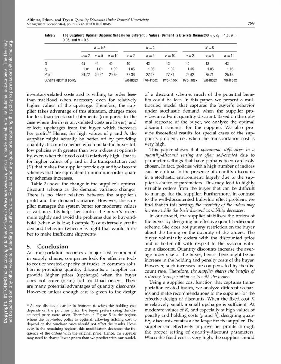
Table 2 The Supplier’s Optimal Discount Scheme for Different � Values. Demand is Discrete Normal�30� � , c1 = 1�0, p =0�05, and h= 0�3
K = 0�5 K = 3 K = 5
� = 2 � = 5 � = 10 � = 2 � = 5 � = 10 � = 2 � = 5 � = 10
Q 45 44 45 40 42 42 40 42 42c0 1�01 1�01 1�02 1�05 1�05 1�05 1�05 1�05 1�05Profit 29�72 29�77 29�65 27�36 27�43 27�39 25�62 25�71 25�66Buyer’s optimal policy Two-index Two-index Two-index Two-index Two-index Two-index
inventory-related costs and is willing to order less-than-truckload when necessary even for relativelyhigher values of the upcharge. Therefore, the sup-plier takes advantage of this situation, charges morefor less-than-truckload shipments (compared to thecase where the inventory-related costs are lower), andcollects upcharges from the buyer which increasesher profit.14 Hence, for high values of p and h, thesupplier might actually be better off by providingquantity-discount schemes which make the buyer fol-low policies with greater than two indices at optimal-ity, even when the fixed cost is relatively high. That is,for higher values of p and h, the transportation cost(K) that makes the supplier provide quantity-discountschemes that are equivalent to minimum-order quan-tity schemes increases.Table 2 shows the change in the supplier’s optimal
discount scheme as the demand variance changes.There is no clear relation between the supplier’sprofit and the demand variance. However, the sup-plier manages the system better for moderate valuesof variance; this helps her control the buyer’s ordersmore tightly and avoid the problems due to buy-and-hold (when ( is low; Example 3) or extremely erraticdemand behavior (when ( is high) that would forceher to make inefficient shipments.
5. ConclusionAs transportation becomes a major cost componentin supply chains, companies look for effective toolsto reduce wasted capacity of trucks. A common solu-tion is providing quantity discounts: a supplier canprovide higher prices (upcharge) when the buyerdoes not order (near-) full truckload orders. Thereare many potential advantages of quantity discounts.However, unless enough care is given to the design
14 As we discussed earlier in footnote 6, when the holding costdepends on the purchase price, the buyer prefers using the dis-counted price more often. Therefore, in Figure 5 in the regionswhere the two-index policy is optimal, allowing holding cost todepend on the purchase price should not affect the results. How-ever, in the remaining regions, this modification decreases the fre-quency of the orders with the original price. Hence, the suppliermay need to charge lower prices than we predict with our model.
of a discount scheme, much of the potential bene-fits could be lost. In this paper, we present a mul-tiperiod model that captures the buyer’s behaviorunder stochastic demand when the supplier pro-vides an all-unit quantity discount. Based on the opti-mal response of the buyer, we analyze the optimaldiscount schemes for the supplier. We also pro-vide theoretical results for special cases of the sup-plier’s problem, i.e., when the transportation cost isvery high.This paper shows that operational difficulties in a
quantity-discount setting are often self-created due toparameter settings that have perhaps been carelesslychosen. In fact, policies with a high number of indicescan be optimal in the presence of quantity discountsin a stochastic environment, largely due to the sup-plier’s choice of parameters. This may lead to highlyvariable orders from the buyer that can be difficultto manage for the supplier. Furthermore, in contrastto the well-documented bullwhip effect problem, wefind that in this setting, the erraticity of the orders mayincrease while the basic demand variability decreases.In our model, the supplier stabilizes the orders of
the buyer by designing an effective quantity-discountscheme. She does not put any restriction on the buyerabout the timing or the quantity of the orders. Thebuyer voluntarily orders with the discounted priceand is better off with respect to the system with-out a discount. Quantity discounts increase the aver-age order size of the buyer, hence there might be anincrease in the holding and penalty costs of the buyer.However, such increases are compensated by the dis-count rate. Therefore, the supplier shares the benefits ofreducing transportation costs with the buyer.Using a supplier cost function that captures trans-
portation-related issues, we analyze different scenar-ios and make recommendations to the supplier for theeffective design of discounts. When the fixed cost Kis relatively small, a small upcharge is sufficient. Atmoderate values of K, and especially at high values ofpenalty and holding costs (p and h), designing quan-tity discounts creates a challenge for the supplier. Thesupplier can effectively improve her profits throughthe proper setting of quantity-discount parameters.When the fixed cost is very high, the supplier should
Copyright:
INF
OR
MS
hold
sco
pyrig
htto
this
Articlesin
Adv
ance
vers
ion,
whi
chis
mad
eav
aila
ble
toin
stitu
tiona
lsub
scrib
ers.
The
file
may
notb
epo
sted
onan
yot
her
web
site
,inc
ludi
ngth
eau
thor
’ssi
te.
Ple
ase
send
any
ques
tions
rega
rdin
gth
ispo
licy
tope
rmis
sion
s@in
form
s.or
g.

Altintas, Erhun, and Tayur: Quantity Discounts Under Demand Uncertainty790 Management Science 54(4), pp. 777–792, © 2008 INFORMS
design discount schemes which essentially act asminimum-order quantity schemes. This, in turn, gen-erates orders which are easy to handle with smallorder variance, eliminates less-than-truckload orders,and allows the supplier to effectively manage herprofits. Furthermore, this observation explains theattempt of many suppliers, like Heinz, to reevaluatetheir discount mechanisms in the past few years.The efficient quantity-discount scheme that we pro-
pose increases the time between orders and shifts thevariability of the system from order sizes to order tim-ing. A possible extension of our analysis would beto study how to best moderate the variation in thenumber of periods between orders as well. Anotherextension could include multiple buyers with signifi-cant heterogeneity. In this case, the supplier may pro-vide different price breaks such that each buyer picksexactly one of the breaks at his optimality. Becauseeach buyer only exercises one price break, the sup-plier will price discriminate her customers based ontheir end customer demand distribution. Yet anotherpossible extension is to analyze multiple items from asingle buyer. Oftentimes suppliers provide discountssuch that the buyer may combine orders of variousproducts to get the discount. This allows the buyer totake advantage of the quantity discount without hav-ing to order excess inventory. Quantity discounts thatallow for combinations of multiple products are dif-ficult to study, but represent an alternative tool thatsuppliers can use to further reduce order variance,and eliminate wait-and-see or buy-and-hold strategiesof the buyer. Additional issues such as time windowsand volume discounts can also be analyzed.
6. Electronic CompanionAn electronic companion to this paper is available aspart of the online version that can be found at http://mansci.journal.informs.org/.
Table A1 Performance of the Best Three-Index∗ Policy Out of All Combinations of c0 ∈ 1�1�3�1�6�,c1 = 0�7, p ∈ 0�15�0�3�0�45�0�6�0�75�, h ∈ 0�15�0�3�0�45�0�6�0�75�, and Q ∈ 10�40�70�100�
Discrete normal† Poisson Discrete uniform†
Three-index∗ optimal: 88.7% Three-index∗ optimal: 87.5% Three-index∗ optimal: 90.7%
Deviation (%) Deviation (%) Deviation (%)
Std�dev� Average Max. Mean Average Max. Std. dev. Average Max.
0�5 0�07 0�25 10 0�71 4�31 2�9 0�44 1�982�0 0�64 2�30 15 0�14 0�87 5�8 0�17 1�254�5 0�31 1�38 20 0�18 0�84 8�7 0�06 0�778�0 0�08 0�86 25 0�22 1�12 11�5 0�06 0�9712�5 0�05 0�63 30 0�22 1�02 14�4 0�00 0�0618�0 0�00 0�00
Median: 0.038% Median: 0.040% Median: 0.012%
∗Two- or three-index policy.†Demand mean is equal to 30.
AcknowledgmentsThe second author was partially supported by NSF AwardDMI-0400345. The authors express their deepest gratitude tothe department editor, Paul Zipkin, the area editor, and thetwo anonymous referees whose constructive comments andsuggestions significantly improved this paper. The authorsalso thank Robert Carlson and Warren Hausman at Stan-ford University, Sunder Kekre at Carnegie Mellon Univer-sity, Prafulla Nabar at Lehman Brothers, and seminar par-ticipants at Cornell University, ENSGI-INPG, Georgia Insti-tute of Technology, London Business School, MassachusettsInstitute of Technology, University of Maryland, the 2004INFORMS Conference at Denver, and the 2004 M&SOMConference at the Technische Universiteit Eindhoven.
Appendix A. Performance of the BestThree-Index PolicyIn the examples we provided throughout the paper, a three-index policy turns out to be optimal in a wide range ofparameter values. This observation leads us to carry out amore detailed numerical analysis on the performance of athree-index policy. Table A1 summarizes the performanceof the best three-index policy for 4,800 settings with differ-ent problem parameters. For all three distributions, the per-centage of the cases where a three-index policy is optimalis steady around 87%–91% averaging 88.83%. For the bestthree-index policy, the maximum deviation from the costof the optimal policy is 4.3% with a median of 0.025%. Asdemand variability increases, a three-index policy generallyperforms much better.Hence, even though a three-index policy is no longer
optimal for the infinite-horizon problem, it performs excep-tionally well under a wide range of problem parameters.Therefore, a three-index policy is an excellent heuristic solu-tion for this rather complicated problem: it is easy to admin-ister and implement, and it captures a high percentage ofthe profits generated by the optimal policy.
Appendix B. Minimum-Order Quantity ProblemIn §4, we show that as transportation costs increase, the sup-plier tends to provide quantity-discount schemes to com-
Copyright:
INF
OR
MS
hold
sco
pyrig
htto
this
Articlesin
Adv
ance
vers
ion,
whi
chis
mad
eav
aila
ble
toin
stitu
tiona
lsub
scrib
ers.
The
file
may
notb
epo
sted
onan
yot
her
web
site
,inc
ludi
ngth
eau
thor
’ssi
te.
Ple
ase
send
any
ques
tions
rega
rdin
gth
ispo
licy
tope
rmis
sion
s@in
form
s.or
g.

Altintas, Erhun, and Tayur: Quantity Discounts Under Demand UncertaintyManagement Science 54(4), pp. 777–792, © 2008 INFORMS 791
pletely eliminate less-than-truckload orders. In this case, forthe buyer, the two-index policy turns out to be optimal andthe problem essentially reduces to a minimum-order quan-tity problem where the buyer always orders at least Q units.This observation leads us to study a special case of the sup-plier’s problem, the minimum-order quantity problem, inmore depth.Imposing a minimum-order quantity cannot by itself
guarantee a well-behaved ordering behavior from the buyer.Consider a case where c0 is very large. Hence, the buyeralways orders with the discount. From Figure 3(b), we knowthat the buyer can follow a buy-and-hold strategy and eventhough he never exercises the original price, the optimalpolicy is not necessarily a two-index policy. However, whenthe supplier sets Q large enough, she can eliminate thispossibility:
Theorem 3. When c0 is very large, there exists a finite Q∗
such that(i) For Q > Q∗, the buyer follows a two-index policy with
indices (S1 S01). The optimal order quantity q∗�x� is as follows%
q∗�x�=max�S1−QQ� when x≤ S01
0 when x > S01�
(ii) As Q increases, S01 converges to S01 = ) − Q�h/�h+ p�� and the buyer’s average cost converges to C�Q�=Qhp/�2�h+ p��.
Proof. The proof is available in the e-companion; see§EC.2. �
The supplier can choose any Q >Q∗ to make the buyerfollow a two-index policy. When the buyer does not usea buy-and-hold strategy for any Q, Q∗ is simply equal tozero: no matter how low the value of Q∗ is, the buyer willalways follow a two-index policy (Figure 3(a)). However,the buyer should also look for the optimal level of discountto eliminate small orders.
Theorem 4. In a quantity-discount problem, for fixed andfinite values of Q, p, h, and c1, there exists a discount z∗�=1− �c1/c0�� < 100% such that(a) for every discount ratio z≥ z∗, the buyer does not exercise
price c0 for any initial inventory position;(b) for every discount ratio z < z∗, the buyer exercises both
prices c0 and c1.
Proof. Available in the e-companion; see §EC.3. �
In Theorem 3, we show that by adjusting Q the suppliercan guarantee that the buyer follows a two-index policy forlarger values of c0. Theorems 3 and 4 together show thatthe supplier can always design a quantity-discount scheme(with a finite Q and a discount rate less than 100%) suchthat the buyer’s optimal policy will be a two-index policy.Actually, the supplier can control the buyer’s ordering
behavior even more tightly. Let 1 be the percentage of theorders which are strictly greater than the truck capacity Cwhen the buyer follows a two-index policy. These can beconsidered as the orders which fall into the second truck.A large 1 value means that the supplier often sends a sec-ond truck which might increase the transportation cost.In Figure B1, for different levels of Q ≤ C, 1 values
are displayed. For these Q values which are greater than
Figure B1 Values of � for Q>Q∗ = 55. Demand is Poisson(20),p= 0�45, and h= 0�15
(%)
0.0
0.2
0.4
0.6
0.8
55 6560 70 8075
Q
1
Q∗ = 55, the buyer does not buy-and-hold and the optimalpolicy is a two-index policy (Theorem 3). As Q increases, 1decreases dramatically. For even a moderate value of Q suchas Q = 60 (3 periods’ demand), the probability of an ordergreater than Q is less than one in a thousand. The opti-mal policy when Q= 60 is a two-index policy with indices(S1 = 36, S01 = 4). For all practical purposes, the inventoryposition almost never falls below S1 − Q = −24 and thebuyer almost always orders exactly Q. In this case, the crit-ical level where the buyer stops ordering S01 is very closeto S01 = 5 and the critical level becomes independent ofdemand variability.In summary, when the setup cost is very high, the opera-
tional objectives of the supplier are in parallel with observ-ing a small OV from the buyer with a high -. This way,the supplier guarantees (with high probability) full or near-full truckloads. In these situations, the supplier essentiallyenforces a minimum quantity to the buyer’s orders. Eventhough this creates an environment with the bullwhip effect,decreasing the order variance is more crucial for the suppliercompared to decreasing the actual variance of orders.
ReferencesAdesso Solutions. 2005. A double-edged sword. Bus. Credit 107(9)
56–59.
Anupindi, R., R. Akella. 1993. An inventory model with commit-ments. Working paper, Northwestern University, Evanston, IL.
Anupindi, R., Y. Bassok. 1998. Supply contracts with quantitycommitments and stochastic demand. S. Tayur, R. Ganeshan,M. Magazine, eds. Quantitative Models for Supply Chain Manage-ment. Kluwer Academic Publishers, Boston, 197–232.
Banta Publications Group. 2004. Transportation costs continue torise. Banta Mailbox (December) 1.
Bassok, Y., R. Anupindi. 1997. Analysis of supply contracts withtotal minimum commitment. IIE Trans. 29(5) 373–381.
Copyright:
INF
OR
MS
hold
sco
pyrig
htto
this
Articlesin
Adv
ance
vers
ion,
whi
chis
mad
eav
aila
ble
toin
stitu
tiona
lsub
scrib
ers.
The
file
may
notb
epo
sted
onan
yot
her
web
site
,inc
ludi
ngth
eau
thor
’ssi
te.
Ple
ase
send
any
ques
tions
rega
rdin
gth
ispo
licy
tope
rmis
sion
s@in
form
s.or
g.
Altintas, Erhun, and Tayur: Quantity Discounts Under Demand Uncertainty792 Management Science 54(4), pp. 777–792, © 2008 INFORMS
Benton, W. C., S. Park. 1996. A classification of literature on deter-mining the lot size under quantity discounts. Eur. J. Oper. Res.92 219–238.
Bertsekas, D. P. 1995. Dynamic Programming and Optimal Control.Athena Scientific, Belmont, MA.
Buchanan, J. M. 1953. The theory of monopolistic quantity dis-counts. Rev. Econom. Stud. 20(3) 199–208.
Cachon, G. 1999. Managing supply chain demand variability withscheduled ordering policies. Management Sci. 45(6) 843–856.
Chen, F., R. Samroengraja. 2004. Order volatility and supply chaincosts. Oper. Res. 52(5) 707–722.
Chen, F., A. Federgruen, Y. Zheng. 2001. Coordination mechanismfor a distribution system with one supplier and multiple retail-ers. Management Sci. 47(5) 693–708.
Cheung, K. L., H. L. Lee. 2002. The inventory benefits of shipmentcoordination and stock rebalancing in a supply chain. Manage-ment Sci. 48(2) 300–306.
Corbett, C. J., X. de Groote. 2000. A supplier’s optimal quantity dis-count policy under asymmetric information. Management Sci.46(3) 444–500.
Dolan, R. J. 1987. Quantity discounts: Managerial issues andresearch opportunities. Marketing Sci. 6(1) 1–23.
Erhun, F., S. Tayur. 2003. Enterprise-wide optimization of totallanded cost at a grocery retailer. Oper. Res. 51(3) 343–353.
Garbor, A. 1955. A note on block tariffs. Rev. Econom. Stud. 23 32–41.Industry Directions Inc. 2005. Manufacturers leverage supply chain
strategy to offset rising energy costs. Executive brief. (October).http://www.industrydirections.com.
Jeuland, A. P., S. M. Shugan. 1983. Managing channel profits. Mar-keting Sci. 2(3) 239–272.
Jucker, J. V., M. J. Rosenblatt. 1985. Single-period inventory modelswith demand uncertainty and quantity discounts: Behavioralimplications and a new solution procedure. Naval Res. Logist.32(4) 537–550.
Lal, R., R. Staelin. 1984. An approach for developing an optimaldiscount policy. Management Sci. 30(12) 1524–1539.
Lee, H. L., M. J. Rosenblatt. 1986. A generalized quantity discountpricing model to increase supplier’s profits. Management Sci.32(9) 1177–1185.
Lee, H. L., V. Padmanabhan, S. Whang. 1997. Information distortionin a supply chain: The bullwhip effect. Management Sci. 43(4)546–558.
Moinzadeh, K., S. Nahmias. 2000. Adjustment strategies for a fixeddelivery contract. Oper. Res. 48(3) 408–423.
Monahan, J. P. 1984. A quantity discount pricing model to increasevendor profits. Management Sci. 30(6) 720–726.
Munson, C. L., M. J. Rosenblatt. 1998. Theories and realities ofquantity discounts: An exploratory study. Production Oper.Management 7(4) 352–369.
Porteus, E. L. 1971. On the optimality of generalized �s S� policies.Management Sci. 17(7) 411–426.
Sethi, S. P. 1984. A quantity discount lot size model with disposals.Internat. J. Production Res. 22 31–39.
Tsay, A., S. Nahmias, N. Agrawal. 1998. Modeling supply chaincontracts: A review. S. Tayur, R. Ganeshan, M. Magazine, eds.Quantitative Models for Supply Chain Management. Kluwer Aca-demic Publishers, Boston, 301–336.
Weng, Z. K. 1995. Channel coordination and quantity discounts.Management Sci. 41(9) 1509–1522.
Copyright:
INF
OR
MS
hold
sco
pyrig
htto
this
Articlesin
Adv
ance
vers
ion,
whi
chis
mad
eav
aila
ble
toin
stitu
tiona
lsub
scrib
ers.
The
file
may
notb
epo
sted
onan
yot
her
web
site
,inc
ludi
ngth
eau
thor
’ssi
te.
Ple
ase
send
any
ques
tions
rega
rdin
gth
ispo
licy
tope
rmis
sion
s@in
form
s.or
g.