Embed Size (px)
Citation preview


Vol.2, No.10, 1057-1179 (2010) NS
Copyright © 2010 SciRes. Openly accessible at http://www.scirp.org/journal/NS/
TABLE OF CONTENTS Volume 2, Number 10, October 2010
ASTRONOMY & SPACE SCIENCES High sensitive and rapid responsive n-type Si: Au sensor for monitoring breath rate
X. L. Hu, J. C. Liang, X. Li, Y. Chen, C. Zou, S. Liu, X. Chen………………………………………………………………1057
CHEMISTRY Preparation and characterization of genipin-cross-linked chitosan microparticles by water-in-oil emulsion solvent diffusion method
J. Karnchanajindanun, M. Srisa-ard, P. Srihanam, Y. Baimark…………………………………………………………………1061 Adsorption studies of cyanide onto activated carbon and γ-alumina impregnated with cooper ions
L. Giraldoa, J. C. Moreno-Pirajánb……………………………………………………………………………………………1066 Structural and electrical characterization of Bi2VO5.5/Bi4Ti3O12 bilayer thin films deposited by pulsed laser ablation technique
N. Kumari, S. B. Krupanidhi, K. B. R. Varma…………………………………………………………………………………1073
EARTH SCIENCE Secular evolution of continental crust: recorded from massif-type charnockites of Eastern Ghats belt, India
S. Bhattacharya, A. K. Chaudhary……………………………………………………………………………………………1079 New experimental constraints: implications for petrogenesis of charnockite of dioritic composition
R. Kar, S. Bhattacharya…………………………………………………………………………………………………………1085
LIFE SCIENCE Cell-PLoc 2.0: an improved package of web-servers for predicting subcellular localization of proteins in various organisms
K. C. Chou, H. B. Shen…………………………………………………………………………………………………………1090 Evolution based on genome structure: the “diagonal genome universe”
K. Sorimachi……………………………………………………………………………………………………………………1104 Assessment of a short phylogenetic marker based on comparisons of 3’ end 16S rDNA and 5’ end 16S-23S ITS nucleotide sequences of the Bacillus cereus group
S. Yakoubou, J.-C. Côté………………………………………………………………………………………………………1113 Origin and SEM analysis of aerosols in the high mountain of Tenerife (Canary Islands)
J. D. Delgado, O. E. García, A. M. Díaz, J. P. Díaz, F. J. Expósito, E. Cuevas, X. Querol, A. Alastuey, S. Castillo……………1119 The Rich-Gini-Simpson quadratic index of biodiversity
R. C. Guiasu, S. Guiasu…………………………………………………………………………………………………………1130 Correlated mutations in the four influenza proteins essential for viral RNA synthesis, host adaptation, and virulence: NP, PA, PB1, and PB2
W. Hu…………………………………………………………………………………………………………………………1138 Effect of abiotic factors on the molluscicidal activity of oleoresin of Zingiber officinale against the snail Lymnaea acuminata
V. Singh, P. Kumar, V. K. Singh, D. K. Singh…………………………………………………………………………………1148 Distribution of polychaetes in the shallow, sublittoral zone of Admiralty Bay, King George Island, Antarctica in the early and late austral summer
L. de S. Barbosa, A. Soares-Gomes, P. C. Paiva………………………………………………………………………………1155 The factorial structure of self-reported androgen-promoted physiological traits
L. Ellis, S. Das…………………………………………………………………………………………………………………1164
PHYSICS Transient response of multilayered hollow cylinder using various theories of generalized thermoelasticity
D. S. Mashat, A. M. Zenkour, K. A. Elsibai……………………………………………………………………………………1171
The figure on the front cover shows the Cell-PLoc 2.0 web-page at http://www.csbio.sjtu.edu.cn/bioinf/Cell-PLoc-2/. See the article published in Natural Science, 2010, Vol. 2, No. 10, pp. 1090-1103 by Kuo-Chen Chou and Hong-Bin Shen.

Natural Science
Journal Information
SUBSCRIPTIONS
The Natural Science (Online at Scientific Research Publishing, www.SciRP.org) is published monthly by Scientific Research
Publishing, Inc., USA.
Subscription rates: Print: $50 per copy.
To subscribe, please contact Journals Subscriptions Department, E-mail: [email protected]
SERVICES
Advertisements
Advertisement Sales Department, E-mail: [email protected]
Reprints (minimum quantity 100 copies)
Reprints Co-ordinator, Scientific Research Publishing, Inc., USA.
E-mail: [email protected]
COPYRIGHT
Copyright© 2010 Scientific Research Publishing, Inc.
All Rights Reserved. No part of this publication may be reproduced, stored in a retrieval system, or transmitted, in any form or by
any means, electronic, mechanical, photocopying, recording, scanning or otherwise, except as described below, without the
permission in writing of the Publisher.
Copying of articles is not permitted except for personal and internal use, to the extent permitted by national copyright law, or under
the terms of a license issued by the national Reproduction Rights Organization.
Requests for permission for other kinds of copying, such as copying for general distribution, for advertising or promotional purposes,
for creating new collective works or for resale, and other enquiries should be addressed to the Publisher.
Statements and opinions expressed in the articles and communications are those of the individual contributors and not the statements
and opinion of Scientific Research Publishing, Inc. We assumes no responsibility or liability for any damage or injury to persons or
property arising out of the use of any materials, instructions, methods or ideas contained herein. We expressly disclaim any implied
warranties of merchantability or fitness for a particular purpose. If expert assistance is required, the services of a competent
professional person should be sought.
PRODUCTION INFORMATION
For manuscripts that have been accepted for publication, please contact:
E-mail: [email protected]
Vol.2, No.10, 1057-1060 (2010)doi:10.4236/ns.2010.210130
Copyright © 2010 SciRes. Openly accessible at http://www.scirp.org/journal/NS/
Natural Science
High sensitive and rapid responsive n-type Si: Au sensor for monitoring breath rate
Xuelan Hu1, Jiachang Liang2*, Xing Li3, Yue Chen4, Chao Zou5, Sheng Liu6, Xin Chen2
1Sino-European Institute of Aviation Engineering, Civil Aviation University of China, Tianjin, China; 2College of Science, Civil Aviation University of China, Tianjin, China; *Corresponding Author: [email protected]; 3Department of Automation, Tianjin Technical Normal Institute, Tianjin, China; 4College of Aeronautical Engineering, Civil Aviation University of China, Tianjin, China; 5China Electronic Standardization Institute, Beijing, China; 6Sino-European Institute of Aviation Engineering, Civil Aviation University of China, Tianjin, China.
Received 23 May 2010; revised 18 July 2010; accepted 24 July 2010.
ABSTRACT
125 µm-breath sensor with high sensitivity and rapid response was prepared by using n-type Si: Au material. Its sensitivity coefficient and time constant were 4 V.sec/L and 38 msec, respec-tively. Its working principle was based on ano- malous resistance effect, which not only increa- sed the sensitivity, but also reduced its time constant greatly. Its signal processing system can select the breath signals and work stably. Therefore, the small changes of breath system can be measured and, especially, patient’s breath rate can be monitored at a distance.
Keywords: Breath sensor; Signal processing system; Deep impurity; Anomalous resistance effect
1. INTRODUCTION
For semiconductors containing shallow impurities, in-cluding n-type silicon, the variation of its resistance Rs with temperature obeys T-3/2 rule, i.e.
Rs = CT-3/2 (1)
where C is proportional constant. For single crystal n-type silicon doped with deep impurities, near room temperature, the relationship between its resistance Rd and temperature T satisfies [1-3]
Rd = C exp [ – (EF – EA) / kT ] (2)
where k is Boltzmann constant, EF Fermi level and EA the deep acceptor level in the band gap of silicon con-taining deep acceptor impurities. For n-type Si: Au (n- type silicon containing deep acceptor impurities of gold), the anomalous resistance effect of exponential term in Eq.2 can increase the sensitivity greatly. To compare the
effects of T-3/2 and exp [– (EF – EA) / kT], we take
kkTEETB
TBEETdTdR
dTdR
dR
dR
AF
AFs
d
s
d
3 / ] / )( [ exp)(
)( )( 2 /
/ 2/1
(3)
Fermi level and the deep acceptor level of gold impurity are equal to 0.57 eV and 0.54 eV, respectively, below the conduction band in the band gap of our n-type Si: Au material and, thus, EF – EA = 0.03 eV. At room tempera-ture (T = 300 K), we have
310 3.1 s
d
dR
dR (4)
Our experimental measuring value is . There- fore, the sensitivity of 125 µm-breath sensor, made by Wheatstone bridge using n-type Si: Au material as bridge arms, can be increased by 103 times, comparing with con- taining shallow impurities [4].
3105.1
Our 125 µm-breath sensor can be used to monitor dif-ferent breath flux and frequencies. In the Wheatstone bridge of our 125 µm-breath sensor, the variation of the offset voltage will play a vital role to the circuit. Gener-ally speaking, the offset voltage is not a constant, but ra- ther a function containing several unknown parameters. It varies according with the changes of ambient tempe- rature and brightness, service voltage and current, even the technical defects during manufacturing. Another fac- tor affecting the offset voltage is the asymmetry between the bridge arms, especially the relevant resistors’ tem-perature coefficient, which depends on the deep impurity. If the offset voltage remains constant, the voltage output of 125 µm-breath sensor only depends on its flux. In order to eliminate the offset voltage drift, some compensation methods and auto-adjusting circuits are adopted. Thus, the sensor with such signal processing system can be used as

X. Hu et al. / Natural Science 2 (2010) 1057-1060
Copyright © 2010 SciRes. http://www.scirp.org/journal/NS/
1058
Openly accessible at
the breath sensor to monitor the patient’s breath rate.
2. EXPERIMENTS
In n-type Si, the concentration of doped phosphorus (shallow donor impurity) was equal to cm-3 and in n-type Si: Au material the concentration of gold (deep acceptor impurity) was equal to cm-3. The doped Au element was diffused in Si substrate by deep doping method [5]. The main part of 125 µm- breath sensor, made of n-type Si: Au material, was a Wheatstone bridge using anisotropic etching n-type Si: Au resistors. The length of each bridge arm was 125 µm. In terms of electrostatic method, the bridge was bonded to a borosilicate grass substrate, which had high thermal isolation capacity. The structure and photograph of the integrated fabrication of the 125 µm-breath sensor were shown in Figures 1 and 2, respectively.
15100.1
15101.1
The schematic diagram of monitoring system of 125 µm-breath sensor was shown in Figure 3. A resistor R was connected in series with the power supply circuit to protect the sensor. The measurement was carried out in a 6 mm-radius tube with the measuring range from 0 to 27 L/min. Before measuring, the circuit should be supplied
Figure 1. The structure of the 125 µm-breath sensor.
Figure 2. Photograph of integrated fabrication of 125 µm-breath sensor.
Figure 3. The schematic diagram of monitoring system of the 125 µm-breath sensor. with power to preheat for 30 minutes. The static and tran- sient characteristics of 125 µm-breath sensor were mea- sured, including the output voltage as well as time con-stant of 125 µm-breath sensor.
3. RESULTS AND DISCUSSION
3.1. Working Principle of 125 µm-breath Sensor
Except for using n-type Si: Au material instead of hot wires to form the electric bridge arms, this 125 µm-breath sensor shares the same principle with the hot wire flow meter. When air flows through the electric bridge, the temperature variation between the two arms perpendicu-lar to the air flow direction is much more than that be-tween the two arms parallel with the air flow direction. Thus, the temperature difference lead to the resistance change of each bridge arm, and then lead to the change of output voltage related with the flux at the output ends. The sensitivity of the sensor depends on the resistance variation of the electric bridge arms when air flows through the sensor. The more the resistance varies, the higher the sensor’s sensitivity is. When the sensor size decreases to micro dimensions, the contact area between the air and bridge arms is also largely reduced. So se-lecting materials which have high sensitivity toward temperature is the key problem. The sensitivity of 125 µm-breath sensor was increased greatly by using n-type Si: Au material, because deep doping method can in-crease the temperature sensitivity of the electric bri- dge’s single arm resistance, as shown in Eq.3 and Eq.4.
3.2. The Static Characteristics of the Monitoring System of 125 µm-breath Sensor
Suppose the measurand is x , output is and the re-sponse time is zero, the function between the measurand and the output should be
y
X. Hu et al. / Natural Science 2 (2010) 1057-1060
Copyright © 2010 SciRes. http://www.scirp.org/journal/NS/
1051059
Openly accessible at
, )( Cxfy (5)
where C is a constant. If the measurand varies , then the output’s varia-
tion should be dx
, )( ] / )( [ dxxKdxdxxdfdy (6)
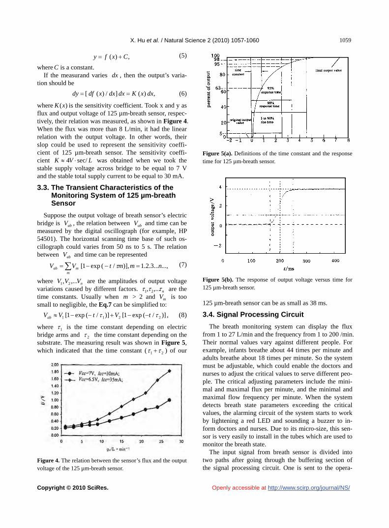
where is the sensitivity coefficient. Took x and y as flux and output voltage of 125 µm-breath sensor, respec-tively, their relation was measured, as shown in Figure 4. When the flux was more than 8 L/min, it had the linear relation with the output voltage. In other words, their slop could be used to represent the sensitivity coeffi-cient of 125 µm-breath sensor. The sensitivity coeffi-cient was obtained when we took the stable supply voltage across bridge to be equal to 7 V and the stable total supply current to be equal to 30 mA.
)(xK
K 4 LV sec/
3.3. The Transient Characteristics of the Monitoring System of 125 µm-breath Sensor
Suppose the output voltage of breath sensor’s electric bridge is ab , the relation between ab and time can be measured by the digital oscillograph (for example, HP 54501). The horizontal scanning time base of such os-cillograph could varies from 50 ns to 5 s. The relation between and time can be represented
V
abV
V
...,...3.2.1)], / ( exp1[ nmmtVVm
mab (7)
where n are the amplitudes of output voltage variations caused by different factors.
VVV ,..., 21
n ,..., 21 are the time constants. Usually when > 2 and mV is too small to negligible, the Eq.7 can be simplified to:
m
)] / ( exp 1[ )] / ( exp1[ 2211 tVtVVab , (8)
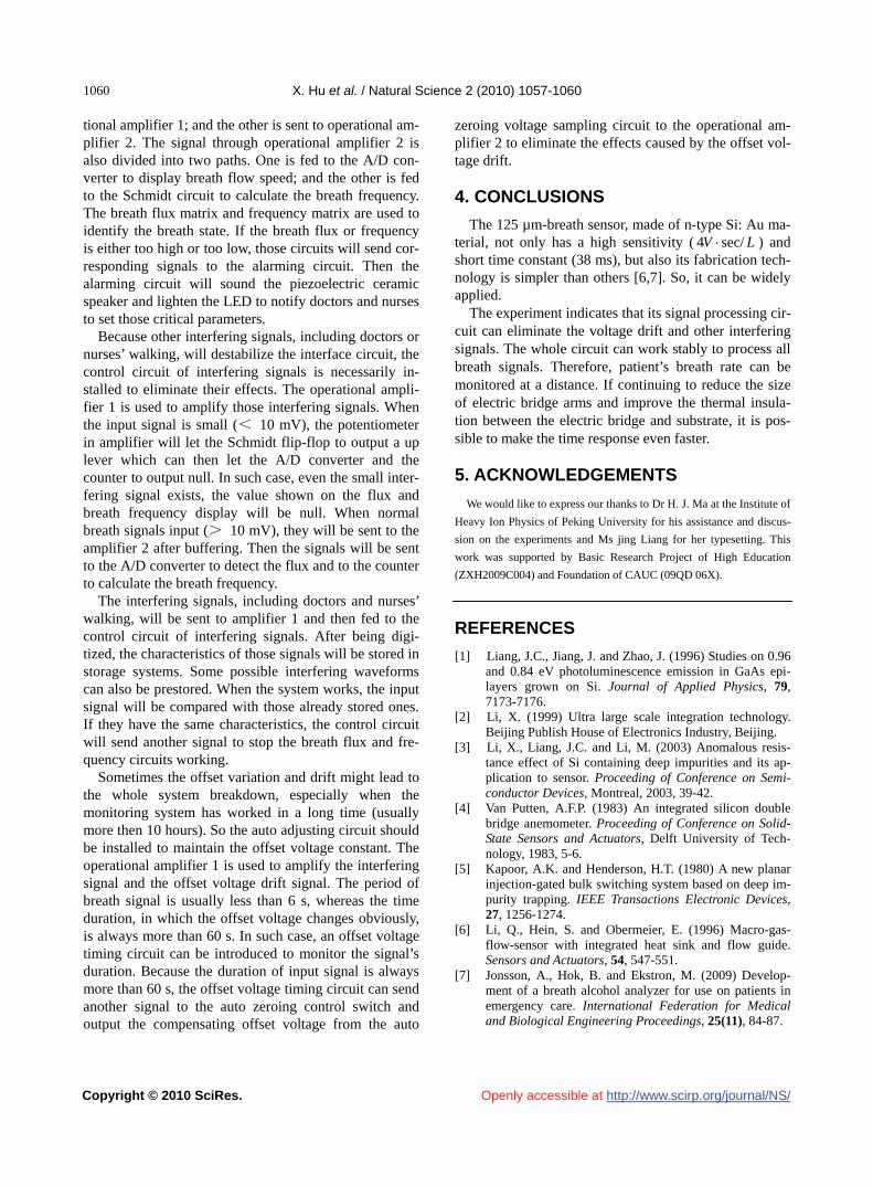
where 1 is the time constant depending on electric bridge arms and 2 the time constant depending on the substrate. The measuring result was shown in Figure 5, which indicated that the time constant ( 21 ) of our
Figure 4. The relation between the sensor’s flux and the output voltage of the 125 µm-breath sensor.
Figure 5(a). Definitions of the time constant and the response time for 125 µm-breath sensor.
Figure 5(b). The response of output voltage versus time for 125 µm-breath sensor. 125 µm-breath sensor can be as small as 38 ms.
3.4. Signal Processing Circuit
The breath monitoring system can display the flux from 1 to 27 L/min and the frequency from 1 to 200 /min. Their normal values vary against different people. For example, infants breathe about 44 times per minute and adults breathe about 18 times per minute. So the system must be adjustable, which could enable the doctors and nurses to adjust the critical values to serve different peo-ple. The critical adjusting parameters include the mini-mal and maximal flux per minute, and the minimal and maximal flow frequency per minute. When the system detects breath state parameters exceeding the critical values, the alarming circuit of the system starts to work by lightening a red LED and sounding a buzzer to in-form doctors and nurses. Due to its micro-size, this sen-sor is very easily to install in the tubes which are used to monitor the breath state.
The input signal from breath sensor is divided into two paths after going through the buffering section of the signal processing circuit. One is sent to the opera-
X. Hu et al. / Natural Science 2 (2010) 1057-1060
Copyright © 2010 SciRes. http://www.scirp.org/journal/NS/
1060
tional amplifier 1; and the other is sent to operational am- plifier 2. The signal through operational amplifier 2 is also divided into two paths. One is fed to the A/D con-verter to display breath flow speed; and the other is fed to the Schmidt circuit to calculate the breath frequency. The breath flux matrix and frequency matrix are used to identify the breath state. If the breath flux or frequency is either too high or too low, those circuits will send cor-responding signals to the alarming circuit. Then the alarming circuit will sound the piezoelectric ceramic speaker and lighten the LED to notify doctors and nurses to set those critical parameters.
Openly accessible at
Because other interfering signals, including doctors or nurses’ walking, will destabilize the interface circuit, the control circuit of interfering signals is necessarily in-stalled to eliminate their effects. The operational ampli-fier 1 is used to amplify those interfering signals. When the input signal is small (< 10 mV), the potentiometer in amplifier will let the Schmidt flip-flop to output a up lever which can then let the A/D converter and the counter to output null. In such case, even the small inter- fering signal exists, the value shown on the flux and breath frequency display will be null. When normal breath signals input (> 10 mV), they will be sent to the amplifier 2 after buffering. Then the signals will be sent to the A/D converter to detect the flux and to the counter to calculate the breath frequency.
The interfering signals, including doctors and nurses’ walking, will be sent to amplifier 1 and then fed to the control circuit of interfering signals. After being digi-tized, the characteristics of those signals will be stored in storage systems. Some possible interfering waveforms can also be prestored. When the system works, the input signal will be compared with those already stored ones. If they have the same characteristics, the control circuit will send another signal to stop the breath flux and fre-quency circuits working.
Sometimes the offset variation and drift might lead to the whole system breakdown, especially when the monitoring system has worked in a long time (usually more then 10 hours). So the auto adjusting circuit should be installed to maintain the offset voltage constant. The operational amplifier 1 is used to amplify the interfering signal and the offset voltage drift signal. The period of breath signal is usually less than 6 s, whereas the time duration, in which the offset voltage changes obviously, is always more than 60 s. In such case, an offset voltage timing circuit can be introduced to monitor the signal’s duration. Because the duration of input signal is always more than 60 s, the offset voltage timing circuit can send another signal to the auto zeroing control switch and
utput the compensating offset voltage from the auto
zeroing voltage sampling circuit to the operational am-plifier 2 to eliminate the effects caused by the offset vol- tage drift.
4. CONCLUSIONS
The 125 µm-breath sensor, made of n-type Si: Au ma- terial, not only has a high sensitivity ( ) and short time constant (38 ms), but also its fabrication tech-nology is simpler than others [6,7]. So, it can be widely applied.
LV sec/4
The experiment indicates that its signal processing cir-cuit can eliminate the voltage drift and other interfering signals. The whole circuit can work stably to process all breath signals. Therefore, patient’s breath rate can be monitored at a distance. If continuing to reduce the size of electric bridge arms and improve the thermal insula-tion between the electric bridge and substrate, it is pos-sible to make the time response even faster.
5. ACKNOWLEDGEMENTS
We would like to express our thanks to Dr H. J. Ma at the Institute of
Heavy Ion Physics of Peking University for his assistance and discus-
sion on the experiments and Ms jing Liang for her typesetting. This
work was supported by Basic Research Project of High Education
(ZXH2009C004) and Foundation of CAUC (09QD 06X).
REFERENCES
[1] Liang, J.C., Jiang, J. and Zhao, J. (1996) Studies on 0.96 and 0.84 eV photoluminescence emission in GaAs epi-layers grown on Si. Journal of Applied Physics, 79, 7173-7176.
[2] Li, X. (1999) Ultra large scale integration technology. Beijing Publish House of Electronics Industry, Beijing.
[3] Li, X., Liang, J.C. and Li, M. (2003) Anomalous resis-tance effect of Si containing deep impurities and its ap-plication to sensor. Proceeding of Conference on Semi-conductor Devices, Montreal, 2003, 39-42.
[4] Van Putten, A.F.P. (1983) An integrated silicon double bridge anemometer. Proceeding of Conference on Solid- State Sensors and Actuators, Delft University of Tech-nology, 1983, 5-6.
[5] Kapoor, A.K. and Henderson, H.T. (1980) A new planar injection-gated bulk switching system based on deep im- purity trapping. IEEE Transactions Electronic Devices, 27, 1256-1274.
[6] Li, Q., Hein, S. and Obermeier, E. (1996) Macro-gas- flow-sensor with integrated heat sink and flow guide. Sensors and Actuators, 54, 547-551.
[7] Jonsson, A., Hok, B. and Ekstron, M. (2009) Develop-ment of a breath alcohol analyzer for use on patients in emergency care. International Federation for Medical and Biological Engineering Proceedings, 25(11), 84-87.o
Vol.2, No.10, 1061-1065 (2010)doi:10.4236/ns.2010.210131
Copyright © 2010 SciRes. http://www.scirp.org/journal/NS/
Natural Science
Openly accessible at
Preparation and characterization of genipin-cross-linked chitosan microparticles by water-in-oil emulsion solvent diffusion method
Jesada Karnchanajindanun, Mangkorn Srisa-ard, Prasong Srihanam, Yodthong Baimark*
Department of Chemistry and Center of Excellence for Innovation in Chemistry, Faculty of Science, Mahasarakham University, Mahasarakham, Thailand; *Corresponding Author: [email protected].
Received 23 May 2010; revised 18 July 2010; accepted 24 July 2010.
ABSTRACT
Chitosan (CS) microparticles with and without cross-linking were prepared by a water-in-oil emulsion solvent diffusion method without any surfactants. Aqueous CS solution and ethyl ace- tate were used as water and oil phases, respec-tively. Genipin was used as a cross-linker. Influ- ences of genipin ratios and cross-linking times on CS microparticle characteristics were inves-tigated. Non-cross-linked and cross-linked CS microparticles were spherical in shape and rough in surface. Microparticle matrices showed po-rous structures. Surface roughness, mean par- ticle sizes and bulk density of CS microparticles increased and their dissolutions in acetic acid solution decreased when genipin ratio and cross- linking time increased.
Keywords: Chitosan microparticles; Porous structure; Genipin; Cross-linking; Morphology
1. INTRODUCTION
Chitosan is a copolymer of 2-glucosamine and N- acetyl-2-glucosamine prepared by alkaline deacetylation of chitin that has received great attention for its possible uses in medical, pharmaceutical and metal ion treatment applications because of its biodegradability, biocompati-bility and high concentration of amine functional groups [1-4]. Chitosan microparticles have usually been fabri-cated by precipitation, spray drying and water-in-oil (W/ O) emulsification-cross-linking methods [5]. The current study describes an alternative method for preparation of cross-linked and non-cross-linked CS microparticles by the W/O emulsion solvent diffusion method.
Genipin was selected as a biocompatible cross-linker. Genipin is a natural water-soluble bi-functional cross- linker. It is obtained from geniposide, a component of
traditional Chinese medicine and is isolated from the fruits of the plant, Gardenial jasminoides Ellis [6].
Genipin is a fully biocompatible reagent about 10,000 times less cytotoxic than glutaraldehyde [7]. The CS device matrices were successfully cross-linked with ge- nipin [8-10].
In this work, a novel approach to the preparation of genipin-cross-linked chitosan microparticles by the sim-ple W/O emulsion solvent diffusion method is reported. Cross-linked chitosan microparticles were solidified and formed after diffusion out of water from emulsion drop-lets of chiosan solution to external continuous phase, ethyl acetate. The influences of cross-linker ratio and cross-linking time on CS microparticle characteristics including morphology, particle size, dissolution and bulk density were investigated and discussed.
2. EXPERIMENTAL
2.1. Materials
Chitosan with degree of de-acetylation and average molecular weight of 90% and 100 kDa, respectively was purchased from Seafresh Chitosan Lab Co., Ltd. (Thai-land). Genipin (Challenge Bioproducts Co. Ltd., Taiwan) and analytical grade ethyl acetate (Lab Scan) were used without further purification.
2.2. Preparation of Chitosan Microparticles
Chitosan solution with 1% w/v was prepared by using a 2% (v/v) acetic acid aqueous solution as a solvent. Chitosan microparticles were prepared by the water- in-oil emulsion solvent diffusion method. The 0.5 mL of 0.5% w/v chitosan solution was added drop-wise to 200 mL of ethyl acetate with a stirring speed of 900 rpm for 1 h. The beaker was tightly sealed with aluminum foil during the emulsification-diffusion process to prevent ethyl acetate evaporation. The chitosan microparticles suspended in ethyl acetate were collected by centrifuga-

J. Karnchanajindanun et al. / Natural Science 2 (2010) 1061-1065
Copyright © 2010 SciRes. http://www.scirp.org/journal/NS/
1062
Openly accessible at
tion before drying in a vacuum oven at room tempera-ture for 6 h.
Genipin-cross-linked chitosan microparticles were pro- duced by the same method. The chitosan and genipin solutions were mixed together under constant stirring at room temperature for cross-linking before microparticle preparation. The final chitosan concentration was 0.5% w/v after cross-linking. The different genipin concentra-tions (5%, 10% and 20% w/w) and cross-linking times (1.5, 3 and 6 h) were investigated.
2.3. Characterization of Chitosan Microparticles
Morphology of the chitosan microparticles was de-termined by scanning electron microscopy (SEM) using a JEOL JSM-6460LV SEM. The microparticles were coated with gold for enhancing conductivity before scan. Mean microparicle size and the coefficient of variation (CV) were calculated for each on SEM images by count- ing a minimum of 100 particles using smile view soft-ware (version 1.02). The CV value was calculated from the following equation:
CV = pD
100 (1)
where is a standard deviation, and Dp is a mean micropar-ticle diameter measured from SEM images. Lower CV val-ues indicate high microparticle monodispersity in size.
Percentage of dissolution of the chitosan microparticles was investigated by shaking 50 mg of the chitosan micro- particles in 1.5 mL of 2% w/v acetic acid aqueous solution at room temperature for 24 h. The residue microparticles were recovered by centrifugation before drying in a vac-uum oven at 50C until its weight remained constant. The percentage of dissolution of the chitosan microparticles was then calculated by following the equation. Each aver-age percentage of dissolution value was calculated from a mean of three measurements (see Eq.2). where initial and remaining CS microparticles are the weights of chitosan microparticles before and after dis-solution test, respectively.
Bulk density of the chitosan microparticles was meas-ured by gas displacement method using an ultrapyc- nometer 1000 (Quantachrom, USA) under helium gas. Each average density value was calculated from a mean of five determinations.
3. RESULTS AND DISCUSSIONS
Here, the water-in-oil (W/O) emulsion solvent diffu-
sion method without any surfactant was used to prepare chitosan (CS) microparticles. The maximum water solu-bility in ethyl acetate is 3.30% (CAS No. 141-78-6). Then the polymer particles should form, if the less than 3.3 mL of aqueous polymer solution (W phase) was added drop-wise into 100 mL of ethyl acetate (O phase) with stirring. The water in dispersed emulsion droplets of CS solution diffused out to the continuous phase, ethyl ace-tate. It was found in our cases that the CS microparticles were successfully prepared using this method. In our preliminary test, the magnetic stirring speed of 900 rpm is found the most appropriate for microparticle prepara-tion. The almost aqueous CS solution could not be bro-ken to form uniform droplets when the stirring speed was lower than 900 rpm. Meanwhile, almost all particles were stuck at the wall of glassware during emulsifica-tion-diffusion process when higher stirring speed than 900 rpm was applied. The chitosan microparticles could not be completely solidified when the stirring time was shorter than 1 h. The CS aggregates were found when higher 0.5 mL of CS solution was used due to its high viscosity of CS solution.
3.1. Morphology and Sizes of CS Microparticles
Figure 1 shows SEM images of non-cross-linked and cross-linked CS microparticles prepared with different genipin ratios. They were nearly spherical in shape sug-gested that the genipin ratios did not effect on the parti-cle shape. Surfaces of these CS microparticles are illus-trated in Figure 2. The non-cross-linked CS microparti-cles in Figure 2(a) showed rough surfaces. This may occur from diffusion out of water from dispersed drop-lets of CS solution to continuous ethyl acetate phase during particle solidification. The surface roughness increased with the genipin ratio as shown in Figures 2(b) -2(d). The results may be explained that the cross- link-ing can increase viscosity of CS solution. The diffusion out of water from cross-linked CS solution droplets was difficult.
The cross-linked CS microparticles prepared with dif-ferent cross-linking times also showed the spherical-like shape, as illustrated in Figures 3(b)-3(d). This indicates that cross-linking times did not effect on the particle shape. The CS microparticles prepared with longer cross- linking time showed rougher surface than the shorter cross-linking time, as shown in Figure 4. This may be due to increasing of the viscosity of CS solution when the cross-linking time increased.
% dissolution = 100 (mg) clesmicroparti CS initial
](mg) clesmicroparti CS remaining(mg) clesmicroparti CS [initial
(2)

J. Karnchanajindanun et al. / Natural Science 2 (2010) 1061-1065
Copyright © 2010 SciRes. http://www.scirp.org/journal/NS/
1061063
Openly accessible at
Figure 1. SEM micrographs of (a) non-cross-linked chitosan microparticles and cross-linked chitosan microparticles with genipin ratios of (b) 5%, (c) 10% and (d) 20% w/w for cross-linking time of 6 h. All bars = 100 m.
Figure 2. Expanded SEM micrographs of surfaces of (a) non- cross-linked chitosan microparticles and cross-linked chitosan microparticles with genipin ratios of (b) 5%, (c) 10% and (d) 20% w/w for cross-linking time of 6 h. All bars = 5 m.
Internal morphology of the CS microparticle matrix was examined through their broken surfaces (Figure 5). It can be seen that the microparticle matrices contained porous structure, resembling a sponge. These sponge-like particles were presumably created by rapid solidification of the chitosan matrix during diffusion out of the water from emulsion droplets. However, the porous structures were completely covered with a continuous outer parti-cle surface. The matrix of cross-linked CS micro-parti- cles was denser than that of the non-cross-linked micro- particles. As example of which is shown in Figure 5(b) for the cross-linked CS microparticles prepared with 20% w/w genipin ratio compared with the non-cross-linked CS microparticles in Figure 5(a).
Figure 3. SEM micrographs of (a) non-cross-linked chitosan microparticles and cross-linked chitosan microparticles with cross-linking times of (b) 1.5, (c) 3 and (d) 6 h for genipin ratio of 20% w/w. All bars = 50 m.
Figure 4. Expanded SEM micrographs of surfaces of (a) non- cross-linked chitosan microparticles and cross-linked chitosan microparticles with cross-linking times of (b) 1.5, (c) 3 and (d) 6 h for genipin ratio of 20% w/w. All bars = 5 m.
Mean particle sizes of the CS microparticles were de-termined from several SEM images instead of scattering method (suspension in water) because of the partial swelling and dissolution of microparticles. The mean par- ticle sizes and CV of the CS microparticles are summa-rized in Table 1. It was found that the particle sizes in-creased when the genipin ratio and the cross-linking time were increased. The CV for every sample is below 30% indicated the CS microparticles with low dispersity in size were formed. The results suggest that the CV of mi- croparticles did not appear to affect the genipin ratio and cross-linking time.
3.2. Dissolution of CS Microparticles
Dissolution behavior of the CS microparticles indi-

J. Karnchanajindanun et al. / Natural Science 2 (2010) 1061-1065
Copyright © 2010 SciRes. http://www.scirp.org/journal/NS/
1064
Openly accessible at
Figure 5. Low-magnification (left column) and high-magnifi-cation (right column) SEM micrographs of broken surfaces of (a) non-cross-linked chitosan microparticles and (b) cross-linked chitosan microparticles with 20% w/w genipin ratio for cross- linking time of 6 h. Bars = 20 and 10 m for (a) and (b), re-spectively in left column. Bars = 5 and 2 m for (a) and (b), respectively in right column.
rectly related to the degree of cross-linking. The higher dissolution of CS microparticles related to lower degree of cross-linking. Figure 6 shows dissolution of the CS microparticles in acetic acid solution for 24 h. The non- cross-linked CS microparticles were completely dissolved. This due to the weak acid solution such as acetic acid solution is a good solvent for CS. The dissolution of mi croparticles was decreased when the CS was cross-linked and increasing the genipin ratio and cross-linking time. The results suggest that the degree of cross-linking in-creased as the genipin ratio and cross-linking time in-creased, according to the literatures [8,9]. This is an im-portant advantage for application in drug delivery with controllable drug release rate. Thus the drug release rates can be tailored by varying the degree of cross-linking.
3.3. Bulk Density of CS microparticles
The porous structures of CS microparticel matrices with and without cross-linking can be clearly determined from their density values, as shown in Figure 7. It was found that the density values increased with the genipin
Table 1. Conditions for preparing chitosan microparticles and their particle sizes.
Sample No. Process parameter
1 2 3 4 5 6
Genipin ratio (% w/w) Cross-linking time (h)
Mean particle size (m) CV (%)
0 0
85 24%
5 6
98 27%
10 6
110 25%
20 6
112 29%
20 1.5 92
28%
20 3
104 29%
Figure 6. Dissolution of chitosan microparticles in 2% w/v acetic acid solution for 24 h prepared with different genipin ratios for cross-linking time of 6 h (above) and different cross- linking times for genipin ratio of 20% w/w (bottom).
Figure 7. Bulk density of chitosan microparticles prepared with different genipin ratios for cross-linking time of 6 h (above) and different cross-linking times for genipin ratio of 20% w/w (bottom).
J. Karnchanajindanun et al. / Natural Science 2 (2010) 1061-1065
Copyright © 2010 SciRes. http://www.scirp.org/journal/NS/
1061065
Openly accessible at
ratio and cross-linking time. This can be explained that the CS molecules were closer together when the higher genipin ratio and cross-linking time were used. There- fore, the denser microparticles were obtained. The bulk density change after cross-linking corresponded to the microparticle matrices of the broken CS microparticles from the SEM images in Figure 5.
4. CONCLUSIONS
Non-cross-linked and genipin-cross-linked chitosan microparticles with spherical-like shapes have been suc-cessfully prepared using the simple and rapid W/O emu- lsion solvent diffusion method. The surface roughness of microparticles increased with genipin ratio and cross- linking time but the particle shape did not change. All chitosan microparticle matricess contained porous struc-tures. The cross-linked microparticles showed denser ma- trices than that of non-cross-linked microparticles. The mean particle sizes and bulk density of microparticles slightly increased as increasing the genipin ratio and the cross-linking time.
This simple W/O emulsion solvent diffusion method is promising for the preparation of drug-loaded chitosan microparticles with and without cross-linking, especially water-soluble drugs. Drug release rates from microparti-cles might be controlled by adjusting the genipin ratio and/or cross-linking time.
5. ACKNOWLEDGEMENTS
This work was supported by Mahasarakham University (fiscal year
2011), the National Metal and Materials Technology Center (MTEC),
National Science and Technology Development Agency (NSTDA),
Ministry of Science and Technology, Thailand (MT-B-52-BMD-
68-180-G) and the Center of Excellence for Innovation in Chemistry
(PERCH-CIC), Commission on Higher Education, Ministry of Educa-
tion, Thailand.
REFERENCES [1] Kumar, M.N.V.R., Muzzarelli, R.A.A., Muzzarelli, C.,
Sashiwa, H. and Domb, A.J. (2004) Chitosan chemistry and pharmaceutical perspectives. Chemical Review, 104, 6017-6084.
[2] Muzzarelli, R.A.A. and Muzzarelli, C. (2005) Chitosan chemistry: Relevance to the biomedical sciences. Advan- ces in Polymer Science, 186, 151-209.
[3] Crini, G. (2005) Recent developments in polysaccharide- based materials used as adsorbents in wastewater treat-ment. Progress in Polymer Science, 30, 38-70.
[4] Learoyd, T.P., Burrows, J.L., French, E. and Seville, P.C. (2008) Modified release of beclometasone dipropionate from chitosan-based spray-dried respirable powders. Pow- der Technology, 187, 231-238.
[5] Agnihotri, S.A., Mallikarjuna, N.N. and Aminabhavi, T. M. (2004) Recent advances on chitosan-based micro- and nanoparticles in drug delivery. Journal of Controlled Re-lease, 100, 5-28.
[6] Mi, F.L., Shyu, S.S. and Peng, C.K. (2005) Characteriza-tion of ring-opening Polymerization of genipin and pH- dependent cross-linking reactions between chitosan and genipin, Journal of Polymer Science, Part A: Polymer Chemistry, 43, 1985-2000.
[7] Nishi, C., Nakajima, N. and Ikada, Y. (1995) In vitro evaluation of cytotoxicity of diepoxy compounds used for biomaterial modification. Journal of Biomedical Ma-terial Research, 29, 829-834.
[8] Yuan, Y., Chesnutt, B.M., Utturkarr, G., Haggard, W.O., Yang, Y., Ong, J.L. and Bumgardner, J.D. (2007) The ef-fect of cross-linking of chitosan microspheres with geni- pin on protein release. Carbohydrate Polymers, 68, 561- 567.
[9] Silva, S.S., Motta, A., Rodrigues, M.T., Pinheiro, A.F.M., Gomes, M.E., Mano, J.F., Reis, R.L. and Migliaresi, C. (2008) Novel genipin-cross-linked chitosan/silk fibroin sponges for cartilage engineering strategies. Biomacromo- lecules, 9, 2764-2774.
[10] Muzzarelli, R.A.A. (2009) Genipin-crosslinked chitosan hydrogels as biomedical and pharmaceutical aids. Carbo- hydrate Polymers, 77, 1-9.

Vol.2, No.10, 1066-1072 (2010)doi:10.4236/ns.2010.210132
Copyright © 2010 SciRes. Openly accessible at http://www.scirp.org/journal/NS/
Natural Science
Adsorption studies of cyanide onto activated carbon and γ-alumina impregnated with cooper ions
Liliana Giraldo1, J.C. Moreno-Piraján2
1Facultad de Ciencias, Departamento de Química, Universidad Nacional de Colombia; [email protected]; 2Facultad de Ciencias, Departamento de Química, Grupo de Investigación en Sólidos Porosos y Calorimetría, Universidad de los Andes, Colombia; [email protected].
Received 5 May 2010; revised 17 June 2010; accepted 20 June 2010.
ABSTRACT
In this research, adsorption of cyanide onto cata- lyst synthesized with activated carbon and γ- alumina used supported and cooper has been studied by means of batch technique. Percent-age adsorption was determined for this catalyst in function of pH, adsorbate concentration and temperature. Adsorption data has been interpret- ed in terms of Freundlich and Langmuir equa-tions. Thermodynamics parameters for the ad-sorption system have been determined at three different temperatures.
Keywords: Activated carbon; Alumina; Cyanide; Isotherms; Thermodynamic
1. INTRODUCTION
Waste water discharged by industrial activities is often contaminated by a variety of toxic or otherwise harmful substances which have negative effects on the water en-vironment. For example, of metal finishing industry and electroplating units is one of the major sources of heavy metals such as (Zn, Cu, Cr, Pb etc.) and cyanide pollu- tants which contribute greatly to the pollution load of the receiving water bodies and therefore increase the envi-ronmental risk [1-4].Cyanide present in effluent water of several industries. Cyanidation has dominated the gold mining industry. In view of the toxicity of cyanide, and the fact that cyanide is fatal in small dosages, authorities have been forced to tighten up plant discharge regulations. It is therefore vital to recover as much cyanide as possi-ble, not only to meet standard requirements, but to strive towards obtaining lower levels of free cyanide (CN-) in tailing and plant effluent [4-8]. The solubility of gold in cyanide solution was recognized as early as 1783 by Scheel (Sweden) and was studied in the 1840s and 1850 s by Elkington and Bagration (Russia), Elsner (German) and Faraday (England) [9]. Elkington also had a patent
for the use of potassium cyanide solutions for electro-plating of gold and silver [9]. Cyanide is a singly-charged anion containing unimolar amounts of carbon and nitro-gen atoms triply-bounded together. It is a strong ligand, capable of complexing at low concentrations with virtu-ally any heavy metal. Because the health and survival of plants and animals are dependent on the transport of these heavy metals through their tissues, cyanide is very toxic. Several systems have been adopted for the reduc-tion of cyanide in mill discharges. There are SO2 assisted oxidation, natural degradation, acidification volatiliza-tion-reneutralization, oxidation and biological treatment. However, in the first three processes, cyanide reduction does not appear to meet the strict regulatory requirements, and as for the fourth process, it is limited to certain cli-mate conditions. The next best process used, is the oxi-dation with hydrogen peroxide where the cyanide con-centration is reduced to low enough levels, but this pro- cess requires an expensive reagent which cannot be re-used [10-16]. Activated carbon was used for the removal of free cyanide from solution, but observed that copper- impregnated carbon yielded far better cyanide removal [17]. However, did not test other metal impregnated car- bons or different metal loadings on the carbon. The use of a metal impregnated carbon system would therefore be more effective in reducing cyanide concentrations in solution. Due to the problem mentioned above, the study on using activated carbon in the removal of free cyanide is being done in our laboratory [18,19]. The adsorption onto activated carbon has found increasing application in the treatment of wastewater, as well as for the recovery of metals from cyanide leached pulps. Activated carbon has a great potential for cyanide waste treatment both in gold extraction plants and effluent from metal finishing plants and hence, it forms a subject studied in the present work. Characterization of activated carbon shows that surface area has an effect although the reactivity of the surface as a result of oxygenated functional groups, e.g.

L. Giraldo et al. / Natural Science 2 (2010) 1066-1072
Copyright © 2010 SciRes. http://www.scirp.org/journal/NS/Openly accessible at
1061067
carboxylate and phenolate is thought to be significant in the sorption of metal cations. Pore size distribution has been used to describe the internal structures and adsorp-tion capacities of activated carbons [20]. The highly ac-tive surface properties of the activated carbon are attrib-uted to the chemical functional groups and the internal surface areas, which typically range from 500 to 3000 m2/g [21]. The effect of copper was studied in the ad-sorption of cyanide onto activated carbon. It was found that the removal capacity was highly improved by the presence of copper [18-21]. It is the aim of this research to use of activated carbon (obtained from cassava peel) [22,23] and alumina impregnated with cooper for obtain catalyst for the removal of cyanide for dilute solutions. The pertinent parameters that influence adsorption such as initial cyanide (CN-) concentration, agitation time, pH and temperature were investigated. Adsorption isotherms at three different temperatures (i.e. 283 K, 313 K, 323 K) have been studied. The adsorption data have been inter-preted using Freundlich and Langmuir isotherms. Vari-ous thermodynamic parameters including the mean en-ergy of adsorption have been calculated.
2. EXPERIMENTAL
All reagents used in the experimental work were of analytical grade (E.MERCK)® Argentmetric (largely AgNO3) titrations were employed for CN- determination [8]. Stock solution of cyanide (1000 mg.L-1) was pre-pared by dissolving Sodium cyanide in distilled water. The concentration range of cyanide prepared from stock solution varied between 10 to 80 mg.L-1.
2.1. Preparation of Catalysts
The activated carbon used in this study was prepared for by pyrolysis of cassava peel in presence of chloride zinc (chemical activities) by our research group. Cassava peel from Colombian Cassava cultives were impregnated with aqueous solutions of ZnCl2 following a variant of the incipient wetness method [22,23] with a specific sur- face area of 1567 m2.g-1.
One of them was obtained commercial (Sasol™) sam- ple of γ-alúmina.
2.1.1. Impregnation Catalysts (activated carbon with cooper was labeled
Cu-AC and γ-alúmina with cooper was labeled Cu-A) were formulated using a solution of Cu(NO3)2.3H2O (5 wt.(%) Cu) as a precursor of the active agent because of its water solubility, lower cost, and lack of poisonous elements. Activated carbons from cassava peel and γ-al- úmina were used as supports. There are two well known methods of loading the metal precursor on the support: incipient wetness impregnation and soaking method. In
this case, the second one was used; the activated carbon and γ-alúmina were soaked in a copper nitrate solution for 8 days under agitation until the equilibrium was rea- ched. The ratio solid/solution (weight base) was equal to 6. The impregnated solids were filtered and scurried during 24 hours. Then, they were dried at 378 K for 24 hours 12.
2.1.2. Thermal Treatment The objective of this step is to transform the copper
salt (cupric nitrate) in copper oxides, which are the ac-tive catalytic agents. The high temperature used descom- poses the nitrate releasing nitrogen oxides. The reactor must work in a nitrogen atmosphere to avoid the com-bustion of the support. The catalysts were treated in the activation reactor, at 830 K for 24 hours. After that, a nitrogen flow was maintained until the reactor reached room temperature 12.
2.2. Characterization
Nitrogen adsorption-desorption isotherms were per-formed using an Autosorb-3B (Quantachrome) equip-ment. Samples of 0.100 g were oven-dried at 378 K during 24 hours and outgassed at 473 K under vacuum for 10 hours. The final pressure was less than 10–4 mbar. Textural parameters were derived from adsorption data. The specific BET surface area was estimated 15. The specific total pore volume (VT) was determined from the adsorption isotherm at the relative pressure of 0.99, converted to liquid volume assuming a nitrogen density of 0.808 g.cm–3. The specific micropore volume (VDR) was determined using the Dubinin-Radushkevich mode l16. The pore size distribution (PSD) was analyzed using the BJH method [17,21,22,23,24].
Acidity and basicity determinations of the support were made by titrating the acid sites with a strong basic solu-tion and the basic sites with a strong acid solution, fol-lowing the protocol detailed by Giraldo et al. [22,23].
The point of charge zero (PZC) of the catalyst were determined for a procedure very similar [24], which are described here. In a beaker were added 0.1 g of finely ground catalyst in an agate mortar and 20 mL of a 0.01 M KCl-0.004 M KOH. The solution was kept under con- stant stirring for 48 h. Then, titration was performed with a 0.1 M HCl solution using a burette and a stream of nitrogen to prevent carbon dioxide from the air is ab-sorbed into the solution and the formation of CO3
-2 and HCO3
-1. The titrant solution was added slowly 0.1 mL and was recorded by adding the aggregate volume and pH of the solution. Furthermore, the evaluation was car-ried 0.01 M solution of KCl -0004 KOH under the same conditions but without catalyst. The PCC of the catalyst was determined by plotting the pH of the solution aga- inst the volume of titrant solution to the solution without
L. Giraldo et al. / Natural Science 2 (2010) 1066-1072
Copyright © 2010 SciRes. http://www.scirp.org/journal/NS/
1068
Openly accessible at
catalyst and the catalyst solution, the pH where these two curves intersect corresponds to the PZC. Another way interpret experimental data is to calculate the burden of surface of the catalyst using the equations reported in literature [24], in this case the pH at which the burden of surface is zero corresponds to the PZC.
Studies of X ray diffraction (XRD) patterns were re-corded at room temperature using a Rigaku diffractome-ter operated at 30 kV and 20 mA, employing Ni-filtered Cu Kα radiation (λ = 0.15418 nm). The crystalline phases were identified employing standard spectra soft-ware.
2.3. Adsorption Studies
The adsorption of CN- on activated carbon and γ-Alu- mina impregnated with Cu was studied by batch-tech-nique [9]. The general method used for these studies is described below: A known weight (i.e., 0.5 g of the Cu- AC or Cu-A) was equilibrated with 25 cm3 of the spiked cyanide solution of known concentrations in Pyrex glass flasks at a fixed temperature in a thermostated shaker water bath for a known period of time (i.e. 30 minutes). After equilibrium the suspension was centrifuged in a stoppered tube for 5 minutes at 4500 rpm, was then fil-tered through Whatman 41 filter paper. All adsorption experiments except where the pH was varied were done at pH 7.20, which was obtained naturally at solution to adsorbent ratio of 50:1. To study the effect of pH, in one set of experiments the pH of the suspensions was adjust- ed by using NaOH/NH4OH and HNO3. The pH of solu-tions was in the range of 3.0-12. The amount of cyanide adsorbed, “X” and the equilibrium cyanide concentration in the solution, “Ce” was always determined volumetri-cally with standard silver Nitrate solution. Adsorption of cyanide on Cu-AC and Cu-A was determined in terms of percentage extraction. Amount adsorbed per unit weight of the Cu-AC or Cu-A, X/m was calculated from the ini- tial and final concentration of the solution, Adsorption capacity for the adsorption of cyanide species has been evaluated from the Freundlich and Langmuir adsorption isotherms were studied at three different temperatures (i.e. 283 K, 313 K, 323 K). The cyanide concentration studied was in the range of 10 pmm to 80 ppm for 50:1 solution to the catalyst.
3. RESULTS AND DISCUSSIONS
3.1. Characterization
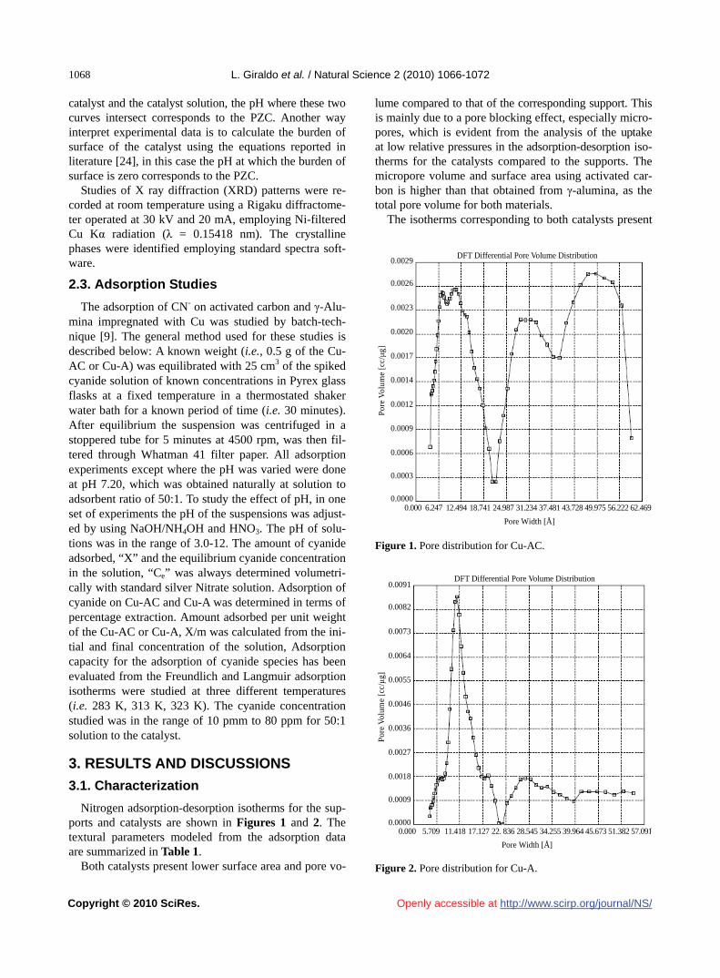
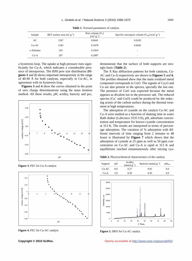
Nitrogen adsorption-desorption isotherms for the sup- ports and catalysts are shown in Figures 1 and 2. The textural parameters modeled from the adsorption data are summarized in Table 1.
Both catalysts present lower surface area and pore vo-
lume compared to that of the corresponding support. This is mainly due to a pore blocking effect, especially micro- pores, which is evident from the analysis of the uptake at low relative pressures in the adsorption-desorption iso-therms for the catalysts compared to the supports. The micropore volume and surface area using activated car-bon is higher than that obtained from γ-alumina, as the total pore volume for both materials.
The isotherms corresponding to both catalysts present
0.000 6.247 12.494 18.741 24.987 31.234 37.481 43.728 49.975 56.222 62.469
Pore Width [Å]
DFT Differential Pore Volume Distribution0.0029
0.0026
0.0023
0.0020
0.0017
0.0014
0.0012
0.0009
0.0006
0.0003
0.0000
Por
e V
olum
e [c
c/μg
]
Figure 1. Pore distribution for Cu-AC.
0.000 5.709 11.418 17.127 22. 836 28.545 34.255 39.964 45.673 51.382 57.091
Pore Width [Å]
DFT Differential Pore Volume Distribution 0.0091
0.0082
0.0073
0.0064
0.0055
0.0046
0.0036
0.0027
0.0018
0.0009
0.0000
Por
e V
olum
e [c
c/μg
]
Figure 2. Pore distribution for Cu-A.
L. Giraldo et al. / Natural Science 2 (2010) 1066-1072
Copyright © 2010 SciRes. http://www.scirp.org/journal/NS/
1061069
Table 1. Textural parameters of catalyst.
Sample BET surface area (m2.g–1) Pore volume (VT)
(cm3.g–1) Specific micropore volume (VDR) (cm3.g–1)
AC 1567 0.6641 0.6245
Cu-AC 1245 0.5478 0.6042
γ-Alúmina 245 0.2454 -
Cu-A 207 0.2087 -
a hysteresis loop. The uptake at high pressure rises signi- ficantly for Cu-A, which indicates a considerable pres-ence of mesoporous. The BJH pore size distribution (Fi- gures 1 and 2) shows important mesoporosity in the range of 40-90 Å for both catalysts, especially in Cu-AC, in agreement with its hysteresis loop.
demonstrate that the surface of both supports are stro- ngly basic (Table 2).
The X Ray diffraction patterns for both catalysts, Cu- AC and Cu-A respectively are shown in Figures 5 and 6. The profiles obtained show that the main oxidized metal compound corresponds to CuO. The signals of Cu2O and Cu are also present in the spectra, specially the last one. The presence of CuO was expected because the metal appears as divalent ion in the precursor salt. The reduced species (Cu+ and CuO) could be produced by the reduc-ing action of the carbon surface during the thermal treat- ment at high temperatures.
Figures 3 and 4 show the curves obtained in the point of zero charge determinations using the mass titration method. All these results, pH, acidity, basicity and pzc,
-0,05
-0,03
-0,01
0,01
0,03
0,05
6 7 8 9 10 11 12 13 1
pH
surf
ace
char
ge,(
C/m
2 )
4
The adsorption of cyanide on the catalyst Cu-AC and Cu-A were studied as a function of shaking time in water Bath shaker (Labconco 3535 US), pH, adsorbate concen- tration and temperature for known cyanide concentration at 313 K. The results are interpreted in terms of percent-age adsorption. The variation of % adsorption with dif-ferent intervals of time ranging from 2 minutes to 48 hours is illustrated by Figure 7 which shows that the adsorption of cyanide at 25 ppm as well as 50 ppm con-centration on Cu-AC and Cu-A is rapid at 313 K and equilibrium reached instantaneously after mixing cya- Table 2. Physicochemical characteristics of the catalyst.
Support pH Acidity
(mmol.g–1) Basicity (mmol.g–1) pHPZC
Cu-AC 8.6 0.27 0.81 9.0
Cu-A 5.8 0.20 0.45 6.0
Figure 3. PZC for Cu-A catalyst.
-0,08
-0,06
-0,04
-0,02
0
0,02
0,04
0 2 4 6 8 10 12 14
pH
surf
ace
char
ge,(
C/m
2 )
0
5000
10000
15000
20000
25000
30000
0 10 20 30 40 50 60 70 80 90
2 Theta
Inte
nsi
ty, u
.a.
Figure 4. PZC for Cu-AC catalyst. Figure 5. DRX for Cu-AC catalys.
Openly accessible at

L. Giraldo et al. / Natural Science 2 (2010) 1066-1072
Copyright © 2010 SciRes. http://www.scirp.org/journal/NS/
1070
Openly accessible at
0
1000
2000
3000
4000
5000
6000
7000
8000
0 10 20 30 40 50 60 70 80 90
2 Theta
Inte
nsity
,u.a
.
Figure 6. DRX Cu-A catalyst.
58
63
68
73
78
83
88
93
98
103
0 15 30 45 60 75 90 105 120 135 150
Time,minutes
%ag
e A
dsor
ptio
n
Cu-A25
Cu-AC50
Cu-A50
Cu-AC25
Figure 7. Effect of shaking time % age Adsorption at 25 ppm and 50 ppm for the synthesized catalyst. nide solution with the catalyst. However, an equilibri-umis reached faster with the catalyst of Cu-AC than with Cu-A; that is associated with the greatest amount of copper that is achieved on the activated carbon adsorb taking into account their surface properties and specific chemical the PZC allowing CN ions adsorb more rapidly on the catalyst surface Cu-AC on the Cu-A.
No significant change in % adsorption values was ob-served up to 48 hours, which indicates that surface pre-cipitation as well as ion exchange may be the possible adsorption mechanism. Therefore, equilibrium time of 20 minutes was selected for all further studies. The ad-sorption is pH dependent, a much greater adsorptive ca pacity for cyanide was observed in neutral solution for both catalyst; moreover it is more higher adsorption ca-pacity for Cu-AC, i.e., pH 7- 8.0 (Table 3 and Table 4).
Because when the pH is reduced, surface charge of the particles becomes increasingly positive and because of the competition of the hydrogen ions for the binding sites,
Table 3. Dependence of absorbance concentration relative to CN- on Cu-A catalyst at 293 K.
pHAmount of CN-
in taken Amount of CN- in sol. At equilibrium
Amount of CN-
Adsorbed Adsorption
(ppm) (ppm) (ppm) (%)
2,064,576,547,289,1411,3412,75
20 20 20 20 20 20 20
6,48 5,44 4,11 2,13 4,11 6,55 7,76
13,52 14,56 15,89 17,87 15,89 13,45 12,24
67,60 72,80 79,45 89,35 79,45 67,45 61,20
Table 4. Dependence of absorbance concentration relative to CN- on Cu-AC catalyst at 293 K.
pH Amount of
CN- in takenAmount of CN- in sol. At equilibrium
Amount of CN-
Adsorbed Adsorption
(ppm) (ppm) (ppm) (%) 2,064,576,547,289,1411,3412,75
20 20 20 20 20 20 20
5,35 3,34 1,23 0,99 2,02 4,66 5,55
14,65 16,66 18,77 19,01 17,98 15,34 14,45
73,25 83,30 93,85 95,05 89,90 75,70 72,25
metal ions tend to desorbs at low pH region, as well a small decrease in cyanide adsorption was observed at pH higher than 9.0. This behavior may be due to the forma-tion of soluble cyanide complexes, which remain in so-lution as dissolved component. Similarly adsorption of cyanide as a function of its concentration was studied by varying the metal concentration from 10ppm to 80 pmm, % age adsorption values decreases with increasing metal concentration (Table 5), which suggest that at least two types of phenomena (i.e. adsorption as well ion-exchange) taking place in the range of metal concentration studied, in addition less favorable lattice positions or exchange sites become involved with increasing metal concentra-tion.
The adsorption in aqueous solutions and adsorption isotherms at three different temperatures (i.e. 278 K, 298 K, 323 K) were obtained by plotting the amount of cya Table 5. Dependence of adsorbate concentration relative to CN- on Cu-AC (this catalyst present major adsorption).
Amount of Adsorbent
CN- in taken
Amount of CN- taken
Amount of CN- in soln.
at Equilibrium
Amount of CN- Adsorbed
Adsorption
(mg (ppm) (ppm) (ppm) (%)
500 500 500 500 500 500 500
5,00 10,00 20,00 40,00 60,00 80,00
100,00
2,42 3,12 1,41
15,65 37,98 41,09 54,58
2,58 6,88 18,52 30,35 38,44 38,91 45,42
51,60 68,00 92,60 75,88 64,06 48,63 45,42

L. Giraldo et al. / Natural Science 2 (2010) 1066-1072
Copyright © 2010 SciRes. http://www.scirp.org/journal/NS/
1071071
Openly accessible at
nide adsorbed on Cu-A and Cu-AC (mg/g) against metal at equilibrium concentration “Ce” (mg/l). Adsorption of cyanide decreases with increasing temperature. Two mo- dels, Langmuir and Freundlich equations, were used to describe experimental data for adsorption isotherms.
The linear form of the Freundlich isotherm model is given by the following relation:
Log x / m = logKF + 1 / nlogCe (1)
where x / m is the amount adsorbed at equilibrium (mg/g), Ce is the equilibrium concentration of the adsorbate (mg/l), and KF and 1 / n are the Freundlich constants related to adsorption capacity and adsorption intensity respectively, of the sorbent. The values of KF and 1/n can be obtained from the intercept and slope respectively, of the linear plot of experimental data of log X / m versus logCe. The linear form of the Langmuir isotherm model can be represented by the following relation:
Ce / x / m = 1 / KLVm + Ce / Vm (2)
where Vm and KL are the Langmuir constants related to the maximum adsorption capacity and the energy of ad-sorption, respectively. These constants can be evaluated from the intercept and slope of the linear plot of experi-mental data of Ce / X / m versus Ce. The Freundlich and Langmuir adsorption isotherms are shown in Figure 3 and Figure 4 (the isotherms linearizated not shown here). The related parameters of Langmuir and Freundlich mo- dels are summarized in Table 6. The results reveal that both the Langmuir isotherm model adequately describes better the adsorption data (See Figure 8).
Calculations of thermodynamic parameters: Thermodynamic parameters such as Gibbs free energy
ΔG° (kJ/mol), change in enthalpy ΔH° (kJ/mol) and change in entropy ΔS° (J.K-1mol-1) for cyanide adsorp-tion were calculated from the distribution constant K [10] by using the following relations:
ΔG° = - RTlnK (3)
ΔG° = ΔH° - (4)
and
K = - ΔH° / RT + Constant (5)
Tables 7 and 8 show the values of thermodynamics parameters ΔH°, ΔS°, ΔG° for Cu-AC and Cu-A catalyst synthesized. The positive value of ΔH° = 6.234 kJ/mole for Cu-AC and 4.897 kJ/mole, which is calculated from Eq.5 and Figure 5, confirms the endothermic nature of the overall adsorption process. The positive value of ΔS° suggests increased randomness at the solid/solution in-terface with some structural change in the adsorbate and adsorbent and also affinity of the Cu-AC and Cu-A to-wards CN-; the values more highest of entropy indicate spontaneous process. A negative value of ΔG° indicates
Table 6. Parameters of Lagmuir and Freundlich for adsorption of cyanide.
Langmuir Freundlich
Qo K R2 Kf n R2 Alumina 221,9725 0,018648 0,99835 7,431714 1,477998 0,99653
Activated Carbon
226,7673 0,029620 0,99781 11,98697 1,628459 0,99330
Cu-A 317,2252 0,041956 0,99700 22,77397 1,759936 0,98713
Cu-Ac 297,2679 0,164927 0,99646 58,15241 2,573350 0,97419
Table 7. Values of thermodynamic data for Adsorption of CN- on Cu-AC.
Temperature K
ΔH° kJ/mol
ΔG° kJ/mol
ΔS° J/K.mol
278 6.234 -8.856 0.0543
298 6.234 -6.636 0.0432
323 6.234 -12.666 0.0585
Table 8. Values of thermodynamic data for Adsorption of CN- on Cu-A.
Temperature K
ΔH° kJ/mol
ΔG° kJ/mol
ΔS° J/K.mol
278 4.897 -6.863 0.0423
298 4.897 -6.963 0.0398
323 4.897 -10.183 0.0467
AluminaActivated Carbon
Cu-A Cu-AC
Langmuir Freundlich
0 10 20 30 40 50 60 70 80
Ce, mg/g
0
50
100
150
200
250
300
x/m
, mg
/g
Figure 8. Langmuir and Freundlich models adjust-ment at 298 K.
the feasibility and spontaneity of the adsorption process, where higher negative value reflects a more energetically favorable adsorption process. The process of adsorption Cu-AC is more favorable.

L. Giraldo et al. / Natural Science 2 (2010) 1066-1072
Copyright © 2010 SciRes. http://www.scirp.org/journal/NS/
1072
4. CONCLUSIONS [8] Tien, C. (1994) Adsorption calculations and modeling. Butterworth-heinemann series in chemical engineering, Butterworth Heinemann, Boston. Keeping the adsorptive nature of Cu-AC and Cu-A in
view it is felt desirable to select batch adsorption process for removal of Cyanide from the industrial wastewater using activated carbon and γ-alumina. The main advan-tages of the procedure are:
[9] Wedl, A.G. and Fulk, J.D. (1991) Cyanide destruction in plating sludges by hot alkaline chlorination. Metal Finish, 89, 33-38.
[10] Gupta, C.G. and Murkherjee, T.K. (2001) Hydrometal-lurgy in extraction process, CRC press, Florida.
1) The cost of starting materials for obtaining the cata-lyst is low and easily available in country.
[11] Zhou, C.D. and Chin, D.T. (1994) Continuous electro-lytic treatment of complex metal cyanides with a rotating barrel plater as the cathode and a packed bed as the an-ode. Plating and Surface Finishing, 81, 70-81.
2) Ease and simplicity of preparation of the catalyst due to non-corrosive and non-poisonous nature of activated carbon and alumina. [12] Gill, J.B., Gans, P., Dougal, J.C. and Johnson, L.H. (1991)
Cyano and thiocyano complexation in solutions of noble metals, Reviews in Inorganic Chemistry, 11, 177-182. 3) Rapid attainment of phase equilibration and good
enrichment as well fitting of adsorption data with Langmuir isotherms.
[13] Bhakta, D., Shukla, S.S. and Margrave, L.J. (1992) A novel photocatalytic method for detoxification of cyanide wastes. Environmental Science & Technology, 26, 625- 634.
4) The positive value of ΔH° and negative values of ΔG° indicate the endothermic and spontaneous na-ture of the adsorption process.
[14] Bhargava, S., Tardío, J., Prasad, J., Föger, K., Akolekar, D. and Grocott, S. (2006) Wet oxidation and catalytic wet oxidation. Industrial & Engineering Chemical Research, 45, 1221-1234. 5. ACKNOWLEDGEMENTS
[15] Lei, L., Hu, X., Chen, G., Porter, J.F. and Yue, P.L. (2000) Wet air oxidation of desizing wastewater from textile in-dustry. Industrial & Engineering Chemical Research, 39, 2896-2905.
The authors wish to thank the Master Agreement established between
Universidad de los Andes and Universidad Nacional de Colombia, and
the Memorandum of Understanding between Departments of Chemis-
try of both Universities. Additionally, special thanks to Fondo Especial
de la Facultad de Ciencias and Proyecto Semilla of Universidad de los
Andes for the partial financial of this research.
[16] Mantzavinos, D., Hellenbrand, R., Livingston, A.G. and Metcalfe, I.S. (1996) Catalytic wet air oxidation of pol- yethylene glycol. Applied Catalysis B: Environmental, 11, 99-107.
[17] Kolaczkowski, S.T., Plucinski, P., Beltran, F.J., Rivas, F. J., and Mc Lurgh, D.B. (1999) Wet air oxidation: A re-view of process technologies and aspects in reactor de-sign, Chemical Engineering Journal, 73, 143-152.
REFERENCES
[1] Abell, M.L. and Barselton, P.J. (1974) The maple V handbook. AP Professional, New York.
[18] Luck, F. (1999) Wet air oxidation: Past, present and fu-ture. Catalysis Today, 53, 81-89.
[2] Contescu, C., Jagiello, J. and Schwarz, J.A. (1995) Pro-ton affinity distributions: A scientific basis for the design and construction of supported metal catalysts. Prepara-tion of Catalysts VI, Scientific Bases for the Preparation of Heterogeneous Catalysts, Elsevier Science, New York.
[19] Pintar, A. (2003) Catalytic process for the purification of drinking water and industrial effluents. Catalysis Today, 77, 451-462.
[20] Fortuny, A., Bengoa, C., Font, J., Catells, F. and Fabregat, A. (1999) Water pollution abatement by catalytic wet air oxidation in a trickle bed reactor, Catalysis Today, 53, 107-112.
[3] Cooper, D. and Plane, A.R. (1966) Cyanide complexes of copper with ammonia and ethylenediamine. Inorganic Chemistry, 5, 1677-1681. [21] Deiana, A.C., Granados, D., Petkovic, L.M., Sardella, M.
F. and Silva, H.S. (2004) Use of grape must binder to obtain activated carbon briquettes. Brazilian Journal of Chemical Engineering, 21, 585-592.
[4] Gupta, A., Johnson, E.F. and Schlossel, R.H. (1987) In-vestigation into the ion exchange of the cyanide com-plexes of Zinc(II), Cadmium(II), and Copper(I) Ions. In-dustrial Engineering Chemistry Research, 26, 588-597. [22] Moreno-Piraján, J.C. and Giraldo, L. (2010) Study of
activated carbons by pyrolysis of cassava peel in the presence of chloride zinc. Journal of Analytical and Ap-plied and Pyrolysis, 87(2), 288-290.
[5] Hogfeldt, E. (1982) Stability constants of metal-ion com-plexes: part A: inorganic ligands, Pergamon Press, Oxford.
[6] Riley, T.C. and Semmens, J.M. (1994) Recovery of cad-mium and cyanide using a combination of ion exchange and membrane extraction. Plating and Surface Finishing, 81, 46-54.
[23] Moreno-Piraján, J.C. and Giraldo, L. (2010) Adsorption of copper from aqueous solution by activated carbons obtained by pyrolysis of cassava peel. Journal of Ana-lytical Applied and Pyrolysis, 7(2), 188-193. [7] Tan, T.C. and Teo, W.K. (1987) Destruction of cyanides
by thermal hydrolysis. Plating and Surface Finishing, 74, 70-76.
[24] Rodríguez-Reinoso F. (1998) The role of carbon materi-als in heterogeneous catalysis, Carbon, 36, 159-164.
Openly accessible at

Vol.2, No.10, 1073-107doi:10.4236/ns.2010.210133
Copyright © 2010 SciRes. http://www.scirp.org/journal/NS/
8 (2010) Natural Science
Openly accessible at
Structural and electrical characterization of Bi2VO5.5 / Bi4Ti3O12 bilayer thin films deposited by pulsed laser ablation technique
Neelam Kumari, Saluru Baba Krupanidhi, Kalidhindi Balakrishna Raju Varma*
Materials Research Centre, Indian Institute of science, Bangalore, India; *Corresponding Author: [email protected].
Received 10 June 2010; revised 13 July 2010; accepted 18 July 2010.
ABSTRACT
The pulsed laser ablation technique has been employed to fabricate bilayer thin films con-sisting of layered structure ferroelectric bis-muth vanadate (Bi2VO5.5) and bismuth titanate (Bi4Ti3O12) on platinized silicon substrate. The phase formation of these films was confirmed by X-ray diffraction (XRD) studies and the crys-tallites in these bilayers were randomly oriented as indicated by diffraction pattern consisting of the peaks corresponding to both the materials. The homogeneous distribution of grains (~300 nm) in these films was confirmed by atomic force microscopy. The cross-sectional scanning electron microscopy indicated the thickness of these films to be around 350 nm. The film ex-hibited P-E hysteresis loops with Pr ~ 11 C/cm2 and Ec ~ 115 kV/cm at room temperature. The dielectric constant of the bilayer was ~ 225 at 100 kHz which was higher than that of homo-geneous Bi2VO5.5 film.
Keywords: Thin Films; Ferroelectric; Dielectric; Laser ablation
1. INTRODUCTION
Fabrication and stabilization of materials that do not occur naturally has been the subject of great interest of current materials research [1]. Recently the investigations of ferroelectric multilayer and superlattices have received considerable attention due to the fact that these kinds of engineered materials have been identified as possessing functional properties in a sense superior to their single phase constituent films [2-4]. The control of properties could be achieved by tailoring the lattices [5] e.g. by la- ttice mismatch induced strain at the interface-strain en-gineering, polarization mismatch enhancing polarization, chemical heterogeneity, which in turn may enhance the
physical properties or in many cases may give rise to new properties which were not exhibited by the starting ma-terials.The Aurivillius family of layered bismuth oxides is a class of ferroelectrics whose properties have been widely studied [6]. More recently, there is a renewed in- terest because of the discovery of fatigue-free behavior in thin films for nonvolatile memory applications [7]. More importantly, Bismuth Titanate [Bi4Ti3O12 (BTO)], which is an n = 3 member of this family has been re-ported to be a very good ferroelectric and electro-optic with small amount of the substitution of impurities, such as La, Sm and Nd for Bi and V, W and Nb for Ti in the pseudoperovskite (Bi2Ti3O10)
2− layers of BTO to im-prove the remnant polarization and fatigue endurance. [8-11]. Bismuth Vanadate [Bi2VO5.5 (BVO)] is a vana-dium analog of the n = 1 member of the Aurivillius fam-ily which has a Curie temperature of 720 K [12-14]. It has been reported in the literature that the composite of BVO and BTO solid solution possesses better physical properties and low leakage current than that of BVO [15]. The single phase BVO thin films have been pre-pared on platinum coated Si substrates and studied their ferroelectric and dielectric properties [16]. It has been found that these films possess non-negligible ionic con-ductivity attributed to the presence of oxide ion vacan-cies in the perovskite layer. Also the contribution of oxygen ion vacancies to the ferroelectric properties was quite high as established through fatigue characteristics.
In this article we report the structural and electrical properties of bilayer stacking of Bi2VO5.5 (BVO) and Bi4Ti3O12 (BTO). We have fabricated bilayer thin films consisting of alternating BVO and BTO layers hence-forth mentioned as BVBT. The presence of a BTO layer along with the BVO layer effectively suppressed the high electrical conductivity of BVO which is commonly observed in the laser ablated BVO thin films deposited on Pt / TiO2 / SiO2 / Si substrates. The BVBT bilayer thin films showed a fair increase in remnant polarization (Pr), and more interestingly a significant reduction in coercive field (Ec), as compared to the homogeneous BVO films

N. Kumari et al. / Natural Science 2 (2010) 1073-1078
Copyright © 2010 SciRes. http://www.scirp.org/journal/NS/
1074
Openly accessible at
of the same thickness. The details pertaining to the struc- tural, dielectric and ferroelectric properties of BV BT bi- layers fabricated on platinized silicon in metal insulator metal (MIM) configuration are illustrated in the follow-ing sections.
2. EXPERIMENTAL
The bilayer structures consisting of BVO and BTO were fabricated by a multitarget-pulsed laser deposition (PLD) technique on platinized silicon substrate in the configuration Au / BVO / BTO / Pt (111) / TiO2 / SiO2 / Si (100). A 248 nm excimer laser (Lambda Physik Com- pex 201) operated at 5 Hz was alternately focused onto the well-sintered freshly polished BVO and BTO rotat-ing targets with an energy density of 2 Jcm-2 at an angle of 45˚ by a UV lens. The substrates were placed parallel to the target at a distance of 3.5 cm and heated to 650℃ by a resistance heater. The chamber was first pumped down to 1 10-6 m bar, and then high purity oxygen was introduced using a mass flow controller to get oxygen partial pressure of 100 m Torr. After deposition of both the layers, the samples were cooled down to room tem-perature under an oxygen pressure of 1 mbar to minim- ize the oxygen ion vacancies. In these cases, the bilayer thin films were prepared with BTO as the first layer and BVO as the final layer with equal layer thickness.
The X-ray diffraction (XRD) studies were carried out to characterize the phase and crystallographic structure of the bilayer films using Cu Kα ~ 1.541 Å radiation (Scintag XR 2000 Diffractometer). Scanning electron microscope (SEM) (Sirion 200) and atomic force micro-scope (AFM) (Veeco CP II) were employed to monitor the microstructure of the films.
For electrical measurements, gold dots of 1.96 × 10⁻³ cm2 area were deposited on the top surface of the films through a shadow mask using thermal evaporation tech- nique. The electrode dots were annealed at 250℃ for 30 min. The Pt surface was used as the bottom electrode for capacitance measurements. The dielectric constant and C-V measurements were performed at a signal strength of 0.5 V using impedance analyzer (HP4294A). The polarization-electric field (P-E) hysteresis was recorded using a Precision Workstation (Radiant Technologies, Inc.) ferroelectric test system in virtual ground mode.
3. RESULTS AND DISCUSSIONS
Bilayered thin films of BVO and BTO were fabricated on platinized silicon substrates by pulsed laser ablation using the optimized deposition conditions for BVO and BTO layers. A schematic diagram of the bilayer thin film grown in this work is shown in Figure 1. Equal thick-
TiO2 / SiO2 / Si
BTO
BVO
Pt
Au
Figure 1. Schematic diagram of a BVBT bilayer thin film. ness (~ 175 nm) of the individual layers was maintained in bilayer films. The BTO layer was grown first on pla- tinized silicon substrate and then immediately followed by the growth of BVO layer without any delay in order to maintain the sharp interface between the two layers. The sequence of the layers was also reversed, but not much difference in terms of physical properties was ob-served, hence the one bilayer structure i.e. BVBT bilayer is discussed as a symbolic representative one.
Figure 2(a) shows the representative XRD pattern of BVBT bilayer film deposited by PLD. The XRD diffrac-tion peaks corresponding to both the BVO and BTO phases were observed and these were indexed on the ba- sis of orthorhombic structure of BVO [JCPDS 42-0135] and BTO [JCPDS 72-1019]. It is observed that the film is polycrystalline in nature and main diffraction peaks of both BVO (113) and BTO (117) appear with higher inten- sities along with the other low intensity peaks. Also, the (002) reflection of BVO along with (004) of BTO appear so close that they overlap giving only one visible peak. The bilayer film possessed an interface between the two individual layers and this interface does influence the physical properties due to the lattice strain at the inter-face. Figure 2(b) shows the (002) diffraction peak cor-responding to BVO of the bilayer thin film. The c-axis lattice parameter calculated for BVO from the (002) peak was found to increase from 15.42 Å for BVO layer [17] to 15.50 Å in BVBT bilayer. This increase in out-of-plane lattice parameter might be due to the in plane compres-sive stress on BVO in BVBT bilayer in the present case in order to keep the cell volume unchanged. Therefore, it is required to grow these films epitaxially and measure the in-plane lattice parameters along with the residual stress in these bilayer films in order to achieve the lattice driven effects in these films.
The surface morphology of the BVBT BL thin film was investigated by contact mode atomic force micro-scope (AFM). Figure 3 shows the surface morphology of BVBT bilayer thin film over a 5 m x 5 m scan area as two-dimensional (a) and three-dimensional (b) mi-

N. Kumari et al. / Natural Science 2 (2010) 1073-1078
Copyright © 2010 SciRes. http://www.scirp.org/journal/NS/
1071075
10.5 11.0 11.5 12.0
(b)
Inte
nsi
ty (
a.u
.)
(002
)
2 (Degree)
BVBTBVO
10.5 11.0 11.5 12.0 2θ (Degree)
I
nten
sity
(a.u
.)
BVBTBVO
(b)
(002
) c = 15.50 Å
c = 15.42 Å
Figure 2. (a) X-ray diffraction pattern of BVBT bilayer thin film. (b) Comparison of BVO and BVBT bi-layer diffraction pattern along (002) plane of BVO.
(b)
(c)
(a)
Figure 3. (a) AFM micrograph showing surface topography, (b) 3D image of BVBT bilayer thin film and (c) line profile.
crographs with the roughness profile mapped using line scan depicted in (c) The BVBT bilayer films exhibited dense surface morphology consisting of distinct grains. Further the homogeneous distribution of grains was ob-served with an average grain size of 0.3 m. The root mean square of the surface roughness (Ra) was around 7 nm as observed from the roughness profile. It indicated a good quality of the deposited bilayer films.
The cross sectional microstructure of BVBT bilayer
was studied by SEM and is depicted in Figure 4 which indicated dense bilayer growth with sharp interface with Pt. A columnar like structure was observed for this sam-ple and the thickness of the sample bilayer film was around 300 nm. It is noteworthy here that we could not distinguish between the top BVO and bottom BTO layer in this bilayer structure. This might be due to the very little difference in the atoms constituting the BVO and BTO layers which scatter the electrons almost with the
Openly accessible at

N. Kumari et al. / Natural Science 2 (2010) 1073-1078
Copyright © 2010 SciRes. http://www.scirp.org/journal/NS/
1076
Openly accessible at
Figure 4. Cross sectional scanning electron micrograph of a representative BVBT bilayer film. same intensity during and as a result the contrast bet- ween the two layers is poor.
In the present study we have further focused on the ferroelectric (FE) properties of these BVBT bilayer thin films deposited on platinized silicon substrate. Polariza-tion measurements were carried out using a Precision Workstation operating in the virtual ground mode as ex- plained earlier. A simple triangular pulse of voltage is applied across the electrodes of the sample which was fabricated in Metal-Insulator-Metal (MIM) configuration and the polarization response of the sample is observed under an integrator circuit. Figure 5(a) shows a typical P-E loop obtained for a BVBT bilayer thin film at room temperature. At the applied voltage of 12 V, the meas-ured values of remnant polarization (Pr) and coercive field (Ec) for ~ 350 nm thick BVBT bilayer film were around 11 C/cm2 and 115 kV/cm, respectively. The non zero switchable polarization observed at zero applied field is a general characteristic of a FE material [18-19]. It showed two key characteristics of a ferroelectric which are, polarization is reversible by an application of
an electric field and polarization remains at a finite value even after the removal of the electric field [20].The value of remnant polarization observed for these bilayer films is higher than that of the homogeneous BVO thin films of similar thickness [16]. Further the asymmetric nature of the P-E loops with respect to electric field axis indicates interface dominated behavior.
The capacitance voltage (C-V) characteristics of a B- VBT bilayer thin film measured at 100 kHz as probing frequency is shown Figure 5(b). The C-V measurements were carried out by applying a small ac signal of 0.5 V amplitude, with a varying dc electric field. The dc volt-age was swept from negative bias (-8 V) to positive (8 V) in steps of 0.1 V with a sweep rate of 0.1 V/s and back again. The butterfly shape of the curve confirmed the ferroelectric nature of the BVBT BL film and the ca-pacitance shows strong voltage dependence. The two ma- xima of the loop correspond to the domain switching voltage in forward and reverse directions where the po-larization reversal takes place. The asymmetry that is observed in C-V curve suggests that the electrodes are asymmetric and the film contains mobile ions or charges accumulated at the interface between the film and the electrode. In addition there is a difference between the capacitance values of the two peaks, which may be due to some defect energy levels in the film.
The dielectric dispersion studies were carried out on BVBT bilayer thin film at room temperature in the fre-quency range of 1 kHz to 1 MHz. Figure 6 shows the variation of dielectric constant ( r ) and the dissipation factor (D) as a function of frequency measured at room temperature. The dielectric constant as well as dissipa-tion factor was found to decrease abruptly in the low frequency region. The variation in dielectric constant is not significant at higher frequencies. Similar trend has been observed at lower frequencies for BVO films grown on platinized silicon substrate [16]. The small
ε
Figure 5. (a) The P-E hysteresis loop and (b) Capacitance- Voltage characteristics of a BVBT BL thin film measured at room temperature.

N. Kumari et al. / Natural Science 2 (2010) 1073-1078
Copyright © 2010 SciRes. http://www.scirp.org/journal/NS/
1071077
Openly accessible at
102 103 104 105 106240
260
280
300
320
340
(a)
Die
lect
ric
con
stan
t (
r')
Frequency (Hz)
25oC(a) 25℃
102 103 104 105 106 Frequency (Hz)
D
iele
ctri
c co
nsta
nt (
340
)
320
300
280
260
240
102 103 104 105 1060.0
0.1
0.2
0.3(b)
Frequency (Hz)
Dis
sip
atio
n f
acto
r (D
)
25oC
102 103 104 105 106 Frequency (Hz)
0.3
0.2
0.1
0.0
(b)
D
issi
patio
n fa
ctor
(D
)
25℃
Figure 6. (a) Variation of dielectric constant and (b) dissipation factor of a BVBT BL thin film as a func
ispersion observed at higher frequency has its contribu-
e observed dielectric constant of B
tion of frequency.
dtion from the response of the grains, while at lower fre-quencies grain boundaries, free charges etc. would con-tribute significantly. However the dielectric loss for B- VBT bilayer thin film shows an increasing trend subse-quent to 100 kHz. The dissipation factor has the mini-mum value (~ 0.03) around 100 kHz, where the dielec-tric constant is ~ 252.
The comparison of thVBT bilayer with that of the single layer BVO and
BTO films is shown in Figure 7. The dielectric constant of BVBT bilayer film shows less dispersion as compared to that of homogeneous BVO film. This might be due to the reduced number of defect states in bilayer films due to the presence of BTO layer. Further the observed
102 103 104 1050
100
200
300
400
500
Die
lect
ric
con
stan
t( r')
Frequency (Hz)
BVOBTOBVBT BL
BVO BTO BVBT BL
102 103 104 105 Frequency (Hz)
500
400
300
200
100
0
D
iele
ctri
c co
nsta
nt (
)
Figure 7. Comparison of dielectric constant of BTO, BTO and
dielectric constant of bilayer film is higher(e.g. ~ 225 at f single layer BVO film.
res consisting of ferroelectric O5.5) and Bismuth titanate
(B
EFERENCES
lank, D.H.A. (2005) Materials science: perlattice. Nature, 433, 369-370.
BVBT bilayer films.
1 M Hz) than that o
4. CONCLUSIONS
Bilayer thin film structuBismuth vanadate (Bi2V
i4Ti3O12) individual layers were fabricated on plati-nized silicon substrate (Pt(111) / Ti / SiO2 / Si) using pulsed laser ablation technique and investigated system-atically their structural and electrical properties. The X-ray diffraction (XRD) studies indicated that bilayer is randomly oriented and the diffraction pattern consists of diffraction peaks from both starting materials. The Ato- mic force microscopy of the films indicates that there is a homogeneous distribution of grains in these films. The cross-sectional scanning electron microscopy established the dense nature of these films. The polarization hystere-sis and C-V studies established the ferroelectric nature of these films. The observed dielectric constant of these bilayer films was higher than that of single layer BVO films.
R
[1] Rijnders, G. and BBuild your own su
[2] Shimuta, T., Nakagawara, O., Makino, T., Arai, S., Ta-bata, H. and Kawai, T. (2002) Enhancement of remanent polarization in epitaxial BaTiO3 / SrTiO3 superlattices with “asymmetric” structure. Journal of Applied Physics, 91, 2290-2294.
[3] Pontes, F.M., Longo, E., Leite, E.R. and Varela, J.A. (2004) Improvement of the dielectric and ferroelectric properties in superlattice structure of Pb(Zr,Ti)O3 thin films grown by a chemical solution route. Applied Physic Letters, 84, 5470-5472.
N. Kumari et al. / Natural Science 2 (2010) 1073-1078
Copyright © 2010 SciRes. http://www.scirp.org/journal/NS/Openly accessible at
1078
ic three-component ferroelectric
6-1588.
ith platinum electrodes, Nature, 374, 627-629.
epitaxially grown Bi4
Crystallogr, 46,
) Phase transition in bismuth vanadate,
te ferroelctrics,
s of ferroelectric bis-
ric properties of ceramics and
f
illius oxide thin films. Ph. D. Thesis, Indian
related materials, Clare-
ctric oxides. Reviews of Modern Phy-
and use in design, Marcel Dekker
[4] Lee, H.N., Christen, H.M., Chisholm, M.F., Rouleau, C. M. and Lowndes, D.H., (2005) Strong polarization en- hancement in asymmetrsuperlattices, Nature, 433, 395-399.
[5] Neaton, J.B. and Rabe, K.M. (2003) Theory of polariza-tion enhancement in epitaxial BaTiO3 / SrTiO3 superlat-tices, Applied Physic Letters, 82, 158
[6] Aurivillius, B. (1949) Mixed bismuth oxides with layer lattices. II. Structure of Bi4Ti3O12. Arkiv for Kemi, 1(54) 463-480.
[7] Araujo, C.A.P. de, Cuchiaro, J.D., McMillan, L.D., Scott, M.C. and Scott, J.F. (1995) Fatigue-free ferroelectric ca-pacitors w
[8] Park, B.H., Kang, B.S., Bu, S.D., Noh, T.W., Lee, J. and Jo, W., (1999) Lanthanum-substituted bismuth titanate for use in non-volatile memories, Nature, 401, 682-684.
[9] Maiwa, H., Lizawa, N., Togawa, D., Hayashi, T., Saka- moto, W., Yamada, M. and Hirano, S. (2003) Electrome-chanical properties of Nd-doped Bi4Ti3O12 films: Acandidate for lead-free thin-film piezoelectrics. Applied Physic Letters, 82, 1760-1762.
[10] Watanabe, T., Funakubo, H., Osada, M., Noguchiand, Y. and Miyayama, M. (2002) Preparation and characteriza-tion of a- and b-axis-oriented Ti do3O12-based thin films with long-range lattice matching, Applied Physic Letters, 81, 1660-1662.
[11] Rae, A.D., Thompson, J.G., Withers, R.L. and Willis, A. C. (1990) Structure refinement of commensurately mo- dulated bismuth titanate, Bi4Ti3O12. Acta474-487.
[12] Borisov, V.N., Poplavko, Y.M, Avakyan, P.B. and Osip-
yan, V.G. (1988
Soviet Physics - Solid State, 30, 904-905. [13] Osipian, V.G., Savchenk, L.M., Elbakyan, V.L. and Avak-
yan, P.B. (1987) Layered boismuth vanadaInorganic Materials, 23, 467-469.
[14] Prasad, K.V.R. and Varma, K.B.R. (1994) Dielectric, thermal and pyroelectric propertiemuth vanadate single crystals, Materials Chemistry and Physics, 38, 406-410.
[15] Prasad, K.V.R. (1994) Investigations into the structural, dielectric and ferroelectsingle crystal of parent and substituted bismuth vanadate. Ph. D. Thesis, Indian Institute of Science, Bangalore.
[16] Kumari, N., Krupanidhi, S.B. and Varma, K.B.R. (2007) Dielectric, impedance and ferroelectric characteristics oc-oriented Bismuth vanadate films grown by pulsed laser deposition. Materials Science and Engineering B, 138, 22-30.
[17] Kumari, N. (2009) Structural, optical and electrical stud-ies on AurivInstitute of Science, Bangalore.
[18] Lines, M.E. and Glass, A.M. (1979) Principles and ap-plications of ferroelectrics and
n Press, Oxford. [19] Dawber, M., Rabe, K.M. and Scott, J.F. (2005) Physics
of thin-film ferroelesics, 77, 1083-1130.
[20] Richerson, D.W. (1992) Modern ceramic engineering: Properties, processingInc., New York.

Vol.2, No.10, 1079-108doi:10.4236/ns.2010.210134
Copyright © 2010 SciRes. http://www.scirp.org/journal/NS/
4 (2010) Natural Science
Openly accessible at
Secular evolution of continental crust: recorded from massif-type charnockites of Eastern Ghats belt, India
Samarendra Bhattacharya1, Ashwini Kumar Chaudhary2*
1Indian Statistical Institute, Kolkata, India; 2Indian Institute of Technology, Roorkee, India; *Corresponding Author: [email protected].
Received 15 July 2010; revised 18 August 2010; accepted 23 August 2010.
ABSTRACT
It is reasonably well established that the Earth has substantially cooled from the Archean to the present and hence the sites, rates and pro- cesses of crust formation must have changed through geologic time. Archean and Proterozoic granitic rocks are the principal record of such changes. Massif-type charnockites in the East-ern Ghats granulite belt, India, of Archean and Proterozoic ages mirror the changing condi-tions and/or processes of continental crust for- mation. Though both can be explained by de-hydration melting of mafic rocks, the conditions differ. Potasium and rubidium rich Proterozoic charnockites have significant negative Eu ano- maly indicating melting at shallow depths in the stability field of plagioclase. In contrast, sodium and strontium rich Archean charnockites with less LREE enrichment and less depletion in Eu indicate melting at greater depths in the stability field of garnet or amphibole.
Keywords: Secular changes; Continental crust; Massif-charnockites; Eastern Ghats
1. INTRODUCTION
The continental crust comprising byouant quartzo- feldspathic materials are difficult to destroy by subduc-tion and hence can be considered as the principal record of crustal evolution through geologic time. New conti-nental crust may form magmatically from underlying mantle. However, mantle melting products are predomi-nantly basaltic, whereas continental crust is andesitic which can not be extracted directly from melting of man-tle-peridotite. Continental crust formation therefore re-quires a second stage/or event of fractional crystalliza-tion [1] or remelting of basaltic magma [2]. Although there remains considerable debate on the processes of crust formation in the Archean compared to those operating in
the later period (post-Archean), significant differences in key geochemical features have been documented between Archean and later granitic rocks [3-5]. Moreover, tec-tonic setting for Archean magmatism as exemplified by TTG remains unresolved. Partial melting may have taken place in subducted slabs [6,7] or in underplated basalt beneath thickened crust or oceanic plateau [8]. TTG suites of Archean greenstone belts are taken as the Ar-chean continental crust, while large varieties of Protero-zoic granitic plutons represent the Proterozoic continen-tal crust (cf. Table 3 in [2]). These authors have pre-sented extensive discussion on these differences from a Granitic perspective and their possible implications on the changing processes and or conditions of crust forma-tion from Archean to Proterozoic times.
Eastern Ghats granulite belt, India, comprises massif- type charnockite as a major component in the regional granulite terrane, and there is unambiguous evidence of different generation of such charnockites. Archaean char- nockites have been described from northern margin against Singhbhum craton and western margin against Bastar craton [9-11]. Some of the massif-type charnockite suites in the central part of the granulite belt record only Proterozoic ages [12,13]. Although, some workers have described magmatic charnockites from the Eastern Ghats, presumably as mantle-derived melt [14], it is difficult to postulate silicic melts directly from mantle-melting. On the other hand, some workers consider enderbitic char-nockites of the Eastern Ghats belt as metamorphosed igneous precursors and commonly describe them as “now enderbite” [15]. Here again, the question of felsic igneous rocks directly derived from mantle remains un-resolved. Dehydration melting experiments have demon- strated that silicic melts of tonalitic, granodioritic and granitic compositions are produced at 8-10 Kbar, and ≥ 850℃ from mafic rocks [16-18]. The massif-type char-nockites in the Eastern Ghats belt are of variable compo-sition and P-T conditions of granulite facies metamor-phism are comparable to the experimental constraints as mentioned above [19, 20]. Thus a remelting of mantle-
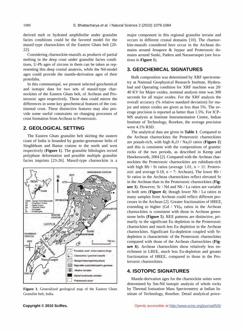
S. Bhattacharya et al. / Natural Science 2 (2010) 1079-1084
Copyright © 2010 SciRes. http://www.scirp.org/journal/NS/
1080
Openly accessible at
derived melt or hydrated amphibolite under granulite facies conditions could be the favored model for the massif-type charnockites of the Eastern Ghats belt [20- 22].
Considering charnockite-massifs as products of partial melting in the deep crust under granulite facies condi-tions, U-Pb ages of zircons in them can be taken as rep-resenting this deep crustal anatexis, while the Nd-model ages could provide the mantle-derivation ages of their protoliths.
In this communiqué, we present selected geochemical and isotopic data for two sets of massif-type char-nockites of the Eastern Ghats belt, of Archean and Pro-terozoic ages respectively. These data could mirror the differences in some key geochemical features of the con-tinental crust. These distinctive features may also pro-vide some useful constraints on changing processes of crust formation from Archean to Proterozoic.
2. GEOLOGICAL SETTING
The Eastern Ghats granulite belt skirting the eastern coast of India is bounded by granite-greenstone belts of Singhbhum and Bastar cratons to the north and west respectively (Figure 1). The granulite lithologies record polyphase deformation and possible multiple granulite facies imprints [23-26]. Massif-type charnockite is a
Figure 1. Generalized geological map of the Eastern Ghats Granulite belt, India.
major component in this regional granulite terrane and occurs in different crustal domains [10]. The charnoc- kite-massifs considered here occur in the Archean do-mains around Jenapore & Jaypur and Proterozoic do-mains around Sunki, Paderu and Naraseraopet (see loca-tions in Figure 1).
3. GEOCHEMICAL SIGNATURES
Bulk composition was determined by XRF spectrome- try at National Geophysical Research Institute, Hydera-bad and Operating condition for XRF machine was 20/ 40 KV for Major oxides, nominal analysis time was 300 seconds for all major oxides. For the XRF analysis the overall accuracy (% relative standard deviation) for ma-jor and minor oxides are given as less than 5%. The av-erage precision is reported as better than 1.5%. For ICP– MS analysis at Institute Instrumentation Centre, Indian Institute of Technology, Roorkee, the average precision were 4.1% RSD.
The analytical data are given in Table 1. Compared to the Archean charnockites the Proterozoic charnockites are potash-rich, with high K2O / Na2O ratios (Figure 2) and this is consistent with the compositions of granitic rocks of the two periods, as described in Kemp and Hawkesworth, 2004 [2]. Compared with the Archean char- nockites the Proterozoic charnockites are rubidium-rich with high Rb / Sr ratios (average 1.01, n = 11: Protero-zoic and average 0.18, n = 7: Archean). The lower Rb / Sr ratios in the Archean charnockites reflect elevated Sr in the Archean than in the Proterozoic charnockites (Fig- ure 3). However, Sr / Nd and Nb / La ratios are variable in both sets (Figure 4); though lower Nb / La ratios in many samples from Archean could reflect different pro- cesses in the Archean [2]. Greater fractionation of HREE, extending to higher (Gd / Yb)N ratios in the Archean charnockites is consistent with those in Archean green-stone belts (Figure 5). REE patterns are distinctive, pri-marily in the significant Eu depletion in the Proterozoic charnockites and much less Eu depletion in the Archean charnockites. Significant Eu-depletion coupled with Sr- depletion is characteristic of the Proterozoic charnockites compared with those of the Archean charnockites (Fig-ure 6). Archean charnockites show relatively less en-richment in LREE, much less Eu-depletion and greater fractionation of HREE, compared to those in the Pro-terozoic charnockites.
4. ISOTOPIC SIGNATURES
Mantle-derivation ages for the charnockite suites were determined by Sm-Nd isotopic analysis of whole rocks by Thermal Ionisation Mass Spectrometry at Indian In-stitute of Technology, Roorkee. Detail analytical proce-

S. Bhattacharya et al. / Natural Science 2 (2010) 1079-1084
Copyright © 2010 SciRes. http://www.scirp.org/journal/NS/
1081081
Tab
le 1
. Sel
ecte
d ox
ides
, tra
ce e
lem
ent a
nd is
otop
ic d
ata
of m
assi
f-ty
pe c
harn
ocki
tes
in E
GB
.
Openly accessible at

S. Bhattacharya et al. / Natural Science 2 (2010) 1079-1084
Copyright © 2010 SciRes. http://www.scirp.org/journal/NS/
1082
7
6
5
4
3
2
1
0
K2O
%
0 1 2 3 4 5 6Na2O%
Figure 2. K2O versus Na2O plot of the charnockites in the Eastern Ghats Granulite belt. Archean charnockites: solid sym- bols; Proterozoic charnockites: open symbols.
10
1
0.1
0.01
Rb/
Sr
0.1 1 10Eu / Eu*
Figure 3. Rb / Sr versus Eu / Eu* plot of the charnockites in the Eastern Ghats Granulite belt. Symbols as in Figure 2.
1.2
1
0.8
0.6
0.4
0.2
0
Nb
/ La
Sr / Nd 0 10 20 30 40 50 60
Figure 4. Nb / La versus Sr / Nd plot of the charnockites in the Eastern Ghats Granulite belt. Symbols as in Figure 2. dure is given in Bhattacharya et al., 2010 [27]. Measured ratios for isotopic composition are normalized to 146Nd / 144Nd = 0.7219 for Nd. The measured ratio of 143Nd / 144Nd for Ames Nd Standard was 0.512138 ± 4 (quoted
10
1
0.1
(Gd
/ Yb)
N
0.1 1 10Eu / Eu*
Figure 5. (Gd / Yb)N versus Eu / Eu* plot of the charnockites in the Eastern Ghats Granulite belt. Symbols as in Figure 2.
Sam
ple
/ Cho
ndri
te
10000
1000
100
10
1La Ce Nd Sm Eu Gd Dy Er Yb Lu
Figure 6. Chondrite normalized REE plot of the charnockites in the Eastern Ghats Granulite belt. value 0.512138).
Mantle-derivation ages (TDM) for the Proterozoic char- nockites vary between 2.3 and 2.8 Ga (Naraseraopet), between 2.3 and 2.4 Ga (Paderu) and between 2.8 and 3.1 Ga (Sunki) and those for the Archean charnockites vary between 3.3 and 3.5 Ga (Jenapore) and between 3.4 and 3.5 Ga (Jaypur) respectively (Table 1).
5. DISCUSSIONS
High Rb / Sr ratios and significant negative Eu-ano- malies in the Proterozoic charnockites indicate residual plagioclase. The implication is that intracrustal melting occurred at shallow depths, in the stability field of pla-gioclase. In contrast, low Rb / Sr ratios, indicating ele-vated Sr, and lack of significant negative Eu-anomalies in the Archean charnockites are indicative of intracrustal melting at greater depths in the stability field of garnet or amphibole [2].

S. Bhattacharya et al. / Natural Science 2 (2010) 1079-1084
Copyright © 2010 SciRes. http://www.scirp.org/journal/NS/
1081083
Openly accessible at
Large discrepancies between crystallization ages (of anatectic charnockitic melt), given by U-Pb zircon ages reported in the literature (Table 1) and mantle derivation ages given by TDM for the Proterozoic charnockites con-firm that older crustal material was present within the source regions of the charnockitic magma [28]. This is in contrast to the relatively little time gap between crystal-lization ages and Nd-model ages for the Archean char-nockites, similar to those observed in Archean TTGs.
6. CONCLUSIONS
These differences in the geochemical and isotopic sig- natures between Archean and Proterozoic charnockites reflect different conditions of crust formation rather than different processes: both can be explained by dehydra-tion melting of hydrated basalt or amphibolite under granulite facies conditions; but Proterozoic charnockites at shallower depths (in plagioclase-stability field) than Archean charnockites (in garnet or amphibole-stability field).
7. ACKNOWLEDGEMENTS
Indian Statistical Institute, Kolkata provided the infrastructural fa-
cilities. Financial support was provided by the Department of Science
and Technology, Government of India, in the form of a research pro-
ject.
REFERENCES
[1] Soesoo, A. (2000) Fractional crystallization of mantle- derived melts as a mechanism for some I-type granite petrogenesis: An example from the Lachlan Fold Belt, Australia. Journal of Geological Society, 157, 135-149.
[2] Kemp, A.I.S. and Hawkesworth, C.J. (2004) Granitic perspectives on the Generation and secular evolution of the continental crust. Treatise on Geochemistry, 3, 349- 411.
[3] Taylor, S.R. and McLennan, S.M. (1985) The continental crust: Its composition and evolution. Blackwell Publish-ing, Oxford.
[4] Taylor, S.R. and McLennan, S.M. (1995) The geochemi-cal evolution of the continental crust. Reviews of Geo-physics, 33, 241-265.
[5] Rudnick, R.L. and Gao, S. (2004) Composition of the continental crust. Treatise on Geochemistry, 3, 1-65.
[6] Condie, K.C. (1998) Episodic continental growth and supercontinents: A mantle avalanche connection? Earth and Planetary Science Letters, 163, 97-108.
[7] Martin, H. (1995) Archean grey gneisses and genesis of continental crust. In: Condie, K.C. Ed., Archean crustal evolution, Elsevier, Netherlands, 205-260.
[8] Whalen, J.B., Percival, J.A., McNiccol, V.J. and Long-staffe, F.J. (2002) A mainly crustal origin for tonalitic granitoid rocks, superior province, Canada: Implications for late archean tectonomagmatic processes. Journal of
Petrology, 43, 1551-1570. [9] Bhattacharya, S., Kar, R., Misra, S. and Teixeira, W.
(2001) Early Archaean continental crust in the Eastern Ghats granulite belt, India: Isotopic evidence from a charnockite suite. Geological Magazine, 138, 609-618.
[10] Rickers, K., Mezger, K. and Raith, M. (2001) Evolution of the continental crust in the Proterozoic Eastern Ghats belt, India and new constraints for Rodinia reconstruction: Implications from Sm-Nd, Rb-Sr and Pb-Pb isotopes. Precambrian Research, 112, 183-210.
[11] Kovach, V.P., Simmat, R., Rickers, K., Berezhnaya, N.G., Salnikova, E.B., Dobmeier, C., Raith, M.M., Yakovleva, S.Z. and Kotov, A.B. (2001) The western charnockite zone of the Eastern Ghats belt, India: An independent crustal province of late Archean (2.8 Ga) and Paleopro-terozoic (1.7-1.6 Ga) terrains. Gond Research, 4, 666-667.
[12] Mezger, K. and Cosca, M.A. (1999) The thermal history of the Eastern Ghats belt (India) as revealed by U-Pb and 40Ar / 39Ar dating of metamorphic and magmatic miner-als: Implications for the SWEAT correlation. Precam-brian Research, 94, 251-271.
[13] Simmat, R. and Raith, M.M. (2008) U-Th-Pb monazite geochronometry of the Eastern Ghats Belt, India: Timing and spatial disposition of poly-metamorphism. Precam-brian Research, 162, 16-39.
[14] Subba Rao, M.V. and Divakara Rao, V. (1988) Chemical constraints on the origin of the charnockites in the East-ern Ghat Mobile belt, India. Chemical Geology, 69, 37-48.
[15] Bhui, U.K., Sengupta, P. and Sengupta, P. (2007) Phase relations in mafic dykes and their host rocks from Kon-dapalle, Andhra Pradesh, India: Implications for the time- depth trajectory of the Paleoproterozoic (late Archean?) granulites from southern Eastern Ghats belt. Precam-brian Research, 156, 153-174.
[16] Wolf, M.B. and Wyllie, P.J. (1994) Dehydration melting of amphibolite at 10 Kbar: Effects of temperature and time. Contributions to Mineralogy and Petrology, 115, 369-383.
[17] Patino Douce, A.E. and Beard, J.S. (1995) Dehydration melting of biotite gneiss and quartz amphibolite from 3 to 15 Kbar. Journal of Petrology, 36, 707-738.
[18] V`ielzeuf, D. and Schmidt, M.W. (2001) Melting rela-tions in hydrous systems revisited: Application to meta- pelites, metagreywackes and metabasalts. Contributions to Mineralogy and Petrology, 141, 251-267.
[19] Bhattacharya, S. (2003) Dehydration melting in mafic rocks in the Eastern Ghats Belt, India: Implications for variable composition of charnockitic melt and heteroge-neity of source rocks. Geological Society of India, 52, 131-144.
[20] Kar, R., Bhattacharya, S. and Sheraton, J.W. (2003) Hornblende dehydration melting in mafic rocks and the link between massif-type charnockite and associated granulites, Eastern Ghats Granulite Belt, India. Contribu-tions to Mineralogy and Petrology, 145, 707-729.
[21] Foley, S., Tiepolo, M. and Vannucci, R. (2002) Growth of early continental crust in subduction zones controlled by melting of amphibolite. Nature, 417, 837-840.
[22] Bhattacharya, S. (2010) Review: The charnockite prob-lem: A twenty-first century perspective. Natural Science, 2, 402-408.
[23] Halden, N.M., Bowes, D.R. and Dash, B. (1982) Struc-

S. Bhattacharya et al. / Natural Science 2 (2010) 1079-1084
Copyright © 2010 SciRes. http://www.scirp.org/journal/NS/ Openly accessible at
1084
tural evolution of migmatites in a granulite facies terrane: Precambrian crystalline complex of Angul, Orissa, India. Transactions of the Royal Society, 73, 109-118.
[24] Bhattacharya, S. (1997) Evolution of Eastern Ghats gra- nulite belt of India in a compressional tectonic regime and juxtaposition against Iron Ore craton of singhbhum by oblique collision-transpression. Proceedings of Indian Academy of Sciences, 106, 65-75.
[25] Sen, S.K., Bhattacharya, S. and Acharyya, A. (1995) A multi-stage pressure-temperature record in the Chilka Lake granulites: The epitome of the metamorphic evolu-tion of Eastern Ghats, journal of metamorphic geology, 13, 287-298.
[26] Dasgupta, S. and Sengupta, P. (2003) Indo-Antarctic cor- relation: A perspective from the Eastern Ghats Granulite
belt, India. Geological Society, 206, 131-144. [27] Bhattacharya, S., Das, P., Chaudhary, A.K. and Saw, A.K.
(2010) Mafic granulite xenoliths in the Eastern Ghats Granulite belt: Implications for lower crustal processes in the southeastern Indian Peninsula. Indian Journal of Ge-ology, 80, 55-69.
[28] McCulloch, M.T. and Chappel, B.W. (1982) Nd isotopic characteristics of S- and I-type granites. Earth and Plane- tary Science Letters, 58, 51-64.
[29] Bhattacharya, S., Kar, R., Teixeira, W. and Basei, M. (2003) High-temperature crustal anatexis in a clockwise P-T path: Isotopic evidence from a granulite-granitoid suite in the Eastern Ghats belt, India. Journal of the Geo-logical Society, 160, 39-46.

Vol.2, No.10, 1085-1089 (2010)doi:10.4236/ns.2010.210135
Copyright © 2010 SciRes. Openly accessible at http://www.scirp.org/journal/NS/
Natural Science
New experimental constraints: implications for petrogenesis of charnockite of dioritic composition
Rajib Kar1, Samarendra Bhattacharya2*
1J.K.College, Purulia, India; 2Indian Statistical Institute, Kolkata, India; *Corresponding Author: [email protected].
Received 13 August 2010; revised 16 September 2010; accepted 21 September 2010.
ABSTRACT
Hornblende-dehydration melting experiments at high temperatures (> 950oC) indicate change of melt composition from tonalite/granodiorite to quartz-diorite; clinopyroxene instead of hornbl- ende as the residual phase and change in melt-ing reaction from peritectic hornblende-dehydr- ation to eutectic clinopyroxene-orthopyroxene- plagioclase. In the light of these experimental results, petrogenesis of a charnockite pluton of homogeneous dioritic composition in the East-ern Ghats Belt, India, can be explained as melt-ing at high-temperatures (> 950oC). Negative Sr and Eu anomalies further indicate plagioclase as a major residual phase, consistent with melt- ing at high-temperatures (> 950oC).
Keywords: Dioritic charnockite; Residual clinopyroxene; Residual plagioclase; Eutectic melting
1. INTRODUCTION
It is quite common that large-scale charnockitic bod-ies are of variable composition from tonalite to granodi- orite, and sometimes even dioritic composition is report- ed [1]. On the other hand, petrogenesis of massif-type charnockites have been variously described: a) mantle- derived and differentiated melt [2]; b) high-temperature melting of dry granulite facies rocks [3]; c) more mafic varieties as mantle-derived melts [4]; d) product of hornblende-dehydration melting in the deep crust [5]. New melting experiments provide constraints on the petrogenesis of charnockitic rocks of dioritic composi-tion. From the Jenapore area in the Eastern Ghats Belt, India, charnockite-massif was described as the product of hornblende-dehydration melting under granulite fa-cies conditions, and with residual hornblende. There the two-pyroxene granulites occur as minor patches and
bands and were explained as peritectic segregates [5]. A stock-like body of charnockite (pluton) occurs in the same locale, a few kilometer to the south (Lat: 20o46' N; Long: 86o05' E). In contrast to the charnockite-massif, it is of more mafic and homogeneous composition at the outcrop-scale and commonly has both orthopyroxene and clinopyroxene.
In the present communication we present geochemical data from the charnockite pluton and in the light of new experimental constraints explain its origin by melting at high-temperatures (≥ 950oC).
2. EXPERIMENTAL CONSTRAINTS
The selected results of the hornblende-dehydration melting experiments is presented in Figure 1. The melts of 900oC and 925oC are tonalitic (normative Qtz / Plag > 0.25) and those above 950oC are quartz dioritic (norma-tive Qtz / Plag < 0.25) in composition. The melt compo-sition changes from corundum normative to diopside nor- mative when temperature increases from 925oC to 950oC. Also there is gradual decrease of plagioclase proportion with temperature rise. Moreover, the orthopyroxene and clinopyroxene are subequal in proportion at 900oC, and orthopyroxene gradually decreases in proportion to a trace amount at 1100oC. These results suggest that the nature of melting reaction changes from hornblende breakdown reaction at 925oC to eutectic clinopyroxene- orthopyroxene-plagioclase melting reaction at 950oC [6].
3. CHARNOCKITE PLUTON
The charnockite pluton at Jenapore is a relatively ho-mogeneous body of two-pyroxene granulite, unlike those occurring as minor bands and patches within the massif- type charnockite described from the area to the north [5]. Also as distinct from those within massif-type charnoc- kite garnet is absent, while clinopyroxene is much more bundant than orthopyroxene (Table 1). a
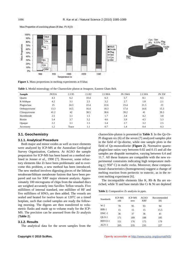
R. Kar et al. / Natural Science 2 (2010) 1085-1089
Copyright © 2010 SciRes. http://www.scirp.org/journal/NS/
1086
Openly accessible at
Figure 1. Mass proportions in melting experiments at 8 kbar. Table 1. Modal mineralogy of the Charnockite pluton at Jenapore, Eastern Ghats Belt.
Sample JN35A 2.J.95 2.J.82 2.J.90A JN 194A 2.J.50A JN 35F
Quartz 4.3 6.2 10.4 6.3 5.7 8.1 8.5
K-feldspar 4.2 3.1 2.5 3.2 2.7 1.8 2.1
Plagioclase 25 24.3 22.4 22.6 23.4 21.5 23
Orthopyroxene 13.3 14.5 16.4 18.3 17.4 14.6 15.3
Clinopyroxene 41.2 42 38.5 38.6 39.2 41 39.3
Hornblende 2.5 3.1 1.5 1.7 3.4 4.2 3.8
Biotite 5.4 3.7 5.2 4.6 3.9 4.5 5.3
Opaque 2.2 3.1 1.5 3.4 2.7 3.2 2.5
Accessory 1.2 Trace 1.1 0.7 1.4 0.4 0.3
3.1. Geochemistry
3.1.1. Analytical Procedure Both major and minor oxides as well as trace elements
were analyzed by ICP-MS at the Australian Geological Survey Organization, Canberra. At AGSO the sample preparation for ICP-MS has been based on a method out- lined in Jenner et al., 1990 [7]. However, some refrac-tory elements like Zr have been problematic and to over- come this problem, a new method has been introduced. The new method involves digesting pieces of the lithium tetraborate/lithium metaborate fusions that have been pre- pared and run for XRF major element analysis. Appro- ximately 100 micrograms of chips from the smashed discs are weighed accurately into Savillex Teflon vessels. Five milliliters of internal standard, one milliliter of HF and five milliliters of HNO3 are then added. The vessels are sealed and heated for twelve hours at 120oC on a timed hotplate, such that cooled samples are ready the follow-ing morning. The digests are then transferred to volu-metric flasks and made up to volume ready for the ICP- MS. The precision can be assessed from the Zr analysis (Table 2).
3.1.2. Results The analytical data for the seven samples from the
charnockite-pluton is presented in Table 3. In the Qz-Or- Pl diagram six (6) of the seven (7) analyzed samples plot in the field of Qz-diorite, while one sample plots in the field of Qz-monzodiorite (Figure 2). Normative quartz: plagioclase ratios vary between 0.02 and 0.15 and all the samples are diopside normative, varying between 6.4 and 11.7. All these features are compatible with the new ex-perimental constraints indicating high temperature melt-ing (≥ 950o C) in mafic rocks. Moreover, these composi-tional characteristics (homogeneous) suggest a change of melting reaction from peritectic to eutectic, as in the re- cent melting experiment [6].
The incompatible elements like K, Rb & Ba are en-riched, while Ti and base metals like Cr & Ni are depleted
Table 2. Comparative Zr analysis in ppm.
StandardsICP-MS
old ICP-MS
new AGSO XRF
Recommended [8]
W-2 78 95 93 94 BIR-1 15 15 15 15.5 DNC-1 36 37 36 41 QLO-1 171 189 188 185 BHVO-1 151 176 175 179 AGV-1 205 235 235 227

Vol.2, No.10, 1085-1089 (2010doi:10.4236/ns.2010.210135
Copyright © 2010 SciRes. http://www.scirp.org/journal/NS/
) Natural Science
Openly accessible at
Table 3. Composition of the charnockite pluton of Jenapore, Eastern Ghats, India.
Area Jenapore Sample JN35A 2.J.95 2.J.82 2.J.90A JN 194A 2.J.50A JN 35F SiO2 49.69 52.03 54.42 52.19 52.74 52.87 53.05 TiO2 2.9 1.72 1.53 1.34 0.97 1.11 1.71 Al2O3 13.85 15.53 15.09 15.74 16.58 16.63 15.29 Fe2O3 2.38 1.36 1.75 1.08 1.46 0.75 1.71 FeO 13.64 9.44 9.18 8.85 8.01 7.78 8.8 MnO 0.22 0.16 0.16 0.15 0.14 0.13 0.15 MgO 3.75 5.5 4.75 6.46 6.94 6.07 5.16 CaO 7.9 8.19 7.28 8.48 8.51 8.68 8.05 Na2O 1.14 2.78 2.96 2.73 2.3 2.26 2.97 K2O 2.07 1.51 1.56 1.26 1.06 1.87 1.79 P2O5 0.75 0.42 0.37 0.28 0.21 0.3 0.41 LOI 1.54 1.28 0.86 1.37 0.98 1.47 0.81 Total 99.83 99.92 99.91 99.93 99.9 99.92 99.9
Trace elements in ppm Cr 9 119 105 185 98 205 78 Ni 8 50.5 33.5 37.5 20 49 24 Ni 8 50.5 33.5 37.5 20 49 24 Sc 45 31.5 31.5 33.5 32 31 34 V 263 193 162 170 167 160 184 Cu 36 26 26 20 22 22 19 Zn 176 120 127 104 97 89 114 Zn 176 120 127 104 97 89 114 Ti 17400 10320 9180 8040 5820 1660 10260 K 8588 6265 6472 5228 4338 7759 7427 Rb 48 54 54.5 34 40 56 49 Ba 1527 727 734 736 376 1066 1076 Sr 341 327 296 325 314 376 324 Zr 329 255 226 177 117 197 257 Nb 35.3 25.3 24.8 15.5 11.6 17 24.1 Th 2.46 1.98 1.51 2.83 8.84 1.49 3.72 U 0.41 0.3 0.48 0.32 0.56 0.27 0.5 La 92.7 55.3 44.9 47.5 56 56.2 64.2 Ce 234 120 97.2 97 115 115 135 Pr 22.7 13.1 11 10.4 11.8 12.2 14.8 Nd 87.7 50.3 43 39.4 42.8 45.2 55.7 Sm 15.5 9.45 8.23 7.06 7.55 7.29 9.85 Eu 3.87 2.26 2.13 1.99 1.6 2.21 2.58 Gd 15 8.92 8.33 7.05 6.96 7.14 9.2 Tb 2.28 1.37 1.32 1.11 1.06 1.07 1.43 Dy 12.9 7.83 7.5 6.32 5.98 5.96 8.01 Ho 2.8 1.69 1.64 1.4 1.29 1.28 1.76 Er 8.11 4.74 4.74 4.09 3.63 3.64 5.07 Yb 6.88 4.07 3.99 3.57 3.2 3.22 4.33 Lu 1.01 0.59 0.59 0.52 0.47 0.46 0.65 ∑ REE 505.45 279.62 234.57 227.41 257.34 260.87 312.58 (La/Sm)N 3.76 3.68 3.43 4.23 4.67 4.85 4.10 (Gd/Lu)N 1.85 1.88 1.76 1.69 1.84 1.93 1.76 Eu/Eu* 0.19 0.19 0.19 0.21 0.17 0.23 0.20
(Figure 3). These features suggest a melt character for these dioritic charnockites. However, Zn is significantly
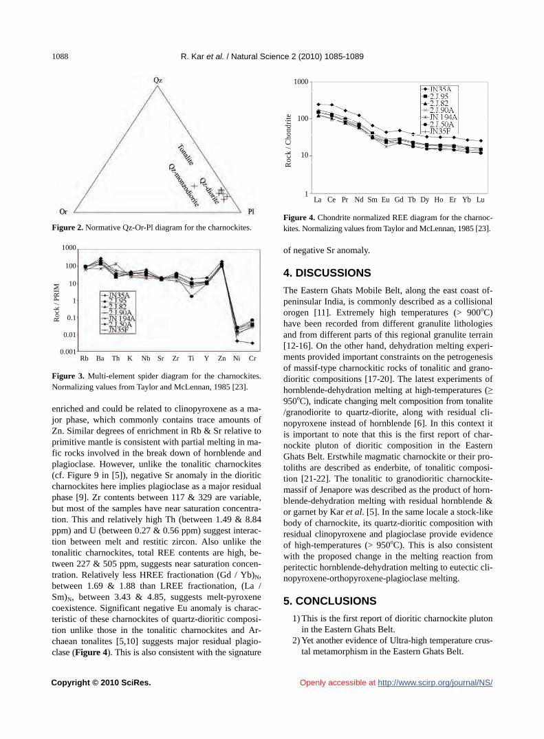
R. Kar et al. / Natural Science 2 (2010) 1085-1089
Copyright © 2010 SciRes. http://www.scirp.org/journal/NS/
1088
Openly accessible at
Figure 2. Normative Qz-Or-Pl diagram for the charnockites.
Roc
k / P
RIM
1000
100
10
1
0.1
0.01
0.001Rb Ba Th K Nb Sr Zr Ti Y Zn Ni Cr
Figure 3. Multi-element spider diagram for the charnockites. Normalizing values from Taylor and McLennan, 1985 [23]. enriched and could be related to clinopyroxene as a ma-jor phase, which commonly contains trace amounts of Zn. Similar degrees of enrichment in Rb & Sr relative to primitive mantle is consistent with partial melting in ma- fic rocks involved in the break down of hornblende and plagioclase. However, unlike the tonalitic charnockites (cf. Figure 9 in [5]), negative Sr anomaly in the dioritic charnockites here implies plagioclase as a major residual phase [9]. Zr contents between 117 & 329 are variable, but most of the samples have near saturation concentra-tion. This and relatively high Th (between 1.49 & 8.84 ppm) and U (between 0.27 & 0.56 ppm) suggest interac-tion between melt and restitic zircon. Also unlike the tonalitic charnockites, total REE contents are high, be-tween 227 & 505 ppm, suggests near saturation concen-tration. Relatively less HREE fractionation (Gd / Yb)N, between 1.69 & 1.88 than LREE fractionation, (La / Sm)N, between 3.43 & 4.85, suggests melt-pyroxene coexistence. Significant negative Eu anomaly is charac-teristic of these charnockites of quartz-dioritic composi-tion unlike those in the tonalitic charnockites and Ar-chaean tonalites [5,10] suggests major residual plagio-clase (Figure 4). This is also consistent with the signature
Roc
k / C
hond
rite
La Ce Pr Nd Sm Eu Gd Tb Dy Ho Er Yb Lu
1000
100
10
1
Figure 4. Chondrite normalized REE diagram for the charnoc- kites. Normalizing values from Taylor and McLennan, 1985 [23]. of negative Sr anomaly.
4. DISCUSSIONS
The Eastern Ghats Mobile Belt, along the east coast of-peninsular India, is commonly described as a collisional orogen [11]. Extremely high temperatures (> 900oC) have been recorded from different granulite lithologies and from different parts of this regional granulite terrain [12-16]. On the other hand, dehydration melting experi-ments provided important constraints on the petrogenesis of massif-type charnockitic rocks of tonalitic and grano-dioritic compositions [17-20]. The latest experiments of hornblende-dehydration melting at high-temperatures (≥ 950oC), indicate changing melt composition from tonalite /granodiorite to quartz-diorite, along with residual cli-nopyroxene instead of hornblende [6]. In this context it is important to note that this is the first report of char-nockite pluton of dioritic composition in the Eastern Ghats Belt. Erstwhile magmatic charnockite or their pro- toliths are described as enderbite, of tonalitic composi-tion [21-22]. The tonalitic to granodioritic charnockite- massif of Jenapore was described as the product of horn- blende-dehydration melting with residual hornblende & or garnet by Kar et al. [5]. In the same locale a stock-like body of charnockite, its quartz-dioritic composition with residual clinopyroxene and plagioclase provide evidence of high-temperatures (> 950oC). This is also consistent with the proposed change in the melting reaction from peritectic hornblende-dehydration melting to eutectic cli- nopyroxene-orthopyroxene-plagioclase melting.
5. CONCLUSIONS
1) This is the first report of dioritic charnockite pluton in the Eastern Ghats Belt.
2) Yet another evidence of Ultra-high temperature crus- tal metamorphism in the Eastern Ghats Belt.

R. Kar et al. / Natural Science 2 (2010) 1085-1089
Copyright © 2010 SciRes. http://www.scirp.org/journal/NS/
1081089
3) Negative Sr and Eu anomalies, unlike those of tona- litic charnockites and Archaean tonalites, imply pla- gioclase as a major residual phase.
Openly accessible at
6. ACKNOWLEDGEMENTS
Melting experiments at the Petrological Laboratory of the Zurich In-
stitute was supported by a Swiss Federal Fellowship to RK. Analytical
data by ICP-MS were acquired by courtesy Dr. J.W. Sheraton.
REFERENCES [1] Young, D.N., Zhao, J.X., Ellis, D.J. and McCulloch, M.T.
(1997) Geochemical and Sr–Nd isotopic mapping of source provinces for the Mawson charnockites, east Ant-arctica: Implications for Proterozoic tectonics and Gond- wana reconstruction. Precambrian Research, 86, 1-19.
[2] Subba Rao, M.V. and Divakara Rao, V. (1988) Chemical constraints on the origin of the charnockites in the East-ern Ghat Mobile Belt, India. Chemical Geology, 69, 37- 48.
[3] Zhao J., Ellis D.J., Kilpatrick, J.A. and McCulloch, M.T. (1997) Geochemical and Sr-Nd isotopic study of char-nockites and related rocks in the northern Prince Charles Mountain, East Antarctica. Precambrian Research, 81, 37-66.
[4] Sheraton, J.W, Tindle, A.G. and Tingey, R.J. (1996) Geo-chemistry, origin, and tectonic setting of granitic rocks of the Prince Charles Mountains, Antarctica. Australian Journal of Geology & Geophysics, 16, 345-370.
[5] Kar, R., Bhattacharya, S. and Sheraton, J.W. (2003) Horn- blende dehydration melting in mafic rocks and the link between massif-type charnockite and associated granu-lites, Eastern Ghats Granulite Belt, India. Contributions to Mineralalogy and Petrology, 145, 707-729.
[6] Kar, R. (2010) Melting experiments in the NCFMASH system at 8 kbar: Implications for the origin of mafic granulites. Indian Journal of Geology, Special Issue on Geodynamic Regimes, Global tectonics and evolution of Precambrian cratonic basins in India. 80, 71-80.
[7] Jenner, G.A., Longerich, H.P., Jackson, S.E. and Fryer, B. J. (1990) ICP-MS a powerfull tool for high-precision trace element analysis in earth science: Evidence from analysis of selected USGS reference samples, Chemical Geology, 83, 133-148.
[8] Govindaraju, K. (1994) 1994 compilation of working values and sample description for 383 geostandards. Geo- standards Newsletter, 18, 1-158.
[9] Tarney, J., Wyborn, L.E.A., Sheraton, J.W. and Wyborn, D. (1987) Trace element differences between Archaean, proterozoic and phanerozoic crustal components: Impli-cations for crustal growth processes. In: Ashwal, L.D. Ed., Workshop on the growth of continental crust, Lunar and Planetary Institute, 139-140.
[10] Nutman, A.P., McGregor, V.R., Friend, C.R.L., Bennet, V. C. and Kinny, P.D. (1996) Itsaq gneiss complex of south-
ern west Greenland; the world’s most extensive record of early crustal evolution (3,900-3,600 Ma). Precambrian Research, 78, 1-39.
[11] Santosh, M., Maruyama, S. and Sato, K. (2009) Anatomy of a Cambrian suture in Gondwana: Pacific-type orogeny in southern India? Gondwana Research, 16, 321-341.
[12] Lal, R.K., Ackermand, D. and Upadhyay, H. (1987) P- T-X relationships deduced from corona textures in sap-phirine-spinel-quartz assemblages from Paderu, southern India. Journal of Petrology, 28, 1139-1168.
[13] Dasgupta, S., Sengupta, P., Fukuoka, M. and Bhattacharya, P.K. (1991) Mafic granulites in the Eastern Ghats, India: Further evidence for extremely high temperature crustal metamorphism. Journal of Geology, 99, 124-133.
[14] Bhowmik, S.K., Dasgupta, S., Hoernes, S. and Bhatta-charya, P.K. (1995) Extremely high-temperature calcare- ous granulites from the Eastern Ghats, India: Evidence for isobaric cooling, fluid buffering, and terminal chan-nelized fluid flow. Europian Journal of Mineralogy, 7, 689-703.
[15] Sen, S.K., Bhattacharya, S. and Acharyya, A. (1995) A multi-stage pressure-temperature record in the Chilka La- ke granulites: The epitome of the metamorphic evolution of Eastern Ghats, India? Journal of Metamorphic Geol-ogy, 13, 287-298.
[16] Bhattacharya, S. and Kar, R. (2002) High-temperature dehydration melting and decompressive P-T path in a granulite complex from the Eastern Ghats, India. Con-tributions to Mineralogy and Petrology, 143,175-191.
[17] Patino Douce, A.E. and Beard, J.S. (1995) Dehydration melting of biotite gneiss and quartz amphibolite from 3 to 15 kbar. Journal of Petrology, 36, 707-738.
[18] Springer, W. and Seck, H.A. (1997) Partial fusion of ba- sic granulites at 5 to 15 kbar: Implications for the origin of TTG magmas. Contributions to Mineralogy and Pe-trology, 127, 30-45.
[19] Lopez, S. and Castro, A. (2001) Determination of the fliud-absent solidus and supersolidus phase relationships of MORB-derived amphibolites in the range 4-14 kbar. American Mineralogist, 86, 1396-1403.
[20] Sisson, T.W., Ratajeski, K. and Hankins, W.B. (2005) Vo- luminous granitic magmas from common basaltic sources. Contributions to Mineralogy and Petrology, 148, 635- 661.
[21] Rickers, K., Mezger, K. and Raith, M., (2001) Evolution of the continental crust in the Proterozoic Eastern Ghats Belt, India and new constraints for Rodinia reconstruc-tion: Implications from Sm-Nd, Rb-Sr and Pb-Pb iso-topes. Precambrian Research, 112, 183-210.
[22] Bhui, U.K., Sengupta, P. and Sengupta, P. (2007) Phase relations in mafic dykes and their host rocks from Kon-dapalle, Andhra Pradesh, India: Implications for the time- depth trajectory of the Paleoproterozoic (late Archean?) granulites from southern Eastern Ghats Belt. Precam-brian Research, 156, 153-174.
[23] Taylor, S.R. and McLennan, S.M. (1985) The continental crust: Its composition and evolution. Blackwell, Oxford.
Vol.2, No.10, 1090-1103 (2010) Natural Science doi:10.4236/ns.2010.210136
Copyright © 2010 SciRes. Openly accessible at http://www.scirp.org/journal/NS/
Cell-PLoc 2.0: an improved package of web-servers for predicting subcellular localization of proteins in various organisms
Kuo-Chen Chou1,2, Hong-Bin Shen1,2 1Gordon Life Science Institute, 13784 Torrey Del Mar Drive, San Diego, CA 92130, USA; [email protected] 2Institute of Image Processing & Pattern Recognition, Shanghai Jiaotong University, 800 Dongchuan Road, Shanghai, 200240, China; [email protected]
Received 5 August 2010; revised 8 September 2010; accepted 12 September 2010.
ABSTRACT
Cell-PLoc 2.0 is a package of web-servers evolved from Cell-PLoc (Chou, K.C. & Shen, H.B., Nature Protocols, 2008, 2:153-162) by a top-down approach to improve the power for predicting subcellular localization of proteins in various organisms. It contains six predictors: Euk-mPLoc 2.0, Hum-mPLoc 2.0, Plant-mPLoc, Gpos-mPLoc, Gneg-mPLoc, and Virus-mPLoc, specialized for eukaryotic, human, plant, Gram- positive bacterial, Gram-negative bacterial, and virus proteins, respectively. Compared with Cell-PLoc, the predictors in the Cell-PLoc 2.0 have the following advantageous features: (1) they all have the capacity to deal with the multiplex proteins that can simultaneiously exist, or move between, two or more subcellular location sites; (2) no accession number is needed for the input of a query protein even if using the “high- level” GO (gene ontology) prediction engine; (3) the functional domain information and sequential evolution information are fused into the “ab initio” sequence-based prediction engine to enhance its accuracy. In this protocol, a step- to-step guide is provided for how to use the web server predictors in the Cell-PLoc 2.0 package, which is freely accessible to the public at http://www.csbio.sjtu.edu.cn/bioinf/Cell-PLoc-2/.
Keywords: Euk-mPLoc 2.0; Hum-mPLoc 2.0; Plant-mPLoc; Gpos-mPLoc; Gneg-mPLoc; Virus-mPLoc; Higher-level GO approach; Ab-initio approach; Functional domain; Sequential evolution; Multiplex proteins
1. INTRODUCTION
The localization of a protein in a cell is one of its
most important attributes. It can provide useful insight about the function of the protein. It is also fundamental to system biology because knowledge of the subcellu-lar locations of proteins is indispensable for in-depth understanding how the biological processes are regu-lated by the intricate pathways at the cellular level [1,2]. Particularly, the information of protein subcel-lular location is very useful for identifying and priori-tizing drug targets [3] during the process of drug de-velopment.
Given an uncharacterized protein sequence, how can we identify which subcellular location site it resides at? Does the protein stay in a single subcellular location or can it simultaneously exist in, or move between, two and more subcellular location sites? Although the answers to these questions can be determined by means of various biochemical experiments, it is time-consuming and labo-rious to acquire the desired information with experimen-tal methods alone. Particularly, in the post-genomic age, the number of newly found protein sequences has in-creased explosively. For instance, in 1986 the Swiss-Prot databank contained merely 3,939 protein sequence en-tries, but the number has since jumped to 519,348 ac-cording to the data released by the same databank on 10- Aug-2010 (www.expasy.org/sprot/relnotes/relstat.html), meaning that the number of protein sequence entries now is more than 131 times the number from about 24 years ago. Facing such an avalanche of protein se-quences, it is highly desired to develop automated me-thods for timely identifying the subcellular locations of uncharacterized proteins based on their sequence infor-mation alone.
Actually, during the past 18 years or so, various com-putational methods were developed in this regard (see, e.g., [4-59].
All the aforementioned methods each have their own advantages and have indeed played a role in stimulating

K. C. Chou et al. / Natural Science 2 (2010) 1090-1103
Copyright © 2010 SciRes. Openly accessible at http://www.scirp.org/journal/NS/
1091091
the development of this area. Meanwhile, they also each have their own limitations. For example, TargetP [15] is one of the popular methods in this area. Its remarkable merit is to make the prediction of the subcellular loca-tion of a protein related to its signal peptide and hence has a clearer biological meaning and basis. But TargetP [15] can only cover four subcellular location sites. For a query protein located outside its coverage scope, TargetP would either fail to predict or the predicted result thus obtained would not make any sense. The similar prob-lem also exists for PSORTb [33], one of the other popu-lar methods in this area.
The other problem for the existing methods listed above is that none of them can be used to deal with mul-tiplex proteins that may simultaneously reside at, or move between, two or more different subcellular loca-tions. Proteins with multiple location sites or dynamic feature of this kind are particularly interesting because they may have some unique biological functions worthy of our special notice [2,3]. Particularly, as pointed out by Millar et al. [60], recent evidence indicates that an in-creasing number of proteins have multiple locations in the cell.
About two years ago, a package of web-servers called Cell-PLoc was published [61] that can be used to predict subcellular localization of proteins in vari-ous organisms. It contained six web-server predictors: Euk-mPLoc [62], Hum-mPLoc [63], Plant-PLoc [64], Gpos-PLoc [65], Gneg-PLoc [66], and Vi-rus-PLoc [67], specialized for eukaryotic, human, plant, Gram-positive bacterial, Gram-negative bac-terial, and virus proteins, respectively. As elucidated in the protocol article [61], each of the six predictors in Cell-PLoc was established by hybridizing the “higher-level” GO (gene ontology) [68] approach and the “ab initio” PseAAC (pseudo amino acid composi-tion) [16] approach, and hence could yield higher success rates as well as cover much wider scope. For example, the Euk-mPLoc predictor can cover up to 22 subcellular location sites. Moreover, of the six predictors in the Cell-PLoc package [61], Euk- mPLoc and Hum- mPLoc can be also used to deal with proteins with multiple-location sites. Therefore, ever since it was published, Cell-PLoc has been widely and increasingly used.
However, the existing version of Cell-PLoc [61] has the following shortcomings. (1) The accession number of a query protein is indispensable as an input in order to utilize the advantage of the “higher-level” GO ap-proach. Many proteins, such as hypothetical and syn-thetic proteins as well as those newly-discovered pro-teins that have not been deposited into databanks yet, do not have accession numbers, and hence cannot be
handled with the GO approach. (2) Even with their accession numbers available, many proteins cannot be meaningfully formulated in a GO space because the current GO database is far from complete yet. (3) Al-though the PseAAC approach was used as a comple-ment in Cell-PLoc [61] that could take some partial sequence order effects into account, the original PseAAC [16,69] did not contain the sequential evolu-tion and functional domain information, and hence would affect the prediction quality. (4) Except Euk-mPLoc (the predictor for eukaryotic proteins) and Hum-mPLoc (the predictor for human proteins), all the other predictors in Cell-PLoc package [61] cannot be used to deal with multiplex proteins.
To address the aforementioned four problems, a top-down approach to enhance the power of Cell-PLoc has been implemented. The new version thus obtained is denoted by Cell-PLoc 2.0. Compared with the old Cell-PLoc [61], Cell-PLoc 2.0 has the following advan-tageous features.
Input Data. By means of the “homology-based GO extraction” strategy as developed recently (see, e.g., [70]), the requirement for the accession number of a query protein is no longer needed even if using the high-er-level GO approach to perform the prediction. This is especially useful for predicting the subcellular location sites of hypothetical proteins or synthetic proteins, as well as those new protein sequences without being de-posited into data banks and hence having no accession numbers assigned yet.
Sequence Information. For those proteins that have no useful GO information to carry out the higher-level prediction, a hybridization approach by fusing the func-tional domain information and sequential evolution in-formation as illustrated in Figure 1 is developed to re-place the simple PseAAC approach [16] in the old Cell-PLoc [61]. As a consequence, the success rates have been remarkably increased for those proteins with-out useful GO numbers.
Multiplex Proteins. In the old Cell-PLoc package [61], only two predictors, i.e., the one specialized for eukaryotic proteins and the one specialized for human proteins, can be used to treat proteins with multiple loca-tion sites. In Cell-PLoc 2.0, all the six predictors, in-cluding those specialized for plant proteins, Gram- posi-tive bacterial proteins, Gram-negative bacterial proteins, and virus proteins, can be used to deal with the multiplex proteins.
Benchmark Datasets. With more experimental data available in Swiss-Prot database (www.ebi.ac.uk/swissprot), to update the data for training the predictors, instead of version 50.7 released on 9-Sept-2006 as used in the old Cell-PLoc [61], the benchmark datasets for training the

K. C. Chou et al. / Natural Science 2 (2010) 1090-1103
Copyright © 2010 SciRes. Openly accessible at http://www.scirp.org/journal/NS/
1092
RPS-BlastSwiss-
Prot
Generate FunD descriptorfor P
Input proteinsequence P
CDDPSI-Blast
Generate PseEvodescriptor for P
Output
Swiss-Prot
Blast
Find the homology proteins of P
GO base
Generate GO descriptor for P
No homology protein
No useful hits
Ensemble classifier 1Fusing different K Ensemble classifier 2 Fusing different K and λ
Figure 1. A flowchart to show the prediction process of the predictors in Cell-PLoc 2.0, where ensemble classifier 1 is for processing the GO descriptor samples, while ensemble classifier 2 is for the FunD (functional domain) and PseEvo (pseudo sequen-tial evolution) descriptor samples. See [70,71] for further explanation.
predictors in Cell-PLoc 2.0 were constructed based on version 55.3 released on 29-April-2008. Moreover, to make all the predictors in Cell-PLoc 2.0 have the capac-ity to deal with the multiplex proteins as well, the se-quences annotated with two or more subcellular location sites were no longer excluded even for plant proteins, Gram-positive bacterial proteins, Gram-negative bac-terial proteins, and virus proteins as done previously in the old Cell-PLoc package [61].
Below, let us describe how to use the new Cell-PLoc 2.0 package to get the desired results.
2. EQUIPMENT AND MATERIALS
Hardware. Same as in the old Cell-PLoc [61], i.e., you need a computer that is able to access to internet.
Data. Your input protein sequences should be in FASTA format. You can enter the sequence of a query protein by either typing or copying-and-pasting it into the input box. Spaces and line breaks will be ignored and will not affect the prediction result.
Programs. Cell-PLoc 2.0 contains the following pro-grams: (1) Euk-mPLoc 2.0 for predicting the subcellular localization of eukaryotic proteins; (2) Hum-mPLoc 2.0 for human proteins; (3) Plant-mPLoc for plant proteins; (4) Gpos-mPLoc for Gram-positive bacterial proteins; (5) Gneg-mPLoc for Gram-negative bacterial proteins; (6) Virus-mPLoc for virus proteins. The six predictors were evolved from Euk-mPLoc [62], Hum-mPLoc [63], Plant- PLoc [64], Gpos-PLoc [65], Gneg-PLoc [66], and Virus- PLoc [67] in the original Cell-PLoc package [61]
through a top-down approach to enhance their power, as elaborated in [70-75], respectively. Note that now all the six predictors in Cell-PLoc 2.0 have the capacity to deal with multiplex proteins as well, as indicated by the cha-racter “m” in front of their partial name “PLoc” that stands for the first character of “multiple”.
3. PROCEDURE
1) Go to the internet at http://www.csbio.sjtu.edu.cn/bioinf/Cell-PLoc-2/ and you will see the top page of the Cell-PLoc 2.0 package on the screen of your computer, as shown in Figure 2.
2) You should use the relevant predictor to conduct the prediction: (1) if your query protein is an eukaryotic one, click the button Euk-mPLoc 2.0; (2) if it is a human protein, click Hum-mPLoc 2.0; (3) if it is a plant protein, click Plant-mPLoc; (4) if it is a Gram-positive bacterial protein, click Gpos-mPLoc; (5) if it is a Gram- negative bacterial protein, click Gneg-mPLoc; (6) if it is a viral protein, click Virus-mPLoc.
3) Without loss of generality, let us take Hum-mPLoc 2.0 as an example. By clicking Hum-mPLoc 2.0, you will be prompted with the top page of the Hum-mPLoc 2.0 web-server predictor (Figure 3). To find the cover-age scope and caveat in using the predictor, click the Read Me button and you will see that the current Hum-mPLoc 2.0 version can cover the following 14 human protein subcellular location sites: (1) centriole, (2) cytoplasm, (3) cytoskeleton, (4) endoplasmic reticulum, (5) endosome, (6) extracell, (7) Golgi apparatus, (8) ly-

K. C. Chou et al. / Natural Science 2 (2010) 1090-1103
Copyright © 2010 SciRes. Openly accessible at http://www.scirp.org/journal/NS/
1091093
Cell-PLoc 2.0: A package of web-servers for predicting subcellular localization of proteins in different organisms
Euk-mPLoc 2.0
Plant-mPLoc
Gneg-mPLoc
Hum-mPLoc 2.0
Gpos-mPLoc
Virus-mPLoc
Figure 2. Illustration to show the Cell-PLoc 2.0 web-page at http://www.csbio.sjtu.edu.cn/bioinf/Cell-PLoc-2/.
Hum-mPLoc 2.0: Predicting subcellular localization of human proteins including those with multiple sites
Read Me Data Citation
Enter the protein sequence (Example):
Submit Clear
Hum-mPLoc 2.0: Predicting subcellular localization of human proteins including those with multiple sites
Read Me Data Citation
Enter the protein sequence (Example):
Submit Clear
Figure 3. A semi-screenshot to show the top page of the web- server predictor Hum-mPLoc 2.0 in the Cell-PLoc 2.0 package. sosome, (9) microsome, (10) mitochondrion, (11) nuc-leus, (12) peroxisome, (13) plasma membrane, and (14) synapse, as schematically shown in Figure 4. You will also see the caveat from the Read Me window how to avoid meaningless prediction. To continue the prediction, go back to the top page of the Hum-mPLoc 2.0 web-server predictor by closing the Read Me window.
4) Enter your query protein sequence into the input box as shown at the centre of Figure 3. The input se-quence should be in FASTA format. A sequence in FASTA format consists of a single-line description, fol-lowed by lines of sequence data. The first character of the description line is a greater-than symbol (“>”) in the first column. All lines should be shorter than 80 charac-ters. Example sequences in FASTA format can be seen by clicking on the Example button right above the input box. For more information about FASTA format, visit http://en.wikipedia.org/wiki/Fasta_format.
5) To get the predicted result, click the Submit button.
NucleusNucleus
Plasma membrane
Cytoplasm
Mitochondria
Endoplasmicreticulum
Cytoskeleton
Peroxisome
Lysosome
Golgiapparatus
Centriole
ExtracellMicrosome
Endosomal
Synapse
Figure 4. Schematic illustration to show the fourteen subcellu-lar location sites of human proteins that are covered by the Hum-mPLoc 2.0 predictor. For example, if using the sequence of query protein 1 in the Example window as an input, you will see the input screen as shown in Figure 5a; after clicking the Submit button, you will see “Cell membrane; Cytoplasm; Nucleus” shown on the predicted location(s) window (Figure 5b), meaning that the query protein is a multip-lex protein, which can simultaneously occur in “cell membrane”, “cytoplasm” and “nucleus” sites, fully con-sistent with experimental observations. However, if us-ing the sequence of query protein 2 in the Example window as an input, you will instead see the input screen as shown in Figure 6a; after clicking the Submit button, you will see “Cytoplasm” shown on the predicted loca-tion(s) window (Figure 6b), meaning that the query protein is a single-location protein residing in “cytop-lasm” compartment only, also fully consistent with ex-perimental observations.
6) By clicking the Citation button, you will find the relevant papers that document the detailed development and algorithm of Hum-mPLoc 2.0.
7) By clicking the Data button, you will find all the benchmark datasets used to train and test the Hum- mPLoc 2.0 predictor.
8) If your query protein sequence is from other organ-ism, click the relevant web-server button (Figure 2) as elaborated in Step 2, and repeat Steps 3-6.
TIMING The computational time for each prediction is within 15 seconds for most cases. The longer the query protein sequence is, the more time it is usually needed.
4. TROUBLESHOOTING
After you click the Submit button, if the server rejects

K. C. Chou et al. / Natural Science 2 (2010) 1090-1103
Copyright © 2010 SciRes. Openly accessible at http://www.scirp.org/journal/NS/
1094
Hum-mPLoc 2.0: Predicting subcellular localization of human proteins including those with multiple sites
Read Me Data Citation
Enter the protein sequence (Example):
Submit Clear
>query protein 1MAKERRRAVLELLQRPGNARCADCGAPDPDWASYTLGVFICLSCSGIHRNIPQVSKVKSV RLDAWEEAQVEFMASHGNDAARARFESKVPSFYYRPTPSDCQLLREQWIRAKYERQEFIY PEKQEPYSAGYREGFLWKRGRDNGQFLSRKFVLTEREGALKYFNRNDAKEPKAVMKIEHL NATFQPAKIGHPHGLQVTYLKDNSTRNIFIYHEDGKEIVDWFNALRAARFHYLQVAFPGA SDADLVPKLSRNYLKEGYMEKTGPKQTEGFRKRWFTMDDRRLMYFKDPLDAFARGEVFIG SKESGYTVLHGFPPSTQGHHWPHGITIVTPDRKFLFACETESDQREWVAAFQKAVDRPML PQEYAVEAHFKHKP
(a)
Your input sequence (358 aa) is:
Citation
Hum-mPLoc 2.0: Predicting subcellular localization of human proteins including those with multiple sites
Read Me Data
Predicted Location(s): Cell membrane; Cytoplasm; Nucleus
Your input sequence (358 aa) is:
Citation
Hum-mPLoc 2.0: Predicting subcellular localization of human proteins including those with multiple sites
Read Me Data Citation
Hum-mPLoc 2.0: Predicting subcellular localization of human proteins including those with multiple sites
Read Me Data
Hum-mPLoc 2.0: Predicting subcellular localization of human proteins including those with multiple sites
Read Me Data
Predicted Location(s): Cell membrane; Cytoplasm; Nucleus
>query protein 1MAKERRRAVLELLQRPGNARCADCGAPDPDWASYTLGVFICLSCSGIHRNIPQVSKVKSVRLDAWEEAQVEFMASHGNDAARARFESKVPSFYYRPTPSDCQLLREQWIRAKYERQEFIYPEKQEPYSAGYREGFLWKRGRDNGQFLSRKFVLTEREGALKYFNRNDAKEPKAVMKIEHLNATFQPAKIGHPHGLQVTYLKDNSTRNIFIYHEDGKEIVDWFNALRAARFHYLQVAFPGASDADLVPKLSRNYLKEGYMEKTGPKQTEGFRKRWFTMDDRRLMYFKDPLDAFARGEVFIGSKESGYTVLHGFPPSTQGHHWPHGITIVTPDRKFLFACETESDQREWVAAFQKAVDRPMLPQEYAVEAHFKHKP
(b)
Figure 5. A semi-screenshot to show the input in the FASTA format for (a) the query protein 1 taken from the Example window, and (b) the output predicted by Hum-mPLoc 2.0 for the query protein sequence in panel (a).
your submission for prediction, consider the following points for troubleshooting.
Check the format of your input data to make sure it complies with the FASTA format as elaborated in Step 4 of the PROCEDURE.
Check the length of your input sequence to make sure it is at least 50 amino acids long; otherwise, it might not be a real protein but its fragment.
Check the amino acid codes of your input sequence to make sure it does not contain any invalid cha-racters.
You might also get meaningless result if the query protein is not among the subcellular location sites cov-ered by the web-server predictor.
5. ANTICIPATED RESULTS
In statistical prediction of subcellular localization of proteins or their any other attributes, it would be mea-ningless to simply say the success rate of a predictor
Hum-mPLoc 2.0: Predicting subcellular localization of human
proteins including those with multiple sites
Read Me Data Citation
Enter the protein sequence (Example):
Submit Clear
>query protein 2MEPSSLELPADTVQRIAAELKCHPTDERVALHLDEEDKLRHFRECFYIPKIQDLPPVDLS LVNKDENAIYFLGNSLGLQPKMVKTYLEEELDKWAKIAAYGHEVGKRPWITGDESIVGLM KDIVGANEKEIALMNALTVNLHLLMLSFFKPTPKRYKILLEAKAFPSDHYAIESQLQLHG LNIEESMRMIKPREGEETLRIEDILEVIEKEGDSIAVILFSGVHFYTGQHFNIPAITKAG QAKGCYVGFDLAHAVGNVELYLHDWGVDFACWCSYKYLNAGAGGIAGAFIHEKHAHTIKP ALVGWFGHELSTRFKMDNKLQLIPGVCGFRISNPPILLVCSLHASLEIFKQATMKALRKK SVLLTGYLEYLIKHNYGKDKAATKKPVVNIITPSHVEERGCQLTITFSVPNKDVFQELEK RGVVCDKRNPNGIRVAPVPLYNSFHDVYKFTNLLTSILDSAETKN
Hum-mPLoc 2.0: Predicting subcellular localization of human proteins including those with multiple sites
Read Me Data Citation
Enter the protein sequence (Example):
Submit Clear
>query protein 2MEPSSLELPADTVQRIAAELKCHPTDERVALHLDEEDKLRHFRECFYIPKIQDLPPVDLS LVNKDENAIYFLGNSLGLQPKMVKTYLEEELDKWAKIAAYGHEVGKRPWITGDESIVGLM KDIVGANEKEIALMNALTVNLHLLMLSFFKPTPKRYKILLEAKAFPSDHYAIESQLQLHG LNIEESMRMIKPREGEETLRIEDILEVIEKEGDSIAVILFSGVHFYTGQHFNIPAITKAG QAKGCYVGFDLAHAVGNVELYLHDWGVDFACWCSYKYLNAGAGGIAGAFIHEKHAHTIKP ALVGWFGHELSTRFKMDNKLQLIPGVCGFRISNPPILLVCSLHASLEIFKQATMKALRKK SVLLTGYLEYLIKHNYGKDKAATKKPVVNIITPSHVEERGCQLTITFSVPNKDVFQELEK RGVVCDKRNPNGIRVAPVPLYNSFHDVYKFTNLLTSILDSAETKN
(a)
Your input sequence (465 aa) is:
Citation
Hum-mPLoc 2.0: Predicting subcellular localization of human proteins including those with multiple sites
Read Me Data
Predicted Location(s): Cytoplasm
>query protein 2MEPSSLELPADTVQRIAAELKCHPTDERVALHLDEEDKLRHFRECFYIPKIQDLPPVDLSLVNKDENAIYFLGNSLGLQPKMVKTYLEEELDKWAKIAAYGHEVGKRPWITGDESIVGLMKDIVGANEKEIALMNALTVNLHLLMLSFFKPTPKRYKILLEAKAFPSDHYAIESQLQLHGLNIEESMRMIKPREGEETLRIEDILEVIEKEGDSIAVILFSGVHFYTGQHFNIPAITKAGQAKGCYVGFDLAHAVGNVELYLHDWGVDFACWCSYKYLNAGAGGIAGAFIHEKHAHTIKPALVGWFGHELSTRFKMDNKLQLIPGVCGFRISNPPILLVCSLHASLEIFKQATMKALRKKSVLLTGYLEYLIKHNYGKDKAATKKPVVNIITPSHVEERGCQLTITFSVPNKDVFQELEKRGVVCDKRNPNGIRVAPVPLYNSFHDVYKFTNLLTSILDSAETKN
Your input sequence (465 aa) is:
Citation
Hum-mPLoc 2.0: Predicting subcellular localization of human proteins including those with multiple sites
Read Me Data
Predicted Location(s): Cytoplasm
Your input sequence (465 aa) is:
Citation
Hum-mPLoc 2.0: Predicting subcellular localization of human proteins including those with multiple sites
Read Me Data Citation
Hum-mPLoc 2.0: Predicting subcellular localization of human proteins including those with multiple sites
Read Me Data
Hum-mPLoc 2.0: Predicting subcellular localization of human proteins including those with multiple sites
Read Me Data
Predicted Location(s): Cytoplasm
>query protein 2MEPSSLELPADTVQRIAAELKCHPTDERVALHLDEEDKLRHFRECFYIPKIQDLPPVDLSLVNKDENAIYFLGNSLGLQPKMVKTYLEEELDKWAKIAAYGHEVGKRPWITGDESIVGLMKDIVGANEKEIALMNALTVNLHLLMLSFFKPTPKRYKILLEAKAFPSDHYAIESQLQLHGLNIEESMRMIKPREGEETLRIEDILEVIEKEGDSIAVILFSGVHFYTGQHFNIPAITKAGQAKGCYVGFDLAHAVGNVELYLHDWGVDFACWCSYKYLNAGAGGIAGAFIHEKHAHTIKPALVGWFGHELSTRFKMDNKLQLIPGVCGFRISNPPILLVCSLHASLEIFKQATMKALRKKSVLLTGYLEYLIKHNYGKDKAATKKPVVNIITPSHVEERGCQLTITFSVPNKDVFQELEKRGVVCDKRNPNGIRVAPVPLYNSFHDVYKFTNLLTSILDSAETKN
(b)
Figure 6. A semi-screenshot to show the input in the FASTA format for (a) the query protein 2 taken from the Example window, and (b) the output predicted by Hum-mPLoc 2.0 for the query protein sequence in panel (a). without specifying what method and benchmark dataset were used to test its accuracy.
The following three cross-validation methods are generally used for examining the effectiveness of a sta-tistical prediction method: (1) the independent dataset test, (2) the sub-sampling (K-fold cross-validation) test, and (3) the jackknife test [76].
For the independent dataset test, although all the pro-teins to be tested are outside the training dataset used to train the predictor and hence can avoid the “memory” effect or bias, the way of how to select the independent proteins for testing could be quite arbitrary unless the number of independent proteins is sufficiently large. This kind of arbitrariness might lead to completely dif-ferent conclusions. For instance, a predictor achieving a higher success rate than the other predictor for a given independent testing dataset might fail to keep so when tested by another independent testing dataset [76].
For the subsampling test, the concrete procedure usually used in literatures is the 5-fold, 7-fold or 10-fold

K. C. Chou et al. / Natural Science 2 (2010) 1090-1103
Copyright © 2010 SciRes. Openly accessible at http://www.scirp.org/journal/NS/
1091095
cross-validation. The problem with the K-fold cross- validation test as such is that the number of possible selections in dividing a benchmark dataset is an astro-nomical figure even for a very simple dataset. For ex-ample, let us consider a highly simplified dataset that consists of 300 proteins classified into five subsets, in which 60 proteins belong to subcellular location #1, 55 to location #2, 70 to location #3, 65 to location #4, and 50 to location #5. For such a simple dataset, the number of possible combinations of taking one-fifth proteins from each of the five subsets will be
1 2 3 4 5
60
60! 55! 70! =
(60 12)!12! (55 11)!11! (70 14)!14!
65! 50! > 5.45 10
(65 13)!13! (50 10)!10!
(1)
where 1 is the number of possible different ways of taking 60 5 12 proteins from subset #1, 2 that of taking 55 5 11 proteins from subset #2, 3 that of taking 70 5 14 proteins from subset #3, 4 that of taking 65 5 13 proteins from subset #4, and 5 that of taking 50 5 10 proteins from site-site-5. As we can see from Eq.1, even for such a simple and small dataset the number of possible ways in selecting the testing dataset for the 5-fold cross-validation would be greater than 605.45 10 . It can be easily conceived that for a benchmark dataset containing over a thousand pro-teins that are classified into more than five subcellular location sites, the number of the possible selections for subsampling test will be even much greater. Accordingly, in any actual subsampling cross-validation tests, only an extremely small fraction of the possible selections are taken into account. Since different selections will always lead to different results even for a same benchmark da-taset and a same predictor, the subsampling test (such as 5-fold cross-validation) cannot avoid the arbitrariness either. A test method unable to yield a unique outcome cannot be deemed as an ideal one.
In the jackknife test, all the proteins in the benchmark dataset will be singled out one-by-one and tested by the predictor trained by the remaining protein samples. During the process of jackknifing, both the training da-taset and testing dataset are actually open, and each pro-tein sample will be in turn moved between the two. The jackknife test can exclude the “memory” effect. Also, the arbitrariness problem as mentioned above for the inde-pendent dataset test and subsampling test can be avoided because the outcome obtained by the jackknife cross-validation is always unique for a given benchmark dataset. As for the possible overestimation in success rate by jackknife test because of only one sample being
singled out at a time for testing, the answer is that as long as the jackknife test is performed on a stringent benchmark dataset in which none of proteins has
25% pairwise sequence identity to any other in a same subcellular location such as those benchmark da-tasets specially constructed for the six predictors in Cell-PLoc 2.0, it is highly unlikely to yield an overesti-mated rate compared with the actual success rate in practical applications, as demonstrated in [72,74] and will be further discussed later. Besides, when the jack-knife test was used to compare two predictors, even if there was some overestimate due to using a less stringent benchmark dataset for one predictor, the same overesti-mate would exist for the other as long as they were both tested by a same dataset.
Accordingly, the jackknife test has been increasingly and widely used by investigators to examine the quality of various predictors (see, e.g., [47,51,55,58,59,77- 107]).
However, even if using the jackknife approach for cross-validation, a same predictor may still generate ob-viously different success rates when tested by different benchmark datasets. This is because the more stringent of a benchmark dataset in excluding homologous and high similarity sequences, or the more number of sub-cellular location sites it covers, the more difficult for a predictor to achieve a high overall success rate, as will be shown later.
The predictors in the old Cell-PLoc package [61] were established by hybridizing the “higher-level” GO approach with the “ab initio” sequence-correlated PseAAC [16] approach. Accordingly, their overall suc-cess prediction rates are generally higher than those by the best of the existing “ab initio” sequence-based ap-proaches without combining with any higher level ap-proach, as elucidated in [61] and demonstrated in a se-ries of previous publications [62-67,108,109], and hence there is no need to repeat here.
Now, in the new version of Cell-PLoc 2.0, the same high success rates will still be achieved by the “high-er-level” GO prediction engine but no requirement for the accession number is needed for the input. And for those proteins without useful GO numbers, the cor-responding success prediction rates will be further enhanced due to fusing the functional domain infor-mation and sequential evolution information into the “ab initio” prediction engine in the Cell-PLoc 2.0 package as illustrated in Figure 1. Accordingly, the overall success rates by the predictors in Cell-PLoc 2.0 are not only higher than those by the other predic-tors but also those by the predictors in the old Cell-PLoc package [61], as can be seen from the fol-lowing comparisons.

K. C. Chou et al. / Natural Science 2 (2010) 1090-1103
Copyright © 2010 SciRes. Openly accessible at http://www.scirp.org/journal/NS/
1096
Table 1. Comparison between each of the six predictors in Cell-PLoc [61] and that in Cell-PLoc 2.0 by jackknife test.
Organism Number of subcellu-lar locations covered
Cell-PLoc Cell-PLoc 2.0
Predictor Overall success
rateg Predictor
Overall success rate
Eukaryotic 22a Euk-mPLoc 39.3% Euk-mPLoc 2.0 64.2%
Human 14b Hum-mPLoc 38.1% Hum-mPLoc 2.0 62.7%
Plant 12c Plant-PLoc 38.0% Plant-mPLoc 63.7%
Gram-positive 4d Gpos-PLoc 72.5% Gpos-mPLoc 82.2%
Gram-negative 8e Gneg-PLoc 71.5% Gneg-mPLoc 85.7%
Virus 6f Virus-PLoc 43.7% Virus-mPLoc 60.3%
aThe corresponding benchmark dataset was taken from the Supporting Information S1 of [70], in which none of protein included has 25% pair-wise sequence identity to any other in a same subcellular location; bThe corresponding benchmark dataset was taken from the Online Supporting Information A of [71], in which none of protein included has 25% pairwise sequence identity to any other in a same subcellular location; cThe corresponding benchmark dataset was taken from Table S1 of [72], in which none of protein included has 25% pairwise sequence identity to any other in a same subcellular location; dThe corresponding benchmark dataset was taken from the Online Supporting Information A of [73], in which none of protein included has 25% pairwise sequence identity to any other in a same subcellular location; eThe corresponding benchmark dataset was taken from the Online Supporting Information A of [74], in which none of protein included has 25% pairwise sequence identity to any other in a same subcellular location; fThe corresponding benchmark dataset was taken from the Online Supporting Information A of [75], in which none of protein included has 25% pairwise sequence identity to any other in a same subcellular location; gNote that in order to make the comparison under exactly the same condition, only the sequences of proteins but not their accession numbers were used as inputs during the prediction.
1) Comparison with the six predictors in Cell-PLoc
[61]. Listed in Table 1 are the overall success rates by Cell-PLoc [61] and Cell-PLoc 2.0 using jackknife tests on six stringent benchmark datasets for eukaryotic, hu-man, plant, Gram-positive bacterial, Gram-negative bacterial, and virus proteins, respectively. For the case of eukaryotic proteins, the comparison was made between the predictor Euk-mPLoc of Cell-PLoc [61] and the predictor Euk-mPLoc 2.0 of Cell-PLoc 2.0 using the benchmark dataset classified into 22 subcellular loca-tions as given in the Supporting Information S1 of [70]. For human proteins, the comparison was made between the predictor Hum-mPLoc of Cell-PLoc [61] and the predictor Hum-mPLoc 2.0 of Cell-PLoc 2.0 using the benchmark dataset classified into 14 subcellular loca-tions as given in the Online Supporting Information A of [71]. And so forth. To avoid homology bias and redun-dancy, none of the proteins included in the six datasets has 25% pairwise sequence identity to any other in a same subcellular location. Also, to make the comparison between the two counterparts under exactly the same condition, only the sequences of proteins but not their accession numbers were used as inputs during the pre-diction. Meanwhile, the false positives (over-predictions) and false negatives (under-predictions) were also taken into account to reduce the scores for calculating the overall success rate. It is instructive to point out that it is much more complicated to count the over-predictions and under-predictions for a system containing both sin-gle-location and multiple-location proteins. For the de-tailed calculation formulation, see Eqs.43-48 as well as
Figure 4 in a comprehensive review [110]. It can be seen from Table 1 that the overall success rates obtained by the predictors in Cell-PLoc 2.0 are about 10-25% higher than those by their counterparts in Cell-PLoc [61].
2) Comparison with PSORTb v.2.0 [33]. The pre-dictor is widely used by biologists for predicting the subcellular locations of Gram-negative bacterial pro-teins. It is with a built-in training dataset covering the following five subcellular location sites: (1) cytoplasm, (2) extracellular, (3) inner membrane, (4) outer mem-brane, and (5) periplasm. The corresponding predictor in Cell-PLoc 2.0 is Gneg-mPLoc that can cover eight subcellular locations of Gram-negative proteins; i.e., in addition to the above five locations, it also covers “fimbrium”, “flagellum”, and “nucleoid”. In order to make the two predictors with different coverage scopes comparable, a degenerate testing dataset was generated by randomly picking testing proteins according to the following criteria: (1) the testing samples must be Gram-negative bacterial proteins; (2) to avoid the un-fair “memory” effect, the testing samples must be not in the training dataset of PSORTb v.2.0, nor in the training dataset of Gneg-mPLoc; (3) the experimen-tally observed subcellular locations of the testing pro-teins are known as clearly annotated in Swiss-Prot da-tabase; (4) their location sites must be within the scope covered by PSORTb v.2.0 for properly using it (for the proteins with multiple location sites, at least one of them should be within the scope covered by PSORTb
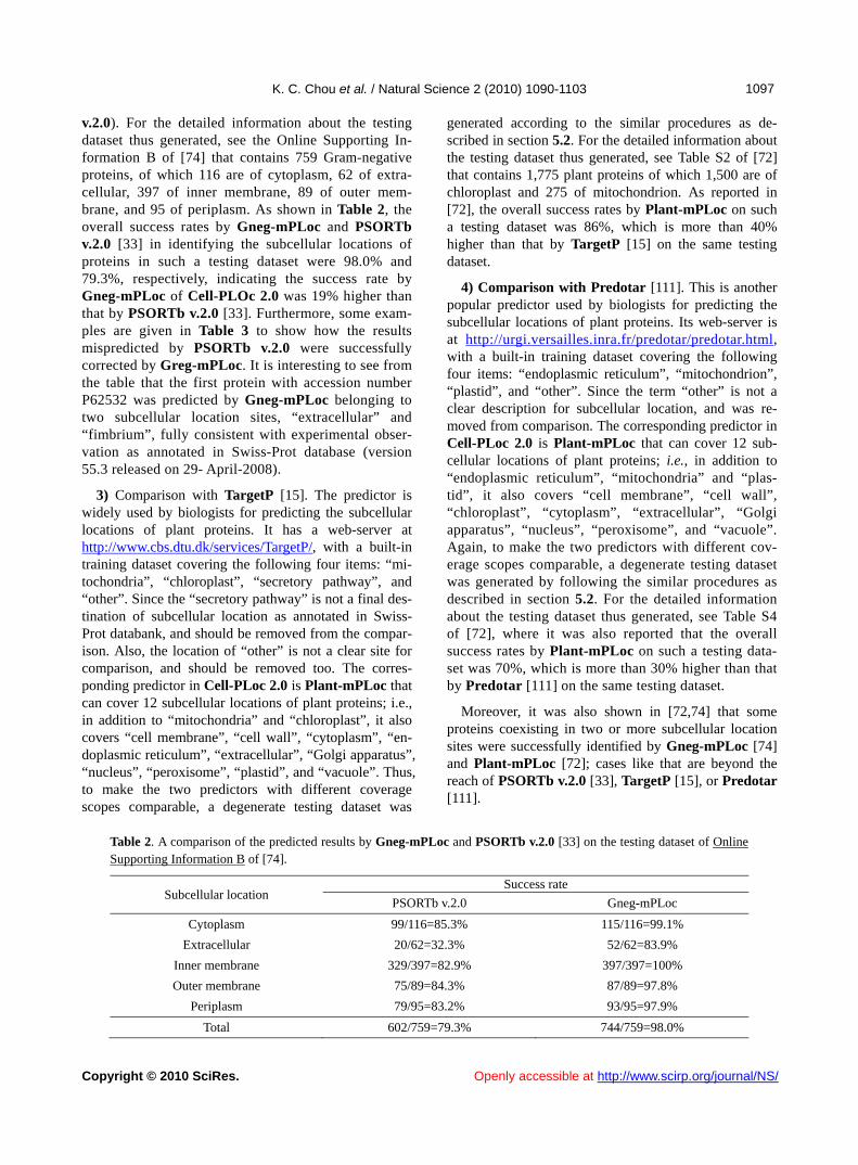
K. C. Chou et al. / Natural Science 2 (2010) 1090-1103
Copyright © 2010 SciRes. Openly accessible at http://www.scirp.org/journal/NS/
1091097
v.2.0). For the detailed information about the testing dataset thus generated, see the Online Supporting In-formation B of [74] that contains 759 Gram-negative proteins, of which 116 are of cytoplasm, 62 of extra-cellular, 397 of inner membrane, 89 of outer mem-brane, and 95 of periplasm. As shown in Table 2, the overall success rates by Gneg-mPLoc and PSORTb v.2.0 [33] in identifying the subcellular locations of proteins in such a testing dataset were 98.0% and 79.3%, respectively, indicating the success rate by Gneg-mPLoc of Cell-PLOc 2.0 was 19% higher than that by PSORTb v.2.0 [33]. Furthermore, some exam-ples are given in Table 3 to show how the results mispredicted by PSORTb v.2.0 were successfully corrected by Greg-mPLoc. It is interesting to see from the table that the first protein with accession number P62532 was predicted by Gneg-mPLoc belonging to two subcellular location sites, “extracellular” and “fimbrium”, fully consistent with experimental obser-vation as annotated in Swiss-Prot database (version 55.3 released on 29- April-2008).
3) Comparison with TargetP [15]. The predictor is widely used by biologists for predicting the subcellular locations of plant proteins. It has a web-server at http://www.cbs.dtu.dk/services/TargetP/, with a built-in training dataset covering the following four items: “mi-tochondria”, “chloroplast”, “secretory pathway”, and “other”. Since the “secretory pathway” is not a final des-tination of subcellular location as annotated in Swiss- Prot databank, and should be removed from the compar-ison. Also, the location of “other” is not a clear site for comparison, and should be removed too. The corres-ponding predictor in Cell-PLoc 2.0 is Plant-mPLoc that can cover 12 subcellular locations of plant proteins; i.e., in addition to “mitochondria” and “chloroplast”, it also covers “cell membrane”, “cell wall”, “cytoplasm”, “en-doplasmic reticulum”, “extracellular”, “Golgi apparatus”, “nucleus”, “peroxisome”, “plastid”, and “vacuole”. Thus, to make the two predictors with different coverage scopes comparable, a degenerate testing dataset was
generated according to the similar procedures as de-scribed in section 5.2. For the detailed information about the testing dataset thus generated, see Table S2 of [72] that contains 1,775 plant proteins of which 1,500 are of chloroplast and 275 of mitochondrion. As reported in [72], the overall success rates by Plant-mPLoc on such a testing dataset was 86%, which is more than 40% higher than that by TargetP [15] on the same testing dataset.
4) Comparison with Predotar [111]. This is another popular predictor used by biologists for predicting the subcellular locations of plant proteins. Its web-server is at http://urgi.versailles.inra.fr/predotar/predotar.html, with a built-in training dataset covering the following four items: “endoplasmic reticulum”, “mitochondrion”, “plastid”, and “other”. Since the term “other” is not a clear description for subcellular location, and was re-moved from comparison. The corresponding predictor in Cell-PLoc 2.0 is Plant-mPLoc that can cover 12 sub-cellular locations of plant proteins; i.e., in addition to “endoplasmic reticulum”, “mitochondria” and “plas-tid”, it also covers “cell membrane”, “cell wall”, “chloroplast”, “cytoplasm”, “extracellular”, “Golgi apparatus”, “nucleus”, “peroxisome”, and “vacuole”. Again, to make the two predictors with different cov-erage scopes comparable, a degenerate testing dataset was generated by following the similar procedures as described in section 5.2. For the detailed information about the testing dataset thus generated, see Table S4 of [72], where it was also reported that the overall success rates by Plant-mPLoc on such a testing data-set was 70%, which is more than 30% higher than that by Predotar [111] on the same testing dataset.
Moreover, it was also shown in [72,74] that some proteins coexisting in two or more subcellular location sites were successfully identified by Gneg-mPLoc [74] and Plant-mPLoc [72]; cases like that are beyond the reach of PSORTb v.2.0 [33], TargetP [15], or Predotar [111].
Table 2. A comparison of the predicted results by Gneg-mPLoc and PSORTb v.2.0 [33] on the testing dataset of Online Supporting Information B of [74].
Subcellular location Success rate
PSORTb v.2.0 Gneg-mPLoc
Cytoplasm 99/116=85.3% 115/116=99.1%
Extracellular 20/62=32.3% 52/62=83.9%
Inner membrane 329/397=82.9% 397/397=100%
Outer membrane 75/89=84.3% 87/89=97.8%
Periplasm 79/95=83.2% 93/95=97.9%
Total 602/759=79.3% 744/759=98.0%

K. C. Chou et al. / Natural Science 2 (2010) 1090-1103
Copyright © 2010 SciRes. Openly accessible at http://www.scirp.org/journal/NS/
1098
Table 3. Some examples to show how the subcellular location sites mispredicted by PSORTb v.2.0 were corrected by Gneg-mPLoc.
Protein accession numberaExperimental result anno-tated in Swiss-Prot data-
base
Predicted result by PSORTb v.2.0
Predicted result by Gneg-mPLoc
P62532 Extracellular; Fimbrium Unknown Extracellular; Fimbrium
Q8X9H8 Cytoplasm Unknown Cytoplasm
P00962 Cytoplasm Unknown Cytoplasm
Q83LY4 Cytoplasm Unknown Cytoplasm
Q8DFR1 Cytoplasm Unknown Cytoplasm
Q84H44 Cytoplasm Unknown Cytoplasm
P27475 Extracellular Unknown Extracellular
O50319 Extracellular Unknown Extracellular
P31518 Extracellular Unknown Extracellular
Q89AD4 Cytoplasm Unknown Cytoplasm
Q56027 Extracellular Unknown Extracellular
O52623 Extracellular Unknown Extracellular
P26219 Cell inner membrane Unknown Cell inner membrane
P77293 Cell inner membrane Unknown Cell inner membrane
P95655 Cell inner membrane Unknown Cell inner membrane.
P04123 Cell inner membrane Periplasm Cell inner membrane
Q47879 Cell outer membrane Unknown Cell outer membrane
P0A935 Cell outer membrane Unknown Cell outer membrane
P00211 Periplasm Cytoplasm Periplasm
P0A182 Periplasm Unknown Periplasm
Q9Z4N3 Periplasm Unknown Periplasm
P31330 Periplasm Cytoplasm Periplasm
a Only the sequences but not the accession numbers were used as inputs during the prediction by Gneg-mPLoc. The accession numbers here are just for the usage of identification.
From the above four comparisons, we can now make the following points very clear. The more stringent a benchmark dataset is in ex-
cluding homologous and high similarity sequences, or the more subcellular location sites it covers, the more difficult for a predictor to achieve a high overall success rate. The impact of the coverage scope on the success rate can be easily understood by just considering the following cases. For a benchmark dataset only covering four subcellular locations each containing same number of proteins, the overall success rate by random assignments would generally be 1/ 4 25% ; while for a benchmark dataset covering 22 subcellular loca-tions, the overall success rate by random assign-ments would be only 1 / 25 4.5% . This means that the former is more than five times the latter.
Also, a predictor examined by jackknife test is very difficult to yield a high success rate when per-formed on a stringent benchmark dataset in which none of proteins included has 25% pairwise sequence identity to any other in a same subset (subcellular location). That is why the overall suc-cess rate achieved by Gneg-mPLoc was 85.7% when examined by the jackknife test on the benchmark dataset of the Online Supporting Infor-mation A of [74] but was 98.0% when examined by the independent dataset test for the proteins in the Online Supporting Information B of [74]. That is also why the overall success rate achieved by Plant-mPLoc was only 63.7% when examined by the jackknife test on the benchmark dataset of Ta-ble S1 of [72] but was over 86% and 70% when tested by the independent proteins of Table S2 and

K. C. Chou et al. / Natural Science 2 (2010) 1090-1103
Copyright © 2010 SciRes. Openly accessible at http://www.scirp.org/journal/NS/
1091099
Table S4 of [72], respectively. However, regardless of using what test methods or test datasets, one thing is crystal clear, i.e., the overall success rates achieved by the six predictors in Cell-PLoc 2.0 are significantly higher than those by its counterparts.
Meanwhile, it has also become understandable why the success rates as originally reported by PSORTb v.2.0 [33], TargetP [15] and Predotar [111] were over-estimated. This is because none of the success rates reported for these predictors was derived by the jackknife test. Also, the benchmark datasets used to test these predictors covered much less subcellular location sites than those used in their counterparts in Cell-PLoc 2.0. Particularly, the benchmark datasets used by PSORTb v.2.0 , Tar-getP and Predotar to estimate their success rates contained many homologous sequences. For in-stance, the cutoff threshold to reduce the homology bias for the benchmark dataset used in Predotar [111] was set at 80%, meaning that only those se-quences which have 80% pairwise sequence identity to any other in a same subset were ex-cluded [111]; while for the benchmark dataset used in TargetP [15] and PSORTb v.2.0 [33], even no cutoff threshold was indicated to remove homo-logous sequences. Compared with the benchmark datasets used in [70-75] where none of proteins in-cluded has 25% pairwise sequence identity to any other in a same subset, the benchmark datasets adopted by PSORTb v.2.0, TargetP, and Predotar are much less stringent and hence cannot avoid homology bias and overestimation.
6. CONCLUDING REMARKS
Evolved from the old Cell-PLoc package [61], Cell-PLoc 2.0 is much more flexible and powerful than the former. In addition to yielding higher success rates than the existing prediction method, all the predictors in Cell-PLoc 2.0 have the capacity to deal with proteins with two or more subcellular location sites. Besides, the predictors in Cell-PLoc 2.0 cover much wider scopes than most of the existing predictors in this area. For in-stance, Hum-mPLoc 2.0 and Euk-mPLoc 2.0 can cove up to 14 sites of human proteins and 22 sites of eukaryo-tic, respectively, which are about two to five times the number of subcellular location sites covered by most of the existing predictors.
However, Cell-PLoc 2.0 also has the following limi-tations and further improvements will be needed with more experimental data available in future. (1) Although Euk-mPLoc 2.0 in the Cell-PLoc 2.0 package can cover 22 sites of eukaryotic proteins, if a query protein is out-
side of the 22 location sites, it would still generate mea-ningless result. Therefore, we shall continuously extend the coverage scope for each of the predictors in the Cell-PLoc series in a timely manner once more statisti-cally significant experimental data will be available in future. (2) For some subcellular locations with very small numbers of proteins, the prediction success rates are still quite low. This is because there are not sufficient location-known proteins in these sites to effectively train the prediction engine. It is anticipated that with more experimental data available for these sites in the future, this kind of situation will be improved. (3) Since the power of Cell-PLoc 2.0 is closely associated with the GO database [68,112,113] and functional domain data-base [114], with the continuous development of the GO database and functional domain database, more useful GO numbers and functional domain information will be incorporated into the prediction engine, further streng-thening its prediction power.
Once further improvements are implemented, the fu-ture version of Cell-PLoc series will be announced via a publication or a webpage.
REFERENCES
[1] Ehrlich, J.S., Hansen, M.D., Nelson, W.J. (2002) Spatio- temporal regulation of Rac1 localization and lamellipo-dia dynamics during epithelial cell-cell adhesion. Dev Cell, 3, 259-270.
[2] Glory, E., Murphy, R.F. (2007) Automated subcellular location determination and high-throughput microscopy. Dev Cell, 12, 7-16.
[3] Smith, C. (2008) Subcellular targeting of proteins and drugs. http://www.biocompare.com/Articles/TechnologySpotlight/976/Subcellular-Targeting-Of-Proteins-And-Drugs.html
[4] Nakai, K., Kanehisa, M. (1991) Expert system for pre-dicting protein localization sites in Gram-negative bacte-ria. Proteins: Structure, Function and Genetics, 11, 95- 110.
[5] Nakashima, H., Nishikawa, K. (1994) Discrimination of intracellular and extracellular proteins using amino acid composition and residue-pair frequencies. Journal of Molecular Biology, 238, 54-61.
[6] Cedano, J., Aloy, P., P'erez-Pons, J.A., Querol, E. (1997) Relation between amino acid composition and cellular location of proteins. Journal of Molecular Biology, 266, 594-600.
[7] Nakai, K., Horton, P. (1999) PSORT: A program for de-tecting sorting signals in proteins and predicting their subcellular localization. Trends in Biochemical Science, 24, 34-36.
[8] Chou, K.C., Elrod, D.W. (1998) Using discriminant func-tion for prediction of subcellular location of prokaryotic proteins. Biochemical and Biophysical Research Com-munications, 252, 63-68.
[9] Reinhardt, A., Hubbard, T. (1998) Using neural networks for prediction of the subcellular location of proteins.
K. C. Chou et al. / Natural Science 2 (2010) 1090-1103
Copyright © 2010 SciRes. Openly accessible at http://www.scirp.org/journal/NS/
1100
Nucleic Acids Research, 26, 2230-2236. [10] Chou, K.C., Elrod, D.W. (1999) Protein subcellular loca-
tion prediction. Protein Engineering, 12, 107-118. [11] Yuan, Z. (1999) Prediction of protein subcellular loca-
tions using Markov chain models. FEBS Letters, 451, 23-26.
[12] Nakai, K. (2000) Protein sorting signals and prediction of subcellular localization. Advances in Protein Chemistry, 54, 277-344.
[13] Murphy, R.F., Boland, M.V., Velliste, M. (2000) Towards a systematics for protein subcellular location: quantita-tive description of protein localization patterns and au-tomated analysis of fluorescence microscope images. Proc. Int. Conf. Intell. Syst. Mol. Biol., 8, 251-259.
[14] Chou, K.C. (2000) Review: Prediction of protein struc-tural classes and subcellular locations. Current Protein and Peptide Science, 1, 171-208.
[15] Emanuelsson, O., Nielsen, H., Brunak, S., von Heijne, G. (2000) Predicting subcellular localization of proteins based on their N-terminal amino acid sequence. Journal of Molecular Biology, 300, 1005-1016.
[16] Chou, K.C. (2001) Prediction of protein cellular attributes using pseudo amino acid composition. PRO-TEINS: Structure, Function, and Genetics (Erratum: ibid., 2001, Vol.44, 60), 43, 246-255.
[17] Feng, Z.P. (2001) Prediction of the subcellular location of prokaryotic proteins based on a new representation of the amino acid composition. Biopolymers, 58, 491-499.
[18] Hua, S., Sun, Z. (2001) Support vector machine approach for protein subcellular localization prediction. Bioinfor-matics, 17, 721-728.
[19] Feng, Z.P., Zhang, C.T. (2001) Prediction of the subcel-lular location of prokaryotic proteins based on the hy-drophobicity index of amino acids. Int. J. Biol. Macro-mol., 28, 255-261.
[20] Feng, Z.P. (2002) An overview on predicting the subcel-lular location of a protein. In. Silico. Biol., 2, 291-303.
[21] Chou, K.C., Cai, Y.D. (2002) Using functional domain composition and support vector machines for prediction of protein subcellular location. Journal of Biological Chemistry, 277, 45765-45769.
[22] Zhou, G.P., Doctor, K. (2003) Subcellular location pre-diction of apoptosis proteins. Proteins: Structure, Func-tion, and Genetics, 50, 44-48.
[23] Pan, Y.X., Zhang, Z.Z., Guo, Z.M., Feng, G.Y., Huang, Z.D., He, L. (2003) Application of pseudo amino acid composition for predicting protein subcellular location: Stochastic signal processing approach. Journal of Protein Chemistry, 22, 395-402.
[24] Park, K.J., Kanehisa, M. (2003) Prediction of protein subcellular locations by support vector machines using compositions of amino acid and amino acid pairs. Bioin-formatics, 19, 1656-1663.
[25] Gardy, J.L., Spencer, C., Wang, K., Ester, M., Tusnady, G.E., Simon, I., Hua, S., deFays, K., Lambert, C., Nakai, K., Brinkman, F.S. (2003) PSORT-B: Improving protein subcellular localization prediction for Gram-negative bacteria. Nucleic Acids Research, 31, 3613-3617.
[26] Huang, Y., Li, Y. (2004) Prediction of protein subcellular locations using fuzzy k-NN method. Bioinformatics, 20, 21-28.
[27] Xiao, X., Shao, S., Ding, Y., Huang, Z., Huang, Y., Chou,
K.C. (2005) Using complexity measure factor to predict protein subcellular location. Amino Acids, 28, 57-61.
[28] Gao, Y., Shao, S.H., Xiao, X., Ding, Y.S., Huang, Y.S., Huang, Z.D., Chou, K.C. (2005) Using pseudo amino acid composition to predict protein subcellular location: approached with Lyapunov index, Bessel function, and Chebyshev filter. Amino Acids, 28, 373-376.
[29] Lei, Z., Dai, Y. (2005) An SVM-based system for pre-dicting protein subnuclear localizations BMC. Bioinfor-matics, 6, 291.
[30] Shen, H.B., Chou, K.C. (2005) Predicting protein sub-nuclear location with optimized evidence-theoretic K-earest classifier and pseudo amino acid composition. Biochem. Biophys. Res. Comm., 337, 752-756.
[31] Garg, A., Bhasin, M., Raghava, G.P. (2005) Support vec-tor machine-based method for subcellular localization of human proteins using amino acid compositions, their or-der, and similarity search. Journal of Biological Chemi-stry, 280, 14427-14432.
[32] Matsuda, S., Vert, J.P., Saigo, H., Ueda, N., Toh, H., Akutsu, T. (2005) A novel representation of protein se-quences for prediction of subcellular location using sup-port vector machines. Protein Sci., 14, 2804-2813.
[33] Gardy, J.L., Laird, M.R., Chen, F., Rey, S., Walsh, C.J., Ester, M., Brinkman, F.S. (2005) PSORTb v.2.0: ex-panded prediction of bacterial protein subcellular locali-zation and insights gained from comparative proteome analysis. Bioinformatics, 21, 617-623.
[34] Gao, Q.B., Wang, Z.Z., Yan, C., Du, Y.H. (2005) Predic-tion of protein subcellular location using a combined feature of sequence. FEBS Letters, 579, 3444-3448.
[35] Chou, K.C., Shen, H.B. (2006) Predicting protein sub-cellular location by fusing multiple classifiers. Journal of Cellular Biochemistry, 99, 517-527.
[36] Guo, J., Lin, Y., Liu, X. (2006) GNBSL: A new integra-tive system to predict the subcellular location for Gram- egative bacteria proteins. Proteomics, 6, 5099-5105.
[37] Xiao, X., Shao, S.H., Ding, Y.S., Huang, Z.D., Chou, K.C. (2006) Using cellular automata images and pseudo amino acid composition to predict protein subcellular lo-cation. Amino Acids, 30, 49-54.
[38] Hoglund, A., Donnes, P., Blum, T., Adolph, H.W., Kohl-bacher, O. (2006) MultiLoc: prediction of protein sub-cellular localization using N-terminal targeting sequences, sequence motifs and amino acid composition. Bioinfor-matics, 22, 1158-1165.
[39] Lee, K., Kim, D.W., Na, D., Lee, K.H., Lee, D. (2006) PLPD: reliable protein localization prediction from im-balanced and overlapped datasets. Nucleic Acids Re-search, 34, 4655-4666.
[40] Zhang, Z.H., Wang, Z.H., Zhang, Z.R., Wang, Y.X. (2006) A novel method for apoptosis protein subcellular locali-zation prediction combining encoding based on grouped weight and support vector machine. FEBS Letters, 580, 6169-6174.
[41] Shi, J.Y., Zhang, S.W., Pan, Q., Cheng, Y.-M., Xie, J. (2007) Prediction of protein subcellular localization by support vector machines using multi-scale energy and pseudo mino acid composition. Amino Acids, 33, 69-74.
[42] Chen, Y.L., Li, Q.Z. (2007) Prediction of apoptosis pro-tein subcellular location using improved hybrid approach and pseudo amino acid composition. Journal of Theoret-
K. C. Chou et al. / Natural Science 2 (2010) 1090-1103
Copyright © 2010 SciRes. Openly accessible at http://www.scirp.org/journal/NS/
1101101
ical Biology, 248, 377–381. [43] Chen, Y.L., Li, Q.Z. (2007) Prediction of the subcellular
location of apoptosis proteins. Journal of Theoretical Bi-ology, 245, 775-783.
[44] Mundra, P., Kumar, M., Kumar, K.K., Jayaraman, V.K., Kulkarni, B.D. (2007) Using pseudo amino acid compo-sition to predict protein subnuclear localization: Ap-proached with PSSM. Pattern Recognition Letters, 28, 1610-1615.
[45] Emanuelsson, O., Brunak, S., von Heijne, G., Nielsen, H. (2007) Locating proteins in the cell using TargetP, Sig-nalP and related tools. Nature Protocols, 2, 953-971.
[46] Lin, H., Ding, H., Feng-Biao Guo, F.B., Zhang, A.Y., Huang, J. (2008) Predicting subcellular localization of mycobacterial proteins by using Chou’s pseudo amino acid composition. Protein & Peptide Letters, 15, 739-744.
[47] Shi, J.Y., Zhang, S.W., Pan, Q., Zhou, G.P. (2008) Using Pseudo Amino Acid Composition to Predict Protein Subcellular Location: Approached with Amino Acid Composition Distribution. Amino Acids, 35, 321-327.
[48] Li, F.M., Li, Q.Z. (2008) Predicting protein subcellular location using Chou's pseudo amino acid composition and improved hybrid approach. Protein & Peptide Let-ters, 15, 612-616.
[49] Tantoso, E., Li, X.B. (2008) AAIndexLoc: Predicting Subcellular Localization of Proteins Based on a New Representation of Sequences Using Amino Acid Indices. Amino Acids, 35, 345-353.
[50] Jiang, X., Wei, R., Zhang, T.L., Gu, Q. (2008) Using the concept of Chou’s pseudo amino acid composition to predict apoptosis proteins subcellular location: an ap-proach by approximate entropy. Protein & Peptide Let-ters, 15, 392-396.
[51] Zhou, X.B., Chen, C., Li, Z.C., Zou, X.Y. (2008) Im-proved prediction of subcellular location for apoptosis proteins by the dual-layer support vector machine. Amino Acids, 35, 383-388.
[52] Ding, Y.S., Zhang, T.L. (2008) Using Chou’s pseudo amino acid composition to predict subcellular localiza-tion of apoptosis proteins: an approach with immune ge-netic algorithm-based ensemble classifier. Pattern Rec-ognition Letters, 29, 1887-1892.
[53] Zhang, S.W., Zhang, Y.L., Yang, H.F., Zhao, C.H., Pan, Q. (2008) Using the concept of Chou’s pseudo amino acid composition to predict protein subcellular localization: an approach by incorporating evolutionary information and von Neumann entropies. Amino Acids, 34, 565-572.
[54] Jin, Y., Niu, B., Feng, K.Y., Lu, W.C., Cai, Y.D., Li, G.Z. (2008) Predicting subcellular localization with AdaBoost learner. Protein & Peptide Letters, 15, 286-289.
[55] Lin, H., Wang, H., Ding, H., Chen, Y.L., Li, Q.Z. (2009) Prediction of Subcellular Localization of Apoptosis Pro-tein Using Chou’s Pseudo Amino Acid Composition. Ac-ta Biotheoretica, 57, 321-330.
[56] Zhang, L., Liao, B., Li, D., Zhu, W. (2009) A novel re-presentation for apoptosis protein subcellular localization prediction using support vector machine. Journal of Theoretical Biology, 259, 361-365.
[57] Zeng, Y.H., Guo, Y.Z., Xiao, R.Q., Yang, L., Yu, L.Z., Li, M.L. (2009) Using the augmented Chou’s pseudo amino acid composition for predicting protein submitochondria locations based on auto covariance approach. Journal of
Theoretical Biology, 259, 366-72. [58] Du, P., Cao, S., Li, Y. (2009) SubChlo: predicting protein
subchloroplast locations with pseudo-amino acid compo-sition and the evidence-theoretic K-nearest neighbor (ET-KNN) algorithm. Journal of Theoretical Biology, 261, 330-335.
[59] Cai, Y.D., He, J., Li, X., Feng, K., Lu, L., Kong, X., Lu, W. (2010) Predicting protein subcellular locations with feature selection and analysis. Protein Pept. Lett., 17, 464-472.
[60] Millar, A.H., Carrie, C., Pogson, B., Whelan, J. (2009) Exploring the function-location nexus: using multiple lines of evidence in defining the subcellular location of plant proteins. Plant Cell, 21, 1625-1631.
[61] Chou, K.C., Shen, H.B. (2008) Cell-PLoc: A package of Web servers for predicting subcellular localization of proteins in various organisms. Nature Protocols, 3, 153- 162.
[62] Chou, K.C., Shen, H.B. (2007) Euk-mPLoc: a fusion classifier for large-scale eukaryotic protein subcellular location prediction by incorporating multiple sites. Journal of Proteome Research, 6, 1728-1734.
[63] Shen, H.B., Chou, K.C. (2007) Hum-mPLoc: An ensem-ble classifier for large-scale human protein subcellular location prediction by incorporating samples with mul-tiple sites. Biochemical and Biophysical Research Com-munications, 355, 1006-1011.
[64] Chou, K.C., Shen, H.B. (2007) Large-scale plant protein subcellular location prediction. Journal of Cellular Bio-chemistry, 100, 665-678.
[65] Shen, H.B., Chou, K.C. (2007) Gpos-PLoc: An ensemble classifier for predicting subcellular localization of Gram- ositive bacterial proteins. Protein Engineering, Design, and Selection, 20, 39-46.
[66] Chou, K.C., Shen, H.B. (2006) Large-scale predictions of Gram-negative bacterial protein subcellular locations. Journal of Proteome Research, 5, 3420-3428.
[67] Shen, H.B., Chou, K.C. (2007) Virus-PLoc: A fusion classifier for predicting the subcellular localization of viral proteins within host and virus-infected cells. Biopo-lymers, 85, 233-240.
[68] Ashburner, M., Ball, C.A., Blake, J.A., Botstein, D., Butler, H., Cherry, J.M., Davis, A.P., Dolinski, K., Dwight, S.S., Eppig, J.T., Harris, M.A., Hill, D.P., Issel- arver, L., Kasarskis, A., Lewis, S., Matese, J.C., Rich-ardson, J.E., Ringwald, M., Rubin, G.M., Sherlock, G. (2000) Gene ontology: Tool for the unification of biology. Nature Genetics, 25, 25-29.
[69] Chou, K.C. (2005) Using amphiphilic pseudo amino acid composition to predict enzyme subfamily classes. Bioin-formatics, 21, 10-19.
[70] Chou, K.C., Shen, H.B. (2010) A new method for pre-dicting the subcellular localization of eukaryotic proteins with both single and multiple sites: Euk-mPLoc 2.0. PLoS ONE, 5, e9931.
[71] Shen, H.B., Chou, K.C. (2009) A top-down approach to enhance the power of predicting human protein subcel-lular localization: Hum-mPLoc 2.0. Analytical Biochemi-stry, 394, 269-74.
[72] Chou, K.C., Shen, H.B. (2010) Plant-mPLoc: A top- down strategy to augment the power for predicting plant protein subcellular localization. PLoS ONE, 5, e11335.

K. C. Chou et al. / Natural Science 2 (2010) 1090-1103
Copyright © 2010 SciRes. Openly accessible at http://www.scirp.org/journal/NS/
1102
[73] Shen, H.B., Chou, K.C. (2009) Gpos-mPLoc: A top- down approach to improve the quality of predicting sub-cellular localization of Gram-positive bacterial proteins. Protein & Peptide Letters, 16, 1478-1484.
[74] Shen, H.B., Chou, K.C. (2010) Gneg-mPLoc: A top- down strategy to enhance the quality of predicting sub-cellular localization of Gram-negative bacterial proteins. Journal of Theoretical Biology, 264, 326-333.
[75] Shen, H.B., Chou, K.C. (2010) Virus-mPLoc: A fusion classifier for viral protein subcellular location prediction by incorporating multiple sites. Journal of Biomolecular Structure & Dynamics, 28, 175-186.
[76] Chou, K.C., Zhang, C.T. (1995) Review: Prediction of protein structural classes. Critical Reviews in Biochemi-stry and Molecular Biology, 30, 275-349.
[77] Fang, Y., Guo, Y., Feng, Y., Li, M. (2008) Predicting DNA-binding proteins: Approached from Chou’s pseudo amino acid composition and other specific sequence fea-tures. Amino Acids, 34, 103-109.
[78] Feng, Y.E., Luo, L.F. (2008) Use of tetrapeptide signals for protein secondary-structure prediction. Amino Acids, 35, 607-614.
[79] Li, Z.C., Zhou, X.B., Dai, Z., Zou, X.Y. (2009) Predic-tion of protein structural classes by Chou’s pseudo amino acid composition: approached using continuous wavelet transform and principal component analysis. Amino Ac-ids, 37, 415-425.
[80] Nanni, L., Lumini, A. (2008) Genetic programming for creating Chou's pseudo amino acid based features for submitochondria localization. Amino Acids, 34, 653-660.
[81] Wang, Y., Xue, Z., Shen, G., Xu, J. (2008) PRINTR: Pre-diction of RNA binding sites in proteins using SVM and profiles. Amino Acids, 35, 295-302.
[82] Zhao, X.M., Chen, L., Aihara, K. (2008) Protein function prediction with high-throughput data. Amino Acids, 35, 517-530.
[83] Jahandideh, S., Abdolmaleki, P., Jahandideh, M., Asada-badi, E.B. (2007) Novel two-stage hybrid neural discri-minant model for predicting proteins structural classes. Biophys. Chem., 128, 87-93.
[84] Chen, K., Kurgan, L.A., Ruan, J. (2008) Prediction of protein structural class using novel evolutionary colloca-tion-based sequence representation. Journal of Computa-tional Chemistry, 29, 1596-1604.
[85] Jahandideh, S., Sarvestani, A.S., Abdolmaleki, P., Jahan-dideh, M., Barfeie, M. (2007) Gamma-Turn types predic-tion in proteins using the support vector machines. Jour-nal of Theoretical Biology, 249, 785-790.
[86] Shao, X., Tian, Y., Wu, L., Wang, Y., L., J., Deng, N. (2009) Predicting DNA- and RNA-binding proteins from sequences with kernel methods. Journal of Theoretical Biology, 258, 289-293.
[87] Yang, J.Y., Peng, Z.L., Yu, Z.G., Zhang, R.J., Anh, V., Wang, D. (2009) Prediction of protein structural classes by recurrence quantification analysis based on chaos game representation. Journal of Theoretical Biology, 257, 618-626.
[88] Anand, A., Suganthan, P.N. (2009) Multiclass cancer classification by support vector machines with class-wise optimized genes and probability estimates. Journal of Theoretical Biology, 259, 533-540.
[89] Chen, C., Chen, L.X., Zou, X.Y., Cai, P.X. (2008) Pre-
dicting protein structural class based on multi-features fusion. Journal of Theoretical Biology, 253, 388-392.
[90] Du, P., Li, Y. (2008) Prediction of C-to-U RNA editing sites in plant mitochondria using both biochemical and evolutionary information. Journal of Theoretical Biology, 253, 579-589.
[91] Jahandideh, S., Hoseini, S., Jahandideh, M., Hoseini, A., Disfani, F.M. (2009) Gamma-turn types prediction in proteins using the two-stage hybrid neural discriminant model. Journal of Theoretical Biology, 259, 517-522.
[92] Lin, H. (2008) The modified Mahalanobis discriminant for predicting outer membrane proteins by using Chou’s pseudo amino acid composition. Journal of Theoretical Biology, 252, 350-356.
[93] Munteanu, C.B., Gonzalez-Diaz, H., Magalhaes, A.L. (2008) Enzymes/non-enzymes classification model com-plexity based on composition, sequence, 3D and topo-logical indices. Journal of Theoretical Biology, 254, 476- 482.
[94] Rezaei, M.A., Abdolmaleki, P., Karami, Z., Asadabadi, E.B., Sherafat, M.A., Abrishami-Moghaddam, H., Fadaie, M., Forouzanfar, M. (2008) Prediction of membrane protein types by means of wavelet analysis and cascaded neural networks. Journal of Theoretical Biology, 254, 817-820.
[95] Vilar, S., Gonzalez-Diaz, H., Santana, L., Uriarte, E. (2009) A network-QSAR model for prediction of genet-ic-component biomarkers in human colorectal cancer. Journal of Theoretical Biology, 261, 449-458.
[96] Wang, T., Xia, T., Hu, X.M. (2010) Geometry preserving projections algorithm for predicting membrane protein types. Journal of Theoretical Biology, 262, 208-213.
[97] Chen, Y., Han, K. (2009) BSFINDER: Finding Binding Sites of HCV Proteins Using a Support Vector Machine. Protein & Peptide Letters, 16, 373-382.
[98] Kannan, S., Hauth, A.M., Burger, G. (2008) Function prediction of hypothetical proteins without sequence si-milarity to proteins of known function. Protein & Peptide Letters, 15, 1107-1116.
[99] Nanni, L., Lumini, A. (2009) A Further Step Toward an Optimal Ensemble of Classifiers for Peptide Classifica-tion, a Case Study: HIV Protease. Protein & Peptide Let-ters, 16, 163-167.
[100] Gu, F., Chen, H. (2009) Evaluating Long-term Relation-ship of Protein Sequence by Use of d-Interval Condition-al Probability and its Impact on Protein Structural Class Prediction. Protein Pept. Lett., 16, 1267-1276.
[101] Ji, G., Wu, X., Shen, Y., Huang, J., Quinn Li, Q. (2010) A classification-based prediction model of messenger RNA polyadenylation sites. Journal of Theoretical Biology, 265, 287-296.
[102] Yang, X.Y., Shi, X.H., Meng, X., Li, X.L., Lin, K., Qian, Z.L., Feng, K.Y., Kong, X.Y., Cai, Y.D. (2010) Classifi-cation of transcription factors using protein primary structure. Protein & Peptide Letters, 17, 899-908.
[103] Gu, Q., Ding, Y.S., Zhang, T.L. (2010) Prediction of G-Protein-Coupled Receptor Classes in Low Homology Using Chou’s Pseudo Amino Acid Composition with Approximate Entropy and Hydrophobicity Patterns. Pro-tein Pept. Lett., 17, 559-567.
[104] Liu, L., He, D., Yang, S., Xu, Y. (2010) Applying che-mometrics approaches to model and predict the binding

K. C. Chou et al. / Natural Science 2 (2010) 1090-1103
Copyright © 2010 SciRes. Openly accessible at http://www.scirp.org/journal/NS/
1101103
affinities between the human amphiphysin SH3 domain and its peptide ligands. Protein Pept. Lett., 17, 246- 253.
[105] Shi, R., Hu, X. (2010) Predicting enzyme subclasses by using support vector machine with composite vectors. Protein Pept. Lett., 17, 599-604.
[106] Wang, T., Yang, J. (2010) Predicting subcellular localiza-tion of gram-negative bacterial proteins by linear dimen-sionality reduction method. Protein Pept. Lett., 17, 32-37.
[107] Yang, J., Jiang, X.F. (2010) A novel approach to predict protein-protein interactions related to Alzheimer’s dis-ease based on complex network. Protein Pept. Lett., 17, 356-366.
[108] Chou, K.C., Shen, H.B. (2006) Hum-PLoc: A novel en-semble classifier for predicting human protein subcellu-lar localization. Biochemical and Biophysical Research Communications, 347, 150-157.
[109] Chou, K.C., Shen, H.B. (2006) Predicting eukaryotic protein subcellular location by fusing optimized evi-dence-theoretic K-nearest neighbor classifiers. Journal of Proteome Research, 5, 1888-1897.
[110] Chou, K.C., Shen, H.B. (2007) Review: Recent progresses in protein subcellular location prediction.
Analytical Biochemistry, 370, 1-16. [111] Small, I., Peeters, N., Legeai, F., Lurin, C. (2004) Predo-
tar: A tool for rapidly screening proteomes for N-terminal targeting sequences. Proteomics, 4, 1581-1590.
[112] Camon, E., Magrane, M., Barrell, D., Binns, D., Fleisch-mann, W., Kersey, P., Mulder, N., Oinn, T., Maslen, J., Cox, A., Apweiler, R. (2003) The gene ontology annotation (GOA) project: Implementation of GO in SWISS- PROT, TrEMBL, and InterPro. Genome Res., 13, 662-672.
[113] Barrell, D., Dimmer, E., Huntley, R.P., Binns, D., O'Do-novan, C., Apweiler, R. (2009) The GOA database in 2009-an integrated Gene Ontology Annotation resource. Nucleic Acids Research, 37, D396-403.
[114] Marchler-Bauer, A., Anderson, J.B., Derbyshire, M.K., DeWeese-Scott, C., Gonzales, N.R., Gwadz, M., Hao, L., He, S., Hurwitz, D.I., Jackson, J.D., Ke, Z., Krylov, D., Lanczycki, C.J., Liebert, C.A., Liu, C., Lu, F., Lu, S., Marchler, G.H., Mullokandov, M., Song, J.S., Thanki, N., Yamashita, R.A., Yin, J.J., Zhang, D., Bryant, S.H. (2007) CDD: A conserved domain database for interactive do-main family analysis. Nucleic Acids Research, 35, D237- D240.
Vol.2, No.10, 1104-1112 (2010)doi:10.4236/ns.2010.210137
Copyright © 2010 SciRes. Openly accessible at http://www.scirp.org/journal/NS/
Natural Science
Evolution based on genome structure: the “diagonal genome universe”
Kenji Sorimachi
Educational Support Center, Dokkyo Medical University, Mibu, Japan; [email protected].
Received 13 July 2010; revised 16 August 2010; accepted 20 August 2010.
ABSTRACT
The ratios of amino acid to the total amino acids and those of nucleotides to the total nucleotides in genes or genomes are suitable indexes to compare whole gene or genome characteristics based on the large number of nucleotides rather than their sequences. As these ratios are strictly calculated from nucleotide sequences, the val-ues are independent of experimental errors. In the present mini-review, the following themes are approached according to the ratios of amino acids and nucleotides to their total numbers in the genome: prebiotic evolution, the chrono-logical precedence of protein and codon forma-tions, genome evolution, Chargaff’s second pa- rity rule, and the origins of life. Amino acid for-mation might have initially occurred during pre- biotic evolution, the “amino acid world”, and amino acid polymerization might chronologically precede codon formation at the end of prebiotic evolution. All nucleotide alterations occurred synchronously over the genome during biolo- gical evolution. After establishing primitive lives, all nucleotide alterations have been governed by linear formulae in nuclear and organelle ge-nomes consisting of the double-stranded DNA. When the four nucleotide contents against each individual nucleotide content in organelles are expressed by four linear regression lines rep-resenting the diagonal lines of a 0.5 square – the “Diagonal Genome Universe”, evolution obeys Chargaff’s second parity rule. The fact that linear regression lines intersect at a single point su- ggests that all species originated from a single life source.
Keywords: Evolution (Prebiotic and Biological); Genome; Origin of Life; Chargaff’s Parity Rules; Organelle; Double- and Single-Strand DNA; Amino Acid; Nucleotide; Linear Formula
1. INTRODUCTION
“The Origin of Species”, written from the observa-tions Charles Darwin made during his voyage on the HMS Beagle, was published in 1859. According to Dar-win’s theory, all species have a common ancestor and a single origin. During the same period when Darwin wrote, Gregor Mendel reported “Mendel’s laws” that accorded with his observations of the inheritance of cer-tain traits in pea plants. The former and latter are based on inter- and intra-species phenotypic expression simi-larities, respectively, and based on long and compara-tively short lifespans, respectively. In general, interspe-cies changes are thought of as “evolution”, while intras-pecies changes are “genetics”. These two great concepts were established by two scientists without any knowl-edge of DNA; although nowadays it is well known that almost all traits of organisms are based on gene charac-teristics. After almost a century, Oswald Avery and co- workers reported in 1944 that DNA is the material of genes and chromosomes [1].
Although it was clarified by Avery’s group that DNA is important material for the inheritance of certain traits in organisms, the structure of DNA, which has an ex-tremely large molecular weight, was completely un-known and, therefore, the mechanisms of trait inheri-tance were also unknown. On the other hand, Ervin Chargaff reported in 1950 that nuclear DNA consists of four nucleotides, and that the nucleotide content rela-tionships are: G = C, A = T, and [(G + A) = (C + T)]. This rule is well known as Chargaff’s first parity rule [2]. He and his colleagues later discovered that these rela-tionships are applicable to the single DNA strand, and this is Chargaff’s second parity rule [3]. After Chargaff’s first parity rule, another great scientific discovery was reported in 1953 by Watson and Crick [4]. Namely, that the DNA structure is double-stranded, and C vs. G and T vs. A pairs are formed between two DNA strands. These two base-pair formations can consistently explain the inheritance of genetic traits from generation to genera-tion. Even though this DNA structure can explain Char-

K. Sorimachi / Natural Science 2 (2010) 1104-1112
Copyright © 2010 SciRes. http://www.scirp.org/journal/NS/
1105
Openly accessible at
gaff’s first parity rule, the second parity rule based on the single DNA strand cannot be explained by the dou-ble-stranded DNA model. Chargaff’s parity rules were originally discovered from a single species and recently it was shown that Chargaff’s second parity rule is appli-cable to interspecies evolution [5]. Nuclear nucleotide relationships were clearly expressed by linear regression lines with extremely high regression coefficients among various species. The single DNA strand which forms the double-stranded DNA has been shown, based on the huge amount of genomic data, to obey Chargaff’s second parity rule [5]. Furthermore, as nucleotide relationships in the coding region are also expressed by linear formu-lae, 64 codons can be correctly estimated from just one nucleotide content [6].
Molecular clock research—using amino acid or nu-cleotide replacement rates [7] has enabled scientists to create a phylogenetic tree representing biological evolu-tion [8-12]. However, as this method is based on se-quences of certain genes among various organisms, we cannot investigate organisms without these genes. Fur-thermore, this method does not fit the research on whole genomes consisting of an extremely large number of nu- cleotides. On the other hand, by using the ratios of nu-cleotides to the total nucleotides or amino acids to the total amino acids after normalization, it is possible to compare certain characteristics among different genes or genomes. As this method is independent not only of sam- ple size but also of species, the method can be recom-mended for comparative studies on genomes consisting of extremely large and different numbers of nucleotides. Using normalized values, each organism can be repre-sented by simple indexes that represent whole genome characteristics. In fact, this method has been applied to genome research and its usefulness proven by using graphic representation or a diagram approach [13]. Visu-alization to study complicated biological systems can provide an intuitive picture and provide useful insights [1 -16]. 4
2. PREBIOTIC EVOLUTION
We have no evidence of “the origin of life”, although there are two distinct ideas: one being that the origin of life was on the primitive Earth and the other that it was derived from another planet (extraterrestrial universe). Based on either idea, “the origin of life” did indeed oc-cur somewhere after the “Big Bang”. Many physical and chemical reactions occurred during prebiotic evolution and substantial materials for the formation of primitive life may have accumulated during this period. For ex-ample, Miller’s experiment showed that amino acids could be formed by electric discharges in the atmosphere on the primitive Earth [17]. Furthermore, amino acids
have been detected in meteorites [18,19]. Accumulation of amino acids might lead to the appearance of amino acid polymers or peptides without the codon system. As well, certain polymers or peptides might have enzyme activity that accelerates amino acid polymerization, which is reported as being able to occur in soil via heat without either enzyme or codon system [20]. The pro-duction of enzymes led to the accumulation of substan-tial materials for “the origin of life”.
Amino acid polymers formed chemically might reflect the amino acid concentrations on the primitive Earth. Sueoka initially investigated the cellular amino acid com- position of bacteria [21] and then we independently ex-amined, not only bacterial but also plant and animal cells [22,23]. Based on amino acid composition patterns, it is clearly shown that cellular amino acid composition is very similar among organisms from bacteria to Homo sapiens [22], as shown in Figure 1. This fact led us to conclude that primitive life forms might have similar amino acid composition presumed from present organ-isms [24]. Based on an amino acid pattern (Figure 1), the ratios of the amino acids that have ultraviolet (UV) absorbance (i.e., phenylalanine, tyrosine and tryptophan) to the total cellular amino acids are very low. To explain this fact, the strong irradiation of UV light might have induced their decomposition and reduced their concen-tration on the primitive Earth. However, the contents of glycine and alanine, which were formed easily in Miller’s experiment, are relatively high [22]. In addition, the contents of hydrophobic amino acids such as leucine, isoleucine, alanine and valine are comparatively high. These amino acids might contribute to self-aggregation of amino acid polymers to form the “coacervate” pro-posed by Aleksandr Oparin through their hydrophobicity under low polymer concentrations.
The basic pattern of cellular amino acid compositions,
Figure 1. Cellular amino acid compositions of Escherichia coli and Homo sapiens on radar charts. Amino acid compositions are expressed as the percentage of total amino acids. Gln and Asn are combined with Glu and Asp, respectively, because the former two are converted to the latter two during hydrolysis [22].
K. Sorimachi / Natural Science 2 (2010) 1104-1112
Copyright © 2010 SciRes. http://www.scirp.org/journal/NS/Openly accessible at
1106
the “star-shape”, is formed with characteristic differen- ces in amino acid contents. The fact that the basic pattern is conserved from bacteria to Homo sapiens, suggests that the pattern is extremely important for organisms on earth. It would be quite interesting to evaluate whether this “star-shape” is conserved on other planets with life in the future, if any is found.
3. CHRONOLOGICAL PRECEDENCE OF PROTEIN AND CODON FORMATION
Evolutionarily, it remains unclear whether protein formation preceded codon formation or codon formation preceded that of protein. However, it should be possible to judge which theory is better at explaining this theme, though it might be impossible to design a complete ex-periment. Amino acids, which are monomers of proteins or peptides, were easily formed by electric discharges in an atmosphere presumed from the primitive Earth [17]. In addition, their polymerizations took place in clay without the codon system [20] and certain products, pro- tein or peptides, might possess an enzymatic activity which accelerates amino acid polymerizations. Eventu-ally, these processes might produce various biomaterials, such as amino acids and their polymers, whereas the production of nucleic acids whose formation requires nitrogenous base and sugar synthesis, their coupling and condensation, might be difficult in the primitive Earth. Although the so-called “RNA world” has been proposed [25], the possibility of the accumulation of RNA, which has UV absorbance at around 250 nm, might be very low under the strong UV irradiation present on the primitive Earth. In general, the composition of polymerization products depends on monomer concentrations and re-flects their free concentration on the primitive Earth, as mentioned above.
Simulation analysis based on random choice of amino acids showed consistent results in which amino acids were polymerized randomly without the codon system [26]. The amino acid composition obtained by a random choice of amino acids from the amino acid pool reflects each amino acid concentration in the pool. After estab-lishing the codon system, the sequence information has been conserved until now. On the other hand, polymeri-zation of nucleotides based on the random choice of nu-cleotides does not yield functional proteins [26]. Even when the codon table is considered for nucleotide poly-mer formation, the amino acid composition depends on the original four nucleotide contents. The nucleotide compositions differ between the coding and non-coding regions, while they are quite similar among the coding or non-coding regions [6,27,28]. Thus, the coding frag-ments that possessed the same characteristics might be
combined through the non-coding fragments with each other like a “patchwork” in the whole genome. This structural model fits the proposed model that the forma-tion of proteins might have preceded codon formation. At present, even though there is no experimental evi-dence for the process of how sequence information of amino acid polymers transfers to codon formation during a codon establishing period, protein formation might precede codon formation based on the present genome structure [26].
4. HOMOGENEITY OF GENOME STRUCTURE
The amino acid sequences of proteins differ, not only among different genes, but also among different species, and naturally, their nucleotide sequences also differ. As these differences relate to evolutionary time [7], this con- cept has been applied to draw phylogenetic trees [8-12]. Using the ratios of each amino acid to the total amino acids, or those of each nucleotide to the total nucleotides, it is possible to compare samples independently regard-ing size, kind and species, even though DNA has an ex-tremely large number of nucleotides.
The method to analyze nucleotide sequences was es-tablished by Frederic Sanger [29], and Allan Maxam and Walter Gilbert [30], and the first complete genome ana- lysis was carried out on Haemophilus influenzae in 1995 [31]. Then the complete genome analyses of species such as human (Homo sapiens) [32,33], mouse (Mus muscu-lus) [34], rat (Rattus norvegicus) [35] and sea urchin (Strongylocentrotus purpuratus) [36] were carried out within the last two decades. Several species of Archaea were also examined and their complete genomes were determined. Based on these intriguing results, the amino acid compositions were presumed from the complete genomes. Surprisingly, the cellular amino acid composi-tions obtained from the whole cell lysates resemble those presumed from the complete genome [24], although the former is based on a different protein mixture and the latter is based on a different gene mixture. The coinci-dence of these two results in our study was not explain-able until the genomic structure was fully understood [37].
The full sequence of mouse cDNA was determined in 2001 [38]. The total number of mouse cDNAs includes 10,465 genes and was divided into two equal parts and the amino acid compositions presumed from the first 5, 10, 50, 100, 500, 1,000 and 5,232 genes, according to the order listed in the data table, were compared between the two parts and within the same parts (Figure 2). The amino acid compositions of gene assemblies resembled those presumed from the complete genome. Of course,

K. Sorimachi / Natural Science 2 (2010) 1104-1112
Copyright © 2010 SciRes. http://www.scirp.org/journal/NS/
1107
Openly accessible at
Asp
Glu Ser
Gly
His
Arg
Thr
Val
Met
Phe
Lys
Tyr Pro
Complete
Ala
Leu
Cys
Ile
Figure 2. Amino acid compositions. Computational amino acid se-quences (10,465) of FANTOM clones were divided into two equal parts; first (red) and latter (green) halves. In both parts, the first 5, 10, 50, 100, 500 and 1,000 genes were used for analyses of amino acid compositions for the units. The numbers of genes were 5,232 and 5, 233 in the first and second halves, respectively. The left side graph shows the amino acid composition based on 10,465 genes [38]. the amino acid compositions presumed from genes differ among various genes. Therefore, the genome structure is constructed homogeneously with certain similar units that encode similar amino acid compositions. The con-sistent result was obtained from the complete Archaeal genome (Methanobacterium thermoautotrophicum) [39], as shown in Figure 3.
When the amino acid composition presumed from the complete genome is expressed by the radar chart, the amino acid composition patterns based on a small seg-ment, encoding 3,000-7,000 amino acid residues, repre-sent the pattern based on the complete genome, as shown in Figures 2 and 3. The consistent result was obtained using the nucleotide composition [40] as well as amino acid composition of the Saccharomyces cerevisiae ge-nome [37]. Additionally, the genome structure resembles the appearance of a “pearl necklace” (Figure 4). Based on this model, the genome is constructed with almost the same putative small units, encoding 3,000-7,000 amino acid residues, over the entire genome. This fact indicates that all nucleotide alterations occurred synchronously over the genome. In addition, based on this fact, the co-incidence between the cellular amino acid composition
1 2 3 4 5
6 7 8 9 10
1-F 3-F 5-F
7-H 9-H
7-F 9-F
1-H 5-H3-H
1
2
3
4
5
7
8
6
9
10AAsp
GluSer
Gly
His
Arg
Thr
AlaProTyr
Val
Met
Cys
Ile
Leu
PheLysB
C
11 22 33 44 55
66 77 88 99 1010
1-F 3-F 5-F
7-H 9-H
7-F 9-F
1-H 5-H3-H
1
2
3
4
5
7
8
6
9
10 1
2
3
4
5
7
8
6
9
10AAsp
GluSer
Gly
His
Arg
Thr
AlaProTyr
Val
Met
Cys
Ile
Leu
PheLysB Asp
GluSer
Gly
His
Arg
Thr
AlaProTyr
Val
Met
Cys
Ile
Leu
PheLysB
C
Figure 3. Radar charts of amino acid compositions calculated from various units of the complete genome of Methanobacterium thermo-autotrophicum. A, the complete M. thermoautotrophicum genome consisting of 1,869 protein genes [39] was divided into 10 or 20 units. Ten units (1-10); based on 186 and 195 genes, half size units (1-H- 9-H); based on 93 genes, single genes (1-F-9-F); based on the first single gene of each unit. Glutamine and asparagine were calculated as glutamic acid and aspartic acid, respectively, and tryptophan (< 1%) was omitted in the radar charts [22].
Figure 4. Model for homogeneous genome structure: a “pearl neck-lace” model. obtained from cell lysates and that presumed from the complete genomes can be explained because each gene characteristics are cancelled in certain units in both dif-ferent analytical systems. The genome homogeneity makes it possible to characterize the genome by the ratios of nucleotide to the total nucleotides and/or those of amino acid values. In fact, bacteria [41] and other organisms such as Archaea and eukaryotes [42] were classified based on these values. Organisms were classified into “GC-type equal to E-type” and “AT-type equal to S-type” represented by high G or C (low T or A), and high A or T (low G or C) contents, respectively, at every third codon position [42]. Similar conclusion was ob-tained from research that examined the content of G + C in a large number of genes [43]. Bacterial classification was carried out by another method with similar results

K. Sorimachi / Natural Science 2 (2010) 1104-1112
Copyright © 2010 SciRes. http://www.scirp.org/journal/NS/
1108
Openly accessible at
[44].
5. GENOME EVOLUTION
All organism’s DNA consists of four nucleotides such as G, C, T and A, and it is possible to simulate their con-tents by a random choice of certain numbers [45]. In addition, the relationships of the four nucleotide contents can be mathematically expressed by linear formulae whether or not the four values correlate to each other. Based on the random choice of nucleotide contents, their relationships are heteroskedastic, although nucleotide content distributions are homogeneous [45]. On the other hand, for example, when plotting four nucleotide con-tents against certain nucleotide content in the complete chloroplast genome, their relationships were expressed by four linear regression lines with high regression coef-ficients [28], as shown in Figure 5. The lines G and C overlap, and the lines T and A overlap. This indicates that G = C and T = A in chloroplast DNA. Thus, chloro-plast genome evolution is governed by Chargaff’s sec-ond parity rule. Plant mitochondrial evolution was also governed by this rule, while animal mitochondrial evo-lution deviated from the rule [28]. These organelles were incorporated into only eukaryotes, which appeared evo-lutionarily later than bacteria. The contents of G or C were less than 0.25 and those of A or T were more than 0.25 [28], as shown in Figure 5. Thus, nucleotide con-tents are biased in organelle DNA because of a shorter evolutionary period compared with nuclear DNA.
6. CHARGAFF’S PARITY RULES
Chargaff’s first parity rule was obtained experimen-tally in 1950 and the rule represents intraspecies: G = C, A = T and [(G + A) = (C + T)]. Nowadays we know that nuclear DNA structure is double-stranded [4] and the first parity rule is easily understandable. However, the second parity rule, which is applicable to the single DNA
0.00
0.10
0.20
0.30
0.40
0.50
0.00 0.05 0.10 0.15 0.20 0.25
Nuc
leot
ide
Con
tent
C Content Figure 5. Nucleotide content relationships in chloroplasts. Four nu-cleotide contents were expressed by C content. Pink squares, C; blue diamonds, G; red triangles, T and green triangles, A. This figure has been presented in Natural Science, 2(5); 519-525, 2010 and reproduced with permission.
strands forming the double-stranded DNA, has been an enigma of how to make the base pairs in the single DNA strand since being published in 1968 [3]. Recently, this puzzle has been solved mathematically [46] based on genome structure homogeneity [37,40] and similarity between the forward and reverse strands [6]. To solve this puzzle, however, the double-stranded structure was necessary [46], as shown in Figure 6. This fact indicates that the genome structure might be double-stranded at the stage of primitive life. Both rules are intraspecies rules.
Mitchell and Bridge examined a large number of complete genomes to determine whether Chargaff’s second parity rule was applicable to interspecies rela-tionships [5] and concluded that only the single DNA strand forming the double-stranded DNA is applicable to the second parity rule [5]. This fact indicates that Char-gaff’s second parity rule is clearly correlated to biologi-cal evolution. In addition, although codon evolution with- in the coding region is expressed by a linear formula, it deviates from Chargaff’s second parity rule [6]. How-ever, when plotting nucleotide contents in the coding or non-coding region agafinst nucleotide content in the complete single DNA strand, genome evolution obeys Chargaff’s second parity rule [28], as shown in Figure 7.
Nucleotide content relationships in the coding or non- coding regions against the nucleotide content in the com- plete single DNA strand between chloroplast and plant mitochondria are expressed by different regression lines [27]. According to this plotting manner, linear regression lines between chloroplast and plant mitochondria inter-sect forming the “V-shape” [27], and similarly, linear regression lines between the coding and non-coding re-gions intersect forming the “V-shape” [27]. These two cases clearly indicate that chloroplast and plant mito-chondria, and the coding and non-coding regions de-scended from similar origins.
Furthermore, when the four nucleotide contents are
3’ Gx , Cx , Tx , Ax Gy , Cy , Ty , Ay
5’ Gx’, Cx’, Tx’, Ax’ Gy’, Cy’, Ty’, Ay’
X
Complement X’ Complement Y’
Y
5’
3’
Figure 6. Double-stranded DNA model. The complete genome was divided into two fragments [46]. The contents of Gx and Cx in the fragment X are expressed via the reverse (comple-mentary) strand by Cy and Gy, respectively, because (Gx ≈ Gy’ = Cy) and (Cx ≈ Cy’ = Gy). Therefore, (Gx + Gy ≈ Gx + Cx) and (Cx + Cy ≈ Cx + Gx). In both equations, as the right hand side is equal, Gx + Gy ≈ Cx + Cy. Finally, G ≈ C. Similarly, T ≈ A.

K. Sorimachi / Natural Science 2 (2010) 1104-1112
Copyright © 2010 SciRes. http://www.scirp.org/journal/NS/
1109
Openly accessible at
Figure 7. Nucleotide relationships in normalized chloroplast values. Upper panel, coding region; lower panel, non-coding region. Red squares, G; green triangles, C; blue diamonds, A; and shallow blue crosses, T. The composition of each nucleotide in the coding or non-coding region was plotted against the G content in the complete single DNA strand. The vertical axis represents the composition of the four nucleotides; the horizontal axis represents the G content in the complete single DNA strand. This figure has been presented in Natural Science 2; 2010 and is reproduced with permission. plotted against the total nucleotide content among vari-ous species, linear regression lines with high regression coefficients are obtained: Using the normalized values, G + C + A + T = 1, Chargaff’s parity rule is alternated as follows: 2G + 2A = 1, A = 0.5 – G, T = 0.5 – G, C = G and (G = G). The lines G and C overlap and the lines A and T overlap, and the former is line symmetrical to the latter against a line (y = 0.25), as shown in Figure 8. Namely, four nucleotide contents expressing by two du-plicate nucleotide contents can be expressed by only one nucleotide content with linear formulae, as shown in Figure 8. The two duplicate nucleotide contents (G or C and A or T) are symmetrical. These formulae do not possess any obvious factor that is based on “Natural Se-lection” proposed by Charles Darwin. This fact clearly indicates that “Natural Selection” might contribute to biological evolution after genome alterations. According to Chargaff’s second parity rule, the intercepts of the lines G and C are close to the origin, while those of the lines A and T are close to 0.5 at the vertical and horizon-
0.5
0.5 0.25
0.25
0
Nucleotide Content
Nu
cle
oti
de
Co
nte
nts
Figure 8. The “Diagonal Genome Universe”. Plotting four nucleotide contents normalized to 1 against certain nucleotide content (i.e., G or C content), G and G contents are expressed by (G = G) and (G = C), respectively, and T and A contents are expressed by (T = 0.5 – G) and (A = 0.5 – G), respectively. For example, if G = 0.1 (white dashed line), C = 0.1, T = 0.4 and A = 0.4. White open square, A or T; yellow closed square, C or G. White dotted line represents the line of symmetry (y = 0.25). Similarly, plotting nucleotide contents against T of A content, (T = T), (T = A), (C = 0.5 – T or A) and (G = 0.5 – T or A) are obtained. tal axes. The slopes of the lines G and C, and those of A and T are 1 and – 1, respectively. All organisms from bacteria to Homo sapiens are located on the diagonal lines of a 0.5 square-the “Diagonal Genome Universe”, using the normalized values. These formulae are not obtained from a simulation analysis using a random choice of nucleotide contents assumed to be organism nucleotide contents [45]. In this case, the nucleotide re-lationships are completely heteroskedastic and Char-gaff’s second parity rule has not been satisfied. The line A overlaps with the line T, and the line G overlaps with the line C [47]. The former overlapped line intersects with the latter overlapped line at 0.25 [47]. Thus, the exchanges of G and C or A and T never take place, while the exchanges of G or C with T or A must take place synchronously, not only within the putative small unit, but also over the entire genome according to Chargaff’s second parity rule. The pair of two duplicate points, G = C and A = T, are symmetrical around y = 0.25, as shown in Figure 8. As a result of the synchronous nucleotide alterations over the genome, the structure of the genome has become homogeneous. Samples that are applicable to Chargaff’s parity rules must satisfy these conditions. Thus, all nucleotide alterations are strictly controlled, not only by the total homo-nucleotide contents and their analog contents, but also by the total hetero-nucleotide and their analog contents, in the complete single DNA strand under Chargaff’s second parity rule [28]. In ani-mal mitochondrial evolution, which deviates from the rule, nucleotide alterations are strictly controlled by just
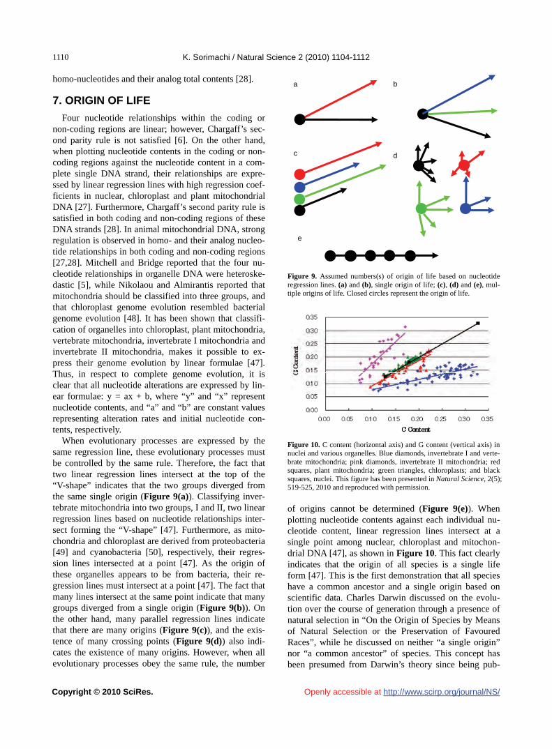
K. Sorimachi / Natural Science 2 (2010) 1104-1112
Copyright © 2010 SciRes. http://www.scirp.org/journal/NS/
1110
Openly accessible at
homo-nucleotides and their analog total contents [28].
7. ORIGIN OF LIFE
Four nucleotide relationships within the coding or non-coding regions are linear; however, Chargaff’s sec-ond parity rule is not satisfied [6]. On the other hand, when plotting nucleotide contents in the coding or non- coding regions against the nucleotide content in a com-plete single DNA strand, their relationships are expre- ssed by linear regression lines with high regression coef-ficients in nuclear, chloroplast and plant mitochondrial DNA [27]. Furthermore, Chargaff’s second parity rule is satisfied in both coding and non-coding regions of these DNA strands [28]. In animal mitochondrial DNA, strong regulation is observed in homo- and their analog nucleo-tide relationships in both coding and non-coding regions [27,28]. Mitchell and Bridge reported that the four nu-cleotide relationships in organelle DNA were heteroske-dastic [5], while Nikolaou and Almirantis reported that mitochondria should be classified into three groups, and that chloroplast genome evolution resembled bacterial genome evolution [48]. It has been shown that classifi-cation of organelles into chloroplast, plant mitochondria, vertebrate mitochondria, invertebrate I mitochondria and invertebrate II mitochondria, makes it possible to ex-press their genome evolution by linear formulae [47]. Thus, in respect to complete genome evolution, it is clear that all nucleotide alterations are expressed by lin-ear formulae: y = ax + b, where “y” and “x” represent nucleotide contents, and “a” and “b” are constant values representing alteration rates and initial nucleotide con-tents, respectively.
When evolutionary processes are expressed by the same regression line, these evolutionary processes must be controlled by the same rule. Therefore, the fact that two linear regression lines intersect at the top of the “V-shape” indicates that the two groups diverged from the same single origin (Figure 9(a)). Classifying inver-tebrate mitochondria into two groups, I and II, two linear regression lines based on nucleotide relationships inter-sect forming the “V-shape” [47]. Furthermore, as mito-chondria and chloroplast are derived from proteobacteria [49] and cyanobacteria [50], respectively, their regres-sion lines intersected at a point [47]. As the origin of these organelles appears to be from bacteria, their re-gression lines must intersect at a point [47]. The fact that many lines intersect at the same point indicate that many groups diverged from a single origin (Figure 9(b)). On the other hand, many parallel regression lines indicate that there are many origins (Figure 9(c)), and the exis-tence of many crossing points (Figure 9(d)) also indi-cates the existence of many origins. However, when all evolutionary processes obey the same rule, the number
●
● ●
● ●●●●
●
a
c
b
d
e
●● ● ● ●
●
●
Figure 9. Assumed numbers(s) of origin of life based on nucleotide regression lines. (a) and (b), single origin of life; (c), (d) and (e), mul-tiple origins of life. Closed circles represent the origin of life.
Figure 10. C content (horizontal axis) and G content (vertical axis) in nuclei and various organelles. Blue diamonds, invertebrate I and verte-brate mitochondria; pink diamonds, invertebrate II mitochondria; red squares, plant mitochondria; green triangles, chloroplasts; and black squares, nuclei. This figure has been presented in Natural Science, 2(5); 519-525, 2010 and reproduced with permission. of origins cannot be determined (Figure 9(e)). When plotting nucleotide contents against each individual nu-cleotide content, linear regression lines intersect at a single point among nuclear, chloroplast and mitochon-drial DNA [47], as shown in Figure 10. This fact clearly indicates that the origin of all species is a single life form [47]. This is the first demonstration that all species have a common ancestor and a single origin based on scientific data. Charles Darwin discussed on the evolu-tion over the course of generation through a presence of natural selection in “On the Origin of Species by Means of Natural Selection or the Preservation of Favoured Races”, while he discussed on neither “a single origin” nor “a common ancestor” of species. This concept has been presumed from Darwin’s theory since being pub-

K. Sorimachi / Natural Science 2 (2010) 1104-1112
Copyright © 2010 SciRes. http://www.scirp.org/journal/NS/
1111
Openly accessible at
lished in 1859, and eventually phylogenetic trees, which have been drawn, represent apparently a single origin of species.
8. CONCLUSIONS
Evolution of all species, from bacteria to Homo sapiens, is governed by genome alterations based on simple lin-ear formulae, including Chargaff’s second parity rule, although their phenotypic expressions show immeasur-able spectra over the past 3.5 billion years. Evolution based on genome alterations can be represented by two lines (G or C and A or T) that are symmetrical about y = 0.25 – the “Diagonal Genome Universe”.
9. ACKNOWLEDGEMENTS
The author expresses his great thanks to Prof. Kuo-Chen Chou, Edi-
tor-in-Chief of Natural Science, for the opportunity to present this
mini-review.
REFERENCES
[1] Avery, O.T., Macleod, C.M. and McCarty, M. (1944) Studies on the chemical nature of the substance inducing transformation of pneumococcal types: Induction of trans- formation isolated from pneumococcus type III. Journal of Experimental Medicine, 79(2), 137-158.
[2] Chargaff, E. (1950) Chemical specificity of nucleic acids and mechanism of their enzymatic degradation. Experi-mentia, 6(6), 201-209.
[3] Rudner, R., Karkas, J.D. and Chargaff, E. (1968) Separa-tion of B. subtilis DNA into complementary strands. 3. Direct analysis. Proceedings of the National Academy of Science, 60(3), 921-922.
[4] Watson, J.D. and Crick, F.H.C. (1953) Genetical implica-tions of the structure of deoxyribonucleic acid. Nature, 171(4361), 964-967.
[5] Mitchell, D. and Bridge, R. (2006) A test of Chargaff’s second rule. Biochemical and Biophysical Research Com- munications, 340(1), 90-94.
[6] Sorimachi, K. and Okayasu, T. (2008) Codon evolution is governed by linear formulas. Amino Acids, 34(4), 661- 668.
[7] Zuckerkandl, E. and Pauling, L.B. (1962) Molecular di- sease, evolution, and genetic heterogeneity. In: Kasha, M. and Pullman, B. Ed., Horizons in Biochemistry, New York Academic, New York, 189-225.
[8] Dayhoff, M.O., Park, C.M. and McLaughlin, P.J. (1977) Building a phylogenetic trees: Cytochrome C. In: Day-hoff, M.O. Ed., Atlas of protein sequence and structure, National Biomedical Foundation, Washington, D.C., 5, 7-16.
[9] Sogin, M.L., Elwood, H.J. and Gunderson, J.H. (1986) Evolutionary diversity of eukaryotic small subunit rRNA genes. Proceedings of the National Academy of Sciences, 83(5), 1383-1387.
[10] DePouplana, L., Turner, R.J., Steer, B.A. and Schimmel,
P. (1998) Genetic code origins: tRNAs older than their synthetases? Proceedings of the National Academy of Sciences, 95(19), 11295-11300.
[11] Doolittle, W.F. and Brown, J.R. (1994) Tempo, mode, the progenote, and the universal root. Proceedings of the Na-tional Academy of Sciences, 91(15), 6721-6728.
[12] Maizels, N. and Weiner, A.M. (1994) Phylogeny from function: Evidence from the molecular fossil record that tRNA originated in replication, not translation. Proceed-ings of the National Academy of Sciences, 91(15), 6729- 6734.
[13] Sorimachi, K. (2009) Evolution from primitive life to Homo sapiens based on visible genome structures: The amino acid world. Natural Science, 1(2), 107-119.
[14] Chou, K.-C. and Zhang, C.T. (1992) Diagrammatization of codon usage in 339 HIV proteins and its biological implication. AIDS Research and Human Retroviruses 8(12), 1967-1976.
[15] Zhang, C.-T. and Chou, K.-C. (1993) Graphic analysis of codon usage strategy in1490 human proteins. Journal of Protein Chemistry, 12(3), 329-335.
[16] Qi, X.Q., Wen, J. and Qi, Z.H. (2007) New 3D graphical representation of DNA sequence based on dual nucleo-tides. Journal of Theoretical Biology, 249(4), 681-690.
[17] Miller, S.L. (1953) Production of amino acids under pos-sible primitive earth conditions. Science, 117(3046), 528- 529.
[18] Kvenvolden, K., Lawless, J., Pering, K., Peterson, E., Flores, J., Ponnamperuma, C., Kaplan, I.R. and Moore, C. (1970) Evidence for extraterrestrial amino-acids and hy-drocarbons in the Murchison meteorite. Nature, 228(5275), 923-926.
[19] Wolman, Y., Haverland, W. and Miller, S.L. (1972) Non-protein amino acids from spark discharges and their com-parison with the Muchison meteorite amino acids. Pro-ceedings of the National Academy of Sciences, 69(4), 809-811.
[20] Lahav, N., White, D. and Chang, S. (1978) Peptide for-mation in the prebiotic era: Thermal condensation of gly-cine in fluctuating clay environments. Science, 201(4350), 67-69.
[21] Sueoka, N. (1961) Correlation between base composition of deoxyribonucleic acid and amino acid composition in proteins. Proceedings of the National Academy of Sci-ences, 47(8), 1141-1149.
[22] Sorimachi, K. (1999) Evolutionary changes reflected by the cellular amino acid composition. Amino Acids, 17(2), 207-226.
[23] Sorimachi, K., Okayasu, T., Akimoto, K. and Niwa, A. (2000) Conservation of the basic pattern of cellular ami- no acid composition during biological evolution in plants. Amino Acids, 18(2), 193-196.
[24] Sorimachi, K., Itoh, T., Kawarabayasi, Y., Okayasu, T., Akimoto, K. and Niwa, A. (2001) Conservation of the basic pattern of cellular amino acid composition during biological evolution and the putative amino acid compo-sition of primitive life forms. Amino Acids, 21(4), 393- 399.
[25] Gilbert, W.R. (1986) The RNA world. Nature, 319, 618. [26] Sorimachi, K. and Okayasu, T. (2007) Mathematical proof
of the chronological precedence of protein formation over codon formation. Current Topics of Peptide and Protein
K. Sorimachi / Natural Science 2 (2010) 1104-1112
Copyright © 2010 SciRes. http://www.scirp.org/journal/NS/Openly accessible at
1112
Research, 8, 25-34. [27] Sorimachi, K. and Okayasu, T. (2008) Universal rules
governing genome evolution expressed by linear formu-las. The Open Genomics Journal, 1(11), 33-43.
[28] Sorimachi, K. (2010) Codon evolution in doublestra- nded organelle DNA: Strong regulation of homo-nucleo-tides and their analog alternations. Natural Science, 2(8), 846-854.
[29] Sanger, F. and Coulson, A.R. (1975) A rapid method for determing sequences in DNA by primed synthesis with DNA polymerase. Journal of Molecular Biology, 94(3), 441-446.
[30] Maxam, A.M. and Gilbert, W. (1977) A new method for sequencing DNA. Proceedings of the National Academy of Sciences, 74(2), 560-564.
[31] Fleischmann, R.D., Adams, M.D., White, O., Clayton, R. A., Kirkness, E.F., Kerlavage, A.R. et al. (1995) Whole- genome random sequencing and assembly of Haemophi-lus influenzae Rd. Science, 269(5223), 496-512.
[32] Lander, E.S., Linton, M.L., Birren, B., Nusbaum, C., Zody, M.C., Baldwin, J., et al. (2001) Initial sequencing and analysis of the human genome. Nature, 409(6822), 860-921.
[33] Venter, J.C., Adams, M.D., Myers, E.W., Li, P.W., Mural, R.J., Sutton, G.G., Smith, H.O., Yandell, M., Evans, C.A., Holt, R.A., et al. (2001) The sequence of the human ge-nome. Science, 291(5507), 1304-1351.
[34] Waterston, R.H., Lindblad-Toh, K., Birney, E., Rogers, J., Abril, J.F., Agarwal, P. et al. (2002) Initial sequencing and comparative analysis of the mouse genome. Nature, 420(6915), 520-562.
[35] Gibbs, R.A., Weinstock, G.M., Metzker M.L., Muzny, D. M., Sondergren, E.J., Scherer, S., et al. (2004) Genome sequence of the Brown Norway rat yield insights into mammalian evolution. Nature, 428(6982), 493-521.
[36] Sodergren E., Weinstock, G.M., Davidson, E.H., Cam-eron, R.A., Gibbs, R.A., Angerer, L.M., et al. (2006) The genome of the sea urchin Strongylocentrotus purpuratus. Science, 314(5801), 941-952.
[37] Sorimachi, K. and Okayasu, T. (2003) Gene assembly consisting of small units with similar amino acid compo-sition in the Saccharomyces cerevisiae genome. Myco-science, 44(5), 415-417.
[38] Kawai, J. (2001) Functional annotation of a full-length mouse cDNA collection. Nature, 409(682), 685-690.
[39] Smith D.R., Doucette-Stamm, L.A., Deloughery, C., Lee, H., Dubois, J., Aldredge, T., et al. (1997) Complete ge-nome sequence of Methanobacterium thermoautotrophi- cum delta H: Functional analysis and comparative ge-nomics. Journal Bacteriology, 179(22), 7135-7155.
[40] Sorimachi, K. and Okayasu, T. (2004) An evolutionary theories based on genomic structures in Saccharomyces cerevisiae and Enchephalitozoon cuniculi. Mycoscience, 45(5), 345-350.
[41] Sorimachi, K. and Okayasu, T. (2004) Classification of eubacteria based on their complete genome: Where does Mycoplasmataceae belong? Proceedings of the Royal So- ciety of London. B (Supplement.), 271(4), S127-S130.
[42] Okayasu, T. and Sorimachi, K. (2008) Organisms can essentially be classified according to two codon patterns. Amino Acids, 36(2), 261-271.
[43] Sueoka, N (1988) Directional mutation pressure and neutral molecular evolution. Proceedings of the National Academy of Sciences, 85(8), 2653-2657.
[44] Qi, Z.H., Wang, J.M. and Qi, X.Q. (2009) Classification analysis of dual nucleotides using dimension reduction. Journal of Theoretical Biology, 260(1), 104-109.
[45] Ebara, Y., Koge, T. and Sorimachi, K. (2010) Evaluation of Chargaff’s parity rules using simulation analysis. Dokkyo Journal of Medical Sciences, 37(2), 139-142.
[46] Sorimachi, K. (2009) A proposed solution to the historic puzzle of Chargaff’s second parity rule. The Open Ge-nomics Journal, 2(3), 12-14.
[47] Sorimachi, K. (2010) Genomic data provides simple evi- dence for a single origin of life. Natural Science, 2(5), 519-525.
[48] Nikolaou, C. and Almirantis, Y. (2006) Deviations from Chargaff’s second parity rule in organelle DNA insights into the evolution of organelle genomes. Gene, 381, 34- 41.
[49] Gray, M.W., Burger, G., Lang, B.F. (1999) Mitochondrial evolution. Science, 283(5407), 1476-1481.
[50] Raven, J.A. and Allen, J.F. (2003) Genomics and chloro-plast evolution: What did cyanobacteria do for plants? Genome Biology, 4(3), 209-215.

Vol.2, No.10, 1113-1118 (2010)doi:10.4236/ns.2010.210138
Copyright © 2010 SciRes. http://www.scirp.org/journal/NS/
Natural Science
Openly accessible at
Assessment of a short phylogenetic marker based on comparisons of 3’ end 16S rDNA and 5’ end 16S-23S ITS nucleotide sequences of the Bacillus cereus group
Sabarimatou Yakoubou1,2, Jean-Charles Côté1*
1Agriculture and Agri-Food Canada, Research Centre, Gouin Blvd, St-Jean-sur-Richelieu, Canada; *Corresponding Author: [email protected]; 2Département des Sciences Biologiques, Université du Québec à Montréal, Succ.“Centre-Ville” Montréal, Canada.
Received 28 May 2010; revised 30 June 2010; accepted 5 July 2010.
ABSTRACT
A short phylogenetic marker previously used in the reconstruction of the Order Bacillales and the genus Bacillus was assessed here at a lower taxa level: species in the Bacillus cereus group: B. anthracis, B. cereus, B. thuringiensis and B. weihenstephanensis. This maker is 220 bp in length. It is a combination of 150 bp at the 3’ end of the 16S rDNA and 70 bp at the 5’ end of the 16S-23S ITS sequence. Three additional Bacillus species, B. halodurans, B. licheniformis and B. subtilis, and Clostridium tetani were included for comparison purposes. A total of eight bacte-rial species and 12 strains were analyzed. A boot- strapped neighbor-joining tree was inferred from comparative analyses of all allelic sequences of the bacterial species and strains under study. Based on its topology, four major Groups were revealed at the 90% nucleotide sequence identi-ties, Group I to IV. Group I contains all alleles of the Bacillus cereus group. Group II contains all alleles of B. halodurans. Group III contains all alleles of B. licheniformis and B. subtilis. Group IV contains all alleles of Clostridium tetani. The 220 bp phylogenetic marker used here could resolve different species from different genera. At the genus level, distant species could be dis-tinguished. Very closely-related species, how-ever, were undistinguishable. Species in the B. cereus group, most notably B. cereus, B. anth- racis and B. thuringiensis, could not be distin- guished. After successfully inferring the phylo- genies of the Order Bacillales and the genus Bacillus, we have met the resolving limit of this short phylogenetic marker: B. cereus, B. an-thracis and B. thuringiensis.
Keywords: Bacillus cereus; 16S RDNA; 16S-23S ITS; Phylogeny
1. INTRODUCTION
The Bacillus cereus group comprises six genetically highly related species: B. cereus sensu stricto, B. an-thracis, B. thuringiensis, B. weihenstephanensis, B. my-coides [1] and B. pseudomycoides [2]. They are Gram- positive, rod-shaped, endospore-forming, either obligate or facultative aerobic bacteria [1].
Bacillus cereus is a ubiquitous soil bacterium. It can be a contaminant of a variety of foods: meats, vegetables and dairy products [3,4]. It can cause diarrheal, and em- etic food poisoning syndromes [5]. It can also be the eti- ologic agent of some opportunistic infections [6,7]. Bac- illus anthracis is the etiologic agent of anthrax, an acute disease in herbivorous mammals, transmissible to other animals, including humans [8]. This species has been st- udied and developed as a biological weapon [9]. Virul- ent strains of B. anthracis carry two plasmids, pXO1 (181 kb) and pXO2 (96 kb) which may be transmitted to others members of Bacillus cereus group [10]. Bacillus thuringiensis is an insect pathogen. It is characterized by the synthesis upon sporulation of a parasporal inclusion body. This inclusion body is made of proteins, the δ-en- dotoxins, which are toxic to several insect larvae [11,12] and other invertebrates [13]. B. thuringiensis formula-tions have been developed for the control of insect pests in agriculture and forestry [14-16] and for the control of insect vectors of human diseases such as malaria, yel- low fever, onchocerciasis, etc [17]. Bacillus weihenstep- hanensis is a psychotolerant species characterized by the ability to grow at 7°C and the absence of growth at 43°C. It is also characterized by the presence of specific signa-ture sequences on the 16S rRNA gene (small subunit ribosomal RNA gene) and the cspA gene (gene encoding the major cold shock protein) [18]. B. mycoides is char-
S. Yakoubou et al. / Natural Science 2 (2010) 1113-1118
Copyright © 2010 SciRes. http://www.scirp.org/journal/NS/Openly accessible at
1114
acterized by the formation of rhizoid colonies and the absence of motility [19]. B. pseudomycoides is pheno-typically similar to B. mycoides and is distinguished by DNA relatedness and fatty acid composition [2].
The 16S rDNA is the macromolecule of choice in the reconstruction of bacterial phylogenies [20-24]. The 16S rDNA, however, cannot distinguish among species in the Bacillus cereus group [25,26]. Genomic approaches have been used in an attempt to elucidate the genetic diversity of three highly closely related species in the B. cereus group: B. cereus, B. anthracis and B. thuringiensis. They appear as a single species on the basis of genetic eviden- ce [27].
In a previous study, a 220 bp marker was developed and used to infer the phylogeny of species in the genus Bacillus and closely-related genera [28]. This marker was a combination of the last 150 bp at the 3’ end of the 16S rDNA and the first 70 bp at the 5’ end of the 16S- 23S rDNA internal transcribed spacer (ITS). More recent- ly, we assessed the usefulness of the 220 bp marker at a higher taxonomic level, the Order Bacillales [29]. This marker showed several advantages over the use of 16S rDNA sequences or the generation of extensive phenoty- pic and genotypic data in phylogenetic analyses. First, the 150 bp at the 3’ end of the 16S rDNA allowed dis-crimination among distantly related species. Owing to its higher rate of nucleotide substitutions, the 70 bp at the 5’ end of the 16S-23S rDNA (ITS) added discriminating power among closely related species from same genus and closely related genera from same family. Because of
its higher percentage of nucleotide sequence divergence than the 16S rDNA, the 220 bp marker could better dis-criminate among closely related Bacillus [28] and Ba-cillales [29] species. Second, the method was simple, ra- pid, suited to large screening programs and easily acces- sible to most laboratories. Third, the marker also revea- led species which appeared misassigned and for which additional characterization appeared warranted.
In the current study, we further analyze the resolving power of this short marker in inferring phylogenies at a much lower taxa level: the Bacillus cereus group.
2. MATERIALS AND METHODS
2.1. Bacterial Species and Strains
Four species in the Bacillus cereus group: B. anthracis, B. cereus, B. thuringiensis and B. weihenstephanensis were analyzed. Three additional Bacillus species, B. ha- lodurans, B. licheniformis and B. subtilis, and Clostrid-ium tetani were included for comparison purposes. A to- tal of eight bacterial species and 12 strains were analy- zed (Table 1). They were selected on the basis that their complete genome sequences were freely available in Ge- nBank at the National Center for Biotechnology Infor-mation (NCBI) completed microbial genomes database (http://www.ncbi.nlm.nih.gov/genomes/lproks.cgi,August 2009). Bacillus mycoides and B. pseudomycoides were not included because their complete genome sequences have not been determined.
Table 1. Bacterial species used in this study.
Genera Species Strain GenBank accession no.
Bacillus anthracis cereus thuringiensis serovar konkukian weihenstephanensis halodurans licheniformis subtilis subsp. subtilis
Ames Ames Ancestor Sterne ATCC 14579 ATCC 10987 E33L 97-27 KBAB4 C-125 ATCC 14580 168
AE016879 AE017334.2 AE017225.1 AE016877.1 AE017194.1 CP000001.1 AE017355.1 NC_010184.1 BA000004.3 AE017333.1 AL009126.3
Clostridium tetani E88 AE015927.1

S. Yakoubou et al. / Natural Science 2 (2010) 1113-1118
Copyright © 2010 SciRes. http://www.scirp.org/journal/NS/Openly accessible at
1111115
2.2. Sequences
The 16S rDNA and 16S-23S ITS for the 12 bacterial species and strains were retrieved from GenBank, for a total of 129 allelic sequences. The last 150 bp at the 3’ end of 16S rDNA and the first 70 bp at the 5’ end of 16S-23S ITS were merged into a single 220 bp sequence for each of the 129 alleles under study as described be-fore [28]. This 220 bp sequence will be used as a phy-logenetic marker for the 12 bacterial species and strains under study.
2.3. Phylogenetic Analyses
All 129 allelic sequences were aligned using ClustalW [30] (data not shown). A neighbor-joining tree was cons- tructed [31], based on the alignment of the 129 alleles of the 220 bp sequence. The tree was bootstrapped using 1,000 random samples. The neighbor-joining tree was dr- awn and printed with Tree Explorer, all components of the Molecular Evolutionary Genetics Analysis (MEGA, version 3.1) software package [32].
3. RESULTS AND DISCUSSIONS
In a previous study, a 220 bp sequence was developed as a DNA marker and used to infer the phylogeny of species in the Gram-positive genus Bacillus and closely- related genera [28]. This marker was a combination of the last 150 bp at the 3’ end of the 16S rDNA and the first 70 bp at the 5’ end of the 16S-23S rDNA internal transcribed spacer (ITS). More recently, we assessed the usefulness of the 220 bp marker by extending its analy-ses at a higher taxonomic level, the Gram-positive Order Bacillales [29]. In parallel, a similar marker was used to infer the phylogeny of the Gram-negative Class γ-pro- teobacteria [33]. In the current study, we further analyze the resolving power of this marker in inferring the phy-logeny at a much lower taxa level: the Bacillus cereus group.
A bootstrapped neighbor-joining phylogenetic tree was inferred from comparative analyses of the 220 bp marker from the 129 alleles from the bacterial species and strains under study (Figure 1). Four major Groups were revealed based on the topology of the neighbor- joining tree at the 90% nucleotide sequence identities, Group I to IV. Group I contains all alleles of the species in the Bacillus cereus group. Group II contains all alleles of B. halodurans. Group III contains all alleles of B. licheniformis and B. subtilis. Group IV contains all al-leles of Clostridium tetani. Based on nucleotide se-quence identities, sub-groups and branches can be re-vealed. Group I can be sub-divided into three sub-groups at the 95% nucleotide sequence identities. Sub-group I-1 encompasses 27 alleles from the B. anthracis strains, 36
alleles from the B. cereus strains, 11 alleles from B. thuringiensis and one allele from B. weihenstephanensis. Sub-group I-2 encompasses six alleles from B. anthracis, two alleles from B. cereus and one allele from B. thur-ingiensis. Sub-group I-3 encompasses 12 alleles from B. weihenstephanensis. A branch corresponding to an allele from B. weihenstephanensis is present between sub-gro- ups I-2 and I-3. Group II contains all eight alleles from B. halodurans. They show at least 20% nucleotide sequen- ce divergences with alleles from the other Bacillus spe-cies. Group III contains all alleles from B. licheniformis and B. subtilis. It can be sub-divided into two sub-groups at the 95% nucleotide sequence identities. Sub-group III-1 encompasses all seven alleles from B. licheniformis. Sub-group III-2 encompasses all ten alleles from B. sub-tilis. Group IV contains all six alleles from Clostridium tetani. These alleles show at least 26% nucleotide se-quence divergence with alleles from species and strains in the genus Bacillus.
In accordance with our previous work on the Order Bacillales, the 220 bp sequence used as a phylogenetic marker was able to group alleles from same species for B. halodurans, B. licheniformis, B. subtilis, and Clostrid-ium tetani, respectively. However, this 220 bp sequence could not group most alleles from same species, exclu-sive of alleles from others, for the B. cereus group. Sub- group I-1 is heterogeneous. It contains alleles from all four species from the B. cereus group. The close prox-imity of B. cereus, B. anthracis and B. thuringiensis is in agreement with previous works based on whole-genome DNA hybridization [34], pulsed-field gel electrophoresis (PFGE) [35], multilocus enzyme electrophoresis (MEE) [36], amplified fragment length polymorphism (AFLP) fingerprinting [37] and multilocus sequence typing (ML- ST) [38,39], which showed that all three species are ge-netically highly related. They appear as a single species on the basis of genetic evidence [27]. Sub-groups I-2 is more homogeneous. It mostly contains alleles from B. an- thracis. Sub-groups I-3 is homogeneous. It only contains alleles from B. weihenstephanensis. As shown earlier, on the genus Bacillus [28] and the Order Bacillales [29], this 220 bp sequence contains 150 bp at the 3’ end of 16S rDNA which allowed discrimination among dis-tantly related species and 70 bp at the 5’ end of 16S-23S ITS which, owing to its higher percentage of nucleotide sequence divergence, added resolving power among clo- sely related species.
Here, species in the B. cereus group, most notably B. cereus, B. anthracis and B. thuringiensis, are too closely related to be discriminated with the 220 bp sequence previously used as a phylogenetic marker. Our work, however, has shown that the alleles in sub-group I-3 could distinguish B. weihenstephanensis from all other species.

S. Yakoubou et al. / Natural Science 2 (2010) 1113-1118
Copyright © 2010 SciRes. http://www.scirp.org/journal/NS/
1116
Openly accessible at
8796
93
100
88
61
100
55
95
74
99
55
99
64
81
96
65
Bacillus anthracis Ames rRNA E5
Bacillus anthracis Ames Ancestor rRNA F
Bacillus anthracis sterne rRNA 9
Bacillus anthracis Ames rRNA C
Bacillus anthracis sterne RNA1Bacillus anthracis Ames rRNA D
Bacillus anthracis Ames Ancestor rRNA EBacillus anthracis sterne RNA2
Bacillus anthracis Ames Ancestor rRNA BBacillus anthracis Ames Ancestor rRNA D
Bacillus anthracis sterne RNA5Bacillus anthracis Ames Ancestor rRNA H
Bacillus anthracis Ames Ancestor rRNA C
Bacillus anthracis sterne RNA6
Bacillus anthracis Ames Ancestor rRNA GBacillus anthracis sterne rRNA 9Bacillus anthracis Ames Ancestor rRNA IBacillus anthracis Ames Ancestor rRNA A
Bacillus anthracis Ames rRNA I Bacillus anthracis sterne RNA7
Bacillus anthracis Ames rRNA F
Bacillus anthracis Ames rRNA A
Bacillus anthracis sterne RNA4
Bacillus anthracis Ames rRNA G Bacillus anthracis Ames rRNA H Bacillus anthracis sterne RNA3Bacillus anthracis Ames rRNA B
Bacillus anthracis Ames Ancestor rRNA JBacillus anthracis sterne RNA10
Bacillus anthracis Ames rRNA J Bacillus anthracis Ames Ancestor rRNA K
Bacillus anthracis Ames rRNA K Bacillus anthracis sterne RNA11
Bacillus cereus 14579 rRNA C
Bacillus cereus 14579 rRNA F5Bacillus cereus 10987 rRNA A5
Bacillus cereus E33L rRNA 9
Bacillus cereus 14579 rRNA GBacillus cereus E33L rRNA 10
Bacillus cereus E33L rRNA 8 Bacillus cereus 10987 rRNA D
Bacillus cereus E33L rRNA 7
Bacillus cereus 14579 rRNA L Bacillus cereus E33L rRNA 2 Bacillus thuringiensis konkukian str. 97-27 rRNA 5Bacillus cereus E33L rRNA 12 Bacillus thuringiensis konkukian str. 97-27 rRNA 3Bacillus cereus 14579 rRNA J Bacillus cereus E33L rRNA 3Bacillus cereus 14579 rRNA I Bacillus thuringiensis konkukian str. 97-27 rRNA 8Bacillus thuringiensis konkukian str. 97-27 rRNA 13
Bacillus cereus 10987 rRNA JBacillus cereus 14579 rRNA H
Bacillus cereus 14579 rRNA D Bacillus cereus 10987 rRNA CBacillus cereus 10987 rRNA E4
Bacillus cereus 14579 rRNA K
Bacillus cereus E33L rRNA 4 Bacillus thuringiensis konkukian str. 97-27 rRNA 10Bacillus thuringiensis konkukian str. 97-27 rRNA 9Bacillus cereus 10987 rRNA KBacillus thuringiensis konkukian str. 97-27 rRNA 11Bacillus cereus 10987 rRNA I
Bacillus cereus 10987 rRNA IBacillus thuringiensis konkukian str. 97-27 rRNA 7
Bacillus cereus E33L rRNA 6
Bacillus thuringiensis konkukian str. 97-27 rRNA 2Bacillus cereus E33L rRNA 1
Bacillus thuringiensis konkukian str. 97-27 rRNA 4
Bacillus cereus 10987 rRNA FBacillus cereus E33L rRNA 11 Bacillus cereus 14579 rRNA M
Bacillus cereus E33L rRNA 5
Bacillus cereus 10987 rRNA B
Bacillus cereus 10987 rRNA H5Bacillus cereus E33L rRNA 13
Bacillus weihenstephanensis rRNA R0001Bacillus cereus 14579 rRNA E Bacillus cereus 10987 rRNA GBacillus thuringiensis konkukian str. 97-27 rRNA 12
Bacillus thuringiensis konkukian str. 97-27 rRNA 1
Bacillus cereus 14579 rRNA A
Bacillus cereus 14579 rRNA B
Bacillus thuringiensis konkukian str. 97-27 rRNA 6Bacillus weihenstephanensis rRNA R0008
Bacillus weihenstephanensis rRNA R0027
Bacillus weihenstephanensis rRNA R0146Bacillus weihenstephanensis rRNA R0030
Bacillus weihenstephanensis rRNA R0071Bacillus weihenstephanensis rRNA R0059Bacillus weihenstephanensis rRNA R0068Bacillus weihenstephanensis rRNA R0054
Bacillus weihenstephanensis rRNA R0094
Bacillus weihenstephanensis rRNA R0065Bacillus weihenstephanensis rRNA R0015
Bacillus weihenstephanensis rRNA R0062
Bacillus weihenstephanensis rRNA R0074Bacillus halodurans C-125 rRNA BBacillus halodurans C-125 rRNA CBacillus halodurans C-125 rRNA DBacillus halodurans C-125 rRNA HBacillus halodurans C-125 rRNA A
Bacillus halodurans C-125 rRNA FBacillus halodurans C-125 rRNA CBacillus halodurans C-125 rRNA G
Bacillus licheniformis 14580 rrna 0010 Bacillus licheniformis 14580 rrna 0021 Bacillus licheniformis 14580 rrna 0016 Bacillus licheniformis 14580 rrna 0001 Bacillus licheniformis 14580 rrna 0013 Bacillus licheniformis 14580 rrna 0004 Bacillus licheniformis 14580 rrna 0008 Bacillus subtilis rrn OBacillus subtilis rrn ABacillus subtilis rrn WBacillus subtilis rrn J
Bacillus subtilis rrn BBacillus subtilis rrn IBacillus subtilis rrn EBacillus subtilis rrn DBacillus subtilis rrn H
Bacillus subtilis rrn GClostridium tetani E888 RNA 5 Clostridium tetani E888 RNA 5
Clostridium tetani E888 RNA 4 Clostridium tetani E888 RNA 3 Clostridium tetani E888 RNA 1 Clostridium tetani E888 RNA 2
Sub- Groups Groups
I
II
III
IV
I-1
I-2
I-3
III-1
III-2
0.01
Figure 1. Bootstrapped neighbor-joining tree inferred from comparative alignment of the 220 bp marker from the 129 alleles from the 12 bacterial species and strains under study. Major groups are indicated in capital roman numerals. Sub-groups are indicated in arabic numerals. Bootstrap values higher than 50% are indicated (expressed as percentage of 1000 replication). The horizontal bar represents 1% nt difference. Bacillus anthracis, B. cereus, B thuringiensis and B. weihenstephanensis’s alleles are written in red, blue, green and brown, respectively. B. halodurans, B. licheniformis, B. subtilis and Clostridium tetani’s alleles are written in black ink.

S. Yakoubou et al. / Natural Science 2 (2010) 1113-1118
Copyright © 2010 SciRes. http://www.scirp.org/journal/NS/
1111117
Openly accessible at
4. CONCLUSIONS
Previous genetic analyses have shown that B. cereus, B. anthracis and B. thuringiensis should be regarded as a single species. We have shown here that a 220 bp marker, used to reconstruct the phylogeny of the Order Bacillales and the family Bacillaceae, was unable to discriminate between these three highly-related species. We have rea- ched the limit of the resolving power of the 220 bp se-quence as a phylogenetic marker: B. cereus, B. anthracis and B. thuringiensis.
REFERENCES [1] Claus, D. and Berkeley, R.C.W. (1986) Genus Bacillus
Cohn, 1872. In: Sneath, P.H.A., Mair, N.S., Sharpe, M.E. and Holt. J.G., Eds., Bergey’s Manual of Systematic Bac-teriology, The Williams & Wilkins Co., Baltimore, 2, 1105-1139.
[2] Nakamura, L.K. (1998) Bacillus pseudomycoides sp. nov. International Journal of Systematic Bacteriology, 48(3), 1031-1035.
[3] Drobniewski, F.A. (1993) Bacillus cereus and related species. Clinical Microbiology Reviews, 6(4), 324-338.
[4] Schoeni, J.L. and Wong, A.C.L. (2005) Bacillus cereus food poisoning and its toxins. Journal of Food Protection, 68(3), 636-648.
[5] Kramer, J.M. and Gilbert, R.J. (1989) Bacillus cereus and other Bacillus species. In: Doyle, M.P., Ed., Foodborne Bacterial Pathogens, Marcel Dekker, Inc., New York, 21- 50.
[6] Das, T., Choudhury, K., Sharma, S., Jalali, S., Nuthethi, R. and the Endophthalmitis Research Group (2001) Cli- nical profile and outcome in Bacillus endophthalmitis. Ophthalmology, 108(10), 1819-1825.
[7] Le Scanff, J., Mohammedi, J.I., Thiebaut, A., Martin, O., Argaud, L. and Robert, D. (2006) Necrotizing gastroente- ritis due to Bacillus cereus in an immunocompromised patient. Infection, 34(2), 98-99.
[8] Logan, N.A. and De Vos, P. (2009) Genus I. Bacillus Cohn 1872, 174AL. In: De Vos, P., Garrity, G.M., Jones, D., Krieg, N.R., Ludwig, W., Rainey, F.A., Schleifer, K.H. and Whitman, W.B., Eds., Bergey’s Manual of Systematic Bacteriology, 2nd Edition, Springer, New York, 3, 21-128.
[9] Inglesby, T.V., O’Toole, T., Henderson, D.A., Bartlett, J.G., Ascher, M.S., Eitzen, E., Friedlander, A.M., Ger-berding, J., Hauer, J., Hughes, J., McDade, J., Osterholm, M.T., Parker, G., Perl, T.M., Russell, P.K. and Tonat, K. (2002) Anthrax as a biological weapon: Updated recom-mendations for management. The Journal of the Ameri-can Medical Association, 287(17), 2236-2252.
[10] Turnbull, P.C.B. (2002) Introduction: Anthrax history, disease and ecology. In: Koehler, T., Ed., Anthrax, Sp- ringer-Verlag, Berlin, 1-20.
[11] Höfte, H. and Whiteley, H.R. (1989) Insecticidal crystal proteins of Bacillus thuringiensis. Microbiological Re-views, 53(2), 242-255.
[12] Garcia-Robles, I., Sánchez, J., Gruppe, A., Martínez-Ra- mírez, A.C., Rausell, C., Real, M.D. and Bravo, A. (2001) Mode of action of Bacillus thuringiensis PS86Q3 strain
in hymenopteran forest pests. Insect Biochemistry and Molecular Biology, 31(9), 849-856.
[13] Feitelson, J.S. (1993) The Bacillus thuringiensis family tree. In: Kim, L., Ed., Advanced Engineered Pesticides, Marcel Dekker Inc., New York, 63-71.
[14] Schnepf, H.E., Crickmore, N., Van Rie, J., Lereclus, D., Baum, J., Feitelson, J., Zeigler, D.R. and Dean, D.H., (1998) Bacillus thuringiensis and its pesticidal crystal proteins. Microbiology and Molecular Biology Reviews, 62(3), 775-806.
[15] Otvos, I.S., Armstrong, H. and Conder, N. (2005) Safety of Bacillus thuringiensis var. kurstaki, applications for insect control to humans and large mammals. In: Côté, J.-C., Otvos, I.S., Schwartz, J.-L. and Vincent, C., Eds., Proceedings of the 6th Pacific Rim Conference on the Biotechnology of Bacillus thuringiensis and its Environ-mental Impact. Montréal, 30 October-3 November 2005, 45-59.
[16] Bravo, A., Gill, S.S. and Soberon, M. (2007) Mode of action of Bacillus thuringiensis Cry and Cyt toxins and their potential for insect control. Toxicon, 49(4), 423-435.
[17] Guillet, P., Chandre F. and Mouchet, J. (1997) L'utili- sation des insecticides en santé publique: état et perspe- ctives. Médecine et Maladies Infectieuses, 27(5), 552- 557.
[18] Lechner, S., Mayr, R., Francis, K.P., Prüß, B.M., Kaplan, T., Wießner-Gunkel, E., Stewart Gordon, S.A.B. and Scherer, S. (1998) Bacillus weihenstephanensis sp. nov. is a new psychrotolerant species of the Bacillus cereus group. International Journal of Systematic Bacteriology, 48(4), 1373-1382.
[19] Nakamura, L.K. and Jackson, M.A. (1995) Clarification of the taxonomy of Bacillus mycoides. International Jour- nal of Systematic Bacteriology, 45(1), 46-49.
[20] Woese, C.R., Kandler, O. and Wheelis, M.L. (1990) To-wards a natural system of organisms: Proposal for the domains Archea, Bacteria and Eucarya. Proceedings of the National Academy of Sciences, USA, 87(12), 4576- 4579.
[21] Amann, R., Ludwig, W. and Schleifer, K.H. (1995) Phy-logenetic identification and in situ detection of individual microbial cells without cultivation. Microbiological Re-view, 59(1), 143-169.
[22] Cilia, V., Lafay, B. and Christen, R. (1996) Sequence heterogeneities among 16S ribosomal RNA sequences and their effect on phylogenetic analyses at species level. Molecular Biolology and Ecology, 13(3), 451-461.
[23] Goto, K., Omura, T., Hara, Y. and Sadaie, Y. (2000) Ap-plication of the partial 16S rDNA sequence as an index for rapid identification of species in the genus Bacillus. Journal of General and Applied Microbiology, 46(1), 1-8.
[24] Sacchi, C.T., Whitney, A.M., Mayer, L.W., Morey, R., Steigerwalt, A., Boras, A., Weyant, R.S. and Popovic, T. (2002) Sequencing of 16S rRNA gene: A rapid tool for identification of Bacillus anthracis. Emerging Infectious Disease, 8(10), 1117-1123.
[25] Ash, C., Farrow, J.A. Dorsch, M. Stackebrandt, E. and Collins, M.D. (1991) Comparative analysis of Bacillus anthracis, Bacillus cereus, and related species on the ba-sis of reverse transcriptase sequencing of 16S rRNA. In-ternational Journal of Systematic Bacteriology, 41(3), 343-346.

S. Yakoubou et al. / Natural Science 2 (2010) 1113-1118
Copyright © 2010 SciRes. http://www.scirp.org/journal/NS/Openly accessible at
1118
[26] Ash, C., Farrow, A.E., Wallbanks, S. and Collins, M.D. (1991) Phylogenetic heterogeneity of the genus Bacillus revealed by comparative analysis of small-subunit-ribo- somal RNA sequences. Letters in Applied Microbiology, 13(4), 202-206.
[27] Vilas-Boas, G.T., Peruca, A.P. and Arantes, O.M. (2007) Biology and taxonomy of Bacillus cereus, Bacillus an-thracis, and Bacillus thuringiensis. Canadian Journal of Microbiology, 53(6), 673-687.
[28] Xu, D. and Côté, J.-C. (2003) Phylogenetic relationships between Bacillus species and related genera inferred from comparison of 3’ end 16S rDNA and 5’ end 16S-23S ITS nucleotide sequences. International Journal of System-atic and Evolutionary Microbiology, 53(3), 695-704.
[29] Yakoubou, S., Xu, D. and Côté, J.-C. (2010) Phylogeny of the order Bacillales inferred from 3’ 16S rDNA and 5’ 16S-23S ITS nucleotide sequences. Natural Science, 2(9), 990-997.
[30] Thompson, J.D., Higgins, D.G. and Gibson, T.J. (1994) CLUSTAL W: Improving the sensitivity of progressive multiple sequence alignment through sequence weighting, positions-specific gap penalties and weight matrix choice. Nucleic Acids Research, 22(22), 4673-4680.
[31] Saitou, N. and Nei, M. (1987) The neighbor-joining me- thod: A new method for reconstructing phylogenetic trees. Molecular Biology and Evolution, 4(4), 406-425.
[32] Kumar, S., Tamura, K. and Nei, M. (2004) MEGA3: Int- egrated software for molecular evolutionary genetics ana- lysis and sequence alignment. Brief Bioinformatic, 5(2), 150-163.
[33] Yakoubou, S. and Côté, J.-C. (2010) Phylogeny of γ-pro- teobacteria inferred from comparisons of 3’ end 16S rRNA
gene and 5’ end 16S-23S ITS nucleotide sequences. Na- tural Science, 2(6), 535-543.
[34] Kaneko, T., Nozaki, R. and Aizawa, K. (1978) Deoxyri-bonucleic acid relatedness between Bacillus anthracis, Bacillus cereus and Bacillus thuringiensis. Microbiology and Immunology, 22(10), 639-641.
[35] Carlson, C.R., Caugant, D.A. and Kolsto, A.-B. (1994) Genotypic diversity among Bacillus cereus and Bacillus thuringiensis strains. Applied and Environmental Micro-biology, 60(6), 1719-1725.
[36] Helgason, E., Caugant, D.A., Olsen, I. and Kolsto, A.-B. (2000) Genetic structure of population of Bacillus cereus and Bacillus thuringiensis isolates associated with pe-riodontitis and other human infections. Journal of Clini-cal Microbiology, 38(4), 1615-1622.
[37] Ticknor, L.O., Kolsto, A.B., Hill, K.K., Keim, P., Laker, M.T., Tonks, M. and Jackson, P.J. (2001) Fluorescent amplified fragment length polymorphism analysis of Norwegian Bacillus cereus and Bacillus thuringiensis soil isolates, Applied and Environmental Microbiology, 67(10), 4863-4873.
[38] Helgason, E., Tourasse, N.J., Meisal, R., Caugant, D.A. and Kolsto, A.B. (2004) Multilocus sequence typing sch- eme for bacteria of the Bacillus cereus group. Applied and Environmental Microbiology, 70(1), 191-201.
[39] Olsen, J., Skogan, G., Fykse, E., Rawlinson, E., Tomaso, H., Granum, P. and Blatny, J. (2007) Genetic distribution of 295 Bacillus cereus group members based on adk-scr- eening in combination with MLST (Multilocus Sequence Typing) used for validating a primer targeting a chromo-somal locus in B. anthracis. Journal of Microbiological Methods, 71(3), 265-274.
Vol.2, No.10, 1119-1129 (2010)doi:10.4236/ns.2010.210139
Copyright © 2010 SciRes. http://www.scirp.org/journal/NS/
Natural Science
Openly accessible at
Origin and SEM analysis of aerosols in the high mountain of Tenerife (Canary Islands)
Juan D. Delgado1,2*, Omaira E. García3, Ana M. Díaz3, Juan P. Díaz3, Francisco J. Expósito3, Emilio Cuevas4, Xavier Querol5, Andrés Alastuey5, Sonia Castillo5 1Área de Ecología, Departamento de Sistemas Físicos, Químicos y Naturales, Universidad Pablo de Olavide, Seville, Spain; *Corresponding Author: [email protected]; 2Instituto Universitario de Enfermedades Tropicales y Salud Pública de Canarias, La Laguna, Tenerife, Canary Islands, Spain; 3Departamento de Física Básica, Universidad de La Laguna, E-38206 La Laguna, Tenerife, Canary Islands, Spain; 4Izaña Observatory, Instituto Nacional de Meteorología, INM, Santa Cruz de Tenerife, Canary Islands, Spain; 5Institute of Environmental Assessment and Water Research (IDÆA), CSIC, Barcelona, Spain.
Received 18 May 2010; revised 21 June 2010; accepted 24 June 2010.
ABSTRACT
Focusing on aerosolized matter of relevance to respiratory health, a major public health issue worldwide, we studied mineral and biological aerosol (bioaerosol) composition (TSP and PM2.5) and geographical origins during dust in-trusions in the Canary Islands. Seven days’ back- ward trajectories were assessed daily during March 2004 with the ends of back trajectories being the sampling station of Izaña (high moun- tain, 2360 m a.s.l. at the Cañadas del Teide Na-tional Park, Tenerife island), a free troposphere site allowing characterization of dust with low influence of other pollutant sources. Scanning electron microscopy (SEM) was used to survey major types of airborne particles in the dust plumes. Control, non-intrusion conditions cor-respond to Atlantic oceanic middle troposphere (OMT) air masses. Of the 14 samples taken, 1 corresponded to a control (clear atmosphere conditions), and the remaining 13 to dust intru-sions, with the following sources: African Dust; EAM: mixture of Europe, Africa and Oceanic; MaA: maritime aerosols. Of the air masses, 79% were directly transported to the islands from Africa, and an increase of African dust events was detected when comparing with a 52-year previous data sequence. Quartz microcristals and aggregates of quartz and platy clay were the dominant minerals identified, with marine salt and gypsum also present. Freshwater dia-tom tests (from two Aulacoseira species) rep-resented the most important biogenic aerosols, although fungi and pollen were also detected. The diverse and complex mixture of respirable
particles in large quantities in airborne dust, especially from nearby Sahara and from the Sahelian region, is of maximum interest for air- way pathology in the Canaries, including the highly visited highlands in Tenerife.
Keywords: Allergens; Bioaerosols; Diatoms; High altitude; Desert dust intrusion; Public health; Scanning electron microscopy
1. INTRODUCTION
The dispersal of abiotic and biological aerosols (bioa- erosols), has a growing interest in interdisciplinary re-search comprising epidemiology, public health and at-mospheric physics. This is due to the great capacity of air masses to transport both viable organisms and inor-ganic dust to remote areas, where they transform local tropospheric conditions [1] and may affect human health [2]. The cell-carrying capacity of wind, long-range and high frequency transport of dust masses, aggravate the effects of seasonal peaks in local allergens through addi-tive and synergic effects. The transport of dust might involve carrying up to 10.000 bacterial cells per gram of soil from some desert areas [3]. For example, diatoms are a large fraction of dust carried from fresh waters of the Saharo-Sahelian areas and Eurasia to remote areas such as the Caribbean [4]. Charles Darwin, on his 1845 voyage aboard the surveying ship H.M.S. Beagle, col-lected African dust in the Atlantic and microscopically detected the occurrence of diatoms in the dust. This same historic dust has been recently analyzed to find at least 16 different viable bacterial lineages and 2 fungal isolates [5].
Although the global amount of species of airborne pathogens is not so far clearly defined, several hundreds
J. D. Delgado et al. / Natural Science 2 (2010) 1119-1129
Copyright © 2010 SciRes. http://www.scirp.org/journal/NS/Openly accessible at
1120
of bacterial lineages, fungi and viruses can be involved in allergy, asthma and pulmonary affections, and air-borne dust is a vehicle for them [6-10]. Inhaled atmos-pheric aerosols of any origin can be associated with a number of diseases and disorders, namely allergic air-ways disease (or asthma), rhinitis and rhinosinusitis, al- veolitis or allergic parenchymal disease, airways or pa- renchymal infections, atypical thoracic pain, anxiety dis- orders, cardiopathy, and meningitis, among others [11-14].
The Canary Islands lay 96 km off the west of the lar- gest dust source on Earth, the Sahara desert (> 9 million square kilometres), being comprised within the “dust- belt”, where the atmospheric dust concentration is inhe- rently very high [15]. Dust transport to the Canaries causes several-fold increase over the standard levels of particu-late matter over the islands [1,16-20]. Although studies relating desert dust to “airborne” diseases in the Canary Islands are scant, dust events reach the archipelago with a high frequency, being associated with augmented pre- valence, morbidity and mortality [12]. There are prece-dents in other regions, such as the Caribbean Sea where increase of frequency in African dust episodes reaching Barbados were associated to a seventeen-fold increase in asthma between 1973 and 1996 [21-23]. In Gran Canaria and Tenerife, type and frequency of asthma symptoms have been analyzed in a large population sample, and climatic conditions have been invoked to explain high prevalences [24].
In this paper we study aerosols from African dust in-trusions at a high altitude ecosystem in Tenerife, Ca-narian archipelago. Specific health effects of minero- genic dust and bioaerosols have not been studied so far in the Canary Islands, and this task is difficult to ap-proach without recognizing the type of particles in-volved. We thus aimed to identify and survey, through scanning electronic microscopy (SEM) analysis, the biological and mineral aerosol particles transported with dust during intrusions of African air masses and from other origins to the Canary Islands. Imaging characteri-zation of dust particles could give us explicit information on aerosol types in relation with complementary data on origin and travelling time of air masses. We related the dust events with the air-mass origin, tracing back the dust trajectories to assess source areas. Our primary concern was on aerosolized particles with a potential interest in public health that are transported with dust plumes from Africa to the Canary Islands.
2. METHODS
2.1. Study Area
We studied air samples searching for biogenic parti-cles (bioaerosols) during a non-intrusion episode (“clean atmosphere”) and during dust invasions to Tenerife, the largest and more densely populated and visited island of this group (Table 1). Our sampling was focused on the
Table 1. Characteristics of air samples from filters taken at the high mountain station of Izaña in Tenerife.
Back Trajectory Particle sampler
type Hour (GMT) and initial
sampling date Hour (GMT) and
final sampling date Cycle volume
(m3) African dust
outbreaks Initial sampling Final sampling
PM2.5 14:44 03/03/04 14:50 04/03/04 731 + EAM EAM
PM2.5 14:58 04/03/04 15:40 05/03/04 506 + EAM EAM
PM2.5 12:22 17/03/04 12:26 18/03/04 731 + AfD AfD
PM2.5 11:05 22/03/04 11:40 23/03/04 733 + AfD AfD
PM2.5 10:12 04/04/04 15:35 05/04/04 732 + MaA MaA
TSP 15:48 03/03/04 15:55 04/03/04 732 + EAM EAM
TSP 16:10 04/03/04 16:20 05/03/04 731 + EAM EAM
TSP 16:30 05/03/04 16:45 06/03/04 731 + EAM EAM
TSP 12:26 11/03/04 15:10 12/03/04 731 – (control) OMT OMT
TSP 12:13 17/03/04 12:17 18/03/04 731 + AfD AfD
TSP 12:23 18/03/04 13:30 19/03/04 732 + AfD EAM
TSP 11:00 22/03/04 11:35 23/03/04 731 + AfD AfD
TSP 11:45 23/03/04 12:20 24/03/04 731 + AfD AfD
TSP 10:05 04/04/04 13:40 05/04/04 732 + MaA MaA
Trajectory codes: OMT: Atlantic Oceanic Middle Troposphere; AfD: African Dust; EAM: mixture of Europe, Africa and Oceanic origins; MaA: maritime aero-
sols.

J. D. Delgado et al. / Natural Science 2 (2010) 1119-1129
Copyright © 2010 SciRes. http://www.scirp.org/journal/NS/
1121121
Openly accessible at
high mountain scrub, at the Teide National Park (free troposphere, over the stable inversion layer, which is found between 1000-1500 m), at the facilities of the In-stituto Nacional de Meteorología (Izaña Observatory, 16º29'58" W; 28º18'32" N; 2360 m a.s.l.) (Figure 1).
The Izaña site is located above a sharp temperature inversion between 500 and 1500 m, thus remaining rela-tively apart from the contamination foci of the low areas and human settlements [25]. At Izaña, the characteriza- tion of African dust is possible with low interference of other pollutant sources [26]. The dust transport is str- ongly seasonal, occurring near the surface in the cold season (October to March) and above two kilometres altitude in the warm season (April to September) [27,28]. We centred the sampling effort in March-April 2004. Annual distribution of particulate matter at low areas in the Canary Islands peaks in winter and shows a mini-mum in summer, whereas in the Tenerife high mountain, the maximum dust incomes occur in summer. Neverthe-less dust episodes are also commonly detected in spring-time in both levels [19,27,28]).
2.2. Dust Trajectories and Origins
To assess the origin of the aerosols, seven days back- ward trajectories were calculated daily at 00 and 12 UTC during March 2004 with HYSPLIT-4 model (Draxler and Hess, 1997 in [27]). The end point of the back tra-jectories was the Izaña station. Physical-chemical aero-
sol properties can be related with the origin and trajec-tory of the aerosol-laden air masses. Díaz [27] and Díaz et al. [28] developed a methodology to characterize the source-transport paths of the aerosol over this region using multivariate clustering analysis. The back trajecto-ries classification is based on the contribution of the main aerosol sources, considering the geographical re-gions, the residence time in these sectors and the altitude of the air mass during the evolution towards the island. With this technique, clusters of back trajectories can be found for different levels of transport and origins of the air masses [28].
2.3. Dust SEM Analysis
TSP (Total Suspended Particles) and PM2.5 (Particu-late Matter with 2.5 micrometers diameter or smaller) were sampled simultaneously on quartz glass filters (Sch- leicher and Schuell, QF20), with high volume samplers MCV CAV-A / M (30 m3/h). Samplers operated for 24 h periods from 03 / 03 / 04 until 05 / 04 / 04, and com-pleted 14 samples (Table 1). We separated part of the filters for scanning electron microscope (SEM) anal- ysis. A small section (< 1 cm2) of each filter was cut and glued onto an aluminium stub and processed for SEM. Complementarily, another section of the filter was gently pressed on an adhesive carbon conductive tab to transfer the filter content to the preparation, then the tab was glued to the stub and processed for SEM. Preparations
#
#
#
TeideNational
Park
#
Izaña
#
SantaCruz
Figure 1. Study area and sampling stations.

J. D. Delgado et al. / Natural Science 2 (2010) 1119-1129
Copyright © 2010 SciRes. http://www.scirp.org/journal/NS/
1122
Openly accessible at
were observed and photographed in a JEOL JSM 6300 electron microscope. We resolved the elemental compo-sition of some particles with X-ray electron probe mi-croanalysis (EDX) (OXFORD 6699) of selected SEM samples. The system operated at 20 kV (operation range: 0.2-30 kV) with a maximum resolution of 3.5 nm.
3. RESULTS
3.1. Dust Trajectories and Origins
Clusters of back trajectories found were: 1) represent- tative of Atlantic oceanic middle troposphere (OMT); 2) air masses originated in the African continent (AfD); 3) mixture of aerosols from at least two of these sources: Europe, Africa and Ocean (EAM); 4) air masses with high load of maritime aerosols (MaA). The average fre-quencies of occurrence of these clusters on March over a 52 year period (1948-2004) were 17% AfD, 24% EAM, 40% OMT and 19% MaA.
Mean altitude for trajectories ending at Izaña was 2970.85 m (range: 0-8119.5 m) in March 2004. The back trajectories analysis for Tenerife for that month showed that air masses were 30% AfD, 24% EAM, 24% OMT and 22% MaA. These values revealed an increase in fre- quency of African dust events (cluster AfD) of 13% at the high mountain site compared with the average value of the 52-year period. In particular, of the 14 samples obtained at Izaña (Table 1), 13 corresponded to mineral dust conditions, where the 79% of the air masses were directly transported from the African continent (43% AfD and 36% EAM), whereas the remaining two repre-sent maritime air masses with presence of dust particles. This last situation is observed most likely during the spring-summer period at Izaña [28], where the air masses cross areas with a high concentration of dust due to a Sahara-Sahel outbreak occurred in previous days. As exemplified in Figure 2 (upper panel), the air mass in cluster AfD progressed at low altitudes while crossing the eastern Sahara desert (particularly between 0 and 15º E) and then gained altitude approaching the Atlas range, finally reaching the end point in the Tenerife high moun- tain at 2360 m. Furthermore, given that a 24 h sampling schedule was applied, the possibility of ascending air masses transporting coastal material up to the summit at Izaña station can not be disregarded [26].
3.2. SEM Survey of Dust Particulate Matter
In our SEM samples, most abiotic and biological or biogenic particles are within the respirable size range. Aerosols presenting a wide size range (including PM2.5 and PM10) were quartz and clay grains, gypsum rods and halite. Crustal aerosols appeared clustered, which increa- sed average lateral dimension of particles. The main bio-
-80 -60 -40 -20 0 20
10
20
30
40
50
60
LongitudeLa
titu
de
-80 -60 -40 -20 0 200
1
2
3
Alti
tud
e (K
m)
0.5
1
1.5
2
2.5
3
3.5
4
4.5
5
5.5
AI
Figure 2. Values of the TOMS AI (Total Ozone Mapping Spectrometer Aerosol Index) for a back trajectory of 24 / 03 / 2004 (black line, below graphic) of African mineral dust esti-mated for Izaña (Tenerife, Canary Islands). The TOMS aerosol index is a relative measure of the amount of aerosol particles absorbing radiation in the atmosphere. The vertical altitude- longitude cross section of the trajectory is shown in the upper panel (maximum at ca. 2400 m a.s.l.). The white arrow points the geographic evolution of the air mass from left to right. The colour scale is adimensional and depicts the TOMS AI. aerosols found here (diatoms) belong to the PM10 frac-tion, although a large amount of fragmented thecae were within the PM2.5 class; pollen grains and one fungal co-nidium were within PM10.
3.3. Aerosols of Biotic Origin
We made only an overview of major aerosol types transported with dust to the Canaries, and we did not quantify the concentration of airborne species. The most abundant biological remains identified in our SEM sam-ples for African dust episodes were diatom siliceous tests (Figure 3). Two species of the genus Aulacoseira Th- waites (1848) (formerly Melosira), were identified: A. granulata (Ehrenb.) Simonsen 1979 and A. islandica (O. Müller) Simonsen (Bacillariophyta). Apart from diatom remains, other biogenic material was difficult to observe in SEM preparations, where the mineral fraction domi-nated. We identified only one fungal taxon, most proba-bly Alternaria sp., as determined from a clavate conidium, showing the loculi under an irregular surface (Figure 3 (A)).
Pollen grains were found by SEM but species could
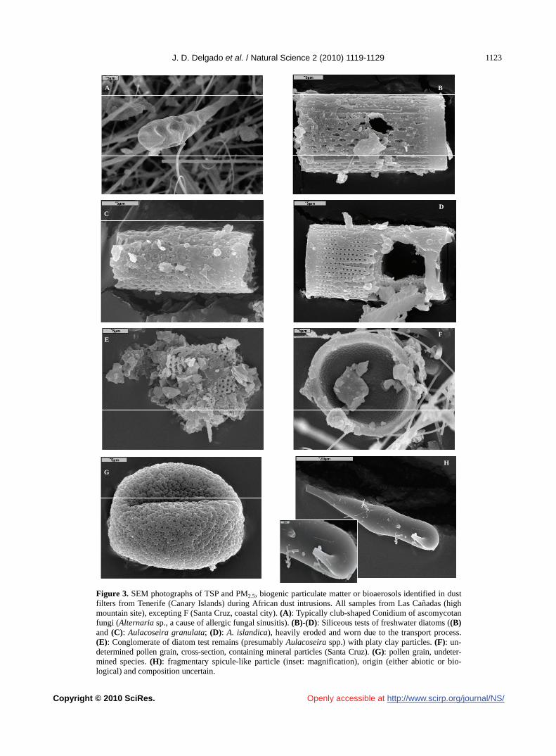
J. D. Delgado et al. / Natural Science 2 (2010) 1119-1129
Copyright © 2010 SciRes. http://www.scirp.org/journal/NS/
1121123
Openly accessible at
A
B
C
D
E
F
G
H
Figure 3. SEM photographs of TSP and PM2.5, biogenic particulate matter or bioaerosols identified in dust filters from Tenerife (Canary Islands) during African dust intrusions. All samples from Las Cañadas (high mountain site), excepting F (Santa Cruz, coastal city). (A): Typically club-shaped Conidium of ascomycotan fungi (Alternaria sp., a cause of allergic fungal sinusitis). (B)-(D): Siliceous tests of freshwater diatoms ((B) and (C): Aulacoseira granulata; (D): A. islandica), heavily eroded and worn due to the transport process. (E): Conglomerate of diatom test remains (presumably Aulacoseira spp.) with platy clay particles. (F): un-determined pollen grain, cross-section, containing mineral particles (Santa Cruz). (G): pollen grain, undeter-mined species. (H): fragmentary spicule-like particle (inset: magnification), origin (either abiotic or bio-logical) and composition uncertain.

J. D. Delgado et al. / Natural Science 2 (2010) 1119-1129
Copyright © 2010 SciRes. http://www.scirp.org/journal/NS/Openly accessible at
1124
not be assigned (Figure 3(G)). Pollen was very rare in filters, which operated during the early spring season when flowering period was not at its peak in the Tenerife high mountain. We failed to identify bacterial cells in filter preparations examined with SEM.
3.4. Aerosols of Abiotic Origin
Filters from the control day (“clean troposphere”) show- ed a very different aspect when compared with filters from dust events (Figures 4(A),4(B)), the latter being con- cealed with a dense mineral-biomineral matrix (Figure 4(C)). The abiotic particulate aerosols identified indivi- dually included clay grades and quartz microcristals (iso- lated or aggregated) of crustal origin (from AfD cluster), and gypsum rods (CaSO4). Halite, cubic and cube-octa-hedra crystals of sea salt (NaCl) were obtained from the OMT cluster correspondent to clear atmospheric condi-tions and incidence of marine aerosol reaching the high mountain area (compare with [26]).
Quartz (SiO2) microcristals (particles from < 10 µm to < 2 µm) formed the dominant or background material in our filters during dust intrusions (Figure 4). Aerosols transported from the Sahara desert are enriched in clay material due to a high residence time in atmosphere caused by a smaller particle size and laminar habit; these clay grade grains are transported as particles of silt size forming aggregates [29,30] (Figure 4).
4. DISCUSSION
As suggested by our filter samples from different ori-gins, Aulacoseira diatom thecae compound the dominant biogenic aerosol, and quartz is the dominant mineral fraction, which also formed up to 60% of dust material in a study from Gran Canaria [31].
The diatoms identified are dominant taxa in fresh wa-ters from N and NW Africa, and can be found through-out the Palaearctic [32]. A. granulata has been recorded in the Arctic probably transported from Siberia [33]. Both A. islandica and A. granulata are typical of eutro-phized and alkaline waters. As far as we know, these species have not been deemed as pathogenic to humans; on the contrary, they are used as bioindicators of fresh-water quality in most studies. They can be transported as viable cells through the ocean, and their importance in the windblown diatom fraction decrease with increasing distance from the African continent [4]. The aeolian tran- sport of diatoms and phytolyths from continental fresh water deposits in the Sahara and Sahel [4,34] should be investigated to assess relative contribution to high inci-dence of environmental airway diseases in the Canaries. We are not aware of detailed clinic studies relating natu-ral (desert) diatom dust with respiratory diseases. Fur-
thermore, concentrations of airborne diatom particles from African deserts and professional exposure to diatom dust are not comparable [35]. Diatoms transported with the dust plumes to the Canaries augment the overall silica content of the aerosols, and silicosis caused by non- crystalline forms of silica have not only occupational but environmental etiology [36]. On the contrary, non-industrial silicosis (known as “desert lung”) has been reported decades ago from autopsy of Bedouine lung tissue, showing high amounts of silica dust of respirable size [37]. More study cases of non-industrial lung or en- vironmental silicosis, have been reported for regions chronically exposed to desert dust (i.e. Himalaya [38]).
The Tenerife highland (> 2000 m a.s.l.) is not a popu-lated area, but it receives > 4 million visitors/year, the most visited volcanic area of the world after Mount Fuji, Japan. There is evidence that symptoms of asthma in lowland patients improve with therapy of high-elevation stays [39,40]; however, episodic but severe dust events may imply additional health risks given the extreme conditions at these altitudes for such long permanencies (moderate hypoxia, high aridity of this area and increa- sed sun radiation exposure, among other stressors). Ori-gin and type of air mass and aerosol load can be pre-dicted and used to establish and prevent potential inter-actions with respiratory disease in susceptible visitors to the island’s National Park.
Particles of different sizes have different ability to pe- netrate the pulmonary system and reach the lung pare- nchyma [41]. Modelling of aerosol inhalation schema-tize the stratification of particle deposition along the human airways depending on their aerodynamic diame-ter [42]. Particulate matter (PM) < 10 µm (PM10) pene-trate the tracheobronchial region; increased deposition in the oropharynx occurs with particles larger than 6 µm, whereas central airway deposition peaks within the 4-6 µm range. Particles like those in Figures 4(B), 4(D) or 4 (I) would be able to reach the central airways. PM be-tween 2-4 µm (PM2.5) reach the alveolar cavities (i.e. lung periphery), where their damage is greater due to higher reactivity [42]. Particles like the one depicted in Figure 4(K) seem of potential interest in this range.
Although a great proportion of diatom remains are within or above the PM10 fraction (particulate matter 10 micrometers in diameter), thereby being potentially re-tained by the trachea and bronchia, a great amount of test fragments are within the PM2.5 fraction, and thus could reach the lung alveolar system [35]. In addition, the role of diatom thecae as carriers of particles of health interest (e.g. bacteria, viruses, fungal or protozoan spores or cists, pollen) can be important, since: a) these remains co-dominate, along with quartz mineral, in many of the dust events of North African origin, and b)
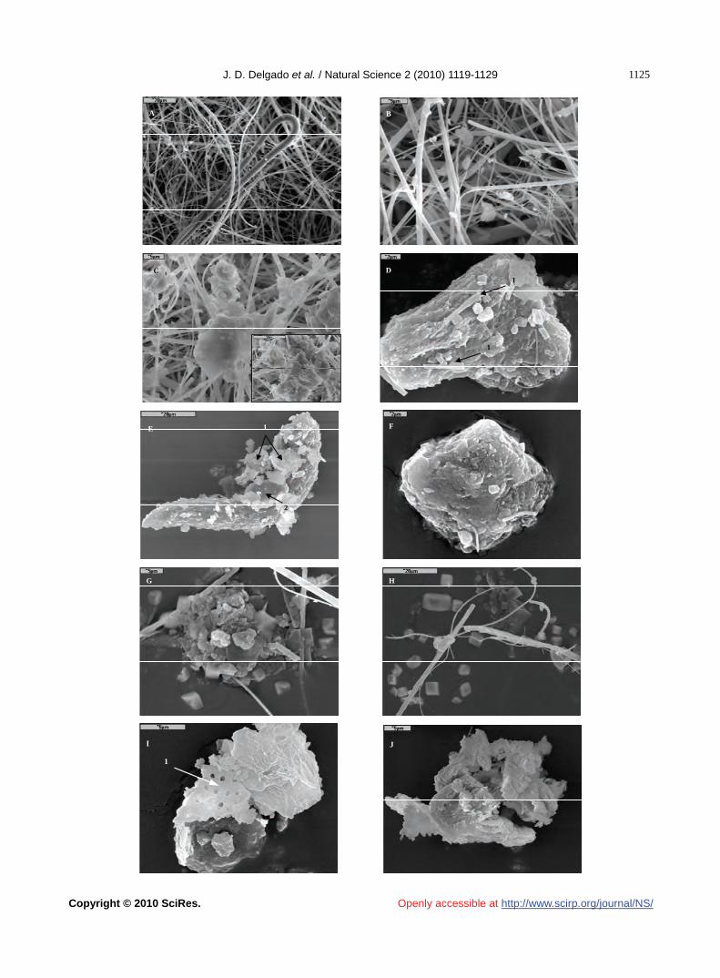
J. D. Delgado et al. / Natural Science 2 (2010) 1119-1129
Copyright © 2010 SciRes. http://www.scirp.org/journal/NS/
1121125
Openly accessible at
A
B
C
1
1
D
2
1 E
F
G
H
I
1
J
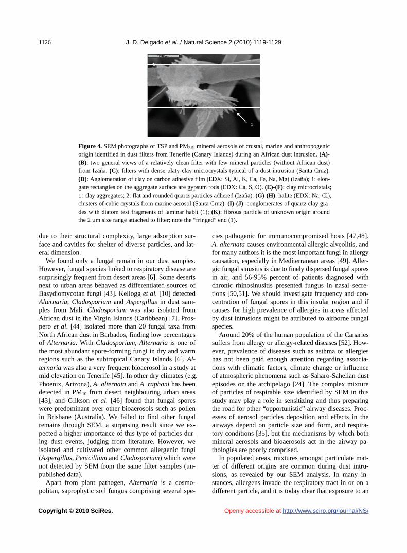
J. D. Delgado et al. / Natural Science 2 (2010) 1119-1129
Copyright © 2010 SciRes. http://www.scirp.org/journal/NS/
1126
Openly accessible at
K
1
Figure 4. SEM photographs of TSP and PM2.5, mineral aerosols of crustal, marine and anthropogenic origin identified in dust filters from Tenerife (Canary Islands) during an African dust intrusion. (A)- (B): two general views of a relatively clean filter with few mineral particles (without African dust) from Izaña. (C): filters with dense platy clay microcrystals typical of a dust intrusion (Santa Cruz). (D): Agglomeration of clay on carbon adhesive film (EDX: Si, Al, K, Ca, Fe, Na, Mg) (Izaña); 1: elon- gate rectangles on the aggregate surface are gypsum rods (EDX: Ca, S, O). (E)-(F): clay microcristals; 1: clay aggregates; 2: flat and rounded quartz particles adhered (Izaña). (G)-(H): halite (EDX: Na, Cl), clusters of cubic crystals from marine aerosol (Santa Cruz). (I)-(J): conglomerates of quartz clay gra- des with diatom test fragments of laminar habit (1); (K): fibrous particle of unknown origin around the 2 µm size range attached to filter; note the “fringed” end (1).
due to their structural complexity, large adsorption sur-face and cavities for shelter of diverse particles, and lat-eral dimension.
We found only a fungal remain in our dust samples. However, fungal species linked to respiratory disease are surprisingly frequent from desert areas [6]. Some deserts next to urban areas behaved as differentiated sources of Basydiomycotan fungi [43]. Kellogg et al. [10] detected Alternaria, Cladosporium and Aspergillus in dust sam-ples from Mali. Cladosporium was also isolated from African dust in the Virgin Islands (Caribbean) [7]. Pros-pero et al. [44] isolated more than 20 fungal taxa from North African dust in Barbados, finding low percentages of Alternaria. With Cladosporium, Alternaria is one of the most abundant spore-forming fungi in dry and warm regions such as the subtropical Canary Islands [6]. Al-ternaria was also a very frequent bioaerosol in a study at mid elevation on Tenerife [45]. In other dry climates (e.g. Phoenix, Arizona), A. alternata and A. raphani has been detected in PM10 from desert neighbouring urban areas [43], and Glikson et al. [46] found that fungal spores were predominant over other bioaerosols such as pollen in Brisbane (Australia). We failed to find other fungal remains through SEM, a surprising result since we ex-pected a higher importance of this type of particles dur-ing dust events, judging from literature. However, we isolated and cultivated other common allergenic fungi (Aspergillus, Penicillium and Cladosporium) which were not detected by SEM from the same filter samples (un-published data).
Apart from plant pathogen, Alternaria is a cosmo-politan, saprophytic soil fungus comprising several spe-
cies pathogenic for immunocompromised hosts [47,48]. A. alternata causes environmental allergic alveolitis, and for many authors it is the most important fungi in allergy causation, especially in Mediterranean areas [49]. Aller-gic fungal sinusitis is due to finely dispersed fungal spores in air, and 56-95% percent of patients diagnosed with chronic rhinosinusitis presented fungus in nasal secre-tions [50,51]. We should investigate frequency and con-centration of fungal spores in this insular region and if causes for high prevalence of allergies in areas affected by dust intrusions might be attributed to airborne fungal species.
Around 20% of the human population of the Canaries suffers from allergy or allergy-related diseases [52]. How- ever, prevalence of diseases such as asthma or allergies has not been paid enough attention regarding associa-tions with climatic factors, climate change or influence of atmospheric phenomena such as Saharo-Sahelian dust episodes on the archipelago [24]. The complex mixture of particles of respirable size identified by SEM in this study may play a role in sensitizing and thus preparing the road for other “opportunistic” airway diseases. Proc-esses of aerosol particles deposition and effects in the airways depend on particle size and form, and respira-tory conditions [35], but the mechanisms by which both mineral aerosols and bioaerosols act in the airway pa-thologies are poorly comprised.
In populated areas, mixtures amongst particulate mat-ter of different origins are common during dust intru-sions, as revealed by our SEM analysis. In many in-stances, allergens invade the respiratory tract in or on a different particle, and it is today clear that exposure to an
J. D. Delgado et al. / Natural Science 2 (2010) 1119-1129
Copyright © 2010 SciRes. http://www.scirp.org/journal/NS/
1121127
Openly accessible at
allergen on or within a carrier pollutant can substantially enhance its allergenic potential [53,54]. Many of the aerosol types overviewed here can incorporate additional pollutants from the atmosphere, and in case of bioaero-sols, surface proteins can be altered and then released into the respiratory system. Synergies between anthro-pogenic aerosols and bioaerosols also deserve attention. Diatom tests, quartz and gypsum fiber-like particles mix to form aggregates, and pollen grains can transport those and other mineral particles (Figures 4(B)-4(F), 4(J)). Important synergies between bioaerosols (mostly pollen, fungi and soil bacteria, but perhaps also viruses) and other atmospheric pollutants (i.e. NOx, VOCs—volatile organic compounds—ozone, tobacco smoke) have been reported in relation with increasing asthma prevalence in urban areas [46]. Pollen secrete eicosanoid-like mole-cules (i.e. leukotriene-like) which act signaling in im-munity and inflammation, and such releasing is favoured by contact of pollen with gases from traffic exhaust and petrol industry [54].
The study of the origin of the air mass through back trajectory would allow knowing the potential of remote subtropical and tropical areas for issuing other disease vectors in dust plumes to the Canary Islands and other places. This tool should be integrated along with quanti-tative and qualitative aerosol characterization in the creation of prevention nets [12,55]. Attention should be paid to candidate disease vectors that can be predicted, through tracing of backward trajectories, to reach the islands with dust intrusions in the next future. In fact, nearly 80% of the air masses reaching the islands have a direct North African origin. SEM analysis is useful as a complementary tool in the morphological identification of new particle types or combinations of particles of interest in disease causation [56]. Moreover, exploratory biopsy of the respiratory mucosa through SEM analysis would prove useful in identifying PM types and linking them as causal factors with atmospheric dust PM. Nev-ertheless, molecular and clinical characterization of the active substances associated to aerosols is a critical and unavoidable step for prevention of dust mass impact on human health [54]. In the Caribbean, relationship be-tween asthma attendance peaks and African dust intru-sions have previously been revealed [23]. For the Canary Islands, where African dust intrusions exert their effects before reaching the Caribbean, the studies dealing with problems posed by dust intrusions on public health re-main anecdotic, whereas effective control of dust effects on human population is a major sanitary goal [12].
5. CONCLUSIONS
Aeolian dust reaching the high altitude areas of the Tenerife island has a larger contribution of North African
air masses, and is formed by a structurally complex mix- ture of biogenic and abiogenic particles, of respirable size and contrasting morphology; we found that the dia-tom test fraction is qualitatively relevant (along with the dominant, background quartz fraction), whereas other biogenic fractions such as pollen or fungi are more scar- ce, or difficult to resolve, at least by means of SEM, and at these elevations within the island. Increasing aridity periods, irregular and torrential rains, changes in vegeta-tion cover and desertification would affect the aerosol load (both biogenic and abiogenic in origin) received by these subtropical islands as dust intrusion events in-crease in frequency [16,17,57].
6. ACKNOWLEDGEMENTS
We thank Juan Luis González Álvarez (SEGAI facilities, ULL) and
Debora Gómez for assistance with SEM. Prof. Dr. Óscar Romero (Uni-
versitaet Bremen, Germany) gently identified diatoms. We acknowledge
to the MEC (Ministry of Education and Science, Spain) and F.E.D.E.R.
founds (E.U.) for the economical support of the following projects:
CGL2005-03428-C04-02, CGL2007-66477-C02-02/CLI, CGL2008-
04740 and PI042005/033. Finally, the authors wish to express their app-
reciation to the operators of Izaña Atmospheric Observatory for their
help on running the instruments.
REFERENCES
[1] Hernández, F., Alonso-Pérez, S., Hernández-Armasa, J., Cuevas, E., Karlsson, L. and Romero-Campos, P.M. (2005) Influence of major African dust intrusions on the 137Cs and 40K activities in the lower atmosphere at the Island of Tenerife. Atmospheric Environment, 39, 4111- 4118.
[2] Main, C.E. (2003) Aerobiological, ecological, and health linkages. Environment International 2003, 29, 347-349.
[3] Kuhlman, K.R., Allenbach, L.B., Ball, C.L., Fusco, W.G., La Duc, M.T., Kuhlman, G.M., Anderson, R.C., Erickson, I.K., Stuecker, T., Benardini, J. and Crawford, R.L. (2005) Enumeration, isolation, and characterization of ultravio-let (UV-C) resistant bacteria from rock varnish in the Whipple Mountains, California. Icarus, 174, 585-595.
[4] Romero, O.E., Lange, C.B., Swap, R.J. and Wefer, G. (1999) Eolian-transported freshwater diatoms and phyto-liths across the equatorial Atlantic record temporal cha- nges in Saharan dust transport patterns. Journal of Geo-physical Research, 104(C2), 3211-3222.
[5] Gorbushina, A.A., Kort, R., Schulte, A., Lazarus, D., Schnetger, B., Brumsack, H.-J., Broughton, W.-J. and Favet, J. (2007) Life in Darwin's dust: Intercontinental transport and survival of microbes in the nineteenth cen-tury. Environmental Microbiology, 9, 2911-2922.
[6] Lacey, J. (1991) Aerobiology and health: The role of airborne fungal spores in respiratory disease. In: Hawk-sworth, D.L. Ed., Frontiers in Mycology. C. A. B. Inter-national, Wallingford, 157-185.
[7] Griffin, D.W., Garrison, V.H., Herman, J.R. and Shinn, E.

J. D. Delgado et al. / Natural Science 2 (2010) 1119-1129
Copyright © 2010 SciRes. http://www.scirp.org/journal/NS/Openly accessible at
1128
A. (2001a) African desert dust in the Caribbean atmos-phere: Microbiology and public health. Aerobiologia, 17, 203-213.
[8] Griffin, D.W., Kellogg, D.A. and Shinn, E.A. (2001b) Dust in the wind: Long range transport of dust in the at-mosphere and its implications for global public and eco-system health. Global Change & Human Health, 2, 20-33.
[9] Griffin, D.W., Westphal, D.L. and Gray, M.A. (2006) Airborne microorganisms in the African desert dust cor-ridor over the mid-Atlantic ridge, Ocean Drilling Pro-gram, Leg 209. Aerobiologia, 22, 211-226.
[10] Kellogg, C.A., Griffin, D.W., Garrison, V.H., Peak, K., Royall, N., Smith, R.R. and Shinn, E.A. (2004) Charac-terization of aerosolized bacteria and fungi from desert dust events in Mali, West Africa. Aerobiologia; 20, 99-110.
[11] Salvaggio, J.E. (1994) Inhaled particles and respiratory disease. The Journal of Allergy and Clinical Immunology, 94, 304-309.
[12] García Carrasco, J., Hernández Vázquez, A., Blasco de la Fuente, A., Rodríguez Hernández, B.C., Rancaño Gila, E. and Núñez Díaz, S. (2001) Invasión de viento sahariano y su impacto en la asistencia sanitaria urgente. Emer- gencias, 13, 372-376.
[13] Pope, C.A., Burnett, R.T., Thun, M.J., Calle, E.E., Krew- ski, D., Ito, K. and Thurston, G.D. (2002) Lung cancer, cardiopulmonary mortality, and long-term exposure to fine particulate air pollution. JAMA, 287, 1132- 1141.
[14] Lee, J.-T., Son, J.-Y. and Cho, Y.-S. (2007) A comparison of mortality related to urban air particles between periods with Asian dust days and without Asian dust days in Seoul, Korea, 2000-2004. Environmental Research, 105, 409-413.
[15] Prospero, J.M. and Lamb, J.P. (2003) African droughts and dust transport to the Caribbean: Climate change and implications. Science, 302, 1024-1027.
[16] Viana, M., Querol, X., Alastuey, A., Cuevas, E. and Rodríguez, S. (2002) Influence of African dust on the levels of atmospheric particulates in the Canary Islands air quality network. Atmospheric Environment, 36, 5861- 5875.
[17] Viana, M., Querol, X., Alastuey, A., Ballester, F., Llop, S., Esplugues, A., Fernández-Patier, R., García dos Santos, S. and Herce, M.D. (2008) Characterising exposure to PM aerosols for an epidemiological study. Atmospheric En-vironment, 42, 1552-1568.
[18] Criado, C. and Dorta P. (2003) An unusual “blood rain” over the Canary Islands (Spain). The storm of January 1999. Journal of Arid Environments, 55, 765-783.
[19] Alonso-Pérez, S., Cuevas, E., Querol, X., Viana, M. and Guerra, J.C. (2007) Impact of the Saharan dust outbreaks on the ambient levels of total suspended particles (TSP) in the marine boundary layer (MBL) of the Subtropical Eastern North Atlantic Ocean. Atmospheric Environment, 41, 9468-9480.
[20] Querol, X., Alastuey, A., Moreno, T., Vian, M.M., Cas- tillo, S., Pey, J., Rodríguez, S., Artiñano, B., Salvador, P., Sánchez M., García, S., Herce, M.D., Fernández-Patier, R., Moreno-Grau, S., Minguillón, M.C., Monfort, E., Sanz, M.J., Palomo-Marín, R., Pinilla-Gil, E., Cuevas E., De La Rosa, J. and Sánchez, A. (2008) Spatial and tem-poral variations in airborne particulate matter (PM10 and PM2.5) across Spain 1999-2005. Atmospheric Environ-
ment, 42, 3964-3979. [21] Prospero, J.M. (1999a) Long-term measurements of the
transport of African mineral dust to the south-eastern United States: Implications for regional air quality. Jour- nal of Geophysical Research, 104, 917-927.
[22] Prospero, J.M. (1999b) Assessing the impact of advected African dust on air quality and health in the Eastern United States. Human and Ecological Risk Assessment, 5, 471-479.
[23] Prospero, J.M., Blades, E., Naidu, R., Mathison, G., Thani, H. and Lavoie, M.C. (2008) Relationship between African dust carried in the Atlantic trade winds and surges in pediatric asthma attendances in the Caribbean. Inter-national Journal of Biometeorology, 52, 823-832.
[24] Julià Serdà, G., Cabrera Navarro, P., Acosta Fernández, O., Martín Pérez, P., Batista Martín, J., Alamo Santana, F., Rodríguez de Castro, F. and Antó Boqué, J.M. (2005) High prevalence of asthma symptoms in the Canary Is-lands: climatic influence? J. Asthma, 42, 507-511.
[25] Rodríguez, S. (1999) Comparación de la variaciones de ozono superficial asociadas a procesos de transporte so- bre y bajo la inversión temperatura subtropical en Tene- rife. Unpublished Thesis, Universidad de La Laguna, Santa Cruz de Tenerife, Spain.
[26] Alastuey, A., Querol, X., Castillo, S., Escudero, M., Avila, A., Cuevas, E., Torres, C., Romero, P.M., Expósito, F., García, O.E., Díaz, J.P., van Dingenen, R. and Putaud, J.P. (2005) Characterisation of TSP and PM2.5 at Izaña and Sta. Cruz de Tenerife (Canary Islands, Spain) during a Saharan dust episode (July 2002). Atmospheric Environ- ment, 39, 4715-4728.
[27] Díaz, A.M. (2006) Caracterización de los aerosoles at- mosféricos y su influencia en los niveles de radiación UV en la región de Canarias, Ph.D. Thesis, University of La Laguna, Tenerife, Spain.
[28] Díaz, A.M., Díaz, J.P., Expósito, F.J., Hernández-Leal, P.A., Savoie, D. and Querol, X. (2006) Air masses and aerosols chemical components in the free troposphere at the Subtropical Northeast Atlantic region, Journal of Atmospheric Chemistry, 53, 63-90.
[29] Pósfai, M. and Molnár, Á. (2000) Aerosol particles in the troposphere: A mineralogical introduction. In: Vaughan, D.J. and Wogelius, R.A., Eds., Environmental Mineralo- gy. Eötvös University Press, Budapest, 197-252.
[30] Thomas, D. Potter, T.D. and Colman, B.R. (2003) Hand- book of weather, climate, and water. John Wiley & Sons, Hoboken.
[31] Gelado, M.D., Dorta, P., Hernández, J.J., Collado, C., Rodríguez, M.J., Cardona, P. and Siruela, V. (2004) Cha- racterisation of African dust outbreaks in Gran Canaria (Canary Islands). Geophysical Research Abstracts, 6, 05227.
[32] Gómez, N., Riera, J.L. and Sabater, S. (1995) Ecology and morphological variability of Aulacoseira granulata (Bacillariophyceae) in Spanish reservoirs. Journal of Pl- ankton Research, 17, 1-16.
[33] Darby, D.A., Burckle, L.H. and Clark D.L. (1974) Air-borne dust on the Arctic ice pack, its composition and fall- out rate. Earth and Planetary Science Letters, 24, 166-172.
[34] Lange, C.B., Romero, O.E., Wefer, G. and Gabric, A. (1998) Offshore influence of coastal upwelling off Mauri- tania, NW Africa, as recorded by diatoms in sediment traps at 2195 m water depth. Deep-Sea Research, 45, 985-
J. D. Delgado et al. / Natural Science 2 (2010) 1119-1129
Copyright © 2010 SciRes. http://www.scirp.org/journal/NS/Openly accessible at
1121129
1013. [35] Derbyshire, E. (2007) Natural minerogenic dust and hu-
man health. AMBIO: A Journal of the Human Environ-ment, 36, 73-77.
[36] Kusaka, Y., Hering, K. and Parker, J. (2005) International classification of HRCT for occupational and environ-mental respiratory diseases. Springer-Verlag, Tokyo.
[37] Bar-Ziv, J. and Goldberg, G.M. (1974) Simple siliceous pneumoconiosis in Negev Bedouins. Arch Environ Health, 29, 121
[38] Norboo, T., Angchuk, P.T., Yahya, M., Kamat, S.R., Poo-ley, F.D., Corrin, B., Kerr, I.H., Bruce, N. and Ball, K.P. (1991) Silicosis in a Himalayan village population: Role of environmental dust. Thorax, 46, 341-343.
[39] Simon, H., Grotzer, M., Nikolaizik, W., Blaser, K. and Schóni, M. (1994) High altitude climate therapy reduces peripheral blood T lymphocyte activation, eosinophilia, and bronchial obstruction in children with house-dust mi- te allergic asthma. Pediatric Pulmonology, 17, 304-311.
[40] Schultze-Werninghaus, G. (2006) Should asthma mana- gement include sojourns at high altitude? Chemical Im-munology and Allergy, 91, 16-29.
[41] Silson, J.E. (1950) Dust inhalation in relation to pulmo-nary disease. Chest, 18, 562-573.
[42] Mitchell, J.P. and Nagel, M.W. (2004) Particle size ana- lysis of aerosols from medicinal inhalers. KONA, 22, 32-65.
[43] Boreson, J., Dillner, A.M. and Peccia, J. (2004) Correlat-ing bioaerosol load with PM2.5 and PM10 concentrations: A comparison between natural desert and urban-fringe aerosols. Atmospheric Environment, 38, 6029-6041.
[44] Prospero, J.M., Blades, E., Mathison, G. and Naidu, R. (2005) Interhemispheric transport of viable fungi and bacteria from Africa to the Caribbean with soil dust. Aerobiologia, 21, 1-19.
[45] La Serna, I. and Domínguez, M.D. (2003) Pólenes y esporas aerovagantes en Canarias: Incidencia en alergias. Colección Materiales Didácticos Universitarios, Serie Bo- tánica 1, SPULL, Tenerife.
[46] Glikson, M., Rutherford, S., Simpson, R., Mitchell, C. and Yago, A. (1995) The microscopic and submicron components of atmospheric particulates occurring during high asthma periods in Brisbane, Queensland, Australia. Atmospheric Environment, 29, 549-562.
[47] Morrison, V.A. and Weisdorf, D.J. (1993) Alternaria: A sinonasal pathogen of immunocompromised hosts. Cli- nical Infectious Diseases, 16, 265-270.
[48] Hospenthal, D.R. and Bennett, J.E. (2000) Miscellaneous
fungi and Prototheca. In: Mandell, G.L., Bennet, J.E. and Dolin, R. Eds., Principles and practice of infectious dis-eases, 5th Edition, Livingstone, Philadelphia, 2772-2780.
[49] D’Amato, G., Chatzigeorgiou, G., Corsico, R., Gioulekas, D., Jäger, L., Jäger, S., Kontou-Fili, K., Kouridakis, S., Liccardi, G., Meriggi, A., Palma-Carlos, A., Palma- Carlos, M.L., Pagan, A., Parmiani, S., Puccinelli, P., Russo, M., Spieksma, F.T., Torricelli, R. and Wuthrich, B. (1997) Evaluation of the prevalence of skin prick test positivity to Alternaria and Cladosporium in patients with suspected respiratory allergy. EEACI Position Paper. Allergy, 52, 711-716.
[50] Lebowitz, R.A., Waltzman, M.N., Jacobs, J.B., Pearlman, A. and Tierno, P.M. (2002) Isolation of fungi by standard laboratory methods in patients with chronic rhinosinusitis. Laryngoscope, 112, 2189-2191.
[51] Braun, H., Buzina, W., Freudenschuss, K., Beham, A. and Stammberger, H. (2003) “Eosinophilic fungal Rhi-nosinusitis”: A common disorder in Europe? Laryngo-scope, 113, 264-269.
[52] Gaig, P., Ferrer, M., Muñoz-Lejarazu, D., Lleonart, R., García-Abujeta, J.L., Caballero, T., Rodríguez, A., Eche- chipia, S., Martínez-Cocera, C., Domínguez, F.J., Gon- zalo, M.A. and Olona, M. (2004) Prevalencia de alergia en la población adulta española. Alergología e Inmuno- logía Clínica, 19, 68-74.
[53] Salvaggio, J.E. and O’Neil, C.E. (1992) Pathogenetic mechanisms in occupational hypersensitivity states. Im-munology and Allergy Clinics of North America, 4, 711- 729.
[54] Behrendt, H., Krämer, U., Schäfer, T., Kasche, A., Eber-lein-König, B., Darsow, U. and Ring, J. (2001) A research concept to study the role of environmental pollutants in allergy. Allergy and Clinical Immunology International, 13, 122-128.
[55] Mastalerz, M., Glikson, M. and Simpson, R.W. (1998) Analysis of atmospheric particulate matter; application of optical and selected geochemical techniques. Interna-tional Journal of Coal Geology, 37, 143-155.
[56] Wittmaack, K., Wehnes, H., Heinzmann, U. and Agerer, R. (2005) An overview on bioaerosols viewed by scan- ning electron microscopy. Science of the Total Environ-ment, 346, 244- 255.
[57] Rodríguez, S., Querol, X., Alastuey, A., Kallos, G. and Kakaliagou, O. (2001) Saharan dust contributions to PM10 and TSP levels in Southern and Eastern Spain. Atmos-pheric Environment, 35, 2433-2447.

Vol.2, No.10, 1130-1137 (2010)doi:10.4236/ns.2010.210140
Copyright © 2010 SciRes. Openly accessible at http://www.scirp.org/journal/NS/
Natural Science
The Rich-Gini-Simpson quadratic index of biodiversity
Radu Cornel Guiasu1, Silviu Guiasu2
1Environmental and Health Studies Program, Department of Multidisciplinary Studies, Glendon College, York University, Toronto, Canada; [email protected]; 2Department of Mathematics and Statistics, Faculty of Pure and Applied Sciences, York University, Toronto, Canada; [email protected].
Received 6 August 2010; accepted 10 September 2010; accepted 13 September 2010.
ABSTRACT
The Gini-Simpson quadratic index is a classic measure of diversity, widely used by ecologists. As shown recently, however, this index is not suitable for the measurement of beta diversity when the number of species is very large. The objective of this paper is to introduce the Rich- Gini-Simpson quadratic index which preserves all the qualities of the classic Gini-Simpson in-dex but behaves very well even when the num-ber of species is very large. The additive parti-tioning of species diversity using the Rich-Gini- Simpson quadratic index and an application from island biogeography are analyzed.
Keywords: Rich-Gini-Simpson Index of Species Diversity; Additive Partitioning of Diversity; Island Biogeography; Biodiversity
1. INTRODUCTION
Measuring the diversity of species in a habitat has been an important area of interest in fields such as con-servation biology, ecology, and biogeography for the last several decades [1]. Let us assume that there are species and let:
n
1,=),,1,=(0,> ii
i pnip (1)
be the relative frequency distribution of these species in the respective habitat. There are three classic measures of diversity:
a) The number of species, or richness: ; nb) The Gini-Simpson quadratic index (abbreviated in
this paper as ): GS
,1=)(1= 2i
iii
i
pppGS (2)
introduced by Gini [2] and adapted for biological studies by Simpson [3];
c) The Shannon entropy (abbreviated as H ):
,ln= iii
ppH (3)
introduced by Shannon [4], as the discrete variant of the continuous entropy defined by Boltzmann [5] in statisti-cal mechanics. There is an extensive literature [1,6-17] about the properties and applications of these measures of diversity.
When the number of species and the relative abundance of species (1) are the only sources of infor-mation available, many other measures of diversity have been proposed. Recently, Jost [18,19] pleaded in favor of the “true” measure of diversity, introduced by Hill [20]:
n
.=)1/(1 r
ri
ir pN
(4)
For , we get: 0 . For 0=r nN = 1=r , r is not defined because the denominator of the exponent,
Nr1 ,
is equal to zero. However, the limit of when rN r tends to 1 is . For )(exp H 2=r we get 1/(1 )GS . In fact, the natural logarithm of (4), i.e. r , is just Ré-nyi’s entropy [21]. There are no sound reasons to call (4) a “true” measure of diversity. It is simply a unifying no-tation, as mentioned in [20]. Besides, by performing ma- thematical transformations on classic measures of diver-sity, like taking the exponential of the Shannon entropy or the reciprocal of the Gini-Simpson quadratic index, for example, we obtain other measures that lose, how-ever, some essential features of the original measures, such as concavity, for instance. Concavity is an essential property of any measure that can be used in an additive partitioning of species diversity. Hoffmann and Hoff-mann [22] are right when asking: “Is there a ‘true’ measure of diversity?” As noticed by Ricotta [23], there is a “jungle of measures of diversity” in the current con-servation biology literature. Under the circumstances, perhaps the best strategy is to remember Occam’s razor and, trying to keep things simple, it may be easier to just
Nln

R. C. Guiasu et al. / Natural Science 2 (2010) 1130-1137
Copyright © 2010 SciRes. http://www.scirp.org/journal/NS/
1131131
Openly accessible at
go back to the classic measures of diversity mentioned before and see how they can be adjusted to address new problems under new circumstances.
The species richness is very simple but ignores the abundance of species. Shannon’s entropy has excel-lent properties but is difficult to estimate and maximiz-ing it subject to linear constraints, generally gives a so-lution satisfying exponential equations which cannot be solved analytically. On the other hand, the Gini-Simpson quadratic index is simpler and generally seems to be preferred by ecologists. Jost [18,19,24], however, noti- ced a troubling anomaly related to . Indeed, if this measure is used in the additive partitioning of species diversity, the corresponding beta diversity approaches zero when the number of species is very large. Thus, for two habitats with no species in common, for instance, the between-habitat diversity tends to zero when the number of species in one of the habitats, or in both of them, tends to infinity, instead of becoming larger as is obviously the case in actual fact.
n
GS
The objective of this paper is to show that the anom-aly just mentioned can be easily fixed. The product be-tween the species richness a) and the measure of diver-sity c), called here the Rich-Gini-Simpson quadratic in-dex and abbreviated as , preserves all the basic properties of and behaves well when the number of species is large. Therefore, is suitable for use in the additive partitioning of species diversity. Subse-quently, the index is applied to data on the avi-faunal diversity on several tropical Indian Ocean islands, using some of the numerical results obtained by Adler [25], in order to show how the alpha, beta, and gamma species diversities change when the usual equal weights for the various habitats are replaced by the relative areas and the relative elevations of the respective islands.
RGSGS
RGS
RGS
2. THE RICH-GINI-SIMPSON INDEX
If there are species in a certain habitat and their relative abundance is given by (1), the Rich-Gini-Simp- son quadratic index is
n
).(1=)(1= 2i
iii
i
pnppnRGS (5)
The concavity of and the maximum value of are analyzed in the Appendix. Thus, we have:
, the maximum corresponding to the uniform distribution: , . As
, the maximum value of is , corresponding to the uniform distri-
bution as well. The essential difference between these two indexes is that is bounded by 1 and tends to 1 when the number of species tends to infinity,
whereas is not bounded and tends to infinity when the number of species tends to infinity. Shan-non’s entropy, on the other hand, has the maximum
, which tends to infinity when the number of species n tends to infinity, but it increases much much more slowly than .
RGS
pi
GS
RGS0
GS =pmax
1 nRGS
nRGS/nGS 1/1=
n1/= ),1,=( ni GS
n
RGS
nln=
2
n
RGSp
GS
Hpmax
N
1=max nGS
GS
RGSn
Pleading against the use of the index, Jost [24] gave the following example: “Suppose a continent has a million equally-common species, and a meteor impact kills 999,900 of the species, leaving 100 species un-touched. Any biologist, if asked, would say that this me-teor impact caused a large absolute and relative drop in diversity. Yet only decreases from 0.999999 to 0.99, a drop of less than 1%”. Jost concluded that: “[The] ecologists relying on will often misjudge the mag-nitude of ecosystem changes. This same problem arises when Shannon entropy is equated with diversity. In con-trast, drops by the intuitively appropriate 99.99%”. This example shows that there is indeed a troubling anomaly in using when the number of species is very large. But has no such a drawback. Indeed, if before the cataclysm there are equally abundant species, then:
GS
1,000,000=
;13.81551050.999999;= =ln= n
1000000,=ln( nn
=1= n
=n
11=
nGS
(exp
==2 nN
H
=)
RGS
exp=)H
999999.1000000,
After the cataclysm, there are only equally abundant species left. Thus:
100
6;=1
n1=GS
exp
2N
GS0.999901%
4.605170180.99;
100,==ln(exp n
=1= n
=H
)n
RGS
=)(H
99.100,== n
Therefore, indicates a decrease in diversity equal to , which is obviously wrong, H indi-cates a decrease in diversity equal to , which is not good enough, whereas , and
2 give a decrease in diversity equal to and , respectively, in agreement with common sense. Let us note that, practically, and
have the same maximum value when the number of species is given, but the index is not a concave function of the relative frequency dis-tribution of species and, consequently, it is not suitable to be used in the additive partitioning of species diversity, whereas the index is.
7% 66.6666666exp
9% 99.9900999
)(H
RGS
),(= 1 npp
RGS
)(H
RGS
exp
N99.9900000
)(exp H
0%
n
,p
3. THE ADDITIVE PARTITIONING OF SPECIES DIVERSITY USING RGS
MacArthur [26] pointed out the need for a theory of within-habitat and between-habitat species diversities. Identify applicable sponsor/s here. (sponsors)

R. C. Guiasu et al. / Natural Science 2 (2010) 1130-1137
Copyright © 2010 SciRes. http://www.scirp.org/journal/NS/
1132
Openly accessible at
He, together with Recher and Cody [27], proposed a measure of the difference between the species diversities of two habitats based on Shannon’s entropy and using equal relative weights for habitats. This measure was also used in the influential book “The theory of island biogeography” by MacArthur and Wilson [28]. Rao [29], without mentioning the paper [27], extended the measure of the difference between the species diversities of two habitats, based also on Shannon’s entropy but using ar-bitrary weights assigned to the two habitats. Whittaker [30,31] proposed linking diversity components between ecological scales by multiplication so that the gamma diversity, measuring the species diversity in a larger re-gion consisting of several ecological communities taken together, is the product of the alpha diversity, which measures the mean species diversity in the local com-munities taken separately, and the beta diversity, repre-senting the variation and changes in mean species diver-sity in a larger region which contains the local ecological communities taken together, as a whole. The beta diver-sity essentially measures the biogeographic changes in species diversity among various locations within a larger region. As such, the beta diversity can be important in leading to the development of geographic strategies for the conservation of species and habitats, as mentioned by Harrison and Quinn [32]. Routledge [33,34] devel-oped Whittaker’s approach. Allan [35] applied an addi-tive linkage of species diversity components according to which the gamma diversity is partitioned into the sum of the alpha diversity and the beta diversity, using the Shannon entropy. Lande [36] dealt with an arbitrary num- ber of habitats and arbitrary weights, using the Shannon entropy, and extended this approach to species richness and to the Gini-Simpson index, recommending the addi-tive partitioning of species diversity as a unifying frame- work for measuring species diversity at different levels of ecological organization. As mentioned by Wagner, Wildi and Ewald [37], in contrast to the multiplicative model, by using the additive partitioning, all species diversity components are measured in the same way and expressed in the same units, so that they can be directly compared. Recently, it was pointed out that the additive partitioning of species diversity is an old idea which shows a new revival. According to Veech, Summerville, Crist and Gering [38], “Lande [36] appears to have been the first to place the additive partitioning of species di-versity in the context of Whittaker’s concepts of alpha, beta, and gamma diversities Viewing gamma diver-sity as the sum of alpha and beta diversities leads to the most operational definition of beta diversity and quanti-fies it in a manner comensurate with the measurement of alpha and gamma diversities. In effect, the revival of
additive diversity partitioning has given new meaning to
beta diversity”. As is a concave function, it is suitable for the
additive partitioning of species diversity. Let be a set of species and let and {
RGS},,{ 1 nxx
}, Jixi},{ Iixi be the species from the habitats and 2h , respectively. The number of species from 1 is 1 and the number of species from 2 is 2 . Obviously, ,
1hh n
h n n nnn 1 2 , and 21 nnn . The species belong only to the habitat 1 , the species { belong only to the habitat 2 , whereas the species
}J
,{ Iixi xi
h
Jih }I,
}i;{xi JI belong to both habitats. We have . },nJ {1,= I
Let },{ Iipi and be the relative fre-quencies of the species from and , respectively. We have:
},{ Jiqi
1h
2h
1.=0,>1;=0,> iJi
iiIi
i qqpp
In general, the beta diversity is the average be-tween-habitat diversity, whereas the alpha diversity is the average diversity of the individual communities or the average within-habitat diversity. Using the additive partitioning of the species diversity, the gamma diversity is the sum of the alpha and beta diversities, or the aver-age total diversity. Let 0>1 , and 0>2 , be two weights assigned to the habitats 1 and 2 , respec-tively, such that 21
h h1= . We use these weights to
calculate the average within-habitat species diversity, i.e. the alpha diversity, and the average relative frequency of the species used in the total species diversity of a larger region that includes the two individual habitats, i.e. the gamma diversity. If the two weights are equal, namely
1/2== 21 , then the average is just the arithmetic mean. These weights, however, may represent the rela-tive areas or the relative elevation of the two habitats, or any other quantitative characteristics of the habitats that can affect the diversity of the species. In this context, alpha diversity refers to the average species diversity in the two habitats 1 and 2 , taken separately, gamma diversity refers to the species diversity in the habitats 1 and 2 , averaged together, whereas beta diversity represents the average between-habitat species diversity as we move from the individual habitats 1 , 2 , aver-aged separately, to the larger region containing the union of 1 and 2 , averaged together. We now use to calculate the alpha, gamma, and beta species diversi-ties. Denote by:
h hh
RGS
h
h h
h h
,1=)(1=)( 2111
iIi
iiIi
pnppnhRGS
,1=)(1=)( 2222
iJi
iiJi
qnqqnhRGS
in which case the alpha diversity is:

R. C. Guiasu et al. / Natural Science 2 (2010) 1130-1137
Copyright © 2010 SciRes. http://www.scirp.org/journal/NS/
1131133
fo , and r
Openly accessible at
).()(= 2211 hRGShRGSDiv
The gamma-diversity is: =),;,(= 2211 hhRGSDiv
=))(1(= 2121 iiiiJIi
qpqpn
,)(1= 221
ii
JIi
qpn
where r i 0=iq fo J0=ip IJ Ii . nThe ity of itiv
of nd th
If both habitats contain the same species, then w
Clearly, if both habitats have the same species and the sa
co cav RGS allows the add e partition species diversity, a e beta-diversity is:
=)()(= DivDivDiv
21112211 )()(= i
Ii
pnnnnn
0.2)( 212
222
iiJIi
iJi
qpnqnn
JI = , , andhich implies IJI = , IJI = , nnn == 21
the beta-diversity p
22
has a sim le expression:
=2= 21
iiIi
iIi
iIi
qpqpnDiv
.)(= 221 ii
Ii
qpn
me abundance of these species, namely ii qp = , ),1,=( ni , then 0=Div .
habita peciIf the two ts have no s es in com
In particular, if the two habitats have no s ecies in co
mon, then =J , 21= nnn , and the beta-diversity is:
)( 2211 nnn
I =Div
.)()( 2222
2111 i
Jii
Ii
qnnpnn
pmmon and in each habitat the species have the same
abundance, namely 11/= npi , )( Ii , and 21/= nqi , )( Ji , then the beta-
=Div diversity is:
=11= 212
221
i
Jii
Ii
qnpn
,1
11
1=2
121
21
nn
nn
which tends to if tends to or / and
k 1. The generalization of the results from this se
Lande [36], the ratio be-tw
nd t ad-di ity,
1n 2n tends to .
Remarction to the case of an arbitrary number of habitats
mhh ,,1 is straightforward. k 2. As mentioned byRemar
een the alpha diversity and the gamma diversity may be used as a similarity index, denoted here by Sim .
Arguing against the use of the GS index a he tive partitioning of species divers Jost [19] discussed
the following example: “Suppose a continent with 30 million equally common species is hit by a plague that kills half the species. How do some popular diversity indices judge this drop in diversity? The Shannon entropy only drops from 17.2 to 16.5; according to this index the plague caused a drop of only 4% in the ‘di-versity’ of the continent. This does not agree well with our intuition that the loss of half the species and half the individuals is a large drop in diversity. The Gini-Simp-son index drops from 0.99999997 to 0.99999993; if this index is equated with ‘diversity’, the continent has lost practically no ‘diversity’ when half its species and indi-viduals disappeared”. Instead of GS and H , Jost proposes the use of )(exp H , which his exam le has the value:
exp
i
=
=
=
=
n
a lo
a lo
p
0e
0
30000000
15000000
ss of
29999999
14999999
ss of
30000000)exp=)(H the plague a
ln(nd:
ln
respond
ning
0nd:
150000
respond
before
after the plague, cor ing to in
men
before the plague a
after the plague, cor ing to in
rmly di
15000000)(exp=)(exp H
5 % fudiversity. However, as )(exp H is not a concav nc-
tion, the additive partitio species diversity cannot be used and should be replaced by the multiplicative partitioning of species diversity as Whittaker [30,31] and Routledge [33,34] proposed. The situation, however, is not as hopeless as it may seem to be. In fact, it is not really hopeless at all. The additive partitioning of species diversity, so popular with some ecologists because it al-lows the alpha, beta, and gamma diversities to be meas-ured in the same way and be expressed in the same units so that they can be directly compared, may in fact be preserved but GS has to be replaced by RGS . Thus, in the case just tioned:
30000=1= nRGS
of
100
100=1= nRGS
5 %diversity, in total agreement with common sense.
Example: If there are 30,000,000 species unifostributed in habitat 1h and 15,000,000 of these spe-
cies are uniformly distributed in habitat 2h , then, using the equal weights 1/2== 21 and th GS index, we obtain:
e
=1=)( 1h30000000
1 , 0.99999997GS
, 0.99999993=1=)( 2hGS
which show almo15000000
1
st no difference in species diversities. Also:
,(2
1)(
2
1= 21 hGShGSDiv 0.99999995=)
h
=),;,(= 2211 hGSDiv

R. C. Guiasu et al. / Natural Science 2 (2010) 1130-1137
Copyright © 2010 SciRes. http://www.scirp.org/journal/NS/
1134
which show that the average between-habitat species
Openly accessible at
2
60000000
1150000001=
0.9999999,=60000000
315000000
2
83,0.00000000=)()(= DivDivDiv
which shows that the between-habitat species diversity is practically zero, in contrast to the fact that 1h has a much higher species diversity than 2h . The similarity index is:
.0.99999995=0.99999995
0.9999999=Sim
Using the Shannon entropy:
which show a very small difference in divers y, in fact a
17.2167,= 30000000ln=)( 1hH
16.5235,=15000000ln=)( 2hH
itdecrease of only 4.03% in 2h with respect to 1h , contrary to common Also sense. :
16.8702,=)(2
1)(
1= 1 HhHDiv
2 2h
=),;,(= 2211 hhHDiv
)60000000
1ln
60000000
1(15000000=
17.0859,=)60000000
3ln
60000000
3(15000000
0.2157,=)()(= DivDivDiv
a very small between-habitat species diversity. The simi- larity index is:
,0.98737756=17.0859
16.8702=Sim
which is much too high. weights Using now the equal 1/2== 21 and the
RGS diversity index, we obtain: =130000000=)( 1
29999999,hRGS
14999999,=115000000=)( 1 hRGS
showing a decrease of in species diversity in 50% plet
2h oncompared to 1h , in com e agreement with comm
sense. Also:
,102.25=)(2
1)(
2
1= Div 7
21 hRGShRGS
=),;,(= 2211 hhRGSDiv
2
60000000
115000000130000000=
,103=60000000
315000000 7
2
,107.5=)()(= 6 DivDivDiv
diversity is 25% of the average total species diversity, whereas the average within-habitat species diversity is 75% of the average total species diversity. However, there are similarities between the two habitats, in the sense that 2h contains half of the species of 1h , there are no species from 2h that are not found in 1h , and both 1h and 2h have their species uniformly istrib-uted. These features make 2h somewhat similar to 1h . Using RGS , the similarity index is:
d
0.7=102.25
=7
Sim 5.103 7
Remark 3. If habitat contains only ne species an
1h o 1x n,d habitat 2h contains only one species 2x , the
obviously:
( 1 DivhRGShRGS 0,=0,=)(0,=) 2
1=4
1
4
112=),
2
1;,
2
1(= 21
hhRGSDiv ,
0.=1
0=1,= SimDiv
4. APPLICATION
ssions of the role and applica-tio
There are many discuns of the measures of species diversity in biogeogra-
phy (for instance, [15,35,39-43]). For example, MacAr-thur and Wilson [28] analyzed the impact of factors such as island area and the distance between the island and the mainland on the species diversity found on various islands. Some of the findings of this classic study were also applied to the study of habitat islands and nature reserves, as well as real islands, surrounded by the sea [43-45]. When MacArthur, Recher and Cody [27] intro-duced their measure of the average difference in species diversity between two habitats, they assigned equal weights to the respective habitats, taking into account only the relative frequencies of the species from the two habitats. More often than not, however, the habitats could be very different in other respects, and some addi-tional factors, like area or elevation, for instance, may also have to be taken into account even when the habi-tats are located in the same general geographic region. These factors may be given various weights, which can be taken into account when calculating the alpha, beta, and gamma species diversities. If there are two habitats
1h , 2h , and their areas (in 2km ) are 1a and 2a , re-spectively, then we may attach to the two habitats the weights: )/(= 2111 aaa and )/(= 2122 aaa res- pectively. The same approach can be applied if the ele-vation (or some other factor of interest) is taken into account.
Adler [25] analyzed the birdspecies diversity on 14

R. C. Guiasu et al. / Natural Science 2 (2010) 1130-1137
Copyright © 2010 SciRes. http://www.scirp.org/journal/NS/
1131135
Ocean. The 139 species of resident birds, be-lo
.
y of Indian peci n at th
Area( m)
Openly accessible at
different tropical archipelagoes and isolated islands in the Indian
the of . see ri-tius ter sity 1.81 he ot p r is n-si low = 9)
nging to 33 families, found on these islands were grouped into three main categories: Continental, Indian Ocean (species found only on Indian Ocean islands, in general), and Endemic (species found only on a single Indian Ocean archipelago or island). Table 1 contains the initial data set consisting of: the absolute frequencies of the Continental species (Cont), Indian Ocean species (IndOc), and Endemic species (End), the area (in 2km ), and the elevation (highest peak in m), for seven archi-pelago / island habitats from the Indian Ocean, as given by Adler [25]. The seven archipelagoes or isola s-lands (equivalent to seven distinct habitats for the pur-poses of this study) are: 1h : Christmas Island; 2h : Rodriguez; 3h : Mauritius; 4h : Reunion; 5h : Sey-chelles; 6h : Aldabra Islands; 7h : Comoro Islands. Our objective here is to calculate e numerical values of e alpha, gamm and beta diversities, using the adratic index R , when the weigh assigned to the archi-pelagoes / islands are equal, or are the relative areas or the relative elevations of the respective archipelagoes / islands
Table 2 contains: jp1, , the relative frequency of Continental species in habitat jh ; jp2, , the relative frequenc
ted i
th th
ta, qu
GS s
Ocean sf En
es i habit j j
e relative frequency o demic species in habitat jh ;
Table 1. Application: The data set.
Cont IndOc End 2 Elevation(
h ; p3, ,
jh km )
1h 7 0 2 135 361
2h 1 0 12 119 396
3h 7 6 15 1865 828
4h 6 6 15 2512 3069
5h 7 1 11 258 905
6h 19 3 1 172 24
7h 32 4 13 2236 2360
Tab 2. Relative frequenc the index. le y and RGS
jh jp1, jp2, jp3, )( jhRGS
1h 0.777778 0.000000 0 22 0.6913.2222 58
2h
RG has3776)
dered Seyc
S index habitat jheci
chiuni
.57
We can that Mau a grea
than t bird sp
her ares diverelagoes o
( RGS = lands co
here, fol ed by Re on ( RGS
is
1.77777and helles ( RGS = 1 8948). The lowest bird species diversity by far is on Rodriguez ( = 0.284024). These values have to be compared with the maximum value of RGS , which in th application is
2=13=1
RGS
n . Dealing with seven habitats, we calculate th ha,
gamma, and beta diversities according to the formulas:
),(7
hRGSDiv
e alp
= jj1=j
=),;;,(= 7711 hhRGSDiv
,13=
2
,
7
1=
3
1=
jij
ji
p
,)()(= DivDivDiv
where the weights are:
:
1.=,7),1,=(0,>7
1=j
jj j
The similarity index is
.=Div
DivSim
Case 1. If we take all seven archits together, as a group, and t
pelago/island habi-ta he weights are:
,7),1,=(,)()( 71 hareaharea
we get the corresponding relative area weights: 0.255584,=
)(= j
harea jj
0.016308,=0.018501,= 321
0.023571,=0.035357,=0.344251,= 654
0.306427,=7
for which we obtain: 1.86103,=1.62633,= DivDiv
0.873887.=0.234693,= SimDiv
Case 2. If we take tats together, as a group,
all seven archipelago/island habi- and the weights are:
,7),1,=(,)(
= jhelevat j
j )()( 71 helevathelevat
we get the following relative elevation weights: 0.104243,=0.049855,=0.045449,= 321
0.0769 0.0000 0.9230 0.284024
0.653061 0.081633 0.265306 1.489380
23 00 77
3h 0.250000 0.214286 0.535714 1.813776
4h 0.222222 0.222222 0.555556 1.777779
5h 0.368421 0.052632 0.578947 1.578948
6h 0.826087 0.130435 0.043478 0.896031
7h
0.003022,=0.113937,=0.386378,= 654
0.297117,=7
for which we obtain: 1.81972,=1.54668,= DivDiv
0.849955.=0.273039,= SimDiv
Case 3. If we take altats together, as a group,
l seven archi elago / island habi- and the weights are equal:
p

R. C. Guiasu et al. / Natural Science 2 (2010) 1130-1137
Copyright © 2010 SciRes. http://www.scirp.org/journal/NS/
1136
Openly accessible at
,7),1,=(,7
1= jj
w
bitat islands found in a ecies diversity tends to be
greater on the island or habitat island with a laror a higher elevation. The above numerical results ob-ta
hap
, Jis index does not behave well es is large and is not suitab
fo
to
h
007) From ecological diversity to biodiver-nd Ruse, M. Eds., The Philosophy of
Biology. Cambridge University Press, Cambridge, 388-
riabilità e mutabilità. In: Pizetti, E. and Rome: Libreria Eredi Virgilio Veschi,
on, C.E. (1948) A mathematical theory of commu-
ber Gastheorie. J.A.
. (1966) Shannon’s formula as a measure of
, E.C. (1966) Species-diversity and pattern-diversity
-12.
diversity. Forest Ecology and
Edition, Benjamin Cum-
ence Publishers, New York.
hicago Press, Chicago and London.
88, 2427-2439.
: Neyman, J. Ed., Fourth Berkeley Symposium on
e obtain the average values:
1.75528,=1.21876,= DivDiv
0.694339.=0.536528,= SimDiv
Generally, for islands or hasimilar geographic region, sp
ger area
ined by using RGS as the main mathematical tool, show that by taking the area and elevation into account, in this order, the alpha and gamma species diversities increase whereas the beta species diversity decreases compared to what pens when we calculate the mean within-habitat and between-habitat species diversity ig-noring such factors. Calculating the alpha, beta, and gamma species diversities by using the relative areas and the relative elevation as weights, we compensate for the lack of homogeneity of the habitats with respect to such essential factors which influence species diversity.
5. CONCLUSIONS
The Gini-Simpson index for species diversity is very popular with many ecologists. Recently, however ost
York. [10] Patil, G.P. and Taillie, C. (1982) Diversity as a concept
and its measurement. Journal of American Statistical Association, 77, 548-567. [18,19,24] showed that th
when the number of speci le r use in the computation of the between-habitat species
diversity, also called the beta diversity. As a result, Jost pleaded in favour of abandoning the Gini-Simpson index and replacing the additive partitioning of species diver-sity, prefered by many ecologists, with the multiplicative partitioning. The objective of this paper is to show that the additive partitioning of species diversity may be preserved but the classic Gini-Simpson index of diver-sity should be replaced by the Rich-Gini-Simpson index, abbreviated as RGS , which behaves well when the number of species is large, while keeping the useful basic properties of the classic Gini-Simpson index un-changed. The properties of the RGS index and its use in the additive partitioning of the species diversity are analyzed. RGS is also applied to data on the avifaunal diversity on several tropical Indian Ocean islands (using some of the numerical data obtai y Adler [25]). The application shows that by using the RGS index as a mathematical ol and introducing weights directly pro-portional with the areas or elevation of the habitats (in this order), the within-habitat species diversity and the total species diversity increase while t e between- habitat species diversity decreases compared to what happens when we calculate the mean within- habitat and between-habitat species diversities ignoring such im-
portant factors.
REFERENCES
[1] Sarkar, S. (2sity. In: Hull, D.L. a
ned b
409. [2] Gini, C. (1912) Va
Salvemini, T. Eds., Memorie di metodologica statistica.
[3] Simpson, E.H. (1949) Measurement of diversity. Nature, 163, 688.
[4] Shannnication. Bell System Technical Journal, 27, 379-423, 623- 656.
[5] Boltzmann, L. (1896) Vorlesungen üBarth edition, Akademische Druck-u, Leipzig.
[6] Pielou, E.Cspecific diversity: Its use and misuse. American Natural-ist, 100, 463-465.
[7] Pielouin the study of ecological succession. Journal of Theo-retical Biology, 10, 370-383.
[8] Pielou, E.C. (1975) Ecological Diversity. Wiley, New York. [9] Guiasu, S. (1977) Information Theory with Applications.
McGraw-Hill, New
[11] Harper, J.L. and Hawksworth, D.L. (1994) Biodiversity: Measurement and estimation. Philosophical Transactions: Biological Sciences, 345, 5
[12] Magnussen, S. and Boyle, T.J.B. (1995) Estimating sam-ple size for inference about the Shannon-Weaver and the Simpson indices of speciesManagement, 78, 71-84.
[13] Krebs, C.J. (2001) Ecology: The experimental analysis of distribution and abundance. 5th mings, San Francisco.
[14] Guiasu, R.C. and Guiasu, S. (2003) Conditional and weight- ed measures of ecological diversity. International Jour-nal of Uncertainty, Fuzziness and Knowledge-Based Sys- tems, 11, 283-300.
[15] Guiasu, R.C. and Guiasu, S. (2003) Entropy in ecology and ethology. Nova Sci
[16] Magurran, A.E. (2004) Measuring biological diversity. Blackwell Publishing, Malden MA.
[17] Maclaurin, J. and Sterelny, K. (2008) What is biodiver-sity? University of C
[18] Jost, L. (2006) Entropy and diversity. Oikos, 113, 363- 375.
[19] Jost, L. (2007) Partitioning diversity into independent alpha and beta components. Ecology,
[20] Hill, M. (1973) Diversity and evenness. A unifying nota-tion and its consequences. Ecology, 54, 427-432.
[21] Rényi, A. (1961) On measures of entropy and informa-tion. InMathematical Statistics and Probability. Berkeley, 547- 561.

R. C. Guiasu et al. / Natural Science 2 (2010) 1130-1137
Copyright © 2010 SciRes. http://www.scirp.org/journal/NS/
1131137
e to Hoffmann and Hoffmann. Ecological Econom-
emism on
Recher, H. and Cody, M. (1966) On
R.H. and Wilson, E.O. (1967) The theory of
d dissimilarity coefficients:
easurement of
[22] Hoffmann, S. and Hoffmann, A. (2008) Is there a “true” diversity? Ecological Economics, 65, 213-215.
Openly accessible at
[23] Ricotta, C. (2005) Through the jungle of biological di-versity. Acta Biotheoretica, 53, 29-38.
[24] Jost, L. (2009) Mismeasuring biological diversity: Re-sponsics, 68, 925-928.
[25] Adler, G.H. (1994). Avifaunal diversity and end tropical Indian Ocean islands. Journal of Biogeography, 21, 85-95.
[26] MacArthur, R.H. (1965) Patterns of species diversity. Bio- logical Review, 40, 510-533.
[27] MacArthur, R.H.,the relation between habitat selection and species diver-sity. American Naturalist, 100, 319-332.
[28] MacArthur, island biogeography. Princeton University Press, Princeton.
[29] Rao, C.R. (1982) Diversity anA unified approach. Theoretical Population Biology, 21, 24-43.
[30] Whittaker, R.H. (1972) Evolution and mspecies diversity. Taxon, 21, 213-251.
[31] Whittaker, R.H. (1977) Evolution of species diversity in land communities. In: Hecht, M.K. and Steere, B.W.N.C. Eds., Evolutionary Biology, Plenum Press, New York, 10, 1-67.
[32] Harrison, S. and Quinn, J. (2006) The importance of - diversity. In: Groom, M.J., Meffe, G.K. and Carroll, C.R. Eds., Principles of Conservation Biology, 3rd Edition, Sinauer Associates Inc. Publishers, Sunderland, 44-45.
[33] Routledge, R.D. (1977) On Whittaker’s components of diversity. Ecology, 58, 1120-1127.
-
diversity. Oecologia,
ecies di-
ic landscape. Landscape Ecology, 15, 219-227.
. Ameri-
geography.
erican Naturalist, 158, 286-299.
[34] Routledge, R.D. (1979) Niche metrics and diversity com
ponents. Oecologia, 43, 121-124. [35] Allan, J.D. (1975) Components of
18, 359-367. [36] Lande, R. (1996) Statistics and partitioning of sp
versity and similarity among multiple communities. Oikos, 76, 5-13.
[37] Wagner, H.H., Wildi, O. and Ewald, K.C. (2000) Addi-tive partitioning of plant species diversity in an agricul-tural mosa
[38] Veech, J.A., Summerville, K.S., Crist, T.O. and Gering, J.C. (2002) The additive partioning of species diversity: Recent revival of an old idea. Oikos, 99, 3-9.
[39] Tramer, E.J. (1969) Bird species diversity: Components of Shannon’s formula. Ecology, 50, 927-929.
[40] Fager, E.W. (1972) Diversity: A sampling studycan Naturalist, 106, 293-310.
[41] Brown, J.H. and Lomolino, M.V. (1998) Bio2nd Edition, Sinauer Associates Inc. Publishers, Sunder-land, MA.
[42] Stirling, G. and Wilsey, B. (2001) Empirical relationships between species richness, evenness, and proportional di-versity. Am
[43] Cox, C.B. and Moore, P.D. (2005) Biogeography: An ecological and evolutionary approach. 7th Edition, Black- well Publishing, Oxford.
[44] Quammen, D. (1997) The song of the Dodo-Island bio-geography in an Age of Extinction. Simon & Schuster Inc., New York.
[45] Powledge, F. (2003) Island biogeography’s lasting impact.BioScience, 53, 1032-1038.
Vol.2, No.10, 1138-1147 (2010)doi:10.4236/ns.2010.210141
Copyright © 2010 SciRes. http://www.scirp.org/journal/NS/
Natural Science
Openly accessible at
Correlated mutations in the four influenza proteins essential for viral RNA synthesis, host adaptation, and virulence: NP, PA, PB1, and PB2
Wei Hu
Department of Computer Science, Houghton College, Houghton, USA; [email protected].
Received 12 July 2010; revised 20 August 2010; accepted 23 August 2010.
ABSTRACT Keywords: Co-mutation; Entropy; Influenza; Mutation; Mutual Information; Pandemic 2009 H1N1; Polymerase The NP, PA, PB1, and PB2 proteins of influenza
viruses together are responsible for the tran-scription and replication of viral RNA, and the latter three proteins comprise the viral poly-merase. Two recent reports indicated that the mutation at site 627 of PB2 plays a key role in host range and increased virulence of influenza viruses, and could be compensated by multiple mutations at other sites of PB2, suggesting the association of this mutation with those at other sites. The objective of this study was to analyze the co-mutated sites within and between these important proteins of influenza. With mutual information, a set of statistically significant co- mutated position pairs (P value = 0) in NP, PA, PB1, and PB2 of avian, human, pandemic 2009 H1N1, and swine influenza were identified, based on which several highly connected net-works of correlated sites in NP, PA, PB1, and PB2 were discovered. These correlation net-works further illustrated the inner functional dependence of the four proteins that are critical for host adaptation and pathogenicity. Mutual information was also applied to quantify the correlation of sites within each individual pro-tein and between proteins. In general, the inter protein correlation of the four proteins was stronger than the intra protein correlation. Fi-nally, the correlation patterns of the four pro-teins of pandemic 2009 H1N1 were found to be closer to those of avian and human than to swine influenza, thus rendering a novel insight into the interaction of the four proteins of the pandemic 2009 H1N1 virus when compared to avian, human, and swine influenza and how the origin of these four proteins might affect the correlation patterns uncovered in this analysis.
1. INTRODUCTION
There are eight single-stranded RNA gene segments in the influenza A virus, which are present as ribonucleo-protein complexes (vRNPs) with nucleoprotein (NP) and polymerase within the virus particle. The viral poly-merase itself is a heterotrimer composed of two basic subunits PB1 and PB2, and one acidic subunit PA, which catalyzes the transcription of viral RNA (vRNA) to mRNA and the replication of vRNA to complementary RNA (cRNA). The primary function of NP is to assem-ble the RNA gene segments into a helical nucleocapsid to provide structural support in vRNPs. After infection, vRNPs are transported into the nucleus where the tran-scription and replication of the viral genome take place, which means it is the vRNP, rather than the vRNA, that is utilized as the template for transcription and replica-tion. Moreover, NP could also function as a multifunc-tional key adaptor for interactions between virus and host cell [1,2].
The influenza polymerase also plays an important role in host adaptation and pathogenicity, and mutations at sites 627,701, and 714 in PB2, 615 in PA, and 319 in NP could result in enhanced polymerase activity to facilitate cross species transmission and virulence [3]. A focal poultry outbreak in Manipur, India in 2007 was caused by a unique influenza A (H5N1) virus that contained two unique amino acid mutations, K116R and I411M, in the PB2 protein [4]. Additionally, several other mutations in PA, PB1, and PB2 were also shown to influence the po-lymerase activity [5-12]. Furthermore, the interaction of NP and PB2 with Importin α1 was found to be a deter-minant of host range as well [13].
The well-known mutation E627K in PB2 is a deter-minant marker for host shifts between avian and human
W. Hu / Natural Science 2 (2010) 1138-1147
Copyright © 2010 SciRes. http://www.scirp.org/journal/NS/
1131139
Openly accessible at
viruses and increased virulence. However, accumulating evidence demonstrated that the mutation at position 627 in PB2 could be compensated by multiple mutations at other sites of PB2 [14,15], implying that mutations in proteins tend to co-occur at different sites to compensate each other in order to maintain the structural and func-tional constraints. To extend our knowledge of the co- mutations in the proteins of influenza, this study em-ployed entropy and mutual information to analyze co- varying sites in NP, PA, PB1, and PB2 and to uncover a set of statistical significant co-mutated sites to reveal and quantify the interactions of these proteins that play a key role in the life cycle of the influenza viruses.
Information theory including entropy and mutual in-formation (MI) enjoyed wide applications in sequence analysis. Mutual information was employed to identify groups of covariant mutations in the sequences of HIV-1 protease and to distinguish the correlated amino acid polymorphisms resulting from neutral mutations and those induced by multi-drug resistance [16]. With en-tropy, a simple informational index was proposed in [17] to reveal the patterns of synonymous codon usage bias. Further, mutual information was utilized in the construc-tion of site transition network based on 4064 HA1 of A/H3N1 sequences from 1968 to 2008, which was able to model the evolutionary path of the influenza virus and to predict seven possible HA mutations for the next an-tigenic drift in the 2009-2010 season [18]. Recently, en-tropy and mutual information were also applied to in-dentify critical positions and co-mutated positions on HA for predicting the antigenic variants [19]. In another report, sequence data of 1032 complete genomes of in-fluenza A virus (H3N2) during 1968-2006 were used to construct networks of genomic co-occurrence to describe H3N2 virus evolutionary patterns and dynamics. It sug-gested that amino acid substitutions corresponding to nucleotide co-changes cluster preferentially in known antigenic regions of HA [20].
To investigate the co-mutations in the proteins of in-fluenza, three separate tasks were performed in this study. The first task was to uncover the variation and co-variation patterns of proteins NP, PA, PB1, and PB2 by the entropy and mutual information computed from their concatenated amino acid sequences. The distribu-tions of entropy and MI obtained reflected the unique sequence characteristics of each protein of avian, human, pandemic 2009 H1N1, and swine influenza viruses, based on which a comparative analysis could be con-ducted to reveal the variation signature of each influenza species. The second task was to zoom in onto each posi-tion pairs in the four proteins to identify a set of statisti-cally significant co-mutated residue pairs (P value = 0), from which several networks of highly correlated sites
could be inferred. These correlated pairs and networks of correlated sites presented, at a different scale, finer in-formation about the co-variation of these four proteins than that from task one. In a sense, the correlation in-formation obtained from task two was pair dependent, i.e., it was about pairs. The third task was to mine the association of these four proteins with a pair independent approach, where the locations of pairs with positive MI values were counted according to each protein or to each functional domain in a protein as described in [21]. The strength of association was measured by the averaged counts of correlated pairs located within each protein or be ween proteins. t
2. MATERIALS AND METHODS
2.1. Sequence Data
The protein sequences of influenza A virus employed in this study were downloaded from the Influenza Virus Resource of the National Center for Biotechnology In-formation (NCBI). All the NP, PA, PB1, and PB2 protein sequences from the same isolates were concatenated into single sequences, and there were 1520 such concatenated sequences of avian viruses, 1928 of human viruses, 164 of pandemic 2009 H1N1, and 232 of swine viruses. These concatenated sequences, rather than the individual protein sequences, were used in our analysis. All the se-quences utilized in the study were aligned with MAFFT [22].
2.2. Entropy and Mutual Information
In information theory [23,24], entropy is a measure of the uncertainty associated with a random variable. Let x be a discrete random variable that has a set of possible values
1 2 3 with probabilities where. The entropy H of { , , , }na a a a 1 2 3, , , np p p p
x is
i i iH x p log p
The mutual information of two random variables is a quantity that measures the mutual dependence of the two variables or the average amount of information that x conveys about , which can defined as y
I x, y H x H y H x, y
where H(x) is the entropy of x, and H(x,y) is the joint entropy of x and y. I (x, y) = 0 if and only if x and y are independent random variables.
In the current study, each of the N columns in a multi-ple sequence alignment of a set of influenza protein se-quences of length N is considered as a discrete random variable ix (1 ≤ i ≤ N) that takes on one of the 20 (n = 20) amino acid types with some probability. H( ix ) has its minimum value 0 if all the amino acids at position i are the same, and achieves its maximum if all the 20

W. Hu / Natural Science 2 (2010) 1138-1147
Copyright © 2010 SciRes. http://www.scirp.org/journal/NS/
1140
Openly accessible at
amino acid types appear with equal probability at posi-tion i, which can be verified by the Lagrange multiplier technique. A position of high entropy means that the amino acids are often varied at this position. While H( ix ) measures the genetic diversity at position i in our current study, I ( ix , jy ) measures the correlation between amino acid substitutions at positions i and j.
2.3. Mutual Information Evaluation
In order to assess the significance of the mutual in-formation value of two positions in a multiple sequence alignment, it is necessary to show that this value is sig-nificantly higher than that based on random sequences. For each pair of positions in a multiple protein sequence alignment, we randomly permuted the amino acids from different sequences at the two positions and calculated the mutual information of these random sequences. This procedure was repeated 1000 times. The P value was calculated as the percentage of the mutual information values of the permuted sequences that were higher than those of the original sequences.
3. RESULTS
3.1. Entropy and Mutual Information of NP, PA, PB1, and PB2
To gain a global view of the sequence variation and co-variation of these four proteins, the entropy and mu-tual information of their concatenated sequences were calculated (Figure 1). The entropy distributions revealed that the swine influenza had the highest overall sequence variation and the pandemic 2009 had the least variation, with avian and human influenza being in the middle. Within each individual influenza species, it appeared that PA had the highest entropy average among the four proteins, with the exception of pandemic 2009 H1N1 (Table 1). Mutual information measures the correlation of the amino acids at two sites in a multiple sequence alignment. Therefore, to offer the information of how each site co-mutated with all other sites within each in-dividual protein and between proteins, for each site, all the MI values associated with this site were summed (Figure 1).
These MI values represented the association between one site and all other sites in the four proteins. The pat-terns of MI distributions were quite different from those of entropy, where the ranking of the overall average MI values was swine (5.9533), human (3.6590), avian (0. 8298), and pandemic 2009 H1N1 (0.0165), suggesting that variation and co-variation were two distinct meas-urements of protein sequence changes. The most co- varying protein in each influenza species was PA in avian, PB1 in human, PA in pandemic 2009 H1N1, and
PA in swine (Table 1).
3.2. Highly Correlated Sites in NP, PA, PB1, and PB2
In order to provide more detailed information about the highly correlated sites, top 50 MI sites in the con-catenated sequences from the four proteins of each in-fluenza species were selected from the sites in Figure 1. Among the top 50 MI sites (Figure 2), there were sev-eral sites that were shared between two different influ-enza species indicating their significant correlation. These top 50 MI sites represented their correlation in a pair independent manner. Next, top 30 MI co-mutated residue pairs of highest MI values (P value = 0) from each influenza species were identified (Table 2), and a collection of highly connected networks of co-varying sites in the four proteins were established based on these 30 statistically significant pairs. There were two avian, one human, two pandemic 2009 H1N1, and one swine correlation networks (Figure 3). All these networks from various influenza species exhibited their preferred con-nectivity among the four proteins. In the two avian net-works, one had only sites from PA and PB1, and the other contained only those from NP, PB1, and PB2. The human network had PA, PB1, and PB2 sites, where the most connected sites were PA_32, PB1_61, and PB1_63. In the two pandemic 2009 networks, the first had sites selected from all four proteins, while the second had only sites from PA, PB1, and PB2. The swine network had sites from all four proteins, where the most con-nected sites were PA_580 and PB2_661. These top 30 MI residue pairs and networks of associated sites pre-sented their correlation in a pair dependent manner.
PB2_627 is a key site for host switches and virulence, which is also the most extensively studied site. Never-theless, only avian viruses had it as one of their top 50 MI sites (Figure 2). To find those sites that related to PB2_627, a set of sites that had high MI values with
Table 1. Averaged entropy and MI of the four proteins.
Entropy NP PA PB1 PB2 Overall Average
Avian 0.0407 0.0499 0.0351 0.0426 0.0420
Human 0.0476 0.0510 0.0448 0.0471 0.0476
Pandemic 2009 0.0040 0.0046 0.0039 0.0050 0.0044
Swine 0.0884 0.1056 0.0751 0.0911 0.0900
MI NP PA PB1 PB2 Overall Average
Avian 0.7560 0.9387 0.7888 0.8358 0.8298
Human 3.3819 3.8160 4.1865 3.2518 3.6590
Pandemic 2009 0.0137 0.0189 0.0157 0.0177 0.0165
Swine 4.7358 7.5761 5.4241 6.0774 5.9533

W. Hu / Natural Science 2 (2010) 1138-1147
Copyright © 2010 SciRes. http://www.scirp.org/journal/NS/
1141141
Figure 1.Entropy and MI of the four proteins. PB2_627 (P value = 0) were included in Table 3, where the MI ranks were based on the MI values of all possible pairs. In swine, PB2_627 appeared to interact exclusively
with sites in PA and PB2, while in avian, PB2_ 627 cor-related with those in NP, PA, PB1, and PB2. The connec-tivity of PB2_627 with other sites in NP, PA, PB1 and
Openly accessible at
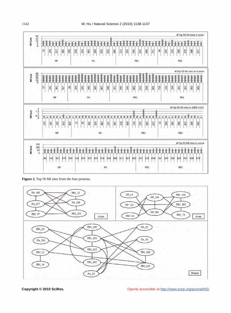
W. Hu / Natural Science 2 (2010) 1138-1147
Copyright © 2010 SciRes. http://www.scirp.org/journal/NS/
1142
Openly accessible at
Figure 2. Top 50 MI sites from the four proteins.

W. Hu / Natural Science 2 (2010) 1138-1147
Copyright © 2010 SciRes. http://www.scirp.org/journal/NS/
1141143
Figure 3. Networks of correlated sites from the four proteins that had high MI values (all with P value = 0).
Table 2. Top 30 MI site pairs from the four proteins (all with P value = 0).
Top 30 pairs in avian
(NP_14,NP_384) (NP_133,NP_149) (NP_133,NP_384) (NP_149,NP_384) (NP_149,PB1_293) (NP_149,PB1_636)
(NP_149,PB2_64) (NP_384,PB1_636) (NP_384,PB1_741) (NP_113,PB1_293) (NP_384,PB2_64) (PA_317,PA_388)
(PA_317,PA_463) (PA_317,PB1_97) (PA_317,PB1_212) (PA_317,PB1_225) (PA_388,PA_463) (PA_388,PB1_212)
(PA_388,PB1_255) (PA_463,PB1_212) (PA_463,PB1_255) (PA_531,PA_659) (PA_607,PB1_169) (PA_607,PB1_169)
(PB1_97,PB1_212) (PB1_97,PB1_255) (PB1_212,PB1_255) (PB1_293,PB1_636) (PB1_293,PB1_741) (PB1_709,PB2_478)
Top 30 pairs in human
(PA_324,PA_325) (PA_324,PB1_634) (PA_325,PA_580) (PA_325,PB1_612) (PA_325,PB1_634) (PA_536,PB1_612)
(PA_536,PB1_632) (PA_580,PB1_612) (PA_602,PB1_100) (PA_602,PB1_632) (PA_602,PB1_634) (PA_602,PB2_559)
(PB1_100,PB1_277) (PB1_100,PB1_634) (PB1_100,PB1_682) (PB1_161,PB1_632) (PB1_161,PB2_227) (PB1_293,PB1_612)
(PB1_293,PB1_643) (PB1_324,PB1_643) (PB1_545,PB1_632) (PB1_602,PB1_718) (PB1_602,PB2_682) (PB1_612,PB1_634)
(PB1_612,PB1_682) (PB1_632,PB1_634) (PB1_632,PB1_682) (PB1_632,PB2_227) (PB1_667,PB2_355) (PB1_718,PB2_682)
Top 30 pairs in 2009 H1N1
(NP_157,PA_89) (NP_181,PA_37) (NP_181,PA_525) (NP_353,PA_68) (NP_353,PB1_359) (PA_37,PA_525)
(PA_68,PB2_471) (PA_89,PB1_124) (PA_89,PB1_632) (PA_89,PB2_526) (PA_169,PB2_649) (PA_262,PB2_677)
(PA_483,PA_646) (PA_483,PB1_171) (PA_483,PB1_368) (PA_525,PB1_124) (PA_525,PB1_632) (PA_646,PB1_171)
(PA_646,PB1_622) (PA_646,PB2_368) (PB1_124,PB1_359) (PB1_124,PB1_632) (PB1_124,PB2_526) (PB1_171,PB1_622)
(PB1_171,PB2_368) (PB1_359,PB1_632) (PB1_359,PB2_526) (PB1_622,PB2_368) (PB1_632,PB2_526) (PB2_109,PB2_588)
Openly accessible at

W. Hu / Natural Science 2 (2010) 1138-1147
Copyright © 2010 SciRes. http://www.scirp.org/journal/NS/
1144
Top 30 pairs in swine
(NP_182,PA_120) (NP_361,NP_375) (NP_361,NP_430) (NP_375,PA_659) (PA_120,PA_580) (PA_120,PB1_92)
(PA_120,PB2_195) (PA_324,PA_401) (PA_324,PA_580) (PA_324,PB2_453) (PA_324,PB2_661) (PA_401,PA_580)
(PA_401,PA_659) (PA_401,PB2_661) (PA_531,PA_580) (PA_531,PA_659) (PA_531,PB2_66) (PA_580,PA_611)
(PA_580,PA_659) (PA_580,PB1_92) (PA_580,PB2_64) (PA_580,PB2_195) (PA_580,PB2_661) (PA_611,PB2_66)
(PB1_92,PB2_195) (PB2_184,PB2_243) (PB2_184,PB2_265) (PB2_243,PB2_265) (PB2_453,PB2_661) (PB2_475,PB2_627)
Table 3. Pearson correlation coefficients of the pair counts between different influenza species in Figures 4 and 5.
(Avian, Human) (Avian,2009 H1N1) (Avian, Swine) (Human,2009 H1N1) (Human, Swine) (2009 H1N1, Swine)
Averaged counts in proteins 0.986644 0.852749 0.974158 0.893431 0.977686 0.78265
Averaged counts in domains 0.63857 0.3873 0.8716 0.7614 0.3893 0.0976
PB2 in human and pandemic 2009 H1N1 viruses was weak, and therefore no such sites were included in this report.
3.3. Correlation within Each Individual Protein and between Proteins
The correlated residue pairs that had a positive MI value were counted according to their location in the four proteins (Figure 4). In general, the inter protein correlation from (NP, PA), (NP, PB1), (NP, PB2), (PA, PB1), (PA, PB2), (PB1, PB2) was stronger than the intra protein correlation (NP, NP), (PA, PA), (PB1, PB1) and (PB2, PB2), with (NP, NP) correlation being the weakest. Figure 4 also indicated that the correlation between PA and PB2 was the strongest in avian, human, and pan-
demic 2009 H1N1, and the correlations of PA and PB2, PA and PB1, and PB1 and PB2 were the strongest in swine. Similarly, Figure 5 showed that the correlation of nuclear localization signals (NLS) of PB2 was the strongest in avian, human, and pandemic 2009 H1N1, and the correlation of the RNA cap binding domain of PB2 was the strongest in swine. To further quantify the correlation of these four proteins, the averaged counts of positions in the functional domains of the four proteins that had a positive MI value with other positions were calculated, based on the domain boundary information given in [21] (Figure 5). Comprehensive phylogenetic analysis suggested that the genes of 2009 pandemic H1N1 were derived from avian (PB2 and PA), human H3N2 (PB1), classical swine (HA, NP and NS), and
Openly accessible at

W. Hu / Natural Science 2 (2010) 1138-1147
Copyright © 2010 SciRes. http://www.scirp.org/journal/NS/
1141145
Openly accessible at
Figure 4. Averaged correlated pair counts in each individual protein and between proteins.
Figure 5. Averaged counts of sites in the functional domains of the four proteins that had a positive MI value with other sites. Table 4. Sites from the four proteins of avian and swine influenza that had high MI values with PB2_627.
Avian Sites MI Rank P value Avian Sites MI Rank P value Swine Sites MI Rank P value
PA_258 163 0.0 PB1_667 332 0.0 PB2_485 21 0.0
PB2_451 207 0.0 NP_211 395 0.0 PB2_199 242 0.0
PA_626 210 0.0 PB2_339 396 0.0 PA_580 331 0.0
PA_596 220 0.0 NP_390 414 0.0 PA_401 338 0.0
PB1_292 226 0.0 PA_445 421 0.0 PA_314 364 0.0
NP_353 256 0.0 PB2_543 424 0.0 PB2_64 412 0.0
PB2_649 262 0.0 NP_178 428 0.0 PA_615 472 0.0
PB2_368 299 0.0 PB2_147 434 0.0 PA_324 473 0.0
PB1_632 307 0.0 PA_399 449 0.0
PB1_196 323 0.0 PB1_255 491 0.0
PB2_390 331 0.0
Eurasian avian-like swine H1N1 (NA and M) lineages [25]. With Pearson correlation coefficients (Table 4), both Figures 4 and 5 consistently illustrated that the correlation patterns of pandemic 2009 H1N1 were mo- re similar to those of avian and human influenza than to swine, thus offering a new insight into the interaction of the four proteins of the pandemic 2009 H1N1 virus when compared with avian, human, and swine influ-enza and how the origin of these four proteins might
contribute to the correlation patterns revealed in this analysis.
4. DISCUSSION
Development of our knowledge about the molecular mechanism of host range restriction and the adaptation of influenza viruses to a new host species remains a cen-tral topic in flu research. The four proteins NP, PA, PB1,
W. Hu / Natural Science 2 (2010) 1138-1147
Copyright © 2010 SciRes. http://www.scirp.org/journal/NS/
1146
Openly accessible at
and PB2 are crucial components in viral RNA synthesis, and are also implicated in host adaptation and patho-genicity. Therefore, clear revelation of the function and action of these four proteins is required. Sequence sur-vey implied that the common host shift markers in the proteins of avian or swine influenza are not present in the pandemic 2009 H1N1 virus. Moreover, introduction of known virulence markers into 2009 H1N1 does not increase its virulence [26,27]. The combination of its pandemic potential and absence of traditional host markers has remained a source for concern and justifies the search for its own host markers outside of the space of classical host markers [28,29].
The PB2 of 2009 H1N1 had a glutamic acid at posi-tion 627, reflecting its avian origin. Typically avian vi-ruses have a glutamic acid (E) at position 627, while human viruses usually have a lysine (K) at this position. Additionally, the presence of a glutamic acid at position 627 in PB2 contributed to the cold sensitivity of poly-merase derived from avian viruses in mammalian cells [3]. However, the clinical experience in 2009 demon-strated that this novel virus was able to transmit and rep-licate in humans efficiently. A natural assumption was that some amino acids at other sites in PB2 might be responsible for its efficiency in reproduction and trans-mission. It turned out that two amino acids, serine (S) at site 590 and arginine (R) at site 591, in PB2, termed SR polymorphism, compensate the lack of amino acid lysine at site 627 in PB2 [15].
Although our mutual information analysis illustrated the connectivity was low between PB2_627, PB2_591, PB2_590, and other sites in pandemic 2009 H1N1, this study discovered three sites correlating with PB2_590, which were NP_480 (MI = 0.0219, P value = 0.033, MI rank = 370), PB1_359 (MI = 0.0060, P value = 0.338, MI rank = 611), and PB1_124 (MI = 0.0011, P value = 0.0, MI rank = 1093). With the same approach, associa-tions with other critical sites such as PB2_701 and PB2_271 could also be detected.
Host range and virulence of influenza viruses are mul-tigenically determined through interactions between the proteins involved, which could be, in part, elucidated with identification of mutations and co-mutations that might confer increased pathogenicity or transmissibility. The absence of familiar host switch markers in 2009 H1N1 added a new dimension in this effort, and moti-vated the extensive search for other mutations or strate-gies that influenza viruses evolved to develop and adapt. To move this direction, this report revealed and quanti-fied the interactions of NP, PA, PB1, and PB2 of avian, human, pandemic 2009 H1N1, and swine influenza, and identified a collection of statistically significant co- varying sites, not only in each individual protein but also
between proteins, for further investigation of their inte-grative biological relevance experimentally.
5. ACKNOWLEDGEMENT
We thank Houghton College for its financial support.
REFERENCES
[1] Neumann, G., Brownlee, G.G., Fodor, E. and Kawaoka, Y. (2004) Orthomyxovirus replication, transcription, and polyadenylation. Curr Top Microbiol Immunol, 283, 121- 143.
[2] Ng, A.K., Zhang, H., Tan, K., et al. (2008) Structure of the influenza virus A H5N1 nucleoprotein: Implications for RNA binding, oligomerization, and vaccine design. The FASEB Journal, 22(10), 3638-3647.
[3] Jürgen, S., (2008) Influenza A virus polymerase: A de-terminant of host range and pathogenicity. In: Klenk H.D., Matrosovich M.N. and Stech J. Eds., Avian Influ-enza. Monogr Virol. Basel, Karger, 27, 187-194.
[4] Mishra, A.C., Cherian, S.S., Chakrabarti, A.K., et al. (2009) A unique influenza A (H5N1) virus causing a fo-cal poultry outbreak in 2007 in Manipur, India. Journal of Virology, 6(1), 26.
[5] Yuan, P.W., Bartlam, M., Lou, Z.Y., et al. (2009) Crystal structure of an avian influenza polymerase PAN reveals an endonuclease active site, Nature, 458, 909-913.
[6] Fodor, E., Crow, M., Mingay, L.J., et al. (2002) A single amino acid mutation in the PA subunit of the influenza virus RNA polymerase inhibits endonucleolytic cleavage of capped RNAs. Journal of Virology, 76(18), 8989-9001.
[7] Hara, K., Schmidt, F.I., Crow, M. and Brownlee, G.G. (2006) Amino acid residues in the N-terminal region of the PA subunit of influenza A virus RNA polymerase play a critical role in protein stability, endonuclease ac-tivity, cap binding, and virion RNA promoter binding. Journal of Virology, 80(16), 7789-7798.
[8] Kerry, P.S., Willsher, N. and Fodor, E. (2008) A cluster of conserved basic amino acids near the C-terminus of the PB1 subunit of the influenza virus RNA polymerase is involved in the regulation of viral transcription. Virology, 373(1), 202-210.
[9] Dias, A., Bouvier, D., Crépin, T., McCarthy, A.A., et al. (2009) The cap-snatching endonuclease of influenza vi-rus polymerase resides in the PA subunit. Nature, 458 (7240), 914-918.
[10] Rolling, T,, Koerner, I,, Zimmermann, P,, Holz, K,, et al. (2009) Adaptive mutations resulting in enhanced poly-merase activity contribute to high virulence of influenza A virus in mice. Journal of Virology, 83(13), 6673-6680.
[11] Bussey, K.A., Bousse, T.L., Desmet, E.A., Kim, B. and Takimoto, T. (2010) PB2 residue 271 plays a key role in enhanced polymerase activity of influenza A viruses in mammalian host cells. Journal of Virology, 84(9), 4395- 4406.
[12] Zhu, H., Wang, J., Wang, P., Song, W., Zheng, Z., Chen, R., Guo, K., Zhang, T., Peiris, J.S., Chen, H. and Guan, Y. (2010) Substitution of lysine at 627 position in PB2 pro-tein does not change virulence of the 2009 pandemic

W. Hu / Natural Science 2 (2010) 1138-1147
Copyright © 2010 SciRes. http://www.scirp.org/journal/NS/Openly accessible at
1141147
H1N1 virus in mice. Virology, 401(1), 1-5. [13] Gabriel, G., Herwig, A. and Klenk, H.D. (2008) Interac-
tion of polymerase subunit PB2 and NP with importin α1 is a determinant of host range of influenza A virus. PLoS Pathog, 4(2), e11
[14] Li, J., Ishaq, M., Prudence, M., et al. (2009) Single muta-tion at the amino acid position 627 of PB2 that leads to increased virulence of an H5N1 avian influenza virus during adaptation in mice can be compensated by multi-ple mutations at other sites of PB2. Virus Research, 144 (1-2), 123-129.
[15] Mehle, A., Doudna, J.A. (2009) Adaptive strategies of the influenza virus polymerase for replication in humans, Proceedings of the National Academy of Sciences, 106(50), 21312-21316.
[16] Liu, Y., Eyal, E. and Bahar, I. (2008) Analysis of corre-lated mutations in HIV-1 protease using spectral cluster-ing. Bioinformatics, 24(10), 1243-1250.
[17] Colman, P.M., Hoyne, P.A. and Lawrence, M.C. (1993) Sequence and structure alignment of paramyxovirus he-magglutinin-neuraminidase with influenza virus neura-minidase. Journal of Virology, 67, 2972-2980.
[18] Xia, Z., Jin, G.L., Zhu, J. and Zhou, R.H. (2009) Using a mutual information-based site transition network to map the genetic evolution of influenza A / H3N2 virus. Bioin-formatics, 25(18), 2309-2317.
[19] Huang, J.-W., King, C.-C. and Yang, J.-M. (2009) Co- evolution positions and rules for antigenic variants of human influenza A / H3N2 viruses. BMC Bioinformatics, 10, S41.
[20] Du, X.J., Wang, Z., Wu, A.P., et al. (2008) Networks of genomic co-occurrence capture characteristics of human
influenza A (H3N2) evolution. Genome Research, 18, 178-187.
[21] Miotto, O., Heiny, A.T., Albrecht, R., García-Sastre, A., et al. (2010) Complete-proteome mapping of human in-fluenza A adaptive mutations: Implications for human transmissibility of zoonotic strains, PLoS One, 5(2), e9025
[22] Katoh, K., Kuma, K., Toh, H. and Miyata, T. (2005) MAFFT version 5: Improvement in accuracy of multiple sequence alignment. Nucleic Acids Research, 33, 511-518.
[23] Cover, T.A. and Thomas, J.A. (1991) Elements of infor-mation theory. John Wiley and Sons, New York.
[24] MacKay, D. (2003) Information theory, inference, and learning algorithms. Cambridge University Press.
[25] Smith, G.J.D., Vijaykrishna, D., et al. (2009) Origins and evolutionary genomics of the 2009 swine-origin H1N1 influenza A epidemic, Nature,459, 1122-1125.
[26] Jagger, B.W., Memoli, M.J., Sheng, Z.-M., et al. (2010) The PB2-E627K mutation attenuates viruses containing the 2009 H1N1 influenza pandemic polymerase. mBio 1 (1), e00067-10.
[27] Herfst, S., Chutinimitkul, S., Ye, J.Q., et al. (2010) In-troduction of virulence markers in PB2 of pandemic swine-origin influenza virus does not result in enhanced virulence or transmission, Journal of Virology, 84(8), 3752-3758.
[28] Hu, W. (2010) Novel host markers in the 2009 pandemic H1N1 influenza A virus. Journal of Biomedical Science and Engineering, 3(6), 584-601
[29] Hu, W. (2010) Nucleotide host markers in the influenza a viruses. Journal of Biomedical Science and Engineering, 3, 684-699.

Vol.2, No.10, 1148-1154 (2010)doi:10.4236/ns.2010.210142
Copyright © 2010 SciRes. http://www.scirp.org/journal/NS/
Natural Science
Openly accessible at
Effect of abiotic factors on the molluscicidal activity of oleoresin of Zingiber officinale against the snail Lymnaea acuminata
Vijya Singh, Pradeep Kumar, V. K. Singh, D. K. Singh
Malacology Laboratory, Department of Zoology, D. D. U., Gorakhpur University, Gorakhpur, India; [email protected].
Received 28 April 2010; revised 30 May 2010; accepted 3 June 2010.
ABSTRACT
Earlier it has been observed that oleoresin of Zingiber officinale is a potent molluscicide ag- ainst Lymnaea acuminata. This snail is the vector of Fasciola species, which cause ende- mic fascioliasis in eastern Uttar Pradesh. As this snail breeds and maintain their population constant through out the year, so that the pre-sent study has been designed to find out the effect of variations in some environmental fac-tors in different seasons, on the molluscicidal activity of oleoresin of Zingiber officinale and its relative effect on certain enzymes viz., acetyl-cholinesterase, acid and alkaline phosphatases in the nervous tissue of the snail Lymnaea acuminata. In this study temperature, pH, dis-solve oxygen, free carbon dioxide, conductivity of the water in control, as well as molluscicide treated water, was measured simultaneously. LC50 value of oleoresin was determined in each month of the year. Toxicity of oleoresin in June-July (24 h LC50 16.54-14.28 mgL-1) is high-est. Acetylcholinesterase, acid and alkaline phosphatases activity in the nervous tissue of the snails treated with sub-lethal concentration of oleoresin was simultaneously measured. Sig- nificant positive rank correlation, in between the acetylcholinesterase or acid phosphatase activ-ity and LC50 of oleoresin was observed. The pre- sent study conclusively shows that variant abi- otic factors can significantly alter the toxicity of oleoresin of Z. officinale in L. acuminata. The most suitable period for control of L. acuminata is June-July.
Keywords: Environmental factors; Acetylcholinesterase; Oleoresin; Temperature; pH
1. INTRODUCTION
It has been reported that, oleoresin of Zingiber offici-nale is a potent molluscicide [1,2]. Fresh water snail Lymnaea acuminata is the intermediate host of liver fluke Fasciola gigantica, causing an endemic fascio-liasis in the cattle population of eastern region of the state of Uttar Pradesh in India [3,4]. An effective method to reduce the incidence of fascioliasis is to control the population of vector snails and, thereby, break the life cycle of these flukes [5-8]. Earlier studies have shown that oleoresin of Zingiber officinale has a powerful mol-luscicidal action on the snail L. acuminate [1,2]. It has also been conclusively shown that acetylcholinesterase (AChE), acid and alkaline phosphatase (ACP and ALP) in the nervous tissue of L. acuminata are very sensitive parameters influenced by molluscicides [7-10]. The aim of the present study was to explore the possibility whether seasonal changes in abiotic factors, viz tem-perature, pH, dissolved oxygen and carbon dioxide, and conductivity of test water can influence the level of AChE, ACP and ALP assayed in each month of the year 2006-2007 following exposure to sublethal concentra-tions (40% and 80%) of 24 h LC50 of oleoresin of Z. off cinale. i
2. MATERIALS AND METHODS
2.1. Test Materials
Oleoresin was obtained by extraction of prepared dried rhizomes of Z. officinale with alcohol. The re-moval of the solvent under vacuum yields oleoresin of Z. officinale [1,11]. Temperature, pH and conductivity of water were measured by thermometer and digital pH and conductivity meters, respectively. Dissolved O2 and CO2 were estimated according to the methods prescribe by APHA [12].

V. Singh et al. / Natural Science 2 (2010) 1148-1154
Copyright © 2010 SciRes. http://www.scirp.org/journal/NS/Openly accessible at
1141149
2.2. Bioassays for LC50
Adult L. acuminata (length 2.25 ± 0.2 cm) were col-lected from Ramgarh Lake, located in almost adjacent to this university campus. Snails were acclimatized in de-chlorinated tap water for 72 h. The snails were ex-posed to different concentrations of oleoresin in glass aquaria containing 3 litres of de-chlorinated water. Ten experimental animals were kept in each aquarium. Con-trol animals were kept in equal volumes of de-chlorin-ated tap water under similar conditions. Mortality of snails was observed after 24, 48, 72, 96 h. No response to a needle probe was taken as evidence of death. Dis-solved O2, CO2 and conductivity, temperature and pH of treated and control group of water was measured simul-taneously with toxicity test at every 24 h of period to 96. Bioassays for the determination of LC50 value was per-formed in each month of the year. Lethal concentration (LC50) values, lower and upper confidence limits (LCL and UCL) and slopes value were calculated by the method of POLO computer program of Robertson et al. [13]. The Product moment correlation coefficient was determined between LC50 and temperature / pH / con-ductivity / dissolved O2 / CO2, of water in each of the twelve months in order to observe any significant corre-lation according to the method of Sokal and Rohlf [14].
2.3. Enzyme Assays
Twenty snails, kept in glass aquaria containing 5 litres of dechlorinated water, were exposed to 40% and 80% of 24 h LC50 of oleoresin in each month. Six such aquaria were set up for each concentration. After 24 h treatment, the snails were washed with water and the nervous tissue was dissected out from the buccal mass for the measurement of enzyme AChE, ACP and ALP activities.
2.3.1. Acetylcholinesterase Acetylcholinesterase (AChE) activity was measured
according to the method of Ellman et al. [15] as modi-fied by Singh et al. [16]. Fifty mg of nervous tissue was homogenized in 1.0 ml of 0.1 M phosphate buffer pH 8.0 for 5 minute in an ice bath and centrifuged at 1000 g for 30 minute at 4°C. Supernatant was used as enzyme source. The change in optical density at 412 nm was recorded for 3 minute after every 30 second interval. Enzyme activity was expressed as µ mol “SH” hydro-lyzed / min / mg protein.
2.3.2. Phosphatases Acid (ACP) and alkaline (ALP) phosphatases activi-
ties were measured by the method of Bergmeyer [17] as modified by Singh and Agarwal [18]. Tissue homogenate (2% w/v) was prepared in ice cold 0.9 % NaCl and cen-trifuged at 5000 g for 20 minute at 4°C. The 4-nitro-
phenyl phosphate disodium was used as substrate. The acid (ACP) and alkaline phosphatases (ALP) activity has been expressed as µmole substrate hydrolyzed /30 min/ mg protein.
2.3.3. Protein Estimation Protein was estimated by the method of Lowry et al.
[19].
2.4. Statistical Analysis
Results have been expressed as mean ± SE of six rep-licates. Rank correlation was applied in between control
and corresponding changes in the enzyme activity in different months of the year [14].
3. RESULTS
There was a significant (P < 0.05) time dependent variation in the toxicity of oleoresin Z. officinale in dif-ferent months of the year against L. acuminata (Table 1); highest toxicity was observed in months of June and July (24 h LC50 14.28-16.54 mgL-1) and lowest (24 h LC50 124.09-126.27 mgL-1) during January and February. A significant positive correlation (r = 0.89; P = 0.001) be-tween LC50 and water pH was noted for each month and at each interval of 24 h exposure (Table 1). A similar finding between LC50 and dissolved O2 (r = 0.82; P = 0.001) was found. Contrastively, significant negative correlation between LC50 and dissolved CO2 (r = 0.86; P = 0.001) and with water temperature (r = 0.91; P = 0.001) was noted. No marked correlation was observed between the LC50 and conductivity of water. High temperature (36 °C), and free CO2 (30.0 ppm), low pH (7.11) and dis-solved oxygen (1.0 ppm) increases the toxicity of oleo-resin against L. acuminata. The slope values were steep and separate estimations of LC50 based on each of the six replicates were found to be with in the 95% confidence limits of LC50. The t-ratio is greater than 1.96 and the heterogeneity factor is less than 1.0. The g value was less than 0.5 at all probability levels.
There was significant positive rank correlation (τ = 0.666; P = 0.02 - 40% of 24 h LC50,, τ = 0.636 P= 0.02 - 80% of 24 h LC50,) between LC50 of different months and corresponding anti AChE activity in the sub-lethal treatment (40% and 80% of 24 h LC50) of nervous tissue of snail L. acuminata. Maximum inhibition in AChE activity (56.09% of control) was observed in snails ex-posed to 80% of 24 h LC50 of oleoresin in month of July (Table 2). There was no significant positive rank corre-lation between LC50 of different months and alkaline phosphatase activity in the sub-lethal treatment (40% and 80% of 24 h LC50) of nervous tissue of snail L. acu-minata (Table 3). Like AChE, there was significant posi-tive rank correlation between LC50 and acid phosphatas
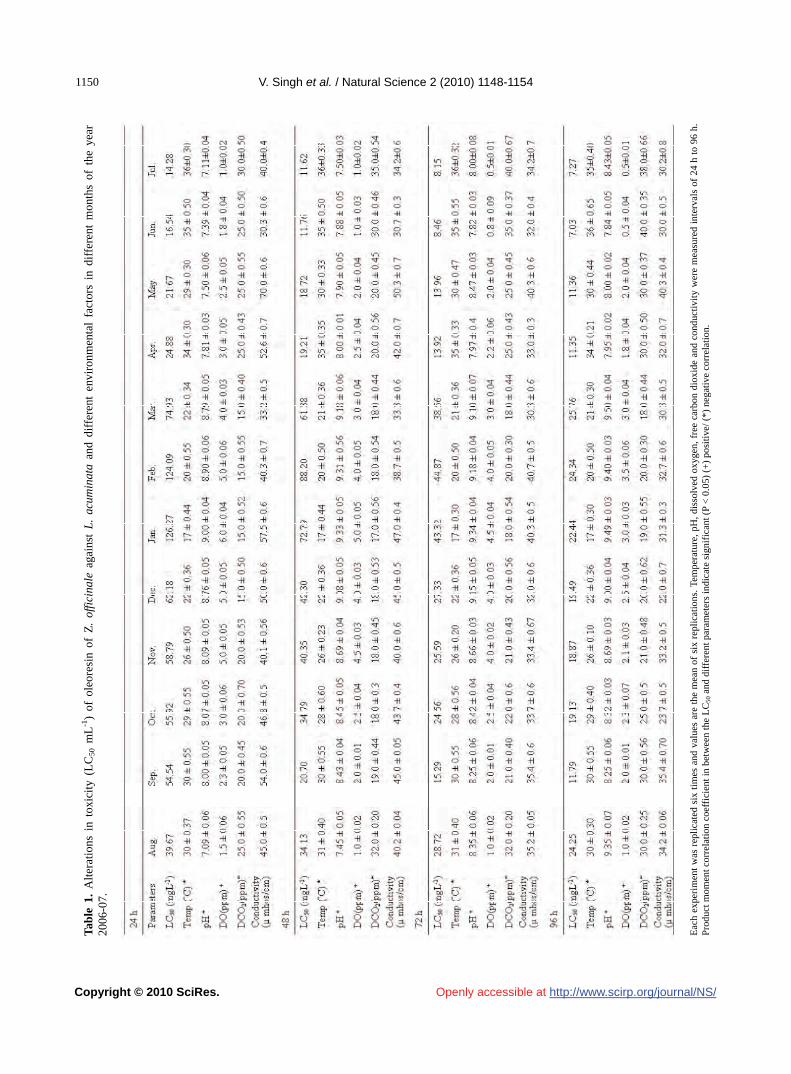
V. Singh et al. / Natural Science 2 (2010) 1148-1154
Copyright © 2010 SciRes. http://www.scirp.org/journal/NS/
1150
Eac
h ex
peri
men
t w
as r
epli
cate
d si
x ti
mes
and
val
ues
are
the
mea
n of
six
rep
lica
tion
s. T
empe
ratu
re, p
H, d
isso
lved
oxy
gen,
fre
e ca
rbon
dio
xide
and
con
duct
ivit
y w
ere
mea
sure
d in
terv
als
of 2
4 h
to 9
6 h.
Pro
duct
mom
ent c
orre
lati
on c
oeff
icie
nt in
bet
wee
n th
e L
C50
and
dif
fere
nt p
aram
eter
s in
dica
te s
igni
fica
nt (
P <
0.0
5) (
+)
posi
tive/
(*)
neg
ativ
e co
rrel
atio
n.
Tab
le 1
. A
ltera
tion
s in
tox
icit
y (L
C50
mL
-1)
of o
leor
esin
of
Z.
offi
cina
le a
gain
st L
. ac
umin
ata
and
diff
eren
t en
viro
nmen
tal
fact
ors
in d
iffe
rent
mon
ths
of t
he y
ear
2006
-07.
Openly accessible at

V. Singh et al. / Natural Science 2 (2010) 1148-1154
Copyright © 2010 SciRes. http://www.scirp.org/journal/NS/Openly accessible at
1151151
Table 2. Effect of 24 h exposure of 40% and 80% of 24 h LC50 of oleoresin of Z. officinale in different months of the year 2006-07 on acetylcholinesterase activity in the nervous tissue of L. acuminata.
Months 24 h LC50 mgL-1 AChE-µ mole “SH” hydrolyzed / min / mg protein
Control a 40% of 24h LC50 80% of 24h LC50
August 39.67 0.093 ± 0.01 (100)
0.091 ± 0.01 (97.84)
0.088 ± 0.01 (94.62)
September 54.54 0.139 ± 0.01 (100)
0.136 ± 0.01 (97.84)
0.132 ± 0.01 (94.96)
October 55.92 0.101 ± 0.02 (100)
0.099 ± 0.01 (98.02)
0.097 ± 0.02 (96.04)
November 58.79 0.106 ± 0.01 (100)
0.103 ± 0.02 (97.17)
0.101 ± 0.01 (95.28)
December 62.18 0.109 ± 0.00 (100)
0.107 ± 0.01 (98.17)
0.105 ± 0.01 (96.33)
January 126.27 0.190 ± 0.00 (100)
0.189 ± 0.01 (99.47)
0.186 ± 0.01 (97.89)
February 124.09 0.176 ± 0.01 (100)
0.175 ± 0.00 (99.43)
0.171 ± 0.00 (97.16)
March 74.93 0.147 ± 0.02 (100)
0.142 ± 0.01 (96.60)
0.134 ± 0.01 (91.16)
April 24.88 0.141 ± 0.02 (100)
0.137 ± 0.01 (93.66)
0.133 ± 0.01 (84.51)
May 21.67 0.104 ± 0.01 (100)
0.101 ± 0.02 (75.92)
0.099 ± 0.03 (70.37)
June 16.54 0.087 ± 0.03 (100)
0.083 ± 0.02 (62.19)
0.074 ± 0.02 (59.75)
July 14.28 0.082 ± 0.02 (100)
0.073 ± 0.01 (63.41)
0.071 ± 0.01 (56.09)
Values are mean ± SE of six replicates. Value in parenthesis indicates % enzyme activity with untreated control taken as 100%. Rank correlation coefficient in between LC50 and AChE activity in treated group indicate significant (P < 0.05) positive (+) correlation. a, Significant (P < 0.05) when one way of ANOVA was applied in between the enzyme activity in different months of the year in control group without treatment. Table 3. Effect of 24 h exposure of 40% and 80% of 24 h LC50 of oleoresin of Z. officinale in different months of the year 2006-07 on alkaline phosphatase activity in the nervous tissue of L. acuminata.
Months 24 h LC50 mgL-1 ALP-µ moles/ 30 min / mg protein
Control 40% of 24 h LC50 80% of 24 h LC50
August 39.67 2.27 ± 0.01 (100)
2.17 ± 0.01 (95.59)
2.14 ± 0.01 (94.27)
September 54.54 3.34 ± 0.01 (100)
3.31 ± 0.01 (99.10)
3.27 ± 0.01 (97.90)
October 55.92 3.27 ± 0.01 (100)
3.23 ± 0.02 (98.77)
3.19 ± 0.02 (97.55)
November 58.79 3.36 ± 0.02 (100)
3.32 ± 0.02 (98.80)
3.27 ± 0.00 (97.32)
December 62.18 3.11 ± 0.00 (100)
3.06 ± 0.02 (98.39)
3.02 ± 0.02 (97.10)
January 126.27 2.89 ± 0.01 (100)
2.85 ± 0.00 (98.62)
2.81 ± 0.01 (97.23)
February 124.09 3.07 ± 0.01 (100)
3.02 ± 0.01 (98.37)
2.98 ± 0.01 (97.06)
March 74.93 3.10 ± 0.00 (100)
3.07 ± 0.00 (99.03)
3.02 ± 0.01 (97.41)
April 24.88 3.45 ± 0.01 (100)
3.42 ± 0.02 (99.13)
3.37 ± 0.02 (97.68)
May 21.67 2.94 ± 0.02 (100)
2.89 ± 0.00 (98.29)
2.86 ± 0.03 (97.28)
June 16.54 1.86 ± 0.03 (100)
1.74 ± 0.02 (93.55)
1.64 ± 0.02 (88.17)
July 14.28 2.36 ± 0.01 (100)
2.23 ± 0.01 (94.49)
2.16 ± 0.02 (91.52)
Values are mean ± SE of six replicates. Value in parenthesis indicates % enzyme activity with untreated control taken as 100%. Rank correlation coefficient in between LC50 and ALP activity in treated group indicate non significant (P < 0.05) positive correlation. a, Significant (P < 0.05) when one way of ANOVA was pplied in between the enzyme activity in different months of the year in control group without treatment. a

V. Singh et al. / Natural Science 2 (2010) 1148-1154
Copyright © 2010 SciRes. http://www.scirp.org/journal/NS/Openly accessible at
1152
(ACP) (τ = 0.606; P= 0.05 - 40% of 24 h LC50, τ = 0.606; P = 0.05 - 80% of 24 h LC50,) activity in the nervous tissue of L. acuminata exposed to sub-lethal treatments of oleoresin in different months. Maximum inhibition in ACP activity (91.00% of control) was observed in snails exposed to 80% of 24 h LC50 in July (Table 4).
4. DISCUSSION
It is clear from result section that toxicity of oleoresin varies with changes in abiotic environmental factors in the water. Effect of abiotic variants in aquatic environ-ment i.e. pH [20], Temperature [21] on the toxicity of different pesticides have been reported. The temperature of water is a significant factor, which alters the toxicity of oleoresin in each month of the year. When the water temperature is higher in summer season June-July, the toxicity of oleoresin is maximum. Contrarily, in winter season, the temperature of water is low and toxicity of oleoresin is less as evident by higher LC50 value. Tem-perature of environment in which the animal resides is a crucial factor, when toxicity of pesticides is determined [22-25]. Osterauer and Kohler [26] reported that the tox-icity of diazinon against zebra fish strongly increased at elevated temperature. Dissolved oxygen is also one of the factors, which alter the toxicity of oleo- resin. Water in winter season holds more oxygen [27]
and as a result, less mortality of snails occurs during this period. At higher water temperature dissolved oxygen concentration decreases which is reflected by higher mortality of the snails. Dissolved oxygen is one of the major components, which is required by snails during metabolic activity [28,29]. Consequently, at higher tem-perature, increasing rate of metabolism in snail body may release more CO2, which affects the pH of water [30,31] As the time duration increases concentration of CO2 increases in the water (released by snails) and it also affects the pH of water. Murphy [32] reported that pesti-cides belonging to organophosphate and carbamate groups are very sensitive to change in pH. Earlier Vas-concellos [33] observed the influence of pH variation on the molluscicidal activity of Euphorbia splendens latex. According to them molluscicidal activity was maximum at pH 5.0 - 6.0 and minimum at pH 7.0 - 8.0. Toxicity of oleoresin is highest at high temperature, CO2 of water as well as low pH, dissolved O2 of water. The low concen-tration of dissolved O2 act as physical stressor on aquatic animals [34] and in the absence of sufficient dissolved O2; the snails appear to become more sensitive against the molluscicide. The pungent moieties of oleoresin are gingerol, zingirone and shogaol [35]. It is conceivable that, the active molluscicidal component, present in the oleoresin might get converted into a more toxic form in
Table 4. Effect of 24h exposure of 40% and 80% of 24h LC50 of oleoresin of Z. officinale in different months of the year 2006-07 on acid phosphatase activity in the nervous tissue of L. acuminata.
Months 24 h LC50 mgL-1 ACP-µ moles/ 30min / mg protein
Control 40% of 24 h LC50 80% of 24 h LC50-
August 39.67 3.15 ± 0.00
(100) 3.04 ± 0.01
(95.51) 2.91 ± 0.01
(92.38)
September 54.54 3.64 ± 0.01
(100) 3.58 ± 0.01
(98.35) 3.52 ± 0.01
(96.70)
October 55.92 3.31 ± 0.01
(100) 3.29 ± 0.01
(99.40) 3.24 ± 0.00
(97.89)
November 58.79 3.34 ± 0.02
(100) 3.32 ± 0.02
(99.40) 3.28 ± 0.01
(98.20)
December 62.18 3.28 ± 0.01
(100) 3.23 ± 0.01
(98.48) 3.19 ± 0.01
(97.26)
January 126.27 3.29 ± 0.01
(100) 3.27 ± 0.00
(99.70) 3.21 ± 0.02
(97.87)
February 124.09 3.40 ± 0.00
(100) 3.39 ± 0.01
(99.70) 3.33 ± 0.01
(97.94)
March 74.93 3.46 ± 0.01
(100) 3.40 ± 0.00
(98.27) 3.34 ± 0.01
(96.53)
April 24.88 3.26 ± 0.01
(100) 3.19 ± 0.01
(97.85) 3.09 ± 0.02
(94.79)
May 21.67 3.45 ± 0.02
(100) 3.38 ± 0.02
(97.97) 3.31 ± 0.02
(95.94)
June 16.54 2.95 ± 0.03
(100) 2.86 ± 0.01
(96.95) 2.72 ± 0.03
(92.20)
July 14.28 3.00 ± 0.01
(100) 2.82 ± 0.01
(94.00) 2.73 ± 0.01
(91.00)
Values are mean ± SE of six replicates. Value in parenthesis indicates % enzyme activity with untreated control taken as 100%. Rank correlation coefficient in between LC50 and ACP activity in treated group indicate significant (P < 0.05) positive (+) correlation. a, Significant (P < 0.05) when one way of ANOVA was pplied in between the enzyme activity in different months of the year in control group without treatment. a

V. Singh et al. / Natural Science 2 (2010) 1148-1154
Copyright © 2010 SciRes. http://www.scirp.org/journal/NS/
1151153
Openly accessible at
the aquarium water or in the snail body due to variant environmental factors in the month of June and July. Earlier, it has been shown that the treatment of oleoresin of Z. officinale caused significant inhibition of AChE, ALP and ACP activity in the nervous tissue of L. acu-minata [9]. The high anti AChE and ACP activity of oleoresin of Z. officinale was observed in months of June-July. The enzyme ALP plays a critical role in pro-tein synthesis, [36] and secretary activity, [37] is com-paratively less inhibited than AChE, Acid phosphatase (ACP), a lysosomal enzyme, [38] plays an important role in autolysis and phagocytosis, pathological necrosis, and overall catabolism, [8,10,39] was reduced significantly. Earlier, it has been observed that increased activity of ACP causes breakdown of existing protein in L. acumi-nata [18], but inhibition of ACP activity in this study indicates that it is not used in breakdown of cellular pro-tein. The rank correlation coefficient applied between the LC50 values of different months and the correspond-ing inhibition in enzyme activity, point out a positive correlation between the LC50 and the inhibition of AChE and ACP. Whereas there was no correlation in between LC50 and ALP activity indicate that ALP is not altered by action of oleoresin in different months.
Accurate prediction of molluscicide fate and toxicity in aqueous environment against snails are hindered due to lack of information that how abiotic factors of aque-ous environment affect the biological activity and related toxicity of molluscicides. Abiotic factors are not only correlated with the lethality of molluscicide, but with each other also. The present study conclusively shows that variant abiotic factors can significantly alter the toxicity of oleoresin of Z. officinale in L. acuminata. It is also obvious that the most suitable period for the control of this snail in India is the month of June, July. It is sug-gested that the treatment of a water body with oleoresin of Z. officinale for the control of L. acuminata and ulti-mately fascioliasis, is not only more potent and cost ef-fective during these months than spending more money by using higher concentrations of this molluscicide dur-ing the rest ten months of the year.
REFERENCES
[1] Singh, S., Singh, V.K. and Singh, D.K. (1997) Mollus-cicidal activity of some common spice plants. Biology, Agriculture and Horticulture, 14, 237-249.
[2] Shukla, S., Singh, V.K. and Singh, D.K. (2006) The ef-fect of single, binary, tertiary, combination of few plant derived molluscicides alone or in combination with syn-ergist on different enzymes in the nervous tissues of the freshwater snail Lymnaea (Radix) acuminata (Lamark). Pesticide Biochemistry and Physiology, 85, 167-173.
[3] Singh, O. and Agarwal, R.A. (1981) Toxicity of certain
pesticides to two economic species of snails in northern India. Journal of Economic Entomology, 74, 568-571.
[4] World Health Organization. (2006) Report of the WHO informal meeting on use of triclabendazole in fascioliasis control, WHO headquarters, Geneva, Switzerland, 17-18 October 2006.
[5] Singh, P., Singh, V.K. and Singh, D.K. (2005) Effect of binary combination of some plant-derived molluscicides with MGK-264 or piperonyl butoxide on the reproduc-tion of the snail Lymnaea acuminata. Pest Management Science, 61, 204-208.
[6] Kumar, P. and Singh, D.K. (2006) Molluscicidal activity of Ferula asafoetida, Syzygium aromaticum and Carum carvi and their active components against the snail Lym-naea acuminata. Chemo 63, 1568-1574.
[7] Kumar, P., Singh, V.K. and Singh, D.K. (2009) Kinetics of enzyme inhibition by active molluscicidal agents fer-ulic acid, umbelliferone, eugenol and limonene in the nervous tissue of snail Lymnaea acuminata. Physiologi-cal Research, 23, 172-177.
[8] Jaiswal, P., Singh, V.K. and Singh, D.K. (2008) Enzyme inhibition by molluscicidal component of Areca catechu and Carica papaya in the nervous tissue of vector snail Lymnaea acuminata. Pesticide Biochemistry and Physiol-ogy, 92, 164-168.
[9] Singh, K. and Singh, D.K. (2000) Toxicity to the snail Lymnaea acuminata of plant-derived molluscicides in combination with synergists. Pest Management Science, 56, 889-898.
[10] Tripathi, S.M., Singh, V.K., Singh, S. and Singh, D.K. (2004) Enzyme inhibition by the molluscicidal agent Pu-nica granatum Linn. bark and Canna indica Linn. root. Physiological Research, 18, 501-506.
[11] Gunther, E. (1975) The essential oils. Robert, E Krieger Publishing Company, NewYork.
[12] American Public Health Association (APHA), (2005) Standard methods for the examination of water and waste water. 21st Edition, Washington, D.C.
[13] Robertson, J.L., Russell, R.M., Preisler, H.K. and Savin, N.E. (2007) Bioassay with Arthropods POLO computer programme for analysis of bioassay data. 2nd Edition, Talor and Francis, CRC Press, 1-224.
[14] Sokal, R.R. and Rohlf, F.J. (1973) Introduction to biosta-tistics. W. H. Freeman & Co., Ltd., San Francisco.
[15] Ellman, G.L., Courtney, K.D., Andres, V. and Feather-stone, R.M. (1961) A new and rapid colorimetric deter-mination of acetylcholinesterase activity. Bio Pharmacol, 7, 88-95.
[16] Singh, D.K., Singh, O. and Agarwal, R.A. (1982) Com-parative study of cholinesterase in two snails. Pila glo-bosa and Lymnaea acuminata. The Journal of Physiology, 78, 467-472.
[17] Bergmeyer, U.H. (1967) Methods of enzymatic analysis. Academic Press, New York, 1129.
[18] Singh, D.K. and Agarwal, R.A. (1989) Toxicity of pi- peronyl butoxide carbaryl synergism on the snail Lym-naea acuminata. Internationale Revue der gesamten Hy-drobiologie und Hydrographie, 74, 689-699.
[19] Lowry, O.H., Rosebrough, N.J., Farr, A.L. and Randall R.J. (1951) Protein measurement with folin phenol rea- gent. The Journal of Biological Chemistry, 193, 265- 275.
[20] Watson, S.J. and Maly, E.J. (1987) Thiocyanate toxicity
V. Singh et al. / Natural Science 2 (2010) 1148-1154
Copyright © 2010 SciRes. http://www.scirp.org/journal/NS/Openly accessible at
1154
to Daphina magna: Modified by pH and temperature. Aqua- tic Toxicol, 10, 1-8.
[21] Sogorb, A., Andreu-Moliner, E.S., Almar, M.M., del Ramo, J. and Nunez, A. (1988) Temperature-toxicity re-lationship of fluvalinate (synthetic pyrethroid) on Pro-cambarus clarkia (Girard) under laboratory conditions. Bull Environ Cantam Toxicol, 40, 13-17.
[22] Schott, J.G. and Georghion, G.P. (1984) Influence of tem-perature on knockdown, toxicity and resistance to pyre-throids in the house fly, Musca domestica. Pesticide Biochemistry and Physiology, 21, 53-62.
[23] Ferrando, M.D., Andreu-Moliner, E.S., Almar, M.M., Ce- rebrian, C. and Nunez, A. (1987) Acute toxicity of or-ganochlorine pesticides to the European eel, Anguilla anguilla. The dependency on exposure time and tem-perature. Bulletin of Environmental Contamination and Toxicology, 39, 365-369.
[24] Schott, J.G. (1995) Effects of temperature on insecticides toxicity. In: Roe, R.M. and Kuhr, R.J. Eds., Reviews in Pesticide Toxicology, North Carolina State University, Ra- leigh, 111-135.
[25] Young, C. (1996) Metal chelates as stomach poison mol-luscicides for introduced pests, Helix aspersa, Theba pisana, Cernuella virgata and Deroceras reticulatum in Australia. In: Henderson, I.F. Ed., Slug and Snail Pests in Agriculture. British Crop Protection Council, Farnham, 237-243.
[26] Osterauer, R. and Kohler, H.R. (2008) Temperature-de- pendent effects of the pesticides thiacloprid and diazinon on the embryonic development of zebra fish (Danio re-rio). Aquatic Toxicol, 86, 485-494.
[27] Waterwatch Australia. (2002) National Technical Manual. Module 4: Physical and chemical parameters. Waterwat- ch Australia Steering Committee Environment Australia, http://www.waterwatch.org.au
[28] Ishak, M.M. and Mohamed, A.M. (1975) Effect of sub-lethal doses of copper sulphate and bayluscide on sur-vival and oxygen consumption of the snail Biomphalaria alexandrina. Hydrobiol, 47, 499-512.
[29] Watten, B.J. (2004) Method and apparatus for control of aquatic vertebrate and invertebrate invasive species. US Patent No. 6821442, 23 November 2004.
[30] Toews, K.L., Shroll, R.M., Wai, C.M. and Smart, N.G.
(1995) pH – Defining equilibrium between water and supercritical CO2– influence on SFE of organics and metal chelates. Analytical Chemistry, 67, 4040-4043.
[31] Berge, J.A., Bjerkeng, B., Pettersen, O., Schaanning, M.T. and Oxnevad, S. (2006) Effects of increased sea water concentrations of CO2 on growth of the bivalve Mytilus edulis L. Chemo, 62, 681-687.
[32] Murphy, G. (2004) Water pH and its Effect on Pesticides. Ministry of Agriculture and Food Ontario, Canada. http://www.gov.on.ca/OMAFRA/english/crops/hort/news/grower/2004/08gn04a1.htm
[33] Vasconcellos, M.C. and Amorim, A. (2003) Molluscici- dal action of the latex of Euphorbia splendens var. his-lopii NEB (Christ Crown) (Euphorbiaceae) against Lym-naea columella (Say, 1817) (Pulmonata; Lymnaeidae), Intermediate host of Fasciola hepatica (Linn. 1758) (Trematode: Fasciolidae). 1-Test in laboratory. Mem Inst Oswaldo Cruz, Rio de Janeiro, 98, 557-563.
[34] Irving, E.C., Lowell, R.B., Culp, J.M., Liber, K., Xie, Q. and Kerrich, R. (2008) Effects of arsenic speciation and low dissolved oxygen condition on the toxicity of the ar-senic to a lotic Mayfly. Environmental Toxicology & Chemistry, 27, 593-590.
[35] Mustafa, T., Srivastava, K.C. and Jensen, K.B. (1993) Drug development report (9) Pharmacology of ginger Zingiber officinale. Journal of Drug Development, 6, 25- 39.
[36] Pilo, B., Asnani, M.B. and Shah, R.V. (1972) Studies on wound healing and repair in pigeon liver III. Histo-chemical studies on acid and alkaline phosphatase activ-ity during the process. J Ani Mor Phy, 19, 205-212.
[37] Ibrahim, A.M., Migazi, M.G. and Dexian, E.S. (1974) Histochemical localization of alkaline phosphatase activ-ity in the alimentary tract of the snail Marisa coruarielis (1). Bul Zoo Soc Egy, 26, 95-105.
[38] Aruna, P., Chetty, C.S., Naidu, R.C. and Swami, K.S. (1979) Acid phosphatase activity in the Indian apple snail Pila globosa (Swainsen) during aestivation and starva-tion stress. Proceedings of Indian Academy Science (In-dia), 88, 363-365.
[39] Abou-Donia, M.B., (1978) Increased acid phosphatase activity in hens following oral dose of Leptophos. Toxi-cology Letters, 2, 199-203.
Vol.2, No.10, 1155-1163 (2010)doi:10.4236/ns.2010.210143
Copyright © 2010 SciRes. http://www.scirp.org/journal/NS/
Natural Science
Openly accessible at
Distribution of polychaetes in the shallow, sublittoral zone of Admiralty Bay, King George Island, Antarctica in the early and late austral summer
Letícia de Souza Barbosa1, Abílio Soares-Gomes1, Paulo Cesar Paiva2* 1Department of Marine Biology, Fluminense Federal University, Niterói, Brazil; [email protected]; [email protected]; 2Department of Zoology, Federal University of Rio de Janeiro, Rio de Janeiro, Brazil; *Corresponding Author: [email protected].
Received 20 July 2010; revised 25 August 2010; accepted 28 August 2010.
ABSTRACT
This study assessed the spatial distribution pa- ttern of soft-sediment polychaetes on the near-shore of Admiralty Bay, King George Island, Antarctica. In the early and late summer of 2003 /04, seven sites at three different depths (20,30 and 60 meters) were sampled using a van Veen grab. 8,668 individuals all told, belonging to 67 species and 23 families, were identified. The families Terebellidae, Syllidae and Maldanidae were the most speciose. Mean densities ranged from 45.2 to 388.1 ind. 0.1 m-2 in the early sum-mer, and from 29 to 183 ind.0.1m-2 in the late. The species Aphelochaeta cincinnata, Levin-senia gracilis and Rhodine antarctica were the most frequent and abundant. Initially, mean biomass ranged from 0.11 to 5.27 g.0.1 m-2, in the early season and from 0.35 to 5.86 g.0.1 m-2 towards the end. Aglaophamus trissophyllus, Eupolymnia sp. and Barrukia cristata were the species with the highest biomass. Polychaete taxocoenosis structure remained similar in both periods. In the early summer, mean densities, biomass and number of species were lower at 30 meters and higher at 60, whereas in the late, these differences were higher among transects. Ice impacts, mainly anchor-ice, in the early summer, as well as icebergs later on, most likely caused the differences encountered.
Keywords: Polychaeta; Soft-Sediment; Benthic Structure; South Shetland Islands; Antarctic Peninsula
1. INTRODUCTION
The Antarctic benthos is characterized by pronounced endemism and a marked dependence on physical condi-
tions, such as sediment patterns, waves and ice effects [1]. Distribution of the benthic community in shallow waters (up to 100 m) could be influenced by depth [2]. According to Sahade et al. [3], benthic density is the highest at 25 meters. From here down to 50 meter depth, there is a decrease [4]. Below this, the community is free from the impacts of icebergs and storms, thereby reach-ing an advanced stage in development. Besides depth, distribution is also influenced by habitat heterogeneity, bottom topography and hydrodynamics, among other factors [2]. Low and stable water temperatures, low fluctuations in salinity during the summer, reduced terri- genous sediment input and the seasonality of food re-sources, could also exert an influence on both the struc-ture and distribution of the Antarctic fauna [1]. Never-theless, according to Barnes & Conlan [5], ice remains as one of the foremost agents of disturbance in shallow water benthos.
The benthic fauna of the Southern Ocean is well known, the polychaetes being one of the most represen-tative groups in soft-sediment habitats [6-8]. The group can account for over 50% of the macrofauna in several Antarctic areas, such as Chile Bay, Greenwich Island [9], Port Foster, Deception Island [10], Arthur Harbour, An-vers Island [11], McMurdo Sound [12] and Admiralty Bay, King George Island [6]. Polychaete composition and distribution in Admiralty Bay was already studied by several authors [6,13-19] and can be summarized in the following zonation patterns: the dominance of Leito-scoloplos kerguelensis, Ophryotrocha notialis and Mi-crospio cf. moorei on shallow bottoms (down to 12 m) and higher densities of Aphelochaeta cincinnata, Apis-tobranchus glacierae, Rhodine antarctica and Levin-senia gracilis further down. According to Conlan et al. [20], certain polychaetes, such as Ophryotrocha notialis, Capitella perarmata, Aphelochaeta sp. and Leitoscolop-los kerguelensis, are dominant in areas under the impact of sea-waste disposal, besides being capable of coloniz-
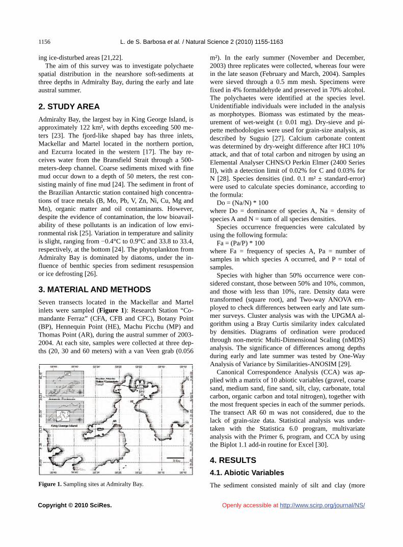
L. de S. Barbosa et al. / Natural Science 2 (2010) 1155-1163
Copyright © 2010 SciRes. http://www.scirp.org/journal/NS/
1156
Openly accessible at
ing ice-disturbed areas [21,22]. The aim of this survey was to investigate polychaete
spatial distribution in the nearshore soft-sediments at three depths in Admiralty Bay, during the early and late austral summer.
2. STUDY AREA
Admiralty Bay, the largest bay in King George Island, is approximately 122 km², with depths exceeding 500 me-ters [23]. The fjord-like shaped bay has three inlets, Mackellar and Martel located in the northern portion, and Ezcurra located in the western [17]. The bay re-ceives water from the Bransfield Strait through a 500- meters-deep channel. Coarse sediments mixed with fine mud occur down to a depth of 50 meters, the rest con-sisting mainly of fine mud [24]. The sediment in front of the Brazilian Antarctic station contained high concentra-tions of trace metals (B, Mo, Pb, V, Zn, Ni, Cu, Mg and Mn), organic matter and oil contaminants. However, despite the evidence of contamination, the low bioavail-ability of these pollutants is an indication of low envi-ronmental risk [25]. Variation in temperature and salinity is slight, ranging from −0.4°C to 0.9°C and 33.8 to 33.4, respectively, at the bottom [24]. The phytoplankton from Admiralty Bay is dominated by diatoms, under the in-fluence of benthic species from sediment resuspension or ice defrosting [26].
3. MATERIAL AND METHODS
Seven transects located in the Mackellar and Martel inlets were sampled (Figure 1): Research Station “Co-mandante Ferraz” (CFA, CFB and CFC), Botany Point (BP), Hennequin Point (HE), Machu Picchu (MP) and Thomas Point (AR), during the austral summer of 2003- 2004. At each site, samples were collected at three dep- ths (20, 30 and 60 meters) with a van Veen grab (0.056
Figure 1. Sampling sites at Admiralty Bay.
m²). In the early summer (November and December, 2003) three replicates were collected, whereas four were in the late season (February and March, 2004). Samples were sieved through a 0.5 mm mesh. Specimens were fixed in 4% formaldehyde and preserved in 70% alcohol. The polychaetes were identified at the species level. Unidentifiable individuals were included in the analysis as morphotypes. Biomass was estimated by the meas-urement of wet-weight (± 0.01 mg). Dry-sieve and pi-pette methodologies were used for grain-size analysis, as described by Suguio [27]. Calcium carbonate content was determined by dry-weight difference after HCl 10% attack, and that of total carbon and nitrogen by using an Elemental Analyser CHNS/O Perkin Elmer (2400 Series II), with a detection limit of 0.02% for C and 0.03% for N [28]. Species densities (ind. 0.1 m² ± standard-error) were used to calculate species dominance, according to the formula:
Do = (Na/N) * 100 where Do = dominance of species A, Na = density of species A and N = sum of all species densities.
Species occurrence frequencies were calculated by using the following formula:
Fa = (Pa/P) * 100 where Fa = frequency of species A, Pa = number of samples in which species A occurred, and P = total of samples.
Species with higher than 50% occurrence were con-sidered constant, those between 50% and 10%, common, and those with less than 10%, rare. Density data were transformed (square root), and Two-way ANOVA em-ployed to check differences between early and late sum- mer surveys. Cluster analysis was with the UPGMA al-gorithm using a Bray Curtis similarity index calculated by densities. Diagrams of ordination were produced through non-metric Multi-Dimensional Scaling (nMDS) analysis. The significance of differences among depths during early and late summer was tested by One-Way Analysis of Variance by Similarities-ANOSIM [29].
Canonical Correspondence Analysis (CCA) was ap-plied with a matrix of 10 abiotic variables (gravel, coarse sand, medium sand, fine sand, silt, clay, carbonate, total carbon, organic carbon and total nitrogen), together with the most frequent species in each of the summer periods. The transect AR 60 m was not considered, due to the lack of grain-size data. Statistical analysis was under-taken with the Statistica 6.0 program, multivariate analysis with the Primer 6, program, and CCA by using the Biplot 1.1 add-in routine for Excel [30].
4. RESULTS
4.1. Abiotic Variables
The sediment consisted mainly of silt and clay (more

L. de S. Barbosa et al. / Natural Science 2 (2010) 1155-1163
Copyright © 2010 SciRes. http://www.scirp.org/journal/NS/Openly accessible at
1157
than 60%) at most transects and depths, although the percentages of fine sand were higher (ca. 30%) in some stations like HE and AR. At 60 meters, slightly lower percentages of both gravel and coarse sand were ob-served, when compared to shallower transects. Calcium carbonate content was slightly higher in the late summer (more than 12%), whereas in the early season, this was lower at 20 and 30 meters, with the lowest (6.5%) at MP. Carbon and nitrogen content were very low (< 1%). CFA, CFB and CFC presented the highest percentages of car-bon content (0.54 to 0.75%), and MP the lowest (0.28 to 0.46%). There was no apparent variation of either vari-able with the increase in depth.
4.2. Polychaete Composition
A total of 8,668 individuals were collected throughout the period. The set of samples yielded 67 species and four morphotypes (Cirratulidae gen. sp.1, Cirratulidae gen. sp.2, Maldanidae gen. sp. and Terebellidae gen. sp.), belonging to 23 families (Table 1). 21 species were col-lected in each sampling survey. The most speciose fami-lies were Terebellidae and Syllidae with seven species each, and Maldanidae with six. The families Glyceridae and Sabellidae were exclusive to the early summer, whereas Nereididae and Serpulidae were to the late sum- mer. The families Nereididae, Serpulidae and Glyceridae were each represented by only one species, viz., Nicon ehlersi, Helicosiphon biscoensis and Glycera capitata, respectively. The sabellids were represented by three species: Euchone pallida, Perkinsiana litorallis and Perkinsiana milae, all somewhat scarce during the summer.
4.3. Dominance and Frequency
In terms of density, the species Aphelochaeta cincinnata, Levinsenia gracilis, Cirratulidae gen. sp. 1, Apistobran-chus glacierae and Rhodine antarctica dominated, throughout the whole period studied. The exceptions were Cirratulidae gen. sp. 1 and A. glacierae, dominant only at the beginning. Throughout, Aphelochaeta cin-cinnata was the most frequent species, with 93.55% in the early summer and 85.71% in the late. The species Levinsenia gracilis and Rhodine antarctica were also constant during the whole study period, with 69.35% and 56.45%, respectively, in the first part, and both 65,48% towards the end. These three species were responsible for 33.7% of total polychaetes in the early summer and 34.7% in the late. Aricidea (Acmira) strelzovi, Leito-scloplos geminus, Brada villosa, Apistobranchus glaci-erae, Barrukia cristata and Cirrophorus brevicirratus were considered common throughout. Scalibregma in-flatum, besides being a low-frequency species during the whole period (8.06% in the early part and 5.95% in the
late), occurred only at 60 meters (Table 1).
4.4. Density and Biomass
Polychaete density ranged from 45.24 to 388.10 ind.0.1 m-2 in the early summer. Apistobranchus glacierae, with the highest score all told, was also responsible for the high result observed at CFC (20 m) (173.21 ± 76.79 ind. 0.1 m-2). The species Aphelochaeta cincinnata at CFB (60 m), Rhodine antarctica at CFC (20 m) and Levin-senia gracilis at CFC (60 m) also presented high values (Figure 2). In the late summer, polychaete density varied from 29.02 to 183.93 ind.0.1 m-2. The highest densities, attributed to R. antarctica, were observed at the MP transect at 20 and 30 meters (Figure 3).
During sampling, a significant variation in density among depths was observed (ANOVA, p < 0.002) (Ta-ble 2), with lower densities at 30 meters when compared to both 20 and 60 (Tukey test, p < 0.005), although no differences among transects were detected (p = 0.599). Nevertheless, this pattern seems to be rather complex, since the interaction between transect and depth was significant (p < 0.02). This interaction occurred at tran-sects CFA and CFC, with no clear bathymetric pattern. On the contrary, in late summer, significant differences were found only among transects (p < 0.002), but not depths (Table 2), with MP and AR presenting higher densities than CFA and CFC (Tukey test, p < 0.05). These differences occurred due to the high densities of cirratulids (Aphelochaeta cincinnata and Cirratulidae gen. sp.1), paraonids (Levinsenia gracilis, Aricidea (Ac-mira) strelzovi and Cirrophorus brevicirratus) and the maldanid Rhodine antarctica, at MP and AR. On the other hand, biomass encountered at both CFA and CFC was low. Surprisingly, polychaete density at CFB was similar to that observed at MP and AR.
In the early summer, biomass means (± standard-error) ranged from 5.27 ± 4.19 g.0.1 m-2 at CFC-20 m, to 0.11 ± 0.06 g.0.1 m-2 at BP-30 m (Figure 4). In the late sea-son, the highest biomass mean was observed at CFB-30 m (5.86 ± 4.72 g.0.1 m-2) and the lowest at BP-30 m (0.35 ± 0.27 g.0.1 m-2) (Figure 5). The species Aglao-phamus ornatus, Eupolymnia sp. and Barrukia cristata presented the highest values. Although Rhodine antarc-tica biomass was not high, it remained constant at MP, all through the later part of summer, this constancy probably contributing to the proximity of values found at all depths.
4.5. Multivariate Analysis
In the early summer, the samples were grouped through cluster analysis, according to depth. The results indi-cated that in the first group, composed of transects MP, BP, AR at 20 meters, and MP and AR at 30 meters, the

L. de S. Barbosa et al. / Natural Science 2 (2010) 1155-1163
Copyright © 2010 SciRes. http://www.scirp.org/journal/NS/Openly accessible at
1158
Table 1. Frequency (Fo) and dominance (Do) of polychaete species in early and late summer, and species codes used in canonical correspondence analysis.
Species Code Family Early summer Late summer
Fo (%) Do Fo (%) Do
Levinsenia gracilis Lev 69.35 17.51 65.48 28.64 Aricidea (Acmira) strelzovi Ari 35.48 4.45 33.33 4.45 Cirrophorus brevicirratus Aph
Paraonidae 12.90 0.85 23.81 3.94
Leitoscoloplos kerguelensis Lek 22.58 1.02 16.67 0.95 Leitoscoloplos geminus Leg 29.03 1.76 21.43 1.13 Scoloplos (Leodamas) marginatus 3.23 0.04 2.38 0.08 Orbinia minima
Orbiniidae
- - 2.38 0.08 Scalibregma inflatum Scalibregmatidae 8.06 0.38 5.95 0.43 Ophelina syringopyge 4.84 0.22 4.76 0.33 Ophelina breviata 3.23 0.07 1.19 0.03 Ophelina sp.
Ophellidae 1.61 0.09 2.38 0.08
Capitella sp.1 1.61 0.02 4.76 0.13 Capitella sp. 2
Capitellidae - - 1.19 0.08
Asychis ampliglypta Asy 11.29 0.44 21.43 1.21 Maldane sarsi antarctica Mal 11.29 0.58 11.90 0.60 Lumbriclymenella robusta Lur 1.61 0.02 10.71 0.38 Rhodine antarctica Rho 56.45 9.50 65.48 20.30 Praxillella sp. 1.61 0.02 - - Maldanidae gen. sp. Mas
Maldanidae
24.19 0.76 19.05 0.98 Austrolaenilla antarctica 4.84 0.07 5.95 0.13 Barrukia cristata Bar 22.58 0.47 21.43 0.73 Harmothoe sp.
Polynoidae - - 1.19 0.03
Glycera capitata Glyceridae 1.61 0.02 - - Eulalia varia - - 2.38 0.05 Eulalia sp. - - 4.76 0.13 Eteone sculpta 1.61 0.02 2.38 0.05 Genetyllis polyphylla 3.23 0.07 3.57 0.15 Anaitides sp.
Phyllodocidae
1.61 0.04 1.19 0.03 Sphaerodoropsis arctowskyensis 6.45 0.20 2.38 0.05 Sphaerodoropsis sp. 1.61 0.02 - - Ephesiella muelenhardte
Sphaerodoridae 1.61 0.04 1.19 0.05
Aglaophamus ornatus Agl Nephtyidae 11.29 0.18 8.33 0.23 Nicon ehlersi Nereididae - - 1.19 0.03 Exogone heterosetosa 4.84 0.20 - - Exogone minuscula 1.61 0.04 - - Exogone heterosetoides 4.84 0.11 8.33 0.30 Exogone sp. 4.84 0.16 1.19 0.03 Syllis sp. 1.61 0.02 - - Branchiosyllis sp. 8.06 0.18 1.19 0.05 Syllides liouvillei
Syllidae
- - 2.38 0.05 Pettiboneia kerguelensis Pet 17.74 1.69 1.19 0.03 Ophryotrocha notialis
Dorvilleidae - - 1.19 0.03
Lumbrineris kerguelensis Lum 8.06 0.11 15.48 0.35 Augeneria sp.
Lumbrineridae 1.61 0.02 2.38 0.05
Apistobranchus glacirae Api Apistobranchidae 24.19 10.03 15.48 0.73 Spiophanes tcherniai 1.61 0.04 4.76 0.15 Laonice antarcticae 1.61 0.02 - - Microspio sp. 1.61 0.33 1.19 0.03 Scolelepis eltaninae 1.61 0.04 - - Pygospiopis dubia
Spionidae
- - 1.19 0.05 Aphelochaeta cf. cincinnata Aph 93.55 30.57 85.71 21.71 Cirratulidae gen. sp. 1 Cir 1 32.26 13.59 19.05 6.11 Cirratulidae gen. sp. 2 Cir 2
Cirratulidae 16.13 2.38 5.95 1.76
Brada villosa Bra 25.81 0.62 25.00 1.18 Pherusa kerguelarum
Flabelligeridae - - 1.19 0.08
Ampharete kerguelensis 3.23 0.04 4.76 0.10 Amphicteis gunneri antarctica Amp 6.45 0.09 15.48 0.70 Anobothrus cf. patagonicus 1.61 0.04 2.38 0.05 Phyllocomus crocea
Ampharetidae
- - 1.19 0.03 Hauchiella tribullata 1.61 0.02 - - Proclea cf. graffii 3.23 0.09 1.19 0.03 Amphitrite kerguelensis - - 1.19 0.03 Eupolymnia sp. Eup 8.06 0.20 21.43 0.53 Terebellides stroemii kerguelensis 8.06 0.24 5.95 0.25 Pista cristata 6.45 0.13 4.76 0.13 Trichobranchus sp. - - 1.19 0.03 Terebelidae gen sp.
Terebellidae
1.61 0.02 - - Euchone palida 1.61 0.02 - - Perkinsiana milae 1.61 0.02 - - Perkinsiana littoralis
Sabellidae 1.61 0.02 - -
Helicosiphon biscoensis Serpulidae - - 1.19 0.05

L. de S. Barbosa et al. / Natural Science 2 (2010) 1155-1163
Copyright © 2010 SciRes. http://www.scirp.org/journal/NS/
1159
Openly accessible at
Figure 2. Mean densities (± stardard-error) of Polychaeta at the transects in early summer. Depths: 20 m = black bars; 30 m = white bars; 60 m = gray bars.
Figure 3. Mean densities (± stardard-error) of Polychaeta at the transects in late summer. Depths: 20 m = black bars; 30 m = white bars; 60 m = gray bars.
Figure 4. Mean biomass (± stardard-error) of Polychaeta at the transects in early summer. Depths: 20 m = black bars; 30 m = white bars; 60 m = gray bars.
Figure 5. Mean biomass (± stardard-error) of Polychaeta at the transects in late summer. Depths: 20 m = black bars; 30 m = white bars; 60 m = gray bars.
Table 2. Results of Two-way ANOVA in early and late sum-mer.
Factors Early summer Late summer
p F p F
Transect 0.599 0.737 0.001 4.286
Depth 0.001 11.716 0.581 0.547
Transect * Depth 0.015 1.554 0.583 0.867
density of Cirratulidae gen. sp. 1 was high, whereas both Branchiosyllis sp. and S. arctowskyensis were absent. In the second group (CFB and CFC at 20 m, HE at 30 m, and MP and HE at 60 m), both R. antarctica and A. glacirae were the most abundant. In the third group, formed by CFA at 20 meters, and CFA, CFB, CFC and BP, all at 30 meters, richness and densities were low in R. antarctica, A. amphiglypta and A. cincinnata. In the last group, A. cincinnata, L. gracilis and Cirratulidae gen. sp. 2 were abundant, and both S. inflatum and A. strelzovi present (Figure 6). The results from cluster analysis were confirmed through nMDS. In the late summer, no clear pattern of clustering, in relation to either transects or depths, was apparent.
When using ANOSIM, no differences were detected in the polychaete community between the periods sam-pled (R global = 0.031; p = 20.5%), although the con-trary was the case as regards depths. In the early summer, communities at 60 meters differed from those found at 20 and 30 meters, whereas in the late season, the only difference was between 20 and 60 meters (Table 3).
Results through Canonical Correlation Analysis (CCA) were rather similar, in both early and late summer. The first axis was responsible for 45.9% of the variance in early summer and 42.8% in late and was positively re-lated to gravel, coarse and fine sand and negatively so to silt, clay, carbonate, carbon and nitrogen contents. The sediment in all transects at 20 meters was coarser, whereas that at 60 meters was characterized by the dominance of silt and clay fractions, and that at 30 me-ters an intermediate pattern between the former two. The second axis accounted for 25.5% and 20.8% of the vari-ance in early and late summer, respectively (Figures 7 and 8). In both summer periods, most species appeared to be associated with gravel, and coarse and fine sand. The maldanids Maldane sarsi antarctica and Asychis amphiglypta were related to stations at 60 meters. The species L. geminus, L. kerguelensis, A. glacirae and C. brevicirratus and Cirratulidae gen sp.1 were positively related with gravel, and coarse and fine sand.
5. DISCUSSION
The number of polychaete species found in the present study was higher than that presented by Sicinski & Ja-
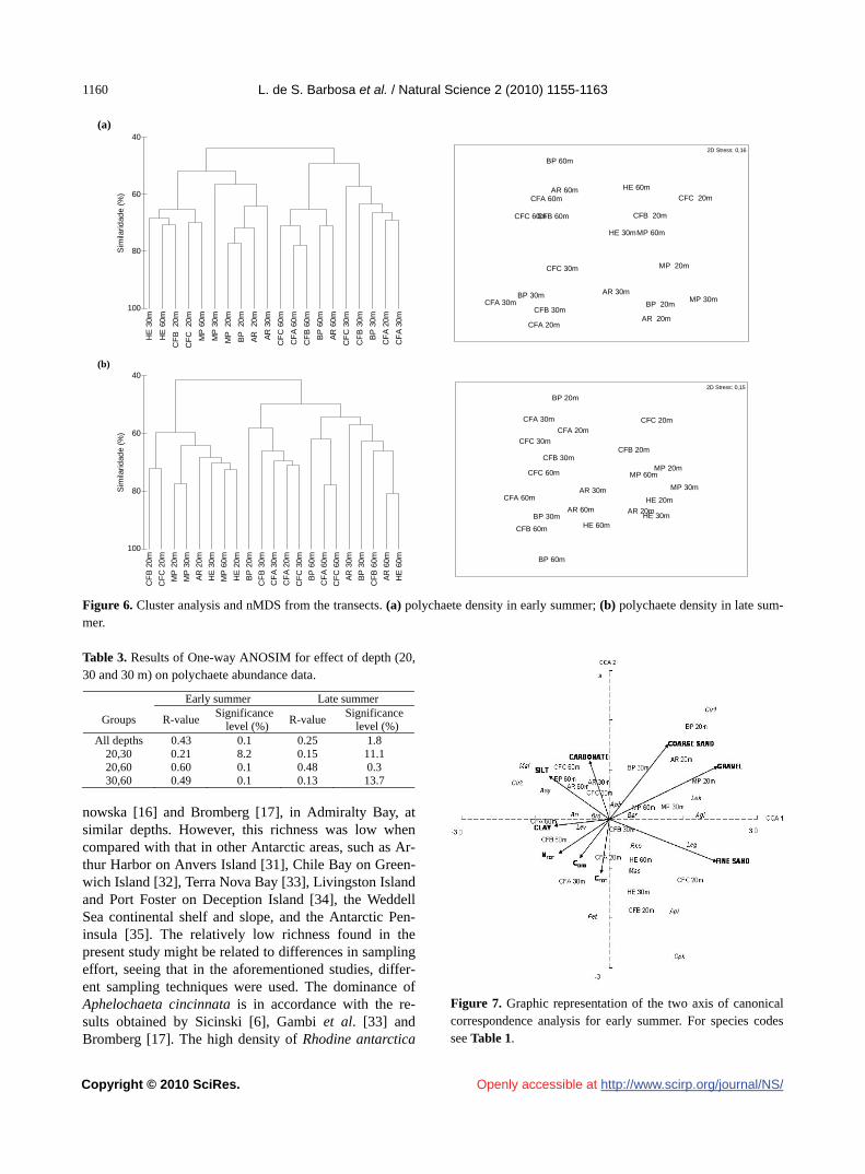
L. de S. Barbosa et al. / Natural Science 2 (2010) 1155-1163
Copyright © 2010 SciRes. http://www.scirp.org/journal/NS/
1160
Openly accessible at
(a)
HE
30m
HE
60m
CF
B
20m
CF
C
20m
MP
60m
MP
30m
MP
20
m
BP
20
m
AR
20
m
AR
30m
CF
C 6
0m
CF
A 6
0m
CF
B 6
0m
BP
60m
AR
60m
CF
C 3
0m
CF
B 3
0m
BP
30m
CF
A 2
0m
CF
A 3
0m
100
80
60
40
Sim
ilarid
ade
(%)
CFA 20m
CFA 30m
CFA 60m
CFB 20m
CFB 30m
CFB 60m
CFC 20m
CFC 30m
CFC 60m
MP 20m
MP 30m
MP 60m
BP 20mBP 30m
BP 60m
AR 20m
AR 30m
AR 60m
HE 30m
HE 60m
2D Stress: 0,16
(b)
CF
B 2
0m
CF
C 2
0m
MP
20m
MP
30m
AR
20m
HE
30m
MP
60m
HE
20m
BP
20m
CF
B 3
0m
CF
A 3
0m
CF
A 2
0m
CF
C 3
0m
BP
60m
CF
A 6
0m
CF
C 6
0m
AR
30m
BP
30m
CF
B 6
0m
AR
60m
HE
60m
100
80
60
40
Sim
ilarid
ade
(%)
CFA 20m
CFA 30m
CFA 60m
CFB 20mCFB 30m
CFB 60m
CFC 20m
CFC 30m
CFC 60mMP 20m
MP 30m
MP 60m
BP 20m
BP 30m
BP 60m
AR 20m
AR 30m
AR 60mHE 20m
HE 30mHE 60m
2D Stress: 0,15
Figure 6. Cluster analysis and nMDS from the transects. (a) polychaete density in early summer; (b) polychaete density in late sum-mer. Table 3. Results of One-way ANOSIM for effect of depth (20, 30 and 30 m) on polychaete abundance data.
Early summer Late summer
Groups R-value Significance level (%)
R-value Significance level (%)
All depths 0.43 0.1 0.25 1.8 20,30 0.21 8.2 0.15 11.1 20,60 0.60 0.1 0.48 0.3 30,60 0.49 0.1 0.13 13.7
nowska [16] and Bromberg [17], in Admiralty Bay, at similar depths. However, this richness was low when compared with that in other Antarctic areas, such as Ar-thur Harbor on Anvers Island [31], Chile Bay on Green-wich Island [32], Terra Nova Bay [33], Livingston Island and Port Foster on Deception Island [34], the Weddell Sea continental shelf and slope, and the Antarctic Pen-insula [35]. The relatively low richness found in the present study might be related to differences in sampling effort, seeing that in the aforementioned studies, differ-ent sampling techniques were used. The dominance of Aphelochaeta cincinnata is in accordance with the re-sults obtained by Sicinski [6], Gambi et al. [33] and Bromberg [17]. The high density of Rhodine antarctica
Figure 7. Graphic representation of the two axis of canonical correspondence analysis for early summer. For species codes see Table 1.

L. de S. Barbosa et al. / Natural Science 2 (2010) 1155-1163
Copyright © 2010 SciRes. http://www.scirp.org/journal/NS/
1161
Openly accessible at
Figure 8. Graphic representation of the two axis of canonical correspondence analysis for late summer. For species codes see Table 1. at the MP transect could be related to its life cycle. Ac-cording to Dayton & Oliver [12], in McMurdo Sound, the individuals of the family Maldanidae may have evolved asexual reproduction in response to high preda-tion and juvenile mortality. The dominance of maldanids was also reported by Gallardo et al. [9], who found a benthic community dominated by Maldane sarsi antarc-tica (Maldane assembly) in Chile Bay. Jazdzewski et al. [24] and Sicinski [6,13] also observed typical maldanid communities at depths over 100 meters.
The highest mean density observed in the early sum-mer was similar to that reported by Sicinski [14]. On the other hand, mean density itself, although in accordance to that observed by Sicinski & Janowska [16], was lower than that reported by other authors [17,33-35]. These differences may reflect variations in sampling design, depth and seasonality. The mean values of biomass were similar to those observed in Admiralty Bay by Sicinski & Janowska [16], and were within the range reported by Gambi et al. [33]. According to Sicinski [13], polychaete biomass at 50 m may vary from 30 to 40 g.m-2 and might be responsible for 15% of the local zoobenthic biomass itself. The species responsible for the increase in bio-mass values, Aglaophamus ornatus and Eupolymnia sp. occurred mainly at 20 and 30 meters, respectively. This may be related to the deposition of organic matter from phytoplankton bloom, which occurs in the early summer [36].
Polychaete taxocoenosis structure remained the same
throughout the period under study, possibly as a result of the prevailing sedimentary conditions (grain-size per-centages) remaining invariable between transects. Nev-ertheless, certain differences were observed during the early and late summer, separately. During the early summer, polychaete mean density, biomass and richness declined at the 30 meters level and increased at the 60. An increase in density related to depth had been previ-ously reported in the Martel inlet [16]. The results in early summer may be an outcome of ice impact. Accor- ding to Sahade et al. [3], ice impacts (icebergs and an-chor-ice) seem to be the major regulating factor of ben-thic assemblages in shallow waters. Although actually not observed in this study, but based mainly on under-water observations, anchor-ice impacts have been im-puted as promoting winter structuring in benthic com-munities. The displacement of established fauna in their area of influence may be attributed to these phenomena, thereby accounting for the low diversity in early summer [37]. According to Dayton et al. [38], the influence of anchor-ice impacts extends down to 33 meters, thus con-stituting the main cause of low diversity in shallow wa-ters. Anchor-ice usually occurs during the winter, but its influence might have extended throughout the early summer of 2003/04, with consequential superficial sediment defaunation, thus making it difficult for the community to recover within a few months.
The increase in temperature in the late summer pro-motes the formation of icebergs. Echeverría & Paiva [39] reported the presence of one in the summer of 2001 at the CFB 25 meter station, where it remained for over 20 days. Iceberg impacts are likely to affect benthic com-munities down to 20 meters. Below this, conditions are more stable, with higher densities, biomass and richness, the area below 30 meters thus presenting a substantial change in benthic megafauna structure, composition and diversity [37]. In both summer periods, most of the spe-cies which appear to be related to coarser sediment frac-tions are motile or discretely motile polychaetes. On the other hand, the maldanids (sessile polychaetes) related to higher percentages of silt and clay, appear mostly at 60 meters. Further analysis of polychaete feeding guilds is necessary to better evaluate their distribution in Admi-ralty Bay.
The possible environmental impacts related to activi-ties of the Brazilian research station (Cmte. Ferraz) were not revealed in this survey, since variability among those transects under the influence of the station itself (CFA, CFB and CFC) was higher than among all the others. Furthermore, the slight variation between early and late summer seems to be more related to natural impacts than to the more intense activities at the research station it-self.
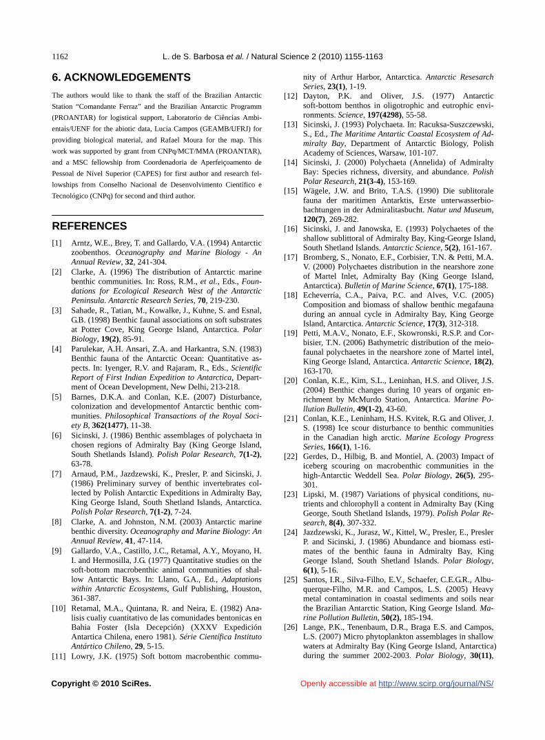
L. de S. Barbosa et al. / Natural Science 2 (2010) 1155-1163
Copyright © 2010 SciRes. http://www.scirp.org/journal/NS/
1162
Openly accessible at
6. ACKNOWLEDGEMENTS
The authors would like to thank the staff of the Brazilian Antarctic
Station “Comandante Ferraz” and the Brazilian Antarctic Programm
(PROANTAR) for logistical support, Laboratorio de Ciências Ambi-
entais/UENF for the abiotic data, Lucia Campos (GEAMB/UFRJ) for
providing biological material, and Rafael Moura for the map. This
work was supported by grant from CNPq/MCT/MMA (PROANTAR),
and a MSC fellowship from Coordenadoria de Aperfeiçoamento de
Pessoal de Nível Superior (CAPES) for first author and research fel-
lowships from Conselho Nacional de Desenvolvimento Científico e
Tecnológico (CNPq) for second and third author.
REFERENCES
[1] Arntz, W.E., Brey, T. and Gallardo, V.A. (1994) Antarctic zoobenthos. Oceanography and Marine Biology - An Annual Review, 32, 241-304.
[2] Clarke, A. (1996) The distribution of Antarctic marine benthic communities. In: Ross, R.M., et al., Eds., Foun-dations for Ecological Research West of the Antarctic Peninsula. Antarctic Research Series, 70, 219-230.
[3] Sahade, R., Tatian, M., Kowalke, J., Kuhne, S. and Esnal, G.B. (1998) Benthic faunal associations on soft substrates at Potter Cove, King George Island, Antarctica. Polar Biology, 19(2), 85-91.
[4] Parulekar, A.H. Ansari, Z.A. and Harkantra, S.N. (1983) Benthic fauna of the Antarctic Ocean: Quantitative as-pects. In: Iyenger, R.V. and Rajaram, R., Eds., Scientific Report of First Indian Expedition to Antarctica, Depart-ment of Ocean Development, New Delhi, 213-218.
[5] Barnes, D.K.A. and Conlan, K.E. (2007) Disturbance, colonization and developmentof Antarctic benthic com-munities. Philosophical Transactions of the Royal Soci-ety B, 362(1477), 11-38.
[6] Sicinski, J. (1986) Benthic assemblages of polychaeta in chosen regions of Admiralty Bay (King George Island, South Shetlands Island). Polish Polar Research, 7(1-2), 63-78.
[7] Arnaud, P.M., Jazdzewski, K., Presler, P. and Sicinski, J. (1986) Preliminary survey of benthic invertebrates col-lected by Polish Antarctic Expeditions in Admiralty Bay, King George Island, South Shetland Islands, Antarctica. Polish Polar Research, 7(1-2), 7-24.
[8] Clarke, A. and Johnston, N.M. (2003) Antarctic marine benthic diversity. Oceanography and Marine Biology: An Annual Review, 41, 47-114.
[9] Gallardo, V.A., Castillo, J.C., Retamal, A.Y., Moyano, H. I. and Hermosilla, J.G. (1977) Quantitative studies on the soft-bottom macrobenthic animal communities of shal-low Antarctic Bays. In: Llano, G.A., Ed., Adaptations within Antarctic Ecosystems, Gulf Publishing, Houston, 361-387.
[10] Retamal, M.A., Quintana, R. and Neira, E. (1982) Ana- lisis cualiy cuantitativo de las comunidades bentonicas en Bahia Foster (Isla Decepción) (XXXV Expedición Antartica Chilena, enero 1981). Série Científica Instituto Antártico Chileno, 29, 5-15.
[11] Lowry, J.K. (1975) Soft bottom macrobenthic commu-
nity of Arthur Harbor, Antarctica. Antarctic Resesarch Series, 23(1), 1-19.
[12] Dayton, P.K. and Oliver, J.S. (1977) Antarctic soft-bottom benthos in oligotrophic and eutrophic envi-ronments. Science, 197(4298), 55-58.
[13] Sicinski, J. (1993) Polychaeta. In: Racuksa-Suszczewski, S., Ed., The Maritime Antartic Coastal Ecosystem of Ad-miralty Bay, Department of Antarctic Biology, Polish Academy of Sciences, Warsaw, 101-107.
[14] Sicinski, J. (2000) Polychaeta (Annelida) of Admiralty Bay: Species richness, diversity, and abundance. Polish Polar Research, 21(3-4), 153-169.
[15] Wägele, J.W. and Brito, T.A.S. (1990) Die sublitorale fauna der maritimen Antarktis, Erste unterwasserbio-bachtungen in der Admiralitasbucht. Natur und Museum, 120(7), 269-282.
[16] Sicinski, J. and Janowska, E. (1993) Polychaetes of the shallow sublittoral of Admiralty Bay, King-George Island, South Shetland Islands. Antarctic Science, 5(2), 161-167.
[17] Bromberg, S., Nonato, E.F., Corbisier, T.N. & Petti, M.A. V. (2000) Polychaetes distribution in the nearshore zone of Martel Inlet, Admiralty Bay (King George Island, Antarctica). Bulletin of Marine Science, 67(1), 175-188.
[18] Echeverría, C.A., Paiva, P.C. and Alves, V.C. (2005) Composition and biomass of shallow benthic megafauna during an annual cycle in Admiralty Bay, King George Island, Antarctica. Antarctic Science, 17(3), 312-318.
[19] Petti, M.A.V., Nonato, E.F., Skowronski, R.S.P. and Cor-bisier, T.N. (2006) Bathymetric distribution of the meio-faunal polychaetes in the nearshore zone of Martel intel, King George Island, Antarctica. Antarctic Science, 18(2), 163-170.
[20] Conlan, K.E., Kim, S.L., Leninhan, H.S. and Oliver, J.S. (2004) Benthic changes during 10 years of organic en-richment by McMurdo Station, Antarctica. Marine Po- llution Bulletin, 49(1-2), 43-60.
[21] Conlan, K.E., Leninham, H.S. Kvitek, R.G. and Oliver, J. S. (1998) Ice scour disturbance to benthic communities in the Canadian high arctic. Marine Ecology Progress Series, 166(1), 1-16.
[22] Gerdes, D., Hilbig, B. and Montiel, A. (2003) Impact of iceberg scouring on macrobenthic communities in the high-Antarctic Weddell Sea. Polar Biology, 26(5), 295- 301.
[23] Lipski, M. (1987) Variations of physical conditions, nu-trients and chlorophyll a content in Admiralty Bay (King George, South Shetland Islands, 1979). Polish Polar Re-search, 8(4), 307-332.
[24] Jazdzewski, K., Jurasz, W., Kittel, W., Presler, E., Presler P. and Sicinski, J. (1986) Abundance and biomass esti-mates of the benthic fauna in Admiralty Bay, King George Island, South Shetland Islands. Polar Biology, 6(1), 5-16.
[25] Santos, I.R., Silva-Filho, E.V., Schaefer, C.E.G.R., Albu-querque-Filho, M.R. and Campos, L.S. (2005) Heavy metal contamination in coastal sediments and soils near the Brazilian Antarctic Station, King George Island. Ma-rine Pollution Bulletin, 50(2), 185-194.
[26] Lange, P.K., Tenenbaum, D.R., Braga E.S. and Campos, L.S. (2007) Micro phytoplankton assemblages in shallow waters at Admiralty Bay (King George Island, Antarctica) during the summer 2002-2003. Polar Biology, 30(11),
L. de S. Barbosa et al. / Natural Science 2 (2010) 1155-1163
Copyright © 2010 SciRes. http://www.scirp.org/journal/NS/Openly accessible at
1163
1438-1492. [27] Suguio, K. (1973) Introdução à sedimentologia. Editora
da Universidade de São Paulo, São Paulo, 317. [28] Skoog, D.A. and Leary, J.J. (1992) Principles of instru-
mental analysis. 4th Edition, Saunders College Publish-ing, Forth Worth, 801.
[29] Clarke, K.R. and Warwick, R.W. Change in marine communities: An aproach to statistical analysis and in-terpretation. Plymouth Marine Laboratory, Bourne Press, Bournemouth, 1994.
[30] Lipkovich, I. and Smith, E.P. (2002) Biplot and singular value decomposition macros for Excel. Journal of Statis-tical Software, 7(5), 1-15.
[31] Richardson, M.D. and Hedgpeth, J.W. (1977) Antarctic soft-bottom macrobenthic community adaptations to a cold stable, highly, productive, glacially affected envi-ronment. In: Llano, G.A., Ed., Adaptations within Ant-arctic Ecosystems, Gulf Publishing, Houston, 181-196.
[32] Gallardo, V., Medrano, S.A. and Carrasco, F.D. (1988) Taxonomic composition of the sublittoral soft-bottom polychaetes of Chile Bay (Greenwich Island, South Shetland Islands, Antarctica). Serie Científica Instituto Antártico Chileno, 37(1), 49-67.
[33] Gambi, M.C., Castelli A. and Guizzardi, M. (1997) Polychaete populations of the shallow soft bottoms off Terra Nova Bay (Ross Sea, Antarctica): Distribution, di-versity and biomass. Polar Biology, 17(3), 199-210.
[34] San Martin, G., Parapar, J., García F.J. and Redondo, M. S. (2000) Quantitative analysis of soft-bottoms infaunal macrobenthic polychaetes from South Shetland Islands (Antarctica). Bulletin of Marine Science, 67(1), 83-102.
[35] Hilbig, B., Verdes, D. and Montiel, A. (2006) Distribu-tion patterns and biodiversity in polychaete communities of the Weddell Sea and Antarctic Peninsula area (South-ern Ocean). Journal of Marine Biological Association of the U.K., 86(4), 711-725.
[36] Mincks, S. and Smith, C.R. (2007) Recruitment patterns in Antarctic Peninsula shelf sediments: Evidence of de-coupling from seasonal phytodetritus pulses. Polar Biol-ogy, 30(5), 587-600.
[37] Nonato, E.F., Brito, T.A.S., Paiva, P.C., Petti, M.A.V. and Corbisier, T.N. (2000) Benthic megafauna of the near-shore zone of Martel Inlet (King George Island, South Shetland Islands, Antarctica): Depth zonation and un-derwater observations. Polar Biology, 23(8), 580-588
[38] Dayton, P.K., Robilliard, G.A., Paine R.T. and Dayton, L. B. (1974) Biological accommodation in the benthic com- munity at McMurdo Sound, Antarctica. Ecological Mo- nographs, 44(1), 105-128.
[39] Echeverría, C.A and Paiva, P.C. (2006) Macrofaunal shallow benthic communities along a discontinuous an-nual cycle at Admiralty Bay, King George Island, Ant-arctica. Polar Biology, 29(3), 263-269.

Vol.2, No.10, 1164-1170 (2010)doi:10.4236/ns.2010.210144
Copyright © 2010 SciRes. http://www.scirp.org/journal/NS/
Natural Science
Openly accessible at
The factorial structure of self-reported androgen-promoted physiological traits
Lee Ellis1, Shyamal Das2 1University Malaya, Department of Anthropology, Kuala Lumpur, Malaysia; [email protected]; 2Elizabeth City State University, North Carolina, USA; [email protected].
Received 27 June 2010; revised 29 July 2010; accepted 4 August 2010.
ABSTRACT
Androgens make major contributions to aver-age sex differences in anatomy, physiology, and behavior. Despite having established their cru-cial role in sexual differentiation, much remains to be learned about how androgens coordinate their influences. The present study was under-taken to shed light on androgenic effects on the body using self-reported survey data. We ana-lyzed the ratings provided by over 11,000 col-lege students on the magnitude of eleven traits that previous research has shown to be influ-enced by testosterone or other androgens. Pre-dictably, the average values for all eleven traits were significantly greater in males than in fe-males. Nevertheless, when data were analyzed separately according to sex of the respondents, some of the traits failed to positively correlate with one another, suggesting that not all an-drogen-influenced traits differentiate in a simple fashion. Factor analysis of these eleven traits by sex reinforced this view by identifying four fac-tors. In men, the primary factor loaded most heavily on: masculine body build, masculine mannerisms, overall physical strength, upper body strength, and lower body strength. The primary factor for women was limited to: upper body strength, lower body strength, and overall physical strength. In both sexes, the primary factor was interpreted as reflecting the influ-ence of perinatal and postpubertal testosterone exposure. The other three factors may reflect the effects of other androgens (e.g., andros-tenediol), or the influence of female hormones such as estradiol. Findings were discussed in terms of future use of self-reported physiologi-cal measures for assessing androgenic effects on the human body.
Keywords: Androgen-promoted physical traits;
Testosterone; Masculinization; Physical strength; Factorial structure; Sex differences
1. INTRODUCTION
A recent literature review provided evidence that the sexes differ in a mired of ways, ranging from easy-to- measure traits (e.g., birth weights and adult body size) to many complex characteristics (e.g., susceptibility to nu-merous diseases, detailed biochemistry, neurology, per-ceptual sensitivities, motor coordination, and even many cognitive and behavioral patterns) [1]. This evidence raises questions about how sex differences are produced. Although the details are still far from fully understood, numerous studies have implicated bodily exposure to androgens as primarily responsible for sex differences in traits [2-5].
In broad terms, the sexual differentiation of animals occurs as follows: The default sex at least for mammals, is female, meaning that males are a genetic variant on the female sex [6-9]. Early in the gestation process of nearly all males, the would-be ovaries are made to begin differentiating into testes instead by genes located on the Y-chromosome [10]. As this occurs in humans during the first five months of gestation, the genitals of males gradually take on a masculine rather than a feminine appearance [11-12].
The gestational aspects of sexual differentiation are referred to as its organizational stage, a stage in humans extending from the first month of gestation into about the fourth month following birth [13]. The second phase of sexual differentiation is known as the activational (or postpubertal) stage. It is marked by the appearance of so-called secondary sex characteristics, but also includes enlargement of the penis and testes in males [14-17].
The traits that are masculinized by bodily exposure to androgens are numerous. They include the following: Growth of body hair [18-20] Darkening of the iris of the eye [21,22] Facial acne [23-25]

L. Ellis et al. / Natural Science 2 (2010) 1164-1170
Copyright © 2010 SciRes. http://www.scirp.org/journal/NS/Openly accessible at
1161165
Darkening of hair color [26,27] Increase in height [28-32] Lowering of the voice [33-37] Increase in upper body strength [15,38,39] Increase in lower body strength [40,42] Increase in masculine body appearance [43-44] Increase in masculine mannerisms [45,46] Despite the abundant evidence that androgens mascu-
linize many aspects of human development, the details are still only vaguely understood. The purpose of the present study was to examine the eleven androgen-in- fluenced traits listed above using self-ratings, with the following three questions in mind. First, are all of these traits in fact sexually dimorphic? Second, within each sex, how well do the eleven traits correlate with one an-other? Third, do the within-sex expressions of these traits cluster together, thereby suggesting that they may be resulting from a limited number of similar androgenic regimens?
2. METHODS
As part of a broad-ranging investigation, a standar- dized questionnaire was completed by a large sample of college students at twenty United States and two Cana-dian universities between 1988 and 1998 involving 3,786 males and 7,697 females [47]. Subjects ranged in age from 18 to 56, with a mean of 22 for both sexes. In terms of race and ethnicity, the subjects were 85% white, 4% black, 2% Native American, 2% Asian / Pacific Islander, 1% Hispanic, and 6% providing no answer.
Eight of the androgen-promoted physiological traits were measured by asking subjects to rate themselves regarding each trait using a 1 to 100 scale, with 100 rep-resenting maximum expression of each trait. These eight traits were: masculine mannerisms, masculine body ap-pearance, physical strength, low deep voice, upper body strength, lower body strength, body-hair development, and facial acne. Height was measured simply in terms of feet and inches (converted to inches). Eye color and hair color were measured, first, by asking subjects to give a one- or two-word description of their eye color and natural hair color. These descriptions were then inter-preted and transcribed into four categories. From highest to lowest values, eye color was coded as being Black, Brown, Hazel / Green, and Blue. For hair color, the four categories were Black, Dark Brown, Light Brown, and Blond. (A copy of the questionnaire is available upon request.)
Analysis was carried out in three stages. First, the sexes were compared regarding their average scores on all eleven traits using a t-test. Second, to determine how well the eleven traits correlated with one another, a cor-relation matrix was created for the sexes separately.
Third, factorial analysis was performed on the eleven traits to assess whether or not some of the traits would form into clusters.
3. RESULTS
Table 1 shows that all eleven androgen-promoted traits are significantly more pronounced in men than in wo- men, with p = 0.000 in all cases except for eye color (which attained significance only at the 0.05 level). This is entirely predictable, given that the levels of testost- erone (and other androgens) are higher for males than for females throughout both the organizational and acti-vational stages of sexual differentiation ([1], pp. 89-93).
Table 2, however, reveals that within each sex, some of the androgen-promoted traits are not positively corre-lated with one another. Such a rather surprising finding can be interpreted as suggesting that the enhancement of androgen-promoted traits does not occur through a uni-tary process. Most notably, the variables of eye color and especially adolescent facial acne correlate negatively with many of the other androgen-influenced traits among both sexes.
The results for factor analyzing responses regarding the eleven androgen-promoted traits are presented in Table 3 for each sex separately. Regarding males (Table 3(a)), the first factor to emerge was named masculinity / strength since it was comprised of masculine manner-isms, masculine body build, and all three of the physical strength measures. We named the second factor pigment because it only loaded strongly on hair color and eye color. Body hair development and adolescent facial acne loaded most heavily on the third factor (with some sec-ondarily strong loadings on upper and lower body strength), which was named dark pigmentation. Finally, height and low-deep voice comprised a fourth factor, which we named physical prowess since both height and low-deep voice are likely to have evolved primarily to intimidate rivals (and possibly impress prospective mates).
Turning to females (Table 3(b)), four factors also emerged. The first factor had to do with strength. Mascu-line mannerisms and body build loaded along with low-deep voice onto a second factor; therefore, we called it female masculinity. The remaining two female factors were identical to those in males, a dark pigmentation fac-tor and a skin-hair factor. It is interesting to note that height loaded heavily on the physical prowess factor in males but failed to load on any factor among females.
4. CONCLUSIONS
While there is no doubt that androgens play a pivotal ole in differentiating males from females, much remains r
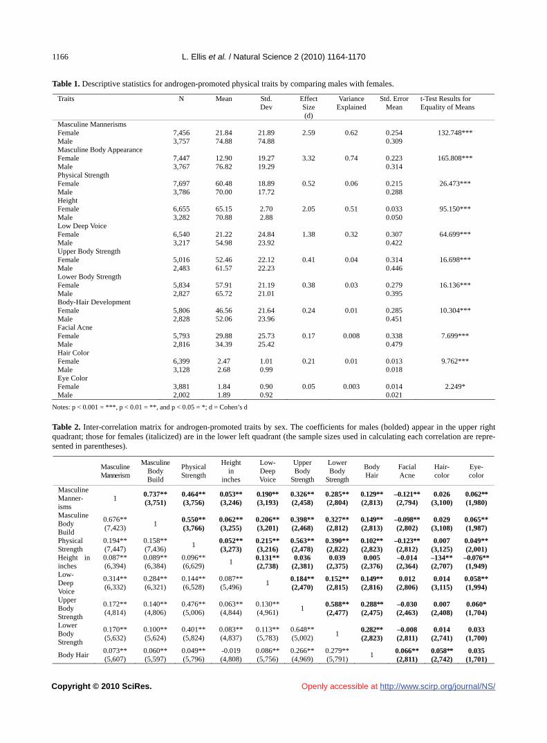
L. Ellis et al. / Natural Science 2 (2010) 1164-1170
Copyright © 2010 SciRes. http://www.scirp.org/journal/NS/Openly accessible at
1166
Table 1. Descriptive statistics for androgen-promoted physical traits by comparing males with females.
Traits N Mean Std. Dev
Effect Size (d)
Variance Explained
Std. Error Mean
t-Test Results for Equality of Means
Masculine Mannerisms Female Male
7,456 3,757
21.84 74.88
21.89 74.88
2.59
0.62
0.254 0.309
132.748***
Masculine Body Appearance Female Male
7,447 3,767
12.90 76.82
19.27 19.29
3.32
0.74
0.223 0.314
165.808***
Physical Strength Female Male
7,697 3,786
60.48 70.00
18.89 17.72
0.52
0.06
0.215 0.288
26.473***
Height Female Male
6,655 3,282
65.15 70.88
2.70 2.88
2.05
0.51
0.033 0.050
95.150***
Low Deep Voice Female Male
6,540 3,217
21.22 54.98
24.84 23.92
1.38
0.32
0.307 0.422
64.699***
Upper Body Strength Female Male
5,016 2,483
52.46 61.57
22.12 22.23
0.41
0.04
0.314 0.446
16.698***
Lower Body Strength Female Male
5,834 2,827
57.91 65.72
21.19 21.01
0.38
0.03
0.279 0.395
16.136***
Body-Hair Development Female Male
5,806 2,828
46.56 52.06
21.64 23.96
0.24
0.01
0.285 0.451
10.304***
Facial Acne Female Male
5,793 2,816
29.88 34.39
25.73 25.42
0.17
0.008
0.338 0.479
7.699***
Hair Color Female Male
6,399 3,128
2.47 2.68
1.01 0.99
0.21
0.01
0.013 0.018
9.762***
Eye Color Female Male
3,881 2,002
1.84 1.89
0.90 0.92
0.05
0.003
0.014 0.021
2.249*
Notes: p < 0.001 = ***, p < 0.01 = **, and p < 0.05 = *; d = Cohen’s d
Table 2. Inter-correlation matrix for androgen-promoted traits by sex. The coefficients for males (bolded) appear in the upper right quadrant; those for females (italicized) are in the lower left quadrant (the sample sizes used in calculating each correlation are repre-sented in parentheses).
Masculine Mannerism
Masculine Body Build
Physical Strength
Height in
inches
Low- Deep Voice
Upper Body
Strength
Lower Body
Strength
Body Hair
Facial Acne
Hair- color
Eye- color
Masculine Manner-isms
1 0.737** (3,751)
0.464** (3,756)
0.053** (3,246)
0.190** (3,193)
0.326**(2,458)
0.285** (2,804)
0.129** (2,813)
–0.121** (2,794)
0.026 (3,100)
0.062** (1,980)
Masculine Body Build
0.676** (7,423)
1 0.550** (3,766)
0.062** (3,255)
0.206** (3,201)
0.398** (2,468)
0.327** (2,812)
0.149** (2,813)
–0.098** (2,802)
0.029 (3,108)
0.065**(1,987)
Physical Strength
0.194** (7,447)
0.158** (7,436)
1 0.052** (3,273)
0.215** (3,216)
0.563** (2,478)
0.390** (2,822)
0.102** (2,823)
–0.123** (2,812)
0.007 (3,125)
0.049**(2,001)
Height in inches
0.087** (6,394)
0.089** (6,384)
0.096** (6,629)
1 0.131**(2,738)
0.036 (2,381)
0.039 (2,375)
0.005 (2,376)
–0.014 (2,364)
–134**(2,707)
–0.076**(1,949)
Low- Deep Voice
0.314** (6,332)
0.284** (6,321)
0.144** (6,528)
0.087** (5,496)
1 0.184** (2,470)
0.152** (2,815)
0.149**(2,816)
0.012 (2,806)
0.014 (3,115)
0.058**(1,994)
Upper Body Strength
0.172** (4,814)
0.140** (4,806)
0.476** (5,006)
0.063** (4,844)
0.130** (4,961)
1 0.588** (2,477)
0.288** (2,475)
–0.030 (2,463)
0.007 (2,408)
0.060* (1,704)
Lower Body Strength
0.170** (5,632)
0.100** (5,624)
0.401** (5,824)
0.083** (4,837)
0.113** (5,783)
0.648** (5,002)
1 0.282** (2,823)
–0.008 (2,811)
0.014 (2,741)
0.033 (1,700)
Body Hair 0.073** (5,607)
0.060** (5,597)
0.049** (5,796)
-0.019 (4,808)
0.086** (5,756)
0.266** (4,969)
0.279** (5,791)
1 0.066** (2,811)
0.058**(2,742)
0.035 (1,701)

L. Ellis et al. / Natural Science 2 (2010) 1164-1170
Copyright © 2010 SciRes. http://www.scirp.org/journal/NS/Openly accessible at
1161167
Facial Acne
0.080** (5,592)
0.046** (5,585)
–0.026* (5,783)
0.016 (4,796)
0.052**(5,743)
0.082**(4,947)
0.089**(5,772)
0.211** (5,745)
1 –0.015 (2,730)
–0.073**(1,693)
Hair- color
–0.039** (6,153)
–0.021 (6,141)
–0.028* (6,382)
–0.075**(5,489)
0.022 (6,331)
–0.035*(4,858)
–0.040**
(5,663)
0.081** (5,636)
–0.028* (5,622)
1 0.440**(1,998)
Eye- color
–0.023 (,3739)
0.001 (3,731)
–0.008 (3,871)
–0.085**(3,824)
0.017 (3,847)
–0.014 (3,298)
–0.010 (3,297)
0.052**(3,277)
–0.017 (3,267)
0.442** (3,880)
1
Note: * p < 0.05 ** p < 0.01 Table 3(a). Factor Loadings for Androgen-Promoted Traits for Males.
Items Factor 1 Factor 2 Factor 3 Factor 4
Masculine Mannerism 0.806 –0.001 –0.125 0.056
Masculine Body Build 0.845 0.011 –0.064 0.071
Height 0.002 –0.158 –0.145 0.835
Low Deep Voice 0.178 0.157 0.290 0.633
Overall Physical Strength 0.780 0.059 0.043 0.082
Upper Body Strength 0.679 0.046 0.445 0.026
Lower Body Strength 0.592 0.023 0.481 0.028
Body Hair 0.172 0.081 0.692 0.066
Facial Acne –0.263 –0.154 0.566 –0.022
Hair Color 0.004 0.832 0.018 –0.064
Eye Color 0.046 0.829 –0.042 0.036
Table 3(b). Factor Loadings for Androgen-Promoted Traits for Females.
Items Factor 1 Factor 2 Factor 3 Factor 4
Masculine Mannerism 0.091 0.856 –0.057 0.050
Masculine Body Build 0.025 0.860 –0.015 0.000
Height 0.132 0.206 –0.212 –0.254
Low Deep Voice 0.119 0.589 0.063 0.017
Overall Physical Strength 0.746 0.164 –0.012 –0.216
Upper Body Strength 0.858 0.096 –0.024 0.134
Lower Body Strength 0.825 0.047 –0.013 0.195
Body Hair 0.299 0.017 0.123 0.677
Facial Acne –0.054 0.101 –0.121 0.775
Hair Color 0.004 0.002 0.835 0.009
Eye Color –0.010 0.028 0.830 0.003
to be learned about which androgens are involved in particular traits and when they have their greatest influ-ences. The present study sheds light on the process by suggesting that in both sexes, four independent factors emerge when eleven androgen-promoted physiological traits are measured. The structures of these four factors are slightly different for males and for females.
In males, the primary factor loads most heavily on masculinity and strength, whereas in females, the load-
ing is strictly on strength. We hypothesize that in both sexes this primary factor is the result of perinatal and postpubertal exposure to testosterone. This hypothesis is consistent with studies showing that testosterone is by far the most consequential sex hormone regarding both masculine mannerisms [46] and muscular strength [15, 41]. To explain why mannerisms in females would not be masculinized by testosterone, we suspect that the lev-els of this hormone to which most females are exposed

L. Ellis et al. / Natural Science 2 (2010) 1164-1170
Copyright © 2010 SciRes. http://www.scirp.org/journal/NS/
1168
Openly accessible at
are insufficient to significantly affect this trait while muscular strength responds to even low amounts of tes-tosterone. Another possibility is that high (female-typical) exposure to estradiol or other female hormones may counteract the effects of testosterone on masculine man-nerisms.
The fact that the same factors for the dark pigmenta-tion factor and the skin-hair factor emerged in both sexes suggests that these traits are (a) the result of androgens other than testosterone, and (b) that the androgen(s) pri-marily responsible for hair growth and facial acne is different from those influencing hair and eye color.
Regarding the three questions posed in the introduc-tion, one can conclude the following: First, all eleven traits that other studies have shown to be androgen- promoted are, as expected, more pronounced in males than in females. Second, within each sex, most of the eleven traits are positively correlated. The fact that there are exceptions leads one to expect that different andro-gens are operating in somewhat different ways within each sex. Third, factor analysis supports this expectation by demonstrating that there are four clusters of andro-gen-promoted traits amongst the eleven traits examined in the present study. We named these four factors and hypothesized that testosterone is responsible for the first (and most prominent) factor for both sexes. In males, this primary factor involved both strength and masculine mannerisms, while in females it only involved strength.
Research is needed to verify these four factors and to look for other androgen-promoted traits within each sex. In future studies, direct measurement would almost cer-tainly provide more reliable data than self-reports. How- ever, the time required for obtaining direct measures with a sufficiently large sample of subjects needed for factor analysis could be prohibitive. It can also be said that the extent to which people can provide accurate in-formation about themselves may surpass expectations. In this regard, we compared the average heights of our subjects to estimates recently given by the Center for Disease Control based on direct measurements [48]. The results were very similar: 70.88 inches or 5’ 9.1” tall in our male sample compared to 5’ 9.2” for the national sample, and 65.15 inches or 5’ 4.3” tall in our female sample compared to 5’ 3.8” for the national sample.
If the four factor structure of androgen-promoted traits revealed in the present study can be replicated, the next phase in this line of research would be to identify each of their specific causes. In other words, what are the ac-tual androgens involved in producing each factor and what is the developmental timing involved?
REFERENCES [1] Ellis, L., Hershberger, S., Field, E., Wersinger, S., Pellis,
S., Geary, D., Palmer, C., Hoyenga, K., Hetsroni, A. and Karadi, K. (2008). Sex differences: Summarizing more than a century of scientific research. Psychology Press, New York.
[2] Alexander, G.M., Welcox, T. and Farmer, M.E. (2009). Hormone-behavior associations in early infancy. Hor-mones and Behavior, 56, 498-502.
[3] Cooke, B., Hegstrom, C.D., Villeneuve, L.S. and Breedlove, S.M. (1998). Sexual differentiation of the vertebrate brain: Principles and mechanisms. Frontiers in Neuroendocrinology, 19, 323-362.
[4] Lutchmaya, S., Baron-Cohen, S., Raggatt, P., Knick-meyer, R. and Manning, J. (2004). 2nd to 4th digit ratios, fetal testosterone and estradiol. Early Human Develop-ment, 77, 23-28.
[5] Zucker, K.J., Beaulieu, N., Bradley, S.J., Grimshaw, G.M. and Wilcox, A. (2001). Handedness in boys with gender identity disorder. Journal of Child Psychology and Psy-chiatry, 42, 767-776.
[6] Dennis, C. (2004). Brain development: The most impor-tant sexual organ. Nature, 427, 390-392.
[7] Goodfellow, P.N. and Lovell-Badge, R. (1993). SRY and sex determination in mammals. Annual Review of Genet-ics, 27, 71-92.
[8] Jost, A., Price, D. and Edwards, R.G. (1970). Hormonal factors in the sexual differentiation of the mammalian foetus. Transactions of the Royal Society of London, 259, 119-130.
[9] Woodson, J.C. and Gorski, R.A. (2000). Structural sex differences in the mammalian brain: Reconsidering the male / female dichotomy. In: Malsumoto, A. Ed., Sexual differentiation of the brain, CRC Press, Boca Raton, pp. 229-239.
[10] Vergnaud, G., Page, D.C., Simmler, M.C., Brown, L., Rouyer, F., Noel, B., et al. (1986) A deletion map of the human Y chromosome based on DNA hybridization. American Journal of Human Genetics, 38, 109-124.
[11] Jost, A. (1983). Genetic and hormonal factors in sex differentiation of the brain. Psychoneuroendocrinology, 8, 183-193.
[12] Carruth, L.L., Reisert, I. and Arnold, A.P. (2002). Sex chromosome genes directly affect brain sexual differen- tiation. Nature Neuroscience, 5, 933-934.
[13] Ellis, L. (1996). The role of perinatal factors in deter-mining sexual orientation. In: Savin-Williams, R. C. and Cohen, K. M. Eds., The Lives of Lesbians, Gays, and Bi-sexuals: Children to Adults, Harcourt Brace, New York, pp. 35-70.
[14] Cohen-Bendahan, C.C., van de Beek, C. and Berenbaum, S.A. (2005). Prenatal sex hormone effects on child and adult sex-typed behavior: Methods and findings. Neuro-science and Biobehavior Review, 29, 353-384.
[15] Fink, B., Thanzami, V., Seydel, H. and Manning, J.T. (2006). Digit ratio and hand-grip strength in German and Mizos men: Cross-cultural evidence for an organizing effect of prenatal testosterone on strength. American Journal of Human Biology, 18, 776-782.
[16] Seale, J.V., Wood, S.A., Atkinson, H.C., Lightman, S.L. and Harbuz, M.S. (2001). Organizational role for testos-terone and estrogen on adult hypothalamic-pituitary- ad-renal axis activity in the male rat. Endocrinology, 146, 1973-1982.

L. Ellis et al. / Natural Science 2 (2010) 1164-1170
Copyright © 2010 SciRes. http://www.scirp.org/journal/NS/Openly accessible at
1161169
[17] Sisk, C.L. and Zehr, J.L. (2005). Pubertal hormones or-ganize the adolescent brain and behavior, Frontiers in Neuroendocrinology, 26, 163-174.
[18] Marshall, W.A. and Tanner, J.M. (1970). Variations in the pattern of pubertal changes in boys. Archives of Disease in Childhood, 45, 13-23.
[19] Lookingbill, D.P., Demers, L.M., Wang, C., Leung, A., Rittmaster, R.S. and Santen, R.J. (1991). Clinical and biochemical parameters of androgen action in normal healthy caucasian versus chinese subjects. Journal of Clinical Endocrinology and Metabolism, 72, 1242-1248.
[20] Giltay, E.J. and Gooren, L.J. (2000). Effects of sex ster-oid deprivation / administration on hair growth and skin sebum production in transsexual males and females. Journal of Clinical Endocrinology & Metabolism, 85, 2913-2921.
[21] Morejohn, G.V. and Genelly, R.E. (1961). Plumage dif-ferentiation of normal and sex-anomalous ring-necked pheasants in response to synthetic hormone implants. The Condor, 63, 101-110.
[22] Coplan, R.J., Coleman, B. and Rubin, K.H. (1998). Shy-ness and little boy blue: Iris pigmentation, gender, and social wariness in preschoolers. Developmental Psycho-biology, 32, 37-44.
[23] Farthing, M., Mattei, A.M., Edwards, C.R.W. and Daw-son, A.M. (1982). Relationship between plasma testos-terone and dihydrotestosterone concentrations and male facial hair growth. British Journal of Dermatology, 107, 559-564.
[24] de Waal, W.J., Torn, M., de Muinck Keizer-Schrama, S. M. P. F., Aarsen, R.S.R. and Drop, S.L.S. (1995). Long term sequelae of sex steroid treatment in the management of constitutionally tall stature. Archives of Disease in Childhood, 73, 311-315.
[25] Thiboutot, D. (2003). Acne: Hormonal concepts and therapy. Clinics in Dermatology, 22, 419-428.
[26] Bubenik, G.A. and Bubenik, A.B. (1985). Seasonal varia-tions in hair pigmentation of white-tailed deer and their relationship to sexual activity and plasma testosterone. Journal of Experimental Zoology, 235, 387-395.
[27] Toro, J., Turner, M. and Gahl, W.A. (1999). Derma-tologic manifestations of hermansky-pudlak syndrome in patients with and without a 16- base pair duplication in the hps1 gene. Archives of Dermatology, 135, 774-780.
[28] Cassorla, F.G., Skerda, M.C., Valk, I.M., Hung, W., Cut-ler, G.B. and Loriaux, D.L. (1984). The effects of sex ste-riods on ulnar growth during adolescence. Journal of Clinical Endocrinology and Metabolism, 58, 717-720.
[29] Bourguignon, J.P., Vandeweghe, M., Vanderschueren- Lodeweyckx, M., Malvaux, P., Wolter, R., Du Caju, M., et al. (1986). Pubertal growth and final height in hypo-pituitary boys: A minor role of bone age at onset of puberty. Journal of Clinical Endocrinology and Metabo-lism, 63, 376-382.
[30] Zemel, B.S. and Katz, S.H. (1986). The contribution of adrenal and gonadal androgens to the growth in height of adolescent males. American Journal of Physical Anthro-pology, 71, 459-466.
[31] Martin, M.M., Martin, A.L. and Mossman, K.L. (1986). Testosterone treatment of constitutional delay in growth and development: Effect of dose on predicted versus de-finitive height. Acta Endocrinology Supplement, 279,
147-152. [32] Jassal, S.K., Barrett-Connor, E. and Edelstein, S.L.
(1995). Low bioavailable testosterone levels predict fu-ture height loss in postmenopausal women. Journal of Bone and Mineral Research, 10, 650-654.
[33] Butler, G., Walker, R.F., Walker, R.V., Teague, P., Riad-Fahmy and Ratcliffe, S. (1989). Salivary testoster-one levels and the progress of puberty in the normal boy. Clinical Endocrinology, 30, 487-596.
[34] Harries, M., Hawkins, S., Hacking, J. and Hughes, I.A. (1998). Changes in the male voice at puberty: Vocal fold length and its relationship to the fundamental frequency of the voice. Journal of Laryngology and Otology, 112, 451-454.
[35] Dabbs, J. M. and Mallinger, A. (1999). High testosterone levels predict low voice pitch among men. Personality and Individual Differences, 27, 801-804.
[36] Nieschlag, E. and Zitzmann, M. (2001). Testosterone levels in healthy men and the relation to behavioural and physical characteristics: Facts and constructs. European Journal of Endocrinology, 144, 183-197.
[37] Bruckert, L., Lienard, J.-S., Lacroix, A., Kreutzer, M. and Leboucher, G. (2006). Women use voice parameters to assess men’s characteristics. Proceedings of the Royal Society B, 273, 83-89.
[38] Hamilton, J.B. (1948). The role of testicular secretions as indicated by the effects of castration in man and by stud-ies of pathological conditions and the short lifespan as-sociated with maleness. Recent Progress of Hormonal Research, 3, 257-322.
[39] Wang, C., Eyre, D.R., Clark, R., Kleinberg, D., Newman, C., Iranmanesh, A., et al. (1996). Sublingual testosterone replacement improves muscle mass and strength, de-creases bone resorption, and increases bone formation markers in hypogonadal men—a clinical research center study. Journal of Clinical Endocrinology and Metabolism, 81, 3654-3662.
[40] Joubert, Y., Tobin, C. and Lebart, C. (1994). Testoster-one-induced masculinization of the rat levator ani muscle during puberty. Developmental Biology, 162, 104-110.
[41] Perry, H.M., Miller, D.K., Patrick, P., & Morley, J.E. (2000). Testosterone and leptin in older African-American men: Relationship to age, strength, function, and season. Metabolism, 49, 1085-1091.
[42] Iannuzzi-Sucich, M., Prestwood, K.M. and Kenny, A.M. (2002). Prevalence of sarcopenia and predictors of skele-tal muscle mass in healthy, older men and women. Jour-nals of Gerontology Series A: Biological Sciences and Medical Sciences, 57, M772-M777.
[43] Bosinski, H.A.G., Schroder, I., Peter, M., Arndt, R., Wille, R. and Sippell, W.G. (1997). Anthropometrical measure-ments and androgen levels in males, females, and hor-monally untreated female-to-male transsexuals. Archives of Sexual Behavior, 26, 143-157.
[44] Wang, C., Swerdloff, R.S. and Iranmanesh, A. (2000). Transdermal testosterone gel improves sexual function, mood, muscle strength, and body composition parame-ters in hypogonadal men. Journal of Clinical Endocri-nology and Metabolism, 85, 2839-2853.
[45] Whalen, R.E. and Edwards, D.A. (1967). Hormonal de-terminants of the development of masculine and feminine behavior in male and female rats. Anatomical Record,

L. Ellis et al. / Natural Science 2 (2010) 1164-1170
Copyright © 2010 SciRes. http://www.scirp.org/journal/NS/Openly accessible at
1170
157, 173-180. [46] Goy, R.W., Bercovitch, F.B. and McBrair, M.C. (1988).
Behavioral masculinization is independent of genital masculinization in prenatally androgenized female rhesus macaques. Hormones and Behavior, 22, 552-571.
[47] Ellis, L. and Cole-Harding, S. (2001). The effects of prenatal stress, and of prenatal alcohol and nicotine ex-
posure, on human sexual orientation. Physiology and Behavior, 74, 213-226.
[48] Ogden, C.L., Fryar, C.D., Carroll, M.D. and Flegal, K.M. (2004). Mean body weight, Height, and body mass index, United States 1960-2002. Advance Data from Vital and Health Statistics, (347), 1-18.

Vol.2, No.10, 1171-1179 (2010)doi:10.4236/ns.2010.210145
Copyright © 2010 SciRes. Openly accessible at http://www.scirp.org/journal/NS/
Natural Science
Transient response of multilayered hollow cylinder using various theories of generalized thermoelasticity
Daoud S. Mashat1, Aahraf M. Zenkour1,2*, Khaled A. Elsibai3
1Department of Mathematics, Faculty of Science, King AbdulAziz University, Jeddah, Saudi Arabia; *Corresponding author: [email protected]; 2Department of Mathematics, Faculty of Science, Kafrelsheikh University, Kafr El-Sheikh, Egypt; 3Department of Mathematics, Faculty of Applied Science, Umm Al-Qura University, Holy Makkah, Saudi Arabia.
Received 7 March 2010; revised 12 April 2010; accepted 16 April 2010.
ABSTRACT
The present paper deals with thermoelastic problems of finitely long hollow cylinder com-posed of two different materials with axial sym- metry. The medium is traction-free, with negli-gible body forces and with internal and external heat generations. The governing equations for different theories of the generalized thermoe-lasticity are written in terms of displacement and temperature increment. The exact solution of the problem; using different theories of gen-eralized thermoelasticity; has been deduced. The analytical expressions for displacements, temperature and stresses are found in final forms, and a numerical example has been taken to discuss the effect of the relaxation times. Finally, the results have been illustrated graphi- cally to find the responses of different theories.
Keywords: Multilayered Hollow Cylinder; Generalized Theories of Thermoelasticity; Relaxa-tion Times
1. INTRODUCTION
The governing equations for displacement and tem-perature fields in the linear dynamical theory of classical thermoelasticity consist of the coupled partial differen-tial equation of motion and Fourier’s law of heat con-duction equation. The equation for displacement field is controlled by a wave type hyperbolic equation, whereas that for the temperature field is a parabolic diffusion type equation. This amounts to the remark that the clas-sical thermoelasticity predicts a finite speed for pre-dominantly elastic disturbances but an infinite speed for predominantly thermal disturbances, which are coupled together. This means that a part of every solution of the equations extends to infinity.
Biot [1] formulated the theory of coupled thermoelas-ticity (named as C-D theory) to eliminate the paradox inherent in the classical uncoupled theory of thermoelas-ticity that the elastic changes have no effect on the tem-perature. But, the classical dynamical coupled theory of thermoelasticity still based on a parabolic heat equation, which predicts an infinite speed for the propagation of heat wave, contradicts the physical facts. Generalized theories of thermoelasticity have been developed that are free from this paradox. Lord and Shulman [2] (L-S the-ory) introduced the theory of generalized thermoelastic-ity based on a new law of heat conduction by incorpo-rating a flux rate term and involved a hyperbolic type of heat transport equation (called the generalized thermoe-lasticity with one relaxation time). The L-S theory was extended by Dhaliwal and Sherief [3] to the case of ani-sotropic media. Uniqueness of the solution for the gen-eralized thermoelasticity with one relaxation time under a variety of conditions was proved by Ignaczak [4] and Sherief and Dhaliwal [5]; respectively. Generalized the-ory of thermoelasticity with two relaxation time pa-rameters has also been proposed. Based on a generalized inequality of thermodynamics, Green and Lindsay [6] developed the theory of thermoelasticity with two re-laxation time parameters (named as G-L theory). The G-L theory doesn’t violate the Fourier’s law of heat con-duction when the body under consideration has a center of symmetry. In this theory, both the equations of motion and heat conduction are hyperbolic but the equation of motion is modified and differs from that of the classical dynamical coupled theory of thermoelasticity.
The axisymetric multilayered hollow cylinder prob-lems have been discussed by some researchers in the un- coupled, coupled and generalized thermoelasticity in the recent years. Jane and Lee [7] considered the thermoe-lasticity of multilayered cylinders subjected to known temperatures at traction-free boundaries by using Lap- lace transform and the finite difference method. Kandil
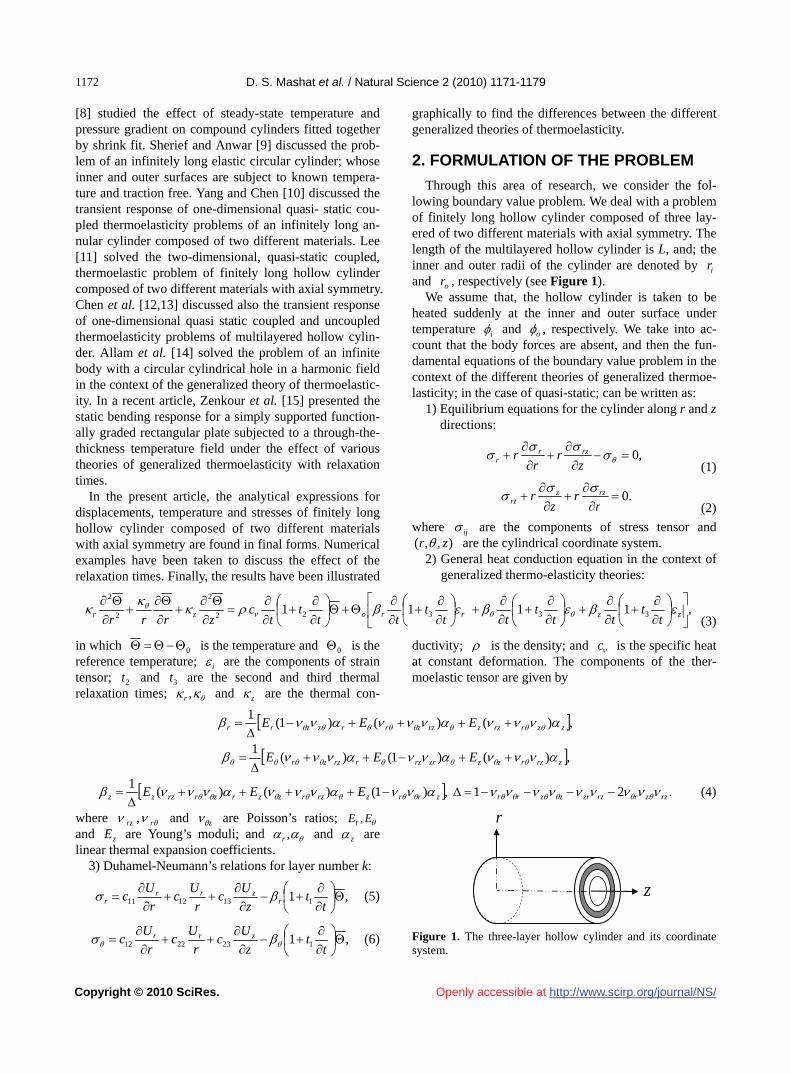
D. S. Mashat et al. / Natural Science 2 (2010) 1171-1179
Copyright © 2010 SciRes. http://www.scirp.org/journal/NS/
1172
Openly accessible at
[8] studied the effect of steady-state temperature and pressure gradient on compound cylinders fitted together by shrink fit. Sherief and Anwar [9] discussed the prob-lem of an infinitely long elastic circular cylinder; whose inner and outer surfaces are subject to known tempera-ture and traction free. Yang and Chen [10] discussed the transient response of one-dimensional quasi- static cou-pled thermoelasticity problems of an infinitely long an-nular cylinder composed of two different materials. Lee [11] solved the two-dimensional, quasi-static coupled, thermoelastic problem of finitely long hollow cylinder composed of two different materials with axial symmetry. Chen et al. [12,13] discussed also the transient response of one-dimensional quasi static coupled and uncoupled thermoelasticity problems of multilayered hollow cylin-der. Allam et al. [14] solved the problem of an infinite body with a circular cylindrical hole in a harmonic field in the context of the generalized theory of thermoelastic-ity. In a recent article, Zenkour et al. [15] presented the static bending response for a simply supported function-ally graded rectangular plate subjected to a through-the- thickness temperature field under the effect of various theories of generalized thermoelasticity with relaxation times.
In the present article, the analytical expressions for displacements, temperature and stresses of finitely long hollow cylinder composed of two different materials with axial symmetry are found in final forms. Numerical examples have been taken to discuss the effect of the relaxation times. Finally, the results have been illustrated
graphically to find the differences between the different generalized theories of thermoelasticity.
2. FORMULATION OF THE PROBLEM
Through this area of research, we consider the fol-lowing boundary value problem. We deal with a problem of finitely long hollow cylinder composed of three lay-ered of two different materials with axial symmetry. The length of the multilayered hollow cylinder is L, and; the inner and outer radii of the cylinder are denoted by and , respectively (see Figure 1).
ir
o
We assume that, the hollow cylinder is taken to be heated suddenly at the inner and outer surface under temperature i
r
and o , respectively. We take into ac-count that the body forces are absent, and then the fun-damental equations of the boundary value problem in the context of the different theories of generalized thermoe-lasticity; in the case of quasi-static; can be written as:
1) Equilibrium equations for the cylinder along r and z directions:
,0
z
rr
r rzrr (1)
.0
r
rz
r rzzrz
(2)
where ij are the components of stress tensor and ),,( zr are the cylindrical coordinate system.
2) General heat conduction equation in the context of generalized thermo-elasticity theories:
rrozr tt
ttt
tc
zrrr
322
2
2
2
11 ,11 33
zz tt
ttt
t
(3)
in which 0 is the temperature and 0 is the reference temperature; i are the components of strain tensor; 2 and are the second and third thermal relaxation times;
t 3t
,r and z are the thermal con-
ductivity; is the density; and is the specific heat at constant deformation. The components of the ther-moelastic tensor are given by
c
,)()()1(1
zzrrzzrzzrrzzrr EEE
,)()1()(1
zrzrzzzrrzrrzzr EEE
,)1()()(1
zrrzrzrzzrzrrzzz EEE
.21 rzzrrzzrzzrr (4)
where rrz , and z are Poisson’s ratios; and z are Young’s moduli; and
EEr ,E ,r and z are
linear thermal expansion coefficients. 3) Duhamel-Neumann’s relations for layer number k:
,1 1131211
t
tz
Uc
r
Uc
r
Uc r
zrrr
(5)
,1 1232212
t
tz
Uc
r
Uc
r
Uc zrr
(6)
r
z
Figure 1. The three-layer hollow cylinder and its coordinate system.
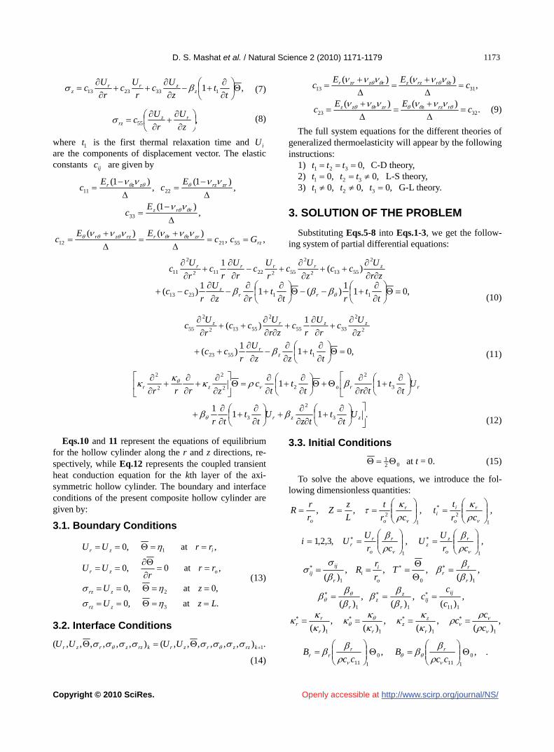
D. S. Mashat et al. / Natural Science 2 (2010) 1171-1179
Copyright © 2010 SciRes. http://www.scirp.org/journal/NS/
1171173
Openly accessible at
,1 1332313
t
tz
Uc
r
Uc
r
Uc z
zrrz
(7)
,55
z
U
r
Uc rz
rz
(8)
where 1 is the first thermal relaxation time and iU are the components of displacement vector. The elastic constants are given by
t
ijc
,)1(
,)1(
2211
zrrzzzr Ec
Ec
,)1(
33
rrzEc
,,)()(
552112 rzzrzrrrzzr Gcc
EEc
,)()(
3113 cEE
c zrrzzrzzrr
.)()(
3223 cEE
c rrzzzrrzz
(9)
The full system equations for the different theories of generalized thermoelasticity will appear by the following instructions:
1) ,0321 ttt0,t t
C-D theory, 2) 1 2 3 0,t L-S theory, 3) 1 2 30, 0,t t t 0, G-L theory.
3. SOLUTION OF THE PROBLEM
Substituting Eqs.5-8 into Eqs.1-3, we get the follow-ing system of partial differential equations:
zr
Ucc
z
Uc
r
Uc
r
U
rc
r
Uc zrrrr
2
55132
2
55222112
2
11 )(1
,01
1)(1
1)( 112313
t
trt
trz
U
rcc rr
z
(10)
2
2
3355
2
55132
2
55
1)(
z
Uc
r
U
rc
zr
Ucc
r
Uc zzrz
,011
)( 15523
t
tzz
U
rcc z
r (11)
rrozr Ut
ttrt
tt
czrrr 3
2
22
2
2
2
11
.111
3
2
3
zzr Ut
ttz
Ut
ttr
(12)
Eqs.10 and 11 represent the equations of equilibrium for the hollow cylinder along the r and z directions, re-spectively, while Eq.12 represents the coupled transient heat conduction equation for the kth layer of the axi-symmetric hollow cylinder. The boundary and interface conditions of the present composite hollow cylinder are given by:
3.1. Boundary Conditions
.at,0
,0at,0
,at0,0
,at,0
3
2
1
LzU
zU
rrr
UU
rrUU
zrz
zrz
ozr
izr
(13)
3.2. Interface Conditions
.),,,,,,(),,,,,,( 1 krzzrzrkrzzrzr UUUU (14)
3.3. Initial Conditions
021 at t = 0. (15)
To solve the above equations, we introduce the fol-lowing dimensionless quantities:
,,,,1
2*
1
2
cr
tt
cr
t
L
zZ
r
rR r
o
ii
r
oo
,,,3,2,111
cr
UU
cr
UUi r
o
zz
r
o
rr
,
)(,,,
)( 101 r
rr
o
ii
r
ijij T
r
rR
,)(
,)(
,)( 11111 c
cc ij
ijr
zz
r
,)(
,)(
,)(
,)( 1111
c
cc
r
zz
rr
rr
.,0,111
0
111
ccB
ccB rr
rr

D. S. Mashat et al. / Natural Science 2 (2010) 1171-1179
Copyright © 2010 SciRes. http://www.scirp.org/journal/NS/
1174
Openly accessible at
0
111
ccB r
zz
Note that, the index “1” represents the thermome-chanical properties of layer 1. Substituting the above imensionless quantities into Eqs.10-12, we get d
ZR
U
L
rcc
Z
U
L
rc
R
Uc
R
U
Rc
R
Uc zororrr
2
55132
22
55222112
2
11 )(1
TtR
BZ
U
RL
rcc r
zo
12313 11
)(
,011
)( 1
TtR
BBr (16)
2
22
3355
2
55132
2
55
1)(
Z
U
L
rc
R
U
Rc
ZR
U
L
rcc
R
Uc zozroz
,011
)( 15523
TtZL
rB
Z
U
RL
rcc o
zro
(17)
TtcTZL
r
RRRo
zr
22
22
2
2
1
rrr UtR
UtR
33
2
11
1 .1 3
2
zo
z UtZL
r
(18) The dimensionless stresses are also given by
,1 1131211
TtZ
U
L
rc
R
Uc
R
Uc r
zorrr
(19)
,1 1232212
TtZ
U
L
rc
R
Uc
R
Uc zorr
(20)
,1 1332313
TtZ
U
L
rc
R
Uc
R
Uc z
zorrz
(21)
,55
Z
U
L
r
R
Uc roz
rz (22)
where
.1
20
r
ijij
ccc
(23)
The solution of Eqs.16-18 may be given by using the following substitutions of r and that satisfy the boundary conditions given in Eq.13:
),sin()()(
),cos()()(
),cos()()(
2
2
1
ZRfwU
ZRfuU
ZRfT
z
r
(24)
where the functions and are given, respectively, by:
1f 2f
).1)((
,)1()1(
2
221
RRRf
RRf
i
i (25) UT , zU
Using Eq.23 into Eqs.15-17, one can get
,d
d1
d
d
d
d1
d
d
d
d1
d
d
,0d
d1 ,0
d
d1
21039387
65143211
tAwtAutAA
wAuAtAwAuAtA
(26)
where
,d
d111
121 f
RRB
R
fBA
,
d
d
d
d12
2
552
2222
2
112 fL
rc
R
fcf
RRRcA o
,d
d1
d
d125523133 fc
RRc
RRc
L
rA o
,134 fBL
rA o
,d
d1
d
d121323555 fc
RRc
RRc
L
rA o
,d
d
d
d12
2
3322
2
556 fL
rcf
RRRcA o
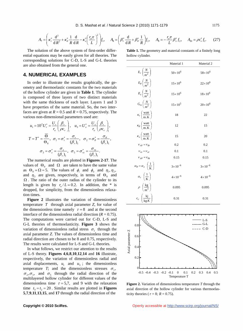
D. S. Mashat et al. / Natural Science 2 (2010) 1171-1179
Copyright © 2010 SciRes. http://www.scirp.org/journal/NS/
1171175
Openly accessible at
,d
d1
d
d1
2
2
2
7 fL
r
RRRA o
zr
,
1
d
d28 f
RRA r
,29 fL
rA z
o (27) .110 fcA
The solution of the above system of first-order differ-
ential equations may be easily given for all theories. The corresponding solutions for C-D, L-S and G-L theories are also obtained from the general one.
4. NUMERICAL EXAMPLES
In order to illustrate the results graphically, the ge-ometry and thermoelastic constants for the two materials of the hollow cylinder are given in Table 1. The cylinder is composed of three layers of two distinct materials with the same thickness of each layer. Layers 1 and 3 have properties of the same material. So, the two inter-faces are given at R = 0.5 and R = 0.75, respectively. The various non-dimensional parameters used are:
,,101
3
1
21
cr
UUu
cr
UUu r
o
zz
r
o
rr
,)(
,)(
,1
21
10 rr
rrTT
.)(
,)( 1
51
3r
rzrz
r
zz
The numerical results are plotted in Figures 2-17. The values of and are taken to have the same value as The values of i and o
05
.0 and
and 3
,, 21 are given, respectively, in terms of 0 and
. The ratio of the outer radius of the cylinder to its length is given by In addition, the * is dropped, for simplicity, from the dimensionless relaxa-tion times.
.2.0/ Lro
Figure 2 illustrates the variation of dimensionless temperature through axial parameter Z, for value of the dimensionless time namely
T8 and at the second
interface of the dimensionless radial direction (R = 0.75). The computations were carried out for C-D, L-S and G-L theories of thermoelasticity. Figure 3 shows the variation of dimensionless radial stress 1 through the axial parameter Z. The values of dimensionless time and radial direction are chosen to be 8 and 0.75, respectively. The results were calculated for L-S and G-L theories.
In what follows, we restrict our attention to the results of L-S theory. Figures 4,6,8,10,12,14 and 16 illustrate, respectively, the variation of dimensionless radial and axial displacements, 1 and 3 ; the dimensionless temperature T; and the dimensionless stresses
u u,1
,, 32 and 5 through the radial direction of the multilayered hollow cylinder for different values of the dimensionless time ,7,5 and 9 with the relaxation time 23 . Similar results are plotted in Figures 5,7,9,11,13,15, and 17 through the radial direction of the
20 tt
Table 1. The geometry and material constants of a finitely long hollow cylinder.
Material 1 Material 2
2m
NEr 61050 61058
2m
NE 61015 61022
2m
NEz 61015 61018
2m
NGrz 51015 61020
K.m
wattr 18 22
K.m
watt 12 15
K.m
wattz 15 20
rr 0.2 0.2
zrrz 0.1 0.1
zz 0.15 0.15
K
1z 6103 6103
K
1r 6104 6104
3m
kg 0.095 0.095
K
ckg
kj 0.31 0.31
1
0.8
0.6
0.4
0.2
0
Axi
al p
aram
eter
Z
-0.5 -0.4 -0.3 -0.2 -0.1 0 0.1 0.2 0.3 0.4 0.5Temperature T
L-SG-L
C-D
Figure 2. Variation of dimensionless temperature T through the axial direction of the hollow cylinder for various thermoelas-ticity theories ( = 8; R = 0.75).

D. S. Mashat et al. / Natural Science 2 (2010) 1171-1179
Copyright © 2010 SciRes. http://www.scirp.org/journal/NS/
1176
Openly accessible at
1
0.8
0.6
0.4
0.2
0
Axi
al p
aram
eter
Z
-0.5 -0.4 -0.3 -0.2 -0.1 0 0.1 0.2 0.3 0.4 0.5Radial stress σ1
G-L
L-S
Figure 3. Variation of dimensionless radial stress 1 thro- ugh the axial direction of the hollow cylinder for L-S and G-L theories ( = 8; R = 0.75). 1
0.8
0.6
0.4
0.2
0
-0.2
-0.4
-0.6
-0.8
Rad
ial d
ispl
acem
ent u
1
0.25 0.375 0.5 0.625 0.75 0.875 1Radial parameter R
τ = 5
τ = 7
τ = 9
L-S
Figure 4. Variation of dimensionless radial displacement through the radial direction of the hollow cylinder for dif-
ferent values of the time parameter 1u
( ). 2032 tt 1
0.7
0.4
0.1
-0.2
-0.5
-0.8
Rad
ial d
ispl
acem
ent u
1
0.25 0.375 0.5 0.625 0.75 0.875 1Radial parameter R
t2 = 20
t2 = 21
t2 = 22
L-S
Figure 5. Variation of dimensionless radial displacement through the radial direction of the hollow cylinder for different values of the relaxation time (
1u
7,32 tt ).
1.5
1.3
1.1
0.9
0.7
0.5
0.3
0.1
-0.1
Axi
al d
ispl
acem
ent u
3
0.25 0.375 0.5 0.625 0.75 0.875 1Radial parameter R
τ = 5
τ = 7
τ = 9
L-S
Figure 6. Variation of dimensionless axial displacement through the radial direction of the hollow cylinder for different values of the time parameter
3u
( ). 2032 tt
1.3
1.6
0.9
0.7
0.5
0.3
0.1
-0.1
Axi
al d
ispl
acem
ent u
3
0.25 0.375 0.5 0.625 0.75 0.875 1Radial parameter R
t2 = 20
t2 = 21
t2 = 22
L-S
Figure 7. Variation of dimensionless axial displacement through the radial direction of the hollow cylinder for different values of the relaxation time (
3u
7,32 tt ).
Tem
pera
ture
T
0.25 0.375 0.5 0.625 0.75 0.875 1Radial parameter R
L-S
τ = 5
τ = 7
τ = 9
2.4
2.1
1.8
1.5
1.2
0.9
0.6
0.3
0
Figure 8. Variation of dimensionless temperature T through the radial direction of the hollow cylinder for different values of the time parameter ( ). 2032 tt

D. S. Mashat et al. / Natural Science 2 (2010) 1171-1179
Copyright © 2010 SciRes. http://www.scirp.org/journal/NS/
1171177
Openly accessible at
1.8
1.6
1.4
1.2
1
0.8
0.6
0.4
Tem
pera
ture
T
0.25 0.375 0.5 0.625 0.75 0.875 1Radial parameter R
t2 = 20
t2 = 21
t2 = 22
L-S
Figure 9. Variation of dimensionless temperature T through the radial direction of the hollow cylinder for different values of the relaxation time ( 7,32 tt ).
30
10
-10
-30
-50
-70
-90
Rad
ial s
tres
s σ 1
0.25 0.375 0.5 0.625 0.75 0.875 1Radial parameter R
τ = 5
τ = 7
τ = 9
L-S
Figure 10. Variation of dimensionless radial stress 1 thro- ugh the radial direction of the hollow cylinder for different values of the time parameter ( ). 2032 tt 30
10
-10
-30
-50
-70
-90
Rad
ial s
tres
s σ 1
0.25 0.375 0.5 0.625 0.75 0.875 1Radial parameter R
L-S
t2 = 20
t2 = 21
t2 = 22
Figure 11. Variation of dimensionless radial stress 1 thro- ugh the radial direction of the hollow cylinder for different values of the relaxation time ( ).
7,32 tt
50
45
40
35
30
25
20
15
10
5
0
-5
Axi
al s
tres
s σ 3
0.25 0.375 0.5 0.625 0.75 0.875 1Radial parameter R
τ = 5
τ = 7
τ = 9
L-S
Figure 12. Variation of dimensionless axial stress 3 through the radial direction of the hollow cylinder for different values of the time parameter ( 2 tt 203 ). 42
37
32
27
22
17
12
7
2
-3
Axi
al s
tres
s σ 3
0.25 0.375 0.5 0.625 0.75 0.875 1Radial parameter R
t2 = 20
t2 = 21
t2 = 22
L-S
Figure 13. Variation of dimensionless axial stress 3 thro- ugh the radial direction of the hollow cylinder for different values of the relaxation time ( 7,32 tt ).
5
4
3
2
1
0
-1
-2
-3
Cir
cum
fere
ntia
l str
ess σ 2
0.25 0.375 0.5 0.625 0.75 0.875 1Radial parameter R
τ = 5
τ = 7
τ = 9
L-S
Figure 14. Variation of dimensionless circumferential stress
2 through the radial direction of the hollow cylinder for different values of the time parameter
( ). 2032 tt

D. S. Mashat et al. / Natural Science 2 (2010) 1171-1179
Copyright © 2010 SciRes. http://www.scirp.org/journal/NS/
1178
Openly accessible at
3.6
2.9
2.2
1.5
0.8
0.1
-0.6
Cir
cum
fere
ntia
l str
ess σ 2
0.25 0.375 0.5 0.625 0.75 0.875 1Radial parameter R
t2 = 20
t2 = 21
t2 = 22
L-S
Figure 15. Variation of dimensionless circumferential stress
2 through the radial direction of the hollow cylinder for different values of the relaxation time ( 7,32 tt ). 200
150
100
50
0
-50
-100
She
ar s
tres
s σ 5
0.25 0.375 0.5 0.625 0.75 0.875 1Radial parameter R
τ = 5
τ = 7
τ = 9
L-S
Figure 16. Variation of dimensionless shear stress 5 through the radial direction of the hollow cylinder for different values of the time parameter ( ). 2032 tt
160
120
80
40
0
-40
-80
She
ar s
tres
s σ 5
0.25 0.375 0.5 0.625 0.75 0.875 1Radial parameter R
t2 = 20
t2 = 21
t2 = 22
L-S
Figure 17. Variation of dimensionless shear stress 5 thro- ugh the radial direction of the hollow cylinder for different values of the relaxation time ( 7,32 tt ).
multilayered hollow cylinder for different values of the relaxation time )22,21,20( 23 tt
7 when the dimen-
sionless time .
5. CONCLUSIONS
The conclusion of the above results may be given as: 1) Figure 2 illustrates that the dimensionless tem-
perature is slightly changed and the differences between C-D, L-S, and G-L are very small (tiny). The coupled theory (C-D) may give results with small relative error compared with those given by Lord and Shulman’s (L-S) and Green and Lindsay’s (G-L) theories. However, the results of L-S and G-L are much closed to each other (see Figure 3).
2) The plots of results given by Lord and Shulman’s theory show that the effect of the dimensionless time is slightly clear in the first layer, but in the second and third layers the effect is not declared. This happened for dimensionless radial and axial displacements (see Figures 4-7), and axial, circum-ferential, and shear stresses (see Figures 12-17).
3) However, for dimensionless temperature and radial stress, the effects of dimensionless time is very clear in the first layer and start to decrease with the increase of radial direction in the second and third layer (see Figures 8-11).
4) The effect of the relaxation time of Lord and Shul-man’s theory in all physical waves (displacements, temperature and stresses) is clear in the first layer, but is less considerable in the second and third lay-ers. This revealed that the effect of the relaxation time has no effect when the dimensionless radius is increasing.
6. ACKNOWLEDGEMENTS
This paper is fully supported by the Deanship of Scientific Research
at King AbdulAziz University, Grant No. 181/428.
REFERENCES
[1] Biot, M. (1956) Thermoelasticity and irreversible the- rmo-dynamics. Journal of Applied Physics, 27, 240-253.
[2] Lord, H.W. and Shulman, Y.A. (1967) A generalized dynamical theory of thermoelasticity. Jornal of Mechan-ics and Physics of Solids, 15, 299-309.
[3] Dhaliwal, R.S. and Sherief, H.H. (1980) Generalized thermoelasticity for anisotropic media. Quarterly of Ap-plied Mathematics, 38, 1-8.
[4] Ignaczak, J. (1979) Uniqueness in generalized thermoe-lasticity. Journal of Thermal Stresses, 2, 171-175.
[5] Sherief, H.H. and Dhaliwal, R. (1980) A uniqueness theorem and a variational principle for generalized ther-moelasticity. Journal of Thermal Stresses, 3, 223-230.

D. S. Mashat et al. / Natural Science 2 (2010) 1171-1179
Copyright © 2010 SciRes. http://www.scirp.org/journal/NS/Openly accessible at
1171179
[6] Green, A. and Lindsay, K. (1972) Thermoelasticity. Journal of Elasticity, 2, 1-7.
[7] Jane, K.C. and Lee, Z.Y. (1999) Thermoelasticity of mul-tilayered cylinder. Journal of Thermal Stresses, 22, 57-74.
[8] Kandil, A. (1975) Investigation of stress analysis in com- pound cylinders under high pressure and temperature. M.Sc. Thesis, CIT Helwan.
[9] Sherief, H.H. and Anwar, M.N. (1988) A problem in generalized thermoelasticity for an infinitely long annu-lar cylinder. International Journal of Engineering Sci-ence, 26, 301-306.
[10] Yan, Y.C. and Chen, C.K. (1986) Thermoelastic transient response of an infinitely long annular cylinder com- posed of two different materials. International Journal of Engineering Science, 24, 569-581.
[11] Lee, Z.-Y. (2006) Generalized coupled transient response of 3-D multilayered hollow cylinder. International Com-
munications in Heat and Mass Transfer, 33, 1002-1012. [12] Chen, C.K., Hung, C.I. and Lee, Z.Y. (2001) Transient
thermal stresses analysis of multilayered hollow cylinder. Acta Mechanica, 151, 75-88.
[13] Chen, C.K., Hung, C.I. and Lee, Z.Y. (2001) Thermoe-lastic transient response of multilayered hollow cylinder with initial interface pressure. Journal of Thermal Str- esses, 24, 987-1006.
[14] Allam, M.N., Elsibai, K.A. and Abouelregal, A.E. (2002) Thermal stresses in a harmonic field for an infinite body with a circular cylindrical hole without energy dissipa-tion. Journal of Thermal Stresses, 25, 57-67.
[15] Zenkour, A.M., Mashat, D.S. and Elsibai, K.A. (2009) Bending analysis of functionally graded plates in the context of different theories of thermoelasticity. Mathe-matical Problems in Engineering, 2009, Article ID 962351, 1-15.