SCIENCE \u0026 TECHNOLOGY A Comparative Study on Standard, Modified and Chaotic Firefly Algorithms

$Page 1: SCIENCE \u0026 TECHNOLOGY A Comparative Study on Standard, Modified and Chaotic Firefly Algorithms$
Pertanika J. Sci. & Technol. 23 (2): 251 - 269 (2015)

SCIENCE & TECHNOLOGYJournal homepage: http://www.pertanika.upm.edu.my/

ISSN: 0128-7680 © 2015 Universiti Putra Malaysia Press.

A Comparative Study on Standard, Modified and Chaotic Firefly Algorithms

Hong Choon Ong1*, Surafel Luleseged Tilahun2 and Suey Shya Tang1

1School of Mathematical Sciences, Universiti Sains Malaysia, 11800 USM, Pulau Pinang, Malaysia2Computational Science Program, College of Nature Sciences,Addis Ababa University, 1176, A.A., Ethiopia

ABSTRACT

Many studies have been carried out using different metaheuristic algorithms on optimisation problems in various fields like engineering design, economics and routes planning. In the real world, resources and time are scarce. Thus the goals of optimisation algorithms are to optimise these available resources. Different metaheuristic algorithms are available. The firefly algorithm is one of the recent metaheuristic algorithms that is used in many applications; it is also modified and hybridised to improve its performance. In this paper, we compare the Standard Firefly Algorithm, the Elitist Firefly Algorithm, also called the Modified Firefly Algorithm with the Chaotic Firefly Algorithm, which embeds chaos maps in the Standard Firefly Algorithm. The Modified Firefly Algorithm differs from the Standard Firefly Algorithm in such a way that the global optimum solution at a particular iteration will not move randomly but in a direction that is chosen from randomly generated directions that can improve its performance. If none of these directions improves its performance, then the algorithm will not be updated. On the other hand, the Chaotic Firefly Algorithm tunes the parameters of the algorithms for the purpose of increasing the global search mobility i.e. to improve the attractiveness of fireflies. In our study, we found that the Chaotic Firefly Algorithms using three different chaotic maps do not perform as well as the Modified Firefly Algorithms; however, at least one or two of the Chaotic Firefly Algorithms outperform the Standard Firefly Algorithm under the given accuracy and efficiency tests.

Keywords: Metaheuristic, optimisation, Standard Firefly Algorithm, Modified Firefly Algorithm, Chaotic Firefly Algorithm

Article history:Received: 25 March 2014Accepted: 15 May 2014

E-mail addresses: [email protected] (Hong Choon Ong)[email protected] (Surafel Luleseged Tilahun)[email protected] (Suey Shya Tang)*Corresponding Author

INTRODUCTION

Generally, optimisation refers to maximisation or minimization of an objective function by finding suitable values for the variables from a set of feasible values. Optimisation solution methods can be categorised into two categories: deterministic algorithms and non-

Hong Choon Ong, Surafel Luleseged Tilahun and Suey Shya Tang

252 Pertanika J. Sci. & Technol. 23 (2): 251 - 269 (2015)

deterministic algorithms. Heuristic or metaheuristic algorithms fall under non-deterministic algorithms. The word ‘heuristic’ comes from a Greek word ‘to find’ or ‘to discover’ while metaheuristic combines the words ‘meta’ and ‘heuristic’ where ‘meta’ means a higher level. However, no difference is recorded between metaheuristic and heuristic; researchers seem to use both names interchangeably. Heuristic algorithms are usually experience-based. Simply put, they are a ‘common-sense’ approach to problem solving (Luke, 2013). They are used to speed up the process of finding a good enough solution based on an educated guess, an intuitive judgment or expertise (Suh et al., 2011). Metaheuristic algorithms are iterative procedures that combine the concepts of exploration and exploitation within feasible regions (Osman & Laporte, 1996). Learning strategies are used to organise information in order to generate near-optimal solutions. Based on previous knowledge and most of the simulated real-life experiments done in this area, heuristic algorithms try to get solutions which are effective to dismantle the problems. They can be applied to many problems as they do not rely on rigorous mathematical characteristics of the problems and may be generally used on global optimisation problems(Fink & Voβ, 1998; Fu et al., 2005; Tilahun & Ong, 2012a; Kopecek, 2014; Maknoon et al., 2014; Cui, 2014).However,they do not guarantee the generation of an exact optimal solution within acceptable timescales (Hopper & Turton, 2000). On the contrary, metaheuristics are likely to generate near-optimal solutions within acceptable timescales. Nowadays, many studies are found to group all stochastic algorithms within random variables and global exploration into metaheuristic algorithms.

Two major search components of metaheuristics are exploration and exploitation. Exploration means looking for diverse solutions by going around entire new regions in a particular search space while exploitation means getting the current best solution by focusing on those found regions. In a case where there is too little exploration and too much exploitation, the algorithm may get trapped within local optima resulting in difficulty in finding the global optimum. Therefore, we need to achieve a balance between these components to improve the convergence of the algorithm (Creppinsek et al., 2000; Yang, 2011). Most metaheuristic algorithms are nature-inspired and they mimic biological, physical or natural phenomena from the real world. Some popular nature-inspired algorithms are the Particle Swarm Optimisation (PSO) algorithm, the Prey-Predator Algorithm (PPA), the Cuckoo Search (CS) algorithm, the Bat Algorithm (BA) and the Firefly Algorithm (FFA). They have different strengths and better performances for a certain class of optimisation problems. It is quite challenging to select the suitable or best algorithm for a specific problem, and this by itself is another optimisation problem.

Nowadays, there are trends to introduce new algorithms, extend and modify the existing algorithms, compare the performance of different algorithms, apply the algorithms in multiple disciplines for optimisation purpose and combine any two algorithms in hybridisation (Fisher et al., 2013). Even though the Firefly Algorithm is one of the recently introduced metaheuristic algorithms (Yang, 2009), it has been used extensively for many applications and has been modified and hybridised for different classes of optimisation problems (Apostolopoulos & Vlachos, 2011; Basu & Mahanti, 2011; Gandomi et. al, 2013; Tilahun & Ong, 2013). In this study, we compared the performances of the Standard (FFA) algorithm, the Modified Firefly Algorithm (MFFA) and the Chaotic Firefly Algorithms (CFFAs) based on eight chosen test

A Comparative Study on Standard, Modified and Chaotic Firefly Algorithms.

253Pertanika J. Sci. & Technol. 23 (2): 251 - 269 (2015)

functions in terms of their accuracy and effectiveness. Three chaotic maps, namely, the Iterative map, the Chebyshev map and the Sinusodial map for the Chaotic Firefly Algorithms, were chosen based on their statistical results and success rate, which can improve the reliability of the global optimality and enhance the quality of the results (Gandomi et al., 2013).In the chaotic map, we varied the parameters, β (the attractiveness coefficient) and γ (light absorption coefficient). If γ is too small and tends to zero, attractiveness becomes constant; and if γ is too large, attractiveness will decrease dramatically, as will be discussed later. Therefore we needed to tune the γ parameter used for all the Firefly Algorithms tested within these two extreme γ values.

BASIC CONCEPTS

Optimisation Problem

Optimisation is a mathematical method to find a maximum or minimum value of an objective function f(x) by choosing a variable from a feasible region, Ω. x* is said to be a solution for a minimisation problem if and only if x* ∈Ω and f(x*) ≤ f(x), ∀∈Ω . We can express the typical minimisation problem in equation (1) and its equivalent maximisation problem in equation (2).

Hence f(x* ) ≤ f(x) for all x∈ Ω

Hence f(x* ) ≥ f(x) for all x∈ Ω

Optimisation algorithms are useful tools for different applications including experimental design, parameter estimation, model development and statistical analysis; process synthesis, analysis, design and retrofit; model predictive control and real-time optimisation. They are also useful in the planning, scheduling and integration of process operations into the supply chain for manufacturing and distribution (Biegler, 2010).

Standard and Modified Firefly Algorithm (FFA, MFFA)

The Modified Firefly Algorithm is an extension or improvement of the Firefly Algorithm (FFA), which is a nature-inspired algorithm that imitates the behaviour of fireflies of flashing light within their bodies to attract mating partners and potential predators (Yang, 2010).

minx∈ℝ𝑛𝑛

𝑓𝑓(𝑥𝑥)

s.t. 𝑥𝑥∈Ω ⊆ℝ𝑑𝑑 (1)

maxx∈ℝ𝑛𝑛

−𝑓𝑓(𝑥𝑥)

s.t. 𝑥𝑥∈Ω ⊆ℝ𝑑𝑑 (2)



There are three assumptions made in adapting this behaviour of fireflies for use in an algorithm:

i. All fireflies are unisex; therefore, a firefly may be attracted to any other firefly;

ii. The attractiveness of fireflies is proportional to their brightness, and for two fireflies, xi and xj, if the brightness of xj ≥ the brightness of xi, then xi will move towards xj. At the same time, attractiveness decreases as distance increases.

iii. The brightness of a firefly is affected or determined by the landscape of the objective function to be optimised

There are two important components affecting the movements of fireflies: the variation of light intensity and the formulation of the attractiveness. As mentioned above, light intensity I decreases as the distance r increases. We can express I(r) as given below:

By combining this with the inverse square law, I (r) can be expressed as:

As the attractiveness is proportional to the light intensity, we now define the attractiveness β as:

where β0 is the attractiveness at r=0. Computationally, it is harder to calculate the exponential function than 1/(1+r2) , hence we approximate the equation of computing the attractiveness β as:

Suppose we have a firefly i located at xi as the brighter firefly while another less bright firefly j is at xj; the firefly j will move towards the firefly i. The location is then updated using the process given below:

where rand is a vector of random numbers 0≤α≤1 and 0.01≤γ≤100 (Yang, 2009).

The distance between two fireflies, namely, firefly i and firefly j, rij, can be computed using Euclidean distance as:

𝐼𝐼(𝑟𝑟) = 𝐼𝐼0 𝑒𝑒−𝛾𝛾𝑟𝑟 (3)

𝐼𝐼(𝑟𝑟) = 𝐼𝐼0 𝑒𝑒−𝛾𝛾𝑟𝑟2 (4)

𝛽𝛽 = 𝛽𝛽0 𝑒𝑒−𝛾𝛾𝑟𝑟2 (5)

𝛽𝛽 =

𝛽𝛽0

1 + 𝛾𝛾𝑟𝑟2 (6)

𝑟𝑟𝑖𝑖𝑖𝑖 = ‖𝑥𝑥𝑖𝑖 − 𝑥𝑥𝑖𝑖

(8)



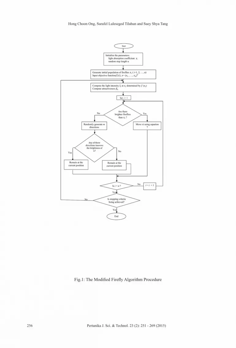
While the same in all the issues discussed above, the Standard and Modified Firefly Algorithms mainly differ in the updating process of the brightest firefly; instead of letting this brightest firefly, xB, which serves as the current global best solution to move randomly, we set the movement direction for it. The purpose for doing so is that we know that if this brightest firefly moves randomly, it may move to a region where its brightness may decrease i.e. the performance of the global best solution for the algorithm may decrease. In order to do so, we generate m unit vectors, u1, u2,…,um, and choose one in which the brightness of the current global best solution will increase if it moves in the particular direction, say U (Tilahun & Ong, 2012b). The movement direction of the brightest firefly can be expressed as below:

where α is the random step length and U is the unit vector chosen from the m directions. If there is no direction from the m unit vectors for the current brightest solution to move in order to increase its performance, the current brightest solution will remain at its existing position. Furthermore, unlike the Standard Firefly Algorithm, in the Modified Firefly Algorithm, β0, which is the attractiveness at r=0, for a firefly this is not taken as 1 but can be expressed as:

where I0i is the intensity at r=0 for firefly i while I0

j is the intensity at r=0 for firefly j and I0

j ≠ 0. The modified firefly algorithm procedure is shown in Fig.1.

Chaotic Firefly Algorithm (CFFA)

Chaos is a type of unique deterministic nonlinear dynamic behaviour and it has been applied widely in communication, automation, pattern recognition and other fields. A dynamic system may be mathematically expressed either by a continuous set of equations or by a discrete system, called a map, as follows:

running in chaotic state. The chaotic sequence

xk:k=0,1,2…

can be used as a spread-spectrum sequence and as a random number sequence. These sequences have already been proven for their easy and fast generation and storage (Heidari-Bateni & McGillem, 1992; Nguyen et al., 2013).

The main idea of using chaotic maps or systems in a Firefly Algorithm is to replace the random variables used in the firefly algorithm with chaotic variables so as to increase its mobility for robust global optimisation. To fulfil this purpose, we tune the parameters β and γ for the attractive movement in chaotic firefly. Tuning the parameters β and γ will affect the results of the convergence rate and the number of algorithm iterations (Arora & Singh, 2013; Yang, 2011).

𝛽𝛽𝑜𝑜 =

𝐼𝐼0𝑖𝑖

𝐼𝐼0 𝑖𝑖

(10)

𝑥𝑥𝑘𝑘+1 = 𝑓𝑓(𝑥𝑥𝑘𝑘) , 0 < 𝑥𝑥𝑘𝑘 < 1, 𝑘𝑘 = 0, 1, 2 … (11)



Fig.1: The Modified Firefly Algorithm Procedure



Although firefly algorithms are efficient enough in optimisation problems, in this study we noticed that the solutions kept on changing as they approached the optimum. Gandomi et al. (2013)suggested to tune the light absorption coefficient, γ, and the attractiveness coefficient, β, using chaotic maps so as to increase the mobility of the solution in the algorithms. The chaotic Firefly Algorithm procedure is shown in Fig.2.

Fig.2: The Chaotic Firefly Algorithm Procedure



Chaotic solutions are affected by three properties: sensitivity of parameters, sensitivity of initial points and randomness (Sharkovsky et al., 1997). For the sensitivity of parameters, slight changes in the parameters or initial values for the data will lead to vastly different future behaviour. On sensitivity of initial points, we can see that if an initial point x0 varies slightly, two sequences found from repeated calculations on a chaotic map with a parameter finally become quite different. For randomness, solutions starting from almost all x0 in [0, 1] wander in [0, 1] as the random number is taken from a uniform distribution.

The characteristic of non-repetition of chaos enables the algorithm to carry out overall searches at a higher speed than stochastic ergodic searches, which depend on probabilities. A random local search may cause the algorithm to be easily trapped in the local minima but Chaotic maps are useful in helping the algorithm to escape this condition.

One-dimensional maps are the simplest systems with the capability of computing a chaotic process (Ram, 2009).In this study, we choose three chaotic maps that have good performance in terms of success rate and statistical analysis which was studied by Gandomi et al. (2013).The maps chosen are the Iterative map, the Chebyshev map and the Sinusodial map. Gandomi et al. (2013) suggested to normalise the chaotic maps between 0 and 2 to produce the simulation results. We embedded these maps into the firefly algorithms for it to become Chaotic Firefly Algorithms (CFFA).

The three chosen chaotic maps were one-dimensional and non-invertible maps. The first map was an Iterative map. It is a mapping function that maps a region back onto itself and is defined as below:

where a∈(0, 1) is the suggested range for the parameter. In this study, we used a=0.5 for all the firefly algorithms being tested.

Secondly we had a Chebyshev map, which is a typical chaotic map called an identity map, defined as:

The third chaotic map we tested was a Sinusodial map. It is defined as below:

Gandomi et al. (2013) suggested to use a=2.3 and x0=0.7, which gave us a simplification of the equation as:

𝑥𝑥𝑘𝑘+1 = 𝑎𝑎𝑥𝑥𝑘𝑘2 sin (𝜋𝜋𝑥𝑥𝑘𝑘)

(14)



In Gandomi et al. (2013), the success rate for evaluating the performance of the algorithms can be calculated using this equation:

where Nall is the number of all trials, Nsuccessful is the number of trials in which is found a successful solution. Here, a run in which the results are close to the global optimum would be considered a successful run. A successful run can be expressed as:

where xgb is the global best obtained by the proposed algorithms and UB is the upper bound while LB is the lower bound of the variable tested.

TEST FUNCTIONS

Standard benchmarks or test functions are useful and important in evaluating the reliability, efficiency and validation of optimisation algorithms. The test functions can be categorised according to their types of continuity, modality and dimensionality. On the continuity of test functions, we used both continuous and discontinuous functions. A function f(x) is said to be continuous at a point c if the limit of the function as x approaches c is the same as the functional value of the function at x=c. If this property is not fulfilled at any point x=c, the function f(x) is said to be discontinuous at c. For the modalities of test functions, we used both unimodal and multimodal functions.

A unimodal function has only one optimum while a multimodal function may have many local optima and global optima. Multimodal functions are useful in testing the ability of optimisation algorithms to escape from a local minimum. In this study, we chose eight test functions under different categories of continuity, modality and dimensionality. One of the selected test functions was a four-dimensional objective function while the rest of the functions chosen were two-dimensional.

Beale Function

The Beale Function is a continuous and unimodal function with sharp peaks at the corners of the input domain. It is a two-dimensional function.The function is defined as:

f1(x)=(1.5 - x1+ x1 x2 )2+(2.25 - x1+x1 x22 )2+(2.625-x1+x1 x2

3)2 )

The variables x1 and x2 are both defined on the interval [-4.5, 4.5]. It is unimodal and contains only one optimum i.e. a global minimum at (x1,x2)=(3, 0.5) giving the value of f1 (x)=0 (Momin & Yang, 2013). Figure 3 shows the graph of f1(x).

𝑆𝑆𝑟𝑟 = 100 ×

𝑁𝑁𝑠𝑠𝑠𝑠𝑠𝑠𝑠𝑠𝑒𝑒𝑠𝑠𝑠𝑠𝑓𝑓 𝑠𝑠𝑢𝑢𝑁𝑁𝑎𝑎𝑢𝑢𝑢𝑢

(16)

‖𝑥𝑥𝑔𝑔𝑔𝑔 − 𝑥𝑥∗‖ ≤ ( 𝑈𝑈𝑈𝑈 − 𝐿𝐿𝑈𝑈) × 10−4 (17)



Leon Function

The Leon Function is a continuous and unimodal function. It is a two-dimensional function.The function is defined as:

f2 (x)=100(x2-x12 )2+(1-x1 )2

The variables x1 and x2 are both defined on the interval [-1.2, 1.2]. The global minimum of the Leon Function at (x1,x2)= (1, 1) gives the value of f2 (x) = 0 (Momin & Yang, 2013). Figure 4 shows the graph of f2 (x) plotted for two-dimensional graph.

Matyas Function

The Matyas Function is a continuous and unimodal function. It is a two-dimensional function.The function is defined as:

f3 (x)=0.26(x12+x2

2)+0.48x1 x2

The variables x1 and x2 are both defined on the interval [-10, 10]. The global minimum of the Matyas function at (x1,x2)= (0, 0) gives the value of f3 (x) = 0 (Momin & Yang, 2013). Figure 5 shows the graph of f3 (x) plotted for a two-dimensional graph.Goldstein Price Function

Goldstein Price Function is a continuous and multimodal function. It is a two-dimensional function.The function is defined as:

f4 (x)=[1+(x1+x2 +1)2 (19-14x1+3x12-14x2+6x1 x2+3x2

2 )]× [30+(2x1-3x2 )2 (18-32x1+12x1

2+48x2-36x1 x2+27x22 )]

The variables x1 and x2 are both defined on the interval [-2, 2]. The global minimum of the Goldstein Price function at (x1,x2)= (0, -1) gives the value of f4 (x) = 3 (Schonlau, 1997). Not far from the global minimum, there are another three local minima. Therefore, it is said to be a difficult problem for minimisation methods due to its having more than one local minimum. Figure 6 shows the graph of f4(x).

Hosaki Function

The Hosaki Function is a continuous and multimodal (bimodal) function. It is a two-dimensional function.The function is defined as below:

The variable x1 is defined on the interval [0, 5] while x2 is defined on the interval [0, 6]. The global minimum of the Hosaki function at (x1,x2)= (4, 2) and the local minimum of the Hosaki function at (x1,x2)= (1, 2) give the value of f5 (x) = -2.3458 (Duan et al., 1992). Figure (7) shows the graph of f5 (x).



Price 1 Function

The Price 1 Function is a continuous and multimodal function. It is a two-dimensional function.The function is defined as:

f6 (x)=(|x1 |-5)2+(|x2 |-5)2

The variables x1 and x2 are both defined on the interval [-500, 500]. There are four global minima of the Price 1 Function at (x1,x2)= (-5, -5), (-5, 5), (5, -5), (5, 5) which give the value of f6 (x) = 0 (Price, 1976). Figure 8 shows the graph of f6 (x).

Bird Function

The Bird Function is a continuous and multimodal function. It is a two-dimensional function.The function is defined as:

The variables x1 and x2 are both defined on the interval [-2π, 2π]. The global minimum of the Bird Function at (x1,x2)= (4.70104, 3.15294) and (-1.58214, -3.13024) gives the value of f7 (x) = -106.764537 (Momin & Yang, 2013). Figure 9 shows the graph of f7 (x) plotted for a two-dimensional graph.

Cosine Mixture Function

The Cosine Mixture Function is a discontinuous and multimodal function. This function can be either in two or four dimensions.The function is defined as:

The variable x1 is defined on the interval [-1, 1]. In this study, we fixed the number of dimensions to four. The minimum of the Cosine Mixture function is found at x1 = 0 to give the values of f8 (x) = -0.2 and f8 (x) = - 0.4 for the two-dimensional and four-dimensional cases respectively. (Momin & Yang, 2013). Figure 10 shows the graph of f8 (x) plotted for the two-dimensional graph.





TAB

LE

1 :

Sim

ulat

ion

Res

ults

of

the

5 D

iffe

rent

Fir

efly

Alg

orit

hms

Test

ed (

j=1,

2,

…,

5) o

n 8

Cho

sen

Test

Fun

ctio

ns (

i=1,

2,

…,

8)

B

ased

on

Max

imum

Num

ber o

f Ite

ratio

ns a

s the

Ter

min

atio

n C

riter

ion



TAB

LE

2:

Sim

ulat

ion

Res

ults

of

the

5 D

iffe

rent

Fir

efly

Alg

orit

hms

Test

ed (

j=1,

2,

…,

5) o

n 8

Cho

sen

Test

Fun

ctio

ns (

i=1,

2,

…,8

)

Bas

ed o

n To

lera

nce

(tol)

as th

e Te

rmin

atio

n C

riter

ion



SIMULATION RESULTS

We carried out tests for the eight functions for the algorithms under two termination criteria, which are the maximum number of iterations and pre-given tolerance. The maximum number of iterations was set as 200 iterations and was tested at 100 trials, with the same random initial solution passing to the entire algorithm in each trial. We recorded the mean functional values and their standard deviations as well to examine the accuracy of the tested functions on different algorithms. At the same time, we compared the mean CPU time needed per trial on the FFA, MFFA and CFFA. Using the second termination criterion, we set a tolerance which was close to the global minimum value. We got the mean number of iterations needed for convergence when the termination criterion was met and the mean CPU time needed per trial for the algorithms respectively. For both tests, we set the number of solutions at 50, 100 and 150 to see whether the number of solutions affected the simulation results. The simulation results for the first test are shown in Table 1 while the simulation results for the second test are shown in Table 2.

Under the maximum number of iterations as termination criteria, the number of iterations for the inner loop was set at 200 and these were tested 100 times repeatedly in the while loop until the best solution (optimal value) was obtained. The results in Table 1 show the sample mean, sample standard deviation and sample mean CPU time for eight test problems (i) under five algorithms (j) in three sets of numbers of fireflies (k). Under these criteria, the accuracy of the algorithms can be compared.

In the first test, for the mean functional values, MFFA, outperformed the other algorithms for all eight test functions i.e. the functional values were the closest to the global minimum values. For instance, when n=50, MFFA outperformed the other algorithms (shown in bold and italics) since its sample mean optimal value was the nearest to the established optimum in all the eight test functions carried out where μ121=0.0032, μ 221=0.0000, μ 321=0.0001, μ 421=3.0262, μ521=-2.3455μσ621=0.0014, μ 721=-106.7020 and μ 821=-0.3346. We noticed that the MFFA achieved the highest accuracy. Besides that, we also observed that at least one of the CFFA (when we see the three chaotic mappings as a group) performed better than the FFA. For instance, when n =100, 7 out of 8 test problems in the CFFAs performed better than FFA (shown in bold and italics) where μ132=0.0131 and μ 152=0.0129 compared to μ 122=0.0152;μ332=0.0007and μ342=0.0006 compared to μ312=0.0008; μ_432=3.1805 compared to μ412=3.3074; μ532=-2.3447 and μ 542=-2.3443 compared to μ 512=-2.3439; μ632=0.2840 and μ642=0.2927compared to μ 612=0.3164; μ 732=-106.5059, μ 742=-106.5120 and μ752=-106.5546 compared to μ712=-106.4639; μ 832=-0.2689 compared to μ 812=-0.2622.

Besides comparing the sample mean optimal value, we can also compared the sample standard deviation for the sample mean value obtained from the 8 test functions. Overall, the sample standard deviation for the MFFA was the smallest among all the five algorithms tested regardless of the number of fireflies set. It indicated that the results from the MFFA were more constant and stable. On the other hand, the performances of the sample standard deviations and CPU times of the FFA and the CFFA depended on the performance of their sample means respectively. For instance (as underlined), σμ121 = 0.0040, σμ 221 = 0.0000, σμ321 = 0.0001, σμ 421= 0.0227, σμ521= 0.0002, σμ621 = 0.0014, σμ 721 = 0.0898 and σμ821 = 0.0163 for n=50; σμ122)=0.0025, σμ 222= 0.0000, σμ322 = 0.0001, σμ 422 = 0.0233, σμ522 = 0.0003, σμ 622 =0.0015,



σμ722)=0.0813 and σ_(μ822) = 0.0169 for n=100; and σμ123 =0.0021, σμ223=0.0000, σμ323=0.0001, σμ423 =0.0179, σμ523 =0.0002, σμ623)=0.0013, σμ723 =0.0648 and σμ823 =0.0185 for n=150. A low standard deviation obtained in MFFA indicated that the optimal sample mean of the optimal solutions obtained for each trial was distributed very close to the optimal sample mean of the optimal solutions i.e. the variation between the means was rather small.

Under the tolerance value accepted according to the established optimum of the eight test problems as termination criteria, the number of iterations for the inner loop was set at 10000 number of times and these iterations were tested 100 times repeatedly until a termination criterion, which achieved a very close solution to the actual optimal solution based on the tolerance given, was obtained.The results in Table 2 show the number of iterations needed for the convergence in each trial with its sample standard deviation and the mean CPU time needed for each trial and its sample standard deviation. Under these criteria, the effectiveness of the algorithms can be compared.

In the second test, for the mean number of iterations, the MFFA also outperformed the other algorithms for all the eight test functions i.e. it converged faster than others and had the least number of iterations. For instance, under f6(shown in bold and italics), when n=50, Itr621=38.3900 compared to Itr611=51.9800, Itr631=60.7300, Itr641=55.2500 and Itr651=54.2300. As was the situation for the first test, there was at least one CFFA (when we saw the three chaotic mappings as a group) converged faster than the FFA. For instance, when n=150, 7 out of 8 test problems in the CFFAs performed better than the FFA (shown in bold and italics) where Itr143=23.6200 and Itr153=23.3800 compared to Itr113=26.1400;Itr233=8.7200 and Itr243=7.4800 compared to Itr213=9.1700; Itr333=18.1800 and Itr353=21.8400 compared to Itr313=22.7100; Itr433=18.6000, Itr443=24.5200 and Itr453=34.2300 compared to Itr413=34.4900;Itr543=17.2800 compared to Itr513=17.6300; Itr743=12.3800compared to Itr713=12.8100; Itr833=46.2300, Itr843=48.9900 and Itr853=38.4100 compared to Itr813=52.4400.

Furthermore, the MFFA needed the least CPU time to converge, followed by both the CFFA and the FFA simultaneously. The sample standard deviations of the number of iterations and the CPU times for convergence depended on the performance of the number of iterations spontaneously. We noticed that the sample standard deviation for MFFA was the least and its CPU time was the least as well since the MFFA had the smallest number of iterations needed to reach the convergence criteria. For instance, under f7 (as underlined), Itr722=12.0300 at σItr722=10.9622 with CPU722=0.2316 (MFFA) when n = 100 has the least number of iterations, standard deviation and CPU time if compared to the results obtained in the FFA and the CFFAs.

Most of the time, when the number of fireflies increased, the optimal values got closer to the established optimum. For instance,μ211=0.0007 for n = 50 had improved to μ212=0.0005 for n = 100 and then further improved toμ213=0.0004 for n = 150. We could see the sample mean was approaching the established optimum when the number of fireflies increased from 50 to 100 and then to 150. This indicated that the number of fireflies had a positive relationship with the optimal sample mean value. Therefore, if we wished to get the best optimal value, what we needed to do was to increase the sample size. We also noticed that the mean number of iterations was actually affected by the tolerance value set for the functions; the smaller the difference between the global minimum value and the tolerance, the fewer the number of iterations were needed for convergence. For instance, f6 was set at the tolerance of 0.1, f1



was set at the tolerance of 0.01, f3 was set at the tolerance of 0.001 where the tolerance in f3 had the smallest different with a global minimum (f3min=0). When n=100, we observed that (underlined) the number of iterations decreased from Itr612=35.5000 to Itr112=34.3700 and then Itr312=23.1800 under the FFA.

Theoretically, exploration is done using a big-step length which can take the solution away from its current neighbourhood. Both of the three versions of Firefly Algorithms have the same exploration property. However, due to the chaos representation of the algorithm parameters in the CFFA, Gandomy et. al. (2013)claimed that it was faster than the Standard Firefly Algorithm. In terms of exploitation, the MFFA has the advanatge of tracking its best and not leaving it unless a better solution is found. Unlike the MFFA, the performance of the other two versions usually fluctuates with the iterations; hence, the MFFA outperformed the other two.

CONCLUSION

This paper discusses the recent versions of Firefly Algorithms, the Chaotic Firefly Algorithm and the Modified Firefly Algorithm, along with the Standard Firefly Algorithm. The Firefly Algorithm is a metaheuristic optimisation algorithm in which randomly generated feasible solutions are assigned as fireflies with a light intensity based on the objective function. A firefly tends to follow brighter fireflies and where no brighter firefly exists, if it is the brightest one, it will move randomly. This random movement is modified in the Modified Firefly Algorithm so that the performance of the algorithm will not fluctuate through iterations and it keeps the best solution throughout the iteration, only replacing it if a better solution is found. On the other hand, by incorporating chaos in determining the values of the algorithm parameter rather than taking it as a constant number, is how the Chaos Firefly operates. Incorporating chaos helps in the fast convergence of the algorithm. In this study, these three versions of Firefly Algorithms were studied and compared based on eight selected test problems of different types. The simulation results for the Standard Firefly Algorithm, the Modified Firefly Algorithm and the Chaos Firefly Algorithm, using the three types of chaos models, suggested that the Modified Firefly Algorithm outperformed the other versions in average performance and also had a smaller standard deviation. Hence, based on the selected test problems, the MFFA was seen to be the most accurate and effective algorithm compared to the Chaos and Standard Firefly Algorithm while at least one mapping of the Chaotic Firefly Algorithm performed better than the Standard Firefly Algorithm.

ACKNOWLEDGEMENTS

This work was supported in part by Universiti Sains Malaysia (U.S.M.) Fundamental Research Grant Scheme (F.R.G.S) No. 203/PMATHS/6711319.

REFERENCESApostolopoulos, T., & Vlachos, A.(2011).Application of the firefly algorithm for solvingthe

economicemissions load dispatch problem. International Journal of Combinatorics.Article ID 523806,23pp.



Arora, S., & Singh, S. (2013). The firefly optimisation algorithm: convergence analysis and parameter selection. International Journal of Computer Applications (0975-8887), 69(3), 48-52.

Basu, B., & Mahanti, G. K. (2011) Firefly and artificial bee colony algorithm forsynthesis of scanned and broad side linear array antenna. Progress InResearch B, 32, 169-190.

Biegler, L. T. (2010). Nonlinear programming: concepts, algorithms,and applications to chemical processes. United States: Mathematical Optimisation Society and the Society for Industrial and Applied Mathematics.

Creppinsek, M., Liu, S. S., & Mernik, M. (2000).Exploration and Exploitation in Evolutionary Algorithms: A survey in Artificial Intelligence: Control Methods, Problem Solving Search - Heuristic method. Department of Computer Science, California State University, Fresno, USA.

Cui, Y. D. (2014). Heuristic for the cutting and purchasing decisions of multiplemetal coils.Omega. 46, 117-125.

Duan, Q. Y., Sorooshian, S., &Gupta, V. (1992). Effective and efficientglobaloptimization for conceptual rainfall -runoff. Water Resources Research, 28(4), 1015-1031.

Fink, A., & Voβ, S. (1998). Applications of modern search methods to pattern sequencing problems.Available from World Wide Web: http://www1.unihamburg. de/IWI/hotframe/psp.pdf

Fister, I., Yang, X. S., & Brest, J. (2013). Swarm and evolutionary computation. A comprehensive review of firefly algorithms. Neural and Evolutionary Computing, 13(1), 34-46.

Fu, L., Sun, D., & Rilett, L. R. (2005). Heuristic shortest path algorithms forapplications: State of the art. Computers & Operations Research,33,3324-3343.

Gandomi, A. H., Yang, X. S., Talatahari, S., & Alvi, A. H. (2013). Communications in Nonlinear Science and Numerical Simulation. Firefly Algorithm with Chaos,18(1), 89-98.

Heidari-Bateni, G., & McGillem, C. D. (1992). Chaotic sequences for Spread Spectrum: An alternative to PN-sequences, Proceedings of 1992 IEEE International Conference on Selected Topics in Wireless Communications, 437-440.

Hopper, E., & Turton, B. C. H. (2000). An empirical investigation of meta-heuristic and heuristic algorithms for a 2D packing problem. European Journal of Operational Research,128(1), 34-57.

Kopecek, P. (2014). Selected heuristic methods used in industrial engineering. Procedia Engineering, 69, 622-629.

Luke, S. (2013). Essentials of metahueristic, 2nd Edition. United States: Lulu.

Maknoon, M.Y., Kone, O., & Baptiste, P. (2014). A sequential priority-based heuristic for scheduling material handling in a satellite cross-dock. Computer & Industrial Engineering, 72, 43-49.

Momin, J., & Yang, X. S. (2013). A literature survey of benchmark functions for globaloptimization problems. Journal of Mathematical Modelling and Numerical Optimisation,4(2), 150–194.

Nguyen, X. Q., Yem, V. V., & Hoang, T. M. (2013).A chaos-based secure direct-sequence/spread-spectrum communicationsystem. Abstract and Applied Analysis, 1, 1-11.

Osman, I. H., & Laporte, G. (1996). Metaheuristics: A bibliography. Annals of Operations Research,63(5), 511-623.

Price, W. L. (1976). A controlled random search procedure for global optimisation. University of Leicester.



Schonlau, M. (1997). Computer experiments and global optimization. Ph.D thesis, University of Waterloo.

Sharkovsky, A. N., Kolyada, S. F., Sivak, A. G., & Fedorenko, V. V. (1997). Fundamental concepts of the theory of dynamical systems (Chapter 1). In Dynamics of one-dimensional maps. Springer Science & Business Media Dordrecht.

Suh,W. J., Park, C. S., & Kim, D. W. (2011). Heuristic vs. metaheuristicoptimization for energy performance of a post building, in: 12th Conferenceof International Building Performance Simulation Association, Sydney, 14-16 November, 2011, Department of Architectural Engineering, Sung Kyun KwanUniversity, Suwon, South Korea.

Tilahun, S. L., & Ong, H. C. (2012a). Bus time tabling as a fuzzy multi objective optimization problem using preference based genetic algorithm, PROMET-Traffic & Transportation, 24(3), 183-191.

Tilahun, S. L., & Ong, H. C. (2012b).Modified firefly algorithm. Journal of Applied Mathematics, 1, 1-12.

Tilahun S. L.,& Ong, H. C. (2013). Vector optimisation using fuzzy preference in evolutionary strategy based firefly. International Journal of Operational Research, 16(1), 81 – 95.

Yang, X. S. (2009). Firefly algorithm for multimodal optimization. In O.Watanabe & T. Zeugmann (Eds.), Stochastic algorithms: Foundations and applications, pp.169-178. Berlin: Springer.

Yang, X. S. (2010). Firefly algorithm(Chapter 10). In Nature-inspired metaheuristic algorithms, 2nd Edition. UK:Luniver Press.

Yang, X. S. (2011). Chaos- firefly algorithm with automatic parameter tuning. International Journal of Swarm Intelligence Research, 2(4), 1-11.

Documents

SCIENCE \u0026 TECHNOLOGY A Comparative Study on Standard, Modified and Chaotic Firefly Algorithms