Remote Sensing of Environment 127 (2012) 223–236

Contents lists available at SciVerse ScienceDirect

Remote Sensing of Environment

j ourna l homepage: www.e lsev ie r .com/ locate / rse

Satellite Microwave remote sensing of contrasting surface water inundation changeswithin the Arctic–Boreal Region

Jennifer D. Watts a,b,⁎, John S. Kimball a,b, Lucas A. Jones a,b, Ronny Schroeder c,d, Kyle C. McDonald c,d

a Flathead Lake Biological Station, The University of Montana, 32125 Bio Station Lane, Polson, MT 59860, USAb Numerical Terradynamic Simulation Group, CHCB 428, 32 Campus Drive, The University of Montana, Missoula, MT 59812, USAc Department of Earth and Atmospheric Sciences, The City College of New York, New York, NY 10031, USAd Jet Propulsion Laboratory, California Institute of Technology, 4800 Oak Grove Drive, Pasadena, CA 91109, USA

⁎ Corresponding author at: Numerical Terradynamic SCampus Drive, The University of Montana, Missoula, MT6706.

E-mail address: jennifer.watts@ntsg.umt.edu (J.D. W

0034-4257/$ – see front matter © 2012 Elsevier Inc. Allhttp://dx.doi.org/10.1016/j.rse.2012.09.003

a b s t r a c t

a r t i c l e i n f o

Article history:Received 23 February 2012Received in revised form 31 August 2012Accepted 7 September 2012Available online 5 October 2012

Keywords:ArcticInundationPermafrostAMSRMODISLandsatClimate change

Surfacewater inundation in the Arctic–Boreal region is dynamic and strongly influences land-atmospherewater,energy and carbon (CO2, CH4) fluxes, and potential feedbacks to climate change. Here we report on recent(2003–2010) surface inundation patterns across the Arctic–Boreal region (≥50°N) andwithinmajor permafrost(PF) zones detected using satellite passive microwave remote sensing retrievals of daily fractional open water(Fw) cover from the AdvancedMicrowave Scanning Radiometer for EOS (AMSR-E). The AMSR-E Fw (25-km res-olution) maps reflect strong microwave sensitivity to sub-grid scale open water variability and compare favor-ably (0.71≤R2≤0.84) with alternative, static Fw maps derived from finer scale (30-m to 250-m resolution)Landsat, MODIS and SRTM radar (MOD44W) data. The AMSR-E retrievals show dynamic seasonal and annualvariability in surface inundation that is unresolved in the static Fwmaps. The AMSR-E Fw record also correspondsstrongly (0.71≤R≤0.87) with regional wet/dry cycles inferred from basin discharge records. An AMSR-E algo-rithm sensitivity analysis shows a conservative estimate of Fw retrieval uncertainty (RMSE) within ±4.1% foreffective resolution of regional inundation patterns and seasonal to annual variability. A regional trend analysisof the 8-year AMSR-E record shows no significant Arctic–Boreal regionwide Fw trend for the period, and insteadreveals contrasting inundation changes within different PF zones. Widespread Fw wetting is detected withincontinuous (92% of grid cells with significant trend; pb0.1) and discontinuous (82%) PF zones, while sporadic/isolated PF areas show widespread (71%) Fw drying trends. These results are consistent with previous studiesshowing evidence of contrasting regional inundation patterns linked to PF degradation and associated changesto surface hydrology under recent climate warming.

© 2012 Elsevier Inc. All rights reserved.

1. Introduction

Surface hydrology in the Arctic–Boreal region is closely linked topermafrost and the balance between precipitation and evapotranspira-tion. Permafrost, soil frozen for two or more years, underlays approxi-mately 64% (19.6×106 km2) of regions above 49°N (Brown et al.,1998). Although permafrost is widespread at high latitudes due to lowmean annual temperatures, it also occurs in the sub-Arctic where local-ized conditions such as poor drainage, dense vegetation and thick or-ganic litter layers reduce surface warming (Shur & Jorgenson, 2007).Extensive wetland and lake systems exist throughout the Arctic–Borealregion, despite the characteristically arid climate, where permafrost orstrata with low permeability impedes vertical soil infiltration andsubsurface drainage (van Huissteden et al., 2011; Woo et al., 2006).However, the relative stability of permafrost within the Arctic–Boreal

imulation Group, CHCB 428, 3259812, USA. Tel.: +1 406 243

atts).

rights reserved.

is uncertain given continued climate warming (Graversen et al., 2008;Hinzman et al., 2005; Kaufman et al., 2009). Changes in precipitationand evapotranspiration (Rawlins et al., 2010; Zhang et al., 2009) willalso affect surface water extent.

Permafrost thaw has been observed throughout the Arctic–Borealregion (Camill, 2005; Frauenfeld et al., 2004; Payette et al., 2004). Icemelt within the frozen soil layer initially increases inundation, but con-tinued thawing is purported to reduce surface water extent throughdrainage pathway expansion (Smith et al., 2007; White et al., 2007). Aparticular concern in the Arctic–Boreal region is the potential for largeglobal methane (CH4) emissions resulting from regional thaw lakeand wetland expansion (Anisimov, 2007; Anisimov & Reneva, 2006;Avis et al., 2011; Walter et al., 2007) because permafrost affectedareas hold a large portion of the global soil organic carbon pool(Tarnocai et al., 2009). Better information regarding permafrost thawand the spatial extent and duration of surface inundation is needed toimprove ecosystem carbon dioxide (CO2) and CH4 emission estimates(Avis et al., 2011; O'Connor et al., 2010).

In Siberia, lake area has reportedly increased in continuous permafrostzones (Walter et al., 2006) and has decreased substantially (Smith et al.,

Table 1Commonly used nomenclature.

Symbol Explanation

Fw Fractional open water coverFwavg AMSR-E Fw, monthly meanFwmx AMSR-E Fw, monthly maximumFws Fw derived from static classification mapsTb AMSR-E brightness temperature, 18.7 and 23.8 GHzTbu Upwelling atmospheric brightness temperatureTbd Downwelling atmospheric brightness temperatureTbs Upwelling surface brightness temperatureTbl Tb emissions from land componentsTbw Tb emissions from water componentsTa Air temperature (~2 m height)Ts Surface temperatureΔ Ratio of Ta to Tsτ Vegetation optical depthVp Total column water vapor in atmosphereε Emissivityεs Emissivity, surfaceεl Emissivity, land surfaceεos Emissivity, bare soilεw Emissivity, open waterta Transmissivitytc Attenuation of upwelling Tbs by canopy and litterΩ Surface roughnessω Vegetation single scattering albedo

224 J.D. Watts et al. / Remote Sensing of Environment 127 (2012) 223–236

2005) where permafrost degradation is more advanced (i.e. discontinu-ous, sporadic, isolated zones). Similar trends have also been documentedinAlaska (Jones et al., 2011a; Yoshikawa&Hinzman, 2003). These region-al observations provide critical insight regarding the influence of perma-frost thaw on surface hydrology, but are specific to point-in-timeconditions for a small portion of the Arctic–Boreal landscape. Satel-lite remote sensing-based assessments using optical-infrared (IR)sensors are regionally extensive but prone to signal degradationfrom persistent clouds, smoke and other atmosphere aerosol effects,and seasonal decreases in solar illumination at higher latitudes (Filyet al., 2003; Jones et al., 2007).

Alternatively, satellite microwave remote sensing is well-suited tomonitor surface inundation owing to its strong sensitivity to surfacewater presence, reduced sensitivity to solar illumination and atmo-sphere contamination, and the deployment of microwave sensors onpolar orbiting satellites that enable daily observations in northernland areas (Kaheil & Creed, 2009). Satellite-based microwave radiome-try has been used to analyze global inundation patterns (Papa et al.,2010). Arctic-specific studies have also examined regional inundation(Fily et al., 2003; Mialon et al., 2005) and associations between surfacewater extent and river discharge (Papa et al., 2008; Schroeder et al.,2010). However, satellite-based microwave remote sensing has yet tobeutilized to examine spatiotemporal relationships between surface in-undation and permafrost zones across the Arctic–Boreal region.

In this study we examine regional patterns, temporal variability andrecent trends in surface inundation across the Arctic–Boreal zone andwithin sub-regions characterized by continuous, discontinuous andsporadic/isolated permafrost. Daily fractional open water cover (Fw)was derived from 18.7 and 23.8 GHz frequency brightness temperature(Tb) series from the AdvancedMicrowave Scanning Radiometer for EOS(AMSR-E), where the Fw retrievals represent the proportional surfacewater cover within 25-kmequal area grid cells (Jones et al., 2010). Frac-tional open water is defined as standing surface water and saturatedsoils that are unmasked by overlying vegetation biomass and moist or-ganic debris, including plant litter and moss layers. Upwelling micro-wave radiance at 18.7 GHz frequency has a limited ability to penetrateoverlying vegetation biomass and moist organic debris, so that mostof the Fw signal originates from standing water emissions within openareas and under low density vegetation cover. This approach differsfrom previous studies (Fily et al., 2003; Papa et al., 2010) because Fwand associated temperature, atmosphere and vegetation factors are de-termined synergistically using multifrequency and polarization Tb re-cords from a single sensor, AMSR-E (Jones et al., 2010, 2011b). Thisapproach allows independence from other ancillary data for determin-ing microwave scattering effects from intervening atmosphere andvegetation layers.

An algorithm sensitivity analysis was first performed to estimateAMSR-E Fw retrieval uncertainty. The daily AMSR-E Fw record wasthen temporally composited to mean monthly and maximum annualvalues; these data were compared against available static open watermaps derived from the UMD Global 250-m Land Water Mask(MOD44W) for the Arctic–Boreal domain and regional Landsat-based(30-m res.) land cover classifications. The AMSR-E Fw data were alsocompared against dynamic river discharge records for major Arcticriver basins to evaluate Fw response to climate variability and periodicwet/dry cycles inferred from the basin discharge records. The Fw resultswere evaluated both regionally and on a per grid-cell basis to documentrecent (2003–2010) inundation changes across the Arctic–Boreal do-main and within the major permafrost zones.

2. Methods

2.1. AMSR-E Fw estimates

The daily Fw retrievals were derived from AMSR-E Tb recordsusing the algorithm described by Jones et al. (2010). The AMSR-E

microwave radiometer was launched in December 2002 on thepolar orbiting (1:30 AM/PM equatorial crossings) EOS Aqua satellite,which has orbital swath convergence and sub-daily temporal sam-pling for northern (≥50°N) regions. The AMSR-E sensor measureshorizontal (H) and vertical (V) polarized Tb values at six (6.9, 10.7,18.7, 23.8, 36.5, 89.0 GHz) frequencies (Kawanishi et al., 2003). TheAMSR-E instrument ceased effective operations in October 2011, buta follow-on mission (AMSR-2; Oki et al., 2010) was launched inMay 2012 aboard the Global Change Observation Mission-Water(GCOM-W1) satellite.

The retrieval algorithm uses AMSR-E 18.7 and 23.8 GHz H- and V-polarized Tb values to estimate Fw, which is the effective open waterfraction in the sensor field of view, surface (~2 m height) air tempera-ture (Ta), vegetation optical depth (τ), and atmosphere (total columnwater vapor; Vp) parameters simultaneously (Jones et al., 2010). Thenomenclature associated with these algorithms and the correspondingFw analysis is presented in Table 1. While the algorithm is applicablefor surface inundation it was not designed to detect soil moisture condi-tions (where surface water is not present) because only higher (18.7and 23.8 GHz) frequency Tb data are used for the Fw retrieval. Prior toalgorithm input, the Tb data are screened for precipitation, radio fre-quency interference (18.7 GHz only), and frozen or snow-covered con-ditions (Jones & Kimball, 2011; Kim et al., 2011). However, ice and wetsnow can persist well above the freezing point during spring onset andwinter warm periods, which sometimes co-occurwith the rapid expan-sion of inundated area from ice and snowmelt. Additionally, lake ice canpersist for many days after thawhas occurred in surrounding landscapeand lake edges. These mixed-phased situations, where liquid water, iceand wet snow co-occur, tend to be classified as non-frozen conditionsby the screening algorithm and result in strong Fw seasonality coincid-ing with annual freeze-thaw cycles. Grid cells with ≥50% (~314 km2)permanent ice or open water cover were identified and screened(masked from further analysis) using the 0.25° gridded UMD MODISland cover product obtained from the Global Land Data AssimilationSystem (GLDAS; Jones et al., 2010). This screening removes 2%(~4.2×105 km2) of non-ocean open water cells associated with largerinland water bodies within the Arctic–Boreal region and is consistentwith the terrestrial focus of the AMSR-E global land parameter database(Jones et al., 2010); the remaining Arctic–Boreal domain spans roughly2.29×107 km2, post-screening.

225J.D. Watts et al. / Remote Sensing of Environment 127 (2012) 223–236

The retrieval algorithm uses a simplified forward radiometric Tbmodel to estimate Fw, Ta, and τ. The forward model is a set of simulta-neous equations expressed in terms of Tb ratios to reduce their depen-dence on temperature (Jones et al., 2010; Njoku & Li, 1999), leavingquantities that are influenced primarily byVp and emissivity (ε). Surfaceemissivity (εs) in turn depends upon Fw and τ. The resulting system ofratio equations (Jones et al., 2010) is then iteratively solved for Vp, Fw,and τ. Jones et al. (2010) report a 3.5 K root mean square error(RMSE) uncertainty across time and space for the temperature re-trievals relative to surface station network air temperature measure-ments, a statistic which incorporates biases from one station toanother. The amount of Fw in the landscape is the primary factorinfluencing estimated εs and Tb sensitivity to Vp, which in turn impactTa retrieval accuracy. Favorable Ta retrieval accuracies therefore provideindirect verification of Fw retrieval accuracy. The error sensitivity anal-ysis presented in the following section quantifies the relationshipbetween Ta and Fw retrieval accuracy, and examines algorithm sensitiv-ity to surface soil moisture variability on the Tb ratios, which is assumedto have negligible impact on the Fw calculations.

2.2. Error sensitivity analysis

An algorithm error sensitivity analysis was conducted to deter-mine Fw retrieval uncertainty by performing Fw retrievals on a simu-lated Tb dataset. The analysis is based on forward and inverse modelsfor 18.7 and 23.8 GHz, H and V polarization Tb data (Jones et al., 2010provides a detailed description of the algorithms). The inverse modelsummarized below (Eqs. 1–2) uses polarization and frequency (p, f)dependent Tb values received by a space borne sensor to estimatelandscape surface characteristics (Section III C in Jones et al., 2010),where Tbu and Tbd are the respective upwelling and downwelling at-mospheric brightness temperatures and Tbs is the upwelling surfacebrightness temperature. Atmospheric attenuation of the microwavesignal by Vp is characterized by its transmissivity (ta); Ω is a surfaceroughness parameter that is assumed to be unity at the AMSR-E inci-dence angle (55° from nadir) and frequencies considered by the algo-rithm (Matzler, 2005).

Tb p;fð Þ ¼ Tbu fð Þ þ ta fð Þ Tbs f ;pð Þ þΩ 1−εs f ;pð Þ� �

Tbdðf Þh i

ð1Þ

Atmospheric absorption and emission are temperature dependentand primarily occur in the lower atmosphere for the 18.7 and 23.8 GHzchannels, allowing the approximation that Tbu fð Þ≅Tbd fð Þ≅ 1−ta fð Þ

� �Ta

(Weng&Grody, 1998). The sensor observed Tbs (Eq. 2) is assumed to rep-resent a mixture of Tb emissions from land (Tbl) and surface water body(Tbw) components; Tbl from a vegetated surface is described as a layerof semi-transparent vegetation over smooth, bare soil. The calculation ofcanopy τ in terms of vegetation water content is described elsewhere(Jones et al., 2010 Section III; Jones et al., 2011b). The characteristicallyhigh dielectric constant of water strongly impacts Tbs and allows for sig-nificant microwave sensitivity to even relatively low Fw levels.

Tbsðf ;pÞ ¼ FwTbwðf ;pÞ þ 1−Fwð ÞTbl f ;pð Þ ð2Þ

The forward model (Section III A in Jones et al., 2010) simulatesthe land surface as amixture of openwater and single scattering veg-etation overlain by a plane-parallel non-scattering atmosphere. Theforward model is summarized below (Eqs. 3–5) and describes Tbemission by land surface components and its upward propagationand interaction with intervening vegetation canopy and atmospherelayers, whereas the inverse model (Eqs. 1–2) uses Tb values receivedby a space borne sensor to estimate landscape surface characteristics(Section III C in Jones et al., 2010). The simplified forward model de-scribes Tb as a linear function of ta and a tc parameter that representsthe attenuation of upwelling soil emissions by the intervening

vegetation canopy and litter layer. This simplified linear function ig-nores the surface reflection terms included in the inverse model byassuming that reflection is low for land surfaces with relativelyhigh emissivity and that the sub-grid scale emissions are averagedby antenna gain (Jones et al., 2010).

Tb p;fð Þ ¼ Ts ta fð Þε p;fð Þ þ 1−taðf Þ� �

δh i

δ≈ Ta

Tsð3Þ

εsðp;f Þ ¼ Fwεwðp;f Þ þ 1−Fwð Þεl p;fð Þ ð4Þ

εlðp;f Þ ¼ εosðp;f Þtc þ 1−ωð Þ 1−tcð Þ ð5Þ

Surface emissivity is a function of both land (εl) and openwater (εw)components; δ is the ratio of Ta to surface temperature (Ts), which com-pensates for a vertical gradient between the two temperature compo-nents. Vegetation single scattering albedo (ω) and emissivity for openwater, bare soil (εos) are parameter constants (Table II in Jones et al.,2010). The Fw, tc, and Vp (which influences ta) parameters are estimatediteratively using temperature insensitive Tb ratios and are describedelsewhere (Jones et al., 2010; Section III C).

For the Monte-Carlo error analysis, Tb values were first simulatedwith the forward model using specified geophysical input parame-ters. Monte Carlo forward simulations were used to generate theresulting Tb dataset. Geophysical parameter space was sampled bydrawing from uniform distributions of each of the following inputparameters over specified ranges: >0–0.5 for volumetric (m3 m−3)soil moisture; 273–303 K for Ta; >0–60 mm for Vp; and vegetationopacity corresponding to canopy water content of 0–10 kg m−2.The impact of cloud liquid water for the considered frequencies is as-sumed to be small relative to other sources of uncertainty forhigh-latitude regions and subsequently was not considered. Waterε is treated as a constant because the algorithm was developed forland-dominated scenes and does not consider in detail the effect ofwaves, foam and salinity, which can be substantial for large waterbodies (Jones et al., 2010, 2011b).

The simulated Tb data were used as inputs to the inverse algo-rithm to estimate Fw and errors were calculated by comparing theintermediate geophysical parameter estimates with those initiallyspecified. The potential error contributions from three primarysources were evaluated including: (1) systematic bias from the sim-plified emission model, (2) random radiometer noise, assumed tofollow a Gaussian distribution with standard deviation of 0.5 K anduncorrelated across Tb channels, and (3) parameter uncertainty. Pa-rameter uncertainty originates primarily from ω and δ. To representparameter uncertainty in the forwardmodel, the two parameters areperturbed with Gaussian noise (standard deviation=0.02) abouttheir respective nominal values of 0.05 and 0.95. Additionally, δ isintended as a calibration parameter to adjust the overall tempera-ture retrieval bias of the inverse model relative to the forwardmodel, and was therefore assigned a slightly higher value of 0.96for the inverse algorithm (Jones et al., 2010). Simulations wereconducted first with all random error sources evaluated separatelyto examine the effects of each individual source. The individualerror sources were then combined to estimate the total overall Fw re-trieval error.

For each combination of errors, we performed 30 simulation setseach with 1000 realizations of Fw varying from 0 to 0.5 in 0.05 incre-ments for a total of 3.3×105 simulations. The accuracy for each Fw in-crement was determined by averaging across the RMSE differencesobtained in each of the 30 sets of realizations. The standard deviationof the RMSE across each set is b0.0015, indicating that the MonteCarlo sampling density was sufficient to produce stable, repeatable re-sults. To partition the relative contribution of error from each source,four combinations of error sources were considered, including system-atic bias from the simplified emission model, random error from

226 J.D. Watts et al. / Remote Sensing of Environment 127 (2012) 223–236

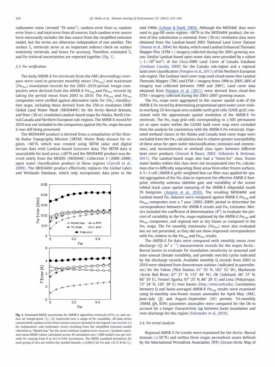
radiometer noise (termed “Tb noise”), random error from ω, randomerror from δ, and total error from all sources. Each random error sourceterm necessarily includes the bias source from the simplified emissionmodel, but the terms are otherwise independent of one another. Thesurface Ta retrievals serve as an important indirect check on surfaceemissivity retrievals, and hence Fw accuracy. Therefore, estimated Taand Fw retrieval uncertainties are reported together (Fig. 1).

2.3. Fw verification

The daily AMSR-E Fw retrievals from the AM (descending) over-pass were used to generate monthly mean (Fwavg) and maximum(Fwmx) inundation records for the 2003–2010 period. Image com-posites were derived from the AMSR-E Fwavg and Fwmx records bytaking the period mean from 2003 to 2010. The Fwavg and Fwmx

composites were verified against alternative static Fw (Fws) classifica-tion maps, including those derived from the 250-m resolution UMDGlobal Land Water Mask (MOD44W) for the Arctic–Boreal domain,and finer (30-m) resolution Landsat-based maps for Alaska, North Cen-tral Canada and Northern European sub-regions. The AMSR-E record for2010was not included in the comparison against the Fws maps becauseit was still being processed.

The MOD44W product is derived from a compilation of the Shut-tle Radar Topography Mission (SRTM) Water Body dataset for re-gions b60°N, which was created using SRTM radar and digitalterrain data with Landsat-based Geocover data. The SRTM data isunavailable for land areas ≥60°N and the MOD44W product was de-rived solely from the MODIS (MOD44C) Collection 5 (2000–2008)open water classification product in these regions (Carroll et al.,2009). The MOD44W product effectively replaces the Global Lakesand Wetlands Database, which only incorporates data prior to the

Fig. 1. Simulated RMSE uncertainty for AMSR-E algorithm retrievals of Fw (a) and sur-face air temperature (Ta) (b) expressed over a range of Fw variability. All data seriescontain both random errors from various sources denoted in the legend (see Section 2.2for explanation) and systematic errors resulting from the simplified emission model(denoted as “Model bias” for the series without random error sources). Symbols repre-sent mean RMSE values calculated across 30 simulation sets (1000 model runs per set)with Fw varying from 0 to 0.5 in 0.05 increments. The RMSE standard deviations foreach group of sets are within the symbol bounds (≤0.0015 for Fw and ≤0.15 K for Ta).

mid-1990s (Lehner & Doell, 2004). Although the MOD44C data wereused to gap-fill some regions b60°N in the MOD44W product, the ex-tent of this substitution is minimal. Finer (30-m) resolution data wereobtained from the Landsat-based 2001 National Land Cover Dataset(Homer et al., 2004) for Alaska, which used Landsat Enhanced ThematicMapper Plus (ETM+) imagery collected during the 2001 growing sea-son. Similar Landsat-based open water data were provided by a subset(~1×106 km2) of the Circa-2000 Land Cover of Canada Database(Geobase Canada, 2009) for the Canada sub-region and a regionalland cover classification (Potapov et al., 2011) of theNorthern Europeansub-region. The Geobase land cover map used cloud/snow-free LandsatThematic Mapper (TM) and ETM+imagery from 1996 to 2005 (80% ofimagery was collected between 1999 and 2001). Land cover dataobtained from Potapov et al. (2011) were derived from cloud-freeETM+imagery collected during the 2003–2007 growing season.

The Fws maps were aggregated to the coarser spatial scale of theAMSR-E Fw record by determining proportional openwater coverwith-in overlying 25-km equal area scalable earth grid cells (EASE-grid) con-sistent with the approximate spatial resolution of the AMSR-E Fwretrievals. The Fws map grid cells corresponding to ≥50% permanentice or open water within the GLDAS land cover map were excludedfrom the analysis for consistency with the AMSR-E Fw retrievals. Vege-tated wetland classes in the Alaska and Canada land cover maps wereexcluded from the Fws calculations due to relative greater susceptibilityof these areas for open water misclassification (omission and commis-sion) and inconsistencies in wetland class types between differentland cover products (Ozesmi & Bauer, 2002; Selkowitz & Stehman,2011). The Landsat-based maps also had a “Snow/Ice” class; frozenwater bodies within this class were not incorporated into Fws calcula-tions due to difficulty separating these areas from other frozen surfaces.A 3×3 cell (AMSR-E grid) weighted box-car filter was applied for spa-tial aggregation of the Fws data to represent the effective AMSR-E foot-print, whereby antenna sidelobe gain and variability of the sensororbital track cause spatial smearing of the AMSR-E ellipsoidal swathTb footprints (Amarin et al., 2010). The resulting MOD44W andLandsat-based Fws datasets were compared against AMSR-E Fwavg andFwmx composites over a 7 year (2003–2009) period to determine thecorrespondence between the AMSR-E results and Fws estimates. Met-rics included the coefficient of determination (R2) to evaluate the per-cent of variability in the Fws maps explained by the AMSR-E Fwavg andFwmx composites, and regional wet or dry biases as compared to theFws maps. The Fw monthly minimums (Fwmn) were also evaluatedbut are not presented, as they did not show improved correspondencewith Fws relative to the Fwavg and Fwmx results.

The AMSR-E Fw data were compared with monthly mean riverdischarge (Q; m3 s−1) measurement records for the major Arctic–Boreal basins to evaluate Fw inundation sensitivity to seasonal andinter-annual climate variability, and periodic wet/dry cycles indicatedby the discharge records. Available monthly Q records from 2003 to2010 were obtained from downstream stations (indicated in parenthe-ses) for the Yukon (Pilot Station; 61° 55′ N, 162° 52′ W), Mackenzie(Arctic Red River; 67° 27′ N, 133° 44′ W), Ob (Salehard; 66° 37′ N,66° 35′ E), Yenisei (Igarka; 67° 25′ N, 86° 28′ E) and Lena (Polyarnaya;72° 24′ N, 126° 20′ E) river basins (http://rims/unh.edu). Correlationsbetween Q and basin-averaged AMSR-E Fwavg results were examinedusing bi-monthly non-frozen season anomalies for April–May (AM),June–July (JJ) and August–September (AS) periods. Tri-monthly(MAM, JJA, SON) parameter anomalies were compared for the Ob toaccount for a longer characteristic lag between basin inundation andriver discharge for this region (Schroeder et al., 2010).

2.4. Fw trend analysis

Regional AMSR-E Fw trends were examined for the Arctic–Borealdomain (≥50°N) and within three major permafrost zones definedby the International Permafrost Association (IPA) Circum-Arctic Map of

227J.D. Watts et al. / Remote Sensing of Environment 127 (2012) 223–236

Permafrost and Ground Ice Conditions (Brown et al., 1998). The continu-ous permafrost zone includes regions where permafrost covers >90% ofthe landscape; the discontinuous permafrost zone is characterized by50–90% permafrost coverage within the landscape; the sporadic/isolatedpermafrost zone represents areaswith high spatial patchiness (b50% per-mafrost coverage) and greater seasonal soil thaw depth.

Inundation trends were examined by applying the Mann–Kendalltrend test (Kendall rank correlation to the annual scale data; a valueof 1 (0) indicates perfect (no) correlation with time) to AMSR-E annualmeans for Fwavg and Fwmx records from 2003 to 2010. Mann–Kendall(MK) is a non-parametric statistical test that determines trend directionand significance, and is often used for hydrological applications becauseit does not assume a particular population distribution (Chandler &Scott, 2011). Normal approximations are used to determine test signif-icance (p-value) with larger sample sizes, whereas exact tests are usedwhen the sample size is small (Hipel & McLeod, 2005; Sheskin, 2004).Mann–Kendall analysis can be influenced by serial correlation, unlessthe magnitude of trend is large (Zhang et al., 2006). As a precautionagainst serial correlation, the Yue–Pilon method was used prior to ap-plying the trend test (Yue et al., 2002). The Yue–Pilon method first ap-plies the non-parametric Theil–Sen estimator that determines themedian slope of all possible paired sample points; the slope and lag-1autocorrelation are removed if autocorrelation is detected (Yue et al.,2002). The slope and resulting uncorrelated residuals are then mergedto create a blended series to which the MK test is applied.

The total AMSR-E Fw inundation extent (km2) was obtained for theArctic–Boreal domain and North American and Eurasian sub-regions(not limited to permafrost regions) on a daily basis and aggregated tomonthly and annual intervals. We expect these area estimates (km2)to be scale dependent, reflecting observations originally obtained ata 22 km native resolution; consequently those obtained from finerscale satellite retrievals might differ from these estimates. Annual Fwextent was also determined regionally for continuous, discontinuous,and sporadic/isolated permafrost zones. The annual number of gridcells with Fw present (Fw>0) was obtained for each region, as wasthe mean annual Fw duration (the number of days per year that Fwwas detected). These records were examined for trends using theMK analysis and trend significance was assessed at a minimum 90%(pb0.1) probability level. The Fw trends were evaluated on a per-gridcell basis across the Arctic–Boreal domain because of spatial heteroge-neity in climate, permafrost condition, and surface characteristics. Therelative proportions of significant (pb0.1) cells with positive and nega-tive trends were determined for each permafrost zone. Trends in Fwduration were also examined on a per-grid cell basis to ascertain thepotential influence of changes in non-frozen season length and the cor-responding period of Fw retrievals on surface inundation trends. Areaswith significant (pb0.1) trends in Fw inundation and Fw durationwere also compared against regions identified as having significantchanges in non-frozen period length (Kim et al., 2012). Trends inFwmn, which may reflect relatively stable lake bodies, were not statisti-cally significant and are not presented in the study results.

Evaluating trends on a per grid-cell basis can substantially in-crease the false discovery rate (Wilks, 2006), which is the expectedproportion of Type I error (false positives) among all significanthypotheses. For example, α=0.1 indicates that there is a 10% chancethat a trendwill be falsely detected per test or that 10% of all tests willbe false positives. Adjusting p-values for false discovery can sub-stantially reduce the number of expected Type I errors because αwill instead correspond to tests showing significant results, ratherthan the total number of tests considered. In addition to per-cellp-values (indicating local significance) we also estimated q-values(adjusted p-values) for each grid cell using the False Discovery Rate(FDR) approach which evaluates characteristics of the p-value distri-bution. This conservative approach can be used to address multiplehypothesis testing and is more robust to spatial dependence(Wilks, 2006).

3. Results

3.1. Error sensitivity analysis

The Monte Carlo error sensitivity analysis indicates total Fw uncer-tainty within ±0.041 (RMSE) with a positive dependence on Fw(Fig. 1). The positive dependence between retrieval uncertainty andFw extent indicates that the simplified emission (forward)model biasesbecomemore prevalent as εs decreases with higher Fw. As εs decreases,the emission model becomes more sensitive to atmospheric factors be-cause the intervening atmosphere contrasts more with a radiometrical-ly dark water background than it does against relatively bright land(Chang &Milan, 1982). In addition, the land fraction decreases as Fw in-creases and the emission model becomes proportionally less sensitiveto εl factors. Minimal Fw retrieval error at lower inundation levels indi-cates that surface soilmoisture variability does not significantly degraderesults relative to other Tb model error sources. In contrast to Fw, the Taretrieval is more sensitive to εs error, which flattens the Ta retrieval un-certainty response at higher Fw levels. For Ta, the error contributions ofω and δ show opposing trends with Fw, resulting from the previoustrade-off between εl and atmospheric sensitivities at higher Fw levels.This tradeoff is more evident for the ω and δ components becausemodel bias is relatively low (b |±1| K) for Ta as a result of algorithm cal-ibration (discussed in Section 2.2). The overall Ta errors from the sensi-tivity analysis range from 3.7 to 4.1 K, compared to the observed 3.5 KTa error relative to Northern Hemisphere weather station records(Jones et al., 2010). This discrepancy indicates that ω and δ are not asvariable as specified and that the simplified emissionmodel adequatelyrepresents surface Ta and Tb observations; these results also indicatethat the reported overall Fw error is a conservative estimate.

3.2. Fw verification and regional patterns

The AMSR-E Fw results compare favorably with theMOD44WandLandsat-based Fws maps for the respective Arctic–Boreal and region-al domains. The Fwavg map composite (AMSR-E Fwavg averaged overthe 2003–2009 period) accounts for 71–84% (R2) of variability in theFws maps, while the Fwmx composites account for a lower 39–80%(R2) of Fws variability (Table 1). The mean RMSE difference betweenthe AMSR-E Fwavg and Fwmx products, and Fws is ≤5%. The strongestregional correspondence (R2=0.84) is observed between AMSR-EFwavg and lower latitude (b60°N) Fws regions where the MOD44Wproduct is partially derived from radar (SRTM) imagery. The lowestcorrespondence (R2=0.39) occurs in western Russia where theFwmx retrievals are higher than corresponding Landsat-based Fws levelsin the largely agricultural and wetland dominated areas. A small nega-tive (dry) bias (i.e. −8.21%≤MRE≤−0.56%) is observed for AMSR-EFwavg relative to Fws (Table 2; Fig. 2), whereas the Fwmx results showa small positive (wet) bias (−0.96≤MRE≤5.48%) (Table 2; Fig. 3). Re-gionally, Fwavg and Fwmx are lower than Fws along major rivers and inglaciated areas characterized by lakes surrounded by shallow, rockysubstrate (e.g. portions of the Northwest Territories and North CentralCanada). In contrast, Fwavg and Fwmx are predominately higher thanthe Fws results in wetland-dominated regions (e.g. Canadian Shield,Yenisey and Lena river basins).

The summer Fwavg and Q anomalies for the five Arctic river basinsshow favorable correlations (R≥0.71; Fig. 4) despite other hydrologicalinfluences on Q, including direct runoff contributions from snowmeltand groundwater (Papa et al., 2008; Syed et al., 2007). Relatively strongcorrelations (R≥0.82) are observed for basins with lower mean sum-mer Fwavg extent, including the Yukon (Fwavg represents 2.07% of thebasin area or 1.72×104 km2), Lena (1.77% or 4.44×104 km2), and Yen-isey (1.85% or 4.51×104 km2). Lower correlations are observed for theOb and Mackenzie (R=0.71 and 0.76, respectively) basins where theproportional Fwavg extent is relatively larger (3.16% or 7.87×104 km2;11.26% or 1.89×105 km2). This lower correspondence is likely due to

Table 2Summary of statistical comparisons for AMSR-E monthly means (Fwavg) and maxi-mums (Fwmx) against the MOD44W static open water (Fws) map for the Arctic–Borealdomain, and regional (Northern Europe, Alaska, North Central CN) Fws maps fromLandsat. Measures of similarity include coefficient of determination (R2), mean residualerror (MRE) for AMSR-E Fw−Fws, and RMSE. The relationships are significant at a 0.05probability level.

Region R2 % MRE % RMSE

Fwavg Fwmx Fwavg Fwmx Fwavg Fwmx

Arctic–Boreal (all) 0.77 0.72 −0.82 4.92 5.55 6.01Arctic–Boreal (b60°N) 0.84 0.75 −0.92 4.43 3.90 4.86Arctic–Boreal (≥60 °N) 0.71 0.69 −0.70 5.48 6.90 7.01N. Europe 0.78 0.39 −0.56 5.34 1.86 3.15Alaska 0.81 0.80 −1.87 3.00 6.27 6.42N. C. Canada 0.75 0.75 −8.21 −0.96 4.53 4.51

228 J.D. Watts et al. / Remote Sensing of Environment 127 (2012) 223–236

extensive Q regulation by basin reservoirs along the Ob and Mackenzierivers (McClelland et al., 2004; Yang et al., 2004). Similarities in relativedry (negative) and wet (positive) year anomalies between Fwavg and Qindicate that the Fw retrievals capture regional wet and dry cyclesreflected in the discharge observations (Fig. 4). Negative Fw and Qanomalies in 2004 for the Yukon, Mackenzie and Yenisey basins coin-cide with regional drought (Alkama et al., 2010; Zhang et al., 2009),while strong positive anomalies in 2007 for the Ob and in 2009 for theYukon, Mackenzie, Lena and Yenisey basins coincide with documentedwet periods (Arndt et al., 2010; Rowland et al., 2009).

Fig. 2. Difference maps between mean annual Fw determined from AMSR-E mean monthly Fuct for the Arctic–Boreal domain and Landsat-based land cover classifications for three suregions where MOD44W or Landsat-based Fws estimates are greater than AMSR-E Fwavg, w

The Fw inundation extent in the Arctic–Boreal region is highestwithin large wetland complexes of the major watersheds, includingthe Canadian Shield, Yukon River Delta, the Kolyma, Indigirka, Lena,Ob-Yenisey, Volga lowlands and Scandinavia (Fig. 5). Seasonal Fw vari-ability is also greatest within these regions, and in the agricultural areasof southwestern Russia, southern Alberta and Saskatchewan CN relativeto other areas in the domain (Fig. 5). On a seasonal basis region-wide Fwinundation (Fig. 6) is lowest in January–February (2.9×105 km2 Fwavg;4.16×105 km2 Fwmx) and highest in July (2.78×106 km2 Fwmx) andAugust (1.94×106 km2 Fwavg). Maximum inundation extent in Eurasiaoccurs in June–July and precedes the August maximum in NorthAmerica (Fig. 6). On an annual basis, the largest Fw inundation year(based on total annual inundation extent) for the Arctic–Boreal domainduring the 2003–2010 observation period coincideswith above-averageprecipitation in North America and Eurasia in 2005 (Shein et al., 2007),whereas the lowest inundation year (2004) coincides with relativelywarm summer conditions in North America and a multi-year (2001–2003) drought in the Arctic–Boreal region (Parker et al., 2006; WMO,2005; Zhang et al., 2008). Similarly, the wettest Fw years for Eurasia(2007) and North America (2010) coincide with relatively warm win-ters and wet summers (Kennedy et al., 2008; WMO, 2011). The lowestFw years observed for North America (2004) and Eurasia (2010) reflectanomalous dry summer conditions in Alaska and western Canada(Kochtubajda et al., 2011; Wendler et al., 2010) and a severe summerdrought in Russia (Wegren, 2011; WMO, 2011). The comparison be-tween AMSR-E Fw and MOD44W Fws inundation extent for the Arctic–Boreal, Eurasia and North America regions indicates that the MOD44W

w (Fwavg) values minus corresponding static Fw (Fws) values from the MOD44W prod-b-regions: Northern Europe (a), Alaska (b) and North Central CN (c). Red hues showhile blue hues indicate regions where AMSR-E Fwavg values are higher than Fws.

Fig. 3. Difference maps between mean annual Fw determined from AMSR-E monthly maximum Fw values (Fwmx) minus corresponding static Fw (Fws) values derived from theMOD44W product for the Arctic–Boreal domain and Landsat-based land cover classifications for three sub-regions: Northern Europe (a), Alaska (b) and North Central CN (c).Red hues show regions where MOD44W or Landsat-based Fws estimates are greater than AMSR-E Fwmx, while blue hues indicate regions where AMSR-E Fwmx values are higherthan Fws.

229J.D. Watts et al. / Remote Sensing of Environment 127 (2012) 223–236

estimates are considerably larger than the Fwavg retrievals and closer tothe summer Fwmx retrievals (Fig. 6). This difference occurs because Fwseasonal variability is not resolved in the static open water product.

3.3. Fw trends

A strong positive (increasing) trend in the annual number of grid cellswith Fwpresent (Fw count) is observed for all permafrost zones (Table 3),at a rate of roughly 140 cells yr−1 (~73,910 km2 or roughly 0.67% peryear; Table 3) when considering Fwmx. This trend is influenced primarilyby Fw changes within Eurasian continuous and sporadic/isolated perma-frost zones, and discontinuous permafrost areas in North America asthese areas show larger (and significant; pb0.1) increases in Fw countsrelative to other regions. An increase in Fw presence is observed for allthree permafrost zones, with the rate of expansion ranging from roughly33 cells yr−1 (discontinuous zone) to 65 cells yr−1 (continuous zone)(Table 4). The strong positive trend in Fw duration observed for theArctic–Boreal region is primarily driven by the continuous and discon-tinuous permafrost zones in North America (Table 3). Changes in Fwduration within these areas (increasing at 0.76 days yr−1 for theArctic–Boreal zone; Table 4)may reflect an overall increase in precipita-tion and lengthening of the non-frozen season (Kim et al., 2012;McClelland et al., 2006). A positive, moderate trend in total Fw inunda-tion (Fw area) is observed only in Fwmx and is primarily influenced bythe Eurasian continuous and North American discontinuous permafrostzones. Although not significant, a weak (p~0.13) positive Fwavg trend isobserved for the continuous permafrost zone and for North Americandiscontinuous permafrost areas. Overall, significant regional trends inthe Fw count and Fw area metrics are not observed when the Arctic–Boreal, North American and Eurasian sub-regions are considered as a

whole (Table 3). Significant decreasing trends in Fw count, Fw durationand Fw area are not observed in the regional analyses.

Areas of widespread Fw inundation increase are observed through-out the continuous permafrost zone when the MK trend test is appliedon a per grid-cell basis (Fig. 7). The continuous permafrost zone has thehighest proportion (92%; 91–94% is the 95% confidence interval for pro-portions) of grid cells with locally significant Fwavg wetting trends,followed by 82% (79–86%) of cells in discontinuous permafrost regions.Conversely, sporadic/isolated permafrost regions show widespread Fwinundation decrease (71%; 66–74%). The overall contrast between inun-dation patterns within the three permafrost zones is similar for Fwmx,but the overall trend extent is weaker compared to the Fwavg results,with 63% (61–65%) and 59% (55–63%) of grid cells showing Fwmx wet-ting trends within respective continuous and discontinuous permafrostzones. In the sporadic/isolated permafrost zone, 48% (44–52%) of Fwmx

grid cells having significant trends show drying. Although widespreadwetting occurs within the continuous permafrost zone, large regionsof drying are also observed in northern Québec and Newfoundland,the Canadian Baffin and Banks islands, north of the Seward Peninsulain Alaska, and the Panteleikha River wetlands in Siberia (Fig. 7). In thediscontinuous permafrost zone the largest regions of drying occur di-rectly south of the Alaska Seward Peninsula and in northern Saskatche-wan CN. Although 71% of grid cells with significant Fwmx trends withinthe sporadic/isolated permafrost zone showdrying, areas ofwetting areobserved in northern British Columbia, northern Saskatchewan andManitoba, east of James Bay in Québec CN, in the Scandinavian Laplandand southern Siberia (Fig. 7). These grid cells are not significant (qb0.1)when controlled for false discovery rate, which is not surprising giventhe small percentage of grid cells within permafrost zones that showlocal trend significance (pb0.1) and the large number of grid cells towhich the trend test was applied. Furthermore, the resulting q-values

Fig. 4. Mean river discharge (Q, m3/s) and corresponding basin-averaged Fwavg (km2) anomalies for the Yukon, Mackenzie, Ob, Lena and Yenisey river basins over the 8 year(2003–2010) AMSR-E record. To minimize temporal lag effects between basin surface water storage and discharge, anomalies were calculated from bi-monthly means duringthe northern summer months (AM, JJ, AS), except for the Ob basin where the anomalies were derived from tri-monthly (MAM, JJA, SON) means. The temporal Q gaps in the Ob,Lena, and Yenisey records are due to missing station observations. Sample sizes for the correlation coefficients (R) range from 17 to 24 anomaly observations. Basin R valuesrange from 0.71 to 0.87 and are significant at the 0.01 probability level.

230 J.D. Watts et al. / Remote Sensing of Environment 127 (2012) 223–236

(~0.45–0.58) are relatively lower in areas that are locally significant(pb0.1) compared to those that are not (~0.68–0.90). Given the con-servative nature of the FDR correction, the relatively lower q-valuesin areas with local significance (pb0.1), and indication of area-widechanges in the regional trend analysis it appears that areas having local-ly significant MK trend reflect physical changes in surface inundationcharacteristics.

Only a small portion of grid cells having locally significant wettingtrends coincide with an increase in Fw duration. Approximately 9%

Fig. 5. Study period (2003–2010) Fw means (left) and corresponding standard deviations (means (Fwavg). The Yukon, Mackenzie, Ob, Lena and Yenisey river basins are outlined in re

(2,831 grid cells) of the Arctic–Boreal permafrost zone shows a signifi-cant increase in AMSR-E Fwavg over the 8 year period (Fig. 7), with amean inundation increase of 0.16% (0.98 km2) per cell yr−1. Approxi-mately 2.6% (74 grid cells) also show a significant (pb0.10) increasingtrend in annual Fw duration (within the Eurasian continuous perma-frost zone). Only 19 of the 74 grid cells with positive Fw duration trendscorrespond with a significant increase in non-frozen season length(Kim et al., 2012) and are located mainly in southeastern Russia. Simi-larly, 2.2% (712 grid cells) of the Arctic–Boreal permafrost zone shows

right) for the Arctic–Boreal domain (≥50°N) as determined from AMSR-E Fw monthlyd.

Fig. 6. Seasonal progressions in AMSR-E Fw area (km2) for selected regions within the Arctic–Boreal domain (≥50 °N) as determined from Fwmonthly means (Fwavg, in gray) and monthlymaximums (Fwmx, in black) for the study period (2003–2010). Static Fw estimates (Fws) from the MOD44W open water map (black, dashed) are presented for the same regions.

231J.D. Watts et al. / Remote Sensing of Environment 127 (2012) 223–236

a significant decrease in Fwavg inundation (Fig. 7) and corresponds to anaverage Fw decline of 0.17% (1.05 km2 per cell yr−1); 2.5% of these (18grid cells, within the sporadic/isolated zone in Québec) are associatedwith a significant decrease in Fwduration but do not correspond to doc-umented trends in non-frozen period length (Kim et al., 2012).

4. Discussion

4.1. Fw verification and surface patterns

The regional inundation patterns derived from the AMSR-E Fw re-trievals are similar to alternative open water maps derived from thefiner scale MOD44W and Landsat products despite the inherent coarserspatial resolution of the AMSR-E footprint. The favorable accuracy ofAMSR-E Fw retrievals is attributed to the strong sensitivity of micro-wave emissivity to landscape variations in surface dielectric constantcaused by the presence of even a small fraction of surfacewater relativeto a non-inundated land surface. Differences between the static openwatermaps (Fws) and dynamic Fw retrievals are primarily due to differ-ences in the seasonal timing and duration of the sensor retrievals.Stronger similarities between AMSR-E Fwavg and MOD44W Fws resultsoccurred at lower (b60°N) latitudes where the MOD44W results arelargely derived from SRTM, which has microwave characteristics simi-lar to AMSR-E, including relative insensitivity to atmosphere effects(e.g. clouds), enhanced sensitivity to surfacewater cover and insensitiv-ity to surface water signal contamination by vegetation (Pietroniro &Leconte, 2005). The stronger regional similarity may also be influenced

by differences in wetland type and characteristic inundation patternsbetween lower and higher latitude regions.

The general Fwavg dry bias reflects the tendency for higher Fws in tem-porally dynamic inundation regions due to limited (e.g. summer-only)satellite optical-IR image collection periods. The AMSR-E Fw results indi-cate large seasonal and inter-annual variability in Arctic–Boreal zoneinundation, with respective Fwavg variability (SD) on the order of ±60%(±6.4×105 km2) and ±3% (±3.1×104 km2); this dynamic variabilityis not adequately represented by the static open water maps. TheAMSR-E Fwavg retrievals are also lower than the Fws results in character-istically dynamic inundation areas along major river corridors and inother areas where inundation is largely absent during dry periods butabundant following seasonal snowmelt or rain events (Brown & Young,2006). Although the AMSR-E Fw dry bias is effectively eliminated orreversed (wet bias) for the Fwmx results, it remains evident along riversystems and seasonally varying lakes and wetlands. In contrast, theAMSR-E Fwavg and Fwmx results are predominately wetter than the Fws

results in wetland dominated landscapes (e.g. Canadian Shield, Yeniseyand Lena river basins). The lower Fws inundation levels within these re-gions may be due to reduced open water detection by optical-IR satellitesensors in areas with higher vegetation density (Kaheil & Creed, 2009;Ozesmi & Bauer, 2002). Excluding vegetated wetland and frozen lakebodies from the Landsat-based Fws calculations may have contributed todifferences between the AMSR-E Fw and Fws results in the Alaska andNorth Central Canada sub-regions. However, similar areas of relativelyhigher AMSR-E Fw inundation, including the Ob-Yenisey lowlands andCanadian Shield, are evident in the MOD44W comparison where theexclusion of wetland and frozen classes is not an issue.

Table 3Mann–Kendall tau trend strength for AMSR-E Fw in the Arctic–Boreal domain, individualpermafrost (PF) zones and associated sub-regions. Trends (years 2003–2010) were esti-mated for the total annual number of grid cells with Fw present (Fw count), themean an-nual duration of Fw inundation (Fw duration), and resolution (25 km) dependentestimates of total annual inundation area (Fw area) derived from Fw monthly means(Fwavg) and maximums (Fwmx). The sub-regions evaluated include North America (NA)and Eurasia (EA), continuous (C), discontinuous (D), and sporadic/isolated (S) PF zones.The possible range for tau is −1 to 1 and the sign indicates trend direction; |1| indicatesa perfect rank agreement with time. Trend significance (in bold) is denoted by * and **for respective 0.1 and 0.05 probability levels.

Region Fw count Fw duration Fw area

Fwavg Fwmx

Arctic–Boreal (≥50°N) 0.34 0.71** 0.33 0.24NA 0.24 0.71** 0.14 0.33EA 0.33 0.52 −0.05 0.14All PF zones 0.81** 0.71** 0.43 0.62*C 0.71** 0.90** 0.53 0.71**D 0.62* 0.71** 0.24 0.43S 0.62* 0.52 −0.14 0.42C-NA 0.24 0.90** 0.42 0.52C-EA 0.62* 0.90** 0.43 0.61*D-NA 0.62* 0.71** 0.52 0.62*D-EA 0.52 0.52 −0.33 −0.05S-NA 0.05 0.52 −0.05 0.14S-EA 0.62* 0.43 0.33 −0.04

232 J.D. Watts et al. / Remote Sensing of Environment 127 (2012) 223–236

The AMSR-E Fw sensitivity to seasonal and annual surfacewater var-iability is also demonstrated in the comparison against river Q. Severe,multi-year (2001–2003) boreal drought conditions (Alkama et al.,2010; Zhang et al., 2008) are manifested as large negative Fw and Qanomalies for the Yukon, Mackenzie and Yenisey rivers in 2004. Largepositive Fw and Q anomalies coincide with major flooding events in2007 for the Ob (Schroeder et al., 2010), and 2009 for the Yukon, Mac-kenzie, Lena and Yenisey due to a combination of river ice jams, rapidsnowmelt and precipitation (Arndt et al., 2010; Rowland et al., 2009).These findings are similar to prior studies reporting strong correlationsbetween satellite microwave Fw retrievals and Q over Arctic river sys-tems (Papa et al., 2010; Schroeder et al., 2010). Linkages betweenbasin Fw and Q response can be complex and do not always show directcorrespondence (Papa et al., 2008), as is observed for the Mackenziebasin in 2004 and 2010. These differences are driven by the timingand duration of spring snowmelt and groundwater contributions,river ice jams, precipitation events, reservoir outflow and other changes

Table 4Theil-Sen slope trend estimates for AMSR-E Fw in the Arctic-Boreal domain, individualpermafrost (PF) zones and associated sub-regions. Trends (years 2003–2010) were es-timated for the total annual number of grid cells with Fw present (Fw count), mean an-nual duration of Fw inundation (Fw duration), and resolution (25 km) dependentestimates of total annual inundation area (Fw area) derived from Fw monthly means(Fwavg) and maximums (Fwmx). The sub-regions evaluated include North America(NA) and Eurasia (EA), continuous (C), discontinuous (D), and sporadic/isolated (S)PF zones. Significant trends (in bold) are denoted by * and ** for respective 0.1 and0.05 probability levels.

Region Fw count Fw duration Fw area (km2 year−1)(cells year−1) (days year−1)

Fwavg Fwmx

Arctic–Boreal (≥50°N) 218.69 0.76** 25,000 98,293NA 10.28 0.80** 4,648 43,787EA 186.78 0.61 −2,938 18,047All PF zones 140.52** 0.64** 36,929 73,910*C 65.34** 0.82** 16,179 16,907**D 33.65* 0.26** 4,583 12,493S 53.39* 0.78 8,285 31,573C-NA −4.59 0.91** 13,375 966C-EA 51.90* 0.76** −1,127 19,772*D-NA 15.97* 0.43** 4,591 10,101*D-EA 16.54 0.11 −3,410 494S-NA 0.85 0.65 5,438 12,287S-EA 38.68* 0.71 7,992 184

in hydrological connectivity and Q that may not correspond directly toFw changes (McClelland et al., 2011). Furthermore, the Fw parametercorresponds directly to surfacewater area,whereasQ can vary indepen-dently in response to additional water storage (e.g. soil, snow, andgroundwater) fluctuations (Landerer et al., 2010).

The AMSR-E Fw patterns for the Arctic–Boreal (≥50°N) domain areconsistent with previous regional observations (Schroeder et al., 2010;Smith et al., 2007). In North America, the AMSR-E Fwavg results revealwidespread inundation within the Canadian Shield region, a landscapecharacterized by expansive peatlands, lake systems and large soil or-ganic carbon pools (Tarnocai, 2006). In Eurasia, Fw inundation is rela-tively extensive within the major Arctic river basins (particularlyalong the Yenisey and in the Okrug–Yugra Ob river region), southernFinland and the Russian Republic of Karelia. More extensive inundationoccurs along the Volga river system and in peatlands of the southernWest Siberian lowlands (Kremenetski et al., 2003). Inundation extentis lowest in the January–February period when a majority of the land-scape is frozen, and is highest in July (Fwmx) and August (Fwavg) follow-ing seasonal thawing and summer precipitation. The earlier seasonalmaximum observed in Fwmx likely reflects extensive overland flow fol-lowing snowmelt and rain events on still-frozen surfaces (Woo et al.,2006). The seasonal inundation variability observed in the AMSR-E Fwretrievals reflects strong correspondence between surface inundationand regional temperature and precipitation patterns in northern land-scapes (Rouse, 2000). This is particularly evident in Eurasia where asharp decline in inundation extent following the summer Fwmaximumcoincides with characteristic high evaporation rates and low precipita-tion in late summer and fall (Landerer et al., 2010; Serreze & Etringer,2003). The temporal Fw variability observed in the major wetland andagricultural regions is also consistent with similar seasonal changes inprecipitation and evaporation for these areas (Rouse, 2000).

4.2. Fw trends

The per-grid cell analysis indicates widespread Fwavg increase with-in continuous permafrost areas and overall declinewithin the sporadic/isolated permafrost zone. These inundation trends concur with reportsfrom localized field studies throughout the Arctic–Boreal region (Joneset al., 2011a; Smith et al., 2005; Walter et al., 2006; Yoshikawa &Hinzman, 2003). The high proportion of grid cells showing positive Fwinundation trends in the discontinuous permafrost zone appears to con-tradict previous reports of declining lake numberswithin discontinuouspermafrost areas in Siberia and Alaska (Smith et al., 2005; Yoshikawa &Hinzman, 2003). A few key differences account for this apparentdiscrepancy. First, our study evaluated a continuous daily Fw record inpermafrost zones across the entire Arctic–Boreal domain over aneight year period, which enabled a relatively precise assessment ofdynamic inundation changes, whereas previous studies wereconstrained by a limited number of observation days and involvedrelatively small spatial domains. Additionally, the AMSR-E Fw re-trievals provide a measure of the proportional surface water coverwithin a relatively coarse (25 km) resolution grid cell, rather thanspecific lake number counts; the Fw retrievals do not resolve individualwater bodies, but are insensitive to signal degradation from low solar il-lumination and atmosphere (clouds, smoke) contamination, and haveenhanced microwave sensitivity to surface inundation in vegetatedareas. These attributes are particularly relevant in Arctic-Boreal land-scapes which have characteristically low solar illumination, shortnon-frozen seasons and frequent cloud cover, and in the continuouspermafrost zonewhere lateral drainage fromprimary lakes can increasethe number of smaller water bodies without an overall change in sur-face water extent (Jones et al., 2011a; White et al., 2007).

The re-distribution of surface water through lateral drainagecould have contributed to the observed expansion in the annualnumber of grid cells with Fw present within permafrost regions. Sat-ellite optical-IR remote sensing analyses might detect an overall

Fig. 7. Significant (pb0.10) Fw trend areas within permafrost (PF) regions for mean annual Fw (Fwavg) determined from AMSR-E mean monthly Fw values from 2003 to 2010. Theblue, light blue-gray and light green areas represent continuous (C), discontinuous (D) and sporadic/isolated (S) PF zones, respectively. The blue areas indicate significant positiveFw trends, while red areas indicate significant negative Fw trends. The relative proportion (%) of grid cells having significant positive or negative trends within each PF zone is sum-marized in the corresponding bar graph; error bars indicate 95% confidence intervals for the PF area proportions.

233J.D. Watts et al. / Remote Sensing of Environment 127 (2012) 223–236

decrease in total water body area where lateral drainage is occurringif smaller water bodies (e.g. ponds, small streams, wetlands) are ob-scured by vegetation, or if only primary lakes are examined. This mayaccount for an apparent discrepancy between a recent MODIS-basedstudy indicating an extensive reduction in surface lake area overnorthern Canada (Carroll et al., 2011), and this study which showsa general Fw increase in many of the same regions, particularly inthe northwestern Canadian Shield. The timing of the MODIS re-trievals used by Carroll et al. (2011) may have also influenced theresulting lake trends as bedrock-underlain water bodies within thisregion depend on precipitation recharge and therefore show strongseasonal and annual variability (Spence & Woo, 2008). Because ourevaluations incorporate daily AMSR-E Fw observations during thenon-frozen period, some of the observed increase in Fw inundationmay be artifacts of a lengthening non-frozen season trend (Kim etal., 2012). However, only a small proportion (2.6%) of grid cellswith significant Fw inundation increase also show a significant in-crease in annual Fw duration, and less than 0.7% of these cells coin-cide with an increase in the non-frozen season. Likewise, only 2.5%of grid cells having a significant decreasing Fw inundation trendalso show a significant change in Fw duration, and none of thesecells indicate a significant trend in non-frozen season length.

Although the per-grid cell analysis shows areas of significant Fwwetting and drying trends within Arctic–Boreal permafrost zones, re-sults from the regional analysis are less clear but indicate that Fw pres-ence and annual duration are increasing. Only the regional Fwmx

(monthly maximum) results indicate increasing trends in inundationarea, although a weak (p=0.13) positive Fwavg trend is detected for

continuous permafrost areas. The overall lack of significant inundationtrends in the regional Fwavg results is likely due to the large spatial var-iability in Fw patterns where areas with positive Fw trends are offset byregions with declining inundation, and the characteristically large tem-poral variability in inundation and relatively short (8 year) AMSR-E Fwrecord. The Fwmx trend is likely more sensitive to surface inundation ex-tremes following spring thaw, snowmelt and precipitation related wet-ting events, whereas Fwavg is temporally smoothed and provides abettermeasure of overall mean inundation state. Smaller, palustrine wet-lands are especially affected by changes in wetting events. Water bodiesare also influenced by changes in precipitation (Rawlins et al., 2010), inaddition to recharge from localized ice melt or lateral drainage (Joneset al., 2011a; White et al., 2007), human-related activities and erosionalprocesses (Hinkel et al., 2007), changes inwater table position anddistur-bance from wildfires (Riordan et al., 2006). The significant increase inregional Fw duration, primarily for the continuous and North Americandiscontinuous permafrost zones, indicates an expanding non-frozen sea-son and corresponding longer inundation period influenced by rainfall(Woo et al., 2006). Increased evapotranspiration could also affect Fwduration in regions where lakes and wetlands are influenced by the sea-sonal water balance (Adam & Lettenmaier, 2008; Riordan et al., 2006).However the overall water balance in the Arctic–Boreal remains largelypositive, as indicated by generally increasing trends in regional riverdischarge (McClelland et al., 2006; Peterson et al., 2002; Rawlins et al.,2010) and the increase in Fw area reported in this study.

The variability in Fw trends throughout the Arctic–Boreal regionreflects large spatial heterogeneity in climate, surface conditions and per-mafrost state. The continuous permafrost zone is particularly susceptible

234 J.D. Watts et al. / Remote Sensing of Environment 127 (2012) 223–236

to degradation due to rapid warming following sub-surface ice melt(Romanovsky et al., 2010). Spatial differences in surface temperatureand snow thickness also influence variability in permafrost thaw (Rigoret al., 2000; Stieglitz et al., 2003). Ecosystem characteristics have allowedpermafrost to persist under climatic conditions no longer conducive to itsformation (Shur & Jorgenson, 2007). Plant canopies reduce understorysnow accumulation (winter ground insulation) and summer radiativewarming; surface organic layersmaintain cool, moist conditions that pro-vide additional thermal buffering (Smith &Riseborough, 2002). These en-vironmental factors allow relatively less degraded permafrost to persistwithindiscontinuous and sporadic/isolatedpermafrost zones. Thawwith-in these regional pockets influences inundation expansion, as was ob-served in Québec CN near Hudson Bay where an abundance of thawlakes has been documented (Watanabe et al., 2011). In some areas, cli-mate warming may overwhelm ecosystem buffering, as was observedin Québec and Labrador CN where surface drying has resulted from in-creased summer warming trends (Mekis & Vincent, 2011) in addition tothaw depth and sub-surface drainage expansion. Extensive peat accumu-lation on thawed surfaces and thermokarst ponds can also decrease openwater inundation area and may be responsible for the observed Fw de-crease in northeastern Canada (Filion & Begin, 1998; Minayeva & Sirin,2010).

5. Conclusions

We conducted an analysis of fractional surface water (Fw) inun-dation for the Arctic–Boreal region using daily satellite passive mi-crowave remote sensing retrievals from the AMSR-E sensor record.The daily Fw retrievals were temporally aggregated to monthlymean (Fwavg) and maximum (Fwmx) temporal intervals and repre-sent the proportion of surface water inundation within an approxi-mate 25-km resolution footprint. Our results indicate largeseasonal and inter-annual variability in Arctic–Boreal regional inun-dation, with respective Fw variability (SD) on the order of ±60% (±6.4×105 km2) and ±3% (±3.1×104 km2). The total annual inunda-tion extent (km2) for the domain was largely stable over the2003–2010 observation period; this finding concurs with an earlierassessment covering the 1993–2000 period (Papa et al., 2010). How-ever, our results also indicate locally significant, contrasting Fwwet-ting and drying trends in permafrost affected areas. Regions ofwidespread inundation increase are observed throughout the con-tinuous permafrost zone, while Fw drying is predominant withinsporadic/isolated permafrost areas. Methane emission levels arestrongly influenced by open water extent (Walter et al., 2007).Areas showing increased Fw wetting are of particular concern as at-mospheric CH4 is a potent greenhouse gas and recent increasesfrom Arctic wetlands have been reported (Bloom et al., 2010). Inlieu of climatic conditions favorable to permafrost developmentand continued surface wetting, an overall decline in Fw inundationarea appears likely (Avis et al., 2011; van Huissteden et al., 2011).Nevertheless, total Arctic–Boreal zone inundation will remain stableif Fw expansion continues to offset regions of inundation decline.

Surface water inundation changes captured by the AMSR-E Fw re-trievals provide an indicator of recent climate variability withinnorthern landscapes, though the spatiotemporal distribution andunderlying drivers of open water change need to be better under-stood to adequately separate longer term inundation trends fromcharacteristically large seasonal and inter-annual Fw variability(Prowse & Brown, 2010). A forward model sensitivity analysis indi-cated that the AMSR-E Fw retrievals are relatively accurate (conser-vative RMSE uncertainty within ±4.1%), and that the Fw resultseffectively detect sub-grid surface inundation relative to finer scale(30-m to 250-m resolution) static open water maps. The relativeconsistency in resolving regional patterns and enhanced microwavesensor capabilities for continuous monitoring provide for improvedresolution of characteristic dynamic seasonality and periodic wet/dry

cycles in surface inundation across the Arctic–Boreal domain. The com-bination of frequent Fw monitoring from satellite passive microwavesensor records and finer scale open water maps available from satelliteoptical-IR and radar sensor records may enable improved resolution ofspatial patterns and seasonal to annual variability in regional waterbodies that can be used in context with available climate data to im-prove understanding of regional climate change impacts to surfacehydrology, energy and carbon cycles in Arctic–Boreal regions. More de-tailed information concerning the temporal variability in inundationextent and the separation of Fw into wetland and lake area componentswill benefit carbon modeling efforts, especially for CH4 emissions,which are strongly influenced by the extent and duration of surfaceinundation.

Acknowledgements

This work was conducted at the University of Montana, at TheCity College of New York, and Jet Propulsion Laboratory, CaliforniaInstitute of Technology under contract to the National Aeronauticsand Space Administration. This work was supported under theNASA Terrestrial Ecology and Making Earth System Data Recordsfor Use in Research Environments (MEaSUREs) programs; theAMSR-E data were provided by the NASA data archive (DAAC) facil-ity at the National Snow and Ice Data Center (NSIDC) using algo-rithms developed at the University of Montana. We also thank Dr.Peter Potapov at South Dakota State University for allowing us touse his land cover dataset.

References

Adam, J. C., & Lettenmaier, D. P. (2008). Application of new precipitation andreconstructed streamflow products to streamflow trend attribution in northernEurasia. Journal of Climate, 21, 1807–1828.

Alkama, R., Decharme, B., Douville, H., Becker, M., Cazenave, A., Sheffield, J., et al.(2010). Global evaluation of the ISBA-TRIP continental hydrological system. Part1: Comparison to GRACE terrestrial water storage estimates and in situ river dis-charges. American Meteorological Society, 11, 583–600.

Amarin, R., Ruf, C., & Jones, L. (2010). Impact of spatial resolution on wind field derivedestimates of air pressure depression in the hurricane eye. Remote Sensing, 2,665–672.

Anisimov, O. A. (2007). Potential feedback of thawing permafrost to the global climatesystem through methane emission. Environmental Research Letters, 2 (7 pp.).

Anisimov, O. A., & Reneva, S. (2006). Permafrost and changing climate: The Russianperspective. Ambio, 35, 169–175.

Arndt, D. S., Baringer, M. O., & Johnson, M. R. (Eds.). (2010). State of the climate in 2009.Bulletin of the American Meteorological Society, 91 (224 pp.).

Avis, C. A., Weaver, A. J., & Meissner, K. J. (2011). Reduction in areal extent ofhigh-latitude wetlands in response to permafrost thaw. Nature Geoscience Letters,4, 444–448.

Bloom, A. A., Palmer, P. I., Fraser, A., Reay, D. S., & Frankenberg, C. (2010). Large-scalecontrols of Methanogenesis inferred from methane and gravity spaceborne data.Science, 327, 322–325.

Brown, J., Ferrians, O. J., Jr., Heginbottom, J. A., & Melnikov, E. S. (1998). Circum-Arcticmap of permafrost and ground-ice conditions. Boulder, CO: National Snow and IceData Center/World Data Center for Glaciology. Digital Media.

Brown, L., & Young, K. L. (2006). Assessment of three mapping techniques to delineatelakes and ponds in a Canadian High Arctic wetland complex. Arctic, 59, 283–293.

Camill, P. (2005). Permafrost thaw accelerates in boreal peatlands during late 20thcentury climate warming. Climatic Change, 68, 135–152.

Carroll, M. L., Townshend, J. R. G., DiMiceli, C. M., Loboda, T., & Sohlberg, R. A. (2011).Shrinking lakes of the Arctic: Spatial relationships and trajectory of change. Geo-physical Research Letters, 38 (5 pp.).

Carroll, M., Townshend, J., DiMiceli, C., Noojipady, P., & Sohlberg, R. (2009). A new globalraster water mask at 250 meter resolution. International Journal of Digital Earth, 2,291–308.

Chandler, R. E., & Scott, E. M. (2011). Statistical methods for trend detection and analysisin the environmental sciences. West Sussex, UK: Wiley & Sons, Ltd. 368 pp.

Chang, A. T., & Milan, A. S. (1982). Retrieval of ocean surface and atmospheric param-eters from multichannel microwave radiometric measurements. IEEE Transactionson Geosciences and Remote Sensing, 217–224.

Filion, L., & Begin, Y. (1998). Recent paludification of kettle holes on the central islandsof Lake Bienville, northern Quebec, Canada. The Holocene, 8, 91–96.

Fily, M., Royer, A., Goita, K., & Prigent, C. (2003). A simple retrieval method for land sur-face temperature and fraction of water surface determination from satellite micro-wave brightness temperatures in sub-arctic areas. Remote Sensing of Environment,85, 328–338.

235J.D. Watts et al. / Remote Sensing of Environment 127 (2012) 223–236

Frauenfeld, O. W., Zhang, T., Barry, R. G., & Gilichinsky, D. (2004). Interdecadal changesin seasonal freeze and thaw depths in Russia. Journal of Geophysical Research, 109(12 pp.).

Geobase Canada (2009). Land Cover, Circa 2000 Vector. Vector Digital Data. Governmentof Canada, Natural Resources Canada, Earth Sciences Sector, Centre for Topo-graphic Information-Sherbrooke.

Graversen, R. G., Mauritsen, T., Tjernstrom, M., Källén, E., & Svensson, G. (2008). Verti-cal structure of recent Arctic warming. Nature, 541, 53–56.

Hinkel, K. M., Jones, B. M., Eisner, W. R., Cuomo, C. J., Beck, R. A., & Frohn, R. (2007).Methods to assess natural and anthropogenic thaw lake drainage on the westernArctic coastal plain of northern Alaska. Journal of Geophysical Research, 112, 9.http://dx.doi.org/10.1029/2006JF000584.

Hinzman, L. D., Bettez, N. D., Bolton, W. R., Chapin, F. S., Dyurgerov, M. B., Fastie, C. L.,et al. (2005). Evidence and implications of recent climate change in northernAlaska and other Arctic regions. Climatic Change, 72, 251–298.

Hipel, K. W., & McLeod, A. I. (2005). Time series modeling of water resources and envi-ronmental systems. Electronic reprint of book (http://www.stats.uwo.ca/faculty/aim/1994Book/) originally published in 1994 by Elsevier, Amsterdam, The Netherlands1013 pp.

Homer, C., Huang, C., Yang, L., Wylie, B., & Coan, M. (2004). Development of a 2001national land cover database for the United States. Photogrammetric Engineeringand Remote Sensing, 70, 829–840.

Jones, L. A., Ferguson, C. R., Kimball, J. S., Zhang, K., Chan, S. T. K., McDonald, K. C., et al.(2010). Satellite microwave remote sensing of daily land surface air temperatureminima and maxima from AMSR-E. IEEE Journal of Selected Topics in Applied EarthObservations and Remote Sensing, 3, 111–123.

Jones, B., Grosse, M. G., Arp, C. D., Jones, M. C., Walter Anthony, K. M., & Romanovsky, V.E. (2011a). Modern thermokarst lake dynamics in the continuous permafrost zone,northern Seward Peninsula, Alaska. Journal of Geophysical Research, 116 (13 pp.).

Jones, M. O., Jones, L. A., Kimball, J. S., & McDonald, K. C. (2011). Satellite passive micro-wave remote sensing for monitoring global land surface phenology. Remote Sensingof Environment, 115, 1102–1114.

Jones, L. A., & Kimball, J. S. (2011). Daily global land surface parameters derived fromAMSR-E. Boulder Colorado USA: National Snow and Ice Data Center. Digital mediahttp://nsidc.org/data/nsidc-0451.html

Jones, L. A., Kimball, J. S., McDonald, K. C., Chan, S. T. K., Njoku, E. G., & Oechel, W. C.(2007). Satellite microwave remote sensing of boreal and Arctic soil temperaturesfrom AMSR-E. IEEE Transactions on Geoscience and Remote Sensing, 45 (15 pp.).

Kaheil, Y. H., & Creed, I. F. (2009). Detecting and downscaling wet areas on Boreal land-scapes. IEEE Geoscience and Remote Sensing Letters, 6, 179–183.

Kaufman, D. S., Schneider, D. P.,McKay, N. P., Ammann, C.M., Bradley, R. S., Briffa, K. R., et al.(2009). Recent warming reverses long-term Arctic cooling. Science, 325, 1236–1239.

Kawanishi, T., Sezai, T., Ito, Y., Imaoka, K., Takeshima, T., Ishido, Y., et al. (2003). TheAdvanced Microwave Scanning Radiometer for the Earth Observing System(AMSR-E), NASDA's contribution to the EOS for global energy and water cyclestudies. IEEE Transactions on Geoscience and Remote Sensing, 41, 184–194.

Kennedy, J., Titchner, H., Parker, D., Beswick, M., Hardwick, J., & Thorne, P. (2008). Globaland regional climate in 2007. Weather, 63, 296–304.

Kim, Y., Kimball, J. S., McDonald, K. C., & Glassy, J. (2011). Developing a global datarecord of daily landscape freeze/thaw status using satellite passive microwave re-mote sensing. IEEE Transactions on Geoscience and Remote Sensing, 49, 949–960.

Kim, Y., Kimball, J. S., Zhang, K., & McDonald, K. C. (2012). Satellite detection of increas-ing Northern Hemisphere non-frozen seasons from 1979 to 2008: Implications forregional vegetation growth. Remote Sensing of Environment, 121, 472–487.

Kochtubajda, B., Burrows, W. R., Green, D., Liu, A., Anderson, K. R., & McLennan, D.(2011). Exceptional cloud-to-ground lightning during an unusually warm summerin Yukon, Canada. Journal of Geophysical Research, 116 (20 pp.).

Kremenetski, K. V., Velichko, A. A., Borisova, O. K., MacDonald, G.M., Smith, L. C., Frey, K. E.,et al. (2003). Peatlands of thewestern Siberian lowlands: current knowledge on zona-tion, carbon content and late Quaternary history. Quaternary Science Reviews, 22,703–723.

Landerer, F. W., Dickey, J. O., & Güntner, A. (2010). Terrestrial water budget of the Eurasianpan-Arctic fromGRACE satellitemeasurements during2003–2009. Journal of GeophysicalResearch, 115 (14 pp.).

Lehner, B., & Doell, P. (2004). Development and validation of a global database of lakes,reservoirs and wetlands. Journal of Hydrology, 296, 1–22.

Matzler, C. (2005). On the determination of surface emissivity from satellite observa-tions. IEEE Geoscience and Remote Sensing Letters, 2, 160–163.

McClelland, J. W., Dery, S. J., Peterson, B. J., Holmes, R. M., & Wood, E. F. (2006). Apan-arctic evaluation of changes in river discharge during the latter half of the20th century. Geophysical Research Letters, 33 (4 pp.).

McClelland, J. W., Holmes, R. M., Dunton, K. H., & Macdonald, R. (2011). The ArcticOcean estuary. Estuaries and Coasts, 34 (16 pp.).

McClelland, J. W., Holmes, R. M., Peterson, B. J., & Stieglitz, M. (2004). Increasing riverdischarge in the Eurasian Arctic: Consideration of dams, permafrost thaw, andfires as potential agents of change. Journal of Geophysical Research, 109 (12 pp.).

Mekis, É., & Vincent, L. A. (2011). An overviewof the secondgeneration adjusted daily pre-cipitation dataset for trend analysis in Canada. Atmosphere-Ocean, 49, 163–177.

Mialon, A., Royer, A., & Fily, M. (2005). Wetland seasonal dynamics and interannualvariability over northern high latitudes, derived from microwave satellite sata.Journal of Geophysical Research, 110 (9 pp.).

Minayeva, T., & Sirin, A. (2010). Arctic peatlands. Arctic biodiversity trends report 2010:Selected indicators of change (pp. 71–74).

Njoku, E. G., & Li, L. (1999). Retrieval of land surface parameters using passive micro-wave measurements at 6–18 GHz. IEEE Transactions on Geosciences and RemoteSensing, 37, 79–93.

O'Connor, F. M., Boucher, O., Gedney, N., Jones, C. D., Folberth, G. A., Coppell, R., et al.(2010). Possible role of wetlands, permafrost, and methane hydrates in the methanecycle under future climate change: A review. Reviews of Geophysics, 48 (33 pp.).

Oki, T., Imaoka, K., & Kachi, M. (2010). AMSR instruments on GCOM-W1/2: Conceptsand applications. Geosciences and Remote Sensing Symposium (IGARSS), 2010 IEEEInternational. 25–30 July, 2010, Honolulu, HI (pp. 1363–1366).

Ozesmi, S. L., & Bauer, M. E. (2002). Satellite remote sensing of wetlands. WetlandsEcology and Management, 10, 381–402.

Papa, F., Prigent, C., Aires, F., Jimenez, C., Rossow, W. B., & Matthews, E. (2010).Interannual variability of surface water extent at the global scale, 1993–2004. Journalof Geophysical Research, 115 (17 pp.).

Papa, F., Prigent, C., & Rossow, W. B. (2008). Monitoring flood and discharge variationsin the large Siberian rivers from a multi-satellite technique. Surveys in Geophysics,29, 297–317.

Parker, D. E., Kennedy, J., & Hardwick, J. (2006). Global and regional climate in 2004.Weather, 60, 197–205.

Payette, S., Delwaide, A., Caccianiga, M., & Beauchemin, M. (2004). Accelerated thawingof subarctic peatland permafrost over the last 50 years. Geophysical Research Let-ters, 31 (4 pp.).

Peterson, B. J., Holmes, R. M., McClelland, J. W., Vorosmarty, C. J., Lammers, R. B.,Shiklomanov, A. I., et al. (2002). Increasing river discharge to the Arctic Ocean.Science, 298, 2171–2173.

Pietroniro, A., & Leconte, R. (2005). A review of Canadian remote sensing and hydrolo-gy, 1999–2003. Hydrological Processes, 19, 285–301.

Potapov, P., Turubanova, S., & Hansen, M. C. (2011). Regional-scale boreal forest coverand change mapping using Landsat data composites for European Russia. RemoteSensing of Environment, 115, 548–561.

Prowse, T. D., & Brown, K. (2010). Appearing and disappearing lakes in the Arctic andtheir impacts on biodiversity. Arctic Biodiversity Trends Report 2010: Selected indica-tors of change (pp. 68–70).

Rawlins, M. A., Steele, M., Holland, M. M., Adam, J. C., Cherry, J. E., Francis, J. A., et al.(2010). Analysis of the Arctic system for freshwater cycle intensification: observa-tions and expectations. Journal of Climate, 23, 5715–5737.

Rigor, I. G., Colony, R. L., & Martin, S. (2000). Variations in surface air temperature ob-servations in the Arctic, 1979–97. Journal of Climate, 896–914.

Riordan, B., Verbyla, D., & McGuire, A. D. (2006). Shrinking ponds in subarctic Alaskabased on 1950–2002 remotely sensed images. Journal of Geophysical Research,111 (11 pp.).

Romanovsky, V. E., Smith, S. L., & Christiansen, H. H. (2010). Permafrost thermal state inthe Polar Northern Hemisphere during the International Polar Year 2007–2009: asynthesis. Permafrost and Periglacial Processes, 21, 106–116.

Rouse, W. R. (2000). The energy and water balance of high-latitude wetlands: controlsand extrapolation. Global Change Biology, 6, 59–68.

Rowland, J. C., Wilson, C. J., Brumby, S. P., & Pope, P. A. (2009). Arctic river mobility: Abaseline assessment. American Geophysical Union, Fall Meeting 2009, abstract#H44C-05.

Schroeder, R., Rawlins, M. A., McDonald, K. C., Podest, E., Zimmermann, R., & Kueppers,M. (2010). Satellite microwave remote sensing of North Eurasian inundation dy-namics: Development of coarse-resolution products and comparison withhigh-resolution synthetic aperture radar data. Environmental Research Letters, 5(7 pp.).

Selkowitz, D. J., & Stehman, S. V. (2011). Thematic accuracy of the National Land CoverDatabase (NLCD) 2001 land cover for Alaska. Remote Sensing of Environment, 115,1401–1407.

Serreze, M. C., & Etringer, A. J. (2003). Precipitation charateristics on the Eurasian Arcticdrainage system. International Journal of Climatology, 23, 1267–1291.

Shein, K. A., Waple, A. M., Diamond, H. J., & Levy, J. M. (2007). State of the climate in2005. World Meteorological Organization No. 1015. 114 pp.

Sheskin, D. J. (2004). Handbook of parametric and nonparametric statistical procedures.Boca Raton, FL: CRC Press/Chapman & Hall 719 pp.

Shur, Y. L., & Jorgenson, M. T. (2007). Patterns of permafrost formation and degradationin relation to climate and ecosystems. Permafrost and Periglacial Processes, 18, 8–19.

Smith, M. W., & Riseborough, D. W. (2002). Climate and the limits of permafrost: azonal analysis. Permafrost and Periglacial Processes, 13, 1–15.

Smith, L. C., Sheng, Y., & MacDonald, G. M. (2007). A first pan-Arctic assessment of theinfluence of glaciation, permafrost, topography and peatlands on Northern Hemi-sphere lake distribution. Permafrost and Periglacial Processes, 18, 201–208.

Smith, L. C., Sheng, Y., MacDonald, G. M., & Hinzman, L. D. (2005). Disappearing Arcticlakes. Science, 308, 1429.

Spence, C., & Woo, M. (2008). Hydrology of the northwestern subarctic Canadian Shield.In M. Woo (Ed.), Cold Region Atmospheric and Hydrologic Studies. The MackenzieGEWEX Experience. Hydrologic processes, Vol. 2. (pp. 235–256) Berlin: Springer-Verlag.

Stieglitz, M., Dery, S. J., Romanovsky, V. E., & Osterkamp, T. E. (2003). The role ofsnow cover in the warming of arctic permafrost. Geophysical Research Letters,30 (4 pp.).

Syed, T. H., Famiglietti, J. S., Zlotnicki, V., & Rodell, M. (2007). Contemporary estimatesof Pan-Arctic freshwater discharge from GRACE and reanalysis. Geophysical Re-search Letters, 34 (6 pp.).

Tarnocai, C. (2006). The effect of climate change on carbon in the Canadian peatlands.Global and Planetary Change, 53, 222–232.

Tarnocai, C., Canadell, J. G., Schuur, A. G., Kuhry, P., Mazhitova, G., & Zimov, S. (2009).Soil organic carbon pools in the northern circumpolar permafrost region. GlobalBiogeochemical Cycles, 23 11 pp.

van Huissteden, J., Berrittella, C., Parmentier, F. J. W., Mi, Y., Maximov, T. C., & Dolman,A. J. (2011). Methane emission by permafrost thaw lakes limited by lake drainage.Nature Climate Change, 1, 119–123.

236 J.D. Watts et al. / Remote Sensing of Environment 127 (2012) 223–236

Walter, K. M., Smith, L. C., & Chapin, F. S., III (2007). Methane bubbling from northernlakes: Present and future contributions to the global methane budget. PhilosophicalTransactions of the Royal Society A, 365, 1657–1676.

Walter, K. M., Zimov, S. A., Chanton, J. P., Verbyla, D., & Chapin, F. S., III (2006). Methanebubbling from Siberian thaw lakes as a positive feedback to climate warming. Na-ture, 443, 71–75.

Watanabe, S., Laurion, I., Chokmani, K., Pienitz, R., & Vincent, W. F. (2011). Optical di-versity of thaw ponds in discontinuous permafrost: A model system for watercolor analysis. Journal of Geophysical Research, 116 (17 pp.).

Wegren, S. K. (2011). Food security and Russia's 2010 drought. Eurasian Geography andEconomics, 52, 140–156.

Wendler, G., Conner, J., Moore, B., Shulski, M., & Stuefer, M. (2010). Climatology ofAlaskan wildfires with special emphasis on the extreme year of 2004. Theoreticaland Applied Climatology, 99, 67–74.

Weng, F., & Grody, N. C. (1998). Physical retrieval of land surface temperature using thespecial sensor microwave imager. Journal of Geophysical Research, 103, 8839–8848.

White, D., Hinzman, L. L., Alessa, L., Cassano, J., Chambers, M., Falkner, K., et al. (2007). Thearctic freshwater system: Changes and impacts. Journal of Geophysical Research, 112(21 pp.).

Wilks, D. S. (2006). On “field significance” and the false discovery rate. Journal of Ap-plied Meteorology and Climatology, 45, 1181–1189.

WMO (2005). WMO statement on the status of the global climate in 2004. The WorldMeteorological Organization WMO-No. 983. 12 pp.

WMO (2011). WMO statement on the status of the global climate in 2010. The WorldMeteorological Organization WMO-No. 1074. 20 pp.

Woo, M., Young, K. L., & Brown, L. (2006). High Arctic wetlands: Their occurrence, hy-drological characteristics and sustainability. Journal of Hydrology, 320, 432–450.

Yang, D., Ye, B., & Shiklomanov, A. (2004). Discharge characteristics and changes overthe Ob river watershed in Siberia. American Meteorological Society, 5, 595–610.

Yoshikawa, K., & Hinzman, L. D. (2003). Shrinking therokarst ponds and groundwaterdynamics in discontinuous permafrost near council, Alaska. Permafrost andPeriglacial Processes, 14, 151–160.

Yue, S., Pilon, P., Phinney, B., & Cavadias, G. (2002). The influence of autocorrlation onthe ability to detect trend in hydrological series. Hydrological Processes, 16,1807–1829.

Zhang, K., Kimball, J. S., Hogg, E. H., Zhao, M., Oechel, W. C., Cassano, J. J., et al. (2008).Satellite-based model detection of recent climate-driven changes in northernhigh-latitude vegetation productivity. Journal of Geophysical Research, 113 (13 pp.).

Zhang, K., Kimball, J. S., Mu, Q., Jones, L. A., Goetz, S. J., & Running, S. W. (2009). Satellitebased analysis of northern ET trends and associated changes in the regional waterbalance from 1983 to 2005. Journal of Hydrology, 379, 92–110.

Zhang, Q., Liu, C., Xu, C., Xu, Y., & Jiang, T. (2006). Observed trends of annual maximumwater level and streamflow during past 130 years in the Yangtze River basin,China. Journal of Hydrology, 324, 255–265.