Embed Size (px)
Citation preview

ROTORCRAFT ENGINE AIR
PARTICLE SEPARATION
A thesis submitted to the University of Manchester
for the degree of Doctor of Philosophy
in the Faculty of Engineering and Physical Sciences
2012
By
Nicholas Michael Bojdo
School of Mechanical, Aerospace & Civil Engineering

Contents
Declaration 12
Copyright 13
Acknowledgments 14
Nomenclature 15
1 Introduction 21
1.1 Motivation . . . . . . . . . . . . . . . . . . . . . . . . . . . . . . . . . . 22
1.2 Problem Description . . . . . . . . . . . . . . . . . . . . . . . . . . . . . 24
1.3 Summary of Work Presented . . . . . . . . . . . . . . . . . . . . . . . . 25
2 Background & Literature Survey 27
2.1 Introduction . . . . . . . . . . . . . . . . . . . . . . . . . . . . . . . . . . 27
2.2 The Brownout Problem . . . . . . . . . . . . . . . . . . . . . . . . . . . 28
2.2.1 Dust Cloud Generation . . . . . . . . . . . . . . . . . . . . . . . 30
2.2.2 Brownout Modelling . . . . . . . . . . . . . . . . . . . . . . . . . 32
2.2.3 Brownout Severity . . . . . . . . . . . . . . . . . . . . . . . . . . 34
2.2.4 Dust Concentration at the Intake . . . . . . . . . . . . . . . . . . 37
2.2.5 Damage to Turboshaft Engines . . . . . . . . . . . . . . . . . . . 40
2.2.6 Summary . . . . . . . . . . . . . . . . . . . . . . . . . . . . . . . 42
2.3 Engine Air Particle Separating Technologies . . . . . . . . . . . . . . . . 43
2.4 Vortex Tube Separators . . . . . . . . . . . . . . . . . . . . . . . . . . . 47
2.4.1 Theoretical & Experimental Literature . . . . . . . . . . . . . . . 48
2.4.2 Scavenge Flow . . . . . . . . . . . . . . . . . . . . . . . . . . . . 49
2.4.3 Helical Vane Design . . . . . . . . . . . . . . . . . . . . . . . . . 50
2.4.4 Vortex Tube Arrangement . . . . . . . . . . . . . . . . . . . . . . 51
2.5 Inlet Barrier Filters . . . . . . . . . . . . . . . . . . . . . . . . . . . . . . 52
2.5.1 Theoretical & Experimental Literature . . . . . . . . . . . . . . . 55
2.5.2 Filter Element Design . . . . . . . . . . . . . . . . . . . . . . . . 56
2

2.5.3 Pleat Design . . . . . . . . . . . . . . . . . . . . . . . . . . . . . 57
2.5.4 Applications . . . . . . . . . . . . . . . . . . . . . . . . . . . . . 59
2.6 Inlet Particle Separators . . . . . . . . . . . . . . . . . . . . . . . . . . . 60
2.6.1 General Features . . . . . . . . . . . . . . . . . . . . . . . . . . . 61
2.6.2 Theoretical & Experimental Literature . . . . . . . . . . . . . . . 64
2.7 Summary . . . . . . . . . . . . . . . . . . . . . . . . . . . . . . . . . . . 65
3 Engine Air Particle Separation Theory 67
3.1 Introduction . . . . . . . . . . . . . . . . . . . . . . . . . . . . . . . . . . 67
3.2 Particulate Classification and Representation . . . . . . . . . . . . . . . 68
3.2.1 Particulate Mass Ingested . . . . . . . . . . . . . . . . . . . . . . 69
3.2.2 Particle Classification . . . . . . . . . . . . . . . . . . . . . . . . 70
3.2.3 Particle Shape . . . . . . . . . . . . . . . . . . . . . . . . . . . . 74
3.2.4 Algebraic Representation of Dust . . . . . . . . . . . . . . . . . . 77
3.2.5 Particle Equations of Motion . . . . . . . . . . . . . . . . . . . . 78
3.2.6 Particle Settling Velocity . . . . . . . . . . . . . . . . . . . . . . 79
3.2.7 Brownout Severity . . . . . . . . . . . . . . . . . . . . . . . . . . 80
3.3 Inlet Barrier Filter Theory . . . . . . . . . . . . . . . . . . . . . . . . . . 83
3.3.1 Porous Media Pressure Drop . . . . . . . . . . . . . . . . . . . . 85
3.3.2 Filter Parameters . . . . . . . . . . . . . . . . . . . . . . . . . . . 93
3.3.3 Separation Efficiency . . . . . . . . . . . . . . . . . . . . . . . . . 95
3.3.4 Summary . . . . . . . . . . . . . . . . . . . . . . . . . . . . . . . 102
3.4 Vortex Tube Separators Theory . . . . . . . . . . . . . . . . . . . . . . . 103
3.4.1 Pressure Drop . . . . . . . . . . . . . . . . . . . . . . . . . . . . 103
3.4.2 Separation Efficiency . . . . . . . . . . . . . . . . . . . . . . . . . 106
3.5 EAPS Comparison Theory . . . . . . . . . . . . . . . . . . . . . . . . . . 108
3.5.1 Overall Separation Efficiency . . . . . . . . . . . . . . . . . . . . 108
3.5.2 Power Required . . . . . . . . . . . . . . . . . . . . . . . . . . . . 109
3.5.3 Engine Erosion . . . . . . . . . . . . . . . . . . . . . . . . . . . . 113
3.5.4 Engine Longevity . . . . . . . . . . . . . . . . . . . . . . . . . . . 115
3.5.5 Engine Improvement Index . . . . . . . . . . . . . . . . . . . . . 116
3.6 Summary . . . . . . . . . . . . . . . . . . . . . . . . . . . . . . . . . . . 116
4 Methodology 118
4.1 Introduction . . . . . . . . . . . . . . . . . . . . . . . . . . . . . . . . . . 118
4.2 Pleated Filter Simulation . . . . . . . . . . . . . . . . . . . . . . . . . . 120
4.2.1 Computational Domain . . . . . . . . . . . . . . . . . . . . . . . 121
4.2.2 Pleat Properties . . . . . . . . . . . . . . . . . . . . . . . . . . . 123
4.2.3 Solution Setup . . . . . . . . . . . . . . . . . . . . . . . . . . . . 125
3

4.2.4 Grid Independence . . . . . . . . . . . . . . . . . . . . . . . . . . 126
4.2.5 Turbulence Model . . . . . . . . . . . . . . . . . . . . . . . . . . 129
4.3 Installed Filter Performance . . . . . . . . . . . . . . . . . . . . . . . . . 131
4.3.1 Computational Domain & Boundary Conditions . . . . . . . . . 132
4.3.2 Solution Setup . . . . . . . . . . . . . . . . . . . . . . . . . . . . 135
4.3.3 Dust Representation . . . . . . . . . . . . . . . . . . . . . . . . . 136
4.3.4 Particle Data Processing . . . . . . . . . . . . . . . . . . . . . . . 137
4.3.5 Grid Independence . . . . . . . . . . . . . . . . . . . . . . . . . . 139
4.3.6 Turbulence Model . . . . . . . . . . . . . . . . . . . . . . . . . . 141
4.4 Summary . . . . . . . . . . . . . . . . . . . . . . . . . . . . . . . . . . . 143
5 Results & Discussion 145
5.1 Introduction . . . . . . . . . . . . . . . . . . . . . . . . . . . . . . . . . . 145
5.2 Fabric Filter Scale . . . . . . . . . . . . . . . . . . . . . . . . . . . . . . 145
5.2.1 Internal Fabric Parameters . . . . . . . . . . . . . . . . . . . . . 146
5.2.2 External Fabric Parameters . . . . . . . . . . . . . . . . . . . . . 147
5.3 Pleat Scale . . . . . . . . . . . . . . . . . . . . . . . . . . . . . . . . . . 149
5.3.1 Flow Analysis . . . . . . . . . . . . . . . . . . . . . . . . . . . . . 149
5.3.2 Geometry Effects . . . . . . . . . . . . . . . . . . . . . . . . . . . 155
5.3.3 Pleat Performance . . . . . . . . . . . . . . . . . . . . . . . . . . 156
5.3.4 Optimum Design Point . . . . . . . . . . . . . . . . . . . . . . . 161
5.4 Intake Scale . . . . . . . . . . . . . . . . . . . . . . . . . . . . . . . . . . 163
5.4.1 Flow Feature Analysis . . . . . . . . . . . . . . . . . . . . . . . . 163
5.4.2 Unprotected Intake Performance . . . . . . . . . . . . . . . . . . 166
5.4.3 IBF-fitted Intake Performance . . . . . . . . . . . . . . . . . . . 168
5.4.4 External Intake Drag . . . . . . . . . . . . . . . . . . . . . . . . . 170
5.4.5 Particle Distribution . . . . . . . . . . . . . . . . . . . . . . . . . 171
5.4.6 Particle Concentration . . . . . . . . . . . . . . . . . . . . . . . . 175
5.5 Summary . . . . . . . . . . . . . . . . . . . . . . . . . . . . . . . . . . . 179
6 Inlet Barrier Filter Design & Performance 181
6.1 Introduction . . . . . . . . . . . . . . . . . . . . . . . . . . . . . . . . . . 181
6.2 Optimum Pleat Design . . . . . . . . . . . . . . . . . . . . . . . . . . . . 182
6.2.1 Pleat Design Quality Factor . . . . . . . . . . . . . . . . . . . . . 183
6.3 IBF Design . . . . . . . . . . . . . . . . . . . . . . . . . . . . . . . . . . 186
6.3.1 Pleat Design Map . . . . . . . . . . . . . . . . . . . . . . . . . . 186
6.3.2 Tuning the Filter . . . . . . . . . . . . . . . . . . . . . . . . . . . 189
6.3.3 IBF Design Protocol . . . . . . . . . . . . . . . . . . . . . . . . . 192
6.4 IBF Performance . . . . . . . . . . . . . . . . . . . . . . . . . . . . . . . 192
4

6.4.1 Transient Performance by Mass Collected . . . . . . . . . . . . . 193
6.4.2 Transient Performance by Duration . . . . . . . . . . . . . . . . 195
6.5 Summary . . . . . . . . . . . . . . . . . . . . . . . . . . . . . . . . . . . 197
7 Comparative Study of EAPS Technology 198
7.1 Introduction . . . . . . . . . . . . . . . . . . . . . . . . . . . . . . . . . . 198
7.2 Model Verification . . . . . . . . . . . . . . . . . . . . . . . . . . . . . . 201
7.2.1 Verification of Vortex Tubes Theory . . . . . . . . . . . . . . . . 202
7.2.2 Verification of Inlet Barrier Filter Model . . . . . . . . . . . . . . 204
7.2.3 Establishing a Usable Brownout Concentration . . . . . . . . . . 206
7.3 Separation Efficiency . . . . . . . . . . . . . . . . . . . . . . . . . . . . . 208
7.3.1 Grade Efficiency . . . . . . . . . . . . . . . . . . . . . . . . . . . 209
7.3.2 Overall Efficiency . . . . . . . . . . . . . . . . . . . . . . . . . . . 211
7.4 Power Requirements . . . . . . . . . . . . . . . . . . . . . . . . . . . . . 213
7.4.1 Pressure Drop . . . . . . . . . . . . . . . . . . . . . . . . . . . . 213
7.4.2 Power Consumption . . . . . . . . . . . . . . . . . . . . . . . . . 214
7.5 Engine Life . . . . . . . . . . . . . . . . . . . . . . . . . . . . . . . . . . 216
7.5.1 Engine Lifetime Extension . . . . . . . . . . . . . . . . . . . . . . 216
7.5.2 Engine Power Deterioration . . . . . . . . . . . . . . . . . . . . . 217
7.6 Summary . . . . . . . . . . . . . . . . . . . . . . . . . . . . . . . . . . . 219
8 Conclusions 221
9 Future Work 226
A Filter Parameters and Parameter Ranges 234
A.1 Pleat Scale Parameters . . . . . . . . . . . . . . . . . . . . . . . . . . . . 234
A.2 Intake Scale Parameters . . . . . . . . . . . . . . . . . . . . . . . . . . . 236
5

List of Tables
2.1 Brownout Background: Sandblaster II Dust Concentrations . . . . . . . 34
2.2 EAPS: The Three EAPS Systems Applications List . . . . . . . . . . . . 45
3.1 Particulate Theory: Common Particle Shape Descriptors . . . . . . . . . 75
3.2 Particulate Theory: Brownout Severity Levels . . . . . . . . . . . . . . . 83
3.3 IBF Theory: Powder PSD Properties Tested by Endo . . . . . . . . . . 92
4.1 Intake Scale Methods: AC Fine PSD . . . . . . . . . . . . . . . . . . . . 136
4.2 Intake Scale Methods: AC Coarse PSD . . . . . . . . . . . . . . . . . . . 136
7.1 EAPS Comparison: Table of Advantages and Disadvantages . . . . . . . 199
7.2 EAPS Verification: Puma/HH-60 Design Parameters . . . . . . . . . . . 207
7.3 Engine Life Comparison: Lifetime Improvement Factor . . . . . . . . . . 217
6

List of Figures
1.1 Motivation: Prouty Installation Losses . . . . . . . . . . . . . . . . . . . 23
1.2 Introduction: EAPS Problems for Engine Operation . . . . . . . . . . . 25
2.1 Brownout Background: Photo of Trailing Blade Tip Vortices . . . . . . 28
2.2 Brownout Background: Flow Modes In Near-Ground Operations . . . . 30
2.3 Brownout Background: Sediment Mobilisation Forces . . . . . . . . . . 31
2.4 Brownout Background: Brownout Cloud Generation Schematic . . . . . 32
2.5 Brownout Background: Sandblaster Sampling Locations . . . . . . . . . 35
2.6 Brownout Background: Sandblaster Mass Concentrations at Rotor Tip . 35
2.7 Brownout Background: Helicopter Intake Types . . . . . . . . . . . . . . 38
2.8 Brownout Background: Density Distribution and Areas of Particle Uplift 40
2.9 Brownout Background: Blade Erosion due to Particle Ingestion . . . . . 41
2.10 EAPS Background: The Three EAPS systems . . . . . . . . . . . . . . . 44
2.11 VTS Background: Vortex Tube Separator from Patent . . . . . . . . . . 48
2.12 VTS Background: Vortex Tube Array from U.S. Patent 3,449,891 . . . . 52
2.13 IBF Background: Diagrammatic Breakdown of IBF . . . . . . . . . . . . 53
2.14 IBF Background: One Embodiment of an IBF with Ducting . . . . . . . 54
2.15 IBF Background: IBF for Sikorsky Blackhawk . . . . . . . . . . . . . . . 59
2.16 IPS Background: IPS General Features . . . . . . . . . . . . . . . . . . 61
2.17 IPS Background: Scroll-type Front-facing IPS . . . . . . . . . . . . . . . 62
2.18 IPS Background: IPS according to U.S. Patent 3,993,463 . . . . . . . . 63
2.19 IPS Background: Generic Inlet Particle Separator . . . . . . . . . . . . . 65
3.1 Particulate Theory: Photograph of South-East Asian Sand Sample . . . 69
3.2 Particulate Theory: Pictorial of Six Dust Samples . . . . . . . . . . . . 71
3.3 Particulate Theory: Diameter Proportions by Mass of Six Dust Samples 71
3.4 Particulate Theory: Particle Motion Forces . . . . . . . . . . . . . . . . 78
3.5 IBF Theory: Porous Pressure Drop Deviation from Darcy’s Law . . . . 87
3.6 IBF Theory: Particle Capture Mechanisms . . . . . . . . . . . . . . . . 96
3.7 IBF Theory: Particle Capture Mechanisms . . . . . . . . . . . . . . . . 97
3.8 VTS Theory: Diagrammatic Representation of a Vortex Tube . . . . . . 103
7

3.9 VTS Theory: Core and Scavenge Pressure Loss Areas . . . . . . . . . . 106
4.1 Introduction to Methods: IBF Problem Breakdown . . . . . . . . . . . . 119
4.2 Pleat Scale Methods: CAD Drawing of an IBF Pleat . . . . . . . . . . . 122
4.3 Pleat Scale Methods: Pleat Computational Domain . . . . . . . . . . . . 124
4.4 Pleat Scale Methods: Whole Domain Discretisation . . . . . . . . . . . . 127
4.5 Pleat Scale Methods: High Grid Resolution Area of Domain . . . . . . . 128
4.6 Pleat Scale Methods: Grid Independence Checks . . . . . . . . . . . . . 129
4.7 Pleat Scale Methods: Turbulence Model Selection . . . . . . . . . . . . . 131
4.8 Intake Scale Methods: Side- and Forward-facing CFD Domains . . . . . 133
4.9 Intake Scale Methods: Discretisation of Whole Forward-facing Domain . 139
4.10 Intake Scale Methods: Close-up of Side-facing Intake Mesh . . . . . . . 140
4.11 Intake Scale Methods: Grid Independence by Pressure Cuts . . . . . . . 141
4.12 Intake Scale Methods: Grid Independence by Total Pressure Loss . . . . 142
4.13 Intake Scale Methods: Turbulence Model Suitability . . . . . . . . . . . 144
5.1 Fibre Scale Results: Effect of Fibre Diameter on Performance . . . . . . 146
5.2 Fibre Scale Results: Effect of Packing Fraction on Performance . . . . . 147
5.3 Fibre Scale Results: Effect of Planar Medium Depth on Performance . . 148
5.4 Fibre Scale Results: Effect of Virtual Pleat Angle on Performance . . . 148
5.5 Pleat Scale Results: Capture Streamtubes & Streamlines . . . . . . . . . 150
5.6 Pleat Scale Results: Total Pressure & Strain Rate . . . . . . . . . . . . 152
5.7 Pleat Scale Results: Velocity Profile Cuts . . . . . . . . . . . . . . . . . 153
5.8 Pleat Simulation Results: Velocity Profile Comparison . . . . . . . . . . 154
5.9 Pleat Simulation Results: Geometrical Properties . . . . . . . . . . . . . 155
5.10 Pleat Simulation Results: Pressure Loss Contribution Breakdown . . . . 156
5.11 Pleat Simulation Results: Effect of Pleat Depth . . . . . . . . . . . . . . 157
5.12 Pleat Simulation Results: Pressure Drop Evolution . . . . . . . . . . . . 158
5.13 Pleat Simulation Results: Velocity and Sand Type Influence . . . . . . . 159
5.14 Pleat Simulation Results: Effect of Filter Medium Parameters . . . . . . 160
5.15 Pleat Simulation Results: Optimum Pleat Angle . . . . . . . . . . . . . 162
5.16 Intake Scale Results: Capture Streamtubes & Streamlines . . . . . . . . 164
5.17 Intake Scale Results: Intake Frictional Loss Contributions . . . . . . . . 167
5.18 Intake Scale Results: Intake Performance Without IBF . . . . . . . . . . 167
5.19 Intake Scale Results: IBF-fitted Intake Performance . . . . . . . . . . . 169
5.20 Intake Scale Results: Homogenised Total Pressure Distribution . . . . . 170
5.21 Intake Scale Results: Flow Field of External Intake Drag Source . . . . 172
5.22 Intake Scale Results: Particle Distribution by Size . . . . . . . . . . . . 174
5.23 Intake Scale Results: Particle Distribution per Filter Angle . . . . . . . 175
8

5.24 Intake Scale Results: Particle Concentration per Freestream Velocity . . 177
5.25 Intake Scale Results: Particle Concentration per Filter Angle . . . . . . 178
6.1 IBF Design: Pleat Quality Factor for 3 Depths . . . . . . . . . . . . . . 184
6.2 IBF Design: Pleat Quality Factor for 3 Velocities . . . . . . . . . . . . . 184
6.3 IBF Design: Pleat Quality Factor for 3 Packing Fractions . . . . . . . . 185
6.4 IBF Design: Pleat Quality Factor for 3 Maximum Pressure Drops . . . . 186
6.5 IBF Design: Photograph of Eurocopter EC145 . . . . . . . . . . . . . . 187
6.6 IBF Design: Optimum Pleat Design Map . . . . . . . . . . . . . . . . . 188
6.7 IBF Design: Efficiency and Pressure Drop versus Superficial Velocity . . 190
6.8 IBF Design: Superficial Velocity versus Pleat Depth . . . . . . . . . . . 191
6.9 IBF Design: Transient Performance by Mass Collected . . . . . . . . . . 194
6.10 IBF Design: Transient Performance by Time for Three Concentrations . 196
7.1 EAPS Verification: VTS Model Verification . . . . . . . . . . . . . . . . 204
7.2 EAPS Verification: IBF Filtration Velocity Effect . . . . . . . . . . . . . 206
7.3 Separation Efficiency Comparison: AC Coarse PSD Verification . . . . . 209
7.4 Separation Efficiency Comparison: Separated Mass Fraction Curves . . 210
7.5 Separation Efficiency Comparison: Separated Mass Fraction Curves . . 210
7.6 Separation Efficiency Comparison: Efficiency with Engine Mass Flow . . 211
7.7 Separation Efficiency Comparison: Efficiency with Time in Brownout . . 212
7.8 Engine Power Comparison: EAPS Pressure Loss with Mass Flow . . . . 213
7.9 Engine Power Comparison: EAPS Power Required . . . . . . . . . . . . 215
7.10 Engine Life Comparison: Engine Deterioration of EAPS-fitted Engine . 218
9

Abstract
The University of Manchester
Nicholas Michael Bojdo
Doctor of Philosophy
Rotorcraft Engine Air Particle Separation
1st October 2012
The present work draws together all current literature on particle separating devicesand presents a review of the current research on rotor downwash-induced dust clouds.There are three types of particle separating device: vortex tube separators; inlet barrierfilters; and inlet particle separators. Of the three, the latter has the longest developmenthistory; the former two are relatively new retrofit technologies. Consequently, thelatter is well-represented in the literature, especially by computational fluid dynamicssimulations, whereas the other two technologies, with specific application to rotorcraft,are found to be lacking in theoretical or numerical analyses. Due to their growingattendance on many rotorcraft currently in operation, they are selected for deeperinvestigation in the present work.
The inlet barrier filter comprises a pleated filter element through which enginebound air flows, permitting the capture of particles. The filter is pleated to increase itssurface area, which reduces the pressure loss and increases the mass retention capability.As particles are captured, the filter’s particle removal rate increases at the expense ofpressure loss. The act of pleating introduces a secondary source of pressure loss, whichgives rise to an optimum pleat shape for minimum pressure drop. Another optimumshape exists for maximum mass retention. The two optimum points however are notaligned. In the design of inlet barrier filters both factors are important. The presentwork proposes a new method for designing and analysing barrier filters. It is foundthat increasing the filter area by 20% increases cycle life by 46%. The inherent inertialseparation ability of side-facing intakes decreases as particles become finer; for the samefine sand, forward-facing intakes ingest 30% less particulate than side-facing intakes.Knowledge of ingestion rates affords the prediction of filter endurance. A filter for onehelicopter is predicted to last 8.5 minutes in a cloud of 0.5 grams of dust per cubicmetre, before the pressure loss reaches 3000 Pascals. This equates to 22 dust landings.
An analytical model is adapted to determine the performance of vortex tube sep-arators for rotorcraft engine protection. Vortex tubes spin particles to the peripheryby a helical vane, whose pitch is found to be the main agent of efficacy. In order toremove particles a scavenge flow must be enacted, which draws a percentage of theinlet flow. This is also common to the inlet particle separator. Results generated fromvortex tube theory, and data taken from literature on inlet particle separators permita comparison of the three devices. The vortex tube separators are found to achieve thelowest pressure drop, while the barrier filters exhibit the highest particle removal rate.The inlet particle separator creates the lowest drag. The barrier filter and vortex tubeseparators are much superior to the inlet particle separator in improving the enginelifetime, based on erosion by uncaptured particles. The erosion rate predicted whenvortex tube separators are used is two times that of a barrier filter, however the latterexperiences a temporal (but recoverable post-cleaning) loss of approximately 1% power.
10

Lay Abstract
The University of Manchester
Nicholas Michael Bojdo
Doctor of Philosophy
Rotorcraft Engine Air Particle Separation
1st October 2012
The similarity between a Bedouin tribesman and Blackhawk helicopter may not beapparent at first. But consider the extreme environment that they endure, and youmay see the connection. The desert hinterland provides numerous problems for their‘vital organs’, which must continue to function amidst swirling dust and sand clouds.To protect his lungs, the Bedouin tribesman wraps his head with a cloth Keffiyeh; toprotect its engines, the Blackhawk helicopter employs an engine inlet sand filter.
However, just as a cloth Keffiyeh is difficult to breathe through, so too is a helicoptersand filter. As air is drawn through a filter cloth, its flow is resisted by friction fromthe individual pores of the fabric. To maintain the required intake of air, more workis required to overcome this resistance. In the case of the Bedouin tribesman, he mustinhale more strongly; in the case of the Blackhawk helicopter, more engine power isrequired. In the latter, this leaves less power available to lift the payload, thus reducingthe helicopter’s capability. To complicate matters, as a filter traps more dust particleson its surface, the resistance increases.
The work presented investigates this resistance, which can be influenced by the filterstructure, local environment, and the helicopter’s operation. By using computers tosimulate the air flowing into the engine intake and through the filter, we can calculatethe energy lost to friction. This allows us to predict the loss of engine power that ahelicopter experiences when using these devices.
11

Declaration
No portion of the work referred to in this thesis has been
submitted in support of an application for another degree or
qualification of this or any other university or other institute
of learning.
12

Copyright
i. The author of this thesis (including any appendices and/or schedules to this
thesis) owns certain copyright or related rights in it (the “Copyright”) and s/he
has given The University of Manchester certain rights to use such Copyright,
including for administrative purposes.
ii. Copies of this thesis, either in full or in extracts and whether in hard or electronic
copy, may be made only in accordance with the Copyright, Designs and Patents
Act 1988 (as amended) and regulations issued under it or, where appropriate,
in accordance with licensing agreements which the University has from time to
time. This page must form part of any such copies made.
iii. The ownership of certain Copyright, patents, designs, trade marks and other intel-
lectual property (the “Intellectual Property”) and any reproductions of copyright
works in the thesis, for example graphs and tables (“Reproductions”), which may
be described in this thesis, may not be owned by the author and may be owned
by third parties. Such Intellectual Property and Reproductions cannot and must
not be made available for use without the prior written permission of the owner(s)
of the relevant Intellectual Property and/or Reproductions.
iv. Further information on the conditions under which disclosure, publication and
commercialisation of this thesis, the Copyright and any Intellectual Property
and/or Reproductions described in it may take place is available in the Univer-
sity IP Policy (see http://www.campus.manchester.ac.uk/medialibrary/policies/
intellectual-property.pdf), in any relevant Thesis restriction declarations deposited
in the University Library, The University Library’s regulations (see http://www.
manchester.ac.uk/library/aboutus/regulations) and in The University’s policy on
presentation of Theses.
13

Acknowledgments
I would firstly like to express my gratitude to my supervisor, Dr Antonio Filippone.
Over the course of the doctoral study Antonio has been a constant source of support
and advice both as a mentor and a friend. I am very grateful for his encouragement
to get my research out into the open, which has benefited me hugely since I started
and will continue to do so — “this is the way forward”. I have enjoyed our fruitful
discussions in the office, often going back to basics with a scrap of paper, a pencil and
some head-scratching to sort an engineering problem out — a welcome respite from
staring at a computer screen all day.
I would like to thank my colleagues and friends in the student village, in particular
Alastair and Neil, whose company over lunch or a game of squash has often been a
much-needed distraction from the studying. I must also express thanks to Ben, whose
proximity to my desk has lent itself well to hearing my constant moaning that, thanks
to him, usually turns into laughter.
I must acknowledge the Engineering and Physical Sciences Research council for funding
my studies through the Doctoral Training Award scheme. I would also like to thank
the Royal Aeronautical Society for funding a conference to the United States, which
was of great benefit to my progress.
Finally I wish to thank my family and good friends for their patience, especially during
the last six months, when I lacked the time to meet up in Manchester or elsewhere,
to make phone calls, or to pay a visit back home. Their love and support carried me
through, and I am forever grateful.
14

Nomenclature
Acronyms & Abbreviations
AC Air Cleaner
AFOSR Air Force Office of Scientific Research
AGARD Advisory Group for Aerospace Research and Development
BERP British Experimental Rotor Programme
CDF Cumulative Density Function
CFD Computational Fluid Dynamics
DL Disk Loading
DSTL Defence Science & Technology Laboratory
DVE Degraded Visual Environment
EAPS Engine Air Particle Separator
Erfc Complementary Error Function
FOD Foreign Object Damage
FQF Filter Quality Factor
IBF Inlet Barrier Filter
IPS Inlet Particle Separator
LIF Life Improvement Factor
MEDEVAC Medical Evacuation
MGT Mean Gas Temperature
MTBO Mean Time Between Overhaul
MURI Multi-disciplinary University Research Initiative
PDF Probability Density Function
PQF Pleat Quality Factor
PSD Particle Size Distribution
SAE Society of Automotive Engineers
SFC Specific Fuel Consumption
TOP Takeoff Power
TX Yarn Tex
VTS Vortex Tube Separator
15

16
Roman Symbols
~a acceleration
A area
Ainj particle injection area
b1−4 drag model coefficients
c particulate mass concentration
cb blade chord length
Cd drag coefficient
C viscous resistance coefficient
Cf overall friction factor
CT thrust coefficient
d diameter
d50 cut diameter
d algebraic mean diameter
D drag
D inertial resistance coefficient
DH hydraulic diameter
e unit vector
E overall efficiency
f friction factor
f number of particles in size range
F force
g gravitational constant
g local duct perimeter
H pitch
Hku Kuwubara hydrodynamic factor
It turbulence intensity
k coefficient of permeability
k empirical constant
kp projected area shape factor
kr engine erosion factor
kv volume shape coefficient
K Kozeny constant
K1−4 empirical parameters for packing fraction
lt turbulence lengthscale
L length
m mass flow rate

17
n number
nc total number of particles per unit volume of dust cake
NB number of blades
Np number of particle size groups
NR number of rotors
NGG gas generator speed
p static pressure
P total pressure
P penetration
Pe Peclet number
q dynamic pressure
Q volume flow rate
r radial position
R radius
RR main rotor radius
Re Reynolds number
s spacing
S scavenge proportion
Sv surface area per unit volume
St Stokes number
t time
T main rotor thrust
u air velocity
Ut terminal velocity
v particle velocity
V volume
w main rotor downwash
W power
Z length

18
Greek Symbols
α filter packing fraction
β engine erosion correlation component
ǫ porosity
φ ingested particle diameter
ϕ particle elongation ratio
Φ particle shape factor
Γv vortex strength
Γw total wake strength
η grade efficiency
κ dynamic shape factor
µg gas viscosity
θ filter angle
θpl pleat angle
ρ density
σ rotor disk solidity
ς particle flatness ratio
τw overall wall shear stress
υ void function
Ωs wake convection frequency
ΩR rotor rotation frequency
ξ layer efficiency
Ψ Wadell sphericity
∞ freestream value
Mathematical Symbols
∇ difference operator
δi,j Kronecker delta
µ algebraic mean diameter
µγ geometric mean diameter
Π product operator
σ algebraic standard deviation
σγ geometric standard deviation
Σ summation operator

19
Subscripts
[.]0 number mean
[.]3 mass mean
[.]32 specific surface mean
[.]ae aerodynamic
[.]avg average quantity
[.]A of intake approach
[.]bu buoyancy
[.]ch of pleat channel
[.]cn centrifugal
[.]co of collector
[.]core of core flow
[.]C of cake
[.]d diffusional
[.]D of intake duct
[.]eff effective
[.]E of single fibre (efficiency)
[.]f of fibre
[.]fed quantity fed
[.]F of filter
[.]FC filter capacity
[.]g of gas
[.]h of helix
[.]i inertial
[.]i interstitial
[.]inj of particle injections
[.]inter between yarn or fibre
[.]intra within yarn or fibre
[.]l long
[.]m intermediate
[.]m by mass
[.]n short
[.]N non-woven
[.]p of particle
[.]pc of collected particulate
[.]pe escaped/unfiltered particulate
[.]pg of gas-particle mix

20
[.]r radial component
[.]r interception
[.]re recovered
[.]s of scavenge conduit
[.]s sieving
[.]s superficial
[.]scav scavenge
[.]t of tube
[.]v of separating region
[.]v pertaining to volume
[.]v by volume
[.]v of vortex
[.]w of wake
[.]W woven
[.]z axial component
[.]θ tangential component
Superscripts
[.]+ dimensionless
[.]∗ optimum value
[.]′
corrected
[.]′
fluctuating

Chapter 1
Introduction
This chapter introduces the thesis, which outlines the context, details the mo-
tivation, and provides a description of the problem. At the end of the chapter
can be found a summary of the work to be presented in this thesis.
Helicopters are required to operate in all manner of environments, but none poses
a greater risk to the engine than one rich in dust and sand. As a helicopter operates
to and from unprepared landing sites its downwash interacts with the ground, causing
great plumes of sediment to be disturbed and lofted into the atmosphere. At the same
time the engine is working close to full power to hover the rotorcraft, and draws a large
amount of mass flow. In this situation an unprotected engine may ingest vast quantities
of hard, high-inertia particles that can be particularly destructive to key components.
The erosion of compressor blades, the glazing of combustion chamber walls and turbine
blades, and the plugging of turbine blade cooling passages can all occur, contributing to
a rapid reduction in the engine lifetime. In addition to the fiscal and temporal costs of
increasing the number of engine overhauls, this event can be extremely hazardous to the
pilot, who may experience a deterioration of engine performance and a shortfall of power
- never a desirable contingency to deal with. As the number of desert operations have
grown, it is hardly a surprise that the last 30 years have seen a massive advancement
in engine protection technology.
Engine protection generally takes one of two forms: blade coatings; or intake filters.
The former technology is relatively nascent in its application to helicopter engines
and does not completely solve the problem [1]. The latter are commonly referred to
as Engine Air Particle Separators or EAPS (eeps) systems. The technology is well
developed and successful at preventing particles getting into the engine but comes with
the price of a performance penalty. It is this performance penalty upon which the
current work is based. The performance penalty arises from a disturbance to the air-
particle streamline that must be enacted by the filter in order to capture or separate
21

CHAPTER 1. INTRODUCTION 22
the particle from the air. Be it a filter fibre or deflector vane, the mechanism for
disturbance exerts an aerodynamic drag force on the air, which is reflected in a loss of
pressure across the device. If particles are arrested within the device, they too add to
the drag force and cause pressure loss. The pressure deficit at the engine face means
more fuel flow is required to achieve the same mass flow hence output power, leaving
the engine with less capability for tasks such as heavy lift or takeoff in hot & high
conditions. Supplementary to the added penalty of the system weight, some intake
EAPS systems also require auxiliary power from the engine in the form of compressor
bleed air, which also contributes to the power shortfall.
The conclusion to this is that despite preventing or at least mitigating the de-
structive effects of sand ingestion, the use of protection for helicopter engines is not
without its costs. It is an essential piece of technology that performs its main duty
well, but anecdotal evidence suggests that due to the performance loss, the protection
is sometimes not worth having [1]. In some cases the performance loss is a function
of time, which means the device needs constant monitoring and maintenance to avoid
unanticipated failure. This contributes to through-life costs, which cover all aspects
of procurement, maintenance, and replacement units, and must be considered in any
business case. Therefore it can be appreciated that for operators working in dust-laden
climes there is a ongoing debate about the worth of particle separators. To enrich
this debate, it would be useful to predict the performance of a device for a given set of
boundary conditions, in order to anticipate behaviour and ultimately operational merit.
The work presented herein aims to achieve such a purpose, through investigation by
qualitative and quantitative engineering analysis.
1.1 Motivation
Every form of automation requires some form of propulsion in order to move, usually
provided by an engine that converts stored energy into kinetic energy. As with all
energy conversion, the process is rarely 100% efficient: some energy is lost, usually
to heat through friction, or through incomplete combustion. With this taken into
account, engines are designed to deliver a certain power output for a given fuel input,
and demonstrate this on the test bed. However, when installed in the airframe it
is often found that the power delivered by the engine is lower than predicted. The
sources of this shortfall are known as installation losses. The shortfall is common to all
installed engines, but varies according to the engine type, the engine housing, the local
environment, and the operation of the vehicle. Helicopter engines are no exception to
this, and it is this power deficit that forms the wider context of the current work.

CHAPTER 1. INTRODUCTION 23
Figure 1.1: Diagrammatic summary of typical sources of installed engine power loss,according to Prouty [2].
The field of aerospace engineering under which installation losses fall is called
engine-airframe integration. Within the discipline of rotorcraft it encompasses all as-
pects of incorporating the powerplant into the helicopter, from the mechanical links
between the power shaft and the rotor gearbox to the blending of the air intake with
the airframe. The loss sources are numerous, as neatly summarised by Prouty [2], an
adaptation of which is given in Figure 1.1. Each source causes either a loss of pressure,
a loss of mass flow, an increase in inlet temperature, or a combination of all three. The
suggestion from the ranges given in Figure 1.1 is that evaluating the magnitude of these
losses is rather difficult; no practical methods currently exist to properly quantify each
installation loss, which means the shortfall in useful power may not often be realised

CHAPTER 1. INTRODUCTION 24
until prototype testing. If these installation losses were quantified, it would be possible
to predict the true helicopter performance at an earlier stage in the development pro-
cess, or update established performance charts accordingly with new power envelopes.
This condition represents the essence of the motivation behind the current work.
1.2 Problem Description
Of the sources listed in Figure 1.1, the particle separator is the most conducive and
presently appropriate technology to extend to engineering analysis. It would be inef-
fectual to build up a model to predict duct and exhaust friction loss and exhaust gas
reingestion without the specific geometry of the helicopter in question. The amount of
compressor bleed and power for engine-mounted accessories is also somewhat difficult
to ascertain without knowledge of the helicopter role, while infrared suppressors are
applicable only to relatively small group of military aircraft. However, particle sepa-
rators play a vital role in prolonging engine life and are employed widely in both the
civil and military sectors. They are a relatively new technology whose development is
ongoing but continually burdened by the unavoidable loss of engine performance.
The effect on the engine is manifold. Firstly, use of an EAPS system can incur a loss
of mass flow, which means the compressor must work harder to achieve the required
output pressure with a reduced amount of air. The additional work is performed by
the turbine, whose mean gas temperature (MGT) rises in response to the extra fuel
burn required to service the increased demand of the compressor. A higher MGT is
not favoured since it reduces the lifetime of the turbine blades, while the additional
fuel required to achieve the same power output increases the specific fuel consumption
(SFC), a metric of engine efficiency (rate of fuel burn). The loss in pressure has a similar
effect: if the compressor applies the same pressure ratio to air of a reduced pressure,
then more fuel is burned to raise the temperature to supply the turbine with enough
energy to achieve the same power output. A higher MGT creates an additional threat
for military vehicles: a raised exhaust temperature produces a more visible infra-red
signature. These negative effects are associated with engine performance.
Another problem caused by pressure loss is engine operability, which refers to the
transient condition of the engine and its ability to reach steady state. Combining the
use of an EAPS device and bleed flow to service onboard systems can result in an
unsteady drain on engine power. The drop in pressure has adverse effects too: an
operating limit known as the engine surge line indicates, for a range of mass flow, the
points at which the inlet pressure is so low that the compressor blades are at risk of
aerodynamic stall. The design point steady state operating line indicates a “safe” range
of mass flows; any source of inlet pressure loss nudges the operating line closer to the
surge line reducing the so-called surge margin hence creating operability problems. In a

CHAPTER 1. INTRODUCTION 25
similar vein, an uneven distribution of pressure across the engine face can result in low
pressure “sinks” at certain azimuthal positions. A compressor blade passing through
such areas may underperform and possibly even stall, causing a reduction in stage
efficiency and a vibration-inducing imbalance of aerodynamic loads. The non-uniform
distribution is caused by interruptions to the intake flow as it passes through an EAPS
device. These problems are summarised in Figure 1.2.
Figure 1.2: Diagrammatic summary of the performance pitfalls of employing EAPSsystems.
Applying engineering analysis to gain a greater understanding of how these devices
work may help to expedite improvements in design while providing predictions of their
performance in order that an unknown quantity from Figure 1.1 may be eliminated.
The aims of this thesis are therefore:
1. To identify and investigate the different types of EAPS systems.
2. To apply engineering analysis, where appropriate, to ascertain device perfor-
mance.
3. To compare and contrast the different EAPS systems.
4. To make recommendations for device improvement through optimised design.
1.3 Summary of Work Presented
To introduce the subject, a background study on all physical processes and mechanisms
involved in engine air particle separation are presented in Chapter 2. This encompasses
the generation of a dust cloud by the helicopter downwash, the subsequent transport
of material to the engine, the scientific classification of such material, and the devices
employed to ensure it does not reach the engine. The damage caused by the ingestion
of such particles in the event that they are not removed is also discussed.

CHAPTER 1. INTRODUCTION 26
To quantify the performance of engine air particle separating systems requires a
good deal of theory, which is corralled from the literature and presented with system-
atic order in Chapter 3. The theory section begins with the governing equations of
particulate dispersion and particle equations of motion, before elaborating on methods
adopted to determine the severity of a dust cloud. Two of the three EAPS systems are
amenable to analytical methods, which are subsequently detailed. The chapter ends
with a selection of methods adopted to facilitate a comparison of the particle separators
available to helicopter engines.
A large part of the present work has been performed using computational fluid
dynamics (CFD). Chapter 4 describes the methodology followed to generate the data
required to enact a parametric study into one of the EAPS devices. The results of
this study are then described in full in Chapter 5, with analysis of the flow field and
explanation of the phenomenological effects that are exploited to expedite superior
device performance.
The latter half of the work presents the main findings of the study, putting to
practical use the results obtained from the parametric study. This part is split into two
main themes: design and performance. Chapter 6 proposes a design protocol for the
device studied using CFD, and verifies this with a performance case study. Chapter 7
pits each EAPS device against each other to assess and compare device efficacy.
The work is completed with a summary of conclusions in Chapter 8 and suggestions
for further work in Chapter 9.

Chapter 2
Background & Literature Survey
This chapter contextualises the study with a review of the brownout problem
— the key concern for helicopters operating in dust-rich environments. It then
introduces the technology of particle separation and presents a literature survey
of the three main technologies employed to protect engines from sand ingestion.
2.1 Introduction
Dusty environments are found all across the globe, as a result of millions of years of
wind erosion and other geomorphologic processes. Thanks to their operational ver-
satility and ability to land on unprepared sites, helicopters frequently encounter such
environments. In certain areas of operation such as south-east Asia and the Middle
East, the dry and dusty conditions are found at high altitudes, where the air is less
dense and sometimes hotter. This medley of harsh conditions can be particularly trou-
blesome to a helicopter engine, which must continue to deliver required power for the
task in hand. If no protection is provided to the engine, the performance deteriorates
rapidly due to damage by sand and dust. If there is any loose sediment around the
landing site, it will be disturbed from rest by the rotor downwash as the helicopter
lands or takes off. If the sediment is small enough, a dust cloud forms and the chances
of particle ingestion are increased. The degree of ingestion is dependent on a number
of factors that relate to the properties of the sand, the design parameters of the rotor,
and the location of the intake with respect to the rotor disk. Once it is established
that a helicopter needs protection from sand ingestion, there are three main technolo-
gies available to implement at the engine intake, all of which vary in their method of
separating particles. The first part of this literature review is intended to contextualise
the whole study by describing the problem of brownout, and why this is hazardous to
the helicopter engine’s health. This provides impetus for the employment of an EAPS
27

CHAPTER 2. BACKGROUND & LITERATURE SURVEY 28
system. The chapter introduces these particle separating technologies with a survey of
the current literature that pertains to their function.
2.2 The Brownout Problem
Brownout is a very serious problem for helicopter pilots. It occurs when the helicopter
is landing or taking off above a loose sediment bed such as the desert floor. In normal
forward flight, a helicopter generates lift by inducing a mass of air to flow through the
rotor disk. The downward momentum of air is balanced by an upward lift force on the
rotor disk which keeps the helicopter airborne. The flow of air leaving the rotor disk
is known as the downwash and is delineated by a series of trailing blade tip vortices
that convect towards the ground. Tip vortices are an aerodynamic consequence of the
difference in pressure between the two surfaces of a lift-generating blade. The vortex is
characterised by a low pressure core which is sometimes visible if the moisture in the
air condenses. This phenomenon is depicted in Figure 2.1.
Figure 2.1: The formation of trailing blade tip vortices, visualised by the condensationof water in the low pressure core. (Photograph © the Author).
The blade tip vortices and downwash combine to form the main rotor wake. In dusty
environments, the impingement of the wake flow and the tip vortices on the ground
causes particles to be disturbed from the sediment bed, leading to the formation of
a dust cloud. The dust cloud is a dangerous event for the pilot. As the intensity
increases, a situation known as degraded visual environment (DVE) occurs, whereby
the pilot loses the spatial orientation cues required to safely fly the aircraft. It has been
reported that the occurrence of brownout is the primary cause of human factor related
mishaps during military operations [3], causing losses of aircraft and personnel [4].
The problem is not limited to airworthiness issues; blade erosion and wear on various

CHAPTER 2. BACKGROUND & LITERATURE SURVEY 29
mechanical parts, and a deterioration of engine performance due to the ingestion of
particulate are also caused by brownout clouds. The latter of these is of the greatest
interest in the present work.
The brownout phenomenon is studied to gain a greater understanding of the par-
ticulate that an engine might ingest. A dust sample from a desert environment will
contain a dispersion of particle diameter, shape, hardness and mineral composition, all
of which are important properties for the prediction of EAPS performance and engine
deterioration. The range of diameters is represented by a particle size distribution
(PSD) which describes the proportion by mass, number or other dimension of a given
particle size. The PSD at the engine intake is dependent on the mechanisms causing
the formation of the brownout cloud during operations close to the dusty ground. How-
ever, before the dynamics of the brownout cloud can be understood, it is first necessary
to understand the broad characteristics of the flow during operations near the ground.
This is helpfully described by Philipps & Brown [5], who describe the transition from
hover to moderate forward flight out of the influence of the ground.
In the so called hover mode, the downwash impinges on the ground and is forced
radially outward in a groundwash jet, as depicted in Figure 2.2a. As a result of wake
instabilities and dissipation, the groundwash jet stagnates, inducing the flow to recircu-
late back towards the rotor. As the rotorcraft begins to move forward, the flow enters
the recirculatory mode, where the “donut-ring” shape found in hover becomes distorted
resulting in the formation of a large vortex at the rotor disk leading edge, as shown in
Figure 2.2b. This causes an appreciable portion of the flow near to the ground to be
reingested through the forward portion of the rotor; a particularly dangerous mode if
that air contains a high concentration of dust. At higher forward speeds, the distorted
donut widens to form a characteristic bow-shape, and passes under the rotor, as seen
in Figure 2.2c. This is known as the ground-vortex mode. Disturbed dust may reach
appreciable heights but cannot be reingested through the rotor. At a certain forward
speed the ground-impingement point passes the rearward extent of the rotor, and the
flow structure is said to be very similar to that created by the rotor when operating in
free air. This is illustrated in Figure 2.2d. The formation of the subsequent brownout
cloud during modes of operation near the ground is discussed in the proceeding sections,
followed by a discussion of what this means for the engine.

CHAPTER 2. BACKGROUND & LITERATURE SURVEY 30
Figure 2.2: Flow modes and associated geometry of the brownout cloud (as representedby the shaded surface) that is produced by a rotor when operating close to the groundduring: a. hover mode; b. recirculatory mode; c. ground vortex mode; d. free airmode. Source: Ref. [5].
2.2.1 Dust Cloud Generation
Recent investigations into the study of the brownout phenomenon have been motivated
by anecdotal evidence, which suggests that a developing dust cloud can vary in severity
and extent for different rotorcraft due to certain rotor design features. The difficulties
encountered in modelling brownout caused by rotor wake interaction with the ground
are related to the unsteady resultant flowfield, non-uniform particulate concentrations,
and the transfer of momentum and energy between the carrier and sediment phases. A
short review of the current literature on the study of brownout is included in the work
of Johnson et al. [6], in which a series of experiments were performed with a two-bladed
rotor system in hover over a sediment bed. Using laser-sheet imagery, the effects of
rotor wake interaction with the ground and the role of vortices in sediment uplift were
studied.

CHAPTER 2. BACKGROUND & LITERATURE SURVEY 31
Figure 2.3: Forces acting on sediment particles at rest beneath a boundary layer flow.Adapted from Ref. [6].
The work describes the mechanism of mobilisation and transport of loose particles
from a sediment bed. Much of the theory of sediment mobilisation is described in
a book by Bagnold [7]. Bagnold observed that to be released from rest, the mean
surface boundary flow over a particle in the sediment bed must exceed a threshold
friction velocity, at which the aerodynamic forces acting on the particle exceed the
gravitational and cohesive forces holding it down, causing an aerodynamic overturning
moment. These forces are illustrated in Figure 2.3. Further release of particles was
observed to occur due to bombardment by saltating particles and particles re-ingested
through the rotor disk. Subsequently, three main transport modes occur: surface creep,
saltation, and suspension. It is the latter of these that must occur if the generation
of a brownout cloud is to occur. Suspension in the flow outside of the sediment bed
boundary layer occurs if the vertical drag on the particle is greater than its immersed
weight. In atmospheric winds, whenever the vertical component of the carrier fluid
velocity is greater than or equal to the settling velocity of the particle, suspension
will happen. Once suspended, the particles follow trajectories based on the relative
magnitude of the forces acting upon them.

CHAPTER 2. BACKGROUND & LITERATURE SURVEY 32
Figure 2.4: A schematic of near-ground aerodynamics and the subsequent brownoutdust cloud problem. Source: Ref. [3].
The same process is observed with tip vortices impinging on the ground during a
helicopter landing. The horizontal component of the vortex first augments the down-
wash to beyond the threshold velocity, while the vertical component lofts the particle
upwards. As they emanate radially outwards, younger vortices are observed to roll
up and merge into older vortices [6], which augments the upwash velocity and lofts
particles higher into the air. The consequence of this is significant uplifting of particles
into the flow domain surrounding the rotor disk, in the form of a brownout cloud. This
whole process is depicted beautifully in Figure 2.4.
Since some of the downwash flow is ultimately re-ingested through the rotor disk, it
follows that some particles may arrive at the engine intake. The size distribution of these
particles is dependent on the upwash velocity; the upwash velocity is dependent on the
strength and frequency of the tip vortices. The downwash too plays a part by adding
to the surface shear, which increases as the rotorcraft approaches the ground. The
successful prediction of a brownout cloud therefore entails the accurate prediction of the
three-dimensional, unsteady flowfield combined with calculations of particle trajectories
and non-uniform particulate concentrations.
2.2.2 Brownout Modelling
In recent years, several groups worldwide have been conducting research into the
brownout problem. Most notably, a team led by Gordon Leishman at the Univer-
sity of Maryland has been conducting a Multi-disciplinary University Research Ini-
tiative (MURI) since 2008, awarded by the Air Force Office of Scientific Research
(AFOSR), to comprehensively investigate rotorcraft brownout, investigating through
small-scale experiments and numerical methods fundamentals of rotor and airframe

CHAPTER 2. BACKGROUND & LITERATURE SURVEY 33
aerodynamics in near-ground operation, fundamentals of particle suspension, and mit-
igation techniques [6], [8], [9], [3]. Elsewhere, Wachspress et al. at Continuum Dy-
namics have been developing high fidelity brownout models for real-time flight sim-
ulations [10], [11], [12], [13]; while Phillips & Brown et al. spent a period of time
investigating the effects of rotor parameters such as blade twist and tip shape on the
resultant dust cloud [14], [5], [15]. The field suffers from a lack of real full-scale ex-
perimental data, although the recent series of “Sandblaster II” tests conducted by the
U.S. Army in 2007 at the Yuma Proving grounds in Arizona is a useful and well-cited
reference [16].
Two routes for mitigation that utilise the results of these studies are explored in
the literature. The first route is to alter the geometry or operating conditions of the
rotorcraft in such a way that the resulting brownout cloud is modified to a shape that
is more conducive to the piloting task (see Refs. [14], [9]). This follows the unexpected
success of the infamous “BERP” profiled blade tip found on EH-101 Merlin rotorcraft,
whose unique twist is thought to be responsible for the “donut-effect” that creates
the brownout-reducing curtain of clean-air around the vehicle. The second route is
to employ an onboard system to augment the pilot’s conventional cues by using, for
example, sensors or electronically-generated imagery (see Refs. [17], [18], [19]).
A requirement for both routes is a deeper understanding of the evolution of the
dust cloud, which is increasingly being met by high-fidelity computational models. A
substantial introduction to the subject and a review of the recent progress in brownout
modelling is given by Phillips & Brown [5], in particular comparing the merits of an
Euler approach preferred by the same authors, versus a Lagrangian approach favoured
by Leishman et al. and Wachspress et al.. In the Euler approach, the particulate load
in the flowfield is represented by a density distribution, whose evolution is governed by
a particle transport equation for the fluid convection and diffusion due to the particles’
random motion. In the Lagrangian approach, particles are individually tracked as they
respond to changes in the drag force exerted on them by the fluid. Their trajectories
are determined numerically by integrating the equations of motion. The Lagrangian
model is favoured for its straightforward use and versatile application, whereas the
Euler approach is considered more mathematically rigorous and does not suffer the
inaccuracies of the former that are caused when particles become diffuse within the
flow [5]. The comparison of methods is made difficult by the lack of real-world, full-
scale data, and in any case this field is relatively young. Therefore it could be considered
premature to judge a particular method on its current facility.

CHAPTER 2. BACKGROUND & LITERATURE SURVEY 34
2.2.3 Brownout Severity
While investigations into brownout mitigation through design are ongoing, the fact
that certain rotor features influence the developing dust cloud additionally implies that
there may be a difference in brownout severity, shape and size from one rotorcraft to
the next. The Sandblaster II program, among achieving other outcomes, showed this
to be true. Six rotorcraft of varying rotor characteristics and disk loadings were tested.
Test airframes performed a hover-taxi manoeuvre in such a way that the nose of the
rotorcraft was always clear of the developing dust cloud (Figure 2.2c) to minimise risk.
Samples of the dust cloud concentration were taken at several locations that varied in
distance from the rotor tip and height above the ground. The three main objectives of
the effort were to develop quantitative field information relating to:
1. Dust cloud densities and particle size distributions
2. Spatial distributions (heights, distances from rotors)
3. Relationship of dust cloud densities to downward rotor force referred to as disk
loading
This is relevant to the present work, since the performance of an EAPS device, and
indeed engine deterioration, may be dependent on the concentration of the dust ingested
by the engine. While there are no data pertaining to particulate density at the engine
intake, the results of the Sandblaster II provide a useful starting point and can be used
in conjunction with current theories to estimate the severity of the brownout cloud for
a given helicopter. These are given in Table 2.1. The sampling station locations are
shown in Figure 2.5.
Table 2.1: Mean Dust Cloud Concentrations for at Each Sampler Height for 6 DifferentRotorcraft at the Yuma Proving Grounds, Arizona [16].
Disk Mean Dust Concentration (gm−3)
Loading F A1 A2 B1 B2 B3 B4
Airframe (Nm−2) (0.5m) (0.5m) (1.4m) (0.5m) (2m) (4.5m) (7m)
UH-1 240 — — 0.31 — 0.22 0.25 0.15
CH-46 287 — — 0.43 — 0.64 0.45 0.43
HH-60 383 1.20 2.09 1.16 2.50 2.19 1.90 1.59
CH-53 479 1.64 3.33 1.96 2.11 1.98 1.49 1.44
V-22 958 1.10 3.47 1.62 1.17 1.28 0.11 1.05
MH-53 479 1.75 3.19 2.11 0.44 0.49 0.49 0.42

CHAPTER 2. BACKGROUND & LITERATURE SURVEY 35
Figure 2.5: Brownout dust sampling locations used in Sandblaster II experiments [16].
0 − 10 10 − 62 62 − 125 125 − 2500
0.1
0.2
0.3
0.4
0.5
0.6
0.7
0.8
Particle Size (µm)
Mas
s C
once
ntra
tion
(gm−3 )
UH−1CH−46HH−60CH−53V−22Mh−53
Figure 2.6: Mass concentrations by particle size band at the rotor tip location for sixrotorcraft, as taken from Sandblaster II tests [16].
The results generally imply that a higher disk loading creates a denser dust cloud,
due to a stronger groundwash jet. The samples taken were also graded into size bands,
shown in Figure 2.6. These data show that a bigger proportion of larger particles are

CHAPTER 2. BACKGROUND & LITERATURE SURVEY 36
lofted into the air at the rotor tip as disk loading is increased. This is expected due
to the larger downwash pressure and higher velocity groundwash jet. However these
date do not link the dust concentration at the rotor disk to the strength of the vortical
upwash mechanism.
The link between rotor design parameters and dust cloud density is explored nu-
merically in the work of Phillips & Brown [5], who observe that for the same thrust
coefficient, a lesser twisted blade produces a more diffuse dust distribution, however
the reverse of this is observed when the configuration is a tandem rotor [14]. The
same authors also investigated the effect of blade tip shape, concluding that there was
no observable effect among the shapes studied other than for the BERP rotor which
exhibited a greater preponderance of dust in the ground vortex and less immediately
below the rotor than the other shapes. Interestingly, the predicted density distribution
does not completely corroborate with the observations made on the EH-101 Merlin,
hence there may be other rotorcraft parameters that affect the brownout cloud, such
as fuselage size and blade root cutout. A study by Wadcock et al. [20] compared a
CFD analysis of the EH-101 Merlin airframe with an experimentally-backed CFD anal-
ysis of a UH-60 Blackhawk. It postulates that the superior brownout behaviour of
the EH-101 could be due to bluff nature of the cabin body, which extends unusually
far forward to 70% of the rotor radius and may consequently reduce the outwash in
the 3rd azimuthal quadrant, hence reduce shear stress at the sediment bed and uplift
fewer particles. The paper also provides substantial images, both experimentally and
computationally derived, of the UH-60 and EH-101 rotor induced flowfields that could
be useful for engine intake analysis. Elsewhere operators have suggested the cause may
be the substantially higher downwash strength (typically around 12% larger) arising
from the lift distribution created by the unique twist of the BERP blade.
While the recent studies into the brownout phenomenon have given the community
a greater understanding of the physics involved, it appears that CFD models have yet to
demonstrate conclusive correlation between particular rotorcraft design parameters and
cannot predict cloud intensity for the generic helicopter. Efforts to mitigate brownout
are, to a degree, confused by the number of rotorcraft parameters, some of which are
aerodynamically interdependent, that can influence the vortical wake. They include:
rotor disk loading, blade loading coefficient, tip speed, rotational frequency, number of
blades, tip shape, number of rotors, rotor configuration, fuselage shape, type and loca-
tion of the tail rotor. To help focus new research, a study by Milluzzo & Leishman [3]
took a more qualitative approach by looking at the growing body of photographic and
videographic evidence of brownout generation and linking dust cloud severity to partic-
ular design parameters and operational characteristics of a given rotorcraft. Severity is
based on several factors: the density of the brownout cloud; the horizontal and vertical

CHAPTER 2. BACKGROUND & LITERATURE SURVEY 37
coverage of the cloud; the tendency for recirculation of dust through the rotor wake;
and the relative distance of the rotor wake off the ground when the dust cloud starts to
develop. A low order correlation is proposed, based the assumption that the resultant
shear at the ground (the fundamental cause of particle mobilisation) is proportional to
some combined average of the downwash flow velocities and the flow induced by the
convecting blade tip vortices. By estimating the average downwash velocity, the total
wake strength, and the trailing vortices’ impingement frequency with classical or low
order methods, the rapidity at which the brownout dust cloud develops can be linked
to the key rotor design parameters.
2.2.4 Dust Concentration at the Intake
The purpose of the brownout study is to provide context to the current work. It is
also conducted to gain a greater understanding of the conditions at the engine intake
that will become integral to EAPS design. It has been shown that the severity of
the brownout cloud and therefore the dust concentration is unique to the rotorcraft
in question; the same holds true of the intake position and inflow conditions. The
intake mass flow rate is dependent on the current operational mode (hover or forward
flight) and the size of the engine, which is chosen to meet the requirements of the
given rotorcraft. Generally speaking, the larger the aircraft the larger the mass flow
requirement. The mass flow requirement is met by increasing the size of the engine or
the number of powerplants, and must be set very early in the rotorcraft design. The
decision is key, because the placement of the engine determines many other rotorcraft
systems such as the power transmission, exhaust duct, and intake/airframe integration;
and is paramount to setting weights & balance.
While the downstream design effects require that the engine position is decided
early, its position is rather arbitrary. However from the standpoint of EAPS design,
the engine position thence intake location may have a significant effect on the mass
of particulate ingested. In his book on intake aerodynamics, Seddon notes that an
intake face orientated parallel to the flow (i.e. a sideways- or upwards-facing intake)
can offer a degree of protection by inertial separation [21]. In most light, single-engine
helicopters the powerplant is located behind the main rotor mast, with its turboshaft
axis aligned with the horizontal axis of the vehicle and its exhaust to the rear, above
the tail boom as modelled on the AgustaWestland AW109 in Figure 2.7a. Occasionally
its axis is at an angle such that the exhaust is beneath the tail boom, for example
on the Robinson R-66 pictured in Figure 2.7b. This arrangement is more typical for
civilian aircraft (see also MD500) due to the low stealth capabilities of an unshielded
hot exhaust. Despite their similar placement, these engines are served by intakes in
different locations. The two AW109 intakes are located on each side of the aircraft,

CHAPTER 2. BACKGROUND & LITERATURE SURVEY 38
under the rotor mast facing sideways, whereas the R-66 intakes face forward and are
lodged in the sides of the main rotor cowl. In a third embodiment of rearward-located
powerplants, the inlets of the twin-engine Eurocopter EC135 are shrouded within a
crowded plenum chamber, as shown in Figure 2.7c. In this example there is no visible
profiled intake on the airframe to serve the engine — the installed engine performance
is not known but it is assumed that the required mass flow is met by drawing in air
through the gap between the engine compartment cowl and the rotor mast. In the
three examples mentioned, the engine air intake is shown in three different locations.
Figure 2.7: Different engine installations and intake types: a. AgustaWestland AW109,sideways-facing intake; b. Robinson R-66, submerged engine; c. Eurocopter EC135,plenum chamber installation; d. Sikorsky S-76, forward-facing side intake; e. Eu-rocopter Super Puma, pitot intake∗. (∗Image reproduced under Creative Commonslicence (CC BY-NC 2.0), © U.S. Pacific Fleet).

CHAPTER 2. BACKGROUND & LITERATURE SURVEY 39
In the same book [21], Seddon looks at helicopter intakes from an aerodynamic
perspective. He breaks the intakes into four distinct types:
1. Pitot intake
2. Forward-facing side intake
3. Sideways-facing intake
4. Plenum chamber installation
As the engine size and number increases, the first two types become more common.
Moving from light to medium helicopters, the engines (usually two or three in number)
migrate outboard and forwards out of the rotor mast shadow to utilise ram pressure
during cruise. This is exemplified by the Sikorsky S-76 in Figure 2.7d. On medium-lift
rotorcraft such as the Eurocopter Super Puma shown in Figure 2.7e, the engines sit
side-by-side above the cabin, with their intakes facing into the flow. This is the classic
pitot intake mentioned by Seddon, which differs from the second type by virtue of its
isolation from airframe boundary layer. Forward-facing side intakes do benefit from
ram pressure recovery, but receive air at a lower total pressure due to friction losses
with the section of airframe ahead of the intake.
The intake location is significant to particulate ingestion by the engine during a
brownout landing. While simulations show that during hover much of the sediment is
uplifted in an area greater than one rotor radius (see Figure 2.8a), anecdotal evidence
suggests that in some cases the uplifted dust can be reingested through the rotor disk
forming a large dome-shaped cloud that engulfs the helicopter. Some of this dust is
likely to reach the engine intakes. Furthermore, during low-speed taxiing in a brownout
cloud, a helicopter can enter a “recirculatory mode” (see Figure 2.2b) whereby sediment
disturbed by the convecting vortices ahead of the moving helicopter is entrained through
the forward half of the rotor disk. This is depicted in Figure 2.8b, which illustrates the
dust density distribution of a five-bladed rotor in slow forward flight, in the absence
of an airframe (note: no colour bar is provided with the image). In this situation a
more forward-located intake may ingest a more highly concentrated particulate than if
it were located behind the rotor mast. While exact dust concentrations may never be
known without proper real-world sampling, this qualitative analysis at least provides
some information for predicting how an EAPS device may perform during brownout,
and what damage, if any, will occur to the engine if particles are ingested.

CHAPTER 2. BACKGROUND & LITERATURE SURVEY 40
Figure 2.8: Results of Euler-approach simulation of rotor-induced dust cloud showing:a. dust density distribution in the flow surrounding a five-bladed rotor in slow forwardflight (as visualised on the vertical plane through the longitudinal centreline of therotor; darker areas show denser dust regions); b. regions of maximal particulate upliftfrom the ground (darker areas show denser dust regions). Source: Ref. [5].
2.2.5 Damage to Turboshaft Engines
The type of damage caused by the ingested particulate is wide-ranging and affects the
whole engine, although it is the compressor at which performance degrades most [22].
In particular, damage to compressor blades includes blunted leading edges, sharpened
trailing edges, reduced blade chords and increased pressure surface roughness (see Fig-
ure 2.9a). In addition to erosion, performance loss can arise from the deposition of

CHAPTER 2. BACKGROUND & LITERATURE SURVEY 41
molten impurities on combustor walls and turbine vanes, leading to flow path modi-
fication (see Figure 2.9b). Such observations are made from numerous experimental
and numerical investigations into the various aspects of particle ingestion, erosion, and
deposition; a review is given by Hamed et al. [23]. Notably, it was found that even
small particles of 1 to 30 µm in size can cause severe damage to exposed components.
Figure 2.9: Effects of particle ingestion on key turboshaft engine components, illus-trating: a. leading and trailing edge erosion of compressor blades; b. agglomeration ofmolten impurities on turbine blades. Images © Crown Copyright.
There are numerous examples of just how damaging particle ingestion can be for an
engine. Severe erosion during the Vietnam War led to engines being withdrawn after
just 100 hours of service, while more recently, during the first Gulf War, unprotected
Lycoming T-53 engines lasted as little as 20 hours [23]. Similarly, during operations
Desert Storm and Desert Shield in the early nineties saw GE T-64 engines lasting
around 120 hours between removals, nearly depleting the U.S. Navy / Marine Corps
inventory of CH-53 engines [1]. After several decades of such experience, it would

CHAPTER 2. BACKGROUND & LITERATURE SURVEY 42
nowadays be opined as negligent to omit the employment of some variant of engine
protection. However, even with protection some particles manage to get through and
cause damage to the engine.
A two-part study by van der Walt & Nurick [22], [24] proposes and validates a
first-order approach for predicting the engine life of helicopters operating in dusty
environments. Since most of the erosion occurs on the compressor and especially on
the first stage, the analysis is concentrated on (and indeed limited to) this part of the
turboshaft engine. It links the erosion rate of metal plates to key variables, such as
blade material properties, quartz content, particle hardness, and particle shape. In
particular, it reports that erosion rate is almost directly proportional to the percentage
of quartz in the dust. It also finds that erosion rate is increased at higher impact
velocities, and climbs linearly with particle size up to a critical diameter. The study is
introduced by justifying the employment of EAPS, but continues to develop a theory of
erosion per unit mass of particulate ingested to account for particles that evade capture
in the separation process. Notably, the trends observed highlight the importance of
knowing the dust properties of the environment of operation when predicting engine
deterioration.
2.2.6 Summary
In an ideal world, the full three-dimensional dust density distribution of each rotorcraft
studied, verified with real data, could be obtained. Additionally, the sand particle
size and shape distribution at the helicopter intakes would also be known. Of course
in reality this is not the case, and what is available in the literature is exploited to
provide as much information as possible about the particulate properties in the flow
around the engine intake. From the results of the Sandblaster II program, typical dust
concentrations for rotorcraft of varying disk loading could be extracted, along with a
breakdown of mass fractions of particle size groups at the rotor tip. From the work of
Phillips & Brown [5], the relative dust concentrations could be estimated for a given
radial position. From the work of Milluzzo & Leishman [3], the general severity of the
brownout cloud could be estimated for a given set of rotor parameters. These can be
combined to yield a particle size distribution and a particulate mass concentration for
a given rotorcraft operating in a brownout cloud. This information can be used to
ascertain the performance of an EAPS system and ultimately predict the deterioration
of the engine.

CHAPTER 2. BACKGROUND & LITERATURE SURVEY 43
2.3 Engine Air Particle Separating Technologies
Helicopter operation within a brownout situation has demonstrated the vulnerability
of turboshaft engines to the ingestion of foreign objects, in particular dust and sand
(see Section 2.2.5). For this reason, helicopter engines are equipped with advanced
separator systems to protect their rotating components from erosion and damage. To
understand the importance of particle separators on modern helicopters, it is helpful
to quote some performance figures. A light utility helicopter with an engine mass flow
of 5.9 kgs−1 drawing particulate-laden air with a dust mass concentration of 2.5 gm−3
ingests around 0.7 kg of sand per minute. According to experiments by van der Walt
& Nurick [22], for an engine of this size there can be a loss of one per cent power
after ingesting just 7 kg of particulate, or operating for just ten minutes in a typical
brownout cloud.
The threats to an engine’s performance are not limited to sand ingestion: in marine
environments, an engine may be vulnerable to corrosion and flame-out as a consequence
of saltwater consumption; in areas of vegetation such as grassy fields, foliage may clog
the air intake passage, causing flow distortion and high pressure losses; and in most
operations foreign objects such as rocks, birds and chunks of ice may devastate a com-
pressor blade, causing a profusion of problems for the engine. Under these demanding
conditions, the use of inlet filters or other means of air-borne particle separation is
therefore essential, if at least to provide a physical barrier to such threats. However,
the use of particle separators does not quite solve the problem; in fact, it creates con-
siderable side effects; these include the added weight and drag, the power requirements
to operate the new systems, the need for constant inspection, reliability issues and the
inevitable costs that arise from installing such devices, including ground logistics.
The use of filters is by no means limited to helicopters. Nearly every piece of
machinery operating in dirty environments has some sort of air filter, or EAPS system,
as was defined in Chapter 1. As a consequence, much of the technology developed for
helicopter applications has relied on technical applications elsewhere. EAPS belong to
one of three categories:
1. Vortex Tube Separators (VTS), that rely on centrifugal forces created by cyclone-
like systems (Figure 2.10a.)
2. Inlet Particle Separators (IPS), that rely on rapid change in curvature of the inlet
geometry (Figure 2.10b.)
3. Inlet Barrier Filters (IBF), that rely on a mesh in front of the inlets to arrest the
particles (Figure 2.10c.)

CHAPTER 2. BACKGROUND & LITERATURE SURVEY 44
Figure 2.10: The three types of EAPS technology: a. Vortex Tube Separator (VTS);b. Inlet Particle Separator (IPS); c. Inlet Barrier Filter (IBF)∗. (∗Image reproducedunder Creative Commons licence (CC BY-NC 2.0), © U.S. Army).
Separators in the second category are available by default on some modern tur-
boshaft engines, and some manufacturers indicate that they can be coupled with the
other two categories of filters. For this reason, they can be considered a category
apart, whilst vortex tubes and inlet barrier filters are more like retrofit technologies.
The decision to implement an IPS system is made much earlier in the aircraft design
process, dictated by the requirements of the airframe manufacturer, whereas VTS and
IBF technologies tend to be implemented on request from the operator. IPS devices are
therefore designed by the engine manufacturer, whilst VTS and IBF technologies are
outsourced by the airframe manufacturer to private companies. A summary of known
applications of the three technologies is shown in Table 2.2.

CHAPTER 2. BACKGROUND & LITERATURE SURVEY 45
Table 2.2: EAPS application list database.
Manufacturer Model VTS IPS IBF
AgustaWestland AW-119 Koala • •AW 109 •AW 139 •NH-90 • •AW 101 / EH-101 Merlin •
Bell Bell 205 • •Bell 206B • •Bell 407 •Bell 429 •OH-58-D •Bell 214 ST •Bell 525 •AH-1W/Z/Y •
Eurocopter EC 130/550 •AS 350 • •EC 120 • •AS 330/332 •EC 135 •EC 225/725 •Gazelle •Puma/SuperPuma/Oryx • •SA315B Lama •SA316 Alouette •EC 665 Tiger •
McDonnell-Douglas MD-500 •MD-900/902 •MD-600N •MDHI OH-6 •
Sikorsky UH-60 A/L/S Blackhawk • •SH-3 •S-76 A+/A++/C+ • •S-60 Seaking •
Boeing CH-47 D/F/S/E/G Chinook •AH-64 A/D Apache • •

CHAPTER 2. BACKGROUND & LITERATURE SURVEY 46
The first IPS system was installed in the General Electric T700 turboshaft engine
for the UH-60 Blackhawk, and was an integral part of the engine design. Later, the
same engine was used on the AH-64 Apache as a default option. However, more recently
it has been recognised that the use of IPS systems can lead to unwanted pressure drops
at the inlet even in cases when a separator is not needed. Thus, a drawback of IPS
systems, designed as part of the engine, is their lack of flexibility. VTS systems have
enjoyed relative success when retrofitted to existing aircraft. The Centrisep “EAPS”
system devised by Pall Aerospace was first supplied to the RAF for operation on the
CH-47 Chinook in 1990, during the Gulf War. Operating in desert environments at
average flying times of 145 hours, there were no engine rejections as a result of erosion.
In contrast at the time, the U.S. Army’s fleet of CH-47 helicopters which were not fitted
with engine protection, suffered an engine rejection rate of 20 to 40 engines per 1000
flight hours due to erosion [25]. The success of the VTS system has led to expansion of
the technology into the civilian sector for rotorcraft of all size, with many manufacturers
implementing the VTS system at the design stage. In contrast to the previous two
technologies, IBF systems are relatively young. The advancements in filtration material
technology have allowed barrier filters to provide particle separation solutions with a
competitive pressure loss. Furthermore, many operators are now replacing the current
EAPS system with IBF, sacrificing increased maintenance time for higher, dependable
separation efficiency.
EAPS systems are assessed by a number of criteria, the most important being their
efficiency of particle removal. To assess efficiency, devices are tested fairly requires
internationally recognised standard dusts. Several exist, representing specific size dis-
tributions that represent or replicate the typical environments in which the device may
be required to operate. Arizona sand has been used for testing turboshaft particle sepa-
rators and other heavy equipment components for decades. A number of sub-categories
of Arizona sand exist, including: Arizona Road Dust, Arizona Silica, AC Fine and AC
Coarse Test Dusts, J726 Test Dusts, and more recently ISO Ultrafine, ISO Fine, ISO
Medium and ISO Coarse Test Dusts. Many military and industrial specifications re-
quire the use of Arizona Test Dust and refer to one or more of the above names. In the
current work, the AC Fine and AC Coarse test dust specifications are used throughout
to quantify EAPS separation efficiency, both as quoted from the literature and in mod-
els derived as part of the study due to their resemblance to typical desert environments
of helicopter operation. Their specific properties are given later in Chapter 4.
In spite of the increased interest in inlet particle separation, the technical literature
on this subject is rather limited, with much of the information derived from interna-
tional patents, manufacturer’s specifications (often unsubstantiated by technical data),

CHAPTER 2. BACKGROUND & LITERATURE SURVEY 47
operating flight manuals (where data are required for certification) and unofficial docu-
ments. To clarify the matter, there are no less than 100 international patents on engine
particle separators, some of which demonstrate a small advancement of the art without
showing any technical performance. The only publication with a wide technical scope
is an AGARD Lecture Series [26], a document now out of print and difficult to retrieve.
Seddon [21] in his book on intake aerodynamics devotes about one page to helicopter
engine inlets. However, filtration & separation is an engineering branch on its own,
with applications on all types of machinery, with a considerable publication record.
The proceeding chapter provides a patent survey of the key technologies, and a review
of literature on their methods of separation.
2.4 Vortex Tube Separators
As particulate-laden air enters a vortex tube separator, it is first met by a set of helical
vanes, which impart a radial and tangential component of velocity to the flow, inducing
rotation. Particles in the air are of greater specific gravity, and so experience a greater
centrifugal force in this rotation. Owing to the effects of inertia, this causes the particles
to be thrown outwards towards the periphery of the tube. The vanes bestow a similar
fate to heavier particles too, by virtue of a design which deflects or trains particles on
impact radially outwards. A second, narrower tube in the base of the device physically
separates the flow into two streams; the core air flow continues to the engine inlet whilst
the particulate-laden “dirty air” is scavenged to the atmosphere.
A survey of patents pertaining to different embodiments of the vortex tube separator
concept was performed. The diagram shown in Figure 2.11 is an example of such a
vortex particle separator, illustrating one embodiment of Ref. [27]. The outer tube,
labelled 12 in Figure 2.11, has an inner diameter of 18mm, a total length of 60 mm,
and a vortex generating region of length 20 mm; however these dimensions vary between
applications. The area labelled 20 in Figure 2.11 is known as the separation region,
in which the vortex forms a clean air core. Adjacent to this and common to all VTS
is a second tube of smaller diameter but co-axial with the main tube, through which
the clean core air (26) flows. In this example it is tapered, increasing in diameter
downstream, but in other inventions the diameter may remain constant. The design
often depends on the means for removing the dirty air. The centrifuged particulate
matter (22) proceeds through the annular orifice between the inner and outer tube and
arrives at a scavenge passage, such as that labelled 46. The dirty air is then often
scavenged away through holes either in the base of the passage, or the tube walls (48)
and proceeds into a chamber common to all scavenge tube outlets and discharged to
the environment. A fan or blower is usually provided to energise the scavenge air flow,
which constitutes from 5% to 20% of the primary airflow. The primary airflow entering

CHAPTER 2. BACKGROUND & LITERATURE SURVEY 48
the device in this example is based on a mass flow 4.4 gs−1, but this will clearly vary
among devices of differing dimension, and local pre-inlet flow conditions.
Figure 2.11: Vortex tube separator according to US Patent 4,985,058 [27].
As with all devices of intake protection, there is a constant battle between achiev-
ing good separation efficiency for a minimum pressure loss. Aside from altering the
arrangement of the tubes, patents often pertain to inventions which improve separa-
tion efficiency for no extra loss of pressure, and vice versa. Some aim to improve the
system efficiency by modifying the helical vanes, or the arrangement of the tube. The
importance of such adjustments is embodied in a sentence found in Ref [27]: “If the
separation efficiency of the inlet system increases from 94% to 95%, the life expectancy
[of the engine] is doubled, and if the efficiency then increases to 97%, the life expectancy
is doubled again.”
2.4.1 Theoretical & Experimental Literature
As a starting point for low order models and qualitative descriptions of particle sepa-
ration by vortices, the book Fundamentals of Particle Technology by Holdich [28] is a
valuable resource. The technology behind vortex tube separators (VTS) is developed
from cyclone separators used, for example, in bagless household vacuum cleaners. In
this embodiment, particulate-laden air enters a cylindrical chamber tangentially caus-
ing fluid rotation within the chamber and a subsequent radial imbalance in particulate
concentration, which can then be bifurcated. However, such devices rely on large mass
flow rates and thus power consumption, which is at a premium for helicopters. On
a smaller scale, an embodiment known as an inline vortex separator can be utilised,
wherein the flow enters a tube axially and maintains this axial direction whilst a swirl
component is applied via static helical vanes. This is depicted in Figure 2.11, which is
taken from a patent of a vortex tube separator for helicopter applications. This depic-
tion is typical of the tubes used widely today. A plurality of such tubes is arranged on
one or more panels which comprise a box that sits in front of the engine air intakes.
There must be a sufficient number of tubes to supply the engine with mass flow. Not
shown in Figure 2.11 is the scavenge chamber into which the particles are drawn, and
the extension of the collector tube through the depth of this scavenge chamber to a

CHAPTER 2. BACKGROUND & LITERATURE SURVEY 49
sealed cavity that becomes the engine intake duct. There is much scope for how these
are arranged, often dependent on the helicopter to which an array is being fitted, as
discussed further in Ref. [29].
The flow inside a vortex tube separator is complex and not fully understood. Em-
pirical and semi-empirical models have been developed, but their usefulness is often
limited to the geometry. Additionally, there are many factors that affect the device
performance. The key geometrical design parameters are the helix pitch, number of
blades, outer tube diameter, inner tube (known as the collector) diameter, and ax-
ial distance between the helix and the collector. Furthermore, the behaviour changes
according to the axial velocity, which is a function of mass flow rate. Owing to this
large array, much of the literature contains case-specific computational fluid dynam-
ics (CFD) studies verified with experimental results. Klujszo et al. [30] conducted a
parametric study on an inline cyclone separator, concluding: that increasing the blade
pitch angle improved separation at the expense of pressure drop; that there is a limit-
ing axial velocity for a given tube beyond which separation efficiency does not improve;
that gradual turning of the flow reduces pressure loss; and that the implementation of
a back cone aft of the helix can enhance performance by displacing a separated flow
region in which inadvertent mixing would otherwise draw unwanted particles into the
core. However unlike the VTS in Figure 2.11, the scavenge chamber in Klujszo’s work
was not fluidised. A similar study by Hobbs [31] on a much larger scale demonstrated
the case-specific nature of CFD of vortex tubes.
In the present work, the vortex tubes are required to supply a sufficient mass flow of
clean air to a helicopter engine. Due to the wide range of intake geometries and engine
sizes, it is probable that no single design is optimum for all rotorcraft. Therefore a
more general analytical model is required that can be used for an initial, low order
prediction of VTS performance and can be applied to numerous embodiments of the
vortex tube separator. Such a mathematical model was derived by Ramachandran
et al. [32] to predict the separation efficiency and pressure drop of an inline cyclone
separator. The authors verified the model with experimental data and illustrated a
good prediction, despite using simplifying assumptions. The validation was conducted
with aerosol particles that migrated radially under centrifugal force, and adhered to
the tube walls where they could be counted. This differs from the embodiment shown
in Figure 2.11, in which particles are captured once they breach a radial position equal
to the radius of the inner tube (collector).
2.4.2 Scavenge Flow
The design of the scavenge flow means has been found to be very important in dictating
the overall efficiency of the system. In Ref. [33] it is reported that “The efficiency of

CHAPTER 2. BACKGROUND & LITERATURE SURVEY 50
a vortex separator is a function of the centrifugal forces developed, the length of the
spinning zone, and the proportion of the scavenge flow to clean air flow. Of course, an
optimum clean air flow is always the primary desideratum. Therefore the scavenge air
should be controlled at the minimum to give effective particle separation.”
The problems connected with controlling the scavenge flow appear to depend on
the design of the vortex tube base. For example, a device may employ a conduit in the
side wall of the scavenge passage for extracting the dirty air to a desired location. If the
orifice becomes clogged, there is risk that flow will re-circulate and enter the clean air
flow tube, exacerbating an already underperforming device. Furthermore, owing to the
high rotational velocities, any particles that fail to be extracted will continue to circulate
inside the scavenge passage, abrading the walls. This could lead to catastrophic failure.
Inventions such as adding a split washer-style flange at the scavenge entrance alleviates
problems such as this, but leads to further losses. Similarly, an increase in complexity
not only affects manufacturability, but increases the possibility of turbulence within
the scavenge passage, leading to the risk of re-ingestion into the clean air flow.
2.4.3 Helical Vane Design
Whilst the main task of the helical vane is to turn the air and cause a vortex, there
have been many modifications to the vane leading edge, airfoil shape, hub length, chord
length, vane trailing edge and vane surface, all driven by the need for greater separation
efficiency and a lower pressure loss. In almost all cases, there are four vanes in a set,
each with a chord length of at least 90 degrees measured along the tube circumference
such that each vane overlaps its neighbour. According to Monson & Rosendahl [34],
such an overlap ensures the application of swirl-force to each dust-air particle, either
aerodynamically or by direct deflection.
The leading edge angle of attack determines the swirl angle of the influent air; a
larger angle of attack produces greater swirl per unit travel at the expense of greater
pressure drop. Monson & Rosendahl [34] continue by pointing out that the desired
angle of attack for a good balance generally lies in the range of 55 to 70 degrees. If
space constraints dictate a shorter hub, then a high angle of attack might be preferred
to achieve the suggested vane overlap of at least 90 degrees.
A patent study has revealed some of the parameters that can be improved to achieve
a greater efficiency. For example, in U.S. Patent 3,517,821 [35] it has been shown
that employing an ellipsoidal leading edge and modifying the high pressure surface to
gradually alter the flow path of the air into a spiral lowers pressure losses. A similar
modification of the low pressure surface improves the pressure coefficient further, by
reducing the intensity of a vortex that adjacent to the leading edge of prior art vanes due
to flow separation. The same inventors also determined experimentally that feathering

CHAPTER 2. BACKGROUND & LITERATURE SURVEY 51
the trailing edge narrows the width of the wake trailing off the vanes, which lowers the
pressure losses proportionally.
It is clear that such improvements are in most cases specific to an existing VTS,
and since no mathematical links have so far been found, modifications are invariably
established through experiments. Other inventors have developed other ideas to im-
prove efficiency for no loss of pressure, such as a second set of vanes located where the
clean air tube usually lies, to separate finer particles [36]; or grooves spanning the vane
length which serve to divert water droplets and other particles that adhere to the vane
surface, to the tube periphery [37]. While no general mathematical theory has been
established for helical vane design in Vortex Tube Separators, no one can doubt the
underlying scientific principles behind these improvements.
2.4.4 Vortex Tube Arrangement
As previously discussed, VTS are invariably arranged in a vortex cleaner array, defined
by Roach [38] as an assembly composed of a plurality of vortex cleaners mounted
together as a unit with their axes arranged in parallel, or a group of such assemblies.
It continues to state that six rows of vortex air cleaners is the maximum number of
rows generally used in air cleaners for good cleaning efficiency, but earlier inventions
pertain to panels containing much larger numbers of VTS arranged side by side to
comprise a panel, such as in U.S. Patent 3,449,891 [39] depicted in Figure 2.12. This
particular patent refers to several embodiments of an idea in which panels of tubes
are arranged to form a box or cylinder, labelled 40. Such an arrangement creates a
chamber which, when a bypass door (60) is opened, can provide axial airflow to the
engine inlets (20). This permits almost full performance of the engine when operating
in clean environments, and an emergency system should the separator become clogged.
However, care must be taken to ensure that the ram recovery offered by forward-facing
tubes does not create a large pressure imbalance between the array panels.
Improvements in the arrangement of VTS have been seen most recently to be driven
by abating noise from the engine, as stricter regulations at airports are introduced.
One source of rotorcraft noise is that which emanates from the compressor, especially
at high mass flow rates during take-off. However, if rotorcraft are expected to land in
dusty environments too, a particle separator is essential in addition to existing noise
attenuation devices. One such device, by Roach [38], in which sound absorption panels
inside the clean air chamber are positioned just aft of the VTS, are arranged in curved,
dog-legged, or in angled formation. This arrangement abates sound waves by deflecting
the airflow, but unfortunately leads to additional pressure losses in this embodiment of
around 0.65 kPa, which is an increase of almost 50% on the pressure losses from the
particle separating device. Nevertheless, it is an increasingly essential piece of hardware

CHAPTER 2. BACKGROUND & LITERATURE SURVEY 52
for rotorcraft, and the pressure losses are somewhat alleviated by deceleration of the
air in the chamber. Such an invention highlights the increasingly complex and novel
approaches being invented in the industry to further enhance the capabilities of VTS
devices.
Figure 2.12: Vortex Cleaner Array with Bypass Door from U.S. Patent 3,449,891 [39]
.
2.5 Inlet Barrier Filters
The term “Inlet Barrier Filter” is applicable to a product that consists of both a filter
medium and a means of attachment to the aircraft. In addition to the filter, an IBF
consists of a cowling to replace an existing section of the airframe (or be incorporated
into a new design), a frame with attachment points, and often a hydraulic-powered
bypass door to allow unrestricted air into the engine in case of filter failure. It is
installed at the engine intake of a helicopter to filter all engine-bound air. On larger
helicopters such as the UH-60 Black Hawk they may be added as an appendage; on
smaller models, such as the Eurocopter AS 350, they are designed into the airframe
as a fully integrated device. To reach the engine inlet, air must pass through what is
known as a barrier filter. A barrier filter is a panel typically comprised of a blended
woven fabric or fibrous filter, folded into a series of pleats and restrained in shape
by two epoxy-coated wire meshes. The pleat provides a large surface area, whilst
the wire mesh provides reinforcement against foreign object damage and protects the
filter material. Several combs provide structural support to the filter, to retain its
shape. A diagrammatic breakdown of an IBF is provided in Figure 2.13, taken from
U.S. Patent 6,595,742 [40]. The filter is mechanically bonded to the frame through
adhesion or physical connection, and is sealed with a potting material, which prevents

CHAPTER 2. BACKGROUND & LITERATURE SURVEY 53
unfiltered air from seeping through gaps in the join. Once the air has passed through
the filter panels, it reaches a chamber from where it is further drawn into the engine
via aerodynamically-profiled ducting, as depicted in Figure 2.14.
Figure 2.13: Diagrammatic breakdown of key components of an Inlet Barrier Filter,according to U.S. Patent 6,595,742 [40].

CHAPTER 2. BACKGROUND & LITERATURE SURVEY 54
Figure 2.14: Diagrammatic representation of one embodiment of an Inlet Barrier Filter.
Inlet Barrier Filters (IBF) are employed throughout the rotorcraft industry to pro-
vide protection to engines from potential blade erosion and Foreign Object Damage
(FOD) caused by particulate ingestion. They were first developed in the 1960s for the
U.S. Army helicopters operating in South East Asia, although this technology was later
abandoned for the IPS design (detailed in Section 2.6). Later in 1991 the technology
was revisited, with the development of a large filter assembly for the CH-47D. A 50%
reduction in clean pressure drop was demonstrated. However, continued use was met
with opposition due to design constraints, technical requirements, servicing and pro-
ducibility and the program was terminated. In a similar exercise, at the request of US
Army Aviation Systems Command, McDonnell Douglas Helicopters developed a filter
in 1991 for the AH-64, but discontinued the program after initial flight tests due to
lack of funding and interest [41]. While direct procurement by the US Army has fluc-
tuated, since the early 1990s development of IBF has continued, most notably through
the private sector by Donaldson Filtration Solutions (formerly Air Filtration Systems,
formerly a subsidiary of Westar Corporation), and there now exists a wide range of air
intake IBF solutions available for small and medium-sized rotocraft.
The method of particle extraction differs from other devices such as the IPS, by
physically stopping particulate matter with a porous screen. This yields exceptionally
high separation efficiencies of up to 99.3% (tested with Arizona AC Coarse Test Dust)
for a relatively low initial loss in pressure. However this loss increases with time, owing
to the gradual formation of cake upon the surface of the filter, which further impedes
flow. To reduce this problem, the filter is inspected and maintained regularly with
wash cycles, and eventually replaced. The filter element is comprised of layers of woven

CHAPTER 2. BACKGROUND & LITERATURE SURVEY 55
cotton or fibrous mats, sandwiched in a pleated wire mesh. Inlet Barrier Filters are
easily adapted, a fact which along with their exceptionally high separation efficiency
contributes to their growing attendance on many modern rotorcraft.
2.5.1 Theoretical & Experimental Literature
There are currently no studies in the literature that predict the performance of an
installed IBF using CFD or analytical theory of pleats of this size other than those
published by this author (see Refs. [42], [43], [44], [45]). Of work pertaining to IBF, there
are two notable contributions. The first is a joint presentation by Scimone & Frey et
al. [41] presented at the 56th Annual Forum of the American Helicopter Society. In this
paper the authors detail the background, filter media technology, design considerations,
and predict the effect on engine performance and lifetime increase using simulation
programs. While providing useful insight into the state of the art, no allusion is made
to the design particulars of the IBF and no real test results are given. Instead the focus
is on comparing the IBF technology to the other particle separators and describing the
main design considerations of an IBF. These are discussed in Chapter 6. Furthermore,
the transient state (due to clogging) is only discussed in relation to activation of the
bypass door - a necessary safety feature which allows unfiltered air to the engine in the
event of IBF failure.
Elsewhere in the literature is a contribution by Ockier et al. [46] in which the flight
testing and certification of an IBF for the Eurocopter EC145 is given. Details of the
instrumentation used during flight testing are provided, along with the manifold tests
for contingencies such as “icing”. Clogging of the IBF is simulated on the test bed
by use of perforated metal plates of varying open area. Trends obtained during flight
tests are given in the form of engine power charts, but results are sanitised of real data.
The most significant detail that can be inferred from this work is the temporal loss of
pressure across the IBF, which was obtained during extensive operational evaluation in
the Mojave Desert, California. Again no actual data are provided but the pressure loss
is shown to rise to a “caution level” after 10 minutes in a heavy dust cloud, and to a
“warning level” after 12 minutes spent in the dust during takeoff and landing (equivalent
to 30 landings in full brownout conditions, according to the authors). While exact data
for the pressure drop at different stages of a filter cycle are unknown, this author has
learnt from conversations with manufacturers and surveying patents, that ball park
figures for the clean filter pressure loss and the acceptable limit of pressure loss when
the filter is clogged, are 600 Pa and 3000 Pa respectively. Combining this information
with that given by Ockier et al. provides reference point for results obtained in the
present work through theoretical analysis.

CHAPTER 2. BACKGROUND & LITERATURE SURVEY 56
Despite the lack of literature directly pertaining to IBF theory, the physical pro-
cesses involved in air filtration by porous media are well represented within the field of
filtration and separation, and can be extrapolated to IBF analysis. This is covered in
the next chapter. There is also a handful of patents that provide an insight into IBF
construction.
2.5.2 Filter Element Design
Any restriction to the airflow at the inlet of an engine will result in a performance loss,
regardless of what measures are put in place to reduce this effect. Engines are designed
to receive a consistent and stable flow of clean laminar air; deviations from this prevent
the engine operating at full performance. Therefore a first design consideration is to
ensure that the filter element is properly sized to permit an adequate quantity of air
to the engine without a large loss of pressure. This is a general design driver for all
types of intake protection. It has been found that the pressure drop across a filter
is reduced by increasing the effective surface area of the filter. Furthermore, it has
been shown that in order to achieve optimal life in erosive environments, the filter
should be sized such that the mean velocity of the air approaching the filter element
at the engine’s commercial Take Off Power (TOP) is less than 30 fts−1 (9.1 ms−1),
and preferably in the range of about 15 fts−1 (4.6 ms−1) to 25 fts−1 (7.6 ms−1), as
reported by Scimone [40]. The velocity of influent air is determined by calculating the
volumetric flow rate per unit of effective filter surface area. Therefore if the volumetric
flow rate of the engine is known, the aforementioned mean velocities can be used as a
ratio value to appropriately size the filter’s projected area.
The total surface area of a filter is governed by the pleat density. The pleat density is
also known as the pleat count, and is expressed as pleats per unit length, usually inches.
By inverting the pleat count the pleat pitch, or pleat width can be found, expressed in
the reference unit. The filtration area is the total area of a single pleat multiplied by
the number of pleats. Sizing may be accomplished by altering the pleat height, pleat
pitch, or altering the shape of the filter within the confines of the opening (for example
by curving the surface). A typical pleat height lies in the range of 1 to 3 inches (2.54
to 7.62 cm), and pleat spacing may be 3 to 6 pleats per inch (1.2 to 2.4 pleats per cm).
Filter elements are typically sized with a sixfold total surface area over profile area. As
well as increasing the filter surface area for no increase in projected area, pleating has
the added benefit of creating structural rigidity within the filter element.
The filter medium itself is a key piece of equipment in the system, since increasing
the separation efficiency by just a few tenths of a percent can drastically improve the
overall performance of the engine. In addition to providing high separation efficiency,

CHAPTER 2. BACKGROUND & LITERATURE SURVEY 57
the material must also be resistant to damage by water and other liquids it may en-
counter during operation. The filter medium is often manufactured from polyester,
felt, or most commonly, woven cotton. In the case of cotton, the filter is constructed
from three to six overlapping layers, woven into a grid pattern. To further improve
efficiency the filter may also be impregnated with oil, which not only helps to capture
finer particles by providing a “tack barrier”, but also functions as a good indicator of
usage by changing from red or green to brown or black, with increased contamination.
The use of oil also bestows upon the filter an ability to repel water, which helps to
prevent absorption and prolongs life.
2.5.3 Pleat Design
The arrangement of the pleats is the key design parameter. Pleat design is a challenge
of compromises. The act of pleating allows the volume of air to be distributed over a
larger area than the filter’s projected area which has the effect of reducing the velocity
perpendicular to the filter surface. The volume flow rate divided by the total filtration
area is sometimes called the superficial velocity ; reducing the superficial velocity gen-
erally reduces the pressure drop, but can also have an adverse effect on the ability of
the filter to capture particles. This is the first compromise. The second, main compro-
mise arises from a phenomenological effect that emerges as a result of pleating. The
gap produced by the act of folding, known as the pleat channel provides a constriction
to the air. While air at the channel walls (or filter medium surface) decelerates and
subsequently permeates the medium, the core air flow in the channel accelerates. This
creates shear layers within the fluid akin to a boundary layer, which cause a loss of
pressure to viscous drag. The narrower the pleat channel i.e. the greater the pleat
density, the greater the loss in pressure. Hence the benefit of pleating to alleviating
pressure loss through filter medium is increasingly diminished as the number of pleats
across the span increases. This also means that there is an optimum pleat density at
which the pressure drop is least.
This phenomenon is the crux of most studies in the literature. Some have tried to
theorise the loss of pressure due to pleating, while others aim to identify key design
features that affect the optimum point such as the filter medium’s permeability. The
permeability of a porous medium is its ability to transmit fluid — a lower permeability
means a greater resistance. Several studies have investigated the optimum pleat design
point (pleat count and pleat depth) at which the pressure drop is minimum. Pui &
Chen [47] solved a modified version of the Navier-Stokes equations for steady laminar
flow through porous media (known as the Darcy-Lapwood-Brinkman equations), using
a finite element method for six media of varying permeability. They found that the
optimum pleat count (for fixed pleat depth) increases with decreasing permeability.

CHAPTER 2. BACKGROUND & LITERATURE SURVEY 58
Lucke & Fissan [48] used these results to verify their own work, which used approximate
solutions to the Navier-Stokes equations to make similar conclusions, but on more
realistic pleat shapes than the rectangular sections used in Pui & Chen’s work.
Other studies look at whether the pressure drop is affected by the method of pleat-
ing. Subrenat et al. [49] contest that a side effect of increasing pleat count is an
overlapping of the filter media at each fold, which reduces the effective cross section
available to the flow. If pleat count continued to increase, the filter would eventually
resemble a solid homogeneous structure of thickness equal to the pleat depth, and the
fluid would flow only through the head of the pleat. This would raise the pressure
drop considerably. This is supported in a study by Wakeman et al. [50], in which a
simulation is performed on a pleated cartridge filter typically used in the filtration of
hydraulic fluids for aeronautical applications. While the filtrate and operating pres-
sure differ greatly from the application discussed in the present study, the conclusions
drawn can be applied. Wakeman et al. found that the effects of pleat crowding and
pleat deformation contributed to a loss in filtration area, which increased with number
of pleats. Furthermore, the effect of material folding was seen to compress the mate-
rial (depthwise) through spanwise tension, and thus lower the local permeability at a
location through which a larger proportion of fluid flows. The consequence of these
pleating effects is a further increase in pressure loss.
However, these contributions differ from the current study in volume flow rate
which is an order of magnitude lower than those typically experienced by IBF; and
in application, which is typically in the removal of aerosols from ventilation air. One
consequence of this is described in the work of Rebaı et al. [51], in which a semi-
analytical model of gas flow in fibrous filters is developed for large filtration velocities
in automotive applications. It is mentioned that in the work of Lucke & Fissan it is
assumed that the velocity profiles in the pleat gap are parabolic, but at high flow rates
the profile is much more flat. Rebaı et al. recognize this and base their model on existing
approximations to the local Navier-Stokes equations derived from similarity solutions
for uniform channels with porous walls. Their resulting one-dimensional model allows
prediction of filter performance for a number of pleat shapes subjected to high flow
volume rate. The results closely match simulations with CFD solutions, and show that
this model is a useful and computationally less expensive tool for modeling laminar
flow at high velocity through a pleated filter. However, it must be remembered that
such filters are used in the automotive industry, hence operate at a smaller lengthscale
and volume flow rate to what is expected of IBF.
In addition to minimising pressure drop, the pleat design can be tuned to optimise
another performance parameter relating to the endurance of the filter. It is called the
holding capacity, and refers to the total mass of particulate a filter can retain before the

CHAPTER 2. BACKGROUND & LITERATURE SURVEY 59
pressure drop reaches a certain level. In a follow-up study, Rebaı et al. [52] introduce
particles into their model to investigate the effect of pleat density on filter capacity.
They find that an optimum pleat count exists at which the filter retains a maximum
mass of particles for a given pressure drop. Crucially, the optimum number of pleats
for enduring performance was found to be greater than that for initial performance.
They found that the optimum design point was sensitive to the flow conditions and
the depth of the pleat: a lower volume flow rate tended to nudge the design point to
a smaller pleat count, while the optimum for a shallower pleat favoured a higher pleat
count. The application in this study is automotive, and the authors assumed a narrow
bandwidth of particles and neglected any inertial effects. Nevertheless it provides useful
conclusions for the current work.
2.5.4 Applications
The application of IBF is evident on all helicopters up to medium-size. In the past,
rotorcraft such as the UH-60 Black Hawk may have been constructed without intake
protection in mind. Consequently the airframe has had to be modified to incorporate
a barrier filter system. U.S Patent 7,192,562 [53] for example pertains to an engine
air filter and sealing system for the UH-60 Black Hawk, which is simply added to the
airframe ahead of the engine inlets, as illustrated in Figure 2.15. The addition is a box
comprising three filter panels and a front-facing bypass door.
Figure 2.15: Engine Air Filter for the Sikorsky UH-60 Black Hawk, according to U.S.Patent 7,192,562 [53].

CHAPTER 2. BACKGROUND & LITERATURE SURVEY 60
The blending of intake protection with the airframe is particularly difficult for larger
rotorcraft, as the greater power requirements are typically met by employing two large
engines which invariably “jut out”. Intakes in the sides of the airframe provide the
engine with sufficient air and in many cases can easily be fitted with intake protection.
Engine manufacturers may leave a plenum chamber ahead of the engine intake such as in
the Bell 206B, which allows space for intake protection to be installed to the customers
needs, be it an IBF or EAPS system. In this helicopter, the intake protection is found
submerged within the airframe. In other embodiments, such as the MD 500, the filter is
blended into the sides of the airframe. Such a choice allows for a greater filter planform
area, which may be required for larger engines.
2.6 Inlet Particle Separators
The term “Inlet Particle Separator” refers to a device which is integral to a gas turbine
engine, fitted at the air inlet for the purpose of cleaning influent, particulate-laden air.
A radial or tangential component of velocity is imparted to influent air, followed by a
length of ducting, causing a change in direction of the flow stream. The linear momen-
tum of particles entrained in the air hinders such a rapid change of direction, which
allows for their easy separation from the core air stream. The now highly concentrated
stream of particles is encouraged into a scavenge conduit and extracted away, as the
clean air continues to the engine. IPS change in shape, size and type, depending on
the engine mass flow rate or whether they are applied to a radial or front facing in-
let. Devices may contain swirl vanes too, which augment separation by the deflection
or centrifuging of particles. Furthermore, improvements to existing IPS can be made
possible by new technologies such as active flow control and adaptive surfaces, which
can modify the device during operation to optimise performance to a current flight
condition.
The most clear-cut distinction between IPS devices is in their application, to either
a front facing inlet or a radial inlet. A front facing, axial IPS device imparts a radial
component of velocity to the incoming flow, whilst accelerating the flow through an
annular duct, and uses an annular splitter to separate the flow into dirty and clean air.
A radial inlet scavenges off particulate from the outer walls of a spiral or U-shaped
duct, via “scoops” located in the periphery of the duct, relying on the principle that
particles will be centrifuged outward as the flow turns through a duct. Swirl vanes are
often employed in addition to front facing inlet to impart a tangential component of
velocity to the flow and further enhance separation. Design of the scavenging system is
also something which is heavily deliberated over, requiring much thought to minimise
weight and maximise compactness. For example, the scavenged particulate may be
exhausted through a radial spiral, or an axial duct. Further application of vanes is

CHAPTER 2. BACKGROUND & LITERATURE SURVEY 61
also sometimes seen, as an additional separator, for de-swirling purposes or to prevent
particulate being regurgitated back into the engine.
2.6.1 General Features
Front-facing IPS are comprised of a central body, co-axial with the engine surrounded
by a cowl, and a splitter positioned to divide the airflow into a dirty flow stream and
a clean flow stream. The central body, labelled 16 in Figure 2.16, directs influent air
through an annular duct of decreasing area between itself and a cowl 18. The shape of
the central body is such that the radius of the annular duct increases with axial distance
from the inlet to a point, and then decreases to the engine inlet at the point labelled
(14). This shape creates a peak (15) at which the flow makes a rapid turn, remaining
attached to the inner surface of the annular duct by viscous forces. The geometry of
the annular duct causes acceleration of the particulate-laden air up to the peak, which
adds linear momentum to the particles. At the peak, most of the particles are unable
to turn with the flow due to their inertia, which projects the particles radially outward.
An annular splitter 17 bifurcates the airflow, segregating the particles into a scavenge
conduit (19), along with 10% to 30% of the air flow. The particles are then discharged
to the atmosphere, as the clean air follows the inner wall of the central body to the
engine.
Figure 2.16: Front-facing IPS according to U.S. Patent 4,389,227 [54].

CHAPTER 2. BACKGROUND & LITERATURE SURVEY 62
Another objective of the IPS is to deflect heavy particulate or other foreign objects
in to the scavenge conduit. This type of pollution may be too heavy to be entrained in
the flow, and so designers must ensure that if particles are to bounce off surfaces, their
rebound will be directed into the scavenge chamber.
Radial inlet or scroll type IPS devices may be integrated into an engine, such as
in U.S. Patent 6,134,874 [55] shown in Figure 2.17, or may have been designed as
an addition to a forward facing inlet as in U.S. Patent 3,993,463 [56] illustrated in
Figure 2.18. In the former case, it can be seen that the particle separator has been
designed integral to the engine by the engine manufacturer. It is unlikely therefore,
that similar embodiments exist, although the concept of designing an air cleaner into
the engine is often performed by the manufacturer. The latter type of radial separator
is designed more as a retrofit to an existing engine, and is added to a front facing inlet,
where space constraints or otherwise prevent the use of an axial IPS.
Figure 2.17: Front-facing scroll-type IPS according to U.S. Patent 6,134,874 [55].
In the embodiment featured in Figure 2.17, air is drawn into the axial compressor
through one of two axially symmetric radial inlets (11) with a concave duct (10). The
forward surface (12) forces the air into an arcuate path, which centrifuges heavier
particles through the bypass duct (14). A cusp lip (15) acts as a flow splitter, for
diverting bypass airflow into the bypass duct. Dirty air is collected from both radial
inlets by an annular conduit 19 and extracted to the atmosphere by exhaust driven jet
pumps.
The radial separator shown in Figure 2.18 is affixed to a forward facing engine inlet.
Air is drawn in radially, through a helicoidal duct (100) which spirals inwardly to the

CHAPTER 2. BACKGROUND & LITERATURE SURVEY 63
engine inlet (110). The heaviest particles are initially guided into a scavenge conduit
(115) which is separated from the main flow path (106) by a wall (114). The resulting
scavenge channel (104) follows the duct outer wall and is further supplied with dirty air
by “louvers” (116) which scavenge centrifuged particles from the duct periphery. The
dirty air is then exhausted to the atmosphere, providing approximately 80% to 85% of
the influent air as relatively clean inlet air to the engine.
Figure 2.18: Radial IPS according to U.S. Patent 3,993,463 [56].
There are advantages and disadvantages to both axial and radial separators. Axial
separators are often selected for engines with dynamic or ram intakes, which are aligned
perpendicular to the airflow to augment pressure recovery. They or their ducted inlets
are located ahead of the main rotor mast, which minimises the risk of exhaust gas
re-ingestion. This is in contrast to radial separators, which are found on engines with
“static” intakes, and are often located aft of the rotor mass. Static intakes receive
airflow through air inlets aligned parallel to the airflow, which when coupled with a
radial inlet of the type shown in Figure 2.17 can lead to increased flow distortion at
the compressor inlet. However, radial inlets are more compact and if integrated into
the engine as in U.S. Patent 6,134,874 [55], carry a significantly lower weight penalty
over front-facing axial IPS devices.
In addition to the three different types of IPS, there are many other manifestations
of the principle, or additions to existing designs. The main design drivers are increased
separation efficiency or a lower pressure loss. This may include a novel centre body

CHAPTER 2. BACKGROUND & LITERATURE SURVEY 64
design, the addition of swirl vanes, an improved scavenging system, but in most cases
patented developments pertain to the actual separation technique. For a full review of
the variations on design see Filippone & Bojdo [42].
2.6.2 Theoretical & Experimental Literature
This type of separator is more amenable to a computational fluid dynamics modelling;
in fact, most of the technical literature on particle separators focuses on IPS systems.
This is perhaps due to the relatively simple design (see Figure 2.19). Since ultimately
the IPS work on the principle of separating the particulate and the “clean” air through
bifurcating tubes, the prediction of phenomena such as collision and rebound are es-
sential. One such example of theory is available in Hamed et al. [57]. These authors
used a combination of deterministic and stochastic particle bounce models with La-
grangian tracking on a fully turbulent solution of the Reynolds-averaged Navier-Stokes
equations. The particle’s path was integrated within the RANS solution up to the
collision or bouncing point. The rebound was stochastic and produced new initial con-
ditions for particle tracking. To calculate the separation efficiency, several thousand
particles have to be tracked from the inlet. The work of Vittal et al. [58] follows a
similar approach, and focuses on the concept of a “vaneless” separator. Particle paths
were predicted through a Lagrangian tracking, although the method only accounted for
boundary layer corrections. The comparisons with tests indicate that the separation
efficiency was up to 90% with a fine sand and a scavenge flow rate in excess of 14%. For
a coarse sand the efficiency was 5% higher. Musgrove et al. [59] addressed the compu-
tational design of an IPS for a jet engine with louver-type channels placed downstream
of the combustor, and a collection chamber for the separated particles. However, this
technology does not appear to be useful for turboshaft engines, for which the particle
separation must be upstream of the compressor.
Saeed & Al-Garni [60] developed a numerical method based on an inverse design
approach. The method uses various levels of approximations, including the reduction
of the IPS to a set of airfoil-like bodies. The particles are tracked with a Lagrangian
method. Crucially, this theory lacks an appropriate model for particle rebound from a
solid surface, and is based on an inviscid flow model, an unlikely event in the best of
cases.
The most recent theoretical work on IPS is that of Taslim & Spring et al. [61]. These
authors used CFD methods coupled with particle dynamics to predict the scavenge
efficiency of a conventional inlet design. The main contribution of this work was the
model of the particle impact, in particular the restitution coefficient and the inelastic
effects. They also investigated the effect of sand properties such as shape and density,
and inlet geometry. They concluded that extremely fine particles (smaller than 10µm)

CHAPTER 2. BACKGROUND & LITERATURE SURVEY 65
cannot be practically separated.
Figure 2.19: Diagrammatic representation of a generic Inlet Particle Separator.
It is evident that the field of IPS analysis by computational fluid dynamics modelling
is ripe with academic study. This is due to the ease with which IPS devices are suited
to this type of analysis. However, despite the scope for geometrical changes and the
various solvers that be used, the field appears rather limited in diversity. In all cases
reviewed including those not cited in this paper, the particle separator is axial type,
and the separator means as per conventional hub and splitter arrangement.
Furthermore, it can be invoked from such papers as those cited above, that the
performance of a hub and splitter are very much dependent on the local flow conditions,
which in turn are determined by the engine mass flow requirements. Therefore each
study case is limited to the engine for which the IPS system is designed. The sensitivity
of IPS design to local conditions renders universal analysis even more difficult when
considering the real life situation, in which the particulate will undoubtedly differ from
those test sands used to verify CFD data. While this may be a common problem in
all areas of particle separator analysis, it highlights the case-specific techniques that
are needed for IPS theoretical analysis. Therefore it is concluded that IPS theory is
not conducive to the more holistic approach adopted in the analysis of VTS and IBF
technologies.
2.7 Summary
The subject area of Engine Air Particle Separation concerns, but is not limited to,
operation of helicopters in dusty environments. When landing or taking off in such

CHAPTER 2. BACKGROUND & LITERATURE SURVEY 66
conditions, the main downwash of the rotor interacts with the loose sediment creating
a brownout cloud. An unprotected engine can suffer extensive damage to its compressor
and turbine if operating in such a cloud. Fortunately there are technological solutions
that remove sand and allow cleaner air to continue to the engine. These solutions are
introduced in this chapter. Vortex tube separators and inlet particle separators both
exploit a particle’s inertia to remove it from the core air stream, while inlet barrier
filters arrest a particle’s motion by capturing it among its fibres. The key features
of each device have been discussed, accompanied with qualitative assessment of their
effectiveness. The two main performance indicators are pressure loss and separation
efficiency; determination of these is essential for any quantitative comparison of the
devices.
In order to enact a quantitative assessment, knowledge of the particulate to be
separated is required. For this reason a comprehensive study on particle classification
was provided. In particular, it is recognised that no two particles are identical, and
representing a sand numerically involves the use of a particle size distribution. Particle
size distributions vary from one location to the next, and can be analysed using a
number of techniques for comparison. The size distribution will also contain a range
of particle shapes, which can be descriptively categorised using the Wadell (degree
of) sphericity. The size and shape distribution is important because it may affect the
resulting brownout cloud. The creation and resulting shape of a brownout cloud is
difficult to predict, as it is caused by the interaction of unsteady rotor wake features
with loose sediment. The rotor wake is different for each rotorcraft and each stage
of the approach to and departure from a landing site, however some consistency has
been noted among rotorcraft with certain common design parameters. The sand is
disturbed by fluid shear layers rubbing tangentially across the sediment bed, or by
bombarding particles that have been reingested through the rotor disk. The rapidity
of cloud generation can be linked to the convecting tip vortices, the strength of which
can be linked back to the geometry of the rotor blade. Combining knowledge of the
particulate properties, the sediment uplift mechanisms, the brownout signature of a
given rotorcraft, and the function of particle separating devices, it is possible to create
a model for engine air particle separation.

Chapter 3
Engine Air Particle Separation
Theory
This chapter presents the key equations that are used to model the performance
of engine air particle separation devices. The physical processes involved in
dust cloud generation, sediment uplift, particle transport, particle capture and
engine erosion are described in theoretical form, to facilitate device comparison.
This is followed by the theory of pressure loss and particle separation by vortex
tube separators and to deeper level, inlet barrier filters.
3.1 Introduction
To achieve the aims set out in the introduction requires a multi-disciplinary understand-
ing of how the brownout cloud affects engine performance. In between the engine and
the dusty atmosphere sits a piece of technology that extracts sand from the air. The
physical processes involved in uplifting sand particle from the sediment bed, transport-
ing it to the intake, and extracting it from the air are multifarious; further mechanisms
are at work if the particle evades capture to interact with the engine components.
There exists a great deal of theory surrounding this topic. In particular, the theory
of sediment uplift and dust cloud generation borrows from classical particle transport
equations Newton’s Laws of motion, and dips into recent theories concerning helicopter
operation close to the ground; the theory of particle extraction from air is deep-rooted
in the field of filtration and separation; and engine damage by particulate ingestion fits
under the remit of transient engine performance.
The differences in particle extraction between each EAPS device are described qual-
itatively in Section 2.3. The literature review revealed the current state of the art in
terms of EAPS theory: plenty of CFD work exists on inlet particle separators, while
67

CHAPTER 3. ENGINE AIR PARTICLE SEPARATION THEORY 68
in comparison vortex tubes and inlet barrier filters have received little attention in the
open rotorcraft research. Since ultimately there are limited time and resources, the
present work omits the IPS systems from theoretical analysis, instead relying on the
current literature to provide performance data for comparison with the other EAPS
systems. Of the remaining two systems, vortex tubes have received more attention for
other applications, and the 1st order theory has been shown to produce some good
results [32]; in the proceeding section the theory is adopted for rotorcraft applications.
In contrast with the other separators, the theory of inlet barrier filters for rotorcraft is
under-represented in aerospace. For this reason it is investigated in much more depth;
there is plenty of theory within the filtration and separation field that can be applied
here. Applying existing models and performing deeper analysis of IBF performance
will facilitate a cross-comparison of all EAPS systems’ behaviour in the mitigation of
engine damage.
3.2 Particulate Classification and Representation
In a sample of dust, no two particles are identical. As an example, Figure 3.1 is a
magnification of a sample from a desert area in the Middle East, which shows a range of
particles from rounded to platelet shaped. This simple fact makes particle classification
a rather troublesome affair. While accurate measuring equipment exists, it would be
impossible to measure every single particle in a given sample. Instead, it is common
to represent a sample of particles with a mean or characteristic diameter. However, if
the particles are highly irregular in shape, the difficulty is of which dimension to use to
obtain the diameter. A simple basis for engineering calculations is the concept of the
equivalent spherical diameter, in which some physical property of the particle is related
to a sphere that would have equality in the same property. The equivalent spherical
diameter depends on the property chosen. For example, the face width of perfectly
cubic particle would be√
π/6 times the diameter of a sphere of equal surface area, but3√
π/6 times the diameter of a sphere of equal volume.
If the equivalent diameter of each particle in a dust sample could be determined,
then a range of diameters of varying quantity would be found. This is called a particle
size distribution. The common approach is to split the sample into size bands and
measure the number or mass of particles within a size band. The result is a curve
that illustrates the proportion of each size band relative to the whole sample. This
curve can be expressed algebraically, or manipulated to show other properties of the
distribution. This data is important to EAPS design because it can inform the designer
of which are the most abundant particles in a given area, allowing the device to be
tailored accordingly. It may also permit more accurate predictions of engine wear. The
following presents the essential theory behind particulate classification, representation,

CHAPTER 3. ENGINE AIR PARTICLE SEPARATION THEORY 69
and is introduced with how the important particle properties are related to the dust
that may reach the engine in a brownout cloud.
Figure 3.1: Photograph of a dust sample from south-west Asia under magnificationshowing range of particle shapes, sizes and composition. Photograph © John Chandler.
3.2.1 Particulate Mass Ingested
The disturbance of dust from the sediment bed creates a dispersion of particles in the
surrounding air. In Section 2.2.3 typical dust concentrations of ≃ 3.5 gm−3 were quoted
from the Sandblaster II tests [16]. This information is used to estimate the mass of dust
reaching the engine. If incompressible flow is assumed, the mass flow of air-particle mix
entering the engine intake system is given by:
mp = cmma (3.1)
where cm is the particulate mass concentration and ma is the engine mass flow rate.
The particulate mass concentration is related to the brownout dust concentration as:
cm =ρpVp
ρpgVpg=
cvρpg
(3.2)
where V corresponds to volume, and cv is the particulate volume concentration ex-
pressed as mass of particles per unit volume of air-particle mix. The dual-phase density,
ρpg can be expressed in terms of the individual phase densities by considering the mass
proportions:
Vpgρpg = ρpVp + ρgVg (3.3)

CHAPTER 3. ENGINE AIR PARTICLE SEPARATION THEORY 70
which reduces to:
ρpg = cv + ρg(1−cvρp
) (3.4)
Substituting Equation 3.4 into Equation 3.2 and simplifying yields an expression for
the dust mass concentration as a function of the brownout concentration and the two
phases’ respective densities:
cm =1
ρg/cv + (1− ρg/ρp)(3.5)
Thence Equation 3.5 can be used with Equation 3.1 to determine the mass of parti-
cles reaching the engine based on the local dust concentration, constituent densities
(assumed constant) and engine inlet conditions.
3.2.2 Particle Classification
The mass of particles reaching the engine will contain a range of sizes and shapes.
An indication of this is given in the Sandblaster II test results [16] and Figure 2.6.
The distribution of particle sizes is likely to vary from one location to the next. As
an example, Figures 3.2 and 3.3 illustrate the percentage by mass of 6 different sand
samples from different locations across the globe; the variation is notable. The main
minerals present in these samples are Quartz, Calcite, Albite and Dolomite, which
have a specific gravity of ≃ 2.7; the particle shapes are not known. The dust may
also contain compounds of iron, as shown in Figure 3.1 which are separated when the
sample is magnetised. To ascertain the performance of an EAPS system would be
nigh on impossible if each individual particle were to be considered; instead the range
of particles and shapes can be represented by a characteristic length or an algebraic
function. A dust sample such as in Figure 3.2 can be discretised into size bands by
sieving or other method, to achieve the data presented in Figure 3.3. The number of
particles in a given size band is counted and expressed as a fraction of the total number,
and usually presented in one of two ways: as a histogram showing the percentage by
mass of each range; or as cumulative undersize curve, whereby the particles are summed
from on size band to the next such that the abscissa gives the fraction of the total
number of particles below a given size.

CHAPTER 3. ENGINE AIR PARTICLE SEPARATION THEORY 71
Figure 3.2: Photographs showing 6 sand samples from locations across the globe. Re-produced with permission by DSTL.
Figure 3.3: Particle diameter proportions as percentage by mass of six sand samplesfrom locations across the globe. Reproduced with permission by DSTL.

CHAPTER 3. ENGINE AIR PARTICLE SEPARATION THEORY 72
For particle transport modelling, it may be more useful to express the distribution
by mass fraction rather than number. This can be achieved by conversion from the
number distribution as follows, as given by Holdich [28]. The mass of a single particle
is:
mp = kvd3pρp (3.6)
where dp is the particle diameter and kv is the volume shape coefficient. For spheres,
the volume shape coefficient is π/6 (≃ 0.524); i.e. it is the factor that the diameter
cubed must be multiplied by in order to give the volume of the shape. For sand it is
said to be in the region of 0.26 to 0.28. The mass of all particles in a given size range
is therefore:
mp = kvd3pρpf (3.7)
where f is the number of particles in that size range. The mass fraction m+p,i, within a
size range and compared to the total mass of the distribution, is the mass in the size
range divided by the mass of the entire distribution:
m+p,i =
kvd3p,iρpfi
∑
kvd3piρpfi=
d3p,ifi∑
d3p,ifi(3.8)
in which the density and volume shape coefficient are assumed to be constant through-
out the all the size grades and can therefore be cancelled. The index i corresponds to
the size range. This is the same expression for volume distribution, since mass scales
proportionally with volume. To use Equation 3.8, a representative particle diameter
is required for the size band; this is usually the mid-point of the grade. Since mass
increases as diameter cubed, it follows that the size distribution curve by mass will be
nudged towards the coarser end of the diameter spectrum, in comparison with a number
distribution. In comparing different dust types for consideration in EAPS modelling,
the mass is the most important, as all systems utilise particle inertia.
Another important parameter to represent a size distribution by is the specific
surface area per unit volume. For a sphere, the surface area is πd2p and the volume is
πd3p/6, so the specific area per unit volume is:
Sv =6
dp(3.9)
Comparing particle diameters in this way can be more useful to transport and fluid flow
problems, especially in porous media because a surface cake composed of particles with
a large surface area will exert a greater amount of viscous drag on the fluid per unit
volume. The specific surface can be found for the whole distribution by considering the

CHAPTER 3. ENGINE AIR PARTICLE SEPARATION THEORY 73
total surface area divided by the total volume of the distribution:
Sv =kp∑
d2p,ifi
kv∑
d3p,ifi(3.10)
where kp is the projected area shape factor, which is π/4 for a sphere. If Equation 3.8
is rewritten as:
d2p,ifi =m+
p,i
dp,i
∑
d3p,ifi (3.11)
it can be substituted into Equation 3.10. The subsequent equation reduces to:
Sv =kpkv
∑ m+p,i
dp,i(3.12)
In non-dimensional form for each particle size group, this is written as:
S+v,i =
kpkv
m+p,i/dp,i
Sv(3.13)
The size distributions by number, mass and specific surface are useful for comparing
dusts from different parts of the world, for certain motivations. However from a mod-
elling standpoint it would be more useful to represent the distribution with a single
particle size. This is achieved by using a mean diameter. The mean diameter can be
calculated for each type of distribution by a method that suits the modelling appli-
cation (e.g. mass-based for inertial transport, specific surface-based for low Reynolds
number drag). The mean diameter is calculated as an arithmetic mean or a geometric
mean, for the three distribution types. The simplest way to calculate the mean is to use
the fractional amount, hence the arithmetic mean diameters by number, mass (volume)
and specific surface are:
dp,0 =
Np∑
i=1
dp,in+i (3.14)
dp,3 =
Np∑
i=1
dp,im+i (3.15)
dp,32 =
Np∑
i=1
dp,iS+v,i (3.16)
respectively, while the geometric mean diameters are:
µγ,0 =
Np∏
i=1
dnip,i (3.17)

CHAPTER 3. ENGINE AIR PARTICLE SEPARATION THEORY 74
µγ,3 =
Np∏
i=1
dmip,i (3.18)
µγ,32 =
Np∏
i=1
dSv,i
p,i (3.19)
The extent of the variation of the size range from these means can be expressed by
their associated standard deviations. The arithmetic standard deviation is given as:
σ =
√
√
√
√
1
Np
Np∑
i=1
(dp,i − dp)2 (3.20)
while the geometric standard deviation is given as:
σγ =
√
√
√
√
1
Np
Np∑
i=1
(ln dp,i − lnµγ)2 (3.21)
where N is the number of particle size ranges.
3.2.3 Particle Shape
Particle shape can considerably influence the nature of the brownout dust cloud. A
flat, flaky particle will descend like a feather oscillating from side to side and take much
longer to reach the ground than a more rounded, heavily eroded particle. This increases
its chances of reaching the engine, where its potential for damage may also depend upon
its shape, or sharpness. Much like the particle size, particle shape distributions can be
obtained with certain imaging techniques (see for example Ref. [62]), but for low order
analysis the particle shape can be approximated using the Wadell sphericity (Ψ), given
as:
Ψ =surface area of sphere of equal volume to the particle
surface area of the particle(3.22)
This uses the property that the sphere has the smallest surface area per unit volume of
any shape. Hence, the value of sphericity will be fractional, or unity for the case of a
sphere. A selection of shape descriptors, corresponding sphericity and typical examples
are given in Table 3.1.

CHAPTER 3. ENGINE AIR PARTICLE SEPARATION THEORY 75
Table 3.1: Common particle shape descriptors and associated sphericities as describedby Wadell. Adapted from Ref. [28].
Descriptor Wadell’s Sphericity Example
Spherical 1.000 glass beads, calibration latex
Rounded 0.820 water worn solids
Cubic 0.806 sugar, calcite
Angular 0.660 crushed minerals
Flaky 0.540 gypsum, talc
Platelet 0.220 clays, kaolin
The descriptors in Table 3.1 can be approximated from visual inspection, how-
ever numerical classification is made by direct measurement which can be difficult to
achieve. In many low order models of particle transport and sedimentology a spheri-
cal particle is assumed. When the shape is irregular, certain dimensional parameters
are used to express the non-sphericity of the particle, such as flatness and elongation
ratio, angularity, degree of sphericity, flakiness index, and shape index. Determining
these parameters by direct measurement is made complicated by the choice of reference
axes. To build up a reliable picture of the shape variability within a sample ultimately
requires a combination of measuring techniques. Fractal analysis, i.e. sorting a sam-
ple into diameter bands, is achieved by sieving; the projected area can be assessed by
microscope; the surface area is estimated from the particle’s light scattering ability
measured by Fraunhofer diffraction; while particle chord length can be determined by
focused beam (laser) reflectance measurement.
A description of the key irregular particle shape parameters is given by Uthus et
al. [63]. There are three orthogonal dimensions to be determined: the longest length
Ll; the intermediate length Lm; and the short length Ln. The flatness ratio ς and
elongation ratio ϕ are computed using these lengths as follows:
ς =Ln
Lm(3.23)
ϕ =Lm
Ll(3.24)
The shape of the aggregates can be described by a shape factor Φ and the sphericity
Ψ. The shape factor is the ratio of the elongation ratio and the flatness ratio:
Φ =ς
ϕ(3.25)

CHAPTER 3. ENGINE AIR PARTICLE SEPARATION THEORY 76
A round or cubic particle will have a shape factor equal to 1. If the shape factor is less
than 1, the particle is more elongated and thin. A blade shaped particle will have a
shape factor greater than 1. The sphericity is defined by Equation 3.22, but can also
be expressed by the flatness and elongation ratios:
Ψ =12.8 3
√
ς2ϕ
1 + ς(1 + ϕ) + 6√
1 + ς2(1 + ϕ2)(3.26)
Another parameter connected with the particle shape and utilised in particle classifi-
cation is the volume shape coefficient kv, whose relevance to the subject is introduced
and described in Equation 3.6 in Section 3.2.2. For a singular particle its application
is rather benign, since there is no precise reference diameter to use, and the volume
can be measured directly. It is more useful at expressing the shape of a generic par-
ticle within a distribution, in which the reference diameter has more relevance for the
application as discussed in Section 3.2.2. However, some models may require specific
particle data rather than distribution properties in order to model particle transport
using the equations of motion. By definition, the sphericity equation gives important
information about the particle shape that is relevant to particle drag, but is too specific
to apply to the whole distribution. Since both scales are required here, an expression
linking the sphericity and the shape coefficient would be useful.
The volume shape coefficients can be expressed in terms of one another by consider-
ing each of their definitions. Consider the an irregular-shaped particle under inspection.
Equating its volume (kvd3p) to a sphere and rearranging for the sphere’s diameter ds
gives:
ds =
(
6kvπ
)1/3
dp (3.27)
where kv is recalled as the factor by which the particle diameter cubed is multiplied to
calculate the volume. The surface area of a sphere is πd2s; assuming the surface area
of an irregular-shaped particle is calculated in the same way but for a characteristic
diameter, the sphericity can be written:
Ψ =π(6π−1kv)
2/3d2pπd2p
=
(
6kvπ
)1/3
(3.28)
rearranging for kv:
kv =πΨ3/2
6(3.29)
Hence an angular particle with Ψ = 0.540 according to Table 3.1 will have a volume
shape coefficient of kv ≃ 0.28. The limitation of this generalisation is that the shape
coefficient cannot exceed π/6, the value of kv for a sphere, which by the true definition of

CHAPTER 3. ENGINE AIR PARTICLE SEPARATION THEORY 77
sphericity may occur in nature. However, the shape coefficient for sand is approximately
what is calculated for an particle of sphericity between “angular” and “flaky”, therefore
this approximation is deemed valid for the present application.
3.2.4 Algebraic Representation of Dust
The mass fraction distribution curves presented in Figure 3.3 are more useful to anal-
ysis if represented algebraically. With caution to reliability, the mean and standard
deviations calculated above can be utilised to achieve this. Without lack of generality
as shown in Figure 3.3, the dust samples found in nature can be assumed to have a
log-normal distribution, represented by a probability density function (PDF):
PDF(x, µ, σ) =1
xσ√2π
exp
[
−(lnx− µ)2
2π2
]
(3.30)
where µ is the mean particle size and σ is the standard deviation of their own respective
natural logarithm. This is a well-known distribution, whose characteristics are given in
several mathematics textbooks. If the geometric mean µγ and standard deviation σγ
are known from a particle sample such as described above, then the values of µ and σ
in Equation 3.30 are:
µ = lnµγ −1
2
(
1 +σγµ2γ
)
(3.31)
σ2 = ln
(
1 +σγµ2γ
)
(3.32)
The cumulative density function is written:
CDF(x, µ, σ) =1
2Erfc
[
− log x− µ
σ√2
]
(3.33)
The functions of x expressed by Equations 3.30 and 3.33 will be useful in theorising
particle separation. Every EAPS system’s ability to capture a given particle is depen-
dent on the particle diameter, hence a prediction of the separation efficiency is likely
to be expressed as a function of particle size. Coupled with the dimensional analysis
techniques described above, these final equations provide the necessary data for the
performance prediction of an EAPS system in a given dusty environment.

CHAPTER 3. ENGINE AIR PARTICLE SEPARATION THEORY 78
3.2.5 Particle Equations of Motion
Figure 3.4: Body forces contributing to particle motion in the air. Adapted from Ref. [6].
To begin modelling the efficacy of an EAPS system, it is necessary to understand the
motion of a particle in the air. The numerous forces are depicted in Figure 3.4. The
trajectory of a particle through the air can be modelled by a Lagrangian approach,
applying Newton’s Second Law of Motion. During particle movement, the forces acting
on a particle include interparticle forces, the gravitational and fluid drag forces, and a
buoyancy force. According to tests by van der Walt et al. [64], the dust concentration
at which particle-on-particle interactions become non-negligible is around 49 gm−3.
This is beyond even the peak dust concentrations of 5 gm−3 anticipated during a
brownout cloud (see Section 2.2.3). Therefore the interparticle forces are discounted
here. The Newtonian momentum equation for a sand particle of mass mp, diameter dp,
acceleration ~a and frontal area Ap in the Lagrangian framework is given by:
mp~a− kvρgd3p~a =
1
2Cdρp~v
2Ap +mp~g (3.34)
where Cd is the drag coefficient, ρg is the air density, and e is the unit vector in the
direction of interest. The particle relative velocity ~v expressed in cylindrical coordinates
is given by:
~v =√
(ur − vr)2 + (uθ − vθ)2 + (uz − vz)2 (3.35)
where the subscripted u and v are the air and particle velocities in the radial (r),
tangential (θ) and axial (z) directions, respectively. Similarly the acceleration vector is
given by:
~a =dv
dt=
[
dvrdt
− v2θr
]
er +
[
dvθdt
+vrvθr
]
eθ +dvzdt
ez (3.36)

CHAPTER 3. ENGINE AIR PARTICLE SEPARATION THEORY 79
where e is the unit vector in the direction of interest. Equation 3.34 can be written as:
~a =
(
Cdρp~vAp
2mp − 2kvρgd3p
)
(~u− ~v) +mp~g
mp − kvρgd3p
= [C(ur − vr) +G] er + [C(uθ − vθ) +G] eθ + [C(uz − vz) +G] ez (3.37)
with C = Cdρp~vAp/2mp − 2kvρgd3p and G = mp~g/mp − kvρgd
3p for simplicity. Compar-
ing Equations 3.36 and 3.37, the components of the particle acceleration in different
directions can be written as:
dvrdt
= C(ur − vr) +v2θr
+G
dvθdt
= C(uθ − vθ)−vrvθr
+G
dvzdt
= C(uz − vz) +G (3.38)
Calculation of the particle drag coefficient is dependent on the particle Reynolds num-
ber, which is given as:
Rep =ρg(~u− ~v)dp
µg(3.39)
A particle can be expected to pass through a range of Reynolds numbers as it reaches
the engine. Accurate drag models exist, including those for non-spherical particles
which employ a shape factor, such as the model by Haider & Levenspiel [65]:
Cd =24
Rep
(
1 + b1Reb2p
)
+b3 +Repb4 +Rep
(3.40)
where the coefficients bi are a function of a shape parameter. Equation 3.40 is valid for
Reynolds numbers below 105.
3.2.6 Particle Settling Velocity
One of the fundamental problems is to decide which particles to filter. Sufficiently small
particles, once lifted from the ground, stay aloft for a considerable time; larger particles
tend to fall under the effect of their own weight. Thus, although the ingestion of larger
particles can be more damaging, their occurrence is less likely. A particle descending
under its own weight experiences an upwards force of buoyancy and fluid drag; when
the forces become balanced the particle has reached terminal settling velocity. The
magnitude of the drag force depends on the Reynolds number of the particle. At
Rep < 2 the drag can be estimated by Stokes Law. Under these conditions there is no

CHAPTER 3. ENGINE AIR PARTICLE SEPARATION THEORY 80
turbulence, hence the terminal descent speed is given as:
Ut =(ρp − ρg)d
2pg
18µg(3.41)
The Arizona AC Fine test dust consists of particles between 2 and 80 µm, but all the
particles below 10 µm make up about 50% of the total mass. A 10 µm particle has a
terminal velocity of U ≃ 0.00833 ms−1, whilst a 80 µm descends at about 0.5 ms−1. To
justify the use of Stokes’ law in the derivation presented here, the Reynolds numbers
of the particles are relatively small. For a descent speed of 0.5 ms−1, an 80 µm particle
has a Rep ≃ 2.9, which is around the point at which turbulent effects become non-
negligible. Using Stokes drag for larger diameters will result in an over-prediction of
the terminal settling velocity due to the emergence of the form drag component.
A settling velocity of 0.5 ms−1 may just be low enough to be picked up by the
engine, or at least entrained well into the dust cloud. Unfortunately, such statements
are true only for particles that are forced only once. The helicopter environment causes
an intermittent forcing of the particles, some of which are on the ground, and others
are aloft in a cloud of dust. The combination of rotor downwash, helicopter movement
and helicopter configuration greatly complicates the matter. See Section 2.2.
3.2.7 Brownout Severity
The link between rotorcraft design parameters and the severity of the characteristic
brownout cloud is reported by the Sandblaster II test results [16] and later studies
based on video evidence by Milluzzo & Leishman [3]. A review of these findings is
given in Section 2.2.3. The study by Milluzzo & Leishman attempted to illustrate a
trend between brownout severity and two macroscale parameters:
1. Total Wake Strength
2. Wake Vortex Impingement Rapidity
The former is related to the strength of the downwash which can be directly related to
the rotorcraft weight or rotor size; the latter is related to the rotational frequency of
the main rotor and the number of blades. These parameters can be derived from rotor
design parameters.
The derivation begins with consideration of the main mechanism that causes dis-
turbance of particles from the ground: fluid shear. The fluid shear develops in the
boundary layer at the sediment surface that forms as the downwash impinges on the
ground and emanates away radially as a groundwash jet. The strength of the ground-
wash slipstream can be approximated by application of classic momentum theory for
a hovering rotor. In the far wake, the slipstream velocity w is linearly proportional to

CHAPTER 3. ENGINE AIR PARTICLE SEPARATION THEORY 81
the average induced velocity in the plane of the rotor disk. By assuming ideal wake
contraction with a rotor in free air, then w is exactly two times the induced velocity at
the rotor disk:
w = 2
√
T
2ρgAR=
√
2DL
ρg(3.42)
where T is the rotor thrust (approximately equal to rotorcraft weight for a single rotor
system), AR is the rotor area and DL is the rotor disk loading. Milluzzo states that
in practice, non-ideal effects increase the average wake velocities by about 10-20%, but
operations in ground effect (when the downwash cannot freely escape from the rotor)
will affect wake velocities as a function of rotor plane distance off the ground. Typical
maximum wake velocities are around 0.7w to 1.2w, hence Equation 3.42 is a reasonable
first order approximation to the maximum average groundwash velocity.
The second main mechanism for sediment uplift is entrainment by the interaction
of convecting tip vortices with the ground (see Figure 2.4). The strength of the tip
vortices, Γv, that are trailed by each of the rotor blades can be approximated by:
Γv ≈ k
(
CT
σ
)
(ΩRRR)cb (3.43)
where from vortex theory k = 2 in hover (although other values may be used based
on empirical evidence), CT is the thrust coefficient, σ is the rotor solidity, ΩR is the
rotational frequency of the rotor, RR is the rotor radius, and cb is the average blade
chord length. The blade loading coefficient, CT /σ, can be written as:
CT
σ=
T
ρgAbΩ2RR
2R
(3.44)
where Ab is the are of the blades. For a given viscous core size (and hence vorticity
distribution), the peak velocities in the wake flow will be proportional to Γv.
It has been observed in experiments that the convecting tip vortices roll up into
one another to create a supervortex. The net circulation of this supervortex is propor-
tional to the number of merging vortices and their strengths. According to Milluzzo
& Leishman the tendency for tip vortices to merge is related to their number (i.e. the
number of blades) and their axial spacing (i.e. a combined disk loading and ground
proximity effect. In this regard, a normalised total wake strength, Γw, can be defined
which is the product of the tip vortex strength and the total number of rotor blades,
normalised with ΩRR2:
Γ∗
w =NRNb
ΩRR2R
Γv ≈ kNRNb(CT /σ)ΩRRRcbΩRR2
R
(3.45)
where NR is the number of rotors and Nb is the number of blades.

CHAPTER 3. ENGINE AIR PARTICLE SEPARATION THEORY 82
Another hypothesis about brownout cloud formation suggests that the average rate
at which sediment is entrained into the flow can be correlated with the frequency at
which the individual blade tip vortices impinge on the ground, which is governed by the
number of blades and the rotor rotational velocity. Referred to as the wake convection
frequency, it is defined by:
Ωs = NRNbΩR (3.46)
From this relationship it can be inferred that a rotorcraft with a greater number of
blades and/or higher rotor rotational speeds may tend to uplift more sediment from the
ground per unit time, all other factors being equal. The wake convection frequency can
be used to establish a quantitative brownout metric by establishing a reduced frequency,
defined as:
ks =Ωscb
2ΩRRR(3.47)
and comparing it with the normalised total wake strength given by Equation 3.45 and
the normalised downwash, defined as:
w∗ =w
ΩRRR(3.48)
where the average downwash w is given by Equation 3.42. Since the total wake strength
can be viewed as a measure of the intensity of the brownout cloud; reduced frequency
can be viewed as a measure of the speed at which the cloud forms; and the average
downwash can be considered as the rate at which the cloud convects radially from the
rotorcraft; it follows that a rotorcraft with high values of the former two parameters
does not necessarily create a severe brownout cloud if its disk loading is large. Similarly
a rotorcraft of moderate disk loading may suffer a terribly dangerous cloud formation
if either of the two other parameters is large.
In these derivations, the authors wish to make clear that in this low-order analysis
no distinction is made between the effects of rotor configuration (i.e. a two-rotor
system may refer to tandem or coaxial arrangement of rotor disks). Additionally, no
accounting has been made for rotor-airframe interaction effects; indeed it was alluded
to in Section 2.2.3 that the blocking effect of the extended Merlin cabin body may help
to reduce the brownout phenomenon.
Nevertheless these analytical solutions provide a useful starting point. Milluzzo
& Leishman apply these metrics to many rotorcraft of known design parameters to
generate quantitative data to corroborate anecdotal evidence and video footage of ro-
torcraft brownout generation. For all rotorcraft for which the authors have data, they
plot the reduced frequency against the normalised total wake strength, and against the
normalised average downwash. Based on the qualitative evidence, they establish three
levels of brownout severity which demarcate the plots into areas bounded by key values

CHAPTER 3. ENGINE AIR PARTICLE SEPARATION THEORY 83
of the abscissae and ordinates mentioned above.
Rotorcraft with Level 1 brownout characteristics generally stir up limited amounts
of dust, which in any case is blown radially away posing little risk of reingestion into
the rotor disk. Level 2 rotorcraft are characterised by their creating of a cloud of much
greater vertical extent, which increases the risk of reingestion and a denser brownout
cloud overall. Level 3 rotorcraft generate the most severe brownout clouds in which
dense plumes or columns of dust are stirred up and recirculated through the rotor disk
propagating the process. Zero visibility is reported in such clouds; a very dangerous
situation for the pilot and probably for the unprotected engine too. For the data set
used in their study, Milluzzo & Leishman suggest the boundaries given in Table 3.2.
Table 3.2: Numerical boundaries for brownout severity levels based on rotor designparameter assessment criteria, as described by Milluzzo & Leishman [3].
Level 1 Level 2 Level 3
0 < Γ∗
w ≤ 0.12 0.12 < Γ∗
w ≤ 0.18 0.18 < Γ∗
w ≤ 0.3
0 < w∗ ≤ 0.112 0.112 < w∗ ≤ 0.17 0.17 < w∗ ≤ 0.2
0 < ks ≤ 0.035 0.035 < ks ≤ 0.06 0.06 < ks ≤ 0.14
The objective of this section is to try to predict the severity of a brownout cloud
of a given rotorcraft in order to anticipate the concentration of particles at its engine
intake. While not providing exact details of the local particulate concentrations, the
anticipated severity level can be married with test data such as the Sandblaster II
results to give an indication of what each level means in terms of dust cloud density.
The method is still young and doubtlessly needs corroborative data, but it at least
allows some educated estimates to be made about the particulate mass concentrations
that a given helicopter engine can be expected to ingest. This will be visited in later
chapters.
3.3 Inlet Barrier Filter Theory
IBF performance is assessed by a number of indicators. The first is the capture effi-
ciency of the filter, which is the proportion of matter removed by a given filter from
a given particulate-laden feed. It is also referred to as the separation efficiency or the
collection efficiency, and owing to the different capture mechanisms described above it
depends upon the particle and filter properties. Filters are often rated with a single
efficiency, which refers to its efficacy in a specific particulate feed such as a test dust.

CHAPTER 3. ENGINE AIR PARTICLE SEPARATION THEORY 84
In reality, a given filter may perform better or worse depending on its construction and
the environment in which it is operating and will improve in capture efficiency as it
collects more particles. In the case of IBF, a huge range of particle shapes and sizes
can be encountered, which means the separation efficiency will vary from location to
location. To establish how an IBF filter medium performs across such conditions, a
method to calculate filter efficiency based on particle size and degree of contamination
is required.
The other important IBF performance indicator is pressure drop. While protecting
the engine from foreign object damage, a side effect of the filter’s presence is an inherent
loss in pressure. This occurs due to friction exerted on the air by the constituent fibres
of the filter. Furthermore as the filter collects particles, the total surface area on which
friction acts increases and the pressure drop rises. The evolution of this rise can be
split into two stages. The first corresponds to particles collecting within the filter, in a
process known as depth filtration. It is during this stage that the separation efficiency
is augmented. When the filter reaches its holding capacity, the particles begin to settle
on the surface, forming what is known as the filter cake. This represents the second
stage of pressure drop evolution, in which the filter cloth acts merely as a support
for the cake, which now takes over as the principle filtration medium. This duality is
considered in a second method, developed in the present work to predict the loss in
pressure across an IBF system.
Broadly speaking, there are two methods of filtration. The first method is depth
filtration, which refers to particle capture within the filter medium, whereby individual
fibres in the fabric intercept particles by one or more capture mechanisms. Owing to
the influence of fluid viscous forces at small particle Reynolds number, the dominance
of any one capture mechanism changes with the slurry properties and filter structure.
To accurately model depth filtration is difficult and has attracted much attention in
the literature, including whole books dedicated to the subject (Refs. [66], [67]). The
second method of filtration is known as surface filtration, in which particles collect on
the surface of a filter or mesh and begin to form a cake. As the cake builds up, it acts
as a filter itself and replaces the filter medium as the main barrier to particles. Once
a layer has formed over the original filter, only particles smaller than the interstitial
pores can permeate through. Both processes are relevant to IBF.
There are also two different categories of fabric filters: nonwoven and woven. The
former are fibrous beds, made up of a random assortment of fibres that operate mainly
by depth filtration. The latter are fibrous yarns ordered in a lattice formation that
mainly employ surface filtration. IBF currently employ a multilayer woven fabric on
the surface of which larger particles collect, but the collection of smaller particles may
also occur within the layers and within the yarns, thus augmenting the filtration process.

CHAPTER 3. ENGINE AIR PARTICLE SEPARATION THEORY 85
Most of the existing IBF contain an oil-impregnated woven cotton filter, but a new non-
woven fabric is being introduced, which purportedly offers a higher separation ability
with the requirement of a tacking agent.
A particle’s motion within the fluid is dependent on its size, shape, mass, temper-
ature and velocity (linear and angular); while its adhesion to the fibres of the filter or
another particle will depend upon its coefficient of restitution, surface roughness and
charge, along with all the varying fluid properties that may influence attractive and
repulsive forces including the tacking agent. However, it is possible to deconstruct the
problem to gain a greater understanding of the mechanisms at work in order to realise
the relevance of particle capture in the context of IBF modelling. First, it is useful to
provide a brief description of the filter structure and the basic properties that are used
to calculate the two main performance parameters of a porous medium: pressure drop
and separation efficiency.
3.3.1 Porous Media Pressure Drop
There are two types of porous media contributing to the pressure drop across IBF
device: the filter medium and the surface cake. The surface cake does not appear
immediately, but accumulates once the filter has reached capacity, which will change
according to the particulate properties but is invariably given as a mass per unit area,
for a filter of a given thickness. The capture of particles adds a source of drag to
the filter, and causes the pressure drop to increase over time. This temporal rise is
significant as the effect of the IBF on engine performance will therefore be transient.
Furthermore, there is a discontinuity in the pressure rise (as observed by Rebaı et
al. [52]) when the surface cake begins to form, characterised by an increase in gradient.
The investigation of this transient pressure drop begins with a look at the fundamentals
of fluid flow through porous media.
There is a great deal of literature in this important area of filtration & separation
which can become overwhelming, however a neat summary of the fundamentals of
porous media flow was found in a book by Holdich [28]. The history of determining
pressure loss through porous media dates back to the 1850s, when Darcy observed a
linear relationship between flow rate and head loss through beds of sand. The well
known Darcy’s Law is based upon his findings:
∆P
L=
µ
k
dV
dt
1
A(3.49)
where ∆P is the pressure drop, L is the length of the sand bed, µ is the fluid viscosity,
dV is the fluid volume passed through in a time of dt, and A is the sand bed cross-
sectional area. The important coefficient of proportionality, k, also referred to as the

CHAPTER 3. ENGINE AIR PARTICLE SEPARATION THEORY 86
coefficient of permeability, is a scalar property that coupled with the viscosity expresses
the ease at which a fluid is transported through a porous matrix. It therefore depends
on the internal geometrical properties of the porous matrix. A permeability of zero
would give rise to infinite resistance. A number of researchers have attempted to fit
theoretical or semi-empirical models to experimental data to obtain a general expression
for k based on properties of the porous matrix. The most famous of these is the Kozeny-
Carman equation, which was derived from the Hagen-Poiseuille equation for laminar
flow of fluid in a circular channel:
∆P
L=
32µ
d2chui (3.50)
where dch is the characteristic channel diameter, and ui is the mean channel velocity.
In extension to porous media, the interstitial velocity — velocity within the pores —
is analogous to the channel velocity, while the characteristic length was deduced by
Kozeny as the volume open to the fluid flow divided by the total surface area over
which it must flow. If the medium porosity is ǫ, then the interstitial velocity and
characteristic channel diameter are:
dch =ALǫ
AL(1− ǫ)Sv=
ǫ
(1− ǫ)Sv(3.51)
ui =Us
ǫ(3.52)
where Sv is the specific surface area per unit volume and Us is the superficial velocity. If
the superficial velocity is written instead as the volume flow rate per unit cross-sectional
area and Equations 3.51 and 3.52 are substituted into Equation 3.50, the widely-known
Kozeny-Carman equation is formed:
∆P
L= µg
[
K(1− ǫ)2S2v
ǫ3
]
dV
dt
1
A(3.53)
where K is the Kozeny constant containing the constants, which includes a factor to
account for the tortuosity of the flow channel. Comparing with the Darcy Equation 3.49,
the permeability coefficient is therefore:
k =ǫ3
K(1− ǫ)2S2v
(3.54)
The Kozeny constant K can be verified with experiment, but an initial approximation
is given by Ergun as 150 (see Chapter 5.11 Bear [68]).
The Kozeny-Carman equation is reliably applicable for laminar flow only; i.e. for
viscous drag by the fluid on the surface of the particles or fibres in the porous matrix.

CHAPTER 3. ENGINE AIR PARTICLE SEPARATION THEORY 87
The limit of its applicability is defined by a modified form of the Reynolds number
which uses the Kozeny characteristic dimension from Equation 3.51 as the reference
length and the interstitial velocity as the reference velocity:
Re′p =ǫ
(1− ǫ)Sv
Us
ǫ
ρ
µg(3.55)
The deviation from the proportional relationship is said to occur at Re′p in the range
of 1 to 10 [68], although Holdich [28] claims laminar flow predominates at Re′p <
2. Figure 3.5 gives a schematic representation of results of a typical one-dimensional
experiment in which the rate of flow is gradually increased. Forcheimer is said to be the
first to suggest a non-linear relationship between flow rate and pressure drop at large
Reynolds number, attributing the divergence to the appearance of turbulence. However,
while the Kozeny-Carman equation is fundamentally based on pipe flow, the onset of
turbulence is observed at a Reynolds number several orders of magnitude lower than in
pipes. Furthermore, the laminar to turbulent transition is gradual. Several researchers
have attempted to explain this phenomenon, refuting Forcheimer’s explanation that it
is due to the inhomogeneity of the medium (large pores “tripping” turbulence earlier
than smaller pores) and instead proposing that inertial forces are always present in
porous media due to pore tortuosity but only become prevalent at Re′p > 1. In fact,
experiments show that full turbulence is only observed at Re′p of between 60 and 150.
The discussion continues; a review of suggestions up to 1972, as just discussed, is given
in Chapter 5.11 of Bear [68].
Figure 3.5: The deviation from the proportionality relationship between pressure dropand flow rate at increasing Reynolds number. Adapted from Bear [68].
If the physics remains unresolved, there is definite consensus on the non-linearity

CHAPTER 3. ENGINE AIR PARTICLE SEPARATION THEORY 88
and the Reynolds number at which it appears. The non-linearity is accounted for by
adding a quadratic term to the Darcy equation. Expressed in terms of the volume flow
rate, the pressure gradient across a porous medium at all Reynolds number is given as:
−∇p = µgQ
AC +
1
2ρg
(
Q
A
)2
D (3.56)
where Q is the volume flow rate, and the constants C and D represent the viscous
and inertial resistance coefficients, respectively. The viscous resistance term is simply
the inverse of the permeability coefficient, given by Equation 3.54 (although this could
be adapted to fit experimental data). The inertial resistance term however is often
derived empirically; again a comprehensive review of derivations is given in Bear. For
a fibrous filter medium used in IBF applications, it is assumed that the fibre diameter
is constant. The viscous and inertial resistance terms as given by Ergun for the filter
medium are:
C =150(1− ǫF )
2
ǫ3Fd2f
(3.57)
D =3.5(1− ǫF )
ǫ3F(3.58)
where df is the fibre diameter.
The equations presented so far are applicable to a clean filter. During operation, it is
known that the IBF filter captures particles of many different shapes and sizes within
its pores, between its constituent fibres or yarns. It is not known, however, exactly
how the pressure drop evolves during this period of clogging, as much will depend on
the particle size distribution and the local flow conditions which are liable to change.
However, it may be possible to ascertain the particulate mass held by the medium at
capacity. The mass of particles collected, mpc, is related to the efficiency of the filter
by:
mpc = EIBF mp (3.59)
where EIBF is the overall capture efficiency of the IBF and mp is the mass flow rate
of particles reaching the filter, given by Equation 3.1. The overall capture efficiency
is derived later in Section 3.3.3. To model the effect of the particle accumulation on
pressure drop, it is assumed that the additional volume acquired by the filter serves to
decrease the medium porosity. The porosity in Equations 3.57 and 3.58 can be written
as a function of mass:
ǫF (mpc) = ǫF (0)−ρpmpc
ZFAF(3.60)
where ǫF (0) is the initial filter porosity (clean state), ρp is the mean particle density, AF
is the total filtration area and mpc is the mass collected over the period of time spent

CHAPTER 3. ENGINE AIR PARTICLE SEPARATION THEORY 89
ingesting particulates. From this relationship it can be seen that the rate of decrease
of filter porosity can be alleviated by a larger filtration surface area, or a thicker filter.
It is recalled that there are two types of porous media contributing to the pressure
drop. When the mass collected within the filter medium surpasses the holding capacity,
the particles collect on the surface as a cake. The cake thickness is also a function of
the mass collected:
Zc =ρpmpc
ǫcAF(3.61)
where ǫc is the cake porosity. The cake porosity is not easy to ascertain, since it
depends upon the constituent particles. Generally speaking a size distribution with a
large spread of particle diameters will result in a denser cake, since the smaller particles
fill up the spaces in between the larger particles. It also depends on the particle shape,
since particles of a greater specific surface exhibit more drag. The porosity may also
change due to compression, however analyses suggest that the compressive forces in this
application would not be large enough to make a significant difference [45]. Owing to
the denser cake, the rate of increase of pressure drop during cake formation is expected
to be greater than during filter clogging. The equations used to predict pressure drop
across the filter could be used here, but would be limited to a monodisperse distribution.
To model the cake performance a different model is proposed.
Cake filtration is a field in its own right. It is commonly referred to as the process
in which separation of particles from slurries is effected by the continued accumulation
of solids on the original medium surface. In solid-liquid filtration, it is exploited in
environmental applications in the removal of toxic impurities from biological waste; in
solid-gas filtration it is used to improve the efficiency of pollutant removal for example
in bag filters for incinerators. For IBF it too aids the separation effort, but more
attention is paid to the side effect of cake formation, which is the elevated pressure
drop.
Much of the current literature on cake filtration aims to establish a more accurate
model for pressure drop prediction, in particular looking at the role of porosity and
the characteristic particle diameter (see work of Tiller et al. [69], [70], [71], [72]; Aguiar
et al. [73], [74], [75]). The models invariably take the form of Equation 3.56 but for
changes to the coefficients to account for polydispersity of the particle sizes. One study
by Wakeman et al. [76] finds that using the mean diameter of a PSD as the characteristic
length can underestimate the pressure drop; instead they suggest that a better estimate
would be obtained if the 5% or 10% size on the cumulative density curve were used in
the Kozeny-Carman equation.
Many of the studies in the literature use low Reynolds number Stokesian flow
through the cake, which maybe typical of the application on which they are based.
In extension of any theory to IBF, the Reynolds number is expected to be higher,

CHAPTER 3. ENGINE AIR PARTICLE SEPARATION THEORY 90
hence the inertial term cannot be neglected. A study by Endo et al. [77] develops a
general theory for a polydisperse distribution for high Reynolds number flow. Three
assumptions are made in the derivation:
1. Particle size distribution obeys the log-normal distribution as follows:
f(ln dp) =1√
2π lnσgexp
[
−(ln dp − ln dpg)2
2 ln2 σg
]
(3.62)
where dpg is the geometric mean diameter and σg is the geometric standard de-
viation.
2. Particles are packed randomly and the cake structure is uniform, even if cake
compression occurs.
3. The void function υ(ǫc) depends only on porosity ǫc.
The void function is implemented to account for the effect of local neighbouring particles
on the apparent change of viscosity of the fluid depending on the porosity or the particle
concentration. The apparent fluid viscosity increases with the increase of the particle
concentration.
The derivation begins by considering the pressure drop as resulting from the drag
force acting on all the particles in the layer. The balance of forces is:
∆PcAc = FcuiUs
AcZc (3.63)
where ∆Pc is the pressure drop in the dust cake layer, Fc is the sum of the drag force
acting on each particle per unit volume of dust cake, Us is the superficial velocity, ui
is the interstitial velocity, Ac is the cake filtration area, and Zc is the cake thickness.
The velocities are related to the cake porosity ǫc by Equation 3.52. Due to the uniform
porosity the pressure drop is assumed to rise linearly with cake height.
To estimate the drag force on a single particle within the Stokesian and non-
Stokesian regimes, the following expression is used, which can be applied to very large
Reynolds number (Rep ≤ 104) based on particle diameter [78]:
Fp =π
8d2vρgu
2i
(
0.55 +4.8
√
Rep,c
)2
κ (3.64)
and
Rep,c =ρguidvµg
(3.65)
where Rep,c is the particle Reynolds number in the cake, dv is the volume equivalent
diameter and κ is the dynamic shape factor, which is defined as the ratio of the drag

CHAPTER 3. ENGINE AIR PARTICLE SEPARATION THEORY 91
force on the particle in question to that on a sphere of the volume equivalent diameter.
Considering all particles in the cake, the drag force can be written as:
Fc =
∫
∞
−∞
Fpυ(ǫc)ncf(ln dv) d(ln dv)
=π
8(0.3025)ρgu
2iκυ(ǫc)ncd
2vg exp(2 lnσg)
+π
8(5.28)
√ρgµgu
1.5i κυ(ǫc)ncd
1.5vg exp
(
9
8ln2 σg
)
+π
8(23.04)µguiκυ(ǫc)ncdvg exp
(
1
2ln2 σg
)
(3.66)
where nc is the total particle number per unit volume of dust cake, dvg is the geometric
mean diameter of dv, and σg is the geometric standard deviation.
The relationship between nc and porosity and ǫc is:
ǫc = 1−∫
∞
−∞
π
6d3vncf(ln dv) d(ln dv)
= 1− π
6nc exp
(
3 ln dvg +9
2ln2 σg
)
(3.67)
Substituting Equation 3.66 and Equation 3.67 to eliminate nc, Fc is given by:
Fc =3
4(0.3025)ρgu
2iκυ(ǫ)
1− ǫ
dvg exp(
52 ln
2 σg)
+3
4(5.28)
√ρgµgu
1.5i κυ(ǫ)
1− ǫ
d1.5vg exp(
278 ln2 σg
)
+3
4(23.04)µguiκυ(ǫ)
1− ǫ
d2vg exp(4 lnσg)(3.68)
Substituting Equation 3.68 into Equation 3.63:
∆Pc = FcuiUa
Zc
= 0.2269ρgU2aZc
(1− ǫ)υ(ǫ)
ǫ3κ
dvg exp(
52 ln
2 σg)
+ 3.96√ρgµgU
1.5a Zc
(1− ǫ)υ(ǫ)
ǫ2.5κ
d1.5vg exp(
278 ln2 σg
)
+ 17.28µgUaZc(1− ǫ)υ(ǫ)
ǫ2κ
d2vg exp(
4 ln2 σg) (3.69)
which is of the form:
∆Pc = AU2a +BU1.5
a + CUa (3.70)

CHAPTER 3. ENGINE AIR PARTICLE SEPARATION THEORY 92
Table 3.3: Particle size and shape distribution parameters of the four powders testedby Endo et al. [77] to verify Equation 3.69.
Dust Name/Type dvg (µm) σ (-) κ (-) ρp (gcm−3)
AC Fine Test Dust 2.0 1.8 1.5 2.65
Alumina Particles 2.0 1.2 1.05 2.42
Alumina Particles 0.7 1.4 1.05 2.42
Talc Particles 2.3 2.0 2.04 2.7
Equation 3.69 was compared with experimental tests on four dusts with the prop-
erties given in Table 3.3. In the experiments, dust cake height, pressure drop and final
cake mass were measured for each of the four powders. Results for all dusts were shown
to correlate well using the theoretical equation. Any spread in the data was attributed
to the void function υ(ǫ), which in theory is a function of only the porosity but seems
to depend on the particle size distribution and shape. Hence the void function is an
important parameter of the cake which should be determined experimentally for a given
dust if Equation 3.69 is to be applied with confidence. In the absence of data from the
field, an estimate for the void function is used:
υ(ǫ) = 165(1− ǫc)
ǫ2c(3.71)
This is derived from an experimental study by Choi et al. [79] in which the dust cake
compressibility of fine fly ashes (from a coal power plant of fluidized bed combustor)
was investigated. The particle size distributions were represented by geometric mean
diameters of 1.2, 2.2, and 3.6 µm, geometric standard deviations of 1.4 1.6 and 1.6,
and adjusted dynamic shape factors of 1.15, 1.28 and 1.64 respectively. The cakes were
tested at face velocities of 0.02 to 0.08 ms−1. The size distribution is narrower than
what is expected in desert conditions (see Section 3.2), while a typical filtration velocity
in an IBF system is around 1.5 ms−1.
As alluded to in Section 2.5.3, the total pressure drop is a combination of the loss
of pressure through the filter cloth, the loss through the cake, and the loss within the
pleat channels. The final source of pressure loss is more difficult to predict, since it
depends on the shape of the boundary layer at the filter surface, which can change in the
depthwise direction, and can alter depending on the permeability of the medium and
the flow conditions. Like the medium loss due to decreasing porosity and cake loss due
to increasing thickness, the pleat channel loss is also dependent on the quantity of mass
collected. Cake layers build up within the pleat channels and reduce the constriction

CHAPTER 3. ENGINE AIR PARTICLE SEPARATION THEORY 93
for the air. The resulting changes to the flow field are difficult to predict with analytical
models. For this reason, the present work uses computational fluid dynamics to solve
the Navier-Stokes equations within the pleat channels (and across the filter medium)
to calculate the total pressure loss as a function of collected mass. This is addressed in
later sections. The equation for the total pressure loss across the IBF considering all
solutions is therefore:
∆PIBF (mpc) = ∆PF (mpc) + ∆Pc(mpc) + ∆Pch(mpc) (3.72)
where ∆PF is the filter medium pressure drop, ∆Pc is the cake pressure drop, and ∆Pch
is the pressure loss in the pleat channels, all of which are functions of mass collected.
3.3.2 Filter Parameters
Before embarking on particle separation theory, some filter parameters pertaining to
the construction are defined. Due to their more ordered construction, there are more
parameters to be defined that relate to woven fabric filters; non-wovens are dealt with
first.
Non-woven Fibrous Filters
The two most important parameters are the fibre diameter df and the packing fraction
α. The packing fraction is the proportion of filter volume occupied by the fibres; it is
the opposite of the porosity (proportion of void spaces in any porous medium) and is
called the medium solidosity when referring to a surface cake. It is defined as follows:
α =Vf
VF=
πd2fLf
AFZF(3.73)
where Vf is the volume of fibres, VF is the filter volume, Lf is the total length of all
fibres, AF is the filter area and ZF is the filter depth. Generally speaking, a larger
packing fraction means a better separation ability at the expense of greater pressure
drop.
The mean pore size, important for the capture of the larger particles, is equivalent to
the interfibre distance. The distance between the fibres is related to the packing fraction
and dependent on the arrangement of the fibre centres. The densest is a staggered
arrangement, with centres triangulated. In this formation the interfibre distance, sf is:
sf =df
α1/2121/4(3.74)

CHAPTER 3. ENGINE AIR PARTICLE SEPARATION THEORY 94
Woven Fabric Filters
A woven fabric filter is made up of yarns. A yarn is spun from a long bundle of fibres
and laid in a pattern called a weave. The weave is made up of strong warp yarns which
provide support, and bulkier weft yarns which act as filler. The lay sequencing can
affect filter performance; for more details see Purchas & Sutherland [80]. In addition to
the weave, the filter structure is affected by parameters such as yarn thickness and yarn
density, which are themselves influenced by packing fraction — the ratio of material
volume to porous matrix volume — and yarn twist — the spun yarn tightness. One
key parameter that defines a filter fabric is the yarn Tex, which is the weight in grams
of 1,000 m of yarn. For a given yarn diameter it is possible to determine the yarn bulk
density:
ρy =4TX
πd2y · 103(3.75)
Where dy is the yarn diameter, and TX refers to the yarn Tex.
Due to its two-part structure, the packing fraction of a woven filter is ambiguous.
The intrayarn packing fraction is the volume of cotton fibers that occupies a length of
yarn, or:
αintra =Vf
Vy=
mfρymyρf
(3.76)
where m refers to the mass of each volume component. Since the mass is the same for
both the fibers and the yarn, it follows that:
αintra =ρyρf
(3.77)
Therefore knowing the fiber density, the intra-yarn packing fraction can be found. The
density of cotton lies between 1.54 gcm−3 and 1.56 gcm−3. The interyarn packing
fraction is the ratio of fabric density to yarn density:
αinter =ρFρy
(3.78)
where ρF is the fabric bulk density, which is given as part of the filter data. For clarity,
it is pointed out that the yarn density is also a bulk density: it is the density of the
yarn as if it were a solid mono-filament, of volume corresponding to the yarn diameter
dy and mass corresponding to the mass of all the fibers in one yarn, mf . The remaining
parameter required is the filter thickness, which is usually provided for a given cotton
fabric.
The interyarn pore size is determined from the warp and weft density, which are
given as a number of threads per unit length. If the thread or yarn diameter is known,
it is possible to ascertain the spacing between each yarn. The maximum pore diameter

CHAPTER 3. ENGINE AIR PARTICLE SEPARATION THEORY 95
is taken from the minimum thread density, be it the warp or weft. The intra-yarn
pore size is a more arbitrary figure, calculated by considering the intra-yarn packing
fraction and fiber diameter. The contribution of fibers to the width of a yarn is divided
by the fiber diameter to determine the number of fibers along a line cross-section of
yarn. Assuming there is an equal quantity of interstices to fibers, the inter-fiber pore
size is calculated by dividing the remaining width across the yarn by the number of
fibers.
Transient Packing Fraction
In both cases the accumulation of particles within the filter medium causes a change
in the internal structure that can affect both the pressure drop and the separation
efficiency. In a simplification used for the present work, the transient packing fraction
is simply the opposite of the transient porosity expressed by Equation 3.60:
α(mpc) = α(0) +ρpmpc
ZFAF(3.79)
where α(0) is the initial filter packing fraction, given by Equation 3.73. The mass of
captured particles, mpc, is given by Equation 3.59.
3.3.3 Separation Efficiency
The separation efficiency of fibrous filters is usually determined experimentally and
quoted as part of the finished product. Efficiency is determined by tests with standard
dusts, for example, a cotton filter may be quoted as having an efficiency of 99.3% for
Arizona AC Coarse test dust. Particle capture by filter fibres is not easy to predict.
Aside from the highly unorganised arrangement of fibres within the mat, the main
difficulty arises from the variation of the different capture mechanisms with Stokes
number. Such theories of fibre-particle interaction are outlined in depth in the books
of Davies [67] and Brown [66]. The four main capture mechanisms are:
1. Diffusion, by which particles are intercepted by fibres as they wander in random
Brownian motion, crossing fluid streamlines.
2. Direct Interception, by which particles follow fluid streamlines around a fibre, but
are intercepted by virtue of their bulk.
3. Inertial Impaction, by which particles possessing too much inertia cannot nego-
tiate the flow path around the fibre and leave the streamline to deposit on the
fibre surface.
4. Sieving, by which a particle is arrested due to its diameter exceeding the diameter
of the interfibre pores.

CHAPTER 3. ENGINE AIR PARTICLE SEPARATION THEORY 96
Figure 3.6: The four single fibre capture mechanisms.
These are depicted in Figure 3.6. Collectively these mechanisms yield a single fibre
efficiency which can be combined with the depth and porosity of the whole filter to
determine the overall separation efficiency. Other capture mechanisms may also be
present, such as van der Waals’ force (arising from a charge imbalance) or electrostatic
attraction. The presence of each mechanism largely depends on the particle size, the
particle incident velocity, the fluid viscosity, and the diameter and charge carrying
capabilities of the fiber. Given that the material used for IBF filters is cotton, and that
the smallest particle size of interest is one micron, the electrostatic and Van der Waals
forces is discounted at this stage, leaving the four capture mechanisms described above
for consideration in the present work.
Single Fiber Theory considers the capture efficiency of an individual fiber when
all capture mechanisms are being utilised by it. If the fibers are randomly assorted,
this theory can be used to calculate the overall capture efficiency of a fabric filter. A
well known method given by Brown [66] assumes that the four capture mechanisms act
independently, and thus have individual respective capture efficiencies. For example, a
fraction (1− η1) of particulate would escape if the first mechanism acted alone. If this
were then subject to a second process, a fraction (1− η1)(1− η2) would escape. For a
system of multiple capture mechanisms, the total single fibre efficiency is thus:
1− ηN =N∏
j=1
(1− ηj) (3.80)
where η is the capture efficiency. Hence for the four capture mechanisms considered
above, the overall single fibre efficiency is:
ηE = 1− (1− ηd)(1− ηr)(1− ηi)(1− ηs) (3.81)

CHAPTER 3. ENGINE AIR PARTICLE SEPARATION THEORY 97
where the subscripts E, d, r, i, and s refer to the total, diffusional, interception,
inertial and sieving mechanisms respectively. The individual mechanisms’ efficiencies
are the subject of much theoretical debate, and invariably become derived through
case-specific experiments. Furthermore, as previously alluded to, there is a heavy non-
linear dependency on Stokes number and Reynolds number (given in Equation 3.39).
The Stokes number is given as:
St =d2pρpUp
18µgdf(3.82)
where Up is the particle velocity. While the Stokes number is valid, the particle is
assumed to be in suspension in the moving air and thus has the same velocity as the
local gas. At low Stokes number, below 0.025, the particles motion is interfered with
by bombardment of gas molecules, as in Brownian diffusion. As the diameter hence
Stokes drag increases, the particle begins to follow fluid streamlines. If the particle
passes close enough to touch the fibre it may be directly intercepted. Beyond a Stokes
number of 0.2 the particle’s inertia causes it to cross streamlines. It increasingly fails
to negotiate the disturbance to flow caused by the presence of a fibre, and is captured.
As particle Reynolds number increase further, the phenomenon of particle bounce may
begin to occur, whereby the adhesive forces present at the particle-fibre interface are
no longer strong enough and the particle evades capture. At this point along the Stokes
number scale there is a temporary dip in collection efficiency. As the diameter increases
further, however, there is a rapid rise in capture efficiency as the fibrous mat begins to
act like a sieve. This journey through Stokes number is depicted in Figure 3.7. These
numerous processes make the prediction of particle fate through a filter rather difficult.
Figure 3.7: The variation in dominance of the main capture mechanisms.
Nevertheless, models do exist to allow an estimation of single fibre efficiency under
given conditions. Dealing with each in turn, the diffusional efficiency is expressed by

CHAPTER 3. ENGINE AIR PARTICLE SEPARATION THEORY 98
Davies [67] as:
ηd = 1.5Pe−2/3 (3.83)
where Pe is the Peclet number, which is a measure of the particle diffusivity within the
fluid. The direct interception efficiency acts over a small range of Stokes number, and
is given by Davies as:
ηr =(1− α)R2
1
HKu(1 +R)2
3(1−α)
(3.84)
where R is the particle to diameter ratio, expressed as:
R =dpdf
(3.85)
and Hku is the Kuwubara hydrodynamic factor which relates to the flowfield around
the fibre. It is expressed as:
Hku = −0.5 lnα− 0.75 + α− 0.25α2 (3.86)
where α is the transient filter packing fraction, given by Equation 3.79. The direct
interception mechanism can be augmented by a tacking agent on the fibres (such as oil
in the case of IBF).
The inertial impaction efficiency is expressed in its most general form according to
Brown [66] as:
ηi =St2e3
St3e3 + 0.77(
1 + K3
Re1/2+ K4
Re
)
St2e2 + 0.58(3.87)
where e is a function of the packing fraction, given by:
e = 1 +K1α+K2α2 (3.88)
In Equations 3.87 and 3.88, the parameters K1−4 are fitted to experimental data on
the filter used. In the absence of this information, typical values can be taken from
Brown for real and model filters whose packing fraction is of a similar order to that of
the filters used for IBF applications.
The sieving efficiency is calculated by considering the arrangement of fibres in the
filter medium as a set of parallel cylinders. If the mean distance between fibres, or
pore size is smaller than the particle diameter, the particle is captured. Of course this
is complicated by the range of particle shapes — a platelet shaped particle may be
permitted in one orientation but not in another — but as has been discussed there are
a number of ways to surmount this problem and find a mean reference diameter such

CHAPTER 3. ENGINE AIR PARTICLE SEPARATION THEORY 99
as the Sauter (d32) diameter given by Equation 3.19. Supposing the particle diameter
dp is one such diameter, the sieving efficiency is given by:
ηs =dp + dfsf − df
(3.89)
where sf is the interfibre distance, given by Equation 3.74.
Combining the efficiencies of the four capture mechanisms by Equation 3.81 achieves
the capture efficiency of a single fibre, but to find the efficiency of the whole filter
a separate model is required. IBF use either a non-woven fibrous filter or a woven
fabric filter. The overall efficiency of a homogeneous fibrous filter is derived from
the layer efficiency, described by Brown [66]. The penetration of identical particles
through a homogeneous filter that captures particles throughout its depth is related
to the thickness. The number of particles captured by a layer of thickness δz will
be proportional to the number incident, N , to the thickness δz and to a constant ξ
describing the efficiency of the filter:
δN = −ξNδz (3.90)
In limiting conditions Equation 3.90 becomes a simple differential equation with the
solution:
N(z) = N(0) exp(−ξz) (3.91)
where ξ is the layer efficiency or filtration index, expressed in units of number re-
moved per unit length, and 0 refers the initial condition. Manipulation of this equation
gives the penetration P of a particle, defined as the proportion of particles of identical
diameter remaining at a distance z from the layer face:
ln(P ) = lnN(z)
N(0)= −ξz (3.92)
which means that the penetration of the aerosol through the filter, plotted on a loga-
rithmic scale against depth on a linear scale gives a straight line, the gradient of which is
directly proportional to the layer efficiency of the filter material. Using Equation 3.73,
the filter depth can be expressed as:
ZF =πd2fLf
4αAF(3.93)
The relationship between layer efficiency and single fibre efficiency is derived by consid-
ering that if a fibre in a filter is orientated at right angles to the flow, the area that it
presents to the flow is equal to the product of the length and the diameter of the fibre.
A fiber that has an efficiency of unity removes from the air all of the particles that

CHAPTER 3. ENGINE AIR PARTICLE SEPARATION THEORY 100
would lie within the volume swept out by its area and the velocity vector of the air,
assumed to be flowing uniformly. The single fibre efficiency is defined as the quotient of
the number of particles actually removed and the number removed by a 100% efficient
fibre. Assuming that all fibres lie perpendicular to the to the airflow, the single fibre
efficiency can be expressed as:
ηE =ξZf
Lfdf/AF(3.94)
Hence it is related to the layer efficiency by substituting ZF from Equation 3.93:
ηE =ξπdf (1− α)
4α(3.95)
The extra factor (1 − α) is added by some authors (in the majority of the literature)
to account for the fact that the fraction, α, of the filter volume occupied by the fibres
is unavailable to the airflow, hence the mean velocity of the air within the filter is
higher by a factor of (1 − α)−1 than the velocity of the air approaching the filter.
Comparing this form with the true fibre efficiency, which is determined by the capture
mechanisms as in Equation 3.81, it can be seen that under certain conditions the single
fibre efficiency may exceed unity. Rearranging Equation 3.95 for ξ and substituting
into Equation 3.92, the penetration of a monodisperse particulate in a homogeneous
fibrous filter is written:
P = exp
(
− 4αZF ηEπ(1− α)df
)
(3.96)
Of course, the likelihood of each particle having identical dimensions is very low; in
reality the distribution is polydisperse which means a different layer efficiency for each
particle size. In a polydisperse distribution, a particle size band is represented by a
characteristic diameter and constitutes a mass fraction of the total concentration (see
Section 3.2). The mass fraction can be represented by a probability density function,
and it was discussed above that the single fibre efficiency too is a function of particle
diameter. Over the whole depth of the filter, the penetration ultimately expresses the
proportion of particles that are not captured; its opposite is the proportion that are
retained, hence it expresses the overall efficiency of the filter. Recalling the transiency
of the packing fraction, the general relationship for the separation efficiency of a ho-
mogeneous fibrous filter expressed in terms of the key filter parameters, as a function
of particle size and collected mass is:
EF,N (x,m) = 1−∫ x2
x1
PDF(x, µ, σ) exp
(
−4α(mpc)ZF ηE(x)
π(1− α(mpc))df
)
dx (3.97)
where x refers to the particle diameter, mpc refers to the total mass of particles collected
within the filter, and PDF(x, µ, σ) is the probability density function of the particle size

CHAPTER 3. ENGINE AIR PARTICLE SEPARATION THEORY 101
distribution, as given in Equation 3.30. This can be used when the filtration medium
employed in the IBF is a fibrous filter.
For woven fabric filters, the same formula can be used but the calculation of the
single fibre efficiency is slightly different owing to the ordered arrangement of yarn-spun
fibres that renders it inhomogeneous. An experiment by Benesse et al. [81] however,
revealed that the effects of non-homogeneity on filtration decrease with increasing layers
of woven fabric filter, due to the inter-yarn pores becoming increasingly blocked by
adjacent layers. Knowing that woven fabric filters for IBF contain 3 to 6 plies of
cloth [40], it is reasonable to apply a modified single fiber theory to determine its
overall efficiency. In a later study, Benesse et al. [82] develop this approach. It is
proposed that single fibre theory for homogeneous media can be extended to woven
fabrics if the filter is defined as an assembly of two homogeneous porous structures:
the inter-yarn pore level (between the yarns); and the intra-yarn pore level (within the
yarns). This is due to the differing filtration behaviour of the two levels. The yarn is
considered as a mono-filament fibre within a fibrous filter bed, whilst the individual
fibers are considered constituents of a separate fibrous bed with the dimensions of the
yarn. Parameters of these separate fibrous media such as filament diameter or filament
density can be obtained from the cloth manufacturer or by direct measurement, and
are defined in Section 3.3.2.
Considering first the intra-yarn level, the separation efficiency is given by Equa-
tion 3.97 with the filter depth exchanged for the yarn diameter and the packing fraction
given by Equation 3.77:
ηintra = 1− exp
(
− 4
π
αintra
(1− αintra)
dyηfdf
)
(3.98)
where ηf is the efficiency of a single fibre within the yarn. Next the yarn is considered
as a single fibre in a fibrous bed with a depth equal to the total woven filter depth, and
a packing fraction given by Equation 3.78. The single yarn capture efficiency is found
with Equation 3.81, using the same capture mechanism formulae but for a different
reference length:
ηinter = 1− (1− ηd,inter)(1− ηr,inter)(1− ηi,inter)(1− ηs,inter) (3.99)
Now consider that the efficiency of the whole filter is dependent on the performance of
the yarns and the fibres. The same principle for multiple capture mechanisms can be
adopted to express the equivalent single fibre efficiency of a woven filter as a function
of the individual capture efficiencies given by Equations 3.98 and 3.99:
ηW = 1− (1− ηinter)(1− ηintra) (3.100)

CHAPTER 3. ENGINE AIR PARTICLE SEPARATION THEORY 102
Continuing with the analogy, the overall separation efficiency of a multi-layer woven
fabric filter used in IBF applications, expressed in the form of Equation 3.97 is given
by:
EF,W (x,m) = 1−∫ x2
x1
PDF(x, µ, σ) exp(−4α(mpc)ZF ηW (x)
π(1− α(mpc))df) dx (3.101)
The choice of Equation 3.101 or Equation 3.97 is dependent on the filter medium
employed in a given IBF, and relies upon knowledge of the filter parameters such
as fibre and yarn thicknesses, and packing fractions. A general expression for IBF
separation efficiency is therefore:
EIBF =
EF,W (x,m) if a woven filter is used
EF,N (x,m) if a non-woven filter is used(3.102)
3.3.4 Summary
In the preceding sections, the theory concerning the two most important performance
parameters of IBF was presented. Their importance will be recognised in the follow-
ing chapters. Separation theory is taken mainly from the book on Air Filtration by
Brown [66]. Four different mechanisms combine to yield an overall separation efficiency
for the filter; the dominance of these mechanisms is a function of the Stokes number
and later the Reynolds number and particle diameter. At a certain diameter the par-
ticle may bounce of the filter; this is difficult to predict and is neglected at the current
level. A slightly modified version of the method presented by Brown is suggested by
Benesse et al. [81] to calculate the separation efficiency when the filter medium is a
woven fabric filter; however there is no similar distinction in the calculation of pressure
drop. The pressure drop equation is an adaptation of the well-known Darcy equation
that includes an inertial term to account for the diversion from linear proportionality
between flow rate and pressure drop found at Reynolds numbers greater than ten. A
different equation taken from the work of Endo et al. [77] is used to predict the pressure
drop across a filter cake.
The calculation of the separation efficiency and the pressure drop depends on the
type of filter medium used (woven or non-woven), the properties of the filter, the prop-
erties of the accumulating dust, and the inflow conditions. If these values are known,
it is possible to predict the performance of an IBF device. The lengthy derivation of
the pressure drop equation implies that much emphasis is placed on knowledge of the
environment of operation, much like when trying to predict the Brownout cloud gener-
ation, or damage to the engine. The sensitivity of the IBF performance to such factors
will be investigated in the proceeding sections. The modelling is also made complicated
by the presence of the pleats, which will also be investigated in the following chapters.

CHAPTER 3. ENGINE AIR PARTICLE SEPARATION THEORY 103
3.4 Vortex Tube Separators Theory
Vortex tubes theory has been derived in the literature (see Section 2.4) but nowadays
much of the work on VTS design is performed using CFD. The exact flow physics within
the vortex tube is not fully understood, but some authors have formulated theory to
predict particle motion and resultant viscous pressure drop with some good agreement
with experiment. Conclusions of note indicate that the performance of a vortex tube
is sensitive to geometrical parameters such as helix pitch, turning length, and scavenge
proportion. The following section provides mathematical derivations from classical
mechanics and turbulent boundary layer theory to obtain expressions for the pressure
drop and separation efficiency of a vortex tube. Such a mathematical model was derived
by Ramachandran et al. [32] for an inline cyclone separator of a similar embodiment
to the tubes used in VTS arrays.. The authors verified the model with experimental
data and illustrated a good prediction, despite using simplifying assumptions. The
validation was conducted with aerosol particles that migrated radially under centrifugal
force, and adhered to the tube walls where they could be counted. This differs from the
embodiment shown in Figure 2.11, in which particles are captured once they breach a
radial position equal to the diameter of the inner tube (collector).
3.4.1 Pressure Drop
Assume the vortex tube resembles the embodiment shown in Figure 3.8, which is a
simplified diagram of a typical vortex tube used in VTS devices. The axial velocity of
the particles and the air is assumed to be equal on entering the tube. The mass of the
particles entering is dependent on the mass concentration of the particulate, cm, but is
considered to be sufficiently small to allow the axial velocity of the air-particle mix ut,
to be calculated by applying conservation of mass for the gas alone [42]:
Figure 3.8: Diagrammatic representation of a single vortex tube separator, illustratingkey geometrical parameters.

CHAPTER 3. ENGINE AIR PARTICLE SEPARATION THEORY 104
ut =mt(1 + cm)
ρgAt − ρgAp + ρpAp≃ mt
ρgAt(3.103)
where mt is the tube mass flow, At is the tube area and Ap is the total projected area
of all the particles. The particles enter the tube and are thrown to the periphery by a
4-bladed (cross-shaped profile) helical vane, which has a pitch Ht defined as the axial
distance travelled by the gas in one revolution of the helix. The tangential velocity of
the gas at a distance r from the axis of the cylinder is:
uθ = 2πrutHt
(3.104)
It is assumed that the gas has no radial component of velocity, that the axial component
of velocity is invariant along the tube, and that the tangential component varies with
radial position. The net velocity of the gas is the vector sum of these two components:
uV TS =√
u2t + u2θ = ut
√
1 +2πr
Ht
2
(3.105)
The value of uV TS varies from a minimum at r = 0 to a maximum at r = Rt, the
tube radius. The average velocity uavg through the helical section of the tube can be
calculated as an area-weighted average of uV TS , which simplifies to:
uavg = ut4π
3R2tH
2t
[
(
H2t
4π2+R2
t
)3/2
−(
Ht
4π2
)3/2]
(3.106)
The pressure drop through the tube is the sum of the loss due to friction and the
dynamic pressure required to fluidise the tangential velocity component in the helix.
Inertial losses are expected, but neglected in this low order analysis due to a lack of
information about the blade shape. The loss due to friction is calculated for each
section of the separator: the helix (h), the separating region (v) (between the helix and
the collector), the collector (co), and the scavenge conduit (s) (the annulus between
the collector and tube walls). See Figure 3.8. The loss is calculated from the Darcy-
Weisbach relationship for flow through a cylinder:
∆P = ρgfLU2
2DH(3.107)
where f is the friction factor, L is the section length, U is the average gas velocity
through the section, and DH is the section hydraulic diameter. The friction factor [83]
is given by:1
f= −1.8 log
(
6.9
Reg
)
(3.108)

CHAPTER 3. ENGINE AIR PARTICLE SEPARATION THEORY 105
where Reg is the Reynolds number of the cylinder flow, given as:
Reg =ρgUDH
µg(3.109)
The hydraulic diameter for each section of the tube is different. For the helix it is
calculated from:
DH,h =4πRt
(2π + 2Nh)(3.110)
where Nh is the number of helical vanes. For the separating region and collector it is
equivalent to their respective diameters (DH,v = 2Rt and DH,co = 2Rco); and for the
scavenge conduit it is given by:
DH,s = DH,t −DH,co (3.111)
The pressure drop due to the required dynamic pressure through the helix is given by:
∆qh = ρgu2avg − u2t
2(3.112)
If the vortex tube is facing forwards and the rotorcraft is moving forwards at a speed
faster than the tube axial velocity, there is an additional term to include to account for
ram pressure recovery, given by:
∆Pram =
12ρg (U∞ − Ua)
2 if U∞ > ut
0 if U∞ ≤ Ua
(3.113)
In the interests of VTS performance prediction, the total tube pressure drop can be
segregated into two parts: the core pressure drop of the air flow continuing to the
engine, and the scavenge pressure drop of the proportion of flow to be ejected with
the separated particles. It assumed that the pressure distribution at the collector
face is uniform, hence the pressure loss at the entry to both the collector and the
scavenge is a summation of the helix pressure loss and the separating region pressure
loss; the remaining pressure loss for the collector and scavenge are calculated from
Equation 3.107 using the respective hydraulic diameters. The pressure drop of the
tube core is thus:
∆Pcore = ∆Ph +∆qh +∆Pv +∆Pco −∆Pram (3.114)
while the pressure drop of the scavenged proportion of the flow is:
∆Pscav = ∆Ph +∆qh +∆Pv +∆Ps −∆Pram (3.115)

CHAPTER 3. ENGINE AIR PARTICLE SEPARATION THEORY 106
For brevity, the portions of the tubes represented by Equations 3.114 and 3.115 are
shown in Figure 3.9.
Figure 3.9: Breakdown of the tube mass flow into the two key areas, core and scavenge,required for VTS pressure drop prediction.
3.4.2 Separation Efficiency
Entering the helix, a particle will experience three forces: a centrifugal force Fcn caused
by its helicoidal motion; a buoyancy force Fbu caused by the displacement of gas; and an
aerodynamic force Fae, which is equal to the Stokes resistance. For a spherical particle
of radial position r, they are given by the following:
Fcn =1
6πρpd
3p
u2θr
(3.116)
Fbu = −1
6πρgd
3p
u2θr
(3.117)
Fae = −3πdpµgur (3.118)
Assuming the process has reached steady state, the balance of forces is:
Fcn + Fbu + Fae = 0 (3.119)
which can be solved for the particle’s radial velocity:
vpr =(ρp − ρg)
18µgd2p
v2pθr
(3.120)
It is assumed that the particle tangential velocity is equal to the gas tangential velocity,
hence vpθ = uθ. Substituting Equation 3.104 in Equation 3.120 at a radial distance
corresponding to the collector distance gives:
vpr,r=Rco =(ρp − ρg)
18µgd2p
u2tRco
H2t
(3.121)
The collector radius is related to the scavenge proportion S by simple geometry, if it is
assumed that the axial velocity at the collector entry is equal to that at the scavenge

CHAPTER 3. ENGINE AIR PARTICLE SEPARATION THEORY 107
entry:
R2co = (1− S)R2
t (3.122)
A simplification here is that the density of the fluid before and after the collector, and
within the scavenge is equal to the gas density. In practice, the scavenge will have a
large proportion of particles and therefore a larger density than the clean, core flow.
It is assumed that at the design stage this is not considered. Consider the cylinder
depicted in Figure 3.8. A mass balance on an infinitesimal slice of length dL of the
collector gives:
Qgcv = Qg(cv − dcv)− vp,r=Rco(2πRco)cvdL (3.123)
where cv is the dust volume concentration (expressed as mass per unit volume; see
Equation 3.2) entering the slice, (cv − dcv) is the concentration of particles leaving
the slice, and vp,RcocvdL is the rate of particle removal into the scavenge conduit.
Substituting Equation 3.121 into Equation 3.123, rearranging, and integrating over the
length of the separating region Lv yields:
cv,L=Lh+Lv
cv,L=Lh
= exp
(
−Qg8π
18µgd2p
Lv
R2coH
2t
)
(3.124)
Since the term on the left hand side represents the concentration of particles remaining
at the collector entrance, the separation or grade efficiency can be expressed by:
ηgrade = 1− exp
(
−Qg8π
18µgd2p
Lv
R2coH
2t
)
(3.125)
The above equation, adapted for the present work from Ramachandran et al. [32],
assumes plug flow of gas through the tube, uniform concentration and complete lateral
mixing due to turbulence in each transverse cross-section. It also neglects the situation
of particles bouncing off the helical vane or becoming re-entrained in the core flow after
deflection from the tube walls, an event that is likely and may hinder or aid separation.
These are reasonable assumptions as a first-order approximation. The cut diameter,
d50, is a length commonly used in the design of cyclone separators. For a particular
tube and design mass flow, it corresponds to the diameter of particles collected with
50% efficiency. Based on Equation 3.125, the cut diameter is:
d50 =
√
18µg(ln 2)R2coH
2t
8πρpQgLv(3.126)
If the anticipated range of particle sizes is expressed by a probability density function
as described in Section 3.2.4, the general relationship for separation efficiency can be

CHAPTER 3. ENGINE AIR PARTICLE SEPARATION THEORY 108
expressed in terms of the cut diameter and particle diameter by substituting Equa-
tion 3.126 into Equation 3.125:
ηV TS(x) = 1− exp
[
− ln 2
(
PDF(x, µ, σ)
d50
)2]
(3.127)
where x refers to the particle diameter, and PDF(x, µ, σ) is the probability density
function of the particle size distribution, as given in Equation 3.30. Hence for a given
vortex tube, the separation efficiency can be found for a range of particle sizes.
3.5 EAPS Comparison Theory
The emergence of the three different particle separating systems over the last thirty
years or so raises the question of which device is the most efficacious in enhancing
engine performance. System efficacy can be measured by a number of criteria; two
have been visited in the preceding chapters, namely pressure drop and efficiency. The
best EAPS system will remove 100% of the particles from the dusty air passing through
it for no loss of pressure. It will not require any additional power from the engine in
order to operate, and will not contribute to airframe drag. The ideal EAPS system
would also be lightweight, low-cost and low maintenance. Clearly a device that matches
these criteria does not exist, but in the comparison of particle separators these drivers
act as barometers to assessing EAPS efficacy. The following section outlines low-order
theoretical models used later in the present work to compare the EAPS devices.
3.5.1 Overall Separation Efficiency
The IBF and VTS separation efficiencies given by Equations 3.102 and 3.127 are ex-
pressed as a function of particle size. For a simpler comparison, it would be useful to
express the efficiency as a single figure, as is favoured by EAPS manufacturers. To
achieve this, a mean separation efficiency can be calculated for the whole distribution,
for a given device. Suppose the size mass fraction of a dust is represented by a function
f(x). The mean efficiency can be expressed algebraically as:
EEAPS =
∫ xmax
xmin
EEAPS(x)f(x) dx (3.128)
or in terms of fractional size groups as:
EEAPS =
Np∑
i=1
mi(1− EEAPS(di)) (3.129)

CHAPTER 3. ENGINE AIR PARTICLE SEPARATION THEORY 109
where Np is the number of size bands, di is the diameter of the size band, and mi is
the mass expressed as a fraction of the total distribution mass. The mass distribution
can also be expressed by a single figure, or mass mean diameter or effective diameter,
as given by Equation 3.15.
For devices that scavenge, rather than collect particles, a correction must be applied
to determine the true separation efficiency, since a portion of the air is removed from
the influent mass flow. The overall efficiency given by the equations above calculates
the mass of particles removed from the total mass fed, which is greater than what would
have ordinarily been sucked into the engine. The correction is quite straightforward:
the particle mass flow in the scavenge line post separation is a summation of the mass of
particles originally within the scavenge proportion, and the mass of particles extracted
from the core mass flow proportion by way of the corrected separation efficiency, E′:
mp,scav = Smp,fed + E′
EAPS(1− S)mp,fed (3.130)
where mp,fed is the particle mass flow rate fed into the vortex tube and mp,scav is
the mass of particles scavenged. The equations used to derived the efficiencies stated
above involved the whole system architecture, and therefore refer to the fraction of
mass extracted from the total mass fed, or:
EEAPS =mp,scav
mp,fed(3.131)
Dividing Equation 3.130 through by mp,fed, substituting in Equation 3.131, and rear-
ranging thus gives an expression for the corrected separation efficiency as a function of
the overall efficiency and the scavenge proportion:
E′
EAPS =1
1− S(EEAPS − S) (3.132)
This means that the corrected separation efficiency is lower than the overall efficiency
calculated in Equations 3.128 and 3.129. For example an EAPS device that scavenges
10% of the flow, and achieves an overall separation efficiency of 90% will achieve a
corrected efficiency of 88.8%. Note, however, that the “unfiltered” 11.2% will be split
between the scavenge line and the core mass flow; the corrected efficiency should only
be used to compare devices, as it does not calculate how much dust will be ingested by
the engine. For this, the prior equations relating to grade efficiency must be used.
3.5.2 Power Required
Another basis for comparison is the total additional power required by the engine to
cater for all requirements of the EAPS system. There are three sources of power loss,
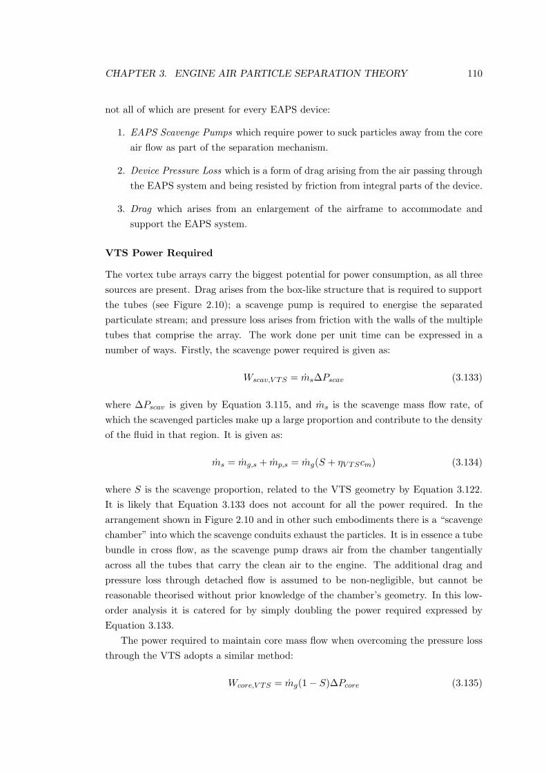
CHAPTER 3. ENGINE AIR PARTICLE SEPARATION THEORY 110
not all of which are present for every EAPS device:
1. EAPS Scavenge Pumps which require power to suck particles away from the core
air flow as part of the separation mechanism.
2. Device Pressure Loss which is a form of drag arising from the air passing through
the EAPS system and being resisted by friction from integral parts of the device.
3. Drag which arises from an enlargement of the airframe to accommodate and
support the EAPS system.
VTS Power Required
The vortex tube arrays carry the biggest potential for power consumption, as all three
sources are present. Drag arises from the box-like structure that is required to support
the tubes (see Figure 2.10); a scavenge pump is required to energise the separated
particulate stream; and pressure loss arises from friction with the walls of the multiple
tubes that comprise the array. The work done per unit time can be expressed in a
number of ways. Firstly, the scavenge power required is given as:
Wscav,V TS = ms∆Pscav (3.133)
where ∆Pscav is given by Equation 3.115, and ms is the scavenge mass flow rate, of
which the scavenged particles make up a large proportion and contribute to the density
of the fluid in that region. It is given as:
ms = mg,s + mp,s = mg(S + ηV TScm) (3.134)
where S is the scavenge proportion, related to the VTS geometry by Equation 3.122.
It is likely that Equation 3.133 does not account for all the power required. In the
arrangement shown in Figure 2.10 and in other such embodiments there is a “scavenge
chamber” into which the scavenge conduits exhaust the particles. It is in essence a tube
bundle in cross flow, as the scavenge pump draws air from the chamber tangentially
across all the tubes that carry the clean air to the engine. The additional drag and
pressure loss through detached flow is assumed to be non-negligible, but cannot be
reasonable theorised without prior knowledge of the chamber’s geometry. In this low-
order analysis it is catered for by simply doubling the power required expressed by
Equation 3.133.
The power required to maintain core mass flow when overcoming the pressure loss
through the VTS adopts a similar method:
Wcore,V TS = mg(1− S)∆Pcore (3.135)

CHAPTER 3. ENGINE AIR PARTICLE SEPARATION THEORY 111
where ∆Pcore is given by Equation 3.114.
The device drag is calculated by considering the total surface area occupied by the
tubes and the supporting planform area. Assuming that all vortex tubes collectively
are designed to supply a design point mass flow mE of air to the engine via each one
of their collectors, the number of tubes required is:
Nt =mE
mc=
mE
ρgugπR2c
(3.136)
It can be inferred visually from Figure 2.10a that a panel of vortex tubes has a larger
area than the total tube area, due to the requirements for support. If the total frontal
area is AP , the total drag acting on the panel is:
DV TS =
12ρg(AP −NtAt)U
2∞
+ (NtAt)(U∞ − ug)2 if U∞ > ug
12ρg(AP −NtAt)U
2∞
if U∞ ≤ ug
(3.137)
where AP is the VTS panel projected area. The power required to overcome drag is:
WD,V TS = DV TSU∞ (3.138)
Summing Equations 3.133, 3.135, and 3.138 yields the total power required for the VTS
system:
WV TS = 2Wscav,V TS +Wcore,V TS +WD,V TS (3.139)
IBF Power Required
The power requirements of the IBF differ to the VTS by the lack of a scavenge pump.
There is a considerable and transient pressure loss across the filter that must be opposed
by the engine:
WF,IBF (mpc) = mg(∆PIBF (mpc) + ∆Pre) (3.140)
where ∆PIBF is the total loss across the IBF filter, as given by Equation 3.72, and
∆PIBF is any pressure recovered due to the forward motion of the aircraft. It is
assumed that unlike the VTS, the supporting structure for the IBF does not contribute
a significant amount to the device drag. The pressure recovery exists at forward speeds
greater than the engine face velocity, or:
∆Pre =
12ρg (U∞ − Ua)
2 if U∞ > Ua
0 if U∞ ≤ Ua
(3.141)

CHAPTER 3. ENGINE AIR PARTICLE SEPARATION THEORY 112
The IBF drag is assumed to be a form drag created by the deceleration of air into the
intake, hence can be calculated similarly:
DIBF =
12ρgAF (U∞ − Ua)
2 if U∞ > Ua
0 if U∞ ≤ Ua
(3.142)
The power required to overcome this drag is:
WD,IBF = DIBFU∞ (3.143)
Summing Equations 3.140 and 3.143 gives an expression for the total power required
to service the IBF:
WIBF (mpc) = WF,IBF (mpc) +WD,IBF (3.144)
It should be remembered that owing to the build up of particles on the filter’s sur-
face, the power required to overcome the pressure drop given by Equation 3.140 is a
function of the total mass collected, given by Equation 3.59. Importantly, this means
Equation 3.144 is transient: the power required to employ an IBF device increases over
time.
IPS Power Required
The IPS is mounted to the front of the engine and is therefore assumed to pose no
additional drag to the airframe; there are no significant adjustments to the intake to
accommodate the IPS that would increase the drag. Therefore the power requirement
to counter drag is neglected here. However, like the VTS, a scavenge pump is required
to extract the separated particles from the core air flow which requires power. The
pressure loss across an IPS is mainly attributable to skin friction at the walls of the
separator, but as the flow turn angle increases, the contribution to pressure drop of form
drag increases [61]. The total pressure loss can be segregated into core and scavenge
flows and combined with respective mass flow rates to calculate the total power required:
WIPS = Wcore,IPS +Wscav,IPS = mg(1− S)∆Pcore + mgS∆Pscav (3.145)
EAPS Power Required
From the above it is clear that the power required to employ a particle separating device
depends on the system chosen. At least one technology requires an increasing dedication
of engine power, while two others draw power for scavenge pumps. In summary, the

CHAPTER 3. ENGINE AIR PARTICLE SEPARATION THEORY 113
power lost to the EAPS system is given by:
WEAPS(mpc) =
WV TS if Vortex Tube Separator used
WIBF (mpc) if Inlet Barrier Filter used
WIPS if Inlet Particle Separator used
(3.146)
where WV TS , WIBF (mpc) and WIPS are given by Equations 3.139, 3.144 and 3.145
respectively. This permits an assessment of the devices based on their power demand
from the engine.
3.5.3 Engine Erosion
The ultimate goal of an EAPS device is to increase the lifetime of a helicopter engine.
Each EAPS system is different; some have lower separation efficiencies, while others
exert an increasing load on the engine. If the EAPS system employed does not achieve
100% efficiency, particles that evade separation will cause damage to the engine. The
engine performance will continue to deteriorate, albeit more slowly. The performance
cost of employing an EAPS system has been visited already in the theory; a complete
assessment tool would consider both the power lost to servicing the EAPS and any
erosion due to unavoidable particulate ingestion.
To facilitate such a tool, a model is needed that predicts engine erosion. Fortunately
there are some in the literature, as described in Section 2.2.5. The work of van der
Walt & Nurick [22] provides a theory for predicting the power deterioration rate as a
function of particle impact velocity and diameter. The power deterioration rate for a
filtered helicopter engine is given as:
Wr = krφUβ (3.147)
where U is the impact velocity, and β is a correlation exponent. The constant kr is
dependent on the engine and erodent properties that are all assumed to be constant for
a specific engine and dust type, hence Equation 3.147 describes a linear relationship
between the mass ingested and the power lost to erosional effects. This linear relation-
ship is proven in van der Walt & Nurick’s study for up to 10% power deterioration after
an initial unsteady stage in which power is actually observed to increase. (This is due
to dust polishing of the blade surface at the very beginning of erosion). For the case of
a sparse dust distribution in which particle-on-particle interactions are negligible, the
engine power loss is given by:
∆W = krmpeUβφ (3.148)
where mpe is the mass of ingested particles. If the mass distribution can be expressed
by fraction and analytically as a function of the particle diameter, Equation 3.148 can

CHAPTER 3. ENGINE AIR PARTICLE SEPARATION THEORY 114
be written more generally as:
∆W = krUβmpe
∫ φmax
φmin
f(φ)φ dφ (3.149)
where f(φ) is a function describing the fractional particle size distribution of the in-
gested particulate. Introducing the mean separation efficiency for the dust PSD from
Equation 3.128 allows the ingested particulate to be written in terms of the total mass
of particles reaching the intake:
∆W = krUβ(1− EEAPS)mp
∫ φmax
φmin
f(φ)φ dφ (3.150)
This can now be divided through by mp to express the erosion rate, or the power loss
per unit mass of particles ingested by the EAPS device.
Wr(mp) = krUβ(1− EEAPS)
∫ φmax
φmin
f(φ)φ dφ (3.151)
If the factor krUβ is known for a particular engine and dust, the only remaining un-
known is the function that describes the size distribution of the ingested particulate,
f(φ). The PSD of the ingested particulate is related to the grade efficiency of the
EAPS device, EEAPS(x), which calculates the separation ability of the device for a
given particle size x. In algebraic form, it relates the ingested PSD to the brownout
PSD:
f(φ) = (1− EEAPS(x))PDF (x, µ, σ) (3.152)
Hence if the dust cloud size distribution is expressed by a function, such as a log-
normal distribution, the ingested PSD can be found. Alternatively, if the dust cloud
distribution is expressed by size bands and mass proportions, the integral over f(φ)
can be expressed as a sum of the filtered size mass fractions:
∫ φmax
φmin
f(φ)φ dφ ≡φmax∑
i=φmin
(1− EEAPS(di))m+i di (3.153)
where di is the representative diameter of the ith size group in the dust cloud PSD and
EEAPS(di) is the corresponding separation efficiency. Incidentally, the sum on the right
hand side is effectively the mean particle diameter by mass as given by Equation 3.15,
which simplifies the expression further. Substitution of whichever of these is most
appropriate into Equation 3.151 yields enough information to predict the erosion rate
of a given engine in a given dust cloud.

CHAPTER 3. ENGINE AIR PARTICLE SEPARATION THEORY 115
3.5.4 Engine Longevity
There are now two identified sources of engine power loss for a helicopter operating in
dusty environment with particle separating technology:
1. Power required to overcome EAPS.
2. Power lost due to erosion by ingested particulate.
Since each EAPS system will carry different power penalties but will achieve varying
levels of separation efficiency, the power loss provides a useful metric in comparing the
key technologies. Summing the sources of loss, the rate of reduction in available engine
power for an EAPS-fitted rotorcraft, as a function of dust mass fed is:
WE(mp) = Wr(mpe) +WEAPS(mpc) (3.154)
wheremp is the mass of particles entering the intake as given by Equation 3.1, mpc is the
mass collected by an EAPS device (only applicable to IBF) as given by Equation 3.59,
and mpe is the mass of particle that evade capture and is ingested by the engine. The
latter quantity is related to mp by the efficiency of the EAPS system in a similar way
to the mass captured by an IBF:
mpe = (1− EEAPS)mp (3.155)
When the system features dual flow paths, it must be remembered that mp refers to
the mass of particles entering the device. Since a portion of the mass flow is scavenged,
this is greater than the mass that would enter an unprotected engine of the same mass
flow. However, Equation 3.127 accounts for this by including the scavenge flow portion
S in the efficiency expression given for VTS and IPS devices. For completeness, the
three EAPS devices’ efficiencies are summarily given as:
EEAPS =
EV TS if Vortex Tube Separator used
EIBF if Inlet Barrier Filter used
EIPS if Inlet Particle Separator used
(3.156)
where EV TS and EIBF are given by Equations 3.127 and 3.102 respectively. The IPS
efficiency EIPS is not given analytically in the present work, but takes the same form
as Equation 3.127 and its value can be taken from test cases in the literature. All
are functions of the particle size. The IBF separation efficiency here is a function of
mass collected; in Section 3.3 it was explained that the filter packing fraction, which
affects both the pressure drop and the separation efficiency, increases with collected
mass, hence is also a function of time.

CHAPTER 3. ENGINE AIR PARTICLE SEPARATION THEORY 116
3.5.5 Engine Improvement Index
A perhaps simpler method for comparing EAPS devices is to calculate the resulting
extension to engine life over unprotected engines. Scimone & Frey [41] discuss a study
by Textron Lycoming which investigated the potential gains offered by EAPS employ-
ment. It used a Life Cycle Cost Model to predict the increased Mean Time Between
Removal (MTBR) offered by installing a particle separator. It found a hundredfold
increase in MTBR can be achieved when using an IBF. In a similar study, mentioned
in the contribution by van der Walt & Nurick [24], the VTS is quoted as been able to
achieve an MTBR of between 10 and 25 times the unprotected engine. An important
point is made: that such predicted values are sensitive to local conditions, dust type,
and dust concentration, so such figures need to be treated as benchmark figures.
From an analytical standpoint, however, verified models can be useful to cross-
compare EAPS devices. A simple method is to express life extension as the ratio of the
erosion rate of an unprotected engine to the erosion rate of a protected engine. If the
integral for the ingested particulate in Equation 3.151 is represented by a effective mean
diameter by mass proportion, φeff , the erosion rate for a protected engine simplifies
to:
Wr(mp) = (1− EEAPS)φeff (3.157)
The erosion rate of an unprotected engine takes the same form as this, but omits the
separation efficiency term (or simply EEAPS = 0) and uses the effective (arithmetic)
mean diameter by mass of the dust cloud, deff . Hence the lifetime improvement factor,
LIF, is given by:
LIF =deff
(1− EEAPS)φeff
(3.158)
This can be used as a quick and effective tool to compare EAPS devices in many
environments, provided the analytical expressions for separation efficiency and PSD
data are known.
3.6 Summary
This chapter provides all the equations necessary to facilitate the ultimate aim of
quantifying EAPS performance. The important equations correspond to the properties
of the sand reaching the engine, and the physics of particle separation. The theory of
pressure loss as a result of drag by the device walls or fibres is also presented, to afford
calculation of the performance penalty of employing EAPS technology. Of the three
technologies, only the VTS and IBF are elaborated on, the latter in the most detail
due to its underrepresentation in the literature. Finally the chapter is concluded with
equations to assess the improvement to engine life that can be achieved when engine

CHAPTER 3. ENGINE AIR PARTICLE SEPARATION THEORY 117
protection is fitted.
The equations of particle classification borrow from classical theory and statistical
analysis. A probability density function can be used to express the size distribution
of a dust algebraically. Alternatively, if the dust has been obtained from the field, it
can be analysed and discretised into size bands with corresponding mass proportions.
Knowledge of the particle size distribution is important for the calculation of separa-
tion efficiency. The ability of an IBF or VTS to remove a particle depends on the
particle’s diameter. Therefore separation efficiency is more accurately expressed as a
grade efficiency, i.e. an efficiency as a function of particle size. Combining the grade
efficiency with the particulate size distribution by mass allows the overall efficiency to
be determined for a given sand. Without a specific sand in question, expressing the
overall efficiency of an EAPS device is meaningless. Similarly, the efficiency is closely
linked to the velocity of the particle; if the device is operating off-design, it may not
achieve the desired separation efficiency.
The theory of pressure loss borrows from modified versions of Darcy’s Law and
turbulent boundary layer theory. It allows the power required to service an EAPS
system to be predicted. Combining the power required to cater for pressure loss with
power to cater for drag and scavenge pumps allows the overall demand on the engine to
be quantified. An additional model is also provided to calculate the loss in engine power
due to erosion by ingested particulate, which will occur since no system can remove
100% of the particles. This model also allows the effect of EAPS to be compared to
the huge curtailment of engine life when no protection is provided.

Chapter 4
Methodology
This chapter outlines the procedure adopted in using computational fluid dy-
namics to perform a parametric study of inlet barrier filter design. To facilitate
the study, the problem is broken into two lengthscales. An overview of the com-
putational methods and practices employed is also given.
4.1 Introduction
In the introduction to the theory section, it was intimated that there would be a deeper
investigation into the performance of the IBF. This is due to there being a substantial
lack of research in this area in the literature. Vortex tubes are well covered by analytical
theory, while inlet particle separators have been investigated by CFD studies in the
literature. The present work aims to bring the understanding of inlet barrier filters to
the same level, in order to more rigorously investigate the effects of EAPS systems on
engine performance. To undertake this, a method is proposed that initially breaks the
problem down into more manageable parts. Following this a procedure is laid out for
a series of computational simulations that aim to investigate the effects of IBF design
features on pressure loss, separation efficiency and holding capacity (see Section 3.3)
through parametric study.
Modelling of IBF is made complicated by the wide bandwidth of lengthscales in-
volved. The performance can be affected as much by micrometre-sized changes in par-
ticle size just as by centimetre-sized changes to the intake geometry. To ease modelling,
the problem is broken down into three scales:
1. Intake Scale
2. Pleat Scale
3. Fibre Scale
118

CHAPTER 4. METHODOLOGY 119
These are depicted in Figure 4.1. Of the three scales, two are taken forward for com-
putational fluid dynamics modelling: the Intake Scale and the Pleat Scale; the Fibre
Scale is covered by the theory detailed in Section 3.3. Since the separation efficiency is
mainly an internal process of the filter medium, it acts at the fibre scale and therefore is
not directly modelled by CFD in the present work. However, the theoretical prediction
can be enhanced by knowledge of the local flow conditions, which can be inherited from
numerical simulation of the fluid passing through a filter pleat.
Figure 4.1: Breakdown of IBF into more manageable parts for analysis: a. IntakeScale; b. Pleat Scale; c. Fibre Scale∗. ∗Fibre Scale Image reproduced under CreativeCommons licence (CC BY-NC 2.0), © BASF - The Chemical Company.

CHAPTER 4. METHODOLOGY 120
The main motivation for the numerical study is to investigate the phenomena asso-
ciated with filtration by pleated porous media, with particular attention to performance
transiency. In pleat design, it is known that an optimum configuration exists for min-
imum pressure drop and maximum holding capacity; as part of the study this will be
sought for IBF applications (see Section 2.5.3). Another important feature is the “el-
bow” in the pressure loss curve that indicates the point at which a surface cake forms.
Knowledge of this may be critical to predicting IBF performance: the already-transient
state is not ideal for the engine, but it could be compounded by a sudden increase in
inlet pressure loss. It would be useful to ascertain the ferocity of the discontinuity, and
the point at which it occurs. To investigate these phenomena, a parametric study is
performed on a single pleat section using CFD.
Since the IBF panel is made up of several scores of pleats, it may be that the
transition from internal clogging to surface filtration is more gradual, as some parts of
the filter reach capacity before others. It was mentioned in Section 2.2.4 that intake
orientation can aid inertial separation; it is probable that the way in which the IBF is
integrated into the airframe may also impact on its performance. To investigate these
hypotheses, a second parametric study is performed using CFD, but at a larger scale.
Combining the two levels of modelling with the Fibre Scale will allow a complete
picture of IBF performance in a number of operational conditions to be formed. The
parametric study will reveal the effect on performance of altering key geometric vari-
ables, to permit design optimisation. The important performance variables to investi-
gate are the dust properties and the inlet mass flow, as these are likely to change most
from one environment to the next and from one rotorcraft to the next. By determining
correlations between these variables and the IBF performance will facilitate the wider
aim of assessing and comparing the efficacy of all three particle separating technologies.
4.2 Pleated Filter Simulation
A computational fluid dynamics experiment is conducted to improve understanding of
pleated filter behaviour for helicopter inlet barrier filters. An IBF module and a close-
up of a filter pleat are shown in Figures 4.1a and 4.1b. There are two main objectives
for the CFD parametric study of a filter pleat:
1. Investigate the effect of filter clogging and cake formation on the pressure loss
evolution.
2. Determine the optimum pleat design for a given set of flow boundary conditions.
The use of CFD to determine pleated filter diagnostics is not new, however there
have been no studies at these lengthscales or Reynolds numbers (characteristic length

CHAPTER 4. METHODOLOGY 121
being the channel width). The nearest study in the literature is the semi-analytical
model for the clogging of pleated filters proposed by Rebaı et al. [52] discussed in
Section 2.5.3, which uses assumptions or simplifications that cannot be applied here.
The total pressure drop across an IBF is attributable to three sources, as given by
Equation 3.72. While the filter medium and surface cake losses can be predicted with
well-established theory, the loss in the channel proves more difficult to model. Rebaı’s
model assumes knowledge of the shape of the velocity profiles within the pleat channels
to calculate the loss to fluid shearing; in the present work the same assumption is not
applied, as the flow is of a higher velocity and is not considered laminar. The equations
used to calculate pressure loss across the filter medium also omit the inertial term in the
Darcy equation, and use a temporal resistance term for the filter medium based on the
clogging evolution of a planar medium. While Rebaı’s model is shown to demonstrate
good agreement with experiment, it is deemed inadequate to deal with the anticipated
flow conditions of IBF pleated filters, hence the use of CFD in the present study.
4.2.1 Computational Domain
The first task is to decide how the pleat is represented computationally and which
dimensions are to be varied. Figure 4.2 shows a computer aided design (CAD) drawing
of an IBF pleat. There can be some confusion as to the meaning of a “pleat”: in some
studies a pleat refers to just one side of the fold; in the present work a “filter pleat”
corresponds to the whole fold, shaded green in Figure 4.2. The pleat is represented by a
two-dimensional (2D) porous domain, which resembles the cross-sectional profile of half
a pleat. Using only half is permitted thanks to symmetry, and reduces computational
time. The rest of the domain is designated “fluid”, and extends one times the filter
thickness upstream and four times the pleat depth downstream as shown in Figure 4.3.
The formation of the cake is represented by a number of thin layers drawn adjacent
to and upstream from the main filter medium. An assumption here is that the cake is
distributed uniformly across the leading surface of the filter. For consistency, the cake
layer thickness is proportional to the filter thickness (≃ 4.5% of the thickness). There
are 9 cake layers in total, as shown in Figure 4.3b.

CHAPTER 4. METHODOLOGY 122
Figure 4.2: CAD drawing of a section of IBF pleats, with a single pleat shaded in green.
The CFD exercise is conducted using AnsysFluent. While known for being highly
numerically dissipative and therefore potentially inaccurate, the solution speed offered
by Fluent was preferred due to the volume of tests to be run. Future work could verify
the code’s accuracy, but until there are experimental results against which to validate
the methodology, the more important outcome is to obtain sufficient data to make
conclusions about pleat design. The software has the capability to solve the Navier-
Stokes equations for free fluid flow, which are derived from the basic principles of mass
momentum and energy. In the present work the fluid is treated as incompressible
therefore considered conservation of only mass and momentum. The conservation of
mass for an incompressible fluid is given as:
∇(ρ~u) = 0 (4.1)
where ~u is the local velocity vector. The conservation of momentum is essentially an
application of Newton’s second law for a continuous fluid. For incompressible flow it is
given as:∂
∂t(ρ~u) +∇(ρ~u~u) = −∇p+ µ∇2~u+ ρ~g + ~F (4.2)
where p is the static pressure, µ∇2~u is the viscous diffusion term, and ~F is a term that
accounts for any external force applied to the fluid, such as a porous medium. Hence
in the cell zones lying within the designated porous zone and cake layers (differentiated

CHAPTER 4. METHODOLOGY 123
in Figure 4.3c), Fluent adds a momentum source term to Equation 4.2 to account for
the presence of a filter:
~F = Si = −
2∑
j=1
Cijµuj +2∑
j=1
1
2ρgujυmag
(4.3)
where Si is the source term for the ith (x or y) momentum equation, and C and
D are the viscous and inertial resistance coefficients described in Section 3.3.1. This
momentum sink term corresponds to the pressure gradient given by Equation 3.56. In
addition to the porous zones, the domain is bounded by four surfaces: a velocity inlet,
(far left in Figure 4.3a) at which the flow conditions of initial velocity and pressure are
prescribed; an outflow (far right in Figure 4.3a); and two symmetry boundaries (top
and bottom in Figure 4.3a).
4.2.2 Pleat Properties
Figure 4.3 illustrates the key dimensions to be varied in this parametric study. The
pleat assumes a shape seen in the real IBF: a triangular-shaped pleat channel with
rounded folds. Incidentally, existing CFD studies have elected to represent different
pleat depth/width combinations using a purely rectangular planform, for ease of mesh-
ing; in the current study a more realistically-shaped planform is employed, both to
facilitate the objectives easier and to broaden the literature. Recalling the objective of
finding an optimum design, the pleat density (or width, number) is varied by altering
the angle θ in Figure 4.3b, while the depth and thickness are varied by varying the
dimensions labelled Zpl and ZF respectively in Figure 4.3a. The fold radius, charac-
terised by the inside edge of the fold, has a length of half the filter thickness. The
narrowest pleat angle tested is 0 degrees, a configuration in which the pleat channel
walls are parallel to each other; in Figure 4.3 the pleat has an angle of 10 degrees.
The exact properties of the filter medium and pleat geometry cannot be sought
without obtaining a real IBF panel. It is not possible to purchase such a panel from the
manufacturers. Fortunately, from the few contributions in the literature that pertain to
IBF and filters for automotive applications, an educated estimate of the key properties
can be inferred. The patent by Scimone [40] suggests the pleat depth lies in the range of
2.5 to 7.5 cm, with a pleat pitch (spacing) of 0.42 to 0.85 cm. From direct measurement
of the IBF for the MD500 (Figure 4.1b) the pleat width is 1 cm. Estimates of the filter
properties are taken from the study of Rebaı et al. [52] automotive applications, which
employ a fibrous filter of porosity 0.95, fibre diameter of 15 microns, and thickness
of 1.5 mm. The filter medium in planar form has a holding capacity of 0.4 kgm−2.
These give some suitable dimensions to carry out the parametric study. Each pleat

CHAPTER 4. METHODOLOGY 124
Figure 4.3: IBF pleat as a computational domain, with filter medium and cake layersrepresented by porous zones. 3-view diagram, showing a. extent of the computationaldomain; b. key dimensions of the pleat geometry; c. close-up of cake layers and filtermedium.

CHAPTER 4. METHODOLOGY 125
section is subjected to a flow of varying velocity between 2 and 12 ms−1 to reflect a
range of engine mass flow rates, at Standard Day conditions. A breakdown of all filter
parameters and the value ranges of those tested is given in Appendix A.
4.2.3 Solution Setup
The important parts of the solution setup here are the viscous and inertial resistance
coefficients featured in Equation 4.3, which are prescribed to the porous zones that
represent the filter pleat and the cake layers. For the filter medium, the coefficients
are given by Equations 3.57 and 3.58. To simulate clogging, each pleat shape is tested
under the same flow conditions over a range of resistances. The increase in filter medium
resistance is imitated by decreasing the porosity according to Equation 3.60, in which
the volume of particles captured by the medium is subtracted from the filter volume.
To facilitate this procedure with a degree of automation, a user-defined function (UDF)
for the porous zone is employed, which exploits the unsteady solver by changing the
properties of the porous zone each time step. During each time step the solution is run
until convergence; the only change from one time step to the next is the resistance of
the porous zone, hence a series of time steps run like an unsteady solution is akin to
running a number of consecutive individual simulations. At each time step, the filter
porosity decreases by a quantity equivalent to collecting a fixed mass of particles.
When the total mass collected is equal to the filter capacity, the filter resistance
coefficients are held constant and the first cake layer is “activated” i.e. is no longer
invisible to the flow and exhibits non-zero resistance terms. The clogging has now
reached the “cake formation” stage. After each subsequent time step the next cake
layer is activated and so on until each of the 9 layers has been tested in the flow.
Since the filter capacity is expressed as a mass per unit projected area, it follows that
each different pleat shape has a unique holding capacity: a filter containing pleats of a
smaller angle (narrower pleat channel) packs more material into a given projected area
hence has a greater capacity. Since all is desired from these simulations is an evolution
of the pressure loss as a function of captured mass, a constant number of times steps
between the clean filter condition and the clogged filter condition is chosen for each
pleat. At the cake layer stage the mass interval is determined by the pleat surface area,
the cake thickness and the cake density.
The viscous and inertial resistances for the cake layers are slightly more difficult to
render, since the pressure drop equation for the cake is of a different form to Equa-
tion 4.3 (contrast with Equation 3.70). To obtain the linear and quadratic term coeffi-
cients (C and D) required for Fluent’s porous model, the cake pressure drop equation,
Equation 3.69, is plotted over a range of velocities of value expected in this application.
All other variables in the equation are known. The cake properties of the test dusts are

CHAPTER 4. METHODOLOGY 126
borrowed from Endo et al. [77]. A second order polynomial is fitted to the resulting
curve, yielding the two required coefficients. While compression of the cake layers may
occur under the drag pressure, initial calculations showed this to be insignificant [45]
hence it is assumed that the cake porosity is constant for each layer.
In summary, to achieve the objective of plotting the pressure drop versus the mass
collected for each case, the unsteady solver is utilised to vary the resistance properties
of a porous zone in a fluid domain. A steady state solution is calculated first, with
the clean filter properties prescribed to the filter section. The unsteady stage is then
commenced, during which the filter resistance increases by an amount reflective of the
capture of an incremental mass of particles, until the total captured mass equals the
filter capacity. At this point the previously “invisible” cake layers are activated in turn
after each subsequent time step, until 9 time steps have passed. For each time step
the solution is converged. The relevant parameters varied at each time step are listed
below. If n is the number of time steps, NFC is the number of time steps to filter
capacity, and Nc is the number of time steps for all cake layers to form and MFC is the
mass captured per unit volume of filter, the mass interval (∆m), filter porosity (ǫF )
and cake porosity (ǫc) are expressed accordingly:
∆m =
(1− ǫF,0)ZFApl(MFC − ρf ) if n ≤ NFC
(1− ǫc,0)ZcAplρp if n > NFC
(4.4)
ǫF =
ǫF,0 − nρp∆mZFApl
if n ≤ NFC
ǫF,FC if n > NFC
(4.5)
ǫc =
0 if n ≤ NFC
ǫc,0 if n > NFC
(4.6)
4.2.4 Grid Independence
To solve the Navier-Stokes equations for the free fluid flow, the domain is discretised
into a mesh of cells each of which updates the flow each iteration in response to input
changes from the cells surrounding it. Generally speaking, the greater the number of
cells in an area of complex geometry, for example the cake-fluid interface, the more
accurate the result. However, when increasing the cell resolution there comes a point
at which the solution shows very little change. Depending on the tolerance set by the
user, at this point the solution is said to be grid independent, i.e. no longer depends
on the grid resolution; increasing the grid size would only cost more computation time.
Grid independence checks are essential for any CFD exercise, if any faith is to be placed
in the results and computational resources are to be maximised.
In the present study, the grid independence check is made more cumbersome by the

CHAPTER 4. METHODOLOGY 127
multitude of pleat designs tested. To be consistent across all designs, the cake thickness
is used as a reference for the minimum cell size in the domain, since it is the shortest
length in each domain tested. The mesh resolution is not homogeneous throughout the
domain: in some areas such as porous interfaces the flow is under more strain than in
other areas and will contain steeper gradients of velocity; areas of steep flow property
gradients require higher resolution grids for greater accuracy and speed of convergence.
The global solution is more sensitive to the accuracy of these areas, hence in designing
an appropriate mesh it is necessary to concentrate efforts on grid independence here.
Similarly in areas of little disturbance to the flow such as far upstream/downstream, it
is a waste of computational time to discretise with high resolution.
In the present case, the area of greatest flow contraction is in the cusp of the
upstream pleat channel. The radius of the cusp is two times the cake thickness, and
remains this for all pleat shapes studied. This justifies the use of the cake thickness
as a reference length. Other areas of steepest velocity gradient are at the fluid-porous
medium interfaces, i.e. the filter surfaces and each cake surface; in these areas the cell
size is similarly small. A triangular mesh is used here to conform smoothly to the curves
of the pleat folds; see Figure 4.5b. As the domain extends upstream and downstream,
the cell size is increased (grid resolution decreased) and a paved quadrilateral cell
distribution is adopted. The range of cell sizes adopted for the pleat domains can be
seen in Figures 4.4 and 4.5.
Figure 4.4: Discretisation of a typical pleat domain, illustrating a coarse mesh at theupstream and downstream extents, and a finer mesh around the pleat.
To reach grid independence, the minimum cell in the domain is varied in size as
a fraction of the cake thickness, i.e. by altering the number of cells across the cake
thickness. The pleat of smallest angle (narrowest channel, 0 degrees) is used as a
test case in the highest velocity flow (12 ms−1), since it is these channels under these
conditions in which the flow contracts the greatest. A number of sizes were tested;
the results of three are presented in Figure 4.6 for illustrative purposes. Figure 4.6a
shows the spanwise-averaged non-dimensional static pressure across the pleat in the
streamwise direction. There are notable differences between each result, but the static
pressure at 1.5Zpl appears to be the same for the two most refined grids. This suggests
that increasing the number of cells across the cake thickness beyond four cells does not
have a profound affect on the result. This is backed up by Figure 4.6b, in which the
total pressure at the domain exit is monitored for the range of mass intervals. This is
the key value in the exercise. The results illustrate little discrepancy when increasing

CHAPTER 4. METHODOLOGY 128
the grid from the medium to the largest resolution, hence a minimum cell size of one
quarter of the cake thickness is chosen for the parametric study.
Figure 4.5: Discretisation of a typical pleat domain, illustrating area of highest celldensity, in which the flow is anticipated to be under the most strain, producing thesteepest velocity gradients: a. representation of cake layers; b. close-up of highlyrefined mesh.

CHAPTER 4. METHODOLOGY 129
−0.5 0 0.5 1 1.50.98
0.985
0.99
0.995
1
x / Zpl
(−)
p x / p ∞
(−
)a.
min(l) = Zc/3 (122,454 cells)
min(l) = Zc/4 (329,437 cells)
min(l) = Zc/5 (710,077 cells)
0 0.4 0.8 1.2 1.60
5
10
15
20
mpc
(gcm−2)
∆
P (
kPa)
b.
min(l) = Zc/3 (122,454 cells)
min(l) = Zc/4 (329,437 cells)
min(l) = Zc/5 (710,077 cells)
Figure 4.6: Grid independence checks for pleat simulations, displaying: a. spanwise-averaged normalised static pressure; b. pressure drop as a function of accumulatedmass per unit area.
4.2.5 Turbulence Model
There are several options available for modifying the way Fluent solves the governing
equations in each cell, such as the way the scalar quantities at the cell centres are
evaluated. The suitability of any one method is usually a compromise between accuracy
and computation time, which are themselves functions of the geometry complexity. In
the absence of real data to compare results with, an in depth study into the differences
between each numerical scheme and solution method would merely be academic and not
advance the present work at this stage. The theory of these methods is well represented
in the literature (see Ferziger & Peric [84]) and is therefore not exhaustively covered
here.
To reflect reality of flow through IBF filters, the fluid is prescribed with a level of
turbulence, which is a measure of the kinetic energy of the eddies in the flow produced
by fluid shear, friction, buoyancy or external forcing. Turbulent flows are characterised
by fluctuating velocity fields, which aid the mixing of and cause fluctuations of mo-
mentum, energy, species concentration and other transported properties. To simulate
these fluctuations fully by directly solving the governing equations would require a great
computational resource. To surmount this problem, the turbulence can be simplified
by removing the small scale velocity fluctuations through time-averaging, ensemble-
averaging or other manipulation to form modified versions of the governing equations.
However, this process creates additional unknowns, which require turbulence models
for determination.
One such method of removing the small scale fluctuations is by Reynolds-averaging,

CHAPTER 4. METHODOLOGY 130
whereby the solution variables in the instantaneous Navier-Stokes equations are decom-
posed into the mean (ensemble-averaged or time-averaged) and fluctuating components.
For the velocity components:
ui = ui + u′i (4.7)
where ui and u′i are the mean and fluctuating velocity components. Substituting these
into Equations 4.1 and 4.2, and expanding the difference operator (∇) (and removing
the overbar from the mean velocity), yields the well-known Reynolds-averaged Navier-
Stokes equations for mass and momentum continuity:
∂ρ
∂t+
∂
∂xi(ρui) = 0 (4.8)
∂
∂t(ρui) +
∂
∂xi(ρuiuj) = − ∂p
∂xi+
∂
∂xi
[
µ
(
∂ui∂xj
+∂ui∂xj
− 2
3δij
∂ul∂xl
)]
+∂
∂xj(−ρu′iu
′
j)
(4.9)
The additional terms that appear represent the effects of turbulence. In particular,
−ρu′iu′
j are known as the Reynolds stresses, which must be modelled in order to close
the momentum equation. There are several approaches to modelling the Reynolds
stresses, each of which are determined by the choice of turbulence model. The choice of
turbulence model will depend on a number of factors such as the physics of the problem,
the level of accuracy required and the computational resources available. In the present
work, a suitable model must chosen to account for high fluid strain rates anticipated
in the pleat channels. Again, a lack of real data makes verification quite difficult to
ascertain the accuracy of a particular model, therefore some computational cost may be
required to guarantee greater assumed accuracy. The 5-equation Reynolds Stress Model
(RSM) is one such model, which is the most elaborate model that Fluent provides. It
costs approximately 50-60% more computation time over the simpler RANS models,
but it has greater potential to give accurate predictions for complex flows. To simulate
turbulence, the user inputs a turbulence intensity and a turbulence lengthscale, which
are used by the RSM to determine the turbulent viscosity.
There are current studies in the literature that use CFD to calculate the pressure
drop across a pleated filter, but they invariably solve for laminar flow only. To compare
the RSM with the k−ǫmodel (a two-equation RANS model), a number of pleat domains
are drawn to replicate the laminar solution obtained by Chen et al. [47]. A low level
of turbulence (0.5%) is prescribed to the flow to justify the requirement of a RANS
model, but to permit comparison with the laminar solutions. The flow conditions are
exactly as is prescribed in the literature. The results are shown in Figure 4.7. At
narrow pleat channel widths the accuracy of the k-ǫ appears to diminish, while the
RSM produces just slightly higher pressure drop results than the literature. While this

CHAPTER 4. METHODOLOGY 131
does not necessarily confirm the suitability of the RSM, it at least suggests that its
use will yield results of a reliable order of magnitude. For completeness the present
work uses: a segregated solver to solve the governing equations for the conservation
of momentum and mass; a 1st Order Upwind scheme to discretise the momentum and
turbulence terms since no change in the results was found when using a higher order
scheme; the PRESTO! scheme, which is recommended for pressure discretisation when
using the porous media model; and the PISO algorithm, which is selected for pressure-
velocity coupling based on its recommendation for transient calculations.
1 2 3 4 50
200
400
600
800
Zpw
(mm)
∆P (
Pa)
Chen et al. (CFD)Laminar SolutionStandard k−ε ModelReynolds Stress Model (RSM)
Figure 4.7: Suitability checks for pleat simulations of two different turbulence models,along with the laminar solution, on the domain featured in the CFD study of Chen etal. [47], where Zpw is the pleat width.
.
4.3 Installed Filter Performance
As mentioned in Section 2.5 there is very little in the technical literature that pertains
to installed IBF performance. From the few contributions available, data are sanitised.
What is known is that the IBF for the EC145 lasts about 12 minutes in a heavy dust
cloud before the pressure drop reaches the maximum permissible, which equates to
around 30 brownout landings & takeoffs [46]. Whether this varies between rotorcraft is

CHAPTER 4. METHODOLOGY 132
not known. A plot of the temporally rising pressure loss provided in the contribution by
Ockier et al. [46] suggests a linear relationship, but the pattern is inconclusive and no
technical detail is provided for the prevailing conditions. These gaps in the knowledge
provide the motivation for the parametric study conducted using CFD at this scale.
The pleat scale results yield a relationship between mass collected and pressure loss
across a single pleat; for the pleat scale results to be useful to the bigger picture, the
“mass collected” on the pleat needs to be converted to a “‘time spent” in the dust
cloud. This is achieved by way of a particle mass flow rate. The particle mass flow
rate is expected to vary spanwise across the filter, therefore each pleat will have its own
pressure drop evolution. To examine how this is effected, a CFD study is performed to
simulate the intake of particulate-laden flow into a helicopter engine. The three main
objectives of the intake scale parametric study are to:
1. Investigate the influence of IBF integration on the spanwise distribution of par-
ticles on a filter panel.
2. Investigate the difference in performance of forward-facing and side-facing intakes.
3. Investigate the effect of dust properties on IBF performance.
4.3.1 Computational Domain & Boundary Conditions
A simplified computational domain is constructed to reflect typical intake-IBF con-
figurations found across the range of rotorcraft. Figure 4.1a shows an upward facing
IBF module for the MD500; in other embodiments such as the MD902 the filter panel
faces to the side or may be angled into the flow to offer a level of pressure recovery in
forward flight. Two representative domains are shown in Figures 4.8a and 4.8b. Each
intake type is subjected to a range of forward flight speeds, including hover, in two
distributions of dust (explained below). Three levels of intake resistance are tested: no
filter; clean filter; and clogged filter. In all cases the filter orientation to the flow is
varied through an angle of θ.
The domain is defined by five types of boundary, as labelled in Figure 4.8. The
green boundary represents the engine, and is prescribed with an “outlet-vent” bound-
ary which will adjust the static pressure to meet a user-specified target mass flow rate.
If any restriction is placed ahead of the outlet vent, the static pressure at the boundary
will decrease accordingly in order to achieve the required mass flow. The remaining
boundary types are dependent on the freestream conditions: during hover, the three
blue boundaries are prescribed as “pressure inlet” boundaries, which allows the atmo-
spheric pressure and turbulence quantities to be prescribed at a far distance from the
inlet; during forward flight the far left boundary is a pressure inlet prescribed with a
dynamic pressure that corresponds to a user-specified forward speed (which is added

CHAPTER 4. METHODOLOGY 133
Figure 4.8: Computational domains representing two types of rotorcraft intake andIBF installation, and illustrating boundary type prescribed to domain edges for: a.side-facing (or upward-facing) intakes; b. forward-facing intakes.

CHAPTER 4. METHODOLOGY 134
to the atmospheric operating pressure), the top boundary is symmetrical to simulate
far field conditions, and the far left is a velocity outlet. The prescription to the far
right boundary is a compromise of sorts. The removal of mass flow from the domain
at the engine boundary must be balanced by the mass flow entering at the inlet, and
the mass flow leaving the domain in order to observe conservation laws. Hence the
velocity at the domain outlet must correspond to a mass flow that when summed with
the engine mass flow is equal to the mass inflow rate. The extent of the domain in
the x- and y-directions (see Figure 4.8) is large enough to ensure that the fraction of
the mass flow leaving the domain at the outlet is almost unity, thus preserving the
simulated freestream velocity. All walls in the domain are prescribed with a no-slip
condition. The energy equation is suppressed, as the flow is treated as incompressible;
while gravity is neglected.
The filter is represented by a “porous jump” boundary, which is essentially a one-
dimensional simplification of the porous media model described in Section 4.2 that
calculates the pressure drop according to the following equation:
∆p = −(
Cu+1
2Dρu2
)
∆ZF (4.10)
where ∆Z is the porous medium (virtual) thickness and u is the filtration velocity
orthogonal to the filter surface. A viscous resistance term (C) and an inertial resistance
term (D) are again required; while instead of being inferred from the number of cells
across a porous zone, the medium thickness is inputted by the user: the porous medium
is merely a membrane between cells. Since mass conservation is observed in the intake
and density is constant, the filtration velocity is a function of the filter area and the
engine mass flow rate only. The filter area increases as the angle θ increases, which
decreases the filtration velocity as:
u =ma
ρgZIBF=
ma cos θ
ρgAa(4.11)
where ZIBF is the filter projected area and Aa is the engine face area. One objective
of the study is to investigate the effect of filter angle on the flow at various stages of
clogging. The stages of clogging are simulated by prescribing values of resistance and
thickness to the porous jump that result in fixed pressure drops. For example, prescrib-
ing a thickness of zero renders the porous jump invisible to the flow, hence there is no
loss in pressure, which simulates the case of there being no filter fitted. For the cases of
clean and clogged filters, pressure drops of 600 Pa and 3000 Pa respectively are desired
across the filter. Since the filtration velocity can be determined from Equation 4.11
which is held constant for all test cases, the remaining variables in Equation 4.10 can

CHAPTER 4. METHODOLOGY 135
be tuned to ensure the pressure drop across each filter, irrespective of angle, is as de-
sired and consistent for each test case. In fact, by rearranging Equation 4.10 for ZF
it can be seen that only the filter thickness needs to be adjusted to achieve the three
different pressure drops. The solution is set up in this way in order to facilitate a fair
comparison of the effect of filter angle on the influent flow; since the pressure drop (at
a given clogging state) is equal for each angle, any difference in pressure loss at the
engine face can be attributed to the geometrical setup of the intake.
4.3.2 Solution Setup
The influence of IBF installation on intake performance is determined by simulating
two intake types to a range of freestream velocities, for a number of filter angles and
filter clogging states. A level of turbulence intensity consistent with the pleat scale
simulations is prescribed, and the flow properties reflect Standard Day conditions. A
breakdown of the parameter ranges is given in Appendix A. Another set of parameters is
introduced to fulfill the objectives of the study. By injecting particles into the domain
at a fixed distance from the filter, the distribution of particles on the filter can be
found. By injecting particles of different size, the effect of different environments can
be investigated.
There are a number of ways to model particle transport in Fluent. One such method
is the Discrete Phase Model (DPM) which simulates the trajectories of particles in a
Lagrangian framework as they interact with the continuous fluid phase. If the partic-
ulate concentration is large enough, the impact of the two-way coupling between the
two phases on the continuous phase can also be included. In the present study the
dispersion of particles is sparse: particle on particle interactions can be neglected and
the particle volume fraction, which is typically less than ≃ 0.5%, is small enough to
have negligible effect on the gas phase. The effect of turbulence on particle trajectories
can also be modelled with stochastic tracking or otherwise if desired, but since there
are no real data to compare with it was considered an unnecessary use of computational
resources.
Once the steady-state continuous phase is solved, the particles are injected into the
domain and their motion computed according to the equations given in Section 3.2.5 of
Chapter 3. The filter edge in the domain is invisible to the particles, but in tracking a
particle it is possible to record the position at which it crosses a boundary i.e. intercepts
the filter. The general procedure for setting up and solving a steady state discrete-phase
problem and obtaining the particle distribution at the filter is outlined below:
1. Solve the continuous-phase flow.
2. Create the discrete-phase injections.

CHAPTER 4. METHODOLOGY 136
3. Track the discrete-phase injections.
4. Record the positions of all particles that cross the filter.
4.3.3 Dust Representation
The discrete phase injections are used to replicate a dust distribution in a brownout
cloud. Since the exact distributions at the inlet are unknown, established test dusts are
adopted as surrogates. As illustrated by Figure 3.3, dust samples can be represented
by a particle size distribution (PSD) that gives the percentage by mass of each particle
diameter in the range. In particle sample analysis it is often the case that a PSD
is given by a of particle size groups. The following data in Tables 4.1 and 4.2 were
obtained from a test dust manufacturer for Arizona Air Cleaner (AC) Fine dust and
Arizona AC Coarse Test Dust. All particles are treated as spherical.
Table 4.1: Particle size groups by mass fractions for AC Fine test dust, as provided byParticle Technology.
dp (µm) 1 3.5 7.5 15 30 57.5
% by mass (m/M)i 17.5 17.5 14 18 17 14
Table 4.2: Particle size groups by mass fractions for AC Coarse test dust, as providedby Particle Technology.
dp (µm) 2.75 8.25 16.5 33 66 132
% by mass (m/M)i 13 11 13 19 28 16
These data are translated into injection parameters in the intake scale computa-
tional domain. Each group is distributed along an injection surface, which lies a distance
of 5AA from the filter and spans an injection area of 5Aa. The injection properties for
each particle size group include: the number of particles; a representative diameter
for the particle group; the velocity of the particles; and the mass flow rate of a single
particle stream. To calculate these values requires a degree of algebraic manipulation.
The number of particles of a given size group is found by determining the mass
concentration of that group. If the dust mass concentration of the whole sample is
known (which is interpreted from sources such as the Sandblaster II study [16]), then
the group concentration is simply:
cm,i = cm
(m
M
)
i(4.12)

CHAPTER 4. METHODOLOGY 137
where cm is the brownout mass concentration given by Equation 3.2 and (m/M)i is the
mass fraction of the particle size group. The interparticle spacing is given by:
sp,i = dp,i
(
kv1 + cm,i
cm,i
)1/3
(4.13)
where kv is the volume shape coefficient as discussed in Section 3.2.2. This can be
proven by simple geometry; a proof is given by Crowe et al. [85]. The number of
particles in a size group injection is derived from the interparticle spacing and injection
area as follows:
ni =Ainj
sp,i(4.14)
where Ainj is the particle injection area. The representative diameter of the particle
group is known; the injection velocity of the particles is assumed to be equal to the
freestream velocity. The remaining requirement is to assign a particle stream mass flow
rate, which is the particle size group mass flow divided by the number of particles:
mij =mi
ni=
1
ni
(m
M
)
icm,iρgU∞Ainj (4.15)
where U∞ is the freestream velocity and j is the particle index within the ith size group.
4.3.4 Particle Data Processing
As a particle stream propagates through the computational domain, its trajectory is
recorded by Fluent. If the stream passes through a permeable boundary (set as “inte-
rior”; a porous jump is one such boundary) its position on that boundary, along with
several other properties of the stream, can be reported by Fluent. Note: in difference
to reality, particles are not arrested in the simulation. If the two phases were coupled
this may affect the flow aft of the filter; in fact a higher order simulation could employ a
user-defined function to increase the resistance of the porous jump as a function of the
particles captured, however a far greater computational resource would be required. Of
the information recorded at the boundary, the particle position, velocity and diameter
are extracted for processing in the present work. With this information it is possible
to ascertain the spanwise variation in mass flow rate.
Firstly the particle velocity is used to infer the stream’s mass flow rate. The particle
stream has an initial mass flow rate and an initial velocity; dividing the mass flow by
the velocity gives a measure of the mass contained per unit length of particle stream
line which by conservation cannot change. If the local velocity at any point along the
stream is known, this can be used to determine the instantaneous mass flow rate, for

CHAPTER 4. METHODOLOGY 138
example at the filter:
ms,ij =mij
U∞
UIBF,ij (4.16)
where the subscript s implies a value along the filter. Consider a small portion of
the filter, for example the length of a pleat width. The mass flow rate of particles
reaching that portion is a summation of all individual streams contained within it.
Since the positions of all the particle streams are known, it is possible to ascertain the
accumulation rate of a pleat at a given spanwise position, for each size group:
ms,i =
ns,i∑
j=1
ms,ij (4.17)
here nj is the number of particle streams of a given size group passing through the
filter boundary at a position s along the filter. Likewise, summing all particle size
group mass flow rates at the local position gives the total pleat accumulation rate:
ms =
ni∑
i=1
ms,i (4.18)
The number of pleats across the filter, npl, is found by dividing the filter width by the
pleat width:
npl =ZIBF
Zpw(4.19)
where Zpw is the pleat width. Hence the total particle accumulation rate, or mass flow
rate for the whole filter is:
mp,IBF =
npl∑
s=1
ms (4.20)
This can be used as a reference to normalise the local mass flow rate given by Equa-
tion 4.18, to illustrate the spanwise distribution of dust mass collecting on the filter.
The particle mass flow rates can also be expressed as a concentration, to permit
comparison with the brownout concentration in the freestream. The mass concentration
is the particle mass flow rate divided by the engine air flow rate:
cm,IBF =mp,IBF
ma(4.21)
This can be used to asses the inherent separation ability of the IBF installation. A
value lower than the brownout dust concentration implies that due to the way it is
integrated into the airframe, a degree of dust separation from the air can be achieved
through particle inertia alone, prior to passing through the filter.

CHAPTER 4. METHODOLOGY 139
4.3.5 Grid Independence
The particulars of the numerical solution are similar to the pleat scale. The iterations
are stopped when the convergence residuals reach 0.00005. A second order upwind
scheme is used to compute quantities at the cell centres, and the pressure-velocity
coupling is solved with the well-known PISO scheme. The PRESTO! scheme was used
for pressure discretisation. The domain is discretised into quadrilateral cells to solve
the Navier-Stokes equations iteratively. The cell size distribution is set to cater for
areas of high velocity gradient, namely at the boundary walls and around the filter
entrance, visible in Figure 4.9. The grids for the two intake types are very similar; a
structured mesh can be used for the majority of the domain, but the area surrounding
the filter is made up of a quadrilateral pave, as shown in Figure 4.10.
Figure 4.9: Discretisation of forward-facing intake computational domain. The celldistribution is the same for the side-facing intake domain.
An independence test with cells of different minimum size is performed for the max-
imum filter angle (50 degrees) for the largest engine mass flow rate (12 kg/s) across
a range of freestream velocities. It is found that a minimum cell size around the fil-
ter of 0.005Aa for both intake types is sufficient to satisfy grid independence. This
is consistently applied to the grids of all domains in the parametric study. Results of
the grid independence test are given in Figures 4.11 and 4.12. Figure 4.11 shows the
local spanwise total pressure distribution taken at two streamwise cut locations, for the
forward-facing intake. The distance of each cut from the intake entrance is measured

CHAPTER 4. METHODOLOGY 140
from the most rearward point on the filter. The flow conditions illustrated here repre-
sent hover, since in this condition the largest degree of flow separation within the intake
is expected, due to the air being drawn from a multitude of angles. By comparing the
ability of each grid size to capture this separation region, a grid independence can be
finalised. The procedure is repeated at other flow conditions, for the side-facing intake.
Coarser meshes than those discussed are also tested, but the results are not presented
here.
Figure 4.10: Close-up of discretised domain for side-facing intake in the region of thefilter and intake entry.
The pressure cuts provide the data for comparison. The two streamwise locations
are chosen because they intersect the separated flow region. This is recognisable in
Figure 4.11 by the large depression in total pressure at a spanwise section of s/Aa =
0.6 to 1.0. A drop in total pressure is also noticeable at a spanwise position of s/Aa =
0 due to the presence of the boundary layer. The absence of this on the opposite wall
indicates stagnant flow, symptomatic of a separated region. The three curves on each
plot represent three grid sizes. Looking at Figure 4.11a, across the majority of the span
the curves are aligned, but at the edge of the boundary layer there is a divergence of the
coarser grid from the two finer grids. This trend continues in Figure 4.11b, and indeed
was observed for other similar cuts along the intake duct. An even greater disparity
was noticed for coarser grids not shown in these results. The difference between the two
finer grids, however, is marginal, indicating the reaching of grid independence. Hence

CHAPTER 4. METHODOLOGY 141
the choice of the intermediate cell size here, of 0.005Aa, for use in the parametric study.
0 0.2 0.4 0.6 0.8 1−3.5
−3
−2.5
−2
−1.5
−1x 10
−3
s / Aa (−)
(P(s
) −
P ∞)
/ P∞ (
−)
a.
min(l) = 0.0060Aa (320,373 cells)
min(l) = 0.0050Aa (500,056 cells)
min(l) = 0.0038Aa (815,754 cells)
0 0.2 0.4 0.6 0.8 1−3.5
−3
−2.5
−2
−1.5
−1x 10
−3
s / Aa (−)
(P(s
) −
P ∞)
/ P∞ (
−)
b.
min(l) = 0.0060Aa (320,373 cells)
min(l) = 0.0050Aa (500,056 cells)
min(l) = 0.0038Aa (815,754 cells)
Figure 4.11: Assessment of intake scale grid independence by spanwise cuts of staticpressure across the forward-facing inlet width at two streamwise locations: a. s/Aa =0; b. s/Aa = 1; where s is the distance from the inlet entrance (outer edge).
To further confirm the adequacy of the chosen grid size, one of the main flow
properties of interest — the total pressure at the engine inlet face — is plotted for
all forward speeds to be tested in the parametric study. The results are shown in
Figure 4.12, illustrating the loss in total pressure as a function of freestream velocity,
expressed in dimensionless terms. A discussion of the reasons for the trend in pressure
loss is left for later chapters, however the results show very little difference between the
three grid sizes.
4.3.6 Turbulence Model
Assurances are sought to confirm the appropriateness of the turbulence model used. For
the same reasons given for the pleat scale, the RSM model is used for turbulence closure,
with the standard wall function used to approximate the solution of the boundary layer.
In the absence of real data, the results are compared with a theoretical model proposed
by Seddon [21] for the prediction of intake performance, in which losses are attributed to
friction with the airframe and intake duct walls. the model is derived from momentum
theory and neglects flow separation. The total pressure lost to friction is split into two
sources: approach loss and duct loss. Approach loss refers to loss of energy to friction
with the airframe — the larger the wetted surface area, the larger the approach loss.
For this reason, pitot intakes (that take in very little airframe boundary layer) perform
better in cruise than the intakes tested in this study. The duct loss is attributable to

CHAPTER 4. METHODOLOGY 142
0 0.5 1 1.5 22
2.5
3
3.5
4x 10
−3
Ua / U∞ (−)
1 −
(P a /
P ∞)
(−)
a.
min(l) = 0.0060Aa (320,373 cells)
min(l) = 0.0050Aa (500,056 cells)
min(l) = 0.0038Aa (815,754 cells)
0 0.5 1 1.5 22
2.5
3
3.5
4x 10
−3
Uf / U∞ (−)
1 −
(P a /
P ∞)
(−)
b.
min(l) = 0.0060Aa (320,373 cells)
min(l) = 0.0050Aa (500,056 cells)
min(l) = 0.0038Aa (815,754 cells)
Figure 4.12: Assessment of intake scale grid independence by total pressure loss betweenthe freestream and engine inlet face, for: a. forward-facing intake; b. side-facing intake.
friction from contact with the internal walls of the intake. The approach loss is given
by:∆PA
qa= Cf,A
(
Aa
A∞
)3
kSA
Aa(4.22)
where Cf,A is the overall friction coefficient for the approach, Aa is the intake en-
try cross-sectional area, A∞ is the capture streamtube cross-sectional area in the far
freestream, and SA is the wetted area of the approach. k is an empirical factor with a
value close to 1.0, which accounts for boundary layer effects at the ends of the intake. It
is assumed to be unity in this study. The ratio Aa/A∞ is the inverse of the freestream
to engine face velocity ratio, Ua/U∞, if the flow is treated as incompressible. The duct
loss is given as:∆PD
qa= Cf,D
∫ l2
l1
(
Aa
A∞
)2 g
Adl (4.23)
where Cf,D is the overall friction coefficient for the duct, A is the local duct cross-
sectional area, g is the local duct perimeter, and the limits l1 and l2 refer to the
streamwise position of the section under analysis. Of these variables, the only unknown
is the skin friction coefficient. To compare the numerical solution to the analytical
solution requires two approaches to approximate the skin friction coefficient. From the
two-dimensional CFD results, the skin friction coefficient is calculated by its definition
of the overall wall shear stress divided by the dynamic pressure. For the approach it is:
Cf,A =τw,A
12ρgU
2∞
(4.24)

CHAPTER 4. METHODOLOGY 143
where τw,A is the overall wall shear stress over the approach, which is given as an output
by the CFD software. For the duct it is:
Cf,D =τw,D12ρgU
2a
(4.25)
where τw,D is the overall wall shear stress over one side of the duct, and SD is the
length of the duct side. Theoretically, there are several approximations for the skin
friction coefficient of a flat plate with a turbulent boundary layer, that can be applied
in the present study. One such approximation is the widely used 1/7th power law,
which defines the skin friction coefficient as:
Cf = 0.0576Re−1/5x (4.26)
which is applicable for 0.5·106 < Rex < 10·106. Substituting Equation 4.25 and 4.26 into
Equation 4.23 affords the comparison of calculated duct loss given in Figure 4.13. The
forward-facing intake shows a good agreement with the theoretical at velocities above
full-flow. Below full-flow there is a noticeable increase in pressure loss, which occurs
due to lip spillage (discussed in the foregoing sections). Since lip spillage disappears at
higher forward speeds, the numerical prediction with the chosen turbulence model more
closely matches the analytical solution. For the side intake, the difference between the
analytical and numerical solutions is greater, and increases with forward speed. This
again is indicative of lip spillage, which for side intakes worsens with forward speed.
These results demonstrate both the appropriateness of the turbulence model used, and
the benefit of the numerical solution over the analytical for such flow predictions that
involve separation.
4.4 Summary
The methodology described hitherto was employed to generate results for a parametric
study of IBF performance, and the development of a design protocol. Due to the wide
range of parameters involved, the study is split into two scales, which are taken forward
for analysis by CFD. The results of the CFD are used in the foregoing chapters to gain
an insight into the fluid dynamics of IBF for helicopters.
The first scale is the pleat scale. The pleat scale idealises an IBF filter pleat as a
two dimensional section representing half a pleat. The CFD solver simulates the loss
of energy of the air to the filter by extracting momentum from the flow in accordance
with the resistive properties of the porous medium. The resistance coefficients of the
porous zone are varied over time to reflect the accumulation of particles within the
pleat. When the pleat reaches a pre-determined capacity, the cake layers in the domain

CHAPTER 4. METHODOLOGY 144
0 0.5 1 1.5 20
0.2
0.4
0.6
0.8
1
U∞ / Ua (−)
∆P /
q a (−
)a.
AnalyticalNumerical
0 0.5 1 1.5 20
0.2
0.4
0.6
0.8
1
U∞ / Ua (−)
∆P /
q a (−
)
b.
AnalyticalNumerical
Figure 4.13: Suitability check for turbulence model used, showing comparison of nu-merical and analytical duct loss, for: a. forward-facing intake; and b. side-facingintake.
are activated, to simulate the reduction in flow area caused by the building up of surface
material. As well as allowing the flow through a pleat to be analysed, this approach
yields a relationship between pressure loss and mass accumulated, which can be used
to compare pleats of different design.
The second scale is the intake scale. This scale is used to simulate the flow into
and around two types of helicopter intake. The intake geometries are simplified, being
composed of flat plates rather than aerodynamically profiled inlets, and are represented
in two dimensions. One objective of the intake scale results is to examine whether there
is any advantage or disadvantage induced by the installed filter on intake performance.
Another objective is to investigate the distribution of particles across the filter at dif-
ferent flow conditions. This is achieved by first solving the continuous flow field, then
injecting particles into the domain, whose motion is subsequently determined by solving
the equations of motion as a response to the continuum flow field.
In isolation, the results generated from the two scales afford useful conclusions about
pleat performance and intake performance. However the results can also be combined
to give a picture of the overall IBF performance. The pressure loss as a function of
mass from the pleat scale results can be married with local dust mass flow rate found
from the intake scale results, to build a temporal characteristic for a given IBF design.
This is investigated in Section 6.4.

Chapter 5
Results & Discussion
This chapter presents the results from the investigation into IBF performance.
The investigation was split into three scales to facilitate this investigation.
Where computational fluid dynamics is employed, the flow features and para-
metric study results are discussed; where analytical models are applied, the
myriad of performance permutations are explored for the key design parame-
ters.
5.1 Introduction
The absence of research into inlet barrier filters in the literature prompted a full inves-
tigation into the effect of design and operational parameters on IBF performance. In
contrast to the other EAPS technology, there was very little technical data upon which
to perform a comparative study of the EAPS devices, which is the ultimate goal of
the present work. On further investigation into IBF function, it was decided that the
parametric study should take place on three levels, in order to facilitate easier anal-
ysis of the wide range of lengthscales. This chapter presents the main findings from
the three scales, and discusses their importance with respect to IBF-installed intake
performance.
5.2 Fabric Filter Scale
The theory of separation efficiency and pressure drop for IBF filters presented in Sec-
tion 3.3, introduced several parameters that can be tailored to produce a high perfor-
mance filtration medium. While very little is known about the medium used for IBF,
it is possible to apply this theory to variable ranges to ascertain the sensitivity of cer-
tain design parameters. The following presents the results of a brief parametric study
145

CHAPTER 5. RESULTS & DISCUSSION 146
performed to investigate the effects of varying properties of the filter medium. The
filter is idealised as a planar fibrous medium (i.e. without pleats), with a uniform fibre
diameter and packing fraction. The numerous filter performance prediction equations
given in Section 3.3 are used to carry out this parametric study.
5.2.1 Internal Fabric Parameters
In the present work, the internal parameters of the fabric refer to the packing frac-
tion and the fibre diameter, however a more in-depth study may investigate the layer
sequencing, the arrangement of the fibres, the size distribution of the fibres, and the
homogeneity of the porosity. Figure 5.1 shows the effect of altering the fibre diameter
on the grade efficiency (separation efficiency over a range of diameters, expressed here
as Stokes number) and the pressure drop. The Stokes number of a given particle is
inversely proportional to the fibre diameter (see Equation 3.82); from Figure 5.1a it is
clear that the grade efficiency is sensitive to changes in fibre diameter, improving with
a decrease in diameter. This is due to the formulation for inertial impaction efficiency
given by Equation 3.87. The improvement offered by decreasing the fibre diameter is
compromised by an increase in the viscous resistance hence pressure drop, which scales
with fibre diameter squared according to Equation 3.57.
10−1
100
101
102
0
0.2
0.4
0.6
0.8
1
St
E IB
F
a.
df = 10 µm
df = 13 µm
df = 16 µm
0 0.5 1 1.50
0.1
0.2
0.3
Us (ms−1)
∆PF (
kPa)
b.
df = 10 µm
df = 13 µm
df = 16 µm
Figure 5.1: The effect of Stokes number and filtration velocity for three filter fibrediameters on: a. grade efficiency; b. pressure drop. (α = 0.05).
Fibrous filters usually have a packing fraction of no greater than 10%. Figure 5.2b
illustrates that increasing the packing fraction by just 4% can triple the pressure drop
across the fibrous mat. As always it is a battle of compromises: the same increase in
packing fraction can remove 18% more of the smallest particles, which can sometimes be

CHAPTER 5. RESULTS & DISCUSSION 147
the most harmful to engines if they breach the filter and manage to reach the turbine
blade cooling passages, hence it may be worthwhile sacrificing pressure loss for the
benefit of prolonging engine life.
10−1
100
101
102
0
0.2
0.4
0.6
0.8
1
St
E IB
F
a.
α = 0.05α = 0.07α = 0.09
0 0.5 1 1.50
0.2
0.4
0.6
Us (ms−1)
∆PF (
kPa)
b.
α = 0.05α = 0.07α = 0.09
Figure 5.2: The effect of Stokes number and filtration velocity for three filter packingfractions on: a. grade efficiency; b. pressure drop. (df = 13 µm).
5.2.2 External Fabric Parameters
The external fabric parameters concern the outer filter dimensions, namely the fibrous
mat thickness and if the filter is pleated, the depth and fold angle of the filter pleats.
Additional parameters not investigated in the present study are the properties of the
wire mesh that sandwiches the filter medium and retains the pleat shape. The concept
of the pleat is virtual at this scale; it is known that pleating introduces a secondary
source of pressure loss, and this is investigated at the pleat scale. At the fabric scale
the only effect of pleating considered is its effect on the filtration velocity, which is seen
to decrease with decreasing pleat angle. The superficial velocity may also be decreased
by increasing the pleat depth.
The effect of modifying these parameters is shown in Figures 5.3 and 5.4. In the
former, the effect of increasing pleat depth is to slightly diminish the grade efficiency
due to a drop in superficial velocity. The same reduction in velocity however leads to a
non-negligible drop in pressure loss, although the reduction rate appears to lessen with
increasing depth. A similar phenomenon is observed when the pleat angle is changed —
a very marginal decrease in grade efficiency, approximately 3%, but a saving of around
50 Pa pressure loss for a decrease of 2 degrees pleat angle. However, this is an idealised
situation. In practice, in addition to the secondary loss of pressure loss in the resulting
channels, the fluid streamlines are likely to be affected by the process of pleating the
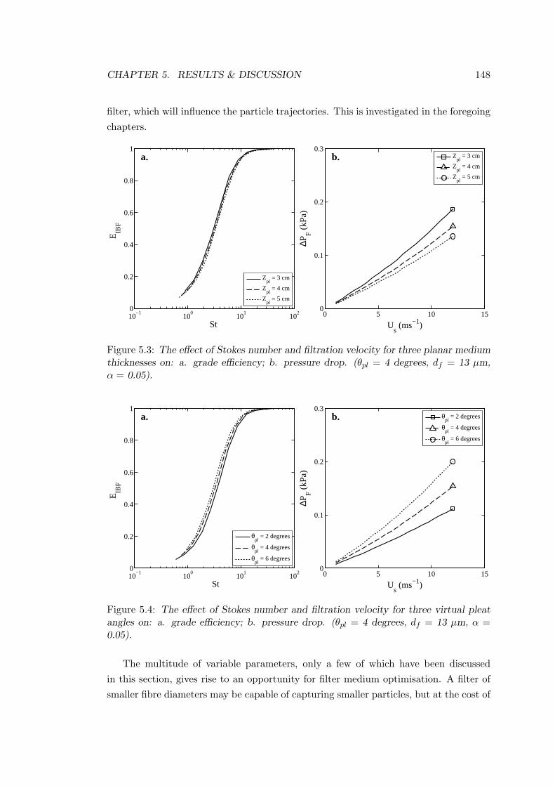
CHAPTER 5. RESULTS & DISCUSSION 148
filter, which will influence the particle trajectories. This is investigated in the foregoing
chapters.
10−1
100
101
102
0
0.2
0.4
0.6
0.8
1
St
E IB
F
a.
Zpl
= 3 cm
Zpl
= 4 cm
Zpl
= 5 cm
0 5 10 150
0.1
0.2
0.3
Us (ms−1)
∆PF (
kPa)
b.
Zpl
= 3 cm
Zpl
= 4 cm
Zpl
= 5 cm
Figure 5.3: The effect of Stokes number and filtration velocity for three planar mediumthicknesses on: a. grade efficiency; b. pressure drop. (θpl = 4 degrees, df = 13 µm,α = 0.05).
10−1
100
101
102
0
0.2
0.4
0.6
0.8
1
St
E IB
F
a.
θpl
= 2 degrees
θpl
= 4 degrees
θpl
= 6 degrees
0 5 10 150
0.1
0.2
0.3
Us (ms−1)
∆PF (
kPa)
b.
θpl
= 2 degrees
θpl
= 4 degrees
θpl
= 6 degrees
Figure 5.4: The effect of Stokes number and filtration velocity for three virtual pleatangles on: a. grade efficiency; b. pressure drop. (θpl = 4 degrees, df = 13 µm, α =0.05).
The multitude of variable parameters, only a few of which have been discussed
in this section, gives rise to an opportunity for filter medium optimisation. A filter of
smaller fibre diameters may be capable of capturing smaller particles, but at the cost of

CHAPTER 5. RESULTS & DISCUSSION 149
an elevated pressure loss. Ultimately a filter medium must be chosen that will perform
best in its intended environment of operation, or for a target particle size. Of course,
this task is made more difficult in extension to helicopter particle filtration, since the
particulate of interest contains a range of particle sizes. However, scope for optimum
performance is present, and represents a possible area of future work.
5.3 Pleat Scale
The flow through the folds of a pleated filter has been studied by several authors in
the past. In Section 2.5.3 the compromise of pleating was discussed, in which the
the benefit of the reduction of filtration velocity that decreases filter medium pressure
loss is increasingly nullified by fluid shear stresses caused by contraction within the
pleat channels. The phenomenon leads to an optimum design point for a given flow
condition, which will be discussed in the foregoing sections. Much of the previous
research performed in the past on pleated filters is case-specific, often using simplified
domains. There are currently no computational studies on inlet barrier filter design
in the open literature, and much of the information relating to IBF has been derived
from international patents and a couple of conference papers. The current work aims
to generate data from CFD solutions of flow through pleats of varying dimension,
in varying flow conditions. During the investigation into IBF pleat design, it was
found that there is a wide spectrum of parameters that govern IBF performance, with
each parameter possessing the potential for tuning for optimum design. However, due
to various constraints, it is not possible to test all parameters and ultimately some
assumptions have had to be made. Of all the parameters, properties of the filter
medium are the most difficult to obtain, as these data are often proprietary. Instead,
values are assumed from real filter fabrics tested in the literature, from one study
in particular (Ref. [52]) which analysed filters for automotive applications. For the
pleat scale study, the values relating to the filter medium are mostly fixed, although
a brief insight into their effect is provided here. The following presents the results of
a parametric study of the effects of pleat sizing, the optimum design point, and the
influence of flow conditions and sand properties on pleat performance.
5.3.1 Flow Analysis
The effect of increasing the number of pleat folds per unit length of span is shown
in Figure 5.5. It is clear that decreasing the pleat angle increases the degree of flow
contraction, which is indicated by the bunching of streamlines and the red areas of
faster flow in Figures 5.5d and 5.5e. The blue areas indicate slow flow, especially
through the filter medium, in which the prescribed porous zone condition performs the
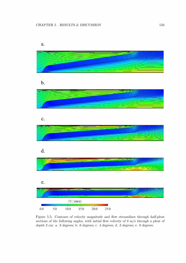
CHAPTER 5. RESULTS & DISCUSSION 150
Figure 5.5: Contours of velocity magnitude and flow streamlines through half-pleatsections of the following angles, with initial flow velocity of 8 m/s through a pleat ofdepth 3 cm: a. 8 degrees; b. 6 degrees; c. 4 degrees; d. 2 degrees; e. 0 degrees.
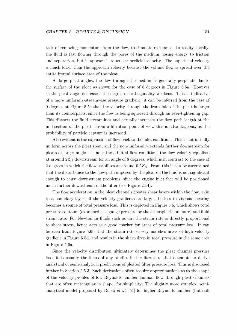
CHAPTER 5. RESULTS & DISCUSSION 151
task of removing momentum from the flow, to simulate resistance. In reality, locally,
the fluid is fast flowing through the pores of the medium, losing energy to friction
and separation, but it appears here as a superficial velocity. The superficial velocity
is much lower than the approach velocity because the volume flow is spread over the
entire frontal surface area of the pleat.
At large pleat angles, the flow through the medium is generally perpendicular to
the surface of the pleat as shown for the case of 8 degrees in Figure 5.5a. However
as the pleat angle decreases, the degree of orthogonality weakens. This is indicative
of a more uniformly-streamwise pressure gradient: it can be inferred from the case of
0 degrees at Figure 5.5e that the velocity through the front fold of the pleat is larger
than its counterparts, since the flow is being squeezed through an ever-tightening gap.
This distorts the fluid streamlines and actually increases the flow path length at the
mid-section of the pleat. From a filtration point of view this is advantageous, as the
probability of particle capture is increased.
Also evident is the expansion of flow back to the inlet condition. This is not initially
uniform across the pleat span, and the non-uniformity extends further downstream for
pleats of larger angle — under these initial flow conditions the flow velocity equalises
at around 2Zpl downstream for an angle of 8 degrees, which is in contrast to the case of
2 degrees in which the flow stabilises at around 0.5Zpl. From this it can be ascertained
that the disturbance to the flow path imposed by the pleat on the fluid is not significant
enough to cause downstream problems, since the engine inlet face will be positioned
much further downstream of the filter (see Figure 2.14).
The flow acceleration in the pleat channels creates shear layers within the flow, akin
to a boundary layer. If the velocity gradients are large, the loss to viscous shearing
becomes a source of total pressure loss. This is depicted in Figure 5.6, which shows total
pressure contours (expressed as a gauge pressure by the atmospheric pressure) and fluid
strain rate. For Newtonian fluids such as air, the strain rate is directly proportional
to shear stress, hence acts as a good marker for areas of total pressure loss. It can
be seen from Figure 5.6b that the strain rate closely matches areas of high velocity
gradient in Figure 5.5d, and results in the sharp drop in total pressure in the same area
in Figure 5.6a.
Since the velocity distribution ultimately determines the pleat channel pressure
loss, it is usually the focus of any studies in the literature that attempts to derive
analytical or semi-analytical predictions of pleated filter pressure loss. This is discussed
further in Section 2.5.3. Such derivations often require approximations as to the shape
of the velocity profiles of low Reynolds number laminar flow through pleat channels
that are often rectangular in shape, for simplicity. The slightly more complex, semi-
analytical model proposed by Rebaı et al. [51] for higher Reynolds number (but still

CHAPTER 5. RESULTS & DISCUSSION 152
Figure 5.6: Illustration of the causes of pressure loss in the pleat channels, as indicatedby contour plots of: a. total pressure contours; b. strain rate magnitude.
laminar) flows relies on the assumption that the velocity profiles resemble the shape of
turbulent boundary layer, allowing their solution through similarity. The present study
is conducted at higher Reynolds number flow prescribed with a level of turbulence to
more closely match the real situation. An analysis of the applicability of Rebaı’s model
can be made by examining the pleat channel velocity profiles from the current work.
To carry out the examination, spanwise cuts are taken at 9 streamwise locations
along the length of the pleat. These are shown in Figure 5.7. The letters under each
cut are references for the plots given in Figure 5.8, which superimposes the streamwise
velocity component at each location for two pleats of differing pleat angle. Dimensions
are normalised to facilitate comparison. There are clear differences between the two
pleat angles, although some can be attributed to a misalignment of the boundary layers
— the filter medium’s upstream and downstream surfaces appear at different spanwise
locations for the same streamwise location; the filter medium region in each plot is
indicated by the almost zero value of streamwise velocity. In Figure 5.8a both pleats
exhibit a flow deceleration (u/U < 1) at the bottom, and an acceleration towards the
top, but the wider pleat profile is flatter for a greater proportion of the channel width.
This trend is evident at almost all locations along the pleat length. A flatter profile
more closely resembles the assumption made by Rebaı et al., but is not present at all
streamwise locations, and cannot be applied for the smaller angle pleats.

CHAPTER 5. RESULTS & DISCUSSION 153
Figure 5.7: Streamwise cuts for velocity profile sampling of half-pleats with pleat anglesof: a. 6 degrees; b. 2 degrees.
In the downstream channel the velocity profiles do not resemble flat, turbulent
boundary layer profiles. These are most clear in Figures 5.8g to 5.8i. For the 2 degree
case the profiles seem perfectly parabolic; at higher pleat angles the streamwise velocity
tends to a linear relationship with span. This is in contrast to the approximation,
but may provide scope for future development of a semi-analytical model for pleats
of this nature. However, the non-conformity of the upstream channel profiles to a
common shape may hinder development. Indeed at the streamwise location “b”, the
profile reflects the large local acceleration of flow due to contraction; at this region the
velocity profiles might be more difficult to predict with an analytical model, which is
particularly pertinent when one considers that this is the principle source of channel
pressure loss.

CHAPTER 5. RESULTS & DISCUSSION 154
0 1 2 30
1
y / Z
pw
a.
θpl
= 2o
θpl
= 6o
0 1 2 30
1b.
0 1 2 30
1c.
0 1 2 30
1
y / Z
pw
d.
0 1 2 30
1e.
0 1 2 30
1f.
0 1 2 30
1
y / Z
pw
u / U
g.
0 1 2 30
1
u / U
h.
0 1 2 30
1
u / U
i.
θpl
= 2o
θpl
= 6o
Figure 5.8: Comparison of x-velocity profiles of two pleat angles at streamwise locationsof x/Zpl = : a. 0.0; b. 0.05; c. 0.2; d. 0.35; e. 0.5; f. 0.65; g. 0.8; h. 0.95 i. 1.0.

CHAPTER 5. RESULTS & DISCUSSION 155
5.3.2 Geometry Effects
As a point of context, an insight into the quantitative effect of varying geometrical
parameters of the pleat is provided. It has been discussed throughout that increasing
the filter surface area by pleating benefits the filtration process. Figure 5.9a shows
the increase in filter surface area per unit of projected area across the range of pleat
dimensions tested in the present work. A four or fivefold increase in surface area can be
achieved with a pleat angle of just 10 degrees, which will result in a filtration velocity
reduced by the same amount. This translates to a much lower filter medium pressure
loss. As filter angle decreases, the area is increased further still, and the gap between
pleats of different depth widens. The patent that provides the most information on
pleat design (Ref. [40]) states that pleating is performed to achieve a roughly sixfold
increase in surface area. Figure 5.9a suggest, therefore, that the chosen pleat angle
would be around 4 - 6 degrees. This provides a reference point for the present study.
0 2 4 6 8 100
3
6
9
12
15
18
θpl
(degrees)
S pl (
m2 m
−2 )
a.
D = 3 cmD = 4 cmD = 5 cm
0 2 4 6 8 100
0.1
0.2
0.3
0.4
0.5
0.6
θpl
(degrees)
HF (
gcm
−2 )
b.
ZF = 1.0 mm
ZF = 1.5 mm
ZF = 2.0 mm
Figure 5.9: Effect of pleat geometrical parameters on key performance parameters of:a. filter surface area per unit projected area (constant thickness of 1.5 mm); b. filtermedium particulate mass capacity per unit projected area (constant depth of 4 cm).
Figure 5.9b shows the effect of pleat angle on the holding capacity of the filter
medium for three filter thicknesses. Since holding capacity is related to the total volume
of the filter per unit projected area, it follows that the relationship resembles that of
specific surface area. A large holding capacity is desired to delay the onset of the cake
accumulation stage, in which the pressure drop generally grows faster per unit mass
collected than during the filter medium clogging stage. The improvement offered by
increasing the filter thickness appears to diminish with decreasing filter angle, but for
a pleat angle of 4 degrees, the time sustained in a brownout cloud before cake buildup

CHAPTER 5. RESULTS & DISCUSSION 156
occurs can be lengthened by 44% by simply doubling the filter thickness from 1.0 mm
to 2.0 mm.
5.3.3 Pleat Performance
The two pressure loss sources have been described quantitatively and analytically, but
to understand how the optimum design point is established, it is useful to illustrate
graphically a breakdown of the pressure loss contributions. Figure 5.10 shows the filter
medium pressure loss and pleat channel pressure loss as functions of the pleat angle at
two filter states. In both plots the contrasting consequences of decreasing the pleat angle
is shown. The slope of the channel pressure loss curve steepens at a greater rate than
the filter medium, a fact that becomes important when considering the two clogging
stages. Figure 5.10b shows the loss contributions at filter capacity. At this stage the
filter medium has a much higher resistance to the flow, as evidenced by the elevated
curve. The plot also implies that pleats of larger angle behave worse if the initial
permeability of the medium were lower. One reason for increasing the permeability
would be to improve the capture efficiency of the filter; a conclusion to draw is that
the optimum pleat angle for minimum pressure drop decreases with decreasing filter
permeability.
0 2 4 6 8 100
1
2
3
4
θpl
(degrees)
∆P (
kPa)
a.
Total Pressure Loss, ∆PTotal
Filter Medium Loss, ∆PMedium
Pleat Channel Loss, ∆PChannel
0 2 4 6 8 100
1
2
3
4
θpl
(degrees)
∆P (
kPa)
b.
Total Pressure Loss, ∆PTotal
Filter Medium Loss, ∆PMedium
Pleat Channel Loss, ∆PChannel
Figure 5.10: Sources of pressure loss across a filter pleat (Zpl = 5 cm, AC Fine testdust, U∞ = 12 m/s), showing characteristic U-shape curve and contributions fromfilter medium and pleat channels, for: a. clean filter (∆mpc = 0); b. clogged filter(∆mpc = MFC).
The effect of rising medium permeability also appears to affect the flow in the pleat
channel, which is elevated in Figure 5.10b, especially at small pleat angles. This is

CHAPTER 5. RESULTS & DISCUSSION 157
because a larger proportion of flow is forced further into the pleat channels as it meets
greater resistance at the filter medium. The contribution of the channel loss increases
further when the cake begins to form, but this is accompanied by the additional re-
sistance offered by the accumulating particles. From the discussion, and the two total
pressure loss curves presented here, it is clear to see that the optimum design point is
highly dependent on the flow conditions and filter properties.
Another filter parameter that affects the performance is the pleat depth. Figure 5.11
shows the effect of increasing the depth of three pleats of varying angles, for two filter
states (analogous to two initial filter permeabilities). In all cases, the effect is to decrease
the pressure drop, although a lack of data for depths of beyond 5 cm hinders conclusions.
In fact, the 2 degrees curve in Figure 5.11b appears to level out at Zpl = 5 cm, suggesting
it may have reached a minimum. At large pleat angles, the effect of increasing the pleat
depth is small as suggested by the almost flat gradient. This is because the pleat width
scales with pleat depth: as depth is increased, the pleat density decreases, which would
ordinarily lead to increased superficial filtration velocity but for the additional surface
area across which the volume flow is spread. One consideration which is not considered
here is the system weight. Figure 5.11 suggests that there is only a benefit to increasing
pleat depth. However, when the weight of the filter panel is considered, and indeed the
space constraints, it may well be sufficient to cap the filter depth at a value beyond
which improvement to the pressure loss is negligible for all pleat angles. For the pleats
in this example, this is approximately 4 cm for both the clean and clogged cases.
3 3.5 4 4.5 50
0.5
1
1.5
2
Zpl
(cm)
∆P (
kPa)
a.
θpl
= 2 degrees
θpl
= 4 degrees
θpl
= 6 degrees
3 3.5 4 4.5 50
1
2
3
4
Zpl
(cm)
∆P (
kPa)
b.
θpl
= 2 degrees
θpl
= 4 degrees
θpl
= 6 degrees
Figure 5.11: The effect of pleat depth on the pressure drop across 3 pleats of differentpleat angle in a flow of 8 m/s, for: a. clean filter (∆mpc = 0); b. clogged filter(∆mpc = MFC).

CHAPTER 5. RESULTS & DISCUSSION 158
The transiency of the pressure drop across an IBF has been discussed throughout the
current work. The numerous parameters that define this temporal characteristic have
also been identified. The results obtained in the pleat scale parametric study permit
an investigation into the effect of altering certain pleat properties on the pressure drop
evolution, which can also be studied. In Figure 5.12, the pressure drop as a function
of mass collected is given for three pleat depths at a fixed pleat angle, and three pleat
angles at a fixed pleat depth. The “elbow” in each curve represents the transition
from the filter medium clogging stage to the cake accumulation stage. This shape is
consistent with the literature on clogging of planar media; both stages exhibit a linear
relationship between collected mass and pressure drop. The cake accumulation stage
is identified by a much steeper curve, highlighting the undesirable consequence of cake
filtration.
0 0.5 1 1.5 20
5
10
15
20
mpc
(gcm−2)
∆P (
kPa)
a.
D = 3 cmD = 4 cmD = 5 cm
0 0.5 1 1.5 20
5
10
15
20
mpc
(gcm−2)
∆P (
kPa)
b.
θpl
= 2 degrees
θpl
= 4 degrees
θpl
= 6 degrees
Figure 5.12: Evolution of pressure loss as a function of mass of AC Fine test dustcollected per square centimetre of projected filter area, across 3 filter pleats of varying:a. pleat depth (θpl = 4 degrees); b. pleat angle (Zpl = 4 cm); while U∞ = 8 m/s.
There are noticeable differences between the curves. Firstly looking at Figure 5.12a,
the effect of increasing pleat depth on holding capacity, as discussed above in Sec-
tion 5.3.2, is to prolong the transition to cake accumulation by approximately 0.5
gcm−2 per centimetre of added depth. A similar benefit is realised in Figure 5.12b for
a decrease in filter angle: narrowing the pleat angle by 4 degrees can double the filter
medium clogging stage. To compare the overall temporal performance of each parame-
ter, consider a limiting pressure drop of 3 kPa, which may be a maximum pressure loss
permissible across an IBF imposed by the operator. When the pressure drop reaches
this level, the filter would be removed and cleaned, or replaced. Figure 5.12a indicates

CHAPTER 5. RESULTS & DISCUSSION 159
that at this point a pleat of depth of 5 cm would have captured around 0.65 gcm−2,
which is in contrast to the pleat of depth of 4 cm, which would have captured 0.55
gcm−2. Comparing pleat angles, the difference is greater still. The extra surface area
offered by a pleat of angle of 2 degrees permits the capture of 0.85 gcm−2, which is 0.3
gcm−2 more than a pleat angle of 4 degrees. A larger mass of particulate captured for
the same pressure drop penalty decreases the number of wash cycles required, which
translates to a saving in maintenance time.
Once in operation, the filter can be expected to experience a number of flow con-
ditions and receive a range of particle sizes. Provision for anticipated conditions can
be made at the design stage, but it is likely that the filter will have to work off-design
during its lifetime. To illustrate the effect of these parameters, the pressure drop is
plotted as a function of flow velocity for three clean pleated filter designs; and plotted
as a function of collected mass for two flow velocities and two sand types. The result
is shown in Figure 5.13. Figure 5.13a shows that a non-linear relationship exists be-
tween flow velocity and pressure loss, the slope of which can be alleviated by increasing
the pleat angle. This suggests that the pleat channel pressure loss is more sensitive
to changes in flow velocity than the medium pressure loss. This is supported by ex-
amination of the curves of same angle but contrasting depths, for which there is very
little difference — since the angle remains constant, there is no change in the channel’s
shape.
0 5 10 150
0.5
1
1.5
U∞ (ms−1)
∆P (
kPa)
a.
Zpl
= 4 cm, θpl
= 6 degrees
Zpl
= 4 cm, θpl
= 2 degrees
Zpl
= 5 cm, θpl
= 2 degrees
0 0.5 1 1.50
10
20
30
mpc
(gcm−2)
∆P (
kPa)
b.
U = 8 ms−1, AC Course
U = 8 ms−1, AC Fine
U = 10 ms−1, AC Fine
Figure 5.13: Effect of two parameters that lead to off-design performance, showing a.influence of flow velocity on clean pressure drop for two pleat depths and two pleatangles; and b. pressure loss as a function of mass collected when filtering AC Fine andAC Course dust, at two flow velocities.
In Figure 5.13b, the temporal pressure drop is shown to be affected by sand type

CHAPTER 5. RESULTS & DISCUSSION 160
in only the cake accumulation stage. This is not a phenomenological effect but a
consequence of the modelling procedure. In the simulations the filter medium porosity
is decreased as a function of mass collected (which translates to a rise in resistance), but
no provision is made for the size of the particles. In reality is it likely that the medium
clogging stage will exhibit differing trends between sand types, as particles of different
size collect at different locations within the medium yielding a non-uniform solidosity.
The effect of uniformity of solidosity on pressure drop is not investigated here, however
if a homogeneous porous matrix is assumed, the temporal rate at which the solidosity
increases can be found for each sand type, based on the temporally-variant separation
efficiency. This is investigated in later sections.
During the cake accumulation stage, the rate of increase of pressure loss is ap-
proximately halved, when composed of the larger-grained AC Course test dust (dp,3 =
28.4µm, σ = 3.7) rather than the AC Fine test dust (dp,3 = 8.8µm, σ = 3.9). Since
the properties of the brownout dust will vary from one area of operation to the next, it
may be difficult to accurately predict the temporal pressure drop rise. Figure 5.13b also
highlights the importance of the volume flow rate through the filter’s projected area.
Suppose the accepted pressure drop limit is 10 kPa, the results show that increasing
the IBF projected area by 20% (hence reducing the flow velocity) increases the length
of a filter cycle by as much as 46%. This again highlights the importance of optimised
IBF design.
0 1 2 30
0.2
0.4
0.6
ZF (mm)
∆P (
kPa)
a.
0 0.05 0.1 0.150
0.3
0.6
0.9
1.2
α (−)
∆P (
kPa)
b.
Figure 5.14: Effect of filter medium properties on clean filter pressure drop for singlepleat (θ = 3 degrees, Zpl = 4 cm, U = 8 m/s) showing: a. influence of mediumthickness; b. influence of medium packing fraction (hence permeability).
For completeness, the parametric study is finished with a brief insight into the
effects of two filter medium parameters. Figure 5.14 shows the response of the pressure

CHAPTER 5. RESULTS & DISCUSSION 161
drop to a change in filter thickness, and a change in filter packing fraction. The former
may be enacted at the design stage to increase the holding capacity (as discussed
in Section 5.3.2), while the latter can improve the separation efficiency, as shown in
Figure 5.2. In this section it was discussed that the time delay in the onset of cake
accumulation can be increased by 44% by doubling the thickness from 1 mm to 2 mm;
in Figure 5.14a the compromise is a more than doubling of clean filter pressure loss.
A similar compromise is inferred from Figure 5.14b when increasing the filter medium
packing fraction, α.
5.3.4 Optimum Design Point
The multifarious parameters that decide the performance of a pleated filter for IBF
can be used to optimise design. Gathering together all parameters discussed thus far,
the data are used to establish the optimum pleat angle for minimum initial pressure
drop and maximum filter cycle time. The maximum filter cycle time is expressed in
terms of mass collected. Since the flow rate of particles reaching the filter is likely
to vary throughout the life cycle, it is more appropriate to express the endurance in
this way. The pleat scale results yielded trends for each parametric case of pressure
drop as a function of mass collected. A filter cycle is “complete” upon reaching a
maximum pressure drop level (although in practice the filters are more often withdrawn
prematurely) that is considered significantly detrimental to engine performance. A
typical value is 3 kPa, which translates to a total pressure loss of around 3% in hover. By
matching this level on each trendline with the mass collected, it is possible to compare
each case based on their mass capture capability. While minimum initial pressure drop
on installation is important, it may be more advantageous from a mission perspective to
prolong the clogging. For such pleat designs of good holding capacity the maintenance
time is reduced, and the power available diminishes at a slower rate. The pilot may
have to cope initially with a larger shortfall in power, but will not experience such a
steep drop off.
Figure 5.15a shows the optimum pleat angle for minimum pressure loss across the
clean filter. The trend lines are 5th order polynomial fits to the data generated from
the parametric study. Owing to the relatively low filter medium permeability assumed,
the effect of increasing pleat angle appears to be minimal beyond a pleat angle of 5
degrees. Interestingly, this corresponds to a pleat shape that offers a sixfold increase in
surface area (according to Figure 5.9, which matches the design proposed in Scimone’s
patent (Ref. [41]). A more pronounced “U-shape” would be in evidence if the filter
medium were thicker, or the permeability were lower (as in Figure 5.10b). From these
data, there is no visible difference to the optimum design point for pleats of different
depth, in flows of contrasting velocity. This is useful to know from a design point of

CHAPTER 5. RESULTS & DISCUSSION 162
view: throughout its lifetime the filter can be expected to experience flows of varying
velocity magnitude; since the optimum point does not vary considerably with velocity,
the filter will be performing at peak performance across a range of engine mass flow
rates.
0 2 4 6 8 100
1
2
3
θpl
(degrees)
∆P
(kP
a)
a.
Zpl
= 3 cm, U = 8 ms−1
Zpl
= 4 cm, U = 8 ms−1
Zpl
= 4 cm, U = 10 ms−1
0 2 4 6 8 100
0.2
0.4
0.6
θpl
(degrees)
mpc
(gc
m−
2 )
b.
AC Coarse, U = 8 ms−1
AC Coarse, U = 10 ms−1
AC Fine, U = 10 ms−1
Figure 5.15: Optimum pleat angle for three pleat depths and a flow velocity of U = 12m/s, for two design criteria: a. minimum clean filter pressure drop; b. maximum massof AC Course test dust collected at ∆PIBF = 3 kPa.
In contrast, Figure 5.15b indicates that for maximum filter cycle lifetime, the pleat
angle ought to be much narrower than the optimum angle for pressure drop. In similar-
ity with the pressure drop results, there is not a great disparity between the optimum
angle (approximately 2.5 degrees) for a flow of 8 m/s and a flow of 10 m/s, when AC
Course test dust is being filtered. Notably however, the results confirm that a lower
flow velocity allows a larger mass of particles to be captured at the optimum design
point. For a flow of finer dust-laden air, it is advantageous to pack more pleats into the
available projected area. In these conditions, with this filter, the optimum point is not
instantly recognisable from the plot. In such a case the best design would be a pleat
of 0 degrees angle.
By comparing the two plots in Figure 5.15, it becomes clear that there is a conflict
in pleat design — does one design for minimum pressure drop of maximum endurance?
The multitude of tailorable parameters creates a flexible and sometimes confusing array
of options for design optimisation. However, the pleat scale parametric study provides
abundant data to afford reliable qualitative analysis and the formation of an IBF design
protocol, presented in Chapter 6.

CHAPTER 5. RESULTS & DISCUSSION 163
5.4 Intake Scale
A simple parametric study is conducted to provide an insight into the effects of IBF
installation on intake performance. The exercise is conducted in two dimensions for
two types of intake domain: forward-facing and sideways-facing intakes. The latter
shape also includes intakes that face upward, but for conciseness will be referred to as
a “side-facing intake” hereon in. The intakes are constructed from straight thin plates:
no attention has been paid to aerodynamic profiling to alleviate flow spillage (unin-
tententional flow separation caused by an adverse pressure gradient). This approach
is adopted to permit a simple, systematic parametric study, in which the principle ge-
ometrical parameter of filter angle is investigated. Hence it is anticipated that from
an aerodynamics standpoint, the intake may perform unfavourably. Additionally, in
order to satisfy computational solution conditions, the domain is extended far forward,
backward, an outward to produce unrealistically long analogues for the airframe-intake
approach (the surface leading up to an intake) and intake duct (the section extend-
ing from the airframe to the engine inlet). Following initial solution of the continuous
phase, particles are injected into the domain and their trajectories tracked. Particle
injections are also idealised: all particles of a certain size group are assumed to be
evenly distributed along an injection plane, a highly improbable situation in reality.
These simplifications nevertheless afford a less computationally-expensive insight into
IBF performance at the “intake scale”; more robust analysis could be made in three
dimensions, but the added complexity adds to the already long list of unknowns. By
performing initial studies such as these, extension to three-dimensions can be made
with a greater degree of engineering foresight, which may save computational cost.
5.4.1 Flow Feature Analysis
The analysis begins with a diagnosis of the intake capture streamtube. The capture
streamtube is common to all intakes, and is bounded by the outermost streamline of flow
entering the intake duct. It is visible in all parts of Figure 5.16, and is well described by
Seddon in Chapter 1 of his book on Intake Aerodynamics [21]. The capture streamtube
splits the flow ahead of the engine into two components: internal and external flow. It
is important because it relates to the amount of air mass that is ingested by an engine,
which is a critical parameter for calculating the engine thrust, or power delivered.
The internal flow represents the portion of freestream air that enters the engine inlet
duct, while the external passes around the intake and is associated with airframe drag.
Assuming the engine mass flow rate remains constant (which is actually not true of
helicopter engines throughout their flight regimes, due to a variation in shaft power
demand), the capture streamtube will change shape. Since helicopters are sometimes

CHAPTER 5. RESULTS & DISCUSSION 164
Figure 5.16: Inlet capture streamtube shown by fluid streamlines and velocity plots fortwo intake types at four freestream velocities: a. forward-facing, hover; b. side-facing,hover; c. forward-facing, Ua/U∞ ≃ 0.15; d. side-facing, Ua/U∞ ≃ 0.15; e. forward-facing, Ua/U∞ ≃ 1; f. side-facing, Ua/U∞ ≃ 1; g. forward-facing, Ua/U∞ ≃ 2; h.side-facing, Ua/U∞ ≃ 2.

CHAPTER 5. RESULTS & DISCUSSION 165
in hover, there will be times during its operation in which the engine gathers air from
all directions - this is illustrated for both intake types in Figures 5.16a and 5.16b.
The capture streamtube is important during a brownout cloud because it represents
the flow catchment area of the intake. The concept of the “aerodynamic duct” is an
analogue of the capture streamtube, and requires the assumption of incompressible
flow, whereby the density of the fluid is considered constant which is true in low-
speed, subsonic flows below Mach 0.3. It can be understood by analysing the transition
from hover to forward flight of a forward-facing helicopter intake. During hover, the
catchment area of an intake is large, which means that particles are drawn from a large
area surrounding the intake. As the helicopter begins to transition to forward flight,
the streamtube takes more of a duct-like shape and reduces in radius. At low forward
speeds, when the freestream velocity is a smaller fraction than the engine volume flow
rate per unit of face area (or engine face velocity), the streamtube has a larger radius
than the intake duct. This is depicted in Figure 5.16c. As the freestream velocity
reaches the same level as the engine face velocity, the intake is said to be operating
at full flow : the streamtube radius is equal to the inlet radius. This is depicted in
Figure 5.16e.
At speeds below the full-flow condition, an intake duct may experience a flow phe-
nomenon known as “spillage”, whereby air drawn into the duct cannot negotiate the
sharp turn and consequently “separates” from the contours of the duct. This is illus-
trated by the large blue area, known as a separation bubble, shown in Figures 5.16a
and 5.16c. Intakes that are expected to operate in low speed flight, such as helicopter
intakes, are often profiled to ease the flow into the intake, in order to alleviate this
source of pressure loss. A similar approach is required in the design of side or upward-
facing intakes, as the same flow effect occurs to a worse degree, and at all flight speeds.
This is evident in Figures 5.16b, 5.16d, 5.16f, and 5.16h. This is the principle reason
why side-facing helicopter intakes perform worse than forward-facing intakes, as will
be shown later. As the freestream velocity increases, the forward motion of the aircraft
provides an excess of mass flow to the engine. The streamtube responds by narrowing
in diameter: the concept of the aerodynamic duct observes conservation of mass; the
mass flow at upstream infinity must be equal to the engine mass flow, hence if the
freestream velocity is larger than the engine face velocity, the streamtube area must
reduce. This is illustrated in Figure 5.16g. Incidentally, the principle is also applicable
to side-facing intakes as shown in Figure 5.16h. The remainder of this chapter discusses
why this is important for intake performance in brownout clouds, and ultimately how
this may affect IBF design.

CHAPTER 5. RESULTS & DISCUSSION 166
5.4.2 Unprotected Intake Performance
Before introducing the IBF into the intake, the performance of the unprotected intake
is assessed. There are several metrics for measuring the performance of an intake, elo-
quently described once again by Seddon. To quantify the losses described qualitatively
in Figure 5.16, the pressure loss due to friction is analysed across a range of flight
speeds, from 0 to 30 knots, which represents the transition from hover to forward flight
at twice the engine face velocity.
The breakdown of frictional losses is given in Figure 5.17. The calculation of each
loss component (approach and duct loss) is made using Equations 4.22 and 4.23. The
loss is normalised with the engine flow dynamic pressure, which is constant at all
freestream velocities due to mass conservation. Since both intake types ingest boundary
layer flow from the same surface, the approach loss curves are identical, and increase
as a function of forward speed. The duct loss curves, however, are different. This can
be attributed to the flow separation within the two intakes, which affects the local flow
velocity — a theoretical intake would not contain separated flow. In particular, owing
to the presence of the separation bubble the flow accelerates, causing greater amounts
of shear stress with walls of the duct. It appears that the effect of lip spillage is greater
for forward-facing intakes at hover and low speed than for side-facing intakes. This
is consistent with Figures 5.16a and 5.16b. The lip spillage for side-facing intakes is
smaller due to the flow being drawn from a less adverse angle. Since helicopters are
often required to operate during hover, these results justify profiling the intake with
a generally decreasing area in order to conform to the wide streamtube shape. The
additional frictional losses during cruise (when power required is at less of a premium)
from such a shape would be outweighed by the elimination of the spillage loss.
The comparison of spillage loss between the two intake types is best made by looking
at the total pressure difference between the freestream and engine face, normalised
with the constant duct dynamic pressure. The data are displayed in Figure 5.18a.
For the forward-facing intake, the lip spillage loss falls with increasing forward speed,
to a minimum at around Ua/U∞ = 1. However, for the side-facing intake the trend is
different. The lip spillage continues to increase with forward-speed due to the separation
shown in Figures 5.16. For this simplified intake it exceeds the theoretical frictional
losses almost sixfold at Ua/U∞ = 2, and confirms why the side intake is the inferior
performer at cruise conditions. Helicopter intake aerodynamicists may account for
spillage in their designs, but it is more likely that attention will be paid to the hover
and low flight conditions, as these are more power-critical situations. Therefore it is
likely that a degree of lip separation will always be experienced by side intakes.
A final metric for assessing intake performance is to examine pressure recovery. This
is an intake’s ability to convert the available dynamic pressure to static pressure at the
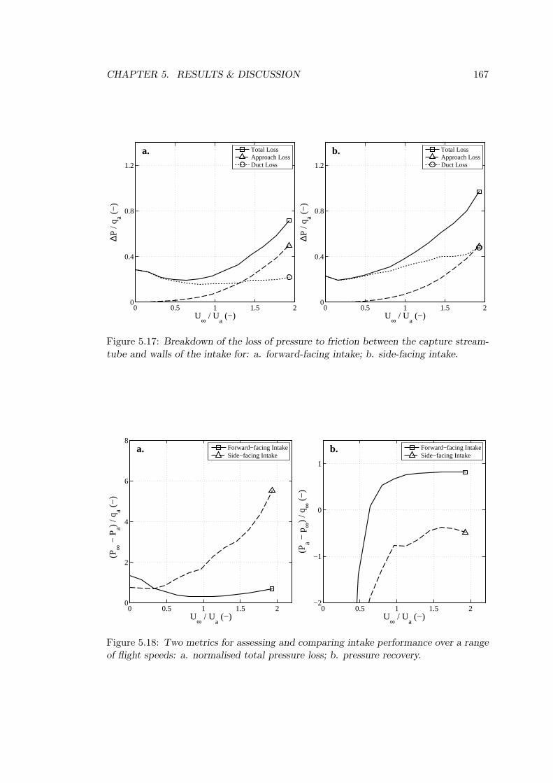
CHAPTER 5. RESULTS & DISCUSSION 167
0 0.5 1 1.5 20
0.4
0.8
1.2
U∞ / Ua (−)
∆P /
q a (−
)
a.
Total LossApproach LossDuct Loss
0 0.5 1 1.5 20
0.4
0.8
1.2
U∞ / Ua (−)
∆P /
q a (−
)
b.
Total LossApproach LossDuct Loss
Figure 5.17: Breakdown of the loss of pressure to friction between the capture stream-tube and walls of the intake for: a. forward-facing intake; b. side-facing intake.
0 0.5 1 1.5 20
2
4
6
8
U∞ / Ua (−)
(P∞ −
Pa)
/ qa (
−)
a.
Forward−facing IntakeSide−facing Intake
0 0.5 1 1.5 2−2
−1
0
1
U∞ / Ua (−)
(Pa −
p∞)
/ q∞ (
−)
b.
Forward−facing IntakeSide−facing Intake
Figure 5.18: Two metrics for assessing and comparing intake performance over a rangeof flight speeds: a. normalised total pressure loss; b. pressure recovery.

CHAPTER 5. RESULTS & DISCUSSION 168
engine face, which is beneficial to the engine. An ideal intake would have a pressure
recovery of 1; in practice this is impossible to achieve when the intake is ingesting
boundary layer air, as in the present study. Well-engineered pitot intakes, however,
can get close. Seddon predicts a maximum pressure recovery of around 0.9 for forward-
facing intakes at Ua/U∞ = 1.5, a maximum of around 0.3 at the same forward speed
for side-facing intakes. Figure 5.18b shows the pressure recovery characteristic of the
intakes tested in the present study. In both cases the shape is as predicted by Seddon,
although a lack of data does not confirm this beyond Ua/U∞ = 2. The forward-facing
intake reaches a maximum of around 0.8 at high forward speeds, however due to the
large penalty sustained through lip spillage, the side-facing intake fails to achieve the
levels quoted by Seddon. In fact, the pressure recovery never breaches zero, implying
that energy is always required by the engine to achieve its required mass flow.
5.4.3 IBF-fitted Intake Performance
The performance of a helicopter intake fitted with an IBF is investigated for the case
of forward-facing and side-facing inlets. The objective of the study is to ascertain
the impact of the filter presence on the intake flowfield. The pressure loss across a
filter is fixed for all designs in order to attribute any additional losses to skin friction
or separation. One of the IBF design criteria is to minimise the superficial velocity
through the filter, which is achieved by increasing the filter projected surface area. The
setup described in Section 4.3.1 allows the surface area to be changed by orientating
the filter at different angles to the flow.
The effect of filter angle in hover is examined. In this situation out of ground
effect, the helicopter engine is running close to maximum power. In Figure 5.19 the
filter angle for both intake types is shown for two filter states: clean (∆P = 0.6 kPa)
and clogged (∆P = 3 kPa). The non-filter pressure losses are isolated by subtracting
the prescribed filter pressure drops from the total pressure loss at the engine face. In
both cases there is negligible variation in total pressure loss across the range of filter
angles — a maximum of 0.01% increase from 0 degrees to 50 degrees is observed for
the side intakes, which is very little when compared with the fraction of total pressure
expended by the air through the filter (≃ 0.6% and ≃ 3.0% for the clean and clogged
states respectively). The non-filter losses are caused by friction with the walls and the
creation of separation bubbles at the walls of the ducts, as illustrated in Figure 5.16a
and 5.16b. In this respect, the side-facing intakes perform better than forward-facing
intakes, and the clogged filter appears to alleviate the pressure loss, but the difference
in real terms is negligible.
The non-uniformity of total pressure during low speed flight and hover can be
inferred from Figure 5.16, in which there are regions of recirculating flow. To maintain

CHAPTER 5. RESULTS & DISCUSSION 169
0 10 20 30 40 500
0.02
0.04
0.06
0.08
0.1
θ (degrees)
1 −
(P a −
∆P IB
F)
/ P∞ (
%)
a.
Forward−facing IntakeSide−facing Intake
0 10 20 30 40 500
0.02
0.04
0.06
0.08
0.1
θ (degrees)
1 −
(P a −
∆P IB
F)
/ P∞ (
%)
b.
Forward−facing IntakeSide−facing Intake
Figure 5.19: Effect of filter orientation angle on total pressure loss during hover for twointake types when the pressure drop across the filter is prescribed as: a. 600 Pa; b.3000 Pa.
mass flow, the air must navigate these separation bubbles. The reduction in effective
flow area causes an increase in local flow velocity, which can cause shearing of the
fluid layers and additional pressure loss, while disturbing the flow uniformity. Taking
spanwise cuts at various locations reveals the resultant inhomogeneity of the total
pressure. Despite their power-related encumbrance, IBF have been known to benefit
engine performance by equalising the distribution of pressure at the engine face. Non-
uniform pressure distribution, or distortion, leads to an imbalance of aerodynamic
loading of the compressor which has the effect of bringing the surge line closer to the
engine operating line (or reducing the working surge margin). This is not a favourable
off-design condition. Exploration of the full effect of IBF on the total pressure on the
operating line represents scope for further work, but as a starting point the data of the
current work can be interpreted to illustrate this benefit of the IBF.
Figure 5.20 shows the spanwise distribution of total pressure at two streamwise
locations in the intake dust, downstream of the filter. The example used is the forward-
facing intake in hover. Each curve represents a different state of resistance at the intake
entrance: no resistance, when no filter is present; a resistance of 0.6 kPa, when the filter
is “clean”; and 3 kPa, when the filter is “clogged”. The results have been normalised to
permit fair comparison — where a pressure drop is artificially prescribed at the intake
such as the case of a clean filter, the pressure lost is re-added to the total pressure loss
at the engine face in order to isolate the losses due wholly to separation and boundary
layer.
Due to the stagnant or low-speed reversed flow symptomatic of a separated flow

CHAPTER 5. RESULTS & DISCUSSION 170
0 0.2 0.4 0.6 0.8 1−2
−1.5
−1
−0.5
0x 10
−3
s / Aa (−)
(P(s
) −
P ∞)
/ P∞ (
−)
a.
No Filter (∆P = 0 kPa)Clean Filter (∆P = 0.6 kPa)Clogged Filter (∆P = 3.0 kPa)
0 0.2 0.4 0.6 0.8 1−2
−1.5
−1
−0.5
0x 10
−3
s / Aa (−)
(P(s
) −
P ∞)
/ P∞ (
−)
b.
No Filter (∆P = 0 kPa)Clean Filter (∆P = 0.6 kPa)Clogged Filter (∆P = 3.0 kPa)
Figure 5.20: Effect of filter presence on spanwise total pressure distribution at twodownstream locations in the intake duct: a. at s = Aa; b. at s = 3Aa; where s is thedistance from the inlet entrance.
region, the total pressure is locally lower than the freestream, or in this case the duct
flow. The depression shown in the right hand side of each plot Figure 5.20 is therefore
indicative of a separation bubble. The spanwise extent of this depression can also be
viewed as a low total pressure “footprint”, that gives an impression of the size of the
separated region. While several more cuts would be needed to illustrate comprehen-
sively, Figure 5.20 suggests that the effect of increasing filter resistance is to reduce
the loss of total pressure to lip spillage during hover or low-speed flight. This effect
can be attributed to the deceleration of the airflow as it approaches the filter, and is a
phenomenon that could be exploited in filter design to reduce total pressure distortion.
5.4.4 External Intake Drag
In forward flight, the effect of increasing the filter angle on intake performance concerns
an interesting area of intake aerodynamics: drag. It is perhaps intuitive that orientating
the filter at an angle to the flow will result in a less airframe drag at high forward
speeds; the anticipated result is explained by analysis of the total pressure distribution
in the external flow, as depicted in Figure 5.21. The consequence of a reduced-diameter
streamtube at high forward speeds is the development of spillage drag, as the external
flow fails to negotiate the intake lip and separates from the nacelle surface. This creates
a region of low pressure and stagnant air, identified by the yellow areas in Figure 5.21
(and blue areas of low velocity in Figure 5.16, which is a type of airframe drag known
as form drag.

CHAPTER 5. RESULTS & DISCUSSION 171
The distinction between internal and external drag needs to be made in intake
design, as it can lead to some confusion. It is well discussed in Chapter 9 of Seddon’s
book. Internal drag accounts for all losses within the capture streamtube, which must
be overcome by the engine in order to maintain core mass flow. The power required by
the engine to perform this task is a summation of the momentum traded with the air,
and the frictional and inertial losses expended in the process. Since a filter is placed
within the confines of the streamtube, it contributes only to these losses, hence does not
directly contribute to airframe drag, despite exerting a form of drag on the core engine
air flow. However, Figure 5.21 shows that strategic integration design can alleviate the
drag resulting from spillage over the intake cowl.
5.4.5 Particle Distribution
The particles are injected into the domain as described in Section 4.3.3 and their tra-
jectories are tracked. The distribution of particles on the filter is recorded to gain a
first order qualitative idea of whether the integration of the filter into the intake may
be designed in such a way that is beneficial to engine performance. Ultimately, IBF
integration may be constrained by intake-airframe architecture, however the following
provides a useful insight into what may be expected. A fine test dust is selected that
contains a range of particles of Reynolds number that is in the inertial and viscous flow
regimes (Rep = 1 to 30).
The particle distribution data is expressed as a particulate concentration, nor-
malised with the freestream condition. A ratio of greater than unity indicates a greater
quantity of particles per unit mass of carrier phase than the freestream condition is
accumulating on the filter. The capture streamtube, discussed above in Section 5.4.1,
is the main influence on particle trajectory. As it changes shape with forward speed or
intake type, the catchment area is altered. The other main property affecting the fate
of a given particle is its Reynolds number. The particle size distribution of AC Fine
test dust contains a great range diameters; over the spectrum of forward speeds there
is an even greater range of Reynolds numbers. Furthermore, the flow either acceler-
ates or decelerates up to the intake face. Using the intake superficial velocity (volume
flow rate per unit area — 8 m/s) as a reference, the particle Reynolds number for AC
Fine dust varies from 1 to 32. The spanwise position is given as a distance along the
filter, normalised by the intake area. The pressure drop across the filter in each of the
following cases is 0.6 kPa, corresponding to the “clean” condition.
Figure 5.22 displays the distribution of three differently-sized particles correspond-
ing to characteristic group diameters of AC Fine test dust, and a filter angle θ of 0
degrees. The distribution of particulate is important because non-uniformity will result
in an inhomogeneous total pressure distribution. For the result of the forward-facing

CHAPTER 5. RESULTS & DISCUSSION 172
Figure 5.21: Separation of external flow leading to airframe drag due to a forward-facing intake, at three filter orientation angles: a. 0 degrees; b. 30 degrees; c. 50degrees.

CHAPTER 5. RESULTS & DISCUSSION 173
filter in low speed flight, below the full flow condition, the peak in the particles of
smaller size (1µm and to a lesser degree 15 µm) at the innermost spanwise location
arises from a local acceleration of the flow as the intake tries to maintain plug flow
whilst contending a separation bubble. The non-uniform distribution becomes impor-
tant when considering the accumulation of particles — certain parts of the filter will
clog at different rates to others, distorting the total pressure distribution, the effect of
which was discussed earlier.
The side-facing intake generally displays an even distribution of particles for the
low-speed condition. There is a lull in particulate concentration of 57.5 µm at the
foremost end of the filter due to particle inertia; by contrast there is a slight peak
in concentration of smaller particles due to a local acceleration of flow caused by a
separation bubble within the intake (see Figure 5.16d). This effect is evident at the
location of the other separation bubble in the intake, just aft of the filter at the rearmost
spanwise location. The flow acceleration in the presence of such a separation bubble
is further evidenced at higher forward speed, during which the flow separation occurs
to a greater extent (see Figure 5.16h). The smaller particles act like tracer particles
in this situation, hence their peak at the foremost spanwise location. For the forward-
facing case, the smaller particles are distributed evenly, which is symptomatic of their
following the fluid streamlines, whereas the larger particles are deposited to a greater
degree at the outermost section due to being influenced slightly by the external flow.
The effect of filter orientation angle, θ, on particle distribution is also investigated.
The geometrical effect of the change of angle is illustrated in Figure 4.8. For this,
the particle groups are combined to represent AC Fine test dust as described in Sec-
tion 4.3.3. It can be seen in both Figures 5.23a and 4.8b that orientating the filter at an
angle to the flow has the effect of reducing the local particulate concentration. In prac-
tice, this would result in a slower increase of pressure loss over time, hence is beneficial
to engine performance. The reduction can be attributed to the increase in filter area,
which reduces the filtration velocity for the same engine mass flow rate. Also evident
in Figure 5.23a is the effect of filter angle on the characteristic concentration peak at
the outermost end of the forward-facing filter. The peak appears to reduce in relative
amplitude, which helps to alleviate a possible source of total pressure distortion.
In summary, the particle distribution is a function of airspeed, particle diameter,
filter angle, and intake type. The distribution is important for the evolution of the
pressure drop and total pressure distortion, although the transient distortion or two-
dimensional distortion has not been investigated here. A particle’s Reynolds number
is the principle property that determines its distribution across a filter. Particles of
Reynolds number below around 0.2 tend to follow fluid streamlines, hence almost act
like tracer particles and reflect local variations in flow velocity. At forward speeds

CHAPTER 5. RESULTS & DISCUSSION 174
0 0.5 10
5
10
s / Aa (−)
(cm
,F /
c m,∞
)i (
−)
a.
dp = 1 µm
dp = 15 µm
dp = 57.5 µm
0 0.5 10
5
10
s / Aa (−)
(cm
,F /
c m,∞
)i (
−)
b.
dp = 1 µm
dp = 15 µm
dp = 57.5 µm
0 0.5 10
1
2
3
s / Aa (−)
(cm
,F /
c m,∞
)i (
−)
c.
dp = 1 µm
dp = 15 µm
dp = 57.5 µm
0 0.5 10
1
2
3
s / Aa (−)
(cm
,F /
c m,∞
)i (
−)
d.
dp = 1 µm
dp = 15 µm
dp = 57.5 µm
Figure 5.22: Spanwise distribution of three particle sizes quantified by normalised con-centration, on a IBF filter (θ = 0 degrees) in two intake configurations, under twoflow conditions: a. forward-facing intake, 2.5-knot flow normal to filter; b. side-facingintake, 2.5-knot flow parallel to filter; c. forward-facing intake, 15-knot flow normal tofilter; d. side-facing intake, 15-knot flow parallel to filter.

CHAPTER 5. RESULTS & DISCUSSION 175
0 0.5 10
5
10
s / Aa (−)
c m,F
/ c m
,∞ (
−)
a.
θ = 0 degreesθ = 30 degreesθ = 50 degrees
0 0.5 10
5
10
s / Aa (−)
c m,F
/ c m
,∞ (
−)
b.
θ = 0 degreesθ = 30 degreesθ = 50 degrees
Figure 5.23: Spanwise distribution of three orientation angles quantified by normalisedconcentration, on a IBF filter in two intake configurations for: a. forward-facing intakein a 2.5-knot flow; b. side-facing intake in a 2.5-knot flow.
greater than the full flow conditions, such particles are evenly distributed across the
filter. This is in contrast to particle of larger Reynolds number, whose trajectories
are influenced by the capture streamtube but to a lesser extent, resulting in an uneven
distribution of particles, weighted towards one end of the filter. The effect of angling the
filter to the flow is to alleviate the non-uniformity created by unequal flow distribution,
and to reduce the concentration of particulate reaching the filter.
5.4.6 Particle Concentration
The expressing of particulate concentration at the filter as a fraction of the freestream
dust concentration (or local brownout severity) permits an assessment of the intake’s
inherent potential to reduce the quantity of particulate reaching the engine. For ex-
ample, intuitively it is easy to understand that a degree of particle inertial separation
is achieved by sideward-facing intakes in forward flight. The following examines the
effect of varying flow conditions and intake geometry changes that influence this.
The first investigation demonstrates the inherent separation capability of a heli-
copter intake. Tests were performed with no resistance prescribed at the intake face to
ascertain how much particulate could be removed from influent air without the use of
an IBF, or any EAPS system. Figure 5.24 shows the effect of increasing the forward
speed of the helicopter on particulate concentration at the intake. Comparing the two
intake types, the results are perhaps counter-intuitive: in Figure 5.24a the anticipated

CHAPTER 5. RESULTS & DISCUSSION 176
increase of separation ability at higher forward speeds for side-facing intakes is in ev-
idence; but is also exhibited by the forward-facing intake. In fact, the forward facing
intake performs better than the side-facing intake at all flight speeds, approximately
30% better at speeds greater than full flow.
To explain this, it must be remembered that the particles in this sample are of a
relatively low Reynolds number. The equations of motion of a particle are given in
Section 3.2.5. In particular, the drag coefficient of a particle (Equation 3.40) is shown
to be inversely proportional to the particle Reynolds number (Equation 3.39). The
extent to which a particle responds to a change in carrier fluid direction is expressed by
its acceleration in that direction (see Equations 3.34 and 3.38), which is proportional to
the relative velocity and particle drag coefficient. Hence a steeper flow relative velocity
gradient combined with a low particle Reynolds number will result in a particle’s motion
more closely reflecting the fluid streamline that has thus far carried it.
As the freestream velocity increases, the capture streamtube becomes “trumpet bell-
shaped”. The curvature of the “bell” steepens with increasing velocity, which elevates
the relative velocity and means that particles more closely follow fluid streamlines. This
has the effect of decreasing the “catchment area” of particles upstream of the intake.
Hence by increasing the forward speed of the rotorcraft one is able to create an inherent
separation capability for a forward facing intake, the consequence of which is seen in
Figure 5.24a. Of course, as airframe speed increases, so too does the inertia of the
approaching particles. Particles of larger diameter, and therefore mass, are increasingly
unable to negotiate the sharp change in fluid curvature. Thus the inherent separation
ability of a forward-facing intake is diminished as particle diameter increases. This is
evident in Figure 5.24b, which is a plot of the maximum particle size in the test dust
range. It is clear that in this case the curves are more similar, and of a higher level of
concentration than that of the whole distribution. It is expected that a coarser dust
distribution would exhibit the more intuitive result described by Seddon [21], whereby
the side intake is the better performer of the two intake types.
Another, perhaps more important observation from Figure 5.24, is that the perfor-
mance of both intake types tends to deteriorate with decreasing flight speed. Crucially,
at speeds below full flow the concentration ratio is above unity: for this particular
particle size distribution, the dust concentration during hover intensifies by almost 15
times, which is not an ideal situation for IBF longevity. (Note: while the results shown
in Figure 5.24 are for the situation of no porous jump at the inlet face, when a re-
sistance was prescribed, only negligible differences in the trend were observed). This
occurs because the catchment area described above increases at low speed, as the cap-
ture streamtube dilates. However, Figure 5.24b shows that particles of larger size are
less sensitive to the effects of this dilation.

CHAPTER 5. RESULTS & DISCUSSION 177
0 0.5 1 1.5 20
5
10
15
U∞ / Ua (−)
c m,F
/ c m
,∞ (
−)
a.
Forward−facing IntakeSide−facing Intake
0 0.5 1 1.5 20
5
10
15
U∞ / Ua (−)
(cm
,F /
c m,∞
)57
.5 µm
(−
)
b.
Forward−facing IntakeSide−facing Intake
Figure 5.24: The variation of particulate concentration with freestream velocity offorward-facing and side-facing intakes (with no IBF attached), for: a. AC Fine testdust; b. monodisperse dust of 50µm diameter.
In practice the streamtube is unlikely to look like the idealised situation shown in
Figure 5.16a due to the influence of the rotor downwash. Indeed, conclusions on the
effect of forward speed on particle concentration need to made with consideration of the
unsteady nature of dust cloud generation and downwash-intake flow interaction. For
a better idea of particle ingestion during hover would require a huge research effort to
examine three-dimensional effects, and may provide scope for future work. Additionally,
the engine mass flow rate is reduced with increasing forward speed (across this relatively
low-speed range), due to the associated decrease in required rotor power when moving
forward. Therefore the condition of constant engine mass flow is ideal; in reality the
concentration ratio at the intake will be further reduced.
A second investigation is conducted to ascertain whether there is any benefit to
orientating the filter at an angle to the oncoming flow. It has already been shown in
Section 5.4.3 that a slight reduction in pressure loss can be achieved by increasing the
angle at forward speeds below full flow, however no difference was found for the situation
of hover. Figure 5.25 shows the effect of filter angle on particulate concentration in three
forward speeds. For both intake types, there is a reduction of as much as 30% for a filter
angled at 50 degrees to the duct axis of symmetry. Not shown in the current figure is the
case of hover, in which an even greater reduction of around 40% is exhibited. Since in
all cases the engine mass flow rate is held constant hence the capture streamtube shape
is almost identical for each angle, the difference can be explained by the fact that the
particulate is distributed over a larger area, and that the filtration superficial velocity
is reduced. It was discussed in Section 2.5.2 that from an IBF design standpoint, it is
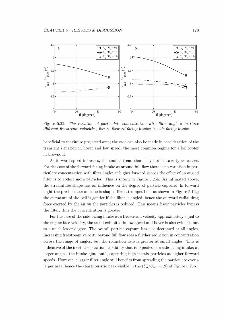
CHAPTER 5. RESULTS & DISCUSSION 178
0 20 40 600
0.5
1
1.5
2
2.5
θ (degrees)
c m,F
/ c m
,∞ (
−)
a.
Ua / U∞ = 0.5
Ua / U∞ = 1.1
Ua / U∞ = 1.9
0 20 40 600
0.5
1
1.5
2
2.5
θ (degrees)
c m,F
/ c m
,∞ (
−)
b.
Ua / U∞ = 0.5
Ua / U∞ = 1.1
Ua / U∞ = 1.9
Figure 5.25: The variation of particulate concentration with filter angle θ in threedifferent freestream velocities, for: a. forward-facing intake; b. side-facing intake.
beneficial to maximise projected area; the case can also be made in consideration of the
transient situation in hover and low speed, the most common regime for a helicopter
in brownout.
As forward speed increases, the similar trend shared by both intake types ceases.
For the case of the forward-facing intake at around full flow there is no variation in par-
ticulate concentration with filter angle; at higher forward speeds the effect of an angled
filter is to collect more particles. This is shown in Figure 5.25a. As intimated above,
the streamtube shape has an influence on the degree of particle capture. In forward
flight the pre-inlet streamtube is shaped like a trumpet bell, as shown in Figure 5.16g;
the curvature of the bell is gentler if the filter is angled, hence the outward radial drag
force exerted by the air on the particles is reduced. This means fewer particles bypass
the filter, thus the concentration is greater.
For the case of the side-facing intake at a freestream velocity approximately equal to
the engine face velocity, the trend exhibited in low speed and hover is also evident, but
to a much lesser degree. The overall particle capture has also decreased at all angles.
Increasing freestream velocity beyond full flow sees a further reduction in concentration
across the range of angles, but the reduction rate is greater at small angles. This is
indicative of the inertial separation capability that is expected of a side-facing intake; at
larger angles, the intake “juts-out”, capturing high-inertia particles at higher forward
speeds. However, a larger filter angle still benefits from spreading the particulate over a
larger area, hence the characteristic peak visible in the (Ua/U∞ =1.9) of Figure 5.25b.

CHAPTER 5. RESULTS & DISCUSSION 179
5.5 Summary
The results from a parametric study into IBF design on two scales are presented.
The first scale concerns the pleats of the filter. The pleats can be tailored to exploit
a phenomenological consequence of pleating, which is the emergence of a secondary
source of pressure loss as the pleat channel is narrowed, yielding an optimum pleat
design for a given set of flow conditions. As the pleat takes on particles the pressure
drop rises, until the filter medium can no longer support further internal accumulation.
At this point the particles collect on the filter surface in the form of a cake. During
the surface clogging stage, the rate of increase of pressure drop is much greater than
internal clogging stage. By increasing the pleat depth or decreasing the pleat angle,
the onset of this second phase can be delayed.
For the properties used in this study, there appears to be no further benefit or cost
to pressure loss as the pleat angle for a filter of fixed pleat depth is increased, and
very little change to this trend as the flow velocity is increased. This means a filter
with these properties will perform at its maximum “clean” performance for all engine
mass flow rates. A lower flow velocity allows more particles to be retained for the same
maximum pressure loss, which extends the cycle life of the filter. This can be achieved
by increasing the filter projected surface area. The optimum design point changes
depending on the initial conditions. A filter of higher initial permeability favours a
wider pleat channel in terms of pressure loss, while a narrower pleat is favoured when
finer particles are to be captured to ensure the pleat is achieving maximum holding
capacity at a prescribed maximum pressure drop.
The second scale investigates the effect of the installed IBF on intake performance,
however results pertaining to the unprotected intake are provided first. The use of CFD
was justified by the modelling of the separation bubble, which is not predicted by the
analytical theory. The effect of lip spillage was seen to be greater for the forward-facing
intake during hover, due to the more extreme change in direction of the flow. When a
filter is installed into the intake, the loss in pressure due to separation and duct loss
was almost negligible in comparison with the pressure drop across the filter. However,
the filter’s presence was shown to benefit total pressure distortion by homogenising the
distribution. The effect was increased as the pressure drop increased, indicating that
despite causing a temporally increasing pressure loss, the clogged filter can still benefit
engine performance. The filter’s presence does not directly contribute to airframe drag,
but it was shown that strategic integration could result in less external spillage drag at
high forward speeds.
When particles were introduced, it was shown that the particle distribution across
a filter is very much dependent on the particle size, and the forward speed relative
to the intake face velocity. At low forward speeds, the forward-facing intake has an

CHAPTER 5. RESULTS & DISCUSSION 180
even distribution of most particle sizes, but particles of 1 µm tend to follow the fluid
streamlines, responding to local flow velocities hence accumulating to a greater degree
at more radially outboard positions. For side-facing intakes the trend is reversed — it
is the larger particles that are less-evenly distributed along the filter due to their inertia
throwing them rearward. The effect of a greater filter angle is to spread the particles
over a larger area, which reduces the overall concentration and would lead to a slower
rise in pressure loss.
The particulate concentration was analysed across the range of forward speeds for
both intake types. Contrary to expectation, if the particle size is small enough the
forward-facing intake ingested a smaller quantity of particulate than the side-facing
intake. As dust size increases, it was shown that the inherent inertial separation ability
of the side-facing intake becomes more prominent. It would also offer a greater degree
of protection against FOD. For both intake types it was shown that an increase in
forward speed results in a decrease in the amount of particulate ingested, due to the
narrowing of the capture streamtube. However at low flight speeds, when the particle
catchment area is greater, the intakes were shown to ingest particulate at a much greater
concentration than the atmospheric conditions. The results also showed that the filter
particulate concentration in hover can be reduced by angling the filter, which increases
the surface area. For side-facing intakes this trend continues but to a lesser degree
at higher forward speeds; for the forward-facing intake the trend reverses at higher
forward speeds due to the curvature of the trumpet-bell shaped capture streamtube
decreasing in severity, thus reducing the inherent separating ability of the intake.

Chapter 6
Inlet Barrier Filter Design &
Performance
This chapter puts into practice the results of the parametric study. It begins
with a discussion of optimum design, followed by the proposal of a design pro-
tocol based on the findings. It then adopts the design protocol to propose a
solution for the Eurocopter EC145 helicopter and presents a temporal perfor-
mance analysis.
6.1 Introduction
The purpose of this chapter is to put into practice some of the quantitative results of the
preceding section, in order to demonstrate a framework for IBF design. The concept
of optimum design for minimum pressure loss and maximum endurance is discussed
and applied to create a solution for the Eurocopter EC145. Once a design is fixed, the
transient performance is predicted using the results of the two scales.
In contrast to the other EAPS technology the IBF performance is transient. The
choice of filter media and pleat design have been shown to dictate this performance
in Chapter 5; a discussion of the filter medium and pleat design considerations is
given in Sections 2.5.2 and 2.5.3. Installation design considerations for a retrofitable
filtration system are multitudinous, relating to much more than the just the tuning of
the filter parameters. Since it is a retrofit technology, many of the design considerations
concern changes to the intake architecture, which introduce new constraints relating
to operability. A breakdown of the key design constraints is provided by Scimone &
Frey [41]:
1. Filter media design and pleat configuration must maximise filtering capability.
181

CHAPTER 6. INLET BARRIER FILTER DESIGN & PERFORMANCE 182
2. The configuration should limit pressure drop variation with airspeed to minimise
the engine’s susceptibility to surge.
3. Surface area must be maximised without sacrificing aircraft handling qualities,
operability, maintainability and structural capabilities.
4. Structural design must consider weight, replaceable panels must be durable, air
loads and crash loads must be addressed.
5. Maintainability design must consider installation and panel removal with flight
safety-assured fastener configurations.
6. Integral seals must be incorporated to maintain filtering integrity.
7. A secondary air source system in the form of a bypass door must be included as
a contingency for severe clogging.
Of these design constraints only the first is comprehensively considered in the present
work. The rest are rather case-specific. For larger mass flow requirements, the com-
plexity of the design is increased, as it becomes more difficult to achieve the desired flow
rate per unit area with a single filter panel. The solution in this case is a multi-faceted
appendage like that shown in Figure 2.10c. When the filter system is external to the
confines of the normal inlet area, the performance may be enhanced through the use of
multiple filter panels, some of which are tailored to take advantage of the flow condi-
tions in hover, others of which are orientated to recover pressure during forward flight.
The case of the multi-faceted IBF is not investigated in the present work, however the
benefits to particle distribution and the pressure recovery of panels in forward flight is
discussed in Section 5.4.
For a full qualitative discussion on all aspects of IBF design, see Scimone & Frey [41].
What follows in the current chapter is an quantitative elaboration of the first design
constraint: maximising filtering capability. The use of CFD to perform a parametric
study affords the investigation of the optimum filter pleat shape for superior IBF per-
formance. In terms of results it is by no means conclusive, due to a shortage of data
for all contributory parameters, but some of the methods presented to determine the
optimum designs are unique to IBF, hence the following can be considered a proof of
concept.
6.2 Optimum Pleat Design
In Section 5.3.4 the concept of the optimum pleat shape was discussed and illustrated
with Figure 5.15. The minima and maxima in the pressure drop and mass collected
plots correspond to the best pleat shape for that particular configuration and set of

CHAPTER 6. INLET BARRIER FILTER DESIGN & PERFORMANCE 183
flow conditions. Crucially these optimum points are not aligned. For this reason a
new design metric — the Pleat Quality Factor (PQF) — is introduced which bases the
optimum pleat design on both performance indicators. It is given as:
PQF =100mpc,max(∆P )
∆P(6.1)
where mpc,max is the total mass collected at the maximum permissible pressure loss.
The Pleat Quality Factor can be used to examine the effects of altering certain flow
properties and filter properties on an optimum design point that caters for both pressure
drop and holding capacity. It is expressed as “grams collected per square centimetre of
projected filter area, per kilopascal of pressure loss (across the clean filter)”; a larger
quantity indicates a better performance. The following sections demonstrate how this
can be used to design a pleated filter for IBF applications.
6.2.1 Pleat Design Quality Factor
The PQF is plotted for a number of filter properties and flow properties to determine
their effect on the optimum IBF design. Figure 6.1 shows the PQF as a function of pleat
angle for three different depths, for two different test dusts. The first obvious trend
is that the PQF is improved with increasing pleat depth, suggesting that it would
be advantageous to extend the pleat as deep as possible. Since the optimum pleat
angle varies very little with pleat depth (a marginal decrease of optimum angle with
increasing depth), this trend implies that it is in fact an optimum pleat aspect ratio for
a filter medium of this thickness and permeability. In effect this means the IBF would
achieve the best PQF if it contained just a single, large pleat spread across its whole
span, as long as the pleat angle were the optimum. Of course such a solution does
not exist — it would be impractical to design such a configuration into an intake and
provide the necessary support. Furthermore increasing the pleat depth has the effect
of decreasing the filtration velocity which reduces the separation efficiency of the filter.
Figure 6.1 also shows that a better filter performance is achieved when a coarser sand
is being filtered.
Next, the influence of volume flow rate per unit projected area (throughput velocity)
is investigated. The results are presented in Figure 6.2. Again, a superior performance is
achieved by the same filter when a coarser dust accumulates, a trend that will be seen
throughout. The importance of reducing the throughput velocity is noticeable here:
reducing the velocity by just 2 m/s can double the PQF, which translates to longer
endurance and lower initial pressure loss. However the optimum pleat angle appears
almost unaffected by velocity, possibly exhibiting a preference to a smaller angle at
higher velocities. The proportion of pressure loss attributable to the medium or the

CHAPTER 6. INLET BARRIER FILTER DESIGN & PERFORMANCE 184
pleat channel is not directly shown here, but the result suggests that they both increase
at the same rate. This becomes significant when it is considered that throughout its life
the IBF will be required to perform at a number of engine power settings, or mass flow
rates; the result implies that even when operating “off-design” the filter is achieving
maximum performance possible.
0 2 4 6 8 100
0.5
1
1.5
2
2.5
θpl
(degrees)
PQ
F (
gcm−
2 kPa−
1 )
a.
D = 3 cmD = 4 cmD = 5 cm
0 2 4 6 8 100
0.5
1
1.5
2
2.5
θpl
(degrees)
PQ
F (
gcm−
2 kPa−
1 )
b.
D = 3 cmD = 4 cmD = 5 cm
Figure 6.1: Pleat Quality Factor as a function of pleat angle, for three different pleatdepths when filtering: a. AC Fine test dust; b. AC Coarse test dust. (ZF = 1.5 mm,α = 0.05, Ua = 8 m/s, max(∆P ) = 3 kPa).
0 2 4 6 8 100
1
2
3
4
θpl
(degrees)
PQ
F (
gcm−
2 kPa−
1 )
a.
Ua = 6 ms−1
Ua = 8 ms−1
Ua = 10 ms−1
0 2 4 6 8 100
1
2
3
4
θpl
(degrees)
PQ
F (
gcm−
2 kPa−
1 )
b.
Ua = 6 ms−1
Ua = 8 ms−1
Ua = 10 ms−1
Figure 6.2: Pleat Quality Factor as a function of pleat angle, for three different through-put velocities when filtering: a. AC Fine test dust; b. AC Coarse test dust. (ZF = 1.5mm, α = 0.05, Zpl = 4 cm, max(∆P ) = 3 kPa).

CHAPTER 6. INLET BARRIER FILTER DESIGN & PERFORMANCE 185
In all examples presented thus far, the initial filter permeability has been fixed. The
permeability is a function of the filter packing fraction; in the next example the effect
of using a filter with a different packing fraction is investigated. The packing fraction
may be increased to improve the separation efficiency of the filter, as demonstrated by
Figure 5.2. In Figure 6.3 an increase in packing fraction is seen to decrease the PQF,
albeit by a modest amount in comparison with the other parameters investigated, and
shift the optimum point to a smaller pleat angle.
0 2 4 6 8 100
0.5
1
1.5
2
2.5
θpl
(degrees)
PQ
F (
gcm−
2 kPa−
1 )
a.
C = 3.78e+09, D = 1.93e+04 (αF = 0.060)
C = 4.48e+09, D = 2.11e+04 (αF = 0.064)
C = 5.25e+09, D = 2.31e+04 (αF = 0.069)
0 2 4 6 8 100
0.5
1
1.5
2
2.5
θpl
(degrees)
PQ
F (
gcm−
2 kPa−
1 )
b.
C = 3.78e+09, D = 1.93e+04 (αF = 0.060)
C = 4.48e+09, D = 2.11e+04 (αF = 0.064)
C = 5.25e+09, D = 2.31e+04 (αF = 0.069)
Figure 6.3: Pleat Quality Factor as a function of pleat angle, for three different packingfractions when filtering: a. AC Fine test dust; b. AC Coarse test dust. (ZF = 1.5 mm,α = 0.05, Zpl = 4 cm, Ua = 8 m/s, max(∆P ) = 3 kPa).
All examples presented so far have also had a maximum allowable pressure drop
of 3 kPa prescribed. In the following example the limit is varied. Figure 6.4 shows
three curves for the two test dusts representing maximum allowable pressure drops of
2.5, 3.0 and 3.5 kPa. The effect of increasing the pressure drop limit is to improve the
filter’s performance, which is understandable when considering the definition of PQF.
Two further trends are observed: firstly, the coarser the sand, the more sensitive is the
PQF to the maximum allowable pressure drop; secondly, for finer dusts the optimum
pleat angle appears to decrease with increasing maximum pressure drop. From a design
standpoint this is significant: the maximum permissible pressure drop may be set by
considering the predicted cost to the engine as a percentage of power loss. For example,
power loss may be more critical to military rotorcraft, which employ a greater numeracy
of additional engine systems such as bleed air or infra-red suppression units than the
typical civil rotorcraft. Hence the maximum allowable limit of pressure drop may be
lower for military applications, thus may require a different filter design.
By calculating the Pleat Quality Factor, it has been possible to examine the effect

CHAPTER 6. INLET BARRIER FILTER DESIGN & PERFORMANCE 186
of flow conditions and filter properties on the optimum pleat angle. Notably, there
was no significant affect on optimum angle observed when different pleat depths were
chosen. This is important from an IBF design perspective because it eliminates one of
the many variables to be considered when tuning a filter for optimum performance.
0 2 4 6 8 100
0.5
1
1.5
2
2.5
θpl
(degrees)
PQ
F (
gcm−
2 kPa−
1 )
a.
∆P = 2.5 kPa∆P = 3.0 kPa∆P = 3.5 kPa
0 2 4 6 8 100
0.5
1
1.5
2
2.5
θpl
(degrees)
PQ
F (
gcm−
2 kPa−
1 )
b.
∆P = 2.5 kPa∆P = 3.0 kPa∆P = 3.5 kPa
Figure 6.4: Pleat Quality Factor as a function of pleat angle, for three different maxi-mum pressure drops when filtering: a. AC Fine test dust; b. AC Coarse test dust. (ZF
= 1.5 mm, α = 0.05, Zpl = 4 cm, Ua = 8 m/s).
6.3 IBF Design
To demonstrate the utility of the optimum pleated filter design point, the findings of the
previous section are put to use in surmising an IBF solution to the Eurocopter EC145.
The EC145 is a light twin-engine utility helicopter with a maximum takeoff weight of
3585 kg, powered by two Turbomeca 1E2 engines that deliver a maximum power of 575
kW. More than two hundred EC145 helicopters have been delivered so far to customers
worldwide (2009) [46]. The largest operator of the EC145 is the US Army, which
operates the aircraft, designated as the UH-72A, in the Light Utility Helicopter role. As
part of its remit, the EC145 is required to operate in dusty environments, and therefore
can expect to experience a number of brownout landings during its mission profile. The
helicopter is chosen to validate a design protocol, and to allow later comparison with
the solution described by Ockier et al. [46]. It is pictured in Figure 6.5.
6.3.1 Pleat Design Map
From a design standpoint the filter must be made to achieve maximum filtering capabil-
ity, which is judged by particle removal rate (separation efficiency), pressure drop, and

CHAPTER 6. INLET BARRIER FILTER DESIGN & PERFORMANCE 187
endurance (maximum holding capacity). Unfortunately, altering the filter parameters
to achieve a high performance by one criterion is usually to the detriment of another.
For example in Section 5.3.4 it was shown that a low pleat density is favoured for a
low clean filter pressure drop, whereas a high pleat count is favoured for holding more
mass; in Section 5.2.1 it was shown that increasing the packing fraction gives the filter
more capture ability at the expense of heightened medium pressure loss.
Figure 6.5: Photograph of Eurocopter EC145∗. (∗Image reproduced under CreativeCommons licence (CC BY-NC-SA 3.0), © Angie Norcup).
The results presented in Section 6.2.1 generated a number of optimum design points
that are seen to alter to varying degree with the flow conditions, filter properties, and
dust properties. The results have been generated for a fixed particle size distribution
and using fixed filter medium properties, which limits their applicability somewhat.
The pleat depth is also constant, however it was discussed in Section 6.2.1 that the
optimum pleat angle varies only marginally with pleat depth. If it assumed that these
represent likely values in practice, the results can be taken forward to demonstrate
a design protocol for IBF. Further work would focus on broadening the envelope of
application. Clear trends already discussed are visible in this map, namely that: a
better Pleat Quality Factor is achievable by driving down the throughput velocity; and
a higher maximum pressure drop favours a narrower pleat design to achieve maximum
performance.
The optimum points are used to create a parameter map for IBF design, shown in
Figure 6.6. Each point on the grid represents an optimum design for a given throughput
velocity and a given prescribed maximum permissible pressure drop. The throughput
velocity is decided by the design point engine mass flow rate, at which the gas turbine

CHAPTER 6. INLET BARRIER FILTER DESIGN & PERFORMANCE 188
generator is running at 100% speed and producing maximum continuous power, which
is required during takeoff and landing. The off-design conditions may prevail for the
majority of the filter life, therefore a more encompassing design may consider the cruise
condition. However in the present case the IBF is designed for the condition at which
the engine is at most risk from particle ingestion, i.e. hover.
3 3.5 4 4.5 5 5.50
0.5
1
1.5
2
Ua = 10 ms−1
Ua = 8 ms−1
Ua = 6 ms−1
max(∆P) = 5.0 kPa
max(∆P) = 4.0 kPa
max(∆P) = 3.0 kPa
max(∆P) = 2.4 kPa
θpl* (degrees)
PQ
F (
gcm−
2 kPa−
1 )
Figure 6.6: Parameter map for optimum pleat design showing iso-lines of throughputvelocity and maximum permissible pressure drop.
The Turbomeca 1E2 has a mass flow rate in the region of 2.1 kg/s. Without know-
ing the airframe geometry around the engine intake, it is difficult to assess the available
space for integration of an IBF. However, the solution proposed by Ockier et al. modi-
fies the roof of the engine compartment nacelle (see Ref. [46]) to accommodate the IBF
panel. The result is a design that does not look too dissimilar to the solution shown
in Figure 2.14. There are two upward-facing filter panels with separate ducting to two
forward facing axial gas turbines. A bypass door allows a portion of the air entering at
the front of the nacelle through the plenum chamber intakes (visible in Figure 6.5) in
case of component malfunction or extreme blockage. To achieve a reasonable through-
put velocity of 8 m/s, the projected filter area required at Standard Day conditions
would be 0.205 m2 which, to put it into context, could be achieved with a panel of
dimensions of approximately 0.3 m × 0.7 m.

CHAPTER 6. INLET BARRIER FILTER DESIGN & PERFORMANCE 189
With the throughput velocity fixed, the next step is to decide the maximum per-
missible pressure drop. As a first estimate, the maximum engine power is used as a
reference. Suppose the maximum loss of power that the engine could afford is 1.3%.
For the Turbomeca 1E2 this translates to a power loss of 7.5 kW. Simplifying the power
required as the energy expended servicing a pressure loss at a given mass flow (as given
by Equation 3.140), at the design mass flow the maximum pressure loss permitted
would be 3.5 kPa. These values are quite malleable to the designer, but are chosen
here in this way to demonstrate a proof of concept; in practice it is possible to use the
map to select the design point based on the power loss requested, and how much space
is available to implement the IBF. Additionally, these are only “design-point” values.
In reality the IBF may spend a lot of its life working “off-design”. Nevertheless there
is a justification for a design based on scientific reasoning. In this example, the chosen
throughput velocity and maximum pressure drop would achieve maximum performance
with a pleat of 4 degrees angle.
6.3.2 Tuning the Filter
The design map yields the optimum pleat angle. While initially created from a filter
with a depth of 4 cm, the fact that depth does not significantly affect the optimum
point allows the map to be assumed for all pleat depths (within the same order of
magnitude). What remains in setting the pleat geometry, therefore, is to decide the
ideal pleat depth. So far the performance criteria of pressure loss and endurance have
been satisfied. The third criterion is the required separation efficiency. In Section 5.2
it was shown that the separation efficiency is a function of the Stokes number, which
itself is a function of the particle diameter, the fibre diameter, and the filtration velocity.
Since the first two parameters are “fixed” in the present case, this leaves the filtration
velocity as the main parameter to tune the filter.
The filtration velocity is directly related to the total filtration surface area. With-
out a more thorough investigation of particle velocity in the vicinity of the pleats, it is
assumed that the filtration velocity is equal to the velocity of the fluid at the porous
medium interface, or the superficial velocity. Theory dictates that the superficial ve-
locity is the volume flow rate divided by the filtration area. Therefore for a fixed pleat
angle the superficial velocity decreases as the pleat depth increases. This is demon-
strated in Figure 5.3.2, which illustrates graphically the effect of pleat depth on specific
surface area. Increasing the pleat depth was shown in Figure 5.11 to reduce the clean
filter pressure drop, however it is also known that separation efficiency increases with
filtration velocity. This gives rise to another compromise. Since the pleat depth gov-
erns the superficial velocity, it can be tuned to find a balance between pressure loss and
separation efficiency.

CHAPTER 6. INLET BARRIER FILTER DESIGN & PERFORMANCE 190
The dependence of separation efficiency on superficial velocity is shown in Fig-
ure 6.7a, for the two test dusts used throughout the present work. The overall effi-
ciency is calculated from the equations given in Chapter 3, using the given properties
of the filter and inflow conditions. For AC Fine test dust, the maximum efficiency is
approximately 96%, which is achievable at high superficial velocities. For AC Coarse
test dust the efficiency is much greater, reaching a maximum of close to unity for all
velocities above 3 m/s. This illustrates the difference in performance when the prop-
erties of the target dust are changed. (It should be remembered that since the same
governing equations are applied, the AC Fine dust particles that escape capture are the
same size as those of the AC Coarse dust that escape capture, but comprise a greater
proportion of the overall particulate mass).
0 1 2 3 4 5 60
0.2
0.4
0.6
0.8
1
Us (ms−1)
EIB
F (
−)
a.
AC FineAC Coarse
0 1 2 3 4 5 60
0.2
0.4
0.6
0.8
1
Us (ms−1)
∆P (
kPa)
b.
Zpl
= 3 cm
Zpl
= 4 cm
Zpl
= 5 cm
Figure 6.7: Effect of superficial velocity on: a. separation efficiency for the two testdusts; b. pressure drop for three pleat depths (when θpl = 4 degrees).
Keeping with the case in hand, it is desirable to aim for a large superficial velocity.
In fact, based on the theory of superficial velocity, Figure 6.7a suggests that for a
throughput velocity of 8 m/s it is preferable to have as little pleating as possible, if any
at all. Since this is not seen in practice, there is either a problem with the filtration
theory, or a problem in the simple derivation of superficial velocity. In fact, when
analysing the results from the CFD simulations, it is found that the area-weighted
average velocity magnitude of the flow at the filter front surface is more than three
times the predicted superficial velocity (although this is not necessarily reflective of the
flow through the body of the filter medium). To see the secondary effect of superficial
velocity, the pressure loss across a number of pleat depths, all with a fixed pleat angle of
4 degrees, is plotted in Figure 6.7b. The data are taken from the pleat scale parametric

CHAPTER 6. INLET BARRIER FILTER DESIGN & PERFORMANCE 191
study, and the superficial velocity is the average of the readings of the front and rear
surface area-weighted average velocity magnitudes. It can be seen that a shallower
pleat permits a faster superficial velocity for the same overall pressure drop. With the
assumption that the filtration velocity is equal to the superficial velocity, this suggests
that a shallower pleat will achieve a higher separation efficiency.
While the assumption of equality perhaps limits the accuracy of the model, it is
probable that the speed at which the particles penetrate the filter is at least proportional
to the superficial velocity. More work is needed here to establish the relationship
between pleat depth and filtration velocity. Using the assumption however allows the
superficial velocity (ergo filtration velocity) to be plotted as a function of pleat depth,
in order to complete the pleat geometry. In Figure 6.8 the relationship is illustrated
for three throughput velocities. The data are extrapolated to span the range of depths
suggested in U.S Patent 6,595,742 with a linear proportionality agreement, although
this underpredicts the superficial velocity at lower pleat depths, which should tend to
the throughput velocity. The pleat depth is chosen by assessing Figures 6.7a and 6.8.
For the case in hand, a depth of 4 cm is chosen, which corresponds to superficial velocity
of 3.02 m/s and yields a separation efficiency of AC Fine test dust of 85.3%.
2 3 4 5 6 7 80
1
2
3
4
5
6
Zpl
(cm)
Us (
ms−
1 )
Ua = 6 ms−1
Ua = 8 ms−1
Ua = 10 ms−1
Figure 6.8: Relationship between superficial velocity and pleat depth for three flowvelocities.
CHAPTER 6. INLET BARRIER FILTER DESIGN & PERFORMANCE 192
6.3.3 IBF Design Protocol
The steps taken to settle on the pleat design can be summarised as a design protocol
for IBF pleat shape optimisation. Despite lacking validation by experiment, the results
afford at least a qualitative analysis that permits the establishment of a framework for
IBF design. The protocol is as follows:
1. Settle on a target Particle Size Distribution against which to protect the engine.
2. Settle on the maximum permissible pressure loss for helicopter engine.
3. Generate a pleat design map using established models or empirical data.
4. Establish a target throughput velocity based on engine mass flow rate and avail-
able intake area.
5. Select a pleat angle based on the pleat design map.
6. Select a pleat depth to achieve desirable separation efficiency
Of these steps, points 3. and 6. represent areas that could be investigated more
deeply to expand the range of results generated in the present study. In particular, if
an analytical or semi-analytical model were used to calculate the quantities required to
build the pleat design map, then the steps could be applied iteratively to arrive at the
ideal solution, since many of the parameters are interdependent. For example the pleat
depth sets the filtration velocity, which in turn determines the separation efficiency,
which dictates how much particulate is captured and potentially alters the pleat design
map, and so on. However some parameters such as the particle size distribution must
be fixed in order to initiate the process, and it is these that ultimately represent the
target capability of the filter.
6.4 IBF Performance
Continuing with the development of a practical IBF solution, the filter design fixed
in the previous section is used to generate transient performance plots for comparison
with the results of the abovementioned study by Ockier et al. [46]. Full comparison is
hindered by a lack of quantitative description pertaining to the filter and intake geome-
try used in Ockier’s work, and an absence of data relating to the transient pressure loss
and properties of the dust cloud. As has been discussed, these are essential parameters
in determining the performance of an IBF. However, certain details are provided about
the filter cycle life in dust clouds of varying severity, which can be used at least as
benchmarks for comparison.

CHAPTER 6. INLET BARRIER FILTER DESIGN & PERFORMANCE 193
The proposed design has a pleat angle (or rather “half-angle”) of 4 degrees, and a
depth of 4 cm. This equates to a single fold-to-fold pleat width of just under 1 cm. The
filter panel is suggested to have a length of 0.7 m and a width of 0.3 m. Assuming the
pleats run widthways, i.e. their ridges are parallel with the shorter panel length, the
specified dimensions equate to a total pleat number of 72.5, or 145 half-pleat sections.
The filter panel in which the pleats are contained faces upwards, flush with the airframe.
Each of these facts presents an opportunity to use the results of both the pleat scale
parametric study and the intake scale study.
The pleat scale results yielded the relationship of pressure drop as a function of mass
collected for a number of different pleat designs, including one with dimensions equal to
the proposed solution here. The intake scale results yielded the spanwise distribution
of particulate across a number of IBF-intake configurations, including the case of a
filter orientated tangentially to the flow, such as the case of an upwards-facing IBF
panel. The spanwise distribution was expressed in dimensionless form, normalised by
the atmospheric dust concentration, allowing the distribution to be determined for any
brownout density. Discretising the span into sections of length equal to the proposed
pleat width yields a unique local dust concentration for each pleat. If each pleat takes
an equal share of the total engine mass flow rate, it is possible to ascertain the mass
flow rate for each pleat along the filter (see Equation 3.1), for a given atmospheric dust
concentration. Combining this with the results of the pleat scale allows the pressure
drop of each pleat on the filter to be expressed as a function of time. In both sets of
results the particle size distribution resembles AC Fine test dust, in keeping with the
rest of the chapter.
The benefit of marrying the two scales in this way is that the transient performance
obtained by averaging the individual pleat temporal pressure drops accounts not only
for the particulate properties, but also the two dimensional flow field of the intake
streamtube. For side and upwards-facing intakes this is especially pertinent, as the
particle distribution is rarely even across the filter, due to particle inertia. Such an
approach allows the effect of this feature on transient IBF performance to be predicted.
The following sections apply the theory to the proposed solution for the EC145 to
generate a temporal evolution of the pressure drop across an IBF.
6.4.1 Transient Performance by Mass Collected
The pressure drop obtained from the merged scales is first expressed for three flight
speeds, as a function of total mass collected on the filter. In this way the transient
pressure drop is independent of the brownout dust concentration, therefore any differ-
ence between the flight speeds can be attributed wholly to the particulate distribution
across the filter. The results are shown in Figure 6.9. The warning level refers to the

CHAPTER 6. INLET BARRIER FILTER DESIGN & PERFORMANCE 194
maximum permissible pressure drop prescribed earlier in the chapter. There is only a
very marginal difference between the two forward flight speeds, however in hover the
pressure drop appears slightly larger for the same quantity of mass collected. During
hover, local variations in the velocity distribution at the filter cause peaks in mass
concentration. These portions of the filter clog at a much quicker rate than the rest
of the filter, taking a disproportionate fraction of the total accumulated mass on the
filter and reaching the unfavourable “cake” stage much sooner. Incidentally, this is the
reason why the curve ends prematurely — while the average pressure drop across the
whole filter remains at a reasonable level, the local pressure drop in those areas of high
concentration reaches the limit of the data obtained.
0 1 2 3 4 50
1
2
3
4
5
Warning Level
(∆P = 3.5 kPa)
Mass Collected (kg)
∆P (
kPa)
U∞ = 0 knots
U∞ = 5 knots
U∞ = 10 knots
Figure 6.9: Pressure drop evolution as a function of total mass collected across asuggested IBF solution for the Eurocopter EC145.
In comparison with the pressure drop evolution curves shown in Section 5.3.3 for the
single pleat, there is a notable difference. When considering all pleats along the filter,
the transition from internal clogging to cake growth occurs much more smoothly. This
is important from a handling qualities standpoint because it removes any abrupt loss of
engine power. The smooth transition can be attributed to the non-uniform distribution
of particulate across the filter, which leads to some pleats reaching the cake stage quicker
than others. Since the pressure drop is an area-weighted average of all the individual

CHAPTER 6. INLET BARRIER FILTER DESIGN & PERFORMANCE 195
pleats, the abrupt change in pressure drop evolution in one pleat is merely absorbed into
the total pressure drop. While this is beneficial to filter performance, there is probably
also an adverse effect of non-uniformity such as total pressure distortion. However this
observation demonstrates the advantage of merging the two scales over using the pleat
scale results alone to determine pressure loss.
The results confirm further the dangerous situation of hover in a brownout cloud.
Not only does the filter draw in particulate from a much larger area (see discussion
in Section 5.4.6), the resulting distribution also exacerbates the pressure loss. The
results of the tests by Ockier et al. make no allusion to the performance difference
between hover and forward flight in a dust cloud, however they do state that between
0.5 and 1.0 kg of dust and sand were captured by the filter before the critical level was
reached. Figure 6.9 suggests that up to 4.5 kg can be captured before the prescribed
limit is reached, although comparison of the two is fairly meaningless without knowing
the warning level adopted in Ockier’s work, or indeed the dust properties, intake flow
properties and so on.
6.4.2 Transient Performance by Duration
Despite the lack of comparable data, some useful figures are provided by Ockier et
al. that pertain to the filter longevity. In a “heavy” dust cloud, which is described
as a condition which “creates an enveloping cloud with full brownout. [The] horizon
and references more than 6 ft away disappear completely”, the authors state that the
time spent in the dust cloud was 12 minutes before the warning level was reached,
which equated to 30 brownout landings. While it is known that the severity of the
brownout cloud is a function of local environment, such observations could be crucial
in ascertaining the IBF’s worthiness as a viable EAPS device. In certain roles, such as
medical evacuations (MEDEVAC), it may not be possible to change the filter on land-
ing, therefore it would be very useful from a mission planning perspective to know how
many landings the filter will last before the bypass door is activated. When assessing
the through-life costs of EAPS systems, knowledge of the transient condition would
enable an estimation of maintenance or cleaning frequency. It would also embellish
the performance charts that exist in rotorcraft flight manuals that by default provide
performance data on operating with a pre-inlet pressure-losing device.
The results from the present work can be used in this respect too. Figure 6.10
displays the pressure drop evolution of the IBF for the EC145 in three dust cloud
concentrations. The filter is seen to last from as long as 8.5 minutes in a light dust cloud,
to a time of 1.8 minutes in a heavy dust cloud of 2.5 gm−3. (The Sandblaster II [16] test
results give an indication of the approximate concentration levels that can be designated
as “heavy”; see Sections 2.2.3 and 7.2.3). For a heavy dust cloud, this estimate is

CHAPTER 6. INLET BARRIER FILTER DESIGN & PERFORMANCE 196
substantially less than that recorded in the work of Ockier, although that the figures
for lower concentrations are of the same order of magnitude is encouraging. To more
reliably assess the numerical validity of the model would require real data sampling for
the concentration at the intake of the EC145, and the respective engine mass flow rate.
Qualitatively there is a similar trend too, in that the evolution becomes increasingly
less affected by particle concentration. Incidentally, the reference velocity used here
corresponds to 5 knots; other results not displayed here show that the endurance of
a filter increases from 3.7 minutes to 6.4 minutes if the reference velocity is increased
from 5 to 10 knots.
0 2 4 6 8 100
1
2
3
4
5
Warning Level
(∆P = 3.5 kPa)
Time in dust cloud (min.)
∆P (
kPa)
cv = 0.5 gm−3
cv = 1.5 gm−3
cv = 2.5 gm−3
Figure 6.10: Pressure drop evolution as a function of time spent in a dust cloud across asuggested IBF solution for the Eurocopter EC145, for three dust concentrations (U∞ =5 knots).
Based on the figures provided by Ockier, a typical brownout landing takes approx-
imately 24 seconds. For the data shown in Figure 6.10, the IBF solution proposed in
this chapter allows the EC145 to make 22, 7.5 and 4.5 landings in dust concentrations
of 0.5 gm−3, 1.5 gm−3, 2.5 gm−3 respectively, per filter cycle. However, the great mul-
titude of parameters makes prediction difficult without validation from the field. With
data such as sand samples from the region of operation and recordings of the quantity
of dust captured per filter cycle, correlated with knowledge of the number of landings
per cycle, it may be possible to comprehensively assess the operational and ultimately

CHAPTER 6. INLET BARRIER FILTER DESIGN & PERFORMANCE 197
economic benefit of an IBF.
6.5 Summary
The concept of the optimum pleat design is ambiguous in the case of IBF. The pleat
angle for minimum pressure drop and maximum holding capacity are not aligned. For
this reason a new metric is introduced. The Pleat Quality Factor gives an indication of
the performance of a given filter, and also exhibits an optimum design point. Both the
magnitude of the PQF and the optimum design point are shown to vary as parameters
of the filter or the flow change. For example, a lower throughput velocity results in a
better PQF, and marginally favours a narrower pleat. These relationships are combined
to create a optimised IBF design map, which can be used to set the pleat angle of a
filter for a given test dust and filter medium. The map provides a number of optimum
design points which are arranged by lines of constant velocity and maximum pressure
drop, allowing the user to find the ideal pleat angle for a given set of constraints.
The map is demonstrated by development of a solution for the Eurocopter EC145.
Using results from the two parametric studies performed, the temporal performance
of the IBF installed into the EC145 is given. The rate of increase of pressure drop
is proportional to the dust concentration and is exacerbated when the helicopter is in
hover. A typical filter cycle time is around 11 minutes in a brownout cloud, before
the pressure drop exceeds the prescribed limit. This equates to 28 “heavy” brownout
landings. The results are facilitated by merging the two parametric study scales, which
allows a feature of non-uniform spanwise particle accumulation to be noticed. Since
each pleat along the filter has a unique mass flow rate, the abrupt transition to the
cake stage of clogging is effectively “smoothed out”, as each pleat reaches the critical
mass at different times. This is beneficial to handling qualities of the aircraft.
The results of the performance prediction showed good agreement with the work
of Ockier et al., but confidence is limited by the absence of technical data. It is hoped
that future work would enable real data from the field to be obtained in order to vali-
date the models proposed and provide a greater capability to predict IBF maintenance
scheduling and ultimately transient performance.

Chapter 7
Comparative Study of EAPS
Technology
This chapter puts into context all the modelling performed in the preceding
chapters. It uses the example of an Aerospatiale Puma helicopter operating
in a dusty environment to provide data with which to compare the three main
protective devices, based on a number of performance criteria.
7.1 Introduction
The physical phenomena utilised to separate particulate from engine bound air have
been shown to give rise to a number of types of EAPS technology. The mechanism
of capture or scavenge, the typical flow rates, and the size of each device is different.
Therefore it is unsurprising that device performance varies. The aim of this chapter is
to corral the results of the research on each device, into a comprehensive method for
quantitative comparison. As a starting point, Table 7.1 gives a qualitative overview of
each device’s advantages and disadvantages.
From an engineering perspective, qualitative analysis will not suffice. Indeed it is the
lack of detail in Table 7.1 that has prompted much of the research in the present work.
Therefore the study is completed with a quantitative comparison of the three EAPS
technologies. The aim of the comparative study is to utilise new EAPS performance
indices that can be used to ascertain the most suitable form of engine protection in
dusty environments. To facilitate this, a model rotorcraft is chosen to which the theory
of EAPS performance is applied. Using known technical data from the literature, the
key rotorcraft and engine design parameters can be sought to provide the intake flow
conditions.
198

CHAPTER 7. COMPARATIVE STUDY OF EAPS TECHNOLOGY 199
Table 7.1: The main advantages and disadvantages of each EAPS system.
EAPS Device Advantages Disadvantages
Vortex Tube • Low pressure drop. • Large frontal area
Separators (VTS) • High separation to achieve required
efficiency. mass flow.
• Bypass door available • Icing issues.
if needed. • Susceptible to FOD.
• Scavenge pump
required.
• Inlet mass flow
extracted to scavenge
particles (≃ 5-10%).
• Integration difficulties.
Inlet Particle • High airflow per unit • Relatively low
Separators (IPS) area, hence low drag. separation efficiency.
• Easily integrated to • Inlet mass flow
engine inlet face. extracted to scavenge
• Low total pressure particles (≃ 15-20%).
distortion. • No bypass capability.
• Ease of optimisation. • Scavenge pump
required.
Inlet Barrier • Very high, temporally • Temporally increasing
Filters (IBF) increasing separation pressure drop due to
efficiency. particle accumulation.
• Reduction of total • Maintenance heavy,
pressure distortion. thus more time-on
• No scavenge mass flow. -ground (for cleaning).
• No bleed flow required • Large surface area
thus lower MGT over required to minimise
engine lifetime. pressure drop.
• Integration
difficulties.

CHAPTER 7. COMPARATIVE STUDY OF EAPS TECHNOLOGY 200
The Aerospatiale SA 330 Puma is chosen as a test case for EAPS comparison. Of
the limited technical data in the literature, this platform is the only rotorcraft alluded
to in analyses of EAPS systems (in addition to the EC145 discussed in Section 6.3).
Elsewhere, authors may be obliged to conceal certain technical data of the engine
studied in order to preserve confidential information of the collaborating manufacturer.
Nevertheless it is still possible to construct a case study from any data available in
order to demonstrate the theory presented in the Chapter 3. If data were to become
available in the future, the models could be applied with ease.
The SA 330 is a four-bladed, twin-engine, medium sized utility helicopter operated
both within the civil and military markets. It was widely-sold and is still in service
today, but is no longer produced. Its successor, based on the same airframe but enlarged
with a new engine, is the highly successful Eurocopter AS 332 Super Puma, which is
pictured in Figure 2.10a with a VTS system attached. Its intakes are the forward-facing
type described in Section 2.2.4. The AS 330 Puma is powered by two Turbomeca Turmo
IVB engines, and is selected as the case due to its use in the work of van der Walt &
Nurick [24]. In this work, an engine power deterioration model is proposed for the
erosion of engines fitted with dust filters. The model is verified with experimental test
results on a Turmo fitted with a VTS particle separating device. The study reveals
certain data pertaining to this engine that would otherwise be unavailable. One such
key property of the engine is the erosion rate factor kUβ . The erosion factor kUβ is
calculated and validated with experimental data from test with a feed of SAE Coarse
test dust (identical to Arizona AC Coarse). The mass flow rate is given indirectly
as ≃ 5.3 kgs−1, a figure which is also given in Flight International’s repository of
engine data [86] for this model. To enable a fair comparison of EAPS technologies, the
same engine and operating conditions must be used; hence these known engine data
provide a useful reference upon which to base the performance prediction of each form
of protection.
The suitability of this engine for retrofitting with a VTS system is illustrated in
Figure 2.10a. Currently there is no IBF solution for this aircraft but a system is
available for the Sikorsky UH-60 Blackhawk (see Figure 2.10c), another medium twin
engine rotorcraft, which suggests that a solution is not beyond possibility for an engine
size of this order of magnitude. Owing to the depth of the study into IBF design
presented in Chapter 6, a reasonable assertion for how such a solution may manifest
can be made.
The suitability of the engine for installation of an IPS, however, is slightly more
challenging since these devices are normally not retro-fitted, and come as part of the
finished engine product. Additionally, the theoretical performance of this device is not
covered in the present work. No analytical solutions exist in the literature, but there are

CHAPTER 7. COMPARATIVE STUDY OF EAPS TECHNOLOGY 201
several studies that solve the governing flow equations numerically and subsequently
provide some IPS performance data. One such study is by Taslim & Spring [61], in
which CFD is used to obtain the separation efficiency and pressure loss across an IPS
for an unnamed engine. The geometry was tested in flows of different mass flow rate.
Notably, the range of mass flow rates covered 0 to 6.5 kgs−1. Assuming the upper
limit is around the design point (NGG = 100% rpm) mass flow of the engine, it is
supposed that IPS being tested is designed for an engine of similar size to the Turmo.
For this reason, and owing to a lack of data elsewhere, the results are extrapolated to
the present work for use in comparing EAPS devices.
The foregoing presents findings of a comparison study of the three EAPS devices, in
which four performance indicators are assessed: separation efficiency; power required;
engine life extension; and engine deterioration rate.
7.2 Model Verification
To facilitate the study, real EAPS solutions for the Turmo engine are imagined. The
design point engine mass flow rate of the engine is 5.3 kgs−1, and the rotorcraft is
operating in a dust cloud composition resembling Arizona AC Coarse test dust.
Despite there currently being no IBF solution for the Puma, an educated assumption
can be made as to how one may be built. A simple initial solution would resemble a
box-like structure attached to the contiguous intakes. Assuming an engine mass flow
of 5.3 kgs−1, the twin engines would require 8.6 m3s−1 of air to operate at the design
point at static sea level. To achieve a desirable IBF performance, the total projected
area would need to be at least 0.87 m2, which would give a volume flow per unit area
through the IBF of 10 ms−1. This can be used with the method given in Chapter 6 to
determine the dimensions of the pleat, which for optimum performance has a depth of 5
cm, angle of 4 degrees, and a medium thickness of 1.5 mm. As with the pleat scale tests,
the filter internal properties (fibre diameter, packing fraction, initial permeability) are
adopted from the material used in the automotive study by Rebaı et al. [51].
For the VTS, the tubes take the dimensions of those used by van der Walt & Nurick,
assumed to have a mass flow rate of 4.5 gs−1 and a scavenge proportion of 10%. There
are 1176 tubes in the array, each of which has a diameter of 18 mm and a length of
60 mm. Unfortunately no details are given about their internal structure. Van der
Walt & Nurick suggest that the frontal area of the VTS panel is of the order of 0.5
m2; calculated using the data given, the total tube frontal area would be less than this,
around 0.3 m2 which suggests that 40% additional frontal area is required to support the
tubes in an array. This can be implemented into the relevant equation. For simplicity,
it is assumed that vortex tubes are all arranged on one panel and orientated to the
same direction; in reality the array may be arranged around a cone as in Figure 2.10a.
CHAPTER 7. COMPARATIVE STUDY OF EAPS TECHNOLOGY 202
The simplification ensures that all tubes achieve the same ram pressure recovery in
forward flight.
The results of the flow solution for the IPS are borrowed from the study by Taslim
& Spring [61], in which a CFD analysis of four inlet geometries was carried out. Three
dimensional Navier-Stokes equations for air and the conservation equations for the sand
particles were solved simultaneously in the Lagrangian framework. An elastic rebound
condition was applied at the walls, and the k−ǫmodel was used with the generalised wall
functions for turbulence closure. Of the four tilt angles investigated, the “0 degrees”
setting gave the best separation efficiency for AC Coarse test dust, and will be the
assumed design in the comparison study. Of the three technologies featured, the IPS
is the least explored despite its relative simplicity, and therefore represents a possible
subject of future research. However, due to its integration with the engine, analysis of
an IPS system would be difficult without collaboration with an engine manufacturer.
The results presented by Taslim & Spring are verified with experimental data and are
in accordance with what is known in the literature about these devices.
The main purpose of an EAPS device is to remove particulate from the air, there-
fore the first assessment metric for cross comparison is the separation efficiency. The
calculation of separation efficiency for each device is not simple, and is invariably a
function of the particle size and the flow field resulting from the construction of the
device. To quote a single figure for separation efficiency would be misleading; an EAPS
device is expected to function across a range of mass flow rates, to filter particles of a
large size spectrum, therefore it is more relevant to compare devices in their transient
performance.
The research presented in the previous chapters can be used to compare device
performance over such ranges. To create a meaningful set of data for comparison
requires application of the theory to consistent dust and flow properties. As stated
above, the sand used as a sample case is the AC Coarse test dust, and the mass flow
is over the range of mass flow rates operated by the Turmo engine. However, before
applying the models, the dimensions of the devices and the dust cloud concentration
need to be fixed.
7.2.1 Verification of Vortex Tubes Theory
While the vortex tube theory proposed by Ramachandran [32] was shown to correlate
well with experimental data, it is accepted that there are many potential sources of error
in predicting the particle trajectory through such a complex geometry. The study by
van der Walt & Nurick [22] (from which the engine erosion model is borrowed) provides
test results of three different vortex tubes attached to the intake of a Turbomeca Turmo,
tasked with filtering AC Coarse test dust over a range of tube mass flow rates. While

CHAPTER 7. COMPARATIVE STUDY OF EAPS TECHNOLOGY 203
some key separator tube dimensions are given by van der Walt & Nurick, the data are
not complete. Of the tube design parameters stated, the helix pitch is omitted. This
is a key parameter in VTS theory, as it determines the radial velocity of the particle
and is a key contributor to pressure loss across the tube. The tube diameter, length,
and scavenge proportion are known, which leaves the collector length (which dictates
the length of the separating region) as the only other unknown.
To determine the unknowns requires a degree of concession. Without proper analysis
of the tube it would be difficult to validate the model for this application. However,
if the unknowns were fixed at values that achieved similar results to the experimental
results, then a level of applicability can be assumed. Figure 7.1 shows the separation
efficiency of AC Coarse test dust as a function of tube mass flow, calculated by theory
for three collector length / helix pitch combinations, correlated with the test data
available. The grade efficiency at each tube mass flow is calculated by the equations
set out in Section 3.4.2, then extended to the efficiency for the whole distribution by
Equation 3.129. For realistic values of helix length (40% and 55% of the tube length)
the theory appears to predict the separation efficiency quite well for tube mass flow
rates around the design point of 4.5 gs−1, but overpredicts the efficiency below 2.5 gs−1.
This could be for a number of reasons. Firstly, particle bounce has been neglected in
the theoretical model, although one would suppose that this assumption affects to a
greater extent the higher inertia particles. Secondly, the particle forces are assumed
to be balanced, which means there is no acceleration of the particle relative to the
air. Clearly, for a particle to transition from purely axial motion to one composed
additionally of a radial and tangential component, requires acceleration. Thirdly, no
accounting for any air-particle mixing in the separating region is made. The separating
region will contain a vortex, with a low pressure core. As the vortex decays the air
pressure will tend to equalise, which may drag some lower inertia particles into the core
flow. The complexity of the physics of flow inside a vortex tube can be appreciated,
and indeed may provide scope for future investigation into this type of EAPS device.
Despite the discrepancies, the agreement around the design mass flow rate permits
use of the theory for further performance calculations. The separation efficiency appears
to be less sensitive to changes to the collector length than the helix pitch. A widely
quoted figure for the separation efficiency of a VTS for AC Coarse test dust is 95%.
Tuning the variable parameters around the values presented in Figure 7.1 to achieve
this (albeit arbitrary) figure yields a set of tube dimensions with which to progress.

CHAPTER 7. COMPARATIVE STUDY OF EAPS TECHNOLOGY 204
1 2 3 4 50.6
0.7
0.8
0.9
1
.m
t (gs−1)
EV
TS
Lc / L
t = 0.12, H
t / L
t = 0.55
Lc / L
t = 0.18, H
t / L
t = 0.55
Lc / L
t = 0.18, H
t / L
t = 0.40
Donaldson 28 TubeTube−A 28 TubeTube−B 28 Tube
Figure 7.1: Theoretically-derived separation efficiency for a range of tube mass flowrates, of three tube designs of varying collector length / helix pitch combinations,plotted with test data from van der Walt & Nurick [22] for three real vortex tubes.
7.2.2 Verification of Inlet Barrier Filter Model
The lack of experimental data relating to IBF makes verification of the model more
troublesome. Instead the degree of applicability is dependent on the reliability of the
theoretical models used to derive the governing equations. These models are all sup-
ported by experimental data, although it is accepted that model inaccuracies may
aggregate, and increase the overall error. Hence the models and results stated hitherto
must be applied with a degree of latitude for their accuracy in predicting IBF per-
formance. Nevertheless the CFD model used is well-established and has been applied
elsewhere to success within industry. Its applicability for the current case was discussed
in Section 4.2.5 and the results match the literature, albeit qualitatively, enough to yield
a proof-of-method design protocol for IBF (see Section 6.3).
To use the results to compare the performance of the EAPS systems available
requires a unifying of the fabric scale and pleat scale results. The fabric scale results
give the transient separation efficiency of the medium, while the pleat scale results yield
the temporal pressure loss across the chosen pleat size. The main stumbling block lies
in determining the filtration velocity for use in the separation efficiency equation. As
has been demonstrated in Figure 5.5, the presence of the pleat significantly modifies

CHAPTER 7. COMPARATIVE STUDY OF EAPS TECHNOLOGY 205
the flow field in the approach to the filter surface. This is likely to influence the entry
Reynolds number of a particle hence its penetration. For planar media, the filtration
velocity is simply the flow rate divided by the surface area; pleated filter theory can
similarly be applied to determine the superficial velocity, using the increased area as
a reference for the total filter surface area. However, when studying the flowfield, it
was found that the area-weighted average velocity magnitude at the filter surface was
greater than the theoretical velocity based on surface area. One explanation for this is
that the air decelerates before and whilst entering the filter medium. During passage
through the filter medium, the velocity is considerably lower than the approach flow.
This is exemplified by the local minima shown in Figure 5.8.
Deciding the filtration velocity is one conundrum; determining the velocity at which
the particle permeates the medium is perhaps even more troublesome. A more in-depth
study may have applied the methods of the intake scale to introduce particles to the
solved flow field of the pleat scale results to record the velocity of the particle passing
across the filter boundary. But such a study is exhaustive alone: ultimately the velocity
depends not only on the properties of the individual particle (size, shape, density) but
also the spanwise position at which it enters the domain. Ultimately a more general
approach is required. To demonstrate the sensitivity of the separation efficiency model
to filtration velocity, Figure 7.2 displays the predicted efficiency of separating AC Coarse
test dust from the influent air for three methods. The first two have been discussed
already; the third is based on the inflow velocity, and assumes that the pleat has no
effect on the particle’s velocity. This may not be too far from reality for the heavier
particles in the spectrum.
The curves essentially represent an envelope of separation efficiency for a filter of
these properties, over a range of typical IBF inflow velocities. The curves appear
to converge with increasing velocity, reaching a minimum discrepancy at 12 ms−1 of
around 4.5%. Theory dictates that the probability of particle capture is improved as
the velocity increases, as the particles possess too much inertia to navigate the fibres.
For this reason a high filtration velocity is desired. For the range of particle sizes found
in the AC Coarse test distribution, the Reynolds number at an initial flow speed of 10
ms−1 varies from 1.4 to 140; the mean particle size by mass for the sample of test dust
used here is 28.4 µm, which equates to a particle Reynolds number of around 20 in this
flow. To provide a first order solution to the dilemma of which filtration velocity to
use, a simple calculation based on Newton’s Second Law is performed to calculate the
response time of a particle of the mass mean diameter. If the flow decelerates from 10
ms−1 to 1.24 ms−1 (the theoretical superficial velocity), a particle of size 28.4 µm and
of drag coefficient 1 would require around 30 cm to reach the same velocity, which is an
order of magnitude higher than the pleat depth. If the same particle were decelerating

CHAPTER 7. COMPARATIVE STUDY OF EAPS TECHNOLOGY 206
to a velocity of 5.089 ms−1 (the area-weighted surface filtration velocity recorded in the
CFD simulation), it would require 4 cm to reach the filtration velocity. This is of the
same order of magnitude as the pleat depth. It is likely that the true average filtration
velocity lies within the lower bracket of velocities featured in Figure 7.2. In the short
distance it has to decelerate to this velocity, a mean size particle of AC Coarse test
dust will probably decelerate to a velocity that lies within the upper bracket. Hence, a
reasonable engineered guess for the particle penetration velocity is that of the middle
curve in Figure 7.2, taken from the CFD simulations. Based on this assertion, the
separation efficiency of a clean filter based on the properties stated above in an inlet
flow of 10 ms−1, is 98.4%. This is 1% less than the (single) value quoted by IBF
manufacturers, but will increase as the filter takes on particles.
0 2.5 5 7.5 10 12.50.8
0.85
0.9
0.95
1
Ua (ms−1)
EIB
F (
−)
Us = U
a
Us = (S
plZ
pl)−1 ∫
s |U
F| ds
Us = U
a / S
pl
Figure 7.2: Pleated IBF separation efficiency prediction as a function of volume flowper unit area (throughput velocity), for three filtration velocity methods (where Us isthe superficial velocity, SF is the filter surface area, and Spl is the specific surface area).
7.2.3 Establishing a Usable Brownout Concentration
To investigate the transiency of EAPS performance requires knowledge of the local
dust concentration. In Section 2.2.3 the results from the Sandblaster II [16] tests were
presented; while in Section 3.2.7, a theory of predicting brownout severity based on
rotorcraft parameters by authors Milluzzo & Leishman [3] was outlined. These are

CHAPTER 7. COMPARATIVE STUDY OF EAPS TECHNOLOGY 207
combined to make an educated guess of the dust concentration around a Puma in a
Brownout landing.
The main rotorcraft design parameters are first compared with a similar aircraft —
the Sikorsky HH-60. The parameters of the two aircraft are listed in Table 7.2. One
of the more important parameters in the generation of brownout is the disk loading,
which is shown to be very similar here. It is combined with the remaining parameters
to derive the severity metrics given by Milluzzo & Leishman. These can be compared
with the brackets provided in Table 3.2 to predict the severity of the brownout cloud.
The normalised wake strength Γ∗
w is a measure of the cloud intensity; the reduced
frequency ks is a measure of the speed at which the cloud forms; while the normalised
average downwash is a measure of rate at which the cloud convects radially away from
the rotorcraft. The values given in Table 3.2 suggest that both aircraft suffer a rapid
development of the dust cloud (Level 3), but that the overall intensity of the cloud is
low (Level 1). The HH-60 has a stronger downwash than the Puma (Level 3 versus
Level 2), which may be beneficial from a engine damage standpoint since the risk of
dust reingestion through the rotor disk is reduced.
Table 7.2: Particle size and shape distribution parameters of the four powders testedby Endo et al. [77] to verify Equation 3.69.
Rotorcraft/ HH-60 Puma
Parameter
Nr 1 1
Nb 4 4
cb 0.53 m 0.50 m
RR 8.17 m 7.00 m
ΩR 258 rpm 270 rpm
DL 383 Nm−2 390 Nm−2
W 8187 kg 7000 kg
Γ∗
w 0.040 0.045
w∗ 0.119 0.113
ks 0.130 0.134
cv 1.16 kgm−3 —
(“A1” from Ref. [16])
The theoretical severity levels can be compared with the real data obtained from the
Sandblaster II tests, to gain a greater understanding of the dust concentration at the
intakes of a Puma, assuming the similarity of the parameters given in Table 3.2 permit

CHAPTER 7. COMPARATIVE STUDY OF EAPS TECHNOLOGY 208
use of the HH-60 as a surrogate. While no dust concentrations are correlated with the
theoretical severity model, certain patterns are observed between the two approaches.
The peak dust concentration for the HH-60 brownout cloud is recorded at station “B1”,
which is at a distance of 30 m away from the rotorcraft, at a height of 0.5 m above
the ground. The dust concentration at this location is 2.50 gm−3; with increasing
height the concentration falls, to a level of 1.59 gm−3 at 7 m. Closer inboard, the
dust concentration at a radial distance equal to the rotor radius is 2.09 gm−3 at 0.5 m,
and 1.16 gm−3 at 1.4 m. While these data do not depict fully the density distribution
completely, they at least give the impression of a cloud evolution that begins with a
dense layer close to the ground, and radiates outward with increasing intensity. Such
a shape is symptomatic of a rotorcraft with high downwash, from which a groundwash
is produced jet that pushes material away from the aircraft.
With low reingestion rates through the rotor disk, one could make the assumption
that the brownout concentration at the engine intakes may not be quite as high as
the peak concentrations found elsewhere in the dust cloud. The preceding discussion
may ultimately be academic, because the reality of the situation is that the dust cloud
topology is unsteady and very difficult to predict. A rough estimate for the dust
concentration at the intake of a Puma is based on the closest station — “A2” —
to the rotor disk, which is 1.16 gm−3. A more reliable estimation is desired, but
perhaps not possible without data recordings from the field. This figure can be inputted
into Equation 3.2 to find the mass concentration cm, which can be substituted into
Equation 3.1 to find the mass of dust fed into the EAPS device or engine, per second.
The composition of the dust is another potential error source. The use of AC Coarse
test dust is a best estimate at the current state of the art. As discussed, it is used as
a reference PSD both in the literature and as a standard in the industry; the practice
is extended here too.
7.3 Separation Efficiency
With the dimensions of the devices set, it is possible to begin comparing the devices.
PSD data for SAE Coarse test dust is extracted from van der Walt & Nurick’s study.
The sample mass proportions for each particle size are more expansive than the sample
used thus far in the study, and are adopted as the reference sand for the VTS and
IBF models due to their use in deriving the engine erosion model. The particles are
treated as spherical. For the IPS prediction, results are limited to what is published
by Taslim & Spring [61]. One of the size distributions tested in this study is indeed
AC Coarse test, but has been sampled differently and consequently exhibits a different
mass fraction curve. However, the concurrence of the cumulative mass fraction curves
used in the two studies confirms that the sand data relate to a similar composition (the

CHAPTER 7. COMPARATIVE STUDY OF EAPS TECHNOLOGY 209
discrepancy can be attributed to the van der Walt PSD data being more refined). This
is shown in Figure 7.3.
10−1
100
101
102
103
0
0.2
0.4
0.6
0.8
1
dp (µm)
Σ i=1
n m
p,i (
−)
van der Walt & NurickTaslim & Spring
Figure 7.3: Cumulative mass fraction curves of AC Coarse PSD data used in the studiesof van der Walt & Nurick [24], and Taslim & Spring [61].
7.3.1 Grade Efficiency
The grade efficiency is first compared, to assess the separation capability of each device
over the range of sizes found in AC Coarse test dust. The results are shown in Figure 7.4.
Both the VTS and IBF separate fully the majority of the range, although the IBF
performs better at removing the smallest particles in the range. This is significant
given that damage can be caused by particles as small as 1µm in diameter. The
data for the IPS are displayed separately due the misalignment of sample size groups,
but illustrate a similar trend, in that beyond a certain particle diameter all particles
are removed from the flow. Notably, the value at which this occurs is a much larger
diameter, around 20 µm, than the maximum size that evades capture by the VTS (9.0
µm) and IBF (4.6 µm) devices.

CHAPTER 7. COMPARATIVE STUDY OF EAPS TECHNOLOGY 210
10−1
100
101
102
103
0
0.04
0.08
0.12
dp (µm)
mp,
i (−
)a.
AC CoarseVTSIBF
10−1
100
101
102
103
0
0.04
0.08
0.12
dp (µm)
mp,
i (−
)
b.
AC CoarseIPS
Figure 7.4: Proportion of mass scavenged or captured for the range of particle sizesthat comprise AC Coarse test dust, when filtered by a. VTS and IBF; b. IPS.
10−1
100
101
102
0
0.05
0.1
0.15
0.2
dp (µm)
Σ i=1
n (
1 −
mp,
i) (−
)
VTSIBFIPS
Figure 7.5: Cumulative mass fraction of ingested particulate for the range of particlesizes that comprise AC Coarse test dust, when filtered by a. VTS and IBF; b. IPS.
The difference in separation efficiency between the three devices becomes meaningful
when it is considered how much of the ingested mass evades capture to reach the engine.
Figure 7.5 displays the cumulative mass fraction of particles that evade capture to be
ingested by the engine. A steeper gradient indicates the portion of size range that will

CHAPTER 7. COMPARATIVE STUDY OF EAPS TECHNOLOGY 211
most dominate the PSD of the ingested particulate, while a flat section indicates that
no particles of that size are ingested (since the cumulative total does not rise). The
last ordinate value on the curve represents the fraction of total mass fed that escapes
capture. Clearly from this plot the IBF performs best, closely followed by the VTS and
then the IPS. A diagnosis of the ingested particulate will be dealt with in the foregoing
sections.
7.3.2 Overall Efficiency
The total mass ingested indirectly leads to assessing the overall efficiency of the de-
vice. As detailed in Section 3.5.1, the overall efficiency of an EAPS device is the mean
separation efficiency over the range of grade efficiencies. For devices that scavenge
a proportion of the influent mass flow, the efficiency is corrected according to Equa-
tion 3.132. Figure 7.6 shows the variation in overall separation efficiency as a function
of engine mass flow rate for the VTS and IBF devices. The comparison with IPS cannot
be made due to a lack of data. Both devices illustrate a dependency on engine mass
flow rate, with the IBF outperforming the VTS by approximately 3.5%, which is con-
sistent across the range. The plot shows that even at low mass flow rates both devices
perform well although the most crucial times for EAPS use are when the helicopter
engine is performing at close to full power, during landing and takeoff.
0 2 4 60.8
0.85
0.9
0.95
1
.m
a (kgs−1)
EE
AP
S (−
)
VTSIBF
Figure 7.6: Overall separation efficiency of VTS and IBF devices as a function of enginemass flow.
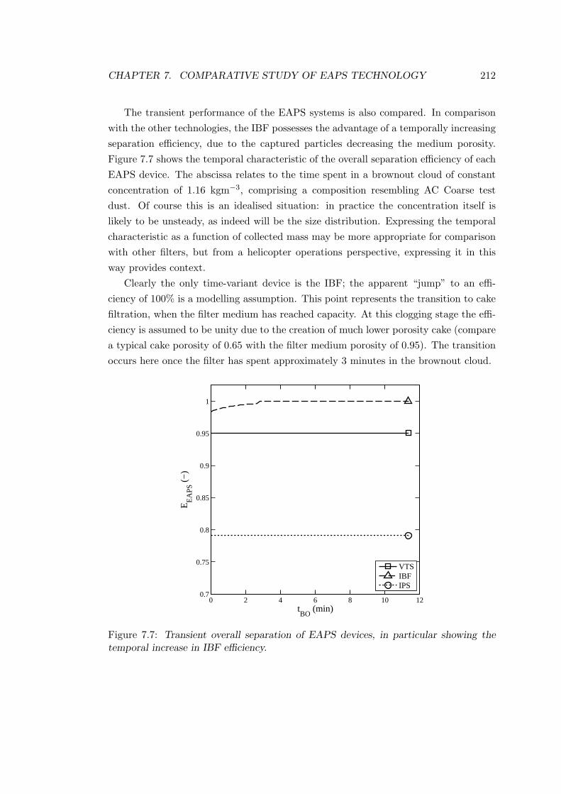
CHAPTER 7. COMPARATIVE STUDY OF EAPS TECHNOLOGY 212
The transient performance of the EAPS systems is also compared. In comparison
with the other technologies, the IBF possesses the advantage of a temporally increasing
separation efficiency, due to the captured particles decreasing the medium porosity.
Figure 7.7 shows the temporal characteristic of the overall separation efficiency of each
EAPS device. The abscissa relates to the time spent in a brownout cloud of constant
concentration of 1.16 kgm−3, comprising a composition resembling AC Coarse test
dust. Of course this is an idealised situation: in practice the concentration itself is
likely to be unsteady, as indeed will be the size distribution. Expressing the temporal
characteristic as a function of collected mass may be more appropriate for comparison
with other filters, but from a helicopter operations perspective, expressing it in this
way provides context.
Clearly the only time-variant device is the IBF; the apparent “jump” to an effi-
ciency of 100% is a modelling assumption. This point represents the transition to cake
filtration, when the filter medium has reached capacity. At this clogging stage the effi-
ciency is assumed to be unity due to the creation of much lower porosity cake (compare
a typical cake porosity of 0.65 with the filter medium porosity of 0.95). The transition
occurs here once the filter has spent approximately 3 minutes in the brownout cloud.
0 2 4 6 8 10 120.7
0.75
0.8
0.85
0.9
0.95
1
tBO
(min)
EE
AP
S (−
)
VTSIBFIPS
Figure 7.7: Transient overall separation of EAPS devices, in particular showing thetemporal increase in IBF efficiency.

CHAPTER 7. COMPARATIVE STUDY OF EAPS TECHNOLOGY 213
7.4 Power Requirements
While separation efficiency defines the proficiency of each device at performing the
main task, the power required to enact the forces of separation is a measure of the
cost. The main source of power is the pressure lost by the flow through the device,
however in some devices power is also required to service a pump to scavenge a portion
of the flow and extracted particles away from the core flow. Additionally, the size and
location of the device on the airframe has an impact on the extra work required by the
engine in the form of accompanying drag. Therefore the method of comparing devices
by power consumed affords a practical assessment of the main drawback of employing
EAPS technology.
0 1 2 3 4 5 6 70
0.2
0.4
0.6
0.8
1
1.2
1.4
1.6
.m
a (kgs−1)
P a / P ∞
(%
)
VTSIBFIPS
Figure 7.8: Effect of engine mass flow rate on EAPS device total pressure loss nor-malised with available pressure in hover at Standard Sea Level conditions.
7.4.1 Pressure Drop
An initial comparison of the pressure loss across each EAPS device is presented first.
Figure 7.8 shows the variation of pressure drop across a range of Turmo engine mass
flow rates for each device. The results suggest that the VTS suffers the least loss of
pressure at the design point mass flow rate of 5.3 kgs−1, and is least sensitive to changes
in mass flow. The IBF performs best at low mass flow rates, although there are data
missing for the IPS at the same operating point. The IPS pressure loss rises sharply

CHAPTER 7. COMPARATIVE STUDY OF EAPS TECHNOLOGY 214
with mass flow rate and is more than double the IBF pressure loss at a mass flow rate
of 6 kgs−1. Expressed as a percentage of the total pressure available, the total pressure
loss at the design mass flow rate of 5.3 kgs−1 for the VTS, IBF and IPS devices is
0.42%, 0.54% and 0.96% respectively. This of course is only true of one engine speed,
during hover, and excludes the capture of particles.
7.4.2 Power Consumption
A more complete picture of the effect of the EAPS system on engine performance is
found by collecting all sources of loss together, calculated from the equations given in
Section 3.5, and plotting the power expended on servicing the EAPS as a fraction of
the maximum power that the engine can deliver, in two scenarios. The first scenario is
the transient condition, in which the helicopter is hovering in a brownout cloud and the
is engine working at the design point mass flow. The second scenario investigates the
power required to service the EAPS in forward flight in order to consider the effect of
device drag, although an assumption is made in that the engine mass flow rate remains
constant, when in practice the engine power requirement (ergo mass flow) reduces
with helicopter forward speed (up to a point — see Chapter 13.2 of Filippone [87] for a
comprehensive discussion of helicopter power requirements in hover and forward flight).
The results are shown in Figure 7.9. In Figure 7.9a the abscissa refers to the
total time spent in the brownout cloud. The fluctuating power required by the IBF
is a manifestation of the cleaning cycles discussed throughout the present work: the
pressure drop across the filter is monitored by a sensor, which notifies the pilot when the
difference reaches an unacceptable level. This may differ between aircraft, depending
on the size of the engine. In the current example a pressure drop limit of 3 kPa was
assigned. It can be seen that the power required at this limit reaches a peak of 1.27%
before the IBF panel is cleaned or replaced after 10 minutes. This equates to 6 filter
cycles per hour in a brownout cloud. Incidentally, the manufacturers of IBF recommend
replacing the filter after 15 wash cycles, which at the current rate is every 2.5 hours
total time spent in a brownout cloud. Of course, the constant conditions are unlikely
to prevail for longer than the 10 or 20 seconds it takes to land or takeoff, but this figure
gives some indication of IBF endurance.
The evolution of the IBF curve is interesting: initially it is the least power-hungry
device, but after approximately 5 minutes its state pushes the IBF beyond the require-
ments of even the IPS. The IPS and VTS are invariant in time, with the VTS requiring
approximately half the power of the IPS. In transition to forward flight, all devices
are assumed to recover pressure from the forward motion of the helicopter with 100%
efficiency, while the drag is seen to act on the area containing the streamtube when
the freestream velocity exceeds the core flow velocity. Pressure recovery is possible if

CHAPTER 7. COMPARATIVE STUDY OF EAPS TECHNOLOGY 215
the axial flow velocity through the device is less than the freestream velocity. When
the engine face velocity exceeds the freestream velocity, a small amount of thrust (or
negative drag) is produced in effect; this thrust is neglected here. (A short discussion
of intake drag is given in Section 5.4.4).
The IPS is positioned just in front of the engine inlet, and therefore does not contain
any components that could cause additional drag. The decrease in power required is
attributable to pressure recovery, which relieves some of the work of the scavenge pump.
For the same reason, a initial decrease in required power is seen to service the VTS
up to a forward speed of around 18 knots, beyond which the power increases due to
the emergence of form drag. The form drag appears at a freestream velocity greater
than the average capture streamtube velocity, hence for much of the range the power
required to service the IBF is constant. The assessment of performance in forward flight
is important in determining the performance of the helicopter in cruise when EAPS are
fitted, which may help to justify the use of engine protection.
0 20 40 600
0.5
1
1.5
2
tBO
(min)
WE
AP
S / W
100%
rpm
(%
)
a.
VTSIBFIPS
0 10 20 300
0.2
0.4
0.6
U∞ (kt)
WE
AP
S / W
100%
rpm
(%
)
b.
VTSIBFIPS
Figure 7.9: Comparison of the power required by each system in two operational sce-narios: a. hover in a brownout cloud of concentration 1.16 kgm−3; b. transition fromhover to forward flight up to 30 knots, with clean IBF and constant engine mass flow.
From this relatively simple analysis, it is established that the IPS requires the most
power for the range studied. However, if the data were extrapolated to higher cruise
speeds, there may be a switching of this trend. Furthermore, the simple modelling
excludes the additional airframe drag created as a consequence of the EAPS device’s
presence, such as described in Section 5.4.4, which would surely become significant at
high freestream velocities. Investigation of this requires further work beyond the remit
of the current study. A final point to make is that it could be argued that since the
IPS is integrated into the engine from the outset by the manufacturers, its effect on

CHAPTER 7. COMPARATIVE STUDY OF EAPS TECHNOLOGY 216
engine performance has already been accounted for. It is the engine manufacturer’s
obligation to deliver the power requested by the client. If optional extras are included
in the specification, they must already be catered for by the power output of the engine.
From a performance loss standpoint, this may make the IPS more favourable over the
other devices, but as will be seen in the forthcoming section, the costs of an inferior
separation efficiency may still dominate the comparison.
7.5 Engine Life
In the preceding section, the three EAPS devices were shown to achieve differing sep-
aration efficiencies. The separation efficiency of a device can be expressed as a single
number for a given dust, but such detail is not sufficient to assess the efficacy of a
device. By looking instead at the grade efficiency that can be achieved by a particle
separator, it is possible to ascertain the size distribution of the particles that evade cap-
ture. No device is 100% efficient, therefore it can be expected that some damage will
be incurred by the engine as a result of erosion or otherwise. Therefore it is important
to know the properties of the particles that are not removed by the EAPS. The size
distribution of the unfiltered particulate can be determined using the same methods
used to ascertain the PSD of the initial dust, as outlined in Section 3.2.2, and can be
calculated theoretically as the opposite of the captured mass of a given particle size.
7.5.1 Engine Lifetime Extension
The financial worth of employing an EAPS system can be quickly established by esti-
mating the extension to engine life over the unprotected case. The Engine Improvement
Index is a metric proposed by van der Walt & Nurick [22] which gives a single number
to express the factor by which an engine life can be extended due to the removal of
particles. The simple metric may also be used to compare EAPS devices with other
protection methods such as blade coatings. The authors use an experimentally-derived
size distribution of unfiltered dust to validate a proposed engine erosion model, which
is described in Section 3.5.3. Using the same expressions for grade efficiency that were
used to create Figure 7.4, the PSD of the particles that evade captured can be found.
From this, an effective mean diameter of the unfiltered particles can be determined and
implemented into Equation 3.158 along with the overall separation efficiency of the
device to yield the Lifetime Improvement Factor (LIF). The results are summarised in
Table 7.3. The condition of hover in a brownout cloud of AC Coarse test dust at the
engine design mass flow rate is used as the test case.
Looking firstly at the Lifetime Improvement Factor, there is a stark contrast between
the three devices. The VTS and IBF eclipse the IPS in terms of extending engine life,

CHAPTER 7. COMPARATIVE STUDY OF EAPS TECHNOLOGY 217
Table 7.3: Summary of Lifetime Improvement Factors of the three EAPS devices, withmass mean diameters (φeff ) of escaped particulate.
EAPS Type EEAPS deff (AC Coarse) φeff LIF
VTS 95.06 % 38.74 µm 1.79 µm 530IBF 98.36 % 38.74 µm 1.48 µm 1325IPS 79.08 % 49.38 µm 6.24 µm 38
by over ten and twenty times respectively. Thanks to its superior overall separation
efficiency, the IBF also outperforms the VTS by more than double, although the mean
particle size of the escaped particulate is slightly larger than the VTS. This can be
explained by examining more closely the grade efficiency of the IBF at these conditions:
across the range of particle sizes, even the largest sizes in the distribution of 100 µm,
the efficiency does not reach unity, unlike its counterpart. Theoretically therefore, a
very small fraction of larger-diameter particulate evades capture and contributes to the
mean diameter seen in Table 7.3. Over time the efficiency does reach 100%, which will
gradually decrease the mean particle size, however the transient case is not considered
here. As a point of clarity, the mean particle size of the initial AC Coarse dust is larger
for the case of the IPS due to use the of different data for the PSD.
Clearly, employment of any device is favourable from a financial perspective, al-
though it would be interesting to carry out a full fiscal comparison study that also
included life extension due to blade coating. It is true that these are unverified theo-
retical estimates, and reflective of just one operational condition, but if it is considered
that an unprotected engine can last just 25 hours in such conditions, an LIF of just 150
can push the engine lifetime due to erosion to a level that is on parity with the regular
MTBO.
7.5.2 Engine Power Deterioration
The main objective of the experiment conducted by van der Walt & Nurick was to
predict the rate of power loss as a function of ingested mass. After an initial unsteady
phase, during which the power was actually observed to increase due to surface polish-
ing, their results showed a linear decrease of engine power with total mass ingested, but
the rate of decrease was observed to lessen with decreasing particle size. This linearity
is observed for up to 10% power loss. The reduction in power was fully attributed to
erosion of the compressor; in practice the smaller particles can impact and coalesce
with the turbine blades at the hot end, causing further deterioration of power, but this
aspect of damage is not modelled here. The proposed formula for engine deterioration

CHAPTER 7. COMPARATIVE STUDY OF EAPS TECHNOLOGY 218
rate is given in Equation 3.151. It requires knowledge of the size distribution of the
particulate that evades capture, and knowledge of the erosion factor kUβ , which is
dependent on the impact velocity of the erodent, the properties of the erodent, and
the properties of the compressor blade. The erosion factor is essentially the ratio of
the power deterioration rate and the effective ingested particle size. It was calculated
after two experiments: firstly after recording the power loss due to the ingestion of
unfiltered SAE Coarse test, and secondly after ingesting particulate unscavenged by a
Donaldson vortex tube separator array; and found to be very similar (-1.40 and -1.45
respectively), suggesting that while some dust properties may influence k, the effect is
minimal.
The findings from the study are applied in the present work. The grade efficiency of
each device gives the mass fraction of each particle size group removed from the initial
test dust; what is not removed contributes to the “ingested” dust particle size distribu-
tion. These data are inputted into Equation 3.151 to give the power deterioration rate
as a function of particulate mass fed into the system. Combining this with the power
required to operate the EAPS systems, as discussed in Section 7.4, allows a holistic
assessment of the impact of EAPS on prolonging engine life in harsh environments.
The results are given in Figure 7.10.
0 5 10 15 20 25 3090
92
94
96
98
100
Mass Fed (kg)
% In
itial
Eng
ine
Pow
er (
%)
UnprotectedVTSIBFIPS
Figure 7.10: Engine power deterioration as a function of mass fed, as predicted by vander Walt & Nurick comparing case of no protection with longevity achieved by thethree EAPS devices.

CHAPTER 7. COMPARATIVE STUDY OF EAPS TECHNOLOGY 219
The ordinate of Figure 7.10 expresses the power loss as a percentage of the initial
power, while the abscissa provides a reference for the total mass fed. The mass fed
refers to the mass of particulate reaching the intake before passing through the EAPS.
Expressing the power loss as a function of mass fed eliminates the need to know the
local dust concentration. However, it must still be assumed that the engine is working
at the design mass flow rate, as this affects the separation efficiency. A striking trend
visible in Figure 7.10 is the rate at which the unprotected engine loses power. After
ingesting just 2 kg of AC Coarse test dust the power is reduced by 8.4%. In contrast, all
EAPS systems exhibit a saving of engine power, even after filtering as much as 30 kg of
dust. At this point, the dust that was not scavenged by the IPS and VTS systems has
contributed to a power loss of 6.1% and 0.6%, which includes the initial power required
to service the device.
The power loss signature of the IBF displays the characteristic fluctuations symp-
tomatic of the cleaning cycles. Interestingly the gradient of the power loss during a
cycle is steeper than the IPS slope. If the maximum permissible pressure loss were
greater, the troughs would extend lower. The power loss of the IBF generally varies
between a minimum of 0.25% to a maximum of 1.25%, with only a slight decrease in
the average quantity. The power loss of the VTS appears to encroach increasingly into
the trend of the IBF, but over the range shown remains less than the average power lost
due to use of an IBF. Extrapolation of the data suggests that the IBF will outperform
the VTS after around 50 kg of dust fed. For a dust concentration of 1.16 gm−3, this
equates to 166 minutes of brownout landing time.
7.6 Summary
The motivation of this Chapter was to contextualise all the work carried out in the
present study. It pits the three main EAPS devices against each other using theoretical
models of varying levels of fidelity. The EAPS are assessed on a number of performance
indicators: grade efficiency, separation efficiency, pressure drop, power required, engine
lifetime extension and engine erosion rate. To facilitate the cross examination, a test
case was set up using the rotorcraft and engine design parameters of an Aerospatiale
SA 330 Puma and the properties of AC Coarse Test dust.
The results show that the VTS is the superior device when assessed on pressure
loss alone at the design point conditions, but show that it is outperformed by the
separation efficiency offered by the IBF. The IPS performance falls short of both the
retro fit technologies in terms of particulate removal, but if the pressure loss is already
catered for in the engine design, the presence of the IPS does not directly affect engine
performance. However, both the IPS and VTS require power to service a scavenge
pump to extract the particulate, which depreciates their worthiness somewhat over

CHAPTER 7. COMPARATIVE STUDY OF EAPS TECHNOLOGY 220
their passive counterpart. The IBF differs from the other technologies by exhibiting
a time-variant power loss, but its superior separation efficiency translates to a much
longer lifetime extension than the VTS and IPS.
All devices permit a fraction of the ingested mass through their systems, which
means the engine does not completely escape damage by erosion. However the extension
to life in harsh environments offered by the VTS and IBF devices would return the
MTBO to more recognisable levels, inasmuch as their removal is scheduled for reasons
other than erosion by particle ingestion. The effect of the power penalty on rotorcraft
performance is not modelled here, but if investigated could provide enough information
to more-holistically assess the financial benefits of employing an engine air particle
separation device.

Chapter 8
Conclusions
The work is concluded with a summary of the main findings of the research,
in which a qualitative and quantitative analysis of particle separation for heli-
copter engines was presented.
1 Inlet Barrier Filter performance can be enhanced significantly by al-
tering the parameters of the internal fabric structure.
In Section 5.2 it was shown that increasing the packing fraction by 4% can increase
the capture efficiency of a fibrous filter by up to 18%, however the same change causes
the pressure drop to triple. In Section 5.3.2 it was shown that the time sustained in
a brownout cloud before excessive pressure loss occurs can be lengthened by 44% by
doubling the filter thickness.
2 The transition from internal clogging to cake accumulation causes a
marked increase in pressure loss rise, but an additional 0.5 gcm−2 can
be collected for the same pressure drop by increasing the pleat depth
by 1 cm.
The characteristic “elbow” on the pressure loss curve is a feature of the relationship
between pressure loss and mass collected, which signifies the transition from internal
filter clogging to cake accumulation. This situation is potentially dangerous for the
helicopter, as the available engine power may suddenly drop off. In Section 5.3.3 it was
shown that the transition can be delayed by employing deeper or narrower pleats. This
also translates to an extension of the MTBO. However as demonstrated in Section 6.3.2,
this must be balanced with retaining a good separation efficiency, which decreases in
accordance with such techniques.
221

CHAPTER 8. CONCLUSIONS 222
3 The optimum pleat angle for minimum pressure drop decreases with
decreasing filter medium permeability, while the optimum angle for
maximum holding capacity decreases as the dust becomes finer.
The discussion of the optimum pleat shape for IBF design has prevailed throughout. In
Section 5.3.3 it was revealed that the larger the filter medium resistance, the smaller the
optimum pleat angle for minimum pressure loss. In the same section it was identified
that the pleat channel pressure loss is more sensitive to changes in flow velocity than the
medium pressure loss. In Section 5.3.4 the optimum pleat angle for maximum holding
capacity of AC Coarse test dust was found to be 2.5 degrees, and was found to decrease
when finer dusts are being filtered.
4 Increasing the IBF projected area by 20% increases the duration of a
filter cycle by 46%, due to the reduction in the flow velocity.
In Section 5.3.4, it was shown that an increase in the projected filter area distributes
the volume flow rate over a larger area, reducing the throughput velocity. This reduces
the pressure loss per kilogram of particulate captured, hence extends the length of the
filter cycle. The optimum design point for minimum clean filter pressure drop was
shown to be invariant with flow velocity.
5 The total pressure lost due to the use of an IBF far outweighs any loss
through flow separation, but the presence of the filter reduces the non-
uniformity of total pressure distortion, and to an increasing degree as
the filter becomes more clogged.
The presence of separated flow, otherwise known as lip spillage, arises in the intake of
forward and side-facing intakes. Its presence causes the flow to accelerate at certain
portions of the filter causing a local increase in particulate density, but the effect on
pressure loss is around 0.05% which is small in comparison with the pressure loss of
0.6% in hover, when a clean filter is installed. However the presence of the filter helps
to homogenise the distorted total pressure that occurs due to the presence of the filter.
This is discussed in Section 5.4.3.
6 In hover, an intake can ingest as much as ten times the quantity of par-
ticles in an area equal to the intake entrance, but this can be reduced
by 44% by angling the filter at 50 degrees to the flow.
The effect of angling the filter was shown to have little impact on the non-filter pressure
drop, however for IBF performance its benefit is twofold. Firstly, the projected area is

CHAPTER 8. CONCLUSIONS 223
increased which reduces the throughput velocity and therefore pressure loss. Secondly,
it spreads the ingested particulate over a larger area, as demonstrated in Section 5.4.5.
In hover for forward-facing intakes, a filter angle of 50 degrees results in a 44% reduction
in the particulate concentration at the filter. The mass of particulate reaching the
filter during hover is much higher than the mass contained in the same area in the
atmospheric conditions, due to a dilation of the capture streamtube.
7 In forward flight beyond the condition of full flow, both forward-facing
and side-facing intakes ingest less particulate per unit area than is con-
centrated in the freestream condition, with the former outperforming
the latter by 30% when the sand is AC Fine test dust.
In forward flight, the capture streamtube of each intake type tested changes shape due
to conservation of mass. The narrowing of the capture streamtube to a smaller area
than the intake area at forward speeds greater than the intake face velocity reduces
the particulate catchment area. It was shown in Section 5.4.6 that if the particulate
is small enough to be influenced by the fluid streamlines, which for AC Fine test dust
it is, then this results in an inherent separation capability. The influence of the fluid
streamtube on the particulate decreases with an increase in particle inertia, but for the
sand tested this allows the forward-facing intake to outperform the side-facing intake,
in terms of passive inertial separation, by up to 30%. The observation adds deviation
from the side-facing superiority trend suggested by Seddon, although the advantage in
avoiding FOD still stands for all forward flight speeds.
8 The optimum pleat design for minimum pressure drop and the opti-
mum point for maximum holding capacity are not aligned; combining
them creates a new metric which is sensitive to flow properties, dust
properties and filter parameters.
Since the optimum design point for minimum pressure drop and the optimum point for
maximum holding capacity are not aligned, a new metric called the Pleat Quality Factor
was proposed in Section 6.2. A larger value of PQF means a better IBF performance.
Key conclusions about IBF design are inherited from this metric. Increasing the pleat
depth improves the PQF at the expense of separation efficiency, but the optimum point
is invariant. A lower throughput velocity results in a better PQF, but also reduces the
filtration efficiency. The optimum design point changes marginally, slightly favouring
a narrower pleat angle. Increasing the filter medium packing fraction decreases the
PQF and nudges the optimum point to a narrower pleat angle, however the separation
efficiency is increased. The same filter performs better when filtering a coarser dust
with a higher prescribed maximum pressure drop.

CHAPTER 8. CONCLUSIONS 224
9 A proposed inlet barrier filter solution for the Eurocopter EC145 lasts
less than 2 minutes in a dust cloud of concentration 2.5 grams per
cubic metre, which equates to approximately 4.5 brownout landings.
Application of a design protocol in Section6.3 for IBF generated a solution for the
Eurocopter EC145, which was combined with the results of the parametric study to
yield a prediction of IBF performance. The pressure drop across the IBF reaches the
critical pressure drop level after 2 minutes in a cloud of 2.5 gm−3, and after 8.5 minutes
in a cloud of 0.5 gm−3. This equates to 4.5 and 22 brownout landings respectively.
The influence of particulate concentration on the gradient of the pressure drop curve is
seen to weaken with increasing concentration. The hover condition is shown to exhibit
an inferior pressure drop rise over forward flight due to a non-uniformity of particulate
distribution.
10 The two stages of filter clogging — internal and surface — are identified
by a discontinuity in the pressure loss curve, however the transition
is “smoothed out” when each pleat is prescribed its own mass flow
rate based on the non-uniform spanwise particle distribution along the
filter.
By marrying the two scales of parametric study in Section 6.4, it was shown that
the abrupt transition to surface clogging disappears. The merger works by taking the
spanwise particle distribution from the intake results and using it to generate a unique
pleat mass flow rate that depends on the spanwise distance along the filter. Since each
pleat has its own mass flow rate, some pleats reach capacity quicker than others, but
their heightened pressure loss is dissipated into the average for the whole filter.
11 The Vortex Tube Separator is the superior device when assessed on
pressure loss alone, but is outperformed by the Inlet Barrier Filter
when judged on separation efficiency; the Inlet Particle Separator has
the lowest drag.
A comparison study in Chapter 7 revealed the key differences between each technology,
and used the performance criteria of separation efficiency, total pressure loss and power
required to assess their utility as EAPS devices. A case study was set up using the
Turbomeca Turmo engine to apply the theories gathered throughout the work. AC
Coarse test dust was used as the test sand. The comparison study revealed that the
VTS exhibited the lowest pressure drop, although the scavenge chamber losses were
only loosely accounted for. The IBF exhibited the highest separation efficiency, which
increased temporally at the expense of increased pressure loss due to the accumulation
CHAPTER 8. CONCLUSIONS 225
of particles, while the IPS contributed the least to drag due to it having no external
parts.
12 When protecting a Turbomeca Turmo engine from the ingestion of
AC Coarse test dust, the Inlet Barrier Filter outperforms the Vortex
Tubes Separator after fifty kilograms of dust have been fed.
The comparison study also investigated the effect of EAPS, both beneficial and costly,
on engine power. The superior separation efficiency offered by the IBF results in a
slower rate of engine erosion than the VTS, but at the expense of a shorter term
shortfall in power due to pressure loss. The VTS exhibits no temporal variation in
pressure loss, but cannot achieve the high efficiency of the IBF. However it achieves the
best performance of all the devices for the first 50 kg of particulate fed to the engine.

Chapter 9
Future Work
This chapter presents some recommendations for further work. In some ways
the project has been like charting a new territory. A corner of the map is now
settled, but there are still unknown pastures to explore beyond the hinterland.
1 Extension of EAPS modelling into three dimensions.
All simulations performed in the current work are in two dimensions, and only focus
on the Inlet Barrier Filter. Indeed it would be difficult to develop a two dimensional
model of a vortex tube. However, with the knowledge garnered from the numerical and
analytical solutions described within the present work, it is a natural step to progress
to three dimensions. This would allow more case-specific, complex geometries to be
tested, given that the fundamental behaviour of these devices has been established.
This would also permit an investigation into the effects on total pressure distortion.
2 Development of an analytical or semi-analytical model for performance
prediction.
The potential saving in time and money by developing an analytical or semi-analytical
model for IBF pleat design would be of huge benefit to the industry. This would require
careful analysis of the flow in the pleat channels and in particular the development of
a relationship between pleat geometry and filtration velocity. Current theories rely on
assumption that Stokes number is low enough for particles to follow streamlines. This
is inadequate for IBF, for which there is a large range of particle Reynolds number,
and high range of flow velocities.
226

Bibliography
[1] F. Colucci, “Safety spotlight: Enduring power,” Vertifilte, vol. 53, no. 2, pp. 25—
27, 2007.
[2] R. Prouty, Helicopter Performance, Stability, and Control. PWS Engineering,
1986.
[3] J. Milluzzo and G. Leishman, “Assessment of rotorcraft brownout severity in terms
of rotor design parameters,” Journal of the American Helicopter Society, vol. 55,
no. 3, pp. 032009–1–9, 2010.
[4] R.T.O, “Rotary-wing brownout mitigation: Technologies and training (Remedes
contre le phenomene de brownout sur les appareils a voilure tournante: Technolo-
gies et entrainement),” tech. rep., NATO Research & Technology Organisation,
2012.
[5] C. Phillips, H. Kim, and R. Brown, “Helicopter brownout - can it be modelled?,”
Aeronautical Journal, vol. 115, no. 1164, pp. 123–133, 2011.
[6] B. Johnson, J. G. Leishman, and A. Sydney, “Investigation of sediment entrain-
ment using dual-phase, high-speed particle image velocimetry,” Journal of the
American Helicopter Society, vol. 55, no. 4, pp. 42003–1–16, 2010.
[7] R. Bagnold, The physics of blown sand and desert dunes. Methuen, 1941.
[8] J. Leishman, “Investigation of sediment entrainment in brownout using high-speed
particle image velocimetry,” in Proceedings of the 65th Annual American Helicopter
Society Forum, (Grapevine, Texas), May 2009.
[9] M. Syal, J. Rauleder, J. K. Tritschler, and J. G. Leishman, “Possibilities of
brownout mitigation using a slotted-tip blade,” in Proceedings of the 29th AIAA
Applied Aerodynamics Conference, (Honolulu, Hawaii), AIAA, June 2011.
227

BIBLIOGRAPHY 228
[10] J. D. Keller, G. R. Whitehouse, D. A. Wachspress, M. E. Teske, and T. R. Quack-
enbush, “A physics-based model of rotorcraft brownout for flight simulation appli-
cations,” in Proceedings of the 62nd American Helicopter Society Annual Forum,
vol. 62, (Phoenix, Arizona), p. 1098, May 2006.
[11] G. R. Whitehouse, D. A. Wachspress, and T. R. Quackenbush, “Aerodynamic
design of helicopter rotors for reduced brownout,” in Proceedings of the Interna-
tional Powered Lift Conference, (Philadelphia, PA), American Helicopter Society
International, Inc., Oct. 2010.
[12] D. A. Wachspress, G. R. Whitehouse, J. D. Keller, K. McClure, P. Gilmore, and
M. Dorsett, “Physics based modeling of helicopter brownout for piloted simula-
tion applications,” in The Interservice/Industry Training, Simulation & Education
Conference (I/ITSEC), vol. 2008, 2008.
[13] D. A. W. G. R. Whitehouse, J. D. K. K. Yu, P. Gilmore, M. Dorsett, K. McClure,
and R. A. SAIC, “A high fidelity brownout model for real-time flight simulations
and trainers,” in Proceedings of the 65th Annual American Helicopter Society Fo-
rum, (Grapevine, Texas), American Helicopter Society International, Inc., 2009.
[14] C. Phillips and R. E. Brown, “The effect of helicopter configuration on the fluid
dynamics of brownout,” in 34th European Rotorcraft Forum, (Liverpool, UK),
2008.
[15] C. Phillips, Computational study of rotorcraft aerodynamics in ground effect and
brownout. PhD thesis, University of Glasgow, 2010.
[16] C. Cowherd Jr, “Sandblaster 2 support of see-through technologies for particulate
brownout,” tech. rep., DTIC Document, 2007.
[17] T. Lueken, N. Peinecke, H. U. Doehler, and R. Lantzsch, “ALLFlight: tackling
the brownout problem,” CEAS Aeronautical Journal, vol. 3, no. 1, pp. 1–15, 2011.
[18] H. U. Doehler and N. Peinecke, “Image-based drift and height estimation for heli-
copter landings in brownout,” Image Analysis and Recognition, pp. 366–377, 2010.
[19] M. Hagelen, G. Briese, H. Essen, T. Bertuch, P. Knott, and A. Tessmann, “A
millimetrewave landing aid approach for helicopters under brown-out conditions,”
in Radar Conference, 2008. RADAR’08. IEEE, pp. 1–4, 2008.
[20] A. J. Wadcock, L. A. Ewing, E. Solis, M. Potsdam, and G. Rajagopalan, “Ro-
torcraft downwash flow field study to understand the aerodynamics of helicopter
brownout,” in American Helicopter Society Southwest Region Technical Specialists’
Meeting, (Dallas-Fort Worth, TX), Ames Research Center, Oct. 2008.

BIBLIOGRAPHY 229
[21] J. Seddon and E. L. Goldsmith, Intake aerodynamics. Amer Inst of Aeronautics
& Aero, 1999.
[22] J. P. V. D. Van Der Walt and A. Nurick, “Erosion of dust-filtered helicopter tur-
bine engines part i: Basic theoretical considerations,” Journal of Aircraft, vol. 32,
pp. 106–111, Jan. 1995.
[23] A. Hamed, W. Tabakoff, and R. Wenglarz, “Erosion and deposition in turboma-
chinery,” Journal of Propulsion and Power, vol. 22, no. 2, pp. 350–360, 2006.
[24] J. P. Van Der Walt and A. Nurick, “Erosion of dust-filtered helicopter turbine
engines part II: erosion reduction,” Journal of Aircraft, vol. 32, pp. 112–117, Jan.
1995.
[25] P. Stallard, “Helicopter engine protection,” Perfusion, vol. 1997, pp. 263–267, July
1997.
[26] J. R. Ballard, “Impact of IPS and IRS configurations on engine installation design,”
Tech. Rep. LS-148, AGARD, 1986.
[27] W. J. C. Prinsloo, P. D. Villiers, and M. C. V. Dijken, “Vortex tube separating
device,” Jan. 1991. U.S. Patent 4,985,058.
[28] R. G. Holdich, Fundamentals of particle technology. Midland Information Tech-
nology and Publishing, 2002.
[29] U. A. M. Department, Engineering Design Handbook. Helicopter Engineering. Part
One. Preliminary Design. Pamphlet A-700200, Alexandria, VA: AMCA, 1974.
[30] L. A. C. Klujszo, P. K. Songfack, M. Rafaelof, and R. K. Rajamani, “Design of
a stationary guide vane swirl air cleaner,” Minerals engineering, vol. 12, no. 11,
pp. 1375–1392, 1999.
[31] A. M. Hobbs, Design and optimization of a vortex particle separator for a hot mix
asphalt plant using computational fluid dynamics. PhD thesis, Georgia Institute
of Technology, 2002.
[32] O. Ramachandran, P. C. Raynor, and D. Leith, “Collection efficiency and pressure
drop for a rotary-flow cyclone,” Filtration & separation, vol. 31, no. 6, pp. 631–636,
1994.
[33] J. Campolong, “Vortex separator,” July 1975. U.S. Patent 3,895,930.
[34] D. R. Monson and T. E. Rosendahl, “Centrifugal separator,” Feb. 1977. U.S.
Patent 4,008,059.

BIBLIOGRAPHY 230
[35] D. R. Monson, D. E. Keller, and J. C. Rothman, “Deflecting element for centrifugal
separators,” June 1970. U.S. Patent 3,517,821.
[36] H. Brockmann, “Multi-stage cyclone separator,” Sept. 1981. U.S. Patent 4,289,611.
[37] T. W. Simpson, “Separator,” Mar. 1981. U.S. Patent 4,255,174.
[38] C. J. Roach, “Vortex air cleaner assembly with acoustic attenuator,” Sept. 1977.
U.S. Patent 4,050,913.
[39] H. N. Shohet, A. F. Amelio, and J. F. Kowalonek, “Engine inlet air particle sepa-
rator,” June 1969. U.S. Patent 3,449,891.
[40] M. J. Scimone, “Aircraft engine air filter and method,” July 2003. U.S. Patent
6,595,742.
[41] M. J. Scimone, D. Flesher, and S. Frey, “High performance barrier filtration sys-
tems,” in Proceedings of the 56th American Helicopter Society Annual Forum,
(Virginia Beach, VA), American Helicopter Society International, Inc., May 2000.
[42] A. Filippone and N. Bojdo, “Turboshaft engine air particle separation,” Progress
in Aerospace Sciences, vol. 46, pp. 224–245, July 2010.
[43] N. Bojdo and A. Filippone, “Performance prediction of inlet barrier filter systems
for rotorcraft engines,” Journal of Aircraft, vol. 48, pp. 1903–1912, June 2011.
[44] N. Bojdo and A. Filippone, “Operational performance parameters of engine inlet
barrier filtration systems for rotorcraft,” The Aeronautical Journal, vol. 116, Sept.
2012.
[45] N. Bojdo and A. Filippone, “Fabric filter performance of helicopter inlet barrier
filters,” Journal of the American Helicopter Society, vol. 57, no. 3, pp. 1–13, 2012.
[46] C. Ockier, H. Muller, L. Wolfgang, C. Kolb, and S. Benedikt, “Flight testing an
engine inlet barrier filter for the EC145,” in Proceedings of the 65th Annual Amer-
ican Helicopter Society Forum, (Grapevine, Texas), American Helicopter Society
International, Inc., May 2009.
[47] D. Y. H. Pui Da-Ren Chen and B. Y. H. Liu, “Optimization of pleated filter design
using a finite-element numerical method,” Journal of Aerosol Science, vol. 24,
no. Supplement 1, pp. S39–S40, 1993.
[48] T. Lucke and H. Fissan, “The prediction of filtration performance of high efficiency
gas filter elements,” Chemical Engineering Science, vol. 51, pp. 1199–1208, Apr.
1996.

BIBLIOGRAPHY 231
[49] A. Subrenat, J. N. Balo, and P. Le Cloirec, “Analysis of pressure drops in pleated
activated carbon cloth filters,” Journal of Environmental Engineering, vol. 126,
no. 6, pp. 562–568, 2000.
[50] R. J. Wakeman, N. S. Hanspal, A. N. Waghode, and V. Nassehi, “Analysis of
pleat crowding and medium compression in pleated cartridge filters,” Chemical
Engineering Research and Design, vol. 83, no. 10, pp. 1246–1255, 2005.
[51] M. Rebaı, M. Prat, M. Meireles, P. Schmitz, and R. Baclet, “A semi-analytical
model for gas flow in pleated filters,” Chemical Engineering Science, vol. 65,
pp. 2835–2846, May 2010.
[52] M. Rebaı, M. Prat, M. Meireles, P. Schmitz, and R. Baclet, “Clogging modeling
in pleated filters for gas filtration,” Chemical Engineering Research and Design,
vol. 88, pp. 476–486, Apr. 2010.
[53] J. F. Stelzer and T. L. Newman, “Engine air filter and sealing system,” Mar. 2007.
U.S. Patent 7,192,462.
[54] J. R. Hobbs, “Gas turbine engine air intake,” June 1983. U.S. Patent 4,389,227.
[55] M. D. Stoten, “Integral inertial particle separator for radial inlet gas turbine en-
gine,” Oct. 2000. U.S. Patent 6,134,874.
[56] S. R. Barr, “Particle separator for turbine engines of aircraft,” Nov. 1976. U.S.
Patent 3,993,463.
[57] A. Hamed, Y. D. Jun, and J. J. Yeuan, “Particle dynamics simulations in inlet
separator with an experimentally based bounce model,” Journal of Propulsion and
Power, vol. 11, no. 2, pp. 230–235, 1995.
[58] B. V. R. Vittal, W. A. Bennett, and D. L. Tipton, “Development of an advanced
vaneless inlet particle separator for helicopter engines,” Journal of Propulsion and
Power, vol. 2, pp. 438–444, Sept. 1986.
[59] G. O. Musgrove, M. D. Barringer, K. A. Thole, E. Grover, and J. Barker, “Com-
putational design of a louver particle separator for gas turbine engines,” ASME
Paper No. GT2009-60199, Proceedings of ASME Turbo Exp, Orlando, FL, 2009.
[60] F. Saeed and A. Al-Garni, “Analysis method for inertial particle separator,” Jour-
nal of Aircraft, vol. 44, no. 4, pp. 1150–1158, 2007.
[61] M. Taslim, A. Khanicheh, and S. Spring, “A numerical study of sand separation
applicable to engine inlet particle separator systems,” Journal of the American
Helicopter Society, vol. 54, no. 4, pp. 042001–1–10, 2009.

BIBLIOGRAPHY 232
[62] V. Glinas and D. Vidal, “Determination of particle shape distribution of clay using
an automated AFM image analysis method,” Powder Technology, vol. 203, no. 2,
pp. 254–264, 2010.
[63] L. Uthus, I. Hoff, and I. Horvli, “Evaluation of grain shape characterization meth-
ods for unbound aggregates,” in Proceedings of the Seventh International Confer-
ence on the Bearing Capacity of Road, Railways and Airfields (BCRA), 2005.
[64] J. P. Van Der Walt and A. Nurick, “Life prediction of helicopter engines fitted
with dust filters,” Journal of Aircraft, vol. 32, pp. 118–123, Jan. 1995.
[65] A. Haider and O. Levenspiel, “Drag coefficient and terminal velocity of spherical
and nonspherical particles,” Powder technology, vol. 58, no. 1, pp. 63–70, 1989.
[66] R. C. Brown, Air Filtration: An Integrated Approach to the Theory and Applica-
tions of Fibrous Filters. Pergamon Press, 1993.
[67] C. N. Davies, Air Filtration. Academic Press, 1973.
[68] J. Bear, Dynamics of Fluids in Porous Media. Elsevier, 1st ed., 1972.
[69] F. M. Tiller and H. Cooper, “The role of porosity in filtration: V. porosity variation
in filter cakes,” AIChE Journal, vol. 8, no. 4, pp. 445–449, 1962.
[70] F. M. Tiller and M. Shirato, “The role of porosity in filtration: VI. new definition
of filtration resistance,” AIChE Journal, vol. 10, no. 1, pp. 61–67, 1964.
[71] F. M. Tiller, N. B. Hsyung, and D. Z. Cong, “Role of porosity in filtration: XII.
filtration with sedimentation,” AIChE Journal, vol. 41, no. 5, pp. 1153–1153, 1995.
[72] F. M. Tiller and J. H. Kwon, “Role of porosity in filtration: XIII. behavior of
highly compactible cakes,” AIChE Journal, vol. 44, no. 10, pp. 2159–2167, 1998.
[73] M. Aguiar and J. Coury, “Cake formation in fabric filtration of gases,” Industrial
and Engineering Chemistry Research, vol. 35, no. 10, pp. 3673–3679, 1996.
[74] L. X. Ito and M. L. Aguiar, “A study of the porosity of gas filtration cakes,”
Brazilian Journal of Chemical Engineering, vol. 26, pp. 307–315, 2009.
[75] E. H. Tanabe, P. M. Barros, K. B. Rodrigues, and M. L. Aguiar, “Experimen-
tal investigation of deposition and removal of particles during gas filtration with
various fabric filters,” Separation and Purification Technology, pp. 187–195, 2011.
[76] R. Wakeman, “The influence of particle properties on filtration,” Separation and
Purification Technology, vol. 58, pp. 234–241, Dec. 2007.

BIBLIOGRAPHY 233
[77] Y. Endo, D.-R. Chen, and D. Y. H. Pui, “Effects of particle polydispersity and
shape factor during dust cake loading on air filters,” Powder Technology, vol. 98,
pp. 241–249, Aug. 1998.
[78] Y. Kousaka, K. Okuyama, A. Shimizu, and T. Yoshida, “Dispersion mechanism of
aggregate particles in air,” J. Chemical Engineering JPN, vol. 12, no. 2, pp. 152–
157, 1979.
[79] J. H. Choi, S. J. Ha, and H. J. Jang, “Compression properties of dust cake of
fine fly ashes from a fluidized bed coal combustor on a ceramic filter,” Powder
technology, vol. 140, no. 1, pp. 106–115, 2004.
[80] D. P. Purchas and K. Sutherland, Handbook of Filter Media. Elsevier, 2nd ed.,
2002.
[81] M. Benesse, L. Le Coq, and C. Solliec, “Study of particle capture mechanisms
in woven activated carbon filters: Image analysis,” in World Filtration Congress,
(New Orleans, LA), 2004.
[82] M. Benesse, L. L. Coq, and C. Solliec, “Collection efficiency of a woven filter made
of multifiber yarn: Experimental characterization during loading and clean filter
modeling based on a two-tier single fiber approach,” Journal of Aerosol Science,
vol. 37, pp. 974–989, Aug. 2006.
[83] F. M. White, Fluid Mechanics. McGraw-Hill, New York, 2nd ed., 1986.
[84] J. H. Ferziger and M. Peric, Computational methods for fluid dynamics, vol. 3.
Springer Berlin etc, 1999.
[85] C. T. Crowe, M. Sommerfeld, and Y. Tsuji, Multiphase flows with particles and
droplets. CRC Press, New York, 1998.
[86] F. International, “Flight archive | 1978 | 0057,” FLIGHT International, vol. 1978,
p. 69, Jan. 1978.
[87] A. Filippone, A. I. o. Aeronautics, and Astronautics, Flight performance of fixed
and rotary wing aircraft. Butterworth-Heinemann, 2006.

Appendix A
Filter Parameters and Parameter
Ranges
The following is a summary of the flow properties, geometric properties, and parameters
that were varied in the pleat scale and intake scale CFD simulations.
A.1 Pleat Scale Parameters
Parameter Symbol Value Unit
Flow Properties
Operating Pressure p∞ 101325 Pa
Air Density ρg 1.225 kgs−1
Air Viscosity µg 1.7894·10−5 kgs−1m−1
Intake Geometry
Pleat Depth Zpl 30 — 50 mm
Pleat Half-Angle θpl 0 — 10 degrees
Pleat Width Zpw 2.0 — 12.8 mm
Filter Thickness ZF 1.0 — 2.5 mm
Engine Properties
Engine Velocity Ua 2 — 12 ms−1
Filter Properties
Filter Medium Capacity MFC 0.399 kgm−2
Filter Fibre Diameter df 13 µm
Filter Medium Porosity ǫF 0.95 (—)
Viscous Resistance Coefficient C 2.588·109 m2
Inertial Resistance Coefficient 1.570·104 m−1
234

APPENDIX A. FILTER PARAMETERS AND PARAMETER RANGES 235
Particulate Properties
Test Dust PSD AC Fine, AC Coarse (–)
Mean Diameter by Mass dp,3 8.83, 28.41 µm
Standard Deviation by Mass σ 3.72, 3.85 µm
Particle Properties
Particle Density ρp 2650 kgm−3
Particle Shape (–) Spherical (–)
Particle Shape Coefficient Φ 0.524 (–)
Cake Properties
Resistance Model (–) Endo et al. (–)
Cake Porosity ǫc 0.65 (–)
Viscous Resistance Coefficient C 3.149·1011 m2
Inertial Resistance Coefficient D 2.229·106 m−1
Solution Details
Min. Cell Size min(l) 0.005Aa m
Pressure Discretisation Scheme (–) PRESTO! (–)
Momentum Discretisation Scheme (–) 1st Order Upwind (–)
Pressure-Velocity Coupling Scheme (–) PISO (–)
Turbulence Modelling
Turbulence Model (–) Reynolds Stress (–)
Turbulence Lengthscale lt 0.01 m
Turbulence Intensity It 3 %

APPENDIX A. FILTER PARAMETERS AND PARAMETER RANGES 236
A.2 Intake Scale Parameters
Parameter Symbol Value Unit
Flow Properties
Operating Pressure p∞ 101325 Pa
Air Density ρg 1.225 kgs−1
Air Viscosity µg 1.7894·10−5 kgs−1m−1
Intake Geometry
Inlet Width Aa 0.3 m
Filter Angle θ 0 — 50 degrees
Filter Width ZIBF 0.3 — 0.42 m
Engine Properties
Engine Mass Flow Rate me 2.94 kgs−1
Engine Inlet Velocity Ua 8 ms−1
Porous Jump Properties
Viscous Resistance Coefficient C 2.588·109 m2
Inertial Resistance Coefficient D 1.570·104 m−1
Pressure Drop ∆P 0 — 3.0 kPa
Medium Thickness ZF 0 — 3.043 mm
Particulate Properties
Particulate Concentration cv 1.0 — 3.0 kgm−3
Test Dust PSD AC Fine, AC Coarse (–)
Mean Diameter by Mass dp,3 8.83, 28.41 µm
Standard Deviation by Mass σ 3.72, 3.85 µm
Particle Properties
Particle Density ρp 2650 kgm−3
Particle Shape (–) Spherical (–)
Particle Shape Coefficient Φ 0.524 (–)
Solution Details
Min. Cell Size min(l) 0.005Aa m
Pressure Discretisation Scheme (–) PRESTO! (–)
Momentum Discretisation Scheme (–) 2nd Order Upwind (–)
Pressure-Velocity Coupling Scheme (–) PISO (–)
Turbulence Modelling
Turbulence Model (–) Reynolds Stress (–)
Turbulence Lengthscale lt 0.01 m
Turbulence Intensity It 3 %


