Embed Size (px)
Citation preview
Rock mass and rippability evaluation
for a proposed open pit mine at
Globe-Progress) near Reefton
A Thesis
submitted in partial fulfilment
of the requirements for the Degree
of
Master of Science in Engineering Geology
by
Philip B. Clark
University of Canterbury
1996

THESIS
Frontispiece
I like rain
by
]PS Experim ce
I like rain falling on my window I like rain splashing on the roof
I like rain dancing on the pavement I like rain when Pm inside
Falling down Falling down
I like rain
(sentiments not felt by most ' Coasters)
Fog starting to settle on New Zealand)s fog capital) Reefton.
11
Abstract Rock mass classification schemes such as the Q System and Rock Mass Rating (RMR)
System have been designed for prediction of tunnel support, but these systems can be
modified from stability analyses to excavatability assessments. Five methods have been
used to classify the rock mass at Globe-Progress with the objective of predicting the type of
equipment that may be used to excavate the open pit:
• Seismic velocity determination
• Size-Strength Method
• RMRSystem
• Weaver's (1975) Rippability Rating System
• MacGregor et aPs (1994) Productivity Prediction Method
Seismic velocity determination and the Size-Strength Method are both easily performed
during the feasibility stages of a project. Seismic velocities are influenced by the degree of
fracturing, compaction, porosity, density and weathering, and they can therefore be used to
provide a preliminary characterisation of the rock mass. The Size-Strength Method uses
the two most important properties of a rock mass for classification, the discontinuity
spacing and the strength of the rock material. Both methods, therefore, provide quick and
accurate assessments of the rock mass quality.
At the investigation or design stage of a project a complete rock mass characterisation
method is used that involves a collection of geological and geotechnical parameters to fully
characterise the rock mass. The method chosen for use at Globe-Progress was the RMR
system, as this method is easily adapted from a stability prediction method to an
excavatability prediction method. Most data required for calculation of the RMR Index is
available from drillcore data logs.
Simple analyses of drillcore log data show that drillcore data has been correctly logged
except for the strength parameter. This was revised for every logged rock mass unit
(RMU) based on quantitative strength determinations and the lithology of each RMU, so
that more accurate excavatability analyses could be made using the RMR System, a
modified version of Weaver's 1975 Rippability Rating Method, and MacGregor et aPs
1994 Productivity Prediction Method.
The ratings for the three rock mass classification methods employed have been contoured
on plans at 20 metre bench levels. The plans show that zones of poor rock, where digging
to easy ripping should be expected, exist in the western pit wall, where the Chemist Shop
Fault is located, and along the northern and eastern walls, following the Globe-Progress
Shear Zone. Most of the overburden is classed as fair to poor rock, where easy to
moderate ripping will be expected, and there is a zone of wealcer rock in the axial fold of
the Globe-Progress Shear Zone.
This study indicates that the proposed open pit is geotechnically feasible to rip. The
preliminary assessments suggest that 90% of the pit area is rippable or marginal and 10% is
expected to non-rippable. The fmal assessments suggest that ripping will be very easy
(> 3500 m3/hr) to difficult (250 - 750 m3/hr) using a Komatsu D575A-2 Bulldozer.
Some areas of overburden may require blasting to further fragment the rock mass and aid
productivity. But there are other factors, such as the bulldozer operator's experience in
ripping similar rock masses, wear and tear on ripper blades, bulldozer maintenance time
and transportation costs, and other restrictions that influence overall productivity and costs
associated with ripping, and which cannot be determined until ripping actually proceeds.
tV
Contents F
. . .. ronttsptece ............................................................................................................ u
Abstract .................................................................................................................. iii
Contents ................................................................................................................. v
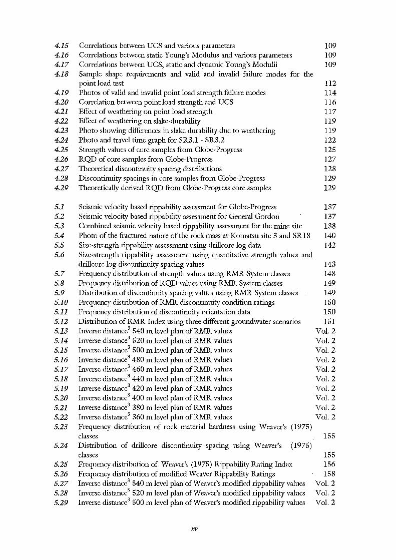
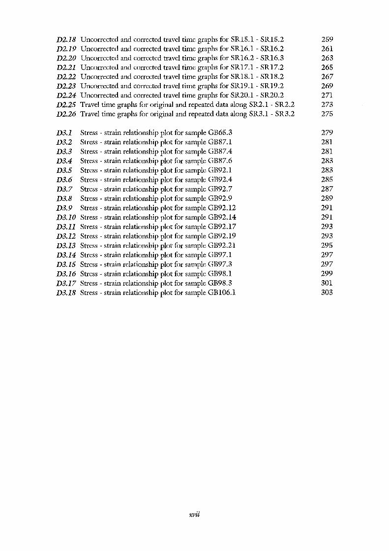
List ofFigures ..................................................................................................... xiv
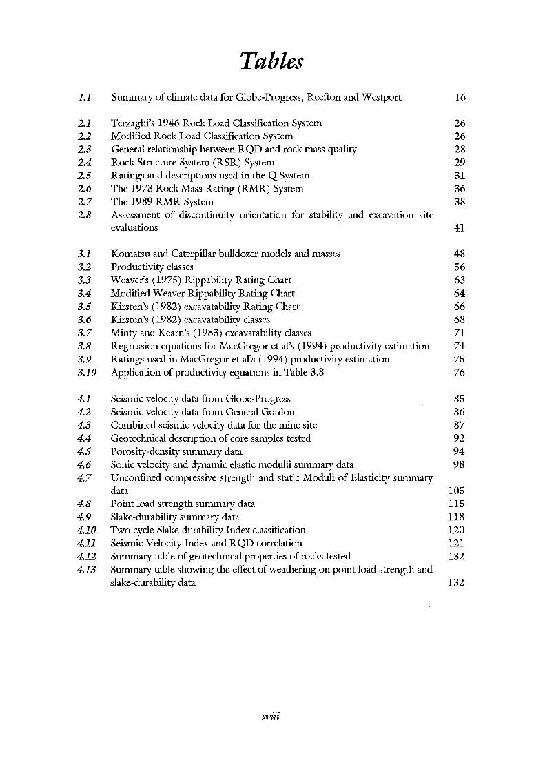
List of Tables ..................................................................................................... xviii
Chapter One
Introduction
1.1 Background .................................................................................................... 1
1.2 Thesis Objectives ........................................................................................... 3
1.3 The study area ................................................................................................ 4
1.3.1 Regional Setting ....................................................................................... 4 1.3.1.1 The Greenland Group ............................................................................. 6 1.3.1.2 The I(aramea Batholith ........................................................................... 7 1.3.1.3 The Reefton Group ................................................................................ 7 1.3.1.4 The Rawles Crag Breccia and Topfer Formation ...................................... 8 1.3.1.5 Tertiary Deposits .................................................................................... 8 1.3.1.6 Quaternary Deposits ............................................................................... 8
1.3.2 Mine site setting and geology ................................................................... 9 1. 3.2.1 Introduction ........................................................................................... 9 1.3.2.2 Structural geology .................................................................................. 9 1.3.2. 3 Structural domains ................................................................................ 10 l. 3.2.4 Mineralisation at Globe-Progress ............................................................ 12 1.3.2.5 Mine site geotechnical investigations ...................................................... 12
1.3.3 Seismic hazard assessment of the goldfield ............................................... 15
1.3.4 Region and mine site climate and vegetation ........................................... 16
1.3.5 Historical Overview of the goldfield ........................................................ 17
v
1.4 Investigation methodology ......................................................................... 17
1.4.1 Rock mass characterisation ....................................................................... 17
1.4.2 Geotechnical investigations ....................................................................... 17
1.4.3 Outcrop and drillcore analysis .................................................................. 18
1.5 Thesis organisation ...................................................................................... 19
Chapter Two
Rock Mass Classification Systems
2.1 Introduction .................................................................................................. 21
2.1.1 Background ............................................................................................... 21
2.1.2 Aims of rock mass classifications .............................................................. 23
2.1.3 Advantages and disadvantages .................................................................. 23
2.2 Rock mass classification systems ................................................................ 24
2.2.1 Rock Load Classification .......................................................................... 24
2.2.2 Rock Quality Designation Index .............................................................. 27
2.2.3 Rock Structure Rating System ................................................................. 28
2.2.4 The Q System ............................................................................................ 30
2.2.5 ISRM geotechnical description of rock masses ........................................ 34
2.3 The RMR System ......................................................................................... 35
2.3.1 The 1973 version ...................................................................................... 35
2.3.2 The 1989 version ...................................................................................... 36 2.3.2.1 Classification Procedure ......................................................................... 36 2.3.2.2 Applications .......................................................................................... 41 2.3.2.3 Advantages and disadvantages of the RMR System ................................ .42
2.4 Rock mass classifications in rippability investigations ........................... 43
2.5 Use of rock mass classifications in open pit mining ............................... 44
2. 5 Summary ......................................................................................................... 45
vi
Chapter Three
Principles and Methods ofRippability Assessment
3.1 Introduction .................................................................................................. 46
3.2 Types of rippers and ripping methods ..................................................... .47
3.3 Geological factors affecting rippability ..................................................... 5!
3.3.1 Introduction .............................................................................................. 5l
3.3.2 Rock type .................................................................... , ............................. 52
3.3.3 Rock hardness or strength ........................................................................ 52
3.3.4 Rock mass structure .................................................................................. 52
3.3.5 Rock material fabric .................................................................................. 54
3.3.6 Site conditions ........................................................................................... 54
3.4 Excavating factors affecting rippability ..................................................... 55
3.4.1 Introduction .............................................................................................. 55
3.4.2 Bulldozer productivity .............................................................................. 55
3.4.3 The contractor, type and condition of equipment used ............................ 56
3.4.4 Method of ripping ..................................................................................... 57
3.5 Previous methods ofrippability assessments ............................................ 57
3.5.1 Bulldozer Manufacturer's seismic velocity charts ..................................... 57
3.5.2 Size-Strength Graphs ................................................................................ 60
3.5.3 Weaver's Rippability Rating Chart .......................................................... 62
3.5.4 IGrsten's Excavatability Index .................................................................. 65
3.5.5 Minty and Kearns' rippability rating system ............................................ 69
3.5.6 MacGregor et at's rippability estimation approach ................................... 72
3.6 Ripping versus blasting ............................................................................... 78
3.7 Synthesis ........................................................................................................ 79
Vtt
Chapter Four
Geotechnical investigations
4.1 Introduction .................................................................................................. 80
4.2 Field Investigations ...................................................................................... 81
4.2.1 Seismic refraction surveys ......................................................................... 81 4.2.1.1 Introduction .......................................................................................... 81 4.2.1.2 Methodology ......................................................................................... 82 4.2.1.3 Results .................................................................................................. 83 4.2.1.4 Discussion ............................................................................................. 88
4.2.2 Observations made on outcrops ................................................................ 90
4.3 Laboratory investigations ............................................................................ 90
4.3.1 Introduction .............................................................................................. 90
4.3.2 Geotechnical sample descriptions ............................................................. 90
4.3.3 Porosity-Density determination ................................................................ 91 4.3.3.1 Introduction .......................................................................................... 91 4.3.3.2 Methodology ......................................................................................... 91 4.3.3.3 Results .................................................................................................. 93 4.3.3.4 Discussion ............................................................................................. 95
4.3.4 Sonic velocity determination ..................................................................... 96 4.3.4.1 Introduction .......................................................................................... 96 4.3.4.2 Methodology ......................................................................................... 96 4.3.4.3 Results .................................................................................................. 97 4.3.4.4 Discussion ............................................................................................. 97
4.3.5 UCS and stress-strain determination ..................................................... 101 4.3.5.1 Introduction ........................................................................................ 101 4.3.5.2 Methodology ....................................................................................... 101 4.3.5.3 Results ................................................................................................ 102 4.3.5.4 Discussion ........................................................................................... 106
4.3.6 Point Load Index determination ............................................................ 111 4.3.6.1 Introduction ........................................................................................ 111 4.3.6.2 Methodology ....................................................................................... 112 4.3.6.3 Results ................................................................................................ 113 4.3.6.4 Discussion ........................................................................................... 113
4. 3. 7 Slake-durability test ................................................................................ 118 4.3.7.1 Introduction ......................................................................................... 118 4. 3. 7.2 Methodology ....................................................................................... 118 4.3.7.3 Results ................................................................................................ 118 4. 3. 7.4 Discussion and interpretations ............................................................. 120
4.4 Comparison between rock masses and rock materials .......................... 120
viii
4.5 Drillcore log analysis ........................................................................... 124
4.5.1 lntroduction ............................................................................................ 124
4.5.2 Strength comparisons ............................................................................. 124
4.5.3 RQD data sets comparison ..................................................................... 126
4.5.4 Discontinuity spacing analysis ................................................................ 126
4.5.5 Other logged data ................................................................................... 130
4.6 Synthesis ...................................................................................................... 130
4.6.1 Field testing ............................................................................................ 130
4.6.2 Laboratory testing .................................................................................. 131
4.6.3 Drill core analysis ................................................................................... 131
Chapter Five
Rippability evaluation of the proposed open pit mine at Globe-Progress
5.1 Introduction ..................................................................................... , .......... 133
5.2 Preliminary rippability evaluation ........................................................... 134
5.2.1 lntroduction ............................................................................................ 134
5.2.2 Seismic velocity determination ............................................................... 134 5 .2.2.1 Komatsu's site visit report .................................................................... 134 5.2.2.2 Rippability assessment based on seismic velocities from this study ......... 136 5.2.2.3 Comparison between Komatsu's data and data from this study .............. 138
5.2.3 Size-strength preliminary assessment ..................................................... 140 5.2.3.1 Introduction ........................................................................................ 140 5.2.3.2 Methodology ....................................................................................... 141 5.2.3.3 Results ................................................................................................ 141
5.3 RMR assessment ........................................................................................ 144
5.3.1 lntroduction ............................................ : ............................................... 144
5.3.2 Methodology ........................................................................................... 144
5.3.3 Results ..................................................................................................... 146
5.3.4 Discussion ............................................................................................... 147
ix
5.4 Final rippability evaluation ....................................................................... 153
5.4.1 Introduction ............................................................................................ 153
5.4.2 Weaver's Rippability Method (1975) ..................................................... 154 5.4.2.1 Introduction ........................................................................................ 154 5.4.2.2 Methodology ....................................................................................... 154 5.4.2.3 Results ................................................................................................ 154 5.4.2.4 Discussion ........................................................................................... 156
5.4.3 The Modified Weaver Rippability Rating .............................................. 157 5.4.3.1 Introduction ........................................................................................ 157 5.4.3.2 Methodology ....................................................................................... 157 5.4.3.2 Results ................................................................................................ 157 5.4.3.4 Discussion ........................................................................................... 158
5.4.4 Prediction of Productivity ...................................................................... 159 5.4.4.1 Introduction ........................................................................................ 159 5 .4.4.2 Methodology ....................................................................................... 159 5.4.4.3 Results ................................................................................................ 161 5.4.4.4 Discussion ........................................................................................... 163
5.5 Comparison between methods ................................................................. 167
5.5.1 Comparison between preliminary rippability prediction methods ......... 167
5.5.2 Comparison between rock mass and rippability evaluations ................. 167
5.6 Synthesis ...................................................................................................... 170
Chapter Six
Summary) conclusions and further work
6.1 Summary ...................................................................................................... 172
6.1.1 General .................................................................................................... 172
6.1.2 Rock mass and rippability classifications ................................................ 173
6.1.3 Geotechnical investigations ..................................................................... 173
6.1.4 Preliminary rippability evaluations ......................................................... 17 6
6.1.5 Complete rock mass and rippability evaluation ...................................... 177
6.2 Conclusions ................................................................................................. 178
6.3 Further work ............................................................................................... 181
X
Acknowledgements ............................................................................................ 182
References ............................................................................................................ 186
Appendix A
Historical Overview
A1 Previous work .............................................................................................. 200
A2 Mining history ............................................................................................. 201
A3 Archaeological value of Globe Hill .......................................................... 203
AppendixB
Terminology
B1 Macraes' geotechnical and geological log descriptions .......................... 205
B2 ISRM geotechnical descriptions (ISRM, 1981) ..................................... 209
B3 MacGregor et aPs (1994) rippability parameter descriptions ............... 214
Appendix C
Barrell)s (1992) Structural mapping
C1 Barrell's structural geology map ............................................................... 218
C2 Barrell's structural domain map ........................................................ : ...... 219
AppendixD
Field and laboratory test results
Dl List of symbols and abbreviations ............................................................ 220
D l.l Generalised Reciprocal Method terminology ......................................... 220
Dl.2 Laboratory testing terminology ............................................................. 221
D2 Seismic refraction surveys .......................................................................... 222
D2.l The Generalised Reciprocal Method ...................................................... 222 D2.l.l Introduction ................................................................................. 222 D2.1.2 Data processing ............................................................................. 223
D2.2 Processed data and plots ......................................................................... 224
D2.3 Seismic refraction data repeatability results ............................................ 272
D3 Laboratory test results ........................................................................ 276
D3.l Porosity- density data ........................................................................... 276
D3.2 Sonic velocity and dynamic Modulus of Elasticity data ......................... 277
D3.3 Stress -strain data and plots .................................................................. 278
D3.4 UCS and static Moduli of Elasticity data ............................................... 304
D3.5 Point load test data ................................................................................ 305
D3.6 Slake- durability test data ..................................................................... 308
AppendixE
Determination of parameters used in rock mass and
rippability evaluation methods
El The RMR System ........................................................................................ 309
El.l Strength ................................................................................................... 309
El.2 RQD ................................................................................................. ; ...... 310
El.3 Discontinuity spacing .............................................................................. 310
El.4 Discontinuity conditions ......................................................................... 310 El.4.1 Length, persistence or continuity .......................................................... 310 E1.4.2 Separation ............................................................................................ 311 E1.4.3 Roughness ........................................................................................... 311 E1.4.4 Infilling ............................................................................................... 312 E1.4.5 Weathering .......................................................................................... 312
El.5 Groundwater ........................................................................................... 313
El.6 Discontinuity orientation ........................................................................ 313
E2 Weaver's 1975 Rippability Rating System .............................................. 314
E2.l Seismic velocity ........................................................................................ 314
E2.2 Hardness .................................................................................................. 314
E2.3 Weathering .............................................................................................. 315
E2.4 Joint spacing ............................................................................................ 315
E2.5 Joint continuity ........................................................................................ 315
E2.6 Joint gouge .............................................................................................. 316
E2.7 Discontinuity orientation ........................................................................ 316
E3 The Modified Weaver Rippability Rating System ................................. 316
E4 MacGregor, et at's (1994) productivity estimation equations .............. 317
E4.l ucs ......................................................................................................... 317
E4.2 Weathering .............................................................................................. 317
E4.3 Grain size ................................................................................................. 317
E4.4 Seismic velocity ................................................................................. 317
E4.5 Defect roughness ..................................................................................... 318
E4.6 Number of defect sets .............................................................................. 318
E4.7 Defect spacing .......................................................................................... 318
E4.8 Structure rating ....................................................................................... 318
E5 Inverse distance weighted average data modelling method .................. 319
xiii
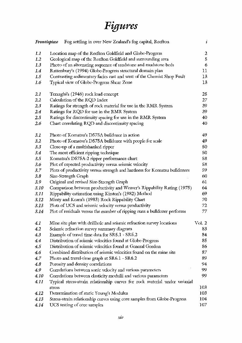
Figures Frontispiece Fog settling in over New Zealand's fog capital, Reefton
1.1 1.2 1.3 1.4 1.5 1.6
2.1 2.2 2.3 2.4 2.5 2.6
3.1 3.2 3.3 3.4 3.5 3.6 3.7 3.8 3.9 3.10 3.11 3.12 3.13 3.14
4.1 4.2 4.3 4.4 4.5 4.6 4.7 4.8 4.9 4.10 4.11
4.12 4.13 4.14
Location map of the Reefton Goldfield and Globe-Progress Geological map of the Reefton Goldfield and surrounding area Photo of an alternating sequence of sandstone and mudstone beds Rattenbury's (1994) Globe-Progress structural domain plan Contrasting sedimentary facies east and west of the Chemist Shop Fault Typical view of Globe-Progress Shear Zone
Terzaghi's (1946) rock load concept Calculation of the RQD Index Ratings for strength of rock material for use in the RMR System Ratings for RQD for use in the RMR System Ratings for discontinuity spacing for use in the RMR System Chart correlating RQD and discontinuity spacing
Photo of Komatsu's D575A bulldozer in action Photo of Komatsu's D575A bulldozer with people for scale Close-up of a multishanked ripper The most efficient ripping technique Komatsu's D575A-2 ripper performance chart Plot of expected productivity versus seismic velocity Plots of productivity versus strength and hardness for Komatsu bulldozers Size-Strength Graph Original and revised Size-Strength Graph Comparison between productivity and Weaver's Rippability Rating (1975) Rippability estimation using Kirsten's (1982) Method Minty and Kearn's (1983) Rock Rippability Chart Plots of UCS and seismic velocity versus productivity Plot of residuals versus the number of ripping runs a bulldozer performs
Mine site plan with drillhole and seismic refraction survey locations Seismic refraction survey summary diagram Example of travel time data for SR5.1- SR5.2 Distribution of seismic velocities found at Globe-Progress Distribution of seismic velocities found at General Gordon Combined distribution of seismic velocities found on the mine site Photo and travel-time graph at SR6.1- SR6.2 Porosity and density correlations Correlations between sonic velocity and various parameters Correlations between elasticity modulii and various parameters Typical stress-strain relationship curves for rock material under uniaxial stress Determination of static Young's Modulus Stress-strain relationship curves using core samples from Globe-Progress UCS testing of core samples
xtV
2 5 6 ll 13 13
25 27 39 39 40 40
49 49 50 50 58 58 59 60 61 64 69 70 72 77
Vol. 2 83 84 85 86 87 89 94 99 99
103 103 104 107
4.15 4.16 4.17 4.18
4.19 4.20 4.21 4.22 4.23 4.24 4.25 4.26 4.27 4.28 4.29
5.1 5.2 5.3 5.4 5.5 5.6
5.7 5.8 5.9 5.10 5.11 5.12 5.13 5.14 5.15 5.16 5.17 5.18 5.19 5.20 5.21 5.22 5.23
5.24
5.25 5.26 5.27 5.28 5.29
Correlations between UCS and various parameters Correlations between static Young's Modulus and various parameters Correlations between UCS, static and dynamic Young's Modulii Sample shape requirements and valid and invalid failure modes for point load test Photos of valid and invalid point load strength failure modes Correlation between point load strength and UCS Effect of weathering on point load strength Effect of weathering on slake-durability Photo showing differences in slake durability due to weathering Photo and travel time graph for SR3.1 - SR3.2 Strength values of core samples from Globe-Progress RQD of core samples from Globe-Progress Theoretical discontinuity spacing distributions Discontinuity spacings in core samples from Globe-Progress Theoretically derived RQD from Globe-Progress core samples
109 109 109
the 112 114 116 117 119 119 122 125 127 128 129 129
Seismic velocity based rippability assessment for Globe-Progress 137 Seismic velocity based rippability assessment for General Gordon 137 Combined seismic velocity based rippability assessment for the mine site 138 Photo of the fractured nature of the rock mass at Komatsu site 3 and SR18 140 Size-strength rippability assessment using drillcore log data Size-strength rippability assessment using quantitative strength values and drillcore log discontinuity spacing values Frequency distribution of strength values using RMR System classes Frequency distribution ofRQD values using RMR System classes Distribution of discontinuity spacing values using RMR System classes Frequency distribution ofRMR discontinuity condition ratings Frequency distribution of discontinuity orientation data Distribution of RMR Index using three different groundwater scenarios Inverse distance 3 540 m level plan of RMR values Inverse distance3 520 m level plan ofRMR values Inverse distance3 500 m level plan ofRMR values Inverse distance3 480 m level plan ofRMR values Inverse distance3 460 m level plan ofRMR values Inverse distance3 440 m level plan ofRMR values Inverse distance 3 420 m level plan of RMR values Inverse distance3 400 m level plan ofRMR values Inverse distance3 380 mlevel plan ofRMR values Inverse distance3 360m level plan ofRMR values Frequency distribution of rock material hardness using Weaver's classes
(1975)
Distribution of drillcore discontinuity spacing using Weaver's (1975) classes Frequency distribution of Weaver's (1975) Rippability Rating Index Frequency distribution of modified Weaver Rippability Ratings Inverse distance3 540 m level plan of Weaver's modified rippability values Inverse distance3 520 m level plan of Weaver's modified rippability values Inverse distance3 500 m level plan of Weaver's modified rippability values
XV
142
143 148 149 149 150 150 151
Vol. 2 Vol. 2 Vol. 2 Vol. 2 Vol. 2 Vol. 2 Vol. 2 Vol. 2 Vol. 2 Vol. 2
155
155 156 158
Vol. 2 Vol. 2 Vol. 2

5.30 5.31 5.32 5.33 5.34 5.35 5.36 5.37 5.38 5.39
5.40
5.41 5.42 5.43 5.44 5.45 5.46 5.47 5.48 5.49 5.50 5.51
A1.1 A1.2
C1.1 C1.2
Inverse distance3 480 m level plan ofWeaver's modified rippability values Inverse distance3 460 m level plan of Weaver's modified rippability values Inverse distance3 440 m level plan of Weaver's modified rippability values Inverse distance3 420 m level plan of Weaver's modified rippability values Inverse distance3 400 m level plan ofWeaver's modified rippability values Inverse distance3 380 m level plan of Weaver's modified rippability values Inverse distance3 360m level plan of Weaver's modified rippability values Frequency distribution for discontinuity roughness values Frequency distribution of MacGregor et aPs (1994) structure rating Frequency distribution of MacGregor et aPs (1994) productivity prediction using Equation 4 Frequency distribution of MacGregor et aPs (1994) productivity prediction using Equation 8 Inverse distance3 540 m level plan of productivity values Inverse distance3 520 m level plan of productivity values Inverse distance3 500 m level plan of productivity values Inverse distance3 480 m level plan of productivity values Inverse distance3 460 m level plan of productivity values Inverse distance3 440 m level plan of productivity values Inverse distance3 420 m level plan of productivity values Inverse distance3 400 m level plan of productivity values Inverse distance3 380m level plan of productivity values Inverse distance3 360m level plan of productivity values Comparison between RMR calculated from Beetham and Coote's (1994) data and actual RMR
Photo of remnants of the B Shaft Photo of the Union Adit
Barrell's structural geology map Barrell's structural domain map
D2.1 Uncorrected and corrected travel time graphs for SR1.1- SR1.2 D2.2 Uncorrected and corrected travel time graphs for SR1.2- SR1.3 D2.3 Uncorrected and corrected travel time graphs for SR2.1- SR2.2 D2.4 Uncorrected and corrected travel time graphs for SR2.2- SR2.3 D2.5 Uncorrected and corrected travel time graphs for SR3.1- SR3.2 D2.6 Uncorrected and corrected travel time graphs for SR4.1- SR4.2 D2.7 Uncorrected and corrected travel time graphs for SR5.1- SR5.2 D2.8 Uncorrected and corrected travel time graphs for SR5.2- SR5.3 D2.9 Uncorrected and corrected travel time graphs for SR6.1- SR6.2 D2.10 Uncorrected and corrected travel time graphs for SR7.1 - SR7.2 D2.11 Uncorrected and corrected travel time graphs for SR8.1- SR8.2 D2.12 Uncorrected and corrected travel time graphs for SR9.1- SR9.2 D2.13 Uncorrected and corrected travel time graphs for SR10.1- SR10.2 D2.14 Uncorrected and corrected travel time graphs for SR11.1- SR11.2 D2.15 Uncorrected and corrected travel time graphs for SR12.1 - SR12.2 D2.16 Uncorrected and corrected travel time graphs for SR13.1- SR13.2 D2.17 Uncorrected and corrected travel time graphs for SR14.1- SR14.2
xvi
Vol. 2 Vol. 2 Vol. 2 Vol. 2 Vol.2 Vol. 2 Vol. 2
162 162
164
165 Vol. 2 Vol. 2 Vol. 2 Vol. 2 Vol. 2 Vol. 2 Vol. 2 Vol. 2 Vol. 2 Vol. 2
168
204 204
218 219
225 227 229 231 233 235 237 239 241 243 245 247 249 251 253 255 257
D2.18 Uncorrected and corrected travel time graphs for SR15.1- SR15.2 259 D2.19 Uncorrected and corrected travel time graphs for SR16.1- SR16.2 261 D2.20 Uncorrected and corrected travel time graphs for SR16.2 - SR16. 3 263 D2.21 Uncorrected and corrected travel time graphs for SR17.1- SR17.2 265 D2.22 Uncorrected and corrected travel time graphs for SR18.1- SR18.2 267 D2.23 Uncorrected and corrected travel time graphs for SR19.1- SR19.2 269 D2.24 Uncorrected and corrected travel time graphs for SR20.1 - SR20.2 271 D2.25 Travel time graphs for original and repeated data along SR2.1- SR2.2 273 D2.26 Travel time graphs for original and repeated data along SR3.1- SR3.2 275
D3.1 Stress - strain relationship plot for sample GB65.3 279 D3.2 Stress -strain relationship plot for sample GB87.1 281 D3.3 Stress - strain relationship plot for sample GB87.4 281 D3.4 Stress - strain relationship plot for sample GB87.6 283 D3.5 Stress - strain relationship plot for sample GB92.1 283 D3.6 Stress- strain relationship plot for sample GB92.4 285 D3.7 Stress- strain relationship plot for sample GB92.7 287 D3.8 Stress- strain relationship plot for sample GB92.9 289 D3.9 Stress -strain relationship plot for sample GB92.12 291 D3.10 Stress- strain relationship plot for sample GB92.14 291 D3.11 Stress- strain relationship plot for sample GB92.17 293 D3.12 Stress - strain relationship plot for sample GB92.19 293 D3.13 Stress - strain relationship plot for sample GB92.21 295 D3.14 Stress -strain relationship plot for sample GB97.1 297 D3.15 Stress - strain relationship plot for sample GB97.3 297 D3.16 Stress -strain relationship plot for sample GB98.1 299 D3.17 Stress -strain relationship plot for sample GB98.3 301 D3.18 Stress- strain relationship plot for sample GB106.1 303
xvii
Tables 1.1 Summary of climate data for Globe-Progress, Reefton and Westport 16
2.1 Terzaghi's 1946 Rock Load Classification System 26 2.2 Modified Rock Load Classification System 26 2.3 General relationship between RQD and rock mass quality 28 2.4 Rock Structure System (RSR) System 29 2.5 Ratings and descriptions used in the Q System 31 2.6 The 1973 Rock Mass Rating (RMR) System 36 2.7 The 1989 RMR System 38 2.8 Assessment of discontinuity orientation for stability and excavation site
evaluations 41
3.1 Komatsu and Caterpillar bulldozer models and masses 48 3.2 Productivity classes 56 3.3 Weaver's (1975) Rippability Rating Chart 63 3.4 Modified Weaver Rippability Rating Chart 64 3.5 Kirsten's (1982) excavatability Rating Chart 66 3.6 Kirsten's (1982) excavatability classes 68 3.7 Minty and Kearn's (1983) excavatability classes 7l 3.8 Regression equations for MacGregor et al's (1994) productivity estimation 74 3.9 Ratings used in MacGregor et al's (1994) productivity estimation 75 3.10 Application of productivity equations in Table 3.8 76
4.1 Seismic velocity data from Globe-Progress 85 4.2 Seismic velocity data from General Gordon 86 4.3 Combined seismic velocity data for the mine site 87 4.4 Geotechnical description of core samples tested 92 4.5 Porosity-density summary data 94 4.6 Sonic velocity and dynamic elastic modulii summary data 98 4.7 Unconfmed compressive strength and static Moduli of Elasticity summary
data 105 4.8 Point load strength summary data 115 4.9 Slal<e-durability summary data 118 4.10 Two cycle Slal<e-durability Index classification 120 4.11 Seismic Velocity Index and RQD correlation 121 4.12 Summary table of geotechnical properties of rocks tested 132 4.13 Summary table showing the effect of weathering on point load strength and
slal<e-durability data 132
XVttt
5.1
5.2
5.3
5.4
5.5
5.6
5.7
5.8
5.9
5.10
5.11
5.12
5.13
6.1 6.2 6.3
D2.1 D2.2 D2.3 D2.4 D2.5 D2.6
Comparison between seismic velocities determined by Komatsu (1994) and in this study Essential core data, other data, RMR Index, rippability ratings and productivity estimation (drillholes GB1-GB10) Essential core data, other data, RMR Index, rippability ratings and productivity estimation (drillholes GB10-GB20) Essential core data, other data. RMR Index, rippability ratings and productivity estimation (drillholes GB21-GB30) Essential core data, other data, RMR Index, rippability ratings and productivity estimation (drillholes GB31-GB40) Essential core data, other data, RMR Index, rippability ratings and productivity estimation (drillholes GB41-GB50) Essential core data, other data, RMR Index, rippability ratings and productivity estimation (drillholes GB51-GB60) Essential core data, other data, RMR Index, rippability ratings and productivity estimation (drillholes GB61-GB 70) Essential core data, other data, RMR Index, rippability ratings and productivity estimation (drillholes GB 7l-GB80) Essential core data, other data, RMR Index, rippability ratings and productivity estimation (drillholes GB81-GB90) Essential core data, other data, RMR Index, rippability ratings and productivity estimation (drillholes GB91-GB100) Essential core data, other data, RMR Index, rippability ratings and productivity estimation (drillholes GB10l-GB106) Summary of estimated productivity for DlO, D475A-2 and D575A-2
Summary of seismic velocity results Summary data from all geotechnical laboratory tests Summary of rock mass and rippability classification predictions
GRM data for SR1.1- SR1.2 GRM data for SR1.2 - SR1.3 GRM data for SR2.1 - SR2.2 GRM data for SR2.2 - SR2.3 GRM data for SR3.1 - SR3.2 GRM data for SR4.1 - SR4.2
D2.7 GRM data for SR5.1- SR5.2 D2.8 GRM data for SR5.2 - SR5.3 D2.9 GRM data for SR6.1 - SR6.2 D2.10 GRM data for SR7.1- SR7.2 D2.11 GRM data for SR8.1 - SR8.2 D2.12 GRM data for SR9.1 - SR9.2 D2.13 GRM data for SR10.1 - SR10.2 D2.14 GRM data for SR11.1- SR11.2 D2.15 GRM data for SR12.1 - SR12.2 D2.16 GRM data for SR13.1- SR13.2 D2.17 GRM data for SR14.1- SR14.2 D2.18 GRM data for SR15.1 - SR15.2 D2.19 GRM data for SR16.1- SR16.2 D2.20 GRM data for SR16.2- SR16.3
xtX
139
Vol. 2
Vol. 2
Vol. 2
Vol. 2
Vol. 2
Vol. 2
Vol. 2
Vol. 2
Vol. 2
Vol. 2
Vol. 2 163
174 175 177
224 226 228 230 232 234 236 238 240 242 244 246 248 250 252 254 256 258 260 262
D2.21 GRM data for SR17.1 - SR17.2 264 D2.22 GRM data for SR18.1 - SR18.2 266 D2.23 GRM data for SR19.1- SR19.2 268 D2.24 GRM data for SR20.1 - SR20.2 270 D2.25 Repeated GRM data for SR2.1 - SR2.2 272 D2.26 Repeated GRM data for SR3.1 - SR3.2 274
D3.1 Porosity - density data 2 7 6 D3.2 Sonic velocity and dynamic Modulus of Elasticity data 277 D3.3 Stress- strain data for sample GB65.3 278 D3.4 Stress- strain data for sample GB87.1 280 D3.5 Stress - strain data for sample GB87.4 280 D3.6 Stress -strain data for sample GB87.6 282 D3.7 Stress- strain data for sample GB92.1 282 D3.8 Stress - strain data for sample GB92.4 284 D3.9 Stress- strain data for sample GB92.7 286 D3.10 Stress- strain data for sample GB92.9 288 D3.11 Stress- strain data for sample GB92.12 290 D3.12 Stress- strain data for sample GB92.14 290 D3.13 Stress- strain data for sample GB92.17 292 D3.14 Stress - strain data for sample GB92.19 292 D3.15 Stress - strain data for sample GB92.21 294 D3.16 Stress- strain data for sample GB97.1 296 D3.17 Stress- strain data for sample GB97.3 296 D3.18 Stress - strain data for sample GB98.1 298 D3.19 Stress- strain data for sample GB98.3 300 D3.20 Stress- strain data for sample GB106.1 302 D3.21 Unconfmed compressive strength and static Moduli of Elasticity data 304 D3.22 Point load test data for unweathered core samples 305 D3.23 Point load test data for slightly weathered irregular lumps 306 D3.24 Point load test data for moderately irregular lumps 307 D3.25 Slake - durability test data 308
E2.1 Weaver's (1975) rockhardness defmition 314
Chapter One
Introduction
1.1 Background
((Should the efforts of the few prospectors still active in the district result even in
a single instance in a successful mine) confidence would probably be restored to
an extent such that capital would be forthcoming for the development of known
lodes) and the reopening of old mines where ore was left which could profitably
be worked by modern methods ..... Lodes prospected in earlier years may repay
investigation in view of the present high price of gold.))
M Gage, 1948.
The above quote seems to be just as apt today as when it was written in a 1948 review of
the Reefton Goldfield, and Globe-Progress, near Reefton, will hopefully be the site for
Macraes Mining Company Limited's (Macraes) ftrst successful mine within the goldfield.
Macraes are also exploring other areas within the Reefton Goldfield that may be mined at a
later date.
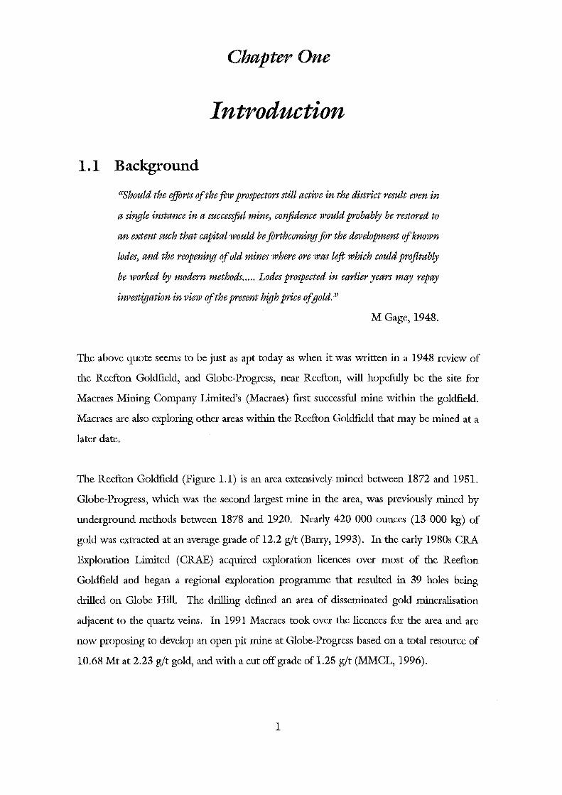
The Reefton Goldfield (Figure 1.1) is an area extensively mined between 1872 and 1951.
Globe-Progress, which was the second largest mine in the area, was previously mined by
underground methods between 1878 and 1920. Nearly 420 000 ounces (13 000 kg) of
gold was extracted at an average grade of 12.2 g/t (Barry, 1993). In the early 1980s CRA
Exploration Limited (CRAE) acquired exploration licences over most of the Reefton
Goldfield and began a regional exploration programme that resulted in 39 holes being
drilled on Globe Hill. The drilling defmed an area of disseminated gold mineralisation
adjacent to the quartz veins. In 1991 Macraes took over the licences for the area and are
now proposing to develop an open pit mine at Globe-Progress based on a total resource of
10.68 Mt at 2.23 g/t gold, and with a cut off grade of 1.25 g/t (MMCL, 1996).
1
N
W~E s Enlargement
South Island
0 5 ,...._.. __ 10 km
'X Mines with past production greater than 500 kg gold. After Barry, 1993
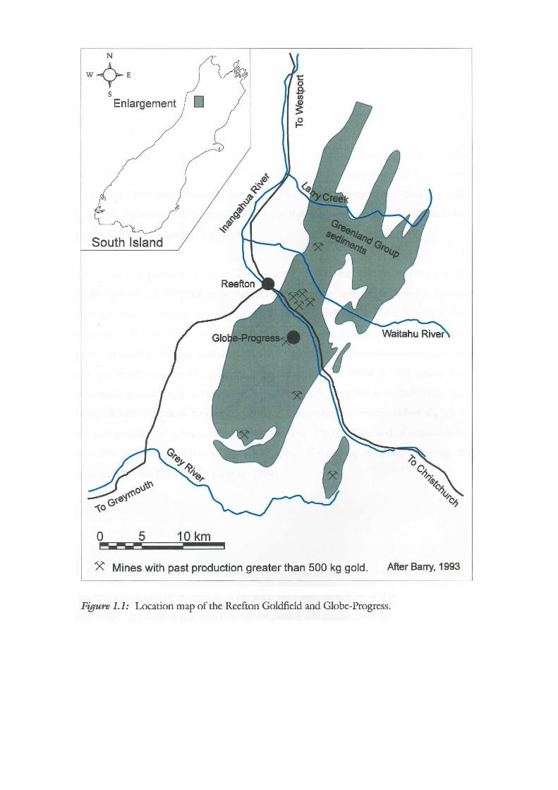
Figure 1.1: Location map of the Reefton Goldfield and Globe-Progress.
To excavate the pit either bulldozer ripping, drill and blast methods, or a combination of
the two will be used. There are two different approaches to estimating the rippability of a
site, one involving characterisation of the rock mass, and the other prediction of the
productivity of a ripping machine. This thesis uses both methods in evaluating the
rippability of the rock mass within the proposed open pit. The site evaluation requires
rock mass and rock material characteristics, as well as information on possible ripping
machinery to be used, and should be performed during the investigation and design stages
of a project. Two simple med1ods are also used to provide a preliminary evaluation of ilie
rippability of the open pit, the type of assessment that might be performed at the feasibility
or early investigation stage of a project.
The preliminary methods of rippability evaluation involve determining variations in the
seismic velocity of the rock mass, where the variations are due to changes in rock
properties such as density, weathering and fracturing, and by using the Modified Size
Strength Method ofPettifer and Fookes (1994), which plots the block size or discontinuity
spacing against the rock material strengili. A complete rippability evaluation requires rock
mass properties that are obtainable from drillcore logs or outcrops, and which were
reevaluated quantitatively so that the rock mass could be classified using d1e Rock Mass
Rating (RMR) System of Bieniawski (1989). This system has been modified slighdy so
that the rippability of the excavation can be classified. The other method of evaluating d1e
rippability involves prediction of the productivity of a ripping machine, following the
procedures oudined by MacGregor et al (1994).
1.2 Thesis Objectives
This thesis provides an evaluation of d1e rock mass and rippability of a proposed open pit
gold mine. Ripping is not a method of excavation commonly used in New Zealand, so
this study provides an excellent opportunity to evaluate methods of rippability evaluation
and apply them to a large database of drillliole data, so that a three dimensional rock mass
and rippability model of the open pit may be produced.
3
There are three specific objectives that are covered by this study:
• To review existing methods of rock mass and rippability classification methods to
ftnd the methods most suited for use at Globe-Progress.
• To carry out fteld and laboratory testing to provide necessary geotechnical
parameters such as porosity and density; strength; relationship between stress and
strain; and seismic and sonic velocities for rock mass characterisation.
• To analyse existing drillhole data and carry out additional surveys to develop a
three-dimensional geotechnical model of the open pit that may assist pit
development.
1.3 The study area
1.3.1 Regional Setting
The Reefton Goldfield lies in the western foothills of the Victoria Ranges and extends from
Larry's Creek in the north to the Grey River in the south (Figure 1.1). The Inangahua
River bisects the goldfield, and most creeks in the goldfield eventually drain into either the
Inangahua River or Grey River.
The goldfield is located with the Buller Terrane, one of two tectonostratigraphic terranes in
Northwest Nelson (Figure 1.2). Basement rocks in the Buller Terrane consist of
Ordovician Greenland Group metasediments (Cooper, 1974; Adams et al, 1975), Early
Devonian Reefton Group shallow marine sediments (Bradshaw and Regan, 1983), and
Late Palaeozoic granitoids from the Karamea Batholith (Cooper, 1989). Overlying the
basement rocks are Cretaceous to Tertiary conglomerates, coal measures and mudstones;
Pleistocene glacial and fluvioglacial deposits; and recent river gravels (Suggate, 1957). All
units are discussed below.
4

N
w{r-E Buller Terrane
s
South Island ~
·S ~ ~ ~
Q
~ ~ ~ ~ ~ ~
cff
Figure 1.2: Geological map of the Reefton Goldfield and surrounding area.
5
u D
D ~ ___.,
Geology of the Reefton Goldfield
Geological Legend
Weathered greywacke and
schist conglomerate, glacial
and fluvioglacial deposits,
recent river gravels.
Conglomerate, sandstone,
siltstone and coal. Marine siltstone.
Quartzose sandstone, carbon-
aceous mudstone and coal.
Conglomerate and Breccia
Volcanogenic sandstone,
mudstone and coal.
Quartzite, foss i I iferous
mudstone and muddy
limestone
Undifferentiated Karamea
Batholith granitoids
Weakly metamorphosed
quartzose sandstone and
argillite (thermal
metamorphism indicated by
dots).
Metasedimentary gneiss and
migmatite.
Fold Fault
Formation Age
Quaternary
Rotokohu Coal Tertiary
Measures
Kaiata Formation
Brunner Coal
Measures
Hawks Crag Cretaceous
Breccia
Topfer Formation Triassic
Reefton Formation Devonian
Karamea Batholith Devonian, Carbon
iferous and
Cretaceous
Greenland Group Ordovician
Victoria Paragneiss Ordovician
Modified from Barry, 1993
1.3.1.1 The Greenland Group
Greenland Group metasediments outcrop discontinuously from Milford Sound in the
soud1 to Karamea in the north. The metasediments consist of alternating sequences of
Ordovician indurated mudstones (argillites) and sandstones (greywackes) interpreted by
Laird (1972) to be turbidite successions. Northeast of Reefton, Greenland Group
sediments have been thermally metamorphosed to hornfels, and southeast of Reefton the
sediments have been metamorphosed to a higher grade to form the Victoria Paragneiss
(SD Weaver,pers com).
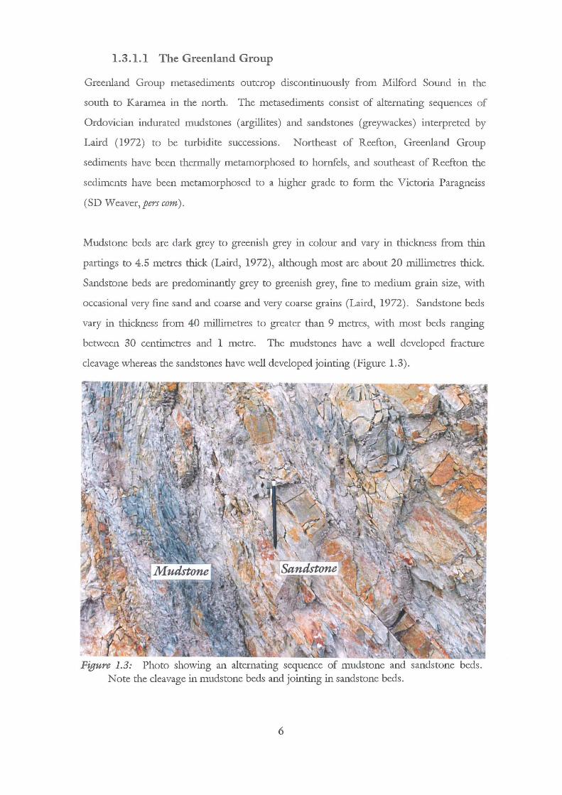
Mudstone beds are dark grey to greenish grey in colour and vary in dllckness from dlin
partings to 4.5 metres dUck (Laird, 1972), although most are about 20 millimetres dUck.
Sandstone beds are predominandy grey to greenish grey, fme to medium grain size, with
occasional very fine sand and coarse and very coarse grains (Laird, 1972). Sandstone beds
vary in dllckness from 40 millimetres to greater than 9 metres, with most beds ranging
between 30 centimetres and l metre. The mudstones have a well developed fracture
cleavage whereas the sandstones have well developed jointing (Figure 1.3) .
Figure 1.3: Photo showing an alternating sequence of mudstone and sandstone Note the cleavage in mudstone beds and jointing in sandstone beds.
6
Petrographic studies by Laird (1972), Laird and Shelley (1974), Nathan (1976) and
Cooper and Craw (1992) show that the Greenland Group has nndergone low grade
metamorphism, with the clay matrix being recrystallised to sericitic muscovite. The
predominance of angular quartz clasts, occasional feldspar clasts and detrital clast<> of
tourmaline, zircon, apatite and muscovite indicates that the provenance was an acidic
granitic source (Laird, 1972; Cooper and Craw, 1992);· and the inclusion of lithic clasts of
chert and mica rich pelites suggests the source rock was most likely to be a quartzose
metasediment that originated from a granitic source (Nathan, 1976; Cooper and Craw,
1992).
1.3.1.2 The Karamea Batholith
The granitoids in the Karamea Batholith form the Victoria Ranges east of Reeftoh and part
of the Paparoa Range west of Reefton. The batholith is divided into two suites, the
Karamea Suite (Carboniferous and Devonian) and the Rahu Suite (Early to Mid
Cretaceous). The Karamea Suite Granitoids contain both I and S type intrusives of biotite
and muscovite granites, granodiorites and tonalites, whereas the Rahu Suite Granitoids are
mainly I-S intermediate type intrusives of biotite granodiorites and muscovite granite
(Muir et al, in press). Karamea Suite Granitoids form most of the Karamea Batholith and
intrude into the Greenland Group. The Rahu Suite Granitoids intrude as high level
plutons and stocks adjacent to and within the batholith.
1.3.1.3 The Reefton Group
The Reefton Group is fonnd west and southwest of Reefton and contains Lower Devonian
fossiliferous mudstone, flaggy limestone and quartzite in fault bonnded outliers (Bradshaw
and Regan, 1983). A thick sandstone unit (Murray Creek Formation) is overlain by an
alternating sequence of limestone (Forgotten Limestone, Lankey Limestone, Y orkey
Limestone and Pepper bush Limestone) and mudstone (Bolitho Mudstone, Adam
Mudstone, Ranft Mudstone and Alexander Mudstone) formations, which are . in turn
overlain by a thin quartzite unit (Kelly Sandstone). The outliers lie nnconformably on
Greenland Group rocks and are not penetrated by the mineralised quartz lodes fonnd in the
Greenland Group.
7
1.3.1.4 The Hawks Crag Breccia and Topfer Formation
The Hawks Crag Breccia and Topfer formation were originally mapped as units belonging
to the Cretaceous Pororari Group (Bowen, 1964), but Raine (1980) found Mid and Late
Triassic flora in the Topfer Formation to the east of Reefton. The Topfer Formation
consists of volcanogenic sandstone and mudstone and minor coal seams and occurs in
faulted outliers. The Late Cretaceous Hawks Crag Breccia outcrops south and east of
Reefton in normal fault bounded grabens. It is composed largely of granitic clasts with
minor amounts of hornfelsic Greenland Group clasts and is assigned to the Pororari Group
(Raine, 1984).
1.3.1.5 Tertiary Deposits
Tertiary sediments in the Reefton Goldfield are divided into Mid Eocene Brunner Coal
Measures, Mid to Late Eocene Kaiata Formation and Pliocene Rotokohu Coal Measures
(Barry, 1993). The Brunner Coal Measures occur on the east side of the Inangahua
Depression and south of Reefton as sequences of basal conglomerate, quartzose sandstone,
sandstone, carbonaceous mudstone and coal (Suggate, 1957). The Kaiata Formation
conformably overlies the Brunner Coal Measures, ranging between glauconitic siltstone
with sandstone and conglomerate to conglomeratic sandstone and siltstone, and represents
a change from a freshwater environment to a marine environment (Suggate, 1957). The
Kaiata Formation is unconformably overlain by the Rotokohu Coal Measures northeast of
Reefton and contains non-marine conglomerate, sandstone, siltstone and lignite. South of
Reefton, the Rotokohu Coal Measures lie directly on Greenland Group (Suggate, 1957).
1.3.1.6 Quaternary Deposits
Overlying the Rotokohu Coal Measures, and possibly infilling the Grey-Inangahua
Depression, are Early Pleistocene freshwater conglomerates and sandstones, known as Old
Man Gravels (Suggate, 1957). In tl1e Late Pleistocene piedmont glaciation and valley
glaciation formed moraines and terraces within tl1e Reefton Goldfield (Suggate, 1957).
Postglacial river gravels have covered the Grey-Inangahua Depression and floodplains of
other rivers in the Reefton Goldfield, and together with the glacial deposits are the source
of placer gold deposits in the region.
8
1.3.2 Mine site setting and geology
1.3.2.1 Introduction
Globe-Progress is located on Globe Hill (see Figure 4.1located in the map and table box),
at the northern end of what Henderson (1917) called the Reefton Plateau. The proposed
open pit is bonnd to the north by Oriental Creek and to the south by Union Creek South.
Both these creeks are deeply incised and drain into Devils Creek. Tailings will be stored in
Devils Creek behind a waste rock stack that will dam Devils Creek and Fossickers Creek,
and a freshwater reservoir will be located in the Fossickers Creek catchment.
The mine site is located almost entirely within Greenland Group sediments. The only area
not nnderlain by Greenland Group sediments is part of Fossickers Creek, a section of
which is nnderlain by Tertiary Brunner Coal Measures. There is also widespread colluvium
ranging in thickness from less than one metre to in excess of fifty metres on most slopes
within the mine site. Descriptions of Greenland Group and Brunner Coal Measures have
been given in Section 1.3.1, therefore, this section discusses structural geology,
mineralisation and geotechnical studies at Globe-Progress.
1.3.2.2 Structural geology
Greenland Group sediments at Globe-Progress are dominated by medium-thick (100 to
1000 mm) bedded sandstone and mudstone, with lesser thick beds (> 1000 mm) and thin
beds (30 to 100 mm; Rattenbury, 1994). Sedimentary structures such as crossbedding,
grading and scouring are apparent in some places, but cleavage and shearing have
overprinted and destroyed most of the earlier sedimentary structures. Cleavage is wealdy
developed in mudstone and very wealc in sandstone (Rattenbury, 1994).
Folds at Globe-Progress are well constrained by the identification of changes in symmetry
of bedding-cleavage relationships. Folds are generally close tight structures steeply inclined
to the west, and the position of their axial trace is well constrained and truncated by the
Globe-Progress Shear Zone. Numerous faults are identifiable in outcrops, most of which
are west dipping reverse faults with a small displacement. Large faults often contain zones
of pug and breccia, and may have sulphide mineralisation associated with them
9
(Rattenbury, 1994). They generally occur in gullies and rarely outcrop (Rattenbury,
1994) as pug and breccia erode more easily than competent Greenland Group rock.
The Globe-Progress Shear Zone is situated in a structurally complex zone near the axis of
the Globe Hill Anticline and is discordant with the regional structure (Hughes, 1992;
Rattenbury, 1994). The shear zone trends WNW and links the NNE trending General
Gordon and Empress shear zones in the south with the Auld Creek and Bonanza shear
zones north of Globe-Progress, as shown by the trend of the fold axes on Figure 1.2.
The Globe-Progress Shear Zone contains three auriferous lodes: the Oriental, Globe and
Progress. The lodes are interpreted to be en echelon structures stacked above each other
(Hughes, 1992). They curve concavely to the SSW with a 70° dip at the surface, flattening
out with depth and terminating against the Chemist Shop Fault. The shear curves around
the northern and eastern slopes of Globe Hill and is discordant to the north trending folds
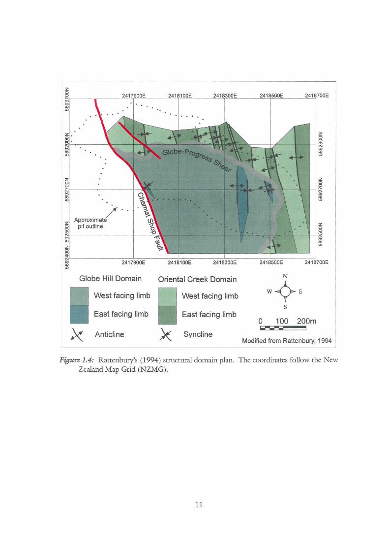
in the hangingwall and footwall of the shear (Figure 1.4). The sense of movement and
displacement is unlmown, but Rattenbury (1994) suggests displacement is greater than
500 m based on displacement of fold axes.
The Chemist Shop Fault trends NNW and dips at a high angle to the east, although the
sense of movement is not lmown. It separates distinctly different sedimentary facies; to the
east are thin to thick bedded sandstone and mudstone; and to the west are very thin to thin
bedded sandstone layers (Rattenbury, 1994; Figure 1.5). Despite considerable exploration
during mining and later in the 1930s, the continuation of the shear zone west of the
Chemist Shop Fault has not been discovered.
1.3.2.3 Structural domains
Barrell (1992), based on geotechnical line mapping of outcrops at Globe-Progress, divided
the open pit area into eight structural domains based on differences in bedding and fold
axes orientation, (Appendix C). Barrell inferred the position of nine faults and eleven fold
axes on the surface, noting that there may be more that were not exposed at the time of
mappmg.
10
/. . Approximate
pit outline
2417900E
Globe Hill Domain Oriental Creek Domain
East facing limb East facing limb
Anticline Syncline
s
0 100 ~---
200m I
Modified from Rattenbury, 1994
Figure 1.4: Rattenbury's (1994) structural domain plan. The coordinates follow the New Zealand Map Grid (NZMG).
ll
Rattenbury (1994) simplified the open pit site into two structural domains separated by
the Globe-Progress Shear Zone. The Globe Hill Domain is the hangingwall block of the
Globe-Progress Shear and the Oriental Creek Domain is the footwall block. Both domains
have been further subdivided into west and east facing fold limbs (Figure 1.4).
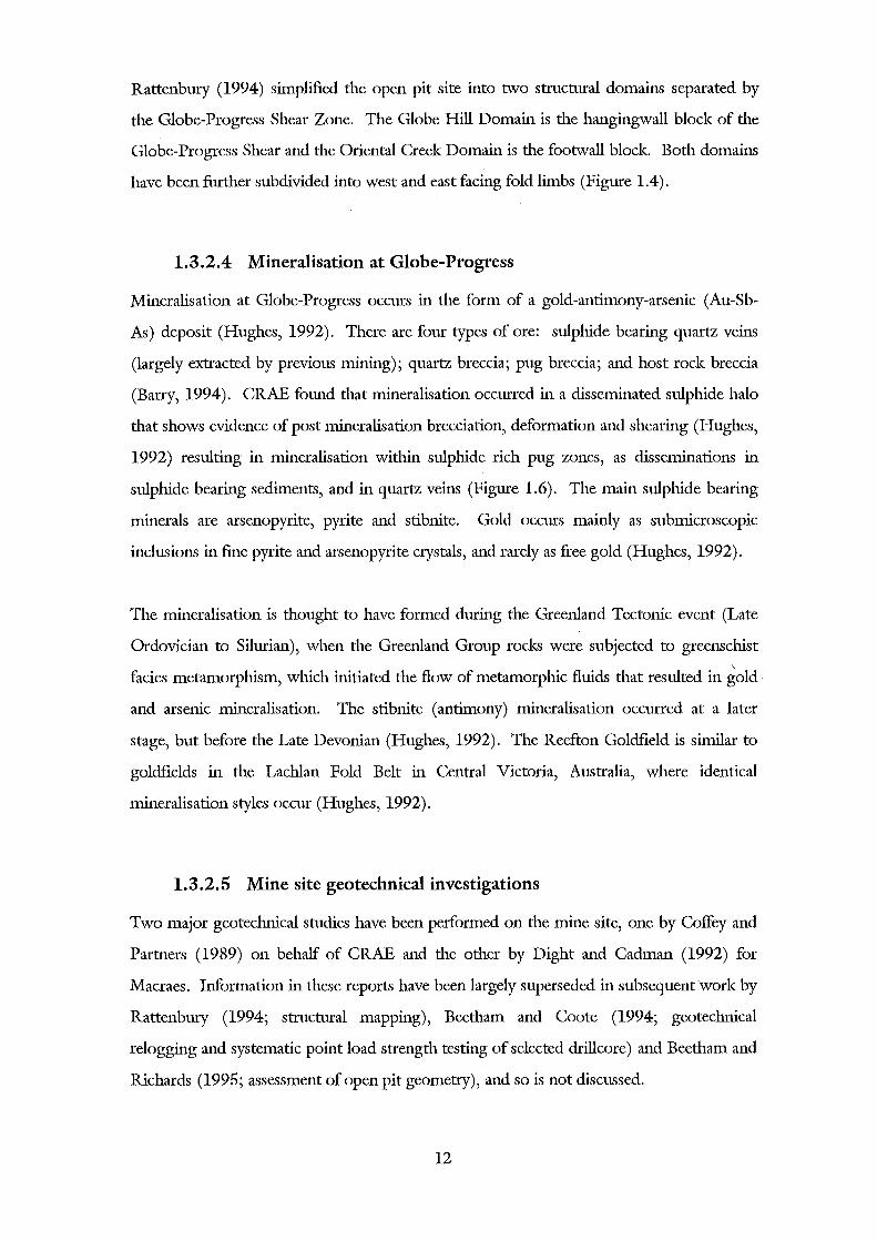
1.3.2.4 Mineralisation at Globe-Progress
Mineralisation at Globe-Progress occurs in the form of a gold-antimony-arsenic (Au-Sb
As) deposit (Hughes, 1992). There are four types of ore: sulphide bearing quartz veins
(largely extracted by previous mining); quartz breccia; pug breccia; and host rock breccia
(Barry, 1994). CRAE found that mineralisation occurred in a disseminated sulphide halo
that shows evidence of post mineralisation brecciation, deformation and shearing (Hughes,
1992) resulting in mineralisation within sulphide rich pug zones, as disseminations in
sulphide bearing sediments, and in quartz veins (Figure 1.6). The main sulphide bearing
minerals are arsenopyrite, pyrite and stibnite. Gold occurs mainly as submicroscopic
inclusions in fme pyrite and arsenopyrite crystals, and rarely as free gold (Hughes, 1992).
The mineralisation is thought to have formed during the Greenland Tectonic event (Late
Ordovician to Silurian), when the Greenland Group rocks were subjected to greenschist
facies metamorphism, which initiated the flow of metamorphic fluids that resulted in gold
and arsenic mineralisation. The stibnite (antimony) mineralisation occurred at a later
stage, but before the Late Devonian (Hughes, 1992). The Reefton Goldfield is similar to
goldfields in the Lachlan Fold Belt in Central Victoria, Australia, where identical
mineralisation styles occur (Hughes, 1992).
1.3.2.5 Mine site geotechnical investigations
Two major geotechnical studies have been performed on the mine site, one by Coffey and
Partners (1989) on behalf of CRAE and the other by Dight and Cadman (1992) for
Macraes. Information in these reports have been largely superseded in subsequent'work by
Rattenbury (1994; structural mapping), Beetham and Coote (1994; geotechnical
relogging and systematic point load strength testing of selected drillcore) and Beetham and
Richards (1995; assessment of open pit geometry), and so is not discussed.
12
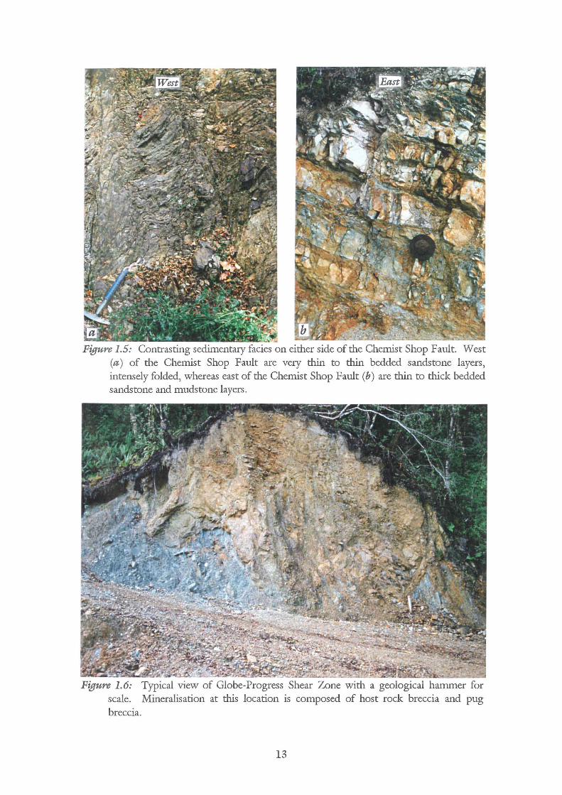
Figure 1.5: Contrasting sedimentary facies on either side of the Chemist Shop Fault. West (a) of the Chemist Shop Fault are very thin to thin bedded sandstone layers, intensely folded, whereas east of the Chemist Shop Fault (b) are thin to thick bedded sandstone and mudstone layers.
Figure 1.6: Typical view of Globe-Progress Shear Zone with a geological hammer for scale. Mineralisation at this location is composed of host rock breccia and pug breccia.
13
Rattenbury (1994) concluded that:
• Bedding surfaces are the most dominant penetrative discontinuity, and that they
mostly dip at a shallow to moderate angle to the west in Globe Hill Domain
(hanging wall domain).
• The Oriental Creek Domain (footwall domain) is more complexly folded and
contains more steeper dipping folds and shear zones than the Globe Hill Domain.
• Shear zones are either steeply dipping or subparallel to bedding and fold axial
planes are typically sheared, especially synclines.
• Rock structures in the western wall are not well known due to a lack of outcrop
and drillcore data but the structural change across the Chemist Shop Fault is
significant, with the western side containing thinly bedded sandstone facies and
the eastern side containing medium bedded sandstone facies.
Beetham and Coote (1994) found:
• Rock masses in the western wall are highly sheared because of the presence of the
Chemist Shop Fault.
• The Globe-Progress Shear is a zone of very poor rock mass quality 15 to 58
metres wide.
• The footwall rock mass appears to be of better quality than the hanging wall rock
• Rock material strengths are greater than previously thought, with Is (50) = 4.9
MPa for sandstone and 2. 9 MPa for mudstone.
• Much of the core has a distinctive drilling-induced brealcage that are often logged
as natural fractures, thereby giving the core lower than expected discontinuity
spacing and RQD values.
• Effects of weathering on rock material occur to a depth of approximately 30
metres and weathering along discontinuities extend to greater depths.
Beetham and Richards (1995) concluded:
• The pit can be divided into three general sectors based on rock mass quality: the
footwall or nortl1ern sector; the hangingwall or southern sector; and the western
end or Chemist Shop Fault sector.
14
• Stability analyses on the pit slopes usmg the Modified Hoek-Brown failure
criterion (Hoek and Brown, 1980) and a bench angle of 47° give factors of safety
greater than 1 for all walls except the western wall, where the bench angles should
be reduced to approximately 35°.
• The assessment of pit slope angles in Greenland Group rocks is supported by
natural slopes in the Reefton area that have shown very few signs of slope failure,
even under strong seismic loading (MM VIII-IX) and, seismic shaking greater
than MM IX has a low probability of occurring during the expected mine life.
1.3.3 Seismic hazard assessment of the goldfield
The Reefton Goldfield is located in a region of moderately high seismicity, approximately
35 km west of the Alpine Fault. Within the region are numerous active faults trending
approximately north-south (Figure 1.2), and two faults in the region have had major
earthquakes on them this century. The Glasgow and Rotokohu Faults moved during the
M57.4 1968 Inangahua earthquake, and the White Creek Fault moved during the M57.8
1929 Murchison earthquake.
Both of these earthquakes caused strong shaking of MM VIII-IX in the Reefton region,
but there were no major slope failures in the Globe-Progress area (Beetham and Richards,
1995), although some buildings in Reefton suffered stmctural damage. A hazard
assessment study by Hancox and Beanland (1994) fotmd active faultc; and structures in the
Reefton area that could cause intense shaking if they were to move, but no active faults or
structures were found on the mine site. Smith and Berryman's 1983 earthquake hazard
map of New Zealand suggests that MM VII shaking on the mine site would occur once
every 20-50 years, MM VIII shaking would occur once every 100 years and MM IX
shaking would occur once every 500 years. Therefore it is unlikely that shaking similar to
that experienced in 1929 and 1968 will occur during the expected mine life.
15
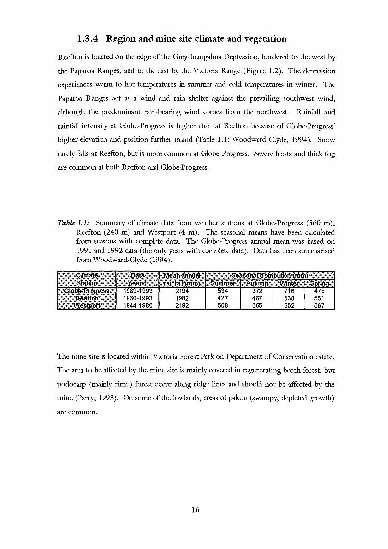
1.3.4 Region and mine site climate and vegetation
Reefton is located on the edge of the Grey-Inangahua Depression, bordered to the west by
the Paparoa Ranges, and to the east by the Victoria Range (Figure 1.2). The depression
experiences warm to hot temperatures in summer and cold temperatures in winter. The
Paparoa Ranges act as a wind and rain shelter against the prevailing southwest wind,
although the predominant rain-bearing wind comes from the northwest. Rainfall and
rainfall intensity at Globe-Progress is higher than at Reefton because of Globe-Progress'
higher elevation and position further inland (Table 1.1; Woodward Clyde, 1994). Snow
rarely falls at Reefton, but is more common at Globe-Progress. Severe frosts and thick fog
are common at both Reefton and Globe-Progress.
Table 1.1: Summary of climate data from weather stations at Globe-Progress (560 m), Reefton (240 m) and Westport (4 m). The seasonal means have been calculated from seasons with complete data. The Globe-Progress annual mean was based on 1991 and 1992 data (the only years with complete data). Data has been summarised from Woodward-Clyde (1994).
The mine site is located within Victoria Forest Park on Department of Conservation estate.
The area to be affected by the mine site is mainly covered in regenerating beech forest, but
podocarp (mainly rimu) forest occur along ridge lines and should not be affected by the
mine (Parry, 1993). On some of the lowlands, areas of pal<ihi (swampy, depleted growth)
are common.
16
1.3.5 Historical Overview of the goldfield
A historical overview of the Reefton Goldfield is beyond the scope of this thesis, but a brief
review of previous geological investigations, history of mining and the archaeological
significance of the area, placing particular emphasis on Globe-Progress, are included as
Appendix A.
1.4 Investigation methodology
1.4.1 Rock mass characterisation
A search through the literature was undertaken to fmd the most appropriate rock mass
classification and rippability evaluation methods for use on the proposed open pit. It was
decided to perform two simple tests (seismic velocity determination and size-strength
determination) that may be performed at the feasibility or early site investigation stage of a
project and to compare these results with Bieniawski's 1989 RMR System; Weaver's 1975
Rippability Rating System and a modified version of this system; and MacGregor et al)s,
1994 Productivity Prediction Method that could be performed during the investigation or
design stages of a project.
1.4.2 Geotechnical investigations
A combination of field tests and laboratory tests were performed to characterise the rock
mass and rock material in order to provide additional data for rock mass and rippability
classifications. Field investigations involved performing seismic velocity tests at Globe
Progress and General Gordon, collecting samples for strength and slalce durability tests,
and inspections of most outcrops and drillcore. Laboratory tests involved determining
unweathered rock material properties such as porosity, density, sonic velocity, point load
strength and uniaxial compressive strength on core, and strength and slalce durability tests
on slightly and moderately weathered irregular samples.
17
The primary field investigation method involved performing seismic velocity tests on the
rock mass at Globe-Progress and General Gordon (proposed site of the waste rock stack,
but also containing significant quantities of ore that may be extracted). Fifteen seismic
refraction traverse lines were performed at Globe-Progress and five seismic refraction lines
were carried out at General Gordon. The seismic refraction surveys were performed so
that a preliminary rippability assessment could be estimated, and so that seismic velocities
could be used in more detailed rippability assessments and compared to sonic velocities
determined from drillcore samples.
Core samples were tested for the following geotechnical parameters: porosity, density,
sonic velocity, strength and strain. Both uniaxial compressive strength and point load
strength tests were performed on core to find a correlation between the two and to
compare the correlation constant with published values. Where possible both diametric
and axial tests were performed to fmd any anisotropy in the core. The sonic velocity can be
compared to the seismic velocity found on the rock mass and strength test data can be
compared with logged strength values to check the accuracy and consistency of drillcore
logs. Porosity and density values correlate with sonic velocities and strength values, so
have been determined as a check on the sonic velocity and strength data to fmd any highly
anomalous samples. The point load test and slake-durability tests were also performed on
irregular samples collected from outcrops and logged as slightly weathered, moderately
weathered and highly weathered to fmd the effect of weathering on the strength and
durability of the rock material.
1.4.3 Outcrop and drillcore analysis
Outcrops from roads, drill tracks and drill pads at Globe-Progress and General Gordon had
previously been logged on a Husky data logger by Barrell (1992) using line traverse
mapping, where all rock material and discontinuity data crossing a line on the outcrop
surface is recorded. Graphical relogging, whereby outcrops were drawn at a· scale of
1:250, by Jowett et al (1996) has also been also performed. Therefore, only visual
inspection and photography of outcrops were required and comparisons were made with
the actual logs to check for consistency in logging. Seismic refraction velocity profiles
18
were also compared with photo logs and graphic logs of Jowett et al (1996) to assist with
seismic refraction interpretation.
A total of 106 diamond drillholes, totalling in excess of 17000 m in length have been
drilled at Globe-Progress by CRAB and Macraes. Drillcore logs exist in graphical form
and as ASCII computer flies. The computer flies were reanalysed using a spreadsheet so
that the RMR and rippability assessments could be made. The total length of diamond
drillcore from which rock mass and rippability assessments were determined was 10360 m.
Only data recorded as rock mass units (RMU) were analysed, as other units lacked the data
required to evaluate the rock mass. Some drillcore was inspected and compared with the
drillcore logs to check for consistency in logging.
l. 5 Thesis organisation
This thesis consists of six chapters and associated appendices. The first chapter list'> the
aims of the research and provides an introduction to the study area and methods of
research. The second chapter introduces the concepts of rock mass characterisation and
discusses six common rock mass classification methods, detailing the RMR System as this
is the most suitable method for use on the open pit. Chapter Three introduces the
concepts of rippability and discusses various factors that influence rippability. Six different
methods of rippability estimation are described and their advantages and disadvantages are
discussed. The fourth chapter describes the various geotechnical investigations used and
summarises and discusses the results of each investigation. An analysis of the drillcore data
used in the rock mass and rippability classifications is also discussed in Chapter Four.
Chapter Five details the rock mass characterisation and rippability assessment performed at
Globe-Progress. It first provides a preliminary rippability assessment using two methods
that could be performed during the feasibility or early investigation stages of a project, then
the computation of the RMR System from drillhole data, then provides a fmal rippability
assessment using two different approaches, one involving characterising the rock mass and
the other estimating the productivity of three sizes of bulldozers that might be used to rip
the pit. The fmal chapter summarises all the results and conclusions and discusses further
research and work that could be performed.
19

Appendix A provides a historical overview of the Reefton Goldfield, detailing previous
geological and geotechnical investigations in the area, the history of mining in the Reefton
Goldfield and an archeological review of Globe-Progress. Appendix B provides description
sheets used by Macraes to log drillcore and outcrops; ISRM (1981) discontinuity and rock
material descriptions and MacGregor's et at (1994) variable descriptions. Appendix C
provides a map of Barrell's (1992) structural domains. Results of all tests are included as
Appendix D and Appendix E discusses all the generalisations and assumptions made in
calculating the RMR, rippability ratings and expected productivity of the rock mass.
20
Chapter2
Rock Mass Classification Systems
2.1 Introduction
2.1.1 Background
Classification systems in general have been defined as the ordering or arrangement of
objects into groups or sets on the basis of their relationships, which can be based on
observable or inferred properties (Sakal, 1974). Rock mass classification systems are no
different and in the last twenty years have become an essential part of the investigation and
design stages of engineering projects. They are an empirical approach to design based on
previous projects and case studies. Most classification systems in use today include
characteristics of both rock material and discontinuities, but other classification systems
only use a simple description of the rock mass, for example the Rock Load Classification
System. Others may only be used for one form of excavation, for example underground
excavations (RSR System or the Q System), slope stability (Slope Mass Rating System),
or rippability (Weaver's 1975 Rippability Rating). Most classification systems have been
designed with the prediction of tunnel support in mind, but others, such as the RMR
System, are easily modified so that they may be applied to excavations, slope stability or
mining projects.
In general, rock mass classification systems categorise rock masses into classes with similar
geotechnical properties. To categorise the rock mass, a number of geotechnical properties
are selected and quantified. These properties can normally be found from drillcore or line
traverses and include rock type, grain size, weathering, fracturing, condition of
discontinuities and groundwater flow. The properties are assigned ratings, depending on
how much they are thought to influence the behaviour of the rock mass. The ratings may
be added or multiplied according to the system used. Rock masses with similar total
21
ratings are expected to behave in th.e same way and may be used to predict the stand-up
time of tunnels, slope stability parameters, rock mass deformability, type of excavation
technique and so on.
Rock masses are normally classified by geologists or engineers, therefore the classification
system should be designed so that anyone using a particular system will get the same result.
Einstein et al (1983) independendy classified rock masses using classification systems
oudined in Section 2.2 and 2.3 and found that the classification systems were not affected
by the subjectivity of the user. This study was very important as rock mass classification
systems need to be reliable and reproducible.
When characterising a rock mass the observations and tests that need to be performed
should be simple, rapid and relevant (Bieniawski, 1973). Most of the data should be
available from drillcore logs, but other data, such as discontinuity persistence, may need to
be estimated based on observations from outcrops or closely spaced drillholes (ISRM,
1981). Other factors, such as rock strength, that have been determined using one form of
identification may need to be correlated with another form of testing. For example,
drillcore strength values qualitatively determined by hardness methods, such as pockedmife
scratch tests or relative hammer hardness (see Appendix B2 for strength defmitions), need
to be correlated with their uniaxial compressive strength values by quantifYing the logged
data with strength values determined from uniaxial compressive strength or point load
strength.
Brief discussions on the main rock mass classification systems are included as Section 2.2,
explaining their advantages and disadvantages and noting reasons why they were not
chosen for use in classifYing the rock mass in the open pit. The Rock Mass Rating (RMR)
System is explained in greater detail in Section 2. 3 as this method was chosen to classifY
the rock mass in the open pit because of its adaptability, whereby it is easily modified to
classifY slope stability or rippability.
22
2.1.2 Aims of rock mass classifications
Sokal (1974) stated that the main purpose of a classification system is to describe the
strUcture and relationship of the constituent objects to each other and to similar objects and
to simplify these relationships in such a way that general statements can be made about
classes of objects. For this reason rock mass classifications have been designed to
standardise site investigations and also to be used as design aids in conjunction with
analytical studies, field observations and engineering judgement.
Bieniawski (1993) stated the main aims of rock mass classifications as:
• To identify the most significant parameters influencing the behaviour of a rock
mass.
• To divide a particular rock mass formation into a number of rock mass classes of
varying quality.
• To provide a basis for understanding the characteristics of each rock mass class.
• To derive quantitative data for engineering design.
• To recommend support guidelines for engineering projects.
• To provide a common basis for communication between engineers and
geologists.
• To relate the experience on rock conditions at one site to the conditions and
experience encountered at others.
2.1.3 Advantages and disadvantages
Like most classification systems, rock mass classifications have their advantages and
disadvantages. If the classification system is used correctly, it can aid an engineering
project considerably, but if it is used for the wrong purpose, or incorrectly, it may be
counterproductive.
23
Bieniawski (1993) listed the major advantages and disadvantages of rock mass
classifications as:
Advantages of rock mass classifications
• Improving the quality of site investigations by calling for the minimum input data
as classification parameters.
• Providing quantitative information for design purposes.
• Enabling better engineering judgement and more effective communication on a
project.
Disadvantages of rock mass classifications
• Using rock mass classifications as the "ultimate empirical cookbook'', that is,
ignoring analytical and observational design methods.
• Using one rock mass classification system only, that is, without cross-checking the
results with at least one other system.
• Using rock mass classifications without enough input data.
• Using rock mass classifications without full realisation of their conservative nature
and their limits arising from the database on which they were developed.
2.2 Rock mass classification systems
2.2.1 Rock Load Classification
The Rock Load Classification Method was developed by Terzaghi (1946). It was one of
the first systems that evaluated rock masses, however, the method can only be used for the
design of steel sets in tunnel support, therefore its use as a classification system is very
limited, especially considering rock bolts and shotcrete are more commonly .used as
support in modern tunnels.
24
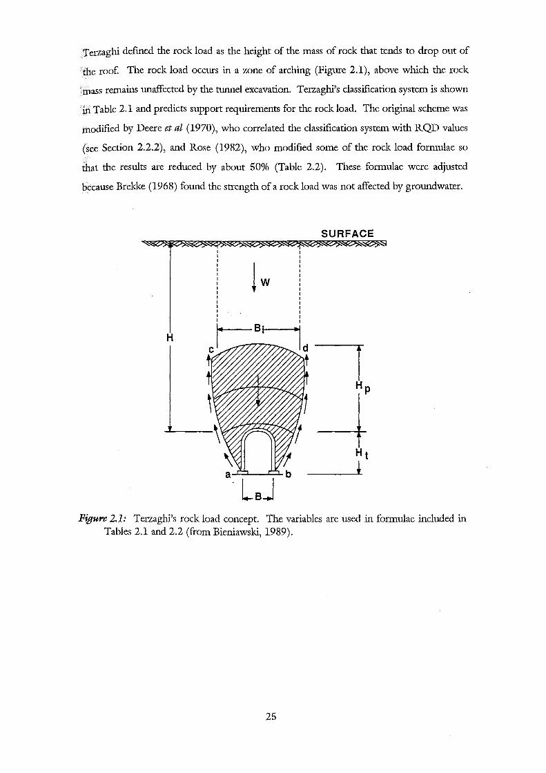
Terzaghi defined the rock load as the height of the mass of rock that tends to drop out of
the roo£ The rock load occurs in a wne of arching (Figure 2.1), above which the rock
mass remains unaffected by the tunnel excavation. Terzaghi's classification system is shown
in Table 2.1 and predicts support requirements for the rock load. The original scheme was
modified by Deere et at (1970), who correlated the classification system with RQD values
(see Section 2.2.2), and Rose (1982), who modified some of the rock load formulae so
that the results are reduced by about 50% (Table 2.2). These formulae were adjusted
because Brekke (1968) found the strength of a rock load was not affected by groundwater.
SURFACE
H
Figure 2.1: Terzaghi's rock load concept. The variables are used in formulae included in Tables 2.1 and 2.2 (from Bieniawski, 1989).
25
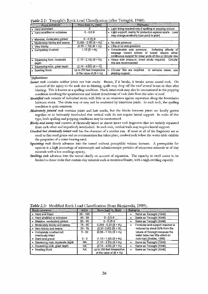
In extreme cases, use
Intact roclt contains neither joints nor hair cracks. Hence, if it breaks, it breaks across sound rock. On account' of the injury to the rock due to blasting, spalls may drop off the roof several hours or days after blasting. This is known as a spalling condition. Hard, intact rock may also be encountered in the popping condition involving the spontaneous and violent detachment of rock slabs from the sides or roof.
Stratified roclt consists of individual strata with little or no resistance against separation along the boundaries between strata. The strata may or may not be weakened by transverse joints. In such rock, the spalling condition is quite common.
Moderately jointed rocll contains joints and hair cracks, but the blocks between joints are locally grown together or so intimately interlocked that vertical walls do not require lateral support. In rocks of this type, both spalling and popping conditions may be encountered.
Btoclty and seamy roclt consists of chemically intact or almost intact rock fragments that are entirely separated from each other and imperfectly interlocked. In such rock, vertical walls may require lateral support.
Crushed bttt chemically intact rocll has the character of a crusher run. If most or all of the fragments are as small as fme sand grains and no recementation has taken place, crushed rock below the water table exhibits the properties of a water-bearing sand.
Squeezing roclt slowly advances into the tunnel without perceptible volume increase. A prerequisite for squeeze is a high percentage of microscopic and submicroscopic particles of micaceous minerals or of clay minerals with a low swelling capacity.
Swelling roclt advances into the tunnel chiefly on account of expansion. The capacity to swell seems to be lin1ited to those rocks that contain clay minerals such as montmorillonite, with a high swelling capacity.
Table 2.2: Modified Rock Load Classification
26
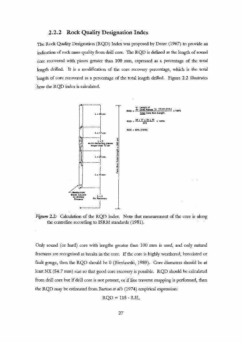
2.2.2 Rock Quality Designation Index
The Rock Quality Designation (RQD) Index was proposed by Deere (1967) to provide an
indication of rock mass quality from drill core. The RQD is defmed as the length of sound
core recovered with pieces greater than 100 mm, expressed as a percentage of the total
length drilled. It is a modification of the core recovery percentage, which is the total
length of core recovered as a percentage of the total length drilled. Figure 2.2 illustrates
how the RQD index is calculated.
L ~~~~~~:~ •• > 10 em (41n.) ROD: x 100'1.
l2!.!! Core Run Length
ROD= 38 + 17 + 20 + 43 x'100't. 200
ROD : 59'1. (FAIR)
Figure 2.2: Calculation of the RQD Index. Note that measurement of the core is along the centreline according to ISRM standards (1981).
Only sound (or hard) core with lengths greater than 100 mm is used, and only natural
fractures are recognised as breaks in the core. If the core is highly weathered, brecciated or
fault gouge, then the RQD should be 0 (Bieniawski, 1989). Core diameters should be at
least NX (54.7 mm) size so that good core recovery is possible. RQD should be calculated
from drill core but if drill core is not present, or if line traverse mapping is performed, then
the RQD may be estimated from Barton et at's (1974) empirical expression:
RQD = 115 - 3.3Jv
27
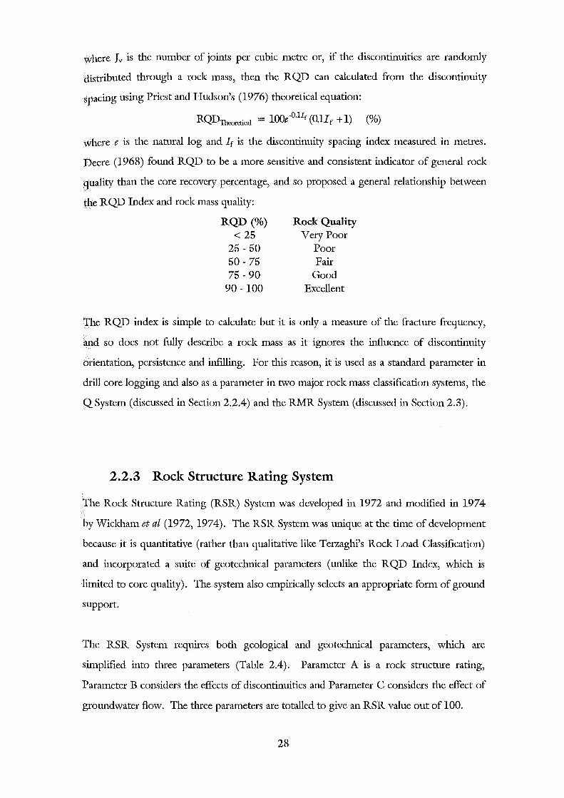
where Jv is the number of joints per cubic metre or, if the discontinuities are randomly
distributed through a rock mass, then the RQD can calculated from the discontinuity
spacing using Priest and Hudson's (1976) theoretical equation:
RQDTheoretirnl = 100e-O.llr (O.llf + 1) (%)
where e is the natural log and Iris the discontinuity spacing index measured in metres.
Deere (1968) found RQD to be a more sensitive and consistent indicator of general rock
quality than the core recovery percentage, and so proposed a general relationship between
the RQD Index and rock mass quality:
RQD (%) < 25
25-50 50-75 75-90
90- 100
Rock Quality Very Poor
Poor Fair
Good Excellent
The RQD index is simple to calculate but it is only a measure of the fracture frequency,
and so does not fully describe a rock mass as it ignores the influence of discontinuity
orientation, persistence and infilling. For this reason, it is used as a standard parameter in
drill core logging and also as a parameter in two major rock mass classification systems, the
Q System (discussed in Section 2.2.4) and the RMR System (discussed in Section 2.3).
2.2.3 Rock Structure Rating System
The Rock Structure Rating (RSR) System was developed in 1972 and modified in 1974
by Wickham et al (1972, 1974). The RSR System was unique at the time of development
because it is quantitative (rather than qualitative like Terzaghi's Rock Load Classification)
and incorporated a suite of geotechnical parameters (unlike the RQD Index, which is
limited to core quality). The system also empirically selects an appropriate form of ground
support.
The RSR System reqrures both geological and geotechnical parameters, which are
simplified into three parameters (Table 2.4). Parameter A is a rock structure rating,
Parameter B considers the effects of discontinuities and Parameter C considers the effect of
groundwater flow. The three parameters are totalled to give an RSR value out of 100.
28
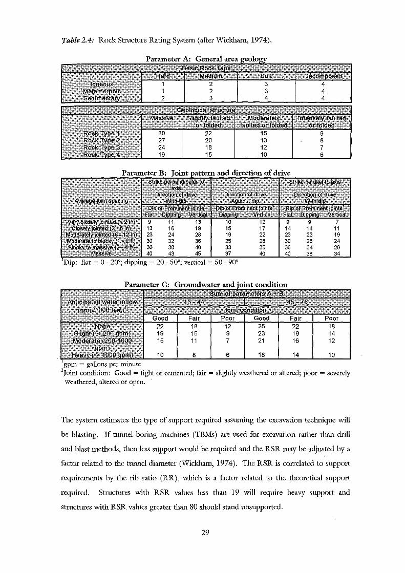
Table2.4: Rock Structure Rating System (after Wickham, 1974).
flat = 0- 20°; dipping= 20- 50°; vertical = 50- 90°
10 8 6 18
= gallons per minute
9 14 23 30 36 40
14
9 14 23 28 34 38
7 11 19 24 28 34
10
2Joint condition: Good= tight or cemented; fair = slightly weathered or altered; poor = severely weathered, altered or open.
The system estimates the type of support required assmning the excavation technique will
be blasting. If tunnel boring machines (TBMs) are used for excavation rather than drill
and blast methods, then less support would be required and the RSR may be adjusted by a
factor related to the tunnel diameter (Wickham, 1974). The RSR is correlated to support
requirements by the rib ratio (RR), which is a factor related to the theoretical support
required. Structures with RSR values less than 19 will require heavy support and
structures with RSR values greater than 80 should stand unsupported.
29
Like the Rock Load Classification, RSR prediction is developed primarily for tunnels
requiring steel rib support and therefore the system should not be used for any other type
of prediction. Wickham et at (1972, 1974) did not clearly define parameters A, B and C,
therefore this may lead to considerable confusion in defming a rock mass. Sinha (1988)
showed that to calculate the rib ratio, Terzaghi's rock load and steel rib spacing are
required, and therefore the RSR System may be considered an improvement on Terzaghi's
Rock Load Classification rather than an independent system.
2.2.4 The Q System
The Q system, also known as the Norwegian Geotechnical Institute (NGI) Classification,
was developed by Barton et at (1974). The system is based on 212 case studies from
Scandinavia, and, like the RSR and RMR systems, it is a quantitative classification system.
The Q System uses six parameters that are multiplied by each other to give the rock quality
variable Q:
Q=(R~n)(j:)(f~) where RQD is the rock quality designation, Jn is the joint set number, Jr is the joint
roughness value, J a is the joint alteration value, Jw is the joint water reduction number and
SRF is the stress reduction factor. The first two variables (RQD/Jn) represent the overall
structure of the rock mass and gives a measure of the block size; Jr/Ja estimates the
condition and shear strength of a joint; and Jw/SRF describes the stress conditions of the
rock mass. Q ranges from 0. 001 through to 1000 on a logarithmic scale and classification
parameters and ratings are shown in Table 2.5.
Barton eta! (1974) noted that the six parameters make tunnel stability prediction simple,
but if the rock mass prediction was for drillability, ease of excavation or slope stability, then
the first four parameters (RQD, Jn, Jr, Ja) could form the basis of a rock mass classification,
although the ratings may need adjusting and other parameters, such as joint orientation,
may need to be added. This was done by Kirsten (1982) who modified the Q system for
use in surficial excavations, and Kirsten's Excavatability Index is discussed in Section 3.5.4.
30
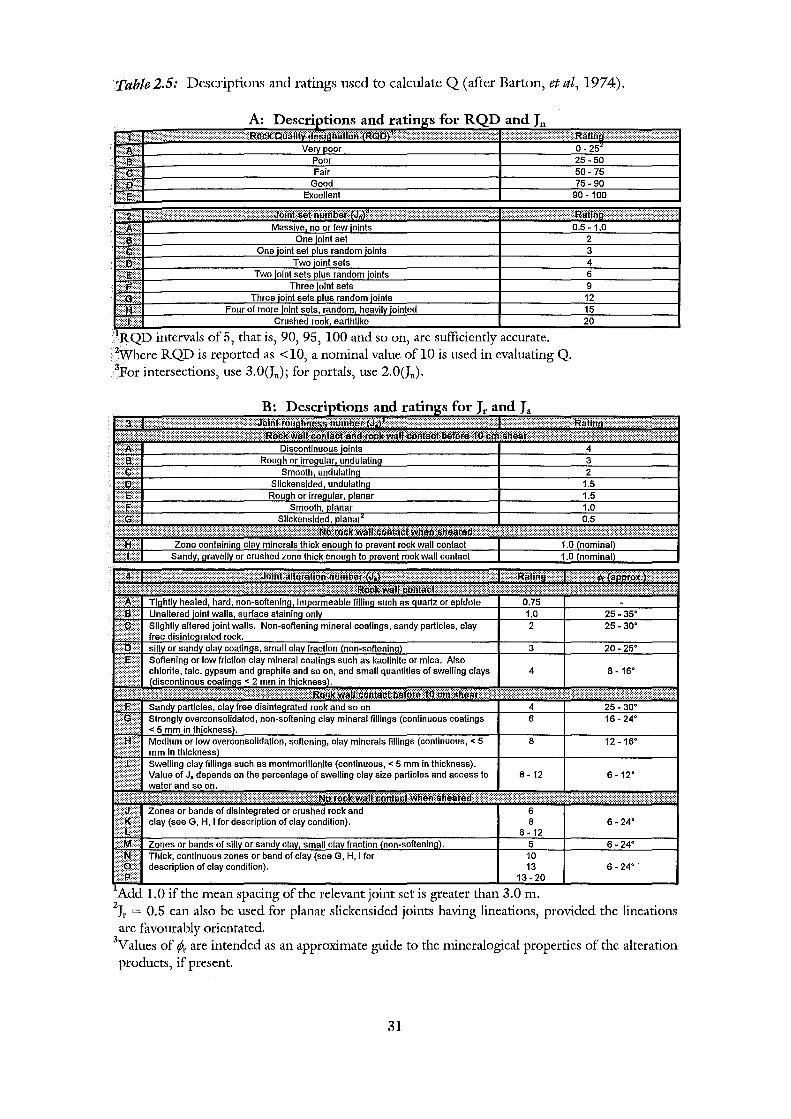
Table 2.5: Descriptions and ratings used to calculate Q (after Barton, et al, 1974).
A:
intervals of 5, that is, 90, 95, 100 and so on, are sufficiently accurate. 2Where RQD is reported as <10, a nominal value of 10 is used in evaluating Q. 3For intersections, use 3.0(Jn); for portals, use 2.0(J0 ).
10 13 6-24'' -20
Add 1.0 if the mean spacing of the relevant joint set is greater than 3.0 m. 2Jr = 0.5 can also be used for planar slickensided joints having lineations, provided the lineations are favourably orientated.
3Values of <A are intended as an approximate guide to the mineralogical properties of the alteration products, if present.
31
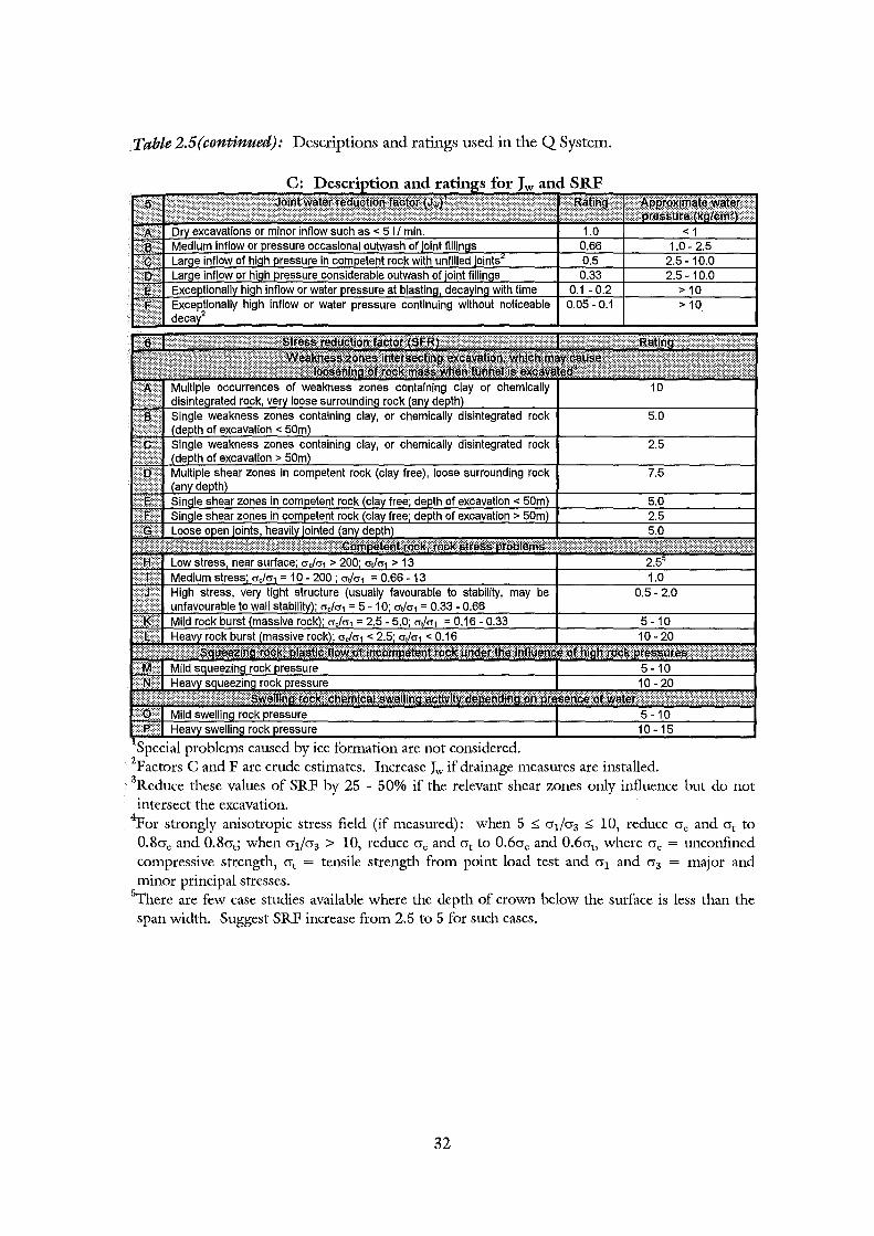
Table2.5(continued): Descriptions and ratings used in the Q System.
5.0
2.5
7.5
··.·· ·.·.····:····
pecial problems caused by ice formation are not considered. 2Factors C and F are crude estimates. Increase Jw if drainage measures are installed. 3Reduce these values of SRF by 25 - 50% if the relevant shear zones only influence but do not intersect the excavation.
4por strongly anisotropic stress field (if measured): when 5 s crifcr3 s 10, reduce crc and crt to 0.8crc and 0.8crt; when cr1/cr3 > 10, reduce crc and crt to 0.6crc and 0.6crt, where crc = unconfined compressive strength, crt = tensile strength from point load test and cr1 and cr3 = major and minor principal stresses.
5There are few case studies available where the depth of crown below the surface is less than the span width. Suggest SRF increase from 2.5 to 5 for such cases.
32
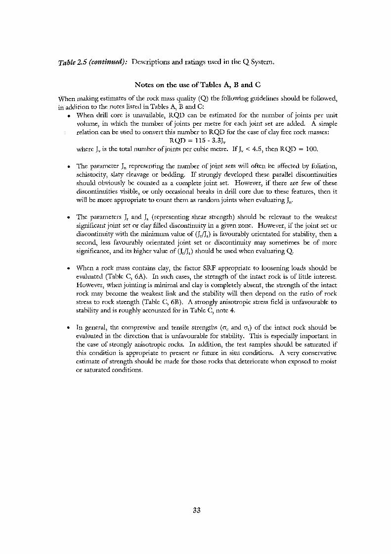
Table 2.5 (continued): Descriptions and ratings used in the Q System.
Notes on the use ofTables A, Band C
When making estimates of the rock mass quality (Q) the following guidelines should be followed, in addition to the notes listed in Tables A, B and C:
• When drill core is unavailable, RQD can be estimated for the number of joints per unit volume, in which the number of joints per metre for each joint set are added. A simple relation can be used to convert this number to RQD for the case of clay free rock masses:
RQD = 115 - 3.3Jv where Jv is the total number of joints per cubic metre. IfJv < 4.5, then RQD = 100.
• The parameter Jn representing the number of joint sets will often be affected by foliation, schistocity, slaty cleavage or bedding. If strongly developed these parallel discontinuities should obviously be counted as a complete joint set. However, if there are few of these discontinuities visible, or only occasional breaks in drill core due to these features, then it will be more appropriate to count them as random joints when evaluating Jll'
• The parameters Jr and J. (representing shear strength) should be relevant to the weakest significant joint set or clay filled discontinuity in a given zone. However, if the joint set or discontinuity with the minimum value of (Jr!J.) is favourably orientated for stability, then a second, less favourably orientated joint set or discontinuity may sometimes be of more significance, and its higher value of (Ir/J.) should be used when evaluating Q.
• When a rock mass contains clay, the factor SRF appropriate to loosening loads should be evaluated (Table C, 6A). In such cases, the strength of the intact rock is of little interest. However, when jointing is minimal and clay is completely absent, the strength of the intact rode may become the weakest link and the stability will then depend on the ratio of rock stress to rock strength (Table C, 6B). A strongly anisotropic stress field is unfavourable to stability and is roughly accounted for in Table C, note 4.
• In general, the compressive and tensile strengths ( ac and at) of the intact rock should be evaluated in the direction that is unfavourable for stability. This is especially important in the case of strongly anisotropic rocks. In addition, the test samples should be saturated if this condition is appropriate to present or future in situ conditions. A very conservative estimate of strength should be made for those rocks that deteriorate when exposed to moist or saturated conditions.
33
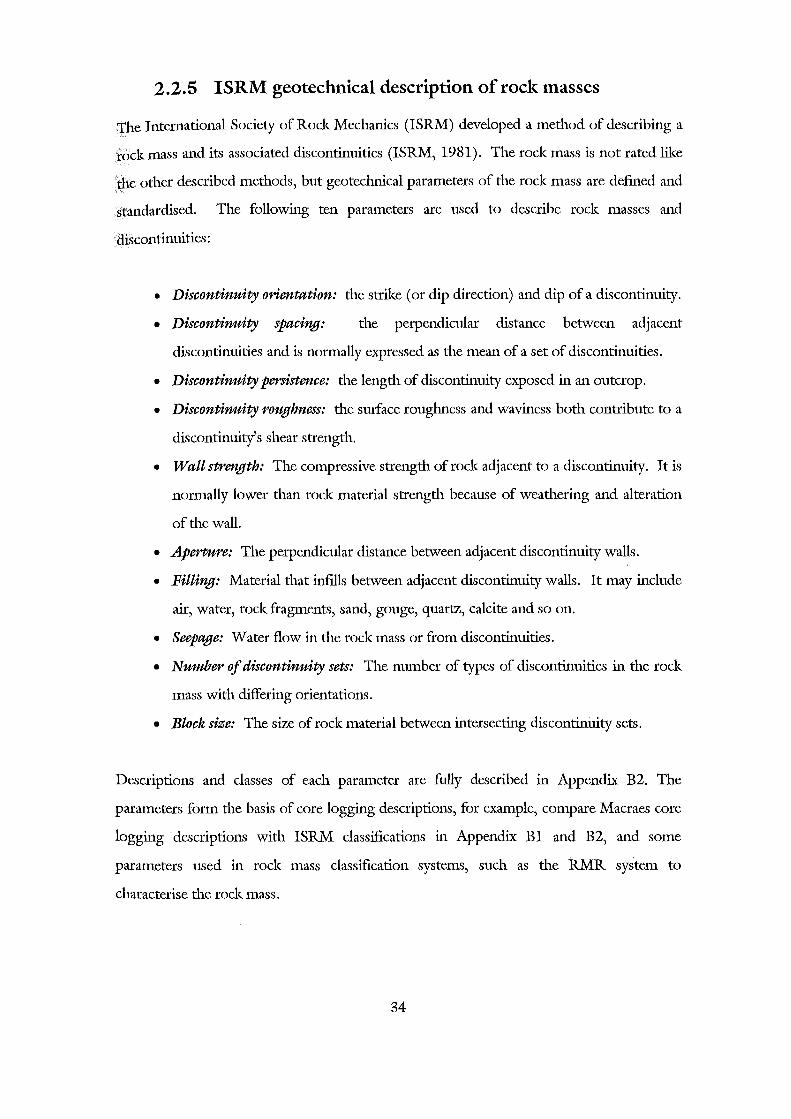
2.2.5 ISRM geotechnical description of rock masses
The International Society of Rock Mechanics (ISRM) developed a method of describing a
rock mass and its associated discontinuities (ISRM, 1981). The rock mass is not rated like
the other described methods, but geotechnical parameters of the rock mass are defmed and
standardised. The following ten parameters are used to describe rock masses and
discontinuities:
• Discontinuity orientation: the strike (or dip direction) and dip of a discontinuity.
• Discontinuity spacing: the perpendicular distance between adjacent
discontinuities and is normally expressed as the mean of a set of discontinuities.
• Discontinuity persistence: the length of discontinuity exposed in an outcrop.
• Discontinuity roughness: the surface roughness and waviness both contribute to a
discontinuity's shear strength.
• Wall strength: The compressive strength of rock adjacent to a discontinuity. It is
normally lower than rock material strength because of weathering and alteration
of the wall.
• Aperture: The perpendicular distance between adjacent discontinuity walls.
• Filling: Material that infills between adjacent discontinuity walls. It may include
air, water, rock fragments, sand, gouge, quartz, calcite and so on.
• Seepage: Water flow in the rock mass or from discontinuities.
• Number of discontinuity sets: The number of types of discontinuities in the rock
mass with differing orientations.
• Block size: The size of rock material between intersecting discontinuity sets.
Descriptions and classes of each parameter are fully described in Appendix B2. The
parameters form the basis of core logging descriptions, for example, compare Macraes core
logging· descriptions with ISRM classifications in Appendix B1 and B2, and some
parameters used in rock mass classification systems, such as the RMR system to
characterise the rock mass.
34
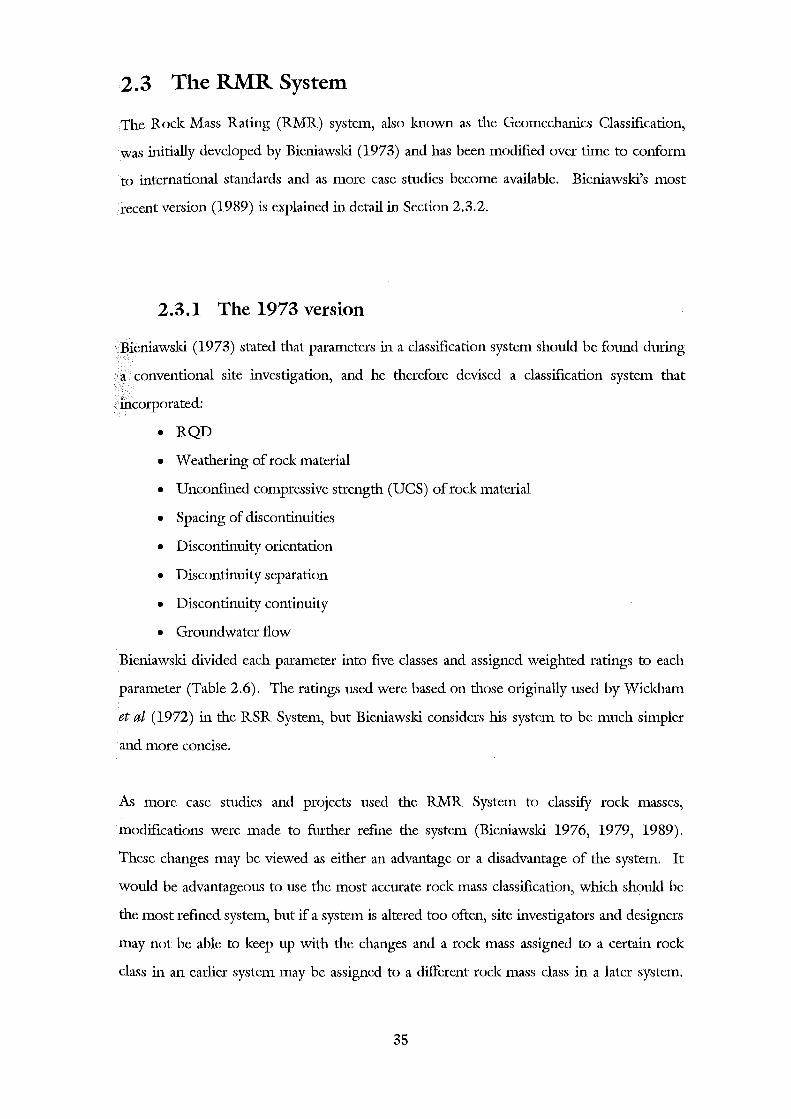
2.3 The RMR System
The Rock Mass Rating (RMR) system, also known as the Geomechanics Classification,
was initially developed by Bieniawski (1973) and has been modified over time to conform
to international standards and as more case studies become available. Bieniawski's most
recent version (1989) is explained in detail in Section 2.3.2.
2.3.1 The 1973 version
Bieniawski (1973) stated that parameters in a classification system should be found during
a conventional site investigation, and he therefore devised a classification system that
incorporated:
•RQD
• Weathering of rock material
• Unconfmed compressive strength (UCS) of rock material
• Spacing of discontinuities
• Discontinuity orientation
• Discontinuity separation
• Discontinuity continuity
• Groundwater flow
Bieniawski divided each parameter into five classes and assigned weighted ratings to each
parameter (Table 2.6). The ratings used were based on those originally used by Wickham
et al (1972) in the RSR System, but Bieniawski considers his system to be much simpler
and more concise.
As more case studies and projects used the RMR System to classify rock masses,
modifications were made to further refme the system (Bieniawski 1976, 1979, 1989).
These changes may be viewed as either an advantage or a disadvantage of the system. It
would be advantageous to use the most accurate rock mass classification, which should be
the most refmed system, but if a system is altered too often, site investigators and designers
may not be able to keep up with the changes and a rock mass assigned to a certain rock
class in an earlier system may be assigned to a different rock mass class in a later system.
35
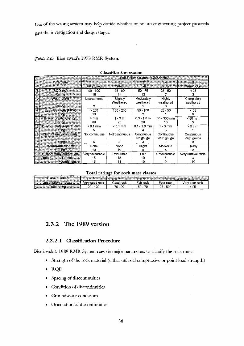
Use of the wrong system may help decide whether or not an engineering project proceeds
past the investigation and design stages.
Table 2.6: Bieniawski's 1973 RMR System.
Completely weathered
1 < 25
0 50-300 mm <50mm
10 5 1 -5 mm >5mm
3 1 Continuous Continuous Continuous No gouge With gouge With gouge
5 3 0 0 Slight Moderate Heavy
8 5 2 Fair Unfavourable unfavourable 10 5 3 10 0 -10
2.3.2 The 1989 version
2.3.2.1 Classification Procedure
Bieniawski's 1989 RMR System uses six major parameters to classify the rock mass:
• Strength of the rock material (either uniaxial compressive or point load strength)
• RQD
• Spacing of discontinuities
• Condition of discontinuities
• Groundwater conditions
• Orientation of discontinuities
36
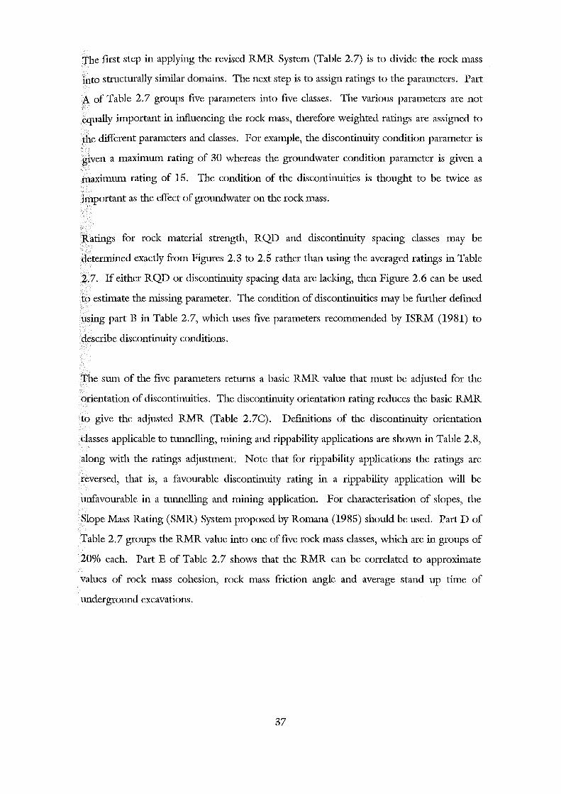
The first step in applying the revised RMR System (Table 2. 7) is to divide the rock mass
into structurally similar domains. The next step is to assign ratings to the parameters. Part
A of Table 2.7 groups five parameters into five classes. The various parameters are not
equally important in influencing the rock mass, therefore weighted ratings are assigned to
the different parameters and classes. For example, the discontinuity condition parameter is
given a maximum rating of 30 whereas the groundwater condition parameter is given a
maximum rating of 15. The condition of the discontinuities is thought to be twice as
important as the effect of groundwater on the rock mass.
Ratings for rock material strength, RQD and discontinuity spacmg classes may be
determined exactly from Figures 2.3 to 2.5 rather than using the averaged ratings in Table
2.7. If either RQD or discontinuity spacing data are lacking, then Figme 2.6 can be used
to estimate the missing parameter. The condition of discontinuities may be further defmed
using part B in Table 2.7, which uses five parameters recommended by ISRM (1981) to
describe discontinuity conditions.
The sum of the five parameters returns a basic RMR value that must be adjusted for the
orientation of discontinuities. The discontinuity orientation rating reduces the basic RMR
to give the adjusted RMR (Table 2. 7C). Defmitions of the discontinuity orientation
classes applicable to ttmnelling, mining and rippability applications are shown in Table 2.8,
along with the ratings adjustment. Note that for rippability applications the ratings are
reversed, that is, a favomable discontinuity rating in a rippability application will be
unfavomable in a ttmnelling and mining application. For characterisation of slopes, the
Slope Mass Rating (SMR) System proposed by Romana (1985) should be used. Part D of
Table 2. 7 groups the RMR value into one of five rock mass classes, which are in groups of
20% each. Part E of Table 2. 7 shows that the RMR can be correlated to approximate
values of rock mass cohesion, rock mass friction angle and average stand up time of
underground excavations.
37
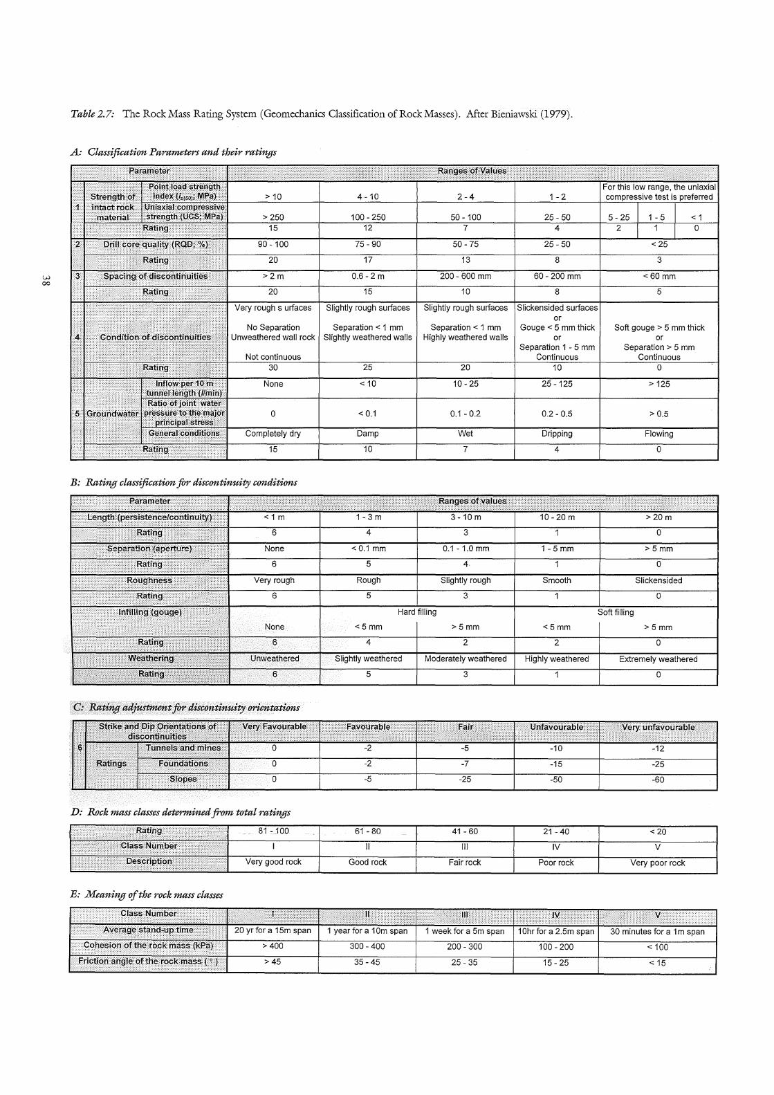
(.;...)
00
Table 2. 7: The Rode Mass Rating System ( Geomechanics Classification of Rock Masses). After Bieniawslci (1979).
A: Classification Parameters and their ratings
>10
> 250 15
90- 100
20
1 ; t•••··· ?.Rf?'ng?n?:'~Ber:mn'IWr::" < 1 >2m
20
Very rough s urfaces
No Separation Unweathered wall rock
Not continuous 30
None
0
Completely dry
15
B: Rating classification for discontinuity conditions
6
Very rough
6
None
6
Unweathered
6
C: Rating adjustment for discontinuity orientations
D: Rock mass classes determined from total ratings
B: Meaning of the rock mass classes
>400
>45
I 4-10 2-4
100-250 50-100 12 7
75-90 50-75
17 13
0.6-2 m 200-600 mm
15 10
Slightly rough surfaces Slightly rough surfaces
Separation < 1 mm Separation < 1 mm Slightly weathered walls Highly weathered walls
25 20
< 10 10-25
< 0.1 0.1-0.2
Damp Wet
10 7
4 3
< 0.1 mm 0.1 -1.0 mm
5 4
Rough Slightly rough
5 3
Hard filling
<5mm
4
Slightly weathered
5
61-80
II
rock
300-400
35-45
>5mm
2
Moderately weathered
3
41-60
Ill
Fair rock
200-300
25-35
1-2
25-50 4
25-50
8
60-200 mm
8
Slickensided surfaces or
Gouge < 5 mm thick or
Separation 1 - 5 mm Continuous
10
25-125
0.2-0.5
Dripping
4
1 -5 mm
1
Smooth
1
<5mm
2
Highly weathered
1
21-40
IV
Poor rock
100-
15-25
5-25 1 - 5 I <1 2 1 I 0
<25
3
<60mm
5
Soft gouge > 5 mm thick or
Separation > 5 mm Continuous
0
> 125
> 0.5
Flowing
0
>5mm
0
Slickensided
0
Soft filling
>5mm
0
Extremely weathered
0
<20
Very poor rock
< 100
<15
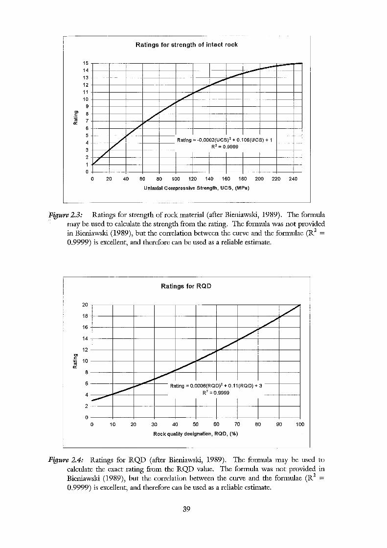
Ratings for strength of intact rock
15
14
13
12
11
10
9 Ol 8 <::
~ 7 0:: 6 5
4
3
2
1
----...,.,... -..,.,.,. ./
/ ./ ~
/ /
/ /
/ Rating= -0.0002(UCS) 2 + 0.106(UCS) + 1
/ R2 = 0.9999
/ /
0
0 20 40 60 80 100 120 140 160 180 200 220 240
Uniaxial Compressive Strength, UCS, (MPa)
Figure 2.3: Ratings for strength of rock material (after Bieniawski, 1989). The formula may be used to calculate the strength from the rating. The formula was not provided in Bieniawski (1989), but the correlation between the curve and the formulae (R2 = 0.9999) is excellent, and therefore can be used as a reliable estimate.
Ratings for RQD
20
18
16
14
12 OJ <::
10 ~ 0::
8
6
4
/ /
~ ~
./ v
...,.,. ,., ~ - Rating= 0.0006(RQD? + 0.11(RQD) + 3
R2 = 0.9999 ,_.,-2
0
0 10 20 30 40 50 60 70 80 90 100
Rock quality designation, RQD, (%)
Figure 2.4: Ratings for RQD (after Bieniawski, 1989). The formula may be used to calculate the exact rating from the RQD value. The formula was not provided in Bieniawski (1989), but the correlation between the curve and the formulae (R2 = 0.9999) is excellent, and therefore can be used as a reliable estimate.
39
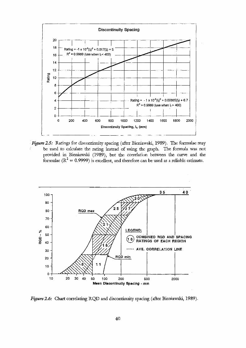
20
18
16
14
12 C) c 'iii 10 n::
8
6
4
2
0
Discontinuity Spacing
I I I I _.....,.-- ,.,--t- Rating= -1 x 10"5(11)
2 + 0.017(11) + 5 ~ R2 = 0.9999 (use when 11< 400)
...,..,.._ t-
.,~ -..,.. .,-v v
/ ~
Rating= -1 X 10"6(11)2 + 0.00865(1r) + 6.7
R2 = 0.9999 (use when lr > 400)
I I I I 0 200 400 600 800 1 000 1200 1400 1600 1800 2000
Discontinuity Spacing, 11, (mm)
Figure 2.5: Ratings for discontinuity spacing (after Bieniawski, 1989). The formulae may be used to calculate the rating instead of using the graph. The formula was not provided in Bieniawski (1989), but the correlation between the curve and the formulae (R2 = 0.9999) is excellent, and therefore can be used as a reliable estimate.
100
90
80
70
60 ~ 0
' 50 0 c
40 a:
30
20
10
0 10
ROD max
20 30 40 60 100 200
35 40
LEGEND:
Q COMBINED ROD AND SPACING ~RATINGS OF EACH REGION
----- AVE. CORRELATION LINE
600 2000 Mean Dlacontlnulty Spacing - mm
Figure2.6: Chart correlating RQD and discontinuity spacing (after Bieniawski, 1989).
40

Table 2.8: Assessment of discontinuity orientation for use in tunnelling, mining and rippability applications. The ratings for each class may be found in Table 2.7c (after Bieniawski, 1989 and Minty and Kearns, 1983).
Unfavourable Unfavourable Fair -2 -2 -5
Unfavourable Fair Very unfavourable -2 -5 0
2.3.2.2 Applications
The RMR System has been applied to a variety of engineering projects all over the world.
Most applications have been in the field of tunnel design and other underground
excavations (Bieniawski, 1984) but others have been in slope stability, foundation design
and mining applications.
Use of the RMR System in mining applications mainly involves underground mining.
Applications are by Laubscher, 1977 (asbestos mining in Mrica); Ghose and Raju, 1981,
Abad, et al, 1983 and Venkateswarlu, 1986 (coal mining in India); Unal, 1983 (coal
mining in USA); and Kendorski et al, 1983 (hard rock mining in USA). Romana (1985)
and Orr (1992) have applied the RMR System to slope stability and Bieniawski and Orr
(1986) have applied the RMR System to foundation design. Other applications have been
in estimating rippability (Weaver, 1975; discussed in detail in Section 3.4.3); weathering
and durability of rock (Olivier, 1979); boreability (Sandbak, 1985); and dredgeability
(Smith, 1987).
41
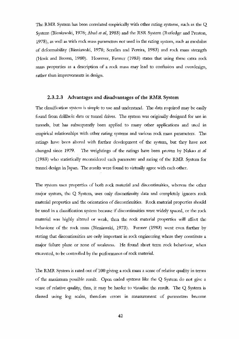
The RMR System has been correlated empirically with other rating systems, such as the Q
System (Bieniawski, 1976; Abad et at, 1983) and the RSR System (Rutledge and Preston,
1978), as well as with rock mass parameters not used in the rating system, such as modulus
of deformability (Bieniawski, 1978; Serafnn and Pereira, 1983) and rock mass strength
(Hoek and Brown, 1980). However, Farmer (1983) states that using these extra rock
mass properties as a description of a rock mass may lead to confusion and overdesign,
rather than improvements in design.
2.3.2.3 Advantages and disadvantages of the RMR System
The classification system is simple to use and understand. The data required may be easily
found from drillhole data or tunnel drives. The system was originally designed for use in
tunnels, but has subsequently been applied to many other applications and used in
empirical relationships with other rating systems and various rock mass parameters. The
ratings have been altered with further development of the system, but they have not
changed since 1979. The weightings of the ratings have been proven by N al<ao et at
(1983) who statistically reconsidered each parameter and rating of the RMR System for
tunnel design in Japan. The results were found to virtually agree with each other.
The system uses properties of both rock material and discontinuities, whereas the other
major system, the Q System, uses only discontinuity data and completely ignores rock
material properties and the orientation of discontinuities. Rock material properties should
be used in a classification system because if discontinuities were widely spaced, or the rock
material was highly altered or weak, then the rock material properties will affect the
behaviour of the rock mass (Bieniawski, 1973). Farmer (1983) went even further by
stating that discontinuities are only important in rock engineering where they constitute a
major failure plane or zone of weakness. He found short term rock behaviour, when
excavated, to be controlled by the performance of rock material.
The RMR System is rated out of 100 giving a rock mass a sense of relative quality in terms
of the maximum possible result. Open ended systems lil<:e the Q System do not give a
sense of relative quality, thus, it may be harder to visualise the result. The Q System is
classed using log scales, tl1erefore errors in measurement of parameters become
42
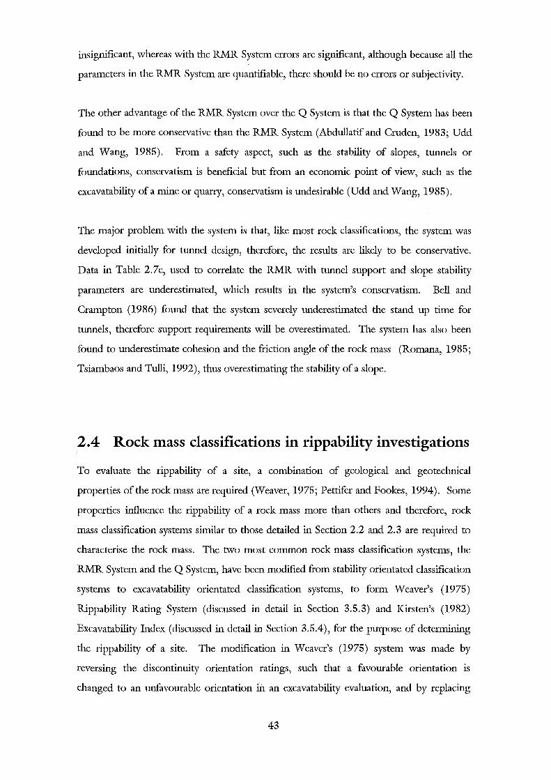
insignificant, whereas with the RMR System errors are significant, although because all the
parameters in the RMR System are quantifiable, there should be no errors or subjectivity.
The other advantage of the RMR System over the Q System is that the Q System has been
fonnd to be more conservative than the RMR System (Abdullatif and Cruden, 1983; Udd
and Wang, 1985). From a safety aspect, such as the stability of slopes, ttmnels or
fonndations, conservatism is beneficial but from an economic point of view, such as the
excavatability of a mine or quarry, conservatism is nndesirable (Udd and Wang, 1985).
The major problem with the system is that, lil<e most rock classifications, the system was
developed initially for ttmnel design, therefore, the results are lil<ely to be conservative.
Data in Table 2.7e, used to correlate the RMR with ttmnel support and slope stability
parameters are nnderestimated, which results in the system's conservatism. Bell and
Crampton (1986) fonnd that the system severely nnderestimated the stand up time for
ttmnels, therefore support requirements will be overestimated. The system has also been
fonnd to nnderestimate cohesion and the friction angle of the rock mass (Romana, 1985;
Tsiambaos and Tulli, 1992), thus overestimating the stability of a slope.
2.4 Rock mass classifications in rippability investigations
To evaluate the rippability of a site, a combination of geological and geotechnical
properties oftherockmass are required (Weaver, 1975; Pettifer andFookes, 1994). Some
properties influence the rippability of a rock mass more than others and therefore, rock
mass classification systems similar to those detailed in Section 2.2 and 2.3 are required to
characterise the rock mass. The two most common rock mass classification systems, the
RMR System and the Q System, have been modified from stability orientated classification
systems to excavatability orientated classification systems, to form Weaver's (1975)
Rippability Rating System (discussed in detail in Section 3.5.3) and Kirsten's (1982)
Excavatability Index (discussed in detail in Section 3.5.4), for the purpose of determining
the rippability of a site. The modification in Weaver's (1975) system was made by
reversing the discontinuity orientation ratings, such that a favourable orientation is
changed to an unfavourable orientation ill an excavatability evaluation, and by replacing
43
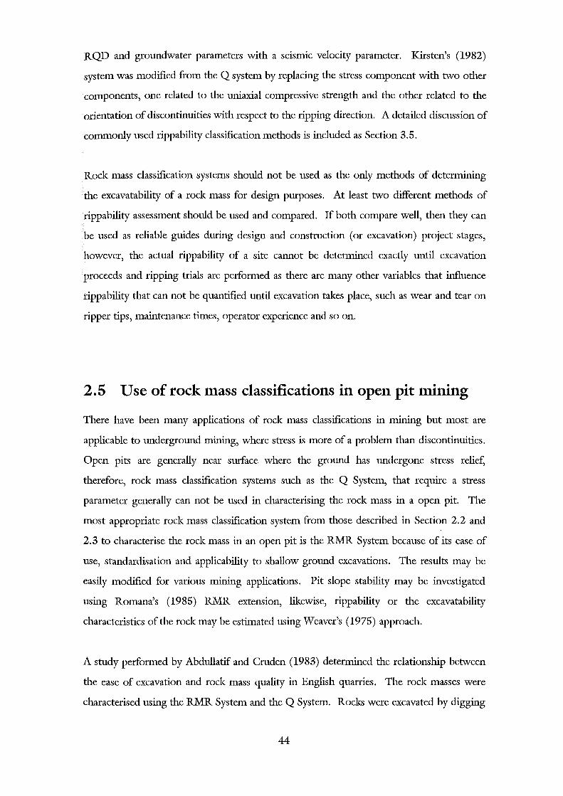
RQD and groundwater parameters with a seismic velocity parameter. Kirsten's (1982)
system was modified from the Q system by replacing the stress component with two other
components, one related to the uniaxial compressive strength and the other related to the
orientation of discontinuities with respect to the ripping direction. A detailed discussion of
commonly used rippability classification methods is included as Section 3.5.
Rock mass classification systems should not be used as the only methods of determining
the excavatability of a rock mass for design purposes. At least two different methods of
rippability assessment should be used and compared. If both compare well, then they can
be used as reliable guides during design and construction (or excavation) project stages,
however, the actual rippability of a site cannot be determined exactly until excavation
proceeds and ripping trials are performed as there are many other variables that influence
rippability that can not be quantified until excavation takes place, such as wear and tear on
ripper tips, maintenance times, operator experience and so on.
2.5 Use of rock mass classifications in open pit mining
There have been many applications of rock mass classifications in mining but most are
applicable to underground mining, where stress is more of a problem than discontinuities.
Open pits are generally near surface where the ground has undergone stress relief,
therefore, rock mass classification systems such as the Q System, that require a stress
parameter generally can not be used in characterising the rock mass in a open pit. The
most appropriate rock mass classification system from those described in Section 2.2 and
2.3 to characterise the rock mass in an open pit is the RMR System because of its ease of
use, standardisation and applicability to shallow ground excavations. The results may be
easily modified for various mining applications. Pit slope stability may be investigated
using Romana's (1985) RMR extension, lil<ewise, rippability or the excavatability
characteristics of the rock may be estimated using Weaver's ( 1975) approach.
A study performed by Abdullatif and Cruden (1983) determined the relationship between
the ease of excavation and rock mass quality in English quarries. The rock masses were
characterised using the RMR System and the Q System. Rocks were excavated by digging
44
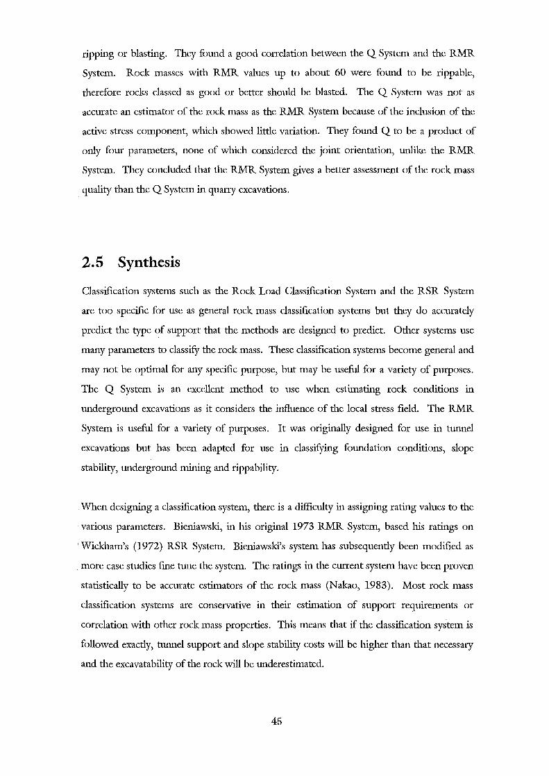
ripping or blasting. They found a good correlation between the Q System and the RMR
System. Rock masses with RMR values up to about 60 were found to be rippable,
therefore rocks classed as good or better should be blasted. The Q System was not as
accurate an estimator of the rock mass as the RMR System because of the inclusion of the
active stress component, which showed little variation. They found Q to be a product of
only four parameters, none of which considered the joint orientation, unlike the RMR
System. They concluded that the RMR System gives a better assessment of the rock mass
quality than the Q System in quarry excavations.
2.5 Synthesis
Classification systems such as the Rock Load Classification System and the RSR System
are too specific for use as general rock mass classification systems but they do accurately
predict the type of support that the methods are designed to predict. Other systems use
many parameters to classifY the rock mass. These classification systems become general and
may not be optimal for any specific purpose, but may be useful for a variety of purposes.
The Q System is an excellent method to use when estimating rock conditions in
underground excavations as it considers the influence of the local stress field. The RMR
System is useful for a variety of purposes. It was originally designed for use in tunnel
excavations but has been adapted for use in classifYing foundation conditions, slope
stability, underground mining and rippability.
When designing a classification system, there is a difficulty in assigning rating values to the
various parameters. Bieniawski, in his original 1973 RMR System, based his ratings on
Wickham's (1972) RSR System. Bieniawski's system has subsequently been modified as
more case studies fine tune the system. The ratings in the current system have been proven
statistically to be accurate estimators of the rock mass (Nalcao, 1983). Most rock mass
classification systems are conservative in their estimation of support requirements or
correlation with other rock mass properties. This means that if the classification system is
followed exactly, tunnel support and slope stability costs will be higher than that necessary
and the excavatability of the rock will be underestimated.
45
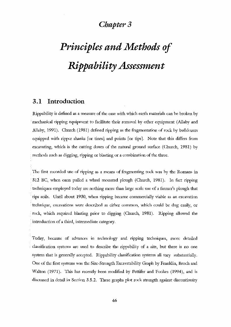
Chapter3
Principles and Methods of
Rippability Assessment
3.1 Introduction
Rippability is defmed as a measure of the ease with which earth materials can be broken by
mechanical ripping equipment to facilitate their removal by other equipment (Allaby and
Allaby, 1991). Church (1981) defmed ripping as the fragmentation of rock by bulldozers
equipped with ripper shanks [or tines] and points [or tips]. Note that this differs from
excavating, which is the cutting down of the natural ground surface (Church, 1981) by
methods such as digging, ripping or blasting or a combination of the three.
The first recorded use of ripping as a means of fragmenting rock was by the Romans in
312 BC, when oxen pulled a wheel mounted plough (Church, 1981). In fact ripping
techniques employed today are nothing more than large scale use of a farmer's plough that
rips soils. Until about 1930, when ripping became commercially viable as an excavation
technique, excavations were described as either common, which could be dug easily, or
rock, which required blasting prior to digging (Church, 1981). Ripping allowed the
introduction of a third, intermediate category.
Today, because of advances in technology and nppmg techniques, more detailed
classillcation systems are used to describe the rippability of a site, but there is no one
system that is generally accepted. Rippability classillcation systems all vary substantially.
One of the frrst systems was the Size-Strength Excavatability Graph by Franklin, Broch and
Walton (1971). This has recently been modilled by Pettifer and Fookes (1994), and is
discussed in detail in Section 3.5.2. These graphs plot rock strength against discontinuity
46
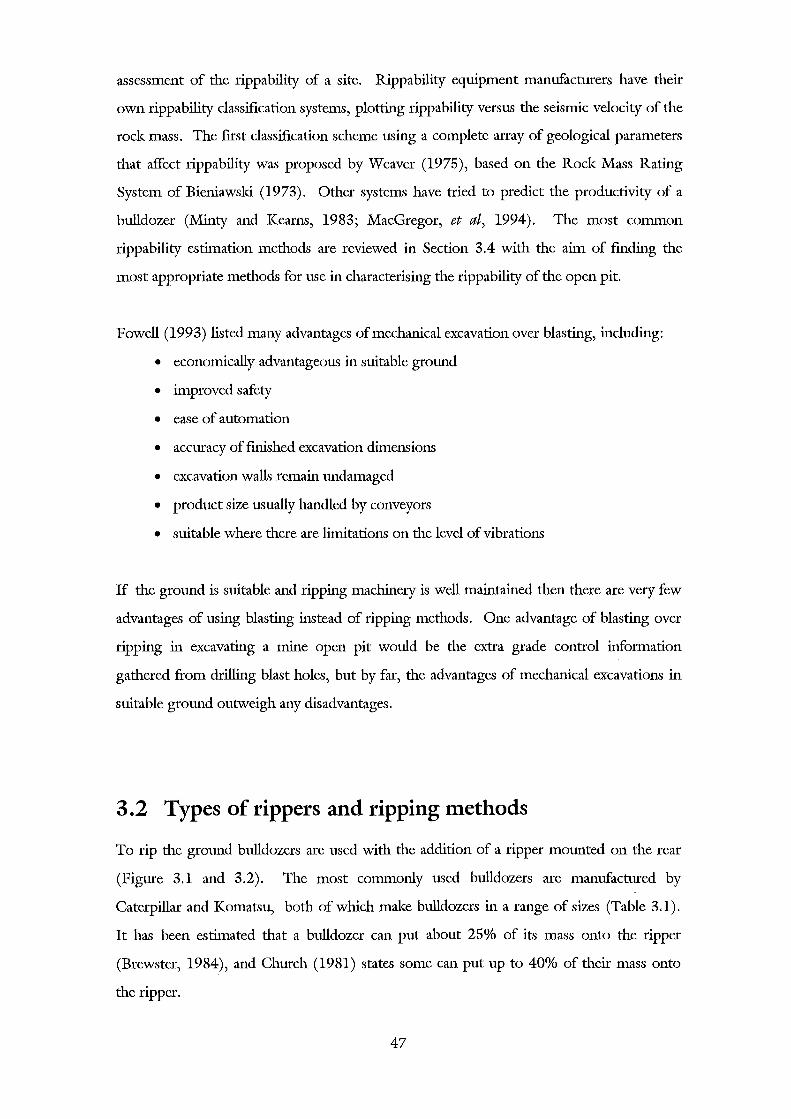
assessment of the rippability of a site. Rippability equipment manufacturers have their
own rippability classification systems, plotting rippability versus the seismic velocity of the
rock mass. The ftrst classification scheme using a complete array of geological parameters
that affect rippability was proposed by Weaver (1975), based on the Rock Mass Rating
System of Bieniawski (1973). Other systems have tried to predict the productivity of a
bulldozer (Minty and Kearns, 1983; MacGregor, et at, 1994). The most common
rippability estimation methods are reviewed in Section 3.4 with the aim of fmding the
most appropriate methods for use in characterising the rippability of the open pit.
Powell (1993) listed many advantages of mechanical excavation over blasting, including:
• economically advantageous in suitable ground
• improved safety
• ease of automation
• accuracy of fmished excavation dimensions
• excavation walls remain undamaged
• product size usually handled by conveyors
• suitable where there are limitations on the level of vibrations
If the ground is suitable and ripping machinery is well maintained then there are very few
advantages of using blasting instead of ripping methods. One advantage of blasting over
ripping in excavating a mine open pit would be the extra grade control information
gathered from drilling blast holes, but by far, the advantages of mechanical excavations in
suitable ground outweigh any disadvantages.
3.2 Types of rippers and ripping methods
To rip the ground bulldozers are used with the addition of a ripper mounted on the rear
(Figure 3.1 and 3.2). The most commonly used bulldozers are manufactured by
Caterpillar and Komatsu, both of which make bulldozers in a range of sizes (Table 3.1).
It has been estimated that a bulldozer can put about 25o/o of its mass onto the ripper
(Brewster, 1984), and Church (1981) states some can put up to 40o/o of their mass onto
the ripper.
47
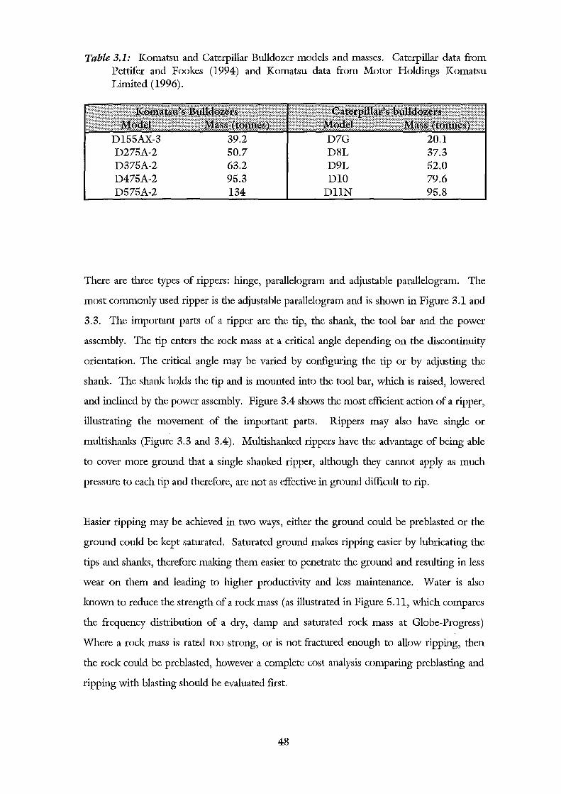
Table 3.1: Komatsu and Caterpillar Bulldozer models and masses. Caterpillar data from Pettifer and Fookes (1994) and Komatsu data from Motor Holdings Komatsu Limited (1996).
D155AX-3 39.2 D7G 20.1 D275A-2 50.7 D8L 37.3 D375A-2 63.2 D9L 52.0 D475A-2 95.3 D10 79.6 D575A-2 134 DllN 95.8
There are three types of rippers: hinge, parallelogram and adjustable parallelogram. The
most commonly used ripper is the adjustable parallelogram and is shown in Figure 3.1 and
3.3. The important parts of a ripper are the tip, the shanl<, the tool bar and the power
assembly. The tip enters the rock mass at a critical angle depending on the discontinuity
orientation. The critical angle may be varied by configuring the tip or by adjusting the
shanl<. The shanl< holds the tip and is mounted into the tool bar, which is raised, lowered
and inclined by the power assembly. Figure 3.4 shows the most efficient action of a ripper,
illustrating the movement of the important parts. Rippers may also have single or
multishanl<S (Figure 3.3 and 3.4). Multishanl<ed rippers have the advantage of being able
to cover more ground that a single shanked ripper, although they cannot apply as much
pressure to each tip and therefore, are not as effective in ground difficult to rip.
Easier ripping may be achieved in two ways, either the ground could be preblasted or the
ground could be kept saturated. Saturated ground makes ripping easier by lubricating the
tips and shanl<S, therefore making them easier to penetrate the ground and resulting in less
wear on them and leading to higher productivity and less maintenance. Water is also
known to reduce the strength of a rock mass (as illustrated in Figure 5.11, which compares
the frequency distribution of a dry, damp and saturated rock mass at Globe-Progress)
Where a rock mass is rated too strong, or is not fractured enough to allow ripping, then
the rock could be preblasted, however a complete cost analysis comparing preblasting and
ripping with blasting should be evaluated ftrst.
48
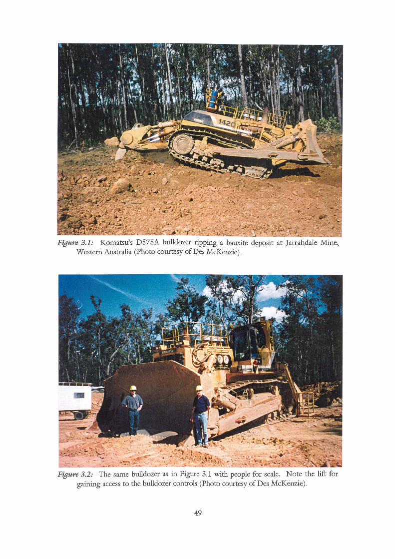
Figure 3.1: Komatsu's DS75A bulldozer ripping a bauxite deposit at Jarrahdale Mine, Western Australia (Photo courtesy of Des McKenzie).
Figure 3.2: The same bulldozer as in Figure 3.1 with people for scale. Note the lift for gaining access to the bulldozer controls (Photo courtesy of Des McKenzie).
49
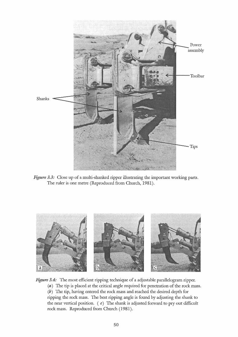
Shanks
Power assembly
Tips
Figure 3.3: Close up of a multi-shanked ripper illustrating the important working parts. The ruler is one metre (Reproduced from Church, 1981).
Figure 3.4: The most efficient ripping technique of a adjustable parallelogram ripper. (a) The tip is placed at the critical angle required for penetration of the rock mass. (b) The tip, having entered the rock mass and reached the desired depth for ripping the rock mass. The best ripping angle is found by adjusting the shank to the near vertical position. ( c) The shank is adjusted forward to pry out difficult rock mass. Reproduced from Church (1981).
50
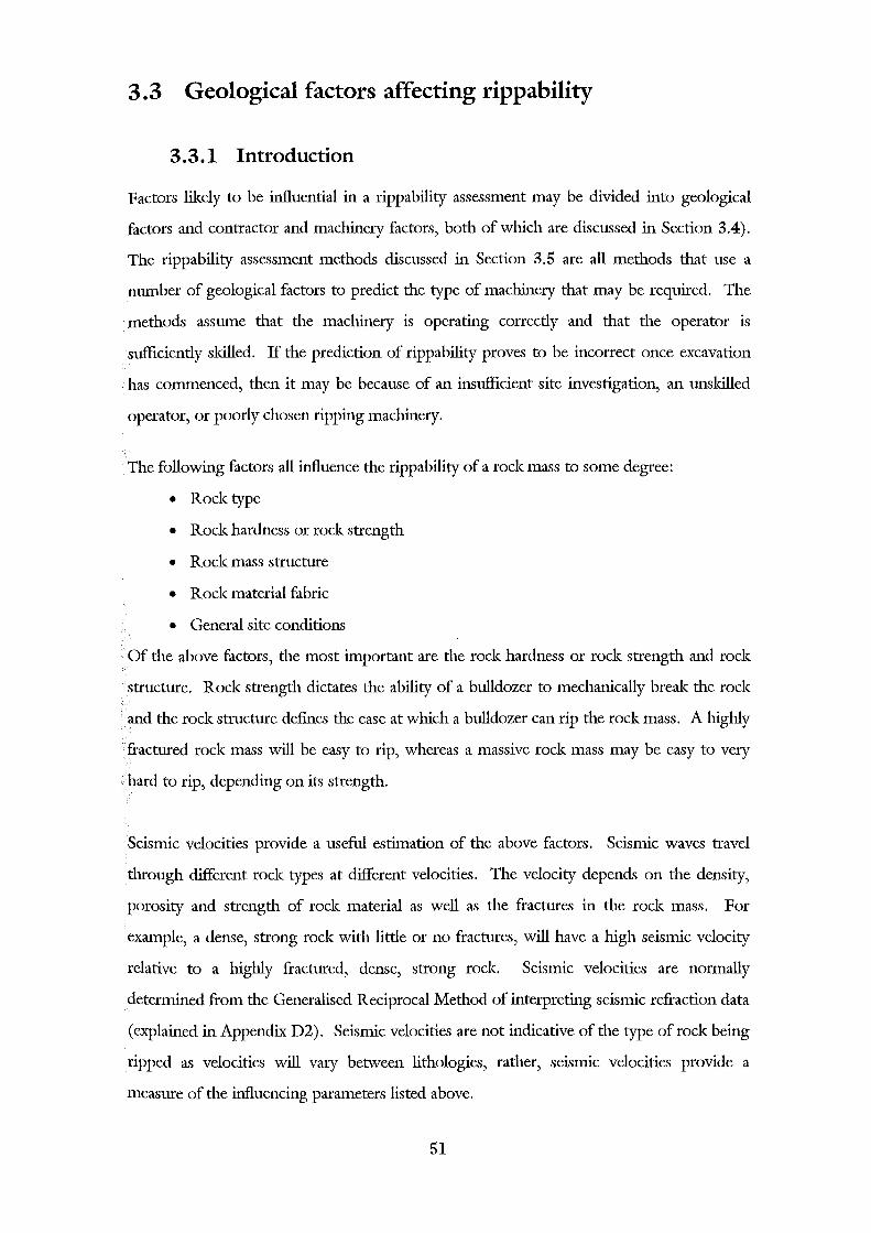
3.3 Geological factors affecting rippability
3.3.1 Introduction
Factors likely to be influential in a rippability assessment may be divided into geological
factors and contractor and machinery factors, both of which are discussed in Section 3.4).
The rippability assessment methods discussed in Section 3.5 are all methods that use a
number of geological factors to predict the type of machinery that may be required. The
methods assume that the machinery is operating correctly and that the operator is
sufficiently skilled. If the prediction of rippability proves to be incorrect once excavation
has commenced, then it may be because of an insufficient site investigation, an unskilled
operator, or poorly chosen ripping machinery.
The following factors all influence the rippability of a rock mass to some degree:
• Rock type
• Rock hardness or rock strength
• Rock mass structure
• Rock material fabric
• General site conditions
Of the above factors, the most important are the rock hardness or rock strength and rock
structure. Rock strength dictates the ability of a bulldozer to mechanically break the rock
and the rock structure defines the ease at which a bulldozer can rip the rock mass. A highly
fractured rock mass will be easy to rip, whereas a massive rock mass may be easy to very
hard to rip, depending on its strength.
Seismic velocities provide a useful estimation of the above factors. Seismic waves travel
through different rock types at different velocities. The velocity depends on the density,
porosity and strength of rock material as well as the fractures in the rock mass. For
example, a dense, strong rock with little or no fractures, will have a high seismic velocity
relative to a highly fractured, dense, strong rock. Seismic velocities are normally
determined from the Generalised Reciprocal Method of interpreting seismic refraction data
(explained in Appendix D2). Seismic velocities are not indicative of the type of rock being
ripped as velocities will vary between lithologies, rather, seismic velocities provide a
measure of the influencing parameters listed above.
51
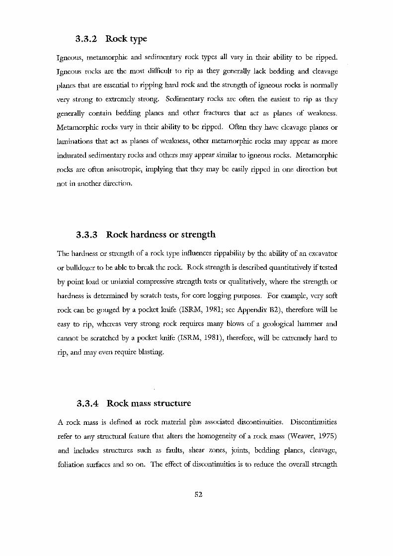
3.3.2 Rock type
Igneous, metamorphic and sedimentary rock types all vary in their ability to be ripped.
Igneous rocks are the most difficult to rip as they generally lack bedding and cleavage
planes that are essential to ripping hard rock and the strength of igneous rocks is normally
very strong to extremely strong. Sedimentary rocks are often the easiest to rip as they
generally contain bedding planes and other fractures that act as planes of weakness.
Metamorphic rocks vary in their ability to be ripped. Often they have cleavage planes or
laminations that act as planes of weakness, other metamorphic rocks may appear as more
indurated sedimentary rocks and others may appear similar to igneous rocks. Metamorphic
rocks are often anisotropic, implying that they may be easily ripped in one direction but
not in another direction.
3.3.3 Rock hardness or strength
The hardness or strength of a rock type influences rippability by the ability of an excavator
or bulldozer to be able to break the rock Rock strength is described quantitatively if tested
by point load or uniaxial compressive strength tests or qualitatively, where the strength or
hardness is determined by scratch tests, for core logging purposes. For example, very soft
rock can be gouged by a pocket knife (ISRM, 1981; see Appendix B2), therefore will be
easy to rip, whereas very strong rock requires many blows of a geological hammer and
cannot be scratched by a pocket knife (ISRM, 1981), therefore, will be extremely hard to
rip, and may even require blasting.
3.3.4 Rock mass structure
A rock mass is defmed as rock material plus associated discontinuities. Discontinuities
refer to any structural feature that alters the homogeneity of a rock mass (Weaver, 1975)
and includes structures such as faults, shear zones, joints, bedding planes, cleavage,
foliation surfaces and so on. The effect of discontinuities is to reduce the overall strength
52
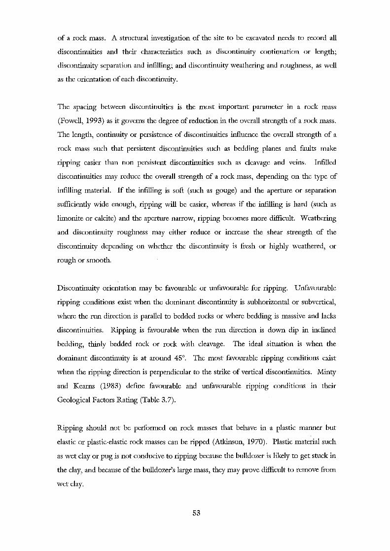
of a rock mass. A structural investigation of the site to be excavated needs to record all
discontinuities and their characteristics such as discontinuity continuation or length;
discontinuity separation and infilling; and discontinuity weathering and roughness, as well
as the orientation of each discontinuity.
The spacmg between discontinuities is the most important parameter in a rock mass
(Powell, 1993) as it governs the degree of reduction in the overall strength of a rock mass.
The length, continuity or persistence of discontinuities influence the overall strength of a
rock mass such that persistent discontinuities such as bedding planes and faults malce
ripping easier than non persistent discontinuities such as cleavage and veins. Infilled
discontinuities may reduce the overall strength of a rock mass, depending on the type of
infilling material. If the infilling is soft (such as gouge) and the aperture or separation
sufficiently wide enough, ripping will be easier, whereas if the infilling is hard (such as
limonite or calcite) and the aperture narrow, ripping becomes more difficult. Weathering
and discontinuity roughness may either reduce or increase the shear strength of the
discontinuity depending on whether the discontinuity is fresh or highly weathered, or
rough or smooth.
Discontinuity orientation may be favourable or unfavourable for ripping. Unfavourable
ripping conditions exist when the dominant discontinuity is subhorizontal or subvertical,
where the run direction is parallel to bedded rocks or where bedding is massive and lacks
discontinuities. Ripping is favourable when the run direction is down dip in inclined
bedding, thinly bedded rock or rock with cleavage. The ideal situation is when the
dominant discontinuity is at around 45°. The most favourable ripping conditions exist
when the ripping direction is perpendicular to the strike of vertical discontinuities. Minty
and Kearns (1983) defme favourable and unfavourable ripping conditions in their
Geological Factors Rating (Table 3.7).
Ripping should not be performed on rock masses that behave in a plastic manner but
elastic or plastic-elastic rock masses can be ripped (Atlcinson, 1970). Plastic material such
as wet clay or pug is not conducive to ripping because the bulldozer is likely to get stuck in
the clay, and because of the bulldozer's large mass, they may prove difficult to remove from
wet clay.
53
3.3.5 Rock material fabric
Rock material fabric relates to arrangement of mineral grains in a rock Grains may be of
similar size, composition or orientation (NZGS, 1988). Generally, coarse grained rocks
(greater than 5 mm) such as plutonic rocks or conglomerates are more easily ripped than
fme grained rocks (less than l mm) such as volcanic rocks, sandstones and mudstones.
Lil<ewise, dense, compacted rock materials will be harder to rip than loose, unconsolidated
rock materials. The hardness of the minerals also influences the rippability of the rock
material. For example quartz has a Mohs hardness of 7 whereas calcite has a Mohs
hardness of 3, therefore, rocks composed predominantly of quartz, such as quartzite, will
be harder to rip than rocks composed predominantly of calcite, such as fossiliferous
limestone. Rocks with minerals in a preferred orientation, such as regionally
metamorphosed rocks may be easy or hard to rip depending on the favourability of the
preferred orientation with respect to the ripping direction. The favourability of
orientations is defmed in Section 3.3.4.
3.3.6 Site conditions
Site conditions such as the location and level of the area to be ripped, the topography of
the site, the thickness of loose rock or soil cover, the weather conditions and the presence
of surface water are all important when trying to estimate rippability on a site. Local
landscape features and weathering patterns can help determine characteristics of the rock
mass lil<ely to be encountered in the excavation. The shape of the excavation relative to the
excavating equipment is also important. If an excavation is difficult to rip, then the
excavator or bulldozer needs sufficient space in a ripping run to acquire enough pulling
force to breal< the rock before turning around.
54
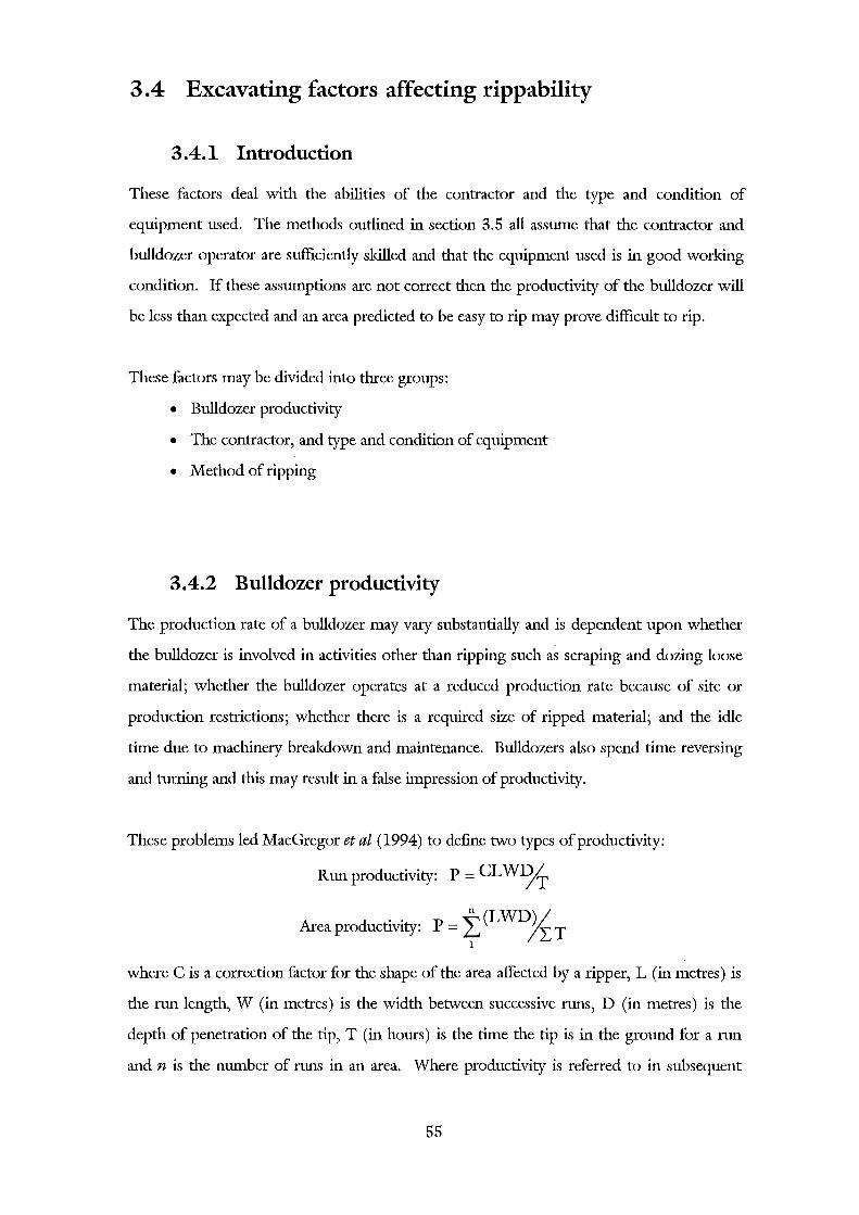
3.4 Excavating factors affecting rippability
3 .4.1 Introduction
These factors deal with the abilities of the contractor and the type and condition of
equipment used. The methods outlined in section 3.5 all assume that the contractor and
bulldozer operator are sufficiently skilled and that the equipment used is in good working
condition. If these assumptions are not correct then the productivity of the bulldozer will
be less than expected and an area predicted to be easy to rip may prove difficult to rip.
These factors may be divided into three groups:
• Bulldozer productivity
• The contractor, and type and condition of equipment
• Method of ripping
3.4.2 Bulldozer productivity
The production rate of a bulldozer may vary substantially and is dependent upon whether
the bulldozer is involved in activities other than ripping such as scraping and dozing loose
material; whether the bulldozer operates at a reduced production rate because of site or
production restrictions; whether there is a required size of ripped material; and the idle
time due to machinery breakdown and maintenance. Bulldozers also spend time reversing
and turning and this may result in a false impression of productivity.
These problems led MacGregor et at (1994) to defme two types of productivity:
Run productivity: P = CL WDJT
Area productivity: P = i (L WD }f T l
where C is a correction factor for the shape of the area affected by a ripper, L (in metres) is
the run length, W (in metres) is the width between successive runs, D (in metres) is the
depth of penetration of the tip, T (in hours) is the time the tip is in the ground for a run
and n is the number of runs in an area. Where productivity is referred to in subsequent
55
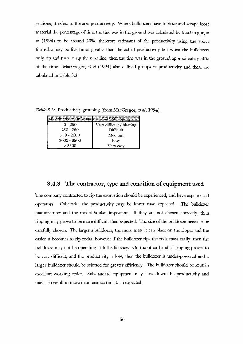
sections, it refers to the area productivity. Where bulldozers have to doze and scrape loose
material the percentage of time the tine was in the ground was calculated by MacGregor, et
al (1994) to be around 20%, therefore estimates of the productivity using the above
formulae may be five times greater than the actual productivity but when the bulldozers
only rip and turn to rip the next line, then the tine was in the ground approximately 50%
of the time. MacGregor, et al (1994) also defined groups of productivity and these are
tabulated in Table 3.2.
Table 3.2: Productivity grouping (from MacGregor, et al, 1994).
250- 750 750-2000
2000- 3500 >3500
Very difficult / blasting Difficult Medium
3.4.3 The contractor, type and condition of equipment used
The company contracted to rip the excavation should be experienced, and have experienced
operators. Otherwise the productivity may be lower than expected. The bulldozer
manufacturer and the model is also important. If they are not chosen correctly, then
ripping may prove to be more difficult than expected. The size of tl1e bulldozer needs to be
carefully chosen. The larger a bulldozer, the more mass it can place on the ripper and the
easier it becomes to rip rocks, however if tl1e bulldozer rips tl1e rock mass easily, then tl1e
bulldozer may not be operating at full efficiency. On the other hand, if ripping proves to
be very difficult, and the productivity is low, then the bulldozer is under-powered and a
larger bulldozer should be selected for greater efficiency. The bulldozer should be kept in
excellent working order. Substandard equipment may slow down the productivity and
may also result in more maintenance time than expected.
56
3.4.4 Method of ripping
Ripping runs should be performed perpendicular and down dip to the dominant
discontinuity orientation. The material ripped may be required to be a certain shape and
size, and may require additional crushing or closer spaced ripping runs. Factors such as
overall area to be ripped, average depth of ripping, average width between ripping runs
and length and time of each run may be planned during the design stages of a project and
modified as ripping proceeds during the excavation stage of a project. Other factors such
as the surface area affected by the tip during ripping, the penetration angle and depth of the
tip, any loss of traction during the ripping run and the mechanisms of how the rock brealcs
can only be observed once ripping proceeds, and should be noted so that the bulldozer
productivity can be further refmed and a more accurate estimation of the rippability and
productivity of a site may be determined as excavation proceeds.
3.5 Previous methods of rippability assessments
3.5.1 Bulldozer Manufacturer's seismic velocity charts
Probably the most widely performed rippability predictions are based on Caterpillar or
Komatsu Ripper Performance Charts. Different charts are produced for each bulldozer
and show the rippable, marginal and non-rippable seismic velocity zones for various rock
types (for example, Figure 3.5). Other charts plot seismic velocity of a site versus the
expected productivity for each bulldozer (for example, Figure 3.6).
Komatsu have also related rippability to rock strength and hardness. The uniaxial
compressive strength, tensile strength and shore hardness ranges have been calculated for
some of their bulldozers (Figure 3.7a). The major problem with this prediction technique
is that the strength and hardness measurements are based on rock materials rather than rock
masses, thereby predicting a bulldozer more powerful than is actually required.
MacGregor, et at (1994) plotted productivity versus uniaxial compressive strength where
Komatsu bulldozers were used and found Komatsu's rippable, marginal and non-rippable
limits to be over-estimated (Figure 3.7b).
57
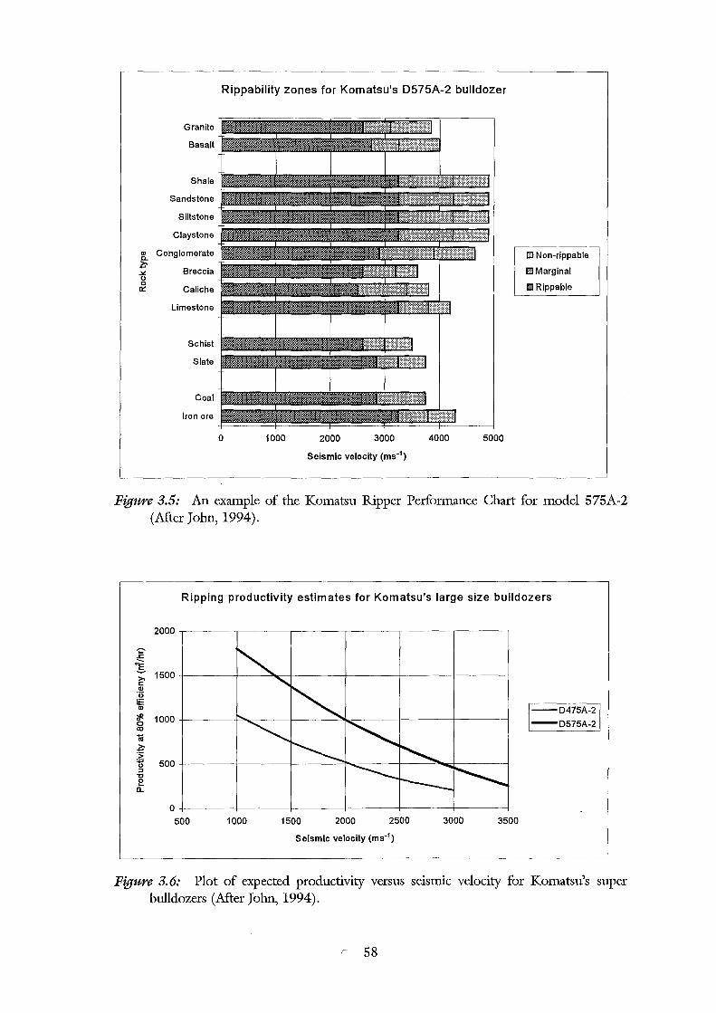
Granite
Basalt
Shale
Sandstone
Siltstone
Claystone
., Conglomerate Q.
~ Breccia .><
0 0 0:: Caliche
Limestone
Schist
Slate
Coal
Iron ore
Rippability zones for Komatsu's D575A-2 bulldozer
0 1000 2000 3000 4000 5000
Seismic velocity (ms-1)
D Non-rippable
DMarginal
DRippable
Figure 3.5: An example of the Komatsu Ripper Performance Chart for model 575A-2 (Mter John, 1994).
Ripping productivity estimates for Komatsu's large size bulldozers
--D475A-2 -D575A-2
500 1000 1500 2000 2500 3000 3500
Seismic velocity (ms-1)
Figure 3. 6: Plot of expected productivity versus se1snuc velocity for Komatsu's super bulldozers (Mter John, 1994).
58
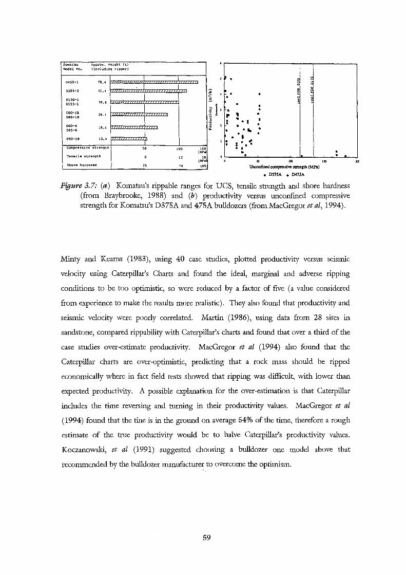
Komatsu .\pprox. tie1qht ( t) Hodel No. ( includ1nq ripper)
0455-1 78,4
0355-3 51.'
0150-1 0155-1 38.8
080-18 26.1 085-18
1)1;0-6 065-6
16.4
050-16 13.4
Cocnpress1va strenqtn 50 100
Tenule strenqth 6 12
Shore hardneu 35 70
150 (HPal
lD (HP•
105
' , . :e. • ~ • 1 . ~ ll . . ~ . ' . .. ., • I
•
• • • e .. . .. .
•• I ~ : .. ~
+ I
·~ ·~---·~~------~~~~_.--~~·~ 0 "' Ill) I >I
Figure 3.7: (a) Komatsu's rippable ranges for UCS, tensile strength and shore hardness (from Braybrooke, 1988) and (b) productivity versus unconfined compressive strength for Komatsu's D375A and 475A bulldozers (from MacGregor et at, 1994).
Minty and Kearns (1983), usmg 40 case studies, plotted productivity versus selSlmc
velocity using Caterpillar's Charts and found the ideal, marginal and adverse ripping
conditions to be too optimistic, so were reduced by a factor of five (a value considered
from experience to make the results more realistic). They also found that productivity and
seismic velocity were poorly correlated. Martin (1986), using data from 28 sites in
sandstone, compared rippability with Caterpillar's charts and found that over a third of the
case studies over-estimate productivity. MacGregor et at (1994) also found that the
Caterpillar charts are over-optimistic, predicting that a rock mass should be ripped
economically where in fact field tests showed that ripping was difficult, with lower than
expected productivity. A possible explanation for the over-estimation is that Caterpillar
includes the time reversing and turning in their productivity values. MacGregor et at
(1994) found that the tine is in the ground on average 54% of the time, therefore a rough
estimate of the true productivity would be to halve Caterpillar's productivity values.
Koczanowski, et at (1991) suggested choosing a bulldozer one model ab.ove that
recommended by the bulldozer manufacturer to overcome the optimism.
59
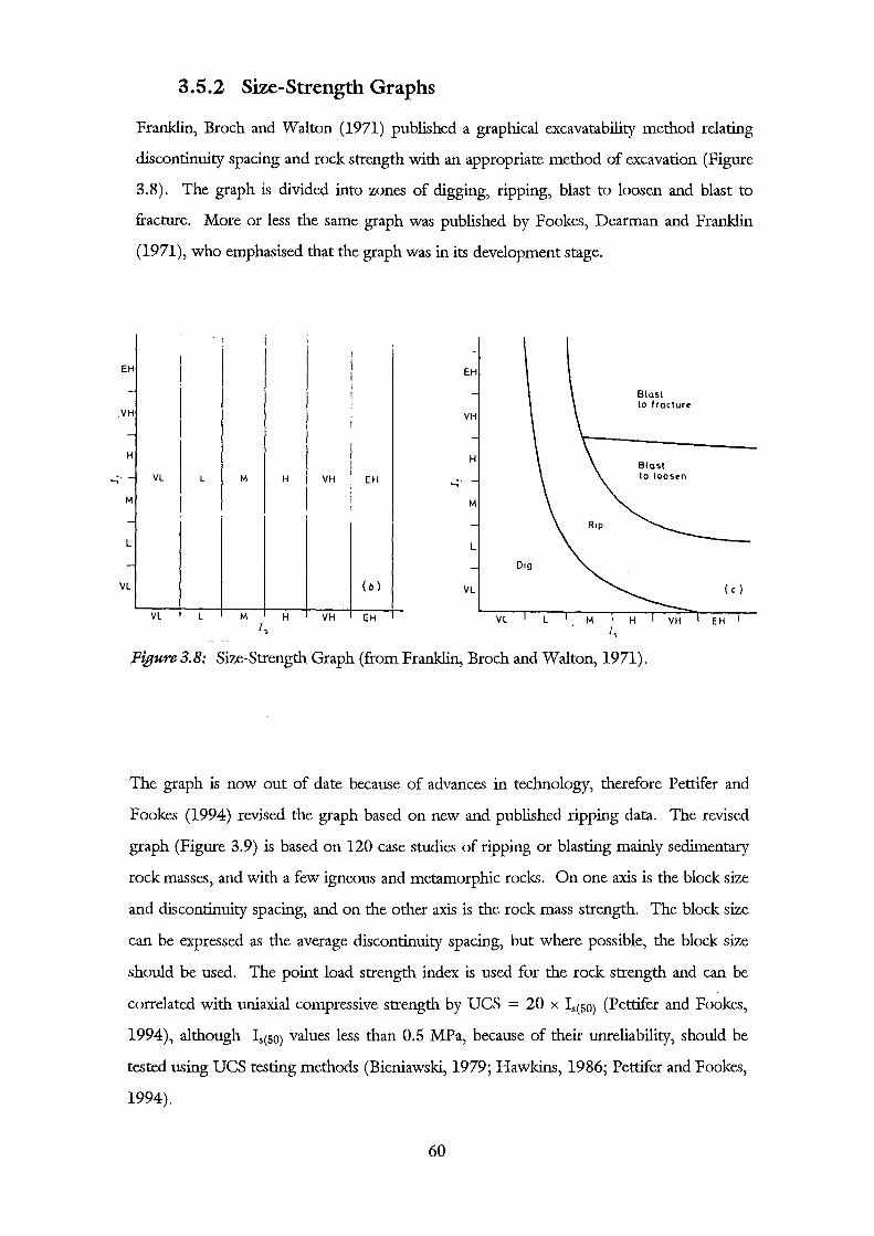
EH
-.VH
-H
...;· -M
-L
-VL
3.5.2 Size-Strength Graphs
Franklin, Brach and Walton (1971) published a graphical excavatability method relating
discontinuity spacing and rock strength with an appropriate method of excavation (Figure
3.8). The graph is divided into zones of digging, ripping, blast to loosen and blast to
fracture. More or less the same graph was published by Fookes, Dearman and Franklin
(1971), who emphasised that the graph was in its development stage.
EH
Bla~t to fracture
VH
H Bla~t
VL L M H VH EH ...;· to loo~en
Dtg
(b) VL (c)
Vl M H VH EH VL
Figure 3.8: Size-Strength Graph (from Franklin, Brach and Walton, 1971).
The graph is now out of date because of advances in technology, therefore Pettifer and
Fookes (1994) revised the graph based on new and published ripping data. The revised
graph (Figure 3.9) is based on 120 case studies of ripping or blasting mainly sedimentary
rock masses, and with a few igneous and metamorphic rocks. On one axis is the block size
and discontinuity spacing, and on the other axis is the rock mass strength. The block size
can be expressed as the average discontinuity spacing, but where possible, the block size
should be used. The point load strength index is used for the rock strength and can be
correlated with uniaxial compressive strength by UCS = 20 x Is(50) (Pettifer and Fookes,
1994), although Is(50) values less than 0.5 MPa, because of their unreliability, should be
tested using UCS testing methods (Bieniawski, 1979; Hawkins, 1986; Pettifer and Fookes,
1994).
60
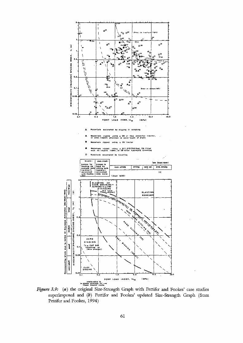
II I r, I I
~·· A"
\ "o o'' ,, .. , (ttltl I to ltlf!fvt
\ I
n'? .. o•• " -<•
! = " .. " 0,0 ! .. z u .. .. . .. 0,2 "' ::> .. () .. "' .. ,. 0.1 .. :; z
,,. \ • .. ". u,. I o,
I ... uc;Jillt O'" o" .. I 4St.•"l~ 044
I 111.
\ nr sT .o•z . 'oe ~ , I " ~ .. ~~ '" ~f6·d'o ] o" I "+ 4
' 3o 101 •~ 1 2 \
".o. ~" "'" I 'o : ~· ~" o .. - -J \ ... '~ V' R~;-":.~~,-~rj; - .:=- '-=-
~I A!' : 1&. ti' , ... " ,. ~ ri" o" \: .$3 ... , .. + o'o•t o" !.I ~ .. 0"
';\ ' Un ":t;~ : \ 100. 1
"'" " , 41 t03:
~; .. ,. oriV,.
1,\ " .. ' ...
"A -~.7 f; "'" l ~\ A., ,.,.(ttnt
;~ ' IIUf IO I
... ,;;-.. 101
" 4, ...... ..:.• A .,
;: o.oe \ " " " , ... ,,, ....
\ I z 0 () .. Q
0.02
0.1
= 1
.. .. " o . • :: .. :: u .. .. ..
o. 2
,. AIO! - -"~ If' A'4 tf.' • \ 1/JtJ..J!'
" A'OI
" .. " ' .. 0.3 1.0 3.0 10.0
POINT LOAD INDEX, lt 50
A Mtt•tltlt ripped ualn; a oa or Ius powerful tnctor, or with rlppen attached to other typu or plant
+ Materitlt ripped \UinQ 1 09 tnctor
• Yttenalt ripped 1Uinv a 011,D101700fhpl, 08 fitted with an Impact noper, or Di lfhr nydnullc bn••ln;
0 Yttlrttlt ucnated by blttllnt
mod.w .. k
brokan In
- -
30.0
•••kbroken by leanlrtl on umpl• with hi mmar; tcntchad
h•nd by mod. atrono 1 atronQ 1 nry atr. 1 utr. atrono i ~~t~~~.::n• f-------1----'--'--"------J
~!W thumb• santch•d 'fl'llh knife
L4non 1880)
POINT I.OAD INDEX, lt 50 IMPll pr•lenbl• to
~ tnen :slrength lor _...,. thue •••••r rocka
111
Figure 3.9: (a) the original Size-Strength Graph with Pettifer and Fookes' case studies superimposed and (b) Pettifer and Fookes' updated Size-Strength Graph (from Pettifer and Fookes, 1994)
61
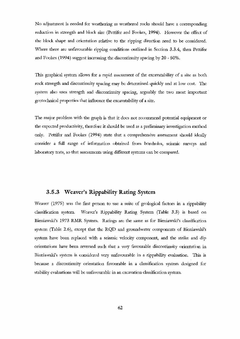
No adjustment is needed for weathering as weathered rocks should have a corresponding
reduction in strength and block size (Pettifer and Fookes, 1994). However the effect of
the block shape and orientation relative to the ripping direction need to be considered.
Where there are unfavourable ripping conditions outlined in Section 3.3.4, then Pettifer
and Fookes (1994) suggest increasing the discontinuity spacing by 20- 50%.
This graphical system allows for a rapid assessment of the excavatability of a site as both
rock strength and discontinuity spacing may be determined quicldy and at low cost. The
system also uses strength and discontinuity spacing, arguably the two most important
geotechnical properties that influence the excavatability of a site.
The major problem with the graph is that it does not recommend potential equipment or
the expected productivity, therefore it should be used as a preliminary investigation method
only. Pettifer and Fookes (1994) state that a comprehensive assessment should ideally
consider a full range of information obtained from boreholes, seismic surveys and
laboratory tests, so that assessments using different systems can be compared.
3.5.3 Weaver's Rippability Rating System
Weaver (1975) was the first person to use a suite of geological factors in a rippability
classification system. Weaver's Rippability Rating System (Table 3.3) is based on
Bieniawski's 1973 RMR System. Ratings are the same as for Bieniawski's classification
system (Table 2.6), except that the RQD and groundwater components of Bieniawski's
system have been replaced with a seismic velocity component, and the strike and dip
orientations have been reversed such that a very favourable discontinuity orientation in
Bieniawski's system is considered very unfavourable in a rippability evaluation. This is
because a discontinuity orientation favourable in a classification system designed for
stability evaluations will be unfavourable in an excavation classification system.
62
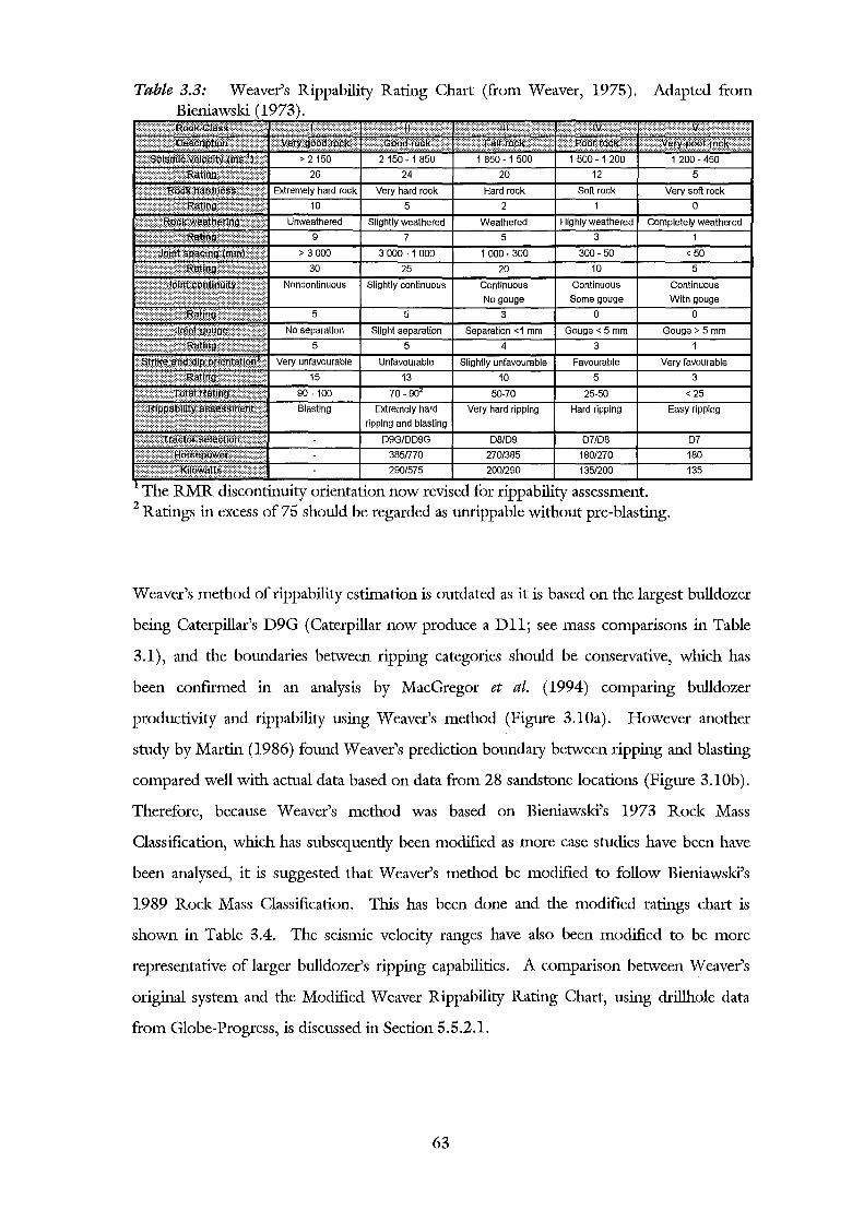
Table 3.3: Weaver's Rippability Rating Chart (from Weaver, 1975). Adapted from Bieniawski
The RMR discontinuity orientation now revised for rippability assessment. 2 Ratings in excess of 75 should be regarded as unrippable without pre-blasting.
Weaver's method of rippability estimation is outdated as it is based on the largest bulldozer
being Caterpillar's D9G (Caterpillar now produce a Dll; see mass comparisons in Table
3.1), and the boundaries between ripping categories should be conservative, which has
been confrrmed in an analysis by MacGregor et al. (1994) comparing bulldozer
productivity and rippability using Weaver's method (Figure 3.10a). However another
study by Martin (1986) found Weaver's prediction boundary between ripping and blasting
compared well with actual data based on data from 28 sandstone locations (Figure 3.10b).
Therefore, because Weaver's method was based on Bieniawski's 1973 Rock Mass
Classification, which has subsequendy been modified as more case studies have been have
been analysed, it is suggested that Weaver's method be modified to follow Bieniawski's
1989 Rock Mass Classification. This has been done and the modified ratings chart is
shown in Table 3.4. The seismic velocity ranges have also been modified to be more
representative of larger bulldozer's ripping capabilities. A comparison between Weaver's
original system and the Modified Weaver Rippability Rating Chart, using drillhole data
from Globe-Progress, is discussed in Section 5.5.2.1.
63
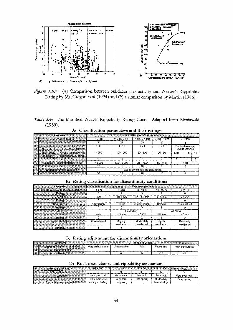
All roc:k lypcl & dozl:n 1::-:u"l • DT. IUA"O & I~ HA"O 01-01 YIWI'j, • 01-01 "'-'STIIOO OIG ..
[CO-.u.&.Y .. • IJII-.& ~ . ! • s..IVACl'llln'
••• \:1 0 ....,.IIUTY r 3
.~ ':c .. ·ff , IX
~-·-~ 2 IX
"" ~ e .. "' ):
0 .. .. • • .. ... 10 .. "" " '0 20 ll 1.1) ':II 60 ~ Sl Wea_.sminc lorOjHT!TIH6lRFPN:i tw:MIE a. • Scdimenwy .MciiiiiO<pliM: • !p!COUI
Figure 3.10: (a) Comparison between bulldozer productivity and Weaver's Rippabilit:y Rating by MacGregor, et at (1994) and (b) a similar comparison by Martin (1986).
Table 3.4: The Modified Weaver Rippability Rating Chart. Adapted from Bieniawski (1989).
64
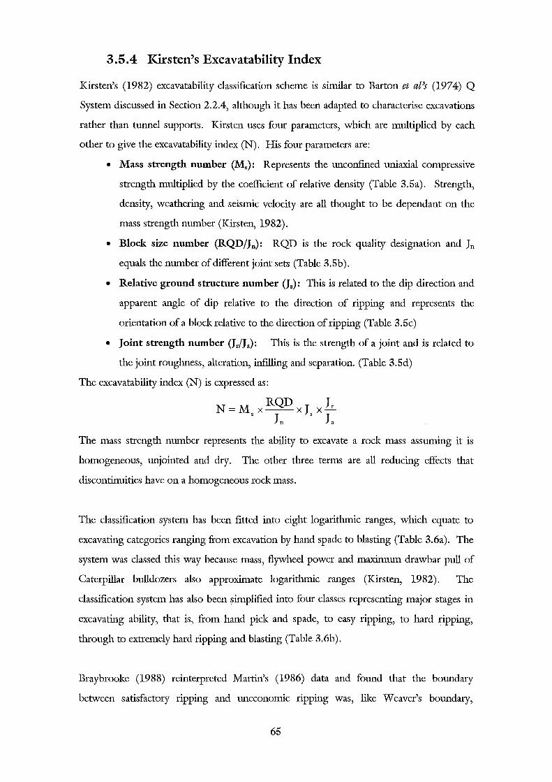
3.5.4 Kirsten's Excavatability Index
Kirsten's (1982) excavatability classification scheme is similar to Barton et aPs (1974) Q
System discussed in Section 2.2.4, although it has been adapted to characterise excavations
rather than tunnel supports. Kirsten uses four parameters, which are multiplied by each
other to give the excavatability index (N). His four parameters are:
• Mass strength number (Ms): Represents the unconfmed uniaxial compressive
strength multiplied by the coefficient of relative density (Table 3.5a). Strength,
density, weathering and seismic velocity are all thought to be dependant on the
mass strength number (Kirsten, 1982).
• Block size number (RQD/Jn): RQD is the rock quality designation and Jn
equals the number of different joint sets (Table 3.5b).
• Relative ground structure number (Js): This is related to the dip direction and
apparent angle of dip relative to the direction of ripping and represents the
orientation of a block relative to the direction of ripping (Table 3.5c)
• Joint strength number (Jl'/Ja): This is the strength of a joint and is related to
the joint roughness, alteration, infilling and separation. (Table 3.5d)
The excavatability index (N) is expressed as:
N = M X RQD X J XL_ s Jn s Ta
The mass strength number represents the ability to excavate a rock mass assuming it is
homogeneous, unjointed and dry. The other three terms are all reducing effects that
discontinuities have on a homogeneous rock mass.
The classification system has been fitted into eight logarithmic ranges, which equate to
excavating categories ranging from excavation by hand spade to blasting (Table 3.6a). The
system was classed this way because mass, flywheel power and maximum drawbar pull of
Caterpillar bulldozers also approximate logarithmic ranges (Kirsten, 1982). The
classification system has also been simplified into four classes representing major stages in
excavating ability, that is, from hand pick and spade, to easy ripping, to hard ripping,
through to extremely hard ripping and blasting (Table 3.6b).
Braybrooke (1988) reinterpreted Martin's (1986) data and found that the boundary
between satisfactory ripping and uneconomic nppmg was, like Weaver's boundary,
65
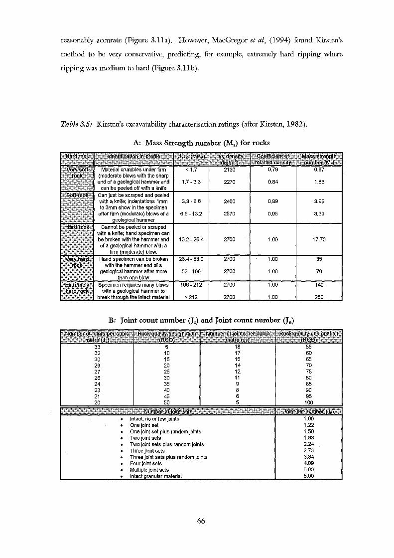
reasonably accurate (Figure 3.lla). However, MacGregor et aJ, (1994) found Kirsten's
method to be very conservative, predicting, for example, extremely hard ripping where
ripping was medium to hard (Figure 3.11b).
Table 3.5: Kirsten's excavatability characterisation ratings (after Kirsten, 1982).
A: Mass Strength number (Ms) for rocks
1.7-3.3 2270 0.84 1.86
3.3-6.6 2400 0.89 3.95
6.6-13.2 2570 0.95 8.39
13.2-26.4 2700 1.00 17.70
26.4-53.0 2700 1.00 35
53-106 2700 1.00 70
106-212 2700 1.00 140
2700 1.00 280
B: Joint count number (Jc) and Joint count number (Jn)
33 5 32 10 30 15 29 20 27 25 26 30 24 35 23 40 21 45 20 50
.. Intact, no or few joints 1.00 • One joint set 1.22
One joint set plus random joints 1.50 • Two joint sets 1.83 • Two joint sets plus random joints 2.24
• Three joint sets 2.73 • Three joint sets plus random joints 3.34 • Four joint sets 4.09
• Multiple joint sets 5.00 • 5.00
66
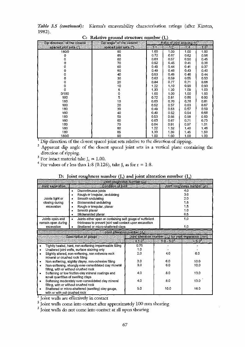
Table 3.5 (continued): Kirsten's excavatability characterisation ratings (after Kirsten, 1982).
180/0 0 0 0 0 0 0 0 0 0 0
0/180 180 180 180 180 180 180 180 180 180 180
1
90 85 80 70 60 50 40 30 20 10 5 0 5 10 20 30 40 50 60 70 80 85 90
1.00 0.72 0.63 0.52 0.49 0.49 0.53 0.63 0.84 1.22 1.33 1.00 0.72 0.63 0.52 0.49 0.49 0.53 0.63 0.84 1.22 1.33 1.00
1.00 0.67 0.57 0.45 0.44 0.46 0.49 0.59 0.77 1.10 1.20 1.00 0.81 0.70 0.57 0.53 0.52 0.56 0.67 0.91 1.32 1.39 1.00
1.00 0.62 0.50 0.41 0.41 0.43 0.46 0.55 0.71 0.99 1.09 1.00 0.86 0.76 0.63 0.57 0.54 0.58 0.71 0.97 1.40 1.45 1 00
1.00 0.56 0.45 0.38 0.37 0.40 0.44 0.53 0.68 0.93 1.03 1.00 0.90 0.81 0.67 0.59 0.56 0.60 0.73 1.01 1.46 1.50
Dip direction of the closest spaced joint sets relative to the direction of ripping. 2 Apparent dip angle of the closest spaced joint sets in a vertical plane containing the
direction of ripping. 3 For intact material take Js = 1.00. 4 For values of r less than 1:8 (0.125), take Js as for r = 1:8.
• Discontinuous joints
• Rough or irregular, undulating Joints tight or • Smooth undulating closing during • Slickensided undulating
excavation • Rough or irregular, planar
• Smooth planar
• • Joints either open or containing soft gouge of sufficient
thickness to prevent joint wall contact upon excavation
• Tightly healed, hard, non-softening impermeable filling • Unaltered joint walls, surface staining only • Slightly altered, non-softening, non cohesive rock 4.0
mineral or crushed rock filling • Non-softening, slightly clayey, non-cohesive filling 3.0 6.0 • Non-softening, strongly over-consolidated clay mineral 3.0 6.0
filling, with or without crushed rock • Softening or low friction clay mineral coatings and 4.0 8.0
small quantities of swelling clays • Softening moderately over-consolidated clay mineral 4.0 8.0
filling, with or without crushed rock • Shattered or micro-shattered (swelling) clay gouge, 5.0 10.0
with or with out crushed rock
Joint walls are effectively in contact 2 Joint walls come into contact after approximately 100 mm shearing 3 Joint walls do not come into contact at all upon shearing
67
4.0 3.0 2.0 1.5 1.5 1.0 0.5 1.0
6.0
10.0 10.0
13.0
13.0
18.0
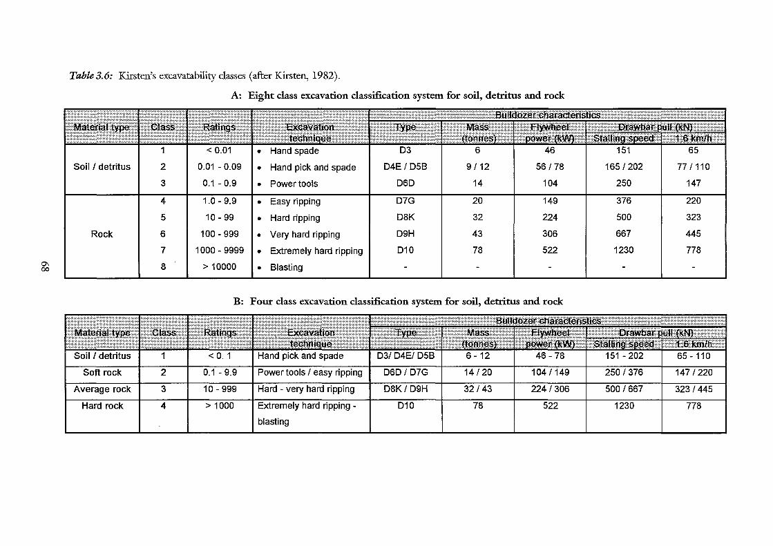
0\ I 00
Table 3.6: Kirsten's excavatability classes (after Kirsten, 1982).
Soil/ detritus I 2
3
4
5
Rock I 6
7
I 8
Soft rock 2
Average rock 3
Hard rock 4
A: Eight class excavation classification system for soil, detritus and rock
• Hand spade
0.01 -0.09 • Hand pick and spade 04E/ 058 9/12 56/78
0.1- 0.9 • Power tools 060 14 104
1.0-9.9 • Easy ripping 07G 20 149
10- 99 • Hard ripping 08K 32 224
100- 999 • Very hard ripping 09H 43 306
1000-9999 • Extremely hard ripping 010 78 522
> 10000 • Blasting
B: Four class excavation classification system for soil, detritus and rock
0.1 - 9.9
10- 999
> 1000
Power tools I easy ripping
Hard - very hard ripping
Extremely hard ripping -
blasting
060/ 07G
08K/ 09H
010
14/20 104/149
32/43 224/306
78 522
165/202 77/110
250 147
376 220
500 323
667 445
1230 778
250/376 147/220
500/667 323/445
1230 778
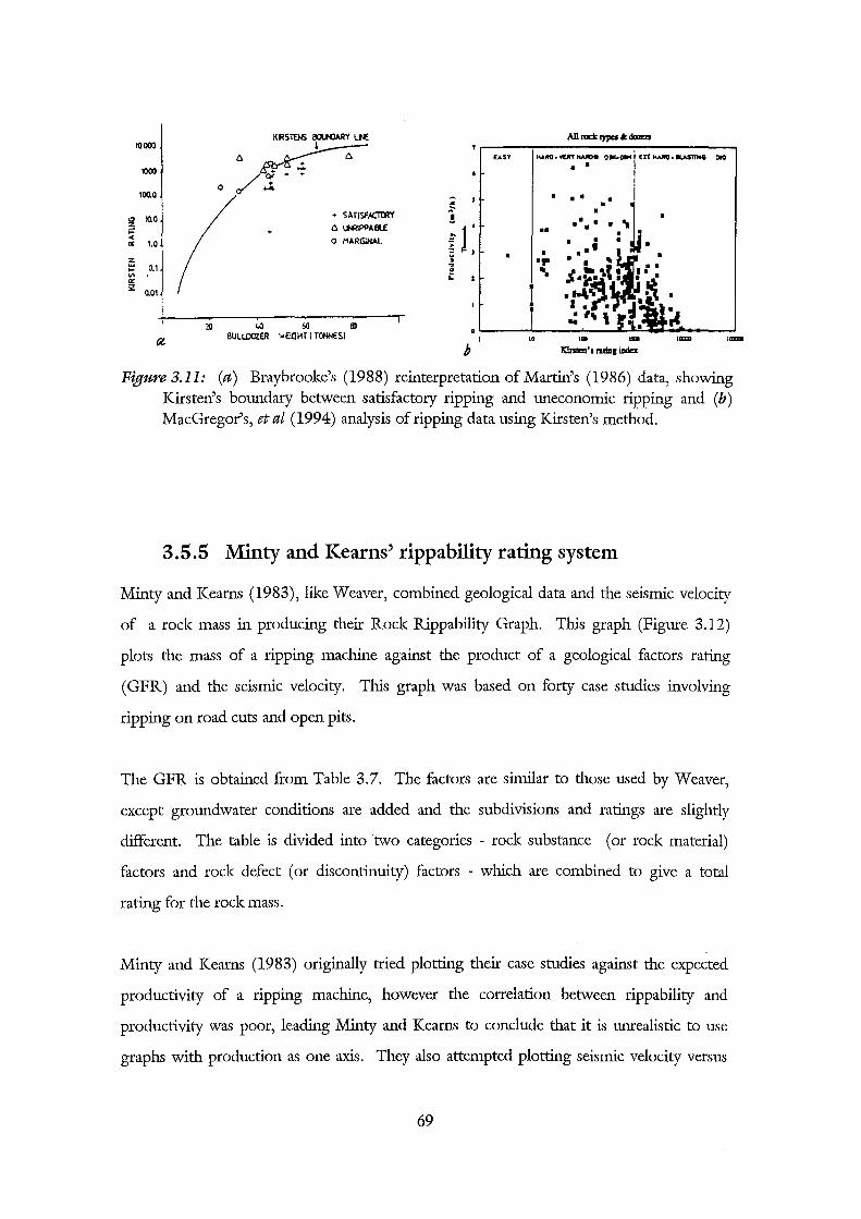
KRS7£16 BOU«lARY LN: All roct !ypei.A: doom 10000
~ c. U,SY KAMJ,.'tl(ft'f~ O ... OIW Ut IWIO ·II.ASliNG CIO
/!.-: • • 1000
0 100.0 • • •
~
~ 10.0 + SATISFKTCIIY ~.
•••• ;:: c. l.fiRU'I'" ll.£ iL •• -< o MARGINAL a: 1.0 • :z: •p ... 0.1 .. ... Q .... VI ~ • a:
i2 0.01 I 20 40 60 !D
0
a BULLDOZER ·~EIGHT I TONNESI I to ,. - ....,. -b K:in='s ratill1 iDdo2.
Figure 3.11: (a) Braybrooke's (1988) reinterpretation of Martin's (1986) data, showing Kirsten's boundary between satisfactory ripping and uneconomic ripping and (b) MacGregor's, et al (1994) analysis of ripping data using Kirsten's method.
3.5.5 Minty and !{earns' rippability rating system
Minty and Kearns (1983), like Weaver, combined geological data and the seismic velocity
of a rock mass in producing their Rock Rippability Graph. This graph (Figure 3.12)
plots the mass of a ripping machine against the product of a geological factors rating
(GFR) and the seismic velocity. This graph was based on forty case studies involving
ripping on road cuts and open pits.
The GFR is obtained from Table 3.7. The factors are similar to those used by Weaver,
except groundwater conditions are added and the subdivisions and ratings are slightly
different. The table is divided into two categories - rock substance (or rock material)
factors and rock defect (or discontinuity) factors - which are combined to give a total
rating for the rock mass.
Minty and Kearns (1983) originally tried plotting their case studies against the expected
productivity of a ripping machine, however the correlation between rippability and
productivity was poor, leading Minty and Kearns to conclude that it is unrealistic to use
graphs with production as one axis. They also attempted plotting seismic velocity versus
69

the GFR for four machinery weight ranges, but there was insufficient data to delineate
rippable, marginal and non-rippable zones. Therefore they plotted the machinery weight
against the product of the GFR and seismic velocity, resulting in a boundary between
satisfactory rippability and marginal rippability. It must be noted however, that their
inferred boundary position does not delineate rippability zones, rather it delineates
workability zones where workability is the ability of the rock mass to be broken into a
product of a desired size for the purpose intended (Minty and Kearns, 1983). Sometimes
ripping breaks up a rock mass into blocks too large and, therefore require further splitting.
In these cases, the rock mass is rippable but not workable.
Minty and Kearns rock rippability determination
120000 -Inferred boundary between marginal and satisfactory
110000 rippability
100000
90000 / /
>- 80000 / ;!: 0 L 0 Qj
70000 > 0 .E Ul 60000 'Qi en
~
Marginal jt'
/_ rippability l/
X
0:: 50000 IL C)
/ v "
40000 ....... I" Satisfactory i,.,..oo" ~ rippability -30000
20000
10000
0
0 10 20 30 40 50 60 70 80 90 100
Mass of ripping machine (tonnes)
Figure 3.12: Minty and Kearns' Rock Rippability Determination Chart (after Minty and Kearns, 1983).
70
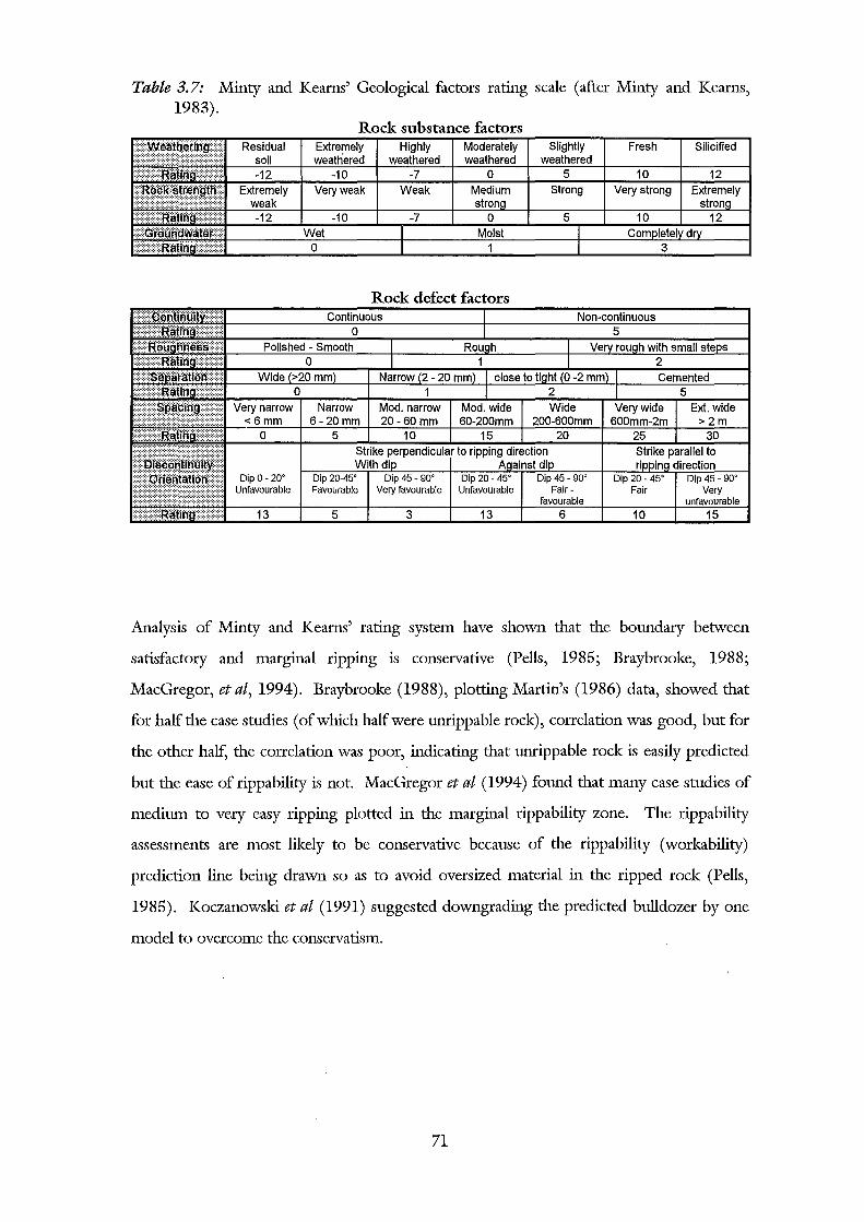
Table 3. 7: Minty and Kearns' Geological factors rating scale (after Minty and Kearns, 1983).
Rock substance factors
Rock defect factors
Analysis of Minty and Kearns' rating system have shown that the boundary between
satisfactory and marginal ripping is conservative (Pells, 1985; Braybrooke, 1988;
MacGregor, et at, 1994). Braybrooke (1988), plotting Martin's (1986) data, showed that
for half the case studies (of which half were unrippable rock), correlation was good, but for
the other half, the correlation was poor, indicating that unrippable rock is easily predicted
but the ease of rippability is not. MacGregor et at (1994) found that many case studies of
medium to very easy ripping plotted in the marginal rippability zone. The rippability
assessments are most likely to be conservative because of the rippability (workability)
prediction line being drawn so as to avoid oversized material in the ripped rock (Pells,
1985). Koczanowski et at (1991) suggested downgrading the predicted bulldozer by one
model to overcome the conservatism.
7l
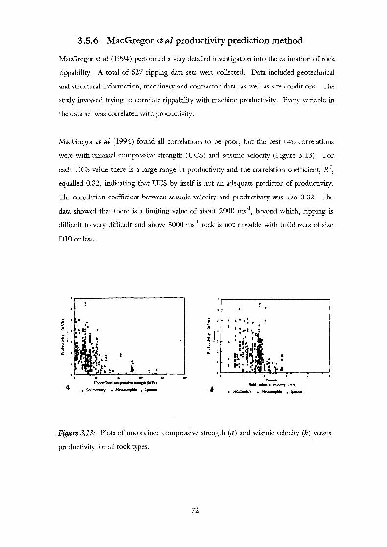
3.5.6 MacGregor et al productivity prediction method
MacGregor et at (1994) performed a very detailed investigation into the estimation of rock
rippability. A total of 527 ripping data sets were collected. Data included geotechnical
and structural information, machinery and contractor data, as well as site conditions. The
study involved trying to correlate rippability with machine productivity. Every variable in
the data set was correlated with productivity.
MacGregor et at (1994) found all correlations to be poor, but the best two correlations
were with uniaxial compressive strength (UCS) and seismic velocity (Figure 3.13). For
each UCS value there is a large range in productivity and the correlation coefficient, R2,
equalled 0.32, indicating that UCS by itself is not an adequate predictor of productivity.
The correlation coefficient between seismic velocity and productivity was also 0.32. The
data showed that there is a limiting value of about 2000 ms -l, beyond which, ripping is
difficult to very difficult and above 3000 ms·1 rock is not rippable with bulldozers of size
D10 or less .
• •
,. 100 1$
UDCCI\flned ccm-pmsm. IUOIIP (MI'a)
• ScdimcDIIry • ~ • z.....,...
• • •·
' -Pleld JOUmic Ydoclty (mill
• Sedlmaltay • ~ • IIJ'CIOQI
Figure 3.13: Plots of unconfmed compressive strength (a) and seismic velocity (b) versus
productivity for all rock types.
72
The study fmmd that no one variable could accurately predict machine productivity,
therefore a stepwise multiple regression analysis was performed. This involved correlating
a total of 22 factors most likely to affect rippability using 351 data sets (all factors are
described in Appendix B3). Factors such as weathering, strength, defect spacing and
bulldozer track conditions were correlated with bulldozer productivity.
A preliminary analysis of the results revealed that some machinery factors such as the
condition of bulldozer and restrictions on movement were very important but these factors
cannot be predicted in a preliminary estimation of the rippability of a site, and therefore
were removed from the regression analysis along with block volume and defect wall
strength, which were also considered too hard to determine during a project's investigation
stage. Despite these factors being removed from the regression, the final accuracy of the
predictions were not significantly reduced (MacGregor et at, 1994).
A list of regression equations with the seven most dominant factors (weathering, grain size,
seismic velocity, defect roughness, the number of defect sets, defect spacing, and a
structural rating) are given in Table 3.8. The correlation coefficients, R2, are poor but they
are they best possible correlations from variables easily determined during the investigation
and design stage of a project. The ratings and calculation of the parameters listed in Table
3.8 are shown in Table 3.9, and a full list of ratings as well as their defmitions is
reproduced in Appendix B3.
The dip angle of the dominant defect and the orientation of ripping relative to the strilce of
the main defect were not found to be significant in the stepwise regression, implying that
the defect orientation does not affect productivity, although MacGregor et at (1994) do
recognise that the relative orientation of a defect does have a significant effect on the
rippability of a rock mass.
When productivity was estimated, MacGregor et at (1994) had to estimate the length of a
ripping run, the depth of penetration of the tip and the width between ripping runs s~ that
excavation was not hindered. MacGregor et at calculated that the largest possible error in a
run productivity estimation would be 40%, but the area productivity should not have an
error this large as the run productivity errors should average out.
73
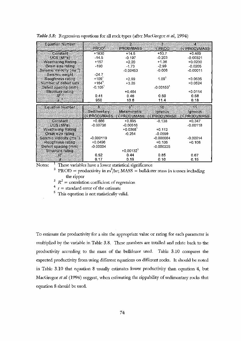
Table 3.8: Regression equations for all rock types (after MacGregor et al, 1994)
-24.7 +1091
+1641
-0.1051
-0.000119 +0.0496 -0.00004
0.52 0.17
+2.99 +3.35
+0.0013i 0.44 0.19
-0.001531
+0.112 -0.0599
-0.000084 +0.106
-0.000225
0.85 0.10
+0.0535 +0.0524
-0.00014 +0.108
0.67 0.15
These variables have a lower statistical significance 2 PROD = productivity in m 3 /hr; MASS = bulldozer mass in tonnes including
the ripper 3 R2 1' ffi' f . = corre ation coe 1c1ent o regress1on 4 s = standard error of the estimate 5 This equation is not statistically valid.
To estimate the productivity for a site the appropriate value or rating for each parameter is
multiplied by the variable in Table 3.8. These numbers are totalled and relate back to the
productivity according to the mass of the bulldozer used. Table 3.10 compares the
expected productivity from using different equations on different rocks. It should be noted
in Table 3.10 that equation 8 usually estimates lower productivity than equation 4, but
MacGregor et al (1994) suggest, when estimating the rippability of sedimentary rocks that
equation 8 should be used.
74
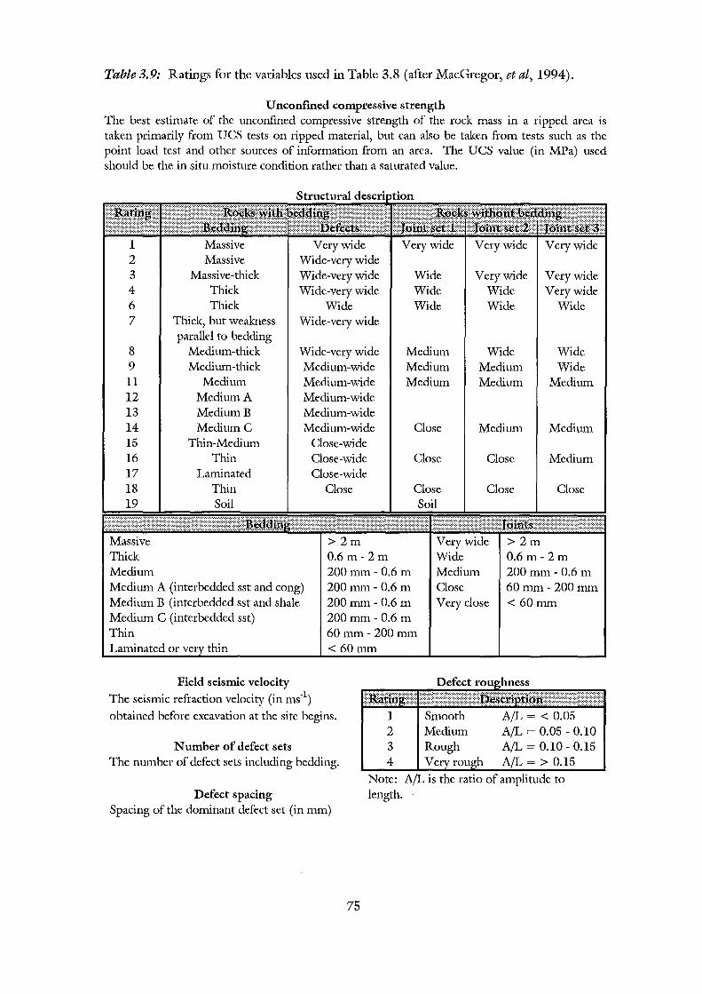
Table 3.9: Ratings for the variables used in Table 3.8 (after MacGregor, et al, 1994).
U nconfmed compressive strength The best estimate of the unconfined compressive strength of the rock mass in a ripped area is taken primarily from UCS tests on ripped material, but can also be taken from tests such as the point load test and other sources of information from an area. The UCS value (in MPa) used should be the in situ moisture condition rather than a saturated value.
1 Massive Very wide Very wide Very wide Very wide 2 Massive Wide-very wide 3 Massive-thick Wide-very wide Wide Very wide Very wide 4 Thiele Wide-very wide Wide Wide Very wide 6 Thiele Wide Wide Wide Wide 7 Thick, but weakness Wide-very wide
parallel to bedding 8 Medium-thick Wide-very wide Medium Wide Wide 9 Medium-thick Medium-wide Medium Medium Wide 11 Medium Medium-wide Medium Medium Medium 12 Medium A Medium-wide 13 MediumB Medium-wide 14 MediumC Medium-wide Close Medium Medium 15 Thin-Medium Close-wide 16 Thin Close-wide Close Close Medium 17 Laminated Close-wide 18 Thin Close Close Close Close 19 Soil Soil
>2m >2m Massive Thiele Medium Medium A (interbedded sst and cong) Medium B (interbedded sst and shale Medium C (interbedded sst)
0.6 m- 2m 200 mm- 0.6 m 200mm- 0.6 m 200mm- 0.6 m 200 mm- 0.6 m 60mm-200mm <60mm
Very wide Wide Medium Close Very close
0.6 m- 2m 200mm- 0.6 m 60mm-200mm <60mm
Thin Laminated or thin
Field seismic velocity The seismic refraction velocity (in ms-1
)
obtained before excavation at the site begins.
Number of defect sets The number of defect sets including bedding.
Defect spacing Spacing of the dominant defect set (in mm)
75
2 3 4
Note: A/Lis the ratio of amplitude to length.
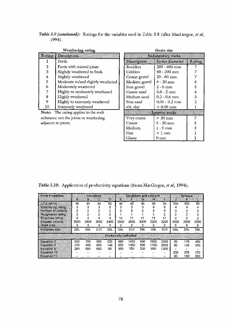
Table 3.9 (continued): Ratings for the variables used in Table 3.8 (after MacGregor, et al, 1994).
1 Fresh 3 Fresh with stained joints 3 Slightly weathered to fresh 4 Slightly weathered 5 Moderate to/and slightly weathered 6 Moderately weathered 7 Highly to moderately weathered 8 Highly weathered 9 Highly to extremely weathered
10 weathered Note: The rating applies to the rock substance not the joints or weathering adjacent to joints.
Boulders Cobbles Coarse gravel Medium gravel Fine gravel Coarse sand Medium sand Fine sand
Grain size
200-600 mm 60-200 mm 20-60 mm 6-20 mm 2-6mm 0.6- 2mm 0.2-0.6 mm 0.06-0.2 mm
1-5 mm < 1mm Omm
7 7 7 6 5 4 3 2
3 1 1
Table 3.10: Application of productivity equations (From MacGregor, et al, 1994).
200 270 270 90 160' 200
76
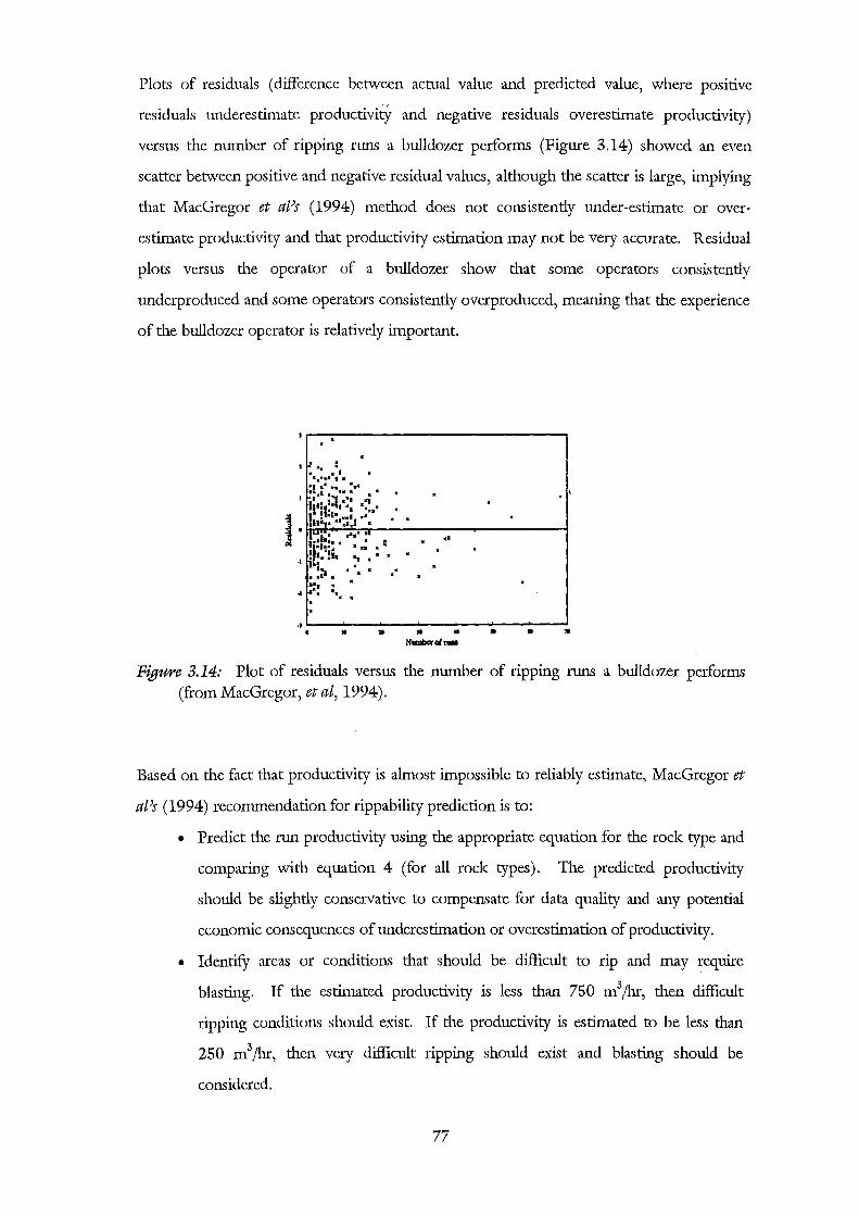
Plot<; of residuals (difference between actual value and predicted value, where positive
residuals underestimate productivity and negative residuals overestimate productivity)
versus the number of ripping runs a bulldozer performs (Figure 3.14) showed an even
scatter between positive and negative residual values, although the scatter is large, implying
that MacGregor et aPs (1994) method does not consistently under-estimate or over
estimate productivity and that productivity estimation may not be very accurate. Residual
plots versus the operator of a bulldozer show that some operators consistently
underproduced and some operators consistently overproduced, meaning that the experience
of the bulldozer operator is relatively important.
. . I .. '
• ' I •.•..- I •
:•.f ....... :.a II 11 II
'i' l)··· -1 ~-=~-- I •, •--..•
i 11.1.~~~.~·. .. . . !~· ..... • . •··•·· ....... :, ..• a ••• • • a 1••••• • ...
I ._•t._ • • ·• ~~- . :w . • !:• • • • • •• -a ~! : . . ' ..
..
·• L-_......_ _____ _._ _________ --J
• .. • • • M.......,.al,_
• • ..
Figure 3.14: Plot of residuals versus the number of ripping runs a bulldozer performs (from MacGregor, et al, 1994).
Based on the fact that productivity is almost impossible to reliably estimate, MacGregor et
aPs (1994) recommendation for rippability prediction is to:
• Predict the run productivity using the appropriate equation for the rock type and
comparing with equation 4 (for all rock types). The predicted productivity
should be slightly conservative to compensate for data quality and any potential
economic consequences of underestimation or overestimation of productivity.
• IdentifY areas or conditions that should be difficult to rip and may require
blasting. If the estimated productivity is less than 750 m3 /hr, then difficult
ripping conditions should exist. If the productivity is estimated to be less than
250 m3 /hr, then very difficult ripping should exist and blasting should be
considered.
77
3.6 Ripping versus blasting
In suitable ground, there are many reasons why ripping is a more suitable form of
excavation technique than blasting, but in ground classed as marginal to rip, bulldozer
productivity may be lower than expected, maintenance time may be higher than expected
and replacement parts may be required more often, making blasting a more cost-effective
excavation method. In suitable ground, ripping is more cost effective, safer and more
flexible (Atkinson, 1970).
When blasting is performed, labour and machines must be moved from the blast areas,
thus reducing labour utilisation and machine availability, whereas ripping bulldozers can
operate continuously. From a safety aspect, ripping is clearly less hazardous than blasting
although good blasting procedures should eliminate most of the dangers associated with
blasting (Atkinson, 1970). Ripping bulldozers can also be used for a variety of purposes
aside from ripping, such as scraping, dozing, moving machinery and stockpiling, malcing
the purchase of a bulldozer almost mandatory whether or not the site is to be ripped.
Ripping at a site results in significantly less ground and air vibrations than blasting
(Atlcinson, 1970). Blasting near urban areas may lead to bad public relations, or may not
even be allowed, depending on local by-laws. Vibrations from blasting may trigger slope
failures as most pit slopes are near equilibrium, resulting in wasted time clearing the debris.
Fragmentation of the rock mass is normally greater by ripping methods than blasting
methods meaning less oversized material would need to be split before processing.
Ripping machines have more accuracy and control over the excavation dimensions than
blasting and pit slope walls will not be damaged by a ripping bulldozer, but they may be
damaged by blasting (Powell, 1993).
One of the greater advantages of ripping over blasting in an open pit is that ripping
bulldozers excavate a thin slice at a time, which, if the orebody is modelled accurately
enough, can result in improved blending of stockpiles (if ore is stockpiled). For example,
the orebody may be modelled into mineable blocks that will be thinner if ripping is used
instead of blasting, resulting in more accurate stockpile blending when ripping.
78

3. 7 Synthesis
Rippability classification methods have been developed as a tool to predict the
excavatability or rippability of a rock mass. Seismic velocity determination and size
strength determination are two methods discussed that are simple and quick and roughly
determine the excavatability of a site. The other methods discussed all require a suite of
geological and geotechnical data to provide a more accurate assessment of the rippability of
a site. This type of assessment should be performed at the investigation or design stages of
a project. However, no rippability classification system is completely accurate, only field
trials can determine exacdy the rippability of the rock mass on a excavation site. The best
approach in evaluating the rippability of a site is to use a system involving all geotechnical
parameters likely to affect the rippability. However, during the feasibility or preliminary
investigation stage of a project, the graphical method of Pettifer and Fookes or seismic
velocity determination may be considered reliable estimates that should be investigated in
greater detail if required.
Where possible, data from drillholes, outcrops, seismic surveys and laboratory tests should
be combined so that a complete rippability assessment, using a number of different
methods, may be appraised.
Rippability site assessments should be performed independent of the lilcely contractor as
contractors obviously have an interest in acquiring a contract to excavate the site, therefore
are likely to malce their rippability assessment optimistic. If no other assessment is
possible, then bulldozer manufacturers assessments should be treated with caution and any
productivity estimate should be roughly halved.
If the productivity is estimated to be difficult or very difficult ripping (less than 750 m 3 /hr)
then blasting should be considered. However the definition of whether ripping is
economic or not is site-specific. The project may only allow limited blasting, exca~ation
may need to proceed rapidly, thereby allowing more blasting, or excavation may need to
proceed at a certain rate. The economics of ripping on a site, therefore, need to be
carefully planned and may vary from site to site.
79

Chapter Four
Geotechnical investigations
4.1 Introduction
To apply the rock mass classification methods oudined in Section 2.2 and rippability
classification methods oudined in Section 3.5, a combination of laboratory and field data
from the mine site was required to characterise the rock mass and rock material. Rock
material (also called rock substance or intact rock) is defmed as intact rock or soil that is
composed of mineral grains or crystals and the associated void or pore space, which may be
air or water filled (Bell and Pettinga, 1983); whereas a rock mass is the rock material and
its associated discontinuities (also called, fractures or defects). Rock materials are studied
at the hand specimen scale and are commonly homogeneous. Rock masses are studied at
the outcrop scale and are often inhomogeneous because of the presence of two or more
different types of rock material and/or discontinuities such as bedding planes, cleavage,
jointing and shears.
Irfan and Dearman (1978) listed the requirements of tests used for classification purposes
as:
• Rapid and simple, involving a minimum of specimen preparation,
• Relevant to the rock properties and engineering problems,
• Capable of discriminating between grades of engineering significance.
All geotechnical tests performed in this study comply with these requirements.
The purpose of the geotechnical testing programme was to:
• Characterise the rock mass and rock material at Globe-Progress,
• QuantifY for use in rock mass classifications, drillcore data that had been
qualitatively logged,
• Provide extra data for rippability evaluations.
80
Field testing involved determining the seismic velocity of the rock mass using the seismic
refraction method. No other field tests were required as all outcrops had been
geotechnically logged by Barrell (1992) and Jowett et al (1996), and structurally mapped
by Rattenbury (1994). A database of 106 diamond-cored drillhole logs of the rock mass at
Globe Hill exists, and these have been logged by many workers over time, for example
Hughes (1992) and Barry (1994). Because the outcrop and drillcore logs existed all that
was required was consistency checks and comparisons between samples collected and their
logged descriptions.
Laboratory testing involved evaluating physical and mechanical properties of the rock
material, and using these properties to provide a rough prediction of the behaviour of the
rock mass. Laboratory tests were also performed to check quantitative rock material data
with qualitatively logged drillhole and outcrop data. The tests performed were:
• Porosity and density determination
• Sonic velocity determination
• Stress-strain relationship
• Uniaxial compressive strength (UCS) and point load strength determination
• Slalce-durability determination
4.2 Field Investigations
4.2.1 Seismic refraction surveys
4.2.1.1 Introduction
The seismic velocity of a rock mass is seen as being related to many geological and physical
properties such as density, compaction and fracturing of the rock mass (Weaver, 1975;
Palmer, 1980; Braybrooke, 1988). For this reason, and because seismic velocity
determination is an easy, inexpensive and non-destructive form of site investigation
providing information on the quality and variability of a rock mass, twenty seismic
refraction surveys were performed on Globe Hill. Sites were chosen to cover the open pit
81
in as much detail as possible, but the location of surveys lines was restricted by the steep
and curving nature of many of the tracks. The seismic velocities found on Globe Hill were
then used to provide a preliminary assessment of the rippability of the mine site and as an
additional parameter in rippability classification systems (detailed in Section 3. 5). The
seismic velocities can also be compared to the sonic velocities found on rock material
(Section 4.4).
The surveys were performed between March 1995 and March 1996 in weather conditions
ranging from fine to drizzle to persistent rain. Fifteen of the line traverses are on Globe
Hill and five of the line traverses are at General Gordon, proposed location of the rock
waste stack The location of each line traverse is shown on Figure 4.1 (in map and table
box).
4.2.1.2. Methodology
The seismic refraction equipment used ( Soiltest single channel signal enhancement
seismograph, model MD-9A) requires a sledgehammer to be impacted against a metal
plate, creating a small seismic wave that is detected by geophones at both ends of the line
traverse. The energy source is moved along the line, while the geophones remain
stationary (Figure 4.2). The elevation of each hammer point was surveyed using a
Soldcisha automatic level, model B-2. Line traverses were between 20 m and 86 m in
length, and most ranged between 30m and 40 m. Seismic refraction lines 2.1-2.2 and
3.1-3.2 were resurveyed six months later to check for consistency and repeatability of
results and this data is included in Appendix D2.3.
The travel time of the first P wave recorded by the seismograph from a hammer point to a
forward and a reverse geophone were recorded for data analysis using the Generalised
Reciprocal Method (GRM; see Appendix D2 for theory and data processing
methodology). This method enables the seismic velocity (or changes in seismic velocity)
of the refracting layer (normally bedrock) underlying the line traverses to be determined
from travel time graphs. The method also allows the radial depth to the refracting layer to
be determined so that seismic refraction profiles can be plotted, although these were not
drawn as only seismic velocities were required for this study.
82
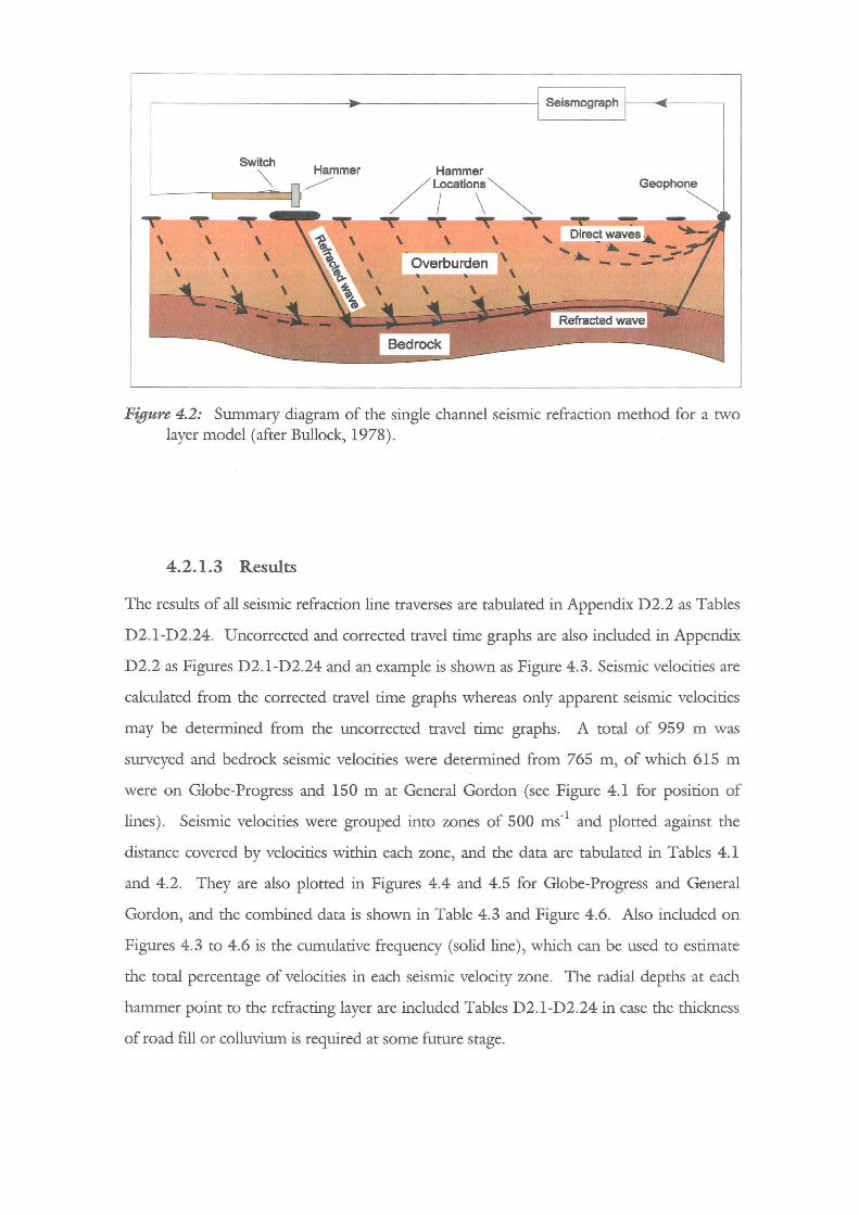
Switch
"" Hammer ~ Geophone
Figure 4.2: Summary diagram of the single channel seismic refraction method for a two layer model (after Bullock, 1978).
4.2.1.3 Results
The results of all seismic refraction line traverses are tabulated in Appendix D2.2 as Tables
D2.1-D2.24. Uncorrected and corrected travel time graphs are also included in Appendix
D2.2 as Figures D2.1 -D2.24 and an example is shown as Figure 4.3. Seismic velocities are
calculated from the corrected travel time graphs whereas only apparent seismic velocities
may be determined from the uncorrected travel time graphs. A total of 959 m was
surveyed and bedrock seismic velocities were determined from 765 m, of which 615 m
were on Globe-Progress and 150 m at General Gordon (see Figure 4.1 for position of
lines) . Seismic velocities were grouped into zones of 500 ms-1 and plotted against the
distance covered by velocities within each wne, and the data are tabulated in Tables 4.1
and 4.2. They are also plotted in Figures 4.4 and 4 .5 for Globe-Progress and General
Gordon, and the combined data is shown in Table 4.3 and Figure 4.6. Also included on
Figures 4.3 to 4.6 is the cumulative frequency (solid line), which can be used to estimate
the total percentage of velocities in each seismic velocity wne. The radial depths at each
hammer point to the refracting layer are included Tables D2.1-D2.24 in case the thickness
of road fill or colluvium is required at some future stage.
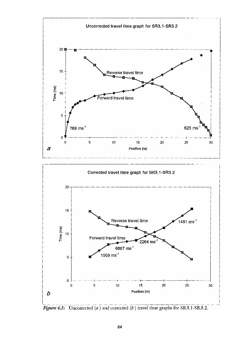
a
b
15
0 .§. Ql 10 E i=
5
0
15
0 .§. Ql 10 E i=
5
0
Uncorrected travel. time graph for SR3.1-SR3.2
5 10 15
Position (m)
20
Corrected travel time graph for SR3.1-SR3.2
5 10 15
Position (m)
20
25
25
Figure4.3: Uncorrected (a) and corrected (b) travel time graphs for SR3.l-SR3.2.
84
30
30
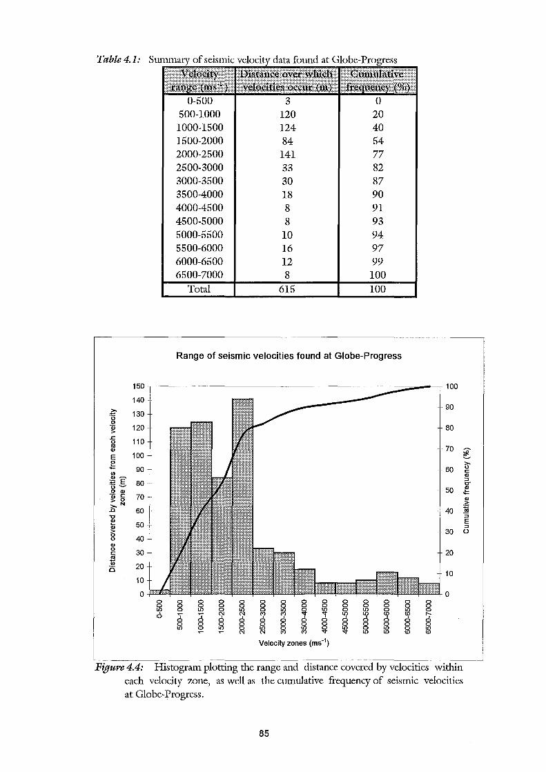
Table4.1:
500-1000 120 20 1000-1500 124 40 1500-2000 84 54 2000-2500 141 77 2500-3000 33 82 3000-3500 30 87 3500-4000 18 90 4000-4500 8 91 4500-5000 8 93 5000-5500 10 94 5500-6000 16 97 6000-6500 12 99 6500-7000 8 100
Range of seismic velocities found at Globe-Progress
150 100
140 >. 90 ~ 130 0 0 Qi 120 80 > .c
110 0 ca 70 Q)
~ E 100 0
~ .::: 90 60 If) c
Q) Q) ~ ::J E E 80 0" o~
50 ~ 0 Q)
Qi 5 70 Q) > ;:,N
.c 60 40 ~ "'0 ~ 50 Q)
> 30 0 0 40 Q) 0
30 20 c ca ~ 20 D 10
10
0 0 0 0 0 0 0 0 0 0 0 0 0 0 0 0 0 0 0 0 0 0 0 0 0 0 0 0 0 0
~ 0 lD 0 lD 0 lD ~ ~
0 lD 0 lD 0 ...... ...... ~ ~ ~ ~ ~ ~ ~ ~ :; I 0 0 0 0 0 0
0 0 0 0 0 0 0 0 0 0 0 0 0 lD 0 lD 0 ~ 0 lD ~ ~ 0 lD 0 lD ...... ...... N (") (") lD lD <D <D
Velocity zones (ms-1)
Figure 4.4: Histogram plotting the range and distance covered by velocities within each velocity zone, as well as the cumulative frequency of seismic velocities at Globe-Progress.
85
::J E ::J 0
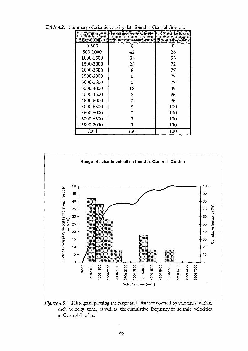
Table4.2:
0-500 0 0 500-1000 42 28
1000-1500 38 53 1500-2000 28 72 2000-2500 8 77 2500-3000 0 77 3000-3500 0 77 3500-4000 18 89 4000-4500 8 95 4500-5000 0 95 5000-5500 8 100 5500-6000 0 100 6000-6500 0 100 6500-7000 0 100
Range of seismic velocities found at General Gordon
~ 50 100
·o 0 45 90 Qi > .c
40 0 80 Ill Q)
~ c: 35 70 :c j >-
0
30 60 c: 1/l,..-... Q)
~§, :::J tT
0 25 50 ~ 0 Q) - c: Q) Q) 0 > N 20 > ~ 40 ~ "0
:; Q) 15 30 E ..... :::J Q)
0 > 0
10 20 0 Q) 0 c: 5 10 ~ 0 0 0
0 0 0 0 0 0 0 0 0 0 0 0 0 0 0 0 0 0 0 0 0 0 0 0 0 0 0 0
~ 0 l!) 0 !9 0 l!)
~ ~ 0 l!) 0 l!) R ...- ...- ~ C? C? II? II? (!) or 0 0 0 0 0 0 0 0 0 0 0 0
0 0 0 0 0 0 0 0 0 0 0 0 0 l!) 0 l!) 0 ~ 0 l!) Sij! ~ 0 l!) 0 l!)
...- N ('") ('") l!) l!) (!) (!)
Velocity zones (ms-1)
Figure 4.5: Histogram plotting the range and distance covered by velocities within each velocity zone, as well as the cumulative frequency of seismic velocities at General Gordon.
86
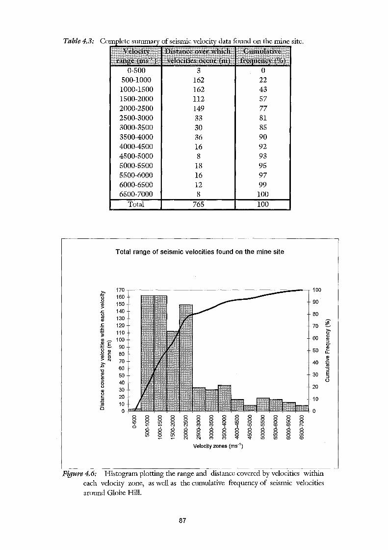
Table4.3:
0-500 3 0 500-1000 162 22
1000-1500 162 43 1500-2000 112 57 2000-2500 149 77 2500-3000 33 81 3000-3500 30 85 3500-4000 36 90 4000-4500 16 92 4500-5000 8 93 5000-5500 18 95 5500-6000 16 97 6000-6500 12 99 6500-7000 8 100
Total range of seismic velocities found on the mine site
~ 170 100
0 160 0 90 Qi 150 > ..c: 140 80 0 lU 130 Ql
c 120 70 :c ~ 110
60 UJ~ 100 ~g 90 0 Ql 50
.Q c 80 Ql 0 > N 70 40 >-..c 60 -o f£ 50 30 Ql > 40 0 0 20 Ql 30 0 c 20 10 lU Ui 10 0 0 0
0 0 0 0 0 0 0 0 0 0 0 0 0 0 0 0 0 0 0 0 0 0 0 0 0 0 0 0 u;> 0 lJ) 0 lJ) 0 lJ)
~ \fj 0 lJ) 0 lJ) 0 ...... ...... C';J ~ C? C? u;> ~ (!)
~ 2; 0 I 0 I 0 0 0 0 0 0 0 0 0 0 0 0 0 0 0 0 0 0 0 0 0 lJ) 0 lJ) 0 lJ) 0 lJ) ~ ~ 0 lJ) 0 lJ)
...... ...... N N ('") ('") lJ) lJ) (!) (!)
Velocity zones (ms-1)
Figure 4.6: Histogram plotting the range and distance covered by velocities within each velocity zone, as well as the cumulative frequency of seismic velocities around Globe Hill.
87
~ >-0 c Ql ::J tT f£ u.. Ql > ~ "5 E ::J (.)
4.2.1.4 Discussion
Seismic velocities fmmd at Globe-Progress range between 620 ms-1 and 6667 ms-\ with a
mean of 2100 ms-1. Figure 4.4 shows the spread of data for Globe-Progress, which is very
fmely skewed and indicates that most of velocities found are less than 2500 ms-1. The same
trend occurs at General Gordon (Figure 4.5), where the more limited data ranges between
508 ms-1 and 5000 ms-\ with a mean of 1950 ms-1. Figure 4.6 combines the data from
Globe-Progress and General Gordon to give the range of seismic velocity data for the mine
site.
Scattering of travel times occurs on some of the corrected travel time graphs (Figures
D2.1-D2.24), and where it is minor the velocities have been averaged for the rock mass.
Where scattering is major, the velocities have been calculated over 2 m intervals (the
hammer spacing), for example SR6.1 - SR6.2, where there is an alternating sequence of
high and low velocities representing an interbedded sequence of siltstone and sandstone
(Figure 4. 7).
Two seismic refraction survey lines, both of which contained a spread of seismic velocities,
were repeated to check for consistency and repeatability of data (Appendix D2.3). This
was done as a check on Kirsten's (1982) statement that the seismic velocity cannot be
determined to an accuracy better than approximately 20%, and that there may be variances
in the order of 1000 ms-1 in apparently identical materials. The results show that the
repeated seismic surveys are more or less identical to the original surveys, and any scatter in
the results may be accounted for by the degree of ground saturation, as the ftrst surveys
were performed in June when the ground was more saturated and the repeat surveys
performed the following March after a significant dry spell. The repeatability of the
seismic refraction data proves that seismic velocity determination is a viable method to use
in estimating characteristics of the rock mass, but the seismic velocities should be
compared with sonic velocities determined on rock material to note variations between
rock mass properties and rock material properties.
88
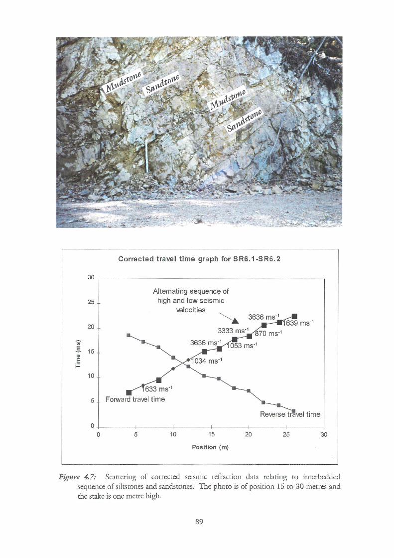
rn .§. 15 Q)
E i=
10
Corrected travel time graph for SR6.1-SR6.2
Alternating sequence of high and low seismic
'velocities
5 Forward tra-..el time
'vel time
0+--------b------_, ________ ,_ ______ -+--------b-------~ 0 5 10 15 20 25 30
Position (m)
Figure 4.7: Scattering of corrected seismic refraction data relating to interbedded sequence of siltstones and sandstones. The photo is of position 15 to 30 metres and the stake is one metre high.
89
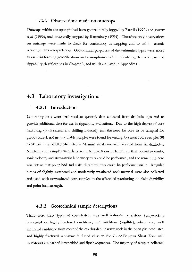
4.2.2 Observations made on outcrops
Outcrops within the open pit had been geotechnically logged by Barrell (1992) and Jowett
et at (1996), and structurally mapped by Rattenbury (1994). Therefore only observations
on outcrops were made to check for consistency in mapping and to aid in seismic
refraction data interpretation. Geotechnical properties of discontinuities types were noted
to assist in forming generalisations and assumptions made in calculating the rock mass and
rippability classifications in Chapter 5, and which are listed in Appendix E.
4.3 Laboratory investigations
4.3.1 Introduction
Laboratory tests were performed to quantify data collected from drillhole logs and to
provide additional data for use in rippability evaluations. Due to the high degree of core
fracturing (both natural and drilling induced), and the need for core to be sampled for
grade control, not many suitable samples were found for testing, but intact core samples 30
to 50 em long of HQ (diameter = 61 mm) sized core were selected from six drillholes.
Nineteen core samples were later recut to 15-18 em in length so that porosity-density,
sonic velocity and stress-strain laboratory tests could be performed, and the remaining core
was cut so that point-load and slalce durability tests could be performed on it. Irregular
lumps of slightly weathered and moderately weathered rock material were also collected
and used with unweathered core samples to the effects of weathering on slake-durability
and point load strength.
4.3.2 Geotechnical sample descriptions
There were three types of core tested: very well indurated sandstone (greywaclce);
brecciated or highly fractured sandstone; and mudstone (argillite), where very well
indurated sandstone form most of the overburden or waste rock in the open pit, brecciated
and highly fractured sandstone is found close to the Globe-Progress Shear Zone and
mudstones are part of interbedded and flysch sequences. The majority of samples collected
90
were very well indurated sandstone as this rock material is expected to be hardest to rip
because of its high intact strength. Mudstones, and brecciated sandstones are all expected
to be relatively easy to rip because of their many laminations and fractures. Only one
mudstone sample was tested for its geotechnical properties as other samples were damaged
during sample preparation. Tested core samples have been labelled according to the
drillhole they originated from and the sample number from that hole; for example
GB92.19 is the 19th sample tested from hole GB92. Samples were then described (Table
4.4) using hand specimen descriptions similar to that used in drillcore logs (see Appendix
B2) so that comparisons could be made between core samples and drillcore logs.
4.3.3 Porosity-Density Determination
4.3.3.1 Introduction
ISRM (1981) state that porosity-density determination is one of the fundamental physical
properties that should be determined for rock classification systems. Although the
properties are not utilised in any of the classifications systems discussed in Chapter 2 and
Chapter 3, the test was still performed because the mechanical performance of rock
material is highly dependent upon porosity and density. This is because the presence of
voids in the fabric of a rock material decreases its strength and increases its deformability
(ISRM, 1981). Density is inversely proportional to porosity, so that rocks with a high
density are expected to have low porosity.
4.3.3.2 Methodology
Samples were prepared and tested following the procedures suggested by ISRM (1981).
The saturation and calliper testing procedure was followed. This method requires
specimens that are geometrically uniform, such as core samples, to be used. All core
samples tested had a small shaving of approximately one millimetre thickness and one
centimetre width that was used for assaying. The shavings volume was estimated and
subtracted from the total volume of each core sample to obtain more accurate values of
porosity and density.
91
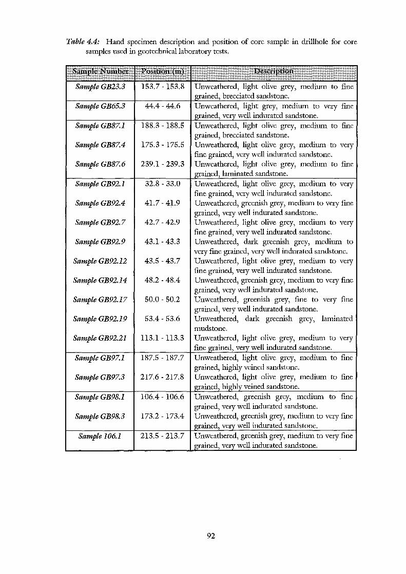
Table 4.4: Hand specimen description and position of core sample in drillhole for core samples used in geotechnical laboratory tests.
Sample GB65.3 44.4-44.6
Sample GB87.1 188.3 - 188.5 Unweathered, light olive grey, medium to fme grained, brecciated sandstone.
Sample GB87.4 175.3- 175.5 Unweathered, light olive grey, medium to very fme grained, very well indurated sandstone.
Sample GB87.6 239.1-239.3 Unweathered, light olive grey, medium to fme laminated sandstone.
Sample GB92.1 32.8 - 33.0 Unweathered, light olive grey, medium to very fme grained, very well indurated sandstone.
Sample GB92.4 41.7-41.9 Unweathered, greenish grey, medium to very fine grained, very well indurated sandstone.
Sample GB92.7 42.7-42.9 Unweathered, light olive grey, medium to very fme grained, very well indurated sandstone.
Sample GB92.9 43.1-43.3 Unweathered, dark greenish grey, medium to very fme grained, very well indurated sandstone.
Sample GB92.12 43.5-43.7 Unweathered, light olive grey, medium to very fme grained, very well indurated sandstone.
Sample GB92.14 48.2 - 48.4 Unweathered, greenish grey, medium to very fme grained, very well indurated sandstone.
Sample GB92.17 50.0- 50.2 Unweathered, greenish grey, fme to very fme grained, very well indurated sandstone.
Sample GB92.19 53.4 - 53.6 Unweathered, dark greenish grey, laminated mudstone.
Sample GB92.21 113.1- 113.3 Unweathered, light olive grey, medium to very fme well indurated sandstone.
Sample GB97.1 187.5- 187.7 Unweathered, light olive grey, medium to fme grained, highly veined sandstone.
Sample GB97.3 217.6 - 217.8 Unweathered, light olive grey, medium to fme veined sandstone.
Sample GB98.1 106.4- 106.6 Unweathered, greenish grey, medium to fme grained, very well indurated sandstone.
Sample GB98.3 173.2 - 173.4 Unweathered, greenish grey, medium to very fme well indurated sandstone.
Sample 106.1 213.5- 213.7
92
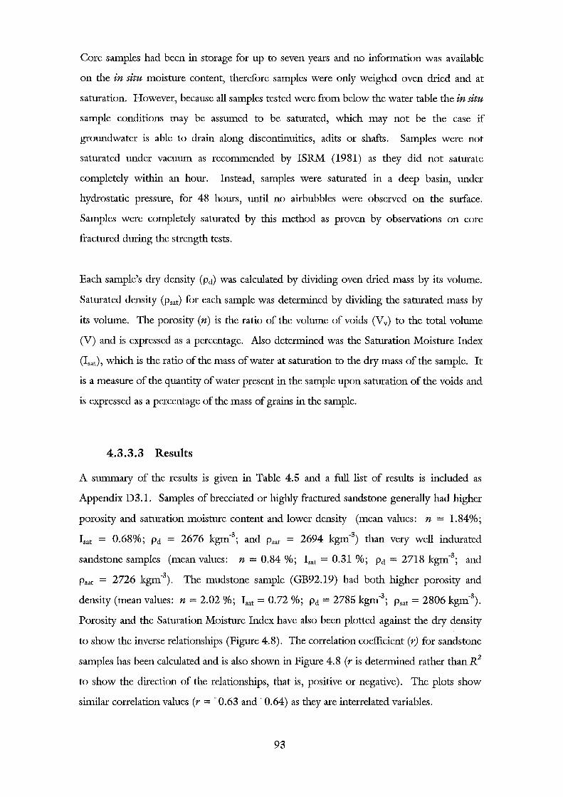
Core samples had been in storage for up to seven years and no information was available
on the in situ moisture content, therefore samples were only weighed oven dried and at
saturation. However, because all samples tested were from below the water table the in situ
sample conditions may be assumed to be saturated, which may not be the case if
groundwater is able to drain along discontinuities, adits or shafts. Samples were not
saturated under vacuum as recommended by ISRM (1981) as they did not saturate
completely within an hour. Instead, samples were saturated in a deep basin, under
hydrostatic pressure, for 48 hours, until no airbubbles were observed on the surface.
Samples were completely saturated by this method as proven by observations on core
fractured during the strength tests.
Each sample's dry density (Pd) was calculated by dividing oven dried mass by its volume.
Saturated density (Psat) for each sample was determined by dividing the saturated mass by
its volume. The porosity (n) is the ratio of the volume of voids (Vv) to the total volume
(V) and is expressed as a percentage. Also determined was the Saturation Moisture Index
(Is at), which is the ratio of the mass of water at saturation to the dry mass of the sample. It
is a measure of the quantity of water present in the sample upon saturation of the voids and
is expressed as a percentage of the mass of grains in the sample.
4.3.3.3 Results
A summary of the results is given in Table 4.5 and a full list of results is included as
Appendix D3.1. Samples of brecciated or highly fractured sandstone generally had higher
porosity and saturation moisture content and lower density (mean values: n = 1.84%;
Isat = 0.68%; Pd = 2676 kgm-3; and Psat = 2694 kgm-3
) than very well indurated
sandstone samples (mean values: n = 0.84 %; Isat = 0.31 %; Pd = 2718 kgm-3; and
Psat = 2726 kgm-3). The mudstone sample (GB92.19) had both higher porosity and
density (mean values: n = 2.02 %; Isat = 0.72 %; Pd = 2785 kgm-3; Psat = 2806 kgm-3
).
Porosity and the Saturation Moisture Index have also been plotted against the dry density
to show the inverse relationships (Figure 4.8). The correlation coefficient (r) for sandstone
samples has been calculated and is also shown in Figure 4.8 (r is determined rather thanR2
to show the direction of the relationships, that is, positive or negative). The plots show
similar correlation values (r = -0.63 and- 0.64) as they are interrelated variables.
93
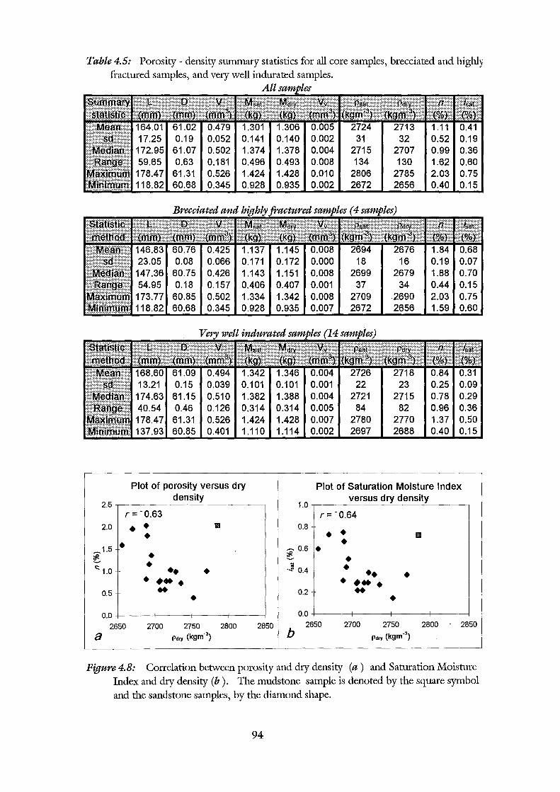
Table 4.5: Porosity - density summary statistics for all core samples, brecciated and highly fractured samples, and very well indurated samples.
All sam~111es
168.60 13.21
174.63 40.54 178.47 137.93
Plot of porosity versus dry density
2.5 ,-------~-----, r = -o.63
2.0 • • Bl
• ~1.5 • ~ • • ~ 1.0 •• • • ... .
0.5 .. •
0.0 -1----1---t---------;f---------j
2650 2700 2750 2800 2850
a Pdry (kgm-3)
2699 37
2709 2672
2679 34
2690 2656
82 2770 2688
0.99 1.62 2.03 0.40
0.75 0.60
Plot of Saturation Moisture Index versus dry density
1.0 ,-------~---'0-----,
r=-0.64 0.8
• • 1111 • ~ 0.6 ~ •
.j 0.4 • •• • . .... 0.2 .. • 0.0 -1----t----+-------+------l
2650 2700 2750 2800 . 2850 b Pdry (kgm-3
)
Figure 4.8: Correlation between porosity and dry density (a) and Saturation Moisture Index and dry density (b). The mudstone sample is denoted by the square symbol and the sandstone samples, by the diamond shape.
94
4.3.3.4 Discussion
In general, the porosity values are very low (mean = 1.06 %, range = 0.40 - 2.03 %) and
the density values are very high (Psat mean= 2719 kgm3, range = 2672 - 2780 kgm3
; Pd
mean = 2709 kgm3, range = 2656- 2770 kgm3
) for sandstones. This is an effect of the
metamorphic alteration that Greenland Group sediments have undergone by compaction,
void closure, and matrix recrystallisation to form sericitic muscovite (Cooper and Craw,
1992).
The brecciated and highly fractured sandstone samples all have higher porosity and lower
density values than the very well indurated sandstones. This higher porosity is probably
associated with secondary porosity, which is a direct result of fracturing and veining. The
mudstone sample had both higher porosity and density values than the very well indurated
sandstone samples, which may be explained by differences in grain lithologies, where
sandstone samples are mainly quartz and lithic fragments (specific gravity: ~ 2.6), and
mudstone samples are mainly sericitic muscovite (specific gravity: ~ 2.8; Cooper and
Craw, 1992). In addition, the mudstone sample swelled slightly upon saturation, resulting
in an increase in void volume and porosity.
The plots of porosity and Saturation Moisture Index with dry density (Figure 4.8) also
include the correlation coefficient (r) for the sandstone samples. The scatter in the results
may be partly accounted for by the estimation of the shaving volume sampled from each
core sample, where if the exact volume is not used minor errors in the results will occur,
but the main reason is the inhomogenity of rock material caused by small fractures and
veins within samples. Fractures will normally be air or water filled (depending on the
saturation condition of the sample), and therefore will affect density and porosity results.
Veins may be calcite or quartz, both of a similar specific gravity to the rock material, but
the veins' porosity will be almost zero, thus affecting the density and porosity results.
95
4.3.4 Sonic velocity determination
4.3.4.1 Introduction
This test was performed to determine the sonic velocities of the rock material, which can
then be compared to the rock mass seismic velocity (Section 4.4) to fmd the Seismic
Velocity Index. The sonic velocities may also be used to determine the dynamic modulii of
elasticity, which are measures of the deformability of rock material. The same core samples
used for porosity-density determination were also used to determine saturated and oven dry
P and S wave sonic (or seismic) velocities (vp (sat); Vs (sat); Vp (dry); and Vs (dry))·
4.3.4.2 Methodology
The time taken for an elastic compressional wave (P wave) and an elastic shear wave (S
wave) to propagate through each core sample was measured following the suggested
methods of ISRM (1981) whereby platens able to generate P and S elastic waves are
connected to a seismic analyser and an oscilloscope to identify the first arrival P and S
waves. The sonic velocity may then be calculated by dividing the time talcen for the first P
or S wave to travel through the sample by the sample's length. A correction factor,
accounting for the time talcen for each wave to travel through the platens (platen delay
constant) and zeroing of the seismic analyser, is also subtracted.
The seismic velocities also may be used to calculate the dynamic moduli of elasticity from
the following formulae:
(3v 2 -4v2) 2 p s
Edyn =pvs { 2 2) vp -vs
(v; -2v?) v - -'--7-----;.-
dyn - 2(v; - v?)
where Edyn is Young's Modulus (GPa), vdyn is Poisson's Ratio (dimensionless), pis density
(kgm"\ Vs is the shear wave velocity (ms-1) and Vp is the compressional wave velocity
(ms-1). When calculating the sonic velocities and dynamic moduli of elasticity, the samples
are assumed to be homogeneous, isotropic and purely elastic, which is rarely the case as
samples may contain minor fractures and veins that affect the sample's homogeneity and
isotropy. Samples normally do behave in an elastic fashion for the low stresses the platens
96
induce upon the samples, but if the sample is extremely weak, then the platen low stresses
may alter the samples, affecting the results. It is assumed that no samples tested were
affected by the low stresses as all behaved in an elastic manner at low stresses (see stress
strain relationships for each sample in Appendix D3.3).
4.3.4.3 Results
The results are summarised in Table 4.6 and the complete data are tabulated in Appendix
D3.2. Brecciated and highly fractured core had lower sonic velocities and dynamic
elasticity modulii than very well indurated core samples, and the mudstone sample had very
low sonic velocities and dynamic elasticity modulii. Graphs correlating P wave velocities
with S wave velocities, saturated density and porosity are shown in Figure 4.9, and Figure
4.10 contains graphs correlating dynamic Young's Modulus with dynamic Poisson's Ratio,
density and porosity. The correlation coefficient (r) for sandstone samples was included on
each plot in Figures 4.9 and 4.10 instead of R 2 to show whether or not data follows a
positive or negative trend.
4.3.4.4 Discussion
Values ofvp (sat) for all sandstone samples range between 3700 ms-1 and 4900 ms-1 and have
a mean of 4357 ms-\ whilst vp (dry) data ranges between 2700 ms-1 and 4500 ms-1 with a
mean value of 3911 ms-1. This data is comparable to the results found by Anon (1994),
whose data, based on five core samples from Globe-Progress, range between 3300 ms-1 and
4700 ms-1. For comparison, the mudstone sample had comparatively low sonic P wave
velocities ( Vp (sat) = 1677 ms-1 and Vp (dry) = 1519 ms-1).
The general trends that may be observed are:
• vp (sat) values (mean = 4357 ms-1) are higher than vp (dry) (mean = 3911 ms-1
),
which is to be expected as the velocity of water (1500 ms-1) filling the voids in the
saturated state is considerably greater than the velocity of air (330 ms-1) filling
the voids when the sample is oven dried.
• Values ofvs (sat) (mean= 1792 ms-1), are lower than Vs (dry) (mean= 2411 ms-1
)
because shear waves cannot pass through liquids, therefore slowing down the S
wave velocity through a saturated sample.
97
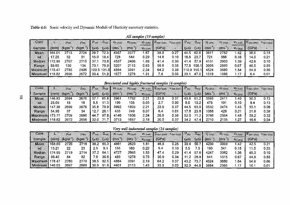
Table4.6: Sonic velocity and Dynamic Moduli ofElasticity summary statistics.
16.8 41.4
56.8 0.35 77.8 108.1,3005 2593 0.67 I 48.5 0.85 2785 2806 1100.5 131.81 4884 3391 2.24 I 64.2 0.38 110.9 155.1 4524 3680 1.84 54.9 0.86 2656 2672 30.4 51.9 1677 1278 1.31 7.4 0.03 33.1 47.0 1519 1086 1.17 6.4 0.01
\Q 00
E:::::::::8~'''"'""""'"''''''''"'~ · · - · - - ---. --· 16
2679 35.8 37 34 12.7 26.1 I 433 249 0.07 I 6.4 0.01 117.8
2709 2690 44.7 97.8 4146 1906 2.24 26.9 0.38 52.0 2672 2656 32.0 71.7 3713 1657 2.18 20.5 0.37 34.2
0.18 1.36
84 82 ,7.6 30.61 483 1278 0.75 30.9 0.34 111.2 28.9 641 1315 0.67 I 44.8 0.85 2780 2770 38.5 82.5 4884 3391 2.19 64.2 0.37 43.2 73.7 4524 3680 1.84 54.9 0.86 2697 2688 30.9 51.9 4401 2113 1.43 33.3 0.03 32.0 44.8 3884 2365 1.17 10.1 0.01
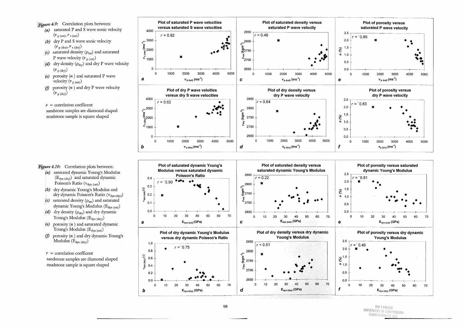
Figure 4.9: Correlation plots between: (a) saturated P and S wave sonic velocity
(v p (sat)' V s (sat))
(b) dry P and S wave sonic velocity (v P (dty)' v s (dty))
(c) saturated density (Psat) and saturated P wave velocity (v p (sat))
(d) dry density (Pruy) and dry P wave velocity
(v p (dty))
(e) porosity (n) and saturated P wave velocity (v p (sat))
(j) porosity (n) and dry P wave velocity (v P (dty))
r = correlation coefficent sandstone samples are diamond shaped mudstone sample is square shaped
Figure 4.10: Correlation plots between: (a) saturated dynamic Young1s Modulus
(Edyn (dty)) and saturated dynamic Poisson1
S Ratio (vdyn (sat))
(b) dry dynamic Young1s Modulus and dry dynamic Poisson1s Ratio (vdyn (dty))
(c) saturated density (Psat) and saturated dynamic Young1s Modulus (Edyn (sat))
(d) dry density (Pdty) and dry dynamic Young1s Modulus (Edyn (dty))
(e) porosity (n) and saturated dynamic Young1s Modulus (Edyn (sat))
(j) porosity (n ) and dry dynamic Y oung1s Modulus (Edyn (dty))
r = correlation coefficent sandstone samples are diamond shaped mudstone sample is square shaped
4000
~3000 ';"
Vl E '::2000
"IV .!!!.
"' :. 1000
0 0
a
4000
~3000 ';"
Vl E ~000
:!!.
"' :. 1000
0 0
b
0.4
0.3 8 ! 0.2 c ,., ..,
:> 0.1
0.0 0
a
1.0
0.8
8 0.6 ~ :!!. c 0.4 ,., ..,
:>
0.2
0.0 0
b
Plot of saturated P wave velocities versus saturated S wave velocities
r = 0.82 •• f ... . \ •• #
1111
1000 2000 3000 4000 5000
V p (sat) (ms"1)
Plot of dry P wave veloities versus dry S wave velocities
r = 0.62 • .41+. • • ... •• • • 1111
1000 2000 3000 4000 5000
v P (dry) (ms"1
)
Plot of saturated dynamic Young's Modulus versus saturated dynamic
Poisson's Ratio
r = -0.90 .... •• ·~ •
1111 ·' • • •
10 20 30 40 50 60 70
Edyn (sat) (GPa)
Plot of dry dynamic Young's Modulus versus dry dynamic Poisson's Ratio
• r =-0.75
• • •
1111 .. ·~ ..... .. .... . 10 20 30 40 50 60 70
Edyn (dry) (GPa)
99
Plot of saturated density versus Plot of porosity versus saturated P wave velocity saturated P wave velocity
2850 r = 0.46
2.5 r=-0.89
2800 1111 2.0 1111 • • '?~ • • E ~ 1.5 • ~2750 • ~ • •• "IV r:::: 1.0 .. .
"' .. ,. 0.2700 • ~· • • 0.5 .. • •
2650 0.0 0 1000 2000 3000 4000 5000 0 1000 2000 3000 4000 5000
c V p (sat) (ms·1) e Vp(sat) (ms"1)
Plot of dry density versus Plot of porosity versus dry P wave velocity dry P wave velocity
2850 2.5 r = 0.64 r = -0.83
2800 2.0 1111 • • ~
1111 • '? E • • 0)
...,_ 1.5 c 2750 • ~ •
·t L • i:' r:::: 1.0 ••• ..,
a. 2700 • • ..... .. , . 0.5 • • • • 2650 • 0.0
0 1000 2000 3000 4000 5000 0 1000 2000 3000 4000 5000
d Vp (dry) (ms"1) f vP (dry) (ms-1)
Plot of saturated density versus Plot of porosity versus saturated saturated dynamic Young's Modulus dynamic Young's Modulus
2850 2.5 r = 0.22 r = -0.81
1111 2.0 1111 •• 2800
<? • • • E - 1.5 ~2750 • c • ... ·. • r:::: 1.0 ••• "IV
"' ••• •• 0.2700 • • • ·' • ~ • • 0.5 • • • • 2650 0.0
0 10 20 30 40 50 60 70 0 10 20 30 40 50 60 70
c Edyn (sat) (GPa) e Edyn (sat) (GPa)
Plot of dry density versus dry dynamic Plot of porosity versus dry dynamic Young's Modulus Young's Modulus
2850 2.5 r = 0.51 r=-0.49
2.0 II • 2800 • '?~ 1111 • E • ......, 1.5 • ~ 2750 • ~ • • • i:' ~ ~·
r:::: 1.0 #• .., • a. 2700 • • • ... • •• ... 0.5 • • • • 2650 • 0.0
0 10 20 30 40 50 60 70 0 10 20 30 40 50 60 70
d Edyn (dry) (GPa) f Edyn (dry) ( GPa)
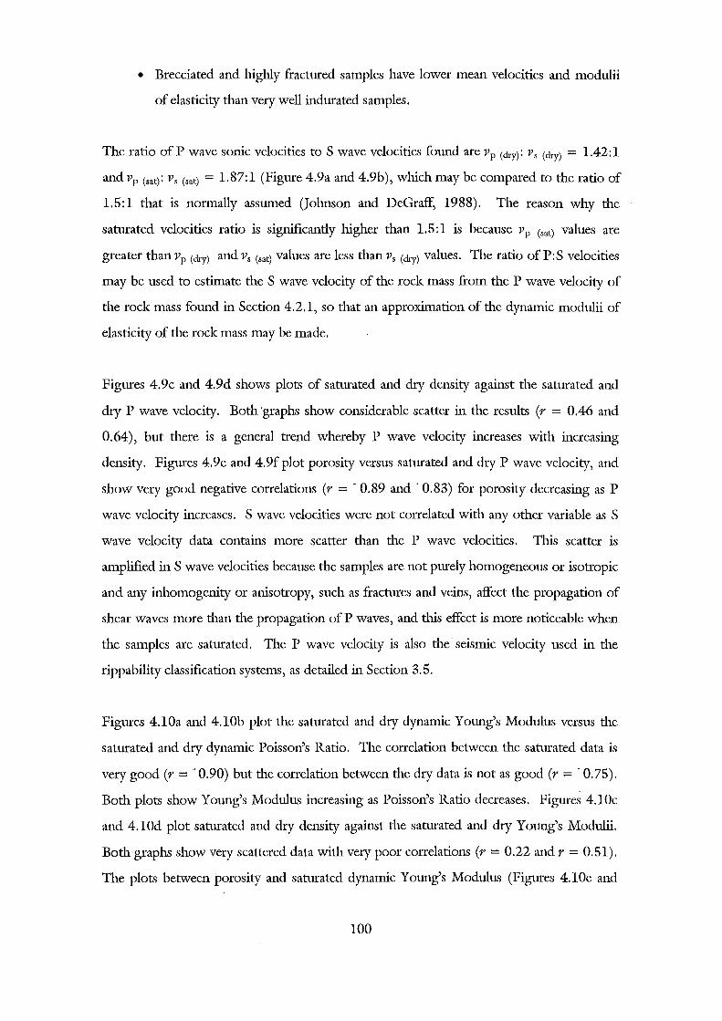
• Brecciated and highly fractured samples have lower mean velocities and modulii
of elasticity than very well indurated samples.
The ratio of P wave sonic velocities to S wave velocities found are vp (dry): Vs (dry) = 1.42:1
and Vp (sat): Vs (sat) = 1.87:1 (Figure 4.9a and 4.9b), which may be compared to the ratio of
1.5:1 that is normally assumed (Johnson and DeGraff, 1988). The reason why the
saturated velocities ratio is significantly higher than 1.5:1 is because Vp (sat) values are
greater than vp (dry) and Vs (sat) values are less than Vs (dry) values. The ratio of P:S velocities
may be used to estimate the S wave velocity of the rock mass from the P wave velocity of
the rock mass found in Section 4.2.1, so that an approximation of the dynamic modulii of
elasticity of the rock mass may be made.
Figures 4.9c and 4.9d shows plots of saturated and dry density against the saturated and
dry P wave velocity. Both ·graphs show considerable scatter in the results (r = 0.46 and
0.64), but there is a general trend whereby P wave velocity increases with increasing
density. Figures 4.9e and 4.9f plot porosity versus saturated and dry P wave velocity, and
show very good negative correlations (r = -0.89 and- 0.83) for porosity decreasing as P
wave velocity increases. S wave velocities were not correlated with any other variable as S
wave velocity data contains more scatter than the P wave velocities. This scatter is
amplified in S wave velocities because the samples are not purely homogeneous or isotropic
and any inhomogenity or anisotropy, such as fractures and veins, affect the propagation of
shear waves more than the propagation of P waves, and this effect is more noticeable when
the samples are saturated. The P wave velocity is also the seismic velocity used in the
rippability classification systems, as detailed in Section 3.5.
Figures 4.10a and 4.10b plot the saturated and dry dynamic Young's Modulus versus the
saturated and dry dynamic Poisson's Ratio. The correlation between the saturated data is
very good (r =- 0.90) but the correlation between the dry data is not as good (r = -0.75).
Both plots show Young's Modulus increasing as Poisson's Ratio decreases. Figur~ 4.l0c
and 4.10d plot saturated and dry density against the saturated and dry Young's Modulii.
Both graphs show very scattered data with very poor correlations (r = 0.22 and r = 0.51).
The plots between porosity and saturated dynamic Young's Modulus (Figures 4.10e and
100
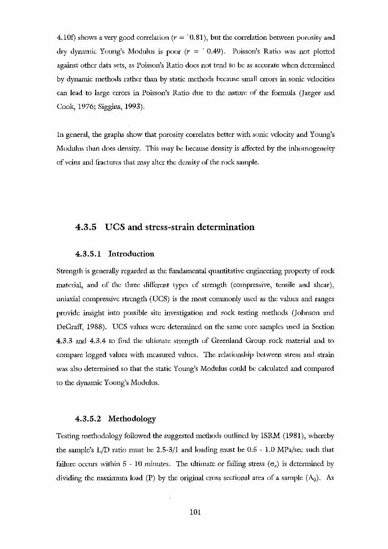
4.10f) shows a very good correlation (r =- 0.81), but the correlation between porosity and
dry dynamic Young's Modulus is poor (r = - 0.49). Poisson's Ratio was not plotted
against other data sets, as Poisson's Ratio does not tend to be as accurate when determined
by dynamic methods rather than by static methods because small errors in sonic velocities
can lead to large errors in Poisson's Ratio due to the nature of the formula (Jaeger and
Coole, 1976; Siggins, 1993).
In general, the graphs show that porosity correlates better with sonic velocity and Young's
Modulus than does density. This may be because density is affected by the inhomogeneity
of veins and fractures that may alter the density of the rock sample.
4.3.5 UCS and stress-strain determination
4.3.5.1 Introduction
Strength is generally regarded as the fundamental quantitative engineering property of rock
material, and of the three different types of strength (compressive, tensile and shear),
uniaxial compressive strength (UCS) is the most commonly used as the values and ranges
provide insight into possible site investigation and rock testing methods (Johnson and
DeGraff, 1988). UCS values were determined on the same core samples used in Section
4.3.3 and 4.3.4 to find the ultimate strength of Greenland Group rock material and to
compare logged values with measured values. The relationship between stress and strain
was also determined so that the static Young's Modulus could be calculated and compared
to the dynamic Young's Modulus.
4.3.5.2 Methodology
Testing methodology followed the suggested methods outlined by ISRM (1981), whereby
the sample's L/D ratio must be 2.5-3/1 and loading must be 0.5 - 1.0 MPa/sec such that
failure occurs within 5 - 10 minutes. The ultimate or failing stress (ere) is determined by
dividing the maximum load (P) by the original cross sectional area of a sample (Ao). As
101
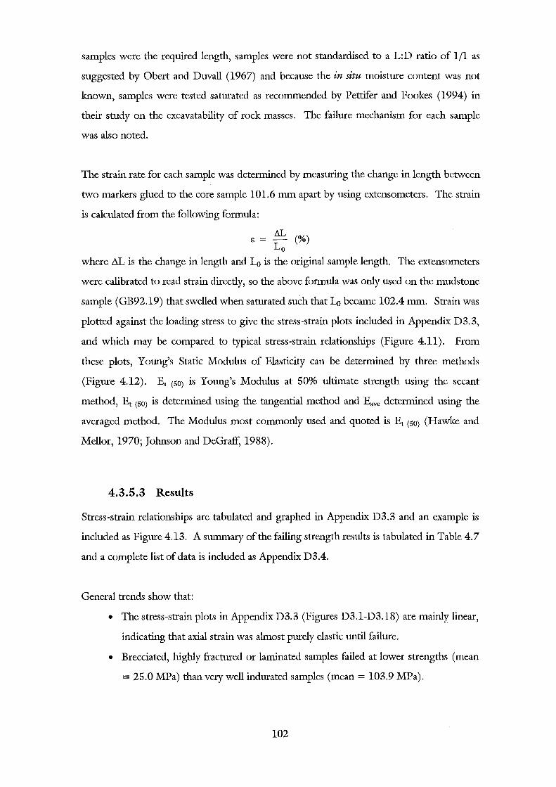
samples were the required length, samples were not standardised to a L:D ratio of 1/1 as
suggested by Obert and Duvall (1967) and because the in situ moisture content was not
known, samples were tested saturated as recommended by Pettifer and Fookes (1994) in
their study on the excavatability of rock masses. The failure mechanism for each sample
was also noted.
The strain rate for each sample was determined by measuring the change in length between
two markers glued to the core sample 101.6 mm apart by using extensometers. The strain
is calculated from the following formula:
~ 8 = - (%)
Lo
where L1L is the change in length and Lo is the original sample length. The extensometers
were calibrated to read strain directly, so the above formula was only used on the mudstone
sample (GB92.19) that swelled when saturated such that Lo became 102.4 mm. Strain was
plotted against the loading stress to give the stress-strain plots included in Appendix D3.3,
and which may be compared to typical stress-strain relationships (Figure 4.11). From
these plots, Young's Static Modulus of Elasticity can be determined by three methods
(Figure 4.12). Es (50) is Young's Modulus at 50% ultimate strength using the secant
method, Et (50) is determined using the tangential method and Eave determined using the
averaged method. The Modulus most commonly used and quoted is Et (50) (Hawke and
Mellor, 1970; Johnson and DeGraff, 1988).
4.3.5.3 Results
Stress-strain relationships are tabulated and graphed in Appendix D3.3 and an example is
included as Figure 4.13. A summary of the failing strength results is tabulated in Table 4.7
and a complete list of data is included as Appendix D3.4.
General trends show that:
• The stress-strain plots in Appendix D3.3 (Figures D3.1-D3.18) are mainly linear,
indicating that axial strain was almost purely elastic until failure.
• Brecciated, highly fractured or laminated samples failed at lower strengths (mean
= 25.0 MPa) than very well indurated samples (mean= 103.9 MPa).
102

fyp~ l clastic Type ll elastic-plastic
t a
€-Basalt
€--Siltstone
Type Ill plnstic-ebstic fype IV plas\ic-elastic-pla>tic
t 1
I 'J a
€-Sandstone :\larblc
Type V plastic-elastic-plastic Type VI elastic-plastic-creep
t a a
Schist Rock salt
Figure 4.11: Typical stress-strain relationship curves for rocks in uniaxial compress10n loaded to failure (from FG Bell, 1993).
Strain, f
t:1
/.I I I I J.o t I I I
Stram, f
.ff)
au~-----------1
~-----
Strain, f
rb
Figure 4.12: Determination of the static Young's Modulus by (a) the secant method, (b) the tangential method and (c) the averaged method (from Johnson and DeGraff, 1988).
103
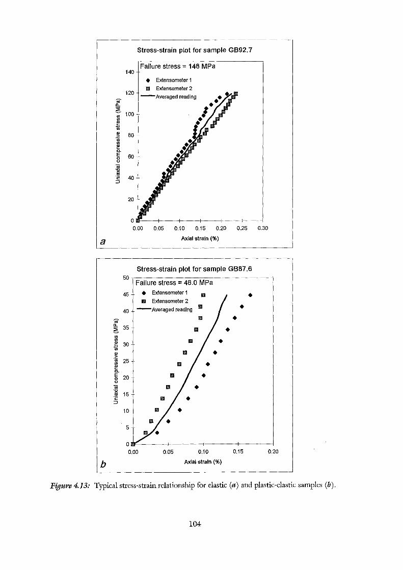
a
b
(U 0..
140
120
Stress-strain plot for sample GB92. 7
Failure stress= 146 MPa
• Extensometer 1
lill Extensometer 2
-Averaged reading
5 Ul 100 Ul ~ 1ii Q)
-~ Ul
~ a. E 0 0
"iii' 0..
5 Ul Ul Q) .... 1ii Q)
-~ Ul Ul Q)
l5.. E 0 0
iii -~ ·c: ::J
80
60
40
20
0~--~----~----+---~----~--~
0.00 0.05 0.10 0.15 0.20 0.25 0.30
Axial strain (%)
Stress-strain plot for sample GB87.6 50
Failure stress = 46.0 MPa
45 • Extensometer 1 1!!1 • lill Extensometer 2
-Averaged reading Ill • 40 Ill •
35 1!!1 • 30
II • 1!!1 •
25 lill •
20 Ill • 1111 •
15 1111 •
10
5
0
0.00 0.05 0.10 0.15
Axial strain(%)
0.20
Figure 4.13: Typical stress-strain relationship for elastic (a) and plastic-elastic samples (b).
104
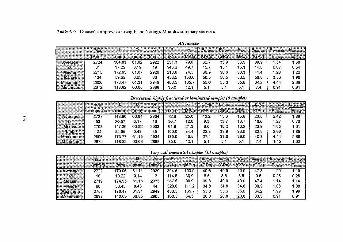
1--' 0 m
Table 4.7: Uniaxial compressive strength and Young's Modulus summary statistics
1::: t S!t rtttJ
31 2715 134
2806 2672
:),j
2719 60
2757 2697
172.95 61.07 2926 218.0 74.5 36.9 59.65 0.63 60 453.5 153.6 50.5 178.47 61.31 2949 488.5 165.7 55.6 118.82 60.68 2888 35.0 12.1 5.1
L.U.O/ U.l f 10 ,j0. ( IL..O ::1.,:)
2903 61.8 21.3 8.6 45 100.0 34.4 22.3
2934 135.0 46.5 27.4 2888 35.0 12.1 5.1
174.95 61.16 2935 287.5 98.9 39.8 38.45 0.45 44 328.0 111.2 34.8 178.4 7 61.31 2949 488.5 165.7 55.6 140.03 60.85 2905 160.5 54.5 20.8
38.3 50.5 55.6 5.1
55.6 20.8
38.3 50.5 55.6 5.1
41.4 56.8 64.2 7.4
1.99 0.91
1.99 0.91
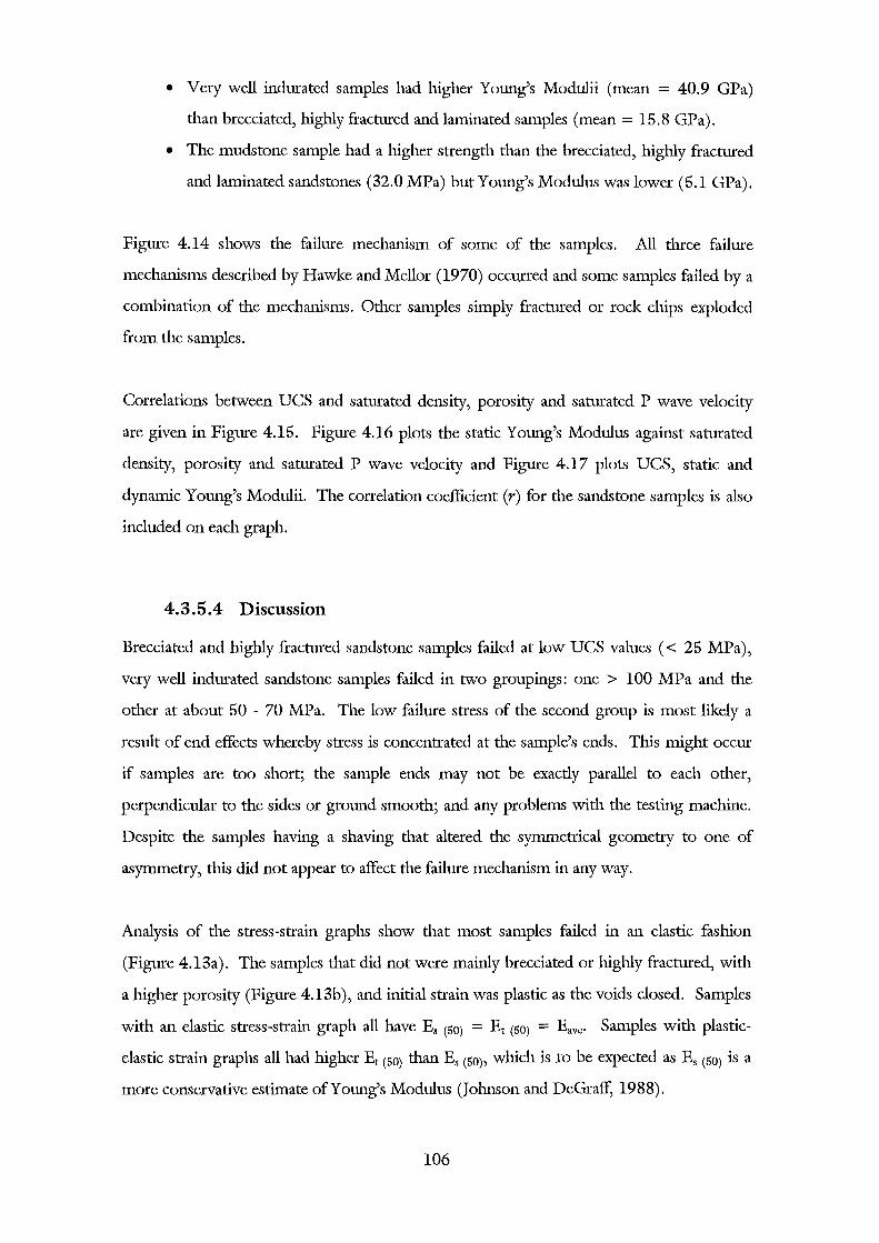
• Very well indurated samples had higher Young's Modulii (mean = 40.9 GPa)
than brecciated, highly fractured and laminated samples (mean= 15.8 GPa).
• The mudstone sample had a higher strength than the brecciated, highly fractured
and laminated sandstones (32.0 MPa) but Young's Modulus was lower (5.1 GPa).
Figure 4.14 shows the failure mechanism of some of the samples. All three failure
mechanisms described by Hawke and Mellor (1970) occmred and some samples failed by a
combination of the mechanisms. Other samples simply fractured or rock chips exploded
from the samples.
Correlations between UCS and saturated density, porosity and saturated P wave velocity
are given in Figure 4.15. Figure 4.16 plots the static Young's Modulus against saturated
density, porosity and saturated P wave velocity and Figure 4.17 plots UCS, static and
dynamic Young's Modulii. The correlation coefficient (r) for the sandstone samples is also
included on each graph.
4.3.5.4 Discussion
Brecciated and highly fractured sandstone samples failed at low UCS values ( < 25 MPa),
very well indurated sandstone samples failed in two groupings: one > 100 MPa and the
other at about 50 - 70 MPa. The low failure stress of the second group is most lil<ely a
result of end effects whereby stress is concentrated at the sample's ends. This might occur
if samples are too short; the sample ends may not be exactly parallel to each other,
perpendicular to the sides or ground smooth; and any problems with the testing machine.
Despite the samples having a shaving that altered the symmetrical geometry to one of
asymmetry, this did not appear to affect the failure mechanism in any way.
Analysis of the stress-strain graphs show that most samples failed in an elastic fashion
(Figure 4.13a). The samples that did not were mainly brecciated or highly fractured, with
a higher porosity (Figure 4.13b ), and initial strain was plastic as the voids closed. Samples
with an elastic stress-strain graph all have Es (50) = Et (50) = Eave· Samples with plastic
elastic strain graphs all had higher Et (50) thanEs (50), which is to be expected as Es (50) is a
more conservative estimate ofYoung's Modulus (Johnson and DeGraff, 1988).
106
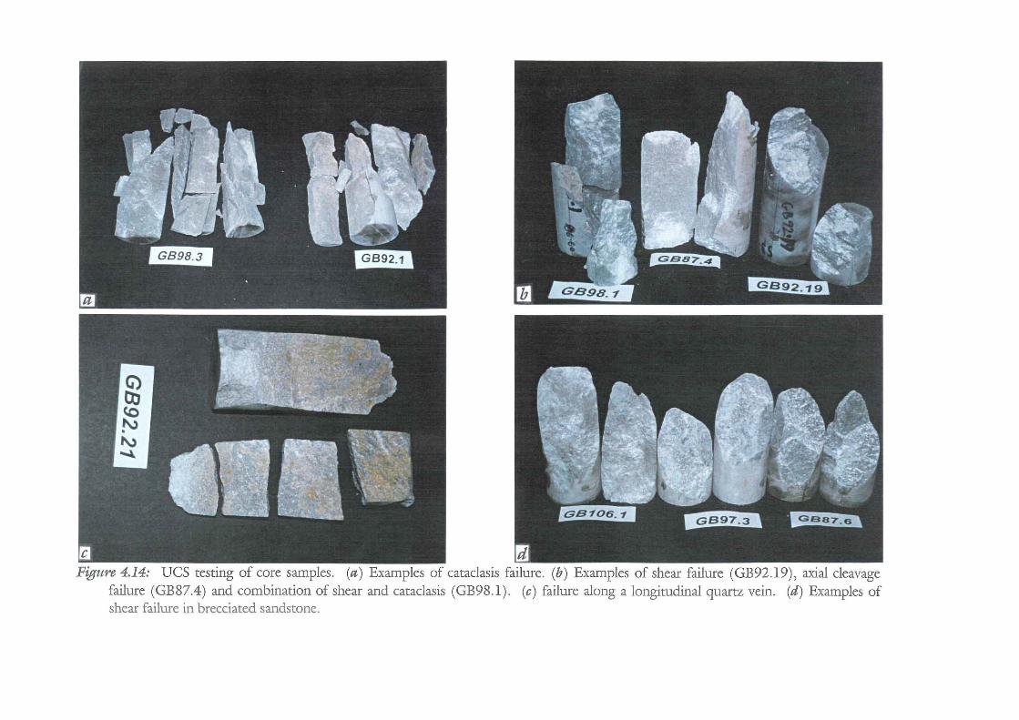
Figure 4.14: UCS testing of core samples. (a) Examples of cataclasis failure. (b) Examples of shear failure (GB92.19), axial cleavage failure (GB87.4) and combination of shear and cataclasis (GB98 .l). (c) failure along a longitudinal quartz vein. (d) Examples of shear failure in brecciated sandstone.
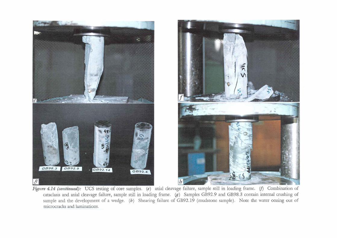
Figure 4.14 (continued): UCS testing of core samples. (e) axial cleavage failure, sample still in loading frame. (j) Combination of cataclasis and axial cleavage failure, sample still in loading frame. (g) Samples GB92.9 and GB98.3 contain internal crushing of sample and the development of a wedge. (h) Shearing failure of GB92.19 (mudstone sample). Note the water oozing out of microcracks and laminations.
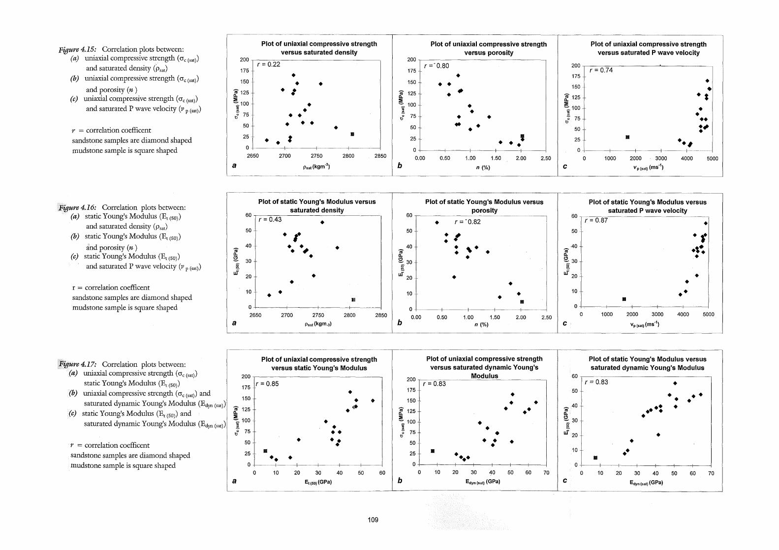
Figure 4.15: Correlation plots between: (a) uniaxial compressive strength ( O'c (sat))
and saturated density (Psat)
(b) uniaxial compressive strength ( O'c (sat))
and porosity (n) (c) uniaxial compressive strength ( O'c (sat))
and saturated P wave velocity (v P (sat))
r = correlation coefficent sandstone samples are diamond shaped mudstone sample is square shaped
Figure 4.16: Correlation plots between: (a) static Young's Modulus (Et (SO))
and saturated density (Psat)
(b) static Young's Modulus (Et(SO))
and porosity (n ) (c) static Young's Modulus (Et (SO))
and saturated P wave velocity (v P (sat))
r = correlation coefficent sandstone samples are diamond shaped mudstone sample is square shaped
Figure 4.17: Correlation plots between: (a) uniaxial compressive strength ( O'c (sat))
static Young's Modulus (Et (SO))
(b) uniaxial compressive strength ( crc (sat)) and
saturated dynamic Young's Modulus (Edyn (sat))
(c) static Young's Modulus (Et (SO)) and
saturated dynamic Young's Modulus (Edyn (sat))
r = correlation coefficent sandstone samples are diamond shaped mudstone sample is square shaped
Plot of uniaxial compressive strength versus saturated density
200 r = 0.22
175 • 150 • • I? 125 • I 0.. :::5 -:::.100 • 10
.!!!. • 0 75 • • b
• • • 50 • 25 : Ill
• • 0 2650 2700 2750 2800 2850
a Psat (kgm·3)
Plot of static Young's Modulus versus
60 saturated density
r = 0.43 • 50 ,. • 40 • ., • I? • 0.. • ~ 30 s
!!!. w 20 • •
10 • • II
0 --
2650 2700 2750 2800 2850
a Psat (kgm.J)
Plot of uniaxial compressive strength versus static Young's Modulus
200 --
175 r = 0.85
• 150 • • I? 125 0..
. ~ ~ 100 • 1?
.!!!. • 0 75 •• b
50 • •• • 1111 25 •• •
0 --+--0 10 20 30 40 50 60
a Et (SOl (GPa)
109
Plot of uniaxial compressive strength Plot of uniaxial compressive strength versus porosity versus saturated P wave velocity
200 r=·0.80 200
175 r = 0.74 • 175 150 • • • 150 - • I? 125 • I? 125 •• 0..
:::5 0.. ~ 100 • :::5
1? ~ 100 • .!!!. • 1? • 0 75 • • .!!!. b 0 75 ••
* b • ., 50 • 50 •
• t Ill 25 25 •• # • • 0 0 0.00 0.50 1.00 1.50 2.00 2.50 0 1000 2000 3000 4000 5000
b n (%) c Vp(sat) (ms"1)
Plot of static Young's Modulus versus Plot of static Young's Modulus versus
60 porosity
60 saturated P wave velocity
---
• r = ·o.82 r = 0.87 • 50 50 • , • •• • 40 • , . 40 .,~ I? • • I?
0.. • 0.. • ~ 30 ~ 30 s s !!!. !!!.
w 20 • ur 20 • • • 10 • 10 •• • Ill Ill
0 0
0.00 0.50 1.00 1.50 2.00 2.50 0 1000 2000 3000 4000 5000
b n (%) c Vp (sat) (ms"1)
Plot of uniaxial compressive strength Plot of static Young's Modulus versus versus saturated dynamic Young's saturated dynamic Young's Modulus
200 Modulus 60 r = 0.83 r = 0.83 •
175 50 • • •• 150 • • • • ~ 125 • •• .....,40 .. •: • Ill a..- • :::5 ~ 30 ~ 100 • 1? s
.!!!. • !!!. 0 75 • w·20 • b
50 • • • • • 25 Ill 10 •• ••• • 1111
0 0 0 10 20 30 40 50 60 70 0 10 20 30 40 50 60 70
b Edyn (sat) (GPa) c Edyn (sat) (GPa)
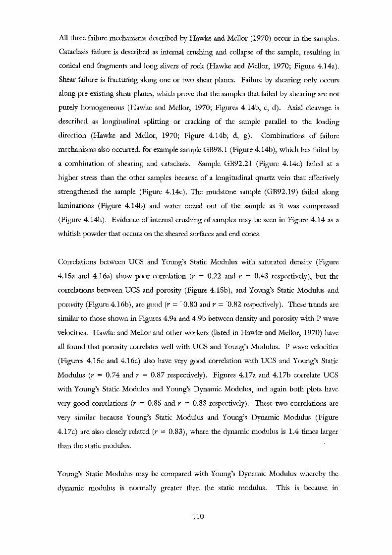
All three failure mechanisms described by Hawke and Mellor (1970) occur in the samples.
Cataclasis failure is described as internal crushing and collapse of the sample, resulting in
conical end fragments and long slivers of rode (Hawke and Mellor, 1970; Figure 4.14a).
Shear failure is fracturing along one or two shear planes. Failure by shearing only occurs
along pre-existing shear planes, which prove that the samples that failed by shearing are not
purely homogeneous (Hawke and Mellor, 1970; Figures 4.14b, c, d). Axial cleavage is
described as longitudinal splitting or cracking of the sample parallel to the loading
direction (Hawke and Mellor, 1970; Figure 4.14b, d, g). Combinations of failure
mechanisms also occurred, for example sample GB98.1 (Figure 4.14b), which has failed by
a combination of shearing and cataclasis. Sample GB92.21 (Figure 4.14c) failed at a
higher stress than the other samples because of a longitudinal quartz vein that effectively
strengthened the sample (Figure 4.14c). The mudstone sample (GB92.19) failed along
laminations (Figure 4.14b) and water oozed out of the sample as it was compressed
(Figure 4.14h). Evidence of internal crushing of samples may be seen in Figure 4.14 as a
whitish powder that occurs on the sheared surfaces and end cones.
Correlations between UCS and Young's Static Modulus with saturated density (Figure
4.15a and 4.16a) show poor correlation (r = 0.22 and r = 0.43 respectively), but the
correlations between UCS and porosity (Figure 4.15b), and Young's Static Modulus and
porosity (Figure 4.16b), are good (r = -0.80 and r = -0.82 respectively). These trends are
similar to those shown in Figures 4.9a and 4.9b between density and porosity with P wave
velocities. Hawke and Mellor and other workers (listed in Hawke and Mellor, 1970) have
all found that porosity correlates well with UCS and Young's Modulus. P wave velocities
(Figures 4.15c and 4.16c) also have very good correlation with UCS and Young's Static
Modulus (r = 0.74 and r = 0.87 respectively). Figures 4.17a and 4.17b correlate UCS
with Young's Static Modulus and Young's Dynamic Modulus, and again both plots have
very good correlations (r = 0.85 and r = 0.83 respectively). These two correlations are
very similar because Young's Static Modulus and Young's Dynamic Modulus (Figure
4.17c) are also closely related (r = 0.83), where the dynamic modulus is 1.4 times larger
than the static modulus.
Young's Static Modulus may be compared with Young's Dynamic Modulus whereby the
dynamic modulus is normally greater than the static modulus. This is because in
110
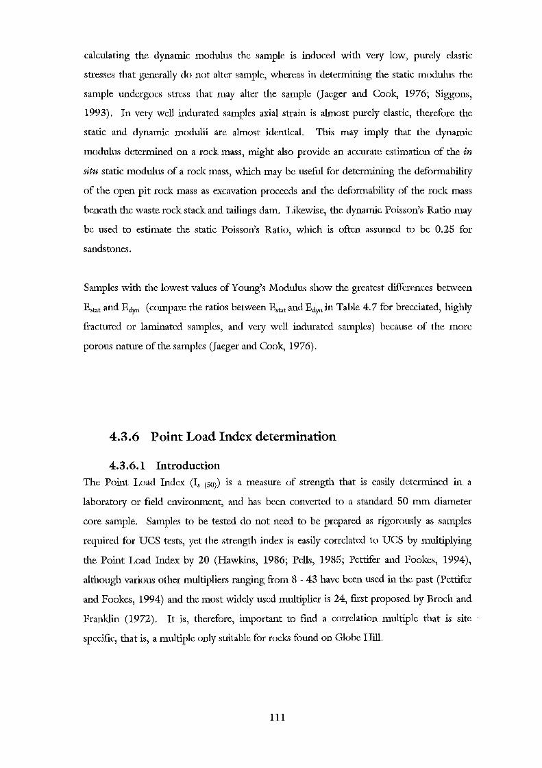
calculating the dynamic modulus the sample is induced with very low, purely elastic
stresses that generally do not alter sample, whereas in determining the static modulus the
sample undergoes stress that may alter the sample (Jaeger and Coole, 1976; Siggons,
1993). In vety well indurated samples axial strain is almost purely elastic, therefore the
static and dynamic modulii are almost identical. This may imply that the dynamic
modulus determined on a rock mass, might also provide an accurate estimation of the in
situ static modulus of a rock mass, which may be useful for determining the deformability
of the open pit rock mass as excavation proceeds and the deformability of the rock mass
beneath the waste rock stack and tailings dam. Lil<ewise, the dynamic Poisson's Ratio may
be used to estimate the static Poisson's Ratio, which is often assumed to be 0.25 for
sandstones.
Samples with the lowest values of Young's Modulus show the greatest differences between
Estat and Edyn (compare the ratios between Estat and Edyn in Table 4. 7 for brecciated, highly
fractured or laminated samples, and very well indurated samples) because of the more
porous nature of the samples (Jaeger and Coole, 1976).
4.3.6 Point Load Index determination
4.3.6.1 Introduction The Point Load Index (Is (SO)) is a measure of strength that is easily determined in a
laboratory or field environment, and has been converted to a standard 50 mm diameter
core sample. Samples to be tested do not need to be prepared as rigorously as samples
required for UCS tests, yet the strength index is easily correlated to UCS by multiplying
the Point Load Index by 20 (Hawkins, 1986; Pells, 1985; Pettifer and Fookes, 1994),
although various other multipliers ranging from 8 - 43 have been used in the past (Pettifer
and Fookes, 1994) and the most widely used multiplier is 24, first proposed by Brach and
Franldin (1972). It is, therefore, important to fmd a correlation multiple that is site
specific, that is, a multiple only suitable for rocks found on Globe Hill.
111
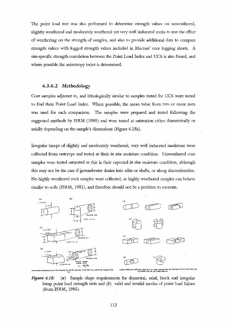
The point load test was also performed to determine strength values on unweathered,
slightly weathered and moderately weathered yet very well indurated rocks to test the effect
of weathering on the strength of samples, and also to provide additional data to compare
strength values with logged strength values included in Macraes' core logging sheets. A
site-specific strength correlation between the Point Load Index and UCS is also found, and
where possible the anisotropy index is determined.
4.3.6.2 Methodology
Core samples adjacent to, and lithologically similar to samples tested for UCS were tested
to fmd their Point Load Index. Where possible, the mean value from two or more tests
was used for each comparison. The samples were prepared and tested following the
suggested methods by ISRM (1985) and were tested at saturation either diametrically or
axially depending on the sample's dimensions (Figure 4.18a).
Irregular lumps of slightly and moderately weathered, very well indurated sandstone were
collected from outcrops and tested at their in situ moisture condition. Unweathered core
samples were tested saturated as this is their expected in situ moisture condition, although
this may not be the case if groundwater drains into adits or shafts, or along discontinuities.
No highly weathered rock samples were collected, as highly weathered samples can behave
similar to soils (ISRM, 1981), and therefore should not be a problem to excavate.
lol
(d)
lbl
W•~
' amen shape rcquinmenu for t•l the dlametul test, tbl the arialtest,{c)the block test. and (d) the lrre&ular lump ten.
lol
I b) tt[j f1t1
I d)
a§J lei~
modes of fallu~ for valid and invalid tcsu. (a) Valid diametf'ld ldU: tb) ulid a:ualtests: (c) valid block tem: (d) invalid core test: tel invalid un.l test.
Figure 4.18: (a) Sample shape requirements for diametral, axial, block and irregular lump point load strength teSts and (b) valid and invalid modes of point load failure (from ISRM, 1985).
112
4.3.6.3 Results
A srunmary of the results is tabulated in Table 4.8, and the full results are .included as
Appendix D3.5. Figure 4.19 shows valid failures for very well indurated and brecciated
core samples. Unweathered, brecciated core samples failed at a very weak Is (50) (mean =
l.ll MPa) whereas unweathered, very well indurated core samples failed at high Is (50)
values (mean = 6.49 MPa). Slightly weathered, very well indurated irregular lumps failed
at a mean value of Is (50) = 5.06 MPa whereas moderately weathered, very well indurated
irregular lumps failed at Is (50) = 2.68 MPa. A plot of Is (50) versus weathering grade is
include .in Section 4.3.7 along with data from the slake-durability test. Mudstone is the
only strongly anisotropic lithology, however the degree of anisotropy could not be
determined as there were no valid failures (see Figure 4.18b) for mudstone samples,
although it was observed that the mudstone failed along laminations for the diametral test
and was considerably stronger in the axial test (roughly perpendicular to laminations).
The Point Load Index (Is (50)) was correlated with UCS values for 18 out of the 19 samples
(the mudstone samples did not have any valid point load test result because they failed
along pre-existing shears or laminations). The data is plotted as Figure 4.20a and has a
correlation coefficient (r) equal to 0.76 and a regression multiple of 17. Figure 4.20a has
also been replotted as Figure 4.20b, where five very well indurated sandstone samples that
failed at weaker UCS values than expected, due to sample end effects, have been removed.
The correlation coefficient (r) improves to 0.89 and the regression multiple increases to 20.
4.3.6.4 Discussion
Figure 4.18a shows that there appears to be two clusters of data, five UCS samples failed
wealcer than expected as a result of end effects. If these samples are removed from the
correlation then r improves from 0.76 to 0.89 and the regression coefficient increases from
17 to 20 (Figure 4.18b). UCS values of Greenland Group rocks may now be calculated
from Is (50) values using the following empirical formula:
O'c = 20 (Is(50)) (MPa)
which is the same empirical formula suggested by Pells (1985) for use with sandstones
around Sydney, and also by Hawkins (1986) and Pettifer and Fookes (1994).
113
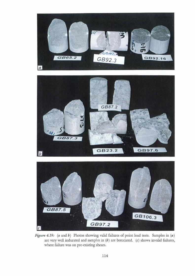
Figure 4.19: (a and b) Photos showing valid failures of point load tests. Samples in (a) are very well indurated and samples in (b) are brecciated. (c) shows invalid failures, where failure was on pre-existing shears.
114
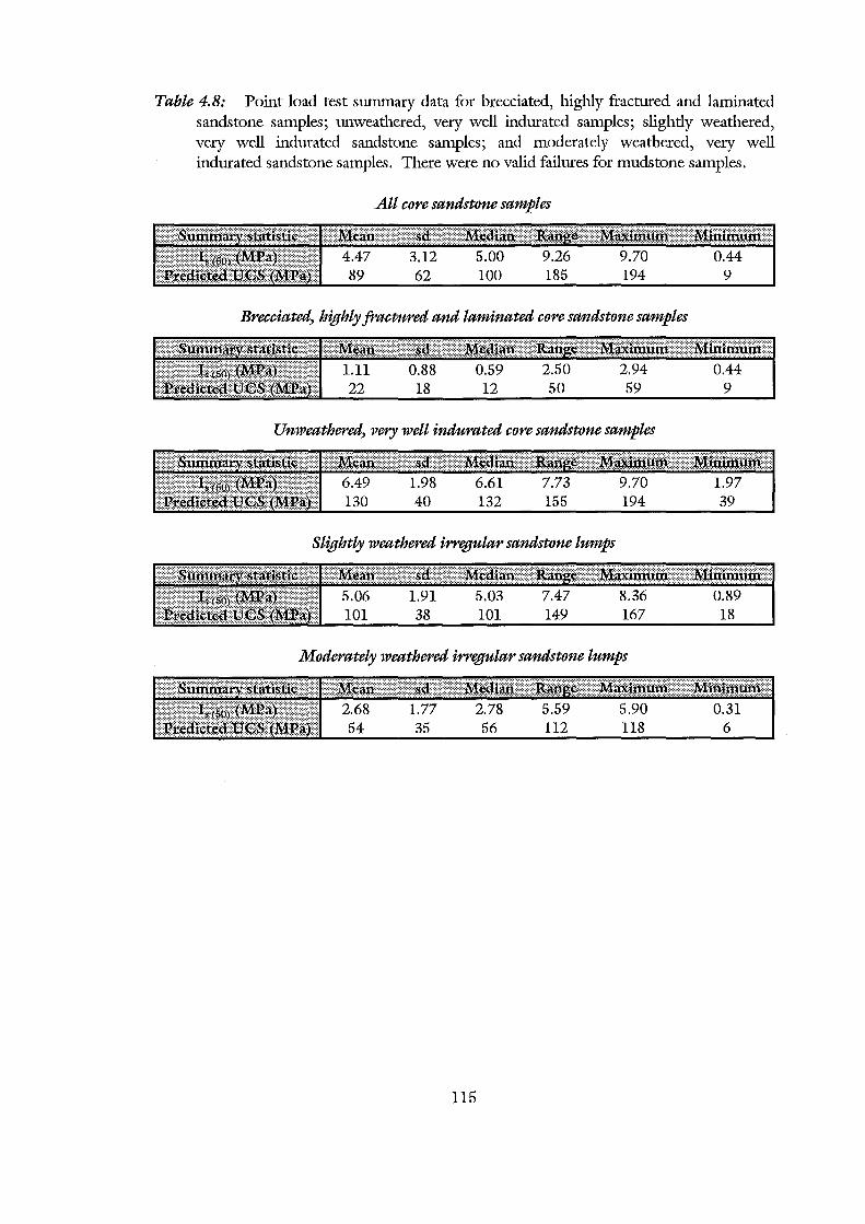
Table 4.8: Point load test summary data for brecciated, highly fractured and laminated sandstone samples; unweathered, very well indurated samples; slightly weathered, very well indurated sandstone samples; and moderately weathered, very well indurated sandstone samples. There were no valid failures for mudstone samples.
All core sandstone samples
Brecciated) highly fractured and laminated core sandstone samples
Unweathered) very well indurated core sandstone samples
Slightly weathered irregular sandstone lumps
Moderately weathered irregular sandstone lumps
115
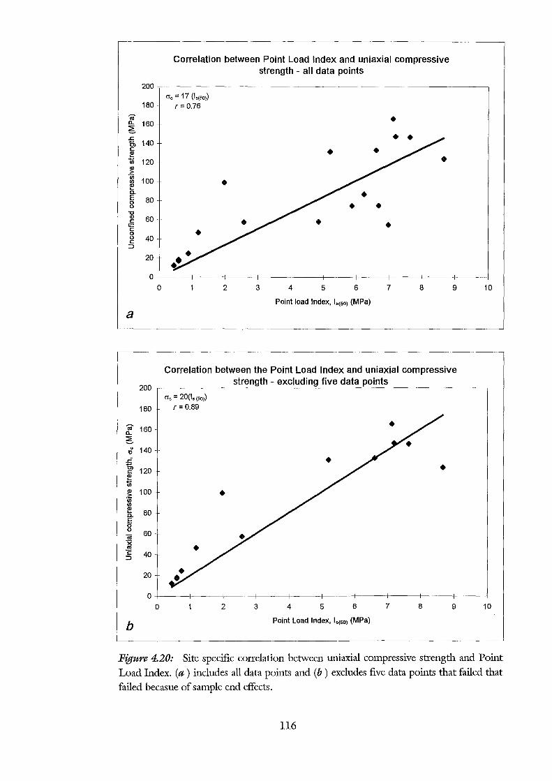
m-0...
6 .r: 0, c ~ 1ii
CD >
"iii Ul CD ..... 0.. E 0 0 "0 CD c
1;::: c 0 0 c ::J
a
m-0...
6
" .r: 0, c CD ..... 1ii CD >
"iii Ul ~ 0.. E 0 0
iii ·~ "E ::J
b
200
180
160
140
120
100
80
60
40
20
0 0
Correlation between Point Load Index and uniaxial compressive strength - all data points
cr0 = 17 (ls(SO))
r = 0.76
•
2 3 4 5 6 7 8
Point load Index, ls(so) (MPa)
9 10
Correlation between the Point Load Index and uniaxial compressive strength - excluding five data points
200,-----------------~--------~------~--------------------~
cr0 = 20(1s (SO))
180 r = 0.89
160
140
120
100
80
60
40
20
0 0 2 3 4 5 6 7 8 9 10
Point Load Index, ls(so) (MPa)
Figure 4.20: Site specific correlation between uniaxial compressive strength and Point
Load Index. (a) includes all data points and (b) excludes five data points that failed that failed becasue of sample end effects.
116
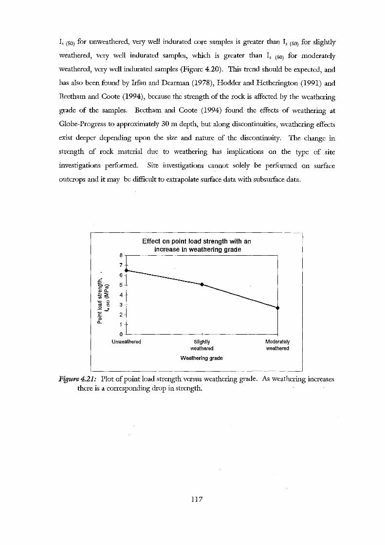
Is (50) for unweathered, very well .indurated core samples is greater than Is (50) for slightly
weathered, very well .indurated samples, which is greater than Is (50) for moderately
weathered, very well .indurated samples (Figure 4.20). This trend should be expected, and
has also been found by Irfan and Dearman (1978), Hodder and Hethermgton (1991) and
Beetham and Coote (1994), because the strength of the rock is affected by the weathermg
grade of the samples. Beetham and Coote (1994) found the effects of weathermg at
Globe-Progress to approximately 30m depth, but along discontinuities, weathermg effects
exist deeper dependmg upon the size and nature of the discontinuity. The change ill
strength of rock material due to weathermg has implications on the type of site
.investigations performed. Site .investigations cannot solely be performed on surface
outcrops and it may be difficult to extrapolate surface data with subsurface data.
:5. C)~
c m Q)ll..
.:::.:::?: Ul ~
1:1 0 m !!!. .2 0 .... c ·a a..
8
7
6
5
4
3
2
0 Unweathered
Effect on point load strength with an increase in weathering grade
Slightly weathered
Weathering grade
Moderately weathered
Figure 4.21: Plot of pomt load strength versus weathermg grade. As weathermg increases there is a corresponding drop ill strength.
117
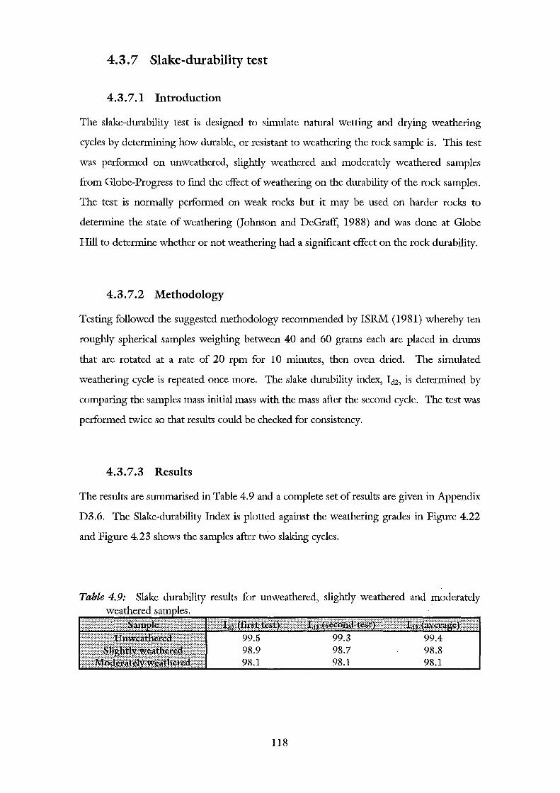
4.3. 7 Slake-durability test
4.3.7.1 Introduction
The slake-durability test is designed to simulate natural wetting and drying weathering
cycles by determining how durable, or resistant to weathering the rock sample is. This test
was performed on unweathered, slightly weathered and moderately weathered samples
from Globe-Progress to fmd the effect ofweathering on the durability of the rock samples.
The test is normally performed on weak rocks but it may be used on harder rocks to
determine the state of weathering (Johnson and DeGraff, 1988) and was done at Globe
Hill to determine whether or not weathering had a significant effect on the rock durability.
4.3.7.2 Methodology
Testing followed the suggested methodology recommended by ISRM (1981) whereby ten
roughly spherical samples weighing between 40 and 60 grams each are placed in drums
that are rotated at a rate of 20 rpm for 10 minutes, then oven dried. The simulated
weathering cycle is repeated once more. The slake durability index, Ic12, is determined by
comparing the samples mass initial mass with the mass after the second cycle. The test was
performed twice so that results could be checked for consistency.
4.3.7.3 Results
The results are summarised in Table 4.9 and a complete set of results are given in Appendix
D3.6. The Slake-durability Index is plotted against the weathering grades in Figure 4.22
and Figure 4.23 shows the samples after two slaking cycles.
Table 4.9: Slake durability results for unweathered, slightly weathered and moderately weathered ""-'-''~ ..... ~·~
98.1 98.1 98.1
118
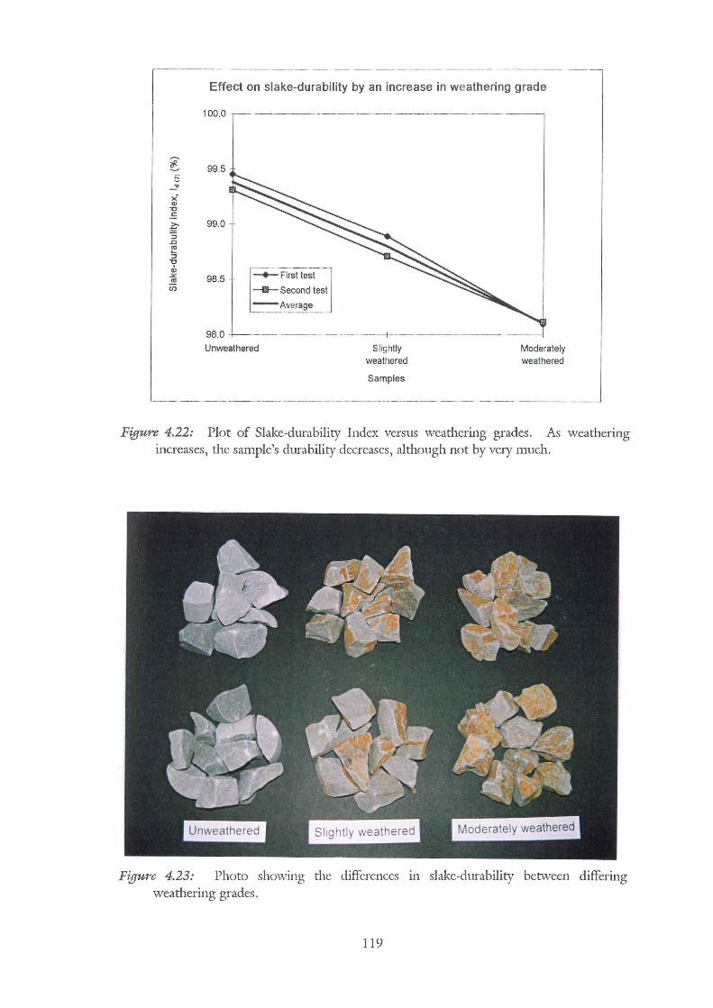
Effect on slake-durability by an increase in weathering grade
100.0 -------------- ----- - ------ -----,
99.5
99.0
~- ------ j -+-First test
--ill- Second test
-Average - -----
98.5
98.0 ·1-- - ---- - --- ------1---------- - - -Unweathered Slightly Moderately
weathered weathered
Samples
Figure 4.22: Plot of Slake-durability Index versus weathering grades. As weathering increases, the sample's durability decreases, although not by ve1y much.
Figure 4.23: Photo showing the differences 111 slake-durability between differing wearl1erli1g grade~.
119
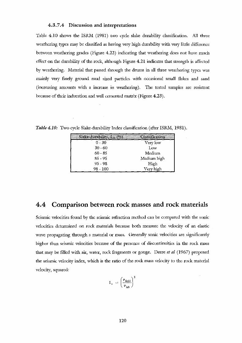
4.3.7.4 Discussion and interpretations
Table 4.10 shows the ISRM (1981) two cycle slake durability classification. All three
weathering types may be classified as having very high durability with very little difference
between weathering grades (Figure 4.22) indicating that weathering does not have much
effect on the durability of the rock, although Figure 4.21 indicates that strength is affected
by weathering. Material that passed through the drums in all three weathering types was
mainly very fmely ground mud sized particles with occasional small flakes and sand
(increasing amounts with a increase in weathering). The tested samples are resistent
because of their induration and well cemented matrix (Figure 4.23).
Table4.10: Two cycle Slake-durability Index classification (after ISRM, 1981).
0- 30 30-60 60-85 85- 95 95-98 98- 100
Very low Low
Medium Medium high
High v
4.4 Comparison between rock masses and rock materials
Seismic velocities found by the seismic refraction method can be compared with the sonic
velocities determined on rock materials because both measure the velocity of an elastic
wave propagating through a material or mass. Generally sonic velocities are significantly
higher than seismic velocities because of the presence of discontinuities in the rock mass
that may be filled with air, water, rock fragments or gouge. Deere et at (1967) proposed
the seismic velocity index, which is the ratio of the rock mass velocity to the rock material
velocity, squared:
(v field)
2
vlab
120
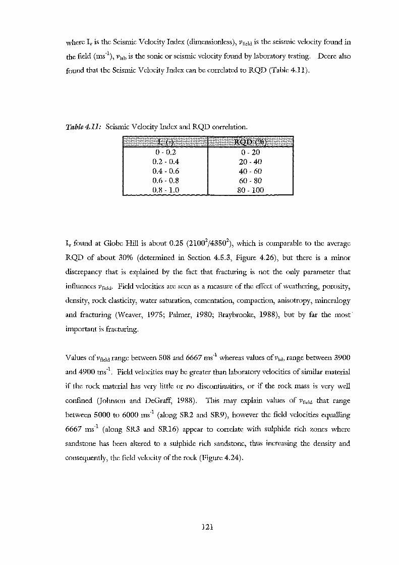
where Iv is the Seismic Velocity Index (dimensionless), Vfield is the seismic velocity found in
the field (ms-1), VJab is the sonic or seismic velocity found by laboratory testing. Deere also
found that the Seismic Velocity Index can be correlated to RQD (Table 4.11).
Table 4.11: Seismic Velocity Index and RQD correlation.
0-0.2 0-20 0.2-0.4 20-40 0.4-0.6 40-60 0.6-0.8 60-80 0.8- 1.0 80- 100
Iv found at Globe Hill is about 0.25 (21002/43502), which is comparable to the average
RQD of about 30% (determined in Section 4.5.3, Figure 4.26), but there is a minor
discrepancy that is explained by the fact that fracturing is not the only parameter that
influences VfieJd· Field velocities are seen as a measure of the effect of weathering, porosity,
density, rock elasticity, water saturation, cementation, compaction, anisotropy, mineralogy
and fracturing (Weaver, 1975; Palmer, 1980; Braybrooke, 1988), but by far the most
important is fracturing.
Values of VfieJd range between 508 and 6667 ms -1 whereas values of VJab range between 3900
and 4900 ms -1 . Field velocities may be greater than laboratory velocities of similar material
if the rock material has very little or no discontinuities, or if the rock mass is very well
confmed (Johnson and DeGraff, 1988). This may explain values of VfieJd that range
between 5000 to 6000 ms-1 (along SR2 and SR9), however the field velocities equalling
6667 ms-1 (along SR3 and SR16) appear to correlate with sulphide rich zones where
sandstone has been altered to a sulphide rich sandstone, thus increasing the density and
consequendy, the field velocity of the rock (Figure 4.24).
121
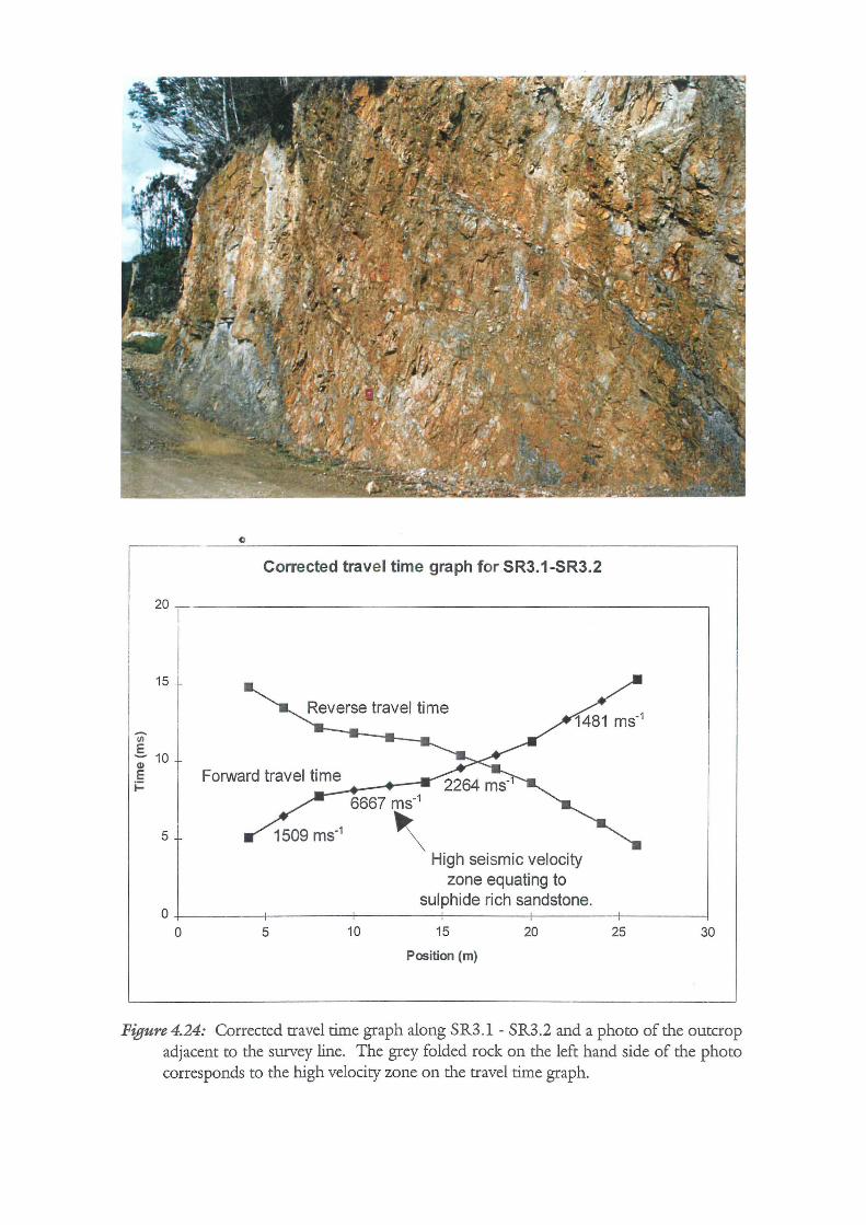
0
Corrected travel time graph for SR3.1-SR3.2
20 ,------------------------------------------------------,
15 .
(i)
.§.. 10 Ql
E i=
5
Forward travel time =....---+--6667 ms-1
' High seismic velocity zone equating to
sulphide rich sandstone. 0+--------+--------+--------+--------+--------+------~
0 5 10 15
Position (m)
20 25 30
Figure 4.24: Corrected travel time graph along SR3 .l - SR3 .2 and a photo of the outcrop adjacent to the survey line. The grey folded rock on the left hand side of the photo corresponds to the high velocity zone on the travel time graph.
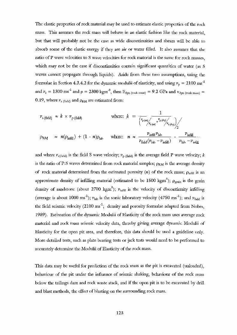
The elastic properties of rock material may be used to estimate elastic properties of the rock
mass. This assumes the rock mass will behave in an elastic fashion like the rock material,
but that will probably not be the case as wide discontinuities and shears will be able to
absorb some of the elastic energy if they are air or water filled. It also assumes that the
ratio of P wave velocities to S wave velocities for rock material is the same for rock masses,
which may not be the case if discontinuities contain significant quantities of water (as S
waves cannot propagate through liquids). Aside from these two assumptions, using the
formulae in Section 4.3.4.2 for the dynamic modulii of elasticity, and using vp = 2100 ms-1
and Vs = 1300 ms-1
and p = 2300 kgm-3, then Edyn (rock mass) = 9.2 GPa and Vdyn (rock mass) =
0.19, where Vs (field) and PRM are estimated from:
V s (fidd) :::::: k X V p (fidd) where: .k l
C'r (saX (sat) /r (;(. (dry)V,
:::::: n(pinfill) + (l - n )Plab where: n :::::: Vinfillvlab Vinfill
and where Vs(field) is the fieldS wave velocity; vp (field) is the average field P wave velocity; k
is the ratio ofP:S waves determined from rock material samples; PRM is the average density
of rock material determined from the estimated porosity (n) of the rock mass; Pinfill is an
approximate density of infilling material (estimated to be 1500 kgm3); Pgrain is the grain
density of sandstone (about 2700 kgm3); Vinfill is the velocity of discontinuity infilling
(average is about 1000 ms-1); Vlab is the sonic laboratory velocity (4750 ms-1
); and VfieJd is
the field seismic velocity (2100 ms-\ density and porosity formulae adapted from Nobes,
1989). Estimation of the dynamic Modulii ofElasticity of the rock mass uses average rock
material and rock mass seismic velocity data, thereby giving average dynamic Modulii of
Elasticity for the open pit area, and therefore, this data should be used a guideline only.
More detailed tests, such as plate bearing tests or jack tests would need to be performed to
accurately determine the Modulii of Elasticity of the rock mass.
This data may be useful for prediction of the rock mass as the pit is excavated (unloaded),
behaviour of the pit under the influence of seismic shaking, behaviour of the rock mass
below the tailings dam and rock waste stack, and if the open pit is to be excavated by drill
and blast methods, the effect of blasting on the surrounding rock mass.
123
4.5 Drillcore log analysis
4.5.1 Introduction
Analyses and checks of the drillcore logs were performed to confirm the accuracy of
logged data before applying ratings to them for rock mass and rippability classifications.
Comparisons were made between logged strength values, and point load strength and UCS
values tested by Beetham and Coote (1994) and this study. Two RQD data sets exist,
which were compared, and the discontinuity spacing was compared to discontinuity
spacing distribution models postulated by Priest and Hudson (1976). Other parameters
such as rock type, grain size and weathering are all assumed to have been correctly logged
as they are simple to describe and do not require any estimation of the parameter.
4.5.2 Strength comparisons
A comparison of the logged strength values and point load test and UCS tested samples
show that strength has been consistently logged incorrectly. The majority of sandstone has
been logged as R3 (equivalent UCS values equal 25 - 50 MPa), yet point load strength
data from Beetham and Coote and this study, as well as UCS values from this study, range
between 8 MPa and 260 MPa (Figure 4.25a; point load strength data converted to UCS by
multiplying by 20). Therefore, some of the sandstone strengths have been over-estimated,
but the majority have been under-estimated. From data collected from point load strength
and UCS tests, a revised strength estimate was made for each logged rock mass unit
(RMU) based on the logged lithology and strength (Figure 4.24b). The revised strength
estimate includes a large group of data in the extremely weak to wealc strength class ( < 25
MPa) that is not present in the actual strength data set. This discrepancy arises because
samples tested for strength by Beetham and Coote (1994) and in this study are biased
towards selecting stronger samples. The assumptions made in determining the revised
strength are included as Appendix ELL
124
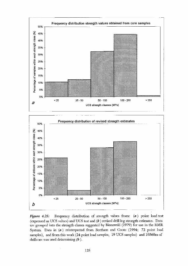
Frequency distribution strength values obtained from core samples 50%
ii 45% U'J U'J m
40% 0 ..c: 0, c 35% ~ iii ..c:
30% 0 m CD c :c 25% ~ U'J CD 20% a. E m U'J 15% .,_ 0 CD Ol 10% .B c CD
E 5% CD a..
0% <25 25-50 50-100 100-250 > 250
a UCS strength classes (MPa)
50% Frequency distribution of revised strength estimates
~ 45% U'J U'J m 40% 0
..c: 0, c 35% CD ..... iii ..c: 30% 0 m CD
c :c ~
25%
~ 20% 0 g ~ 15% .,_ 0 CD Ol
10% .B c CD
E CD 5% a..
0% <25 25-50 50-100 100-250 > 250
b UCS strength classes (MPa)
Figure 4.25: Frequency distribution of strength values from: (a ) point load test (expressed as UCS values) and UCS test and (b) revised drill log strength estimates. Data are grouped into the strength classes suggested by Bienawski (1979) for use in the RMR System. Data in (a) reinterpreted from Beetham and Coote (1994; 72 point load samples), and from this work (24 point load samples, 19 UCS samples) and 10360m of drillcore was used determining (b ) .
125
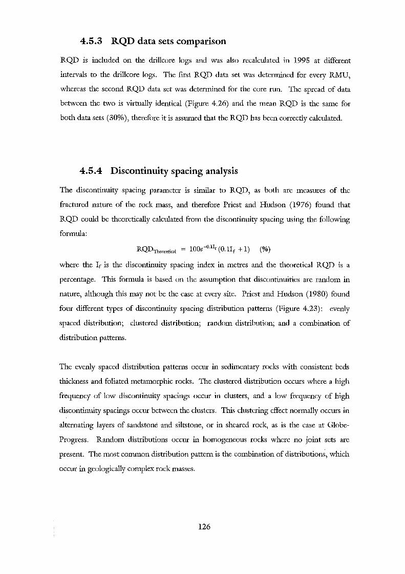
4.5.3 RQD data sets comparison
RQD is included on the drillcore logs and was also recalculated in 1995 at different
intervals to the drillcore logs. The first RQD data set was determined for every RMU,
whereas the second RQD data set was determined for the core run. The spread of data
between the two is virtually identical (Figure 4.26) and the mean RQD is the same for
both data sets (30% ), therefore it is assumed that the RQD has been correctly calculated.
4.5.4 Discontinuity spacing analysis
The discontinuity spacing parameter is similar to RQD, as both are measures of the
fractured nature of the rock mass, and therefore Priest and Hudson (1976) found that
RQD could be theoretically calculated from the discontinuity spacing using the following
formula:
RQDTheoretical = lOOe-O.llr(O.llr +l) (%)
where the Ir is the discontinuity spacing index in metres and the theoretical RQD is a
percentage. This formula is based on the assumption that discontinuities are random in
nature, although this may not be the case at every site. Priest and Hudson (1980) found
four different types of discontinuity spacing distribution patterns (Figure 4.23): evenly
spaced distribution; clustered distribution; random distribution; and a combination of
distribution patterns.
The evenly spaced distribution patterns occur in sedimentary rocks with consistent beds
thickness and foliated metamorphic rocks. The clustered distribution occurs where a high
frequency of low discontinuity spacings occur in clusters, and a low frequency of high
discontinuity spacings occur between the clusters. This clustering effect normally occurs in
alternating layers of sandstone and siltstone, or in sheared rock, as is the case at Globe
Progress. Random distributions occur in homogeneous rocks where no joint sets are
present. The most common distribution pattern is the combination of distribution~, which
occur in geologically complex rock masses.
126
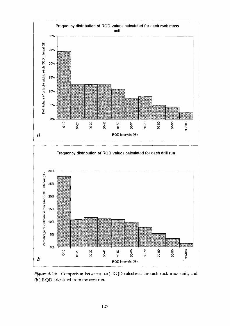
30%
~ iii 25% i:: Q)
£ 0 0
20% 0::: .c 0 I'll Q)
s:: :c 15% '§ ~ 0 0
~ 10% ...... 0 Q) C)
~ 5% Q) 0 .... Q)
11..
0%
a
30%
~ iii i:: 25% Q)
~ 0 0 0::: 20% .c 0 I'll Q)
s:: :c 15% '§ ~ 0 .Q
10% :;:: u ...... 0 Q) C)
5% I'll "E Q)
E Q)
11.. 0%
b
Frequency distribution of RQD values calculated for each rock mass unit
0 0 0
~ 0 0 0 0 0 ......
~ ~ $ ~ I';- ~ ~ I 0 0 0
N (') lJ) (0 f'-. co
RQD intervals(%)
Frequency distribution of RQD values calculated for each drill run
0 0 0 ~
0 0 0 0 0 ...... C';J ~ u;> ~ I';- co ~ 0 0 0 0 ~ 0 0 0
N (') lJ) (0 f'-. co
RQD intervals(%)
0 0 ...... 0 0')
0 0 ...... 0 0')
Figure 4.26: Comparison between: (a ) RQD calculated for each rock mass unit; and (b) RQD calculated from the core run.
127
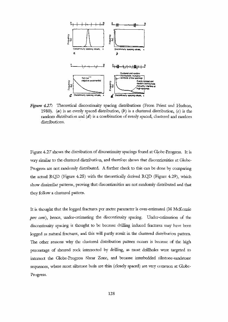
~, I /· I B .
n
D~onhnlnly SOOCIOQ VOtue1, t
a.
A . \ I
\' B .
C Discootirutly SPOCif'oll VOl-, l
A If" u
~ F .:: \.
L..:::::::===-J ~ly SllOCJt1Q ~ •
b
Figure 4.27: Theoretical discontinuity spacing distributions (From Priest and Hudson, 1980). (a) is an evenly spaced distribution, (b) is a clustered distribution, (c) is the random distribution and (d) is a combination of evenly spaced, clustered and random distributions.
Figure 4.27 shows the distribution of discontinuity spacings found at Globe-Progress. It is
very similar to the clustered distribution, and therefore shows that discontinuities at Globe
Progress are not randomly distributed. A further check to this can be done by comparing
the actual RQD (Figure 4.25) with the theoretically derived RQD (Figure 4.29), which
show dissimilar patterns, proving that discontinuities are not randomly distributed and that
they follow a clustered pattern.
It is thought that the logged fractures per metre parameter is over-estimated (M McKenzie
pers com), hence, under-estimating the discontinuity spacing. Under-estimation of the
discontinuity spacing is thought to be because drilling induced fractures may have been
logged as natural fractures, and this will partly result in the clustered distribution pattern.
The other reasons why the clustered distribution pattern occurs is because of the high
percentage of sheared rock intersected by drilling, as most drillholes were targeted to
intersect the Globe-Progress Shear Zone, and because interbedded siltstone-sandstone
sequences, where most siltstone beds are thin (closely spaced) are very common at Globe
Progress.
128
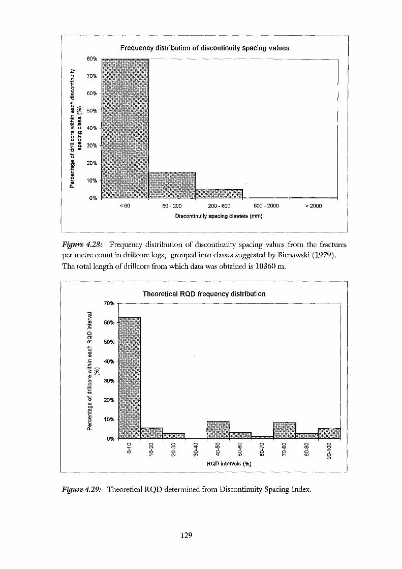
Frequency distribution of discontinuity spacing values
80%
~ 70% ::J
c ~ 0 0 60% If)
:0 .c 0~
Ill~ 50% .!: If) .c If)
~fl 40% Q) Cl ..... 0 .!: 0 0
Ill 30%
~ a.. If) -0
Q) 20% Cl Ill "E Q) 0
10% ..... Q)
a..
0% < 60 60-200 200-600 600-2000 > 2000
Discontinuity spacing classes (mm)
Figure 4.28: Frequency distribution of discontinuity spacing values from the fractures per metre count in drillcore logs, grouped into classes suggested by Bienawski (1979).
The total length of drillcore from which data was obtained is 10360 m.
Theoretical RQD frequency distribution 70%
~ Q) 60% E 0 0 0:: 50% .c 0 Ill Q)
c 40% :c :!::::::-.. ;;'* ~~
30% 0 .Q 1:: u -0 20% Q) Cl
~ Q) 10% 0 ..... Q)
a..
0% ..... ·:·
0 0 0
~ 0 0 0 0 .....
~ f? l{) (!)
"' ro
I I I 0 0 0 ~ 0 0 N C') l{) (!) f'-.
RQD intervals(%)
Figure 4.29: Theoretical RQD determined from Discontinuity Spacing Index.
129
4.5.5 Other logged data Logged parameters such as rock type, colour, grain size, weathering and alteration, and
discontinuity descriptions such as type, habit, roughness, infilling and infilling width are all
easily described as they are based on visual descriptions rather than estimations (lilce the
rock material strength and discontinuity spacing parameters). Therefore, it is assumed that
logged data such as rock type, colour, grain size, weathering, alteration, discontinuity type,
habit, roughness, infilling and infilling width have been logged correctly.
4.6 Synthesis
4.6.1 Field testing
Globe-Progress has been studied in detail by many workers, including Barrell (1992;
geotechnical line mapping), Rattenbury (1994; structural mapping) and Jowett et al
(1996; bench zero geotechnical mapping). The abundance of field investigations meant
very little additional field work was required. Seismic refraction line traverses were
surveyed to collect rock mass seismic velocity data, which could be used as a preliminary
rippability assessment (see Section 5.2.2) and also for comparisons with sonic velocities
determined from core samples of rock material. Fifteen seismic refraction surveys were
performed at Globe-Progress and five seismic refraction survey lines were performed at
General Gordon, site of the waste rock stack Frequency distribution diagrams of seismic
velocities grouped into 500 ms-1 were plotted and the mean seismic velocity at each site
was calculated to be 2100 ms-1 at Globe-Progress, 1950 ms-1 at General Gordon, and in
total, a mean seismic velocity of2100 ms-1 was found.
130
4.6.2 Laboratory testing
The following laboratory tests were performed on drillcore to acqrure quantitative
geoteclmical information of rock materials found at Globe-Progress:
• Porosity-density determination
• Sonic velocity determination
• Stress-strain relationship
• UCS and point load strength comparison
• Slalce durability determination
In addition to the above tests, the point load strength and slalce-durability of moderately
weathered and slightly weathered irregular lumps were compared to point load strength
and slalce-durability of unweathered core samples.
There were three broad groups of rock material tested:
• Very well indurated sandstone
• Brecciated or highly fractured sandstone
• Mudstone
The mean values from the tests listed above for each ·type of rock material are given in
Table 4.12. In addition to the above tests, the point load strength and slalce-durability of
unweathered, slightly weathered and moderately weathered samples were tested to find the
effect of weathering on strength and durability of the rock material (Table 4.13).
4.6.3 Drill core analysis
An analysis of drillcore log data was performed to assess the reliability of drillcore data. It
was found that:
• logged strength values had been under-estimated.
• RQD was logged correctly.
• Distribution of discontinuity spacmg data follows a clustered distribution
whereby closely spaced discontinuities are more common than widely spaced
discontinuities.
131
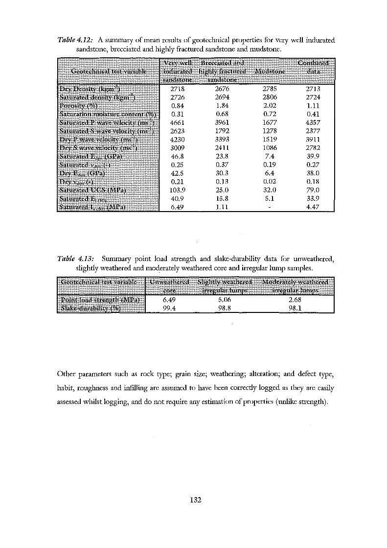
Table 4.12: A summary of mean results of geoteclmical properties for very well indurated sandstone, brecciated and highly fractured sandstone and mudstone.
2806 1.84 2.02 1.11
0.31 0.68 0.72 0.41 4661 3961 1677 4357 2623 1792 1278 2377 4230 3393 1519 3911 3009 2411 1086 2782 46.8 23.8 7.4 39.9 0.25 0.37 0.19 0.27 42.5 30.3 6.4 38.0 0.21 0.13 0.02 0.18
103.9 25.0 32.0 79.0 40.9 15.8 5.1 33.9 6.49 1.11 4.47
Table 4.13: Summary point load strength and slal<e-durability data for nnweathered, slighdy weathered and moderately weathered core and irregular lump samples.
Other parameters such as rock type; grain size; weathering; alteration; and defect type,
habit, roughness and infilling are assumed to have been correcdy logged as they are easily
assessed whilst logging, and do not require any estimation of properties (unlike strength).
132

ChapterS
Rippability evaluation of the proposed open pit
mine at Globe-Progress
5 .l Introduction
Chapters 2 and 3 briefly discussed various rock mass and rippability classification methods
and detailed the techniques most suited for classifying the open pit rock mass at Globe
Progress. Chapter 4 provided additional data and analysed the drillcore log data that was
used in the rock mass classifications. In this chapter the rock mass and rippability methods
detailed in Chapters 2 and 3, using data discussed in Chapter 4, are applied to the rock
mass at Globe-Progress.
The first stage in classifying the rock mass was to apply two simple methods that may be
performed at the feasibility and early investigation stage of a project (Section 5.2), followed
by a more detailed investigation that fully characterises the rock mass using a suite of
geological and geotechnical properties (Sections 5. 3 and 5.4). This type of rock mass
assessment may be performed during the investigation and design stages of a project. The
classification systems used should not be used as stand-alone site investigation studies.
They should be compared with other forms of geotechnical investigations, but they can be
used as guides to the location of areas that will be easy or difficult to excavate.
133
5.2 Preliminary rippability evaluation
5.2.1 Introduction
An initial or preliminary rippability assessment was performed to test whether or not a
more detailed rippability evaluation was required. If the preliminary analyses showed that
the excavatability of the pit to be marginal to non-rippable (very hard ripping to blasting),
then blasting would most lilcely be used and the excavatability of the pit would not be
required. If the preliminary analyses show that the pit is rippable (easy to hard ripping),
then a more detailed rippability investigation would be required to identifY the diggable,
easy ripping, moderate ripping and hard ripping zones. The preliminary rippability
assessments performed are both simply achieved with minimal effort and interpretation,
and therefore can be used in the feasibility and early site investigation stages of a project.
The approach undertalcen was to use two different methods: one involving determination
of seismic velocities, similar to the approach undertalcen by bulldozer manufacturers and
contractors, such as Caterpillar and Komatsu, who wish to sell their ripping machinery to
the buyer; and the other method involves comparing the spacing of discontinuities in a
rock mass and the corresponding rock material strength, the two parameters most
influential on the excavatability of a rock mass. This approach is commonly known as the
Size-Strength Method and plots the strength of a rock material against its block size or
discontinuity spacing. The method was originally designed by Franldin et al (1971) and
was recently updated by Pettifer and Fookes (1994).
5.2.2 Seismic velocity determination
5.2.2.1 Komatsu's site visit report
A study to determine seismic velocities at Globe-Progress was undertalcen by John (1994)
for Komatsu, and involved limited seismic velocity determination at four sites (see Figure
4.1 for locations). Site 1A and 1B and 3 were within the defmed pit limits, although no
data was obtained at site 3 because of the heavily fractured nature of the rock at this
134

location (John, 1994). Site 2 was just outside the pit limits but at a lower ground level,
possibly indicative of the structure within the open pit. Site 4 was on a back road leading
into the proposed mine site, where the rock mass is expected to be typical of that found in
the open pit.
Tests were performed with geophone spacings at 3m, 7 m, and 12.3 mat site 1A, 3m, 7
m, and 12 m at site 1B, 3 m, 8 m and 12 m at site 2 and 3 m, 7 m, 13 m, at site 4. All
tests were performed three times to check the consistency in results. All tests were found
to be consistent, with the tests performed at 3m spacing yielding higher velocities (range
between 968 ms-1 and 2200 ms-1) the tests performed at wider spacing (ranging between
609 ms-1 and 2000 ms-\
The report is lacking in details but it appears that no attempt has been made to process the
results following a standard method of data interpretation such as the Generalised
Reciprocal Method, therefore the velocities are apparent velocities, which are always less
than true velocities (see Appendix D2.1.2 for the definitions of apparent and true seismic
velocities), and are therefore not indicative of the rock mass quality.
John's (1994) recommendations based on field tests and observations on drillcore were:
• at least 60% of the rock mass is lilcely to be rippable using a Komatsu D475A-2
bulldozer at a productivity rate of 450 m3 /hr
• at least 80% of the rock mass is lilcely to be rippable using the Komatsu D575A-2
bulldozer at a productivity rate of 850 m3 /hr
The productivity figures quotes are at 80% efficiency, meaning the bulldozer is ripping
80% of the time. MacGregor et al (1994) stated that bulldozers normally rip 54% (range
between 30% and 90%) of the time if the bulldozer is just ripping and turning, or 21%
(range between 1% and 60%) of the time if the bulldozer is required to push scrapers
and/or doze loose material, therefore the productivity figures quoted by Komatsu are lilcely
to be higher than the actual productivity.
135
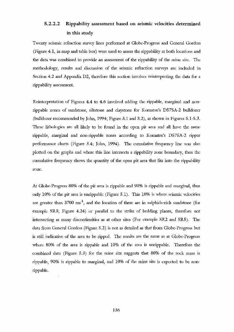
5.2.2.2 Rippability assessment based on seismic velocities determined
in this study
Twenty seismic refraction survey lines performed at Globe-Progress and General Gordon
(Figure 4.1, in map and table box) were used to assess the rippability at both locations and
the data was combined to provide an assessment of the rippability of the mine site. The
methodology, results and discussion of the seismic refraction surveys are included in
Section 4.2 and Appendix D2, therefore this section involves reinterpreting the data for a
rippability assessment.
Reinterpretation of Figures 4.4 to 4.6 involved adding the rippable, marginal and non
rippable wnes of sandstone, siltstone and claystone for Komatsu's D575A-2 bulldozer
(bulldozer recommended by John, 1994; Figure 3.1 and 3.2), as shown in Figures 5.1-5.3.
These lithologies are all lilcely to be found in the open pit area and all have the same
rippable, marginal and non-rippable wnes according to Komatsu's D575A-2 ripper
performance charts (Figure 3.4; John, 1994). The cumulative frequency line was also
plotted on the graphs and where this line intersects a rippability wne boundary, then the
cumulative frequency shows the quantity of the open pit area that fits into the rippability
wne.
At Globe-Progress 80% of the pit area is rippable and 90% is rippable and marginal, thus
only 10% of the pit area is unrippable (Figure 5.1). This 10% is where seismic velocities
are greater than 3700 ms-\ and the location of these are in sulphide-rich sandstone (for
example SR3; Figure 4.24) or parallel to the strilce of bedding planes, therefore not
intersecting as many discontinuities as at other sites (For example SR2 and SR5). The
data from General Gordon (Figure 5.2) is not as detailed as that from Globe-Progress but
is still indicative of the area to be ripped. The results are the same as at Globe-Progress
where 80% of the area is rippable and 10% of the area is unrippable. Therefore the
combined data (Figure 5.3) for the mine site suggests that 80% of the rock mass is
rippable, 90% is rippable to marginal, and 10% of the mine site is expected to be non
rippable.
136
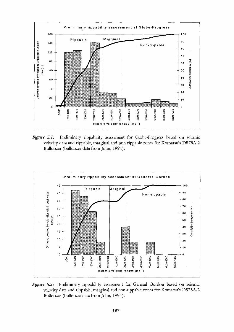
Preliminary rippability assessment at Globe-Progress
160 100
z;. R ippable ·o 140 0 a; >
90 Non-rippable
80 .c
120 0 .. Ol c 70 £
100 "j CJ)
60 ~ >-
Ol I p ·o 0 Ol 80 a; c > 0
>-N
..0
"U 60 ~ Ol > 0 0 40 Ol
0 c Ol
50 ::J <T Ol .:::
40 Ol > ~ :5
30 E ::J 0
0 c 20 tl i5 20
10
0 0 0 0 0 0 0 0 0 0 lO 0 lO 0 0 0 ~
0 0 0 0 a lO ~ ~
a 0 0 0 a 0 0 0 lO 0 lO 0 :g ~
ID 1';-0 0
0 a 0 0 0 lO 0 lO lO lO ID ID
0 0 0 0 0
~ ~ ~a• ~ ~a~ g §NI 0 g 0
~ ~ ~ ~ Seismic velocity ranges (ms- 1
)
Figure 5.1: Preliminary rippability assessment for Globe-Progress based on seismic velocity data and rippable, marginal and non-rippable zones for Komatsu's D575A-2 Bulldozer (bulldozer data from John, 1994).
Preliminary rippability assessment at General Gordon
45 100 Rippable
Non-rippable 90 ·o
40 0 a; >
80 .c 35 0 ..
Ol
70 ~
60 >-0 c Ol ::J
50 <T
~ Ol
40 > :g
c :c 30 ~ CJ) Ol
I ;E 25 0 0 Ol a; c > 0 20 >- N ..0 "U
:5
30 E "' 0
~ 15 Ol > 0 0
20 Ol 10 0 c ..
10 ]!
5 0
0 0 a a 0 a 0 0
'? 0 lO a ~ 2;
0 0 lO 0
0 a 0 a a a a a a 0 a a 0 a a 0 a a a a 0 a a lO a lO 0 lO a lO a lO a ~ ~ '? '? ..,. ..,. :g :g ID
~ 1';-a a 0 0 0 0 0 a 0 0 a a a a a a 0 0
~ 0 ~ a lO a '4 a lO 0 lO N "' "'
..,. lO lO ID ID
Seismic velocity ranges (ms- 1 )
Figure 5.2: Preliminary rippability assessment for General Gordon based on se1srmc velocity data and rippable,marginal and non-rippable zones for Komatsu's D575A-2 Bulldozer (bulldozer data from John, 1994).
137
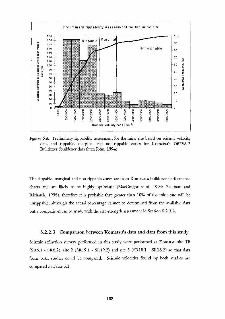
Preliminary rippability assessment for the mine site
170 100
160 90 £(
0 150 0
Non-rippable 80
Qi 140 > ..c
130 0
"' 70 ~
60 >. 0 c Ql ::J
50 <T ~ lL Ql
40 > ~ ::;
Ql 120 c
:c 11 0 ~ 11) 100 Ql I E 90 0 0 Ql Qi c 80 > 0
1> N
70 "0 60 ~
30 E ::J 0
Ql > 50 0 0
Ql 40 20 0
c 30 "' 1ii 0 20 10
10
0 0 0 0 0 0 0 0 0 0 0 0 0 0 I{) 0 I{)
~ I{) 0
<;I "? "? 'f "? 0 0 0 0 0 0
0 0 0 0 0 0 0 0 I{) 0 I{) 0 "? "? "? t-;-0 0 0 0
0 0 0 0 0 0 0 0 "? 0 I{) 0
~ ~ <;I 0 a 0
0 0 0 0 0 0 0 I{) 0 I{) 0 I{) N N (") (") '<t '<t
0 0 0 0 0 I{) 0 I{) I{) I{) <0 <0
0 0 0 I{) 0 I{)
~ ~
Seismic velocity zone (ms"1 )
Figure 5.3: Preliminary rippability assessment for the mine site based on seismic velocity data and rippable, marginal and non-rippable zones for Komatsu's D575A-2 Bulldozer (bulldozer data from John, 1994).
The rippable, marginal and non-rippable zones are from Komatsu's bulldozer performance
charts and are likely to be highly optimistic (MacGregor et al, 1994; Beetham and
Richards, 1995), therefore it is probable that greater than 10% of the mine site will be
unrippable, although the actual percentage cannot be determined from the available data
but a comparison can be made with the size-strength assessment in Section 5.2.3.2.
5.2.2.3 Comparison between Komatsu's data and data from this study
Seismic refraction surveys performed in this study were performed at Komatsu site 1B
(SR6.1 - SR6.2), site 2 (SR19.1 - SR19.2) and site 3 (SR18.1 - SR18.2) so that data
from both studies could be compared. Seismic velocities found by both studies are
compared in Table 5.1.
138
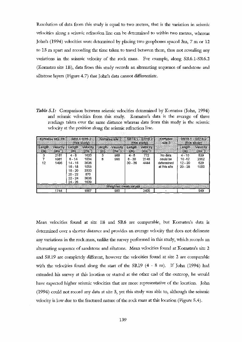
Resolution of data from this study is equal to two metres, that is the variation in seismic
velocities along a seismic refraction line can be determined to within two metres, whereas
John's (1994) velocities were determined by placing two geophones spaced 3m, 7 m or 12
to 13m apart and recording the time taken to travel between them, thus not revealing any
variations in the seismic velocity of the rock mass. For example, along SR6.1-SR6.2
(Komatsu site 1B), data from this study records an alternating sequence of sandstone and
siltstone layers (Figure 4. 7) that John's data cannot differentiate.
Table 5.1: Comparison between seismic velocities determined by Komatsu (John, 1994) and seismic velocities from this study. Komatsu's data is the average of three readings talcen over the same distance whereas data from this study is the seismic velocity at the position along the seismic refraction line.
4-8 1633 8- 14 1034 14-16 3636 16-18 1053 18-20 3333 20-22 870 22-24 3636 24-26 1639
No data could be
determined at this site
Mean velocities found at site 1B and SR6 are comparable, but Komatsu's data is
determined over a shorter distance and provides an average velocity that does not delineate
any variations in the rock mass, unlike the survey performed in this study, which records an
alternating sequence of sandstone and siltstone. Mean velocities found at Komatsu's site 2
and SR19 are completely different, however the velocities found at site 2 are comparable
with the velocities found along the start of the SR19 (4 - 8 m). If John (1994) had
extended his survey at this location or started at the other end of the outcrop, he would
have expected higher seismic velocities that are more representative of the location. John
(1994) could not record any data at site 3, yet this study was able to, although the seismic
velocity is low due to the fractured nature of the rock mass at this location (Figure 5.4).
139
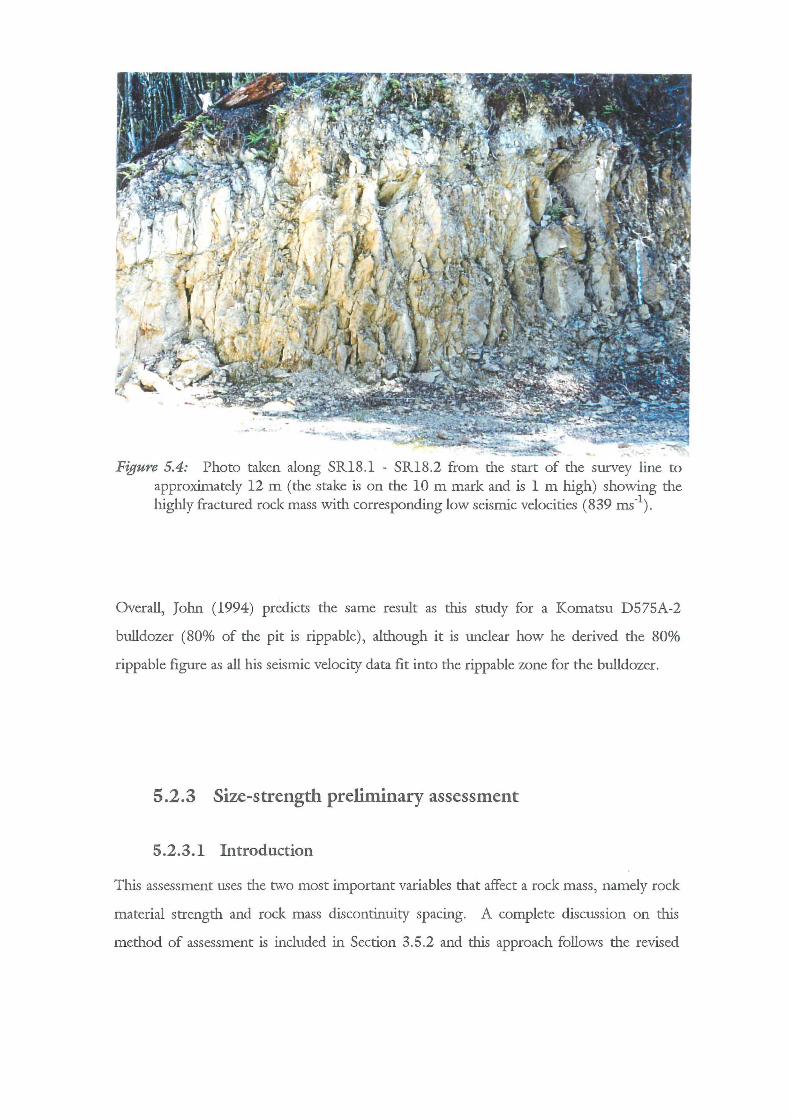
Figure 5.4: Photo taken along SR18.1 - SR18.2 from the start of the survey line to approximately 12m (the stake is on the 10m mark and is 1 m high) showing the highly fractured rock mass with corresponding low seismic velocities (839 ms.1
).
Overall, John (1994) predicts the same result as this study for a Komatsu D575A-2
bulldozer (80% of the pit is rippable), although it is unclear how he derived the 80%
rippable figure as all his seismic velocity data fit into the rippable zone for the bulldozer.
5.2.3 Size-strength preliminary assessment
5.2.3.1 Introduction
This assessment uses the two most important variables that affect a rock mass, namely rock
material strength and rock mass discontinuity spacing. A complete discussion on this
method of assessment is included in Section 3.5.2 and this approach follows the revised
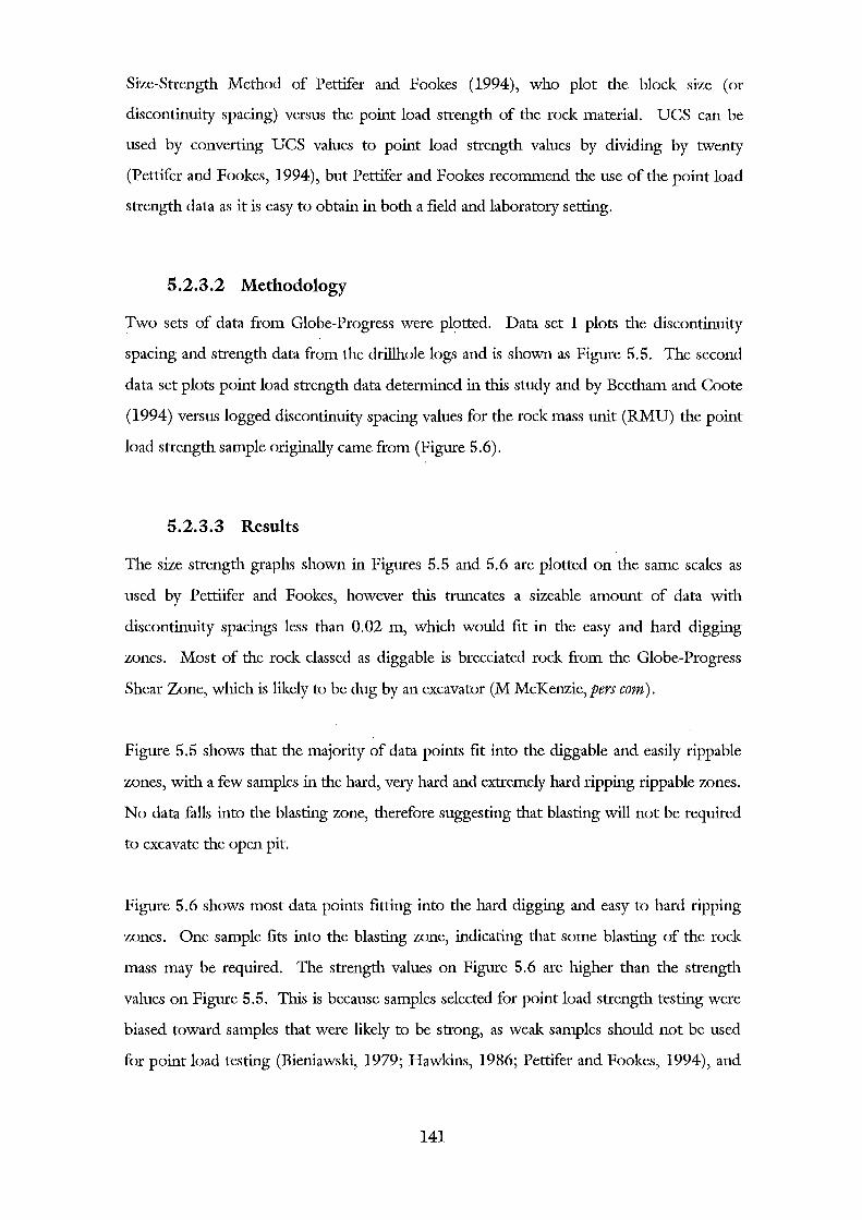
Size-Strength Method of Pettifer and Fookes (1994), who plot the block size (or
discontinuity spacing) versus the point load strength of the rock material. UCS can be
used by converting UCS values to point load strength values by dividing by twenty
(Pettifer and Fookes, 1994), but Pettifer and Fookes recommend the use of the point load
strength data as it is easy to obtain in both a field and laboratory setting.
5.2.3.2 Methodology
Two sets of data from Globe-Progress were plotted. Data set 1 plots the discontinuity
spacing and strength data from the drillhole logs and is shown as Figure 5.5. The second
data set plots point load strength data determined in this study and by Beetham and Coote
(1994) versus logged discontinuity spacing values for the rock mass unit (RMU) the point
load strength sample originally came from (Figure 5.6).
5.2.3.3 Results
The size strength graphs shown in Figures 5.5 and 5.6 are plotted on the same scales as
used by Pettiifer and Fookes, however this truncates a sizeable amount of data with
discontinuity spacings less than 0.02 m, which would fit in the easy and hard digging
zones. Most of the rock classed as diggable is brecciated rock from the Globe-Progress
Shear Zone, which is likely to be dug by an excavator (M McKenzie, pers com).
Figure 5.5 shows that the majority of data points fit into the diggable and easily rippable
zones, with a few samples in the hard, very hard and extremely hard ripping rippable zones.
No data falls into the blasting zone, therefore suggesting that blasting will not be required
to excavate the open pit.
Figure 5.6 shows most data points fitting into the hard digging and easy to hard ripping
zones. One sample fits into the blasting zone, indicating that some blasting of the rock
mass may be required. The strength values on Figure 5.6 are higher than the strength
values on Figure 5.5. This is because samples selected for point load strength testing were
biased toward samples that were likely to be strong, as weak samples should not be used
for point load testing (Bieniawski, 1979; Hawkins, 1986; Pettifer and Fookes, 1994), and
141
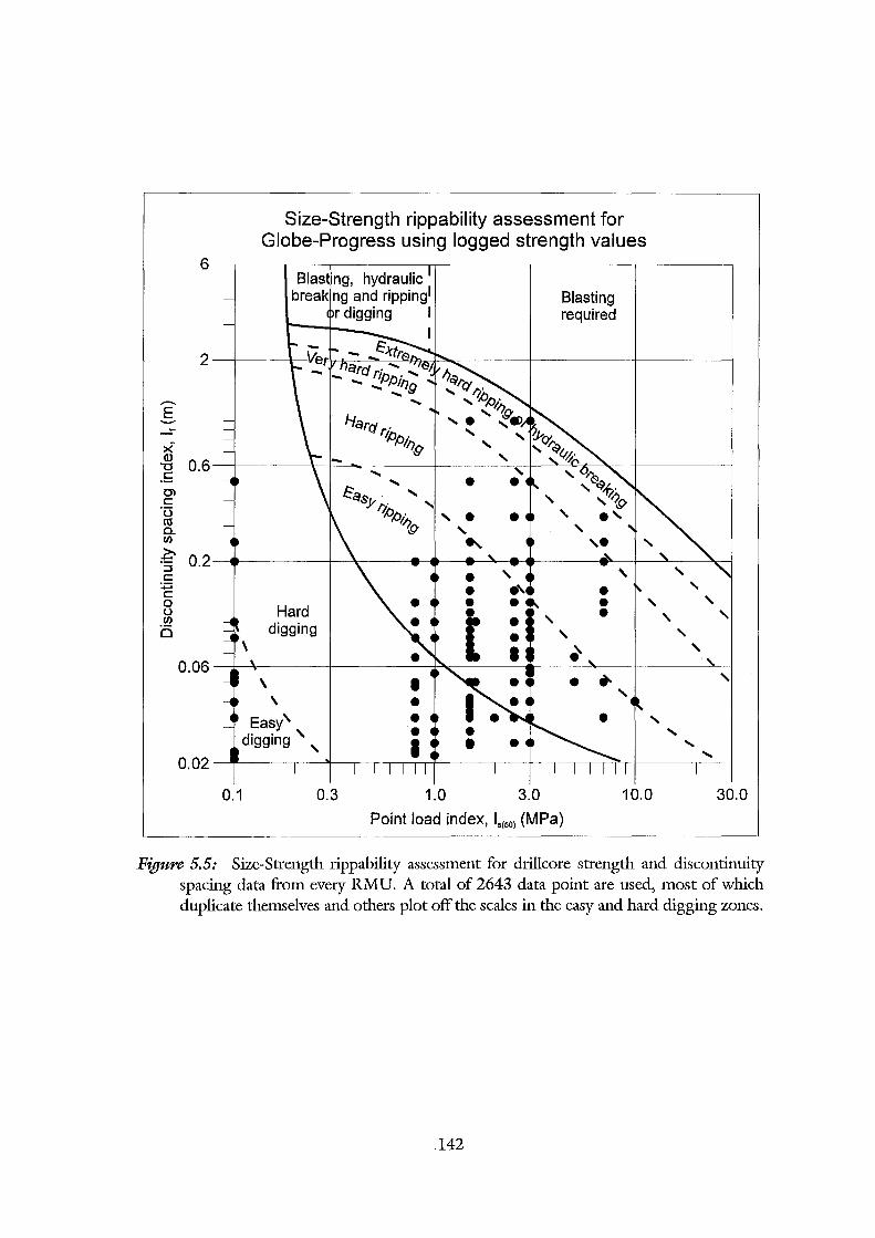
~ "'0 . £ OJ c
"(3 ro 0. 1/)
6
2
0.6
Size-Strength rippability assessment for Globe-Progress using logged strength values
ng, hydraulic 1 Blast break ng and ripping! Blasting
r digging I required I
.....
Hqf(j r: I!Jp·
'11).9
..... ..... •
~ 0.2~.--------+~~--~~~~~--~----~~-+--~--~ c
:;::; c 0 0 1/)
0 Hard
digging
• • • o.o6~~r------+--------~~------~----~---r------~
'
0.1 0.3 1.0 3.0 10.0 30.0
Point load index, r.(so) (MPa)
Figure 5.5: Size-Strength rippability assessment for drillcore strength and discontinuity spacing data from every RMU. A total of 2643 data point are used, most of which duplicate themselves and others plot off the scales in the easy and hard digging zones.
142
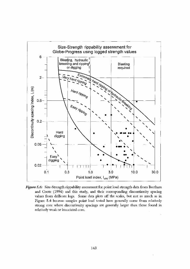
....... E -~ x-Q)
"'0 c OJ c ·o co a. en ~ :::l c
:;::::; c 0 0 en
i:S
Size-Strength rippability assessment for Globe-Progress using logged strength values
6--.---~----.---------~---------,----------.---------,
Blast ng, hydraulic 1
break ng and rippingl
0.6
0.2
Hard digging
\
0.06 \
\
Easy' digging'
0.02
0.1
r digging I
'
•
0.3 1.0
' . '
•
' '
3.0
Blasting required
.... ' . ' 10.0
Point load index, l.(so> (MPa)
'
30.0
Figure 5.6: Size-Strength rippability assessment for point load strength data from Beetham and Coote (1994) and this study, and their corresponding discontinuity spacing values from drillcore logs. Some data plots off the scales, but not as much as in Figure 5.4 because samples point load tested have generally come from relatively strong core where discontinuity spacings are generally larger than those found in relatively weak or brecciated core.
143
also because the logged strength values have been under-estimated. Despite the bias
toward sampling stronger specimens, Figure 5.6 should be used as the correct size-strength
rippability prediction chart as the sampling bias creates a more conservative excavatability
estimation, which is better than an over-estimation of the excavatability during a feasibility
study, because an over-estimation of the excavatability of a site may lead to under-design
during the project design stage.
5.3 RMR assessment
5.3.1 Introduction
The rock mass rating system was chosen to classify the rock mass because of its ease of use,
standardisation with ISRM rock mass descriptions, and also because of its suitability to the
characterisation of relatively shallow rock structures. It may also be calculated from
Macraes drillcore data logs.
A database of 106 diamond drilled core exists for the rock mass at Globe-Progress,
totalling in excess of 17 000 metres of core. However, only 10 360 metres contained
sufficient information to calculate its RMR. The other 6 640 metres of drill core is either
logged as precollar, stapes, fill or lost core, or has not been logged in sufficient detail (for
example, drillcore logged by CRAE).
5.3.2 Methodology
Calculation of the RMR follows Table 2.7 and 2.8 and Figures 2.3, 2.4 and 2.5. A
complete discussion on generalisations and assumptions made for each parameter ts
included as Appendix E1 and a brief discussion on each variable is included below.
144
A comparison between logged strength values and point load test with UCS tested samples
shows that strength has been logged incorrectly (see Section 4.5). Some of the sandstone
strengths have been over-estimated, but the majority have been under-estimated. Therefore
a revised strength estimate was used for each logged RMU, and this was devised from the
logged lithology and strength for each RMU. The assumptions made in determining the
revised strength are included in Appendix ELL
RQD for the drillcore has twice been calculated. A comparison between the two is
included in Section 4.5 and shows the spread of data between the two to be virtually
identical, therefore it is assumed that the RQD has been correctly calculated and no
adjustments were required for this variable.
The Discontinuity Spacing Index follows a clustered distribution pattern. It was also
thought that it may have been under-estimated (see Section 4.6), but because the
discontinuity spacing parameter follows a logarithmic scale, any error is minimised, and
therefore no adjustment or correction was applied to this data set.
The condition of discontinuities parameter is only determined for the main discontinuity in
each RMU. As all the parameters used to calculate the discontinuity condition parameter
are easily determined, it is assumed that they have been logged correctly and no corrections
or adjustments have been made.
The groundwater variable is the only variable that could not be determined from tl1e
drillcore data and no information could be found on the in situ groundwater condition,
but, as most of the drillcore is below the water table, it is likely that the rock mass will be
saturated. However, during mining the open pit is expected to be drained such that the pit
should be completely dry, although tlus may be a problem at Globe-Progress where rainfall
is hlgh (see Table Ll), and therefore the rock mass in the open pit is expected to be damp
(J Taylor pers com). Three groundwater scenarios (dry, damp and saturated) have been
determined for the RMR, thus calculating three possible values of RMR.
145
The RMR includes a discontinuity orientation correction factor that adjusts the basic
RMR depending on the application of the RMR; for example, if the RMR is to be
determined for slope stability, then different corrections are applied than if the RMR was
applied to a tunnel or other underground excavation (see Table 2.7C). For both of these
applications, a discontinuity orientation favourable to the stability of the excavation will be
unfavourable to its excavatability. For this reason, the inverse of Bieniawski's (1979)
discontinuity orientation descriptions were used; that is, if a discontinuity is favourable for
a stability analysis, then it will be unfavourable for excavatability. Rattenbury (1994)
found the most persistent discontinuity to be bedding and therefore the orientation of
bedding surfaces is used for this parameter. To correctly calculate the orientation of
bedding smfaces from drillcore, the drillcore needs to be orientated, which it is not at
Globe-Progress. Rattenbury (1994) reorientated some core samples to obtain
discontinuity orientations at depth. He found that bedding planes appeared to be
consistent with depth, therefore surface bedding orientations could be used as an
approximation of the discontinuity orientation at depth.
This thesis is concerned with assessing the rippability or excavatability of the open pit, and
therefore discontinuity orientation corrections are adjusted according to the favourability
or unfavourability of a discontinuity to excavatability rather than stability. If, in the future,
the RMR is required for a stability application, then only a simple reversal of the ratings is
required, for example, a favourable discontinuity in an excavatability application has a
rating of -10, which can easily be adjusted to unfavourable, with a rating of -2, for a
stability application.
5.3.3 Results
The RMR for every logged RMU is shown in Tables 5.2 to 5.12 (ten drillholes per table;
included in map and table box), along with essential data from drillcore logs. Strength,
RQD, discontinuity spacing, discontinuity condition and discontinuity orientation have
been plotted in Figures 5.7 to 5.11 using data ranges used in the RMR System to show the
distribution of data for each parameter. As the data set is very large, the frequency
distribution for each parameter should be indicative of the rock mass within the open pit,
146
for example, 80% of the discontinuities are rated favourable or very favourable to
excavating, therefore 80% of the discontinuities in the open pit area should be favourable
or very favourable to excavating. Frequency distribution plots of the three RMR scenarios
are shown in Figure 5.12 and contoured plans of the RMR assuming damp groundwater
conditions is given in Figures 5.13-5.22 (in map and table box).
5.3.4 Discussion
The strength distribution (Figure 5. 7b) is trimodal, where the weakest strengths represent
brecciated or shear zone rock mass and the highest strength are represented by very well
indurated sandstone. The intermediate mode represents strength estimates of siltstone and
mudstone and interbedded sandstone-siltstone sequences. The revised strength data were
based on point load strength (converted to UCS) and UCS, and on lithological drillcore
data. The distribution of quantitatively determined strength is given in Figure 5.7a, and
the discrepancy between the distribution patterns of the revised strength estimate and
actual strength data is explained by the fact that strength tests were biased toward testing
strong samples rather than weak samples (although limited testing was done on weak
samples), because the weaker rock is mainly breccia or clay pug, in which strength values
cannot readily be quantified.
Figure 5.8 and 5.9 plot the distribution ofRQD and discontinuity spacing classes used in
the RMR System and show rl1at most of the drillcore quality is weak, with a cluster of very
closely spaced discontinuities. This may be an effect of the drilling, whereby holes were
targeted to intersect the shear zone, therefore intersecting relatively more sheared rock.
Figure 5.10 shows the distribution of the condition of discontinuities parameter from the
RMR System. The maximum rating possible is 30 for unweathered, very rough
discontinuities wirl1no separation, infilling or continuity, and the minimum rating possible
is 0 for extremely wead1ered, slickensided or polished discontinuities with separation and
infilling greater than 5 mm and continuity of greater than 20 m (see Table 2. 7b). The
spread of discontinuity condition ratings found from drillcore is 5 to 30, with a mean of
19, which indicates most of the discontinuities are of moderate quality.
147
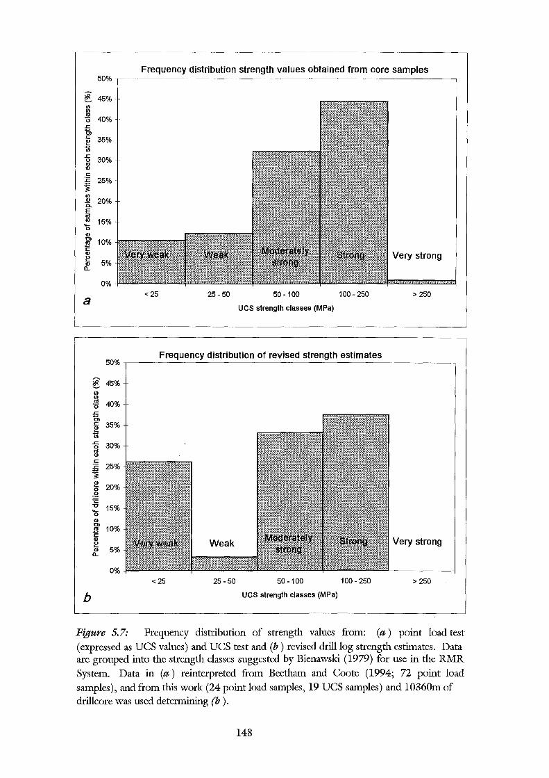
Frequency distribution strength values obtained from core samples 50%
~ 45%
"' "' Ill 40% 0
.r:; 0, c 35% ~ Ui .r:;
30% 0 Ill Q)
c £ 25% ·;::
"' Q) 20% a. E Ill
"' 15% ..... 0 Q) C)
10% !! c Q) 0 ... 5% Q)
Very strong n..
0% <25 25-50 50-100 100-250 > 250 a
UCS strength classes (MPa)
50% Frequency distribution of revised strength estimates
~ 45%
"' "' Ill 40% 0 .r:; 0, c 35% ~ Ui .r:;
30% 0 Ill Q)
c £ 25% ·;:: ~ 20% 0 g :§
15% ..... 0 Q) C)
10% Ill "E Q)
E 5% Q)
n..
Very strong
0%
< 25 25-50 50-100 100-250 > 250
b UCS strength classes (MPa)
Figure 5.7: Frequency distribution of strength values from: (a) point load test (expressed as UCS values) and UCS test and ( b ) revised drill log strength estimates. Data are grouped into the strength classes suggested by Bienawski (1979) for use in the RMR System. Data in (a) reinterpreted from Beetham and Coote (1994; 72 point load samples), and from this work (24 point load samples, 19 UCS samples) and 10360m of drillcore was used determining (b ) .
148
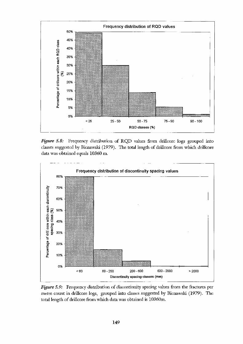
Ul Ul m 0 0 0 0:: L: 0 m Q)
c :c ~-Q)~ 5 g ·;:::: u ..... 0 Q) C) m "E Q)
e Q)
a..
50%
45%
40%
35%
30%
25%
20%
15%
10%
5%
0%
< 25
Frequency distribution of RQD values
25-50 50-75
RQD classes(%)
75-90 90-100
Figure 5.8: Frequency distribution of RQD values from drillcore logs grouped into classes suggested by Bienawski (1979). The total length of drillcore from which drillcore data was obtained equals 10360 m.
Frequency distribution of discontinuity spacing values 80%
~ 70% ·:; c E 0
60% 0 Ul '0 L: 0~
m~ 50% .!: Ul L: Ul
j~ 40% Q) C) .... 0 .!: 0 0
m
~ a. 30% Ul
..... 0 Q) C) 20% m "E Q)
e Q) 10% a..
0%
< 60 60-200 200-600 600-2000 > 2000.
Discontinuity spacing classes (mm)
Figure 5.9: Frequency distribution of discontinuity spacing values from the fractures per metre count in drillcore logs, grouped into classes suggested by Bienawski (1979). The total length of drillcore from which data was obtained is 10360m.
149
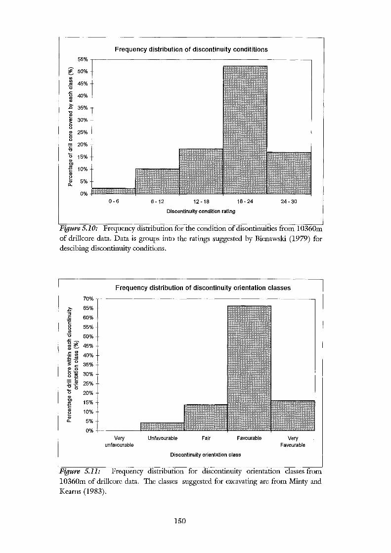
Frequency distribution of discontinuity condititions
55%
~ 50% 1/) 1/)
45% (U
0 ..c 0 40% (U Q)
>- 35% .a 1:J ~
30% Q)
> 0 0
~ 25% 0 0
20% -o -0 15% Q) C)
.B 10% c: Q) 0 ....
5% Q)
a..
0%
0-6 6-12 12-18 18-24 24-30
Discontinuity condition rating
Figure 5.10: Frequency distribution for the condition of disontinuities from 10360m of drillcore data. Data is groups into the ratings suggested by Bienawski (1979) for descibing discontinuity conditions.
70%
z. 65% ·:; c: 60% ~ 0 55% 0 1/)
:a 50% ..c~ g<>'! 45% m~
c: 1/)
40% :c 1/) (U
:!::::!() :;: c: ~ .Q
35%
o-o.B 30% - c: :;:: -~ 25% 1:J ....
- 0 0 20% Q) C)
15% ~ Q) 10% 0 .... Q)
a.. 5%
0%
Frequency distribution of discontinuity orientation classes
Very unfavourable
Unfavourable Fair Favourable
Discontinuity orientation class
Very Favourable
Figure 5.11: Frequency distribution for discontinuity orientation classes from 10360m of drillcore data. The classes suggested for excavating are from Minty and Kearns (1983).
150
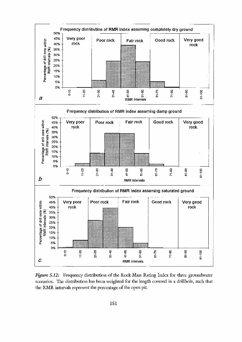
Frequency distribution of RMR index assuming completely dry ground 50%,------------,-----------,-----------,------------,-----------~
c 45% £ 40% "§'
~~ 35% 0 ~ 0 II) 30% :=Iii ... c:
25% "C Q) ..... ~ 0 c
~oc 20% <U::!E 15% "En:: Q) 0 10% ... Q)
0.. 5%
0%
a
50% c
45% :c ~ 40% ~~ 35% 0 ~ 0 II)
30% :=Iii ... c: 25% "C Q) ..... ~
0 c 20% ~oc
<U::!E 15% "En:: Q) 10% ~ Q) 5% 0..
0%
b
50% c 45% :c j 40% ~~ 35% o~
0 II) 30% :=Iii ... c: 25% "C Q) ..... ~
0 c 20% ~oc
<U::!E 15% "En:: Q) 10% 0 ... Q)
5% 0..
0%
c
Very poor Poor rock rock
Fair rock Good rock
0 0 ..... 0 II,'
~ Iii RMR intervals
Frequency distribution of RMR index assuming damp ground
Very poor rock
:·:.:·:·::::::
0 0 ..... ~ 0 ..... .....
Poor rock
0 0 <? .., c;; M
Fair rock Good rock
0 0 0 0 II,' 'II "; '9 ~ i'ii (0 r:::
RMR intervals
Very good rock
0 0 ..... ' .....
m
Very good rock
0 0 a,> 0 ..... co ' a;
Frequency distribution of RMR index assuming saturated ground
Very poor Poor rock Fair rock Good rock Very good rock rock
0 0 0 0 0 0 0 0 0 0 ..... ~ <? .., II,' 'II "; '9 a,> 0 0 ..... ..... c;; M ~ i'ii (0 r::: co ' ..... a;
RMR intervals
Figure 5.12: Frequency distribution of the Rock Mass Rating Index for three groundwater scenarios. The distribution has been weighted for the length covered in a drillhole, such that the RMR intervals represent the percentage of the open pit.
151
The frequency distribution plot of discontinuity orientation (Figure 5.11), where the
discontinuity orientation is the orientation of bedding surfaces, shows that greater than
80% of the bedding surfaces are favourable or very favourable for excavation in a east to
west direction.
Figure 5.12 shows the calculated RMR assuming the open pit will be dry, damp and
saturated. The RMR Index is greater for a dry pit (mean = 45 with a range between 18
and 89) and the mean and data ranges decrease with increasing water content (the damp
RMR Index mean= 40 with a range between 13 and 84; and the saturated RMR Index
mean = 34 with a range between 7 and 78). Most of the rock mass in the three scenarios
is either poor or fair (RMR index between 20 and 60) and very little very good rock
(RMR Index greater than 80) exists.
Figures 5.13 to 5.22 show contoured plans of the damp RMR (groundwater scenario most
likely to occur in the pit) values at 20 m bench heights through the pit. These plans have
been produced using Medsystem, a mine modelling computer package, and modelled using
a weighted inverse distance3 modelling technique (see Appendix ES) using a block
dimension of 5 m x 5 m. Only rock mass data within the pit boundary are plotted and
data is further constrained by using a two domain pit model, where any RMR value
intersecting the Globe-Progress Shear Zone domain is only extrapolated within that
domain and any RMR value intersecting the overburden domain will only be extrapolated
within that domain. This effectively constrains data such that weal<: rock will not be
predicted outside of the shear zone domain and good quality rock in the overburden
domain will not be extrapolated into the shear zone domain. The maximum distance data
is extrapolated is 80 m where drillhole data are sparse but most drillholes are less than 50 m
apart (see Figure 4.1), therefore giving a relatively accurate model.
The plans show two zones of poor to very poor rock, one following the Globe-Progress
Shear Zone (see Figure 4.1 for location of the shear zone in relation to the pit outline)
curving around the northern and eastern pit walls, while the other zone is along the
western wall of the open pit (see Figures 5.15 to 5.17 through the centre of the pit). The
majority of overburden is classed as fair to poor rock, but there are areas of good rock (see
Figures 5.15 to 5.17). No very good rock is estimated in the bench plans, although there
152
may be small areas between the bench levels. The plans also show relatively poor rock in
the fold axis of the Globe-Progress Shear Zone (see Figures 5.14, 5.17, 5.19 and 5.20),
which should be expected as fold axes are often zones of greater deformation. The same
trends are shown on plans of overburden leachability, where high sulphide zones (more
likely to leach) are located in the fold axis of the Globe-Progress Shear Zone, along the
western wall and the shear zone itself (J Taylor, pers com) and inert zones (not expected to
leach) are located where there are zones of good rock. There does not appear to be any
significant decrease in rock mass quality associated with the weathered rock mass near pit
surface (compare Figures 5.13 and 5.14, near the pit surface, with Figures 5.20 and Figure
5.19, near the pit base), which was proven for rock material in Chapter 4.
5.4 Final rippability evaluation
5.4.1 Introduction
The fmal rippability evaluation involved determining the rippability of the proposed open
pit area using a suite of geological and geotechnical parameters. Two rippability prediction
methods were chosen, one method was based on the RMR System, classifying the rock
mass, and the other method attempts to predict the productivity of a chosen bulldozer.
The first method used was the Weaver Rippability Prediction Method (Weaver, 1975).
This is an outdated system based on the first RMR system by Bieniawski (1973), so was
modified to follow the current RMR system of Bieniawski (1989). The second method
used was devised by MacGregor et al (1994). It is a statistical based method that fmds the
best correlation between various geological and geotechnical parameters and the
productivity of a chosen bulldozer.
153
5.4.2 Weaver's Rippability Method (1975)
5.4.2.1 Introduction
This method is based on Bieniawski's 1973 RMR System, therefore it is outdated as the
RMR System has been modified three times (see Bieniawski, 1976, 1979, 1989). The
system also predicts the size of ripping bulldozer suitable, but the largest bulldozer in 1975
was Caterpillar's D9 (about 42 tonnes, compared to the largest bulldozer today,
Komatsu's D575A-2 at 134 tonnes), therefore Weaver's 1975 method is expected to be
very conservative.
5.4.2.2 Methodology
Calculation of Weaver's Rippability Rating Method follows Tables 3.2 and 2.8.
Assumptions and generalisations made for each parameter are outlined in Appendix E2 and
a short discussion follows below. Weaver's Rippability Rating System is based on
Bieniawski's 1973 RMR System, substituting groundwater and RQD for the seismic
velocity of the rock mass, therefore, the same assumptions made for the RMR are made for
this rating system, although the class intervals and ratings are slightly different.
Seismic velocities were determined on the surface, where the rock mass has undergone
weathering and joint relaxation. For this reason it was decided not to attempt correlating
seismic velocities with drillcore data, instead, the mean seismic velocity (2100 ms-1) was
used as an estimate of the seismic velocity of the rock mass, although the seismic velocity
may be higher at depth where the rock mass is unweathered and joints less open.
5.4.2.3 Results
Weaver's Rippability Rating for every RMU is included on Tables 5.2 to 5.12 along with
the essential data from the drillcore logs. Frequency distribution graphs of the rock
material hardness, and discontinuity spacing (using different classes to those in the RMR
System) are given as Figures 5.23 and 5.24. Weathering was not plotted up as most of the
rock mass is unweathered. The discontinuity orientation frequency distribution is the same
as in Figure 5.10. The frequency distribution of the rippability classes are shown in
154
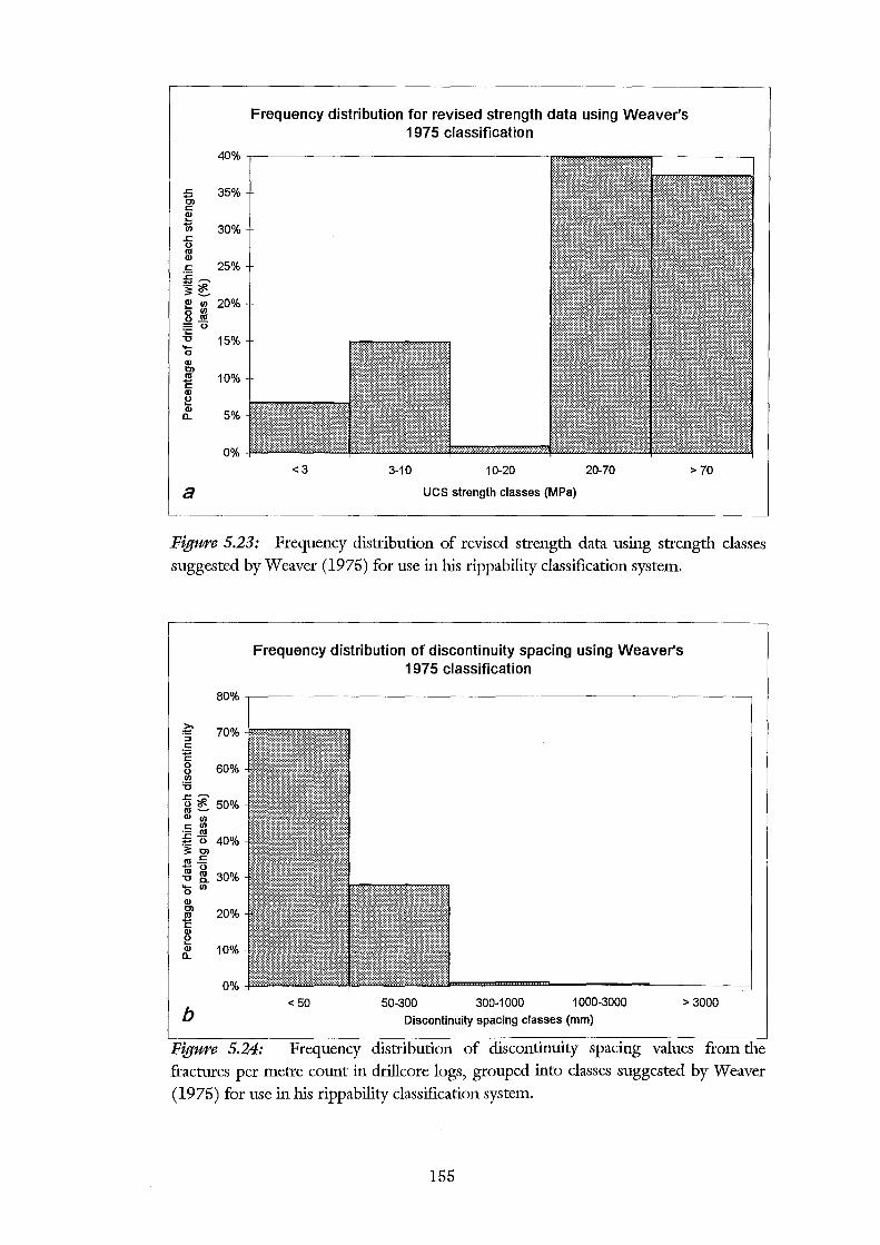
.c -m c ~
"iii .c 0
"' Q)
c
~~ :::~ ~ Ill 0 Ill o.!!! = 0
~ .,_ 0 Q) Ol
"' c Q)
~ Q)
n..
a
40%
35%
30%
25%
20%
15%
10%
5%
0%
Frequency distribution for revised strength data using Weaver's 1975 classification
<3 3-10 10-20 20-70
UCS strength classes (MPa)
> 70
Figure 5.23: Frequency distribution of revised strength data using strength classes suggested by Weaver (1975) for use in his rippability classification system.
Frequency distribution of discontinuity spacing using Weaver's 1975 classification
:§ 70% J,"""'"""'"""'"" :§ c 8 60% Ill :0 .c ~ g ~50% Q) Ill c Ill :c.!!! :!:::: 0 40% :;:: Ol
"' .!: +' 0
~ ~ 30% '0 Ill Q)
~ 20% c Q)
~ /f. 10%
0%
b <50 50-300 300-1000 1000-3000
Discontinuity spacing classes (mm)
> 3000
Figure 5.24: Frequency distribution of discontinuity spacing values from the fractures per metre count in drillcore logs, grouped into classes suggested by Weaver (1975) for use in his rippability classification system.
155
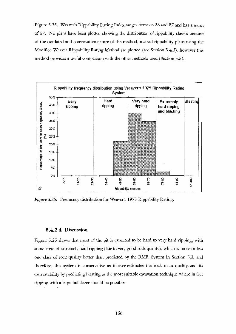
Figure 5.25. Weaver's Rippability Rating Index ranges between 38 and 87 and has a mean
of 57. No plans have been plotted showing the distribution of rippability classes because
of the outdated and conservative nature of the method, instead rippability plans using the
Modified Weaver Rippability Rating Method are plotted (see Section 5.4.3). however this
method provides a useful comparison with the other methods used (Section 5.5).
Rippability frequency distribution using Weaver's 1975 Rippability Rating System
50%
Easy Hard Very hard Extremely Ul Ul 45% ripping ripping ripping hard ripping Ill 0
~ 40% and blasting :a Ill a. 35% a.
·;:: .s:: 0 30% Ill Ql
.E..-. 25% Ql'#. .... ~
0 0
=c 20% "U -0 15% Ql Cl
~ 10% Ql e Ql 5% a.
0% 0 0 0 0 0 0 0 0 0 0 ~ ~ <? 'i lr? «? ~ ~ a,> 0 0 ~
~ r::i (ry ~ Iii <0 r::: co ' ~ Oi a Rippability classes
Figure 5.25: Frequency distribution for Weaver's 1975 Rippability Rating.
5.4.2.4 Discussion
Figure 5.25 shows that most of the pit is expected to be hard to very hard ripping, with
some areas of extremely hard ripping (fair to very good rock quality), which is more or less
one class of rock quality better than predicted by the RMR System in Section 5.3, and
therefore, this system is conservative as it over-estimates the rock mass quality. and its
excavatability by predicting blasting as the most suitable excavation technique where in fact
ripping with a large bulldozer should be possible.
156
5.4.3 The Modified Weaver Rippability Rating
5.4.3.1 Introduction
Weaver's 1975 method has been updated in Table 3.3 to follow Bieniawski's 1989 RMR
System. This updates the rippability system so that parameters and their ranges now
follow ISRM terminology. The seismic velocity ranges have also increased to account for
the increase in bulldozer sizes and capabilities, but the ranges are lower than those used by
Komatsu and Caterpillar as their seismic velocities ranges are considered to over-estimate
the rippability of a rock mass (Braybrooke, 1988; MacGregor et al, 1994).
5.4.3.2 Methodology
Calculation of the Modified Weaver Rippability Ratings follow Tables 3.3 and 2.8 and
Figures 2.3, 2.4 and 2.5. The generalisations and assumptions used to calculate this rating
are the same as for the RMR, except that there is no groundwater or RQD variable, both
of which have been replaced with the average seismic velocity of the pit area (2100 ms·\
5.4.3.2 Results
The Modified Weaver Rippability Rating for each RMU is shown in Tables 5.2-5.12 (in
map and table box). The frequency distribution for each parameter (except for seismic
velocity), is the same as for the RMR (Figures 5.7 to 5.11) and the frequency distribution
for the rippability ratings are shown as Figure 5.26. The Modified Rippability Rating
Index ranges between 27 and 81, with a mean of 50. The rippability ratings have also been
plotted on Figures 5.27 to 5.36 (in map and table box) using the same modelling
technique used to plot the RMR distribution (Section 5.3).
157
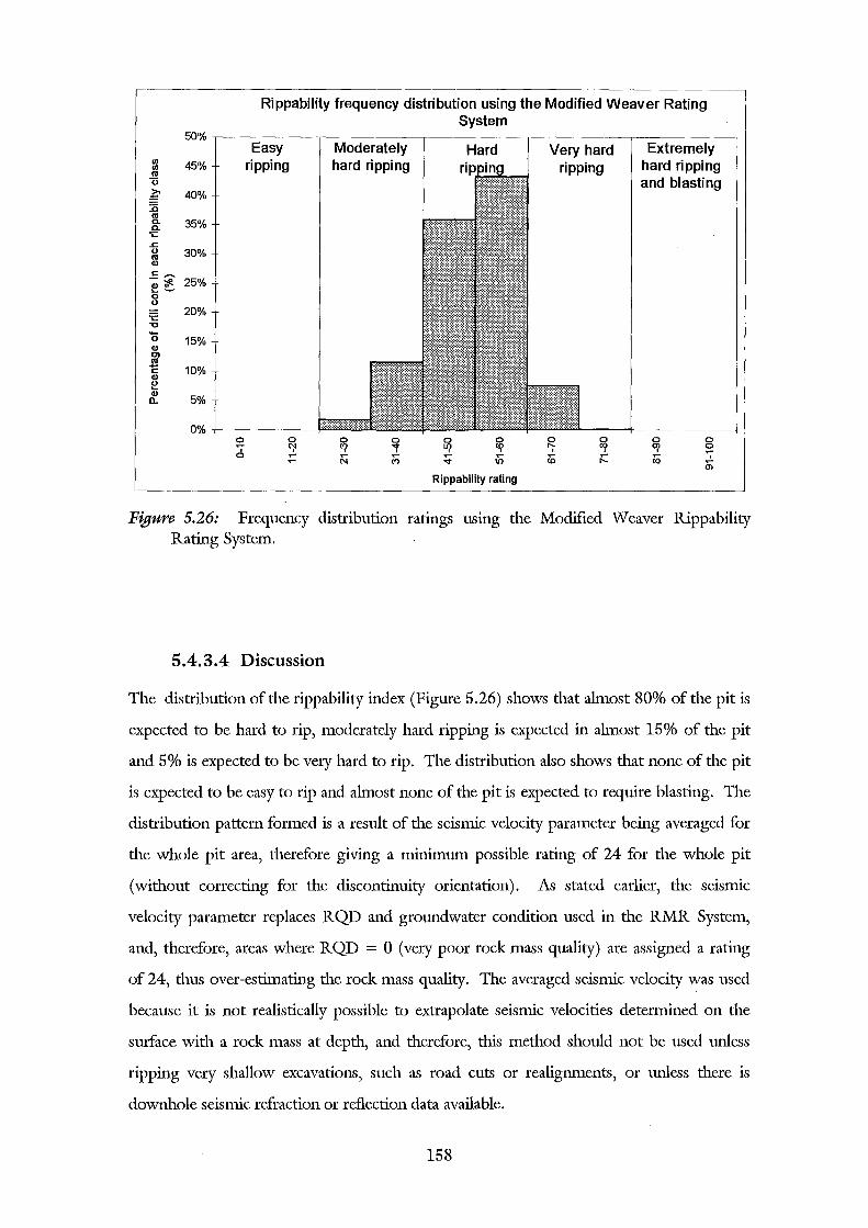
Rippability frequency distribution using the Modified Weaver Rating System
5.4.3.4 Discussion
The distribution of the rippability index (Figure 5.26) shows that almost 80% of the pit is
expected to be hard to rip, moderately hard ripping is expected in almost 15% of the pit
and 5% is expected to be very hard to rip. The distribution also shows that none of the pit
is expected to be easy to rip and almost none of the pit is expected to require blasting. The
distribution pattern formed is a result of the seismic velocity parameter being averaged for
the whole pit area, therefore giving a minimum possible rating of 24 for the whole pit
(without correcting for the discontinuity orientation). As stated earlier, the seismic
velocity parameter replaces RQD and groundwater condition used in the RMR System,
and, therefore, areas where RQD = 0 (very poor rock mass quality) are assigned a rating
of 24, thus over-estimating the rock mass quality. The averaged seismic velocity was used
because it is not realistically possible to extrapolate seismic velocities determined on the
surface with a rock mass at depth, and therefore, this method should not be used unless
ripping very shallow excavations, such as road cuts or realignments, or unless there is
downhole seismic refraction or reflection data available.
158
The rippability plans (Figures 5.27 to 5.36; in map and table box) show that most of the
pit is expected to be hard to rip. The plans do not delineate the shear zone along the
northern and eastern pit walls, or the Chemist Shop Fault along the western pit wall.
Therefore these plans should not be relied upon for any planning.
5.4.4 Prediction ofProductivity.
5.4.4.1 Introduction
MacGregor et aPs (1994) method of predicting the productivity of a selected bulldozer was
used on drillcore data. The method does not rate the rock mass lilce the RMR System or
Weaver's Rippability Rating System, rather it selects parameters that influence the
excavatability of a rock mass the most, and predicts the productivity from a correlation
formula between the expected productivity and the influencing parameters. As it does not
rate the rock mass on a set scale (although some of the parameters are rated) and because it
uses parameters easily determined during site investigations or from drillcore data, it may
serve as a useful comparison with results from the RMR System.
MacGregor recommends using two equations to relate the productivity back to the rock
mass. Equation 4 is based on 354 case studies of ripping in all rock types and Equation 8
is based on case studies of ripping only in sedimentary rock masses (the· number of case
studies is unlcnown).
5 .4.4.2 Methodology
Calculation of the expected productivity uses the formulae in Table 3.8 and the description
of each variable is given in Table 3.9 and Appendix B3. Generalisations and assumptions
made are included in Appendix E4 and a brief description of each variable is included
below.
159
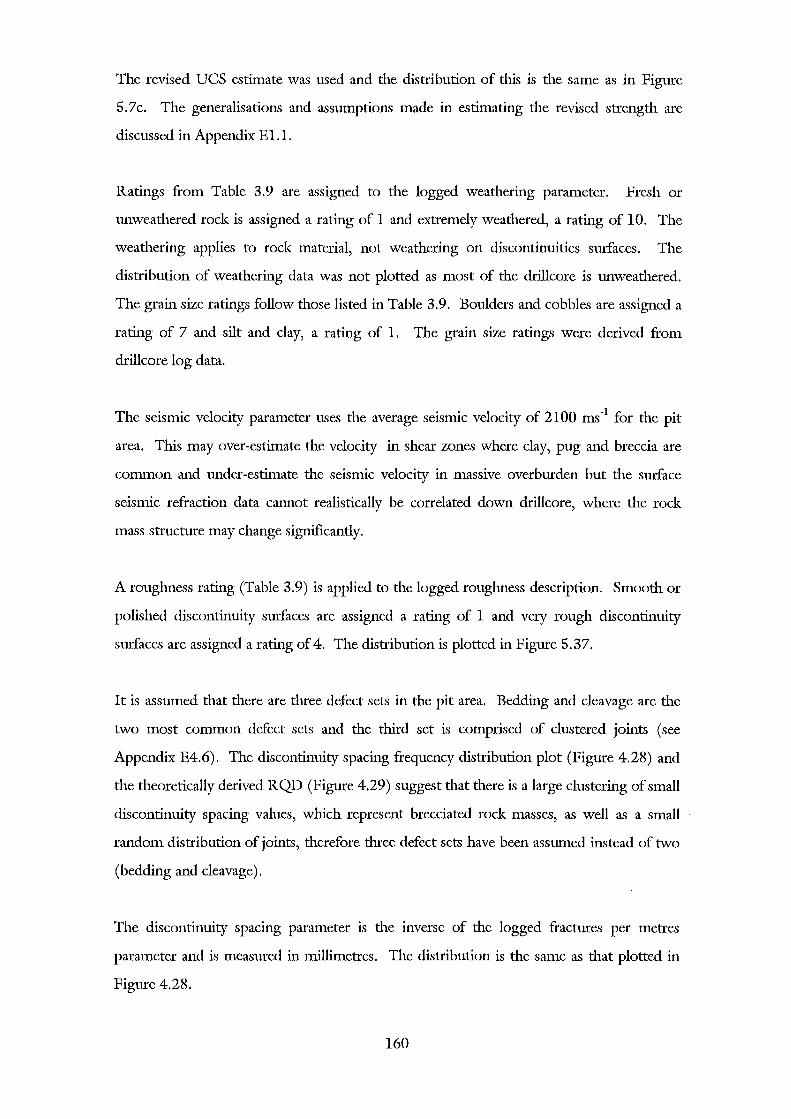
The revised UCS estimate was used and the distribution of this is the same as in Figure
5.7c. The generalisations and assumptions made in estimating the revised strength are
discussed in Appendix ELL
Ratings from Table 3.9 are assigned to the logged weathering parameter. Fresh or
unweathered rock is assigned a rating of 1 and extremely weathered, a rating of 10. The
weathering applies to rock material, not weathering on discontinuities surfaces. The
distribution of weathering data was not plotted as most of the drillcore is unweathered.
The grain size ratings follow those listed in Table 3.9. Boulders and cobbles are assigned a
rating of 7 and silt and clay, a rating of l. The grain size ratings were derived from
drillcore log data.
The seismic velocity parameter uses the average seismic velocity of 2100 ms-1 for the pit
area. This may over-estimate the velocity in shear zones where clay, pug and breccia are
common and under-estimate the seismic velocity in massive overburden but the surface
seismic refraction data cannot realistically be correlated down drillcore, where the rock
mass structure may change significantly.
A roughness rating (Table 3.9) is applied to the logged roughness description. Smooth or
polished discontinuity surfaces are assigned a rating of 1 and very rough discontinuity
surfaces are assigned a rating of 4. The distribution is plotted in Figure 5.37.
It is assumed that there are three defect sets in the pit area. Bedding and cleavage are the
two most common defect sets and the third set is comprised of clustered joints (see
Appendix E4.6). The discontinuity spacing frequency distribution plot (Figure 4.28) and
the theoretically derived RQD (Figure 4.29) suggest that there is a large clustering of small
discontinuity spacing values, which represent brecciated rock masses, as well as a small
random distribution of joints, therefore three defect sets have been assumed instead of two
(bedding and cleavage).
The discontinuity spacing parameter is the inverse of the logged fractures per metres
parameter and is measured in millimetres. The distribution is the same as that plotted in
Figure 4.28.
160
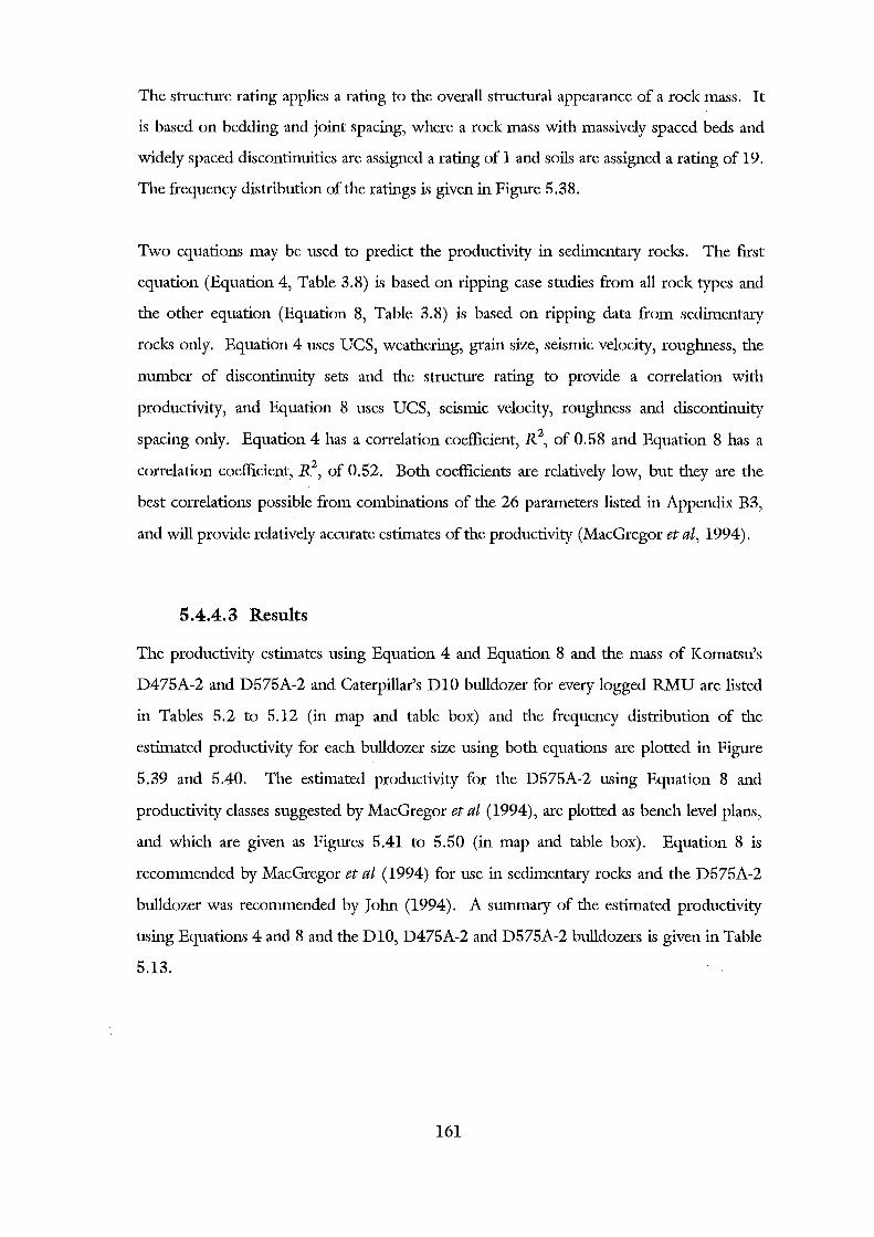
The structure rating applies a rating to the overall structural appearance of a rock mass. It
is based on bedding and joint spacing, where a rock mass with massively spaced beds and
widely spaced discontinuities are assigned a rating of 1 and soils are assigned a rating of 19.
The frequency distribution of the ratings is given in Figure 5.38.
Two equations may be used to predict the productivity in sedimentary rocks. The ftrst
equation (Equation 4, Table 3.8) is based on ripping case studies from all rock types and
the other equation (Equation 8, Table 3.8) is based on ripping data from sedimentary
rocks only. Equation 4 uses UCS, weathering, grain size, seismic velocity, roughness, the
number of discontinuity sets and the structure rating to provide a correlation with
productivity, and Equation 8 uses UCS, seismic velocity, roughness and discontinuity
spacing only. Equation 4 has a correlation coefficient, R 2, of 0.58 and Equation 8 has a
correlation coefficient, R2, of 0.52. Both coefficients are relatively low, but they are the
best correlations possible from combinations of the 26 parameters listed in Appendix B3,
and will provide relatively accurate estimates of the productivity (MacGregor et al, 1994).
5.4.4.3 Results
The productivity estimates using Equation 4 and Equation 8 and the mass of Komatsu's
D475A-2 and D575A-2 and Caterpillar's D10 bulldozer for every logged RMU are listed
in Tables 5.2 to 5.12 (in map and table box) and the frequency distribution of the
estimated productivity for each bulldozer size using both equations are plotted in Figure
5.39 and 5.40. The estimated productivity for the D575A-2 using Equation 8 and
productivity classes suggested by MacGregor et at (1994), are plotted as bench level plans,
and which are given as Figures 5.41 to 5.50 (in map and table box). Equation 8 is
recommended by MacGregor et at (1994) for use in sedimentary rocks and the D575A-2
bulldozer was recommended by John (1994). A summary of the estimated productivity
using Equations 4 and 8 and the D10, D475A-2 and D575A-2 bulldozers is given in Table
5.13.
161
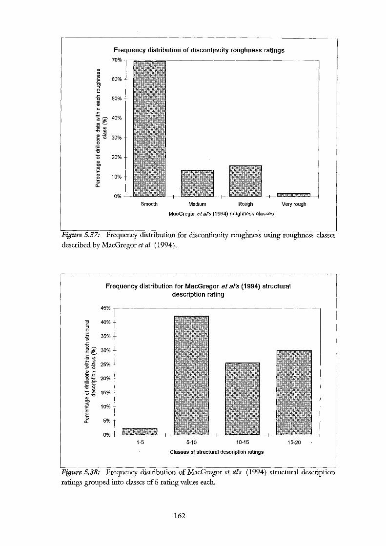
Frequency distribution of discontinuity roughness ratings
70%
Ul Ul G) c 60% .c C) ::J e .c 50% 0 m G)
c :c: j* m~
40%
1U ~ u m G)-
30% .._ 0 0 .Q =[: "U - 20% 0 G) C)
~ G) 10% E G)
a..
0%
Smooth Medium Rough Very rough
MacGregor eta/'s (1994) roughness classes
Figure 5.37: Frequency distribution for discontinuity roughness using roughness classes described by MacGregor et at (1994).
Frequency distribution for MacGregor eta/'s (1994) structural description rating
45%.------------------------------------------------------.
40%
35%
30%
25%
20%
15%
10%
5%
0% u.,ITJ·=·=·=···,ITJ=··.· •§ill_-+---1-5 5-10 10-15 15-20
Classes of structural description ratings
Figure 5.38: Frequency distribution of MacGregor et at's (1994) structural description ratings grouped into classes of 5 rating values each.
162
Table 5.13: Summary of estimated productivity for D10, D475A-2 and D575A-2 bulldozers.
D10 1050 0-4800 • 46% difficult and very difficult ripping
• 52% and medirun D475A-2 1500 0-6900 • 39% difficult and very difficult ripping
• 62% to medirun · D575A-2 3000 0- 13750 • 46% medirun to very difficult ripping
54% and
DlO 850 70-4150 • 7 4% difficult and very difficult ripping
• 25% and medirun D475A-2 1250 100- 5600 • 63% difficult ripping
• 30% to medirun D575A-2 2450 200-11900 • 72% moderate and difficult ripping
• 26%
5.4.4.4 Discussion
The distribution of expected productivity values (Figures 5.39 and 5.40; Table 5.13)
shows that the Equation 4 produces a wider range and a higher mean than Equation 8.
This trend was also found by MacGregor et at (1994) who suggested that Equation 8
should be used to estimate bulldozer productivity and also to be compared with Equation 4
data. The wider range in Equation 4 data malces estimation of the rippability of the site
harder to predict as the data ranges suggest two or more different sized bulldozers should
be used whereas with Equation 8 data, most data fits into one or two productivity classes,
therefore requiring only one sized bulldozer to excavate the overburden. For instance,
using Equation 8 data, 7 4% of the open pit is expected to be difficult to very difficult to rip
using a D10, 63% is expected to be difficult to rip with a D475A-2 and 72% is expected
to be medirun to difficult to rip with a D575A-2 bulldozer.
As the D575A-2 provides the most productive ripping capabilities, bench level plans
plotting the estimated productivity have been produced as Figures 5.41 to 5.50 (in map
and table box). These plans have been modelled using inverse distance3 modelling (see
163
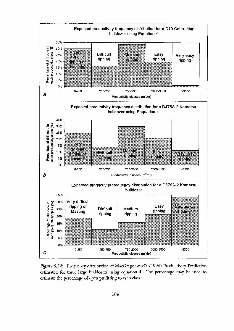
Expected productivity frequency distribution for a D1 0 Caterpillar bulldozer using Equation 4
35%,-----------,-----------.-----------.-----------~--------~
.!: ~ 30% Q)~
.... Ul
8 l(l 25% :=o -5 .?:' 20% '0~ ~~ 15%
1i [ 10% e.s::: ~ m 5%
Difficult ripping
Easy Very easy ripping
0% ..p====='-1' a
b
c
0-250 250-750 750-2000 2000-3500 >3500
Productivity classes (m3/hr)
Expected productivity frequency distribution for a D475A-2 Komatsu bulldozer using Eequation 4
35%,-----------,-----------.----------,,----------,-----------,
.!: ~ 30% Q)~
8 ~ 25% :=o -5.?;- 20% ._ ·:; 0;:;
~~ 15%
1i [ 10% e.s::: ~ m 5%
0%
35%
.!: ~ 30% Q)~ .... Ul
25% 0 Ul o m :=o -5.?;- 20% '0~ Q) 0 15% C) :::I mu
.... 0 c .... 10% Q) a. e.s:::
Q) 0 a.. m 5% Q)
0%
0-250 250-750 750-2000 2000-3500 >3500
Productivity classes (m3/hr)
Expected productivity frequency distribution for a D575A-2 Komatsu bulldozer
Very difficult ripping or blasting
0-250
Difficult ripping
Medium ripping
Easy
250-750 750-2000 2000-3500 >3500 Productivity classes (m3/hr)
Figure 5.39: Frequency distribution of MacGregor et at's (1994) Productivity Prediction estimated for three large bulldozers using equation 4. The percentage may be used to estimate the percentage of open pit fitting to each class.
164
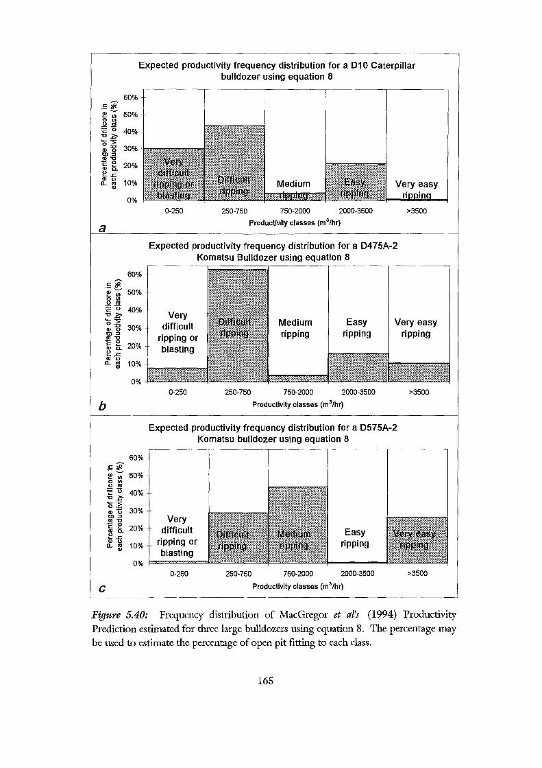
Expected productivity frequency distribution for a 010 Caterpillar bulldozer using equation 8
60% .!: ~ ~
~ Ul 50% 0 Ul
0 "' ~0 40% ""C >. '-:!:::::: 0 .:::
30% CDO Ol::J ni""C ~ 0
20% c ... (I) 0.. ~..c: (I) 0
10% D.. "' (I)
0%
a
60%
.!: ~ ~~ 50% 0 Ul 0 "' ~0 40% ~~ 0 .::: CDO 30% Ol::J ni""C ~ 0 c ... 20% (I) 0..
~..c: (I) 0 D.."' 10% (I)
0%
b
60%
.!: ~ ~~ 50% 0 Ul 0 "' ~0 40% ""C~ '0 :~ CDO 30% Ol::J ni""C ~ 0 c ... 20% (I) 0.. ~..c: (I) 0
10% D.. "' (I)
0%
c
Medium
0-250 250-750 750-2000 2000-3500
Productivity classes (m3/hr)
Expected productivity frequency distribution for a D475A-2 Komatsu Bulldozer using equation 8
>3500
Very Medium Easy Very easy difficult
ripping or ripping ripping
blasting
·:·.;
0-250 250-750 750-2000 2000-3500
Productivity classes (m3/hr)
Expected productivity frequency distribution for a D575A-2 Komatsu bulldozer using equation 8
Very difficult
ripping or blasting
0-250 250-750 750-2000
Easy ripping
2000-3500
Productivity classes (m3/hr)
ripping
>3500
>3500
Figure 5.40: Frequency distribution of MacGregor et al's (1994) Productivity Prediction estimated for three large bulldozers using equation 8. The percentage may be used to estimate the percentage of open pit fitting to each class.
165
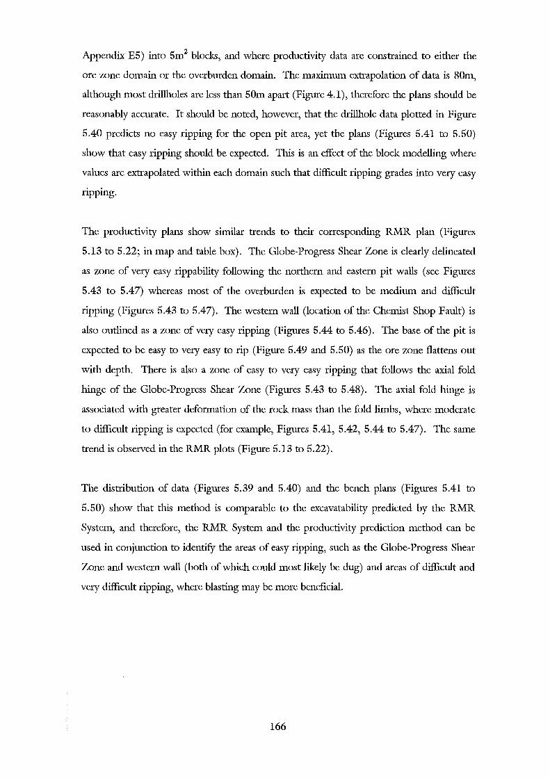
Appendix E5) into 5m2 blocks, and where productivity data are constrained to either the
ore zone domain or the overburden domain. The maximum extrapolation of data is 80m,
although most drillholes are less than 50m apart (Figure 4.1), therefore the plans should be
reasonably accurate. It should be noted, however, that the drillhole data plotted in Figure
5.40 predicts no easy ripping for the open pit area, yet the plans (Figures 5.41 to 5.50)
show that easy ripping should be expected. This is an effect of the block modelling where
values are extrapolated within each domain such that difficult ripping grades into very easy
nppmg.
The productivity plans show similar trends to their corresponding RMR plan (Figures
5.13 to 5.22; in map and table box). The Globe-Progress Shear Zone is clearly delineated
as zone of very easy rippability following the northern and eastern pit walls (see Figures
5.43 to 5.47) whereas most of the overburden is expected to be medium and difficult
ripping (Figures 5.43 to 5.47). The western wall (location of the Chemist Shop Fault) is
also outlined as a zone ofvery easy ripping (Figures 5.44 to 5.46). The base of the pit is
expected to be easy to very easy to rip (Figure 5.49 and 5.50) as the ore zone flattens out
with depth. There is also a zone of easy to very easy ripping that follows the axial fold
hinge of the Globe-Progress Shear Zone (Figures 5.43 to 5.48). The axial fold hinge is
associated with greater deformation of the rock mass than the fold limbs, where moderate
to difficult ripping is expected (for example, Figures 5.41, 5.42, 5.44 to 5.47). The same
trend is observed in the RMR plots (Figure 5.13 to 5.22).
The distribution of data (Figures 5.39 and 5.40) and the bench plans (Figures 5.41 to
5.50) show that this method is comparable to the excavatability predicted by the RMR
System, and therefore, the RMR System and the productivity prediction method can be
used in conjunction to identify the areas of easy ripping, such as the Globe-Progress Shear
Zone and western wall (both of which could most likely be dug) and areas of difficult and
very difficult ripping, where blasting may be more beneficial.
166
5.5 Comparison between methods
5.5.1 Comparison between preliminary rippability prediction methods
The preliminary rippability estimation using seismic velocity determination predicts that
90% of the pit area is rippable or marginal, and 10% of the pit will be unrippable. This
estimate is based on surface data only, and therefore, it should not used as a prediction of
the whole pit. Size-strength determination uses drillcore data, and thus, can be used to
provide a three dimensional preliminary rippability assessment of the open pit rather than a
two dimensional assessment using seismic refraction techniques. This method predicted
that almost all of the pit will be rippable.
The seismic refraction rippability assessment should be a better estimator of the rippability
of a rock mass because seismic velocities are dependant upon the strength, density,
weathering, compaction and fracturing of a rock mass (Weaver, 1975; Palmer, 1980;
Braybrooke, 1988) whereas the size-strength method is only dependant upon the strength
and fracturing of a rock mass. Therefore, in open pit or quarry design, downhole seismic
refraction or reflection surveys should be performed to provide a three-dimensional
rippability model. However, surface seismic refraction surveys such as those performed in
this study are useful for determining the excavatability of shallow excavations such as road
cuts or alignments.
5.5.2 Comparison between rock mass and rippability evaluations
The three methods chosen to evaluate the rippability of the open pit were all easily
determined from drillcore data and limited field investigations to provide three
dimensional rippability models of the open pit.
The first method used was the RMR System, which predicts the quality of the rock mass.
This may be compared to the rock mass quality of Hoek and Brown ( 1980 ) who correlate
their rock mass quality with the RMR, but as the rock mass quality is relatively old and the
RMR System has been updated since 1980, the correlation between the two may not be
very accurate. This is illustrated in Figure 5.51, which plots Beetham and Coote (1994)
167
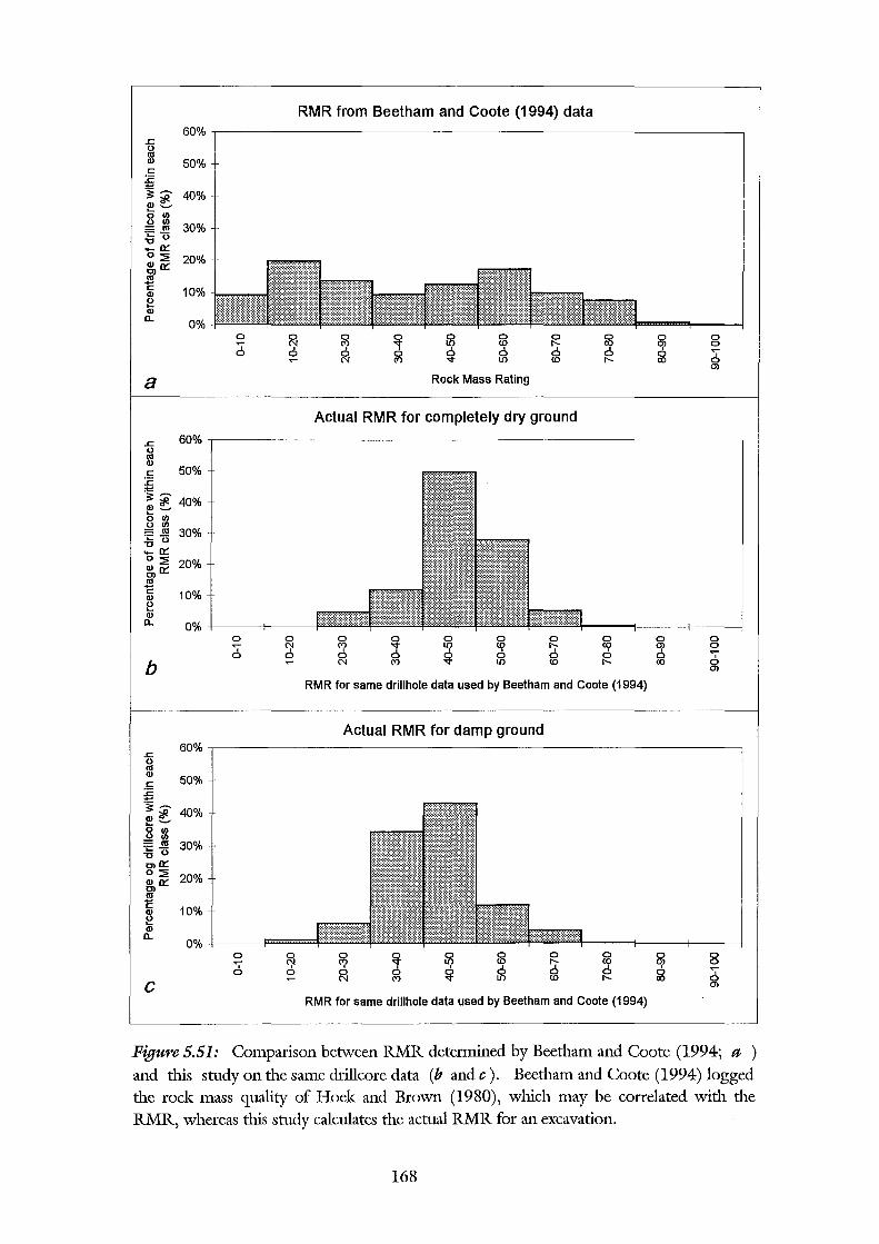
RMR from Beetham and Coote (1994) data 60%
.r:: 0 m Q) 50% r::: £ -~~
~e':, 40%
0 Ul 0 Ul
30% = m ~0 -a:: 0::2 20% ~0:: m "E 10% Q) 0 ... Q)
a. 0%
0 0 0 ~
0 0 0 0 0 0 ~ <i' ~ u;> (0 1';- ~ ~ 0 0 0 ~ 0 0 ~ 0 I
N (V) l() (0 ['-.. 00 0 0)
a Rock Mass Rating
Actual RMR for completely dry ground
.r:: 60% 0 m Q)
r::: 50% :c j * 40% ~~ 0 Ul 0 Ul = m 30% :§0 -a:: 0:;2 20% ~0::
~ 10% Q) 0 ... Q)
a. 0% 0 0 0
~ 0 0 0 0 0 0
~
~ ~ u;> (0
~ 00
~ 0
I 0 0 ~ 0 0 0 ~ 0 b N (V) l() (0 ['-.. 00
0)
RMR for same drillhole data used by Beetham and Coote (1994)
Actual RMR for damp ground 60% .r::
0 m Q)
50% r::: :c ~- 40% Q)~ ... ~ 0 Ul 0 Ul = m 30% -co 0)0:: 0::2
20% 010:: 01 m "E
10% Q) 0 ... Q)
a. 0%
0 0 0
~ 0 0 0 0 0 0
~ <i' ~ u;> (0 1';- <X? ~ 0 0 0 ~
0 ~ 0 0 0 0 c N (V) l() (0 ['-.. 00 0)
RMR for same drillhole data used by Beetham and Coote (1994)
Figure 5.51: Comparison between RMR determined by Beetham and Coote (1994; a ) and this study on the same drill core data ( b and c ) . Beetham and Coote ( 1994) logged the rock mass quality of Hoek and Brown (1980), which may be correlated with the RMR, whereas this study calculates the actual RMR for an excavation.
168
qualitatively logged, rock mass quality (converted to RMR) with the quantitatively
determined RMR (assuming a completely dry and a damp rock mass) using the same
drillcore data. The differences between the two are because of the outdated correlation
between rock mass quality and RMR used and because Beetham and Coote (1994)
qualitatively logged the drillcore, which may not be as accurate as a quantitative
assessment, but it still provides a relatively accurate assessment considering the speed a
qualitative assessment takes compared to the time taken to quantitatively log a rock mass.
Weaver's 1975 Rippability Rating Method estimates the quality of the rock mass to be
approximately one category of rock greater than that predicted by the RMR System, and
therefore over-estimates the quality of the rock mass and the type of excavation equipment
that could be used. The Modified Weaver Rippability Rating System updates the 1975
version, but also over-estimates the quality of the rock mass. This over-estimation is due to
the use of seismic velocities as a parameter, but as the aim of this thesis was to produce a
three-dimensional rock mass and rippability model and because seismic velocities were only
determined at the smface, then this method should not be used to estimate the rippability
of an excavation such as an open pit or quarry, however it can be used to determine the
rippability of shallow excavations, such as road cuttings. Furthermore, because seismic
velocities are seen as a measure of other parameters affecting the rippability of a site, they
should only be used as a preliminary assessment, similar to the approach undertaken in
Section 5.2.2 as other methods such as the RMR System fully describe the rock mass using
parameters that influence the rock mass, not parameters, such as seismic velocity, that are
.influenced by other parameters.
MacGregor et al)s (1994) Productivity Prediction Method classes the rock mass into ranges
of productivity based on a selected bulldozer. The method uses parameters that were
statistically found to influence rippability of a rock mass. Some parameters such as the
bulldozer operator and wear and tear of the ripper influence the rippability of a site to some
degree but these parameters cannot be determined during a site investigation. Two
equations may be used to predict the productivity of a site, one related to all rock types and
the other related to sedimentary rocks only. Equation 4, related to all rock types, estimates
a wider range of productivity values and a greater mean value that Equation 8 (used for
sedimentary rocks only), and therefore, data using Equation 8 are plotted for bench levels.
169
RMR, Modified Weaver Rippability Rating and Productivity bench level plans have been
produced (in map box) and may be compared. The rippability rating method predicts
most of the open pit to be hard ripping and does not delineate zones that should be easily
rippable, such as the western wall (location of the Chemist Shop Fault) and the Globe
Progress Shear Zone. For this reason, the rippability plans should not be used to model
the excavatability of the pit, instead, the RMR or Productivity Prediction Method or a
combination of the two could be used to model the excavatability of the open pit. Note,
however, that the productivity prediction should only be used for Komatsu's D575A-2
bulldozer (or another similar sized bulldozer), as the productivity is dependant upon the
mass of the bulldozer and the method of ripping, that is, the method assumes excavation is
by bulldozer ripping, not digging or a combination of blasting and ripping. However,
MacGregor, et al (1994) recommend using their method to identify zones that will be easy
or difficult to excavate whatever the excavation technique used.
Both the RMR and Productivity Prediction methods appear to accurately assess the
excavatability of the rock mass. Both methods identify the Globe-Progress Shear Zone and
western wall as being very easy and easy to excavate (or very poor to poor rock mass
quality) and both methods predict weaker rock in the axial hinge of the Globe-Progress
Shear Zone and better rock mass quality (or more difficult excavatability) on the limbs of
the shear zone. Therefore both methods can be used with some confidence to model the
excavatability of the open pit.
5. 6 Synthesis
The rippability assessment undertaken for this thesis was to first perform a preliminary
assessment that could be performed at the feasibility or early site investigation stages of a
project, then, if ripping appears to be feasible, apply a more comprehensive rippability
assessment.
170

The first preliminary assessment performed was seismic velocity determination at Globe
Progress and General Gordon. The seismic refraction surveys were performed along roads
and drill pads, adjacent to outcrops. This method was used because the seismic velocity of
a rock mass is dependant upon the strength, weathering, density and fracturing of the rock
mass (Weaver, 1975; Palmer, 1980; Braybrooke, 1988). Results show that 90% of the pit
area is rippable and marginal, and 10% of the open pit area is unrippable.
The other preliminary assessment method used was the Revised Size-Strength Chart, which
plots the strength of a rock material against the discontinuity spacing (or block size) of the
rock mass. This method had the advantage over seismic velocity determination in that the
data could be used from the drill log data, thereby giving a three-dimensional assessment.
Results show that almost none of the open pit area would require blasting and that most of
the data actually fits into easy and hard digging classes.
Both preliminary assessments confirmed that it would be possible to rip the overburden in
the open pit and dig the shear zone, however a more detailed rippability assessment should
be performed to fully characterise the rock material and rock mass in the open pit.
The complete rock mass characterisation and rippability assessment should not be
performed on its own, rather, it should be compared to at least one other method
(preferably more if possible) to aid interpretation and identification of diggable, easy
ripping, difficult ripping and blasting zones. The methods chosen to assess the
excavatability of the rock mass in the open pit were the RMR System, Weaver~s 1975
Rippability Rating System and MacGregor et aPs (1994) Productivity Prediction Method.
The RMR System and MacGregor et al)s (1994) Productivity Prediction Method both
delineate the Globe-Progress Shear Zone and western wall as being of poor quality, and
hence, easily rippable and the rest of the pit to be moderate to difficult ripping, with very
rare locations that may require blasting, whereas a modified version of Weaver's
Rippability Rating System predicts greater than 80% of the open pit to be hard ripping
and does not delineate wealcer or stronger rippability zones.
171
Chapter six
Summary, conclusions
and further work
6.1 Summary
6.1.1 General
The Globe-Progress proposed open pit mine is located within Greenland Group sediments
that are highly deformed. Because of this, ripping is seen as a feasible excavating
alternative to drill and bhist techniques. In suitable ground ripping has many benefits over
drill and blast methods including:
• economically advantageous
• improved safety
• ease of automation
• accuracy of finished excavation dimensions
• excavation walls remain undamaged
• product size usually handled by conveyors
• suitable where there are limitations on the level of vibrations
• bulldozers are multipurpose machines that may also be used for dozing, scraping,
stockpiling and moving equipment.
The aims of this thesis were to evaluate the rippability of the open pit, with the aim of
producing a three dimensional block model of the rock mass and rippability of the open
pit. To achieve this primary aim suitable rock mass and rippability classification systems
were required along with drillcore data and data from supplementary geotechnical
investigations.
172
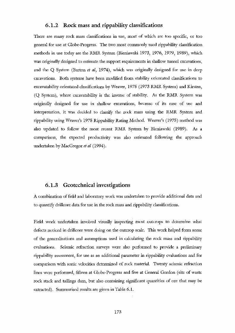
6.1.2 Rock mass and rippability classifications
There are many rock mass classifications in use, most of which are too specific, or too
general for use at Globe-Progress. The two most commonly used rippability classification
methods in use today are the RMR System (Bieniawski 1973, 1976, 1979, 1989), which
was originally designed to estimate the support requirements in shallow tunnel excavations,
and the Q System (Barton et al, 1974), which was originally designed for use in deep
excavations. Both systems have been modified from stability orientated classifications to
excavatability orientated classifications by Weaver, 1975 (1973 RMR System) and Kirsten,
(Q System), where excavatability is the inverse of stability. As the RMR System was
originally designed for use in shallow excavations, because of its ease of use and
interpretation, it was decided to classify the rock mass using the RMR System and
rippability using Weaver's 1975 Rippability Rating Method. Weaver's (1975) method was
also updated to follow the most recent RMR System by Bieniawski (1989). As a
comparison, the expected productivity was also estimated following the approach
undertaken by MacGregor et al (1994).
6.1.3 Geotechnical investigations
A combination of field and laboratory work was undertaken to provide additional data and
to quantify drillcore data for use in the rock mass and rippability classifications.
Field work undertaken involved visually inspecting most outcrops to determine what
defects noticed in drillcore were doing on the outcrop scale. This work helped form some
of the generalisations and assumptions used in calculating the rock mass and rippability
evaluations. Seismic refraction surveys were also performed to provide a preliminary
rippability assessment, for use as an additional parameter in rippability evaluations and for
comparison with sonic velocities determined of rock material. Twenty seismic refraction
lines were performed, fifteen at Globe-Progress and five at General Gordon (site of waste
rock stack and tailings dam, but also ·containing significant quantities of ore that may be
extracted). Summarised results are given in Table 6.1.
173
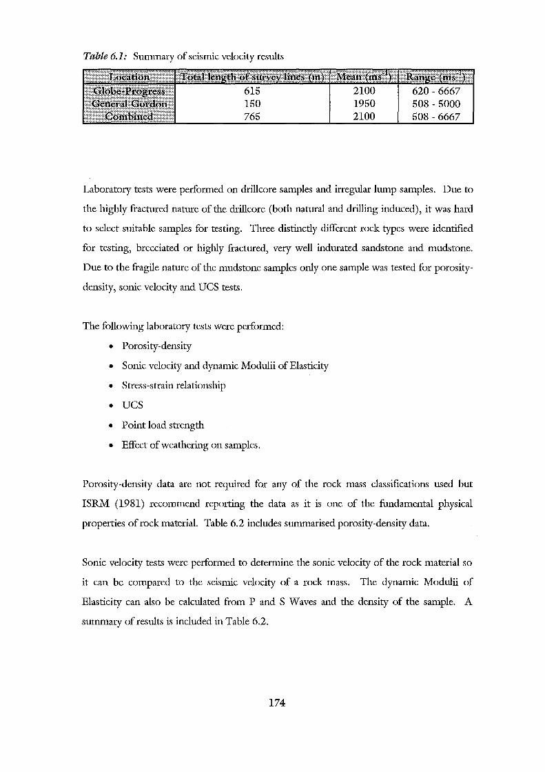
Table 6.1: Summary of seismic velocity results
765 1950 2100
620-6667 508- 5000 508- 6667
Laboratory tests were performed on drillcore samples and irregular lump samples. Due to
the highly fractured nature of the drillcore (both natural and drilling induced), it was hard
to select suitable samples for testing. Three distinctly different rock types were identified
for testing, brecciated or highly fractured, very well indurated sandstone and mudstone.
Due to the fragile nature of the mudstone samples only one sample was tested for porosity
density, sonic velocity and UCS tests.
The following laboratory tests were performed:
• Porosity-density
• Sonic velocity and dynamic Modulii of Elasticity
• Stress-strain relationship
• ucs • Point load strength
• Effect of weathering on samples.
Porosity-density data are not required for any of the rock mass classifications used but
ISRM (1981) recommend reporting the data as it is one of the fundamental physical
properties of rock material. Table 6.2 includes summarised porosity-density data.
Sonic velocity tests were performed to determine the sonic velocity of the rock material so
it can be compared to the seismic velocity of a rock mass. The dynamic Modulii of
Elasticity can also be calculated from P and S Waves and the density of the sample. A
summa..ty of results is included in Table 6.2.
174
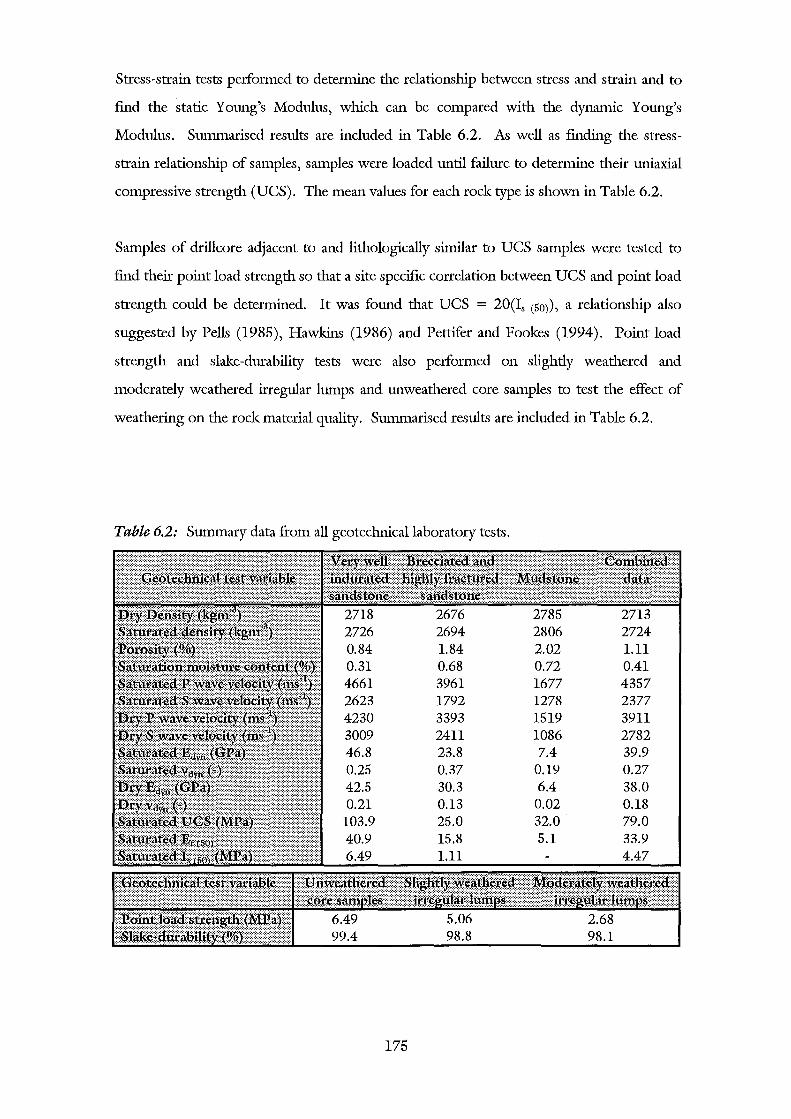
Stress-strain tests performed to determine the relationship between stress and strain and to
fmd the static Young's Modulus, which can be compared with the dynamic Young's
Modulus. Summarised results are included in Table 6.2. As well as fmding the stress
strain relationship of samples, samples were loaded until failure to determine their uniaxial
compressive strength (UCS). The mean values for each rock type is shown in Table 6.2.
Samples of drillcore adjacent to and lithologically similar to UCS samples were tested to
fmd their point load strength so that a site specific correlation between UCS and point load
strength could be determined. It was found that UCS = 20(Is (So)), a relationship also
suggested by Pells (1985), Hawkins (1986) and Pettifer and Fookes (1994). Point load
strength and slake-durability tests were also performed on slightly weathered and
moderately weathered irregular lumps and unweathered core samples to test the effect of
weathering on the rock material quality. Summarised results are included in Table 6.2.
Table 6.2: Summary data from all geotechnical laboratory tests.
2726 2694 2806 0.84 1.84 2.02 1.11 0.31 0.68 0.72 0.41 4661 3961 1677 4357 2623 1792 1278 2377 4230 3393 1519 3911 3009 2411 1086 2782 46.8 23.8 7.4 39.9 0.25 0.37 0.19 0.27 42.5 30.3 6.4 38.0 0.21 0.13 0.02 0.18
25.0 32.0 79.0 15.8 5.1
175
The above tests were all performed to assist in the quantitative analysis of drillcore data. It
was found that strength was mostly under-estimated, and it was occasionally over
estimated. Therefore, using the point load strength from this study and Beetham and
Coote's (1994) data, the logged strengths were revised to give a better approximation of
the strength of the rock material. RQD was logged twice using different intervals. Both
distributions are similar, therefore it is assumed that RQD has been correctly calculated.
Discontinuity spacing data follows a clustered distribution, where there is a concentration
of very close discontinuities. Other drillcore parameters such as grain size and weathering
are assumed to have been logged correctly.
6.1.4 Preliminary rippability evaluations
Two preliminary tests were performed to ascertain whether or not it was feasible to rip the
open pit. The first method involved determining variations in seismic velocities around the
open pit and comparing those with rippable, marginal and non-rippable zones for the
Bulldozer recommended by John (1994) for use in ripping the open pit. The second
method plots the strength of rock material versus its corresponding discontinuity spacing
on a revised size-strength graph (Pettifer and Fookes, 1994).
Seismic velocity determination results show that 90% of the pit area is rippable or marginal
and 10% of the open pit area is unrippable. The size-strength method suggests that almost
all of the pit area is rippable.
Both methods suggest that is feasible to rip the pit and therefore, it was decided to perform
a more detailed investigation that would identify zones of easy ripping (or poor rock),
moderately hard ripping (fair rock) and difficult ripping (good rock).
176
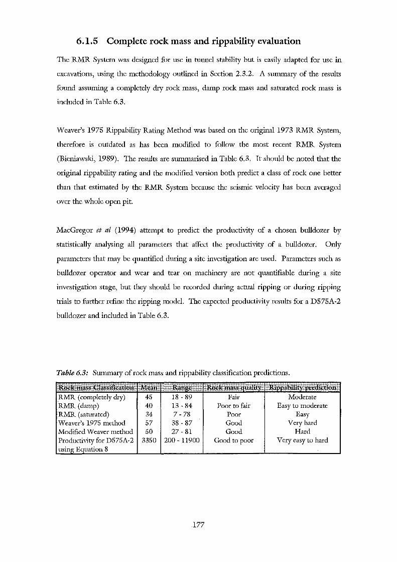
6.1.5 Complete rock mass and rippability evaluation
The RMR System was designed for use in tunnel stability but is easily adapted for use in
excavations, using the methodology oudined in Section 2.3.2. A summary of the results
found assuming a completely dry rock mass, damp rock mass and saturated rock mass is
included in Table 6.3.
Weaver's 1975 Rippability Rating Method was based on the original 1973 RMR System,
therefore is outdated as has been modified to follow the most recent RMR System
(Bieniawski, 1989). The results are summarised in Table 6.3. It should be noted that the
original rippability rating and the modified version both predict a class of rock one better
than that estimated by the RMR System because the seismic velocity has been averaged
over the whole open pit.
MacGregor et al (1994) attempt to predict the productivity of a chosen bulldozer by
statistically analysing all parameters that affect the productivity of a bulldozer. Only
parameters that may be quantified during a site investigation are used. Parameters such as
bulldozer operator and wear and tear on machinery are not quantifiable during a site
investigation stage, but they should be recorded during actual ripping or during ripping
trials to further refine the ripping model. The expected productivity results for a D575A-2
bulldozer and included in Table 6.3.
Table 6.3: Summary of rock mass and rippability classification predictions.
RMR (completely dry) 45 18-89 Fair Moderate RMR (damp) 40 13-84 Poor to fair Easy to moderate RMR (saturated) 34 7-78 Poor Easy Weaver's 1975 method 57 38-87 Good Very hard Modified Weaver method 50 27-81 Good Hard Productivity for D575A-2 3350 200- 11900 Good to poor Very easy to hard
tion 8
177
Bench level plans have been plotted up for the RMR, Modified Weaver Rippability Rating
and MacGregor et atJs (1994) expected productivity and are included in the map and table
box. Zones easy to excavate are the Globe-Progress Shear Zone, which follows the
northern and eastern pit walls, and the western pit wall, where the Chemist Shop Fault is
located. There is also a weak Z<Jne in the axial hinge of the Globe-Progress Shear Zone that
has undergone more deformation than the shear limbs (adjacent to the axial hinge. The
shear limbs are generally fair to good rock, which equates to moderate to hard (difficult)
ripping using a D575A-2 bulldozer.
6.2 Conclusions
• Seismic refraction surveys are an excellent site investigation technique that can be
performed at the feasibility and early investigation stages of a project because the seismic
velocity of a rock mass is dependent upon its weathering, strength, density, porosity,
compaction and fracturing, and therefore provides an overall assessment of the rock
mass quality.
• Seismic velocity determination on the mine site rock mass found that 90% of the open
pit area is of rippable to marginal rippability and that 10% of the pit area is expected to
be unrippable using Komatsu's D575A-2 bulldozer.
• The Size-Strength Excavatability Method is another excellent site investigation method
that can be performed early in a projects planning stages, as it plots the two properties
of a rock mass most influential to excavatability.
• Size-strength determination found that almost all of the pit area should be easy digging
through to very hard ripping, with a very small proportion of the pit area requiring
blasting.
178
• The preliminary rippability assessment undertaken estimates that most of the pit will be
diggable to rippable, and therefore a more accurate site investigation utilising a suite of
geological and geotechnical parameters was performed to identifY locations of diggable,
rippable and blastable zones.
• Analyses of the drillcore data found that strength values were logged incorrecdy, some
values were over-estimated but most values were under-estimated. Therefore a revised
strength estimate was determined based on quantitative strength measurements and the
logged lithology.
• The RMR System is the best rock mass classification method to use in classifying the
rock mass in the open pit as it uses a thorough rock material and discontinuity
description, whereas the other major rock mass classification system (the Q System) is
more applicable to characterising rock masses in deep tunnels and underground
excavations.
• The RMR System was designed for use in predicting the stability of tunnels but is easily
modified to predict the excavatability of a rock mass by reversing the discontinuity
orientation parameter such that a favourable orientation in a stability analysis will be
unfavourable for an excavation.
• Most of the rock mass in the open pit is rated poor to fair and the wealcer rock masses
are located in the western pit wall (where the Chemist Shop Fault is located), following
the Globe-Progress Shear Zone along the northern and eastern pit walls and in the fold
axis of the Globe-Progress Shear.
• Weaver's 1975 Rippability Rating Method was originally adapted from Bieniawski's
1973 RMR System, and therefore should be updated to follow Bieniawski's 1989 RMR
System. This modification has been performed by replacing the RQD and groundwater
parameters in the RMR System with a seismic velocity parameter in the rippability
rating method and reversing the discontinuity orientation ratings. However, seismic
velocities of rock masses are also fimctions of degree of weathering, density and
179
strength, and it is therefore, probably better to use a modified version of the RMR
System to assess the excavatability of a rock mass.
• There is less of a data spread in the rippability rating as it requires a seismic velocity
parameter, which was averaged for the pit area because seismic velocities determined on
the ground surface will be less than seismic velocities determined on unweathered, less
fractured (or relaxed) rock masses at depth. This has the effect of over-estimating the
rock mass quality and prediction of the most appropriate form of excavation.
• MacGregor et a!Ys (1994) Productivity Prediction Method was determined by
correlating parameters influential to rippability with the productivity of a bulldozer.
However the correlation is not very good (R2 = 0.58), and therefore, there must have
been considerable scatter original data set. MacGregor et al (1994) noted this problem
and recommended locating areas that should be difficult to rip.
• There are similar trends between the RMR Index and estimated productivity of a
Komatsu D575A-2 bulldozer, whereby locations of poor rock mass equate to high
productivity and zones of easy ripping. However most of the easy ripping zones are
located in brecciated and sheared rock that contain significant quantities of pug, and
thus acts in a plastic manner such that a heavy bulldozer should not attempt ripping the
shear zone.
• Areas identified to be hard to excavate could be saturated to weaken the rock mass and
assist with excavation, however this may lead to other problems associated with
groundwater.
• The contoured plans of RMR Index, Rippability Rating and estimated productivity
give a visual representation of the excavatability of a rock mass, but these plans should
not be used on their own. If excavation of the pit proceeds, orientated geotechnical
drillholes should be drilled to provide additional data for use in determiriing the
excavatability of the rock mass.
180
• Modelling techniques such as inverse distance and Kriging are normally applied to
estimate ore reserves and the ratio of waste rock to ore, but this study has shown that
these modelling techniques can easily be applied to rock mass classification methods to
characterise the rock mass.
6.3 Further work
• It is possible to apply the methodology used here to assess the excavatability of rock
mass at other sites in the Reefton Goldfield, and if underground mining is contemplated
then the rock mass can be classified using the Q system or one of the RMR extensions
designed for use in hard rock undergound mining.
• This study has provided a preliminary excavatability assessment, based on se1srmc
refraction data, at General Gordon. A complete excavatability assessment, following
procedures used in the study, could be performed once computer drillcore logs are
completed.
• Pit wall stability can be determined using Romana's (1985) Slope Mass Rating, which
is a modification of the RMR System, and the results can be compared to kinematic
slope stability assessments.
• It may be advantageous to quantitatively test rock material parameters at other
exploration sites so that the information can be used in core logging.
• As excavation proceeds, comparisons should be made between actual bench level data
and predicted bench level data. If ripping is to be used then the estimated productivity
for the chosen bulldozer should be compared to the actual ripping and other factors
such as the length of ripping runs and wear and tear of ripper tips and bulldozer tracks
should be carefully monitored to further refme the estimated productivity of a bulldozer.
181
Acknowledgements
The following people all deserve my gratitude and appreciation for their help and assistance
during the course of this study.
Firstly, thanks to Macraes, Reefton for encouraging their head office as to the value of this
project and to Macraes, Head Office, for their "enthusiasm" shown in student research.
Secondly thanks to my supervisor David Bell for all the encouragement and guidance (and
red wine), and for providing helpful comments on all chapter drafts plus for staying up
past the witching hour reading my final thesis draft.
Thirdly thanks to the staff at Macraes Reefton, especially Mark McKenzie (Project
Geologist) for experience in the field of rock mass classification and to John Taylor (Senior
Mine Planning Engineer) for his advice on various mining matters and plotting up of
computer plans. I am also indebted to Colin Legge of Medsystems, Australia for
generating the plans in the map box (delaying his trip down south by half a day) and
designing a printing routine so that I didn't have to crash the big very expensive computer.
A big slap on the back must also go to Jimmy and Ron who slaved away banging a
sledgehammer against a metal plate in very hot sun (very rarely) and pouring rain (most
commonly) and probably wondering what they were doing?? Thanlcs also to Des
MacKenzie for the photos of Komatsu's "super dozer" and Lisa for photocopying, binding
various reports and ordering pizzas etc etc. Thanlcs also to everyone else I met at Reefton
including the chef at Cee Cee's (but not the chef at the hospital).
Fourthly, thanlcs to the Mason Trust for financial assistance with travel and thesis
preparation costs and to Macraes, Reefton for the accommodation, food, field assistance
and printing of plans and tables.
182

Thanks also to Joe Campbell, David Nobes, Jarg Pettinga and Steve Weaver of the
academic staff at University of Canterbury and Laurie Richards from Lincoln University
for providing helpful comments on various parts of this thesis.
Thanks also to the technical staff in the Geological Sciences Department, especially Mike
Finnemore for his computer literacy; Cathy Knight for the organising of gear, setting up
of lab equipment, useful advice and help with fieldwork during the early stages of this
project etc etc etc; Arthur Nicholas for workshop advice and slides; Rob Spiers for putting
up with me as I cut samples, Kerry Swanson for photos and slides and Michelle Wright for
money.
Thanks again to Dave Bell, Cathy Knight and Jonny McNee for their assistance m
smashing core samples in the civil engineering materials lab and to George Clark from the
civil engineering materials lab for allowing us to do so.
More thanks to my classmates, Al, Anna, Carl, Chris, Jonny, Nick, Rachel, Sarah and
Sonia and other friends who have kept me sane away from varsity.
Still more thanks to my Parents and sisters for putting up with me over the last few months
and especially thanks for all the microwaveable meals.
Lastly, thanks to Macraes for the use of the four wheel drive (PTO) ....
183
Oops!
NB : There were no dents or scratches -just a little bit of mud on the other side.
And if you were wondering what effect the writing up of an engineering geological thesis
and using excel can do to the body then PTO.
184

Tailpiece
Arrrrrgh!!!!!
185

References
Abad, J; B Celada; E Chacon; V Gutierrez; and E Hidalgo; 1983: Application of
geomechanical classification to predict the convergence of coal mine galleries and to
design their supports, Proceedings of the 5th International Congress on Rock Mechanics,
ISRM, Melbourne, volume 2, pages E15-E19.
Abdullatif, OM and DM Cruden; 1983: The relationship between rock mass quality and
ease of excavation, Bulletin of the International Association of Engineering Geology,
volume 28, pages 183-187.
Adams, CJD; CT Harper; and MG Laird; 1975: K-Ar ages of low grade metasediments
of the Greenland and Waiuta Groups in Wesdand and Buller, New Zealand, New
Zealand journal of Geology and Geophysics, volume 18, pages 39-48.
Allaby, A and M Allaby; 1991: The Concise Oxford Dictionary of Earth Sciences, Oxford
University Press, Oxford, 410 pages.
Anon; 1994: Report to Mark McKenzie, Report by Works Consultancy Services, 2 pages.
Atkinson, T; 1970: Ground preparation by ripping in open pit mining, Mining Magazine,
volume 122, pages 458-469.
Australian Geomechanics Society; 1975: Engineering classification of sedimentary rocks in
the Sydney area, Australian Geomechanical journal, volume G5, number l.
Barrell, D; 1992: Geotechnical line mappmg, Globe-Progress Prospect, Reefton,
Unpublished Report for Macraes Mining Company Limited) Reefton, 58 pages.
186
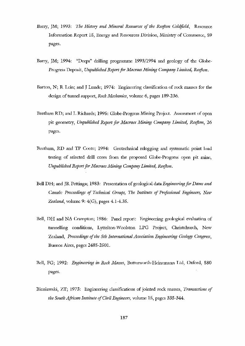
Barry, JM; 1993: The History and Mineral Resources of the Reefton Goldfield, Resource
Information Report 15, Energy and Resources Division, Ministry of Commerce, 59
pages.
Barry, JM; 1994: "Deeps" drilling prograrrune 1993/1994 and geology of the Globe
Progress Deposit, Unpublished Report for Macraes Mining Company Limited) Reefton.
Barton, N; R Lein; and J Lunde; 1974: Engineering classification of rock masses for the
design of tunnel support, Rock Mechanics, volume 6, pages 189-236.
Beetham RD; and L Richards; 1995: Globe-Progress Mining Project. Assessment of open
pit geometry, Unpublished Report for Macraes Mining Company Limited) Reefton, 26
pages.
Beetham, RD and TP Coote; 1994: Geoteclmical relogging and systematic point load
testing of selected drill cores from the proposed Globe-Progress open pit mine,
Unpublished Report for Macraes Mining Company Limited) Reefton.
Bell DH; and JR Pettinga; 1983: Presentation of geological data Engineering for Dams and
Canals: Proceedings of Technical Groups) The Institute of Professional Engineers) New
Zealand, volume 9: 4(G), pages 4.1-4.35.
Bell, DH and NA Crampton; 1986: Panel report: Engineering geological evaluation of
tunnelling conditions, Lyttelton-Woolston LPG Project, Christchurch, New
Zealand, Proceedings of the 5th International Association Engineering Geology Congress,
Buenos Aires, pages 2485-2501.
Bell, FG; 1992: Engineering in Rock Masses, Butterworth-Heinemann Ltd, Oxford, 580
pages.
Bieniawsld, ZT; 1973: Engineering classifications of jointed rock masses, Transactions of
the South African Institute of Civil Engineers) volume 15, pages 335-344.
187
Bieniawski, ZT; 1976: Rock mass classifications in rock engineering, Proceedings of the
Symposium of Exploration for Rock Engineering, AA BaJkema, Johannesburg, volume 1,
pages 97-106.
Bieniawski, ZT; 1978: Determining rock mass deformability: Experience from case
histories, International journal of Rock Mechanics and Mining Sciences, volume 15,
pages 237-247.
Bieniawski, ZT; 1979: The Geomechanics Classification in rock engineering applications,
Proceedings of the Fourth International Congress on Rock Mechanics) ISRM, Montreux,
volume 2, pages 41-48.
Bieniawski, ZT; 1984: Rock Mechanics Design in Mining and Tunnelling, AA Balkema,
Rotterdam, 272 pages.
Bieniawski, ZT; 1989: Engineering Rock Mass Classifications: A Complete Manual For
Engineers and Geologists in Mining) Civil) and Petroleum Engineering, John Wiley and
Sons, New York, 251 pages.
Bieniawski, ZT; 1993: Classification of rock masses for engineering: The RMR System
and future trends, Comprehensive Rock Engineering) Principles) Practice and Projects:
Volume 3 Rock Testing and Site Characterisation, edited by JA Hudson, Pergamon
Press, Oxford, volume 3, pages 553-573.
Bieniawski, ZT and CM Orr; 1986: Rapid site appraisal for dam foundations by the
Geomechanics Classification, Proceedings of the 12th Congress on Large Dams)
ICOLD, Mexico City, pages 483-501.
Bowen, FE; 1964: Geologica/Map ofNeJv Zealand) Sheet 15: Butler, scale 1:250 000.
188
Bradshaw, MA; and BD Regan; 1983: Stratigraphy and structure of the Devonian rocks
of Inangahua Outlier, Reefton, New Zealand, New Zealand Journal of Geology and
Geophysics, volume ll, pages 92-122.
Braybrooke, JC; 1988: The state of the art of rock cuttability and rippability prediction,
Proceedings of the Fifth Australia New Zealand Conftrence on Geomechanics, pages
13-42.
Breldce, TL; 1968: Blocky and seamy rock in tunnelling, Bulletin of the Association of
Engineering Geology, volume 5, pages 1-12.
Brewster, PJ; 1984: Ripping techniques, Australian Geomechanics Society - Excavation
Characteristics Seminar, November 1984.
Brach, E; and JA Franldin; 1972: The point load strength test, The International journal of
Rock Mechanics and Mining Science, volume 9, pages 669-697.
Bullock, SJ; 1978: The case for using multichannel seismic refraction equipment and
techniques for site investigation, Bulletin of the Association of Engineering Geologists,
volume 15, pages 19-35.
Church, HK; 1981: ExcavationHandbook, McGraw-Hill, New York, 1024 pages.
Coffey and Partners; 1989: Preliminary geotechnical study, Globe-Progress Mine,
Reefton, Unpublished Report for CRAExplorationLimited~ Ree.fton, 93 pages.
Cooper, AF and D Craw; 1992: Petrographic analysis and report on core samples from
the Globe-Progress Project area, Reefton, Unpublished Report for Macraes Mining
Company Limited~ Ree.fton, 44 pages.
Cooper, RA; 1974: Age of the Greenland and Waiuta Groups, New Zealand Journal of
Geology and Geophysics, volume 17, pages 955-962.
189
Cooper, RA; 1989: Early Palaeozoic Terranes of New Zealand,]ournal ofthe Royal Society
ofNew Zealand, volume 19, pages 73-112.
Deere, DU; 1967: Geological considerations, Rock Mechanics in Engineering Practice,
edited by KG Stagg and 0 Zienkiewicz, John Wiley and Sons, London, pages 1-20.
Deere, DU; AJ Hendron; FA Patton; and EJ Cording; 1968: Design of surface and near
surface construction in rock, Proceedings of the 8th US Symposium on Rock Mechanics,
AIME, New York, pages 237-302.
Deere, DU; RB Peck; H Parker; JE Monsees; and B Schmidt; 1970: Design of tunnel
support systems, Highway Research Record, volume 339, pages 26-33.
Dight, PM and JK Cadman; 1992: Geotechnical study for the Globe-Progress gold
deposit, Reefton, New Zealand, Unpublished Report for Macraes Mining Company
Limitedy Ree.fton, 60 pages.
Edge, AB and TH Laby; 1931: The Principles and Practice of Geophysical Prospecting,
Cambridge University Press.
Einstein, HH; DE Thompson; AS Azzouz; KP O'Reilly; MS Schultz; and S Ordun; 1983:
Comparison of five empirical tunnel classification methods - accuracy, effect of
subjectivity and available information, Proceedings of the 5th International Congress on
Rock Mechanics, ISRM, Melbourne, volume 1, pages C303-C313.
Farmer, IW; 1983: Engineering Behaviour of Rocks, Second edition, Chapman and Hall,
London, 208 pages.
Fookes, PG; WR Dearman; and JA Franldin; 1971: Some engineering aspects of rock
weathering with field examples from Dartmoor and elsewhere, Quarterly journal of
Engineering Geology, volume 4, pages 139-185.
190
Powell, RJ; 1993: The mechanics of rock cutting, Comprehensive Rock Engineeringy
Principlesy Practice and Projects: Volume 4y Excavationy Support and Monitoring, edited
by JA Hudson, Pergamon Press, Oxford, pages 155-176.
Franldin, JA; E Brach; and G Walton; 1971: Logging the mechanical character of rock,
Transactions of the Institution of Mining and Metallurgy, volume 80A, pages 1-9.
Gage, M; 1948: The geology of the Reefton quartz lodes, New Zealand Geological Bulletin
45, 72 pages.
Gage, M and FA McNeill; 1940: Geophysical investigations in the area between Waiuta
and Merrijigs, New Zealand journal of Science and Technology, volume 22, pages 155-
165.
Ghose, AK and NM Raju; 1981: Characterisation of rock mass vis-a-vis application of
rock bolting in Indian coal measures, Proceedings of the 22nd US Symposium on Rock
Mechanics, MIT, Cambridge, pages 422-427.
Hancox, GT and S Beanland; 1994: Evaluation of fault displacement hazard at the Globe
Progress mine site area, Reefton, Unpublished Report for Macraes Mining Company
Limitedy Reefton.
Hatherly, PJ and MJ Neville; 1986: Experience with the Generalised Reciprocal Method
of seismic refraction interpretation for shallow engineering site investigation,
Geophysics, volume 51, pages 255-265.
Hawkes, I and M Mellor; 1970: Uniaxial testing m rock mechanics laboratories,
Engineering Geology, volume 4, pages 177-285.
191
Hawkins, AB; 1986: Rock descriptions, Site Investigation Practice: Assessing BS5930, edited
by AB Hawkins, Geological Society, Engineering Geology Special Publication 2,
pages 59-66.
Hawkins, LV; 1961: The Reciprocal Method of routine shallow se1srmc refraction
investigations, Geophysics, volume 26, pages 806-819.
Henderson, J; 1917: The geology and mineral resources of the Reefton Subdivision, New
Zealand Geological Bulletin 18, 232 pages.
Henderson, J; 1921: Reefton Coalfield, New Zealand journal of Science and Technology,
volume 4, pages 18-24.
Hodder, APW; and Hetherington, JR; 1991: A quantitative study of the weathering of
Greywacke, Engineering Geology, volume 31, pages 353-368.
Hoek, E and ET Brown; 1980: Underground Excavations in Rock, Institution of Mining
and Metallurgy, London, 527 pages.
Hughes, S; 1992: The geology of the Globe-Progress gold-antimony-arsenic deposit,
Reefton, Westland, Unpublished &port for Macraes Mining Company Limitedy &efton,
32 pages.
Irfan, TY; and WR Dearman; 1978: Engineering classification and index properties of a
weathered granite, Bulletin of the International Association of Engineering Geology,
volume 17, pages 79- 90.
ISRM; 1981: Rock Characterisationy Testing and Monitoring. International Society for Rock
Mechanics Suggested Methodsy ET Brown (editor), Pergamon Press, Oxford, 211
pages.
192
ISRM; 1985: Suggested method for determining point load strength, International
journal of Rnck Mechanicsy Mining Sciences and Geomechanics Abstracts, volume 22,
pages 51-60.
Jaeger, JC; and NGW Cook; 1976: Fundamentals of Rnck Mechanics, Second edition,
Chapman and Hall, London, 585 pages.
John, I; 1994: Site visit report, Globe-Progress development, near Reefton, New Zealand,
Unpublished Report for Macraes Mining Company Limitedy Rcefton, 13 pages.
Johnson, RB; and JV DeGraff; 1988: Principles. of Engineering Geology, John Wiley and
Sons, New York, 497 pages.
Jowett, T; H McLauchlan; and P Lundy; 1996: Bench-zero mapping, Unpublished Report
for Macraes Mining Company Limitedy Rcefton.
Kendorski, F; R Cummings, ZT Bieniawski; and E Skinner; 1983: Rock mass
classification for block caving mine drift support, Proceedings of the 5th International
Congress onRnckMechanics, ISRM, Melbourne, volume 1, pages B51-B63.
Kirsten, HAD; 1982: A classification system for excavation m natural materials,
Transactions of the South African Institute of Civil Engineers, volume 24, pages
293-308.
Koczanowski, M; GR Mostyn; and F MacGregor; 1991: An expert system for rock
rippability assessment, Proceedings of the SePenth International Congress on Rnck
Mechanicsy ISRM, Montreux, volume 3, pages 275-279.
Laird, MG; 1972: Sedimentology of the Greenland Group in the Paparoa Range, West
Coast, South Island, New Zealand, New Zealand journal of Geology and Geophysics,
volume 15, pages 372-393.
193
Laird, MG and D Shelley; 1974: Sedimentation and early tectonic history of the
Greenland Group, Reefton, New Zealand, New Zealand Journal of Geology and
Geophysics, volume 17, pages 839-854.
Laubscher, DH; 1977: Design aspects and effectiveness of support systems in different
mining situations, Transactions of the Institute of Mining and Metallut;gy, volume 86,
pages A1-A7.
MacGregor, F; R Fell; GR Mostyn; G Hocking; and G McNally; 1994: The estimation
of rock rippability, Quarterly Journal of Engineering Geology, volume 27, pages
123-144.
Martin, JM; 1986: Predicting the rippability of sandstone in Southeast Queensland,
Proceedings of the 13th Australian Road &search Board Conference, pages 119-132.
McGovern-Wilson, R; 1992: Globe Hill Archaeological Survey, Unpublished &port for
Macraes Mining Company Limited) &efton, 205 pages.
Minty, EJ and GK Kearns; 1983: Rock mass workability, Collected Case Studies in
Engineering Geology) Hydrogeology and Environmental Geology, edited by MJ Knight,
EJ Minty, RB Smith, Geological Society of Australia Special Publication ll, pages
59-81.
MMCL; 1996: Annual &port 1995, 64 pages.
Modriniak, Nand E Marsden; 1938: Experiments in Geophysical Survey in New Zealand,
New Zealand Department of Science and Industrial &search Geological Memoirs,
volume 4, 90 pages.
Motor Holdings Komatsu Limited; 1996: Komatsu's big dozers for heavy metal fans
everywhere, On track) the Bulletin for Construction) Forestry) Mining and Quarrying,
April-May 1996, pages 4-5.
194
Muir, RJ; SD Weaver; JD Bradshaw; GN Eby; JA Evans; and TR Ireland; In press:
Geochemistry of the Karamea Batholith, New Zealand, and comparisons with the
Lachlan Fold Belt granites of Southeast Australia, Lithos.
Nakao, K; S Iihoshi; and S Koyama; 1983: Statistical reconsiderations on the parameters
for geomechanics classification, Proceedings of the 5th International Congress on Rock
Mechanics, ISRM, Melbourne, volume 1, pages B13-B16.
Nathan, S; 1976: Geochemistry of the Greenland Group (Early Ordovician), New
Zealand, New Zeala,nd journal of Geology and Geophysics, volume 19, pages 683-706.
Nobes, DC; 1989: A test of a simple model of the acoustic vlocity in marine sediments,
journal oftheAcoustic Society of America, volume 86, pages 290-294.
NZGS; 1988: Guidelines for the field description of soils and rocks in engineering use, 42 pages.
Obert, L; and Duvall, WI; 1967: Rock Mechanics and the Design of Structures in Rock, John
Wiley and Sons, New York, 650 pages.
Olivier, HJ; 1979: A new engineering geological rock durability classificationJ Engineering
Geology, volume 14, pages 255-279.
Orr, CM; 1992: Assessment of rock slope stability using the Rock Mass Rating (RMR)
System, Proceedings of the Australian Institute of Mining and Metallur;gy, number 2,
pages 25-29.
Palmer, D; 1980: The Generalised Reciprocal Method of Seismic Refraction Interpretation,
Society of Exploration Geophysicists, 104 pages.
Parry, C; 1993: The Globe-Progress Project, Reefton, New Zealand Mining, volume 10,
June 1993, pages 8-11.
195
Pells, P]N; 1985: Engineering properties of the Hawkesbury Sandstone, Engineering
Geology of the Sydney Region, edited by P]N Pells, Ballcema, Rotterdam, pages
179-197.
Pettifer, GS; and PG Fookes; 1994: A revision of the graphical method for assessing the
excavatability of rock, Quarterly journal of Engineering Geology, volume 27, pages
145-164.
Priest, SD and JA Hudson; 1976: Discontinuity Spacings in Rock, International journal of
Rock Mechanicsy Mining Sciences and Geomechanics Abstracts, volume 13, pages
135-148.
Raine, ]I; 1980: Palynology of the Triassic Topfer Formation, Reefton, South Island,
New Zealand, Abstracts of the Fifth Gondwana Symposiumy Wellingtony New Zealandy
1980.
Raine, ]I; 1984: Outline of a palynological zonation of Cretaceous to Paleogene terrestrial
sediments in the West Coast region, South Island, New Zealand, New Zealand
Geological Survey Report 109, 82 pages.
Rattenbury, MS; 1994: Structural geology of the Globe Hill area, Reefton, Unpublished
Report for Macraes Mining Company Limite~ Reefton. 34 pages.
Romana, M; 1985: New adjustment ratings for application ofBieniawski Classification to
slopes, Proceedings of the International Symposium of Rock Mechanics in Excavationsy
Mining and Civil Works, ISRM, Mexico City, page 59-68.
Rose, D; 1982: Revising Terzaghi's tunnel rock load coefficients, Proceedings of the 23rd
US Symposium onRockMechanics, AIME, New York, pages 953-960.
196
Rutledge, JC and RL Preston; 1978: New Zealand experience with engineering
classifications of rock for the prediction of tunnel support, Proceedings of the
International Tunnelling Symposium, Tokyo, pages 23-29.
Sandbak, LA; 1985: Roadheader drift excavation and geomechanics rock classification,
Proceedings of Rapid excavations and Tunnelling Conference, AIME, New York,
volume 2, page 902-916.
Serafun, JL and JP Pereira; 1983: Considerations of the geomechanics classification of
Bieniawski, Proceedings of the International Symposium of Engineering Geological
Underground Construction, LNEC, Lisbon, volume 1, pages II.33-II.42.
Siggons, AF; 1993: Dynamic elastic tests for rock engineering, Comprehensive Rock
Engineering) Principles) Pra,ctice and Projects: Volume 3 Rnck Testing and Site
Characterisation, edited by JA Hudson, Pergamon Press, Oxford, volume 3, pages
601-634.
Sinha, RS; 1988: Discussion of the RSR Model, Proceedings of the Symposium on Rock
Classification for Engineering Purposes, ASTM Special Technical Publication 984,
Philadelphia, pages 35-49.
Smith, HJ; 1987: Estimating the mechanical dredgeability of rock, Proceedings of the 28th
US Symposium on Rock Mechanics, AA Balkema, Boston, pages 943-935.
Smith, WD and KR Berryman; 1983: Revised estimates of earthquake hazard in New
Zealand, Bulletin of the New Zealand National Society for Earthquake Engineering)
volume 16.
Sakal, RR; 1974: Classification: purposes, principles, progress and prospects, Science)
volume 185, pages 1115-1123.
197
Suggate, RP; 1957: The geology of the Reefton Subdivision, New Zealand Geological
Bulletin 56, 146 pages.
Swan, ARH and M Sandilands; 1995: Introduction to Geological Data Analysis, Blackwell
Science Limited, Oxford, 446 pages.
Terzaghi, K; 1946: Rock defects and loads on tunnel support, Rock Tunnelling Wtth Steel
Supports, edited by RV Proctor and T White, Commercial Shearing Company,
Youngstown, USA, pages 15-99.
Tsiambaos, G and D Telli; 1992: Application of rock mass classification systems on
stability of limestone slopes, Proceedings of the 6th International Symposium on
Landslides, Christchurch, New Zealand, AA Balkema, Rotterdam, volume 2,
pages 1065-1069.
Udd, JE and HWang; 1985: A comparison of some approaches to the classification of
rock masses for geotechnical purposes, Proceedings of the 26th US Symposium on Rock
Mechanics, Rapid City, South Dal<ota, volume 1, pages 69-78.
Unal, E; 1983: Design Guidelines and Roof Control Standards for Coal Mine Roofs, PhD
thesis, Pennsylvania State University, Pennsylvania, 355 pages.
Urquhart, DF; 1956: The investigation of deep leads by the seismic refraction method,
Bulletiny Bureau of Mineral Resourcesy Australiay Volume 35.
Venkateswarlu, V; 1986: Geomechanics Classification of Coal Measure Rocks vis-a-vis Roof
Supports, PhD thesis, Indian School of Mines, Dhanbad, 251 pages.
Von Haast, J; 1861: Report of a topographical and geological exploration of the western districts
of the Nelson Provincey NeJV Zealand.
198
Weaver, JM; 1975: Geological factors significant in the assessment of rippability,
Transactions of the South African Institute of Civil Engineersy volume 17, pages
313-316.
Wickham, GE; HR Tiedemann; and EH Skinner; 1972: Support determination based on
geologic predictions, Proceedings of the Rapid Excavation and Tunnelling Conference,
AIME, New York, volume 1, pages 43-64.
Wickham, GE; HR Tiedemann; and EH Skinner; 1974: Ground Support Prediction
Model - RSR Concept, Proceedings of the Rapid Excavation and Tunnelling Conference,
AIME, New York, pages 691-707.
Williams, GJ; 1930: Report on the Reefton Coalfield, Applied Journal for the House of
Representativesy New Zealand, volume C-2B, 2.
Woodward Clyde; 1994: Surface water hydrology, Globe-Progress Project, Reefton,
Unpublished Report for Macraes Mining Company Limitedy Rcefton, 63 pages.
199
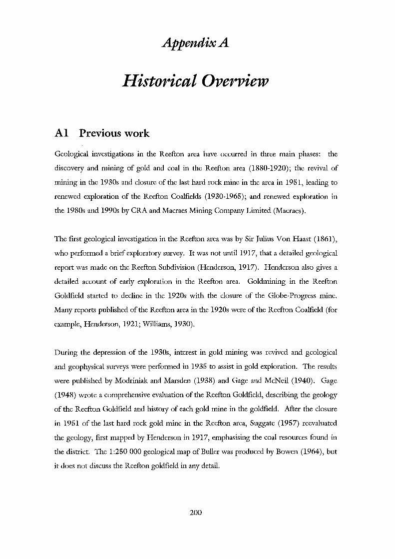
Appendix A
Historical Overview
AI Previous work
Geological investigations in the Reefton area have occurred in three main phases: the
discovery and mining of gold and coal in the Reefton area (1880-1920); the revival of
mining in the 1930s and closure of the last hard rock mine in the area in 1951, leading to
renewed exploration of the Reefton Coalfields (1930-1965); and renewed exploration in
the 1980s and 1990s by CRA and Macraes Mining Company Limited (Macraes).
The ftrst geological investigation in the Reefton area was by Sir Julius Von Haast (1861),
who performed a brief exploratory survey. It was not until1917, that a detailed geological
report was made on the Reefton Subdivision (Henderson, 1917). Henderson also gives a
detailed account of early exploration in the Reefton area. Goldmining in the Reefton
Goldfield started to decline in the 1920s with the closure of the Globe-Progress mine.
Many reports published of the Reefton area in the 1920s were of the Reefton Coalfield (for
example, Henderson, 1921; Williams, 1930).
During the depression of the 1930s, interest in gold mining was revived and geological
and geophysical surveys were performed in 1935 to assist in gold exploration. The results
were published by Modrinial< and Marsden (1938) and Gage and McNeil (1940). Gage
(1948) wrote a comprehensive evaluation of the Reefton Goldfield, describing the geology
of the Reefton Goldfield and history of each gold mine in the goldfield. After the closure
in 1951 of the last hard rock gold mine in the Reefton area, Suggate (1957) reevaluated
the geology, ftrst mapped by Henderson in 1917, emphasising the coal resources found in
the district. The 1:250 000 geological map of Buller was produced by Bowen (1964), but
it does not discuss the Reefton goldfield in any detail.
200
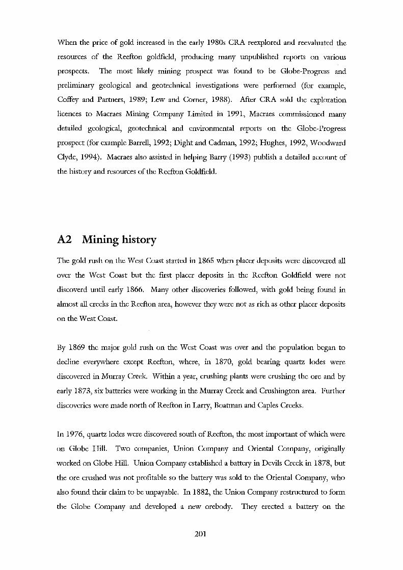
When the price of gold increased in the early 1980s CRA reexplored and reevaluated the
resources of the Reefton goldfield, producing many unpublished reports on various
prospects. The most likely mining prospect was found to be Globe-Progress and
preliminary geological and geotechnical investigations were performed (for example,
Coffey and Partners, 1989; Lew and Corner, 1988). Mter CRA sold the exploration
licences to Macraes Mining Company Limited in 1991, Macraes commissioned many
detailed geological, geotechnical and environmental reports on the Globe-Progress
prospect (for example Barrell, 1992; Dight and Cadman, 1992; Hughes, 1992, Woodward
Clyde, 1994). Macraes also assisted in helping Barry (1993) publish a detailed account of
the history and resources of the Reefton Goldfield.
A2 Mining history
The gold rush on the West Coast started in 1865 when placer deposits were discovered all
over the West Coast but the first placer deposits in the Reefton Goldfield were not
discoverd until early 1866. Many other discoveries followed, with gold being found in
almost all creeks in the Reefton area, however they were not as rich as other placer deposits
on the West Coast.
By 1869 the major gold rush on the West Coast was over and the population began to
decline everywhere except Reefton, where, in 1870, gold bearing quartz lodes were
discovered in Murray Creek Within a year, crushing plants were crushing the ore and by
early 1873, six batteries were working in the Murray Creek and Crushington area. Further
discoveries were made north ofReefton in Larry, Boatman and Caples Creeks.
In 1976, quartz lodes were discovered south ofReefton, the most important of which were
on Globe Hill. Two companies, Union Company and Oriental Company, originally
worked on Globe Hill. Union Company established a battery in Devils Creek in 1878, but
the ore crushed was not profitable so the battery was sold to the Oriental Company, who
also found their claim to be unpayable. In 1882, the Union Company restructured to form
the Globe Company and developed a new orebody. They erected a battery on the
201
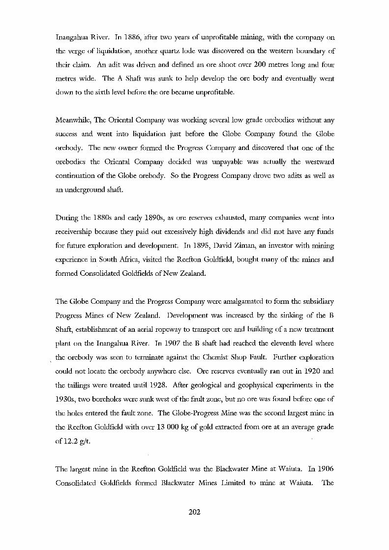
Inangahua River. In 1886, after two years of unprofitable mining, with the company on
the verge of liquidation, another quartz lode was discovered on the western boundary of
their claim. An adit was driven and defined an ore shoot over 200 metres long and four
metres wide. The A Shaft was sunk to help develop the ore body and eventually went
down to the sixth level before the ore became unprofitable.
Meanwhile, The Oriental Company was working several low grade orebodies without any
success and went into liquidation just before the Globe Company found the Globe
orebody. The new owner formed the Progress Company and discovered that one of the
orebodies the Oriental Company decided was unpayable was actually the westward
continuation of the Globe orebody. So the Progress Company drove two adits as well as
an underground shaft.
During the 1880s and early 1890s, as ore reserves exhausted, many companies went into
receivership because they paid out excessively high dividends and did not have any funds
for future exploration and development. In 1895, David Ziman, an investor with mining
experience in South Mrica, visited the Reefton Goldfield, bought many of the mines and
formed Consolidated Goldfields ofNew Zealand.
The Globe Company and the Progress Company were amalgamated to form the subsidiary
Progress Mines of New Zealand. Development was increased by the sinking of the B
Shaft, establishment of an aerial ropeway to transport ore and building of a new treatment
plant on the Inangahua River. In 1907 the B shaft had reached the eleventh level where
the orebody was seen to terminate against the Chemist Shop Fault. Further exploration
could not locate the orebody anywhere else. Ore reserves eventually ran out in 1920 and
the tailings were treated until1928. Mter geological and geophysical experiments in the
1930s, two boreholes were sunk west of the fault zone, but no ore was found before one of
the holes entered the fault zone. The Globe-Progress Mine was the second largest mine in
the Reefton Goldfield with over 13 000 kg of gold extracted from ore at an average grade
of12.2 g/t.
The largest mine in the Reefton Goldfield was the Blackwater Mine at Waiuta. In 1906
Consolidated Goldfields formed Blackwater Mines Limited to mine at W aiuta. The
202
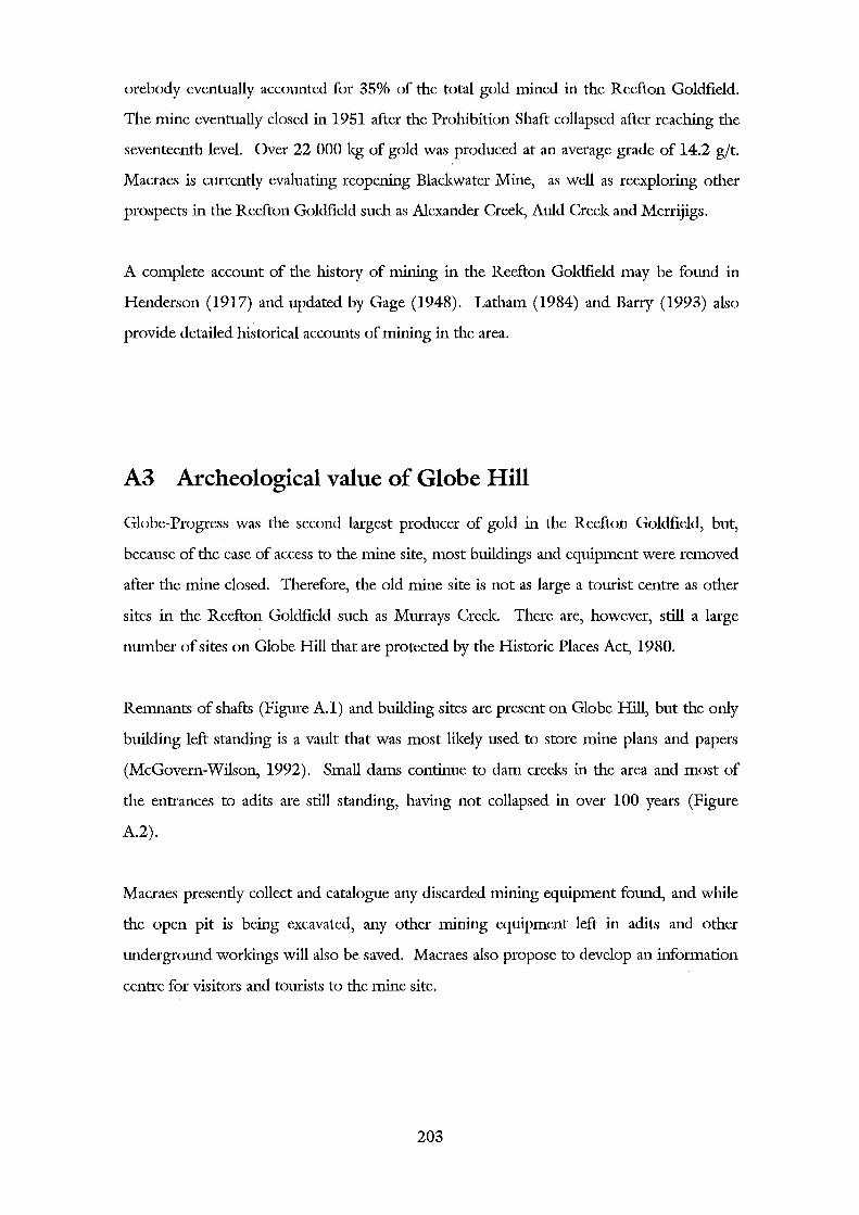
orebody eventually accounted for 35% of the total gold mined in the Reefton Goldfield.
The mine eventually closed in 1951 after the Prohibition Shaft collapsed after reaching the
seventeenth level. Over 22 000 kg of gold was produced at an average grade of 14.2 g/t.
Macraes is currendy evaluating reopening Blackwater Mine, as well as reexploring other
prospects in the Reefton Goldfield such as Alexander Creek, Auld Creek and Merrijigs.
A complete account of the history of mining in the Reefton Goldfield may be found in
Henderson (1917) and updated by Gage (1948). Latham (1984) and Barry (1993) also
provide detailed historical accounts of mining in the area.
A3 Archeological value of Globe Hill
Globe-Progress was the second largest producer of gold in the Reefton Goldfield, but,
because of the ease of access to the mine site, most buildings and equipment were removed
after the mine closed. Therefore, the old mine site is not as large a tourist centre as other
sites in the Reefton Goldfield such as Murrays Creek. There are, however, still a large
number of sites on Globe Hill that are protected by the Historic Places Act, 1980.
Remnants of shafts (Figure A.1) and building sites are present on Globe Hill, but the only
building left standing is a vault that was most lilcely used to store mine plans and papers
(McGovern-Wilson, 1992). Small dams continue to dam creeks in the area and most of
the entrances to adits are still standing, having not collapsed in over 100 years (Figure
A.2).
Macraes presendy collect and catalogue any discarded mining equipment found, and while
the open pit is being excavated, any other mining equipment left in adits and other
underground workings will also be saved. Macraes also propose to develop an information
centre for visitors and tourists to the mine site.
203
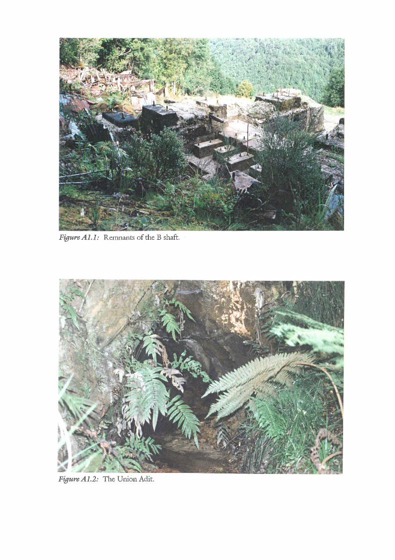
FigureAl.l: Remnants of the B shaft.
FigureA1.2: The Union Adit.
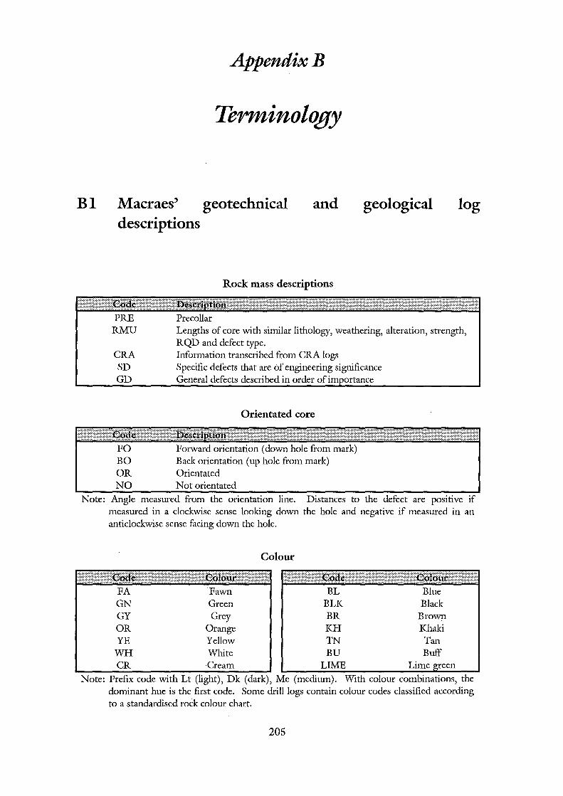
Bl
AppendixB
Terminology
Macraes' geotechnical and geological log descriptions
PRE RMU
CRA SD GD
FO BO OR NO
Rock mass descriptions
Precollar Lengths of core with similar lithology, weathering, alteration, strength, RQD and defect type. Information transcribed from CRA logs Specific defects that are Of engineering significance General defects described in order of
Orientated core
Forward orientation (down hole from mark) Back orientation (up hole from mark) Orientated Not orientated
Note: Angle measured from the orientation line. Distances to the defect are positive if measured in a clockwise sense looking down the hole and negative if measured in an anticlockwise sense facing down the hole.
Colour
::f::,_I\~i,ll~:~r _,···daae .. :;··:_ :·i~. :.:··:·:·:=~·:·.: .... :_i::·=1m~1o~.·l::::::I!iiii FA Fawn BL Blue GN Green BLK Black GY Grey BR Brown OR Orange KH Khaki YE Yellow TN Tan
WH White BU Buff CR Cream LIME Lime green
Note: Prefix code with Lt (light), Dk (dark), Me (medium). With colour combinations, the dominant hue is the first code. Some drill logs contain colour codes classified according to a standardised rock colour chart.
205
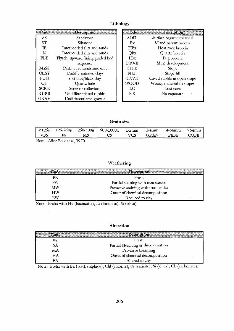
ss ST IB IS
FLY
MaSS CLAY PUG QT
SCRE RUBB GRAV
<l25J..t VFS
Lithology
Sandstone SOIL Siltstone Bx
Interbedded silts and sands HBx Interbedded silts and muds QBx
Flysch, upward fining graded bed PBx sequence DRVE
Distinctive sandstone unit STPE Undifferentiated clays FILL
soft blue/black clay CAVE Quartz lode WOOD
Scree or colluvium LC Undifferentiated rubble NX Undifferentiated
Grain size
l25-250J..t FS
250-500J..t MS
500-lOOOJ..t cs
l-2mm vcs
Surface organic material Mixed parent breccia
Host rock breccia Quartz breccia
Pug breccia Mine development
Stope Stope fill
Caved rubble in open stope Woody material in stapes
2-4mm GRAN
Lost core No exposure
4-64mm PEBB
>64mm COBB
Note: After Folk et al, 1970.
FR sw
MW HW EW
Weathering
Partial staining with iron oxides Pervasive staining with iron oxides Onset of chemical decomposition
Reduced to Note: Prefix with He (haematite), Li (limonite), Si (silica)
Alteration
FR SA Partial bleaching or discolouration
MA Pervasive bleaching HA Onset of chemical decomposition EA Altered to
Note: Prefix with Bk (black sulphide), Chl (chlorite), Se (sericite), Si (silica), Cb (carbonate).
206
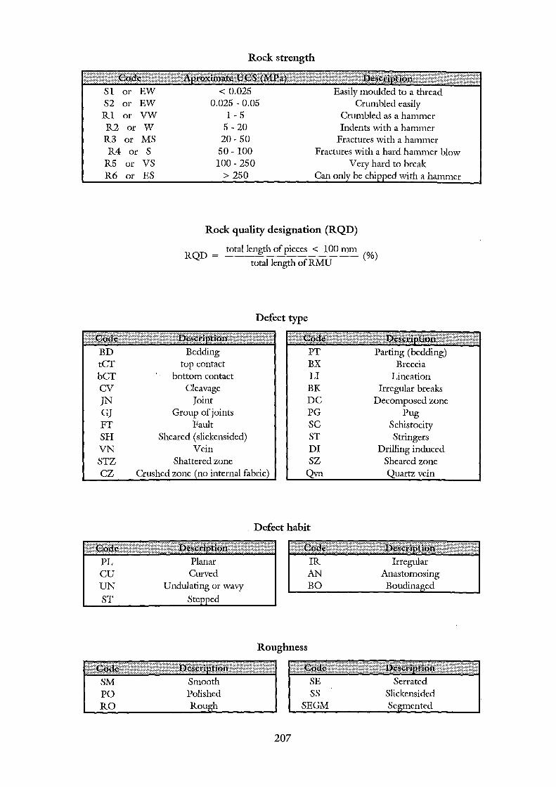
Rock strength
S1 or EW S2 or EW R1 or VW R2 or W R3 or MS R4 or S
R5 or VS R6 or ES
< 0.025 0.025-0.05
1-5 5-20 20-50 50- 100 100-250
> 250
Easily moulded to a thread Crumbled easily
Crumbled as a hammer Indents with a hammer
Fractures with a hammer Fractures with a hard hammer blow
Very hard to break Can be with a hammer
Rock quality designation (RQD)
total length of pieces < 100 mm RQD = (%)
BD Bedding tCf top contact bCf bottom contact CV Cleavage J~ Joint GJ Group of joints FT Fault SH Sheared (slickensided) ~ Vein STZ Shattered zone CZ Crushed zone
PL cu u~
ST
SM PO RO
Planar Curved
Undulating or wavy
Smooth Polished
total length of RMU
Defect type
::::::::Itf4fRm:titttt1J:::m::::::~tl::r::ni.iit!ii.iiiSIIImi:m1:r:rr PT Parting (bedding) BX LI BK DC PG sc ST DI sz
Qvn
Defect habit
IR AN BO
Roughness
207
SE ss
SEGM
Breccia Lineation
Irregular breaks Decomposed zone
Pug Schistocity Stringers
Drilling induced Sheared zone Quartz vein
Irregular Anastomosing
Serrated Slickensided
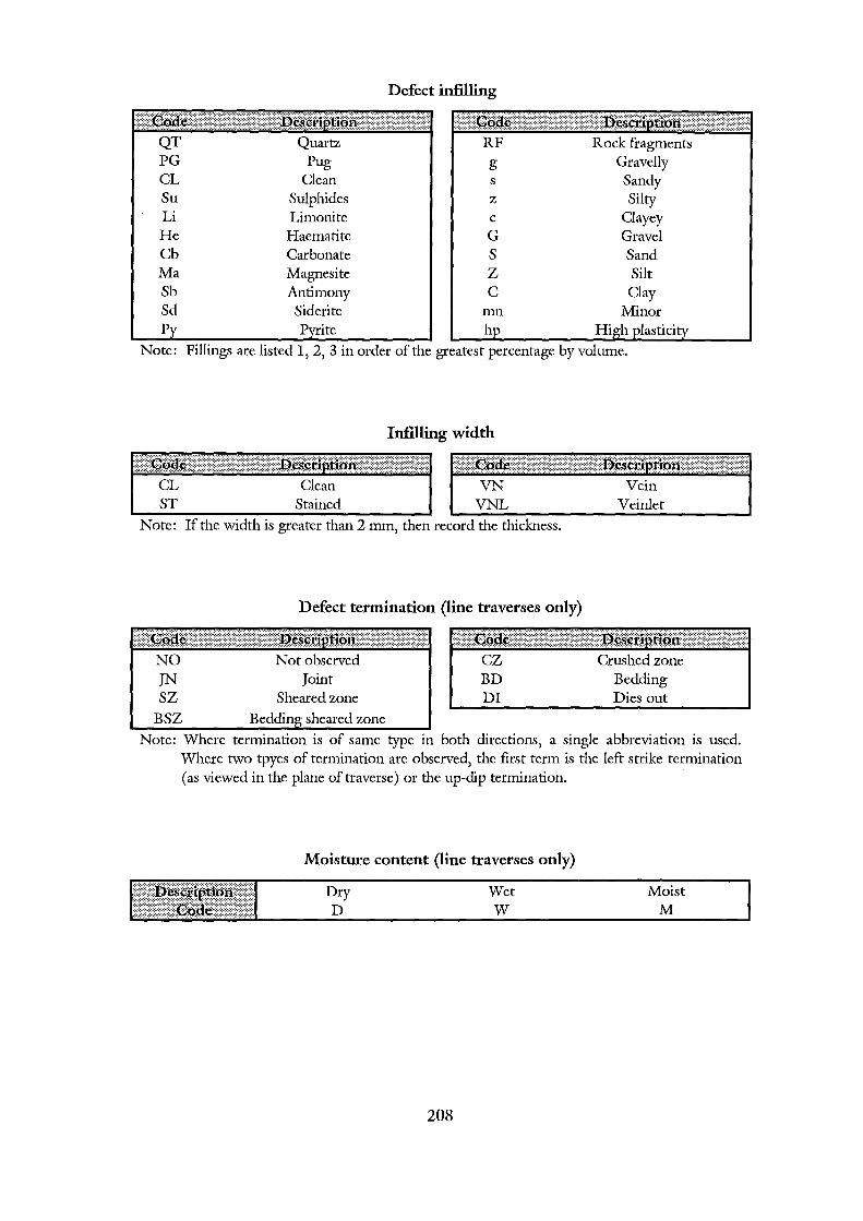
QT PG CL Su Li He Cb Ma Sb Sd
Quartz Pug
Clean Sulphides Limonite
Haematite Carbonate Magnesite Antimony
Siderite
Defect infilling
RF Rock fragments g Gravelly s Sandy z Silty c Clayey G Gravel s Sand z Silt c Clay
mn Minor
Note: Fillings are listed l, 2, 3 in order of the greatest percentage by volume.
Infilling width
Stained VNL Note: If the width is greater than 2 mm, then record the thickness.
NO
JN sz
BSZ
Defect termination (line traverses only)
Not observed Joint
Sheared zone
sheared zone
cz BD DI
Crushed zone Bedding Dies out
Note: Where termination is of same type in both directions, a single abbreviation is used. Where two tpyes of termination are observed, the first term is the left strike termination (as viewed in the plane of traverse) or the up-dip termination.
Moisture content (line traverses only)
Dry D
208
Wet w
Moist M
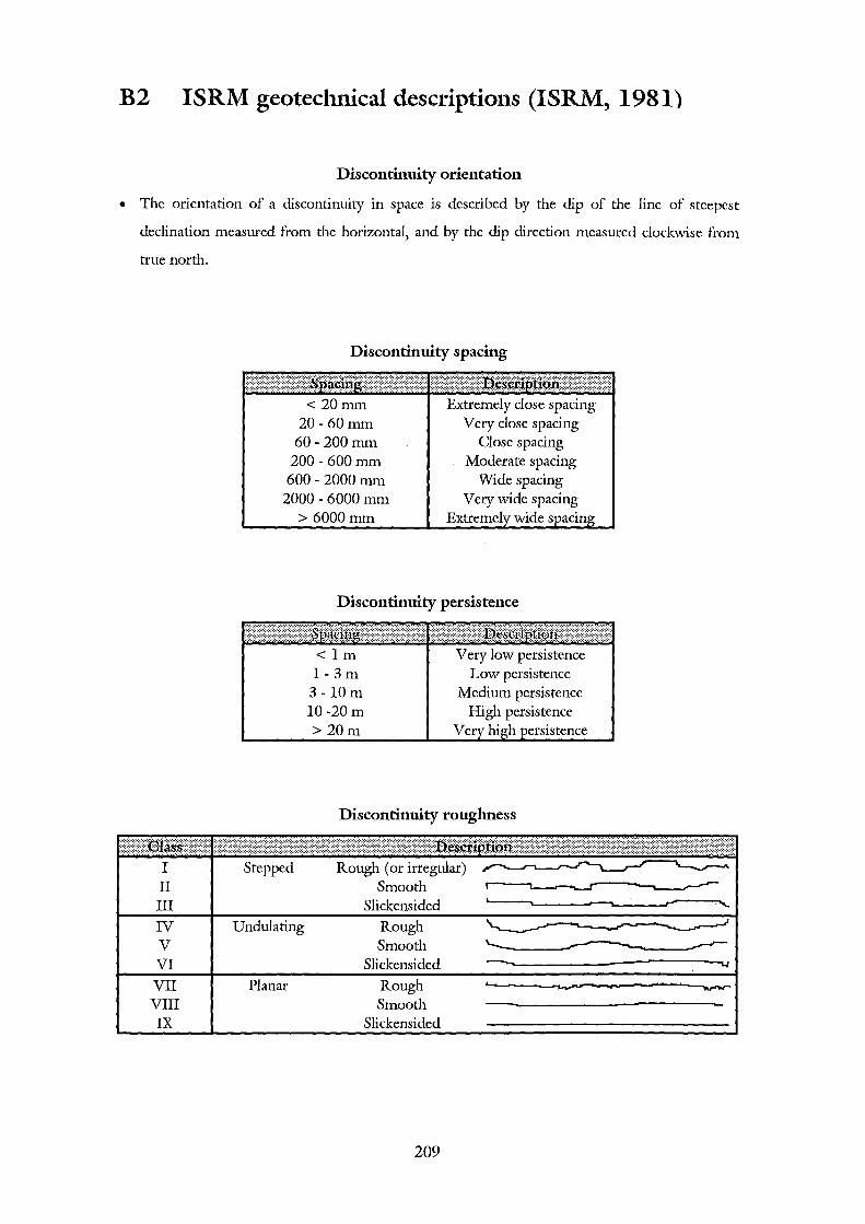
B2 ISRM geotechnical descriptions (ISRM, 1981)
Discontinuity orientation
• The orientation of a discontinuity in space is described by the dip of the line of steepest
declination measured from the horizontal, and by the dip direction measured clockwise from
true north.
II III IV v VI VII VIII IX
Discontinuity spacing
<20mm 20- 60mm 60-200 mm
200- 600mm 600-2000 mm
2000 - 6000 mm > 6000mm
Extremely close spacing Very close spacing
Close spacing Moderate spacing
Wide spacing Very wide spacing
wide
Discontinuity persistence
Undulating
Planar
< lm 1-3m 3 -lOrn 10-20 m >20m
Very low persistence Low persistence
Medium persistence High persistence
v
Discontinuity. roughness
Rough (or irregular) Smooth
Slickensided
Rough Smooth
Slickensided
Rough Smooth
Slickensided
209
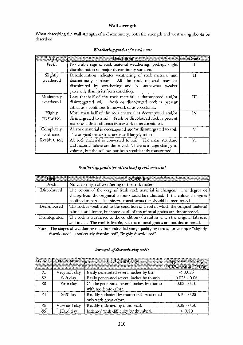
Wall strength
When describing the wall strength of a discontinuity, both the strength and weathering should be described.
Slightly weathered
Moderately weathered
Highly weathered
Completely weathered
Residual soil
Weathering grades of a rock mass
No visible sign of rode material weathering: prehaps slight discolouration on surfaces. Discolouration indicates weathering of rock material and discontinuity surfaces. All the rock material may be discoloured by weathering and be somewhat weaker
than in its fresh condition. Less thanhalf of the rock material is decomposed and/or disintergrated soil. Fresh or discoloured rock is present either as a continous framework or as corestones. More than half of the rock material is decomposed and/or disintergrated to a soil. Fresh or discoloured rock is present either as a discontinuous framework or as corestones. All rode material is decomposed and/or disintergrated to soil. The mass structure is still intact. All rock material is converted to soil. The mass structure and material fabric are destroyed. There is a large change in
but the soil has not been ·
Weatheringgrades(or alteration) of rock material
I
II
III
IV
v
VI
Discoloured The colour of the original fresh rock material is changed. The degree of change from the origninal colour should be indicated. If the colour change is confined to mineral constituents this should be mentioned.
Decomposed The rock is weathered to the condition of a soil in which the original material fabric is still but some or all of the mineral are ed.
Disintegrated The rock is weathered to the condition of a soil in which the original fabric is still intact. The rock is but the mineral
Note: The stages of weathering may be subdivided using qualifying terms, for example "slightly discoloured", "moderately discoloured", "highly discoloured''.
Strength of discontinuity watts
0.10- 0.25
210

RO
R1
R2
R3
Extremely weak rock Very weak
rock
Weak rock
Medi urn strong rock
Strength of discontinuity watts (continued)
Indented by thumbnail.
Crumbles under firm blows with point of geological hammer, can be peeled by a
Can be peeled by a pocketknife with difficulty, shallow indentations made by firm blow with point of geological hammer. Cannot be scraped or peeled with a pocketknife, specimen can be fractured with single firm blow of a geological hammer.
0.25- l.O
1-5
5- 25
25-50
R4 Strong rock Specimen requires more than one blow of 50- 100 hammer to fracture it.
R5 Very strong Specimen requires many blows of a 100 - 250 rock hammer to fracture it.
R6 Extremely Specimen can only be chipped with > 250 rock hammer.
Note Grades S1 - S6 apply to cohesive soils, for example clays, silty clays and combinations of silts and clays with sand generally slow draining. Discontinuity wall strength will generally be characterised be grades RO - R6 (rock) while S1 - S6 (clay) will generally apply to filled discontinuities (see Filling). Some rounding of strength values have been made when converting to SI units.
Discontinuity aperture
< 0.1mm Very tight 0.1-0.25 mm Tight Closed fractures 0.25-0.5 mm 0.5-2.5 mm Open 2.5-10 mm Moderately wide Gapped features
> 10mm Wide 1-10 em Very wide
10- 100 em Extremely wide Open fractures > 100 em Cavernous
211
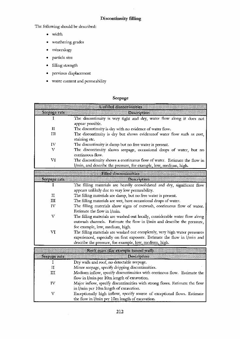
Discontinuity filling
The following should be described:
• width
• weathering grades
• mineralogy
• particle size
• filling strength
• previous displacement
• water content and permeability
I
II III
IV v
VI
I
II III IV
v
VI
I II III
IV
v
Seepage
The discontinuity is very tight and dry, water flow along it does not appear possible. The discontinuity is dry with no evidence of water flow. The discontinuity is dry but shows evidenceof water flow such as rust, staining etc. The discontinuity is damp but no free water is present. The discontinuity shows seepage, occassional drops of water, but no continuous flow. The discontinuity shows a continuous flow of water. Estimate the flow in
and describe the for low mt•n1·11m
The filling materials are heavily consolidated and dry, significant flow appears unlikely due to very low permeability. The filling materials are damp, but no free water is present. The filling materials are wet, have occassional drops of water. The filling materials show signs of outwash, continuous flow of water. Estimate the flow in ljmin. The filling materials are washed out locally, considerable water flow along outwash channels. Estimate the flow in ljmin and describe the pressure, foe example, low, medium, high. The filling materials are washed out completely, very high water pressures experienced, especially on first exposure. Estimate the flow in ljmin and describe the foe low mf'll1111m
Dry walls and roof, no detectable seepage. Minor seepage, specify dripping discontinuities. Medium inflow, specify discontinuities with continous flow. Estimate the flow in ljmin per lOrn length of excavation. Major inflow, specify discontinuities with strong flows. Estimate the flow in ljmin per lOrn length of excavation. Exceptionally high inflow, specify source of exceptional flows. Estimate the flow in lOrn of excavation.
212
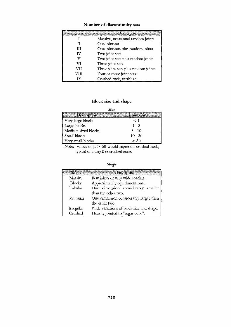
Number of discontinuity sets
I Massive, occasional random joints II One joint set III One joint sets plus random joints IV Two joint sets V Two joint sets plus random joints VI Three joint sets VII Three joint sets plus random joints VIII Four or more joint sets IX Crushed earthlike
Block size and shape
Size
<1 1- 3 3- 10 10-30 > 30
Note: values of Jv > 60 would represent crushed rock, typical of a clay free crushed zone.
Massive Blocky Tabular
Columnar
Irregular Crushed
Shape
Few joints or very wide spacing. Approximately equidimensional. One dimension considerably smaller than the other two. One dimension considerably larger than the other two. Wide variations of block size and shape.
· cube".
213
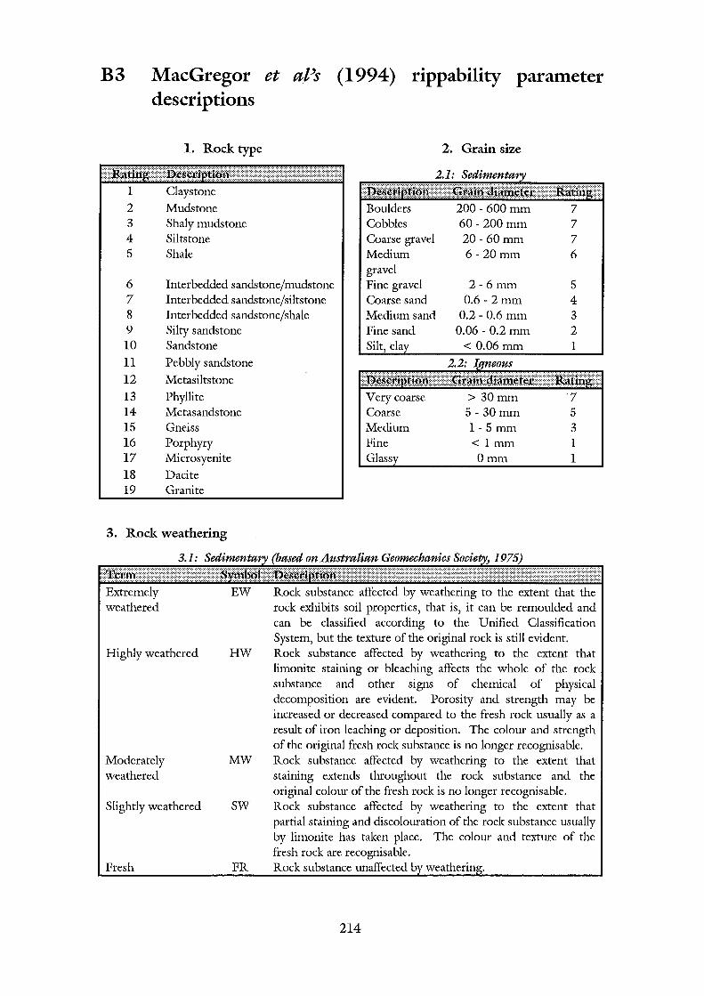
B3 MacGregor et aPs (1994) rippability parameter descriptions
1. Rock type 2. Grain size
1 Claystone 2 Mudstone 7 3 Shaly mudstone 60- 200mm 7 4 Siltstone Coarse gravel 20- 60mm 7 5 Shale Medium 6-20 mm 6
gravel 6 Interbedded sandstone/mudstone Fine gravel 2-6mm 5 7 Interbedded sandstone/siltstone Coarse sand 0.6- 2mm 4 8 Interbedded sandstone/shale Medium sand 0.2-0.6 mm 3 9 Silty sandstone 10 Sandstone
ll Pebbly sandstone
12 Metasiltstone
13 Phyllite l4 Metasandstone 15 Gneiss 16 Porphyry 17 Microsyenite
18 Dacite 19 Granite
3. Rock weathering
Extremely weathered
Highly weathered
Moderately weathered
Slightly weathered
Fresh
EW
HW
MW
sw
FR
Fine sand 0.06- 0.2mm 2
Very coarse > 30mm 7 Coarse 5- 30mm 5 Medium 1-5 mm 3 Fine < 1mm 1
Omm 1
Rock substance affected by weathering to the extent that the rock exhibits soil properties, that is, it can be remoulded and can be classified according to the Unified Classification System, but the texture of the original rock is still evident. Rock substance affected by weathering to the extent that limonite staining or bleaching affects the whole of the rock substance and other signs of chemical of physical decomposition are evident. Porosity and strength may be increased or decreased compared to the fresh rock usually as a result of iron leaching or deposition. The colour and strength of the original fresh rock substance is no longer recognisable. Rock substance affected by weathering to the extent that staining extends throughout the rock substance and the original colour of the fresh rock is no longer recognisable. Rock substance affected by weathering to the extent that partial staining and discolouration of the rock substance usually by limonite has taken place. The colour and texture of the fresh rock are recognisable. Rock substance unaffected
214
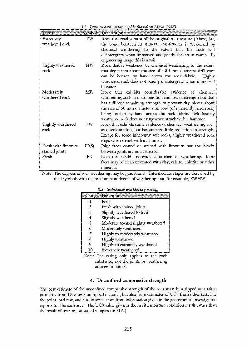
Extremely weathered rock
Highly weathered rock
Moderately weathered rock
Slightly weathered rock
Fresh with limonite stained joints Fresh
EW
HW
MW
sw
Rock that retains most of the original rock texture (fabric) but the bond between its mineral constituents is weakened by chemical weathering to the extent that the rock will disintergrate when immersed and gently shaken in water. In engineering usage this is a soil. Rock that is weakened by chemical weathering to the extent that dry pieces about the size of a 50 mm diameter drill core can be broken by hand across the rock fabric. Highly weathered rock does not readily disintergrate when immersed in water. Rock that exhibits considerable evidence of chemical weathering, such as discolouration and loss of strength but that has sufficent remaining strength to prevent dry pieces about the size of 50 mm diameter drill core (of inherently hard rock) being broken by hand across the rode fabric. Moderately weathered rock does not ring when struck with a hammer. Rock that exhibits some evidence of chemical weathering, such as discolouration, but has suffered little reduction in strength. Except for some inherently soft rocks, slighly weathered rock rings when struck with a hammer.
FRSt Joint faces coated or stained with limonite but the blocks
FR between joints are unweathered. Rock that exhibits no evidence of chemical weathering. Joint faces may be clean or coated with clay, calcite, chlorite or other minerals.
Note: The degrees of rock weathering may be gradational. Intermediate stages are described by dual symbols with the predominant degree of weathering first, for example, EWHW.
1 Fresh 3 Fresh with stained joints 3 Slightly weathered to fresh 4 Slightly weathered 5 Moderate to/and slightly weathered 6 Moderately weathered 7 Highly to moderately weathered 8 Highly weathered 9 Highly to extremely weathered 10 weathered
Note: The rating only applies to the rock substance, not the joints or weathering adjacent to joints.
4. Unconfined compressive strength
The best estimate of the unconfined compresive strength of the rock mass in a ripped area taken primarily from UCS tests on ripped material, but also from estimates of UCS from other tests like the point load test, and also in some cases from information given in the geotechnical investigation reports for the each area. The UCS value given is the in situ moisture condition result rather than the result of tests on saturated samples (in MPa).
215
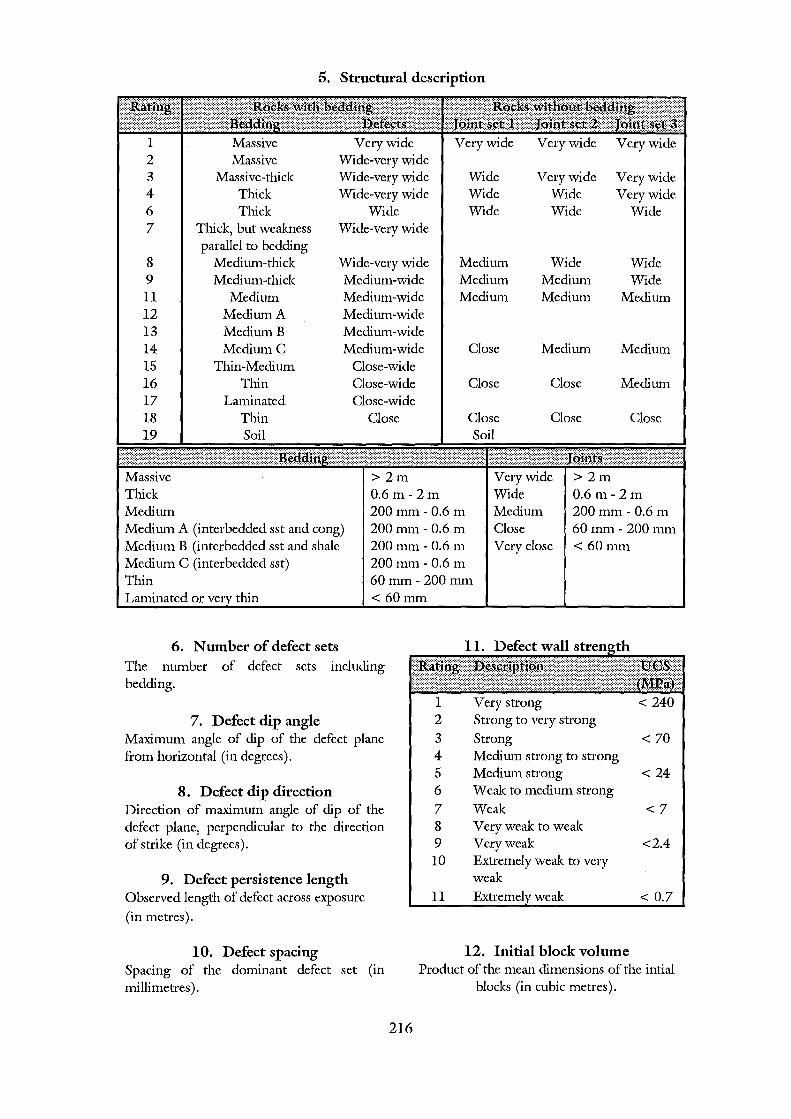
5. Structural description
1 Massive Very wide Very wide Very wide Very wide 2 Massive Wide-very wide 3 Massive-thick Wide-very wide Wide Very wide Very wide 4 Thiele Wide-very wide Wide Wide Very wide 6 Thiele Wide Wide Wide Wide 7 Thick, but weakness Wide-very wide
parallel to bedding 8 Medium-thick Wide-very wide Medium Wide Wide 9 Medium-thick Medium-wide Medium Medium Wide ll Medium Medium-wide Medium Medium Medium 12 Medium A Medium-wide 13 MediumB Medium-wide 14 MediumC Medium-wide Close Medium Medium 15 Thin-Medium Close-wide 16 Thin Close-wide Close Close Medium 17 Laminated Close-wide 18 Thin Close Close Close Close 19 Soil Soil
Massive Thick Medium Medium A (interbedded sst and cong) Medium B (interbedded sst and shale Medium C (interbedded sst)
>2m 0.6 m- 2m 200 mm- 0.6 m 200mm- 0.6 m 200mm- 0.6 m 200mm- 0.6 m 60mm-200mm <60mm
Very wide Wide Medium Close Very close
>2m 0.6m-2m 200mm- 0.6 m 60mm- 200mm < 60mm
Thin Laminated or thin
6. Number of defect sets The number of defect sets including bedding.
7. Defect dip angle Maximum angle of dip of the defect plane from horizontal (in degrees).
8. Defect dip direction Direction of maximum angle of dip of the defect plane, perpendicular to the direction of strike (in degrees).
9. Defect persistence length Observed length of defect across exposure (in metres).
I 0. Defect spacing Spacing of the dominant defect set (in millimetres).
216
1 Very strong < 240 2 Strong to very strong 3 Strong < 70 4 Medium strong to strong 5 Medium strong < 24 6 Weak to medium strong 7 Weak <7 8 Very weak to weak 9 Very weak <2.4 10 Extremely weak to very
weak
ll weak < 0.7
12. Initial block volume Product of the mean dimensions of the intial
blocks (in cubic metres).
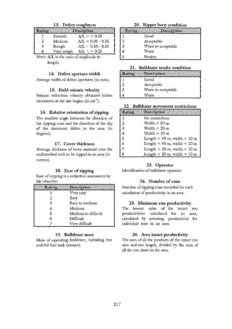
l 2 3 4
Smooth Medium Rough v
A/L = < 0.05 A/L = 0.05 - 0.10 A/L = 0.10- 0.15
= > 0.15 Note: AfL is the ratio of amplitude to
length.
14. Defect aperture width Average width of defect apertures (in mm).
15. Field seismic velocity Seismic refraction velocity obtained before excavation at the site begins (in ms-1
).
16. Relative orientation of ripping The smallest angle between the direction of the ripping runs and the direction of the dip of the dominent defect in the area (in degrees).
17. Cover thickness Average thickness of loose material over the undisturbed rock to be ripped in an area (in metres).
18. Ease of ripping Ease of ripping is a subjective assessment by the observer.
l Very easy 2 Easy 3 Easy to medium 4 Medium 5 Medium to difficult 6 Difficult 7 v difficult
19. Bulldozer mass Mass of operating bulldozer, including tine and full fuel tank ( tonnes) . ,
3 4 5
Acceptable Worn to acceptable Worn Broken
21. Bulldozer tracks condition
l:~l.\iii,nili:~~l~~ll~l~l~l~'~\llii!itiiil~::l~lj~:~l~l~~l:::~~ll\~~~~:l~~ll~Ii\~l:~~:~:~l~lill:i:~li~~:::=~::~~:~:~~::; l Good 2 3 4
Acceptable Worn to acceptable Worn
22. Bulldozer movement restrictions
I!i!:mi:::Illl~!:::::~llUl:iiriei~9P. :::::l~l~ti:~tllt't;Il~i~l~~lt~~~~i~:tt_tl1l _Jl~~lllt::~::
217
l No restrictions 2 Width< 50 m 3 4 5 6 7 8
Width< 20m Width< 10m Length< 50 m, width< 20m Length < 50 m, width < 10m Length < 20 m, width < 20 m Length< 20m, width< 10m
23. Operator Identification of bulldozer operator
24. Number of runs Number of ripping runs recorded for each calculation of productivity in an area.
25. Minimum run productivity The lowest value of the intact run productivities calculated for an area, calculated by assessing productivity for individual runs in an area.
26. Area intact productivity The sum of all the products of the intact run area and run length, divided by the sum of all the run times in the area.
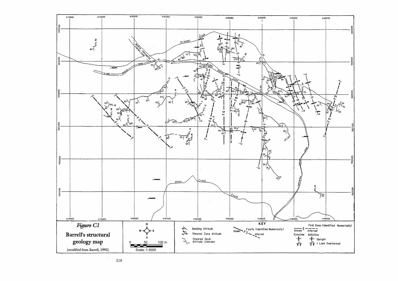
417800E 417900E 418000E . 418100E 418200E 418300E 418400E
I 418500E 418600E
1-----t------------------t------------------t------------------+------------------t------------------+------------------+--------~--------+-----------------~--------------z
"'
N
"' ...J .... ... eo{"
C\..
z
~~----~~~ ~~--------------~----------------_,______________ i
C\.. I I I
"""\)
z
~-----+------------------+------------------t------------------+---------------~~-------------------~----------------r+--~~------------+-- ~-------------r--------------i 0 z
~ ...J z ~ g
----~------------------r------------------t-----------------tr-----------------,r------------~~-4~----------------,r------------------4~~--------~~~--~~-------------~ 60
417800E 417900E
FigureCl
Barrell's structural geology map
(modified from Barrell, 1992)
218
·-
418000E 418100E
N
W~B s
0 50 100m ------Scale: 1 :3000
418200E
Bedding Attitude
Sheared Zone Attitude
Sheered Rock, Attitude Unknown
418300E 418400E
KEY ~k Faults (Identified Numerically)
nown F3 ......_ ... inferred ......
Fold Axes (Identified Numerically)
kn;;;; 3 -infe;:;:-ed
Syncline
+ -IT
Anticline + Upright fi I limb Overturned
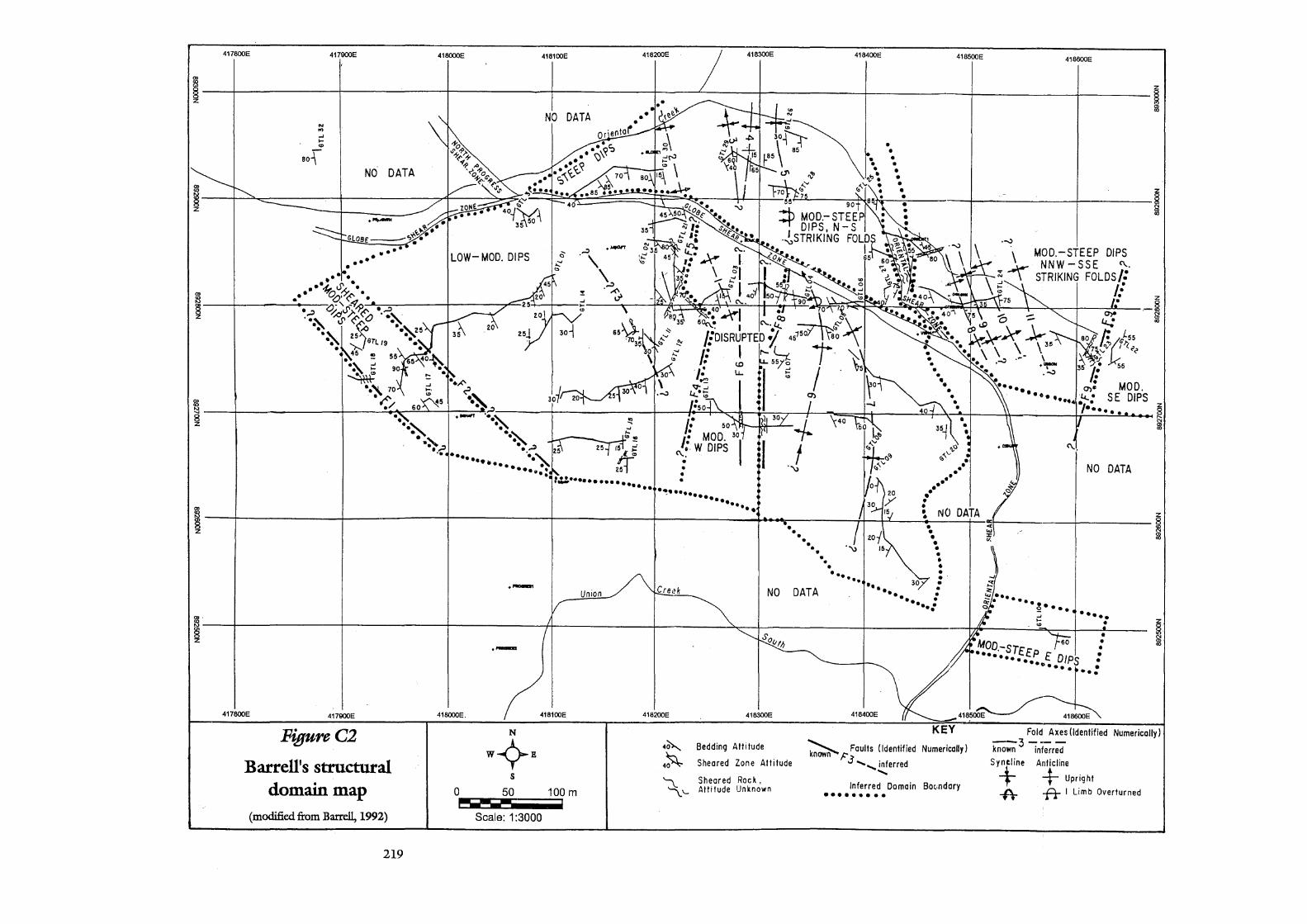
417800E
N
"' .... .... U>
eo{"
417900E
••• • • ···~ ~~.
NO. DATA
·-•• • •
418000E
LOW- MOD. DIPS
lN .•• v0 . ~ • • ~z-----+--------~~--~-' -4~--.-~------~r-------~~ ~ • ..., ~J'~·~ .,..., .
··~ i.S' ~ 0 ·~ ·~ ~ ··" 25 ·~ 25 ·~
··~ ")...... GTL/9 • ••
• 45 !!! 55
·~ .... . .... ~
··~ 70 ·r-:
418100E 418200E 418300E
NO DATA
418400E
• • • • • • •
418500E 418800E
~~~---------~-------------+----------i
z ~z ------~------------------+-------~·./~ •• ~~~---+~==~ ··~
~---------r-------------:~~--t-----~~.t.~~~~i\--f.t-v~---f--~~~~±i--------~~~~~+-----~~----------+T~~~~LL~~ ~ • 50 co
: MOD. 30
' ·-~..., .. ~.·w DIPS 1
• • •
·~······ .·· •• •
••• • •
••••••• • lN '•• • i NO DATA ~ ----~r-------------------+-------------------t-------------------r------------------+------------------~ .. ~-.-------------f~-4~----~~~~~~~=-
417800E 417900E
FigureC2
Barrell's structural domain map
(modified from Barrcll, 1992)
219
·-
418000E. 418100E
N
W~R s
0 50 100m --------Scale: 1 :3000
418200E
4~
4~
~'-
NO
418300E
Bedding Alii tude
Sheared Zone Altitude
Sheared Rod, Alii tude Unknown
•• • • • ··. '"\) ~
DATA
~ . • • . .. : . ••• •• • 30 : .... :
••• • •••
418400E
~ Faults (Identified Numerically) nown F'
.3 ..... , inferred .......
Inferred Domain Bo~·ndary •••••••••
C\. •
NO DATA
418800E
Fold Axes (Identified Numerically) --3---known inferred Syntline Anticline
+ + Upright
-A- ft I Limb Overturned
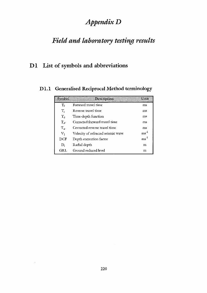
AppendixD
Field and laboratory testing results
D l List of symbols and abbreviations
D 1.1 Generalised Reciprocal Method terminology
ms
Tr Reverse travel time ms
Td Time-depth function ms
Tcf Corrected forward travel time ms
Tcr Corrected reverse travel time ms
V1 Velocity of refracted seismic wave -1 ms
DCF Depth correction factor -1 ms
Dr Radial depth m
GRL Ground reduced level m
220
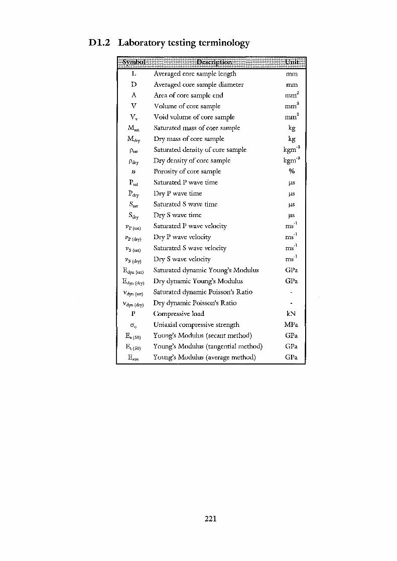
D 1.2 Laboratory testing terminology
L Averaged core sample length mm
D Averaged core sample diameter mm
A Area of core sample end 2 mm
v Volume of core sample mm3
Vv Void volume of core sample 3 mm
M.at Saturated mass of core sample kg
Mdry Dry mass of core sample kg
Psat Saturated density of core sample kgm-3
Pdry Dry density of core sample kgm-3
n Porosity of core sample %
psat Saturated P wave time j..lS
pdry Dry P wave time j..lS
ssat Saturated S wave time j..lS
sdry Dry S wave time j..lS
Saturated P wave velocity -l Vp (sat) ms
Dry P wave velocity -l Vp (dry) ms
Saturated S wave velocity -l Vs (sat) ms
Dry S wave velocity -l Vs (dry) ms
Edyn (sat) Saturated dynamic Young's Modulus GPa
Edyn (dry) Dry dynamic Young's Modulus GPa
Ydyn (sat) Saturated dynamic Poisson's Ratio
Ydyn (dry) Dry dynamic Poisson's Ratio
p Compressive load kN
Cl"c Uniaxial compressive strength MPa
Es(SO) Young's Modulus (secant method) GPa
Et(SO) Young's Modulus (tangential method) GPa
Eave Young's Modulus (average method) GPa
221
D2 Seismic refraction survey data
D2.l The Generalised Reciprocal Method
D2.l.l Introduction
The Generalised reciprocal method ( GRM) is the interpretation method most commonly
used on seismic refraction data. It is a variation of the reciprocal method developed from
Hawkins (1961) after earlier work by Edge and Laby (1931) and Urquhart (1956). The
reciprocal method uses the reciprocal time (travel time) between two geophones to fmd the
seismic velocity of the rock mass below the geophones. The GRM involves combining the
reciprocal time with fmward and reverse travel times to more accurately defme the time to
the refractor.
The reciprocal method assumes a planar refractor between the forward and reverse seismic
waves, therefore refractor irregularities are smoothed out (Palmer, 1980), whereas the
GRM uses an XY distance (distance between two shot points) that may be adjusted to
produce a more detailed refractor (Hatherly and Neville, 1986). Both methods are
insensitive to dip angles up to 20° (Palmer, 1980) unlike other methods such as the delay
time method and the intercept time method that require planar refractors with dips less
than so (Palmer 1980).
For the seismic line traverses surveyed, the optimum XY distance was not calculated as it is
not always possible to calculate it when the refractor is less than 20m deep because of
factors such as irregular topography, variable near-surface layers and inhomogeneous rock
mass (Hatherly and Neville, 1986). Instead, a zero XY spacing has been used and malces
the GRM similar to the Reciprocal Method of Hawkins (1961), which Palmer (1980)
shows to be a special case of the GRM.
222
D2.1.2 Data processing
Forward and reverse travel times are plotted against the shot points as time-distance curves.
These plots give the apparent seismic velocities of the refractor and are shown in Figures
D2.1 - D2.24 as uncorrected travel time graphs. From these plots, the initial velocity (Vo)
is calculated from the first few travel times recorded, which are direct arrivals and represent
the velocity of the upper layer. Using the total forward and reverse times, an average
reciprocal time maybe calculated by the expression:
TR = (Tftotal + Trtotal) (s) 2
where TR is the reciprocal time, Tf total is the total forward time and Tr total is the total
reverse time. Using the reciprocal time and forward and reverse times at each shot point,
the depth to the refractor in units of time is calculated by:
Td = (Tf +Tr -TR) 2 (s)
where Tf is the forward travel time, Tr is the reverse travel time and Td is the time-depth.
The time-depth is subtracted from the forward and reverse travel times at each shot point
to give the corrected forward and reverse travel times:
Tf -Td =Tcf (s)
where Tcf is the corrected forward travel time and Tcr is the corrected reverse travel time.
The corrected travel times represent the travel time to a point on the refractor below each
shot position. The corrected forward and reverse travel times are plotted with respect to
the shot position so that true seismic velocities may be calculated. These plots are shown
in Appendix D2.2. Using the initial seismic velocity and seismic velocity of the refractor, a
depth conversion factor (DCF) is calculated from the expression:
DCF = Vo VI (ms-1 ) (V{- vg)7i
The DCF is multiplied by the time-depth to give a radial depth (Dr) to the refractor. The
GRL (ground reduced level) and radial depths for each shot point may be plotted to show
a cross section of the survey line.
223
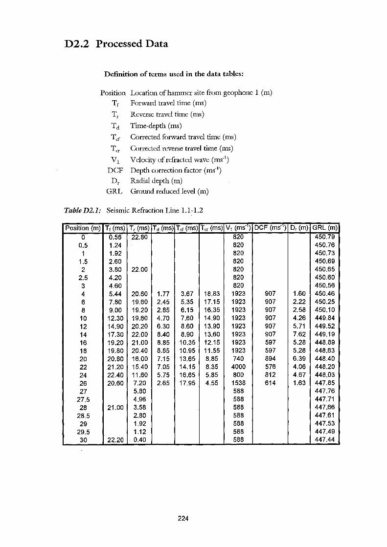
D2.2 Processed Data
Definition of terms used in the data tables:
Position Location of hammer site from geophone 1 (m) Tr Forward travel time (ms)
Tr Reverse travel time (ms)
Td Time-depth (ms)
Tcf Corrected forward travel time (ms)
Tcr Corrected reverse travel time (ms)
V 1 Velocity of refracted wave ( ms-1)
DCF Depth correction factor (ms-1)
Dr Radial depth (m)
GRL Ground reduced level (m)
TableD2.1: Seismic Refraction Line l.l-1.2
Position (m) Tr (ms) Tr (ms) Td (ms) Tor (ms) Tor (ms) v1 (ms-) DCF (ms-) Dr (m) GRL (m)
0 0.56 22.80 820 450.79 0.5 1.24 820 450.76 1 1.92 820 450.73
1.5 2.60 820 450.69 2 3.80 22.00 820 450.65
2.5 4.20 820 450.60 3 4.60 820 450.56 4 5.44 20.60 1.77 3.67 18.83 1923 907 1.60 450.46 6 7.80 19.60 2.45 5.35 17.15 1923 907 2.22 450.25 8 9.00 19.20 2.85 6.15 16.35 1923 907 2'.58 450.10
10 12.30 19.60 4.70 7.60 14.90 1923 907 4.26 449.84 12 14.90 20.20 6.30 8.60 13.90 1923 907 5.71 449.52 14 17.30 22.00 8.40 8.90 13.60 1923 907 7.62 449.19 16 19.20 21.00 8.85 10.35 12.15 1923 597 5.28 448.89 18 19.80 20.40 8.85 10.95 11.55 1923 597 5.28 448.63 20 20.80 16.00 7.15 13.65 8.85 740 894 6.39 448.40 22 21.20 15.40 7.05 14.15 8.35 4000 576 4.06 448.20 24 22.40 11.60 5.75 16.65 5.85 800 812 4.67 448.03 26 20.60 7.20 2.65 17.95 4.55 1538 614 1.63 447.85 27 5.80 588 447.76
27.5 4.96 588 447.71 28 21.00 3.58 588 447.66
28.5 2.80 588 447.61 29 1.92 588 447.53
29.5 1.12 588 447.49 30 22.20 . 0.40 588 447.44
224
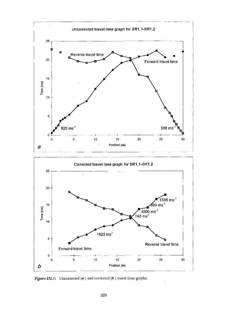
0
a
Uncorrected travel time graph for SR1.1-SR1.2
5 10 15
Position (m)
20
Corrected travel time graph for SR1.1-SR1.2
25 30
25,---------------------------------------------------------,
Iii' g Q)
E i=
b
20
15
10
5
Forward travel time
0 5 10 15
Position (m)
20
Figure D2.1: Uncorrected (a) and corrected (b) travel time graphs.
225
25 30
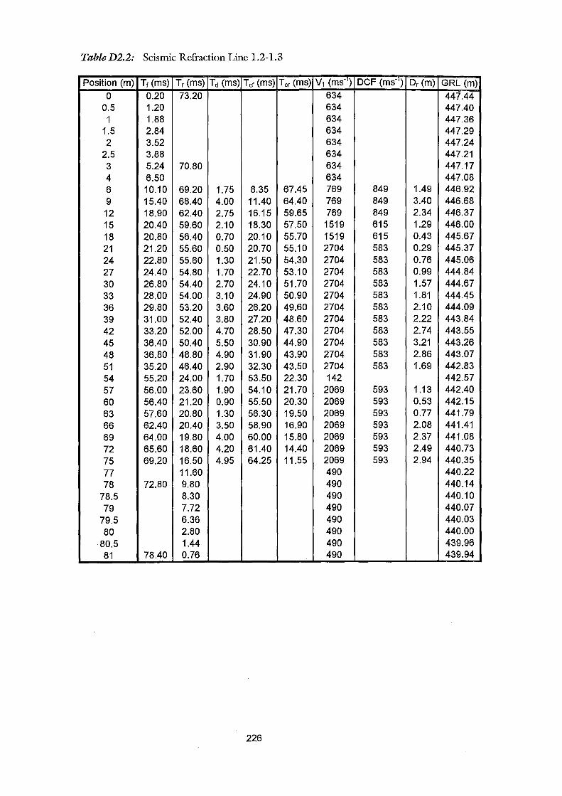
Table D2.2: Seismic Refraction Line 1.2-l. 3
Position (m) Tt (ms) Tr (ms) Td (ms) Tct (ms) Tcr (ms) v1 (ms-1) DCF (ms'') Dr (m) GRL (m)
0 0.20 73.20 634 447.44 0.5 1.20 634 447.40 1 1.88 634 447.36
1.5 2.84 634 447.29 2 3.52 634 447.24
2.5 3.88 634 447.21 3 5.24 70.80 634 447.17 4 6.50 634 447.08 6 10.10 69.20 1.75 8.35 67.45 769 849 1.49 446.92 9 15.40 68.40 4.00 11.40 64.40 769 849 3.40 446.68
12 18.90 62.40 2.75 16.15 59.65 769 849 2.34 446.37 15 20.40 59.60 2.10 18.30 57.50 1519 615 1.29 446.00 18 20.80 56.40 0.70 20.10 55.70 1519 615 0.43 445.67 21 21.20 55.60 0.50 20.70 55.10 2704 583 0.29 445.37 24 22.80 55.60 1.30 21.50 54.30 2704 583 0.76 445.06 27 24.40 54.80 1.70 22.70 53.10 2704 583 0.99 444.84 30 26.80 54.40 2.70 24.10 51.70 2704 583 1.57 444.67 33 28.00 54.00 3.10 24.90 50.90 2704 583 1.81 444.45 36 29.80 53.20 3.60 26.20 49.60 2704 583 2.10 444.09 39 31.00 52.40 3.80 27.20 48.60 2704 583 2.22 443.84 42 33.20 52.00 4.70 28.50 47.30 2704 583 2.74 443.55 45 36.40 50.40 5.50 30.90 44.90 2704 583 3.21 443.26 48 36.80 48.80 4.90 31.90 43.90 2704 583 2.86 443.07 51 35.20 46.40 2.90 32.30 43.50 2704 583 1.69 442.83 54 55.20 24.00 1.70 53.50 22.30 142 442.57 57 56.00 23.60 1.90 54.10 21.70 2069 593 1.13 442.40 60 56.40 21.20 0.90 55.50 20.30 2069 593 0.53 442.15 63 57.60 20.80 1.30 56.30 19.50 2069 593 0.77 441.79 66 62.40 20.40 3.50 58.90 16.90 2069 593 2.08 441.41 69 64.00 19.80 4.00 60.00 15.80 2069 593 2.37 441.08 72 65.60 18.60 4.20 61.40 14.40 2069 593 2.49 440.73 75 69.20 16.50 4.95 64.25 11.55 2069 593 2.94 440.35 77 11.60 490 440.22 78 72.80 9.80 490 440.14
78.5 8.30 490 440.10 79 7.72 490 440.07
79.5 6.36 490 440.03 80 2.80 490 440.00
80.5 1.44 490 439.96 81 78.40 0.76 490 439.94
226
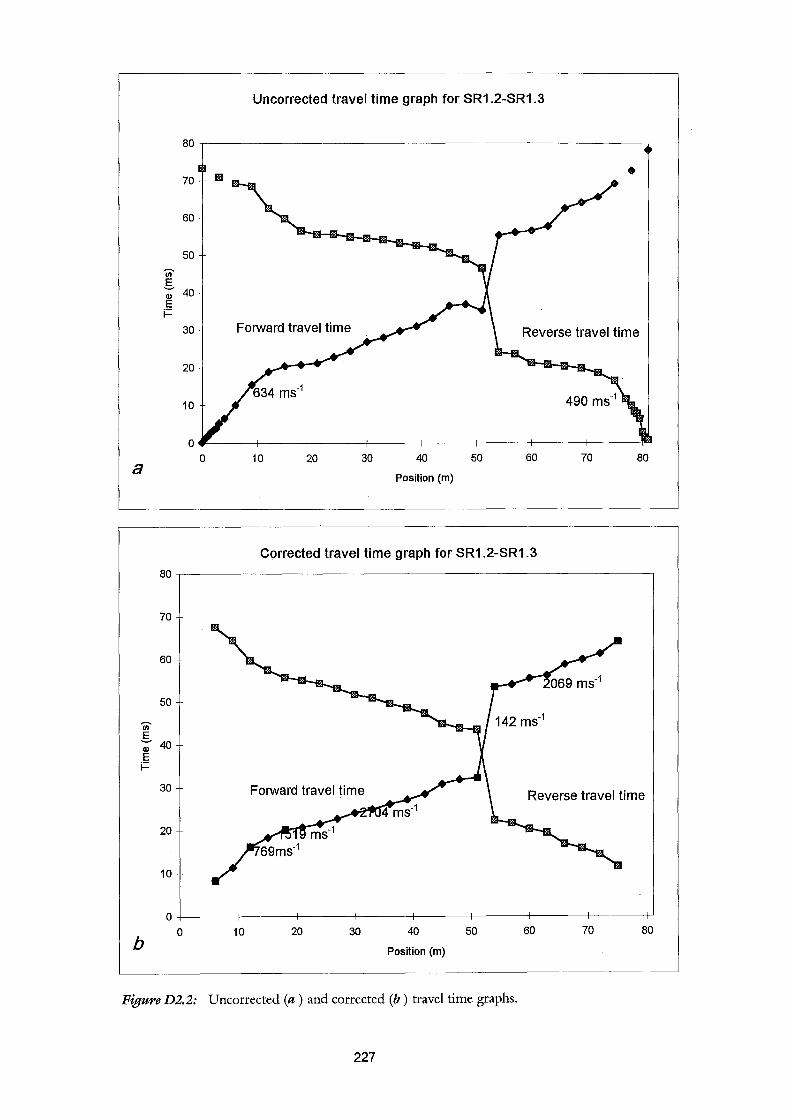
80
70
60
50 (i)
.s 40 Ql
E i=
30
20
10
0 0 a
80
70
60
50
(i)
.s 40 Ql E i=
30
20
10
0
b 0
Uncorrected travel time graph for SR1.2-SR1.3
•
Forward travel time Reverse travel time
10
10 20 30 40
Position (m)
50 60 70 80
Corrected travel time graph for SR1.2-SR1.3
Forward travel time
20 30 40
Position (m)
50
142 ms·1
Reverse travel time
60 70 80
Figure D2.2: Uncorrected (a) and corrected (b) travel time graphs.
227
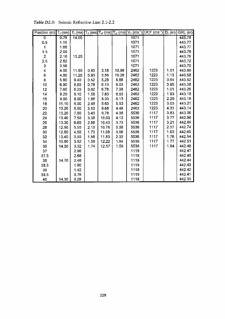
Table D2.3: Seismic Refraction Line 2.1-2.2
Position (m) Tt (ms) Tr (ms) Td (ms) Tot (ms) Tor (ms) v1 (ms:;) DCF (ms::r) Dr (m) GRL (m)
0 0.76 14.00 1071 443.78 0.5 1.16 1071 443.77 1 1.68 1071 443.77
1.5 2.04 1071 443.76 2 2.16 13.20 1071 443.76
2.5 2.82 1071 443.72 3 3.56 1071 443.70 4 4.00 11.80 0.83 3.18 10.98 2462 1223 1.01 443.69 6 4.80 11.20 0.93 3.88 10.28 2462 1223 1.13 443.58 8 5.80 9.40 0.52 5.28 8.88 2462 1223 0.64 443.52
10 6.90 8.80 0.78 6.13 8.03 2462 1223 0.95 443.38 12 7.60 8.20 0.82 6.78 7.38 2462 1223 1.01 443.26 14 9.20 8.10 1.58 7.63 6.53 2462 1223 1.93 443.18 16 9.90 8.00 1.88 8.03 6.13 2462 1223 2.29 443.18 18 11.10 8.00 2.48 8.63 5.53 2462 1223 3.03 443.21 20 13.20 8.00 3.53 9.68 4.48 2462 1223 4.31 443.14 22 13.20 7.80 3.43 9.78 4.38 5536 1117 3.83 443.06 24 13.40 7.50 3.38 10.03 4.13 5536 1117 3.77 442.98 26 13.30 6.60 2.88 10.43 3.73 5536 1117 3.21 442.89 28 12.90 5.50 2.13 10.78 3.38 5536 1117 2.37 442.74 30 12.80 4.80 1.73 11.08 3.08 5536 1117 1.93 442.60 32 13.40 3.90 1.58 11.83 2.33 5536 1117 1.76 442.54 34 13.80 3.52 1.59 12.22 1.94 5536 1117 1.77 442.51 36 14.30 3.32 1.74 12.57 1.59 5536 1117 1.94 442.46 37 2.96 1119 442.47
37.5 2.68 1119 442.45 38 14.70 2.48 1119 442.44
38.5 1.90 1119 442.43 39 1.42 1119 442.42
39.5 0.78 1119 442.41 40 14.30 0.28 1119 442.35
228
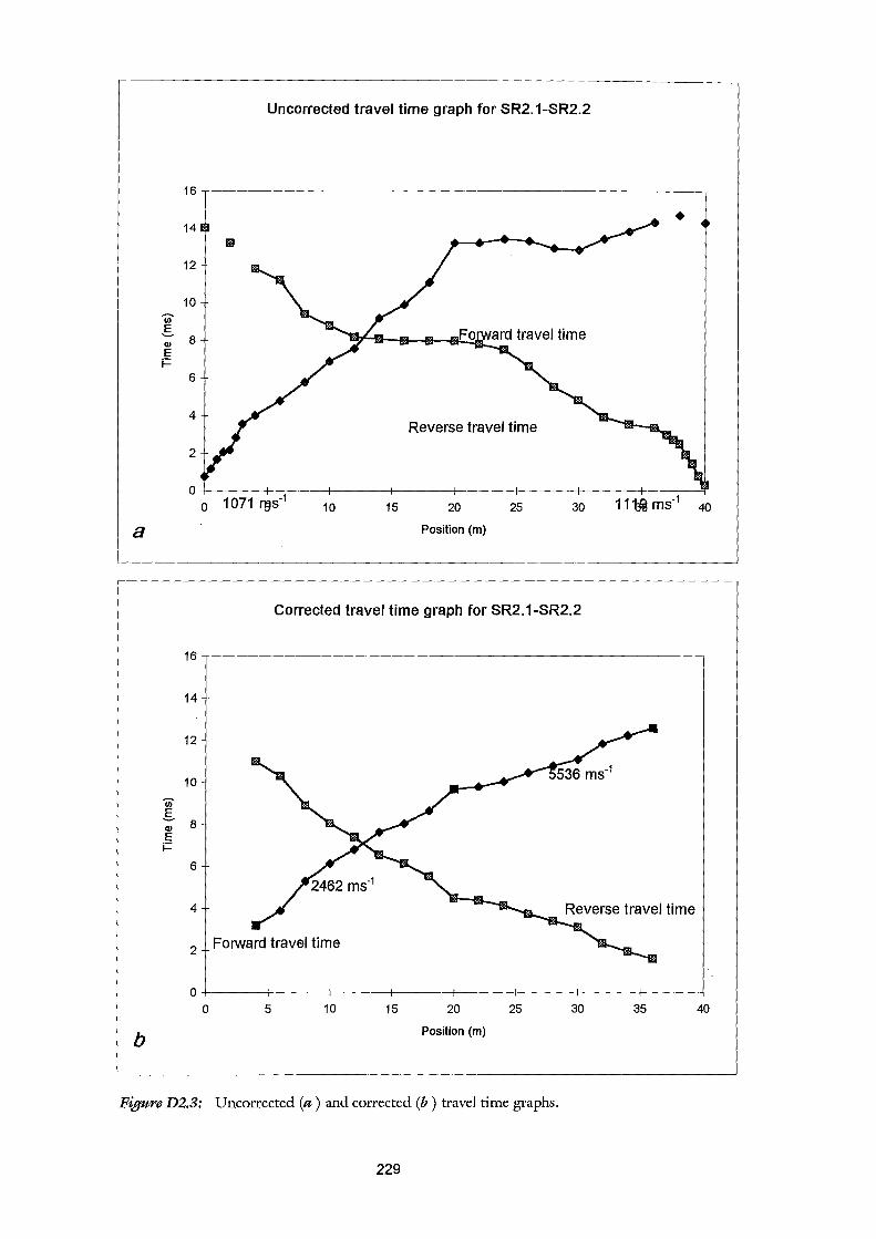
Uncorrected travel time graph for SR2.1-SR2.2
16
• 14 11!11
12
10 (i) g
8 Q)
E j::
6
4 Reverse travel time
2
0 0 1071 rns·1
10 15 20 25 30 11-tj ms·1 40
a Position (m)
Corrected travel time graph for SR2.1-SR2.2
16
14
12
10 (i) g
8 Q)
E j::
6
4
2
0 0 5 10 15 20 25 30 35 40
b Position (m)
Figure D2.3: Uncorrected (a) and corrected (b) travel time graphs.
229
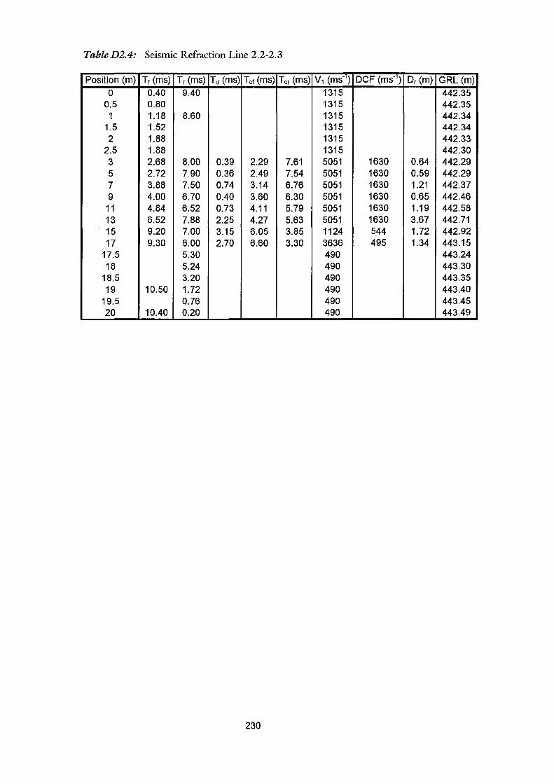
TableD2.4: Seismic Refraction Line 2.2-2.3
Position (m) Tr (ms) Tr (ms) Td (ms) Tor (ms) Tor (ms) v1 (ms-) DCF (ms-) Dr (m) GRL (m) 0 0.40 9.40 1315 442.35
0.5 0.80 1315 442.35 1 1.18 8.60 1315 442.34
1.5 1.52 1315 442.34 2 1.88 1315 442.33
2.5 1.88 1315 442.30 3 2.68 8.00 0.39 2.29 7.61 5051 1630 0.64 442.29 5 2.72 7.90 0.36 2.49 7.54 5051 1630 0.59 442.29 7 3.88 7.50 0.74 3.14 6.76 5051 1630 1.21 442.37 9 4.00 6.70 0.40 3.60 6.30 5051 1630 0.65 442.46
11 4.84 6.52 0.73 4.11 5.79 5051 1630 1.19 442.58 13 6.52 7.88 2.25 4.27 5.63 5051 1630 3.67 442.71 15 9.20 7.00 3.15 6.05 3.85 1124 544 1.72 442.92 17 9.30 6.00 2.70 6.60 3.30 3636 495 1.34 443.15
17.5 5.30 490 443.24 18 5.24 490 443.30
18.5 3.20 490 443.35 19 10.50 1.72 490 443.40
19.5 0.76 490 443.45 20 10.40 0.20 490 443.49
230
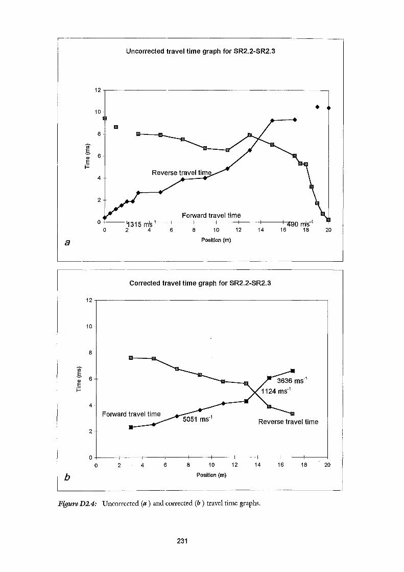
12
10
m 8
Iii g
6 Q)
E i=
4
2
0 0
a
0 2
b
Uncorrected travel time graph for SR2.2-SR2.3
2 6
Forward travel time
8 10
Position (m)
12 14
Corrected travel time graph for SR2.2-SR2.3
4 6 8 10
Position (m)
12 14
Figure D2.4: Uncorrected (a) and corrected (b) travel time graphs.
231
•
16 20
16 18 20
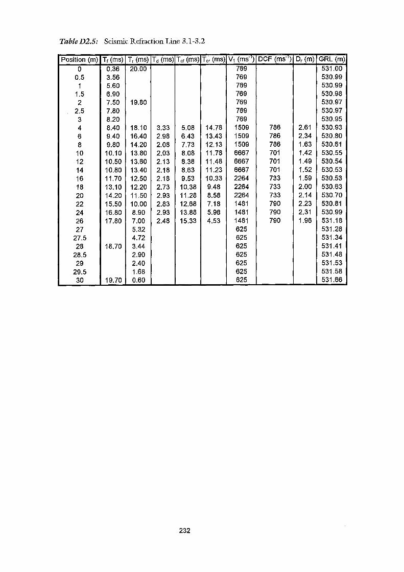
TableD2.5: Seismic Refraction Line 3.1-3.2
Position (m) Tr (ms) Tr (ms) Td (ms) Tor (ms) Tor (ms) v1 (ms"T) DCF (ms:;) Dr (m) GRL (m)
0 0.36 20.00 769 531.00 0.5 3.56 769 530.99 1 5.60 769 530.99
1.5 6.90 769 530.98 2 7.50 19.80 769 530.97
2.5 7.80 769 530.97 3 8.20 769 530.95 4 8.40 18.10 3.33 5.08 14.78 1509 786 2.61 530.93 6 9.40 16.40 2.98 6.43 13.43 1509 786 2.34 530.80 8 9.80 14.20 2.08 7.73 12.13 1509 786 1.63 530.61
10 10.10 13.80 2.03 8.08 11.78 6667 701 1.42 530.55 12 10.50 13.60 2.13 8.38 11.48 6667 701 1.49 530.54 14 10.80 13.40 2.18 8.63 11.23 6667 701 1.52 530.53 16 11.70 12.50 2.18 9.53 10.33 2264 733 1.59 530.53 18 13.10 12.20 2.73 10.38 9.48 2264 733 2.00 530.63 20 14.20 11.50 2.93 11.28 8.58 2264 733 2.14 530.70 22 15.50 10.00 2.83 12.68 7.18 1481 790 2.23 530.81 24 16.80 8.90 2.93 13.88 5.98 1481 790 2.31 530.99 26 17.80 7.00 2.48 15.33 4.53 1481 790 1.96 531.18 27 5.32 625 531.28
27.5 4.72 625 531.34 28 18.70 3.44 625 531.41
28.5 2.90 625 531.48 29 2.40 625 531.53
29.5 1.68 625 531.58 30 19.70 0.60 625 531.66
232
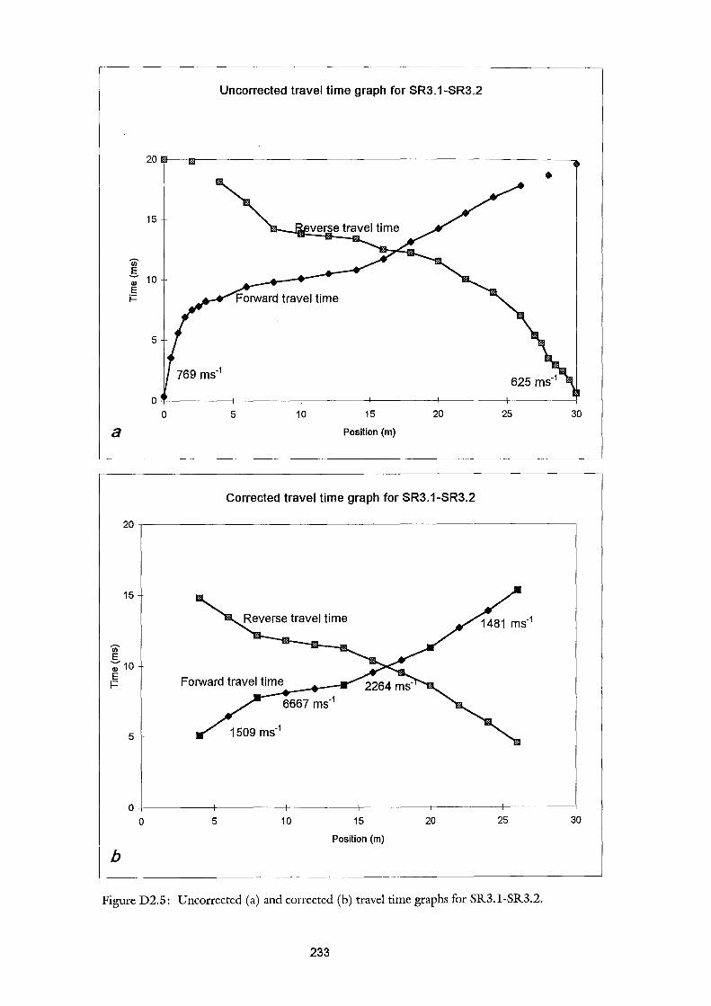
a
15
(j)
.s Q) 10 E i=
5
Uncorrected travel time graph for SR3.1-SR3.2
5 10 15
Position (m)
20
Corrected travel time graph for SR3.1-SR3.2
25 30
20~------------------------------------------------------~
(j) E
15
-; 10
~ Forward travel time ---_....~~--
6667 ms·1
5
O+---------r-------~---------+--------~--------4-------~
0 5 10
b
15
Position (m)
20 25
Figure D2.5: Uncorrected (a) and corrected (b) travel time graphs for SR3.l-SR3.2.
233
30
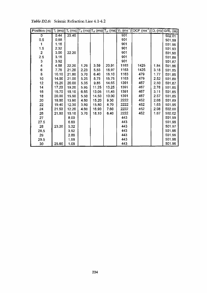
Table D2. 6: Seismic Refraction Line 4.1-4.2
Position (m) Tr (ms) Tr (ms) Td (ms) Tor (ms) Tor (ms) v1 (ms-1) DCF (ms-1
} Dr (m) GRL (m) 0 0.44 23.40 901 502.01
0.5 0.68 901 501.99 1 1.16 901 501.96
1.5 2.32 901 501.93 2 3.00 22.20 901 501.90
2.5 3.16 901 501.88 3 3.92 901 501.87 4 4.88 22.20 1.29 3.59 20.91 1163 1425 1.84 501.86 6 7.76 21.20 2.23 5.53 18.97 1163 1425 3.18 501.85 8 10.10 21.80 3.70 6.40 18.10 1163 479 1.77 501.85 10 14.00 21.00 5.25 8.75 15.75 1163 479 2.52 501.88 12 15.20 20.00 5.35 9.85 14.65 1391 467 2.50 501.87 14 17.20 19.20 5.95 11.25 13.25 1391 467 2.78 501.85 16 19.70 18.10 6.65 13.05 11.45 1391 467 3.11 501.85 18 20.00 15.50 5.50 14.50 10.00 1391 467 2.57 501.85 20 19.80 13.90 4.60 15.20 9.30 2222 452 2.08 501.89 22 19.40 12.30 3.60 15.80 8.70 2222 452 1.63 501.95 24 21.50 12.20 4.60 16.90 7.60 2222 452 2.08 502.00 26 21.80 10.10 3.70 18.10 6.40 2222 452 1.67 502.02 27 8.00 443 501.99
27.5 6.60 443 501.98 28 23.20 5.32 443 501.97
28.5 3.92 443 501.96 29 2.88 443 501.96
29.5 1.68 443 501.96 30 25.60 1.08 443 501.96
234
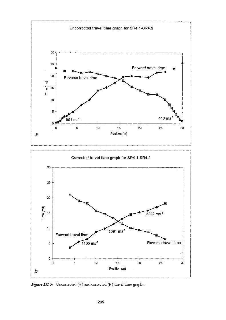
a
b
til g Q)
E i=
25
20
til g Q) 15 E i=
10
5
30
25
20
15
10
5
0
0
l!ll
0
Uncorrected travel time graph for SR4.1-SR4.2
Forward travel time •
5 10 15
Position (m)
20
Corrected travel time graph for SR4.1-SR4.2
5 10 15
Position (m)
20
443 ms-1
25
25
FigureD2.6: Uncorrected (a) and corrected (b) travel time graphs.
235
30
30
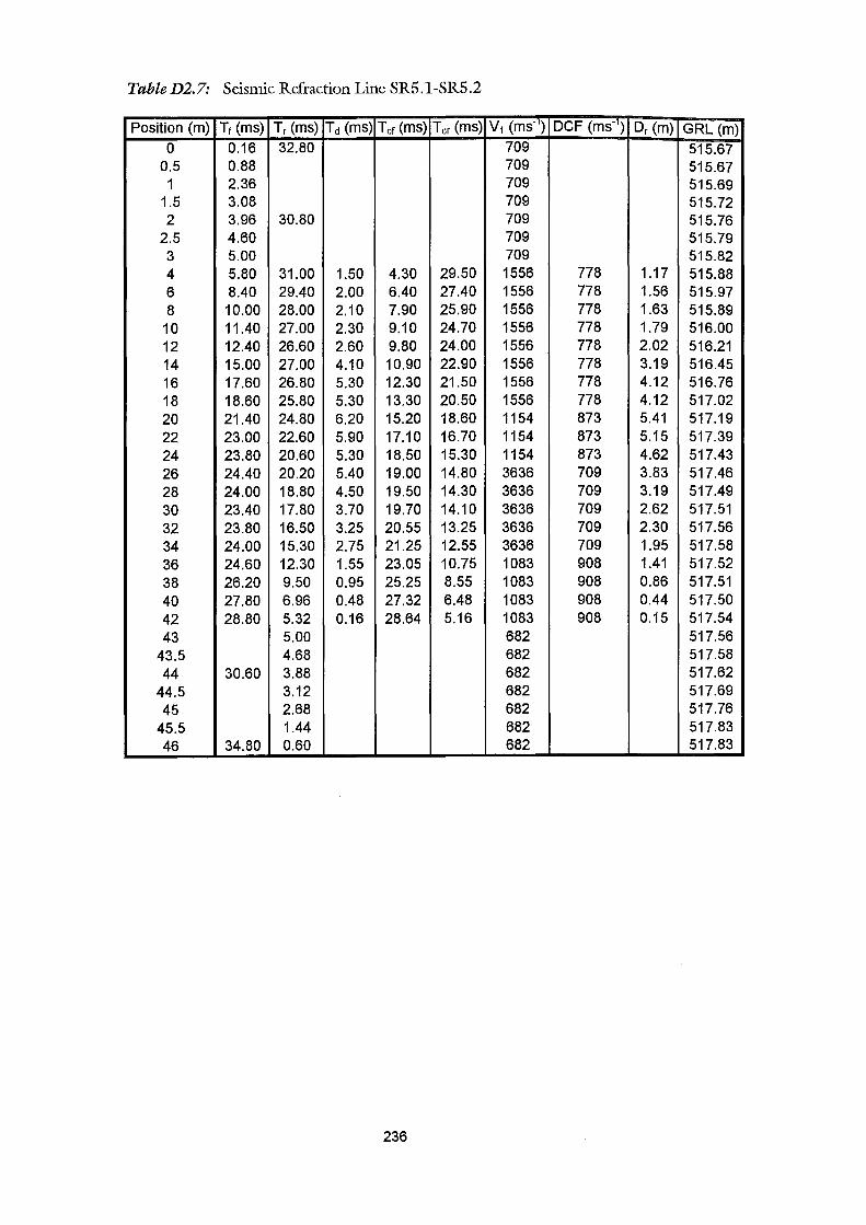
TableD2.7: Seismic Refraction Line SR5.1-SR5.2
Position (m) Tt (ms) Tr (ms) Td (ms) Tct (ms) Tcr (ms) v1 (ms::;) DCF (ms ) Dr (m) GRL (m) 0 0.16 32.80 709 515.67
0.5 0.88 709 515.67 1 2.36 709 515.69
1.5 3.08 709 515.72 2 3.96 30.80 709 515.76
2.5 4.60 709 515.79 3 5.00 709 515.82 4 5.80 31.00 1.50 4.30 29.50 1556 778 1.17 515.88 6 8.40 29.40 2.00 6.40 27.40 1556 778 1.56 515.97 8 10.00 28.00 2.10 7.90 25.90 1556 778 1.63 515.89
10 11.40 27.00 2.30 9.10 24.70 1556 778 1.79 516.00 12 12.40 26.60 2.60 9.80 24.00 1556 778 2.02 516.21 14 15.00 27.00 4.10 10.90 22.90 1556 778 3.19 516.45 16 17.60 26.80 5.30 12.30 21.50 1556 778 4.12 516.76 18 18.60 25.80 5.30 13.30 20.50 1556 778 4.12 517.02 20 21.40 24.80 6.20 15.20 18.60 1154 873 5.41 517.19 22 23.00 22.60 5.90 17.10 16.70 1154 873 5.15 517.39 24 23.80 20.60 5.30 18.50 15.30 1154 873 4.62 517.43 26 24.40 20.20 5.40 19.00 14.80 3636 709 3.83 517.46 28 24.00 18.80 4.50 19.50 14.30 3636 709 3.19 517.49 30 23.40 17.80 3.70 19.70 14.10 3636 709 2.62 517.51 32 23.80 16.50 3.25 20.55 13.25 3636 709 2.30 517.56 34 24.00 15.30 2.75 21.25 12.55 3636 709 1.95 517.58 36 24.60 12.30 1.55 23.05 10.75 1083 908 1.41 517.52 38 26.20 9.50 0.95 25.25 8.55 1083 908 0.86 517.51 40 27.80 6.96 0.48 27.32 6.48 1083 908 0.44 517.50 42 28.80 5.32 0.16 28.64 5.16 1083 908 0.15 517.54 43 5.00 682 517.56
43.5 4.68 682 517.58 44 30.60 3.88 682 517.62
44.5 3.12 682 517.69 45 2.68 682 517.76
45.5 1.44 682 517.83 46 34.80 0.60 682 517.83
236
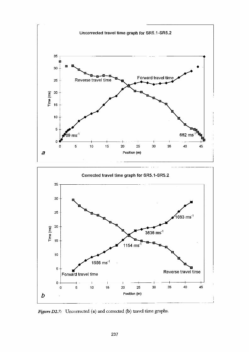
Uncorrected travel time graph for SR5.1-SR5.2
35
30
25
(jj' 20 .s Q)
E i= 15
10
5
0 0 5 10 15 20 25 30 35 40 45
a Position (m)
Corrected travel time graph for SR5.1-SR5.2
35
30
25
(jj' 20 .s Q)
E i= 15
10
5
Forward travel time
0+-----+-----+-----~----~----~----~----~----~----~
0 5 10 15 20 25 30 35 40 45
b Position (m)
FigureD2.7: Uncorrected (a) and corrected (b) travel time graphs.
237
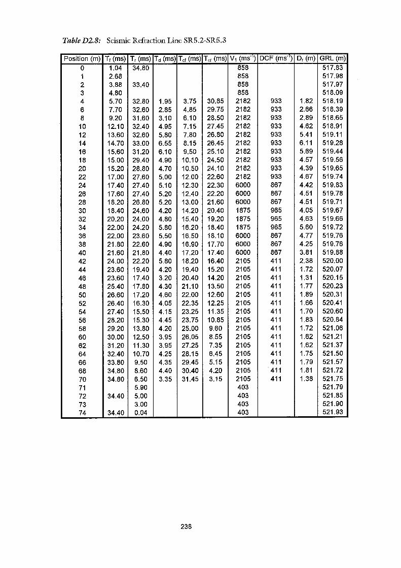
TableD2.8: Seismic Refraction Line SR5.2-SR5.3
Position (m) Tt (ms) Tr (ms) Td (ms) Tct (ms) Tcr (ms) v1 (ms-) DCF (ms-) Dr (m) GRL (m)
0 1.04 34.80 858 517.83 1 2.68 858 517.98 2 3.88 33.40 858 517.97 3 4.80 858 518.09 4 5.70 32.80 1.95 3.75 30.85 2182 933 1.82 518.19 6 7.70 32.60 2.85 4.85 29.75 2182 933 2.66 518.39 8 9.20 31.60 3.10 6.10 28.50 2182 933 2.89 518.65 10 12.10 32.40 4.95 7.15 27.45 2182 933 4.62 518.91 12 13.60 32.60 5.80 7.80 26.80 2182 933 5.41 519.11 14 14.70 33.00 6.55 8.15 26.45 2182 933 6.11 519.28 16 15.60 31.20 6.10 9.50 25.10 2182 933 5.69 519.44 18 15.00 29.40 4.90 10.10 24.50 2182 933 4.57 519.56 20 15.20 28.80 4.70 10.50 24.10 2182 933 4.39 519.65 22 17.00 27.60 5.00 12.00 22.60 2182 933 4.67 519.74 24 17.40 27.40 5.10 12.30 22.30 6000 867 4.42 519.83 26 17.60 27.40 5.20 12.40 22.20 6000 867 4.51 519.78 28 18.20 26.80 5.20 13.00 21.60 6000 867 4.51 519.71 30 18.40 24.60 4.20 14.20 20.40 1875 965 4.05 519.67 32 20.20 24.00 4.80 15.40 19.20 1875 965 4.63 519.66 34 22.00 24.20 5.80 16.20 18.40 1875 965 5.60 519.72 36 22.00 23.60 5.50 16.50 18.10 6000 867 4.77 519.76 38 21.80 22.60 4.90 16.90 17.70 6000 867 4.25 519.76 40 21.60 21.80 4.40 17.20 17.40 6000 867 3.81 519.88 42 24.00 22.20 5.80 18.20 16.40 2105 411 2.38 520.00 44 23.60 19.40 4.20 19.40 15.20 2105 411 1.72 520.07 46 23.60 17.40 3.20 20.40 14.20 2105 411 1.31 520.15 48 25.40 17.80 4.30 21.10 13.50 2105 411 1.77 520.23 50 26.60 17.20 4.60 22.00 12.60 2105 411 1.89 520.31 52 26.40 16.30 4.05 22.35 12.25 2105 411 1.66 520.41 54 27.40 15.50 4.15 23.25 11.35 2105 411 1.70 520.60 56 28.20 15.30 4.45 23.75 10.85 2105 411 1.83 520.84 58 29.20 13.80 4.20 25.00 9.60 2105 411 1.72 521.06 60 30.00 12.50 3.95 26.05 8.55 2105 411 1.62 521.21 62 31.20 11.30 3.95 27.25 7.35 2105 411 1.62 521.37 64 32.40 10.70 4.25 28.15 6.45 2105 411 1.75 521.50 66 33.80 9.50 4.35 29.45 5.15 2105 411 1.79 521.57 68 34.80 8.60 4.40 30.40 4.20 2105 411 1.81 521.72 70 34.80 6.50 3.35 31.45 3.15 2105 411 1.38 521.75 71 5.90 403 521.79 72 34.40 5.00 403 521.85 73 3.00 403 521.90 74 34.40 0.04 403 521.93
238
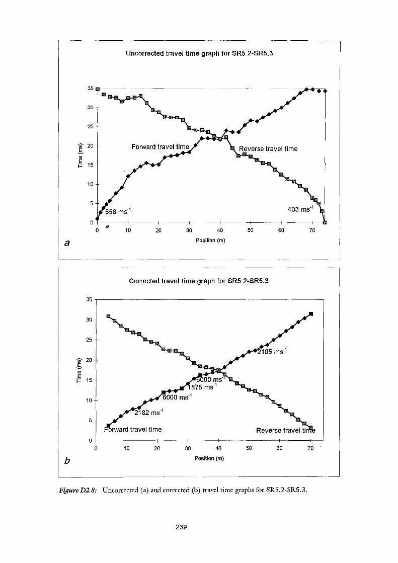
Uncorrected travel time graph for SR5.2-SR5.3
35
30
25
Ul 20 .§. Q)
E 15 i=
10
5 403 ms·1
0 0
'PI' 10 20 30 40 50 60 70
a Position (m)
Corrected travel time graph for SR5.2-SR5.3
35
30
25
Ul 20 .§. Q)
E i= 15
10
5
0 0 10 20 30 40 50 60 70
b Position (m)
FigureD2.8: Uncorrected (a) and corrected (b) travel time graphs for SR5.2-SR5.3.
239

TableD2.9: Seismic Refraction Line SR6.1-SR6.2
Position (m) Tt (ms) Tr (ms) Td (ms) Tct (ms) Tcr (ms) v1 (ms-1) DCF (ms-1
) Dr (m) GRL (m)
0 0.44 24.80 442 506.34 0.5 1.52 442 506.28 1 2.92 442 506.21
1.5 3.96 442 506.15 2 4.96 23.60 442 506.08
2.5 6.32 442 506.02 3 8.30 442 505.97 4 9.50 21.00 2.45 7.05 18.55 1633 618 1.51 505.86 6 11.20 20.00 2.80 8.40 17.20 1633 618 1.73 505.74 8 13.10 19.70 3.60 9.50 16.10 1633 618 2.22 505.71 10 15.40 17.60 3.70 11.70 13.90 1034 697 2.58 505.52 12 18.00 16.70 4.55 13.45 12.15 1034 697 3.17 505.34 14 19.60 14.60 4.30 15.30 10.30 1034 697 3.00 505.18 16 20.00 13.90 4.15 15.85 9.75 3636 585 2.43 505.01 18 22.00 12.10 4.25 17.75 7.85 1053 691 2.94 504.78 20 22.40 11.30 4.05 18.35 7.25 3333 587 2.38 504.61 22 24.80 9.10 4.15 20.65 4.95 870 773 3.21 504.43 24 25.00 8.20 3.80 21.20 4.40 3636 585 2.22 504.28 26 25.20 5.96 2.78 22.42 3.18 1639 618 1.72 504.12 27 4.88 714 504.03
27.5 4.16 714 503.99 28 25.80 3.16 714 503.96
28.5 3.10 714 503.94 29 2.20 714 503.91
29.5 1.80 714 503.84 30 26.40 0.36 714 503.81
240
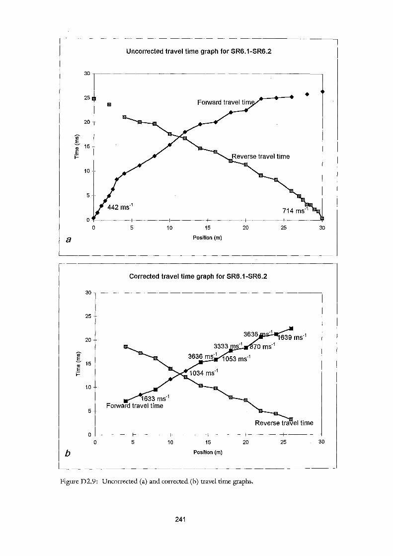
a
25
20
'iii' ..s Q) 15 E i=
10
5
0
Uncorrected travel time graph for SR6.1-SR6.2
5 10 15
Position (m)
20
Corrected travel time graph for SR6.1-SR6.2
25
Reverse travel time
30
0+--------+--------~------~---------r--------~------~
0 5
b 10 15
Position (m)
20
Figure D2.9: Uncorrected (a) and corrected (b) travel time graphs.
241
25 30

TableD2.10: Seismic Refraction Line SR7.l-SR7.2
Position (m) Tr (ms) Tr (ms) Td (ms) Tor (ms) Tor (ms) v1 (ms-) DCF (ms"l) Dr (m) GRL (m)
0 0.48 26.80 374 546.25 0.5 1.48 374 546.23 1 2.36 374 546.22
1.5 3.80 374 546.21 2 5.20 24.20 374 546.21
2.5 6.60 374 546.28 3 8.50 374 546.28 4 10.60 24.60 4.30 6.30 20.30 1000 403 1.73 546.29 6 13.50 24.20 5.55 7.95 18.65 1000 403 2.24 546.37 8 17.40 23.80 7.30 10.10 16.50 1000 790 5.77 546.29
10 16.40 18.40 4.10 12.30 14.30 1000 790 3.24 545.99 12 15.00 16.20 2.30 12.70 13.90 4444 626 1.44 545.66 14 15.60 15.80 2.40 13.20 13.40 4444 626 1.50 545.26 16 17.80 15.60 3.40 14.40 12.20 1875 657 2.23 545.08 18 18.80 14.10 3.15 15.65 10.95 1875 657 2.07 544.84 20 20.20 14.00 3.80 16.40 10.20 1875 657 2.50 544.83 22 20.20 9.80 1.70 18.50 8.10 1200 724 1.23 544.93 24 21.20 6.80 0.70 20.50 6.10 1200 724 0.51 545.1 26 21.80 5.60 0.40 21.40 5.20 1200 724 0.29 545.2 27 5.20 620 545.23
27.5 4.30 620 545.26 28 23.40 3.50 620 545.29
28.5 2.44 620 545.33 29 1.84 620 545.39
29.5 1.16 620 545.44 30 26.40 0.36 620 545.52
242
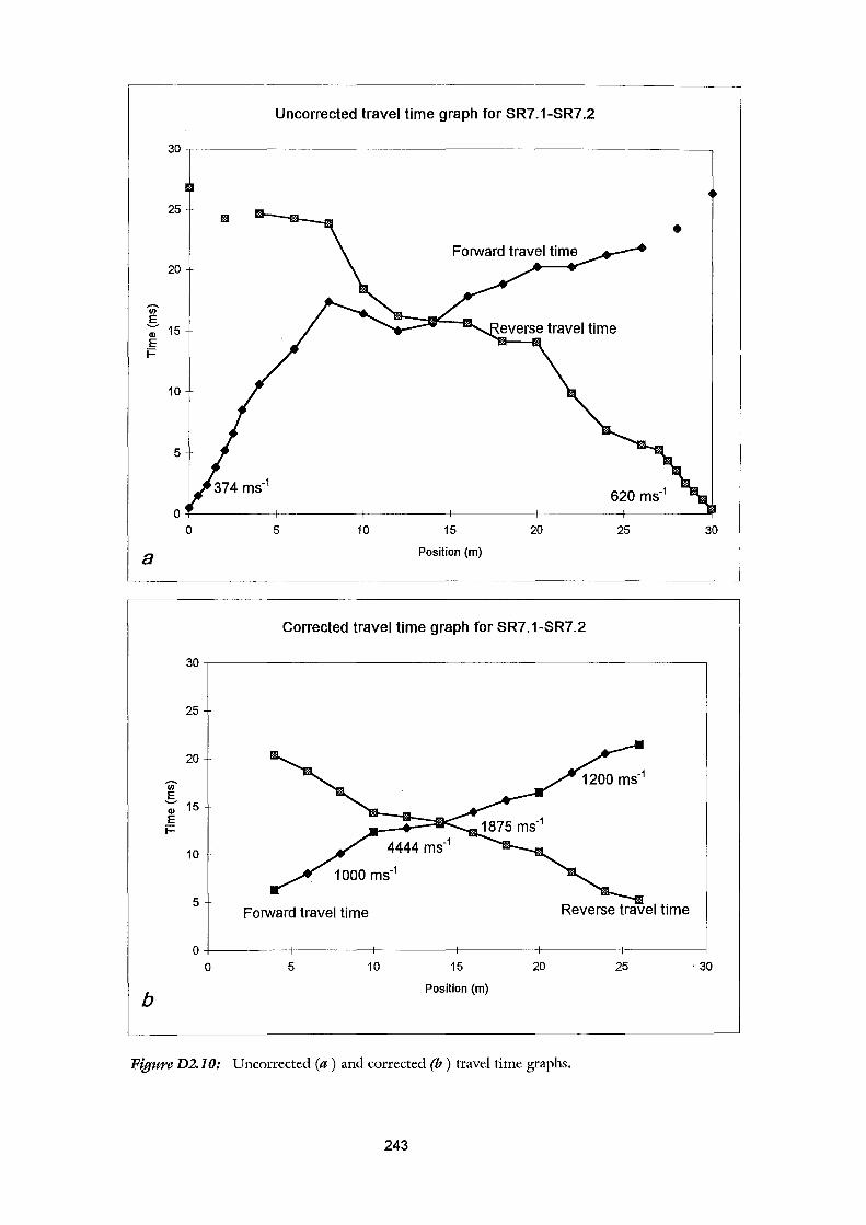
Iii' g Q)
E i=
a
b
Uncorrected travel time graph for SR7 .1-SR7 .2
30.---------------------------------------------------------~
25
• 20
15
10
5
620 ms·1
0+---------+---------+---------+---------+---------+-------~
0
30
25
20
Iii' g
15 Q)
E i=
10
5
0 0
5 10 15
Position (m)
20 25
Corrected travel time graph for SR7 .1-SR7 .2
Forward travel time
5 10 15
Position (m)
Reverse travel time
20 25
30
. 30
Figure D2.10: Uncorrected (a) and corrected (b) travel time graphs.
243
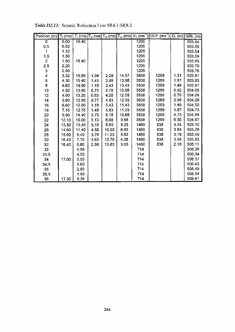
TableD2.11: Seismic Refraction Line SR8.l-SR8.2
Position (m) Tr (ms) Tr (ms) Td (ms) Tor (ms) Tor (ms) v1 (ms-) DCF (ms-1) Dr (m) GRL (m)
0 0.00 16.40 1205 503.44 0.5 0.52 1205 503.50 1 1.32 1205 503.54
1.5 1.50 1205 503.59 2 1.80 16.40 1205 503.65
2.5 2.20 1205 503.70 3 2.80 1205 503.76 4 3.32 15.60 1.04 2.29 14.57 3838 1269 1.31 503.81 6 4.30 15.40 1.43 2.88 13.98 3838 1269 1.81 503.93 8 4.60 14.60 1.18 3.43 13.43 3838 1269 1.49 503.97
10 4.50 13.80 0.73 3.78 13.08 3838 1269 0.92 504.05 12 4.90 13.20 0.63 4.28 12.58 3838 1269 0.79 504.08 14 5.60 12.80 0.77 4.83 12.03 3838 1269 0.98 504.29 16 6.60 12.60 1.18 5.43 11.43 3838 1269 1.49 504.50 18 7.10 12.70 1.48 5.63 11.23 3838 1269 1.87 504.73 20 9.90 14.40 3.73 6.18 10.68 3838 1269 4.73 504.88 22 12.10 15.00 5.13. 6.98 9.88 3838 1269 6.50 504.97 24 13.80 13.40 5.18 8.63 8.23 1460 838 4.34 505.10 26 14.60 11.40 4.58 10.03 6.83 1460 838 3.84 505.29 28 15.00 9.40 3.78 11.23 5.63 1460 838 3.16 505.49 30 16.40 7.70 3.63 12.78 4.08 1460 838 3.04 505.83 32 16.40 5.60 2.58 13.83 3.03 1460 838 2.16 506.11 33 4.88 714 506.26
33.5 4.50 714 506.34 34 17.00 3.90 714 506.37
34.5 3.60 714 506.43 35 2.80 714 506.49
35.5 1.80 714 506.54 36 17.30 0.36 714 506.61
244
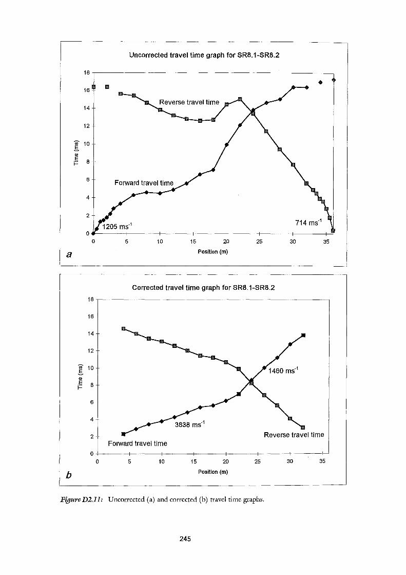
Uncorrected travel time graph for SR8.1-SR8.2
18
• 16 Ell
14
12
Ui' 10 g CD E 8 i=
6
4
2 714 ms·1
0 0 5 10 15 20 25 30 35
a Position (m)
Corrected travel time graph for SR8.1-SR8.2
18
16
14
12
Ui' 10 g CD E 8 i=
6
4
2 Forward travel time
0 0 5 10 15 20 25 30 35
b Position (m)
FigureD2.11: Uncorrected (a) and corrected (b) travel time graphs.
245
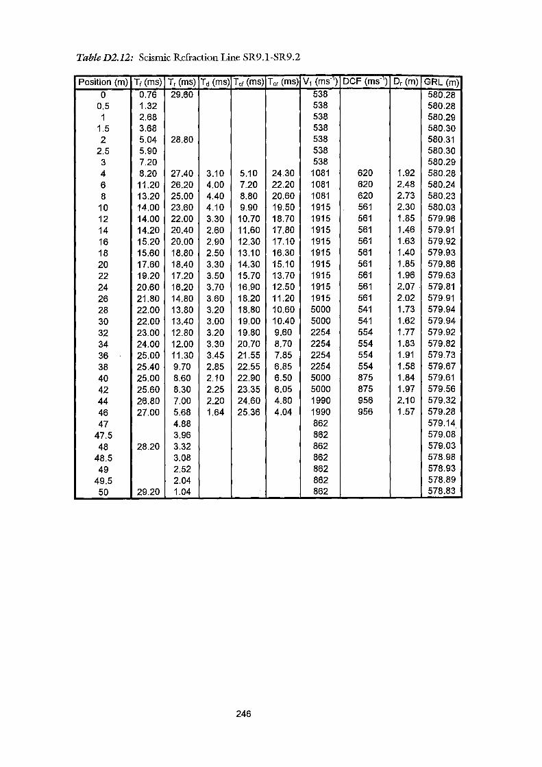
TableD2.12: Seismic Refraction Line SR9.l-SR9.2
Position (m) Tr (ms) Tr (ms) Td (ms) Tcr (ms) Tcr (ms) v1 (ms"1) DCF (ms·) Dr (m) GRL (m)
0 0.76 29.60 538 580.28 0.5 1.32 538 580.28 1 2.68 538 580.29
1.5 3.68 538 580.30 2 5.04 28.80 538 580.31
2.5 5.90 538 580.30 3 7.20 538 580.29 4 8.20 27.40 3.10 5.10 24.30 1081 620 1.92 580.28 6 11.20 26.20 4.00 7.20 22.20 1081 620 2.48 580.24 8 13.20 25.00 4.40 8.80 20.60 1081 620 2.73 580.23
10 14.00 23.60 4.10 9.90 19.50 1915 561 2.30 580.03 12 14.00 22.00 3.30 10.70 18.70 1915 561 1.85 579.96 14 14.20 20.40 2.60 11.60 17.80 1915 561 1.46 579.91 16 15.20 20.00 2.90 12.30 17.10 1915 561 1.63 579.92 18 15.60 18.80 2.50 13.10 16.30 1915 561 1.40 579.93 20 17.60 18.40 3.30 14.30 15.10 1915 561 1.85 579.86 22 19.20 17.20 3.50 15.70 13.70 1915 561 1.96 579.63 24 20.60 16.20 3.70 16.90 12.50 1915 561 2.07. 579.81 26 21.80 14.80 3.60 18.20 11.20 1915 561 2.02 579.91 28 22.00 13.80 3.20 18.80 10.60 5000 541 1.73 579.94 30 22.00 13.40 3.00 19.00 10.40 5000 541 1.62 579.94 32 23.00 12.80 3.20 19.80 9.60 2254 554 1.77 579.92 34 24.00 12.00 3.30 20.70 8.70 2254 554 1.83 579.82 36 25.00 11.30 3.45 21.55 7.85 2254 554 1.91 579.73 38 25.40 9.70 2.85 22.55 6.85 2254 554 1.58 579.67 40 25.00 8.60 2.10 22.90 6.50 5000 875 1.84 579.61 42 25.60 8.30 2.25 23.35 6.05 5000 875 1.97 579.56 44 26.80 7.00 2.20 24.60 4.80 1990 956 2.10 579.32 46 27.00 5.68 1.64 25.36 4.04 1990 956 1.57 579.28 47 4.88 862 579.14
47.5 3.96 862 579.08 48 28.20 3.32 862 579.03
48.5 3.08 862 578.98 49 2.52 862 578.93
49.5 2.04 862 578.89 50 29.20 1.04 862 578.83
246
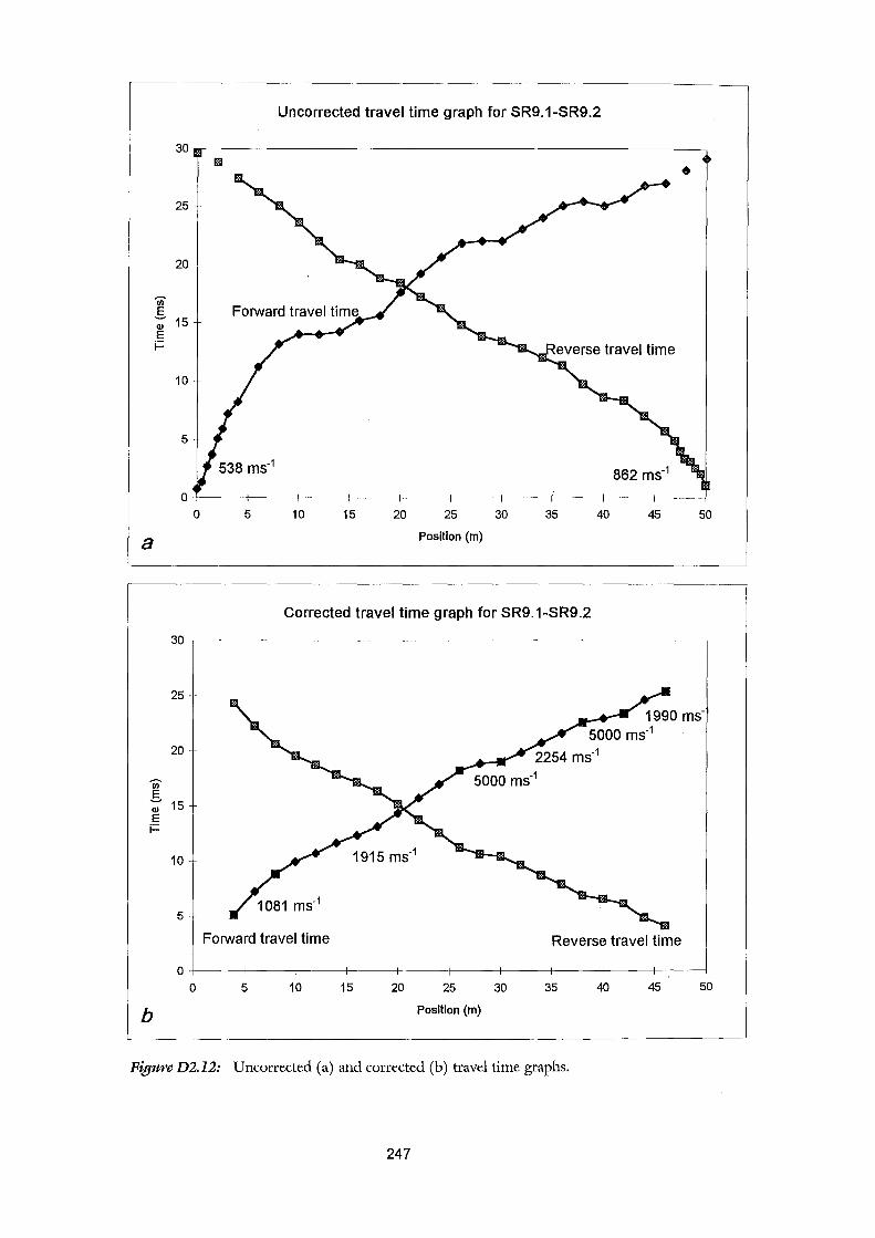
Uncorrected travel time graph for SR9.1-SR9.2
30m-------------------------------------------------------~
• 25
20
Ul ..s G) 15 E i=
a
10
5
862 ms·1
0+-----r-----~---4-----+-----+----~----4-----+-----+---~
0 5 10 15 20 25
Position (m)
30 35
Corrected travel time graph for SR9.1-SR9.2
40 45 50
30.---------------------------------------------------------,
25
20
Ul ..s G) 15 E i=
b
10
5
Forward travel time Reverse travel time
0+-----+-----~--~~---4-----+-----+----~----~----~--~
0 5 10 15 20 25
Position (m)
30 35 40 45 50
Figure D2.12: Uncorrected (a) and corrected (b) travel time graphs.
247
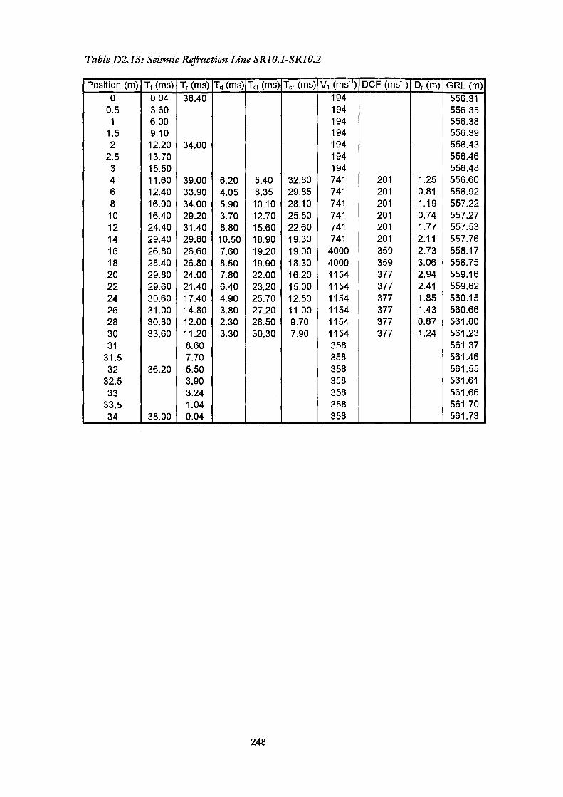
Table D2.13: Seisnnc Refraction Line SR10.1-SR10.2
Position (m) Tt (ms) Tr (ms) Tct (ms) Tot (ms) Tor (ms) v1 (ms=l) DCF (ms-) Dr (m) GRL (m) 0 0.04 38.40 194 556.31
0.5 3.60 194 556.35 1 6.00 194 556.38
1.5 9.10 194 556.39 2 12.20 34.00 194 556.43
2.5 13.70 194 556.46 3 15.50 194 556.48 4 11.60 39.00 6.20 5.40 32.80 741 201 1.25 556.60 6 12.40 33.90 4.05 8.35 29.85 741 201 0.81 556.92 8 16.00 34.00 5.90 10.10 28.10 741 201 1.19 557.22
10 16.40 29.20 3.70 12.70 25.50 741 201 0.74 557.27 12 24.40 31.40 8.80 15.60 22.60 741 201 1.77 557.53 14 29.40 29.80 10.50 18.90 19.30 741 201 2.11 557.76 16 26.80 26.60 7.60 19.20 19.00 4000 359 2.73 558.17 18 28.40 26.80 8.50 19.90 18.30 4000 359 3.06 558.75 20 29.80 24.00 7.80 22.00 16.20 1154 377 2.94 559.16 22 29.60 21.40 6.40 23.20 15.00 1154 377 2.41 559.62 24 30.60 17.40 4.90 25.70 12.50 1154 377 1.85 560.15 26 31.00 14.80 3.80 27.20 11.00 1154 377 1.43 560.66 28 30.80 12.00 2.30 28.50 9.70 1154 377 0.87 561.00 30 33.60 11.20 3.30 30.30 7.90 1154 377 1.24 561.23 31 8.60 358 561.37
31.5 7.70 358 561.46 32 36.20 5.50 358 561.55
32.5 3.90 358 561.61 33 3.24 358 561.66
33.5 1.04 358 561.70 34 38.00 0.04 358 561.73
248
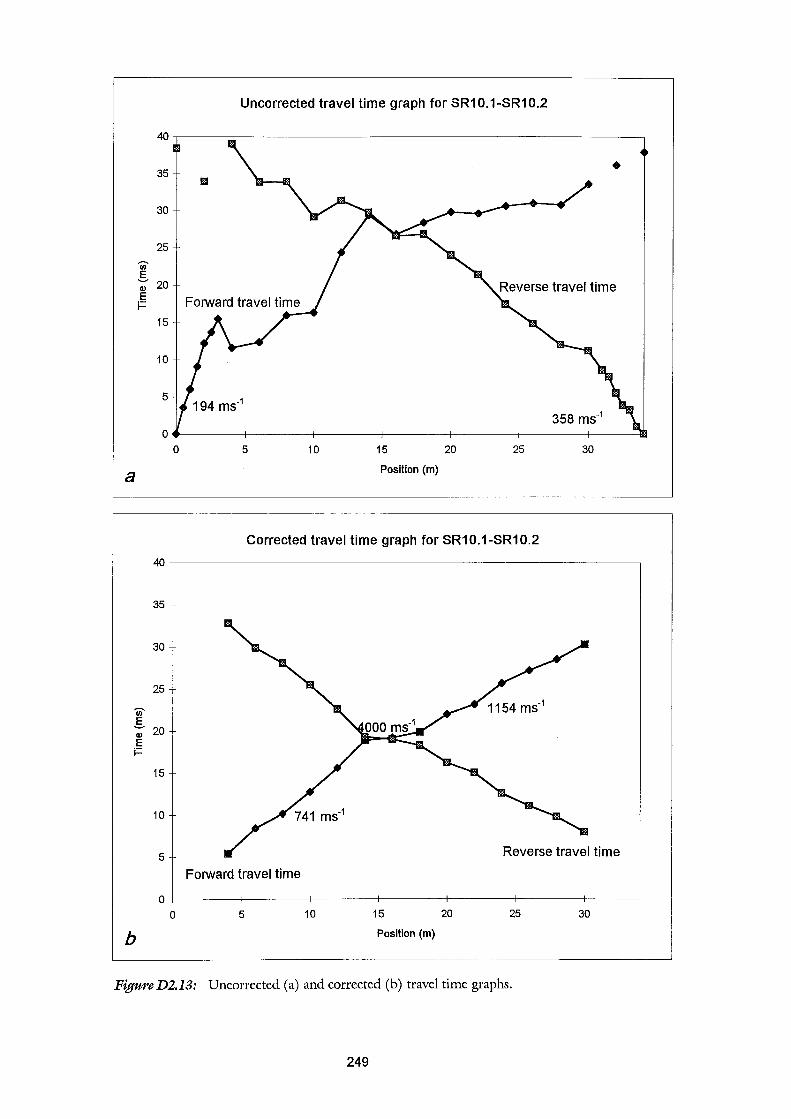
Uncorrected travel time graph for SR10.1-SR10.2
40
• 35
30
25
Ul 5 20 Q)
E F
15
10
5
358 ms·1
0 0 5 10 15 20 25 30
a Position (m)
Corrected travel time graph for SR1 0.1-SR1 0.2
40
35
30
25
Ul 5 20 Q)
E F
15
10
5 Reverse travel time
Forward travel time
0+-------1-------~------~-------+------~--------~--~
0 5 10 15 20 25 30
b Position (m)
FigureD2.13: Uncorrected (a) and corrected (b) travel time graphs.
249
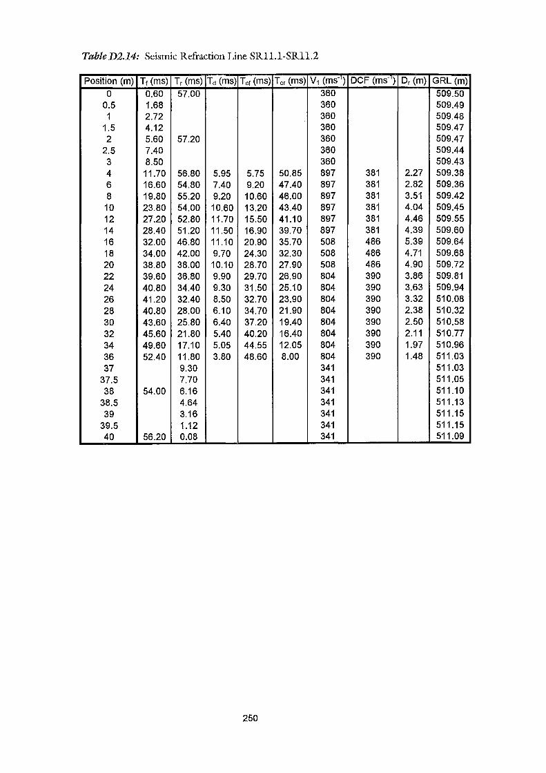
TableD2.14: Seismic Refraction Line SRll.l-SRll.2
Position (m) Tr (ms) Tr (ms) Td (ms) Tor (ms) Tor (ms) v1 (ms-1) DCF (ms-1
) Dr (m) GRL (m)
0 0.60 57.00 360 509.50 0.5 1.68 360 509.49 1 2.72 360 509.48
1.5 4.12 360 509.47 2 5.60 57.20 360 509.47
2.5 7.40 360 509.44 3 8.50 360 509.43 4 11.70 56.80 5.95 5.75 50.85 897 381 2.27 509.38 6 16.60 54.80 7.40 9.20 47.40 897 381 2.82 509.36 8 19.80 55.20 9.20 10.60 46.00 897 381 3.51 509.42 10 23.80 54.00 10.60 13.20 43.40 897 381 4.04 509.45 12 27.20 52.80 11.70 15.50 41.10 897 381 4.46 509.55 14 28.40 51.20 11.50 16.90 39.70 897 381 4.39 509.60 16 32.00 46.80 11.10 20.90 35.70 508 486 5.39 509.64 18 34.00 42.00 9.70 24.30 32.30 508 486 4.71 509.68 20 38.80 38.00 10.10 28.70 27.90 508 486 4.90 509.72 22 39.60 36.80 9.90 29.70 26.90 804 390 3.86 509.81 24 40.80 34.40 9.30 31.50 25.10 804 390 3.63 509.94 26 41.20 32.40 8.50 32.70 23.90 804 390 3.32 510.08 28 40.80 28.00 6.10 34.70 21.90 804 390 2.38 510.32 30 43.60 25.80 6.40 37.20 19.40 804 390 2.50 510.58 32 45.60 21.80 5.40 40.20 16.40 804 390 2.11 510.77 34 49.60 17.10 5.05 44.55 12.05 804 390 1.97 510.96 36 52.40 11.80 3.80 48.60 8.00 804 390 1.48 511.03 37 9.30 341 511.03
37.5 7.70 341 511.05 38 54.00 6.16 341 511.10
38.5 4.64 341 511.13 39 3.16 341 511.15
39.5 1.12 341 511.15 40 56.20 0.08 341 511.09
250
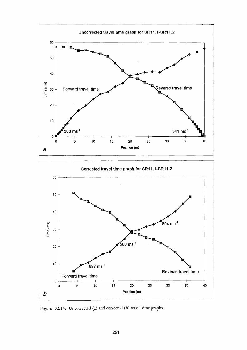
50
40
Ul 5 Ql 30 E i=
20
10
Uncorrected travel time graph for SR11.1-SR11.2
•
341 ms·1
0~-----4------~------~----~------r------+------+-----~
a
Ul 5 Ql E i=
b
0 5 10 15 20
Position (m)
25 30
Corrected travel time graph for SR11.1-SR11.2
35 40
60,---------------------------------------------------------~
50
40
30
20
10
Forward travel time 0+------4------~------+-----~------~------~----~------~
0 5 10 15 20
Position (m)
25 30 35 40
Figure D2.14: Uncorrected (a) and corrected (b) travel time graphs.
251
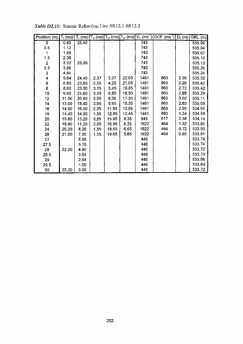
TableD2.15: Seismic Refraction Line SR12.l-SR12.2
Position (m) Tr (ms) Tr (ms) Td (ms) Tcr (ms) Tcr (ms) v1 (ms=1) DCF (ms-) Dr (m) GRL (m)
0 0.80 25.40 743 535.00 0.5 1.12 743 535.04 1 1.68 743 535.07
1.5 2.36 743 535.10 2 3.32 25.00 743 535.13
2.5 3.88 743 535.20 3 4.84 743 535.24 4 5.64 24.40 2.37 3.27 22.03 1461 863 2.05 535.32 6 6.80 23.60 2.55 4.25 21.05 1461 863 2.20 535.42 8 8.60 23.00 3.15 5.45 19.85 1461 863 2.72 535.42
10 9.90 21.60 3.10 6.80 18.50 1461 863 2.68 535.29 12 11.50 20.80 3.50 8.00 17.30 1461 863 3.02 535.11 14 13.00 18.40 3.05 9.95 15.35 1461 863 2.63 535.08 16 14.00 16.00 2.35 11.65 13.65 1461 863 2.03 534.91 18 14.40 14.00 1.55 12.85 12.45 1461 863 1.34 534.59 20 19.80 13.20 3.85 15.95 9.35 645 617 2.38 534.14 22 19.80 11.20 2.85 16.95 8.35 1622 464 1.32 533.95 24 20.20 8.20 1.55 18.65 6.65 1622 464 0.72 533.90 26 21.00 7.00 1.35 19.65 5.65 1622 464 0.63 533.81 27 6.80 446 533.74
27.5 5.70 446 533.74 28 22.20 4.90 446 533.72
28.5 3.64 446 533.70 29 2.64 446 533.66
29.5 1.00 446 533.69 30 25.20 0.08 446 533.72
252
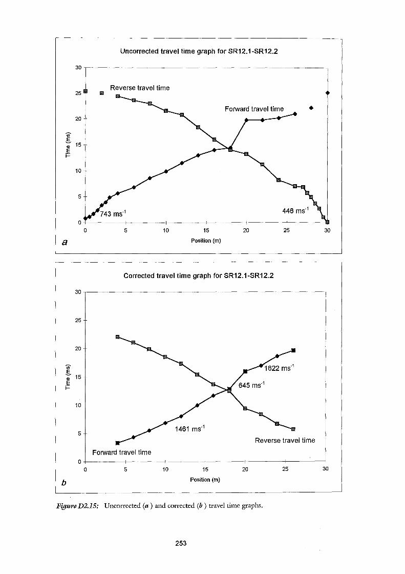
Uncorrected travel time graph for SR 12.1-SR 12.2
30,------------------------------------------------------------
25 m
20
Ul §. Q) 15 E i=
10
5
a 0
Reverse travel time
5 10 15
Position (m)
20
Corrected travel time graph for SR12.1-SR12.2
•
446 ms·1
25 30
30.----------------------------------------------------------.
25
20
Ul §. Q) 15 E i=
10
5
0
b
Forward travel time
0 5
1461 ms·1
Reverse travel time
10 15 20 25
Position (m)
Figure D2.15: Uncorrected (a) and corrected (b) travel time graphs.
253
30
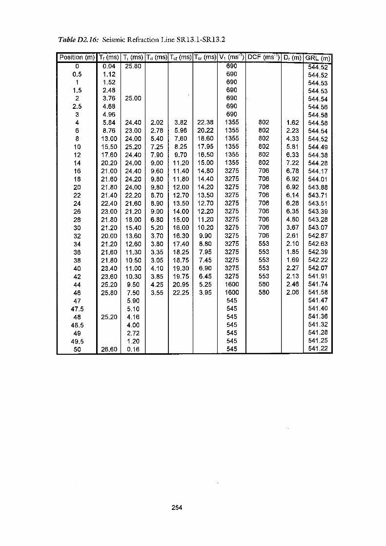
TableD2.16: Seismic Refraction Line SR13.1-SR13.2
Position (m) Tr (ms) Tr (ms) Td (ms) Tcr (ms) Tcr (ms) v1 (ms-1) DCF (ms-) Dr (m) GRL (m)
0 0.04 25.80 690 544.52 0.5 1.12 690 544.52 1 1.52 690 544.53
1.5 2.48 690 544.53 2 3.76 25.00 690 544.54
2.5 4.68 690 544.56 3 4.96 690 544.58 4 5.84 24.40 2.02 3.82 22.38 1355 802 1.62 544.58 6 8.76 23.00 2.78 5.98 20.22 1355 802 2.23 544.54 8 13.00 24.00 5.40 7.60 18.60 1355 802 4.33 544.52
10 15.50 25.20 7.25 8.25 17.95 1355 802 5.81 544.49 12 17.60 24.40 7.90 9.70 16.50 1355 802 6.33 544.38 14 20.20 24.00 9.00 11.20 15.00 1355 802 7.22 544.28 16 21.00 24.40 9.60 11.40 14.80 3275 706 6.78 544.17 18 21.60 24.20 9.80 11.80 14.40 3275 706 6.92 544.01 20 21.80 24.00 9.80 12.00 14.20 3275 706 6.92 543.88 22 21.40 22.20 8.70 12.70 13.50 3275 706 6.14 543.71 24 22.40 21.60 8.90 13.50 12.70 3275 706 6.28 543.51 26 23.00 21.20 9.00 14.00 12.20 3275 706 6.35 543.39 28 21.80 18.00 6.80 15.00 11.20 3275 706 4.80 543.28 30 21.20 15.40 5.20 16.00 10.20 3275 706 3.67 543.07 32 20.00 13.60 3.70 16.30 9.90 3275 706 2.61 542.87 34 21.20 12.60 3.80 17.40 8.80 3275 553 2.10 542.63 36 21.60 11.30 3.35 18.25 7.95 3275 553 1.85 542.39 38 21.80 10.50 3.05 18.75 7.45 3275 553 1.69 542.22 40 23.40 11.00 4.10 19.30 6.90 3275 553 2.27 542.07 42 23.60 10.30 3.85 19.75 6.45 3275 553 2.13 541.91 44 25.20 9.50 4.25 20.95 5.25 1600 580 2.46 541.74 46 25.80 7.50 3.55 22.25 3.95 1600 580 2.06 541.58 47 5.90 545 541.47
47.5 5.10 545 541.40 48 25.20 4.16 545 541.36
48.5 4.00 545 541.32 49 2.72 545 541.28
49.5 1.20 545 541.25 50 26.60 0.16 545 541.22
254
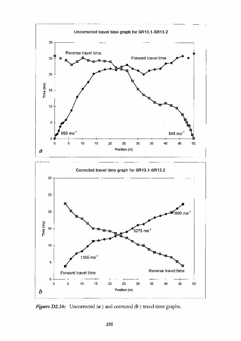
Uncorrected travel time graph for SR13.1-SR13.2
.30,----------------------------------------------------.
a
25 111!1
20
00 _§_ Q) 15 E i=
10
5
0
Reverse travel time
5 10 15 20 25
Position (m)
30 35 40
Corrected travel time graph for SR13.1-SR13.2
•
545 ms-1
45 50
30.---------------------------------------------------~
25
20
00 _§_ Q) 15 E i=
10
5
1355 ms-1
Forward travel time Reverse travel time
0+----4-----r----+----4-----r----+---~-----r----+----4
0 5 10 15 20
b
25
Position (m)
30 35 40 45
Figure D2.16: Uncorrected (a) and corrected (b) travel time graphs.
255
50
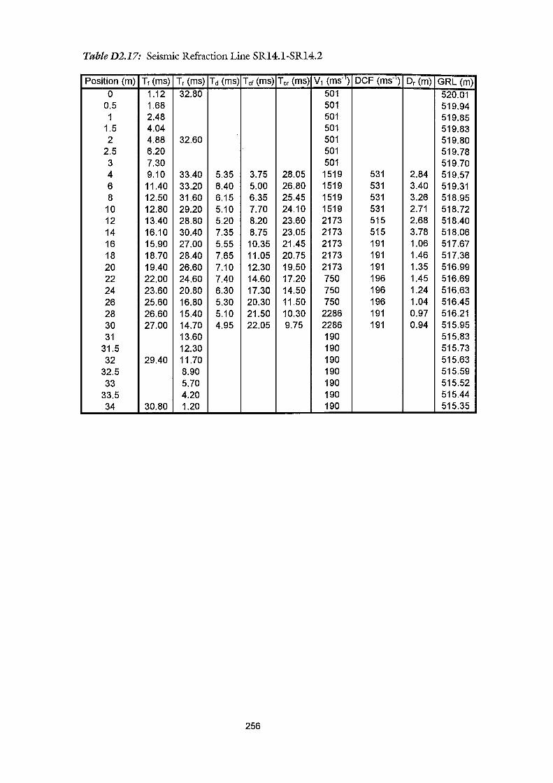
TableD2.17: Seismic Refraction Line SR14.l-SR14.2
Position (m) Tt (ms) Tr (ms) Td (ms) Tot (ms) Tor (ms) v1 (ms-1) DCF (ms-1) Dr (m) GRL (m)
0 1.12 32.80 501 520.01 0.5 1.68 501 519.94 1 2.48 501 519.85
1.5 4.04 501 519.83 2 4.88 32.60 501 519.80
2.5 6.20 501 519.78 3 7.30 501 519.70 4 9.10 33.40 5.35 3.75 28.05 1519 531 2.84 519.57 6 11.40 33.20 6.40 5.00 26.80 1519 531 3.40 519.31 8 12.50 31.60 6.15 6.35 25.45 1519 531 3.26 518.95
10 12.80 29.20 5.10 7.70 24.10 1519 531 2.71 518.72 12 13.40 28.80 5.20 8.20 23.60 2173 515 2.68 518.40 14 16.10 30.40 7.35 8.75 23.05 2173 515 3.78 518.06 16 15.90 27.00 5.55 10.35 21.45 2173 191 1.06 517.67 18 18.70 28.40 7.65 11.05 20.75 2173 191 1.46 517.36 20 19.40 26.60 7.10 12.30 19.50 2173 191 1.35 516.99 22 22.00 24.60 7.40 14.60 17.20 750 196 1.45 516.69 24 23.60 20.80 6.30 17.30 14.50 750 196 1.24 516.63 26 25.60 16.80 5.30 20.30 11.50 750 196 1.04 516.45 28 26.60 15.40 5.10 21.50 10.30 2286 191 0.97 516.21 30 27.00 14.70 4.95 22.05 9.75 2286 191 0.94 515.95 31 13.60 190 515.83
31.5 12.30 190 515.73 32 29.40 11.70 190 515.63
32.5 8.90 190 515.59 33 5.70 190 515.52
33.5 4.20 190 515.44 34 30.80 1.20 190 515.35
256

Uncorrected travel time graph for SR14.1-SR14.2
35
llll
30 • 25
Iii' 20 g G)
E i= 15
10
5 190 ms·1
0 0 5 10 15 20 25 30
a Position (m)
Corrected travel time graph for SR14.1-SR14.2
35,-------------------------------------------------------.
b
30
25
Iii' 20 g G)
E i= 15
10
5
0
1519 ms-1
FoiWard travel time
5 10 15
Position (m)
Reverse travel time
20 25 30
FigureD2.17: Uncorrected (a) and corrected (b) travel time graphs.
257
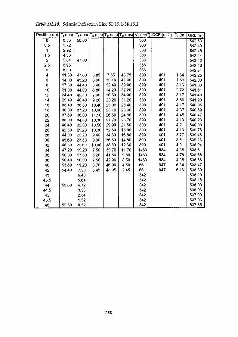
TableD2.18: Seismic Refraction Line SR15.l-SR15.2
Position (m) Tr (ms) Tr (ms) Td (ms) Tor (ms) Tor (ms) v1 (ms'1) DCF (ms-) Dr (m) GRL (m) 0 0.56 50.00 366 542.53
0.5 1.72 366 542.49 1 2.92 366 542.46
1.5 4.36 366 542.44 2 5.84 47.60 366 542.42
2.5 6.96 366 542.40 3 8.30 366 542.34 4 11.50 47.60 3.85 7.65 43.75 899 401 1.54 542.25 6 14.00 45.20 3.90 10.10 41.30 899 401 1.56 542.08 8 17.80 44.40 5.40 12.40 39.00 899 401 2.16 541.83
10 21.00 44.00 6.80 14.20 37.20 899 401 2.72 541.61 12 24.40 42.80 7.90 16.50 34.90 899 401 3.17 541.40 14 29.40 40.40 9.20 20.20 31.20 899 401 3.69 541.20 16 33.40 38.80 10.40 23.00 28.40 899 401 4.17 540.95 18 36.00 37.20 10.90 25.10 26.30 899 401 4.37 540.69 20 37.60 36.00 11.10 26.50 24.90 899 401 4.45 540.47 22 38.00 34.00 10.30 27.70 23.70 899 401 4.13 540.23 24 40.40 32.00 10.50 29.90 21.50 899 401 4.21 540.00 26 42.80 29.20 10.30 32.50 18.90 899 401 4.13 539.76 28 44.00 26.20 9.40 34.60 16.80 899 401 3.77 539.48 30 45.60 23.80 9.00 36.60 14.80 899 401 3.61 539.13 32 48.80 22.60 10.00 38.80 12.60 899 401 4.01 538.94 34 47.20 19.20 7.50 39.70 11.70 1463 584 4.38 538.81 36 50.00 17.80 8.20 41.80 9.60 1463 584 4.78 538.68 38 50.40 16.00 7.50 42.90 8.50 1463 584 4.38 538.56 40 53.60 11.20 6.70 46.90 4.50 661 947 6.34 538.47 42 54.40 7.90 5.45 48.95 2.45 661 947 5.16 538.30 43 6.48 542 538.19
43.5 5.64 542 538.16 44 53.60 4.72 542 538.09
44.5 3.96 542 538.03 45 2.84 542 537.99
45.5 1.52 542 537.93 46 52.80 0.52 542 537.85
258

Uncorrected travel time graph for SR15.1-SR15.2
55
50 ll!l
45
40
35
(jj' 30 .§. CD E 25 i=
20
15
10
5
542 ms-1
0 0 5 10 15 20 25 30 35 40 45
a Position (m)
Corrected travel time graph for SR15.1-SR15.2
55
50
45
40
35
(jj' 30 .§. CD E 25 i=
20
15
10
5 Forward travel time Reverse travel time
0 0 5 10 15 20 25 30 35 40 45
b Position (m)
Figure D2.18: Uncorrected (a) and corrected (b) travel time graphs.
259
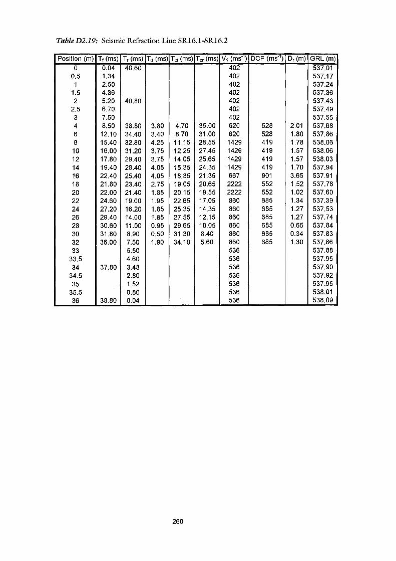
TableD2.19: Seismic Refraction Line SR16.l-SR16.2
Position (m) Tt (ms) Tr (ms) Td (ms) Tcr (ms) Tcr (ms) v1 (ms-) DCF (ms-1} Dr (m) GRL (m)
0 0.04 40.60 402 537.01 0.5 1.34 402 537.17 1 2.50 402 537.24
1.5 4.36 402 537.36 2 5.20 40.80 402 537.43
2.5 6.70 402 537.49 3 7.50 402 537.55 4 8.50 38.80 3.80 4.70 35.00 620 528 2.01 537.68 6 12.10 34.40 3.40 8.70 31.00 620 528 1.80 537.86 8 15.40 32.80 4.25 11.15 28.55 1429 419 1.78 538.06 10 16.00 31.20 3.75 12.25 27.45 1429 419 1.57 538.06 12 17.80 29.40 3.75 14.05 25.65 1429 419 1.57 538.03 14 19.40 28.40 4.05 15.35 24.35 1429 419 1.70 537.94 16 22.40 25.40 4.05 18.35 21.35 667 901 3.65 537.91 18 21.80 23.40 2.75 19.05 20.65 2222 552 1.52 537.78 20 22.00 21.40 1.85 20.15 19.55 2222 552 1.02 537.60 22 24.60 19.00 1.95 22.65 17.05 860 685 1.34 537.39 24 27.20 16.20 1.85 25.35 14.35 860 685 1.27 537.53 26 29.40 14.00 1.85 27.55 12.15 860 685 1.27 537.74 28 30.60 11.00 0.95 29.65 10.05 860 685 0.65 537.84 30 31.80 8.90 0.50 31.30 8.40 860 685 0.34 537.83 32 36.00 7.50 1.90 34.10 5.60 860 685 1.30 537.86 33 5.50 536 537.88
33.5 4.60 536 537.95 34 37.80 3.48 536 537.90
34.5 2.80 536 537.92 35 1.52 536 537.95
35.5 0.80 536 538.01 36 38.80 0.04 536 538.09
260
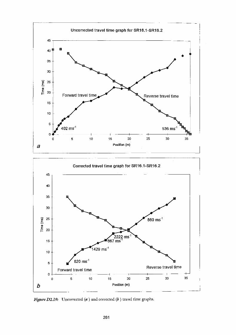
Uncorrected travel time graph for SR16.1-SR16.2
45
40 II
• 35
30
VI 25 ,S Q)
E 20 i=
15
10
5 536 ms-1
0 0 5 10 15 20 25 30 35
a Position (m)
Corrected travel time graph for SR16.1-SR16.2
45
40
35
30
VI 25 ,S Q)
E 20 i=
15
10
5
Forward travel time Reverse travel time
0 0 5 10 15 20 25 30 35
b Position (m)
Figure D2.19: Uncorrected (a) and corrected (b) travel time graphs.
261
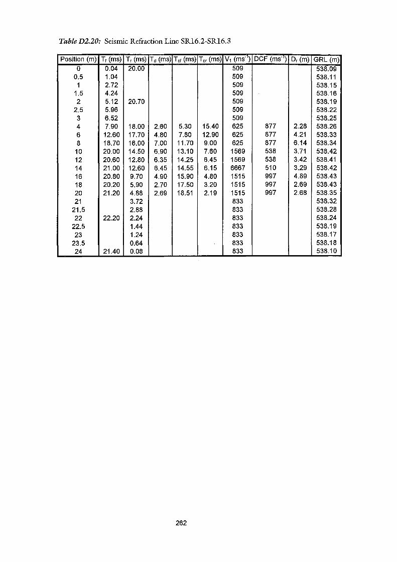
TableD2.20: Seismic Refraction Line SR16.2-SR16.3
Position (m) Tt (ms) Tr (ms) Td (ms) Tct (ms) Tcr (ms) v1 (ms-) DCF (ms-1) Dr (m) GRL (m)
0 0.04 20.00 509 538.09 0.5 1.04 509 538.11 1 2.72 509 538.15
1.5 4.24 509 538.16 2 5.12 20.70 509 538.19
2.5 5.96 509 538.22 3 6.52 509 538.25 4 7.90 18.00 2.60 5.30 15.40 625 877 2.28 538.26 6 12.60 17.70 4.80 7.80 12.90 625 877 4.21 538.33 8 18.70 16.00 7.00 11.70 9.00 625 877 6.14 538.34
10 20.00 14.50 6.90 13.10 7.60 1569 538 3.71 538.42 12 20.60 12.80 6.35 14.25 6.45 1569 538 3.42 538.41 14 21.00 12.60 6.45 14.55 6.15 6667 510 3.29 538.42 16 20.80 9.70 4.90 15.90 4.80 1515 997 4.89 538.43 18 20.20 5.90 2.70 17.50 3.20 1515 997 2.69 538.43 20 21.20 4.88 2.69 18.51 2.19 1515 997 2.68 538.35 21 3.72 833 538.32
21.5 2.88 833 538.28 22 22.20 2.24 833 538.24
22.5 1.44 833 538.19 23 1.24 833 538.17
23.5 0.64 833 538.18 24 21.40 0.08 833 538.10
262
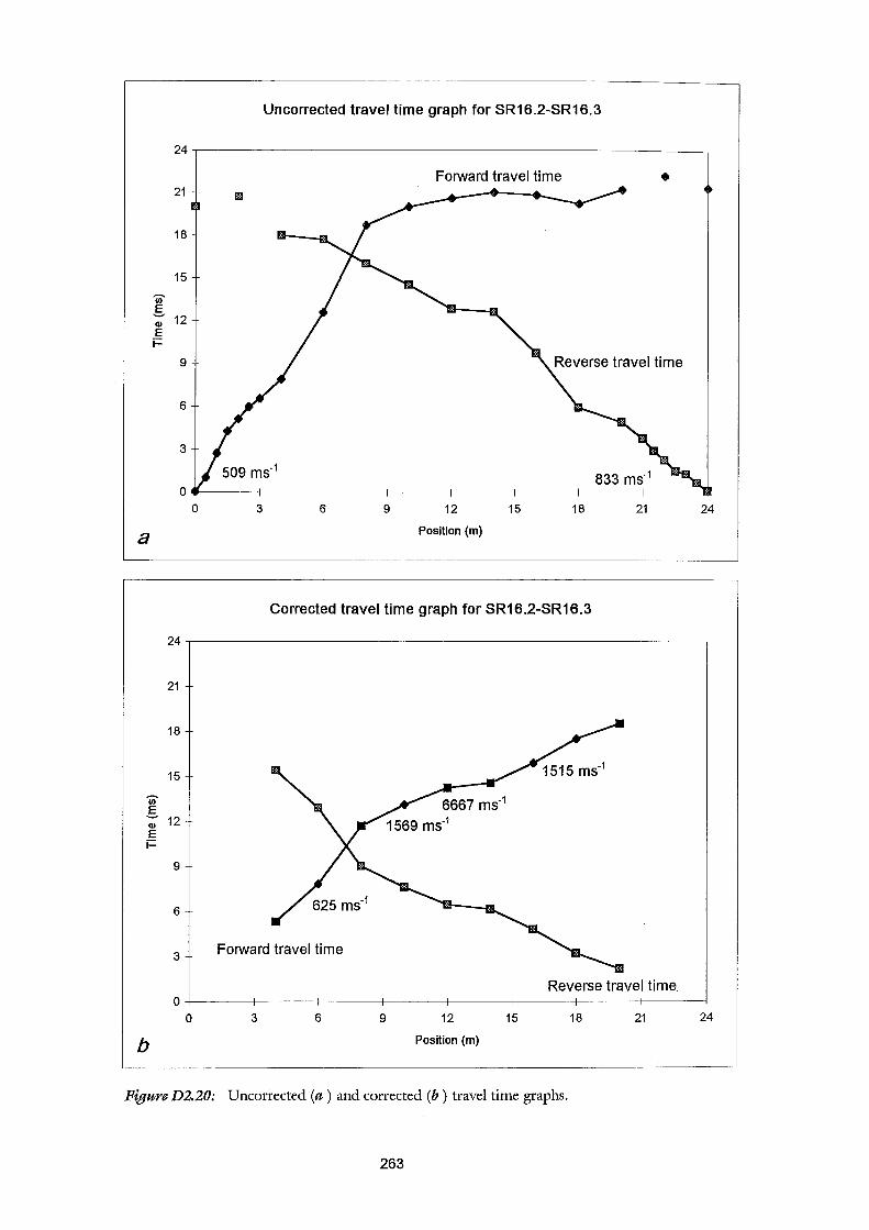
24
21
18
15
Iii' §.
12 Ql E i=
9
6
3
0 0
a
24
21
18
15
Iii' §.
12 Ql E i=
9
6
3
0
0
b
3
Uncorrected travel time graph for SR16.2-SR16.3
6 9
Forward travel time
12
Position (m)
15 18
Corrected travel time graph for SR16.2-SR16.3
833 ms-1
21
•
Forward travel time
3 6 9 12
Position (m)
Reverse travel time.
15 18 21
Figure D2.20: Uncorrected (a) and corrected (b) travel time graphs.
263
24
24
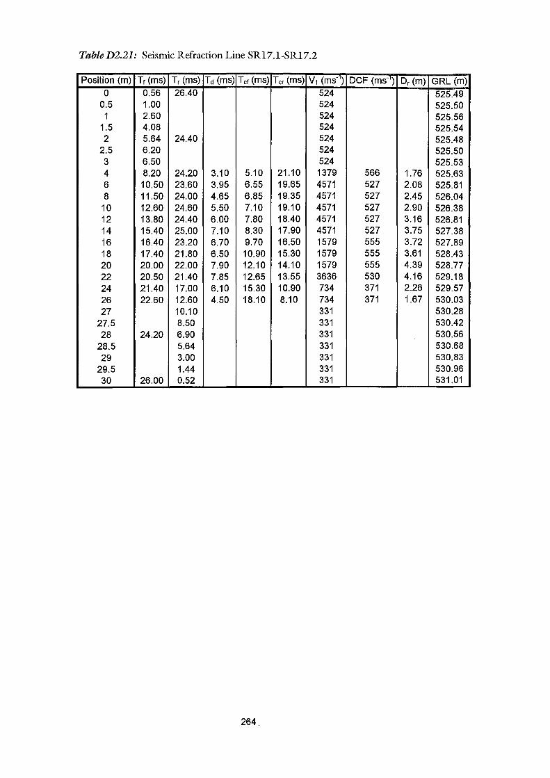
TableD2.21: Seismic Refraction Line SR17.l-SR17.2
Position (m) Tt (ms) Tr (ms) Td (ms) Tcr (ms) Tcr (ms) v1 (ms-1) DCF (ms-1
) Dr (m) GRL (m) 0 0.56 26.40 524 525.49
0.5 1.00 524 525.50 1 2.60 524 525.56
1.5 4.08 524 525.54 2 5.64 24.40 524 525.48
2.5 6.20 524 525.50 3 6.50 524 525.53 4 8.20 24.20 3.10 5.10 21.10 1379 566 1.76 525.63 6 10.50 23.60 3.95 6.55 19.65 4571 527 2.08 525.81 8 11.50 24.00 4.65 6.85 19.35 4571 527 2.45 526.04
10 12.60 24.60 5.50 7.10 19.10 4571 527 2.90 526.38 12 13.80 24.40 6.00 7.80 18.40 4571 527 3.16 526.81 14 15.40 25.00 7.10 8.30 17.90 4571 527 3.75 527.38 16 16.40 23.20 6.70 9.70 16.50 1579 555 3.72 527.89 18 17.40 21.80 6.50 10.90 15.30 1579 555 3.61 528.43 20 20.00 22.00 7.90 12.10 14.10 1579 555 4.39 528.77 22 20.50 21.40 7.85 12.65 13.55 3636 530 4.16 529.18 24 21.40 17.00 6.10 15.30 10.90 734 371 2.26 529.57 26 22.60 12.60 4.50 18.10 8.10 734 371 1.67 530.03 27 10.10 331 530.28
27.5 8.50 331 530.42 28 24.20 6.90 331 530.56
28.5 5.64 331 530.68 29 3.00 331 530.83
29.5 1.44 331 530.96 30 26.00 0.52 331 531.01
264.
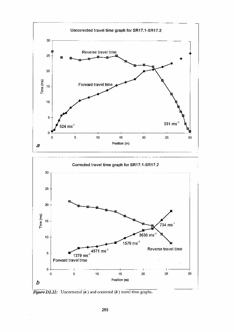
Uncorrected travel time graph for SR17.1-SR17.2
30~------------------------------------------------------.
a
25
20
Ui' g Q) 15 E i=
10
5
0 5
Reverse travel time
10 15
Position (m)
20
Corrected travel time graph for SR17.1-SR17.2
•
331 ms-1
25 30
30,-------------------------------------------------------~
25
20
Ui' g Q) 15 E i=
10
5 4571 ms-1
1379 ms-1
Forward travel time
Reverse travel time
0+-------~~-------+--------~--------~-------+--------~
0 5
b
10 15
Position (m)
20
Figure D2.21: Uncorrected (a) and corrected (b) travel time graphs.
265
25 30

TableD2.22: Seismic Refraction Line SR18.1-SR18.2
Position (m) Tr (ms) Tr (ms) Td (ms) Tor (ms) Tor (ms) v1 (ms:1) DCF (ms-1) Dr (m) GRL (m) 0 0.08 39.60 595 563.69
0.5 1.16 595 563.66 1 2.12 595 563.61
1.5 3.44 595 563.59 2 4.00 38.60 595 563.57
2.5 4.52 595 563.54 3 5.16 595 563.51 4 6.80 37.40 1.80 5.00 35.60 839 844 1.52 563.41 6 9.80 35.40 2.30 7.50 33.10 839 844 1.94 563.23 8 13.20 34.40 3.50 9.70 30.90 839 844 2.95 562.96
10 16.90 33.20 4.75 12.15 28.45 839 844 4.01 562.81 12 18.60 33.20 5.60 13.00 27.60 2352 615 3.44 562.73 14 22.00 31.40 6.40 15.60 25.00 629 1835 11.74 562.41 16 25.20 28.00 6.30 18.90 21.70 629 1835 11.56 562.16 18 30.00 25.20 7.30 22.70 17.90 629 1835 13.39 561.74 20 33.40 22.60 7.70 25.70 14.90 629 1835 14.13 561.40 22 34.00 19.80 6.60 27.40 13.20 1000 398 2.63 561.05 24 35.60 17.30 6.15 29.45 11.15 1000 398 2.45 560.74 26 35.80 13.30 4.25 31.55 9.05 1000 398 1.69 560.41 28 38.20 11.40 4.50 33.70 6.90 1000 398 1.79 560.08 29 9.50 370 559.91
29.5 7.52 370 559.87 30 40.40 5.76 370 559.74
30.5 3.72 370 559.64 31 2.24 370 559.58
31.5 1.08 370 559.57 32 41.60 0.60 370 559.56
266
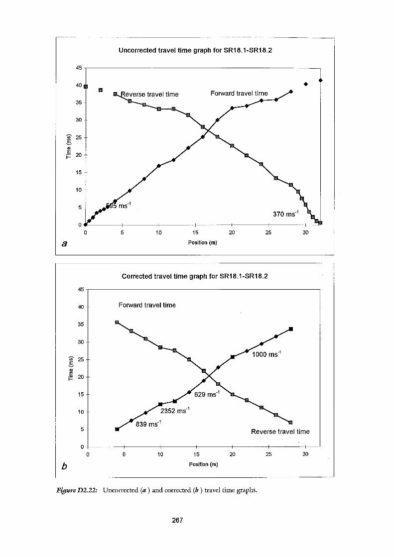
45
40 m
35
30
Ul 25 §. Q)
E 20 i=
15
10
5
0 0
a
45
40
35
30
Ul 25 §. Q)
E 20 i=
15
10
5
0 0
b
Uncorrected travel time graph for SR18.1-SR18.2
5 10 15
Position (m)
20 25
Corrected travel time graph for SR18.1-SR18.2
Forward travel time
•
370 ms-1
30
Reverse travel time
5 10 15
Position (m)
20 25 30
Figure D2.22: Uncorrected (a) and corrected (b) travel time graphs.
267
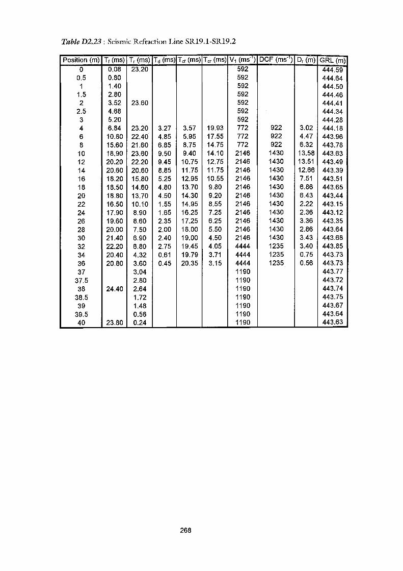
TableD2.23: Seismic Refraction Line SR19.1-SR19.2
Position (m) Tt (ms) Tr (ms) Td (ms) Tct (ms) Tcr (ms) v1 (ms-1) DCF (ms-1
) Dr (m) GRL (m) 0 0.08 23.20 592 444.59
0.5 0.80 592 444.64 1 1.40 592 444.50
1.5 2.80 592 444.46 2 3.52 23.60 592 444.41
2.5 4.68 592 444.34 3 5.20 592 444.28 4 6.84 23.20 3.27 3.57 19.93 772 922 3.02 444.18 6 10.80 22.40 4.85 5.95 17.55 772 922 4.47 443.96 8 15.60 21.60 6.85 8.75 14.75 772 922 6.32 443.78
10 18.90 23.60 9.50 9.40 14.10 2146 1430 13.58 443.63 12 20.20 22.20 9.45 10.75 12.75 2146 1430 13.51 443.49 14 20.60 20.60 8.85 11.75 11.75 2146 1430 12.66 443.39 16 18.20 15.80 5.25 12.95 10.55 2146 1430 7.51 443.51 18 18.50 14.60 4.80 13.70 9.80 2146 1430 6.86 443.65 20 18.80 13.70 4.50 14.30 9.20 2146 1430 6.43 443.44 22 16.50 10.10 1.55 14.95 8.55 2146 1430 2.22 443.15 24 17.90 8.90 1.65 16.25 7.25 2146 1430 2.36 443.12 26 19.60 8.60 2.35 17.25 6.25 2146 1430 3.36 443.35 28 20.00 7.50 2.00 18.00 5.50 2146 1430 2.86 443.64 30 21.40 6.90 2.40 19.00 4.50 2146 1430 3.43 443.68 32 22.20 6.80 2.75 19.45 4.05 4444 1235 3.40 443.85 34 20.40 4.32 0.61 19.79 3.71 4444 1235 0.75 443.73 36 20.80 3.60 0.45 20.35 3.15 4444 1235 0.56 443.73 37 3.04 1190 443.77
37.5 2.80 1190 443.72 38 24.40 2.64 1190 443.74
38.5 1.72 1190 443.75 39 1.48 1190 443.67
39.5 0.56 1190 443.64 40 23.80 0.24 1190 443.63
268
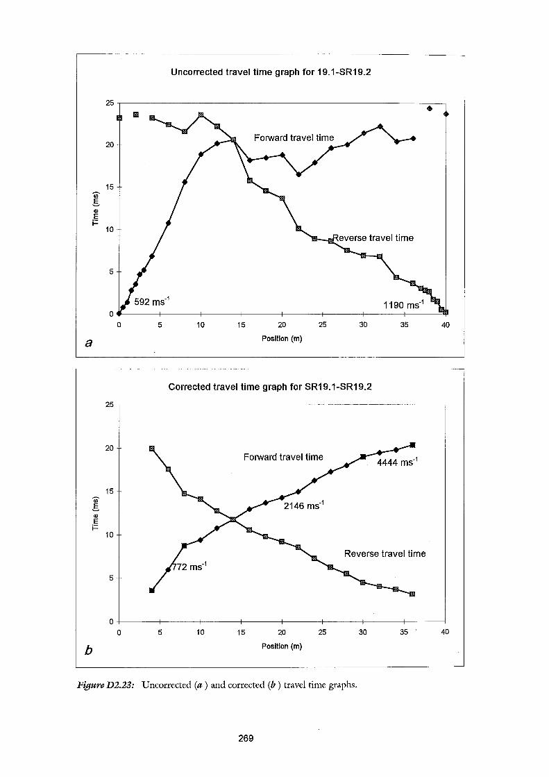
a
Ul §, Q)
E i=
b
Uncorrected travel time graph for 19.1-SR19.2
25,-------------------------------------------------------~-. •
20
15
10
5
1190 ms-1
0.-----~-------r------+-----~~-----r------+-------~----~
0 5 10 15 20
Position (m)
25 30
Corrected travel time graph for SR19.1-SR19.2
35 40
25,----------------------------------------------------------.
20 Forward travel time
15
10
Reverse travel time
5
0+-----~-------r------+-----~-------r------+-----~~-----i
0 5 10 15 20
Position (m)
25 30 35 . 40
Figure D2.23: Uncorrected (a) and corrected (b) travel time graphs.
269
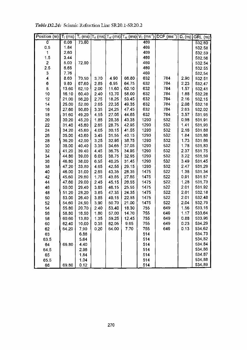
TableD2.24: Seismic Refraction Line SR20.1-SR20.2
Position (m) Tr (ms) Tr (ms) Td (ms) Tor (ms) Tor (ms) v1 (ms-) DCF (ms-1) Dr(m) GRL (m) 0 0.08 73.60 469 532.60
0.5 1.84 469 532.58 1 2.60 469 532.59
1.5 3.44 469 532.56 2 5.00 72.90 469 532.54
2.5 6.68 469 532.55 3 7.76 469 532.54 4 8.60 70.50 3.70 4.90 66.80 632 784 2.90 532.51 6 9.80 67.60 2.85 6.95 64.75 632 784 2.23 532.47 8 13.60 62.10 2.00 11.60 60.10 632 784 1.57 532.41 10 16.10 60.40 2.40 13.70 58.00 632 784 1.88 532.28 12 21.00 56.20 2.75 18.25 53.45 632 784 2.16 532.15 14 25.00 52.00 2.65 22.35 49.35 632 784 2.08 532.16 16 27.60 50.80 3.35 24.25 47.45 632 784 2.63 532.02 18 31.60 49.20 4.55 27.05 44.65 632 784 3.57 531.95 20 30.20 45.20 1.85 28.35 43.35 1290 532 0.98 531.91 22 31.40 45.60 2.65 28.75 42.95 1290 532 1.41 531.93 24 34.20 45.60 4.05 30.15 41.55 1290 532 2.16 531.88 26 35.00 43.60 3.45 31.55 40.15 1290 532 1.84 531.86 28 36.20 42.00 3.25 32.95 38.75 1290 532 1.73 531.86 30 38.00 40.40 3.35 34.65 37.05 1290 532 1.78 531.83 32 41.20 39.40 4.45 36.75 34.95 1290 532 2.37 531.75 34 44.80 39.00 6.05 38.75 32.95 1290 532 3.22 531.59 36 46.80 38.00 6.55 40.25 31.45 1290 532 3.49 531.45 38 47.20 33.80 4.65 42.55 29.15 1290 532 2.47 531.29 40 46.00 31.00 2.65 43.35 28.35 1475 522 1.38 531.34 42 45.60 29.60 1.75 43.85 27.85 1475 522 0.91 531.57 44 47.60 29.00 2.45 45.15 26.55 1475 522 1.28 531.73 46 50.00 29.40 3.85 46.15 25.55 1475 522 2.01 531.92 48 51.20 28.20 3.85 47.35 24.35 1475 522 2.01 532.18 50 53.00 26.40 3.85 49.15 22.55 1475 522 2.01 532.48 52 54.60 24.90 3.90 50.70 21.00 1475 522 2.04 532.79 54 55.80 20.70 2.40 53.40 18.30 755 649 1.56 533.16 56 58.80 16.50 1.80 57.00 14.70 755 649 1.17 533.64 58 60.60 13.80 1.35 59.25 12.45 755 649 0.88 533.96 60 62.40 10.00 0.35 62.05 9.65 755 649 0.23 534.29 62 64.20 7.90 0.20 64.00 7.70 755 649 0.13 534.62 63 6.88 514 534.73
63.5 5.64 514 534.82 64 66.80 4.40 514 534.84
64.5 2.96 514 534.86 65 1.84 514 534.87
65.5 1.04 514 534.88 66 69.80 0.12 514 534.89
270
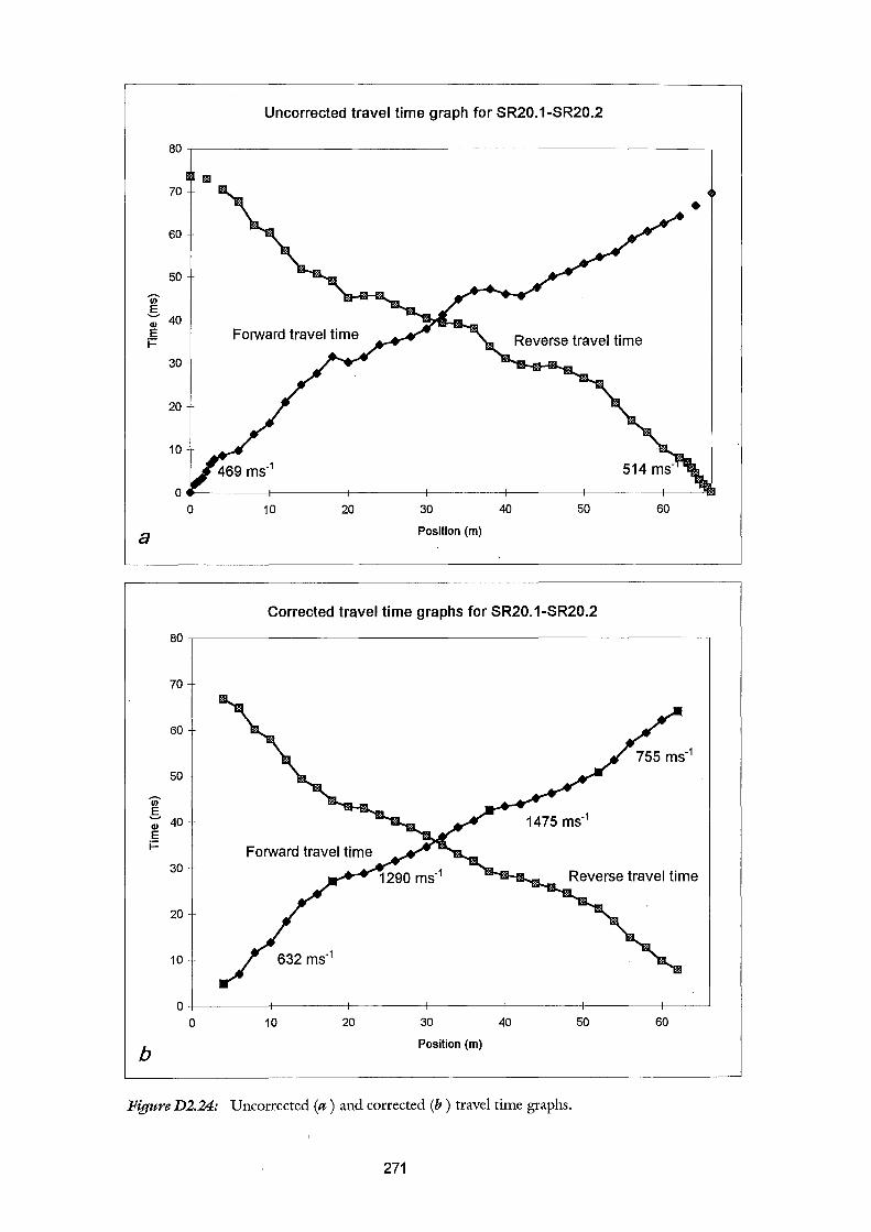
Uncorrected travel time graph for SR20.1-SR20.2
80
1111 70
60
50
Iii' g
40 Q)
E i=
30
20
10
0 0 10 20 30 40 50 60
a Position (m)
Corrected travel time graphs for SR20.1-SR20.2
80
70
60
50
Iii' g
40 Q)
E i=
30
20
10
0 0 10 20 30 40 50 60
b Position (m)
Figure D2.24: Uncorrected (a) and corrected (b) travel time graphs.
271
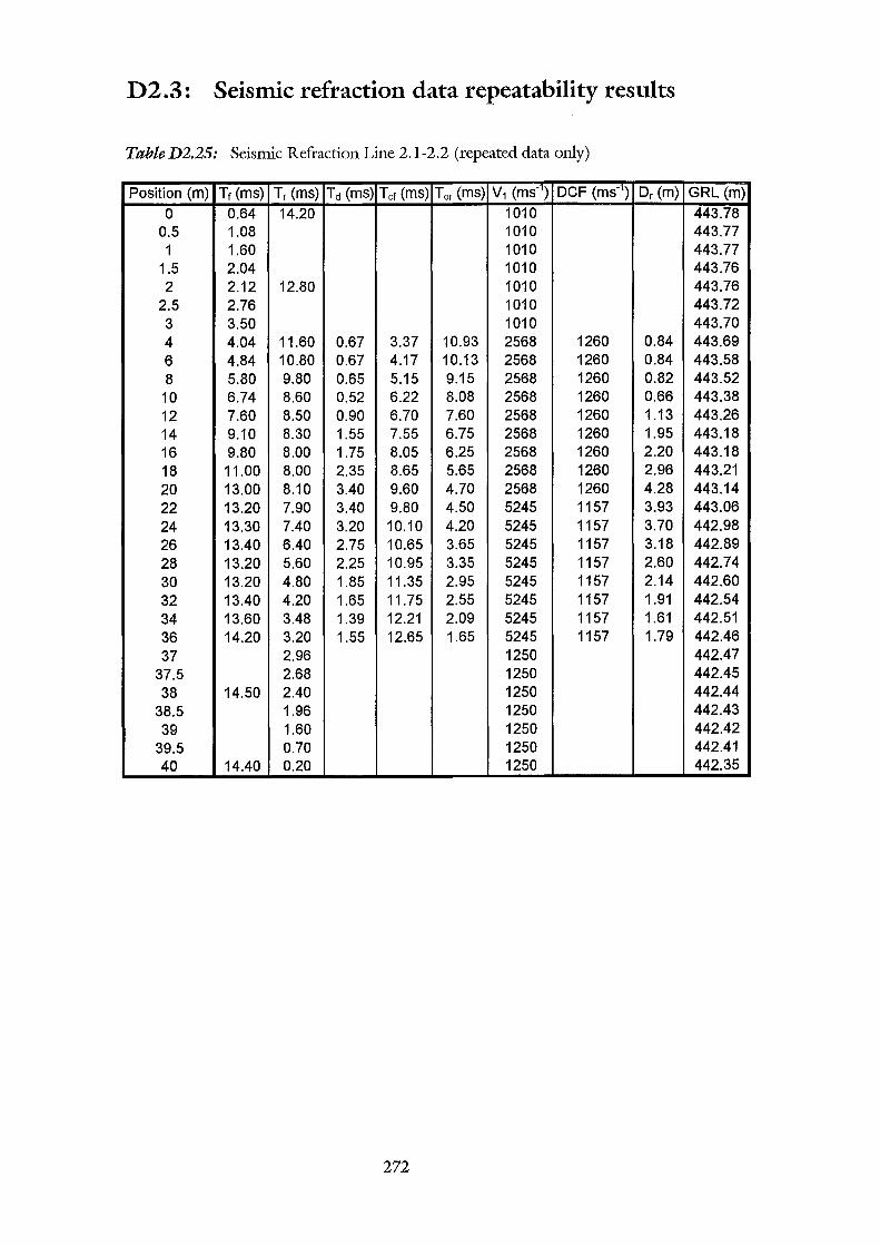
D2.3: Seismic refraction data repeatability results
TableD2.25: Seismic Refraction Line 2.1-2.2 (repeated data only)
Position (m) Tr (ms) Tr (ms) Td (ms) Tor (ms) Tor (ms) v1 (ms-1) DCF (ms-1
) Dr (m) GRL (m)
0 0.64 14.20 1010 443.78 0.5 1.08 1010 443.77 1 1.60 1010 443.77
1.5 2.04 1010 443.76 2 2.12 12.80 1010 443.76
2.5 2.76 1010 443.72 3 3.50 1010 443.70 4 4.04 11.60 0.67 3.37 10.93 2568 1260 0.84 443.69 6 4.84 10.80 0.67 4.17 10.13 2568 1260 0.84 443.58 8 5.80 9.80 0.65 5.15 9.15 2568 1260 0.82 443.52 10 6.74 8.60 0.52 6.22 8.08 2568 1260 0.66 443.38 12 7.60 8.50 0.90 6.70 7.60 2568 1260 1.13 443.26 14 9.10 8.30 1.55 7.55 6.75 2568 1260 1.95 443.18 16 9.80 8.00 1.75 8.05 6.25 2568 1260 2.20 443.18 18 11.00 8.00 2.35 8.65 5.65 2568 1260 2.96 443.21 20 13.00 8.10 3.40 9.60 4.70 2568 1260 4.28 443.14 22 13.20 7.90 3.40 9.80 4.50 5245 1157 3.93 443.06 24 13.30 7.40 3.20 10.10 4.20 5245 1157 3.70 442.98 26 13.40 6.40 2.75 10.65 3.65 5245 1157 3.18 442.89 28 13.20 5.60 2.25 10.95 3.35 5245 1157 2.60 442.74 30 13.20 4.80 1.85 11.35 2.95 5245 1157 2.14 442.60 32 13.40 4.20 1.65 11.75 2.55 5245 1157 1.91 442.54 34 13.60 3.48 1.39 12.21 2.09 5245 1157 1.61 442.51 36 14.20 3.20 1.55 12.65 1.65 5245 1157 1.79 442.46 37 2.96 1250 442.47
37.5 2.68 1250 442.45 38 14.50 2.40 1250 442.44
38.5 1.96 1250 442.43 39 1.60 1250 442.42
39.5 0.70 1250 442.41 40 14.40 0.20 1250 442.35
272
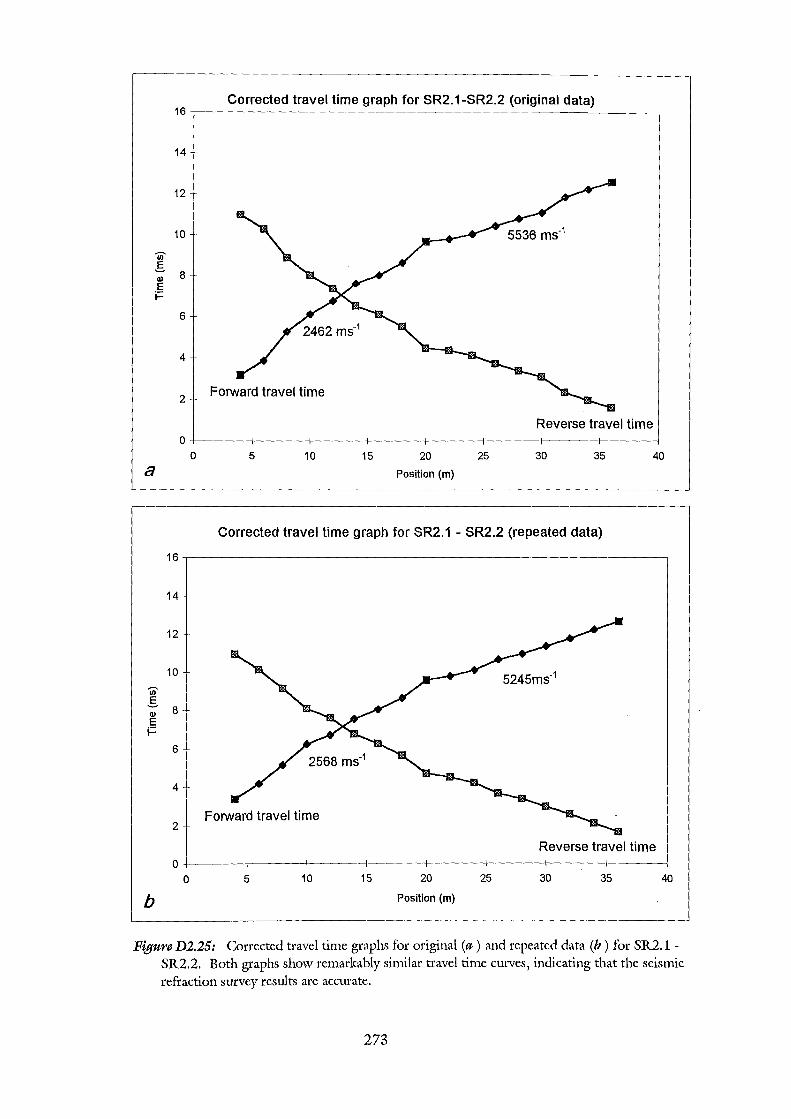
16
14
12
10
Ul ..§,
8 Q)
E i=
6
4
2
0 0
a
16
14
12
10
Ul ..§,
8 Q)
E i=
6
4
2
0 0
b
Corrected travel time graph for SR2.1-SR2.2 (original data)
5 10 15 20
Position (m)
Reverse travel time
25 30 35
Corrected travel time graph for SR2.1 - SR2.2 (repeated data)
40
Reverse travel time
5 10 15 20
Position (m)
25 30 35 40
Figure D2.25: Corrected travel time graphs for original (a) and repeated data (b) for SR2.l -SR2.2. Both graphs show remarkably similar travel time curves, indicating that the seismic refraction survey results are accurate.
273
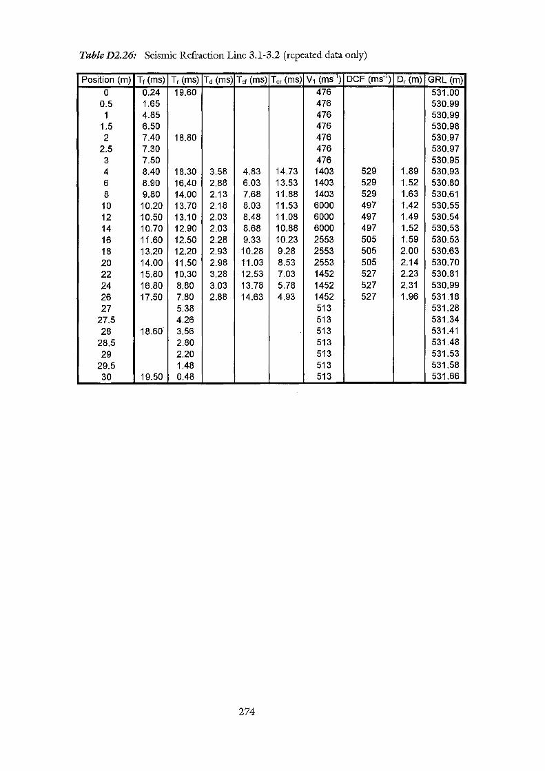
TableD2.26: Seismic Refraction Line 3.1-3.2 (repeated data only)
Position (m) Tr (ms) Tr (ms) Td (ms) Tct (ms) Tcr (ms) V1 (msC1) DCF (ms-1) Dr (m) GRL (m)
0 0.24 19.60 476 531.00 0.5 1.65 476 530.99 1 4.85 476 530.99
1.5 6.50 476 530.98 2 7.40 18.80 476 530.97
2.5 7.30 476 530.97 3 7.50 476 530.95 4 8.40 18.30 3.58 4.83 14.73 1403 529 1.89 530.93 6 8.90 16.40 2.88 6.03 13.53 1403 529 1.52 530.80 8 9.80 14.00 2.13 7.68 11.88 1403 529 1.63 530.61
10 10.20 13.70 2.18 8.03 11.53 6000 497 1.42 530.55 12 10.50 13.10 2.03 8.48 11.08 6000 497 1.49 530.54 14 10.70 12.90 2.03 8.68 10.88 6000 497 1.52 530.53 16 11.60 12.50 2.28 9.33 10.23 2553 505 1.59 530.53 18 13.20 12.20 2.93 10.28 9.28 2553 505 2.00 530.63 20 14.00 11.50 2.98 11.03 8.53 2553 505 2.14 530.70 22 15.80 10.30 3.28 12.53 7.03 1452 527 2.23 530.81 24 16.80 8.80 3.03 13.78 5.78 1452 527 2.31 530.99 26 17.50 7.80 2.88 14.63 4.93 1452 527 1.96 531.18 27 5.38 513 531.28
27.5 4.26 513 531.34 28 18.60 3.56 513 531.41
28.5 2.80 513 531.48 29 2.20 513 531.53
29.5 1.48 513 531.58 30 19.50 0.48 513 531.66
274
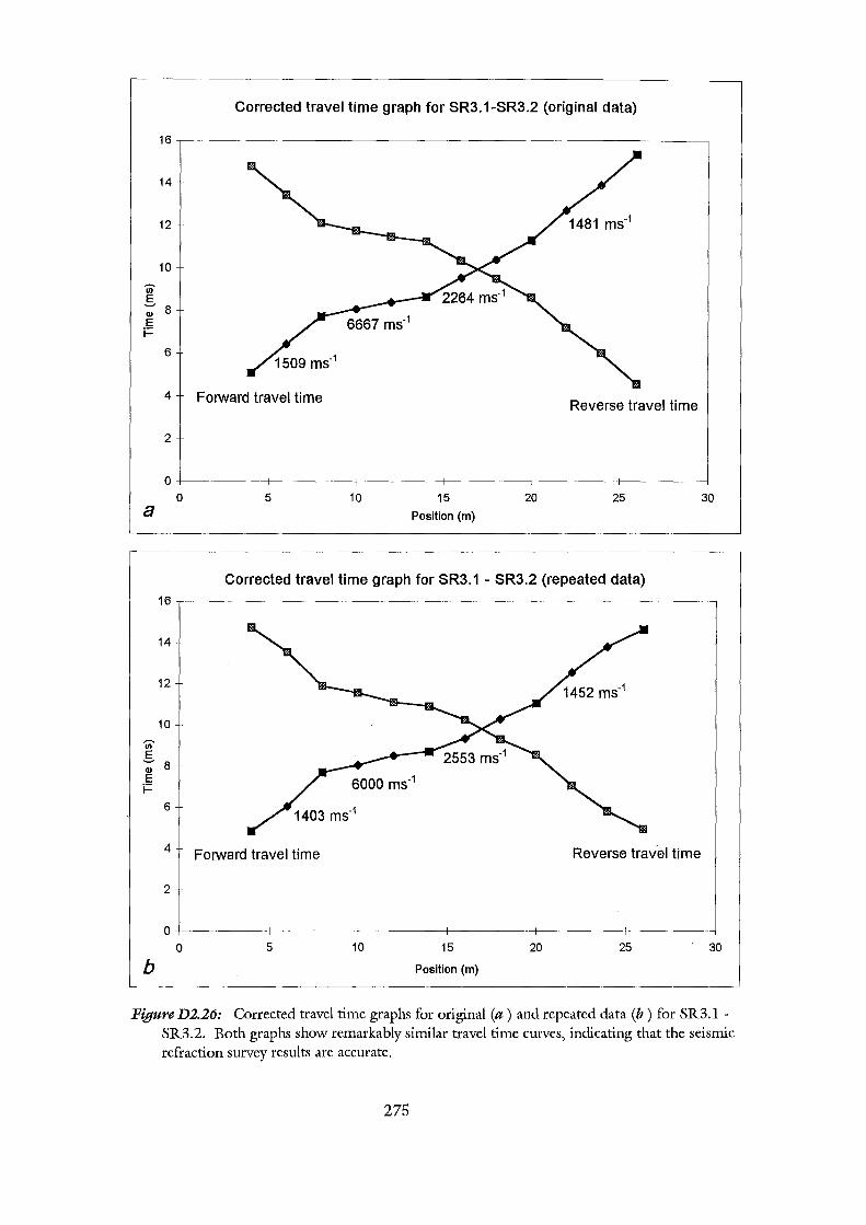
(j) §. Q)
E i=
a
(j) §. Q)
E i=
b
Corrected travel time graph for SR3.1-SR3.2 (original data)
16
14
12
10
8
6
4 Forward travel time Reverse travel time
2
0+-~~~~+---------+---------+---------+---------4-------~
0
16
14
12
10
8
6
4
2
5 10 15
Position (m)
20 25
Corrected travel time graph for SR3.1 - SR3.2 (repeated data)
Forward travel time Reverse travel time
30
0+---------~--~----~---------r---------+---------+--------~
0 5 10 15
Position (m)
20 25 30
Figure D2.26: Corrected travel time graphs for original (a) and repeated data (b) for SR3.lSR3.2. Both graphs show remarkably similar travel time curves, indicating that the seismic refraction survey results are accurate.
275
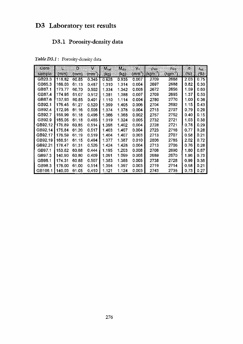
D3 Laboratory test results
D3 .l Porosity-density data
Table D3.1 : Porosity-density data
GB23 .85 0. 0.928 2709 2688 GB65.3 166.03 61.13 0.487 1.310 1.314 0.004 2697 2688 0.30 GB87.1 173.77 60.70 0.502 1.334 1.342 0.008 2672 2656 0.60 GB87.4 174.95 61.07 0.512 1.381 1.388 0.007 2709 2695 0.50 GB87.6 137.93 60.85 0.401 1.110 1.114 0.004 2780 2770 0.36 GB92.1 176.45 61.27 0.520 1.399 1.405 0.006 2704 2692 0.43 GB92.4 172.95 61.16 0.508 1.374 1.378 0.004 2715 2707 0.79 0.29 GB92.7 168.99 61.18 0.496 1.366 1.368 0.002 2757 2752 0.40 0.15 GB92.9 165.05 61.18 0.485 1.319 1.324 0.005 2732 2721 1.03 0.38
GB92.12 176.89 60.85 0.514 1.398 1.402 0.004 2728 2721 0.78 0.29 GB92.14 175.84 61.20 0.517 1.403 1.407 0.004 2723 2716 0.77 0.28 GB92.17 176.59 61.19 0.519 1.404 1.407 0.003 2713 2707 0.58 0.21 GB92.19 168.51 61.15 0.494 1.377 1.387 0.010 2806 2785 2.02 0.72 GB92.21 178.47 61.31 0.526 1.424 1.428 0.004 2713 2706 0.76 0.28 GB97.1 153.82 60.68 0.444 1.195 1.203 0.008 2708 2690 1.80 0.67 GB97.3 140.90 60.80 0.409 1.091 1.099 0.008 2689 2670 1.96 0.73 G898.1 174.31 60.88 0.507 1.383 1.388 0.005 2738 2728 0.99 0.36 G898.3 176.00 61.00 0.514 1.394 1.397 0.003 2719 2714 0.58 0.21
GB106.1 140.03 61.05 0.410 1.121 1.124 0.003 2743 2735 0.73 0.27
276
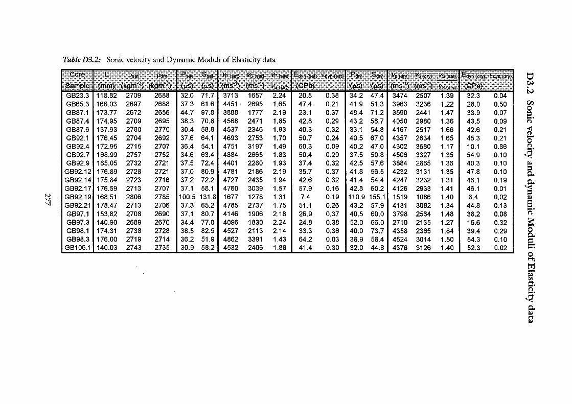
Table D3.2: Sonic velocity and Dynamic Moduli of Elasticity data
tJ eN
GB23.3 118.82 2709 2688 32.0 71.7 3713 1657 2.24 20.5 0.38 34.2 47.4 3474 2507 1.39 32.3 0.04 ~
GB65.3 166.03 2697 2688 37.3 61.6 4451. 2695 1.65 47.4 0.21 41.9 51.3 3963 3236 1.22 28.0 0.50 ('-) 0
GB87.1 173.77 2672 2656 44.7 97.8 3888 1777 2.19 23.1 0.37 48.4 71.2 3590 2441 1.47 33.9 0.07 e. GB87.4 174.95 2709 2695 38.3 70.8 4568 2471 1.85 42.8 0.29 43.2 58.7 4050 2980 1.36 43.5 0.09 n GB87.6 137.93 2780 2770 30.4 58.8 4537 2346 1.93 40.3 0.32 33.1 54.8 4167 2517 1.66 42.6 0.21 ~ GB92.1 176.45 2704 2692 37.6 64.1 4693 2753 1.70 50.7 0.24 40.5 67.0 4357 2634 1.65 45.3 0.21 0 GB92.4 172.95 2715 2707 36.4 54.1 4751 3197 1.49 60.3 0.09 40.2 47.0 4302 3680 1.17 10.1 0.86 n ..... GB92.7 168.99 2757 2752 34.6 63.4 4884 2665 1.83 50.4 0.29 37.5 50.8 4506 3327 1.35 54.9 0.10 ~ GB92.9 165.05 2732 2721 37.5 72.4 4401 2280 1.93 37.4 0.32 42.5 57.6 3884 2865 1.36 40.3 0.10 ~
GB92.12 176.89 2728 2721 37.0 80.9 4781 2186 2.19 35.7 0.37 41.8 56.5 4232 3131 1.35 47.8 0.10 8. GB92.14 175.84 2723 2716 37.2 72.2 4727 2435 1.94 42.6 0.32 41.4 54.4 4247 3232 1.31 46.1 0.19
~ GB92.17 176.59 2713 2707 37.1 58.1 4760 3039 1.57 57.9 0.16 42.8 60.2 4126 2933 1.41 46.1 0.01
= N I GB92.19 168.51 2806 2785 100.5 131.8 1677 1278 1.31 7.4 0.19 110.9 155.1 1519 1086 1.40 6.4 0.02 ~ '-l 9 '-l GB92.21 178.47 2713 2706 37.3 65.2 4785 2737 1.75 51.1 0.26 43.2 57.9 4131 3082 1.34 44.8 0.13 ..... GB97.1 153.82 2708 2690 37.1 80.7 4146 1906 2.18 26.9 0.37 40.5 60.0 3798 2564 1.48 38.2 0.08 n GB97.3 140.90 2689 2670 34.4 77.0 4096 1830 2.24 24.8 0.38 52.0 66.0 2710 2135 1.27 16.6 0.32 ~ GB98.1 174.31 2738 2728 38.5 82.5 4527 2113 2.14 33.3 0.36 40.0 73.7 4358 2365 1.84 39.4 0.29 GB98.3 176.00 2719 2714 36.2 51.9 4862 3391 1.43 64.2 0.03 38.9 58.4 4524 3014 1.50 54.3 0.10 ~
GB106.1 140.03 2743 2735 30.9 58.2 4532 2406 1.88 41.4 0.30 32.0 44.8 4376 3126 1.40 52.3 0.02 =:-: 0 ~
trl -~ C'l:l
~-n ..... ~ ~ ~ n-~
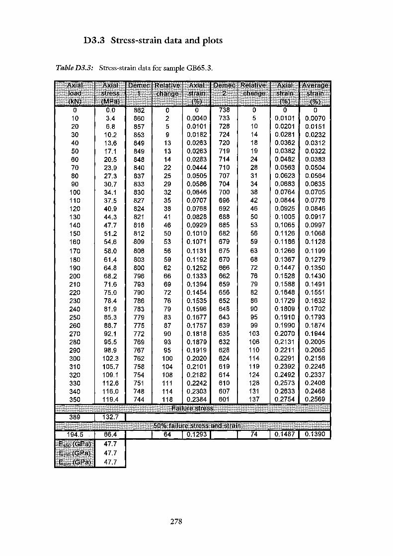
D3.3 Stress-strain data and plots
TableD3.3: Stress-strain data for sample GB65.3.
20 30 40 50 60 70 80 90
100 110 120 130 140 150 160 170 180 190 200 210 220 230 240 250 260 270 280 290 300 310 320 330 340 350
0.0 3.4 6.8 10.2 13.6 17.1 20.5 23.9 27.3 30.7 34.1 37.5 40.9 44.3 47.7 51.2 54.6 58.0 61.4 64.8 68.2 71.6 75.0 78.4 81.9 85.3 88.7 92.1 95.5 98.9 102.3 105.7 109.1 112.6 116.0 119.4
47.7 47.7
860 857 853 849 849 848 840 837 833 830 827 824 821 816 812 809 806 803 800 796 793 790 786 783 779 775 772 769 767 762 758 754 751 748 744
0 2 0.0040 733 5 0.0101 728 9 0.0182 724
13 0.0263 720 13 0.0263 719 14 0.0283 714 22 0.0444 710 25 0.0505 707 29 0.0586 704 32 0.0646 700 35 0.0707 696 38 0.0768 692 41 0.0828 688 46 0.0929 685 50 0.1010 682 53 0.1071 679 56 0.1131 675 59 0.1192 670 62 0.1252 666 66 0.1333 662 69 0.1394 659 72 0.1454 656 76 0.1535 652 79 0.1596 648 83 0.1677 643 87 0.1757 639 90 0.1818 635 93 0.1879 632 95 0.1919 628
624 619 614 610 607 601
278
0 0 0 5 0.0101 0.0070 10 0.0201 0.0151 14 0.0281 0.0232 18 0.0362 0.0312 19 0.0382 0.0322 24 0.0482 0.0383 28 0.0563 0.0504 31 0.0623 0.0564 34 0.0683 0.0635 38 0.0764 0.0705 42 0.0844 0.0776 46 0.0925 0.0846 50 0.1005 0.0917 53 0.1065 0.0997 56 0.1126 0.1068 59 0.1186 0.1128 63 0.1266 0.1199 68 0.1367 0.1279 72 0.1447 0.1350 76 0.1528 0.1430 79 0.1588 0.1491 82 0.1648 0.1551 86 0.1729 0.1632 90 0.1809 0.1702 95 0.1910 0.1793 99 0.1990 0.1874
103 0.2070 0.1944 106 0.2131 0.2005 110 0.2211 0.2065 114 0.2291 0.2156 119 0.2392 0.2246 124 0.2492 0.2337
0.2573 0.2408 0.2633 0.2468 0.2754 0.2569
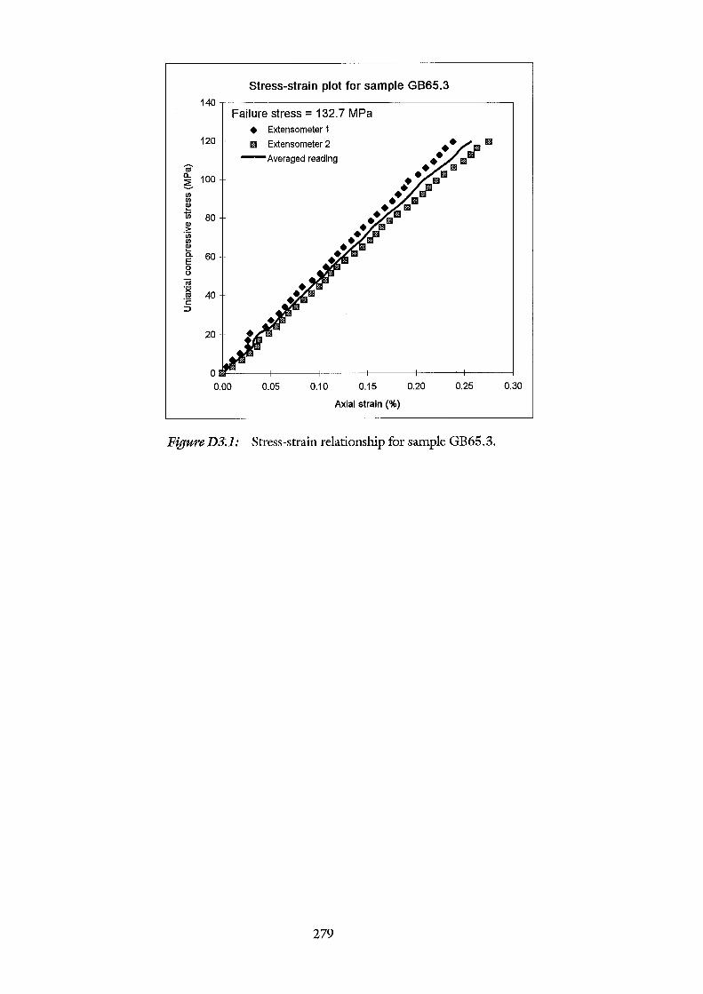
Stress-strain plot for sample GB65.3 140.--------------------------------------,
Failure stress= 132.7 MPa • Extensometer 1
120 i!ll Extensometer 2
m-n. 6 100
::! f!! 1ii 80 ~
"iii Ul f!! E" so 0 0
iii -~ 40 ·c: ::J
20
-Averaged reading
OmF~---+------~-----4------~------~----~
0.00 0.05 0.10 0.15 0.20 0.25 0.30
Axial strain (%)
Figure D3.1: Stress-strain relationship for sample GB65.3.
279
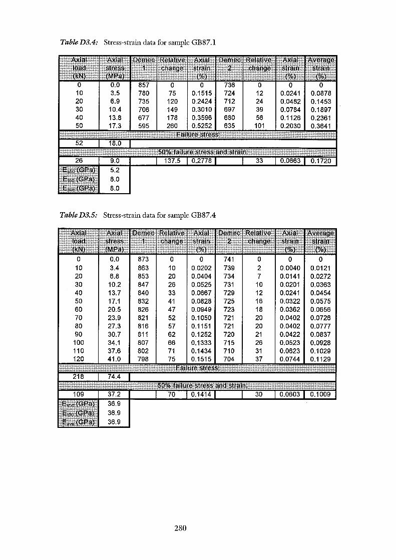
TableD3.4: Stress-strain data for sample GB87.l
0 10 20 30 40 50
8.0 8.0
780 735 706 677 595
75 0.1515 120 0.2424 149 0.3010 178 0.3596 260 0.5252
Table D3.5: Stress-strain data for sample GB87.4
10 20 30 40 50 60 70 80 90
100 110 120
3.4 6.8
10.2 13.7 17.1 20.5 23.9 27.3 30.7 34.1 37.6 41.0
36.9 36.9
863 10 0.0202 853 20 0.0404 847 26 0.0525 840 33 0.0667 832 41 0.0828 826 47 0.0949 821 52 0.1050 816 57 0.1151 811 62 0.1252 807 0.1333 802 0.1434 798 0.1515
280
724 12 0.0241 712 24 0.0482 697 39 0.0784 680 56 0.1126 635 101 0.2030
0 739 2 0.0040 0.0121 734 7 0.0141 0.0272 731 10 0.0201 0.0363 729 12 0.0241 0.0454 725 16 0.0322 0.0575 723 18 0.0362 0.0656 721 20 0.0402 0.0726 721 20 0.0402 0.0777
21 0.0422 0.0837 26 0.0523 31 0.0623 37 0.0744
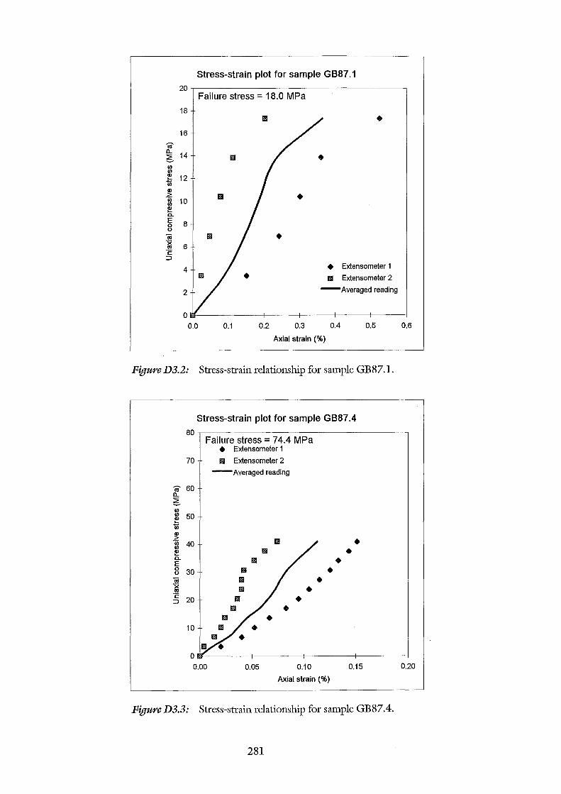
Stress-strain plot for sample GB87 .1
20 Failure stress = 18.0 MPa
18 1111 •
16
-m a.
14 6 • Vl Vl ~ 12 Ui Q)
-~ • Vl 10 Vl Q) .... a. E 8 0 0
iii 1111 • ·x 6 111 ·c:
::J
4 • Extensometer 1 1111 • 1!11 Extensometer 2
2 -Averaged reading
0 0.0 0.1 0.2 0.3 0.4 0.5 0.6
Axial strain(%)
FigureD3.2: Stress-strain relationship for sample GB87.l.
Stress-strain plot for sample G887 .4
80 Failure stress= 74.4 MPa
• Extensometer 1
70 II Extensometer 2
-Averaged reading
-m 60 a. 6 Vl Vl 50 IE Ui Q)
.~ II • Vl 40 Vl ~ 1!11 • a. 1111 • E 0 30 m • 0
iii llll • ')( lill • 111 ·c:
20 m • ::J m •
1!11
10
0
0.00 0.05 0.10 0.15 0.20
Axial strain (%)
Figure D3.3: Stress-strain relationship for sample GB87.4.
281
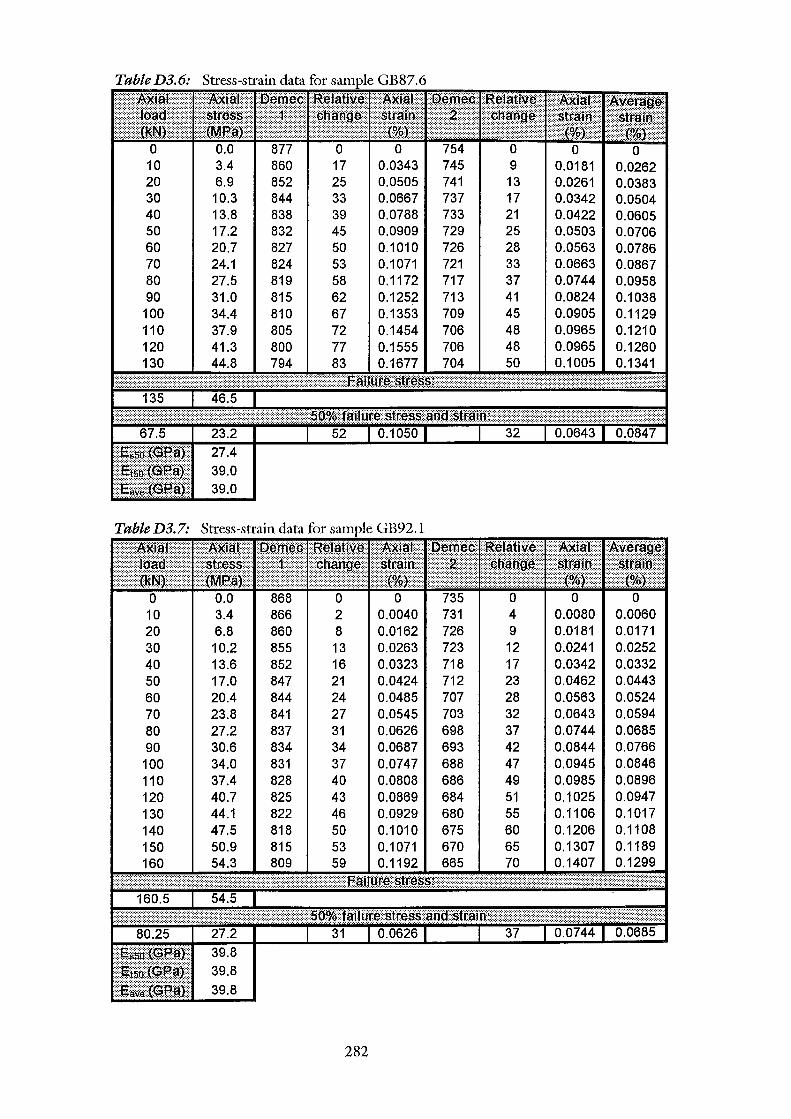
20 30 40 50 60 70 80 90
100 110 120 130
20 30 40 50 60 70 80 90
100 110 120 130 140
0.0 3.4 6.9
10.3 13.8 17.2 20.7 24.1 27.5 31.0 34.4 37.9 41.3 44.8
39.0
0.0 3.4 6.8 10.2 13.6 17.0 20.4 23.8 27.2
39.8 39.8
877 0 860 17 852 25 844 33 838 39 832 45 827 50 824 53 819 58 815 62 810 67 805 72 800 77 794 83
868 866 860 8 855 13 852 16 847 21 844 24 841 27 837 31 834 34 831 37 828 40 825 43 822 46 818 50 815 53 809 59
282
0 0 0.0343 745 9 0.0181 0.0262 0.0505 741 13 0.0261 0.0383 0.0667 737 17 0.0342 0.0504 0.0788 733 21 0.0422 0.0605 0.0909 729 25 0.0503 0.0706 0.1010 726 28 0.0563 0.0786 0.1071 721 33 0.0663 0.0867 0.1172 717 37 0.0744 0.0958 0.1252 713 41 0.0824 0.1038 0.1353 709 45 0.0905 0.1129 0.1454 706 48 0.0965 0.1210 0.1555 706 48 0.0965 0.1260 0.1677 704 50 0.1005 0.1341
0 0.0040 731 4 0.0080 0.0060 0.0162 726 9 0.0181 0.0171 0.0263 723 12 0.0241 0.0252 0.0323 718 17 0.0342 0.0332 0.0424 712 23 0.0462 0.0443 0.0485 707 28 0.0563 0.0524 0.0545 703 32 0.0643 0.0594 0.0626 698 37 0.0744 0.0685 0.0687 693 42 0.0844 0.0766 0.0747 688 47 0.0945 0.0846 0.0808 686 49 0.0985 0.0896 0.0869 684 51 0.1025 0.0947 0.0929 680 0.1106 0.1017 0.1010 675 0.1206 0.1108 0.1071 0.1307 0.1189 0.1192 0.1407 0.1299
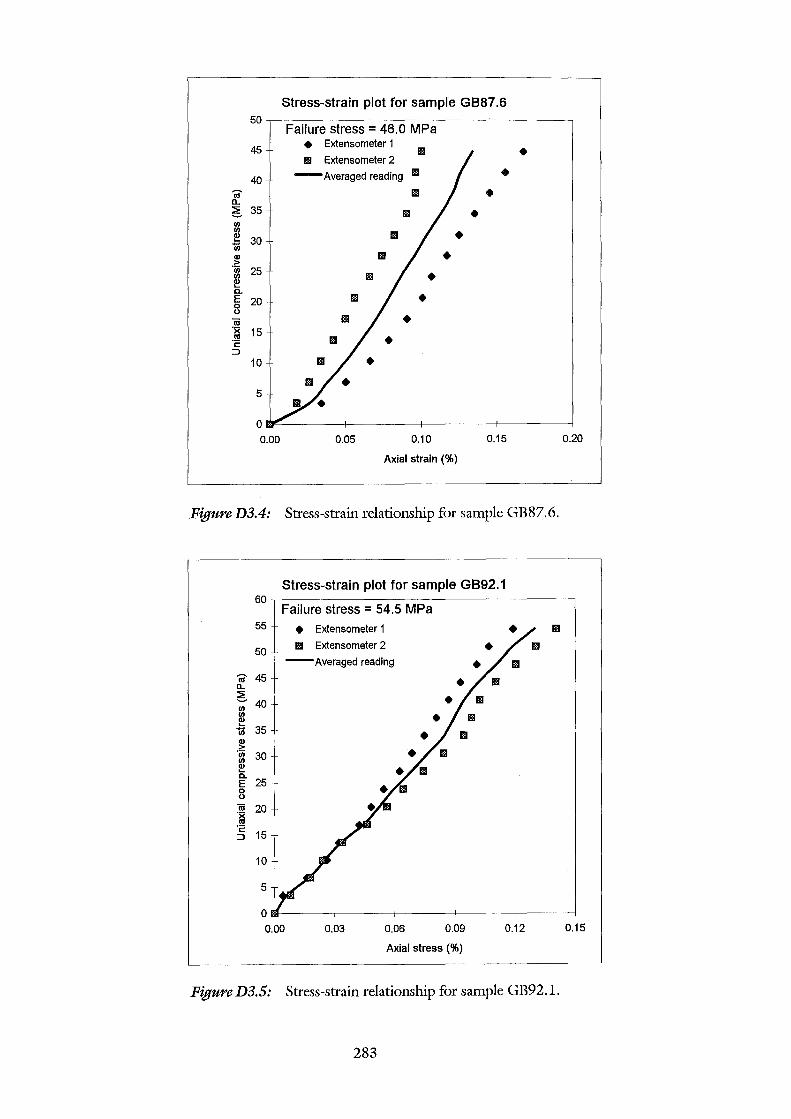
Stress-strain plot for sample GB87.6 50
Failure stress = 46.0 MPa
45 • Extensometer 1 1111 • 11!1 Extensometer 2
40 -Averaged reading 1111 • m 1111 • a. ~ 35 1111 • (/) (/)
Iii • ~ 30 (ij CD 1111 • >
"iii 25 (/) Iii • ~ a. E 20 11!1 • 0 0
(ij IIIII • ·x 15 I'll ·;:: 11!1 • :J 10
5
0 0.00 0.05 0.10 0.15 0.20
Axial strain(%)
Figure D3.4: Stress-strain relationship for sample GB87.6.
Stress-strain plot for sample GB92.1 60.--------------------------------------,
55
50
m45 a. 6 40 gj ~ (ij 35 g! -~ 30 ~ a. E 25 0 0
m 20 -~ ·;:: :J 15
10
5
Failure stress = 54.5 MPa • Extensometer 1
1111 Extensometer 2
-Averaged reading
Ill
0111-------+-------~------~----~------~
0.00 0.03 0.06 0.09 0.12 0.15
Axial stress(%)
FigureD3.5: Stress-strain relationship for sample GB92.l.
283
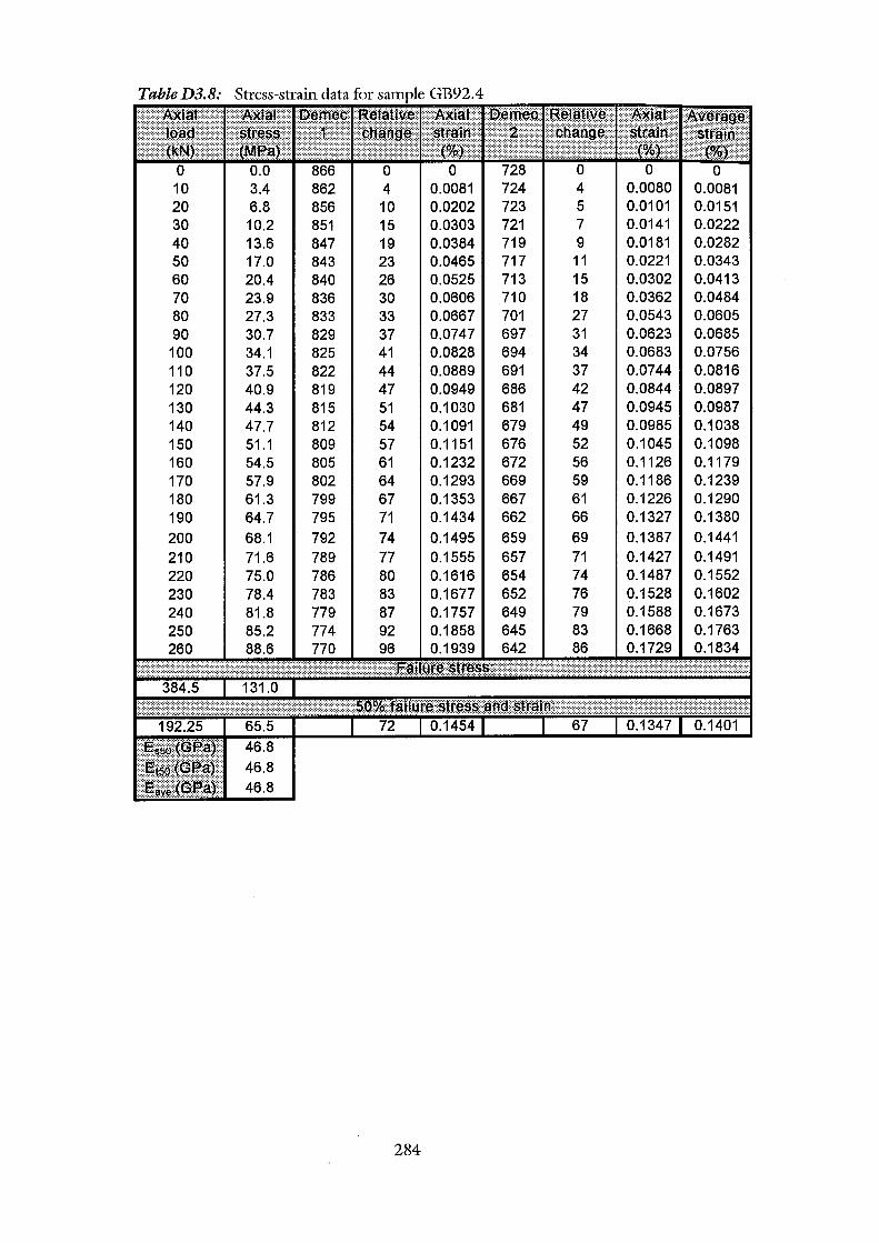
10 20 30 40 50 60 70 80 90
100 110 120 130 140 150 160 170 180 190 200 210 220 230 240 250 260
3.4 6.8
10.2 13.6 17.0 20.4 23.9 27.3 30.7 34.1 37.5 40.9 44.3 47.7 51.1 54.5 57.9 61.3 64.7 68.1 71.6 75.0 78.4 81.8 85.2 88.6
46.8 46.8
862 4 856 10 851 15 847 19 843 23 840 26 836 30 833 33 829 37 825 41 822 44 819 47 815 51 812 54 809 57 805 61 802 64 799 67 795 71 792 74 789 77 786 80 783 83 779 87 774 92 770 96
284
0 728 0 0.0081 724 0.0080 0.0081 0.0202 723 0.0101 0.0151 0.0303 721 0.0141 0.0222 0.0384 719 9 0.0181 0.0282 0.0465 717 11 0.0221 0.0343 0.0525 713 15 0.0302 0.0413 0.0606 710 18 0.0362 0.0484 0.0667 701 27 0.0543 0.0605 0.0747 697 31 0.0623 0.0685 0.0828 694 34 0.0683 0.0756 0.0889 691 37 0.0744 0.0816 0.0949 686 42 0.0844 0.0897 0.1030 681 47 0.0945 0.0987 0.1091 679 49 0.0985 0.1038 0.1151 676 52 0.1045 0.1098 0.1232 672 56 0.1126 0.1179 0.1293 669 59 0.1186 0.1239 0.1353 667 61 0.1226 0.1290 0.1434 662 66 0.1327 0.1380 0.1495 659 69 0.1387 0.1441 0.1555 657 71 0.1427 0.1491 0.1616 654 74 0.1487 0.1552 0.1677 652 76 0.1528 0.1602 0.1757 649 79 0.1588 0.1673 0.1858 645 83 0.1668 0.1763 0.1939 642 86 0.1729 0.1834
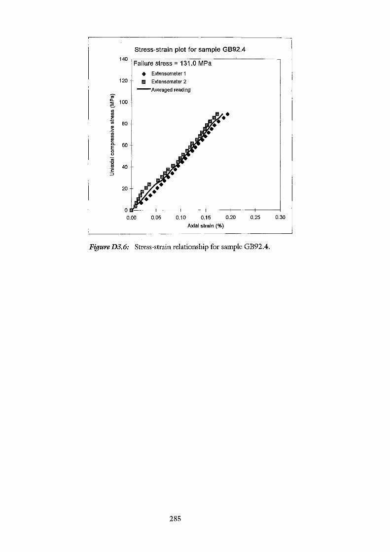
Stress-strain plot for sample GB92.4 140.---------------------------------------
Failure stress = 131.0 MPa
• Extensometer 1
120 IIIII Extensometer 2
"' a. 5 100 Ul
~ 1ii 80 ~
"iii Ul Q)
E.. 60 E 0 0
iii -~ ·c: ::J
40
20
-Averaged reading
0~~--~----~------+-----~-----+----~
0.00 0.05 0.10 0.15 0.20 0.25 0.30
Axial strain (%)
Figure D3. 6: Stress-strain relationship for sample GB92.4.
285
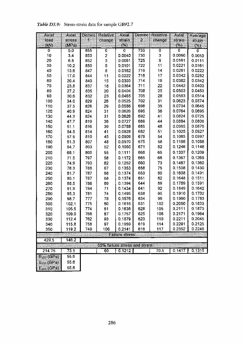
TableD3.9: Stress-strain data for sample GB92.7
10 20 30 40 50 60 70 80 90
100 110 120 130 140 150 160 170 180 190 200 210 220 230 240 250 260 270 280 290 300 310 320 330 340 350
0.0 3.4 6.8 10.2 13.6 17.0 20.4 23.8 27.2 30.6 34.0 37.5 40.9 44.3 47.7 51.1 54.5 57.9 61.3 64.7 68.1 71.5 74.9 78.3 81.7 85.1 88.5 91.9 95.3 98.7
102.1 105.5 109.0 112.4 115.8 119.2
55.6 55.6
0 853 2 0.0040 852 3 0.0061 850 5 0.0101 847 8 0.0162 844 11 0.0222 840 15 0.0303 837 18 0.0364 835 20 0.0404 832 23 0.0465 829 26 0.0525 826 29 0.0586 824 31 0.0626 824 31 0.0626 819 36 0.0727 816 39 0.0788 814 41 0.0828 810 45 0.0909 807 48 0.0970 803 52 0.1050 800 55 0.1111 797 58 0.1172 793 62 0.1252 788 67 0.1353 787 68 0.1374 787 68 0.1374 786 69 0.1394 784 71 0.1434 781 74 0.1495 777 78 0.1576 775 80 0.1616 774 81 0.1636 768 87 0.1757 762 93 0.1879 758 97 0.1959 749 106 0.2141
286
733 0 0 730 3 0.0060 0.0050 725 8 0.0161 0.0111 722 11 0.0221 0.0161 719 14 0.0281 0.0222 716 17 0.0342 0.0282 714 19 0.0382 0.0342 711 22 0.0442 0.0403 708 25 0.0503 0.0453 705 28 0.0563 0.0514 702 31 0.0623 0.0574 698 35 0.0704 0.0645 695 38 0.0764 0.0695 692 41 0.0824 0.0725 689 44 0.0884 0.0806 685 48 0.0965 0.0876 682 51 0.1025 0.0927 679 54 0.1085 0.0997 675 58 0.1166 0.1068 671 62 0.1246 0.1148 668 65 0.1307 0.1209 665 68 0.1367 0.1269 660 73 0.1467 0.1360 658 75 0.1508 0.1430 653 80 0.1608 0.1491 651 82 0.1648 0.1511 644 89 0.1789 0.1591 641 92 0.1849 0.1642 638 95 0.1910 0.1702 634 99 0.1990 0.1783 631 102 0.2050 0.1833 628 105 0.2111 0.1873 625 108 0.2171 0.1964 623 110 0.2211 0.2045 619 114 0.2291 0.2125 616 117 0.2352 0.2246
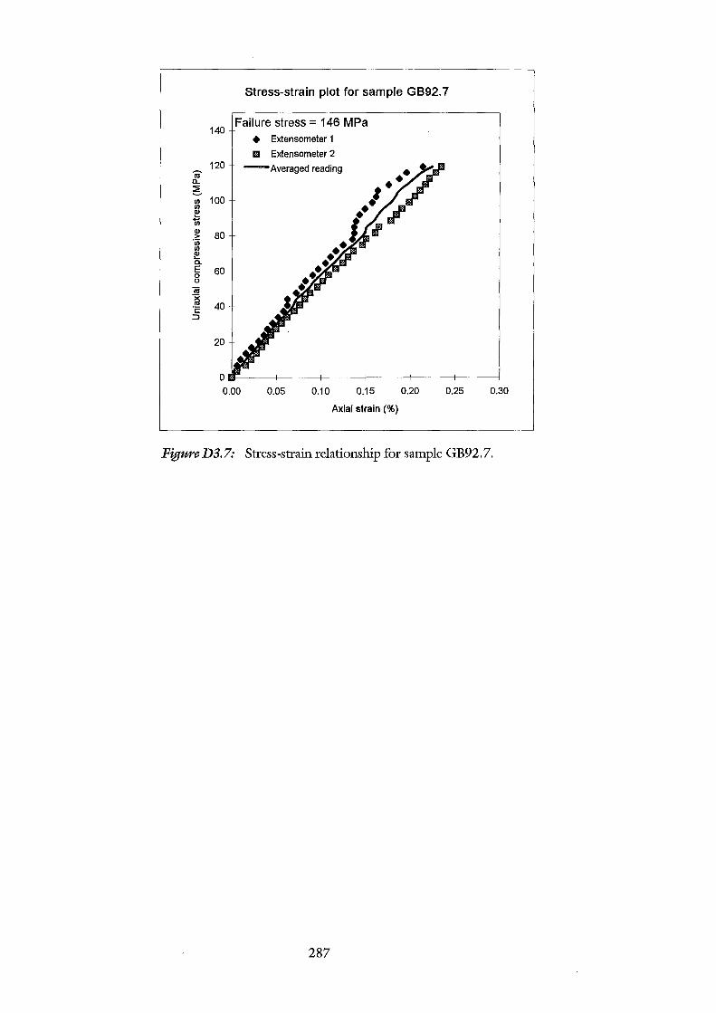
Stress-strain plot for sample GB92. 7
Failure stress= 146 MPa 140
120
• Extensometer 1
Ill Extensometer 2
-Averaged reading
"' 100 ~ iii Q)
-~ gJ ~ D. E 0 0
80
60
40
20
om=----~-----+----~------+-----4-----~
0.00 0.05 0.10 0.15 0.20 0.25 0.30
Axial strain (%)
Figure D3. 7: Stress-strain relationship for sample GB92. 7.
287
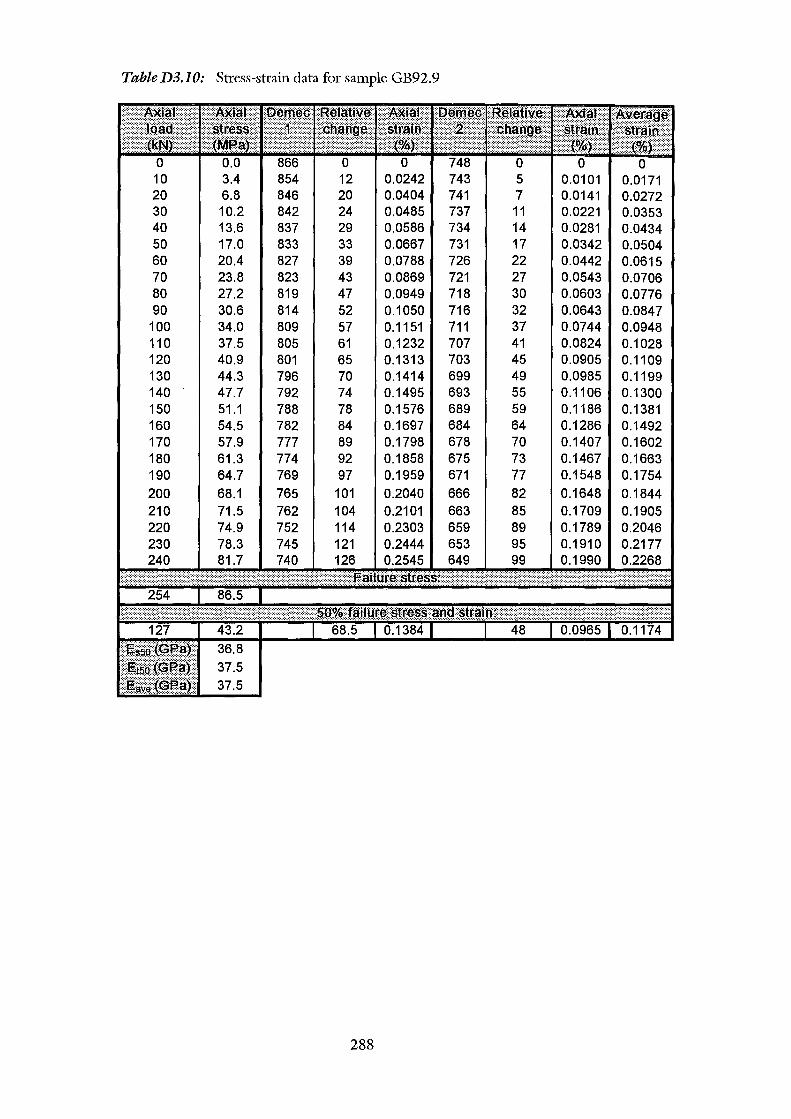
Table D3.10: Stress-strain data for sample GB92.9
0 0 10 3.4 854 12 0.0242 743 5 0.0101 0.0171 20 6.8 846 20 0.0404 741 7 0.0141 0.0272 30 10.2 842 24 0.0485 737 11 0.0221 0.0353 40 13.6 837 29 0.0586 734 14 0.0281 0.0434 50 17.0 833 33 0.0667 731 17 0.0342 0.0504 60 20.4 827 39 0.0788 726 22 0.0442 0.0615 70 23.8 823 43 0.0869 721 27 0.0543 0.0706 80 27.2 819 47 0.0949 718 30 0.0603 0.0776 90 30.6 814 52 0.1050 716 32 0.0643 0.0847
100 34.0 809 57 0.1151 711 37 0.0744 0.0948 110 37.5 805 61 0.1232 707 41 0.0824 0.1028 120 40.9 801 65 0.1313 703 45 0.0905 0.1109 130 44.3 796 70 0.1414 699 49 0.0985 0.1199 140 47.7 792 74 0.1495 693 55 0.1106 0.1300 150 51.1 788 78 0.1576 689 59 0.1186 0.1381 160 54.5 782 84 0.1697 684 64 0.1286 0.1492 170 57.9 777 89 0.1798 678 70 0.1407 0.1602 180 61.3 774 92 0.1858 675 73 0.1467 0.1663 190 64.7 769 97 0.1959 671 77 0.1548 0.1754 200 68.1 765 101 0.2040 666 82 0.1648 0.1844 210 71.5 762 104 0.2101 663 85 0.1709 0.1905 220 74.9 752 114 0.2303 659 89 0.1789 0.2046 230 78.3 745 121 0.2444 653 95 0.1910 0.2177 240 81.7 740 126 0.2545 649 99 0.1990 0.2268
288
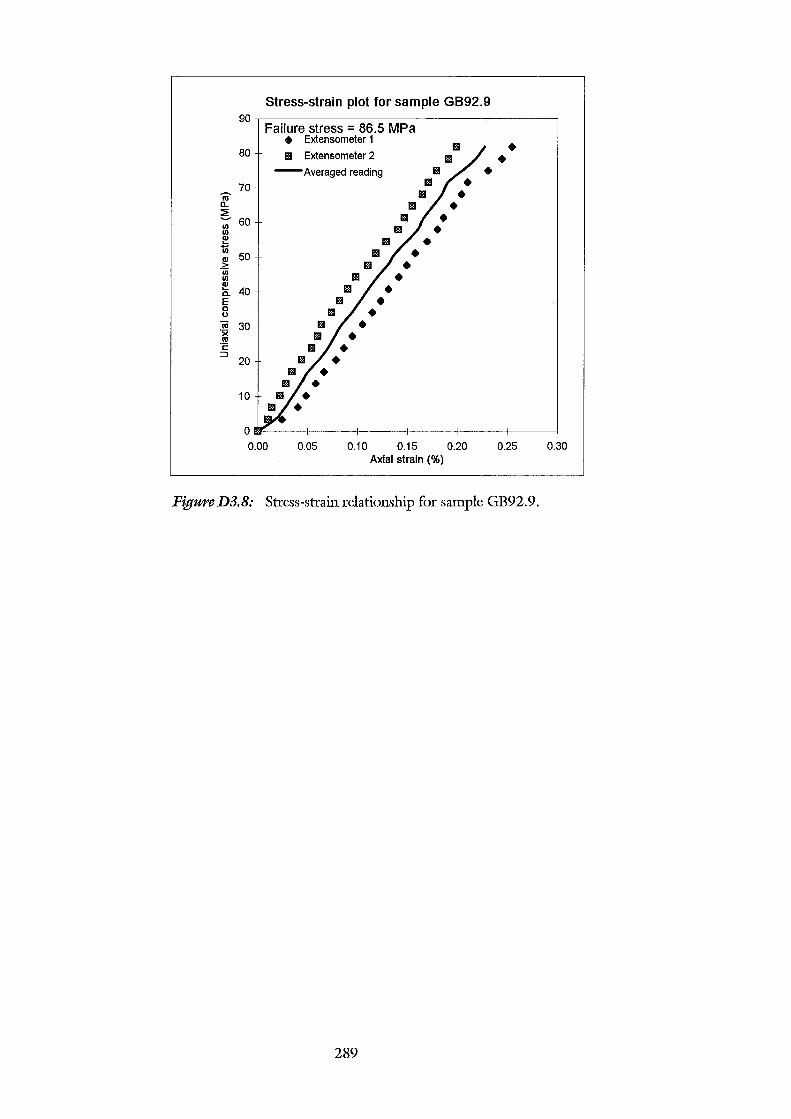
Stress-strain plot for sample GB92.9 90
Failure stress = 86.5 MPa • Extensometer 1
80 Ill
Ill Extensometer 2 1111
-Averaged reading 11!1
70 Ill • m- Ill • a. Iii • 5 60 1111 • VI Iii • VI ~ Ill • 1il
50 1111 • Q)
-~ l!l!l • VI Ill • VI ~ 40 1111 • c. E l!l!l • 0 Ill • 0
"iii 30 1!11 • ·x 1!11 • m ·c: 11!1 • :::J 1!1 • 20
Ill • 1111 • 10 1111 • m •
0
0.00 0.05 0.10 0.15 0.20 0.25 0.30 Axial strain (%)
FigureD3.8: Stress-strain relationship for sample GB92.9.
289
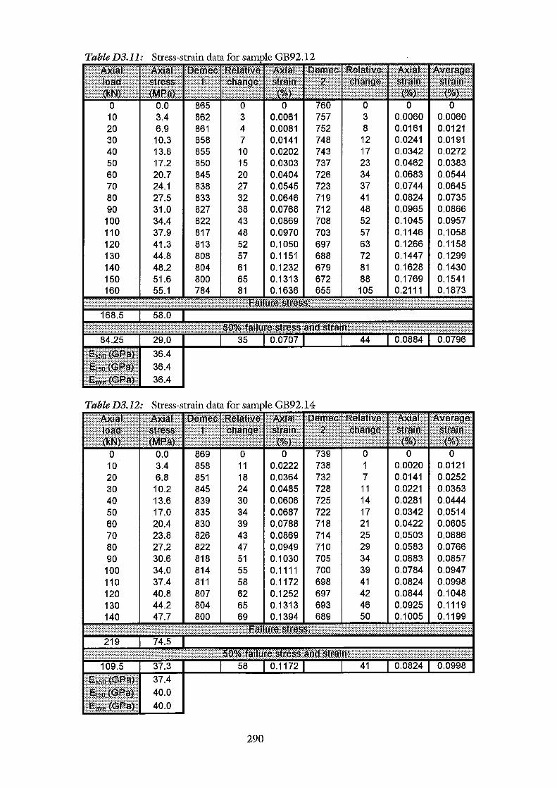
0 10 20 30 40 50 60 70 80 90
100 110 120 130 140 150 160
10 20 30 40 50 60 70
6.9 10.3 13.8 17.2 20.7 24.1 27.5 31.0 34.4
3.4 6.8 10.2 13.6 17.0 20.4 23.8 27.2
40.0 40.0
861 858 855 850 845 20 838 27 833 32 827 38 822 43 817 48 813 52 808 57 804 61 BOO 65 784 81
0 858 11 851 18 845 24 839 30 835 34 830 39 826 43 822 47 818 51 814 55 811 58 807 804 BOO
290
0 0 0.0061 757 0.0060 0.0060 0.0081 752 8 0.0161 0.0121 0.0141 748 12 0.0241 0.0191 0.0202 743 17 0.0342 0.0272 0.0303 737 23 0.0462 0.0383 0.0404 726 34 0.0683 0.0544 0.0545 723 37 0.0744 0.0645 0.0646 719 41 0.0824 0.0735 0.0768 712 48 0.0965 0.0866 0.0869 708 52 0.1045 0.0957 0.0970 703 57 0.1146 0.1058 0.1050 697 63 0.1266 0.1158 0.1151 72 0.1447 0.1299 0.1232 81 0.1628 0.1430 0.1313 0.1769 0.1541 0.1636 0.2111 0.1873
0 0.0222 0.0020 0.0121 0.0364 0.0141 . 0.0252 0.0485 728 0.0221 0.0353 0.0606 725 0.0281 0.0444 0.0687 722 0.0342 0.0514 0.0788 718 0.0422 0.0605 0.0869 714 0.0503 0.0686 0.0949 710 0.0583 0.0766 0.1030 705 0.0683 0.0857 0.1111 700 0.0784 0.0947 0.1172 698 0.0824 0.0998 0.1252 697 0.1048 0.1313 693 0.1119 0.1394 689 0.1199
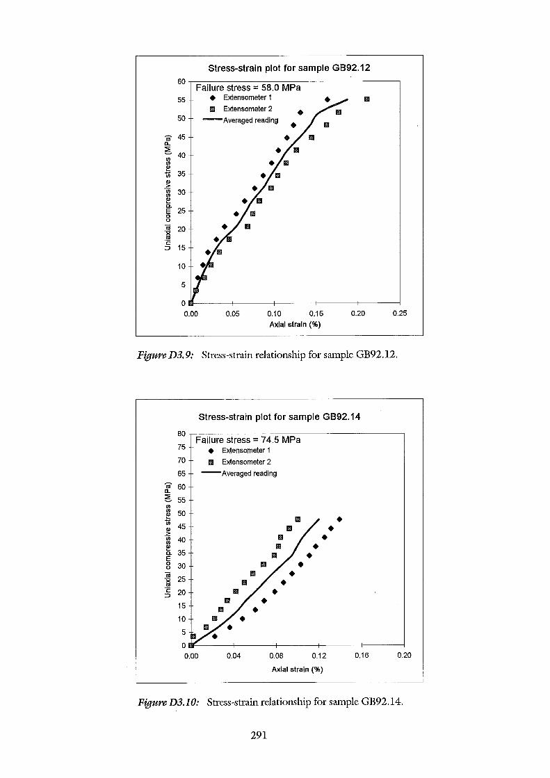
-m n.. 5 Ul Ul ~
1ii Q)
-~ Ul Ul ~ D. E 0 0
iii -~ ·c: :J
Stress-strain plot for sample GB92.12 60.--------------------------------------,
Failure stress = 58.0 MPa 55
50
45
40
35
30
25
20
15
10
5
0 0.00
• Extensometer 1
1111 Extensometer 2
-Averaged reading
0.05 0.10
•
0.15 Axial strain (%)
1111
0.20 0.25
FigureD3.9: Stress-strain relationship for sample GB92.12.
-m n.. 5 Ul Ul ~ 1ii Q) > ·u; Ul ~ D. E 0 0
iii -~ ·c: :J
80
75
70
65
60
55
50
45
40
35
30
25
20
15
10
5
Stress-strain plot for sample GB92.14
Failure stress= 74.5 MPa • Extensometer 1
Iii Extensometer 2
-Averaged reading
1111
1!11
1111
•
Ill 1111
Iii Iii • •
• • • •
• • •
0~------+-------+-------+-------+-----~
0.00 0.04 0.08 0.12 0.16 0.20
Axial strain(%)
FigureD3.10: Stress-strain relationship for sample GB92.14.
291
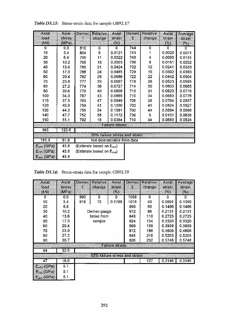
TableD3.13: Stress-strain data for sample GB92.17
0 0 10 3.4 20 6.8 30 10.2 40 13.6 50 17.0 60 20.4 70 23.8 80 27.2 90 30.6
100 34.0 110 37.5 120 40.9 130 44.3 140 47.7 150 51.1
43.8
0 804 6 0.0121 799 11 0.0222 795 15 0.0303 789 21 0.0424 786 24 0.0485 782 28 0.0566 777 33 0.0667 774 36 0.0727 770 40 0.0808 767 43 0.0869 763 47 0.0949 759 51 0.1030 756 54 0.1091
0.1172 0.0364
(Estimate based on Eave)
(Estimate based on Eave)
TableD3.14: Stress-strain data for sample GB92.19
0 10 20 30 40 50 60 70 80 90
0.0 3.4 6.8 10.2 13.6 17.0 20.4 23.9 27.3 30.7
5.1 5.1
72
Demec gauge broke from
sample
292
744 743 740 736 732 729 722 718 714 713 710 706 703 700 739 710
998 972 948 924 899 872 848 826
0 0 0.0020 0.0071 0.0080 0.0151
8 0.0161 0.0232 12 0.0241 0.0333 15 0.0302 0.0393 22 0.0442 0.0504 26 0.0523 0.0595 30 0.0603 0.0665 31 0.0623 0.0716 34 0.0683 0.0776 38 0.0764 0.0857 41 0.0824 0.0927 44 0.0884 0.0988 5 0.0101 0.0636
34 0.0683 0.0524
0 0 0 40 0.0991 0.1390 60 0.1486 0.1486 86 0.2131 0.2131 110 0.2725 0.2725 134 0.3320 0.3320 159 0.3939 0.3939 186 0.4608 0.4608 210 0.5203 0.5203 232 0.5748 0.5748
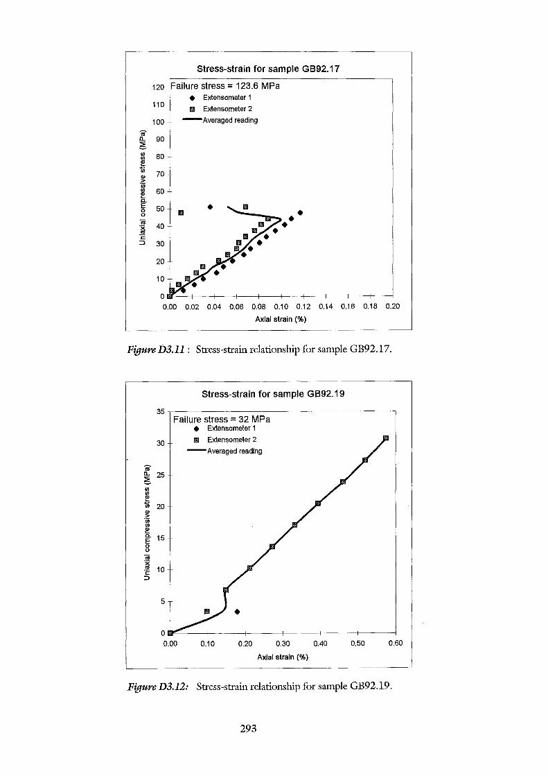
Stress-strain for sample GB92.17
120 ailure stress = 123.6 MPa
110
100
-m a. 90 5
80
70
60
50
40
30
20
10
• Extensometer 1
IIIII Extensometer 2
-Averaged reading
0~--4---~--~---+---+--~--~~--~--+-~
0.00 0.02 0.04 0.06 0.08 0.10 0.12 0.14 0.16 0.18 0.20
Axial strain (%)
Figure D3.11 : Stress-strain relationship for sample GB92.17.
Stress-strain for sample GB92.19
35.-----------------------------------------~
30
-m a. 25 5 lZ ~ Ui 20 ~ 'iii (/)
~ ~ 15 0 0
iii ·~ ·c: 10 ::l
5
Failure stress = 32 MPa • Extensometer 1
1111 Extensometer 2
-Averaged reading
• o~~---+------4------4------~----~------~
0.00 0.10 0.20 0.30 0.40 0.50 0.60
Axial strain (%)
Figure D3.12: Stress-strain relationship for sample GB92.19.
293
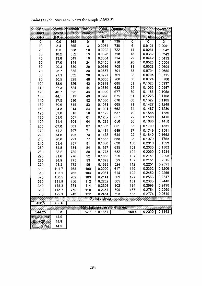
Table D3.15: Stress-strain data for sample GB92.2l
0 0.0 868 0 0 10 3.4 865 3 0.0061 6 0.0121 0.0091 20 6.8 858 10 0.0202 14 0.0281 0.0242 30 10.2 852 16 0.0323 18 0.0362 0.0343 40 13.6 849 19 0.0384 22 0.0442 0.0413 50 17.0 844 24 0.0485 26 0.0523 0.0504 60 20.3 839 29 0.0586 31 0.0623 0.0604 70 23.7 835 33 0.0667 35 0.0704 0.0685 80 27.1 832 36 0.0727 701 35 0.0704 0.0715 90 30.5 828 40 0.0808 700 36 0.0724 0.0766
100 33.9 826 42 0.0848 685 51 0.1025 0.0937 110 37.3 824 44 0.0889 682 54 0.1085 0.0987 120 40.7 822 46 0.0929 677 59 0.1186 0.1058 130 44.1 819 49 0.0990 675 61 0.1226 0.1108 140 47.5 816 52 0.1050 670 66 0.1327 0.1189 150 50.9 815 53 0.1071 665 71 0.1427 0.1249 160 54.3 814 54 0.1091 662 74 0.1487 0.1289 170 57.6 810 58 0.1172 657 79 0.1588 0.1380 180 61.0 807 61 0.1232 657 79 0.1588 0.1410 190 64.4 804 64 0.1293 656 80 0.1608 0.1450
200 67.8 801 67 0.1353 651 85 0.1709 0.1531 210 71.2 797 71 0.1434 649 87 0.1749 0.1591 220 74.6 795 73 0.1475 644 92 0.1849 0.1662 230 78.0 791 77 0.1555 638 98 0.1970 0.1763 240 81.4 787 81 0.1636 636 100 0.2010 0.1823 250 84.8 784 84 0.1697 635 101 0.2030 0.1863 260 88.2 780 88 0.1778 632 104 0.2090 0.1934 270 91.6 776 92 0.1858 629 107 0.2151 0.2005 280 94.9 775 93 0.1879 629 107 0.2151 0.2015 290 98.3 772 96 0.1939 624 112 0.2251 0.2095 300 101.7 768 100 0.2020 617 119 0.2392 0.2206 310 105.1 765 103 0.2081 614 122 0.2452 0.2266 320 108.5 762 106 0.2141 609 127 0.2553 0.2347 330 111.9 756 112 0.2262 605 131 0.2633 0.2448 340 115.3 754 114 0.2303 602 134 0.2693 0.2498 350 118.7 750 118 0.2384 599 137 0.2754 0.2569 360 122.1 746 122 0.2464 598 138 0.2774 0.2619
44.9
294
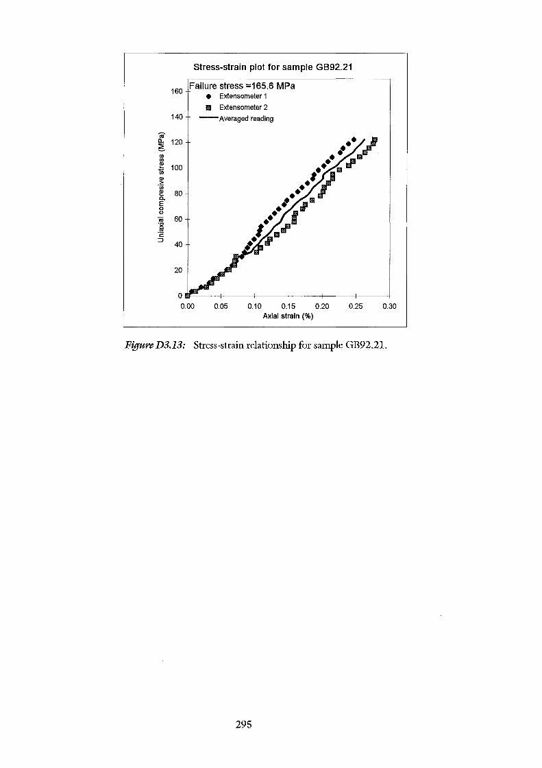
Stress-strain plot for sample GB92.21
• Extensometer 1 Failure stress =165.6 MPa
160
B Extensometer 2
140 -Averaged reading
m-a. 120 ~ Ill Ill
~ 100 1ii g!
"iii ~ a. E 0 0
80
60
40
20
OmF~--4------+----~------~----+-----~
0.00 0.05 0.10 0.15 0.20 0.25 0.30 Axial strain (%)
Figure D3.13: Stress-strain relationship for sample GB92.2l.
295
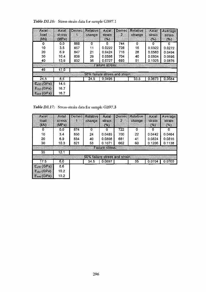
TableD3.16: Stress-strain data for sample GB97.l
Table D3.17: Stress-strain data for sample GB97.3
10.2 10.2
296
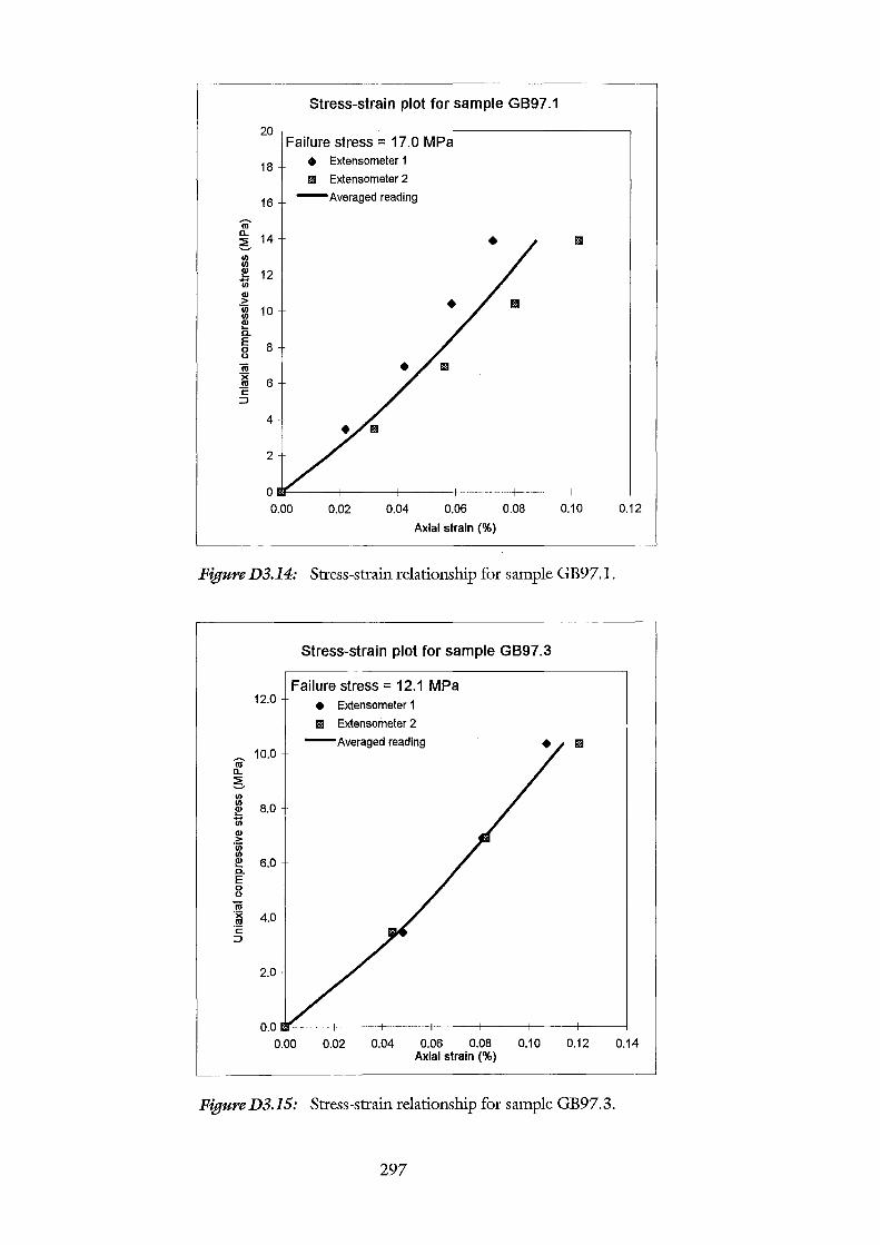
Stress-strain plot for sample GB97.1
20.----------------------------------------,
18
16
Iii' D.. 5 14 U) U)
I! 12 1ii !l!
"iii 10 ~ a. ~ 8 0
n; -~ 6 ·c: ::>
4
2
Failure stress= 17.0 MPa • Extensometer 1
m Extensometer 2
-Averaged reading
1!11
0~-----+------~----~----~------+-----~
0.00 0.02 0.04 0.06 0.08 0.10
Axial strain (%)
Figure D3.14: Stress-strain relationship for sample GB97.l.
12.0
10.0 Iii' D..
5 U)
~ 8.0 1ii !l! "iii U)
~ 6.0 a. E 0 0
n; -~ 4.0 ·c: ::>
2.0
Stress-strain plot for sample GB97.3
Failure stress = 12.1 MPa • Extensometer 1
m Extensoineter 2
-Averaged reading m
0.12
0.0 ~----+-----~--~------+-----+----~------~
0.00 0.02 0.04 0.06 0.08 0.10 0.12 0.14 Axial strain(%)
Figure D3.15: Stress-strain relationship for sample GB97.3.
297
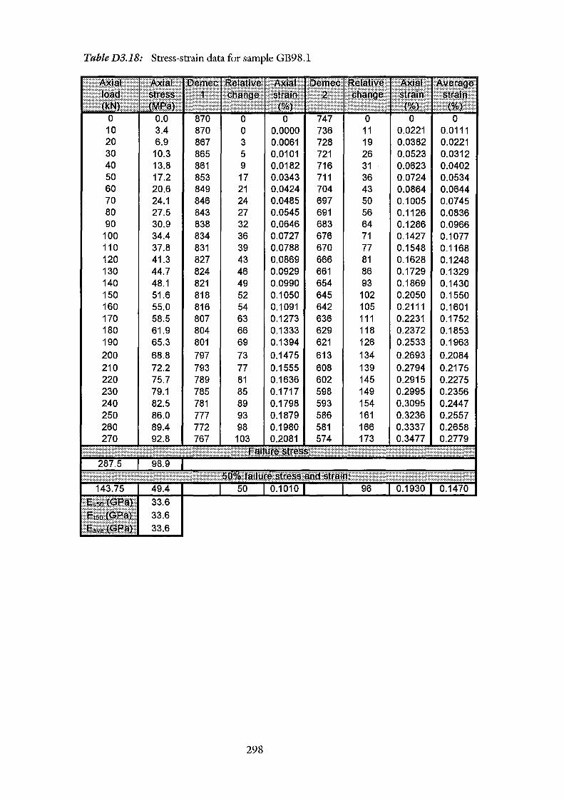
Table D3.18: Stress-strain data for sample GB98.l
0.0 870 0 0 747 0 0 0 10 3.4 870 0 0.0000 736 11 0.0221 0.0111 20 6.9 867 3 0.0061 728 19 0.0382 0.0221 30 10.3 865 5 0.0101 721 26 0.0523 0.0312 40 13.8 861 9 0.0182 716 31 0.0623 0.0402 50 17.2 853 17 0.0343 711 36 0.0724 0.0534 60 20.6 849 21 0.0424 704 43 0.0864 0.0644 70 24.1 846 24 0.0485 697 50 0.1005 0.0745 80 27.5 843 27 0.0545 691 56 0.1126 0.0836 90 30.9 838 32 0.0646 683 64 0.1286 0.0966
100 34.4 834 36 0.0727 676 71 0.1427 0.1077 110 37.8 831 39 0.0788 670 77 0.1548 0.1168 120 41.3 827 43 0.0869 666 81 0.1628 0.1248 130 44.7 824 46 0.0929 661 86 0.1729 0.1329 140 48.1 821 49 0.0990 654 93 0.1869 0.1430 150 51.6 818 52 0.1050 645 102 0.2050 0.1550 160 55.0 816 54 0.1091 642 105 0.2111 0.1601 170 58.5 807 63 0.1273 636 111 0.2231 0.1752 180 61.9 804 66 0.1333 629 118 0.2372 0.1853 190 65.3 801 69 0.1394 621 126 0.2533 0.1963 200 68.8 797 73 0.1475 613 134 0.2693 0.2084 210 72.2 793 77 0.1555 608 139 0.2794 0.2175 220 75.7 789 81 0.1636 602 145 0.2915 0.2275 230 79.1 785 85 0.1717 598 149 0.2995 0.2356 240 82.5 781 89 0.1798 593 154 0.3095 0.2447 250 86.0 777 93 0.1879 586 161 0.3236 0.2557 260 89.4 772 98 0.1980 581 166 0.3337 0.2658 270 92.8 767 103 0.2081 574 173 0.3477 0.2779
298
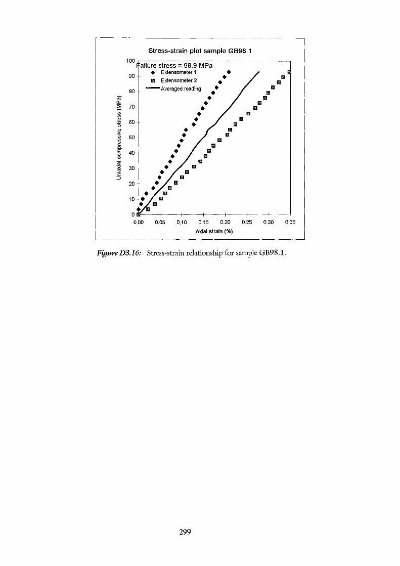
Stress-strain plot sample GB98.1 100,-------------------------------------~
ailure stress = 98.9 MPa
• Extensometer 1 • 90 • 1111 11!1 Extensometer 2 • 1111
80 -Averaged reading • IIIII
• 1111
ro • 1!11 n. • 1!11 ~ 70 • IIIII Ul • 1111 Ul ~ 60 • Ill iii • llill Q) • llill > • 1111 'iii 50 Ul • 1111 ~ • 1111 a. E 40 • llill 0 • 11!1 0
iU • Ill ·x 30 • llill m • 1111 ·c: ::J • lill
20 • 1111
• 1111
• 1!11 10 • lill
• 1111 1!11
0~----~---4-----+----~----+-----~--~
0.00 0.05 0.10 0.15 0.20 0.25 0.30 0.35
Axial strain (%)
FigureD3.16: Stress-strain relationship for sample GB98.l.
299
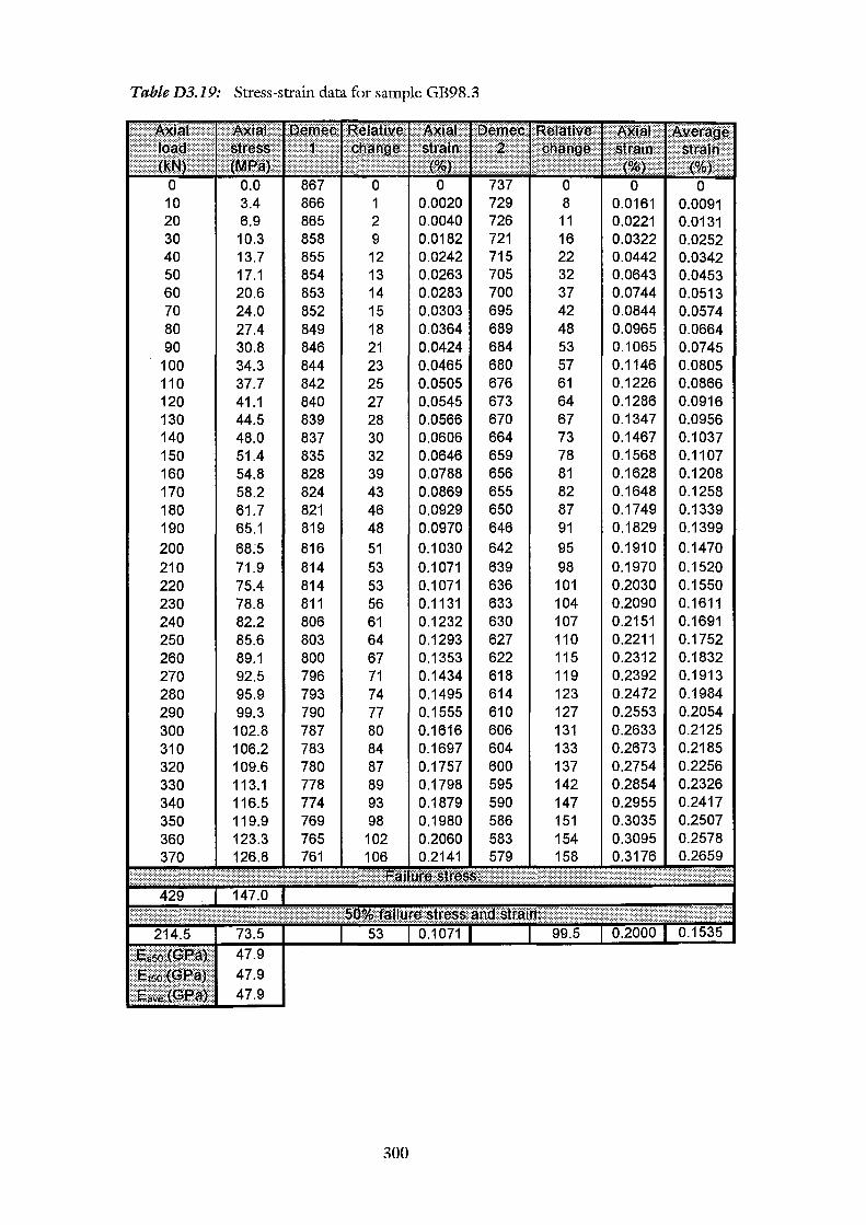
Table D3.19: Stress-strain data for sample GB98.3
0 10 20 30 40 50 60 70 80 90
100 110 120 130 140 150 160 170 180 190 200 210 220 230 240 250 260 270 280 290 300 310 320 330 340 350 360 370
20.6 24.0 27.4 30.8 34.3 37.7 41.1 44.5 48.0 51.4 54.8 58.2 61.7 65.1 68.5 71.9 75.4 78.8 82.2 85.6 89.1 92.5 95.9 99.3
102.8 106.2 109.6 113.1 116.5 119.9 123.3 126.8
47.9 47.9
86 866 0.0020 865 0.0040 858 9 0.0182 855 12 0.0242 854 13 0.0263 853 14 0.0283 852 15 0.0303 849 18 0.0364 846 21 0.0424 844 23 0.0465 842 25 0.0505 840 27 0.0545 839 28 0.0566 837 30 0.0606 835 32 0.0646 828 39 0.0788 824 43 0.0869 821 46 0.0929 819 48 0.0970 816 51 0.1030 814 53 0.1071 814 53 0.1071 811 56 0.1131 806 61 0.1232 803 64 0.1293 800 67 0.1353 796 71 0.1434 793 74 0.1495 790 77 0.1555 787 80 0.1616 783 84 0.1697 780 87 0.1757 778 89 0.1798 774 93 0.1879 769 0.1980 765 0.2060 761 0.2141
300
0 0 729 8 0.0161 0.0091 726 11 0.0221 0.0131 721 16 0.0322 0.0252 715 22 0.0442 0.0342 705 32 0.0643 0.0453 700 37 0.0744 0.0513 695 42 0.0844 0.0574 689 48 0.0965 0.0664 684 53 0.1065 0.0745 680 57 0.1146 0.0805 676 61 0.1226 0.0866 673 64 0.1286 0.0916 670 67 0.1347 0.0956 664 73 0.1467 0.1037 659 78 0.1568 0.1107 656 81 0.1628 0.1208 655 82 0.1648 0.1258 650 87 0.1749 0.1339 646 91 0.1829 0.1399 642 95 0.1910 0.1470 639 98 0.1970 0.1520 636 101 0.2030 0.1550 633 104 0.2090 0.1611 630 107 0.2151 0.1691 627 110 0.2211 0.1752 622 115 0.2312 0.1832 618 119 0.2392 0.1913 614 123 0.2472 0.1984 610 127 0.2553 0.2054 606 131 0.2633 0.2125 604 133 0.2673 0.2185 600 137 0.2754 0.2256 595 142 0.2854 0.2326
147 0.2955 0.2417 0.3035 0.2507 0.3095 0.2578 0.3176 0.2659
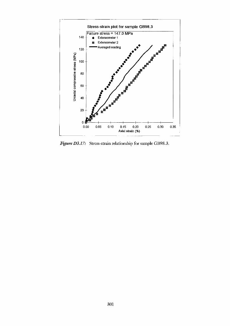
140
120
m-n. ~ Ill 100
~ 1il Q)
-~ Ill Ill ~ a. E 0 0
80
60
40
20
Stress-strain plot for sample GB98.3
Failure stress= 147.0 MPa • Extensometer 1
111 Extensometer 2
-Averaged reading
0~----~--~----~----4-----~----~--~
0.00 0.05 0.10 0.15 0.20 0.25 0.30 0.35 Axial strain (%)
FigureD3.17: Stress-strain relationship for sample GB98.3.
301
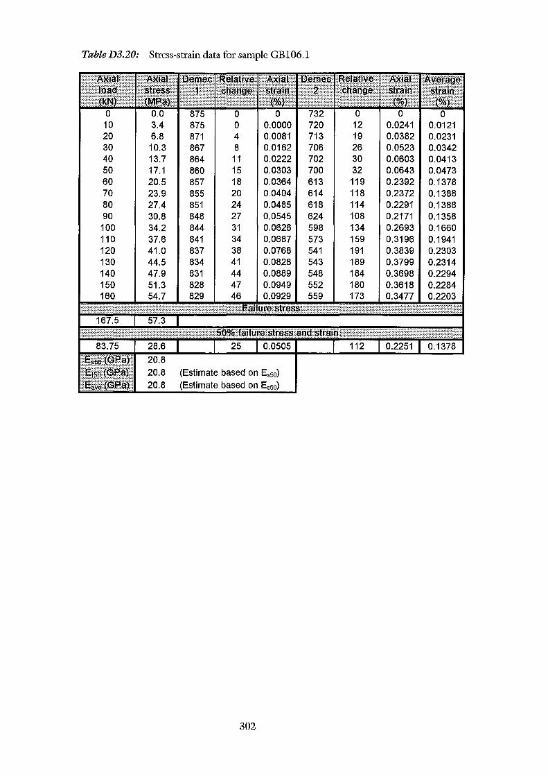
TableD3.20: Stress-strain data for sample GB106.1
0 0 10 3.4 0.0000 720 12 0.0241 0.0121 20 6.8 0.0081 713 19 0.0382 0.0231 30 10.3 8 0.0162 706 26 0.0523 0.0342 40 13.7 11 0.0222 702 30 0.0603 0.0413 50 17.1 15 0.0303 700 32 0.0643 0.0473 60 20.5 18 0.0364 613 119 0.2392 0.1378 70 23.9 855 20 0.0404 614 118 0.2372 0.1388 80 27.4 851 24 0.0485 618 114 0.2291 0.1388 90 30.8 848 27 0.0545 624 108 0.2171 0.1358
100 34.2 844 31 0.0626 598 134 0.2693 0.1660 110 37.6 841 34 0.0687 573 159 0.3196 0.1941 120 41.0 837 38 0.0768 541 191 0.3839 0.2303 130 44.5 834 41 0.0828 543 189 0.3799 0.2314 140 47.9 831 44 0.0889 548 184 0.3698 0.2294 150 51.3 828 47 0.0949 552 180 0.3618 0.2284 160 54.7 829 46 0.0929 559 173 0.3477 0.2203
20.8 (Estimate based on Es5o) 20.8 (Estimate based on Es5o)
302
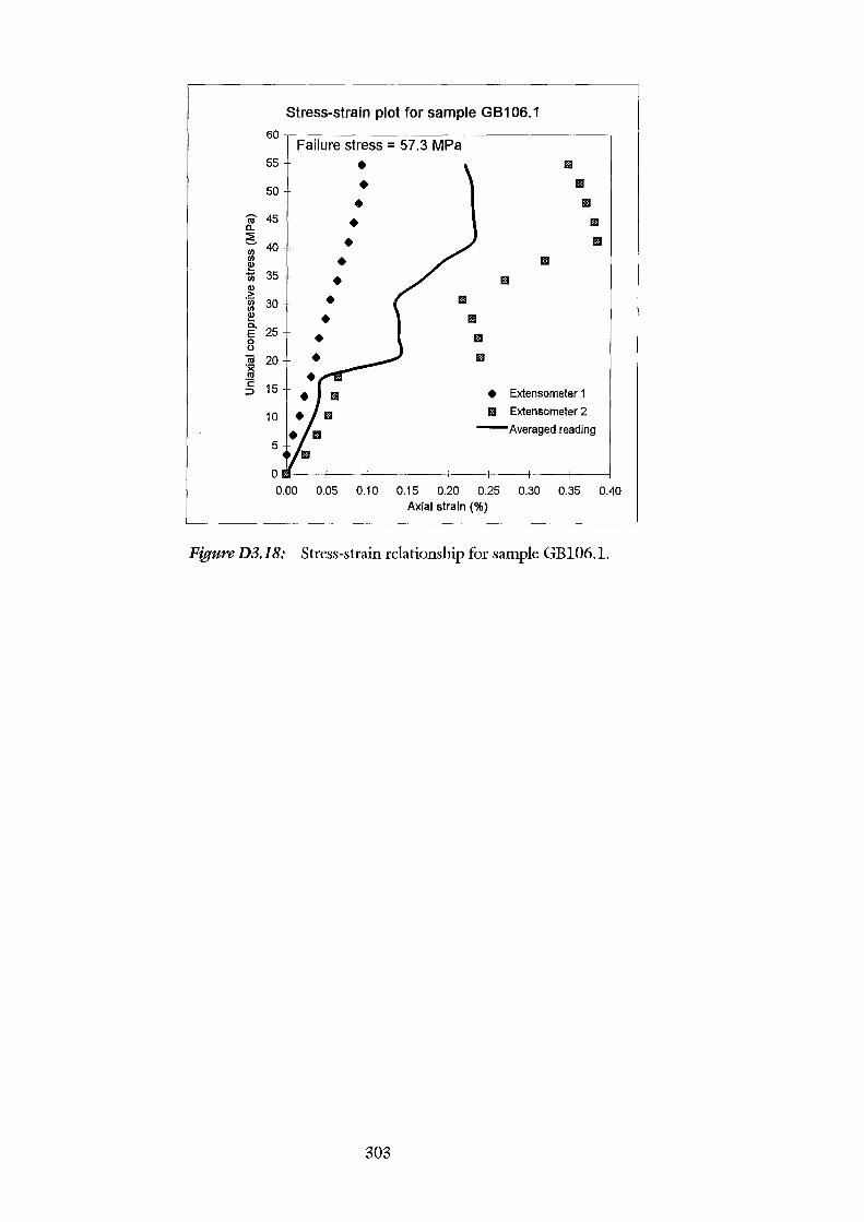
Stress-strain plot for sample GB1 06.1
60 Failure stress= 57.3 MPa
55 • Ill
50 • Ill
• 1111
"iii' 45 • 1111 0..
5 40 • 1111 Ill Ill • 1!11 ~ 1ii 35 • Ill Q)
> • Ill "iii 30 Ill Q) • 1111 l5.. E 25 Ill 0 0
iii 20 1111 ·x cu ·c:
15 ::J • Extensometer 1
10 Ill Extensometer 2
-Averaged reading 5
ow---~----r----r--~----1----+----+---~
0.00 0.05 0.10 0.15 0.20 0.25 0.30 0.35 0.40 Axial strain (%)
Figure D3.18: Stress-strain relationship for sample GB106.l.
303
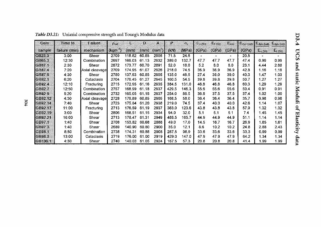
Table D3.21: Uniaxial compressive strength and Young's Modulus data ti ~
~
d 118.82 60.85 2905 71.5 24.6 - - - 20.5 - - 0
12:30 Combination 2697 166.03 61.13 2932 389.0 132.7 47.7 47.7 47.7 47.4 0.99 0.99 en 2:30 Shear 2672 173.77 60.70 2891 52.0 18.0 5.2 8.0 8.0 23.1 4.44 2.88 ~
:::: 7:20 Axial cleavage 2709 174.95 61.07 2926 218.0 74.5 36.9 36.9 36.9 42.8 1.16 1.16 p. 4:30 Shear 2780 137.93 60.85 2905 135.0 46.5 27.4 39.0 39.0 40.3 1.47 1.03 "' ,...,. 6:20 Cataclasis 2704 176.45 61.27 2945 160.5 54.5 39.8 39.8 39.8 50.7 1.27 1.27 ~ p. 12:10 Fracturing 2715 172.95 61.16 2935 384.5 131.0 46.8 46.8 46.8 60.3 1.29 1.29 n 12:50 Combination 2757 168.99 61.18 2937 429.5 146.3 55.6 55.6 55.6 50.4 0.91 0.91 ~ 8:20 Combination 2732 165.05 61.18 2937 254.0 86.5 36.8 37.5 37.5 37.4 1.02 1.00
C),)
1§1!!111iiiil 4:30 Axial cleavage 2728 176.89 60.85 2905 168.5 58.0 36.4 36.4 36.4 35.7 0.98 0.98 §-
0 7:40 Shear 2723 175.84 61.20 2938 219.0 74.5 37.4 40.0 40.0 42.6 1.14 1.07 = ~ 11:00 Fracturing 2713 176.59 61.19 2937 363.0 123.6 43.8 43.8 43.8 57.9 1.32 1.32 0
~ 3:00 Shear 2806 168.51 61.15 2934 94.0 32.0 5.1 5.1 5.1 7.4 1.45 1.45 td 16:00 Shear 2713 178.47 61.31 2949 488.5 165.7 44.9 44.9 44.9 51.1 1.14 1.14 -~ 1:40 Shear 2708 153.82 60.68 2888 49.0 17.0 14.5 16.7 16.7 26.9 1.85 1.61 "' p. 1:40 Shear 2689 140.90 60.80 2900 35.0 12.1 8.6 10.2 10.2 24.8 2.88 2.43 n .... 8:50 Combination 2738 174.31 60.88 2908 287.5 98.9 33.6 33.6 33.6 33.3 0.99 0.99 ~ 13:00 Cataclasis 2719 176.00 61.00 2919 429.0 147.0 47.9 47.9 47.9 64.2 1.34 1.34 p. 4:30 Shear 2740 140.03 61.05 2924 167.5 57.3 20.8 20.8 20.8 41.4 1.99 1.99 ~ ,...,.
~
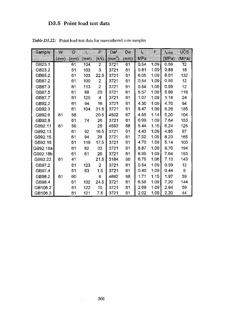
D3.5 Point load test data
Table D3.22: Point load test data for unweathered core samples
GB23.1 61 104 2 3721 61 0.54 1.09 0.59 12 GB23.2 61 103 3 3721 61 0.81 1.09 0.88 18 GB65.2 61 103 22.5 3721 61 6.05 1.09 6.61 132 GB87.2 61 100 2 3721 61 0.54 1.09 0.59 12 GB87.3 61 113 2 3721 61 0.54 1.09 0.59 12 GB87.5 61 98 20 3721 61 5.37 1.09 5.88 118 GB87.7 61 125 4 3721 61 1.07 1.09 1.18 24 GB92.2 61 94 16 3721 61 4.30 1.09 4.70 94 GB92.3 61 104 31.5 3721 61 8.47 1.09 9.26 185
GB92.6 61 58 20.5 4502 67 4.55 1.14 5.20 104 GB92.8 61 74 26 3721 61 6.99 1.09 7.64 153
GB92.11 61 59 25 4593 68 5.44 1.15 6.24 125 GB92.13 61 92 16.5 3721 61 4.43 1.09 4.85 97 GB92.15 61 94 28 3721 61 7.52 1.09 8.23 165 GB92.16 61 119 17.5 3721 61 4.70 1.09 5.14 103
GB92.18a 61 62 33 3721 61 8.87 1.09 9.70 194 GB92.18b 61 61 26 3721 61 6.99 1.09 7.64 153 GB92.22 61 41 21.5 3184 56 6.75 1.06 7.13 143
GB97.2 61 123 2 3721 61 0.54 1.09 0.59 12 GB97.4 61 63 1.5 3721 61 0.40 1.09 0.44 9
GB98.2 61 60 8 4682 68 1.71 1.15 1.97 39 GB98.4 61 102 24.5 3721 61 6.58 1.09 7.20 144
GB106.2 61 122 10 3721 61 2.69 1.09 2.94 59 GB106.3 61 121 7.5 3721 61 2.02 1.09 2.20 44
305
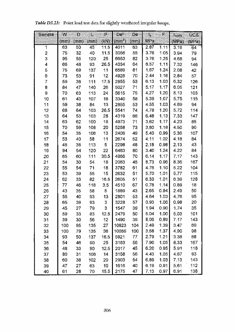
Table D3.23: Point load test data for slightly weathered irregular lumps.
63 50 45 11.5 63 2.87 1.11 3.19 64 2 75 32 40 11.5 3056 55 3.76 1.05 3.94 79 3 95 55 120 25 6653 82 3.76 1.25 4.68 94 4 66 48 93 26.5 4034 64 6.57 1.11 7.32 146 5 75 69 137 11 6589 81 1.67 1.24 2.08 42 6 73 53 91 12 4926 70 2.44 1.16 2.84 57 7 8 9 10 11 12 13 14 15 16 17 18 19 20 21 22 23
59 84 70 61 59 68 64 63 70 54 53 48 94 65 54
38 47 63 43 38. 64 53 62
111 17.5 2855 140 26 5027 113 24 5615 107 18 3340 84 13 2855 103 26.5 5541 103 28 4319 100 18 4973
53 71 75 58 53 74 66 71
59 108 20 5258 73 35 106 13 2406 49 40 58 11 267 4 52 38 113 5 2298 48 54 120 22 6463 80 60 111 30.5 4966 70 30 54 18 2063 45
6.13 1.03 6.32 5.17 1.17 6.05 4.27 1.20 5.13 5.39 1.07 5.75 4.55 1.03 4.69 4.78 1.20 5.72 6.48 1.13 7.33 3.62 1.17 4.23 3.80 1.18 4.50 5.40 0.99 5.36 4.11 1.02 4.18 2.18 0.98 2.13 3.40 1.24 4.22 6.14 1.17 7.17 8.73 0.96 8.36
126 121 103 115 94
114 147 85 90
107 84 43 84 143 167
55 54 71 18 3782 61 4.76 1.10 5.22 104 53 39 55 15 2632 51 5.70 1.01 5.77 115
24 62 33 82 16.5 2605 51 6.33 1.01 6.39 128 25 77 46 118 3.5 4510 67 0.78 1.14 0.89 18 26 27 28 29 30 31 32 33 34 35 36
43 35 58 5 1889 43 2.65 0.94 2.49 55 40 93 13 2801 53 4.64 1.03 4.76 65 39 93 3 3228 57 0.93 1.06 0.98 45 27 79 3 1547 39 1.94 0.90 1.74 59 33 83 12.5 2479 50 5.04 1.00 5.03 39 30 56 12 1490 39 8.06 0.89 7.17 100 85 135 27 10823 104 2.49 1.39 3.47 100 79 135 36 10059 100 3.58 1.37 4.90 93 50 137 16.5 5921 77 2.79 1.21 c 3.38 54 46 90 25 3163 56 7.90 1.05 8.33 48 33 90 12.5 2017 45 6.20 0.95 5.91
50 95 20 35 101 143 69 98 68 167 118
37 80 31 106 14 3158 56 4.43 1.05 4.67 93 38 60 38 102 20 2903 54 6.89 1.03 7.13 143 39 40
47 27 63 10 1616 40 6.19 0.91 5.61 61 28 70 15.5 2175 47 7.13 0.97 6.91
306
112 138
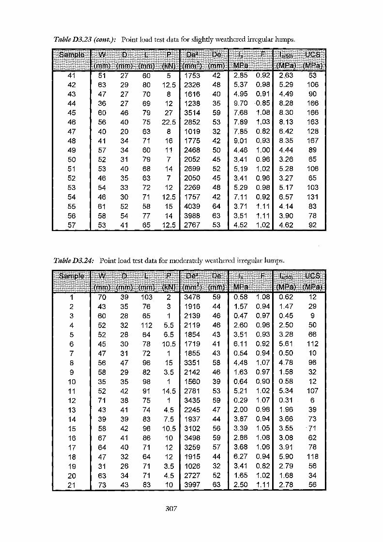
Table D3.23 (cont.): Point load test data for slightly weathered irregular lumps.
42 43 44 45 46 47 48 49 50 51 52 53 54 55 56 57
51 63 47 36 60 56 40 41 57 52 53 46 54 46 61 58 53
27 29 27 27 46 40 20 34 34 31 40 35 33 30 52 54 41
60 5 1753 42 80 12.5 2326 48 70 8 1616 40 69 12 1238 35 79 27 3514 59 75 22.5 2852 53 63 8 1019 32 71 16 1775 42 60 11 2468 50 79 7 2052 45 68 14 2699 52 63 7 2050 45 72 12 2269 48 71 12.5 1757 42 58 15 4039 64 77 14 3988 63 65 12.5 2767 53
2.85 0.92 2.63 5.37 0.98 5.29 4.95 0.91 4.49 9.70 0.85 8.28 7.68 1.08 8.30 7.89 1.03 8.13 7.85 0.82 6.42 9.01 0.93 8.35 4.46 1.00 4.44 3.41 0.96 3.26 5.19 1.02 5.28 3.41 0.96 3.27 5.29 0.98 5.17 7.11 0.92 6.57 3.71 1.11 4.14 3.51 1.11 3.90 4.52 1.02 4.62
53 106 90 166 166 163 128 167 89 65 106 65 103 131 83 78 92
TableD3.24: Point load test data for moderately weathered irregular lumps.
1 70 39 103 2 3476 59 0.58 1.08 0.62 12 2 43 35 76 3 1916 44 1.57 0.94 1.47 29 3 60 28 65 1 2139 46 0.47 0.97 0.45 9 4 52 32 112 5.5 2119 46 2.60 0.96 2.50 50 5 6 7 8 9
10 11 12 13 14 15 16 17 18 19 20 21
52 45 47 56 58 35 52 71 43 39 58 67 64 47 31
28 30 31 47 29 35 42 38 41 39 42 41 40 32 26
63 34 73 43
64 6.5 1854 43 3.51 0.93 3.28 66 78 10.5 1719 41 6.11 0.92 5.61 112 72 1 1855 43 0.54 0.94 0.50 10 96 15 3351 58 4.48 1.07 4. 78 96 82 3.5 2142 46 1.63 0.97 1.58 32 98 1 1560 39 0.64 0.90 0.58 12 91 14.5 2781 53 5.21 1.02 5.34 107 75 1 3435 59 0.29 1.07 0.31 6 74 4.5 2245 47 2.00 0.98 1.96 39 83 7.5 1937 44 3.87 0.94 3.66 73 96 10.5 3102 56 3.39 1.05 3.55 . 71 86 10 3498 59 2.86 1.08 3.08 62 71 12 3259 57 3.68 1.06 3.91 78 64 12 1915 44 6.27 0.94 5.90 118 71 3.5 1026 32 3.41 0.82 2.79 56 71 4.5 2727 52 1.65 1.02 1.68 34
56 83 10 3997 63 2.50 1.11 2.78
307
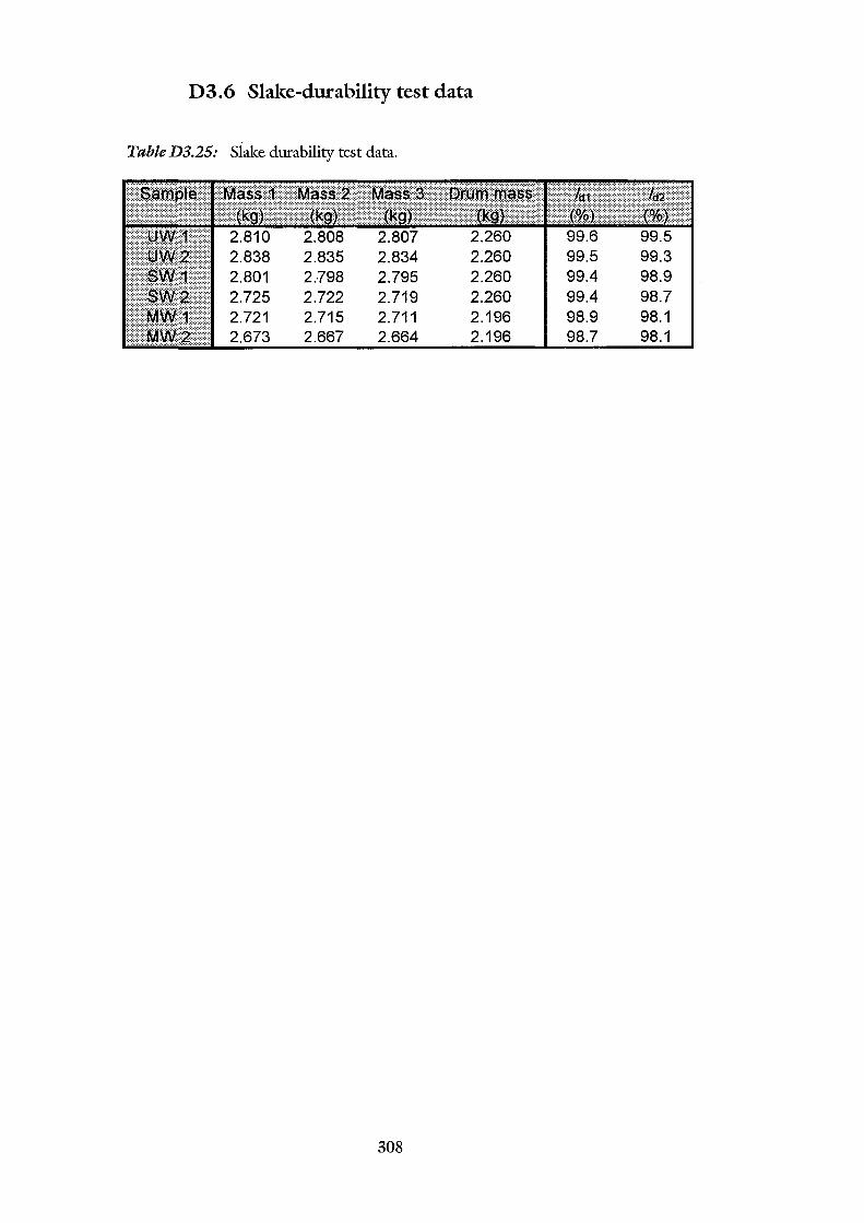
D3.6 Slake-durability test data
Table D3.25: Slake durability test data.
2.807 2.838 2.834 99.3 2.801 2.798 2.795 2.260 98.9 2.725 2.722 2.719 2.260 98.7 2.721 2.715 2.711 2.196 98.9 98.1 2.673 2.667 2.664 2.196 98.7 98.1
308
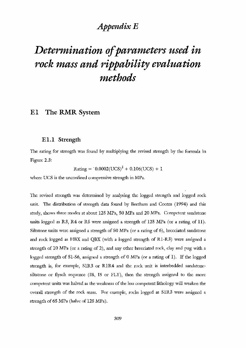
I
AppendixE
Determination of parameters used in rock mass and rippability evaluation
methods
El The RMR System
El.l Strength
The rating for strength was fmmd by multiplying the revised strength by the formula in
Figure 2.3:
Rating = -0.0002(UCS)2 + 0.106(UCS) + 1
where UCS is the unconfmed compressive strength in MPa.
The revised strength was determined by analysing the logged strength and logged rock
unit. The distribution of strength data found by Beetharn and Coates (1994) and this
study, shows three modes at about 125 MPa, 50 MPa and 20 MPa. Competent sandstone
units logged as R3, R4 or R5 were assigned a strength of 125 MPa (or a rating of ll).
Siltstone units were assigned a strength of 50 MPa (or a rating of 6), brecciated sandstone
and rock logged as HBX and QBX (with a logged strength of R1-R3) were assigned a
strength of 10 MPa (or a rating of 2), and any other brecciated rock, clay and pug with a
logged strength of S1-S6, assigned a strength of 0 MPa (or a rating of 1). If the logged
strength is, for example, S1R3 or R1R4 and the rock unit is interbedded sandstone
siltstone or flysch sequence (IB, IS or FLY), then the strength assigned to the more
competent units was halved as the weakness of the less competent lithology will weaken the
overall strength of the rock mass. For example, rocks logged as S1R3 were assigned a
strength of 65 MPa (halve of 125 MPa).
309
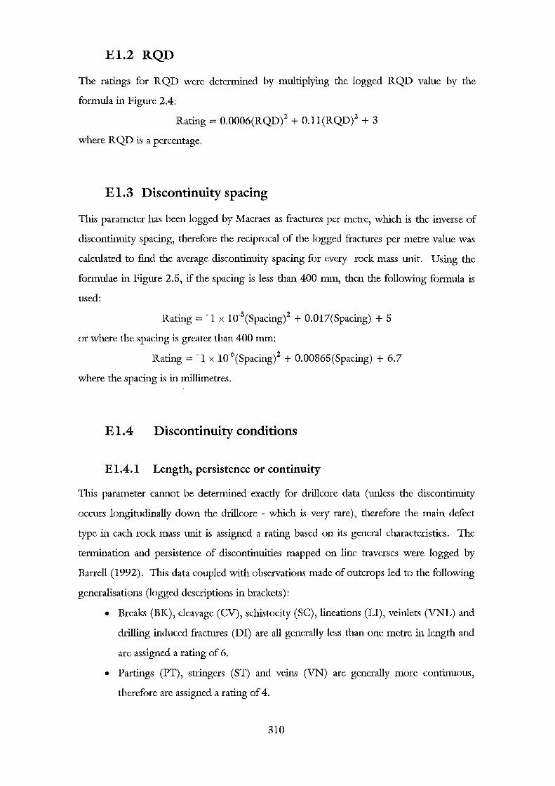
El.2 RQD
The ratings for RQD were determined by multiplying the logged RQD value by the
formula in Figure 2.4:
Rating = 0.0006(RQD)2 + O.ll(RQD)2 + 3
where RQD is a percentage.
El.3 Discontinuity spacing
This parameter has been logged by Macraes as fractures per metre, which is the inverse of
discontinuity spacing, therefore the reciprocal of the logged fractures per metre value was
calculated to fmd the average discontinuity spacing for every rock mass unit. Using the
formulae in Figure 2.5, if the spacing is less than 400 mm, then the following formula is
used:
Rating = -1 x 10⁻⁵(Spacing)2 + 0.017(Spacing) + 5
or where the spacing is greater than 400 mm:
Rating= -1 x l0-6(Spacing)2 + 0.00865(Spacing) + 6.7
where the spacing is in millimetres.
E 1.4 Discontinuity conditions
El.4.l Length, persistence or continuity
This parameter cannot be determined exactly for drillcore data (unless the discontinuity
occurs longitudinally down the drillcore - which is very rare), therefore the main defect
type in each rock mass unit is assigned a rating based on its general characteristics. The
termination and persistence of discontinuities mapped on line traverses were logged by
Barrell (1992). This data coupled with observations made of outcrops led to the following
generalisations (logged descriptions in brackets):
• Breaks (BK), cleavage (CV), schistocity (SC), lineations (LI), veinlets (VNL) and
drilling induced fractures (D I) are all generally less than one metre in length and
are assigned a rating of 6.
• Partings (PT), stringers (ST) and veins (VN) are generally more continuous,
therefore are assigned a rating of 4.
310
• Joints (JN) generally range between one and 10 metres, therefore are assigned a
ratingof3.5 (meanofratings 3 and4).
• Bedding planes (BD, tCT, bCT) generally range between three and twenty metres
so are assigned a rating of2 (mean of 1 and 3).
• Shears (SH), shear zones (SZ), crush zones (CZ), shattered zones (STZ),
decomposed zones (DC), faults (FT), pug (PG) and breccia (BX) are generally
persistent if the rock unit is brecciated, so are assigned a rating of 0, but if the
rock unit is a sandstone or similar, then the discontinuity persistence is not as
great, and the parameter is assigned a rating of 3.
El.4.2 Separation
The separation, spacing or infilling width of a discontinuity is described by Macraes as
being clean (CL), stained (ST), a vein (VN) or a veinlet (VNL) and if the spacing is
greater than 2 mm, then the thickness is recorded. If no data is recorded then it is assumed
that the separation is zero and is given a rating of 6. If the discontinuities are clean or
stained, or vein or veinlet are recorded, then a rating of 5 is assigned, based on an average
of the ratings assigned to spacings between 0 and 1 mm. If the separation is between 1 - 5
mm, the rating is 1 and if the separation is greater than 5 mm, then the rating is 0.
El.4.3 Roughness
Discontinuities have been logged as rough (RO), smooth (SM), rough-smooth (ROSM),
polished (PO), slickensided (SS), serrated (SE) or segmented (SEGM). The following
ratings are applied:
• Serrated and segmented discontinuities are given a rating of 6
• Rough discontinuities given a rating of 5
• Smooth-rough discontinuities are given a rating of 3
• Smooth discontinuities are assigned a rating of 1
• Polished and slickensided discontinuities are assigned a rating of 0.
311
If the separation is wide enough, or if the discontinuity is infilled with clay or pug, the
influence of roughness will be negligible (Bieniawski, 1989), therefore in rock mass units
with sufficiently wide infilling, the roughness is assigned a rating of 0.
El.4.4 Inftlling
If the discontinuities in a rock mass unit are infilled, then the three most prominent types
of infilling are recorded, although only the most common infilling type is used to assign a
rating. Infilling materials were sorted into hard and soft, for example, pug and clay are
soft, and quartz mineralisation is hard. The infilling width was also used to assign ratings:
• If no data is recorded then the rating is 6.
• If the main filling type is hard, and the infilling width is greater than 5 mm, then
the rating is 4.
• If the main filling type is hard and the infilling width is less than 5 mm, then the
rating is 2.
• If the main filling type is soft and the infilling width is greater than 5 mm, then
the rating is 2.
• If the main filling type is soft and the infilling width is less than 5 mm, then the
rating is 0.
El.4.5 Weathering
No information on the weathering of discontinuity surfaces was included on the drill logs,
but the weathering of the rock mass unit was instead. The rock mass unit weathering was
used and assumed to be the same as the weathering on discontinuity surfaces based on
observations made on drillcore. Most of the drillcore material and discontinuity surfaces
are unweathered, except near the surface, where rock mass units may be slightly weathered,
moderately weathered or highly weathered and the discontinuity surfaces may be a
weathering grade lower, therefore introducing a small error into the weathering parameter
oftheRMR.
312
El.5 Groundwater
The rock mass below the watertable is expected to be saturated unless groundwater is able
to drain along adits, shafts or discontinuities. The open pit is expected to be drained so
that the open pit should be completely dry, although this may be a problem at Globe
Progress because of high rainfall (see Section 1.3.5). Therefore three scenarios are used in
calculating the RMR. The rock mass is assumed to be saturated, damp, and completely
dry.
El.6 Discontinuity orientation
To excavate the open pit, it is advantageous to use the favourability of the discontinuity
orientations to assist excavation. The most common discontinuity, or the discontinuity
most beneficial to excavatability and rippability are bedding planes. Rattenbury (1994)
structurally mapped the open pit area, mapping bedding plane orientations from outcrops,
and reorientating core to check bedding plane orientations at depth. Core reorientation
involved orientating the core according the recorded hole azimuth and inclination, then
rotating the core until the cleavage orientation or cleavage-bedding intersection lineation
matches that of the regional mean. The reorientation of core assumes that (from
Rattenbury, 1994):
• The core length has not been inverted during handling,
• The regional mean cleavage/intersection lineation reflects the local
cleavage/intersection lineation orientation where the core was drilled,
• The bedding orientation in the core is representative of the region around the
core.
He found that bedding planes appeared to be consistent with depth. Therefore to
determine the favourability of a discontinuity orientation, it was first assumed that
excavation will proceed in a east to west direction, parallel to the main dip direction
(perpendicular to the strike), then the favourability was assessed following Minty and
Kearns' (1983) guidelines (Table 2.8).
313
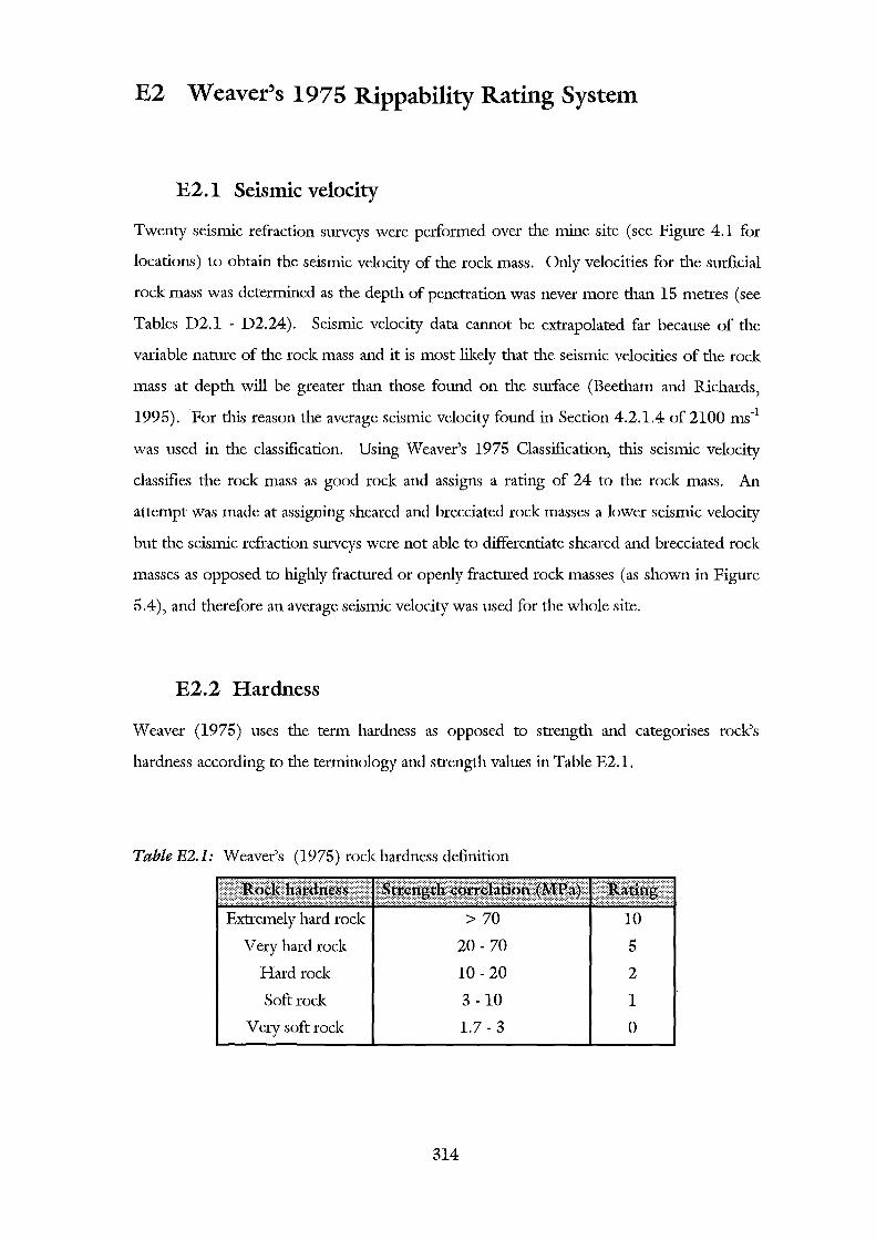
E2 Weaver's 1975 Rippability Rating System
E2.1 Seismic velocity
Twenty seismic refraction surveys were performed over the mine site (see Figure 4.1 for
locations) to obtain the seismic velocity of the rock mass. Only velocities for the surficial
rock mass was determined as the depth of penetration was never more than 15 metres (see
Tables D2.1 - D2.24). Seismic velocity data cannot be extrapolated far because of the
variable nature of the rock mass and it is most likely that the seismic velocities of the rock
mass at depth will be greater than those found on the surface (Beetham and Richards,
1995). For this reason the average seismic velocity found in Section 4.2.1.4 of 2100 ms-1
was used in the classification. Using Weaver's 1975 Classification, this seismic velocity
classifies the rock mass as good rock and assigns a rating of 24 to the rock mass. An
attempt was made at assigning sheared and brecciated rock masses a lower seismic velocity
but the seismic refraction surveys were not able to differentiate sheared and brecciated rock
masses as opposed to highly fractured or openly fractured rock masses (as shown in Figure
5.4), and therefore an average seismic velocity was used for the whole site.
E2.2 Hardness
Weaver (1975) uses the term hardness as opposed to strength and categorises rock's
hardness according to the terminology and strength values in Table E2.l.
TableE2.1: Weaver's (1975) rockhardness definition
Extremely hard rock > 70 10
Very hard rock 20-70 5
Hard rock 10-20 2
Soft rock 3-10 1
Very soft rock 1.7-3 0
314

To assign the rating for this parameter, the revised strength (determination of the revised
strength is explained in Section El.1) was assigned a rating according to Table E2.l.
E2.3 Weathering
Weaver (1975) uses weathering of the rock mass as opposed to weathering of discontinuity
surfaces like Bieniawski (1989). Weathering of the rock mass was logged by Macraes and
is assigned a rating according to Table 3.3.
E2.4 Joint spacing
This parameter was logged by Macraes as fractures per metre, which is the inverse of joint
spacing, and therefore the inverse of the fractures per metre parameter was calculated to
fmd the average joint spacing for every rock mass unit. The average joint spacing was then
assigned a rating using Table 3.3.
E2.5 Joint continuity
This parameter cannot be determined exactly for drill core data (unless the discontinuity
occurs longitudinally down the drillcore - which is very rare), therefore the main defect
type in each rock mass unit is assigned a rating based on its general characteristics. The
termination and persistence of discontinuities mapped on line traverses were logged by
Barrell (1992). This data coupled with observations made of outcrops led to the following
generalisations (logged descriptions in brackets):
• Breaks (BK), cleavage (CV), schistocity (SC), lineations (LI), veinlets (VNL) and
drilling induced fractures (DI) are all generally non-continuous to slightly
continuous and are assigned a rating of 5.
• Partings (PT), bedding (BD), bedding contacts(tCT, bCT), joints (JT), joint sets
(GJ), stringers (ST) and veins (VN) are continuous and do not normally contain
any infilling gouge, and therefore are assigned a rating of 3.
• Shears (SH), shear zones (SZ), crush zones (CZ), shattered zones (STZ),
decomposed zones (DZ), faults (FT), pug (PG) and breccia (BX) are generally
continuous and contain gouge, and therefore are given a rating ofO.
315
E2.6 Joint gouge
This parameter requires both joint separation (or infilling width) and the predominant type
of infilling to determine the rating for every rock mass unit. The infilling width is
described as either, clean (CL), stained (ST), a vein (VN) or a veinlet (VNL) and if the
width is greater than 2 mm, then the thickness is also recorded. If no data is logged, then
it is assmned that there is no joint separation. Ratings are assigned using Table 3.3 as
follows:
• Veins, stained or clean surfaces or no separation are assigned a rating of 5.
• If the infilling width is greater than 2 mm and there is no infilling, then they are
assigned a rating of 4.
• If the main infilling type is clay or pug and the infilling width is less than 5 mm,
then they are given a rating of 3.
• If the predominant infilling type is clay or pug and the infilling width is greater
than 5 mm, then the rock mass unit is assigned a rating of l.
E2. 7 Discontinuity orientation
Weaver (1975) did not quantify what a favourable or unfavourable strike and dip
orientation was, and therefore Minty and Kearns (1983) strike and dip orientation
guidelines (Table 2.8) were used to determine the favourability of an orientation. Ratings
were assigned using Table 3.3 and the assumptions outlined in Section El.6.
E3 The Modified Weaver Rippability Rating System
As this system is based on the latest RMR System, the same assmnptions made in
determining the RMR System (Appendix E1) are used in calculating the Modified Weaver
Rippability Rating System, except that groundwater and RQD parameters are replaced by
a seismic velocity parameter, which was averaged for the whole pit (as discussed in Section
E2.1).
316

E4 MacGregor, et at's (1994) productivity estimation equations
E4.l UCS
MacGregor et aPs (1994) productivity estimation equations require the actual unconfmed
compressive strength as opposed to a rating value. The revised strength estimate has been
used for this parameter and the assumptions and generalisations made in determining the
revised strength are outlined in Section ELL
E4.2 Weathering
MacGregor et al (1994) use weathering of the rock mass in their equations as opposed to
weathering of discontinuity surfaces. Weathering of the rock mass was logged by Macraes
and is assigned a rating according to the descriptions in Table 3.9.
E4.3 Grain size
MacGregor et al (1994) found the grain size to be a major influence on the productivity of
a bulldozer. Macraes logged the grain size of the sediments, and therefore, the grain size is
assigned ratings according to Table 3.9. If the grain size varies, for example fme sand and
course sand are present in the drillcore, then MacGregor et aPs (1994) ratings are averaged
such that, for example, FSCS (fme sand - coarse sand) is assigned a rating of 2. 75 (mean
of2 and 3.5).
E4.4 Seismic velocity
MacGregor et al (1994) require the actual seismic velocity in their productivity estimation
equations. The average seismic velocity was used for this parameter (as explained in
Section E2.1). The seismic velocity parameter does not influence the fmal productivity as
much as strength and the structural rating, therefore any lack of variation in the seismic
velocity parameter is not very important.
317
E4.5 Defect roughness
Macraes logged defect or discontinuity rouglmess and this parameter is assigned a rating
according to the description given in Table 3.9.
E4.6 Number of defect sets
This parameter requires only the number of defect sets and not their orientation with
respect to the ripping direction. The two most penetrative defect sets are bedding and
cleavage. The clustered joint set pattern found in Section 4.5.4 roughly equate to one
defect set because of its distribution pattern (see Figure 4.27b). Therefore it is assumed
that there are three defect sets in open pit area.
E4. 7 Defect spacing
MacGregor et a! (1994) use the actual defect spacing in their productivity equations.
Macraes logged fractures per metre, which is the inverse of defect spacing, and therefore,
the inverse of fractures per metre was used for this parameter.
E4.8 Structure rating
MacGregor et aPs (1994) stmctural rating is the relationship between bedding and defect
spacing. This parameter is assigned ratings according to Table 3.9. The logged rock unit
parameter was used for this parameter using the following assumptions (logged
descriptions in brackets) based on field observations:
• Breccia (Bx), host rock breccia (HBx), pug breccia (PBx), quartz breccia (QBx),
gravel (GRA V), clay (CLAY), pug (PUG), scree material (SCRE), mbble
(RUBB) and soil (SOIL) were all assigned a rating of19.
• Interbedded silts and muds (IS) and interbedded silts, muds and breccia (ISBx)
were assigned a rating of 17.
• Quartz lodes (QT) were assigned a rating of 16.
• Interbedded silts, sands and muds (IBIS) were assigned a rating of 15.
318
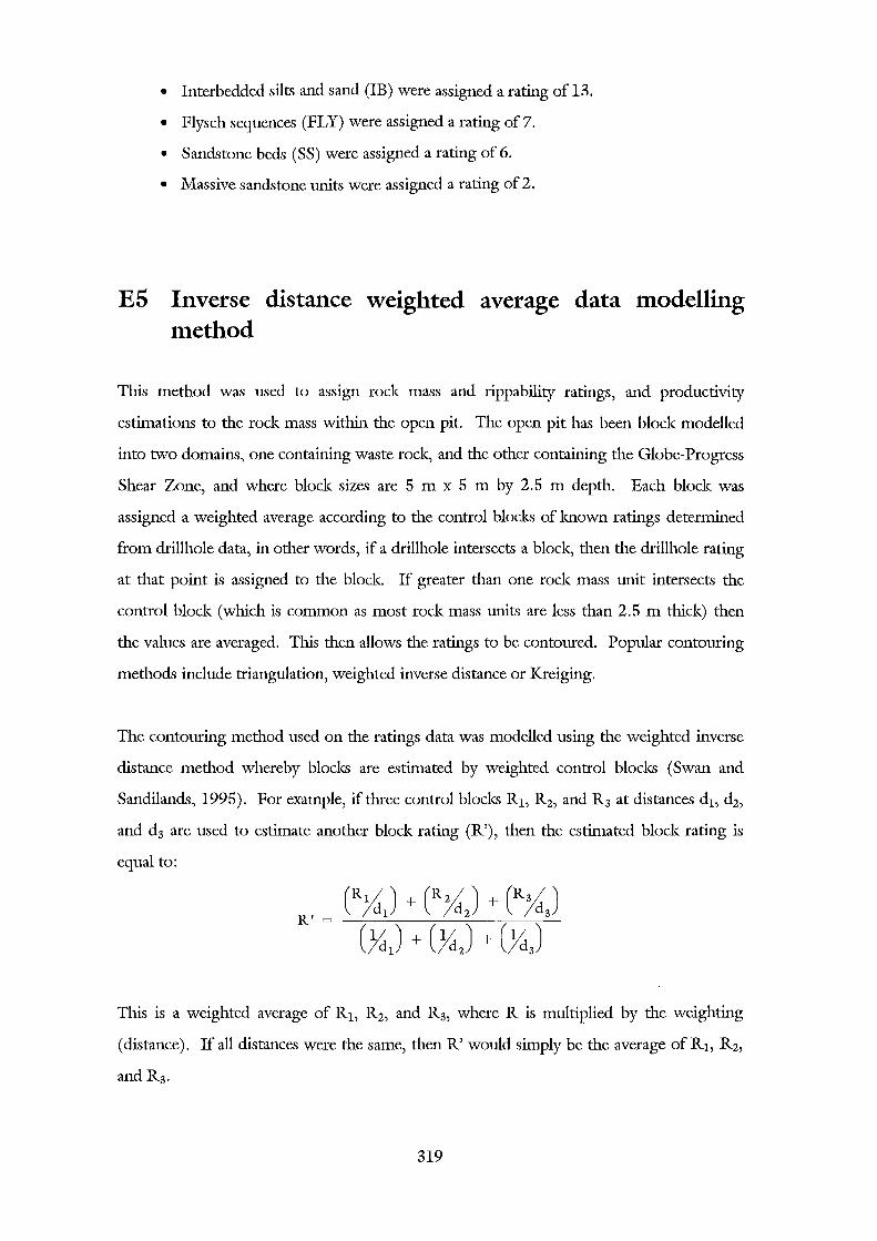
• Interbedded silts and sand (IB) were assigned a rating of 13.
• Flysch sequences (FLY) were assigned a rating of 7.
• Sandstone beds (SS) were assigned a rating of 6.
• Massive sandstone units were assigned a rating of 2.
E5 Inverse distance weighted average data modelling method
This method was used to assign rock mass and rippability ratings, and productivity
estimations to the rock mass within the open pit. The open pit has been block modelled
into two domains, one containing waste rock, and the other containing the Globe-Progress
Shear Zone, and where block sizes are 5 m x 5 m by 2.5 m depth. Each block was
assigned a weighted average according to the control blocks of known ratings determined
from drillhole data, in other words, if a drillhole intersects a block, then the drillhole rating
at that point is assigned to the block If greater than one rock mass unit intersects the
control block (which is common as most rock mass units are less than 2.5 m thick) then
the values are averaged. This then allows the ratings to be contoured. Popular contouring
methods include triangulation, weighted inverse distance or Kreiging.
The contouring method used on the ratings data was modelled using the weighted inverse
distance method whereby blocks are estimated by weighted control blocks (Swan and
Sandilands, 1995). For example, if three control blocks R1, R 2, and R 3 at distances d1, d2,
and d3 are used to estimate another block rating (R'), then the estimated block rating is
equal to:
R' = (R(ciJ + (R~J + (R~J
(X!J + (X!J + (X!J
This is a weighted average of R1, R 2, and R 3, where R is multiplied by the weighting
(distance). If all distances were the same, then R' would simply be the average of R1, Rz,
andR3•
319
The common notation of the above equation is written as:
R'= ~(R(ciJ
tc~~J !=l
If large distances are used, then the distance weighting may be varied by squaring or
cubing the distance weighting, that is, (l/d2) or (l/d3
), making the data more reliable.
Block modelling the data assumed a maximum distance of 80 m, and therefore the distance
weighting was cubed. The estimates produced for every block is within the range of the
contributing control blocks, and which is adequate for these purposes as ranges are plotted
rather than actual values.
320


