Robustness analysis of finite precisionimplementations

Eric Goubault and Sylvie Putot

CEA Saclay Nano-INNOV, CEA LIST, Laboratory for the Modelling and Analysis ofInteracting Systems, Point Courrier 174, 91191 Gif sur Yvette CEDEX,

{Eric.Goubault,Sylvie.Putot}@cea.fr

Abstract. A desirable property of control systems is to be robust to in-puts, that is small perturbations of the inputs of a system will cause onlysmall perturbations on its outputs. But it is not clear whether this prop-erty is maintained at the implementation level, when two close inputs canlead to very different execution paths. The problem becomes particularlycrucial when considering finite precision implementations, where any el-ementary computation can be affected by a small error. In this context,almost every test is potentially unstable, that is, for a given input, thecomputed (finite precision) path may differ from the ideal (same com-putation in real numbers) path. Still, state-of-the-art error analyses donot consider this possibility and rely on the stable test hypothesis, thatcontrol flows are identical. If there is a discontinuity between the treat-ments in the two branches, that is the conditional block is not robust touncertainties, the error bounds can be unsound.We propose here a new abstract-interpretation based error analysis of fi-nite precision implementations, relying on the analysis of [16] for round-ing error propagation in a given path, but which is now made soundin presence of unstable tests. It automatically bounds the discontinuityerror coming from the difference between the float and real values whenthere is a path divergence, and introduces a new error term labeled by thetest that introduced this potential discontinuity. This gives a tractable er-ror analysis, implemented in our static analyzer FLUCTUAT: we presentresults on representative extracts of control programs.

1 Introduction

In the analysis of numerical programs, a recurrent difficulty when we want toassess the influence of finite precision on an implementation, is the possibilityfor a test to be unstable: when, for a given input, the finite precision controlflow can differ from the control flow that would be taken by the same executionin real numbers. Not taking this possibility into account may be unsound if thedifference of paths leads to a discontinuity in the computation, while taking itinto account without special care soon leads to large over-approximations.

And when considering programs that compute with approximations of realnumbers, potentially unstable tests lie everywhere: we want to automaticallycharacterize conditional blocks that perform a continuous treatment of inputs,

and are thus robust, and those that do not. This unstable test problem is thusclosely related to the notion of continuity/discontinuity in programs, first intro-duced in [18]. Basically, a program is continuous if, when its inputs are slightlyperturbed, its output is also only slightly perturbed, very similarly to the conceptof a continuous function. Discontinuity in itself can be a symptom of a majorbug in some critical systems, such as the one reported in [2], where a F22 Rap-tor military aircraft almost crashed after crossing the international date line in2007, due to a discontinuity in the treatment of dates. Consider the toy programpresented on the left hand side of Figure 1, where input x takes its real value in[1, 3], with an initial error 0 < u << 1, that can come either from previous finiteprecision computations, or from any uncertainty on the input such as sensorimperfection. The test is potentially unstable: for instance, if the real value of xat control point [1] is rx[1] = 2, then its floating-point value is fx[1] = 2 + u. Thusthe execution in real numbers would take the then branch and lead at controlpoint [2] to ry[2] = rx[1] + 2 = 4, whereas the floating-point execution would take

the else branch and lead to fy[4] = fx[1] = 2 + u. The test is not only unstable,

but also introduces a discontinuity around the test condition (x == 2). Indeed,for rx[1] = 2, there is an error due to discontinuity of fy[4] − r

y[2] = −2 + u. Of

course, the computation of z around the test condition is continuous.

In the rest of the paper, we propose a new analysis, that enhances earlier workby the authors [16], by computing and propagating bounds on those discontinuityerrors. This previous work characterized the computation error due to the im-plementation in finite precision, by comparing the computations in real-numberswith the same computations in the floating-point semantics, relying on the stabletest assumption: the floating-point number control flow does not diverge fromthe real number control flow. In its implementation in FLUCTUAT [7], in thecase when the analysis determined a test could be unstable, it issued a warning,and the comparison between the two semantics could be unsound. This issue,and the stable test assumption, appear in all other (static or dynamic) existinganalyzes of numerical error propagation; the expression unstable test is actuallytaken from CADNA [6], a stochastic arithmetic instrumentation of programs, toassert their numerical quality. In Hoare provers dealing with both real numberand floating-point number semantics, e.g. [1] this issue has to be sorted out bythe user, through suitable assertions and lemmas.

Here as in previous work, we rely on the relational abstractions of real numberand floating numbers semantics using affine sets (concretized as zonotopes) [14,15, 9, 10, 16]. But we now also, using these abstractions, compute and solve con-straints on inputs such that the execution potentially leads to unstable tests,and thus accurately bound the discontinuity errors, computed as the differenceof the floating-point value in one branch and the real value in another, when thetest distinguishing these two branches can be unstable.

Let us exemplify and illustrate this analysis on the program from Figure 1.The real value of input x will be abstracted by the affine form rx[1] = 2+εr1, where

εr1 is a symbolic variable with values in [−1, 1]. Its error is ex[1] = u and its finite

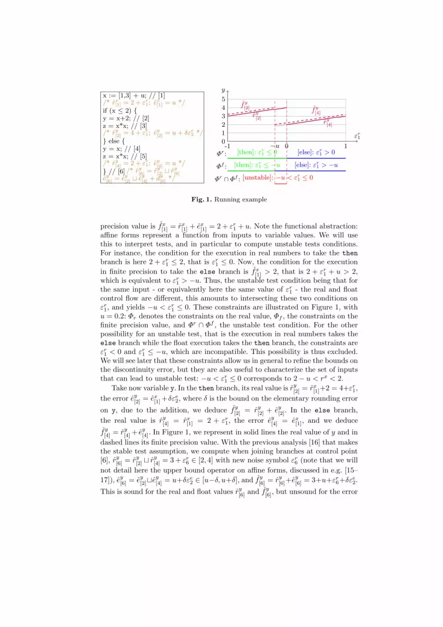
x := [1,3] + u; // [1]/* rx[1] = 2 + εr1; ex[1] = u */if (x ≤ 2) {y = x+2; // [2]z = x*x; // [3]/* ry[2] = 4 + εr1; ey[2] = u+ δεe2 */

} else {y = x; // [4]z = x*x; // [5]/* ry[4] = 2 + εr1; ey[4] = u */

} // [6] /* ry[6] = ry[2] t ry[6]

ey[6] = ey[2] t ey[4] + dy[6] */

εr1

-1 0−u 1

y

0

1

2

3

4

5

Φr:

Φf :

[then]: εr1 ≤ 0 [else]: εr1 > 0

[then]: εr1 ≤ −u [else]: εr1 > −u

Φr ∩ Φf : [unstable]: −u < εr1 ≤ 0

ry[2]

fy[2] fy

[4]

ry[4]

Fig. 1. Running example

precision value is fx[1] = rx[1] + ex[1] = 2 + εr1 + u. Note the functional abstraction:affine forms represent a function from inputs to variable values. We will usethis to interpret tests, and in particular to compute unstable tests conditions.For instance, the condition for the execution in real numbers to take the then

branch is here 2 + εr1 ≤ 2, that is εr1 ≤ 0. Now, the condition for the execution

in finite precision to take the else branch is fx[1] > 2, that is 2 + εr1 + u > 2,which is equivalent to εr1 > −u. Thus, the unstable test condition being that forthe same input - or equivalently here the same value of εr1 - the real and floatcontrol flow are different, this amounts to intersecting these two conditions onεr1, and yields −u < εr1 ≤ 0. These constraints are illustrated on Figure 1, withu = 0.2: Φr denotes the constraints on the real value, Φf , the constraints on thefinite precision value, and Φr ∩ Φf , the unstable test condition. For the otherpossibility for an unstable test, that is the execution in real numbers takes theelse branch while the float execution takes the then branch, the constraints areεr1 < 0 and εr1 ≤ −u, which are incompatible. This possibility is thus excluded.We will see later that these constraints allow us in general to refine the bounds onthe discontinuity error, but they are also useful to characterize the set of inputsthat can lead to unstable test: −u < εr1 ≤ 0 corresponds to 2− u < rx < 2.

Take now variable y. In the then branch, its real value is ry[2] = rx[1]+2 = 4+εr1,

the error ey[2] = ex[1] +δεe2, where δ is the bound on the elementary rounding error

on y, due to the addition, we deduce fy[2] = ry[2] + ey[2]. In the else branch,

the real value is ry[4] = rx[1] = 2 + εr1, the error ey[4] = ex[1], and we deduce

fy[4] = ry[4] + ey[4]. In Figure 1, we represent in solid lines the real value of y and in

dashed lines its finite precision value. With the previous analysis [16] that makesthe stable test assumption, we compute when joining branches at control point[6], ry[6] = ry[2] t r

y[4] = 3 + εr6 ∈ [2, 4] with new noise symbol εr6 (note that we will

not detail here the upper bound operator on affine forms, discussed in e.g. [15–

17]), ey[6] = ey[2]tey[4] = u+δεe2 ∈ [u−δ, u+δ], and fy[6] = ry[6]+e

y[6] = 3+u+εr6+δεe2.

This is sound for the real and float values ry[6] and fy[6], but unsound for the error

because of the possibility of an unstable test. Our new analysis, when joiningbranches, also computes bounds for ry[4]− r

y[2] = 2 + εr1− (4 + εr1) = −2 under the

unstable test condition −u < εr1 ≤ 0 (or 2 − u < rx < 2): a new discontinuityterm is added and the error is now ey[6] + dy[6] where dy[6] = −2χ[−u,0](ε1) and

χ[a,b](x) equals 1 if x is in [a, b] and 0 otherwise.

Related work In [3], the authors introduce a continuity analysis of programs.This approach is pursued in particular in [5, 4], where several refinements of thenotion of continuity or robustness of programs are proposed, another one beingintroduced in [20]. These notions are discussed in [8], in which an interactiveproof scheme for proving a general form of robustness is discussed. In [20], thealgorithm proposed by the authors symbolically traverses program paths andcollects constraints on input and output variables. Then for each pair of pro-gram paths, the algorithm determines values of input variables that cause theprogram to follow these two paths and for which the difference in values of theoutput variable is maximized. We use one of their examples (transmission shift,Section 5), and show that we reach similar conclusions. One difference betweenthe approaches is that we give extra information concerning the finite precisionflow divergence with respect to the real number control flow, potentially exhibit-ing flawed behaviors. Also, their path-sensitive analysis can exhibit witnesses forworst discontinuity errors, but at the expense of a much bigger combinatorialcomplexity. Actually, we will show that our unstable test constraints also allowus to provide indication on the inputs leading to discontinuity errors.

Robustness has also been discussed in the context of synthesis and validationof control systems, in [19, 24]. The formalization is based on automata theoreticmethods, providing a convenient definition of a metric between Buchi automata.Indeed, robustness has long been central in numerical mathematics, in particularin control theory. The field of robust control is actually concerned in provingstability of controlled systems where parameters are only known in range. Anotion which is similar to the one of [24], but in the realm of real numbers andcontrol of ordinary differential equations, is the input-output stability/continuityin control systems as discussed in [23].

This problematic is also of primary importance in computational geometry,see for instance [22] for a survey on the use of “robust geometric predicates”.Nevertheless, the aim pursued is different from ours: we are mostly interestedin critical embedded software, where the limited resources generally prevent theuse of complicated, refined arithmetic algorithms.

Contents Our main contribution is a tractable analysis that generalizes boththe abstract domain of [16] and the continuity or robustness analyses: it ensuresthe finite precision error analysis is now sound even in the presence of unstabletests, by computing and propagating discontinuity error bounds for these tests.

We first review in Section 2 the basics of the relational analysis based onaffine forms for the abstraction of real number semantics necessary to under-stand this robustness analysis presented here. We then introduce in Section 3our new abstract domain, based on an abstraction similar to that of [16], but

refined to take care of unstable tests properly. We present in Section 4 some re-finements that are useful for reaching more accurate results, but are not centralto understand the principles of the analysis. We conclude with some experimentsusing our implementation of this abstraction in our static analyzer FLUCTUAT.

2 Preliminaries: affine sets for real valued analysis

We recall here the key notions on the abstract domains based on affine sets forthe analysis of real value of program variables that will be needed in Sections 3and 4 for our robustness analysis. We refer to [12, 14, 15, 9, 10] for more details.

From affine arithmetic to affine sets Affine arithmetic is a more accurateextension of interval arithmetic, that takes into account affine correlations be-tween variables. An affine form is a formal sum over a set of noise symbols εi

xdef= αx0 +

n∑i=1

αxi εi,

with αxi ∈ R for all i. Each noise symbol εi stands for an independent componentof the total uncertainty on the quantity x, its value is unknown but boundedin [-1,1]; the corresponding coefficient αxi is a known real value, which gives themagnitude of that component. The same noise symbol can be shared by severalquantities, indicating correlations among them. These noise symbols can notonly model uncertainty in data or parameters, but also uncertainty coming fromcomputation. The values that a variable x defined by an affine form x can takeis in the range γ(x) = [αx0 −

∑ni=1 |αxi |, αx0 +

∑ni=1 |αxi |] .

The assignment of a variable x whose value is given in a range [a, b], is definedas a centered form using a fresh noise symbol εn+1 ∈ [−1, 1], which indicates

unknown dependency to other variables: x = (a+b)2 + (b−a)

2 εn+1.The result of linear operations on affine forms is an affine form, and is thus

interpreted exactly. For two affine forms x and y, and a real number λ, we haveλx + y = (λαx0 + αy0) +

∑ni=1(λαxi + αyi )εi. For non affine operations, we select

an approximate linear resulting form, and bounds for the error committed usingthis approximate form are computed, that are used to add a new noise term tothe linear form.

As a matter of fact, the new noise symbols introduced in these linearizationprocesses, were given different names in [15, 16]: the ηj symbols. Although theyplay a slightly different role than that of εi symbols, for sake of notationalsimplicity, we will only give formulas in what follows, using the same εi symbolsfor both types of symbols. The values of the variables at a given control point asa linearized function of the values of the inputs of the program, that we generallyidentify with a prefix of the εi vector. The uncertainties, due to the abstractionof non-linear features such as the join and the multiplication will be abstractedon a suffix of the εi vector - previously the ηj symbols.

In what follows, we use the matrix notations of [15] to handle affine sets, thatis tuples of affine forms. We noteM(n, p) the space of matrices with n lines and

p columns of real coefficients. A tuple of affine forms expressing the set of valuestaken by p variables over n noise symbols εi, 1 ≤ i ≤ n, can be represented bya matrix A ∈M(n+ 1, p).

Constrained affine sets As described in [10], we interpret tests by adding someconstraints on the εi noise symbols, instead of having them vary freely into [-1,1]: we restrain ourselves to executions (or inputs) that can take the consideredbranch. We can then abstract these constraints in any abstract domain, thesimplest being intervals, but we will see than we actually need (sub-)polyhedricabstractions to accurately handle unstable tests. We note A for this abstractdomain, and use γ : A → ℘(Rn) for the concretisation operator, and α : ℘(Rn)→A for some “abstraction” operator, not necessarily the best one (as in polyhedra,this does not exist): we only need to be able to get an abstract value from a setof concrete values, such that X ⊆ γ ◦ α(X).

This means that abstract values X are now composed of a zonotope identifiedwith its matrix RX ∈ M(n + 1, p), together with an abstraction ΦX of theconstraints on the noise symbols, X = (RX , ΦX). The concretisation of suchconstrained zonotopes or affine sets is γ(X) =

{tCXε | ε ∈ γ(ΦX)

}. For Φ ∈ A,

and x an affine form, we note Φ(x) the interval [J−, J+] with J− and J+ givenby the linear programs J− = infε∈γ(Φ) x(ε) and J+ = supε∈γ(Φ) x(ε).

Example 1. For instance on the running example, starting with program variablex in [1, 3], we associate the abstract value X with RX = (2 1), i.e. x = 2 + ε1,and γ(ΦX) = γ(ε1) = [−1, 1]. The interpretation of the test if (x<=2) in thethen branch is translated into constraint ε1 ≤ 0, thus γ(ΦX) = [−1, 0]. Then,the interval concretisation of x is γ(x) = [2− 1, 2] = [1, 2].

Transfer functions for arithmetic expressions Naturally, the transfer func-tions described in the unconstrained case are still correct when we have addi-tional constraints on the noise symbols; but for the non linear operations such asthe multiplication, the constraints can be used to refine the result by computingmore accurate bounds on the non affine part which is over-approximated by anew noise term, solving with a guaranteed linear solver1 the linear programmingproblems supε∈γ(ΦX) ε (resp. inf). Transfer functions are described, respectivelyin the unconstrained and constrained cases in [15] and [10], and will not bedetailed here, except in the example below.

Example 2. Consider the computation z=x*x at control point 3 in the then

branch of the running example (Figure 1). If computed as in the unconstrainedcase, we write z[3] = (2 + ε1)(2 + ε1) = 4 + 4ε1 + (ε1)2, which, using the factthat (ε1)2 is in [0,1], can be linearized using a new noise symbol by z[3] =4.5+4ε1 +0.5ε3 (new noise symbol called ε3 because introduced at control point3). The concretisation of z[3], using ε1 ∈ [−1, 0], is then γ(z[3]) = [0, 5].

1 For an interval domain for the constraints on noise symbols, a much more straight-forward computation can be made, of course.

But it is better to use the constraint on ε1 to linearize z=x*x at the center ofthe interval ε1 ∈ [−1, 0]: we then write z[3] = (1.5+(ε1 +0.5))(1.5+(ε1 +0.5)) =2.25 + 1.5 + (ε1 + 0.5) + (ε1 + 0.5)2, which, using (ε1 + 0.5)2 ∈ [0, 0.25], can belinearized as z[3] = 3.875 + 3ε1 + 0.125ε3. Its concretisation is γ(z[3]) = [0.75, 4].

In the else branch, z=x*x interpreted at control point 5 with ε1 ∈ [0, 1] islinearized by z[5] = (2.5 + (ε1 − 0.5))(2.5 + (ε1 − 0.5)) = 3.875 + 5ε1 + 0.125ε5.And γ(z[5]) = [3.75, 9].

Join We need an upper bound operator to combine abstract values coming fromdifferent branches. The computation of upper bounds (and if possible minimalones) on constrained affine sets is a difficult task, already discussed in severalpapers [14, 15, 10, 11], and orthogonal to the robustness analysis presented here.We will thus consider we have an upper bound operator on constrained affinesets we note t, and focus on the additional term due to discontinuity in tests.

3 Robustness analysis of finite precision computations

We introduce here an abstraction which is not only sound in presence of unstabletests, but also exhibits the potential discontinuity errors due to these tests. Formore concision, we insist here on what is directly linked to an accurate treatmentof these discontinuities, and rely on previous work [16] for the rest.

3.1 Abstract values

As in the abstract domain for the analysis of finite precision computations of [16],we will see the floating-point computation as a perturbation of a computationin real numbers, and use zonotopic abstractions of real computations and er-rors (introducing respectively noise symbols εri and εej), from which we getan abstraction of floating point computations. But we make here no assump-tions on control flows in tests and will interpret tests independently on the realvalue and the floating-point value. For each branch, we compute conditions forthe real and floating-point executions to take this branch. The test interpreta-tion on a zonotopic value [10] lets the affine sets unchanged, but yields con-straints on noise symbols. For each branch, we thus get two sets of constraints:εr = (εr1, . . . , ε

rn) ∈ ΦXr for the real control flow (test computed on real values

RX), and (εr, εe) = (εr1, . . . , εrn, ε

e1, . . . , ε

em) ∈ ΦXf for the finite precision control

flow (test computed on float values RX + EX).

Definition 1. An abstract value X, defined at a given control point, for a pro-gram with p variables x1, . . . , xp, is thus a tuple X = (RX , EX , DX , ΦXr , Φ

Xf )

composed of the following affine sets and constraints, for all k = 1, . . . , p:RX : rXk = rX0,k +

∑ni=1 r

Xi,k ε

ri where εr ∈ ΦXr

EX : eXk = eX0,k +∑ni=1 e

Xi,k ε

ri +

∑mj=1 e

Xn+j,k ε

ej where (εr, εe) ∈ ΦXf

DX : dXk = dX0,k +∑oi=1 d

Xi,k ε

di

fXk = rXk + eXk where (εr, εe) ∈ ΦXf

where

– RX ∈ M(n+ 1, p) is the affine set defining the real values of variables, andthe affine form rXk giving the real value of xk, is defined on the εri ,

– EX ∈M(n+m+1, p) is the affine set defining the rounding errors (or initialuncertainties) and their propagation through computations as defined in [16],and the affine form eXk is defined on the εri that model the uncertainty onthe real value, and the εei that model the uncertainty on the rounding errors,

– DX ∈M(o+ 1, p) is the affine set defining the discontinuity errors, and dXkis defined on noise symbols εdi ,

– the floating-point value is seen as the perturbation by the rounding error ofthe real value, fXk = rXk + eXk .

– ΦXr is the abstraction of the set of constraints on the noise symbols suchthat the real control flow reaches the control point, εr ∈ ΦXr , and ΦXf is theabstraction of the set of constraints on the noise symbols such that the finiteprecision control flow reaches the control point, (εr, εe) ∈ ΦXf .

A subtlety is that the same affine set RX is used to define the real value andthe floating-point value as a perturbation of the real value, but with differentconstraints: the floating-point value is indeed a perturbation by rounding errorsof an idealized computation that would occur with the constraints ΦXf .

3.2 Test interpretation

Consider a test e1 op e2, where e1 and e2 are two arithmetic expressions, andop an operator among ≤, <,≥, >,=, 6=, the interpretation of this test in our ab-stract model reduces to the interpretation of z op 0, where z is the abstractionof expression e1 - e2 with affine sets:

Definition 2. Let X be a constrained affine set over p variables. We defineZ = [[e1 op e2]]X by Y = [[xp+1 := e1 − e2]]X in Z = dropp+1([[xp+1 op 0]]Y ),where function dropp+1 returns the affine sets from which component p+ 1 (theintermediary variable) has been eliminated.

As already said, tests are interpreted independently on the affine sets forreal and floating-point value. We use in Definition 3, the test interpretation onconstrained affine sets introduced in [10]:

Definition 3. Let X = (RX , EX , DX , ΦXr , ΦXf ) a constrained affine set. We

define Z = ([[xk op 0]]X by(RZ , EZ , DZ) = (RX , EX , DX)

ΦZr = ΦXr⋂α(εr | rX0,k +

∑ni=1 r

Xi,kε

ri op 0

)ΦZf = ΦXf

⋂α(

(εr, εe) | rX0,k + eX0,k +∑ni=1(rXi,k + eXi,k)εri +

∑mj=1 e

Xn+j,kε

ej op 0

)Example 3. Consider the running example. We start with rx[1] = 2 + εr1, ex[1] = u.The condition for the real control flow to take the then branch is rx[1] = 2+εr1 ≤ 2,

thus Φr is εr1 ∈ [−1, 0]. The condition for the finite precision control flow to take

the then branch is fx[1] = rx[1] + ex[1] = 2 + εr1 + u ≤ 2, thus Φf is εr1 ∈ [−1,−u].

3.3 Interval concretisation

The interval concretisation of the value of program variable xk defined by theabstract value X = (RX , EX , DX , ΦXr , Φ

Xf ), is, with the notations of Section 2:

γr(rXk ) = ΦXr (rX0,k +

∑ni=1 r

Xi,k ε

ri )

γe(eXk ) = ΦXf (eX0,k +

∑ni=1 e

Xi,k ε

ri +

∑mj=1 e

xn+j,k ε

ej)

γd(dXk ) = ΦXf (dX0,k +

∑ol=1 d

xl,k ε

dl )

γf (fXk ) = ΦXf (rX0,k + eX0,k +∑ni=1(rXi,k + eXi,k) εri +

∑mj=1 e

xn+j,k ε

ej)

Example 4. Consider variable y in the else branch of our running example.The interval concretisation of its real value on ΦXr , is γr(r

y[4]) = ΦXr (2 + εr1) =

2 + [0, 1] = [2, 3]. The interval concretisation of its floating-point value on ΦXf ,

is γf (fy[4]) = ΦXf (ry[4] + u) = 2 + [−u, 1] + u = [2, 3 + u]. Actually, ry[4] is defined

on ΦXr ∪ ΦXf , as illustrated on Figure 1, because it is both used to abstract thereal value, or, perturbed by an error term, to abstract the finite precision value.

In other words, the concretisation of the real value is not the same when itactually represents the real value at the control point considered (γr(r

Xk )), or

when it represents a quantity which will be perturbed to abstract the floating-point value (in the computation of γf (fXk )).

3.4 Transfer functions: arithmetic expressions

We rely here on the transfer functions of [16] for the full model of values andpropagation of errors, except than some additional care is required due to theseconstraints. As quickly described in Section 2, constraints on noise symbols canbe used to refine the abstraction of non affine operations. Thus, in order tosoundly use the same affine set RX both for the real value and the floating-pointvalue as a perturbation of a computation in real numbers, we use constraintsΦXr ∪ ΦXf to abstract transfer functions for the real value RX in arithmetic

expressions. Of course, we will then concretize them either for ΦXf or ΦXr , asdescribed in Section 3.3.

Example 5. Take the running example. In example 2, we computed the real formrz in both branches, interpreting instruction z=x*x, for both sets of constraintsΦr. In order to have an abstraction of rz that can be soundly used both forthe floating-point and real values, we will now need to compute this abstractionand linearization for Φr ∪ Φf . In the then branch, εr1 is now taken in [−1, 0] ∪[−1,−u] = [−1, 0], so that rz[3] = 3.875 + 3εr1 + 0.125εr3 remains unchanged.

But in the else branch, εr1 is now taken in [0, 1] ∪ [−u, 1] = [−u, 1], so thatz=x*x can still be linearized at εr1 = 0.5 but we now have rz[5] linearized from

(2.5 + (εr1 − 0.5))(2.5 + (εr1 − 0.5)) = 6.25 + 5(εr1 − 0.5) + (εr1 − 0.5)2 where

−0.5 − u ≤ εr1 − 0.5 ≤ 0.5, so that rz[5] = (3.75 + (0.5+u)2

2 ) + 5εr1 + (0.5+u)2

2 εr5 =

3.875 + u+u2

2 + 5εr1 + (0.125 + u+u2

2 )εr5.

3.5 Join

In this section, we consider we have upper bound operator t on constrainedaffine sets, and focus on the additional term due to discontinuity in tests. Asfor the meet operator, we join component-wise the real and floating-point parts.But, in the same way as for the transfer functions, the join operator depends onthe constraints on the noise symbols: to compute the affine set abstracting thereal value, we must consider the join of constraints for real and float control flow,in order to soundly use a perturbation of the real affine set as an abstraction ofthe finite precision value.

Let us consider the possibility of an unstable test: for a given input, thecontrol flows of the real and of the finite precision executions differ. Then, whenwe join abstract values X and Y coming from the two branches, the differencebetween the floating-point value of X and the real value of Y , (RX +EX)−RY ,and the difference between the floating-point value of X and the real valueof Y , (RY + EY ) − RX , are also errors due to finite precision. The join oferrors EX , EY , (RX + EX) − RY and (RY + EY ) − RX can be expressed asEZ +DZ , where EZ = EX tEY is the propagation of classical rounding errors,and DZ = DXtDY t(RX−RY )t(RY −RX) expresses the discontinuity errors.

The rest of this section will be devoted to an accurate computation of thesediscontinuity terms. A key point is to use the fact that we compute these termsonly in the case of unstable tests, which can be expressed as an intersectionof constraints on the εri noise symbols. Indeed this intersection of constraintsexpress the unstable test condition as a restriction of the sets of inputs (orequivalently the εri ), such that an unstable test is possible. The fact that thesame affine set RX is used both to abstract the real value, and the floating-pointvalue when perturbed, is also essential to get accurate bounds.

Definition 4. We join two abstract values X and Y by Z = X t Y defined asZ = (RZ , EZ , DZ , ΦXr ∪ ΦYr , ΦXf ∪ ΦYf ) where

(RZ , ΦZr ∪ ΦZf ) = (RX , ΦXr ∪ ΦXf ) t (RY , ΦYr ∪ ΦYf )

(EZ , ΦZf ) = (EX , ΦXf ) t (EY , ΦYf )

DZ = DX tDY t (RX −RY , ΦXf u ΦYr ) t (RY −RX , ΦYf u ΦXr )

Example 6. Consider again the running example, and let us restrict ourselvesfor the time being to variable y. We join X = (ry[2] = 4+εr1, e

y[2] = u+δεe2, 0, ε

r1 ∈

[−1, 0], (εr1, εe2) ∈ [−1,−u] × [−1, 1]) coming from the then branch with Y =

(ry[4] = 2 + εr1, ey[4] = u, 0, εr1 ∈ [0, 1], εr1 ∈ [−u, 1]) coming from the else branch.

Then we can compute the discontinuity error due to the first possible unstabletest, when the real takes the then branch and float takes the else branch:ry[4] − r

y[2] = 2 + εr1 − 4 + εr1 = −2, for εr1 ∈ ΦYf ∩ ΦXr = [−u, 1] ∩ [−1, 0] = [−u, 0]

(note that the restriction on εr1 is not used here but will be in more general cases).The other possibility of an unstable test, when the real takes the else branch andfloat takes the then branch, occurs for εr1 ∈ ΦXf ∩ΦYr = [−1,−u]∩ [0, 1] = ∅: theset of inputs for which this unstable test can occur is empty, it never occurs. Weget Z = (3 + εr6, u+ δεe2,−2χ[−u,0](ε

r1), (εr1, ε

r6) ∈ [−1, 1]2, (εr1, ε

r6, ε

e2) ∈ [−1, 1]3).

4 Technical matters

We gave here the large picture. Still, there are some technical matters to considerin order to efficiently compute accurate bounds for the discontinuity error in thegeneral case. We tackle some of them in this section.

4.1 Constraint solving using slack variables

Take the following program, where the real value of inputs x and y are in range[-1,1], and both have an error bounded in absolute value by some small value u:

x := [ - 1 , 1 ] + [ -u , u ] ; // [ 1 ] ; 0 < u << 1y := [ - 1 , 1 ] + [ -u , u ] ; // [ 2 ]i f ( x < y )

t = y - x ; // [ 3 ]else

t = x - y ; // [ 4 ]

The test can be unstable, we want to prove the treatment continuous. Before thetest, rx[1] = εr1, ex[1] = uεe1, ry[2] = εr2, ey[2] = uεe2. The conditions for the control flow

to take the then branch are εr1 < εr2 for the real execution, and εr1+uεe1 < εr2+uεe2for the float execution. The real value of t in this branch is rt[3] = εr2− εr1. In the

else branch, the conditions are the reverse and rt[4] = εr1 − εr2.Let us consider the possibility of unstable tests. The conditions for the

floating-point to take the else branch while the real takes the then branch areεr1 + uεe1 ≥ εr2 + uεe2 and εr1 < εr2, from which we can deduce −2u < εr1 − εr2 < 0.Under these conditions, we can bound rt[4]−r

t[3] = 2(εr1−εr2) ∈ [−4u, 0]. The other

unstable test is symmetric, we thus have proven that the discontinuity error isof the order of the error on inputs, that is the conditional block is robust.

Note that on this example, we needed more than interval constraints onnoise symbols, and would in general have to solve linear programs. However,we can remark that constraints on real and floating-point parts share the samesubexpressions on the εr noise symbols. Thus, introducing slack symbols suchthat the test conditions are expressed on these slack variables, we can keepthe full precision when solving the constraints in intervals. Here, introducingεr3 = εr1 − εr2, the unstable test condition is expressed as εr3 < 0 and εr3 > −2u.This is akin to using the first step of the simplex method for linear programs,where slack variables are introduced to put the problem in standard form.

4.2 Linearization of non affine computations near the test condition

There can be a need for more accuracy near the test conditions: one situation iswhen we have successive joins, where several tests may be unstable, such as theinterpolator example presented in the experiments. In this case, it is necessaryto keep some information on the states at the extremities when joining values(and get rid of this extra information as soon as we exit the conditional block).More interesting, there is a need for more accuracy near the test condition whenthe conditional block contains some non linear computations.

Example 7. Consider again the running example. We are now interested in vari-able z. There is obviously no discontinuity around the test condition; still, ourpresent abstraction is not accurate enough to prove so. Remember from Exam-ples 2 and 5 that we linearize in each branch x*x for Φr ∪ Φf , introducing newnoise symbols εr3 and εr5. Let us consider the unstable test when the real exe-cution takes the then branch and the floating-point execution the other branch,the corresponding discontinuity error rz[5] − r

z[3], under unstable test constraint

−u < εr1 < 0, is:

rz[5] − rz[3] =

u+ u2

2+ 2εr1 + (0.125 +

u+ u2

2)εr5 − 0.125εr3. (1)

In this expression, from constraint −u < εr1 < 0 we can prove that u+u2

2 + 2εr1 +u+u2

2 εr5 is of the order of the input error u. But the new noise term 0.125(εr5 −εr3) is only bounded by [−0.25, 0.25]. We thus cannot prove continuity here.This is illustrated on the left-hand side of Figure 2, on which we representedthe zonotopic abstractions rz[3] and rz[5]: it clearly appears that the zonotopic

abstraction is not sufficient to accurately bound the discontinuity error (in theellipse), that will locally involve some interval-like computation. Indeed, in thelinearization of rz[3] (resp rz[5]), we lost the correlation between the new symbol εr3(resp εr5), and symbol εr1 on which the unstable test constraint is expressed. Asa matter of fact, we can locally derive in a systematic way some affine boundsfor the new noise symbols used for linearization in terms of the existing noisesymbols, using the interval affine forms of [13], centered at the extremities of theconstraints (ΦXr ∪ ΦXf )(εri ) of interest.

In the then branch, we have εr1 ∈ [−1, 0], and z=x*x is linearized from 3.75+(εr1+0.5)+(εr1+0.5)2, using (ε1+0.5)2 ∈ [0, 0.25], into rz[3] = 3.875+3εr1+0.125εr3.

We thus know at linearization time that εr3 = f(εr1) = 8(εr1 + 0.5)2 − 1. Usingthe mean value theorem around εr1 = 0 and restricting εr1 ∈ [−0.25, 0], we write

εr3(εr1) = f(0) +∆εr1,

where interval ∆ bounds the derivative f ′(εr1) in the range [−0.25, 0]. We getεr3 = 1 + 16([−0.25, 0] + 0.5)εr1 = 1 + [4, 8]εr1, which we can also write 1 + 8εr1 ≤εr3 ≤ 1 + 4εr1 for εr1 ∈ [−0.25, 0]. Variable z can thus locally (for εr1 ∈ [−0.25, 0])be expressed more accurately as a function of εr1, this is what is represented bythe darker triangular region inside the zonotopic abstraction, on the right-handside of Figure 2.In the same way, εr5 can be expressed in the else branch as an affine form

1 + ∆′εr1 with interval coefficient ∆′, so that with the unstable test constraint−u < εr1 < 0, we can deduce from Equation (1) that there exists some constantK such that |rz[5]−r

z[3]| ≤ Ku, that is the test is robust. Of course, we could refine

even more the bounds for the discontinuity error by considering linearization onsmaller intervals around the boundary condition.

εr1

-0.5 0 0.5

z

2

3

4

5

6

7

rz[3]

rz[5]

εr1

-0.25 0

z

3

4

Fig. 2. Improvement by local linearization for non affine computations

5 Experiments

In what follows, we analyze some examples inspired by industrial codes andliterature, with our implementation in our static analyzer FLUCTUAT.

A simple interpolator The following example implements an interpolator, affineby sub-intervals, as classically found in critical embedded software. It is a ro-bust implementation indeed. In the code below, we used the FLUCTUAT asser-tion FREAL WITH ERROR(a,b,c,d) to denote an abstract value (of resulting typefloat), whose corresponding real values are x ∈ [a, b], and whose correspondingfloating-point values are of the form x+ e, with e ∈ [c, d].

f loat R1 [ 3 ] , E, r e s ;R1 [ 0 ] = 0 ; R1 [ 1 ] = 5 ∗ 2 . 2 5 ; R1 [ 2 ] = R1 [ 1 ] + 20 ∗ 1 . 1 ;E = FREAL WITH ERROR(0 . 0 , 1 00 . 0 , - 0 . 00001 , 0 . 00001 ) ;i f (E < 5)

r e s = E∗2.25 + R1 [ 0 ] ;else i f (E < 25)

r e s = (E-5)∗1 .1 + R1 [ 1 ] ;else

r e s = R1 [ 2 ] ;return r e s ;

The analysis finds that the interpolated res is within [-2.25e-5,33.25], withan error within [-3.55e-5,2.4e-5], that is of the order of magnitude of the inputerror despite unstable tests.

A simple square root function This example is a rewrite in some particular case,of an actual implementation of a square root function, in an industrial context:

double sqr t2 = 1.414213538169860839843750;double S , I ; I = DREAL WITH ERROR(1 , 2 , 0 , 0 . 0 0 1 ) ;i f ( I>=2)

S = sqr t2 ∗(1+( I /2- 1 )∗ ( . 5 -0 .125∗ ( I /2- 1 ) ) ) ;elseS = 1+( I-1)∗( .5+( I -1)∗( -.125+( I - 1 )∗ . 0 6 2 5 ) ) ;

With the former type of analysis within FLUCTUAT, we get the unsound result- but an unstable test is signalled - that S is proven in the real number semanticsto be in [1,1.4531] with a global error in [-0.0005312,0.00008592].

As a matter of fact, the function does not exhibit a big discontinuity, but still,it is bigger than the one computed above. At value 2, the function in the then

branch computes sqrt2 which is approximately 1.4142, whereas the else branch

computes 1+0.5-0.125+0.0625=1.4375. Therefore, for instance, for a real numberinput of 2, and a floating-point number input of 2+ulp(2), we get a computationerror on S of the order of 0.0233. FLUCTUAT, using the domain described inthis paper finds that S is in the real number semantics within [1,1.4531] with aglobal error within [-0.03941,0.03895], the discontinuity at the test accountingfor most of it, i.e. an error within [-0.03898,0.03898] (which is coherent withrespect to the rough estimate of 0.0233 we made).

Transmission shift from [20] We consider here the program from [20] that im-plements a simple model of a transmission shift: according to a variable angle

measured, and the speed, lookup tables are used to compute pressure1 andpressure2, and deduce also the current gear (3 or 4 here). As noted in [20],pressure1 is robust. But a small deviation in speed can cause a large deviationin the output pressure2. As an example, when angle is 34 and speed is 14,pressure2 is 1000. But if there is an error of 1 in the measurement of angle,so that its value is 35 instead of 34, then pressure2 is found to be 0. Similarlywith an error of 1 on speed: if it is wrongly measured to be 13 instead of 14,pressure2 is found equal to 0 instead of 1000, again.

This is witnessed by our discontinuity analysis. For angle in [0,90], with anerror in [-1,1] and speed in [0,40], with an error in [-1,1], we find pressure1 equalto 1000 without error and pressure2 in [0,1000] with an error in [-1000,1000],mostly due to test if (oval <= 3) in function lookup2 2d. The treatment ongear is found discontinuous, because of test if (3*speed <= val1).

Householder Let us consider the C code printed on the left hand side of Figure 3,which presents the results of the analysis of this program by FLUCTUAT. Thisprogram computes in variable Output, an approximation of the square root ofvariable Input, which is given here in a small interval [16.0,16.002]. The programiterates a polynomial approximation until the difference between two successiveiterates xn and xnp1 is smaller than some stopping criterion. At the end, it checksthat something indeed close to the mathematical square root is computed, byadding instruction should be zero = Output-sqrt(Input); Figure 3 presentsthe result of the analysis for the selected variable should be zero, at the endof the program. The analyzer issues an unstable test warning, which line in theprogram is highlighted in red. On the right hand side, bounds for the floating-point, real values and error of should be zero are printed. The graph with theerror bars represents the decomposition on the error on its provenance on thelines of the program analyzed: in green are standard rounding errors, in purplethe discontinuity error due to unstable tests. When an error bar is selected (here,the purple one), the bounds for this error are printed in the boxes denoted “Atcurrent point”. The analyzer here proves that when the program terminates, thedifference in real numbers between the output and the mathematical square rootof the input is bounded by [−1.03e−8, 1.03e−8]: the algorithm in real numbersindeed computes something close to a square root, and the method error is ofthe order of the stopping criterion eps. The floating-point value of the differenceis only bounded in [−1.19e−6, 1.19e−6], and the error mainly comes from the

Fig. 3. Fluctuat analysis of the Householder scheme: error due to unstable test is purple

instability of the loop condition: this signals a difficulty of this scheme whenexecuted in simple precision. And indeed, this scheme converges very quickly inreal numbers (FLUCTUAT proves that it always converges in 6 iterations forthe given range of inputs), but there exists input values in [16.0,16.002] for whichthe floating-point program never converges.

6 Conclusion

We have proposed an abstract interpretation based static analysis of the ro-bustness of finite precision implementations, as a generalization of both softwarerobustness or continuity analysis and finite precision error analysis, by abstract-ing the impact of finite precision in numerical computations and control flowdivergences. We have demonstrated its accuracy, although it could still be im-proved. We could also possibly use this abstraction to automatically generateinputs and parameters leading to instabilities. In all cases, this probably in-volves resorting to more sophisticated constraint solving: indeed our analysiscan generate constraints on noise symbols, which we only partially use for thetime being. We would thus like to go along the lines of [21], which refined theresults of a previous version of FLUCTUAT using constraint solving, but usingmore refined interactions in the context of the present abstractions.

References

1. S. Boldo and J.-C. Filliatre. Formal Verification of Floating-Point Programs. In18th IEEE International Symposium on Computer Arithmetic, June 2007.

2. D. Bushnell. Continuity analysis of floating point software, 2011.

3. S. Chaudhuri, S. Gulwani, and R. Lublinerman. Continuity analysis of programs.In POPL, pages 57–70, 2010.

4. S. Chaudhuri, S. Gulwani, and R. Lublinerman. Continuity and robustness ofprograms. Commun. ACM, 55(8):107–115, 2012.

5. S. Chaudhuri, S. Gulwani, R. Lublinerman, and S. NavidPour. Proving programsrobust. In SIGSOFT FSE, pages 102–112, 2011.

6. J.-M. Chesneaux, J.-L. Lamotte, N. Limare, and Y. Lebars. On the new cadnalibrary. In SCAN, 2006.

7. D. Delmas, E. Goubault, S. Putot, J. Souyris, K. Tekkal, and F. Vedrine. Towardsan industrial use of fluctuat on safety-critical avionics software. In FMICS, 2009.

8. I. Gazeau, D. Miller, and C. Palamidessi. A non-local method for robustnessanalysis of floating point programs. In QAPL, pages 63–76, 2012.

9. K. Ghorbal, E. Goubault, and S. Putot. The zonotope abstract domain taylor1+.In Proceedings of CAV’09, volume 5643 of LNCS, pages 627–633. Springer, 2009.

10. K. Ghorbal, E. Goubault, and S. Putot. A logical product approach to zonotopeintersection. In Proceedings of CAV’10, volume 6174 of LNCS, 2010.

11. E. Goubault, T. Le Gall, and S. Putot. An accurate join for zonotopes, preservingaffine input/output relations. ENTCS, 287:65–76, 2012. Proceedings of NSAD’12.

12. E. Goubault and S. Putot. Static analysis of numerical algorithms. In Proceedingsof Static Analysis Symposium, LNCS 4134, pages 18–34. Springer-Verlag, 2006.

13. E. Goubault and S. Putot. Under-approximations of computations in real numbersbased on generalized affine arithmetic. In SAS, pages 137–152, 2007.

14. E. Goubault and S. Putot. Perturbed affine arithmetic for invariant computationin numerical program analysis. CoRR, abs/0807.2961, 2008.

15. E. Goubault and S. Putot. A zonotopic framework for functional abstractions.CoRR, abs/0910.1763, 2009.

16. E. Goubault and S. Putot. Static analysis of finite precision computations. InProceedings of VMCAI’11, volume 6538 of LNCS, pages 232–247. Springer, 2011.

17. Eric Goubault, Sylvie Putot, and Franck Vedrine. Modular static analysis withzonotopes. In SAS, pages 24–40, 2012.

18. D. Hamlet. Continuity in sofware systems. In ISSTA, pages 196–200, 2002.19. R. Majumdar, E. Render, and P. Tabuada. A theory of robust software synthesis.

CoRR, abs/1108.3540, 2011.20. R. Majumdar and I. Saha. Symbolic robustness analysis. In RTSS, 2009.21. O. Ponsini, C. Michel, and M. Rueher. Refining abstract interpretation based value

analysis with constraint programming techniques. In CP, LNCS, 2012.22. J. R. Shewchuk. Adaptive precision floating-point arithmetic and fast robust geo-

metric predicates. Discrete & Computational Geometry, 18:305–363, 1996.23. E. D. Sontag. Smooth stabilization implies coprime factorization, 1989.24. P. Tabuada, A. Balkan, S. Y. Caliskan, Y. Shoukry, and R. Majumdar. Input-

output robustness for discrete systems. In EMSOFT, pages 217–226, 2012.