Rheology of Red Blood Cells with Acoustic Force

Spectroscopy (AFS)

Xamanie Seymonson

Thesis Bachelor Project Physics and AstronomyStudy Physics & Astronomy (BSc)Version Final versionSize 15 ECConducted Between 01 - 04 - 2019 & 01 - 07 - 2019Studentnumber 11226552Daily Supervisor Giulia Bergamaschi MScSupervisor Prof. Gijs J.L. WuiteExaminer Dr. David FokkemaUniversity Universiteit van Amsterdam

Vrije Universiteit AmsterdamFaculty Faculty of ScienceInstitute Physics of Living SystemsDate of Submission July 19, 2019

Abstract

Red blood cells (or erythrocytes) are vital for the overall health of our bodies; as they arethe carriers of oxygen and carbon dioxide to and from every other cell in our body. Whilethey are being pushed through our veins they undergo large deformations, therefore theyhave a very flexible and elastic membrane. Studies have found that due to their deformability,changes in their structure can occur during diseases which greatly influence their mechanics. Inorder to develop better treatments for such diseases it is crucial for us to properly understandthe mechanics of healthy red blood cells. Therefore, during this project we wanted to develop aworkflow to analyse the mechanics of healthy red blood cells with acoustic force spectroscopy.The acoustic force spectroscopy setup allows us to perform oscillatory stress experimentsbetween 0.01Hz and 1Hz on multiple erythrocytes at once in a highly parallel fashion. Inorder to analyse the obtained data a python script was developed which is able to nicelyseparate the viscous and the elastic behaviours of the cells. From the data we can speculatethat the elastic component did not undergo active changes within the regime we examined.However, the influence of the viscous component starts to linearly increase starting from0.03Hz with a slope of 0.49 ± 0.06 which is nicely in the viscoelastic regime. A hypothesis forthis effect is loss of linkage between the cytoskeleton and the lipid bilayer of the cellmembrane,however, more data is needed in order to confirm this hypothesis. What we have been able toshow is that acoustic force spectroscopy can be used for rheology experiments of erythrocytes,and that the workflow developed during this project can be adapted for rheology experimentsof other cells, nuclei or synthetic polymeric material in order to obtain a better understandingof their mechanics.

Samenvatting

Onze rode bloedcellen zijn bijzonder belangrijk voor onze lichamelijke gezondheid. Zijzijn de dragers van zuurstof en stikstof van en naar alle andere cellen en kunnen hun taakuitvoeren doordat ze gepompt worden door onze bloedvaten. Tijdens hun traject door al onzebloedvaten komen ze ook in hele nauwe plekken terecht (zoals de haarvaten) en daar wordenze erg vervormd. Dit kan omdat rode bloedcellen erg flexibel zijn en elastische celmembranenhebben. Vanwege hun flexibiliteit zijn rode bloedcellen vatbaar voor permanente vervormin-gen tijdens verschillende ziekten. Deze permanente vervormingen beınvloeden hun werkza-amheid en het is daarom erg belangrijk om een goed begrip te hebben van hoe gezonde rodebloedcellen mechanisch in elkaar zitten voor de ontwikkeling van medische behandelingen omdeze ziekten tegen te gaan. Om bij te dragen aan het begrip van hoe rode bloedcellen inelkaar zitten is er tijdens dit bachelor projekt een poging gemaakt tot het ontwikkelen vaneen experimentele methode waarbij de mechanica van de cellen geanalyseerd kan worden metbehulp van “acoustic force spectroscopy”. Met de “acoustic force spectroscopy” techniek koneen oscillerende kracht uitgeoefend worden op meerdere bloedcellen tegelijkertijd en kon devervorming van de cellen gemeten worden (de oscillerende krachten hadden frequenties tussen0.01Hz en 1Hz). Verder is er voor het analyseren van de data een “python” code geschreven.Deze code kon de elastische en de vloeibare component van de vervorming van de cellenscheiden. Met deze thesis wordt aangetoond dat “acoustic force spectroscopy” gebruikt kanworden voor reologie experimenten om meer kennis te vergaren in de mechanica van rodebloedcellen en dat de ontwikkelde experimentele methode (inclusief de python code) gebruiktkan worden voor soortgelijke experimenten op andere cellen, celkernen of materialen gemaaktvan polymeren.

Contents

1 Introduction 41.1 The importance of Red Blood Cell mechanics . . . . . . . . . . . . . . . . . . . . . 41.2 Investigating the rheological properties of cells . . . . . . . . . . . . . . . . . . . . 5

1.2.1 Oscillatory rheology . . . . . . . . . . . . . . . . . . . . . . . . . . . . . . . 51.2.2 Acoustic Force Spectroscopy . . . . . . . . . . . . . . . . . . . . . . . . . . 71.2.3 Method development for rheology on erythrocytes with AFS . . . . . . . . 8

2 Methodology 92.1 Force calibration of the AFS setup . . . . . . . . . . . . . . . . . . . . . . . . . . . 92.2 Oscillatory experiments on RBCs . . . . . . . . . . . . . . . . . . . . . . . . . . . . 10

2.2.1 Data analysis protocol . . . . . . . . . . . . . . . . . . . . . . . . . . . . . . 11

3 Results 133.1 Force Calibration measurements . . . . . . . . . . . . . . . . . . . . . . . . . . . . 133.2 Acoustic rheology of RBCs . . . . . . . . . . . . . . . . . . . . . . . . . . . . . . . 13

4 Discussion 154.1 Conclusion . . . . . . . . . . . . . . . . . . . . . . . . . . . . . . . . . . . . . . . . 16

Appendices 17

A Python code developed for data analysis 17

B Supplementary figures 21

C Statistics 22

3

1 Introduction

1.1 The importance of Red Blood Cell mechanics

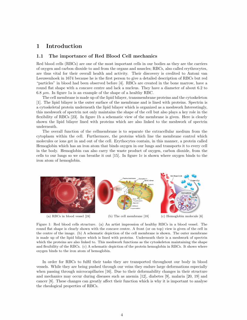
Red blood cells (RBCs) are one of the most important cells in our bodies as they are the carriersof oxygen and carbon dioxide to and from the organs and muscles; RBCs, also called erythrocytes,are thus vital for their overall health and activity. Their discovery is credited to Antoni vanLeeuwenhoek in 1674 because he is the first person to give a detailed description of RBCs but red“particles” in blood had been observed before [4]. RBCs are created in the bone marrow, have around flat shape with a concave centre and lack a nucleus. They have a diameter of about 6.2 to6.8 µm. In figure 1a is an example of the shape of a healthy RBC.

The cell membrane is made up of the lipid bilayer, transmembrane proteins and the cytoskeleton[1]. The lipid bilayer is the outer surface of the membrane and is lined with proteins. Spectrin isa cytoskeletal protein underneath the lipid bilayer which is organized as a meshwork Interestingly,this meshwork of spectrin not only maintains the shape of the cell but also plays a key role in theflexibility of RBCs [23]. In figure 1b a schematic view of the membrane is given. Here is clearlyshown the lipid bilayer lined with proteins which are also linked to the meshwork of spectrinunderneath.

The overall function of the cellmembrane is to separate the extracellular medium from thecytoplasm within the cell. Furthermore, the proteins which line the membrane control whichmolecules or ions get in and out of the cell. Erythocytes contain, in this manner, a protein calledHemoglobin which has an iron atom that binds oxygen in our lungs and transports it to every cellin the body. Hemoglobin can also carry the waste product of oxygen, carbon dioxide, from thecells to our lungs so we can breathe it out [15]. In figure 1c is shown where oxygen binds to theiron atom of hemoglobin.

(a) RBCs in blood vessel [24] (b) The cell membrane [18] (c) Hemoglobin molecule [6]

Figure 1: Red blood cells structure. (a) An artist impression of healthy RBCs in a blood vessel. Theround flat shape is clearly shown with the concave centre. A front (or on top) view is given of the cell inthe centre of the image. (b) A schematic depiction of the cell membrane is shown. The outer membraneis made up of the lipid bilayer which is lined with proteins. Underneath their is a meshwork of spectrinwhich the proteins are also linked to. This meshwork functions as the cytoskeleton maintaining the shapeand flexibility of the RBCs. (c) A schematic depiction of the protein hemoglobin in RBCs. It shows whereoxygen binds to the iron atom of hemoglobin.

In order for RBCs to fulfil their tasks they are transported throughout our body in bloodvessels. While they are being pushed through our veins they endure large deformations especiallywhen passing through microcapillaries [16]. Due to their deformability changes in their structureand mechanics may occur during diseases such as anemia [12], diabetes [9], malaria [20, 19] andcancer [8]. These changes can greatly affect their function which is why it is important to analysethe rheological properties of RBCs.

4

1.2 Investigating the rheological properties of cells

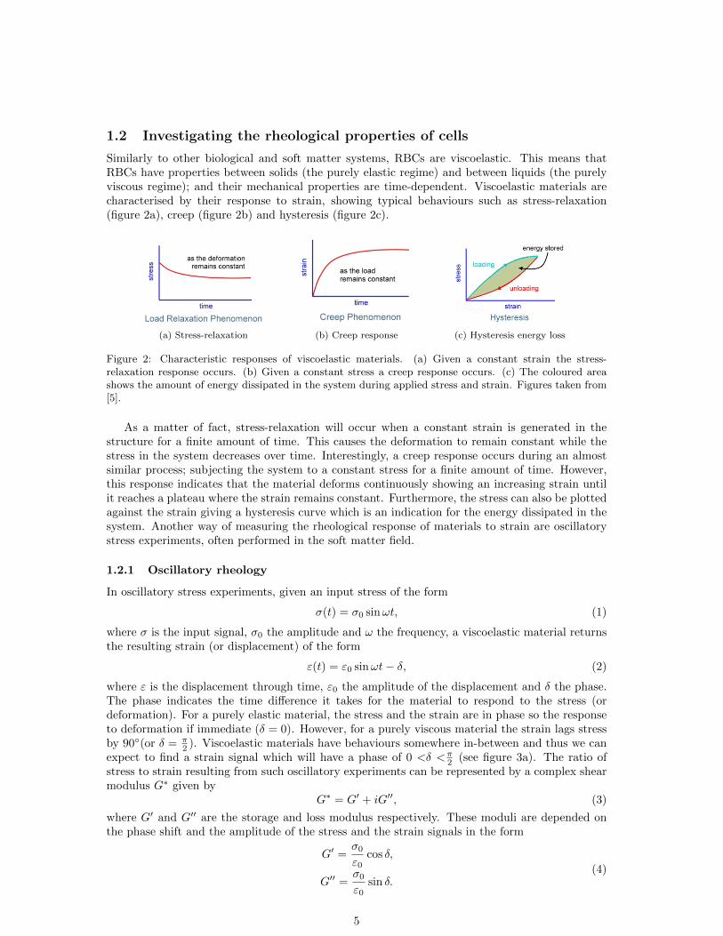
Similarly to other biological and soft matter systems, RBCs are viscoelastic. This means thatRBCs have properties between solids (the purely elastic regime) and between liquids (the purelyviscous regime); and their mechanical properties are time-dependent. Viscoelastic materials arecharacterised by their response to strain, showing typical behaviours such as stress-relaxation(figure 2a), creep (figure 2b) and hysteresis (figure 2c).

(a) Stress-relaxation (b) Creep response (c) Hysteresis energy loss

Figure 2: Characteristic responses of viscoelastic materials. (a) Given a constant strain the stress-relaxation response occurs. (b) Given a constant stress a creep response occurs. (c) The coloured areashows the amount of energy dissipated in the system during applied stress and strain. Figures taken from[5].

As a matter of fact, stress-relaxation will occur when a constant strain is generated in thestructure for a finite amount of time. This causes the deformation to remain constant while thestress in the system decreases over time. Interestingly, a creep response occurs during an almostsimilar process; subjecting the system to a constant stress for a finite amount of time. However,this response indicates that the material deforms continuously showing an increasing strain untilit reaches a plateau where the strain remains constant. Furthermore, the stress can also be plottedagainst the strain giving a hysteresis curve which is an indication for the energy dissipated in thesystem. Another way of measuring the rheological response of materials to strain are oscillatorystress experiments, often performed in the soft matter field.

1.2.1 Oscillatory rheology

In oscillatory stress experiments, given an input stress of the form

σ(t) = σ0 sinωt, (1)

where σ is the input signal, σ0 the amplitude and ω the frequency, a viscoelastic material returnsthe resulting strain (or displacement) of the form

ε(t) = ε0 sinωt− δ, (2)

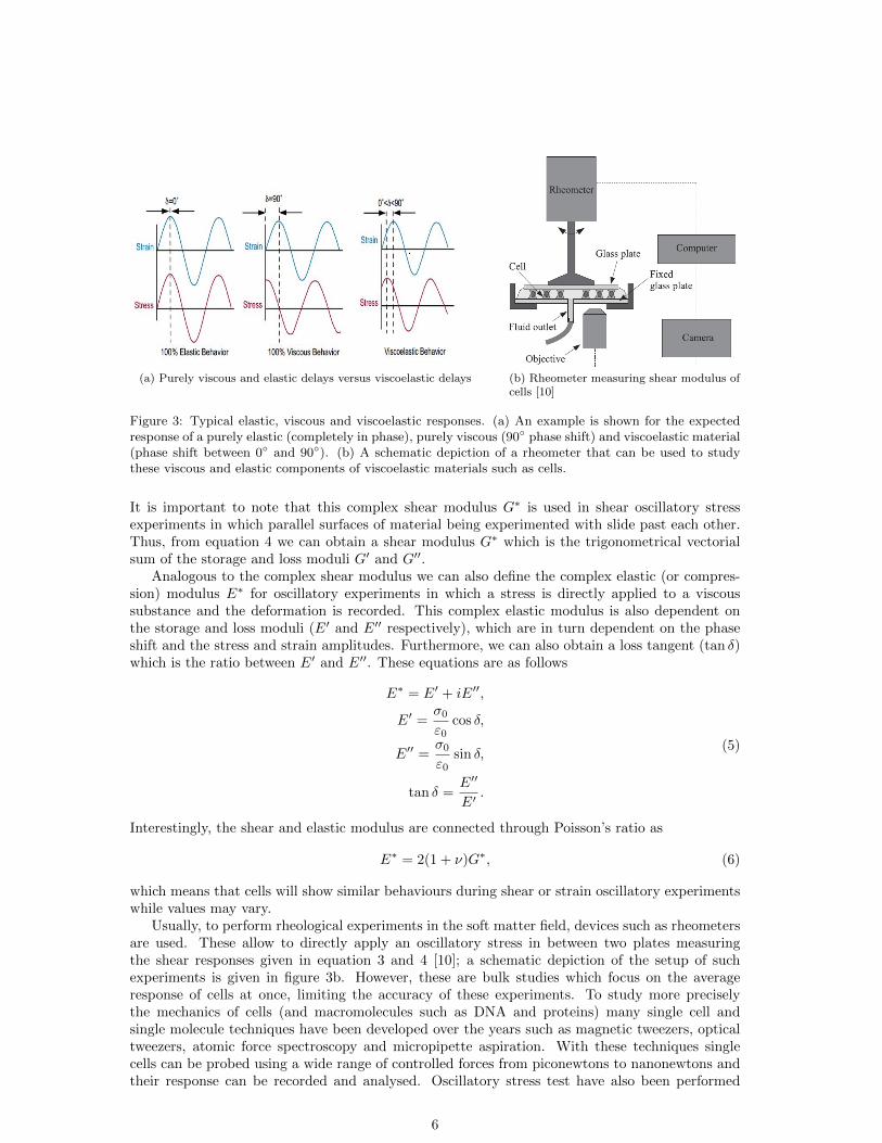
where ε is the displacement through time, ε0 the amplitude of the displacement and δ the phase.The phase indicates the time difference it takes for the material to respond to the stress (ordeformation). For a purely elastic material, the stress and the strain are in phase so the responseto deformation if immediate (δ = 0). However, for a purely viscous material the strain lags stressby 90◦(or δ = π

2 ). Viscoelastic materials have behaviours somewhere in-between and thus we canexpect to find a strain signal which will have a phase of 0 <δ <π

2 (see figure 3a). The ratio ofstress to strain resulting from such oscillatory experiments can be represented by a complex shearmodulus G∗ given by

G∗ = G′ + iG′′, (3)

where G′ and G′′ are the storage and loss modulus respectively. These moduli are depended onthe phase shift and the amplitude of the stress and the strain signals in the form

G′ =σ0ε0

cos δ,

G′′ =σ0ε0

sin δ.(4)

5

(a) Purely viscous and elastic delays versus viscoelastic delays (b) Rheometer measuring shear modulus ofcells [10]

Figure 3: Typical elastic, viscous and viscoelastic responses. (a) An example is shown for the expectedresponse of a purely elastic (completely in phase), purely viscous (90◦ phase shift) and viscoelastic material(phase shift between 0◦ and 90◦). (b) A schematic depiction of a rheometer that can be used to studythese viscous and elastic components of viscoelastic materials such as cells.

It is important to note that this complex shear modulus G∗ is used in shear oscillatory stressexperiments in which parallel surfaces of material being experimented with slide past each other.Thus, from equation 4 we can obtain a shear modulus G∗ which is the trigonometrical vectorialsum of the storage and loss moduli G′ and G′′.

Analogous to the complex shear modulus we can also define the complex elastic (or compres-sion) modulus E∗ for oscillatory experiments in which a stress is directly applied to a viscoussubstance and the deformation is recorded. This complex elastic modulus is also dependent onthe storage and loss moduli (E′ and E′′ respectively), which are in turn dependent on the phaseshift and the stress and strain amplitudes. Furthermore, we can also obtain a loss tangent (tan δ)which is the ratio between E′ and E′′. These equations are as follows

E∗ = E′ + iE′′,

E′ =σ0ε0

cos δ,

E′′ =σ0ε0

sin δ,

tan δ =E′′

E′.

(5)

Interestingly, the shear and elastic modulus are connected through Poisson’s ratio as

E∗ = 2(1 + ν)G∗, (6)

which means that cells will show similar behaviours during shear or strain oscillatory experimentswhile values may vary.

Usually, to perform rheological experiments in the soft matter field, devices such as rheometersare used. These allow to directly apply an oscillatory stress in between two plates measuringthe shear responses given in equation 3 and 4 [10]; a schematic depiction of the setup of suchexperiments is given in figure 3b. However, these are bulk studies which focus on the averageresponse of cells at once, limiting the accuracy of these experiments. To study more preciselythe mechanics of cells (and macromolecules such as DNA and proteins) many single cell andsingle molecule techniques have been developed over the years such as magnetic tweezers, opticaltweezers, atomic force spectroscopy and micropipette aspiration. With these techniques singlecells can be probed using a wide range of controlled forces from piconewtons to nanonewtons andtheir response can be recorded and analysed. Oscillatory stress test have also been performed

6

on, for example, nuclei using atomic force microscopy (AFM) [13] and on F-actin solution usingmagnetic beads [25]. Typically, these single molecule techniques can only probe one cell at a timewhich limits how much data can be obtained for statistics [21]. In order to solve these problems anew method was developed relatively recently (2014), namely acoustic force spectroscopy, whichcombines the accuracy of single-molecule techniques with multiplexing.

1.2.2 Acoustic Force Spectroscopy

Acoustic Force spectroscopy (AFS) is a relatively new method which uses acoustic forces to probecells (or molecules) that are tethered between a glass surface and a microsphere (bead). Withthis technique multiple cells can be symmetrically probed during one measurement, giving anadvantage in data collecting for statistics. Furthermore, this technique makes it possible to usehighly controllable forces in the piconewton range and thus giving an advantage to more accurateprobing.

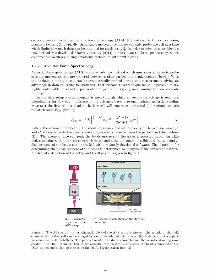
In the AFS setup a piezo element is used through which an oscillating voltage is sent to amicrofluidics (or flow cell). This oscillating voltage creates a resonant planar acoustic standingwave over the flow cell. A bead in the flow cell will experience a vertical (z-direction) acousticradiation force Frad given by

Frad = −V∇[

1− κ?

4κmp

2 −(ρ? − 1

)2ρ? + 1

ρmν2

], (7)

with V the volume of the bead, p the acoustic pressure and ν the velocity of the acoustic wave. ρ?

and κ? are respectively the density and compressibility ratio between the particle and the medium[21]. The acoustic force can push the beads upwards to the acoustic pressure node. An LEDmakes imaging with a 40× air-spaced objective and a digital camera possible and the x, y and z-displacement of the beads can be tracked with previously developed software. The algorithm fordetermining the z-displacement of the beads is determined by analysis of the diffraction pattern.A schematic depiction of the setup and the flow cell is given in figure 4.

(a) Schematicdepiction of theAFS setup

(b) Schematic depiction of the flow cellzoomed in

Figure 4: The AFS setup. (a) A schematic view of the AFS setup is shown. The sample in the fluidchamber of the flow cell can be imaged by use of an inferted microscope. (b) A depiction of a typicalmeasurement of DNA tethers. The piezo element is the driving force behind the acoustic standing wavecreated in the fluid chamber. Due to the acoustic force created by this wave the beads connected to theDNA tethers are pulled up stretching the DNA. Figures taken from [3]

7

1.2.3 Method development for rheology on erythrocytes with AFS

The AFS setup, as previously described, has already been used to study the mechanics of DNA byperforming force-extension experiments [21]. Recently, it has also been used to study propertiesof RBCs by performing force-clamp experiments while introducing changes in the cell mechanicsvia chemical additions [22]. During these experiments highly controlled forces were used in thepiconewton range; which are also ideal for performing oscillatory stress tests in order to stay in thelinear regime. This gives us the opportunity to understand the viscous and elastic properties ofhealthy RBCs separately as we can untangle them from equation 5. Furthermore, oscillatory stresstests on human blood have been performed by using other methods [11, 2] but these experimentshave not yet been done on single RBCs. The goal during this project is to show that AFS can beused to study the viscoelastic properties of RBCs by performing oscillatory stress tests on singlecells. Furthermore, we want to develop an analysis workflow to study the obtained data from theoscillatory experiments and understand the viscous and elastic properties of healthy RBCs.

8

2 Methodology

2.1 Force calibration of the AFS setup

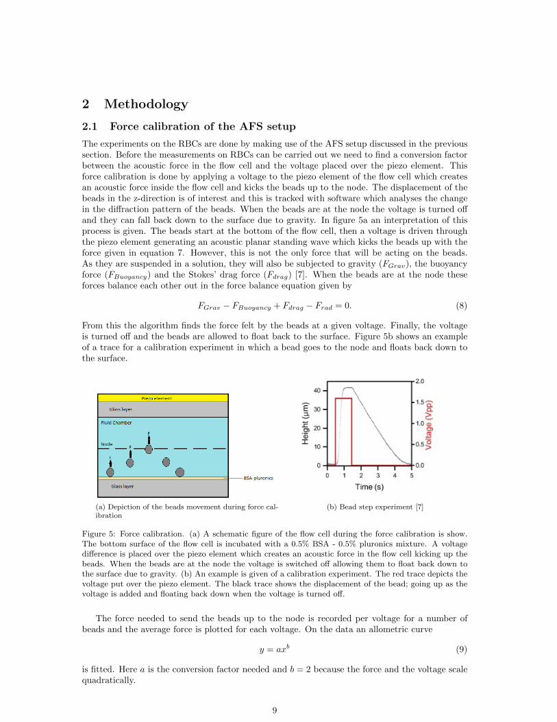
The experiments on the RBCs are done by making use of the AFS setup discussed in the previoussection. Before the measurements on RBCs can be carried out we need to find a conversion factorbetween the acoustic force in the flow cell and the voltage placed over the piezo element. Thisforce calibration is done by applying a voltage to the piezo element of the flow cell which createsan acoustic force inside the flow cell and kicks the beads up to the node. The displacement of thebeads in the z-direction is of interest and this is tracked with software which analyses the changein the diffraction pattern of the beads. When the beads are at the node the voltage is turned offand they can fall back down to the surface due to gravity. In figure 5a an interpretation of thisprocess is given. The beads start at the bottom of the flow cell, then a voltage is driven throughthe piezo element generating an acoustic planar standing wave which kicks the beads up with theforce given in equation 7. However, this is not the only force that will be acting on the beads.As they are suspended in a solution, they will also be subjected to gravity (FGrav), the buoyancyforce (FBuoyancy) and the Stokes’ drag force (Fdrag) [7]. When the beads are at the node theseforces balance each other out in the force balance equation given by

FGrav − FBuoyancy + Fdrag − Frad = 0. (8)

From this the algorithm finds the force felt by the beads at a given voltage. Finally, the voltageis turned off and the beads are allowed to float back to the surface. Figure 5b shows an exampleof a trace for a calibration experiment in which a bead goes to the node and floats back down tothe surface.

(a) Depiction of the beads movement during force cal-ibration

(b) Bead step experiment [7]

Figure 5: Force calibration. (a) A schematic figure of the flow cell during the force calibration is show.The bottom surface of the flow cell is incubated with a 0.5% BSA - 0.5% pluronics mixture. A voltagedifference is placed over the piezo element which creates an acoustic force in the flow cell kicking up thebeads. When the beads are at the node the voltage is switched off allowing them to float back down tothe surface due to gravity. (b) An example is given of a calibration experiment. The red trace depicts thevoltage put over the piezo element. The black trace shows the displacement of the bead; going up as thevoltage is added and floating back down when the voltage is turned off.

The force needed to send the beads up to the node is recorded per voltage for a number ofbeads and the average force is plotted for each voltage. On the data an allometric curve

y = axb (9)

is fitted. Here a is the conversion factor needed and b = 2 because the force and the voltage scalequadratically.

9

Beads and Flow cell preparation. For all experiments “shooting” beads are used. Theseare beads which are not coated with biochemical substances such as, for example streptavidin orconcanavalin A. The beads were made of silicon dioxide (SiO2) and had a size of 6.59 ± 0.16 µm.In order to prepare the beads for the experiment they were first washed with phosphate-bufferedsaline (PBS) in a centrifuge by spinning them down for 2 minutes with a speed of 500rcf at 23◦C.They are then resuspended in ringer’s buffer, which is a solution that has a similar salt and glucoseconcentration as the human body and helps to maintain a constant pH value [17]. The flow cellis incubated for a minimum of 30 minutes with a 0.5% BSA - 0.5% pluronics mixture to preventthe beads from sticking to the surface. Before flushing the beads into the flow cell some ringer’sbuffer is flushed in to remove the excess BSA-pluronics.

2.2 Oscillatory experiments on RBCs

In order to perform oscillatory experiments on RBCs they need to be attached to the surface ofthe flow cell. The RBCs are collected right before the experiments from one healthy donor byfinger pricking and diluted in Ringer’s buffer to keep ATP production active. Furthermore, thebeads need to be attached to the cells so they can be probed.

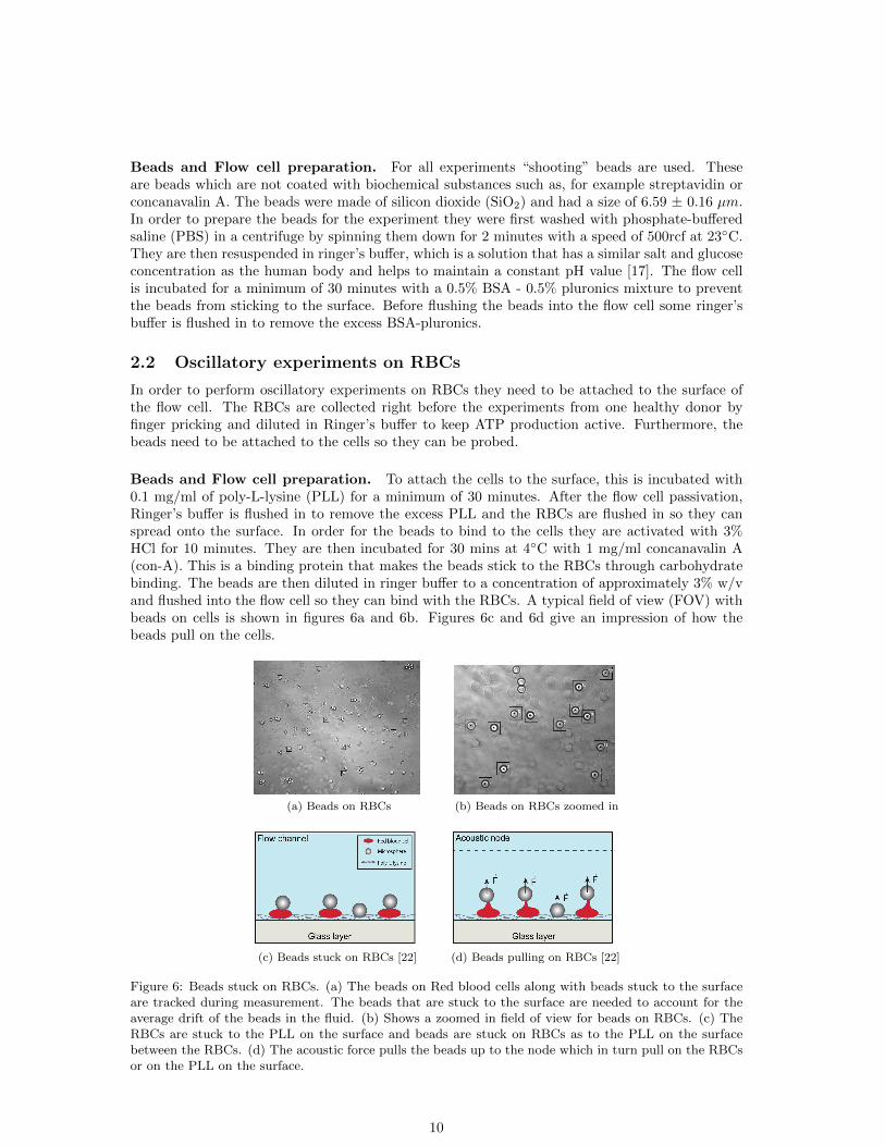
Beads and Flow cell preparation. To attach the cells to the surface, this is incubated with0.1 mg/ml of poly-L-lysine (PLL) for a minimum of 30 minutes. After the flow cell passivation,Ringer’s buffer is flushed in to remove the excess PLL and the RBCs are flushed in so they canspread onto the surface. In order for the beads to bind to the cells they are activated with 3%HCl for 10 minutes. They are then incubated for 30 mins at 4◦C with 1 mg/ml concanavalin A(con-A). This is a binding protein that makes the beads stick to the RBCs through carbohydratebinding. The beads are then diluted in ringer buffer to a concentration of approximately 3% w/vand flushed into the flow cell so they can bind with the RBCs. A typical field of view (FOV) withbeads on cells is shown in figures 6a and 6b. Figures 6c and 6d give an impression of how thebeads pull on the cells.

(a) Beads on RBCs (b) Beads on RBCs zoomed in

(c) Beads stuck on RBCs [22] (d) Beads pulling on RBCs [22]

Figure 6: Beads stuck on RBCs. (a) The beads on Red blood cells along with beads stuck to the surfaceare tracked during measurement. The beads that are stuck to the surface are needed to account for theaverage drift of the beads in the fluid. (b) Shows a zoomed in field of view for beads on RBCs. (c) TheRBCs are stuck to the PLL on the surface and beads are stuck on RBCs as to the PLL on the surfacebetween the RBCs. (d) The acoustic force pulls the beads up to the node which in turn pull on the RBCsor on the PLL on the surface.

10

Experimental assay. Once the sample is set we can perform oscillatory stress tests on thecells. A voltage peak-to-peak amplitude, which corresponds to a force pulling on the beads, ismodulated at a specified frequency causing the acoustic force to oscillate at the set amplitude ina sinusoidal manner. The frequency range used for these experiments was between 0.01 Hz and 1Hz. The oscillating z-displacement of the beads is recorded and, using the force calibration, theoscillating voltage is converted into force. These two signals are of interest, more precisely thephase shift between the input force and output cellular response.

2.2.1 Data analysis protocol

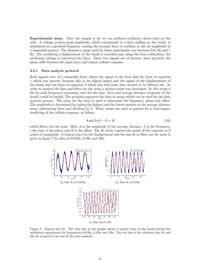
Both signals were of a sinusoidal form, where the signal of the force had the form of equation1 which was smooth (because this is our digital input) and the signal of the displacements ofthe beads had the form of equation 2 which also had noise that needed to be filtered out. Inorder to analyse the data and filter out the noise a python script was developed. In this script afile for each frequency containing rows for the time, force and average distance (response of thebeads) could be loaded. The program separates the data in arrays which can be used for the dataanalysis process. The array for the force is used to determine the frequency, phase and offset.The amplitude is determined by taking the highest and the lowest number in the average distancearray, subtracting them and dividing by 2. These values are used as guesses for a least-squaresinefitting of the cellular response, as follows

A sin(2πft− δ) +B (10)

which filters out the noise. Here A is the amplitude of the average distance, f is the frequency,t the time, δ the phase and B is the offset. The fit nicely capture the peaks of the response in 3orders of magnitude. A typical trace for the displacement and the sine fit to filter out the noise isgiven in figure 7 for data of 0.01Hz, 0.1Hz and 1Hz.

(a) Sine fit of 0.01Hz (b) Sine fit of 0.1Hz

(c) Sine fit of 1Hz

Figure 7: Typical sine fit. The blue line in the graphs shows a typical trace of the beads during theoscillation experiments for frequencies 0.01Hz, 0.1Hz and 1Hz. The red line is the obtained sine fit andthis fit is used for the rest of the data analysis.

11

(a) Force and displacement traces (b) Time delay

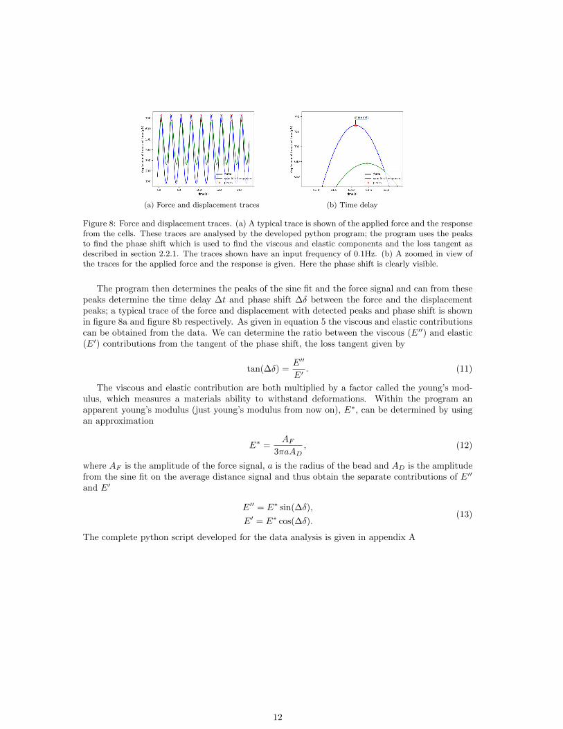
Figure 8: Force and displacement traces. (a) A typical trace is shown of the applied force and the responsefrom the cells. These traces are analysed by the developed python program; the program uses the peaksto find the phase shift which is used to find the viscous and elastic components and the loss tangent asdescribed in section 2.2.1. The traces shown have an input frequency of 0.1Hz. (b) A zoomed in view ofthe traces for the applied force and the response is given. Here the phase shift is clearly visible.

The program then determines the peaks of the sine fit and the force signal and can from thesepeaks determine the time delay ∆t and phase shift ∆δ between the force and the displacementpeaks; a typical trace of the force and displacement with detected peaks and phase shift is shownin figure 8a and figure 8b respectively. As given in equation 5 the viscous and elastic contributionscan be obtained from the data. We can determine the ratio between the viscous (E′′) and elastic(E′) contributions from the tangent of the phase shift, the loss tangent given by

tan(∆δ) =E′′

E′. (11)

The viscous and elastic contribution are both multiplied by a factor called the young’s mod-ulus, which measures a materials ability to withstand deformations. Within the program anapparent young’s modulus (just young’s modulus from now on), E∗, can be determined by usingan approximation

E∗ =AF

3πaAD, (12)

where AF is the amplitude of the force signal, a is the radius of the bead and AD is the amplitudefrom the sine fit on the average distance signal and thus obtain the separate contributions of E′′

and E′

E′′ = E∗ sin(∆δ),

E′ = E∗ cos(∆δ).(13)

The complete python script developed for the data analysis is given in appendix A

12

3 Results

3.1 Force Calibration measurements

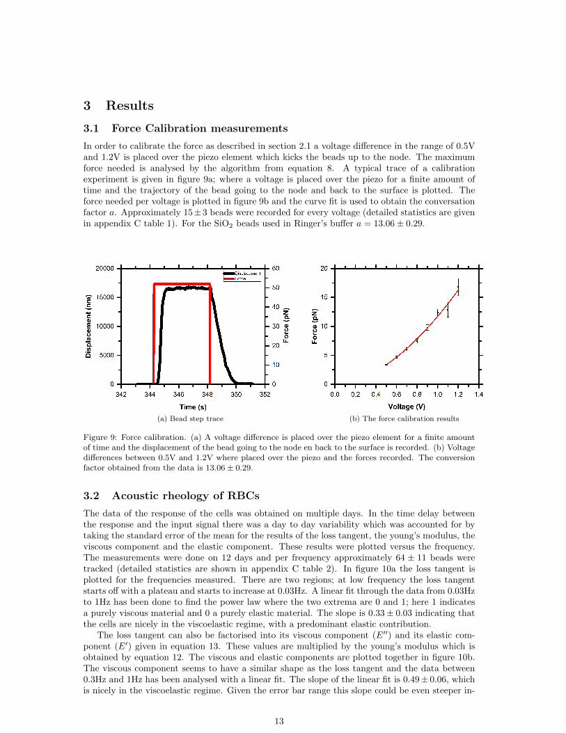
In order to calibrate the force as described in section 2.1 a voltage difference in the range of 0.5Vand 1.2V is placed over the piezo element which kicks the beads up to the node. The maximumforce needed is analysed by the algorithm from equation 8. A typical trace of a calibrationexperiment is given in figure 9a; where a voltage is placed over the piezo for a finite amount oftime and the trajectory of the bead going to the node and back to the surface is plotted. Theforce needed per voltage is plotted in figure 9b and the curve fit is used to obtain the conversationfactor a. Approximately 15±3 beads were recorded for every voltage (detailed statistics are givenin appendix C table 1). For the SiO2 beads used in Ringer’s buffer a = 13.06± 0.29.

(a) Bead step trace (b) The force calibration results

Figure 9: Force calibration. (a) A voltage difference is placed over the piezo element for a finite amountof time and the displacement of the bead going to the node en back to the surface is recorded. (b) Voltagedifferences between 0.5V and 1.2V where placed over the piezo and the forces recorded. The conversionfactor obtained from the data is 13.06 ± 0.29.

3.2 Acoustic rheology of RBCs

The data of the response of the cells was obtained on multiple days. In the time delay betweenthe response and the input signal there was a day to day variability which was accounted for bytaking the standard error of the mean for the results of the loss tangent, the young’s modulus, theviscous component and the elastic component. These results were plotted versus the frequency.The measurements were done on 12 days and per frequency approximately 64 ± 11 beads weretracked (detailed statistics are shown in appendix C table 2). In figure 10a the loss tangent isplotted for the frequencies measured. There are two regions; at low frequency the loss tangentstarts off with a plateau and starts to increase at 0.03Hz. A linear fit through the data from 0.03Hzto 1Hz has been done to find the power law where the two extrema are 0 and 1; here 1 indicatesa purely viscous material and 0 a purely elastic material. The slope is 0.33± 0.03 indicating thatthe cells are nicely in the viscoelastic regime, with a predominant elastic contribution.

The loss tangent can also be factorised into its viscous component (E′′) and its elastic com-ponent (E′) given in equation 13. These values are multiplied by the young’s modulus which isobtained by equation 12. The viscous and elastic components are plotted together in figure 10b.The viscous component seems to have a similar shape as the loss tangent and the data between0.3Hz and 1Hz has been analysed with a linear fit. The slope of the linear fit is 0.49± 0.06, whichis nicely in the viscoelastic regime. Given the error bar range this slope could be even steeper in-

13

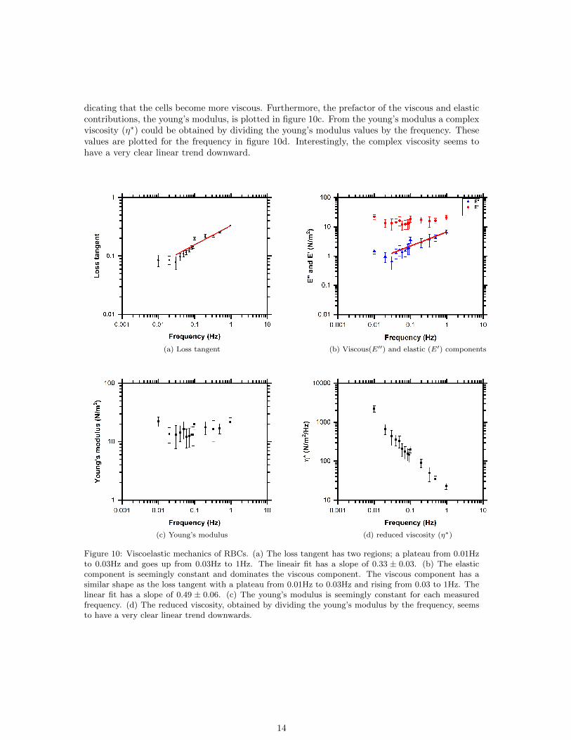
dicating that the cells become more viscous. Furthermore, the prefactor of the viscous and elasticcontributions, the young’s modulus, is plotted in figure 10c. From the young’s modulus a complexviscosity (η∗) could be obtained by dividing the young’s modulus values by the frequency. Thesevalues are plotted for the frequency in figure 10d. Interestingly, the complex viscosity seems tohave a very clear linear trend downward.

(a) Loss tangent (b) Viscous(E′′) and elastic (E′) components

(c) Young’s modulus (d) reduced viscosity (η∗)

Figure 10: Viscoelastic mechanics of RBCs. (a) The loss tangent has two regions; a plateau from 0.01Hzto 0.03Hz and goes up from 0.03Hz to 1Hz. The lineair fit has a slope of 0.33 ± 0.03. (b) The elasticcomponent is seemingly constant and dominates the viscous component. The viscous component has asimilar shape as the loss tangent with a plateau from 0.01Hz to 0.03Hz and rising from 0.03 to 1Hz. Thelinear fit has a slope of 0.49 ± 0.06. (c) The young’s modulus is seemingly constant for each measuredfrequency. (d) The reduced viscosity, obtained by dividing the young’s modulus by the frequency, seemsto have a very clear linear trend downwards.

14

4 Discussion

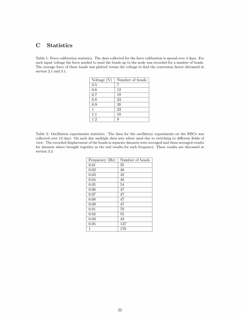
Comparing figure 10a and 10b there seems to be a resemblance between the shape of the losstangent and E′′. Given that E′ is seemingly constant, that means that the viscous component isthe determining factor for the slope of the loss tangent. Our loss tangent values are nicely in linewith literature, such as measurements for fibroblast cells within a frequency range of 0.01Hz and30Hz [10]. However, our results do indicate that RBCs are softer in comparison to fibroblast, asthey found a seemingly constant loss tangent between 0.25 and 0.35 (see appendix B figure 12)while we found a loss tangent in a wider range, specifically between 0.084±0.019 and 0.328±0.014.This data does make sense because RBCs do not have a nucleus and thus are more flexible thanfibroblast cells. The increase of the loss tangent indicates that the response of the RBCs becomesincreasingly “fluid” as the frequency increases. Furthermore, the elastic (G′) and viscous (G′′)components they found both increase parallel to each other in a linear fashion as the frequencyincreases (see appendix B figure 12). Interestingly, our elastic component E′ is constant over thefrequency range used, while our viscous E′′ component does increase in a linear fashion. Alsoimportant to note is that the experiments on the fibroblast cells were oscillatory shear stress testsand thus the shear moduli are computed. The relation between the shear moduli and elastic moduliis given in equaction 6, which explains why our values are not in the same range as [10]. Anotherexplanation could be the prefactor used for the elastic and viscous component, namely the young’smodulus depicted in figure 10c. An approximation was used to determine the values of the young’smodulus given in equation 12. However, this approximation was adapted from [25] where a beadwas completely embedded in viscoelastic material as opposed to the beads used for this experimentwhich are on top of viscoelastic material, thus this approximation could have an influence on thevalues obtain causing them not to be in line with [10]. However, the constant behaviour of theelastic component can be an indication that probing cells at these forces and frequencies (whichare, in comparison to other research, on the low side) doesn’t actively probe a change in elasticbehaviour of the cells. Interestingly, for the RBCs the elastic behaviour would mainly be dueto the cytoskeleton, i.e. the meshwork of spectrin. The fairly constant elastic component thushints that the spectrin is not actively deformed in this frequency region. Furthermore, the viscouscomponent would mainly be due to the outer side of the cell; the lipid bilayer.

Between 0.01Hz and 0.03Hz the viscous component is seemingly constant. Interestingly, start-ing from 0.03Hz the viscous component starts to rise linearly which indicates that as the frequencyincreases the cells become more deformable or “fluid”. That the cells become more “fluid” startingfrom 0.03Hz can be due to loss of linkage between the lipid bilayer and the spectrin meshworkas the beads pull on the cells. This effect would gradually dominate the membrane fluctuationswhich the increasing viscous component possibly hints to. Furthermore, this loss of linkage couldbe possible because the beads used where activated with con-A, which is a lectin that binds to theglycoproteins of lipid bilayer; some of these glycoproteins are directly connected to spectrin whichmakes it easier to pop out linkage with the lipid bilayer. Important to note is that PLL, whichwas used to incubate the surface, causes the cells to spread out over the surface and thus slightlystretching them horizontally while the beads stretch them vertically during measurement. As thefrequency increases this could cause the bond between the glycoproteins and the spectrin to snapgiving way to a more viscous response of the cells. Furthermore, examining the plot of the com-plex viscosity (figure 10d) it has a clear linear trend downwards, which shows that with increasingfrequency, the resistance of the cells to deformation decreases (they “flow” easier or become more“fluid”). In order to confirm this, further measurements can be done using a different bindingprotein for the beads, which does not make a direct connection to glycoproteins and thereforeto spectrin or using no binding proteins. Also, another binding agent could be used to coat thesurface which does not cause the erythrocytes to spread out as PLL does but instead allows themto retain their original concave disk shape. A possibility could be using fibronectin instead as itwas recently observed in the lab that when fibronectin was used to incubate the surface that theRBCs retained their shape (unpublished data). Furthermore, tests could be done with additionof chemicals that act on the lipid bilayer or the spectrin, in order to understand which structuralcomponents contribute to the viscous and elastic behaviour.

15

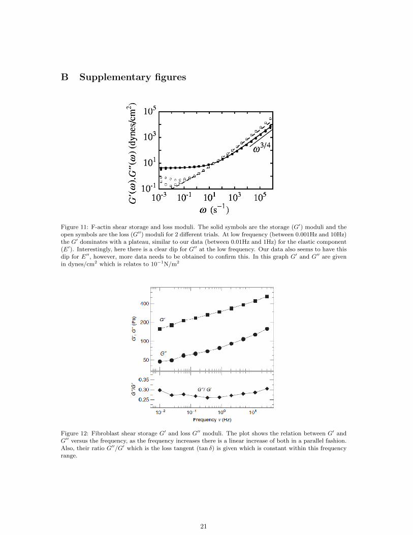
Examining the first three points for E′′ in figure 10b they seem to give way to a dip in the datainstead of a plateau. This could be possible as very similar behaviour was found for oscillatoryexperiments on F-actin solutions in the frequency range of 10−3Hz to 105Hz [14]. In the range of0.01Hz and 1Hz our results closely match the shape of the graph for the storage and loss moduliversus the frequency [14]; our E′ and their G′ having a plateau shape, and our E′′ and their G′′

seemingly having a dip at low frequency. However, as they performed shear oscillatory stress testthe values are not in line (the graph of [14] is given in appendix B figure 11 for comparison). Thisdip was ruled out for the data shown here, because the viscous and elastic component combinedfor the loss tangent do give a plateau for these points. The first point is also higher for boththe viscous and elastic component which could be due to a systematic error. Furthermore, thereis no data obtained at lower frequencies to confirm that the viscous component plays a moresignificant role in that region in comparison to 0.01Hz to 0.03Hz. Therefore, it would be beneficialto obtain data at even lower frequencies. With this data it is not possible to say with certaintywhich structural component contributes to the viscous behaviour to become more present as thefrequency increases starting from 0.03Hz, thus more measurements are needed.

4.1 Conclusion

During this project the goal was to develop an analysis workflow to understand the viscous andelastic contributions of healthy erythrocytes’ mechanics with the AFS setup. In order to probe theRBCs mechanics the AFS setup allowed for oscillatory experiments to be performed on multiplecells at once in parallel in the linear regime. The frequencies used during these experimentswere between 0.01Hz and 1Hz, and the data showed that for this frequency range the elasticbehaviour was not actively probed. Therefore, a speculation that can be made is that this datahints that the spectrin network underneath the lipid bilayer did not undergo large deformations inthis regime. Furthermore, the data shows that there is an increase in viscous behaviour startingfrom 0.03Hz; this could be due to breakage of linkage between proteins in the lipid bilayer tothe spectrin meshwork underneath giving way to a more “fluid” cellmembrane. This hypothesiscould be a possibility because the beads used for probing were coated with con-A which binds tothe glycoproteins in the lipid bilayer, some of which are directly connected to spectrin. However,more data is needed in order to solidify this hypothesis. With our current data we cannot saywith certainty which structural components of the erythrocytes are responsible to the viscous andelastic behaviours of their mechanics. However, what we have been able to show is that AFS canbe used for these rheology experiments on cells and that the algorithm developed for data analysiscan give us an insight into the cell mechanics. This analysis workflow can also be adapted forother cell types, nuclei or synthetic polymeric material.

16

Appendices

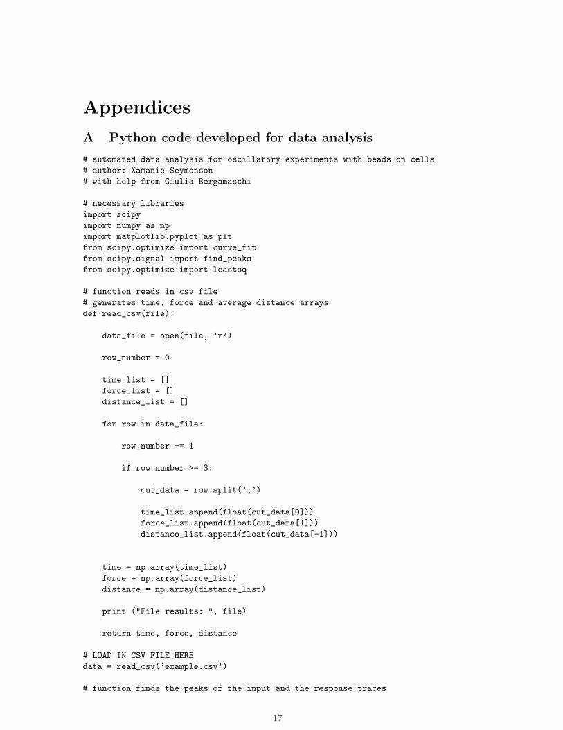
A Python code developed for data analysis

# automated data analysis for oscillatory experiments with beads on cells

# author: Xamanie Seymonson

# with help from Giulia Bergamaschi

# necessary libraries

import scipy

import numpy as np

import matplotlib.pyplot as plt

from scipy.optimize import curve_fit

from scipy.signal import find_peaks

from scipy.optimize import leastsq

# function reads in csv file

# generates time, force and average distance arrays

def read_csv(file):

data_file = open(file, ’r’)

row_number = 0

time_list = []

force_list = []

distance_list = []

for row in data_file:

row_number += 1

if row_number >= 3:

cut_data = row.split(’,’)

time_list.append(float(cut_data[0]))

force_list.append(float(cut_data[1]))

distance_list.append(float(cut_data[-1]))

time = np.array(time_list)

force = np.array(force_list)

distance = np.array(distance_list)

print ("File results: ", file)

return time, force, distance

# LOAD IN CSV FILE HERE

data = read_csv(’example.csv’)

# function finds the peaks of the input and the response traces

17

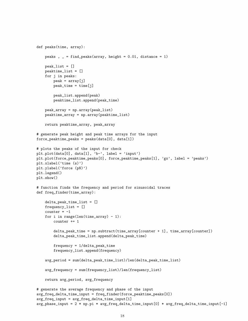
def peaks(time, array):

peaks , _ = find_peaks(array, height = 0.01, distance = 1)

peak_list = []

peaktime_list = []

for j in peaks:

peak = array[j]

peak_time = time[j]

peak_list.append(peak)

peaktime_list.append(peak_time)

peak_array = np.array(peak_list)

peaktime_array = np.array(peaktime_list)

return peaktime_array, peak_array

# generate peak height and peak time arrays for the input

force_peaktime_peaks = peaks(data[0], data[1])

# plots the peaks of the input for check

plt.plot(data[0], data[1], ’b-’, label = ’input’)

plt.plot(force_peaktime_peaks[0], force_peaktime_peaks[1], ’gx’, label = ’peaks’)

plt.xlabel(’time (s)’)

plt.ylabel(’force (pN)’)

plt.legend()

plt.show()

# function finds the frequency and period for sinusoidal traces

def freq_finder(time_array):

delta_peak_time_list = []

frequency_list = []

counter = -1

for i in range(len(time_array) - 1):

counter += 1

delta_peak_time = np.subtract(time_array[counter + 1], time_array[counter])

delta_peak_time_list.append(delta_peak_time)

frequency = 1/delta_peak_time

frequency_list.append(frequency)

avg_period = sum(delta_peak_time_list)/len(delta_peak_time_list)

avg_frequency = sum(frequency_list)/len(frequency_list)

return avg_period, avg_frequency

# generate the average frequency and phase of the input

avg_freq_delta_time_input = freq_finder(force_peaktime_peaks[0])

avg_freq_input = avg_freq_delta_time_input[1]

avg_phase_input = 2 * np.pi * avg_freq_delta_time_input[0] * avg_freq_delta_time_input[-1]

18

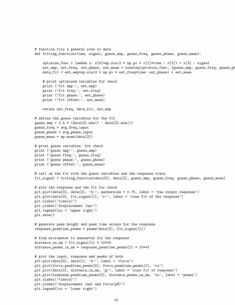
# function fits a general sine to data

def fitting_function(time, signal, guess_amp, guess_freq, guess_phase, guess_mean):

optimize_func = lambda x: x[0]*np.sin(2 * np.pi * x[1]*time - x[2]) + x[3] - signal

est_amp, est_freq, est_phase, est_mean = leastsq(optimize_func, [guess_amp, guess_freq, guess_phase, guess_mean])[0]

data_fit = est_amp*np.sin(2 * np.pi * est_freq*time- est_phase) + est_mean

# print optimized variables for check

print (’fit amp:’, est_amp)

print (’fit freq:’, est_freq)

print (’fit phase:’, est_phase)

print (’fit offset:’, est_mean)

return est_freq, data_fit, est_amp

# define the guess variables for the fit

guess_amp = 0.5 * (data[2].max() - data[2].min())

guess_freq = avg_freq_input

guess_phase = avg_phase_input

guess_mean = np.mean(data[2])

# print guess variables for check

print (’guess amp:’, guess_amp)

print (’guess freq:’, guess_freq)

print (’guess phase:’, guess_phase)

print (’guess offset:’, guess_mean)

# call on the fit with the guess variables and the response trace

fit_signal = fitting_function(data[0], data[2], guess_amp, guess_freq, guess_phase, guess_mean)

# plot the response and the fit for check

plt.plot(data[0], data[2], ’b-’, markersize = 0.75, label = ’raw output response’)

plt.plot(data[0], fit_signal[1], ’r-’, label = ’sine fit of the response’)

plt.xlabel(’time(s)’)

plt.ylabel(’displacement (um)’)

plt.legend(loc = ’upper right’)

plt.show()

# generate peak height and peak time arrays for the response

response_peaktime_peaks = peaks(data[0], fit_signal[1])

# from micrometer to nanometer for the response

distance_in_nm = fit_signal[1] * 10**3

distance_peaks_in_nm = response_peaktime_peaks[1] * 10**3

# plot the input, response and peaks of both

plt.plot(data[0], data[1], ’b-’, label = ’force’)

plt.plot(force_peaktime_peaks[0], force_peaktime_peaks[1], ’rx’)

plt.plot(data[0], distance_in_nm, ’g-’, label = ’sine fit of response’)

plt.plot(response_peaktime_peaks[0], distance_peaks_in_nm, ’rx’, label = ’peaks’)

plt.xlabel(’time(s)’)

plt.ylabel(’displacement (nm) and force(pN)’)

plt.legend(loc = ’lower right’)

19

plt.show()

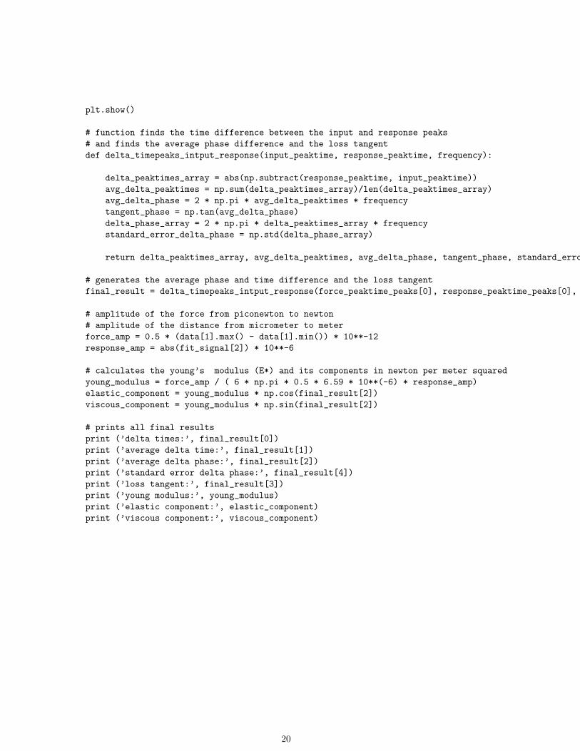
# function finds the time difference between the input and response peaks

# and finds the average phase difference and the loss tangent

def delta_timepeaks_intput_response(input_peaktime, response_peaktime, frequency):

delta_peaktimes_array = abs(np.subtract(response_peaktime, input_peaktime))

avg_delta_peaktimes = np.sum(delta_peaktimes_array)/len(delta_peaktimes_array)

avg_delta_phase = 2 * np.pi * avg_delta_peaktimes * frequency

tangent_phase = np.tan(avg_delta_phase)

delta_phase_array = 2 * np.pi * delta_peaktimes_array * frequency

standard_error_delta_phase = np.std(delta_phase_array)

return delta_peaktimes_array, avg_delta_peaktimes, avg_delta_phase, tangent_phase, standard_error_delta_phase

# generates the average phase and time difference and the loss tangent

final_result = delta_timepeaks_intput_response(force_peaktime_peaks[0], response_peaktime_peaks[0], fit_signal[0])

# amplitude of the force from piconewton to newton

# amplitude of the distance from micrometer to meter

force_amp = 0.5 * (data[1].max() - data[1].min()) * 10**-12

response_amp = abs(fit_signal[2]) * 10**-6

# calculates the young’s modulus (E*) and its components in newton per meter squared

young_modulus = force_amp / ( 6 * np.pi * 0.5 * 6.59 * 10**(-6) * response_amp)

elastic_component = young_modulus * np.cos(final_result[2])

viscous_component = young_modulus * np.sin(final_result[2])

# prints all final results

print (’delta times:’, final_result[0])

print (’average delta time:’, final_result[1])

print (’average delta phase:’, final_result[2])

print (’standard error delta phase:’, final_result[4])

print (’loss tangent:’, final_result[3])

print (’young modulus:’, young_modulus)

print (’elastic component:’, elastic_component)

print (’viscous component:’, viscous_component)

20

B Supplementary figures

Figure 11: F-actin shear storage and loss moduli. The solid symbols are the storage (G′) moduli and theopen symbols are the loss (G′′) moduli for 2 different trials. At low frequency (between 0.001Hz and 10Hz)the G′ dominates with a plateau, similar to our data (between 0.01Hz and 1Hz) for the elastic component(E′). Interestingly, here there is a clear dip for G′′ at the low frequency. Our data also seems to have thisdip for E′′, however, more data needs to be obtained to confirm this. In this graph G′ and G′′ are givenin dynes/cm2 which is relates to 10−1N/m2

Figure 12: Fibroblast shear storage G′ and loss G′′ moduli. The plot shows the relation between G′ andG′′ versus the frequency, as the frequency increases there is a linear increase of both in a parallel fashion.Also, their ratio G′′/G′ which is the loss tangent (tan δ) is given which is constant within this frequencyrange.

21

C Statistics

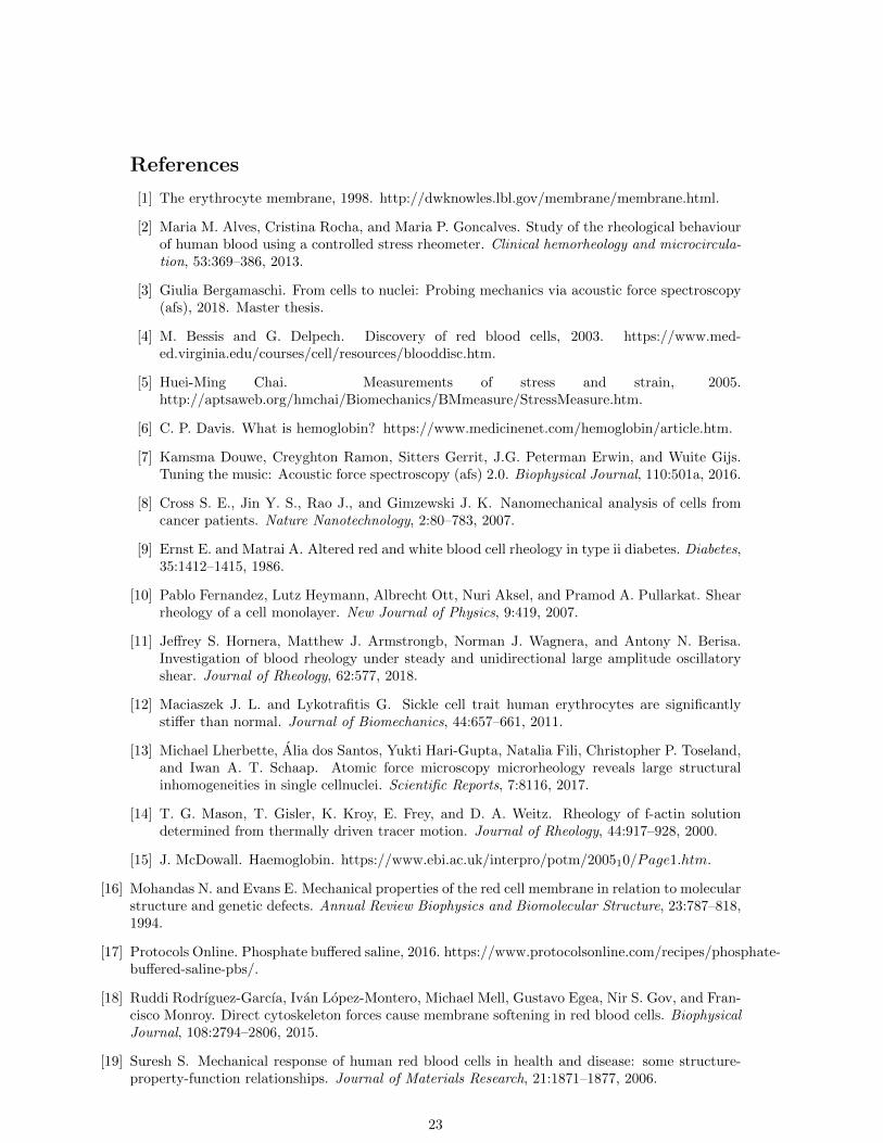
Table 1: Force calibration statistics. The data collected for the force calibration is spread over 4 days. Foreach input voltage the force needed to send the beads up to the node was recorded for a number of beads.The average force of these beads was plotted versus the voltage to find the conversion factor discussed insection 2.1 and 3.1.

Voltage (V) Number of beads0.5 70.6 120.7 190.8 230.9 201 231.1 101.2 9

Table 2: Oscillation experiments statistics. The data for the oscillatory experiments on the RBCs wascollected over 12 days. On each day multiple data sets where used due to switching to different fields ofview. The recorded displacement of the beads in separate datasets were averaged and these averaged resultsfor datasets where brought together in the end results for each frequency. These results are discussed insection 3.2

Frequency (Hz) Number of beads0.01 350.02 480.03 420.04 480.05 540.06 470.07 470.08 470.09 470.01 700.02 550.03 430.05 1371 179

22

References

[1] The erythrocyte membrane, 1998. http://dwknowles.lbl.gov/membrane/membrane.html.

[2] Maria M. Alves, Cristina Rocha, and Maria P. Goncalves. Study of the rheological behaviourof human blood using a controlled stress rheometer. Clinical hemorheology and microcircula-tion, 53:369–386, 2013.

[3] Giulia Bergamaschi. From cells to nuclei: Probing mechanics via acoustic force spectroscopy(afs), 2018. Master thesis.

[4] M. Bessis and G. Delpech. Discovery of red blood cells, 2003. https://www.med-ed.virginia.edu/courses/cell/resources/blooddisc.htm.

[5] Huei-Ming Chai. Measurements of stress and strain, 2005.http://aptsaweb.org/hmchai/Biomechanics/BMmeasure/StressMeasure.htm.

[6] C. P. Davis. What is hemoglobin? https://www.medicinenet.com/hemoglobin/article.htm.

[7] Kamsma Douwe, Creyghton Ramon, Sitters Gerrit, J.G. Peterman Erwin, and Wuite Gijs.Tuning the music: Acoustic force spectroscopy (afs) 2.0. Biophysical Journal, 110:501a, 2016.

[8] Cross S. E., Jin Y. S., Rao J., and Gimzewski J. K. Nanomechanical analysis of cells fromcancer patients. Nature Nanotechnology, 2:80–783, 2007.

[9] Ernst E. and Matrai A. Altered red and white blood cell rheology in type ii diabetes. Diabetes,35:1412–1415, 1986.

[10] Pablo Fernandez, Lutz Heymann, Albrecht Ott, Nuri Aksel, and Pramod A. Pullarkat. Shearrheology of a cell monolayer. New Journal of Physics, 9:419, 2007.

[11] Jeffrey S. Hornera, Matthew J. Armstrongb, Norman J. Wagnera, and Antony N. Berisa.Investigation of blood rheology under steady and unidirectional large amplitude oscillatoryshear. Journal of Rheology, 62:577, 2018.

[12] Maciaszek J. L. and Lykotrafitis G. Sickle cell trait human erythrocytes are significantlystiffer than normal. Journal of Biomechanics, 44:657–661, 2011.

[13] Michael Lherbette, Alia dos Santos, Yukti Hari-Gupta, Natalia Fili, Christopher P. Toseland,and Iwan A. T. Schaap. Atomic force microscopy microrheology reveals large structuralinhomogeneities in single cellnuclei. Scientific Reports, 7:8116, 2017.

[14] T. G. Mason, T. Gisler, K. Kroy, E. Frey, and D. A. Weitz. Rheology of f-actin solutiondetermined from thermally driven tracer motion. Journal of Rheology, 44:917–928, 2000.

[15] J. McDowall. Haemoglobin. https://www.ebi.ac.uk/interpro/potm/200510/Page1.htm.

[16] Mohandas N. and Evans E. Mechanical properties of the red cell membrane in relation to molecularstructure and genetic defects. Annual Review Biophysics and Biomolecular Structure, 23:787–818,1994.

[17] Protocols Online. Phosphate buffered saline, 2016. https://www.protocolsonline.com/recipes/phosphate-buffered-saline-pbs/.

[18] Ruddi Rodrıguez-Garcıa, Ivan Lopez-Montero, Michael Mell, Gustavo Egea, Nir S. Gov, and Fran-cisco Monroy. Direct cytoskeleton forces cause membrane softening in red blood cells. BiophysicalJournal, 108:2794–2806, 2015.

[19] Suresh S. Mechanical response of human red blood cells in health and disease: some structure-property-function relationships. Journal of Materials Research, 21:1871–1877, 2006.

23

[20] Suresh S., Spatz J., Mills J. P., Micoulet A., Dao M., Lim C. T., Beil M., and Seufferlein T.Connections between single-cell biomechanics and human disease states: gastrointestinal cancerand malaria. Acta Biomaterialia, 1:15–30, 2005.

[21] G. Sitters, D. Kamsma, G. Thalhammer, M.Ritsch-Marte, E. Peterman, and G. Wuite. Acousticforce spectroscopy. Nature Methods, 2014.

[22] R. Sorkin, G. Bergamaschi, D. Kamsma, G. Brand, E. Dekel, Y. Ofir-Biriz, A. Rudik, M. Gironella,F. Ritort, N. Regev-Rudzki adn W. Roos, and G. Wuite. Probing cellular mechanics with acousticforce spectroscopy. MBoC, 29:2006 – 2011, 2018.

[23] Ke Xu. The amazing flexibility of red blood cells: Super-resolution microscopy reveals fine detailof cellular mesh underlying cell membrane, 2018. https://www.eurekalert.org/pubreleases/2018−01/uoc−−taf013118.php.

[24] R. Zatonskiy. Red blood cells in vein or artery, flow inside a living organism, 3d ren-dering. https://www.stocklib.com/media-75920589/red-blood-cells-in-vein-or-artery-flow-inside-inside-a-living-organism-3d-rendering.html?keyword=Blood.

[25] F. Ziemann, J. Radler, and E. Sackmann. Local measurements of viscoelastic moduli of entangledactin networks using an oscillating magnetic bead micro-rheometer. Biophysical Journal, 66:2210–2216, 1994.

24