Measuring acoustic habitats

Measuring acoustic habitats

NathanD.Merchant1, 2, 3*, KurtM. Fristrup4, Mark P. Johnson5, Peter L. Tyack5, Matthew J.

Witt6, PhilippeBlondel3 and SusanE. Parks2

1Centre for Environment, Fisheries & Aquaculture Science (Cefas), Lowestoft, Suffolk NR33 0HT, UK; 2Department of Biology,

SyracuseUniversity, Syracuse, NY 13244, USA; 3Department of Physics, University of Bath, Bath BA2 7AY, UK; 4Natural

Sounds andNight SkiesDivision, National Park Service, Fort Collins, CO80525, USA; 5ScottishOceans Institute, University of

St. Andrews, St. Andrews, Fife KY16 8LB, UK; and 6Environment and Sustainability Institute, University of Exeter, Penryn

TR10 9FE, UK

Summary

1. Many organisms depend on sound for communication, predator/prey detection and navigation. The acoustic

environment can therefore play an important role in ecosystem dynamics and evolution. A growing number of

studies are documenting acoustic habitats and their influences on animal development, behaviour, physiology

and spatial ecology, which has led to increasing demand for passive acoustic monitoring (PAM) expertise in the

life sciences. However, as yet, there has been no synthesis of data processing methods for acoustic habitat moni-

toring, which presents an unnecessary obstacle to would-be PAManalysts.

2. Here, we review the signal processing techniques needed to produce calibrated measurements of terrestrial

and aquatic acoustic habitats.We include a supplemental tutorial and template computer codes in MATLAB and R,

which give detailed guidance on how to produce calibrated spectrograms and statistical analyses of sound levels.

Key metrics and terminology for the characterisation of biotic, abiotic and anthropogenic sound are covered,

and their application to relevant monitoring scenarios is illustrated through example data sets. To inform study

design and hardware selection, we also include an up-to-date overview of terrestrial and aquatic PAM instru-

ments.

3. Monitoring of acoustic habitats at large spatiotemporal scales is becoming possible through recent advances

in PAM technology. This will enhance our understanding of the role of sound in the spatial ecology of acousti-

cally sensitive species and inform spatial planning to mitigate the rising influence of anthropogenic noise in these

ecosystems. As we demonstrate in this work, progress in these areas will depend upon the application of consis-

tent and appropriate PAMmethodologies.

Key-words: acoustic ecology, ambient noise, anthropogenic noise, bioacoustics, ecoacoustics,

habitat monitoring, passive acoustic monitoring, remote sensing, soundscape

Introduction

The increasing sophistication of passive acoustic monitoring

(PAM) – the recording of sound in a habitat – has led to new

insights in the study of acoustically sensitive organisms over a

wide range of spatial and temporal scales (Van Parijs et al.

2009; Blumstein et al. 2011). Such studies point towards the

fundamental role of sound for many species and ecosystems,

mediating processes as diverse as predator–prey interactions

(Remage-Healey, Nowacek & Bass 2006), larval settlement

(Simpson et al. 2005) and coordinated behaviour (Boinski &

Campbell 1995).

The acoustical backdrop to these phenomena is by nomeans

a silent world: the evolution of acoustic signalling has taken

place in the context of a varying natural background (Wiley &

Richards 1978; Brumm & Slabbekoorn 2005) to which organ-

isms adapt their acoustic behaviour (Morton 1975). This back-

ground sound is generated by weather processes (wind, rain,

thunder), seismic events and competing biotic sound (Hilde-

brand 2009; Pijanowski et al. 2011). However, since the advent

of large-scale industrialisation, acoustic habitats have become

increasingly disrupted by anthropogenic noise. On land, these

sources include road, rail and air transport, and industrial

activity (Barber, Crooks & Fristrup 2010), while underwater,

shipping, offshore construction, oil and gas exploration, and

sonar operations contribute to the soundscape (Payne &Webb

1971; Hildebrand 2009). In both domains, this noise can mask

acoustic cues (Brumm & Slabbekoorn 2005; Clark et al. 2009)

and elicit behavioural responses (Sun&Narins 2005;Nowacek

et al. 2007), with the potential to cause chronic physiological

stress (Rolland et al. 2012; Francis & Barber 2013) and wider

effects on populations (National Research Council 2005) and

communities (Francis, Ortega & Cruz 2009). Awareness of*Correspondence author. E-mail: [email protected]

© 2015 The Authors. Methods in Ecology and Evolution published by John Wiley & Sons Ltd on behalf of British Ecological Society.

This is an open access article under the terms of the Creative Commons Attribution License,

which permits use, distribution and reproduction in any medium, provided the original work is properly cited.

Methods in Ecology and Evolution 2015, 6, 257–265 doi: 10.1111/2041-210X.12330

http://creativecommons.org/licenses/by/4.0/

these human impacts has brought renewed urgency to the

study of acoustic habitats and their influences on ecosystem

processes (Francis &Barber 2013).

The rapid expansion of this field has been driven by major

advances in PAM technology and has led to growing demand

for acoustics expertise in the life sciences. Over the past two

decades, the development of cost-effective autonomous record-

ing units has revolutionised bioacoustics in both air (Mennill

et al. 2012; Digby et al. 2013) and underwater (Sousa-Lima

et al. 2013). Marine bioacoustics has been particularly driven

by technological innovation, with new perspectives offered by

non-invasive recording tags (Burgess et al. 1998; Johnson &

Tyack 2003), autonomous gliders (Rudnick, Davis & Eriksen

2004; Baumgartner & Fratantoni 2008), drifting platforms

(Wilson, Benjamins & Elliott 2013) and region-scale cabled

ocean observatories (Favali, Beranzoli & de Santis 2015).

However, there is currently a lack of clear guidance on how

to analyse PAM data to produce calibrated measurements.

Calibrated data provide absolute measures of biotic, abiotic

and anthropogenic sound levels, which are necessary to draw

meaningful comparisons of habitats through time and at dif-

ferent locations. Here, we seek to address this deficit through a

user-friendly guide to the methods that underpin the study of

acoustic habitats. We detail the signal processing steps

required to produce absolute measurements of sound pressure

and demonstrate the use of analytical techniques to describe

variability and trends in sound levels and to characterise dis-

crete acoustic events. In doing so, we emphasise the consider-

able overlap in acoustic analysis methods in air and

underwater, and the potential for both terrestrial and aquatic

bioacoustics to benefit from greater integration and knowledge

exchange.

Monitoring platforms

Technology has shaped the development of bioacoustics.

Advances in instrumentation, data storage capacity and data

analysis capabilities have opened up new avenues of research

while enriching established areas. To help contextualise histori-

cal constraints on data collection and inform the design of

future habitat monitoring programs, this section briefly sum-

marises the capabilities and limitations of the main types of

PAM platform. We first consider fixed platforms – those

designed to be deployed at one location for days or longer –and then mobile platforms – those that record while in motion

or are portable and deployed for short periods.

FIXED PLATFORMS

The recent expansion in the study of acoustic habitats has been

facilitated by the development of autonomous acoustic record-

ers: self-contained digital instruments that can be fixed to ter-

restrial structures or moored to the seafloor to record the

soundscape continuously on the scale of months (Mennill

et al. 2012; Sousa-Lima et al. 2013; see Table 1 for a selection

of commercially available devices). These are generally more

cost-effective and easier to deploy than cabled systems and can

be positioned in arrays to investigate spatial characteristics of

acoustic habitats and to localise and track sound sources (Van

Parijs et al. 2009; Blumstein et al. 2011). Each unit consists of

battery-powered electronics for digital data acquisition and

storage within a weather- or waterproof housing. The acoustic

transducer (microphone or hydrophone) may be mounted on

the device or attached via a cable. Deployment longevity is lim-

ited by power consumption and data storage capacity, both of

which continue to improve as the technology evolves (Sousa-

Lima et al. 2013). Supplementing the inbuilt power supply

with an external source (solar panel or additional battery) or

duty cycling the ‘on time’ can increase longevity. Habitat mon-

itoring can continue indefinitely if recorders are regularly ser-

viced to replenish batteries and data storage, and systems are

also being developed for remote data retrieval over wireless

communication networks (e.g. Wildlife Acoustics Song

Stream; SMRU Marine PAMBuoy). Seafloor-mounted sys-

tems can be recovered using acoustic release devices, although

acoustic release malfunction and trawling by fishing vessels are

common field hazards (Dudzinski et al. 2011). Theft and van-

dalism are also potential concerns (Clarin et al. 2013), as well

as damage fromwildlife and biofouling.

Cabled systems have long been used to monitor underwater

sound (Wenz 1961) and consist of seafloor-mounted hydro-

phones connected to shore stations providing power and data

acquisition. In recent years, cable-mounted systems have seen

a resurgence with the expansion of cabled ocean observatories,

for example the NEPTUNE, VENUS and RSN networks in

the North-east Pacific (Favali, Beranzoli & de Santis 2015).

The capacity for real-time acoustic monitoring and the less fre-

quent servicing required (compared to autonomous units) are

the principal advantages of cabled systems, although the asso-

ciated costs of deployment, maintenance and management of

these long-term devices and the large volumes of data they gen-

erate are correspondingly high.

MOBILE PLATFORMS

In air, a convenient and portable tool for acoustic habitatmon-

itoring is the commercial sound level meter, which makes cali-

brated measurements of sound pressure level (SPL; Table 2;

Appendix S1, Eqn 17). However, many sound level meters

apply standardised filters known as A- and C-weightings,

which modify the signal to approximate the frequency

response of human hearing (Kinsler et al. 1999). It is therefore

important to consider whether the frequency range of interest

coincides with human audibility (which it may, e.g. Brumm

2004) and whether a human frequency-weighted metric is

appropriate. Some sound level meters have an unweighted set-

ting (known as Z-weighting, flat or linear), but are still limited

to the nominal frequency range of human hearing.

These limitations of the sound level meter can be avoided by

instead making calibrated sound level measurements using

portable or autonomous field recorders. This has long been

standard practice in aquatic bioacoustics (Au & Hastings

2008), where portable field recorders are used to record data

from a hydrophone lowered over the side of a drifting vessel.

© 2015 The Authors. Methods in Ecology and Evolution published by John Wiley & Sons Ltd on behalf of British Ecological Society.,

Methods in Ecology and Evolution, 6, 257–265

258 N. D. Merchant et al.

Unlike data from sound level meters, field recordings also

enable post hoc analyses to identify components of the acoustic

environment or to produce other acoustical metrics. Calibrating

the recordings requires knowledge of the relevant hardware

specifications and an understanding of the signal processing

steps required for the calibration procedure (Appendix S1,

Section 3). Although such calibrated measurements of terres-

trial acoustic habitats have been made (Waser & Brown 1986),

these are the exception: habitat monitoring studies more com-

monly report relative (i.e. uncalibrated) sound spectra (Boinski

& Campbell 1995), sometimes supplemented by measurements

made with sound level meters (Lengagne& Slater 2002).

Portable field recorders are well suited to short-term surveys

in favourable weather conditions. A battery-powered digital

audio recorder can be rapidly deployed with a microphone

mounted on a hand-held boom or tripod, lashed to vegetation,

or with a hydrophone lowered to a desired depth in the water.

Care should be taken to minimise incidental noise from the

presence of the monitoring platform and noise generated by

flow of air or water past the acoustic sensor (known as flow

noise or ‘pseudonoise’).

Other mobile platforms have largely been developed for

marine bioacoustics applications. For example, to study mar-

ine mammal behaviour, acoustic tags have been developed

which are temporarily attached to animals via suction cups,

recording sound and trackingmovement for up to several days

(Burgess et al. 1998; Johnson & Tyack 2003). While these

devices have been effective in studying vocalisations in ceta-

ceans (Johnson et al. 2004) and exposure to high-amplitude

anthropogenic noise (DeRuiter et al. 2013), the ability to

record lower-amplitude low-frequency sound is limited: the

movement of the animal through the water causes turbulence

around the hydrophone, producing flow noise which contami-

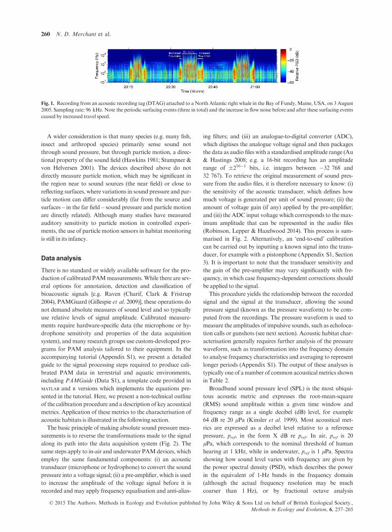
nates low frequencies (Johnson & Tyack 2003), and acoustic

time series are periodically disrupted by surfacing events

(Fig. 1) and vocalisations of the host animal. Application of

similar recording tags to terrestrial wildlife has thus far been

limited to one study of wild mule deer (Odocoileus hemionus;

Lynch et al. 2013). Emerging mobile platforms also include

autonomous underwater gliders (Rudnick, Davis & Eriksen

2004; Baumgartner & Fratantoni 2008), which can be

deployed for up to several hundred days, and freely drifting

platforms (Wilson, Benjamins & Elliott 2013), which minimise

flow noise in high tidal flow environments by moving with the

current.

GENERAL CONSIDERATIONS

The ability of PAM systems to accurately record sound is lim-

ited by several factors: dynamic range, frequency range and

system self-noise. The dynamic range is the ratio of the highest

to the lowest amplitude that can bemeasured by a given system

and can be scaled to higher or lower amplitudes by adding gain

to the signal (within the limitations of the device’s own self-

noise; Johnson, Partan &Hurst 2013;Merchant et al. 2013). If

the gain is too low, quieter sounds may not be recorded (Rem-

pel et al. 2013), and if it is too high, loud sounds can saturate

the system, leading to distortion of the signal through clipping

(Madsen & Wahlberg 2007; Fristrup & Mennitt 2012). A

PAM system should be chosen whose frequency range encom-

passes the spectral content of all sounds of interest to the study.

This range is limited to half the sampling rate of the recordings

(the Nyquist frequency), and by the sensitivity of the trans-

ducer and any filtering in the recording system (Appendix S1;

Madsen & Wahlberg 2007). System self-noise is noise gener-

ated by the recording system and acoustic transducer and can

limit the ability of a system to record low-amplitude sound

(Fristrup & Mennitt 2012; Johnson, Partan & Hurst 2013). It

is therefore important to consider self-noise specifications

when selecting a PAM system, and where possible to measure

self-noise levels by making recordings in a quiet location iso-

lated from sources of vibration.

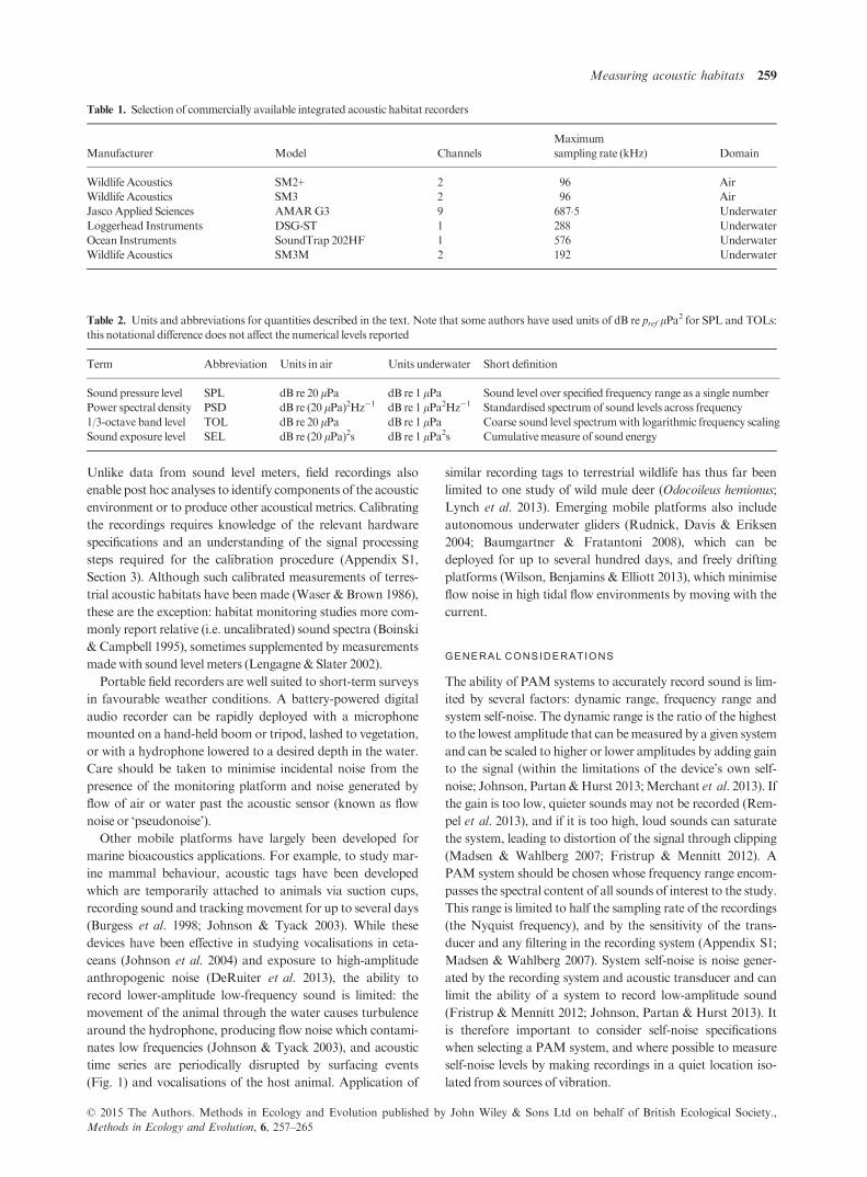
Table 1. Selection of commercially available integrated acoustic habitat recorders

Manufacturer Model Channels

Maximum

sampling rate (kHz) Domain

Wildlife Acoustics SM2+ 2 96 Air

Wildlife Acoustics SM3 2 96 Air

JascoApplied Sciences AMARG3 9 687�5 Underwater

Loggerhead Instruments DSG-ST 1 288 Underwater

Ocean Instruments SoundTrap 202HF 1 576 Underwater

Wildlife Acoustics SM3M 2 192 Underwater

Table 2. Units and abbreviations for quantities described in the text. Note that some authors have used units of dB re pref lPa2 for SPL and TOLs:

this notational difference does not affect the numerical levels reported

Term Abbreviation Units in air Units underwater Short definition

Sound pressure level SPL dB re 20 lPa dB re 1 lPa Sound level over specified frequency range as a single number

Power spectral density PSD dB re (20 lPa)2Hz�1 dB re 1 lPa2Hz�1 Standardised spectrum of sound levels across frequency

1/3-octave band level TOL dB re 20 lPa dB re 1 lPa Coarse sound level spectrumwith logarithmic frequency scaling

Sound exposure level SEL dB re (20 lPa)2s dB re 1 lPa2s Cumulativemeasure of sound energy



Measuring acoustic habitats 259

A wider consideration is that many species (e.g. many fish,

insect and arthropod species) primarily sense sound not

through sound pressure, but through particle motion, a direc-

tional property of the sound field (Hawkins 1981; Stumpner &

von Helversen 2001). The devices described above do not

directly measure particle motion, which may be significant in

the region near to sound sources (the near field) or close to

reflecting surfaces, where variations in sound pressure and par-

ticle motion can differ considerably (far from the source and

surfaces – in the far field – sound pressure and particle motion

are directly related). Although many studies have measured

auditory sensitivity to particle motion in controlled experi-

ments, the use of particle motion sensors in habitat monitoring

is still in its infancy.

Data analysis

There is no standard or widely available software for the pro-

duction of calibrated PAMmeasurements.While there are sev-

eral options for annotation, detection and classification of

bioacoustic signals [e.g. Raven (Charif, Clark & Fristrup

2004), PAMGuard (Gillespie et al. 2009)], these operations do

not demand absolute measures of sound level and so typically

use relative levels of signal amplitude. Calibrated measure-

ments require hardware-specific data (the microphone or hy-

drophone sensitivity and properties of the data acquisition

system), andmany research groups use custom-developed pro-

grams for PAM analysis tailored to their equipment. In the

accompanying tutorial (Appendix S1), we present a detailed

guide to the signal processing steps required to produce cali-

brated PAM data in terrestrial and aquatic environments,

including PAMGuide (Data S1), a template code provided in

MATLAB and R versions which implements the equations pre-

sented in the tutorial. Here, we present a non-technical outline

of the calibration procedure and a description of key acoustical

metrics. Application of these metrics to the characterisation of

acoustic habitats is illustrated in the following section.

The basic principle of making absolute sound pressure mea-

surements is to reverse the transformations made to the signal

along its path into the data acquisition system (Fig. 2). The

same steps apply to in-air and underwater PAMdevices, which

employ the same fundamental components: (i) an acoustic

transducer (microphone or hydrophone) to convert the sound

pressure into a voltage signal; (ii) a pre-amplifier, which is used

to increase the amplitude of the voltage signal before it is

recorded and may apply frequency equalisation and anti-alias-

ing filters; and (iii) an analogue-to-digital converter (ADC),

which digitises the analogue voltage signal and then packages

the data as audio files with a standardised amplitude range (Au

& Hastings 2008; e.g. a 16-bit recording has an amplitude

range of �216�1 bits, i.e. integers between �32 768 and

32 767). To retrieve the original measurement of sound pres-

sure from the audio files, it is therefore necessary to know: (i)

the sensitivity of the acoustic transducer, which defines how

much voltage is generated per unit of sound pressure; (ii) the

amount of voltage gain (if any) applied by the pre-amplifier;

and (iii) the ADC input voltage which corresponds to the max-

imum amplitude that can be represented in the audio files

(Robinson, Lepper & Hazelwood 2014). This process is sum-

marised in Fig. 2. Alternatively, an ‘end-to-end’ calibration

can be carried out by inputting a known signal into the trans-

ducer, for example with a pistonphone (Appendix S1, Section

3). It is important to note that the transducer sensitivity and

the gain of the pre-amplifier may vary significantly with fre-

quency, in which case frequency-dependent corrections should

be applied to the signal.

This procedure yields the relationship between the recorded

signal and the signal at the transducer, allowing the sound

pressure signal (known as the pressure waveform) to be com-

puted from the recordings. The pressure waveform is used to

measure the amplitudes of impulsive sounds, such as echoloca-

tion calls or gunshots (see next section). Acoustic habitat char-

acterisation generally requires further analysis of the pressure

waveform, such as transformation into the frequency domain

to analyse frequency characteristics and averaging to represent

longer periods (Appendix S1). The output of these analyses is

typically one of a number of common acoustical metrics shown

in Table 2.

Broadband sound pressure level (SPL) is the most ubiqui-

tous acoustic metric and expresses the root-mean-square

(RMS) sound amplitude within a given time window and

frequency range as a single decibel (dB) level, for example

64 dB re 20 lPa (Kinsler et al. 1999). Most acoustical met-

rics are expressed as a decibel level relative to a reference

pressure, pref, in the form X dB re pref. In air, pref is 20

lPa, which corresponds to the nominal threshold of human

hearing at 1 kHz, while in underwater, pref is 1 lPa. Spectrashowing how sound level varies with frequency are given by

the power spectral density (PSD), which describes the power

in the equivalent of 1-Hz bands in the frequency domain

(although the actual frequency resolution may be much

coarser than 1 Hz), or by fractional octave analysis

Fig. 1. Recording from an acoustic recording tag (DTAG) attached to aNorth Atlantic right whale in the Bay of Fundy,Maine, USA, on 3 August

2005. Sampling rate: 96 kHz. Note the periodic surfacing events (three in total) and the increase in flow noise before and after these surfacing events

caused by increased travel speed.




(typically 1/3-octave band levels, TOLs), which measures

the power in frequency bands that widen exponentially with

increasing frequency and are evenly spaced on a logarithmic

frequency axis (Fig. 3c). Finally, the sound exposure level

(SEL) is a summation of sound energy through time over a

specified duration and is often used to assess cumulative

exposure to noise.

An emerging area of study is the use of acoustic indices as

proxy indicators of biodiversity and species composition (Tow-

sey, Parsons & Sueur 2014). Various new statistical indices

(e.g. acoustic diversity index, acoustic complexity index) have

been applied in comparative studies of distinct habitats for this

purpose, so far with mixed results (Lellouch et al. 2014; Tow-

sey, Parsons & Sueur 2014). It remains to be seen to what

extent such techniques will complement field observations of

biodiversity and automatic detection and classification of spe-

cies via PAM.

Habitat characterisation

Acoustic habitats can be described by statistical analysis of

sound levels and by time-series representations. Based on the

metrics outlined above and defined in Appendix S1, this sec-

tion illustrates how these techniques can be used effectively for

various habitat monitoring applications. In general, statistical

analyses are more suited to characterising variability and com-

paring acoustic habitats at differing times or locations, while

discrete events and trends in sound levels are better described

by time series.

STATIST ICAL ANALYSIS

There are several ways to calculate the average sound level

from a series of shorter measurements, each of which has

particular advantages. The most common metric is the

Fig. 2. Signal path and calibration sequence

for a typical passive acoustic monitoring sys-

tem.ADC, analogue-to-digital converter.

(a) (b)

(c) (d)

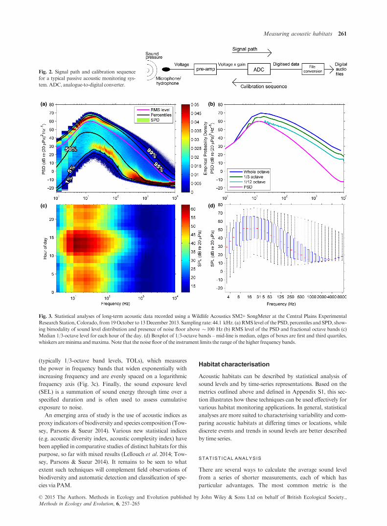
Fig. 3. Statistical analyses of long-term acoustic data recorded using a Wildlife Acoustics SM2+ SongMeter at the Central Plains Experimental

Research Station, Colorado, from 19October to 13December 2013. Sampling rate: 44.1 kHz. (a) RMS level of the PSD, percentiles and SPD, show-

ing bimodality of sound level distribution and presence of noise floor above � 100 Hz (b) RMS level of the PSD and fractional octave bands (c)

Median 1/3-octave level for each hour of the day. (d) Boxplot of 1/3-octave bands –mid-line is median, edges of boxes are first and third quartiles,

whiskers areminima andmaxima.Note that the noise floor of the instrument limits the range of the higher frequency bands.




RMS level (see Fig. 3), which is the mean of the squared

sound pressure computed before it is converted to dB

(Appendix S1, Eqn 18). The RMS level is the most preva-

lent averaging metric, perhaps due to the historic centrality

of Leq in terrestrial noise characterisation (Leq is the equiva-

lent RMS level during a specified period, which correlates

with human noise disturbance), and its direct relation to

SPL, which makes it independent of the length of the time

segments used in the original analysis (unlike other averag-

ing metrics; Merchant et al. 2012). However, the RMS level

is also strongly influenced by the highest sound levels (it

can be >95th percentile in some cases; Merchant et al.

2013) and so should be used with caution if applied to

recordings with intermittent high-amplitude events (e.g. pile

driving; Madsen 2005).

Alternative averages can give more statistically representa-

tive measures of sound levels than the RMS level. The mode,

defined as the sound level corresponding to the maximum

probability density at each frequency, is (by definition) the

most representative metric, although few studies have made

use of it (e.g. Parks, Urazghildiiev & Clark 2009; Merchant

et al. 2012) and there is the potential for multimodality to pro-

duce misleading results (Fig. 3a; Merchant, et al. 2012, 2013).

Median sound levels (Fig. 3d; known as L50 in terrestrial noise

assessment) can also be used as an indicator of typical sound

levels in a habitat (e.g. Klinck et al. 2012). These are more

robust than the mode and are generally insensitive to limita-

tions in the dynamic range of the recording instrument.

The range of sound levels in a habitat can be assessed by

plotting the percentile levels across the frequency spectrum

(Fig. 3a; Richardson et al. 1995; Castellote, Clark & Lammers

2012). These are alternatively known as exceedance levels,

although the percentiles are reversed, for example the 95% ex-

ceedance level, L95, is equivalent to the 5th percentile. Percen-

tiles provide an approximate indication of the distribution of

sound levels and may be useful in characterising the potential

extent of acoustic masking for a particular species (Clark et al.

2009). Amore comprehensive analysis of the sound level distri-

bution is given by the spectral probability density (SPD; Mer-

chant et al. 2013), whereby the empirical probability density of

sound levels in each frequency band is presented (Fig. 3a). This

shows the modal structure and outlying data in the underlying

distribution, which helps to interpret averages and percentiles.

It can also reveal limitations in the recording system: for exam-

ple, in the SPD shown in Fig. 3a, the self-noise of the instru-

ment appears to limit recording of the lowest sound levels in

the habitat above c. 100 Hz, evidenced by the flattening gradi-

ent of the lowest data points and their convergence with the

mode above this frequency.

Other statistical analyses include average levels for particu-

lar temporal periods to examine cyclical trends, such as diel,

seasonal or annual variability (see Fig. 3c, although other con-

figurations are also used, e.g. Radford et al. 2008), and box-

and-whisker plots (Fig. 3d; Bassett et al. 2012) showing the

spread of quartiles in each band.

In the frequency domain, fine-scale variations in the sound

spectrum can be assessed using the PSD, which is often com-

puted at 1-Hz resolution (Fig. 3b), although this can be com-

putationally demanding when processing and storing large

data sets. Frequency resolution can be reduced using either

coarser PSDs or fractional octave analysis, most commonly in

1/3-octave bands (Appendix S1, Eqns 13–16), wherein the fre-

quency range of the band is directly proportional to the centre

frequency (constant Q). For some taxa (e.g. mammals), con-

stant Q frequency bands are a particularly useful tool for

acoustic habitat analysis, as they can approximate the response

of the auditory system. It is important to note that the spectral

slope of the fractional octave band levels differs from the PSD

(Fig. 3b), as the bands are scaled logarithmically with fre-

quency (i.e. they widen with increasing frequency), meaning

that higher frequency bands integrate energy over larger fre-

quency ranges. For this reason, spectra with differing fre-

quency bandwidths (e.g. PSD and 1/3-octave) cannot be

directly compared.

TIME SERIES

Time series are used to characterise discrete events, such as

vocal behaviour or anthropogenic noise events (typically in the

form of spectrograms), and to track temporal trends in sound

levels, usually in particular frequency bands (e.g. TOLs or

broadband level).

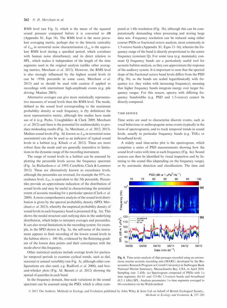
A widely used time-series plot is the spectrogram, which

comprises a series of PSD measurements showing how the

sound level varies with time at each frequency (Fig. 4a). Sound

sources can then be identified by visual inspection and by lis-

tening to the sound files (depending on the frequency range),

or by automatic detection and classification. The time and

(a)

(b)

Fig. 4. Time-series analysis of ship passages recorded using an autono-

mous marine acoustic recording unit (MARU; developed by the Bio-

acoustics Research Program at Cornell University) in Stellwagen Bank

National Marine Sanctuary, Massachusetts Bay, USA, in April 2010.

Sampling rate: 2 kHz. (a) Spectrogram composed of PSDs with 1-s

time segments; (b) 63- and 125-Hz 1/3-octave bands and broadband

(0.2–1 kHz) SPL. Analysis parameters: 1-s time segments averaged to

60-s resolution via theWelchmethod.




frequency resolution of the spectrograms must be sufficiently

high to resolve the sound events under consideration, and over-

lapping time windows may be used to smooth data in the time

domain and to ensure sounds at the boundary between time

windows are represented (Appendix S1, Section 4).

As well as describing discrete events, time series are used to

track trends in sound levels in particular frequency bands

(Fig. 4b), often in the context of long-term anthropogenic

noise studies (e.g.Miksis-Olds, Bradley&Niu 2013).

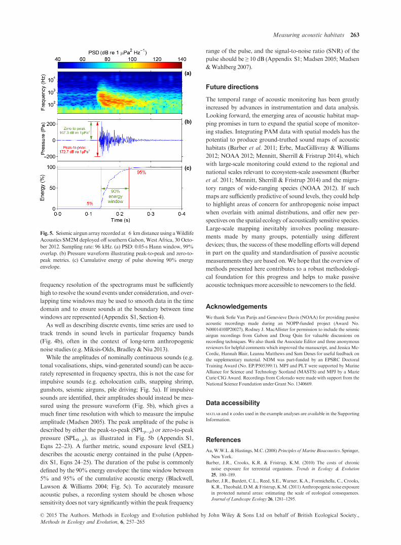
While the amplitudes of nominally continuous sounds (e.g.

tonal vocalisations, ships, wind-generated sound) can be accu-

rately represented in frequency spectra, this is not the case for

impulsive sounds (e.g. echolocation calls, snapping shrimp,

gunshots, seismic airguns, pile driving; Fig. 5a). If impulsive

sounds are identified, their amplitudes should instead be mea-

sured using the pressure waveform (Fig. 5b), which gives a

much finer time resolution with which to measure the impulse

amplitude (Madsen 2005). The peak amplitude of the pulse is

described by either the peak-to-peak (SPLp�p) or zero-to-peak

pressure (SPL0�p), as illustrated in Fig. 5b (Appendix S1,

Eqns 22–23). A further metric, sound exposure level (SEL)

describes the acoustic energy contained in the pulse (Appen-

dix S1, Eqns 24–25). The duration of the pulse is commonly

defined by the 90% energy envelope: the time window between

5% and 95% of the cumulative acoustic energy (Blackwell,

Lawson & Williams 2004; Fig. 5c). To accurately measure

acoustic pulses, a recording system should be chosen whose

sensitivity does not vary significantlywithin the peak frequency

range of the pulse, and the signal-to-noise ratio (SNR) of the

pulse should be ≥ 10 dB (Appendix S1; Madsen 2005; Madsen

&Wahlberg 2007).

Future directions

The temporal range of acoustic monitoring has been greatly

increased by advances in instrumentation and data analysis.

Looking forward, the emerging area of acoustic habitat map-

ping promises in turn to expand the spatial scope of monitor-

ing studies. Integrating PAM data with spatial models has the

potential to produce ground-truthed sound maps of acoustic

habitats (Barber et al. 2011; Erbe, MacGillivray & Williams

2012; NOAA 2012; Mennitt, Sherrill & Fristrup 2014), which

with large-scale monitoring could extend to the regional and

national scales relevant to ecosystem-scale assessment (Barber

et al. 2011; Mennitt, Sherrill & Fristrup 2014) and the migra-

tory ranges of wide-ranging species (NOAA 2012). If such

maps are sufficiently predictive of sound levels, they could help

to highlight areas of concern for anthropogenic noise impact

when overlain with animal distributions, and offer new per-

spectives on the spatial ecology of acoustically sensitive species.

Large-scale mapping inevitably involves pooling measure-

ments made by many groups, potentially using different

devices; thus, the success of these modelling efforts will depend

in part on the quality and standardisation of passive acoustic

measurements they are based on.We hope that the overview of

methods presented here contributes to a robust methodologi-

cal foundation for this progress and helps to make passive

acoustic techniquesmore accessible to newcomers to the field.

Acknowledgements

We thank Sofie Van Parijs and Genevieve Davis (NOAA) for providing passive

acoustic recordings made during an NOPP-funded project (Award No.

N0001410IP20027), Rodney J. MacAllister for permission to include the seismic

airgun recordings from Gabon and Doug Quin for valuable discussions on

recording techniques. We also thank the Associate Editor and three anonymous

reviewers for helpful comments which improved the manuscript, and JessicaMc-

Cordic, Hannah Blair, LeannaMatthews and Sam Denes for useful feedback on

the supplementary material. NDM was part-funded by an EPSRC Doctoral

Training Award (No. EP/P505399/1). MPJ and PLT were supported by Marine

Alliance for Science and Technology Scotland (MASTS) and MPJ by a Marie

Curie CIGAward. Recordings from Colorado were made with support from the

National Science Foundation underGrantNo. 1340669.

Data accessibility

MATLAB and R codes used in the example analyses are available in the Supporting

Information.

References

Au,W.W.L.&Hastings,M.C. (2008)Principles ofMarine Bioacoustics. Springer,

NewYork.

Barber, J.R., Crooks, K.R. & Fristrup, K.M. (2010) The costs of chronic

noise exposure for terrestrial organisms. Trends in Ecology & Evolution

25, 180–189.Barber, J.R., Burdett, C.L., Reed, S.E., Warner, K.A., Formichella, C., Crooks,

K.R., Theobald,D.M.&Fristrup,K.M. (2011)Anthropogenic noise exposure

in protected natural areas: estimating the scale of ecological consequences.

Journal of Landscape Ecology 26, 1281–1295.

(a)

(b)

(c)

Fig. 5. Seismic airgun array recorded at 6 kmdistance using aWildlife

Acoustics SM2Mdeployed off southern Gabon,West Africa, 30 Octo-

ber 2012. Sampling rate: 96 kHz. (a) PSD: 0.05-s Hann window, 99%

overlap. (b) Pressure waveform illustrating peak-to-peak and zero-to-

peak metrics. (c) Cumulative energy of pulse showing 90% energy

envelope.




Bassett, C., Polagye, B., Holt, M. & Thomson, J. (2012) A vessel noise budget for

Admiralty Inlet, Puget Sound, Washington (USA). The Journal of the Acous-

tical Society of America 132, 3706–3719.Baumgartner, M.F. & Fratantoni, D.M. (2008) Diel periodicity in both sei

whale vocalization rates and the vertical migration of their copepod prey

observed from ocean gliders. Limnology and Oceanography 53, 2197–2209.

Blackwell, S.B., Lawson, J.W. &Williams,M.T. (2004) Tolerance by ringed seals

(Phoca hispida) to impact pipe-driving and construction sounds at an oil pro-

duction island. The Journal of the Acoustical Society of America 115, 2346–2357.

Blumstein, D.T., Mennill, D.J., Clemins, P., Girod, L., Yao, K., Patricelli, G.

et al. (2011)Acousticmonitoring in terrestrial environments usingmicrophone

arrays: applications, technological considerations and prospectus. Journal of

Applied Ecology 48, 758–767.Boinski, S. & Campbell, A.F. (1995) Use of trill vocalizations to coordinate troop

movement among white-faced capuchins: a second field test. Behaviour 132,

875–901.Brumm,H. (2004) The impact of environmental noise on song amplitude in a ter-

ritorial bird. Journal of Animal Ecology 73, 434–440.Brumm, H. & Slabbekoorn, H. (2005) Acoustic communication in noise.

Advances in the Study of Behavior 35, 151–209.Burgess, W.C., Tyack, P.L., Le Boeuf, B.J. & Costa, D.P. (1998) A programma-

ble acoustic recording tag and first results from free-ranging northern elephant

seals. Deep Sea Research Part II: Topical Studies in Oceanography 45, 1327–1351.

Castellote, M., Clark, C.W. & Lammers, M.O. (2012) Acoustic and behavioural

changes by fin whales (Balaenoptera physalus) in response to shipping and air-

gunnoise.Biological Conservation 147, 115–122.Charif, R.A., Clark, C.W. & Fristrup, K.M. (2004) Raven 1.2 User’s Manual.

Cornell Laboratory of Ornithology, Ithaca,NewYork.

Clarin, B.M., Bitzilekis, E., Siemers, B.M. &Goerlitz, H.R. (2013) Personal mes-

sages reduce vandalism and theft of unattended scientific equipment.Methods

in Ecology and Evolution 5, 125–131.Clark, C.W., Ellison, W.T., Southall, B.L., Hatch, L., Van Parijs, S.M., Fran-

kel, A. & Ponirakis, D. (2009) Acoustic masking in marine ecosystems:

intuitions, analysis, and implication. Marine Ecology Progress Series 395,

201–222.DeRuiter, S.L., Southall, B.L., Calambokidis, J., Zimmer, W.M.X., Sadykova,

D., Falcone, E.A. et al. (2013) First direct measurements of behavioural

responses by Cuvier’s beaked whales to mid-frequency active sonar. Biology

Letters 9, 20130223.

Digby, A., Towsey,M., Bell, B.D. & Teal. P.D. (2013) A practical comparison of

manual and autonomous methods for acoustic monitoring. Methods in Ecol-

ogy and Evolution 4, 675–683.Dudzinski, K.M., Brown, S.J., Lammers, M., Lucke, K., Mann, D.A., Sim-

ard, P. et al. (2011) Trouble-shooting deployment and recovery options

for various stationary passive acoustic monitoring devices in both shallow-

and deep-water applications. The Journal of the Acoustical Society of

America 129, 436–448.Erbe, C.,MacGillivray,A.&Williams,R. (2012)Mapping cumulative noise from

shipping to informmarine spatial planning.The Journal of the Acoustical Soci-

ety of America 132, EL423–EL428.Favali, P., Beranzoli, L. & de Santis, A. (2015) Seafloor Observatories: A New

Vision of the Earth from theAbyss. Springer-Praxis, UK.

Francis, C.D. & Barber, J.R. (2013) A framework for understanding noise

impacts on wildlife: an urgent conservation priority. Frontiers in Ecology and

the Environment 11, 305–313.Francis, C.D., Ortega, C.P. & Cruz, A. (2009) Noise pollution changes avian

communities and species interactions.Current Biology 19, 1415–1419.Fristrup,K.M. &Mennitt, D. (2012) Bioacoustical monitoring in terrestrial envi-

ronments.Acoustics Today 8, 16–24.Gillespie, D., Mellinger, D.K., Gordon, J., McLaren, D., Redmond, P.,

McHugh, R., Trinder, P., Deng, X.Y. & Thode, A. (2009) PAMGUARD:

Semiautomated open source software for real-time acoustic detection and

localization of cetaceans. The Journal of the Acoustical Society of America 125,

2547–2547.Hawkins, A.D. (1981) The hearing abilities of fish.Hearing and Sound Communi-

cation in Fishes (eds W.N. Tavolga, A.N. Popper & R.R. Fay), pp. 109–137.Springer, NewYork.

Hildebrand, J.A. (2009) Anthropogenic and natural sources of ambient noise in

the ocean.Marine Ecology Progress Series 395, 5–20.Johnson, M.P. & Tyack, P.L. (2003) A digital acoustic recording tag for measur-

ing the response of wild marine mammals to sound. IEEE Journal of Oceanic

Engineering 28, 3–12.

Johnson, M., Madsen, P.T., Zimmer, W.M.X., Aguilar de Soto, N. & Tyack,

P.L. (2004) Beaked whales echolocate on prey. Proceedings of the Royal Soci-

ety of London. Series B 271, S383–S386.Johnson, M., Partan, J. & Hurst, T. (2013) Low complexity lossless compression

of underwater sound recordings.The Journal of theAcoustical Society of Amer-

ica 133, 1387–1398.Kinsler, L.E., Frey, A.R., Coppens, A.B. & Sanders, J.V. (1999) Fundamentals of

Acoustics, 4th edn.Wiley,NJ.

Klinck, H., Nieukirk, S.L., Mellinger, D.K., Klinck, K., Matsumoto, H., &

Dziak, R.P. (2012) Seasonal presence of cetaceans and ambient noise levels in

polar waters of the North Atlantic. The Journal of the Acoustical Society of

America 132, EL176–EL181.Lellouch, L., Pavoine, S., Jiguet, F., Glotin, H. & Sueur, J. (2014) Monitoring

temporal change of bird communities with dissimilarity acoustic indices.Meth-

ods in Ecology and Evolution 5, 495–505.Lengagne, T. & Slater, P.J.B. (2002) The effects of rain on acoustic communica-

tion: tawny owls have good reason for calling less in wet weather. Proceedings

of the Royal Society of London. Series B 269, 2121–2125.Lynch, E., Angeloni, L., Fristrup, K., Joyce, D. &Wittemyer, G. (2013) The use

of on-animal acoustical recording devices for studying animal behavior. Ecol-

ogy and Evolution 3, 2030–2037.Madsen, P.T. (2005) Marine mammals and noise: Problems with root mean

square sound pressure levels for transients. The Journal of the Acoustical Soci-

ety of America 117, 3952–3957.Madsen, P.T. &Wahlberg, M. (2007) Recording and quantification of ultrasonic

echolocation clicks from free-ranging toothed whales. Deep-Sea Research

Part I: Oceanographic Research Papers 54, 1421–1444.Mennill, D.J., Battiston, M., Wilson, D.R., Foote, J.R. & Doucet, S.M. (2012)

Field test of an affordable portable wirelessmicrophone array for spatial moni-

toring of animal ecology and behaviour.Methods in Ecology and Evolution 3,

704–712.Mennitt, D., Sherrill, K. & Fristrup, K. (2014) A geospatial model of ambient

sound pressure levels in the contiguous United States. The Journal of the

Acoustical Society of America 135, 2746–2764.Merchant, N.D., Blondel, P., Dakin, D.T. & Dorocicz, J. (2012) Averaging

underwater noise levels for environmental assessment of shipping. The Journal

of the Acoustical Society of America 132, EL343–EL349.Merchant, N.D., Barton, T.R., Thompson, P.M., Pirotta, E., Dakin, D.T. &

Dorocicz, J. (2013) Spectral probability density as a tool for ambient noise

analysis.The Journal of the Acoustical Society of America 133, EL262–EL267.Miksis-Olds, J.L., Bradley, D.L. & Niu, X.M. (2013) Decadal trends in Indian

Ocean ambient sound. The Journal of the Acoustical Society of America 134,

3464–3475.Morton, E.S. (1975) Ecological sources of selection on avian sounds. The Ameri-

canNaturalist 109, 17–34.NationalResearchCouncil (2005)MarineMammalPopulations andOceanNoise:

Determining when Noise Causes Biologically Significant Effects. National

Academy Press,Washington,DC.

NOAA (2012) CetSound project. Available at: http://cetsound.noaa.gov/

index.html [accessed 4 June 2014].

Nowacek, D.P., Thorne, L.H., Johnston, D.W. & Tyack, P.L. (2007) Responses

of cetaceans to anthropogenic noise.Mammal Review 37, 81–115.Parks, S.E., Urazghildiiev, I. & Clark, C.W. (2009) Variability in ambient noise

levels and call parameters of NorthAtlantic right whales in three habitat areas.

The Journal of the Acoustical Society of America 125, 1230–1239.Payne,R. &Webb, D. (1971) Orientation bymeans of long range acoustic signal-

ing in baleen whales. Annals of the New York Academy of Sciences 188, 110–141.

Pijanowski, B.C., Villanueva-Rivera, L.J., Dumyahn, S.L., Farina, A., Krause,

B.L., Napoletano, B.M., Gage, S.H. & Pieretti, N. (2011) Soundscape ecology:

the science of sound in the landscape.BioScience 61, 203–216.Radford, C., Jeffs, A., Tindle, C. &Montgomery, J. (2008) Temporal patterns in

ambient noise of biological origin from a shallowwater temperate reef.Oecolo-

gia 156, 921–929.Remage-Healey, L., Nowacek, D.P. & Bass, A.H. (2006) Dolphin foraging

sounds suppress calling and elevate stress hormone levels in a prey species the

Gulf toadfish. Journal of Experimental Biology 209, 4444–4451.Rempel, R.S., Francis, C.M., Robinson, J.N. & Campbell, M. (2013) Compari-

son of audio recording system performance for detecting andmonitoring song-

birds. Journal of Field Ornithology 84, 86–97.Richardson, W.J., Greene, C.R., Malme, C.I. & Thompson, D.H. (1995)Marine

Mammals andNoise. Academic Press, SanDiego.

Robinson, S.P., Lepper, P.A. &Hazelwood, R.A. (2014)Good Practice Guide for

UnderwaterNoiseMeasurement. NPLGood PracticeGuideNo. 133.National

Physical Laboratory, UK.




Rolland, R.M., Parks, S.E., Hunt, K.E., Castellote, M., Corkeron, P.J., Now-

acek, D.P., Wasser, S.K. & Kraus, S.D. (2012) Evidence that ship noise

increases stress in right whales. Proceedings of the Royal Society of London.

Series B 279, 2363–2368.Rudnick, D.L., Davis, R.E. & Eriksen, C.C. (2004) Underwater gliders for ocean

research.Marine Technology Society Journal 38, 73–84.Simpson, S.D., Meekan, M., Montgomery, J., McCauley, R. & Jeffs, A. (2005)

Homeward sound.Science 308, 221.

Sousa-Lima, R., Norris, T.F., Oswald, J.N. & Fernandes, D.P. (2013) A review

and inventory of fixed autonomous recorders for passive acoustic monitoring

ofmarinemammals.AquaticMammals 39, 23–53.Stumpner, A.& vonHelversen,D. (2001) Evolution and function of auditory sys-

tems in insects.DieNaturwissenschaften 88, 159–170.Sun, J.W.C. & Narins, P.M. (2005) Anthropogenic sounds differentially affect

amphibian call rate.Biological Conservation 121, 419–427.Towsey,M., Parsons, S. & Sueur, J. (2014) Ecology and acoustics at a large scale.

Ecological Informatics 21, 1–3.Van Parijs, S.M., Clark, C.W., Sousa-Lima, R.S., Parks, S.E., Rankin, S.,

Risch, D. & Van Opzeeland, I.C. (2009) Management and research

applications of real-time and archival passive acoustic sensors over vary-

ing temporal and spatial scales. Marine Ecology Progress Series 395, 21–36.

Waser, P.M. & Brown, C.H. (1986) Habitat acoustics and primate communica-

tion.American Journal of Primatology 10, 135–154.Wenz, G.M. (1961) Some periodic variations in low-frequency acoustic ambient

noise levels in the ocean. The Journal of the Acoustical Society of America 33,

64–74.

Wiley, R.H. & Richards, D.G. (1978) Physical constraints on acoustic communi-

cation in the atmosphere: Implications for the evolution of animal vocaliza-

tions.Behavioral Ecology and Sociobiology 3, 69–94.Wilson, B., Benjamins, S. & Elliott, J. (2013) Using drifting passive echolocation

loggers to study harbour porpoises in tidal-stream habitats. Endangered Spe-

cies Research 22, 125–143.

Received 23 September 2014; accepted 8December 2014

Handling Editor:DavidHodgson

Supporting Information

Additional Supporting Information may be found in the online version

of this article.

Appendix S1.PAMGuide tutorial.

Data S1. PAMGuide.zip - Zipped archive of R and MATLAB codes

for PAMGuide.




Documents

Measuring acoustic habitats