Paper Number:

acp-2017-1114

Title

Source influence on emission pathways and ambient PM2.5 pollution over India (2015-2050)

Author list

Chandra Venkataraman, Michael Brauer, Kushal Tibrewal, Pankaj Sadavarte, Qiao Ma, Aaron

Cohen, Sreelekha Chaliyakunnel, Joseph Frostad, Zbigniew Klimont, Randall V. Martin, Dylan

B. Millet, Sajeev Philip, Katherine Walker, Shuxiao Wang

We thank the reviewers for their comments, which have been carefully addressed in detail. A point

by point response (in red) is provided below, which have been reflected as revisions to the

manuscript.

[NOTE: All page and line numbers in the response, refer to the revised version of the

manuscript]

Response to Referee Comments 1:

General comments

The work of Venkataraman et al. deals with the investigation of PM sources in India which

experiences severe air pollution problems, under current emissions and future emission scenarios

which assume cleaner and more energy efficient technologies. This work wants to address two

scientific questions strongly related with HTAP, such as the identification of regional PM2.5

pollution levels and their sources and the changes in PM2.5 levels as a result of air pollution and

climate change abatement efforts. The paper is overall well written and fits with the purposes of

the HTAP special issue; therefore I recommend it for publication after developing the following

comments.

Specific comments

1)-page 2 line 5: please provide a reference for the population statistics

Page 2 line 7: Required reference cited.

“India hosts the world’s second largest population (UNDP, 2017)”

Ref:

United Nations, Department of Economic and Social Affairs, Population Division (2017). World

Population Prospects: The 2017 Revision, Key Findings and Advance Tables. Working Paper No.

ESA/P/WP/248.

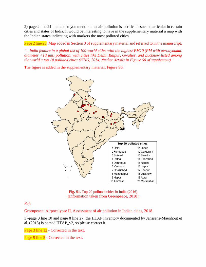
2)-page 2 line 21: in the text you mention that air pollution is a critical issue in particular in certain

cities and states of India. It would be interesting to have in the supplementary material a map with

the Indian states indicating with markers the most polluted cities.

Page 2 line 25: Map added in Section 3 of supplementary material and referred to in the manuscript.

“...India feature in a global list of 100 world cities with the highest PM10 (PM with aerodynamic

diameter <10 µm) pollution, with cities like Delhi, Raipur, Gwalior, and Lucknow listed among

the world’s top 10 polluted cities (WHO, 2014; further details in Figure S6 of supplement).”

The figure is added in the supplementary material, Figure S6.

Fig. S1. Top 20 polluted cities in India (2016)

(Information taken from Greenpeace, 2018)

Ref:

Greenpeace: Airpocalypse II, Assessment of air pollution in Indian cities, 2018.

3)-page 3 line 10 and page 8 line 27: the HTAP inventory documented by Janssens-Maenhout et

al. (2015) is named HTAP_v2, so please correct it.

Page 3 line 12 - Corrected in the text.

Page 9 line 5 - Corrected in the text.

4)-page 3 line 27: can you shortly describe the “engineering model approach” on which your

emission estimates are based, although documented in other publications. This will help in

understanding the source of data for the technology penetrations and air pollution control measures

(refer to page 4 line 5).

Page 4 line 1: Description added to the text:

“An engineering model approach, goes beyond fuel divisions and uses technology parameters for

process and emissions control technologies, including technology type, efficiency or specific fuel

consumption, and technology-linked emission factors (g of pollutant/ kg of fuel) to estimate

emissions.”

5)-page 3 line 8: I guess residential emissions do not only include water and space heating but also

all the other domestic activities like cooking. Please correct this sentence.

Clarification:

Yes, the residential sector does contain other activities such as cooking and lighting, but the

sentence here refers to the assumption in the seasonality in emissions from certain activities. The

seasonality is assumed only for space and water heating activities.

Page 4 line 12: The sentence is reframed to convey this information.

“Residential sector activities are comprised of cooking and water heating, largely with traditional

biomass stoves; lighting, using kerosene lamps; and warming of homes and humans, with biomass

fuels. Seasonality is included for water heating and home warming.”

6)-page 4 line 20: the authors should clarify why their database does not include emission estimates

of CO, NH3 and PM10? Later in the manuscript the authors say that NH3 is indeed taken from

MIX. Why was not it possible to calculate them with your methodology? How is the consistency

among all pollutants (in terms of activity data, technologies, abatement and spatial distribution) is

guaranteed? NH3 is a crucial compound for the formation of secondary PM, so consistency with

other SOA precursors is needed. Moreover, you refer to the paper by Li et al. 2017 for the MIX

inventory, however, this inventory is only till 2010. How did you obtain emissions for 2015?

Clarification:

In regard to PM-10, the present inventory does not presently include its calculation, but it can be

estimated using the current methodology, in future updates to the inventory.

Page 4, line 28: Discussion added.

“Emissions of CO are included in the inventory (Pandey et al., 2014; Sadavarte et al., 2014),

however, CO was not input to the GEOS-Chem simulations, since it is not central to atmospheric

chemistry of secondary PM-2.5 formation on annual time-scales.”

Page 11, line 18: Discussion added.

“Emissions of NH3 arise primarily from sources like animal husbandry, not addressed in the

present inventory. Therefore, they are taken from (Li et al., 2017). Owing to large uncertainties in

future emissions, these were held the same in future scenarios, as for 2015. Emission magnitudes

of NH3 could affect secondary nitrate, which typically contributes to less than 5% of PM-2.5 mass,

thus not influencing overall results in any significant manner.”

7)-page 5 line 21: The authors mention the “shift to non-fossil generation”. Can the authors clarify

towards what type of energy source India will move? In addition, as general comment on the future

scenarios, the authors should mention how much realistic/feasible are they. Why Indian emissions

cannot increase even at a higher speed compared to 2015 since quite some time is required before

future policies to reduce the emissions in India will become effective?

Page 5, line 28: Discussion added.

“The S2 scenario assumes shifts to non-fossil generation which would occur under India

Nationally Determined Contribution (India’s NDC, 2015) in the power sector, consistent with a

shift to 40% renewables including solar, wind and hydro power by 2030 (NDC, 2015). The NDC

goals of India are suggested to be realistic (CAT, 2017; Ross and Gerholdt, 2017), with

achievement of non-fossil share of power generation projected to lie between 38%-48% by 2030,

as well as adoption of tighter emission standards for desulphurization and de-NOx technologies

in thermal plants (MoEFCC, 2015), at a rate consistent with expected barriers (CSE, 2016).

Further, changes assumed in the transport sector reflect promulgated growth in public vehicle

share (NTDPC, 2013; Guttikunda and Mohan, 2014; NITI Aayog, 2015) and promulgated

regulation (Auto Fuel Policy Vision 2025, 2014, MoRTH, 2016), along with realistic assumptions

of implementation lags in adoption of BS VI standards (ICRA 2016). Other assumptions include

modest increases in industrial energy efficiency under the perform achieve and trade (PAT)

scheme (Level 2, IESS, Niti Aayog, 2015 );”

Ref:

CAT: Climate Action Tracker - India, [online] Available from:

http://climateactiontracker.org/countries/india/2017.html (Accessed 5 March 2018), 2017.

Ross, K. and Gerholdt, R.: Achieving India’s Ambitious Renewable Energy Goals: A Progress

Report, World Resources Institute, [online] Available from:

http://www.wri.org/blog/2017/05/achieving-indias-ambitious-renewable-energy-goals-progress-

report (Accessed 5 March 2018), 2017.

8)-The authors should compare their scenarios assumptions (including references therein) and

results with the recent work by Li et al. (2017).

Li, C., McLinden, C., Fioletov, V., Krotkov, N., Carn, S., Joiner, J., Streets, D., He, H., Ren, X., Li,

Z., and Dickerson, R. R.: India Is Overtaking China as the World’s Largest Emitter of

Anthropogenic Sulfur Dioxide, Scientific Reports, 7, 14304, 10.1038/s41598-017-14639-8, 2017.

Page 10, line 1: Discussion added.

“Bottom-up estimates of SO2 emissions from our inventory (Pandey et al., 2014; Sadavarte et al.,

2014) are consistent with the recent estimates from the satellite based study (Li et al., 2017) from

2005-2016, both showing a steady growth. Present day emissions of SO2 (8.1 Mt yr-1) are at the

lower end of the range of 8.5-11.3 Mt yr-1suggested by Li et al. 2017. Large future increases in

SO2 emissions, estimated here in the REF and S2 scenarios are consistent with findings of Li et

al. 2017.”

9)-page 8 lines 24-43: as supplementary information, it would be interesting to look at some

additional emission inventory comparisons for the common years (e.g. 2008 and 2010): e.g.

HTAP_v2, REAS, ECLIPSE and your inventory. This can be shown both as total/sector-specific

emissions comparison and grid-maps.

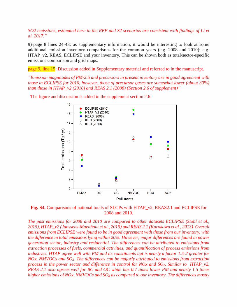
page 9, line 15: Discussion added in Supplementary material and referred to in the manuscript.

“Emission magnitudes of PM-2.5 and precursors in present inventory are in good agreement with

those in ECLIPSE for 2010, however, those of precursor gases are somewhat lower (about 30%)

than those in HTAP_v2 (2010) and REAS 2.1 (2008) (Section 2.6 of supplement)”

The figure and discussion is added in the supplement section 2.6:

Fig. S4. Comparisons of national totals of SLCPs with HTAP_v2, REAS2.1 and ECLIPSE for

2008 and 2010.

The past emissions for 2008 and 2010 are compared to other datasets ECLIPSE (Stohl et al.,

2015), HTAP_v2 (Janssens-Maenhout et al., 2015) and REAS 2.1 (Kurokawa et al., 2013). Overall

emissions from ECLIPSE were found to be in good agreement with those from our inventory, with

the difference in total emissions lying within 20%. However, major differences are found in power

generation sector, industry and residential. The differences can be attributed to emissions from

extraction processes of fuels, commercial activities, and quantification of process emissions from

industries. HTAP agree well with PM and its constituents but is nearly a factor 1.5-2 greater for

NOx, NMVOCs and SO2. The differences can be majorly attributed to emissions from extraction

process in the power sector and difference in control for NOx and SO2. Similar to HTAP_v2,

REAS 2.1 also agrees well for BC and OC while has 0.7 times lower PM and nearly 1.5 times

higher emissions of NOx, NMVOCs and SO2 as compared to our inventory. The differences mostly

come from inclusion of agricultural emissions (such as fertilizer application and manure

management of livestock), non-combustion emissions primarily from solvent use, paint use,

evaporative emissions from vehicles, emissions from fuel extraction processes and emissions

released from soil in REAS 2.1. Other causes of difference include use of different emission factors

and methodologies for emissions estimates, particularly for the residential biomass combustion

and transportation. In other inventories, activity data are primarily taken from energy

consumption estimates by International Energy Agency (IEA), where as in our inventory the

activity data is calculated using food consumption at the state level and end-use energy for cooking

(Habib et al., 2004) and vehicular sales to arrive at on-road vehicular population considering age

of the vehicles (Pandey and Venkataraman, 2014).

Ref:

Habib, G., Venkataraman, C., Shrivastava, M., Banerjee, R., Stehr, J. W. and Dickerson, R. R.:

New methodology for estimating biofuel consumption for cooking: Atmospheric emissions of black

carbon and sulfur dioxide from India, Global Biogeochem. Cycles, 18(3), 1–11,

doi:10.1029/2003GB002157, 2004.

10)-page 11 line 25: why meteorological data are not available beyond 2012?

Page 12 line 12: Discussion added.

“South Asia nested meteorological fields were not yet available post-2012 due to a change in the

GEOS assimilation system in 2013. Therefore, we conducted standard simulations to test

meteorology from the years 2010 to 2012. We chose the year 2012 as our meteorology year, as

the simulation results using this year best represented the mean PM2.5 concentration from 2010

to 2012. A three month initialization period was used to remove the effects of initial conditions.”

11)-page 13 line 14: why do we observe higher concentrations in northern India? Is it only due to

the fact that most of the sources are located in that area or are there other reasons?

Page 14, line 22: Discussion added.

“High PM-2.5 concentrations in northern India can be attributed both to higher local emissions,

especially of organic carbon, and to synoptic transport patterns leading to confinement of regional

emissions of particulate matter and precursor gases in the northern plains (e.g. Sadavarte et al.,

2016), borne out in high concentrations of secondary particulate sulphate and dust.”

Ref: Sadavarte, P., Venkataraman, C., Cherian, R., Patil, N., Madhavan, B. L., Gupta, T.,

Kulkarni, S., Carmichael, G. R. and Adhikary, B.: Seasonal differences in aerosol abundance and

radiative forcing in months of contrasting emissions and rainfall over northern South Asia, Atmos.

Environ., 125, 512–523, doi:10.1016/j.atmosenv.2015.10.092, 2016.

12)-page 16 line 13: PM2.5 concentration from road transport seems to be rather low (below 2

ug/m3). Are emissions from re-suspension included?

Clarification:

Yes, the emissions from re-suspension dust is included in the “Anthropogenic dust” category. The

emissions under the Transport category only include the emissions from combustion in vehicles.

13)-page 17 lines 22-24: the authors should clarify why district level urban population is used to

distribute on-road gasoline emissions. Transport emissions should be distributed over roads (with

different type of weights) and not over population proxies. The authors could provide in a

supplementary table the proxies used to grid emissions from different sectors.

Page 4 line 18: Spatial proxy table added in the supplement information, Table S1 and referred to

in the manuscript.

“Spatial proxies used to estimate gridded emissions over India are described in Table S1 of the

supplement.”

Page 19, line 12: Discussion added.

“Gasoline vehicles mostly consist of two-, three- and four-wheeler private vehicles in use in urban

areas. In the present regional-scale inventory therefore represented using population, pending

improved road based proxies for air-quality studies at urban scales.”

14)-Table1: please clarify what you mean with “emissions of anthropogenic dust removed”. If the

dust is collected/removed it does not contribute to atmospheric emissions.

Clarification:

It is a typo error, the word “removed” should not be mentioned in the table and has been deleted.

15)-Figure 7 reports PM2.5 concentrations by state, however, it is not clear how this is calculated.

Do the authors estimate emissions for each Indian state using statistics of each state and then they

evaluate PM2.5 concentrations by state? Please clarify.

Page 15 line 18: Discussion added.

“Simulated PM2.5 concentrations from the model are weighted by population for each state. This

is calculated by multiplying the concentration in each grid cell (0.1 x 0.1 degree) by the population,

summing this quantity for all grid cells that lie within a state and then dividing by the total

population in each state.”

16)-Table S1: it is not clear why NH3 (and possibly also PM10 and CO) emissions by state are not

reported here.

See response to comment 6.

17)-Table S2: it would be good to report a short description in how the uncertainty bands have

been calculated using the cited studies.

Page 4, line 33: Description added in supplementary material and referred to in the manuscript.

“Uncertainties in the activity rates, calculated analytically using methods described more fully in

previous publications (Pandey and Venkataraman 2014; Pandey et al. 2014; Sadavarte and

Venkataraman, 2014) are shown in Table S3 of the supplement.”

Description added in Section 3 of the supplement information:

“Uncertainties in the activity rates were calculated analytically, assuming normal distribution for

the underlying uncertainties in all input quantities. For each input: (a) the mean and standard

deviation calculated from a set of available (three or more) data points; (b) upper and lower

bounds assumed based on two data points; or (c) a representative uncertainty assumed from

similar data, where only one data-point exists. Uncertainty in the emission factors was estimated

from the standard deviation in the set of compiled emission factors of a particular pollutant from

a particular fuel technology combination. If the emission factor being used was taken from a single

reported source, the reported rating was quantified using the percentage errors cited in IPCC

(2006a,b) and EMEP (2009). The measured emission factors with unspecified uncertainties were

assigned the highest-known uncertainty for the same pollutant and those from similar

technologies. Wherever emission factor measurements for a technology were not available an

emission factor from a similar technology was chosen and assigned 100% uncertainty (<5% of

the technologies fall under this category, including fluidized bed combustors and sponge-iron

kilns). A spreadsheet-based approach was developed for combining uncertainties in activity rates

and emission factors. A normal/lognormal distribution was assumed for when standard deviation

was less/greater than 30% of the mean. Uncertainty propagation in the product of two variables

was followed using the sum-of-quadrature rule, calculated analytically. The upper and lower

emission bounds were calculated using the resultant lognormal parameters (geometric mean and

geometric standard deviation).”

Refs:

EMEP, 2009. EMEP/EEA Air Pollutant Emission Inventory Guidebook. European Environment

Agency, Copenhagen.

IPCC, 2006a. IPCC Guidelines for National Greenhouse Gas Inventories. In: Energy, vol. 2.

IPCC, 2006b. IPCC Guidelines for National Greenhouse Gas Inventories. In: General Guidance

and Reporting, vol. 1.

18)-Table S4: it would be interesting to know more details about the technologies applied on the

private vehicles. The authors could report the share of two/three wheelers and passenger cars as

well as the corresponding emission standards (share and emission levels) applied on these vehicles.

Is gasoline the most used fuel for private vehicles?

Discussion added in the supplementary information, Section S2.3:

“Emissions from on-road vehicles are based from a previous study (Pandey and Venkataraman,

2014). The detailed list of vehicle category is included in the study (Table 3, Pandey and

Venkataraman, 2014). Two-wheelers contribute the most to the fleet of private vehicles with

approximately 82% share, followed by passenger cars (15%) and three-wheelers (3%). For

present day, all vehicles are assumed to be compliant with BS III standards with 2 wheelers having

the highest emission levels for PM2.5 followed by three wheelers (0.5 times lower) and gasoline

cars (0.1 times lower). Private gasoline vehicles consisting of two-, three- and four-wheeler

vehicles which consume nearly 14.0 MT/yr gasoline, compared to 5 MT/yr of diesel consumed by

4-wheeler diesel cars (Pandey and Venkataraman, 2014). Future shifts to BS IV and BS VI

emission standards lead to reductions in emission levels by 80% and 90% respectively.”

Ref: Pandey, A. and Venkataraman, C.: Estimating emissions from the Indian transport sector

with on-road fleet composition and traffic volume, Atmos. Environ., 98, 123–133,

doi:10.1016/j.atmosenv.2014.08.039, 2014.

Technical corrections

-You should use in the text and in the graphs the “Mt” units instead of “MT”

Corrected

-page 1 line 30: please rephrase as following: “… and a very large shift (80-85%) to non-fossil

electricity generation, an overall reduction in PM2.5 concentrations below 2015 levels was

achieved”.

Rephrased

-page 2 line 15: please reformulate as following: (particulate matter in a size fraction with diameter

smaller than 2.5 μm)

Page 2 line 17: Rephrased

-page 4 line 20: please replace “reside” with “residues”.

Page 4 line 27: Corrected

-page 11 line 21: please correct as following: “mass to organic”

Page 12 line 10: Corrected

-page 11 line 22: please change to Philip et al. (2014b)

Page 12 line 11: Corrected

-page 14 line 26: “The simulated change in sectoral contribution to population-weighted PM2.5

concentrations, is evaluated” please remove the “comma”

Page 16 line 6: Corrected

-page 18 line 15: “The present findings imply that desirable levels of air quality, may not be

widespread” please remove the “comma”

Corrected

-Figure S3 should not be in black and white but with colors.

Figure replaced

Referee Comments 2:

This study developed scenarios of sectoral emissions of PM2.5 and its precursors for 2015-2050

and further assessed the impacts of individual source-sectors on PM2.5 pollution through GESO-

Chem model simulations over India. Based on model simulations authors have shown that under

the present day emissions most states in India exceed NAAQ standard of 40 g/m3 (annual mean).

Based on emission evaluation under proposed regulations authors have shown further deterioration

of air-quality in 2030 and 2050, even in highly ambitious scenario 10 states in India will not meet

the current NAAQ standard in 2050. Overall, their finding suggests that residential biomass

burning and agricultural residue burning is the primary largest sector (highly uncertain sector and

not validated with the in-situ data) contributing to the large regional background of PM2.5

pollution in India. The paper presents interesting analyses and will be an important resource for

the community. However, I have some queries given below and certain key issues need to be

addressed for improving the discussion section before it can be accepted for publication. Please

find some suggestions below which I hope the authors may find useful for revising the MS for

improving the discussion on the issues that affect the uncertainty/certainty of present findings and

conclusions.

First Concern:

My major concern is lack of sufficient validation/evaluation of the capability of a well respected

model to simulate chemical species over India, a region with limited publicly available

observations. These are very important for meaningful future research too as PM2.5 is a pollutant

derived from several precursor emissions with varied sources. Currently the work does not

acknowledge such issues and puts too much stock by the model results. Even the model was

previously applied to study PM2.5 over India relating satellite AOD to ground-level PM2.5, there

has not been a great deal of comparison of model results against observations in previous studies.

Global off-line models have large difficulties in simulating chemical species over India

(Surenderan et al., 2015, 2016 AE). Therefore it is essential to build confidence in the ability of

GEOS-Chem model (since it is finest resolution) to simulate species distributions reasonably well

so that it can be used for sensitivity simulations (such as performed for this study) and to

understand future air quality projections. Large biases in model may influence the regional PM2.5

fields in the future projections which I believe make it difficult to draw conclusions that are of

scientific value. The authors should clearly address this point by comparing the model with the

observed PM2.5 for greater understanding of model biases and recognition of areas needing

improvement. As a part of evaluation work for HTAP-II PM2.5 and BC data (mostly from the

published literature (not necessary for the same year)) has been compiled for more than 15 stations

in India which can be shared to the author for model validation. Of course, I cannot categorically

state that there is a problem, but I do find in figure 4 & 5 that the model has difficulties in

simulating the species distribution. There is always a problem of representativeness when

comparing coarse-scale models to point observations and perhaps this could be a problem. I would

also suggest to the authors to review how they have compared the simulated PM2.5 (model lowest

level??) with in-situ observations and satellite AOD (model field interpolated to satellite overpass

time).

Clarification:

We appreciate the referee’s suggestion to further evaluate model predictions, which is definitely

needed. However, this is strongly limited by the availability of coherent speciated PM-2.5 datasets

over India. Therefore, we feel that, at the end of a long and detailed study, exploiting all available

measurements, it would be difficult to do another intercomparison well, without taking care to

understand details of earlier observation periods proposed, effects of interannual variability, the

inherent problems of comparing spatially averaged model output to in-situ measurements, making

a close match of model output with sampling times, etc. Further, with observations coming from

years quite different from that of the simulation, an evaluation of this nature might not yield much

further insight into model performance. We have added the discussion below, explicitly

acknowledging the need for more detailed model evaluation in future.

Page 14, line 10: Discussion added.

“Direct comparison of spatially averaged model output with satellite products or in-situ

measurements typically incorporate significant uncertainty. A broad evaluation was undertaken

here, without a match of model output to specific sampling time or satellite overpass time. Thus,

some differences would arise from modelled meteorology not faithfully representing actual

meteorological conditions during the measurement period. With these caveats, we acknowledge

the need for coherent measurement campaigns to map concentrations of both PM2.5 and its

chemical constituents over India, to improve model evaluation and future air quality

management.”

Are NH3 emissions fixed to 2015 level in BAU, S2 and S3 scenarios? NH3 is important compound

for the formation of secondary aerosols and agricultural activity is one of the major sources of

NH3 in India, particularly in the rural India where residential bio-fuel and biomass burning is

dominant. It is necessary to clarify how authors have treated NH3 in 2015 and further in BAU, S2

and S3 scenarios. Considering projected growth in agricultural sector in India it is believed that

NH3 emissions will increase further (Sutton et al., 2017). Therefore, it may have some implication

on future PM2.5 levels.

Page 11, line 18: Discussion added.

“Emissions of NH3 arise primarily from sources like animal husbandry, not addressed in the

present inventory. Therefore, they are taken from (Li et al., 2017). Owing to large uncertainties in

future emissions, these were held the same in future scenarios, as for 2015. Emission magnitudes

of NH3 could affect secondary nitrate, which typically contributes to less than 5% of PM-2.5 mass,

thus not influencing overall results in any significant manner.”

Second concern:

It is understandable that due to lack of primary measurements concerning several important

emission types (e.g. NMVOCs), the magnitude of these emissions are still poorly constrained in

the emission inventories and are yet to be validated using in-situ data or with representative

emission factors determined from measurements conducted within India from major sources.

However, it is necessary to highlight these existing uncertainties arising from the data limiting

factors and which are currently substituted through use of emission factors that may not be

representative of emission sources in the South Asian atmospheric environment.

1) The authors should provide a speciated list (even in supplement would do) for the NMVOCs

considered in this work. Individual NMVOCs have different PM formation potential and without

such information it is not possible for the reader to assess how well this class or precursor has been

constrained.

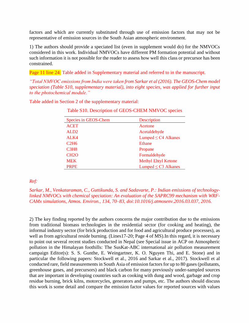
Page 11 line 24: Table added in Supplementary material and referred to in the manuscript.

“Total NMVOC emissions from India were taken from Sarkar et al (2016). The GEOS-Chem model

speciation (Table S10, supplementary material), into eight species, was applied for further input

to the photochemical module.”

Table added in Section 2 of the supplementary material:

Table S10. Description of GEOS-CHEM NMVOC species

Species in GEOS-Chem Description

ACET Acetone

ALD2 Acetaldehyde

ALK4 Lumped ≤ C4 Alkanes

C2H6 Ethane

C3H8 Propane

CH2O Formaldehyde

MEK Methyl Ehtyl Ketone

PRPE Lumped ≤ C3 Alkanes

Ref:

Sarkar, M., Venkataraman, C., Guttikunda, S. and Sadavarte, P.: Indian emissions of technology-

linked NMVOCs with chemical speciation: An evaluation of the SAPRC99 mechanism with WRF-

CAMx simulations, Atmos. Environ., 134, 70–83, doi:10.1016/j.atmosenv.2016.03.037, 2016.

2) The key finding reported by the authors concerns the major contribution due to the emissions

from traditional biomass technologies in the residential sector (for cooking and heating), the

informal industry sector (for brick production and for food and agricultural produce processes), as

well as from agricultural reside burning. (Lines17-20; Page 4 of MS).In this regard, it is necessary

to point out several recent studies conducted in Nepal (see Special issue in ACP on Atmospheric

pollution in the Himalayan foothills: The SusKat-ABC international air pollution measurement

campaign Editor(s): S. S. Gunthe, E. Weingartner, K. O. Nguyen Thi, and E. Stone) and in

particular the following papers: Stockwell et al., 2016 and Sarkar et al., 2017). Stockwell et al

conducted rare, field measurements in South Asia of emission factors for up to 80 gases (pollutants,

greenhouse gases, and precursors) and black carbon for many previously under-sampled sources

that are important in developing countries such as cooking with dung and wood, garbage and crop

residue burning, brick kilns, motorcycles, generators and pumps, etc. The authors should discuss

this work is some detail and compare the emission factor values for reported sources with values

used in their work and shown in Table S7. This is important to gauge how much uncertainty can

arise from use of variable emission factors. Secondly, the work by Sarkar et al. 2017 provides

valuable insights on where current emission inventories need to be improved for better

representation of emission source contributions. It provides quantitative information regarding the

source contributions of the major NMVOC sources in the Kathmandu Valley. Combining high-

resolution in situ NMVOC data and model analyses, it showed that REAS v2.1 overestimates the

contribution of residential biofuel use and industries. This is very pertinent to discuss and include

in the context of the present work for the following reasons. The use of emission factors from

residential biofuel sources for determining ambient source contributions without adequately

accounting for the deposition and/ or other loss that can occur for the indoor emissions due to

household cooking/heating and their net emission to outdoor environment can lead to gross over

estimation of the emissions as an atmospheric source. The results of Sarkar et al., 2017, which is

focused on NMVOCs appear to point towards such loss processes being significant and if true,

this is likely to be even more important for PM2.5 that has higher deposition tendency than gases.

These important aspects need to highlighted and addressed so that future work can benefit from

such insights. Are there any similar NMVOC datasets reported from the Indian region? It would

be good for the authors to mention these if possible. For many of the biomass burning sources, it

is now recognized that combustion efficiency can be even more important than the fuel

composition for the emission factors (Roden et al., 2006; Martinsson et al., 2015). Recent relevant

work on open agricultural stubble fire emissions of NMVOC from north-west India (Kumar et al.,

2018) which appeared after the present work was already in ACPD, may also be helpful for

discussing issues pertaining to the inadequate accounting of all gaseous organic gases and

uncertainties concerning emission factors.

Clarification:

As pointed out by the reviewer, one of the key findings of this work, suggests the significance of

residential biomass, informal industry sector and agricultural residue burning, to annual PM-2.5

concentrations. However, the reviewer appears to suggest that NMVOC emissions, which

influence atmospheric secondary organic aerosol, could govern the present source attribution.

Sensitivity simulations, made in the present study, with and without secondary organic aerosol

estimation, not reported in the paper but reproduced here (below, Fig. R1), reveal that surface

concentrations of SOA were a negligible contributor to those of PM-2.5 in the present simulations,

contributing at most 1-2 ug/m-3 of PM-2.5 mass. Therefore, the source attribution reported in this

work, is not influenced much by SOA, but rather a combination of primary PM-2.5 (organic matter,

black carbon, mineral matter) and secondary sulphate, which is attributed by source. Details of

the GEOS-Chem NMVOC speciation scheme have been added.

In terms of outdoor penetration of indoor smoke from residential biomass, it has been estimated

that for typical ventilation and particle deposition rates encountered in rural kitchens in India,

about 80% or more of the emissions would penetrate to ambient air (Venkataraman et al. 2005).

Therefore, we believe that the source attribution estimated in this study, would not be unduly

governed by residential biomass emissions, and is thus robust.

However, we agree that there continue to be significant gaps in our understanding of the

contribution of both primary and secondary organic aerosol to ambient fine particulate matter in

the Indian region. The following discussion is added:

FIGURE R1: Sensitivity simulation of secondary organic aerosol to annual mean ambient PM-2.5

concentrations over India.

Page 14 Line 1: Discussion added.

As discussed earlier, NMVOC emissions from India were taken from a recent technology-linked

inventory, deployed in WRF-CAMx and evaluated with satellite and in-situ observations (Sarkar

et al. 2016). However, uncertainties still remain to be addressed in the calculation of secondary

PM-2.5 constituents, especially secondary organic aerosols, whose precursor NMVOC emissions

in developing countries, are still uncertain from lack of speciation measurements under

combustion conditions (Roden et al., 2006; Martinsson et al., 2015) typically encountered in

traditional technologies in residential cooking and heating and informal industry including brick

production. Recent studies (Stockwell et al., 2016) attempted to fill this gap. Such findings must be

incorporated into future emission inventory evaluation for further refining regional PM-2.5

calculations. While the present study did include calculation of both primary and secondary

organic matter, as constituents of PM-2.5, a detailed study of the sources and fate of total or

secondary organic aerosol over the Indian region, is beyond the scope of this work.

Ref:

Martinsson, J., Eriksson, A. C., Nielsen, I. E., Malmborg, V. B., Ahlberg, E., Andersen, C.,

Lindgren, R., Nyström, R., Nordin, E. Z., Brune, W. H., Svenningsson, B., Swietlicki, E., Boman,

C. and Pagels, J. H.: Impacts of Combustion Conditions and Photochemical Processing on the

Light Absorption of Biomass Combustion Aerosol, Environ. Sci. Technol., 49(24), 14663–14671,

doi:10.1021/acs.est.5b03205, 2015.

Roden, C. A., Bond, T. C., Conway, S. and Pinel, A. B. O.: Emission Factors and Real-Time Optical

Properties of Particles Emitted from Traditional Wood Burning Cookstoves, Environ. Sci.

Technol., 40(21), 6750–6757, doi:10.1021/es052080i, 2006.

Stockwell, C. E., Christian, T. J., Goetz, J. D., Jayarathne, T., Bhave, P. V., Praveen, P. S.,

Adhikari, S., Maharjan, R., DeCarlo, P. F., Stone, E. A., Saikawa, E., Blake, D. R., Simpson, I. J.,

Yokelson, R. J. and Panday, A. K.: Nepal Ambient Monitoring and Source Testing Experiment

(NAMaSTE): emissions of trace gases and light-absorbing carbon from wood and dung cooking

fires, garbage and crop residue burning, brick kilns, and other sources, Atmos. Chem. Phys.,

16(17), 11043–11081, doi:10.5194/acp-16-11043-2016, 2016.

Venkataraman, C., Habib, G., Eiguren-Fernandez, A., Miguel, A. H., Friedlander, S. K.:

Residential Biofuels in South Asia: Carbonaceous Aerosol Emissions and Climate Impacts,

Science, 307(5714), 1454–1456, doi:10.1126/science.1104359, 2005.

Minor issues:

M1) Page 10, line 30: ‘open burning were derive from the global GEFD-4s database’ This

statement suggests that the authors have used both GEFD-4s open burning emissions as well their

own estimated biomass burning emissions for 2015, BAU, S2 and S3. How different GEFD-4s

open burning is from the open burning assessed in the present work? Authors should clearly

address this point.

Page 11, line 14: Sentence reframed.

“In addition to the emissions described in section 2.2.2, other emissions such as open burning

except agricultural residue burning, which includes forest fires were derived from the global

GFED-4s database”

M2) Page 13, lines 25-30: I have some reservations about the statement made here because

sectorial emission distribution is so diverse in India that some regions may see significant change

in air quality even in S2 scenario but not necessarily as a regional mean. I would welcome a figure

with summary statistics about PM2.5 concentrations for BAU, S2 and S3 scenario for 2105, 2030

and 2050 (e.g., box-whisker plots mean, median, standard deviation, and P25, P75).

Page 15, line 11: Plot added in Supplementary material and referred to in the manuscript.

“The mean population-weighted PM2.5 concentrations for 2015 and future scenarios for India is

shown in Figure S7 of supplement.”

Figure added in supplement, section 3:

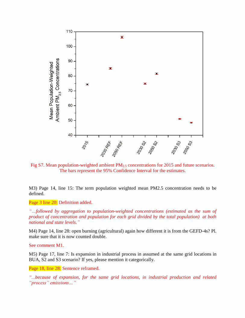
Fig S7. Mean population-weighted ambient PM2.5 concentrations for 2015 and future scenarios.

The bars represent the 95% Confidence Interval for the estimates.

M3) Page 14, line 15: The term population weighted mean PM2.5 concentration needs to be

defined.

Page 3 line 20: Definition added.

“…followed by aggregation to population-weighted concentrations (estimated as the sum of

product of concentration and population for each grid divided by the total population) at both

national and state levels.”

M4) Page 14, line 28: open burning (agricultural) again how different it is from the GEFD-4s? Pl.

make sure that it is now counted double.

See comment M1.

M5) Page 17, line 7: Is expansion in industrial process in assumed at the same grid locations in

BUA, S2 and S3 scenario? If yes, please mention it categorically.

Page 18, line 28: Sentence reframed.

“...because of expansion, for the same grid locations, in industrial production and related

“process” emissions…”

Revised manuscript with changes highlighted

1

Source influence on emission pathways and ambient PM2.5 pollution

over India (2015-2050)

Chandra Venkataraman1,3, Michael Brauer2, Kushal Tibrewal3, Pankaj Sadavarte3,4, Qiao Ma5, Aaron

Cohen6, Sreelekha Chaliyakunnel7, Joseph Frostad8, Zbigniew Klimont9, Randall V. Martin10, Dylan B.

Millet7, Sajeev Philip10,11, Katherine Walker6, Shuxiao Wang5,12 5

1Department of Chemical Engineering, Indian Institute of Technology Bombay, Powai, Mumbai, India 2School of Population and Public Health, The University of British Columbia, Vancouver, British Columbia V6T1Z3, Canada 3Interdisciplinary program in Climate Studies, Indian Institute of Technology Bombay, Powai, Mumbai, India 4Institute for Advanced Sustainability Studies (IASS), Berliner Str. 130, 14467 Potsdam, Germany 10 5State Key Joint Laboratory of Environment Simulation and Pollution Control, School of Environment, Tsinghua University,

Beijing 100084, China 6Health Effects Institute, Boston, MA 02110, USA 7Department of Soil, Water, and Climate, University of Minnesota, Minneapolis–Saint Paul, MN 55108, USA 8Institute for Health Metrics and Evaluation, University of Washington, Seattle, WA 98195, USA 15 9International Institute for Applied Systems Analysis, Laxenburg, Austria 10Department of Physics and Atmospheric Science, Dalhousie University, Halifax, Nova Scotia B3H 4R2, Canada 11 NASA Ames Research Center, Moffett Field, California, USA 12State Environmental Protection Key Laboratory of Sources and Control of Air Pollution Complex, Beijing 100084, China

Correspondence to: Chandra Venkataraman (chandra@iitb.ac.in) 20

Abstract. India currently experiences degraded air quality, with future economic development leading to challenges for air

quality management. Scenarios of sectoral emissions of fine particulate matter and its precursors were developed and evaluated

for 2015-2050, under specific pathways of diffusion of cleaner and more energy efficiency technologies. The impacts of

individual source-sectors on PM2.5 concentrations were assessed through systematic simulations of spatially and temporally

resolved particulate matter concentrations, using the GEOS-Chem model, followed by population-weighted aggregation to 25

national and state levels. We find that PM2.5 pollution is a pan-India problem, with a regional character, not limited to urban

areas or megacities. Under present day emissions, levels in most states exceeded the national PM2.5 standard (40 µg/m3).

Sources related to human activities were responsible for the largest proportion of the present-day population exposure to PM2.5

in India. About 60% of India’s mean population-weighted PM-2.5 concentrations arise from anthropogenic source-sectors,

with the balance from “other” sources, windblown dust and extra-regional sources. Leading contributors are residential 30

biomass combustion, power plant and industrial coal combustion and anthropogenic dust (including coal fly-ash, fugitive road

dust and trash burning). Transportation, brick production, and distributed diesel were other contributors to PM-2.5. Future

evolution of emissions under regulations set at current levels and promulgated levels, yielded further deterioration in air-quality

in 2030 and 2050. Under an ambitious prospective policies scenario, promoting very large shifts away from traditional biomass

technologies and coal-based electricity generation, significant reductions in PM-2.5 levels are achievable in 2030 and 2050. 35

Effective mitigation of future air pollution in India requires adoption of aggressive prospective regulation, currently not

2

formulated, for a three-pronged switch away from (i) biomass-fuelled traditional technologies, (ii) industrial coal-burning and

(iii) open burning of agricultural residues. Future air pollution is dominated by industrial process emissions, reflecting larger

expansion in industrial, rather than residential energy demand. However, even under the most active reductions envisioned,

the 2050 mean exposure, excluding any impact from windblown mineral dust, is estimated to be nearly three times higher than

the WHO Air Quality Guideline. 5

1. Introduction

India hosts the world’s second largest population (UNDP, 2017), but accounts for only 6% of the world’s total primary energy

use (IEA, 2015). However, India is an emerging economy with significant growth in a multitude of energy-use activities in

industry and transport sectors, as well as in residential, agricultural and informal industry sectors (Sadavarte and

Venkataraman, 2014; Pandey et al. 2014). With expansion in power generation (CEA, 2016) and industrial production 10

(Planning Commission, Government of India, 2013), emissions from these sectors were estimated to have increased about

two-fold between 1995-2015 (Sadavarte and Venkataraman, 2014). There is a steady demand for motorized vehicles for both

personal and public transport, with an increase in ownership of motorized two-wheeler motorcycles and scooters and four-

wheeler cars (MoRTH, 2012.), in both rural and urban areas. Traditional technologies, and the use of solid biomass fuels, are

widespread in the residential sector (cooking with biomass fuel cook stoves and lighting with kerosene wick lamps), the 15

agricultural sector (open burning of agricultural residues for field clearing), and the informal industry sector, (brick production,

processing of food and agricultural products). Ambient PM2.5 (particulate matter in a size fraction with aerodynamic diameter

smaller than 2.5 µm) concentrations are influenced by emissions of both primary or directly emitted PM2.5, and its precursor

gases, including SO2, NH3, NOx, and NMVOCs (Non-methane volatile organic compounds), whose atmospheric reactions

yield secondary particulate sulphate, nitrate and organic carbon, while reactions of NOx and NMVOCs also increase ozone 20

levels. Ozone precursor gases and particulate black carbon and organic carbon (BC and OC) are identified in the list of short-

lived climate pollutants or SLCPs (CCAC, 2014).

Air quality is a public health issue of concern in India. According to the World Health Organization (WHO), 37 cities from

India feature in a global list of 100 world cities with the highest PM10 (PM with aerodynamic diameter <10 µm) pollution, 25

with cities like Delhi, Raipur, Gwalior, and Lucknow listed among the world’s top 10 polluted cities (WHO, 2014; further

details in Figure S6 of supplement). Recent studies (Ghude et al. 2016; Chakraborty et al. 2015), have built upon products of

the Task Force on Hemispheric Transport of Air Pollutants (TF-HTAP), using HTAP emission inventories (for 2010) in a

regional chemistry model to address air quality in India. Widespread PM2.5 and O3 pollution was found under present-day

emission levels, which considerably impact human mortalities and life expectancy. To extend the understanding of ambient 30

air pollution to multiple (regional and national) scales, for multiple pollutants, methods which combine chemical transport

modelling, with data from satellite retrievals combined with available monitoring data, have been developed (van Donkelaar

3

et al., 2010; Brauer et al. 2012, 2016; Dey et al., 2012; Shaddick et al., 2018) and can be used to evaluate current levels and

trends. The latest GBD 2015 estimates indicate that the population-weighted mean PM2.5 concentration for India as a whole

was 74.3 µg/m3 in 2015, up from about 60 µg/m3 in 1990 (Cohen et al., 2017). At current levels, 99.9% of the Indian population

is estimated to live in areas where the World Health Organization (WHO) Air Quality Guideline of 10 µg/m3 was exceeded.

Nearly 90% of people lived in areas exceeding the WHO Interim Target 1 of 35 µg/m3. 5

Strategies for mitigation of air pollution require understanding pollutant emissions, differentiated by emitting sectors and by

sub-national regions, representing both present day conditions and future evolution under different pathways of growth and

technology change. Future projections of emissions, for climate relevant species, are available in the representative

concentration pathway (RCP) scenarios (Fujino et al. 2006; Clarke et al. 2007; Van Vuuren et al. 2007; Riahi et al. 2007;

Hijioka et al. 2008), more recently for the Shared Socioeconomic Pathways (SSPs) scenarios (Riahi et al., 2017; Rao et al., 10

2017), while primary PM2.5 is included in inventories like ECLIPSE (Klimont et al., 2017, 2018). Inventories developed for

HTAP_v2 (Janssens-Maenhout et al. 2015) address emissions of a suite of pollutants for 2008 and 2010. These scenarios and

emission datasets are developed through globally consistent methodologies, leaving room for refinement through more detailed

regional studies. Thus, in this work we develop and evaluate sectoral emission scenarios of fine particulate matter and its

precursors and constituents from India, during 2015-2050, under specific pathways of diffusion of cleaner and more energy 15

efficiency technologies. The work is broadly related to HTAP scientific questions including understanding of (i) sensitivity of

regional PM2.5 pollution levels to magnitudes of emissions from source-sectors and (ii) changes in PM2.5 levels as a result of

expected, as well as ambitious, air pollution and climate change abatement efforts. The impacts of individual source-sectors

on PM2.5 concentrations is assessed through simulation of spatially and temporally resolved particulate matter concentrations,

using the GEOS-Chem chemical transport model, followed by aggregation to population-weighted concentrations (estimated 20

as the sum of product of concentration and population for each grid divided by the total population) at both national and state

levels.

Section 2 discusses the development of the emission inventory, disaggregated by sector, for the year 2015 and future

projections to 2050; Section 3 describes the GEOS-Chem model, the simulation parameters and evaluation; Section 4 discusses 25

simulated PM2.5 concentration by sector, at national and state levels under present day and future emission scenarios; and the

last section discusses findings and conclusions.

2. Present day and future emissions

2.1. Present day emissions (2015)

An emission inventory was developed for India, for the year 2015, based on an “engineering model approach” using 30

technology-linked energy-emissions modelling adapted from previous work (Pandey and Venkataraman 2014; Pandey et al.

2014; Sadavarte and Venkataraman, 2014), to estimate multi-pollutant emissions including those of SO2, NOx, PM2.5, black

4

carbon (BC), organic carbon (OC), and non-methane volatile organic compounds (NMVOCs). An engineering model

approach, goes beyond fuel divisions and uses technology parameters for process and emissions control technologies, including

technology type, efficiency or specific fuel consumption, and technology-linked emission factors (g of pollutant/ kg of fuel)

to estimate emissions.

5

The inventory disaggregates emissions from technologies and activities, in all major sectors. Plant level data (installed

capacity, plant load factor, and annual production) are used for 830 individual large point sources, in heavy industry and power

generation sectors, while light industry activity statistics (energy consumption, industrial products, solvent use, etc.) are from

sub-state (or district) level (CEA 2010; CMA 2007a,b, 2012; MoC 2007; FAI 2010; CMIE 2010; MoPNG 2012; MoWR 2007).

Technology-linked emission factors and current levels of deployment of air pollution control technologies are used. Vehicular 10

emissions include consideration of vehicle technologies, vehicle age distributions, and super-emitters among on-road vehicles

(Pandey and Venkataraman, 2014). Residential sector activities comprise of cooking and water heating, largely with traditional

biomass stoves; lighting, using kerosene lamps; and warming of homes and humans, with biomass fuels. Seasonality included

for water heating and home warming. The “informal industries” sector includes brick production (in traditional kiln

technologies like the Bull’s trench kilns and clamp kilns, using both coal and biomass fuels) and food and agricultural product 15

processing operations (like drying and cooking operations related to sugarcane juice, milk, food-grain, jute, silk, tea, and

coffee). In addition, monthly mean data on agricultural residue burning in fields, a spatio-temporally discontinuous source of

significant emissions, were calculated using a bottom-up methodology (Pandey et al. 2014). Spatial proxies used to estimate

gridded emissions over India are described in Table S1 of the supplement.

20

India emissions for 2015 of PM2.5, BC, OC, SO2, NOx, and NMVOCs by sector (Figure 1) arose from three main sources: (i)

residential biomass fuel use (for cooking and heating); (ii) coal burning in power generation and heavy industry; and (iii) open

burning of agricultural residues for field clearing. Table 1 provides a description of sectors and constituent source

categories. Emissions linked to incomplete fuel combustion, including PM2.5 (9.1 Mt/yr, or million tonnes per year), BC (1.3

Mt/yr) and OC (2.3 Mt/y) and NMVOCs (33.4 Mt/yr), arose primarily from traditional biomass technologies in the residential 25

sector (for cooking and heating), the informal industry sector (for brick production and for food and agricultural produce

processes), as well as from agricultural residue burning. Emissions of SO2 (8.1 Mt/yr) and NOx (9.5 Mt/yr) arose largely from

coal boilers in industry and power sectors and from vehicles in the transport sector. Emissions of CO are included in the

inventory (Pandey et al., 2014; Sadavarte et al., 2014), however, CO was not input to the GEOS-Chem simulations, since it is

not central to atmospheric chemistry of secondary PM-2.5 formation on annual time-scales. 30

Detailed tabulations of 2015 emissions of each pollutant at the state level are provided in Table S2 of the supplement.

Uncertainties in the activity rates, calculated analytically using methods described more fully in previous publications (Pandey

and Venkataraman 2014; Pandey et al. 2014; Sadavarte and Venkataraman, 2014) are shown in Table S3 of the supplement.

5

2.2. Future emission pathways (2015-2050)

2.2.1. Description of future emission scenarios

We develop and evaluate three future scenarios which extend from 2015-2050, which are likely to bound the possible amplitude

of future emissions, based on the expected future evolution of sectoral demand, following typical methods in previous studies

(Cofala et al., 2007; Ohara et al., 2007). These include a reference (REF) scenario and two scenarios (S2 and S3) representing 5

different levels of deployment of high-efficiency, low-emissions technologies (Table 2). The scenarios capture varying levels

of emission control, with no change in current (2015) regulations, corresponding to very slow uptake of new technology (REF),

adoption of promulgated regulations, corresponding to effective achievement of targets (S2), and adoption of ambitious

prospective regulations, corresponding to those well beyond promulgated regulations (S3). In both S2 and S3, despite

expanding sectoral demand, there is reduced energy consumption from adoption of clean energy technologies, at different 10

levels.

The methodology for emission projection includes estimation of future evolution in (i) sectoral demand, (ii) technology mix,

(iii) energy consumption, and (iv) technology-linked emission factors (Figure S1 of supplement). Activity levels in future years

by source category (e.g. GWh installed capacity in power, vehicle-km travelled in transport, industrial production, e.g. in tons, 15

population of users in residential), were apportioned to various technology divisions, using assumed evolving technology mix,

for three different scenarios. Activity at the technology division level was used to derive corresponding future energy (and

fuel) consumption and related emissions using technology-based emission factors.

With 2015 as the base year, growth rates in sectoral demand were identified for thermal power plants, industries, residential, 20

brick kilns and informal industries, on-road transportation and agricultural sectors for 2015-2030 and 2030-2050 (Table S4 of

supplement). Sectoral growth, estimated as ratios of 2050 to 2015 demand, were 5.1, 3.8, 3.2, 1.3, 1.4 respectively, for building

sector, electricity generation, heavy industries, residential sector, and agricultural residue burning, with the largest growth in

the building and electricity generation sectors (Figure S2 of supplement).

25

Table 2 shows regulation levels for different sectors under the three scenarios, through to 2050. The REF and S2 scenarios

capture both energy efficiency and emissions control, continuing under current regulation, or broadly under promulgated future

policies. The S2 scenario assumes shifts to non-fossil generation which would occur under India Nationally Determined

Contribution (India’s NDC, 2015) in the power sector, consistent with a shift to 40% renewables including solar, wind and

hydro power by 2030 (NDC, 2015). The NDC goals of India are suggested to be realistic (CAT, 2017; Ross and Gerholdt, 30

2017), with achievement of non-fossil share of power generation projected to lie between 38%-48% by 2030, as well as

adoption of tighter emission standards for desulphurization and de-NOx technologies in thermal plants (MoEFCC, 2015), at a

rate consistent with expected barriers (CSE, 2016). Further, changes assumed in the transport sector reflect promulgated

6

growth in public vehicle share (NTDPC, 2013; Guttikunda and Mohan, 2014; NITI Aayog, 2015) and promulgated regulation

(Auto Fuel Policy Vision 2025, 2014, MoRTH, 2016), along with realistic assumptions of implementation lags in adoption of

BS VI standards (ICRA 2016). Other assumptions include modest increases in industrial energy efficiency under the perform

achieve and trade (PAT) scheme (Level 2, IESS, Niti Aayog, 2015 ); modest increases in non-fired-brick walling materials

(UNDP, 2009; Maithel, personal communication, 2016); slow shift to more efficient residential energy technologies and fuels 5

(Level 2, IESS, Niti Aayog, 2015); and minor reduction in agricultural residue burning.

However, in the S3 scenario, adoption of ambitious regulation, well beyond those currently promulgated is assumed. This

includes very significant shifts to non-fossil power generation (Anandarajah and Gambhir 2014; Shukla and Chaturvedi 2012;

Level 4, IESS, Niti Aayog, 2015); near-complete shift to high efficiency industrial technologies (MoP 2012, Level 4, IESS, 10

Niti Aayog, 2015); large public vehicle share (NITI Aayog, 2015), energy efficiency improvements in engine technology

(MoP, 2015), large share of electric and CNG vehicles (NITI Aayog, 2015); complete switch to LPG/PNG or biogas or high-

efficiency gasifier stoves for residential cooking and heating (Level 4, IESS, Niti Aayog, 2015) and to solar and electric lighting

(National Solar Mission, 2010) by 2030; significant (by 2030) and complete (by 2050) phase-out of agricultural residue

burning, through a switch to mulching practices (Gupta, 2014). Further details of the shift in technologies can be found in 15

Table S5 of supplement and related discussion in supplementary information (see supplement, section S2.3).

As alluded to earlier, there is a reduction in total energy consumption in future years, despite increase in activity, in scenarios

S2 and S3, which assume large deployment of high-efficiency energy technologies. The projected energy demand under the

three scenarios (Figure S3, supplement section S2.4) is in general agreement with published work (Anandarajah and Gambhir 20

2014; Chaturvedi and Shukla 2014; Parikh 2012; Shukla et al. 2009), of 95 EJ to 110 EJ for reference scenarios (Parikh, 2012;

Shukla and Chaturvedi 2012) and 45-55 EJ for low carbon pathways (Anandarajah and Gambhir 2014; Chaturvedi and Shukla

2014) in 2050. Projections of CO2 emissions to 2050, of 7200 Mt yr-1 in REF and 2000 Mt yr-1 in S3, are broadly consistent

with published 2050 values of 7200-7800 million tonnes y-1 CO2 for reference cases, and 2500-3400 million tonnes y-1 CO2

under different low carbon scenarios (Anandarajah and Gambhir 2014; Shukla et al. 2009). 25

Technology based emission factors, for over 75 technology/activity divisions, are described in previous publications (Pandey

et al. 2014; Sadavarte and Venkataraman 2014). In addition to fuel combustion, emissions are estimated from industrial

“process” activities predominant in industries such as those producing cement and non-ferrous metals, and refineries producing

iron and steel (Table S8, supplement section S2.5). In fired-brick production, recently measured emission factors for this sector 30

of PM2.5, BC and OC (Weyant et al.,2014) are used (Table S8 of supplement), while for gases, in the absence of measurements

from brick kilns, those of coal stokers are used. In the transport sector, emission factors for seven categories of vehicles, across

two vintage classes, were applied to a modelled on-road vehicle age distribution (Pandey and Venkataraman, 2014). For future

emissions, recommendations from the Auto Fuel Policy 2025 (Auto Fuel Vision and Policy 2025) along with accounting of

7

the measures to leapfrog directly to BS-VI for all on-road vehicle categories (MoRTH, 2016). To be consistent with our

scenario descriptions, the REF scenario still takes into account the BS-V standards for 2030 and 2050 while the effect of

dynamic policy reforms is reflected in the tech-mix in S2 and S3 scenarios by assuming different levels of BS-VI. The share

of BS-VI is kept at modest levels owing to delay in availability of BS-VI compliant fuels and difficulties in making the

technologies adaptive to Indian road conditions as well as cost-effective (ICRA, 2016), however, would not affect emission 5

factors significantly (Table S8 of supplement).

2.2.2. Estimated emission evolution (2015-2050)

The net effect of scenario based assumptions is that under the REF scenario, emissions are projected to increase steadily over

time. Under the S2 scenario, they are also projected to increase but at a slower rate. Only under the most ambitious scenario,

S3, are appreciable reductions in emissions of the various air pollutants expected. 10

Emissions of PM2.5 evolve from present-day levels of 9.1 Mt/yr to 2050 levels of 18.5, 11.5 and 3.0 Mt/yr, respectively, in the

three scenarios (Figure 2 a, b, c). These arise from three main sources: (i) traditional biomass technologies in residential, brick

production and informal industry, (ii) coal burning in power generation and heavy industry, and (iii) open burning of

agricultural residues for field clearing. In Figures 1-3, emissions shown are only from agricultural burning, while those from 15

forest and wildfires, taken from global products, described later, are input to the simulations. In all future scenarios, there is

faster growth of industry and electricity generation than of residential energy demand; the former which contribute nearly 60–

70% of future emissions. Thus, controlling emissions of PM2.5 should come from these sectors. As is quite evident (Figure 2

b and c), assuming large shifts to non-coal power generations in scenarios S2 (40-60%) and S3 (75-80%) in S3 contribute most

to reductions in future emissions of PM2.5. Further reductions in emissions are obtained through shifts to cleaner technology 20

and fuels in the residential sector such as use of gasifiers and LPG for cooking, electricity and solar devices for lighting and

heating, and complete phase out of open burning of agricultural waste. Black carbon and co-emitted organic carbon have very

similar sources with the largest emissions arising from traditional biomass technologies in the residential and informal industry

sectors and from agricultural field burning. Future reductions in BC (Figure 2 d,e,f ) and OC (Figure 2 g,h,i ) emissions result

from a number of policies addressing residential and informal industry sectors as well as agricultural practices. These includes 25

actions that enable a shift to cleaner residential energy solutions and a shift away from fired-brick walling materials toward

greater use of clean brick production technologies, as well as a shift away from agricultural field burning through the

introduction of mulching practices (assumed in S3). Future increases in transport demand could lead to increased BC emissions

from diesel-powered transport, thus providing an important decision lever in favour of the introduction of compressed natural

gas (CNG) or non-fossil-electricity powered public transport (in S3). While diesel particle filters provide a technology for 30

diesel PM and BC control, challenges remain including the supply of low-sulphur fuel and compliance with NOx emission

standards.

8

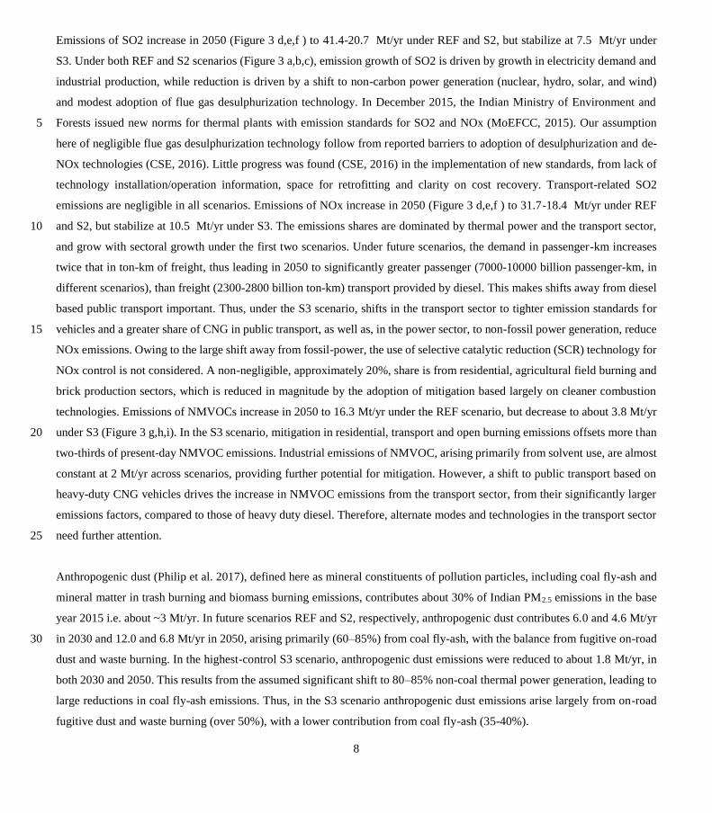
Emissions of SO2 increase in 2050 (Figure 3 d,e,f ) to 41.4-20.7 Mt/yr under REF and S2, but stabilize at 7.5 Mt/yr under

S3. Under both REF and S2 scenarios (Figure 3 a,b,c), emission growth of SO2 is driven by growth in electricity demand and

industrial production, while reduction is driven by a shift to non-carbon power generation (nuclear, hydro, solar, and wind)

and modest adoption of flue gas desulphurization technology. In December 2015, the Indian Ministry of Environment and

Forests issued new norms for thermal plants with emission standards for SO2 and NOx (MoEFCC, 2015). Our assumption 5

here of negligible flue gas desulphurization technology follow from reported barriers to adoption of desulphurization and de-

NOx technologies (CSE, 2016). Little progress was found (CSE, 2016) in the implementation of new standards, from lack of

technology installation/operation information, space for retrofitting and clarity on cost recovery. Transport-related SO2

emissions are negligible in all scenarios. Emissions of NOx increase in 2050 (Figure 3 d,e,f ) to 31.7-18.4 Mt/yr under REF

and S2, but stabilize at 10.5 Mt/yr under S3. The emissions shares are dominated by thermal power and the transport sector, 10

and grow with sectoral growth under the first two scenarios. Under future scenarios, the demand in passenger-km increases

twice that in ton-km of freight, thus leading in 2050 to significantly greater passenger (7000-10000 billion passenger-km, in

different scenarios), than freight (2300-2800 billion ton-km) transport provided by diesel. This makes shifts away from diesel

based public transport important. Thus, under the S3 scenario, shifts in the transport sector to tighter emission standards for

vehicles and a greater share of CNG in public transport, as well as, in the power sector, to non-fossil power generation, reduce 15

NOx emissions. Owing to the large shift away from fossil-power, the use of selective catalytic reduction (SCR) technology for

NOx control is not considered. A non-negligible, approximately 20%, share is from residential, agricultural field burning and

brick production sectors, which is reduced in magnitude by the adoption of mitigation based largely on cleaner combustion

technologies. Emissions of NMVOCs increase in 2050 to 16.3 Mt/yr under the REF scenario, but decrease to about 3.8 Mt/yr

under S3 (Figure 3 g,h,i). In the S3 scenario, mitigation in residential, transport and open burning emissions offsets more than 20

two-thirds of present-day NMVOC emissions. Industrial emissions of NMVOC, arising primarily from solvent use, are almost

constant at 2 Mt/yr across scenarios, providing further potential for mitigation. However, a shift to public transport based on

heavy-duty CNG vehicles drives the increase in NMVOC emissions from the transport sector, from their significantly larger

emissions factors, compared to those of heavy duty diesel. Therefore, alternate modes and technologies in the transport sector

need further attention. 25

Anthropogenic dust (Philip et al. 2017), defined here as mineral constituents of pollution particles, including coal fly-ash and

mineral matter in trash burning and biomass burning emissions, contributes about 30% of Indian PM2.5 emissions in the base

year 2015 i.e. about ~3 Mt/yr. In future scenarios REF and S2, respectively, anthropogenic dust contributes 6.0 and 4.6 Mt/yr

in 2030 and 12.0 and 6.8 Mt/yr in 2050, arising primarily (60–85%) from coal fly-ash, with the balance from fugitive on-road 30

dust and waste burning. In the highest-control S3 scenario, anthropogenic dust emissions were reduced to about 1.8 Mt/yr, in

both 2030 and 2050. This results from the assumed significant shift to 80–85% non-coal thermal power generation, leading to

large reductions in coal fly-ash emissions. Thus, in the S3 scenario anthropogenic dust emissions arise largely from on-road

fugitive dust and waste burning (over 50%), with a lower contribution from coal fly-ash (35-40%).

9

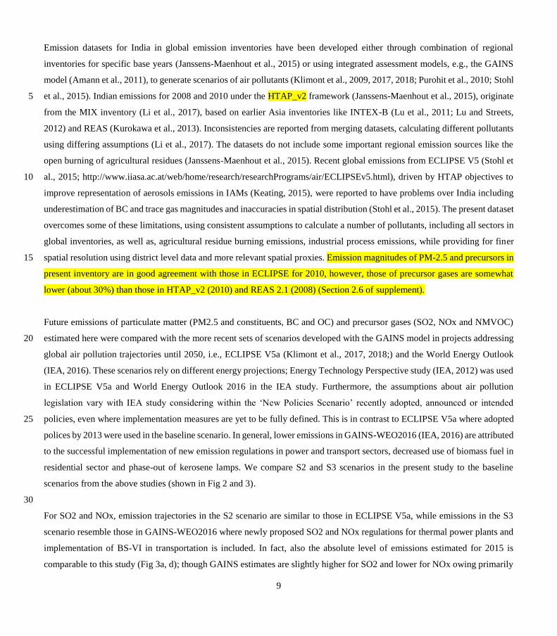
Emission datasets for India in global emission inventories have been developed either through combination of regional

inventories for specific base years (Janssens-Maenhout et al., 2015) or using integrated assessment models, e.g., the GAINS

model (Amann et al., 2011), to generate scenarios of air pollutants (Klimont et al., 2009, 2017, 2018; Purohit et al., 2010; Stohl

et al., 2015). Indian emissions for 2008 and 2010 under the HTAP_v2 framework (Janssens-Maenhout et al., 2015), originate 5

from the MIX inventory (Li et al., 2017), based on earlier Asia inventories like INTEX-B (Lu et al., 2011; Lu and Streets,

2012) and REAS (Kurokawa et al., 2013). Inconsistencies are reported from merging datasets, calculating different pollutants

using differing assumptions (Li et al., 2017). The datasets do not include some important regional emission sources like the

open burning of agricultural residues (Janssens-Maenhout et al., 2015). Recent global emissions from ECLIPSE V5 (Stohl et

al., 2015; http://www.iiasa.ac.at/web/home/research/researchPrograms/air/ECLIPSEv5.html), driven by HTAP objectives to 10

improve representation of aerosols emissions in IAMs (Keating, 2015), were reported to have problems over India including

underestimation of BC and trace gas magnitudes and inaccuracies in spatial distribution (Stohl et al., 2015). The present dataset

overcomes some of these limitations, using consistent assumptions to calculate a number of pollutants, including all sectors in

global inventories, as well as, agricultural residue burning emissions, industrial process emissions, while providing for finer

spatial resolution using district level data and more relevant spatial proxies. Emission magnitudes of PM-2.5 and precursors in 15

present inventory are in good agreement with those in ECLIPSE for 2010, however, those of precursor gases are somewhat

lower (about 30%) than those in HTAP_v2 (2010) and REAS 2.1 (2008) (Section 2.6 of supplement).

Future emissions of particulate matter (PM2.5 and constituents, BC and OC) and precursor gases (SO2, NOx and NMVOC)

estimated here were compared with the more recent sets of scenarios developed with the GAINS model in projects addressing 20

global air pollution trajectories until 2050, i.e., ECLIPSE V5a (Klimont et al., 2017, 2018;) and the World Energy Outlook

(IEA, 2016). These scenarios rely on different energy projections; Energy Technology Perspective study (IEA, 2012) was used

in ECLIPSE V5a and World Energy Outlook 2016 in the IEA study. Furthermore, the assumptions about air pollution

legislation vary with IEA study considering within the ‘New Policies Scenario’ recently adopted, announced or intended

policies, even where implementation measures are yet to be fully defined. This is in contrast to ECLIPSE V5a where adopted 25

polices by 2013 were used in the baseline scenario. In general, lower emissions in GAINS-WEO2016 (IEA, 2016) are attributed

to the successful implementation of new emission regulations in power and transport sectors, decreased use of biomass fuel in

residential sector and phase-out of kerosene lamps. We compare S2 and S3 scenarios in the present study to the baseline

scenarios from the above studies (shown in Fig 2 and 3).

30

For SO2 and NOx, emission trajectories in the S2 scenario are similar to those in ECLIPSE V5a, while emissions in the S3

scenario resemble those in GAINS-WEO2016 where newly proposed SO2 and NOx regulations for thermal power plants and

implementation of BS-VI in transportation is included. In fact, also the absolute level of emissions estimated for 2015 is

comparable to this study (Fig 3a, d); though GAINS estimates are slightly higher for SO2 and lower for NOx owing primarily

10

to differences in emission factors for coal power plants. Bottom-up estimates of SO2 emissions from our inventory (Pandey et

al., 2014; Sadavarte et al., 2014) are consistent with the recent estimates from the satellite based study (Li et al., 2017) from

2005-2016, both showing a steady growth. Present day emissions of SO2 (8.1 Mt yr-1) are at the lower end of the range of

8.5-11.3 Mt yr-1suggested by Li et al. 2017. Large future increases in SO2 emissions, estimated here in the REF and S2

scenarios are consistent with findings of Li et al. 2017. 5

For particulate matter species, the GAINS model estimates lower 2015 emissions mostly because of the differences for

residential use of biomass as well as emissions from open burning. However, considering the uncertainties associated with

quantification of biomass use and emission factors (e.g., Bond et al., 2004; Klimont et al., 2009, 2017; Venkataraman et al.,

2010) the differences are acceptable. The future evolution of emissions of BC and OC shows similar features among the studies 10

with S2 comparable to ECLIPSE V5a and S3 to IEA (2016), however the S3 scenario brings much stronger reduction due to

faster phase-out of kerosene for lighting and stronger reduction of biomass used for cooking; the latter feature is especially

visible for emissions of OC (Fig 2d,g). For total PM2.5 (Fig. 2a) scenarios developed with the GAINS model do not show a

very large difference and fall short of the reductions achieved in the S3 case where significant mitigation reduction is not

achieved in residential sector for also in power sector and industry which in GAINS are either already controlled in the baseline 15

(power sector) or continue to grow, industrial processes offsetting the benefits of reduction in other sectors.

Emissions of NMVOCs (Fig 3g) monotonically increase in ECLIPSE V5a, becoming higher than those in S2, by 2030, which

however, mimic those in GAINs-WEO2016, through to 2050. While there is also a fairly large difference in estimate for the

base year (mostly due to residential combustion of biomass, open burning, and solvent use sector), obviously the assumptions 20

about the future policies are different as both ECLIPSE V5a and IEA study include more conservative assumptions about

reduction of biomass use and eradication of open burning practices while at the same time continued growth in industrial

emissions, i.e., solvent applications. Further analysis of differences between the S2 scenario and the ECLIPSE V5a and

GAINS-WEO2016 is shown in the supplement (Fig S5).

25

Further, the emission projections were also compared with emissions estimated in the four representative concentration

pathways (RCP) scenarios adopted by the IPCC as a common basis for modelling future climate change (Fujino et al. 2006;

Clarke et al. 2007; Van Vuuren et al. 2007; Riahi et al. 2007; Hijioka et al. 2008). The RCP scenarios were designed to

represent a range of possible future climate outcomes in terms of radiative forcing watts per square meter (Wm-2) values (2.6,

4.5, 6.0, and 8.5) in 2100 relative to pre-industrial levels. Overall, Indian emissions of SO2, NOx, and BC estimated here in 30

the REF and S2 scenarios, which do not apply stringent controls, were 2 to 3 times higher than the largest emissions estimated

in the RCP8.5 scenario in 2030 and 2050, as a result of differences in assumptions made or in the list of sources included

(Table S9 of supplement). As all RCP scenarios considered principally one type of air pollution trajectory assuming that air

pollutant emissions will be successfully reduced with economic growth. Consequently, in the longer term the range of

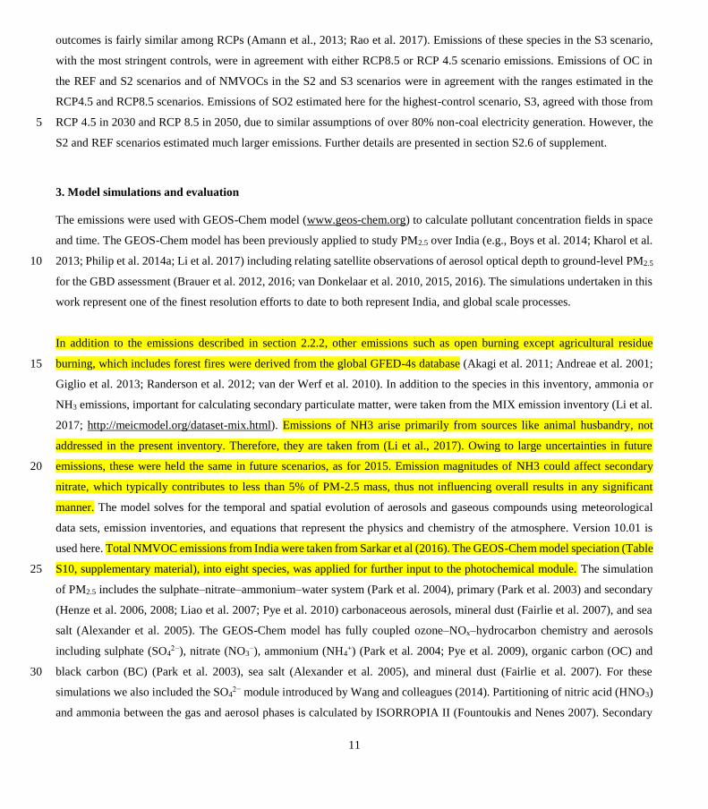
11

outcomes is fairly similar among RCPs (Amann et al., 2013; Rao et al. 2017). Emissions of these species in the S3 scenario,

with the most stringent controls, were in agreement with either RCP8.5 or RCP 4.5 scenario emissions. Emissions of OC in

the REF and S2 scenarios and of NMVOCs in the S2 and S3 scenarios were in agreement with the ranges estimated in the

RCP4.5 and RCP8.5 scenarios. Emissions of SO2 estimated here for the highest-control scenario, S3, agreed with those from

RCP 4.5 in 2030 and RCP 8.5 in 2050, due to similar assumptions of over 80% non-coal electricity generation. However, the 5

S2 and REF scenarios estimated much larger emissions. Further details are presented in section S2.6 of supplement.

3. Model simulations and evaluation

The emissions were used with GEOS-Chem model (www.geos-chem.org) to calculate pollutant concentration fields in space

and time. The GEOS-Chem model has been previously applied to study PM2.5 over India (e.g., Boys et al. 2014; Kharol et al.

2013; Philip et al. 2014a; Li et al. 2017) including relating satellite observations of aerosol optical depth to ground-level PM2.5 10

for the GBD assessment (Brauer et al. 2012, 2016; van Donkelaar et al. 2010, 2015, 2016). The simulations undertaken in this

work represent one of the finest resolution efforts to date to both represent India, and global scale processes.

In addition to the emissions described in section 2.2.2, other emissions such as open burning except agricultural residue

burning, which includes forest fires were derived from the global GFED-4s database (Akagi et al. 2011; Andreae et al. 2001; 15

Giglio et al. 2013; Randerson et al. 2012; van der Werf et al. 2010). In addition to the species in this inventory, ammonia or

NH3 emissions, important for calculating secondary particulate matter, were taken from the MIX emission inventory (Li et al.

2017; http://meicmodel.org/dataset-mix.html). Emissions of NH3 arise primarily from sources like animal husbandry, not

addressed in the present inventory. Therefore, they are taken from (Li et al., 2017). Owing to large uncertainties in future

emissions, these were held the same in future scenarios, as for 2015. Emission magnitudes of NH3 could affect secondary 20

nitrate, which typically contributes to less than 5% of PM-2.5 mass, thus not influencing overall results in any significant

manner. The model solves for the temporal and spatial evolution of aerosols and gaseous compounds using meteorological

data sets, emission inventories, and equations that represent the physics and chemistry of the atmosphere. Version 10.01 is

used here. Total NMVOC emissions from India were taken from Sarkar et al (2016). The GEOS-Chem model speciation (Table

S10, supplementary material), into eight species, was applied for further input to the photochemical module. The simulation 25

of PM2.5 includes the sulphate–nitrate–ammonium–water system (Park et al. 2004), primary (Park et al. 2003) and secondary

(Henze et al. 2006, 2008; Liao et al. 2007; Pye et al. 2010) carbonaceous aerosols, mineral dust (Fairlie et al. 2007), and sea

salt (Alexander et al. 2005). The GEOS-Chem model has fully coupled ozone–NOx–hydrocarbon chemistry and aerosols

including sulphate (SO42−), nitrate (NO3

−), ammonium (NH4+) (Park et al. 2004; Pye et al. 2009), organic carbon (OC) and

black carbon (BC) (Park et al. 2003), sea salt (Alexander et al. 2005), and mineral dust (Fairlie et al. 2007). For these 30

simulations we also included the SO42− module introduced by Wang and colleagues (2014). Partitioning of nitric acid (HNO3)

and ammonia between the gas and aerosol phases is calculated by ISORROPIA II (Fountoukis and Nenes 2007). Secondary

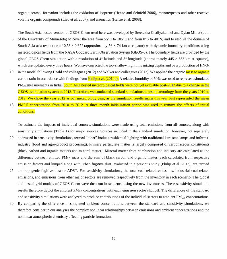
12

organic aerosol formation includes the oxidation of isoprene (Henze and Seinfeld 2006), monoterpenes and other reactive

volatile organic compounds (Liao et al. 2007), and aromatics (Henze et al. 2008).

The South Asia nested version of GEOS-Chem used here was developed by Sreelekha Chaliyakunnel and Dylan Millet (both

of the University of Minnesota) to cover the area from 55°E to 105°E and from 0°S to 40°N, and to resolve the domain of 5

South Asia at a resolution of 0.5° × 0.67° (approximately 56 × 74 km at equator) with dynamic boundary conditions using

meteorological fields from the NASA Goddard Earth Observation System (GEOS-5). The boundary fields are provided by the

global GEOS-Chem simulation with a resolution of 4° latitude and 5° longitude (approximately 445 × 553 km at equator),

which are updated every three hours. We have corrected the too-shallow nighttime mixing depths and overproduction of HNO3

in the model following Heald and colleagues (2012) and Walker and colleagues (2012). We applied the organic mass to organic 10

carbon ratio in accordance with findings from Philip et al. (2014b). A relative humidity of 50% was used to represent simulated

PM2.5 measurements in India. South Asia nested meteorological fields were not yet available post-2012 due to a change in the

GEOS assimilation system in 2013. Therefore, we conducted standard simulations to test meteorology from the years 2010 to

2012. We chose the year 2012 as our meteorology year, as the simulation results using this year best represented the mean

PM2.5 concentration from 2010 to 2012. A three month initialization period was used to remove the effects of initial 15

conditions.

To estimate the impacts of individual sources, simulations were made using total emissions from all sources, along with

sensitivity simulations (Table 1) for major sources. Sources included in the standard simulation, however, not separately

addressed in sensitivity simulations, termed “other” include residential lighting with traditional kerosene lamps and informal 20

industry (food and agro-product processing). Primary particulate matter is largely composed of carbonaceous constituents

(black carbon and organic matter) and mineral matter. Mineral matter from combustion and industry are calculated as the

difference between emitted PM2.5 mass and the sum of black carbon and organic matter, each calculated from respective

emission factors and lumped along with urban fugitive dust, evaluated in a previous study (Philip et al. 2017), are termed

anthropogenic fugitive dust or ADST. For sensitivity simulations, the total coal-related emissions, industrial coal-related 25

emissions, and emissions from other major sectors are removed respectively from the inventory in each scenario. The global

and nested grid models of GEOS-Chem were then run in sequence using the new inventories. These sensitivity simulation

results therefore depict the ambient PM2.5 concentrations with each emission sector shut off. The differences of the standard

and sensitivity simulations were analyzed to produce contributions of the individual sectors to ambient PM2.5 concentrations.

By comparing the difference in simulated ambient concentrations between the standard and sensitivity simulations, we 30

therefore consider in our analyses the complex nonlinear relationships between emissions and ambient concentrations and the

nonlinear atmospheric chemistry affecting particle formation.

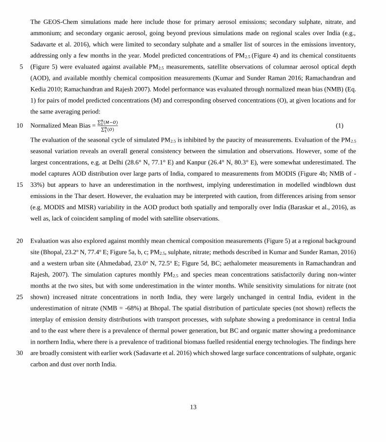
13

The GEOS-Chem simulations made here include those for primary aerosol emissions; secondary sulphate, nitrate, and

ammonium; and secondary organic aerosol, going beyond previous simulations made on regional scales over India (e.g.,

Sadavarte et al. 2016), which were limited to secondary sulphate and a smaller list of sources in the emissions inventory,

addressing only a few months in the year. Model predicted concentrations of PM2.5 (Figure 4) and its chemical constituents

(Figure 5) were evaluated against available PM2.5 measurements, satellite observations of columnar aerosol optical depth 5

(AOD), and available monthly chemical composition measurements (Kumar and Sunder Raman 2016; Ramachandran and

Kedia 2010; Ramachandran and Rajesh 2007). Model performance was evaluated through normalized mean bias (NMB) (Eq.

1) for pairs of model predicted concentrations (M) and corresponding observed concentrations (O), at given locations and for

the same averaging period:

Normalized Mean Bias = ∑ (𝑀−𝑂)𝑛1

∑ (𝑂)𝑛1

(1) 10

The evaluation of the seasonal cycle of simulated PM2.5 is inhibited by the paucity of measurements. Evaluation of the PM2.5

seasonal variation reveals an overall general consistency between the simulation and observations. However, some of the

largest concentrations, e.g. at Delhi (28.6° N, 77.1° E) and Kanpur (26.4° N, 80.3° E), were somewhat underestimated. The

model captures AOD distribution over large parts of India, compared to measurements from MODIS (Figure 4b; NMB of -

33%) but appears to have an underestimation in the northwest, implying underestimation in modelled windblown dust 15

emissions in the Thar desert. However, the evaluation may be interpreted with caution, from differences arising from sensor

(e.g. MODIS and MISR) variability in the AOD product both spatially and temporally over India (Baraskar et al., 2016), as

well as, lack of coincident sampling of model with satellite observations.

Evaluation was also explored against monthly mean chemical composition measurements (Figure 5) at a regional background 20

site (Bhopal, 23.2o N, 77.4o E; Figure 5a, b, c; PM2.5, sulphate, nitrate; methods described in Kumar and Sunder Raman, 2016)

and a western urban site (Ahmedabad, 23.0o N, 72.5o E; Figure 5d, BC; aethalometer measurements in Ramachandran and

Rajesh, 2007). The simulation captures monthly PM2.5 and species mean concentrations satisfactorily during non-winter

months at the two sites, but with some underestimation in the winter months. While sensitivity simulations for nitrate (not

shown) increased nitrate concentrations in north India, they were largely unchanged in central India, evident in the 25

underestimation of nitrate (NMB = -68%) at Bhopal. The spatial distribution of particulate species (not shown) reflects the

interplay of emission density distributions with transport processes, with sulphate showing a predominance in central India

and to the east where there is a prevalence of thermal power generation, but BC and organic matter showing a predominance

in northern India, where there is a prevalence of traditional biomass fuelled residential energy technologies. The findings here

are broadly consistent with earlier work (Sadavarte et al. 2016) which showed large surface concentrations of sulphate, organic 30

carbon and dust over north India.

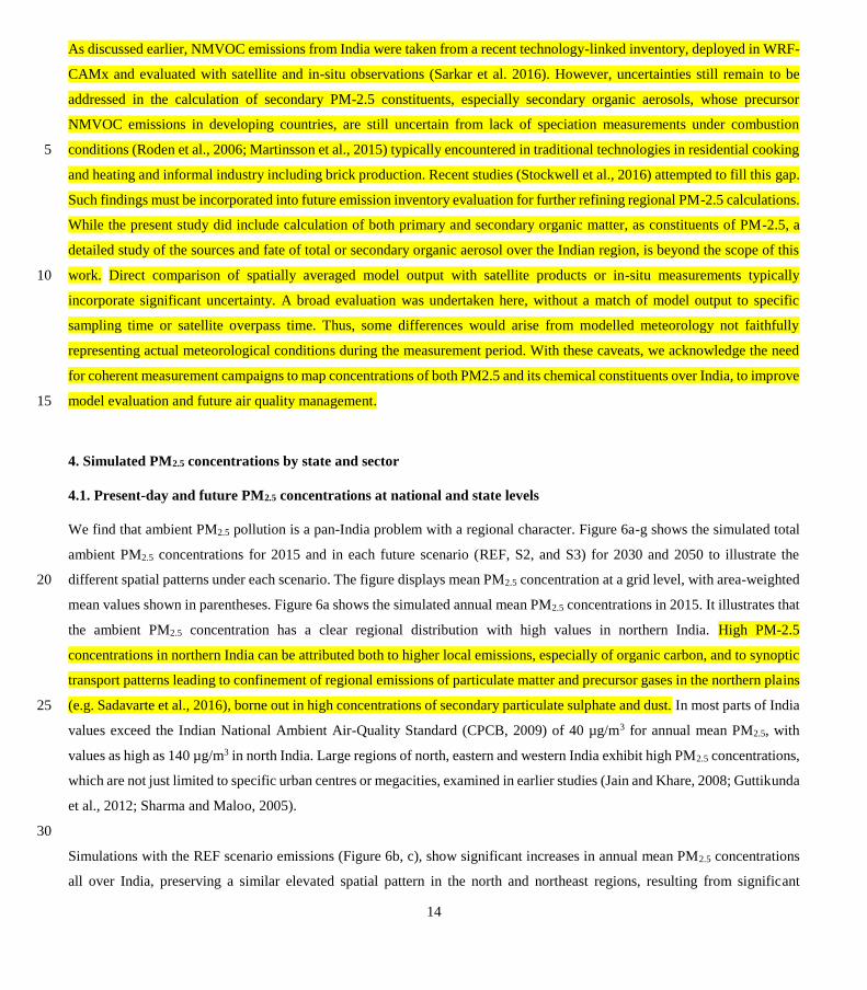
14

As discussed earlier, NMVOC emissions from India were taken from a recent technology-linked inventory, deployed in WRF-

CAMx and evaluated with satellite and in-situ observations (Sarkar et al. 2016). However, uncertainties still remain to be

addressed in the calculation of secondary PM-2.5 constituents, especially secondary organic aerosols, whose precursor

NMVOC emissions in developing countries, are still uncertain from lack of speciation measurements under combustion

conditions (Roden et al., 2006; Martinsson et al., 2015) typically encountered in traditional technologies in residential cooking 5

and heating and informal industry including brick production. Recent studies (Stockwell et al., 2016) attempted to fill this gap.

Such findings must be incorporated into future emission inventory evaluation for further refining regional PM-2.5 calculations.

While the present study did include calculation of both primary and secondary organic matter, as constituents of PM-2.5, a

detailed study of the sources and fate of total or secondary organic aerosol over the Indian region, is beyond the scope of this

work. Direct comparison of spatially averaged model output with satellite products or in-situ measurements typically 10

incorporate significant uncertainty. A broad evaluation was undertaken here, without a match of model output to specific

sampling time or satellite overpass time. Thus, some differences would arise from modelled meteorology not faithfully

representing actual meteorological conditions during the measurement period. With these caveats, we acknowledge the need

for coherent measurement campaigns to map concentrations of both PM2.5 and its chemical constituents over India, to improve

model evaluation and future air quality management. 15

4. Simulated PM2.5 concentrations by state and sector

4.1. Present-day and future PM2.5 concentrations at national and state levels

We find that ambient PM2.5 pollution is a pan-India problem with a regional character. Figure 6a-g shows the simulated total

ambient PM2.5 concentrations for 2015 and in each future scenario (REF, S2, and S3) for 2030 and 2050 to illustrate the

different spatial patterns under each scenario. The figure displays mean PM2.5 concentration at a grid level, with area-weighted 20

mean values shown in parentheses. Figure 6a shows the simulated annual mean PM2.5 concentrations in 2015. It illustrates that

the ambient PM2.5 concentration has a clear regional distribution with high values in northern India. High PM-2.5

concentrations in northern India can be attributed both to higher local emissions, especially of organic carbon, and to synoptic

transport patterns leading to confinement of regional emissions of particulate matter and precursor gases in the northern plains

(e.g. Sadavarte et al., 2016), borne out in high concentrations of secondary particulate sulphate and dust. In most parts of India 25

values exceed the Indian National Ambient Air-Quality Standard (CPCB, 2009) of 40 µg/m3 for annual mean PM2.5, with

values as high as 140 µg/m3 in north India. Large regions of north, eastern and western India exhibit high PM2.5 concentrations,

which are not just limited to specific urban centres or megacities, examined in earlier studies (Jain and Khare, 2008; Guttikunda

et al., 2012; Sharma and Maloo, 2005).

30

Simulations with the REF scenario emissions (Figure 6b, c), show significant increases in annual mean PM2.5 concentrations

all over India, preserving a similar elevated spatial pattern in the north and northeast regions, resulting from significant

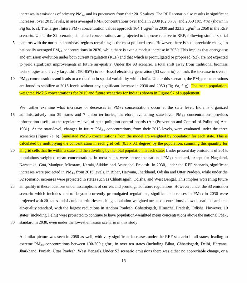
15

increases in emissions of primary PM2.5 and its precursors from their 2015 values. The REF scenario also results in significant

increases, over 2015 levels, in area averaged PM2.5 concentrations over India in 2030 (62.3.7%) and 2050 (105.4%) (shown in

Fig 6a, b, c). The largest future PM2.5 concentration values approach 164.1 µg/m3 in 2030 and 323.3 µg/m3 in 2050 in the REF

scenario. Under the S2 scenario, simulated concentrations are projected to improve relative to REF, following similar spatial

patterns with the north and northeast regions remaining as the most polluted areas. However, there is no appreciable change in 5

nationally averaged PM2.5 concentrations in 2030, while there is even a modest increase in 2050. This implies that energy-use

and emission evolution under both current regulation (REF) and that which is promulgated or proposed (S2), are not expected

to yield significant improvements in future air-quality. Under the S3 scenario, a total shift away from traditional biomass

technologies and a very large shift (80-85%) to non-fossil electricity generation (S3 scenario) controls the increase in overall

PM2.5 concentrations and leads to a reduction in spatial variability within India. Under this scenario, the PM2.5 concentrations 10

are found to stabilize at 2015 levels without any significant increase in 2030 and 2050 (Fig. 6a, f, g). The mean population-

weighted PM2.5 concentrations for 2015 and future scenarios for India is shown in Figure S7 of supplement.

We further examine what increases or decreases in PM2.5 concentrations occur at the state level. India is organized

administratively into 29 states and 7 union territories, therefore, evaluating state-level PM2.5 concentrations provides 15

information useful at the regulatory level of state pollution control boards (Air (Prevention and Control of Pollution) Act,

1981). At the state-level, changes in future PM2.5 concentrations, from their 2015 levels, were evaluated under the three

scenarios (Figure 7a, b). Simulated PM2.5 concentrations from the model are weighted by population for each state. This is

calculated by multiplying the concentration in each grid cell (0.1 x 0.1 degree) by the population, summing this quantity for

all grid cells that lie within a state and then dividing by the total population in each state. Under present day emissions of 2015, 20

populations-weighted mean concentrations in most states were above the national PM2.5 standard, except for Nagaland,

Karnataka, Goa, Manipur, Mizoram, Kerala, Sikkim and Arunachal Pradesh. In 2030, under the REF scenario, significant

increases were projected in PM2.5 from 2015 levels, in Bihar, Haryana, Jharkhand, Odisha and Uttar Pradesh, while under the

S2 scenario, increases were projected in states such as Chhattisgarh, Odisha, and West Bengal. This implies worsening future

air quality in these locations under assumptions of current and promulgated future regulations. However, under the S3 emission 25

scenario which includes control beyond currently promulgated regulations, significant decreases in PM2.5 in 2030 were

projected with 20 states and six union territories reaching population-weighted mean concentrations below the national ambient

air-quality standard, with the largest reductions in Andhra Pradesh, Chhattisgarh, Himachal Pradesh, Odisha. However, 10

states (including Delhi) were projected to continue to have population-weighted mean concentrations above the national PM2.5

standard in 2030, even under the lowest emission scenario in this study. 30

A similar picture was seen in 2050 as well, with very significant increases under the REF scenario in all states, leading to

extreme PM2.5 concentrations between 100-200 µg/m3, in over ten states (including Bihar, Chhattisgarh, Delhi, Haryana,

Jharkhand, Punjab, Uttar Pradesh, West Bengal). Under S2 scenario emissions there was either no appreciable change, or a

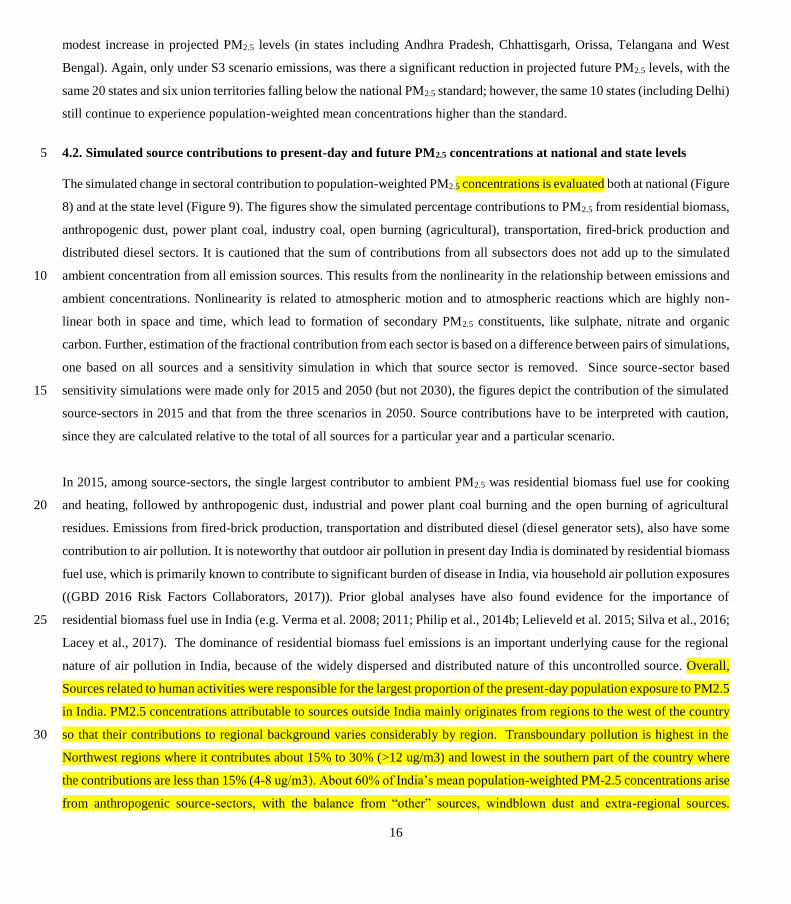
16

modest increase in projected PM2.5 levels (in states including Andhra Pradesh, Chhattisgarh, Orissa, Telangana and West

Bengal). Again, only under S3 scenario emissions, was there a significant reduction in projected future PM2.5 levels, with the

same 20 states and six union territories falling below the national PM2.5 standard; however, the same 10 states (including Delhi)

still continue to experience population-weighted mean concentrations higher than the standard.

4.2. Simulated source contributions to present-day and future PM2.5 concentrations at national and state levels 5

The simulated change in sectoral contribution to population-weighted PM2.5 concentrations is evaluated both at national (Figure

8) and at the state level (Figure 9). The figures show the simulated percentage contributions to PM2.5 from residential biomass,

anthropogenic dust, power plant coal, industry coal, open burning (agricultural), transportation, fired-brick production and

distributed diesel sectors. It is cautioned that the sum of contributions from all subsectors does not add up to the simulated

ambient concentration from all emission sources. This results from the nonlinearity in the relationship between emissions and 10

ambient concentrations. Nonlinearity is related to atmospheric motion and to atmospheric reactions which are highly non-

linear both in space and time, which lead to formation of secondary PM2.5 constituents, like sulphate, nitrate and organic

carbon. Further, estimation of the fractional contribution from each sector is based on a difference between pairs of simulations,

one based on all sources and a sensitivity simulation in which that source sector is removed. Since source-sector based

sensitivity simulations were made only for 2015 and 2050 (but not 2030), the figures depict the contribution of the simulated 15

source-sectors in 2015 and that from the three scenarios in 2050. Source contributions have to be interpreted with caution,

since they are calculated relative to the total of all sources for a particular year and a particular scenario.

In 2015, among source-sectors, the single largest contributor to ambient PM2.5 was residential biomass fuel use for cooking

and heating, followed by anthropogenic dust, industrial and power plant coal burning and the open burning of agricultural 20

residues. Emissions from fired-brick production, transportation and distributed diesel (diesel generator sets), also have some

contribution to air pollution. It is noteworthy that outdoor air pollution in present day India is dominated by residential biomass

fuel use, which is primarily known to contribute to significant burden of disease in India, via household air pollution exposures

((GBD 2016 Risk Factors Collaborators, 2017)). Prior global analyses have also found evidence for the importance of

residential biomass fuel use in India (e.g. Verma et al. 2008; 2011; Philip et al., 2014b; Lelieveld et al. 2015; Silva et al., 2016; 25

Lacey et al., 2017). The dominance of residential biomass fuel emissions is an important underlying cause for the regional

nature of air pollution in India, because of the widely dispersed and distributed nature of this uncontrolled source. Overall,

Sources related to human activities were responsible for the largest proportion of the present-day population exposure to PM2.5

in India. PM2.5 concentrations attributable to sources outside India mainly originates from regions to the west of the country

so that their contributions to regional background varies considerably by region. Transboundary pollution is highest in the 30

Northwest regions where it contributes about 15% to 30% (>12 ug/m3) and lowest in the southern part of the country where

the contributions are less than 15% (4-8 ug/m3). About 60% of India’s mean population-weighted PM-2.5 concentrations arise

from anthropogenic source-sectors, with the balance from “other” sources, windblown dust and extra-regional sources.

17

Leading contributors are residential biomass combustion, power plant and industrial coal combustion and anthropogenic dust

(including coal fly-ash, fugitive road dust and trash burning). Total dust (wind-blown and anthropogenic) together contributed

39%, while transportation, brick production, and distributed diesel were other contributors to PM-2.5.

In 2050, future source contributions, are dominated by power plant coal and industrial coal, in both REF and S2 scenarios, 5

followed by residential biomass. In both REF and S2 scenarios (Figures 2 and 3) expansion in electricity generation and

industry overtakes emissions offsets, leading to 1.5-2 and 1.75-3 times emission increases, respectively, in emissions of PM2.5

and its precursor gases, through to 2050. The future expansion projected in power plant and industrial coal use, in both these

scenarios, exceeds the growth in biomass fuel use in the residential sector, which follows population increases. Future source

contributions to emissions of PM2.5 and precursor gas emissions are about 60% from coal burning in electricity generation and 10

industry, with the remainder from biomass energy use in the residential sector, which is directly reflected in source

contributions to ambient PM2.5. The power plant coal contribution to PM2.5 increases in the REF and S2 scenarios, however, it

decreases in the S3 scenario, from assumptions of very high penetration (80-85%) of non-fossil electricity generation. The

industrial coal contribution to PM2.5 concentrations increases above 2015 levels in all future scenarios, reflecting expansion in

industry and related “process emissions.” This finding suggests that even more stringent measures than those assumed in the 15

scenarios are needed to reduce the influence of industrial coal combustion on ambient pollution levels.

Interestingly, the influence of residential biomass emissions on PM2.5 reduces in 2050, even in the REF scenario, from the

relative increase in that of industrial coal. In the S2 and S3 scenarios, assumptions of future shift from residential biomass to

cleaner LPG/PNG and advanced low-emission gasifier stoves, leads to its decreased contribution to PM2.5 concentrations. In 20

the S3 scenario, assumptions of a complete switch away from traditional residential biomass technologies, leads to this sector

having the lowest influence on PM2.5 concentrations (less than 1.8%). The validity of such assumptions rests upon careful

review and effective implementation of national programmes recently launched for expansion of cleaner residential fuels

(Pradhan Mantri Ujjwala Yojana, 2016) as well as sustainable adoption of these low emissions approaches. The influence of

anthropogenic dust is projected to increase in REF and S2 scenarios while decreasing observed only in the S3 scenario. On the 25

other hand, the influence of total dust is projected to increase in all future scenarios, largely from decreases in the influence of

other PM2.5 sources. Total and anthropogenic dust concentrations are projected to increase under all scenarios. Dust from

anthropogenic activities (anthropogenic dust) is a larger contributor to total dust in REF (47% of total dust, compared with

23% in 2015) and S2 (36% of total dust), while its contributions in S3 (13%) are low. Overall, in S3, total dust (in this scenario

dominated by windblown mineral dust) is the largest contributor to ambient PM2.5, as a result of the dramatic reductions in 30

emissions projected for all of the other sectors (including anthropogenic dust) in this ambitious scenario. Further examination

is needed of the contribution and amelioration of sources in the “other” category, not simulated separately here, which includes

trash burning, urban fugitive dust, residential lighting with kerosene and informal industry related to food and agricultural

product processing which relies on traditional technologies and biomass fuel.

18

The PM2.5 concentration from transportation sources remains low (<2 µg/m3) under all scenarios but does not decrease in the

ambitious scenario. This is related both to the lower magnitude of transportation emissions, relative to other sources, as well

as, the relatively coarse model grid (50 km x 67 km). That the transportation contribution decreases in REF but increases in

S3 relative to 2015 reflects competing trends from 2015 to 2050 where emissions per vehicle generally decrease but with an 5

increase in vehicle-km. Specifically, passenger-km increase about 4-fold from 2015 to 2050 but with reductions of 15 to 55%

in primary PM2.5 emissions along with increases in transport-related SO2 (27 to 73%) and NOx (93 to 121%) emissions,

depending on the scenario. Further, emissions from transportation may be affected by reductions in emissions from other

sectors and non-linear atmospheric chemistry (e.g., reductions in other combustion sources leaving more ammonia available

to react with transportation combustion products to form secondary PM). Indeed, evaluation of simulation results indicates 10

that the sensitivity of nitrate to transportation sources in scenario S2 is larger than the nitrate sensitivity in the REF scenario.

This suggests that increased available ammonia in S2, resulting from reductions in emissions from other sectors, leads to

increased particulate ammonium nitrate formation associated with transportation emissions, relative to the REF scenario.

Furthermore, for a number of reasons --because we are estimating sectoral contributions to ambient PM2.5 based on the

fractional contribution from each sector, because transportation is small relative to the other sectors and because the spatial 15

pattern of the fraction of transport emissions does vary from scenario to scenario --- it is also possible that the decrease in REF,

followed by increases in S2 and S3, is an artefact due to increasing fractional contributions from transport relative to other

sectors where the decreases are much more dramatic.

Changes in source contributions to PM2.5, between 2015 and 2050, are analysed at state level (Figure 9), wherein patterns 20

similar to those at the national level are seen. Residential biomass fuel use (Figure 9a) was the dominant source influencing

PM2.5 in 2015, on both national and state scale. The trade-off between relative decreases in residential biomass, and increases

in industrial coal on future PM2.5, is seen in the REF, S2 and S3 scenarios, at the state level. In Figure 9a (residential biomass)

note the red-blue-green lines lie below the black dots, while in Figure 9c (industrial coal), they all lie above the black dots, and

in Figure 9d (power plant coal) only red-blue lines lie above the black dots. Residential biofuel influence reduces in all 25

scenarios in 2050, reaching between 1-2% at the state level, across all states. Anthropogenic dust (Figure 9b) show decreasing

influence while total dust shows increasing influence on PM2.5 in the S3 scenario, even at the state level, for reasons discussed

above. There is an increase in the influence of industrial coal (Figure 9c) on PM2.5 in all states under all three scenarios, because

of expansion, for the same grid locations, in industrial production and related “process” emissions, e.g. grinding and milling

operations in cement industry, despite improved technology efficiencies assumed in the industrial sector. Industrial emission 30

increases are highest in Andhra Pradesh, Jharkhand, Karnataka, Odisha and Tamil Nadu. Further refinement of scenarios must

be made to include more stringent industrial emission control technologies. The power plant coal (Figure 9d) influence

increases in the REF and S2 scenarios in all states, however largest increases are seen in Andhra Pradesh, Chhattisgarh, Odisha,

West Bengal and Telangana. Under S3 scenario emissions, the power plant coal influence decreases in all states, but has the

19

largest decreases in the same states as above, indicating that the emissions are influenced by high electricity generation in these

states, with uniform assumptions made on the shift to non-fossil generation. However, future PM2.5 levels are strongly

influenced by industrial and power plant coal use, across most states. The influence of open burning (Figure 9e) appears to

change in 2050 under REF and S2 scenarios, not from absolute changes in open burning, but from changes, relative to decreases

in the influence of other sources. However, under S3 scenario emissions, in which a complete phase out of open burning is 5

assumed, there are uniform decreases in all states, leaving a negligible influence. The influence of brick production (Figure

9f) on PM2.5 has a negligible increase in the REF scenario at the national level, however, it shows significant increases at the

state levels, from 2015 to 2050, in Bihar, Himachal Pradesh, Punjab, Uttar Pradesh and Uttarakhand, the major brick producing

states. While the influence of brick production decreases in almost all states under the S3 scenario, it still contributes about

2% in these states through to 2050. The influence of transportation (Figure 9g) increases significantly under the S3 scenario 10

in a few states like Bihar, Jharkhand, Uttar Pradesh and West Bengal, a likely artefact from the spatial distribution proxy,

which uses district level urban population to distribute on-road gasoline emissions. Gasoline vehicles mostly consist of two-,

three- and four-wheeler private vehicles in use in urban areas. In the present regional-scale inventory therefore represented

using population, pending improved road based proxies for air-quality studies at urban scales.

15

Overall, sources significantly influencing PM2.5 levels include residential biomass in all regions, open burning of agricultural

residues in north India, and power plant and industrial coal combustion in eastern and south India. In north India, PM-2.5

concentrations arise primarily from residential biomass combustion, followed by the open burning of agricultural residues. In

contrast, in eastern and south India, while residential biomass combustion is dominant, coal burning in the power and industrial

sector is the next important source. Wind-blown dust contributes significantly to PM-2.5 in north-west India, while 20

anthropogenic dust (largely coal fly-ash) contributes significantly to PM-2.5 in eastern and south India. Under an ambitious

prospective policies scenario, promoting very large shifts away from traditional biomass technologies and coal-based

electricity generation, significant reductions in PM-2.5 levels are achievable in 2030 and 2050. Future air pollution is

dominated by industrial process emissions, reflecting larger expansion in industrial, rather than residential energy demand.

Potential future contributions of anthropogenic dust are large, while those from transportation and distributed diesel sources 25

are also projected to increase substantially, although small in comparison to other sources.

5. Conclusions

This work represents the most comprehensive examination to date of a systematic analysis of source influence, including all

sources, on present and future air pollution on a regional scale over India. Elevated annual mean PM2.5 concentrations are a

pan-India problem, with a regional character, not limited to urban areas or megacities. Under present day emissions, 30

simulations indicate that population-weighted mean concentrations in most states are above the national PM2.5 standard. Under

present day (2015) emissions, residential biomass fuel use for cooking and heating is the largest single sector influencing

20

outdoor air pollution across most of India. The dominance of residential biomass fuel emissions is an important underlying

cause for the regional nature of air pollution in India, because of the widely dispersed and distributed nature of this uncontrolled

source. Agricultural residue burning is the next important source, especially in north-west and north India. This large influence

on an annual basis, suggests even larger impacts during the burning periods (typically Apr-May and Oct-Dec). In eastern and

peninsular India, the influence of coal burning in thermal power plants and industry follows that of residential biomass 5

combustion. Anthropogenic dust (including coal fly-ash, mineral matter from combustion and urban fugitive dust), brick

production and vehicular emissions are also important sources. Overall, the findings suggest a large regional background of

PM2.5 pollution (from residential biomass, agricultural residue burning and power plant and industrial coal), subjacent to that

from local sources (transportation, brick kilns, distributed diesel) in peri-urban areas and megacities.

10

If no action is taken, population exposures to PM-2.5 are likely to increase substantially in India by 2050. Evolution of

emissions under current regulation (REF) and promulgated or proposed regulation (S2), yields a deterioration in future air-

quality future air-quality in 2030 and 2050. Only under the S3 scenario, of ambitious prospective regulation, not yet formulated,

promoting a total shift away from traditional biomass technologies and a very large shift (80-85%) to non-fossil electricity

generation, is there an overall reduction in PM2.5 concentrations below 2015 levels, both in 2030 and 2050, with 20 states and 15

six union territories projected to reach population-weighted mean concentrations below the national ambient air-quality

standard. However, even under the most active reductions envisioned, the 2050 population-weighted mean exposure for the

S3 scenario, excluding any impact from windblown mineral dust, is estimated to be nearly three times higher than the WHO

Air Quality Guideline. Further exploration of air pollution mitigation measures must address the industrial sector, including

process emissions, dispersed sources including trash burning and urban fugitive dust, and traditional technologies in residential 20

lighting and informal industry. This study shows that future emission increases in India, if realized, could have important

implications for air pollution and climate change on regional and hemispheric scales. Importantly, a government led initiative

for detailed emission inventory development at national state and city levels is needed to support air-quality management.

Incorporation of detailed Indian emissions, along with their rationalization to other Asian and global inventories, into multi-

model studies over the Indian domain would provide insight into atmospheric processes, still lacking in this region. 25

Acknowledgements

Partial support for this work was provided by the Health Effects Institute, Boston. KT acknowledges PhD assistantship from

the NCAP-COALESE grant of the Ministry of Environment Forests and Climate Change, India. DBM and SC acknowledge

support from NASA (#NNX14AP89G), NSF (#AGS-1148951), and the Minnesota Supercomputing Institute. We

acknowledge Dr. Sarath Guttikunda, Co-Director, Urbanemissions.info, Goa, India, for datasets of present-day and future 30

emissions from trash burning and urban fugitive dust.

21

References

Air (Prevention and Control of Pollution) Act, http://envfor.nic.in/legis/air/air1.html, (last access: 1 December, 2017), 1981.

Akagi, S. K., Yokelson, R. J., Wiedinmyer, C., Alvarado, M. J., Reid, J. S., Karl, T., Crounse, J. D., and Wennberg, P. O.:

Emission factors for open and domestic biomass burning for use in atmospheric models, Atmos. Chem. Phys., 11, 4039-4072,

doi:10.5194/acp-11-4039-2011, 2011. 5

Alexander, B., Park, R.J., Jacob, D.J., Li, Q.B., Yantosca, R.M., Savarino, J., Lee, C.C.W. and Thiemens, M.H.,: Sulfate

formation in sea‐salt aerosols: Constraints from oxygen isotopes, J. Geophys. Res-Atmos., 110(D10), 2005.

Amann, M., Bertok, I., Borken-Kleefeld, J., Cofala, J., Heyes, C., Höglund-Isaksson, L., Klimont, Z., Nguyen, B., Posch, M.,

Rafaj, P., Sandler, R., Schöpp, W., Wagner, F., and Winiwarter, W.: Cost-effective control of air quality and greenhouse gases

in Europe: Modeling and policy applications, Environ. Modell. Softw., 26, 1489–1501, 2011. 10

Amann, M., Klimont, Z., and Wagner, F.: Regional and Global Emissions of Air Pollutants: Recent Trends and Future

Scenarios, Annu. Rev. Env. Resour., 38, 31–55, https://doi.org/10.1146/annurev-environ-052912-173303, 2013.

Anandarajah, G. and Gambhir, A.: India’s CO2 Emission Pathways to 2050: What Role Can Renewables Play? Appl. Energ.,

131, 79–86, http://dx.doi.org/10.1016/j.apenergy.2014.06.026, 2014.

Andreae, M. O., & Merlet, P.: Emission of trace gases and aerosols from biomass burning, Global Biogeochem. Cy., 15(4), 15

955-966, 2001.

Auto Fuel Vision and Policy 2025: Auto Fuel Vision and Policy 2025, Report of the Expert Committee, Government of India,

http://www.petroleum.nic.in/sites/default/files/autopol.pdf, (last access: 1 December, 2017), 2014.

Baraskar, A., Bhushan M., Venkataraman, C. and Cherian, R.: An offline constrained data assimilation technique for aerosols:

Improving GCM simulations over South Asia using observations from two satellite sensors, Atmos. Environ., 132, 36-48, 20

2016.

Brauer, M., Amann, M., Burnett, R.T., Cohen, A., Dentener, F., Ezzati, M., Henderson, S.B., Krzyzanowski, M., Martin, R.V.,

Van Dingenen, R. and Van Donkelaar, A.: Exposure assessment for estimation of the global burden of disease attributable to

outdoor air pollution, Environ. Sci. Technol, 46(2), 652-660, 2012.

Brauer, M., Freedman, G., Frostad, J., Van Donkelaar, A., Martin, R.V., Dentener, F., Dingenen, R.V., Estep, K., Amini, H., 25

Apte, J.S. and Balakrishnan, K.: Ambient air pollution exposure estimation for the global burden of disease 2013, Environ.

Sci. Technol., 50(1), 79-88, 2016.

Bond, T.C., Streets, D.G., Yarber, K.F., Nelson, S.M., Woo, J.H. and Klimont, Z.: A technology‐based global inventory of

black and organic carbon emissions from combustion, J. Geophys. Res-Atmos., 109(D14), 2004.

Boys, B.L., Martin, R.V., Van Donkelaar, A., MacDonell, R.J., Hsu, N.C., Cooper, M.J., Yantosca, R.M., Lu, Z., Streets, D.G., 30

Zhang, Q. and Wang, S.W.: Fifteen-year global time series of satellite-derived fine particulate matter. Environ. Sci. Technol.,

48(19), 11109-11118, 2014.

22

CAT: Climate Action Tracker - India, [online] Available from: http://climateactiontracker.org/countries/india/2017.html

(Accessed 5 March 2018), 2017.

CCAC: Climate and Clean Air Coalition Annual Report, September, 2013 - August, 2014.Climate and Clean Air Coalition,

CCAC Secretariat, Paris, 2014.

CEA: Annual Report 2010-2011, Central Electricity Authority, Ministry of Power, Government of India, 2010. 5

CEA: Draft National Electricity Plan (Volume 1), Central Electricity Authority, Ministry of Power, Government of India,

December, 2016.

Chaturvedi, V. and Shukla, P.R.: Role of energy efficiency in climate change mitigation policy for India: assessment of co-

benefits and opportunities within an integrated assessment modeling framework, Climatic change, 123(3-4), 597-609, 2014.

Chakraborty, T., Beig, G., Dentener, F.J. and Wild, O.: Atmospheric transport of ozone between Southern and Eastern Asia, 10

Sci. Total Environ., 523, 28-39, 2015.

Clarke, L., Edmonds J., Jacoby, H., Pitcher, H., Reilly, J., Richels, R.: Scenarios of Greenhouse Gas Emissions and

Atmospheric Concentrations. Sub-report 2.1A of Synthesis and Assessment Product 2.1 by the U.S. Climate Change Science

Program and the Subcommittee on Global Change Research, Department of Energy, Office of Biological & Environmental

Research, Washington, 7 DC., USA, 154, 2007. 15

CMA: Basic Data, Cement Manufacturers’ Association, New Delhi, 2007a.

CMA: Annual Cement Statistics, Coal Manufacturers' Association, New Delhi,2007b.

CMA: Annual Report 2011-12, Cement Manufacturers’ Association, New Delhi, 2012.

CMIE: Economic Intelligence Service - Energy 2010, Centre for Monitoring of Indian Economy Pvt. Ltd, New Delhi, 2010.

Cofala, J., Amann, M., Klimont, Z., Kupiainen, K. and Höglund-Isaksson, L.: Scenarios of global anthropogenic emissions of 20

air pollutants and methane until 2030, Atmos. Environ., 41(38), 8486-8499, 2007.

Cohen, A.J., Brauer, M., Burnett, R., Anderson, H.R., Frostad, J., Estep, K., Balakrishnan, K., Brunekreef, B., Dandona, L.,

Dandona, R. and Feigin, V.: Estimates and 25-year trends of the global burden of disease attributable to ambient air pollution:

an analysis of data from the Global Burden of Diseases Study 2015, The Lancet, 389(10082), 1907-1918, 2017.

CPCB: National Ambient Air Quality Standards, Central Pollution Control Board, 25

http://cpcb.nic.in/National_Ambient_Air_Quality_Standards.php, (last access: 1 December, 2017), 2009.

CSE: New Environmental Norms for the Power Sector. Proceedings and Recommendations of the Stakeholder Workshop

Organized by CSE, Centre for Science and Environment, New Delhi, http://cseindia.org/userfiles/new-environmental-norms-

report.pdf, (last access: 1 December, 2017), 2016.

Dey, S., Di Girolamo, L., van Donkelaar, A., Tripathi, S.N., Gupta, T. and Mohan, M.: Variability of outdoor fine particulate 30

(PM 2.5) concentration in the Indian subcontinent: a remote sensing approach, Remote Sens. Environ., 127, 153-161, 2012.

FAI: Fertilizer Statistics 2001-2011, Fertilizer Association of India, New Delhi, 2010.

Fairlie TD, Jacob DJ, Park RJ.: The impact of transpacific transport of mineral dust in the United States, Atmos Environ, 41(6),

1251–1266, 2007.

23

Fountoukis, C. & Nenes, A.: ISORROPIA II: A computationally efficient thermodynamic equilibrium model for K+-Ca2+-

Mg2+-NH4+-Na+-SO42•- NO3•-Cl•-H2O aerosols, Atmos. Chem. Phys., 7, 4639–4659, 2007.

Fujino, J., Nair, R., Kainuma, M., Masui, T., Matsuoka, Y.: Multi-gas mitigation analysis on stabilization scenarios using AIM

global model. Multigas Mitigation and Climate Policy, The Energy Journal Special Issue, 2006.

GBD 2016 Risk Factors Collaborators: Global, regional, and national comparative risk assessment of 84 behavioural, 5

environmental and occupational, and metabolic risks or clusters of risks, 1990–2016: a systematic analysis for the Global

Burden of Disease Study 2016, Lancet (London, England), 390(10100), 1345–1422. http://doi.org/10.1016/S0140-

6736(17)32366-8, 2017.

Ghude, S.D., Chate, D.M., Jena, C., Beig, G., Kumar, R., Barth, M.C., Pfister, G.G., Fadnavis, S. and Pithani, P.: Premature

mortality in India due to PM2.5 and ozone exposure, Geophys. Res. Lett., 43(9), 4650-4658, 2016. 10

Giglio, L., Randerson, J. T. and van der Werf, G. R.: Analysis of daily, monthly, and annual burned area using the fourth-

generation global fire emissions database (GFED4), J. Geophys. Res. Biogeo., 118(1), 317-328, 2013.

Gupta, R.: Essays on Air Pollution, Global Warming and Agricultural Productivity, PhD Dissertation, Indian Statistical

Institute, New Delhi, 2014.

Guttikunda, S. K., & Jawahar, P.: Application of SIM-air modeling tools to assess air quality in Indian cities. Atmos. Environ., 15

62, 551-561, 2012.

Guttikunda, S.K., Mohan, D.: Re-fueling road transport for better air quality in India, Energ. Policy, 68, 556-561, 2014.

Heald, C.L., Collett Jr, J.L., Lee, T., Benedict, K.B., Schwandner, F.M., Li, Y., Clarisse, L., Hurtmans, D.R., Van Damme,

M., Clerbaux, C. and Coheur, P.F.: Atmospheric ammonia and particulate inorganic nitrogen over the United States, Atmos.

Chem. Phys., 12(21), 10295-10312, 2012. 20

Habib, G., Venkataraman, C., Shrivastava, M., Banerjee, R., Stehr, J. W. and Dickerson, R. R.: New methodology for

estimating biofuel consumption for cooking: Atmospheric emissions of black carbon and sulfur dioxide from India, Global

Biogeochem. Cycles, 18(3), 1–11, doi:10.1029/2003GB002157, 2004.

Henze, D. K., and Seinfeld, J. H.: Global secondary organic aerosol from isoprene oxidation, Geophys. Res. Lett., 33: L09812,

doi:10.1029/2006GL025976, 2006. 25

Henze, D.K., Seinfeld, J.H., Ng, N.L., Kroll, J.H., Fu, T.M., Jacob, D.J. and Heald, C.L., Global modeling of secondary organic

aerosol formation from aromatic hydrocarbons: high-vs. low-yield pathways, Atmos. Chem. Phys., 8(9), 2405-2420, 2008.

Hijioka, Y., Matsuoka, Y., Nishimoto, H., Masui, M. and Kainuma, M.: Global GHG emissions scenarios under GHG

concentration stabilization targets, Journal of Global Environmental Engineering, 13, 97-108, 2008.

ICRA: Indian Automobile Industry: Proposed BS-VI Emission Standards. ICRA Limited, New Delhi, available at: 30

http://www.icra.in/Files/ticker/SH-2016-Q2-6-ICRA-Passenger%20vehicles.pdf, 2016.

IEA: Energy Technology Perspectives 2012 Pathways to a Clean Energy System, International Energy Agency, IEA/OECD,

France, https://www.iea.org/publications/freepublications/publication/ETP2012_free.pdf, 2012.

24

IEA: India Energy Outlook. World Energy Outlook Special Report. International Energy Agency, IEA / OECD, France,

available at: https://www.iea.org/publications/freepublications/publication/IndiaEnergyOutlook_WEO2015.pdf, 2015.

IEA: Energy and Air Pollution. World Energy Outlook Special Report. International Energy Agency, IEA / OECD, France,

available at:

https://www.iea.org/publications/freepublications/publication/WorldEnergyOutlookSpecialReport2016EnergyandAirPollutio5

n.pdf, 2016.

IESS, NITI Aayog: India Energy Security Scenarios, 2047, NITI Aayog, Govt of India, available at: http://iess2047.gov.in/,

2015.

India’s NDC. India’s Nationally Determined Contribution (NDC): Working Towards Climate Justice 2015 Report – UNFCCC,

available at: http://www4.unfccc.int/, 2015. 10

Jain, S., & Khare, M.: Urban air quality in mega cities: a case study of Delhi City using vulnerability analysis, Environ. Monit.

Assess., 136(1), 257-265, 2008.

Janssens-Maenhout, G., Crippa, M., Guizzardi, D., Dentener, F., Muntean, M., Pouliot, G., Keating, T., Zhang, Q., Kurokawa,

J., Wankmüller, R. and Denier van der Gon, H.: HTAP_v2. 2: a mosaic of regional and global emission grid maps for 2008

and 2010 to study hemispheric transport of air pollution, Atmos. Chem. Phys., 15(19), 11411-11432, 2015. 15

Keating, T.: The HTAP (GAINS/ECLIPSE v5) Scenarios, HTAP Workshop on Global Emission Scenarios, International

Institute for Applied Systems Analysis, Laxenburg, February 11-13, 2015, available at:

http://www.htap.org/meetings/2015/2015_May_11-15/Powerpoint%20Presentations/Wednesday/Keating%20Scenarios.pdf,

2015.

Kharol, S.K., Martin, R.V., Philip, S., Vogel, S., Henze, D.K., Chen, D., Wang, Y., Zhang, Q. and Heald, C.L.: Persistent 20

sensitivity of Asian aerosol to emissions of nitrogen oxides, Geophys. Res. Lett., 40(5), 1021-1026, 2013.

Klimont, Z., Cofala, J., Xing, J., Wei, W., Zhang, C., Wang, S., Kejun, J., Bhandari, P., Mathur, R., Purohit, P., Rafaj, P.,

Chambers, A., Amann, M.: Projections of SO2, NOx and carbonaceous aerosols emissions in Asia, Tellus, 61b, 602-617, 2009.

Klimont, Z., Kupiainen, K., Heyes, C., Purohit, P., Cofala, J., Rafaj, P., Borken-Kleefeld, J. and Schöpp, W.: Global

anthropogenic emissions of particulate matter including black carbon, Atmos. Chem. Phys., 17(14), 8681-8723, 2017. 25

Klimont, Z., Höglund-Isaksson, L., Heyes, C., Rafaj, P., Schöpp, W., Cofala, J., Purohit, P., Borken-Kleefeld, J., Kupiainen,

K., Kiesewetter, G., Winiwarter, W., Amann, M, Zhao, B., Wang, S.X., Bertok, I., Sander, R.: Global scenarios of air pollutants

and methane: 1990-2050. In preparation, 2018.

Kumar, S. and Sunder Raman, R.: Inorganic ions in ambient fine particles over a National Park in central India: Seasonality,

dependencies between SO42- , NO3-, and NH4+, and neutralization of aerosol acidity, Atmos. Environ. 143:152–163, 2016. 30

Kurokawa, J., Ohara, T., Morikawa, T., Hanayama, S., Janssens-Maenhout, G., Fukui, T., Kawashima, K., and Akimoto, H.:

Emissions of air pollutants and greenhouse gases over Asian regions during 2000–2008: Regional Emission inventory in ASia

(REAS) version 2, Atmos. Chem. Phys., 13, 11019–11058, doi:10.5194/acp-13-11019-2013, 2013.

25

Lacey, F. G., Henze, D. K., Lee, C. J., van Donkelaar, A. and Martin, R. V.: Transient climate and ambient health impacts due

to national solid fuel cookstove emissions, P. Natl. Acad. Sci. USA, 114(6), 1269–1274, doi:10.1073/pnas.1612430114, 2017.

Lelieveld, J., Evans, J.S., Fnais, M., Giannadaki, D. and Pozzer, A.: The contribution of outdoor air pollution sources to

premature mortality on a global scale, Nature, 525(7569), 367-371, 2015.

Li, C., McLinden, C., Fioletov, V., Krotkov, N., Carn, S., Joiner, J., Streets, D., He, H., Ren, X., Li, Z., and Dickerson, R. R.: 5

India Is Overtaking China as the World’s Largest Emitter of Anthropogenic Sulfur Dioxide, Scientific Reports, 7, 14304,

10.1038/s41598-017-14639-8, 2017.

Li, M., Zhang, Q., Kurokawa, J.I., Woo, J.H., He, K., Lu, Z., Ohara, T., Song, Y., Streets, D.G., Carmichael, G.R. and Cheng,

Y.: MIX: a mosaic Asian anthropogenic emission inventory under the international collaboration framework of the MICS-

Asia and HTAP. Atmos. Chem. Phys., 17(2), 935, 2017. 10

Liao, H., Henze, D. K., Seinfeld, J. H., Wu, S., Mickley L. J.: Biogenic secondary organic aerosol over the United States:

Comparison of climatological simulations with observations, J Geophys. Res.,112(D6), 201, doi:10.1029/2006JD007813,

2007.

Lu, Z. and Streets, D. G.: Increase in NOx Emissions from Indian Thermal Power Plants during 1996–2010: Unit-Based

Inventories and Multisatellite Observations, Environ. Sci. Technol., 46, 7463–7470, doi:10.1021/es300831w, 2012. 15

Lu, Z., Zhang, Q., and Streets, D. G.: Sulfur dioxide and primary carbonaceous aerosol emissions in China and India, 1996–

2010, Atmos. Chem. Phys., 11, 9839–9864, doi:10.5194/acp-11-9839-2011, 2011.

Martinsson, J., Eriksson, A. C., Nielsen, I. E., Malmborg, V. B., Ahlberg, E., Andersen, C., Lindgren, R., Nyström, R., Nordin,

E. Z., Brune, W. H., Svenningsson, B., Swietlicki, E., Boman, C. and Pagels, J. H.: Impacts of Combustion Conditions and

Photochemical Processing on the Light Absorption of Biomass Combustion Aerosol, Environ. Sci. Technol., 49(24), 14663–20

14671, doi:10.1021/acs.est.5b03205, 2015.

MoC: Coal Directory of India, 2006-07, Coal Controller’s Organisation, Ministry of Coal, Government of India, Kolkata,

2007.

MoEFCC: http://pib.nic.in/newsite/PrintRelease.aspx?relid=133726, Press Release, Ministry of Environment, Forest and

Climate Change, Government of India, 2015. 25

MoPNG: Indian Petroleum and Natural Gas Statistics 2011-12. Ministry of Petroleum and Natural Gas, Government of India,

New Delhi, 2012.

MoP: PAT Perform, Achieve and Trade, Ministry of Power, Government of India, 2012.

MoP: Energy Efficient Norms for Power Plants, Press Information Bureau. Ministry of Power, Government of India, available

at: http://pib.nic.in/newsite/PrintRelease.aspx?relid=117384, 2015. 30

MoRTH: Road Transport Year Book 2009-10 & 2010-11, Ministry of Road Transport and Highways, Government of India,

New Delhi, 2012.

MoRTH: http://pib.nic.in/newsite/PrintRelease.aspx?relid=134232, Press Release, Ministry of Road Transport and Highways,

Government of India, 2016.

26

MoWR: Ministry of Water Resources, Government of India, 2006-2007, Minor Irrigation Census, available at:

http://micensus.]v.in/intnat.html, 2007.

National Solar Mission: http://www.mnre.gov.in/solar-mission/jnnsm/introduction-2/, Ministry of New and Renewable

Energy, Government of India, 2010.

NITI Aayog: India Energy Security Scenarios (IESS) 2047. New Delhi: NITI Aayog, available at: http://indiaenergy.gov.in/, 5

2015.

NTDPC: Moving India to 2032, India transport report, Government of India, National Transport Development Policy

Committee, India, New Delhi, available at: http://planningcommission.nic.in/reports/genrep/NTDPC_ Vol_01.pdf, 2013.

Ohara, T.A.H.K., Akimoto, H., Kurokawa, J.I., Horii, N., Yamaji, K., Yan, X. and Hayasaka, T.: An Asian emission inventory

of anthropogenic emission sources for the period 1980–2020, Atmos. Chem. Phys., 7(16), 4419-4444, 2007. 10

Pandey, A., Sadavarte, P., Rao, A. B., & Venkataraman, C.: Trends in multi-pollutant emissions from a technology-linked

inventory for India: II. Residential, agricultural and informal industry sectors, Atmos. Environ., 99, 341-352.

doi:10.1016/j.atmosenv.2014.09.080 , 2014.

Pandey, A. and Venkataraman, C.: Estimating emissions from the Indian transport sector with on-road fleet composition and

traffic volume, Atmos. Environ., 98: 123-133, http://dx.doi.org/10.1016/j.atmosenv.2014.08.039. 2014. 15

Parikh, K.: Sustainable Development and Low Carbon Growth Strategy for India, Energy, 40(1): 31–38,

http://dx.doi.org/10.1016/j.energy.2012.01.013, 2012.

Park, R.J., Jacob, D.J., Chin, M. and Martin, R.V.: Sources of carbonaceous aerosols over the United States and implications

for natural visibility, J. Geophys. Res. Atmos., 108(D12), 2003.

Park, R. J., Jacob, D. J., Field, B. D., Yantosca, R. M., Chin, M.: Natural and transboundary pollution influences on sulfate-20

nitrate-ammonium aerosols in the United States: Implications for policy, J Geophys Res 109:D15204; doi:

10.1029/2003JD004473, 2004.

Philip, S., Martin, R.V., Pierce, J.R., Jimenez, J.L., Zhang, Q., Canagaratna, M.R., Spracklen, D.V., Nowlan, C.R., Lamsal,

L.N., Cooper, M.J. and Krotkov, N.A.: Spatially and seasonally resolved estimate of the ratio of organic mass to organic

carbon, Atmos. Environ., 87, 34-40, 2014a. 25

Philip, S., Martin, R.V., van Donkelaar, A., Lo, J.W.H., Wang, Y., Chen, D., Zhang, L., Kasibhatla, P.S., Wang, S., Zhang, Q.

and Lu, Z.: Global chemical composition of ambient fine particulate matter for exposure assessment, Environ. Sci. Technol.,

48(22), 13060-13068, 2014b.

Philip, S., R. Martin, G. Snider, C. Weagle, A.V. Donkelaar, M. Brauer, D. Henze, Z. Klimont, C. Venkataraman, S.

Guttikunda and Q. Zhang.: Anthropogenic fugitive, combustion and industrial dust is a significant, underrepresented fine 30

particulate matter source in global atmospheric models, Environ. Res. Lett., 2017.

Planning Commission, Government of India: Twelfth Fifth Year Plan (2012-2017), Economic sectors. Volume 2, 2013.

Pradhan Mantri Ujjwala Yojana: http://www.pmujjwalayojana.com/ , (last access: 1December 2017), 2016.

27

Purohit, P., Amann, M., Mathur, R., Gupta, I., Marwah, S., Verma, V., Bertok, I., Borken-Kleefeld, J., Chambers, A., Cofala,

J. and Heyes, C., Gains Asia: Scenarios for cost-effective control of air pollution and greenhouse gases in India, 2010.

Pye, H.O.T., Liao, H., Wu, S., Mickley, L.J., Jacob, D.J., Henze, D.K. and Seinfeld, J.H.: Effect of changes in climate and

emissions on future sulfate‐nitrate‐ammonium aerosol levels in the United States, J. Geophys. Res. Atmos., 114(D1), 2009.

Pye, H.O.T., Chan, A.W.H., Barkley, M.P. and Seinfeld, J.H.: Global modeling of organic aerosol: The importance of reactive 5

nitrogen (NO x and NO 3), Atmos. Chem. Phys., 10(22), 11261-11276, 2010.

Ramachandran. S and Kedia, S.: Black carbon aerosols over an urban region: radiative forcing and climate impact, J Geo Res

Atmos., 15, D10202; doi:10.1029/2009 JD013560, 2010.

Ramachandran S, and Rajesh TA.: Black carbon aerosol mass concentrations over Ahmedabad, an urban location in western

India: comparison with urban sites in Asia, Europe, Canada, and the United States. J Geo Res Atmos., 112:D06211; 10

doi:10.1029/2006JD007488, 2007.

Randerson, J. T., Chen, Y., Werf, G. R., Rogers, B. M., & Morton, D. C.: Global burned area and biomass burning emissions

from small fires, J. Geophys. Res. Biogeo., 117(G4), 2012.

Rao, S., Klimont, Z., Smith, S.J., Van Dingenen, R., Dentener, F., Bouwman, L., Riahi, K., Amann, M., Bodirsky, B.L., van

Vuuren, D.P. and Reis, L.A.: Future air pollution in the Shared Socio-economic Pathways, Global Environ. Chang., 42, 346-15

358, 2017.

Riahi, K. Gruebler, A. and Nakicenovic N.: Scenarios of long-term socio-economic and environmental development under

climate stabilization, Technol. Forecast. Soc., 74, 7, 887-935, 2007.

Riahi, K., Van Vuuren, D.P., Kriegler, E., Edmonds, J., O’neill, B.C., Fujimori, S., Bauer, N., Calvin, K., Dellink, R., Fricko,

O. and Lutz, W.: The shared socioeconomic pathways and their energy, land use, and greenhouse gas emissions implications: 20

an overview, Global Environ. Chang., 42, 153-168, 2017.

Roden, C. A., Bond, T. C., Conway, S. and Pinel, A. B. O.: Emission Factors and Real-Time Optical Properties of Particles

Emitted from Traditional Wood Burning Cookstoves, Environ. Sci. Technol., 40(21), 6750–6757, doi:10.1021/es052080i,

2006.

Ross, K. and Gerholdt, R.: Achieving India’s Ambitious Renewable Energy Goals: A Progress Report, World Resources 25

Institute, [online] Available from: http://www.wri.org/blog/2017/05/achieving-indias-ambitious-renewable-energy-goals-

progress-report (Accessed 5 March 2018), 2017.

Sadavarte, P. and Venkataraman, C.: A technology-linked multi-pollutant inventory of Indian energy-use emissions: I. Industry

and transport sectors, Atmos. Environ., 99, 353-364, http://dx.doi.org/10.1016/j.atmosenv.2014.09.081, 2014.

Sadavarte, P., Venkataraman, C., Cherian, R., Patil, N., Madhavan, B. L., Gupta, T., Kulkarni, S., Carmichael, G. R. and 30

Adhikary, B.: Seasonal differences in aerosol abundance and radiative forcing in months of contrasting emissions and rainfall

over northern South Asia, Atmos. Environ., 125, 512–523, doi:10.1016/j.atmosenv.2015.10.092, 2016.

28

Sarkar, M., Venkataraman, C., Guttikunda, S. and Sadavarte, P.: Indian emissions of technology-linked NMVOCs with

chemical speciation: An evaluation of the SAPRC99 mechanism with WRF-CAMx simulations, Atmos. Environ., 134, 70–

83, doi:10.1016/j.atmosenv.2016.03.037, 2016.

Shaddick, G., Thomas, M. L., Green, A., Brauer, M., van Donkelaar, A., Burnett, R., Chang, H. H., Cohen, A., Dingenen, R.

Van, Dora, C., Gumy, S., Liu, Y., Martin, R., Waller, L. A., West, J., Zidek, J. V and Pruss-Ustun, A.: Data integration model 5

for air quality: a hierarchical approach to the global estimation of exposures to ambient air pollution, J. R. Stat. Soc. Ser. C

(Applied Stat., 67(1), 231–253, doi:10.1111/rssc.12227, 2018.

Sharma, M. and Maloo, S.: Assessment of ambient air PM 10 and PM 2.5 and characterization of PM 10 in the city of Kanpur,

India, Atmos. Environ., 39(33), 6015-6026. 2005.

Shukla, P. R., Agarwal, P., Bazaz, A. B., Agarwal, N., Kainuma, M., Masui, T., Fujino, J., Matsuuoka, Y., Hibino, G., Ehara, 10

T.: Low Carbon Society Vision 2050 India, Indian Institute of Management Ahmedabad, National Institute for Environmental

Studies, Kyoto University, Mizuho Information & Research Institute, 1–28,

http://2050.nies.go.jp/report/file/lcs_asia/indialcs.pdf, 2009.

Shukla, P. R. and Chaturvedi, V.: Low Carbon and Clean Energy Scenarios for India: Analysis of Targets Approach, Energ.

Econ. 34(SUPPL. 3): S487–95, http://dx.doi.org/10.1016/j.eneco.2012.05.002, 2012. 15

Silva, R.A., Adelman, Z., Fry, M.M. and West, J.J.: The impact of individual anthropogenic emissions sectors on the global

burden of human mortality due to ambient air pollution, Environ. Health Persp., 124(11), 1776, 2016.

Stockwell, C. E., Christian, T. J., Goetz, J. D., Jayarathne, T., Bhave, P. V., Praveen, P. S., Adhikari, S., Maharjan, R., DeCarlo,

P. F., Stone, E. A., Saikawa, E., Blake, D. R., Simpson, I. J., Yokelson, R. J. and Panday, A. K.: Nepal Ambient Monitoring

and Source Testing Experiment (NAMaSTE): emissions of trace gases and light-absorbing carbon from wood and dung 20

cooking fires, garbage and crop residue burning, brick kilns, and other sources, Atmos. Chem. Phys., 16(17), 11043–11081,

doi:10.5194/acp-16-11043-2016, 2016.

Stohl, A., Aamaas, B., Amann, M., Baker, L. H., Bellouin, N., Berntsen, T. K., Boucher, O., Cherian, R., Collins, W.,

Daskalakis, N., Dusinska, M., Eckhardt, S., Fuglestvedt, J. S., Harju, M., Heyes, C., Hodnebrog, Ø., Hao, J., Im, U., Kanakidou,

M., Klimont, Z., Kupiainen, K., Law, K. S., Lund, M. T., Maas, R., MacIntosh, C. R., Myhre, G., Myriokefalitakis, S., Olivié, 25

D., Quaas, J., Quennehen, B., Raut, J.-C., Rumbold, S. T., Samset, B. H., Schulz, M., Seland, Ø., Shine, K. P., Skeie, R. B.,

Wang, S., Yttri, K. E., and Zhu, T.: Evaluating the climate and air quality impacts of short-lived pollutants, Atmos. Chem.

Phys., 15, 10529–10566, https://doi.org/10.5194/acp-15-10529-2015, 2015.

UNDP: Energy Efficiency Improvements in the Indian Brick Industry, available at: www.resourceefficientbricks.org/, United

Nations Development Programme, 2009. 30

UNDP: World Population Prospects, The 2017 Revision, Key Findings and Advance Tables, Working Paper No.

ESA/P/WP/248, United Nations, Department of Economic and Social Affairs, Population Division, 2017.

29

van der Werf, G. R., Randerson, J. T., Giglio, L., Collatz, G. J., Mu, M., Kasibhatla, P. S., & van Leeuwen, T. T.: Global fire

emissions and the contribution of deforestation, savanna, forest, agricultural, and peat fires (1997–2009), Atmos. Chem. Phys.,

10(23): 11707-11735, 2010.

van Vuuren, D., M. den Elzen, P. Lucas, B. Eickhout, B. Strengers, B. van Ruijven, S. Wonink, R. van Houdt,: Stabilizing

greenhouse gas concentrations at low levels: an assessment of reduction strategies and costs, Climatic Change, 5

doi:10.1007/s/10584-006-9172-9, 2007.

van Donkelaar A, Martin RV, Brauer M, Kahn R, Levy R, Verduzco C, et al.: Global estimates of ambient fine particulate

matter concentrations from satellite-based aerosol optical depth: Development and application, Environ. Health Persp., 118(6),

847–855, doi:10.1289 /ehp.0901623, 2010.

van Donkelaar A, Martin RV, Brauer M, Boys BL.: Use of satellite observations for long-term exposure assessment of global 10

concentrations of fine particulate matter, Environ. Health Persp., 123, 135–143, doi:10.1289/ehp.1408646, 2015.

Van Donkelaar, A., Martin, R.V., Brauer, M., Hsu, N.C., Kahn, R.A., Levy, R.C., Lyapustin, A., Sayer, A.M. and Winker,

D.M.: Global estimates of fine particulate matter using a combined geophysical-statistical method with information from

satellites, models, and monitors, Environ. Sci. Technol., 50(7), 3762-3772, 2016.

Venkataraman, C., Sagar, A.D., Habib, G., Lam, N. and Smith, K.R.: The Indian national initiative for advanced biomass 15

cookstoves: the benefits of clean combustion, Energy Sustain. Dev., 14(2), 63-72, 2010.

Verma, S., Venkataraman, C. and Boucher, O.: Origin of surface and columnar Indian Ocean Experiment (INDOEX) aerosols

using source‐and region‐tagged emissions transport in a general circulation model, J. Geophysi. Res. Atmos., 113(D24), 2008.

Verma, S., Venkataraman, C. and Boucher, O.: Attribution of aerosol radiative forcing over India during the winter monsoon

to emissions from source categories and geographical regions, Atmos. Environ., 45(26), 4398-4407, 2011. 20

Walker, J. M., Philip, S., Martin, R. V., Seinfeld, H.: Simulation of nitrate, sulfate, and ammonium aerosols over the United

States, Atmos. Chem. Phys., 12, 11213–11227, 2012.

Wang, Y., Zhang, Q., Jiang, J., Zhou, W., Wang, B., He, K., Duan, F., Zhang, Q., Philip, S. and Xie, Y.: Enhanced sulfate

formation during China's severe winter haze episode in January 2013 missing from current models, J. Geophys. Res. Atmos.,

119(17), 2014. 25

Weyant, C.L., Athalye, V., Ragavan, S., Rajarathnam, U., Lalchandani, D., Maithel, S., Bond, T.C.: Emissions from South

Asian brick production, Environ. Sci. Technol., 2014.

WHO: WHO’s Ambient Air Pollution database-Update 2014, Ginebra, Suiza, World Health Organization (WHO), 2014.

30

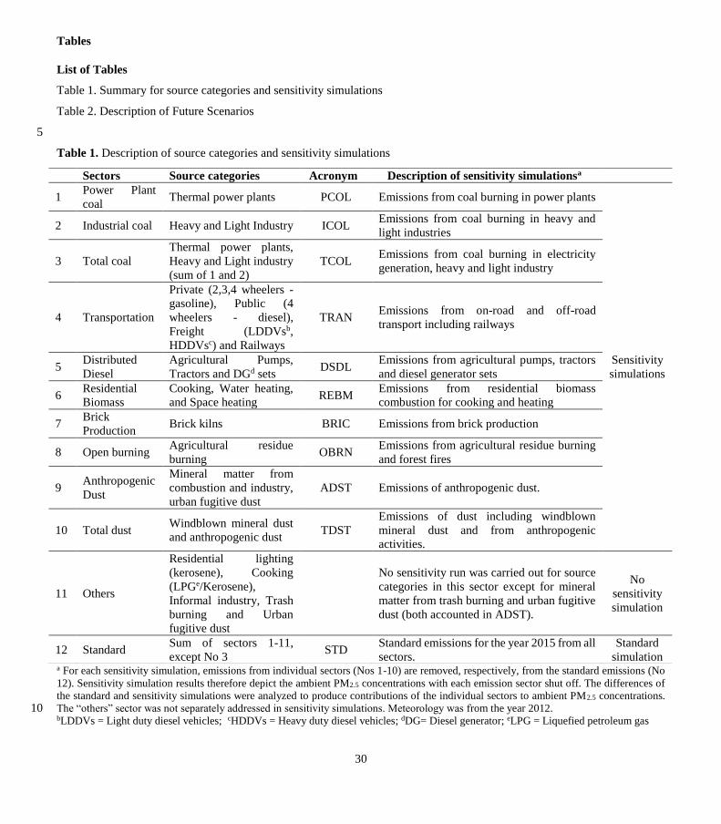
30

Tables

List of Tables

Table 1. Summary for source categories and sensitivity simulations

Table 2. Description of Future Scenarios

5

Table 1. Description of source categories and sensitivity simulations

a For each sensitivity simulation, emissions from individual sectors (Nos 1-10) are removed, respectively, from the standard emissions (No

12). Sensitivity simulation results therefore depict the ambient PM2.5 concentrations with each emission sector shut off. The differences of

the standard and sensitivity simulations were analyzed to produce contributions of the individual sectors to ambient PM2.5 concentrations.

The “others” sector was not separately addressed in sensitivity simulations. Meteorology was from the year 2012. 10 bLDDVs = Light duty diesel vehicles; cHDDVs = Heavy duty diesel vehicles; dDG= Diesel generator; eLPG = Liquefied petroleum gas

Sectors Source categories Acronym Description of sensitivity simulationsa

1 Power Plant

coal Thermal power plants PCOL Emissions from coal burning in power plants

2 Industrial coal Heavy and Light Industry ICOL Emissions from coal burning in heavy and

light industries

3 Total coal

Thermal power plants,

Heavy and Light industry

(sum of 1 and 2)

TCOL Emissions from coal burning in electricity

generation, heavy and light industry

4 Transportation

Private (2,3,4 wheelers -

gasoline), Public (4

wheelers - diesel),

Freight (LDDVsb,

HDDVsc) and Railways

TRAN Emissions from on-road and off-road

transport including railways

5 Distributed

Diesel

Agricultural Pumps,

Tractors and DGd sets DSDL

Emissions from agricultural pumps, tractors

and diesel generator sets

Sensitivity

simulations

6 Residential

Biomass

Cooking, Water heating,

and Space heating REBM

Emissions from residential biomass

combustion for cooking and heating

7 Brick

Production Brick kilns BRIC Emissions from brick production

8 Open burning Agricultural residue

burning OBRN

Emissions from agricultural residue burning

and forest fires

9 Anthropogenic

Dust

Mineral matter from

combustion and industry,

urban fugitive dust

ADST Emissions of anthropogenic dust.

10 Total dust Windblown mineral dust

and anthropogenic dust TDST

Emissions of dust including windblown

mineral dust and from anthropogenic

activities.

11 Others

Residential lighting

(kerosene), Cooking

(LPGe/Kerosene),

Informal industry, Trash

burning and Urban

fugitive dust

No sensitivity run was carried out for source

categories in this sector except for mineral

matter from trash burning and urban fugitive

dust (both accounted in ADST).

No

sensitivity

simulation

12 Standard Sum of sectors 1-11,

except No 3 STD

Standard emissions for the year 2015 from all

sectors.

Standard

simulation

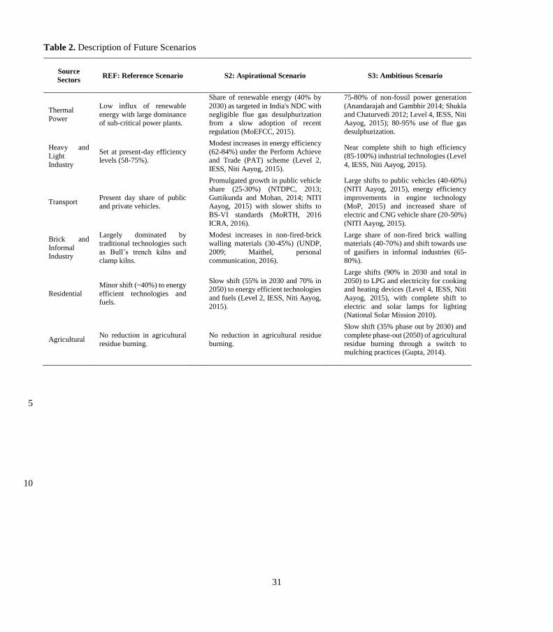
31

Table 2. Description of Future Scenarios

Source

Sectors REF: Reference Scenario S2: Aspirational Scenario S3: Ambitious Scenario

Thermal

Power

Low influx of renewable

energy with large dominance of sub-critical power plants.

Share of renewable energy (40% by

2030) as targeted in India's NDC with

negligible flue gas desulphurization from a slow adoption of recent

regulation (MoEFCC, 2015).

75-80% of non-fossil power generation

(Anandarajah and Gambhir 2014; Shukla

and Chaturvedi 2012; Level 4, IESS, Niti Aayog, 2015); 80-95% use of flue gas

desulphurization.

Heavy and

Light

Industry

Set at present-day efficiency levels (58-75%).

Modest increases in energy efficiency

(62-84%) under the Perform Achieve and Trade (PAT) scheme (Level 2,

IESS, Niti Aayog, 2015).

Near complete shift to high efficiency

(85-100%) industrial technologies (Level

4, IESS, Niti Aayog, 2015).

Transport Present day share of public and private vehicles.

Promulgated growth in public vehicle

share (25-30%) (NTDPC, 2013;

Guttikunda and Mohan, 2014; NITI Aayog, 2015) with slower shifts to

BS-VI standards (MoRTH, 2016

ICRA, 2016).

Large shifts to public vehicles (40-60%)

(NITI Aayog, 2015), energy efficiency

improvements in engine technology (MoP, 2015) and increased share of

electric and CNG vehicle share (20-50%)

(NITI Aayog, 2015).

Brick and

Informal Industry

Largely dominated by traditional technologies such

as Bull’s trench kilns and

clamp kilns.

Modest increases in non-fired-brick walling materials (30-45%) (UNDP,

2009; Maithel, personal

communication, 2016).

Large share of non-fired brick walling materials (40-70%) and shift towards use

of gasifiers in informal industries (65-

80%).

Residential

Minor shift (~40%) to energy

efficient technologies and fuels.

Slow shift (55% in 2030 and 70% in

2050) to energy efficient technologies

and fuels (Level 2, IESS, Niti Aayog,

2015).

Large shifts (90% in 2030 and total in

2050) to LPG and electricity for cooking

and heating devices (Level 4, IESS, Niti

Aayog, 2015), with complete shift to

electric and solar lamps for lighting (National Solar Mission 2010).

Agricultural No reduction in agricultural

residue burning. No reduction in agricultural residue

burning.

Slow shift (35% phase out by 2030) and

complete phase-out (2050) of agricultural

residue burning through a switch to mulching practices (Gupta, 2014).

5

10

32

Figures

List of Figures

Figure 1. National Emissions of Particulate matter and Precursor Gases for 2015 (Mt/yr). Emissions of NOx are in Mt yr-1 of

NO; SO2 in Mt yr-1 of SO2. 5

Figure 2. Sectoral emission of fine (a) particulate matter, (d) black carbon and (g) organic carbon under the three scenarios,

for 2015-2030 (column 1). Difference of higher efficiency/emission control scenarios from reference(S2 & S3) are shown in

column 2 (b,e,h) and column 3 (c,f,i). Emissions from ECLIPSE V5a and GAINS-WEO2016 are shown for comparison.

Figure 3. Sectoral emission of fine (a) SO2, (d) NOx and (g) NMVOCs under the three scenarios, for 2015-2030 (column 1).

Difference of higher efficiency/emission control scenarios from reference(REF & S2) are shown in column 2 (b,e,h) and 10

column 3 (c,f,i). Emissions from ECLIPSE V5a and GAINS-WEO2016 are shown for comparison.

Figure 4. Model Evaluation by (a) comparison of simulated annual mean PM2.5 concentrations with in-situ observations

(circles = observations) and (b) comparison of modeled annual mean AOD over India with observations from MODIS.

Figure 5. Evaluation of model performance (NMB) in capturing seasonal variation in chemical species concentrations at two

sites in India. 15

Figure 6. Simulated PM2.5 concentration a) 2015 b) 2030 REF c) 2050 REF d) 2030 S2 e) 2050 S2 f) 2030 S3 g) 2050 S3.

(Values in the parenthesis represent area-weighted average PM2.5 concentration for India).

Figure 7. Population-weighted mean ambient PM2.5 concentrations by state for (a) 2015 and 2030 (REF, S2 and S3) and (b)

2015 and 2050 (REF, S2 and S3).

Figure 8. Percentage contribution to ambient PM2.5 attributable to different sources in 2015 and 2050 all three scenarios. 20

Figure 9. Percentage contribution of (a) Residential Biomass, (b) Anthropogenic dust, (c) Industrial coal, (d) Power plant coal,

(e) Open burning, (f) Brick production, (g) Transportation and (h) Distributed Diesel attributable to ambient PM2.5

concentration by state (2015 – 2050).

25

30

33

Figure 1. National Emissions of Particulate matter and Precursor Gases for 2015 (Mt/yr). Emissions of NOx are in Mt yr-1 of

NO; SO2 in Mt yr-1 of SO2.

5

34

Figure 2. Sectoral emission of fine (a) particulate matter, (d) black carbon and (g) organic carbon under the three scenarios,

for 2015-2030 (column 1). Difference of higher efficiency/emission control scenarios from reference(S2 & S3) are shown in

column 2 (b,e,h) and column 3 (c,f,i). Emissions from ECLIPSE V5a and GAINS-WEO2016 are shown for comparison. 5

35

Figure 3. Sectoral emission of fine (a) SO2, (d) NOx and (g) NMVOCs under the three scenarios, for 2015-2030 (column 1).

Difference of higher efficiency/emission control scenarios from reference(S2 & S3) are shown in column 2 (b,e,h) and column

3 (c,f,i). Emissions from ECLIPSE V5a and GAINS-WEO2016 are shown for comparison.

5

10

15

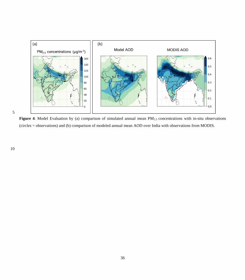
36

5

Figure 4. Model Evaluation by (a) comparison of simulated annual mean PM2.5 concentrations with in-situ observations

(circles = observations) and (b) comparison of modeled annual mean AOD over India with observations from MODIS.

10

37

Figure 5. Evaluation of model performance (NMB) in capturing seasonal variation in chemical species concentrations at two

sites in India

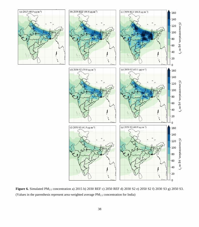
38

Figure 6. Simulated PM2.5 concentration a) 2015 b) 2030 REF c) 2050 REF d) 2030 S2 e) 2050 S2 f) 2030 S3 g) 2050 S3.

(Values in the parenthesis represent area-weighted average PM2.5 concentration for India)

39

Figure 7. Population-weighted mean ambient PM2.5 concentrations by state for (a) 2015 and 2030 (REF, S2 and S3) and (b)

2015 and 2050 (REF, S2 and S3)

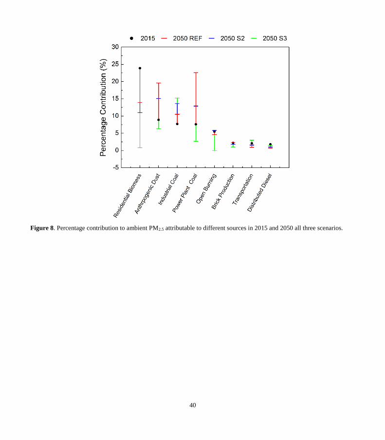
40

Figure 8. Percentage contribution to ambient PM2.5 attributable to different sources in 2015 and 2050 all three scenarios.

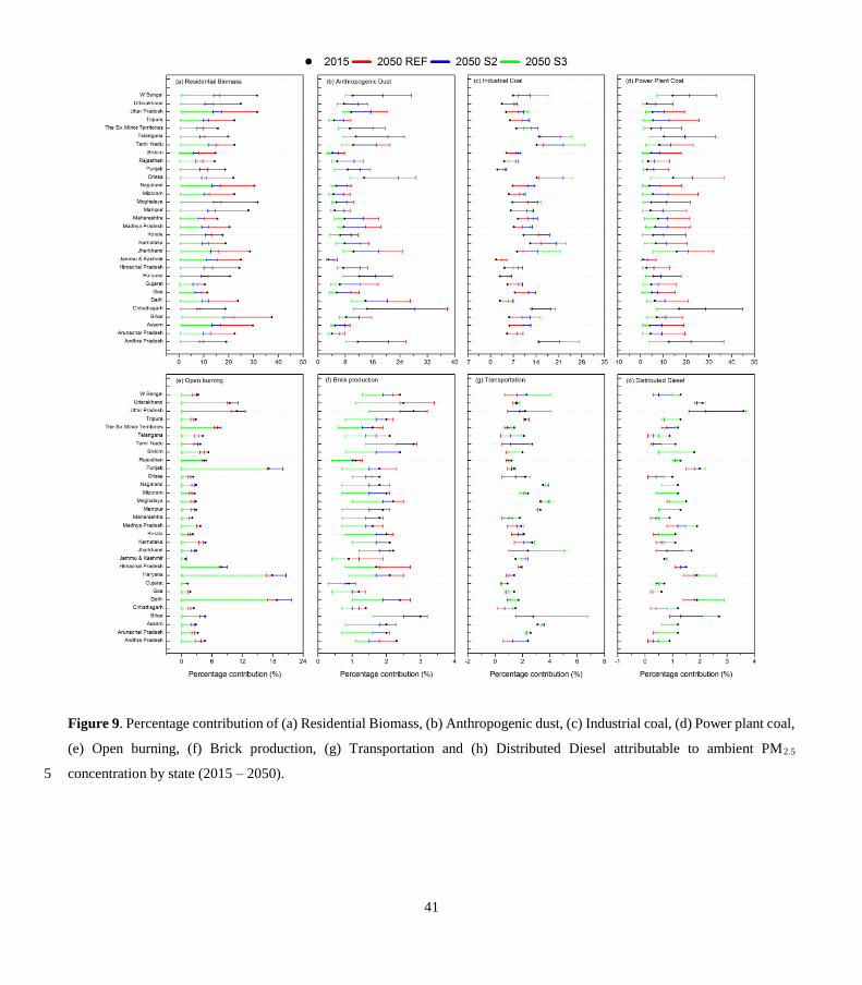
41

Figure 9. Percentage contribution of (a) Residential Biomass, (b) Anthropogenic dust, (c) Industrial coal, (d) Power plant coal,

(e) Open burning, (f) Brick production, (g) Transportation and (h) Distributed Diesel attributable to ambient PM2.5

concentration by state (2015 – 2050). 5

Manuscript with changes Marked-up

1

Source influence on emission pathways and ambient PM2.5 pollution

over India (2015-2050)

Chandra Venkataraman1,3, Michael Brauer2, Kushal Tibrewal3, Pankaj Sadavarte3,4, Qiao Ma5, Aaron

Cohen6, Sreelekha Chaliyakunnel7, Joseph Frostad8, Zbigniew Klimont9, Randall V. Martin10, Dylan B.

Millet7, Sajeev Philip10,11, Katherine Walker6, Shuxiao Wang5,12 5

1Department of Chemical Engineering, Indian Institute of Technology Bombay, Powai, Mumbai, India 2School of Population and Public Health, The University of British Columbia, Vancouver, British Columbia V6T1Z3, Canada 3Interdisciplinary program in Climate Studies, Indian Institute of Technology Bombay, Powai, Mumbai, India 4Institute for Advanced Sustainability Studies (IASS), Berliner Str. 130, 14467 Potsdam, Germany 10 5State Key Joint Laboratory of Environment Simulation and Pollution Control, School of Environment, Tsinghua University,

Beijing 100084, China 6Health Effects Institute, Boston, MA 02110, USA 7Department of Soil, Water, and Climate, University of Minnesota, Minneapolis–Saint Paul, MN 55108, USA 8Institute for Health Metrics and Evaluation, University of Washington, Seattle, WA 98195, USA 15 9International Institute for Applied Systems Analysis, Laxenburg, Austria 10Department of Physics and Atmospheric Science, Dalhousie University, Halifax, Nova Scotia B3H 4R2, Canada 11 NASA Ames Research Center, Moffett Field, California, USA 12State Environmental Protection Key Laboratory of Sources and Control of Air Pollution Complex, Beijing 100084, China

Correspondence to: Chandra Venkataraman (chandra@iitb.ac.in) 20

Abstract. India currently experiences degraded air quality, with future economic development leading to challenges for air

quality management. Scenarios of sectoral emissions of fine particulate matter and its precursors were developed and evaluated

for 2015-2050, under specific pathways of diffusion of cleaner and more energy efficiency technologies. The impacts of

individual source-sectors on PM2.5 concentrations were assessed through GEOS-Chem model systematic simulations of

spatially and temporally resolved particulate matter concentrations, using the GEOS-Chem model, followed by population-25

weighted aggregation to national and state levels. We find that PM2.5 pollution is a pan-India problem, with a regional character,

not limited to urban areas or megacities. Under present day emissions, levels in most states exceeded the national PM2.5

standard (40 µg/m3). Sources related to human activities were responsible for the largest proportion of the present-day

population exposure to PM2.5 in India. About 60% of India’s mean population-weighted PM-2.5 concentrations arise from

anthropogenic source-sectors, with the balance from “other” sources, windblown dust and extra-regional sources. Leading 30

contributors are residential biomass combustion, power plant and industrial coal combustion and anthropogenic dust (including

coal fly-ash, fugitive road dust and trash burning). Transportation, brick production, and distributed diesel were other

contributors to PM-2.5. Future evolution of emissions under current regulation or under promulgated or proposed regulation,

yield deterioration in future air-quality in 2030 and 2050. Only under a scenario where more ambitious measures are

introduced, promoting a total shift away from traditional biomass technologies and a very large shift (80-85%) to non-fossil 35

electricity generation, was an overall reduction in PM2.5 concentrations below 2015 levels achieved. In this scenario,

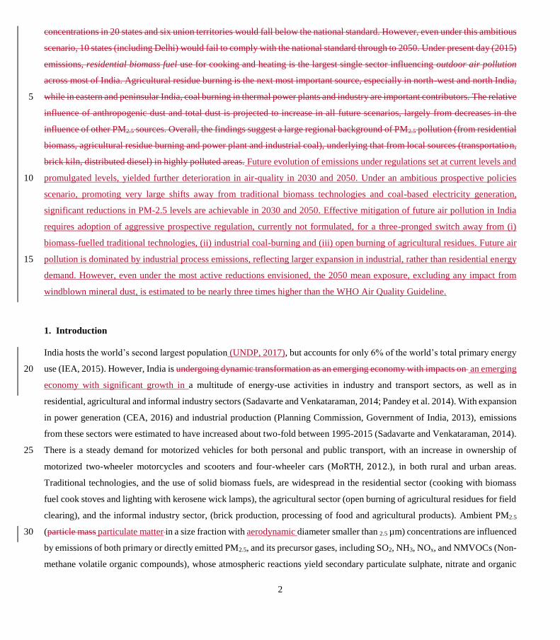
2

concentrations in 20 states and six union territories would fall below the national standard. However, even under this ambitious

scenario, 10 states (including Delhi) would fail to comply with the national standard through to 2050. Under present day (2015)

emissions, residential biomass fuel use for cooking and heating is the largest single sector influencing outdoor air pollution

across most of India. Agricultural residue burning is the next most important source, especially in north-west and north India,

while in eastern and peninsular India, coal burning in thermal power plants and industry are important contributors. The relative 5

influence of anthropogenic dust and total dust is projected to increase in all future scenarios, largely from decreases in the

influence of other PM2.5 sources. Overall, the findings suggest a large regional background of PM2.5 pollution (from residential

biomass, agricultural residue burning and power plant and industrial coal), underlying that from local sources (transportation,

brick kiln, distributed diesel) in highly polluted areas. Future evolution of emissions under regulations set at current levels and

promulgated levels, yielded further deterioration in air-quality in 2030 and 2050. Under an ambitious prospective policies 10

scenario, promoting very large shifts away from traditional biomass technologies and coal-based electricity generation,

significant reductions in PM-2.5 levels are achievable in 2030 and 2050. Effective mitigation of future air pollution in India

requires adoption of aggressive prospective regulation, currently not formulated, for a three-pronged switch away from (i)

biomass-fuelled traditional technologies, (ii) industrial coal-burning and (iii) open burning of agricultural residues. Future air

pollution is dominated by industrial process emissions, reflecting larger expansion in industrial, rather than residential energy 15

demand. However, even under the most active reductions envisioned, the 2050 mean exposure, excluding any impact from

windblown mineral dust, is estimated to be nearly three times higher than the WHO Air Quality Guideline.

1. Introduction

India hosts the world’s second largest population (UNDP, 2017), but accounts for only 6% of the world’s total primary energy

use (IEA, 2015). However, India is undergoing dynamic transformation as an emerging economy with impacts on an emerging 20

economy with significant growth in a multitude of energy-use activities in industry and transport sectors, as well as in

residential, agricultural and informal industry sectors (Sadavarte and Venkataraman, 2014; Pandey et al. 2014). With expansion

in power generation (CEA, 2016) and industrial production (Planning Commission, Government of India, 2013), emissions

from these sectors were estimated to have increased about two-fold between 1995-2015 (Sadavarte and Venkataraman, 2014).

There is a steady demand for motorized vehicles for both personal and public transport, with an increase in ownership of 25

motorized two-wheeler motorcycles and scooters and four-wheeler cars (MoRTH, 2012.), in both rural and urban areas.

Traditional technologies, and the use of solid biomass fuels, are widespread in the residential sector (cooking with biomass

fuel cook stoves and lighting with kerosene wick lamps), the agricultural sector (open burning of agricultural residues for field

clearing), and the informal industry sector, (brick production, processing of food and agricultural products). Ambient PM2.5

(particle mass particulate matter in a size fraction with aerodynamic diameter smaller than 2.5 µm) concentrations are influenced 30

by emissions of both primary or directly emitted PM2.5, and its precursor gases, including SO2, NH3, NOx, and NMVOCs (Non-

methane volatile organic compounds), whose atmospheric reactions yield secondary particulate sulphate, nitrate and organic

3

carbon, while reactions of NOx and NMVOCs also increase ozone levels. Ozone precursor gases and particulate black carbon

and organic carbon (BC and OC) are identified in the list of short-lived climate pollutants or SLCPs (CCAC, 2014).

Air quality is a public health issue of concern in India. According to the World Health Organization (WHO), 37 cities from

India feature in a global list of 100 world cities with the highest PM10 (PM with aerodynamic diameter <10 µm) pollution 5

globally, with cities like Delhi, Raipur, Gwalior, and Lucknow listed among the top 10 polluted cities (WHO, 2014; further

details in Figure S6 of supplement). Recent studies addressing air quality in India (Ghude et al. 2016; Chakraborty et al. 2015),

have built upon products of the Task Force on Hemispheric Transport of Air Pollutants (TF-HTAP), using HTAP emission

inventories (for 2010) in a regional chemistry model (Ghude et al. 2016) to address air quality in India. Widespread PM2.5

and O3 pollution was found under present emission levels, which considerably impact human mortalities and life expectancy. 10

To extend the understanding of ambient air pollution to multiple (regional and national) scales, for multiple pollutants, methods

which combine chemical transport modelling, with data from satellite retrievals combined with with available monitoring data,

have been developed (van Donkelaar et al., 2010; Brauer et al. 2012, 2016; Dey et al., 2012, Shaddick et al., 2018) and can be

used to evaluate current levels and trends. The latest GBD 2015 estimates indicate that the population-weighted mean PM2.5

concentration for India as a whole was 74.3 µg/m3 in 2015, up from about 60 µg/m3 in 1990 (Cohen et al., 2017). At current 15

levels, 99.9% of the Indian population is estimated to live in areas where the World Health Organization (WHO) Air Quality

Guideline of 10 µg/m3 was exceeded. Nearly 90% of people lived in areas exceeding the WHO Interim Target 1 of 35 µg/m3.

Strategies for mitigation of air pollution require understanding pollutant emission, differentiated by emitting sectors and by

sub-national regions, representing both present day conditions and future evolution under different pathways of growth and 20

technology change. Future projections of emissions, for climate relevant species, are available in the representative

concentration pathway (RCP) scenarios (Fujino et al. 2006; Clarke et al. 2007; Van Vuuren et al. 2007; Riahi et al. 2007;

Hijioka et al. 2008), more recently for the Shared Socioeconomic Pathways (SSPs) scenarios (Riahi et al., 2017; Rao et al.,

2017), while primary PM2.5 is included in inventories like ECLIPSE (Klimont et al., 2017, 2018). Inventories developed for

HTAP_v2 (Janssens-Maenhout et al. 2015) address emissions of a suite of pollutants for 2008 and 2010. These scenarios and 25

emission datasets are developed through globally consistent methodologies, leaving room for refinement through more detailed

regional studies. Thus, in this work we develop and evaluate sectoral emission scenarios of fine particulate matter and its

precursors and constituents from India, during 2015-2050, under specific pathways of diffusion of cleaner and more energy

efficiency technologies. The work is broadly related to HTAP scientific questions including understanding of (i) sensitivity of

regional PM2.5 pollution levels to magnitudes of emissions from source-sectors and (ii) changes in PM2.5 levels as a result of 30

expected, as well as ambitious, air pollution and climate change abatement efforts. The impacts of individual source-sectors

on PM2.5 concentrations is assessed through simulation of spatially and temporally resolved particulate matter concentrations,

using the GEOS-Chem chemical transport model, followed by aggregation to population-weighted concentrations (estimated

4

as the sum of product of concentration and population for each grid divided by the total population) at both national and state

levels.

Section 2 discusses the development of the emission inventory, disaggregated by sector, for the year 2015 and future

projections to 2050; Section 3 describes the GEOS-Chem model, the simulation parameters and evaluation; Section 4 discusses 5

simulated PM2.5 concentration by sector, at national and state levels under present day and future emission scenarios; and the

last section discusses findings and conclusions.

2. Present day and future emissions

2.1. Present day emissions (2015)

An emission inventory was developed for India, for the year 2015, based on an “engineering model approach” using 10

technology-linked energy-emissions modelling adapted from previous work (Pandey and Venkataraman 2014; Pandey et al.

2014; Sadavarte and Venkataraman, 2014), to estimate multi-pollutant emissions including those of SO2, NOx, PM2.5, black

carbon (BC), organic carbon (OC), and non-methane volatile organic compounds (NMVOCs). An engineering model

approach, goes beyond fuel divisions and uses technology parameters for process and emissions control technologies, including

technology type, efficiency or specific fuel consumption, and technology-linked emission factors (g of pollutant/ kg of fuel) 15

to estimate emissions.

The inventory disaggregates emissions from technologies and activities, in all major sectors. Plant level data (installed

capacity, plant load factor, and annual production) are used for 830 individual large point sources, in heavy industry and power

generation sectors, while light industry activity statistics (energy consumption, industrial products, solvent use, etc.) are from 20

sub-state (or district) level (CEA 2010; CMA 2007a,b, 2012; MoC 2007; FAI 2010; CMIE 2010; MoPNG 2012; MoWR 2007).

Technology-linked emission factors and current levels of deployment of air pollution control technologies are used. Vehicular

emissions include consideration of vehicle technologies, vehicle age distributions, and super-emitters among on-road vehicles

(Pandey and Venkataraman, 2014). Residential sector emission estimates, based on Pandey et al. (2014), include seasonality

in water and space heating activities comprise of cooking and water heating, largely with traditional biomass stoves; lighting, 25

using kerosene lamps; and warming of homes and humans, with biomass fuels. Seasonality included for water heating and

home warming. The “informal industries” sector includes brick production (in traditional kiln technologies like the Bull’s

trench kilns and clamp kilns, using both coal and biomass fuels) and food and agricultural product processing operations (like

drying and cooking operations related to sugarcane juice, milk, food-grain, jute, silk, tea, and coffee). In addition, monthly

mean data on agricultural residue burning in fields, a spatio-temporally discontinuous source of significant emissions, were 30

calculated using a bottom-up methodology (Pandey et al. 2014). Spatial proxies used to estimate gridded emissions over India

are described in Table S1 of the supplement.

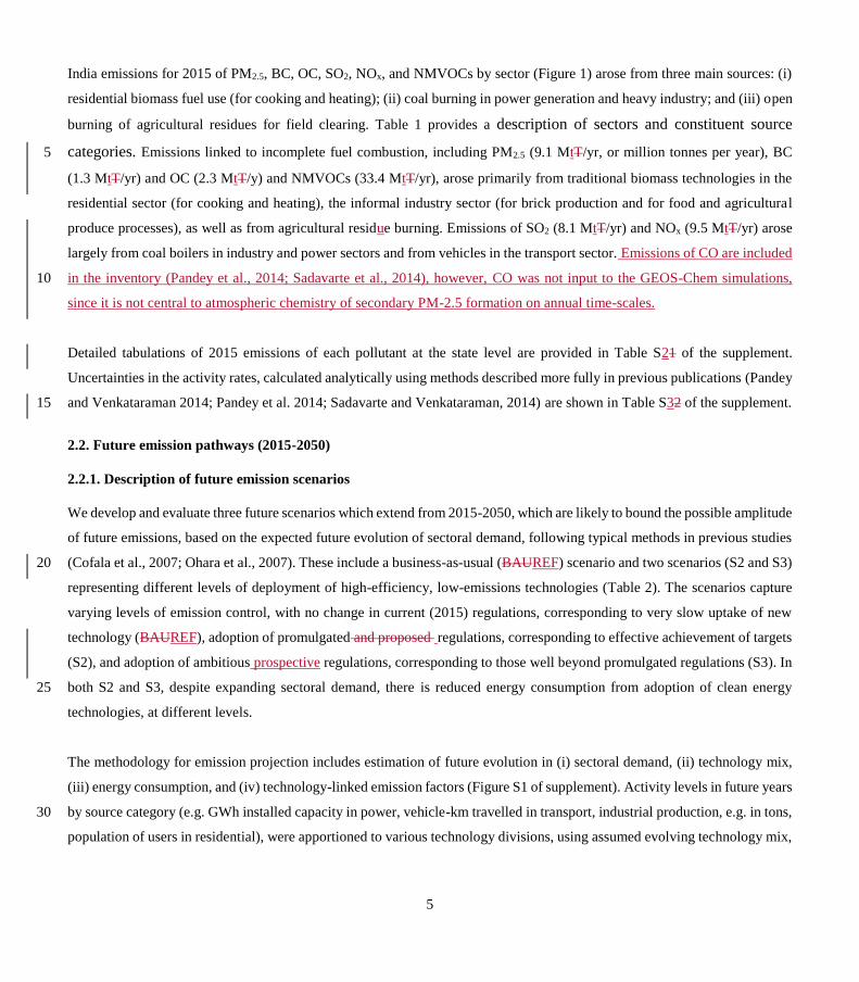
5

India emissions for 2015 of PM2.5, BC, OC, SO2, NOx, and NMVOCs by sector (Figure 1) arose from three main sources: (i)

residential biomass fuel use (for cooking and heating); (ii) coal burning in power generation and heavy industry; and (iii) open

burning of agricultural residues for field clearing. Table 1 provides a description of sectors and constituent source

categories. Emissions linked to incomplete fuel combustion, including PM2.5 (9.1 MtT/yr, or million tonnes per year), BC 5

(1.3 MtT/yr) and OC (2.3 MtT/y) and NMVOCs (33.4 MtT/yr), arose primarily from traditional biomass technologies in the

residential sector (for cooking and heating), the informal industry sector (for brick production and for food and agricultural

produce processes), as well as from agricultural residue burning. Emissions of SO2 (8.1 MtT/yr) and NOx (9.5 MtT/yr) arose

largely from coal boilers in industry and power sectors and from vehicles in the transport sector. Emissions of CO are included

in the inventory (Pandey et al., 2014; Sadavarte et al., 2014), however, CO was not input to the GEOS-Chem simulations, 10

since it is not central to atmospheric chemistry of secondary PM-2.5 formation on annual time-scales.

Detailed tabulations of 2015 emissions of each pollutant at the state level are provided in Table S21 of the supplement.

Uncertainties in the activity rates, calculated analytically using methods described more fully in previous publications (Pandey

and Venkataraman 2014; Pandey et al. 2014; Sadavarte and Venkataraman, 2014) are shown in Table S32 of the supplement. 15

2.2. Future emission pathways (2015-2050)

2.2.1. Description of future emission scenarios

We develop and evaluate three future scenarios which extend from 2015-2050, which are likely to bound the possible amplitude

of future emissions, based on the expected future evolution of sectoral demand, following typical methods in previous studies

(Cofala et al., 2007; Ohara et al., 2007). These include a business-as-usual (BAUREF) scenario and two scenarios (S2 and S3) 20

representing different levels of deployment of high-efficiency, low-emissions technologies (Table 2). The scenarios capture

varying levels of emission control, with no change in current (2015) regulations, corresponding to very slow uptake of new

technology (BAUREF), adoption of promulgated and proposed regulations, corresponding to effective achievement of targets

(S2), and adoption of ambitious prospective regulations, corresponding to those well beyond promulgated regulations (S3). In

both S2 and S3, despite expanding sectoral demand, there is reduced energy consumption from adoption of clean energy 25

technologies, at different levels.

The methodology for emission projection includes estimation of future evolution in (i) sectoral demand, (ii) technology mix,

(iii) energy consumption, and (iv) technology-linked emission factors (Figure S1 of supplement). Activity levels in future years

by source category (e.g. GWh installed capacity in power, vehicle-km travelled in transport, industrial production, e.g. in tons, 30

population of users in residential), were apportioned to various technology divisions, using assumed evolving technology mix,

6

for three different scenarios. Activity at the technology division level was used to derive corresponding future energy (and

fuel) consumption and related emissions using technology-based emission factors.

With 2015 as the base year, growth rates in sectoral demand were identified for thermal power plants, industries, residential,

brick kilns and informal industries, on-road transportation and agricultural sectors for 2015-2030 and 2030-2050 (Table S34 5

of supplement). Sectoral growth, estimated as ratios of 2050 to 2015 demand, were 5.1, 3.8, 3.2, 1.3, 1.4 respectively, for

building sector, electricity generation, heavy industries, residential sector, and agricultural residue burning, with the largest

growth in the building and electricity generation sectors (Figure S2 of supplement).

Table 2 shows regulation levels for different sectors under the three scenarios, through to 2050. The BAUREF and S2 scenarios 10

capture both energy efficiency and emissions control, continuing under current regulation, or broadly under promulgated future

policies. This assumes shifts to non-fossil generation which would occur under India Nationally Determined Contribution

(India’s NDC, 2015) in the power sector; negligible flue gas desulphurization from a slow adoption of recent regulation

(MoEFCC, 2015); modest increases in industrial energy efficiency under the perform achieve and trade (PAT) scheme (Level

2, IESS, Niti Aayog, 2015 ); promulgated growth in public vehicle share (NTDPC, 2013; Guttikunda and Mohan, 2014; NITI 15

Aayog, 2015) and changes in engine technology (Auto Fuel Policy Vision 2025, 2014), however, with a slow shift to BS-VI

standards from barriers to availability of fuel of required standards (ICRA, 2016); The S2 scenario assumes shifts to non-

fossil generation which would occur under India Nationally Determined Contribution (India’s NDC, 2015) in the power sector,

consistent with a shift to 40% renewables including solar, wind and hydro power by 2030 (NDC, 2015). The NDC goals of

India are suggested to be realistic (CAT, 2017; Ross and Gerholdt, 2017), with achievement of non-fossil share of power 20

generation projected to lie between 38%-48% by 2030, as well as adoption of tighter emission standards for desulphurization

and de-NOx technologies in thermal plants (MoEFCC, 2015), at a rate consistent with expected barriers (CSE, 2016). Further,

changes assumed in the transport sector reflect promulgated growth in public vehicle share (NTDPC, 2013; Guttikunda and

Mohan, 2014; NITI Aayog, 2015) and promulgated regulation (Auto Fuel Policy Vision 2025, 2014, MoRTH, 2016), along

with realistic assumptions of implementation lags in adoption of BS VI standards (ICRA 2016). Other assumptions include 25

modest increases in industrial energy efficiency under the perform achieve and trade (PAT) scheme (Level 2, IESS, Niti Aayog,

2015 ); modest increases in non-fired-brick walling materials (UNDP, 2009; Maithel, personal communication, 2016); slow

shift to more efficient residential energy technologies and fuels (Level 2, IESS, Niti Aayog, 2015); and minor reduction in

agricultural residue burning.

30

However, in the S3 scenario, adoption of ambitious regulation, well beyond those currently promulgated is assumed. This

includes very significant shifts to non-fossil power generation (Anandarajah and Gambhir 2014; Shukla and Chaturvedi 2012;

Level 4, IESS, Niti Aayog, 2015); near-complete shift to high efficiency industrial technologies (MoP 2012, Level 4, IESS,

Niti Aayog, 2015); large public vehicle share (NITI Aayog, 2015), energy efficiency improvements in engine technology

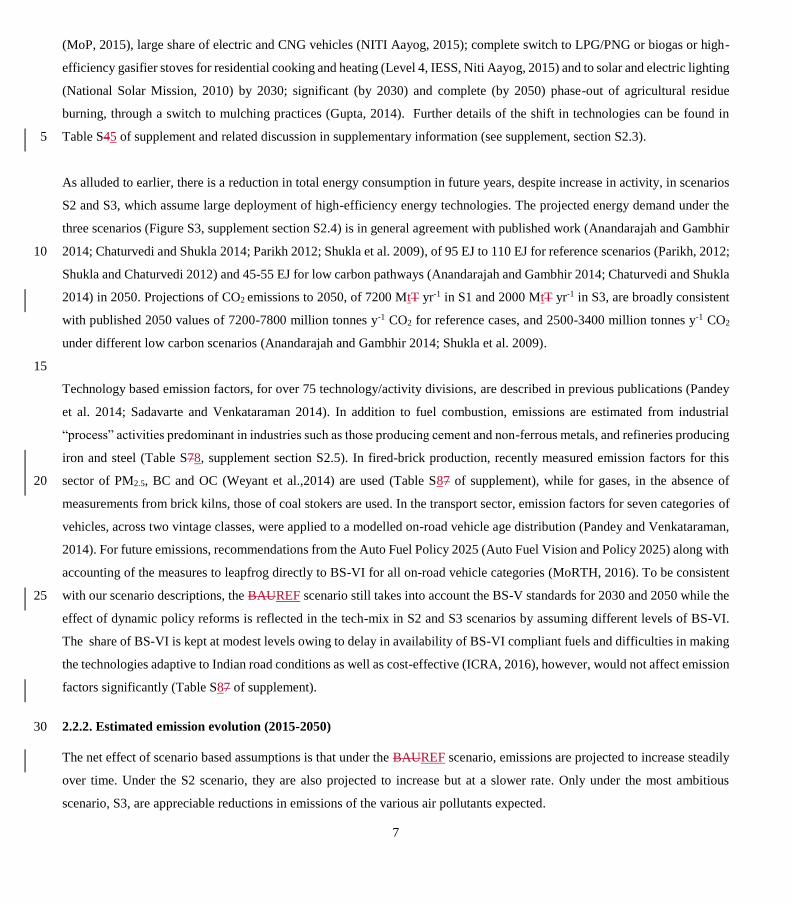
7

(MoP, 2015), large share of electric and CNG vehicles (NITI Aayog, 2015); complete switch to LPG/PNG or biogas or high-

efficiency gasifier stoves for residential cooking and heating (Level 4, IESS, Niti Aayog, 2015) and to solar and electric lighting

(National Solar Mission, 2010) by 2030; significant (by 2030) and complete (by 2050) phase-out of agricultural residue

burning, through a switch to mulching practices (Gupta, 2014). Further details of the shift in technologies can be found in

Table S45 of supplement and related discussion in supplementary information (see supplement, section S2.3). 5

As alluded to earlier, there is a reduction in total energy consumption in future years, despite increase in activity, in scenarios

S2 and S3, which assume large deployment of high-efficiency energy technologies. The projected energy demand under the

three scenarios (Figure S3, supplement section S2.4) is in general agreement with published work (Anandarajah and Gambhir

2014; Chaturvedi and Shukla 2014; Parikh 2012; Shukla et al. 2009), of 95 EJ to 110 EJ for reference scenarios (Parikh, 2012; 10

Shukla and Chaturvedi 2012) and 45-55 EJ for low carbon pathways (Anandarajah and Gambhir 2014; Chaturvedi and Shukla

2014) in 2050. Projections of CO2 emissions to 2050, of 7200 MtT yr-1 in S1 and 2000 MtT yr-1 in S3, are broadly consistent

with published 2050 values of 7200-7800 million tonnes y-1 CO2 for reference cases, and 2500-3400 million tonnes y-1 CO2

under different low carbon scenarios (Anandarajah and Gambhir 2014; Shukla et al. 2009).

15

Technology based emission factors, for over 75 technology/activity divisions, are described in previous publications (Pandey

et al. 2014; Sadavarte and Venkataraman 2014). In addition to fuel combustion, emissions are estimated from industrial

“process” activities predominant in industries such as those producing cement and non-ferrous metals, and refineries producing

iron and steel (Table S78, supplement section S2.5). In fired-brick production, recently measured emission factors for this

sector of PM2.5, BC and OC (Weyant et al.,2014) are used (Table S87 of supplement), while for gases, in the absence of 20

measurements from brick kilns, those of coal stokers are used. In the transport sector, emission factors for seven categories of

vehicles, across two vintage classes, were applied to a modelled on-road vehicle age distribution (Pandey and Venkataraman,

2014). For future emissions, recommendations from the Auto Fuel Policy 2025 (Auto Fuel Vision and Policy 2025) along with

accounting of the measures to leapfrog directly to BS-VI for all on-road vehicle categories (MoRTH, 2016). To be consistent

with our scenario descriptions, the BAUREF scenario still takes into account the BS-V standards for 2030 and 2050 while the 25

effect of dynamic policy reforms is reflected in the tech-mix in S2 and S3 scenarios by assuming different levels of BS-VI.

The share of BS-VI is kept at modest levels owing to delay in availability of BS-VI compliant fuels and difficulties in making

the technologies adaptive to Indian road conditions as well as cost-effective (ICRA, 2016), however, would not affect emission

factors significantly (Table S87 of supplement).

2.2.2. Estimated emission evolution (2015-2050) 30

The net effect of scenario based assumptions is that under the BAUREF scenario, emissions are projected to increase steadily

over time. Under the S2 scenario, they are also projected to increase but at a slower rate. Only under the most ambitious

scenario, S3, are appreciable reductions in emissions of the various air pollutants expected.

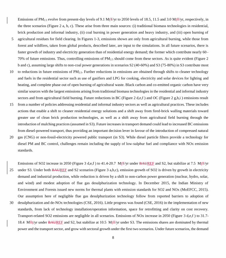
8

Emissions of PM2.5 evolve from present-day levels of 9.1 MtT/yr to 2050 levels of 18.5, 11.5 and 3.0 MtT/yr, respectively, in

the three scenarios (Figure 2 a, b, c). These arise from three main sources: (i) traditional biomass technologies in residential,

brick production and informal industry, (ii) coal burning in power generation and heavy industry, and (iii) open burning of

agricultural residues for field clearing. In Figures 1-3, emissions shown are only from agricultural burning, while those from 5

forest and wildfires, taken from global products, described later, are input to the simulations. In all future scenarios, there is

faster growth of industry and electricity generation than of residential energy demand; the former which contribute nearly 60–

70% of future emissions. Thus, controlling emissions of PM2.5 should come from these sectors. As is quite evident (Figure 2

b and c), assuming large shifts to non-coal power generations in scenarios S2 (40-60%) and S3 (75-80%) in S3 contribute most

to reductions in future emissions of PM2.5. Further reductions in emissions are obtained through shifts to cleaner technology 10

and fuels in the residential sector such as use of gasifiers and LPG for cooking, electricity and solar devices for lighting and

heating, and complete phase out of open burning of agricultural waste. Black carbon and co-emitted organic carbon have very

similar sources with the largest emissions arising from traditional biomass technologies in the residential and informal industry

sectors and from agricultural field burning. Future reductions in BC (Figure 2 d,e,f ) and OC (Figure 2 g,h,i ) emissions result

from a number of policies addressing residential and informal industry sectors as well as agricultural practices. These includes 15

actions that enable a shift to cleaner residential energy solutions and a shift away from fired-brick walling materials toward

greater use of clean brick production technologies, as well as a shift away from agricultural field burning through the

introduction of mulching practices (assumed in S3). Future increases in transport demand could lead to increased BC emissions

from diesel-powered transport, thus providing an important decision lever in favour of the introduction of compressed natural

gas (CNG) or non-fossil-electricity powered public transport (in S3). While diesel particle filters provide a technology for 20

diesel PM and BC control, challenges remain including the supply of low-sulphur fuel and compliance with NOx emission

standards.

Emissions of SO2 increase in 2050 (Figure 3 d,e,f ) to 41.4-20.7 MtT/yr under BAUREF and S2, but stabilize at 7.5 MtT/yr

under S3. Under both BAUREF and S2 scenarios (Figure 3 a,b,c), emission growth of SO2 is driven by growth in electricity 25

demand and industrial production, while reduction is driven by a shift to non-carbon power generation (nuclear, hydro, solar,

and wind) and modest adoption of flue gas desulphurization technology. In December 2015, the Indian Ministry of

Environment and Forests issued new norms for thermal plants with emission standards for SO2 and NOx (MoEFCC, 2015).

Our assumption here of negligible flue gas desulphurization technology follow from reported barriers to adoption of

desulphurization and de-NOx technologies (CSE, 2016). Little progress was found (CSE, 2016) in the implementation of new 30

standards, from lack of technology installation/operation information, space for retrofitting and clarity on cost recovery.

Transport-related SO2 emissions are negligible in all scenarios. Emissions of NOx increase in 2050 (Figure 3 d,e,f ) to 31.7-

18.4 MTt/yr under BAUREF and S2, but stabilize at 10.5 MtT/yr under S3. The emissions shares are dominated by thermal

power and the transport sector, and grow with sectoral growth under the first two scenarios. Under future scenarios, the demand

9

in passenger-km increases twice that in ton-km of freight, thus leading in 2050 to significantly greater passenger (7000-10000

billion passenger-km, in different scenarios), than freight (2300-2800 billion ton-km) transport provided by diesel. This makes

shifts away from diesel based public transport important. Thus, under the S3 scenario, shifts in the transport sector to tighter

emission standards for vehicles and a greater share of CNG in public transport, as well as, in the power sector, to non-fossil

power generation, reduce NOx emissions. Owing to the large shift away from fossil-power, the use of selective catalytic 5

reduction (SCR) technology for NOx control is not considered. A non-negligible, approximately 20%, share is from residential,

agricultural field burning and brick production sectors, which is reduced in magnitude by the adoption of mitigation based

largely on cleaner combustion technologies. Emissions of NMVOCs increase in 2050 to 16.3 MtT/yr under the BAUREF

scenario, but decrease to about 3.8 MtT/yr under S3 (Figure 3 g,h,i). In the S3 scenario, mitigation in residential, transport and

open burning emissions offsets more than two-thirds of present-day NMVOC emissions. Industrial emissions of NMVOC, 10

arising primarily from solvent use, are almost constant at 2 MtT/yr across scenarios, providing further potential for mitigation.

However, a shift to public transport based on heavy-duty CNG vehicles drives the increase in NMVOC emissions from the

transport sector, from their significantly larger emissions factors, compared to those of heavy duty diesel. Therefore, alternate

modes and technologies in the transport sector need further attention.

15

Anthropogenic dust (Philip et al. 2017), defined here as mineral constituents of pollution particles, including coal fly-ash and

mineral matter in trash burning and biomass burning emissions, contributes about 30% of Indian PM2.5 emissions in the base

year 2015 i.e. about ~3 MtT/yr. In future scenarios BAUREF and S2, respectively, anthropogenic dust contributes 6.0 and 4.6

MTt/yr in 2030 and 12.0 and 6.8 MtT/yr in 2050, arising primarily (60–85%) from coal fly-ash, with the balance from fugitive

on-road dust and waste burning. In the highest-control S3 scenario, anthropogenic dust emissions were reduced to about 1.8 20

MtT/yr, in both 2030 and 2050. This results from the assumed significant shift to 80–85% non-coal thermal power generation,

leading to large reductions in coal fly-ash emissions. Thus, in the S3 scenario anthropogenic dust emissions arise largely from

on-road fugitive dust and waste burning (over 50%), with a lower contribution from coal fly-ash (35-40%).

Emission datasets for India in global emission inventories have been developed either through combination of regional 25

inventories for specific base years (Janssens-Maenhout et al., 2015) or using integrated assessment models, e.g., the GAINS

model (Amann et al., 2011), to generate scenarios of air pollutants (Klimont et al., 2009, 2017, 2018; Purohit et al., 2010; Stohl

et al., 2015). Indian emissions for 2008 and 2010 under the HTAP_v2 framework (Janssens-Maenhout et al., 2015), originate

from the MIX inventory (Li et al., 2017), based on earlier Asia inventories like INTEX-B (Lu et al., 2011; Lu and Streets,

2012) and REAS (Kurokawa et al., 2013). Inconsistencies are reported from merging datasets, calculating different pollutants 30

using differing assumptions (Li et al., 2017). The datasets do not include some important regional emission sources like the

open burning of agricultural residues (Janssens-Maenhout et al., 2015). Recent global emissions from ECLIPSE V5 (Stohl et

al., 2015; http://www.iiasa.ac.at/web/home/research/researchPrograms/air/ECLIPSEv5.html), driven by HTAP objectives to

improve representation of aerosols emissions in IAMs (Keating, 2015), were reported to have problems over India including

10

underestimation of BC and trace gas magnitudes and inaccuracies in spatial distribution (Stohl et al., 2015). The present dataset

overcomes some of these limitations, using consistent assumptions to calculate a number of pollutants, including all sectors in

global inventories, as well as, agricultural residue burning emissions, industrial process emissions, while providing for finer

spatial resolution using district level data and more relevant spatial proxies. Emission magnitudes of PM-2.5 and precursors in

present inventory are in good agreement with those in ECLIPSE for 2010, however, those of precursor gases are somewhat 5

lower (about 30%) than those in HTAP_v2 (2010) and REAS 2.1 (2008) (Section 2.6 of supplement).

Future emissions of particulate matter (PM2.5 and constituents, BC and OC) and precursor gases (SO2, NOx and NMVOC)

estimated here were compared with the more recent sets of scenarios developed with the GAINS model in projects addressing

global air pollution trajectories until 2050, i.e., ECLIPSE V5a (Klimont et al., 2017, 2018;) and the World Energy Outlook 10

(IEA, 2016). These scenarios rely on different energy projections; Energy Technology Perspective study (IEA, 2012) was used

in ECLIPSE V5a and World Energy Outlook 2016 in the IEA study. Furthermore, the assumptions about air pollution

legislation vary with IEA study considering within the ‘New Policies Scenario’ recently adopted, announced or intended

policies, even where implementation measures are yet to be fully defined. This is in contrast to ECLIPSE V5a where adopted

polices by 2013 were used in the baseline scenario. In general, lower emissions in GAINS-WEO2016 (IEA, 2016) are attributed 15

to the successful implementation of new emission regulations in power and transport sectors, decreased use of biomass fuel in

residential sector and phase-out of kerosene lamps. We compare S2 and S3 scenarios in the present study to the baseline

scenarios from the above studies (shown in Fig 2 and 3).

For SO2 and NOx, emission trajectories in the S2 scenario are similar to those in ECLIPSE V5a, while emissions in the S3 20

scenario resemble those in GAINS-WEO2016 where newly proposed SO2 and NOx regulations for thermal power plants and

implementation of BS-VI in transportation is included. In fact, also the absolute level of emissions estimated for 2015 is

comparable to this study (Fig 3a, d); though GAINS estimates are slightly higher for SO2 and lower for NOx owing primarily

to differences in emission factors for coal power plants. Bottom-up estimates of SO2 emissions from our inventory (Pandey et

al., 2014; Sadavarte et al., 2014) are consistent with the recent estimates from the satellite based study (Li et al., 2017) from 25

2005-2016, both showing a steady growth. Present day emissions of SO2 (8.1 Mt yr-1) are at the lower end of the range of

8.5-11.3 Mt yr-1suggested by Li et al. 2017. Large future increases in SO2 emissions, estimated here in the REF and S2

scenarios are consistent with findings of Li et al. 2017.

For particulate matter species, the GAINS model estimates lower 2015 emissions mostly because of the differences for 30

residential use of biomass as well as emissions from open burning. However, considering the uncertainties associated with

quantification of biomass use and emission factors (e.g., Bond et al., 2004; Klimont et al., 2009, 2017; Venkataraman et al.,

2010) the differences are acceptable. The future evolution of emissions of BC and OC shows similar features among the studies

with S2 comparable to ECLIPSE V5a and S3 to IEA (2016), however the S3 scenario brings much stronger reduction due to

11

faster phase-out of kerosene for lighting and stronger reduction of biomass used for cooking; the latter feature is especially

visible for emissions of OC (Fig 2d,g). For total PM2.5 (Fig. 2a) scenarios developed with the GAINS model do not show a

very large difference and fall short of the reductions achieved in the S3 case where significant mitigation reduction is not

achieved in residential sector for also in power sector and industry which in GAINS are either already controlled in the baseline

(power sector) or continue to grow, industrial processes offsetting the benefits of reduction in other sectors. 5

Emissions of NMVOCs (Fig 3g) monotonously increase in ECLIPSE V5a, becoming higher than those in S2, by 2030, which

however, mimic those in GAINs-WEO2016, through to 2050. While there is also a fairly large difference in estimate for the

base year (mostly due to residential combustion of biomass, open burning, and solvent use sector), obviously the assumptions

about the future policies are different as both ECLIPSE V5a and IEA study include more conservative assumptions about 10

reduction of biomass use and eradication of open burning practices while at the same time continued growth in industrial

emissions, i.e., solvent applications. Further analysis of differences between the S2 scenario and the ECLIPSE V5a and

GAINS-WEO2016 is shown in the supplement (Fig S45).

Further, the emission projections were also compared with emissions estimated in the four representative concentration 15

pathways (RCP) scenarios adopted by the IPCC as a common basis for modelling future climate change (Fujino et al. 2006;

Clarke et al. 2007; Van Vuuren et al. 2007; Riahi et al. 2007; Hijioka et al. 2008). The RCP scenarios were designed to

represent a range of possible future climate outcomes in terms of radiative forcing watts per square meter (Wm-2) values (2.6,

4.5, 6.0, and 8.5) in 2100 relative to pre-industrial levels. Overall, Indian emissions of SO2, NOx, and BC estimated here in

the BAUREF and S2 scenarios, which do not apply stringent controls, were 2 to 3 times higher than the largest emissions 20

estimated in the RCP8.5 scenario in 2030 and 2050, as a result of differences in assumptions made or in the list of sources

included (Table S89 of supplement). As all RCP scenarios considered principally one type of air pollution trajectory assuming

that air pollutant emissions will be successfully reduced with economic growth. Consequently, in the longer term the range of

outcomes is fairly similar among RCPs (Amann et al., 2013; Rao et al. 2017). Emissions of these species in the S3 scenario,

with the most stringent controls, were in agreement with either RCP8.5 or RCP 4.5 scenario emissions. Emissions of OC in 25

the BAUREF and S2 scenarios and of NMVOCs in the S2 and S3 scenarios were in agreement with the ranges estimated in

the RCP4.5 and RCP8.5 scenarios. Emissions of SO2 estimated here for the highest-control scenario, S3, agreed with those

from RCP 4.5 in 2030 and RCP 8.5 in 2050, due to similar assumptions of over 80% non-coal electricity generation. However,

the S2 and BAUREF scenarios estimated much larger emissions. Further details are presented in section S2.6 of supplement.

3. Model simulations and evaluation 30

The emissions were used with GEOS-Chem model (www.geos-chem.org) to calculate pollutant concentration fields in space

and time. The GEOS-Chem model has been previously applied to study PM2.5 over India (e.g., Boys et al. 2014; Kharol et al.

12

2013; Philip et al. 2014a; Li et al. 2017) including relating satellite observations of aerosol optical depth to ground-level PM2.5

for the GBD assessment (Brauer et al. 2012, 2016; van Donkelaar et al. 2010, 2015, 2016). The simulations undertaken in this

work represent one of the finest resolution efforts to date to both represent India, and global scale processes.

In addition to the emissions described in section 2.2.2, other open burning emissions emissions such as open burning except 5

agricultural residue burning, which includes forest fires were derived from the global GFED-4s database (Akagi et al. 2011;

Andreae et al. 2001; Giglio et al. 2013; Randerson et al. 2012; van der Werf et al. 2010). In addition to the species in this

inventory, ammonia or NH3 emissions, important for calculating secondary particulate matter, were taken from the MIX

emission inventory (Li et al. 2017; http://meicmodel.org/dataset-mix.html). Emissions of NH3 arise primarily from sources

like animal husbandry, not addressed in the present inventory. Therefore, they are taken from (Li et al., 2017). Owing to large 10

uncertainties in future emissions, these were held the same in future scenarios, as for 2015. Emission magnitudes of NH3 could

affect secondary nitrate, which typically contributes to less than 5% of PM-2.5 mass, thus not influencing overall results in

any significant manner. The model solves for the temporal and spatial evolution of aerosols and gaseous compounds using

meteorological data sets, emission inventories, and equations that represent the physics and chemistry of the atmosphere.

Version 10.01 is used here. Total NMVOC emissions from India were taken from Sarkar et al (2016). The GEOS-Chem model 15

speciation (Table S10, supplementary material), into eight species, was applied for further input to the photochemical module.

The simulation of PM2.5 includes the sulphate–nitrate–ammonium–water system (Park et al. 2004), primary (Park et al. 2003)

and secondary (Henze et al. 2006, 2008; Liao et al. 2007; Pye et al. 2010) carbonaceous aerosols, mineral dust (Fairlie et al.

2007), and sea salt (Alexander et al. 2005). The GEOS-Chem model has fully coupled ozone–NOx–hydrocarbon chemistry

and aerosols including sulphate (SO42−), nitrate (NO3

−), ammonium (NH4+) (Park et al. 2004; Pye et al. 2009), organic carbon 20

(OC) and black carbon (BC) (Park et al. 2003), sea salt (Alexander et al. 2005), and mineral dust (Fairlie et al. 2007). For these

simulations we also included the SO42− module introduced by Wang and colleagues (2014). Partitioning of nitric acid (HNO3)

and ammonia between the gas and aerosol phases is calculated by ISORROPIA II (Fountoukis and Nenes 2007). Secondary

organic aerosol formation includes the oxidation of isoprene (Henze and Seinfeld 2006), monoterpenes and other reactive

volatile organic compounds (Liao et al. 2007), and aromatics (Henze et al. 2008). 25

The South Asia nested version of GEOS-Chem used here was developed by Sreelekha Chaliyakunnel and Dylan Millet (both

of the University of Minnesota) to cover the area from 55°E to 105°E and from 0°S to 40°N, and to resolve the domain of

South Asia at a resolution of 0.5° × 0.67° (approximately 56 × 74 km at equator) with dynamic boundary conditions using

meteorological fields from the NASA Goddard Earth Observation System (GEOS-5). The boundary fields are provided by the 30

global GEOS-Chem simulation with a resolution of 4° latitude and 5° longitude (approximately 445 × 553 km at equator),

which are updated every three hours. We have corrected the too-shallow nighttime mixing depths and overproduction of HNO3

in the model following Heald and colleagues (2012) and Walker and colleagues (2012). We applied the organic mass to organic

carbon ratio in accordance with findings from Philip et al.and colleagues (2014b). A relative humidity of 50% was used to

13

represent simulated PM2.5 measurements in India. To select the year of meteorology, we conducted standard simulations using

the same emissions and different meteorology from the years 2010 to 2012, as the meteorological fields were not yet available

post-2012. South Asia nested meteorological fields were not yet available post-2012 due to a change in the GEOS assimilation

system in 2013. Therefore, we conducted standard simulations to test meteorology from the years 2010 to 2012. We chose the

year 2012 as our meteorology year, as the simulation results using this year best represented the mean PM2.5 concentration 5

from 2010 to 2012. A three months initialization period was used to remove the effects of initial conditions.

To estimate the impacts of individual sources, simulations were made using total emissions from all sources, along with

sensitivity simulations (Table 1) for major sources. Sources included in the standard simulation, however, not separately

addressed in sensitivity simulations, termed “other” include residential lighting with traditional kerosene lamps and informal 10

industry (food and agro-product processing). Primary particulate matter is largely composed of carbonaceous constituents

(black carbon and organic matter) and mineral matter. Mineral matter from combustion and industry are calculated as the

difference between emitted PM2.5 mass and the sum of black carbon and organic matter, each calculated from respective

emission factors and lumped along with urban fugitive dust, evaluated in a previous study (Philip et al. 2017), are termed

anthropogenic fugitive dust or ADST. For sensitivity simulations, the total coal-related emissions, industrial coal-related 15

emissions, and emissions from other major sectors are removed respectively from the inventory in each scenario. The global

and nested grid models of GEOS-Chem were then run in sequence using the new inventories. These sensitivity simulation

results therefore depict the ambient PM2.5 concentrations with each emission sector shut off. The differences of the standard

and sensitivity simulations were analyzed to produce contributions of the individual sectors to ambient PM2.5 concentrations.

By comparing the difference in simulated ambient concentrations between the standard and sensitivity simulations, we 20

therefore consider in our analyses the complex nonlinear relationships between emissions and ambient concentrations and the

nonlinear atmospheric chemistry affecting particle formation.

The GEOS-Chem simulations made here include those for primary aerosol emissions; secondary sulphate, nitrate, and

ammonium; and secondary organic aerosol, going beyond previous simulations made on regional scales over India (e.g., 25

Sadavarte et al. 2016), which were limited to secondary sulphate and a smaller list of sources in the emissions inventory,

addressing only a few months in the year. Model predicted concentrations of PM2.5 (Figure 4) and its chemical constituents

(Figure 5) were evaluated against available PM2.5 measurements, satellite observations of columnar aerosol optical depth

(AOD), and available monthly chemical composition measurements (Kumar and Sunder Raman 2016; Ramachandran and

Kedia 2010; Ramachandran and Rajesh 2007). Model performance was evaluated through normalized mean bias (NMB) (Eq. 30

1) for pairs of model predicted concentrations (M) and corresponding observed concentrations (O), at given locations and for

the same averaging period:

Normalized Mean Bias = ∑ (𝑀−𝑂)𝑛1

∑ (𝑂)𝑛1

(1)

14

The evaluation of the seasonal cycle of simulated PM2.5 is inhibited by the paucity of measurements. Evaluation of the PM2.5

seasonal variation reveals an overall general consistency between the simulation and observations. However, some of the

largest concentrations, e.g. at Delhi (28.6° N, 77.1° E) and Kanpur (26.4° N, 80.3° E), were somewhat underestimated. The

model captures AOD distribution over large parts of India, compared to measurements from MODIS (Figure 4b; NMB of -

33%) but appears to have an underestimation in the northwest, implying underestimation in modelled windblown dust 5

emissions in the Thar desert. However, the evaluation may be interpreted with caution, from differences arising from sensor

(e.g. MODIS and MISR) variability in the AOD product both spatially and temporally over India (Baraskar et al., 2016), as

well as, lack of coincident sampling of model with satellite observations.

Evaluation was also explored against monthly mean chemical composition measurements (Figure 5) at a regional background 10

site (Bhopal, 23.2o N, 77.4o E; Figure 5a, b, c; PM2.5, sulphate, nitrate; methods described in Kumar and Sunder Raman, 2016)

and a western urban site (Ahmedabad, 23.0o N, 72.5o E; Figure 5d, BC; aethalometer measurements in Ramachandran and

Rajesh, 2007). The simulation captures monthly PM2.5 and species mean concentrations satisfactorily during non-winter

months at the two sites, but with some underestimation in the winter months. While sensitivity simulations for nitrate (not

shown) increased nitrate concentrations in north India, they were largely unchanged in central India, evident in the 15

underestimation of nitrate (NMB = -68%) at Bhopal. The spatial distribution of particulate species (not shown) reflects the

interplay of emission density distributions with transport processes, with sulphate showing a predominance in central India

and to the east where there is a prevalence of thermal power generation, but BC and organic matter showing a predominance

in northern India, where there is a prevalence of traditional biomass fuelled residential energy technologies. The findings here

are broadly consistent with earlier work (Sadavarte et al. 2016) which showed large surface concentrations of sulphate, organic 20

carbon and dust over north India. However, there is a strong need for coherent measurement campaigns to map concentrations

of both PM2.5 and its chemical constituents over India, to improve model evaluation and future air quality management.

As discussed earlier, NMVOC emissions from India were taken from a recent technology-linked inventory, deployed in WRF-

CAMx and evaluated with satellite and in-situ observations (Sarkar et al. 2016). However, uncertainties still remain to be 25

addressed in the calculation of secondary PM-2.5 constituents, especially secondary organic aerosols, whose precursor

NMVOC emissions in developing countries, are still uncertain from lack of speciation measurements under combustion

conditions (Roden et al., 2006; Martinsson et al., 2015) typically encountered in traditional technologies in residential cooking

and heating and informal industry including brick production. Recent studies (Stockwell et al., 2016) attempted to fill this gap.

Such findings must be incorporated into future emission inventory evaluation for further refining regional PM-2.5 calculations. 30

While the present study did include calculation of both primary and secondary organic matter, as constituents of PM-2.5, a

detailed study of the sources and fate of total or secondary organic aerosol over the Indian region, is beyond the scope of this

work. Direct comparison of spatially averaged model output with satellite products or in-situ measurements typically

incorporate significant uncertainty. A broad evaluation was undertaken here, without a match of model output to specific

15

sampling time or satellite overpass time. Thus, some differences would arise from modelled meteorology not faithfully

representing actual meteorological conditions during the measurement period. With these caveats, we acknowledge the need

for coherent measurement campaigns to map concentrations of both PM2.5 and its chemical constituents over India, to improve

model evaluation and future air quality management.

4. Simulated PM2.5 concentrations by state and sector 5

4.1. Present-day and future PM2.5 concentrations at national and state levels

We find that ambient PM2.5 pollution is a pan-India problem with a regional character. Figure 6a-g shows the simulated total

ambient PM2.5 concentrations for 2015 and in each future scenario (BAUREF, S2, and S3) for 2030 and 2050 to illustrate the

different spatial patterns under each scenario. The figure displays mean PM2.5 concentration at a grid level, with area-weighted

mean values shown in parentheses. Figure 6a shows the simulated annual mean PM2.5 concentrations in 2015. It illustrates that 10

the ambient PM2.5 concentration has a clear regional distribution with high values in northern India. High PM-2.5

concentrations in northern India can be attributed both to higher local emissions, especially of organic carbon, and to synoptic

transport patterns leading to confinement of regional emissions of particulate matter and precursor gases in the northern plains

(e.g. Sadavarte et al., 2016), borne out in high concentrations of secondary particulate sulphate and dust. In most parts of India

values exceed the Indian National Ambient Air-Quality Standard (CPCB, 2009) of 40 µg/m3 for annual mean PM2.5, with 15

values as high as 140 µg/m3 in north India. Large regions of north, eastern and western India exhibit high PM2.5 concentrations,

which are not just limited to specific urban centres or megacities, examined in earlier studies (Jain and Khare, 2008; Guttikunda

et al., 2012; Sharma and Maloo, 2005).

Simulations with the BAUREF scenario emissions (Figure 6b, c), show significant increases in annual mean PM2.5 20

concentrations all over India, preserving a similar elevated spatial pattern in the north and northeast regions, resulting from

significant increases in emissions of primary PM2.5 and its precursors from their 2015 values. The BAUREF scenario also

results in significant increases, over 2015 levels, in area averaged PM2.5 concentrations over India in 2030 (62.3.7%) and 2050

(105.4%) (shown in Fig 6a, b, c). The largest future PM2.5 concentration values approach 164.1 µg/m3 in 2030 and 323.3 µg/m3

in 2050 in the BAUREF scenario. Under the S2 scenario, simulated concentrations are projected to improve relative to 25

BAUREF, following similar spatial patterns with the north and northeast regions remaining as the most polluted areas.

However, there is no appreciable change in nationally averaged PM2.5 concentrations in 2030, while there is even a modest

increase in 2050. This implies that energy-use and emission evolution under both current regulation (BAUREF) and that which

is promulgated or proposed (S2), are not expected to yield significant improvements in future air-quality. Under the S3

scenario, a total shift away from traditional biomass technologies and a very large shift (80-85%) to non-fossil electricity 30

generation (S3 scenario) controls the increase in overall PM2.5 concentrations and leads to a reduction in spatial variability

within India. Under this scenario, the PM2.5 concentrations are found to stabilize at 2015 levels without any significant increase

16

in 2030 and 2050 (Fig. 6a, f, g). The mean population-weighted PM2.5 concentrations for 2015 and future scenarios for India

is shown in Figure S7 of supplement.

We further examine what increases or decreases in PM2.5 concentrations occur at the state level. India is organized

administratively into 29 states and 7 union territories, therefore, evaluating state-level PM2.5 concentrations provides 5

information useful at the regulatory level of state pollution control boards (Air (Prevention and Control of Pollution) Act,

1981). At the state-level, changes in future PM2.5 concentrations, from their 2015 levels, were evaluated under the three

scenarios (Figure 7a, b). Simulated PM2.5 concentrations from the model are weighted by population for each state. This is

calculated by multiplying the concentration in each grid cell (0.1 x 0.1 degree) by the population, summing this quantity for

all grid cells that lie within a state and then dividing by the total population in each state. Under present day emissions of 2015, 10

populations-weighted mean concentrations in most states were above the national PM2.5 standard, except for Nagaland,

Karnataka, Goa, Manipur, Mizoram, Kerala, Sikkim and Arunachal Pradesh. In 2030, under the BAUREF scenario, significant

increases were projected in PM2.5 from 2015 levels, in Bihar, Haryana, Jharkhand, Odisha and Uttar Pradesh, while under the

S2 scenario, increases were projected in states such as Chhattisgarh, Odisha, and West Bengal. This implies worsening future

air quality in these locations under assumptions of current and promulgated future regulations. However, under the S3 emission 15

scenario which includes control beyond currently promulgated regulations, significant decreases in PM2.5 in 2030 were

projected with 20 states and six union territories reaching population-weighted mean concentrations below the national ambient

air-quality standard, with the largest reductions in Andhra Pradesh, Chhattisgarh, Himachal Pradesh, Odisha. However, 10

states (including Delhi) were projected to continue to have population-weighted mean concentrations above the national PM2.5

standard in 2030, even under the lowest emission scenario in this study. 20

A similar picture was seen in 2050 as well, with very significant increases under the BAUREF scenario in all states, leading

to extreme PM2.5 concentrations between 100-200 µg/m3, in over ten states (including Bihar, Chhattisgarh, Delhi, Haryana,

Jharkhand, Punjab, Uttar Pradesh, West Bengal). Under S2 scenario emissions there was either no appreciable change, or a

modest increase in projected PM2.5 levels (in states including Andhra Pradesh, Chhattisgarh, Orissa, Telangana and West 25

Bengal). Again, only under S3 scenario emissions, was there a significant reduction in projected future PM2.5 levels, with the

same 20 states and six union territories falling below the national PM2.5 standard; however, the same 10 states (including Delhi)

still continue to experience population-weighted mean concentrations higher than the standard.

4.2. Simulated source contributions to present-day and future PM2.5 concentrations at national and state levels

The simulated change in sectoral contribution to population-weighted PM2.5 concentrations, is evaluated both at national 30

(Figure 8) and at the state level (Figure 9). The figures show the simulated percentage contributions to PM2.5 from residential

biomass, anthropogenic dust, power plant coal, industry coal, open burning (agricultural), transportation, fired-brick

production and distributed diesel sectors. It is cautioned that the sum of contributions from all subsectors does not add up to

17

the simulated ambient concentration from all emission sources. This results from the nonlinearity in the relationship between

emissions and ambient concentrations. Nonlinearity is related to atmospheric motion and to atmospheric reactions which are

highly non-linear both in space and time, which lead to formation of secondary PM2.5 constituents, like sulphate, nitrate and

organic carbon. Further, estimation of the fractional contribution from each sector is based on a difference between pairs of

simulations, one based on all sources and a sensitivity simulation in which that source sector is removed. Since source-sector 5

based sensitivity simulations were made only for 2015 and 2050 (but not 2030), the figures depict the contribution of the

simulated source-sectors in 2015 and that from the three scenarios in 2050. Source contributions have to be interpreted with

caution, since they are calculated relative to the total of all sources for a particular year and a particular scenario.

In 2015, among source-sectors, the single largest contributor to ambient PM2.5 was residential biomass fuel use for cooking 10

and heating, followed by anthropogenic dust, industrial and power plant coal burning and the open burning of agricultural

residues. Emissions from fired-brick production, transportation and distributed diesel (diesel generator sets), also have some

contribution to air pollution. It is noteworthy that outdoor air pollution in present day India is dominated by residential biomass

fuel use, which is primarily known to contribute to significant burden of disease in India, via household air pollution exposures

((GBD 2016 Risk Factors Collaborators, 2017)). Prior global analyses have also found evidence for the importance of 15

residential biomass fuel use in India (e.g. Verma et al. 2008; 2011; Philip et al., 2014b; Lelieveld et al. 2015; Silva et al., 2016;

Lacey et al., 2017). The dominance of residential biomass fuel emissions is an important underlying cause for the regional

nature of air pollution in India, because of the widely dispersed and distributed nature of this uncontrolled source. Overall,

sources related to human activities were responsible for the largest proportion of the present-day population exposure to PM2.5

in India. PM2.5 concentrations attributable to sources outside India mainly originates from regions to the west of the country 20

so that their contributions to regional background varies considerably by region. Transboundary pollution is highest in the

Northwest regions where it contributes about 15% to 30% (>12 ug/m3) and lowest in the southern part of the country where

the contributions are less than 15% (4-8 ug/m3). About 60% of India’s mean population-weighted PM-2.5 concentrations arise

from anthropogenic source-sectors, with the balance from “other” sources, windblown dust and extra-regional sources.

Leading contributors are residential biomass combustion, power plant and industrial coal combustion and anthropogenic dust 25

(including coal fly-ash, fugitive road dust and trash burning). Total dust (wind-blown and anthropogenic) together contributed

39%, while transportation, brick production, and distributed diesel were other contributors to PM-2.5.

In 2050, future source contributions, are dominated by power plant coal and industrial coal, in both BAUREF and S2 scenarios,

followed by residential biomass. In both BAUREF and S2 scenarios (Figures 2 and 3) expansion in electricity generation and 30

industry overtakes emissions offsets, leading to 1.5-2 and 1.75-3 times emission increases, respectively, in emissions of PM2.5

and its precursor gases, through to 2050. The future expansion projected in power plant and industrial coal use, in both these

scenarios, exceeds the growth in biomass fuel use in the residential sector, which follows population increases. Future source

contributions to emissions of PM2.5 and precursor gas emissions are about 60% from coal burning in electricity generation and

18

industry, with the remainder from biomass energy use in the residential sector, which is directly reflected in source

contributions to ambient PM2.5. The power plant coal contribution to PM2.5 increases in the BAUREF and S2 scenarios,

however, it decreases in the S3 scenario, from assumptions of very high penetration (80-85%) of non-fossil electricity

generation. The industrial coal contribution to PM2.5 concentrations increases above 2015 levels in all future scenarios,

reflecting expansion in industry and related “process emissions.” This finding suggests that even more stringent measures than 5

those assumed in the scenarios are needed to reduce the influence of industrial coal combustion on ambient pollution levels.

Interestingly, the influence of residential biomass emissions on PM2.5 reduces in 2050, even in the BAUREF scenario, from

the relative increase in that of industrial coal. In the S2 and S3 scenarios, assumptions of future shift from residential biomass

to cleaner LPG/PNG and advanced low-emission gasifier stoves, leads to its decreased contribution to PM2.5 concentrations. 10

In the S3 scenario, assumptions of a complete switch away from traditional residential biomass technologies, leads to this

sector having the lowest influence on PM2.5 concentrations (less than 1.8%). The validity of such assumptions rests upon

careful review and effective implementation of national programmes recently launched for expansion of cleaner residential

fuels (Pradhan Mantri Ujjwala Yojana, 2016) as well as sustainable adoption of these low emissions approaches. The influence

of anthropogenic dust is projected to increase in BAUREF and S2 scenarios while decreasing observed only in the S3 scenario. 15

On the other hand, the influence of total dust is projected to increase in all future scenarios, largely from decreases in the

influence of other PM2.5 sources. Total and anthropogenic dust concentrations are projected to increase under all scenarios.

Dust from anthropogenic activities (anthropogenic dust) is a larger contributor to total dust in BAUREF (47% of total dust,

compared with 23% in 2015) and S2 (36% of total dust), while its contributions in S3 (13%) are low. Overall, in S3, total dust

(in this scenario dominated by windblown mineral dust) is the largest contributor to ambient PM2.5, as a result of the dramatic 20

reductions in emissions projected for all of the other sectors (including anthropogenic dust) in this ambitious scenario. Further

examination is needed of the contribution and amelioration of sources in the “other” category, not simulated separately here,

which includes trash burning, urban fugitive dust, residential lighting with kerosene and informal industry related to food and

agricultural product processing which relies on traditional technologies and biomass fuel.

25

The PM2.5 concentration from transportation sources remains low (<2 µg/m3) under all scenarios but does not decrease in the

ambitious scenario. The PM2.5 concentration from transportation sources remains low (<2 µg/m3) under all scenarios but does

not decrease in the ambitious scenario. This is related both to the lower magnitude of transportation emissions, relative to other

sources, as well as, possibly the relatively coarse model grid (50 km x 67 km). That the transportation contribution decreases

in BAUREF but increases in S3 relative to 2015 reflects competing trends from 2015 to 2050 where emissions per vehicle 30

generally decrease but with an increase in vehicle-km. Specifically, passenger-km increase about 4-fold from 2015 to 2050

but with reductions of 15 to 55% in primary PM2.5 emissions along with increases in transport-related SO2 (27 to 73%) and

NOx (93 to 121%) emissions, depending on the scenario. Further, emissions from transportation may be affected by reductions

in emissions from other sectors and non-linear atmospheric chemistry (e.g., reductions in other combustion sources leaving

19

more ammonia available to react with transportation combustion products to form secondary PM). Indeed, evaluation of

simulation results indicates that the sensitivity of nitrate to transportation sources in scenario S2 is larger than the nitrate

sensitivity in the BAUREF scenario. This suggests that increased available ammonia in S2, resulting from reductions in

emissions from other sectors, leads to increased particulate ammonium nitrate formation associated with transportation

emissions, relative to the BAUREF scenario. Furthermore, for a number of reasons --because we are estimating sectoral 5

contributions to ambient PM2.5 based on the fractional contribution from each sector, because transportation is small relative

to the other sectors and because the spatial pattern of the fraction of transport emissions does vary from scenario to scenario -

-- it is also possible that the decrease in BAUREF, followed by increases in S2 and S3, is an artefact due to increasing fractional

contributions from transport relative to other sectors where the decreases are much more dramatic.

10

Changes in source contributions to PM2.5, between 2015 and 2050, are analysed at state level (Figure 9), wherein patterns

similar to those at the national level are seen. Residential biomass fuel use (Figure 9a) was the dominant source influencing

PM2.5 in 2015, on both national and state scale. The trade-off between relative decreases in residential biomass, and increases

in industrial coal on future PM2.5, is seen in the BAUREF, S2 and S3 scenarios, at the state level. In Figure 9a (residential

biomass) note the red-blue-green lines lie below the black dots, while in Figure 9c (industrial coal), they all lie above the black 15

dots, and in Figure 9d (power plant coal) only red-blue lines lie above the black dots. Residential biofuel influence reduces in

all scenarios in 2050, reaching between 1-2% at the state level, across all states. Anthropogenic dust (Figure 9b) show

decreasing influence while total dust shows increasing influence on PM2.5 in the S3 scenario, even at the state level, for reasons

discussed above. There is an increase in the influence of industrial coal (Figure 9c) on PM2.5 in all states under all three

scenarios, because of expansion, for the same grid locations, in industrial production and related “process” emissions, e.g. 20

grinding and milling operations in cement industry, despite improved technology efficiencies assumed in the industrial sector.

Industrial emission increases are highest in Andhra Pradesh, Jharkhand, Karnataka, Odisha and Tamil Nadu. Further

refinement of scenarios must be made to include more stringent industrial emission control technologies. The power plant coal

(Figure 9d) influence increases in the BAUREF and S2 scenarios in all states, however largest increases are seen in Andhra

Pradesh, Chhattisgarh, Odisha, West Bengal and Telangana. Under S3 scenario emissions, the power plant coal influence 25

decreases in all states, but has the largest decreases in the same states as above, indicating that the emissions are influenced by

high electricity generation in these states, with uniform assumptions made on the shift to non-fossil generation. However,

future PM2.5 levels are strongly influenced by industrial and power plant coal use, across most states. The influence of open

burning (Figure 9e) appears to change in 2050 under BAUREF and S2 scenarios, not from absolute changes in open burning,

but from changes, relative to decreases in the influence of other sources. However, under S3 scenario emissions, in which a 30

complete phase out of open burning is assumed, there are uniform decreases in all states, leaving a negligible influence. The

influence of brick production (Figure 9f) on PM2.5 has a negligible increase in the BAUREF scenario at the national level,

however, it shows significant increases at the state levels, from 2015 to 2050, in Bihar, Himachal Pradesh, Punjab, Uttar

Pradesh and Uttarakhand, the major brick producing states. While the influence of brick production decreases in almost all

20

states under the S3 scenario, it still contributes about 2% in these states through to 2050. The influence of transportation (Figure

9g) increases significantly under the S3 scenario in a few states like Bihar, Jharkhand, Uttar Pradesh and West Bengal, a likely

artefact from the spatial distribution proxy, which uses district level urban population to distribute on-road gasoline emissions.

Gasoline vehicles mostly consist of two-, three- and four-wheeler private vehicles in use in urban areas. In the present regional-

scale inventory therefore represented using population, pending improved road based proxies for air-quality studies at urban 5

scales.

Overall, sources significantly influencing PM2.5 levels include residential biomass in all regions, open burning of agricultural

residues in north India, and power plant and industrial coal combustion in eastern and south India. In north India, PM-2.5

concentrations arise primarily from residential biomass combustion, followed by the open burning of agricultural residues. In 10

contrast, in eastern and south India, while residential biomass combustion is dominant, coal burning in the power and industrial

sector is the next important source. Wind-blown dust contributes significantly to PM-2.5 in north-west India, while

anthropogenic dust (largely coal fly-ash) contributes significantly to PM-2.5 in eastern and south India. Under an ambitious

prospective policies scenario, promoting very large shifts away from traditional biomass technologies and coal-based

electricity generation, significant reductions in PM-2.5 levels are achievable in 2030 and 2050. Future air pollution is 15

dominated by industrial process emissions, reflecting larger expansion in industrial, rather than residential energy demand.

Potential future contributions of anthropogenic dust are large, while those from transportation and distributed diesel sources

are also projected to increase substantially, although small in comparison to other sources.

5. Conclusions 20

This work represents the most comprehensive examination to date of a systematic analysis of source influence, including all

sources, on present and future air pollution on a regional scale over India. Elevated annual mean PM2.5 concentrations are a

pan-India problem, with a regional character, not limited to urban areas or megacities. Under present day emissions,

simulations indicate that population-weighted mean concentrations in most states are above the national PM2.5 standard. Under

present day (2015) emissions, residential biomass fuel use for cooking and heating is the largest single sector influencing 25

outdoor air pollution across most of India. The dominance of residential biomass fuel emissions is an important underlying

cause for the regional nature of air pollution in India, because of the widely dispersed and distributed nature of this uncontrolled

source. Agricultural residue burning is the next important source, especially in north-west and north India. This large influence

on an annual basis, suggests even larger impacts during the burning periods (typically Apr-May and Oct-Dec). In eastern and

peninsular India, the influence of coal burning in thermal power plants and industry follows that of residential biomass 30

combustion. Anthropogenic dust (including coal fly-ash, mineral matter from combustion and urban fugitive dust), brick

production and vehicular emissions are also important sources. Overall, the findings suggest a large regional background of

21

PM2.5 pollution (from residential biomass, agricultural residue burning and power plant and industrial coal), subjacent to that

from local sources (transportation, brick kilns, distributed diesel) in peri-urban areas and megacities.

If no action is taken, population exposures to PM-2.5 are likely to increase substantially in India by 2050. Evolution of

emissions under current regulation (BAUREF) and promulgated or proposed regulation (S2), yields a deterioration in future 5

air-quality future air-quality in 2030 and 2050. Only under the S3 scenario, of ambitious measures not yet formulated,

promoting a total shift away from traditional biomass technologies and a very large shift (80-85%) to non-fossil electricity

generation, is there an overall reduction in PM2.5 concentrations below 2015 levels, both in 2030 and 2050, with 20 states and

six union territories projected to reach population-weighted mean concentrations below the national ambient air-quality

standard. The present findings imply that desirable levels of air quality, may not be widespread, even under development 10

along pathways adopted in the lowest emission scenario. However, even under the most active reductions envisioned, the

2050 population-weighted mean exposure for the S3 scenario, excluding any impact from windblown mineral dust, is estimated

to be nearly three times higher than the WHO Air Quality Guideline. Further exploration of air pollution mitigation measures

must address the industrial sector, including process emissions, dispersed sources including trash burning and urban fugitive

dust, and traditional technologies in residential lighting and informal industry. This study shows future emission increases in 15

India which, if realized, could have important implications for air pollution and climate change on regional and hemispheric

scales. Importantly, a government led initiative for detailed emission inventory development at national state and city levels is

needed to support air-quality management. Incorporation of detailed Indian emissions, along with their rationalization to other

Asian and global inventories, into multi-model studies over the Indian domain would provide insight into atmospheric

processes, still lacking in this region. 20

Acknowledgements

Partial support for this work was provided by the Health Effects Institute, Boston. KT acknowledges PhD assistantship from

the NCAP-COALESE grant of the Ministry of Environment Forests and Climate Change, India. DBM and SC acknowledge

support from NASA (#NNX14AP89G), NSF (#AGS-1148951), and the Minnesota Supercomputing Institute. We

acknowledge Dr. Sarath Guttikunda, Co-Director, Urbanemissions.info, Goa, India, for datasets of present-day and future 25

emissions from trash burning and urban fugitive dust.

30

22

References

Air (Prevention and Control of Pollution) Act, http://envfor.nic.in/legis/air/air1.html, (last access: 1 December, 2017), 1981.

Akagi, S. K., Yokelson, R. J., Wiedinmyer, C., Alvarado, M. J., Reid, J. S., Karl, T., Crounse, J. D., and Wennberg, P. O.:

Emission factors for open and domestic biomass burning for use in atmospheric models, Atmos. Chem. Phys., 11, 4039-4072,

doi:10.5194/acp-11-4039-2011, 2011. 5

Alexander, B., Park, R.J., Jacob, D.J., Li, Q.B., Yantosca, R.M., Savarino, J., Lee, C.C.W. and Thiemens, M.H.,: Sulfate

formation in sea‐salt aerosols: Constraints from oxygen isotopes, J. Geophys. Res-Atmos., 110(D10), 2005.

Amann, M., Bertok, I., Borken-Kleefeld, J., Cofala, J., Heyes, C., Höglund-Isaksson, L., Klimont, Z., Nguyen, B., Posch, M.,

Rafaj, P., Sandler, R., Schöpp, W., Wagner, F., and Winiwarter, W.: Cost-effective control of air quality and greenhouse gases

in Europe: Modeling and policy applications, Environ. Modell. Softw., 26, 1489–1501, 2011. 10

Amann, M., Klimont, Z., and Wagner, F.: Regional and Global Emissions of Air Pollutants: Recent Trends and Future

Scenarios, Annu. Rev. Env. Resour., 38, 31–55, https://doi.org/10.1146/annurev-environ-052912-173303, 2013.

Anandarajah, G. and Gambhir, A.: India’s CO2 Emission Pathways to 2050: What Role Can Renewables Play? Appl. Energ.,

131, 79–86, http://dx.doi.org/10.1016/j.apenergy.2014.06.026, 2014.

Andreae, M. O., & Merlet, P.: Emission of trace gases and aerosols from biomass burning, Global Biogeochem. Cy., 15(4), 15

955-966, 2001.

Auto Fuel Vision and Policy 2025: Auto Fuel Vision and Policy 2025, Report of the Expert Committee, Government of India,

http://www.petroleum.nic.in/sites/default/files/autopol.pdf, (last access: 1 December, 2017), 2014.

Baraskar, A., Bhushan M., Venkataraman, C. and Cherian, R.: An offline constrained data assimilation technique for aerosols:

Improving GCM simulations over South Asia using observations from two satellite sensors, Atmos. Environ., 132, 36-48, 20

2016.

Brauer, M., Amann, M., Burnett, R.T., Cohen, A., Dentener, F., Ezzati, M., Henderson, S.B., Krzyzanowski, M., Martin, R.V.,

Van Dingenen, R. and Van Donkelaar, A.: Exposure assessment for estimation of the global burden of disease attributable to

outdoor air pollution, Environ. Sci. Technol, 46(2), 652-660, 2012.

Brauer, M., Freedman, G., Frostad, J., Van Donkelaar, A., Martin, R.V., Dentener, F., Dingenen, R.V., Estep, K., Amini, H., 25

Apte, J.S. and Balakrishnan, K.: Ambient air pollution exposure estimation for the global burden of disease 2013, Environ.

Sci. Technol., 50(1), 79-88, 2016.

Bond, T.C., Streets, D.G., Yarber, K.F., Nelson, S.M., Woo, J.H. and Klimont, Z.: A technology‐based global inventory of

black and organic carbon emissions from combustion, J. Geophys. Res-Atmos., 109(D14), 2004.

Boys, B.L., Martin, R.V., Van Donkelaar, A., MacDonell, R.J., Hsu, N.C., Cooper, M.J., Yantosca, R.M., Lu, Z., Streets, D.G., 30

Zhang, Q. and Wang, S.W.: Fifteen-year global time series of satellite-derived fine particulate matter. Environ. Sci. Technol.,

48(19), 11109-11118, 2014.

23

CAT: Climate Action Tracker - India, [online] Available from: http://climateactiontracker.org/countries/india/2017.html

(Accessed 5 March 2018), 2017.

CCAC: Climate and Clean Air Coalition Annual Report, September, 2013 - August, 2014.Climate and Clean Air Coalition,

CCAC Secretariat, Paris, 2014.

CEA: Annual Report 2010-2011, Central Electricity Authority, Ministry of Power, Government of India, 2010. 5

CEA: Draft National Electricity Plan (Volume 1), Central Electricity Authority, Ministry of Power, Government of India,

December, 2016.

Chaturvedi, V. and Shukla, P.R.: Role of energy efficiency in climate change mitigation policy for India: assessment of co-

benefits and opportunities within an integrated assessment modeling framework, Climatic change, 123(3-4), 597-609, 2014.

Chakraborty, T., Beig, G., Dentener, F.J. and Wild, O.: Atmospheric transport of ozone between Southern and Eastern Asia, 10

Sci. Total Environ., 523, 28-39, 2015.

Clarke, L., Edmonds J., Jacoby, H., Pitcher, H., Reilly, J., Richels, R.: Scenarios of Greenhouse Gas Emissions and

Atmospheric Concentrations. Sub-report 2.1A of Synthesis and Assessment Product 2.1 by the U.S. Climate Change Science

Program and the Subcommittee on Global Change Research, Department of Energy, Office of Biological & Environmental

Research, Washington, 7 DC., USA, 154, 2007. 15

CMA: Basic Data, Cement Manufacturers’ Association, New Delhi, 2007a.

CMA: Annual Cement Statistics, Coal Manufacturers' Association, New Delhi,2007b.

CMA: Annual Report 2011-12, Cement Manufacturers’ Association, New Delhi, 2012.

CMIE: Economic Intelligence Service - Energy 2010, Centre for Monitoring of Indian Economy Pvt. Ltd, New Delhi, 2010.

Cofala, J., Amann, M., Klimont, Z., Kupiainen, K. and Höglund-Isaksson, L.: Scenarios of global anthropogenic emissions of 20

air pollutants and methane until 2030, Atmos. Environ., 41(38), 8486-8499, 2007.

Cohen, A.J., Brauer, M., Burnett, R., Anderson, H.R., Frostad, J., Estep, K., Balakrishnan, K., Brunekreef, B., Dandona, L.,

Dandona, R. and Feigin, V.: Estimates and 25-year trends of the global burden of disease attributable to ambient air pollution:

an analysis of data from the Global Burden of Diseases Study 2015, The Lancet, 389(10082), 1907-1918, 2017.

CPCB: National Ambient Air Quality Standards, Central Pollution Control Board, 25

http://cpcb.nic.in/National_Ambient_Air_Quality_Standards.php, (last access: 1 December, 2017), 2009.

CSE: New Environmental Norms for the Power Sector. Proceedings and Recommendations of the Stakeholder Workshop

Organized by CSE, Centre for Science and Environment, New Delhi, http://cseindia.org/userfiles/new-environmental-norms-

report.pdf, (last access: 1 December, 2017), 2016.

Dey, S., Di Girolamo, L., van Donkelaar, A., Tripathi, S.N., Gupta, T. and Mohan, M.: Variability of outdoor fine particulate 30

(PM 2.5) concentration in the Indian subcontinent: a remote sensing approach, Remote Sens. Environ., 127, 153-161, 2012.

FAI: Fertilizer Statistics 2001-2011, Fertilizer Association of India, New Delhi, 2010.

Fairlie TD, Jacob DJ, Park RJ.: The impact of transpacific transport of mineral dust in the United States, Atmos Environ, 41(6),

1251–1266, 2007.

24

Fountoukis, C. & Nenes, A.: ISORROPIA II: A computationally efficient thermodynamic equilibrium model for K+-Ca2+-

Mg2+-NH4+-Na+-SO42•- NO3•-Cl•-H2O aerosols, Atmos. Chem. Phys., 7, 4639–4659, 2007.

Fujino, J., Nair, R., Kainuma, M., Masui, T., Matsuoka, Y.: Multi-gas mitigation analysis on stabilization scenarios using AIM

global model. Multigas Mitigation and Climate Policy, The Energy Journal Special Issue, 2006.

GBD 2016 Risk Factors Collaborators: Global, regional, and national comparative risk assessment of 84 behavioural, 5

environmental and occupational, and metabolic risks or clusters of risks, 1990–2016: a systematic analysis for the Global

Burden of Disease Study 2016, Lancet (London, England), 390(10100), 1345–1422. http://doi.org/10.1016/S0140-

6736(17)32366-8, 2017.

Ghude, S.D., Chate, D.M., Jena, C., Beig, G., Kumar, R., Barth, M.C., Pfister, G.G., Fadnavis, S. and Pithani, P.: Premature

mortality in India due to PM2.5 and ozone exposure, Geophys. Res. Lett., 43(9), 4650-4658, 2016. 10

Giglio, L., Randerson, J. T. and van der Werf, G. R.: Analysis of daily, monthly, and annual burned area using the fourth-

generation global fire emissions database (GFED4), J. Geophys. Res. Biogeo., 118(1), 317-328, 2013.

Gupta, R.: Essays on Air Pollution, Global Warming and Agricultural Productivity, PhD Dissertation, Indian Statistical

Institute, New Delhi, 2014.

Guttikunda, S. K., & Jawahar, P.: Application of SIM-air modeling tools to assess air quality in Indian cities. Atmos. Environ., 15

62, 551-561, 2012.

Guttikunda, S.K., Mohan, D.: Re-fueling road transport for better air quality in India, Energ. Policy, 68, 556-561, 2014.

Heald, C.L., Collett Jr, J.L., Lee, T., Benedict, K.B., Schwandner, F.M., Li, Y., Clarisse, L., Hurtmans, D.R., Van Damme,

M., Clerbaux, C. and Coheur, P.F.: Atmospheric ammonia and particulate inorganic nitrogen over the United States, Atmos.

Chem. Phys., 12(21), 10295-10312, 2012. 20

Habib, G., Venkataraman, C., Shrivastava, M., Banerjee, R., Stehr, J. W. and Dickerson, R. R.: New methodology for

estimating biofuel consumption for cooking: Atmospheric emissions of black carbon and sulfur dioxide from India, Global

Biogeochem. Cycles, 18(3), 1–11, doi:10.1029/2003GB002157, 2004.

Henze, D. K., and Seinfeld, J. H.: Global secondary organic aerosol from isoprene oxidation, Geophys. Res. Lett., 33: L09812,

doi:10.1029/2006GL025976, 2006. 25

Henze, D.K., Seinfeld, J.H., Ng, N.L., Kroll, J.H., Fu, T.M., Jacob, D.J. and Heald, C.L., Global modeling of secondary organic

aerosol formation from aromatic hydrocarbons: high-vs. low-yield pathways, Atmos. Chem. Phys., 8(9), 2405-2420, 2008.

Hijioka, Y., Matsuoka, Y., Nishimoto, H., Masui, M. and Kainuma, M.: Global GHG emissions scenarios under GHG

concentration stabilization targets, Journal of Global Environmental Engineering, 13, 97-108, 2008.

ICRA: Indian Automobile Industry: Proposed BS-VI Emission Standards. ICRA Limited, New Delhi, available at: 30

http://www.icra.in/Files/ticker/SH-2016-Q2-6-ICRA-Passenger%20vehicles.pdf, 2016.

IEA: Energy Technology Perspectives 2012 Pathways to a Clean Energy System, International Energy Agency, IEA/OECD,

France, https://www.iea.org/publications/freepublications/publication/ETP2012_free.pdf, 2012.

25

IEA: India Energy Outlook. World Energy Outlook Special Report. International Energy Agency, IEA / OECD, France,

available at: https://www.iea.org/publications/freepublications/publication/IndiaEnergyOutlook_WEO2015.pdf, 2015.

IEA: Energy and Air Pollution. World Energy Outlook Special Report. International Energy Agency, IEA / OECD, France,

available at:

https://www.iea.org/publications/freepublications/publication/WorldEnergyOutlookSpecialReport2016EnergyandAirPollutio5

n.pdf, 2016.

IESS, NITI Aayog: India Energy Security Scenarios, 2047, NITI Aayog, Govt of India, available at: http://iess2047.gov.in/,

2015.

India’s NDC. India’s Nationally Determined Contribution (NDC): Working Towards Climate Justice 2015 Report – UNFCCC,

available at: http://www4.unfccc.int/, 2015. 10

Jain, S., & Khare, M.: Urban air quality in mega cities: a case study of Delhi City using vulnerability analysis, Environ. Monit.

Assess., 136(1), 257-265, 2008.

Janssens-Maenhout, G., Crippa, M., Guizzardi, D., Dentener, F., Muntean, M., Pouliot, G., Keating, T., Zhang, Q., Kurokawa,

J., Wankmüller, R. and Denier van der Gon, H.: HTAP_v2. 2: a mosaic of regional and global emission grid maps for 2008

and 2010 to study hemispheric transport of air pollution, Atmos. Chem. Phys., 15(19), 11411-11432, 2015. 15

Keating, T.: The HTAP (GAINS/ECLIPSE v5) Scenarios, HTAP Workshop on Global Emission Scenarios, International

Institute for Applied Systems Analysis, Laxenburg, February 11-13, 2015, available at:

http://www.htap.org/meetings/2015/2015_May_11-15/Powerpoint%20Presentations/Wednesday/Keating%20Scenarios.pdf,

2015.

Kharol, S.K., Martin, R.V., Philip, S., Vogel, S., Henze, D.K., Chen, D., Wang, Y., Zhang, Q. and Heald, C.L.: Persistent 20

sensitivity of Asian aerosol to emissions of nitrogen oxides, Geophys. Res. Lett., 40(5), 1021-1026, 2013.

Klimont, Z., Cofala, J., Xing, J., Wei, W., Zhang, C., Wang, S., Kejun, J., Bhandari, P., Mathur, R., Purohit, P., Rafaj, P.,

Chambers, A., Amann, M.: Projections of SO2, NOx and carbonaceous aerosols emissions in Asia, Tellus, 61b, 602-617, 2009.

Klimont, Z., Kupiainen, K., Heyes, C., Purohit, P., Cofala, J., Rafaj, P., Borken-Kleefeld, J. and Schöpp, W.: Global

anthropogenic emissions of particulate matter including black carbon, Atmos. Chem. Phys., 17(14), 8681-8723, 2017. 25

Klimont, Z., Höglund-Isaksson, L., Heyes, C., Rafaj, P., Schöpp, W., Cofala, J., Purohit, P., Borken-Kleefeld, J., Kupiainen,

K., Kiesewetter, G., Winiwarter, W., Amann, M, Zhao, B., Wang, S.X., Bertok, I., Sander, R.: Global scenarios of air pollutants

and methane: 1990-2050. In preparation, 2018.

Kumar, S. and Sunder Raman, R.: Inorganic ions in ambient fine particles over a National Park in central India: Seasonality,

dependencies between SO42- , NO3-, and NH4+, and neutralization of aerosol acidity, Atmos. Environ. 143:152–163, 2016. 30

Kurokawa, J., Ohara, T., Morikawa, T., Hanayama, S., Janssens-Maenhout, G., Fukui, T., Kawashima, K., and Akimoto, H.:

Emissions of air pollutants and greenhouse gases over Asian regions during 2000–2008: Regional Emission inventory in ASia

(REAS) version 2, Atmos. Chem. Phys., 13, 11019–11058, doi:10.5194/acp-13-11019-2013, 2013.

26

Lacey, F. G., Henze, D. K., Lee, C. J., van Donkelaar, A. and Martin, R. V.: Transient climate and ambient health impacts due

to national solid fuel cookstove emissions, P. Natl. Acad. Sci. USA, 114(6), 1269–1274, doi:10.1073/pnas.1612430114, 2017.

Lelieveld, J., Evans, J.S., Fnais, M., Giannadaki, D. and Pozzer, A.: The contribution of outdoor air pollution sources to

premature mortality on a global scale, Nature, 525(7569), 367-371, 2015.

Li, C., McLinden, C., Fioletov, V., Krotkov, N., Carn, S., Joiner, J., Streets, D., He, H., Ren, X., Li, Z., and Dickerson, R. R.: 5

India Is Overtaking China as the World’s Largest Emitter of Anthropogenic Sulfur Dioxide, Scientific Reports, 7, 14304,

10.1038/s41598-017-14639-8, 2017.

Li, M., Zhang, Q., Kurokawa, J.I., Woo, J.H., He, K., Lu, Z., Ohara, T., Song, Y., Streets, D.G., Carmichael, G.R. and Cheng,

Y.: MIX: a mosaic Asian anthropogenic emission inventory under the international collaboration framework of the MICS-

Asia and HTAP. Atmos. Chem. Phys., 17(2), 935, 2017. 10

Liao, H., Henze, D. K., Seinfeld, J. H., Wu, S., Mickley L. J.: Biogenic secondary organic aerosol over the United States:

Comparison of climatological simulations with observations, J Geophys. Res.,112(D6), 201, doi:10.1029/2006JD007813,

2007.

Lu, Z. and Streets, D. G.: Increase in NOx Emissions from Indian Thermal Power Plants during 1996–2010: Unit-Based

Inventories and Multisatellite Observations, Environ. Sci. Technol., 46, 7463–7470, doi:10.1021/es300831w, 2012. 15

Lu, Z., Zhang, Q., and Streets, D. G.: Sulfur dioxide and primary carbonaceous aerosol emissions in China and India, 1996–

2010, Atmos. Chem. Phys., 11, 9839–9864, doi:10.5194/acp-11-9839-2011, 2011.

Martinsson, J., Eriksson, A. C., Nielsen, I. E., Malmborg, V. B., Ahlberg, E., Andersen, C., Lindgren, R., Nyström, R., Nordin,

E. Z., Brune, W. H., Svenningsson, B., Swietlicki, E., Boman, C. and Pagels, J. H.: Impacts of Combustion Conditions and

Photochemical Processing on the Light Absorption of Biomass Combustion Aerosol, Environ. Sci. Technol., 49(24), 14663–20

14671, doi:10.1021/acs.est.5b03205, 2015.

MoC: Coal Directory of India, 2006-07, Coal Controller’s Organisation, Ministry of Coal, Government of India, Kolkata,

2007.

MoEFCC: http://pib.nic.in/newsite/PrintRelease.aspx?relid=133726, Press Release, Ministry of Environment, Forest and

Climate Change, Government of India, 2015. 25

MoPNG: Indian Petroleum and Natural Gas Statistics 2011-12. Ministry of Petroleum and Natural Gas, Government of India,

New Delhi, 2012.

MoP: PAT Perform, Achieve and Trade, Ministry of Power, Government of India, 2012.

MoP: Energy Efficient Norms for Power Plants, Press Information Bureau. Ministry of Power, Government of India, available

at: http://pib.nic.in/newsite/PrintRelease.aspx?relid=117384, 2015. 30

MoRTH: Road Transport Year Book 2009-10 & 2010-11, Ministry of Road Transport and Highways, Government of India,

New Delhi, 2012.

MoRTH: http://pib.nic.in/newsite/PrintRelease.aspx?relid=134232, Press Release, Ministry of Road Transport and Highways,

Government of India, 2016.

27

MoWR: Ministry of Water Resources, Government of India, 2006-2007, Minor Irrigation Census, available at:

http://micensus.]v.in/intnat.html, 2007.

National Solar Mission: http://www.mnre.gov.in/solar-mission/jnnsm/introduction-2/, Ministry of New and Renewable

Energy, Government of India, 2010.

NITI Aayog: India Energy Security Scenarios (IESS) 2047. New Delhi: NITI Aayog, available at: http://indiaenergy.gov.in/, 5

2015.

NTDPC: Moving India to 2032, India transport report, Government of India, National Transport Development Policy

Committee, India, New Delhi, available at: http://planningcommission.nic.in/reports/genrep/NTDPC_ Vol_01.pdf, 2013.

Ohara, T.A.H.K., Akimoto, H., Kurokawa, J.I., Horii, N., Yamaji, K., Yan, X. and Hayasaka, T.: An Asian emission inventory

of anthropogenic emission sources for the period 1980–2020, Atmos. Chem. Phys., 7(16), 4419-4444, 2007. 10

Pandey, A., Sadavarte, P., Rao, A. B., & Venkataraman, C.: Trends in multi-pollutant emissions from a technology-linked

inventory for India: II. Residential, agricultural and informal industry sectors, Atmos. Environ., 99, 341-352.

doi:10.1016/j.atmosenv.2014.09.080 , 2014.

Pandey, A. and Venkataraman, C.: Estimating emissions from the Indian transport sector with on-road fleet composition and

traffic volume, Atmos. Environ., 98: 123-133, http://dx.doi.org/10.1016/j.atmosenv.2014.08.039. 2014. 15

Parikh, K.: Sustainable Development and Low Carbon Growth Strategy for India, Energy, 40(1): 31–38,

http://dx.doi.org/10.1016/j.energy.2012.01.013, 2012.

Park, R.J., Jacob, D.J., Chin, M. and Martin, R.V.: Sources of carbonaceous aerosols over the United States and implications

for natural visibility, J. Geophys. Res. Atmos., 108(D12), 2003.

Park, R. J., Jacob, D. J., Field, B. D., Yantosca, R. M., Chin, M.: Natural and transboundary pollution influences on sulfate-20

nitrate-ammonium aerosols in the United States: Implications for policy, J Geophys Res 109:D15204; doi:

10.1029/2003JD004473, 2004.

Philip, S., Martin, R.V., Pierce, J.R., Jimenez, J.L., Zhang, Q., Canagaratna, M.R., Spracklen, D.V., Nowlan, C.R., Lamsal,

L.N., Cooper, M.J. and Krotkov, N.A.: Spatially and seasonally resolved estimate of the ratio of organic mass to organic

carbon, Atmos. Environ., 87, 34-40, 2014a. 25

Philip, S., Martin, R.V., van Donkelaar, A., Lo, J.W.H., Wang, Y., Chen, D., Zhang, L., Kasibhatla, P.S., Wang, S., Zhang, Q.

and Lu, Z.: Global chemical composition of ambient fine particulate matter for exposure assessment, Environ. Sci. Technol.,

48(22), 13060-13068, 2014b.

Philip, S., R. Martin, G. Snider, C. Weagle, A.V. Donkelaar, M. Brauer, D. Henze, Z. Klimont, C. Venkataraman, S.

Guttikunda and Q. Zhang.: Anthropogenic fugitive, combustion and industrial dust is a significant, underrepresented fine 30

particulate matter source in global atmospheric models, Environ. Res. Lett., 2017.

Planning Commission, Government of India: Twelfth Fifth Year Plan (2012-2017), Economic sectors. Volume 2, 2013.

Pradhan Mantri Ujjwala Yojana: http://www.pmujjwalayojana.com/ , (last access: 1December 2017), 2016.

28

Purohit, P., Amann, M., Mathur, R., Gupta, I., Marwah, S., Verma, V., Bertok, I., Borken-Kleefeld, J., Chambers, A., Cofala,

J. and Heyes, C., Gains Asia: Scenarios for cost-effective control of air pollution and greenhouse gases in India, 2010.

Pye, H.O.T., Liao, H., Wu, S., Mickley, L.J., Jacob, D.J., Henze, D.K. and Seinfeld, J.H.: Effect of changes in climate and

emissions on future sulfate‐nitrate‐ammonium aerosol levels in the United States, J. Geophys. Res. Atmos., 114(D1), 2009.

Pye, H.O.T., Chan, A.W.H., Barkley, M.P. and Seinfeld, J.H.: Global modeling of organic aerosol: The importance of reactive 5

nitrogen (NO x and NO 3), Atmos. Chem. Phys., 10(22), 11261-11276, 2010.

Ramachandran. S and Kedia, S.: Black carbon aerosols over an urban region: radiative forcing and climate impact, J Geo Res

Atmos., 15, D10202; doi:10.1029/2009 JD013560, 2010.

Ramachandran S, and Rajesh TA.: Black carbon aerosol mass concentrations over Ahmedabad, an urban location in western

India: comparison with urban sites in Asia, Europe, Canada, and the United States. J Geo Res Atmos., 112:D06211; 10

doi:10.1029/2006JD007488, 2007.

Randerson, J. T., Chen, Y., Werf, G. R., Rogers, B. M., & Morton, D. C.: Global burned area and biomass burning emissions

from small fires, J. Geophys. Res. Biogeo., 117(G4), 2012.

Rao, S., Klimont, Z., Smith, S.J., Van Dingenen, R., Dentener, F., Bouwman, L., Riahi, K., Amann, M., Bodirsky, B.L., van

Vuuren, D.P. and Reis, L.A.: Future air pollution in the Shared Socio-economic Pathways, Global Environ. Chang., 42, 346-15

358, 2017.

Riahi, K. Gruebler, A. and Nakicenovic N.: Scenarios of long-term socio-economic and environmental development under

climate stabilization, Technol. Forecast. Soc., 74, 7, 887-935, 2007.

Riahi, K., Van Vuuren, D.P., Kriegler, E., Edmonds, J., O’neill, B.C., Fujimori, S., Bauer, N., Calvin, K., Dellink, R., Fricko,

O. and Lutz, W.: The shared socioeconomic pathways and their energy, land use, and greenhouse gas emissions implications: 20

an overview, Global Environ. Chang., 42, 153-168, 2017.

Roden, C. A., Bond, T. C., Conway, S. and Pinel, A. B. O.: Emission Factors and Real-Time Optical Properties of Particles

Emitted from Traditional Wood Burning Cookstoves, Environ. Sci. Technol., 40(21), 6750–6757, doi:10.1021/es052080i,

2006.

Ross, K. and Gerholdt, R.: Achieving India’s Ambitious Renewable Energy Goals: A Progress Report, World Resources 25

Institute, [online] Available from: http://www.wri.org/blog/2017/05/achieving-indias-ambitious-renewable-energy-goals-

progress-report (Accessed 5 March 2018), 2017.

Sadavarte, P. and Venkataraman, C.: A technology-linked multi-pollutant inventory of Indian energy-use emissions: I. Industry

and transport sectors, Atmos. Environ., 99, 353-364, http://dx.doi.org/10.1016/j.atmosenv.2014.09.081, 2014.

Sadavarte, P., Venkataraman, C., Cherian, R., Patil, N., Madhavan, B. L., Gupta, T., Kulkarni, S., Carmichael, G. R. and 30

Adhikary, B.: Seasonal differences in aerosol abundance and radiative forcing in months of contrasting emissions and rainfall

over northern South Asia, Atmos. Environ., 125, 512–523, doi:10.1016/j.atmosenv.2015.10.092, 2016.

29

Sarkar, M., Venkataraman, C., Guttikunda, S. and Sadavarte, P.: Indian emissions of technology-linked NMVOCs with

chemical speciation: An evaluation of the SAPRC99 mechanism with WRF-CAMx simulations, Atmos. Environ., 134, 70–

83, doi:10.1016/j.atmosenv.2016.03.037, 2016.

Shaddick, G., Thomas, M. L., Green, A., Brauer, M., van Donkelaar, A., Burnett, R., Chang, H. H., Cohen, A., Dingenen, R.

Van, Dora, C., Gumy, S., Liu, Y., Martin, R., Waller, L. A., West, J., Zidek, J. V and Pruss-Ustun, A.: Data integration model 5

for air quality: a hierarchical approach to the global estimation of exposures to ambient air pollution, J. R. Stat. Soc. Ser. C

(Applied Stat., 67(1), 231–253, doi:10.1111/rssc.12227, 2018.

Sharma, M. and Maloo, S.: Assessment of ambient air PM 10 and PM 2.5 and characterization of PM 10 in the city of Kanpur,

India, Atmos. Environ., 39(33), 6015-6026. 2005.

Shukla, P. R., Agarwal, P., Bazaz, A. B., Agarwal, N., Kainuma, M., Masui, T., Fujino, J., Matsuuoka, Y., Hibino, G., Ehara, 10

T.: Low Carbon Society Vision 2050 India, Indian Institute of Management Ahmedabad, National Institute for Environmental

Studies, Kyoto University, Mizuho Information & Research Institute, 1–28,

http://2050.nies.go.jp/report/file/lcs_asia/indialcs.pdf, 2009.

Shukla, P. R. and Chaturvedi, V.: Low Carbon and Clean Energy Scenarios for India: Analysis of Targets Approach, Energ.

Econ. 34(SUPPL. 3): S487–95, http://dx.doi.org/10.1016/j.eneco.2012.05.002, 2012. 15

Silva, R.A., Adelman, Z., Fry, M.M. and West, J.J.: The impact of individual anthropogenic emissions sectors on the global

burden of human mortality due to ambient air pollution, Environ. Health Persp., 124(11), 1776, 2016.

Stockwell, C. E., Christian, T. J., Goetz, J. D., Jayarathne, T., Bhave, P. V., Praveen, P. S., Adhikari, S., Maharjan, R., DeCarlo,

P. F., Stone, E. A., Saikawa, E., Blake, D. R., Simpson, I. J., Yokelson, R. J. and Panday, A. K.: Nepal Ambient Monitoring

and Source Testing Experiment (NAMaSTE): emissions of trace gases and light-absorbing carbon from wood and dung 20

cooking fires, garbage and crop residue burning, brick kilns, and other sources, Atmos. Chem. Phys., 16(17), 11043–11081,

doi:10.5194/acp-16-11043-2016, 2016.

Stohl, A., Aamaas, B., Amann, M., Baker, L. H., Bellouin, N., Berntsen, T. K., Boucher, O., Cherian, R., Collins, W.,

Daskalakis, N., Dusinska, M., Eckhardt, S., Fuglestvedt, J. S., Harju, M., Heyes, C., Hodnebrog, Ø., Hao, J., Im, U., Kanakidou,

M., Klimont, Z., Kupiainen, K., Law, K. S., Lund, M. T., Maas, R., MacIntosh, C. R., Myhre, G., Myriokefalitakis, S., Olivié, 25

D., Quaas, J., Quennehen, B., Raut, J.-C., Rumbold, S. T., Samset, B. H., Schulz, M., Seland, Ø., Shine, K. P., Skeie, R. B.,

Wang, S., Yttri, K. E., and Zhu, T.: Evaluating the climate and air quality impacts of short-lived pollutants, Atmos. Chem.

Phys., 15, 10529–10566, https://doi.org/10.5194/acp-15-10529-2015, 2015.

UNDP: Energy Efficiency Improvements in the Indian Brick Industry, available at: www.resourceefficientbricks.org/, United

Nations Development Programme, 2009. 30

UNDP: World Population Prospects, The 2017 Revision, Key Findings and Advance Tables, Working Paper No.

ESA/P/WP/248, United Nations, Department of Economic and Social Affairs, Population Division, 2017.

30

van der Werf, G. R., Randerson, J. T., Giglio, L., Collatz, G. J., Mu, M., Kasibhatla, P. S., & van Leeuwen, T. T.: Global fire

emissions and the contribution of deforestation, savanna, forest, agricultural, and peat fires (1997–2009), Atmos. Chem. Phys.,

10(23): 11707-11735, 2010.

van Vuuren, D., M. den Elzen, P. Lucas, B. Eickhout, B. Strengers, B. van Ruijven, S. Wonink, R. van Houdt,: Stabilizing

greenhouse gas concentrations at low levels: an assessment of reduction strategies and costs, Climatic Change, 5

doi:10.1007/s/10584-006-9172-9, 2007.

van Donkelaar A, Martin RV, Brauer M, Kahn R, Levy R, Verduzco C, et al.: Global estimates of ambient fine particulate

matter concentrations from satellite-based aerosol optical depth: Development and application, Environ. Health Persp., 118(6),

847–855, doi:10.1289 /ehp.0901623, 2010.

van Donkelaar A, Martin RV, Brauer M, Boys BL.: Use of satellite observations for long-term exposure assessment of global 10

concentrations of fine particulate matter, Environ. Health Persp., 123, 135–143, doi:10.1289/ehp.1408646, 2015.

Van Donkelaar, A., Martin, R.V., Brauer, M., Hsu, N.C., Kahn, R.A., Levy, R.C., Lyapustin, A., Sayer, A.M. and Winker,

D.M.: Global estimates of fine particulate matter using a combined geophysical-statistical method with information from

satellites, models, and monitors, Environ. Sci. Technol., 50(7), 3762-3772, 2016.

Venkataraman, C., Sagar, A.D., Habib, G., Lam, N. and Smith, K.R.: The Indian national initiative for advanced biomass 15

cookstoves: the benefits of clean combustion, Energy Sustain. Dev., 14(2), 63-72, 2010.

Verma, S., Venkataraman, C. and Boucher, O.: Origin of surface and columnar Indian Ocean Experiment (INDOEX) aerosols

using source‐and region‐tagged emissions transport in a general circulation model, J. Geophysi. Res. Atmos., 113(D24), 2008.

Verma, S., Venkataraman, C. and Boucher, O.: Attribution of aerosol radiative forcing over India during the winter monsoon

to emissions from source categories and geographical regions, Atmos. Environ., 45(26), 4398-4407, 2011. 20

Walker, J. M., Philip, S., Martin, R. V., Seinfeld, H.: Simulation of nitrate, sulfate, and ammonium aerosols over the United

States, Atmos. Chem. Phys., 12, 11213–11227, 2012.

Wang, Y., Zhang, Q., Jiang, J., Zhou, W., Wang, B., He, K., Duan, F., Zhang, Q., Philip, S. and Xie, Y.: Enhanced sulfate

formation during China's severe winter haze episode in January 2013 missing from current models, J. Geophys. Res. Atmos.,

119(17), 2014. 25

Weyant, C.L., Athalye, V., Ragavan, S., Rajarathnam, U., Lalchandani, D., Maithel, S., Bond, T.C.: Emissions from South

Asian brick production, Environ. Sci. Technol., 2014.

WHO: WHO’s Ambient Air Pollution database-Update 2014, Ginebra, Suiza, World Health Organization (WHO), 2014.

30

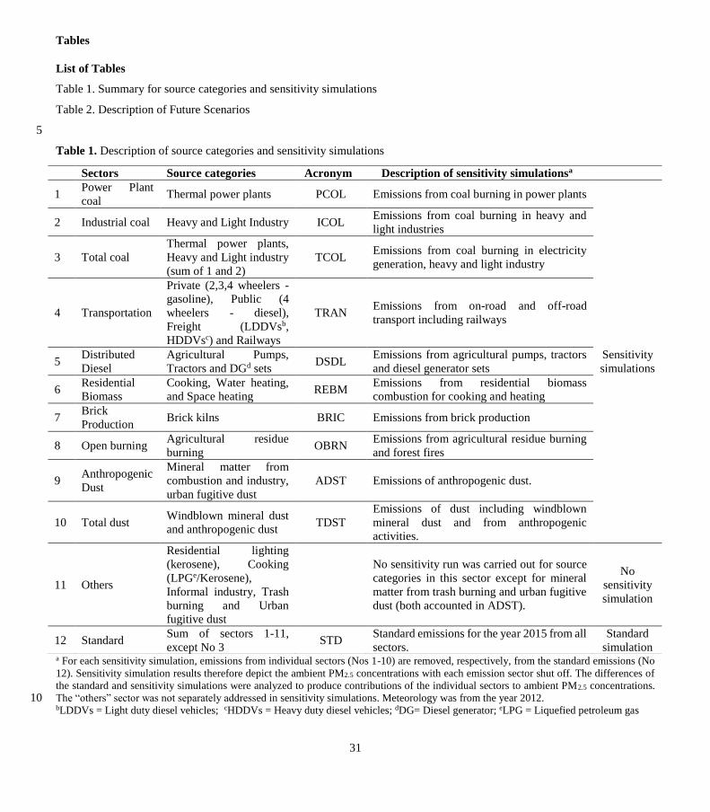
31

Tables

List of Tables

Table 1. Summary for source categories and sensitivity simulations

Table 2. Description of Future Scenarios

5

Table 1. Description of source categories and sensitivity simulations

a For each sensitivity simulation, emissions from individual sectors (Nos 1-10) are removed, respectively, from the standard emissions (No

12). Sensitivity simulation results therefore depict the ambient PM2.5 concentrations with each emission sector shut off. The differences of

the standard and sensitivity simulations were analyzed to produce contributions of the individual sectors to ambient PM2.5 concentrations.

The “others” sector was not separately addressed in sensitivity simulations. Meteorology was from the year 2012. 10 bLDDVs = Light duty diesel vehicles; cHDDVs = Heavy duty diesel vehicles; dDG= Diesel generator; eLPG = Liquefied petroleum gas

Sectors Source categories Acronym Description of sensitivity simulationsa

1 Power Plant

coal Thermal power plants PCOL Emissions from coal burning in power plants

2 Industrial coal Heavy and Light Industry ICOL Emissions from coal burning in heavy and

light industries

3 Total coal

Thermal power plants,

Heavy and Light industry

(sum of 1 and 2)

TCOL Emissions from coal burning in electricity

generation, heavy and light industry

4 Transportation

Private (2,3,4 wheelers -

gasoline), Public (4

wheelers - diesel),

Freight (LDDVsb,

HDDVsc) and Railways

TRAN Emissions from on-road and off-road

transport including railways

5 Distributed

Diesel

Agricultural Pumps,

Tractors and DGd sets DSDL

Emissions from agricultural pumps, tractors

and diesel generator sets

Sensitivity

simulations

6 Residential

Biomass

Cooking, Water heating,

and Space heating REBM

Emissions from residential biomass

combustion for cooking and heating

7 Brick

Production Brick kilns BRIC Emissions from brick production

8 Open burning Agricultural residue

burning OBRN

Emissions from agricultural residue burning

and forest fires

9 Anthropogenic

Dust

Mineral matter from

combustion and industry,

urban fugitive dust

ADST Emissions of anthropogenic dust.

10 Total dust Windblown mineral dust

and anthropogenic dust TDST

Emissions of dust including windblown

mineral dust and from anthropogenic

activities.

11 Others

Residential lighting

(kerosene), Cooking

(LPGe/Kerosene),

Informal industry, Trash

burning and Urban

fugitive dust

No sensitivity run was carried out for source

categories in this sector except for mineral

matter from trash burning and urban fugitive

dust (both accounted in ADST).

No

sensitivity

simulation

12 Standard Sum of sectors 1-11,

except No 3 STD

Standard emissions for the year 2015 from all

sectors.

Standard

simulation

32

Table 2. Description of Future Scenarios

Source

Sectors REF: Reference Scenario S2: Aspirational Scenario S3: Ambitious Scenario

Thermal

Power

Low influx of renewable

energy with large dominance of sub-critical power plants.

Share of renewable energy (40% by

2030) as targeted in India's NDC with

negligible flue gas desulphurization from a slow adoption of recent

regulation (MoEFCC, 2015).

75-80% of non-fossil power generation

(Anandarajah and Gambhir 2014; Shukla

and Chaturvedi 2012; Level 4, IESS, Niti Aayog, 2015); 80-95% use of flue gas

desulphurization.

Heavy and

Light

Industry

Set at present-day efficiency levels (58-75%).

Modest increases in energy efficiency

(62-84%) under the Perform Achieve and Trade (PAT) scheme (Level 2,

IESS, Niti Aayog, 2015).

Near complete shift to high efficiency

(85-100%) industrial technologies (Level

4, IESS, Niti Aayog, 2015).

Transport Present day share of public and private vehicles.

Promulgated growth in public vehicle

share (25-30%) (NTDPC, 2013;

Guttikunda and Mohan, 2014; NITI Aayog, 2015) with slower shifts to

BS-VI standards (MoRTH, 2016

ICRA, 2016).

Large shifts to public vehicles (40-60%)

(NITI Aayog, 2015), energy efficiency

improvements in engine technology (MoP, 2015) and increased share of

electric and CNG vehicle share (20-50%)

(NITI Aayog, 2015).

Brick and

Informal Industry

Largely dominated by traditional technologies such

as Bull’s trench kilns and

clamp kilns.

Modest increases in non-fired-brick walling materials (30-45%) (UNDP,

2009; Maithel, personal

communication, 2016).

Large share of non-fired brick walling materials (40-70%) and shift towards use

of gasifiers in informal industries (65-

80%).

Residential

Minor shift (~40%) to energy

efficient technologies and fuels.

Slow shift (55% in 2030 and 70% in

2050) to energy efficient technologies

and fuels (Level 2, IESS, Niti Aayog,

2015).

Large shifts (90% in 2030 and total in

2050) to LPG and electricity for cooking

and heating devices (Level 4, IESS, Niti

Aayog, 2015), with complete shift to

electric and solar lamps for lighting (National Solar Mission 2010).

Agricultural No reduction in agricultural

residue burning. No reduction in agricultural residue

burning.

Slow shift (35% phase out by 2030) and

complete phase-out (2050) of agricultural

residue burning through a switch to mulching practices (Gupta, 2014).

5

10

33

Figures

List of Figures

Figure 1. National Emissions of Particulate matter and Precursor Gases for 2015 (Mt/yr). Emissions of NOx are in Mt yr-1 of

NO; SO2 in Mt yr-1 of SO2. 5

Figure 2. Sectoral emission of fine (a) particulate matter, (d) black carbon and (g) organic carbon under the three scenarios,

for 2015-2030 (column 1). Difference of higher efficiency/emission control scenarios from reference(S2 & S3) are shown in

column 2 (b,e,h) and column 3 (c,f,i). Emissions from ECLIPSE V5a and GAINS-WEO2016 are shown for comparison.

Figure 3. Sectoral emission of fine (a) SO2, (d) NOx and (g) NMVOCs under the three scenarios, for 2015-2030 (column 1).

Difference of higher efficiency/emission control scenarios from reference(REF & S2) are shown in column 2 (b,e,h) and 10

column 3 (c,f,i). Emissions from ECLIPSE V5a and GAINS-WEO2016 are shown for comparison.

Figure 4. Model Evaluation by (a) comparison of simulated annual mean PM2.5 concentrations with in-situ observations

(circles = observations) and (b) comparison of modeled annual mean AOD over India with observations from MODIS.

Figure 5. Evaluation of model performance (NMB) in capturing seasonal variation in chemical species concentrations at two

sites in India. 15

Figure 6. Simulated PM2.5 concentration a) 2015 b) 2030 REF c) 2050 REF d) 2030 S2 e) 2050 S2 f) 2030 S3 g) 2050 S3.

(Values in the parenthesis represent area-weighted average PM2.5 concentration for India).

Figure 7. Population-weighted mean ambient PM2.5 concentrations by state for (a) 2015 and 2030 (REF, S2 and S3) and (b)

2015 and 2050 (REF, S2 and S3).

Figure 8. Percentage contribution to ambient PM2.5 attributable to different sources in 2015 and 2050 all three scenarios. 20

Figure 9. Percentage contribution of (a) Residential Biomass, (b) Anthropogenic dust, (c) Industrial coal, (d) Power plant coal,

(e) Open burning, (f) Brick production, (g) Transportation and (h) Distributed Diesel attributable to ambient PM2.5

concentration by state (2015 – 2050).

25

30

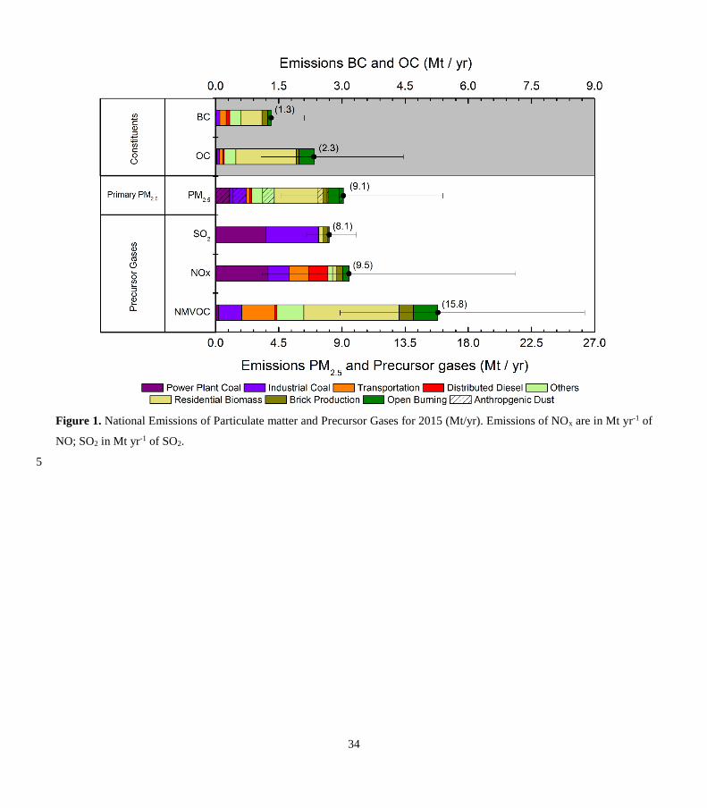
34

Figure 1. National Emissions of Particulate matter and Precursor Gases for 2015 (Mt/yr). Emissions of NOx are in Mt yr-1 of

NO; SO2 in Mt yr-1 of SO2.

5

35

Figure 2. Sectoral emission of fine (a) particulate matter, (d) black carbon and (g) organic carbon under the three scenarios,

for 2015-2030 (column 1). Difference of higher efficiency/emission control scenarios from reference(S2 & S3) are shown in

column 2 (b,e,h) and column 3 (c,f,i). Emissions from ECLIPSE V5a and GAINS-WEO2016 are shown for comparison. 5

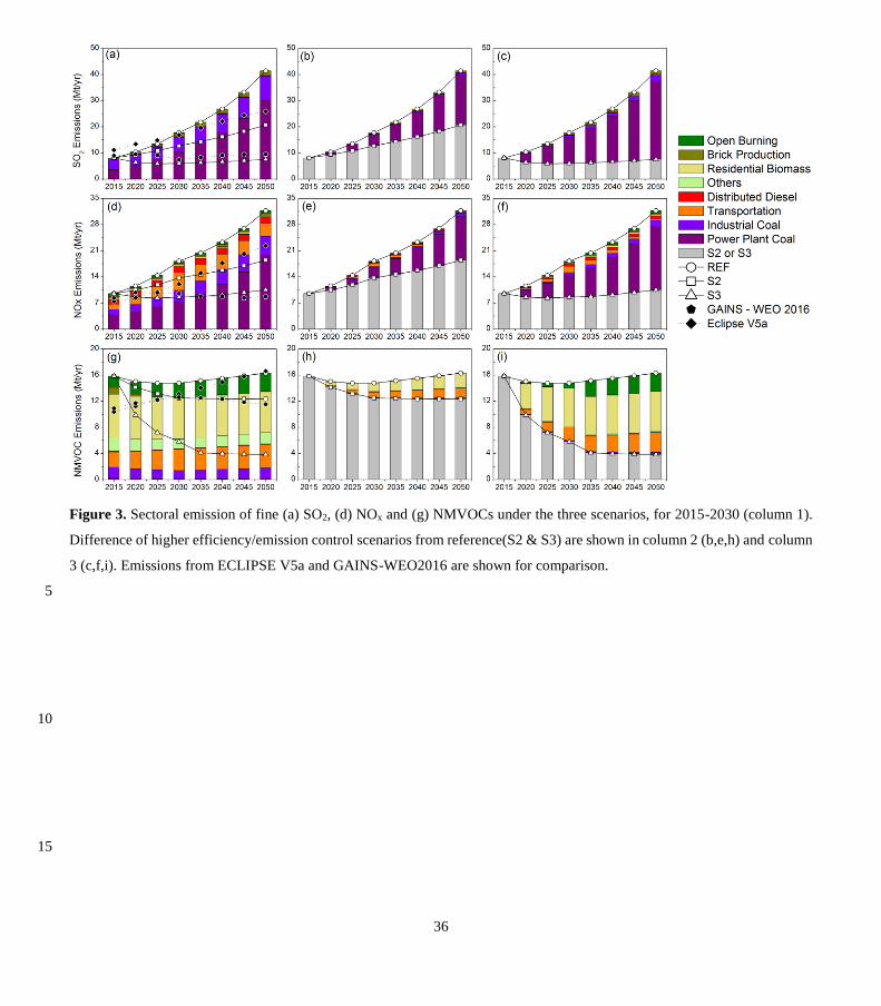
36

Figure 3. Sectoral emission of fine (a) SO2, (d) NOx and (g) NMVOCs under the three scenarios, for 2015-2030 (column 1).

Difference of higher efficiency/emission control scenarios from reference(S2 & S3) are shown in column 2 (b,e,h) and column

3 (c,f,i). Emissions from ECLIPSE V5a and GAINS-WEO2016 are shown for comparison.

5

10

15

37

5

Figure 4. Model Evaluation by (a) comparison of simulated annual mean PM2.5 concentrations with in-situ observations

(circles = observations) and (b) comparison of modeled annual mean AOD over India with observations from MODIS.

10

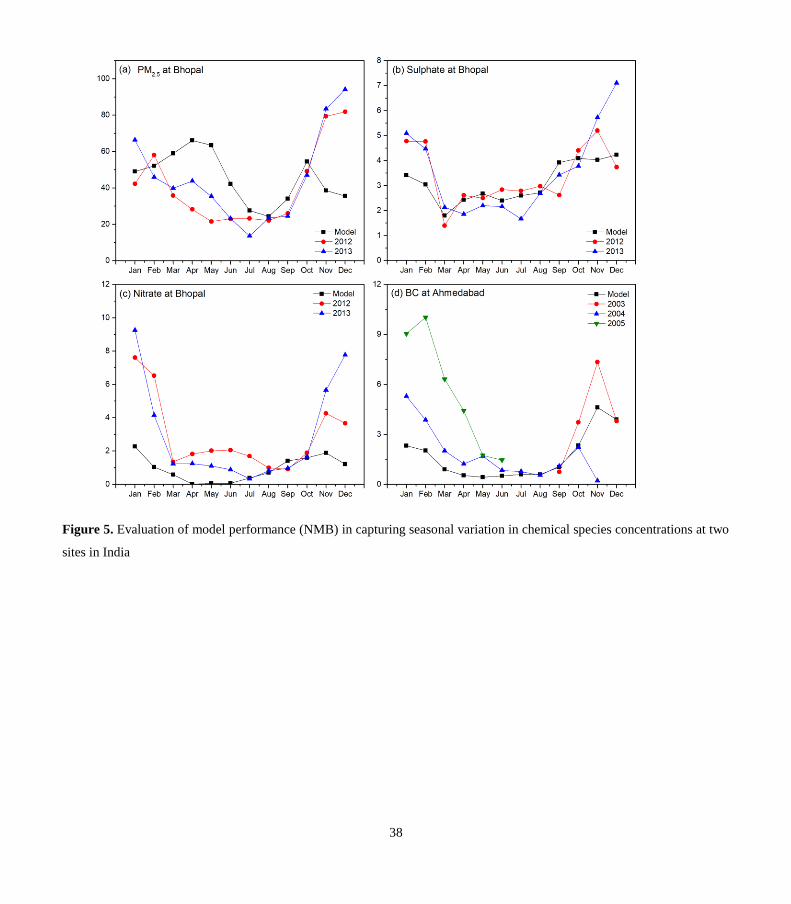
38

Figure 5. Evaluation of model performance (NMB) in capturing seasonal variation in chemical species concentrations at two

sites in India

39

Figure 6. Simulated PM2.5 concentration a) 2015 b) 2030 REF c) 2050 REF d) 2030 S2 e) 2050 S2 f) 2030 S3 g) 2050 S3.

(Values in the parenthesis represent area-weighted average PM2.5 concentration for India)

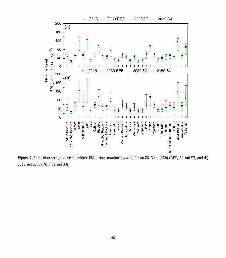
40

Figure 7. Population-weighted mean ambient PM2.5 concentrations by state for (a) 2015 and 2030 (REF, S2 and S3) and (b)

2015 and 2050 (REF, S2 and S3)

41

Figure 8. Percentage contribution to ambient PM2.5 attributable to different sources in 2015 and 2050 all three scenarios.

42

Figure 9. Percentage contribution of (a) Residential Biomass, (b) Anthropogenic dust, (c) Industrial coal, (d) Power plant coal,

(e) Open burning, (f) Brick production, (g) Transportation and (h) Distributed Diesel attributable to ambient PM2.5

concentration by state (2015 – 2050). 5

SUPPLEMENTARY MATERIAL

Source influence on emission pathways and ambient PM2.5

pollution over India (2015-2050)

Chandra Venkataraman1,3, Michael Brauer2, Kushal Tibrewal3, Pankaj Sadavarte3,4, Qiao Ma5,

Aaron Cohen6, Sreelekha Chaliyakunnel7, Joseph Frostad8, Zbigniew Klimont9, Randall V.

Martin10, Dylan B. Millet7, Sajeev Philip10,11, Katherine Walker6, Shuxiao Wang5,12

1Department of Chemical Engineering, Indian Institute of Technology Bombay, Powai, Mumbai, India 2School of Population and Public Health, The University of British Columbia, Vancouver, British Columbia V6T1Z3,

Canada 3Interdisciplinary program in Climate Studies, Indian Institute of Technology Bombay, Powai, Mumbai, India 4Institute for Advanced Sustainability Studies (IASS), Berliner Str. 130, 14467 Potsdam, Germany 5State Key Joint Laboratory of Environment Simulation and Pollution Control, School of Environment, Tsinghua

University, Beijing 100084, China 6Health Effects Institute, Boston, MA 02110, USA 7Department of Soil, Water, and Climate, University of Minnesota, Minneapolis–Saint Paul, MN 55108, USA 8Institute for Health Metrics and Evaluation, University of Washington, Seattle, WA 98195, USA 9International Institute for Applied Systems Analysis, Laxenburg, Austria 10Department of Physics and Atmospheric Science, Dalhousie University, Halifax, Nova Scotia B3H 4R2, Canada 11 NASA Ames Research Center, Moffett Field, California, USA 12State Environmental Protection Key Laboratory of Sources and Control of Air Pollution Complex, Beijing 100084,

China

Correspondence to: Chandra Venkataraman (chandra@iitb.ac.in)

List of Figures:

Figure S1. Methodology for estimation of future sectoral activity, apportionment to technology mix and

related scenario based emissions. .................................................................................................................. 6 Figure S2. Sectoral Growth between 2015- 2050. Growth rates were computed based on analysis of existing

data and reviewed literature. ......................................................................................................................... 7 Figure S3. Energy Evolution in Scenarios REF, S2 and S3 ....................................................................... 13 Figure S4. Comparisons of national totals of SLCPs with HTAP_v2, REAS2.1 and ECLIPSE for 2008 and

2010. ........................................................................................................................................................... 17 Figure S5. Percentage deviation in emissions of ECLIPSE V5a and GAINS-WEO2016 from emissions of

this study by sector. ..................................................................................................................................... 18 Figure S6. Top 20 polluted cities in India (2016) ...................................................................................... 21 Figure S7. Mean population-weighted ambient PM2.5 concentrations for 2015 and future scenarios. The

bars represent the 95% Confidence Interval for the estimates. ................................................................... 22

List of Tables:

Table S1. Spatial proxies used to distribute emissions................................................................................. 3 Table S2. Emissions for 2015 by state (MT/yr) ........................................................................................... 4 Table S3. Uncertainty Bounds (95% Confidence Levels) for Indian Emissions of Individual Pollutants by

Sector ............................................................................................................................................................ 5 Table S4. Sectoral growth rates for 2015-2030 and 2030-2050 ................................................................... 7 Table S5. Technology fraction for major emissions emitting sectors .......................................................... 9 Table S6. Specific energy per unit activity for each technology (PJ/activity) ........................................... 11 Table S7. Energy demand for each technology (EJ/year) .......................................................................... 13 Table S8. Emission factors of SLCP's, fine particulate matter and CO2 (g/kg of fuel used) ..................... 15 Table S9. Representative Concentration Pathways (RCP) scenarios values over India............................. 20 Table S10. Description of GEOS-CHEM NMVOC species ...................................................................... 21

S1. Present day emissions at state-level and sectoral uncertainties in emissions

Table S1. Spatial proxies used to distribute emissions

Source Category/Activity Proxies Reference

Brick production

Distributed at district level using district-wise no.

of household built using burnt bricks, excluding

the cities with high population densities and

distributing the emissions from those city grids in

the surrounding grids.

Census, 2011

Food and agro processing

(Jaggery making, cashewnut

processing unit, tea and

coffee drying, spices drying,

silk reeling and dairy

processing)

Jaggery making – district level sugarcane

produced Ministry of Agriculture;

Cashewnut, tea, coffee – distributed to specific

districts with production as proxy

Cashew Manufacturer’s

Association;

Spices drying – district level spices produced Indian Tea Association;

Silk reeling – distributed to specific states

(production) carrying this activity with rural

population further at district level

Coffee Board of India;

Dairy processing – emissions distributed

according to state production and further acc. to

rural population at district level

Central silk board;

Department of animal

husbandry

Thermal power, Cement,

Fertilizer, Iron & Steel (ISP

& Secondary producers),

Non-ferrous, Refineries

Point sources with specific latitude and longitude

known Web source

Other industry, Iron & Steel

(EAF, IF, Sponge iron)

Distributed at district level using urban population

as proxy Census, 2011

On-road gasoline vehicles &

LDV diesel vehicles

Distributed at district level using urban population

as proxy Census, 2011

On-road diesel vehicles

including HDV, Buses and

Superemitters

Distributed on road network with following

assumption: 40% National highway; 30% Golden

Quadrilateral network; 20% State highway and

10% District roads and city grids

25 × 25km2 Gridded

shape-file showing

various road networks

Residential cooking – solid

fuel (fuelwood/

dungcake/crop residue/ coal)

Distributed at district level using no. of

households using fuelwood, dungcake, crop

residue and coal as fuel

Census, 2011 Residential cooking – LPG/

kerosene/biogas

Distributed at district level using no. of

households using LPG, kerosene and biogas as

fuel

Residential lighting –

kerosene Distributed at district level using rural population

Agricultural residue burning Distributed at district level using district-wise

cereals and sugarcane produced during 2010-11

Ministry of Agriculture,

2011

Agriculture diesel use Distributed at district level using district-wise area

cultivated during 2010-11

Ministry of Agriculture,

2011

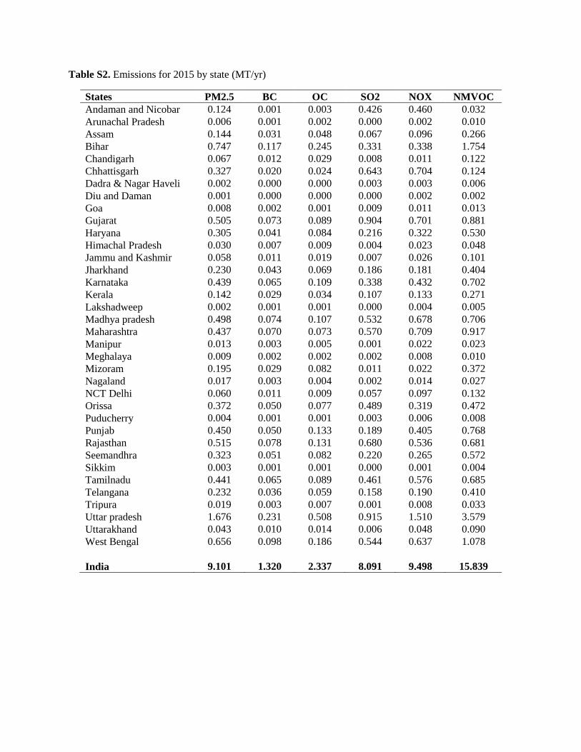
Table S2. Emissions for 2015 by state (MT/yr)

States PM2.5 BC OC SO2 NOX NMVOC

Andaman and Nicobar 0.124 0.001 0.003 0.426 0.460 0.032

Arunachal Pradesh 0.006 0.001 0.002 0.000 0.002 0.010

Assam 0.144 0.031 0.048 0.067 0.096 0.266

Bihar 0.747 0.117 0.245 0.331 0.338 1.754

Chandigarh 0.067 0.012 0.029 0.008 0.011 0.122

Chhattisgarh 0.327 0.020 0.024 0.643 0.704 0.124

Dadra & Nagar Haveli 0.002 0.000 0.000 0.003 0.003 0.006

Diu and Daman 0.001 0.000 0.000 0.000 0.002 0.002

Goa 0.008 0.002 0.001 0.009 0.011 0.013

Gujarat 0.505 0.073 0.089 0.904 0.701 0.881

Haryana 0.305 0.041 0.084 0.216 0.322 0.530

Himachal Pradesh 0.030 0.007 0.009 0.004 0.023 0.048

Jammu and Kashmir 0.058 0.011 0.019 0.007 0.026 0.101

Jharkhand 0.230 0.043 0.069 0.186 0.181 0.404

Karnataka 0.439 0.065 0.109 0.338 0.432 0.702

Kerala 0.142 0.029 0.034 0.107 0.133 0.271

Lakshadweep 0.002 0.001 0.001 0.000 0.004 0.005

Madhya pradesh 0.498 0.074 0.107 0.532 0.678 0.706

Maharashtra 0.437 0.070 0.073 0.570 0.709 0.917

Manipur 0.013 0.003 0.005 0.001 0.022 0.023

Meghalaya 0.009 0.002 0.002 0.002 0.008 0.010

Mizoram 0.195 0.029 0.082 0.011 0.022 0.372

Nagaland 0.017 0.003 0.004 0.002 0.014 0.027

NCT Delhi 0.060 0.011 0.009 0.057 0.097 0.132

Orissa 0.372 0.050 0.077 0.489 0.319 0.472

Puducherry 0.004 0.001 0.001 0.003 0.006 0.008

Punjab 0.450 0.050 0.133 0.189 0.405 0.768

Rajasthan 0.515 0.078 0.131 0.680 0.536 0.681

Seemandhra 0.323 0.051 0.082 0.220 0.265 0.572

Sikkim 0.003 0.001 0.001 0.000 0.001 0.004

Tamilnadu 0.441 0.065 0.089 0.461 0.576 0.685

Telangana 0.232 0.036 0.059 0.158 0.190 0.410

Tripura 0.019 0.003 0.007 0.001 0.008 0.033

Uttar pradesh 1.676 0.231 0.508 0.915 1.510 3.579

Uttarakhand 0.043 0.010 0.014 0.006 0.048 0.090

West Bengal 0.656 0.098 0.186 0.544 0.637 1.078

India 9.101 1.320 2.337 8.091 9.498 15.839

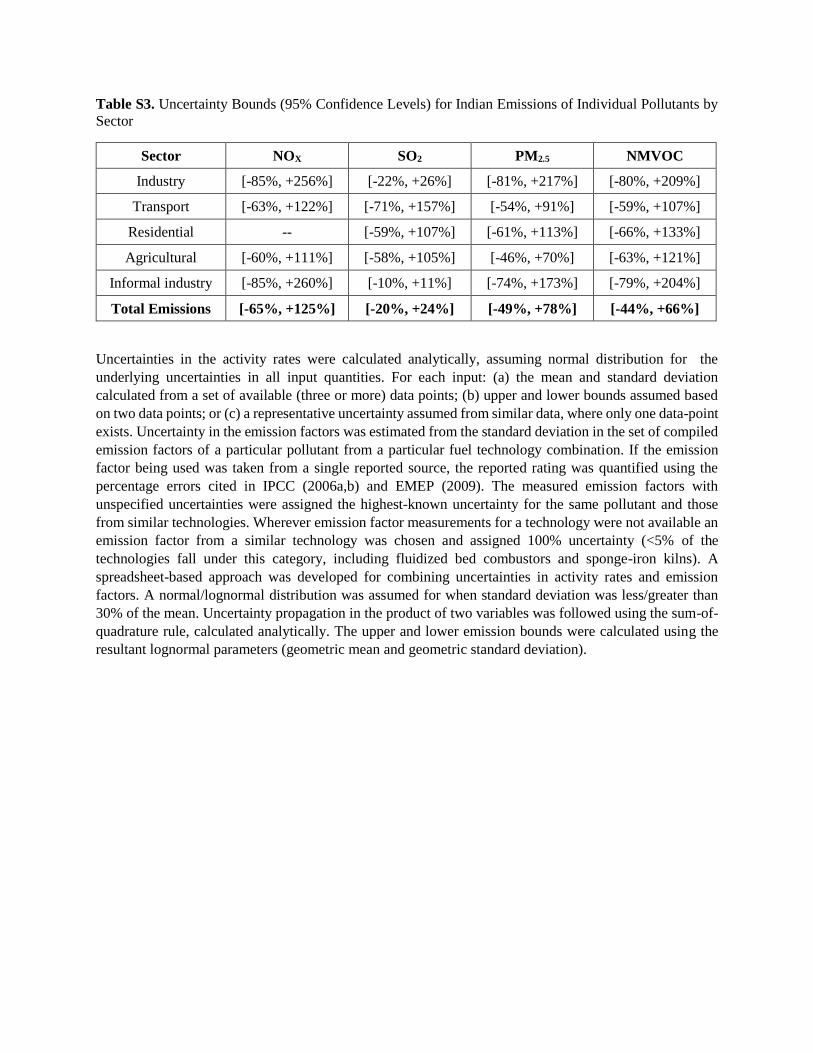
Table S3. Uncertainty Bounds (95% Confidence Levels) for Indian Emissions of Individual Pollutants by

Sector

Sector NOX SO2 PM2.5 NMVOC

Industry [-85%, +256%] [-22%, +26%] [-81%, +217%] [-80%, +209%]

Transport [-63%, +122%] [-71%, +157%] [-54%, +91%] [-59%, +107%]

Residential -- [-59%, +107%] [-61%, +113%] [-66%, +133%]

Agricultural [-60%, +111%] [-58%, +105%] [-46%, +70%] [-63%, +121%]

Informal industry [-85%, +260%] [-10%, +11%] [-74%, +173%] [-79%, +204%]

Total Emissions [-65%, +125%] [-20%, +24%] [-49%, +78%] [-44%, +66%]

Uncertainties in the activity rates were calculated analytically, assuming normal distribution for the

underlying uncertainties in all input quantities. For each input: (a) the mean and standard deviation

calculated from a set of available (three or more) data points; (b) upper and lower bounds assumed based

on two data points; or (c) a representative uncertainty assumed from similar data, where only one data-point

exists. Uncertainty in the emission factors was estimated from the standard deviation in the set of compiled

emission factors of a particular pollutant from a particular fuel technology combination. If the emission

factor being used was taken from a single reported source, the reported rating was quantified using the

percentage errors cited in IPCC (2006a,b) and EMEP (2009). The measured emission factors with

unspecified uncertainties were assigned the highest-known uncertainty for the same pollutant and those

from similar technologies. Wherever emission factor measurements for a technology were not available an

emission factor from a similar technology was chosen and assigned 100% uncertainty (<5% of the

technologies fall under this category, including fluidized bed combustors and sponge-iron kilns). A

spreadsheet-based approach was developed for combining uncertainties in activity rates and emission

factors. A normal/lognormal distribution was assumed for when standard deviation was less/greater than

30% of the mean. Uncertainty propagation in the product of two variables was followed using the sum-of-

quadrature rule, calculated analytically. The upper and lower emission bounds were calculated using the

resultant lognormal parameters (geometric mean and geometric standard deviation).

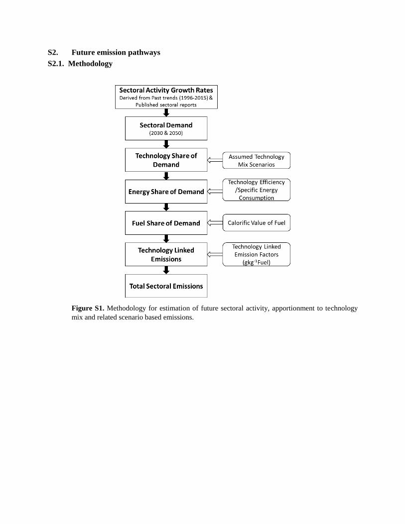
S2. Future emission pathways

S2.1. Methodology

Figure S1. Methodology for estimation of future sectoral activity, apportionment to technology

mix and related scenario based emissions.

S2.2. Evolution of sectoral demand

Figure S2. Sectoral Growth between 2015- 2050. Growth rates were computed based on analysis of existing

data and reviewed literature.

Table S4. Sectoral growth rates for 2015-2030 and 2030-2050

Sectors Activity Name Activity Growth rates in % per year

2015 2015 - 2030 2030 - 2050

Growth

rate from

2000-

2015 data

IESSaGrowth

Rate

Published

growth

rate

This

Study

IESSaGrowth

Rate

Published

growth

rate

This

Study

Electricity generation

Installed capacity (GW)

270 6.89 6.31 6.7b 6.63 1.84 NIL 1.84

Industry

Production (MT)

Cement 215 5.06 5.63 7.08c 6.07 2.86 NIL 3.1

Iron and steel 88 4.49 8.03 3.26d 4.5 2.93 NIL 2.5

Fertilizer 190 1.77 1.04 2.86e 2.32 0.02 NIL 0.04

Non-ferrous 4 6.65 9.74 11.3f 11.3 6.77 NIL 6.23

Brick

production

Number of bricks

(in billion)

(similar to

construction

growth)

250 NIL NIL 6.6g 6.6 NIL NIL 3.37

Transport

Passenger-kilometre (in

billion)

9997 6.54* 5.02 NIL 5.78 2.42 NIL 2.89

Freight-kilometre (in billion)

2564 3.61 - NIL 3.61 - NIL 1.8

Residential

Household number

(in million)

(similar to population growth)

270 1.39 1.88 1.1h 1.25 1.57 0.47h 0.53

Agriculture Crop production

(KT) 578 1.02 NIL ~ 1 to 1.1i 1.02 NIL NIL 1.02

(i.e. cereal produced)

* Growth rate calculated for data from 1996 - 2015

Sources: [Short forms in brackets]

a) India Energy Security Scenarios 2047, NITI Aayog, Govt. of India, 2015 [NITI Aayog 2015] b) Data from the Ministry of Environment, Forest and Climate Change (MoEFCC) analysed by the Prayas Energy Group, 2011 [MoEFCC,

2011]

c) International Energy Agency, 2009 [IEA, 2009] d) Dr.A.S.Firoz, Economic Research Unit, 2014 [Firoz, 2014]

e) Industry Group for Petroleum & Natural Gas Regulatory Board, 2013 [PNGRB, 2013]

f) Prof. K.S.S. Murthy, Gen. Secretary, Aluminium Association of India, 2014 [Murthy, 2014] g) Maithelet. al., Study report prepared by Green Knowledge Solutions, New Delhi, 2012 [Maithel et al., 2012]

h) Shukla, P. R., et al. "Low Carbon Society Vision 2050. India. Indian Institute of Management Ahmedabad." National Institute for

Environmental Studies, Kyoto University and Mizuho Information & Research Institute,2009 [Shukla et al., 2009] i) Ray, D.K., Mueller, N.D., West, P.C. and Foley, J.A., 2013. Yield trends are insufficient to double global crop production by 2050. PloS one,

8(6), p.e66428. [Ray et. al., 2013]

S2.3 Evolution of technology mix

In 2015, power generation was almost entirely from subcritical pressure thermal power plants with an

average gross efficiency of 30.5% (IEP, 2006; IESS, NITI Aayog 2015). A switch to more efficient

technologies such as supercritical (SC), ultra-supercritical (USC), and integrated gasification combined

cycle (IGCC) is expected in future. For 2030 and 2050, respectively, the non-fossil shares were assumed to

be 30% and 40% in REF, 40% and 60% in S2, and 75% and 80% in S3. The assumed technology mix in

S2 follows the NDC’s proposed non-fossil share of 2030. In S3, it is consistent with high efficiency-low

carbon growth cases in earlier studies (Anandarajah and Gambhir 2014; Shukla and Chaturvedi 2012; Level

4, IESS, Niti Aayog, 2015). The transition of thermal power plants sub-critical boiler technology to more

efficient technologies like super-critical, ultra-super-critical and integrated gasification combined cycle

(IGCC) is based on published scenarios (IEP, 2006; IESS, Niti Aayog, 2015).

Emissions from on-road vehicles are based from a previous study (Pandey and Venkataraman, 2014). The

detailed list of vehicle category is included in the study (Table 3, Pandey and Venkataraman, 2014). Two-

wheelers contribute the most to the fleet of private vehicles with approximately 82% share, followed by

passenger cars (15%) and three-wheelers (3%). For present day, all vehicles are assumed to be compliant

with BS III standards with 2 wheelers having the highest emission levels for PM2.5 followed by three

wheelers (0.5 times lower) and gasoline cars (0.1 times lower). Future shifts to BS IV and BS VI emission

standards lead to reductions in emission levels by 80% and 90% respectively. In the transport sector, current

technology shares are 81% private vehicles (two-wheeler, three-wheeler and cars) and 19% public vehicles

(buses and taxis) (Pandey and Venkataraman, 2014). The share of private vehicles is projected to increase

in a reference scenario till 2030, especially for two-wheelers and cars (NTDPC, 2013; Guttikunda and

Mohan, 2014). However, beyond 2030, as GDP stabilizes, no further increase in private vehicle share is

assumed, with a greater demand for public transport. Therefore, in the S2 scenario, private vehicle share is

assumed as 75% and 70% in 2030 and 2050, respectively. For S3 private vehicle share is assumed to

decrease rapidly to 60% in 2030 and 40% in 2050 in consistent with Level 2 of IESS (NITI Aayog, 2015)

(Table S5). For future emissions, Auto Fuel Policy (Auto Fuel Policy Vision 2025, 2014) recommendations

were applied, wherein 2/3-wheelers were proposed to have Bharat Stage (BS)-IV standards from 1st April

2015, light and heavy duty diesel vehicles to have BS-Va and BS-Vb. There is a recent proposal to leapfrog

directly to BS-VI for all on-road vehicle categories by 2020 (MoRTH, 2016). However, scenarios used

here, do not reflect such a quick change, keeping the share of BS-VI at modest levels owing to expected

delays in availability of BS-VI compliant fuels and/or difficulties in making the technologies adaptive to

Indian road conditions as well as cost-effective (ICRA, 2016), along with the use of non-BS-VI compliant

vehicles in peri-urban and rural areas. In the transport sector, engine efficiency improvements are not

foreseen to have significant increases across technologies (e.g. across BS-III to BS-VI) as these standards

primarily govern the control of emissions of air pollutants. Until 2015 there were no fuel economy standards

for India. However, energy efficiency improvement are assumed over the years in the S3 scenario keeping

in mind the recently proposed fuel economy targets (MoP, 2015)

In the brick sector, currently 76% of total bricks are produced by Bull's trench kilns (BTK) and 21% by

clamp kilns. Clamp kilns are highly polluting, with sun-dried bricks, stacked alternately with layers of

powdered fuel, allowed to smolder until the bricks are baked. The demand for non-fired-brick walling

materials is currently negligible, but expected to rise (10-25% in REF, 30-45% in S2 and 40-75% in S3 for

2030-2050), from increased availability of hollow-block technology and the governmental incentives for

fly-ash bricks (UNDP, 2009). For fired bricks, cleaner technologies include a retrofit to existing Bull’s

trench kilns, called zig-zag firing, or significantly more capital intensive, vertical shaft brick kilns (VSBK)

which have increased efficiency. For small clamp kilns, it is believed that regulation may not be effective,

so a constant activity level, but a decreasing share was assumed in future, with new cleaner technologies

filling growing demand (personal communication, Maithel, 2015).

Evolution of technologies in informal industry from say traditional wood furnaces, presently supplying all

energy requirements, to gasifier and LPG based technologies is assumed to increase in 2030 and 2050

respectively, to 20% and 35% in S2 and 65% and 80% in S3 (Table S5).

India’s rural population largely depends on biomass fuels for cooking and lighting (Venkataraman et al.

2010). Although India has introduced improved biomass cook-stoves to improve fuel efficiency and to

reduce smoke exposure using chimneys or combustion improvements, further technological improvements

or alternatives are required to reach LPG-like emission levels to reduce disease risk due to household

biomass burning. The REF scenario assumes an increasing penetration rate of liquefied petroleum gas

(LPG) and piped natural gas (PNG) typical of 1995–2015 (Pandey et al. 2014). In the S2 and S3 scenarios,

assumed future switch in residential energy to use of LPG/PNG or low-emission biomass gasifier stoves

and biogas, is consistent with energy efficiency increases proposed in Levels 2 and 4 of the IESS (NITI

Aayog 2015). We use lower rates of clean technology adoption in the residential sector in both the REF and

S2 scenarios, because no current legislation or standards target this sector, but a complete switch away from

traditional biomass fuels in S3. In case of lighting, 37% usage is of highly polluting kerosene wick lamps

and lanterns, which emit large amounts of black carbon (Lam et al. 2012), while the balance is of electricity,

with less than 1% solar lamps. Residential lighting is assumed to shift from a modest present-day

dependence on kerosene to a complete switch to electricity and solar lamps in 2030 and 2050 (National

Solar Mission 2010), a change expected with a national promotion of renewable energy.

In the agricultural sector it is assumed, based on satellite active fire cycles in agricultural land-use

areas(Venkataraman et al., 2006), that residues of cereal and sugarcane are burned in field. Gupta (2014)

indicated greater mechanization of agriculture, with decrease in amounts of residue, but increase in

incidence of field burning, needed to clear the rubble consisting of 6-12 inch stalks, before sowing.

Mulching technology was reported to allow sowing even through rubble and loosely spread residue, thus

avoiding burning for field clearing. The present work applies different levels of mulching, replacing field

burning, in future years (Table S5).

Table S5. Technology fraction for major emissions emitting sectors

Sector

Source

Categories TechMix REF S2 S3

2015 2030 2050 2030 2050 2030 2050

Thermal

power Thermal power

Fossil-fuel energy 0.70 0.70 0.60 0.60 0.40 0.25 0.2

Coal fraction 0.61 0.59 0.48 0.48 0.24 0.20 0.12

Gas fraction 0.09 0.11 0.12 0.12 0.16 0.05 0.08

Non-carbon

energy 0.30 0.30 0.40 0.40 0.60 0.75 0.80

Sub-critical 1.00 0.90 0.70 0.65 0.55 0.40 0.30

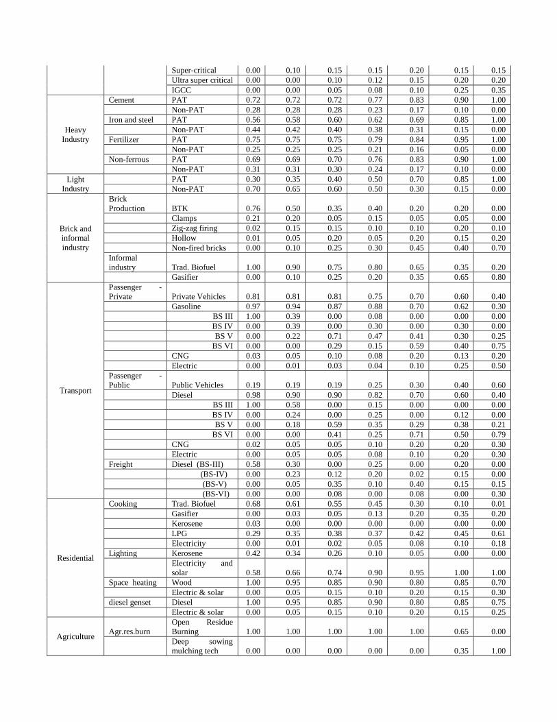
Super-critical 0.00 0.10 0.15 0.15 0.20 0.15 0.15

Ultra super critical 0.00 0.00 0.10 0.12 0.15 0.20 0.20

IGCC 0.00 0.00 0.05 0.08 0.10 0.25 0.35

Heavy

Industry

Cement PAT 0.72 0.72 0.72 0.77 0.83 0.90 1.00

Non-PAT 0.28 0.28 0.28 0.23 0.17 0.10 0.00

Iron and steel PAT 0.56 0.58 0.60 0.62 0.69 0.85 1.00

Non-PAT 0.44 0.42 0.40 0.38 0.31 0.15 0.00

Fertilizer PAT 0.75 0.75 0.75 0.79 0.84 0.95 1.00

Non-PAT 0.25 0.25 0.25 0.21 0.16 0.05 0.00

Non-ferrous PAT 0.69 0.69 0.70 0.76 0.83 0.90 1.00

Non-PAT 0.31 0.31 0.30 0.24 0.17 0.10 0.00

Light

Industry

PAT 0.30 0.35 0.40 0.50 0.70 0.85 1.00

Non-PAT 0.70 0.65 0.60 0.50 0.30 0.15 0.00

Brick and

informal

industry

Brick

Production BTK 0.76 0.50 0.35 0.40 0.20 0.20 0.00

Clamps 0.21 0.20 0.05 0.15 0.05 0.05 0.00

Zig-zag firing 0.02 0.15 0.15 0.10 0.10 0.20 0.10

Hollow 0.01 0.05 0.20 0.05 0.20 0.15 0.20

Non-fired bricks 0.00 0.10 0.25 0.30 0.45 0.40 0.70

Informal

industry Trad. Biofuel 1.00 0.90 0.75 0.80 0.65 0.35 0.20

Gasifier 0.00 0.10 0.25 0.20 0.35 0.65 0.80

Transport

Passenger -

Private Private Vehicles 0.81 0.81 0.81 0.75 0.70 0.60 0.40

Gasoline 0.97 0.94 0.87 0.88 0.70 0.62 0.30

BS III 1.00 0.39 0.00 0.08 0.00 0.00 0.00

BS IV 0.00 0.39 0.00 0.30 0.00 0.30 0.00

BS V 0.00 0.22 0.71 0.47 0.41 0.30 0.25

BS VI 0.00 0.00 0.29 0.15 0.59 0.40 0.75

CNG 0.03 0.05 0.10 0.08 0.20 0.13 0.20

Electric 0.00 0.01 0.03 0.04 0.10 0.25 0.50

Passenger -

Public Public Vehicles 0.19 0.19 0.19 0.25 0.30 0.40 0.60

Diesel 0.98 0.90 0.90 0.82 0.70 0.60 0.40

BS III 1.00 0.58 0.00 0.15 0.00 0.00 0.00

BS IV 0.00 0.24 0.00 0.25 0.00 0.12 0.00

BS V 0.00 0.18 0.59 0.35 0.29 0.38 0.21

BS VI 0.00 0.00 0.41 0.25 0.71 0.50 0.79

CNG 0.02 0.05 0.05 0.10 0.20 0.20 0.30

Electric 0.00 0.05 0.05 0.08 0.10 0.20 0.30

Freight Diesel (BS-III) 0.58 0.30 0.00 0.25 0.00 0.20 0.00

(BS-IV) 0.00 0.23 0.12 0.20 0.02 0.15 0.00

(BS-V) 0.00 0.05 0.35 0.10 0.40 0.15 0.15

(BS-VI) 0.00 0.00 0.08 0.00 0.08 0.00 0.30

Residential

Cooking Trad. Biofuel 0.68 0.61 0.55 0.45 0.30 0.10 0.01

Gasifier 0.00 0.03 0.05 0.13 0.20 0.35 0.20

Kerosene 0.03 0.00 0.00 0.00 0.00 0.00 0.00

LPG 0.29 0.35 0.38 0.37 0.42 0.45 0.61

Electricity 0.00 0.01 0.02 0.05 0.08 0.10 0.18

Lighting Kerosene 0.42 0.34 0.26 0.10 0.05 0.00 0.00

Electricity and

solar 0.58 0.66 0.74 0.90 0.95 1.00 1.00

Space heating Wood 1.00 0.95 0.85 0.90 0.80 0.85 0.70

Electric & solar 0.00 0.05 0.15 0.10 0.20 0.15 0.30

diesel genset Diesel 1.00 0.95 0.85 0.90 0.80 0.85 0.75

Electric & solar 0.00 0.05 0.15 0.10 0.20 0.15 0.25

Agriculture Agr.res.burn

Open Residue

Burning 1.00 1.00 1.00 1.00 1.00 0.65 0.00

Deep sowing

mulching tech 0.00 0.00 0.00 0.00 0.00 0.35 1.00

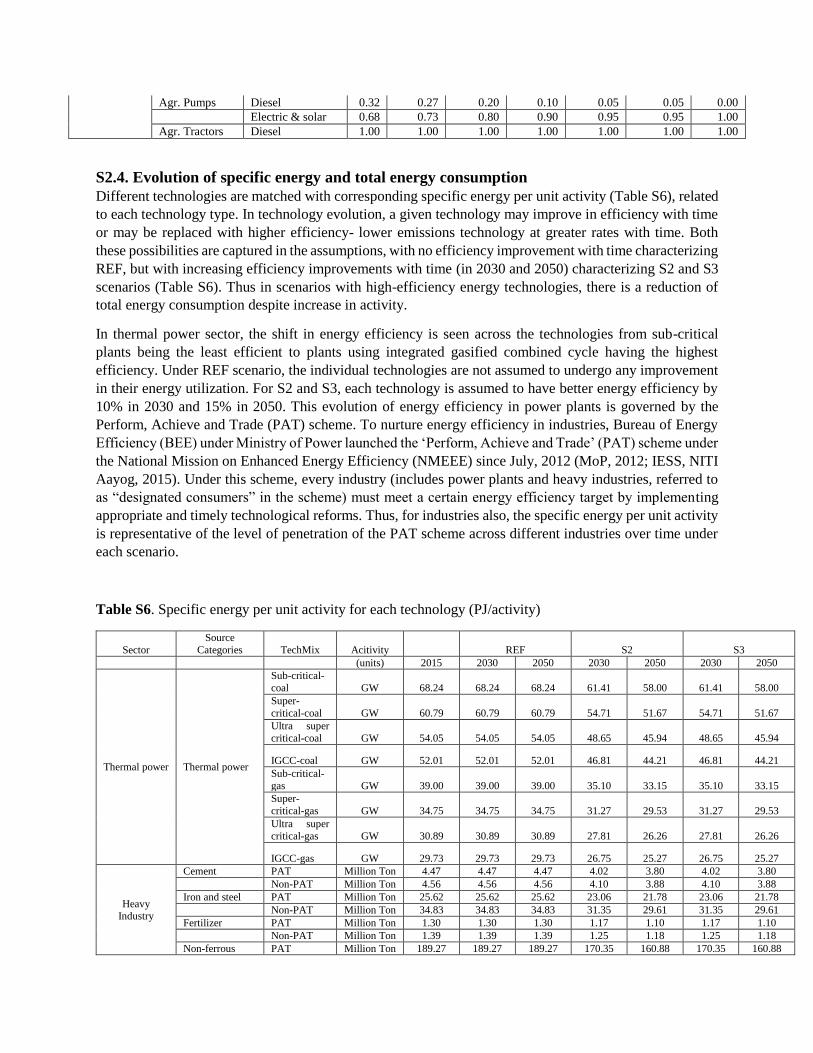
Agr. Pumps Diesel 0.32 0.27 0.20 0.10 0.05 0.05 0.00

Electric & solar 0.68 0.73 0.80 0.90 0.95 0.95 1.00

Agr. Tractors Diesel 1.00 1.00 1.00 1.00 1.00 1.00 1.00

S2.4. Evolution of specific energy and total energy consumption

Different technologies are matched with corresponding specific energy per unit activity (Table S6), related

to each technology type. In technology evolution, a given technology may improve in efficiency with time

or may be replaced with higher efficiency- lower emissions technology at greater rates with time. Both

these possibilities are captured in the assumptions, with no efficiency improvement with time characterizing

REF, but with increasing efficiency improvements with time (in 2030 and 2050) characterizing S2 and S3

scenarios (Table S6). Thus in scenarios with high-efficiency energy technologies, there is a reduction of

total energy consumption despite increase in activity.

In thermal power sector, the shift in energy efficiency is seen across the technologies from sub-critical

plants being the least efficient to plants using integrated gasified combined cycle having the highest

efficiency. Under REF scenario, the individual technologies are not assumed to undergo any improvement

in their energy utilization. For S2 and S3, each technology is assumed to have better energy efficiency by

10% in 2030 and 15% in 2050. This evolution of energy efficiency in power plants is governed by the

Perform, Achieve and Trade (PAT) scheme. To nurture energy efficiency in industries, Bureau of Energy

Efficiency (BEE) under Ministry of Power launched the ‘Perform, Achieve and Trade’ (PAT) scheme under

the National Mission on Enhanced Energy Efficiency (NMEEE) since July, 2012 (MoP, 2012; IESS, NITI

Aayog, 2015). Under this scheme, every industry (includes power plants and heavy industries, referred to

as “designated consumers” in the scheme) must meet a certain energy efficiency target by implementing

appropriate and timely technological reforms. Thus, for industries also, the specific energy per unit activity

is representative of the level of penetration of the PAT scheme across different industries over time under

each scenario.

Table S6. Specific energy per unit activity for each technology (PJ/activity)

Sector

Source

Categories TechMix Acitivity REF S2 S3

(units) 2015 2030 2050 2030 2050 2030 2050

Thermal power Thermal power

Sub-critical-

coal GW 68.24 68.24 68.24 61.41 58.00 61.41 58.00

Super-

critical-coal GW 60.79 60.79 60.79 54.71 51.67 54.71 51.67

Ultra super

critical-coal GW 54.05 54.05 54.05 48.65 45.94 48.65 45.94

IGCC-coal GW 52.01 52.01 52.01 46.81 44.21 46.81 44.21

Sub-critical-

gas GW 39.00 39.00 39.00 35.10 33.15 35.10 33.15

Super-

critical-gas GW 34.75 34.75 34.75 31.27 29.53 31.27 29.53

Ultra super

critical-gas GW 30.89 30.89 30.89 27.81 26.26 27.81 26.26

IGCC-gas GW 29.73 29.73 29.73 26.75 25.27 26.75 25.27

Heavy Industry

Cement PAT Million Ton 4.47 4.47 4.47 4.02 3.80 4.02 3.80

Non-PAT Million Ton 4.56 4.56 4.56 4.10 3.88 4.10 3.88

Iron and steel PAT Million Ton 25.62 25.62 25.62 23.06 21.78 23.06 21.78

Non-PAT Million Ton 34.83 34.83 34.83 31.35 29.61 31.35 29.61

Fertilizer PAT Million Ton 1.30 1.30 1.30 1.17 1.10 1.17 1.10

Non-PAT Million Ton 1.39 1.39 1.39 1.25 1.18 1.25 1.18

Non-ferrous PAT Million Ton 189.27 189.27 189.27 170.35 160.88 170.35 160.88

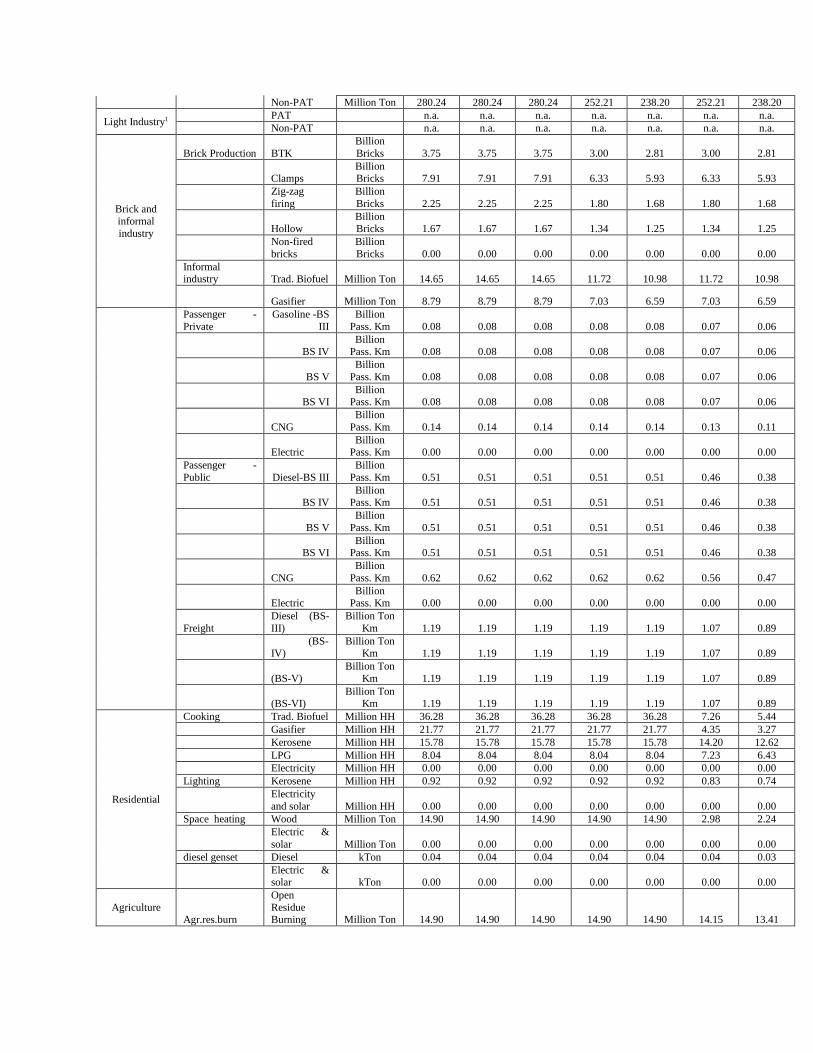
Non-PAT Million Ton 280.24 280.24 280.24 252.21 238.20 252.21 238.20

Light Industry1 PAT n.a. n.a. n.a. n.a. n.a. n.a. n.a.

Non-PAT n.a. n.a. n.a. n.a. n.a. n.a. n.a.

Brick and informal

industry

Brick Production BTK

Billion

Bricks 3.75 3.75 3.75 3.00 2.81 3.00 2.81

Clamps Billion Bricks 7.91 7.91 7.91 6.33 5.93 6.33 5.93

Zig-zag

firing

Billion

Bricks 2.25 2.25 2.25 1.80 1.68 1.80 1.68

Hollow Billion Bricks 1.67 1.67 1.67 1.34 1.25 1.34 1.25

Non-fired

bricks

Billion

Bricks 0.00 0.00 0.00 0.00 0.00 0.00 0.00

Informal industry Trad. Biofuel Million Ton 14.65 14.65 14.65 11.72 10.98 11.72 10.98

Gasifier Million Ton 8.79 8.79 8.79 7.03 6.59 7.03 6.59

Passenger -

Private

Gasoline -BS

III

Billion

Pass. Km 0.08 0.08 0.08 0.08 0.08 0.07 0.06

BS IV Billion

Pass. Km 0.08 0.08 0.08 0.08 0.08 0.07 0.06

BS V

Billion

Pass. Km 0.08 0.08 0.08 0.08 0.08 0.07 0.06

BS VI Billion

Pass. Km 0.08 0.08 0.08 0.08 0.08 0.07 0.06

CNG

Billion

Pass. Km 0.14 0.14 0.14 0.14 0.14 0.13 0.11

Electric Billion

Pass. Km 0.00 0.00 0.00 0.00 0.00 0.00 0.00

Passenger -

Public Diesel-BS III

Billion

Pass. Km 0.51 0.51 0.51 0.51 0.51 0.46 0.38

BS IV Billion

Pass. Km 0.51 0.51 0.51 0.51 0.51 0.46 0.38

BS V

Billion

Pass. Km 0.51 0.51 0.51 0.51 0.51 0.46 0.38

BS VI

Billion

Pass. Km 0.51 0.51 0.51 0.51 0.51 0.46 0.38

CNG

Billion

Pass. Km 0.62 0.62 0.62 0.62 0.62 0.56 0.47

Electric Billion

Pass. Km 0.00 0.00 0.00 0.00 0.00 0.00 0.00

Freight

Diesel (BS-

III)

Billion Ton

Km 1.19 1.19 1.19 1.19 1.19 1.07 0.89

(BS-IV)

Billion Ton Km 1.19 1.19 1.19 1.19 1.19 1.07 0.89

(BS-V)

Billion Ton

Km 1.19 1.19 1.19 1.19 1.19 1.07 0.89

(BS-VI)

Billion Ton Km 1.19 1.19 1.19 1.19 1.19 1.07 0.89

Residential

Cooking Trad. Biofuel Million HH 36.28 36.28 36.28 36.28 36.28 7.26 5.44

Gasifier Million HH 21.77 21.77 21.77 21.77 21.77 4.35 3.27

Kerosene Million HH 15.78 15.78 15.78 15.78 15.78 14.20 12.62

LPG Million HH 8.04 8.04 8.04 8.04 8.04 7.23 6.43

Electricity Million HH 0.00 0.00 0.00 0.00 0.00 0.00 0.00

Lighting Kerosene Million HH 0.92 0.92 0.92 0.92 0.92 0.83 0.74

Electricity

and solar Million HH 0.00 0.00 0.00 0.00 0.00 0.00 0.00

Space heating Wood Million Ton 14.90 14.90 14.90 14.90 14.90 2.98 2.24

Electric &

solar Million Ton 0.00 0.00 0.00 0.00 0.00 0.00 0.00

diesel genset Diesel kTon 0.04 0.04 0.04 0.04 0.04 0.04 0.03

Electric & solar kTon 0.00 0.00 0.00 0.00 0.00 0.00 0.00

Agriculture Agr.res.burn

Open

Residue Burning Million Ton 14.90 14.90 14.90 14.90 14.90 14.15 13.41

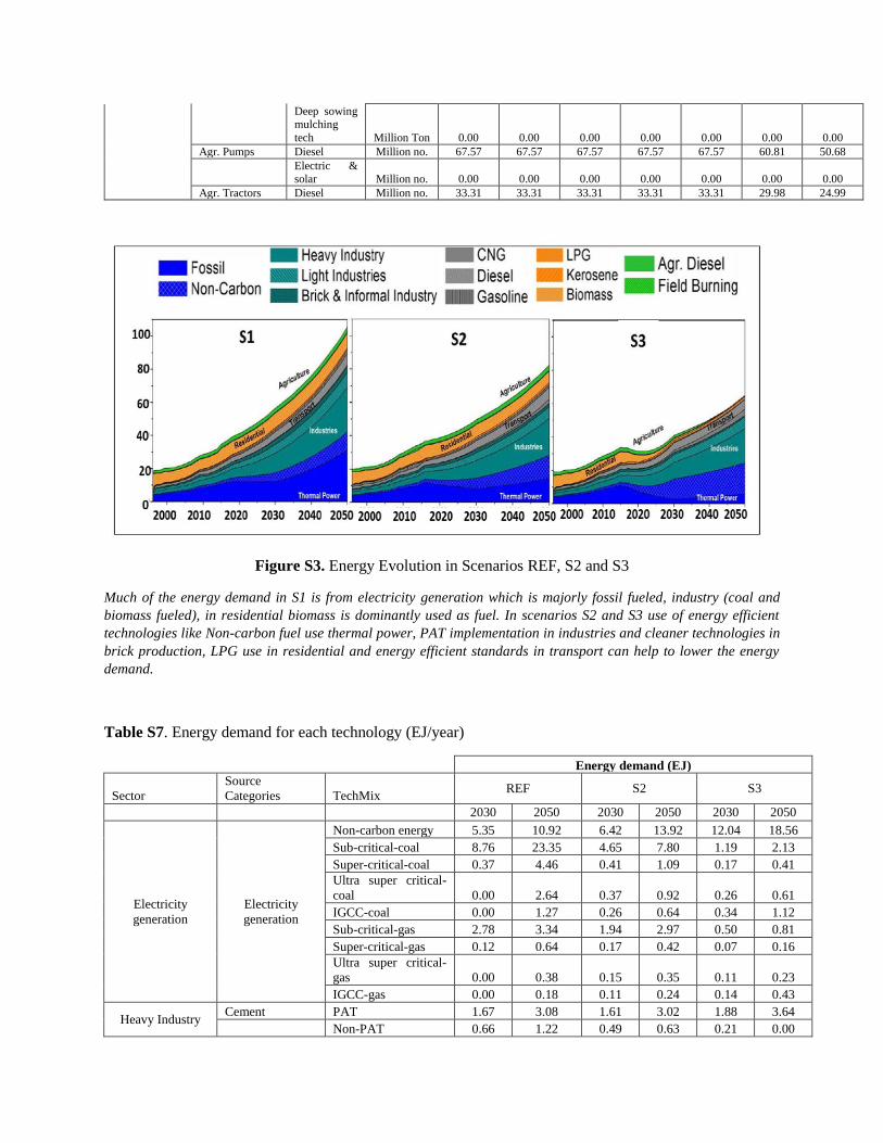
Deep sowing mulching

tech Million Ton 0.00 0.00 0.00 0.00 0.00 0.00 0.00

Agr. Pumps Diesel Million no. 67.57 67.57 67.57 67.57 67.57 60.81 50.68

Electric & solar Million no. 0.00 0.00 0.00 0.00 0.00 0.00 0.00

Agr. Tractors Diesel Million no. 33.31 33.31 33.31 33.31 33.31 29.98 24.99

Figure S3. Energy Evolution in Scenarios REF, S2 and S3

Much of the energy demand in S1 is from electricity generation which is majorly fossil fueled, industry (coal and

biomass fueled), in residential biomass is dominantly used as fuel. In scenarios S2 and S3 use of energy efficient

technologies like Non-carbon fuel use thermal power, PAT implementation in industries and cleaner technologies in

brick production, LPG use in residential and energy efficient standards in transport can help to lower the energy

demand.

Table S7. Energy demand for each technology (EJ/year)

Energy demand (EJ)

Sector

Source

Categories TechMix REF S2 S3

2030 2050 2030 2050 2030 2050

Electricity

generation

Electricity

generation

Non-carbon energy 5.35 10.92 6.42 13.92 12.04 18.56

Sub-critical-coal 8.76 23.35 4.65 7.80 1.19 2.13

Super-critical-coal 0.37 4.46 0.41 1.09 0.17 0.41

Ultra super critical-

coal 0.00 2.64 0.37 0.92 0.26 0.61

IGCC-coal 0.00 1.27 0.26 0.64 0.34 1.12

Sub-critical-gas 2.78 3.34 1.94 2.97 0.50 0.81

Super-critical-gas 0.12 0.64 0.17 0.42 0.07 0.16

Ultra super critical-

gas 0.00 0.38 0.15 0.35 0.11 0.23

IGCC-gas 0.00 0.18 0.11 0.24 0.14 0.43

Heavy Industry Cement PAT 1.67 3.08 1.61 3.02 1.88 3.64

Non-PAT 0.66 1.22 0.49 0.63 0.21 0.00

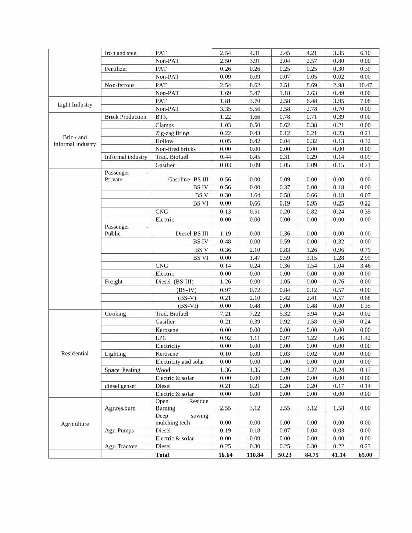
Iron and steel PAT 2.54 4.31 2.45 4.21 3.35 6.10

Non-PAT 2.50 3.91 2.04 2.57 0.80 0.00

Fertilizer PAT 0.26 0.26 0.25 0.25 0.30 0.30

Non-PAT 0.09 0.09 0.07 0.05 0.02 0.00

Non-ferrous PAT 2.54 8.62 2.51 8.69 2.98 10.47

Non-PAT 1.69 5.47 1.18 2.63 0.49 0.00

Light Industry PAT 1.81 3.70 2.58 6.48 3.95 7.08

Non-PAT 3.35 5.56 2.58 2.78 0.70 0.00

Brick and

informal industry

Brick Production BTK 1.22 1.66 0.78 0.71 0.39 0.00

Clamps 1.03 0.50 0.62 0.38 0.21 0.00

Zig-zag firing 0.22 0.43 0.12 0.21 0.23 0.21

Hollow 0.05 0.42 0.04 0.32 0.13 0.32

Non-fired bricks 0.00 0.00 0.00 0.00 0.00 0.00

Informal industry Trad. Biofuel 0.44 0.45 0.31 0.29 0.14 0.09

Gasifier 0.03 0.09 0.05 0.09 0.15 0.21

Passenger -

Private Gasoline -BS III 0.56 0.00 0.09 0.00 0.00 0.00

BS IV 0.56 0.00 0.37 0.00 0.18 0.00

BS V 0.30 1.64 0.58 0.66 0.18 0.07

BS VI 0.00 0.66 0.19 0.95 0.25 0.22

CNG 0.13 0.51 0.20 0.82 0.24 0.35

Electric 0.00 0.00 0.00 0.00 0.00 0.00

Passenger -

Public Diesel-BS III 1.19 0.00 0.36 0.00 0.00 0.00

BS IV 0.48 0.00 0.59 0.00 0.32 0.00

BS V 0.36 2.10 0.83 1.26 0.96 0.79

BS VI 0.00 1.47 0.59 3.15 1.28 2.99

CNG 0.14 0.24 0.36 1.54 1.04 3.46

Electric 0.00 0.00 0.00 0.00 0.00 0.00

Freight Diesel (BS-III) 1.26 0.00 1.05 0.00 0.76 0.00

(BS-IV) 0.97 0.72 0.84 0.12 0.57 0.00

(BS-V) 0.21 2.10 0.42 2.41 0.57 0.68

(BS-VI) 0.00 0.48 0.00 0.48 0.00 1.35

Residential

Cooking Trad. Biofuel 7.21 7.22 5.32 3.94 0.24 0.02

Gasifier 0.21 0.39 0.92 1.58 0.50 0.24

Kerosene 0.00 0.00 0.00 0.00 0.00 0.00

LPG 0.92 1.11 0.97 1.22 1.06 1.42

Electricity 0.00 0.00 0.00 0.00 0.00 0.00

Lighting Kerosene 0.10 0.09 0.03 0.02 0.00 0.00

Electricity and solar 0.00 0.00 0.00 0.00 0.00 0.00

Space heating Wood 1.36 1.35 1.29 1.27 0.24 0.17

Electric & solar 0.00 0.00 0.00 0.00 0.00 0.00

diesel genset Diesel 0.21 0.21 0.20 0.20 0.17 0.14

Electric & solar 0.00 0.00 0.00 0.00 0.00 0.00

Agriculture

Agr.res.burn

Open Residue

Burning 2.55 3.12 2.55 3.12 1.58 0.00

Deep sowing

mulching tech 0.00 0.00 0.00 0.00 0.00 0.00

Agr. Pumps Diesel 0.19 0.18 0.07 0.04 0.03 0.00

Electric & solar 0.00 0.00 0.00 0.00 0.00 0.00

Agr. Tractors Diesel 0.25 0.30 0.25 0.30 0.22 0.23

Total 56.64 110.84 50.23 84.75 41.14 65.00

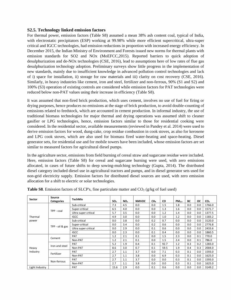
S2.5. Technology linked emission factors

For thermal power, emission factors (Table S8) assumed a mean 38% ash content coal, typical of India,

with electrostatic precipitators (ESP) working at 99.98% while more efficient supercritical, ultra-super

critical and IGCC technologies, had emission reductions in proportion with increased energy efficiency. In

December 2015, the Indian Ministry of Environment and Forests issued new norms for thermal plants with

emission standards for SO2 and NOx (MoEFCC,2015). Reported barriers to quick adoption of

desulphurization and de-NOx technologies (CSE, 2016), lead to assumptions here of low rates of flue gas

desulphurization technology adoption. Preliminary surveys show little progress in the implementation of

new standards, mainly due to insufficient knowledge in advanced pollution control technologies and lack

of i) space for installation, ii) storage for raw materials and iii) clarity on cost recovery (CSE, 2016).

Similarly, in heavy industries like cement, iron and steel, fertilizer and non-ferrous, 90% (S1 and S2) and

100% (S3) operation of existing controls are considered while emission factors for PAT technologies were

reduced below non-PAT values using their increase in efficiency (Table S8).

It was assumed that non-fired brick production, which uses cement, involves no use of fuel for firing or

drying purposes, hence produces no emissions at the stage of brick production, to avoid double-counting of

emissions related to feedstock, which are accounted in cement production. In informal industry, the use of

traditional biomass technologies for major thermal and drying operations was assumed shift to cleaner

gasifier or LPG technologies, hence, emission factors similar to those for residential cooking were

considered. In the residential sector, available measurements (reviewed in Pandey et al. 2014) were used to

derive emission factors for wood, dung-cake, crop residue combustion in cook stoves, as also for kerosene

and LPG cook stoves, which are also used for biomass fired water-heating and space-heating. Diesel

generator sets, for residential use and for mobile towers have been included, whose emission factors are set

similar to measured factors for agricultural diesel pumps.

In the agriculture sector, emissions from field burning of cereal straw and sugarcane residue were included.

Here, emission factors (Table S8) for cereal and sugarcane burning were used, with zero emissions

allocated, in cases of future shifts to deep sowing-mulching technology (Gupta, 2014). The distributed

diesel category included diesel use in agricultural tractors and pumps, and in diesel generator sets used for

non-grid electricity supply. Emission factors for distributed diesel sources are used, with zero emission

allocation for a shift to electric or solar technologies.

Table S8. Emission factors of SLCP's, fine particulate matter and CO2 (g/kg of fuel used)

Sector Source Categories

TechMix SO2 NOx NMVOC CH4 CO PM2.5 BC OC CO2

Thermal power

TPP - coal

Sub-critical 7.3 4.5 0.0 0.0 1.5 1.8 0.0 0.0 1766.0

Super-critical 6.5 4.0 0.0 0.0 1.3 1.6 0.0 0.0 1571.7

Ultra super critical 5.7 3.5 0.0 0.0 1.2 1.4 0.0 0.0 1377.5

IGCC 4.9 3.0 0.0 0.0 1.0 1.2 0.0 0.0 1183.2

TPP - oil & gas

Sub-critical 0.0 3.8 0.0 0.2 0.7 0.0 0.0 0.0 3120.0

Super-critical 0.0 3.4 0.0 0.2 0.6 0.0 0.0 0.0 2776.8

Ultra super critical 0.0 2.9 0.0 0.1 0.6 0.0 0.0 0.0 2433.6

IGCC 0.0 2.3 0.0 0.1 0.4 0.0 0.0 0.0 1860.5

Heavy Industry

Cement PAT 1.2 2.1 0.1 0.0 1.5 2.3 0.0 0.1 770.0

Non-PAT 1.2 2.1 0.1 0.0 1.5 2.4 0.0 0.1 786.0

Iron and steel PAT 5.2 1.9 0.4 0.1 92.7 1.2 0.3 0.2 1283.0

Non-PAT 8.6 3.0 0.7 0.1 59.5 1.9 0.4 0.3 2004.0

Fertilizer PAT 2.7 1.1 3.7 0.0 7.1 0.3 0.1 0.0 1593.0

Non-PAT 2.7 1.1 3.8 0.0 6.9 0.3 0.1 0.0 1625.0

Non-ferrous PAT 2.7 1.1 3.7 0.0 0.0 0.3 0.1 0.0 1593.0

Non-PAT 2.7 1.1 3.8 0.0 0.0 0.3 0.1 0.0 1625.0

Light Industry PAT 15.6 2.9 0.0 0.1 0.6 0.0 0.0 0.0 3149.2

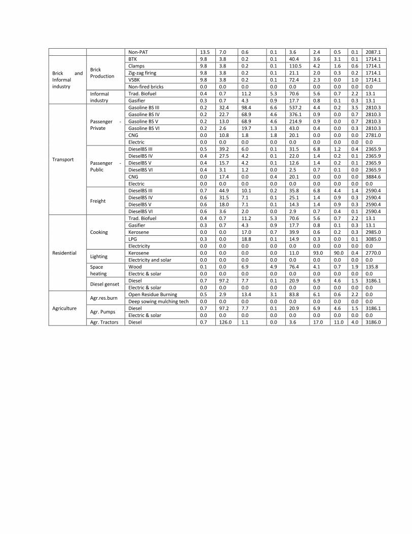
Non-PAT 13.5 7.0 0.6 0.1 3.6 2.4 0.5 0.1 2087.1

Brick and Informal industry

Brick Production

BTK 9.8 3.8 0.2 0.1 40.4 3.6 3.1 0.1 1714.1

Clamps 9.8 3.8 0.2 0.1 110.5 4.2 1.6 0.6 1714.1

Zig-zag firing 9.8 3.8 0.2 0.1 21.1 2.0 0.3 0.2 1714.1

VSBK 9.8 3.8 0.2 0.1 72.4 2.3 0.0 1.0 1714.1

Non-fired bricks 0.0 0.0 0.0 0.0 0.0 0.0 0.0 0.0 0.0

Informal industry

Trad. Biofuel 0.4 0.7 11.2 5.3 70.6 5.6 0.7 2.2 13.1

Gasifier 0.3 0.7 4.3 0.9 17.7 0.8 0.1 0.3 13.1

Transport

Passenger - Private

Gasoline BS III 0.2 32.4 98.4 6.6 537.2 4.4 0.2 3.5 2810.3

Gasoline BS IV 0.2 22.7 68.9 4.6 376.1 0.9 0.0 0.7 2810.3

Gasoline BS V 0.2 13.0 68.9 4.6 214.9 0.9 0.0 0.7 2810.3

Gasoline BS VI 0.2 2.6 19.7 1.3 43.0 0.4 0.0 0.3 2810.3

CNG 0.0 10.8 1.8 1.8 20.1 0.0 0.0 0.0 2781.0

Electric 0.0 0.0 0.0 0.0 0.0 0.0 0.0 0.0 0.0

Passenger - Public

DieselBS III 0.5 39.2 6.0 0.1 31.5 6.8 1.2 0.4 2365.9

DieselBS IV 0.4 27.5 4.2 0.1 22.0 1.4 0.2 0.1 2365.9

DieselBS V 0.4 15.7 4.2 0.1 12.6 1.4 0.2 0.1 2365.9

DieselBS VI 0.4 3.1 1.2 0.0 2.5 0.7 0.1 0.0 2365.9

CNG 0.0 17.4 0.0 0.4 20.1 0.0 0.0 0.0 3884.6

Electric 0.0 0.0 0.0 0.0 0.0 0.0 0.0 0.0 0.0

Freight

DieselBS III 0.7 44.9 10.1 0.2 35.8 6.8 4.4 1.4 2590.4

DieselBS IV 0.6 31.5 7.1 0.1 25.1 1.4 0.9 0.3 2590.4

DieselBS V 0.6 18.0 7.1 0.1 14.3 1.4 0.9 0.3 2590.4

DieselBS VI 0.6 3.6 2.0 0.0 2.9 0.7 0.4 0.1 2590.4

Residential

Cooking

Trad. Biofuel 0.4 0.7 11.2 5.3 70.6 5.6 0.7 2.2 13.1

Gasifier 0.3 0.7 4.3 0.9 17.7 0.8 0.1 0.3 13.1

Kerosene 0.0 0.0 17.0 0.7 39.9 0.6 0.2 0.3 2985.0

LPG 0.3 0.0 18.8 0.1 14.9 0.3 0.0 0.1 3085.0

Electricity 0.0 0.0 0.0 0.0 0.0 0.0 0.0 0.0 0.0

Lighting Kerosene 0.0 0.0 0.0 0.0 11.0 93.0 90.0 0.4 2770.0

Electricity and solar 0.0 0.0 0.0 0.0 0.0 0.0 0.0 0.0 0.0

Space heating

Wood 0.1 0.0 6.9 4.9 76.4 4.1 0.7 1.9 135.8

Electric & solar 0.0 0.0 0.0 0.0 0.0 0.0 0.0 0.0 0.0

Diesel genset Diesel 0.7 97.2 7.7 0.1 20.9 6.9 4.6 1.5 3186.1

Electric & solar 0.0 0.0 0.0 0.0 0.0 0.0 0.0 0.0 0.0

Agriculture

Agr.res.burn Open Residue Burning 0.5 2.9 13.4 3.1 83.8 6.1 0.6 2.2 0.0

Deep sowing mulching tech 0.0 0.0 0.0 0.0 0.0 0.0 0.0 0.0 0.0

Agr. Pumps Diesel 0.7 97.2 7.7 0.1 20.9 6.9 4.6 1.5 3186.1

Electric & solar 0.0 0.0 0.0 0.0 0.0 0.0 0.0 0.0 0.0

Agr. Tractors Diesel 0.7 126.0 1.1 0.0 3.6 17.0 11.0 4.0 3186.0

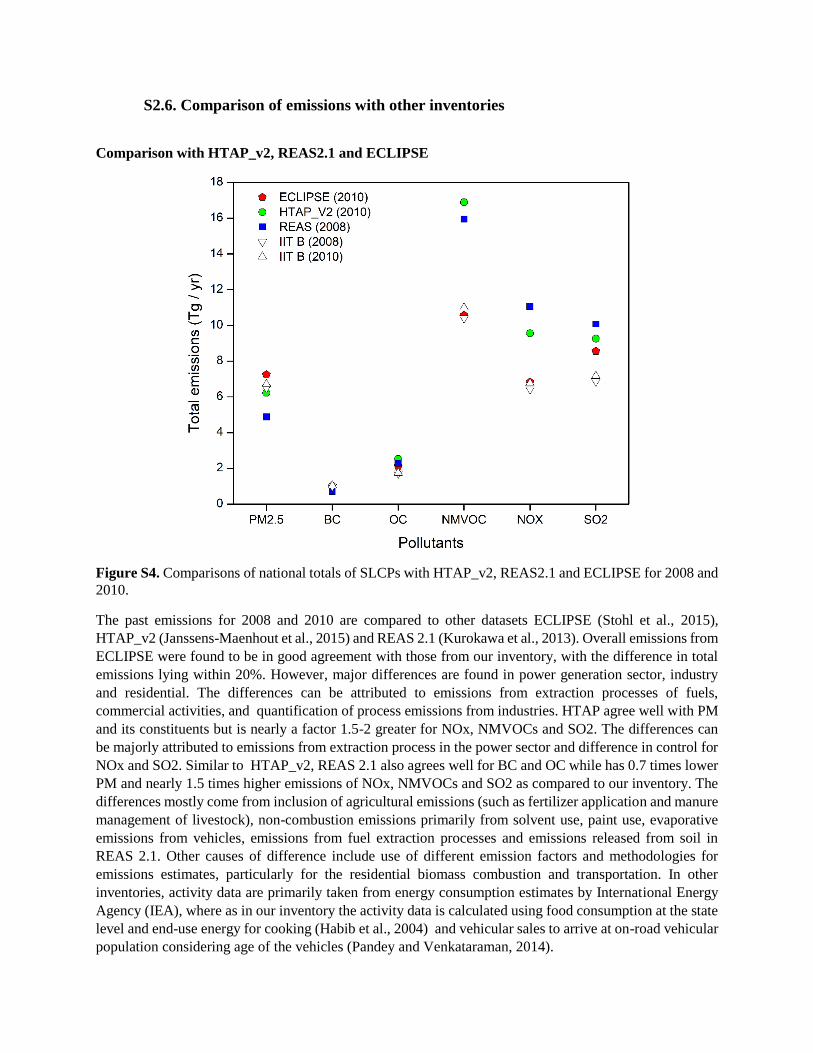
S2.6. Comparison of emissions with other inventories

Comparison with HTAP_v2, REAS2.1 and ECLIPSE

Figure S4. Comparisons of national totals of SLCPs with HTAP_v2, REAS2.1 and ECLIPSE for 2008 and

2010.

The past emissions for 2008 and 2010 are compared to other datasets ECLIPSE (Stohl et al., 2015),

HTAP_v2 (Janssens-Maenhout et al., 2015) and REAS 2.1 (Kurokawa et al., 2013). Overall emissions from

ECLIPSE were found to be in good agreement with those from our inventory, with the difference in total

emissions lying within 20%. However, major differences are found in power generation sector, industry

and residential. The differences can be attributed to emissions from extraction processes of fuels,

commercial activities, and quantification of process emissions from industries. HTAP agree well with PM

and its constituents but is nearly a factor 1.5-2 greater for NOx, NMVOCs and SO2. The differences can

be majorly attributed to emissions from extraction process in the power sector and difference in control for

NOx and SO2. Similar to HTAP_v2, REAS 2.1 also agrees well for BC and OC while has 0.7 times lower

PM and nearly 1.5 times higher emissions of NOx, NMVOCs and SO2 as compared to our inventory. The

differences mostly come from inclusion of agricultural emissions (such as fertilizer application and manure

management of livestock), non-combustion emissions primarily from solvent use, paint use, evaporative

emissions from vehicles, emissions from fuel extraction processes and emissions released from soil in

REAS 2.1. Other causes of difference include use of different emission factors and methodologies for

emissions estimates, particularly for the residential biomass combustion and transportation. In other

inventories, activity data are primarily taken from energy consumption estimates by International Energy

Agency (IEA), where as in our inventory the activity data is calculated using food consumption at the state

level and end-use energy for cooking (Habib et al., 2004) and vehicular sales to arrive at on-road vehicular

population considering age of the vehicles (Pandey and Venkataraman, 2014).

Evaluation with ECLIPSE V5a and GAINS-WEO2016

Figure S5. Percentage deviation in emissions of ECLIPSE V5a and GAINS-WEO2016 from emissions of

this study by sector.

(Percentage deviation is calculated as (IITB S2 – ECLIPSE V5a) / ECLIPSE V5a and (IITB S2 – GAINS

WEO2016) / GAINS WEO2016).

Evaluation with RCP scenarios

RCP2.6 assumes net negative CO2 emissions after around 2070. RCP4.5 and RCP6.0 aim for a smooth

stabilization of concentrations by 2150 and RCP8.5 stabilizes concentrations only by 2250. However, RCP

scenarios are not tied to any specific socio-economic and technology evolution pathway, making difficult

any direct comparison of underlying assumptions, while permitting a comparison of gross emission

magnitudes.

Estimated Indian emissions from the RCP scenarios, of SO2, NOx, and NMVOCs, and for BC and OC, for

2005-2050 at 50×50 km resolution, were used for the evaluation.

(http://tntcat.iiasa.ac.at/RcpDb/dsd?Action=htmlpage&page=download). The sectors used corresponding

to ones in this study, included Energy (Power Plants, Energy Conversion, Extraction, and Distribution),

Domestic (Residential and Commercial), Industry (combustion & processing), Surface Transportation and

Agriculture waste burning in fields. Gridded emissions in kg m-2 s-1 are summed over the Indian landmass

and converted to million tonnes y-1 (Table S9). The present estimates do not include emissions from soils

and animal rearing or from shipping and aviation, rather they focus on energy use and solvent based

activities. Therefore, corresponding sectors in the RCP database were excluded from the evaluation.

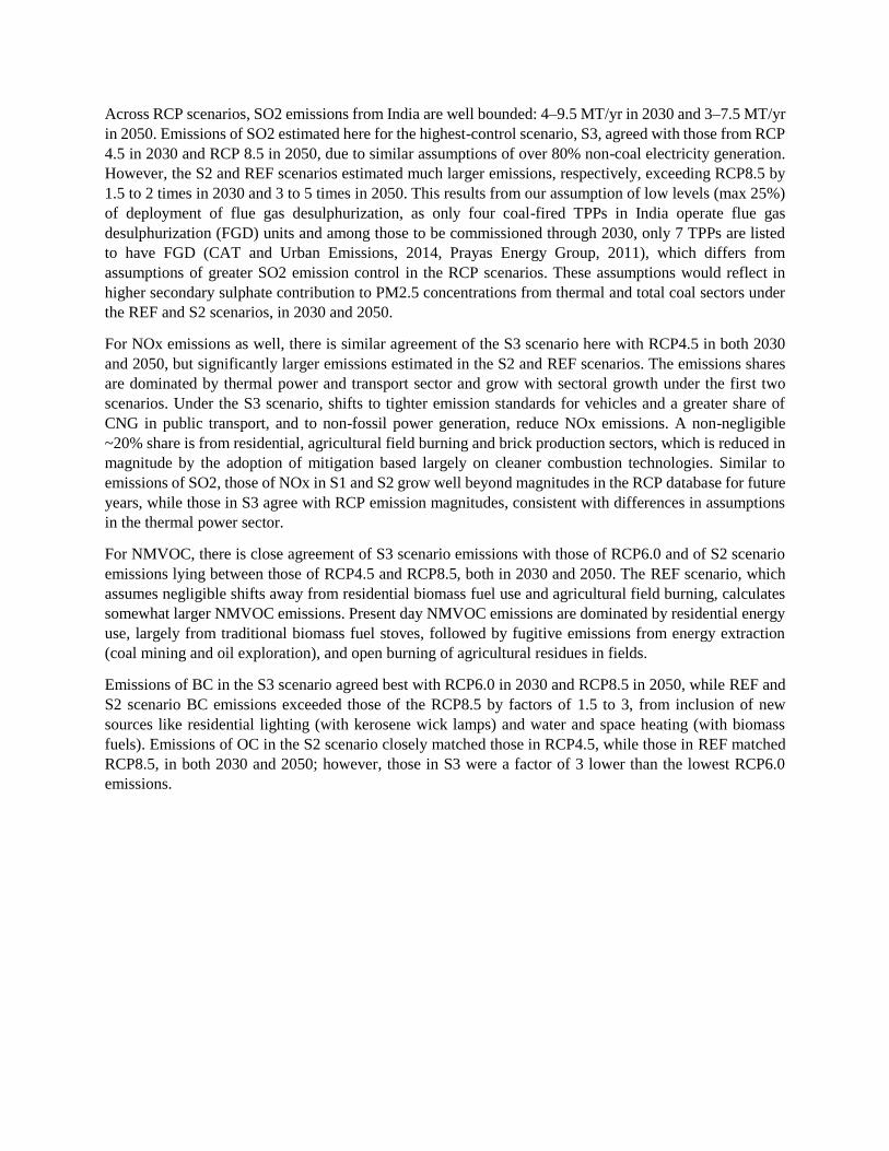
Across RCP scenarios, SO2 emissions from India are well bounded: 4–9.5 MT/yr in 2030 and 3–7.5 MT/yr

in 2050. Emissions of SO2 estimated here for the highest-control scenario, S3, agreed with those from RCP

4.5 in 2030 and RCP 8.5 in 2050, due to similar assumptions of over 80% non-coal electricity generation.

However, the S2 and REF scenarios estimated much larger emissions, respectively, exceeding RCP8.5 by

1.5 to 2 times in 2030 and 3 to 5 times in 2050. This results from our assumption of low levels (max 25%)

of deployment of flue gas desulphurization, as only four coal-fired TPPs in India operate flue gas

desulphurization (FGD) units and among those to be commissioned through 2030, only 7 TPPs are listed

to have FGD (CAT and Urban Emissions, 2014, Prayas Energy Group, 2011), which differs from

assumptions of greater SO2 emission control in the RCP scenarios. These assumptions would reflect in

higher secondary sulphate contribution to PM2.5 concentrations from thermal and total coal sectors under

the REF and S2 scenarios, in 2030 and 2050.

For NOx emissions as well, there is similar agreement of the S3 scenario here with RCP4.5 in both 2030

and 2050, but significantly larger emissions estimated in the S2 and REF scenarios. The emissions shares

are dominated by thermal power and transport sector and grow with sectoral growth under the first two

scenarios. Under the S3 scenario, shifts to tighter emission standards for vehicles and a greater share of

CNG in public transport, and to non-fossil power generation, reduce NOx emissions. A non-negligible

~20% share is from residential, agricultural field burning and brick production sectors, which is reduced in

magnitude by the adoption of mitigation based largely on cleaner combustion technologies. Similar to

emissions of SO2, those of NOx in S1 and S2 grow well beyond magnitudes in the RCP database for future

years, while those in S3 agree with RCP emission magnitudes, consistent with differences in assumptions

in the thermal power sector.

For NMVOC, there is close agreement of S3 scenario emissions with those of RCP6.0 and of S2 scenario

emissions lying between those of RCP4.5 and RCP8.5, both in 2030 and 2050. The REF scenario, which

assumes negligible shifts away from residential biomass fuel use and agricultural field burning, calculates

somewhat larger NMVOC emissions. Present day NMVOC emissions are dominated by residential energy

use, largely from traditional biomass fuel stoves, followed by fugitive emissions from energy extraction

(coal mining and oil exploration), and open burning of agricultural residues in fields.

Emissions of BC in the S3 scenario agreed best with RCP6.0 in 2030 and RCP8.5 in 2050, while REF and

S2 scenario BC emissions exceeded those of the RCP8.5 by factors of 1.5 to 3, from inclusion of new

sources like residential lighting (with kerosene wick lamps) and water and space heating (with biomass

fuels). Emissions of OC in the S2 scenario closely matched those in RCP4.5, while those in REF matched

RCP8.5, in both 2030 and 2050; however, those in S3 were a factor of 3 lower than the lowest RCP6.0

emissions.

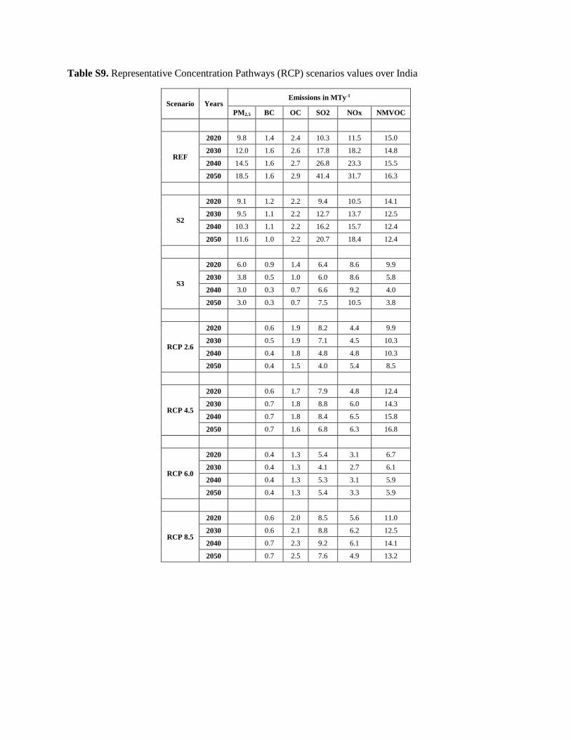
Table S9. Representative Concentration Pathways (RCP) scenarios values over India

Scenario Years Emissions in MTy-1

PM2.5 BC OC SO2 NOx NMVOC

REF

2020 9.8 1.4 2.4 10.3 11.5 15.0

2030 12.0 1.6 2.6 17.8 18.2 14.8

2040 14.5 1.6 2.7 26.8 23.3 15.5

2050 18.5 1.6 2.9 41.4 31.7 16.3

S2

2020 9.1 1.2 2.2 9.4 10.5 14.1

2030 9.5 1.1 2.2 12.7 13.7 12.5

2040 10.3 1.1 2.2 16.2 15.7 12.4

2050 11.6 1.0 2.2 20.7 18.4 12.4

S3

2020 6.0 0.9 1.4 6.4 8.6 9.9

2030 3.8 0.5 1.0 6.0 8.6 5.8

2040 3.0 0.3 0.7 6.6 9.2 4.0

2050 3.0 0.3 0.7 7.5 10.5 3.8

RCP 2.6

2020 0.6 1.9 8.2 4.4 9.9

2030 0.5 1.9 7.1 4.5 10.3

2040 0.4 1.8 4.8 4.8 10.3

2050 0.4 1.5 4.0 5.4 8.5

RCP 4.5

2020 0.6 1.7 7.9 4.8 12.4

2030 0.7 1.8 8.8 6.0 14.3

2040 0.7 1.8 8.4 6.5 15.8

2050 0.7 1.6 6.8 6.3 16.8

RCP 6.0

2020 0.4 1.3 5.4 3.1 6.7

2030 0.4 1.3 4.1 2.7 6.1

2040 0.4 1.3 5.3 3.1 5.9

2050 0.4 1.3 5.4 3.3 5.9

RCP 8.5

2020 0.6 2.0 8.5 5.6 11.0

2030 0.6 2.1 8.8 6.2 12.5

2040 0.7 2.3 9.2 6.1 14.1

2050 0.7 2.5 7.6 4.9 13.2

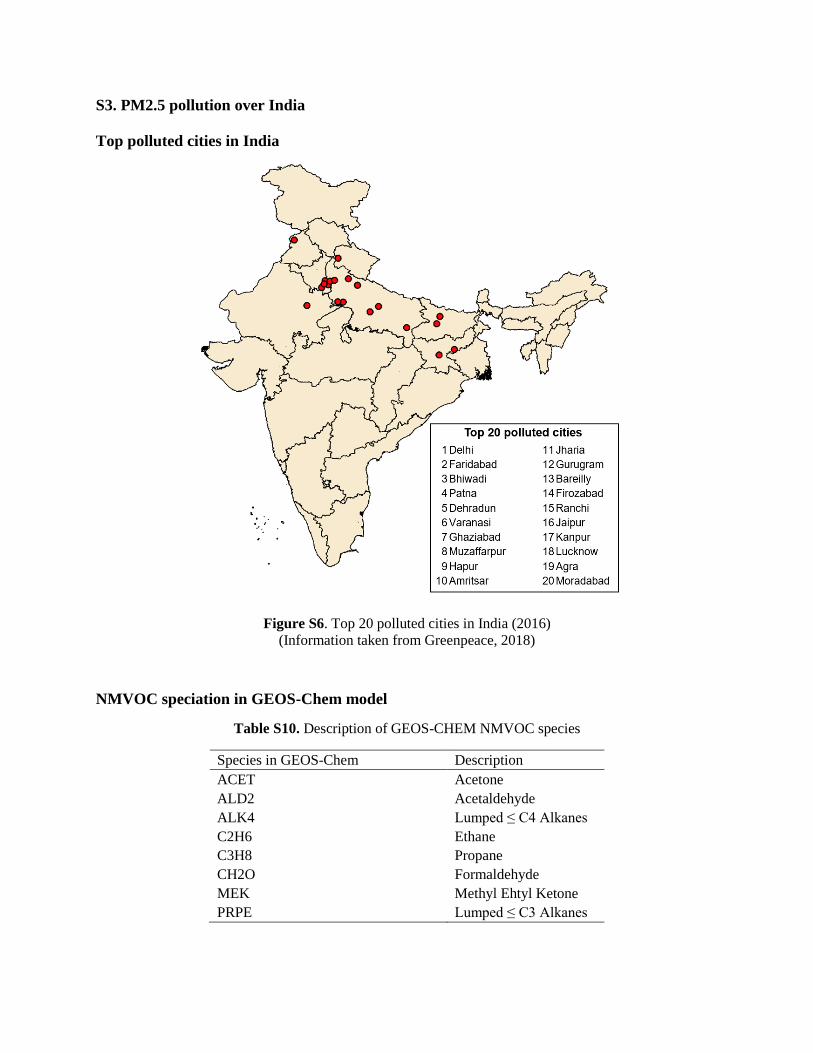
S3. PM2.5 pollution over India

Top polluted cities in India

Figure S6. Top 20 polluted cities in India (2016)

(Information taken from Greenpeace, 2018)

NMVOC speciation in GEOS-Chem model

Table S10. Description of GEOS-CHEM NMVOC species

Species in GEOS-Chem Description

ACET Acetone

ALD2 Acetaldehyde

ALK4 Lumped ≤ C4 Alkanes

C2H6 Ethane

C3H8 Propane

CH2O Formaldehyde

MEK Methyl Ehtyl Ketone

PRPE Lumped ≤ C3 Alkanes

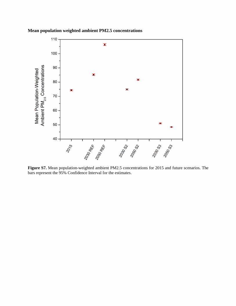
Mean population weighted ambient PM2.5 concentrations

Figure S7. Mean population-weighted ambient PM2.5 concentrations for 2015 and future scenarios. The

bars represent the 95% Confidence Interval for the estimates.

References

Anandarajah, G. and Gambhir, A.: India’s CO2 Emission Pathways to 2050: What Role Can Renewables

Play? Applied Energy, 131, 79–86, http://dx.doi.org/10.1016/j.apenergy.2014.06.026, 2014

Auto Fuel Vision and Policy 2025. Report of the Expert Committee: Auto Fuel Vision and Policy

2025.Government of India, http://petroleum.nic.in/docs/reports/autopol.pdf, 2014.

CAT and Urban Emissions: Coal Kills: Health Impacts of Air Pollution from India’s Coal Power

Expansion, Conservation Action Trust (CAT), Mumbai. http://www.indiaairquality.info/wp-

content/uploads/docs/Air%20Pollution%20from%20India%20Coal%20TPPs%20-%20LowRes.pdf, 2014.

CSE: New Environmental Norms for the Power Sector. Proceedings and Recommendations of the

Stakeholder Workshop Organized by CSE, Centre for Science and Environment, New Delhi.

http://cseindia.org/userfiles/new-environmental-norms-report.pdf, 2016.

EMEP: EMEP/EEA Air Pollutant Emission Inventory Guidebook. European Environment Agency,

Copenhagen, 2009.

Firoz, A. S.: Long Term Perspectives for Indian Steel Industry, Ministry of Steel, Economic Research Unit

mimeo, New Delhi, May, 2014.

Greenpeace: Airpocalypse II, Assessment of air pollution in Indian cities, 2018.

Gupta, R.: Essays on Air Pollution, Global Warming and Agricultural Productivity. PhD Dissertation,

Indian Statistical Institute, New Delhi, 2014.

Guttikunda, S.K., Mohan, D.: Re-fueling road transport for better air quality in India, Energy Policy 68,

556-561, 2014.

ICRA: Indian Automobile Industry: Proposed BS-VI Emission Standards. ICRA Limited, New Delhi,

http://www.icra.in/Files/ticker/SH-2016-Q2-6-ICRA-Passenger%20vehicles.pdf, 2016.

IEA (International Energy Agency), (2009). Cement Technology Roadmap. Report by International Energy

Agency and World Business Council for Sustainable Development. Pages- 36,

https://www.iea.org/publications/freepublications/publication/Cement.pdf. Last accessed 1/April/2016.

IEP: Integrated Energy Policy: Report of the Expert Committee. New Delhi, India. Government of India

Planning Commission. Available: http://planningcommission.nic.in/reports/genrep/rep_intengy.pdf,

accessed: 14 August 2017, 2006.

IESS, NITI Aayog: India Energy Security Scenarios, 2047, NITI Aayog, Govt of India, Available:

http://iess2047.gov.in/, accessed: 1 April 2015, 2015.

IPCC: IPCC Guidelines for National Greenhouse Gas Inventories, Energy, vol. 2, 2006a.

IPCC: IPCC Guidelines for National Greenhouse Gas Inventories, General Guidance and Reporting, vol.

1, 2006b.

Lam, N.L., Chen, Y., Weyant, C., Venkataraman, C., Sadavarte, P., Johnson, M.A., Smith, K.R., Brem,

B.T., Arineitwe, J., Ellis, J.E., Bond, T.C., Household light makes global heat: high black carbon emissions

from kerosene wick lamps, Environ. Sci. Technol, 46, 13531-13538, 2012.

Maithel, S., Uma, R., Bond, T., Baum, E., Thao, V.T.K., (2012). Brick Kilns Performance Assessment,

Emissions Measurements, & A Roadmap for Cleaner Brick Production in India Study report prepared by

Green Knowledge Solutions, New Delhi, India.

http://www.unep.org/ccac/Portals/50162/docs/Brick_Kilns_Performance_Assessment.pdf. Last accessed:

1/April/2016.

Murthy, K.S.S.: Indian Aluminium Demand to Grow 5 Times by 2030 by Prof. K.S.S. Murthy, Gen.

Secretary, Aluminium Association of India, 2014.

MoEFCC: http://pib.nic.in/newsite/PrintRelease.aspx?relid=133726. Press Release. Ministry of

Environment, Forest and Climate Change. Government of India, 2015.

MoP: PAT Perform, Achieve and Trade. Ministry of Power, Government of India, 2012.

MoP: Energy Efficient Norms for Power Plants. Press Information Bureau. Ministry of Power. Government

of India. Available: http://pib.nic.in/newsite/PrintRelease.aspx?relid=117384, accessed 11 August 2017,

2015.

MoRTH: http://pib.nic.in/newsite/PrintRelease.aspx?relid=134232. Press Release. Ministry of Road

Transport and Highways. Government of India, 2016.

National Solar Mission, Ministry of New and Renewable Energy, Govt. of India

http://www.mnre.gov.in/solar-mission/jnnsm/introduction-2/, 2010.

NITI Aayog: India Energy Security Scenarios (IESS) 2047. New Delhi: NITI Aayog weblink:

http://indiaenergy.gov.in/, 2015

NTDPC: Moving India to 2032, India transport report, Government of India, National Transport

Development Policy Committee, India, New Delhi,

http://planningcommission.nic.in/reports/genrep/NTDPC_ Vol_01.pdf, accessed: 1 April 2016, 2013.

Pandey, A. and Venkataraman, C.: Estimating emissions from the Indian transport sector with on-road fleet

composition and traffic volume, Atmos. Environ., 98, 123–133, doi:10.1016/j.atmosenv.2014.08.039,

2014.

PNGRB: Vision 2030, Natural Gas Infrastructure in India. Report by Industry Group for Petroleum &

Natural Gas Regulatory Board, India, 2013.

Prayas Energy Group: Thermal Power Plants on the anvil: Implications and Need for Rationalisation. Pune,

India, 2011.

Ray, D.K., Mueller, N.D., West, P.C. and Foley, J.A.: Yield trends are insufficient to double global crop

production by 2050. PloS one, 8(6), p.e66428, 2013.

Shukla, P. R., Agarwal, P., Bazaz, A. B., Agarwal, N., Kainuma, M., Masui, T., Fujino, J., Matsuuoka, Y.,

Hibino, G., Ehara, T.: Low Carbon Society Vision 2050 India, Indian Institute of Management Ahmedabad,

National Institute for Environmental Studies, Kyoto University, Mizuho Information & Research Institute,

1–28, http://2050.nies.go.jp/report/file/lcs_asia/indialcs.pdf, 2009.

Shukla, P. R. and Chaturvedi, V.: Low Carbon and Clean Energy Scenarios for India: Analysis of Targets

Approach. Energy Economics 34(SUPPL. 3): S487–95. http://dx.doi.org/10.1016/j.eneco.2012.05.002,

2012.

UNDP: Energy Efficiency Improvements in the Indian Brick Industry. Available:

www.resourceefficientbricks.org/, United Nations Development Programme, 2009.

Venkataraman, C., Habib, G., Kadamba, D., Shrivastava, M., Leon, J.F., Crouzille, B., Boucher, O. and

Streets, D.G.: Emissions from open biomass burning in India: Integrating the inventory approach with high‐

resolution Moderate Resolution Imaging Spectroradiometer (MODIS) active‐fire and land cover data.

Global biogeochemical cycles, 20(2), 2006.

Venkataraman, C., Sagar, A.D., Habib, G., Lam, N. and Smith, K.R.: The Indian national initiative for

advanced biomass cookstoves: the benefits of clean combustion. Energy for Sustainable Development,

14(2), pp.63-72, 2010.