Relative Efficiency of Single-Outlier Discordancy Tests for Processing Geochemical Data on Reference Materials and Application to Instrumental Calibrations by a Weighted Least-Squares

Relative Efficiency of Single-Outlier Discordancy Tests forProcessing Geochemical Data on Reference Materials andApplication to Instrumental Calibrations by a WeightedLeast-Squares Linear Regression Model

Vol. 33 — N° 1 p . 2 9 - 4 9

Numerous studies report geochemical data on reference materials (RMs) processed by outlier-basedmethods that use univariate discordancy tests.However, the relative efficiency of the discordancytests is not precisely known. We used an extensivegeochemical database for thirty-five RMs from fourcountries (Canada, Japan, South Africa and USA) to empirically evaluate the performance of ninesingle-outlier tests with thirteen test variants. Itappears that the kurtosis test (N15) is the mostpowerful test for detecting discordant outliers insuch geochemical RM databases and is closely followed by the Grubbs type tests (N1 and N4) andthe skewness test (N14). The Dixon-type tests (N7,N8, N9 and N10) as well as the Grubbs type test(N2) depicted smaller global relative efficiency criterion values for the detection of outlying observations in this extensive database. Upper discordant outliers were more common than thelower discordant outliers, implying that positivelyskewed inter-laboratory geochemical datasets aremore frequent than negatively skewed ones andthat the median, a robust central tendency indicator,is likely to be biased especially for small-sizedsamples. Our outlier-based procedure should beuseful for objectively identifying discordant outliersin many fields of science and engineering and forinterpreting them accordingly. After processing thesedatabases by single-outlier discordancy tests andobtaining reliable estimates of central tendency anddispersion parameters of the geochemical data forthe RMs in our database, we used these statisticaldata to apply a weighted least-squares linearregression (WLR) model for the major elementdeterminations by X-ray fluorescence spectrometryand compared the WLR results with an ordinary

De nombreuses études présentent des donnéesgéochimiques sur les matériaux de références, données traitées par des méthodes statistiques éliminant des valeurs aberrantes avec des tests dediscordance univariés. Mais l'efficacité de ces testsde discordance est mal connue. Nous avons travaillé sur une base de données géochimiquesimportante, reposant sur trente cinq RM provenantde quatre pays (Canada, Japan, South Africa etUSA) afin d'évaluer empiriquement les performancesde neuf tests et treize variations de ces neuf tests. Le test kurtosis (N15) se révèle être le test le pluspuissant pour détecter les valeurs aberrantes danscette base de données, suivi de près par les tests de type Grubbs (N1 et N4) et par le test sur la dissymétrie (N14). Les tests de type Dixon (N7, N8,N9 et N10) ainsi que le test de type Grubbs N2donnent de plus petites valeurs du critère d'efficacitéglobale relative dans la détection de l'allure générale de cette importante base de données. Les valeurs aberrantes supérieures étaient plus fréquentes que les valeurs aberrantes inférieures;ceci implique que les données géochimiques inter-laboratoires biaisées vers le haut sont plus fréquentes que celles qui sont biaisées vers le baset que la médiane, indicateur robuste d'une répartition centré, a des chances d'être biaisée toutspécialement pour les échantillons de petite taille.Notre protocole basé sur les valeurs aberrantesdevrait être utile dans la recherche objective devaleurs aberrantes dans de nombreux domainesscientifiques et en ingénierie et leur interprétationcorrecte. Après avoir traité ces bases de donnéesavec les tests de valeurs aberrantes discordantes et obtenu des estimations fiables de la tendancecentrale et des paramètres de dispersion des

2 9

0309

Surendra P. Verma*, Lorena Díaz-González and Rosalinda González-Ramírez

Departamento de Sistemas Energéticos, Centro de Investigación en Energía, Universidad Nacional Autónoma de México, Priv. Xochicalco s/no., Col Centro, Apartado Postal 34, Temixco 62580, Mexico* Corresponding author. e-mail: [email protected]

© 2009 The Authors. Journal compilation © 2009 International Association of Geoanalysts

GEOSTANDARDS and

RESEARCHGEOANALYTICAL

Reference materials (RMs) are routinely used forquality control purposes in all sciences including theEarth sciences (e.g., Potts and Kane 1992, Quevauvilleret al. 1996, Dybczynski et al. 1998, Mahwar et al.1998, Namiesnik and Zygmunt 1999, Vendemiatto andEnzweiler 2001, Gabrovská et al. 2006, Santoyo et al.2006, Hayes et al. 2007, Verma et al. 2008, Verma andQuiroz-Ruiz 2008). Traditionally, the calibration of ananalytical instrument has been achieved through anordinary least-squares linear regression (OLR) model.However, recently there has been an increasing trend touse weighted least-squares linear regression (WLR)models (Baumann 1997, Santoyo and Verma 2003,Sayago et al. 2004, Guevara et al. 2005, Asuero andGonzález 2007, S te l iopoulos and S t icke l 2007,Tellinghuisen 2007), for which reliable estimates of bothcentral tendency and dispersion parameters should beavailable for all RMs to be used in a given calibration.

To obtain these statistical estimates, inter-laboratorygeochemical data on RMs have been processed tradi-tionally by both robust and outlier-based methods.Robust methods have been used for processing RMsfrom France, but after the elimination of the so-called“gross” outliers (e.g., Govindaraju and Roelandts 1989).Inter- laboratory data for RMs from the USA (e.g. ,Gladney et al. 1992) and Japan (e.g., Imai et al. 1995)were processed by an outlier-based scheme using theso called “two standard deviation” method (see Barnettand Lewis 1994, Verma 1998, and Verma et al. 2008for more details on this class of statistical method).Similarly, the data for RMs from the International AtomicEnergy Agency ( IAEA) have also been evaluated

through some kind of the outlier-based scheme (e.g.,Dybczynski et al. 1979, Verma 2004, Villeneuve et al.2004). The results of the robust methods for microgab-bro PM-S and dolerite WS-E (Govindaraju et al. 1994)were compared with the outlier-based methods byVerma (1997) and Verma et al. (1998), respectively.The univariate discordancy tests, being an integral partof the outlier-based methods, have also been appliedfor processing RM databases by Guevara et al. (2001)and Velasco-Tapia et al. (2001).

According to the ISO Guide 35 (ISO 1989), howe-ver, an elaborate procedure involving several roundsof data collection from several laboratories should becarried out in order to certify RMs, and the detectionand elimination of discordant outliers is not particularlyencouraged. Nevertheless, for older RMs, such asthose dealt with in the present work, the statisticalmethod of detection and elimination of discordant out-liers may be the only one available to “correctly” eva-luate them. This is because the statistically correctapplication of some robust methods, such as the trim-med mean or Winsorised mean, requires the distribu-tion of these outliers to be known a priori, and othermethods, such as the median, trimean or Gastwirth´smean, demand a symmetrical distribution of the out-lying observations (Barnett and Lewis 1994, Verma2005). Furthermore, the outlier procedures can beused for other kinds of experimental data in manyfields of science and engineering (Verma and Quiroz-Ruiz 2006a, b). The statistically correct identification ofthese discordant outliers will be useful for a betterinterpretation of the experimental data.

3 0

GEOSTANDARDS and



least-squares linear regression model. An advantage in using our outlier procedure and thenew concentration values and uncertainty estimatesfor these RMs was clearly established.

Keywords: reference materials, robust methods, outlier-based methods, consecutive tests, Dixon tests,Grubbs tests, skewness, kurtosis, X-ray fluorescencespectrometry.

données géochimiques de notre base de données,nous avons utilisé les données statistiques pourappliquer un modèle de régression linéaire desmoindres carrés pondérés (WLR) pour analyser leséléments majeurs par spectrométrie de fluorescenceX et nous avons comparé ces résultats avec ceuxobtenus par un modèle de régression linéaire demoindres carrés ordinaire (OLR). On montre finalement clairement le bénéfice obtenu avec notreprocédure basée sur les valeurs aberrantes ainsique l'intérêt des nouvelles estimations des concentrations des RM et de leurs incertitudes.

Mots-clés : matériau de référence, méthodes robustes,méthodes basées sur les valeurs aberrantes, tests consécutifs, tests de Dixon, tests de Grubbs, dissymétrie, kurtosis, spectrométrie de fluorescence X.Received 22 Oct 07 — Accepted 11 Jul 08

On the other hand, the robust method approachpracticed for obtaining the central tendency parameterin some older RMs also relies on the standard devia-tion as the dispersion parameter (e.g., Govindarajuand Roelandts 1989), whose unbiased estimate verymuch depends on the absence of discordant outlier(s)that , i f present , can seriously distort this est imate(Barnett and Lewis 1994, Verma 1997, 2005, Verma etal. 2008). For the purpose of identifying such discor-dant outliers, therefore, the present methodology, ini-tially proposed by Verma (1997), but much improvedby the availability of new, precise critical values (e.g.,Verma et al. 2008), can now be advantageously applied.

The discordancy tests (single- as well as multiple-outlier types) originally proposed by both Dixon (1951)and Grubbs (1950, 1969) have been very popular andare still in wide use in different fields (e.g., Barnett andLewis 1994, Li et al. 2003, Serbst et al. 2003, Farre etal. 2006, Gabrovská et al. 2006, Sang et al. 2006,Verma and Quiroz-Ruiz 2006a, b, 2008, Hayes et al.2007, Verma et al. 2008). Several other discordancytests are also available for this purpose, most notableamong which are the skewness and kurtosis tests(Barnett and Lewis 1994, Verma 1997, Velasco andVerma 1998, Verma and Quiroz-Ruiz 2006a, b, 2008).

Velasco et al. (2000) compare the performance orefficiency of outlier tests using the rare earth element(REE) data for twenty-six RMs. However, at that timebecause of the unavailability of critical values for cer-tain sample sizes (e.g., for n > 30 for Dixon tests N7 toN10; Dixon 1951; see Verma and Quiroz-Ruiz 2006a,or n > 20 for test N2; see Barnett and Lewis 1994,Verma and Quiroz-Ruiz 2006b; n being the total num-ber of observations in a given univariate dataset), alltests could not be applied to all cases in their databa-se by Velasco et al. (2000). This seriously limited theperformance evaluation of the outlier tests.

The relative efficiency of these tests is important fordeciding if the application of a smaller number of testswould suffice in an outlier-based scheme, or if all theavailable tests should be applied as originally sugges-ted by Verma (1997). In this work we present theresults of our empirical evaluation of the relative effi-ciency of all nine presently available single-outlier testsfor normal univariate data with thirteen test variants(Barnett and Lewis 1994, Verma et al. 2008) using anextensive database (i.e., data for all major and traceelements, including the REE, in thirty-five RMs). It hasbeen possible to use all RM data because precise and

accurate critical values (or percentage points) are nowavailable for these tests for all values of n from 3, 4 or5 (depending on the type of statistics) up to 30,000(Verma and Quiroz-Ruiz 2006a, b, 2008, Verma et al.2008). We also illustrate the advantage of using thesecentral tendency and dispersion parameters derivedfrom the present statistical methodology for the calibra-tion of X-ray fluorescence spectrometry through a WLRregression model as compared to an OLR model com-monly practiced in most analytical laboratories.

Database, tests evaluated and their categorisation

The data for all major and trace elements, alongwith the analytical techniques (classified according toVelasco-Tapia et al. 2001), were compiled for a total ofthirty-five RMs from four countries: (i) Canada (Abbey(1979) and Gladney and Roelandts (1990) for MRG-1,SY-2 and SY-3) ; ( i i ) Japan (ht tp ://r iodb02. ibase.aist.go.jp/earthsci/welcome.html for JA-1, JA-2, JA-3,JB-1, JB-1a, JB-2, JB-3, JF-1, JF-2, JG-1, JG-1a, JG-2,JG-3, JH-1, JP-1, JR-1, and JR-2); ( i i i ) South Africa(Steele et al. (1972, 1978) for NIM-D, NIM-G, NIM-L,NIM-N, NIM-P and NIM-S); and (iv) USA (Flanagan(1986) for GSM-1; Gladney (1988) for BIR-1 and W-2;Gladney and Roelandts (1988) for BHVO-1, QLO-1and RGM-1; Gladney et al. (1991) for DTS-1 and W-1;Gladney et al. (1992) for G-2).

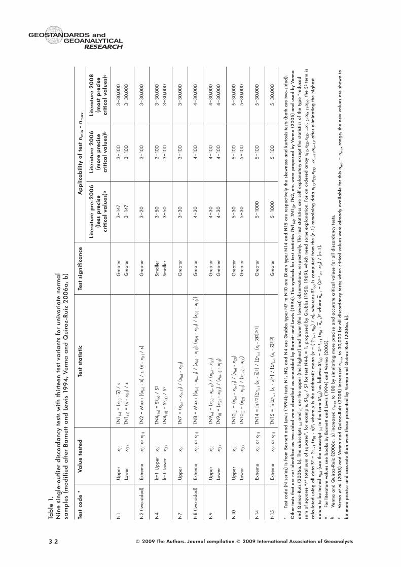
The nine single-outlier tests with thirteen variants(Table 1) evaluated in this work are: N1 (N1_Upperand N1_Lower ) , N2 (N2_Ex t reme) , N4 (N4k =1_Upper and N4k = 1_Lower), N7 (N7_Upper), N8(N8_Extreme), N9 (N9_Upper and N9_Lower), N10(N10_Upper and N10_Lower ) , N14 ( s kewnessN14_Extreme) and N15 (kurtosis N15_Extreme).

A “finite” statistical sample drawn from a normalpopulation can be designated as: x1,x2,x3,...,xn-2,xn-1,xn.If these observations (e.g., analytical data) are arran-ged in an ascending order, the new array may becalled x(1),x(2),x(3),...,x(n-2),x(n-1),x(n). The statistical samplesof analytical data for a given element in a RM werekept separately according to the analytical methodused to determine them; these methods were categori-sed into eight method-groups following Velasco-Tapiaet al. (2001). All of these individual cases of statisticalsamples constituted the “applicable” cases in our data-base of thirty-five RMs. For a particular chemical ele-ment in a RM, these statistical samples arising fromdifferent analytical methods were combined into a

3 1

GEOSTANDARDS and



3 2

GEOSTANDARDS and



Tab

le 1

.N

ine

sing

le-o

utlie

r d

isco

rda

ncy

test

s w

ith t

hirt

een

test

va

ria

nts

for

univ

ari

ate

nor

ma

l sa

mp

les

(mod

ified

aft

er B

arn

ett

and

Lew

is 1

99

4,

Verm

a a

nd Q

uiro

z-Ru

iz 2

00

6a

, b

)

Test

co

de

*Va

lue

test

edTe

st s

tati

stic

Test

sig

nifi

canc

eA

pp

lica

bili

ty o

f te

st n

min

- n m

ax

Lite

ratu

re p

re-2

00

6Li

tera

ture

20

06

Lite

ratu

re 2

00

8(le

ss p

reci

se(m

ore

pre

cise

(mo

st p

reci

secr

itic

al

valu

es)a

crit

ica

l va

lues

)bcr

itic

al

valu

es)c

N1

Upp

erx (

n)TN

1(u

)=

(x(n

)-

x) /

sG

reat

er3

–14

73

–10

03

–3

0,0

00

Low

erx (

1)

TN1

(1)=

(x-

x (1

)) /

sG

reat

er3

–14

73

–10

03

–3

0,0

00

N2

(tw

o-si

ded)

Extre

me

x (n)

or x

(1)

TN2

= M

ax :

{(x (

n)-

x) /

s, (

x-

x (1

) / s

}G

reat

er3

–2

03

–10

03

–3

0,0

00

N4

k=1

Upp

erx (

n)TN

4(1

u)=

S2

(n)/

S2Sm

alle

r3

–5

03

–10

03

–3

0,0

00

k=1

Low

erx (

1)

TN4

(1l)

= S

2(1

)/

S2Sm

alle

r3

–5

03

–10

03

–3

0,0

00

N7

Upp

erx (

n)TN

7 =

(x(n

)-

x (n-

1))

/ (x

(n)-

x (1

))G

reat

er3

–3

03

–10

03

–3

0,0

00

N8

(tw

o-si

ded)

Extre

me

x (n)

or x

(1)

TN8

= M

ax :

{(x (

n)-

x (n-

1))

/ (x

(n)-

x (1

)), (x

(2)-

x (1

)) /

(x(n

)-

x (1

))}G

reat

er4

–3

04

–10

04

–3

0,0

00

N9

Upp

erx (

n)TN

9(u

)=

(x(n

)-

x (n-

1))

/ (x

(n)-

x (2

))G

reat

er4

–3

04

–10

04

–3

0,0

00

Low

erx (

1)

TN9

(l)=

(x(2

)-

x (1

)) /

(x(n

-1)-

x (1

))G

reat

er4

–3

04

–10

04

–3

0,0

00

N10

Upp

erx (

n)TN

10(u

)=

(x(n

)-

x (n-

1))

/ (x

(n)-

x (3

))G

reat

er5

–3

05

–10

05

–3

0,0

00

Low

erx (

1)

TN10

(l)=

(x(2

)-

x (1

)) /

(x(n

-2)-

x (1

))G

reat

er5

–3

05

–10

05

–3

0,0

00

N14

Extre

me

x (n)

or x

(1)

TN14

= [n

1/2

{Σn i=

1(x

i-

x)3}

/ {Σ

n i=1

(xi-

x)2}3

/2]

Gre

ater

5–

100

05

–10

05

–3

0,0

00

N15

Extre

me

x (n)

or x

(1)

TN15

= [n

{Σn i=

1(x

i-

x)4}

/ {Σ

n i=1

(xi-

x)2}2

]G

reat

er5

–10

00

5–

100

5–

30

,00

0

*

T

est

cod

e (N

ser

ies)

is

from

Ba

rnet

t a

nd L

ewis

(19

94

); t

ests

N1,

N2

, a

nd N

4 a

re G

rub

bs

typ

e; N

7 t

o N

10 a

re D

ixon

typ

e; N

14 a

nd N

15 a

re r

esp

ectiv

ely

the

skew

ness

and

kur

tosi

s te

sts

(bot

h a

re t

wo-

sid

ed).

Oth

er t

ests

tha

t a

re n

ot i

den

tifie

d a

s tw

o-si

ded

wer

e cl

ass

ified

as

one-

sid

ed b

y B

arn

ett

and

Lew

is (

199

4).

The

sym

bol

s fo

r te

st s

tatis

tics

TN1

(u),

TN1

(l),

TN2

, et

c. w

ere

pro

pos

ed b

y Ve

rma

(2

00

5)

and

use

d b

y Ve

rma

and

Qui

roz-

Ruiz

(2

00

6a

, b

). Th

e su

bsc

rip

ts (u

)a

nd (l

)a

re t

he u

pp

er (

the

hig

hest

) a

nd l

ower

(th

e lo

wes

t) o

bse

rva

tions

, re

spec

tivel

y. T

he t

est

sta

tistic

s a

re s

elf

exp

lana

tory

exc

ept

the

sta

tistic

s of

the

typ

e “r

educ

edsu

m o

f sq

uare

s “/

” to

tal

sum

of

squa

res”

, fo

r ex

am

ple

, S2

(n)

/ S2

for

test

N4

-k =

1,

pro

pos

ed b

y G

rub

bs

(19

50

, 19

69

), w

hich

nee

d s

ome

exp

lana

tion.

For

an

ord

ered

arr

ay

x (1

),x(2

),x(3

),...,

x (n-

2),x

(n-1

),x(n

), th

e S2

term

is

calc

ula

ted

usi

ng a

ll d

ata

S2

= Σ

n i=1

(x(i

)-

x)2,

whe

re x

is t

he a

rith

met

ic m

ean

(x=

( Σ

n i=1

x (i))

/ n)

, w

here

as

S2(n

)is

com

put

ed f

rom

the

(n-

1)

rem

ain

ing

da

ta x

(1),x

(2),x

(3),.

..,x (

n-2

),x(n

-1),

aft

er e

limin

atin

g t

he h

ighe

std

atu

m t

o b

e te

sted

x(n

)(s

ee t

he s

ubsc

rip

t (n

)in

the

ter

m S

2(n

)) a

s fo

llow

s: S

2(n

)=

Σn-

1i=

1(x

(i)

- x n

-1)2

whe

re x

n-1

= (

Σn-

1i=

1x (

i))

/ (n

-1).

aFo

r lit

era

ture

va

lues

see

boo

ks b

y B

arn

ett

and

Lew

is (

199

4)

and

Ver

ma

(2

00

5).

bVe

rma

and

Qui

roz-

Ruiz

(2

00

6a

, b

) in

crea

sed

nm

ax

to 1

00

by

sim

ula

ting

mor

e p

reci

se a

nd a

ccur

ate

cri

tica

l va

lues

for

all

dis

cord

anc

y te

sts.

cVe

rma

et

al.

(20

08

) a

nd V

erm

a a

nd Q

uiro

z-Ru

iz (

20

08

) in

crea

sed

nm

ax

to 3

0,0

00

for

all

dis

cord

anc

y te

sts;

whe

n cr

itica

l va

lues

wer

e a

lrea

dy

ava

ilab

le f

or t

his

n min

– n

ma

x ra

nge,

the

new

va

lues

are

sho

wn

tob

e m

ore

pre

cise

and

acc

ura

te t

han

even

tho

se p

rese

nted

by

Verm

a a

nd Q

uiro

z-Ru

iz (

20

06

a,

b).

single statistical sample only after the discordancy tests(single-outlier type tests; Table 1) and significance tests(ANOVA for three or more method-groups, or F andStudent’s t tests for two method-groups) demonstratedat the strict 99% confidence level that none of themhad any discordant outliers and all were drawn from asingle normal population or identical normal popula-tions. On the contrary, the data from one or sometimesmore analytical method-groups were not combinedinto this final statistical sample for estimating the cen-tral tendency and dispersion parameters.

The discordancy tests of a single-outlier type nor-mally evaluate either an upper outlier x(n), e.g., test N1(N1_Upper ) , a lower ou t l i e r x (1 ) , e .g . , t e s t N1(N1_Lower), or an extreme outlier x(n) or x(1) (whicheverof the two is farther away from the central tendencyparameter), e.g., test N2 (see Table 1), as a possiblediscordant outlier under a contamination model (moredetails on such models are given at the end of thenext section).

The single-outlier discordancy tests can be appliedconsecutively to test as many outliers as a given test iscapable of detecting as discordant (Barnett and Lewis1994, Verma 1997, 1998, Verma et al. 2008). Thus, agiven test, e.g., N1_Upper, is applied to test the valuex(n), and if this value is declared to be a discordantoutlier in this first iteration (“Iteration 1”), the same testis again applied (this is called consecutive testing byBarnett and Lewis 1994) to the remaining data for tes-ting a second upper outlier; this represents “Iteration2”. The iterations are thus numbered consecutively. Thetest is repeated until no more discordant outliers areidentified.

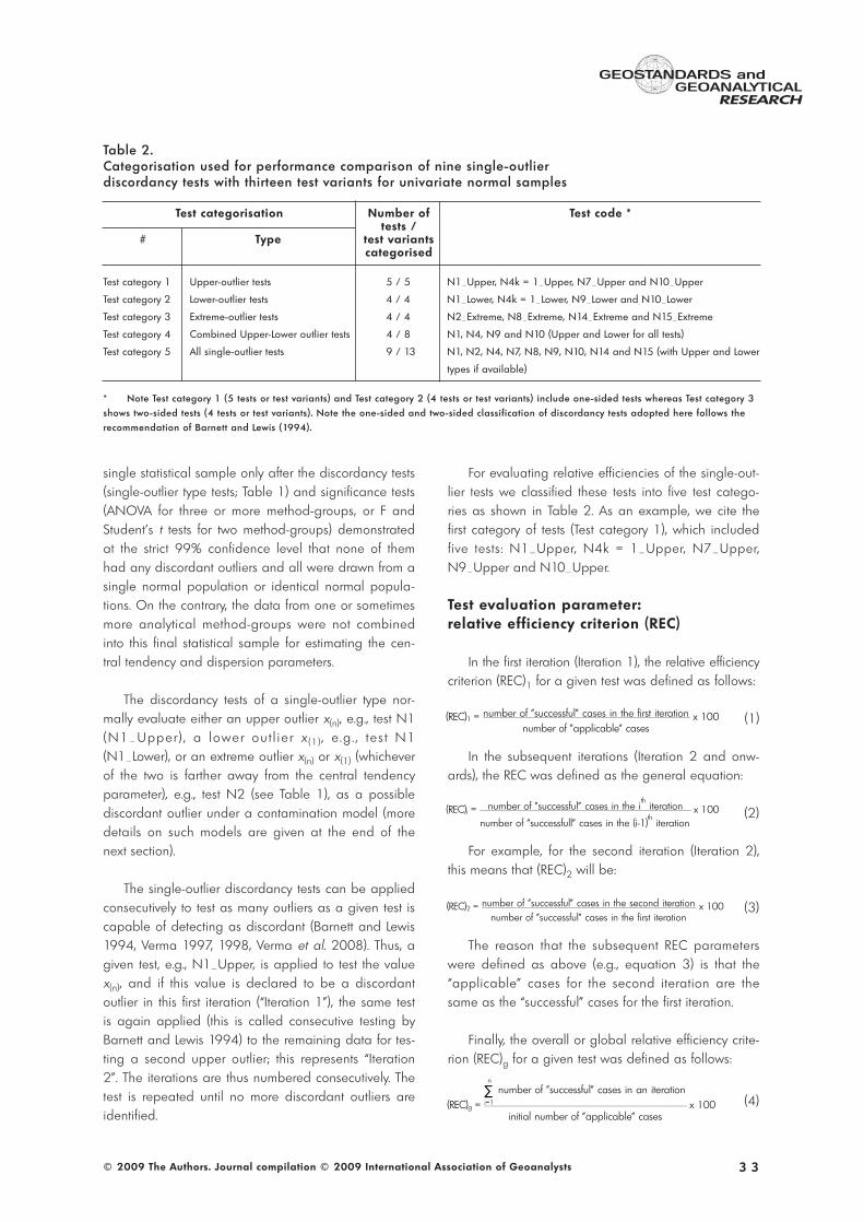
For evaluating relative efficiencies of the single-out-lier tests we classified these tests into five test catego-ries as shown in Table 2. As an example, we cite thefirst category of tests (Test category 1), which includedfive tests: N1_Upper, N4k = 1_Upper, N7_Upper,N9_Upper and N10_Upper.

Test evaluation parameter: relative efficiency criterion (REC)

In the first iteration (Iteration 1), the relative efficiencycriterion (REC)1 for a given test was defined as follows:

(1)

In the subsequent iterations (Iteration 2 and onw-ards), the REC was defined as the general equation:

(2)

For example, for the second iteration (Iteration 2),this means that (REC)2 will be:

(3)

The reason that the subsequent REC parameterswere defined as above (e.g., equation 3) is that the“applicable” cases for the second iteration are thesame as the “successful” cases for the first iteration.

Finally, the overall or global relative efficiency crite-rion (REC)g for a given test was defined as follows:

(4)

3 3

GEOSTANDARDS and



Table 2.Categorisation used for performance comparison of nine single-outlier discordancy tests with thirteen test variants for univariate normal samples

Test categorisation Number of Test code *tests /

# Type test variantscategorised

Test category 1 Upper-outlier tests 5 / 5 N1_Upper, N4k = 1_Upper, N7_Upper and N10_Upper

Test category 2 Lower-outlier tests 4 / 4 N1_Lower, N4k = 1_Lower, N9_Lower and N10_Lower

Test category 3 Extreme-outlier tests 4 / 4 N2_Extreme, N8_Extreme, N14_Extreme and N15_Extreme

Test category 4 Combined Upper-Lower outlier tests 4 / 8 N1, N4, N9 and N10 (Upper and Lower for all tests)

Test category 5 All single-outlier tests 9 / 13 N1, N2, N4, N7, N8, N9, N10, N14 and N15 (with Upper and Lower

types if available)

* Note Test category 1 (5 tests or test variants) and Test category 2 (4 tests or test variants) include one-sided tests whereas Test category 3shows two-sided tests (4 tests or test variants). Note the one-sided and two-sided classification of discordancy tests adopted here follows therecommendation of Barnett and Lewis (1994).

(REC)g =number of "successful" cases in an iteration∑

i=1

n

initial number of "applicable" cases x 100

(REC)1 = number of "successful" cases in the first iterationnumber of "applicable" cases

x 100

(REC)i = number of "successful" cases in the ith iteration

number of "successfull" cases in the (i-1)th iteration

x 100

(REC)2 = number of "successful" cases in the second iterationnumber of "successful" cases in the first iteration

x 100

where the iteration number i varied from 1 to n (n beingthe final iteration considered for the REC calculations).

Thus, the overall REC parameter (REC)g takes intoaccount the fact that a given test might identify a firstoutlier as discordant in Iteration 1, but also a secondone in Iteration 2, and so on. Therefore, the number ofdiscordant outliers should be summed up for this parti-cular test to calculate (REC)g from equation (4), thenumber of initial “applicable” cases being the same asthe “applicable” cases for the first iteration. Thus, if agiven test detected an outlier in Iteration 1 but failedto do so in Iteration 2 for any of these “successful”

cases, its overall (REC)g value would remain the sameas that for Iteration 1, i.e., for this particular test, (REC)g= (REC)1. However, if a test also detected a discordantoutlier in the second iteration, we should have for thistest: (REC)g > (REC)1.

For any REC to be statistically meaningful, we arbi-trarily set a lower limit to the total number of appli-cable cases for each of the tests to be at least 30 inany given iteration, below which we did not calculateindividual REC values for that particular iteration. Wealso note that theoretically the REC values are expec-ted to be close to zero under the null hypothesis (H0)

3 4

GEOSTANDARDS and



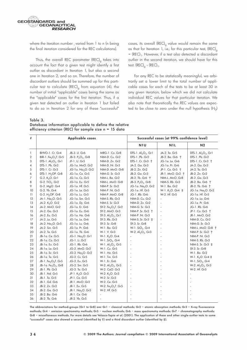
Table 3.Database information applicable to define the relative efficiency criterion (REC) for sample size n = 15 data

# Applicable cases Successful cases (at 99% confidence level)

N1U N1L N2

1 BHVO-1_Cr_Gr4 JB-3_U_Gr6 MRG-1_Co_Gr8 DTS-1_Al2O3_Gr1 JA-2_Ta_Gr5 DTS-1_Al2O3_Gr12 BIR-1_Fe2O3T_Gr5 JB-3_P2O5_Gr8 NIM-D_Cu_Gr2 DTS-1_Pb_Gr2 JB-2_Ba_Gr6 † DTS-1_Pb_Gr23 DTS-1_Al2O3_Gr1 JF-1_U_Gr5 NIM-D_Zn_Gr2 DTS-1_Cr_Gr3 † JG-1a_La_Gr6 DTS-1_Cr_Gr3 †4 DTS-1_Pb_Gr2 JG-1a_MnO_Gr2 NIM-D_Ni_Gr3 JA-2_Ga_Gr3 JG-1a_Pr_Gr6 JA-2_Ga_Gr35 DTS-1_Cr_Gr3 JG-1a_Na2O_Gr2 NIM-D_MnO_Gr8 JB-2_Zn_Gr2 JP-1_Co_Gr5 † JA-2_Ta_Gr56 DTS-1_H2OP_Gr8 JG-1a_Co_Gr5 NIM-G_Sr_Gr3 JB-2_Ga_Gr3 JR-1_MnO_Gr2 † JB-2_Zn_Gr27 G-2_K2O_Gr1 JG-1a_Cs_Gr5 NIM-L_Ba_Gr2 JB-2_Tb_Gr6 † NIM-L_MnO_Gr8 JB-2_Ga_Gr38 G-2_TiO2_Gr2 JG-1a_Eu_Gr5 NIM-L_MnO_Gr8 JB-3_P2O5_Gr8 NIM-S_Rb_Gr3 JB-2_Ba_Gr6 †9 G-2_MgO_Gr4 JG-1a_Hf_Gr5 NIM-P_Sr_Gr2 JG-1a_Na2O_Gr2 W-1_Ba_Gr2 JB-2_Tb_Gr6 †10 G-2_Yb_Gr4 JG-1a_La_Gr5 NIM-P_Ni_Gr3 JG-1a_Hf_Gr5 W-1_K2O_Gr4 ‡ JG-1a_Na2O_Gr211 G-2_H2OP_Gr8 JG-1a_Lu_Gr5 NIM-P_MnO_Gr8 JG-1_Rb_Gr6 W-2_Hf_Gr5 JG-1a_Hf_Gr512 JA-1_Na2O_Gr5 JG-1a_Sm_Gr5 NIM-S_Rb_Gr3 NIM-D_Cu_Gr2 - JG-1a_La_Gr613 JA-2_K2O_Gr2 JG-1a_Dy_Gr6 NIM-S_Sr_Gr3 NIM-D_Zn_Gr2 - JG-1a_Pr_Gr614 JA-2_MnO_Gr2 JG-1a_Er_Gr6 SY-2_Fe2O3T_Gr2 NIM-G_Sr_Gr3 - JG-1_Rb_Gr615 JA-2_Ga_Gr3 JG-1a_Eu_Gr6 SY-2_MnO_Gr3 NIM-P_Sr_Gr2 † - JP-1_Co_Gr5 †16 JA-2_Eu_Gr5 JG-1a_Ho_Gr6 SY-3_Al2O3_Gr1 NIM-P_Ni_Gr3 - JR-1_MnO_Gr217 JA-2_La_Gr5 JG-1a_La_Gr6 SY-3_Rb_Gr3 NIM-S_Sr_Gr3 ‡ - NIM-D_Cu_Gr218 JA-2_Na2O_Gr5 JG-1a_Lu_Gr6 SY-3_Sr_Gr8 SY-3_Sr_Gr8 - NIM-G_Sr_Gr319 JA-2_Sm_Gr5 JG-1a_Pr_Gr6 W-1_Ba_Gr2 W-1_SiO2_Gr4 - NIM-L_MnO_Gr8 †20 JA-2_Ta_Gr5 JG-1a_Tb_Gr6 W-1_V_Gr3 W-2_Al2O3_Gr3 - NIM-P_Sr_Gr2 †21 JB-1a_Ce_Gr5 JG-1_Na2O_Gr1 W-1_K2O_Gr4 - - NIM-P_Ni_Gr322 JB-1a_Co_Gr5 JG-1_Li_Gr2 W-1_SiO2_Gr4 - - NIM-S_Rb_Gr323 JB-1a_Eu_Gr5 JG-1_Rb_Gr6 W-1_Al2O3_Gr5 - - NIM-S_Sr_Gr3 ‡24 JB-1a_La_Gr5 JG-2_MnO_Gr2 W-1_Cu_Gr5 - - SY-3_Sr_Gr825 JB-1a_Sc_Gr5 JG-2_Na2O_Gr2 W-1_Ho_Gr5 - - W-1_Ba_Gr226 JB-1a_Ta_Gr5 JG-2_Cs_Gr5 W-1_Tm_Gr5 - - W-1_K2O_Gr4 ‡27 JB-1_Fe2O3T_Gr5 JG-2_Eu_Gr5 W-1_Er_Gr6 - - W-1_SiO2_Gr428 JB-1a_Fe2O3_Gr8 JG-2_Sm_Gr5 W-2_Al2O3_Gr3 - - W-2_Al2O3_Gr329 JB-1_Pb_Gr3 JG-2_Ta_Gr5 W-2_CaO_Gr3 - - W-2_Hf_Gr530 JB-1_Nd_Gr5 JP-1_K2O_Gr3 W-2_K2O_Gr3 - - -31 JB-1_Ta_Gr5 JP-1_Co_Gr5 W-2_Sr_Gr3 - - -32 JB-1_Gd_Gr6 JR-1_MnO_Gr2 W-2_Ce_Gr5 - - -33 JB-2_Zn_Gr2 JR-1_Eu_Gr5 W-2_Fe2O3T_Gr5 - - -34 JB-2_Ga_Gr3 JR-1_Na2O_Gr5 W-2_Hf_Gr5 - - -35 JB-2_Ba_Gr6 JR-1_Ce_Gr6 - - - -36 JB-2_Tb_Gr6 JR-2_Yb_Gr5 - - - -

The abbreviations for method-groups (Gr1 to Gr8) are: Gr1 – classical methods; Gr2 – atomic absorption methods; Gr3 – X-ray fluorescencemethods; Gr4 – emission spectrometry methods; Gr5 – nuclear methods; Gr6 – mass spectrometry methods; Gr7 – chromatography methods;Gr8 – miscellaneous methods. For more details see Velasco-Tapia et al. (2001). The application of these and other single-outlier tests to some“successful” cases also showed a second (identified by †) and a third discordant outlier (identified by ‡).

that all samples were drawn from a normal populationwithout any “statistical” contamination. The alternatehypothesis (H1) being tested is related to a suitablecontamination model, according to which an extremeobservation came from a different distribution (shiftedmean, greater standard deviation or both) than theremaining observations in a given sample. Barnett andLewis (1994) is an excellent source for more details on

these hypotheses and models. Finally, we emphasisethat, following Verma (1998), the discordancy testswere applied to the statistical samples derived from asingle analytical method-group at the strict confidencelevel of 99%.

An example of the REC calculations: We illustratethe meaning and calculation of the REC parameter for

3 5

GEOSTANDARDS and



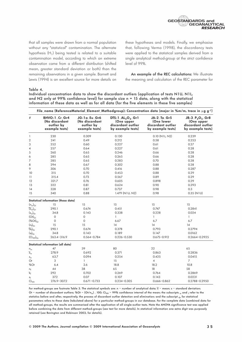
Table 4.Individual concentration data to show the discordant outliers (application of tests N1U, N1L, and N2 only at 99% confidence level) for sample size n = 15 data, along with the statistical information of these data as well as for all data (for the five elements in these five samples)

File_name (ReferenceMaterial_Element_Methodgroup): Concentration data (major in %m/m, trace in μg g-1)

# BHVO-1_Cr_Gr4 JG-1a_Eu_Gr6 DTS-1_AL2O3_Gr1 JA-2_Ta_Gr5 JB-3_P2O5_Gr8(No discordant (No discordant (One upper (One lower (One upper

outlier by outlier by discordant outlier discordant outlier discordant outlierexample tests) example tests) by example tests) by example tests) by example tests)

1 230 0.309 0.130 0.10 (N1L, N2) 0.2392 241 0.49 0.212 0.58 0.2533 252 0.60 0.227 0.61 0.274 257 0.64 0.227 0.61 0.285 260 0.65 0.246 0.66 0.286 285 0.65 0.265 0.66 0.287 285 0.65 0.283 0.70 0.288 294 0.67 0.302 0.88 0.289 306 0.70 0.416 0.88 0.28710 315 0.70 0.453 0.88 0.2911 315.4 0.73 0.567 0.89 0.2912 321.7 0.76 0.605 0.898 0.2913 322 0.81 0.624 0.90 0.29314 328 0.87 0.737 0.98 0.315 340 0.88 1.479 (N1U, N2) 0.98 0.35 (N1U)

Statistical information (these data)(nin)Gr 15 15 15 15 15(xin)Gr 290.1 0.674 0.451 0.747 0.2841(sin)Gr 34.8 0.143 0.338 0.228 0.024(Ot)Gr 0 0 1 1 1(%Ot)Gr 0 0 6.67 6.7 6.7(nf)Gr 15 15 14 14 14(xf)Gr 290.1 0.674 0.378 0.793 0.2794(sf)Gr 34.8 0.143 0.189 0.147 0.0162(CL99)Gr 263.4–316.9 0.564–0.784 0.226–0.530 0.675–0.912 0.2664–0.2925

Statistical information (all data)nin 47 39 80 22 65xin 278.9 0.692 0.371 0.863 0.2836sin 63.7 0.094 0.254 0.425 0.0415Ot 3 1 15 4 7%Ot 6.4 2.6 18.8 18.2 10.8nf 44 38 65 18 58xf 292 0.702 0.269 0.764 0.2869sf 37.2 0.07 0.107 0.143 0.0231CL99 276.9–307.2 0.671–0.733 0.234–0.305 0.666–0.862 0.2788–0.2950

For method-groups see footnote Table 3. The statistical symbols are: n – number of analytical data; x – mean; s – standard deviation; Ot – number of discordant outliers; %Ot – (Ot/nin) . 100; CL99 – 99% confidence interval of the mean; the subscripts in and f refer to the statistics before and after, respectively, the process of discordant outlier detection and elimination; and the subscript Gr for statistical parameters refers to these data (tabulated above) for a particular method-groups in our database. For the complete data (combined data forall method-groups, the results are summarised after the application of all single-outlier tests. Note the ANOVA significance test was appliedbefore combining the data from different method-groups (see text for more details). In statistical information one extra digit was purposelyretained (see Bevington and Robinson 2003, for details).

a particular example of sample size n = 15 in our data-base. First, all cases of this particular sample size wereidentified in the database (see Table 3 for a synthesis ofthese sets). Thus, a total of 106 “applicable” cases exis-ted for n = 15 in our database (Table 3). For example,the first “applicable” case listed in Table 3 is BHVO-1_Cr_Gr4, i.e., there were fifteen data for Cr (see Table4 for the listing of these individual data) in BHVO-1 byanalytical method-group # 4 - emission spectrometrymethods; similarly, the second applicable case is BIR-1_Fe2O3T_Gr5 (Fe2O3

t data for BIR-1 by method-group# 5 - nuclear methods), and so on. For illustrative pur-poses, Table 3 also reports explicitly the results of theapplication of just three discordancy test variants (seeTable 1 for more details on these test variants; the othervariants for tests N3 to N15 were similarly applied, butwere not included in Table 3 for the sake of simplicity):N1U (test N1 for the upper outlier); N1L (test N1 for thelower outlier); and N2 (test N2 for an extreme outlier).Table 3 lists all cases in which one or sometimes morediscordant outliers were detected in 106 “applicable”cases; these cases were termed the “successful” cases fora particular discordancy test. Thus, during Iteration 1tests N1U, N1L and N2 detected one outlier in 20, 11,and 29 cases (Table 3), and using equation (1) above,the corresponding REC values (REC)1 would be about18.9, 10.4 and 27.4, respectively. The application ofthese and other single-outlier tests showed the presenceof a discordant second outlier in some of these “success-ful” cases (identified by † in Table 3) and also a thirddiscordant outlier in still fewer cases (identified by ‡;Table 3). For the cases with only one discordant outlierpresent, i.e., those cases not identified by † or ‡ in anyof the columns corresponding to the “successful” cases inTable 3, we note that (REC)g = (REC)1, of which a fewse lec ted cases are d i scussed be low fo r the%DiscordantOutliers parameter.

%DiscordantOutliers (%Ot) parameter

Note that the REC parameter is not synonymouswith %DiscordantOutliers (%otd in Verma 1997, or %Ot

in Velasco-Tapia et al. 2001). For a given analyticalmethod-group, the (%Ot)Gr parameter for a givenelement in a RM can be defined as:

(5)

For the complete dataset for a given element in aRM, the %Ot can be similarly defined as:

(6)

Here, a “combined” case refers to all analyticaldata of an element in a RM, obtained from all analyt-ical methods.

The major distinction between the REC and %Otparameters is that the former refers to all “applicable”cases whereas the latter is for one particular “applicable”case, either for a single method-group (here referred toas (%Ot)Gr) or for a “combined” case of all method-groups (simply called %Ot). The REC parameter can onlybe defined for a statistically significant number of“applicable” cases (equations 1 to 4) whereas the %Otparameter is generally meaningful for one particular“applicable” or “combined” case (equations 5 and 6).

If we were to consider only the three single-outliertests (N1U, N1L and N2), the (%Ot)Gr would be onlyabout 6.7% for all those cases that are listed in any ofthe last three columns (under the heading “successfulcases”, Table 3) but are not identified by the symbols †and ‡. For the latter, because two or three outliers, res-pectively, were identified as discordant by the presentsingle-outlier test method, the (%Ot)Gr would be about13.3% or 20.0%, respectively.

For all other “applicable” cases (those cases thatare listed in the first three columns but are not presentin the other columns could be termed, on the contrary,as “unsuccessful” cases although we did not use thisterm), the (%Ot)Gr for each of them will be exactly zeroif we were to consider only these three single-outliertests (Table 3).

An example of %Ot calculations: We used selec-ted cases from Table 3 as examples to illustrate thedifference between (%Ot)Gr or %Ot. In Table 4 we pre-sent five cases selected from Table 3, for which the(%Ot)Gr was either 0% (BHVO-1_Cr_Gr4 and JG-1_Eu_Gr6) or about 6.7% (DTS-1_Al2O3_Gr1, JA-2_Ta_Gr5, and JB-3_P2O5_Gr8). Table 4 also providesthe statistical information for these data (individuallylisted) as well as for the complete data (not individuallylisted) for all methods for these elements. For the latter,the %Ot parameter varied from 2.6 to 18.8% (for alliterations - see the final lowest part of Table 4).

Results

Relative efficiency criterion (REC)

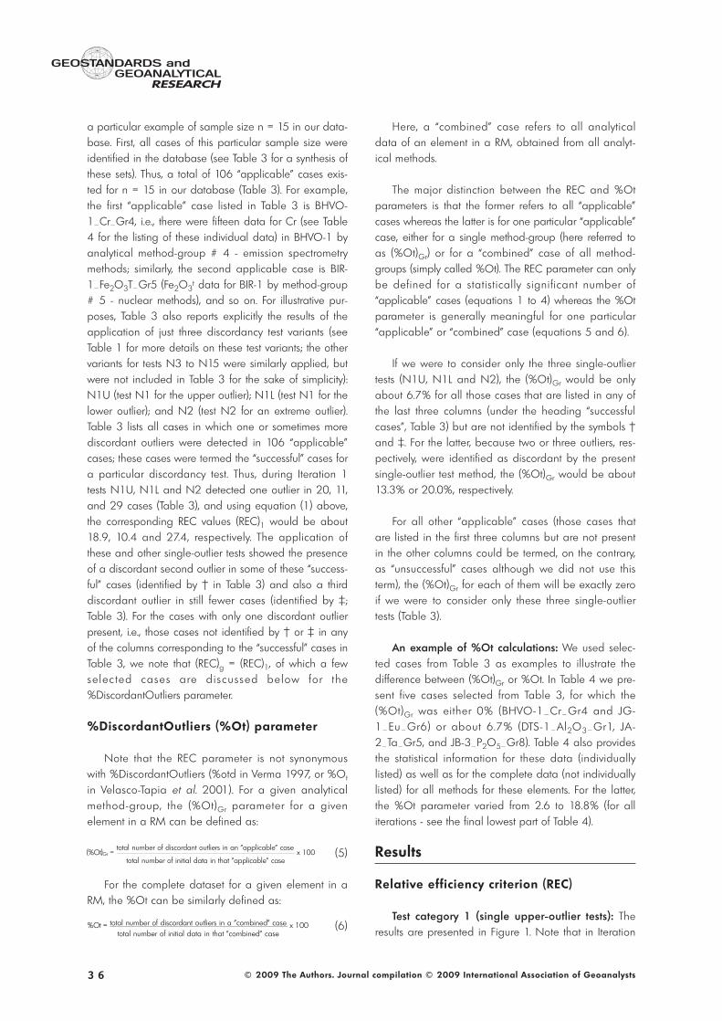
Test category 1 (single upper-outlier tests): Theresults are presented in Figure 1. Note that in Iteration

3 6

GEOSTANDARDS and



(%Ot)Gr =total number of discordant outliers in an "applicable" case

total number of initial data in that "applicable" case x 100

%Ot = total number of discordant outliers in a "combined" casetotal number of initial data in that "combined" case

x 100

3 7

GEOSTANDARDS and



0

10

20

30

40

50

N1U N4U1 N7U N9U N10U

Iteration 1(a)

0

10

20

30

40

50


Iteration 2(b)

0

10

20

30

40

50


Iteration 3(c)

0

10

20

30

40

50


Iteration 4(d)

Figure 1. The relative efficiency criterion (REC) of the discordancy tests in Test category 1 (see Table 2 for categorisation).

The five tests of the upper outlier type compared in Test category 1 are: N1U - N1_Upper, N4U1 - N4k = 1_Upper,

N7U - N7_Upper, N9U - N9_Upper and N10U - N10_Upper. Note that in order to facilitate a better visual comparison

of (REC)1 to (REC)4 values, the same y-scale (0-50%) was maintained throughout Figures 1-5. The number of cases to

which a given test was applied is also presented explicitly in this and later figure captions. (a) Iteration 1 (5336 cases

with sample sizes n ≥ 3 for N1U, N4U1, and N7U; 4490 cases with sample sizes n ≥ 4 for N9U; and 3889 cases with

sample sizes n ≥ 5 for N10U); (b) Iteration 2 (973 cases for N1U, 979 for N4U1, 846 for N7U, 759 for N9U, and 681

for N10U); and (c) Iteration 3 (155 cases for N1U, 157 for N4U1, 83 for N7U, 61 for N9U, and 51 for N10U).

(REC

) 1(%

)(R

EC) 3

(%)

(REC

) 4(%

)(R

EC) 2

(%)

1 the tests were applied to a different number of casesdepending on the minimum sample size applicablefor a given test statistic (5336 cases of n ≥ 3 for N1U,N4U1, and N7U; 4490 cases of n ≥ 4 for N9U; and3889 cases of n ≥ 5 for N10U; see Table 1). We alsoemphasise that the (REC)1 values were very similar(more importantly, they maintained the trends anddifferences between the (REC)1 values as explained inthis and the later sections) when all these tests wereapplied to the ident ical cases (3889 cases wi thsample sizes n ≥ 5), implying that the overall (REC)gvalues did not strongly depend on whether all “appli-cable” cases (Iteration 1; Figure 1a) or the same caseswere considered for all tests (the results of the latterare not shown graphically). This was also true for othertest categories.

For Iteration 1 (Figure 1a), the Grubbs type tests(N1U and N4U1) showed sl ightly greater (REC)1values (18.2 and 18.3%) than the Dixon type tests(N7U, N9U and N10U; 15.9-17.5%). The (REC)2 and(REC)3 values (for iterations 2 and 3; Figure 1b, c) for

the Grubbs type tests (15.9-22.3%) were notably grea-ter than the Dixon type tests (6.0-13.1%). For Iteration 4(Figure 1d), a significant number (> 30) of “applicable”cases being the number of the “successful” cases forIteration 3, persisted only for the Grubbs type tests(N1U and N4U1), for which the (REC)4 values werealso greater (31.4 and 32.4%) than for the earlier ite-rations. Discordant outliers were still detected for a fewcases up to Iteration 6 for these Grubbs type tests.

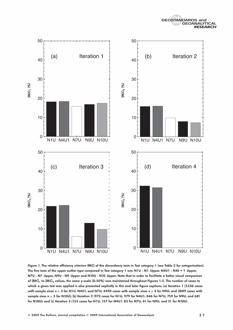
Test category 2 (single lower-outlier tests): Theresults are presented in Figure 2. For Iteration 1 (Figure2a), the Grubbs type tests (N1L and N4L1) showedsomewhat smaller (REC)1 than the Dixon type tests(N9L and N10L; 9.1 and 9.7%). However, for Iteration2 (Figure 2b), the (REC)2 values for these two Grubbstype tests were significantly greater (10.9 and 11.5%)than those for the Dixon type tests (5.6 and 7.4%). ForIteration 3 (Figure 2c), similar (REC)3 values (11.8 and12.5%) were obtained for the Grubbs type tests (N1Land N4L1) whereas no outliers (0% REC) were detec-ted by the Dixon type tests (N9L and N10L). Outliers

3 8

GEOSTANDARDS and



0

10

20

30

40

50

N1L N4L1 N9L N10L

Iteration 1(a)

0

10

20

30

40

50

N1L N4L1 N9L N10L

Iteration 2 (b)

0

10

20

30

40

50

N1L N4L1 N9L N10L

Iteration 3 (c)

Figure 2. The relative efficiency criterion (REC) of the discordancy tests in Test category 2 (see Table 2 for categorisation).

The four tests of the lower outlier type compared in Test category 2 are: N1L - N1_Lower, N4L1 - N4k = 1_Lower, N9L -

N9_Lower and N10L - N10_Lower. (a) Iteration 1 (5336 cases for N1L and N4L1, 4490 for N9L; and 3889 for N10L);

(b) Iteration 2 (439 cases for N1L, 444 for N4L1, 408 for N9L, and 377 for N10L); and (c) Iteration 3 (48 cases for N1L,

51 for N4L1, 23 for N9L, and 28 for N10L), note no outliers were detected as discordant by N9L and N10L in this iteration.

(REC

) 1(%

)(R

EC) 3

(%)

(REC

) 2(%

)

were detected as discordant for a few cases up toIteration 4 by N1L and N4L1.

Also note that for Iteration 1, the (REC)1 values (8.2-9.7%) were significantly smaller than those for theupper outlier versions of these tests (15.9-18.3%; see

Test category 1 above; compare Figures 2a and 1a).This is an interesting observation concerning the distri-bution of discordant outliers in geochemical data onRMs; discordant upper outliers (x(n)) are more commonthat discordant lower outliers (x(1)). In fact, the compari-son of the performance of upper- and lower-outlier

3 9

GEOSTANDARDS and



0

10

20

30

40

50

N2 N8 N14 N15

Iteration 1(a)

0

10

20

30

40

50

N2 N8 N14 N15

Iteration 3(c)

0

10

20

30

40

50

N2 N8 N14 N15

Iteration 4(d)

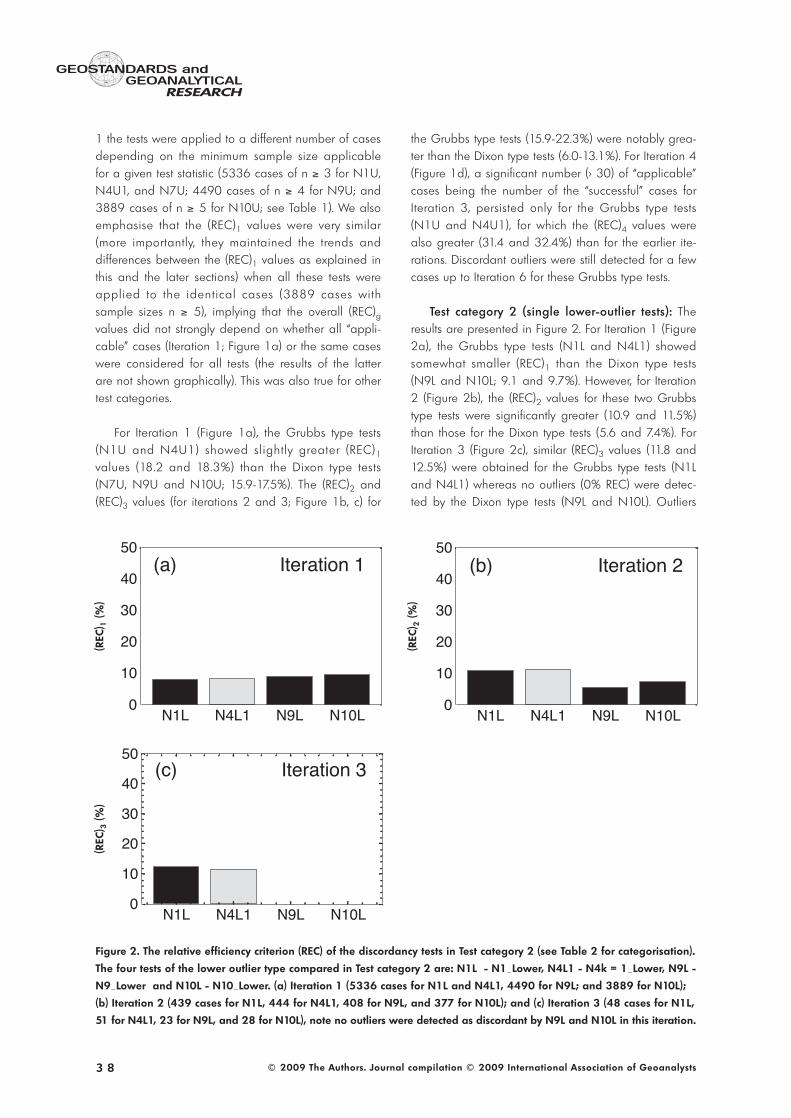
Figure 3. The relative efficiency criterion (REC) of the discordancy tests in Test category 3 (see Table 2 for

categorisation). The four tests (two-sided) of the extreme outlier type compared in Test category 3 are: N2

(Grubbs type), N8 (Dixon type), N14 (skewness), and N15 (kurtosis). (a) Iteration 1 (5336 cases for N2, 4490 for

N8, and 3889 for N14 and N15); (b) Iteration 2 (1210 cases for N2, 893 for N8, 838 for N14, and 988 for N15);

(c) Iteration 3 (222 cases for N2, 96 for N8, 201 for N14, and 245 for N15); and (d) Iteration 4 (45 cases for N2,

1 for N8, 75 for N14, and 87 for N15). Iteration 5 (29 cases for N14 and 40 for N15) is not shown.

(REC

) 1(%

)(R

EC) 3

(%)

(REC

) 4(%

)(R

EC) 2

(%)

0

10

20

30

40

50

N2 N8 N14 N15

Iteration 2(b)

versions of tests (Figures 1a-d and 2a-c; (REC)1, (REC)2and (REC)3 values of Test category 1 and Test category2, respectively) suggests that positively skewed inter-laboratory geochemical datasets are more commonlypresent than negatively skewed ones. This implies thatthe robust estimates of central tendency, such as themedian, the trimean and the Gastwirth´s mean, arelikely to be biased, especially for small-sized samples.

Test category 3 (single extreme-outlier tests): Theresults are presented in Figure 3. These tests are alsoclassified by Barnett and Lewis (1994) as two-sidedtests, whereas the tests in the earlier categories (Testcategory 1 and Test category 2) are known as one-sided. For Iteration 1 (Figure 3a), the kurtosis test (N15)showed the greatest (REC)1 value (25.4%), followed bythe Grubbs type test (N2; 22.7%) and the skewnesstest (N14; 21.5%), with the Dixon type test (N8) presen-ting the smallest value (19.9%). For iterations 2 and 3(Figure 3b, c), both the skewness and kurtosis tests(N14 and N15) showed very high (REC)2 values (24.0-37.3%) as compared to the Grubbs type test (N2; 18.3and 20.3%) and the Dixon type test (N8; 8.3 and10.8%). For Iteration 4 (Figure 3d), the Dixon type test(N8) was applicable for only eight cases (being the“successful” cases for this test in Iteration 3) whereas allthe other tests (N2, N14 and N15) were applied to asignificantly large number of cases (45, 75 and 87, res-pectively) and showed very high (REC)4 values (33.3%,38.6% and 46.0%, respectively; Figure 3d). Iteration 5(not plotted in Figure 3) also showed good applicabili-ty of both the skewness and kurtosis tests, with (REC)5values of 44.8% and 42.5%, respectively although forthe former, the number of “applicable” cases was 29(slightly less than “30 cases” set by us as the lowerlimit for the REC calculations). Outliers were detectedas discordant by tests of category 3 for up to 6, 7 and8 iterations for tests N2, N14 and N15, respectively.

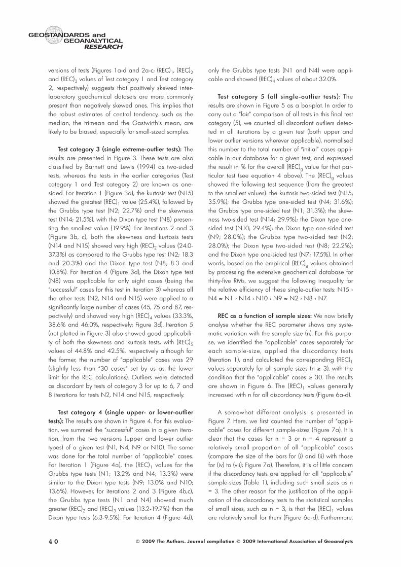
Test category 4 (single upper- or lower-outliertests): The results are shown in Figure 4. For this evalua-tion, we summed the “successful” cases in a given itera-tion, from the two versions (upper and lower outliertypes) of a given test (N1, N4, N9 or N10). The samewas done for the total number of “applicable” cases.For Iteration 1 (Figure 4a), the (REC)1 values for theGrubbs type tests (N1; 13.2% and N4; 13.3%) weresimilar to the Dixon type tests (N9; 13.0% and N10;13.6%). However, for iterations 2 and 3 (Figure 4b,c),the Grubbs type tests (N1 and N4) showed muchgreater (REC)2 and (REC)3 values (13.2-19.7%) than theDixon type tests (6.3-9.5%). For Iteration 4 (Figure 4d),

only the Grubbs type tests (N1 and N4) were appli-cable and showed (REC)4 values of about 32.0%.

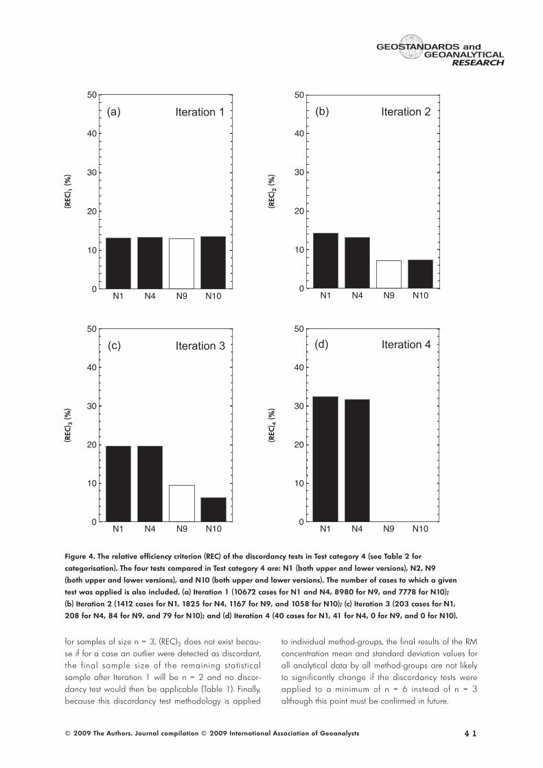
Test category 5 (all single-outl ier tests) : Theresults are shown in Figure 5 as a bar-plot. In order tocarry out a “fair” comparison of all tests in this final testcategory (5), we counted all discordant outliers detec-ted in all iterations by a given test (both upper andlower outlier versions wherever applicable), normalisedthis number to the total number of “initial” cases appli-cable in our database for a given test, and expressedthe result in % for the overall (REC)g value for that par-ticular test (see equation 4 above). The (REC)g valuesshowed the following test sequence (from the greatestto the smallest values): the kurtosis two-sided test (N15;35.9%); the Grubbs type one-sided test (N4; 31.6%);the Grubbs type one-sided test (N1; 31.3%); the skew-ness two-sided test (N14; 29.9%); the Dixon type one-sided test (N10; 29.4%); the Dixon type one-sided test(N9; 28.0%); the Grubbs type two-sided test (N2;28.0%); the Dixon type two-sided test (N8; 22.2%);and the Dixon type one-sided test (N7; 17.5%). In otherwords, based on the empirical (REC)g values obtainedby processing the extensive geochemical database forthirty-five RMs, we suggest the following inequality forthe relative efficiency of these single-outlier tests: N15 >N4 ≈ N1 > N14 > N10 > N9 ≈ N2 > N8 > N7.

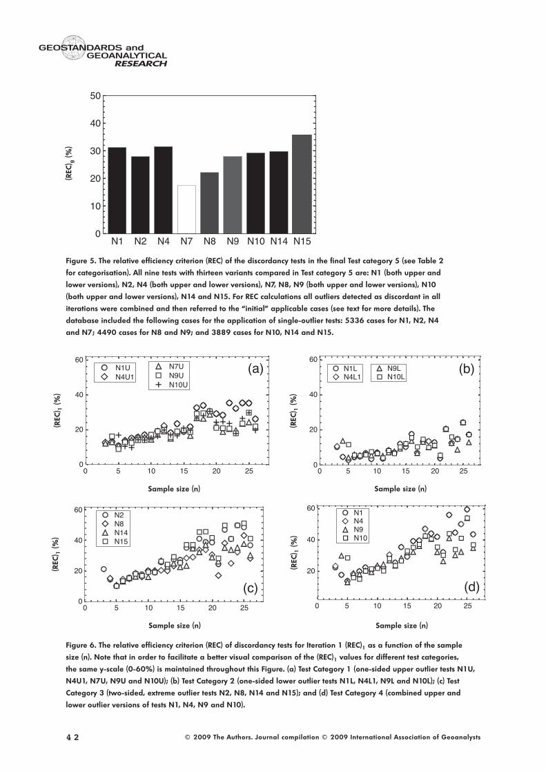
REC as a function of sample sizes: We now brieflyanalyse whether the REC parameter shows any syste-matic variation with the sample size (n). For this purpo-se, we identified the “applicable” cases separately foreach sample-s ize, appl ied the discordancy tes ts(Iteration 1), and calculated the corresponding (REC)1values separately for all sample sizes (n ≥ 3), with thecondition that the “applicable” cases ≥ 30. The resultsare shown in Figure 6. The (REC)1 values generallyincreased with n for all discordancy tests (Figure 6a-d).

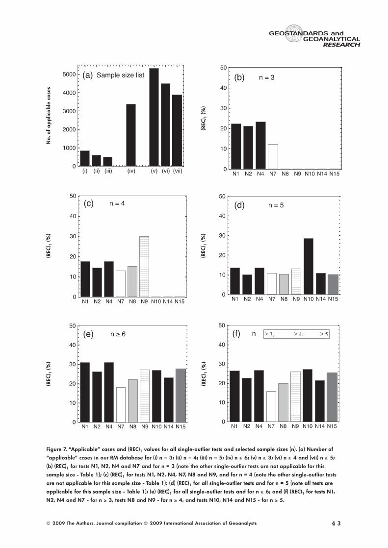
A somewhat dif ferent analysis is presented inFigure 7. Here, we first counted the number of “appli-cable” cases for different sample-sizes (Figure 7a). It isclear that the cases for n = 3 or n = 4 represent arelatively small proportion of all “applicable” cases(compare the size of the bars for (i) and (ii) with thosefor (iv) to (vii); Figure 7a). Therefore, it is of little concernif the discordancy tests are applied for all “applicable”sample-sizes (Table 1), including such small sizes as n= 3. The other reason for the justification of the appli-cation of the discordancy tests to the statistical samplesof small sizes, such as n = 3, is that the (REC)1 valuesare relatively small for them (Figure 6a-d). Furthermore,

4 0

GEOSTANDARDS and



for samples of size n = 3, (REC)2 does not exist becau-se if for a case an outlier were detected as discordant,the f inal sample s ize of the remaining stat is t icalsample after Iteration 1 will be n = 2 and no discor-dancy test would then be applicable (Table 1). Finally,because this discordancy test methodology is applied

to individual method-groups, the final results of the RMconcentration mean and standard deviation values forall analytical data by all method-groups are not likelyto significantly change if the discordancy tests wereapplied to a minimum of n = 6 instead of n = 3although this point must be confirmed in future.

4 1

GEOSTANDARDS and



0

10

20

30

40

50

N1 N4 N9 N10

Iteration 1(a)

0

10

20

30

40

50

N1 N4 N9 N10

Iteration 2(b)

0

10

20

30

40

50

N1 N4 N9 N10

Iteration 3(c)

0

10

20

30

40

50

N1 N4 N9 N10

Iteration 4(d)

Figure 4. The relative efficiency criterion (REC) of the discordancy tests in Test category 4 (see Table 2 for

categorisation). The four tests compared in Test category 4 are: N1 (both upper and lower versions), N2, N9

(both upper and lower versions), and N10 (both upper and lower versions). The number of cases to which a given

test was applied is also included. (a) Iteration 1 (10672 cases for N1 and N4, 8980 for N9, and 7778 for N10);

(b) Iteration 2 (1412 cases for N1, 1825 for N4, 1167 for N9, and 1058 for N10); (c) Iteration 3 (203 cases for N1,

208 for N4, 84 for N9, and 79 for N10); and (d) Iteration 4 (40 cases for N1, 41 for N4, 0 for N9, and 0 for N10).

(REC

) 1(%

)(R

EC) 3

(%)

(REC

) 4(%

)(R

EC) 2

(%)

4 2

GEOSTANDARDS and



0

10

20

30

40

50

N1 N2 N4 N7 N8 N9 N10 N14 N15

Figure 5. The relative efficiency criterion (REC) of the discordancy tests in the final Test category 5 (see Table 2

for categorisation). All nine tests with thirteen variants compared in Test category 5 are: N1 (both upper and

lower versions), N2, N4 (both upper and lower versions), N7, N8, N9 (both upper and lower versions), N10

(both upper and lower versions), N14 and N15. For REC calculations all outliers detected as discordant in all

iterations were combined and then referred to the “initial” applicable cases (see text for more details). The

database included the following cases for the application of single-outlier tests: 5336 cases for N1, N2, N4

and N7; 4490 cases for N8 and N9; and 3889 cases for N10, N14 and N15.

(REC

) g(%

)

(REC

) 1(%

)(R

EC) 1

(%)

(REC

) 1(%

)

Sample size (n)

Sample size (n)

Sample size (n)

Sample size (n)

(REC

) 1(%

)

0

20

40

60

10 15 20 25

N7UN9UN10U

(a)N1UN4U1

500

20

40

60

10 15 20 25

N9LN10L

(b)N1LN4L1

50

0

20

40

60

10 15 20 25

N2N8N14N15

(c)50

20

40

60

10 15 20 25

N1N4N9N10

(d)50

Figure 6. The relative efficiency criterion (REC) of discordancy tests for Iteration 1 (REC)1 as a function of the sample

size (n). Note that in order to facilitate a better visual comparison of the (REC)1 values for different test categories,

the same y-scale (0-60%) is maintained throughout this Figure. (a) Test Category 1 (one-sided upper outlier tests N1U,

N4U1, N7U, N9U and N10U); (b) Test Category 2 (one-sided lower outlier tests N1L, N4L1, N9L and N10L); (c) Test

Category 3 (two-sided, extreme outlier tests N2, N8, N14 and N15); and (d) Test Category 4 (combined upper and

lower outlier versions of tests N1, N4, N9 and N10).

4 3

GEOSTANDARDS and



0

1000

2000

3000

4000

5000

(i) (ii) (iii) (iv) (v) (vi) (vii)

(a) Sample size list

0

10

20

30

40

50

N1 N2 N4 N7 N8 N9 N10 N14 N15

(b) n = 3

0

10

20

30

40

50

N1 N2 N4 N7 N8 N9 N10 N14 N15

(c) n = 4

0

10

20

30

40

50

N1 N2 N4 N7 N8 N9 N10 N14 N15

(d) n = 5

0

10

20

30

40

50

N1 N2 N4 N7 N8 N9 N10 N14 N15

(e) n ≥ 6

0

10

20

30

40

50

N1 N2 N4 N7 N8 N9 N10 N14 N15

(f) ≥ 3, ≥ 4, ≥ 5n

Figure 7. “Applicable” cases and (REC)1 values for all single-outlier tests and selected sample sizes (n). (a) Number of

“applicable” cases in our RM database for (i) n = 3; (ii) n = 4; (iii) n = 5; (iv) n ≥ 6; (v) n ≥ 3; (vi) n ≥ 4 and (vii) n ≥ 5;

(b) (REC)1 for tests N1, N2, N4 and N7 and for n = 3 (note the other single-outlier tests are not applicable for this

sample size - Table 1); (c) (REC)1 for tests N1, N2, N4, N7, N8 and N9, and for n = 4 (note the other single-outlier tests

are not applicable for this sample size - Table 1); (d) (REC)1 for all single-outlier tests and for n = 5 (note all tests are

applicable for this sample size - Table 1); (e) (REC)1 for all single-outlier tests and for n ≥ 6; and (f) (REC)1 for tests N1,

N2, N4 and N7 - for n ≥ 3, tests N8 and N9 - for n ≥ 4, and tests N10, N14 and N15 - for n ≥ 5.

No.

of a

pp

lica

ble

ca

ses

(REC

) 1(%

)

(REC

) 1(%

)(R

EC) 1

(%)

(REC

) 1(%

)(R

EC) 1

(%)

The (REC)1 values for the discordancy test catego-ries 1 to 5 are presented in Figure 7b-f, respectively.For small sample sizes such as n = 4 and n = 5 in ourRM database, the Dixon-type tests (N9 and N10, res-pectively), presented very high (REC)1 values (Figures7c, d). For larger samples of size n ≥ 6, the Grubbstype tests (N1 and N4) showed somewhat greater(REC)1 values than most other tests (Figure 7e). Finally,

when the tests were applied to all “applicable” cases,i.e., N1 to N7 for n ≥ 3, N8 and N9 for n ≥ 4, andN10 to N15 for n ≥ 5 (Table 1), the Grubbs type tests(N1 and N4), Dixon type tests (N9 and N10) and kur-tosis test (N15) showed somewhat greater (REC)1 thanthe remaining tests (Figure 7f). However, note that thisis only a “partial” result - (REC)1 parameter - of theapplication of discordancy tests; for the “complete”

4 4

GEOSTANDARDS and



0

2

4

6

8

10 (a)

0 20 40 60 80 100

0

1000

2000

3000

4000

0(0,5]

(5,10](10,15]

(15,20](20,25]

(25,30](30,35]

> 35

(c)

0

20

40

60

80

100

(b)

0 20 40 60 80 100

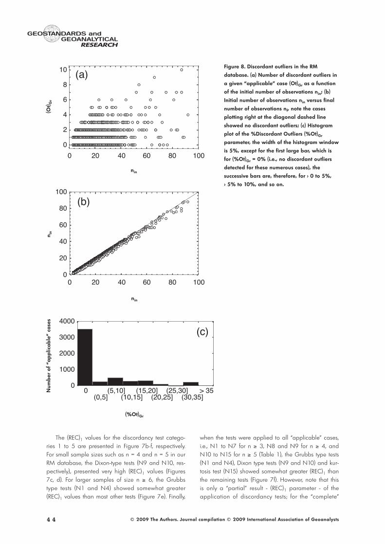
Figure 8. Discordant outliers in the RM

database. (a) Number of discordant outliers in

a given “applicable” case (Ot)Gr as a function

of the initial number of observations nin; (b)

Initial number of observations nin versus final

number of observations nf, note the cases

plotting right at the diagonal dashed line

showed no discordant outliers; (c) Histogram

plot of the %Discordant Outliers (%Ot)Gr

parameter, the width of the histogram window

is 5%, except for the first large bar, which is

for (%Ot)Gr = 0% (i.e., no discordant outliers

detected for these numerous cases), the

successive bars are, therefore, for > 0 to 5%,

> 5% to 10%, and so on.

(Ot) G

rn i

nN

umb

er o

f “a

pp

lica

ble

” ca

ses

nin

nin

(%Ot)Gr

result , the overall REC value - (REC)g parameter -should instead be considered (Figure 5).

Distribution of discordant outliers

We now briefly present in Figure 8 the distributionof discordant outliers in the “applicable” cases in ourRM database. First, it is important to note that a largenumber of “applicable” cases showed no discordantoutliers. This is true because a large number of casesplot close to the 0 value of the y-axis in Figure 8a, orclose to the diagonal “zero discordant outlier” dashedline in Figure 8b, and constitute the largest bar in thehistogram plot in Figure 8c. Second, the number of dis-cordant outliers was limited to about ten observationsfor a maximum sample size of 100 (Figure 8a). This isalso shown in Figure 8b, in which most cases plotclose to the diagonal dashed line. Finally, the frequen-cy of the occurrence of (%Ot)Gr values of 5-35% issignificantly less than the frequency of (%Ot)Gr = 0%(compare the size of the bars with that of the “zerodiscordant outlier” large bar; Figure 8c); furthermore, inour RM database the (%Ot)Gr values are limited to amaximum value of about 35%, with only a few excep-tions of greater (%Ot)Gr.

Calibration of X-rayfluorescence spectrometry

The present methodology involving the applicationof the single-outlier tests to our RM database (compi-led from Steele et al. (1972, 1978), Abbey (1979),

Flanagan (1986), Gladney (1988), Gladney andRoelandts (1988, 1990), Gladney et al. (1991, 1992),and the internet address http://riodb02.ibase.aist.go.jp/earthsci/welcome.html accessed for the last time inJune 2007) is capable of providing reliable estimatesof both central tendency (mean) and dispersion (stan-dard deviation) parameters. The actual values of theseparameters for the RMs compiled in this work will beestimated and reported in future, after the applicationof the complete multiple-test method of Verma (1997),i.e., involving both single-outlier as well as multiple-outlier tests, after the RM database is adequatelyupdated by incorporating more recent literature data(i.e., those reported after 1978 for the RMs from SouthAfrica and after 1988-1992 for the RMs from Canadaand USA); this work is currently in progress.

The availability of “statistically correct” estimates ofboth central tendency and dispersion parameters canenable us to achieve instrumental calibrations using aWLR model instead of the conventional OLR modelgenerally applied for this purpose in most laboratories.We present the improvement achieved by a WLRmodel for the calibration of the major elements by X-ray fluorescence spectrometry (XRF) as compared tothe OLR model. In addition to the RMs, the blank andmonitor discs (or beads) were also routinely analysedby XRF. All intensities were corrected for matrix effectsand instrumental drift; more details on the XRF proce-dure will be presented elsewhere (M. Guevara and S.P.Verma, manuscript in preparation). The final calibrationresults were documented as the intercept and slope

4 5

GEOSTANDARDS and



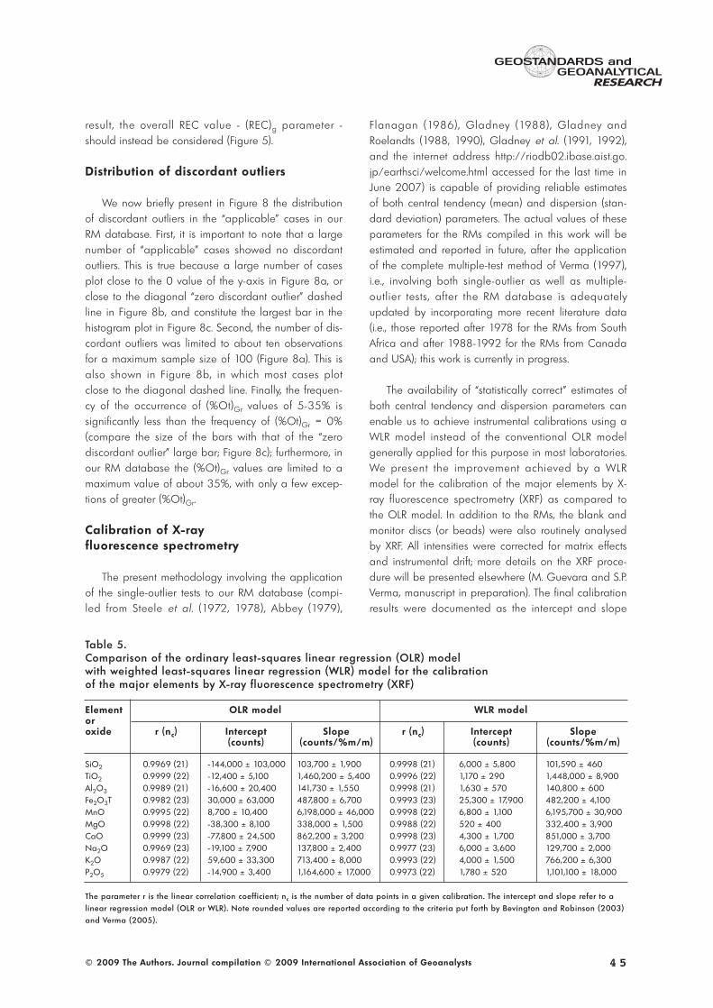
Table 5.Comparison of the ordinary least-squares linear regression (OLR) model with weighted least-squares linear regression (WLR) model for the calibration of the major elements by X-ray fluorescence spectrometry (XRF)

Element OLR model WLR modeloroxide r (nc) Intercept Slope r (nc) Intercept Slope

(counts) (counts/%m/m) (counts) (counts/%m/m)

SiO2 0.9969 (21) -144,000 ± 103,000 103,700 ± 1,900 0.9998 (21) 6,000 ± 5,800 101,590 ± 460TiO2 0.9999 (22) -12,400 ± 5,100 1,460,200 ± 5,400 0.9996 (22) 1,170 ± 290 1,448,000 ± 8,900Al2O3 0.9989 (21) -16,600 ± 20,400 141,730 ± 1,550 0.9998 (21) 1,630 ± 570 140,800 ± 600Fe2O3T 0.9982 (23) 30,000 ± 63,000 487,800 ± 6,700 0.9993 (23) 25,300 ± 17,900 482,200 ± 4,100MnO 0.9995 (22) 8,700 ± 10,400 6,198,000 ± 46,000 0.9998 (22) 6,800 ± 1,100 6,195,700 ± 30,900MgO 0.9998 (22) -38,300 ± 8,100 338,000 ± 1,500 0.9988 (22) 520 ± 400 332,400 ± 3,900CaO 0.9999 (23) -77,800 ± 24,500 862,200 ± 3,200 0.9998 (23) 4,300 ± 1,700 851,000 ± 3,700Na2O 0.9969 (23) -19,100 ± 7,900 137,800 ± 2,400 0.9977 (23) 6,000 ± 3,600 129,700 ± 2,000K2O 0.9987 (22) 59,600 ± 33,300 713,400 ± 8,000 0.9993 (22) 4,000 ± 1,500 766,200 ± 6,300P2O5 0.9979 (22) -14,900 ± 3,400 1,164,600 ± 17,000 0.9973 (22) 1,780 ± 520 1,101,100 ± 18,000

The parameter r is the linear correlation coefficient; nc is the number of data points in a given calibration. The intercept and slope refer to alinear regression model (OLR or WLR). Note rounded values are reported according to the criteria put forth by Bevington and Robinson (2003)and Verma (2005).

values, including their uncertainty estimates (95%confidence limits as suggested by ISO 1989). Thesestatistical parameters thus define the regression equa-tions for all major elements or oxides (Table 5).

Both OLR and WLR models showed relatively high,statistically significant (Bevington and Robinson 2003,Verma 2005) linear correlation coefficient (r) values (r >0.9969 for the number of calibration points = 21-23;Table 3). The WLR model always provided a smallerintercept (closer to zero) than the OLR model. The res-pective uncertainties were also smaller for the WLRmodel. Although the slopes of the regression lines forthe two models were generally similar, the WLR modelgenerally showed smaller uncertainty values for theslopes. Thus, the regression equations of the WLR modelwere of “better” quality (intercepts close to zero andsmaller uncertainties on both intercept and slope coeffi-cients) than the respective equations of the OLR model.The WLR should, therefore, provide more accurate esti-mates of the major element data in unknown samplesas compared to the frequently used OLR model.

Final remarks

These REC results are generally consistent with theearlier empirical evaluations of Velasco and Verma(1998) and Velasco et al. (2000), in which the impor-tance of skewness and kurtosis tests was well establi-shed for efficiently detecting discordant outliers. Thesuperiority of the kurtosis test (N15) over all other testsis documented for the first time. Nevertheless, becausea very extensive database of thirty-five RMs, involvingall major and trace elements, was used in the presentwork and all “applicable” cases could be processedusing new, precise and accurate critical values (Vermaand Quiroz-Ruiz 2006a, b, 2008, Verma et al. 2008),the statistical inferences drawn here are more firmlyvalid than in these earlier studies. The kurtosis test(N15), Grubbs type tests (N1 and N4) and skewnesstest (N14) are to be preferred in comparison with theDixon type tests (N7, N8, N9 and N10) as well as theGrubbs type test (N2).

We should also point out that our outlier-basedprocedure should be especially useful for objectivelyidentifying discordant outliers in many fields of scienceand engineering as has been discussed in detail byVerma and Quiroz-Ruiz (2006a, b). The fields, forwhich example cases and literature references wereprovided by these authors, are: agriculture, astronomy,biology, biomedicine, biotechnology, chemistry, electronics,

environmental and pollution research, food scienceand technology, geochemistry, geochronology, isotopegeology, meteorology, nuclear science, palaeontology,petroleum research, quality assurance and assessmentprogrammes, soil science, structural geology, waterresearch and zoology. After the proper identification ofdiscordant outliers, these can be interpreted accordin-gly and appropriately depending on the expertise ofthe scientific or engineering field.

Conclusions

An extensive geochemical database of thirty-fivereference materials from Canada, Japan, South Africaand the USA was used to evaluate nine single-outliertests with thirteen variants. The statistical evaluation ofthese single-outlier tests showed the relative efficienciesof these tests (represented by the (REC)g parameter) inthe following sequence: N15 > N4 ≈ N1 > N14 > N10> N9 ≈ N2 > N8 > N7. The number of discordant out-liers in the database identified by the present single-outlier method was relatively small (from 0 to 10) forsample sizes up to 100. The (%Ot)Gr parameter mostfrequently was zero and for a significantly lesser num-ber of cases its value was limited to a maximum ofabout 35%. The WLR model was shown to provide“better quality” calibration equations with the interceptscloser to zero and the uncertainties on both the inter-cept and slope generally smaller than the OLR model.

Acknowledgements

We thank the editor Mireille Polvé for extending aninformal invitation to contribute to Geostandards andGeoanalyt ical Research and for an eff ic ient andunbiased editorial handling of our manuscript. Thiswork was motivated by an invitation from Phil Potts tothe first author (SPV) to review the statistical methodsfor processing geochemical databases. The presentcontribution is the first step towards this goal; furtherwork is currently in progress. The second and thirdauthors (LDG and RGR) are grateful to Conacyt for ascholarship to carry out doctoral studies at CIE-UNAM.Alfredo Quiroz-Ruiz is thanked for efficiently maintai-ning our personal computers and guiding us at thedata compilation stage of our work. Our presentationwas considerably improved from the critical commentsand suggestions from three anonymous reviewers. Weare also grateful to Mirna Guevara for allowing us touse the unpubl ished XRF laboratory data, whichenabled us to demonstrate the importance of our workfor instrumental calibrations.

4 6

GEOSTANDARDS and



References

Abbey S. (1979)Reference materials - rock samples SY-2, SY-3, MRG-1.Energy, Mines and Resources (Canada), Report 79-35,66pp.

Asuero A.G. and González G. (2007)Fitting straight lines with replicated observations by linearregression. III. Weighting data. Critical Reviews inAnalytical Chemistry, 37, 143-172.

Barnett V. and Lewis T. (1994)Outliers in statistical data. John Wiley and Sons(Chichester), 584pp.

Baumann K. (1997)Regression and calibration for analytical separation techniques. Part II: Validation, weighted and robustregression. Process Control and Quality, 10, 75-112.

Bevington P.R. and Robinson D.K. (2003)Data reduction and error analysis for the physicalsciences. McGrawHill (New York), 320pp.

Dixon W.J. (1951)Ratios involving extreme values. Annals of MathematicalStatistics, 22, 68-78.

Dybczynski R., Tugsavul A. and Suschny O. (1979)Soil-5, a new IAEA certified reference material for traceelement determinations. Geostandards Newsletter, 3,61-87.

Dybczynski R., Polkowska-Motrenko H., Samczynski Z. and Szopa Z. (1998)Virginia tobacco leaves (CTA-VTL-2) - new Polish CRM forinorganic trace analysis including microanalysis.Fresenius’ Journal of Analytical Chemistry, 360,384-387.

Farre M., Martinez E., Hernando M.D., Fernandez-Alba A., Fritz J., Unruh E., Mihail O.,Sakkas V., Morbey A., Albanis T., Brito F., Hansen P.D. and Barcelo D. (2006)European ring exercise on water toxicity using differentbioluminescence inhibition tests based on Vibrio fischeri,in support to the implementation of the water frameworkdirective. Talanta, 69, 323-333.

Flanagan F.J. (1986)Rock reference samples, San Marcos Gabbro, GSM-1and Lakeview Mountain Tonalite, TLM-1. GeostandardsNewsletter, 10, 111-119.

Gabrovská D., Rysova J., Filova V., Plicka J., Cuhra P., Kubik M. and Barsova S. (2006)Gluten determination by gliadin enzyme-linked immunosorbent assay kit: Interlaboratory study. Journal ofAOAC International, 89, 154-160.

Gladney E.S. (1988)1987 compilation of elemental concentration data forUSGS BIR-1, DNC-1 and W-2. Geostandards Newsletter,12, 63-118.

Gladney E.S. and Roelandts I. (1988)1987 compilation of elemental concentration data forUSGS BHVO-1, MAG-1, QLO-1, RGM-1, SCo-1, SDC-1,SGR-1 and STM-1. Geostandards Newsletter, 12, 253-262.

Gladney E.S. and Roelandts I. (1990)1988 compilation of elemental concentration data forCCRMP reference rock samples SY-2, SY-3 and MRG-1.Geostandards Newsletter, 14, 373-458.

Gladney E.S., Jones E.A., Nickell E.J. and Roelandts I. (1991)1988 compilation of elemental concentration data forUSGS DTS-1, G-1, PCC-1 and W-1. GeostandardsNewsletter, 15, 199-396.

Gladney E.S., Jones E.A., Nickell E.J. and Roelandts I. (1992)1988 compilation of elemental concentration data forUSGS AGV-1, GSP-1 and G-2. GeostandardsNewsletter, 16, 111-300.

Govindaraju K. and Roelandts I. (1989)1988 compilation report on trace elements in six ANRTrock reference samples: Diorite DR-N, serpentinite UB-N,bauxite BX-N, disthene DT-N, granite GS-N and potashfeldspar FK-N. Geostandards Newsletter, 13, 5-67.

Govindaraju K., Potts P.J., Webb P.C. and Watson J.S. (1994)1994 Report on Whin Sill dolerite WS-E from Englandand Pitscurrie microgabbro PM-S from Scotland:Assessment by one hundred and four international laboratories. Geostandards Newsletter, 18, 211-300.

Grubbs F.E. (1950)Sample criteria for testing outlying observations. Annalsof Mathematical Statistics, 21, 27-58.

Grubbs F.E. (1969)Procedures for detecting outlying observations in samples.Technometrics, 11, 1-21.

Guevara M., Verma S.P. and Velasco-Tapia F. (2001)Evaluation of GSJ intrusive rocks JG1, JG2, JG3, JG1a,and JGb1 by an objective outlier rejection statistical procedure. Revista Mexicana de Ciencias Geológicas,18, 74-88.

Guevara M., Verma S.P., Velasco-Tapia F., Lozano-Santa Cruz R. and Girón P. (2005)Comparison of linear regression models for quantitativegeochemical analysis: An example using X-ray fluorescence spectrometry. Geostandards andGeoanalytical Research, 29, 271-284.

Hayes K., Kinsella A. and Coffey N. (2007)A note on the use of outlier criteria in Ontario laboratoryquality control schemes. Clinical Biochemistry, 40,147-152.

Imai N., Terashima S., Itoh S. and Ando A. (1995)1994 compilation values for GSJ reference samples,“Igneous rock series”. Geochemical Journal, 29, 91-95.

ISO (1989)ISO Guide 35: Certification of reference materials -general and statistical principles. InternationalOrganization for Standardization (Geneva), 32pp.

4 7

GEOSTANDARDS and



references

Li X.J., Zhang H., Ranish J.A. and Aebersold R. (2003)Automated statistical analysis of protein abundanceratios from data generated by stable-isotope dilution andtandem mass spectrometry. Analytical Chemistry, 75,6648-6657.

Mahwar R.S., Verma N.K., Chakrabarti S.P. andBiswas D.K. (1998)Development and use of reference materials in India -status and plans. Fresenius’ Journal of AnalyticalChemistry, 360, 291-295.

Namiesnik J. and Zygmunt B. (1999)Role of reference materials in analysis of environmentalpollutants. The Science of the Total Environment, 218,243-257.

Potts P.J. and Kane J.S. (1992)Terminology for geological reference material values: Aproposal to the International Organisation forStandardisation (ISO), producers and users.Geostandards Newsletter, 16, 333-341.

Quevauviller P., Maier E.A., Griepink B., Fortunati U., Vercoutere K. and Muntau H. (1996)Certified reference materials of soils and sewage sludgesfor the quality control of trace element environmentalcontrol. Trends in Analytical Chemistry, 15, 504-513.

Sang H.Q., Wang F., He H.Y., Wang Y.L., Yang L.K.and Zhu R.X. (2006)Intercalibration of ZBH-25 biotite reference material utilized for K-Ar and Ar-40-Ar-39 age determination. ActaPetrologica Sinica, 22, 3059-3078.

Santoyo E. and Verma S.P. (2003)Determination of lanthanides in synthetic standards byreversed-phase high performance liquid chromatographywith the aid of a weighted least-squares regressionmodel: Estimation of method sensitivities and detectionlimits. Journal of Chromatography A, 997, 171-182.

Santoyo E., Guevara M. and Verma S.P. (2006)Determination of lanthanides in international geochemical reference materials by reversed-phase highperformance liquid chromatography: An application oferror propagation theory to estimate total analysis uncertainties. Journal of Chromatography A, 1118, 73-81.

Sayago A., Boccio M. and Asuero A.G. (2004)Fitting straight lines with replicated observations by linearregression: The least squares postulates. Critical Reviewsin Analytical Chemistry, 34, 39-50.

Serbst J.R., Burgess R.M., Kuhn A., Edwards P.A.,Cantwell M.G., Pelletier M.C. and Berry W.J. (2003)Precision of dialysis (peeper) sampling of cadmium inmarine sediment interstitial water. Archives ofEnvironmental Contamination and Toxicology, 45,297-305.

Steele T.W., Russell B.G., Goudvis R.G., Domel G.and Levin J. (1972)Preliminary report on the analysis of the six NIMROCgeochemical standard samples. National Institute forMetallurgy (Randsburg, South Africa), Report 1351,74pp.

Steele T.W., Wilson A., Goudvis R., Ellis P.J. andRadford A.J. (1978)Analyses of the NIMROC reference samples for minorand trace elements. National Institute for Metallurgy(Randsburg, South Africa), Report 1945, 218pp.

Steliopoulos P. and Stickel E. (2007)Estimation of performance characteristics of a confirmation method for thyreostats in plasma by meansof a weighted least-squares approach. AnalyticaChimica Acta, 592, 181-186.

Tellinghuisen J. (2007)Weighted least-squares in calibration: What differencedoes it make? The Analyst, 132, 536-543.

Vendemiatto M.A. and Enzweiler J. (2001)Routine control of accuracy in silicate rock analysis by X-ray fluorescence spectrometry. GeostandardsNewsletter: The Journal of Geostandards andGeoanalysis, 25, 283-291.

Velasco F. and Verma S.P. (1998)Importance of skewness and kurtosis statistical tests foroutlier detection and elimination in evaluation of geochemical reference materials. MathematicalGeology, 30, 109-128.

Velasco F., Verma S.P. and Guevara M. (2000)Comparison of the performance of fourteen statisticaltests for detection of outlying values in geochemical reference material databases. Mathematical Geology,32, 439-464.

Velasco-Tapia F., Guevara M. and Verma S.P. (2001)Evaluation of concentration data in geochemical reference materials. Chemie der Erde, 61, 69-91.

Verma M.P. (2004)A revised analytical method for HCO3

- and CO32-

determinations in geothermal waters: An assessment ofIAGC and IAEA interlaboratory comparisons.Geostandards and Geoanalytical Research, 28,391-409.

Verma S.P. (1997)Sixteen statistical tests for outlier detection and rejectionin evaluation of international geochemical referencematerials: Example of microgabbro PM-S. GeostandardsNewsletter. The Journal of Geostandards andGeoanalysis, 21, 59-75.

Verma S.P. (1998)Improved concentration data in two international geochemical reference materials (USGS basalt BIR-1 and GSJ peridotite JP-1) by outlier rejection. GeofísicaInternacional, 37, 215-250.

Verma S.P. (2005)Estadística básica para el manejo de datos experimentales: Aplicación en la geoquímica (geoquimiometría). UNAM (Mexico), D.F., 186pp.

Verma S.P. and Quiroz-Ruiz A. (2006a)Critical values for six Dixon tests for outliers in normalsamples up to sizes 100, and applications in scienceand engineering. Revista Mexicana de CienciasGeológicas, 23, 133-161.

4 8

GEOSTANDARDS and



references

Verma S.P. and Quiroz-Ruiz A. (2006b)Critical values for 22 discordancy test variants for outliersin normal samples up to sizes 100, and applications inscience and engineering. Revista Mexicana de CienciasGeológicas, 23, 302-319.

Verma S.P. and Quiroz-Ruiz A. (2008)Critical values for 33 discordancy test variants for outliersin normal samples for very large sizes of 1,000 to30,000. Revista Mexicana de Ciencias Geológicas, 25,369-381.

Verma S.P., Orduña-Galván L.J. and Guevara M. (1998)SIPVADE: A new computer programme with seventeenstatistical tests for outlier detection in evaluation of international geochemical reference materials and itsapplication to Whin Sill dolerite WS-E from England andSoil-5 from Peru. Geostandards Newsletter: The Journalof Geostandards and Geoanalysis, 22, 209-234.

Verma S.P., Quiroz-Ruiz A. and Díaz-González L. (2008)Critical values for 33 discordancy test variants for outliersin normal samples up to sizes 1000, and applications inquality control in Earth Sciences. Revista Mexicana deCiencias Geológicas, 25, 82-96.

Villeneuve J.-P., de Mora S. and Cattini C. (2004)Determination of organochlorinated compounds andpetroleum in fish-homogenate sample IAEA-406: Resultsfrom a worldwide interlaboratory study. Trends inAnalytical Chemistry, 23, 501-510.

4 9

GEOSTANDARDS and



Documents

Relative Efficiency of Single-Outlier Discordancy Tests for Processing Geochemical Data on Reference Materials and Application to Instrumental Calibrations by a Weighted Least-Squares