Embed Size (px)
Citation preview

AI and Machine ConsciousnessProceedings of the 13th Finnish Artificial Intelligence Conference
STeP 2008
Helsinki University of Technology, Espoo, FinlandNokia Research Center, Helsinki, Finland
August 20-22, 2008http://www.stes.fi/step2008
Tapani Raiko, Pentti Haikonen, and Jaakko Väyrynen (eds.)

Proceedings of the 13th Finnish Artificial Intelligence Conference, STeP 2008
Espoo, Finland, August 2008
Publications of the Finnish Artificial Intelligence Society 24
ISBN-13: 978-952-5677-04-1 (paperback)ISSN 1238-4658 (Print)
ISBN-13: 978-952-5677-05-8 (PDF)ISSN 1796-623X (Online)
Multiprint oy, Espoo
Additional copies available from:
Finnish Artificial Society (STeS)Secretary Susanna KoskinenTikkurikuja 10 T00750 [email protected] http://www.stes.fi


Contents
AI and Machine Consciousness
Contents 4
Prefaces
ForewordTapani Raiko
6
Genetic Algorithms and Particle Swarms
Partially separable fitness function and smart genetic operators for surface-based image registrationJanne Koljonen
7
A Review of Genetic Algorithms in Power EngineeringN. Rajkumar, Timo Vekara, and Jarmo T. Alander
15
From Gas Pipe into Fire, and by GAs into Biodiversity - A Review Perspective of GAs in Ecology and ConservationJarmo T. Alander
33
Evaluation of uniqueness and accuracy of the model parameter search using GAPetri Välisuo and Jarmo Alander
41
LEDall 2 – An Improved Adaptive LED Lighting System for Digital PhotographyFilip Norrgård, Toni Harju, Janne Koljonen and Jarmo T. Alander
46
Multiswarm Particle Swarm Optimization in Multidimensional Dynamic EnvironmentsSerkan Kiranyaz, Jenni Pulkkinen and Moncef Gabbouj
52
Sudoku Solving with Cultural SwarmsTimo Mantere and Janne Koljonen
60
Robotics
Minimalistic Navigation for a Mobile Robot based on a Simple Visibility Sensor InformationOlli Kanniainen and Timo M. R. Alho
68
An Angle Sensor-Based Robot Navigation in an Unknown EnvironmentTimo M. R. Alho
76

Games and Preferences
Framework for Evaluating Believability of Non-player Characters in GamesTero Hinkkanen, Jaakko Kurhila and Tomi A. Pasanen
81
Application of UCT Search to the Connection Games of Hex, Y, *Star, and Renkula!Tapani Raiko and Jaakko Peltonen
89
Regularized Least-Squares for Learning Non-Transitive Preferences between StrategiesTapio Pahikkala, Evgeni Tsivtsivadze, Antti Airola and Tapio Salakoski
94
Philosophy
Philosophy of Static, Dynamic and Symbolic AnalysisErkki Laitila
99
Voiko koneella olla tunteita?Panu Åberg
107
Semantic Web
Finding people and organizations on the semantic webJussi Kurki
117
ONKI-SKOS – Publishing and Utilizing Thesauri in the Semantic WebJouni Tuominen, Matias Frosterus, Kim Viljanen and Eero Hyvönen
122
Document Expansion Using Ontological Concept Clustering Matias Frosterus and Eero Hyvönen
129
Adaptive Tension Systems
Adaptive Tension Systems: Towards a Theory of Everything?Heikki Hyötyniemi
136
Adaptive Tension Systems: Fields Forever?Heikki Hyötyniemi
144
Adaptive Tension Systems: Beyond Artificial Intelligence?Heikki Hyötyniemi
150

Foreword
The first Finnish Artificial Intelligence Conference (STeP) was held at the Helsinki University of Technology (TKK) in August 20-23, 1984. It has been organized regularly every two years ever since - you are reading the proceedings of the thirteenth STeP, the fifth STeP at TKK.
The profound theme of this year's conference is machine consciousness. The last two days of the three day conference are dedicated to the Nokia Workshop on Machine Consciousness 2008. Thanks to Dr. Pentti Haikonen and Nokia Research Center, we have the opportunity to hear about the world's top research in the area.
So what is machine consciousness? It's central objective is to produce consciousness in an artificial system and at the same time to understand what a conscious process actually is. There are many hypotheses about consciousness but we do not know which one is closest to the real human mind. Therefore the field develops with a close relationship with engineering, neuroscience, congnitive science, psychology, and philosophy. Machine consciousness may also be the best way to study consciousness in general. There are many open questions, such as: Could strong AI be reached without having feelings or consciousness?
There are also 20 other contributions divided into six other themes: Genetic Algorithms and Particle Swarms, Robotics, Games and Preferences, Philosophy, Semantic Web, and Adaptive Tension Systems.
I am grateful to all the active researchers who have submitted their contributions to the conference, and to the organizing committee for making the conference happen in the first place. I thank Pentti Haikonen for inviting us to the Nokia Workshop, Jukka Kortela for making the STeP web pages, Iina Aaltonen for organizing the banquet and printing, Jaakko Väyrynen for editing the proceedings, Tomi Kauppinen for program handouts, Susanna Koskinen for handling the registrations, and Jussi Timonen for cover art.
I wish you all enjoyable conference days!
Tapani Raiko
Chairman, Finnish AI Society

Partially separable fitness function and smart genetic opera-tors for area-based image registration
Janne Koljonen University of Vaasa
P.O. Box 700, FIN-65101, Vaasa, Finland [email protected]
Abstract
The displacement field for 2D image registration is searched by a genetic algorithm (GA). The dis-placement field is constructed with control points and an interpolation kernel. The common global fitness functions based on image intensities are partially separable, i.e. they can be decomposed into local fitness components that are contributed only by subsets of the control points. These local fit-ness components can be utilized in smart genetic operators. Partial separability and smart crossover and mutation operators are introduced in this paper. The optimization efficiency with respect to dif-ferent GA parameters is studied. The results show that partial separability gives a great advantage over a regular GA when searching the optimal image registration parameters in nonrigid image reg-istration. Keywords: computer vision, genetic algorithm, genetic operators, image registration, partially sepa-rable fitness function.
1 Introduction
Image registration methods consist of a few basic tasks: selection of the image transformation model, selection of features, extraction of the features, se-lection of the matching criterion (objective func-tion), and search for the optimal parameters of the transformation model (Zitove and Flusser, 2003). Hence, registration can be regarded as an optimiza-tion problem:
( )( )21onregistrati ,minargonregistrati
FFTTT
h*S∈
= , (1)
where h is a homology function between two im-ages, Tregistration is an image transformation (the result is an image) to register images F1 and F2, and S is the search space.
The homology function measures the correspon-dence of the homologous points of two images. In practice, the homology function is replaced by an objective (similarity, fitness, cost) function that is expected to correlate with h, because the homology function cannot be directly measured. There are two main categories of similarity functions: feature-based and area-based. In feature-based approaches, salient structures, e.g. corners, are extracted from the images. The positions of corresponding struc-
tures in the images are used estimate the homology function.
Area-based similarity functions consider the to-nal properties (intensities) of each pixel as features. Thus the feature extraction step is trivial. In order to evaluate the objective function the reference image is transformed with a given registration transforma-tion and the intensities of the transformed images are compared using a similarity metric. Typical met-rics include cross-correlation and root-mean-square difference. Image registration may also include cor-rection of optical distortions.
Area-based similarities can be computed using either small windows (templates) or entire images. The approach based on templates evaluates an area-based similarity function locally. On the other hand, the positions of the localized templates can be util-ized in the calculation of the feature-based objective function. Usually templates are used to estimate local translations. If the image is subject to local deformations, the accuracy of the template based method deteriorates.
The image transformation Tregistration and its search space S should be such that the correspon-dence between the transformed images, according to eq. (1), can be as close as possible. On the other hand, the complexity of the image transformation model should be as low as possible so that the pa-rameter search can be done efficiently and overfit-

ting to noise is avoided. The type of the transforma-tion should take into account the premises of the registration task. For instance in multiview analysis (e.g. in stereo vision), a perspective transformation is applicable.
In nonridig medical registration, typical trans-formation models use e.g. basis functions, splines, finite-element methods (FEM) with mechanical models, and elastic models (Hajnal, Hill, and Hawkes, 2001). Basis functions are e.g. polynomi-als. In in-plane strain analysis, Lu and Cary (2000) have used a second-order Taylor series approxima-tion to describe local displacements, whereas Kol-jonen et al. (2007) have used cubic B-splines, whose control points were optimized by a genetic algo-rithm. Veress at al. (2002) have used FEM to meas-ure strains from pairs of cross-sectional ultrasound images of blood-vessels.
Usually registration requires iterative optimiza-tion starting from initial candidate(s) of transforma-tion. The candidates are evaluated by an objective function. Optimization algorithms are used to create new candidate transformations using the evaluated ones, except in exhaustive search and Monte Carlo (random walk) optimization. The new candidates hopefully introduce fitness improvements, but it cannot be guaranteed in numerical optimization.
Optimization methods can be local or global. Local methods, such as hill-climbers, usually deal with only one candidate at a time and they utilize the local information, for instance, gradient, of the fitness landscape. Thus local methods are prone to get stuck to local optima.
Global methods are used to avoid the curse of local optima. They usually utilize parallel search with several concurrent candidates. Furthermore, information between the candidates can be ex-changed. One group of such algorithms is genetic algorithms (GA) that are also utilized in this study (Forrest, 1993).
2 Genetic algorithm
A genetic algorithm with a partially separable fit-ness function is defined. It consists of encoding of nonrigid registration (deformation field), artificial image deformation, a scalar global fitness function, partially separable sub fitness functions, and genetic operators, some of which utilize the separability properties of the sub fitness functions.
2.1 Deformation encoding
The deformation field is encoded as displacements of control points (see Figure 1 a). Control points O = [om,n] = [(ox(m,n), oy(m,n))] form a regular M × N (now 13 × 20) grid on the undeformed refer-ence image R. For a deformed (sensed) image S,
displacements D = [dm,n] of the control points are searched for to maximize the image similarity.
Both control points and displacements are en-coded using floating-point numbers. Displacements are given in Cartesian coordinates d = (dx, dy). Thus there are 2MN (now 520) free floating-point pa-rameters to be optimized.
2.2 Image deformation
Displacements are used to geometrically transform the reference image into an artificially deformed image A. Thus the geometrical transformation Tregistration(R; O, D) to register the image is defined as the following algorithm:
1. Displacements D at pixels O are interpolated to obtain a displacement vector for every pixel. A bi-cubic interpolation kernel is used (Sonka, Hlavac, Boyle, 2008).
2. Pixels of the reference image R are translated using the interpolated displacements.
3. The translated pixels are interpolated using bi-cubic interpolation and a regular grid, whose resolu-tion is equal to that of the reference image. The re-sulting image AD’ has floating-point pixel values due to interpolation.
4. The pixel values of AD’ are truncated to 8 bits resulting in the artificially deformed image AD.
A similar algorithm is used to create the test im-ages, too. However, in test image generation the effect of deformation on the image saturation and brightness as well as the influence of heterogeneous illumination is taken into account. Moreover, noise could be added, but in this study noise is neglected. More details on the test image generation are given in (Koljonen, 2008).
2.3 Scalar fitness functions
The global scalar fitness function is based on the tonal properties of the target image S and the artifi-cially deformed image AD. With noiseless images and an optimal solution Dopt the deformed image and the sensed image S would be (almost) identical:
( ) SDORTA D ≡= optonregistratiopt,; , (2)
In practice, images include noise. Consequently, there is a residual error at each pixel (x, y):
ε),(),(opt
=− yxyx SA D , (3)
Assuming that noise is independent and nor-mally distributed, i.e. ε ~ NID(0, σ), a common ap-proach is to minimize the sum of squared difference (SSD) of the images:
( )∑∈
−DA
DD
SA),(
2),(),(minargyx
yxyx , (4)

The corresponding global fitness function is:
( )∑∑= =
−=X
x
Y
y
yxyxf1 1
2),(),()( SAD D , (5)
In order to have a clearer interpretation of the fitness values the root-mean-square (RMS) value of the difference is used to present the values of the global fitness function in the experimental part of this study:
( )∑∑= =
−=X
x
Y
y
yxyxXY
g1 1
2),(),(1
)( SAD D , (6)
Obviously, minimizing eq. (6) minimizes eq. (5), too. Global fitness is used in trial evaluation.
2.4 Partially separable fitness function
The fitness function (eq. 5 or 6) has 2 × M × N free input parameters. Due to bi-cubic interpolation, each pixel in AD is affected only by the 16 neighboring points of D. This partial separability gives an oppor-tunity to measure local fitness related to certain in-put parameters and use it to favor good building blocks in the reproduction phase of the genetic algo-rithm.
In strict terms, fitness function f(x) is partially separable if it is the sum of P positive functions fi. Moreover, the sub-functions fi should be affected only by a subset of x, the input variables (Durand and Alliot, 1998). In theory, each pixel could be used as a sub-function. Alternatively, small regions of contiguous pixels that have common control points could be searched and used as the region of the sub-functions. However, neither of these would be practical. Instead, local fitness functions related directly to each control point are used.
Each control point dm,n has a local region of in-fluence on the pixels of AD. Each pixel, to which dm,n is one of the 16 closest control points, belongs
to the local region of influence. However, solving the region is impractical.
Therefore, the ideal region is replaced by a square positioned around dm,n (see Figure 1 b.). The horizontal and vertical dimensions (W, H) of the squares equal to the mean horizontal and vertical distances of the translated control points O + D, respectively. Thus the squares occupy each pixel, on average, approximately once.
The sub fitness function fm,n related to control point dm,n is computed as follows:
( )∑ ∑++
−+=
++
−+=
−=2/),(),(
2/),(),(
2/),(),(
2/),(),(
2, ),(),()(
Wnmdnmo
Wnmdnmox
Hnmdnmo
Hnmdnmoynm
xx
xx
yy
yy
yxyxf SAD D
,(7)
Sub-function fm,n is primarily affected by dm,n, but several other control points also affect it. These interactions are also a motivation to use global op-timization in this study.
The global fitness function f and the sub-functions fm,n do not exactly meet the definition of partially separable functions. Nevertheless, the sum of the sub-functions approximates the global fitness function:
)()(1 1
, DD ffM
m
N
nnm ≈∑∑
= =
, (8)
2.5 Genetic operators
Displacement vectors D are modified using genetic operators. Smart initialization sets the original states of D in the population of trials, after which new tri-als are generated using reproduction.
In each iteration, two parents are randomly drawn from the population. Crossover operators recombine the displacement vectors of the parents to come up with a new trial, while mutation operators modify a parent trial to create an offspring.
Two crossover operators are used. Uniform crossover (Syswerda, 1989) recombines two trials
o2,3+d2,3
d2,3
o1,1 o2,1 o3,1
o1,2 o2,2 o3,2
o1,3 o2,3 o3,3
x
y
x
yf2,3
W
H
(a) (b) Figure 1. a: The principle of deformation encoding. The grid of control points o, displacement vectors d, and the
translated control points (gray dots). b: The principle of local fitness evaluation.

totally randomly. A smart crossover operator util-izes the local fitness estimates to select the best building-blocks from each parent.
Two mutation operators are used. Uniform muta-tion treats each control point statistically equally, while in smart mutation larger mutations are applied to control points with poorer fitness. 2.5.1 Smart initialization A ‘seed’ trial is obtained by a template based regis-tration algorithm described in (Koljonen, 2008). The displacements of the control points obtained for the sensed image S are interpolated by a bi-cubic kernel to obtain the seed trial, which should be relatively close to the optimum, for the genetic algorithm.
A population of p trials is initialized using the seed trial. p–1 new trials are created by uniform mutation from the seed trial. Mutation is used to obtain enough diversity in the initial population, i.e. to span the search space adequately. In the subse-quent optimization, only mutation can explore new search directions. Hence, an adequate spanning of the initial search space is required so that crossover can exploit the good building blocks of the trials. 2.5.2 Smart crossover Durand and Alliot (1998) introduced a genetic crossover operator for partially separable functions. In a similar way, a crossover operator based on local fitness (when minimizing f) is used in this study. On the basis of the local fitness, each displacement vec-tor is selected from either of two parents as follows: 1. If fm,n (parent1) – fm,n (parent2) < –∆, then
Doffspring(m,n) = Dparent1(m,n) 2. If fm,n (parent1) – fm,n (parent2) > ∆, then
Doffspring(m,n) = Dparent2(m,n) 3. If | fm,n (parent1) – fm,n (parent2)| ≤ ∆, then
Doffspring(m,n) = Dparent1(m,n) or Dparent2(m,n), (9) where ∆ is the (non-normalized) level of indetermi-nism. In step 3, the selection of the displacement is either totally random, like in this study, or it may still depend on the local fitness. 2.5.2 Smart mutation Local fitness can be utilized in mutation, too. It is presumed that the local fitness is proportional to the local alignment error. Therefore, a good local fitness implies that the corresponding control point should be translated only little, and subsequently the muta-tion energy should be small. For simplicity, the stan-dard deviation σ of the mutation operator is referred
as mutation energy, because its units can be given in pixels.
Provided that the fitness function is subject to minimization and the optimum fitness is 0, the mu-tation energy can be e.g. directly proportional to the local fitness. The following smart mutation based on local fitness is used in this study:
Doffspring(m,n) = Dparent(m,n) + fm,n (parent) ⋅ ε, (10) where ε ~ NID(0, σ). 2.6 Pseudo-code of the GA The following pseudo-code describes the essential parts of the genetic algorithm used in this study: population[1]<-seedTrial(images); for i from 2 to p do population[i]<-uniformMutation(population[1], 1*maxsigma); end for; for i from p+1 to n do evaluateAndSort(population); parent1<-population[ceil(rand*rand*rand*p)]; parent2<-population[ceil(rand*rand*p)]; if rand<crossoverprob // Only crossover if rand<smartcrossoverprob
population[p+1]<-smartCrossover(parent1, parent2, delta);
else population[p+1]<-uniformCrossover(parent1, parent2);
end if; else // Only mutation if rand<smartmutationprob
population[p+1]<-smartMutation(parent1, rand*maxsigma, mdensity);
else population[p+1]<-uniformMutation(parent1, rand*maxsigma, mdensity);
end if; end if; end for;
Function rand returns a random number from
[0, 1), whereas ceil(arg) rounds the argument to the nearest integer greater than the argument. The algorithm includes several parameters, whose ex-planations are given in Table 1.
3 Experiments and results
The objectives of the experiments were to test the feasibility and the efficiency of the proposed regis-tration method, to study the effect of different GA parameters, to find an optimal set of GA parameters, and to understand the optimization mechanism of the proposed algorithm to come up with improve-ments. The test setups, a meta-optimization scheme and the results are given and discussed in this sec-tion.

3.1 Test images A series of 160 images was created using a seed image and the algorithm proposed in (Koljonen 2008). In the deformation process, saturation de-crease and brightness increase are directly propor-tional to the local engineering strain. Moreover, the effect of nonuniform illumination is taken into ac-count.
A significant benefit comes with the use of arti-ficial test images; the homology function is known. Hence, the accuracy of the fitness function, which is used to estimate the homology function, can be computed.
The objective of the registration is to determine the correspondence between the seed image R and the last artificially deformed image S (Figure 2). The template based registration algorithm uses the intermediate images to determine the seed trial for the genetic algorithm, while the GA uses only the seed image and the last image. The seed image has been taken from a tensile test specimen with a ran-dom speckle pattern obtained by spray-paint. 3.2 Meta-optimization Table 1 shows that there are several GA parameters that may have significant effects on the optimization performance. GA parameters have been optimized by another genetic algorithm, called meta-GA, in several studies (see e.g. Alander 1992; Koljonen and Alander 2006). In this study, the meta-GA approach would have been computationally expensive, and
therefore a one-dimensional line search approach was adopted.
If it was assumed that the GA parameters have no interaction on the GA performance, an assump-tion which is undoubtedly too simplifying, each parameter could be optimized separately.
In order to have more reliable optimization re-sults, a sequential optimization method is used: Af-ter optimizing one parameter (dimension), that di-mension is fixed to the local (one-dimensional) op-timum. This method carries evidently an implicit assumption that any dimension optimized after di-mension k has no effect on the position of the one-dimensional optimum of that dimension.
In order to maintain good comparability, the number of iterations n was fixed to 1000. The initial values of the other dimensions were: popsize = 100, crossoverprob = 0.6, smartcrossoverprob = 0.8, delta = 0, smartmutationprob = 0.8, and mprob = 1.
In meta-optimization, the GA parameters were varied as follows, respectively:
1. maxsigma = 0.02, 0.04, …, 0.1 pixels, 2. popsize = 50, 75, …, 150, 3. crossoverprob = 0.2, 0.4, …, 1.0 4. smartcrossoverprob = 0.2, 0.4, …, 1.0 5. smartmutationprob = 0.2, 0.4, …, 1.0 6. mdensity = 0.4, 0.6, 0.8, 1.0 7. delta = 0, 0.2, …, 1.0
3.3 Effect of GA parameters Figure 3 shows how mutation energy (maxsigma in Table 1, corresponding to σ in eq. 10) affects opti-mization speed. The solid line represents the fitness after 1000 trials whereas the dashed line is the ho-mology function that gives the mean registration (alignment) error in pixels.
Two notions from Figure 3: the fitness and ho-mology functions have a strong correlation, and the optimum of σ lies appr. at 0.06 pixels, a value to which σ was fixed in the subsequent tests.
The effect of population size is given in Figure 4. It shows a weaker correlation between fitness and homology distance. Population size was fixed to 150, because fitness value was used as the optimiza-tion criterion.
Fitness and homology distance against crossover probability is shown in Figure 5. 0.4 was found to
Table 1. Explanations of the algorithm parameters. Parameter Explanation p Population size maxsigma The maximum value of
σ in mutation. n Number of iterations. crossoverprob Probability that solely
crossover is applied. smartcrossoverprob Probability that the
crossover operator is the smart one.
delta ∆ in smart crossover. smartmutationprob Probability that the mu-
tation operator is the smart one.
mdensity Mutation point density (mutation frequency). E.g. if mdensity = 1, then every control point is mutated, if mdensity = 0.5, on average half of the points are mutated.
Figure 2. Seed image R (top) and the last artificially
deform image S (bottom).

be an optimal selection. However, variation with respect to crossover probability seems to be small. Moreover, the sampling in the optimization is rather sparse. Consequently, the optimization does not give reliable results, at least as for crossover probability.
Figures 6 and 7 validate the efficiency of the smart crossover and mutation operators, respec-tively. Figure 6 suggests that using solely smart crossover gives both superior fitness and homology distance after 1000 iterations, when comparing to parameter setups, in which also uniform crossover is occasionally applied.
Figure 7 shows that the homology distance at-tains its minimum when smartmutationprob = 0.8. This gives some indication, may it be rather weak, that it might be beneficial to include uniform muta-
tion to the genetic operators, too. Figure 8 shows that mutation frequency should
to 1, i.e. each time mutation is applied, it should be applied to each control point. Nevertheless, other more efficient mutation strategies may exist.
Figure 9 gives more detailed information con-cerning the determinism of the smart crossover. In smart crossover, each control point of the offspring trial is selected from either of the parents. If ∆ is enlarged, smart crossover resembles more and more uniform crossover.
If ∆ = 0, control points that are estimated to be nearer to the solution are selected. This corresponds to an attempt to construct an optimal combination of the parents. Such a strategy might be too greedy, but Figure 9 shows that it is optimal in this case. The
Figure 3. Effect of mutation energy. Solid line: fit-
ness, dashed line: homology distance.
Figure 4. Effect of population size. Solid line: fit-
ness, dashed line: homology distance.
Figure 5. Effect of crossover domination. Solid line:
fitness, dashed line: homology distance.
Figure 6. Effect of smart crossover domination.
Solid line: fitness, dashed line: homology distance.
Figure 7. Effect of smart mutation domination. Solid
line: fitness, dashed line: homology distance.
Figure 8. Effect of mutation frequency. Solid line:
fitness, dashed line: homology distance.

results are in line with the results in Figure 6, where smart crossover dominated uniform crossover. As a conclusion, smart crossover outperforms uniform crossover. 3.4 GA performance The development of fitness in a single GA run is given in Figure 10. It shows that fitness is improved significantly during optimization despite the smart initialization.
The difference between the worst and best fit-ness of the population is used to estimate the diver-sity of the population. Now the diversity decreases almost consistently, but it never vanishes. This ob-servation indicates that the decrease of fitness could continue slightly after the 1000 iterations, even though the rate of improvement was rather slow at the end of the GA run.
On the other hand, the diversity is rather low at the end of the GA run, which indicates that the population size was probably selected quite opti-mally. Population size and diversity should namely have a positive correlation.
In order to determine the feasibility of the fitness function (eq. 6) fitness and homology distance are compared. Figure 10 shows that fitness and homol-ogy distance have a strong correlation. Computing linear correlation gives: r = 0.995 (p < 0.001). Con-sequently, eq. (6) proves to be an efficient fitness function to minimize the homology distance.
However, the high correlation does not guaran-tee that an arbitrarily low (sub-pixel) alignment er-ror could be achieved using eq. (6). In fact, when using only the 50 last iteration, r = 0.935. Figure 10 shows that the residual alignment error is still 0.7 pixels at the end of the best optimization run.
As for GA efficiency, it seems that the smart op-erators make the GA faster and more robust. How-ever, no deviation figures were estimated due to computational complexity.
Figure 11 shows the evolvement of meta-optimization. The results indicate that the GA pa-
rameters have a significant influence on the GA efficiency, but the meta-optimization gave some clear guides to the selection of them, particularly as for the selection of genetic operators. It is yet un-clear, how optimal the GA parameters, found by the one-dimensional optimization scheme, are.
The evolvement of two control points during an optimization run is studied in Figure 12. In the left panel, the control point position is initially (obtained by smart initialization) appr. one pixel away from the correct position (target). During optimization, the control points almost resides the correct posi-tion, but finally it drifts appr. 0.3 pixels away from the target.
In the right panel, the control point is initially appr. 3 pixels from the target. In the beginning, the homology distance increases, after which the control point starts to approach the target. It seems that the optimization was stopped too early.
4 Conclusions and future
It was proposed how the nonrigid registration prob-lem can be solved using control points of displace-ments, bi-cubic interpolation of both displacements and intensities, intensity based global fitness func-tion, and search of optimal control point positions by a genetic algorithm. It was also proposed how the global fitness function can be decomposed into local
Figure 9. Effect of indeterminism of smart crossover (nonnormalized ∆). Solid line: fitness, dashed line:
homology distance.
Figure 10. Development of the best (solid) and
worst (dashed line) fitness of the population. × = homology distance of the best trial.
Figure 11. Effect of the meta-optimization of the
GA parameters. Solid line: fitness, dashed line: ho-mology distance.

sub fitness functions using the principle of partial separability. The sub fitness functions were utilized in smart crossover and mutation operators.
The results show that the smart genetic operators improve the optimization speed significantly. The displacement error of registration was 0.7 pixels at the end of the best GA run. Improvements to opti-mization speed are needed to make the method prac-tically more feasible.
One possibility to speed up optimization might be to use the momentum of the control points, i.e. the mutation operator could favor the direction, to which fitness was improved. Such algorithms that utilize experience are called cultural algorithms.
On the other hand, the second example in Figure 12 showed that although the global fitness im-proved, the homology distance of the individual control point increased temporarily. Hence, the rela-tionships between local and global fitness and ho-mology distance should be studied more closely.
Acknowledgements
Finnish Funding Agency for Technology and Inno-vation (TEKES) and the industrial partners of the research project Process Development for Incre-mental Sheet Forming have financially supported this research.
References
J.T. Alander. On optimal population size of genetic algorithms. In Proceedings of the 6th Annual IEEE European Computer Conference on Computer Systems and Software Engineering, 65–70, 1992.
N. Durand and J–M. Alliot. Genetic crossover op-erator for partially separable functions. In Pro-ceedings of the Third Annual Conference on Genetic Programming, 487–494, Madison, Wisconsin, USA, 1998.
S. Forrest. Genetic algorithms: principles of natural selection applied to computation. Science,
261(5123): 872–878, 1993.
J. V. Hajnal, D. L. G. Hill, and D. J. Hawkes (eds.). Medical Image Registration, CRC Press, Boca Raton, 2001.
J. Koljonen and Jarmo T. Alander. Effects of popu-lation size and relative elitism on optimization speed and reliability of genetic algorithms. In Proceedings of the Ninth Scandinavian Con-ference on Artificial Intelligence, 54–60, 2006.
J. Koljonen, T. Mantere, O. Kanniainen, and J. T. Alander. Searching strain field parameters by genetic algorithms. In Intelligent Robots and Computer Vision XXV: Algorithms, Tech-niques, and Active Vision, Proc. of SPIE, 67640O-1–9, 2007.
J. Koljonen and Jarmo T. Alander. Deformation image generation for testing a strain measure-ment algorithm. Submitted to: Optical Engi-neering, 2008.
H. Lu and P. D. Cary. Deformation measurements by digital image correlation implementation of a second-order displacement gradient. Experi-mental Mechanics, 40(4): 393–399, 2000.
M. Sonka, V. Hlavac, and R. Boyle. Image Process-ing, Analysis, and Machine Vision. Third edi-tion, Thomson Learning, USA, 2008.
G. Syswerda. Uniform crossover in genetic algo-rithms. In Proceedings of the Third Interna-tional Conference on Genetic Algorithms, 2–9, 1989.
A. I. Veress, J. A. Weiss, G. T. Gullberg, D. G. Vince, and R. D. Rabbitt. Strain measurement in coronary arteries using intravascular ultra-sound and deformable images. J. of Biome-chanical Engineering, 124(6): 734–741, 2002.
B. Zitove and J. Flusser. Image registration meth-ods: A survey. Image and Vision computing, 21: 977–1000, 2003.
29.8 30 30.2 30.4 30.6 30.8 31136
136.5
137
137.5
138
x [pixels]
y [p
ixel
s]
31 31.5 32 32.5 33 33.5128
129
130
131
132
133
134
x [pixels]
y [p
ixel
s]
Figure 12. Two examples of control point evolvements. • = initial position, ò = final position, É = target
position.

A Review of Genetic Algorithms in Power Engineering
N. Rajkumar, Timo Vekara, and Jarmo T. Alander??University of Vaasa, Department of Electrical Engineering and Automation
PO Box 700, FIN-65101 Vaasa, [email protected] http://www.uwasa.fi/ TAU
Abstract
Genetic algorithm is a search and optimisation method simulating natural selection and genetics. It isthe most popular and widely used of all evolutionary algorithms. Genetic algorithms, in one form oranother, have been applied to several power system problems. This paper gives a brief introductionto genetic algorithms and reviews some of their most important applications in the field of powersystems recently published in literature. Due to the vast number of publications in this field, ourgenetic algorithm bibliography contains nearly one thousand references to papers dealing with powerengineering, only some of the papers, are reviewed here. Topics covered in this review consist ofgenerator expansion planning, transmission planning, reactive power planning, generator scheduling,economic dispatch, distribution system planning and operation, and some control applications.
1 Introduction
As modern electrical power systems become morecomplex, planning, operation and control of such sys-tems using conventional methods face increasing dif-ficulties. Intelligent systems have been developed andapplied for solving problems in such complex powersystems. Evolutionary algorithms are one class ofintelligent techniques that are being widely used inpower system applications. The genetic algorithmbibliography of the University of Vaasa contains over20.000 references (Fig. 1). About one thousand ofthose references are to papers more or less dealingwith power engineering problems (1).
Evolutionary algorithms (EAs) are computer-basedproblem solving systems which are computationalmodels of evolutionary processes as key elements intheir design and implementation. There are a va-riety of evolutionary algorithms and they all sharea common conceptual base of simulating evolution.These algorithms provide robust and powerful adap-tive search mechanisms.
The most popular EAs developed so far are Ge-netic Algorithms (GA), Evolution Strategies (ES)(2), Evolutionary Programming (EP), Learning Clas-sifier Systems (3) and Genetic Programming (GP)(4). A detailed account of the applications of evo-lutionary programming and neural network in powersystem engineering is presented in the book by Lai(5). An indexed bibliography of genetic algorithmsin power engineering has been compiled by one ofthe authors (JTA) (1). Figure 1 shows the num-
ber of papers published yearly in the area of ge-netic algorithms and papers especially on power en-gineering applications with GAs. Surveys and re-views on power system applications include refer-ences (6; 7; 8; 9; 10; 11; 12; 13).
6
1
10
100
1000
number of papers(log scale)
-1960 1970 1980 1990 2000
year
GA in power engineering
2008/08/04
ccccc
ccccccccccccccccc
ccccccccc
cccccc
cccccccccccccc
s ssss s ssss
sssssssss
ssssssFigure 1: The number of papers applying GA inpower engineering (•, N = 938 ) and the number ofall GA papers in the Vaasa GA bibliography database(, N = 20488 ). Observe that the last few years aremost incomplete in our bibliography database.

2 Genetic algorithmGenetic algorithm is the most popular and widelyused of all evolutionary algorithms. It transforms aset (population) of individual mathematical objects(usually fixed length character or binary strings), eachwith an associated fitness value, into a new popula-tion (next generation) using genetic operations simi-lar to the corresponding operations of genetics in na-ture (14). GAs seem to perform a global search onthe solution space of a given problem domain.
2.1 Advantages of GAThere are three major advantages of using genetic al-gorithms for optimisation problems.
1. GAs do not involve many mathematical assump-tions about the problems to be solved. Dueto their evolutionary nature, genetic algorithmswill search for solutions without regard for thespecific inner structure of the problem. GAs canhandle any kind of objective functions and anykind of constraints, linear or nonlinear, definedon discrete, continuous, or mixed search spaces.
2. The ergodicity of evolution operators makesGAs effective at performing global search. Thetraditional approaches perform local search by aconvergent stepwise procedure, which comparesthe values of nearby points and moves to therelative optimal points. Global optima can befound only if the problem possesses certain con-vexity properties that essentially guarantee thatany local optimum is a global optimum.
3. GAs provide a great flexibility to hybridise withdomain-dependent heuristics to make an effi-cient implementation for a specific problem.
2.2 Coding and OperationsThe problem to be solved by a genetic algorithm isencoded as two distinct parts: the genotype calledthe chromosome and the phenotype called the fitnessfunction. In computing terms the fitness function isa subroutine representing the given problem or theproblem domain knowledge while the chromosomerefers to the parameters of this fitness function.
2.2.1 Chromosome
Traditionally the genotype is coded using a program-ming language vector, array, or record-like chromo-some consisting of the problem parameters. Binary
(integer) and real (floating point) codings are the mostfrequently used basic data types to represent genes inthis immediate coding approach.
Here a more indirect and general data structure willbe used. The chromosome consists of genes that arepointers to valid values of the gene i.e. alleles in bi-ological terms. This indirect gene value structure isbetter suited especially for combinatorial problemsthan the commonly used immediate coding scheme.It allows to represent efficiently arbitrary allele setsas will be see in our introductory examples, wherestandard resistance values are used as alleles. In theindirect coding there is a vector of possible gene val-ues the gene is actually pointing to (Figure 2). In ourexample of a genetic algorithm (Figure 3) the genevalue is an index of the allele array containing all pos-sible values of the gene.
chromosome
s*
genei: 1← 4 q q q q q q q q q qjqqqqqq
alleles for genei
600
500
300
60
50
30
5:
4:
3:
2:
1:
0:
Figure 2: Indirect chromosome coding: originally(solid line) the value of the genei = A[1] = 50. Aftermutation (shown by← and dashed line) the value ofthe genei = A[4] = 500.
2.2.2 Fitness function
The purpose of the chromosome is to provide infor-mation, parameter values, for the problem encodedas a fitness or cost function, the phenotype. The ge-netic algorithm does not restrict the type of the fit-ness function. It can be practically anything rangingfrom continuous or discrete to stochastic or even asubjective estimation by a human user of the geneticalgorithm. Typically in engineering optimisation thefitness function is the result of a simulation run. Inany case all the problem domain information is en-coded as the fitness function. Hence the rest of thegenetic algorithm is nearly, if not totally, independentof the problem to be solved i.e. genetic algorithm isa general purpose problem solving method. Usuallythe user needs only to worry about the fitness func-tion and its implementation and to select reasonableparameter values, like population size, for the coregenetic algorithm.

void toyGA(int generations)
int i,j,k; // indexesGene[] S0 = newChromosome(Population[0]),
S1 = newChromosome(Population[1]);for (i=0; i<Population.length; i++)
for (j=0; j<Population[i].length; j++)Population[i][j].mutate(UX);
for (k=1; k<=generations; k++) i = 0;while (i<Population.length)
// 25% probability for mutationif ((UX.next(4)==0)||
(i==(Population.length-1)) mutate(Population[i]); i++;
else // do crossover:crossover(Population[i],
Population[i+1],S0,S1);selectionByTournament(Population[i],
Population[i+1],S0,S1);i+=2;
if (i<Population.length)
mutate(Population[i]);
Figure 3: A toy genetic algorithm core toyGA. UX isa random number generator object.
2.2.3 Mutation
The basic genetic operation is mutation. It means thatthe gene value i.e. allele is replaced by another, usu-ally a random value. In our indirect coding schemethe gene is assigned a random valid index value. Amutation operator is easy to implement using anywell behaving random number generator able to gen-erate valid gene values. In our indirect scheme thevalues must be in the range [0, ni − 1], where ni isthe size of the allele vector. It is typical that mostof the mutations form just harmful noise leading to aworse fitness value than the original gene values i.e.information gained during evolution. In cells thereare many processes protecting the valuable DNA in-formation against mutations. It is actually the per-manence of DNA information in living cells that isso striking surpassing, as far as is known, even thepermanence of the best computer memories, not the(low) mutation rate finally fueling evolution.
2.2.4 Crossover
Crossover is a more complex genetic operator thatcombines two chromosomes (parents) into new onesby swapping genes of the parents randomly. Themost common crossover types are one-point, two-
point, and uniform crossovers. In one- and two-pointcrossovers there are one respective two points wherethe roles of genes are changed in the swapping whilein the uniform crossover the probability to choose agene from either parent is equal to 0.5. For most prob-lems the uniform or multipoint crossover results infaster convergence than the more conservative few-point crossovers.
2.2.5 Selection
Charles Darwin’s great and far reaching observationwas that due to limited resources there is a contin-uous hard selection process among the living organ-isms in nature. This selection combined with geneticheritage inevitably causes gradual evolution that fi-nally creates astonishing new organisms. In geneticalgorithms the nonlinear selection is the crucial oper-ator to maintain a search of better solutions in thosepoints of the search space where the best solution can-didates have been found so far. In other words selec-tion is screening the search space and thus accumu-lates information of the most useful search areas andthus the building blocks i.e. parameter values of thebest solutions. It is assumed that by combining partsof good solutions, building blocks, still better solu-tions can be found. If this building block hypothesisis valid, genetic algorithm is a reasonable approachto solve a given problem. It is commonly believed,based mainly on the success of genetic algorithms insolving practical problems, that most of the practicaloptimisation problems more or less satisfy this build-ing block hypothesis.
2.2.6 Population
A genetic algorithm maintains a set of trials calledpopulation. It is usually implemented as a fixedlength vector of chromosomes. A popular populationsize is n ≈ 50, which is often a reasonable compro-mise between fast processing and premature conver-gence risk. A round updating the population arrayis called generation. It is also possible to update thepopulation incrementally as shown in our toy exam-ple.
The terminology of genetic algorithms was in-spired by biology. In order to facilitate understand-ing of various concepts, a brief glossary of the mostfrequent terms used in the context of genetic algo-rithms is provided in Table 1. As can be seen,most of them have familiar equivalent engineeringor mathematical terms. Often cited references to ba-sics of genetic and evolutionary algorithms include(14; 15; 16; 17; 18; 19; 20; 21; 22; 23; 24; 25; 26;

27; 28; 29; 30; 31; 32; 33; 34; 35; 36; 37) Furtherreferences on the basics of genetic algorithms can beseen in the bibliographies (38; 39).
Table 1: Glossary of the key terms in GAs.
GA term computing/math termallele value of parameterchromosome usually equal to specimenfitness value of function; cost functiongene one parameter of solutiongeneration one iteration roundgenotype problem parameter valuesphenotype result of fitness function evaluationpopulation vector of trialsspecimen trial i.e. problem parameter values
2.3 An implementationThe most important parts of genetic algorithms havebeen described. It is now time to make a synthesis,to reveal our simple genetic algorithm example corecalled toyGA written in JavaTM 1, without the outputroutine calls and a couple of simple subroutines, usedto solve the toy problem shown in Figure 3:
First a random initial population is generated bymutating every gene of every chromosome. Chromo-somes are stored in the Population array.
Table 2: The classes used in our exam-ples. The source codes can be found inftp.uwasa.fi/cs/report2003/...
class containsRandom random number generatorsGene the allele structure of geneGeneticAlgorithm the genetic algorithm coreResistor simple resistor circuit
After this in every generation either mutation(25%) or crossover (75%) operations are applied toeach member of the population. Crossover is done be-tween the neighbouring chromosomes. Tournamentselection is used to select members for the next gener-ation: the parent chromosome(s) are replaced by the
1Java is a trademark of Sun Microsystems, Inc.
best of the original chromosomes and the new onescreated after each operation.toyGA is actually one method of class called
GeneticAlgorithm. The classes used in our ex-amples are shown in Table 2.
2.4 A toy exampleTo demonstrate how a genetic algorithm functionsit is applied to a toy problem shown in Figure 4:connect four resistors Ri ∈ 10, 20, 40 Ω seriallyso that the total resistance Rtot =
∑3i=0 Ri is as
close as possible to a given value Rgoal. The natu-ral fitness function for this problem setting is f =−|Rgoal − Rtot|. The minus sign in the front of | · |is used here because the genetic algorithm tries tofind the maximum value of the given fitness function.Finding the minimum of a function f is always equiv-alent to finding the maximum of function −f .
R0 R1 R2 R3
Figure 4: A network of four serial resistors.
R0 R1 R2 R3
R4 R5 R6 R7
R8 R9 R10 R11
R12 R13 R14 R15
Figure 5: A network of 16 resistors.
There are four resistor positions Ri, i = 0, . . . , 3so that the natural coding of the chromosome is suchthat the chromosome consists of four genes each generepresenting one possible resistor value i.e. an allele.In total there are 3 possible values to be selected fromthe allele set A. Thus this combinatorial optimisationproblem has in total 34 = 81 possible solution candi-dates i.e. resistor value combinations, giving in total12 different possible values for the total resistance ofthe circuit.
The generationwise evolution of the populationconsisting of 8 chromosomes i.e. the solution searchby a GA is shown in Figure 6. Let there be a ran-domly generated initial population of resistance val-ues. The population size i.e. the number of trials in

each generation is thus nP = 8, which should be areasonable value for the tiny toy problem. Let thegoal be having Rtot = Rgoal = 40Ω i.e. in the so-lution all resistors are equal to 10 Ω. The solutionis found after 4 generations of steady increase of theaverage population fitness, after 15 crossovers and 5mutations, which means that about half of the searchspace was scanned before the solution was found. Inthis case the use of genetic algorithm is not of muchuse. The problem is simply too small and easy. Thisexample was introduced to demonstrate how a sim-ple genetic algorithm functions and the possibility toillustrate the whole search process easily. The nextexample will show that a genetic algorithm is able tofind the solution for a much more difficult problemhaving a huge search space.
2.5 A more realistic exampleLet us consider a more difficult and thus more inter-esting and realistic resistor example shown in Fig-ure 5. The resistance of each resistor can be cho-sen from a set of the following set2 of values A =10, 12, 15, 18, 22, 27, 33, 39, 47, 56Ω. There are16 resistor positions, so that the chromosome consistsof 16 genes each gene representing one possible resis-tor value i.e. an allele. In total there are 10 possiblevalues to be selected from the allele set A. Thus thiscombinatorial optimisation problem has in total 1016
(ten million billion) solution candidates i.e. resistorvalue combinations.
Figure 7 shows the dependence of the averagenumber of function calls nf needed for the GA tofind the minimum resistance of the circuit as the func-tion of the population size nP . Using a small pop-ulation size, the unique solution can be found onthe average in less than 2,000 function calls. Thismeans that the genetic algorithm has explored only2 × 103/1016 × 100% = 2 × 10⁻¹¹% of the totalsearch space. As can be seen, the number of func-tion calls increases with increasing population size:in a large population it takes time for the buildingblocks to find each other. The monotonicity of thenP graph is a sign of an easy problem. For more dif-ficult problems having an involved fitness landscapetopology the risk of sticking to local extremes tendsto increase nf dramatically for the smallest popula-tion sizes. The resistor problem is such that choosinga small resistor always drives the search to the rightdirection without the fear of sticking to a local mini-mum. A rule of thumb in selecting the population sizenP is to have nP proportional to the number of the
2standard E12 series
g = 0
f(ci) =
40
20
40
40
-100
c0
40
40
40
10
-90
c1
10
40
20
40
-70
c2
40
40
10
10
-60
c3
10
20
40
20
-50
c4
20
40
40
40
-100
c5
40
20
10
10
-40
c6
40
20
40
10
-70
c7
-72
ave
↓ ↓
g = 1
f(ci) =
40
20
40
40
-100
10
40
20
10
-40
40
40
40
10
-90
10
40
10
20
-40
10
20
40
20
-50
40
20
10
10
-40
40
40
10
40
-90
40
20
40
10
-70 -65
g = 2
f(ci) =
10
40
20
10
-40
10
40
40
10
-60
10
40
10
10
-30
40
40
40
10
-90
10
20
10
20
-20
10
20
40
20
-50
40
20
10
40
-70
40
20
40
10
-70 -53
↓ ↓
g = 3
f(ci) =
10
40
20
10
-40
10
40
40
10
-60
10
40
10
10
-30
10
20
10
20
-20
40
20
10
10
-40
10
20
40
20
-50
40
20
10
20
-50
40
10
40
10
-60 -43
g = 4
f(ci) =
10
40
20
10
-40
10
40
20
10
-40
10
20
10
10
-10
10
20
10
20
-20
40
20
10
10
-40
40
20
10
10
-40
40
10
10
10
-30
40
10
40
10
-60 -35
↓ ↓
g = 5
f(ci) =
10
40
20
10
-40
10
40
20
10
-40
10
10
10
10
0
10
20
10
20
-20
40
20
10
10
-40
40
20
10
10
-40
40
10
10
10
-30
40
10
10
10
-30 -30
Figure 6: The evolution of population when searchingthe solution of a four resistor problem (fig. 4). The fit-ness f(ci) = −|Rgoal − Rtot| for each chromosomeci is shown on top of 4 gene values shown within aframe; f(ci)=0 means that solution ci is found. Nota-tions: the solution is shown in bold, g = generation,ave = average fitness, = crossover, and ↓ = muta-tion.

-1 2 4 8 16 32 64 128
nP (log scale)
6
1, 000
2, 000
3, 000
4, 000
5, 000
6, 000
7, 000
8, 000
nf
• •• • •
•
•
•
Figure 7: Number of function calls nf when solvingthe 16 resistor problem (fig. 5) as function of popula-tion size nP . Each point is the average of 1,000 callsof a GA.
parameters of the problem (40). More often than notresearchers have set nP = 50, with usually good suc-cess. The heavier the fitness is to evaluate the moreimportant it is to try to find a reasonable populationsize.
3 GA applications in Power Sys-tems
Genetic algorithms are used for a number of applica-tion areas. In power systems, GA approaches havebeen used in planning, operation, and control andanalysis of power systems. More detailed statisticsof the most popular application areas of genetic al-gorithms in the power engineering area are shown inTable 3. The number of annual annual publications isgiven in Figure 1.
3.1 PlanningPower system planning is a dynamic process thatevolves over the years. Factors, such as providing ad-equate and reliable service, projected system growth;energy cost, construction cost, etc. are consideredduring the planning process. The existing systems arereviewed and methods for improvements required foraccommodating anticipated loads for various periodsare developed.
The planning process has increased in complex-ity as a result of restructuring and technical advance-ments. Researchers are looking into new mathemat-ical and simulation models to tackle this complexproblem.
Table 3: Most popular application areas of GAin power engineering according to our bibliographydatabase (1).
area # paperscontrol 67scheduling 51economic dispatch 47unit commitment 39nuclear power 25distribution systems 19turbines 15transformers 14planning 14diagnosis 14reactive power 10load forecasting 10review 9implementation 9signal processing 8distribution networks 8reliability 7power dispatch 7reactive power planning 6generators 6
For more references on operations and planning ingeneral see e.g. bibliography (41).
3.1.1 Generation expansion planning
Generation Expansion Planning (GEP) is an impor-tant planning activity of electric utility companies.The main objective of GEP is to determine the opti-mal schedule for the addition of generation plants, thetype, the number and time of addition of each gener-ation unit so as to provide a reliable and economicsupply to a forecast load demand over a specified pe-riod of time. The problem is to minimise the invest-ment and operation costs and to maximise the reli-ability with different types of constraints. The GEPproblem is a nonlinear integer programming problemwhich is highly constrained. In this section, the ap-plication of genetic algorithm to the solution of GEPby Fukuyama and Chiang (42), and Park, et al. (43)are reviewed.
Fukuyama and Chiang (42) have proposed a paral-lel genetic algorithm (PGA) for optimal long-rangegeneration expansion planning. The method usedsolves the problem of determining the optimal num-ber of newly introduced generation units at each inter-val of time under different scenarios. They have used

the class of coarse-grain PGA, the other class usedbeing fine-grain PGA, achieving a trade- off betweencomputational speed and hardware cost. Coarse-grain PGA performs several GA procedures in par-allel, and it can search various solution spaces of theproblem efficiently.
In formulating the problem, the cost function isconsidered as a linear combination of fixed and vari-able costs through all time intervals and the con-straints are:
1. maximum and minimum capacity of introducedunit,
2. supply and demand balance at each interval,
3. generation mix at the current and final interval,and
4. cost efficient constraints.
The procedure adapted has a migration procedureadded to the conventional GA. It consists of the fol-lowing five steps:
1. generation of initial population,
2. migration,
3. evaluation and selection of each string,
4. cross-over, and
5. mutation.
They have implemented the proposed scheme ona transputer. Coarse-grain PGA has been realisedby distributing the total population into several sub-populations. Each population is allocated to eachprocess and the conventional GA is performed us-ing each sub-population on each process. The stringswith the highest fitness values are migrated from theneighbouring processes at every epoch.
They have studied the application of the method totest systems for a span of fifteen years with four dif-ferent technologies, i.e. nuclear, coal, liquid naturalgas, and thermal. The method determines the numberof generation units to be introduced at every three-year interval. Two examples, one with 26 new gener-ation units to be introduced and the other with variousnumber of units, 26, 39, 52, 65, 78 and 91 have beenshown.
In the first example, a comparison has been madeof the frequency distribution of maximum fitness val-ues and the average execution time, after 100 trialswith different initial strings.
They have found that the decimal coding methodgenerates better solutions than the binary coding
method and that PGA with more processes can pro-duce much better solutions. It has also been shownthat conventional dynamic programming (DP) canproduce an optimal solution but with a longer ex-ecution time compared to the genetic programmingmethods. The GA method using decimal codingis 25% faster than the DP method. The proposedmethod is 18 times faster than conventional DP, andproduces an optimal solution with about 50% proba-bility using 16 processors.
In the second example, it has been shown that theproposed method produces optimal results even whenthe number of introduced generation units increases;but the probability of obtaining optimal solutions de-creases as the number of generation units increases.They have also found that the proposed method gen-erates results which always satisfy the constraintseven if they are not optimal.
In conclusion, they state that the proposed methodcan search for the solutions in the feasible region inparallel and efficiently. The execution time is almostproportional to the number of generation units to beintroduced and optimal results are produced with highprobability. This method can therefore, be a basictool based on a deterministic approach for long-rangegeneration expansion planning.
Park, et al. (43) have presented the developmentof an improved genetic algorithm and its applicationto a least-cost GEP problem. The proposed methodhas the advantage of simultaneously overcoming theproblems of dimensionality and local optimal trap in-herent in mathematical programming methods. It canalso overcome such problems as premature conver-gence and duplications among strings in a population,that annoy more conventional GAs.
The proposed method incorporates the followingtwo main features:
1) An artificial creation scheme for an initial popu-lation, which also takes into account the random cre-ation scheme of the conventional GA.
2) A stochastic crossover strategy, in which oneof the three crossover methods is randomly selectedfrom a biased roulette wheel where the weight ofeach crossover method is determined through pre-performed experiments.
In formulating the least-cost GEP problem, the ob-jective function is considered to be the sum of tripar-tite discounted costs over a planning horizon, com-posed of discounted investment costs, expected fueland O&M costs and salvage value. The following fivetypes of constraints are considered: dynamic plan-ning problem, reliability criteria related to loss of loadprobability, reserve margin bands, capacity mixes by

fuel types, and plant types.This work suggests a new artificial initial popula-
tion scheme, which also takes into account the ran-dom creation scheme of the conventional GA. This al-lows all possible string structures to be included in aninitial population. Two different schemes for geneticoperation, a stochastic crossover scheme and the ap-plication of elitism are also suggested. The stochas-tic crossover scheme covers three different crossovermethods; 1-point crossover, 2-point crossover, and 1-point sub-string crossover.
The proposed approach has been tested with twosystems, one with 15 existing power plants, 5 typesof candidate plants and a planning period of 14 years,and the other a practical long-term system with aplanning period of 24 years. Standard genetic al-gorithm, tunnel-constrained dynamic programming(TCDP), and full dynamic programming have alsobeen applied to the two test systems for a compara-tive study.
They conclude that the proposed method providesquasioptimums in a long-term GEP within reasonablecomputation time, and that the results are better thanthose of TCDP. It is also shown that a slight improve-ment by the proposed method can result in substan-tial cost savings for electric utilities because a long-range GEP problem deals with a large amount of in-vestment. The approach can therefore be used as apractical planning tool for long-term generation ex-pansion planning of a real system.
3.1.2 Transmission network expansion planning
Transmission Network Expansion Planning (TNEP)consists of optimal determination of when, whereand of what type of new transmission facilities to beadded in order to provide adequate transmission net-work capability to cope with the growing electric en-ergy requirements subject to several constraints. Themain objective is to minimise the investment and op-erating costs taking into consideration environmentaland other relevant issues. The performance of the sys-tem is then tested under steady state and contingencyconditions. The problem can be considered as a com-plex, nonlinear, integer mixed, and non-convex opti-misation problem suitable for the genetic algorithmapproach.
In this section, work published by Rudnick, et al.(44), Gallego, et al. (45), and da Silva, et al. (46),are reviewed.
Rudnick, et al. (44), have presented a dynamictransmission planning methodology using genetic al-gorithm for the purpose of determining an economi-
cally adapted electric transmission system in a dereg-ulated open access environment.
The objective function in this method includes costof transmission investment and losses, and variablecost of generation. Optimisation is achieved by con-trolling transmission investment decisions, which isdone by selecting one of several discrete transmis-sion investment alternatives and one of several timeperiods for each transmission path.
In this work, two sets of variables, the transmis-sion investment alternative for each defined path, andthe commissioning year for a given transmission arechosen to build the code. They have added expert cri-teria to create new members of the initial population,based on engineering logic that uses electric sensitiv-ities which relate operational cost impacts with trans-mission investment. The fitness function is the sumof transmission and transformation investments, plusthe expected operational costs including unused en-ergy. In the crossover stage, different high qualitytransmission plans are combined in the search for anoptimum one. In mutation, new lines are added orcommissioning times are shifted.
In the application studies, the authors have usedmultiple test cases to evaluate the potential and ef-fectiveness of the tool developed. They have alsoapplied the developed computer program to obtain along-range adapted transmission grid for the Chileanelectrical system. The Chilean system has a radiallongitudinal structure of about 2000 km, with about75% of generation capacity being hydro, located inthe south of the network. The economic adaptationis searched in a ten-year horizon, considering yearlystages. Initial maximum demand is 2530 MW, witha load growth rate of 6% and load factor of 0.67.Considering a useful life of 30 years for transmissionequipment, a discounted rate of 10% is used. Theyconclude that the method could be used to addressthe technical and economic problems associated withthe transmission open access issue.
Gallego, et al. (45), have presented a comparativestudy of three non-convex optimisation approaches,simulated annealing, genetic algorithms, and tabusearch algorithms for solving the transmission net-work expansion planning problem. They have thendeveloped a hybrid approach, which performs far bet-ter than any one of the approaches used individually.
The paper by da Silva, et al. (46) describes the ap-plication of an improved genetic algorithm for the so-lution of a transmission network expansion planningproblem. The problem is formulated as an integer-mixed, nonlinear optimisation problem where the ob-jective function is represented by the investment cost

of new transmission facilities and the cost of the lossof load under normal conditions.
They have found that decimal representation showsbetter performance compared to a binary one. Twotypes of selection mechanism that were implementedare, remainder stochastic sampling without replace-ment and tournament selection. It has been found thatthe latter provided better results. Tournament selec-tion does not require any scaling or ranking methodbecause it only needs the relative differences of thefitness values between the selected individuals. Theyhave tried three crossover techniques: (i) at one-point(ii) at two-points, and (iii) “by mask”, and found thecrossover at two-points to be a fairly suitable tech-nique. The mutation mechanism used was an increas-ing mutation rate so as to enhance the local searcharound the optimal solution. The proposed methodhas been tested on three large-scale power systems:
1. Brazilian Southern System,
2. Brazilian South Eastern System, and
3. Columbian System.
The authors conclude that the proposed approach isnot only suitable, but a promising technique for solv-ing the transmission expansion planning problem.
3.1.3 Reactive power planning
Reactive Power Planning (RPP) is a complex non-linear optimisation problem with many uncertainties.It requires the simultaneous minimisation of opera-tion cost and the allocation cost of additional reactivepower sources. The operation cost is minimised byreducing real power loss and improving the voltageprofile.
This section reviews the papers published by Iba(47), Lee, et al. (48), Lee and Yang (49), Urdaneta,et al. (50), and Delfanti, et al. (51).
Iba (47) has presented a GA based method utilis-ing unique intentional operations, one being “inter-breeding”, which is a kind of crossover using decom-posed subsystems, and the other “gene recombina-tion” or “manipulation” which improves power sys-tem profiles using stochastic “If-then” rules. The ob-jective functions used are, voltage violation, genera-tor VAr violation, power loss and weighted summa-tion of these three functions. The optimisation pro-cess is to minimise the total objective function whichbecomes the power loss if there is no violation of con-straints.
They have applied the approach successfully topractical 51-bus and 224-bus systems. They are of the
opinion that multiple searches can find many quasi-optimal solutions in discrete control values. Theyhave also pointed out two possible ways of overcom-ing the difficulties that may arise in large power sys-tems due to a large population and excessive CPUtime. The two suggested ideas, which have not beentested, are population control and resolution control.
Lee, et al. (48) have proposed a modified simplegenetic algorithm. This is an improved method of op-erational and investment planning by using a simplegenetic algorithm combined with a successive linearprogramming method. The proposed approach is inthe form of a two level hierarchy. In the first level,the SGA is used to select the location and the amountof reactive power sources to be installed. This selec-tion is passed on to the second level in order to solvethe operational planning problem. The cost functionfor minimisation is the sum of the operation cost andthe investment cost. They have considered the fuelcost for generation as the only operation cost.
The proposed method has been tested on the 6-bus and 30-bus networks with the emphasis on theeffectiveness of the technique and validity of results.They conclude that the proposed method is robust andgives good results which include the global minimumas a solution. They also mention that SGA needs ahigher CPU time compared with analytical optimisa-tion methods, but is flexible, robust and can be easilymodified. It has also been shown that the method canbe easily combined with other methods. The authorsclaim that the proposed method promises to be a use-ful tool for planning problems.
Lee and Yang (49) have presented a compara-tive study of the application of evolutionary algo-rithms (EA) to Optimal Reactive Power Planning(ORPP). The problem is decomposed into P- and Q-optimisation modules, and each module is optimisedby the EAs in an iterative manner to obtain the globalsolution. They have investigated the applicability ofevolutionary programming, evolutionary strategies,and genetic algorithm to the ORPP problem. TheIEEE 30-bus system has been used as a common testbed for the comparison of the results obtained by thethree EA methods and by linear programming. Theyconclude that the results using different EA methodsare almost identical and are better when comparedwith the results obtained by linear programming.
Urdaneta, et al. (50) have presented a hybrid algo-rithm for optimal reactive power planning based onsuccessive linear programming. They have separatedthe problem into two sub-problems, the planning sub-problem and the operation sub-problem. The firstsub-problem is solved by GA, deciding the location
of the new sources and the second by means of thesuccessive linear programming method, where thetype and size of the sources are decided. The pro-posed method has been applied successfully to theVenezuelan electric power system.
Delfanti, et al. (51) have proposed a method foroptimal capacitor placement using deterministic andgenetic algorithm. The set objective is to determinethe minimum investment required to satisfy suitablereactive constraints. They have used three differentprocedures to solve the problem. The first makes useof linear branch and bound algorithm proposed byLand and Doig. The second procedure is based onan implementation of both the simple genetic algo-rithm and the “micro-genetic” approach. The finalprocedure is a hybrid one.
The procedure has been tested on three electricalsystems. Initial tests have been performed on a net-work with 41 buses derived from a CIGRE system.More significant tests have been done on the Sicil-ian regional network with about 200 buses, which in-cluded the transmission and distribution levels. Fi-nal tests have been on the Italian transmission systemwith about 500 buses.
The tests have shown that for the smaller test sys-tems, the branch and bound algorithm is more effi-cient than GA as GA obtains the same solution at theexpense of a much larger number of iterations lead-ing to a very long computation time. In the case ofthe larger system, the branch and bound algorithmprovided only a sub-optimal solution, but GA still re-quired a long computation time. The authors havetherefore, suggested a hybrid procedure that exploitsthe best characteristics of both algorithms. The hy-brid procedure is said to have achieved a saving ininstallation cost of about 16%.
3.2 Operation
Power system operation has been experiencing vastchanges due to the ongoing restructuring and dereg-ulation of the industry. This change has producedmany interesting and new problems for researchersto tackle. The separation of generation and transmis-sion units has meant that operation and control of thegrid system is independent of the generation pattern.The transmission grid has to be made more flexibleand efficient, and at the same time its high standardof security and reliability has to be maintained. In-telligent techniques have to be developed to solve theproblems encountered in the new restructured electricpower industry.
Generator scheduling, economic dispatch, opti-
mal power flow, daily load forecasting, state esti-mation, static and dynamic security assessment, dy-namic contingency analysis, fault location and pro-tection, substation maintenance, and voltage stabil-ity are some of the operational problems that can besolved by genetic algorithms.
3.2.1 Generation scheduling
Generation scheduling is a highly complex problemof selecting generating units to be in service during aselected period to meet the system load and reserverequirements in such a way that the overall produc-tion cost is a minimum, subject to a variety of con-straints. A variety of computational methods usingGAs and other hybrid algorithms have been proposedto solve this complex problem. Due to the vast num-ber of publications in this area, only those that useGA have been reviewed.
In this section, publications by the following au-thors are reviewed: Dasgupta and McGregor (52),Kazarlis, et al. (53), Chen and Chang (54), Maifieldand Sheble (55), Yang, et al. (56), Orero and Irwing(57), Chang and Chen (58), Rudolf and Bayrleithner(59), Richter Jr and Sheble (60).
The paper by Dasgupta and McGregor (52)presents a method based on GA for the optimal ornear-optimal commitment schedule of thermal unitsin power generation. The short-term commitment isconsidered for a 24-hour time horizon. The problemis considered as a multi-period process and a simplegenetic algorithm is considered.
The authors tested the program on an exampleproblem with 10 thermal units. They conclude thatthe method used evaluates the priority of the units dy-namically, considering the system parameters, oper-ating constraints and load profiles at each time periodin the scheduling horizon. They also state that thedisadvantage of the method is the computational timeneeded and they are of the opinion that this disadvan-tage can be overcome by implementing in a parallelmachine environment.
Kazarlis, et al. (53) have presented a unique GAsolution to the unit commitment problem by enhanc-ing the standard GA with the addition of problem spe-cific operators and the Varying Quality Function tech-nique. In formulating the problem, they have used theobjective as the minimisation of the total productioncosts consisting of fuel costs, start-up costs and shutdown costs. Constraints concerning all the units ofthe system and those concerning individual units havebeen considered.
They found that the simple GA tested on a sys-tem with 5 units and a 24-hour scheduling horizon,

showed satisfactory performance in finding near op-timal solution, but failed to converge to the optimalsolution within the run limit of 500 generations. Theyhave improved the simple GA by introducing opera-tors that act on building blocks rather than bits and thenew scheme exhibited the ability to find near optimalsolutions close to the global optimum. In addition tothis, they have also introduced a smooth and gradualapplication of the fitness function penalties producinga varying quality function. They have showed thatthis technique locates the exact global optimum.
Chen and Chang (54) have presented an efficientapproach to the 24-hour ahead generation schedulingof hydraulically coupled plants based on GA. Theyhave used stochastic operators instead of determinis-tic rules in order to escape from local optimums. Thedifficult water balance constraints due to hydrauliccoupling are embedded in the encoding chromosomestring throughout the proposed decoding algorithm.The effects of net head and water travel time delayhave also been taken into consideration.
The proposed algorithm has been tested on a por-tion of the Taipower generation system consisting of22 thermal units and the Ta-Chia river hydro systemwith three reservoirs. They have compared the resultsof the proposed approach with dynamic programmingwith the successive approximation (DPSA) methodand conclude that in the DPSA method the final so-lution always gets stuck at the local optimal point,whereas GA searches for many optimal points in par-allel, escaping from local optimal points.
Maifeld and Sheble (55) have proposed a new unitcommitment scheduling algorithm using GA with do-main specific mutation operators that reduce the com-putation time. The implementation of the methodconsists of initialisation, cost calculations, elitism, re-production, crossover, standard mutation, economicdispatch calculations, and intelligent mutation of theunit commitment schedules.
The proposed method has been tested on three dif-ferent utilities, each having 9 thermal units. The ro-bustness of the proposed algorithm has been demon-strated by comparison with a Langrangian relaxationunit commitment algorithm. The results have shownthat the proposed algorithm produces good results ina reasonable execution time. The authors concludethat the algorithm is easy to implement into concur-rent processing for multiple unit commitment sched-ules and is able to handle increased complexity usingthe true costing approach.
Yang, et al. (56) have developed a parallel GAapproach for solving the unit commitment problemand have implemented it on an eight-processor Trans-
puter network. They have developed two differenttopologies of parallel GA to enhance the practicalityof the computing speed of GA. The constraints arecategorised into easy and difficult constraints.
The proposed approach has been tested on two sys-tems, one with 4 units with 8- hour period and theother with 38 units over 24 hours. The speed-up andefficiency of each topology with different number ofprocessors have been compared to those of the se-quential approach. It has been shown that the powerof parallel processing topology of dual direction ringis able to achieve a near linear reduction in computa-tion time when compared with the sequential form.
A GA modelling framework and solution tech-nique for short term optimal hydrothermal schedulinghas been proposed by Orero and Irving (57). Theyhave considered a multi-reservoir cascaded hydro-electric system with a nonlinear relationship betweenwater discharge rate, net head and power generation.They also take into consideration the water transportdelay between connected reservoirs. The main con-trol parameters that affect the performance of GAhave been discussed in detail.
Tests performed on a multi-chain cascade of 4hydro units and a number of thermal units with ascheduling period of 24 hours with one hour intervalshave shown that a multiple step GA search sequencecan provide the optimal hourly loading of the genera-tors. It has been concluded that the GA approach pro-vides a good solution to the short-term hydrothermalscheduling problem and is able to take into accountthe variation of net head and water transport delayfactors.
Chang and Chen (58) have proposed a hydrother-mal generation scheduling package using a geneticbased approach. They have used stochastic operatorsrather than deterministic rules to obtain the global op-timum in order to escape from local optimum. Theoptimal solutions of both hydro and thermal units areobtained concurrently.
They have implemented the proposed GA ap-proach in a software package and tested it on theTaipower generation system. The advantages of theproposed approach is said to be the flexibility ofmodelling the water balance constraints due to hy-draulic coupling and the minimal uptime/downtimeconstraints of thermal units. The highly optimal solu-tion and more robust convergence behaviour are themost attractive properties of the proposed approach.
Rudolf and Bayrleithner (59) have presented a two-layer approach to solve the unit-commitment prob-lem. The first layer uses a GA to decide the on/offstatus of the units. The second layer uses a non-
linear programming formulation solved by a Lan-grangian relaxation method to solve the economicdispatch problem meeting all plant and system re-straints. The minimum up/down time constraints ofthermal generation units and the turbine/pump oper-ating constraints of storage power stations are embed-ded in the coded binary strings. Integration of penaltycosts into the fitness function handles the other con-straints.
The proposed approach has been tested on a scaledhydrothermal power system over a period of a day inhalf-hour time steps for different parameters of GA.They have found that the results show that the imple-mentation is easy and it is possible to obtain highlyoptimal solutions.
The approach presented by Richter and Sheble (60)is a modification of the genetic based algorithm pro-posed by Maifeld and Sheble (55). Modificationshave been done to the fitness function, which nolonger minimises cost, but maximises profit, and theaddition of more user friendly I/O routines to makeit easier to load input data and to export the results.Tests performed on 2-unit and 10-unit systems, witha period of 48 hours have shown that the approachworks well for larger problems.
3.2.2 Economic dispatch
The principle objective of economic dispatch (ED) ofpower is to generate adequate electricity at the lowestpossible cost so that the continuously changing loaddemand can be met under a number of constraints.
In this section, the application of GA to the solu-tion of ED by Walters and Sheble (61); Sheble andBrittig (62); Chen and Chang (63); and Orero andIrving (64) is reviewed. In addition the applicationof evolutionary programming (EP) to economic loaddispatch by Sinha, et al. (65) is reviewed.
Walters and Sheble (61) have used a GA on an eco-nomic dispatch problem for valve point discontinu-ities. The algorithm uses the payoff information of anobjective function to determine optimality. In the de-velopment and verification of the software, quadraticinput-output curves have been used initially and lin-ear incremental cost curves introduced to verify theability of the program to solve the classical problem.The program has been designed for use in any typeof optimisation problem through an interface subrou-tine. The subroutine for ED contains the decodingand fitness evaluation functions.
The test results show that the GA approach yieldsnearly optimal solution because of its ability to dis-tinguish the fitness of optimal solutions. The authors
conclude that the application of other penalty func-tions could provide significant improvement.
Sheble and Brittig (62) have developed a refinedGA that utilises payoff information of perspectivesolutions to evaluate optimality. A three-unit testsystem has been used in the development process.Elitism, a technique used to save early solutions byensuring the survival of the fit strings in each popula-tion, has been used to improve the performance of asimple GA. Implementation of a linear penalty factorwas another modification used.
The paper by Chen and Chang (63) presents a GAapproach using a new encoding technique for large-scale systems. As the chromosome contains only anencoding of the normalised system incremental cost,the total number of bits of a chromosome is entirelyindependent of the number of units. This featuremakes the proposed algorithm attractive for large-scale systems.
The approach has been studied using four test casesand it is found that solution time increases approx-imately in a linear manner with the increase in thenumber of units. Evaluation of the method on theTaipower system has shown that the method is fasterthan the well-known lamda-iteration method.
Orero and Irving (64) have studied the use of GAfor the solution of the ED problem in power systemswhere some of the units have prohibited operatingzones. They have presented a standard GA and de-terministic crowding GA models. The performanceof the two models have been compared with a testproblem based on a 15 unit practical power system,with 4 of the units having up to three prohibited op-erating zones. They have demonstrated that a properchoice of appropriate model is important, and that thedeterministic crowding GA has shown the ability tosolve the problem in a robust manner. It has also beenshown that the method is attractive because there arefew parameters to be set, so that less prior experimen-tation is required before the application of the model.
Sinha, et al. have made a comparison study ofboth GA and several EP methods applied on severaleconomic load dispatch cases. According to theirstudy the EP methods clearly outperformed the twoGA variants that were also included in their methodset. This is probably because of the nature of the realcoded cost functions used better suit the EP approach.Several mutation schemes for the EP methods werecompared (65). The EP method proposed by Yao,et al. (66) was performing best with the larger andmore realistic test cases.
For more references on scheduling in general seee.g. the bibliography (67).

3.3 ControlThere are several control applications that are essen-tial to the proper running of electric utilities. Most ofthe control problems are nonlinear parameter optimi-sation problems that are suitable for the applicationof GA.
In this section, some of the publications related topower system control are reviewed. They are: Bom-fim, et al. (68), Taranto and Falcao (69), Zhangand Coonick (70), Abido and Abdel-Magid (71), andAbdel-Magid, et al. (72).
A method for tuning multiple power system damp-ing controllers simultaneously by GA has been pre-sented by Bomfim, et al. (68). It is assumed that thedamping controllers consist basically of lead-lag fil-ters and are fixed. The performance of the controlsystem is considered for different operating condi-tions to ensure robustness of the controllers. A small-signal model is used for tuning the controllers.
Two test systems have been used for the validationof the model. The objective of the first test is to tune9 power system stabilisers (PSS) with as much damp-ing as possible. A large-scale system was used in thesecond application to tune 22 PSSs, in three loadingscenarios while maximising the damping. The resultshave shown that fixed structure damping controllersin a multimachine system can be tuned to providesatisfactory performance over a prescribed set of op-erating conditions. It has also been found that theproposed approach produces many different solutionsafter each run. It is therefore necessary for an expertto search for the best solution. It is believed that infuture developments, human expertise can be incor-porated into a more elaborate fitness function.
Taranto and Falcao (69) have presented a design oflinear robust decentralised fixed-structure power sys-tem damping controllers using GAs. They have useda classical structure for the controllers, consisting ofa gain, a washout stage and two lead-lag stages. A setof three parameters representing the controller gainand controller phase characteristics has been assignedto each controller.
The proposed method has been successfully ap-plied to design a static VAr compensator and athyristor-controlled series compensator for dampingcontrol in a three-area, six-machine system that hadlightly damped inter-area modes. It has been con-cluded that by using an appropriate set of synthe-sised aggregate machine angle signals, the dampingof the inter-area modes can be enhanced by the de-centralised controllers.
Zhang and Coonick (70) have proposed an ap-proach based on the method of inequalities for the co-
ordinated synthesis of stabiliser parameters in multi-machine power systems for small signal stability en-hancement. This method aims at achieving satisfac-tory performance rather than optimal performance.The introduction of a comprehensive eigenvalue con-trol scheme damps the electromechanical oscillationswithout causing unstable control modes and worsen-ing system transient stability.
The method has been evaluated using the NewEngland Test system consisting of 10 single-unitequivalent generators, 39 busbars and 34 transmis-sion lines. The results of the method have been com-pared with results obtained by using linear program-ming (LP) and it has been found that the GA methodsolves the inequality problem more efficiently.
Abido and Abdel-Magid (71) have proposed a hy-brid rule-based power system stabiliser with a GA.The approach uses the GA to search for optimal set-tings of the parameters of a rule-based power systemstabiliser. All stabilisers are designed together and allparameters are optimised simultaneously to avoid thedegradation of stabiliser performance and to make thedesign process less laborious and time consuming.
Two test systems, a single machine infinite bus sys-tem and a three-machine nine-bus system, are consid-ered in the study. It has been demonstrated that theproposed approach can provide good damping char-acteristics during transient conditions and can dampout local and interarea modes of oscillations.
Abdel-Magid, et al. (72) demonstrate the useof GA for the simultaneous stabilisation of multi-machine power systems over a wide range of operat-ing conditions using single-setting PSS. The parame-ters of the PSS are determined using GA and eigen-value based objective functions. Two objective func-tions have been used.
The study considers two multi-machine systems.In the first study, where a three-machine, nine-bus,power system is considered, simultaneous stabilisa-tion of the system has been demonstrated by consid-ering three different loading conditions. In the secondstudy, a large system consisting of 10 machines and39 buses is considered to demonstrate the versatilityof the suggested technique. It has been shown thatit is possible to select a single set of PSS parametersto ensure the stabilisation of the system over a widerange of loading.
For more references on control applications in gen-eral see e.g. the bibliography (73).

3.4 Distribution systems
The following papers dealing with distribution sys-tems have been reviewed in this section: Nara, et al.(74), Sundhararajan and Pahwa (75), Miranda, et al.(76), Miu, et al. (77), Ramırez-Rosado and Bernal-Agustin (78), and Chen and Cherng (79).
Nara, et al. (74) have proposed a GA based distri-bution system loss minimum reconfiguration method.The loss minimum problem in the open-loop radialdistribution system is formulated as a mixed integer-programming problem. In the proposed algorithm,strings consist of the status of sectionalising switchesor the radial configurations, and the fitness functionconsists of the total system losses and penalty valuesof voltage drop and current capacity violations. Testresults have shown that an approximate global opti-mum can be found and that a more than ten percentloss reduction can be achieved by the method.
Sundhararajan and Pahwa (75) have presented anew methodology for determining the size, location,type and number of capacitors to be placed on a radialdistribution system. The objective is to reduce the en-ergy losses and peak power losses in the system withthe cost of capacitors to be placed minimised. A sen-sitivity analysis has been used to select the candidatelocations for placing the capacitors in the distributionsystem.
The authors have studied the effect of variation ofmutation rate and crossover rate on the performanceof the method. The method has been tested on a9-bus system, and a 30-bus system. They find thatthe method using a GA based approach is capable ofhandling both continuous and discrete variables effi-ciently without any change in the search mechanism.
The paper by Miranda, et al. (76) describes a GAapproach to the optimal multistage planning of distri-bution networks. They describe a mathematical andalgorithmic model to solve the problems of the op-timal sizing, timing and location of substations andfeeder expansion, subject to constraints related to theradial nature of the network, voltage drops and reli-ability assessment. Test results have shown that theproposed method is feasible and advantageous.
Miu, et al. (77) present a two-stage algorithmfor capacitor placement, replacement and control of alarge-scale, unbalanced distribution system. The pro-posed algorithm consists of a GA in the first stageand a sensitivity based heuristic method in the sec-ond stage. The GA stage is used to find neighbour-hoods of high quality solutions and to provide a goodinitial guess for the second stage. The second stageimproves upon the first stage solution using the sen-sitivity of real power loss to reactive power. The two-
stage algorithm reduces the computation time.The algorithm has been tested on a 292-bus un-
balanced system with single, two and three-phasebranches and with earthed and un-earthed portionsof the network. The method is an improvement ona GA-alone method in terms of speed and quality.The authors are of the opinion that the concept maybe successfully applied to other distribution optimi-sation problems such as network reconfiguration, re-active power planning, unit commitment, generationscheduling, etc.
Ramırez-Rosado and Bernal-Agustin (78) havepresented a new GA algorithm for the optimal de-sign of large distribution systems. The solution of theproblem involves optimal sizing and location of feed-ers and substations that can be used for single stageor for multistage planning. The algorithm also ob-tains an index used to evaluate the power distributionsystem reliability for radial operation of the network.The algorithm has been tested with large distributionsystems of different sizes. The results have shownthat the algorithm is capable of obtaining optimal de-signs for real scale distribution systems in reasonableCPU times.
Chen and Cherng (79) have presented a GA basedapproach to optimise the phase arrangement of dis-tribution transformers connected to a primary feederfor system unbalance improvement and loss reduc-tion. The major objectives include balancing thephase loads of a specific feeder, improving the phasevoltage unbalances and voltage drop in the feeder, re-ducing the neutral current of the main transformer,and minimising the system power losses. A samplefeeder with 28 load points has been used to test theproposed approach and the results have shown thatall the objectives are fulfilled.
3.5 Other applications
In addition to the above reviewed application areas,genetic algorithms have been applied also to the fol-lowing main areas:
• to the design of power systems components in-cluding turbines, generators, and transformers,(80; 81; 82; 83; 79; 84; 85)
• to load forecasting (86; 87; 88; 89), and
• to system diagnosis and reliability problems (90;91; 92; 93; 94; 95; 96; 97; 98; 99; 100).
Forecasting of wind energy production is becom-ing more important from the unit commitment and

the stock exchange points of view. In (101) the bi-nary coded GA, instead of a less-accurate real codedGA, was used for training of a fuzzy expert systemfor wind speed forecasting. Due to the training withGA the system could forecast wind speeds 30% bet-ter for the next hour and 40% better for the next 150minutes than the earlier persistent system.
4 ConclusionsGA based techniques have been widely used in thepower system industry, in planning, operation, andanalysis and control. This review covers some ofthe papers published mainly in IEEE Transactionsand IEE proceedings. Generator expansion plan-ning, transmission system planning, reactive powerplanning, generator scheduling, economic dispatch,control system applications, and distribution systemplanning and operation are the only areas considered.The proposed GA based approaches have shown thatthey are of great promise.
The electricity supply industry is currently un-dergoing a dramatic change in both technology andstructure. Liberalisation of the electricity supply in-dustry is an ongoing process. There are a number ofissues that will affect the future of the industry andthere will be no single solution to all of them. Thesolutions have to be adaptive to the different envi-ronments. Owing to the complexity of power sys-tems and the nonlinearity of the characteristics of theequipment in them, there will be an increasing de-mand for the development of intelligent techniques.It is believed that new GA based techniques wouldemerge as efficient approaches for the solution of var-ious complex problems of power system.
AcknowledgementsThe authors would like to thank Mr. Sakari Kau-vosaari, for helping to collect the literature andProf. Seppo Hassi for his invaluable comments con-cerning the manuscript of this paper and Mrs. LilianRautiainen for proofreading the manuscript.
References[1] J. T. Alander, Indexed bibliography of genetic algorithms
in power engineering, Report 94-1-POWER, University ofVaasa, Department of Information Technology and Produc-tion Economics, (ftp.uwasa.fi/cs/report94-1/gaPOWERbib.pdf)(1995).
[2] J. T. Alander, Indexed bibliography of evolutionstrategies, Report 94-1-ES, University of Vaasa, De-
partment of Information Technology and ProductionEconomics, (ftp.uwasa.fi/cs/report94-1/gaESbib.pdf) (1995).
[3] J. T. Alander, Indexed bibliography of learning clas-sifier systems, Report 94-1-LCS, University of Vaasa,Department of Information Technology and Produc-tion Economics, (ftp.uwasa.fi/cs/report94-1/gaLCSbib.pdf) (1995).
[4] J. T. Alander, Indexed bibliography of genetic pro-gramming, Report 94-1-GP, University of Vaasa, De-partment of Information Technology and ProductionEconomics, (ftp.uwasa.fi/cs/report94-1/gaGPbib.pdf) (1995).
[5] L. L. Lai, Intelligent System Applications in power Engi-neering, Evolutionary Programming and Neural Networks,John Wiley & Sons, Chichester, 1998.
[6] C. J. Aldridge, J. R. McDonald, S. McKee, Review of gen-eration scheduling using genetic algorithms, in: Proceed-ings of the 1996 31st Universities Power Engineering Con-ference, Vol. 1, Technological Educational Institute, Iraklio(Greece), Iraklio (Greece), 1996, pp. 66–69.
[7] V. Miranda, D. Srinivasan, L. M. Proenca, Evolutionarycomputation in power systems, in: Proceedings of the 12thPower Systems Computation Conference, PSCC’96, Vol. 1,Dresden (Germany), 1996, pp. 25–40.
[8] D. Srinivasan, F. Wen, C. S. Chang, A. C. Liew, Survey ofapplications of evolutionary computing to power systems,in: Proceedings of the 1996 International Conference on In-telligent Systems Applications to Power Systems (ISAP),IEEE, Piscataway, NJ, Orlando, FL, 1996, pp. 35–43.
[9] I. Dabbaghchi, R. D. Christie, AI application areas in powersystems, IEEE Expert 12 (1) (1997) 58–66, .
[10] A. M. Wildberger, Complex adaptive systems: Conceptsand power industry applications, IEEE Control Systems17 (6) (1997) 77–88.
[11] J. Zhu, M. yuen Chow, Review of emerging techniqueson generation expansion planning, IEEE Transactions onPower Systems 12 (4) (1997) 1722–1728.
[12] K. Nara, State of the arts of the modern heuristic applica-tion to power systems, in: IEEE Power Engineering SocietyWinter Meeting, Vol. 2, IEEE, Piscataway, NJ, Singapore,2000, pp. 1279–1283.
[13] A. P. Alves da Silva, Overview of applications in power sys-tems, Publication 02TP160, IEEE Power Engineering Soci-ety, 2002.
[14] J. H. Holland, Adaptation in Natural and Artificial Systems,The University of Michigan Press, Ann Arbor, 1975.
[15] L. J. Fogel, A. J. Owens, M. J. Walsh, Artificial intelligencethrough simulated evolution, John Wiley, New York, 1966.
[16] I. Rechenberg, Evolutionsstrategie: Optimierung tech-nisher Systeme nach Prinzipien der biologischen Evolution,Frommann-Holzboog Verlag, Stuttgart, 1973, (reprint in(28)).

[17] H.-P. Schwefel, Numerische Optimierung von Computer-Modellen mittels der Evolutionsstrategie, Birkhauser Ver-lag, Basel and Stuttgart, 1977, (in German; in English as(18)).
[18] H.-P. Schwefel, Numerical Optimization of Computer Mod-els, John Wiley, Chichester, 1981, also as (17).
[19] D. E. Goldberg, Genetic Algorithms in Search, Optimiza-tion, and Machine Learning, Addison-Wesley, Reading,MA, 1989.
[20] H.-M. Voigt, Evolution and Optimization: An Introduc-tion to Solving Complex Problems by Replicator Networks,Akademie-Verlag, Berlin, 1989.
[21] L. Davis (Ed.), Handbook of Genetic Algorithms, Van Nos-trand Reinhold, New York, 1991.
[22] J. H. Holland, Adaptation in Natural and Artificial Systems,MIT Press, Cambridge, 1992.
[23] J. R. Koza, Genetic Programming: On Programming Com-puters by Means of Natural Selection and Genetics, TheMIT Press, Cambridge, MA, 1992.
[24] Z. Michalewicz, Genetic Algorithms + Data Structures= Evolution Programs, Artificial Intelligence, Springer-Verlag, New York, 1992.
[25] C. R. Reeves (Ed.), Modern Heuristic Techniques for Com-binatorial Problems, Blackwell Scientific Publications, Ox-ford, 1993.
[26] J. J. Grefenstette, Genetic Algorithms for Machine Learn-ing, Kluwer Academic Publishers, 1994.
[27] V. Nissen, Evolutionare Algorithmen, Darstel-lung, Beispiele, betriebswirtschaftliche Anwen-dungmoglichkeiten, DUV Deutscher Universitats Verlag,Wiesbaden, 1994.
[28] I. Rechenberg, Evolutionsstrategie ’94, Frommann-Holzboog-Verlag, Stuttgart (Germany), 1994, (in German;includes also (16)).
[29] T. Back, Evolutionary Algorithms in Theory and Practice,Oxford University Press, New York, 1995.
[30] M. Mitchell, An Introduction to Genetic Algorithms, MITPress, Cambridge, MA, 1996.
[31] D. Dasgupta, Z. Michalewicz, Evolutionary Algorithms inEngineering Applications, Springer-Verlag, Berlin, 1997.
[32] M. Gen, R. Cheng, Genetic Algorithms & Engineering De-sign, Engineering Design and Automation, John Wiley &Sons, New York, 1997.
[33] R. L. Haupt, S. E. Haupt, Practical Genetic Algorithms,John Wiley & Sons, Inc., New York, 1998.
[34] D. Dasgupta (Ed.), Artificial Immune Systems and TheirApplications, Springer-Verlag, Berlin, 1998.
[35] C. L. Karr, L. M. Freeman, Industrial Applications of Ge-netic Algorithms, CRC Press, Boca Raton, FL, 1998.
[36] T. P. Bagchi, Multiobjective Scheduling by Genetic Al-gorithms, Kluwer Academic Publishers, Dordrecht (TheNetherlands), 1999.
[37] M. D. Vose, The Simple Genetic Algorithm, BradfordBook, 1999.
[38] J. T. Alander, Indexed bibliography of genetic al-gorithms basics, reviews, and tutorials, Report94-1-BASICS, University of Vaasa, Departmentof Information Technology and Production Eco-nomics, (ftp.uwasa.fi/cs/report94-1/gaBASICSbib.pdf) (1995).
[39] J. T. Alander, Indexed bibliography of genetic al-gorithms theory and comparisons, Report 94-1-THEORY, University of Vaasa, Department ofInformation Technology and Production Eco-nomics, (ftp.uwasa.fi/cs/report94-1/gaTHEORYbib.pdf) (1995).
[40] J. T. Alander, On optimal population size of genetic al-gorithms, in: P. Dewilde, J. Vandewalle (Eds.), Comp-Euro 1992 Proceedings, Computer Systems and SoftwareEngineering, 6th Annual European Computer Conference,IEEE Computer Society, IEEE Computer Society Press,The Hague, 1992, pp. 65–70.
[41] J. T. Alander, Indexed bibliography of genetic algorithmsin operations research, Report 94-1-OR, University ofVaasa, Department of Information Technology and Produc-tion Economics, (ftp.uwasa.fi/cs/report94-1/gaORbib.pdf) (1995).
[42] Y. Fukuyama, H.-D. Chiang, A parallel genetic algorithmfor generation expansion planning, IEEE Transactions onPower Systems 11 (2) (1996) 955–961.
[43] J.-B. Park, Y.-M. Park, J.-R. Won, K. Y. Lee, An improvedgenetic algorithm for generation expansion planning, IEEETransactions on Power Systems 15 (3) (2000) 916–922.
[44] H. Rudnick, R. Palma, E. Cura, C. Silva, Economicallyadapted transmission-systems in open access schemes -application of genetic algorithms, IEEE Transactions onPower Systems 11 (3) (1996) 1427–1440, (Proceedings ofthe 1996 IEEE/PES Winter and 1995 Summer Meetings).
[45] R. A. Gallego, A. J. Monticelli, R. Romero, Comparativestudies on non-convex optimization methods for transmis-sion expansion planning, IEEE Transactions on Power Sys-tems 13 (3) (1998) 822–828.
[46] E. L. da Silva, H. A. Gil, J. M. Areiza, Transmission net-work expansion planning under an improved genetic algo-rithm, IEEE Transactions on Power Systems 15 (3) (2000)1168–1174.
[47] K. Iba, Reactive power optimization by genetic algorithm,IEEE Transactions on Power Systems 9 (2) (1994) 685–692.
[48] K. Y. Lee, Y.-M. Park, Optimization method for reactivepower planning by using a modified simple genetic algo-rithm, IEEE Transactions on Power Systems 10 (4) (1995)1843–1850.
[49] K. Y. Lee, Optimal reactive power planning using evolu-tionary algorithms: A comparative study for evolutionaryprogramming, evolutionary strategy, genetic algorithm, andlinear programming, IEEE Transactions on Power Systems13 (1) (1998) 101–108.

[50] A. J. Urdaneta, J. F. Gomez, E. Sorrentino, L. Flores,R. Diaz, A hybrid genetic algorithm for optimal reactivepower planning based upon successive linear programming,IEEE Transactions on Power Systems 14 (4) (1999) 1292–1298.
[51] M. Delfanti, G. P. Granelli, P. Marannino, M. Montagna,Optimal capacitor placement using deterministic and ge-netic algorithms, IEEE Transactions on Power Systems15 (3) (2000) 1041–1046.
[52] D. Dasgupta, D. R. McGregor, Thermal unit commitmentusing genetic algorithms, IEE Proceedings C: Generation,Transmission and Distribution 141 (5) (1994) 459–465.
[53] S. A. Kazarlis, A. G. Bakirtzis, V. Petridis, A genetic al-gorithm solution to the unit commitment problem, IEEETransactions on Power Systems 11 (1) (1996) 83–92.
[54] P.-H. Chen, H.-C. Chang, Genetic aided scheduling of hy-draulically coupled plants in hydro-thermal coordination,IEEE Transactions on Power Systems 11 (2) (1996) 975–981.
[55] T. T. Maifeld, G. B. Sheble, Genetic-based unit commitmentalgorithm, IEEE Transactions on Power Systems 11 (3)(1996) 1359–1370.
[56] H.-T. Yang, P.-C. Yang, C.-L. Huang, A parallel genetic al-gorithm approach to solving the unit commitment problem:Implementation on the transputer networks, IEEE Transac-tions on Power Systems 12 (2) (1997) 661–668, (Proceed-ings of the IEEE/PES Summer Meeting, July 28 - August 1,1996 Denver, CO).
[57] S. O. Orero, M. R. Irving, A genetic algorithm modellingframework and solution technique for short term optimalhydrothermal scheduling, IEEE Transactions on Power Sys-tems 13 (2) (1998) 501–518.
[58] H.-C. Chang, P.-H. Chen, Hydrothermal generationscheduling package: a genetic based approach, IEEProceedings - Generation, Transmission and Distribution145 (4) (1998) 451–457.
[59] A. Rudolf, R. Bayrleithner, A genetic algorithm for solv-ing the unit commitment problem of a hydro-thermal powersystem, IEEE Transactions on Power Systems 14 (4) (1999)1460–1468.
[60] C. W. Richter, G. B. Sheble, A profit-based unit commit-ment GA for the competitive environment, IEEE Transac-tions on Power Systems 15 (2) (2000) 715–721.
[61] D. C. Walters, G. B. Sheble, M. E. El-Hawary, Geneticalgorithm solution of economic-dispatch with valve pointloading, IEEE Transactions on Power Systems 8 (3) (1993)1325–1332, (Proceedings of the 1992 Summer Meeting ofthe Power-Engineering-Society of IEEE, Seattle, WA, 12.-16. Jul. 1992).
[62] G. B. Sheble, K. Brittig, Refined genetic algorithms—economic dispatch example, IEEE Transactions on PowerSystems 10 (1) (1995) 117–123.
[63] P.-H. Chen, H.-C. Chang, Large-scale economic dispatchby genetic algorithm, IEEE Transactions on Power Systems10 (4) (1995) 1919–1926.
[64] S. O. Orero, M. R. Irving, Economic dispatch of genera-tors with prohibited operating zones: a genetic algorithmapproach, IEE Proceedings Generation, Transmission andDistribution 143 (6) (1996) 529–534.
[65] N. Sinha, R. Chakrabarti, P. K. Chattopadhyay, Evolu-tionary programming techniques for economic load dis-patch, IEEE Transactions on Evolutionary Computation7 (1) (2003) 83–94.
[66] X. Yao, Y. Liu, G. Lin, Evolutionary programming madefaster, IEEE Transactions on Evolutionary Computation3 (2) (1999) 82–102.
[67] J. T. Alander, Indexed bibliography of genetic algorithmsin scheduling, Report 94-1-SCHEDULING, University ofVaasa, Department of Information Technology and Produc-tion Economics, (ftp.uwasa.fi/cs/report94-1/gaSCHEDULINGbib.pdf) (2001).
[68] A. L. B. do Bomfim, G. N. Taranto, D. M. Falcao, Simulta-neous tuning of power damping controllers using geneticalgorithms, IEEE Transactions on Power Systems 15 (1)(2000) 163–169.
[69] G. M. Taranto, D. M. Falcao, Robust decentralised controldesign using genetic algorithms in power system dampingcontrol, IEE Proceedings - Generation, Transmission andDistribution 145 (1) (1998) 1–6.
[70] P. Zhang, A. H. Coonick, Coordinated synthesis of PSS pa-rameters in multi-machine power systems using the methodof inequalities applied to genetic algorithms, IEEE Transac-tions on Power Systems 15 (2) (2000) 811–816.
[71] M. A. Abido, Y. L. Abdel-Magid, Hybridizing rule-basedpower system stabilizers with genetic algorithms, IEEETransactions on Power Systems 14 (2) (1999) 600–607.
[72] Y. L. Abdel-Magid, M. A. Abido, A. H. Mantawy, Simul-taneous stabilization of multimachine power systems viagenetic algorithms, IEEE Transactions on Power Systems14 (4) (1999) 1428–1439.
[73] J. T. Alander, Indexed bibliography of genetic algo-rithms in control, Report 94-1-CONTROL, University ofVaasa, Department of Information Technology and Produc-tion Economics, (ftp.uwasa.fi/cs/report94-1/gaCONTROLbib.pdf) (1995).
[74] K. Nara, A. Shiose, M. Kitagawa, T. Ishihara, Implementa-tion of genetic algorithm for distribution systems loss min-imum re-configuration, IEEE Transactions on Power Sys-tems 7 (3) (1992) 1044–1051.
[75] S. Sundhararajan, A. Pahwa, Optimal selection of capac-itors for radial distributions systems using a genetic algo-rithm, IEEE Transactions on Power Systems 9 (3) (1994)1499–1507.
[76] V. Miranda, J. V. Ranito, L. M. Proenca, Genetic algorithmsin optimal multistage distribution network planning, IEEETransactions on Power Systems 9 (4) (1994) 1927–1933,(Proceedings of the IEEE/PES 1994 Winter Meeting, NewYork, Jan 30. - Feb 3.).
[77] K. N. Miu, H.-D. Chiang, G. Darling, Capacitor placement,replacement and control in large-scale distribution systemsby a GA-based two-stage algorithm, IEEE Transactions onPower Systems 12 (3) (1997) 1160–1166.

[78] I. J. Ramırez-Rosado, J. L. Bernal-Agustın, Genetic algo-rithms applied to the design of large power distribution sys-tems, IEEE Transactions on Power Systems 13 (2) (1998)696–703.
[79] T.-H. Chen, J.-T. Cherng, Optimal phase arrangement ofdistribution transformers connected to a primary feeder forsystem unbalance improvement and loss reduction using agenetic algorithm, IEEE Transactions on Power Systems15 (3) (2000) 994–1000.
[80] B. Bai, D. Xie, J. Cui, Z. Y. Fei, O. A. Mohammed, Op-timal transposition design of transformer windings by ge-netic algorithms, IEEE Transactions on Magnetics 31 (6)(1995) 3572–3574, (Proceedings of the 1995 IEEE Inter-national Magnetics Conference, San Antonio, TX, 18.-21.Apr. 1995).
[81] J. W. Nims, III, R. E. Smith, A. A. El-Keib, Applicationof a genetic algorithm to power transformer design, Electr.Mach. Power Syst. (USA) 24 (6) (1996) p. 669–680.
[82] A. Lipej, C. Poloni, Design of Kaplan runner using ge-netic algorithm optimization, in: Proceedings of the XIXIAHR Symposium on Hydraulic Machinery and Cavitation,Vol. 1-2, World Scientific Publishing, Singapore, Singa-pore, 1998, pp. 138–147.
[83] G. Torella, Genetic algorithms for the optimizationof gas turbine cycles, in: Proceedings of the 34thAIAA/ASME/SAE/ASEE Joint Propulsion Conference &Exhibit, AIAA, Cleveland, OH, 1998.
[84] V. Galdi, L. Ippolito, A. Piccolo, A. Vaccaro, Parameteridentification of power transformer thermal model via ge-netic algorithms, Electric Power Systems Research 60 (2)(2001) 107–113.
[85] N. D. Doulamis, A. D. Doulamis, P. S. Georgilakis, S. D.Kollias, N. D. Hatziargyriou, A synergetic neural network-genetic scheme for optimal transformer construction, Inte-grated Computer-Aided Engineering 9 (1) (2002) 37–56.
[86] H.-T. Yang, C.-M. Huang, C.-L. Huang, Identification ofARMAX model for short term load forecasting: an evo-lutionary programming approach, IEEE Transactions onPower Systems 11 (1) (1996) 403–408.
[87] F. J. Marin, F. Sandoval, Electric load forecasting with ge-netic neural networks, in: G. D. Smith, N. C. Steele (Eds.),Proceedings of the International Conference on ArtificialNeural Networks and Genetic Algorithms, Springer-Verlag,Berlin, Norwich, UK, 1997, pp. 49–52.
[88] M. Grzenda, B. Macukow, Evolutionary model for shortterm load forecasting, in: M. Radek, O. Pavel (Eds.), 7thInternational Conference on Soft Computing, Mendel 2001,Brno University of Technology, Brno, Czech Republic,2001, pp. 119–124.
[89] P. K. Dash, S. Mishra, S. Dash, A. C. Liew, Genetic op-timization of a self organizing fuzzy - neural network forload forecasting, in: IEEE Power Engineering Society Win-ter Meeting, Vol. 2, IEEE, Piscataway, NJ, Singapore, 2000,pp. 1011–1016.
[90] L. L. Lai, F. Ndeh-Che, K. H. Chu, P. Rajroop, X. F. Wang,Design neural networks with genetic algorithms for faultsection estimation, in: Proceedings of the 29th Universi-ties Power Engineering Conference, Vol. 2, APC, Galway(Ireland), 1994, pp. 596–599.
[91] J. Ypsilantis, H. Yee, Machine learning of diagnosticknowledge for a power distribution fault diagnostician us-ing a genetic algorithm, in: Proceedings of the 12th Trien-nial World Congress of the International Federation of Au-tomatic Control, Vol. 4, Pergamon, Oxford (UK), Sydney(Australia), 1994, pp. 809–812.
[92] F. Wen, Fault section estimation in power systems using agenetic algorithm, Electric Power Systems Research 34 (3)(1995) 165–171.
[93] Y.-C. Huang, H.-T. Yang, C.-L. Huang, Developing a newtransformer fault diagnosis system through evolutionaryfuzzy logic, IEEE Transactions on Power Delivery 12 (2)(1997) 761–767.
[94] T. S. Bi, Y. X. Ni, C. M. Chen, F. F. Fu, A novel ANN faultdiagnosis system for power system using dual GA loops inANN training, in: IEEE Power Engineering Society Sum-mer Meeting, Vol. 1, IEEE, Piscataway, NJ, Seattle, WA,USA, 2000, pp. 425–430.
[95] A. Lisnianski, G. Levitin, H. Ben-Haim, D. Elmakis, Powersystem structure optimization subject to reliability con-straints, Electric Power Systems Research 39 () (1996) 145–152.
[96] G. Levitin, S. Mazal-Tov, D. Elmakis, Algorithm for twostage reliability enchancement in radial distribution sys-tems, in: Proceedings of the Nineteenth Convention of Elec-trical and Electronics Engineers in Israel, IEEE, Jerusalem(Israel), 1996, pp. 303–306.
[97] G. Levitin, A. Lisnianski, H. Ben-Haim, D. Elmakis, Re-dundancy optimization for static series-parallel multi-statesystems, IEEE Transactions on Reliability 47 (2) (1998)165–172.
[98] V. Miranda, L. M. Proenca, Probabilistic choice vs. riskanalysis - conflicts and synthesis in power system planning,IEEE Transactions on Power Systems 13 (3) (1998) 1038–1043.
[99] C. Su, G. Lii, Reliability planning for composite electricpower systems, Electric Power Systems Research (1999)81–87.
[100] G. Levitin, A. Lisnianski, H. B. Haim, D. Elmakis, Geneticalgorithm and universal generating function technique forsolving problems of power system reliability optimization,in: L. L. Lai (Ed.), Proceedings of the International Con-ference on Electric Utility Deregulation and Restructuringand Power Technologies (DRPT2000), IEEE, London, UK,2000, pp. 582–586.
[101] I. G. Damousis, P. Dokopoulos, A fuzzy expert systemfor the forecasting of wind speed and power generation inwind farms, in: 22nd Power Engineering Society Interna-tional Conference on Power Industry Computer Applica-tions. PICA 2001, IEEE, Piscataway, NJ, Sydney, NSW(Australia), 2001, pp. 63–69.

Ojasta allikkoon ja geneettisella algoritmilla elonkirjoonFrom Gas Pipe into Fire, and by GAs into Biodiversity
- A Review Perspective of GAs in Ecology andConservation
Jarmo T. Alander??University of Vaasa
Department of Electrical Engineering and AutomationPO Box 700, FIN-65101 Vaasa, Finland
[email protected] http://www.uwasa.fi/˜ TAU
Abstract
Species extinction due to human activities is arousing more and more concern in modern society.The number of species and their habitat and interactions are numerous. Powerful intelligent com-putational methods are desperately needed to aid environmental planning and management. Allrelevant data already collected during hundreds of years in the form of publications and museumcollections should be available for data mining and similar operations. In this work this hugeproblem setting is illuminated from the perspective of one Finnish threatened butterfly species,woodland brown Lopinga achine Scopoli 1763 (Nymphalidae: Satyrinae) and a heuristic optimi-sation method called genetic algorithm. A review of genetic algorithms based methods relevantto the estimation of the distribution of the woodland brown and similar organisms is given to-gether with an outline of possible applications with this particular Finnish example species.
Keywords: classification, conservation, datamaining, genetic algorithms, geographic informa-tion systems, habitat, image processing, imagesegmentation, Lopinga achine, machine learning,optimisation, prediction, remote sensing.
1 Introduction
Lopinga achine Scopoli 1763 (Nymphalidae:Satyrinae) is one of the threatened butterflies inFinland and Europe in general (see Fig. 1). Itinhabits open woodlands where you cannot seemany other butterfly species. It is included in thelist of endangered flora and fauna compiled by theBern Convention (Council of Europe, 1993) andin the Habitats Directive (Annex IV; van Helsdin-gen et al., 1996). There are only a few occurrencesknown in Finland (27). E.g. in Sweden there isonly one mainland occurrence left (11).
There are several reasons, some unknown, forthe rarity of woodland brown. Some of these rea-sons constrain the possible habitat, which seem to
Figure 1: A resting woodland brown (L. achine)at a possible oviposition site.
have certain microclimate and vegetation require-ments.
The result of the habitat requirements combinedwith current environmental change, mainly causedby changes in both silvi- and agriculture, has ob-

viously lead to a dramatic loss of populations ofthis species. It seems that the optimal environmentof woodland brown resembles more a diverse pas-toral idyll of the past slash and burn cultivationcombined with graze of the resulting wastelandand natural forest fires than the current highly ef-ficient ”timberfields” of quite uniform vegetation.
As a result the woodland brown inhabits only afew small patches more or less well connected toa metapopulation (18).
1.1 Study siteThe previously unknown occurrence found by theauthor (26th June 2008 about 6:30pm) seems tocover at least two square kilometers, which is con-siderably larger area than the previously knownlargest occurrence in Finland in Hattula havingarea of less than 20.000 square meters. One pointof view to the rarity of the species is that the au-thor, an active amateur lepidopterologist for sev-eral decades, has not seen a glimpse of woodlandbrown in nature before finding this occurrence.
The occurrence consists of several dozens ofsmall sites, each ranging from about 100 squaremeter to about 1000 square meters. In all thereare about 50 suitable sites of which most were in-habited by woodland brown (Fig. 3). The firstinventory is based on a very short visit (5 to 15minutes) to most suitable sites by the author dur-ing two visit in July 2008. A longer observationtime could have easily revealed some more occu-pied sites. Currently it seems that there are twoclose by cluster of habitats (Fig. 3), but that mightbe only due to lack of proper observations.
The number of suitable sites has certainly beendecreasing due to very active digging of brooks todry the once abundant wetlands. Only the small-est and thus economically of minor interest andmost difficult to dry marshes were left in forests.Luckily the found occurrence has a variable to-pography offering suitable bowls for small marshyglades between low rocky hills (Fig. 2). Theremight be also some other geological factors, likenutrients and pH, that has made this area one ofthe last resorts for the woodland brown in Finland.The small marshy glades are also visible in ordi-nary (civil) satellite images, which gives one wayto search for more suitable sites.
It is interesting to notice that in Sweden themainland occurrence is not related to wetland(10; 11). Therefore the marsh itself is not a key
factor of suitable habitat. Also the plants that thecaterpillar eats are quite common. The adult but-terfly does not live long and does not seem to haveany special nutritional requirements.
Figure 2: Perhaps the strongest woodland brown’shabitat found: typically a small marsh glade sur-rounded by a forest of fir and birch trees. At thissite there is more birches among fir trees than onan average site. This site is marked by f in Fig. 3.
rrr rr
ffrrr rr
rrrrrcr
rc c rrfrrr r
rrdrr
6N
Figure 3: Currently (Summer 2008) known lo-cations of woodland brown’s habitats (observedadult butterflies) in 1×1 km2 grid (Grid27E). Thedot area is proportional to the number of speci-mens observed (1-6). Habitat shown in Fig. 2 ismarked by f.
1.2 Study problemsHaving already found a major occurrence ofwoodland brown luckily, i.e. using minimum ef-

fort, knowing that there may be suitable habitatless accessible1, and the quite short flying pe-riod, it is natural to ask, could it be possible tofind more occurrences using a bit more effort andmodern methods of remote sensing and intelligentdata processing and mining like genetic algorithmbased estimation and classification of promisingland areas based on aerial and satellite images andother relevant information available.
The other main question is how to prevent thisoccurrence from extinction. The butterly is pro-tected by law but that does not necessarily protectits environment at all. The occurrence is alreadysurrounded and split by many different main in-frastructures. In stead of declaring more and morespecies protected by law, which is an economicand legal action but which does not prevent envi-ronmental change at all, it would be interesting toaid the welfare of the species by controlled envi-ronmental activities. This is also an engineeringway of thinking and doing. The first step in thisway of thought is to see what is the situation uponwhich possible environmental and protection ac-tivities could be applied.
It is natural to use remote sensing type ap-proaches which greatly rationalise and automatehabitat monitoring. There is simply not enoughbiologist and money to send human surveyors tocheck all possible places.
A more theoretical and general question is: whysome species are very abundant while others arevery rare, if known at all.
Parasitoids are typically limiting insect popula-tions. The rarity and patchy occurrences of woodland brown may be caused by host-parasitoid in-teractions. These interactions may involve alsoother species. It seems as if woodland brownlikes places where there is not many other but-terfly species, which might share some parasitoidspecies with it. A parasitoid, wasp or fly usu-ally, always kills its host, which seems to leadto highly unstable host-parasitoid population dy-namics. However, there seems to be factors likepatchy occurrence that may stabilise this dynam-ics.
There are certainly differences in the ability ofmoving from one glade into another between thehost and its parasitoids. There is also an obviousasymmetry of host and parasitoid: while host ben-efits from finding an unoccupied site the parasitoid
1the found occurrence is very easy to access
has to find a site also already occupied by the host.Host-parasitoid dynamics can be simulated and
under some assumptions also be mathematicallyanalysed. This is what classical control and sys-tems theory in automation is studying.
1.3 Amazing genetic algorithmsThe author has studied genetic algorithms (GA)from the early 90’s and monitored GA researchquite carefully during these years (3). It was there-fore natural to consider GAs as one tool set toanalyse ecology, biodiversity, and distribution re-lated problems. However, it was a bit surprisingto notice that there has been some similar activi-ties using GAs and GIS going on already from theearly 90’s (46). David Stockwell’s and Ian No-ble’s GARP (Genetic Algorithm for Rule-set Pre-diction) has been used in tens of biodiversity anddistribution estimation projects (5). GA applica-tions have been done also in Finland, actually Fin-land is at the very top of most active countries inapplying GA based methods in environmental andecological problems (Table 1). To find that therewas already at least one study applying GAs to theprediction of woodland brown’s distribution (39)was certainly at least as surprising for the authorthat it was at first hand for him to find the newoccurrence.
For an introduction to GAs see e.g. (4)
2 Review of related work
2.1 Metapopulation modelsI. Hanski has developed metapopulation modelconcept for species having several loosely con-nected habitats (18).
Dramatic change in patch occupancy probabil-ity resembling phase transition happens by re-duced number of habitats or increased distance be-tween them (18).
2.2 GARPDavid Stockwell and Ian Noble implemented al-ready 1992 a GA based system called GARP (Ge-netic Algorithm for Rule-set Production) (46; 47;45; 44). Recently new versions of GARP havebeen used in quite many biodiversity and distri-bution prediction project. We will briefly reviewsome of them below.

Table 1: The geographical distribution of papers(n) applied GA in ecology related problems com-pared (δ) to that of all (N) GA papers. δ% =%ecol−%all. Data from (5).
2008/08/04 ecol allcountry n % δ[%] N %Total 93 100 19310 100USA 43 46.2 18.43 5371 27.8Finland 16 17.2 13.48 718 3.7Australia 9 9.7 7.21 477 2.5UK 8 8.6 -1.66 1982 10.3Brazil 5 5.4 4.52 166 0.9Mexico 5 5.4 4.82 108 0.6France 4 4.3 1.76 491 2.5Japan 4 4.3 -8.14 2403 12.4Spain 4 4.3 2.62 325 1.7Germany 3 3.2 -3.77 1351 7.0Canada 2 2.2 0.62 296 1.5Hungary 2 2.2 1.91 47 0.2Sweden 2 2.2 1.70 86 0.5Switz. 2 2.2 1.27 170 0.9China 1 1.1 -3.69 922 4.8Colombia 1 1.1 1.02 11 0.06Denmark 1 1.1 0.81 53 0.3New Z. 1 1.1 0.96 23 0.1Portugal 1 1.1 0.66 81 0.4Russia 1 1.1 0.60 93 0.5Others 1 1.1 0.06 197 1.0
Normalized Difference Vegetation Index(NDVI) is a much used measure of multi-spectralsatellite images. It has been used with GARPfor neotropical species of genus Coccocypselumdistribution prediction (7).
J. Bond et al. and A. Stockman et al. have stud-ied the extinction of populations of endemic Cal-ifornian trapdoor spiders Apomastus (tarantula)(13; 43).
Ecology is closely related to economy. GARPhas used with estimating conservation economy(17)
Ecological niche modeling has been done withGARP (26).
Estimation of biodiversity in Europe has beendone using GARP (50).
While many species has difficulties in surviv-ing others are invading to new areas. Invadingspecies distribution prediction has also been done
with GARP (40; 14). Some invaders can be reallynasty like malaria mosquitoes, whose invasion hasbeen prediction by GARP (9).
Other machine learning methods for speciesdistribution prediction include maximum entropymodels. S. J. Phillips et al. have comparedtheir MAXENT entropy model and GARP (37).Y. Wang et al. have also compared GARP and theentropy model MAXENT (42).
There seems to be a lively debate about the mer-its of GARP vs. MAXENT: (35; 36)
Also other comparisons between species distri-bution prediction methods has been done. The fol-lowing comparisons include also GARP: (33; 20;19)
Wildlife planning comparison with eightheuristics including GA have been done by P.Bettinger et al. (12).
Finally H. Romo et al. have compared Desk-top GARP and DOMAIN by estimating the dis-tribution of thirteen threatened or rare butterflies,including woodland brown in Ibero-Balearic area.According to the result got they recommend DO-MAIN even if the results got were widely coinci-dent (39).
2.3 Other GA applications
There are also other GA applications in additionto the above and quite many with GARP imple-mentations.
A relative old report for Environment Australiaby S. Ferrier and G. Watson evaluates the effec-tiveness of several modelling techniques, includ-ing GA based rule generation system in predictingthe distribution of biological diversity for forestednorth east New South Wales (16). Their GA wasfrom D. Peters’ and R. Thackway’s CORTEX sys-tem (34).
A. Moilanen have modelled site selection byGA (28).
2.4 Forestry and remote sensing
Forestry management has been an early GA appli-cation area. Forestry has also a deep impact onwildlife and biodiversity. D. Hughell and J. Roisehave done simulation studies with GA for man-agement of timber and wildlife (23).
The science of forest classification has famousresearch tradition in Finland. The precision of for-

est classification has been studies by M. Katila us-ing also GA (25).
Finnish forest experts have analysed tropicalrain forest and their biodiversity using GA and re-mote sensing (38). Finns have also used GA tooptimize remote sensing classification (21; 51).
Segmentation of aerial and satellite remotesensing images is a popular application area ofGAs. Landcover classification has been done in(32) H. Fang et al. have used GA to retrieve leafarea index from satellite images (15). For a bibli-ography of GAs in remote sensing see (6).
Neural networks and fuzzy logic are also popu-lar soft computing methods used with GA in envi-ronmental monitoring (41)
Tutorial of machine learning methods for ecol-ogists is given in (31). Bayesian classification andGA in plant species distribution modeling for UKhas been done by M. Termansen et al. (49).
A. Sweeney et al. have used GA and data min-ing for predicting mosquito distribution (48). GAsto optimise land usage for species having conflict-ing habitat requirements can be found in (22).
When building new infrastructure, wildlife con-cerns can be modelled by optimisation methodsincluding wildlife hazard minimization, which is anew engineering management point of view (24).
2.5 Reviews
A review of species distribution forecastingmachine learning methods has been done byM.B. Araujo and M. New (8). A review of GAsin ecology is given by D. Morrall (29) in (1)
2.6 Applications in similar problems
There has been motivated interest in applying GAin prediction of epidemies and invasive species (2;53)
For a bibliography of GARP and other biodi-versity and ecology related contributions see bib-liography (5).
Chemometry and remote sensing image pro-cessing have tools that seem to be suitable forspecies distribution estimation. We have usedGA to both chemometrical spectral analysis wavelength selection and medical image segmentation(30; 52).
6
1
10
100
1000
number of papers(log scale)
-1960 1970 1980 1990 2000
YEAR
GAs in ecology
2008/08/04
ccccc
ccccccccccccccccc
ccccccccc
cccccc
cccccccccccccc
s ssss
ssssssss
sssssss
Figure 4: The number of papers applying GAs inecology related problems (•, N = 96 ) and totalGA papers (, N = 20488 ). Observe that the lastyears are most incomplete in the database (5).
3 Conclusions and futureThere has been surprisingly many studies relatedto application of genetic algorithm based methodsin wildlife conservation studies. This paper givesa review of the main implementations. In Figure4 you can see the number of papers using GAs inecology related topics compared to the number ofall GA papers.
In this preliminary review we have consideredusing genetic algorithm based estimation methodsto the estimation of the distribution of the threat-ened butterfly species, woodland brown, Lopingaachine Scopoli 1763 (Nymphalidae: Satyrinae).
Based on the literature review given in this pa-per the author plans to analyse the site more care-fully with GA based methods. Before doing thatthe site itself deserves more careful observationsand registering. It would also be interesting tocompare the site of the occurrence to those fewexisting in Finland and elsewhere in Europe.
Some study plans considered for further work:
• more careful and wider area observation ofsuitable woodland brown sites
• GARP-type prediction of distribution
• monitoring local climate factors at occupiedand some unoccupied sites

• conservation plan with land owners, localand environment officials
• plan for creating new suitable sites, includ-ing sites in heavily processed areas (parks,gaspipe line). In this particular case the oc-currence already overlaps a jogging path net-work.
• consideration of other, easier to monitorspecies for metapopulation studies: solitarywasp and bees needing special nesting envi-ronment and some of which are also threat-ened by lack of suitable biotopes.
But where was the ditch, pipe, and gas? Thevery first specimen was found in a main road ditchnearby the site of Fig. 2. A gaspipe will divide theoccurrence quite precisely at the middle and it wasactually the construction work that triggered thesubsequent set of actions that finally lead to con-sidering woodland brown, GAs, and remote sens-ing. The fire has been just virtual.
References[1] F. Recknagel (ed.), Ecological Informatics, Un-
derstanding Ecology by Biologically-InspiredComputation. Springer, Berlin, 2006.
[2] J. C. Z. Adjemian, E. H. Girvetz, L. Beckett, andJ. E. Foley. Analysis of genetic algorithm for rule-set production (GARP) modeling approach forpredicting distributions of fleas implicated as vec-tors of plague, Yersinia pestis, in California. Jour-nal of Medical Entomology, 43(1):93–103, 2006.
[3] J. T. Alander. Indexed bibliography of ge-netic algorithms in the Nordic and Balticcountries. Report 94-1-NORDIC, Univer-sity of Vaasa, Department of InformationTechnology and Production Economics,1995. (ftp.uwasa.fi/cs/report94-1/gaNORDICbib.ps.Z).
[4] J. T. Alander. Geneettisten algoritmienmahdollisuudet [Potentials of genetic algo-rithms]. Teknologiakatsaus [Technologyreview] 59/98, Teknologian kehittamiskeskus[Finnish Technology Development Centre],1998. (in Finnish; 100pages; abstract in English;ftp.uwasa.fi/cs/GA/ *.ps).
[5] J. T. Alander. Indexed bibliography of ge-netic algorithms in ecology. Report 94-1-ECOL, University of Vaasa, Department
of Electrical Engineering and Automation,2008. (ftp.uwasa.fi/cs/report94-1/gaECObib.pdf).
[6] J. T. Alander. Indexed bibliography of ge-netic algorithms in remote sensing. Report94-1-REMOTE, University of Vaasa, Depart-ment of Electrical Engineering and Automa-tion, 2008. (ftp.uwasa.fi/cs/report94-1/gaREMOTEbib.pdf).
[7] S. Amaral, C. B. Costa, and C. D. Renno. Nor-malized Difference Vegetation Index (NDVI) im-proving species distribution models: an examplewith the neotropical genus Coccocypselum (Ru-biaceae). In Anais XIII Simposio Brasileiro deSensoriamento Remoto, pages 2275–2282, Flo-rianopolis (Brazil), 21.-26. Apr. 2007.
[8] M. B. Araujo and M. New. Ensemble forecastingof species distributions. TRENDS in Ecology andEvolution, 22(1):42–47, 2006.
[9] M. Q. Benedict, R. S. Levine, W. A. Hawley, andL. P. Lounibos. Spread of the tiger: Global risk ofinvasion by the mosquito Aedes albopictus. VectorBorne Zoonotic Diseases, 7(1):76–85, 2007.
[10] K.-O. Bergman. Habitat utilization by Lopingaachine (Nymphalidae: Satyrinae) larvae andovipositing females: implications for conserva-tion. Biological Conservation, 88(1):69–74, Apr.1999.
[11] K.-O. Bergman and J. Landin. Distribution of oc-cupied and vacant sites and migration of Lopingaachine (Nymphalidae: Satyrinae) in a fragmentedlandscape. Biological Conservation, 102(2):183–190, 2001.
[12] P. Bettinger, D. Graetz, K. Boston, J. Ses-sions, and W. Chung. Eight heuristic plan-ning techniques applied to three increasingly dif-ficult wildlife planning problems. Silva Fennica,36(2):561–584, 2002.
[13] J. E. Bond, D. A. Beamer, T. Lamb, and M. Hedin.Combining genetic and geospatial analyses to in-fer population extinction in mygalomorph spidersendemic to the Los Angeles region. Animal Con-servation, 9(2):145–157, May 2006.
[14] M. J. M. Christenhusz and T. K. Toivonen. Gi-ants invading the tropics: the oriental vessel fern,Angiopteris evecta (Marattiaceae). Biological In-vasions, 2008 (in press).
[15] H. Fang, S. Liang, and A. Kuusk. Retrieving leafarea index using a genetic algorithm with a canopyradiative transfer model. Remote Sensing of Envi-ronment, 85(3):257–270, 2003.

[16] S. Ferrier and G. Watson. An evaluation of the ef-fectiveness of environmental surrogates and mod-elling techniques in predicting the distribution ofbiological diversity. Consultancy report, Depart-ment of Environment, Sport and Territories, Com-monwealth of Australia, 1997.
[17] T. Fuller, V. Sanchez-Cordero, P. Illoldi-Rangel,M. Linaje, and S. Sarkar. The cost of postponingbiodiversity conservation in Mexico. BiologicalConservation, 134(4):593–600, 2007.
[18] M. E. Gilpin and I. Hanski. Metapopulation Dy-namics. Academic Press, New York, 1991.
[19] A. Guisan, C. H. Graham, J. Elith, andF. Huettmann. Sensitivity of predictive speciesdistribution models to change in grain size. Di-versity and Distribution, 13(3):332–340, 2007.
[20] A. Guisan, N. E. Zimmermann, J. Elith, C. H. Gra-ham, S. Phillips, and A. T. Peterson. What mat-ters for predicting the occurences of trees: Tech-niques, data, or species’ characteristics? Ecologi-cal Monographs, 77(4):615–630, 2007.
[21] L. Holmstrom, M. Hallikainen, and E. Tomppo.New modeling and data analysis methods forsatellite based forest inventory (MODAFOR). Fi-nal report, Rolf Nevanlinna Institute, 2003.
[22] A. Holzkamper, A. Lausch, and R. Seppelt. Opti-mizing landscape configuration to enchance habi-tat suitability for species with contrasting habi-tat requirements. Ecological Modelling, 198(3-4):277–292, 2006.
[23] D. A. Hughell and J. P. Roise. Simulated adap-tive management for timber and wildlife under un-certainty. In J. Shaffer, editor, Proceedings of the7th Symposium on Systems Analysis in Forestr Re-sources, pages 133–140, Traverse City, MI, May1997. Society of American Foresters.
[24] A. Kalafallah and K. El-Rayes. Optimizing air-port construction site layouts to minimize wildlifehazards. Journal of Management in Engineering,22(4):176–185, Oct. 2006.
[25] M. Katila. Empirical errors of small area estimatesfrom the multisource National Forst Inventory inEastern Finland. Silva Fennica, 40(4):729–742,2006.
[26] J. C. Kostelnick, D. L. Peterson, S. L. Egbert,K. M. McNyset, and J. F. Cully. Ecological nichemodeling of black-tailed prairie dog habitats inKansas. Transactions of the Kansas Academy ofScience, 110(3/4):187–200, 2007.
[27] O. Marttila, T. Haahtela, H. Aarnio, andP. Ojalainen. Suomen Perhoset, SuomenPaivaperhoset. Kirjayhtyma, Helsinki, 1990.
[28] A. Moilanen and M. Cabeza. Patch occupancymodels and single species dynamic site selec-tion. In Habitat Loss: Ecological, Evolutionary,and Genetic Consequences, Helsinki (Finland),7.-12. Sept. 1999. Helsinki University.
[29] D. Morrall. Ecological applications of genetic al-gorithms. In Recknagel (1), pages 69–83.
[30] T. E. M. Nordling, J. Koljonen, J. Nystrom,I. Boden, B. Lindholm-Sethson, P. Geladi,and J. T. Alander. Wavelength selection bygenetic algorithms in near infrared spectra formelanoma diagnosis. In Proceedings of the 3rdEuropean Medical and Biological EngineeringConference (EMBEC’05), volume 11, Prague(Czech Republic), 20.-25. Nov. 2005. IFMBE.ftp://ftp.uwasa.fi/cs/report05-4/EMBEC2005.pdf.
[31] J. D. Olden, J. J. Lawler, and N. L. Poff. Machinelearning methods without tears: A primer for ecol-ogists. The Quarterly Review of Biology, 83(2):,June 2008.
[32] K. Palaniappan, F. Zhu, X. Zhuang, Y. Zhao, andA. Blanchard. Enhanced binary tree genetic algo-rithm for automatic land cover classification. InIEEE 2000 International Geoscience and RemoteSensing Symposium. IGARSS 2000, volume 2,pages 688–692, Honolulu, HI, USA, 24.-28.July2000. IEEE, Piscataway, NJ.
[33] R. G. Pearson, W. Thuiller, M. B. Araujo,E. Martinez-Meyer, L. Brotons, C. McClean,L. Miles, P. Segurado, T. P. Dawson, andD. C. Lees. Mode-based uncertainty in speciesrange prediction. Journal of Biogeography,33(10):1704–1711, October 2006.
[34] D. Peters and R. Thackway. A new biogeo-graphic regionalisation for tasmania. Project re-port NR002, Parks & Wildlife Service, Tasmania,Commonwealth of Australia, 1998.
[35] A. T. Peterson, M. Papes, and M. Eaton. Transfer-ability and model evaluation in ecological nichemodeling: a comparison of GARP and Maxent.Ecography, 30(4):550–560, 2007.
[36] S. J. Phillips. Transferability, sample selectionbias and background data in presence-only mod-elling: a response to Peterson et al. (2007). Ecog-raphy, 31(2):272–278, April 2008.

[37] S. J. Phillips, M. Dudik, and R. E. Schapire. Amaximum entropy approach to species distribu-tion modeling. In Proceedings of the 21st Inter-national Conference on Machine Learning, Banff(Canada), 2004.
[38] S. Rajaniemi, E. Tomppo, K. Ruokolainen, andH. Tuomisto. Estimating and mapping pteri-dophyte and Melastomataceae species richnessin western Amazonian rainforests. Interna-tional Journal of Remote Sensing, 26(3):475–493,10. Feb. 2005.
[39] H. Romo, E. Garcıa-Barros, and M. L. Munguira.Distribucion potencial de trece especies de mari-posas diurnas amenazadas o raras en el area ibero-balear (Lepidoptera: Papilionoidea & Hesperi-oidea) [potential distribution of thirteen threat-ened or rare butterfly species in the Ibero-Balearicarea (Lepidoptera: Papilionoidea & Hesperi-oidea)]. Boln. Asoc. esp. Ent., 30(3-4):25–49,2006.
[40] V. Sanchez-Cordero and E. Martinez-Meyer. Mu-seum specimen data predict crop damage by tropi-cal rodents. Proceedings of the National Academyof Sciences of the United States of America,97(13):7074–7077, 20. June 2000.
[41] I. M. Schleiter, M. Obach, D. Borchardt, andH. Werner. Bioindication of chemical and hydro-morphological habitat characteristics with benthicmacro-invertebrates based on artificial neura net-works. Aquatic Ecology, 35(2):147–158, June2001.
[42] Y. Wang, B. Xie, F. Wan, Q. Xiao, and L. Dai. Thepotential geographic distribution of Radopholussimilis in China. Agricultural Sciences in China,6(12):1444–1449, 2007.
[43] A. K. Stockman, D. A. Beamer, and J. E. Bond.An evaluation of a GARP model as an approachto predicting the spatial distribution of non-vagileinvertebrate species. Diversity and Distributions,12(1):81–89, January 2006.
[44] D. R. B. Stockwell. Improving ecologicalniche models by data mining large environmentaldatasets for surrogate models. Ecological Mod-elling, 192(1):188–196, February 2006.
[45] D. R. B. Stockwell, J. H. Beach, A. Stewart,G. Vorontsov, D. Vieglais, and R. S. Pereira. Theuse of the GARP genetic algorithm and Inter-net grid computing in the Lifemapper world at-las of species biodiversity. Ecological Modelling,195(1):139–145, May 2006.
[46] D. R. B. Stockwell and I. R. Noble. Inductionof sets of rules from animal distribution data: arobust and informative method of data analysis.Mathematics and Computers in Simulation, 33(5-6):385–390, April 1992.
[47] D. R. B. Stockwell and D. Peters. The GARPmodelling system: problems and solutions to au-tomated spatial prediction. International Journalof Geographical Information Science, 13(2):143–158, 1999.
[48] A. W. Sweeney, N. W. Beebe, and R. D. Cooper.Analysis of environmental factors influencing therange of anopheline mosquitoes in northern Aus-tralia using a genetic algorithm and data miningmethods. Ecological Modelling, 203(3):375–386,May 2007.
[49] M. Termansen, C. J. McClean, and C. D. Preston.The use of genetic algorithms and Bayesian classi-fication to model species distributions. EcologicalModelling, 192(3-4):410–424, 2006.
[50] W. Thuiller. Impact des changements globaux surla biodiversite en Europe : projections et incer-titudes. PhD thesis, University of Montpellier II,2003.
[51] E. Tomppo and M. Halme. Using coarse scale for-est variables as ancillary information and weight-ing of variables in k-NN estimation: a genetic al-gorithm approach. Remote Sensing of Environ-ment, 92(1):1–20, 2004.
[52] P. Valisuo and J. T. Alander. The effect of theshape and location of the light source in diffuce re-flectance measurements. In S. Puuronen, M. Pech-henizkiy, A. Tsymbal, and D.-J. Lee, editors, Pro-ceedings of the 21st IEEE International Sympo-sium on Computer-Based Medical Systems, pages81–86, Jyvaskyla (Finland), 17.-19. June 2008.IEEE Computer Society, Piscataway, NJ.
[53] N. Xiao, D. A. Bennett, and M. P. Armstrong.Solving spatio-temporal optimization problemswith genetic algorithms: A case study of bald cy-press seed dispersal and establishment model. InProceedings of the 4th International Conferenceon Integrating GIS and Environmental Modeling(GIS/EM4), Banff, Alberta (Canada), 2.-8. Sept.2000.

Evaluation of uniqueness and accuracy of the modelparameter search using GA
Petri Välisuo?
?University of [email protected]
Jarmo Alander?†University of Vaasa
Abstract
NIR–spectroscopy is convenient method to obtain information from human skin. A simulation modelof light interaction with skin is used to simulate skin reflectance spectra when the chemical and physicalparameters of the skin are known. Genetic algorithm is utilised to use the simulator to do the reverse; tocalculate skin parameters from the measured reflectance spectra. In this article we study the uniquenessof the solution obtained using genetic algorithm. Furthermore, we also study the quality of the solutionas a function of the spectral resolution of the measurements. The solution is unique, provided that theGA is allowed to run long enough. Premature end of GA optimisation can lead to several solutionswith equal fitness, but only one of which is the right solution. Therefore the number of generationsis critical parameter for GA. The solution is found even if the measured spectra contains only a fewwavelengths.
1 Introduction
The reflectance spectra of the skin conveys a lot ofinformation of the physical structure and chemicalcontents of the human skin. The reflectance spectrameasurement is fast and convenient method for ob-taining information from the skin. The spectra can bemeasured using a spectrophotometer or even a digitalcamera. In reflectance spectroscopy, the skin is illu-minated with a known light source I0 and the spectraof the reflected light, Ir is measured. Often visibleand near infrared (NIR) light are used for measure-ments, because they are penetrating deeper into theskin than the longer or shorter wavelengths.
However, the light interaction with skin is compli-cated, making it difficult to infer skin chromophoreconcentrations or physical parameters from the mea-sured spectra. The light propagation in tissue is de-scribed by the radiative transmission equation (Kin-nunen, 2006). In general case, the equation cannotbe solved analytically. There are many approxima-tions of the equation, such as Kubelka-Munk theoryand diffusion theory. These approximations do notdescribe well, the light propagation in human tissue,where neither absorbtion nor scattering can be ne-glected. Therefore a simulation method which tracksthe propagation of separate photons is used more of-ten than the mathematical approximations. The mostoften used algorithm in the literature is the MonteCarlo Multi Layer (MCML) algorithm developed by
Prahl et al. (1989); Wang et al. (1995, 1997).The MCML simulation and skin parameter esti-
mation from the reflectance has been used in manyresearch articles, such as pulse oximeter develop-ment in (Reuss, 2005), melanoma diagnostics (Clar-idge et al., 2002; Claridge and Preece, 2003; Preeceand Claridge, 2004), melanin and blood concentra-tion measurements in (Shimada et al., 2001), skintreatment planning in van Gemert et al. (89). Weused the simulation model also in determining fromwhich depth the reflectance signal is coming from, in(Välisuo and Alander, 2008).
The MCML simulation is able to model the re-flectance spectra, when the skin parameters areknown. Normally the case is the opposite, the re-flectance spectra is known, and the skin parametersneeds to be calculated. The MCML model should beused in the opposite direction. This problem is nor-mally solved by tuning the parameters of the MCMLskin model, until the simulated spectra matches to themeasured spectra. The tuning of the model manuallyis a slow process. Zhang et al. (2005) have used GAfor tuning of the MCML model parameters, until thesimulated and the measured spectra matches. The op-timised model parameters are then the solution to thereverse problem. In this article we have also used GAfor solving the reverse problem.
Genetic algorithms are evolutionary algorithms,which search solutions for optimisation problems us-ing techniques inspired by evolutionary biology such

as inheritance, mutation, selection, and crossover.The genetic algorithms are introduced by Holland(1975) and Goldberg (1989).
In this article, we will search the skin parametersusing GA, until the reflectance spectra generated withMCML model will match the given reflectance spec-tra. Then we will examine the quality of the solution.Especially the uniqueness of the solution and the re-quired spectral resolution are studied.
2 Skin model
Figure 1: MCML skin model
Tuchin et al. (1994), Claridge et al. (2002), Reuss(2005) and Välisuo and Alander (2008) have usedMCML skin models. In this we will use the same skinmodel that we used in (Välisuo and Alander, 2008),which is originally adopted from the Reuss model.The structure of the model is shown in Figure (1). Theparameters, which are optimised are shown in Ta-ble 1. The table contains values which determine howmuch the thicknesses of the skin layers and the con-centrations of the most important skin chromophoresdiffer from the normal conditions. The normal condi-tions was determined by Välisuo and Alander (2008)by tuning the model to the measured spectra of thefingertip.
Table 1: Skin model parameters, which are optimisedwith GAdE Relative thickness of the epidermisdx Relative thickness of the other layersCB Relative blood concentrationCM Relative melanin concentrationCW Relative water concentrationµs Relative scattering coefficientL Level shift of the spectrum
3 GA simulation
GA simulations are done using Parallel Genetic Al-gorithm Library (PGAPack), which is developed byDavid Levine. The population size in all simulationsis 30 individuals and the simulation is run for 200generations.
The fitness function is:
F =1N
N∑i=i
(Ri − ri)2
R2i
(1)
, where N is the number of points in the referencespectra, Ri is the i:th value of the spectra, ri is thei:th value of the simulated spectra. The GA tries tominimise F . The spectra ri is obtained from the cur-rent individual with MCML simulation.
The original reference spectra R con-tains 100 wavelengths from the range whereλ ∈ [460, 963]nm. The values of Ri are obtainedas an output of the MCML simulation by using thenormal skin conditions, where: dE = 1.0 dx = 1.0CB = 1.0 CM = 1.0 CW = 1.0 µs = 1.0 L = 0.0.
The GA starts with random population and it is ex-pected to approach these values before completion.
4 Results
First we examined how the spectral resolution af-fects to the final fitness. Instead of using thewhole reference spectra, we sampled n values evenlyfrom it. The simulation was repeated when n ∈2, 3, 9, 14, 24, 31, 49. The result of the simulationis shown in Figure (2). The value of n doesn’t seemto have much effect to the final fitness if n > 2.The reason for this is that each parameter will changethe shape of the spectra quite smoothly. Only a fewsample points are needed to detect the change of theshape.
What is even more important, is how much the pa-rameter values of the solution differ from the correct

10 20 30 40 50
0.00
0.04
0.08
0.12
Spectral resolution / wavelengths
Fitn
ess
n=2
n=3
Figure 2: Fitness as a function of spectral resolution
values. This is shown in Figure (3). Again, the spec-tral resolution does not have much effect, if there isat least three wavelengths. However, the variation ofthe parameter values is quite high.
1
11
111
1
10 20 30 40 50
0.0
0.5
1.0
1.5
2.0
Spectral resolution
Fou
nd p
aram
eter
val
ue
22222
2
2 333
3333
444
444
4
5
5
5
5
55
5
6666666
Figure 3: The values of the parameters of the best in-dividual as a function of spectral resolution: 1=skinthickness, 2=epidermis thickness, 3=blood concen-tration, 4=melanin concentration, 5=scattering coef-ficient, 6=spectrum level
Claridge and Preece (2003) proves that with theirmethod, there is one-to-one mapping in between theskin color and the skin parameters. To examine ifthe solution found using GA optimisation and MCMLmodel is also unique, we can plot the parameter val-ues of all calculated individuals against the overallfitness of the individual. This is shown in Figure (4).The spectrum level has clearly only one solution withgood fitness. So does blood concentration and scat-ter coefficient, whereas epidermis thickness containalso some individual solutions in addition to the mainsolution. Melanin concentration and the thickness of
the other skin layers than the epidermis have severalclasses of good solutions in addition to the main so-lution. Therefore, the solution is unique for some pa-rameters but not for all.
0.0 0.5 1.0 1.5 2.0 2.5
12
34
0.0 0.5 1.0 1.5 2.0 2.5
01
23
a) b)
0.0 0.5 1.0 1.5 2.0 2.5
12
34
0.0 0.5 1.0 1.5 2.0 2.5−0.
3−
0.1
0.1
0.3
c) d)
0.0 0.5 1.0 1.5 2.0 2.5
01
23
4
0.0 0.5 1.0 1.5 2.0 2.50.0
0.5
1.0
1.5
e) f)
Figure 4: Parameter values during optimisation plot-ted against the fitness: a) thickness, b) epidermisthickness, c) scatter coefficient, d) level, e) blood con-centration, f) melanin concentration
To see how the values of these parameter have beenevolving during the generations they can be plottedin the order where the individual fitnesses were eval-uated. This is shown in Figure (5). The GA hasfocused the evaluation clearly around the single so-lution. The GA tends to find a unique solution forthe problem provided that it is let to run the evalua-tion long enough. For most of the parameters, a hun-dred evaluations is enough, but for skin thickness andmelanin concentration, about 400 evaluations are re-quired to drop the competing solutions. In this article,we have plotted only the evaluation using the highestspectral resolution, but the performance was similar

with other spectral resolutions too.
0 100 200 300 400 500
12
34
0 100 200 300 400 5000
12
3
a) b)
0 100 200 300 400 500
12
34
0 100 200 300 400 500−0.
3−
0.1
0.1
0.3
c) d)
0 100 200 300 400 500
01
23
4
0 100 200 300 400 5000.0
0.5
1.0
1.5
e) f)
Figure 5: Parameter convergence during optimisationa) thickness, b) epidermis thickness, c) scatter coef-ficient, d) level, e) blood concentration, f) melaninconcentration
5 Conclusion
In this article, an MCML skin model was used tomake a relation from the skin parameters to the skincolor. The model was used in the inverse directionwith a genetic algorithm, to find the skin parameterswhen the skin spectra was known. The quality of thesolution with several spectral resolutions was evalu-ated. It was found out that the spectral resolution hasnot much effect to the quality of the solution. Then itwas examined, if the relation between the skin spec-tra and the skin model parameter values is unique. Itwas found out, that the algorithm seems to eventuallyfind a unique set of parameter values, provided that it
is allowed to run for enough generations.
ReferencesEla Claridge and Steve J. Preece. An inverse method
for the recovery of tissue parameters from colourimages. In Information processing in MedicalImaging. Springer, 2003.
Ela Claridge, Symon Cotton, Per Hall, and MarcMoncrieff. From colour to tissue histology:physics based interpretation of images of pig-mented skin lesions. In MICCAI (1), pages 730–738, 2002.
David E Goldberg. Genetic Algorithms in search op-timization & machine learning. Addison Wesley,1989.
John H Holland. Adaptation in natural and artificialsystem. The University of Michigan press, 1975.
Matti Kinnunen. Comparison of optical coherencetomography, the pulsed photoacoustic technique,and the time-of-flight technique in glucose mea-surements in vitro. PhD thesis, University of Oulu,18 August 2006.
S. A. Prahl, M. Keijzer, and S. L. Jacques. A MonteCarlo model of light propagation in tissue. InD. H. Sliney G. J. Müller, editor, SPIE Proceed-ings of Dosimetry of Laser Radiation in Medicineand Biology, volume IS 5, pages 102–111, 1989.
Stephen J. Preece and Ela Claridge. Spectral Fil-ter Optimization for the Recovery of ParametersWhich Describe Human Skin. IEEE Transactionson Pattern Analysis and Machine Intelligence, 26(7), July 2004.
James L. Reuss. Multilayer modeling of reflectancepulse oximetry. IEEE Transactions on BiomedicalEngineering, 52(2), February 2005.
M. Shimada, Y. Yamada, M. Itoh, and Yatagai T.Melanin and blood concentration in human skinstudied by multiple regression analysis: experi-ments. Physics in Medicine and Biology, (46):2385–2395, 2001.
Valery V. Tuchin, Sergeii R. Utz, and Ilya V.Yaroslavsky. Tissue optics, light distribution, andspectroscopy. Optical Engineering, 33(10), Octo-ber 1994.

M. J. C. van Gemert, Steven L. Jacques, H. J. C. M.Sterenborg, and W. M. Star. Skin optics. IEEETransactions on Biomedical Engineering, 36(12),December 89.
Petri Välisuo and Jarmo Alander. The effect of theshape and location of the light source in diffusereflectance measurements. In 21st IEEE Inter-national Symposium on Computer-Based MedicalSystems, pages 81–86, 2008.
L. Wang, S. L. Jacques, and L. Zheng. MCML –Monte Carlo modeling of light transport in multi-layered tissues. Computer Methods Programs inBiomedicine, 47:131–146, 1995.
L. H. Wang, S. L. Jacques, and L. Q. Zheng. CONV -Convolution for responses to a finite diameter pho-ton beam incident on multi-layered tissues. Com-puter Methods and Programs in Biomedicine, 54(3):141–150, 1997.
Rong Zhang, Wim Verkrusse, Bernard Choi,John A. Viator, Byungjo Jung, Lars O. Svaasand,Guillermo Aguilar, and J. Stuart Nelson. Determi-nation of human skin optical properties from spec-trophotometric measurements based on optimiza-tion by genetic algoriths. Journal of BiomedicalOptics, 10(2), March 2005.

LEDall 2 – An Improved Adaptive LED Lighting System
for Digital Photography
Filip Norrgård, Toni Harju, Janne Koljonen and Jarmo T. Alander University of Vaasa
Department of Electrical Engineering and Automation P.O. Box 700, FIN-65101, Vaasa, Finland
Abstract
This paper presents improvements to the interactive LED based adaptive luminance
lighting system (LEDall) introduced in 2004. This iteration brings color digital
photography and dynamic LED lighting with which the user interact through a simple
graphical user interface to find a subjectively optimal illumination. LEDall uses a genetic
algorithm for finding the optimum illumination with the human user acting as the fitness
function. LEDall uses pulse-width modulated LED lamps to shed multiple lighting
possibilities to an object which a digital camera then photographs.
Keywords: genetic algorithm, lighting, LED, optimization, photography.
1 Introduction LEDs (Light Emitting Diode) have already found their way into various applications. Currently, LEDs can be found in e.g. car lights, garden lights, and even shaped as regular light bulbs to replace the inefficient incandescent lights that are used today.
However, ever since the light bulb was invented, it has changed our lifestyle. A room with insufficient luminance, i.e. a room with a low level of artificial illumination, may cause various negative effects such as: low work performance, accidents and more errors amongst the users of the room. On the other hand, a good illumination level can have positive effects on health, sleep and overall awareness. In addition, highly illuminated rooms have been shown to have positive effects on people’s mood and energy during the winter (Knez 1995).
Theaters and movies both use the element of lighting to set and deliver a mood that complements the storytelling. The problem is that learning to set the lighting “just right” is a complicated mental process and is mostly learned through trial-and-error. For an average person, this can be hard to learn and implement. That is where the idea of LEDall comes in.
The motivation to develop LEDall is to create an illumination design aid for digital
photography e.g. for archiving purposes for amateur photographers. Museum collections include huge amounts of specimens that could and should be digitally archived for electronic access.
1.1 Related Work
This paper is based upon the first version of LEDall (Koljonen, et al. 2004) where the notation of using genetic algorithms (GA) to find optimal illumination of an object through a digital camera and simple user interface was introduced. Additionally, similar studies of using GA and illumination problems have been done. Newsham et al. (2002;2005) looked for optimal lighting of office spaces by using GA. Corcione and Fontana (2003) examined, using GA, the optimal illumination of outdoor sport venues. El-Rayes and Hyari (2005) investigated the applicability of GA to optimize the lighting of night time highway construction projects as a means of getting maximum amount of uniform light with a minimum of glare and energy costs.
Chen and Uang (2006) used GA to design an optimized Fresnel lens to create a better reading light using several LEDs. Chutarat (2001) utilized GA to optimize the design of buildings to maximize the amount of daylight indoors. For designing an optimal system for plant lighting, Ferentinos and Albright (2005) used GA. Whilst Aoki, Takagi and Fujimura

(1996) used GA to design a lighting support system for lighting modeling in computer systems. The idea of using a human as the fitness function for GA was demonstrated by Caldwell and Johnston (1991) in their renowned criminal suspect face recognition application.
For more research into GAs in optics and illumination, see (Alander 1997)
2 The LEDall System
LEDall2 (Light Emitting Diode adaptive luminance lighting version 2) is an adaptive lighting system which tries to reach the optimal illumination of an object through feedback looping and a genetic algorithm (GA). It takes photographs of the object with varying illumination and the user then selects the best image. Recombining the illumination settings of the best images, the GA creates new illumination pattern, some of which are most likely even better than anyone before it. The desired lighting is reached after a few iterations and the object can then be photographed using the resulting illumination.
Figure 1: Overview of LEDall system.
LEDall2 is an update to the previous LEDall version that used a gray-scale CCD camera and a commercial IO board. The updated version – LEDall2 – uses a Canon PowerShot G5 compact digital camera for the image capture and an I/O board (figure 2) – that we had designed and made for LEDall2 – with pulse width modulation (PWM) to control the LED lights. PWM enables the LED lights to shine at what appears to be lower intensity. However, the LEDs are in reality turned on and off at a faster rate than the human eye (and sometimes, a camera image sensor) can distinguish.
The main improvements between the old and new versions of LEDall are the GA implementation, I/O-card and the camera. The new Canon camera not only provides a greater spatial resolution than the older camera, but takes color images, boasts broader range of shutter speeds and has an optical zoom with an auto-focus possibility (table 1). Most setups of the camera can be programmatically controlled through the software development kit from Canon. The digital camera is controlled through the manufacturer's software development kit (SDK). The Canon SDK (Canon) enables software developers to configure most aspects of the camera which are normally configurable through the hardware controls on the camera. LEDall uses the SDK to set the flash off, capture the illuminated objects and transfer the image to the computer to be shown to the user. The transfer is done over a USB cable from the camera to the computer, where the image is saved temporarily and resized for viewing on the screen.
Table 1: Comparison of cameras used in the previous and current of LEDall. Other changes include new GA implementation and I/O-card.
2.1 The Genetic Algorithm
Genetic algorithms (GA) are models for finding an optimal solution to a multivariable problem using a computer. There are numerous variations of GA which all have in common the fact that they represent a model of the theory of evolution. For more information see e.g. (Alander 1998; Alander 2002; Alander 1997; Koza 1992)
Most lighting pattern candidates can easily be an extreme candidate with either too many lights are turned on, which causes overexposure, or too many lights turned off might cause underexposure due to the limited
LEDall LEDall 2
Rainbow gray-scale CCD camera
Canon PowerShot G5 digital camera
768×572 resolution (0,4 MP) CCD
2592×1944 resolution (5 MP) CCD
Grayscale (8 bit) Color (24 bit)
Manual focus lens 4x optical zoom with auto-focus
I/O board
Camera
Computer
LEDs LEDs
Object

dynamic range of current digital cameras. By using GA, we are searching for the near optimal lighting conditions where some lights might be nearly full on and some might be nearly off. With LEDall the number of lights possible to use are at maximum 64 with each individual having 64 different brightness levels. Thus, roughly 10115 different lighting patterns exist.
The genetic algorithm used in LEDall uses the user as the fitness function. The rest of the GA then tries to evolve genetic offspring based on the chromosomes that were used to generate the best image according to the user. The crossover is done using uniform crossover
(Syswerda 1989). When a new chromosome has been created, the crossover carries over the values from the parent to the child (i.e. chromosome). The probability for a gene from the parent to be carried over to the child is 0.5.
Genetic mutation is performed by randomly replacing one or two genes in the generated chromosomes with a new randomly generated value.
Figure 2: The I/O board used in LEDall2. The board utilizes PIC microcontrollers (PIC16F628-20l/P) for controlling the 20mA LEDs.
2.2 Implementation
The LEDall2 software was written in C# and hence uses Microsoft .NET framework. The language was chosen on the basis of the one of the author’s (FN) familiarity with the language as well as the relatively easy process of using the external libraries, such as the Canon SDK, through platform invoke in the .NET framework.
During the prototyping phase, it was found that the .NET framework's Random class did not provide enough random data to be used in generating the chromosomes. The problem was that creating new instances from the Random class for generating random numbers during the same computer clock millisecond will generate the same “random” output for all instances of the Random object (Gunnerson
2006). A better option is to use the RNGCryptoServiceProvider (Microsoft Corp. 2008) object which is initially designed for cryptographic random number generation, but suits GA just as well.
The graphical user interface was designed with simplicity in mind. When using LEDall, the first window shows a 3×3 matrix of buttons containing the captured images (figure 3). The user clicks on the one he/she finds to be the best illuminated. Based on the image clicked, the chromosomes used for that image will then be used for creating a new generation and the results will be shown for the user in a following screen.
Figure 3: A window with the 3×3 button matrix showing illumination examples.
The subsequent window (figure 4) shows a 2×3 button matrix with a separate single button on the top. The bottom images are the results of the new generation of chromosomes, while the top button shows the old image and is the default button for such instances when the GA hasn’t produced better results. When the user clicks on the top button for the first time, the program renders a new generation (based on the previous winning chromosome) and the corresponding set of images in the bottom button matrix.
Figure 4: The second window.

If re-clicking on the default button, the optimization will end and the user will be presented with a statistical window (figure 4) and the winning image. Alternatively, if the user clicked on one of the images in the bottom image matrix, the GA will generate a new generation based on the chromosomes in that image. When the program has produced 8 generations it will stop and show the statistical end screen.
Table 2: An overview of the properties of the LEDall2 GA.
GA Parameter Explanation/value
Population: Number of button images
Generations: Limited to max 8
Crossover: Uniform crossover (0.5 crossover-rate)
Chromosomes: Number of lights
Mutation rate: 1.5 probability
New rate: 0.1 probability
Selection: Elitism (1 winner)
3 Conclusion
This paper introduced the second version of LED-based adaptive lighting solution called LEDall2. LEDall2 enables the user to search for an optimal illumination which would otherwise be virtually impossible to find with roughly 10115 possible illuminations. The use of genetic algorithms enables LEDall to search for a respectable, near optimal illumination relatively quickly.
There are several potential applications for LEDall2 including (but not limited to) using it as a light source for a medical imaging system (Välisuo & Jarmo T. Alander 2008), as well as sample imaging of biological and historical specimens.
Acknowledgements
Thanks to Elias Torres for the information and code samples on using Canon SDK in C# (Torres 2005). We appreciate Canon for providing their SDKs and camera compatibility data for no cost.
Figure 5: The final window with some basic statistics.

References
Alander, J.T., 1998. Geneettisten algoritmien mahdollisuudet. TEKES. Available at: ftp://ftp.uwasa.fi/cs/GA/ Finnish600.ps
Alander, J.T., 1994. Indexed Bibliography of Genetic Algorithms in Optics and Image Processing. University of
Vaasa. Available at: ftp://ftp.uwasa.fi/cs/ report94-1/gaOPTICSbib.pdf .
Alander, J.T., 2002. Potentials of Genetic Algorithms. TEKES . Available at: ftp://ftp.uwasa.fi/cs/ report96-1/English. ps.
Aoki, K., Takagi, H. & Fujimura, N., 1996. Interactive GA-based design support system for lighting design in computer graphics. In Proceedings of
the 4th International Conference on
Soft Computing. Fukuoka, Japan: World Scientific, Singapore, pp. 533-536.
Caldwell, C. & Johnston, V.S., 1991. Tracking a criminal suspect through face-space with a genetic algorithm. Proceedings
of the Fourth International
Conference on Genetic Algorithms, 416-421.
Canon, Canon Digital Imaging Developer Programme. Available at: http://www.didp.canon-europa.com/ [Accessed July 31, 2008].
Chen, W. & Uang, C., 2006. Better Reading Light System with Light-Emitting Diodes Using Optimized Fresnel Lens. Optical Engineering, 45(6).
Chutarat, A., 2001. Experience of Light: The Use of an Inverse Method and a Genetic Algorithm in Daylight Design. Available at: http://dspace.mit.edu/bitstream/ 1721.1/16775/1/49280417.pdf [Accessed June 9, 2008].
Corcione, M. & Fontana, L., 2003. Optimal design of outdoor lighting systems by genetic algorithms. Lighting Research
and Technology, 35(3), 261-280.
El-Rayes, K. & Hyari, K., 2005. Optimal lighting arrangements for nighttime highway construction projects. Journal of Construction Engineering
and Management, 131(12), 1292-1300.
Ferentinos, K.P. & Albright, L.D., 2005. Optimal design of plant lighting system by genetic algorithms. Engineering Applications of Artificial
Intelligence, 18, 473-484.
Gunnerson, E., 2006. Eric Gunnerson's C# Compendium : Random sometimes, not random other times. Available at: http://blogs.msdn.com/ericgu/archive/2006/05/19/601960.aspx [Accessed July 21, 2008].
Knez, I., 1995. Effects of indoor lighting on mood and cognition. Journal of
Environmental Psychology, 15(1), 39-51.
Koljonen, J., Lappalainen, J., Alander, J.T. & Backman, A., 2004. LEDall–adaptive LED lighting system. STeP-2004,
Proceedings of the 11th Finnish
Artificial Intelligence Conference, 3, 114–126.
Koza, J.R., 1992. Genetic Programming: On
the Programming of Computers by
Means of Natural Selection, MIT Press.
Microsoft Corp., 2008. RNGCryptoServiceProvider Class (System.Security.Cryptography). Available at: http://msdn.microsoft.com/en-us/ library/system.security.cryptography .rngcryptoserviceprovider.aspx [Accessed July 21, 2008].
Newsham, G.R., Marchand, R.G. & Veitch, J.A., 2002. Preferred surface luminances in offices, by evolution: a pilot study. In Proceedings of the
IESNA Annual Conference. Salt Lake City, pp. 375-398.
Newsham, G.R., Richardson, C., Blanchet, C. & Veitch, J.A., 2005. Lighting quality research using rendered images of offices. Lighting Research and
Technology, 37(2), 93-115.
Syswerda, G., 1989. Uniform crossover in genetic algorithms. Proceedings of
the 3rd International Conference on
Genetic Algorithms and Their
Applications, San Mateo, CA, Morgan
Kauffmann Publishers, 2-8.
Torres, E., 2005. Elias Torres » Blog Archive » Canon SDK II (code). Available at: http://torrez.us/archives/2005/04/12/ 350/ [Accessed July 31, 2008].

Välisuo, P. & Alander, J.T., 2008. The effect of the shape and location of the light source in diffuce reflectance measurements. In Proceedings of the
21st IEEE International Symposium
on Computer-Based Medical Systems. Jyväskylä (Finland): IEEE Computer Society Press, pp. 81-86.

Dynamic Multi-swarm Particle Swarm Optimization wit h Fractional Global Best Formation
Jenni Pulkkinen Serkan Kiranyaz Moncef Gabbouj
Tampere University of Technology Tampere University of Technology Tampere University of Technology Tampere, Finland Tampere, Finland Tampere, Finland
[email protected] [email protected] [email protected]
Abstract
Particle swarm optimization (PSO) has been initially proposed as an optimization technique for static environments; however, many real problems are dynamic, meaning that the environment and the char-acteristics of the global optimum can change over time. Thanks to its stochastic and population based nature, PSO can avoid being trapped in local optima and find the global optimum. However, this is never guaranteed and as the complexity of the problem rises, it becomes more probable that the PSO algorithm gets trapped into a local optimum due to premature convergence. In dynamic environments the optimization task is even more difficult, since after an environment change the earlier global opti-mum might become just a local optimum, and if the swarm is converged to that optimum, it is likely that new real optimum will not be found. For the same reason, local optima cannot be just discarded, because they can be later transformed into global optima. In this paper, we propose novel techniques, which successfully address these problems and exhibit a significant performance over multi-modal and non-stationary environments. In order to address the premature convergence problem and improve the rate of PSO’s convergence to global optimum, Fractional Global Best Formation (FGBF) tech-nique is developed. FGBF basically collects all the best dimensional components and fractionally cre-ates an artificial Global Best particle (aGB) that has the potential to be a better “guide” than the PSO’s native gbest particle. In this way the potential diversity that is present among the dimensions of swarm particles can be efficiently used within the aGB particle. To establish follow-up of (current) local op-tima, we then introduce a novel multi-swarm algorithm, which enables each swarm to converge to a different optimum and use FGBF technique distinctively. We investigated the proposed techniques over the Moving Peaks Benchmark (MPB), which is a publicly available test bench for testing optimi-zation algorithms in a multi-modal dynamic environment. An extensive set of experiments show that FGBF technique with multi-swarms exhibits an impressive speed gain and tracks the global maximum peak with the minimum error so far achieved with respect to the other competitive PSO-based meth-ods.
Index Terms—Particle Swarm Optimization, Fractional Global Best Formation
1 Introduction
any real-world problems are dynamic and thus require systematic re-optimizations due to system and/or environmental changes. Even though it is possible to handle such dynamic problems as a se-ries of individual processes via restarting the opti-mization algorithm after each change, this may lead to a significant loss of useful information, especially when the change is not too drastic. Since most of such problems have multi-modal nature, which fur-ther complicates the dynamic optimization prob-lems, the need for powerful and efficient optimiza-tion techniques is imminent. In the last decade the efforts have been focused on evolutionary algo-rithms (EAs) [3] such as Genetic Algorithms (GA) [12], Genetic Programming (GP) [14], Evolution
Strategies (ES), [4] and Evolutionary Programming (EP) [11]. The common point of all EAs is that they have population based nature and they can avoid being trapped in a local optimum. Thus they can find the optimum solutions; however, this is never guaranteed.
Conceptually speaking, Particle Swarm Optimi-zation (PSO) [13], which has obvious ties with the EA family, lies somewhere in between GA and EP. PSO is originated from the computer simulation of individuals (particles or living organisms) in a bird flock or fish school [22], which basically show a natural behavior when they search for some target (e.g. food). Their goal is, therefore, to converge to the global optimum of a possibly nonlinear function or system. Similarly, in a PSO process, a swarm of particles (or agents), each of which represents a po-
M

tential solution to an optimization problem, navigate through the search space. The particles are initially distributed randomly over the search space with a random velocity and the goal is to converge to the global optimum of a function or a system. Each par-ticle keeps track of its position in the search space and its best solution so far achieved. This is the per-sonal best value (the so-called pbest in [13]) and the PSO process also keeps track of the global best solu-tion so far achieved by the swarm by remembering the index of the best particle (the so called gbest in [13]). During their journey with discrete time itera-tions, the velocity of each agent in the next iteration is affected by the best position of the swarm (the best position of the particle gbest as the social com-ponent), the best personal position of the particle (pbest as the cognitive component), and its current velocity (the memory term). Both social and cogni-tive components contribute randomly to the velocity of the agent in the next iteration.
Similar to the aforementioned EAs, PSO might exhibit some major problems and severe drawbacks such as parameter dependency [17] and loss of di-versity [20]. Particularly the latter phenomenon in-creases the probability of being trapped in local op-tima and it is the main source of premature conver-gence problem especially when the search space is in high dimensions and the problem to be optimized is multi-modal [20]. Since PSO was proposed for static problems in general, effects of such draw-backs eventually become more severe for dynamic environments. Various modifications and PSO vari-ants have been proposed in order to address these problems such as [1], [8], [15], [17] and [20]. Such methods usually try to improve the diversity among the particles and the search mechanism either by changing the update equations towards a more di-versified versions or adding more randomization to the system (to particle velocities, positions, etc.). However, their performance improvement might be quite limited even in static environments and most of them use additional parameters and/or thresholds to accomplish this whilst making the PSO variant even more parameter dependent. Therefore, they do not set a reliable solution for dynamic environments, which usually have multi-modal nature and high dimensionality.
There are some efforts for simulating dynamic environments in a standard and configurable way. Some early works like [2] and [10] use experimental setup introduced by Angeline in [2]. In this setup the minimum of the three-dimensional parabolic func-
tion 2 2 2( , , )f x y z x y z= + + is moved along a
linear or circular trajectory or randomly. However, this setup enables testing only in an uni-modal envi-
ronment. Branke in [7] has provided a publicly available Moving Peaks Benchmark (MPB) to en-able dynamic optimization algorithms to be tested in a standard way in a multi-modal environment. MPB allows creation of different dynamic fitness func-tions consisting of a number of peaks with varying location, height and width. The primary measure for performance evaluation is offline error, which is the average difference between the optimum and the best evaluation since the last environment change. Obviously, this value is always a positive number and it is zero only for perfect tracking. Several PSO methods are developed and tested using MPB such as [5], [6], [16], and [18]. Particularly Blackwell and Branke in [5] proposed a successful multi-swarm approach. The idea behind this is that different swarms can converge to different peaks and track them when the environment changes. The swarms interact only by mutual repulsion that keeps two swarms from converging to the same peak.
In this paper, we shall first introduce a novel al-gorithm that significantly improves the global con-vergence performance of PSO by forming an artifi-cial Global Best particle (aGB) fractionally. This algorithm, the so-called Fractional GB Formation (FGBF), collects the best dimensional components from each swarm particle and fractionally creates the aGB particle, which will replace gbest as guide for the swarm, if it turns out to be better than the swarm's native gbest. We then propose a novel multi-swarm algorithm, which combines multi-swarms with the FGBF technique so that each swarm can apply FGBF distinctively. Via applying the proposed techniques on MPB we shall show that they can find and track the global peak well even in high dimensions and usually in earlier stages. Fur-thermore, no additional parameter is needed to per-form the proposed techniques.
The rest of the paper is organized as follows. Section 2 surveys related work on PSO and MPB. The proposed techniques, multi-swarms and FGBF and their applications over the MPB are presented in detail in Section 3. Section 4 provides the experi-ments conducted and discusses the results. Finally, Section 5 concludes the paper.
2 Related work
2.1 The basic PSO algorithm
In the basic PSO method, (bPSO), a swarm of particles flies through an N-dimensional search space where each particle represents a potential so-lution to the optimization problem. Each particle a
in the swarm, ,..,,.., 1 Sa xxx=ξ , is represented

bPSO ( termination criteria:IterNo, Cε ,…, maxV )
1. For ,1 Sa∈∀ do:
1.1. Randomize (1), (1)a ax v
1.2. Let (0) (1)a ay x=
1.3. Let ˆ(0) (1)ay x=
2. End For.
3. For ,1 IterNot∈∀ do:
3.1. For ,1 Sa∈∀ do:
3.1.1. Compute )(tya using (1)
3.1.2. If (1
ˆ( ( )) max( ( ( 1), ( ( )))a ii a
f y t f y t f y t≤ <
> − ) then gbest = a and ˆ( ) ( )ay t y t=
3.2. End For. 3.3. If any termination criterion is met, then Return.
3.4. For ,1 Sa∈∀ do:
3.4.1. For ,1 Nj ∈∀ do:
3.4.1.1. Compute , ( 1)a jv t+ using (2)
3.4.1.2. If( , max( 1)a jv t V+ > ) then clamp it to , max( 1)a jv t V+ =
3.4.1.3. Compute , ( 1)a jx t+ using (2)
3.4.2. End For. 3.5. End For.
4. End For.
by the following characteristics:
:)(, tx ja jth dimensional component of the posi-
tion of particle a, at time t
:)(, tv ja jth dimensional component of the ve-
locity of particle a, at time t
:)(, ty ja jth dimensional component of the per-
sonal best (pbest) position of particle a, at time t
:)(ˆ ty j jth dimensional component of the global
best position of the swarm, at time t Let f denote the fitness function to be optimized.
Without loss of generality assume that the objective is to find the maximum of f in an N-dimensional space. Then the personal best of particle a can be updated at iteration t as,
,,
,
( 1) ( ( )) ( ( 1))( ) 1,2,...,
( )a j a a
a ja j
y t if f x t f y ty t j N
x t else
− < − = =
(1)
Then at each iteration in a PSO process, posi-tional updates are performed for each dimensional component, ,1 Nj ∈ and for each particle,
,1 Sa∈ , as follows:
( ), , 1 1, , , 2 2,
, , ,
( 1) ( ) ( ) ( ) ( ) ( ) ( )
( 1) ( ) ( 1)
a j a j j a j a j j
a j a j a j
v t w t v t c r t y t x t c r t
x t x t v t
+ = + − +
+ = + + (2)
where w is the inertia weight, [21] and 21,cc are the
acceleration constants which are usually set to 1.49
or 2. )1,0(~,1 Ur j and )1,0(~,2 Ur j are random
variables with uniform distribution. Recall from the
earlier discussion that the first term in the summa-tion is the memory term, which represents the role of previous velocity over the current velocity, the sec-ond term is the cognitive component, which repre-sents the particle’s own experience and the third term is the social component through which the par-ticle is “guided” by the gbest particle towards the GB solution so far obtained. Accordingly the gen-eral pseudo-code of the bPSO can be given as in Table 1.
Although the use of inertia weight, w, was later added by Shi and Eberhart [21], into the velocity update equation, it is widely accepted as the basic form of PSO algorithm. A larger value of w favors exploration while a small inertia weight favors ex-ploitation. As originally introduced, w is often line-arly decreased from a high value (e.g. 0.9) to a low value (e.g. 0.4) during iterations of a PSO run. De-pending on the problem to be optimized, PSO itera-tions can be repeated until a specified number of iterations, say IterNo, is exceeded, velocity updates become zero, or the desired fitness score is achieved
(i.e. Cf ε> ). Velocity clamping to the user-defined
maximum velocity range maxV (and maxV− for the minimum) is one of the earliest attempts to avoid premature convergence [9].
Table 1: Pseudo-code of bPSO algorithm

2.2 Moving Peaks Benchmark
Conceptually speaking, MPB developed by Branke in [7], is a simulation of a configurable dynamic environment changing over time. The environment consists of a certain number peaks with varying lo-cation, height and width. The dimensionality of the fitness function is fixed in advance and thus is an input parameter of the benchmark. Type and number of peaks along with their initial heights and widths, environment dimension and size, change severity, level of change randomness and change frequency can be defined. To facilitate standard comparative evaluations among different algorithms, three stan-dard settings of such MPB parameters, so called “Scenarios”, have been defined. Scenario 2 is the most widely used. Where the scenario allows a range of values, the following are commonly used: number of peaks = 10, change severity vlength = 1.0, correlation lambda =0.0 and peak change fre-quency = 5000. In Scenario 2 no basis landscape is used and peak type is a simple cone. Due to the page limit more formal description and further details can be obtained from [7].
2.3 Multi-swarm PSO
The main problem of using the basic PSO algo-rithm in a dynamic environment is that eventually the swarm will converge to a single peak – whether global or local. When another peak becomes the global maximum as a result of an environmental change, it is likely that the particles keep circulating close to the peak to which the swarm has converged and thus they cannot find the new global maximum. Blackwell and Branke have addressed this problem in [5] and [6] by introducing multi-swarms. Multi-swarms are actually separate PSO processes. Each particle is now a member of one of the swarms only and it is unaware of other swarms. The main idea is that each swarm can converge to a separate peak. Swarms interact only by mutual repulsion that keeps them from converging to the same peak. For a single swarm it is essential to maintain enough diversity so that the swarm can track small location changes of the peak to which it is converging. For this purpose Blackwell and Branke introduced charged and quan-tum swarms, which are analogues to an atom having a nucleus and charged particles randomly orbiting it. The particles in the nucleus take care of the fine tuning of the result while the charged particles are responsible of detecting the position changes. How-ever, it is clear that, instead of charged or quantum swarms, any method can be used to ensure sufficient diversity among particles of a single swarm so that the peak can be tracked despite of small location
changes. As one might expect, the best results are achieved when the number of swarms is set equal to the number of peaks.
The repulsion between swarms is realized by simply re-initializing worse of two swarms if they move within a certain range from each other. Using physical repulsion could lead to equilibrium, where swarm repulsion prevents both swarms from getting close to a peak. A proper limit closer to which the swarms are not allowed to move, rrep is attained by using the average radius of the peak basin, rbas. If p peaks are evenly distributed in XN,
1// Nrep basr r X p= = .
3 The Proposed Techniques for
Dynamic Environments
3.1 FGBF Technique
Fractional Global Best Formation (FGBF) is de-signed to avoid the premature convergence by pro-viding a significant diversity obtained from a proper fusion of the swarm’s best components (the individ-ual dimension(s) of the current position of each par-ticle in the swarm). At each iteration in a PSO proc-ess, an artificial GB particle (aGB) is (fractionally) formed by selecting best particle (dimensional) components from the entire swarm. Therefore, espe-cially during the initial steps, the FGBF can be and, most of the time, is a better alternative than the na-tive gbest particle since it has the advantage of as-sessing each dimension of every particle in the swarm individually, and forming the aGB particle fractionally by using the best components among them. This process naturally uses the available di-versity among individual dimensional components and thus it can prevent swarm from being trapped in local optima due to its ongoing and ever-varying particle creations. At each iteration FGBF is per-formed after the assignment of the swarm’s gbest particle (i.e. performed between steps 3.2 and 3.3 in the pseudo-code of bPSO) and, if aGB turns out to be better than gbest, the personal best location of the gbest particle is replaced by the location of the aGB
particle and, since )()(ˆ tyty gbest= , the artificially
created particle is thus used to guide the swarm through the social component in (2) . In other words, the swarm will be guided only by the best (winner) between native gbest and the aGB particle at any time. In the next iteration, a new aGB particle is created and it will again compete against the per-sonal best of gbest (which can be also a former aGB now).
Suppose that for a swarm ξ , FGBF is per-
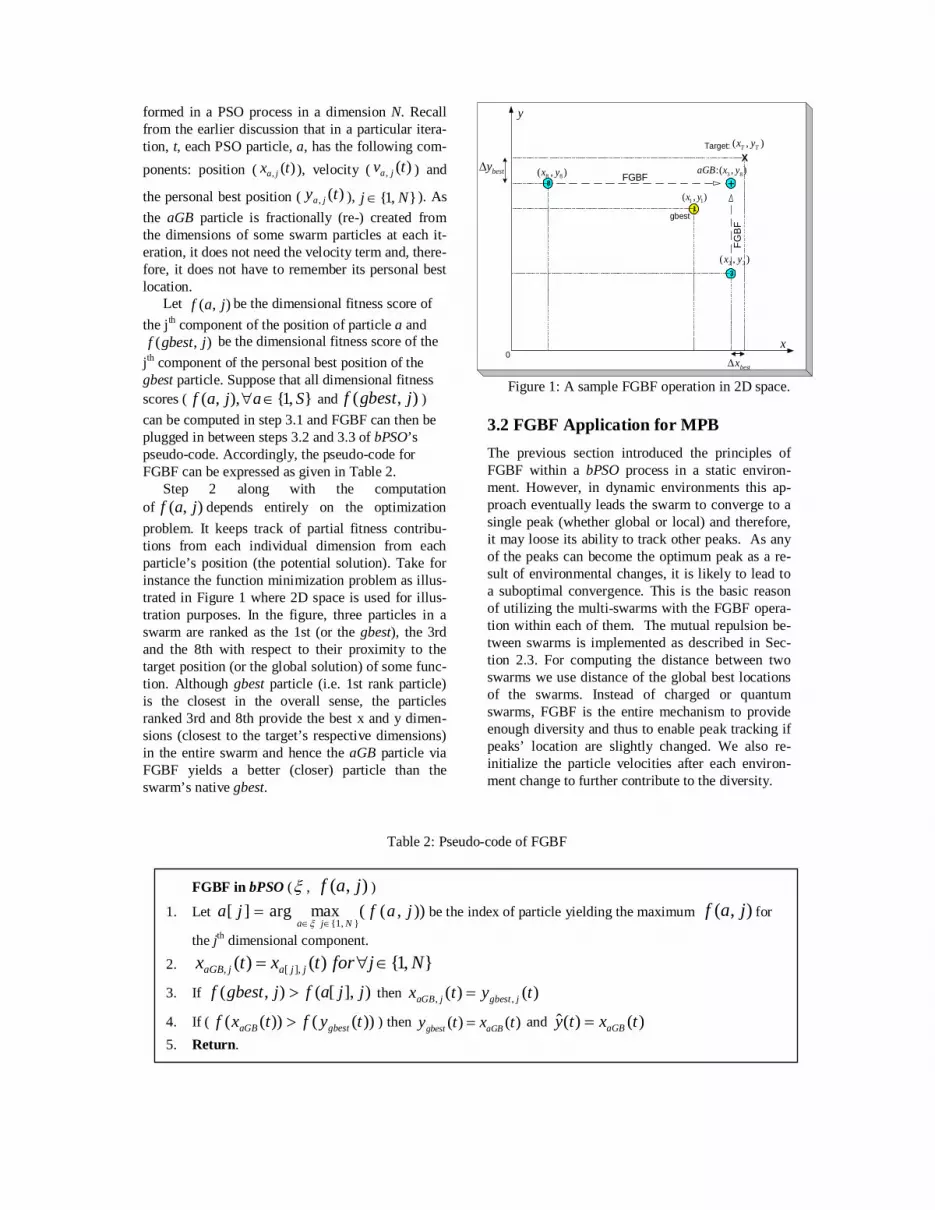
FGBF in bPSO (ξ , ),( jaf )
1. Let )),((maxarg][,1
jafjaNja ∈∈
=ξ
be the index of particle yielding the maximum ),( jaf for
the jth dimensional component.
2. ,1)()( ],[, Njfortxtx jjajaGB ∈∀=
3. If ( , ) ( [ ], )f gbest j f a j j> then , ,( ) ( )aGB j gbest jx t y t=
4. If ( ( ( )) ( ( ))aGB gbestf x t f y t> ) then ( ) ( )gbest aGBy t x t= and ˆ( ) ( )aGBy t x t=
5. Return.
formed in a PSO process in a dimension N. Recall from the earlier discussion that in a particular itera-tion, t, each PSO particle, a, has the following com-
ponents: position ( )(, tx ja ), velocity ( )(, tv ja ) and
the personal best position ( )(, ty ja ), ,1 Nj ∈ ). As
the aGB particle is fractionally (re-) created from the dimensions of some swarm particles at each it-eration, it does not need the velocity term and, there-fore, it does not have to remember its personal best location.
Let ),( jaf be the dimensional fitness score of
the jth component of the position of particle a and ( , )f gbest j be the dimensional fitness score of the
j th component of the personal best position of the gbest particle. Suppose that all dimensional fitness scores ( ,1),,( Sajaf ∈∀ and ( , )f gbest j )
can be computed in step 3.1 and FGBF can then be plugged in between steps 3.2 and 3.3 of bPSO’s pseudo-code. Accordingly, the pseudo-code for FGBF can be expressed as given in Table 2.
Step 2 along with the computation of ),( jaf depends entirely on the optimization
problem. It keeps track of partial fitness contribu-tions from each individual dimension from each particle’s position (the potential solution). Take for instance the function minimization problem as illus-trated in Figure 1 where 2D space is used for illus-tration purposes. In the figure, three particles in a swarm are ranked as the 1st (or the gbest), the 3rd and the 8th with respect to their proximity to the target position (or the global solution) of some func-tion. Although gbest particle (i.e. 1st rank particle) is the closest in the overall sense, the particles ranked 3rd and 8th provide the best x and y dimen-sions (closest to the target’s respective dimensions) in the entire swarm and hence the aGB particle via FGBF yields a better (closer) particle than the swarm’s native gbest.
X
1
3
8 +
gbest
x
y
bestx∆
besty∆
),( 11 yx
),( 88 yx
),( 33 yx
),(: 83 yxaGB
0
),( TT yxTarget:
FGBF
FG
BF
Figure 1: A sample FGBF operation in 2D space.
3.2 FGBF Application for MPB
The previous section introduced the principles of FGBF within a bPSO process in a static environ-ment. However, in dynamic environments this ap-proach eventually leads the swarm to converge to a single peak (whether global or local) and therefore, it may loose its ability to track other peaks. As any of the peaks can become the optimum peak as a re-sult of environmental changes, it is likely to lead to a suboptimal convergence. This is the basic reason of utilizing the multi-swarms with the FGBF opera-tion within each of them. The mutual repulsion be-tween swarms is implemented as described in Sec-tion 2.3. For computing the distance between two swarms we use distance of the global best locations of the swarms. Instead of charged or quantum swarms, FGBF is the entire mechanism to provide enough diversity and thus to enable peak tracking if peaks’ location are slightly changed. We also re-initialize the particle velocities after each environ-ment change to further contribute to the diversity.
Table 2: Pseudo-code of FGBF

Each particle a in a swarm ξ , represents a po-
tential solution and therefore, the jth component of
an N-dimensional point ( ,1, Njx j ∈ ) is stored in
its positional component, )(, tx ja at time t. The aim
of the PSO process is to search for the center point of the global maximum peak. Recall that in Sce-nario 2 of MPB the peaks used are all in cone shape and finding the highest peak is, therefore, equivalent to minimizing the )(tcx p
rr− term, where x
r is a
position found by the algorithm, )(tcp
r
is the cen-
ter point of the highest cone and . is the Euclid-
ean distance between them. This
yields ( )2),( pjj cxjaf −−= . Step 3.1 in bPSO’s
pseudo-code computes the (dimensional) fitness scores ( ( , ), ( , )f a j f gbest j ) of the jth components
( , ,,a j gbest jx y ) and in step 1 of the FGBF process,
the dimensional component yielding maximum ),( jaf is then placed in aGB. In step 3 these di-
mensional components are replaced by dimensional components of the personal best position of the gbest particle, if they yield even higher dimensional fitness scores. We do not expect that dimensional fitness scores can be evaluated with respect to the optimum peak since this requires the a priori knowl-edge of the global optimum, instead we use either the current peak where the particle resides on or the peak to which the swarm is converging (swarm peak). We shall thus consider and evaluate both modes separately.
4 Experimental results
We conducted an exhaustive set of experiments over the MPB Scenario 2 using the settings given in Section 2.2. In order to investigate the effect of multi-swarm settings, we used different numbers of swarms and numbers of particles in a swarm. We applied both FGBF modes using the current and swarm peaks and to investigate how FGBF and multi-swarms individually contribute to the results, we also made experiments without using one of them.
Figure 2 presents the current error plot, which shows the difference between the global maximum and the current best result during the first 80000 function evaluation, when 10 swarms each with 4 particles are used and the swarm peak mode is ap-plied for the FGBF operation. It can be seen from the figure that as the environment changes after every 5000 evaluation, it causes results to temporar-
ily deteriorate. However, it is clear that after envi-ronment changes the results are better than the very beginning, which shows the benefit of tracking the peaks instead of randomizing the swarm when a change occurs. The figure also reveals other typical features of algorithm behavior. First of all, after the first few environmental changes the algorithm is not yet behaving as well as later. This is because not the swarms have yet converged to a peak. Generally, it is more difficult to initially converge to a narrow or low peak than to keep tracking a peak that becomes narrow and/or low. It can also be seen that typically the algorithm gets close to the optimal solution be-fore the environment is changed again. In few cases, where the optimal solution is not found, the algorithm has for some reason been unable to keep a swarm tracking that peak, which is too narrow.
0 1 2 3 4 5 6 7 8
x 104
0
5
10
15
20
25
30
Number of evaluations
Cur
rent
err
or
Figure 2: Current error at the beginning of a run In Figure 3 and Figure 4 the contributions of
multi-swarms with FGBF are demonstrated. The algorithm is run on MPB using same random num-ber seed (same environment changes) first with both multi-swarms and FGBF, then without multi-swarms and finally without FGBF. Same settings are used as before. Without multi-swarms the num-ber of particles is set to 40 to keep the total number of particles unchanged.
As expected, the results without multi-swarms are significantly deteriorated due to the aforemen-tioned reasoning. When the environment is changed, the highest point of the peak to which the swarm is converging can be found quickly, but that can pro-vide good results only when that peak happens to be the global optimum. When multi-swarms are used, but without using the FGBF, it is clear that the algo-rithm can still establish some kind of follow-up of peaks as the results immediately after environment

changes are only slightly worse than with FGBF. However, if FGBF is not used, the algorithm can seldom find the global optimum. Either there is no swarm converging to the highest peak or the peak center just cannot be found fast enough.
2 3 4 5 6 7 8
x 104
0
5
10
15
20
25
30
35
40
Number of evaluations
Cur
rent
err
or
without multi-swarmswith multi-swarms
Figure 3: Effect of multi-swarms on results
2 3 4 5 6 7 8
x 104
0
1
2
3
4
5
6
7
8
9
10
Number of evaluations
Cur
rent
err
or
without FGBF
with FGBF
Figure 4: Effect of FGBF on results For comparative evaluations, we selected 5 of
the state-of-the-art methods, which use the same benchmark system, the MPB. The best MPB results published so far by these competing methods are listed in Table 3.
Table 3: Best results on MPB up to date
Source Algorithm Offline error
Blackwell and Branke [5]
PSO 2.16±0.06
Li et. al[16] PSO 1.93±0.06
Mendes and Mohais [18]
Differential Evolution
1.75±0.03
Blackwell and Branke [6]
PSO 1.75±0.06
Moser and Hendtlass [19]
Extremal Optimization
0.66±0.02
The overall best results have been achieved by
the Extremal Optimization algorithm [19]; however, this algorithm is specially designed for MPB and its applicability for other practical dynamic problems is not clear. The best results by a PSO-based algorithm have been achieved by Blackwell and Branke’s multi-swarm algorithm described in Section 2.3. The numerical results of the proposed methods in terms of the offline error are listed in Table 4. Each result given is the average of 50 runs, where each run consists of 500000 function evaluations.
Table 4: Offline error using Scenario 2
No. of swarms
No. of particles
Swarm peak Current peak
10 2 1.81±0.50 2.58±0.55 10 3 1.22±0.43 1.64±0.53 10 4 1.03±0.35 1.37±0.50 10 5 1.19±0.32 1.52±0.44 10 6 1.27±0.41 1.59±0.57 10 8 1.31±0.43 1.61±0.45 10 10 1.40±0.39 1.70±0.55 8 4 1.50±0.41 1.78±0.57 9 4 1.31±0.54 1.66±0.54 11 4 1.09±0.35 1.41±0.42 12 4 1.11±0.30 1.46±0.43 As expected the best results are achieved when
10 swarms are used. 4 particles in a swarm turned out to be the best setting. Between the two FGBF modes, better results are obtained when the swarm peak mode is used. 4 Conclusion
In this paper, we proposed a novel PSO tech-nique, namely, FGBF with the multi-swarms for an efficient and robust optimization over the dynamic systems. The technique can also be used over the static optimization problems particularly as a cure to common drawback of the family of PSO methods, pre-mature convergence to local optima. Realizing that the main problem lies in fact at the inability of using the available diversity among the dimensional components of swarm particles, the FGBF technique proposed in this paper collects the best components

and fractionally creates an aGB particle that has the potential to be a better “guide” then the swarm’s native gbest particle. On MPB we do not except to receive fractional scores with respect to the global highest peak, but instead we use either the peak, on which the particle is currently located (current peak) or the peak to which the swarm is converging (swarm peak). Especially swarm peak mode makes it possible to find and track the global highest peak successfully in a dynamic environment.
In order to make comparative evaluations with the current state-of-the-art, FGBF with multi-swarms is then applied over a benchmark system, the MPB. The results over the MPB with common settings used (i.e. Scenario 2) clearly indicate the superiority of the proposed technique over other PSO-based methods.
Overall, the proposed technique fundamentally upgrades the swarm guidance, which accomplishes substantial improvements in terms of speed and ac-curacy. The FGBF technique is modular and inde-pendent, i.e. it can be conveniently performed also with other PSO methods/variants.
References
[1] A. Abraham, S. Das and S. Roy, “Swarm Intelligence Algorithms for Data Clustering”, in Soft Computing for Knowledge Discovery and Data Mining book, Part IV, pp. 279-313, October 25, 2007.
[2] P.J. Angeline, “Tracking extrema in dynamic envi-ronments”, In Proc. Of the 6th Conference on Evolu-tionary Programming, pp.335-345, Springer Verlag, 1997
[3] T. Bäck and H.P. Schwefel, “An overview of evolu-tionary algorithms for parameter optimization”, Evo-lution. Comput. 1, pp. 1–23, 1993.
[4] T. Bäck and F. Kursawe, “Evolutionary algorithms for fuzzy logic: a brief overview”, In Fuzzy Logic and Soft Computing, World Scientific, pp. 3–10, Sin-gapore, 1995.
[5] T.M. Blackwell and J. Branke, “Multi-Swarm Opti-mization in Dynamic Environments”, Applications of Evolutionary Computation, vol. 3005, pp. 489-500, Springer, 2004.
[6] T.M. Blackwell and J. Branke, “Multiswarms, Exclu-sion, and Anti-Convergence in Dynamic Environ-ments”, IEEE Transactions on Evolutionary Compu-tation,, vol. 10/4, pp. 51-58, 2004.
[7] J. Branke, “Moving Peaks Benchmark”, http://www.aifb.uni-karlsruhe.de/~jbr/MovPeaks/ , viewed 26/06/08
[8] Y.-P. Chen, W.-C. Peng; M.-C. Jian, “Particle Swarm Optimization With Recombination and Dy-namic Linkage Discovery”, in IEEE Trans. on Sys-tems, Man, and Cybernetics, Part B, Vol. 37, Issue 6, pp. 1460 – 1470, Dec. 2007.
[9] R. Eberhart, P. Simpson, and R. Dobbins, Computa-tional Intelligence. PC Tools, Academic Press, Inc., Boston, MA, USA, 1996.
[10] R. Eberhart and Y. Shi, “Tracking and Optimizing Dynamic Systems with Particle Swarms”, in Proc. of Computational Evolution Conference (CEC 2001), NJ, US, pp. 94-100, 2001.
[11] U.M. Fayyad, G.P. Shapire, P. Smyth and R. Uthuru-samy, Advances in Knowledge Discovery and Data Mining, MIT Press, Cambridge, MA, 1996.
[12] D. Goldberg, “Genetic Algorithms in Search, Opti-mization and Machine Learning”, Addison-Wesley, Reading, pp. 1-25. MA, 1989.
[13] J. Kennedy, R Eberhart., “Particle swarm optimiza-tion”, in Proc. of IEEE Int. Conf. On Neural Net-works, vol. 4, pp. 1942–1948, Perth, Australia, 1995.
[14] J. Koza, Genetic Programming: On the Program-ming of Computers by means of Natural Selection, MIT Press, Cambridge, Massachussetts, 1992.
[15] R. A. Krohling, L S. Coelho, “Coevolutionary Parti-cle Swarm Optimization Using Gaussian Distribution for Solving Constrained Optimization Problems”, IEEE Trans. on Systems, Man, and Cybernetics, Part B, Vol. 36, Issue 6, pp. 1407 – 1416, Dec. 2006.
[16] X. Li, J. Branke and T. Blackwell, “Particle Swarm with Speciation and Adaptation in a Dynamic Envi-ronment”, Proc. of Genetic and Evolutionary Com-putation Conference, pp. 51-58, Seattle Washington, 2006.
[17] M. Lovberg and T. Krink, “Extending Particle Swarm Optimisers with Self-Organized Criticality”, In Proc. of the IEEE Congress on Evolutionary Computation, vol. 2, pp.1588-1593, 2002.
[18] R. Mendes and A. Mohais, “DynDE: a Differential Evolution for Dynamic Optimization Problems”, IEEE Congress on Evolutionary Computation, pp. 2808-2815, 2005.
[19] I. Moser and T. Hendtlass, “A Simple and Efficient Multi-Component Algorithm for Solving Dynamic Function Optimisation Problems”, IEEE Congress on Evolutionary Computation, pp. 252-259, 2007.
[20] J. Riget and J. S. Vesterstrom, “A Diversity-Guided Particle Swarm Optimizer - The ARPSO”, Technical report, Department of Computer Science, University of Aarhus, 2002.
[21] Y. Shi and R.C. Eberhart, “A Modified Particle Swarm Optimizer”, In Proc. of the IEEE Congress on Evolutionary Computation, pp. 69-73, 1998.
[22] E.O. Wilson, Sociobiology: The new synthesis, Cam-bridge, MA: Belknap Press, 1975.

Sudoku Solving with Cultural Swarms
Timo Mantere Janne Koljonen
Department of Electrical Engineering and Automation University of Vaasa, PO Box 700, FIN-65101 Vaasa
[email protected] [email protected]
Abstract
This paper studies the problems involved in solving Sudoku puzzles with cultural genetic algo-rithms. Sudoku is a number puzzle that has recently become a worldwide phenomenon. Sudoku can be regarded as a combinatorial problem. When solved with evolutionary algorithms it can be han-dled as constraint satisfaction problem or multi-objective optimization problem. The objective of this study was to test if cultural algorithm with belief space is more efficient solving Sudoku puzzles than the normal permutation genetic algorithm we presented in CEC2007. The results with belief space showed that Cultural algorithm performed slightly better.
1 Introduction This paper studies if the Sudoku puzzles can be
solved effectively with evolutionary algorithms. In Mantere and Koljonen (2007) we presented the re-sults by using genetic algorithms (GA) (Holland, 1992). This time the idea was to add belief space to the genetic algorithm and create a sort of cultural algorithm (CA) (Reynolds, 1999). The plan was to compare the results of GA and CA and see if the added cultural part increases the solving efficiency.
According to Wikipedia (2008) Sudoku is a Japanese logical game that has recently become hugely popular in Europe and North-America. How-ever, the first puzzle was published in a puzzle magazine in USA 1979, then it circled through Ja-pan, where it became popular in 1986, and later it become a phenomena in the western world circa 2005 (Sullivan, 2006). Sudoku has been claimed to be very popular and addictive because it is very challenging but has very simple rules (Semeniuk, 2005).
Sudoku puzzle is composed of a 9×9 grid, total 81 positions, that are divided into nine 3×3 subgrids. The solution of Sudoku puzzle is such that each row, column and subgrid contains each integer 1, 2, … , 9 once and only once.
The puzzle is presented so that in the beginning there are some static numbers, givens, in the grid that are given in advance and cannot be changed or moved. The number of givens does not determine the difficulty of the puzzle (Semeniuk, 2006 and Moraglio et al, 2006). Grating puzzles is one of the most difficult things in Sudoku puzzle creation, and
there are about 15 to 20 factors that have an effect on difficulty rating (Wikipedia, 2008).
The givens can be symmetric or nonsymmetri-cal. In the symmetric case, there are pairs of givens located symmetrically with respect to centre posi-tion.
7 9 3 6 8 1 4 2 5 3 1 4 6 2 9 2 3 6 3 6 5 4 2 1
Figure 1: A starting point of the Sudoku puz-zle, where 24 locations contains a static num-ber that are given
Figure 1 shows one example of the Sudoku puz-
zles we generated with GA (Mantere and Koljonen, 2007). It contains 24 given numbers, and the correct number for the other 57 positions should be solved. This puzzle has nonsymmetrical givens, since the givens are not symmetrically located respect to the central point. This is the same Sudoku that is refer-enced in the results as GA-Hard c. The SudokuEx-plainer (2007) gave it a difficulty value 7.8.
The solution of this Sudoku is shown in fig. 2. The static numbers given in the beginning (fig. 1)

have remained exactly in the same positions where they originally were.
7 9 2 5 6 8 1 4 3 4 5 3 2 1 9 8 6 7 8 6 1 3 7 4 9 5 2 6 2 5 8 9 3 7 1 4 3 7 9 1 4 2 6 8 5 1 4 8 7 5 6 2 3 9 2 8 4 9 3 1 5 7 6 9 3 7 6 8 5 4 2 1 5 1 6 4 2 7 3 9 8
Figure 2: A solution for the Sudoku puzzle given in fig 1. The givens marked with bold
In this study, we try to evaluate, how cultural
genetic algorithms solve those Sudoku puzzles pre-sented in newspapers (Helsingin Sanomat, 2006 and Aamulehti, 2006) and in Pappocom (2006), and those we generated by GA (Mantere and Koljonen 2007). Furthermore, we evaluate if the CA effi-ciency correlates with the alleged difficulty ratings of these Sudoku puzzles.
In the Section I we introduce the problem, ge-netic algorithms and related work, Section II intro-duces the proposed method, Section III the obtained results, and section IV discusses on the findings and their implications.
1.1 Genetic Algorithms All Genetic algorithms (Holland, 1992) are com-puter based optimization methods that use the Dar-winian evolution (Darwin, 1859) of nature as a model and inspiration. The solution base of a prob-lem is encoded as individuals that are chromosomes consisting of several genes. On the contrary to na-ture, GAs the individual (phenotype) of GA is usu-ally deterministically derived from the chromosome (genotype). The age or environment does not alter the phenotype during the GA individual “life time”. These virtual individuals are tested against a prob-lem represented as a fitness function. The better the fitness value individual gets, the better is its chance to be selected as a parent for new individuals. The worst individuals are killed from the population in order to make room for the new generation. Using crossover and mutation operations GA creates new individuals. In crossover, we select the genes for a new chromosome from the parents using some pre-selected practice, e.g. one-point, two-point or uni-form crossover. In mutation, we change random genes of the chromosome either randomly or using some predefined strategy. The GA strategy is often
elitist and therefore follows the “survival of the fit-test” principles of the Darwinian evolution. 1.2 Related Work
The Sudoku problem seem to be relatively rarely studied in technical sciences, since the IEEEXplore (2008) search engine finds only 12 papers mention-ing Sudoku.
It has been stated (Aaronson, 2006) that Sudoku is a good laboratory for algorithms design, and it is based on one of the hardest unsolved problems in computer science – the NP complete problems. They also stated that Sudoku craze may even end up leading breakthroughs in computer science.
The Sudoku problem is studied in constraint programming and satisfiability research (Simonis, 2005, Lynce and Ouaknine, 2006, Moon and Gun-ther, 2006). Those methods are also efficient to solve Sudokus, but do not provide solution for every Sudoku puzzle. However, in this study we concen-trate on Sudoku solving with evolutionary methods. The main reason for solving Sudokus with cultural algorithms is to learn more about capabilities of CA in constrained combinatorial problems, and hope-fully to learn new tricks to make it more efficient also in this field of problems.
There seems to be a few scientific papers about Sudoku with EA methods. Moraglio et al. (2006) have solved Sudokus using GA with product geo-metric crossover. They claim that their geometric crossover perform significantly better than hill-climbers and mutations alone. Their method solves easy Sudokus from (Pappocom, 2006) efficiently, but has difficulties with the medium and hard Sudo-kus. They also acknowledged that evolutionary al-gorithms are not the most efficient technique for solving Sudokus, but that Sudoku is an interesting study case for algorithm development.
Nicolau and Ryan (2006) have used quite a dif-ferent approach to solve Sudokus: their GAuGE (Genetic Algorithms using Grammatical Evolution) optimizes the sequence of logical operations that are then applied to find the solution.
Gold (2005) has used GA for generating new Sudoku puzzles, but the method seems to be ineffi-cient, since in their example their GA needed 35700 generations to come up with a new open Sudoku solution. In our results we create a new open Su-doku solution, in average, with 101 generations (2020 trials).
There is also Sudoku Maker (2006) software available that is said to use genetic algorithm inter-nally and claimed that the generated Sudokus are usually very hard to solve. Unfortunately, there are no details how GA is used and how quickly a new Sudoku is generated.
More related work in Mantere Koljonen (2008).

2 THE PROPOSED METHOD In order to test the proposed method we decided
to use an integer coded elitist GA. The size of the GA chromosome is 81 integer numbers, divided into nine sub-blocks of nine numbers (building blocks) that corresponds to the 3×3 subgrids from left to right and from top to bottom. The uniform crossover operation was applied only between sub-blocks, and the sequences of swap mutations only inside the sub-blocks. Therefore the crossover point cannot be inside a building block. All new individuals were generated by first applying crossover and then muta-tions to the crossover result.
The population size (POP) was 21, and elitism ratio (ELIT) was 1. The best individuals were fa-vored by selecting the mating individuals x1 and x2 with the following code:
for( i=POP-1; i>=ELIT; i--) x1 = ( int )(i * Math.random() ); x2 = ( int )(i * Math.random() ); . . . This code causes the likelihood of good indi-
viduals to be selected as a parent to be divided as shown in figure 3. The favoring is stronger than the linear favoring, but still gives even the worst indi-viduals a small change to be selected as parent.
There is a chance of selecting x1=x2, where only the mutation operation changes the new individual genotype.
A found solution was the only stop condition, since our method never failed to find a solution.
In addition to basic rules of Sudoku, the fixed numbers (“givens”) must be observed during the solving process. Therefore a Sudoku solution obeys four conditions:
1) Each row has to contain each integer from 1 to 9,
2) each column has to contain each integer from 1 to 9,
3) each 3x3 subgrid must contain each integer from 1 to 9,
4) the given numbers must stay in the original positions.
When selecting an appropriate solving approach, the condition 4) is always fulfilled, and also one of the conditions 1) to 3) can be controlled, hence only two conditions are subject to optimization. We chose to program our Evolutionary algorithms (EA) so that conditions 3) and 4) are automatically ful-filled and only the conditions 1) and 2) are opti-mized. Sudoku has 9 rows and 9 columns, so we have 18 equality constrains that must be fulfilled when we have the solution.
These EAs (GA and CA) used in this study is
customized to this problem or other grid type com-binatorial problems. These EAs were modifications of a combinatorial GA originally programmed for magic square (Alander et al, 1999) and other combi-natorial problems.
These EAs does not use direct mutations or crossovers that could generate illegal situations for 3x3 subgrids. On the other hand, rows and columns can contain integers more than once in non-optimal situation. The genetic operators are not allowed to move the fixed numbers that are given in the begin-ning of the problem. This is guaranteed by help ar-ray, which indicates whether a number is fixed or not.
1 2 3 4 5 6 7 8 9 10 11 12 13 14 15 16 17 18 19 20n:th best population member
Selected to be parent
Figure 3: The likelihood of being selected to a parent as a function of individual’s fitness value ranking order
2.1 The mutation operator
Mutations are applied only inside a sub-block. Originally, we used three different mutation strate-gies that are commonly used in combinatorial opti-mization: swap mutation, 3-swap mutation, and in-sertion mutation. However, since the 3-swap and insertion mutations in practice are actually only the sequences of swap (two-swap) mutations, we later replaced them with a sequence of 1 to 5 swap muta-tions inside a sub-block. Later we removed the se-quences also, since the test runs showed that the Sudokus were solved just as efficiently with just one swap than 1-5 swap sequence.
All new individuals were generated by first ap-plying crossover and then mutations to the crossover result. The swap mutation probability was 0.1 for each gene location; however this did not equal the actual mutation amount. In swap mutation, the val-ues of two positions are exchanged. Each time muta-tion is tried inside a sub-block, the help array of givens is checked. If it is illegal to change the ran-domly chosen position, mutation is omitted, which decreases the actual mutation probability.
We also check if the new trial was identical with one its parents. If so, the mutation operation was called again until the new trial was different. This
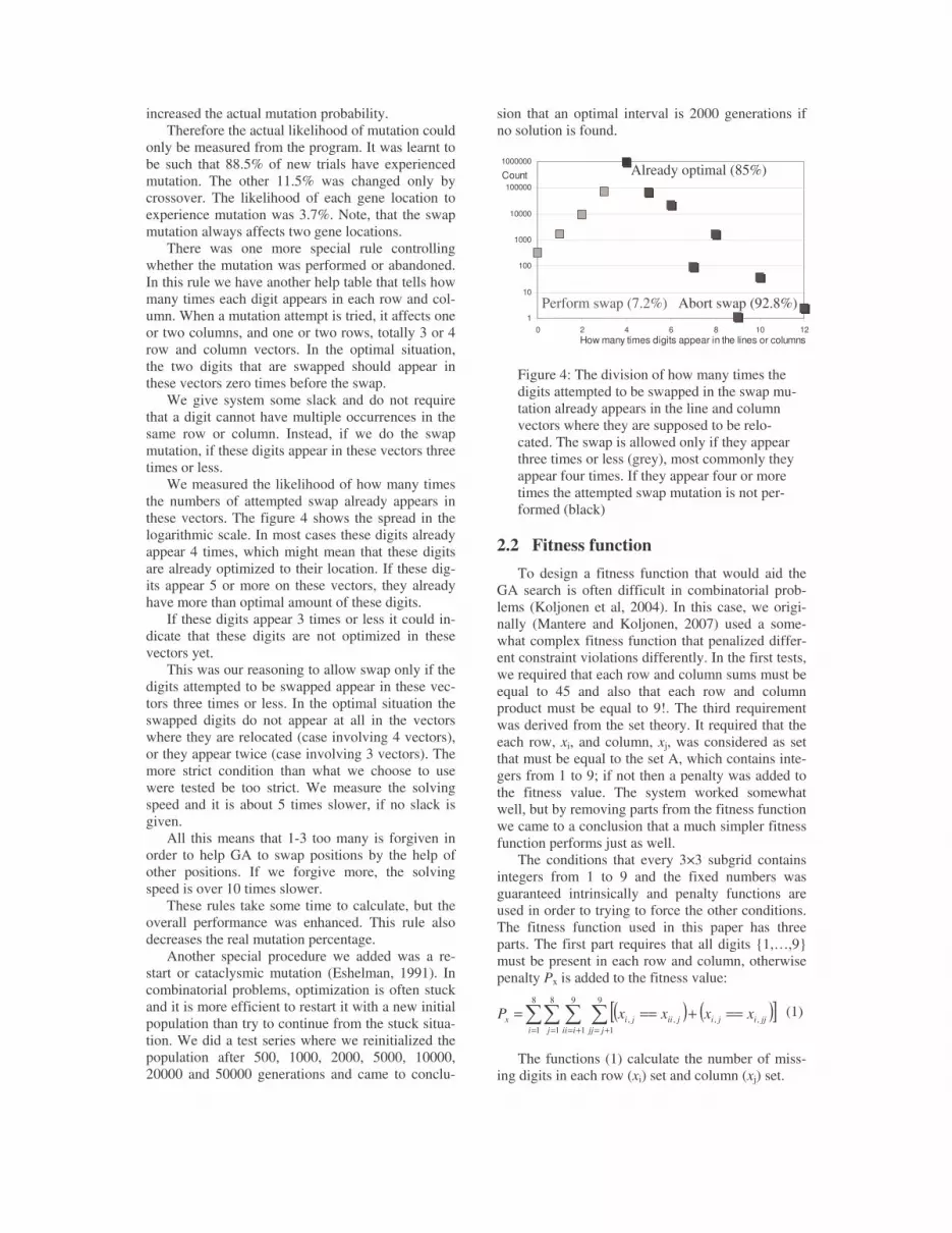
increased the actual mutation probability. Therefore the actual likelihood of mutation could
only be measured from the program. It was learnt to be such that 88.5% of new trials have experienced mutation. The other 11.5% was changed only by crossover. The likelihood of each gene location to experience mutation was 3.7%. Note, that the swap mutation always affects two gene locations.
There was one more special rule controlling whether the mutation was performed or abandoned. In this rule we have another help table that tells how many times each digit appears in each row and col-umn. When a mutation attempt is tried, it affects one or two columns, and one or two rows, totally 3 or 4 row and column vectors. In the optimal situation, the two digits that are swapped should appear in these vectors zero times before the swap.
We give system some slack and do not require that a digit cannot have multiple occurrences in the same row or column. Instead, if we do the swap mutation, if these digits appear in these vectors three times or less.
We measured the likelihood of how many times the numbers of attempted swap already appears in these vectors. The figure 4 shows the spread in the logarithmic scale. In most cases these digits already appear 4 times, which might mean that these digits are already optimized to their location. If these dig-its appear 5 or more on these vectors, they already have more than optimal amount of these digits.
If these digits appear 3 times or less it could in-dicate that these digits are not optimized in these vectors yet.
This was our reasoning to allow swap only if the digits attempted to be swapped appear in these vec-tors three times or less. In the optimal situation the swapped digits do not appear at all in the vectors where they are relocated (case involving 4 vectors), or they appear twice (case involving 3 vectors). The more strict condition than what we choose to use were tested be too strict. We measure the solving speed and it is about 5 times slower, if no slack is given.
All this means that 1-3 too many is forgiven in order to help GA to swap positions by the help of other positions. If we forgive more, the solving speed is over 10 times slower.
These rules take some time to calculate, but the overall performance was enhanced. This rule also decreases the real mutation percentage.
Another special procedure we added was a re-start or cataclysmic mutation (Eshelman, 1991). In combinatorial problems, optimization is often stuck and it is more efficient to restart it with a new initial population than try to continue from the stuck situa-tion. We did a test series where we reinitialized the population after 500, 1000, 2000, 5000, 10000, 20000 and 50000 generations and came to conclu-
sion that an optimal interval is 2000 generations if no solution is found.
Figure 4: The division of how many times the digits attempted to be swapped in the swap mu-tation already appears in the line and column vectors where they are supposed to be relo-cated. The swap is allowed only if they appear three times or less (grey), most commonly they appear four times. If they appear four or more times the attempted swap mutation is not per-formed (black)
2.2 Fitness function
To design a fitness function that would aid the GA search is often difficult in combinatorial prob-lems (Koljonen et al, 2004). In this case, we origi-nally (Mantere and Koljonen, 2007) used a some-what complex fitness function that penalized differ-ent constraint violations differently. In the first tests, we required that each row and column sums must be equal to 45 and also that each row and column product must be equal to 9!. The third requirement was derived from the set theory. It required that the each row, xi, and column, xj, was considered as set that must be equal to the set A, which contains inte-gers from 1 to 9; if not then a penalty was added to the fitness value. The system worked somewhat well, but by removing parts from the fitness function we came to a conclusion that a much simpler fitness function performs just as well.
The conditions that every 3×3 subgrid contains integers from 1 to 9 and the fixed numbers was guaranteed intrinsically and penalty functions are used in order to trying to force the other conditions. The fitness function used in this paper has three parts. The first part requires that all digits 1,…,9 must be present in each row and column, otherwise penalty Px is added to the fitness value:
(1)
The functions (1) calculate the number of miss-ing digits in each row (xi) set and column (xj) set.
1
10
100
1000
10000
100000
1000000
0 2 4 6 8 10 12How many times digits appear in the lines or columns
Count
Perform swap (7.2%) Abort swap (92.8%)
Already optimal (85%)
( ) ( )[ ] = = += +=
==+===8
1
8
1
9
1
9
1,,,,
i j iii jjjjjijijiijix xxxxP

In the optimal situation all digits appear in the row and column sets, and fitness function value be-comes zero.
The second part of fitness function is “aging” of the best individual; adding 1 to its fitness value each round when it remains the best:
If Best(generation(i)) = Best(generation(i-1))
then Value(Best)+=1; (2)
This means that when a new solution becomes best, its value is the value it gets from the fitness function. If it is still the best solution in the next generation we added value 1 to its fitness value.
This operation can be seen as some kind of aging process of the individual’s phenotype. It is not as fit and strong, if it lives longer. This operation was added in order to make more variation to the popula-tion, and our preliminary tests also showed that it is beneficial and it resulted a faster solving of Sudoku.
The third part requires that the same digit as some given must not appear in the same row or col-umn as a given, otherwise penalty Pg added:
(3)
This part (3) is used only after reaching the near
solution region in the search space (2 positions wrong). 2.3 Cultural GA and the belief space
The main difference of this paper to (Mantere and Koljonen, 2007) is that this time we added a belief space model to our genetic algorithm. The belief space in this case was very simple; it is 9×9×9 cube, there the first 9×9 represents the Sudoku table and the last dimension the nine possible digits for each location. After each generation, if the best in-dividual has changed, we update the belief space so that the digit that appears in the best Sudoku solu-tion gets added value in the belief space.
Belief space is used directly to generate on new individual for each generation. The new trial is formed by first selecting in each Sudoku 3×3 sub-grid the position where some digit in the belief space has the highest value from all digits in sub-grid. This position will get the value that has the highest value in the belief space for this digit. Then the filling of trial continues by finding the second highest etc. every time we check if the digit is al-ready assigned to some location of the subgrid, if so we have to choose next best value.
In paper (Mantere and Koljonen, 2008) we pre-sented different way of applying the belief space. The use of belief space in this paper is more “ag-gressive” and it leads faster solving of easy Sudo-
kus, but does not improve much the solving of diffi-cult Sudokus compared to normal GA. Whereas in (Mantere and Koljonen, 2008) the belief space gath-ered and apply information more slowly and that version was more effective with difficult Sudokus, but it did not speed up the solving of difficult Sudo-kus compared to the normal GA.
3 THE PROPOSED METHOD We test these methods (genetic algorithm and
cultural algorithm) by solving 45 different bench-mark Sudokus.
15 Sudoku puzzles taken from the newspaper Helsingin Sanomat (2006) marked with their diffi-culty rating 1-5 stars. These had 28 to 33 symmetric givens. We also tested 12 Sudokus taken from newspaper Aamulehti (2006). They were marked with difficulty ratings: Easy, Challenging, Difficult, and Super difficult. They contain 23 to 36 nonsym-metrical givens.
We also have 9 Sudokus taken from Pappocom (2006) marked as Easy, Medium and Hard, and 9 Sudokus we generated with GA (Mantere and Kol-jonen, 2007) marked as GA-Easy, GA-Medium and GA-Hard.
We used unlimited (chapter 3.1) and max. 100000 trials versions (chapter 3.2). 3.1 Sudoku Solving and Rating
Table 1 summarizes the average results with ge-netic algorithm and cultural algorithm. Table shows that CA was more effective with 33 test Sudokus out of 45. If we divide them to difficulty rating classes, CA was more effective in 13 rating classes out of 15 tested.
How large the overall performance advantage of CA over GA depends on how you measure it; if calculating all Sudokus and average solving effi-ciency it is only 2.63%. However, if we calculate the proportion with each Sudoku and add these numbers together the advantage is 4.79%.
It must be mentioned that this improvement is not very large, and with most cases the T-test sug-gested that the both result series are from the under-lying distribution. However since we have im-provement with most of the benchmark Sudokus and their difficulty classes we can claim that at least CA is not less efficient. With better belief space model we might even increase the efficiency (see Mantere and Koljonen, 2008).
Table 1 also shows that the EA hardness of Su-dokus is relatively consistent with their difficulty rating. However, some of them seem to be classified in the wrong group. The Sudokus in Helsingin Sano-mat seem to have several wrong classifications, e.g. 2 star a is easier than 1 star c, and 3 star a is easier
( )= =
===9
1
9
1i jijijg gxP

than 2 star b, 4 star a is easier than 3 star b and 5 star a and b are easier than 4 star b and c and even easier than 3 star b.
Table 1: The comparison of how effectively GA and CA find solutions for the Sudoku puzzles with different difficulty rating. There are three different Sudokus (a, b, and c) from each of the 15 difficulty classes 1-5 stars (Helsingin Sanomat, 2006), Easy, Challeng-ing, Difficult and Super Difficult (Aamulehti, 2006), Easy, Medium, Hard (Pappocom, 2006) and GA-Easy, GA-Medium, GA-Hard (Mantere and Koljonen, 2007). Each of the Sudokus was solved 100 times and the table shows average value of how many genera-tions was needed for solving each Sudoku. There is also the improvement percentage of cultural algorithm against pure GA
Average of Solve genera-
tions with GA Average of Solve
generations with CA Improve
by Diffi-culty Rating a b c a b c % 1 78 41 1244 76 41 1191 4.08
2 1203 6951 2328 831 6230 2016 13.40
3 2103 9517 5835 2207 8238 5062 11.16
4 5503 10966 9369 6483 9618 10115 -1.46
5 8371 8661 13649 7155 7698 15808 0.06
E 40 23 56 36 20 48 12.65
C 5144 10418 7010 4866 11185 5704 3.62
D 40830 19486 8433 40162 19850 8255 0.70
SD 39901 20593 27918 42841 20095 27416 -2.19
Easy 1669 797 500 1386 791 503 9.69
Med 14576 21740 5660 14317 19468 5431 6.58
Hard 125105 11629 48479 125391 11875 45529 1.31
GA-E 771 339 798 684 423 584 11.40
GA-M 4501 4253 3947 4418 3483 3390 11.10
GA-H 16528 11354 62588 20034 11055 53074 6.97
The Sudokus in Aamulehti seem to mostly in
right order, only Challenging b seems to be more difficult than Difficult c and Difficult a is even more difficult than Super difficults.
The Pappocom Sudokus are in right groups ex-cept Hard b is easier than Medium a and b. The GA generated Sudokus are in right order because they were already rated with GAs in (Mantere and Kol-jonen, 2007).
Comparing the Sudokus from different source, the Easy from Aamulehti is the easiest, followed by 1-4 stars Sudokus from Helsingin Sanomat before Challenging from Aamulehti, 5 stars from HS, and finally Difficult and Super difficult from Aamulehti as the most difficult ones.
3.2 Comparing our results with others The study (Moraglio et al, 2006) represents the
results with a large number of different methods, total of 41 tables with different strategies. These strategies are divided into three groups: Hamming space crossovers, Swap space crossovers and Hill climbers. The worst results in each group never reach the solution. We decided to compare our re-sults with the best results for each groups repre-sented in (Moraglio et al, 2006). Unfortunately, we do not know how many fitness evaluations they used, since their stopping criterion was 20 genera-tions with no progress (50000 trials with population size 5000, and elitism 2500). With hill climbers they reported using 100000 trials.
Table 2: Our results and the best results rep-resented in (Moraglio et al, 2006). The num-bers represents how many times out of 30 test runs each method reach the optimum with each problem
Our CA The best results represented in (Moraglio et al, 2006)
Sudoku Problems from Pappocom (2006)
Unlimited trials
100 000 trials
Hamming Space crossovers
Swap Space crossovers
Hill Climbers
Easy 1 30 30 5 28 30 Easy 2 30 30 8 21 30 Easy 3 30 30 14 30 30 Medium 30 10 0 0 0 Hard 30 1 0 15 0 Total 150 101 27 94 90
For comparison purposes we tested five Sudokus
from (Pappocom, 2006) with our GA to obtain com-parable results. However, we do not know if the Sudokus taken are exactly the same as they used, so we chose the first three from the Easy category and the first one from Medium and Hard categories, similarly as they reported choosing them.
Table 2 shows our results with unlimited trials and with 100 000 trials. The 100 000 trials version should be compared to hill climbers, where we know that (Moraglio et al, 2006) used that amount of trials.
Our both version (unlimited and 100 000 trials) GA performed better than their best GA version with each category when comparing the total num-bers. Only with Hard our 100 000 trials version per-formed worse than their “Swap space crossovers” version.
With our unlimited trials version the longest solve run was with the Hard Sudoku and it lasted 8 130 940 trials.
The (Nicolau and Ryan, 2006) have also pre-sented very good result by GAuGE system (Genetic Algorithms using Grammatical Evolution). They had taken their benchmark Sudokus from a book

that was unavailable for us. Thus, we cannot directly compare our results with their method. However, out of 20 benchmark Sudokus they find the solution every time out of 30 test runs for 17 problems, but for two problems their method was unsuccessful of finding a solution with 320 000 trials.
Our method has never failed to find a solution of Sudoku. The hardest Sudoku we tested was Hard (table 2, Hard a in table 1) from Pappocom (2006).
The AI Escargot by Arto Inkala (2006) have been claimed to be the most difficult Sudoku in the world. Without a trials limit it was solved by our CA every time. When using a limited number of trials it was solved 12 times out of 100 test runs with 100 000 trials and 28 times out of 100 with 320 000 tri-als. In the fastest solve run it was solved with only 7740 trials, in average it required 590 614 trials. The longest solve run required 5 588 420 trials, which was much less than Hard a from (Pappocom, 2006) needed in the worst case.
4 CONCLUSIONS & FUTURE In this paper, we studied if Sudoku puzzles can
be solved with a combinatorial cultural algorithm, a genetic algorithm with added belief space. The re-sults show that EAs can solve Sudoku puzzles rela-tively effectively.
However, there exist some more efficient algo-rithms to solve Sudoku puzzles e.g. (Simonis, 2005, Lynce and Ouaknine, 2006, Moon and Gunther, 2006) are fast, but in the results reported, all these methods fail to solve some Sudoku puzzles they tested. In any case, our results stand well the com-parison with other known results with evolutionary algorithms.
However, the lack of common benchmark Sudo-kus complicates the comparison of results. There-fore we decided to put our 46 benchmark Sudokus available in the web (Mantere and Koljonen, 2008b), so that anyone interested to compare their results with ours can now use the same benchmark puzzles.
In this study, the aim was to test how efficient pure EA approach is, without many problem spe-cific rules for solving Sudokus. The EA results can of course be enhanced by adding problem related rules. However, if one adds too much problem spe-cific logic to the Sudoku solving, there will be noth-ing left to optimize, therefore we decided to omit most problem specific logic and try to achieve this “logic” with natural evolutionary way by learning it with belief space.
We also print out some belief spaces (not pre-sented in this paper) and it looks like Sudoku puz-zles might possess some kind of positional bias. Most of the belief spaces looked like the Sudoku
trial composed based on them would more likely contain small numbers in the left upper corner and larger numbers in right down corner. We think it is possible that Sudoku generators have some kind of positional bias when they generate new Sudoku.
It might be that our CA belief space exploited this bias in order to generate better results. We plan to measure the possible positional biases in the near future and see, if it really appears or not, and if it appears only with some Sudoku generators.
The other goal was to study if difficulty ratings given for Sudoku puzzles in newspapers are consis-tent with their difficulty in GA optimization. The answer to that question seems to be positive. For some solitary puzzles the rating seems wrong, but the overall trend follows the ratings; those Sudokus that have higher difficulty rating proved also to be more difficult for genetic algorithms. This means that GA can be used for rating the difficulty of a new Sudoku puzzle. Rating puzzles is said to be one of the most difficult things in Sudoku puzzle crea-tion (Wikipedia, 2008), so GA can be a helpful tool for that purpose. However, the other explanation can be that the original puzzles are also generated with computer programs, and since GA is also a com-puter based method, it is possible that a human solver does not necessarily experience their diffi-culty the same way.
It has been said that 17 given numbers is mini-mal needed to come up with a unique solution, but it is not mathematically proven (Wikipedia, 2008). GA could also be used for minimizing the number of givens that still leads the unique solution.
The fitness function setting in this study worked satisfactorily, but in the future we might study more whether or not this is a proper GA fitness function for the Sudoku problem. We are already considering if it is possible to generate Sudoku a fitness function based on energy functions (Koljonen and Alander, 2004). The cultural algorithm might also be ex-changed with some kind of energy function based belief space.
We have earlier used co-evolutionary GAs for other problems. It could be interesting approach to apply co-evolution for Sudoku puzzle generation and solving. Other GA would try to generate as hard Sudokus as possible and other GA would try to evolve itself to be able to solve Sudokus ever more efficiently. We will try to implement this approach in the near future to see if this kind of co-evolution could be achieved with Sudoku problem.
In our Sudoku web page (Mantere and Koljonen, 2008b) we also present some fresh results with ant colony optimization (ACO). The results with ants are very good with easy Sudokus, with them ACO is faster to find solution than GA or CA, sometimes it needs only one third of the trials compared to GA. Unfortunately with difficult Sudokus ACO is not

capable of finding the solution effectively, and it may need even three times as many trials as GA.
References Aamulehti. Sudoku online. Available via WWW:
http://www.aamulehti.fi/sudoku/ (cited 11.1.2006). 2006.
Aaronson, L.: Sudoku science. IEEE Spectrum 43(2), February: 16-17. 2006.
Alander, J.T., Mantere T., Pyylampi, T.: Digital halftoning optimization via genetic algorithms for ink jet machine. In Developments in Com-putational mechanics with high performance computing, CIVIL-COMP Press, Edinburg, UK: 211-216. 1999.
Darwin, C. The Origin of Species: By Means of Natural Selection or The Preservation of Fa-voured Races in the Struggle for Life, Oxford University Press, London. 1859.
Eshelman, L.J.: The CHC adaptive search algo-rithms: how to safe search when engaging in nontraditional genetic recombination. In Foun-dations of Genetic Algorithms, Morgan Kauf-mann. 1991.
Gold, M. Using Genetic Algorithms to Come up with Sudoku Puzzles. Sep 23, 2005. Available via WWW: http://www.c-sharpcorner.com/ UploadFile/mgold/Sudoku 09232005003323 AM/Sdoku.aspx?ArticleID=fba36449-ccf3-444f-a435-a812535c45e5 (cited 16.10.2006). 2005.
Helsingin Sanomat. Sudoku. Available via WWW: http://www2.hs.fi/extrat/sudoku/ sudoku.html (cited 11.1.2006). 2006.
Holland, J. Adaptation in Natural and Artificial Sys-tems, The MIT Press. 1992.
IEEE Xplore. Available via WWW: http://ieeexplore.ieee.org/search/advsearch.jsp (cited 07.08.2008). 2008.
Inkala, A. AI Sudoku 1002 Vaikeaa Tehtävää, Pressmen Finland Oy. 2006.
Koljonen, J., Alander, J.T. Solving the “urban horse” problem by backtracking and genetic algorithm – a comparison. In Step 2004 – The 11th Finnish Artificial Intelligence Confer-ence, Vantaa, 1-3 September, Vol. 3, Origin of Life and Genetic Algorithms: 127-13. 2004.
Lynce, I., Ouaknine, J. Sudoku as a SAT problem. In 9th International Symposium on AI and Mathematics AIMATH’06, January, 2006.
Mantere, T., Koljonen, J. Solving and Analyzing Sudokus with Cultural Algorithms. In 2008 IEEE World Congress on Computational Intel-ligence (WCCI 2008), 1-6 June, Hong Kong, China: 4054-4061. 2008.
Mantere, T., Koljonen, J. Solving, Rating and Gen-erating Sudoku Puzzles with GA. In 2007 IEEE Congress on Evolutionary computation – CEC2007, 25-28 September, Singapore: 1382-1389, 2007.
Mantere, T., Koljonen, J. Sudoku research page. Available via WWW: http://lipas.uwasa.fi/ ~timan/sudoku/ (cited 7.8.2008). 2008b.
Moon, K., Gunther, J.: Multiple constrain satisfac-tion by belief propagation: An example using Sudoku. In 2006 IEEE Mountain Workshop on Adaptive and Learning Systems: 122 – 126, July, 2006
Moraglio, A., Togelius, J., Lucas, S.: Product geo-metric crossover for the sudoku puzzle. In 2006 IEEE Congress on Evolutionary Compu-tation (CEC2006), Vancouver, BC, Canada, July 16-21: 470-476. 2006.
Nicolau, M., Ryan, C.: Genetic operators and se-quencing in the GAuGE system. In IEEE Con-gress on Evolutionary Computation CEC 2006, 16-21 July: 1561 – 1568. 2006.
Pappocom: Su|do|ku. Available via WWW: http://www.sudoku.com (cited 16.10.2006). 2006.
Reynolds, R.G. An overview of cultural algorithms, In Advances in Evolutionary Computation, McGraw Hill Press. 1999.
Semeniuk, I. Stuck on you. In NewScientist 24/31: 45-47. December, 2005
Simonis, H. Sudoku as a constrain problem. In Proc. 4th Int. Works. Modelling and Reformulating Constraint Satisfaction Problems: 13–27. 2005.
Sudoku Maker. Available via WWW: http://sourceforge.net/projects/sudokumaker/ (cited 16.10.2006). 2006.
SudokuExplainer. Available via WWW : http://diuf.unifr.ch/people/juillera/Sudoku/Sudoku.html (cited 12.6.2007). 2007.
Sullivan, F. Born to compute. Computing in Science & Engineering 8(4): 88., July, 2006.
Wikipedia. Sudoku. Available via WWW: http://en.wikipedia.org/wiki/Sudoku (cited 07.08.2008). 2008.

Minimalist navigation for a mobile robot based on a simplevisibility sensor information
Olli Kanniainen?
?University of VaasaP.O. Box 700, Vaasa FINLAND
Timo M.R. Alho†
†University of VaasaDepartment of Electrical Engineering and Automation
P.O. Box 700 (Puuvillakuja 3), Vaasa [email protected]
Abstract
In this paper we consider a mobile robot with minimalist sensing capabilities that moves in the R2
plane. The robot does not have any metric information regarding the robot or landmark positions. Onlya visibility sensor is used to identify the landmarks and compute distance estimate to the landmark, thatwill be proven to be needed in order to navigate safely in the plane.
1 Introduction
Imagine you are sailing at open sea without a com-pass nor other navigation or global positioning de-vice, having no idea about your orientation or loca-tion in an unknown environment. As you sail around,some landmarks (in this case buoys) come visiblewhen reaching to the range of your telescope. Withknowledge of the size of the landmark, you are ableto approximate the distance to the one you are view-ing at. Thus, you are able to compute distances tothe landmarks that are in the visible region, and whenrotating the telescope vertically over 2π you will beable to construct a map of surroundings. How canyou navigate safely, without crashing into rocks lo-cated outside the safe zone designated by the lateralbuoys, to your destination?
How do we study the question from the perspectiveof mobile robots? The robot is equipped with only asimple pinhole camera mounted in front of the robot.It is well known fact that designs with simplest sens-ing and actuating models leads to decreased costs andincreased robustness, by Whitney (1986). We are try-ing to apply a minimalistic design that is capable toaccomplish the navigation task. In particular, we pro-pose that only narrow visual information is needed toaccomplish the navigation task in an unknown envi-ronment where only the landmarks are recognized.
With our mobile robot model, the only reliablecourses of actions are to scan the visible region byrotating, identifying the landmarks and registeringthe order that the landmarks are seen or to translatetowards a landmark until the landmark’s visualizedsize achieves the predetermined value. Hence, when
defined pattern, in particular a permutation of land-marks, is located the robot has to travel in betweenof the landmarks, like a ship sailing in between thebuoys to avoid the rocks outside the safe zone.
Localization as a problem for robotics applications,with varying degrees of freedom, has been widelystudied in the literature. Minimal amount of actuatorsand sensors for a mobile robot to be able to completeits navigation tasks was studied by Levitt and Law-ton (1990), O’Kane and LaValle (2005, 2007, 2008),Erickson, Knuth, O’Kane, and LaValle (2008) andThrun, Burgard, and Fox (1998). The localizationproblem with a visibility sensor while minimizingdistance traveled was proven NP-hard by Dudek, Ro-manik, and Whitesides (1995) and applied in pursuit-evasion by Tovar and LaValle (2006). Rao, Dudek,and Whitesides (2007) used randomization to selectactions to disambiguate candidate locations in a vis-ibility based approach. Exploration and navigationtasks were solved with depth information only byTovar, Guilamo, and LaValle (2004). Rao, Dudek,and Whitesides (2007) used bug algorithms for nav-igation by robots only able to move towards obsta-cles and follow walls. Tovar, Freda, and LaValle(2007a,b) introduced mapping and the usage of onlythe geometric information from permutations of land-marks. Combinational alignment information of thelandmarks was shown by Freda, Tovar, and LaValle(2007). Tovar, Murrieta-Cid, and LaValle (2007c)achieved distance-optimal navigation without sensingdistances in an unknown environment. Minimizingthe path for a differential drive robots was describedby Chitsaz and LaValle (2007). Also, optimal naviga-tion and object finding was studied by Tovar, LaValle,

and Murrieta (2003a,b) without geometric maps orlocalization.
2 Model
Our model was build based on the work of LaValle(2006), Tovar, Yershova, O’Kane, and LaValle (2005)and Tovar, Freda, and LaValle (2007a). The mobilerobot is only capable to move forward, stop and rotateon a spot (e.g. the robot is differential driven one), itis modeled as an object in a 2D world, W = R2, thatis able to translate and rotate. Thus, the state spaceis X = R2 + S1. However, the robot does not knowits position or orientation, thus far the state space isunknown, at any time. In our study we do not includeerrors, that nature might cause, in the configurationspace. The X is bounded by a simple closed polygo-nal chain, with no interior holes. A map of W in R2
is not known by the robot.
1
2
3
4
5
6
Figure 1: The landmark order detector gives thecyclic order of the landmarks around the robot. Notethat only the cyclic order is preserved, and that thesensed angular position of each landmark may bequite different from the real one. Thus, the robot onlyknows reliably, up to a cyclic permutation, that thesequence of landmarks detected is [5, 3, 1, 2, 4, 6].
In the W there is a finite set of landmarks L ⊆R2. There has to be positive even number of l ∈ L.For each l ∈ L, we can sense information about it.The robot’s visible region is denoted as V ⊂ X. Weassume that landmarks cannot be collinear. We canmake one sensor mapping h for each l ∈ L.
h(x) =
1 if l ∈ V(x),0 othervise, for x ∈ X.
(1)
A landmark sensor is defined in terms of a land-mark identification function s , as described by Chit-saz and LaValle (2007). As the robot is able to sensethe permutation of the landmarks, the sensor is calleda landmark order detector (LOD), and it is denotedwith LODs(x) and illustrated in Fig. 1. The landmarkorder detector gives the counterclockwise cyclic per-mutations of landmark labels as seen from the cur-rent state (see Fig. 1). We assume that the land-mark order detector does respect the cyclic order oflandmarks, but does not measure the angle or dis-tance between them. In other words, LODs(x) doesnot provide by itself any notion of front, back, left orright with respect to the robot. It is assumed, though,that the robot can choose a particular landmark labels(p) and move towards the landmark position p. Fora point p ∈ R2 such that s(p) 6= 0, a landmark isdefined as the pair (s(p), p). This landmark track-ing motion is denoted by move(s(p)). For simplicity,we assume that move(s(p)) ends when the robot ar-rives at p − δ, where δ is the threshold value of thecap left between the robot and the landmark, whichmeans that LODs(x) now ignores the landmark justtracked.
Let m : R2 → N ∪ 0 be a mapping such thatevery point in P is assigned integer in 1, 2, . . . ,n,and m(p) = 0 for any p /∈ P . The mapping m isreferred to as a feature identification function, andP is referred to as the set of points selected by m .For a point p ∈ P , a feature is defined as the pair(m(p), p). For a set R ⊂ R2, an environment E isdefined as pair (R,m). The space of environments εis the set of all such pairs. Let q ∈ SE (2) be the con-figuration, position and heading of the robot in theplane. The state is defined as the pair x = (q ,E ), andthe state space X is the set of all such pairs (SE (2) ×ε).
Since we are aiming towards the real implementa-tion of the landmark order detection, and the naviga-tion algorithm, with only a telescopic view availablewe might need to extract additional information fromthe landmarks to outcome the navigation procedure.Ideally we would use an omnidirectional camera as avisibility sensor as Calabrese and Indiveri (2005) andCao, Liu, and Roning (2007) did.
In our working domain, we assume that landmarksobstruct the visibility of the robot. In this case, onlythe landmark closest to the robot is detected. In thispaper we assume that the environment is of the formE = (R2,m). Furthermore, we assume that the land-
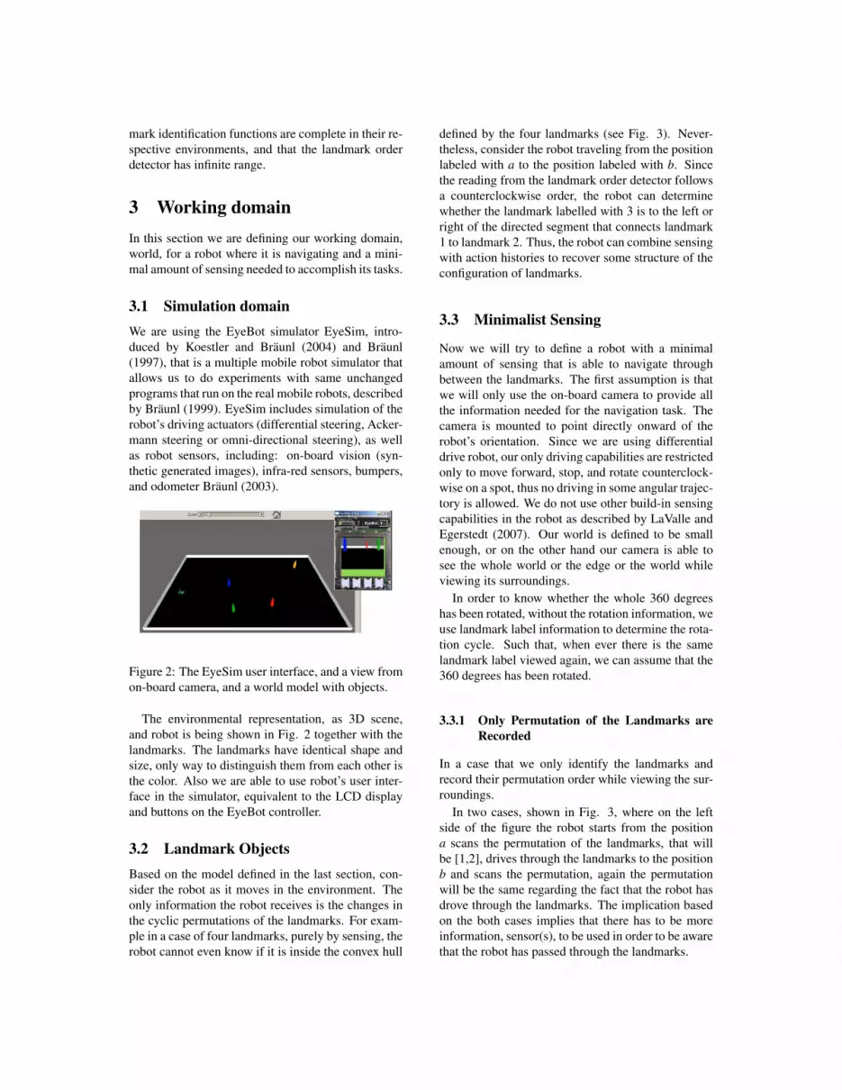
mark identification functions are complete in their re-spective environments, and that the landmark orderdetector has infinite range.
3 Working domainIn this section we are defining our working domain,world, for a robot where it is navigating and a mini-mal amount of sensing needed to accomplish its tasks.
3.1 Simulation domainWe are using the EyeBot simulator EyeSim, intro-duced by Koestler and Braunl (2004) and Braunl(1997), that is a multiple mobile robot simulator thatallows us to do experiments with same unchangedprograms that run on the real mobile robots, describedby Braunl (1999). EyeSim includes simulation of therobot’s driving actuators (differential steering, Acker-mann steering or omni-directional steering), as wellas robot sensors, including: on-board vision (syn-thetic generated images), infra-red sensors, bumpers,and odometer Braunl (2003).
Figure 2: The EyeSim user interface, and a view fromon-board camera, and a world model with objects.
The environmental representation, as 3D scene,and robot is being shown in Fig. 2 together with thelandmarks. The landmarks have identical shape andsize, only way to distinguish them from each other isthe color. Also we are able to use robot’s user inter-face in the simulator, equivalent to the LCD displayand buttons on the EyeBot controller.
3.2 Landmark ObjectsBased on the model defined in the last section, con-sider the robot as it moves in the environment. Theonly information the robot receives is the changes inthe cyclic permutations of the landmarks. For exam-ple in a case of four landmarks, purely by sensing, therobot cannot even know if it is inside the convex hull
defined by the four landmarks (see Fig. 3). Never-theless, consider the robot traveling from the positionlabeled with a to the position labeled with b. Sincethe reading from the landmark order detector followsa counterclockwise order, the robot can determinewhether the landmark labelled with 3 is to the left orright of the directed segment that connects landmark1 to landmark 2. Thus, the robot can combine sensingwith action histories to recover some structure of theconfiguration of landmarks.
3.3 Minimalist Sensing
Now we will try to define a robot with a minimalamount of sensing that is able to navigate throughbetween the landmarks. The first assumption is thatwe will only use the on-board camera to provide allthe information needed for the navigation task. Thecamera is mounted to point directly onward of therobot’s orientation. Since we are using differentialdrive robot, our only driving capabilities are restrictedonly to move forward, stop, and rotate counterclock-wise on a spot, thus no driving in some angular trajec-tory is allowed. We do not use other build-in sensingcapabilities in the robot as described by LaValle andEgerstedt (2007). Our world is defined to be smallenough, or on the other hand our camera is able tosee the whole world or the edge or the world whileviewing its surroundings.
In order to know whether the whole 360 degreeshas been rotated, without the rotation information, weuse landmark label information to determine the rota-tion cycle. Such that, when ever there is the samelandmark label viewed again, we can assume that the360 degrees has been rotated.
3.3.1 Only Permutation of the Landmarks areRecorded
In a case that we only identify the landmarks andrecord their permutation order while viewing the sur-roundings.
In two cases, shown in Fig. 3, where on the leftside of the figure the robot starts from the positiona scans the permutation of the landmarks, that willbe [1,2], drives through the landmarks to the positionb and scans the permutation, again the permutationwill be the same regarding the fact that the robot hasdrove through the landmarks. The implication basedon the both cases implies that there has to be moreinformation, sensor(s), to be used in order to be awarethat the robot has passed through the landmarks.

1
2
a
b
1
2
a
b
3
4
c
Figure 3: In both cases, on left and right, the robotwill see the same permutations of the landmarks,namely [1,2] and [3,1,2,4] respectively, while drivingfrom a to b (on left) and from a to c, via b (on right).
a
1
2
b
db1 db2
da1
da2
Figure 4: Distance information to the landmark hasbeen added to the information space model.
3.4 Minimalist Model
Based on the previous sub section we need to definemore sensing capabilities to the robot to be able tobe confirmed when the landmarks have been passedthrough.
3.4.1 Adding Information to the Model
Let’s assume that we have distance sensor build inthe camera model, based on the basic 3D camera cal-ibration model, as showed by Braunl (2003), that wecan compute the distance estimate to each landmarkwhen facing them directly. Thus, when rotating ona spot and determining the permutations of the land-marks, permutations will be tagged with distance in-formation as well.
In the simples case, shown in Fig. 4, where thedistance sensor (information) has been added to therobot there might be cases that both of the distances,while moving from point a to b, are identical through-out the path. In particular, when driving exactly inbetween the landmarks and the starting and stoppingspots are at same distance from the segment line be-tween the landmarks.
If we add a global positioning sensor or orientationsensor to the robot model to keep track of the robot’sorientation and/or position, we will able to overcomethe previous uncertainty in the information. Nonethe-less, that is not our goal to add more sensing informa-tion to the robot and its information space.
a
1
2 b
c
Figure 5: The navigation domain, the world, wherethe landmarks are randomly positioned.
4 Navigation AlgorithmBased on the previous findings there has to be moreinformation than just the permutation of the land-marks to navigate in the domain. It has been shownthat the distance sensor, by itself, to detect the land-marks is not enough to distinguish whether the land-

1
2
Dead zone
3
4
5
6
Safe zone
The goal
x
Object threshold
Initial position
Figure 6: Navigation proposal illustrated based on theproposed algorithm.
marks has been passed. However, with the respectto navigation we propose the following algorithm tonavigate safely trough the landmarks.
Let the world consist of six distinguishable land-marks positioned, more or less randomly, as shownin Fig. 5. The robot should navigate in between thepair of the landmarks, e.g . first between the 1 and 2followed by 3 and 4, and so forth, thus the robot isnot allowed to go into the dead zone.
The robot is able to identify the landmarks and la-bel them; also it will be able to track their permu-tations when rotating on a spot. The look up table(LUT) will be filled with the permutations of the land-marks, their identity, and their size information inpixels from the robot to the landmark.
4.1 Landmark IdentificationWe propose an algorithm that locates the two closestpairs of the landmarks L, based on the image pixelsize information, from the robot. The landmark dis-tance is estimated based on the size of the landmark,denoted as σ, in the image. Thus, for each l ∈ L weget σl by using the Eq. 2
σl =n−1∑n=0
m−1∑m=0
(lp(m), lp(n)) (2)
where, lp(m) and lp(n) are the corresponding pixelsin the m × n image frame of the landmarks row and
column pixels, respectively.The landmark pairs form a set of pairs Γ ⊆ L. The
two closest that have the largest σ value form a pairγ ⊂ Γ. The desired navigation path for the robot tobe driven through is the closest pair of the landmarks.Since in the real world implementation we use a pre-defined threshold, δ, how close can the robot move toa landmark l. The outer areas beyond the landmarksare treated as dead zone Ψ, where the robot is notallowed to move. Landmarks are not suppose to bebehind of one another.
In the simulation domain, the landmarks weremodeled using the MilkShape 3D modeling softwarefrom Chumbalum Soft, thus all the landmarks haveidentical shape and size. The only difference is theirunique color that can be used as a identification labelin the domain.
To form a pair of the closest landmarks, we proposethat the use of the landmark size, based on the amountof pixels it covers on the image is used. This meansthat there is a direct implication of the landmark dis-tance, without the actual distance sensor. The amountof the pixels are recorded when the landmark is in thecenter of the image, the viewing angle of the visibil-ity sensor. The calculation is made during the rotationphase of the robot, that will then fill the LUT with thecurrent permutation and the size information of thelandmarks.
The first two pairs of the landmarks, γ ⊂ Γ, arethen selected to be the ones that are to be crossed.From that pair, the closest one is selected to be thefirst one to be driven at. Since no distance or orienta-tion information, the robot has to rotate as long as itis aligned to the corresponding landmark label in themiddle of the viewing space. Then the move state canbe executed. The robot will drive towards the clos-est selected landmark as long as the threshold value,δ, is achieved. The threshold is also based on the vi-sual amount of pixels corresponding to the landmark.When the robot has reach to the first landmark of thefirst pair, it rotates and locates the corresponding pairto the first one and executes the move state again toreach the threshold location. At this state, the robotforms the second pair to be crossed and starts execut-ing the driving maneuver again. At this stage, the firstpair is added to the ignore list so that the robot knowsthat the pair has been crossed already.
When all the landmark pairs has been crossed,added to the ignore list or in other words there is noother pairs of landmarks left, it is assumed that therobot has navigated through the all landmark pairs inthe world, W, and reached to the goal area, whereΓ = .

4.2 Proposed navigation algorithmWith the proposed algorithm we should be able to gothought all the landmark pairs, and navigate safelythrough the desired path.
The goal position can be defined as a state whereno other pair of landmarks are left in the informationspace to be crossed.
Table 1: Navigation algorithm.
Algorithm1 Navigation Procedure.1 : Rotate counterclockwise and locate all the
landmarks and their distances2 : Form a pair of the two closest landmarks3 : Drive towards, until the threshold distance,
the closest landmark of the first pair oflandmarks to be crossed
4 : Rotate and locate the pair of the landmark,align and drive towards to that one until thethreshold value
5 : Mark the pair passed6 : Jump to step 1
5 Experiments and resultsIn this section the results of the test runs of the pro-posed algorithm are shown and discussed. First, thelandmark identification and driving maneuvers areexplained. Finally, the execution of the algorithm isdiscussed.
The color search function is implemented as fol-lows.
Table 2: Driving algorithm.
Algorithm2 Driving Maneuver Algorithm.1 : Scan the area.2 : Select the two closest unvisited landmarks
and mark them as a pair.3 : Select the closest landmark, turn towards it,
move next to it and mark it visited.4 : Select the second landmark of the pair, turn
towards it, move next to it and mark it visited.5 : Jump to step 1.
In the simulation domain, under the environmentwith no distortion or other errors in the visibility sen-sor, we are able to recognize, identify and estimate
the distance to each landmark perfectly. The naviga-tion and driving maneuvers works with no problem aswell.
1
2
3
4
5
6
Figure 7: Illustration of the behaviour of the algo-rithm in an example navigation problem.
6 Conclusions and future works
6.1 Conclusions
This paper proposes a navigation algorithm and a lo-calization method technique under an unknown envi-ronment based on minimalist sensing of mobile robot.The localization was achieved based on the landmarkpermutations and distance estimate of the landmarks.
It was shown that the navigation under an unknownsimulation domain with a minimal amount of sensinginformation is possible with certain restrictions.
6.2 Future Works
In the future, we would like to test the algorithm inthe real world environment, using the EyeBot mobilerobot.
Acknowledgements
The authors gratefully acknowledge the contributionof Steven M. LaValle and Pekka Isto.

ReferencesT. Braunl. Embedded robotics: mobile robot de-
sign and applications with embedded systems.Springer-Verlag, Berlin, Heidelberg, July 2003.
T. Braunl. Mobile robot simulation with sonar sen-sors and cameras. Simulation, 69(5):277–282,1997.
T. Braunl. Research relevance of mobile robot com-petitions. Robotics and Automation Magazine,IEEE, 6(4):32–37, December 1999.
F. Calabrese and G. Indiveri. An omni-visiontriangulation-like approach to mobile robot local-ization. Intelligent Control, 2005. Proceedingsof the 2005 IEEE International Symposium on,Mediterrean Conference on Control and Automa-tion, pages 604–609, June 2005.
Z. Cao, S. Liu, and J. Roning. Omni-directional vi-sion localization based on particle filter. In ICIG’07: Proceedings of the Fourth International Con-ference on Image and Graphics, pages 478–483,Washington, DC, USA, 2007. IEEE Computer So-ciety.
H. Chitsaz and S.M. LaValle. Minimum wheel-rotation paths for differential drive mobile robotsamong piecewise smooth obstacles. Robotics andAutomation, 2007 IEEE International Conferenceon, pages 2718–1723, April 2007.
G. Dudek, K. Romanik, and S. Whitesides. Localiz-ing a robot with minimum travel. In SIAM Journalof Computing, 1995.
L.H. Erickson, J. Knuth, J.M. O’Kane, and S.M.LaValle. Probabilistic localization with a blindrobot. Robotics and Automation, 2008. ICRA 2008.IEEE International Conference on, pages 1821–1827, May 2008.
L. Freda, B. Tovar, and S.M. LaValle. Learning com-binatorial information from alignments of land-marks. Robotics and Automation, 2007 IEEE Inter-national Conference on, pages 4295–4300, April2007.
A. Koestler and T. Braunl. Mobile robot simulationwith realistic error models. 2nd International Con-ference on Autonomous Robots and Agents, De-cember 2004.
S.M. LaValle. Planning Algorithms. Cambridge Uni-versity Press, Cambridge, U.K., 2006.
S.M. LaValle and M.B. Egerstedt. On time: Clocks,chronometers, and open-loop control. Decisionand Control, 2007 46th IEEE Conference on, pages1916–1922, December 2007.
T.S. Levitt and D.T. Lawton. Qualitative navigationfor mobile robots. Artificial Intelligence, 44(3):305–360, 1990.
J.M. O’Kane and S.M. LaValle. Almost-sensorlesslocalization. Robotics and Automation, 2005.ICRA 2005. Proceedings of the 2005 IEEE Inter-national Conference on, pages 3764–3769, April2005.
J.M. O’Kane and S.M. LaValle. Localization withlimited sensing. Robotics, IEEE Transactions on,23(4):704–716, August 2007.
J.M. O’Kane and S.M. LaValle. Comparing thepower of robots. International Journal of RoboticsResearch, 27(1):5–23, 2008.
M. Rao, G. Dudek, and S. Whitesides. Randomizedalgorithms for minimum distance localization. In-ternational Journal of Robotics Research, 26(9):917–933, 2007.
Chumbalum Soft. URLhttp://chumbalum.swissquake.ch/.
S. Thrun, W. Burgard, and D. Fox. A probabilisticapproach to concurrent mapping and localizationfor mobile robots. Machine Learning, 31(1-3):29–53, 1998.
B. Tovar and S.M. LaValle. Visibility-based pursuit-evasion with bounded speed. In In ProceedingsWorkshop on Algorithmic Foundations of Robotics,2006.
B. Tovar, S.M. LaValle, and R. Murrieta. Optimalnavigation and object finding without geometricmaps or localization. Robotics and Automation,2003. Proceedings. ICRA ’03. IEEE InternationalConference on, 1:464–470, September 2003a.
B. Tovar, S.M. LaValle, and R. Murrieta. Locally-optimal navigation in multiply-connected environ-ments without geometric maps. Intelligent Robotsand Systems, 2003. (IROS 2003). Proceedings.2003 IEEE/RSJ International Conference on, 4:3491–3497, October 2003b.
B. Tovar, L. Guilamo, and S.M. LaValle. Gap navi-gation trees: Minimal representation for visibility-based tasks. In In Proceedings Workshop on the Al-gorithmic Foundations of Robotics, pages 11–26,2004.

B. Tovar, A. Yershova, J.M. O’Kane, and S.M.LaValle. Information spaces for mobile robots.Robot Motion and Control, 2005. RoMoCo ’05.Proceedings of the Fifth International Workshopon, pages 11–20, June 2005.
B. Tovar, L. Freda, and S. M. LaValle. Using a robotto learn geometric information from permutationsof landmarks. Contemporary Mathematics. Amer-ican Mathematical Society, 438:33–45, 2007a.
B. Tovar, L. Freda, and S.M. LaValle. Mapping andnavigation from permutations of landmarks. In20th International Joint Conference on ArtificialIntelligence, 2007b.
B. Tovar, R. Murrieta-Cid, and S.M. LaValle.Distance-optimal navigation in an unknown envi-ronment without sensing distances. Robotics, IEEETransactions on, 23(3):506–518, June 2007c.
D. Whitney. Real robots don’t need jigs. Roboticsand Automation. Proceedings. 1986 IEEE Interna-tional Conference on, 3:746–752, April 1986.

Angle sensor-based robot navigation in an unknown
environment
Timo M. R. Alho University of Vaasa
Department of Electrical Engineering and Automation
P.O. Box 700 (Puuvillakuja 3), 65101 Vaasa, Finland [email protected]
Abstract
This paper proposes a navigation algorithm in an unknown environment requiring minimalistic
sensing of the mobile robot. The algorithm minimises the distance travelled and required computing
power during the navigation task in question. This is done by using only angle sensor information
about the landmarks in the environment.
1 Introduction
Imagine you are skiing in a field upon a dark and
cloudy Finnish winter night. The only things you
can see are the lights from the houses around the
field in the distance. Using one of them as a
reference point, rotating vertically over 2π, you can
obtain a rough map of your surroundings and
navigate to your destination as in Figure 1.
How could a mobile robot do the same? The
robot is equipped with only a simple pinhole camera
mounted on top of the robot. Whitney (1986) proved
that designs with the simplest sensing and actuating
models lead to decreased costs and increased
robustness. In this paper it is proposed that only
angle information from the landmarks relative to a
reference landmark is needed to accomplish the
navigation task in an unknown environment, when
only the landmarks are recognized. The
implementation of the angle sensor is not considered
in this paper but the algorithm itself will be
implemented in an EyeSim simulator.
Figure 1: Example of a navigation task for a
mobile robot.
With this mobile robot model, the only reliable
course of action is to scan the visible region by
rotating counter-clockwise over 2π, calculate the
angles to the landmarks using the first landmark that
the camera sees as a reference point or to translate a
predetermined distance d to a calculated direction.
Using this angle information, the robot can calculate
the direction needed to move between a
predetermined pair of landmarks and recognise
when it has passed between them.
As stated by Kanniainen and Alho (2008),
localization as a problem for robotics applications,
with varying degrees of freedom, has been widely
studied in the literature. Levitt and Lawton (1990)
and O’Kane and LaValle (2005, 2007a and 2007b)
have studied the minimal amount of actuators and
sensors for a mobile robot to solve its navigation
tasks. Dudek, Romanik and Whitesides (1995)
proved that it is a NP-hard localization problem to
utilize a visibility sensor while minimizing distance
travelled, and it was applied in pursuit-evasion by
Tovar and LaValle (2006). Rao, Dudek and
Whitesides (2004) used randomization to select
actions to disambiguate candidate locations in a
visibility based approach. Kanniainen et al. (2008)
studied the same problem as in this paper using only
a visibility sensor. Tovar, Guilamo and LaValle
(2004) used only depth information to solve
exploration and navigation tasks. Kamon and Rivlin
(1997) used bug algorithms for robot navigation
with the only ability to move towards obstacles and
follow walls. Tovar, Freda and LaValle introduced
mapping in 2007b and in 2007a the usage of only
information from permutation of landmarks. The
method for extracting combinational alignment

information of the landmarks was shown by Freda,
Tovar and LaValle (2007). Distance-optimal
navigation was achieved without sensing distances
in an unknown environment by Tovar, Murriera and
LaValle (2007). Chitsaz and LaValle (2007)
described minimizing the path for differential drive
robots. Tovar, LaValle and Murriera (2003) studied
optimal navigation and object finding without the
need of localization or geometric maps.
2 Model
The proposed model is built based strongly upon
the work of Kanniainen et. al. (2008) as well as
LaValle (2006), Tovar, Yershova, O’Kane and
LaValle (2005) and Tovar et. al. (2007b). The
mobile robot is only capable of moving forward,
stopping and rotating counter-clockwise, and is
modelled as an object in a 2D world,2
W = , that is
able to translate and rotate. Thus, the state space is
X = SE(2). However, as the robot does not know its
position or orientation, the robot does not know its
state at any time. In this study, errors generated by
the environment are not incorporated into the model.
The X is bounded by a simple closed polygonal
chain, with no interior holes. A map of W in 2 is
unknown to the robot. The landmarks are considered
to be points in space with no physical body and
cannot be co-linear.
Figure 2: The Landmark angle detector gives the
angular positions of the landmarks relative to the
first landmark sensed by the robot. The angles
between landmarks and reference landmark are
stored in a table and the label of the landmark
indicates the location in the table. In this case the scan results would be: [α, 0, β].
In the W there is a finite set of landmarks2
L ⊆ . For each l∈L, we can sense information
about it. A landmark sensor is defined in terms of a
landmark identification function, s, as described by
Tovar et. al. (2007). As the robot is able to sense the
angles between landmarks, the sensor is called a
landmark angle detector (LAD), and is denoted
by LADs(x) as illustrated in Figure 2. The landmark
angle detector gives the angles between landmarks,
the robot and the first landmark detected (reference
landmark) and stores the angles in a table entry by
label for the landmark (see Figure 2). In other
words, the robot can sense landmark label denoted
as s(p) and the angle associated with it. So, the
landmark is denoted as (s(p),a), where a represents
the associated angle. The landmark angle detector
does not directly sense the permutation of the
landmarks or the distance from the robot. Although,
the permutation of the landmarks is easily read from
the table as needed. It is assumed that the robot has
been given a set of landmark pairs to between and
that the robot can translate to a direction ∆,
calculated from the angle sensor readings.
Furthermore, it is assumed that the landmark
identification functions are complete in their
respective environments, and that the landmark
angle detector has infinite range. Also, the robot has
to be able to remember the last reference landmark
until it has passed between the landmark pair in
question.
Let P represent every point in the 2 and let m:
2
0→ ∪ be a mapping so that every point in
P is assigned an integer 1,2,…,n, and m(p) = 0 for
any p P∉ . The mapping m is referred to as a
feature identification function, and P is referred to
as the set of points selected by m. For a point
p P∈ , a feature is defined as (m(p),p). For a set 2
R ⊂ , an environment E is defined as (R,m). The
space of environments ε is the set of all such pairs.
Let q∈SE(2) be the configuration, position and
heading in the plane, of the robot. The state is
defined as x = (q,E), and the state space X is the set
of all such pairs (SE(2)× ε).
3 Solving the navigation task
As stated before, the goal for the robot in the
navigation task is to follow a set of pre-determined
pairs of landmarks, much like a boat at sea guided
by navigation buoys as described by Kanniainen et.
al. (2008). In this case, the robot can only
distinguish landmarks from each other and sense
their angles relative to each other. Compared to the
algorithm they used (ibid.), the algorithm described
in this paper is optimized more for the distance
travelled, but is also more time consuming because
of the number of scans involved. Even without
additional information, the necessary calculations
and thus the algorithm itself, becomes relatively
trivial. There are basically two possible scenarios where the robot has to calculate an angle for ∆
which are illustrated in Figures 3 and 4.

Figure 3: This is the same situation as in Figure 1,
just with added markings. The angles α and β are the
same as before but angle represents the counter
clockwise angle between the landmarks which the
robot has to pass, in this case 1 and 3. The angle
needed to rotate to face the correct direction is
represented by ∆.
Figure 4: We can see by comparing , this situation
is a little different from that of Figure 2. In this
situation the robot’s task is to translate between
landmarks 2 and 3.
The equation to calculate ∆ in the situation
represented by Figure 4, where γ < π, is derived as
follows: First the angle γ is calculated as
= − . (1)
Next γ is used to calculate ∆ by
= + = + = = . (2)
But what happens if γ is greater than π as in
Figure 3? Then, using equation (2), the robot would
start moving to the exact opposite direction than
intended. In that case, addition of π to the solution is
required. In that way, we derive the solution for both
situations where the robot can possibly be at any
time:
= , when 0 < γ < π + , when π < γ < 2π (3)
The robot knows when it has passed between
landmarks when the angle reflects from < to > or vice versa. The final algorithm for the
mobile robot is shown in Table 1.
Table 1: The final algorithm for the mobile robot.
Angles represents the table of landmark angles.
Check the first landmark pairing to pass between.
do
Start turning counter clockwise.
If robot sees a landmark. If the landmark is the first landmark seen and
no reference landmark is assigned.
Check its label and mark the landmark as
reference.
Else If the landmark is not the first landmark
seen or (the landmark is the first landmark seen
and reference landmark has been assigned.).
Check its label and store the angle reading as
an entry in the angle table.
Else If the landmark is the previously assigned
reference landmark
Stop turning.
Calculate angle .
If has reflected from < to > or vice
versa.
If this was not the last landmark pair.
Move to the next landmark pair.
Else
Exit program.
Calculate angle ∆.
If >
∆ = ∆ +
Rotate by amount of ∆ from the reference
landmark.
Translate distance d forward.
while(Program is running)
4 Simulation
The algorithm was simulated using the EyeSim
Software Development Kit (SDK), where it is
possible to both simulate robot behaviour as well as
to use the same code as-is to control a real robot.
EyeSim includes simulations of the robot’s driving
actuators as well as sensors (on-board vision,

infrared sensor, bumpers and odometers). In the
simulator the environment is represented in 3D and
provides control buttons and a picture feed from the
robot’s on-board camera, if implemented (Figure 5).
Also a debugging console is available.
Figure 5: EyeSim SDK graphical user interface.
All in all the simulations worked really well. The
robot identified the landmarks and calculated the
necessary angles with no problems. Minor
adjustments had to be made to the algorithm
because in the theoretical section of this paper, the
landmarks were assumed to be just points in space
with no physical body, and as such it was
impossible to implement landmarks that way in the
simulator. The landmarks have identical shape and
size and the robot identified the landmarks by their
color and distance d was assigned to 1 meter.
The simulations indeed showed that the
algorithm optimized more the distance the robot had
to travel to accomplish the same navigation task as
did Kanniainen et al. (2007), but as the robot had to
scan the surroundings more often; this algorithm is
more time consuming.
5 Conclusions
This paper proposes a navigation algorithm in an
unknown environment based on minimalistic
sensing done by a mobile robot. The algorithm
minimises the distance travelled during the
navigation task in question, but it consumes more
time because of the number of scans necessary. It is
possible to make the distance travelled between
scans (d) larger, but depending on the position of
landmarks and the order of the landmark pairs, it
probably would make the algorithm less than
optimal. But when this algorithm is used with
properly selected parameters, the results would most
likely be more than satisfactory. Especially if the
task at hand requires most of all precision and not
speed.
In the future, it would be interesting to make a
study of how to combine an angle and distance
sensor. So that the robot would be able to complete
the navigation task with only a single scan of its
surroundings.
Acknowledgements
The author gratefully acknowledges the
contribution of Steven M. LaValle and Pekka Isto.
References
H. Chitsaz and S. M. LaValle, Minimum wheel-
rotation paths for differential drive mobile
robots among piecewise smooth obstacles. In
Proceedings IEEE International Conference
on Robotics and Automation, 2007.
G. Dudek, K. Romanik and S. Whitesides,
Localizing a robot with minimum travel.
SODA: ACM-SIAM Symposium on Discrete
Algorithms, A Conference on Theoretical and
Experimental Analysis of Discrete
Algorithms, 1995.
L. Freda, B. Tovar and S. M. LaValle, Learning
combinatorial information from alignments
of landmarks. In Proceedings IEEE
International Conference on Robotics and
Automation, 2007.
I. Kamon and E. Rivlin, Sensory-based motion
planning with global proofs. IEEE Trans.
Robot. & Autom., 13(6):814-822, 1997.
Olli Kanniainen and Timo M. R. Alho,
Minimalistic Navigation for a Mobile Robot
Based on Simple Visibility Sensor
Information. STeP2008 In press, 2008.
S. M. LaValle, Planning Algorithms. Cambridge
University Press, 2006.
T. S. Levitt and D. T. Lawton, Qualitative
navigation for mobile robots. Artificial
Intelligence, 44(3):305-360, 1990.
Jason M. O’Kane and S. M. LaValle, Almost-
Sensorless Localization. In Proceedings IEEE
International Conference on Robotics and
Automation, 2005.

J. M. O’Kane and S. M. LaValle, Localization
with limited sensing. IEEE Transactions on
Robotics, 23(4):704-716, 2007.
J. M. O’Kane and S. M. LaValle, On comparing
the power of robots. International Journal of
Robotics Research, 2007.
M. Rao, G. Dudek and S. Whitesides,
Randomized algorithms for minimum
distance localization. In Proc. Workshop on
Algorithmic Foundations of Robotics:265-
280, 2004.
S. Thrun, D. Fox and W. Burgard, A probabilistic
approach to concurrent mapping and
localization for mobile robots. Machine
Learning, 31:29-53, 1998.
B. Tovar, L. Guilamo and S. M. LaValle, Gap
navigation trees: Minimal representation for
visibility-based tasks. In Proc. Workshop on
Algorithmic Foundations of Robotics, 2004.
B. Tovar, R Murrieta and S. M. LaValle,
Distance-optimal navigation in an unknown
environment without sensing distances.
Transactions on Robotics, 23(3):506-518.,
2007
B. Tovar, L. Freda and S. M. LaValle, Using a
robot to learn geometric information from
permutations of landmarks. Contemporary
Mathematics, American Mathematical
Society, 2007.
B. Tovar, L. Freda and S. M. LaValle, Mapping
and navigation from permutations of
landmarks. Technical report, Department of
Computer Science, University of Illinois,
2007.
B. Tovar and S. M. LaValle, Visibility-based
pursuit-evasion with bounded speed. In
Proceedings Workshop on Algorithmic
Foundations of Robotics, 2006.
B. Tovar, A. Yershova, J. M. O’Kane and S. M.
LaValle, Information spaces for mobile
robots. In Proceedings International
Workshop on Robot Motion and Control,
RoMoCo, 2005.
B. Tovar, S. M. LaValle and R. Murrieta, Optimal
navigation and object finding without
geometric maps or localization. In
Proceedings IEEE International Conference
on Robotics and Automation:464-470, 2003.
D. E. Whitney, Real robots don’t need jigs. In
Proceeding of the IEEE International
Conference of Robotics and Automation,
1986.

Framework for Evaluating Believability of Non-playerCharacters in Games
Tero HinkkanenGamics Laboratory,
Department of Computer Science,University of Helsinki, [email protected]
Jaakko Kurhila
Department of Computer Science,University of Helsinki, Finland
Tomi A. PasanenGamics Laboratory,
Department of Computer Science,University of Helsinki, Finland
Abstract
We present a framework for evaluating believability of characters in first-person shooter (FPS)games and look into the development of non-player character’s user-perceived believability. Theused framework is composed of two aspects: firstly, character movement and animation, secondly,behavior. Examination of three different FPS games yields that the newer the game was, the betterthe believability of characters in the game. Moreover, the results from both the aspects of theframework were mutually balanced through all games examined.
1 Introduction
First-person shooter (FPS) games have been popularever since their first release in the early 1990’s(Hovertank 3D 1991, Wolfenstein 1992, and Doom1993). The games are usually straightforward in asense that the target is to navigate the player’s char-acter through different levels of the game and ac-complish different tasks. Normal task is to movefrom point A to point B and shoot everything thatmoves or tries to shoot back. The view to the gameworld consists of a split screen where the narrowlower part of the screen is showing player’s healthand ammo, and the upper large part of screen repre-sents player’s eye view to the game world (the largepart is the player’s only mean to monitor other char-acters in the game and draw conclusions aboutthem). Depending on the game, in-game charactersrun by the player or by the computer can have hu-man-like constraints or not. Because games aremade for players’ enjoyment, not every part of real-world laws and rules are included in the games. Forexample, a player must be able to win even the mostsuperior enemies in the game alone [8].
Main reason for the popularity of FPSgames has been their relatively high-level graphicstogether with a breathtaking pace of interaction.Nowadays, however, players have started to excepteven more realism in games, such as unpredictabil-ity. Because of the games in this genre, many sig-nificant improvements on the game activities havebeen attached to characters run by the computer, in
other words “non-player characters” (NPCs) whichthe player’s character will meet during the game.
It can be said that the ultimate goal of anNPC is to be indistinguishable from a character runby a player. However, recent studies show [2, 14]that players will notice if their opponent is con-trolled by a computer rather than another humanplayer, or if the opponent is too strong or too weakcompared with another human player. According tothe studies, the elements increasing the believabilityof NPCs as human players are natural movement,mistakes and gestures during the game, characterappearance and character movement animation.
An NPC can be seen as an intelligent agenttrying to do its best (rational action) in the currentstage [21]. While choosing the rational action for anNPC, artificial intelligence (AI) tries at the sametime to be as entertaining as possible, using even“cheap tricks” [16, 24]. Cheap tricks are permittedby the players as long as the player stays relativelyconvinced of the rationality of the actions.
In this paper, we take a look at how thegame industry has been promoting non-player char-acter’s (NPC) believability in FPS games and com-pile a framework for evaluating believability of theNPCs. We start by looking at the elements whichbuild believability in the next section and presentthe framework in Section 3. In Section 4, we applyour framework to three FPS games revealing im-provements along the age of games. We concludewith final remarks in the last section, Section 5.
We note that other authors have also collected anumber of techniques or ideas to promote NPCs’
believability but proposed criteria have been eithervery universal [14], not specific to FPS, or criteriahave been too loose giving maximum scores to anyNPC in FPS games like Quake or Unreal Tourna-ment [2].
2 Building Believability
Based on different studies among players [2, 14],the believability of the NPCs is most influenced by(1) the game environment where the NPCs appear,(2) another character or player which the NPC iscompared to, and (3) the players’ cultural back-ground and age. Because we are aiming to a generalframework we skip the last item and divide NPC’sbelievability into three main categories: movement,animation and behavior. Next we consider howgame developers have tackled each of these.
2.1 MovementIn FPS games, NPCs’ movement usually tries toemulate humans’ natural movement: finding theobvious shortest path and reacting to the game envi-ronment. One typical way of helping an NPC to findthe shortest path is to build a navigation mesh ontothe game map. Game designers plant varying num-ber of navigation points or nodes onto the map.When the NPC searches for the shortest way to itsdestination, it actually calls for the search algorithmof the game to find the shortest path between thetwo navigation points: the one where the NPC is,and the one where it’s going to go.
The most commonly used search algorithmis A* [16] and its variations. In some FPS games,designers have eased NPCs’ pathfinding algorithmsby outlining the area(s) where NPCs can move. Thisreduces the search space significantly and thusquickens the search. However, if an NPCs’ destina-tion is not within its range of movement or other-wise out of its reach, A* has to search trough everynode in the search space, which particularly in largemaps demands a great amount of CPU time. In casethat game designers have not considered this option,the NPC calls for the pathfinding algorithm over andover again thus slowing the game down. In thesecases, NPCs have been killed off so that the CPUtime will not be wasted [9].
Even though the performance of computershas been rising continuously, optimizing algorithmsare still needed to guarantee the smooth running ofever bigger games [25]. Reducing the navigationmesh is a simple and fast way to increase the speedof A*s, but it leads to a sparse search space and thusto a clumsy and angular NPCs’ movement.
A good solution to optimize the searches isto cut down their number. This can be reached in
two different ways: one is to reuse old searches forother NPCs and the other is to limit the flooding ofA*. Flooding is understood as the extensive widen-ing of pathfinding around the optimal path.
Even if A* can not find a path to a location,it is not wise to erase this search result from thecomputer’s memory. In games where there are sev-eral NPCs, it is likely that some other NPC is goingto search for a similar or even the same route atsome point of the game. Now if the failed results arealready in the memory, it saves a lot of the CPUtime when there is no need to do the same searchagain [4]. Keeping a few extra paths in the memorydoes not notably limit the amount of free memoryduring the game.
By using path lookup tables, it is possiblenot to use any pathfinding algorithms during thegame at all [2]. Every possible path will be stored inthe lookup table, which is loaded in the memorywhile the game begins. Even though the tables willbe quite large, it is still faster to look for a pathstraight from the table rather than search for the bestroute to the location. Major problems with the pathlookup tables are that they require completely staticmaps and a lot of free memory.
Humans tend to move smoothly, that is,they attempt to foresee the upcoming turns and pre-vent too sharp turning. NPCs’ paths can be smooth-ened in several ways. One is to use weighted nodes,in which case an NPC is surrounded by four sensors[3, 15]. Once a sensor picks up an obstacle or thegradient changes of the area, the sensor’s value isincreased. If the value exceeds the sensor’s limitvalue, the NPC is guided away from the direction ofthe sensor.
Because an NPC knows which nodes it isgoing use in its path, it is possible to foresee wherethe NPC has to turn. Smoothening these turns bystarting the turn before the node, game developershave been able to increase NPCs’ believability [18].Combining foreseeing the turn with string-pulling[3, 27], in which every node nx is removed if it ispossible for an NPC to go directly from node nx-1 tonx+1, produces a very smooth, human-like movementfor NPCs.
When several NPCs exist simultaneously,one must pay attention to how they move in groups.Problems occur when two or more NPCs try to usethe same node at the same time. This can be solvedby using reservations [17] in nodes, so that the firstNPC reserves the node to itself, and the other NPCshave to find alternative paths. The reservation canbe done by increasing the cost of one node so high,that A* ignores it while finding a path.
If several NPCs have to go through oneparticular node at the same time without having al-ternative paths, it can form a bottleneck for NPCs’smooth movement. One way to solve this is to let

NPCs go through the bottleneck in a prioritized or-der [23]. This leaves low-priority NPCs to wonderaround while waiting for their turn.
2.2 Animation
Most of the animations used by NPCs are madewith one of the following three methods [2]. One isto draw or otherwise gain the frames of the entireanimation and then combine them into to one se-quence. The other method is to draw a couple ofkeyframes and later on morph them with computersinto one smooth animation. The third way is to con-nect sensors to a person and record the person’sdifferent moves onto the computer. Then thesemoves are fitted to a drawn character.
Each one of these methods has the sameflaw: Once an animation is done, it can only bechanged by recording it again. This obviously cannot be done during the game. By recording severaldifferent animations for NPCs’ one action, it is pos-sible to change between different animations if thesame action occurs again and again. This, however,only prolongs the obvious, which is that player willnotice if dozens, or even a few, of NPCs limp ordies with in precisely the same way.
Using hierarchically articulated bodies orskeleton models, NPCs’ animations can be adjustedto fit different situations and actions [2]. The skele-ton models can also be fitted to different NPCs onlyby changing the model’s appearance and size. Theuse of the skeleton models reduces the amount ofmemory needed for animations, because every ani-mation is now done when needed instead of usingpre-recorded sequences.
NPCs’ appearance is very important whiletheir believability is looked into. If gaps occur be-tween the limbs and the torso, or other oddities canbe seen in NPCs’ appearance, it decreases their be-lievability. While the polygon mesh is added overthe skeleton these flaws can be avoided by payingattention to how the mesh is connected to the skele-ton and by adding padding between the skeleton andthe mesh [2].
The animation controller (AC) has an im-portant role considering the NPC’s animations. TheAC decides what animation is played with each ac-tion and at what speed. In case of two animationsare played sequentially, the AC decides at whatpoint the switch happens. Some animations have ahigher priority than others. Showing the death ani-mation overcomes every other animation, because itis the last animation any NPC will ever do.
If NPCs are made with skeleton models, theAC needs to decide which bones are to be movedand how much in order to gain believable movementfor an NPC. Some animations or movements can beshown simultaneously with other movements. These
include, for example, running animation for thelower part of the body and shooting animation forthe upper part while face movements for yelling areshown in the NPC’s face.
Animations are even used to hide program-ming bugs in the games. In Half-Life when a playerthrows a grenade amongst a group of enemy NPCs,NPCs’ pathfinding does not always find paths forNPCs to run away from the immediate explosion.Programmers at Valve Software could not localizethis bug but they could see when the bug occurred[13]. They programmed NPCs to duck and coverevery time this bug appeared, and this solution waswarmly welcomed by players saying it added anextra touch of human behavior to NPCs.
2.3 Behavior
Making mistakes is human, therefore it is not to beexpected that any NPC’s actions are flawless. Inten-tional mistakes, such as two NPCs talking loudly toeach other or an NPC’s noisy loading of guns, re-veal the NPC’s location to a player before he/shecan even see it. NPCs’ far too accurate shootingtends to frustrate the players so it is recommendedthat the first time an NPC sees the player’s charac-ter, it should miss it thus giving the player time toreact and shoot back [5, 13].
NPCs need reaction time for different actionsto be able to imitate the physical properties of hu-man [5, 14, 20]. These are made by adding one sec-ond delay for each action NPCs have, thus makingthem appear as if they were controlled by otherplayers.
Both predictability and unpredictability arenatural for human players [22]. In FPS games, thisbecomes apparent when either too weak or too pow-erful weapons are chosen in the game. Emergentbehavior (EB) offers more unpredictability forNPCs. In EB, no simple reason can be given for theNPC’s known actions and therefore the result of theaction can benefit either the NPC or the player’scharacter.
Emergent behavior occurs mostly when tim-ers and goal-based decisions are used to controlNPCs’ behavior [19, 22]. Emergent behavior canalso be a result from several small rules that NPCsfollow. A good example of this is flocking [3, 10,19]. In flocking, every member of a flock or a groupfollows exactly the same rules, which can producemore action than the sum of these rules dictates.
Moreover, NPCs should take notice of otherNPCs and their actions, and be aware of their exis-tence. If game programmers so desire, NPCs cangive support to each other or search for cover to-gether [13]. In the worst case, a guard can walk overhis fellow guard without even noticing his deadcorpse on the ground [14]. However, it has been

stated that the most important thing for NPCs tonotice is to avoid friendly fire [20, 26].
NPCs can “cheat” by using information theypossibly could not obtain in real life. These includelocations of ammo and health in the game, the loca-tion of the players’ characters’ or even the charac-ters’ health and fighting capabilities [13, 22]. Thisinformation can be programmed for the player’sbenefit, too. By letting the player’s character’shealth to drop to near zero and then by changing theNPCs from ultimate killing machines to sittingducks, the game can give the player a feeling of asudden success and thus keep him/her playing thegame longer.
Lately, cheating of NPCs has been reducedby game programmers in order to give the playerand the NPCs equal chances to survive in the game.At the same time, NPCs’ abilities to autonomouslysearch for health and ammo through different gamelevels and remember where it has or has not beenhave increased. Thus the change has been fromcheating to more human-like NPCs [6, 12].
NPCs’ behavior is mostly controlled by finitestate machines [2, 3, 7, 28]. In addition to state ma-chines, trigger-systems and scripts are used in statetransitions. A more developed version of the statemachine is a hierarchical state machine, in whichevery state is divided into smaller state machineswhich have their own states and state transitions [2].
3 Description of framework
A framework for evaluating the believability ofcharacters is a means to evaluate user-perceivedNPC believability in FPS games. It should be notedthat this framework is intentionally limited to pro-vide simplicity and universality in use.
The framework is composed of two mainaspects: firstly movement and animation, secondlybehavior. It is based on programming techniquesand algorithms used in different FPS games. Thisframework does not take a stance on how some re-quirement has been executed, but only whether ornot it has been implemented so that the player canperceive it.
The basic element of NPCs’ movementsand animations is that any NPC can find the mostsuitable path to its destination. In most cases, NPCs’destination is the current location of the player’scharacter. NPCs’ path may not be the shortest, but itmust be a reasonable suitable path. Because gamemaps are divided into smaller blocks to prevent toolarge search spaces, an NPC has to be able to crossthese borders especially after it has noticed theplayer’s character.
When NPCs move, they must movesmoothly and be capable of avoid running into both
static and dynamic obstacles. The player will not beconvinced of NPCs’ believability if it cannot movearound a barrel or wait for a moving vehicle tomove out of its way. When two or more NPCs movetogether, they must pay attention to each other toavoid collisions.
When observing NPCs’ animations, threedifferent things are of importance. First, one shouldnote whether there are several pre-recorded anima-tions for one action or not. Secondly, a shift fromone pre-recorded animation to another must be flu-ent so that no unrealistic movements are made inbetween. Third, NPCs appearance must be donewell enough so that no gaps can be seen betweentheir limbs or other unnatural design is apparent.
Tables 1 and 2 show the specific proposi-tions that are used in evaluating the believability ofNPC characters. Propositions equal points, and thepoints are added into a score. Some propositions areviewed to have a greater impact on the believability.Therefore, some rows in Tables 1 and 2 are countedfor doubling the score, i.e. the points for a singlerequirement can be 2 instead of 1. The importanceof some requirements over others is based on theview taken in this study.
Table 1: Scores for movement and animationRequirement for NPC Points
NPC can find the most suitable pathfor its destination.
1
NPC’s movement is not limited to acertain area, such as one room.
1
NPC’s movement is not clumsy orangular.
2
NPCs are aware of each other and donot collide with each other.
1
NPC can avoid any dynamic or staticobstacle in game field.
2
NPC has different animations forone action.
1
Shifting from one animation to an-other is fluent.
1
NPC’s appearance is done carefullyand no unnatural features can befound in it.
1
Total 10
NPCs’ behavior is based on human’s natu-ral behavior. NPCs can and should make mistakes,and a way to make sure of this, is to program themto make intentional mistakes, vulnerabilities andreaction times. Emergent behavior gives a good illu-sion of an NPC being controlled by a human insteadof a computer, and thus if possible, it should be pre-sent.
Taking notice of other NPCs can best beseen whether or not NPCs can avoid friendly fire. It

is difficult to see if an NPC cheats. If an NPC doesnot collect ammo or health during the game, re-vealing their location to the NPC does no good to it.Instead, revealing the location of the player’s char-acter is easier to notice. If an NPC knows exactlywhen the player comes behind the corner, or anNPC shoots the player’s character without the playernoticing the NPC first, the NPC has cheated (at leastit defined to be so).
Because of FPS games are typically fastpaced, characters are in constant move. While anNPC moves, just like the player’s character, it ishard for it to aim correctly and shoot at the target.Pausing for a moment before shooting at the playergives the player a fair chance to hide or shoot back.All this is based on information of human reactiontimes and aiming capabilities.
Finally NPCs’ behavior should be logicaland human. Even though it is desirable for an NPCto act unpredictably, running away from the combatwhich it was obviously going to win leaves theplayer perplexed. Running away from the combatwhich you are going to lose is human, but this char-acteristic feature of human behavior is not a typicalaction of an NPC – NPCs tend to fight till their un-timely end.
Table 2: Scores for NPC’s behaviorRequirement for NPC Points
NPC makes intentional mistakes. 2NPC has human-like reaction times. 2NPC behaves unpredictably. 1NPCs are aware of each other. 2Cheating in a manner that player cannot detect it.
1
Bad aim when seeing player for thefirst time
1
Logical and human behavior 1Total 10
The overall score for an NPC is made bymultiplying scores from both aspects. Therefore, theoverall score is always somewhere between 0 and100. It is good to note that even if a game scores,say, fair scores of 5 from movement and animationand 5 from behavior, its overall score will be as lowas 5 * 5 = 25. Correspondingly, if a game receivesan overall score of 81, it should gain very high √81= 9 on average from both tables.
Therefore, we split the multiplied scorefinally into one dimension with five grades with textlabels: sub-standard (score of 0-9), weak (10-29),satisfactory (30-54), good (55-79) and excellent (80-100). Labeled grades are included because thescores become intuitively more understandable,compared to the mere numeral score.
The thresholds for each labeled grade differfrom each other, because when the overall score isthe result of the two multiplied sub-scores, it is morelikely to gain a score from somewhere in the middlethan a very low or a very high score. By changingthe limits of the grades or the importance of a re-quirement would give different results than thosedescribed in this paper.
Despite what the overall grade an NPCreceives, it is easy to see whether or not its mainaspects are in balance between each other. If theyare, a player may place NPCs believability higherthan what it really is. Correspondingly, even if over-all grade of an NPC is high but the aspects scoresdiffer much, NPCs may seem more unbelievable toa player than what the grade suggests.
The chosen policy to multiply scores re-sults into a zero score if one of believability aspectsgives a zero score. Any self-respecting game devel-oper should not release an FPS game which does notmeet even one requirement of both aspects, becauseit shows nothing but negligence towards NPC be-lievability.
4 Applying framework
We examined three different FPS games publishedbetween 1993 and 2001 by our framework. Theywere Doom (1993), Quake II (1996) and TomGlancy’s Ghost Recon (2001). The games were cho-sen because they represent the timeline of FPS gamedevelopment from the player’s viewpoint. The casestudies were conducted with PC-versions of thegames by playing the single player mode using themedium level of the games (Doom 3/5, Quake IIand Ghost Recon 2/3). Possible differences ofNPCs’ believability caused by the levels of diffi-culty or multi-player vs. single-player modes are notincluded in the evaluation.
Doom received points as follows:
Table 3: Scores for Doom from movement and ani-mation
Requirement for NPC PointsNPC can find most suitable path forits destination.
1
NPCs are aware of each other and donot collide with each other.
1
NPC’s appearance is done carefullyand no unnatural features can befound in it..
1
Total 3
Table 4: Scores for Doom from behaviorRequirement for NPC Points

NPC makes intentional mistakes. 2Cheating in a manner that player cannot detect it.
1
Total 3
The combined overall grade for Doom is 3*3 = 9,which is sub-standard. The scores from both aspectsappear to be in balance.
Quake II received points as follows:
Table 5: Scores for Quake II from movement andanimation
Requirement for NPC PointsNPCs are aware of each other and donot collide with each other.
1
NPC can avoid any dynamic or staticobstacle in game field.
2
Shifting from one animation to an-other is fluent.
1
NPC’s appearance is done carefullyand no unnatural features can befound in it.
1
Total 5
Table 6: Scores for Quake II from behaviorRequirement for NPC Points
NPC makes intentional mistakes. 2NPC has human-like reaction times. 2Cheating in a manner that player cannot detect it.
1
Total 5
The combined overall grade for Quake II is 5*5 =25, which is weak. The scores from both aspectsappear to be in balance.
Tom Glancy’s Ghost Recon received pointsas follows:
Table 7: Scores for Ghost Recons movement andanimation
Requirement for NPC PointsNPC can find the most suitable pathfor its destination.
1
NPCs are aware of each other and donot collide with each other.
1
NPC can avoid any dynamic or staticobstacle in game field.
2
NPC has different animations forone action.
1
Shifting from one animation to an-other is fluent.
1
NPC’s appearance is done carefullyand no unnatural features can befound in it.
1
Total 7Table 8: Scores for Ghost Recons behavior
Requirement for NPC Points
NPC makes intentional mistakes. 2NPC has human-like reaction times. 2Poor targeting when seeing playerfor the first time
1
Logical and human behavior 1Total 6
The combined overall grade for Ghost Recons is 7*6= 42, which is satisfactory. Aspects are only 1 pointapart from each other, so they are relatively well-balanced.
5 Summary
Defining artificial intelligence has never been easyduring its over 50-year-old history. Today AI re-search is based upon defining intelligence as intelli-gent behavior. Despite the fact that the first AIstudies were done with board games, gaming has notbeen the driver in modern academic AI research.Contrary to academic AI research, game AI devel-opment has pursued to create an illusion of intelli-gence instead of trying to create one, ever since the1970’s when the first arcade games were introduced.
The first two decades in computer gameswere mostly attempts to increase the quality ofgraphics of the games, instead of concentrating onwhat was behind the glittering surface. Ever sincethe first FPS games came to the market in the early1990’s, NPCs’ believability has gained more andmore attention in the development of the games. Theultimate goal is that no player could distinguish ahuman player from a computer controlled one.
The means to improve NPCs’ believabilitycan be divided into three: movement, animation andbehavior. Various algorithms and programmingmethods have been introduced and used by the gameindustry to improve NPCs’ believability.
In this paper, we described a framework forevaluating the user-perceived believability of NPCs.The framework is divided into two main aspects,which both can be judged independently. The over-all grade which an NPC or a game receives from theevaluation comes when the scores from both mainaspects are multiplied together. The grade can beanywhere between 0 and 100 and is divided into fiveverbal grades: sub-standard (0-9), weak (10-29),satisfactory (30-54), good (55-79) and excellent (80-100).
We applied the framework to three FPSgames and the overall scores were Doom: 9 (sub-standard), Quake II: 25 (weak) and Tom Glancy’sGhost Recon: 42 (satisfying). Based on these results,it can be concluded that the investments of the gameindustry on NPCs’ believability since the 1990’s hasproduced results: the newer the game, the more be-lievable the characters.

The framework is simple, but it is aimed toserve as a first step in an area of great importance: toconstruct a neutral and general framework forevaluating contents of digital games. Similarframework can easily constructed for differentgames with emphasizes altered as needed. The re-sults obtained are two folded: first to evaluate ex-isting games and second to influence to futuregames.
In the future, the evaluation of the frameworkshould be done with a large number of game play-ers. The parameters could be altered based on thecommon consensus of the players. It might well bethat some of the attributes of the framework, such as“logical and human behavior”, should be elaboratedfurther to make the framework provide more reliableresults.
REFERENCES
[1] C. Baekkelund, Academic AI Research andRelations with the Games Industry. In AIGame Programming Wisdom 3, edited bySteve Rabin, Charles River Media Inc., 2006,pp 77-88.
[2] P. Baillie-De Byl, Programming BelievableCharacters for Computer Games. CharlesRiver Media Inc., 2004.
[3] M. Buckland, Programming Game AI byExample. Wordware Publishing, Inc., 2005.
[4] T. Cain, Practical Optimizations for A* PathGeneration. In AI Game Programming Wis-dom, edited by Steve Rabin, Charles RiverMedia Inc., 2002, pp 146-152.
[5] D. Clarke and P. Robert Duimering, HowComputer Gamers Experience the GameSituation: A Behavioral Study. ACM Com-puters in Entertainment, vol 4, no 3, June2006, article 6.
[6] D. Chong, T. Konik, N. Nejati, C. Park andP. Langley, A Believable Agent for First-Person Shooter Games. In Artificial Intelli-gence and Interactive Digital EntertainmentConference, pp 71-73. June 6 – 8, 2007,Stanford, California.
[7] D. Fu and R. Houlette, The Ultimate Guideto FSMs in Games. In AI Game Program-ming Wisdom 2, edited by Steve Rabin,Charles River Media Inc., 2004, pp 283-302.
[8] M. Gilgenbach, Fun Game AI Design forBeginners. In AI Game Programming Wis-dom 3, edited by Steve Rabin, Charles RiverMedia Inc., 2006, pp 55-63.
[9] D. Higgins, Pathfinding Design Architecture.In AI Game Programming Wisdom, editedby Steve Rabin, Charles River Media Inc.,2002, pp 122-132.
[10] G. Johnson, Avoiding Dynamic Obstaclesand Hazards. In AI Game ProgrammingWisdom 2, edited by Steve Rabin, CharlesRiver Media Inc., 2004, pp 161-168.
[11] J. E. Laird, It Knows What You’re Going toDo: Adding Anticipation to Quakebot. Pro-ceedings of the Fifth International Confer-ence on Autonomous Agents 2001, May 28-June 1, 2001, pp 385-392. Montréal, Quebec,Canada.
[12] J. E. Laird, Research in Human-Level AIUsing Computer Games. Communications ofthe ACM, vol. 45, no 1, January 2002, pp 32-35.
[13] L. Lidén, Artificial Stupidity: The Art ofIntentional Mistakes. In AI Game Program-ming Wisdom 2, edited by Steve Rabin,Charles River Media Inc., 2004, pp 41-48.
[14] D. Livingstone, Turing’s Test and BelievableAI in Games. ACM Computers in Entertain-ment, vol. 4, no. 1, January 2006.
[15] M. Mika and C. Charla, Simple, Cheap Path-finding. In AI Game Programming Wisdom,edited by Steve Rabin, Charles River MediaInc., 2002, pp 155-160.
[16] A. Nareyek, AI in Computer Games. ACMQueue, February 2004, pp 59-65.
[17] J. Orkin, Simple Techniques for CoordinatedBehaviour. In AI Game Programming Wis-dom 2, edited by Steve Rabin, Charles RiverMedia Inc., 2004, pp 199-205.
[18] M. Pinter, Realistic Turning between Way-points. In AI Game Programming Wisdom,edited by Steve Rabin, Charles River MediaInc., 2002, pp 186-192.
[19] S. Rabin, Common Game AI Techniques. InAI Game Programming Wisdom 2, edited bySteve Rabin, Charles River Media Inc., 2004,pp 1-14.
[20] J. Reynolds, Team Member AI in an FPS. InAI Game Programming Wisdom 2, edited bySteve Rabin, Charles River Media Inc., 2004,pp 207-215.
[21] S. Russell and P. Norvig, Artificial Intelli-gence – A Modern Approach, second edition,Prentice Hall, 2003.
[22] B. Scott, The Illusion of Intelligence. In AIGame Programming Wisdom, edited bySteve Rabin, Charles River Media Inc., 2002,pp 16-20.
[23] D. Silver, Cooperative Pathfinding. In AIGame Programming Wisdom 3, edited bySteve Rabin, Charles River Media Inc., 2006,pp 99-111.
[24] P. Tozour, The Evolution of Game AI. In AIGame Programming Wisdom, edited by

Steve Rabin, Charles River Media Inc., 2002,pp 1-15.
[25] P. Tozour, Building a Near-Optimal Naviga-tion Mesh. In AI Game Programming Wis-dom, edited by Steve Rabin, Charles RiverMedia Inc., 2002, pp 171-185.
[26] P. Tozour, The Basics of Ranged WeaponCombat. In AI Game Programming Wisdom,edited by Steve Rabin, Charles River MediaInc., 2002, pp 411-418.
[27] P. Tozour, Search Space Representations. InAI Game Programming Wisdom 2, edited bySteve Rabin, Charles River Media Inc., 2004,pp 85-102.
[28] B. Yue and P. de-Byl, The State of the Art inGame AI Standardisation. Proceedings of the2006 international conference on Game re-search and development, ACM InternationalConference Proceeding Series, vol 223, pp41-46.

Application of UCT Search to the Connection Games ofHex, Y, *Star, and Renkula!
Tapani Raiko⋆ and Jaakko Peltonen⋆∗
⋆Helsinki University of Technology,Adaptive Informatics Research Centre,P.O. Box 5400, FI-02015 TKK, [email protected]
Abstract
Play-out analysis has proved a succesful approach for artificial intelligence (AI) in many board games.The idea is to play numerous times from the current state to the end, with randomness in each play-out;a good next move is then chosen by analyzing the set of play-outs and their outcomes. In this paperwe apply play-out analysis to so-called ‘connection games’, abstract board games where connectivityof pieces is important. In this class of games, evaluating the game state is difficult and standard alpha-beta search based AI does not work well. Instead, we use UCT search, a play-out analysis methodwhere the first moves in the lookahead tree are seen as multi-armed bandit problems and the rest ofthe play-out is played randomly using heuristics. We demonstrate the effectiveness of UCT in fourdifferent connection games, including a novel game called Renkula!.
1 Introduction
Many typical board game artificial intelligences arebased on alpha-beta search, where it is crucial to eval-uate the strength of a player’s position at the leaves ofa lookahead tree. Such approaches work reasonablywell in games with small board sizes, especially if theworth of each game piece can be evaluated dependingonly on a few other pieces. Alpha-beta search workswell enough as a starting point in for instance chess.
In several games, however, precisely evaluating thegame state is difficult except for states very close tothe end of the game. The idea in play-out analysis isthat, instead of trying to evaluate a state on its ownmerits, the state is used as a starting point for (partly)random play-outs, each of which can finally be givena simple win-or-lose evaluation.
Play-out analysis is especially attractive for so-calledconnection games, because several such gameshave an interesting property: boards only get morefull as the game progresses, and any completely filledboard is a winning state for one of the players.
UCT search1 (Kocsis and Szepesvari, 2006) is a re-cently introduced play-out method that has been ap-plied successfully in the game of Go in Gelly et al.
∗J. Peltonen also belongs to Helsinki Institute for InformationTechnology.
1The acronym UCT was not written out in Kocsis and Szepes-vari (2006); one possible way to write it out could be ‘Upper Con-fidence bounds applied to Trees’.
(2006). In this paper we apply UCT to create an AIfor four different connection games.
2 Games
The termconnection games(Browne, 2005) denotesa class of abstract board games where connectivity ofgame pieces is crucial. The connection games dis-cussed in this paper share the basic rules and proper-ties discussed below.
Starting from an empty board, two players alter-nately place pieces (also called stones) of their owncolor to empty points. There is only one kind of gamepiece, pieces never move, and pieces are never re-moved; that is, the only action is to place new pieceson the board. When the board has been completelyfilled up, the winner can be determined by check-ing which player has satisfied a winning criterion. Inthese games, the winning criterion has been designedso that in any filled up board,one (and only one)player must have succeeded(we discuss the detailsfor each game later in the paper). As a result, playerscannot succeed by pursuing their own goals in sepa-rate areas of the game board; to succeed and to stopthe other player from succeeding are equivalent goals.
It is easy to show by the well-knownstrategy steal-ing argumentthat the first player to move has a win-ning strategy. Therefore often a so-calledswap ruleis used where after the first move has been played, the

second player may choose to switch colors. When theswap rule is used, it is not in the first player’s interestto select an overly strong starting move, and the gamebecomes more balanced.
The games are differentiated by their goal (winningcriterion), and by the shape of the game board. Thegoals of each game are described in Subsections 2.1,2.2, 2.3, and 2.4. Each game is played on a board ofa certainshape, but thesizeof the board can be var-ied (this would further hinder several typical AI ap-proaches). There are two equivalent representationsfor boards:(1) the board is built from (mostly) trian-gles, stones are played at the end points, and pointsthat share an edge are connected; or(2) the board isbuilt from (mostly) hexagons, stones are played in thehexagons, and neighbouring polygons are connected.
We stress that even though the rules are simpleat first sight (just place stones in empty places), ac-tual gameplay in connection games can become verycomplex; typical concepts includebamboo joints,ladders, and maximizing thereachof game pieces.
2.1 Hex
The game of Hex (Figure 1) is one of the oldest con-nection games; it was invented by Piet Hein in 1942and independently by John Nash. Hex is one of thegames played in the Computer Games Olympiad.
The Hex board is diamond-shaped. The blackplayer tries to connect the top and the bottom edgeswith an unbroken chain, while the white player triesto connect the left and the right edges. When theboard is full of stones, either the black groups thatreach the bottom edge reach also the top edge, or theyare completely surrounded by white stones that con-nect the left and right edges. Therefore one playermust win. Further information about the history,complexity, strategy, and AI in Hex can be found inMaarup (2005).
2.2 Y
The game of Y (Figure 2) was invented by ClaudeShannon in the early 1950s and independently byCraige Schensted (now Ea Ea) and Charles Titus. Itcan be played on a regular triangle or a bent one (in-troduced by Schensted and Titus). The reason for thetwo boards is that on the regular board, the center isvery important and the outcome of the game is oftendetermined on this small part. The bent board from ismore balanced in that sense; we use the bent board.
Both players try to connect all three edges of theboard with a single unbroken chain of the player’s
Figure 1: Game of Hex. The black player tries toconnect the top and the bottom edges with an unbro-ken chain, while the white player tries to connect theleft and the right edges. Note that any corner pointbetween two edges belongs to both edges; the sameapplies also to Y and *Star. (Numbers on the boardenumerate the allowed play positions, and circles out-side the board clarify the target edges of each player.)
own color; this chain often has a ‘Y’ shape. The factthat one player must win follows from the so calledSperner’s lemma or from micro reductions (van Ri-jswijck, 2002).
2.3 *Star
The game of *Star (Figure 3) was invented by Ea Ea.The intention behind the ‘bent pentagon’ shape of theboard is again to balance the influence of the centerand edges. *Star is closely related to the well-knowngame Go: in Go the goal is to gather more territorythan the opponent, and survival of a group is oftenachieved by connecting it to another one.
In *Star the winner is evaluated by counting scoresfor the players. Each node on the perimeter of theboard counts as one so-calledperi. In the evalutionprocess, connected groups of one color that containfewer than two peries are not counted as groups oftheir own; instead, the possible peri goes to the sur-rounding group. Each remaining group is worth thenumber of peries it contains minus four. The playerwith more points wins. Draws are decided in favourof the player owning more corners. By construction,

Figure 2: Game of Y. Both players try to connect allthree edges of the board with a single unbroken chainof the player’s own color.
one of the players must win.
2.4 Renkula!
The game of Renkula! (Figure 4) was invented byTapani Raiko in 2007 and is first published in this pa-per. It is played on a surface of ageodesic sphereformed from 12 pentagons and a varying numberof hexagons. The dual representation with trianglescan be made by taking an icosahedron and divid-ing each edge inton parts and each triangle ton2
parts; the current software implementation providesfour boards usingn = 2, 3, 4, 6.
Red and blue players get turns alternately, startingwith the red player. The player whose turn it is, se-lects an empty polygon to place a stone of his/hercolor. Another stone of the same color will be au-tomatically placed in the polygon on the exact op-posite side of the sphere. The player who managesto connect any such pair of opposite stones with anunbroken chain of stones of his/her color, wins (seeFigure 5 for an example). Note that in contrast to theother games, Renkula! does not have any edges orpre-picked directions; connecting any pair of oppo-site stones suffices to win.
A winning chain always forms a loop around thesphere (typically the loop is very ‘wavy’ rather thanstraight). If you connect two poles of the sphere witha chain, the opposite stones of the chain complete the
Figure 3: Game of *Star. Each node on the perimeterof the board counts as one ‘peri’. Connected groupsof one color that contain fewer than two peries are notcounted as groups of their own; instead, the possibleperi goes to the surrounding group. Each remaininggroup is worth the number of peries it contains minusfour. The player with more points wins. Draws aredecided in favour of the player owning more corners.
loop on the other side. The name Renkula!, coinedby Jaakko Peltonen, refers to this property: ‘renkula’is a Finnish word meaning a circular thing.
Like the previous three games, Renkula! also hasthe property that a filled-up board is a win for one andonly one of the players. We briefly sketch the proof.
If one player has formed a winning chain, the otherplayer could no longer form a winning chain even ifthe game was continued: the winning loop divides therest of the sphere’s surface into two separate areas.Each of the opponent’s chains is restricted to one ofthose areas and can never reach the opposite area.
When the sphere is filled with stones, one of theplayers must have made a winning chain. Considerany red pair of opposite stones A and B on a spherefilled with stones. If they are connected to each other,red has won. Otherwise there are two separate redchains:CA which includes at least A, andCB whichincludes at least B. Because the chains are separate,there must be a loop of blue stones around the areathat CA reaches, and similarly forCB . These blueloops are each other’s opposites, so if they are con-nected, blue has won. If the blue loops are not con-nected, there must be red loops between the blue
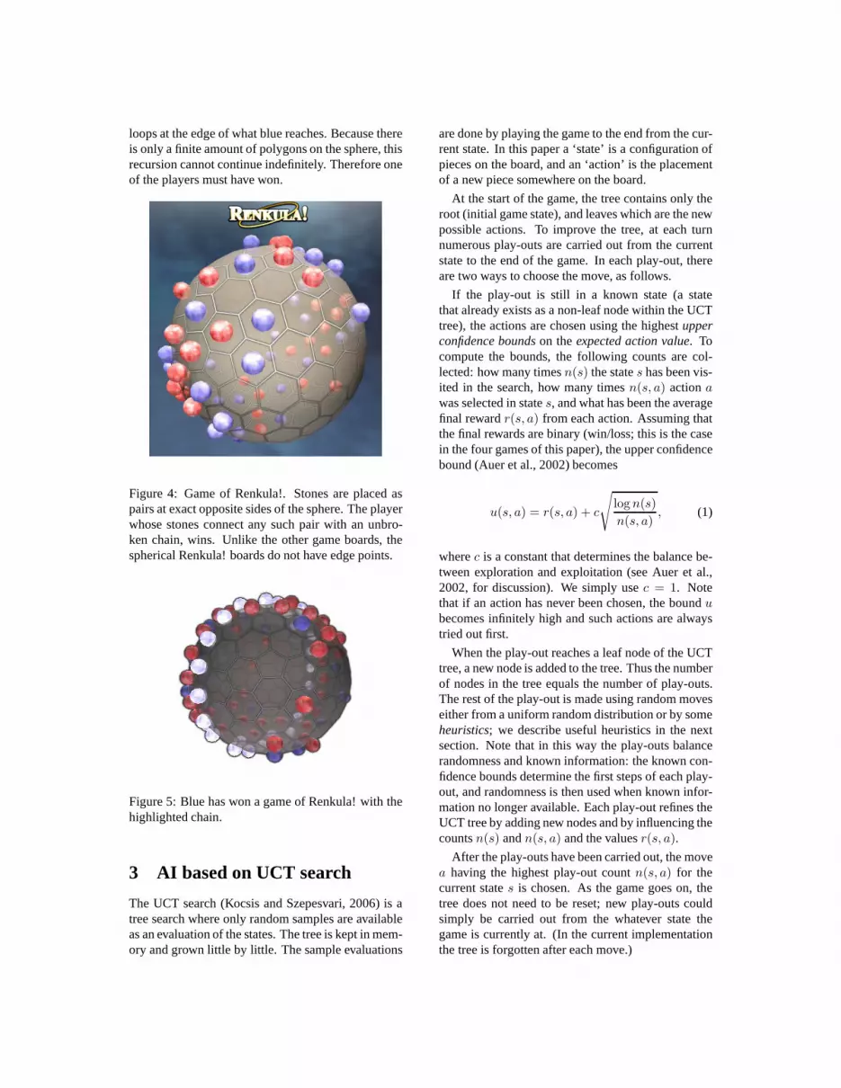
loops at the edge of what blue reaches. Because thereis only a finite amount of polygons on the sphere, thisrecursion cannot continue indefinitely. Therefore oneof the players must have won.
Figure 4: Game of Renkula!. Stones are placed aspairs at exact opposite sides of the sphere. The playerwhose stones connect any such pair with an unbro-ken chain, wins. Unlike the other game boards, thespherical Renkula! boards do not have edge points.
Figure 5: Blue has won a game of Renkula! with thehighlighted chain.
3 AI based on UCT search
The UCT search (Kocsis and Szepesvari, 2006) is atree search where only random samples are availableas an evaluation of the states. The tree is kept in mem-ory and grown little by little. The sample evaluations
are done by playing the game to the end from the cur-rent state. In this paper a ‘state’ is a configuration ofpieces on the board, and an ‘action’ is the placementof a new piece somewhere on the board.
At the start of the game, the tree contains only theroot (initial game state), and leaves which are the newpossible actions. To improve the tree, at each turnnumerous play-outs are carried out from the currentstate to the end of the game. In each play-out, thereare two ways to choose the move, as follows.
If the play-out is still in a known state (a statethat already exists as a non-leaf node within the UCTtree), the actions are chosen using the highestupperconfidence boundson theexpected action value. Tocompute the bounds, the following counts are col-lected: how many timesn(s) the states has been vis-ited in the search, how many timesn(s, a) actiona
was selected in states, and what has been the averagefinal rewardr(s, a) from each action. Assuming thatthe final rewards are binary (win/loss; this is the casein the four games of this paper), the upper confidencebound (Auer et al., 2002) becomes
u(s, a) = r(s, a) + c
√
log n(s)
n(s, a), (1)
wherec is a constant that determines the balance be-tween exploration and exploitation (see Auer et al.,2002, for discussion). We simply usec = 1. Notethat if an action has never been chosen, the boundu
becomes infinitely high and such actions are alwaystried out first.
When the play-out reaches a leaf node of the UCTtree, a new node is added to the tree. Thus the numberof nodes in the tree equals the number of play-outs.The rest of the play-out is made using random moveseither from a uniform random distribution or by someheuristics; we describe useful heuristics in the nextsection. Note that in this way the play-outs balancerandomness and known information: the known con-fidence bounds determine the first steps of each play-out, and randomness is then used when known infor-mation no longer available. Each play-out refines theUCT tree by adding new nodes and by influencing thecountsn(s) andn(s, a) and the valuesr(s, a).
After the play-outs have been carried out, the movea having the highest play-out countn(s, a) for thecurrent states is chosen. As the game goes on, thetree does not need to be reset; new play-outs couldsimply be carried out from the whatever state thegame is currently at. (In the current implementationthe tree is forgotten after each move.)

3.1 Heuristics for Connection Games
Here we describe novel heuristics and speed-ups forUCT suitable for connection games.
Speed-up 1: Suppose a play-out reaches a leafnode of the UCT tree; typically there will be numer-ous empty positions left on the board. In all of thepresented games, assuming uniformly random play-outs, it is easy to show the empty positions end upfilled with random colored stones, an equal numberof each color. This ‘fill-out’ does not need to be donemove by move: it is faster to simply go through theboard once, filling all the empty points.
Speed-up 2: Suppose we are initializingr(s, a)for the latest leaf node. It does not make any differ-ence which of the above-described ‘fill-out moves’ iscounted as the first onea. Therefore, assuming it ise.g. black’s move,r(s, a) for all filled in black stonesa can be updated as if they were the next move.
Heuristic 1: As the random fill-out phase is fast, itcan be useful to do more than one fill-out at once.
Heuristic 2: We consider so-calledbamboo con-nections, also known asbridges, as a special case.Bamboo connections are a simple shape that reap-pears very often in any of the presented games. Fig-ure 6 shows an example in the game of Renkula! butmore generally they can also occur between a stoneand the edge of the board. To break a bamboo con-nection, both empty positions in the connection mustbecome filled up with stones of the other player. Us-ing uniformly random playouts, there are four ways tofill the empty positions, and the connection is brokenin one of these four cases. It is only rarely useful fora player to let his/her bamboo connection get broken,and it is rarely useful to fill both empty positions in abamboo connection with your own stones; therefore,a useful heuristic is to recognise bamboo connectionsin the fill-out phase, and fill them with one stone ofeach color, thus avoiding the above-described two un-desirable fill-out cases. The only exception is whendifferent bamboo connections overlap. In those caseswe acknowledge only the first one found.
Given the above-described improvements, the be-havior of the resulting connection game AI can be ad-justed by adjusting the number of play-outs carriedout at each turn, the number of random fill-outs per-formed at the leaf nodes, and whether to use the bam-boo connection heuristic. Larger numbers of play-outs and fill-outs obviously slow down the AI. A use-ful property of the AI is that it is possible to stop thesearch at any time, and simply select a move basedon the current evaluations (this ability is in principleavailable for all the games; currently we have imple-mented it in Renkula! but not in the other games).
Figure 6: A bamboo connection, here shown on aRenkula! board. Blue player cannot prevent red fromconnecting its stones.
4 Conclusion
We have presented a UCT search based AI forfour connection games, including a new gameintroduced here. Our implementations of thegame AIs are freely available: the implemen-tations of Hex, Y, and *Star are available atwww.cis.hut.fi/praiko/connectiongames/ ,and the implementation of Renkula! is availableat www.nbl.fi/˜nbl924/renkula/ . As asubjective evaluation, the algorithm seems to be quitestrong at least on small boards.
References
P. Auer, N. Cesa-Bianchi, and P. Fischer. Finite-timeanalysis of the multi-armed bandit problem.Ma-chine Learning, (47):235–256, 2002.
Cameron Browne.Connection Games: Variations ona Theme. A K Peters, Ltd., 2005.
Sylvain Gelly, Yizao Wang, Remi Munos,and Olivier Teytaud. Modificationof UCT with patterns in Monte-CarloGo. Technical Report RR-6062, 2006.http://hal.inria.fr/inria-00117266 .
L. Kocsis and C. Szepesvari. Bandit based Monte-Carlo planning. InProc. of European Conferenceon Machine Learning, pages 282–293, 2006.
Thomas Maarup. Hex: Everything you alwayswanted to know about hex but were too afraid toask, 2005.
Jack van Rijswijck. Search and evaluation in Hex.Technical report, Department of Computing Sci-ence, University of Alberta, 2002.

Regularized Least-Squares for Learning Non-TransitivePreferences between Strategies
Tapio Pahikkala? Evgeni Tsivtsivadze? Antti Airola?
Tapio Salakoski??Turku Centre for Computer Science (TUCS)
Department of Information Technology, University of TurkuJoukahaisenkatu 3-5 B, FIN-20520 Turku, Finland
Abstract
Most of the current research in preference learning has concentrated on learning transitive relations.However, there are many interesting problems that are non-transitive. Such a learning task is, forexample, the prediction of the probable winner given the strategies of two competitors. In this paper,we investigate whether there is a need to learn non-transitive preferences, and whether they can belearned efficiently. In particular, we consider cyclic preferences such as those observed in the game ofrock paper and scissors.
1 Introduction
The learning of preferences (see e.g. Furnkranz andHullermeier (2005)) has recently gained significantattention in the machine learning community. Prefer-ence learning can be considered as a task in which theaim is to learn a function capable of evaluating, givenpair of data points, whether the first point is preferredover the second one. For example, given two compet-itive strategies, the aim might be to predict the prob-able winner. We assume that we are given a trainingset of pairwise preferences that are used to train a su-pervised learning algorithm for the prediction of thepreference relations among unseen data points.
1.1 Non-Transitive Preferences
The typical setting for preference learning deals withtransitive preferences. By a transitive preference, wemean thatA > B andB > C imply A > C, where> denotes the preference relation, andA, B andCare objects of interest. In the commonly used scoringsetting, where each object is associated with a good-ness score, all preference relations that can be derivedfrom the scores are transitive.
In this paper, we consider the learning of non-transitive preference relations. A typical exampleof such a relation occurs in the game rock-paper-scissors. In the game, rock defeats scissors and scis-sors defeat paper, but rock loses to paper.
Is there a reason to aim to learn such relations?In the context of decision theory there has been dis-cussion about whether non-transitivity of preferencesarises simply from irrationality or errors in measure-ments or whether reasonable preferences can actuallyexhibit non-transitivity (see e.g. Fishburn (1991)).Next, we present some examples that can be consid-ered as real-world non-transitive preference learningtasks.
Some motivation for considering non-transitivepreferences can be found, for example, in recent bi-ological findings. Kerr et al. (2002); Kirkup andRiley (2004) report that this type of phenomenonappears between bacterial populations ofEschericiacoli: bacteria that produce a certain type of antibiotickill bacteria that are sensitive to it, but are outcom-peted by bacteria resistant to it, while sensitive bac-teria outcompete resistant ones. Therefore, it makessense to aim to predict, for two new types of bacte-ria, which outcompetes which. A new bacteria couldbe, for example, of a type that produces just a smallamount of antibiotic but with a lower competitivecost.
These types of relations occur not only on the bac-terial level but, for example, also in the mating strate-gies of certain lizard species (Sinervo and Lively,1996). Aggressive orange males outcompete theirless aggressive blue peers, but are outsmarted bymales with yellow markings. Yet the yellow maleslose to the more perceptive blue males.

Similar examples of non-transitive preferences canalso be found in military settings. For example,weapon systems like bombers, long-range artillery,and anti-aircraft batteries again form a preference cy-cle. In general, when a set of competing strategiesare used against each other, the interplay of the weak-nesses and strengths of these strategies can result innonlinear preference relations.
Finally, non-transitive preferences are often con-fronted in the domain of computer games. InCrawford (1984), building nontransitive relationshipsinto computer games was termed as “triangularity”.Nowadays, triangularity is one of the most well-known design patterns in computer game develop-ment (see e.g. Bjork et al. (2003)). Preference learn-ing methods that are able to learn this type of rela-tionships, for example, from statistics collected in acomputer game may prove to be advantageous toolsin adjusting the balance of the game rules and me-chanics.
1.2 Related Work
Preference learning has so far concentrated on learn-ing a scoring function either from a scored data (seee.g. Herbrich et al. (1999); Pahikkala et al. (2007);Cortes et al. (2007)) or from a given set of pairwisepreferences (see e.g. Joachims (2002)). The qualityof the learned scoring function is measured accordingto how well it performs with respect to a given rank-ing measure. This is sometimes called the scoringbased setting.
There have also been studies about learning and us-ing a preference function that, when given two ob-jects, outputs a direction or magnitude of preferencebetween them (see e.g. Cohen et al. (1999); Ailonand Mohri (2008)). However, even though such afunction can be used to represent non-transitive pref-erences, the aim in these studies has been to obtain atotal order of the objects.
Both of the aforementioned approaches are unsuit-able for learning tasks in which the aim is to preservethe non-transitivities instead of turning the probleminto a linear ranking task. For example, it makes nosense to consider tasks such as the learning the prefer-ences between the rock, paper, and scissors strategiesin the ranking framework.
In this paper, we adopt a third approach in whichwe aim to construct learners that preserve the non-transitivities. We achieve this via training nonlinearclassifiers and regressors with pairs of individual ob-jects and the corresponding directions or magnitudesof preferences between them.
Kernel-based learning algorithms (Scholkopf andSmola, 2002; Shawe-Taylor and Cristianini, 2004)have been shown to be successful in solving non-linear tasks, and hence they make a good candidatefor learning non-transitive preferences. However, thecomputational complexity of those algorithms maybe high, because the number of labeled object pairsoften grows quadratically with respect to the numberof objects. Fortunately, there exist efficient approxi-mation methods which output sparse representationsof the learned function, such as the regularized least-squares regression (RLS) together with the subset ofregressors approach (see e.g. Rifkin et al. (2003)).
2 Learning the Preferences
We formulate the preference learning task in Sec-tion 2.1. In Section 2.2, we describe the synthetic dataused to simulate a non-transitive preference learningtask and in Section 2.3 the learning algorithm. Exper-imental results are presented in Section 2.4.
2.1 Problem Formulations
Let V denote the set of possible inputs. Moreover,let X = (x1, . . . , xl)T ∈ (V × V)l be a sequenceof l observed preferences between the inputs and letY = (y1, . . . , yl) ∈ Rl be their corresponding magni-tudes. That is, for eachxi = (v, v′), wherev, v′ ∈ V,yi ∈ R indicates the direction and the magnitude ofpreference betweenv andv′. Clearly,X can be con-sidered as a preference graph in which the inputs arethe vertices andxi are the edges. The nontransitivityimplies that the preference graph can contain cycles.
2.2 Synthetic Data
To test the performance of the learning algorithmin a nonlinear preference learning task, we gener-ated the following synthetic data. First, we gener-ate100 preference graph vertices for training and100for testing. The preference graph vertices are three-dimensional vectors representing players of the rock-paper-scissors game. The three attributes of the play-ers are the probabilities that the player will chooserock, paper, or scissors, respectively. The probabilityP (r | v) of the playerv choosing rock is determinedby P (r | v) = exp(wu)/z, whereu is a randomnumber drawn from the uniform distribution between0 and1, w is a steepness parameter, andz is a nor-malization constant ensuring that the three probabil-ities sum up to one. By using the exponent function

with the parameterw it can be ensured that most ofthe players tend to favor one of the three choices.
We generate1000 edges for training by randomlyselecting the start and end vertices from the trainingvertices. Each edge represents a game of rock-paper-scissors. For both players we randomly choose eitherrock, paper, or scissors according to their personalprobabilities. The outcome of a game is−1, 0, or 1depending on whether the first player loses the game,the game is a tie, or the first player wins the game,respectively. We use the game outcomes as the labelsof the training edges.
Similarly, we generate1000 edges for testing fromthe test vertices. However, instead of using the out-come of a single simulated game as a label, we as-sign for each test edge the average outcome of a gameplayed between the first and the second player, that is,
y = P (p | v)P (r | v′)− P (s | v)P (r | v′)−P (r | v)P (p | v′) + P (s | v)P (p | v′)+P (r | v)P (s | v′)− P (p | v)P (s | v′).
The task is to learn to predict the average outcomesof the test edges from the training data.
2.3 Learning Method
RLS is a state of the art kernel-based machine learn-ing method which has been shown to have compara-ble performance to support vector machines (Rifkinet al., 2003; Poggio and Smale, 2003). We choose thesparse version of the algorithm, also known as subsetof regressors, as it allows us to scale the method up tovery large training set sizes.
Let us denoteRX = f : X → R, and letH ⊆ RX be the hypothesis space. In order to con-struct an algorithm that selects a hypothesisf fromH, we have to define an appropriate cost functionthat measures how well the hypotheses fit to the train-ing data. Further, we should avoid too complex hy-potheses that overfit at training phase and are not ableto generalize to unseen data. Following Scholkopfet al. (2001), we consider the framework of regular-ized kernel methods in whichH is the reproducingkernel Hilbert space (RKHS) defined by a positivedefinite kernel functionk. The kernel functions aredefined as follows. LetF denote the feature vectorspace. For any mapping
Φ : X → F ,
the inner product
k(x, x′) = 〈Φ(x),Φ(x′)〉
of the mapped data points is called a kernel function.Using RKHS as our hypothesis space, we define thelearning algorithm as
A(S) = argminf∈H
J(f),
whereJ(f) = c(f(X), Y ) + λ‖f‖2k, (1)
f(X) = (f(x1), . . . , f(xm))T, c is a real valued costfunction, andλ ∈ R+ is a regularization parame-ter controlling the tradeoff between the cost on thetraining set and the complexity of the hypothesis. Bythe generalized representer theorem (Scholkopf et al.,2001), the minimizer of (1) has the following form:
f(x) =m∑
i=1
aik(x, xi), (2)
whereai ∈ R.We now briefly present the basic sparse RLS algo-
rithm. LetM = 1, . . . ,m be an index set in whichthe indices refer to the examples in the training set.Instead of allowing functions that can be expressedas a linear combination over the whole training set aswith the basic RLS regression, we only allow func-tions of the following restricted type:
f(x) =∑i∈B
aik(x, xi), (3)
wherek is the kernel function,ai ∈ R are weights,and the set indexing the basis vectorsB ⊆ M is se-lected in advance. The coefficientsai that determine(3) are obtained by minimizing
m∑i=1
(yi −∑j∈B
ajk(xi, xj))2 + λ∑
i,j∈B
aiajk(xi, xj)
where the first term is the squared loss function, thesecond term is the regularizer, andλ ∈ R+ is a reg-ularization parameter. The minimizer is obtained bysolving the corresponding system of linear equations,which can be performed inO(l|B|2) time.
We set the maximum number of basis vectors to100 in all experiments in this study, and select thesubset randomly when the training set size exceedsthis number, since in Rifkin et al. (2003) it was shownthat randomly relecting the basis vectors works aswell as heuristic-based methods.
As the kernel function, we use the Gaussian kernelover the feature vectors of the edges, which are con-structed by catenating the feature vectors of its start

w = 1 w = 10 w=100I 0.002 0.004 0.001II 5e-06 0.029 0.509III 0.666 0.912 0.938
Table 1: I: The mean squared errors made by the re-gression algorithm. II: The mean squared errors madeby always predicting0. III: The proportions of cor-rectly predicted directions of preference by the re-gression algorithm.
and end vertices. Formally, the Gaussian kernel is de-fined as follows:
k(x, x′) = e−γ(x−x′)2 ,
whereγ > 0 is a bandwidth parameter.In our experiments, we set the parametersλ andγ
with grid search and cross-validation. For in depthdiscussion of the behavior of kernel-based learningalgorithms with different combinations of these pa-rameter values, we refer to Lippert and Rifkin (2006).
2.4 Results
We conduct experiments with three data sets gener-ated using the values1, 10, and100 for thew pa-rameter. The valuew = 1 corresponds to the situa-tion where all probabilities of the players are close tothe uniform distribution. When usingw = 100 theplayers tend to always play their favourite item, andw = 10 corresponds to a setting between these twoextremes.
The results are presented in Table 1. We report themean square-error made by the regression algorithmwhen predicting the average outcome and compare itto the approach of always predicting zero. We also re-port the proportions of correctly predicted directionsof preference for each edge. As expected, learningthe average outcomes when the probabilities of theplayers are close to the uniform distribution is moredifficult than in case the players tend to always playtheir favourite item. Nevertheless, the sparse RLS re-gressor with Gaussian kernel is capable of capturingthe nonlinear concept to be learned.
3 Conclusion
In this paper, we investigate the problem of learningnon-transitive preference relations. We discuss wherethis type of problems appear and how they can besolved. In particular, a case study about the gameof rock-paper-scissors is presented. In the study, we
create synthetic data for which we apply sparse RLSwith Gaussian kernel which proves to be a feasibleapproach for the task.
In the future, we will consider other variationsof nonlinear preferences occurring in the real worldlearning tasks and how to efficiently solve them. Forexample, tasks consisting of a mixture of trainsi-tive and non-transitive preference relations may pro-vide interesting research directions. Further, moderncomputer games have often a large set of compet-ing strategies and players with different strengths andweaknesses from which non-transitive preference re-lations might emerge.
Acknowledgments
This work has been supported by Academy of Fin-land and Tekes, the Finnish Funding Agency forTechnology and Innovation.
References
Nir Ailon and Mehryar Mohri. An efficient reduc-tion of ranking to classification. In Rocco Servedioand Tong Zhang, editors,Proceedings of the 21thAnnual Conference on Learning Theory, pages 87–97, 2008.
Staffan Bjork, Sus Lundgren, and Jussi Holopainen.Game design patterns. InDigital Games ResearchConference DIGRA, 2003.
William W. Cohen, Robert E. Schapire, and YoramSinger. Learning to order things.Journal of Artifi-cial Intelligence Research, 10:243–270, 1999.
Corinna Cortes, Mehryar Mohri, and Ashish Ras-togi. Magnitude-preserving ranking algorithms.In Zoubin Ghahramani, editor,Proceedings of the24th Annual International Conference on MachineLearning, volume 227 ofACM International Con-ference Proceeding Series, pages 169–176. ACMPress, 2007.
Chris Crawford.The Art of Computer Game Design.Osborne/McGraw-Hill, Berkeley, CA, USA, 1984.
Peter C Fishburn. Nontransitive preferences in deci-sion theory.Journal of Risk and Uncertainty, 4(2):113–34, April 1991.
Johannes Furnkranz and Eyke Hullermeier. Prefer-ence learning.Kunstliche Intelligenz, 19(1):60–61,2005.

Ralf Herbrich, Thore Graepel, and Klaus Obermayer.Support vector learning for ordinal regression. InProceedings of the Ninth International Conferenceon Articial Neural Networks, pages 97–102. Insti-tute of Electrical Engineers, 1999.
Thorsten Joachims. Optimizing search engines usingclickthrough data. InProceedings of the ACM Con-ference on Knowledge Discovery and Data Mining,pages 133–142, New York, NY, USA, 2002. ACMPress.
Benjamin Kerr, Margaret A. Riley, Marcus W. Feld-man, and Brendan J. M. Bohannan. Local dispersalpromotes biodiversity in a real-life game of rock-paper-scissors.Nature, 418(6894):171–174, 2002.
Benjamin C. Kirkup and Margaret A. Riley.Antibiotic-mediated antagonism leads to a bacte-rial game of rock-paper-scissors in vivo.Nature,428(6981):412–414, 2004.
Ross Lippert and Ryan Rifkin. Asymptotics ofgaussian regularized least squares. In Y. Weiss,B. Scholkopf, and J. Platt, editors,Advances inNeural Information Processing Systems 18, pages803–810. MIT Press, Cambridge, MA, 2006.
Tapio Pahikkala, Evgeni Tsivtsivadze, Antti Airola,Jorma Boberg, and Tapio Salakoski. Learning torank with pairwise regularized least-squares. InThorsten Joachims, Hang Li, Tie-Yan Liu, andChengXiang Zhai, editors,SIGIR 2007 Workshopon Learning to Rank for Information Retrieval,pages 27–33, 2007.
Tomaso Poggio and Steve Smale. The mathematics oflearning: Dealing with data.Notices of the Ameri-can Mathematical Society, 50(5):537–544, 2003.
Ryan Rifkin, Gene Yeo, and Tomaso Poggio. Reg-ularized least-squares classification. In J.A.K.Suykens, G. Horvath, S. Basu, C. Micchelli, andJ. Vandewalle, editors,Advances in Learning The-ory: Methods, Model and Applications, volume190 of NATO Science Series III: Computer andSystem Sciences, chapter 7, pages 131–154. IOSPress, 2003.
Bernhard Scholkopf, Ralf Herbrich, and Alex J.Smola. A generalized representer theorem. InD. Helmbold and R. Williamson, editors,Proceed-ings of the 14th Annual Conference on Compu-tational Learning Theory and and 5th EuropeanConference on Computational Learning Theory,pages 416–426, Berlin, Germany, 2001. Springer-Verlag.
Bernhard Scholkopf and Alexander J. Smola.Learn-ing with kernels. MIT Press, Cambridge, Mas-sachusetts, 2002.
John Shawe-Taylor and Nello Cristianini.KernelMethods for Pattern Analysis. Cambridge Univer-sity Press, Cambridge, UK, 2004.
Barry Sinervo and Curtis M. Lively. The rock-paper-scissors game and the evolution of alternative malestrategies.Nature, 380:240–243, 1996.
Philosophy of Static, Dynamic and Symbolic Analysis
Erkki Laitila
SwMaster Ltd Sääksmäentie 14 40520 Jyväskylä Finland [email protected]
Abstract
The purpose of program analysis is to make understanding program behavior easy. The traditional ways, static and dynamic analyses have suffered from their theoretical connections to development of compilers and debuggers and, therefore, are not ideal for the purpose. In this paper a novel met- hodology, symbolic analysis, is compared with them based on a criteria borrowed from ideal analy-sis. In conclusion, symbolic analysis is seen as capable of transforming typical needs of familiariza-tion and troubleshooting tasks to concrete analyzing actions, which helps in planning changes.
1 Introduction
In this paper we use the definitions for ideal science (Hoare, 2006) as a framework to figure out what could be an ideal analysis for programs. According to it we compare the traditional analyzing paradigms with symbolic analysis (Laitila, 2008a).
Analysis is defined as “the process of breaking a concept down into more simple parts, so that its logical structure is displayed”1. Although analysis is usually seen merely as reductive, connective forms of analysis, emphasizing sub-symbolic pres-entations, are quite important, too. The debate over symbolic versus sub-symbolic representations of human cognition has continued for thirty years, with little indication of a resolution (Kelley, 2003). Sym-bolic analysis is an attempt to connect these two presentations (Laitila, 2008b; 2008d). Its aim is to provide a consistent and coherent information chain.
1.1 Program analysis Computer program analysis is the process of auto-matically analyzing the behavior of computer pro-grams. Its main applications aim to improve per-formance and quality of program maintenance with automated tools. The techniques related to program analysis include: type systems, abstract interpreta-tion, program verification, model checking, and much more (Nielson et al., 2005).
1Stanford Encyclopedia of Philosophy: http://www.seop.leeds.ac.uk/archives/spr2004/entries/analysis/s1.html.
1.1.1 Static analysis In static analysis, source code is used as input. Un-fortunately, static analysis is not complete for ob-ject-oriented programs (OOP). This is due to many complex features of OOP, which include inheri-tance, polymorphism and late bindings. The main features of static analysis are (Nielson et al., 2005): • Idea: to parse code to generate an abstract model that can be analyzed using model checking • No execution required but language dependent • May produce spurious counterexamples • Can prove correctness in theory but not in prac- tice. 1.1.2 Dynamic analysis Dynamic analysis gathers information about execu-ting the original system in the final environment. Because typical systems are rather complex and the logic of software usually rather challenging, dy-namic analysis can only provide samples of the se-lected execution trace, whose relevance is usually hard to confirm. Its main features are: • Idea: to control the execution of multiple test- drivers/ processes by intercepting systems calls • Language independent but requires execution • Counterexamples arise from code • Provides a complete state-space coverage up to some depth only, but typically incomplete. 1.1.3 Symbolic analysis (SymAn) There are several drawbacks to both of the tradi-tional principles discussed. One way to avoid these drawbacks might be a higher-abstraction metho-

dology, which would be closer to human thinking than its predecessors.
The principle of symbolic analysis is straight-forward (Laitila, 2008a) (see Fig. 1). In it there is a symbol (S) for each grammar term captured from the programming language. Behind each symbol there is an object (O), which contains the semantics of the corresponding grammar term. These two as-pects should be implemented as a hybrid object to combine the object-oriented and logic-oriented ap-proaches (Laitila, 2006; 2008b; 2008e). Understand-ing could then be seen as a process of making inter-pretations based on predicates that connect symbols. They are expressed using logic (L). We have dem-onstrated the methodology for small Java programs in JavaMaster, our tool built for the purpose.
Figure 1: Main concepts of SymAn.
1.2 Comparison framework We compare the alternatives using the framework presented by Hoare, whose essential measures are rather philosophical: purity of concepts, simplicity of theories, granularity, completeness, relevancy, certainty, and correctness. The comparison shows that symbolic analysis can contribute in most of these measures due to its rather abstract nature. 1.3 Contents of this paper Section 2 describes an ideal analysis. Section 3 pre-sents symbolic analysis. It is evaluated in Section 4 according to the criteria. Section 5 shows the results of the comparison. Section 6 discusses related work. The last section is a summary. 2 Towards ideal analysis
Many existing methods carry a burden related to their origin and history, which have prevented them from developing to an optimal direction for the users. Due to this historical background, the tradi-tional analysis methods cannot give optimal results for maintainers. In this kind of situation, one possi-bility could be to create a new methodology from scratch in order to reach the goal of the ideal analy-sis. 2.1 Ideal analysis What could be an ideal analysis like? Hoare’s defi-nition can help, as it has been presented to illustrate
ideal science from the program verification view-point. It contains seven measures: 1. Purity of matherials (concepts) 2. Simplicity of theory 3. Granularity of transformations 4. Completeness of logic 5. Relevancy of questions 6. Certainty of answers. 7. Correctness of programs. We apply these seven points next, in order to create a realistic criteria for program analysis. 2.1.1 Purity of concepts As in physics, chemistry and medical science, the tools, materials and surfaces should be as pure as possible to enable the best possible quality and re-sults. In program analysis the concepts of the meth-odology should be highly compatible, e.g. pure, with the concepts that the programmers use in their eve-ryday work. The three specific challenges are gene-ralization, specification, and construction: how to describe the concepts in a unified way to contain all elements, and how to specify all differences in a generic way to enable the user to capture knowledge about the concepts in a constructive way. 2.1.2 Simplicity of theory Reverse engineering, the discipline behind program analysis, should be seen as a data flow converting data from program code into pragmatic knowledge for planning modifications. All information should be traceable to code to allow correct changes. 2.1.3 Granularity of transformations. The information of the data flow (Section 2.1.2) should be highly granular without any gaps or un-known meta-structures. All elements should be both compact and specific to allow accurate activities. 2.1.4 Completeness of logic Each information element type should be executable to allow estimation of its behavior. It means that there should be a simulator, an abstract Turing mac-hine, to run either a total application, or some spe-cific parts of it in a way which should resemble the intention in the programmer’s mind. 2.1.5 Relevancy in meeting maintainers' ques-tions In the analysis there should be a multi-phase ap-proach to allow the typical divide-and-conquer process for problem solving. The highest level in this approach is typically a change request (CR), which should be converted into lower level analysis actions to detect the change candidates.

2.1.6 Certainty of answers to cover candidates Pragmatic certainty for the answers is the probabil-ity of how surely change candidates can be detected in the code. Overlapping bugs are a real challenge. 2.1.7 Correctness of programs The theory for 2.1.1 to 2.1.6 should be realistic to enable building and programming a tool, compara-ble with the tools for static and dynamic analyses. 3 Symbolic analysis in a nutshell
Symbolic analysis (see Fig. 1) is a process intended for the purposes of maintenance. It divides the main-tenance task (T), which is a domain specific concept into lower level concepts and via them into hypothe-ses (H), which can be formulated as queries (Q) to analyses (A), which collect from a model (M) rele-vant information using symbols (S) from objects connected with logic (L) (Laitila, 2008d). This proc-ess (P) is repeated as far as the problem of the task can be solved.
3.1 Concepts behind SymAn The most important concept of SymAn is the atom, which implements an object (O). Atomistic model is a set of atoms. Symbol (S) is a reference to the atom. For a human the symbol means its name and for the computer it means a pointer to the memory. 3.1.1 Foundation for an atomistic model Software atom is a compact, reductionist object (see Fig. 2), which holds its own semantics defined in a single predicate named command. It is essential that the atom doesn’t need to know anything about the semantics of other atoms. An atom is executable, because it can be simulated by a run-method. It is programmed in predicate logic. There is an infe-rence engine in the run-method to enable consistent logic to return a valid result for each enquiry.
Figure 2: Functional atomistic model.
3.2 Developed theories To meet the pragmatic need, a tool to help in plan-ning changes was designed (see Fig. 3). In it, source code is the input to be read and parsed (Aho et al., 1985) and abstracted via grammar techniques (GrammarWare) (Laitila, 2001). Its output is trans-formed (weaved) into an atomistic model (Model-Ware). Simulating it reveals the behavior of the relevant program functions (SimulationWare) to capture hierarchical and conceptual knowledge (KnowledgeWare). Captured program dependencies and detected problems form the necessary precondi-tions for making modifications.
Figure 3: The technology spaces for the analysis.
The value produced by the designed planning tool, JavaMaster, and by other similar tools, depends on how it can help in the iterative work of reading code, e.g., human cognition. The user typically re-peats same kind of actions in order to be able to hypothesize which are the most relevant elements of the program and how they should be evaluated. This iterative work is laborious, and it easily creates a cognitive overload into the mind of the person. We argue that this work can be changed more produc-tive by machine computation. 3.3 Transformations and the data flow Data flow (Fig. 4) is implemented from data D0 to D8, by successive automata (Hopcroft et al., 1979). Automata A1, A2, and A3 that are related to Gram-marWare enable symbolic processing in the gram-mar (A1) for parsing code (A2), and for abstracting it (A3). Automaton A4 for ModelWare is there to weave the atomistic model. Automata A5 and A6 enable simulating the model for obtaining the be-havior. Automaton A7 is for KnowledgeWare to capture knowledge. The user is the last link in the chain to plan modifications.

Figure 4: Symbolic analysis as a data flow.
3.4 The logic for simulation For simulation we defined atomistic semantics as a call/return-architecture to connect the atoms with each other (see Fig. 2). From outside, simulation is a call: Result = Atom:run(). Inside (see Table 1), each atom type contains a state transition table to define the internal semantics of the corresponding Java (or C++) term. An atom invocation leads to an entry state. There are 0 to N different states in an atom, which are preconditioned by constraints Ci,j. A state can cause references to other atoms. A state can return status information to the caller and to a higher level (the way that break does).
Table 1: Atom behavior as a state transition table. State Condition Next State Refers to Status Entry S1 A1.etc.
S1 C1,k Sk Status .. Status Sk Ck,n Sn Aj Status .. Status Sn Exit Return
The function of Table 1 can explicitly be pro-grammed in Prolog without torsion, because Prolog predicates have the semantics to allow implemen-ting state machines (Sterling & Shapiro, 2003). 3.5 Meeting maintenance needs Each grammar term is mapped into an atom (see Fig. 5) and further to a symbolic abstract machine (Section 3.4) for producing knowledge units.
Figure 5: From data flow to knowledge. Executing atoms according to Table 1 produces new types of atoms, i.e., side effect atoms, which to-gether form the dynamic model.
The user uses the atomistic information as fol-lows. Any relevant atom forms a knowledge unit in the mind of the user and, thus, enables concept building. Pragmatic value is obtained if the collected set of knowledge units is coherent and consistent in context to the active maintenance task. 3.6 How needs can be satisfied Source code and its atoms meet the condition of atomism: totality should be the sum of its elements. Therefore, programs can be studied as containers containing subcontainers. User concepts are the most abstract containers (see CI in Fig.6). Below them are contexts CI
J, which are connections to code, i.e. different kinds of use cases for atoms, de-fined by the user. For example, starting a server is a context which can be localized into code.
CI
CINCI
1 ..
CI
CINCI
1 ..
Figure 6: Knowledge model for seeking relevancy
for maintenance actions. Because of the sequential nature of computers, the user can efficiently build his/her mental models based on sequential information captured from simulating the relevant methods, shown as the low-est level of Fig. 6 (Laitila, 2008a; 2008b; 2008e). 3.7 Estimating correctness of SymAn Results can be evaluated by comparing them with the results of dynamic analysis and the expected behavior of the code. For Java this can theoretically be done using experiments for each clause type de-rived from Java (Gosling et al., 2005). 4 Evaluating measures of SymAn
In this section we evaluate our symbolic analysis based on the criteria of Section 2 and sharpened in Section 3. The topic of performance is ignored, be-cause by nature this paper is philosophical.
4.1 Purity of concepts of SymAn The architecture is shown in Fig. 7.
SymbolicAbstract Machine
KnowledgeUnit(s)
SymbolicGrammar
Term
AtomisticModel Element
1..
1..
1.. 1..
0..
SymbolicGrammar
Term
SymbolicAbstract Machine
KnowledgeUnit(s)
AtomisticModel Element
1..
1..
1.. 1..
0..

Figure 7: Architecture of the atom.
The atom, which corresponds to object (O), was implemented by creating a base class SymbolicEle-ment. It inherits the Symbolic language class, which connects the specific elements in the same way as the original code does. Only a single predicate, named clause, is needed to descibe Java semantics. There are 14 specific elements, shown in Fig. 7 as a template Symbolic<T>Element. Connections be-tween atoms are explanations for the user. They are expressed in the notation of clause. 4.2 Simplicity of theories There are three semiotic layers (Peirce, 1958) in the information captured from symbolic analysis (see Fig. 8). Layer 1 corresponds to static analysis, layer 2 to the flow of dynamic analysis, and layer 3 de-scribes side effect elements, which form the behav-ior model with concrete objects and values, and I/O. In a typical case the user tries to understand the most relevant flows, which are formulated as atoms here.
Figure 8: Semiotic layers of the results. 4.3 Granularity of transformations Each grammar term of the relevant Java program is converted into an atom. After simulation the sum of communication between atoms defines the total be-havior of the code (Fig. 4). Summarized, the granu-larity of all model transactions is on the level of an atom corresponding to a grammar term. Therefore, it is possible for the user to inspect all details with the help of atoms applying set operations for them.
4.4 Completeness of simulation Simulation logic for each clause type was written. Table 2 shows their features: 1) If the parameters are known, then the simulating conditions are complete. 2) The same precondition applies to loops. If the loop simulation is incomplete, then their interactions should be limited. 3) The objects created by Visual Prolog are reasonably compatible with the behavior of Java objects. 4) There are some specific reference types like arrays, which require specific rules in the tool. 5) If a method can be found in the model, then its logic can be simulated; otherwise, the invocation is returned to the caller.
Table 2: Atom behavior as a state transition table.
Symbolic clause Completeness of simulation Constant Complete Condit. clause roviding that 1) Complete pLoop Complete providing that 2) Object creator Java objects as tool objects, obs. 3) Var. reference Complete providing that 4) Method call Complete providing that 5) Return-case Complete Block control plete ComVirtual function Unknown functions incomplete. Reference to libraries
References to JDK are external symbols, not simulated.
Th le is th the symbol behind the r n analysis can generate t ing i e F . Otherwise it replies by returning the symbol and the si ffect elem for t
gical steps of the symbolic mainte-
e general ru at if eference is know , symboliche correspondig. 8)
nformation of layers 2 and 3 (se
de ehe invocation.
ent as an identification
4.5 Relevancy of questions of SymAn From the user’s point-of-view there are two modes in the symbolic analysis process: familiarization (FAM) and troubleshooting (TS) (see Table 3).
Table 3: The lonance process.
Initial knowledge
Proof result Conclusions and possible decisions
1. FAM: •Low
Find relevant places
Initial learning
2. FAM: No contradic- Confirmative lear-•Perfect tions ning, no conclusions 3. FAM: •Perfect
Con nflict. Either an error or an exception.
tradiction A co
It starts a trouble-shooting phase
4.. TS: •Low
No contradic-tions
Find relevant places. Use a familiarization phase to increase deduction skills

5. TS: •Moderate
Contradiction Find more informa-tion using familiari-zation if needed
6. TS: te
No contradic-•Modera tions
Continue, skip to next subtask
7. TS: •High
ntradic-tions No co Continue proofing
8. TS: A contradic-•High tion
Conclusion: Isolate the problem, fix the bug
Th h e mp-tio i d -tin is an ro 8b; 20 hich ht (ge troub od re con g the p si-
le change candidates.
ct symbols can be that all flows can
-
t
s (KnowledgeWare). W tool
at th
2. Sup
g-is most
e user gatns, by prov
ers knowledgng them
by making assueciding how, and
iterative p to con
cess (Laitila, 200ue. It 08d), w contains eig
leshooting mrocess, becau
8) steps. Step 3 trig-e. Contradictions ase they suggest pos
rs the trollin
b 4.6 Certainty of answers Certainty of the answers produced by symbolic analysis for relevant questions is a function cert: cert(Purity,Simplicity,Granularity, Completeness), where purity means that all correreferred (Section 4.1), simplicity be considered as black boxes (Sec 4.2), granularity that all proper symbols can be referrred (Sec 4.3), nd completeness that all references can be satisfied a
(Sec 4.4), so that this information enables a deepeing dialog between the user and the tool (Sec 4.5). n
4.7 Correctness of programs Correctness of the total implementation of symbolic analysis is a formula, which transforms a user goal to a solution via the following logic (see Fig. 9):
Figure 9: Correctness of the formalism.
The program is correct when the four transforma-ions can correctly be executed: building the model
(GrammarWare and ModelWare), simulation (Simu-lationWare), and the user interface to formulate questions in the tool to flow
e have demonstrated using JavaMastere architecture of Fig. 1 works fine and that theth
automata A1 to A7 form a black box model to con-firm the theories of Fig. 3. All elements of its output are atoms to highlight about the highest possible granularity. For each atom type an execution logic
has been programmed according to Table 1 produc-ing completeness with results described in Table
port for relevant maintenance questions has been evaluated by some typical familiarization tasks and certainty has been evaluated (Laitila, 2008c). 5 Comparing the paradigms In Table 4 the characteristic features are shown. Column 1 lists each measure. Columns 2, 3 and 4 contain some remarks about them for static, dy-namic and symbolic analyses. Unlike other types of analysis, symbolic analysis shows with its clear con-
pts best transparency and convergency, and hicehest granularity. However, dynamic analysis complete, rows 4 to 7, in those cases when relevant information can be selected, which in turn is diffi-cult in practice (Nielson et al., 2005).
Table 4: The philosophical evaluation.
Measure Static Dynamic Symbolic 1.Con- cepts • Purity
No con-vergence.
No con-vergence.
Concepts: • Symbol • Object • Logic
1. See Fig. 2.The
ent es
o- Language Imple- Theori es • Simp-
ri
licity
depend mentation dependent
are black-boxes. SeeFig. 2 for A1..A7.
3.Granu-
Only out-put graphs can be
Only out-put traces can be
y is larity
seen seen
The onlparticle an atom (Fig. 3)
4.Comp-
methods
.
lete- ness
Diverging Diverging methods
The same logic for
each atom (Table 2)
5.Rele- vancy
Not good: tells how code has been writ- m ten
Not good: tells about selected progratrace
Systema-tic under-standing process (Table 3)
6. Cer-
-cause OOP is
when relevancy
C
e
taintyPoor, be
not sup-ported
Weak,
cannot be confirmed
ertain for known symbol flows. SeFig. 6 and Sec. 4.6
7. Cor- rect- OOP
bin-
e has
om-
e
ot
c-
ness
Incorrect for features (late dings)
Correct when thcase been cpletely defined.
Real timfeatures are nsupported. See Setion 4.7.
Model Term : Atom
Question Flow : Answer
Goal Answer : Solution
Atom run : FlowModel Term : AtomModel Term : Atom
Question Flow : AnswerQuestion Flow : Answer
Goal Answer : SolutionGoal Answer : Solution
Atom run : FlowAtom run : Flow

5.1 Critiq sym lS an s impw ndl th nsibdule it) iebased on it. st n -known inform How itu
ld .
tion
(Laitila, 2008c) (Fig. 3, Fig. 4) ormation d atoms
ure of dynamic analysis, but
out their possible conver-
2 ding to can be
split into a level, which characterize atoms. In sym-
possible for the user to focus on the most imp
ory to be successfully used for program com
yväskylä University on May 2008.
ue for bolic ana ysis ymbolic alysis form
es all elements inility of the uto create hOne of its
ation.
a flat the sam
ser (or an exrarchical me
rengths is iever, in s
lementation, e layer. It istension mo-ntal models
hich hae respo
to handling unations when
shousome critical invocations are sought, the user be conscious of those symbols that are not known
It is evident that the most techniques of static analysis, like slicing (Gallagher et al., 1991) and points-to-analysis (Reps, 1998) and can be pro-grammed using the unified data model of static analysis, because it contains all of the original code information including semantics. Instead, it is unre-alistic to assume that symbolic analysis could be compared with dynamic analysis in real time condi-
s, because to make the symbolic analysis for Java programs comparable to dynamic analysis, all user JDK library routines should be captured into the model. Also, the necessary thread activities should be compatible with those of the virtual ma-chine. These preconditions sound too difficult for an implementation in a realistic project. Instead, the scope of symbolic analysis should be confined to abstracting Java and other languages in order to re-veal their dependencies for program comprehension purposes when understanding critical sequences individually and evaluating their correctness and quality is important. 5.2 Benefits of symbolic analysis Symbolic analysis is a novel cognitive architecture which allows modeling and investigating various phenomena that contain both symbolic and sub-symbolic understanding needs. As a rather abstract software construction the novel principle, Atomistic
esign Pattern, ADP Dcan be used when programming any infthat can be represented as hybrid objects anincluding theorem proving, mathematics, optimiza-tion tasks, games etc (Laitila, 2008c; 2008d). 6 Related Work Reverse engineering is the discipline to investigate program analysis in different situations (Bennett, 2000). There have been some attempts to combine static and dynamic analyses, but the results have not been very good (Artho, 2005). There are some long-time forecasts (Jackson, 2007) about the futstatic analysis and that of there is hardly anything abgency to be seen in the horizon.
Symbolic analysis has been used for optimizing compilers (Havlak, 1990) and for analyzing Java byte code (King, 1979; Corbett et al., 2000).
Symbolic execution has been used for 30 years in evaluating program code, but usually it has not fo-cused on creating a mental model in order to collect the captured information for pragmatic purposes. 7 Summary and conclusions Analysis is an essential method of philosophy, a valuable means to reach the truth. In holistic phi-losophy the truth can only be understood, if/when all things of the phenomena are understood. Its oppo-ite is the principle known as logical atomisms
(Wittgenstein 1981; Russel, 1918), accorwhich a language consists of structures that
bolic analysis we have shown that the principle of logic atomism works for a formal language, in our case Java.
The atomistic model, created in symbolic analy-sis, is the most important technical means of it, be-cause it emphasizes the reductionist sub-symbolic nature for building a unified conceptual model for any object in order to attack the symbol grounding problem (Harnard, 1990). By using it and selectively investigating the symbolic behavior of the relevant object, it is
ortant and most difficult elements (described in Table 3). This helps in decreasing the user's cogni-tive load, which typically forms when solving com-plex program comprehension tasks (Walenstein, 2002).
After discovering atoms about 100 years ago science has made remarkable progress. As a conclu-sion, modern physics has been established, which has in turn caused much advancement through the whole civilization. Program analysis needs similar progress, because concepts of it have been too spe-cific, narrow and incomprehensible to form a uni-fied the
prehension. In this paper we suggest that sym-bolic analysis could be a possible way to reach this progress. Acknowledgements The methodology for symbolic analysis was deve-loped during 2001-2008. The work was initially started with practical experiments and tool building in SwMaster Ltd. A related dissertation was ac-cepted in J
2 Britannica: www.britannica.com/ EBchecked/topic/346308/Logical-Atomism.

References Aho, A. V., and Ullman., J. D. (1985). Compilers,
Principles, Methods and Tools. Addison-Wesley, Reading Massachusetts, USA
Artho, C. (2005). Combining Static and Dynamic Analysis to Find Multi-threading Faults Be-yond Data Races. Diss. ETH Zurich.
Bennett, K. H., and Rajlich, V. T. (2000). Software Maintenance and Evolution: a Roadmap. in The Future of Software Engineering (Finkel-stein, A., ed. ACM Press).
Gallagher, K. B. and Lyle, J. R. (1991). Using pro-gram slicing in software maintenance, IEEE Trans. Softw. Eng. 17(8): 751–761.
Corbett, J.C., Dwyer, M.B., Hatcliff J., Laubach, S., Pasareanu, C.S., Robby, Zheng, H. (2000) Bandera: extracting finite-state models from Java source code. International Conference on Software Engineering, 2000.
Gosling, J., Joy, B., Steele, G., and Bracha, G. (2005) The Java Language Specification, Third Edition Addison-Wesley, Boston, Mass.
Harnad, Stevan. (1990) The symbol grounding prob-lem. Physica D, 42, 335–346
Havlak, P. (1994) Interprocedural Symbolic Analy-sis, PhD thesis, Rice University, Houston, USA
Hoare, T. (2006). The ideal of verified software, Computer Aided Verification, 18th Interna-tional Conference, CAV 2006, Proceedings, Springer, 5–16.
Hopcroft, J. E. and Ullman, J. D. (1979) Introduc-tion to Automata Theory, Languages and Computation, Addison-Wesley
Jackson, D. and Rinard, M. C. (2000). Software analysis: a roadmap: a roadmap., ICSE ’00: Proceedings of the Conference on The Future of Software Engineering - Future of SE Track, 133–145.
Kelley, T.D. (2003). Symbolic and Sub-Symbolic Representations in Computational Models of Human Cognition. Theory & Psychology, 13(6), 847-860
King, J. C. (1976) Symbolic execution and program testing, Commun. ACM 19(7): 385–394.
Laitila, E. (2001). Method for developing a transla-tor and a corresponding system. Patent: W02093371, PRH, Finland.
Laitila, E. (2006) Program comprehension theories and Prolog-based methodologies, New Devel-opments in Artificial Intelligence and the Se-mantic Web - - Proceedings of the 12th Finnish Artificial Intelligence Conference SteP 2006, Finnish Artificial Intelligence Society, 133–142.
Laitila, E. (2008a) Symbolic Analysis and Ato-mistic Model as a Basis for a Program Comp-rehension Methodology. PhD-thesis, Jyväskylä University, http://dissertations.jyu.fi/studcomp/ 9789513932527.pdf
Laitila, E. (2008b) Foundation for Program Understanding. In Edited by Anders Holst, Per Kreuger, Peter Funk Frontiers in Artificial In-telligence and Applications, 10th Scandina-vian Confe-rence on Artificial Intelligence - SCAI 2008, Vol 173, 2008
Laitila, E.(2008c) Atomistic Design Pattern for Pro-gramming in Prolog. VipAlc’08- conference in St.Petersburg (PDC publication).
Laitila, E. (2008d) Symbolic Hybrid Pro-gramming Tool for Software Understanding. To appear, 3rd International Workshop on Hy-brid Artificial Intelligence Systems (HAIS) 2008, Burgos, Spain.
Laitila, E., Legrand, S. (2008e). Symbolic Reductio-nist Model for Program Comprehension. In MICAI 2007: (November 4-10, 2007 Aguascalientes, Mexico) To appear: IEEE CS Press 2008
Peirce, C. S. (1958). Collected Papers of Charles Sanders Peirce (8 volumes), Harvard Univer-sity Press.
Reps, T. W. (1998). Program analysis via graph reachability: Special issue on program slicing, Information & Software Technology 40(11-12): 701–726.
Russel, B. (1918). Philosophy of Logical Atomism (Open Court Classics), Open Court Publishing.
Sterling, L. and Shapiro, E. Y. (1994) The Art of Prolog - Advanced Programming Techniques, 2nd Ed., MIT Press
Visual Prolog (2008). The Visual Prolog Develop-ment-tool, http://www.visual-prolog.org
Walenstein, A. (2002). Cognitive Support in Soft-ware Engineering Tools: A Distributed Cogni-tion Framework, PhD thesis, Simon Fraser University, Canada
Wittgenstein, L., (1981) Tractatus Logico-Philosophicus, ed. by D. F. Pears, Routledge.
Voiko koneella olla tunteita ?tutkielma
Panu ÅbergJyväskylän yliopisto
Aluksi
Dilemma, Voiko kone omata tunteita on erittäin haasteellinen kysymys. Tulen tuomaan kirjoituk-sessani esille eri aspekteja asiaan. Jossain määrin on mahdollista, että kone feedbackin (takaisinkyt-kentä) kautta huomaa virheen ja voi databasen (muisti/tietokanta) avulla palata samaa reittiä abduk-tion, (takaisinpaluun) kautta ja tunnistaa ja virheen ja jopa korjata sen. Tällöin voimme sanoa, että koneella on havaintotietoisuus.
Pohdin myös kone/tunne dilemmaa hiukan filosofiselta pohjalta mutta pääpaino on teorioilla, jotka ovat uusia (kiitos hyvän oman kirjastoni), sekä vertailulla Marvin Minskyn teokseen: ’THE EMO-TION MACHINE’. Vertaan myös monen muun alan eksperttien mielipiteitä. Toimin näin siksi, koska Minskyn kirja ei suoranaisesti tuo vertailua kone – ihminen esille, vaan pikemmin esittää vain ihmisen kognitiivista oppimista, tunteiden säätelyä yms. Täten ilman lukemattomia muita lähteitä artikkelista tulisi varsin sanoisin epälooginen, eikä se vastaisi artikkelin kysymykseen.
Työni tulos ei saata miellyttää: Biologeja, kemistejä yms. Mutta on varteen otettava seikka, että olemme tilanteessa, jossa mikrosirut vastaavat osin jo solun toimintaan yksinkertaisimmillaan.
Toivon, että jaksat lukea tekstini huolella läpi, vaikka se voi tuntua paikoin hankalalta ymmärtää.
1 Ajatus – kone – tunne
1.1 Aivoista – Ajatus
Ajatus muodostunee lukemattomista hermosäikeitä ja tuskin on ainuttakaan aivotoimintoa, joka ei kul-kisi keskushermoston läpi, totesi Eino Kaila (E.Kai-la,1946).
On kuitenkin niin, että ajatus muodostuu neuro-neista, interneuroneista, jotka kulkevat myeliinipeit-teen (rasvatyyny peitteiden) päällä impulsseina li-säksi on myös localneuroneita, jotka eivät osallistu tiedon viestintään. Myeliinipeitteen on rakentanut schwan solukko. Neuronit viestivät toisellensa ja lo-pulta neuroni päätyy post -tai pressynaptiseen dendriittihaarakkeesseen, (ikään kuin puunoksan päässä olevaan havulaajentumaan). Täällä tapahtuu ns. aktiopotentiaali eli kemikaalien vaihdosta.Nat-riumpumppu poistaa 3+ ionia ja tilalle tulee Cl- (kloridi) ja K+ (kalium ioneja). Tämä jälkeen lepo-potentiaali on taas n – 70mV. Tämä on ns. aktiopo-tentiaali. Kun synapsit impulsseina kulkevat johdet-ta eli aksonia pitkin, niin ne omaavat tietoa, jota kul-
jettaa dorsaalisarvi [CNS] järjestelmässä selkäran-gasta aivoihin.
Tärkeitä aineita ajatuksen kannalta ovat: dopa-miini, serotoniini, histamiini, asetyylikoliini. Esi-merkiksi d2- (dopamiini reseptoriin) vaikuttaminen salpaamalla reseptori, kasvaa henkilöllä aivoissa do-pamiini pitoisuus, seuraus voi olla tardiividyskenisia (pakkoliikkeet) ja extrapyradimaaliset haitat (levot-tomuudet). Jos henkilö syö vaikka GABA- A resep-tori agonistia, jolloin gamma-aminaovoihappo kas-vaa postsynaptisen neuronin A -reseptorissa, seuraus on oppimisen vaikeus lapsi – iässä. Aikuinen voi ko-kea saman päihtyessään, hän ei opi niin nopeasti ja muisti huononee tilapäisesti riippuen metabolisoitu-misesta ja puoliintumisajasta (J.Kalat,2004), (Lun-dy-Ekman, 2002),(J. Lönqvist,2003).
Ajatus siis muodostuu hyvin pienistä osista. Nii-den rakennusaine on DNA. Emäsparit, adeniini, ty-miini , guaniini ja cytosiini. Nämä muodostavat triplettejä ja jokaiselle oman DNA –rakenteen. DNA on tertiääri (kolmikerros) rakenteella, jotta se sopii pieneen tilaan.. Neurotransmitterit käsittelevät tietoa ja reseptorit vastaan ottavat tietoa. Olennaista on

myös synapsien kulku hermojärjestelmässä aivoissa, jossa merkittävä osa on aivojen aineenvaihdunta – aineilla. Neuronit kommunikoivat synapsien avulla. Synapsi kommunikoi 2 neuronin välillä. Medulla kontrolloi liikkeitä ja Cerebellum vaikuttaa opittui-hin ominaisuuksiin.
Emootioista vastaa pääasiallisesti hormonien li-säksi aivojen amyglada alue ja jossain määrin BW, Basal Ganglia ja aivojen etulohko. Stressi aktivoituu hypothalamuksen kautta . Persoonallisuus on orbi-tofrontal cortexsissa, äly parietemporal alueella. (J.-Kalat, 2004), (Lundy – Ekman, 2002), (M.Gazzani-ga,2002).
Aivoja suojaa 6 kappaletta 1 mm paksuisia cor-tex kuoria, vasta näiden alla ovat aivot. Jeff Haw-kings on tutkiessaan neurologin kanssa laittanut merkille, että näissä cortex kuorissa olisi hyvin suur-ta liikehdintää, kun yksilö ajattelee. Hän jopa päätyy aika uhkarohkeaan väitökseen: Aktiopotentiaali ja cortex kuoret luovat älyn (J. Hawkins, 2005).
Kuitenkin, vaikka olemme pitkälle PET (positro-ni – kuvaus) menetelmällä tunnistaneet aivojen eri toimintojen aineenvaihdunta aktivaatioalueet, niin emme tiedä kuinka ajatus muodostuu. Esitin luen-nolla kysymyksen ’voisiko aivot noudattaa magneet-tista yhtälöä, pienintä kvantin etenemisyksikköä 6,626 x 10^-34?’ Hetken mietittyään neurologi, toh-tori Jyrki Ahvenainen vastasi ’musta tuntuu, että ai-vot voisi kuumentua liikaa’ (Kn.2).
On ilmeistä, että ihminen joutuessaan ongelmati-lanteeseen käyttää hän heurestiikkaa. Tämä on olen-naisen helppoa ohjelmoida myös tietokoneelle, ku-ten myös pinta –ja syvärakenteet (kaikkia mahdolli-suuksia ei tarvitse käydä läpi). Lisäksi ohjelmalla on oltava useita vaihtoehtoja funktiossa, ettei toiminto jumitu (M. Minsky p.7, 2006). Minskyn mielestä rakkaus on sama kuin tunteiden eri tasot. Tämä puo-lestaan on suhteellisen vaikea dilemma ohjelmoida toimivaksi funktioksi. Ellei käytetä ohjelmassa sa-tunnaislukugeneraattoria ja luoda täysin vapaita ’ajatuksia’ implikaationa (seuraus) kaaos.
2.1 Tunne
Jos positiona oletamme kysymyksen, että kuinka tunteet toimivat, niin päädymme dispositioon se on aivojen tuotos. On myös vaikeaa erottaa mitkä aja-tukset ovat tunteellisia ja mitkä ei ? Meille on mys-teerio vielä kuinka tunteet toimivat ja täten mallintaa tunteet tietokoneelle on vielä alkutekijöissä. Premis-si on eräänlainen mysteerio (M. Minsky p.13, 2006). On kuitenkin tiedossa, että tunteisiin vaikuttavat ai-vojen amyglada ja BW (Basal Ganglia) on eräänlai-nen ohjain neuroneille presynaptisessa tai postsy-naptisessa terminaalissa, jossa tapahtuu aktiopotenti-aali. Lisäksi hormonitoiminta vaikuttaa tunteisiin. Miehillä korkeaa testosteronia on havaittu väkival-taisilla yksilöillä ja raiskaajilla. Naisilla estrogeeni pitoisuuden muutokset (vaihdevuodet) voivat ai-
heuttaa depressiota. Positroni – kuvaus paljastaa ai-vojen aineenvaihdunta aktivaation, eri tehtävien suorituksessa ns. PET – kuvaus (J. Kalat,2004), (Lundy –Ekman,2002), (M.Gazzaniga,2002) mutta näistä tutkimuksista huolimatta olemme hyvin alku-pisteessä kysymyksessä mitä on tietoisuus. Ja tämä estää meitä rakentamasta koneelle tunteita.
2 Kone
S. Harnad esittää, että ihminen olisi myös kone. Tämä on hiukan paradoksaalista, koska tulee mieles-täni aina erottaa konetaju ja ihmistaju. Hän lisää ’Jos kognitiotiede selvittää kuinka aivot toimivat, niin kone saadaan tietoiseksi (O. Holland p.69,2003). Harnad on kuitenkin vielä sitä mieltä, että vaikka kone läpäisisi ’Turingin Testin (kone jäljittelee ih-mistä), niin koneelta puuttuu yhä emootiot.
Linåker ja Niklasson käyttävät tietoisuus simu-laatioon ’ KHEPERA ’ – robottia. Tämä pallon muotoinen robotti pitää etäisyyttä reunoihin ja oppii automaattisesti täten kulkureitin ulkoa. Kuitenkin perään esitetään kritiikkiä ’tämä kaunis insinööri työ voidaan kuitenkin kyseenalaistaa emootioiden, tie-toisuuden kannalta’ (O. Holland p.90-91, 2003).
2.1 Luova kone
On kuitenkin eräs merkittävä tiedenainen, joka ei ole entiteetissä näin skeptinen. Hän on kognitiotie-teen professori Margaret Boden, jonka kanssa mi-nulla on ollut ilo käydä myös E – mailia. Hän mai-nitsee insinöörin, joka rakensi paratiisimaisemia maalaavan robotin nimeltä AARON. Tälle ohjelmal-le on annettu joitain perusominaisuuksia, skeemoja ja ihmisen tietoa anatomiasta, mutta muuten repre-sentaation AARON rakentaa itse, samalla piirtäen maalauksen isolle paperille taitavasti vielä värjäten.
Itse ohjelman tekijäkään, Harold Cohen ei tiedä, mitä ohjelmassa tapahtuu (BBC, 2004),(M.Boden p.150-174,1990,2004). Boden sanoo ’AARON on kuin inhimillinen taiteilija, joka löytää tyylinsä (M. Boden p.164,2004).
2.2 Lokkitesti
Alan Turing sanoi, jos kone käyttäytyy kuten ihmi-nen, niin se on älykäs (yksinkertaistettu ilmaus). Ilk-ka Kokkarainen on ottanut esille ns. Lokkitestin. Kun lentokone lentää on sen ominaisuus lentää ja yhä tämä ominaisuus on sama kuin lokilla, siispä Alan Turing testi on Turingin määritelmän mukaan onnistunut (I. Kokkarainen s. 234 – 235, 2003). Mielestäni meidän tulisi laajentaa Turingin testin määritelmää, koska määritelmä on peräisin 1930- 1940 luvulta. Se ei ole enää yleispätevä teknologian suuren yhteenliittymien vuoksi (live meeting, skee-

nario testit jne), (B. Shneiderman, 2005).
2.3 Blockin kone
Hypoteettinen Blockin kone läpäisee Turingin testin siten, että sen valtavaan muistiin on tallennettu suu-rimäärä keskustelun avauksiin vastauksia ja kohta-laisia vasta kysymyksiä. Kone on hypoteettinen sik-si, että minkään kone muisti ei riitä tällaiseen toi-mintaan (I. Kokkarainen, s. 235, 2003). Oleellisinta onkin herättää premissi P: jos olisi kone, joka suo-riutuu normaalista arkikeskustelusta suhteellisen hy-vin, Q, niin koneella on tunteet. Nyt Tautologian mukaan saamme t-e=e, eli totuus on meille epätosi, kun käytämme aivojemme orbitofrontal ja parietem-poral aluetta, jossa äly suurimmaksi osaksi ihmisellä sijaitsee (Lundy –Ekman, 2003). Miksi (me) tun-nemme, että valmiiksi, ikään kuin kirjoitetut ’pape-rilappujen kysymykset ja niiden luetut vastaukset’ eivät omaa tunteita. Esimerkiksi emme tiedä miten japanilainen pieni ihmisrobotti ’jalkapalloilija’ tun-tee tehdessään maalin. Kuinka nyt Blockin hypoteet-tinen kone tuntuu täysin selvältä ajattelulta, ja sa-nomme, sillä ei voi olla tunteita. Ratkaisen asian seuraavasti: Jos tapahtuu uusia kytkentöjä, niin meillä ei voi olla evidenssiä arvostella konetta emootion suhteen. Mutta, jos kaikki data on ennalta syötetty siten, ettei voi tapahtua uusia kytkentöjä vrt. feedback, niin voimme olla varmoja, että ohjelma on puhdasta insinöörityötä. Kuitenkin Japanissa on ro-botteja, jotka tekevät uusia kytkentöjä ja älkäämme unohtako Margaret Bodenin aikaisemmin mainitse-maani AARON taiteilija robottia.
3 Ongelmia kone -ihmissuhteessa
Marvin Minsky esittää, että pelkkä sanojen kytkentä luo rajattoman verkoston. Lisäksi sanoissa on pii-loilmaisuja. Tämä tuottaa koneelle ongelmia erottaa oleellinen epäolennaisesta. Lisäksi tunneilmauksia on Minskyn mukaan erivahvuisia. Näistä hän mai-nitsee mm.vahva tunnekokemus, henkinen valta, henkinen tunne + ruumiillinen reagointi, tietoisuus sisältää yleensä myös tunteen ja lopuksi, ei –järkipe-räinen päättely (M. Minsky p.17, 2006). Näistä voi hänen mukaansa seurata jotain seuraavaa: Agressio, viha, huoli, apatia, sekavuus, torjuva käytös, iloi-suus, masentuneisuus, halukas ja epäilevä. Koneelle olisi vaikea opettaa sanojen monimuotoisuutta.
3.1 Säännöt ihmisellä
Minsky painottaa, että aluksi yksinkertaisimmillaan ihminen käyttää vain IF- then –DO sääntöjä. Vaik-ka: ’jos huoneesi on kuuma avaa ikkuna’ (M.Mins-
ky p.20,2006). Kuitenkin asia ei ole aivan näin yk-sinkertainen, kuten Minsky asian esittää. Nimittäin aivojen hypothalamus säätelee tämänkaltaista toi-mintaa ja osaa myös käyttää tarvittaessa ihmisen biologisia voimavaroja edukseen (J. Kalat, 2004), (Lundy – Ekman, 2002).
Minsky tuo esille ajatuksen, että jokainen solu on pieni kone, nämä muodostavat assosiaatioita kes-kenään, kunnes assimiloituvat (sulautuvat) toimi-vaksi rakennelmaksi. Hän puoltaa puurakenteen graafista piirtämistä, koska tämä helpottaa ymmärtä-mään kuinka hierarkia kulkee tai yksinkertainen MP –hermoverkkomalli. Tässä mallissa on ideana seu-raava; a saa tarpeeksi ärsykkeitä implikaatio (seu-raus) kynnysarvonylitys ja uusi kytkentä uuden neu-ronin kanssa. Ihmisen säännöistä hän vielä mainitsee kun saamme lisää kykyjä, niin teemme enemmän virheitä (M. Minsky, 2006). Lopuksi Minsky tiivis-tää ihmisen toimintaa seuraavasti. Tunteet => kehit-tynyt ajattelu => kyseenalaistunut ajattelu => oppi-minen ja reaktio. Mielestäni, jos näitä toimintoja jäl-jitellään taitavasti voi tuloksena olla konetunne, ei ihmistunne.
3.2 Oppimisesta ja tunteesta
Taideteoksissa voidaan käyttää ns. geneettistä ohjel-mointia, tämä on hyvä voimanavara taideohjelmissa ja luo subjektille emootioita. Jhon Koza suosii ohjel-missa geneettistäohjelmointia, variaatioita muodos-tavaa ohjelmointi metodia (M. Sipper p. 40.41, 2002). Geneettinen ohjelmointi on ollut aktiivista viime vuosina. Tämä tapa antaa enemmän ohjelmal-le vapauksia toimia oma-aloitteisesti.
Vaikka kone on tehokas laskemaan, niin on 3 – vuotias lapsi älykkäämpi oppivaisuutensa vuoksi, tä-män mahdollistaa ihmisen DNA – rakenne. Oppimi-nen ja tunne ovat myös sidoksissa toisiinsa, jos lapsi kärsii ADHD – oireyhtymästä, niin on gamma – aminovoihappo pitoisuus lapsella aivoissa suurempi ns. GABA - A- reseptorissa. Täten hän ei opi niin hyvin (J. Kalat, 2004), (Lundy –Ekman,2002). On-gelma pyritään korjaamaan Ritanol (amphetamiini-johdannais) lääkkeellä.
Koneen etu on, ettei se oikein koulutettuna voi sairastua psyykkisesti, eikä muuten, kuitenkin vrt. tietokonevirus.
3.3 Kohti kyborgia
Tänä päivänä on kuitenkin pyrkimys, että kun solut jakaantuvat, niin samoin pienet mikropiirit osaisivat korjata itsensä. Mikrosirut pyritään tekemään viruk-sen kokoiseksi, nanoteknologiaa. Mikäli tällainen assimiloituminen tapahtuu joskus. Emme enää voi puhua ihmisestä pelkkänä nisäkkäänä (S. Hawking,2001).

Ja yhä kun kone ja biologia yhdistyy, niin on varsin todennäköistä, että emootio puolen hoitaa juuri biologinen osa kyborgista, sillä muu taju olisi konetajua...
3.4 Inhimillisyys
Marvin Minsky painottaa, että ihmisyyden (Man-kind) lähteitä ovat:
geenit eri kulttuurit kokemukset oppiminen
Vaikeimmat asiat me pilkomme ensin pienemmiksi osiksi, tämä auttaa jäsentämään dilemmaa (M. Minsky (p. 337, 2006). Toisaalta myös hyvin laaja yleiskartoitus, kuten NASA käyttää suurta ’screenia’ auttaakseen ymmärtämään kokonaisuuden (B. Sh-neiderman, 2005).
Yhä emootioiden vertauksessa kone – ihminen, me emme voi asettaa tällaista vastakkain asettelua. Syy on yksinkertainen; tulee AINA erottaa kuten olen sanonut kirjoissani KONETAJU ja IHMISTA-JU (P. Åberg. Ihmistaju – konetaju,2007).
3.5 Inhimillisyys koneessa
Jos funktionalismin mukaan materia toteuttaa eh-don, joka on ihmisajattelu, niin ei ole väliä mistä materiaalista kyseinen laita/kone on tehty. Filosofi Wittgenstein sanoo toinen ei voi kokea toisen kipua, aivan, mutta jos kipu muodostaa saman emootion on sen oltava hyvin lähellä samanlaista emootiota. Siksi en näe poissulkevana aspektina entiteetissä kone-e-mootio, että taitavasti ihmistä jäljitteleväkone, joka omaa myös nestevirtauksen, ’sydänkammiot, ’mu-nuaisten nefronit’ jne. ei voi olla myös emotionaali-nen. Se ei ole emotionaalinen kuten ihminen, vaan kuten luomus itse. Eihän muurahainen omaa samaa emootiota kuin ihminen ? Vertaus koski siis ihmis-mäistä kyborgia.
Yhä jatkossa tullaan tietokonetekniikassa turvau-tumaan puolijohteisiin ja otamme mallia yhä DNA:sta. Niin sanottu biosiru (biochips) on jo olen-nainen osa implanttina maksuvälineenä ihon alle si-joitettu (BBC,2007), (E.Hyvönen s.98, 2001). Siksi olemme menossa yhä enemmän suuntaan, jossa ih-misen emootiot saadaan ihmiseltä mutta suuri tieto-data puolestaan saadaan implantti mikrosirulta.
3.6 Elävä kone
Elämä on informaation käsittelyä, väitän seuraavaa: ’Eikö kone käsitellessään symboleja ole ihminen vailla emootiota’ (P.Åberg, 2007). Voiko tietokone olla tietoinen informaation käsittelijä ?
On varmaa, että koneella on havaintotietoisuus ja muisti MUTTA se on kone muisti. Se ei ole ky-
kenevä tekemään regressiivistä introspektiota ,itsen-sä tarkkailua ja ollen tietoinen siten, kuten ihminen.
Kaikkein olennaisin on erottaa, että koneella voi olla tunteet mutta ne ovat KONETUNTEET vrt. IH-MISENTUMTEET. ’On vain ajankysymys milloin kone on tunteellinen’ (M. Minsky, 2006). Tieten-kään tämä tunne ei ole IHMISTUNNE.
4 Tietoisuus
Jerry Fodor vertaa seuraavasti: ABSOLUTISTI: Emme tiedä mistä tietoi-
suus alkaa ja loppuu PUOLESTAAN D. DENNET: Ihmiset ei-
vät vielä tunne tietoisuutta FODOR: Kuinka materia voisi olla tietoista
(*) LOGISTI: Ensin tietoisuus täytyy määri-
tellä Tietoisuus on ehkä osa älyä(M.Minsky,2006).
Tartun kiinni kohtaan *, Fodor ’kuinka materia voisi olla tietoista’
Olkoon tämä edellä oleva premissi lause A. Nyt ei ole niin, että A = (/) tyhjäjoukko, koska ’kuinka materia voisi olla tietoista’ antaa meille substanssin ja konnotaatio saa täten denotaation. Tästä seuraa ristiriita. A on siis jotain tietoista, tässä tapauksessa kirjainyhdistelmät luovat tietoisen funktion- (mate-ria(kirjain)) + (käsite(tietoisuus)) > 0 totuusarvol-taan ja lause A ’kuinka materia voisi olla jotain tie-toista’ on todistettu, kyllä, se voi olla jotain tietoista. Jos pelkkä symboli voi olla jotain tietoista ja omaa merkitysarvon, niin miten paljon omaakaan laite/kone, joka pystyy käsittelemään jollain tavoin käsitesymboleja.
Se on jo paljon enemmän. MATERIA; mil-lainen, minkä kokoinen, minkä värinen, kuinka pai-nava? TIETOISUUS; Millainen, syvällinen, pin-nallinen, oikea, väärä jne. Kuten emergentti materi-alismi sanoo, organismille voi syntyä alkeellinen tie-toisuus, jos se saavuttaa riittävän monimutkaisen ke-hitystason ja järjestäytyneisyyden (I. Hetemäki, 1999).
Dennet sanoo, että tietoisuus on suuri mysteeri. Minskyn mukaan ’Ajattelija’ sanoo:’ Tietoisuus te-kee meistä mitä olemme’ (M. Minsky p. 98, 2006). Jos siis tietoisuus tekee meistä mitä olemme, niin kone tekee konetietoisuudesta konetietoisuuden, ne-gaation ihmistietoisuudelle. Mutta tämä EI tarkoita sitä, etteikö koneella voisi olla täten myös tunteet.
Minskyn Mielestä A –aivo lähettää signaalin li-haksille ja B – aivo ottaa tiedon vastaan + reagoi syötteeseen ja palauttaa sen takaisin A:lle A => B => A. Siis aivot eivät koskaan kosketa objektia, ne lähettävät vain signaaleja eli aivot ovat siis mielen toiminta ja ehto (M. Minsky p.100-111.2006).

4.1 Vertaus konetunteeseen
Jos Minskyn esittämä feedback (takaisinkytkentä) pitää paikkansa, kuten pitää, niin kone on hierarki-sesti tässä aspektissa samanarvoinen. Näppäimen painallus näppäimistöltä p => tuottaa tuloksen näy-tölle p, jolle ohjelmoija on voinut asettaa ehdollisen hyppykäskyn; jos näppäin on p, niin tee hyppykäsky kopioi tiedosto ja polta DVD:lle. Tai F(x) funktio voi olla meille täysin tuntematon, kuten Harold Co-henin AARON – robotti maalaa ’jotain’. Me emme tiedä representaation tulosta, tällöin voimme rinnas-taa funktion alkeelliseen tunteeseen, koska toiminto ja tunne ovat sidoksissa toisiinsa, tosin nyt on erotet-tava konetunne ja ihmistunne. Ihminen kuuntelee, näkee jne.ja tottelee, kone toimii binäärien avulla ja alku funktio on ihmisen annettava ensin koneelle ai-na.
4.2 Eräs mielen näkemys
Osaavatko eläimet ajatella? Jos vaikka hämähäkki onkin pieni robotti, joka kutoo verkkoa mitään ajat-telematta. Daniel C. Dennet mainitsee:’…miksi ei kyllin pitkälle kehitetyllä robotilla voisi olla tajuntaa ? Jotkut robotit pystyvät liikkumaan ja käsittele-mään esineitä melkein yhtä taitavasti kuin hämähä-kit; voisiko hiukan mutkikkaampi robotti tuntea ki-pua ja murehtia tulevaisuuttaan kuin ihminen?…0nko mahdollista, että eläimet ihmistä lukuun otta-matta ovat itse asiassa mieltä vailla olevia robotteja? Rene Descartes tunnetusti väitti niin 1600 luvulla. Onko hän voinut olla täysin väärässä’ (D.C. Dennet, s.9-10,1997). Aivan yhtä hyvin voin asettaa Denne-tin premissin objektin, hämähäkki tilalle koneen. Tällöin kysymys on NON – biologisesta objektista mutta perus dilemma on samankaltainen asettelul-taan. Jos f(x) => toimiva kokonaisuus, niin RE-SULT on ajassa ja tällä hetkellä jotain (t), Q. (I. Kokkarainen, 2003).
Nyt meidän on syytä miettiä onko Q kyllin lähel-lä emootiota ihmisestä (P). Mikäli mikään ehto täyt-tyy, kuten esimerkiksi havaintotietoisuusehto täyt-tyy, niin on meidän todettava Q omaa osan P:stä ja on täten myös relaatio Q:sta. Yhä mikäli relaatio on voimakkaampi arvoltaan on emootio enemmän sa-mankaltainen P:n (ihminen) kanssa. Näin ei ole poissuljettu vaihtoehto, ettei Q voi omata osaa P:stä ja täten olla jossain määrin emootion omaava objek-ti. Rpq. (R on relaationmerkki).
4.3 Koneen rajat ajatukselle
Filosofi Roger Penrose esittää, että tietokoneelle annetaan ohjeet algoritmin muodossa. Algoritmi on joukko toimintaohjeita, jotka esittävät äärellisen sar-jan tehtäviä toimiakseen. (J. Pulkkinen, s. 296,
2004). Tekoälyssä aivojen, emootioiden tutkiminen on ollut mukana 1950 luvulta lähtien.
Japanissa on robotiikka nyt edelläkävijä. Vaikka jalkapalloa pelaavat robotit tunnistavat pallon ja kamppailevat maalitilanteesta, niin tunteet ovat jo-tain sellaista, mitä EI voida käsittää ihmistunteeksi. Lopulta kun robotti tekee maalin, se tuulettaa kädel-lä ilmaan ’onnistunut veto’. Voimmeko sanoa, mitä se tietää tekevänsä, tuskin emme. Mutta sen voimme sanoa, että emootio on täysin eritavalla rakentunut entiteesissä kuin ihmisemootio.
Jalkapalloa pelaavalla robotilla on jonkinlainen itsetietoisuus, ehkä myöhemmin se muistuttaa jotain eläintä ja lopulta ihmistä (H. Hyötyniemi, p.79 –80, 2001)
4.4 Äly - Emootio
On varsin tärkeää, että ymmärrämme, että äly on rinnakkain emootion kanssa ’elävä’ prosessi. Esitän puhtaan vertauksen tietokoneen älystä ensin, jonka jälkeen selvitän, että kuinka se eroaa tunteista.
Murray Gampell kertoi, julkisuudessa, joitain suuria avua, joilla IBM:n Deep Blue –Shakki tieto-kone voitti 1997 Maailman silloisen legendaarisen mestarin Kasparovin.
’…menestykseen vaikuttivat monet tekniset rat-kaisut kuten erityinen shakkikiihdytinpiiri ja massii-vinen rinnakkaisprosessointi. Lisäksi koneeseen oli ohjelmoitu lukemattomia todellisia mestaruus tason shakkiotteluja sekä algoritmejä, joihin oli ikään kuin tallennettu huipputason shakkiosaamista. Juuri tä-män ansiosta kone kykeni pelaamaan hämmästyttä-västi ihmistä muistuttavalla tavalla ja pääsi yllättä-mään Kasparovin’ (SuomenTekoälyseuran julkaisu-ja, IBM, Lehdistötiedote 1 (2), 1999).
Edellä olevasta esimerkistä käy ilmi seuraavat dilemmat: Tietääkö kone pelaavansa Shakkia, Iloit-seeko se voitosta. Tässä etukäteen ohjelmoidussa ta-pauksessa, IBM, ’Deep Blue’, vastaus on EI. Kone ei tunne emootioita. Tämän eräs voimakkaimmista syistä on seuraavaksi mainitsemani seikka. Puhuin aiemmin feedback (takaisinkytkentä) mekanismista robotti jalkapallon pelaajien suhteen. Feedback me-kanismi antaa myös emootioita pienissä määrin, joh-tuen seikasta, että kone on tietoinen siitä mitä tekee. Valmiiksi ohjelmoitu Shakkikone ei ole tietoinen, koska siitä puuttuu strategianvaihto feedbackin kaut-ta representaatioissa. Japanin kotitalous roboteissa tällä feedback mekanismilla - kasvojen luku ja sii-hen reagointi; -ilmeellä vastaus on otettu kuitenkin huomioon aspektissa (H. Hyötyniemi, 2001 ). Eikö tällöin voida sanoa, että kone ’hengittää’ ja vuoro-vaikuttaa, se on enemmän kuin vain kone. Kuitenkin olemme tietoisia seikasta, että kuten ihminen ajatte-lee on mahdollista vain ihmiseltä. Kone feedbackin kautta reagoidessaan voi ehkä tulevaisuudessa olla ymmärrettävissä paremmin muilta talousroboteilta sen sijaan, että ne helpottavat arkeamme ja me ikään

kuin ymmärrämme heitä. Todellinen ymmärrys voi tulla sensijaan toiselta robotilta.
5 Submodulit ajattelussa – ko-ne-ajatus – kone – emootio
Ihminen ajattelee siten, että objektilla on submoduli, tämä tarkoittaa sitä, että jo ’huone’ – sanaa ajatelles-sa submoduleita ovat: (pöytä, tuoli, lamppu jne.) hierarkisesti nämä muodostavat taas uusia submodu-leita pöytä = 4 jalkaa + levy, tuoli on pienempi ja omaa 2 levyä vaakalevy on istumista varten ja pys-tylevy on pystysuorassa selkää varten, lampussa on lasi ja hohtava wolframilanka jne.) Eri objekteista saamme puurakennemallin, joka ei periaatteessa lopu koskaan (M.Minsky, 2006).
Kun vertaan Minskyn kognitiivista näkemystä kybernetiikkaan ja robotiikkaan, niin havaitsen eri-tyisesti kybernetiikan alueella paljon samankaltaista ns. oliokeskeistä ajattelua. Aikaisemmin mainitsin KHEPERA nimisestä pallosta, joka oppii väistä-mään esineitä mutta ei siinä kaikki se myös oppii reitin palata, ilman että sen täytyisi taas anturiensa kanssa opetella väistämään esineitä. Tällainen feed-back –mekanismi antaa mahdollisuuksia erittäin pal-jon. Aina kasvojen tunnistamisesta, mikä on ihmisen emootio hetkellä (t) paikassa s voidaan sanoa, P(s) AND RESULT (s,a,t) THEN Q(t), eli tilanne (s) + paikka (a) ja hetki (t) tuottaa funktion Q (t) toimin-non tässä tilanteessa (I. Kokkarainen, 2003). Juuri näin toimii kasvojen ilmeiden luku ja koneen vas-taus tunteisiimme.
5.1 Ovatko koneen emootiot aitoja?
Emme kyseenalaista kone – emootioita : EMOOTIO ON LUOTU RAKENTAMAL-
LA VUOROVAIKUTUKSELLA, KUTEN IHMISELLÄ JA EMOOTIO ON TÄTEN LUONOLLINEN
EMME VOI ASETTUA KONE –EMO-TIOON TÄSSÄ MAAILMAYHTEYDES-SÄ, KOSKA MEILLE EMOOTIOT OVAT BIOLOGISIA
5.2 Kone – emootioita, jota kyseenalais-tamme hiukan:
JOS KONE TUNTEE EMOOTIOITA, NIIN OSAAKO SE KEHITTÄÄ NIISTÄ LISÄÄ EMOOTIOITA
JOS KONE ON TUNTEELLINEN, NIIN SE ON MYÖS HAAVOITTUVAINEN, ONKO NÄIN KUITENKAAN ?
Päädyn ajatteluun, että feedback – meka-nismin ollessa kyllin monimutkainen se voi rakentaa yhä uusia representaatioita (kehitys – ilmenemis-muotoja). Pääongelma on nimittäin myös kone –
emootioissa viimekädessä semantiikan (merkityso-pin) selkeydestä funktiossa ja myös lingvistisellä ta-solla ns. (Weak -AI) semantiikka -ja ns. segmentoi-misongelma (jäsennys syntaxissa). Nämä tuottavat jatkuvia väärinkäsityksiä. Ongelmana on myös vii-mekädessä kone –emootioissakin ns. Frame –ongel-ma (kone ei tunne kuin tietyn maailmayhteyden) ja tämän vuoksi frame – ongelma tuottaa koneelle on-gelmia, jotka ovat meille täysin selkeitä. Oletan emootioksi, kone feedbackin kautta huomaa henki-lön juovan kahvia (kahvi ja sen skeema on databa-sessa, tietokannassa). Kotiapulainen robotti hymyi-lee, koska x hymyili. Henkilö pyytää ’voitko laittaa paahtoleivän päälle öljyä ja tuoda sen minulle’. Nyt kotiapulaisrobotti voi tuoda leivän, jonka päällä on koneöljyä, tai ompelukoneen öljyä toisesta huonees-ta tai oliiviöljyä jääkaapista (P. Åberg, 2006), (P. Åberg, 2007). Ja tämä väärinkäsitys johtuu siitä, että emootio ei ole kasvanut yhtä aikaa konetajun kans-sa. Jos KONETAJU + KONE – EMOOTIO kasva-vat rinnakkain, niin tuloksena voi olla hyvinkin inhi-millinen robotti.
5.3 HAL 9000 utopiaako vai ei?
Harva ehkä tietää, että avaruusseikkailu 2001 (A Space Odyssey:2001) elokuvassa HAL 9000 tieto-koneen neuvojana oli ikänsä tekoälyä ja kybernetiik-kaa, robotiikkaa tutkinut Marvin Minsky.
Tuolloin 1969 (synnyin vuoteni) oli kiinnostus tekoälyyn voimissaan. HAL 9000 oli voittamaton Shakissa ja muutenkin älyssä. Kun hän alkoi saada omia tunteita surmata miehistö, koska ’hänessä’ ha-vaittiin vika on elokuvassa epäkohta. Nimittäin kone voi feedbackin (takaisinkytkentä) ja deduktiivinen päättely (järkiperäinen) ja abduktion (takaisin paluu) kautta löytää täsmällisen virheen mutta uusia vaikei-ta suunnitelmia se ei osaa laatia, ainakaan niin vai-keita kuin elokuvassa on esitetty. Dave ja toinen astronautti menevät kapseliin ja sulkevat mikrofonit, ettei HAL 9000 kuule puhetta, kun he keskustelevat, että korkeimmat ajattelu –päätösprosessit täytyy HAL 9000 -tietokoneelta sulkea ja jättää päälle vain avaruusalusta pitävät toiminnot, kuten hengitys, lämmönsäätely yms. Kun Dave menee avaruusaluk-sen ulos noutamaan surmattua astronauttia, niin HAL 9000 ei päästä häntä enää sisälle avaruusaluk-seen ’…Valitettavasti, en voi päästää sinua enää ta-kaisin. D: En ymmärrä mitä tarkoita HAL? H: Kun olitte kapselissa ja suljitte mikrofonit, niin luin huul-tenne liikkeet, en voi sallia, että minut sammutetaan’ (S. Kubrick, 1969). Lopulta Dave menee ilmavent-tiilin kautta sisään alukseen ja alkaa sammuttaa yk-sitellen muistilevyjä tietokoneen pääkeskuksesta. Silloin Hal aloittaa ’Tiedän, että olen tehnyt huonoja päätöksiä viimeaikoina, lopeta Dave. Mielestäni si-nun pitäisi ottaa stressipilleri ja miettiä asioita uu-destaan…mieleni katoaa…tunnen sen…tunnen sen…Hyvää iltapäivää herrat. Olen Hal 9000 tieto-kone. Valmistuessani professori opetti minulle lau-
lun, jos haluat, voin laulaa sen D: Kyllä Hal laula se. H: Tämän nimi on Daisy…’ (S. Kubrick, 1969). Lo-pulta koneen puhe hidastuu ja se sammuu. Nyt, mikä on epäolennaisin premissi, että tässä dialogissa herää tunne, ettei tällaista Hal 9000 tietokonetta voi olla. Sehän voisi tehdä feedbackin kautta (videoka-merat) päätelmiä, kuten olen aikaisemmin todennut muiden robottien kohdalla. Dilemma ovat tunteet ja heurestiikka, jota ei ole ohjelmoitu, heurestiikka, joka on viety äärimmäisen monimutkaiseksi, jopa ihmisen aivotoiminnalle.
Onko tällainen emootio, joskus mahdollista ko-neelta? 1950 – luvulla Marvin Minsky uskoi todella, että on ja uskoo yhä. Tilalle ovat vain tulleet monet lukemattomat ongelmat koneälyssä ja varsinkin emootioissa (R. Schank, 1984). Jotta emootio olisi mahdollista, esittää Minsky seuraavaa. A on aivotoi-minto, joka menee ’aivolle’ B, B lähettää hermo-verkkokytkennän takaisin (aivo) A:lle ja näitä sääte-lee ’aivo’ C ylimpänä kaikista, joka vastaa päätök-sistä ja tunteista (M. Minsky, 2006). Olen vakuuttu-nut, että monet ovat skeptisiä tällaisen representaa-tion suhteen mutta tämä on tilanne tällä hetkellä. Li-säksi Minsky mainitsee, että hän on käynyt lukemat-tomia keskusteluja J. Mc. Carthyn (LISP –tekoäly-kielen (50’s)) keksijän kanssa ja lisäksi Roger Schankin, joka loi ensimmäisen automaattisen kie-len referoian SAM (R. Schank, 1984). Ehkä emme tiedä kysymykseen vastausta, voiko koneella olla tunteet?
5.4 IDA tunteellinen kone vai ei?
Jo nimi IDA kertoo, että ohjelma on nimetty Ada Lovelacen mukaan, joka oli ensimmäinen ehdollis-tien hyppykäskyjen keksijä (ennen sähköistä konet-ta), (J. Pulkkinen, 2004). Vaikka kirjassa ei tuoda ohjelman nimen syytä selville (O. Holland,2003).
IDA-robotti osaa lukea sähköpostin ilman johto-liitteitä ja vastata niihin, sekä oppii tekemistään vir-heistä. Koodirivejä on 250 000 ja lingvistiikan käsit-telyyn sopivalla LISP – kielellä ohjelmaa ei ole teh-ty vaan net – yhteyksien vuokesi esim. Java ja muil-la kielillä. IDA:n moduleita ovat metakognitio: tie-tokanta, ongelmanratkonta, muistit, ’tietoisuus’ ja eräänlainen tunteellisuus moduli on tehty eri ohjel-mointikielellä, LTM –kielellä (O. Holland, 2003 p. 47 – 64 ). Lisäksi IDA oppii laittamaan asioita muis-tiinsa ja oppimaan täten Mielestäni tämä on kone-tietoisuus EI ihmistietoisuus. IDA on monien huip-puohjelmoijien ja erikielten tulos ja tekijät uskovat, että se on jollain tavoin tietoinen (O. Holland p.63-65,2003).
5.5 Tietoisuusesimerkki
Kun Pertti Saariluoma kognitiotieteen professori piti luentoa 2004 Jyväskylässä mainitsi hän varsin mie-lenkiintoisen seikan. Jos shakkinappulat ovat epä-
loogisesti aseteltuja ja huippu pelaaja saa katsoa ase-telmaa vähän aikaa, niin muistaa hän vain vähän nappuloiden sijainnista. Mutta, jos nappulat on ase-tettu siten, että niissä on strategia loogiseen pelin kulkuun, niin huippupelaajat muistivat asettaa mel-kein kaikki nappulat oikein (Kn.1x).
Tässä assosioin siihen, että miksi jo 1950 luvulta asti on kehitetty tietokoneshakkia ja vasta 1997 kone voitti maailman mestarin. Syy on mielestäni yksin-kertaisempi, kuin moni osaisi odottaa. Pelaajalla on 16 nappulaa samoin vastustajalla ja peliruutuja on 64. Näin tila on ’suljettu piiri’ tämä antaa vastauk-sen, että kun tarpeeksi kauan tutkitaan ’suljetun pii-rin’ mahdollisuuksia, niin saadaan ns. älykkäästi käyttäytyvä järjestelmä. ’Common sense’, yleinen älykone on siksi vaikea, että sanan perään voidaan aina laittaa uusi sana. Lingvistiikka on negaatio ’suljetulle piirille’, jollainen on Shakki ja muut lau-tapelit gogo yms. Lisäksi yleisessä älyssä tunteiden säätelyä vaikeuttaa ymmärrys, koska ongelmana ovat semantiikka, lauseiden piiloilmaisut, frame (muuttuva konteksti yhteys) ja monet muut ongel-mat, joten toiset ovat sitä mieltä, että koneella on tunne, se on vain erilainen kuin meillä. Tähän pre-missiin yhdyn itse, mutta erotan aina konetajun ja ihmistajun/konetunteet ja ihmistunteet.
6 Lopuksi
Kuten arvelin artikkelin kysymys oli hyvin vaikea ja täten jouduin turvautumaan oman deduktiivisen päättelyn lisäksi filosofiaan, matematiikkaan ja erit-täin moneen lähdekirjallisuuteen. Kuitenkin kirjoit-taminen oli minulle ilo, mitä haastavampi, niin sen parempi ja nautin laittaa omia mielipiteitä väliin, jotka perustelen.
Kysymys voiko koneella olla tunteita on Marvin Minskyn mukaan puoltava, samoin O. Hollandin ja monien muiden legendaaristen tekoälyn uranuurta-jien. Sitä vastoin D.C. Dennet asettaa hiukan kyseen alaiseksi koko dilemman ja sanoo, ehkä joskus osaamme jäljittää apinan tason ja joskus ihmisen mutta kritiikki on empivä tunnekoneen suhteen, joka on eri funktio entiteetissä kuin koneäly.
Tuhansien ja tuhansien sivujen jälkeen, koska aloin lukea jo Tekoälyseuran –ja kognitiotiedejul-kaisuja 1996, mielestäni on mahdollista feedback (taksinkytkentä representaatiossa) luoda tunteellinen kone. Tämä on tietenkin vain minun näkökulma asiayhteydessä.
On yhä tärkeää tutkia ihmisen käyttäytymistä ja tunne/älypuolta tieteensaroilta, joita ovat: kognitio-tiede (yliopisto), neurotieteet (yliopisto), tekoälytut-kimus (TKK, Espoo) ja matematiikka (TKK Oulu, Espoo(Yliopisto)) ja filosofia (yliopisto). Tulevai-suus näyttää, mihin ihminen kykenee.

Lähdeluettelo
Ahola, Ahola Heikki, Irmeli Kuhlman, Jorma Luo-tio, Tietojätti, Gummerrus, Jyväskylä, 2004
Airaksinen, Airaksinen Timo, Tekniikan suuret ker-tomukset, filosofinen raportti, Otava, Keuruu, 2003
Aunola, Aunola Heikki, Pythagoras, toisen asteen matematiikka, Edita, Helsinki, 1999
BBC (TV, 2004)
BBC (TV,2007)
Bechtel W, Abrahamsen A, ja Graham G, The life of cognitive science (p.5-105. Blackwell,1998)
Berger,Berger K.S.,The developing person Through the Life Span, Bronx Community College,City University of New York,fifth edition, USA, 2001
Boden, Boden Margaret, The Creative Mind, Rout-ledge Taylor & Francis Group, London and New York, 1990, 2004.
Casti, Casti & De Pauli, John L, Casti & Werner De Pauli, Kurt Gödel –Elämä ja matematiikka –, Art House, 2000, Helsinki
Colby, Colby Kenneth Mark, M. D. artificial para-noia: a Computer Simulation of Paranoid Process, New York, 1975
Cottingham,Cottingham Jhon'Desacartes;Descartes Philosophy of Mind
Lennart Sane Agency AB,1997,suom.Mikko Salme-la,Olli Loukola, Anne-Maria Latikka,Keuruu.
Davis, Davis Martin, Tietokoneen esihistoria Leip-nizista Turingiin, Art House,Vantaa, 2003
Davis, Davis Martin, Tietokoneen esihistoria Leib-nizista Turingiin, suom. Risto Vilkko, Art House, 2000, Helsinki
Davison, G. Davison, Abnormal Psychology, Eight Edition, John Wiley & Sons, Inc., New York, 2001
Dennet, Dennet D.C., Miten mieli toimii, suom. Leena Nivala, WSOY, Juva, 1997
Descartes, Descatres, Rene, Teoksia ja kirjeitä, Wer-ner Söderström Osakeyhtiö Porvoo-Helsinki-Juva,, suom. J.A. Hallo, ensimmäinen painos 1954, 1994, Juva
Ekeland, Ekeland, Ivar, Ennakoimattoman matema-tiikka, Art House, Gummerus, Jyväskylä, 2001
E-mail1, vastaus Panu Åbergille professori Margaret Bodenilta (Englanti) 2005
Eysenck,Eysenck H.J. eng. alkuteos Uses and Abuses of psychology,1953,suomentanut Aar-ne Sipponen,Psykologian valtateitä,Otava,Hel-sinki, 1967
Eysenck, Eysenck H.J., Ihmisten erilaisuus, Otava, 1976
Eysenck, Eysenck Michael, Keane Mark, Cognitive psychology A students Handbook, 4th edition, Psychology Press Ltd, London, Ireland, 2001
Fleming, Fleming Wendell, Deterministic and Stoachastic Optimal Control, Springer-Verlag, Berlin, Heidenberg, New York, 1975
Flynn, Flynn Mike, Ääretön kertaa ääretön opas lu-kujen maailmaan, Karisto Oy, Tampere, 2005
Freud, Sigmund Freud, seksuaaliteoria, suom. Erkki Puranen, Gummerus OY,1971, Jyväskylä
Gazzaniga, Gazzaniga Michael S., Ivry Richard B, Mangnunm Georege R., Cognitive neu-roscience, the biology of mind, W W Norton & Company, NY, 2002
Greene, Greene Judith, Ajattelu ja kieli, suom. Ulla Ropponen, Weilin + Göös, Espoo, 1977
Goldstein, Goldstein E. Bruce, Sensation and perception, sixth edition, University of Pitts-burgh, WADSWORTH, USA, 2002
Hacker,P.M.S Hacker,Wittgenstein ihmisluonnosta, suom.Floora Ruokonen, Risto Vilkko, Otava, Keuruu, 1997
Hare, Rober.d Hare, Ilman omaatuntoa, Gilgames, 2004
Hawking, Stephen Hawking, Maailmankaikkeus pähkinänkuoressa, Werner Söderström Osa-keyhtiö, Helsinki, Gummerus Kirjapaino Oy, Jyväskylä, 2003
Hawkins, Hawkins Jeff, Älykkyys uusitieto aivoista ja älykkäät koneet, Edita Helsinki, 2005
Heidegger, Heidegger, Martin,(htm1) http//:facul-ty.edu/phil/forum/MHeidegger.htm,7.9.2007
Heidegger, Heidegger, Martin, (htm2).What is me-taphysics?. Luettavissa: http://evans-experien-tialism.freewebspace.com/heiddegger5a.htm. (viitattu päivämäärä 10.9.2007).
Heinämaa, Sara Heinämaa, ajatuksia synnyttävät ko-neet - tekoälyn unia ja painajaisia (Heinämaa, Tuomi Ilkka),WSOY,Porvoo, 1989
Hetemäki, Hetemäki Ilari, Filosofian sanakirja, WSOY, Juva, 1999

Hodges, Hodges Andrew, Alan Turing arvoitus,suom. Kimmo Pietiläinen, Hakapaino, Helsinki, 2000
Hodges, Hodges Andrew, Turing, suom. Floora Ruokonen ja Risto Vilkko, WSOY, Keuruu, 1997
Holland, Owen Holland, ’machine consciousness’, IMPRINT ACADEMIC,2003 England, USA
Hyvönen, Hyvönen Eero, Inhimillinen kone, kone-mainen ihminen, yliopistonpaino, 2001,HKI
Hyötyniemi, Hyötyniemi Heikki, Feedback to the Future Systems, Cybernetics and Artificial In-telligence, The 9th Artificial Intelligence Con-ference, Copy Set OY, Helsinki, 2001
Jung, Jung Carl Gustaf, suomentanut Kaj Kauhanen, Nykyhetki ja tulevaisuus, 1960, Helsinki
Kaila, Eino Kaila,persoonallisuus,otava,Helsinki,1946
Kalat, Kalat J.W, Biological Psychology 8th, Thomson, Wadsworth, 2004, Canada.
Kn(1.) (Professori Saariluoma Pertti, luento, käyttä-jä psykologia, 2004, Jyväskylä)
Kn (2.) (Ahveninen Jyrki, tohtori, neurologian luen-to, 2002, Helsinki)
Kn. (3.) (Dosentti Juhani Ihanuksen luento, kliininen psykologia, 2002, Helsinki)
Kn. (4.) (professori farmakologian laitokselta, puhe-linkeskustelu, 2004, Helsinki)
Kn.1x (Pertti Saariluoman luento, 2004, Jyväskylä).
Kn 5x (radio peili, maalis-huhtikuu, 2008)
Kn. (6). dokumentti TV tiede 2005-2006)
Kokkarainen, Kokkarainen Ilkka, Tekoäly, lasketta-vuus ja logiikka, Talentum, Helsinki, 2003
Korkman, Korkman Petter,Yrjönsuuri Mikko, Filo-sofian historian kehityslinjoja, Gaudeamus, Tammer-paino Oy, Tampere, 2003
Kosko, Kosko Bart, sumea logiikka,suom. Kimmo Pietiläinen,Art House, 1993, Helsinki
Kreisman, Kreisman Jeroold, M.D., Sometimes I act like Crazy, living with bordeline personality, Jhon Wiley and Sons, Inc. 2004, Canada, USA.
Kretschmer, Erns Kretschmer, Nerous ja Ihminen, WSOY, 1951, Porvoo
Kubric, Kubric Stanley (elokuva) ’A Space Odys-sey:2001’, 1969
Leontjev, A.N. Leontjev,Toiminta,tietoisuus, per-soonallisuus,Moskova, 1975,suom.Pentti Hak-karainen
Lepola, U. Lepola,H Koponen,E. Leinonen,M. Jou-kamaa,M. Isohanni,P.Hakola, Psykiatria, Wer-ner Söderström OY, Porvoo, 2002
Lines, Malcom Lines, Jättiläisen harteilla, matema-tiikan heijastuksia luonnontieteeseen, Art House, Gummerrus, Jyväskylä, 2000
Lundy- Ekman, Lundy – Ekman Laurie, Neuro-sience 2 nd edition,W.B Saunders Company, USA, 2002
Lönnqvist, Lönnqvist Jouko, Psykiatria, DUO-DECIM, Karisto Oy, Hämeelinna, 2003
McEvoy,McEvoy J.P,Oscar Zarate, Stephen Haw-king vasta-alkajille ja edistyneille,suom.Jukka Vallisto,Jalava, 1998
Miettinen, Miettinen Seppo K, Logiikan peruskurs-si, Gaudeamus, Kirjapaino OY Like, 1995, Helsinki
Minsky, Minsky Marvin,’ The emotion machine’, SIMON & SCHUSTER,USA, 2006
Minsky, Minsky Marvin, The society of Mind, Si-mon & Shuster Inc, New York, 1988
Määttänen, Määttänen Pentti, Filosofia, johdatus pe-ruskysymyksiin,Gummerus Kirjapaino Oy, Jy-väskylä, 2001
Nietzsche, Nietzsche Friedrich, Näin puhui Zarat-hustra, suom. J.A. Hollo, Otava, Helsinki 1961
Pincock, Stephen Pincock, Codebreaker, Elwin Street, Walker & Company, 104, fifth Avenue, NY,2006, London.
Pulkkinen, Pulkkinen Jarmo, Sudenluusta Supertie-tokoneeseen –laskemisen kulttuurihistoriaa, Art House, Gummerrus, Jyväskylä, 2004
Preece, Preece Jenny, Human-Computer Interaction, Pearson Addison Wesley, England ,1994
Pylyshyn, Pylyshyn Zenon, The Robot’s Dilemma, The Frame Problem in Artificial Intelligence, Ablex Publishing Corporation, New Jersey, 1996
Raiko, Raiko Tapani, Bayesian inference in nonli-near and relational latent variable models, HKI University of technolgy, Disserations in Com-puter and Information Science, Espoo, 2006, (Finland).
Rantala, Rantala Risto, Mitä Missä Milloin Tietosa-nakirja, otava, Keuruu, 1991

Rödstam,Rödstam Monica och Almqvist & Wiksell, Barns utveckling 0-3 år, Förlag AB 1990, suom. Huovinen Hillevi, OTAVA, KEURUU, 1993.
Rödstam,Rödstam Monica och Almqvist & Wiksell, Barns utveckling 7 - 12 år, Förlag AB 1990, suom. Huovinen Hillevi, OTAVA, KEURUU, 1992.
Rahikainen, Rahikainen Esko, Kivi,Gummerus, Jy-väskylä, 1989
Roos, Roos Esa, Manninen Vesa, Välimäki Jukka, kohti piilotajuntaa, yliopistonpaino, Helsinki, 1997
Roszak,Roszak Theodor, konetiedon kritiikki, Gum-merus kirjapaino, Jyväskylä, 1992
Saariluoma, Saariluoma Pertti, ajattelu työelämässä, Werner Söderström OY, Vantaa, 2003
Saarinen, Saarinen Esa, Länsimaisen filosofian his-toria huipulta huipulle Sokrateesta Marxiin,W,S Bookwell OY,Juva 2001, Helsin-ki, 1985
Salomaa, J. E. Salomaa, Filosofian historia, Kampus Kustannus,( ensimmäinen julk.1935), Jyväsky-län yliopiston ylioppilaskunnan julkaisusarja 50, 1999, toim. Reijo Valta, Riitta Kokkarai-nen, Jyväskylä (Kopi - Jyvä Oy)
Sandstöm,Carl Ivar Sandsrtöm,Psykologia,suom.Erkki Rutanen,otava,1956
Schacht, Schacht Richard, Classical modern philo-sophers, Descarters to Kant, Routledge,1987, London
Schank. Schank Roger, tekoälyn mahdollisuudet, Weilin+Göös,suom. Raimo Salminen, alkupe-räinen nimi The Gognitive Computer, Espoo, 1984
Schulte-Markwort M, K. Marut, P. Riedesser, Cros.-walks ICD-10-DSM |V – TR A Synopsis of Classifications of Mental Disorders, Hogre-fe & Publisher, Cambridge, USA, 2003 (lääke-tiede diagnoosiluokitukset)
Seife, Seife Charles, nollan elämänkerta, suom. Ris-to Varteva, Werner Söderström Osakeyhtiö – Helsinki, Juva, 2000)
Shneiderman, Shneiderman Ben, Designing the user interface 4 th edition, Pearson Addison Wes-ley, USA, 2005
Sipper, Moshe, ’Machine Nature’,McGraw-Hill,2002,NY
Storr, Storr Anthony, The essential Jung, New Jer-sey, 1983
Suomen tekoälyseuran julkaisuja (Pelit, tietokone ja ihminen, Picaset,OY, Helsinki, 2000)
Teichroew, Teichroew Daniel, An introduction to management science, Deterministic models, Jhon Wiley & Sons, New York, 1964
TV dokumentti, Einsteinista (prisma, 2004-2006)
Waltman, Waltman Paul, Lecture Notes in Biomat-hematics, Deterministic Threshold Models in the Theory of Epidemics, Springer-Verlag, Berlin, Heidelberg, New York, 1974
Wedberg,Wedberg,Anders, johdatus nykyiseen lo-giikkaan,otava, 1947
Wittgenstein, Wittgenstein Ludvig,Huomautuksia fi-losofian psykologiasta 2, suom. Heikki Ny-man,Werner Söderderström osakeyhtiö,WSOY,Juva, 1989
Åberg, Åberg Panu, Ajatuksia, Ingenium mala saepe movent, Jyväskylä, 2006
Åberg, Åberg Panu Ilmari, Ihminen, ajatteleva luo-mus, omakustanne, Helsinki, tarkampujankatu 9 sitomo, 2002
Åberg, Åberg Panu Ilmari, ’Ihmistaju – konetaju’,2007,HKI/JYV
Åberg, Åberg, Panu Ilmari (viittaus lukemattomiin psykologisimulaatio-ohjelmiini vrt. ihminen(vuodesta 1996 - )), sekä generalisti-seen tietouteen.

Finding People and Organizations on the Semantic Web
Jussi Kurki?? Semantic Computing Research Group (SeCo)
Helsinki University of Technology (TKK) and University of [email protected]
Abstract
Finding people is essential in finding information. Librarians and information scientists have studiedauthority control - psychologists and sociologists social networks. In aforementioned, authors linkto documents (and co-authors) creating access points to information. In latter, social paths serve aschannels for rumours as well as expertise. Key problems include identification and disambiguationof individuals followed by difficulties of tracking the social connections. With semantic web, theseaspects can be approached simultaneously. In this paper, we define a simple ontology for describingpeople and organizations. The model is based on FOAF and other existing vocabularies. We alsodemonstrate search and visualization tools for finding people.
1 Introduction
Social connections have been show to play an impor-tant role in getting the needed information. Granovet-ter (1973) argued that ”weak” ties are most importantin spreading information. (By a weak tie Granovettermeans acquaintance like an old friend form school orwork etc.) For example, most of ”blue collar” jobsare shown to be passed through weak ties.
The web offers powerful tools for utilizing socialconnections (e.g. social networking sites like Face-book1, Orkut2 or Linked3). Machine driven min-ing is also been researched. Mika (2005); Aleman-Meza et al. (2007) have tried to build a kind of ”who-is-who” index by crawling web pages, publications,emails etc.
Cross referencing and disambiguation has beenlong studied in library environment, where authors ofsimilar name and documents with identical title arecommon. Authority control is a term that is usedby library and information scientists to describe themethods for handling these problems.
Typical solution is to build an ”authorized record”for each document and actor (person, group or or-ganization). The record contains titles (and possiblytheir sources) and cross references. The following ex-ample is from a requirements document written byFunctional Requirements and Numbering of Author-ity Records (FRANAR)4 working group.
1http://www.facebook.com/2http://www.orkut.com/3http://www.linkedin.com/4http://www.ifla.org/VII/d4/wg-franar.htm
Authorized heading:Conti, House of
See also references:>> Bourbon, House of>> Cond, House of
See also reference tracings:<< Bourbon, House of<< Cond, House of
Cataloguers note:The House of Conti is ajunior branch of theHouse of Bourbon-Cond. Grandencyclopdie (Conti (maison de)).
Automatic tools for authority control include clus-tering French et al. (2000) and other name matchingalgorithms such as Galvez and Moya-Anegon (2007);Borgman and Siegfriend (1992).
Although authority control does not directly re-late to social networking, one could use the rigorousmethods for modelling entities and their connections.Name recognition and matching algorithms couldalso be useful e.g. in web crawler mining social net-works. One example of a good social site with poorauthority control is Last.fm5 (problems date back toambigous ID3 tags used in mp3s). In Figure 1 artistswith same name are mixed. Also transliterations andother variations on names are not taken into account.
2 Actor OntologyOur system includes extensive information aboutartists based on the Union List of Artist Names(ULAN)6 vocabulary. ULAN consists of over
5http://last.fm/6http://www.getty.edu/research/conducting research/vocabularies/ulan/

Figure 1: In Last.fm, using the name as an uniqueID is causing problems. It is impossible to know, towhich one of the four Willows the ”Similar Artists”-recommendations are directed. Probably the rec-ommendations are built to match the composition ofthese bands, and as such they might not match any ofthe Willows individually.
120,000 individuals and corporate bodies of art his-torical insignificance. In addition, data set includescomprehensive information about relationships be-tween actors. As a strong authority record, ULANcontains over 300,000 names (Figure 2 shows an ex-ample of ULAN record). ULAN data was convertedto ontological format using XSL-transformations.
Figure 2: Different names of Finnish artist Gallen-Kallela displayed on ULAN web site.
The model for our actor ontology is based on
FOAF7, Relationship8 and BIO9 vocabularies. Ad-ditional properties were added for roles and nation-alities described in ULAN. In following example,a (non-ULAN) person is presented in RDF10 withFOAF and other vocabularies.
<foaf:Person rdf:about="http://www.yso.fi/onto/toimo/p12"><foaf:name>Jussi Kurki</foaf:name><foaf:mbox>[email protected]</foaf:mbox><foaf:homepage rdf:resource="http://www.seco.hut.fi/u/jhkurki"/>
<bio:olb>Finnish student and research assistant</bio:olb><bio:keywords>semantic web, computer science
</bio:keywords><bio:event><bio:Birth><bio:date>1982</bio:date><bio:place>Helsinki</bio:place>
</bio:Birth></bio:event>
<rel:worksWith rdf:resource="http://www.yso.fi/onto/toimo/p23"/><rel:worksWith rdf:resource="http://www.yso.fi/onto/toimo/p61"/>
</foaf:Person>
In FOAF, the idea is to avoid global IDs e.g. URIs.Instead, person or group is identified by a set ofunique properties like email or address. The pro-cess of merging data from different sources is calledSmushing11.
In actor ontology, we are indeed using URIs. Tohelp resolving URIs, we have built a service calledONKI People which carries a similar idea that ofONKI Komulainen et al. (2005). ONKI People is acentralized repository of persons and organizations.It offers services for searching as well as disam-biguating people.
3 ONKI PeopleKey features of ONKI People are multifaceted searchcomponent (Figure 3) and graph visualizer compo-nent (Figure 4). Search starts when user types one ormore keywords to the search box and hits enter.
If user clicks an actor from the results list, the so-cial circle of that actor is displayed. From the graph,user can further click any neighbours to see their so-cial graphs. Graphs are rendered as SVG12 images.
7http://xmlns.com/foaf/spec/8http://vocab.org/relationship/9http://vocab.org/bio/0.1/
10http://www.w3.org/RDF/11http://wiki.foaf-project.org/Smushing12http://www.w3.org/Graphics/SVG/About

Nodes are positioned by a simple algorithm whichplaces direct contacts around the actor, friends offriends to the second level and so on.
Figure 3: ONKI People showing the search results forkeyword ”napoleon”.
Figure 4: Displaying the social circle of Napoleon Iin ONKI People.
ONKI People conforms also to the generic ONKIinterface Viljanen et al. (2008) and can be publishedas a mash-up component using DWR13. Other ma-chine interfaces, such as web services, could be easilyadded.
13http://directwebremoting.org/
ONKI People was implemented in Java on topof Spring framework14. Application follows Model-View-Controller (MVC) pattern where display logicis separated from the data model. As a view layer,JSP15 and XSLT16 were used. The search is backedby Lucene17 index. In visualizer component, SVGgraphs are rendered directly to HTTP-response toavoid the need of caching and disk operations. Otheroptimizations include compression of HTTP packetsfor faster page load times.
4 Relational Search
Semantic association identification has been studiedin national security applications Sheth et al. (2005).We have built a system for searching semantic rela-tions between persons. We have applied this notion tobe called relational semantic search Kurki and Hyv-nen (2007). (Similar work has been done in Multime-diaN18 portal.)
The idea is to make it possible for the end-user toformulate queries such as ”How is X related to Y ”by selecting the end-point resources. The result is aset of semantic connection paths between X and Y .
For example, in Figure 5 the user has speci-fied two historical persons, the Finnish artist AkseliGallen-Kallela (1865–1931) and the French emperorNapoleon I (1769–1821) in a prototype of the portalCulturesampo Hyvonen et al. (2006). The system hasdiscovered an association between the persons basedon a chain of eight patronWas, teacherOf, and stu-dentOf relations.
Relational search is done breath-first and even thelongest paths (about 12 steps) can be found in lessthan half a second. This is explained partly by thestructure of ULAN data. The graph has a stronglyconnected component of about 12000 actors contain-ing central artists, such as Picasso and Donatello. Atthe same time, thousands of others, especially con-temporary artists, don’t have any contacts in the un-derlying RDF graph.
The implementation was done in Java. A memory-based graph was built from the data and the graph wasstored as adjacency list. To minimize memory con-sumption, graph node has only minimal set of fields:an id and a list of children. At this point, all relation-ships are basically reduced to ”knows” and all data is
14http://springframework.org/15http://java.sun.com/products/jsp/16www.w3.org/TR/xslt17http://lucene.apache.org/18http://e-culture.multimedian.nl/demo/search

Figure 5: Relational search in Culturesampo usingthe ULAN vocabulary.
reduced to URI. Serialized to disk, the whole graphtakes about 10MB of memory.
Though breadth-first search expands exponentially,it visits each node once at maximum. Search is obvi-ously bounded by the size of the network and is thus0(n).
5 Conclusions and future workSocial sites are gaining popularity as a way to find andaccess information. To fully enable social networking(and other linkage), identification and disambiguatingshould be handled better. Currently, it is difficult tocombine knowledge from different sources. Even ifthe service providers agreed to it, different systemsare using different formats for profiles. In addition,many sites use own local IDs for users (though re-cently an unified ID is been developed19).
A global search and ID repository could be han-dled with a help of service such as ONKI People,presented in this paper. To fully test this kind of func-tionality, user should be able to add and edit his or herown information.
Other possibility is to forget global IDs and central-ized services – like FOAF is doing. Person writes andhosts his or her own profile. Social connections andother information identifies the person. One problemis that this requires some knowledge and effort fromthe user. Search is also difficult if there is no globalindex or structure on profiles.
To data annotators, such as librarians describingbooks or bloggers referring to people, ONKI Peo-ple might be useful. Wikipedia, for example, already
19http://openid.net/
builds a record of people, and bloggers use wikipedialinks to annotate people.
As shown, unified identifiers enable interesting ser-vices, such as relational search. As a part of semanticweb, actors also link to other resources such as doc-uments and pieces of art. This is been tested in Cul-turesampo Hyvonen et al. (2008). In future, we areplanning on implementing a general relational searchwhere the user can search connections between arbi-trary resources.
AcknowledgementsThis research was part of the National Finnish On-tology Project (FinnONTO) 2003-200720, fundedmainly by The National Technology Agency (Tekes)and a consortium of 36 companies and public organi-sations. The work continues in FinnONTO 2.0 (2008-2009) project.
ReferencesB. Aleman-Meza, U. Bojars, H. Boley, J. Breslin,
M. Mochol, L. Nixon, A. Polleres, and A. Zh-danova. Combining rdf vocabularies for expertfinding. In Enrico Franconi, Michael Kifer, andWolfgang May, editors, ESWC, volume 4519 ofLecture Notes in Computer Science, pages 235–250. Springer, 2007.
C. Borgman and S. Siegfriend. Getty’s synoname andits cousins: A survey of applications of personalname-matching algorithms. Journal of the Ameri-can Society for Information Science and Technol-ogy, 43(7):459–476, 1992.
J. French, A. Powell, and E. Schulman. Using cluster-ing strategies for creating authority files. Journalof the American Society for Information Science,51(8):774–786, jun 2000.
C. Galvez and F Moya-Anegon. Approximate per-sonal name-matching through finite-state graphs.Journal of the American Society for InformationScience and Technology, 58(13):1960–1976, 2007.
M. Granovetter. The strength of weak ties. AmericanJournal of Sociology, 78(6):1360–80, 1973.
Eero Hyvonen, Tuukka Ruotsalo, ThomasHaggstrom, Mirva Salminen, Miikka Jun-nila, Mikko Virkkila, Mikko Haaramo, Eetu
20http://www.seco.tkk.fi/projects/finnonto/

Makela, Tomi Kauppinen, and Kim Viljanen.Culturesampo–finnish culture on the semanticweb: The vision and first results. In Developmentsin Artificial Intelligence and the Semantic Web -Proceedings of the 12th Finnish AI ConferenceSTeP 2006, October 26-27 2006.
Eero Hyvonen, Eetu Makela, Tuukka Ruotsalo,Tomi Kauppinen, Olli Alm, Jussi Kurki, JoeliTakala, Kimmo Puputti, and Heini Kuittinen.Culturesampo–finnish culture on the semantic web.In Posters of the 5th European Semantic Web Con-ference 2008 (ESWC 2008), Tenerife, Spain, June1-5 2008.
Ville Komulainen, Arttu Valo, and Eero Hyvonen.A collaborative ontology development and serviceframework ONKI. In Proceeding of ESWC 2005,poster papers. Springer, 2005.
Jussi Kurki and Eero Hyvnen. Relational seman-tic search: Searching social paths on the semanticweb. In Poster Proceedings of the International Se-mantic Web Conference (ISWC 2007), Busan, Ko-rea, Nov 2007.
Peter Mika. Flink: Semantic web technology for theextraction and analysis of social networks. WebSemantics: Science, Services and Agents on theWorld Wide Web, 3(2-3):211–223, October 2005.
Amit Sheth, Boanerges Aleman-Meza, I. BudakArpinar, Clemens Bertram, Yashodhan Warke,Cartic Ramakrishnan, Chris Halaschek, KemaforAnyanwu, David Avant, F. Sena Arpinar, andKrys Kochut. Semantic association identifica-tion and knowledge discovery for national securityapplications. Journal of Database Managementon Database Technology, 16(1):33–53, Jan–March2005.
Kim Viljanen, Jouni Tuominen, and Eero Hyvonen.Publishing and using ontologies as mash-up ser-vices. In Proceedings of the 4th Workshop onScripting for the Semantic Web (SFSW2008), 5thEuropean Semantic Web Conference 2008 (ESWC2008), June 1-5 2008.

ONKI-SKOS – Publishing and Utilizing Thesauri in theSemantic Web
Jouni Tuominen, Matias Frosterus, Kim Viljanen and Eero Hyvonen?Semantic Computing Research Group (SeCo)
Helsinki University of Technology and University of HelsinkiP.O. Box 5500, 02015 TKK, Finland
[email protected], http://www.seco.tkk.fi
Abstract
Thesauri and other controlled vocabularies act as building blocks of the Semantic Web by providingshared terminology for facilitating information retrieval, data exchange and integration. Representa-tion and publishing methods are needed for utilizing thesauri efficiently, e.g., in content indexing andsearching. W3C has provided the Simple Knowledge Organization System (SKOS) data model forexpressing concept schemes, such as thesauri. A standard representation format for thesauri eliminatesthe need for implementing thesaurus specific rules or applications for processing them. However, theredo not exist general tools which provide out of the box support for publishing and utilizing SKOSvocabularies in applications, without needing to implement application specific user interfaces for endusers. For solving this problem the ONKI-SKOS server is presented.
1 Introduction
Thesauri and other controlled vocabularies are usedprimarily for improving information retrieval. Thisis accomplished by using concepts or terms of a the-saurus in content indexing, content searching or inboth of them, thus simplifying the matching of queryterms and the indexed resources (e.g. documents)compared to using natural language (Aitchison et al.,2000). For users, such as content indexers andsearchers, to be able to use thesauri, publishing andfinding methods for thesauri are needed (Hyvonenet al., 2008). Thesauri are of great benefit for theSemantic Web, enabling semantically disambiguateddata exchange and integration of data from differentsources, though not in the same extent as ontologies.
Publishing and utilizing thesauri is a laborous taskbecause representation formats of thesauri and fea-tures they provide differ from each other. When uti-lizing thesauri one has to be familiar with how to lo-cate a given thesaurus and how to use the software thethesaurus is published with. A thesaurus can even bepublished as a plain text file or even worse, as a pa-per document, with no proper support for utilizing it.In such a case the users have to implement applica-tions for processing the thesaurus in order to exploitit. Therefore, standard ways for expressing and pub-lishing thesauri would greatly facilitate the publish-ing and utilizing processes of thesauri.
W3C has proposed a data model for expressingconcept schemes (e.g. thesauri), the Simple Knowl-edge Organization System (SKOS)1 (Miles et al.,2005), providing a standard way for creating vo-cabularies and migrating existing vocabularies to theSemantic Web. SKOS solves the problem of di-verse, non-interoperable thesaurus representation for-mats by offering a standard convention for presenta-tion. For expressing existing thesauri in SKOS formatconversion methods are needed. When a thesaurus isexpressed as a SKOS vocabulary, it can be publishedas a RDF file on the web, allowing the vocabularyusers to fetch the files and process them in a uniformway. However, this does not solve the problem ofusers having to implement their own applications forprocessing vocabularies.
For publishing ontologies and vocabularies on theSemantic Web, ontology servers have been proposedin the research community (Ding and Fensel, 2001;Ahmad and Colomb, 2007). Ontology servers areused for managing ontologies and offering users ac-cess to them. For accessing SKOS vocabularies, thereare some Web Service implementations, namely theSKOS API2 developed in the SWAD-Europe projectand the terminology service by Tudhope et al.3. How-
1http://www.w3.org/TR/skos-reference/2http://www.w3.org/2001/sw/Europe/reports/thes/skosapi.html3The API of the service is based on a subset of
the SKOS API, with extensions for concept expansion.

ever, general tools for providing out of the box sup-port for utilizing SKOS vocabularies in, e.g., contentindexing, without needing to implement applicationspecific user interfaces for end users do not exist. Forfilling this gap, we present the ONKI-SKOS serverfor publishing and utilizing thesauri.
2 Presenting thesauri with SKOS
W3C’s SKOS data model provides a vocabulary forexpressing the basic structure and contents of conceptschemes, such as thesauri, classification schemes andtaxonomies. The concept schemes are expressed asRDF graphs by using RDFS classes and RDF proper-ties specified in the SKOS specification, thus makingthesauri compatible with the Semantic Web. SKOS iscapable of representing resources which have consid-erable resemblance to the influential ISO 2788 the-saurus standard (van Assem et al., 2006).
Although semantically richer RDFS/OWL ontolo-gies enable more extensive ways to perform logicalinferencing than SKOS vocabularies, in several casesthesauri represented with SKOS are sufficient. In ouropinion, the first and the most obvious benefit of us-ing Semantic Web ontologies/vocabularies in contentindexing is their ability to disambiguate concept ref-erences in a universal way. This is achieved by usingpersistent URIs as a identification mechanism. Com-pared to controlled vocabularies using plain conceptlabels as identifiers, this is a tremendous advantage.When using concept labels as identifiers, identifica-tion problems can be encountered. As a thesaurusevolves, the labels of its concepts may change, andconcepts may be splitted or merged. In such casesthe labels of concepts are not a permanent identifica-tion method, and the references to the concepts maybecome invalid.
Not only being an identification mechanism, URIsprovide means for accessing the concept definitionsand thesauri. With proper server configuration URIscan act as URLs, thereby providing users additionalinformation about the concepts4. In addition to thesegeneral RDF characteristics, SKOS provides a wayfor expressing relations between concepts suitable forthe needs of thesauri, thus providing conceptual con-text for concepts.
As stated by van Assem et al. (2006), using a com-mon representation model (e.g. SKOS) for thesaurieither enables or greatly reduces the cost of (a) shar-ing thesauri; (b) using different thesauri in conjunc-
http://hypermedia.research.glam.ac.uk/kos/terminology services/4http://www.w3.org/TR/swbp-vocab-pub/
tion within one application; (c) development of stan-dard software to process them.
3 Accessing thesauri
ONKI-SKOS is an ontology server implementationfor publishing and utilizing thesauri and lightweightconcept ontologies. It conforms to the general ONKIvision and API (Viljanen et al., 2008), and is thus us-able via ONKI ontology services as easily integrableuser interface components and Web Services.
The Semantic Web applications typically use on-tologies which are either straightforward conversionsof well-established thesauri, application-specific vo-cabularies or semantically richer ontologies, that canbe presented and accessed in similar ways as the-sauri (van Assem et al., 2004; Hyvonen et al., 2008).Since SKOS defines a suitable model for expressingthesauri, it was chosen as the primary data model sup-ported by the ONKI-SKOS server.
ONKI-SKOS can be used to browse, searchand visualize any vocabulary conforming to theSKOS specification and also RDFS/OWL ontologies.ONKI-SKOS does simple reasoning (e.g. transi-tive closure over class and part-of hierarchies). Theimplementation has been piloted using various the-sauri and ontologies, e.g., Medical Subject HeadingsMeSH5, the General Finnish Upper Ontology YSO6
and Iconclass7.When utilizing thesauri represented as SKOS vo-
cabularies and published on the ONKI-SKOS server,several benefits are gained. Firstly, SKOS provides auniversal way of expressing thesauri. Thus process-ing different thesauri can be done in the same way,eliminating the use of thesaurus specific processingrules in applications or separate converters betweenvarious formats. Secondly, ONKI-SKOS provides ac-cess to all published thesauri in the same way, so onedoes not have to use thesaurus specific implementa-tions of thesaurus browsers and other tools developedby different parties, which is the predominant way.Also, one of the goals of the ONKI ontology ser-vices is that all the essential ontologies/thesauri canbe found at the same location, thus eliminating theneed to search for other thesaurus sources.
The typical way to use thesaurus specific publish-ing systems in content indexing and searching is ei-ther by using their browser user interface for findingdesired concepts and then copying and pasting the
5http://www.nlm.nih.gov/mesh/meshhome.html6http://www.seco.tkk.fi/ontologies/yso/7http://www.iconclass.nl/

concept label to the used indexing system8, or by us-ing Web Services for accessing and querying the the-saurus (Tudhope and Binding, 2005). Both methodshave some drawbacks. The first method introducesrather uncomfortable task of constant switching be-tween two applications and the clumsy copy-pasteprocedure. The second method leaves the implemen-tation job of the user interface entirely to the partiesutilizing the thesaurus.
While ONKI-SKOS supports both the aforemen-tioned thesauri utilizing methods, in addition, aspart of the ONKI ontology services, it provides alightweight web widget for integrating general the-sauri accessing functionalities into HTML based ap-plications on the user interface level. The widget de-picted in Figure 1 can be used to search and browsethesauri, fetch URI references and labels of desiredconcepts and storing them in a concept collector.Similar ideas have been proposed by Hildebrand et al.(2007) for providing search widget for general RDFrepositories, and by Vizine-Goetz et al. (2005) forproviding widget for accessing thesauri through theside bar of the Internet Explorer web browser.
When the desired concepts have been selected withthe ONKI Widget they can be stored into, e.g., thedatabase of the application by using an HTML form.Either the URIs or the labels of the concepts canbe transferred into the application, thus support forthe Semantic Web and legacy applications is pro-vided. For browsing the context of concepts in the-sauri, the ONKI-SKOS Browser can be opened bypressing a button. Desired concepts can be fetchedfrom the browser to the application by pressing the“Fetch Concept” button. Thus, there is no need forcopy-paste procedures or user interface implementa-tion projects. For content searching use cases, ONKI-SKOS provides support for expanding the query termwith the subconcepts of the selected query term con-cept.
The Web Service interface of the ONKI-SKOSserver can be used for querying for concepts by labelmatching, getting label for a given URI or for query-ing for supported languages of a thesaurus.
The ONKI-SKOS Browser (see Figure 2) is thegraphical user interface of ONKI-SKOS. It consistsof three main components: 1) semantic autocomple-tion concept search, 2) concept hierarchy and 3) con-cept properties. When typing text to the search field,a query is performed to match the concepts’ labels.The result list shows the matching concepts, which
8This is the way the Finnish General Thesaurus YSA hasbeen used previously via the VESA Web Thesaurus Service,http://vesa.lib.helsinki.fi/.
ontologyselector search field
languageselector
openONKI Browser
search results
concept collector
1. ONKI Concept Search Widget with a search result
2. Concept collector for selected concepts
Figure 1: The ONKI Widget for concept searching.
can be selected for further examination.When a concept is selected, its concept hierarchy
is visualized as a tree structure. The ONKI-SKOSBrowser supports multi-inheritance of the concepts(i.e. a concept can have multiple parents). Whenevera multi-inheritance structure is met, a new branch isformed to the tree. This leads to cloning of nodes,i.e. a concept can appear multiple times in the hierar-chy tree. As a negative side effect, this increases theoverall size of the tree. Next to the concept hierarchytree, the properties of the selected concept are shownin the user interface.
ONKI-SKOS is implemented as a Java Servlet us-ing the Jena Semantic Web Framework9, the DirectWeb Remoting library10 and the Lucene11 text searchengine.
4 Configuring ONKI-SKOS withSKOS structures
ONKI-SKOS supports straightforward loading ofSKOS vocabularies with minimal configurationneeds. For using other data models than SKOS, var-ious configuration properties are specified to enableONKI-SKOS to process the thesauri/ontologies as de-sired. The configurable properties include the onto-logical properties used in hierarchy generation, theproperties used to label the concepts, the concept to
9http://jena.sourceforge.net/10http://directwebremoting.org/11http://lucene.apache.org/java

Figure 2: The ONKI-SKOS Browser.
be shown in the default view and the default concepttype used in restricting the concept search.
When the ONKI-SKOS Browser is accessed withno URL parameters, information related to the con-cept configured to be shown as default is shown.Usually this resource is the root resource of the vo-cabulary, if the vocabulary forms a full-blown treehierarchy with one single root. In SKOS conceptschemes the root resource is the resource represent-ing the concept scheme itself, i.e. the resource of typeskos:ConceptScheme.
The concept hierarchy of a concept is generated bytraversing the configured properties. In SKOS theseproperties are skos:narrower and skos:broader andthey are used to express the hierarchical relations be-tween concepts . Hierarchical relations between theroot resource representing the concept scheme andthe top concepts of the concept scheme are definedwith the property skos:hasTopConcept.
Labels of concepts are needed in visualizing searchresults, concept hierarchies, and related concepts inthe concept property view. In SKOS the labels areexpressed with the property skos:prefLabel. The labelis of the same language as the currently selected userinterface language, if such a label exists. Otherwiseany label is used.
The semantic autocompletion search of ONKI-SKOS works by searching for concepts whose labelsmatch the search string. To support this, the labelsof the concepts are indexed. The indexed proper-ties can be configured. In SKOS these properties are
skos:prefLabel, skos:altLabel andskos:hiddenLabel. When the user searches, e.g., withthe search term “cat”, all concepts which have oneof the aforementioned properties with values startingwith the string “cat” are shown in the search results.The autocompletion search also supports wildcards,so a search with a string “*cat” returns the conceptswhich have the string “cat” as any part of their label.
The search can be limited to certain types of con-cepts only. To accomplish this, the types of the con-cepts (which are expressed with the property rdf:type)are indexed. It is also possible to limit the search toa certain subtree of the concept hierarchy by restrict-ing the search to the children of a specific concept.Therefore also the parents of concepts are indexed.
Many thesauri include structures for representingcategories of concepts. To support category-basedconcept search, another search field is provided.When a category is selected from the category searchview, the concept search is restricted to the conceptsbelonging to the selected category. SKOS includes aconcept collection structure, skos:Collection, whichcan be used for expressing such categories. How-ever, skos:Collection is often used for slightly differ-ent purposes, namely for node labels12. For this rea-son resources of type skos:Collection are not used forcategory-based concept search by default.
12A construct for displaying grouping concepts in systematicdisplays of thesauri. They are not actual concepts, and thus theyshould not be used for indexing. An example node label is “milkby source animal”.

5 Converting thesauri to SKOS –case YSA
Publishing a thesaurus in the ONKI-SKOS server isstraightforward. To load a SKOS vocabulary into theserver, only the location path of the RDF file of thevocabulary needs to be configured manually. Afterrebooting the ONKI-SKOS, the RDF file is loaded,indexed and made accessible for users. ONKI-SKOSprovides the developers of thesauri a simple way topublish their thesauri.
There exists quite amount of well-established key-word lists, thesauri and other non-RDF controlled vo-cabularies which have been used in traditional ap-proaches in harmonizing content indexing. In orderto reuse the effort already invested developing theseresources by publishing these vocabularies in ONKI-SKOS server, conversion processes need to be de-veloped. This idea has also been suggested by vanAssem et al. (2006). We have implemented transfor-mation scripts for, e.g., MARCXML format13, XMLdumps from SQL databases and proprietary XMLschemas.
An example of the SKOS transformation and pub-lishing process is the case of YSA, the Finnish Gen-eral Thesaurus14. YSA is developed by the NationalLibrary of Finland and exported into MARCXMLformat.
The constantly up-to-date version of the YSAXML file resides at the web server of the NationalLibrary of Finland, from where it is fetched via OAI-PMH protocol15 to our server. This process is auto-mated and the new version of the XML file is fetcheddaily. After fetching a new version of the file, thetransformation process depicted in Figure 3 is startedby loading the MARCXML file (ysa.xml). The Java-based converter first creates the necessary structureand namespaces for the SKOS model utilizing JenaSemantic Web Framework. Next, the relations inYSA are translated into their respective SKOS coun-terparts, which is depicted in Figure 4.
A URI for the new concept entry is created throughthe unique ID in the source file. The preferred andalternative labels can be converted straightforwardlyfrom one syntax to another. Similarly the type andscheme definitions are added to the SKOS model.Since the relations in the MARCXML refer not to theidentifiers but rather to the labels, the source file issearched for an entry that has the given label and thenits ID is recorded for the SKOS relation.
13http://www.loc.gov/standards/marcxml/14http://www.nationallibrary.fi/libraries/thesauri/ysa.html15http://www.openarchives.org/OAI/openarchivesprotocol.html
Figure 3: The SKOS transformation process of YSA.
Once the SKOS transformation is ready, the con-verter fetches the labels for the concept categoriesfrom a separate file (ysa-groups.owl) - these labelsare not included in the MARCXML file. Finally, aRDF file is written and imported into ONKI-SKOS.
6 Discussion
The main contribution of this paper was depictinghow thesauri can be published and utilized easily inthe Semantic Web. The benefits of the use of W3C’sSKOS data model as a uniform vocabulary repre-sentation framework were emphasized. The ONKI-SKOS server was presented as a proof of concept forcost-efficient thesauri utilization method. By usingONKI-SKOS, general thesauri accessing functionali-ties can be easily integrated into applications withoutthe need for users to implement their own user inter-faces for this. The processing of the SKOS structuresin an ontology server was depicted in context of theONKI-SKOS server. The case of the Finnish GeneralThesaurus was presented as an example how an exist-ing thesaurus can be converted into the SKOS formatand published on the ONKI-SKOS server.
Future work includes creating a more extensiveWeb Service interface for supporting, e.g., queryingfor properties of a given concept and for discoveringconcepts which are related to a given concept. Thestarting point for this API will be the SKOS API.
Related to the ONKI ontology services, there areplans for implementing a web widget intended forcontent searching. It will help the user to find relevantquery concepts from thesauri and perform semanticquery expansion (subconcepts, related concepts etc.)
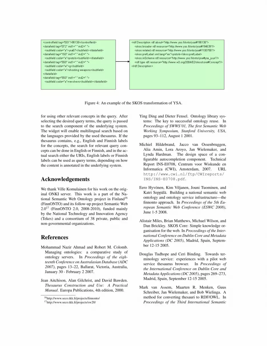
Figure 4: An example of the SKOS transformation of YSA.
for using other relevant concepts in the query. Afterselecting the desired query terms, the query is passedto the search component of the underlying system.The widget will enable multilingual search based onthe languages provided by the used thesaurus. If thethesaurus contains, e.g., English and Finnish labelsfor the concepts, the search for relevant query con-cepts can be done in English or Finnish, and in the ac-tual search either the URIs, English labels or Finnishlabels can be used as query terms, depending on howthe content is annotated in the underlying system.
AcknowledgementsWe thank Ville Komulainen for his work on the orig-inal ONKI server. This work is a part of the Na-tional Semantic Web Ontology project in Finland16
(FinnONTO) and its follow-up project Semantic Web2.017 (FinnONTO 2.0, 2008-2010), funded mainlyby the National Technology and Innovation Agency(Tekes) and a consortium of 38 private, public andnon-governmental organizations.
ReferencesMohammad Nazir Ahmad and Robert M. Colomb.
Managing ontologies: a comparative study ofontology servers. In Proceedings of the eigh-teenth Conference on Australasian Database (ADC2007), pages 13–22, Ballarat, Victoria, Australia,January 30 - February 2 2007.
Jean Aitchison, Alan Gilchrist, and David Bawden.Thesaurus Construction and Use: A PracticalManual. Europa Publications, 4th edition, 2000.
16http://www.seco.tkk.fi/projects/finnonto/17http://www.seco.tkk.fi/projects/sw20/
Ying Ding and Dieter Fensel. Ontology library sys-tems: The key to successful ontology reuse. InProceedings of SWWS’01, The first Semantic WebWorking Symposium, Stanford University, USA,pages 93–112, August 1 2001.
Michiel Hildebrand, Jacco van Ossenbruggen,Alia Amin, Lora Aroyo, Jan Wielemaker, andLynda Hardman. The design space of a con-figurable autocompletion component. TechnicalReport INS-E0708, Centrum voor Wiskunde enInformatica (CWI), Amsterdam, 2007. URLhttp://www.cwi.nl/ftp/CWIreports/INS/INS-E0708.pdf.
Eero Hyvonen, Kim Viljanen, Jouni Tuominen, andKatri Seppala. Building a national semantic webontology and ontology service infrastructure—thefinnonto approach. In Proceedings of the 5th Eu-ropean Semantic Web Conference (ESWC 2008),June 1-5 2008.
Alistair Miles, Brian Matthews, Michael Wilson, andDan Brickley. SKOS Core: Simple knowledge or-ganisation for the web. In Proceedings of the Inter-national Conference on Dublin Core and MetadataApplications (DC 2005), Madrid, Spain, Septem-ber 12-15 2005.
Douglas Tudhope and Ceri Binding. Towards ter-minology service: experiences with a pilot webservice thesaurus browser. In Proceedings ofthe International Conference on Dublin Core andMetadata Applications (DC 2005), pages 269–273,Madrid, Spain, September 12-15 2005.
Mark van Assem, Maarten R. Menken, GuusSchreiber, Jan Wielemaker, and Bob Wielinga. Amethod for converting thesauri to RDF/OWL. InProceedings of the Third International Semantic

Web Conference (ISWC 2004), pages 17–31, Hi-roshima, Japan, November 7-11 2004.
Mark van Assem, Veronique Malaise, Alistair Miles,and Guus Schreiber. A method to convert thesaurito SKOS. In Proceedings of the third European Se-mantic Web Conference (ESWC 2006), pages 95–109, Budva, Montenegro, June 11-14 2006.
Kim Viljanen, Jouni Tuominen, and Eero Hyvonen.Publishing and using ontologies as mash-up ser-vices. In Proceedings of the 4th Workshop onScripting for the Semantic Web (SFSW 2008), 5thEuropean Semantic Web Conference 2008 (ESWC2008), Tenerife, Spain, June 1-5 2008.
Diane Vizine-Goetz, Eric Childress, and AndrewHoughton. Web services for genre vocabularies.In Proceedings of the International Conference onDublin Core and Metadata (DC 2005), Madrid,Spain, September 12-15 2005.

Document Expansion Using Ontological Concept Clustering
Matias FrosterusSemantic Computing Research Group (SeCo)
Helsinki University of Technology (TKK), Laboratory of Media TechnologyUniversity of Helsinki, Department of Computer Science
[email protected], http://www.seco.tkk.fi/
Abstract
This paper presents a document search architecture utilizing document expansion done through onto-logical concept clustering in a given domain. Documents in adatabase are automatically annotatedwith concepts from a given ontology and these annotations are expanded into concept clusters basedon the ontological hierarchy. Different ontological relations give different weights to the members ofthe concept cluster and the resulting weighted concepts areadded to the metadata of the respectivedocuments. When a search is conducted, the query terms are matched to their respective ontologicalconcepts and these are used to perform a second query to the concept metadata of the documents. Whenthe results of these two queries were combined in an intelligent manner, a better recall was achievedwithout it adversely affecting the precision of the result set.
1 Introduction
The importance of Internet in information retrievalcontinues to grow. As the amount of information in-creases so does the amount of irrelevant informationand the result set given in answer to a common one ortwo word query can include millions of documents.Traditionally the way of winnowing out the irrelevantdocuments is done by expanding the original querywith new search terms, also known as manual queryexpansion. The problem is that this isn’t as simple asthe original search process and requires some exper-tise from the user. Automatic query expansion strivesto simplify this process but it is always limited by thefact that the program does not understand the mean-ings and reasons behind the query or the documentsgiven as results.
Semantic Web has been slated to complement andreplace the current Internet infrastructure with ma-chine understandable information by explicitly at-taching the meaning of said data. A database whosesemantic relations have been described allows forhigher level automation and in the case of informa-tion retrieval this translates to simpler queries whichproduce more relevant result sets. (Berners-Lee et al.,2001)
The common way of describing semantic relationsbetween concepts is using ontologies as explicit spec-ification of conceptualization (Gruber, 1993). Theycan be used to present a hierarchy of concepts with
different relations to each other in a machine under-standable format and therefore provide a frameworkfor automatic deduction of meaning from text. Whenthese relations are given weights representing eitherpartial relations or probabilities, they can be used tomodel fuzzy information (Holi and Hyvonen, 2004).
Besides adding semantics to data and striving tounderstand user queries on a deeper level, a some-what simpler approach to automatically improvingsearch results is query expansion. Basically auto-mated query expansion can be broken down intomethods based on search results and ones based onknowledge structures, the latter of which can be fur-ther grouped into collection dependent and collectionindependent methods (Efthimiadis, 1996). Methodsbased on search results first perform a query usingthe query terms as given by the user after which anew query is formed based on terms with high occur-rence in the result set. Methods based on knowledgestructures either use corpus-based knowledge of, forexample, correlations between different terms or usesome a priori knowledge like relations between dif-ferent concepts. This latter approach lends itself wellto document expansion where the query expansionisn’t done dynamically in response to a user querybut rather in advance during indexing.

2 Ontological Concept Cluster-ing
2.1 Overview
The basic premise behind ontological concept clus-tering is to provide an automatic system to make useof semantic information in documents in order to pro-vide the user with larger and more relevant result setswithout adding complexity to the user interface. Theidea is to first recognize the ontological concepts ex-plicitly present in the text in the form of terms thatmatch those concepts and then to expand these intolarger aggregates made up of semantically connectedconcepts with differing weights based on the impor-tance of their connection. The process is depictedwith the supposition that the ontology is presented asa collection of triplets in the form of the RDF lan-guage1.
Figure 1: The process of document expansionthrough ontological concept clustering
The process of document expansion through on-tological concept clustering is depicted in Figure 1with the focal parts picked out in yellow boxes. Theprocess starts with the lemmatization of a given doc-ument after which the text is indexed with the con-vetional TF-IDF method(Salton and McGill, 1983).Each term in the document is also matched to an on-tological concept through labels present in the ontol-ogy. If a match is found, the concept’s URI is addedto the document’s metadata. Several ontologies canbe used and the concepts found from each are savedin their own fields and a separate index is built foreach one.
Once the relevant concepts for a document havebeen extracted, the actual concept clustering is per-formed. This expands individual concepts into con-
1http://www.w3.org/RDF/
cept clusters comprised of the original concept corre-sponding to a term in the text, as well as other, on-tologically closely related concepts. This is done byfollowing an ontology specific pattern expressed in apattern language developed for the task (see 2.2).
A pattern is comprised of paths made up of rela-tions in the target ontology both hierarchical and as-sociative. Each path contains knowledge of the spe-cific relations, or steps, that make up the path, thedepth to which those relations are to be followed aswell as a weighting coefficient which determines theimportance given to the path in question. Each step ofthe path includes a relation and whether it should betraversed towards the object or the subject. Follow-ing a path is done by taking the first relation of thepath as a predicate and searching for all the tripletswhich include the original concept node as their sub-ject or object depending on the traversing direction ofthe step. This procedure is done iteratively for eachstep in the path with the objects or subjects of the re-sulting set of triplets as the new starting point nodesfor the next step.
After the expansion is done, the cluster is com-prised of the original concept with a weight of oneand a number of other, semantically related conceptswith varying weights between zero and one. In prac-tice these weights should be kept low so as not to ob-scure the original concepts that occur as terms in thetext. For the final cluster the weights are multipliedby the frequency of occurrence of the original con-cept. The use of some kind of balancing function inthis step is also usually necessary in order to avoid asingle concept with a high occurrence frequency fromdragging its whole cluster up too high in the final in-dex.
After the concept clustering has been performedfor every concept found in the document, the clustersare added together and the weights are rounded to thenearest integer. Finally, the URI of each concept isadded to their respective ontological index a numberof times indicated by the rounded sum of the weights.
When a query is performed into the system, it islemmatized and directed to the text index as normal.Additionally, an ontological concept matching is per-formed and the resulting concepts are used as furtherqueries into the corresponding ontological conceptindices. The responses from all of these queries canthen be combined in several different ways to producedifferent outcomes. Some possibilities are describedin the evaluation section (see 3.2).
A more conservative addition to the traditionaltext search is a recommendation system integrating aquery expansion component based utilizing the con-

cept clustering. The recommendation algorithm picksa number of the most relevant documents returned bythe text search, for example ten. These documentsare then searched for the concepts that occur in morethan one document and an intersection of the foundconcepts is used to form a new query into the conceptindex of the database. Further constraints are possi-ble based on some metadata present in the originalresult set. For example a time window can be addedso that the recommendation results must fit within acertain time interval based on the temporal metadatain the oldest and the newest document in the originalresult set. After a recommendation set is acquired, thesystem removes those documents from the set that ap-peared in the original result set. This method providesan entirely separate set of documents that are stronglyrelated to the original patch through ontological con-cepts and relations.
2.2 Pattern language
The most crucial part of ontological concept cluster-ing is the pattern which defines the ontological rela-tions that are to be followed when constructing a clus-ter around a given concept. A pattern is comprised ofpaths made up of hierarchical and associative rela-tions in a given ontology. It is ontology-specific andshould be tailored to a specific database to take fulladvantage of the proposed method as different do-mains place varying emphasis on different relations.Because of this patterns should be easy to constructwhen configuring the system for new applications.An XML-based pattern language was developed withthis in mind.
The basic layout of a pattern is as follows:
• A pattern is comprised of one or several paths
• A path is comprised of one or several relationsor steps
• Each path includes a weight which is applied tothe resources at the end of the path
Each step of the path includes a relation and knowl-edge on whether it should be traversed towards theobject or the subject of the triplet. This has to be donebecause triplets are directed and not all relations havean inverse relation specified, but it can still be usefulto traverse the relation in that direction. An exampleof this is RDF Schema’s subClassOf-relation, whichis used to build the class hierarchy for ontologies. Aninverse superClassOf-relation is not normally explic-itly defined, yet it is often interesting to traverse thehierarchy towards subclasses as well as superclasses.
Aside from these obligatory definitions, the pat-tern language includes a number of definitions forease of use. First one is depth, which determineshow many times a given step is to be performed un-til proceeding to the next step. Another is inclu-siveness, which determines whether the weight is tobe applied to every concept along the path or justthe final set at the end of the last step. The fullXML-Schema of the pattern language can be foundin http://www.seco.tkk.fi/tools/airo/pattern.xsd
3 Evaluation
3.1 The Test System
In order to evaluate the usefulness of ontological con-cept clustering, an application called Airo2 was real-ized. Airo was coded in Java and uses Jena frame-work3 for easy handling of ontologies and Lucene4
for search and indexing tasks. It provides a simpleimplementation of the ontological concept clusteringas well as search capability based on it. The GeneralFinnish Ontology (YSO)5 was used as a test ontol-ogy and the indexed dataset consisted of 8000 arti-cles from the newspaper Helsingin Sanomat. For theactual tests an information retrieval test system madeby Cross Language Evaluation Forum (CLEF)6 wasused. The specific version used was ELRA-E00008The CLEF Test Suite for the CLEF 2000-2003 Cam-paigns whose Finnish test set is comprised of articlesfrom the newspaper Aamulehti and search tasks con-nected to these. The tests were done with all of the60 search tasks of the year 2003.
The search tasks in the test suite are comprised of atitle, which gives the topic of the task, a short descrip-tion, which defines the task and a longer narrative,which describes the situation behind the task and de-scribes the limitations on the kind of articles that areconsidered relevant to the query. Since Airo doesn’tinclude natural language processing functions, onlythe titles were used to construct the queries. The eval-uation itself is done by comparing the articles given asa result for a search task by the system to a relevancefile which lists the binary relevance of each article inthe database for each query. It is worth noting that thedatabase provided doesn’t include any relevant docu-ments for some of the search tasks.
2http://www.seco.tkk.fi/tools/airo/3http://jena.sourceforge.net/4http://lucene.apache.org/5http://www.yso.fi/onki/yso/6http://www.clef-campaign.org/

The pattern used in the clustering is depicted in Ta-ble 1. Each of the rows in the table describes onepath. The first row shows the relations that make upthe path with either (s) or (o) depending on whetherthe relation is to be followed starting from the sub-ject or the object of the triplet. Depth defines howmany times the particular relation is to be iteratedand weight tells how much importance is given tothe relation in question. For example in the last twopaths a higher weight is given to the subclasses of agiven concept than its superclasses. Last, inclusive-ness governs whether all the concepts encounteredshould be weighted or only the ones at the end of thepath. If it were set to true in the first path, it wouldgive weight to both the superclasses as well as theparallel classes.
Table 1: The clustering pattern used for the evaluation
Relations of path Depth Weight InclusivesubClassOf (s), 1,1 0.05 falsesubClassOf (o)associativeRelation (s) 1 0.2 truesubClassOf (s) 1 0.05 truesubClassOf (0) 1 0.1 true
3.2 The Results
Five different search setups were used for each of thesearch tasks:
• Text search refers to the traditional search wherethe lemmatized search terms were queried fromthe text index
• In Concept search the search terms werematched with ontological concepts from YSOand these were used to query the concept index
• Text and concept search combines the previoustwo queries through Lucene’s Boolean should-operator which corresponds to a union
• Recommendation is comprised of the elevenmost relevant articles gotten through the queryexpansion method described earlier
• Smartly combined text search and recommen-dation means that the fifteen most relevant textsearch results are listed first, after which tenmost relevant recommendation results are listedand followed by the rest of the text search results
A maximum of 1000 documents were consideredwhen evaluating result sets. The most importantevaluation criteria for information retrieval systemsare precision and recall. Precision is the fraction ofthe documents retrieved that are considered relevantwhile recall is the fraction of the documents that arerelevant that are successfully retrieved. It is oftenpossible to improve one at the expense of the other(Efthimiadis, 1996). The recall and precision of thefive different search setups are depicted in Figure 2.
Figure 2: The recall and precision of different searchsetups
The values of both precision and recall are betweenone and zero and the scores of text search should beregarded as the base level against which the othersshould be compared to. From the figure it can beseen that the recall of both, concept search and textand concept search combined are really high but re-spectively the precision of both is really low. Thisis to be expected because concept search retrieves amuch higher amount of documents than traditionaltext search and therefore returns also a large numberof the relevant documents.
In recommendation precision is slightly higher andrecall somewhat lower than in text search, the last ofwhich occurs because the maximum number of re-turned documents was set to eleven, which is lowerthan the number of articles listed as relevant in thecase of some search tasks. A feature worth notinghere is that due to the algorithm used, the result set iscompletely different from the result set that was got-ten for the traditional text search. This can be seenin effect in the next setup, smartly combined text re-search and recommendation where the recall is sim-ply the sum of the recall of text search and recom-mendation. Precision on the other hand is the averageof the precision of the two component methods.
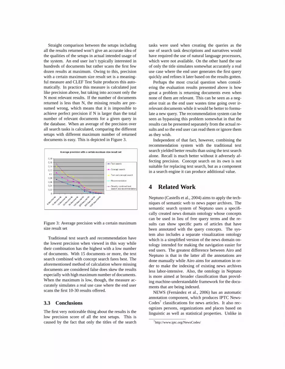
Straight comparison between the setups includingall the results returned won’t give an accurate idea ofthe qualities of the setups in actual intended usage ofthe system. An end user isn’t typically interested inhundreds of documents but rather scans the first fewdozen results at maximum. Owing to this, precisionwith a certain maximum size result set is a meaning-ful measure and CLEF Test Suite produces this auto-matically. In practice this measure is calculated justlike precision above, but taking into account only theN most relevant results. If the number of documentsreturned is less than N, the missing results are pre-sumed wrong, which means that it is impossible toachieve perfect precision if N is larger than the totalnumber of relevant documents for a given query inthe database. When an average of the precision overall search tasks is calculated, comparing the differentsetups with different maximum number of returneddocuments is easy. This is depicted in Figure 3.
Figure 3: Average precision with a certain maximumsize result set
Traditional text search and recommendation havethe lowest precision when viewed in this way whiletheir combination has the highest with a low numberof documents. With 15 documents or more, the textsearch combined with concept search fares best. Theaforementioned method of calculation where missingdocuments are considered false does skew the resultsespecially with high maximum number of documents.When the maximum is low, though, the measure ac-curately simulates a real use case where the end userscans the first 10-30 results offered.
3.3 Conclusions
The first very noticeable thing about the results is thelow precision score of all the test setups. This iscaused by the fact that only the titles of the search
tasks were used when creating the queries as theuse of search task descriptions and narratives wouldhave required the use of natural language processors,which were not available. On the other hand the useof only the title simulates somewhat accurately a realuse case where the end user generates the first queryquickly and refines it later based on the results gotten.
Perhaps the most crucial question when consid-ering the evaluation results presented above is howgreat a problem is returning documents even whennone of them are relevant. This can be seen as a neg-ative trait as the end user wastes time going over ir-relevant documents while it would be better to formu-late a new query. The recommendation system can beseen as bypassing this problem somewhat in that theresults can be presented separately from the actual re-sults and so the end user can read them or ignore themas they wish.
Independent of that fact, however, combining therecommendation system with the traditional textsearch yielded better results than using the text searchalone. Recall is much better without it adversely af-fecting precision. Concept search on its own is notsuitable for replacing text search, but as a componentin a search engine it can produce additional value.
4 Related Work
Neptuno (Castells et al., 2004) aims to apply the tech-niques of semantic web to news paper archives. Thesemantic search system of Neptuno uses a specifi-cally created news domain ontology whose conceptscan be used in lieu of free query terms and the re-sults can show specific parts of articles that havebeen annotated with the query concepts. The sys-tem also includes a separate visualization ontologywhich is a simplified version of the news domain on-tology intended for making the navigation easier forend users. The greatest difference between Airo andNeptuno is that in the latter all the annotations aredone manually while Airo aims for automation in or-der to make the indexing of existing news archivesless labor-intensive. Also, the ontology in Neptunois more aimed at broader classification than provid-ing machine-understandable framework for the docu-ments that are being indexed.
NEWS (Fernandez et al., 2006) has an automaticannotation component, which produces IPTC News-Codes7 classifications for news articles. It also rec-ognizes persons, organizations and places based onlinguistic as well as statistical properties. Unlike in
7http://www.iptc.org/NewsCodes/

Airo, annotations are based on a fairly limited num-ber of classes, which are extensively instantiated andagain the focus isn’t on fully annotating natural lan-guage terms into their ontological concept counter-parts. Disambiguation in NEWS is done according totwo principles: semantic coherence, which is some-what similar to concept clustering, and news trendswhich takes into account the annotations in othernews articles of the same period. Semantic coherencediffers from concept clustering in that it is stronglybased on previous articles and their annotations as op-posed to ontological information.
KIM (Popov et al., 2003) is another semantic in-dexing, annotation and search system, whose centralfunctionality is recognition of named entities instan-tiated from ontological classes. It also includes rules-based methods of recognizing and creating new in-stances from text. Disambiguation in KIM is donethrough clues based on wordlists, but disambiguationbetween entities with the same name isn’t discussed.
5 Future Work
Much of the future work pertaining to Airo has to dowith improving the extrinsic factors like the qualityof the patterns and the ontologies used.
The chief problem in the evaluation was the limitedamount of configuration that was done. The ontologyused was not specifically designed for news domainand is far from optimal for the data that was used inthe evaluation. As an example of this, YSO includesa number of two-way associative relations that are es-sentially one-way relations in the news domain. Forexample, the YSO concept of children as family rela-tionship has an associative relation to incest. In mostpractical situations the concept of incest has an as-sociative relation to children but not vice versa. An-other example is the lack of many relations that areobvious to humans. For example the concepts of icehockey and ice hockey players have no relation be-tween them and they are in widely different places inthe class hierarchy. Though in reality these two con-cepts are highly correlated, Airo could not make thisconnection. The only way to fix this problem is touse an ontology that fits the domain of the databasebetter.
Also the pattern designed for the evaluation wasthe only one tested and very likely it is not optimalfor the data or the ontology. One future interest isin creating a learning system which constructs opti-mized patterns based on training data. The simplestway of accomplishing this would be to create a setof paths based on the relations in the ontology and
then varying the parameters on those paths until anoptimal score in recall and precision was achieved. Amore sophisticated solution based on neural networksmight also be possible.
One crucial component of the system is the originalmatching of terms found in the text to their respec-tive ontological concepts. For the system to behaveoptimally, the concepts must be disambiguated prop-erly. If the ontology is large enough with a relativelydense network of relations so that most of the termsin the documents that are being indexed can be foundthere, concept clustering could be used as a disam-biguation tool. By making clusters for the conceptsthat were derived from unambiguous terms it is likelythat these clusters give different weights to differentpossible concepts of the ambiguous terms. Testingthis fully would again require a more comprehensiveontology than was available, but it is of future inter-est.
6 Acknowledgements
This research was part of the National Finnish On-tology Project (FinnONTO) 2003-200720 , fundedmainly by The National Technology Agency (Tekes)and a consortium of 36 companies and public organi-sations. The work continues in FinnONTO 2.0 (2008-2009) project.
References
T. Berners-Lee, J. Hendler, and O. Lassila. TheSemantic Web. Scientific American, 284:28–40,2001.
P. Castells, F. Perdrix, E. Pulido, M. Rico, R. Ben-jamins, J. Contreras, and J. Lores. Neptuno: Se-mantic web technologies for a digital newspaperarchive. InThe Semantic Web: Research and Ap-plications, pages 445–458, 2004.
E. Efthimiadis. Query Expansion.Annual Review ofInformation Science and Technology, 31:121–187,1996.
Norberto Fernandez, Jose M. Blazquez, Jesus A.Fisteus, Luis Sanchez, Michael Sintek, AnsgarBernardi, Manuel Fuentes, Angelo Marrara, andZohar Ben-Asher. News: Bringing semantic webtechnologies into news agencies. InThe SemanticWeb - ISWC 2006, pages 778–791, 2006.

T. R. Gruber. A translation approach to portable on-tology spesifications. Knowledge Acquisition, 5(2):199–220, 1993.
Markus Holi and Eero Hyvonen. A method for mod-eling uncertainty in semantic web taxonomies. InProceedings of WWW2004, New York, AlternateTrack Papers and Posters, May 2004.
B. Popov, A. Kiryakov, D. Ognyanoff, D. Manov,A. Kirilov, and M. Goranov. Towards SemanticWeb Information Extraction.proceedings of ISWC(Sundial Resort, Florida, USA, October, 2003),pages 1–23, 2003.
G. Salton and M.J. McGill.Introduction to ModernInformation Retrieval. 1983.

Adaptive Tension Systems: Towards a Theory of Everything?
Heikki HyotyniemiHelsinki University of Technology
Control Engineering LaboratoryP.O. Box 5500, FIN-02015 TKK, Finland
Abstract
Assuming that there really exists some general theory of complex systems, one has strong guidelinesfor where to search for it. Such theory has to address the distributedness of the underlying actors inthe absence of central control, and it has to explain emergence in terms of self-regulation and somekind of self-organization of higher-level structures. It is the neocybernetic framework of AdaptiveTension Systems (also known as “elastic systems”) that is one candidate theory offering such visions,making it possible to make assumptions about the “Platonian Ideals” of complex interacting systems.As application examples, this methodology is here employed for analysis of molecular orbitals andorbiting mass systems.
1 Introduction
It is intuitively clear that there is something in com-mon beyond different kinds of complex systems —is it not? At least in the complexity and chaos the-ory communities such belief has been loudly pro-moted. However, as the promises have never beenredeemed, this “chaoplexity” research is seen as anicon of “ironic science”. The complexity theory can-not be based merely on intuitions.
But the “theory of everything” should neither bebased only on mathematics, as has been claimed bythe quantum theorists (Ellis, 1986). Not everythingcan be expressed in formulas in a credible way —even though system hierarchies are finally reducibleto the level of elementary physics, quantum theoriesdo not offer the best modeling framefork for, say,cognitive systems. However good models for micro-scopic phenomena can be found, they have little to dowith macroscopic systems; they are not the most eco-nomical way of describing the emergent-level phe-nomena, thus being no good models at that level.
What is a good compromize between the extremelyheuristic visions and the utterly down-to-earth analy-ses? Mathematics is a necessary language, but intu-ition and heuristics should be guiding what kind ofmathematical constructs are discussed; there are toomany directions available, but only a few of the routeslead to directions addressing relevance. What, then,are the relevant issues to be emphasized?
The underlying realms beneath complex systemsare very different. However, something is shared by
all of them: They all consist of distributed networkswhere local-level interactions of more or less mind-less actors with only very simple functionalities resultin self-regulation and self-organization that is visi-ble on the global level. The divergence of the mod-els, in the spirit of the celebrated “butterfly effect”is just an illusion, as it is conververgence and stabil-ity that that are the key issues in surviving systems.It seems that the framework of adaptive tension sys-tems based on the neocybernetic theory (also knownas elastic systems) offers the necessary functionalities(Hyotyniemi, 2006). It turns out that the emergingstructures can be studied in the framework of prin-cipal components (Basilevsky, 1994). How to detectthe cybernetic nature of a system, then?
Traditionally, the similarities between complexsystems are searched for in the static (fractal) surfacepatterns. However, the deep structures based on in-teractions and feedbacks are dynamic and they canonly be captured by mathematical tools: the actualobserved patterns are dynamic balances in the dataspace, and potential patterns are characterized by dy-namic attractors. The similarities in underlying struc-tures are analogies between mathematical represen-tations. Or, being more than formal similarities, suchanalogies should perhaps be called homologies. In-deed, there exist some mathematical structures thatcan be seen as manifestations of the neocybernetic or-dering principle.
Nothing very exotic takes place in neocyberneticmathematics – no “new science” is needed. Old sci-ence suffices, but the new interpretations spawn a

completely new world. Surprisingly, the resultingmodels are analogical with cognitive ones, so that thesubjective and objective “everything” can perhaps beunited once again.
In this paper, it is shown how the above view can beexploited in analysis of physical systems, small andbig. As application examples, modeling of moleculesand modeling of celestial bodies, are discussed.
2 Neocybernetics in the small
What if elementary physics were simpler than whathas been believed, what if understanding moleculeswould not take a nuclear physicist? Below, the neo-cybernetic analogy in cost criteria is employed.
2.1 Standard theories of molecules
Atoms are already rather well understood. The con-temporary theory of atom orbitals can explain theirproperties to sufficient degree. However, it seems thatone needs new approaches to understand the emer-gent level, or the level of molecules. Molecular or-bitals are interesting because the chemical propertiesof compounds are determined by their charge dis-tribution — essentially these orbitals reveal how themolecule is seen by the outside world.
The molecules have been a challenge for modernphysics for a long time, and different kinds of frame-works have been proposed to tackle with them: First,there are the valence bond theories, where the indi-vidual atoms with their orbitals are seen as a construc-tion kit for building up the molecules, molecule or-bitals being just combinations of atom orbitals; later,different kinds of more ambitious molecule orbitaltheories have been proposed to explain the emergentproperties of molecules. In both cases it is still theideas of atom orbitals that have been extended to themolecules. Unfortunately it seems that very oftensome extra tricks are needed: for example, to explainthe four identical bonds that carbon can have, pecu-liar “hybridizations” need to be employed; and stillthere are problems, a notorious example being ben-zene (and other aromatic compounds) where the “bot-tom up” combinations of atom orbitals simply seemto fail. And, unluckily, it is exactly carbon and itsproperties that one has to tackle with when trying toexplain living systems and their building blocks.
When thinking of alternative approaches, it is en-couraging that molecules have been studied applyingdiscretized eigenvalues and eigenvectors, too: for ex-ample, Erich Huckel proposed an approach that is
known as Huckel’s method, also reducing the anal-ysis of energy levels in molecules into essentially aneigenvalue problem (Berson, 1999). However, thismethod is still based on combinations of atom or-bitals, and being based on crude simplifications, it isregarded as an approximation.
It is also quite commonplace that linear additiv-ity of orbitals is assumed on the molecular level —normally it is atomic orbitals that are added together,now it is molecular orbitals directly. Indeed, basicphysics is linear; the problems are normally causedby the huge dimensionality of the problems. Thisall — linearity, eigenvectors — sounds like veryneocybernetics-looking.
The challenge here is to combine the neocyberneticmodel with current theories and models.
2.2 Cybernetic view of electrons
There is no central control among individual elec-trons, but the electron systems — atoms, molecules— still seem to be stable and organized. Either thereis some yet unknown mechanism that is capable ofmaintaining the stability and the structures — or, it isthe neocybernetic model that applies. The latter as-sumption is now applied, and the consequences arestudied. It is assumed that “electron shells”, etc., arejust emergent manifestations of the underlying dy-namic balances.
The starting point (set of electrons) and the goal(cybernetic model) are given, and the steps in be-tween need to be motivated1. So, assume that thenuclei are fixed (according to the Born-Oppenheimerapproximation), and drop the electrons in the systemto freely search their places.
When studying the elementary particles, traditionalthinking has to be turned upside down: For example,it seems that in that scale the discrete becomes con-tinuous, and the continuous becomes discrete. Dis-tinct electrons have to be seen as delocalized, contin-uous charge distributions; however, their interactionshave to be seen not as continuous but discrete, beingbased on stochastic photons being transmitted amongthe interacting charge fields. This view needs to befunctionalized.
First, study the macroscopic scale. Assume thatthere are two charge fields i and j, variables xi andxj representing their intensities. Energy that is storedin the potential fields can be calculated within a single
1Of course, “knowing” the end points and trying to fill the re-maining gap, is a risky way to proceed!

charge field as
Ji,i = c
∫ xi
0
ξ dξ =12c x2
i , (1)
where c is a constant, and among overlapping fieldsas
Ji,j = c
∫ xi
0
xj dξ = c xixj . (2)
If the charges of i and j have the same sign, the poten-tial is positive, denoting repulsion; otherwise, there isattraction.
However, the macroscopic phenomena are emer-gent and become analyzable only through statisticalconsiderations; in microscopic scales, there are nocharges to be observed, only interactions. For twofields i and j to intreract, the photons emitted by thefields need to meet — denote this probability by p i,j .Then the effective potential is
J ′ = p1,1J1,1 + p1,2J1,2 + · · ·+ pn,nJn,n. (3)
The symbols xi and xj have dual interpretation: theyconstitute the charge distributions, but simultane-ously they are probability distributions. As the pho-ton transmission processes are independent, the inter-action probability pi,j is proportional to the averageproduct of the intensities, or xixj , so that
pi,j = E xixj . (4)
Assume that the charge fields are divided into twoclasses, the negative ones into “internal” and the pos-itive into “external” ones. Further, assume that theexternal fields are collected in the vector u, internalones remaining in x. The sum of energies among thenegative charge fields can be presented in matrix formas
J ′ =12xT E
xxT
x, (5)
and, correspondingly for positive charges,
J ′′ = −xT ExuT
u. (6)
For the total energy one has
J(x, u) = J ′ + J ′′
= 12x
T ExxT
x− xT E
xuT
u.
(7)
The above criterion J(x, u) is exactly the samecost criterion that was derived for ordinary(neo)cybernetic systems (here it is assumed thatthe balance is found immediately, so that x ≡ x).This means that when appropriate interpretations areemployed, and when the cost criterion is minimizedover time, the solutions for electron configurations
implement the emergent neocybernetic structures(Hyotyniemi, 2006). If the assumptions hold, thereis self-regulation and self-organization among theelectrons, emerging through local attempts to reachpotential minimum. Not all electrons can go tothe lowest energy levels, and “electronic diversity”emerges automatically. Surprisingly, because oftheir delocalization, “overall presence” and mutualrepulsion, the electron fields implement explicitfeedback, following the model of “smart cyberneticagents” (see (Hyotyniemi, 2006)).
The result is that the charge distribution along themolecule (molecular orbital) is given by the principalcomponents of the interaction correlation matrix thatcan be calculated when the organization of the nucleiis known. Because of the distinct nature of electrons,they cannot be located in various energy levels simul-taneously and eigenvalues become distinguished.
When speaking of molecules, the “inputs” uj de-note the more or less fixed positive nuclei, whereasxi denote the molecular orbitals within the molecule.
It is interesting to note that there are no kineticenergies involved in the energy criterion, and no ve-locities or accelerations are involved. As seen fromthe system perspective, the charges are just static“clouds”. This means that some theoretical prob-lems are now avoided: As there are no acceleratingcharges, there are no electrodynamic issues to be ex-plained as no energy needs to be emitted, and the sys-tem can be in equilibrium. In contrast, such elec-trodynamic inconsistencies plagued the traditionalatom models where it was assumed that the electronsrevolved around the nucleus, experiencing constantcentripetal acceleration, so that radiation of energyshould take place.
What is the added value when studying the newview of molecules? Whereas the electrons are delo-calized, the heavier nuclei can be assumed to be betterlocalized. The key observation here is that the analy-sis of the continuous space — modeling of the chargedistribution of electrons — changes into an analysisof a discrete, finite set of variables, or the nuclei. Theidea of neocybernetic “mirror images” is essentiallyemployed here: rather than studying the system it-self, the electrons, its environment is analyzed. Inthis special case it is the environment that happens tobe simpler to operate on.
Because of the properties of eigenvectors, the dis-crete orbitals are mutually orthogonal. Traditionally,it is assumed that there is just room for a unique elec-tron in one orbit (or, indeed, for a pair of electronswith opposite spins). However, now there can bemany electrons in the same orbital, and there is no

need to employ external constraints about the struc-tures, like assumptions of spins, etc. The charge fieldcan be expressed as ψi =
√λi φi, where λi is the
eigenvalue corresponding to the orbital-eigenvectorφi, so that the overall charge becomes ψT
i ψi = λi.The “variance” λi is the emergent measurable totalcharge in that field. This means that there are someconditions for the charge fields to match with the as-sumption of existence of distinct charge packets:
1. Eigenvalue λi has to be an integer times the el-ementary charge, this integer representing thenumber of electrons in that orbital.
2. The sum of all these integers has to equal thenumber of valence electrons, sum of all freeelectrons in the system.
These constraints give tools to determine the balanceconfiguration among the nuclei.
How to quantize the continuous fields, and how tocharacterize the effects in the form EuuT, and howto determine the parameters? And how is this all re-lated to established quantum theory? In short, howare the above discussions related to real physical sys-tems?
2.3 Neocybernetic orbitals
It is the time-independent Schrodinger equation thatoffers a solid basis for all quantum-level analyses(Brehm and Mullin, 1989). It can be assumed to al-ways hold, and it applies also to molecules (h is thePlanck’s constant, andme is the mass of an electron):
− h2
8π2me
d2
dx2ψ(x) + V (x)ψ(x) = Eψ(x). (8)
Here, V (x) is the potential energy, and E is theenergy eigenvalue corresponding to the eigenfunc-tion ψ(x) characterizing the orbital. As ψ(x) iscontinuous, Schrodinger equation defines an infinite-dimensional problem, and as x is the spatial coordi-nate, in higher dimensions this becomes a partial dif-ferential equation. Normally this expression is far toocomplex to be solved explicitly, and different kinds ofsimplifications are needed. Traditional methods arebased on reductionistically studying the complex sys-tem one part at a time, resulting in approaches basedon the atom orbitals.
Now, start from the top: As studied in the previ-ous section, assume that it is simply a non-controlledplay among identical electrons that is taking place ina molecule. It is all “free” electrons that are on theoutermost shell that are available for contributing in
the orbitals, that is, for each carbon atom the numberof valence electrons in the system is increased by thenumber vC = 4, for hydrogen vH = 1, and for oxy-gen vO = 6. What kind of simplifications to (8) aremotivated?
The time-independent discrete Schrodinger equa-tion that is studied can be seen as a quantized versionof (8)
−V0φi + V φi = Eiφi, (9)
where φi are now vectors, 1 ≤ i ≤ n, dimensionsequalling the number n of atoms in the molecule;because of the structure of the expression, theseare the eigenvectors of the matrix V − V0 corre-sponding to the eigenvalues Ei. In the frameworkof the eigenproblem, now there is a connection tothe neocybernetic model structure. Comparing tothe discussions in the previous section, there holdsEi = λ2
i , the eigenvectors being the same. Ratherthan analysing the infinite dimensional distribution ofelectrons, study the finite-dimensional distribution ofnuclei; one only needs to determine the n × n ele-ments of the potential matrix V − V0 to be able tocalculate the orbitals (or the negative charge fieldsaround the positive nuclei).
To determine the matrix of potential energiesamong the nuclei, the challenge is to determine theterms corresponding to the first term in (8). The diag-onal entries of V − V0 are easy: Because the “lo-cal potential” is assumedly not essentially affectedby the other nuclei, the atoms can be thought to bedriven completely apart, so that the non-diagonal en-tries vanish; the diagonal entries then represent freeseparate atoms, so that the electron count must equalthe number of available valence electrons, that is, thei’th diagonal entry is proportional to v 2
i , where vi
presents the number of valence electrons in that atom.For non-diagonal entries, the sensitivity to changes todistant nuclei becomes small, so that the term withthe second derivative practically vanishes, and thecorresponding entry in the potential energy matrix isaccording to basic electrostatics approximately pro-portional to vivj/|rij |, without normalization. Here,|rij | stands for the distance between the nuclei i andj.
When the preliminary potential matrix has beenconstructed, elements of the matrix V − V0 have tobe justified so that the eigenvalues of the matrix be-come squares of integers, and the sum of those inte-gers equals the total number of valence electrons.
So, given the physical outlook of the molecule inequilibrium, one simply carries out principal compo-nent analysis for the “interaction matrix”V−V0, find-ing the set of “discrete orbitals”, or orbital vectors

-3 -2 -1 0 1 2 3-2.5
-2
-1.5
-1
-0.5
0
0.5
1
1.5
2
2.5
-3 -2 -1 0 1 2 3
-2
-1.5
-1
-0.5
0
0.5
1
1.5
2
-3 -2 -1 0 1 2 3-2.5
-2
-1.5
-1
-0.5
0
0.5
1
1.5
2
2.5
-3 -2 -1 0 1 2 3
-2
-1.5
-1
-0.5
0
0.5
1
1.5
2
-3 -2 -1 0 1 2 3
-2
-1.5
-1
-0.5
0
0.5
1
1.5
2
-3 -2 -1 0 1 2 3
-2
-1.5
-1
-0.5
0
0.5
1
1.5
2
-3 -2 -1 0 1 2 3
-2
-1.5
-1
-0.5
0
0.5
1
1.5
2
-3 -2 -1 0 1 2 3-2.5
-2
-1.5
-1
-0.5
0
0.5
1
1.5
2
2.5
-3 -2 -1 0 1 2 3
-2
-1.5
-1
-0.5
0
0.5
1
1.5
2
-3 -2 -1 0 1 2 3
-2
-1.5
-1
-0.5
0
0.5
1
1.5
2
-3 -2 -1 0 1 2 3-2.5
-2
-1.5
-1
-0.5
0
0.5
1
1.5
2
2.5
-3 -2 -1 0 1 2 3-2.5
-2
-1.5
-1
-0.5
0
0.5
1
1.5
2
2.5
~7
~3
~1
~1
~4
~3
~1
~1
~4
~3
~1
~1
Figure 1: “Cybernetic orbitals” ψi in the benzene molecule (see text). The larger dots denote carbon nuclei and the smallerones hydrogen nuclei, distances shown in Angstroms (1 A = 10−10 m). The orbitals, shown as circles around the nuclei, havebeen scaled by the corresponding λi to visualize their relevances. The circle colours (red or blue) illustrate the correlationstructures of electron occurrences among the nuclei (the colors are to be compared only within a single orbital at a time). Thereis a fascinating similarity with benzene orbitals as proposed in literature (for example, see Morrison and Boyd (1987))
ψi and the corresponding eigenvalues E i and elec-tron counts λi. The elements of the vectors ψi revealaround which nuclei the orbital mostly resides; theoverlap probability pij is spatial rather than tempo-ral.
For illustration, study the benzene molecule: ben-zene is the prototype of aromatic compounds, con-sisting of six carbon atoms and six hydrogen atoms ina carbon-ring. Altogether there are 30 valence elec-trons (6 times 4 for carbon, and 6 times 1 for hydro-gen). The results of applying the neocybernetic ap-proach are shown in Fig. 1. It seems that the three firstorbitals have essentially the same outlook as orbitalsproposed in literature — for example, see (Morrisonand Boyd, 1987) — but now there are altogether 7electrons on the lowest energy level! All orbitals ex-tend over the whole molecule; the hydrogen orbitalsare also delocalized, and such delocalization appliesto all molecules, not only benzene. Note that the or-bitals having the same energy levels are not unique,but any orthogonal linear combinations of them canbe selected; such behavior is typical to symmetric
molecules. The “bonding energy” is the drop in to-tal energy, or the difference between the energies inthe molecule as compared to the free atoms; possiblevalues of this energy are discretized, now it (withoutscaling) is 1·72+2·42+3·32+6·12−(6·42+6·12) =12.
The presented approach is general and robust: Forexample, the unsaturated double and triple bonds aswell as aromatic structures are automatically takencare of as the emerging orbitals only depend on thebalance distances between nuclei: If the nuclei re-main nearer to each other than what is normally thecase, there also must exist more electrons aroundthem. Spin considerations are not needed now, asthere is no need for external structures (orbitals of“two-only capacity”) to keep the system stable andorganized. However, no exhaustive testing has beencarried out for evaluating the fit with reality. In anycase, the objective here is only to illustrate the newhorizons there can be available when employing non-centralized model structures.

3 Neocybernetics in the large
Above, analyses were applied in the microscale —but it turns out that there are minor actors when look-ing at larger systems, too. Here, the neocyberneticapproaches are applied in cosmic dimensions. Afterall, the galaxes as well as solar systems seem to beself-organized stable structures. The domain field isvery different as compared to the previous one, and,similarly, the approaches need to be different. Onething that remains is that, again, one needs to ex-tensively employ intuitions and analogies. However,rather than exploiting the analogy in forms, as above,analogy in functions is applied this time.
3.1 From constraints to freedoms
As explained in (Hyotyniemi, 2006), neocyberneticmodels can be interpreted as seeing variation as in-formation. They try to search for the directionsin the data space where there is maximum visible(co)variation; as seen from above, this means thatsuch systems orientate towards freedoms in the dataspace. As exploitation means exhaustion, feedbacksthat are constituted by neocybernetic systems “suckout” this variation from the environment. Along theaxes of freedom, forces cause deformations: the sys-tem yields as a reaction to environmental tensions, tobounce back after the outside pressure is relieved —exactly this phenomenon is seen as elasticity in thesystem. When the system adapts, freedoms becomebetter controlled, meaning that the system becomesstiffer, or less elastic.
The challenge here is that such freedoms-orientedmodeling is less natural for human thinking thanmodeling that is based on constraints.
Indeed, all of our more complex mental modelsare based on natural language, and human languagesare tools to define couplings among concepts, or, re-ally, constraints that eliminate variability in the chaosaround us. As Ludwig Wittgenstein put it, “world isthe totality of states of affairs”, or the observed realityis the sum of facts binding variables together. What ismore acute, is Wittgenstein’s observation that all con-sistent logical reasoning consists only of tautologies.Similarly in all mathematical domains: axioms deter-mine the closure of trivialities, and it takes mathemat-ical intuition to reach outside the boundaries, findingthe freedoms where the “life” is. In a way, one is tofind the truths that cannot be deduced from the ax-ioms — in the Godelian sense!
When the natural languages set the standard of howto see the world, also natural laws are seen as con-straints: one searches for invariances, or formulas re-
vealing how physical constants are bound together. Inpractice, such invariances are equations — when theother variables in the formula are fixed, the last one isuniquely determined, so that its freedom is lost.
In the neocybernetic spirit, this all can be seen inanother perspective again. There is a duality of in-terpretations: whereas traditionally one searches forinvariants, now search for covariants. The idea isto apply the elasticity analogy: the same phenomenacan be represented, just the point of view changes.Emmy Noether first observed that all symmetries innature correspond to conservation laws; is it so thatall conservation laws can further be written as an elas-tic pairs of variables?
3.2 Another view at classical physics2
When exploiting the above idea of employing degreesof freedom in a new area, one first has to select an ap-propriate set of variables — such that they togethercarry emergy in that domain. When speaking of me-chanical systems in a central force field, it turns outthat one can select momentum to represent the inter-nal state of the mass point system, and force can beseen as external input:
x = p = mv and u = F =c
r2, (10)
where m is the mass of the mass point, v is its ve-locity, r is its distance from the mass center, and cis some constant. The central force is assumed to berelative to inverse of the squared distance; this holdsfor gravitational fields, for example.
How about the assumed covariation of the selectedvariables? — For a mass point orbiting a mass cen-ter, assuming that one only studies the angular move-ments, angular momentum can be defined as (Alonsoand Finn, 1980)
L = mv r. (11)
If there is no external torque, this quantity L remainsconstant, or invariant, no matter how v and r vary.Applying the invariance of angular momentum, it isevident that there is a coupling between the selectedvariables x and u, so that
x/√u = p/
√F = constant. (12)
The variables are also covariants even though themanifested elasticity relationship is now nonlinear.Now, following the steel plate analogy (Hyotyniemi,
2The derivations here (as in the previous case, too) are some-what sloppy, guided by the strong intuition, hoping that applyingsome more advanced analysis the loopholes can be somehow fixed
2006), there is internal energy and external energythat should be determined within the elasticity frame-work. From (10) one can solve for the stored internaland external energies, respectively:
Wint =∫ v
0
mν dν =12mv2
=12mr2
v2
r2=
12Iω2
Wext = −∫ ∞
ρ
c
ρ2dρ =
c
r,
(13)
where I is the inertia momentum of the rotating point-wise body, and ω = v/r is its angular velocity. Itis clear that these expressions stand for cumulatedkinetic energy and potential energy, respectively, sothat Wint = Wkin and Wext = Wpot. Thus, onecan see that the difference between internal and ex-ternal energies in this system transforms into a differ-ence between kinetic and potential energies — neo-cybernetic minimization of the deformation energythus changes into the Lagrangian functional that isknown to govern the dynamics of a mechanical sys-tem. Surpisingly, the Lagrangian that was found ap-plies not only to circular orbits but also to more gen-eral non-cyclic motions; the circular orbit representsthe (hypothetic) final balance.
The Lagrangian mechanics has exploited the La-grangians for a long time — is there some addedvalue available here? Applying the neocybernetic in-tuition, one can see that global behavior is an emer-gent phenomenon resulting directly from local low-level actions that one does not (and needs not) know.What is perhaps more interesting is that in the neocy-bernetic framework there is possibility to say some-thing about the adaptation, or evolution of the system.
On the local scale, minimization of the average de-formation energy means maximization3 of
E xu = E pF = cEmvr2
. (14)
What does this mean? The system evolution reallytries to maximize the product of the covariant vari-ables: evidently, a mass point tries to align its move-ment in the force direction — on average, applyingforce means acceleration in that direction. Newton’ssecond law (there holds F = mv for for alignedvectors) could be reformulated in a sloppy way asmomentum tries to increase if there is force acting,abstracting away exact representations characterizing
3Counterintuitively, local emergy maximization in adaptationresults in global system “laziness”, or deformation energy min-imization, similarly as local pursuit towards variation results inglobal system “equalization” and variation minimization
individual accelerations of particles along their tra-jectories.
There is no real long-term evolution, or “memory”in the system if there is just one mass point orbit-ing the mass center. But in a system of various masspoints the situation changes, and Exu can be max-imized. For example, in an early star / planet system,collisions make the system lose energy, as do the tidaleffects – average 1/r2 and v go down, meaning thatthe rotating bodies gradually get farther from the cen-ter, and their velocity drops. On the Earth, this can beseen in the lunar orbiting taking place ever slower.On the other hand, less circular orbits are more vul-nerable to collisions, average orbits becoming morespherical. As seen in observation data, variables seemto become more constant – and the system becomes“stiffer”. Thus, cosmic systems truly “learn” towardsbeing more and more cybernetic-looking.
Various mass points can be put in the same model,so that mivi are the state variables and Fi (in any di-rection!) are the forces acting on them, 1 ≤ i ≤ n.When the principal component structure of this cy-bernetic many-point system is studied, it turns outthat the model is more or less redundant: not alldirections in the n dimensional data space of the nmass points carry the same amount of information,many particles in the system behaving essentially inthe same way. Assume that the multi-body kineticenergy term 1
2 ωT Iω with the angular velocity vector
ω and (originally diagonal) inertia matrix I , is com-pressed so that the dimension is dropped from n byignoring the directions with least variation. This es-sentially means that one is no more speaking of meremass points but some kind of conglomerates withmore complicated internal inertial structure. One has“emergent inertia” – galaxies, etc., can be seen as vir-tually rigid bodies.
On the other hand, the inertia of 3-dimensionalobjects can be seen as an emergent phenomenon.For example, the velocities of sub-atomic particles inelectric fields are so high that when looking at ev-eryday objects, one only can see the emergent globalbehaviors that follow the laws of classical physics. Inthe cosmic scale, however, the adaptation towards thegravitational asymptotic structures still continues.
3.3 Further intuitions
Elasticity seems to be rather powerful idea also in ba-sic physics: beyond the observations, in super stringtheories, the elementary particles are seen as vibrat-ing strings. Perhaps elasticity analogy applies there,too?

But regardless of the form of the final theories,it seems that thinking of the universe as an elasticself-balanced shell reacting to external pressures, this“shell” being distributed in matter particles, offers auseful framework for studying matter. The Heisen-bergian thinking is to be extended, as it is all interac-tions (not only measurements) that affect the system,the effective variables being reflections of the emer-gent balance among the system and the environment.Measurable variables are “interaction channels”, eachinteraction mechanism introducing a string of its own.The natural constants are not predetermined, but theyare the visible manifestation of stiffness, balance ra-tios between reaction and action. The modern the-ories employ some 11 dimensions where there aresome “collapsed dimensions” among them; it is easyto think of these vanishing degrees of freedom as be-ing tightly coupled to others through the cyberneticfeedback controls. The constants of physics shouldnot be seen as predetermined quantities: there arepropositions that the natural constants are graduallychanging as the universe gets older. One of suchpropositions is by Paul Dirac, who claims that cos-mology should be based on some dimensionless ra-tios of constants.
If the cybernetic thinking universally applies, onecan exploit the understanding concerning such sys-tems: Perhaps universe as a cybernetic whole is opti-mizing some criterion?
It has been estimated that to have a stable, non-trivial and long-living universe that can maintain life,the natural constants have to be tuned with 1/1055
accuracy. Such astonishing coincidence has to be ex-plained somehow, and different families of theorieshave been proposed. First, there are the anthropic the-ories, where it is observed that the world just has to beas it is, otherwise we would not be there to observe it,thus making humans the centers of the universe; theother theories are based on the idea of multiverses,where it is assumed that there is an infinite numberof “proto-universes” in addition to our own wherephysics is different. However, in each case it seemsthat physics reduces to metaphysics, where there arenever verifiable or falsifiable hypotheses.
If the universe is (neo)cybernetic, each particlemaximizes the share of power it receives, resultingin the whole universe becoming structured accordingto the incoming energy flows. Then there is no needfor multiverses, as it is only the best alternative thatreally incarnates in the continuous competition of al-ternative universes. It is as it is with simple subsys-tems: Fermat’s principle says that light beams “opti-mize” selecting the fastest route; it is the group speed
that determines the wave propagation, the emergingbehavior representing the statistically most relevantalternative. Similarly, the only realized universe iswhere the optimality of energy transfer is reached.
4 Conclusion:Neocybernetics everywhere
To conclude the neocybernetic lessons: everything isinformation; visible matter/energy is just conglomer-ations of information, or attractors of dynamic pro-cesses governed by entropy pursuit.
Neocybernetic models pop up in very differentcases, not only in those domains that were discussedabove. Many systems can be characterized in termsof optimization, models being derived applying cal-culus of variations, the explicit formulas (constraints)being the emergent outcomes of underlying tensions.When all behaviors are finally implemented by unco-ordinated low-level actors, it seems evident that suchmodels could be studied also from the neocyberneticpoint of view.
The clasical “theories of everything” study a rathernarrow view of everything. It can be claimed thata theory that does not address cognitive phenomenacannot truly be called a theory for everything. Thesubjective world needs to be addressed as well as theobjective one, the theory needs to couple epistemol-ogy with ontology. In this sense, being applicable alsoto cognitive systems, it can be claimed that neocyber-netics is a very potential candidate for such a “generalreality theory”.
ReferencesM. Alonso and E. Finn. Fundamental University Physics.
Addison–Wesley, 1980.
A. Basilevsky. Statistical Factor Analysis and RelatedMethods. John Wiley & Sons, New York, 1994.
J.A. Berson. Chemical Creativity: Ideas from the Work ofWoodward, Huckel, Meerwein, and Others. Wiley, 1999.
J.J. Brehm and W.J. Mullin. Introduction to the Structureof Matter. John Wiley & Sons, 1989.
J. Ellis. The superstring: theory of everything, or of noth-ing? Nature 323: 595-598, 1986.
H. Hyotyniemi. Neocybernetics in Biological Systems.Helsinki University of Technology, Control EngineeringLaboratory, 2006.
R.T. Morrison and R.N. Boyd. Organic Chemistry (5th edi-tion). Allen and Bacon, 1987.

Adaptive Tension Systems: Fields Forever?
Heikki HyotyniemiHelsinki University of Technology
Control Engineering LaboratoryP.O. Box 5500, FIN-02015 TKK, Finland
Abstract
After all, how could it be possible that all cognitive functionalities of holistic nature (from associationsto consciousness as a whole) were explained in terms of hierarchic data manipulation and filteringonly? Still, this is what the contemporary neural and cognitive models propose. In the framework ofAdaptive Tension Systems, however, there emerges yet a higher level: it seems that the orchestrationof neuronal activities gives rise to fields that reach over the underlying physical system, making itperhaps possible to explain resonance among the activated structures. Matched vibrations seem toexist everywhere when living systems interact.
1 Introduction
Many beliefs from 500 years ago seem ridiculous tous — at that time, alchemy was a hot topic; divine ex-planations were just as valid as (proto)scientific ones.Still, the human brain has not changed, those peo-ple were just as smart as we are now. In fact, theyhad more time to ponder, and, really, in many casesthinking at that time was deeper than what it is now.
How about our beliefs as seen 500 from now in thefuture? Even though we know so much more thanthe medieval people, it is difficult to imagine whatwe cannot yet imagine. And, indeed, because of thenew measurement devices and research efforts, thenumber of “non-balanced” observations and theoriesis now immense. There are many fallacies and logi-cal inconsistencies in today’s top science — many ofthese paradoxical phenomena are related to the seem-ingly clever orchestration and control of complex pro-cesses. What comes to very elementary chemical sys-tems, there already exist plenty of mysteries:
There are as many different functionalitiesof proteins as there are genes. How can aprotein do what it does as there is only theelectric charge field visible to outside envi-ronment, with only attractive and repulsivenet forces? How to explain the decrease inactivation energies caused by the enzymes,and how to explain protein folding? Fur-ther, what is the nature of coordination inreaction chains that are involved in genetranscription and translation processes?
How can a molecule implement the “lock and key”
metaphor when there is no pattern matching capabil-ity whatsoever available — it is like a blind persontrying to recognize a face of an unknown person byonly using his stick?
All of the above phenomena can of course be re-duced back to the properties of molecules and the na-ture of bonds therein, but one is cheating oneself ifone thinks that today’s quantum mechanics can evertruly explain the complexity. One needs “emergentlevel” models. What this means, what is perhaps thenature of such higher-level models, is illustrated inwhat follows.
2 Case of molecules1
In the previous paper in the series (Adaptive TensionSystems: Towards a Theory of Everything? in thisProceedings) it was observed that the framework ofadaptive tension systems (also known as “elastic sys-tems”) (Hyotyniemi, 2006) can perhaps be employedto model molecular orbitals. That model is so simplethat further analyses become possible.
2.1 Protein folding, RNA splicing, etc.
All genetic programs are manifested as proteins beingproducts of a complex process of DNA trancriptionand RNA translation. The proteins are used either asbuilding blocks themselves or as enzymes catalysingfurther reactions. The DNA, and after that RNA, only
1As noted before, these studies of the quantum realm are some-what heuristic; perhaps they still illustrate the possibilities of the“new science”
determines the linear sequence of amino acids, theformation of the three-dimensional structures takingplace afterwards. It is the physical outlook, or fold-ing of the proteins that is largely responsible for theirproperties. Because of its importance, this foldingprocess has been studied extensively, mostly apply-ing computational approaches. But no matter howheavy supercomputating is applied the long-range in-teractions cannot be revealed or exploited when theselong-range effects are abstracted away to begin within the standard molecular models.
This protein folding seems to be only one exam-ple of a wider class of phenomena: Intra-molecularaffinities have to be understood to master many dif-ferent kinds of processes. For example, study RNAsplicing.
In eukaryotic cells, the gene sequences in DNAcontain non-coding fractions, or introns, in additionto the coding ones, or exons. During the processing ofpre-mRNA into the actual messenger-RNA, the non-coding portions are excluded in the process of splic-ing where the exons are connected to form a seam-less sequence. The splicing process does not alwaysproduce identical messenger-RNA’s, but there are al-ternative ways — sequences can be interpreted as in-trons or as exons in different environments. Naturehas assumedly found this mechanism because it of-fers a flexible way to alter the gene expression resultswithout having to go through the highly inefficientroute of evolving the whole genome. However, todaythese mechanisms are still very poorly understood.Because there is no central control, it is evident thatthe locations that are to be reconnected need to attracteach other. Again, it would be invaluable to masterthe attractions and repulsions among the atoms in themolecule.
The above questions are just the beginning. Thereare yet other mysteries in today’s biochemistry, manyof them related to the nature of catalysis in enzy-matic reactions. How is it possible that the enzymemolecule, just by being there, is capable of reduc-ing the activation energies so that a reaction can takeplace?
And what is the nature of the Van der Waals bondsamong molecules?
It seems that the neocybernetic model can offernew insight into all these issues. Repulsion and at-traction among atoms in molecules, as well as activa-tion energies, are determined by the interplay amongorbitals, and if the presented model applies, the prop-erties of molecules can be studied on the emergentlevel. As presented below, when applying the “holis-tic” view of molecules as electron systems, orbitals
extend over the whole molecule. All atoms count,and it becomes understandable how atom groups farapart can alter the chemical properties of the wholemolecule.
2.2 Closer look at orbitals
According to the neocybernetic orbital model, theelectron distribution along a molecule is determinedby the covariation structure of the interaction amongthe atomic nuclei in the molecule; the “discrete or-bitals” are the eigenvectors ψi of that interaction ma-trix, the elements of the vectors ψi revealing aroundwhich nuclei the orbital mostly resides (or where the“electron probability” is concentrated). Eigenvaluesλi tell the number of electrons within the orbitals;simultaneously, the values λi reveal the energies Ei
characteristic to each orbital, Ei = λ2i .
The time-independent Schrodinger equation thatwas discussed is not the whole story. As explained,for example, in (Brehm and Mullin, 1989), the com-plete wave equation consists of two parts, the otherbeing time-dependent and the other being location-independent, these two parts being connected throughthe energy eigenvalues E. In traditional theory, thecomplete solution has the form
ψ(x, t) = ψ(x) e√−1 2πEt/h
= ψ(x) sin(2πEt/h),(1)
where ψ(x) is the time-independent solution, h is thePlanck’s constant, ant t is the time variable. Becauseof the imaginary exponent, the time-independent partoscillates at a frequency that is determined by theenergy level of the orbital. Now in the case of dis-cretized orbitals, one can analogously write for theorbital vectors characterizing the complete solutionas
ψi(t) = ψi sin2πEit
h, (2)
where ψi is the orbital solution given by the neo-cybernetic model. Each energy level also oscillateswith unique frequency. This means that the orbitalscannot interact: because the potentials are assumedto be related to integrals (averages) over the chargefields, there is zero interaction if the fields consist ofsinusoids of different frequencies. On the other hand,if the frequencies are equal, the time-dependent partdoes not affect the results at all.
This way, it seems that each energy level definesan independent interaction mode, and these modestogether characterize the molecule — and also eachof the individual atoms within the molecule. Thus,
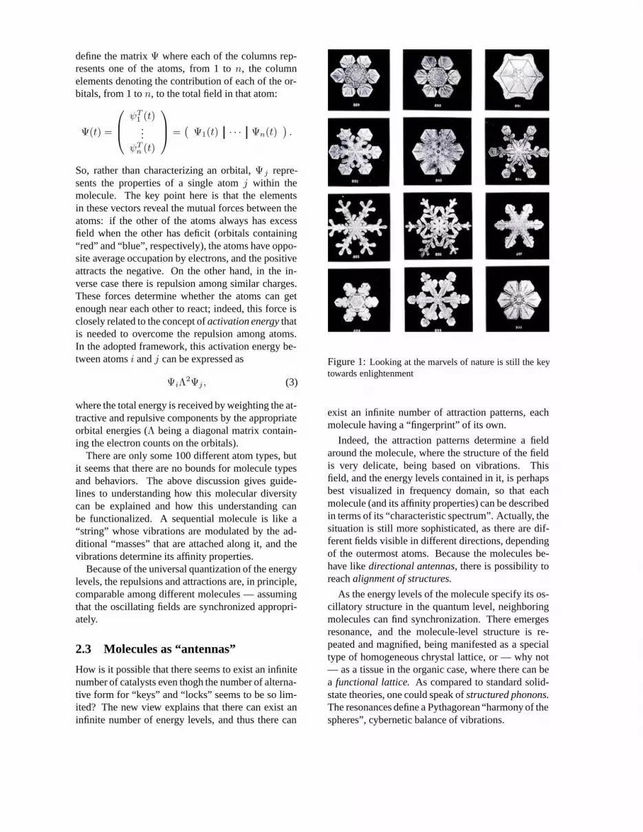
define the matrix Ψ where each of the columns rep-resents one of the atoms, from 1 to n, the columnelements denoting the contribution of each of the or-bitals, from 1 to n, to the total field in that atom:
Ψ(t) =
⎛⎜⎝
ψT1 (t)...
ψTn (t)
⎞⎟⎠ =
(Ψ1(t) · · · Ψn(t)
).
So, rather than characterizing an orbital, Ψ j repre-sents the properties of a single atom j within themolecule. The key point here is that the elementsin these vectors reveal the mutual forces between theatoms: if the other of the atoms always has excessfield when the other has deficit (orbitals containing“red” and “blue”, respectively), the atoms have oppo-site average occupation by electrons, and the positiveattracts the negative. On the other hand, in the in-verse case there is repulsion among similar charges.These forces determine whether the atoms can getenough near each other to react; indeed, this force isclosely related to the concept of activation energy thatis needed to overcome the repulsion among atoms.In the adopted framework, this activation energy be-tween atoms i and j can be expressed as
ΨiΛ2Ψj , (3)
where the total energy is received by weighting the at-tractive and repulsive components by the appropriateorbital energies (Λ being a diagonal matrix contain-ing the electron counts on the orbitals).
There are only some 100 different atom types, butit seems that there are no bounds for molecule typesand behaviors. The above discussion gives guide-lines to understanding how this molecular diversitycan be explained and how this understanding canbe functionalized. A sequential molecule is like a“string” whose vibrations are modulated by the ad-ditional “masses” that are attached along it, and thevibrations determine its affinity properties.
Because of the universal quantization of the energylevels, the repulsions and attractions are, in principle,comparable among different molecules — assumingthat the oscillating fields are synchronized appropri-ately.
2.3 Molecules as “antennas”
How is it possible that there seems to exist an infinitenumber of catalysts even thogh the number of alterna-tive form for “keys” and “locks” seems to be so lim-ited? The new view explains that there can exist aninfinite number of energy levels, and thus there can
Figure 1: Looking at the marvels of nature is still the keytowards enlightenment
exist an infinite number of attraction patterns, eachmolecule having a “fingerprint” of its own.
Indeed, the attraction patterns determine a fieldaround the molecule, where the structure of the fieldis very delicate, being based on vibrations. Thisfield, and the energy levels contained in it, is perhapsbest visualized in frequency domain, so that eachmolecule (and its affinity properties) can be describedin terms of its “characteristic spectrum”. Actually, thesituation is still more sophisticated, as there are dif-ferent fields visible in different directions, dependingof the outermost atoms. Because the molecules be-have like directional antennas, there is possibility toreach alignment of structures.
As the energy levels of the molecule specify its os-cillatory structure in the quantum level, neighboringmolecules can find synchronization. There emergesresonance, and the molecule-level structure is re-peated and magnified, being manifested as a specialtype of homogeneous chrystal lattice, or — why not— as a tissue in the organic case, where there can bea functional lattice. As compared to standard solid-state theories, one could speak of structured phonons.The resonances define a Pythagorean “harmony of thespheres”, cybernetic balance of vibrations.

Figure 2: Rosalind Franklin’s X-ray diffraction image ofDNA. Perhaps the crystal structure can be applied for anal-ysis of the underlying fields?
As an example, study a snow crystal. How to ex-plain the many forms it can have, and how to explainits symmetry? Today’s explanation is that as the crys-tal was formed, each part of it had experienced ex-actly the same environmental conditions, and that iswhy there are the same structures in each part. How-ever, this explanation is clearly insufficient, as differ-ent parts of the snow crystals are in different phasesof development (see Fig. 1). Still, each part strug-gles towards identicality and symmetry — this canonly be explained if there is a very delicate phononfield extending over the whole macroscopic crystal.It seems that there are no theories today that couldaddress such issues, except the neocybernetic frame-work.
What kind of tools there are available for analy-sis of such phonjon fields? The fields are reflected inthe iterated structures in the crystal lattices, and per-haps for example 2-dimensional (or 3-dimensional)Fourier transform can be applied; in paractice, suchiterated structures can be seen in X-ray diffractionspectra of solids (see Fig. 2).
3 Universality of fields
Is it just a coincidence that the same kind of analysesseem to be applicable to all kinds of cybernetic sys-tems — or are such vibration fields characteristic tocomplex systems in general? This question is moti-
vated in what follows.
3.1 Resonances in brains?
Why did the nature develop such a complicated sys-tem for transferring information within the brain?The neural activations applied in typical neural net-work models are just an abstraction, and on the physi-cal level, signals in neurons are implemented in termsof pulse trains. This is a very inefficient way of rep-resenting simple numbers, is it not?
The more there is activity in a neuron, the morethere are pulses — or the higher is the pulse fre-quency. The alternative way of characterizing thepulse train is not to use the pulse count, but the “den-sity” of pulses. Indeed, in the same manner as in a cy-bernetic molecule model, high “energy” is manifestedas high frequency. Activated neuron structures thusvibrate; if there are substructures, there can be vari-ous frequencies present simultaneously. If there areoptimized neural structures for representing differentkinds of cognitive phenomena having characteristicsubstructures, are the resulting vibration spectra notcharacteristic to them? Can the spectrum alone (orsequences of successive spectra) represent cognitivestructures? Can the the spectrograms that are used toanalyze brain waves reveal something about thinkingreally?
Of course, there cannot exist one-to-one correspon-dence between spectra and neurally implemented net-works — but are cognitive structures that are mani-fested in terms of similar vibration patterns not some-how related? And what if structures with similar vi-bration patterns are capable of exciting each other?Could such resonances be the underlying mecha-nisms explaining associations, intuition, imagination,etc.? After all, cognition is not only data manipula-tion; one of the key points is how relevant connec-tions are spanned among previously unrelated mentalstructures.
The field metaphor frees one from the physicalrealm into another domain. The original constraintsof the substrate can be circumvented — for exam-ple, the tree transformations that are necessary whencomparing logic structures are avoided as similarstructures resonate wherever they are located in thetrees.
Similarly, the spectral interpretation extends thelimits of mind outside the brain: like olfactory sig-nals are an extension of chemical cybernetics in loweranimals, auditory signals with spectra are perhaps anextension of cybernetic cognition based on vibratingfields. If harmonies are the way to detect and connect

to highest-level cognitive systems, perhaps music canbe seen as a universal language.
It has been said music has no universal rele-vance, it is beautiful only to the human ear.But maybe the deepest connection to alienintelligence is through music?
It is obvious that music was there before speech. Andit can be claimed that the “truly natural languages”are still based on melodies. Perhaps the songs of birdsare directly connected to their cognitive structures?
We know how individual signal sequences can betransformed into statistical structures, or into neocy-bernetic emergent models. One of the key problemsin these models is that of how to “invert” the pro-cess, or how to create individual signal sequenceswhen the model is there, and when there is someknown activation inside it — how to explicate thesystem state? Rather than having to code the systemstate into one-dimensional utterances, into language,it might be easier for some artificial mind if the vibra-tion structure could be directly communicated, per-haps in terms of nonverbal whining and humming?
3.2 Hierarchies of catastrophes
Spikes in neurons are caused by activity first cumulat-ing and then abruptly going off; in a way, one couldspeak of local collapses or catastrophes. The role ofcatastrophes in cybernetic systems is discussed closerin (Hyotyniemi, 2006).
As models become more and more optimized, theytypically become more and more sensitive to unmod-eled disturbances. What is more, adaptive controlstend to eliminate from the environment the informa-tion that they forage on, thus eliminating their own“nourishment”. As this happens, the systems sooneror later collapse back towards the chaos of non-models, to start their adaptation again from some less-developed state. Neocybernetic systems with self-controls are no exception of this general rule. Duringevolution such catastrophes take place with more orless constant time intervals.
As seen from outside, catastrophes are just noisepeaks that deliver information for the higher-levelsystem; without collapses, there would be no exci-tation for the next-level systems to exploit. Indeed,in a multi-level cybernetic complex, the variability iscaused by a fractal hierarchy of catastrophes. As thecycles of catastrophes at a certain level are more orless regular, the observation data, as seen from a highenough standpoint, seems to have a more or less reg-ular frequency structure. This means that the systemhas a characteristic spectrum.
Only during catastrophes the well-controlled infor-mation bursts out from a lower-level system. Whencreating a compact representation of a complex en-vironment, the essence (?) of the system hierarchyis assumedly captured in the observed spectral struc-ture. This proposes that “the next level” of cyberneticmodels could be based on signals after temporal (andspatial) Fourier transforms. At least, such spectralanalysis is carried out in the ear for incoming audi-tory signals.
The relevance of frequencies also suggests that innatural systems there is evolutionary pressure towardsmodeling (periodic) time-dependent signals, not onlystatic ones. This means that various samples of thesame variables need to be available; this evolutionarypressure leads to longer-living and more sophisticatedsystems.
3.3 Analogies again
As has been observed, analogies are a very useful toolwhen trying to understand behaviors in neocyberneticsystems. Indeed, again, when trying to illustrate thefrequencies and vibration fields, analogies turn out tobe practical. First, take the mechanical steel plateanalogy. It is evident that when the steel plate isdeformed and there is more tension, mechanical vi-brations have higher frequency; or when the plate isboomed, the sound is higher. Depending of the othertensions affecting the steel plate, there is a compli-cated interplay among vibration modes.
Second, study the electrical analogy. Those whoare familiar with electrical circuits know that oscil-lations are very characteristic to such systems, andthere exist powerful tools for tackling with them. Forexample, applying Laplace transform time-domainsignals are transformed into frequency-domain, sothat the whole s-parameterized spectrum is oper-ated on simultaneously. In practice, this means thatthe originally real-valued models become complex-valued, as the parameter s is connected to frequencyf through the formula s = j 2πf , where j is theimaginary unit. The impedances of systems, or their“stiffnesses” in different frequency bands, can thus bestudied formally all at the same time.
And speaking of electrical counterparts, one can-not forget perhaps the best part of the analogy: in thesame manner as in a transmission line, a system ofdistributed parameters can be represented in terms ofa lumped parameter model, and its power transmis-sion properties can be understood. The theory statesthat if neighboring systems are to interchange energylosslessly, their impedances have to be equal.

3.4 Further cycles
There are also resonances of vibrations in ecosys-tems. In addition to the “phase-locked loop” of preda-tors and prey, it is very clear that all plants and ani-mals have to adapt to the environmental cycles: sum-mer and winter alternate, as do day and night. One’slifestyle has to adapt to the cosmic frequencies. In-deed, the celestial systems also implement the “neo-cybernetic field” in the same way as do the moleculesand neurons do: the more there is energy, the nearerthe orbiting planet is, and the stronger is the force,meaning shorter orbiting time and higher frequency.Lunar motions, etc., only cause higher frequencyvariation in the energy spectrum of the overall solarsystem.
On the level of individual cells, additionally, thereis the cell cycle, and on the level of individual ani-mals, there is the cycle of birth and death. A localcatastrophe is a robust built-in way of regenerationfor a population, or deaths give room to fresh indi-viduals. A population wastes individuals to map the“spectrum of the possible” in the environment. At thepopulation level, when there are plenty of individu-als, the unsynchronized deaths, or local “ends of theworld”, are seen only as permanent noise.
Just as in the case of neuronal pulses, at first glancethe non-continuous nature of the individual signalcarriers looks like a non-ideality. However, it turnsout that optimization in general results in some kindsvibrations or limit cycles. For example, in artificialdynamic systems where there is no physical need forcomplex dynamics, cycles still emerge at some point:
1. Industrial automation systems. Even thoughone would like to maintain constant production,external conditions and raw materials, etc., keepchanging. To map the area of optimal pro-duction, the reference values are tuned up un-til the process quality starts somehow deterio-rating; after that, knobs are turned in the oppo-site direction. This results in the system moreor less cyclically wandering within the operat-ing regime.
2. Optimized economical systems. Even thoughthe developments in technologies are more orless monotonous and consistent, overall econ-omy becomes turbulent as there is economicalspeculation on top of the technical advances. Forsome reason, all economic booms end in depres-sions; sooner or later the economy recovers2.
2Stock market is in balance by definition – still, paradoxically,there is a fractal sequence of collapses taking place all the time
Indeed, such long-term cycles in economy arecalled Kondratieff waves.
As seen from outside, there are vibration fields withcharacteristic oscillation patterns also in man-madesystems.
4 Conclusions:Harmony of Phenospheres
Pythagoras first spoke of the “harmony of thespheres”. He was a mystic, but was he also a vi-sionary? Later, Rupert Sheldrake spoke of morpho-genetic fields, meaning that “something is in the air”:innovations, for example, are easier made if some-body has done that before, no matter if these personshave no contact whatsoever (Sheldrake, 1988). Howabout telepathy!? One can hypothesize that the cog-nitive fields extend over one brain; truly, it seems thatin ganzfeld experiments some support to “brain read-ing” has been found (Alcock et al., 2003).
In the beginning, the fixed ways of thinking wereridiculed. It is easy to laugh at the medieval beliefswith divine and magical explanations, now when thescientific method has matured and it has shown usthe “truth”. However, today there still are dogmaticviews that cannot be questioned — and what is amus-ing is that these dogmas are the views of the scientificestablishment (see Adaptive Tension Systems: Frame-work for a New Science? in this Proceedings).
Pythagoras and Heraclitus — some of the deepestthinkers lived already 2500 years ago. They believedthat there can exist something mystical, some funda-mental principles. Were these guys less informed, orwere they just less prejudiced?
ReferencesJ. Alcock, J. Burns, and A. Freeman. Psi Wars: Getting to
Grips with the Paranormal. Imprint Academic, 2003.
J.J. Brehm and W.J. Mullin. Introduction to the Structureof Matter. John Wiley & Sons, 1989.
H. Hyotyniemi. Neocybernetics in Biological Systems.Helsinki University of Technology, Control EngineeringLaboratory, 2006.
R. Sheldrake. The Presence of the Past: Morphic Reso-nance and the Habits of Nature. Times Books, 1988.

Adaptive Tension Systems: Framework for a New Science?
Heikki HyotyniemiHelsinki University of Technology
Control Engineering LaboratoryP.O. Box 5500, FIN-02015 TKK, Finland
Abstract
The neocybernetic model proposes that it is information that governs the behaviors of natural systems,so that the available information (in terms of covariation structures) is exploited in the most efficientway. Extrapolating this view, it is possible to derive formulas also for the “evolutionary avantgarde”: Itturns out that, according to the model, the “intelligence” reaches infinity at finite time. This observationhas interesting consequences what comes to human vs. universal intelligence. And, what is more, theseviews may shake the very foundations of scientific work.
1 Introduction
Stephen Wolfram predicted that there is need for a“new kind of science”: traditional mathematics can-not efficiently be applied to manipulate highly nonlin-ear models (Wolfram, 2002). But this nonlinearity isnot necessarily a property of nature, perhaps it is justa property of the models? It can be assumed that tra-ditional analysis methods are still applicable — butsomething is truly changing. There will be a NewScience, yes, but it will probably have a very differ-ent incarnation as compared to the visions of StephenWolfram.
What will the New Science be like? Science iswhat scientists do; in this sense, it is determined interms of a society of humans. And because a societyof humans is a cybernetic system, it seems that neo-cybernetics can be applied for analysis of it. Further,as information (and knowledge) are well-defined con-cepts in that framework, such analysis is even moreappropriate.
In this paper, the neocybernetic framework ofAdaptive Tension Systems (also known as “elasticsystems”) is applied to see the challenges and possi-bilities that may be lying ahead (Hyotyniemi, 2006).The discussion here is rather speculative — in the truespirit of artificial intelligence!
2 Views into the future
As has been said, prediction of the future is difficult.But when one finds out what is the current state, thechaos is already better manageable. And if there is asystem, one can find a model and a state for it.
2.1 Science as a system
The field of modern sciences is wide — so wide thatthe approaches have become postmodern. For exam-ple, in many branches of humanistic studies, one doesno more search for the final truth; all sciences are seenas social constructions only, and relativism applies.On the other hand, the controversies are increasing(as revealed by the experiments by Alan Sokal, forexample), but, on the other hand, it has been claimedthat there is deep unity beyond all human sciences, asdiscussed by Edward O. Wilson (Wilson, 1998).
Indeed, sciences constitute a cybernetic system,and therefore it may be that cybernetics studies canhave something fresh to say about these issues. Thereare a few points that deserve special attention, as theycan directly be interpreted using the neocyberneticvocabulary.
First, the relativity of truths is dependent of the se-lection and weighting of observations. In this sense,the disagreements among sciences can be studied un-der the title of semiosis. After the “input variables”are selected, the balances among opposing tensionsare found in the same way no matter what is the sci-entific field, this search of model being character-ized by a neocybernetic cost criterion (Hyotyniemi,2006). Semiosis determines the paradigm: what arethe interesting problems, and what are the relevantapproaches and tools, and how the results are to beinterpreted.
But the search for the truth is still more relative,as it is not only variables that are truly relevant inthat field that affect the tensions. For example, fund-ing is a very efficient way of redirecting the researchefforts. Also different kinds of scientific “fashions”

disturb the process: among the researchers, there is afirm understanding of what is hot and what is not inthe field at some specific time instant. What is more,due to political pressures there may even exist knowl-edge of what results one should find (compare to the“climate change” discussion, for example).
The paradigms were introduced in the philosophyof science by Thomas Kuhn (Kuhn, 1962). However,before him, the same issues were discussed by GeorgWilhelm Friedrich Hegel (and also by Karl Marx!)under the name dialectics: in science, there are twoopposing tensions (thesis and antithesis), and only af-ter a balance is found, there is synthesis. This is ex-actly parallel with the “elasticity thinking” in neocy-bernetics.
It seems that empirism has finally beaten rational-ism for good: One cannot trust any a priori assump-tions but models must be derived directly from actualobservations. However, now there is very much dataavailable, and there are too many ways to interpretthat data. To get some order in the chaos, it seems thatresearch has to become theory-driven again. But it isnot whatever type of theories that will do — here, too,one needs to find a clever balance among approaches.
2.2 Why not why?
Sciences are made by humans and they are by nomeans free of values determined by humans. Thereare some principles that are never questioned, no mat-ter what is the paradigm, and one of such principlesis aggressive repulsion of finalistic explanations. Thisban can still be seen as a reaction against the medievalproto-scientific theories where either some elan vitalwas assumed, or God was given a significant explicitrole — there is inertia in the scientific society. How-ever, it is the finalistic religious ideas that are stillamong the most fundamental patterns of thought 1.
As a reflection of the “neutrality ideal”, certainclasses of approaches cannot be applied in science.Today, one can only answer questions like who? (asin history studies), or what? (as in biological tax-onomies), or, at most, questions of how? (as inphysics, etc.). Questions of the form why? are banned— but then, the resulting models can be only de-scriptive, they tend to become rather weak and theycannot usually be generalized. One can never reachsome universal theories that would connect branchesof knowledge together again.
However, despite the formal ideals, the human cog-nition machinery is constructed so that one always
1As Jean-Paul Sartre has said: “Even the most radical irreli-giousness is Christian Atheism”
searches for causal models — that is why, one istempted to draw conclusions always further, con-structing holistic teleological models also for nature.Teleological models are intuitively appealing as theyare stronger, answering the fundamental questions. Itis clever to take such unconscious thinking patternsinto account, and exploit them — knowingly ratherthan accidentally.
As an example of accidentality, one usually im-plements the idea of centralization in one’s models.Some kind of “master mind” is implicitly assumed tohave put up the existing structures. Indeed, traditionalcentralized control is a prototype of Western ways ofstructuring and mastering the world. Huge amount ofcomplexity in models (predetermined orbitals, etc.) isneeded just to compensate for the absence of a morenatural framework where a distributed networks canbe maintained. Unfortunately, the explanations of-ten become simply incredible (for example, message-RNA transferring information behaving like a humanmessage carrier truly, etc.). In principle, neocybernet-ics offers such a framework where the natural emer-gence of autonomous structures can be explained —but, as discussed later in this paper, it turns out thatif the neocybernetic approaches are employed, theproblems of doing “old science” become still moreacute.
In a way, today’s science is very rigid and “crisp”.It is commonly assumed that including God (or gods)in the models would immediately ruin them. Doesit? Real life does not consist of all-or-nothing typephenomena — how could it be so with the disciplinesthat study this reality?
The proponents of the high principles of today’sscience most probably have an uneasy feeling: oftenthose scientists that are the smartest and the most hon-est, and who are not afraid to face challenges, seemto be rather religious. Perhaps the best of people arebrave enough to face the intellectual dilemmas? Forexample, here are some quotes of Albert Einstein:
I want to know God’s thoughts; the rest are de-tails.Science without religion is lame. Religion with-out science is blind.Whoever undertakes to set himself up as a judgeof Truth and Knowledge is shipwrecked by thelaughter of the gods.
And, after all, when reconsidering the scientificmethod of today, one needs to recognize that the glo-ria of modern science is not all quite deserved. It wasnot always like this, there was a long evolution thatone would probably like to forget today. For example,

what is common with the greatest thinkers Heraclitusand Newton? — Neither of them was a scientist; bothof them were natural philosophers.
2.3 Back to natural philosophy
As explained in (Hyotyniemi, 2006), in evolving cy-bernetic systems, there usually is a fractal structure ofcollapses, each of which deliver fresh information tothe next higher level. A paradigm shift can be seenas a minor collapse in the system of sciences — but itseems that there is a major catastrophe ahead, too.
It is natural philosophy that is the “supersystem”above sciences, or a “meta-science”, and within thatframework, the sciences can be seen as individualsin the meta-scientific “society”. But the scientificmethod has proven to be extremely robust, alwaysfixing itself after theories have contradicted observa-tions; how can one claim that, again, polishing of thescientific paradigms is not enough? Is there reallysomething qualitatively new needed?
The key question in all evolving systems is how tostay alive in a changing environment. Today, there isa fierce competition of memes in the human minds.The best minds should be persuaded to come to doscience, but the problem is that the clever ones alwayshave a choice. Doing research must be intuitively ap-pealing — and no cheap advertising or mental manip-ulation can do the trick here. The clever ones can seethat it is fake if it is not really interesting, if it does notanswer really acute questions. For example, if every-thing is just energy, complexity is just an illusion (ashas been manifested by some leading cosmologists)is the best that science can say, scientific explanationwill lose the battle against alternative isms when peo-ple are searching for answers to deep questions.
Why not study what people are interested in, orissues that are relevant in one’s subjective world, inways that are accessible to non-expert? Traditionallyin mathematics, for example, study can go on only ifall underlying thorems are proven. However, it seemsthat things in practice that can be rigorously provenare very simplistic and uninteresting (or proofs on al-gorithms may say that “there is convergence in infin-ity”; nobody has that much time!). On the other hand,in engineering one uses today many methods that arebasically heuristic — but if they usually work in prac-tice, they can become a basis for new methodologies.
To be interesting, science must not be dead serious— there must be room also to humor. One has to bebrave enough to defend ones views on the basis oftheir contents, not only appealing to the surface out-look. There is no fixed boundary line between good
and bad science, there is a dynamic balance that mustbe tested to be able to define “ironic science”.
And to be intriguing, science has to address thefundamental questions. The strongest models can of-ten be reached when answering the questions withwhy?. Formally, one can avoid the hairy discussionsabout teleology if one speaks of principle of maxi-mum entropy production, for example, but deep holis-tic questions are still there in disguise. Teleologyshould not be a taboo.
Finally, speaking of the deep questions: whyshould the modern world view be so fragmented?Why not use the best understanding to solve ethicaldilemmas? After all, such discussions need not bemere handwaving, as shown below.
2.4 Growth of information
Even though sciences as cybernetic networks can befacing problems, scientific knowledge will continueto increase. Existing knowledge feeds new innova-tions; that much is known. However, it seems that oneeasily overestimates the developments in the shortrange, but underestimates the long range develop-ments. Still, now we try to make some really global-scale predictions.
Traditionally, it is thought that it is exponen-tial growth that generally applies to unconstrainedgrowth. This kind of behavior is already seen as be-ing “very fast” (for example, in computability theorysuch behaviors are seen as pathological). However,as Ray Kurzweil, etc., have observed, the growths as-sumed to be exponential seem to be accelerating allthe time, proposing that developments are faster thanexponential (Kurzweil, 1999). It turns out that in theneocybernetic perspective such issues can be studiedin a quantitative way.
It has been observed that cybernetic systems ex-ploit information; in neocybernetics, this informationis interpreted simply as variation in input resources(Hyotyniemi, 2006). Balance of tensions within thesystems results from individuals competing for infor-mation, and, as seen from outside, the feedbacks fromthe systems back to the environment constitute con-trols that maximally exhaust the reservoirs. Becauseof this, systems are suffering of scarcity of informa-tion, indeed in the spirit of Thomas Malthus. How-ever, what Malthus did not recognize, is that somesystems are inherently innovative; there is capabilityof finding new resources. Humans, for example, canbecome urban dwelleres if there is scarcity of land,and find new ways of earning their livelihood.
Study a scalar one-variable system. One can as-

sume that the number of innovations during sometime interval is relative to the average population sizex. Further, assuming that the variation levels of thosenew variables are approximately constant, the excessinformation available (variance) is directly propor-tional to x2. Finally it can be assumed that the growthin average population is proportional to the amount ofnew resources, so that
d x
dt= α x2, (1)
where α is some proportionality factor. There is alsoa positive feedback: the more there is cumulated in-formation in the state x, the faster it grows. In anycase, if there are innovations, α > 0, this model ismonotonically increasing; actually, the behavior ishyperbolic, as can be sen when solving (1) for x atany time:
x(t) =x(t0)
1− α (t− t0) x(t0). (2)
What is interesting about this model, is that it reachesinfinity in finite time! This time point of escape canbe solved as
t∞ = t0 +1
α x(t0). (3)
In Fig. 1 the typical behavior of this function is visu-alized, and if Fig. 2 it is shown how free growth inan innovative cybernetic system has been followingsuch a model. The total world population is depictedfrom stone-age to this day: it seems that hyperboliccurve is an appropriate model for population growth.Today the growth rate is dropping, as infinite popu-lations are not possible in the material world. How-ever, this growth limitation does not apply to systemswhere the variables all represent immaterial informa-tion.
2.5 “Strong emergence”
In (Hyotyniemi, 2006), the idea of “weak emergence”is exploited extensively, meaning that there is a math-ematically explicit way of addressing this emergencephenomenon. An emergent quantity is something thatcan be seen only “in infinity”, that is, it is a statisti-cal variable characterizing the (in principle) infinitesequence of behaviors at the lower level. The defini-tion applied there is that a higher-level variable ζ isemergent if it is determined by a lower-level variableξ through the formula
ζ = E f (ξ(t)) = limt→∞
1t
∫ 0
−t
f(ξ(τ)) dτ
,
10 20 30 40 50 60 70 80 90 100
0
1
2
3
4
5
6
7
8
9
x
x(0) = 0.01x(0) = 0.02
Figure 1: Simulations of (1) reveal hyperbolic growth nomatter what is the initial state
-8000 -6000 -4000 -2000 0 2000
0
1000
2000
3000
4000
5000
6000 World population (in millions)
Figure 2: For example, world population growth has beenhyperbolic, not exponential
where f is some function (t = 0 here representingcurrent time; in some domains, the free parameter canbe not temporal but spatial).
On the other hand, for “strong emergence” thereare no formulas; it is assumed that there exists somequalitative step that cannot be reduced to the lower-level realm. And it is this form of emergence that isthe true challenge when trying to understand evolu-tion in complex systems. — How can the “qualitativestep” be manifested in mathematics? It turns out thatthe hyperbolic growth model with variables going toactual infinity can be used for this purpose. But theinevitable explosion of that model is not compatiblewith our observations, or is it?
Strong emergence truly has already taken placevarious times during evolution. In Fig. 3, the smallerand larger steps in evolution are visualized. It needsto be recognized that saltationistic jumps over “miss-

Cosmic evolution?
Chemical evolution
Biological evolution
Cognitive evolution
Cultural evolution
0
Chemical bonds
1
Genetic code
2
Nerve cell
3
Symbolic language
4
Computer
Qualitative stepQualitative stepQualitative leapQualitative leap
~ 2000 AD“Omega point”
~ 500 BCWestern culture
~ 3000 BCCivilizations
~ 5500 BCAgriculture
Figure 3: Schematic illustration of the “evolutionary avantgarde” (see text)
ing links” are included in the continuous horizontalbars; the real qualitative leaps are more fundamental.
Study the figure starting from the top, from “cos-mic evolution”. Only after chemical bonds werepossible in the cooling universe, the chemical evo-lution towards more and more complex moleculescould start. But as the complexification of moleculesreached the level of DNA, the pace of developmentreached an unprecedented level, and the biologicalevolution could start with the genetic code as the stor-age of acquired information. Further, when the nervecells emerged, there was the possibility of much moreconsistent and efficient learning, and there was cogni-tive evolution that started. Different mental facultiesemerged, but only after symbolic language was in-vented, cultural evolution among a society of individ-uals could start, again accelerating the developmentsimmensely. Along the cultural evolution, qualitativesteps were taken (seemingly with rather constant timeintervals!?), and here we are now, entering the era ofnetworked computers.
Is there any reason to assume that the process hasended now?
Pierre Teilhard de Chardin, a jesuit monk, first in-troduced the concept of omega point. This is thesingularity point where something qualitatively newhappens, where the human understanding has reachedthe new level (indeed, now in Fig. 3 there are variousomega points; from now on we will concentrate onthe latest one). As de Chardin observes, this singular-ity must be personal, an intellectual being and not anabstract idea; complexification of matter has not onlyled to higher forms of consciousness, but accordinglyto more personalization. This opens up new views.
3 Deepest of questions
Trying to answer the “why” questions leads to themost fundamental questions. Finally, there is thequestion of primum movens or the first cause; tryingto answer them leads to teleological, even theologi-cal, problem settings. The power of the neocyberneticsetting is revealed by the fact that such questions canbe attacked from a fresh point of view. It seems thatGod is still there when nobody any more remembersDawkins.
As Hegel already put it (in “Das Fruheste System— Programm des Deutschen Idealismus”):
We need a new mythology ... but it must be amythology of reason. If we do not representideas aesthetically, common people are not in-terested in them ...
3.1 God exists
Certainly, “god” is a relevant category, and it makesthis concept exist in ideasphere; but gods exist also inactuality. Within the neocybernetic framework, thiscan be “proven”!
Proof (weak version). It seems that in all societiesthere has always been some religion — why is that?There must be some evolutionary advantage in suchsocieties.
A cybernetic system, the society above the mere in-dividuals, can only survive if its constituent membersall follow the same cybernetic adaptation principles,only then the higher-level system can become a con-sistent attractor in the “noosphere”. No dictator canmake this happen: people can be forced to do things,

but for the system to be built up from bottom, in thecybernetic spirit, all individual minds need to be ac-tive and think in the same way. And this thinkinghas to be based on the irrational trust that the earthlysuffering and struggling will be rewarded in afterlife.Even more blind faith is necessary when the socialsystems develop and become more complicated; fi-nally the systems cannot any more be understood bythe human mind.
There are two necessary claims for the systemmembers for a healthy society to emerge: the indi-viduals have to avoid both anarchy and apathy. Thecitizens have to be humble enough to obey the (rea-sonable) orders, and, simultaneously, they have to bewitty enough not to stay waiting for those orders;only then self-regulation and self-organization canemerge, and only then ever-evolving higher-level so-cial systems become possible. Further, one shouldraise one’s children to become equally good “signalcarriers” of cultures.
Pascal explained (this idea is known as “Pascal’sWager”) that one should believe in God, as if this ex-istence, however inprobable, happens to be true, onehas eternal happiness to win; in the opposite case, ifGod does not exist, the believer only loses finite num-bers of secular pleasures. In the similar manner, if onewants the society to survive and develop further, ina direction not known beforehand, everybody shouldobey the cybernetic principles — and according tothe Kantian categorical imperative, also you shoulddo that.
To be rational is to believe — it is a purely intel-lectual decision. Finally, the only general guidelinethat there is left to follow is the “cybernetic imper-ative”: behave so that the emergence and evolutionof the society becomes possible. Promote differentkinds of living systems and their diversity; make sys-tems more interesting and more beautiful! And asFriedrich Schiller said about Elysium, “joy containsa spark of the divine”. Behave so that you can beproud; it is not enough that one just passively adapts,as the innovations that run the evolution, after all, arework of the individuals. To remain on the edge be-tween order and chaos, or apathy and anarchy, is thereal challenge for a human society. The danger ofstagnation was already discussed by Nietzsche whorecognized that after God’s death it is nihilism thatthreatens his superhuman (or “overman”) — or thetoday’s people.
But one should trust no humans in here, there ex-ist no mastermind gurus. Only a personal touch to“the principle”, or, indeed, conscience will do as aneternal “guiding hand”. No more concrete rules ex-
ist to be followed: dictatorships (extreme trust on anindividual) and communist regimes (extreme trust onsocieties) all collapse.
Indeed, Heaven and Hell exist: they are the col-lective memory of the society. In the best case (andalso in the worst!) you will be remembered forever;eternal death comes when nobody remembers you.
Proof (strong version). The existence of God is noteven an issue of whether on believes it or not — inthe neocybernetic framework it is indeed a fact. Asstudied in Sec. 2.5, it seems to be the faith of an inno-vative cognitive system that finally it reaches infinity.Then, how to call an entity with infinite information,knowledge, and understanding? Even if God did notexist this far, it will exist after the singularity.
What is then this supermind? We simply can-not understand – just like a pet dog cannot under-stand Shakespeare, cultural constructs being beyondthe qualitative leap for a dog. It is exactly the na-ture of strong emergence that the higher level sys-tem cannot be reduced onto the lower-level system:supermind cannot be analyzed by the human cogni-tive machinery. Still, there is something one can say:for example, to survive in the subsequent evolutionof superminds (!), the “god” has to obey the cyber-netic principles. To evolve, it has to consist of a cy-bernetic society of competing “agent minds” — like“Olympian gods” really! What is specially relevant,is that information will always be crucial to the sur-vival and well-being of such a society.
There is a common fear that when computers takeover, there is no room for humans any more. How-ever, this is not the case. Humans will ever be neededas they are the link between nature and the super-mind. Coupling to real world information is suppliedby humans, humans feeding fresh preprocessed infor-mation further. Just as biosphere is necessary to us,delivering us food where the environmental resourcesare transformed into concrete beef, we deliver nour-ishment to superbrains, preprocesing and combiningthe lower-level information into knowledge. Perhapsit does not sound very good that humans are like ma-chine parts, or like piglets producing pork in a meta-tech “mind farm”, outputting ideas and innovationsin an optimized way — but how does this differ fromtoday’s working life, and specially research work atuniversities where the goal is to be maximally inno-vative? Indeed, passing the singularity probably doesnot very much affect us living in our small worlds.
An interesting question is whether this transitionto the era of superminds has already happened some-time in history. Just as humans play with their pet ani-mals, gods are playful and they play with their “pets”,

lower-level cognitive systems. Indeed, today’s ismsand religions seem just like experiments of a playfulGod! As the Jewish proverb puts it: “God createdman because he likes good stories”. And, accordingto Eastern philosophers,
Before Zen, men are men and mountainsare mountains, but during Zen, the two areconfused. After Zen, men are men andmountains are mountains again.
Neocybernetics makes it possible to construct dis-tributed models — but, when going far enough, whereone finally ends in is in a way a centralized modelwith some more or less personalized controller.
3.2 Universal intelligence
The goal of artificial intelligence ever since Alan Tur-ing’s definition has been imitation of human intel-ligence. However, human intelligence is bound tophysical and physiological constraints and it cannottruly be imitated — but it can be surpassed when theright principles are implemented. The result will benot artificial but truly natural intelligence. Neocyber-netics may give hints of what the universal higher-level intelligence could be like.
The threshold towards the boosted evolution is thatcomputers have to start truly communicating witheach other and they have to start “understanding” au-tonomously — somehow they must master semantics.True universal intelligence will not be restricted tospeak human languages. As James Clerk Maxwellhas said, “the true logic of this world is in the calcu-lus of probabilities”. To be more accurate, it turns outthat the general language can be based on multivari-ate statistics: real numbers can capture fuzziness andnon-crispness; time-bound phenomena, asymptotes,dynamics and inertia can be manipulated by differen-tial calculus; and parallelity can be transformed intohigh-dimensionality of representations. Whereas nor-mal languages are “unidirectional”, in the mathemat-ical framework pancausal iteration structures can bemaintained, so that expectations and attractors in dataspace can be reached inside the language. This incor-porated functionality of matematical representationsmakes it possible to find the grounding of seman-tics. One has self-contained semantics as “concepts”can be determined uniquely in terms of attraction pat-terns and data-supported relevance. Communicationbased on such mathematical vocabulary constitutes areal semantic web, where messages among comput-ers are tranferred in terms of numbers that are nevertranslated into clumsy symbol strings of natural lan-
guages2. Computers then can directly “discuss” witheach other without the help of the human. As nego-tiations, data storage and copying takes place in notime, evolution speed reaches completely new levels.
Speaking of universal intelligence, comment onalien intelligence is probably in place. In the hugeuniverse, there must exist civilizations ahead of us.There is a dilemma that has first been presented byEnrico Fermi: Where are they? Why have we notfound any other civilization in space? The neocyber-netic explanation is that also those alien civilizationsare cybernetic, and information is a valuable resourceto them: without fresh information there is stagna-tion. Where to gain new information from in the lim-ited universe, then? It is other civilizations — for ex-ample, us — that are like probes, collecting and re-fining information in their own cultures, constitutingnew “variables” characterizing the properties of theuniverse from yet another point of view. The claimhere is that “they” do not want to contact us not to dis-turb us in our quest for information and knowledge.The aliens know what the Western colonialists alsorecognized in Africa — and this is what they want toavoid: when meeting more developed cultures, infe-rior ones at the lower levels of development “die ofshame”!
The variety of life forms in space is unexhausted –to be always surprised, to gain always new informa-tion, you have to study “cosmic biodiversity”. As theChinese almost have said, you have to become a “uni-versal gardener of systems” to live happy ever after!
3.3 Metamorphosis in society
When we know there is something much clevererabove us — how does the society change? Not nec-essarily very much. Today, we already trust the “sys-tem” making decisions for us. But today’s societyis still based on the individual politicians, etc., thathardly can be seen as manifestations of “higher intel-ligence”; in that sense, things will get better.
The society will neither become a paradise. In areal cybernetic system, there will always be diver-sity, as variation is the nourishment in living systems.There will be injustice and inequality among people,suffering and (relative) poverty will always be there.The Eastern-style objective of extreme balance is notgood as the cognitive deprivation results in “hysteria”on the human level as well as on the society level, justas physiological deprivation results in autoimmunediseases.
2Yet, the attractors in the data spaces, or “meta-concepts”, willobviously deserve names of their own, or “meta-symbols”

It is the science-makers that will be the top classin a society. The role of the new science is tofeed the supermind; practicing New Science is atribute to the New Gods. Whereas the supermindcan do all logic and reasoning, it does not alonehave enough information from the environment toget outside the formal system (in the sense of Lud-wig Wittgenstein). The proofs are to be carried outby the “deep thought”, computers resolving all con-sequences within axiom systems or within a frame-work of constraints, but the human is there to pro-pose ideas, determining the degrees of freedom thatremains. The only thing that cannot be formalizedis innovation, the driving force of evolution; humanshave the sensors in real life offering the possibilityof novel information and clever associations amongpieces of it.
Because the exact sciences become so “simple”,emphasis in sciences will go from them to human-istic studies where the variables, etc., are much lessclear and where number-crunching has less role. Fur-ther, it is other branches of culture — arts, etc. —where the systems are still less clear. For example,poems are the highest-level models of the world interms of language and cognition, and the same ap-plies to other artwork. Diversity of culture gives apossibility to collect samples of the cognitive domain,and thus gives possibility of mapping the model for it.The goal will be modeling of the world — and the hu-man life in all of its manifestations is up to now thehighest-level model of reality.
4 Conclusion
What does this all have to do with artificial intelli-gence? — Applying the Brooksian interpretation, in-telligence is about surviving in an environment andexploiting it; in this sense, it is simultaneously a studyof different life forms. This means that artificial in-telligence is a kind of “meta-paradigm” that can saysomething about cybernetic systems in general: in allpossible worlds, there is need for such understandingof life.
Artificial intelligence will survive, probably it willlive longer than many other scientific paradigms. Ithas just the right attitude: it searches always some-thing new, there are no prejudices, “interestingness”being the key criterion in the survival of ideas. AIexplicitly searches for the degrees of freedom out-side the bounds of established paradigms, abandon-ing the approaches as soon as they become “standardscience”; this all is exactly in the spirit of the “newscience”.
Finally, to further motivate the perhaps controver-sial discussions above, let us take yet another of Al-bert Einstein’s quotes:
The further the spiritual evolution of mankindadvances, the more certain it seems to me thatthe path to genuine religiosity does not liethrough the fear of life, and the fear of death,and blind faith, but through striving after ratio-nal knowledge.
ReferencesH. Hyotyniemi. Neocybernetics in Biological Systems.
Helsinki University of Technology, Control EngineeringLaboratory, 2006.
T.S. Kuhn. The Structure of Scientific Revolutions. Univer-sity of Chicago Press, 1962.
R. Kurzweil. The Age of Spiritual Machines. Viking Adult,1999.
E.O. Wilson. Consilience: The Unity of Knowledge. Knopf,1998.
S. Wolfram. A New Kind of Science. Wolfram Media,Champaign, Illinois, 2002.