Regularization, maximum entropy and probabilistic methods in mass spectrometry data processing problems

International Journal of Mass Spectrometry 215 (2002) 175–193

Regularization, maximum entropy and probabilistic methodsin mass spectrometry data processing problems

A. Mohammad-Djafari∗, J.-F. Giovannelli, G. Demoment, J. Idier

Laboratoire des Signaux et Systèmes, Unité mixte de recherche n 8506 (CNRS-Supélec-UPS), Supélec,Plateau de Moulon, 3 rue Joliot-Curie, 91192 Gif-sur-Yvette Cedex, France

Received 16 July 2001; accepted 5 November 2001

Abstract

This paper is a synthetic overview of regularization, maximum entropy and probabilistic methods for some inverse problemssuch as deconvolution and Fourier synthesis problems which arise in mass spectrometry. First we present a unified descriptionof such problems and discuss the reasons why simple naıve methods cannot give satisfactory results. Then we briefly presentthe main classical deterministic regularization methods, maximum entropy-based methods and the probabilistic Bayesianestimation framework for such problems. The main idea is to show how all these different frameworks converge to theoptimization of a compound criterion with a data adequation part and an a priori part. We will however see that the Bayesianinference framework gives naturally more tools for inferring the uncertainty of the computed solutions, for the estimation ofthe hyperparameters or for handling the myopic or blind inversion problems. Finally, based on Bayesian inference, we presenta few advanced methods particularly designed for some mass spectrometry data processing problems. Some simulation resultsillustrate mainly the effect of the prior laws or equivalently the regularization functionals on the results one can obtain intypical deconvolution or Fourier synthesis problems arising in different mass spectrometry technique. (Int J Mass Spectrom215 (2002) 175–193) © 2002 Elsevier Science B.V. All rights reserved.

Keywords:Regularization; Maximum entropy; Bayesian inference; Deconvolution; Fourier synthesis

1. Introduction

1.1. Data processing problems in mass spectrometry

In mass spectrometry, the data acquisition andprocessing is an essential part of the final measure-ment process. Even if, in some cases, only somepre-processing is done during the acquisition process,the post-acquisition data processing is a vital part ofmany new mass spectrometry instruments. The mainreason is that the raw data do not, in general, directlyrepresent the parameters of interest. These raw data

∗ Corresponding author. E-mail: [email protected]

are, in general, transformed and distorted version ofthe ideal physical quantity of interest which is themass distribution of the object under the test.

Some distortions are related directly to the measure-ment system, for example the blurring effect of thetime-of-flight (TOF) [1] mass spectrometry data canbe written as a simple one-dimensional convolutionequation:

g(τ) =∫

f (t)h(τ − t)dt, (1)

whereh(t) is the point spread function (psf) of blur-ring effect,f (t) the desired mass distribution andg(t)the data. Fig. 1 shows an example where in place of

1387-3806/02/$20.00 © 2002 Elsevier Science B.V. All rights reserved.PII S1387-3806(01)00562-0

176 A. Mohammad-Djafari et al. / International Journal of Mass Spectrometry 215 (2002) 175–193

Fig. 1. Blurring effect in TOF mass spectrometry data: (a) desired spectra; (b) observed data.

observing the signalf (t) in (a) the signalg(t) in (b)has been observed.

Some others are due to the output parts of the instru-ment, for example the interaction and coupling effectof focal plane detectors (FPD) [2] or non-uniformityof ion conversion devices (electron multipliers) ingeneral and in matrix-assisted laser desorption ioniza-tion (MALDI) techniques in particular. These distor-tions can be written as a two-dimensional convolutionequation:

g(x′, y′) =∫∫

f (x, y)h(x′ − x, y′ − y)dx dy. (2)

In some other mass spectrometry techniques such asFourier transform ion cyclotron resonance (FT-ICR),

the observed data are related to the Fourier transform(FT) or Laplace transform (LT) of the mass distribu-tion:

g(τ) =∫

f (s)exp{−sτ } dω,

with s = jω or s = jω + α, (3)

where α is an attenuation factor. Fig. 2 shows anexample of the theoretical spectrumf (s) in (a) andthe corresponding observed datag(τ) in (b). We mayobserve that, due to the attenuation and the noise inthe data, a simple inversion by inverse FT (c) maynot give satisfactory result.

In this paper we try to give a unified approach todeal with all these problems. For this purpose, first we

A. Mohammad-Djafari et al. / International Journal of Mass Spectrometry 215 (2002) 175–193 177

Fig. 2. The reference spectrum (a), its corresponding simulated data in FT-ICR (b) and the inverse FT of the data (c).

note that all these problems are special cases of

g(s) =∫

f (r)h(r, s)dr. (4)

Then, we assume that the unknown functionf (r)can be described by a finite number of parameters

x = [x1, . . . , xn]:

f (r) =n∑

j=1

xjbj (r), (5)

wherebj (r) are known basis functions. With this as-sumption the raw datay(i) = g(si ), i = 1, . . . , m are


related to the unknown parametersx by

y(i) = g(si ) =n∑

j=1

Ai,j xj ,

withAi,j =∫

bj (r)h(r, si )dr, (6)

which can be written in the simple matrix formy =Ax. The inversion problem can then be simplified tothe estimation ofx given A andy. Two approachesare then in competition: (a) the dimensional controlapproach which consists in an appropriate choice ofthe basis functionsbj (r) andn ≤ m in such a waythat the equationy = Ax be well conditioned; (b) themore general regularization approach where a classicalsampling basis forbj (r) with desired resolution ischoose no matter ifn > m or if A is ill-conditioned.

In the following, we follow the second approachwhich is more flexible for adding more general priorinformation onx. We must also remark that, in gen-eral, it is very hard to give a very fine mathematicalmodel to take account for all the different steps of themeasurement process. However, very often, we canfind a rough linear model for the relation between thedata and the unknowns (one- or two-dimension con-volution or FT or any other linear transformation). Butthis model may depend on some unknown parame-tersθ , for example the amplitude and the width of theGaussian shape psf. It is then usual to write

y = Aθx + ε, (7)

whereε is a random vector accounting for the remain-ing uncertainties of the model and the measurementnoise process.

When the direct model is perfectly known, themain objective of the data processing step is to obtainan estimatex of the x such thatx optimizes someoptimality criteria. We will see that, very often, a datamatching criterion such as a least square (LS) crite-rion J (x) = ‖y − Ax‖2 does not give satisfactoryresults. This is, in general due toill-posednessof theproblem which, in the case of linear problems, resultsin ill-conditioned linear systems of equations [3]. Toobtain a satisfactory result, we need to introduce some

prior information about the errors and about the un-knownsx. This can be done through the generalreg-ularization theoryor in a more general way throughthe probabilistic inference and statistical estimation.In probabilistic methods, the rough prior informa-tions about the errorsε and the unknownsx are usedto assign the prior probability distributionp(ε|φ1)

and p(x|φ2) where φ1 and φ2 are their respectiveparameters.

Thus, the first steps of solving the problem are toclearly identifyx, A, θ andy and to define an opti-mality criterion forx which may also depends on thehyperparametersφ = [φ1,φ2]. The next step is to findan efficient algorithm to optimize it, and finally, thethird step is to characterize the obtained solution. Wewill however see that these steps are forcibly depen-dent to each other.

In this paper we focus on this general problem. Wefirst consider the case where the model is assumedto be perfectly known (A and θ known). This is thesimpleinversion problem. Then we consider the moregeneral case where we have also to infer aboutθ . Thisis themyopicor blind inversionproblem. We may alsowant to infer on the hyperparametersφ from the data(unsupervised inversion). In some cases, we may havetwo sets of data, one with known input (for calibrationor point spread function estimation purposes) and onewith unknown input. Finding an optimal solution forthe psf and the unknown input from the two sets ofdata can be considered asmulti-channel blind decon-volution.

1.2. Why simple naıve methods do not givesatisfaction?

When the degradation model is assumed to be per-fectly known, we are face to a simple inversion prob-lem. However, even in this case

• the operatorA may not be invertible (A−1 does notexists);

• it may admit more than one inverse (∃B1 andB2|B1(A) = B2(A) = I whereI is the identityoperator);


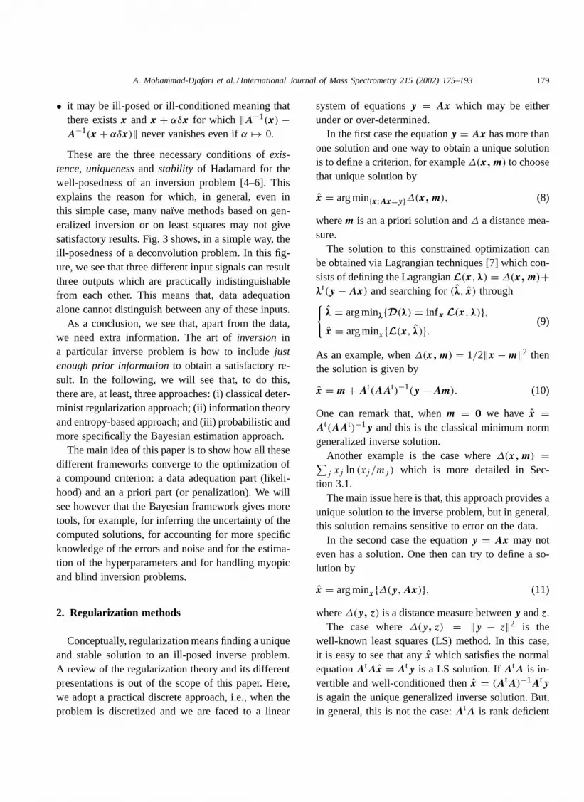
• it may be ill-posed or ill-conditioned meaning thatthere existsx andx + αδx for which ‖A−1(x) −A−1(x + αδx)‖ never vanishes even ifα �→ 0.

These are the three necessary conditions ofexis-tence, uniquenessand stability of Hadamard for thewell-posedness of an inversion problem [4–6]. Thisexplains the reason for which, in general, even inthis simple case, many naıve methods based on gen-eralized inversion or on least squares may not givesatisfactory results. Fig. 3 shows, in a simple way, theill-posedness of a deconvolution problem. In this fig-ure, we see that three different input signals can resultthree outputs which are practically indistinguishablefrom each other. This means that, data adequationalone cannot distinguish between any of these inputs.

As a conclusion, we see that, apart from the data,we need extra information. The art ofinversion ina particular inverse problem is how to includejustenough prior informationto obtain a satisfactory re-sult. In the following, we will see that, to do this,there are, at least, three approaches: (i) classical deter-minist regularization approach; (ii) information theoryand entropy-based approach; and (iii) probabilistic andmore specifically the Bayesian estimation approach.

The main idea of this paper is to show how all thesedifferent frameworks converge to the optimization ofa compound criterion: a data adequation part (likeli-hood) and an a priori part (or penalization). We willsee however that the Bayesian framework gives moretools, for example, for inferring the uncertainty of thecomputed solutions, for accounting for more specificknowledge of the errors and noise and for the estima-tion of the hyperparameters and for handling myopicand blind inversion problems.

2. Regularization methods

Conceptually, regularization means finding a uniqueand stable solution to an ill-posed inverse problem.A review of the regularization theory and its differentpresentations is out of the scope of this paper. Here,we adopt a practical discrete approach, i.e., when theproblem is discretized and we are faced to a linear

system of equationsy = Ax which may be eitherunder or over-determined.

In the first case the equationy = Ax has more thanone solution and one way to obtain a unique solutionis to define a criterion, for example∆(x, m) to choosethat unique solution by

x = arg min{x;Ax=y}∆(x, m), (8)

wherem is an a priori solution and∆ a distance mea-sure.

The solution to this constrained optimization canbe obtained via Lagrangian techniques [7] which con-sists of defining the LagrangianL(x,λ) = ∆(x, m)+λt(y − Ax) and searching for(λ, x) through{

λ = arg minλ{D(λ) = inf x L(x,λ)},x = arg minx{L(x, λ)}.

(9)

As an example, when∆(x, m) = 1/2‖x − m‖2 thenthe solution is given by

x = m + At(AAt)−1(y − Am). (10)

One can remark that, whenm = 0 we havex =At(AAt)−1y and this is the classical minimum normgeneralized inverse solution.

Another example is the case where∆(x, m) =∑j xj ln (xj /mj ) which is more detailed in Sec-

tion 3.1.The main issue here is that, this approach provides a

unique solution to the inverse problem, but in general,this solution remains sensitive to error on the data.

In the second case the equationy = Ax may noteven has a solution. One then can try to define a so-lution by

x = arg minx{∆(y,Ax)}, (11)

where∆(y, z) is a distance measure betweeny andz.The case where∆(y, z) = ‖y − z‖2 is the

well-known least squares (LS) method. In this case,it is easy to see that anyx which satisfies the normalequationAtAx = Aty is a LS solution. IfAtA is in-vertible and well-conditioned thenx = (AtA)−1Aty

is again the unique generalized inverse solution. But,in general, this is not the case:AtA is rank deficient


Fig. 3. Ill-posedness of a deconvolution problem: inputs on the left give practically indistinguishable outputs.

or ill-conditioned and we need to constrain the spaceof the admissible solutions. The constraint LS is thendefined as

x = arg minx∈C{‖y − Ax‖2}, (12)

whereC is a convex set. The choice of the setC is pri-mordial to satisfy the three conditions of a well-posedsolution. An example is the positivity constraint:C ={x : ∀j, xj > 0}. Another example isC = {x :

‖x‖2 ≤ α} where the solution can be computed viathe optimization of

J (x) = ‖y − A(x)‖2 + λ‖x‖2. (13)

The main technical difficulty is the relation betweenα and λ. The minimum norm LS solution can alsobe computed using the singular values decomposition,where there is a link between the choice of the thresh-old for truncation of the singular values andα or λ.


In the general case, it is always possible to define aunique solution as the optimizer of a compound crite-rion J (x) = ‖y −Ax‖2 +λF(x) or the more generalcriterion

J (x) = ∆1(y,Ax) + λ∆2(x, m), (14)

where∆1 and∆2 are two distances or discrepancymeasures,λ a regularization parameter andm is an apriori solution. The main questions here are: (i) howto choose∆1 and∆2 and (ii) how to determineλ andm. For the first question, many choices exist:

• Quadratic orL2 distance:∆(x, z) = ‖x − z‖2 =∑j (xj − zj )

2;• Lp distance:∆(x, z) = ‖x−z‖p = ∑

j |xj −zj |p;• Kullback distance:∆(x, z) = ∑

j xj ln (xj /zj ) −(xj − zj );

• roughness distance:∆(x, z) any of the previous dis-tances withzj = xj−1 or zj = (xj−1 + xj−1)/2 orany linear functionzj = ψ(xk, k ∈ N (j)) whereN (j) stands for the neighborhood ofj . (One cansee the link between this last case and the Gibbsianenergies in the Markovian modeling of signals andimages).

The second difficulty in this approach is determinationof the regularization parameterλ which is discussedat the end of this paper, but its description is out ofthe scope of this paper.

As a simple example, we consider the case whereboth∆1 and∆2 are quadratic:J (x) = ‖y −Ax‖2

W +λ‖x − m‖2

Q with the notation‖z‖2W = ztWz. The

optimization problem, in this case, has an analytic so-lution

x = (AtWA + λQ)−1(AtWy − Qm), (15)

which is a linear function of the a priori solutionmand the datay. Note also that whenm = 0, Q = I

andW = I we havex = (AtA+λI )−1Aty and whenλ = 0 we obtain the generalized inverse solutionsx =(AtA)−1Aty.

As we mentioned before, the main practical diffi-culties in this approach are the choice of∆1 and∆2

and determination of the hyperparametersλ and theinverse covariance matricesW andQ.

3. Maximum entropy methods

3.1. Classical ME methods

The notion of entropy has been used in differentways in inversion problems. The classical approachis consideringx as a distribution and the datay aslinear constraints on them. Then, assuming that thedata constraints are satisfied by a non-empty set ofsolutions, a unique solution is chosen by maximizingthe entropy

S(x) = −∑j

xj ln xj , (16)

or by minimizing the cross-entropy or the Kullback–Leibler distance betweenx and a default solutionm

KL (x, m) =∑j

xj lnxj

mj

− (xj − mj), (17)

subject to the linear constraintsy = Ax. This methodcan be considered as a special case of the regulariza-tion technique described in previous section for theunder-determined case. Here, we have∆(x, m) =KL (x, m) and the solution is given by

xj = mj exp[−[Atλ]j ],

with λ = arg minλ{D(λ) = λty − G(Atλ,m)},(18)

whereG(s, m) = ∑j mj (1 − exp[−sj ]). Unfortu-

nately hereD(λ) is not a quadratic function ofλ andthus there is not an analytic expression forλ. However,it can be computed numerically and many algorithmshave been proposed for its efficient computation. Seefor example [8,9] and the cited references for morediscussions on the computational issues and algorithmimplementation.

For other choices of entropy expressions and thepresentation of the optimization problem in continuouscase (functions and operators in place of vectors andmatrices) see [10].

However, even if in these methods, thanks toconvex analysis and Lagrangian techniques, the con-strained optimization of (16) or (17) can be replaced


by an equivalent unconstrained optimization, the ob-tained solutions satisfy the uniqueness condition ofwell-posedness but not always the stability one [5,6].

3.2. Entropy as a regularization functional

Entropy (16) or cross-entropy (17) has also beenused as a regularization functional∆2(x, m) in (14).The main difficulty in this approach is the determina-tion and proper signification of the regularization pa-rameterλ. Note that the criterion

J (x) = ‖y − Ax‖2 + λKL (x, m), (19)

is convex onRn+ and the solution, when exists, isunique and can be obtained either by any simplegradient-based algorithm or by using the same La-grangian technique giving:

xj = mj exp[−[Atλ]j ],

with

λ = arg minλ

{D(λ) = λty − G(Atλ,m) + 1

λ‖λ‖2

}.

(20)

Note that the only difference between (18) and (20)is the extra term 1/λ‖λ‖2 in D(λ). Note also that thesolution is not a linear function of the datay, but alinear approximation to it can be obtained by replacingKL (x, m) by its Taylor series expansion up to thesecond order which writes

J (x) = ‖y − Ax‖2 + λ(x − m)tdiag[m]−1(x − m),

which gives

x = m + diag[m](A diag[m]At + λ−1I )−1(y − Am).

3.3. Maximum entropy in the mean

The following summarizes the different steps of theapproach:

• Considerx as the mean value of a quantityX ∈ C,whereC is a compact set on which a probability lawP is defined:x = EP {X}, and the datay as exactequality constraints on it:y = Ax = AEP {X}.

• Determine P by minimizing KL(P ;µ) subjectto the data constraints. Hereµ(x) is a referencemeasure corresponding to the prior informationon the solution. The solution is obtained via theLagrangian and is given by

dP(x,λ) = exp[λt[Ax] − lnZ(λ)] dµ(x),

whereZ(λ) =∫C

exp[λt[Ax]] dµ(x).

The Lagrange parameters are obtained by search-ing the unique solution of∂ lnZ(λ)/∂λi = yi, i =1, · · · ,M.

• The solution to the inverse problem is then definedas the expected value of this distribution:x(λ) =EP {X} = ∫

x dP(x,λ).These steps are very formal. In fact, it is possible

to show that the solutionx(λ) can be computed intwo ways:

• Via optimization of a dual criterion: the solutionxis expressed as a function of the dual variables =Atλ by x(s) = ∇sG(s,m) where

G(s,m) = lnZ(s,m) = ln∫C

exp[stx] dµ(x),

m = Eµ{X} =∫C

x dµ(x)andλ

= arg maxλ{D(λ) = λty − G(Atλ)}.• Via optimization of a primal or direct criterion:

x = arg minx∈C{H(x,m)}s.t., y = Ax whereH(x,m)

= sups{stx − G(s,m)}.

What is interesting here is the link between thesetwo options. Note that

• FunctionsG andH depend on the reference mea-sureµ(x).

• The dual criterionD(λ) depends on the data andthe functionG.

• The primal criterionH(x,m) is a distance measurebetweenx andm which means:H(x,m) ≥ 0 andH(x,m) = 0 iff x = m; H(x,m) is differentiableand convex onC andH(x,m) = ∞ if x /∈ C.


• If the reference measure is separable:µ(x) =∏Nj=1µj (xj ) then P is too: dP(x,λ) = ∏N

j=1dPj (xj ,λ) and we have

G(s,m) =∑j

gj (sj ,mj ),

H(x,m) =∑j

hj (xj ,mj ), xj = g′j (sj ,mj ),

wheregj is the logarithmic Laplace transform ofµj : gj (s) = ln

∫exp[sx] dµj (x); and hj is the

convex conjugate ofgj : hj (x) = maxs{sx−gj (s)}.The following table gives three examples of choices

for µj and the resulting expressions forgj andhj :

µj (x) gj (s) hj (x,m)

Gaussian exp[−(1/2)(x − m)2] 1/2(s − m)2 1/2(x − m)2

Poisson mx/x! exp[−m] exp[m − s] −x ln (x/m) + m − x

Gamma xα−1 exp[−x/m] ln (s − m) − ln (x/m) + (x/m) − 1

We may remark that the two famous expressions ofBurg and Shannon entropies are obtained as specialcases. For more details see [11–21].

As a conclusion, we see that the maximum entropyin mean extends in some way the classical ME ap-proach by giving other expressions for the criterion tooptimize. Indeed, it can be shown that where ever weoptimize a convex criterion subject to the data con-straints we are optimizing the entropy of some quan-tity related to the unknowns and vise versa. As a fi-nal remark, we see that even if this information the-ory approach gives some more insights for the choiceof criteria to optimize, it is more difficult to accountfor the errors on the data and there is no tools for thedetermination of the hyperparameters.

4. Bayesian estimation approach

In Bayesian approach, the main idea is to translateour prior knowledge about the errors and about theunknowns to prior probability laws. Then, using theBayes rule the posterior law of the unknowns is ob-tained from which we deduce an estimate for them.

To illustrate this, let consider the case of linear in-verse problemsy = Ax + ε. The first step is towrite down explicitly our hypothesis: starting by thehypothesis thatε is zero-mean (no systematic error),white (no correlation for the errors) and assuming thatwe may only have some idea about its energyσ 2

ε =1/(2φ), and using either the intuition or the maximumentropy principle (MEP) lead to a Gaussian prior law:ε ∼ N (0,1/(2φ)I ). Then, using the direct modely = Ax + ε with this assumption leads to

p(y|x, φ) ∝ exp[−φ‖y − Ax‖2]. (21)

The next step is to assign a prior law to the unknownsx. This step is more difficult and needs more caution.

Again here, let illustrate it through a few examples. Inthe first example, we assume that, a priori we do nothave (or we do not want or we are not able to accountfor) any knowledge about the correlation between thecomponents ofx. This leads us to

p(x) =∏j

pj (xj ). (22)

Now, we have to assignpj (xj ). For this, we mayassume to know the mean valuesmj and some ideaabout the dispersions around these mean values. Thisagain leads us to Gaussian lawsN (mj , σ

2xj), and if

we assumeσ 2xj

= 1/(2θ),∀j , we obtain

p(x) ∝ exp[−θ∑j

|xj − mj |2]

= exp[−θ‖x − m‖2]. (23)

With these assumptions, using the Bayes rule, we ob-tain

p(x|y) ∝ exp[−φ‖y − Ax‖2 − θ‖x − m‖2]. (24)

This posterior law contains all the information wecan have onx (combination of our prior knowledge


and data). Ifx was a scalar or a vector of only twocomponents, we could plot the probability distribu-tion and look at it. But, in practical applications,x

may be a vector with huge number of components.For this reason, in general, we may choose apointestimatorto summarize it (best representing value).For example, we can choose the valuex which cor-responds to the maximum ofp(x|y)—the maximuma posteriori (MAP) estimate, or the valuex whichcorresponds to the mean of this posterior—thepos-terior mean (PM) estimate. We can also generatesamples (using any Monte Carlo method) from thisposterior and just look at them as a movie or usethem to compute the PM estimate. We can also useit to compute the posterior covariance matrix fromwhich we can infer on the uncertainty of the proposedsolutions.

In the Gaussian priors case already presented, it iseasy to see that, the posterior law is also Gaussian andthe both estimates are the same and can be computedby minimizing

J (x) = − lnp(x|y) = ‖y − Ax‖2 + λ‖x − m‖2,

with λ = θ

φ= σ 2

ε

σ 2x

. (25)

We may note here the analogy with the quadraticregularization criterion (14) with the emphasis thatthe choice∆1(y,Ax) = ‖y − Ax‖2 and∆2(x,m) =‖x − m‖2 are the direct consequences of Gaus-sian choices for prior laws of the noise and the un-knownsx.

The Gaussian choice forpj (xj ) may not always bea pertinent one. For example, we may a priori knowthat the distribution ofxj around their meansmj aremore concentrated but great deviations from them arealso more likely than a Gaussian distribution [22]. Thisknowledge can be translated by choosing a generalizedGaussian law

p(xj ) ∝ exp

[− 1

2σ 2x

|xj − mj |p], 1 ≤ p ≤ 2.

(26)

In some cases we may know more, for example wemay know thatxj are positive values. Then a Gamma

prior law

p(xj ) = G(α,mj ) ∝ (xj /mj )−α exp[−xj /mj ],

(27)

would be a better choice.In some other cases we may know thatxj are dis-

crete positive values. Then a Poisson prior law

p(xj ) ∝mxjj

xj !exp[−mj ] (28)

is a better choice.In all these cases, the MAP estimates are al-

ways obtained by minimizing the criterionJ (x) =− lnp(x|y) = ‖y − Ax‖2 + λF(x) whereF(x) =− lnp(x). It is interesting to note the different expres-sions we obtain forF(x) for these choices containalso different entropy expressions for thex.

When, a priori we know thatxj are not independent,for example when they represents the pixels of animage, we may use a Markovian modeling

p(xj |xk, k ∈ S) = p(xj |xk, k ∈ N (j)), (29)

whereS = {1, . . . , N} stands for the whole set ofpixels andN (j) = {k : |k − j | ≤ r} stands forrthorder neighborhood ofj .

With some assumptions about the border limits [23],such models again result to the optimization of thesame criterion with

F(x) = ∆2(x, z) =∑j

φ(xj , zj )

wherezj = ψ(xk, k ∈ N (j)), (30)

with different potential functionsφ(xj , zj ).A simple example is the case wherezj = xj−1 and

φ(xj , zj ) any function in between the following:{|xj − zj |α, α ln

xj

zj+ xj

zj,

xj lnxj

zj+ (xj − zj )

}

See [24–26] for some more discussion and propertiesof these potential functions.


5. Main conclusion and unifying viewpoint

As one of the main conclusions here, we see that, acommon tool between the three previous approachesis defining the solution as the optimizer of a compoundcriterion: a data dependent part∆1(y,Ax) and an apriori part ∆2(x,m). In all cases, the expression of∆1(y,Ax) depends on the direct model and the hy-pothesis on the noise and the expression of∆2(x,m)

depends on our prior knowledge ofx. The only differ-ence between the three approaches is the argumentsleading to these choices. In classical regularization,the arguments are based on notion of energy, in maxi-mum entropy approach they are based on informationtheory, and in Bayesian approach, they are based onthe choice of the prior probability laws.

However, the Bayesian approach has some more ex-tra features: it gives naturally the tools to account foruncertainties and errors of modeling and data throughthe likelihoodp(y|x). It also gives natural tools toaccount for any prior information about the unknownsignal through the prior probability lawp(x). We alsohave access to the whole posteriorp(x|y) from which,not only we can define an estimate but also, we canquantify its corresponding uncertainty. For example,in the Gaussian case, we can use the diagonal ele-ments of posterior covariance matrix to put error barson the computed solution. We can also compare pos-terior and prior laws of the unknowns to measure theamount of information contained in the observed data.Finally, as we will see in the last section, we have finertools for hyperparameters estimation and for handlingmyopic or blind deconvolution problems. In the fol-lowing we keep this approach and present methodswith finer prior modeling more appropriate for massspectrometry signal processing applications.

6. Advanced methods

6.1. Bernoulli–Gamma and generalizedGaussian modeling

In mass spectrometry, the unknown quantityx ismainly composed of positive pulses. One way to model

this prior knowledge is to imagine a binary valued ran-dom vectorz with p(zj = 1) = α andp(zj = 0) =1−α, and describe the distribution ofx hierarchically

p(xj |zj ) = zjp0(xj ), (31)

with p0(xj ) being either a Gaussianp(xj ) =N (m, σ 2) or a Gamma lawp(xj ) = G(a, b). Thesecond choice is more appropriate while the first re-sults on simpler estimation algorithms. The inferencecan then be done through the joint posterior

p(x, z|y) ∝ p(y|x)p(x|z)p(z). (32)

The estimation ofz is then calleddetectionand thatof x estimation. The case where we assumep(z) =∏

j p(zj ) = αn1(1 − α)(n−n1) with n1 the numberof ones andn the length of the vectorz, is calledBernoulli process and this modelization forx is calledBernoulli–Gaussianor Bernoulli–Gammaas a func-tion of the choice forp0(xj ).

The difficult step in this approach is the detectionstep which needs the computation of

p(z|y) ∝ p(z)

∫p(y|x)p(x|z)dx (33)

and then the optimization over{0,1}n wheren is thelength of the vectorz. The cost of the computation ofthe exact solution is huge (a combinatorial problem).

Many approximations to this optimization havebeen proposed which result to different algorithms forthis detection–estimation problem [27]. To avoid com-plex and costly algorithms of detection–estimationand still be able to catch the mass spectrometry pulseshape prior information, there is a simpler model-ing: generalized Gaussian modelingwhich consist ofassumingp(x) ∝ exp[−θ

∑j |xj |α], 1 ≤ α ≤ 2 or

p(x) ∝ exp[−θ∑

j |xj − xj−1|α] or still a combina-tion of them

p(x) ∝ exp[−θ0

∑j

|xj |α0 − θ1

∑j

|xj − xj−1|α1].

(34)

The first one translates the fact that, if we plot thehistogram of a typical spectrum, we see that greatnumber of samples are near to zero, but there are


samples which can go very far from this axis. Thesecond expression translates the same fact but onthe differences between two consecutive samplesand the third choice combines the two facts. Themore interesting fact of such a choice as a priorlaw for x is that the corresponding MAP criterionis convex and the computation of the solutions canbe done easily by any gradient-based type algo-rithm.

6.2. A mixed background and impulsivesignal modeling

In some techniques of mass spectrometry, a bettermodel forx is to assume it as the sum of two com-ponentsx = x1 + x2: a smooth backgroundx1 andpulse shapex2. To catch the smoothness ofx1 we canassign a Gaussian distributionp(x1) = N (x10,Rx1)

and to catch the pulse shape ofx2 we can again ei-ther use the Bernoulli–Gamma or Bernoulli–Gaussianmodels of the previous section or use a generalizedGaussian prior

p(x2) ∝ exp[−θ∑j

|x2j |α]. (35)

The inference can then be done through the jointposteriorp(x1, x2|y) ∝ p(y|x)p(x1)p(x2) whichwrites

lnp(x1, x2|y)= ‖y − A(x1 + x2)‖2

+(x1 − x10)tR−1

x1(x1 − x10)

−θ∑j

|x2j |α. (36)

One possible way to estimatex1 andx2 is the jointoptimization of this posterior through the followingrelaxation iterations:{

x1 = (AtA + λ1R−1x1)−1(Aty1 + λ1m1),

x2 = arg maxx2{ lnp(x1, x2|y)}.

6.3. Hierarchical modeling

Another approach is a hierarchical modeling.As an appropriate example, we proposep(x|z) =

N (z, σ 2z I ) and p(z) = N (0,Rz) with Rz =

σ 2z (D

tD)−1 which leads to

− lnp(x, z|y) = ‖y − Ax‖2 + λ‖x − z‖2 + µ‖Dz‖2.

(37)

Its joint optimization can be obtained through the fol-lowing relaxation iterations:

x = (AtA + λI )−1(Aty + λz),

z = λ

(DtD + λ

µI

)−1

x.(38)

A better choice forp(x|z) is p(x|z) ∝ exp[−θ∑j |xj − zj |α] which leads to

− lnp(x, z|y)= ‖y − Ax‖2 + µ∑j

|xj − zj |α

+λ‖Dz‖2. (39)

The main drawback of this model is that− lnp(x, z|y)is neither quadratic inz nor in x. However, the so-lution can be obtained via an iterative gradient-basedalgorithm.

7. Numerical experiment

The main objective of this section is to illustratesome of the points we discussed in previous sections.As we discussed, one of the main critical points ininverse problems is the choice of appropriate priorlaws. In this paper, we only focus on this point and wegive a very brief comparison of results obtained withsome of the aforementioned prior law choices. Wehave limited ourselves to the prior laws which resultto concave MAP criteria to avoid the difficult task ofglobal optimization problems.

We also limit ourselves to two inverse problems:deconvolution and Fourier synthesis. This comparisoncan be done objectively on simulated data. However,we must generate data representing some real and dif-ficult situations to be able to see the differences be-tween different methods. For this reason, we simulated


Fig. 4. Simple deconvolution results for the first reference spectrum. The original spectrum and data are those of Fig. 1. (a) Quadraticregularization (QR); (b) QR with positivity constraint; (c) MAP estimation with generalized Gaussian prior; (d) MAP estimation with−x ln x prior; (e) MAP estimation with lnx prior.


Fig. 5. Deconvolution results of Fig. 4 showed in logarithmic scale: (a) Gaussian prior; (b) truncated Gaussian prior; (c) truncatedgeneralized Gaussian prior; (d) entropicx ln x − x prior; (e) entropic lnx + x prior.


two spectra:

(i) a simple case where the background is flat(Fig. 1a) and

(ii) a more complicated case where the background isnot flat (Fig. 2a).

We used these spectra as references for measuringthe performances of the proposed data processingmethods.

7.1. Simple deconvolution

For this case, first we used the first spectrum asthe reference. Then using it, we simulated data byconvoluting it with a Gaussian shape psf and addedsome noise (white Gaussian such that SNR= 20 dB).Fig. 1 shows this original spectrum and the associatedsimulated data. Then, using these data, we appliedsome of the different methods previously explained.

Fig. 4 shows these results. All these results are ob-tained by optimizing the MAP criterion

J (x) = − lnp(x|y) ∝ ‖y − Ax‖2 + λφ(x),

with different prior lawsp(x) ∝ exp[−λφ(x)]. Themain objective of these experiments is to show theeffects of the prior lawp(x) or equivalently thechoice of the regularization functionalφ(x) on theresults. We limited ourselves here to the followingchoices:

(a) Gaussian or equivalently quadratic regularizationφ(x) = α

∑x2j , α > 0;

(b) Gaussian truncated on positive axis or equiva-lently quadratic regularization with positivity con-straintφ(x) = α

∑x2j , xj > 0, α > 0;

(c) Generalized Gaussian or equivalentlyLp regular-ization withφ(x) = α

∑ |xj |p, p = 1.1, xj > 0,α > 0;

(d) Shannon (x ln x) entropyφ(x) = α(∑

xj ln xj −xj ), xj > 0, α > 0;

(e) Burg ( lnx) entropy or equivalently Gamma priorφ(x) = α(

∑ln xj + xj ), xj > 0, α > 0.

Fig. 5 shows the same result on a logarithmic scalefor the amplitudes to show in more detail the low

amplitude pulses. We used log(1 + y) scale in placeof y scale which has the advantage of being equal tozero fory = 0.

As it can be seen from these results, Gaussian prioror equivalently quadratic regularization does not givesatisfactory result, but in almost all the other casesthe results are satisfactory, because the correspondingpriors are more in agreement with the nature of theunknown input signal. The Gaussian prior (a) is not atall appropriate, Gaussian truncated to positive axis (b)is a better choice. The generalized Gaussian (c) andthe −x ln x entropic priors (d) give also practicallythe same results than the truncated Gaussian case. TheGamma prior (e) seems to give slightly better result(less missing and less artifacts) than all the others. Thiscan be explained if we compare the shape of all thesepriors shown in Fig. 6. The Gamma prior is sharpernear to zero and has longer tail than other priors. It thusenforces signals with greater number of samples nearto zero and still leaves the possibility to have very highamplitude pulses. However, we must be careful on thisinterpretation, because all these results depend alsoon the hyperparameterλ whose value may be criticalfor this conclusion. In these experiments, we used thesame value for all cases. Description and discussionof the methods to estimateλ from the data is out of

Fig. 6. Plots of the different prior lawsp(x) ∝ exp[−αφ(x)]:(a) truncated Gaussianφ(x) = x2, α = 3; (b) truncated gen-eralized Gaussianφ(x) = xp , p = 1.1, α = 4; (c) entropicφ(x) = x ln x−x, α = 10; (d) entropicφ(x) = ln x+x, α = 0.1.


Fig. 7. Reconstructed spectra in FT-NMR data: (a) shows the weighted FFT solution; (b), (c) and (d), respectively, givesx1, x2 andx = x1 + x2. The true peaks are given by circles and the true background is given by dashed lines.


focus of this paper. We can, however, mention that, ingeneral, the results are not too sensitive to this valuewhen it is fixed to the right scale.

7.2. Fourier synthesis inversion in NMR massspectrometry

As a second example, we used the second spectrumas the reference. But here, we simulated the FID datathat one could observe using a relaxation ofτ = 0.2.Here also, we added some noise on the data and then,using them, we applied the mixed backgroundandpulse shape signal model previously explained in thispaper. Fig. 7 shows the result which is obtained moreprecisely by optimizing the following criterion:

J (x1, x2)= − lnp(x1, x2|y) = ‖y − A(x1 + x2)‖2

+λ1

∑j

(x1(j + 1) − x1(j))2

+λ0

∑j

|x2(j)|,

which involves a usual data-based term and two reg-ularization terms: the first one addresses the smoothbackgroundx1 and the second one addresses the im-pulsive componentx2. The chosen heavy-tailedL2 −L1 potential function is a hyperbolic cost [28,29]. Sothat, J is strictly convex and the estimated object isdefined as the minimizer ofJ overRn+. The optimiza-tion is achieved by an iterative coordinate descent al-gorithm [7]. The minimizersx1, x2 andx = x1 + x2

are given in Fig. 7(b)–(d). It is to be compared to the“weighted FFT” solution of Fig. 7(a). The proposedsolution accounts for positivity and clearly separatesbackground and peaks. Moreover, the peaks are moreaccurately identified.

8. Conclusions

In this paper we presented a synthetic overviewof regularization, maximum entropy and probabilisticmethods for linear inversion problems arising in massspectrometry. We discussed the reasons why simple

naıve methods cannot give satisfactory results and theneed for some prior knowledge about the unknowns toobtain satisfactory results. We then presented brieflythe main classical regularization, maximum entropybased and the Bayesian estimation-based methods.We showed how all these different frameworks con-verge to the optimization of a compound criterion.We discussed the superiority of the Bayesian frame-work which gives more tools for the estimation of thehyperparameters or for inferring the uncertainty ofthe computed solutions or for handling the myopic orblind inversion problems. Finally, we presented someadvanced methods based on Bayesian inference andparticularly designed for some mass spectrometrydata processing problems. We illustrated some nu-merical results simulating deconvolution and Fouriersynthesis problems to illustrate the results we can ob-tain using some of the presented methods. The mainobjective of these numerical experiments was to showthe effect of different choices for prior laws or equiv-alently the regularization functional on the result.

However, as we have remarked in previous sec-tions, in general, the solution of an inverse problemdepends on our prior hypothesis on errorsε and onx. In practical applications, we can only formalizethese hypothesis either through prior probabilities orthrough regularization functionals depending on somehyperparameters (regularization parameter for exam-ple). Determination of these hyperparameters from thedata becomes then a crucial part of the problem. De-scription of the methods to handle this problem is outof focus of this paper. Interested readers can refer to[30] for deterministic methods such as cross-validationtechnics or to [31–42] for Bayesian inference-basedmethods.

Another point we did not discussed is the validityof linear model with additive noisey = Hx + ε andall the hypothesis needed to write down the likelihoodp(y|x). For example, we assumedε to be additive andindependent of the inputx. This may not be true, butit simplifies the derivation ofp(y|x) from pε(ε). Ifthis hypothesis is correct, thenp(y|x) = pε(y−Hx).If this is not the case, we have to account for it inthe expression ofp(y|x). Then, all the other steps


of the Bayesian inference do not change. However, iflnp(y|x) is not a quadratic function ofx, the conse-quent computations of the posterior law summaries orits sampling may be more difficult. This is also true forthe hypothesis thatε is white. This assumption is alsoused to simplify the expression ofp(y|x), but this canbe handled more easily than the previous hypothesisif it is not true. For example, if we can assume it toGaussian and model its covariance matrixRε , we canuse it easily in the expression of the likelihood whichbecomesp(y|x) = N (y − Hx,Rε). Also, as men-tioned by one of reviewers of this paper, in some tech-niques of mass spectrometry, the Gaussian assumptionfor ε may not be valid, because what is measured isproportional to the number of ions. Then, a Poissondistribution forp(y|x) will be a better choice.

Other problems we did not consider in this paperare myopic or blind inverse problems. As a typicalexample, consider deconvolution problems (1) or (2)where the psfsh(t) or h(x, y) are partially known. Forexample, we know that they have a Gaussian shape,but the amplitudea and the widthσ of the Gaussianare unknown. Noting byθ = (a, σ ) the problem thenbecomes the estimation of bothx and θ from y =Aθx + ε. The case where we know exactly the shapebut not the gaina is calledauto-calibrationand thecase where we only know the support of the psf but notits shape is calledblind deconvolution. In the first caseθ = a and in the second caseθ = [h(0), . . . , h(p)].We must note however that, in general, the blindinverse problems are much harder than the simple in-version. Taking the deconvolution problem, we haveseen in introduction that, the problem even when thepsf is given is ill-posed. The blind deconvolution thenis still more ill-posed, because here there are morefundamental under determinations. For example, it iseasy to see that, we can find an infinite number of pairs(h, x) which result to the same convolution producth × x. This means that, to find satisfactory methodsfor these problems need much more precise priorknowledge both onx and onh, and in general, theinputs must have more structures (be rich in informa-tion content) to be able to obtain satisfactory results.Conceptually however, the problem is identical to the

estimation of hyperparameters. Interested readers canrefer to the following papers [27,43] for a few exam-ples. We are still working on these points. We havealso to mention that we have not yet applied thesemethods to real data in spectrometry and we are inter-ested and prospective to evaluate them on real data.

References

[1] R.J.E. Cotter, in: Proceedings of the Oxford ACS SymposiumSeries on Time-of-Flight Mass Spectrometry, Vol. 549,Oxford, UK, 1994.

[2] K. Birkinshaw, Fundamentals of focal plane detectors, J. MassSpectrom. 32 (1997) 795–806.

[3] G. Demoment, Image reconstruction and restoration: overviewof common estimation structure and problems, IEEE Trans.Acoustics, Speech Signal Proceedings ASSP 37 (12) (1989)2024–2036.

[4] J. Hadamard, Sur les Problems aux Drives Partielles et LeurSignification Physique, Princeton University Bulletein, 13.

[5] M.Z. Nashed, G. Wahba, Generalized inverses in reproducingkernel spaces: an approach to regularization of linear operatorsequations, SIAM J. Math. Anal. 5 (1974) 974–987.

[6] M.Z. Nashed, Operator-theoretic and computationalapproaches to ill-posed problems with applications to antennatheory, IEEE Trans. Antennas Propagat. 29 (1981) 220–231.

[7] D.P. Bertsekas, Nonlinear Programming, Athena Scientific,Belmont, MA, 1995.

[8] J. Skilling, Theory of maximum entropy image reconstruction,in: J.H. Justice (Ed.), Proceedings of the Fourth Max. Ent.Workshop on Maximum Entropy and Bayesian Methodsin Applied Statistics, Cambridge University Press, Calgary,1984.

[9] J. Skilling, in: J. Skilling (Ed.), Maximum Entropy andBayesian Methods: Classical Maximum Entropy, KluwerAcademic Publishers, Dordrecht, 1989, pp. 45–52.

[10] J.M. Borwein, A.S. Lewis, Duality relationships forentropy-like minimization problems, SIAM J. Control 29 (2)(1991) 325–338.

[11] D. Dacunha-Castelle, F. Gamboa, Maximum d’entropie etproblème des moments, Annal. Institut Henri Poincaré 26 (4)(1990) 567–596.

[12] F. Gamboa, Méthode du Maximum d’Entropie sur la Moyenneet Applications, Thèse de Doctorat, Université de Paris-Sud,Orsay, Décembre 1989.

[13] J. Navaza, On the maximum entropy estimate of the electrondensity function, Acta Crystallogr. A 41 (1985) 232–244.

[14] G. Le Besnerais, Méthode du Maximum d’Entropie sur laMoyenne, Critères de Reconstruction d’Image et Synthèsed’Ouverture en Radio-Astronomie, Thèse de Doctorat,Université de Paris-Sud, Orsay, Décembre 1993.

[15] J.-F. Bercher, G. Le Besnerais, G. Demoment, The maximumentropy on the mean method, noise and sensitivity, MaximumEntropy and Bayesian Methods, Kluwer Academic Publishers,Cambridge, UK, 1994, pp. 223–232.


[16] J.-F. Bercher, G. Le Besnerais, G. Demoment, Buildingconvex criteria for solving linear inverse problems, in:Proceedings of the International Workshop on InverseProblems, Ho-Chi-Minh City, Vietnam, 1995, pp. 33–44.

[17] R.T. Rockafellar, Convex Analysis, Princeton UniversityPress, Princeton, 1970.

[18] R.T. Rockafellar, Lagrange multipliers and optimality, SIAMRev. 35 (2) (1993) 183–238.

[19] J.M. Borwein, A.S. Lewis, Partially finite convexprogramming. Part I. Quasi relative interiors and dualitytheory, Math. Program. 57 (1992) 15–48.

[20] J.M. Borwein, A.S. Lewis, Partially finite convexprogramming. Part II. Explicit lattice models, Math. Program.57 (1992) 49–83.

[21] A. Decarreau, D. Hilhorst, C. Lemaréchal, J. Navaza,Dual methods in entropy maximization: application to someproblems in crystallography, SIAM J. Optimiz. 2 (2) (1992)173–197.

[22] C.A. Bouman, K.D. Sauer, A unified approach to statisticaltomography using coordinate descent optimization, IEEETrans. Image Processing 5 (3) (1996) 480–492.

[23] S. Geman, D. Geman, Stochastic relaxation, Gibbsdistributions, and the Bayesian restoration of images, IEEETrans. Pattern Anal. Machine Intell. PAMI 6 (6) (1984) 721–741.

[24] A. Mohammad-Djafari, J. Idier, Scale invariant Bayesianestimators for linear inverse problems, in: Proceedings of theFirst ISBA Meeting, San Francisco, CA, 1993.

[25] S. Brette, J. Idier, A. Mohammad-Djafari, Scale invariantMarkov models for Bayesian inversion of linear inverseproblems, in: J. Skilling, S. Sibusi (Ed.), MaximumEntropy and Bayesian Methods, Kluwer Academic Publishers,Cambridge, UK, 1994, pp. 199–212.

[26] S. Brette, J. Idier, A. Mohammad-Djafari, Scale invariantMarkov models for linear inverse problems, in: Proceedingsof the Section on Bayesian Statistical Sciences, AmericanStatistical Association, Alicante, 1994, pp. 266–270.

[27] F. Champagnat, Y. Goussard, J. Idier, Unsuperviseddeconvolution of sparse spike trains using stochasticapproximation, IEEE Trans. Signal Processing 44 (12) (1996)2988–2998.

[28] P. Ciuciu, J. Idier, J.-F. Giovannelli, Regularized estimationof mixed spectra using a circular Gibbs–Markov model, IEEETrans. Signal Processing 49 (10) (2001) 2201–2213.

[29] P.J. Huber, Robust Statistics, Wiley, New York, 1981.[30] G.H. Golub, M. Heath, G. Wahba, Generalized cross-

validation as a method for choosing a good ridge parameter,Technometrics 21 (2) (1979) 215–223.

[31] P. Hall, D.M. Titterington, Common structure of techniquesfor choosing smoothing parameter in regression problems, J.R. Stat. Soc. B 49 (2) (1987) 184–198.

[32] T.J. Hebert, R. Leahy, Statistic-based MAP imagereconstruction from Poisson data using Gibbs prior, IEEETrans. Signal Processing 40 (9) (1992) 2290–2303.

[33] V. Johnson, W. Wong, X. Hu, C.-T. Chen, Image restorationusing Gibbs priors: boundary modeling, treatement ofblurring, and selection of hyperparameter, IEEE Trans. PatternAnal. Machine Intell. PAMI 13 (5) (1984) 413–425.

[34] D.M. Titterington, Common structure of smoothingtechniques in statistics, Int. Stat. Rev. 53 (2) (1985) 141–170.

[35] L. Younès, Estimation and annealing for Gibbsian fields,Annal. Institut Henri Poincaré 24 (2) (1988) 269–294.

[36] L. Younes, Parametric inference for imperfectly observedGibbsian fields, Prob. Th. Rel. Fields 82 (1989) 625–645.

[37] C.A. Bouman, K.D. Sauer, Maximum likelihood scaleestimation for a class of Markov random fields penalty forimage regularization, in: Proceedings of the InternationalConference on Acoustic, Speech and Signal Processing, Vol.V, 1994, pp. 537–540.

[38] J.A. Fessler, A.O. Hero, Complete data spaces and generalizedEM algorithms, in: Proceedings of the InternationalConference on Acoustic, Speech and Signal Processing,Minneapolis, MN, 1993, pp. 1–4.

[39] K.-Y. Liang, D. Tsou, Empirical Bayes and conditionalinference with many nuisance parameters, Biometrika 79 (2)(1992) 261–270.

[40] N. Fortier, G. Demoment, Y. Goussard, GCV and MLmethods of determining parameters in image restoration byregularization: fast computation in the spatial domain andexperimental comparison, J. Vis. Commun. Image Represent.4 (2) (1993) 157–170.

[41] A. Mohammad-Djafari, On the estimation of hyperparametersin Bayesian approach of solving inverse problems, in:Proceedings of the International Conference on Acoustic,Speech and Signal Processing, IEEE, Minneapolis, MN, 1993,pp. 567–571.

[42] A. Mohammad-Djafari, A full Bayesian approach for inverseproblems, in: K. Hanson, R.N. Silver (Eds.), KluwerAcademic Publishers, Santa Fe, NM, 1996, pp. 135–143.

[43] A. Mohammad-Djafari, N. Qaddoumi, R. Zoughi, A blinddeconvolution approach for resolution enhancement ofnear-field microwave images, in: F. Prêteux, A. Mohammad-Djafari, E. Dougherty (Eds.), Mathematical Modeling,Bayesian Estimation and Inverse Problems, Vol. 3816, SPIE99, Denver, CO, USA, 1999, pp. 274–281.

Documents

Regularization, maximum entropy and probabilistic methods in mass spectrometry data processing problems