Centre de Referència en Economia Analítica

Barcelona Economics Working Paper Series

Working Paper nº 269

Regions of Rationality: Maps for bounded agents

Robin M. Hogarth and Natalia Karelaia

October, 2005

Regions of rationality: Maps for bounded agents

Robin M. Hogartha∗

& Natalia Karelaiab

ICREAa

& Universitat Pompeu Fabraa, Barcelona

H. E. C., Lausanne, b

Switzerland

October 2005

∗ The authors are grateful for feedback received at workshops at the Center for Decision Research at

the University of Chicago, Universitat Pompeu Fabra, Carnegie-Mellon University, the Haas

School of Business at the University of California, Berkeley, and Toulouse University. This

research was financed partially by a grant from the Spanish Ministerio de Educación y Ciencia.

For correspondence, please contact Robin M. Hogarth at Universitat Pompeu Fabra, Department of

Economics and Business, Ramon Trias Fargas 25-27, 08005, Barcelona, Spain. (Tel: +34 93 542

2561, Fax + 34 93 542 1746). Email: robin.hogarth@upf.edu, natalia.karelaia@unil.ch

2

Abstract

An important problem in descriptive and prescriptive research in decision

making is to identify “regions of rationality,” i.e., the areas for which simple, heuristic

models are and are not effective. To map the contours of such regions, we derive

probabilities that models identify the best of m alternatives (m > 2) characterized by k

attributes (k > 1). The models include a single variable (lexicographic), variations of

elimination-by-aspects, equal weighting, hybrids of the preceding, and models

exploiting dominance. We compare all with multiple regression. We illustrate the

theory with twenty simulated and four empirical datasets. Fits between predictions

and realizations are excellent. However, the terrain mapped by our work is complex

and no single model is “best.” We further provide an overview by regressing the

performance of the different models on factors characterizing environments. We

conclude by outlining how our work can be extended to exploring the effects of

different loss functions as well as suggesting further topics for future research.

Keywords: Decision making, Bounded rationality, Lexicographic rules, Choice

theory.

JEL classification: D81, M10.

3

In his autobiography, Herbert Simon (1991) used the metaphor of a maze to

characterize a person’s life. In this metaphor, people are continually faced by choices

involving two or more alternatives, the outcomes of which cannot be perfectly

predicted from the information available prior to choosing.1 Extending this metaphor,

the maze of choices a person faces can be thought of as a journey that crosses

different regions varying in the types of questions posed.

If endowed with unbounded rationality, one could simply calculate the optimal

responses for all decisions. However, following Simon’s insights, the bounded nature

of human cognitive capacities necessarily leads to following satisficing mechanisms.

Fortunately, satisficing does not imply unsatisfactory outcomes if the type of response

used is appropriate to the region in which choice is exercised. But it also raises the

issue of facing the consequences of inappropriate choices.

In this paper, we characterize the maze of choices that people face as involving

different “regions of rationality” where success depends on identifying decision rules

that are appropriate to each region. In some regions, for example, the simplest random

choice rule might be sufficient (e.g., when choosing a lottery ticket). In other regions,

returns to computationally demanding algorithms are potentially important (e.g.,

planning production in an oil refinery). What people need therefore is knowledge – or

maps – that indicate the demand for rationality in different regions. In particular,

since attention is the scarce resource (Simon, 1978), it is critical to know what and

how much information should be sought to make decisions in different regions.

The purpose of this paper is to contribute to defining maps that characterize

regions of rationality for common decisions problems. This topic is important for

both descriptive and prescriptive reasons. For the former, there is a great need to

1 As Simon (1991) points out, this metaphor also underlies his classic (1956) paper on what an

organism needs to be able to choose effectively in given environments.

4

understand the conditions under which simple, boundedly rational decision rules are

and are not effective (see below). At the same time, this knowledge is critical for

prescribing when people should use such rules, i.e., as decision aids. Specifically, we

consider decisions between two or more alternatives based on information that is

probabilistically related to the criterion of choice. The structure of these tasks can be

conceptualized as involving either multiple-cue prediction or multi-attribute choice

and, as such, is common. In all cases, we construct theoretical models that predict the

effectiveness in different regions of several, simple choice rules – or heuristics (see

below) – thereby mapping the contours in which the various models are more or less

successful.

Following Simon’s initial insights, the interest in describing the implications

of simple models of decision making has grown exponentially over the last five

decades (see, e.g., Conlisk, 1996; Goldstein & Hogarth, 1997; Kahneman, 2003;

Koehler & Harvey, 2004). An important source of controversy in this research has

centered on the extent to which the simple rules or “heuristics” that people use for

making decisions are effective. In particular, great interest was stimulated by research

on so-called “heuristics and biases” (Kahneman, Slovic, & Tversky, 1982) that

demonstrated how simple (or less than fully rational) processes produce outcomes that

deviate from normative prescriptions. Similarly, much work demonstrated that

simple, statistical decision rules have superior predictive performance relative to

unaided human judgment in a wide range of tasks (see, e.g., Dawes, Faust, & Meehl,

1989; Kleinmuntz, 1990).

An alternative view is that people possess a repertoire of boundedly rational

decision rules that they apply in specific circumstances (Gigerenzer & Selten, 2001).

Thus, heuristics can also produce appropriate responses. Specifically, Gigerenzer and

5

his colleagues have demonstrated how what they call “fast and frugal rules” can rival

the predictive ability of complex algorithms (Gigerenzer, Todd, & the ABC Research

Group, 1999). In their terms, bounded rationality can produce “ecologically rational”

behavior, i.e., behavior that is appropriate in its “niche” but does not assume an

underlying optimization model. What is unclear from this work, however, is where

these niches are located in the regions of rationality.

Reviewing the empirical evidence, it is clear that there are occasions when

heuristic rules violate normative prescriptions as well as occasions when simple rules

lead to surprisingly successful outcomes. The role of theory, therefore, is to specify

the circumstances in which both kinds of results occur or, to use the metaphor of this

paper, to map the regions of rationality.

Our goal is to illuminate this issue and our approach is theoretical. It involves

specifying analytical models for simple processes that can be used for either multi-

attribute choice or multiple-cue prediction. Specifically, we derive probabilities that

these models will correctly select the best of m alternatives (m > 2) based on k

attributes or cues (k > 1). We also compare their effectiveness with optimizing and

naïve benchmarks. The theoretical development enables the assessment of important

environmental factors such as differential cue validities, inter-correlations of

attributes, whether attributes/cues are measured by continuous or binary variables,

levels of error in data, and the interactions between these factors.

This paper is organized as follows. In section I, we briefly review relevant

literature. Next, in section II we specify the models we examine. In section III, we

consider models based on continuous variables and derive conditions for choosing the

best of three alternatives using a single variable prior to generalizing the number of

alternatives and the use of different models. In section IV, we derive analogous

6

conditions for models based on binary attributes or cues. In section V, we test our

theories on twenty simulated and four empirical datasets and find excellent fits

between predictions and realizations. We also provide an overview by regressing the

performance of the different models on factors characterizing environments. Our

results emphasize that relative model performance is a complex function of several

factors and that theoretical models are needed to understand this complexity, i.e., to

map the regions of rationality. For example, we identify regions where different

models do and do not exhibit similar performance. At the same time, our results are

consistent with some general trends that have been demonstrated previously in

simulations (e.g., effects of inter-correlation among predictor variables). We also

identify new regions where “less is more” (i.e., predictions are improved if less

information is used). Finally, in section VI we provide concluding comments as well

as suggestions for further research.

I. Evidence on the predictive effectiveness of simple models

Interest in the efficacy of simple models for decision making has existed for

some time with, in particular, numerous empirical demonstrations of how models

based on simple equal (or unit) weighting schemes predict as well as or more

accurately than more complex algorithms such as multiple regression (see, e.g.,

Dawes & Corrigan, 1974; Dawes, 1979). Gigerenzer and Goldstein (1996) have

further shown how a simple, non-compensatory lexicographic model that uses binary

cues (“take the best” or TTB) is surprisingly accurate in predicting the better of two

alternatives across several empirical datasets and outperforms the compensatory,

equal weighting (EW) model (Gigerenzer et al., 1999).

7

Other studies have used simulation. Payne, Bettman and Johnson (1993), for

example, explored tradeoffs between effort and accuracy. Using continuous variables

and a weighted additive model as the criterion, they demonstrated the effects on

simple model performance of two important environmental variables, dispersion in

the weighting of variables and the extent to which choices involved dominance. (See

also Thorngate, 1980). Based on conceptual considerations, Shanteau and Thomas

(2000) defined environments as “friendly” or “unfriendly” to different models and

also demonstrated these effects through simulations.

More recently, Fasolo, McClelland, and Todd (in press) examined multi-

attribute choice in a simulation using continuous variables (involving 21 options

characterized by six attributes). Their goal was to assess how well choices by models

with differing numbers of attributes could match total utility and, in doing so, they

varied levels of average inter-correlations among the attributes and types of weighting

functions. Results showed important effects for both. With differential weighting, one

attribute was sufficient to capture at least 90% of total utility. With positive inter-

correlation among attributes, there was little difference between equal and differential

weighting. With negative inter-correlation, however, equal weighting was sensitive to

the number of attributes used (the more, the better).

Despite these empirical demonstrations involving simulated and real data,

research to date has generally lacked theoretical models for understanding how

characteristics of models interact with those of environments. Some work has,

however, considered specific cases. Einhorn and Hogarth (1975), for example,

provided a theoretical rationale for the effectiveness of equal weighting relative to

multiple regression. Martignon and Hoffrage (1999; 2002) and Katsikopoulos and

Martignon (2003) explored the conditions under which TTB or equal weighting

8

should be preferred in binary choice. Hogarth and Karelaia (2004; in press) and

Baucells, Carrasco, and Hogarth (2005) have examined why TTB and other simple

models perform well with binary attributes in error-free environments. And, Hogarth

and Karelaia (2005) provided a theoretical analysis for the special case of binary

choice with continuous attributes.

II. Models considered

Whereas the essence of fully rational models involves choosing or predicting

by optimally combining all relevant evidence, heuristic models are characterized by

the use of limited subsets of the same information and/or simplifying combination

rules (e.g., equal weighting of variables). The heuristic models we examine (see

Table 1) reflect these considerations and can be classified into three categories: (A)

models based on single variables or subsets of the available information; (B) equal

weighting models; and (C) hybrid models that combine characteristics of the two

preceding categories. In addition, we consider lower and upper benchmark models:

(D) simple models that exploit dominance (see comments below); and (E) multiple

regression (see also comments below).

We further examine how the type of data affects model performance by

including, where possible, versions of the models based on both continuous and

binary attributes/cues.2 Generally speaking, we would expect models based on

continuous variables to outperform their binary counterparts. However, what is not

clear a priori is the size of such differences and how these might vary under different

2 In our simulations and empirical work, we generate binary variables by median splits of the

continuous variables and in this manner make direct comparisons between results based on binary and

continuous variables.

9

conditions. We indicate the use of the two kinds of data for the same models by

suffixes: –c for “continuous,” and –b for “binary”.

Since most of the models we consider have been considered in the literature

(see previous section), we limit discussion here to making a few links. First, the

DEBA model (number 3) is a deterministic version of Tversky’s (1972) elimination-

by-aspects (EBA) model. For binary choice, this model is identical to the TTB model

of Gigerenzer and Goldstein (1996). Variables used as attributes/cues for this model

are binary in nature and, although the amount of information consulted by this model

for each choice varies according to the characteristics of the alternatives, many

decisions are based on a single attribute. In the continuous case, this is best matched

by the single variable model (SV, number 1) which is equivalent to the lexicographic

model investigated by Payne et al. (1993).

Second, with binary variables as cues/attributes, the EW model predicts

frequent ties between alternatives. However, rather then resolving such choices at

random, we use hybrid models that exploit partial knowledge. Specifically,

EW/DEBA and EW/SVb are models that, first, attempt to choose according to EW. If

this results in a tie, DEBA or SVb is used as a tie-breaker (see also Hogarth &

Karelaia, in press).

Third, it is illuminating to compare the performance of simple heuristics with

benchmarks. For lower or “naïve” benchmarks, we include two models that simply

exploit dominance, Domran (DR), numbers 8 and 9. (Simply stated, choose an

alternative if it dominates the other(s). If not, choose at random.) As an upper or

“normative/sophisticated” benchmark, we use multiple regression (models 10 and

11).3

3 We are fully aware that multiple regression is not necessarily “the” optimal model for all tasks.

10

It is important to emphasize that the models differ in the demands they make

on cognitive resources, specifically on prior knowledge and the amount of

information to be processed. We therefore indicate, on the right of Table 1,

differential requirements in terms of prior information, information to consult,

calculations, and numbers of comparisons to be made (minimum to maximum). For

example, Table 1 shows that the EW and DR models require no prior information

other than the signs of the zero-order correlations between the cues and the criterion

(this is a minimum requirement). On the other hand, the lexicographic, DEBA, and

hybrid models need to know which cue(s) is(are) most important. Against this, the

lexicographic and DEBA models do not necessarily use all cues and require no

calculations. The cost of DR models lies mainly in the number of comparisons that

have to be made.

------------------------------------------------

Insert Table 1 about here

------------------------------------------------

In this paper, we concentrate on accuracy or the probabilities that models

make appropriate choices/predictions. However, and as demonstrated by Payne et al.

(1993), it is important to bear in mind that heuristic models differ in their information

processing costs.

Our goal is to develop theoretical models that predict model performance

across different environments. However, based on the characteristics of the models,

two hypotheses can be suggested. First (as noted above), we would expect models

based on continuous variables to outperform their binary counterparts. Second,

models that resolve ties of other models would be expected to be more accurate than

the latter. Hence DEBA should be more accurate than SVb, and EW/DEBA and

11

EW/SVb more accurate than EWb. However, whether DEBA is more accurate than

SVc will depend on environmental characteristics.

A priori, three types of environmental variables can be expected to affect

absolute and relative model performance. These are, first, the distribution of “true”

cue validities4 (i.e., how the environment weights different variables, cf., Payne et al.,

1993); second, the level of redundancy or inter-correlation among the cues; and third,

the level of “noise” in the environment (i.e., its inherent predictability). Of these

factors, increasing noise will undoubtedly decrease performance of all models and, by

extension, differences between the models. However, apart from this main effect, it is

difficult to intuit how all other factors will combine to determine absolute and relative

model performances. To achieve this, we need to develop appropriate theory for each

of our models.

III. Models with continuous variables

Choosing the best using a single variable (SV). For expository reasons, we

consider first the case of selecting the best of three alternatives using a single variable

(SV). Specifically, imagine choosing from a distribution characterized by two

correlated random variables, one of which is a criterion, Y, and the other an attribute,

X. Furthermore, assume that alternative A is preferred over alternatives B and C if

ya > yb and ya > yc.5 Now, imagine that the only information about A, B, and C are

the values that they exhibit on the attribute, X. Denote these specific values by xa , xb,

and xc , respectively. Without loss of generality, assume that xa > xb and xa > xc and

that the decision rule is to choose the alternative with the largest value of X, i.e., in

4 The cue validity for a particular cue/attribute is defined by its correlation with the criterion. 5 We denote random variables by upper case letters, e.g., Y and X, and specific values or realizations by

lower case letters, e.g., y and x. As an exception, we use lower case Greek letters to denote random

error variables, e.g., ε.

12

this case A. The probability that A is in fact the correct choice

can therefore be characterized by the joint probability that Ya > Yb

given that xa > xb and Ya > Yc conditioned on xa > xc, in other words,

( ) ( ){ }ccaacabbaaba xXxXYYxXxXYYP =>=>∩=>=> .

To determine this probability, assume that Y and X are both standardized

normal variables, i.e., both are N(0,1). Moreover, the two variables are positively

correlated (if they are negatively correlated, simply multiply one by -1). Denote the

correlation by the parameter yxρ , ( yxρ >0). Given these facts, it is possible to

represent Ya, Yb, and Yc by the equations:

aayxa XY ερ += (1)

bbyxb XY ερ += (2)

and ccyxc XY ερ += (3)

where εa , εb and, εc are normally distributed error terms, each with mean of 0 and

variance of ( )21 yxρ− , independent of each other and of Xa, Xb , and Xc.

Using equations (1), (2), and (3) the differences between Ya and Yb, on the one

hand, and Ya and Yc , on the other, can be written as

( ) ( )babayxba XXYY εερ −+−=− (4)

and

( ) ( )cacayxca XXYY εερ −+−=− (5)

Thus, Ya >Yb and Ya > Yc if

( ) abbayx XX εερ −>− (6)

and

( ) accayx XX εερ −>− (7)

13

( ) ( ){ }ccaacabbaaba xXxXYYxXxXYYP =>=>∩=>=> can now be

reframed as the probability that both the right hand side of (6) is smaller than

ρyx(Xa - Xb) and the right hand side of (7) is smaller than ρyx(Xa –Xc). As can be seen,

these latter terms are the products of ρyx, the correlation between Y and X, and the

differences between Xa and Xb, and Xa and Xc. In other words, the larger the

correlation between Y and X, and the larger the differences between Xa and Xb, and Xa

and Xc, the greater ( ) ( ){ }ccaacabbaaba xXxXYYxXxXYYP =>=>∩=>=> =

( )( ) ( )( ){ }cayxacbayxab xxxxP −<−∩−<− ρεερεε (8)

To determine this probability, we make use of the facts that the differences

between the error terms, (εb - εa) and (εc - εa), are both normally distributed with

means of 0 and variances of ( )212 yxρ− . Standardizing (εb - εa) and (εc - εa), we can re-

express equation (8) as

( )( ) ( )( ){ }cayxacbayxab xxxxP −<−∩−<− ρεερεε =

( )( )

( )( )

−

−<∩

−

−<

22

21

1212 yx

cayx

yx

bayx xxz

xxzP

ρ

ρ

ρ

ρ (9)

where z1 and z2 are standardized normal variables with means of 0 and variances of 1.

Moreover, z1 and z2 jointly follow a bivariate normal distribution. Therefore, the

target probability (9) can be written as

∫ ∫∞− ∞−

−−

−

ab acl l z

zz

dzdze 21

)1(2

2

2

2112

1 ρ

ρσπσ (10)

where z = 2

2

221

2

2

1

2211

2

zzzz

zzzz

σσσρ

σ+− ;

( )( )212 yx

bayx

ab

xxl

ρ

ρ

−

−= ;

( )( )212 yx

cayx

ac

xxl

ρ

ρ

−

−= ;

121

== zz σσ ; and 21 ,zzσρ = .

14

In Appendix A, we show that ρ = ½. Thus, we can write

( ) ( ){ }ccaacabbaaba xXxXYYxXxXYYP =>=>∩=>=> =

( )∫ ∫∞− ∞−

+−−ab acl lzzzz

dzdze 213

2 2221

21

3

1

π (11)

Figure 1 illustrates the probabilities of SV correctly choosing the best of three

alternatives for different values of (Xa - Xb) and (Xa - Xc). In the panel on the left, (a),

(xa - xc) is held constant at a low value of 0.3; on the right, (b), it is held constant at a

high value, 2.0. The lines in the figures reflect the effects of combining these fixed

levels with different values of (xa - xb), from 0.1 to 3.0. As can be observed, if one of

the two differences, (xa - xb) or (xa - xc), is small, the probability of a correct choice

varies between 0.4 and 0.5. However, as both grow larger, so do the corresponding

probabilities.

----------------------------------------------

Insert Figure 1 about here

----------------------------------------------

To generalize the above, assume that there are m (m > 3) alternatives from

which to choose and that each has a specific X value, xl, l = 1,…., m. Without loss of

generality, assume that x1 has the largest value and we wish to know the probability

that the corresponding alternative has the largest value on the criterion. Generalizing

from the above, this probability can be calculated using properties of the multivariate

normal distribution and, in this case, can be written,

=∫ ∫∞−

−∞−

−*1

*1

11....),(...

d

m

d

zz dzdzVzm

µϕ

( )∫ ∫∞−

−∞−

′−

−

− −*1

*1 1

112

1

2/)1(

2/1

....2

...

d

m

dzVz

m

zdzdze

Vmz

π

(12)

15

where ( )2

*

12 yx

iyx

i

dd

ρ

ρ

−= for 1,1 −= mi , the elements of ),...,,( 121 −=′

mzzzz are jointly

distributed normal variables, with means of zero and variances of one, and 1−

zV is

the inverse of the (m-1) x (m-1) variance-covariance matrix where each diagonal

element is equal to 1 and all off-diagonal elements equal ½ (see Appendix A). In

Appendix B we derive the analytical expression for the probability of selecting the

optimal choice among four alternatives by using just one variable. For binary choice,

that is, when m = 2, analogous derivations lead to similar expressions to those shown

above (see Hogarth & Karelaia, 2005).

Overall probabilities. The probabilities given above are those associated with

particular observations, i.e., that A is larger than B and C given that a specific value,

xa, exceeds specific values xb and xc. However, it is also instructive to consider the

overall expected accuracy of SV, i.e., the overall probability that SV makes the

correct choice when sampling at random from the population of alternatives.

Overall, SV can make successful choices in three ways: selecting A when xa is

bigger than xb and xc ; selecting B when xb is bigger than xa and xc ; and selecting C

when xc is bigger than xa and xb. The probabilities of these events are,

( ) ( )( ) ( ) ( )( ){ }cabacaba YYYYXXXXP >∩>∩>∩> ,

( ) ( )( ) ( ) ( )( ){ }cbabcbab YYYYXXXXP >∩>∩>∩> , and

( ) ( )( ) ( ) ( )( ){ }bcacbcac YYYYXXXXP >∩>∩>∩>

respectively, and the overall probability is the sum of the three terms. However, since

each of the terms is equal to the others, the sum can be re-expressed as

( ) ( )( ) ( ) ( )( ){ }cabacaba YYYYXXXXP >∩>∩>∩>3 .

16

To derive analytically the overall probability of correct choice by SV when

sampling at random from the underlying population of alternatives, the latter

expression should be integrated across all possible values that can be taken by

01 >−= ba XXD , and 02 >−= ca XXD . That is

2121

00

*1

*2

),(),(3 dddddzdzVzVd

d d

zzdd

∫ ∫∫∫∞− ∞−

∞∞

µϕµϕ (13)

where ),( 21 zzz =′ ,

=

12/1

2/11zV , ),( 21 ddd =′ ,

=

21

12dV , ( )2

1*

1

12 yx

yxdd

ρ

ρ

−= ,

and ( )2

2*

2

12 yx

yxdd

ρ

ρ

−= . (In Table 3, discussed below, we generalize these formulas for

choosing one of m alternatives.)

Equal weighting (EW) and multiple regression (MR). What are the predictive

accuracies of models that make use of several, k, cues or variables, k > 1? We

consider two models that have often been used in the literature. One is equal

weighting (EW – see Dawes & Corrigan, 1974; Einhorn & Hogarth, 1975). The other

is multiple regression (MR). To analyze these models, assume that the criterion

variable, Y, can be expressed as a function

Y = f(X1, X2,…..,Xk) (14)

where the k predictor variables are multivariate normal, each with mean of 0 and

standard deviation of 1. For EW, the predicted Y value associated with any vector of

observed x’s is equal to ∑=

k

j

jxk 1

1or x . Similarly, the analogous prediction in MR is

given by ∑=

k

j

jjxb1

or ŷ where the bj’s are estimated regression coefficients. In using

these models, therefore, the decision rules are to choose according to the largest x for

EW and the largest y value for MR.

17

How likely are EW and MR to make the correct choice? Following the same

rationale as the single variable (SV) case, we show in Table 2 the formulas used in

deriving the analogous probabilities for EW and MR (as well as SV) when choosing

the best of three alternatives using the properties of the bivariate normal distribution.

These are the initial equations (corresponding to equations 1, 2, and 3), the accuracy

conditions (corresponding to equations 6 and 7), the relevant error variances, and

finally the upper limits of integration, i.e. abl and acl , used to calculate probabilities

when applying equation (11).

----------------------------------------------

Insert Tables 2 & 3 about here

----------------------------------------------

Similarly, when calculating the probabilities of choosing correctly between

four or more alternatives for EW and MR, we can apply the multivariate normal

distribution in analogous fashion to that of SV (cf. equation 12 above and Appendix

B).

In Table 3, we present the formulas for the overall expected accuracy of EW

and MR in a given environment or population, analogous to those for SV, i.e. to

equation (13), for choosing one of m alternatives. In particular, we present the

elements that are specific for different models, such as the variance-covariance

matrix, dV , and the upper integration limits of integration, *

id .

IV. Models with binary variables

To discuss expected predictive performance of models based on binary

variables, we first assume that the dependent variable, Y, can be thought of as being

generated by a linear model of the form

18

∑=

++=k

j

jjWaY1

ςγ (15)

where Wj = 0, 1 are the binary variables (j = 1,…,k), the γj are weighting parameters

and ς is a normally distributed error term (see also below).

To derive theoretical predictions for models using binary variables, we adopt a

similar approach to that used with continuous variables. We therefore focus on issues

that differ between the continuous and binary cases.

Choosing the best using a single binary variable (SVb). Assuming that wa >

wb and wa > wc, the probability that SVb chooses correctly between three alternatives,

A, B, and C is ( ) ( ){ }ccaacabbaaba wWwWYYwWwWYYP =>=>∩=>=> .

To determine this probability, recall that Y is a standardized normal variable

N(0,1). The binary variable, W, however, only takes values of 0 and 1 and thus has a

mean of 0.5 and standard deviation, wσ , of 0.5.6 Denoting the correlation between Y

and W by ρyw, (ρyw > 0), we can express Y by

ςσρ

++= WaYw

yw

SVb

or, simply, ςρ ++= WaY ywSVb 2 (16)

whereς is a normally distributed error term N( 0, 21 ywρ− ).7

Proceeding in similar fashion to the continuous case, we obtain the

expression for the probability of SVb predicting correctly:

( )∫ ∫∞− ∞−

+−−ab ach hzzzz

dzdze 213

2 2221

21

3

1

π (17)

6 Recall that binary variables are created by median splits of continuous variables. 7 Since E(Y) = 0, it follows that the intercept ywSVba ρ−= .

19

where ( )( )212

2

yw

bayw

ab

wwh

ρρ

−

−= ;

( )( )212

2

yw

cayw

ac

wwh

ρ

ρ

−

−= .

Since both ( )ba ww − and ( )ca ww − are equal to one, the two upper integration limits

are the same: ( )212

2

yw

yw

acab hhρ

ρ

−== .

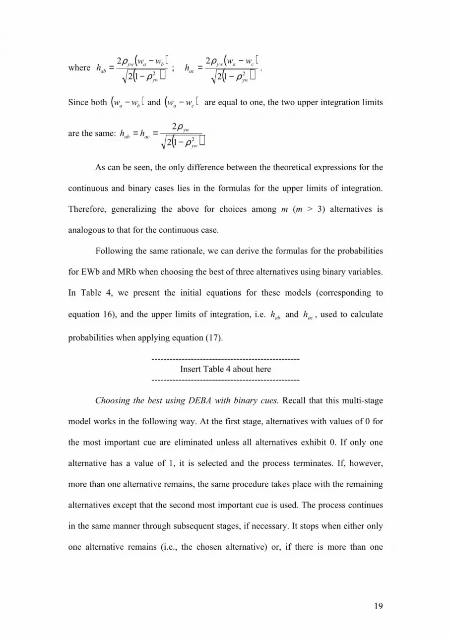
As can be seen, the only difference between the theoretical expressions for the

continuous and binary cases lies in the formulas for the upper limits of integration.

Therefore, generalizing the above for choices among m (m > 3) alternatives is

analogous to that for the continuous case.

Following the same rationale, we can derive the formulas for the probabilities

for EWb and MRb when choosing the best of three alternatives using binary variables.

In Table 4, we present the initial equations for these models (corresponding to

equation 16), and the upper limits of integration, i.e. abh and ach , used to calculate

probabilities when applying equation (17).

-------------------------------------------------

Insert Table 4 about here

-------------------------------------------------

Choosing the best using DEBA with binary cues. Recall that this multi-stage

model works in the following way. At the first stage, alternatives with values of 0 for

the most important cue are eliminated unless all alternatives exhibit 0. If only one

alternative has a value of 1, it is selected and the process terminates. If, however,

more than one alternative remains, the same procedure takes place with the remaining

alternatives except that the second most important cue is used. The process continues

in the same manner through subsequent stages, if necessary. It stops when either only

one alternative remains (i.e., the chosen alternative) or, if there is more than one

20

alternative but no more cues, choice is determined at random among the remaining

alternatives.

The probability that a given alternative was chosen correctly by DEBA is the

probability that the sequence of decisions (or eliminations) made by the model at each

stage is correct. Thus, since at each stage of the model decisions are made conditional

on the preceding stages, the key parameters in estimating these probabilities are the

partial correlations between Y and Wj, j = 1,…,k (i.e., controlling for previous stages).

For the first stage, this is 1ywρ , for the second

12 .wywρ , for the third, 213 . wwywρ , and so

on.8

For example, assume that there are three alternatives A, B, and C and that A

has been chosen by a process whereby C was eliminated at the first stage and B at the

third stage. Starting backwards, consider the decisions the model makes at each stage.

That is, the probability that DEBA correctly selected A over B at the third

stage, controlling for the elimination of C at the first stage, is

( ) ( ){ }11113333 ccbbcbbbaaba wWwWYYwWwWYYP =>=>∩=>=> . This probability

can be calculated by making use of the appropriate partial correlations – in this case,

213 . wwywρ and 1ywρ – and adapting the single variable equations (e.g., the general

equation 10 9). At the second stage, the model makes no decision. At the first stage,

it eliminates C so we need to calculate additionally the probability that A could

have been correctly selected only with information available at this stage:

( ) ( ){ }11111111 ccbbbcccaaca wWwWYYwWwWYYP =>=>∩=>=> . This can be also

found through an adapted expression (10), using1ywρ . Importantly, the events

8 For example, ( )( ) .11 22

.

211

2112

12

wwyw

wwywyw

wyw

ρρ

ρρρρ

−−

−=

9 The terms that need to be adapted in the expression (10) are the upper limits or integration and 21 ,zzσ .

21

represented by the probability expressions for the first and third stages are disjunctive.

Therefore, the probability that DEBA makes the correct decision in this case is equal

to the sum of the two expressions.

Consider another example involving three alternatives A, B, and C. Assume

that DEBA eliminates C at the first stage and at the third stage picks either A or B at

random (this will happen if A and B are identical). Thus, the 0.5 probability that

DEBA makes the correct decision at the third stage should be “discounted” by the

probability that C, eliminated at the first stage, is not better than A and B. That is

( ) ( ){ }( )1111111115.0 bbccbcaaccac wWwWYYwWwWYYP =>=>∩=>=>− .

More generally, the probability of DEBA making the correct choice has to be

calculated on a case-by-case basis taking into account, at each stage, the probability

that the selected alternative should be chosen over the alternative(s) eliminated at that

stage using the partial correlation of the cue appropriate to the stage. Moreover, the

probability for each case includes the probabilities of successful decisions at each

stage. If at the final stage, there are two or more alternatives, the appropriate random

probability is adjusted by the probability that correct decisions were taken at previous

stages (see, e.g., the example above).10

Choosing the best using the EW-SV model with binary cues (EW-SVb). The

first stage of this model uses EWb. If a single alternative is chosen, the probability of

it being correct is found by applying the formula for EWb. If two or more alternatives

are tied, a second stage consists of selecting the alternative favored by the first cue.

To calculate the probability that this is correct, one needs to calculate the joint

probability that the selected alternative (a) is larger than the alternatives eliminated at

10 In this section, we have only indicated the general strategy for calculating relevant probabilities for

DEBA. The details involve repeated applications of the same probability theory principles applied in

many different situations (Karelaia & Hogarth, in preparation).

22

the first stage, and (b) larger than the other alternatives considered at the second stage.

(To calculate these probabilities, use is made of the appropriate analogs to equation

17). Any ties remaining after stage two are resolved at random with a corresponding

adjustment being made to the probability calculations.

Choosing the best using the EW-DEBA model with binary cues (EW-DEBA).

This model starts as EWb. If EWb chooses one alternative, the probability of correct

choice of the model coincides with that for EWb. If two or more alternatives are tied,

the DEBA model is used to choose between the remaining alternatives and

probabilities are calculated accordingly (see above).

V. Empirical evidence

Our equations provide exact theoretical probabilities for assessing

performance of the different models in specified conditions, i.e., to map the contours

of the regions of rationality. However, several factors affect absolute and relative

performance levels of the models (e.g., cue validities,

inter-correlation among

variables, continuous vs. binary variables, error), and it is difficult to assess their

importance simply by inspecting the formulas.

We therefore use both simulated and empirical data to illuminate model

performance under different conditions. Real data have the advantage of testing the

theory in specific, albeit limited environments. Simulated data, on the other hand,

facilitate testing model predictions over a wide range of environments. We first

consider the simulated data.

Simulation design and method. The simulation design used for choosing the

best from two, three and four alternatives is presented in Table 5. Overall, we

specified 20 different populations that are subdivided into four sets or cases – A, B, C,

23

and D – each of which contains five sub-cases (labeled 1, 2, 3, 4, and 5). Since, a

priori, several factors might be thought important, we would have liked to vary these

orthogonally. However, correlations between factors restrict implementing a fully

systematic design. We therefore varied some factors at the level of the cases (A, B, C,

and D) and others across sub-cases (i.e., within A, B, C, and D).

At the level of cases, A and B involved three cues or attributes whereas cases

C and D involved five. Cases A and C had little or no inter-cue correlation; cases B

and D had moderate to high intercorrelation.

---------------------------------------------

Insert Table 5 about here

---------------------------------------------

Across sub-cases (i.e., from 1 through 5 within each of A, B, C, and D), we

varied: (1) the variability of cue validities (maximum less minimum); (2) the validity

of the first (i.e., most important) cue; (3) average validity; and (4) the correlation

between y and x . For all, values increase from the sub-cases 1 through 5. As a

consequence, the R2 on initial fit for MR also increases across sub-cases. This implies

that the sub-cases 1 involve high levels of error whereas the sub-cases 5 are, in

principle, quite predictable environments. Sub-cases 2, 3, and 4 fall between these

extremes.

To conduct the simulation, we defined 20 sets of standardized multivariate

normal distributions with the parameters specified in Table 5 and generated samples

of size 40 from each of these populations. The observations in each sample were split

at random on a 50/50 basis into fitting and prediction sub-samples and model

parameters were estimated on the fitting sub-sample. Two, three or four alternatives

(as appropriate) were then drawn at random from this sub-sample and, using the

estimated model parameters, probabilities of correctly selecting the best of these

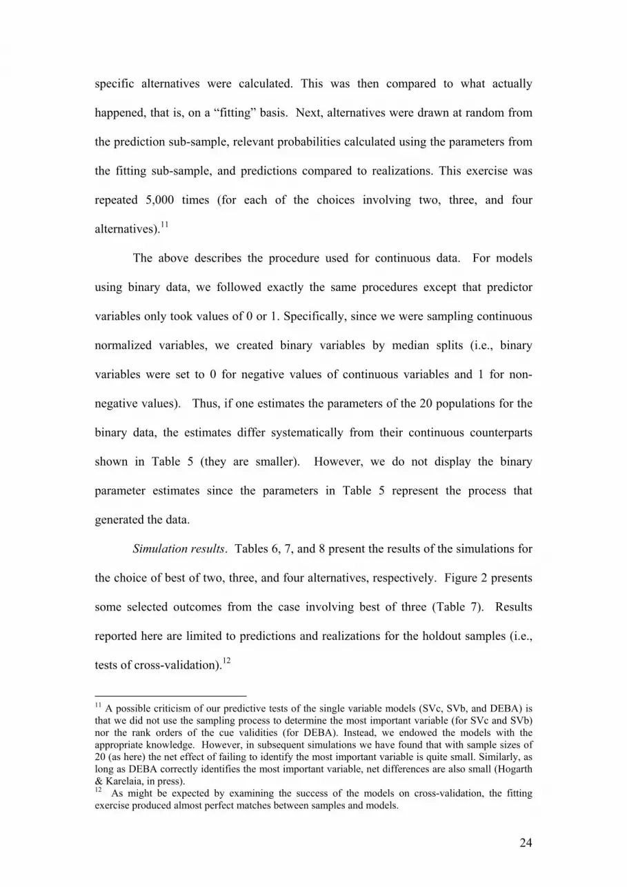
24

specific alternatives were calculated. This was then compared to what actually

happened, that is, on a “fitting” basis. Next, alternatives were drawn at random from

the prediction sub-sample, relevant probabilities calculated using the parameters from

the fitting sub-sample, and predictions compared to realizations. This exercise was

repeated 5,000 times (for each of the choices involving two, three, and four

alternatives).11

The above describes the procedure used for continuous data. For models

using binary data, we followed exactly the same procedures except that predictor

variables only took values of 0 or 1. Specifically, since we were sampling continuous

normalized variables, we created binary variables by median splits (i.e., binary

variables were set to 0 for negative values of continuous variables and 1 for non-

negative values). Thus, if one estimates the parameters of the 20 populations for the

binary data, the estimates differ systematically from their continuous counterparts

shown in Table 5 (they are smaller). However, we do not display the binary

parameter estimates since the parameters in Table 5 represent the process that

generated the data.

Simulation results. Tables 6, 7, and 8 present the results of the simulations for

the choice of best of two, three, and four alternatives, respectively. Figure 2 presents

some selected outcomes from the case involving best of three (Table 7). Results

reported here are limited to predictions and realizations for the holdout samples (i.e.,

tests of cross-validation).12

11 A possible criticism of our predictive tests of the single variable models (SVc, SVb, and DEBA) is

that we did not use the sampling process to determine the most important variable (for SVc and SVb)

nor the rank orders of the cue validities (for DEBA). Instead, we endowed the models with the

appropriate knowledge. However, in subsequent simulations we have found that with sample sizes of

20 (as here) the net effect of failing to identify the most important variable is quite small. Similarly, as

long as DEBA correctly identifies the most important variable, net differences are also small (Hogarth

& Karelaia, in press). 12 As might be expected by examining the success of the models on cross-validation, the fitting

exercise produced almost perfect matches between samples and models.

25

To simplify reading the tables, note that realizations are underlined (e.g., 62),

and that the largest realization for each population (i.e., per column) is presented in

bold (e.g., 65). In addition, when MRc is the largest, we also denote the second largest

in bold. We further show mean realizations for each column and row in the tables.

The column means thus represent the average realizations of all models within

specific populations whereas the row means characterize average model performance

across populations.

We first note that, with the exception of multiple regression (MR), the match

between model predictions and realizations is quite close in all cases. MR makes large

errors for cases C and D and particularly when the differences between maximum and

minimum cue validities are smallest (sub-cases 1 and 2). Although we used adjusted

R2 in making predictions, the adjustment was insufficient in these situations.

13

-----------------------------------------------------------

Insert Tables 6, 7, 8 and Figure 2 about here

-----------------------------------------------------------

Qualitatively, the relative effectiveness of the models is quite similar whether

one looks at the results for best of two, three, or four. What changes, of course, is the

general level of performance which diminishes as the number of alternatives

increases. This can be seen by comparing the columns of mean realizations of Tables

6, 7, and 8, i.e., at the extreme right hand sides of the tables.

Within each table, an initial, overall impression is the lack of large differences

between the performances of the different models. However, there are systematic

effects.

13 One can also argue with some justification that the ratio of observations to predictor variables is too

small to use multiple regression (particularly for cases C and D). However, we are particularly

interested in observing how well the different models work in environments where there are not many

observations.

26

First, consider whether predictor variables are binary or continuous. The use of

binary as opposed to continuous variables implies a loss of information. As such, we

expected that models based on continuous variables would predict better than their

binary counterparts. Indeed, this is always the case in three direct comparisons: SVc

vs. SVb, EWc vs. EWb, and MRc vs. MRb. Specifically, note that SVb and EWb are

both handicapped relative to SVc and EWc in that they necessarily predict many ties

that are resolved at random. Thus, so long as the knowledge in SVc and EWc implies

better than random predictions, models based on continuous variables are favored.

On the other hand, the performance of DRb dominates DRc for cases A, C,

and D with performance being quite similar for case B (for best of two, three, and

four). It would appear that DRb exploits more cases of “apparent” dominance than

DRc which (as a consequence) decides more choices at random. Thus, to the extent

that the “additional” dominance cases detected by DRb relative to DRc have more

than a random chance of being correct, DRb outpredicts DRc. Whereas the DR

models represent naïve baseline strategies, we believe this finding is important

because it demonstrates how a simple strategy can exploit the structure of the

environment such that more information (in the form of continuous as opposed to

binary variables) does not improve performance (a so-called “less is more” effect,

Goldstein & Gigerenzer, 2002; Hertwig & Todd, 2003).

Second, models that resolve ties perform better than their counterparts that are

unable to do so (e.g., DEBA vs. SVb, and EW/DEBA and EW/SVb vs. EW).

However, in the presence of redundancy, these differences are quite small (i.e., for

cases B and D). More interesting is the comparison between SVc and DEBA. The

former uses a single, continuous variable. The latter relies heavily on one binary

variable but can also use others depending on circumstances. It is thus not clear

27

which strategy actually uses more information. However, once again, characteristics

of the environment determine which strategy is more successful. SVc dominates

DEBA in case B as well as for much of cases A and D. On the other hand, DEBA

dominates SVc in case C.

In Figure 2, we have chosen to illustrate the performance of five models across

all the environments for the choice of best of three (i.e., data from Table 7). Two of

these models, DRb and MRc are depicted because they represent, respectively, naïve

and “sophisticated” benchmarks. The other models, SVc, DEBA, and EWc are quite

different types of heuristics (see Table 1). Both SVc and DEBA require prior

knowledge of what is important (DEBA more so than SVc). However, they use little

information and neither involves any computation. (DEBA, it should be recalled, also

operates on binary data.) EWc, on the other hand, does not require knowledge of

differential importance of variables but does use all information available and needs

some computational ability.

In interpreting Figure 2, it is instructive to recall that cases A and C (on the

left) represent environments with low redundancy whereas cases B and D (on the

right) have higher levels of redundancy. Also within each case, the amount of noise

in the environment decreases as one moves from sub-case 1 (on the left) to sub-case 5

(on the right).

As expected, in the noisier environments (sub-cases 1), the performances of all

models are degraded such that differences are small. However, as error decreases

(i.e., moving right toward sub-cases 5), model performances vary by environmental

conditions. With low redundancy (cases A and C), there appear to be large

differences in model performance. However, in the presence of redundancy (cases B

and D), there are two distinct classes of models: SVc and MRc have similar

28

performance levels and are superior to the others. We further note that SVc is most

effective in case B and also does well as environmental predictability increases in

cases A and D. DEBA is never the best model but performs quite adequately in case

C where EWc has the best performance. Of the benchmark models, DRb generally

lags behind the other models (as would be expected). Finally, although MRc is

typically one of the better models, it does not dominate in all environments.

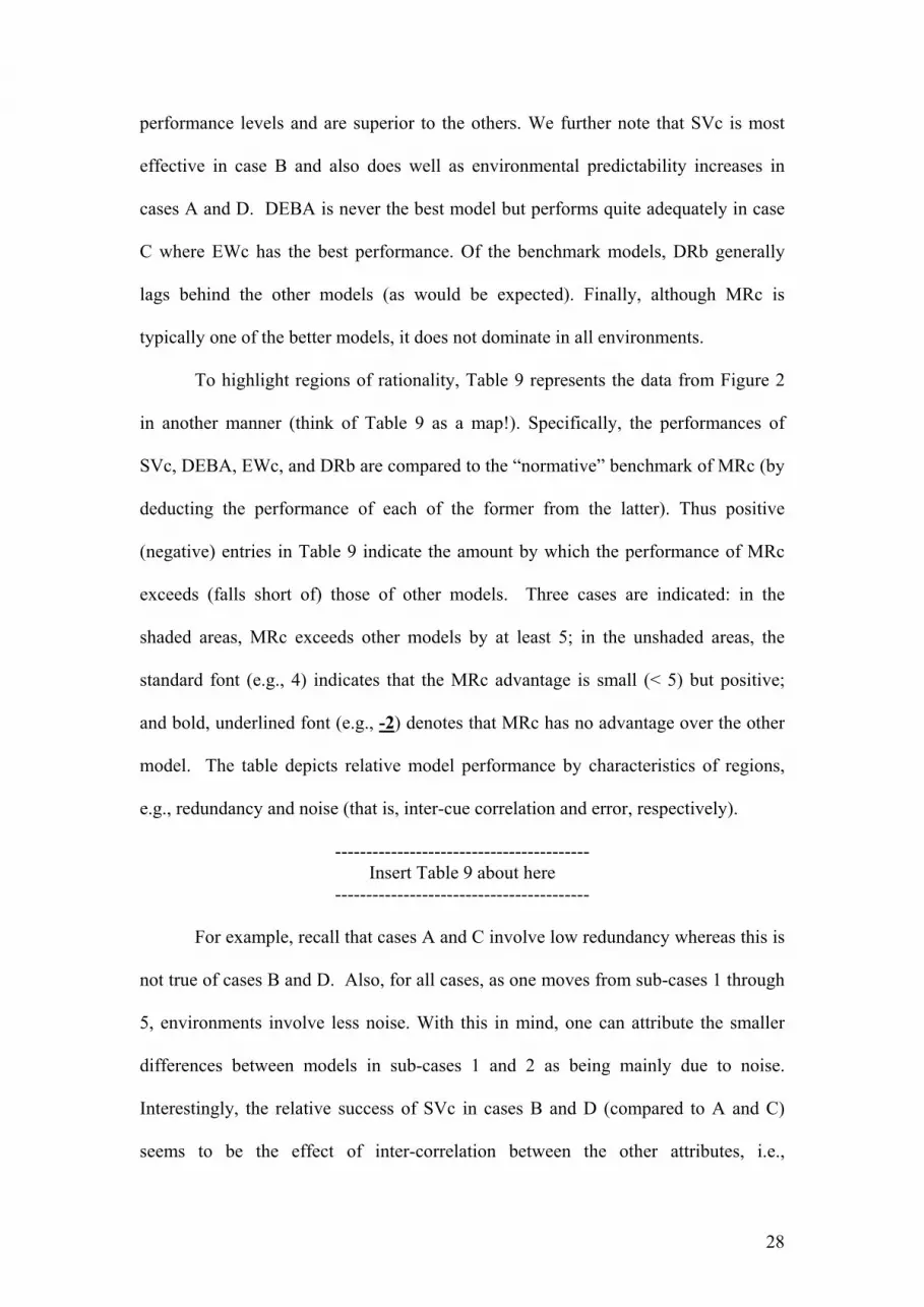
To highlight regions of rationality, Table 9 represents the data from Figure 2

in another manner (think of Table 9 as a map!). Specifically, the performances of

SVc, DEBA, EWc, and DRb are compared to the “normative” benchmark of MRc (by

deducting the performance of each of the former from the latter). Thus positive

(negative) entries in Table 9 indicate the amount by which the performance of MRc

exceeds (falls short of) those of other models. Three cases are indicated: in the

shaded areas, MRc exceeds other models by at least 5; in the unshaded areas, the

standard font (e.g., 4) indicates that the MRc advantage is small (< 5) but positive;

and bold, underlined font (e.g., -2) denotes that MRc has no advantage over the other

model. The table depicts relative model performance by characteristics of regions,

e.g., redundancy and noise (that is, inter-cue correlation and error, respectively).

-----------------------------------------

Insert Table 9 about here

-----------------------------------------

For example, recall that cases A and C involve low redundancy whereas this is

not true of cases B and D. Also, for all cases, as one moves from sub-cases 1 through

5, environments involve less noise. With this in mind, one can attribute the smaller

differences between models in sub-cases 1 and 2 as being mainly due to noise.

Interestingly, the relative success of SVc in cases B and D (compared to A and C)

seems to be the effect of inter-correlation between the other attributes, i.e.,

29

redundancy. Table 9 is only presented as an illustration. The data from Tables 6, 7,

and 8 can clearly be used to create maps that highlight different aspects of the

decision making terrain.

A further way of summarizing factors that affect the performance of the

different models is to consider the regression of model performance on statistics that

describe the characteristics of the 20 simulated environments (Table 5). In other

words, consider regressions for each of our eleven models of the form

iii ZP τδ += (18)

where iP is the performance realization of model i (i = 1, …, 11); Z is the (20 x 3) x s

matrix of independent variables (statistics characterizing the datasets where there are

three choice situations, i.e., best of two, three, or four alternatives); iδ is the s x 1

vector of regression coefficients; and iτ is a normally distributed error term with

constant variance, independent of Z.

To characterize the environments or datasets (the Z matrices), we chose the

following variables: variability of cue validities (max less min), the validity of the

most important cue (1yx

r ), the validity of the average of the cues ( xyr ), average inter-

correlation of the cues, average validity of the cues, number of cues, and R2 for MRc

and MRb.14

We also used dummy variables to model the effects of choosing between

different numbers of alternatives. Dummy1 captures the effect of choosing from three

as opposed to two alternatives, and Dummy2 the additional effect of choosing from

four alternatives. Results of the regression analyses are summarized in Table 10.

14 We only used R2 as an independent variable for MRc and MRb because we thought it would be

appropriate for these models. For the other models, however, it was deemed more illuminating to

characterize performance by the other measures (R2 and these other measures are correlated in different

ways). It should also be noted that we used the same statistics (based on continuous variables) to

characterize the environments for models using both continuous and binary variables on the grounds

that the underlying environments were based on continuous variables.

30

---------------------------------------------------

Insert Table 10 about here

---------------------------------------------------

We used a step-wise procedure with entry (exit) thresholds for the variables of

<.05 (>.10) for the probability of the F statistic. All coefficients for the models shown

in Table 10 are statistically significant (p < .001) and all regressions fit the data well

(see R2 and estimated standard errors at the foot of Table 10). The constant term is

fairly high across all models and measures the level of performance that would be

expected of the models in binary choice absent information about the environment

(approximately 50, i.e., from 42 to 65). Dummy1 indicates how much such

performance would fall when choosing between three alternatives (between 11 and

14), and Dummy2 shows the additional drop experienced when choosing among four

alternatives (between 6 and 9).

For SVc and SVb, only one other variable is significant, the correlation

between the single variable and the criterion. This makes intuitive sense as does the

fact that the regression coefficient is larger with continuous as opposed to binary

variables (50 vs. 29). The DEBA and EW models are all heavily influenced by the

correlation between the criterion and x . Recall, however, that this correlation is itself

an increasing function of average cue validity and the number of cues but decreasing

in the inter-correlation between cues (see the formula in footnote 1 to Table 2). Thus,

ceteris paribus, increasing inter-correlation between the cues reduces the absolute

performance levels of these models. DEBA differs from the EW models in that the

correlation of the most valid cue is a significant predictor. This matches expectations

in that DEBA relies heavily on the validity of the most important cue whereas EW

weights all cues equally. (We also note that the SV models weight the most valid cue

more heavily than DEBA.) As to the Domran models, the interpretation of the signs of

31

all coefficients is not obvious. Finally, for MRc it comes as little surprise that R2

should be so important although this variable is less salient for MRb.

A possible surprise is that variability in cue validities (maximum less

minimum) was not a significant factor for most models. One might have thought, a

priori, that such dispersion would have been important for DEBA (cf., Payne et al.,

1993). However, this is not the case and is consistent with theoretical analyses of

DEBA that show that its accuracy is relatively robust to different “weighting

functions” (Hogarth & Karelaia, in press; Baucells, Carrasco, & Hogarth, 2005).

Finally, whereas the regression statistics paint an interesting picture of model

performance in the particular environments observed, we caution against

overgeneralization. We only observed restricted ranges of the environmental statistics

(i.e., characteristics) and thus cannot comment on what might happen beyond these

ranges. Our approach, however, does suggest a way to illuminate model x

environment interactions.

To summarize, across all 20 environments that, inter alia, are subject to

different levels of error, the relative performances of the different models were not

seen to vary greatly when faced with the same tasks (e.g., choose best of three

alternatives). However, there were systematic differences due to interactions between

characteristics of models and environments. Thus, whereas the additional information

contained in continuous as opposed to binary variables benefits some models, e.g., SV

and EW, it can be detrimental to others, e.g., DR. Second, models varied in the extent

to which they were affected by specific environmental characteristics. SV models, for

example, depend heavily on the validity of the most valid cue whereas this only

affects EW models through its impact on average cue validity. Interestingly, the

validity of the average of the cues was seen to have more impact on the performance

32

of DEBA than the validity of the most valid cue. Average inter-correlation of

predictors or redundancy tends to reduce performance of all models (except SV).

Overall, results do match some general trends noted in previous simulations

(Payne et al., 1993; Fasolo et al., in press); however, patterns are not simple to

describe. The value of our work, therefore, is that we now possess the means to make

precise predictions for various simple, heuristic models in different environments.

That is, given specified environments, we can predict a priori both levels of model

performance and which models will be more or less effective.

An important environmental factor we did not vary was the impact of

different distributions of specific kinds of alternatives. Instead, we simulated random

drawings of alternatives given the population characteristics defined in Table 5. We

did not, for example, skew the sampling process to include or exclude

disproportionate numbers of, say, dominating or dominated alternatives (cf., Payne

et al., 1993). As we have argued elsewhere (Hogarth & Karelaia, 2004), the

distribution of alternatives can have important effects on both the general level of

performance achieved by models as well as relative performance (some distributions,

for example, are relatively “friendly” or “unfriendly” to specific models, Shanteau &

Thomas, 2000). On the other hand, since our methodology can make specific

predictions for each case encountered, it can easily handle the effects of sampling

from different distributions of alternatives.

Empirical data. We used datasets from three different areas of activity. The

first involved performance data of the 60 leading golfers in 2003 classified by the

Professional Golf Association (PGA) in the USA.15

From these data (N = 60), we

examined two dependent variables: “all-round ranking” and “total earnings.” The first

15 These data were obtained from the webpage http://www.pgatour.com/stats/leaders/r/2003/120. They

are performance statistics of golfers in the main PGA Tour for 2003.

33

is a measure based on eight performance statistics. For our models, we chose three

predictor variables that account for 67% of the variance in the criterion. These were

mean numbers – across rounds played – of birdies, total scores, and putts. Since the

first variable was negatively related to the criterion, it was rescaled (multiplying

by -1).

Eighty-two percent of the variance in the second golf criterion, total earnings,

could be explained by three variables, “number of top 10 finishes,” “all-round

ranking” (the previous dependent variable), and “number of consecutive cuts.” Of

these, all-round ranking was negatively correlated with the criterion and so rescaled

(multiplying by -1).

The second dataset consisted of rankings of PhD economics programs in the

USA on the basis of a 1993 study by the National Research Council (N = 107).16

Three variables accounted for 80% of the variance in the rankings: number of PhD’s

produced by programs for the academic years 1987-88 through 1991-1992, total

number of program citations in the period 1988-1992 divided by number of program

faculty, and percentage of faculty with research support.

The third dataset was taken from the UK consumer organization Which?’s

assessments of digital cameras in 2004 (N = 49).17

Three variables were found to

explain 72% of the variance in total test scores: image quality, picture downloading

time, and focusing.

Table 11 summarizes statistical characteristics of these datasets (analogous to

the experimental design of the simulations in Table 5). As can be seen, there is little to

moderate variability in cue validities (compare Economics PhD programs with the

other datasets); all datasets have at least one highly valid cue; average inter-

16 For more details, see the webpage http://www.phds.org 17 For further details, see the webpage http://sub.which.net

34

correlation varies from moderate to low (Consumer reports: Digital cameras); and

there are high correlations between the criteria and the means of the predictor

variables.

The testing procedure was similar to the simulation methodology. We divided

each sample at random on a 50/50 basis into fitting and testing sub-samples. Model

parameters were then estimated on the fitting sub-sample and these parameters used to

calculate the probabilities that the models would correctly choose the best of two,

three, and four alternatives that had also been randomly drawn from the same sub-

sample. This was the fitting exercise. To test the models’ predictive abilities, two,

three, and four alternatives were drawn at random from the second or testing sub-

sample and, using the parameters estimated from the data in the first or fitting sub-

sample, model probabilities were calculated for the specific cases and subsequently

compared to realizations. This exercise was repeated 5,000 times such that the data

reported in Table 12 shows the aggregation of all these cases. Also similar to the

simulation methodology, we created binary datasets by using median splits of the

continuous variables.

---------------------------------------------------

Insert Tables 11, 12 and Figure 3 about here

---------------------------------------------------

Table 12 has been constructed in similar fashion to Tables 6, 7, and 8 except

that we show results for choosing the best out of two, three, and four alternatives

within columns for each dataset.

Once again, there is an excellent fit between predictions and realizations.18

The largest differences occur, as before, with MR. Overall, the models have fairly

high levels of performance which, naturally, diminish as the number of alternatives

18 For this reason, we do not present here the excellent fits achieved by the models on the fitting

samples.

35

increases (however, perhaps, not as much as might have been thought a priori. See, in

particular, Economics PhD programs). As with the simulated datasets, the SV, EW,

and MR models with continuous variables outperform their binary counterparts (with

one exception in 36 comparisons) but DRb dominates DRc. As to the SVc versus

DEBA comparison, SVc outperforms DEBA by some margin on the Golf rankings

and Golf earnings datasets but DEBA dominates SVc on the other two datasets. From

a statistical viewpoint, these two datasets differ from the others in that the Economics

PhD programs has low variability of cue validities and Consumer reports: Digital

Cameras has low average cue inter-correlation.

Differences between models on the different datasets are highlighted in Figure

3 where we again show the performances of SVc, DEBA, EWc, DRb, and MRc.

Although the datasets have some similarities (e.g., the validities of the first cue and

the correlations between the criteria and the means of the predictor variables are

almost the same), other differences (notably variability in cue validities and levels of

cue inter-correlations) are sufficient to change the relative effectiveness of the models.

SVc is very effective for the Golf rankings and Golf earnings data, EWc predicts the

Economics PhD programs well and DEBA is best for the Consumer reports: Digital

Cameras data. As to the two benchmark models, DRb generally has the lowest

performance but, with the exception of the Consumer reports: Digital cameras

dataset, is close to DEBA. For all datasets, MRc is always one of the better models

but it does not dominate the other models. Finally, we emphasize once again the

close fit between our model predictions and the empirical realizations demonstrated in

Table 12. Taken as a whole, our theoretical models account for complex patterns of

data.

36

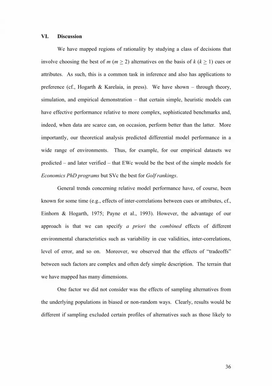
VI. Discussion

We have mapped regions of rationality by studying a class of decisions that

involve choosing the best of m (m > 2) alternatives on the basis of k (k > 1) cues or

attributes. As such, this is a common task in inference and also has applications to

preference (cf., Hogarth & Karelaia, in press). We have shown – through theory,

simulation, and empirical demonstration – that certain simple, heuristic models can

have effective performance relative to more complex, sophisticated benchmarks and,

indeed, when data are scarce can, on occasion, perform better than the latter. More

importantly, our theoretical analysis predicted differential model performance in a

wide range of environments. Thus, for example, for our empirical datasets we

predicted – and later verified – that EWc would be the best of the simple models for

Economics PhD programs but SVc the best for Golf rankings.

General trends concerning relative model performance have, of course, been

known for some time (e.g., effects of inter-correlations between cues or attributes, cf.,

Einhorn & Hogarth, 1975; Payne et al., 1993). However, the advantage of our

approach is that we can specify a priori the combined effects of different

environmental characteristics such as variability in cue validities, inter-correlations,

level of error, and so on. Moreover, we observed that the effects of “tradeoffs”

between such factors are complex and often defy simple description. The terrain that

we have mapped has many dimensions.

One factor we did not consider was the effects of sampling alternatives from

the underlying populations in biased or non-random ways. Clearly, results would be

different if sampling excluded certain profiles of alternatives such as those likely to

37

dominate others or be dominated.19

On the other hand, our theoretical method allows

us to make case-by-case predictions such that – through suitable aggregation – we

could make predictions for samples drawn in specific, non-random ways provided the

same sampling procedures are used in both fitting and holdout samples. Showing the

effects of such non-random sampling is thus a straightforward task that can be

addressed in future research.

This paper is also limited by the criterion used to measure model effectiveness,

i.e., the emphasis on probability of correct choices. This might seem restrictive in that

it assumes a “hit or miss” criterion with no consideration as to how “good” the other

alternatives are. We accept this limitation in the present work but emphasize that our

methodology can be easily extended to other loss functions.

First, for simplicity, consider an example of binary choice using a single

variable (SV) where our methodology is used to determine the probability than

alternative A is better than alternative B. That is, instead of determining the

probability that Ya is greater than Yb (or equivalently 0>− ba YY ), we could also

consider the probability that cYY ba >− where c > 0. In order to find this value, we

need to modify the inequalities involving error differences. For example, the

inequality (6), written as ( ) abbayx XX εερ −>− , becomes:

( ) abbayx cXX εερ −>−− (6´)

and we proceed as before with the calculations. Moreover, by repeating this

calculation for different values of c, one can investigate how much better Ya is likely

to be compared to Yb. As an example, one can calculate the value of c for which

{ } 5.0>>− cYYP ba or other meaningful levels of probability.

19 Note that we would not be able to apply our “overall formulas” (e.g., equation 13) to these

populations because they assume unbiased, random sampling.

38

Second, our theoretical models can be used to specify not just the probability

that one alternative will be correctly selected but also the probabilities for all

alternatives. For example, imagine choosing between three alternatives A, B, and C

using the SV model and having observed cba xxx >> . Above, we calculated the

probability ( ) ( ){ }ccaacabbaaba xXxXYYxXxXYYP =>=>∩=>=> . However,

we could also have calculated the probability that B is the largest, that is

( ) ( ){ }ccbbcbbbaaab xXxXYYxXxXYYP =>=>∩=>=> and so on. In other

words, we can specify the probabilities associated with all possibilities. Given such

distributions over possible outcomes, it is straightforward to consider the effects of

different loss functions, a topic we also leave for further research.

Future work could also build on our theoretical approach to consider variations

of the models we have examined here. For example, models might involve mixtures

of categorical and continuous variables or the effects of different types of error. How,

for instance, would simple models perform when there are errors in the variables

(perhaps due to measurement problems) or missing values? In addition, it will be

important to investigate effects due to deviations from assumptions of normal

distributions examined in this paper. Clearly many further elaborations can be

undertaken.

Our work has particular implications for decision making when attention is a

scarce resource. As stated by Simon (1978):

In a world in which information is relatively scarce, and where problems for

decision are few and simple, information is almost always a positive good. In a

world where attention is a major scarce resource, information may be an

expensive luxury, for it may turn our attention from what is important to what

is unimportant. We cannot afford to attend to information simply because it is

there (Simon, 1978, p. 13).

39

By way of illustration, Simon described executives whose management

information systems provide excessive, detailed information. Our work also

identified regions where more information does not necessarily lead to better

decisions and, if we assume that more complex models require more cognitive effort

(or computational cost), there are many areas where there is no tradeoff between

accuracy and effort. For example, in cases B and D illustrated in Figure 2, the simple

SVc model is more accurate than the other models indicated across almost the whole

range of conditions and, yet, it uses less information. On the other hand, EWc is

generally best in case C where SVc lags behind the other models. However, EWc uses

more information than both SVc and DEBA such that one can ask whether the

additional predictive ability is worth its cost.

The models we examined might also be used in applied areas such as

consumer research (cf., Bettman, Luce, & Payne, 1998). That is, instead of assuming

that consumers make tradeoffs across many attributes, simpler SV or EW models can

be constructed after eliciting a few simple questions concerning, say, relative

importance of attributes. For example, we have shown elsewhere that if people have

loose preferences characterized by binary attributes, the outputs of DEBA are

remarkably consistent with more complex, linear tradeoff models (Hogarth &

Karelaia, in press). However, it would be a mistake to assume that consumer

preferences can always be modeled by one simple model (e.g., EW). Indeed, our

theoretical analysis provides the basis for deciding which models are suited to

different environments.

As suggested, our models clearly have many implications for prescriptive

work. In addition to determining when heuristic models are appropriate for specific,

applied problems in, for example, forecasting performance, personnel assessment and

40

recruitment, medical decision making, etc, heuristic models are useful supports for

more complicated, decision analytical modeling. When, for instance, does one need to

assess tradeoffs precisely, or can heuristic-based simplifications suffice? Here theory

such as developed in this paper has great practical use for determining which heuristic

to use, and when.

Finally, in a world where attention is the scarce resource, we note that

“rational behavior” consists of finding the appropriate match between a decision rule

and the task with which it is confronted – a principle that is valid for both descriptive

and prescriptive approaches to decision making. On considering both dimensions,

therefore, we do not need to assume unlimited computational capacity. However, by

relaxing this assumption, we incur two costs. The first, analyzed in this paper, is to

identify the task conditions under which specific heuristic rules are and are not

effective, i.e., to develop maps of the regions of rationality. The second, that awaits

further research, is to elucidate the conditions under which people do or do not

acquire such knowledge. In other words, how do people build maps of their decision

making terrain? To be effective, people do not need much computational ability to

make choices in the mazes that define their environments. However, they do need

task-specific knowledge or maps.

41

References

Baucells, M., Carrasco, J. A., & Hogarth, R. M. (2005). Cumulative dominance and

heuristic performance in binary multiattribute choice. Barcelona: Working paper

IESE, UPC, and UPF.

Bettman, J. R., Luce, M. F., & Payne, J. W. (1998). Constructive consumer choice

processes. Journal of Consumer Research, 25, 187-217.

Conlisk, J. (1996). Why bounded rationality? Journal of Economic Literature, 34 (2),

669-700.

Dawes, R. M., (1979). The robust beauty of improper linear models. American

Psychologist, 34, 571-582.

Dawes, R. M., & Corrigan, B. (1974). Linear models in decision making. Psychological

Bulletin, 81, 95-106.

Dawes, R. M., Faust, D., & Meehl, P. E. (1989). Clinical versus actuarial judgment.

Science, 243, 1668-1674.

Einhorn, H. J., & Hogarth, R. M. (1975). Unit weighting schemes for decision making.

Organizational Behavior and Human Performance, 13, 171-192.

Fasolo, B., McClelland, G. H., & Todd, P. M. (in press). Escaping the tyranny of choice:

When fewer attributes make choice easier. Marketing Theory.

Gigerenzer, G., & Goldstein, D. G. (1996). Reasoning the fast and frugal way: Models of

bounded rationality. Psychological Review, 103, 650-669.

Gigerenzer, G., & Selten, R. (2001). (Eds.) Bounded rationality: The adaptive toolbox.

Cambridge, MA: The MIT Press.

Gigerenzer, G., Todd, P. M., and the ABC Research Group. (1999). Simple heuristics that

make us smart. New York: Oxford University Press.

42

Goldstein, D. G., & Gigerenzer, G. (2002). Models of ecological rationality: The

recognition heuristic. Psychological Review, 109 (1), 75-90.

Goldstein, W. M., & Hogarth, R. M. (1997). Judgment and decision research: Some

historical context. In W. M. Goldstein & R. M. Hogarth (eds.), Research on

judgment and decision making: Currents, connections and controversies. New

York: Cambridge University Press.

Hertwig, R., & Todd, P. M. (2003). More is not always better: The benefits of cognitive

limits. In D. J. Hardman & L. Macchi (eds.), Thinking: Psychological perspectives

on reasoning, judgment and decision making. Chichester, England: Wiley.

Hogarth, R. M., & Karelaia, N. (2004). “Take-the-Best” and other simple strategies:

Why and when they work “well” in binary choice. Barcelona: Universitat Pompeu

Fabra, DEE working paper.

Hogarth, R. M., & Karelaia, N. (2005). Ignoring information in binary choice with

continuous variables: When is less “more”? Journal of Mathematical Psychology,

49, 115-124.

Hogarth, R. M., & Karelaia, N. (in press). Simple models for multi-attribute choice with

many alternatives: When it does and does not pay to face tradeoffs with binary

attributes. Management Science.

Kahneman, D. (2003). Maps of bounded rationality: Psychology for behavioral

economics. American Economic Review, 93(5), 1449-1475.

Kahneman, D., Slovic, P., & Tversky, A. (1982). (Eds.) Judgment under uncertainty:

Heuristics and biases. New York: Cambridge University Press.

Karelaia, N., & Hogarth, R. M. (in preparation). On predicting performance of DEBA

models in the presence of error. Barcelona: Universitat Pompeu Fabra

Katsikopoulos, K., & Martignon, L. (2003). Paired comparisons: Ordering or adding

43

attributes? Working paper, Max-Planck Institute for Human Development, Berlin.

Kleinmuntz, B. (1990). Why we still use our heads instead of formulas: Toward an

integrative approach. Psychological Bulletin, 107, 296-310.

Koehler, D., & Harvey, N. (eds.) (2004). Blackwell Handbook of Judgment and Decision

Making. Oxford, UK: Blackwell.

Martignon, L., & Hoffrage, U. (1999). Why does one-reason decision making work? A

case study in ecological rationality. In G Gigerenzer, P. M. Todd and the ABC

Research Group. Simple heuristics that make us smart (pp. 119-140). New York:

Oxford University Press.

Martignon, L., & Hoffrage, U. (2002). Fast, frugal, and fit: Simple heuristics for paired

comparison. Theory and Decision, 52, 29-71.

Payne, J. W., Bettman, J. R., & Johnson, E. J. (1993). The adaptive decision maker. New

York: Cambridge University Press.

Shanteau, J., & Thomas, R. P. (2000). Fast and frugal heuristics: What about unfriendly

environments? Behavioral and Brain Sciences, 23, 762-763.

Simon, H. A. (1956). Rational choice and the structure of environments. Psychological

Review, 63, 129-138.

Simon, H. A. (1978). Rationality as process and product of thought. American Economic

Review, 68 (2), 1-16

Simon, H. A. (1991). Models of my life. New York: Basic Books.

Thorngate, W. (1980). Efficient decision heuristics. Behavioral Science, 25, 219-225.

Tversky, A. (1972). Elimination by aspects: A theory of choice. Psychological

Review, 79, 281-299.

44

Table 1 -- Models tested

Number of comparisons

(A). Single Variable (SV) models

Prior

information*

Information

to consult Calculations

min max

1 Lexicographic

-- SVc

Choice depends solely on cue with the greatest validity (see, e.g., Payne et

al., 1993).

2 Lexicographic

-- SVb

Model 1 above but based on binary variables.

The most

important cue

( )2

1−mm

3 DEBA Deterministic version of Tversky's (1972) elimination-by-aspects model

(EBA). For binary choice, this is the same as the take-the-best model of

Gigerenzer and Goldstein (1996).

Rank-order

of

importance

of cues

Variable

None ( )1−m

( )2

1−mmk

(B). Equal weight (EW) models

4 EWc All cues are accorded equal weight (see, e.g., Einhorn & Hogarth, 1975).

5 EWb All cues are accorded equal weight (see, e.g., Dawes, 1979), None All m sums ( )1−m

( )2

1−mm

(C). Hybrid models

6 EW/DEBA Choose according to equal weights. If this results in a tie, use DEBA to

resolve the choice (Hogarth & Karelaia, in press).

7 EW/SVb Choose according to equal weights. If this results in a tie, resolve conflict

by the single most important variable

Rank-order

of

importance

of cues

All m sums ( )1−m

( )2

1−mm

(D). Domran (DR) models

8 DRc If an alternative dominates, choose it. Otherwise, choose at random

between non-dominated alternatives.

9 DRb Same as DRc except based on binary variables.

None All None ( )1−mk ( )

2

1−mmk

(E). Multiple regression (MR)

10 MRc Well-known statistical model.

11 MRb Same as MRc except based on binary variables.

Importance

of cues All

km products,

m sums ( )1−m

( )2

1−mm

* For all models, the decision maker is assumed to know the sign of the zero order correlation between cues and the criterion.

NOTE: m = number of alternatives, k = number of attributes, cues

45

Table 2 – Key formulas for different models using continuous variables (for choosing best of three)

Accuracy Error Upper integration limits,

conditions variances abl and acl

Single variable (SVc)

aayxa XY ερ += ( ) abbayx XX εερ −>− 2(21 yxρ− )

( ))1(2 2

yx

bayx xx

ρ

ρ

−

−

bbyxb XY ερ += ( ) accayx XX εερ −>− ( )

)1(2 2

yx

cayx xx

ρ

ρ

−

−

ccyxc XY ερ +=

Equal weights (EWc)

aaxxya vXY += )/( σρ ( ) abbaxxy vvXX −>−)/( σρ 2(21 xyρ− )

( )( )212 xyx

baxy xx

ρσ

ρ

−

−

bbxxyb vXY += )/( σρ ( ) accaxxy vvXX −>−)/( σρ ( )

( )212 xyx

caxy xx

ρσ

ρ

−

−

ccxxyc vXY += )/( σρ

Multiple regression (MRc)

aaa uYY += ˆ ( ) abba uuYY −>− ˆˆ 2 )1( 2

adjR− ( )

)1(2

ˆˆ

2

adj

ba

R

yy

−−

bbb uYY += ˆ ( ) acca uuYY −>− ˆˆ

ccc uYY += ˆ ( )

)1(2

ˆˆ

2

adj

ca

R

yy

−−

46

Notes:

1. jixx

yxxyk

k

ρρρ

)1(1 −+= where k = number of x variables, yxρ = average correlation between y and the x’s, and

jixx

ρ = average inter-correlations amongst the x’s.

2. ( )jixxx k

kρσ )1(1

1 −+=

3. ( ) ( )( )kn

nRRadj −

−−−= 111 22 where n = number of observations.

4. The probability of optimal choice out of three is given by:

( )∫ ∫∞− ∞−

+−−ab acl lzzzz

dzdze 213

2 2221

21

3

1

π,

with upper integration limits being specific for different choice strategies.

5. Correlations between the standardized normal variables ( )21

12 yx

abzρ

εε

−

−= and ( )2

2

12 yx

aczρ

εε

−

−= are all equal to ½ – see Appendix A.

47

Table 3 – Formulas for overall predictive accuracy of models using continuous variables

(for choosing best of m)

Model dV Upper limits of integration

*

id , for 1,1 −= mi

SVc

2...1

.........

1...2

( )212 yx

iyxd

ρ

ρ

−

EWc

xx

xx

σσ

σσ

2...

.........

...2

2

2

( )212 xyx

ixy d

ρσ

ρ

−

MRc

22

22

2...

.........

...2

adjadj

adjadj

RR

RR

)1(2 2

adj

i

R

d

−

Notes:

Overall expected probability of success is given by:

1111

00

......),(....),(....

*1

*1

−∞−

−∞−

∞∞

∫ ∫∫∫−

m

d

m

d

zzdd dddddzdzVzVdmm

µϕµϕ

where ),...,,( 121 −=′mzzzz , ),...,,( 121 −=′

mdddd , and

=1...2/1

.........

2/1...1

zV .

dV and *

id , for 1,1 −= mi , are specific for different choice strategies.

See also notes to Table 2.

48

Table 4 – Key formulas for different models using binary variables (for choosing best of three)

Model Upper integration limits

abh ach

Single variable

(SVb)

ςσρ

++= WaYw

yw

SVb ( )

( )212 yww

bayw ww

ρσ

ρ

−

−

( )( )212 yww

cayw ww

ρσ

ρ

−

−

Equal weights

(EWb)

ξσρ

++= WaYw

wy

EWb

( )( )212 wyw

bawy ww

ρσ

ρ

−

−

( )( )212 wyw

cawy ww

ρσ

ρ

−

−

Multiple

regression (MRb)

ζ+=YY ˆ

( ))1(2

ˆˆ

2

adj

ba

R

yy

−−

( )

)1(2

ˆˆ

2

adj

ba

R

yy

−−

( Y and 2

adjR are based on binary variables W’s)

Notes:

1. jiww

ywwyk

k

ρρρ

)1(1 −+= ,

where k = number of x variables,

ywρ = average correlation between y and the w’s, and

jiwwρ = average inter-correlations amongst the w’s.

2. ( )jiwww k

kρσ )1(1

1 −+=

3. ( ) ( )( )kn

nRRadj −

−−−= 111 22

where n = number of observations.

4. The probability of optimal choice out of three is given by

( )∫ ∫∞− ∞−

+−−ab ach hzzzz

dzdze 213

2 2221

21

3

1

π,

with upper integration limits being specific for different choice strategies.

5. Since the error terms have means of zero, the intercepts SVba and EWba are equal

to ywρ− and w

wy

σρ2

− , respectively.

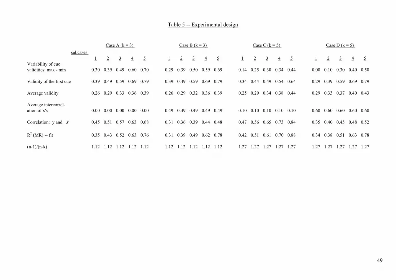
49

Table 5 -- Experimental design

subcases

1 2 3 4 5 1 2 3 4 5 1 2 3 4 5 1 2 3 4 5

Variability of cue

validities: max - min 0.30 0.39 0.49 0.60 0.70 0.29 0.39 0.50 0.59 0.69 0.14 0.25 0.30 0.34 0.44 0.00 0.10 0.30 0.40 0.50

Validity of the first cue 0.39 0.49 0.59 0.69 0.79 0.39 0.49 0.59 0.69 0.79 0.34 0.44 0.49 0.54 0.64 0.29 0.39 0.59 0.69 0.79

Average validity 0.26 0.29 0.33 0.36 0.39 0.26 0.29 0.32 0.36 0.39 0.25 0.29 0.34 0.38 0.44 0.29 0.33 0.37 0.40 0.43

Average intercorrel-

ation of x's 0.00 0.00 0.00 0.00 0.00 0.49 0.49 0.49 0.49 0.49 0.10 0.10 0.10 0.10 0.10 0.60 0.60 0.60 0.60 0.60

Correlation: y and 0.45 0.51 0.57 0.63 0.68 0.31 0.36 0.39 0.44 0.48 0.47 0.56 0.65 0.73 0.84 0.35 0.40 0.45 0.48 0.52

R2 (MR) -- fit 0.35 0.43 0.52 0.63 0.76 0.31 0.39 0.49 0.62 0.78 0.42 0.51 0.61 0.70 0.88 0.34 0.38 0.51 0.63 0.78

(n-1)/(n-k) 1.12 1.12 1.12 1.12 1.12 1.12 1.12 1.12 1.12 1.12 1.27 1.27 1.27 1.27 1.27 1.27 1.27 1.27 1.27 1.27

Case A (k = 3) Case B (k = 3) Case C (k = 5) Case D (k = 5)

x

50

subcases Mean

1 2 3 4 5 1 2 3 4 5 1 2 3 4 5 1 2 3 4 5 realizations

Single Variable models

1 Lexicographic -- SVc Predictions 63 67 71 75 80 63 67 71 74 79 61 65 67 69 72 60 63 70 75 80

Realizations 62 66 70 74 80 63 66 71 75 80 59 65 66 68 72 59 62 71 75 79 69

2 Lexicographic -- SVb Predictions 59 61 64 67 69 59 61 64 67 69 58 60 61 63 65 57 59 64 66 69

Realizations 60 62 64 66 69 59 61 64 67 69 58 59 62 63 65 57 60 64 67 69 63

3 DEBA Predictions 63 66 68 72 74 61 62 64 66 68 63 66 69 72 77 60 63 66 67 70

Realizations 64 67 69 72 74 62 62 64 66 68 63 67 69 73 77 60 63 66 68 70 67

Equal Weight models

4 EWc Predictions 66 68 70 72 75 61 62 63 65 66 66 69 73 77 83 62 63 66 67 68

Realizations 65 67 69 71 73 61 61 63 65 66 65 69 73 76 83 62 63 66 67 69 68

5 EWb Predictions 62 63 65 67 68 59 60 62 63 64 63 66 69 71 75 61 62 64 65 66

Realizations 61 63 64 67 68 58 60 61 63 63 63 65 68 71 75 63 63 64 66 66 65

Hybrid models

6 EW/DEBA Predictions 63 65 68 70 73 60 62 63 65 67 64 67 71 73 78 61 63 64 66 68

Realizations 64 65 69 71 73 60 62 64 66 67 63 67 70 73 78 60 63 65 67 68 67

7 EW/SVb Predictions 63 65 67 70 72 60 61 63 65 66 64 67 70 73 77 61 63 64 66 68

Realizations 63 64 68 70 72 59 62 63 65 66 63 66 70 72 77 60 63 65 66 67 66

Domran models

8 DRc Fit 57 57 58 59 60 58 59 59 62 63 54 54 54 55 56 58 59 61 61 62

Realizations 57 57 58 59 60 58 59 60 60 64 54 54 54 55 55 57 59 61 61 62 58

9 DRb Fit 61 62 63 64 67 59 60 60 63 64 60 61 62 65 67 60 62 63 64 65

Realizations 60 62 63 64 66 59 60 62 63 64 59 61 63 65 68 60 61 63 64 65 63

Multiple regression

10 MRc Predictions 69 72 75 79 83 68 70 74 78 84 72 74 77 80 88 69 70 74 78 84

Realizations 64 67 71 76 82 62 65 71 76 82 61 67 70 76 85 56 59 67 72 80 70

11 MRb Predictions 62 62 64 65 67 63 63 65 67 69 65 66 66 67 67 65 65 67 68 70

Realizations 56 58 61 64 66 56 59 62 66 70 53 56 58 59 61 54 54 57 61 66 60

Mean realizations 61 63 66 69 71 60 62 64 67 69 60 63 66 68 72 59 61 64 67 69

Note: Bold figures denote largest realization in each column or second largest if MRc is largest.

Table 6 -- Predictions and realizations (% correct) for simulated data: Best of "two"

Case A Case B Case C Case D

51

subcases Mean

1 2 3 4 5 1 2 3 4 5 1 2 3 4 5 1 2 3 4 5 realizations

Single Variable models

1 Lexicographic -- SVc Predictions 49 54 59 64 71 49 54 59 64 71 47 51 54 56 61 45 49 58 64 70

Realizations 50 54 58 64 71 51 53 58 64 70 47 52 53 55 62 46 49 58 64 70 57

2 Lexicographic -- SVb Predictions 44 48 51 53 56 44 47 50 53 57 43 46 47 49 52 41 44 50 53 57

Realizations 44 47 50 53 57 44 47 50 52 56 43 44 47 48 52 41 44 51 54 57 49

3 DEBA Predictions 50 53 56 60 64 46 49 51 54 56 49 53 57 60 67 45 49 52 55 58

Realizations 50 54 56 59 63 46 48 50 53 55 48 53 57 61 66 45 49 53 55 57 54

Equal Weight models

4 EWc Predictions 52 55 58 61 64 46 48 50 51 53 53 57 62 67 75 48 50 52 53 55

Realizations 52 55 57 61 64 45 48 51 51 52 52 57 62 66 74 47 50 51 52 53 55

5 EWb Predictions 47 49 51 53 55 44 46 47 49 50 49 52 56 59 65 46 48 50 51 53

Realizations 47 49 51 54 55 44 45 47 47 50 48 51 56 58 65 46 47 52 51 54 51

Hybrid models

6 EW/DEBA Predictions 49 52 55 58 61 46 47 49 52 54 50 54 58 62 68 46 48 51 52 55

Realizations 50 53 54 58 62 46 47 49 52 53 50 54 58 61 68 47 49 50 51 54 53

7 EW/SVb Predictions 49 51 54 57 60 45 47 49 51 53 50 54 57 61 67 46 48 51 52 55

Realizations 49 52 53 57 61 45 47 48 51 52 50 54 57 60 66 47 49 50 51 54 53

Domran models

8 DRc Fit 44 44 45 45 47 48 48 50 51 52 38 39 39 39 39 47 48 49 49 50

Realizations 44 44 46 45 47 48 48 49 51 52 38 39 39 39 39 46 48 48 49 51 46

9 DRb Fit 50 51 52 54 56 47 49 50 51 53 49 50 52 53 57 50 51 52 52 54

Realizations 49 51 54 54 55 48 49 51 49 53 49 50 52 54 55 48 50 51 52 54 51

Multiple regression

10 MRc Predictions 57 60 64 69 76 52 55 59 63 70 58 63 67 71 82 52 53 58 62 68

Realizations 51 57 60 67 74 49 52 57 63 69 49 55 62 67 69 46 49 56 63 69 59

11 MRb Predictions 46 47 49 51 53 47 49 51 53 56 52 52 53 53 54 52 53 55 56 58

Realizations 42 45 48 52 55 42 46 48 52 58 40 43 44 47 51 39 40 46 50 55 47

Mean realizations 48 51 53 57 60 46 48 51 53 56 47 50 53 56 61 45 48 52 54 57

Note: Bold figures denote largest realization in each column or second largest if MRc is largest.

Table 7 -- Predictions and realizations (% correct) for simulated data: Best of "three"

Case A Case B Case C Case D

52

subcases

1 2 3 4 5 1 2 3 4 5 1 2 3 4 5 1 2 3 4 5 Mean

Single Variable models realizations

1 Lexicographic -- SVc Predictions 42 46 52 58 65 41 46 52 58 65 39 44 46 49 54 37 41 52 58 65

Realizations 41 46 52 56 65 42 45 52 58 66 38 44 45 49 55 37 41 52 58 65 50

2 Lexicographic -- SVb Predictions 35 38 41 44 47 35 38 41 44 47 34 37 38 40 43 33 35 41 44 48

Realizations 35 38 40 44 48 36 38 41 44 48 34 37 38 41 43 33 34 41 44 48 40

3 DEBA Predictions 41 44 47 52 56 38 39 42 45 47 41 45 50 53 60 37 39 44 45 49

Realizations 42 45 47 51 55 39 39 42 44 46 41 46 50 54 60 38 40 44 45 49 46

Equal Weight models

4 EWc Predictions 45 48 51 54 58 38 40 42 44 46 45 50 56 61 70 40 42 44 46 48

Realizations 45 47 50 53 56 38 39 42 43 45 44 50 54 60 70 39 42 44 44 47 48

5 EWb Predictions 39 41 43 46 48 36 37 39 41 42 41 45 49 53 58 38 40 42 43 45

Realizations 38 41 41 45 48 37 37 38 40 42 42 45 48 52 58 37 39 42 42 45 43

Hybrid models

6 EW/DEBA Predictions 41 44 47 50 54 36 39 40 42 44 43 47 51 56 62 38 40 43 44 47

Realizations 41 44 46 51 54 38 39 42 42 44 43 47 51 55 61 37 41 42 42 47 45

7 EW/SVb Predictions 40 43 46 49 53 36 38 40 42 44 42 46 50 54 60 38 40 42 43 46

Realizations 40 43 45 49 52 37 38 41 41 43 42 46 50 54 59 37 41 42 42 46 44

Domran models

8 DRc Fit 37 37 38 38 39 43 44 44 45 47 31 31 31 31 31 42 42 43 43 44

Realizations 37 37 38 38 39 42 43 44 45 47 30 30 31 31 31 41 42 43 43 44 39

9 DRb Fit 45 45 47 48 49 42 44 44 45 48 44 45 47 49 51 44 45 47 46 47

Realizations 43 45 47 48 50 42 43 44 45 46 44 45 47 48 50 44 45 46 47 48 46

Multiple regression

10 MRc Predictions 50 54 58 63 71 44 47 52 57 64 51 55 61 66 78 44 46 51 56 63

Realizations 45 48 54 60 69 40 44 51 57 65 41 48 55 61 76 38 40 50 56 65 53

11 MRb Predictions 38 39 41 43 45 39 41 43 45 49 45 45 46 46 48 45 45 48 50 52

Realizations 33 36 39 42 45 34 37 40 45 50 31 35 35 37 43 30 30 36 39 47 38

Mean realizations 40 43 45 49 53 39 40 43 46 49 39 43 46 49 55 37 40 44 46 50

Note: Bold figures denote largest realization in each column or second largest if MRc is largest.

Table 8 -- Predictions and realizations (% correct) for simulated data: Best of "four"

Case A Case B Case C Case D

53

subcases:** 1 2 3 4 5 1 2 3 4 5

Case A SVc 1 2 1 3 4 Case B SVc -2 -1 -1 -1 0

DEBA 1 2 4 8 11 DEBA 3 5 7 10 15 3 cues/

EWc -1 1 3 6 10 EWc 4 5 7 11 18 attributes

DRb 2 6 6 13 19 DRb 1 3 6 14 16

Case C SVc 1 3 9 11 17 Case D SVc 0 0 -3 -2 -1

DEBA 1 2 5 6 14 DEBA 1 0 3 8 12 5 cues/

EWc -3 -2 0 1 5 EWc -1 -1 5 10 16 attributes

DRb 0 5 10 13 24 DRb -2 -2 5 11 15

High Low High Low

noise noise noise noise

* Entries are performance (best of "three") of MRc less specified models.

Shaded regions indicate areas where MRc's advantage > 4%; bold type shows no advantage or disadvantage of MRc.

** Parameters specifying the sub-cases are provided in Table 5 -- descriptions in bold.

Table 9 -- Mapping relative success of different models: Realizations relative to MRc*

No/low redundancy Moderate/high redundancy

54

Models: SVc SVb DEBA EWc EWb EW/ EW/ DRc DRb MRc MRb

DEBA SVb

Regression coefficients* for:

Constant 42 47 44 42 42 43 43 65 51 43 49

Dummy1 -12 -14 -13 -13 -14 -14 -13 -13 -11 -11 -13

Dummy2 -7 -9 -8 -7 -8 -8 -8 -7 -6 -7 -9

Number of cues 1 -5 -3

Validity of the first cue 50 29 11 50

Correlation y and 32 50 37 45 32 26 -15

Variability of cue validities: max - min -42 17

Average cue validity 19 38

Average intercorrelation of x's 4 3 9 -4 6

R2

¨¨ ¨¨ ¨¨ ¨¨ ¨¨ ¨¨ ¨¨ ¨¨ ¨¨ 42 22

Regression statistics:

R2

0.99 0.99 0.99 0.98 0.99 0.99 0.99 0.98 0.99 0.98 0.99

Estimated standard error 1.30 0.72 1.13 1.43 1.04 1.18 1.23 1.47 0.62 1.54 0.93

* All regression coefficients are statistically significant (p < .001).

Table 10 -- Regressions of model performance (realizations) on environmental characteristics

x

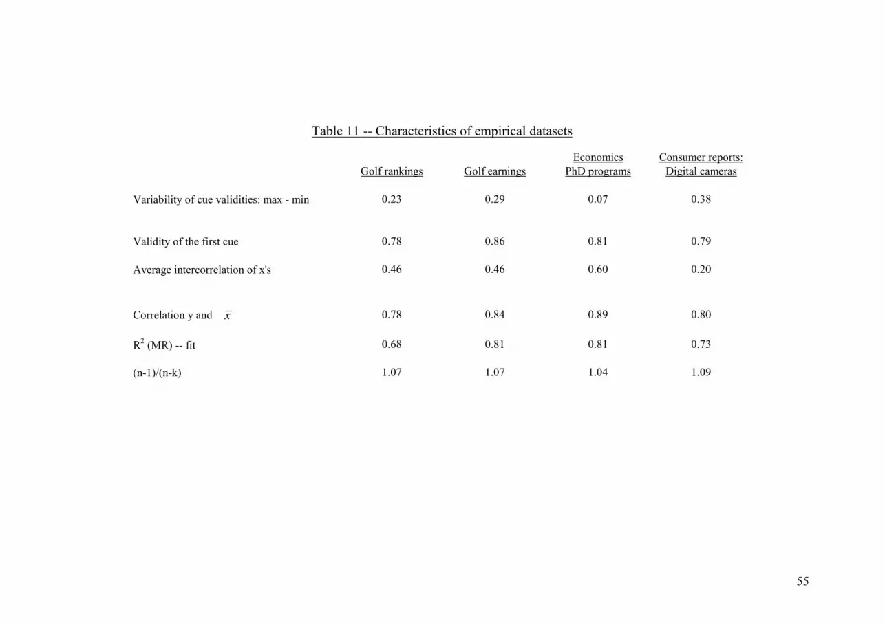
55

Economics Consumer reports:

Golf rankings Golf earnings PhD programs Digital cameras

Variability of cue validities: max - min 0.23 0.29 0.07 0.38

Validity of the first cue 0.78 0.86 0.81 0.79

Average intercorrelation of x's 0.46 0.46 0.60 0.20

Correlation y and 0.78 0.84 0.89 0.80

R2 (MR) -- fit 0.68 0.81 0.81 0.73

(n-1)/(n-k) 1.07 1.07 1.04 1.09

Table 11 -- Characteristics of empirical datasets

x

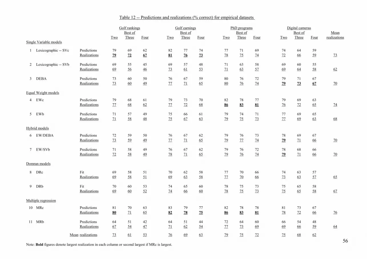
56

Golf rankings Golf earnings PhD programs Digital cameras

Mean

Two Three Four Two Three Four Two Three Four Two Three Four realizations

Single Variable models

1 Lexicographic -- SVc Predictions 79 69 62 82 77 74 77 71 69 74 64 59

Realizations 79 72 67 81 76 73 78 75 74 72 66 59 73

2 Lexicographic -- SVb Predictions 69 55 45 69 57 48 71 63 58 69 60 55

Realizations 69 56 46 73 61 53 71 63 57 69 64 58 62

3 DEBA Predictions 73 60 50 76 67 59 80 76 72 79 71 67

Realizations 73 60 49 77 71 65 80 76 74 79 73 67 70

Equal Weight models

4 EWc Predictions 79 68 61 79 73 70 82 78 77 79 69 63

Realizations 77 68 62 77 72 68 86 83 81 76 72 65 74

5 EWb Predictions 71 57 49 75 66 61 79 74 71 77 69 65

Realizations 71 58 48 75 67 63 79 75 73 77 69 63 68

Hybrid models

6 EW/DEBA Predictions 72 59 50 76 67 62 79 76 73 78 69 67

Realizations 73 59 49 77 71 65 79 77 74 79 71 66 70

7 EW/SVb Predictions 71 58 49 76 67 62 79 76 72 78 68 66

Realizations 72 58 49 78 71 65 79 76 74 79 71 66 70

Domran models

8 DRc Fit 69 58 51 70 62 58 77 70 66 74 63 57

Realizations 69 58 51 69 63 58 77 70 66 73 63 57 65

9 DRb Fit 70 60 53 74 65 60 78 75 73 75 65 58

Realizations 69 60 52 74 66 60 78 75 73 75 65 58 67

Multiple regression

10 MRc Predictions 81 70 63 83 79 77 82 78 78 81 73 67

Realizations 80 71 65 82 78 75 86 83 81 78 72 66 76

11 MRb Predictions 64 51 42 64 51 44 72 64 60 66 54 48

Realizations 67 54 47 71 62 54 77 73 69 69 66 59 64

Mean realizations 73 61 53 76 69 63 79 75 72 75 68 62

Note: Bold figures denote largest realization in each column or second largest if MRc is largest.

Table 12 -- Predictions and realizations (% correct) for empirical datasets

Best of Best of Best of Best of

57

Figure 1

(a) (b)

0.1 0.2 0.3 0.4 0.5 0.6 0.7 0.8 0.9

0.4

0.5

0.6

0.7

0.8

0.9

1

rho(X,Y)

prob

abili

ty o

f co

rrec

t se

lect

ion

Xa-Xc=0.3

Xa-Xb=3 21

0.30.1

0.1 0.2 0.3 0.4 0.5 0.6 0.7 0.8 0.90.3

0.4

0.5

0.6

0.7

0.8

0.9

1Xa-Xc=2

rho(X,Y)

prob

abili

ty o

f co

rrec

t se

lect

ion

Xa-Xb=3 2

1

0.3 0.1

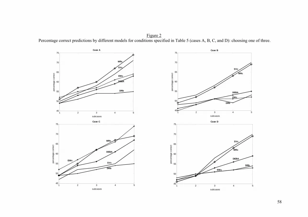
58

Figure 2

Percentage correct predictions by different models for conditions specified in Table 5 (cases A, B, C, and D): choosing one of three.

1 2 3 4 545

50

55

60

65

70

75pe

rcen

tage

cor

rect

subcases

Case A

DRb

MRc

SVc

EWc

DEBA

1 2 3 4 545

50

55

60

65

70

75

perc

enta

ge c

orre

ct

Case B

subcases

MRc

SVc

EWc

DEBA

DRb

1 2 3 4 545

50

55

60

65

70

75

perc

enta

ge c

orre

ct

Case C

subcases

EWc

MRc

SVc

DEBA

DRb

1 2 3 4 545

50

55

60

65

70

75

perc

enta

ge c

orre

ct

Case D

subcases

SVc

MRc

DEBA

EWc

DRb

59

Figure 3

Percentage correct predictions by different models for real data sets specified in Table 12

one of two one of three one of four50

55

60

65

70

75

80

85pe

rcen

tage

cor

rect

Golf rankings

SVc

MRc

EWc

DEBA

DRb

one of two one of three one of four

50

55

60

65

70

75

80

85

perc

enta

ge c

orre

ct

Golf earnings

SVc

MRc

EWc

DEBA

DRb

one of two one of three one of four50

55

60

65

70

75

80

85

perc

enta

ge c

orre

ct

Economics PhD programs

EWc, MRc

DEBA

DRb

SVc

one of two one of three one of four

50

55

60

65

70

75

80

85

perc

enta

ge c

orre

ct

Consumer reports: Digital cameras

MRc

EWc

DRb

SVc

DEBA

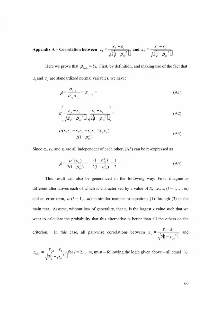
60

Appendix A – Correlation between ( )21

12 yx

abzρ

εε

−

−= and ( )2

2

12 yx

aczρ

εε

−

−=

Here we prove that 21 ,zzρ = ½. First, by definition, and making use of the fact that

1z and 2z are standardized normal variables, we have:

===21

21

21

,

,

zz

zz

zz σσσ

σρ (A1)

( ) ( ) =

−

−

−

−22

12,

12 yx

ac

yx

ab

ρ

εε

ρ

εεσ (A2)

)1(2

)(2

yx

aacaabcb

ρεεεεεεεεσ

−+−−

(A3)

Since εa, εb, and εc are all independent of each other, (A3) can be re-expressed as

=−

=)1(2

)(2

2

yx

a

ρεσρ

2

1

)1(2

)1(2

2

=−

−

yx

yx

ρρ

(A4)

This result can also be generalized in the following way. First, imagine m

different alternatives each of which is characterized by a value of X, i.e., xl (l = 1,…, m)

and an error term, εl (l = 1,…m) in similar manner to equations (1) through (3) in the

main text. Assume, without loss of generality, that x1 is the largest x value such that we

want to calculate the probability that this alternative is better than all the others on the

criterion. In this case, all pair-wise correlations between ( )2

1

1

12 yx

l

lzρ

εε

−

−= and

( )2

11

11

12 yx

l

lzρ

εε

−

−= +

+ for l = 2,….m, must – following the logic given above – all equal ½.

61

Appendix B – Choosing the best of four: the single variable model (SV)

Consider the case of four alternatives, A, B, C, and D with unknown values on

the criterion variable, Y. Assume further that A is the preferred choice if ya > yb,

ya > yc, and ya > yd. Without loss of generality, let alternative A have the largest

value on a single attribute, X, i.e., xa > xb, xa > xc, and xa > xd. Given that it has

the largest value, what is the probability that A is the optimal choice, i.e.,

( ) ( ) ( ){ }ddaadaccaacabbaaba xXxXYYxXxXYYxXxXYYP =>=>∩=>=>∩=>=> ?

Analogically to the case of choice out of three alternatives, and making use of equation (12)

in the main text, this probability can be found as

( )( ) ( )( ) ( )( ){ }=−<−−<−−<− cdyxadcayxacbayxab xxxxxxP ρεερεερεε II

( )( )

( )( )

( )( )

−

−<

−

−<

−

−<

23

22

21

121212 yx

dayx

yx

cayx

yx

bayx xxz

xxz

xxzP

ρ

ρ

ρ

ρ

ρ

ρII (B1)

where z1, z2, and z3 are standardized normal variables, jointly distributed with all

covariances being equal to ½ (see Appendix A).

Applying the properties of the trivariate normal distribution (i.e., expression

(12)), we find the target probability as:

( ) ( )( ) ( )

=+++−

∫ ∫ ∫∞− ∞−

+++++−

∞−

ab ac adl lzzzzzzzzz

l

dzdzdze 3212

1

4

3

231312

2

23

2

13

2

122

3

32312123

22

21

212

1

ρρρρρρπ

( ) ( )∫ ∫ ∫∞− ∞−

+++++−

∞−

ab ac adl lzzzzzzzzz

l

dzdzdze 3212

1

4

3

23

32312123

22

21

2

1

π (B2)

where ( )( )212 yx

bayx

ab

xxl

ρ

ρ

−

−= ;

( )( )212 yx

cayx

ac

xxl

ρ

ρ

−

−= ;

( )( )212 yx

dayx

ad

xxl

ρ

ρ

−

−= .