Expectations in Micro Data: Rationality Revisited†

Hugo Benítez-Silva‡

SUNY – Stony Brook Debra S. Dwyer,

SUNY – Stony Brook Wayne-Roy Gayle, University of Virginia

, and Thomas J. Muench

SUNY-Stony Brook

November 23, 2006

Abstract An increasing number of longitudinal data sets collect expectations information regarding a variety of future individual level events and decisions, providing researchers with the opportunity to explore expectations over micro variables in detail. We present a theoretical framework and an econometric methodology to use that type of information to test the Rational Expectations (RE) hypothesis in models of individual behavior. This RE assumption at the micro level underlies a majority of the research in applied fields in economics, and it is the common foundation of most work in dynamic models of individual behavior. We present tests of three different types of expectations using two different panel data sets that represent two very different populations. In all three cases we cannot reject the RE hypothesis. Our results support a wide variety of models in economics, and other disciplines, that assume rational behavior. Keywords: Rational Expectations, Retirement, Longevity, and Education Expectations, Instrumental Variables, Sample Selection. JEL classification: D84, J26 † We would like to acknowledge outstanding research assistance from Huan Ni. The Michigan Retirement Research Center (MRRC) and the TIAA-CREF Institute made this research possible through their financial support of two related projects. Benítez-Silva also acknowledges the financial support from NIH grant AG1298502 on a related project, and also from the Fundación BBVA, and the Spanish Ministry of Science and Technology through project number SEJ2005-08783-C04-01, and wants to thank the Department of Economics at the University of Maryland and the Department of Economics at Universitat Pompeu Fabra for their hospitality during the completion of this paper. Three anonymous referees provided excellent comments and suggestions. Any remaining errors are the authors’. ‡ Corresponding Author: Department of Economics. SUNY-Stony Brook. Stony Brook, NY 11794-4384. Phone: (631) 632-7551; Fax: (631) 632-7516; e-mail: hugo.benitez-silva@sunysb.edu

1

1. Introduction An increasing number of large longitudinal data sets now collect expectations information regarding

future individual level events and decisions, providing researchers with the opportunity to explore

expectations over micro variables in detail. The growing body of research studying expectations

includes the literatures that analyze wage and income expectations (Dominitz and Manski 1996 and

1997, Das and van Soest 1997 and 2000, and Das, Dominitz, and van Soest 1999), fertility

expectations and pregnancy outcomes (Van Hoorn and Keilman 1997, Van Peer 2000, and Walker

2003), the connection between Social Security expectations and retirement savings (Lusardi 1999,

Dominitz, Manski, and Heinz 2002), the relationship between retirement expectations and retirement

outcomes (Bernheim 1989, Dwyer and Hu 1999, Disney and Tanner 1999, Coronado and Perozek

2001, Hurd and Retti 2001, Forni 2002, Dwyer 2002, and Mastrogiacomo 2003), and consumption

patterns after retirement (Haider and Stephens 2003, and Hurd and Rohwedder 2003).

In this paper we present a theoretical framework and an econometric methodology to use

expectation information to test the Rational Expectations (RE) hypothesis in models of individual

behavior. We then use the Health and Retirement Study (HRS) to analyze retirement and longevity

expectations, and the youth cohort of the National Longitudinal Survey of Labor Market Experience

(NLSY79) to analyze education expectations. We find that these three types of expectations are

consistent with the RE hypothesis. Our results support the use of a wide variety of models in

economics that assume rational behavior.

Our definition and approach to testing the RE hypothesis will be consistent with the views

expressed by the precursors of this assumption.1 We will maintain that agents’ subjective beliefs about

the evolution of a set of variables of interest coincide with the objectively measurable population

probability measure. This is consistent with the characterization of Muth (1961) and Lucas (1972).

2

The main difference is that instead of concentrating on forecasts of market level variables we

focus on how individuals form expectations over micro variables that are in some cases under their

control. Economists and social scientists, in an ongoing effort to improve our model specifications, are

growing increasingly interested in expectation measures as possible sources of additional heterogeneity

in individual characteristics that might reflect underlying differences in preference and beliefs

parameters––which if left out of the models often bias the effects of related observables.

It is important to distinguish that while in macroeconomic theory the RE hypothesis is

understood mainly as an equilibrium concept, thanks largely to Lucas’ seminal contributions, where

expectations affect the stochastic evolution of the economy and this evolution in turn affects

expectations formation, in microeconomic applications the concept is used as a synonym of individual

rationality or an efficient use of information with regard to individual level variables. The latter implies

that somehow the economy is in equilibrium. This RE assumption at the micro level underlies a

majority of the research in applied fields in economics, and it is at the forefront of most work in

dynamic models of individual behavior. This is primarily because most household and individual level

data sources are rich in micro variables and it is the responsibility of the researcher to try to control for

the macroeconomic environment in which those decisions are made.

The debate over whether testing rational expectations is a worthwhile enterprise goes back

almost three decades. Prescott (1977) expressed a strong opinion against testing the hypothesis, while

Simon (1979), Tobin (1980), Revankar (1980), Zarnowitz (1984), and Lovell (1986) considered the

direct analysis of expectations an important project. Manski (1990) advocated for the careful use of

any kind of intentions data, especially if to be used to predict behavior. More recently, Manski (2004)

1 For a survey of the early contributions see the special issue in the Journal of Money, Credit and Banking edited by McCallum (1980), also Sheffrin (1983). For a more recent discussion see Sargent (1995).

3

has emphasized the importance of analyzing expectations formation, and Hamermesh (2004) discusses

the usefulness of subjective outcomes in economics.2

The efforts to test the hypothesis began in the context of the analysis of price expectations by

Turnovsky (1970), the term structure of interest rates with the work of Sargent (1972), Shiller (1973),

and Modigliani and Shiller (1973), and then with the life cycle permanent income hypothesis in a

stream of literature that started with the work of Hall (1978), and then compared forecasts of market

variables with realizations like in Figlewski and Watchtel (1981, 1983), Kimball Dietrich and Joines

(1983), de Leeuw and McKelvey (1981 and 1984), Gramlich (1983), Kinal and Lahiri (1988), and

Keane and Runkle (1990), and more recently, Lee (1996), Davies and Lahiri (1999), Metin and Muslu

(1999), and Christiansen (2003).3 Finally, work by Leonard (1982) analyzed wage expectations of

employers, and Fair (1993) analyzed the question in the context of large macroeconomic models. In all

these cases the concern was with market level variables, and the evidence in these and many other

studies is mixed. Below, we propose a slightly different approach in line with Bernheim (1990), and

recent work by Benítez-Silva and Dwyer (2005 and 2006), and use panel data available through the

HRS and the NLSY79 to follow two very different cohorts of individuals in the way they form

retirement and longevity expectations in one case, and education expectations in the other.

It is important to clarify that if our tests reject the Rational Expectations (RE) hypothesis, two

very different, but nonetheless connected, interpretations are possible. First, we could conclude that

models of rational behavior expect too much of individuals, forcing us to abandon the “full rationality

hypothesis” that agents behave “as if” they were making the large number of computations implied by

the theory. One possible alternative to the fully rational model could be an adaptive learning model

2 Friedman (1951), as quoted in Ericsson and Hendry (1999), advocates for emphasizing the testing of hypothesis in the social sciences. Also, our empirical strategy, which uses two different data sets corresponding to two different populations and three different types of questions to test an underlying structural expectation formation mechanism, we believe, passes Ericsson and Hendry (1999)’s demanding tests of how to approach empirical testing of hypothesis. 3 Pesando (1976) tests the RE hypothesis using cash flow forecasts of life insurance companies. He finds weak evidence in favor of the hypothesis.

4

which introduces a form of bounded rationality, in which individuals use standard econometric and

statistical techniques to make and adjust their forecasts of relevant variables, with RE emerging as an

equilibrium of this trial and error process (see, for example, Pesaran 1987, and Evans and Honkapohja

2001 for presentations of these type of models). Second, we could conclude that reality is much more

complex than even most dynamic models assume, with individuals forming expectations (maybe

rational ones) not over a fixed probability distribution of uncertain events, but over a family of

distributions for each source of uncertainty. This involves individuals learning over time about the

characteristics of these distributions and updating their priors as new information comes along.4

The first conclusion would be a set back for a large body of research in economics, since it

would put into question an attractive and central tool. The second, would mean that we need more

realistic economic models, which are likely to be more complex, but also more attentive to details of

the process of expectations formation by individuals.

Finally, if our tests do not reject the rational expectations hypothesis, we can at least continue

to rely on that rationality, and the strategies used to model it, as a good first approximation to behavior

by individual decision makers. Furthermore, it would then be reasonable to use some of these variables

in modeling complex economic situations, an objective that Haavelmo (1958) already emphasized, as

quoted in Savage (1971).5

The conceptual model and the econometric specifications are presented in section 2. Section 3

provides information about the data sets used in the empirical work. Section 4 discusses the

identification of the econometric specifications, and reports our main findings. Section 5 concludes.

4 This suggests a model of expectations and learning which could be interpreted as building upon the work of Bewley (1986, 1987) and his interpretation of the original ideas of Knight (1921) about decision making under risk and uncertainty. 5 “If we could use explicitly […] variables expressing what people think the effects of their actions are going to be, we would be able to establish relations that could be more accurate and have more explanatory power,” Haavelmo (1958, p.357)

5

2. Conceptual and Econometric Framework

Benitez-Silva and Dwyer (2005), building on Bernheim’s (1990) model of expectation

formation, develop a test of rational expectations using repeated observations of retirement

expectations. We present their methodology here with some modifications, especially in the

econometric specification that we estimate, so it can be applied not only to retirement expectations but

also to longevity and educational attainment expectations.

2.1. A Model and a Test of Rational Expectations using Micro Data

Suppose an individual and a researcher are trying to predict a variable X, which the individual

has either decided will be determined as a function of a sequence of random variables (for example,

retirement and educational attainment) or believes is determined (for example, longevity) by such a

sequence:

1 2( , ,..., ).TX h ω ω ω= (1)

The sequence of vector-valued variables inside the parenthesis will be observed by the individual at

time periods t=1,2,…,T. Then the individual will either take action X after some or all the ωt’s have

been observed, or the event being predicted will occur.

Let 1

tt t t

ω=

Ω = be the information known at period t and let ( )1 2, ,t t tω ω ω= where all of ωt is

observed by the individual, but only 1tω is observed by the econometrician. Let then 1 1

1

t

t t tω

=Ω = . Then

we can define

,tet XEX Ω= (2)

where E is the expectations operator. This is the most commonly used representation of the RE

hypothesis, which takes as the rational expectation of a variable its conditional mathematical

6

expectation (Sargent and Wallace 1976).6 This guarantees that errors in expectations will be

uncorrelated with the set of variables known at time t.

Variables included in the vector representing the information set Ω come from models of

individual behavior, and typically include socio-economic and demographic characteristics. Using the

law of iterated expectations and assuming that the conditional distribution (not just its mean) of the

new information is correctly forecasted by the agents, from (2) we get:

,]|,[ 11etttttt

et XXEXEEXE =Ω=ΩΩ=Ω ++ ω (3)

where ωt+1 represents information that comes available between periods t and t+1. Then from (3) we

can write the evolution of expectations through time as

,11 ++ += tet

et XX η (4)

where ],|[ 111 tet

ett XEX Ω−= +++η and therefore E(ηt+1|Ωt)=0. Notice that ηt+1 is a function of the new

information received since period t, ωt+1. From this characterization of the evolution of expectations

we can test the RE hypothesis with the following regression:

11, , , 1,

e et i t i t i t iX Xα β γ ε+ += + + Ω + , (5)

where α is a constant, and γ is a vector of parameters that estimate the effect of information in period t

on period’s t+1 expectations. The RE hypothesis implies that α=γ=0, and β=1. A weak RE test, in the

terminology of Lovell (1986) and Bernheim (1990), assumes that γ is equal to a vector of zeros, and

tests for α=0 and β=1––effectively testing whether expectations follow a random walk. The strong RE

test is less restrictive, and also tests for γ=0.

Notice, that a value of α and/or γ different from zero can be consistent with the rational

expectations hypothesis in an analysis using a relatively short panel in the presence of macro shocks,

6 Schmalensee (1976) using experimental data emphasizes the importance of analyzing higher moments of the distribution of expectations. Due to data limitations we are unable to do so in our analysis.

7

common to all agents. The fact that the study of retirement and longevity expectations only uses short

panels to average out these possible macro shocks for a given individual, likely works in the direction

of over-rejecting the RE hypothesis regarding these coefficients, compared with a situation where we

would have a very long panel that would allow to average these possible macro shocks over time.7

In deriving the empirical test from the conceptual framework we have assumed that individuals

report the mathematical expectation (mean) of the distribution of retirement ages, surviving

probabilities, and educational attainment in years. This assumption will be jointly tested with the

Rational Expectation Hypothesis, but there is no clear methodology to clarify whether individuals

report the mean, the median, or the mode of the distribution. Furthermore, it is reasonable to conjecture

that maybe respondents are not reporting the mean (or the median) of the distribution of the variable of

interest but the mode.8 For all purposes it is not testable whether the answers to these questions

represent means of distributions, or the most likely outcomes. Das, Dominitz, and van Soest (1999)

analyze categorical responses to expectations questions, and state that if we believe agents are

responding the mode, then having only quantitative information on the variable of interest can prevent

us from performing a Rational Expectations test. However, the paper acknowledges the difficulty in

disentangling what the answers to expectations actually are.

7 In the empirical applications using the HRS, we include a time trend in our specifications, and also performed sensitivity analysis by including unemployment rates over time. Given that in the HRS we are using micro survey data that spans only a ten year period from 1992-2002, we cannot be certain that there is sufficient variation in the macroeconomic effects. However, the earlier part of the nineties was very different from the later part of the survey period, leading us to believe we do indeed have reasonable proxies of macroeconomic shocks. In any case, the findings reported in the paper do not change with the different characterization of these macroeconomic controls 8 From the actual wording of the questions relatively little can be inferred, since the questions are rather ambiguous and open to interpretation. In the first round of interviews there were two types of questions regarding retirement expectations, one asked: When do you think you will retire? Which could be answered giving an age, a date, or in years remaining. The other asked: Are you currently planning to stop working altogether or work fewer hours at a particular date or age, to change the kind of work you do when you reach a particular age, have you not given it much thought, or what? And we use the answer to the stop working altogether option. The only one consistently used across waves is the second way of asking. Strictly speaking this can be considered retirement plans, but are widely described as retirement expectations. In the case of longevity expectations the question is worded as follows: What is the percent chance that you will live to be 75 or more? For education expectations, the question is worded as follows: As things now stand, what is the highest grade or year you think you will actually complete?

8

It is also reasonable to argue that reports of modes are likely to change less than reports of

means, and are likely to be exposed to comparatively less measurement error problems. In our analysis

of expectations there is quite a lot of change going on regarding the expectations reports over time, so

this probably indicates that the assumption regarding reports of the means is not obviously wrong. For

example, in the retirement expectations data, more than 50% of individuals change their retirement

expectations report from wave to wave. However, the average change is rather small, around 0.4 years,

but the standard deviation of this change is quite large, around 4.6 years. Both in the estimation sample

and in the whole sample, of the 50% that changes their reports, a bit more than 60% change their

reports upwards, which ends up resulting in the positive average change overall. Change is especially

pervasive among those who report at some point that they will never retire, since almost two thirds of

them end up reporting an actual expected retirement age. Even if we only restrict attention to those that

actually reported a given age in two consecutive waves, the percentage changing is similar, and the

average change of the same order of magnitude. The only difference is that in the latter case the

standard deviation of the change is a bit smaller. Interestingly, among those that change their reports

55% change their expected retirement age by more than 2 years.

In the case of longevity expectations, where individuals report the probability of living to age

75 or more, the proportion of individuals who change their reports from wave to wave is even higher,

almost 70% of them change. The changes are (almost exactly) evenly split between those that report

higher and lower probabilities compared with the previous wave. The average percentage point change

from wave to wave is between 1.4 and 2.2 (depending on whether we restrict attention to the

estimation sample or the full sample), with a standard deviation of around 27 percentage points.

Among those that change, 81% of the individuals change their reports by more than 10 percentage

points, and around 50% change their reports by more than 20 percentage points. This case suggests,

9

even more clearly than for the retirement model, that individuals report the mean of the distribution,

since it seems hard to believe the reports of the mode would change so much.

Regarding educational attainment expectations, 41% of the sample changed their reports from

year to year, with 56% of them changing them upwards. The average change is 0.11 years, but the

standard deviation is 1.6 years. So even in this case, in which teenagers are asked only one year apart,

there is considerable change in their reports.

2.2 Econometric Specifications and Estimation Strategies

Estimating (5) is in principle straightforward, but the likely presence of measurement error in the

dependent variable and its lag, along with a concern regarding endogeneity, combined with a potential

sample selection bias concern (given that not all individuals answer the expectations questions)

complicate the methodology.9

Measurement Error

As with all survey data, measurement error in proxy variables is a concern. We are particularly

interested in accounting for possibly noisy self-reports of the expectation variables, and reporting

errors that may be correlated with measurement errors in other factors or omitted variables. We will be

assuming that the measurement error that individuals incur is in no way correlated with the rationality

of their expectations formation process but has more to do, for example, with the differences across

individuals in the environment faced in each wave of the panel. For example, the month and year of the

survey can have an effect on the amount of noise in the expectation variable; because it affects the

9 The possible presence of focal points in the expectations variables (retirement, longevity, and educational attainment expectations show considerable probability mass in particular values of the distribution) can give rise to non-normal regression errors, since the distribution of the dependent variable, and the main independent variable could be considered bimodal. In general the results of conditional moments estimation, for example OLS, are fairly robust to this problem, especially if the sample size is fairly large. The most important properties of the linear estimators (that they are the best linear unbiased estimators and consistent, and that the variance estimator is unbiased and consistent allowing us to use conventional tests), survive the non-normality of the errors. However, there can be a loss of efficiency. This loss of efficiency is in part ameliorated by the fact that we use a GMM estimator to estimate the IV and the Corrected IV specification. This estimator is consistent against unknown forms of heterokedasticity, which alleviates the consequences of the non-normality of the errors.

10

degree of rounding in the measure of age and the variable of interest.10 Then the interview

environment would affect the report over time in a way that is not observed. This component of self-

reports can bias the coefficient of interest in a significant way. In order to eliminate this noise, we

want to capture the true component of the expectation and purge it of this source of bias. If

measurement error was not a problem we would expect the β coefficient of the IV estimator to be very

close to the one from the OLS specification, assuming validity of the instruments set.

Since people are reporting expectations over uncertain events, we expect some degree of reporting

error that may be correlated with unobserved factors. In fact, Bernheim (1988) finds that retirement

expectations are reported with noise, and this is also likely to be true of expected educational

attainment since even completed education is reported with error (Black, Sanders, and Taylor 2003),

and also longevity expectations when answered as probabilities of surviving to a certain age.

Sample Selection Bias

As it often happens in survey data, there will be item non-response among our variables of interest.

In the case of this potential selection problem we will be making the implicit assumption (and this is

true in any econometric application that tries to solve the selection bias problem à la Heckman 1979,

and wants to make a statement about the general population under analysis) that those that do not

respond the question of interest would use the same process to analyze information if they were to

actually answer the question as those that answer the question. In other words, we assume that those

who do not respond to the expectations questions are not following a completely different model

(maybe irrational) to decide their expectations. Rather they use the same model of behavior but for a

number of observable and unobservable reasons they did not report our dependent variable, and we

suspect that the inclusion in the sample is therefore non-random.

10 Individuals responded to the retirement expectation question either reporting an expected retirement age, an expected year of retirement, or in years left to expected retirement. The last two ways of responding are likely to create considerable rounding errors, since they did not allow individuals to report a month or fractional answers.

11

Econometric Specification

We present a four equation, three step system estimation to correct for the likely measurement error

problem using instrumental variables analysis, along with the potential sample selection bias concerns.

This model extends to our particular problem the model presented by Wooldridge (2002, p. 567),

which is a parametric version of the model presented (as an extension to their baseline case) in Section

2.4 of Das, Newey and Vella (2003),11 to consistently estimate the effect of previous expectation on

current expectation, and from (5) we write

1, 1 , 1 ,1 1,1e et i t i t i t iX X Zα β γ ε+ += + + + , (6)

, 2 2 ,1 1 ,2 1 ,3 ,2et i t i t i t i t iX Z Z Zα γ λ µ ε= + + + + (7)

1 3 3 ,1 2 ,2 2 ,3 1 ,4 3 , 11( 0), 0ei t i t i t i t i i t i iY Z Z Z Z with X observed whenYα γ λ µ η ε= + + + + + > > , (8)

2 4 4 ,1 3 ,2 3 ,3 2 ,4 4 , 1, 21( 0), 0e ei t i t i t i t i i t i t i iY Z Z Z Z with X and X observed whenYα γ λ µ η ε += + + + + + > > (9)

where we explicitly account for the fact that in the structural equation we restrict attention to

individuals who report expectations in consecutive periods, but there are individuals for whom we

observe the expectations in period t but not in period t+1, and in order to appropriately correct for the

possible selection into equation (7), it is necessary to estimate a separate selection equation, since the

propensity to being observed in period t should not be conditioned on observability in period t+1.

The econometric procedure first estimates the selection equations (8) and (9) using probit

specifications, introducing as exclusion restrictions with respect to the structural equation two groups

of variables, represented by Z3 and Z4, and then consistently estimates (6) by performing a modified

2SLS procedure, where the first stage, equation (7), includes as regressors the exogenous variables

11 Even in the non-parametric setting, identification depends on the exclusion restrictions between the reduced form and the main equation(s). Given that the asymptotic theory for this particular non-parametric model has not been developed, inference is less straightforward. In addition, the non-parametric model does not identify the constant, the statistical significance of which is part of our RE test. The parametric version of the model that we implement is at the same time simple, and proves to be robust. It is flexible in terms of the correlation structure between the error terms of the equations, and no assumptions are made about the distribution of the error terms in the endogenous equation.

12

used in (8) with the exception of Z4, the Inverse Mills’ ratio from the probit equation (8), and

additional instruments Z2 which are restrictions with respect to the structural equation, the validity of

which will be tested. The structural equation then includes the remaining exogenous variables and the

Inverse Mills’ ratio from the probit equation (9). Non-parametric identification of equation (6) requires

only that there are at least two exclusion restrictions from equations (7) and (9) to the main equation,

and the non-parametric identification of equation (7) requires the existence of an element in Z4. This

procedure allows for arbitrary correlation between the disturbances in the system.12

Notice that this formulation makes explicit exclusion restrictions between the selection equation (8)

and the first stage of the IV procedure. In general it is believed that imposing exclusion restrictions on

reduced form equation is unnecessary. However, if we were not to impose this restriction the

coefficient on the Inverse Mills ratio estimated in the first stage of the IV procedure would only be

identified off the functional form assumption of the selection equation. Although technically correct

this can be problematic. As discussed in Vella (1998, p. 135), certain variables which in our sample

have a fairly small range (for example age), can lead to the apparent linearity of the inverse Mills’

ratio, which can result in weak identification of the selection model, inflated second step standard

errors, and what is even more troubling in our case, unreliable estimates of the coefficients of interest.

Therefore, including some variable(s), Z4 in the equations above, which affects the selection equation

but does not affect the first stage of the 2SLS would be justified in order to avoid the complete reliance

on the non-linearity resulting from the functional form assumptions of the selection equation, and

deliver consistent estimates of the parameters of interest.

Clearly the trade off here is between reliance on nonlinearities resulting from functional form

assumptions and debatable exclusion restrictions. We have opted for estimating a model which is non-

12 It is possible to estimate this system of equations by ignoring equation (8), and only concentrating on the possible selection of observing consecutive expectation values. The actual empirical results from that methodology are not

13

parametrically identified, and therefore robust to the convenient functional form assumption of the

selection procedures.

In a related context, this strategy is actually advocated by Das, Newey and Vella (2003, p. 39 and

40) since in their set up they do not rely on functional form assumptions, and need the exclusion

restrictions to identify a similar model. The main difference with the model presented in Section 2.4 of

their paper is that we have to deal with a separate selection into the first stage of the IV procedure,

given the nature of our analysis using reported expectations over time.

In the selection equation (9) we have decided to only include covariates as of time t, we have

experimented with including t+1 variables, and also a battery of residuals of the regressions of t+1

variables on their lagged values, which are then also included in the main equation. Although some

coefficients in the main equation changed as a result of these modifications, the results we report in the

paper are robust to this characterization of the selection process.

In Section 4 we will discuss in some detail identification issues for each of the empirical

applications, and we will also discuss the sensitivity analysis we have undertaken to check the

robustness of our results to different characterizations of the instruments and exclusion restrictions in

the estimation procedure.

3. The DATA: The HRS and the NLSY79

3.1. The HRS: Retirement and Longevity Expectations

The combination of demographic, health, and socio-economic data as well as expectations data

collected in the HRS make it a natural source for empirical work testing rational expectations. Here we

analyze retirement and longevity expectations of older Americans using the first six waves of the HRS,

a nationally representative longitudinal survey of 7,700 households headed by an individual aged 51 to

61 as of the first interviews in 1992-93. The sixth round of data was collected in 2002.

substantially different from the ones we will discuss in Section 4, but we believe that not acknowledging the proper set up

14

3.1.1. Retirement Expectations

In this analysis we include respondents that are working, full time or part time, in any wave, and

non-employed (but searching for jobs) that report retirement plans. We only include respondents for

waves when they are between the ages of 51 and 61 since this represents the planning horizon for

retirement and avoids biases that might arise from responses to Social Security Retirement incentives

that start at age 62. In each wave respondents are asked when they plan to fully or partially depart

from the labor force and whether they have thought about retirement. Most of the people who have not

thought about retirement do not report an expected age. Around 15% of respondents report that they

will never retire. We have assigned an age of 77 for those who never retire, as a proxy for estimated

longevity (based on the life tables).13

Column one of Table 1 presents summary statistics for the full HRS sample we use to study

retirement expectations. Since we restrict attention to individuals that have not retired the average age

is just above 56 years, most of them are employed by someone else, with around 10% reporting

themselves as self-employed. Most of these individuals are in fairly good health, are married, have

some kind of health insurance coverage, and over 40% of them either have a Bachelor’s degree or a

higher degree.

Columns two and three of the table break down the sample according to the selection criteria;

whether or not individuals report thinking about retirement. Around 20% of the sample gave reported

an expectation in two consecutive waves. Those who did not report a retirement expectation in two

waves are less likely to be employed during the panel, and have lower income, and are less likely to

have health insurance. They are also more likely to be female and less educated, their parents are less

likely to have reached retirement age, and their parents had slightly less education.

of the model we are tackling, would subtract from the generality of the methodology we are proposing.

15

3.1.2. Longevity Expectations

As an additional test of our hypotheses we use the data on expected longevity collected in the

HRS. Respondents are asked to report their expected probability of surviving to age 75 or more, and

we use this as our dependent variable. Because the question is only asked for respondents who are not

older than 65, our sample includes all respondents between the ages of 40 and 65 from the first six

waves of the HRS.14

Column one of Table 2 tabulates summary statistics for the full HRS sample we use to study

longevity expectations. The average age in our sample is just shy of 58 years, and on average they

report a 66% probability of living up to age 75. 84% of the respondents are white, but only 35% are

males. Almost 40% of the sample has either a bachelor or a professional degree, and they are on

average in fairly good health.15 From analyzing columns two and three of the table, we can observe

that those that did not answer the expectations questions in two consecutive waves are less likely to

have health insurance, are 4 years older on average, and are less likely to be white and more likely to

be male. Non-respondents have more grandchildren and they are less likely to have experienced the

death of a parent in the two years prior to the interview.

3.2. Educational Attainment Expectations

To test the RE hypothesis on educational attainment expectations of the youth we use the NSLY79,

a nationally representative longitudinal survey that follows individuals over the period 1979 to 2000,

13 We have performed extensive sensitivity analysis of the treatment of those that report they plan to never retire. We have varied the age we assign, and have excluded them from the analysis (so that they are only included in the selection model). The main results regarding our hypotheses are highly robust across all specifications as discussed in Section 4. 14 Hurd and McGarry (1995), Hill, Perry, and Willis (2005), and Benítez-Silva and Ni (2006) analyze these subjective survival probabilities in the Health and Retirement Study. 15 Regarding health variables, the self-rated health is a categorical variable which takes values from 1 to 5, where 1 represents poor health, 2 fair health, 3 good health, 4 very good health, and 5 excellent health. We also use an index for chronic disease, which incorporates information on seven diseases; namely, high blood pressure, diabetes, cancer, lung disease, heart disease, stroke, and arthritis. The chronic disease index is 1 if the individual has all the diseases, and 0 if he has none of them. Notice that each chronic disease contributes 1/7 to the index. Similarly, we have generated an index for ADLs and IADLs, which includes information on whether the individual has problems performing 23 daily activities. This measure takes the value 1 if the individual has difficulty in doing all these 23 activities, and 0 if he has no difficulty performing any of these 23, again each ADL or IADL contributes 1/23 to the index.

16

who were 14 to 21 years of age as of January 1, 1979. Interviews were conducted on an annual basis

through 1994, after which they adopted a biennial interview schedule. In the 1979, 1981, and 1982

surveys, each respondent was asked what the highest educational grade level they expected to

complete. This analysis makes use of the responses in the 1981 and 1982 waves. The sample is

selected by excluding respondents of ages greater than 15 as of January 1, 1979 (to avoid individuals

that have completed their schooling), military entrants, and respondents never observed to enroll in

high school. The resulting sample size includes 2,398 respondents.

Table 3 presents summary statistics for the sample of 2,398 respondents just described. On average

individuals expect to complete a bit less than 14 years of education, which translates in almost two

years of college, their parents on average completed almost 11 years of schooling, they have some

labor market experience, around a fourth of them are black, and 18% are Hispanic. They have an

average of 3.6 siblings and on average 2.1 of them are in school and are older than the respondent. The

table also shows that only around 3% of the sample did not answer the question on expected

educational attainment. This small group comes from slightly poorer families, are younger, more likely

to be females, their parents completed less years of education, and are more likely to be white.

Additionally, they have fewer siblings in school, and less of them are older than the respondent.

Contrary to the case of the HRS (especially for retirement expectations), selection plays a minor role in

the NLSY79 sample due to the fact that most individuals did answer the main question of interest.

4. Empirical Results

4.1. The Retirement Expectations Model

Identification of the models we are going to estimate to account for measurement error require

some exclusion restrictions which must be correlated with the expectation as of time t but not with the

error term or any new information relevant to the t+1 expectation. Our instruments include time t

subjective survival to age 85 probabilities and an indicator of smoking behavior as instruments

17

correlated with the rate of time preference. We also use whether the respondent is financially

knowledgeable, trying to capture the likelihood of planning more accurately or after gathering more

information. Additionally, we have also included a number of time invariant measures as exclusion

restrictions, since they are natural candidates to affect the expectations at time t, but not the

expectations at time t+1, once we account for the former. These variables include an indicator for

being white, an indicator for being male, and indicators of whether the individual has a bachelor’s

degree or a professional degree.

Finally, we also use age as an exclusion restriction. This restriction requires some attention. We

consider age to be a good proxy for the information set which can affect how individuals form

expectations, since as we age we learn more about uncertain relevant factors regarding retirement so

that older respondents might plan more accurately. It is then reasonable to include it in the first stage

regression of the lagged dependent variable as an exclusion restriction (and consequently in the

selection equation, following the estimation strategy outlined in the last section) given that the natural

and predictable evolution of age across waves for all respondents makes it unnecessary to account for

it in the structural equation.

Given the over-identification of the IV models we will be estimating, we will test the validity of all

these restrictions.16

In order to estimate the selection corrected, and the corrected IV models we need additional

exclusion restrictions in the selection equation (9) with respect to the structural equation (Z3 and Z4 in

the formulations presented in Section 2). These include indicators for whether the father and the

mother of the respondent reached retirement age, the father’s and mother’s educational attainment, and

16 Given the large number of exclusion restrictions, it is natural to inquire about the need for such a large set, given that we only have one endogenous variable. We have performed an extensive sensitivity analysis of the instrument set and it is worth emphasizing that age is the key exclusion restriction in our estimations of retirement expectations. Even in a just identified IV specification with age as the only exclusion restriction, the coefficient of the lagged expectation variable moves very close to unity, but the standard error is twice as large as in the preferred specification. The rest of the exclusion

18

whether or not each parent lived to age 85. The latter capture whether the parents lived long during

their retirement years. In the full corrected IV estimation we also need some exclusion restriction in the

selection equation (8) with respect to the first stage of the 2SLS (Z4 in the formulation of equation (8))

in order to avoid relying only on the probit assumption regarding the propensity to answer the

retirement expectations questions as of time t. We use whether the father and mother of the respondent

reached retirement age. Even though it could be argued that this could have an effect on the reported

expectations, robustness checks have shown that this relationship is quite weak, especially once we

control for whether the parents reached age 85, since parents who reached age 85 were almost surely

retired during a considerable period of their lives. Identification of these three step model is of course

contingent on whether the restrictions are exogenous and valid, and we will test them appropriately.

Table 4 presents the weak and strong RE tests for the expected retirement model using four

different specifications.17 In all cases the estimators control for clustering (Deaton 1997), given that we

often have more than one observation per person over time. First, we perform an F-test based on the

null hypothesis that β=1 in equation (4), to test the weak RE hypothesis.18 Once we control for

measurement error, and selection, we obtain a coefficients for β of 0.908 for the weaker test, and given

the precision of the estimate we can reject that is equal to unity at the 5% significance level but not at

the 10%, and therefore that retirement expectations follow a random walk. Given that the selection

term is estimated to be significant, the corrected-IV is our preferred specification. This relatively

borderline negative result is in large part due to the fact that this weak test can be quite problematic,

since is likely affected by omitted variable biases, in particular by the macro indicators that turn out to

restrictions by themselves only move the coefficient to around 0.7, even though they past the robustness and exogeneity tests, but help improve the efficiency of the estimator considerably when used along with age. 17 In all the tables that follow the level of statistical significance of the coefficients is represented, as is customary, by asterisks indicating significance or rejection of a null hypothesis of the coefficient being equal to zero. 18 For the pooled OLS estimation this test is effectively a unit root test, and as such, following the literature on testing unit roots in panel data surveyed by Bond, Nauges, and Windmeijer (2002), we perform a correction to obtain the appropriate critical value. However, this matters very little since the unit root hypothesis is soundly rejected.

19

be significant in the strong test, and the assumption that all the time t variables do not affect the time

t+1 expectation is therefore rather arbitrary and econometrically suspect. If we include the wave

indicators as the only additional regressors in this specification then the β parameter for the weak test

is equal to 0.9697 with a standard error of 0.05, clearly failing to reject the RE hypothesis in its weak

form.

For the strong RE test, which should be considered as the more general and robust, we estimate

the model of equations (6) to (9) using the corrected IV procedure. Also we estimate equation (6) by

pooled OLS, equations (6) and (9) by the traditional selection correction à la Heckman (1979), and

equations (6) and (7) by IV. In the corrected IV procedure the β parameter is estimated to be equal to

1.045 with a fairly small standard error, and the selection term is significant, again indicating that this

is our preferred specification.19 Notice, however, that the selection bias is not too large since the

uncorrected-IV estimates of the β parameter is 1.08 with a very similar standard error.20

The reported results for the uncorrected IV and corrected IV procedures are the product of

robustly estimating the system of equations via GMM, which provides robustness against unknown

forms of heterokedasticity.21 These results clearly indicate that we cannot reject the RE hypothesis

regarding retirement expectations. 22

19 We can observe here a common drawback of IV estimation procedures; the increase in standard errors of the estimates, which in the strong RE test more than double those of the OLS and selection corrected models. However, notice that the coefficient of interest also more than doubles, therefore the level of significance remains unchanged. 20 We have performed extensive sensitivity analysis of the treatment of those that report they plan to never retire. First, our results change very little if instead of using age 77 as the default for this response we use a lower or higher number. And even if we eliminate completely this group and control for it in the selection correction procedure, the results do not change in any significant way. In general, if the default value is a higher age the standard errors of the parameters of interest go up (0.12 instead of 0.06, with a parameter estimate for the Strong RE test of 1.017, when the never age is set to 90), and the parameter estimate is a bit higher when the default value is a bit lower (1.07859, with a standard error of 0.0579 when the never age is set to 70). Also, if we assimilate a never response to a missing then the coefficient on the lagged expectation is a bit higher (goes up to 1.088) than the one reported in our preferred specification, but still not different from 1 given its precision. 21 In the implementation of this procedure we have followed the practical suggestions in Baum, Schaffer, and Stillman (2003). 22 The findings are robust across many specifications and empirical techniques including panel data methods. Much of the individual component is explained by time-invariant variables (there is no remaining individual component in a random effects model if we exclude these covariates).

20

Comparing the different specifications, it is worth emphasizing that the coefficient of interest

significantly changes, and approximates the value predicted by the theory, after controlling for

measurement error. Nothing constrains the β coefficient of the IV specification to move towards 1, and

the fact that it does, can be interpreted as support of our estimation strategy to uncover the structural

parameters of the models of rational expectations formation.23

It is natural to ask ourselves the reason behind the difference in point estimates we obtain for

our main parameter of interest, which allows us to test the RE hypothesis, when we go from the OLS

results to the IV estimators. Notice that the OLS estimates, strongly reject the RE hypothesis, with a β

coefficient only slightly above 0.4. If endogeneity is a problem, with its source either in measurement

error or a classical problem of omitted variable biases, it is possible to justify this negative result as

resulting from the violation of the OLS assumption about the lack of correlation between the variable

of interest and the errors in equation (6). The measurement error problem, as explained in section 2,

seems to us as a more plausible explanation, especially because a comparison of the variance of the

residuals of the first stage of the IV with the variance of the predicted value of the endogenous variable

suggests a significant measurement error problem that could be biasing the coefficient of interest by as

much as 50%, since those two variances are of similar magnitude.24

Given that measurement error is a valid concern regarding our variables of interest, it all comes

down to whether we trust the exclusion restrictions we have made regarding the fact that some

variables affect retirement expectations as of time t but are not correlated with the disturbances in

equation (6). The best we can do to convince the reader of the validity of the instruments is to perform

23 Notice that in columns three and four of Table 4 (and also Tables 5 and 6), we do not report the adjusted R2 measure of fit as is common practice. These types of measures do not have independent significance in structural IV estimation. Our objective is to estimate population parameters, which we consider invariant to the particular identification method (instrumental variables), which leads to a calculation of the adjusted coefficient of determination which can easily result in negative values of this summary measure. See Ruud (2000, p. 515-516) for a discussion. 24 This suggests a noise to signal ratio of around 1, which as discussed in Arellano (2003) is not an uncommon situation in micro data, especially in a survey in the field every two years. The estimated bias is of a similar magnitude for the longevity expectations, and slightly smaller for education expectations.

21

the tests suggested in the literature, so we follow the suggestions in Bound, Jaeger, and Baker (1995),

Staiger and Stock (1997), Stock, Wright, and Yogo (2002), and Baum, Schaffer, and Stillman (2003),

and find that we have robust instruments, with very large F statistics in the first stage of the IV

procedure, considerably larger than the minimum value (around 10) suggested in Staiger and Stock

(1997), and also discussed in Stock, Wright, and Yogo (2002), as a good rule of thumb to check

whether we are in the presence of weak instruments (see Tables A.2. and A.3. in the Appendix).

Also, the model is overidentified, which allows us to test whether our instruments are

exogenous with respect to the error term in the structural equation. A rejection of this test would

suggest that the instruments are either not truly exogenous or they should be included in the main

regression of interest. In all cases we cannot reject the overidentifying restrictions.

It is also important, given the impact on our conclusions for the retirement model, to clarify the

reason why we believe that the disturbances in equation (9), the main selection equation, could be

correlated with the disturbances in (6). Among the many possible explanations, the one that seems

more plausible to us is that those more likely to have thought about retirement seem to have been

exposed to some events or information, which we fail to capture with the set of exogenous variables

that we use to estimate (9). This makes them more likely to change their expectations. This suggests

that among those that report not thinking about retirement there are many that have not been exposed

to a situation where they have been forced to think about it beyond minimum plans. If this is the reason

for the correlation, estimating an uncorrected model will lead to an upward bias in β, since we would

be left with a sample more likely to report changes in their plans, and a majority of the adjustments are

upwards as discussed in Section 2. It is also reasonable to expect biases in the other coefficients,

including the constant. The key is that the correlation is still present after controlling for a large set of

observed characteristics.

22

Notice that the RE hypothesis also predicts that in the strong test the information available at

time t should not be significant after controlling for time t expectations when estimating (6). In this

case we find that after controlling for sample selection and measurement error most of these factors are

no longer significant, but it is important to separate the individual level variables from the proxies for

the macro shocks, represented by the wave indicators. The joint hypotheses that all the individual level

coefficients are equal to zero cannot be rejected at any traditional level of significance, and the same is

true of the estimates of the constant, validating the other predictions of the RE hypothesis regarding

retirement expectations.25

Our results show that the wave indicators are jointly significant, suggesting that individuals are

not perfectly accounting for some macroeconomic effects, and the relatively short panel we have

available cannot average out those effects over time.

Finally, Tables A.1., to A.3., in the Appendix, provide the results of the estimation of the main

selection equation (9), and the first stage estimation of the traditional IV and the corrected IV

estimators for the weak and strong RE test.

4.2. The Longevity Expectations Model

To identify this model we can follow exactly the same methodology as in the retirement

expectations model, and therefore need instruments for the lagged dependent variable to account for

the measurement error problem, and some exclusion restrictions to identify the selection correction

equations. The exclusion restrictions of the first stage of the IV procedure with respect to the structural

equation include age, self-reported health at time t, and indicators for being male and white. These

25 It is true, however, that this is trivially the case if individuals never adjust their expectations, which might be consistent with modal responses rather than expected outcomes. But as discussed in Section 2 plenty of adjustment goes on in the data.

23

exclusions strike us as quite reasonable since their effects on the t+1 expectations are likely to work

only through the time t expectations.26

We then use indicators of the recent death of the father or mother, and the mother’s educational

attainment as exclusion restrictions from the selection equation to the structural equation (Z3 in the

notation of equations (6) to (9)). Notice, however, that the estimation procedure allows these variables

to affect the time t longevity expectations. Additionally, the indicator of whether the respondent is

financially knowledgeable is another exclusion restriction in the selection model of equation (9), since

we believe this is correlated with one’s propensity to respond to expectation data. This financial

knowledge indicator is also an exclusion restriction of the selection model of equation (8) with respect

to the first stage of the IV procedure (Z4 in the notation of the econometric model).

Table 5 presents the tests for the expected longevity model, using the HRS sample. For the strong

test the main prediction of the RE hypothesis, that the coefficient on the lagged expectation variable is

equal to unity, cannot be rejected once we account for measurement error. In this case there is no

evidence of selection bias, and the uncorrected IV specification is the preferred one. For the strong test

the main parameter of interest is estimated to be equal to 0.964, with fairly small standard errors. The

exclusion restrictions are tested as very robust and highly correlated with the longevity expectation as

of time t, and they also pass the test of over-identifying restrictions, suggesting that we cannot reject

they are valid instruments. For the weak RE test the β parameter is estimated to be equal to 0.941, and

is estimated with a lot of precision, and in this case we can reject the RE hypothesis, likely a result of

omitted variable biases since some of the coefficients of the exogenous variables are actually

significant in the strong test, including the macro indicators.

26 Notice that in contrast to the retirement expectations model, education indicators are not used as exclusion restrictions since education is strongly correlated with health investments and health attitudes, and therefore these measures are not exogenous with respect to the structural equation. Also, it is worth emphasizing that just about any combination of these four exclusion restrictions leads to parameter estimates of our coefficient of interest very close to unity.

24

One difference with the model of retirement expectations is that the prediction of the theory

regarding the lack of joint significance of the information available at time t is rejected not only for the

macro level variables, but also regarding the individual level variables. The latter is mainly driven

(they are the only significant ones in the estimation on top of the wave indicators) by two variables; the

self-reported health change from time t-1 to time t, and the indicator for having a professional degree.

Our interpretation for the significance of the health change variable is that this measure of health

dynamics is likely to be serially correlated, and reporting, for example, a health improvement in the

recent past is likely to be followed by a period where health might not necessarily improve, delivering

a kind of mean reversion effect that would explain the negative and significant coefficient in the

estimation. This suggests that this variable might be capturing health deviations from the mean health

as estimated by individuals. On the other hand, highly educated individuals have different attitudes

towards their health and health investments, which could result in unobserved behavior, or be

correlated with unobserved characteristics, with a time invariant component.

Given the nature of the analysis regarding longevity expectations, it would be natural to worry

about an additional source of selection into the sample used for estimation, which can result in biased

coefficients, survivorship bias. It is plausible to expect that those dying between the waves would be

the ones reporting lower probabilities of surviving to certain ages, leaving our sample of survivors as a

selected group of respondents that expect to live longer. In fact, we have used the exit interview

information from all available waves of the HRS to compare the expected survival probabilities of

those we know survived to the next wave, with the expected probabilities of those we know die

between waves (about 7% of the original wave 1 sample had died by wave 6). Our findings indicate

that eventual survivors reported significantly higher probabilities of living to age 75 and 85, suggesting

that survivorship bias could be an issue in our data. In order to assess the effects of this additional

source of selection in our sample we have followed the recommendations in Portrait, Alessie, and

25

Deeg (2004) to construct additional selection correction terms, and have included them in our preferred

specifications. Even though in most cases these additional selection terms were significant, the effects

on the results we have reported in this section were negligible.27 One possible problem of actually

controlling for this additional selection concern is that the correction terms we have constructed to

account for this possible bias are likely to be correlated with the selection term regarding responses to

the longevity questions. The reason for this concern is that those that ended up dying between waves

were considerably less likely to report expected longevity probabilities. In fact, the difference in

response rates is around 14 percentage points, and it is highly significant. If the probability to respond

is serially correlated, it is likely that the unobserved components that make someone more likely to

respond are correlated with the unobserved components that make that same individual more likely to

survive. This would mean that the introduction of the additional correction terms would result in

collinearity problems and additional biases of its own.

Tables A.4., to A.6., in the Appendix, provide the results of the estimation of the main selection

equation (9), and the first stage estimation of the traditional IV and the corrected IV estimators for the

weak and strong RE test using longevity expectations.

4.3. The Educational Attainment Model

In this case the measurement-error robust IV estimates are identified off the parents’

educational attainment measures, which we assume only affect the educational attainment expectations

through the lagged expectations. The latter also means that the selection model has as exclusion

restrictions with respect to the structural equation the parents’ educational attainments, and the

exclusion restrictions with respect to the first stage of the IV procedure (Z4 in equations (8), which are

also additional exclusion restriction with respect to the main equation) are the number of siblings in

school, and the number of older siblings. These exclusions restrictions imply that in this case Z3 is the

27 These results are available from the authors upon request.

26

empty set in the formulation of equations (6) to (9). For the NLSY, selection is unlikely to be an

important issue in this empirical application since only 79 of almost 2,400 individuals did not answer

the expectations questions.

Table 6 reports the results for the NLSY79 sample of testing rational expectations for

educational attainment. The results show that we cannot reject the RE hypotheses regarding

educational attainment once we control for measurement error. The weak RE test estimates the β

parameter to be 0.982, with a small standard error, and in this case we cannot reject the presence of

sample selection, however, the results of the corrected IV model are virtually identical in this case. For

the strong RE test we find little evidence of selection bias, therefore, our preferred specification

estimates an overidentified IV model. In that model we estimate β to be 0.991 with a larger standard

error than in the weak test.

In both cases we can soundly reject that we have weak instruments, given the strong correlation

between the parents’ education and the individuals’ education expectations as of time t. Additionally,

the test of over-identifying restrictions widely supports the validity of the instrument set at any

traditional level of significance (see Tables A.8. and A.9. in the Appendix).28

Finally, the additional predictions of the RE hypothesis cannot be rejected in this case, with

strong support, at any traditional level of significance, for the joint hypotheses that all the coefficients

of the exogenous variables as of time t are equal to zero, and the same is true of the estimates of the

constant.

5. Conclusions

We have tested the Rational Expectations hypothesis in the formation of expectations for

retirement and longevity using a representative sample of older Americans, and educational attainment

28 Just identified models, using either of the parents’ education variables, delivered almost identical parameter estimates, but with slightly larger standard errors.

27

expectations using a representative sample of younger Americans, relying on the same methodology.

In all three types of expectations applications we cannot reject the RE hypothesis after controlling for

reporting errors, and in some cases sample selection. These results support the use of the expectations

variables in the growing number of data sets that provide this type of information, and support the use

of models that use this assumption in micro data.

The methodology we present can be easily applied in many other contexts where repeated

observations of expectations variables at the micro level are collected. The results of this analysis are

meant to foster further discussion and research on the issues surrounding the role of expectations in

economics and the social sciences, and in particular the importance and validity of the Rational

Expectations hypothesis.

28

References

Arellano M (2003) Panel Data Econometrics. Oxford University Press. Baum CF, Schaffer ME, and Stillman S (2003) Instrumental Variables and GMM: Estimation and Testing. Stata Journal 3-1: 1—31. Benítez-Silva H, and Dwyer DS (2005) The Rationality of Retirement Expectations and the Role of New Information. Review of Economics and Statistics 87-3: 587—592. Benítez-Silva H, and Dwyer DS (2006): Expectation Formation of Older Married Couples and the Rational Expectations Hypothesis. Labour Economics 13-2: 191—218. Benítez-Silva H, and Ni H (2006) Health Stocks and Health Flows in an Empirical Model of Expected Longevity. Manuscript, SUNY-Stony Brook. Bernheim BD (1988) Social Security benefits: An empirical study of expectations and realizations. In: Issues in Contemporary Retirement, E. Lazear and R. Ricardo-Campbell (eds.). 312—345. Palo Alto: Hoover Institution. Bernheim BD (1989) The timing of retirement: A comparison of expectations and realizations. In: The Economics of Aging, D. Wise (ed.) Chicago: University of Chicago Press, 335—355. Bernheim BD (1990) How Do the Elderly Form Expectations? An Analysis of Responses to New Information. In: Issues in the Economics of Aging, D. Wise (ed.) Chicago: University of Chicago Press, 259—285. Bewley TF (1986) Knightian Decision Theory: Part I. Cowles Foundation Discussion Paper No. 807, Yale University. Bewley TF (1987) Knightian Decision Theory, Part II: Intertemporal Problems. Cowles Foundation Discussion Paper No. 835, Yale University. Black D, Sanders S, and Taylor L (2003) Measurement of Higher Education in the Census and Current Population Survey. Journal of the American Statistical Association 98-463: 545—554. Bond S, Nauges C, and Windmeijer F (2002) Unit Root and Identification in Autoregressive Panel Data Models: A Comparison of Alternative Tests. IFS Working Paper. Bound J, Jaeger DA, and Baker RM (1995) Problems with Instrumental Variables Estimation When the Correlation Between the Instruments and the Endogenous Explanatory Variable is Weak. Journal of the American Statistical Association 90-430: 443—450. Christiansen C (2003) Testing the expectations hypothesis using long-maturity forward rates. Economics Letters 78: 175—180.

29

Coronado JL, and Perozek M (2001) Wealth Effects and the Consumption of Leisure: Retirement Decisions During the Stock Market Boom of the 1990s. Manuscript, Federal Reserve Board. Das M, Dominitz J, and Van Soest A (1999) Comparing Predictions and Outcomes: Theory and Application to Income Changes. Journal of the American Statistical Association 94-445: 75—85. Das M, and van Soest A (1997) Expected and Realized Income Changes: Evidence from the Dutch Socio-Economic Panel. Manuscript, Tilburg University. Das M, and van Soest A (2000) Expected versus Realized Income Changes: A Test of the Rational Expectations Hypothesis. Manuscript, Tilburg University. Das M, Newey W, and Vella F (2003) Nonparametric Estimation of Sample Selection Models. Review of Economic Studies 70: 33—58. Davies A, and Lahiri K (1999) Re-examining the rational expectations hypothesis using panel data on multi-period forecasts. In: Analysis of panels and limited dependent variable models. Cheng Hsiao, Kajal Lahiri, Lung-Fei Lee, and M. Hashem Pesaran (Eds.) Cambridge University Press. Deaton A (1997) The Analysis of Household Surveys. Baltimore: Johns Hopkins Press de Leeuw F, and McKelvey MJ (1981) Price Expectations of Business Firms. Brookings Papers on Economic Activity 1981-1: 299—314. de Leeuw F, and McKelvey MJ (1984) Price Expectations of Business Firms: Bias in the Short and Long Run. American Economic Review 14: 99—110. Disney R, and Tanner S (1999) What can we learn from Retirement Expectations data? IFS Working Paper Series W99/17. Dominitz J, and Manski CF (1996) Eliciting Student Expectations of the Returns to Schooling. Journal of Human Resources 31-1: 1—26. Dominitz J, and Manski CF (1997) Using expectations data to study subjective income expectations. Journal of the American Statistical Association 92: 855—867. Dominitz J, Manski CF, and Heinz J (2002) Social Security Expectations and Retirement Savings Decisions. NBER Working Paper 8718. Dwyer DS (2002) Planning for Retirement: The Role of Health Shocks. Manuscript, SUNY-Stony Brook. Dwyer DS, and Hu J (1999) The Relationship Between Retirement Expectations and Realizations: The Role of Health Shocks. In: Forecasting Retirement Needs and Retirement Wealth. Olivia Mitchell, P. Brett Hammond, and Anna M. Rappaport (Eds.) University of Pennsylvania Press. Ericsson NR, and Hendry DF (1999) Encompassing and rational expectations: How sequential corroboration can imply refutation. Empirical Economics 24-1: 1—21.

30

Evans GW, and Honkapohja S (2001) Learning and Expectations in Macroeconomics. Princeton University Press: Princeton and Oxford. Fair RC (1993) Testing the Rational Expectations Hypothesis in Macroeconomic Models. Oxford Economic Papers 45-2: 169—190. Figlewski S, and Wachtel P (1981) The Formation of Inflationary Expectations. Review of Economics and Statistics 63-1: 1—10. Figlewski S, and Wachtel P (1983) Rational Expectations, Information Efficiency, and Tests using Survey Data. Review of Economics and Statistics 65-3: 529—531. Forni L (2002) Expectations and Outcomes. Manuscript, Central Bank of Italy. Friedman M (1951) Comment. In: Haberler G (ed.) Conference on business cycles, National Bureau of Economic Research, New York, 107—114 Gramlich EM (1983) Models of Inflation Expectations Formation: A Comparison of Household and Economic Forecasts. Journal of Money, Credit, and Banking 15: 155—173. Haavelmo T (1958) The Role of the Econometrician in the Advancement of Economic Theory. Econometrica 26-3: 351—357. Haider S, and Stephens M (2003): “Is there a Retirement-Consumption Puzzle? Evidence Using Subjective Retirement Expectations. Forthcoming, Review of Economics and Statistics. Hall R (1978) Stochastic Implications of the Life Cycle-Permanent Income Hypothesis: Theory and Evidence. Journal of Political Economy 86: 971—987. Hamermesh DS (2004) Subjective Outcomes in Economics. Southern Economic Journal 71-1: 2—11. Heckman JJ (1979) Sample Selection Bias as a Specification Error. Econometrica 47-1: 153—161. Hill D, Perry M, and Willis RJ (2005) Estimating Knightian uncertainty from survival probability questions on the HRS. Manuscript, University of Michigan. Hurd M, and McGarry K (1995) Evaluation of the subjective probabilities of survival in the health and retirement study. Journal of Human Resources 30: s7-s56. Hurd M, and Retti M (2001) The Effects of Large Capital Gains on Work and Consumption: Evidence from four waves of the HRS. Manuscript, RAND Corporation, Santa Monica. Hurd M, and Rohwedder S (2003) The Retirement-Consumption Puzzle: Anticipated and Actual Declines in Spending and Retirement. NBER Working Paper 9586. Keane MP, and Runkle DE (1990) Testing the Rationality of Price Forecasts: New Evidence from Panel Data. American Economic Review 80-4: 714—735.

31

Kimball Dietrich J, and Joines DH (1983) Rational Expectations, Information Efficiency, and Tests using Survey Data: A comment. Review of Economics and Statistics 65-3: 525—529 Kinal T, and Lahiri K (1988) A Model of Ex Ante Real Interest Rates and Derived Inflation Forecasts. Journal of the American Statistical Association 83-403: 665—673. Knight FH (1921) Risk, Uncertainty and Profit. Boston and New York: Houghton Mifflin. Lee K (1996) An Economic Application of Time Domain Chebyshev Filters: A Test of the Permanent Income Hypothesis. The Statistician 45-1: 65—76. Leonard JS (1982) Wage Expectations in the Labor Market: Survey Evidence on Rationality. Review of Economics and Statistics 64: 157—161. Lovell MC (1986) Tests of Rational Expectations Hypothesis. American Economic Review 76-1: 110—124. Lucas RE (1972) Expectations and the Neutrality of Money. Journal of Economic Theory 4: 103—124. Lusardi A (1999) Information, Expectations, and Savings for Retirement. In: Behavioral Dimensions of Retirement Economics, Henry J Aaron (Ed.) Brookings Institute. Manski CF (1990) The Use of Intentions Data to Predict Behavior: A Best Case Analysis. Journal of the American Statistical Association 85: 934—940. Manski CF (2004) Measuring Expectations. Econometrica 72-5: 1329–1376. Mastrogiacomo M (2003) On Expectations, Realizations and Partial Retirement. Manuscript. Tinbergen Institute. McCallum BT (1980) Rational Expectations. Edited volume of the Journal of Money, Credit and Banking 12-4. Metin K, and Muslu I (1999) Money demand, the Cagan model, testing rational expectations vs. adaptive expectations: The case of Turkey. Empirical Economics 24-3: 415–426. Modigliani F, and Shiller RJ (1973) Inflation, Rational Expectations and the Term Structure of Interest Rates. Economica 40-157: 12—43. Muth JF (1961) Rational Expectations and the Theory of Price Movements. Econometrica 29-3: 315—335. Pesando JE (1976) Rational Expectations and Distributed Lag Expectations Proxies. Journal of the American Statistical Association 71-353: 36—42. Pesaran, M. Hashem (1987) The Limits to Rational Expectations. Basil Blackwell: Oxford and New York.

32

Prescott E (1977) Should Control Theory be Used for Economic Stabilization? Journal of Monetary Economics Suppl.: 13—38. Portrait F, and Alessie R, and Deeg D (2004) Disentangling the Age, Period, and Cohort Effects Using a Modeling Approach: An Application to Trends in Functional Limitations at Older Ages. Manuscript, Utrecht University. Revankar NS (1980) Testing of the Rational Expectations Hypothesis. Econometrica 48-6: 1347—1363. Ruud PA (2000) An Introduction to Classical Econometric Theory. Oxford University Press: New York and Oxford. Sargent TJ, and Wallace N (1976) Rational Expectations and the Theory of Economic Policy. Journal of Monetary Economics 2: 169—183. Sargent TJ (1972) Rational Expectations and the Term Structure of Interest Rates. Journal of Money, Credit and Banking 4-1.1: 74—97. Sargent TJ (1995) Adaptation of Macro Theory to Rational Expectations. Manuscript. Hoover Institution and University of Chicago. Savage LJ (1971) Elicitation of Personal Probabilities and Expectations. Journal of the American Statistical Association 66-336: 783—801. Schmalensee R (1976) An Experimental Study of Expectation Formation. Econometrica 44-1: 17—41. Sheffrin SM (1983) Rational Expectations. Cambridge Surveys of Economic Literature by Cambridge University Press: Cambridge. Shiller RJ (1973) Rational Expectations and the Term Structure of Interest Rates: Comment. Journal of Money Credit and Banking 5-3: 856—860. Simon HA (1979) Rational Decision Making in Business Organizations. American Economic Review 69-4: 493—513. Staiger D, and Stock JH (1997) Instrumental Variables Regression with Weak Instruments. Econometrica 65-3: 557—586. Stock JH, Wright JH, and Yogo M (2002) A Survey of Weak Instruments and Weak Identification in Generalized Method of Moments. Journal of Business and Economics Statistics 20-4: 518—529. Tobin J (1980) Asset Accumulation and Economic Activity. The University of Chicago Press. Turnovsky SJ (1970) Empirical Evidence on the Formation of Price Expectations. Journal of the American Statistical Association 65-332: 1441—1454.

33

Vella F (1998) Estimating Models with Sample Selection Bias: A Survey. Journal of Human Resources 33-1: 127—169. Van Hoorn W, and Keilman N (1997) Birth expectations and their use in fertility forecasting. Eurostat Working Papers E4/1997-4. Van Peer C (2000) Desired and realized fertility in selected FFS-countries. Manuscript, Population and Family Study Centre, Brussels. Walker JR (2003) Pregnancy and Fertility Expectations: Estimates of Bounded Rationality and Unintended Births. Manuscript, University of Wisconsin-Madison. Wooldridge JM (2002) Econometric Analysis of Cross Section and Panel Data. MIT Press. Zarnowitz V (1984) Business Cycle Analysis and Expectational Survey Data. NBER Working Paper 1378.

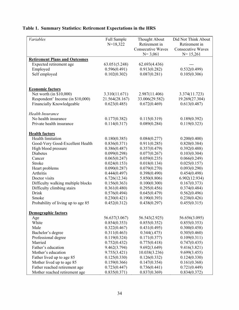
34

Table 1. Summary Statistics: Retirement Expectations in the HRS

Variables Full Sample N=18,322

Thought About Retirement in

Consecutive Waves N= 3,061

Did Not Think About Retirement in

Consecutive Waves N= 15,261

Retirement Plans and Outcomes Expected retirement age Employed Self employed Economic factors Net worth (in $10,000) Respondent’ Income (in $10,000) Financially Knowledgeable Health Insurance No health insurance Private health insurance Health factors Health limitation Good-Very Good-Excellent Health High blood pressure Diabetes Cancer Stroke Heart problems Arthritis Doctor visits Difficulty walking multiple blocks Difficulty climbing stairs Drink Smoke Probability of living up to age 85 Demographic factors Age White Male Bachelor’s degree Professional degree Married Father’s education Mother’s education Father lived up to age 85 Mother lived up to age 85 Father reached retirement age Mother reached retirement age

63.051(5.248) 0.596(0.491) 0.102(0.302)

3.310(11.671) 21.564(28.167)

0.623(0.485)

0.177(0.382) 0.114(0.317)

0.180(0.385) 0.836(0.371) 0.386(0.487) 0.099(0.298) 0.065(0.247) 0.024(0.153) 0.090(0.287) 0.444(0.497) 6.726(12.34) 0.156(0.363) 0.361(0.480) 0.576(0.494) 0.230(0.421) 0.452(0.312)

56.637(3.067) 0.854(0.353) 0.322(0.467) 0.311(0.463) 0.119(0.324) 0.752(0.432) 9.462(3.794) 9.755(3.421) 0.125(0.330) 0.159(0.366) 0.723(0.447) 0.835(0.371)

62.693(4.436) 0.913(0.282) 0.087(0.281)

2.987(11.406) 33.006(29.582)

0.672(0.469)

0.115(0.319) 0.089(0.284)

0.084(0.277) 0.911(0.285) 0.357(0.479) 0.077(0.267) 0.059(0.235) 0.018(0.134) 0.079(0.270) 0.398(0.490) 5.850(8.806) 0.100(0.300) 0.295(0.456) 0.645(0.479) 0.190(0.393) 0.438(0.297)

56.543(2.925) 0.855(0.352) 0.431(0.495) 0.344().475) 0.171(0.377) 0.775(0.418) 9.692(3.649)

10.038(3.236) 0.126(0.332) 0.147(0.354) 0.736(0.441) 0.837(0.369)

---

0.532(0.499) 0.105(0.306)

3.374(11.723) 19.269(27.304)

0.613(0.487)

0.189(0.392) 0.119(0.323)

0.200(0.400) 0.820(0.384) 0.392(0.488) 0.103(0.304) 0.066(0.249) 0.025(0.157) 0.093(0.290) 0.454(0.498)

6.902(12.934) 0.167(0.373) 0.374(0.484) 0.562(0.496) 0.238(0.426) 0.455(0.315)

56.656(3.095) 0.855(0.353) 0.300(0.458) 0.305(0.460) 0.109(0.311) 0.747(0.435) 9.416(3.821) 9.699(3.455) 0.124(0.330) 0.161(0.368) 0.721(0.449) 0.834(0.372)

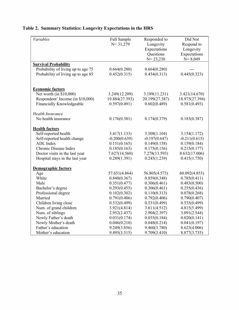
35

Table 2. Summary Statistics: Longevity Expectations in the HRS

Variables Full Sample N= 31,279

Responded to Longevity

Expectations Questions N= 23,230

Did Not Respond to Longevity

Expectations N= 8,049

Survival Probability Probability of living up to age 75 Probability of living up to age 85 Economic factors Net worth (in $10,000) Respondent’ Income (in $10,000) Financially Knowledgeable Health Insurance No health insurance Health factors Self-reported health Self-reported health change ADL Index Chronic Disease Index Doctor visits in the last year Hospital stays in the last year Demographic factors Age White Male Bachelor’s degree Professional degree Married Children living close Num. of grand children Num. of siblings Newly Father’s death Newly Mother’s death Father’s education Mother’s education

0.664(0.280) 0.452(0.315)

3.249(12.209) 19.884(27.393)

0.597(0.491)

0.176(0.381)

3.417(1.133) -0.200(0.639) 0.151(0.165) 0.185(0.163)

7.627(14.560) 0.289(1.391)

57.651(4.864) 0.840(0.367) 0.351(0.477) 0.293(0.455) 0.102(0.302) 0.791(0.406) 0.532(0.499) 3.921(4.814) 2.952(2.437) 0.031(0.174) 0.046(0.210) 9.249(3.856) 9.495(3.515)

0.664(0.280) 0.454(0.313)

3.189(11.231) 20.199(27.387)

0.602(0.489)

0.174(0.379)

3.508(1.104) -0.197(0.647) 0.149(0.158) 0.175(0.156)

7.278(13.593) 0.245(1.239)

56.805(4.573) 0.859(0.348) 0.306(0.461) 0.306(0.461) 0.110(0.313) 0.792(0.406) 0.531(0.499) 3.611(4.512) 2.904(2.397) 0.035(0.184) 0.048(0.214) 9.460(3.780) 9.709(3.410)

---

0.445(0.323)

3.421(14.670) 18.975(27.394)

0.581(0.493)

0.183(0.387)

3.154(1.172) -0.211(0.615) 0.159(0.184) 0.215(0.177)

8.632(17.006) 0.415(1.750)

60.092(4.853) 0.785(0.411) 0.483(0.500) 0.255(0.436) 0.078(0.268) 0.790(0.407) 0.535(0.499) 4.815(5.499) 3.091(2.544) 0.020(0.141) 0.041(0.197) 8.623(4.006) 8.877(3.735)

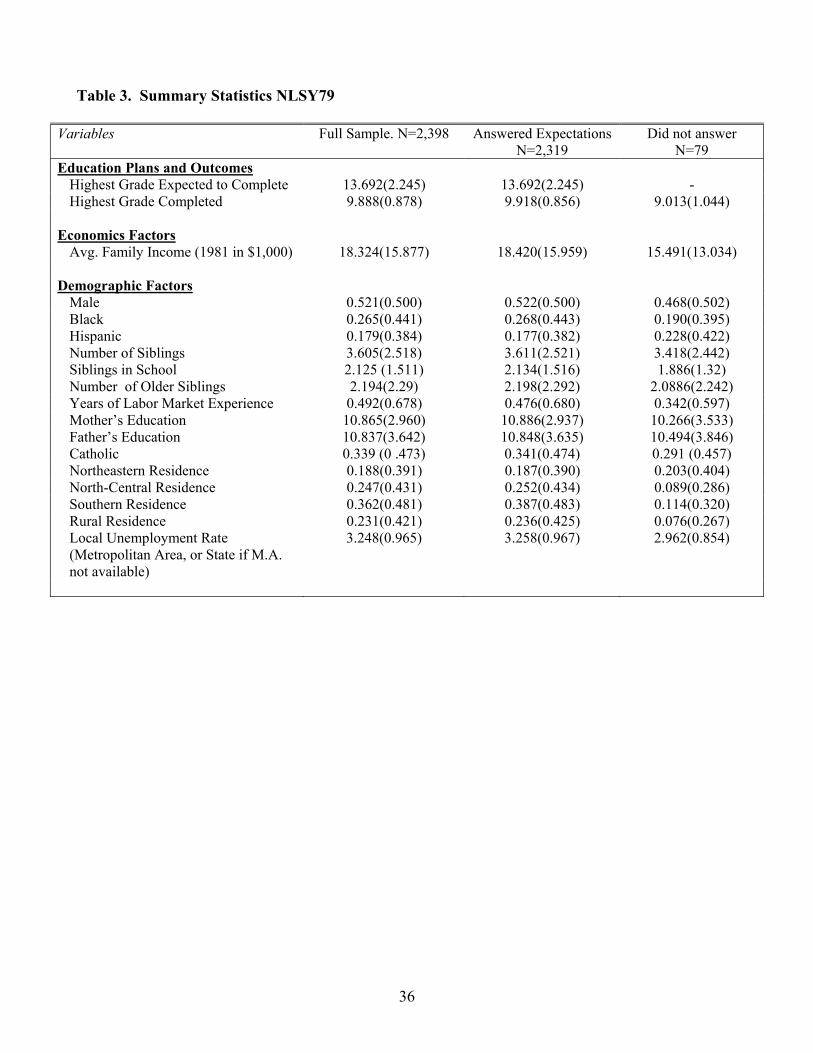
36

Table 3. Summary Statistics NLSY79

Variables Full Sample. N=2,398 Answered Expectations N=2,319

Did not answer N=79

Education Plans and Outcomes Highest Grade Expected to Complete 13.692(2.245) 13.692(2.245) - Highest Grade Completed 9.888(0.878) 9.918(0.856) 9.013(1.044)

Economics Factors

Avg. Family Income (1981 in $1,000) 18.324(15.877) 18.420(15.959) 15.491(13.034) Demographic Factors

Male 0.521(0.500) 0.522(0.500) 0.468(0.502) Black 0.265(0.441) 0.268(0.443) 0.190(0.395) Hispanic 0.179(0.384) 0.177(0.382) 0.228(0.422) Number of Siblings Siblings in School Number of Older Siblings

3.605(2.518) 2.125 (1.511) 2.194(2.29)

3.611(2.521) 2.134(1.516) 2.198(2.292)

3.418(2.442) 1.886(1.32)

2.0886(2.242) Years of Labor Market Experience 0.492(0.678) 0.476(0.680) 0.342(0.597) Mother’s Education 10.865(2.960) 10.886(2.937) 10.266(3.533) Father’s Education Catholic

10.837(3.642) 0.339 (0 .473)

10.848(3.635) 0.341(0.474)

10.494(3.846) 0.291 (0.457)

Northeastern Residence 0.188(0.391) 0.187(0.390) 0.203(0.404) North-Central Residence 0.247(0.431) 0.252(0.434) 0.089(0.286) Southern Residence 0.362(0.481) 0.387(0.483) 0.114(0.320) Rural Residence 0.231(0.421) 0.236(0.425) 0.076(0.267) Local Unemployment Rate (Metropolitan Area, or State if M.A. not available)

3.248(0.965) 3.258(0.967) 2.962(0.854)

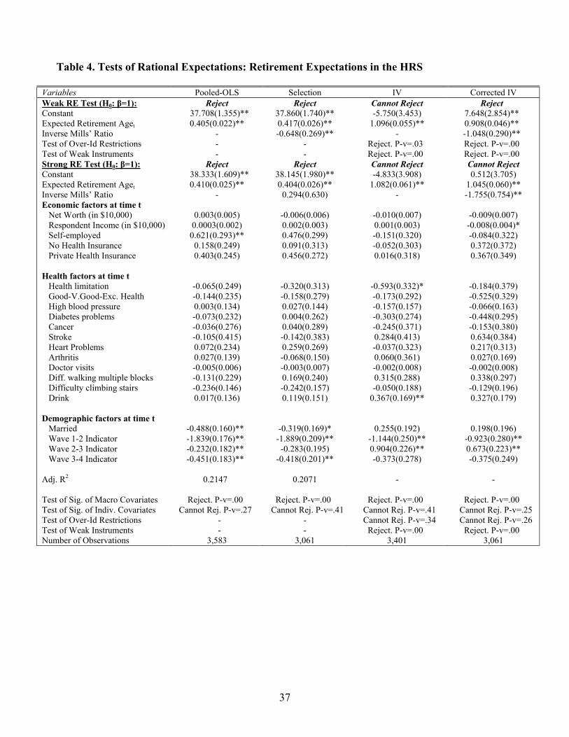
37

Table 4. Tests of Rational Expectations: Retirement Expectations in the HRS

Variables Pooled-OLS Selection IV Corrected IV Weak RE Test (H0: β=1): Constant Expected Retirement Aget Inverse Mills’ Ratio Test of Over-Id Restrictions Test of Weak Instruments Strong RE Test (H0: β=1): Constant Expected Retirement Aget Inverse Mills’ Ratio Economic factors at time t Net Worth (in $10,000) Respondent Income (in $10,000) Self-employed No Health Insurance Private Health Insurance Health factors at time t Health limitation Good-V.Good-Exc. Health High blood pressure Diabetes problems Cancer Stroke Heart Problems Arthritis Doctor visits Diff. walking multiple blocks Difficulty climbing stairs Drink Demographic factors at time t Married Wave 1-2 Indicator Wave 2-3 Indicator Wave 3-4 Indicator Adj. R2

Test of Sig. of Macro Covariates Test of Sig. of Indiv. Covariates Test of Over-Id Restrictions Test of Weak Instruments Number of Observations

Reject 37.708(1.355)** 0.405(0.022)**

- - -

Reject 38.333(1.609)** 0.410(0.025)**

-

0.003(0.005) 0.0003(0.002) 0.621(0.293)**

0.158(0.249) 0.403(0.245)

-0.065(0.249) -0.144(0.235) 0.003(0.134) -0.073(0.232) -0.036(0.276) -0.105(0.415) 0.072(0.234) 0.027(0.139) -0.005(0.006) -0.131(0.229) -0.236(0.146) 0.017(0.136)

-0.488(0.160)** -1.839(0.176)** -0.232(0.182)** -0.451(0.183)**

0.2147

Reject. P-v=.00

Cannot Rej. P-v=.27 - -

3,583

Reject 37.860(1.740)** 0.417(0.026)** -0.648(0.269)**

- -

Reject 38.145(1.980)** 0.404(0.026)** 0.294(0.630)

-0.006(0.006) 0.002(0.003) 0.476(0.299) 0.091(0.313) 0.456(0.272)

-0.320(0.313) -0.158(0.279) 0.027(0.144) 0.004(0.262) 0.040(0.289) -0.142(0.383) 0.259(0.269) -0.068(0.150) -0.003(0.007) 0.169(0.240) -0.242(0.157) 0.119(0.151)

-0.319(0.169)* -1.889(0.209)** -0.283(0.195)

-0.418(0.201)**

0.2071

Reject. P-v=.00 Cannot Rej. P-v=.41

- -

3,061

Cannot Reject -5.750(3.453)

1.096(0.055)** -

Reject. P-v=.03 Reject. P-v=.00 Cannot Reject -4.833(3.908)

1.082(0.061)** -

-0.010(0.007) 0.001(0.003) -0.151(0.320) -0.052(0.303) 0.016(0.318)

-0.593(0.332)* -0.173(0.292) -0.157(0.157) -0.303(0.274) -0.245(0.371) 0.284(0.413) -0.037(0.323) 0.060(0.361) -0.002(0.008) 0.315(0.288) -0.050(0.188)

0.367(0.169)**

0.255(0.192) -1.144(0.250)** 0.904(0.226)** -0.373(0.278)

-

Reject. P-v=.00 Cannot Rej. P-v=.41 Cannot Rej. P-v=.34

Reject. P-v=.00 3,401

Reject 7.648(2.854)** 0.908(0.046)** -1.048(0.290)** Reject. P-v=.00 Reject. P-v=.00 Cannot Reject 0.512(3.705)

1.045(0.060)** -1.755(0.754)**

-0.009(0.007) -0.008(0.004)* -0.084(0.322) 0.372(0.372) 0.367(0.349)

-0.184(0.379) -0.525(0.329) -0.066(0.163) -0.448(0.295) -0.153(0.380) 0.634(0.384) 0.217(0.313) 0.027(0.169) -0.002(0.008) 0.338(0.297) -0.129(0.196) 0.327(0.179)

0.198(0.196) -0.923(0.280)** 0.673(0.223)** -0.375(0.249)

-

Reject. P-v=.00 Cannot Rej. P-v=.25 Cannot Rej. P-v=.26

Reject. P-v=.00 3,061

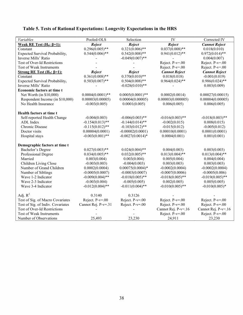
38

Table 5. Tests of Rational Expectations: Longevity Expectations in the HRS

Variables Pooled-OLS Selection IV Corrected IV Weak RE Test (H0: β=1): Constant Expected Survival Probabilityt Inverse Mills’ Ratio Test of Over-Id Restrictions Test of Weak Instruments Strong RE Test (H0: β=1): Constant Expected Survival Probabilityt Inverse Mills’ Ratio Economic factors at time t Net Worth (in $10,000) Respondent Income (in $10,000) No Health Insurance Health factors at time t Self-reported Health Change ADL Index Chronic Disease Doctor visits Hospital stays Demographic factors at time t Bachelor’s Degree Professional Degree Married Children Living Close Number of Grand Children Number of Siblings

Wave 1-2 Indicator Wave 2-3 Indicator Wave 3-4 Indicator Adj. R2

Test of Sig. of Macro Covariates Test of Sig. of Indiv. Covariates Test of Over-Id Restrictions Test of Weak Instruments Number of Observations

Reject 0.296(0.005)** 0.544(0.006)**

- - -

Reject 0.361(0.008)** 0.503(0.007)**

-

0.0004(0.0001)** 0.00003(0.00005)

-0.003(0.005)

-0.004(0.003) -0.154(0.013)** -0.115(0.012)** 0.00004(0.0001) -0.003(0.001)**

0.027(0.003)** 0.034(0.005)** 0.003(0.004) -0.003(0.003)

0.0002(0.0004) -0.0005(0.0007) -0.009(0.004)** -0.003(0.004)

-0.012(0.004)**

0.3140 Reject. P-v=.00

Cannot Rej. P-v=.31 - -

25,493

Reject 0.321(0.006)** 0.542(0.008)** -0.049(0.007)**

- -

Reject 0.370(0.010)** 0.504(0.008)** -0.028(0.010)**

0.0005(0.0001)** 0.00004(0.00005)

0.0001(0.005)

-0.006(0.003)** -0.144(0.014)** -0.103(0.012)**

-0.00002(0.0001) -0.0027(0.0014)*

0.024(0.004)** 0.032(0.005)** 0.003(0.004) -0.004(0.003)

0.00075(0.0004)* -0.0003(0.0007) -0.018(0.005)** -0.005(0.005)

-0.011(0.004)**

0.3126 Reject. P-v=.00 Reject. P-v=.00

- -

23,230

Reject 0.037(0.008)** 0.941(0.012)**

- Reject. P-v=.00 Reject. P-v=.00 Cannot Reject 0.018(0.018)

0.964(0.024)** -

0.0002(0.0014) 0.00003(0.000005)

0.006(0.005)

-0.016(0.003)** -0.002(0.015) -0.015(0.012)

0.00010(0.0001) 0.0004(0.001)

0.004(0.003) 0.013(0.004)** 0.005(0.004) 0.003(0.003)

-0.0002(0.0004) -0.0007(0.0006) -0.018(0.005)**

0.002(0.005) -0.010(0.005)**

-

Reject. P-v=.00 Reject. P-v=.00

Cannot Rej. P-v=.16 Reject. P-v=.00

24,911

Cannot Reject 0.018(0.010)

0.972(0.014)** 0.004(0.007)

Reject. P-v=.00 Reject. P-v=.00 Cannot Reject -0.001(0.019)

0.986(0.024)** 0.003(0.009)

0.00027(0.00015) 0.00004(0.00005)

0.006(0.005)

-0.018(0.003)** 0.008(0.015) -0.005(0.012)

0.0001(0.0001) 0.001(0.001)

0.003(0.003) 0.013(0.004)** 0.004(0.004) 0.003(0.003)

-0.0002(0.0004) -0.0005(0.006)

-0.019(0.005)** 0.005(0.005)

-0.010(0.005)* -

Reject. P-v=.00 Reject. P-v=.00

Cannot Rej. P-v=.16 Reject. P-v=.00

23,230

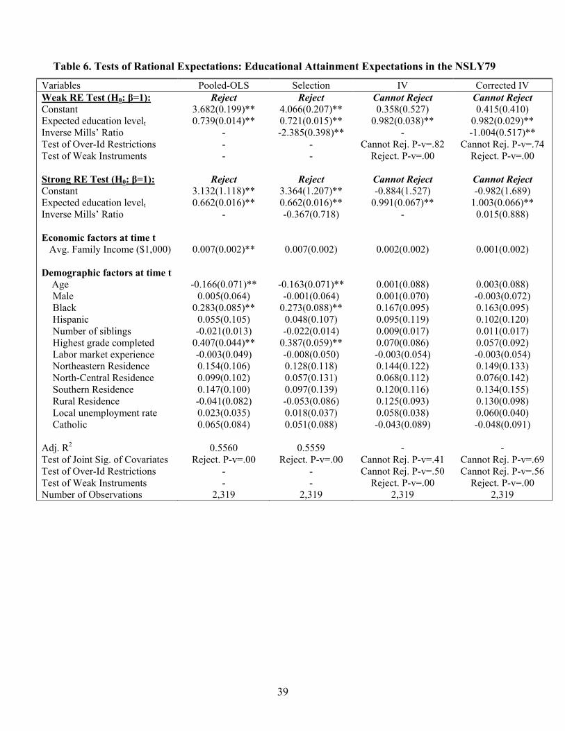
39

Table 6. Tests of Rational Expectations: Educational Attainment Expectations in the NSLY79

Variables Pooled-OLS Selection IV Corrected IV Weak RE Test (H0: β=1): Constant Expected education levelt Inverse Mills’ Ratio Test of Over-Id Restrictions Test of Weak Instruments Strong RE Test (H0: β=1): Constant Expected education levelt Inverse Mills’ Ratio Economic factors at time t Avg. Family Income ($1,000) Demographic factors at time t Age

Male Black Hispanic Number of siblings Highest grade completed Labor market experience Northeastern Residence North-Central Residence Southern Residence Rural Residence Local unemployment rate Catholic

Adj. R2

Test of Joint Sig. of Covariates Test of Over-Id Restrictions Test of Weak Instruments Number of Observations

Reject 3.682(0.199)** 0.739(0.014)**

- - -

Reject 3.132(1.118)** 0.662(0.016)**

-

0.007(0.002)**

-0.166(0.071)** 0.005(0.064)

0.283(0.085)** 0.055(0.105) -0.021(0.013)

0.407(0.044)** -0.003(0.049) 0.154(0.106) 0.099(0.102) 0.147(0.100) -0.041(0.082) 0.023(0.035) 0.065(0.084)

0.5560

Reject. P-v=.00 - -

2,319

Reject 4.066(0.207)** 0.721(0.015)** -2.385(0.398)**

- -

Reject 3.364(1.207)** 0.662(0.016)** -0.367(0.718)

0.007(0.002)

-0.163(0.071)** -0.001(0.064)

0.273(0.088)** 0.048(0.107) -0.022(0.014)

0.387(0.059)** -0.008(0.050) 0.128(0.118) 0.057(0.131) 0.097(0.139) -0.053(0.086) 0.018(0.037) 0.051(0.088)

0.5559

Reject. P-v=.00 - -

2,319

Cannot Reject 0.358(0.527)

0.982(0.038)** -

Cannot Rej. P-v=.82 Reject. P-v=.00

Cannot Reject -0.884(1.527)

0.991(0.067)** -

0.002(0.002)

0.001(0.088) 0.001(0.070) 0.167(0.095) 0.095(0.119) 0.009(0.017) 0.070(0.086) -0.003(0.054) 0.144(0.122) 0.068(0.112) 0.120(0.116) 0.125(0.093) 0.058(0.038) -0.043(0.089)

-

Cannot Rej. P-v=.41 Cannot Rej. P-v=.50

Reject. P-v=.00 2,319

Cannot Reject 0.415(0.410)

0.982(0.029)** -1.004(0.517)**

Cannot Rej. P-v=.74 Reject. P-v=.00

Cannot Reject -0.982(1.689)

1.003(0.066)** 0.015(0.888)

0.001(0.002)

0.003(0.088) -0.003(0.072) 0.163(0.095) 0.102(0.120) 0.011(0.017) 0.057(0.092) -0.003(0.054) 0.149(0.133) 0.076(0.142) 0.134(0.155) 0.130(0.098) 0.060(0.040) -0.048(0.091)

-

Cannot Rej. P-v=.69 Cannot Rej. P-v=.56

Reject. P-v=.00 2,319

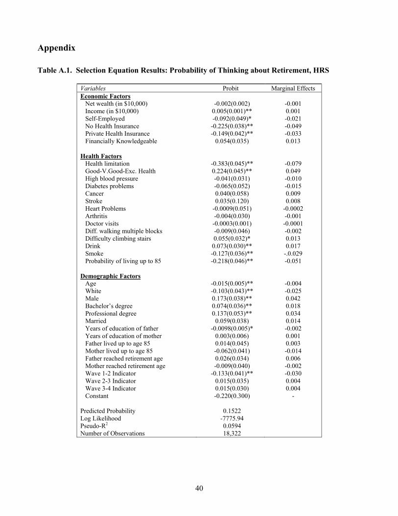
40

Appendix Table A.1. Selection Equation Results: Probability of Thinking about Retirement, HRS

Variables Probit Marginal Effects Economic Factors Net wealth (in $10,000) Income (in $10,000) Self-Employed No Health Insurance Private Health Insurance Financially Knowledgeable Health Factors Health limitation Good-V.Good-Exc. Health High blood pressure Diabetes problems Cancer Stroke Heart Problems Arthritis Doctor visits Diff. walking multiple blocks Difficulty climbing stairs Drink Smoke Probability of living up to 85 Demographic Factors Age White Male Bachelor’s degree Professional degree Married Years of education of father Years of education of mother Father lived up to age 85 Mother lived up to age 85 Father reached retirement age Mother reached retirement age Wave 1-2 Indicator Wave 2-3 Indicator Wave 3-4 Indicator Constant Predicted Probability Log Likelihood Pseudo-R2 Number of Observations

-0.002(0.002)

0.005(0.001)** -0.092(0.049)*

-0.225(0.038)** -0.149(0.042)**

0.054(0.035)

-0.383(0.045)** 0.224(0.045)** -0.041(0.031) -0.065(0.052) 0.040(0.058) 0.035(0.120)

-0.0009(0.051) -0.004(0.030)

-0.0003(0.001) -0.009(0.046) 0.055(0.032)*

0.073(0.030)** -0.127(0.036)** -0.218(0.046)**

-0.015(0.005)** -0.103(0.043)** 0.173(0.038)** 0.074(0.036)** 0.137(0.053)** 0.059(0.038)

-0.0098(0.005)* 0.003(0.006) 0.014(0.045) -0.062(0.041) 0.026(0.034) -0.009(0.040)

-0.133(0.041)** 0.015(0.035) 0.015(0.030) -0.220(0.300)

0.1522

-7775.94 0.0594 18,322

-0.001 0.001 -0.021 -0.049 -0.033 0.013

-0.079 0.049 -0.010 -0.015 0.009 0.008

-0.0002 -0.001

-0.0001 -0.002 0.013 0.017

-.0.029 -0.051

-0.004 -0.025 0.042 0.018 0.034 0.014 -0.002 0.001 0.003 -0.014 0.006 -0.002 -0.030 0.004 0.004

-

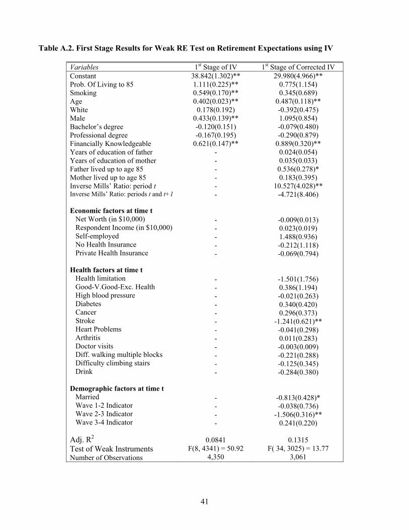
41

Table A.2. First Stage Results for Weak RE Test on Retirement Expectations using IV

Variables 1st Stage of IV 1st Stage of Corrected IV Constant Prob. Of Living to 85 Smoking Age White Male Bachelor’s degree Professional degree Financially Knowledgeable Years of education of father Years of education of mother Father lived up to age 85 Mother lived up to age 85 Inverse Mills’ Ratio: period t Inverse Mills’ Ratio: periods t and t+1 Economic factors at time t Net Worth (in $10,000) Respondent Income (in $10,000) Self-employed No Health Insurance Private Health Insurance Health factors at time t Health limitation Good-V.Good-Exc. Health High blood pressure Diabetes Cancer Stroke Heart Problems Arthritis Doctor visits Diff. walking multiple blocks Difficulty climbing stairs Drink

Demographic factors at time t Married Wave 1-2 Indicator Wave 2-3 Indicator Wave 3-4 Indicator Adj. R2 Test of Weak Instruments Number of Observations

38.842(1.302)** 1.111(0.225)** 0.549(0.170)** 0.402(0.023)**

0.178(0.192) 0.433(0.139)** -0.120(0.151) -0.167(0.195)

0.621(0.147)** - - - - - - - - - - - - - - - - - - - - - - - - - - -

0.0841 F(8, 4341) = 50.92

4,350

29.980(4.966)** 0.775(1.154) 0.345(0.689)

0.487(0.118)** -0.392(0.475) 1.095(0.854) -0.079(0.480) -0.290(0.879)

0.889(0.320)** 0.024(0.054) 0.035(0.033)

0.536(0.278)* 0.183(0.395)

10.527(4.028)** -4.721(8.406)

-0.009(0.013) 0.023(0.019) 1.488(0.936) -0.212(1.118) -0.069(0.794)

-1.501(1.756) 0.386(1.194) -0.021(0.263) 0.340(0.420) 0.296(0.373)

-1.241(0.621)** -0.041(0.298) 0.011(0.283) -0.003(0.009) -0.221(0.288) -0.125(0.345) -0.284(0.380)

-0.813(0.428)* -0.038(0.736)

-1.506(0.316)** 0.241(0.220)

0.1315

F( 34, 3025) = 13.77 3,061

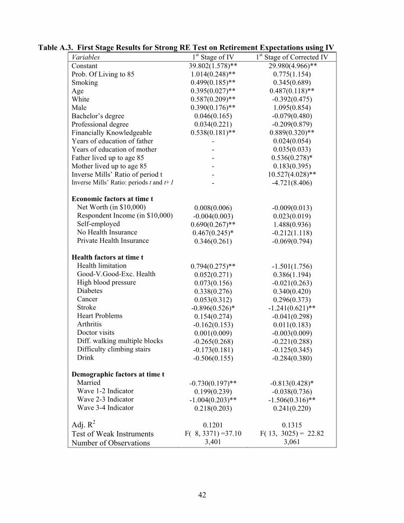
42

Table A.3. First Stage Results for Strong RE Test on Retirement Expectations using IV Variables 1st Stage of IV 1st Stage of Corrected IV Constant Prob. Of Living to 85 Smoking Age White Male Bachelor’s degree Professional degree Financially Knowledgeable Years of education of father Years of education of mother Father lived up to age 85 Mother lived up to age 85 Inverse Mills’ Ratio of period t Inverse Mills’ Ratio: periods t and t+1 Economic factors at time t Net Worth (in $10,000) Respondent Income (in $10,000) Self-employed No Health Insurance Private Health Insurance Health factors at time t Health limitation Good-V.Good-Exc. Health High blood pressure Diabetes Cancer Stroke Heart Problems Arthritis Doctor visits Diff. walking multiple blocks Difficulty climbing stairs Drink

Demographic factors at time t Married Wave 1-2 Indicator Wave 2-3 Indicator Wave 3-4 Indicator Adj. R2 Test of Weak Instruments Number of Observations

39.802(1.578)** 1.014(0.248)** 0.499(0.185)** 0.395(0.027)** 0.587(0.209)** 0.390(0.176)**

0.046(0.165) 0.034(0.221)

0.538(0.181)** - - - - - -

0.008(0.006) -0.004(0.003)

0.690(0.267)** 0.467(0.245)* 0.346(0.261)

0.794(0.275)** 0.052(0.271) 0.073(0.156) 0.338(0.276) 0.053(0.312)

-0.896(0.526)* 0.154(0.274) -0.162(0.153) 0.001(0.009) -0.265(0.268) -0.173(0.181) -0.506(0.155)

-0.730(0.197)** 0.199(0.239)

-1.004(0.203)** 0.218(0.203)

0.1201

F( 8, 3371) =37.10 3,401

29.980(4.966)** 0.775(1.154) 0.345(0.689)

0.487(0.118)** -0.392(0.475) 1.095(0.854) -0.079(0.480) -0.209(0.879)

0.889(0.320)** 0.024(0.054) 0.035(0.033)

0.536(0.278)* 0.183(0.395)

10.527(4.028)** -4.721(8.406)

-0.009(0.013) 0.023(0.019) 1.488(0.936) -0.212(1.118) -0.069(0.794)

-1.501(1.756) 0.386(1.194) -0.021(0.263) 0.340(0.420) 0.296(0.373)

-1.241(0.621)** -0.041(0.298) 0.011(0.183) -0.003(0.009) -0.221(0.288) -0.125(0.345) -0.284(0.380)

-0.813(0.428)* -0.038(0.736)

-1.506(0.316)** 0.241(0.220)

0.1315

F( 13, 3025) = 22.82 3,061

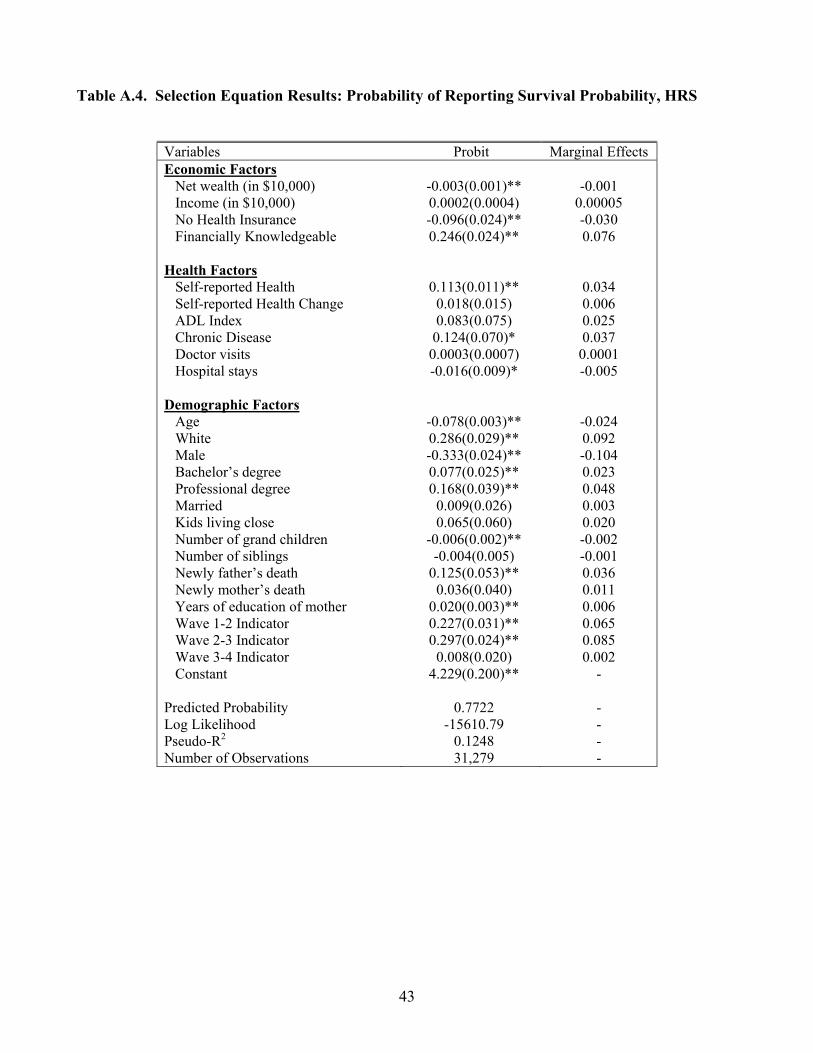
43

Table A.4. Selection Equation Results: Probability of Reporting Survival Probability, HRS

Variables Probit Marginal Effects Economic Factors Net wealth (in $10,000) Income (in $10,000) No Health Insurance Financially Knowledgeable Health Factors Self-reported Health Self-reported Health Change ADL Index Chronic Disease Doctor visits Hospital stays Demographic Factors Age White Male Bachelor’s degree Professional degree Married Kids living close Number of grand children Number of siblings Newly father’s death Newly mother’s death Years of education of mother Wave 1-2 Indicator Wave 2-3 Indicator Wave 3-4 Indicator Constant Predicted Probability Log Likelihood Pseudo-R2 Number of Observations

-0.003(0.001)** 0.0002(0.0004) -0.096(0.024)** 0.246(0.024)**

0.113(0.011)** 0.018(0.015) 0.083(0.075)

0.124(0.070)* 0.0003(0.0007) -0.016(0.009)*

-0.078(0.003)** 0.286(0.029)** -0.333(0.024)** 0.077(0.025)** 0.168(0.039)**

0.009(0.026) 0.065(0.060)

-0.006(0.002)** -0.004(0.005)

0.125(0.053)** 0.036(0.040)

0.020(0.003)** 0.227(0.031)** 0.297(0.024)**

0.008(0.020) 4.229(0.200)**

0.7722

-15610.79 0.1248 31,279

-0.001

0.00005 -0.030 0.076

0.034 0.006 0.025 0.037

0.0001 -0.005

-0.024 0.092 -0.104 0.023 0.048 0.003 0.020 -0.002 -0.001 0.036 0.011 0.006 0.065 0.085 0.002

- - - - -

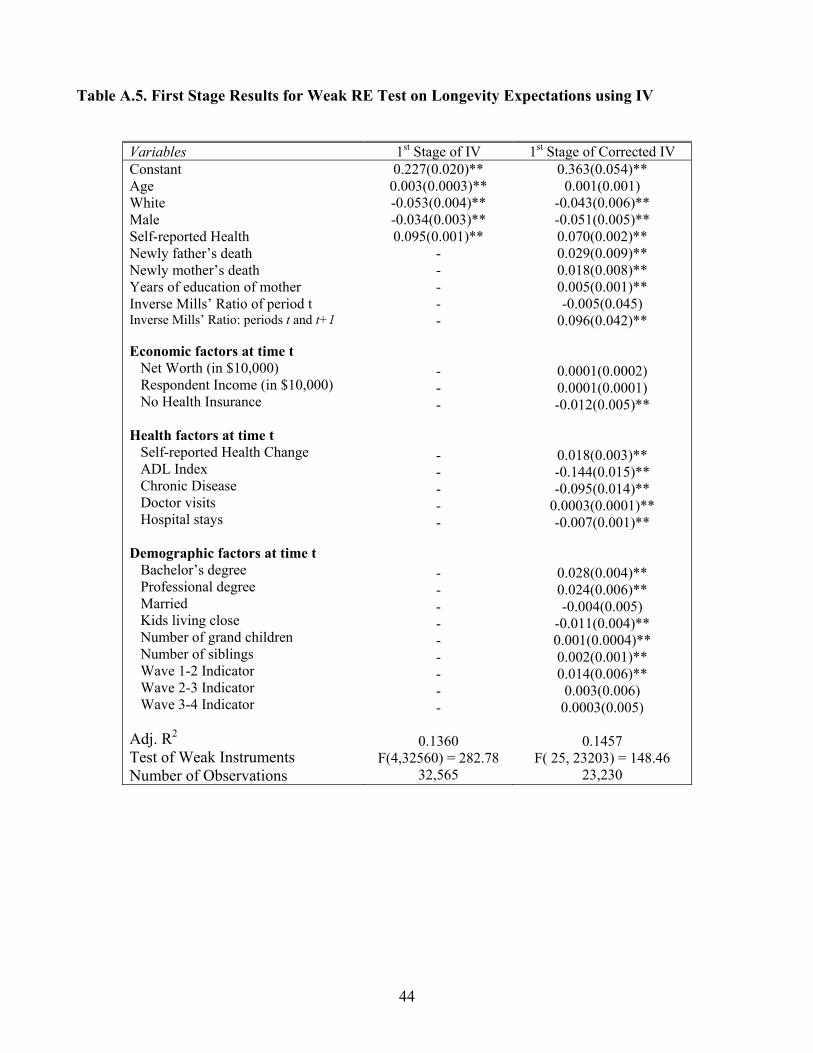
44

Table A.5. First Stage Results for Weak RE Test on Longevity Expectations using IV

Variables 1st Stage of IV 1st Stage of Corrected IV Constant Age White Male Self-reported Health Newly father’s death Newly mother’s death Years of education of mother Inverse Mills’ Ratio of period t Inverse Mills’ Ratio: periods t and t+1 Economic factors at time t Net Worth (in $10,000) Respondent Income (in $10,000) No Health Insurance Health factors at time t Self-reported Health Change ADL Index Chronic Disease Doctor visits Hospital stays Demographic factors at time t Bachelor’s degree Professional degree Married Kids living close Number of grand children Number of siblings Wave 1-2 Indicator Wave 2-3 Indicator Wave 3-4 Indicator Adj. R2 Test of Weak Instruments Number of Observations

0.227(0.020)** 0.003(0.0003)** -0.053(0.004)** -0.034(0.003)** 0.095(0.001)**

- - - - - - - - - - - - - - - - - - - - - -

0.1360 F(4,32560) = 282.78

32,565

0.363(0.054)** 0.001(0.001)

-0.043(0.006)** -0.051(0.005)** 0.070(0.002)** 0.029(0.009)** 0.018(0.008)** 0.005(0.001)** -0.005(0.045)

0.096(0.042)**

0.0001(0.0002) 0.0001(0.0001) -0.012(0.005)**

0.018(0.003)** -0.144(0.015)** -0.095(0.014)**

0.0003(0.0001)** -0.007(0.001)**

0.028(0.004)** 0.024(0.006)** -0.004(0.005)

-0.011(0.004)** 0.001(0.0004)** 0.002(0.001)** 0.014(0.006)**

0.003(0.006) 0.0003(0.005)

0.1457

F( 25, 23203) = 148.46 23,230

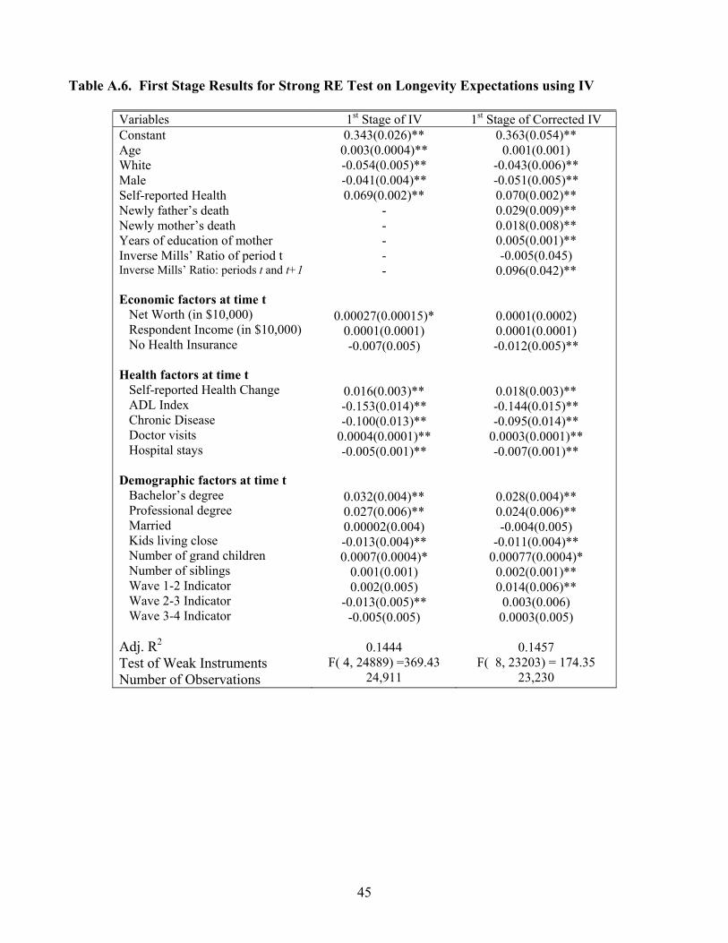
45

Table A.6. First Stage Results for Strong RE Test on Longevity Expectations using IV

Variables 1st Stage of IV 1st Stage of Corrected IV Constant Age White Male Self-reported Health Newly father’s death Newly mother’s death Years of education of mother Inverse Mills’ Ratio of period t Inverse Mills’ Ratio: periods t and t+1 Economic factors at time t Net Worth (in $10,000) Respondent Income (in $10,000) No Health Insurance Health factors at time t Self-reported Health Change ADL Index Chronic Disease Doctor visits Hospital stays Demographic factors at time t Bachelor’s degree Professional degree Married Kids living close Number of grand children Number of siblings Wave 1-2 Indicator Wave 2-3 Indicator Wave 3-4 Indicator Adj. R2 Test of Weak Instruments Number of Observations

0.343(0.026)** 0.003(0.0004)** -0.054(0.005)** -0.041(0.004)** 0.069(0.002)**

- - - - -

0.00027(0.00015)* 0.0001(0.0001) -0.007(0.005)

0.016(0.003)** -0.153(0.014)** -0.100(0.013)**

0.0004(0.0001)** -0.005(0.001)**

0.032(0.004)** 0.027(0.006)** 0.00002(0.004) -0.013(0.004)** 0.0007(0.0004)*

0.001(0.001) 0.002(0.005)

-0.013(0.005)** -0.005(0.005)

0.1444

F( 4, 24889) =369.43 24,911

0.363(0.054)** 0.001(0.001)

-0.043(0.006)** -0.051(0.005)** 0.070(0.002)** 0.029(0.009)** 0.018(0.008)** 0.005(0.001)** -0.005(0.045)

0.096(0.042)**

0.0001(0.0002) 0.0001(0.0001) -0.012(0.005)**

0.018(0.003)** -0.144(0.015)** -0.095(0.014)**

0.0003(0.0001)** -0.007(0.001)**

0.028(0.004)** 0.024(0.006)** -0.004(0.005)

-0.011(0.004)** 0.00077(0.0004)*

0.002(0.001)** 0.014(0.006)**

0.003(0.006) 0.0003(0.005)

0.1457

F( 8, 23203) = 174.35 23,230

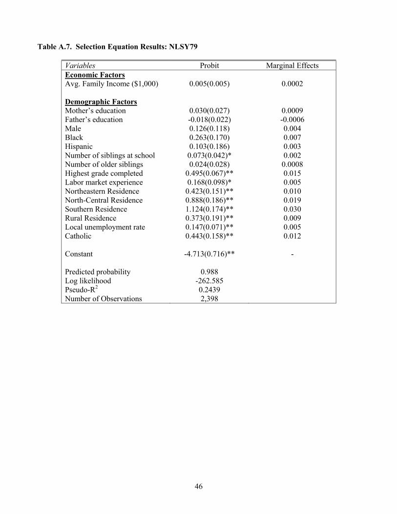
46

Table A.7. Selection Equation Results: NLSY79

Variables Probit Marginal Effects Economic Factors Avg. Family Income ($1,000) Demographic Factors Mother’s education Father’s education Male Black Hispanic Number of siblings at school Number of older siblings Highest grade completed Labor market experience Northeastern Residence North-Central Residence Southern Residence Rural Residence Local unemployment rate Catholic Constant Predicted probability Log likelihood Pseudo-R2 Number of Observations

0.005(0.005)

0.030(0.027) -0.018(0.022) 0.126(0.118) 0.263(0.170) 0.103(0.186) 0.073(0.042)* 0.024(0.028)

0.495(0.067)** 0.168(0.098)* 0.423(0.151)** 0.888(0.186)** 1.124(0.174)** 0.373(0.191)** 0.147(0.071)** 0.443(0.158)**

-4.713(0.716)**

0.988

-262.585 0.2439 2,398

0.0002

0.0009 -0.0006 0.004 0.007 0.003 0.002 0.0008 0.015 0.005 0.010 0.019 0.030 0.009 0.005 0.012

-

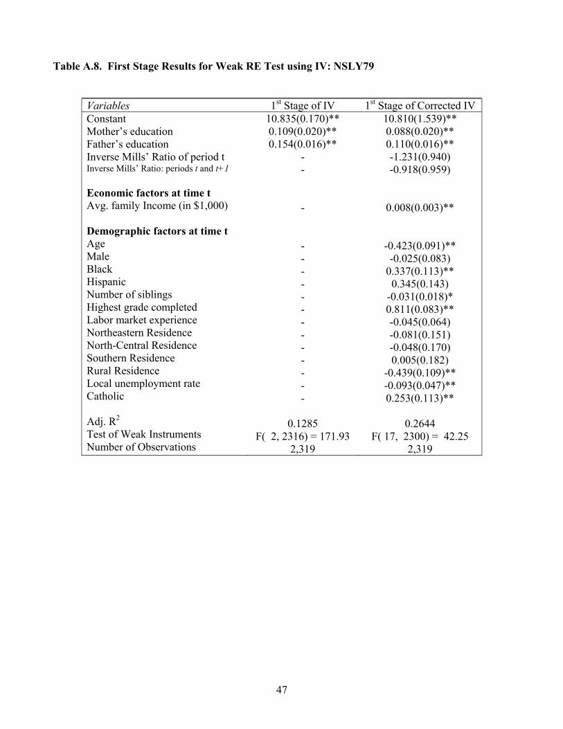
47

Table A.8. First Stage Results for Weak RE Test using IV: NSLY79

Variables 1st Stage of IV 1st Stage of Corrected IV Constant Mother’s education Father’s education Inverse Mills’ Ratio of period t Inverse Mills’ Ratio: periods t and t+1 Economic factors at time t Avg. family Income (in $1,000) Demographic factors at time t Age Male Black Hispanic Number of siblings Highest grade completed Labor market experience Northeastern Residence North-Central Residence Southern Residence Rural Residence Local unemployment rate Catholic Adj. R2 Test of Weak Instruments Number of Observations

10.835(0.170)** 0.109(0.020)** 0.154(0.016)**

- - - - - - - - - - - - - - - -

0.1285 F( 2, 2316) = 171.93

2,319

10.810(1.539)** 0.088(0.020)** 0.110(0.016)** -1.231(0.940) -0.918(0.959)

0.008(0.003)**

-0.423(0.091)** -0.025(0.083)

0.337(0.113)** 0.345(0.143)

-0.031(0.018)* 0.811(0.083)** -0.045(0.064) -0.081(0.151) -0.048(0.170) 0.005(0.182)

-0.439(0.109)** -0.093(0.047)** 0.253(0.113)**

0.2644

F( 17, 2300) = 42.25 2,319

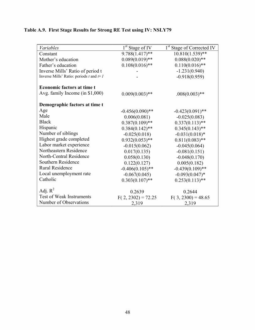
48

Table A.9. First Stage Results for Strong RE Test using IV: NSLY79

Variables 1st Stage of IV 1st Stage of Corrected IV Constant Mother’s education Father’s education Inverse Mills’ Ratio of period t Inverse Mills’ Ratio: periods t and t+1 Economic factors at time t Avg. family Income (in $1,000) Demographic factors at time t Age Male Black Hispanic Number of siblings Highest grade completed Labor market experience Northeastern Residence North-Central Residence Southern Residence Rural Residence Local unemployment rate Catholic Adj. R2 Test of Weak Instruments Number of Observations

9.788(1.417)** 0.089(0.019)** 0.108(0.016)**

- -

0.009(0.003)**

-0.456(0.090)** 0.006(0.081)

0.387(0.109)** 0.384(0.142)** -0.025(0.018)

0.932(0.053)** -0.015(0.062) 0.017(0.135) 0.058(0.130) 0.122(0.127)

-0.406(0.105)** -0.067(0.045)

0.303(0.107)**

0.2639 F( 2, 2302) = 72.25

2,319

10.810(1.539)** 0.088(0.020)** 0.110(0.016)** -1.231(0.940) -0.918(0.959)

.008(0.003)**

-0.423(0.091)** -0.025(0.083)

0.337(0.113)** 0.345(0.143)** -0.031(0.018)* 0.811(0.083)** -0.045(0.064) -0.081(0.151) -0.048(0.170) 0.005(0.182)

-0.439(0.109)** -0.093(0.047)* 0.253(0.113)**

0.2644

F( 3, 2300) = 48.65 2,319