ELSEVIER Atmospheric Research 42 (1996) 75-88

ATMOSPHERIC RESEARCH

Regional rainfall distribution for Canada

Kaz A d a m o w s k i a, Younes Ali la b, Paul J. Pilon c a University of Ottawa, Department of Civil Engineering, Ottawa, Ontario, KIN 6N5, Canada

b Greater Vancouuer Regional District, Burnaby, B.C., VSH 4G8, Canada " Environment Canada, Atmospheric Environment Service, Ottawa, Ontario, K1A OH3, Canada

Received 4 December 1994; accepted 17 February 1995

Abstract

Current point rainfall frequency analysis techniques used in engineering design are outdated. In this study, data distribution and analytical techniques are reviewed, and a new method for regional analysis of rainfall is presented. The regional analysis is performed using data across Canada, and takes advantage of recently developed linear order statistics of L-moments.

Numerical analysis of 320 stations showed that Canada may be considered as one homoge- neons region with respect to L-skewness and L-kurtosis. However, the L-coefficient of variation shows regional variability that is related to the mean annual precipitation (MAP). A regional parent distribution is identified as the general extreme value (GEV), with parameters depending on MAP and storm duration. These findings differ from present methodology, whereby the Gumbel I distribution is used irrespective of storm duration.

1. Introduction

The knowledge of rainfall Intensity-Duration-Frequency (1DF) relationships is of fundamental importance in hydrology. IDF curves are used in developing design storms and are also needed in many hydrologic models and procedures in computation of water quantity and quality characteristics. In developing IDF curves, statistical frequency analysis is employed, whereby an annual extreme rainfall series of given duration is described by an assumed probability density function (Gumbel I distribution has been used in Canada). Such a statistical procedure has many inherent deficiencies including distributional assumptions, record length availability, difficulty in modeling of space- time characteristics, extrapolation problems in space-time, and others.

One of the more serious deficiencies of IDF curves concerns the space-t ime characteristics and extrapolation of point rainfall. In practical applications, IDF curves are usually extrapolated in space using available maps (Hogg and Carr, 1985) or

0169-8095/96/$15.00 Copyright © 1996 Elsevier Science B.V. All rights reserved. SSDI 0169-8095(95)00054-2

76 K. Adamowski et al. /Atmospheric Research 42 (1996) 75-88

different transposition and interpolation schemes (WMO, 1983). However, such ap- proaches have their limitations, and are often inappropriate in the absence of physically justified procedures.

To address such a deficiency, it is possible to develop regional IDF curves. Regionalization techniques are widely used in flood frequency analysis and have shown the ability to significantly reduce the uncertainties in quantile estimates relative to that inherent in the at-site approach (Lettenmaier et al., 1987; Potter, 1987; Pilon and Adamowski, 1992).

Schaefer (1990) used precipitation data from Washington State to conduct a regional analysis using an "index flood" type methodology. He showed that the coefficient of variation (C v) and skewness (C~) vary systematically with the MAP. The study area was found to be climatically heterogeneous, and homogeneous sub-regions were delineated within the heterogeneous region based on MAP values. However, recent studies for flood data (Gabriele and Arnell, 1991; Ribeiro-Correa and Rousselle, 1993) indicate that different parameters (i.e., C v, C s) can be assumed to be approximately constant over different spatial scales. In particular, the skewness was found to be constant over a larger area than the coefficient of variation, which in turn varies less over space that the mean value. Furthermore, Pilon et al. (1991) have found that the probability distribution of extreme rainfall events depends on the duration of rainfall. Therefore, these newest studies reveal that current assumptions in the IDF curve developments are not valid. They also indicate that the estimate based on regional information is more accurate that those based on the single site records.

The utility of regional analysis depends on the satisfactory solution of the following: the selection and verification of homogenous regions, the identification of regional probability distributions, and the estimation of the regional distributions' parameters.

All of these issues require the knowledge of statistical parameters such as skewness and kurtosis. Unfortunately, the estimates of these parameters have serious theoretical and practical drawbacks (Royston, 1991). However, Hosking (1990) developed L-mo- ments techniques which have several advantages over conventional moment parameters and have no serious drawbacks.

The purpose of this paper is to use the method of L-moments to define homogenous regions and to investigate the identification of a regional distribution for annual maxima precipitation for Canada.

1.1. The linear moment statistics

The rth L-moments of a random variable x have been defined as (Hosking, 1990):

1 * Ar = fo x(F) Pr- ,( F)dF (1) in which

• ~ r - k ( r ) ( r k k ) f k P~ = ( - 1) k (2)

k = 0

where F(x ) is the cumulative distribution of x, and x (F) is the quantile function for the distribution. The first L-moment, A~, is the arithmetic mean, while the second

K. Adamowski et al, /Atmospheric Research 42 (1996) 75-88 77

L-moment, A 2, is a measure of dispersion analogous to the standard deviation. Hosking found it convenient to standardize the higher L-moments such that the rth L-moment ratio is given by:

A~ 7 r = - - (3)

A2

where % is a measure of the symmetry of the sample and is referred to as L-skewness, 74 is considered a measure of peakedness and is referred to as L-kurtosis, and 7 = A2/A ~ is analogous to the conventional coefficient of variation.

For a random sample xl, x2, . . . , Xn, let xl:, <x2: . < ... <_x,,:,, be the ordered sample. The rth sample L-moment, I r, can be estimated by:

r l ( ) Z Z . . . . k Xir ,° (4)

l<_il<i 2 i,<_n k=O

or alternatively

n

--At= E P r * l( Pi:n)Xi:n ( 5 ) i = 1

where the probability Pi:n is estimated using an empirical plotting position formula. Hosking (1990) indicated that At, is asymptotically equivalent to l r, but that A r is not an unbiased estimator of A r, rather the bias is of stochastic order n-~.

Since in practical experience, plotting position estimators sometimes yield a better estimate of parameters and quantiles when a distribution is fitted to the data, Eq. (5) has been suggested to estimate L-moments and is used in this study. For a finite sample, the sample L-moment ratio is estimated by t~ = (Ar/A~); where t~ is called the rth sample L-moment ratio.

While sample L-moments are considered virtually unbiased even for short sample lengths (n < 20), a correction factor for the L-kurtosis as suggested by Hosking and Wallis (1993) is adopted in the computational procedure.

In this paper, the L-moments are used to delineate and test homogeneous regions and identify a regional distribution for Canada.

2. Data

Numerical analysis in this study is performed on rainfall data from 320 meteorologi- cal stations in Canada. The data represents wide climatic variability that exists in Canada. Precipitation varies widely throughout Canada, with the greatest average annual precipitation of 6655 mm at Henderson Lake, B.C., and the least annual precipitation of 12.7 mm at Arctic Bay, NWT. There are seven different climatological regions in Canada (Hare and Thomas, 1979). The vast, mostly uninhabited area of northern Canada contains several different climatic regions, but is not included in this study due to the lack of suitable rainfall observations.

78 K. Adamowski et al. / Atmospheric Research 42 (1996) 75-88

Table 1 Total number of gauged stations and average record length

Province Number of sites Record length

Alberta 24 22 British Columbia 60 18 Manitoba 22 20 Maritimes 40 20 Ontario 70 21 Quebec 74 18 Saskatchewan 30 21 Canada 320 19

Canada's official climate archives contain measurements from approximately 3043 observing sites; historic records are available from approximately 3000 more locations. However, recording gauge precipitation data exists for 320 stations only. The number of stations and the available record length used in this study is shown in Table 1. Most of these stations are located in southern Canada, where most people live.

The observed data was screened using various tests (Pilon and Harvey, 1994) and was found to be independent, trend free and random. The data used in the analysis is composed of an annual extreme series which consists of the largest precipitation amount in each year of record for an assumed durations of 5, 10, 15, 30, 60 and 120 rain.

3. Regional analysis

In regional analysis, it is necessary to specify homogenous regions and identify probability distributions applicable to each region. The parameters of such a regional parent distribution are in turn related to hydrometeorological variables which govern the generation mechanism of precipitation. The procedures are simplified by defining large regions termed "homogeneous" whereby all but one (often the annual mean) of the extreme variable characteristics are either proved or assumed to be constant. The number of functional relationships is then reduced to one, and the regionalization is known as the " index" method, introduced first by Dalrymple (1960).

This method is adopted in the present study whereby indexing is performed on statistical parameters rather than quantiles of the distribution. Furthermore, to overcome discontinuities encountered at regional boundaries the geographical definition of a region is avoided. A group of sites that are not necessarily contiguous in space can form a homogeneous network (Acreman and Wiltshire, 1987; Cavadias, 1989; Burn, 1990).

The delineation of homogeneous regions is based on the variability of statistical parameters of L-coefficient of variation (t), L-skewness (t3), and L-kurtosis 04). These parameters S, are also used to identify a regional parent probability distribution. The influence of climate and storm duration on the characteristics of such distributions is also investigated.

K. Adamowski et al. / Atmospheric Research 42 (1996) 75-88 79

An L-moment ratio diagram is used along with statistical tests to compare sample estimates of the dimensionless ratios t, t 3, t4, with their population counterparts for a range of assumed distributions.

3.1. Delineation and statistical testing of homogeneous regions

The statistical testing of homogeneity follows the approach suggested by Hosking and Wallis (1993), using L-moments, whereby a group of gauged basins is first hypothesized to be homogeneous. Weighted average L-moment statistics are used to compute representative parameters of the whole network. If the network has N sites each with n i length of record, its L-moment ratios are computed as follow:

~_ ~nit? (6) }r= EN=,ni

The values of t 3 (L-skewness) and t 4 (L-kurtosis) are superimposed on the theoreti- cal L-moment ratio diagram, and first candidate distribution is identified. The assess- ment of the time and space sampling characteristic of this identified parent distribution would then be the basis of verifying the assumption of homogeneity for the specified region. This assumption is tested using Monte Carlo simulation procedures.

In order, to avoid any commitment to a particular two or three-parameter distribution, the four-parameter Kappa distribution (Hosking, 1988) is used for Monte Carlo simula- tions. The Kappa distribution is fitted to the weighted average L-moments h, ?, ?3, and ?4- Samples drawn from this parent are used to replicate the number of sites and the number of observations at each of these sites. A large number (500) of synthetically generated networks are then replicated. The following three measures of the between-site variability of sample L-moments are computed: 1. Based on the L-coefficient of variation (t), the weighted standard deviation of t is

calculated as V~,

y~f=, ni ( t ( i ) _ ~)2

= Ef=,ni (7)

2. Based on t and t 3, the weighted average distance from the site to the network's mean on the t vs. t 3 L-moment ratio diagram is then calculated as V 2,

Ei~ ,ni t3) V 2 ~--- El= 1 ni

(8)

3. Based on t 3 and t4, the weighted average distance from the site to the network weighted mean on the t 3 vs. t 4, L-moment ratio diagram is calculated as V 3,

~iNl ni¢ t~ i) -- ?3 )2 + (t(4i) - "t, )2

V s = E / U n ' (9)

80 K. Adamowski et a l . / Atmospheric Research 42 (1996) 75-88

If V denotes any of the three measures V 1, V 2, or V 3, the homogeneity measure is given by (Hosking and Wallis, 1993):

(robs- ~,) H = (10)

where Vob s is the real network value of either V l, V 2, or V3; and /z v and o-v are the mean and standard deviation of the 500 values of their synthetic counterpart. This measure of homogeneity accounts for the difference between statistical and operational homogeneity; where the latter is defined as that acceptable degree of heterogeneity in a region for which the regional analysis is still considered more accurate than single site analysis.

Hosking and Wallis (1993) using Monte Carlo experiments suggested that the region under testing should be regarded as operationally "acceptably" homogeneous if H < 1, "possibly" heterogeneous if 1 < H < 2, and "definitely" heterogeneous if H > 2.

In this study, an additional statistical homogeneity test is proposed which is based on parametric bootstrapping and hypothesis testing. The between-site variability of sample L-moments in a network of N sites each with n i record length is measured by the following:

I. Weighted variance of t:

o-? = ~ L , n , (11)

2. Weighted variance of t3:

r L ' " ' ( ' ? - h)2 (12) ¢2~ = ~7=, n,

3. Weighted variance of t4:

~'~N ,n,(t(4i)_- 2 o.2= ,= t4) (13)

2L ,n ,

If O-2 denotes any of the three measures o -2, o-22, or o'2; the homogeneity is measured by (Alila et al., 1993):

s= (0-°2~- ~ ) 100 (14) O-o2

where o-o2~ is the real network value of either o-z 2, 0-22, o-z; and /z¢~ is the mean of the 500 values of its synthetic counterpart. The /,~: quantify the amount of variation (sampling noise) of L-moment statistics that would be expected had the network been homogenous. The values of the S statistic, on the other hand, quantify the amount of variation (signal) of L-moment statistics in excess of sampling noise and attributed to climatic factors.

If?. Adamowski et al. /Atmospheric Research 42 (1996) 75-88 81

3.2. Identification of homogeneous region in higher order L-moments

The hypothesis that Canada could be considered as a homogeneous region in t 3 and t 4 is tested for each rainfall duration using the H and S statistic; results are given in Table 2. Values of S statistic indicate that the synthetic variance in sample t 3 and tz is similar to the observed variance. In other words, the signal portion of the variability in sample of t 3 and t 4 is relatively small in comparison with the noise for all analyzed storms. At the 90% confidence level, the difference in variability of t 3 and t 4 between the observed and synthetic networks is not significant. Since the synthetic replication of the whole network of sites uses the observed record length it can be concluded that the between-site variability of t 3 and t 4 is almost completely explained by the time sampling variability.

The hypothesis that Canada is one homogeneous region in t 3 and t 4 is further supported by the Hv3 statistic with values in the "acceptably" homogeneous range. However, some heterogeneity is detected in V 2 by the H test and in t by the S test for all storm durations. The S statistic results indicate that the variability of t 3 and t 4 is not distinguishable from sampling error.

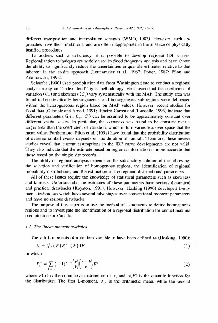
Plots of t 3 and t 4 a r e made against the MAP in order to ascertain if these statistics vary with MAP. Fig. 1 and Fig. 2 show typical plots for the 60-min duration. No relationship is depicted for either t 3 nor t 4. This supports the statistical testing of homogeneity whereby the variability of both L-moment ratios are due to sampling error.

In summary, the study area can be assumed as a homogeneous region in both t 3 and t 4 whereby the best representative regional parameters would be the weighted average values for each storm duration.

3.3. Identification of homogeneous sub-regions in lower order L-moments

The hypothesis that Canada is one homogeneous region in L-coefficient of variation (t) is tested using the H and S statistics; results are given in Table 2. For a region to be "acceptably" homogeneous the H values should be less than unity. As is seen from Table 2, the H values range from 6.5 to 8.5. The S statistic indicates that from 44 to 53% of the variability in it for all storm durations is attributable to sampling error. Thus, the study area could not be considered as homogeneous and further delineation into sub-regions is required.

Table 2

Results of the H (Eq. 10) and S (Eq. 14) statistical tests o f homogene i ty

S torm durat ion (rain) L-coeff ic ient o f variat ion L-skewness L-kurtosis

H,~ S (%) Ho~ S (%) H ~,~ S (%)

5 6.5 48 1.8 - 2 0.7 27

10 7.7 53 3.9 16 1.7 40

15 8.5 56 3.0 - - 3 1.2 30

30 7.6 52 0.9 - 11 - 0 . l 15

60 7.7 53 0.8 -- 22 0.2 6

120 6.7 47 - - 0 . 9 - 4 2 - 1.9 - 9

82

0.8

K. Adamowski et al. / Atmospheric Research 42 61996) 75-88

L-SKEWNESS

0.6

0.4

0.2

0

im •

• •mm4m m m • •

wamm •

27 : '_ 2:::: • , j , •

O~ gl mmmm •

• Imm mum

• m •

~ • b iJlmmll • • . • I m~m r ~ L

, l i . , , - , . , . l . . 'm" • . . . .

i i i ~ i i I I /

Iron a • im

ml.., . - 0 . 2 I t I l i

0 0 . 5 1 1 .5 2 2 . 5 3 3 . 5

MAP (ram)(Thousands) Fig. 1. Relationship of mean annual precipitation with L-skewness at each station for the 60-min storm.

The validity of any statistic in delineating and testing homogeneous regions in potentially multivariant space should be supported by some physical evidence. For example, a group of sites that are homogeneous and portray similar statistical character- istics may reflect similar climatic conditions. MAP values can numerically describe arid and wet climates, and as such can be used to explain the behaviour of some of the variation of L-moments in space. For this purpose, groupings of about 15 stations within a small range of MAP were formed for each duration. Each of these groups is now called a homogeneous sub-region in t terms. This assumption is verified by the S and H statistics and it was found that 28 out of 30 sub-regions passed the test of homogeneity. Hence MAP is used to define climatologically homogeneous sub-regions in which the variability in t is not in excess of that normally caused by sampling error.

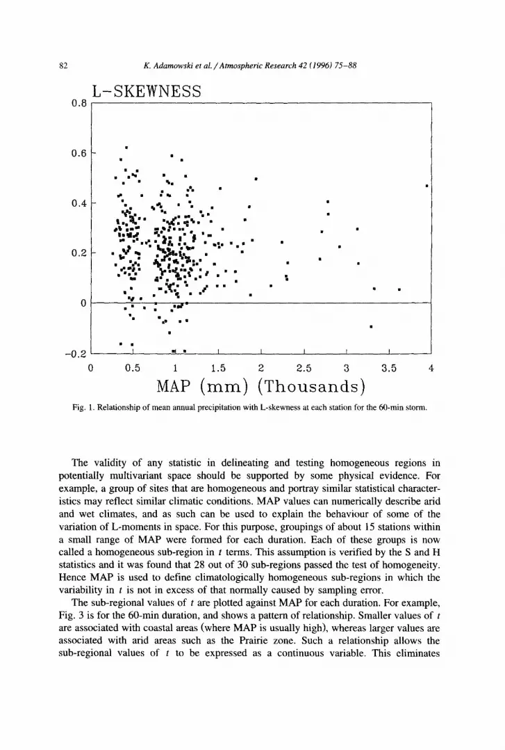
The sub-regional values of t are plotted against MAP for each duration. For example, Fig. 3 is for the 60-rain duration, and shows a pattern of relationship. Smaller values of t are associated with coastal areas (where MAP is usually high), whereas larger values are associated with arid areas such as the Prairie zone. Such a relationship allows the sub-regional values of t to be expressed as a continuous variable. This eliminates

0.8

K. Adamowski et al. /Atmospheric Research 42 (1996) 75-88

L-KURTOSIS

83

0.6

0.4

0.2

-0 .2

0 4

• . ". •

im~ • • s

Im • m • - m mill

• ; . , .

. . . ;; • ~'.. %...,; .- ." • • • • ii o im •

mml~ m • ~ 7,,mD,.ll ~ II • mm~ im IFO II m im n'mV •

..,.,, • .. QI' Q...%g.. ". • .X'I" ~..~.a,$,.~- ....

| ' I l l . _ , , w • ~ . i L • == • • a=m I m~ i~_ • •

• . " ; . - . . s . . ~ . . . . . • lp

• • |= • • ~ m a • II lm ii mm

fill

I ,I I

0.5 1 1.5

MAP (mm)

I f [ P

2 2.5 3 3.5

(Thousands) Fig. 2. Relationship of mean annual precipitation with L-kurtosis at each station for the 60-min storm.

boundary problems normally associated with the geographic definition of homogeneous regions.

In summary, L-kurtosis and L-skewness are found to be approximately constant over a larger area than the L-coefficient of variation, which in turn varies less than the mean value. Such analysis is known as the "hierarchical" regionalization approach and has been adopted in several studies (Fiorentino et al., 1987; Gabriele and Arnell, 1991). This approach is also adopted for regional precipitation analysis in this study.

3.4. Identif ication o f a paren t distribution

The statistical test of homogeneity revealed that t 3 and t 4 variability over Canada displays no specific pattern, and that observed variability of these statistics may be attributed to sampling noise. In such a case, the weighted average values (with respect to sample length) would be the representative regional parameters. Regional t 3 and t 4 values are computed for each storm duration and superimposed on the theoretical L-moment ratios diagram (Fig. 4). It can be seen from Fig. 4 that Canadian precipitation data can be described by a general extreme value (GEV) distribution.

84

0 .3

K. Adamowski et al. / Atmospheric Research 42 (1996) 75-88

L - C O E F F I C I E N T O F V A R I A T I O N

0 . 2 5

0 .2

0 . 1 5

0.1

• OBSERVED

•l

• • ~... . . . .

- - BEST FIT

0 . 0 5 I i i

0 1 2 3 4

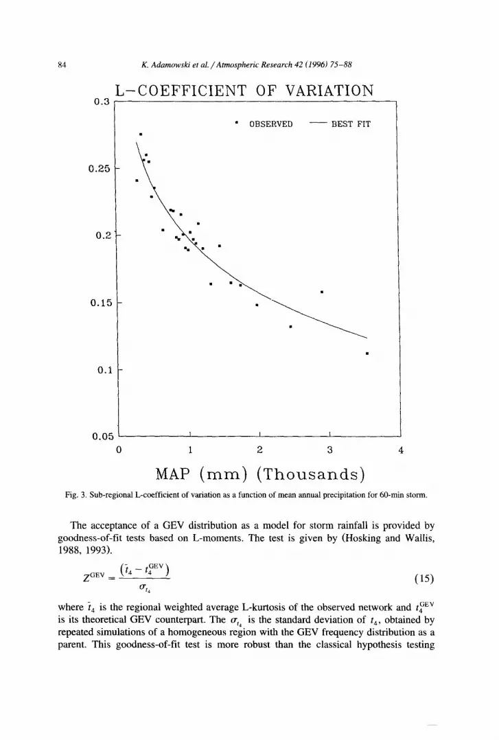
M A P ( r a m ) ( T h o u s a n d s ) Fig. 3. Sub-regional L-coefficient of variation as a function of mean annual precipitation for 60-min storm.

The acceptance of a GEV distribution as a model for storm rainfall is provided by goodness-of-fi t tests based on L-moments. The test is given by (Hosking and Wallis, 1988, 1993).

z °EV (}4- t4~Ev) (15) trt 4

where }4 is the regional weighted average L-kurtosis of the observed network and t~ Ev is its theoretical GEV counterpart. The 6r a is the standard deviation of G, obtained by repeated simulations of a homogeneous region with the GEV frequency distribution as a parent. This goodness-of-fi t test is more robust than the classical hypothesis testing

K. Adamowski et al. /Atmospheric Research 42 (1996) 75-88 85

L-KURTOSIS 0 . 3

0 . 2 5

0 . 2

0 , 1 5

0 . I

- - G L O GAM . . . . . . GEV O EVI

• OBSERVED

i " I j

_ ..'"

_...-"

. . ° -

t t I I I

0 0 . 0 5 0 . 1 0 . 1 5 0 . 2 0 . 2 5 0 . 3

L-SKEWNESS Fig. 4. Average relat ionships for regional L-kurtosis and L-skewness o f the 5, 10, 15, 30, 60 and 120-min

annual rainfall ext remes in Canada .

Table 3

Results o f the Z goodness-of - f i t test (Eq. 15)

Distr ibut ion 5 rnin I0 rain 15 min 30 min 60 min 2 h 6 h 12 h 24 h

G L O 5.45 5.88 6.83 7.57 5.84 4.81 4.94 5.34 7.46

GEV - 1.06 - 1.01 - 0 . 0 9 1.13 - 0 . 3 8 - 1.36 1.48 - 1.57 - 0 . 0 9

G N O - 2 . 4 3 - 2 . 1 5 - 1.44 - 0 . 4 5 - 2 . 3 7 - 3 . 5 2 - 3 . 2 7 - 3 . 1 5 - 1.60

P3 - 5 . 4 1 - 4 . 8 7 - 4 . 4 5 - 3 . 7 0 - 6 . 1 9 - 7 . 6 0 - 6 . 8 4 - 6 . 4 8 - 4 . 9 4

G P A - 15.82 - 16.36 - 1 5 . 6 9 - 13.66 - 15.05 - 1 6 . 0 5 - 16.39 - 17.35 - 17.15

G L O = general ized logistic, G E V = general ized extreme value, G N O = general ized normal , P3 = Pearson type

III, and G P A = general ized pareto distribution.

86 K. Adamowski et al./ Atmospheric Research 42 (1996) 75-88

method since it uses regional rather than single site data, to discriminate between alternative distributions (Cong et al., 1993). The results from this test as presented in Table 3 support the selection of GEV as a regional distribution.

The quantile function of the GEV distribution is given by

x = ~'+ k ( 1 - ( - l o g F ) *) (16)

L-MOMENT RATIO (t3) 0.23

0 .22

0.21

0.2

0 .19

0 . 1 8 I ! I I Z I t I I I I [ z t t i t

3 30 300

TIME (min i Fig. 5. Regional average L-skewness as a function of storm duration for Canadian rainfall extremes.

K. Adamowski et al. / Atmospheric Research 42 (1996) 75-88 87

The parameters ~, a and k are related to the theoretical L-moment statistics of the distribution through the following relationships (Hosking, 1990):

o~ A1 = - r ( 1 + k ) ) ( 1 7 )

OL = - 2 - k ) r ( 1 + K) (18)

2 ( 1 - 3 -k) 3 (19) 7"3= (1 _ 2 -k )

(1 -- 6.2 -k + 10.3 - k - 5.4 -k) r = ( 1 - 2 k) (20)

The above equations can be used to fit the regional distribution. This is beyond the scope of this paper.

Fig. 5 shows the weighted average regional L-skewness for all of Canada for various storm durations, with values beyond the lower bound of the extreme value type II distribution. It is evident that the current practice of assuming Gumhle I distribution regardless of storm duration is not valid (Gumbel I is a particular case of the GEV family of distributions with a constant theoretical L-skewness of 0.1699). Fig. 5 indicates further that the parameters of the regional parent distribution of rainfall data are dependent on the duration of the rainfall.

4. Conclusions

Regional analyses were performed on annual extreme rainfall data from 320 stations in Canada. The results indicate that: 1. Canada may be considered as one homogeneous region in L-skewness and L-kurto-

sis; 2. the L-coefficient of variation is heterogeneous for Canada. However, it is shown that

it is related to mean annual precipitation (MAP). This is used to subdivide Canada into homogeneous subregions;

3. the annual maxima of precipitation data can be described by the general extreme value distribution, the parameters of which depend on storm duration and mean annual precipitation.

References

Acreman, M.C. and Wiltshire, S.C., 1987. Identification of regional frequency analysis. EOS, 68(44). Alila, Y., Adamowksi, K., Pilon, P.J. and Kowalchuk, M.Z., 1993. A regional approach in the identification,

estimation and hypothesis testing of probability distributions of annual maximum flows. Proc. Int. Conf. Stochastic and Statistical Methods in Hydrology and Environmental Engineering, 21-23 June, University of Waterloo, Waterloo, Canada.

88 K. Adamowski et al. / Atmospheric Research 42 (1996) 75-88

Burn, D.B., 1990. An appraisal of the 'region of influence' approach to flood frequency analysis. Hydrol. Sci., 35(2): 149-165.

Cavadias, G.S., 1989. Regional flood estimation by canonical correlation. Proc. Ann. Conf. Canadian Society for Civil Engineering, June 8-10, St. John's, Newfoundland.

Cong, S., Li, Y., Vogel, J.L. and Schaake, J.C., 1993. Identification of the underlying distribution form of precipitation by using regional data. Water Rescour. Res., 29(4): 1103-1111.

Dalrymple, T., 1960, Flood frequency analysis. U.S. Geological Survey Water Supply, Paper 1543-A. Fiorentino, Gabriele, M.S., Rossi, F., and Versace, P., 1987. Hierarchical approach for regional flood

frequency analysis. In: V.P. Singh (Editor), Regional Flood Frequency Analysis. D. Reidel, Norwell, Mass., pp. 35-49.

Gabriele, S. and Arnell, N., 1991. A hierarchical approach to regional flood frequency analysis. Water Rescour. Res., 27(6): 1281-1289.

Hare, F.K. and Thomas, M.K., 1979. Climate Canada, 2nd edn. John Wiley, Canada. Hogg, W.D. and Carr, D.A., 1985. Rainfall Frequency Atlas for Canada, Environment Canada. Atmospheric

Environment Service. Hosking, J.R.M., 1988. The 4-parameter kappa distribution. Research Report, RC13412. IBM Research,

Yorktown Heights, NY. Hosking, J.R.M., 1990. L-moments: Analysis and estimation of distribution using linear combination of order

statistics. J.R. Stat. Soc., Set. B, 52(1): 105-124. Hosking, J.R.M. and Wallis, J.R., 1988. The effect of inter-site dependence on regional flood frequency

analysis. Water Rescour. Res. 24(4): 588-600. Hosking, J.R.M. and Wallis, J.R., 1993. Some statistics useful in regional frequency analysis. Water Rescour.

Res., 29(2): 271-281. Lettenmaier, D.P., Wallis, J.R. and Wood, E.F., 1987. Effect of regional heterogeneity on flood frequency

estimation. Water Rescour. Res., 23(2): 313-324. Pilon, P.J. and Adamowski, K., 1992. The value of regional information to flood frequency analysis using the

method of L-moments. Can. J. Civil Eng., 19: 137-147. Pilon, P.J., Adamowski, K. and Alila, Y., 1991. Regional analysis of annual maxima precipitation using

L-moments. Atmos. Res. J., 27: 81-92. Pilon, P.J. and Harvey, K.D,, 1994. Consolidated Frequency Analysis, CFA Package, Environment Canada.

Atmospheric Environment Service, Ottawa, Ontario. Potter, K.W., 1987. Research on flood frequency analysis: 1983-1986. Rev. Geophys., 25(2): 113-118. Ribeiro-Correa, J. and Rousselle, J., 1993. A hierarchical and empirical bayes approach for the regional

Pearson type III distribution. Water Rescour. Res., 29(2): 435-444. Royston, P., 1991. Which measures of skewness and kurtosis are best. Stat. Med., 10:1-11. Schaefer, M.G., 1990. Regional analysis of precipitation annual maxima in Washington State. Water Rescour.

Res., 26(1): 119-131. WMO, 1983. Guide to hydrologic practices, Vol. II, Analysis Forecasting and Other Applications. WMO-No.

168, Geneva, Switzerland.