Embed Size (px)
Citation preview
econstorMake Your Publications Visible.
A Service of
zbwLeibniz-InformationszentrumWirtschaftLeibniz Information Centrefor Economics
Luintel, Kul B.; Selim, Sheikh; Bajracharya, Pushkar
Working Paper
Reforms, Incentives and Banking Sector Productivity:A Case of Nepal
Cardiff Economics Working Papers, No. E2014/14
Provided in Cooperation with:Cardiff Business School, Cardiff University
Suggested Citation: Luintel, Kul B.; Selim, Sheikh; Bajracharya, Pushkar (2014) : Reforms,Incentives and Banking Sector Productivity: A Case of Nepal, Cardiff Economics WorkingPapers, No. E2014/14, Cardiff University, Cardiff Business School, Cardiff
This Version is available at:http://hdl.handle.net/10419/109044
Standard-Nutzungsbedingungen:
Die Dokumente auf EconStor dürfen zu eigenen wissenschaftlichenZwecken und zum Privatgebrauch gespeichert und kopiert werden.
Sie dürfen die Dokumente nicht für öffentliche oder kommerzielleZwecke vervielfältigen, öffentlich ausstellen, öffentlich zugänglichmachen, vertreiben oder anderweitig nutzen.
Sofern die Verfasser die Dokumente unter Open-Content-Lizenzen(insbesondere CC-Lizenzen) zur Verfügung gestellt haben sollten,gelten abweichend von diesen Nutzungsbedingungen die in der dortgenannten Lizenz gewährten Nutzungsrechte.
Terms of use:
Documents in EconStor may be saved and copied for yourpersonal and scholarly purposes.
You are not to copy documents for public or commercialpurposes, to exhibit the documents publicly, to make thempublicly available on the internet, or to distribute or otherwiseuse the documents in public.
If the documents have been made available under an OpenContent Licence (especially Creative Commons Licences), youmay exercise further usage rights as specified in the indicatedlicence.
www.econstor.eu
Cardiff Economics Working Papers
Working Paper No. E2014/14
Reforms, Incentives and Banking Sector Productivity:
A Case of Nepal
Kul B Luintel, Sheikh Selim and Pushkar Bajracharya
August 2014
Cardiff Business School
Aberconway Building
Colum Drive
Cardiff CF10 3EU
United Kingdom
t: +44 (0)29 2087 4000
f: +44 (0)29 2087 4419
business.cardiff.ac.uk
This working paper is produced for discussion purpose only. These working papers are expected to be
publishedin due course, in revised form, and should not be quoted or cited without the author’s written
permission.
Cardiff Economics Working Papers are available online from:
econpapers.repec.org/paper/cdfwpaper/ and
business.cardiff.ac.uk/research/academic-sections/economics/working-papers
Enquiries: [email protected]
1
Reforms, Incentives and Banking Sector Productivity: A Case of Nepal
Kul B Luintel*#
Cardiff University
Sheikh Selim#
University of Westminster
Pushkar Bajracharya#
Tribhuvan University
Abstract:
We model banks as profit-cum-utility maximizing firms and study, inter alia,
bankers’ incentives (optimal effort) and incentive driven productivity following
deregulations. Our model puts to test a panel of Nepalese commercial banks which
went through deep financial reforms in the recent past. We find that (i) bankers’
efforts and productivity have notably improved in Nepal, (ii) bankers’ efforts
significantly explain the banking sector’s productivity, (iii) the proportion of non-
performing loans has considerably declined, and (iv) banking services have become
costly, although the bank spread has moderately declined. Our approach is different
from the widely used data envelopment analysis (DEA) of bank productivity, hence
complements the literature. It also informs the current policy debate in Nepal where
the Central Bank is seen to be geared towards regulating the financial system and
micro-managing the banking institutions.
JEL Codes: G21, G28, O43, O53.
Keywords: Reforms; incentives; productivity; panel integration; cointegration;
simulation.
*Corresponding author.
# We are thankful for the constructive suggestions received from the high ranking
officials of the Central Bank and Commercial Banks of Nepal at the Nepalese
Bankers’ Association seminar, Kathmandu, December 2013. We are also thankful to
the seminar participants at Cardiff Business School, Southampton Management
School, Universidad de Alicante and those at the CFE (2013) conference, London.
The usual disclaimer applies.

2
Reforms, Incentives and Banking Sector Productivity: A Case of Nepal
1. Introduction
The world has seen sustained financial liberalization, increasing privatization
and gradual loosening of capital controls since the mid-1990s. The economic thinking
behind all this is that the financial entities, functioning under liberalized financial
regimes, operate at higher levels of efficiency and productivity. Productivity
improvements may ensue from different sources yet the notion that reforms-led
private – i.e. the individual institution’s – incentive is vital in enhancing productivity
and growth is a fundamental one.1 Put differently, a deregulated financial system is
viewed as incentivizing institutions (in this instance banks) for higher levels of effort,
productivity and profitability.
A large body of literature (Fare et al., 1994; Humphrey and Pulley, 1997;
Wheelock and Wilson, 1999; Mukherjee et al., 2001; Ihsan and Hassan, 2003;
Tirtiroglu, 2005; Pasiouras, 2008; Delis et al., 2011; to name but a few) examines
bank efficiency and productivity following reforms and regulatory changes. They are
panel as well as country-specific studies which mostly employ non-parametric data
envelopment analysis (DEA) to compute various efficiency decompositions –
technical efficiency, scale efficiency, efficiency change (catching up or falling
behind) – and productivity growth. 2
Whilst valuable, DEA analysis is a measure of relative efficiency with respect
to the sample at hand, one cannot be confident that the banks on the efficient frontier
are indeed operating optimally; instead, they may merely represent the best practices
contained in the data. Whether the best practices are indeed the optimal ones are an
entirely different matter. Furthermore, Wheelock and Wilson (1999; p 213) point out
that efficiency evaluation through DEA could give a misleading picture, especially
when the banking sector is going through major changes.3
This paper aims to contribute to the literature by analysing, among other
things, bankers’ optimal efforts (incentive) and incentive driven productivity
following deregulations and reforms. Our approach differs from DEA in that we
model banks as profit-cum-utility maximizing firms. We directly model bankers’
optimal level of productivity rather than relative productivity, as is done under DEA.
Reforms and liberalization avail opportunities and incentivize banks to optimize. It is
anticipated that bankers will increase their efforts and productivity.
3
Our theoretical model combines banks’ output technology with their
optimizing behaviour. Banks’ technical production function is Cobb-Douglas which is
standard in the literature (Clark, 1984, 1988; Humphrey, 1991). We derive banks’
‘institutional’ production function, which embeds banks’ profit-cum-utility
maximizing optimal levels of effort, thereby capturing bankers’ optimal response to
institutional changes. In this setup, banking sector productivity becomes endogenous
to bankers’ optimal level of effort, relative input-output prices and some technical
parameters.
Often, bank profitability surges following liberalization but this surge could
also be realised through increased volume (quantity) of bank activities – i.e. increased
volumes of deposits and credits – and bank spread (cost of bank services) rather than
through the productivity gains. Therefore, the effects of financial deregulation and
reforms on the cost of bank services and bank productivity remain important public
policy issues.
Our analytical model is put to examine Nepalese financial liberalization and
reforms. Nepal is one of the least developed and poorest countries of the world which
has witnessed Maoist insurgency and the overthrow of the Monarchy in 2008. Nepal
embarked on deep and far reaching banking and financial sector reforms through two
episodes of liberalization implemented during 1986-89 and 1992-1994. The latter
episode, in particular, opened up the country’s financial sector and brought about
profound structural changes to it. Although financial reforms were concluded in 1994,
the activities were lacklustre until after 2000 due to the launch of armed insurgency
(People’s War) by the Maoists in 1996. However, since 2002 Nepal’s financial system
has been through fundamental changes (see Section 3). In our view, Nepalese banking
sector makes an interesting test case and its scrutiny would provide important policy
insights as to whether reforms have produced anticipated productivity improvements
in Nepal’s banking sector. This analysis is also useful in informing the current policy
debate in Nepal where the Central Bank is widely perceived as intruding the free
functioning of financial markets through new regulations and attempting to retract
from liberal policies in order to micro-manage the banking institutions.
We employ cutting-edge econometric methods in our empirical estimations.
To preview our main results, bankers’ optimal level of effort, optimal bank
productivity and bank profitability have considerably improved in Nepal following
financial liberalization. The ratio of non-performing to total loan has considerably

4
declined from 24.6% in 2004 to 3.4% in 2012. Formal tests show that bankers’ efforts
significantly explain bank productivity. Evidence also suggests that in recent years the
bank spread has slightly reduced, indicating competitive pressure, yet banking
services have become more costly. On the whole, financial reforms and liberalization
have been a fruitful experience in Nepal.
The rest of the paper is organized as follows. We present our analytical model
in the following section; Section 3 briefly outlines the financial regimes of Nepal and
argues why Nepal is an interesting test case; econometric specification and data are
discussed in Section 4; empirical methodologies are discussed in Section 5; empirical
results are presented in Section 6; calibrations and simulation of optimal effort and
productivity are discussed in Section 7; and Section 8 concludes the paper.
2. Model
Financial liberalization, among other things, frees prices. Interest (deposit and
lending) rates, bankers’ wages, CEOs’ pay and other incentives such as bonuses, are
competitively determined but there are always entry and exit restrictions in the
banking industry. These restrictions are maintained by the Central Bank which may
be motivated by its concerns over financial fragility and/or some notional optimal size
of the banking industry in the economy. Restrictions to entry and exit have important
implications because they allow banks to earn positive economic profits even in the
long run.
We construct a partial equilibrium model where a representative banker,
following liberalization, operates with a competitive environment and minimizes its
cost function to achieve the maximum feasible level of profit. 4 The representative
banker is a decision making unit (DMU) and has full flexibility and freedom in
decision making. This can be viewed as the CEO of a large bank making decisions
which are fully implemented by his staff.
In order to model the incentive driven productivity, we need to specify banks’
production function. There are alternative ways to measure bank inputs and output in
the literature. Prominent ones are the production approach (Berger and Humphrey,
1992) and the intermediation approach (Sealy and Lindley, 1997; Aly et al., 1990;
Delis et al., 2011). As in Wheelock and Wilson (1999), ‘a mutually exclusive
distinction’ between inputs and output is vital for modelling productivity hence we
follow the intermediation approach. We specify that banks use three inputs, namely,
5
labour (bank staff, N), total fixed asset (F), and total deposits (D) to produce their
output (Q). Labour is measured by the number of full-time equivalent bank
employees; total fixed asset is the book value of premises and other fixed assets,
which is equivalent to physical capital stock; and deposits are the total deposit
liabilities. Bank output is measured by total credits and investment.5 The technical
constant returns to scale (CRTS) Cobb-Douglas production function for bank output
is:
)1(321
0
aaaDFNaQ
Where ,00a ; [0,1], 1,2,3ia i are the share parameters such that
3
1
1i
ia .
N is the incentive (effort) augmented labour (N) and 0a captures the banking
technology. The parameter denotes the level of effort or broadly defined incentive
level of a typical (representative) banker which may change in response to changes in
policies and institutions. The idea is that following liberalization banks become more
incentivized and increase their level of effort (quality of work). This is precisely the
raison d’être of financial liberalization and reforms. Such efforts may include the
banker’s willingness to embark on new types of lending, investments and services
which might have been restricted and/or barred hitherto. It is plausible to think that
the quality of N and F may also improve due to the hiring of more qualified staff,
computerization and the opening up of new branches in more strategic locations. We
assume the quality of inputs and the level of effort to be positively correlated. In other
words, banks invest in inputs’ quality in order to increase their effort level (or make
their effort more effective).
Increased banker’s effort ( ) in a deregulated environment is likely to
impact on banks’ levels of risk. The general perception is that deregulation increases
banks’ risks. However, conceptually the level of risk could go either way – an
aggressive lending by the banker may increase the level of risk whereas a prudent
lending may do just the opposite. Since our focus is on the outcome of liberalization
and deregulations – i.e. whether reforms incentivized bankers and increased banking
sector productivity – the analysis is essentially an ex post one. Hence, we can
conveniently sidestep the issue of uncertainty and capture the level of bank risk
exposure through the ratio of performing to total loans ( ). The higher the the
lower tends to be the risk exposure and vice versa. Given that the production function
6
(1) is homogeneous of degree one, inclusion of simply scales bank productivity.
Any increase in performing (non-performing) loans scales up (down) the level of total
factor productivity of banks and vice versa; it does not alter our analytical results
which we show in the appendix. The production function in per-banker terms can be
expressed as:
)2(321
0
aaadfaq
Where q, f, and d represent output, total fixed assets and total deposit per banker. The
banker chooses the level of inputs such that the total cost TC of renting these inputs
(i.e. the opportunity cost of owning these factors) is minimized. Let us denote the unit
cost of these three inputs by 3,2,1, iwi . The banker chooses the input set ( N ,
F and D ) in order to minimize:
)3(321 DwFwNwTC
subject to (1). The consolidated first order condition associated with this cost
minimization problem is:
)4(
3
3
2
2
1
1
Qa
Dw
Qa
Fw
Qa
Nw
Equation (4) is the standard result in cost minimization which states that the ratio of
marginal cost to marginal revenue or its reciprocal should be the same across all the
inputs employed. Substituting (4) into (3) and imposing the CRTS condition, with
some algebraic manipulation, the optimal total cost function is given by:
i
a
i QwTC i )5(*
where 321
3210
1aaa
aaaa , and *TC is the minimum value function of TC in (3)
subject to (1) which depends on unit input costs, the level of output and share
parameters. The optimum cost of production per-banker is therefore:
* { } (6)ia
i
i
tc w q
Let p denote the market clearing price per unit of credit. Then, the total revenue per
banker is:
(7)tr pq
7
Input and output prices that banks face tend to differ and they are likely to change
differently following liberalization. We capture this byp
wi
a
ii
, the ratio of the
observed weighted input to output prices. From (6) and (7) and utilizing , the profit
per banker is given by:
)8(1 qp
The banker likes profit but dislikes effort and is mindful of the trade-off between
profit and the utility cost of effort. The bankers’ utility from working in the bank is
defined over profits and effort levels as:6
)9(,1
U
Where parameter 1,0 is the elasticity of substitution between profit and effort.
The marginal utility of profit is constant but the marginal disutility of effort is
increasing with the higher level of effort. The relative risk aversion equivalent
coefficient of this utility function is given by
1. The is the disutility parameter;
its value ensures that the utility function is jointly strictly quasi-concave. The
representative banker chooses effort level, , in order to maximize (9) subject to (8)
and (2). The representative banker’s utility maximization problem is:
1 2 3
0
max ,
. . 1
a a a
U
s t p q
q a f d
The solution to this problem gives us the optimal level of effort as:
)10(11 1
32
1
10
*
a
aadfaap
The variable * is the optimal level of effort of a representative banker following
liberalization. It depends on input and output prices, substitution parameter, technical
parameters and deposits and fixed assets per banker. When the banking sector goes
through reforms, the relative price of input and output – i.e. the spread – changes,
which affects bankers’ optimal effort (incentive) level. Substituting the optimal level
of effort (10) into the technical production function (1), we get:
)11(321 DFBNQ
8
and the share parameters are
1
1
1
22
1
33
1
1(12)
1
(13)1
(14)1
a
a
a
a
a
a
In line with McMillan et al. (1989) we label (11) as the “institutional” production
function of a bank which is different from the technical production function (1).
Whereas equation (1) is the technical relationships between inputs and output,
equation (11) additionally captures bankers’ optimal responses (efforts) to regulatory
changes. Although si are empirically different from isa nonetheless3
1
1i
i
, which
continues to preserve the CRTS assumption. The parameters of the technical
production function, 3,2,1, iai and institutional production function, 3,2,1, ii are
related through the substitution parameter .7 The technical production function (1)
contains an unobservable input, N , whereas the institutional production function
(11) is defined over all observable inputs (N, F and D). The effort parameter is now
embedded into the optimal productivity parameter, B, which captures the bankers’
optimal response to reforms and liberalization. The banking sector’s optimal
productivity parameter, B , is given by:
1
11 1
11 1
1 111 1
0 1
11 (15)
aaa aaa aB a a p
In equation (15) the bankers’ incentive driven productivity ( incB ) is captured by the
term:
1
111 (16)a
aincB p
incB is directly affected by the reform-induced changes in the input and output prices
that shape the incentive structure of the banking sector. The rest of the expression on
the RHS of equation (15) is a constant term which only has a scale effect on incB .
Empirically, this scaling effect is close to unity (see below). If the banking sector
productivity improves following liberalization, then we expect an evident positive
trend in both incB and B .
9
3. Financial Regimes and Reforms in Nepal
Nepal is one of the poorest countries of the world with a per capita income of
current US$ 619. Nepal is landlocked and sandwiched between two giants of Asia,
viz. China and India with over a billion populations each. Nepal has a population of
26.40 million.8
Nepal has a banking history of over three-quarters of a century – the country’s
first ever commercial bank was established in 1937 followed by the establishment of
the Central Bank in 1956. However, the financial sector was under the firm grip of the
authorities until the reforms that concluded in 1994. Only two commercial banks and
one development bank operated until 1984 and the financial sector was largely
dormant. The appointment of government bureaucrats, often retired ones, as the
banks’ CEOs was the norm. Banking and financial sector policies were dominated by
a socialist banking philosophy, similarly to those in India (Burgess and Pande, 2005).9
Nepal Rastra Bank (the Central Bank of Nepal, henceforth NRB) operated a
highly controlled regime of interest rate management: “there were about 20 controlled
bank rates differentiated between sectors, use of funds and types of collaterals” (NRB,
1996; p 50). The term structures of interest rates were fully controlled. A liquidity
requirement of at least 25% – comprising a minimum of 5% of total deposit in
government securities and a further 20% of other liquid assets including reserves at
the Central Bank – was in operation. Commercial banks were barred from taking
foreign currency deposits. A regime of directed credit programmes existed which
made it mandatory for banks to channel as high as 25% of their total lending to the
State-defined Priority Sectors, encompassing agriculture, cottage industries, exports
etc. Interest rates on Priority Sector lending were always set at low levels and
commercial banks were penalised if they did not meet the target of 25%.
Nepal initiated an important step towards financial openness in1984. Foreign
banks, for the first time ever, were allowed to open joint venture banks (in a joint
investment with Nepalese investors) in the country. This led to the establishment of
three foreign joint venture banks under foreign management – Nepal Arab Bank
Limited, Nepal Indo Swiss Bank, Nepal ANZ Grindlays Bank – making a total of five
commercial banks. They were the sole commercial banks in operation until 1990. The
openness of 1984 was followed by the first phase of financial liberalization (1986-
1989) which mainly focussed on interest rate liberalization. Initially, NRB
relinquished the micro management of interest rates; it only set the minimum deposit
10
rate. Banks were also given freedom to set their lending rates, subject to an upper
limit of 15% on the priority sector lending only. NRB completely deregulated its
interest rate policy in August 1989 – banks and financial institutions were given a free
hand in setting their deposit and lending rates at their own discretion. The statutory
liquidity ratio and credit ceilings were abolished and the sale of government securities
through open market operations was initiated. The first phase of liberalization was
quite important in setting interest rates free to market forces, but the controls on
foreign exchange and entry into and exit from the financial sector were tightly
maintained.
The second phase of financial liberalization, which started in 1992, focussed
on foreign exchange liberalization and further opening up of the financial sector.
Nepalese currency was made fully convertible into current accounts in 1993 and
measures of capital account liberalization were adopted. Exporters could retain 100%
of their export earnings in foreign currencies and maintain bank accounts in
convertible currencies. Commercial banks were also authorized to issue credit in
foreign currencies; foreign investors could expatriate 100% profit to their habitat. The
private sector could enter into the banking and financial sector with ease and with or
without foreign participation.
Although the second phase of liberalization concluded in 1994, which fully
opened up the financial sector, these policy reforms remained largely dormant – there
was no zest in financial sector activities – until after 2000. This was due to the
political instability triggered by the launch of Maoists insurgency in 1996. However,
post 2000 Maoists entered into dialogue with political parties which saw the end of
insurgency in 2005. Following the prospects of the end of Maoist insurgency and the
ensuing peace and security, the second phase of liberalisation began to take effect
since 2002. 10 This quickly led to deep structural changes and a restructuring of the
Nepalese financial sector. The number of commercial banks more than doubled –
from 13 in 2000 to 31 in 2013. The number of development banks has reached 88
from only seven in 2000. Furthermore, a whole host of new types of financial
institutions have proliferated which either did not exist or had no significant presence
pre-1994 reform. They include 69 Finance Companies, 24 Microfinance Development
Banks, 16 Savings and Credit Co-operatives and 36 NGOs (financial
intermediaries).11 The old and large banks also went through deep restructuring.
Nepal Bank Limited and Rastriya Banijya Bank, the two oldest and largest
11
commercial banks of the country, respectively, had as high as 56% and 60% of their
total loan portfolio classed as non-performing in 2002. Both banks had reduced their
non-performing loan to around 6% by 2012. Given the scale of structural
transformation and the restructuring of the banking sector following the last episode
of liberalization, Nepal makes an interesting test case for the financial reforms-led
productivity growth in the banking sector and we examine this through our analytical
model presented in section 2.
4. Econometric Specification and Data
The analytical model presented in Section 2 derives the optimal level of
incentivized effort ( * ) of a banker which is embedded in the institutional production
function (11). In order to compute bankers’ incentivized optimal productivity, we
need to estimate the structural parameters ( 1 , 2 and 3 ) of the institutional
production function. The log-linearized auxiliary regression of the institutional
production function, for a panel of banks, takes the following form:
1 2 3log log log log (17)it i t i it i it it itQ N F D e
(i= 1,…,M; and t=1,…,T).
Specification (17) is a fixed effects panel model. The subscripts “i” and “t” denote the
cross-sectional and time series dimensions, respectively; i captures the bank-specific
fixed effects and t captures the time effects. Since the regression is specified in
logarithms, the parameters are elasticities. Equation (17) specifies parameters as bank
(panel unit) specific. In the estimation we allow both for the heterogeneity (bank-
specific) and the homogeneity (industry-wide) of parameters across panel units. All
parameters are expected to resume positive signs a priori and one would expect the
point estimate (elasticity) of total deposit liabilities to be by far the largest in a bank’s
production function.
We have collected data on Nepalese individual commercial banks’ total
deposits (D), total loans and advances (L), investments (I), fixed assets (F), interest
expenses on deposits (RE), interest income (RY), bank staff (N), staff expenses (NE),
other operating expenses (OE) and operating profit ( ). As of 2013, 31 commercial
banks are in operation in Nepal but 14 of them are new: they came into operation in
2007 or later. These 14 new banks, due to their very short data length, could not be
12
considered for any credible econometric analysis. Furthermore, most of these new
entrants have yet to consolidate their banking activities. Of the remaining 17 banks,
we have obtained complete and consistent quarterly data for 12 banks covering a
sample period of 11 years – 2002(1) to 2012(1). 12 The choice of this sample period is
deliberate to focus on the most intense period of banking activities following
liberalization. As stated above, policy reforms remained largely dormant until the
cessation of Maoists insurgency that began in 2002 and the insurgency ended in 2005
hence the choice of the sample. Our data set consists of an unbalanced panel of 12
banks with 420 quarterly observations. They are the major commercial banks of
Nepal accounting for about 70% of the banking activities of the country. Analysis of
this sample of banks is deemed sufficient to discern whether reforms and
liberalization have incentivized bankers in Nepal and whether the banking sector
productivity has improved. All data series have been directly obtained from the office
of the Governor of NRB. 13 The relevant nominal variables are deflated by CPI as the
deflator. 14
5. Empirical Methodology
Macro-panel data of this nature are widely reported to be non-stationary (unit
root) processes (see, among others, Luintel et al., 2008) requiring an application of
non-stationary panel data econometrics in estimating the parameters of (17). Panel
unit root and panel cointegration tests are shown to have better power properties than
the time series tests in small or moderate samples.
A number of panel unit root tests are proposed in the literature which can be
summarized as the first and second generation tests. The former assume cross-
sectional independence – a prickly issue in macro panel data – while the latter allow
for cross-sectional dependence. The frequently applied first generation panel unit root
tests in the empirical literature include those of Im, Pesaran and Sin (2003; hereafter
IPS), Fisher-ADF (Maddala and Wu, 1999) and Hadri (2000). The IPS test tests the
null of a unit root for each cross-sectional unit against the alternative that only a
fraction of cross-sectional units may contain a unit root. This test does not maintain
stationarity across all groups under the alternative hypothesis. Further, it also allows
for the heterogeneity of persistence, dynamics and error variance across groups.
13
The Fisher-ADF test employs the p-values of a unit root test. Under the null of
a unit root for all M (cross-sectional) units, the quantity: 1
log( )M
i
i
is asymptotically
2
2M ; where i is the p-value of the unit root test on the ith series of the ith panel unit.
Hadri’s test tests the null of stationarity against the alternative of a unit root; a
common persistence parameter is assumed across all cross-sectional units. Hadri also
derives autocorrelation and heteroskedasticity consistent LM tests under the null of
stationarity. Hlouskova and Wagner (2006), however, warn that Hadri’s tests suffer
from size distortion in the presence of autocorrelations.
The second generation tests are relatively new and are gaining momentum in
empirical applications for obvious reasons. Gengenbach et al.(2010) show that the
cross-sectionally augmented IPS (CIPS) test (Pesaran, 2007) is one of the powerful
second generation panel unit root tests. This test accounts for both cross-sectional
dependence and residual serial correlation while testing for the null of a unit root. For
the sake of robustness, we employ IPS, Fisher-ADF, Hadri and the truncated CIPS
tests on each of the data series of our panel.
Pedroni (1999) and Kao (1999), among others, propose panel cointegration
tests to explore if non-stationary panel data form a linear cointegrating (long-run
equilibrating) relationship. They are residual-based tests of cointegration – extensions
of the time series tests of Engle and Granger (1987) on panel settings. Pedroni (ibid.)
proposes seven tests of panel cointegration – four of them are within-dimension tests
that assume homogeneous cointegrating vectors across panel units and the remaining
three are between-dimension tests (referred to as Group Mean Statistics), which allow
for heterogeneous cointegrating vectors across panel units. The between-dimension
estimators exhibit lower size distortions than the within-dimension estimators and the
group t-statistic is shown to be the most powerful one amongst the three between-
dimension panel cointegration tests (Pedroni, 2004). The Kao (1999) test is similar to
Pedroni’s tests except that Kao allows for heterogeneous intercepts but assumes
homogeneous slope parameters across panel units. We report a range of cointegration
tests proposed by Pedroni (1999) and Kao (1999) so that we could reach a robust
conclusion on the cointegrating relationship vis-à-vis our institutional production
function.
14
The OLS level regressions, employed to test cointegration in the panel, are not
informative of the significance or otherwise of the cointegrating vectors because of
the well-known inference problems (cf. Engle and Granger, 1987). Therefore, we
estimate the cointegrating parameters through Fully Modified OLS (FMOLS; Phillips
and Hansen, 1990) and Dynamic OLS (DOLS; Stock and Watson, 1993; Kao et al.,
1999).
6. Empirical Results
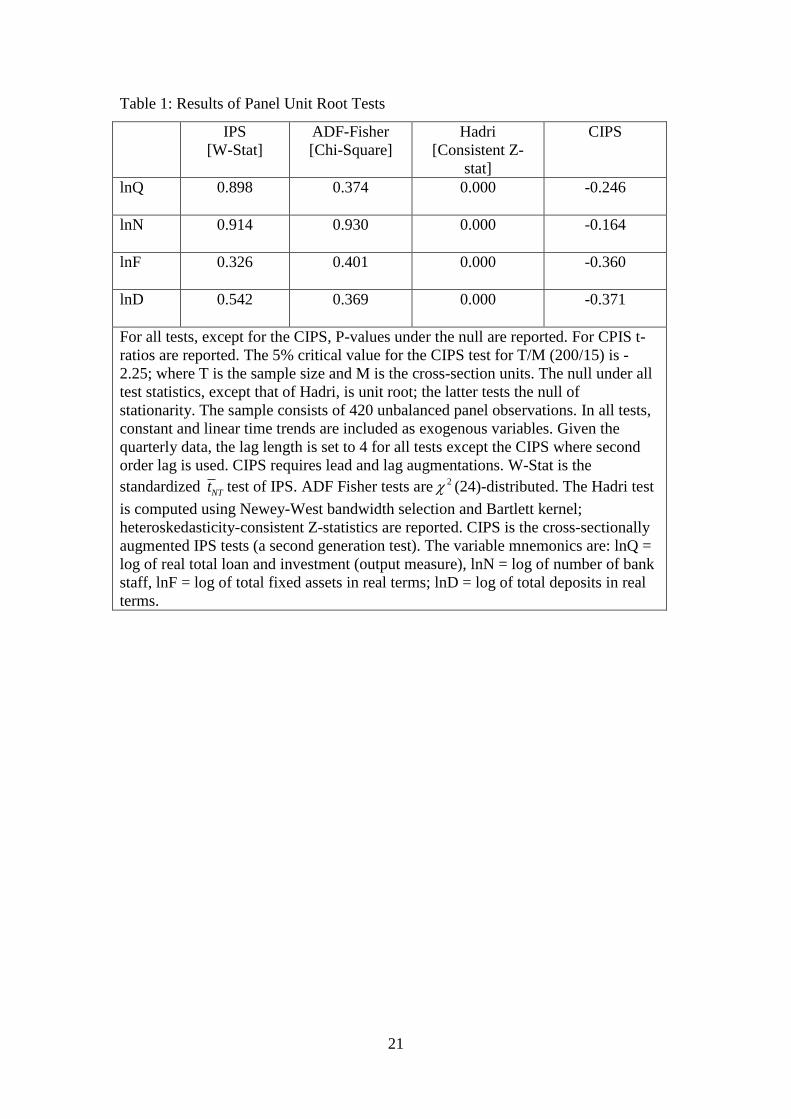
Results of panel unit root tests are reported in Table 1. The first three
columns pertain to the first generation of panel unit root tests. The IPS and ADF-
Fisher tests do not reject the null of a unit root for any of the level series in the panel.
Hadri’s test decisively rejects the null of level stationarity. Both types of first
generation tests (those testing the null of a unit root and the null of stationarity) reveal
that our panel data is non-stationary. This is further confirmed by the CIPS – a second
generation – test which accounts for cross-sectional dependence. CIPS tests cannot
reject the null of unit root for any of the data series in our panel. The results in Table
1 are based on the most general specifications that include cross-section-specific
intercepts and linear trends. All individual series in the panel are found to be first-
difference stationary, signifying that our panel data series are unit root processes.15
Table 1 about here
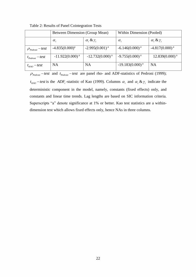
Table 2 reports the results of panel cointegration tests on bankers’ institutional
production function (11). Both the between-dimension and the within-dimension tests
proposed by Pedroni (1999) are reported. These tests are performed under two
deterministic settings including: (i) bank-specific constant only, and (ii) bank-specific
constants and linear time trend. We also report the panel cointegration tests proposed
by Kao (1999) for the sake of robustness. We attach more importance to the between-
dimension tests and, particularly, the Pedronit test , which is shown to have better
power properties.
Table 2 about here
The null of non-cointegration of bankers’ log linearised institutional
production function (17) is decisively rejected by all the tests reported in Table 2. The
precision of these tests is very high and the results are robust to different test methods
that vary considerably in their underlying assumptions. Overall, there is strong
15
empirical support for the bankers’ institutional production function as a long-run
equilibrium relationship.
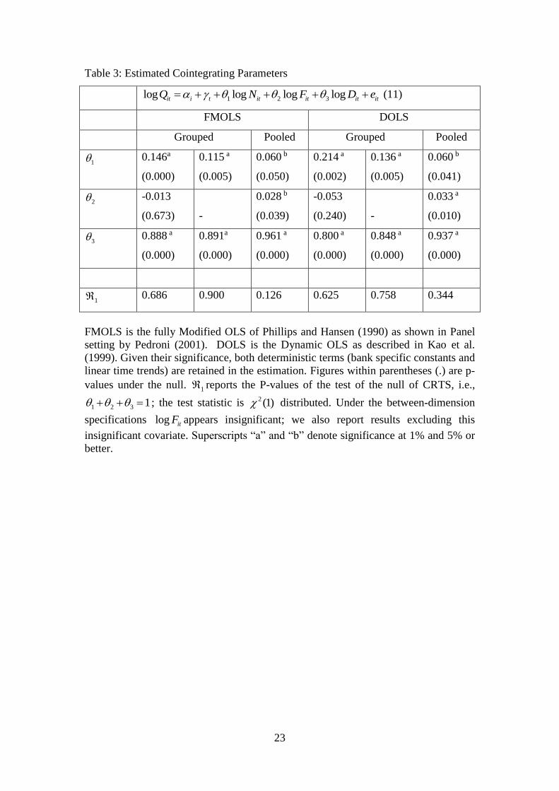
Estimates of the cointegrating parameters (vectors) are reported in Table 3.
Results show that two covariates of institutional production function, namely, the
bank staff and the total deposit liabilities appear positively signed and highly
significant across all specifications, which is consistent with a priori expectations.
The stock of total fixed assets, however, shows mixed results. It appears positive and
statistically significant under pooled (within-dimension) estimators but insignificant
under grouped (between- dimensions) estimators. The insignificance of total fixed
assets is somewhat surprising but this may be partly explained by the relative
constancy (the lack of sufficient variation) of fixed assets in these banks.16
Table 3 about here
One of the fundamental assumptions of our analytical model is that the
bankers’ production function follows CRTS. We explicitly test this restriction and
report the results in row 1 . In no case is the CRTS restriction rejected by the data.
We re-estimate two (Grouped) specifications by dropping the insignificant log itF
variable and re-assessing the CRTS assumption. Results show that CRTS is
maintained.
On balance, one would prefer the between-dimension FMOLS estimates of
industry-wide parameters because they allow share parameters to differ across
individual banks. The within-dimension (Pooled) estimates treat the share parameters
as being the same across all banks. In view of the significance of all three covariates,
we report simulation results based on the pooled FMOLS estimates. However, the
qualitative nature of our simulation results is robust, irrespective of the set of
parameter used.
It is important to note that although the CRTS is not rejected statistically, the
sum of the point estimates of the within-dimension estimates under FMOLS amounts
to 1.049 rather than 1.0 but we need parameters to sum exactly to unity for
simulations. Since the sum of these point estimates is 4.9% higher than unity, we
scaled down all three parameters by 4.9% each and tested whether this restriction is
data acceptable. Indeed, we find the scaled down parameters of 1 0.057 , 2 0.027
and 3 0.916 , which sum to unity, are data acceptable – a test of these parametric
restrictions as the cointegrating vector generates a p-value of 2(3) 0.110 under the
16
null. We use these data congruent parameters which pass CRTS restrictions and sum
to unity for simulations.17
7. Bankers’ Incentive and Bank Productivity
In order to simulate the bankers’ optimal level of effort (10) and the
incentivized optimal productivity (15), we need solutions for the parameters of
technical production function (1) - 0, 1 2 3, ,a a a a ; the elasticity of substitution, ; the
disutility parameter, ; and the series of input and output prices – 1 2 3, ,w w w and p .
We use the CRTS consistent estimates of 1 0.057 , 2 0.027 and 3 0.916 as the
structural parameters of our institutional production function (11). Given the
restriction 1,0 , some iteration reveals that for 0.40,0.55 the system
converges, hence we use 51.0 . The parametric value of 51.0 combined with
equations (12), (13) and (14) and the point estimates of is provide solutions:
1 0.110a , 2 0.025a and 3 0.865a . The remaining parameters and 0a are related
through the equilibrium condition321
3210
1aaa
aaaa . Since all denominators are
constants, we set 10 a which gives 1.586 . 18 The disutility parameter has a scale
effect on the optimal level of effort ( * ) and productivity ( B ). Simulations
conveniently converge for ]4.0,09.0[ hence we employ 10.0 .19
The marginal cost of bank staff ( 1w ) is proxied by the average hourly wage
rate of a banker in 12 sample banks. Each bank employee is assumed to work 40
hours per week and there are 48 bank working weeks per year giving, on average, 12
bank working weeks per quarter. 20 However, the simulated results remain robust to
hourly wages based on 36-44 working hours per week and/or 13 weeks per quarter.
The unit cost (shadow price) of total fixed assets ( 2w ) for the ith bank is taken to be
the deposit weighted market (market for the ith bank is defined as all the banks in the
sample except the ith bank) interest (one year fixed deposit) rate. The unit cost of
deposits ( 3w ) is the average deposit rate (total interest payment on deposits/total
deposits) for each bank. The unit output price ( p ) is computed as the ratio of loan
interest income over total bank loan (i.e. the average unit price of a loan). Using the
above parameter values and input-output prices, we simulate, among others, bankers’
17
optimal level of effort, effort driven productivity, average input cost and revenue per
unit of bank output, and the spread for the banking industry.
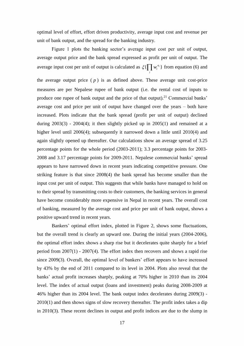
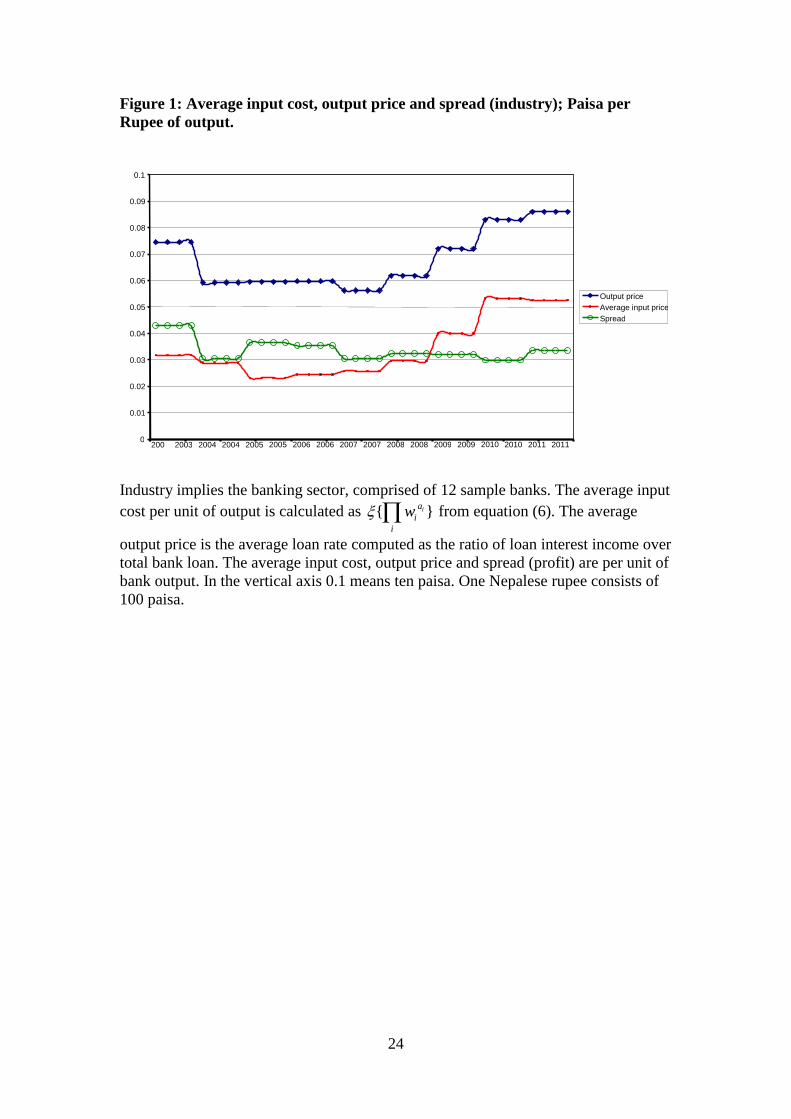
Figure 1 plots the banking sector’s average input cost per unit of output,
average output price and the bank spread expressed as profit per unit of output. The
average input cost per unit of output is calculated as { }ia
i
i
w from equation (6) and
the average output price ( p ) is as defined above. These average unit cost-price
measures are per Nepalese rupee of bank output (i.e. the rental cost of inputs to
produce one rupee of bank output and the price of that output).21 Commercial banks’
average cost and price per unit of output have changed over the years – both have
increased. Plots indicate that the bank spread (profit per unit of output) declined
during 2003(3) - 2004(4); it then slightly picked up in 2005(1) and remained at a
higher level until 2006(4); subsequently it narrowed down a little until 2010(4) and
again slightly opened up thereafter. Our calculations show an average spread of 3.25
percentage points for the whole period (2003-2011); 3.3 percentage points for 2003-
2008 and 3.17 percentage points for 2009-2011. Nepalese commercial banks’ spread
appears to have narrowed down in recent years indicating competitive pressure. One
striking feature is that since 2008(4) the bank spread has become smaller than the
input cost per unit of output. This suggests that while banks have managed to hold on
to their spread by transmitting costs to their customers, the banking services in general
have become considerably more expensive in Nepal in recent years. The overall cost
of banking, measured by the average cost and price per unit of bank output, shows a
positive upward trend in recent years.
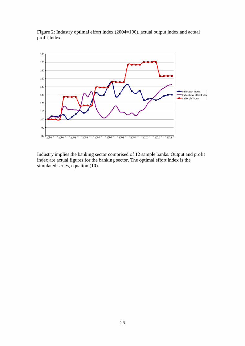
Bankers’ optimal effort index, plotted in Figure 2, shows some fluctuations,
but the overall trend is clearly an upward one. During the initial years (2004-2006),
the optimal effort index shows a sharp rise but it decelerates quite sharply for a brief
period from 2007(1) - 2007(4). The effort index then recovers and shows a rapid rise
since 2009(3). Overall, the optimal level of bankers’ effort appears to have increased
by 43% by the end of 2011 compared to its level in 2004. Plots also reveal that the
banks’ actual profit increases sharply, peaking at 70% higher in 2010 than its 2004
level. The index of actual output (loans and investment) peaks during 2008-2009 at
46% higher than its 2004 level. The bank output index decelerates during 2009(3) -
2010(1) and then shows signs of slow recovery thereafter. The profit index takes a dip
in 2010(3). These recent declines in output and profit indices are due to the slump in
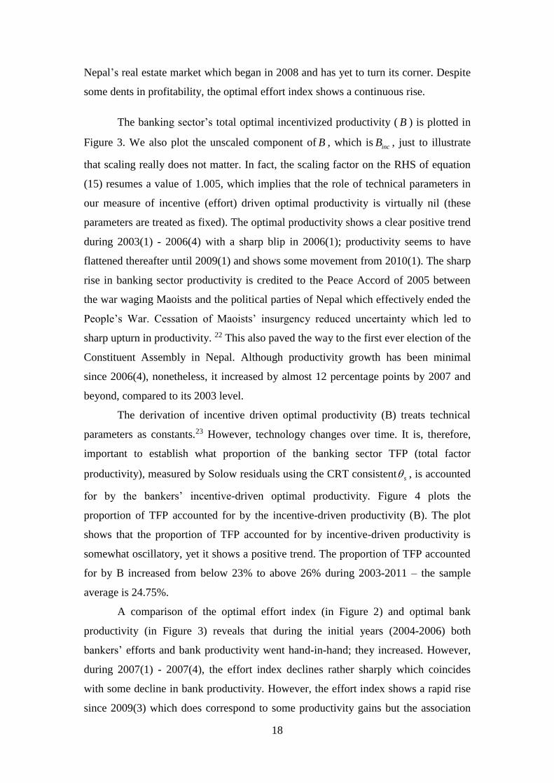
18
Nepal’s real estate market which began in 2008 and has yet to turn its corner. Despite
some dents in profitability, the optimal effort index shows a continuous rise.
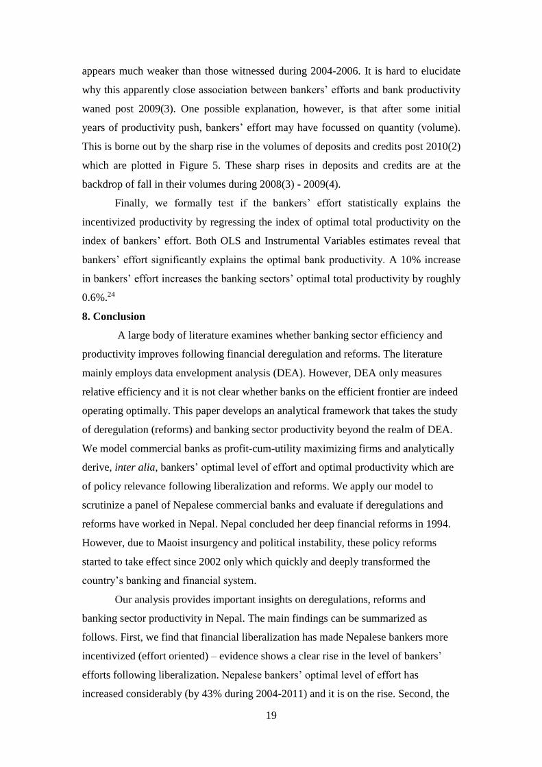
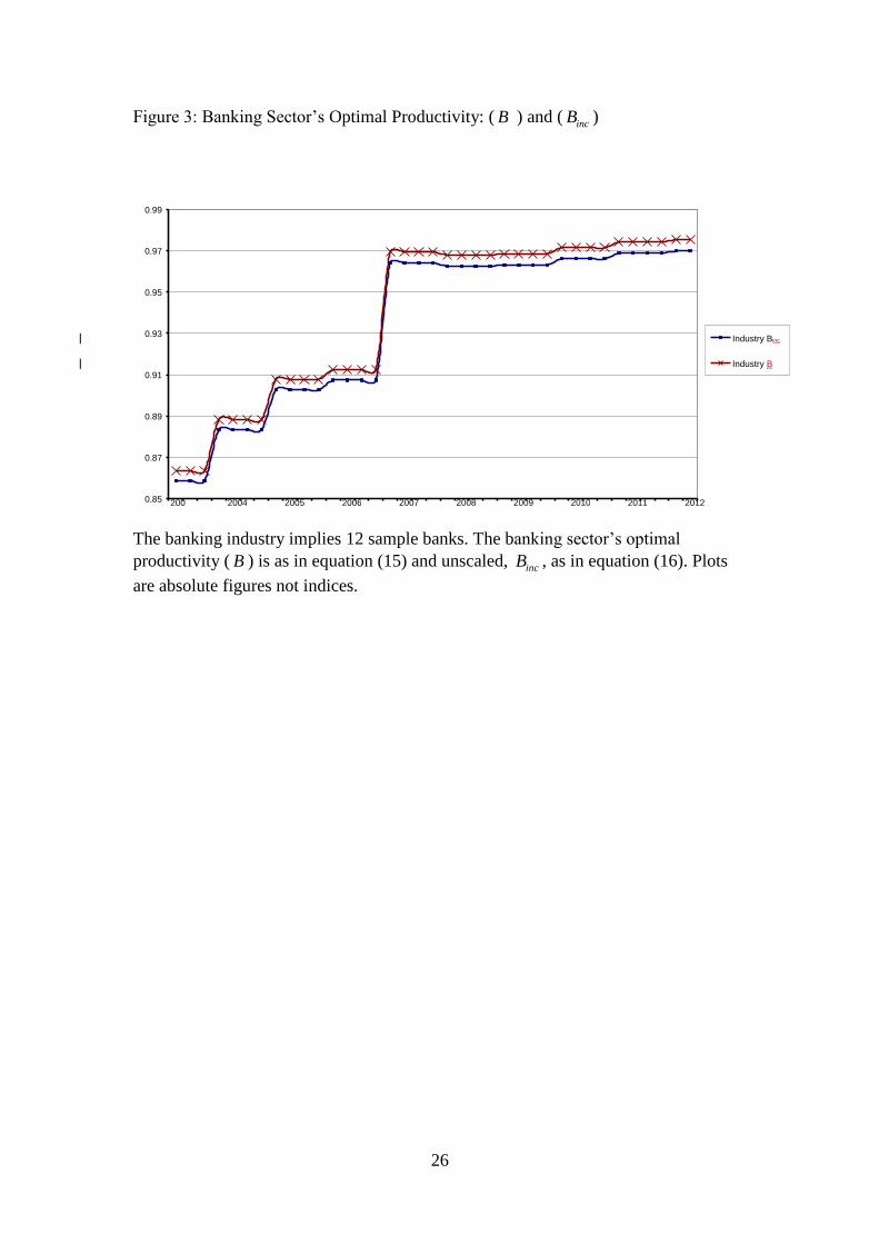
The banking sector’s total optimal incentivized productivity ( B ) is plotted in
Figure 3. We also plot the unscaled component of B , which isincB , just to illustrate
that scaling really does not matter. In fact, the scaling factor on the RHS of equation
(15) resumes a value of 1.005, which implies that the role of technical parameters in
our measure of incentive (effort) driven optimal productivity is virtually nil (these
parameters are treated as fixed). The optimal productivity shows a clear positive trend
during 2003(1) - 2006(4) with a sharp blip in 2006(1); productivity seems to have
flattened thereafter until 2009(1) and shows some movement from 2010(1). The sharp
rise in banking sector productivity is credited to the Peace Accord of 2005 between
the war waging Maoists and the political parties of Nepal which effectively ended the
People’s War. Cessation of Maoists’ insurgency reduced uncertainty which led to
sharp upturn in productivity. 22 This also paved the way to the first ever election of the
Constituent Assembly in Nepal. Although productivity growth has been minimal
since 2006(4), nonetheless, it increased by almost 12 percentage points by 2007 and
beyond, compared to its 2003 level.
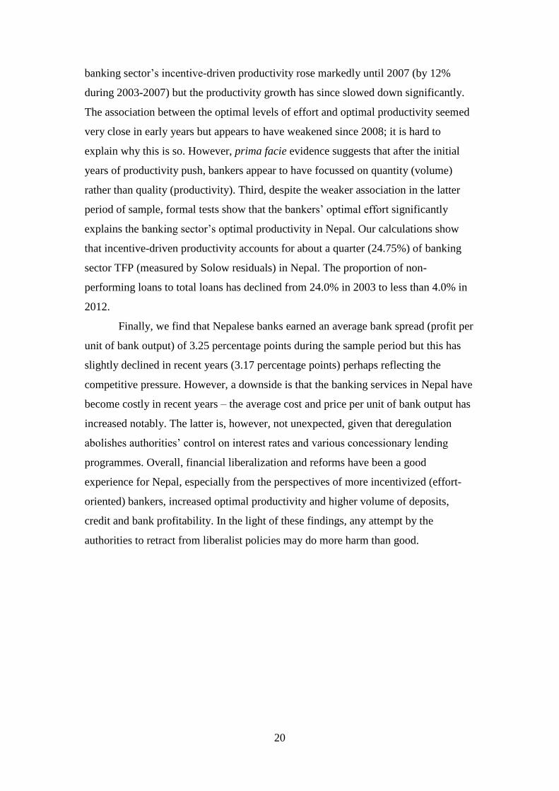
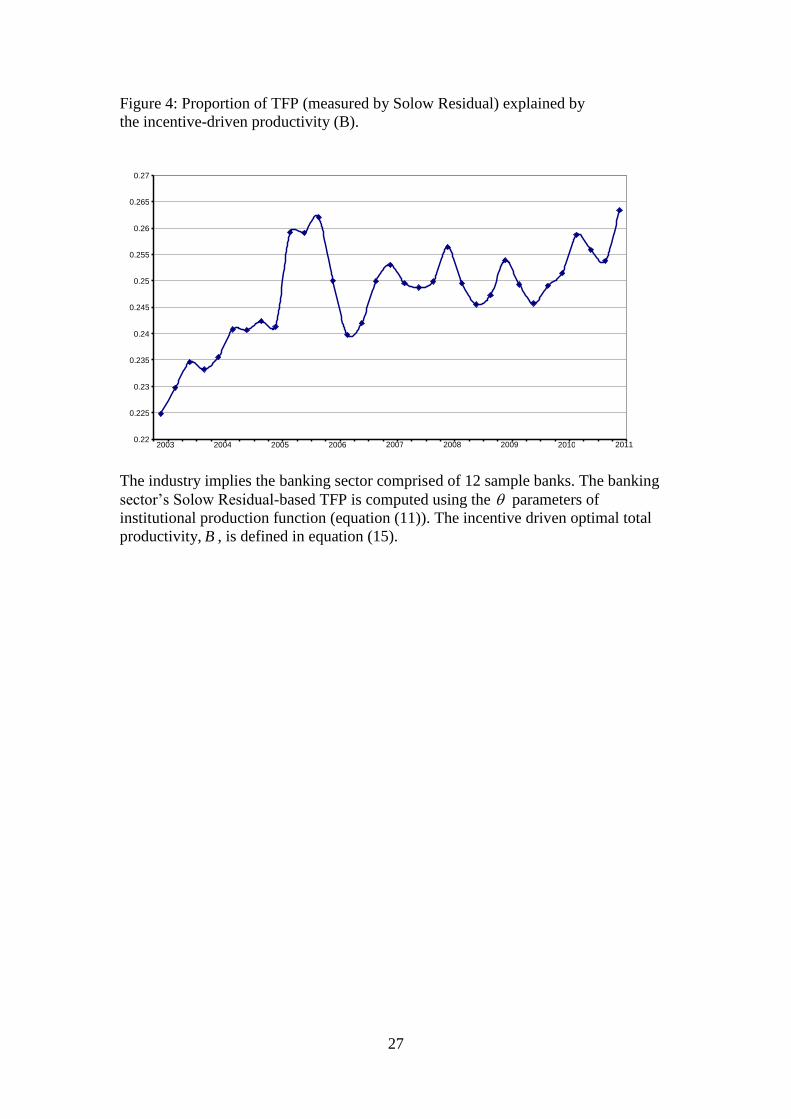
The derivation of incentive driven optimal productivity (B) treats technical
parameters as constants.23 However, technology changes over time. It is, therefore,
important to establish what proportion of the banking sector TFP (total factor
productivity), measured by Solow residuals using the CRT consistent s , is accounted
for by the bankers’ incentive-driven optimal productivity. Figure 4 plots the
proportion of TFP accounted for by the incentive-driven productivity (B). The plot
shows that the proportion of TFP accounted for by incentive-driven productivity is
somewhat oscillatory, yet it shows a positive trend. The proportion of TFP accounted
for by B increased from below 23% to above 26% during 2003-2011 – the sample
average is 24.75%.
A comparison of the optimal effort index (in Figure 2) and optimal bank
productivity (in Figure 3) reveals that during the initial years (2004-2006) both
bankers’ efforts and bank productivity went hand-in-hand; they increased. However,
during 2007(1) - 2007(4), the effort index declines rather sharply which coincides
with some decline in bank productivity. However, the effort index shows a rapid rise
since 2009(3) which does correspond to some productivity gains but the association
19
appears much weaker than those witnessed during 2004-2006. It is hard to elucidate
why this apparently close association between bankers’ efforts and bank productivity
waned post 2009(3). One possible explanation, however, is that after some initial
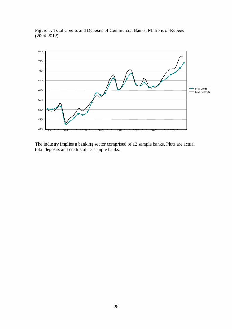
years of productivity push, bankers’ effort may have focussed on quantity (volume).
This is borne out by the sharp rise in the volumes of deposits and credits post 2010(2)
which are plotted in Figure 5. These sharp rises in deposits and credits are at the
backdrop of fall in their volumes during 2008(3) - 2009(4).
Finally, we formally test if the bankers’ effort statistically explains the
incentivized productivity by regressing the index of optimal total productivity on the
index of bankers’ effort. Both OLS and Instrumental Variables estimates reveal that
bankers’ effort significantly explains the optimal bank productivity. A 10% increase
in bankers’ effort increases the banking sectors’ optimal total productivity by roughly
0.6%.24
8. Conclusion
A large body of literature examines whether banking sector efficiency and
productivity improves following financial deregulation and reforms. The literature
mainly employs data envelopment analysis (DEA). However, DEA only measures
relative efficiency and it is not clear whether banks on the efficient frontier are indeed
operating optimally. This paper develops an analytical framework that takes the study
of deregulation (reforms) and banking sector productivity beyond the realm of DEA.
We model commercial banks as profit-cum-utility maximizing firms and analytically
derive, inter alia, bankers’ optimal level of effort and optimal productivity which are
of policy relevance following liberalization and reforms. We apply our model to
scrutinize a panel of Nepalese commercial banks and evaluate if deregulations and
reforms have worked in Nepal. Nepal concluded her deep financial reforms in 1994.
However, due to Maoist insurgency and political instability, these policy reforms
started to take effect since 2002 only which quickly and deeply transformed the
country’s banking and financial system.
Our analysis provides important insights on deregulations, reforms and
banking sector productivity in Nepal. The main findings can be summarized as
follows. First, we find that financial liberalization has made Nepalese bankers more
incentivized (effort oriented) – evidence shows a clear rise in the level of bankers’
efforts following liberalization. Nepalese bankers’ optimal level of effort has
increased considerably (by 43% during 2004-2011) and it is on the rise. Second, the
20
banking sector’s incentive-driven productivity rose markedly until 2007 (by 12%
during 2003-2007) but the productivity growth has since slowed down significantly.
The association between the optimal levels of effort and optimal productivity seemed
very close in early years but appears to have weakened since 2008; it is hard to
explain why this is so. However, prima facie evidence suggests that after the initial
years of productivity push, bankers appear to have focussed on quantity (volume)
rather than quality (productivity). Third, despite the weaker association in the latter
period of sample, formal tests show that the bankers’ optimal effort significantly
explains the banking sector’s optimal productivity in Nepal. Our calculations show
that incentive-driven productivity accounts for about a quarter (24.75%) of banking
sector TFP (measured by Solow residuals) in Nepal. The proportion of non-
performing loans to total loans has declined from 24.0% in 2003 to less than 4.0% in
2012.
Finally, we find that Nepalese banks earned an average bank spread (profit per
unit of bank output) of 3.25 percentage points during the sample period but this has
slightly declined in recent years (3.17 percentage points) perhaps reflecting the
competitive pressure. However, a downside is that the banking services in Nepal have
become costly in recent years – the average cost and price per unit of bank output has
increased notably. The latter is, however, not unexpected, given that deregulation
abolishes authorities’ control on interest rates and various concessionary lending
programmes. Overall, financial liberalization and reforms have been a good
experience for Nepal, especially from the perspectives of more incentivized (effort-
oriented) bankers, increased optimal productivity and higher volume of deposits,
credit and bank profitability. In the light of these findings, any attempt by the
authorities to retract from liberalist policies may do more harm than good.
21
Table 1: Results of Panel Unit Root Tests
IPS
[W-Stat]
ADF-Fisher
[Chi-Square]
Hadri
[Consistent Z-
stat]
CIPS
lnQ
0.898 0.374 0.000 -0.246
lnN
0.914 0.930 0.000 -0.164
lnF
0.326 0.401 0.000 -0.360
lnD
0.542 0.369 0.000 -0.371
For all tests, except for the CIPS, P-values under the null are reported. For CPIS t-
ratios are reported. The 5% critical value for the CIPS test for T/M (200/15) is -
2.25; where T is the sample size and M is the cross-section units. The null under all
test statistics, except that of Hadri, is unit root; the latter tests the null of
stationarity. The sample consists of 420 unbalanced panel observations. In all tests,
constant and linear time trends are included as exogenous variables. Given the
quarterly data, the lag length is set to 4 for all tests except the CIPS where second
order lag is used. CIPS requires lead and lag augmentations. W-Stat is the
standardized NTt test of IPS. ADF Fisher tests are 2 (24)-distributed. The Hadri test
is computed using Newey-West bandwidth selection and Bartlett kernel;
heteroskedasticity-consistent Z-statistics are reported. CIPS is the cross-sectionally
augmented IPS tests (a second generation test). The variable mnemonics are: lnQ =
log of real total loan and investment (output measure), lnN = log of number of bank
staff, lnF = log of total fixed assets in real terms; lnD = log of total deposits in real
terms.
22
Table 2: Results of Panel Cointegration Tests
Between Dimension (Group Mean) Within Dimension (Pooled)
i &i t
i &i t
Pedroni test -4.835(0.000)a -2.995(0.001) a -6.146(0.000) a -4.817(0.000) a
Pedronit test -11.922(0.000) a -12.732(0.000) a -9.755(0.000) a 12.839(0.000) a
KAOt test NA NA -19.183(0.000) a NA
Pedroni test and Pedronit test are panel rho- and ADF-statistics of Pedroni (1999);
KAOt test is the tADF -statistic of Kao (1999). Columns i and &i t indicate the
deterministic component in the model, namely, constants (fixed effects) only, and
constants and linear time trends. Lag lengths are based on SIC information criteria.
Superscripts “a” denote significance at 1% or better. Kao test statistics are a within-
dimension test which allows fixed effects only, hence NAs in three columns.
23
Table 3: Estimated Cointegrating Parameters
1 2 3log log log logit i t it it it itQ N F D e (11)
FMOLS DOLS
Grouped Pooled Grouped Pooled
1 0.146a
(0.000)
0.115 a
(0.005)
0.060 b
(0.050)
0.214 a
(0.002)
0.136 a
(0.005)
0.060 b
(0.041)
2 -0.013
(0.673)
-
0.028 b
(0.039)
-0.053
(0.240)
-
0.033 a
(0.010)
3 0.888 a
(0.000)
0.891a
(0.000)
0.961 a
(0.000)
0.800 a
(0.000)
0.848 a
(0.000)
0.937 a
(0.000)
1 0.686 0.900 0.126 0.625 0.758 0.344
FMOLS is the fully Modified OLS of Phillips and Hansen (1990) as shown in Panel
setting by Pedroni (2001). DOLS is the Dynamic OLS as described in Kao et al.
(1999). Given their significance, both deterministic terms (bank specific constants and
linear time trends) are retained in the estimation. Figures within parentheses (.) are p-
values under the null. 1 reports the P-values of the test of the null of CRTS, i.e.,
1 2 3 1 ; the test statistic is 2 (1) distributed. Under the between-dimension
specifications log itF appears insignificant; we also report results excluding this
insignificant covariate. Superscripts “a” and “b” denote significance at 1% and 5% or
better.
24
Figure 1: Average input cost, output price and spread (industry); Paisa per
Rupee of output.
Industry implies the banking sector, comprised of 12 sample banks. The average input
cost per unit of output is calculated as { }ia
i
i
w from equation (6). The average
output price is the average loan rate computed as the ratio of loan interest income over
total bank loan. The average input cost, output price and spread (profit) are per unit of
bank output. In the vertical axis 0.1 means ten paisa. One Nepalese rupee consists of
100 paisa.
0
0.01
0.02
0.03
0.04
0.05
0.06
0.07
0.08
0.09
0.1
2003
2003 2004 2004 2005 2005 2006 2006 2007 2007 2008 2008 2009 2009 20100
2010 2011 2011
Output price Average input price Spread
25
Figure 2: Industry optimal effort index (2004=100), actual output index and actual
profit Index.
Industry implies the banking sector comprised of 12 sample banks. Output and profit
index are actual figures for the banking sector. The optimal effort index is the
simulated series, equation (10).
80
90
100
110
120
130
140
150
160
170
180
2004 2004 2005 2006 2007 2007 2008 2009 2010 2010 2011
Ind output Index Ind optimal effort Index Ind Profit Index
26
Figure 3: Banking Sector’s Optimal Productivity: ( B ) and (incB )
The banking industry implies 12 sample banks. The banking sector’s optimal
productivity ( B ) is as in equation (15) and unscaled, incB , as in equation (16). Plots
are absolute figures not indices.
0.85
0.87
0.89
0.91
0.93
0.95
0.97
0.99
2003
2004 2005 2006 2007 2008 2009 2010 2011 2012
Industry Binc
Industry B
27
Figure 4: Proportion of TFP (measured by Solow Residual) explained by
the incentive-driven productivity (B).
The industry implies the banking sector comprised of 12 sample banks. The banking
sector’s Solow Residual-based TFP is computed using the parameters of
institutional production function (equation (11)). The incentive driven optimal total
productivity, B , is defined in equation (15).
0.22
0.225
0.23
0.235
0.24
0.245
0.25
0.255
0.26
0.265
0.27
2003 2004 2005 2006 2007 2008 2009 2010 2011
28
Figure 5: Total Credits and Deposits of Commercial Banks, Millions of Rupees
(2004-2012).
The industry implies a banking sector comprised of 12 sample banks. Plots are actual
total deposits and credits of 12 sample banks.
4000
4500
5000
5500
6000
6500
7000
7500
8000
2004 2005 2006 2007 2008 2009 2010 2011
Total Credit Total Deposits
29
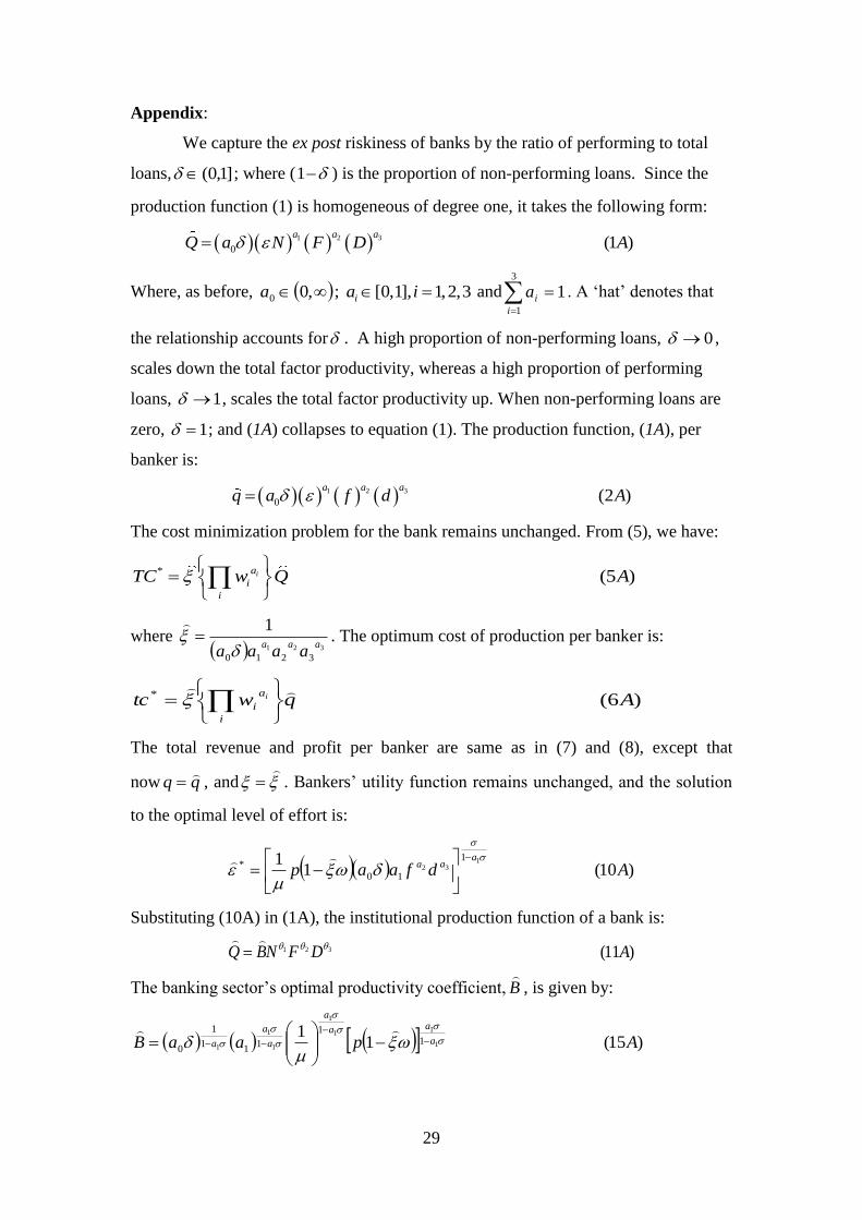
Appendix:
We capture the ex post riskiness of banks by the ratio of performing to total
loans, ]1,0( ; where (1 ) is the proportion of non-performing loans. Since the
production function (1) is homogeneous of degree one, it takes the following form:
1 2 3
0 (1 )a a a
Q a N F D A
Where, as before, ,00a ; [0,1], 1,2,3ia i and
3
1
1i
ia . A ‘hat’ denotes that
the relationship accounts for . A high proportion of non-performing loans, 0 ,
scales down the total factor productivity, whereas a high proportion of performing
loans, 1 , scales the total factor productivity up. When non-performing loans are
zero, 1 ; and (1A) collapses to equation (1). The production function, (1A), per
banker is:
1 2 3
0 (2 )a a a
q a f d A
The cost minimization problem for the bank remains unchanged. From (5), we have:
* (5 )ia
i
i
TC w Q A
where 321
3210
1aaa
aaaa
. The optimum cost of production per banker is:
)6(* Aqwtci
a
ii
The total revenue and profit per banker are same as in (7) and (8), except that
now qq
, and
. Bankers’ utility function remains unchanged, and the solution
to the optimal level of effort is:
)10(11 1
32
1
10
* Adfaapa
aa
Substituting (10A) in (1A), the institutional production function of a bank is:
)11(321 ADFNBQ
The banking sector’s optimal productivity coefficient, B
, is given by:
)15(11
1
11
1
1
1
11
1
11
1
1
0 ApaaB a
aa
a
a
a
a
30
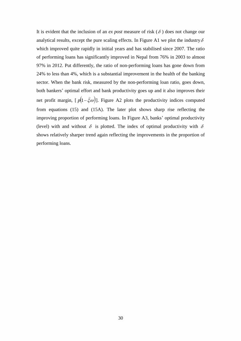
It is evident that the inclusion of an ex post measure of risk ( ) does not change our
analytical results, except the pure scaling effects. In Figure A1 we plot the industry
which improved quite rapidly in initial years and has stabilised since 2007. The ratio
of performing loans has significantly improved in Nepal from 76% in 2003 to almost
97% in 2012. Put differently, the ratio of non-performing loans has gone down from
24% to less than 4%, which is a substantial improvement in the health of the banking
sector. When the bank risk, measured by the non-performing loan ratio, goes down,
both bankers’ optimal effort and bank productivity goes up and it also improves their
net profit margin, [
1p ]. Figure A2 plots the productivity indices computed
from equations (15) and (15A). The later plot shows sharp rise reflecting the
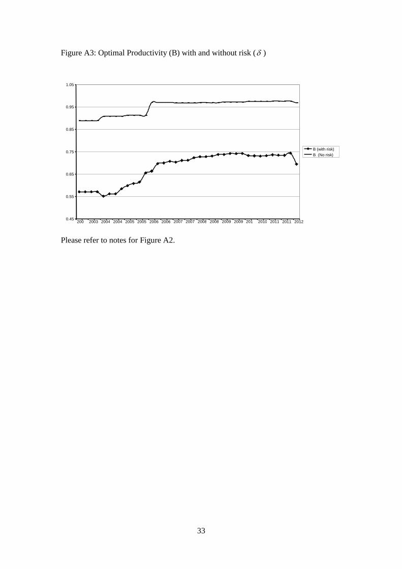
improving proportion of performing loans. In Figure A3, banks’ optimal productivity
(level) with and without is plotted. The index of optimal productivity with
shows relatively sharper trend again reflecting the improvements in the proportion of
performing loans.
31
Figure A1: Ratio of Performing to Total Loans ( Industry)
The industry implies the banking sector is comprised of 12 sample banks.
0.7
0.75
0.8
0.85
0.9
0.95
1
2003
2003 2004 2005 2006 2006 2007 2008 2009 2009 2010 2011 2012
32
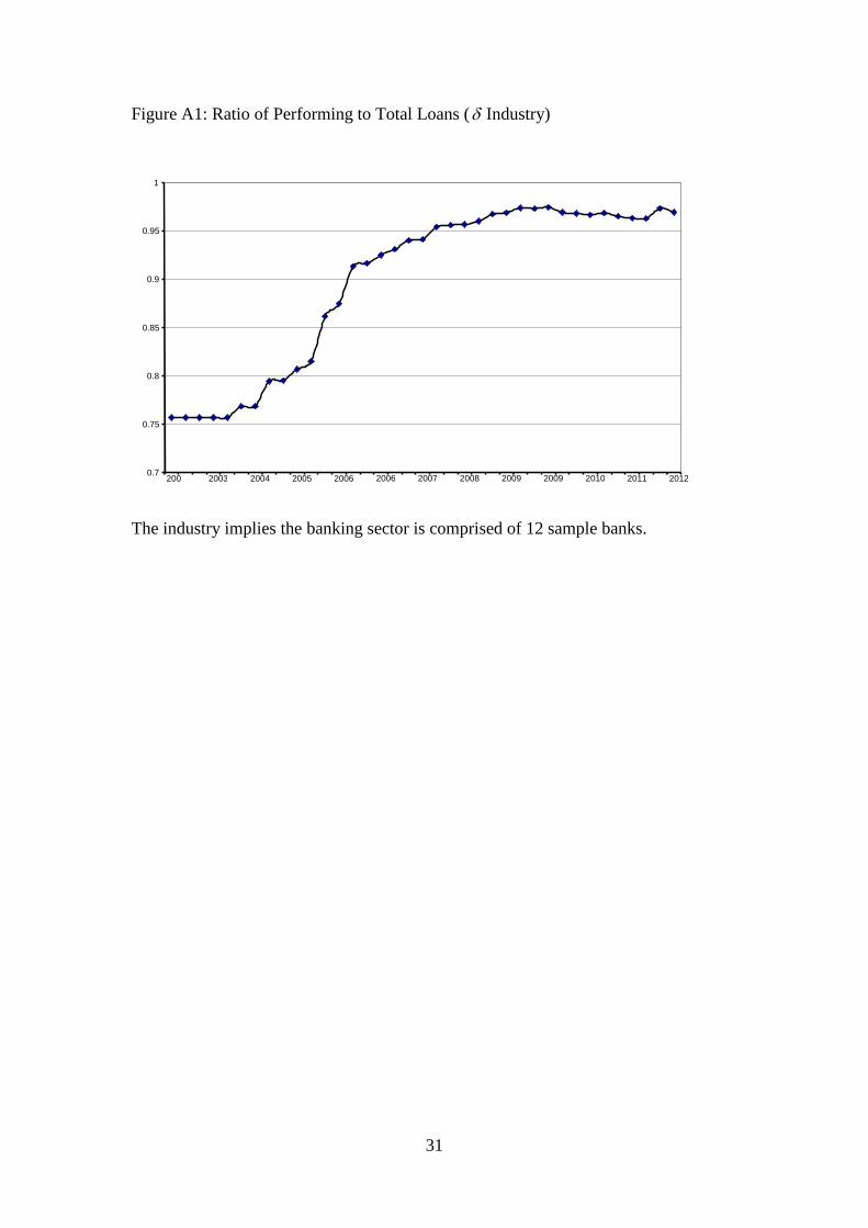
Figure A2: Optimal Effort ( * ) with and without risk ( )
Risk ( ) is measured by the proportion of performing to total bank loans. The
proportion of non-performing loans is (1 ). We apply time varying in computing
effort index with risk.
75
85
95
105
115
125
135
145
155
165
2004 2004 2005 2006 2007 2007 2008 2009 2010 2010 2011
Effort Index (with risk) Effort Index (no risk)
33
Figure A3: Optimal Productivity (B) with and without risk ( )
Please refer to notes for Figure A2.
0.45
0.55
0.65
0.75
0.85
0.95
1.05
2003
2003 2004 2004 2005 2005 2006 2006 2007 2007 2008 2008 2009 2009 2010
2010 2011 2011 2012
B (with risk) B (No risk)
34
References
Aly, H. Y., R. Grabowski, C. Pasurka, and N. Rangan (1990) “Technical, scale and
allocative efficiencies in US banking: An empirical investigation”, The Review of
Economics and Statistics, 72, 211-218.
Berger, A.N., and D.B. Humphrey (1992) “Measurement and Efficiency Issues in
Commercial Banking”, in Z. Griliches (ed.), Output Measurement in the Service
Sectors, National Bureau of Economic Research, Studies in Income and Wealth, Vol.
56, University of Chicago Press (Chicago, IL), 245-279.
Burgess, R. and R. Pande (2005) “Do Rural Banks Matter? Evidence from Indian
Social Banking Experiment”, American Economic Review, 95(3), 780-795.
Clark, J. (1984) “Estimation of Economies of Scale in Banking Using a Generalized
Functional Form”, Journal of Money, Credit, and Banking, 16, 53-68.
Clark, J. (1988) “Economies of Scale and Scope at Depository Financial Institutions:
A Review of the Literature”, Federal Reserve Bank of Kansas City Economic Review,
73, 16-33.
Delis, M. D., P. Molyneux and F. Pasiouras (2011) “Regulations and Productivity
Growth in Banking: Evidence from Transition Economies”, Journal of Money, Credit
and Banking, 43(4), 735-764.
Engle, R. F and C. J. Granger (1987) “Co-integration and Error Correction:
Representation, Estimation, and Testing”, Econometrica, 55(2), 251-276.
Fare, R., S. Grosskopf, M. Norris and Z. Zhang (1994) “Productivity Growth,
Technical Progress, and Efficiency Change in Industrialized Countries”, The
American Economic Review, 84(1), 66-83.
Gengenbach, C. F. Palm and J. Urbain (2010) “Panel Unit Root Tests in the Presence
of Cross-Sectional Dependencies: Comparison and Implications for Modelling”,
Econometric Reviews, 29(2), 111-145.
Hadri, K. (2000) “Testing for stationarity in heterogeneous panel data”, Econometrics
Journal 3(2), 148-161.
Hlouskova, J. and M. Wagner (2006) “The performance of panel unit root and
stationarity tests: results from a large-scale simulation study”. Econometric Reviews
25(1), 85-116.
Humphrey, D. B. (1991) “Productivity in Banking and Effects from Deregulation”
Economic Review, Federal Reserve Bank of Richmond, March/April: 16-28.
Humphrey, D. B. and L. B. Pulley (1997) “Bank’s responses to deregulation: profits,
technology, and efficiency”, Journal of Money, Credit and Banking, 29, 73-93.
35
Ihsan, I. and M. Hassan (2003) “Financial deregulation and total factor productivity
change: An empirical study of Turkish commercial banks”, Journal of Banking &
Finance, 27(8), 1455-1485.
Im, K. S., Pesaran, H. and Shin, Y. (2003). “Testing for unit roots in heterogeneous
panels”, Journal of Econometrics 115(1), 53-74.
Kao, C. (1999) “Spurious regression and residual-based tests for cointegration in
panel data”, Journal of Econometrics, 90(1), 1-44.
Kao, C., M-H. Chiang and B. Chen (1999) “International R&D Spillovers: An
Application of Estimation and Inference in Panel Cointegration”, Oxford Bulletin of
Economics and Statistics (61), 693-711.
Luintel, K. B., M. Khan, P. Arestis and K. Theodoridis (2008) “Financial Structure
and Economic Growth”, Journal of Development Economics, 86(1), 181-200.
Maddala, G. and S. Wu (1999) “A comparative study of unit root tests with panel data
and a new simple test”, Oxford Bulletin of Economics and Statistics 61(S1), 631-652.
McMillan, J., J. Whalley and L. Zhu (1989) “The Impact of China’s Economic
Reforms on Agricultural Productivity Growth”, Journal of Political Economy, 97
(August), 781-807.
Mukherjee, K., S. C. Ray and S. Miller (2001) “Productivity growth in large US
commercial banks: The initial post-deregulation experience”, Journal of Banking &
Finance, 25(5), 913-939.
Nepal Rastra Bank, “40 Years of Nepal Rastra Bank”, Kathmandu, April 1996.
Pasiouras, F. (2008) “International evidence on the impact of regulations and
supervision on banks’ technical efficiency: an application of two-stage data
envelopment analysis”, Review of Quantitative Finance and Accounting, 30(2), 187-
223.
Pedroni, P. (1999) “Critical values for cointegration tests in heterogeneous panels
with multiple regressors”, Oxford Bulletin of Economics and Statistics, 61(Special
Issue), 653-670.
Pedroni, P. (2001) “Purchasing power parity tests in cointegrated panels”, The Review
of Economics and Statistics, 83(4), 727-731.
Pedroni, P. (2004) “Panel cointegration: asymptotic and finite sample properties of
pooled time series tests with an application to the PPP hypothesis”, Econometric
Theory, 20(3), 597-625.
Pesaran, M. H. (2007) “A simple panel unit root test in the presence of cross-section
dependence, Journal of Applied Econometrics, 22(2), 265-312.
36
Phillips, P. C. and B. E. Hansen (1990) “Statistical Inference in Instrumental
Variables Regression with I(1) Processes”, Review of Economic Studies, 57(1), 99-
125.
Sealey, C. W and J. T. Lindley (1997) “Inputs, outputs and a theory of production and
cost at depository financial institutions”, Journal of Finance, 32, 1251-1266.
Stock, J. and M. Watson (1993) “A Simple Estimator of Cointegrating Vectors in
Higher Order Integrated Systems”, Econometrica, 55, 1035-1056.
Tirtiroglu, K., K. Daniels and E. Tirtiroglu (2005) “Deregulation, Intensity of
Competition, Industry Evolution and the Productivity Growth of US Commercial
Banks”, Journal of Money, Credit and Banking, 37(2), 339-360.
Wheelock, D. C. and P. W. Wilson, (1999) “Technical Progress, Inefficiency, and
Productivity Change in U.S. Banking, 1984-1993”, Journal of Money, Credit and
Banking, 31(2), 212-234.
37
1 For example, McMillan et al. (1989) in analysing Chinese agricultural reforms that
incentivised (rewarded) individual farmers, concluded that “rewarding individual
effort yields large benefit” (ibid., p. 783).
2 Some of these studies subsequently employ parametric methods to model the
productivity and efficiency measures computed through DEA.
3 To see this, imagine a scenario where the whole of the banking industry makes an
average efficiency gain of 5% but this gain would look inefficient if the efficient
frontier moves up by 10%.
4 The non-zero profit in the long-run raises the theoretical possibility of banks
producing an infinite amount of output. While we acknowledge this theoretical
possibility we do not regard it as being of much practical relevance.
5 Lack of data prevented us from using the off-balance-sheet items in our measure of
bank output. However, our measure of bank output is consistent with those of Delis et
al. (2011), among others.
6 Utility from profit could be seen as tangible (bonuses) and intangible (fame) rewards
which tend to be positively associated with the level of profits. Given that our focus is
on bank productivity, we do not model the details of incentive packages.
7 It is trivial that from (12), (13) and (14) that: 1
11
11
a ,
1
122
111a and
1
133
111a .
8 Data on GDP per capita in current US dollars are for 2011 and obtained from the
World Bank at http://www.worldbank.org/en/country/nepal. Population figures are
from the 2011 census, Nepal.
38
9 Under the social banking philosophy authorities, among other things, dictated that
commercial banks expand their branch networks across countries in tandem with
nationally declared banking density objectives of one bank branch per 30,000 head of
population.
10 The precise year 2002 is suggested by the seminar participants (high ranking
officials of the Central Bank, Commercial Banks and the Government and of Nepal)
at the Nepalese Bankers’ Association seminar, Kathmandu, December 2013. We are
grateful for this suggestion.
11 Figures on the growth of financial institutions are taken from Banking and
Financial Statistics, mid-July, 2012, No. 58, NRB.
12 One of our sample banks has a minimum data length of 7 years – 2006(3) to
2012(1) – as it was opened in 2006.
13 We are thankful to the Governor of NRB, Dr Y R Khatiwada, for the data. The 12
commercial banks covered are: Bank of Kathmandu Ltd. (1995), Everest Bank Ltd.
(1994), Global Bank Ltd. (2006), Himalayan Bank Ltd. (1993), Kumari Bank Ltd.
(2001), Laxmi Bank Ltd. (2002), Machhapuchhre Bank Ltd. (2000), Nabil Bank Ltd.
(1984), Nepal Bank Ltd. (1937), Nepal Investment Bank Ltd. (1986), Rastrya
Banijya Bank Ltd. (1966) and Standard Chartered Bank Nepal Ltd. (1987). Figures
within parentheses (.) indicate the date of bank operation. As stated in the text, they
constitute the major commercial banks of Nepal.
14 Data on quarterly GDP deflator are not available in Nepal.
15 Results of first difference stationarity are not reported, to conserve space, but are
available on request.
39
16 The fixed assets of banks tend to change slowly compared to bank output,
employment and total deposit liabilities.
17 The parameter estimates of the last column of DOLS results reported in Table 3
sum to 1.03. A reduction of 3.0% of each parameter to make them sum to unity is also
not rejected by the test. The p-value of the test is 2(3) 0.194 . The Grouped
parameters under FMOLS and DOLS sum to 1.006 and 0.984, respectively (columns
which delete the insignificant itF ).
18 Parameter0a is the constant term of the technical production function (equation
(1)). The estimates of the constant term of the institutional production function range
between 0.024 to 2.498 under different specifications (not reported in Table 3). Our
simulation results are robust to values of 00 10a .
19 Iteration reveals that for wide-ranging values of 0.01 10 the simulated values
of * and B remain fairly robust.
20 The average hourly wage rate ( 1w ) is calculated as follows. First, the quarterly
average wage bill for staff is computed by dividing the total quarterly wage bill by the
total number of staff. Then the quarterly average wage bill is divided by 40x12;
where 40 represents the hours worked per week and there are 12 working weeks in a
quarter.
21 Nepalese currency is known as Rupees and one Rupee consists of 100 Paisa.
22 We are thankful to the seminar participants at the Nepal Bankers’ Association,
Kathmandu, in explaining (reconciling) this sharp upturn in banking sector
productivity with the Peace Accord of 2005.
23 A time varying approach of estimation would allow the technical parameter to be
time dependent but data constraints preclude us from using it.
40
24 The estimated regression is: log 4.441 0.054log * 0.005sldmyB ; where B is
the index of simulated total optimal productivity, * is the index of simulated
optimal effort and ‘sldmy’ is the slope dummy for 2006(1)-(2) to capture the blip in
productivity (see Figure 3). The constant term and the slope parameters resume p-
values of 0.000, 0.024 and 0.000, respectively, hence are statistically highly
significant. The reported results pertain to the first order residual serial correlation
(AR(1)) correction. The R-bar square is 0.93 and DW statistic is 1.72. Results appear
almost identical when the IV estimator is used.


