Embed Size (px)
Citation preview

REDUCEUser’s and
Contributed Packages Manual
Version 3.8
Anthony C. HearnSanta Monica, CAand Codemist Ltd.
Email: [email protected]
July 2003

Copyright c©2004 Anthony C. Hearn. All rights reserved.
Registered system holders may reproduce all or any part of this publicationfor internal purposes, provided that the source of the material is clearlyacknowledged, and the copyright notice is retained.

3
Preface
This volume has been prepared by Codemist Ltd. from the LATEX documen-tation sources distributed with REDUCE 3.8. It incorporates the User’sManual, and documentation for all the User Contributed Packages as a sec-ond Part. A common index and table of contents has been prepared. Wehope that this single volume will be more convenient for REDUCE usersthan having two unrelated documents. Particularly in Part 2 the text of theauthors has been extensively edited and modified and so the responsibilityfor any errors rests with us.
Parts I and III were written by Anthony C. Hearn. Part II is based on textsby:Werner Antweiler, Victor Adamchik, Joachim Apel, Alan Barnes, AndreasBernig, Yu. A. Blinkov, Russell Bradford, Chris Cannam, Hubert Caprasse,C. Dicrescenzo, Alain Dresse, Ladislav Drska, James W. Eastwood, JohnFitch, Kerry Gaskell, Barbara L. Gates, Karin Gatermann, Hans-GertGrabe, David Harper, David Hartley, Anthony C. Hearn, J. A. van Hulzen,V. Ilyin, Stanley L. Kameny, Fujio Kako, C. Kazasov, Wolfram Koepf,A. Kryukov, Richard Liska, Kevin McIsaac, Malcolm A. H. MacCallum, Her-bert Melenk, H. M. Moller, Winfried Neun, Julian Padget, Matt Rebbeck,F. Richard-Jung, A. Rodionov, Carsten and Franziska Schobel, RainerSchopf, Stephen Scowcroft, Eberhard Schrufer, Fritz Schwarz, M. Spiri-donova, A. Taranov, Lisa Temme, Walter Tietze, V. Tomov, E. Tournier,Philip A. Tuckey, G. Ucoluk, Mathias Warns, Thomas Wolf, FrancisJ. Wright and A. Yu. Zharkov.
February 2004Codemist Ltd“Alta”, Horsecombe ValeCombe DownBath, England

4

Contents
I REDUCE User’s Manual 29
Abstract 33
1 Introductory Information 37
2 Structure of Programs 43
2.1 The REDUCE Standard Character Set . . . . . . . . . . . . . 43
2.2 Numbers . . . . . . . . . . . . . . . . . . . . . . . . . . . . . . 44
2.3 Identifiers . . . . . . . . . . . . . . . . . . . . . . . . . . . . . 45
2.4 Variables . . . . . . . . . . . . . . . . . . . . . . . . . . . . . 46
2.5 Strings . . . . . . . . . . . . . . . . . . . . . . . . . . . . . . . 47
2.6 Comments . . . . . . . . . . . . . . . . . . . . . . . . . . . . . 48
2.7 Operators . . . . . . . . . . . . . . . . . . . . . . . . . . . . . 48
3 Expressions 53
3.1 Scalar Expressions . . . . . . . . . . . . . . . . . . . . . . . . 53
3.2 Integer Expressions . . . . . . . . . . . . . . . . . . . . . . . . 54
3.3 Boolean Expressions . . . . . . . . . . . . . . . . . . . . . . . 55
3.4 Equations . . . . . . . . . . . . . . . . . . . . . . . . . . . . . 57
3.5 Proper Statements as Expressions . . . . . . . . . . . . . . . 58
5
6 CONTENTS
4 Lists 59
4.1 Operations on Lists . . . . . . . . . . . . . . . . . . . . . . . . 59
4.1.1 LIST . . . . . . . . . . . . . . . . . . . . . . . . . . . . 60
4.1.2 FIRST . . . . . . . . . . . . . . . . . . . . . . . . . . . 60
4.1.3 SECOND . . . . . . . . . . . . . . . . . . . . . . . . . 60
4.1.4 THIRD . . . . . . . . . . . . . . . . . . . . . . . . . . 60
4.1.5 REST . . . . . . . . . . . . . . . . . . . . . . . . . . . 60
4.1.6 . (Cons) Operator . . . . . . . . . . . . . . . . . . . . 60
4.1.7 APPEND . . . . . . . . . . . . . . . . . . . . . . . . . 61
4.1.8 REVERSE . . . . . . . . . . . . . . . . . . . . . . . . 61
4.1.9 List Arguments of Other Operators . . . . . . . . . . . 61
4.1.10 Caveats and Examples . . . . . . . . . . . . . . . . . . 61
5 Statements 63
5.1 Assignment Statements . . . . . . . . . . . . . . . . . . . . . 64
5.1.1 Set Statement . . . . . . . . . . . . . . . . . . . . . . . 65
5.2 Group Statements . . . . . . . . . . . . . . . . . . . . . . . . 65
5.3 Conditional Statements . . . . . . . . . . . . . . . . . . . . . 66
5.4 FOR Statements . . . . . . . . . . . . . . . . . . . . . . . . . 67
5.5 WHILE . . . DO . . . . . . . . . . . . . . . . . . . . . . . . . . 69
5.6 REPEAT . . . UNTIL . . . . . . . . . . . . . . . . . . . . . . . 70
5.7 Compound Statements . . . . . . . . . . . . . . . . . . . . . . 70
5.7.1 Compound Statements with GO TO . . . . . . . . . . 72
5.7.2 Labels and GO TO Statements . . . . . . . . . . . . . 73
5.7.3 RETURN Statements . . . . . . . . . . . . . . . . . . 73
6 Commands and Declarations 75
6.1 Array Declarations . . . . . . . . . . . . . . . . . . . . . . . . 75

CONTENTS 7
6.2 Mode Handling Declarations . . . . . . . . . . . . . . . . . . . 76
6.3 END . . . . . . . . . . . . . . . . . . . . . . . . . . . . . . . . 77
6.4 BYE Command . . . . . . . . . . . . . . . . . . . . . . . . . . 77
6.5 SHOWTIME Command . . . . . . . . . . . . . . . . . . . . . 78
6.6 DEFINE Command . . . . . . . . . . . . . . . . . . . . . . . 78
7 Built-in Prefix Operators 79
7.1 Numerical Operators . . . . . . . . . . . . . . . . . . . . . . . 79
7.1.1 ABS . . . . . . . . . . . . . . . . . . . . . . . . . . . . 80
7.1.2 CEILING . . . . . . . . . . . . . . . . . . . . . . . . . 80
7.1.3 CONJ . . . . . . . . . . . . . . . . . . . . . . . . . . . 80
7.1.4 FACTORIAL . . . . . . . . . . . . . . . . . . . . . . . 80
7.1.5 FIX . . . . . . . . . . . . . . . . . . . . . . . . . . . . 81
7.1.6 FLOOR . . . . . . . . . . . . . . . . . . . . . . . . . . 81
7.1.7 IMPART . . . . . . . . . . . . . . . . . . . . . . . . . 81
7.1.8 MAX/MIN . . . . . . . . . . . . . . . . . . . . . . . . 81
7.1.9 NEXTPRIME . . . . . . . . . . . . . . . . . . . . . . 82
7.1.10 RANDOM . . . . . . . . . . . . . . . . . . . . . . . . 82
7.1.11 RANDOM NEW SEED . . . . . . . . . . . . . . . . . 82
7.1.12 REPART . . . . . . . . . . . . . . . . . . . . . . . . . 83
7.1.13 ROUND . . . . . . . . . . . . . . . . . . . . . . . . . . 83
7.1.14 SIGN . . . . . . . . . . . . . . . . . . . . . . . . . . . 83
7.2 Mathematical Functions . . . . . . . . . . . . . . . . . . . . . 83
7.3 DF Operator . . . . . . . . . . . . . . . . . . . . . . . . . . . 87
7.3.1 Adding Differentiation Rules . . . . . . . . . . . . . . 87
7.4 INT Operator . . . . . . . . . . . . . . . . . . . . . . . . . . . 88
7.4.1 Options . . . . . . . . . . . . . . . . . . . . . . . . . . 89
7.4.2 Advanced Use . . . . . . . . . . . . . . . . . . . . . . . 90

8 CONTENTS
7.4.3 References . . . . . . . . . . . . . . . . . . . . . . . . . 90
7.5 LENGTH Operator . . . . . . . . . . . . . . . . . . . . . . . . 90
7.6 MAP Operator . . . . . . . . . . . . . . . . . . . . . . . . . . 91
7.7 MKID Operator . . . . . . . . . . . . . . . . . . . . . . . . . 92
7.8 PF Operator . . . . . . . . . . . . . . . . . . . . . . . . . . . 93
7.9 SELECT Operator . . . . . . . . . . . . . . . . . . . . . . . . 93
7.10 SOLVE Operator . . . . . . . . . . . . . . . . . . . . . . . . . 94
7.10.1 Handling of Undetermined Solutions . . . . . . . . . . 96
7.10.2 Solutions of Equations Involving Cubics and Quartics 97
7.10.3 Other Options . . . . . . . . . . . . . . . . . . . . . . 99
7.10.4 Parameters and Variable Dependency . . . . . . . . . 100
7.11 Even and Odd Operators . . . . . . . . . . . . . . . . . . . . 104
7.12 Linear Operators . . . . . . . . . . . . . . . . . . . . . . . . . 105
7.13 Non-Commuting Operators . . . . . . . . . . . . . . . . . . . 106
7.14 Symmetric and Antisymmetric Operators . . . . . . . . . . . 106
7.15 Declaring New Prefix Operators . . . . . . . . . . . . . . . . . 107
7.16 Declaring New Infix Operators . . . . . . . . . . . . . . . . . 108
7.17 Creating/Removing Variable Dependency . . . . . . . . . . . 109
8 Display and Structuring of Expressions 111
8.1 Kernels . . . . . . . . . . . . . . . . . . . . . . . . . . . . . . 111
8.2 The Expression Workspace . . . . . . . . . . . . . . . . . . . 113
8.3 Output of Expressions . . . . . . . . . . . . . . . . . . . . . . 114
8.3.1 LINELENGTH Operator . . . . . . . . . . . . . . . . 114
8.3.2 Output Declarations . . . . . . . . . . . . . . . . . . . 115
8.3.3 Output Control Switches . . . . . . . . . . . . . . . . 116
8.3.4 WRITE Command . . . . . . . . . . . . . . . . . . . . 120
8.3.5 Suppression of Zeros . . . . . . . . . . . . . . . . . . . 122

CONTENTS 9
8.3.6 FORTRAN Style Output Of Expressions . . . . . . . 122
8.3.7 Saving Expressions for Later Use as Input . . . . . . . 125
8.3.8 Displaying Expression Structure . . . . . . . . . . . . 126
8.4 Changing the Internal Order of Variables . . . . . . . . . . . 128
8.5 Obtaining Parts of Algebraic Expressions . . . . . . . . . . . 128
8.5.1 COEFF Operator . . . . . . . . . . . . . . . . . . . . 128
8.5.2 COEFFN Operator . . . . . . . . . . . . . . . . . . . . 129
8.5.3 PART Operator . . . . . . . . . . . . . . . . . . . . . 130
8.5.4 Substituting for Parts of Expressions . . . . . . . . . . 131
9 Polynomials and Rationals 133
9.1 Controlling the Expansion of Expressions . . . . . . . . . . . 134
9.2 Factorization of Polynomials . . . . . . . . . . . . . . . . . . . 134
9.3 Cancellation of Common Factors . . . . . . . . . . . . . . . . 137
9.3.1 Determining the GCD of Two Polynomials . . . . . . 138
9.4 Working with Least Common Multiples . . . . . . . . . . . . 138
9.5 Controlling Use of Common Denominators . . . . . . . . . . . 139
9.6 REMAINDER Operator . . . . . . . . . . . . . . . . . . . . . 139
9.7 RESULTANT Operator . . . . . . . . . . . . . . . . . . . . . 140
9.8 DECOMPOSE Operator . . . . . . . . . . . . . . . . . . . . . 141
9.9 INTERPOL operator . . . . . . . . . . . . . . . . . . . . . . . 142
9.10 Obtaining Parts of Polynomials and Rationals . . . . . . . . . 142
9.10.1 DEG Operator . . . . . . . . . . . . . . . . . . . . . . 143
9.10.2 DEN Operator . . . . . . . . . . . . . . . . . . . . . . 143
9.10.3 LCOF Operator . . . . . . . . . . . . . . . . . . . . . 144
9.10.4 LPOWER Operator . . . . . . . . . . . . . . . . . . . 145
9.10.5 LTERM Operator . . . . . . . . . . . . . . . . . . . . 145
9.10.6 MAINVAR Operator . . . . . . . . . . . . . . . . . . . 146

10 CONTENTS
9.10.7 NUM Operator . . . . . . . . . . . . . . . . . . . . . . 146
9.10.8 REDUCT Operator . . . . . . . . . . . . . . . . . . . 146
9.11 Polynomial Coefficient Arithmetic . . . . . . . . . . . . . . . 147
9.11.1 Rational Coefficients in Polynomials . . . . . . . . . . 147
9.11.2 Real Coefficients in Polynomials . . . . . . . . . . . . 148
9.11.3 Modular Number Coefficients in Polynomials . . . . . 149
9.11.4 Complex Number Coefficients in Polynomials . . . . . 150
10 Substitution Commands 151
10.1 SUB Operator . . . . . . . . . . . . . . . . . . . . . . . . . . 151
10.2 LET Rules . . . . . . . . . . . . . . . . . . . . . . . . . . . . 152
10.2.1 FOR ALL . . . LET . . . . . . . . . . . . . . . . . . . . 155
10.2.2 FOR ALL . . . SUCH THAT . . . LET . . . . . . . . . . 156
10.2.3 Removing Assignments and Substitution Rules . . . . 156
10.2.4 Overlapping LET Rules . . . . . . . . . . . . . . . . . 157
10.2.5 Substitutions for General Expressions . . . . . . . . . 157
10.3 Rule Lists . . . . . . . . . . . . . . . . . . . . . . . . . . . . . 160
10.4 Asymptotic Commands . . . . . . . . . . . . . . . . . . . . . 166
11 File Handling Commands 169
11.1 IN Command . . . . . . . . . . . . . . . . . . . . . . . . . . . 169
11.2 OUT Command . . . . . . . . . . . . . . . . . . . . . . . . . . 170
11.3 SHUT Command . . . . . . . . . . . . . . . . . . . . . . . . . 171
12 Commands for Interactive Use 173
12.1 Referencing Previous Results . . . . . . . . . . . . . . . . . . 174
12.2 Interactive Editing . . . . . . . . . . . . . . . . . . . . . . . . 174
12.3 Interactive File Control . . . . . . . . . . . . . . . . . . . . . 176

CONTENTS 11
13 Matrix Calculations 177
13.1 MAT Operator . . . . . . . . . . . . . . . . . . . . . . . . . . 177
13.2 Matrix Variables . . . . . . . . . . . . . . . . . . . . . . . . . 178
13.3 Matrix Expressions . . . . . . . . . . . . . . . . . . . . . . . . 178
13.4 Operators with Matrix Arguments . . . . . . . . . . . . . . . 179
13.4.1 DET Operator . . . . . . . . . . . . . . . . . . . . . . 179
13.4.2 MATEIGEN Operator . . . . . . . . . . . . . . . . . . 180
13.4.3 TP Operator . . . . . . . . . . . . . . . . . . . . . . . 181
13.4.4 Trace Operator . . . . . . . . . . . . . . . . . . . . . . 181
13.4.5 Matrix Cofactors . . . . . . . . . . . . . . . . . . . . . 181
13.4.6 NULLSPACE Operator . . . . . . . . . . . . . . . . . 182
13.4.7 RANK Operator . . . . . . . . . . . . . . . . . . . . . 183
13.5 Matrix Assignments . . . . . . . . . . . . . . . . . . . . . . . 183
13.6 Evaluating Matrix Elements . . . . . . . . . . . . . . . . . . . 184
14 Procedures 185
14.1 Procedure Heading . . . . . . . . . . . . . . . . . . . . . . . . 186
14.2 Procedure Body . . . . . . . . . . . . . . . . . . . . . . . . . 187
14.3 Using LET Inside Procedures . . . . . . . . . . . . . . . . . . 189
14.4 LET Rules as Procedures . . . . . . . . . . . . . . . . . . . . 190
14.5 REMEMBER Statement . . . . . . . . . . . . . . . . . . . . . 192
15 User Contributed Packages 193
16 Symbolic Mode 197
16.1 Symbolic Infix Operators . . . . . . . . . . . . . . . . . . . . 200
16.2 Symbolic Expressions . . . . . . . . . . . . . . . . . . . . . . 200
16.3 Quoted Expressions . . . . . . . . . . . . . . . . . . . . . . . 200
16.4 Lambda Expressions . . . . . . . . . . . . . . . . . . . . . . . 201

12 CONTENTS
16.5 Symbolic Assignment Statements . . . . . . . . . . . . . . . . 202
16.6 FOR EACH Statement . . . . . . . . . . . . . . . . . . . . . . 202
16.7 Symbolic Procedures . . . . . . . . . . . . . . . . . . . . . . . 202
16.8 Standard Lisp Equivalent of Reduce Input . . . . . . . . . . . 203
16.9 Communicating with Algebraic Mode . . . . . . . . . . . . . 203
16.9.1 Passing Algebraic Mode Values to Symbolic Mode . . 204
16.9.2 Passing Symbolic Mode Values to Algebraic Mode . . 207
16.9.3 Complete Example . . . . . . . . . . . . . . . . . . . . 208
16.9.4 Defining Procedures for Intermode Communication . . 208
16.10Rlisp ’88 . . . . . . . . . . . . . . . . . . . . . . . . . . . . . . 209
16.11References . . . . . . . . . . . . . . . . . . . . . . . . . . . . . 210
17 Calculations in High Energy Physics 211
17.1 High Energy Physics Operators . . . . . . . . . . . . . . . . . 211
17.1.1 . (Cons) Operator . . . . . . . . . . . . . . . . . . . . 211
17.1.2 G Operator for Gamma Matrices . . . . . . . . . . . . 212
17.1.3 EPS Operator . . . . . . . . . . . . . . . . . . . . . . 213
17.2 Vector Variables . . . . . . . . . . . . . . . . . . . . . . . . . 214
17.3 Additional Expression Types . . . . . . . . . . . . . . . . . . 214
17.3.1 Vector Expressions . . . . . . . . . . . . . . . . . . . . 214
17.3.2 Dirac Expressions . . . . . . . . . . . . . . . . . . . . 215
17.4 Trace Calculations . . . . . . . . . . . . . . . . . . . . . . . . 215
17.5 Mass Declarations . . . . . . . . . . . . . . . . . . . . . . . . 216
17.6 Example . . . . . . . . . . . . . . . . . . . . . . . . . . . . . . 216
17.7 Extensions to More Than Four Dimensions . . . . . . . . . . 218
18 REDUCE and Rlisp Utilities 219
18.1 The Standard Lisp Compiler . . . . . . . . . . . . . . . . . . 219

CONTENTS 13
18.2 Fast Loading Code Generation Program . . . . . . . . . . . . 220
18.3 The Standard Lisp Cross Reference Program . . . . . . . . . 221
18.3.1 Restrictions . . . . . . . . . . . . . . . . . . . . . . . . 222
18.3.2 Usage . . . . . . . . . . . . . . . . . . . . . . . . . . . 222
18.3.3 Options . . . . . . . . . . . . . . . . . . . . . . . . . . 223
18.4 Prettyprinting Reduce Expressions . . . . . . . . . . . . . . . 223
18.5 Prettyprinting Standard Lisp S-Expressions . . . . . . . . . . 224
19 Maintaining REDUCE 225
II Additional REDUCE Documentation 229
20 ALGINT: Integration of square roots 233
21 APPLYSYM: Infinitesimal symmetries 237
22 ARNUM: An algebraic number package 241
22.1 DEFPOLY . . . . . . . . . . . . . . . . . . . . . . . . . . . . 241
22.2 SPLIT FIELD . . . . . . . . . . . . . . . . . . . . . . . . . . 243
23 ASSIST: Various Useful Utilities 245
23.1 Control of Switches . . . . . . . . . . . . . . . . . . . . . . . . 245
23.2 Manipulation of the List Structure . . . . . . . . . . . . . . . 246
23.3 The Bag Structure and its Associated Functions . . . . . . . 248
23.4 Sets and their Manipulation Functions . . . . . . . . . . . . . 251
23.5 General Purpose Utility Functions . . . . . . . . . . . . . . . 251
23.6 Properties and Flags . . . . . . . . . . . . . . . . . . . . . . . 255
23.7 Control Functions . . . . . . . . . . . . . . . . . . . . . . . . 256
23.8 Handling of Polynomials . . . . . . . . . . . . . . . . . . . . . 258
23.9 Handling of Transcendental Functions . . . . . . . . . . . . . 260

14 CONTENTS
23.10Coercion from lists to arrays and converse . . . . . . . . . . . 261
23.11Handling of n–dimensional Vectors . . . . . . . . . . . . . . . 261
23.12Handling of Grassmann Operators . . . . . . . . . . . . . . . 261
23.13Handling of Matrices . . . . . . . . . . . . . . . . . . . . . . . 262
24 ATENSOR: Tensor Simplification 267
24.1 Basic tensors and tensor expressions . . . . . . . . . . . . . . 267
24.2 Operators for tensors . . . . . . . . . . . . . . . . . . . . . . . 268
24.3 Switches . . . . . . . . . . . . . . . . . . . . . . . . . . . . . . 269
25 AVECTOR: Vector Algebra 271
25.1 Vector declaration and initialisation . . . . . . . . . . . . . . 271
25.2 Vector algebra . . . . . . . . . . . . . . . . . . . . . . . . . . 272
25.3 Vector calculus . . . . . . . . . . . . . . . . . . . . . . . . . . 273
25.4 Volume and Line Integration . . . . . . . . . . . . . . . . . . 276
26 BOOLEAN: A package for boolean algebra 279
26.1 Entering boolean expressions . . . . . . . . . . . . . . . . . . 279
26.2 Normal forms . . . . . . . . . . . . . . . . . . . . . . . . . . . 280
26.3 Evaluation of a boolean expression . . . . . . . . . . . . . . . 282
27 CALI: Commutative Algebra 285
28 CAMAL: Celestial Mechanics 287
28.1 Operators for Fourier Series . . . . . . . . . . . . . . . . . . . 287
28.2 A Short Example . . . . . . . . . . . . . . . . . . . . . . . . . 289
29 CGB: Comprehensive Grobner Bases 291
29.1 Introduction . . . . . . . . . . . . . . . . . . . . . . . . . . . . 291
29.2 Using the REDLOG Package . . . . . . . . . . . . . . . . . . 292
CONTENTS 15
29.3 Term Ordering Mode . . . . . . . . . . . . . . . . . . . . . . . 292
29.4 CGB: Comprehensive Grobner Basis . . . . . . . . . . . . . . 292
29.5 GSYS: Grobner System . . . . . . . . . . . . . . . . . . . . . 293
29.5.1 Switch CGBGEN: Only the Generic Case . . . . . . . 294
29.6 GSYS2CGB: Grobner System to CGB . . . . . . . . . . . . . 294
29.7 Switch CGBREAL: Computing over the Real Numbers . . . . 295
29.8 Switches . . . . . . . . . . . . . . . . . . . . . . . . . . . . . . 296
30 CHANGEVR: Change of Variables in DEs 297
30.1 An example: the 2-D Laplace Equation . . . . . . . . . . . . 298
31 COMPACT: Compacting expressions 299
32 CRACK: Overdetermined systems of DEs 301
33 CVIT:Dirac gamma matrix traces 305
34 DEFINT: Definite Integration for REDUCE 307
35 DESIR: Linear Homogeneous DEs 311
36 DFPART: Derivatives of generic functions 315
36.1 Generic Functions . . . . . . . . . . . . . . . . . . . . . . . . 315
36.2 Partial Derivatives . . . . . . . . . . . . . . . . . . . . . . . . 316
36.3 Substitutions . . . . . . . . . . . . . . . . . . . . . . . . . . . 318
37 DUMMY: Expressions with dummy vars 321
38 EDS: Exterior differential systems 325
38.1 Introduction . . . . . . . . . . . . . . . . . . . . . . . . . . . . 325
38.2 Data Structures and Concepts . . . . . . . . . . . . . . . . . . 326
38.2.1 EDS . . . . . . . . . . . . . . . . . . . . . . . . . . . . 326
16 CONTENTS
38.2.2 Coframing . . . . . . . . . . . . . . . . . . . . . . . . . 326
38.2.3 Systems and background coframing . . . . . . . . . . . 326
38.2.4 Integral elements . . . . . . . . . . . . . . . . . . . . . 327
38.2.5 Properties and normal form . . . . . . . . . . . . . . . 327
38.3 The EDS Package . . . . . . . . . . . . . . . . . . . . . . . . 328
38.3.1 Constructing EDS objects . . . . . . . . . . . . . . . . 328
38.3.2 Inspecting EDS objects . . . . . . . . . . . . . . . . . 329
38.3.3 Manipulating EDS objects . . . . . . . . . . . . . . . . 330
38.3.4 Analysing and Testing exterior systems . . . . . . . . 331
38.3.5 Switches . . . . . . . . . . . . . . . . . . . . . . . . . . 332
38.3.6 Auxilliary functions . . . . . . . . . . . . . . . . . . . 332
38.3.7 Experimental Functions . . . . . . . . . . . . . . . . . 332
39 EXCALC: Differential Geometry 335
39.1 Declarations . . . . . . . . . . . . . . . . . . . . . . . . . . . . 336
39.2 Exterior Multiplication . . . . . . . . . . . . . . . . . . . . . . 337
39.3 Partial Differentiation . . . . . . . . . . . . . . . . . . . . . . 338
39.4 Exterior Differentiation . . . . . . . . . . . . . . . . . . . . . 338
39.5 Inner Product . . . . . . . . . . . . . . . . . . . . . . . . . . . 339
39.6 Lie Derivative . . . . . . . . . . . . . . . . . . . . . . . . . . . 340
39.7 Hodge-* Duality Operator . . . . . . . . . . . . . . . . . . . . 340
39.8 Variational Derivative . . . . . . . . . . . . . . . . . . . . . . 341
39.9 Handling of Indices . . . . . . . . . . . . . . . . . . . . . . . . 342
39.10Metric Structures . . . . . . . . . . . . . . . . . . . . . . . . . 343
39.11Riemannian Connections . . . . . . . . . . . . . . . . . . . . . 345
39.12Ordering and Structuring . . . . . . . . . . . . . . . . . . . . 345
40 FIDE: Finite differences for PDEs 347

CONTENTS 17
41 FPS: Formal power series 351
42 GENTRAN: A code generation package 353
42.1 Simple Use . . . . . . . . . . . . . . . . . . . . . . . . . . . . 354
42.2 Precision . . . . . . . . . . . . . . . . . . . . . . . . . . . . . . 355
42.2.1 The EVAL Function . . . . . . . . . . . . . . . . . . . 355
42.2.2 The :=: Operator . . . . . . . . . . . . . . . . . . . . 356
42.2.3 The ::= Operator . . . . . . . . . . . . . . . . . . . . . 356
42.2.4 The ::=: Operator . . . . . . . . . . . . . . . . . . . . 357
42.3 Explicit Type Declarations . . . . . . . . . . . . . . . . . . . 358
42.4 Expression Segmentation . . . . . . . . . . . . . . . . . . . . . 359
42.5 Template Processing . . . . . . . . . . . . . . . . . . . . . . . 360
42.6 Output Redirection . . . . . . . . . . . . . . . . . . . . . . . . 363
43 GEOMETRY: Plane geometry 365
43.1 Introduction . . . . . . . . . . . . . . . . . . . . . . . . . . . . 365
43.2 Basic Data Types and Constructors . . . . . . . . . . . . . . 366
43.3 Procedures . . . . . . . . . . . . . . . . . . . . . . . . . . . . 366
43.4 Examples . . . . . . . . . . . . . . . . . . . . . . . . . . . . . 370
44 GNUPLOT: Plotting Functions 373
45 GROEBNER: A Grobner basis package 377
45.1 . . . . . . . . . . . . . . . . . . . . . . . . . . . . . . . . . . . 378
45.1.1 Term Ordering . . . . . . . . . . . . . . . . . . . . . . 378
45.2 The Basic Operators . . . . . . . . . . . . . . . . . . . . . . . 379
45.2.1 Term Ordering Mode . . . . . . . . . . . . . . . . . . . 379
45.2.2 GROEBNER: Calculation of a Grobner Basis . . . . . 379
45.2.3 GZERODIM?: Test of dim = 0 . . . . . . . . . . . . . 380

18 CONTENTS
45.2.4 GDIMENSION, GINDEPENDENT SETS . . . . . . . 381
45.2.5 GLEXCONVERT: Conversion to a Lexical Base . . . 381
45.2.6 GROEBNERF: Factorizing Grobner Bases . . . . . . 382
45.2.7 GREDUCE, PREDUCE: Reduction of Polynomials . 385
45.3 Ideal Decomposition & Equation System Solving . . . . . . . 386
46 IDEALS: Arithmetic for polynomial ideals 387
46.1 Initialization . . . . . . . . . . . . . . . . . . . . . . . . . . . 387
46.2 Bases . . . . . . . . . . . . . . . . . . . . . . . . . . . . . . . 388
46.2.1 Operators . . . . . . . . . . . . . . . . . . . . . . . . . 388
47 INEQ: Support for solving inequalities 389
48 INVBASE: Involutive Bases 391
48.1 The Basic Operators . . . . . . . . . . . . . . . . . . . . . . . 391
48.1.1 Term Ordering . . . . . . . . . . . . . . . . . . . . . . 391
48.1.2 Computing Involutive Bases . . . . . . . . . . . . . . . 392
49 LAPLACE: Laplace transforms etc. 395
50 LIE: Classification of Lie algebras 399
50.1 liendmc1 . . . . . . . . . . . . . . . . . . . . . . . . . . . . . . 399
50.2 lie1234 . . . . . . . . . . . . . . . . . . . . . . . . . . . . . . . 400
51 LIMITS: A package for finding limits 401
51.1 Normal entry points . . . . . . . . . . . . . . . . . . . . . . . 401
51.2 Direction-dependent limits . . . . . . . . . . . . . . . . . . . . 402
52 LINALG: Linear algebra package 405
52.1 Introduction . . . . . . . . . . . . . . . . . . . . . . . . . . . . 405
52.1.1 Basic matrix handling . . . . . . . . . . . . . . . . . . 405

CONTENTS 19
52.1.2 Constructors . . . . . . . . . . . . . . . . . . . . . . . 406
52.1.3 High level algorithms . . . . . . . . . . . . . . . . . . . 406
52.1.4 Predicates . . . . . . . . . . . . . . . . . . . . . . . . . 406
52.2 Explanations . . . . . . . . . . . . . . . . . . . . . . . . . . . 406
52.3 Basic matrix handling . . . . . . . . . . . . . . . . . . . . . . 407
52.4 Constructors . . . . . . . . . . . . . . . . . . . . . . . . . . . 409
52.5 Higher Algorithms . . . . . . . . . . . . . . . . . . . . . . . . 413
52.6 Fast Linear Algebra . . . . . . . . . . . . . . . . . . . . . . . 415
53 MATHML : MathML Interface for REDUCE 417
54 MODSR: Modular solve and roots 421
55 MRVLIMIT: Limits of “exp-log” functions 423
56 NCPOLY: Ideals in non–comm case 427
56.1 Setup, Cleanup . . . . . . . . . . . . . . . . . . . . . . . . . . 428
56.2 Left and right ideals . . . . . . . . . . . . . . . . . . . . . . . 429
56.3 Grobner bases . . . . . . . . . . . . . . . . . . . . . . . . . . . 430
56.4 Left or right polynomial division . . . . . . . . . . . . . . . . 431
56.5 Left or right polynomial reduction . . . . . . . . . . . . . . . 431
56.6 Factorisation . . . . . . . . . . . . . . . . . . . . . . . . . . . 431
56.7 Output of expressions . . . . . . . . . . . . . . . . . . . . . . 432
57 NORMFORM: matrix normal forms 433
57.1 Smithex . . . . . . . . . . . . . . . . . . . . . . . . . . . . . . 434
57.2 Smithex int . . . . . . . . . . . . . . . . . . . . . . . . . . . . 434
57.3 Frobenius . . . . . . . . . . . . . . . . . . . . . . . . . . . . . 434
57.4 Ratjordan . . . . . . . . . . . . . . . . . . . . . . . . . . . . . 435
57.5 Jordansymbolic . . . . . . . . . . . . . . . . . . . . . . . . . . 435
20 CONTENTS
57.6 Jordan . . . . . . . . . . . . . . . . . . . . . . . . . . . . . . . 436
58 NUMERIC: Solving numerical problems 439
58.1 Syntax . . . . . . . . . . . . . . . . . . . . . . . . . . . . . . . 439
58.1.1 Intervals, Starting Points . . . . . . . . . . . . . . . . 439
58.1.2 Accuracy Control . . . . . . . . . . . . . . . . . . . . . 440
58.2 Minima . . . . . . . . . . . . . . . . . . . . . . . . . . . . . . 440
58.3 Roots of Functions/ Solutions of Equations . . . . . . . . . . 441
58.4 Integrals . . . . . . . . . . . . . . . . . . . . . . . . . . . . . . 442
58.5 Ordinary Differential Equations . . . . . . . . . . . . . . . . . 443
58.6 Bounds of a Function . . . . . . . . . . . . . . . . . . . . . . 444
58.7 Chebyshev Curve Fitting . . . . . . . . . . . . . . . . . . . . 445
58.8 General Curve Fitting . . . . . . . . . . . . . . . . . . . . . . 446
58.9 Function Bases . . . . . . . . . . . . . . . . . . . . . . . . . . 448
59 ODESOLVE: Ordinary differential eqns 451
59.1 Use . . . . . . . . . . . . . . . . . . . . . . . . . . . . . . . . . 452
59.2 Commentary . . . . . . . . . . . . . . . . . . . . . . . . . . . 453
60 ORTHOVEC: scalars and vectors 455
60.1 Initialisation . . . . . . . . . . . . . . . . . . . . . . . . . . . 455
60.2 Input-Output . . . . . . . . . . . . . . . . . . . . . . . . . . . 456
60.3 Algebraic Operations . . . . . . . . . . . . . . . . . . . . . . . 456
60.4 Differential Operations . . . . . . . . . . . . . . . . . . . . . . 458
60.5 Integral Operations . . . . . . . . . . . . . . . . . . . . . . . . 460
61 PHYSOP: Operator Calculus 463
61.1 The NONCOM2 Package . . . . . . . . . . . . . . . . . . . . 463
61.2 The PHYSOP package . . . . . . . . . . . . . . . . . . . . . . 464

CONTENTS 21
61.2.1 Type declaration commands . . . . . . . . . . . . . . . 464
61.2.2 Ordering of operators in an expression . . . . . . . . . 465
61.2.3 Arithmetic operations on operators . . . . . . . . . . . 466
61.2.4 Special functions . . . . . . . . . . . . . . . . . . . . . 468
62 PM: A REDUCE pattern matcher 471
62.1 The Match Function . . . . . . . . . . . . . . . . . . . . . . . 472
62.2 Qualified Matching . . . . . . . . . . . . . . . . . . . . . . . . 473
62.3 Substituting for replacements . . . . . . . . . . . . . . . . . . 473
62.4 Programming with Patterns . . . . . . . . . . . . . . . . . . . 474
63 QSUM: q-hypergeometric sums 477
63.1 Elementary q-Functions . . . . . . . . . . . . . . . . . . . . . 477
63.2 The QGOSPER operator . . . . . . . . . . . . . . . . . . . . . . 479
63.3 The QSUMRECURSION operator . . . . . . . . . . . . . . . . . . 479
63.4 Global Variables and Switches . . . . . . . . . . . . . . . . . . 480
64 RANDPOLY: Random polynomials 483
64.1 Optional arguments . . . . . . . . . . . . . . . . . . . . . . . 484
64.2 Advanced use of RANDPOLY . . . . . . . . . . . . . . . . . . 484
64.3 Examples . . . . . . . . . . . . . . . . . . . . . . . . . . . . . 486
65 RATAPRX: Rational Approximations 489
65.1 . . . . . . . . . . . . . . . . . . . . . . . . . . . . . . . . . . . 490
65.1.1 Periodic Representation . . . . . . . . . . . . . . . . . 490
65.1.2 Continued Fractions . . . . . . . . . . . . . . . . . . . 490
65.1.3 Pade Approximation . . . . . . . . . . . . . . . . . . . 492
66 REACTEQN: Chemical reaction equations 495

22 CONTENTS
67 REDLOG: Logic System 497
67.1 Introduction . . . . . . . . . . . . . . . . . . . . . . . . . . . . 497
67.1.1 Contexts . . . . . . . . . . . . . . . . . . . . . . . . . 497
67.1.2 Overview . . . . . . . . . . . . . . . . . . . . . . . . . 498
67.2 Context Selection . . . . . . . . . . . . . . . . . . . . . . . . . 499
67.3 Format and Handling of Formulas . . . . . . . . . . . . . . . 499
67.3.1 First-order Operators . . . . . . . . . . . . . . . . . . 499
67.3.2 OFSF Operators . . . . . . . . . . . . . . . . . . . . . 500
67.3.3 DVFSF Operators . . . . . . . . . . . . . . . . . . . . 500
67.3.4 ACFSF Operators . . . . . . . . . . . . . . . . . . . . 501
67.3.5 Extended Built-in Commands . . . . . . . . . . . . . . 501
67.3.6 Global Switches . . . . . . . . . . . . . . . . . . . . . . 501
67.4 Simplification . . . . . . . . . . . . . . . . . . . . . . . . . . . 501
67.4.1 Standard Simplifier . . . . . . . . . . . . . . . . . . . . 501
67.4.2 Tableau Simplifier . . . . . . . . . . . . . . . . . . . . 502
67.4.3 Grobner Simplifier . . . . . . . . . . . . . . . . . . . . 502
67.5 Normal Forms . . . . . . . . . . . . . . . . . . . . . . . . . . . 503
67.5.1 Boolean Normal Forms . . . . . . . . . . . . . . . . . 503
67.5.2 Miscellaneous Normal Forms . . . . . . . . . . . . . . 503
67.6 Quantifier Elimination and Variants . . . . . . . . . . . . . . 503
67.6.1 Quantifier Elimination . . . . . . . . . . . . . . . . . . 503
67.6.2 Generic Quantifier Elimination . . . . . . . . . . . . . 504
67.6.3 Linear Optimization . . . . . . . . . . . . . . . . . . . 505
68 RESET: Reset REDUCE to its initial state 507
69 RESIDUE: A residue package 509
70 RLFI: REDUCE LaTeX formula interface 511

CONTENTS 23
71 ROOTS: A REDUCE root finding package 515
71.1 Top Level Functions . . . . . . . . . . . . . . . . . . . . . . . 515
71.1.1 Functions that refer to real roots only . . . . . . . . . 515
71.1.2 Functions that return both real and complex roots . . 516
71.1.3 Other top level functions . . . . . . . . . . . . . . . . 517
71.2 Switches Used in Input . . . . . . . . . . . . . . . . . . . . . . 518
71.3 Root Package Switches . . . . . . . . . . . . . . . . . . . . . . 519
72 RSOLVE: Rational polynomial solver 521
72.1 Examples . . . . . . . . . . . . . . . . . . . . . . . . . . . . . 522
73 SCOPE: Source code optimisation package 523
74 SETS: A basic set theory package 527
74.1 Infix operator precedence . . . . . . . . . . . . . . . . . . . . 527
74.2 Explicit set representation and MKSET . . . . . . . . . . . . 528
74.3 Union and intersection . . . . . . . . . . . . . . . . . . . . . . 528
74.4 Symbolic set expressions . . . . . . . . . . . . . . . . . . . . . 528
74.5 Set difference . . . . . . . . . . . . . . . . . . . . . . . . . . . 529
74.6 Predicates on sets . . . . . . . . . . . . . . . . . . . . . . . . 529
74.6.1 Set membership . . . . . . . . . . . . . . . . . . . . . 530
74.6.2 Set inclusion . . . . . . . . . . . . . . . . . . . . . . . 530
74.6.3 Set equality . . . . . . . . . . . . . . . . . . . . . . . . 532
75 SPARSE: Sparse Matrices 533
75.1 Introduction . . . . . . . . . . . . . . . . . . . . . . . . . . . . 533
75.2 Sparse Matrix Calculations . . . . . . . . . . . . . . . . . . . 533
75.3 Linear Algebra Package for Sparse Matrices . . . . . . . . . . 534
75.3.1 Basic matrix handling . . . . . . . . . . . . . . . . . . 534

24 CONTENTS
75.3.2 Constructors . . . . . . . . . . . . . . . . . . . . . . . 534
75.3.3 High level algorithms . . . . . . . . . . . . . . . . . . . 534
75.3.4 Predicates . . . . . . . . . . . . . . . . . . . . . . . . . 535
76 SPDE: Symmetry groups of PDE’s 537
76.1 System Functions and Variables . . . . . . . . . . . . . . . . . 537
77 SPECFN: Package for special functions 541
77.1 Simplification and Approximation . . . . . . . . . . . . . . . . 543
77.2 Constants . . . . . . . . . . . . . . . . . . . . . . . . . . . . . 543
77.3 Functions . . . . . . . . . . . . . . . . . . . . . . . . . . . . . 543
78 SPECFN2: Special special functions 547
78.1 REDUCE operator HYPERGEOMETRIC . . . . . . . . . . . 547
78.2 Enlarging the HYPERGEOMETRIC operator . . . . . . . . . 548
79 SUM: A package for series summation 549
80 SUSY2: Super Symmetry 553
80.1 Operators . . . . . . . . . . . . . . . . . . . . . . . . . . . . . 554
80.1.1 Operators for constructing Objects . . . . . . . . . . . 554
80.1.2 Commands . . . . . . . . . . . . . . . . . . . . . . . . 555
80.2 Options . . . . . . . . . . . . . . . . . . . . . . . . . . . . . . 557
81 SYMMETRY: Symmetric matrices 559
81.1 Operators for linear representations . . . . . . . . . . . . . . . 559
81.2 Display Operators . . . . . . . . . . . . . . . . . . . . . . . . 561
82 TAYLOR: Manipulation of Taylor series 563
83 TPS: A truncated power series package 569
CONTENTS 25
83.1 Basic Truncated Power Series . . . . . . . . . . . . . . . . . . 570
83.1.1 PS Operator . . . . . . . . . . . . . . . . . . . . . . . 570
83.1.2 PSORDLIM Operator . . . . . . . . . . . . . . . . . . 571
83.2 Controlling Power Series . . . . . . . . . . . . . . . . . . . . . 572
83.2.1 PSTERM Operator . . . . . . . . . . . . . . . . . . . 572
83.2.2 PSORDER Operator . . . . . . . . . . . . . . . . . . . 572
83.2.3 PSSETORDER Operator . . . . . . . . . . . . . . . . 572
83.2.4 PSDEPVAR Operator . . . . . . . . . . . . . . . . . . 573
83.2.5 PSEXPANSIONPT operator . . . . . . . . . . . . . . 573
83.2.6 PSFUNCTION Operator . . . . . . . . . . . . . . . . 573
83.2.7 PSCHANGEVAR Operator . . . . . . . . . . . . . . . 573
83.2.8 PSREVERSE Operator . . . . . . . . . . . . . . . . . 574
83.2.9 PSCOMPOSE Operator . . . . . . . . . . . . . . . . . 574
83.2.10PSSUM Operator . . . . . . . . . . . . . . . . . . . . . 575
83.2.11Arithmetic Operations . . . . . . . . . . . . . . . . . . 576
83.2.12Differentiation . . . . . . . . . . . . . . . . . . . . . . 577
83.3 Restrictions and Known Bugs . . . . . . . . . . . . . . . . . . 577
84 TRI: TeX REDUCE interface 579
84.1 Switches for TRI . . . . . . . . . . . . . . . . . . . . . . . . . 579
84.1.1 Adding Translations . . . . . . . . . . . . . . . . . . . 580
84.2 Examples of Use . . . . . . . . . . . . . . . . . . . . . . . . . 581
85 TRIGSIMP: Trigonometric simplification 585
85.1 Simplifiying trigonometric expressions . . . . . . . . . . . . . 585
85.2 Factorising trigonometric expressions . . . . . . . . . . . . . . 587
85.3 GCDs of trigonometric expressions . . . . . . . . . . . . . . . 588
86 WU: Wu algorithm for poly systems 589

26 CONTENTS
87 XCOLOR: Color factor in gauge theory 591
88 XIDEAL: Grobner for exterior algebra 595
88.1 Operators . . . . . . . . . . . . . . . . . . . . . . . . . . . . . 596
88.2 Switches . . . . . . . . . . . . . . . . . . . . . . . . . . . . . . 597
88.3 Examples . . . . . . . . . . . . . . . . . . . . . . . . . . . . . 598
89 ZEILBERG: Indef & definite summation 601
89.1 The GOSPER summation operator . . . . . . . . . . . . . . . 601
89.2 EXTENDED GOSPER operator . . . . . . . . . . . . . . . . 602
89.3 SUMRECURSION operator . . . . . . . . . . . . . . . . . . . 603
89.4 HYPERRECURSION operator . . . . . . . . . . . . . . . . . 603
89.5 HYPERSUM operator . . . . . . . . . . . . . . . . . . . . . . 604
89.6 SUMTOHYPER operator . . . . . . . . . . . . . . . . . . . . 605
89.7 Simplification Operators . . . . . . . . . . . . . . . . . . . . . 606
90 ZTRANS: Z-transform package 609
III Standard Lisp Report 613
91 The Standard Lisp Report 615
91.1 Introduction . . . . . . . . . . . . . . . . . . . . . . . . . . . . 615
91.2 Preliminaries . . . . . . . . . . . . . . . . . . . . . . . . . . . 617
91.2.1 Primitive Data Types . . . . . . . . . . . . . . . . . . 617
91.2.2 Classes of Primitive Data Types . . . . . . . . . . . . 621
91.2.3 Structures . . . . . . . . . . . . . . . . . . . . . . . . . 621
91.2.4 Function Descriptions . . . . . . . . . . . . . . . . . . 622
91.2.5 Function Types . . . . . . . . . . . . . . . . . . . . . . 623
91.2.6 Error and Warning Messages . . . . . . . . . . . . . . 624

CONTENTS 27
91.2.7 Comments . . . . . . . . . . . . . . . . . . . . . . . . . 624
91.3 Functions . . . . . . . . . . . . . . . . . . . . . . . . . . . . . 624
91.3.1 Elementary Predicates . . . . . . . . . . . . . . . . . . 624
91.3.2 Functions on Dotted-Pairs . . . . . . . . . . . . . . . . 627
91.3.3 Identifiers . . . . . . . . . . . . . . . . . . . . . . . . . 629
91.3.4 Property List Functions . . . . . . . . . . . . . . . . . 631
91.3.5 Function Definition . . . . . . . . . . . . . . . . . . . . 633
91.3.6 Variables and Bindings . . . . . . . . . . . . . . . . . 635
91.3.7 Program Feature Functions . . . . . . . . . . . . . . . 637
91.3.8 Error Handling . . . . . . . . . . . . . . . . . . . . . . 640
91.3.9 Vectors . . . . . . . . . . . . . . . . . . . . . . . . . . 641
91.3.10Boolean Functions and Conditionals . . . . . . . . . . 642
91.3.11Arithmetic Functions . . . . . . . . . . . . . . . . . . . 643
91.3.12MAP Composite Functions . . . . . . . . . . . . . . . 648
91.3.13Composite Functions . . . . . . . . . . . . . . . . . . . 650
91.3.14The Interpreter . . . . . . . . . . . . . . . . . . . . . . 655
91.3.15 Input and Output . . . . . . . . . . . . . . . . . . . . 657
91.3.16LISP Reader . . . . . . . . . . . . . . . . . . . . . . . 662
91.4 System GLOBAL Variables . . . . . . . . . . . . . . . . . . . 662
91.5 The Extended Syntax . . . . . . . . . . . . . . . . . . . . . . 664
91.5.1 Definition . . . . . . . . . . . . . . . . . . . . . . . . . 664
91.5.2 The Extended Syntax Rules . . . . . . . . . . . . . . . 666
IV Appendix 669
A Reserved Identifiers 671
Index 673

28 CONTENTS

Part I
REDUCE User’s Manual
29

31
REDUCEUser’s Manual
Version 3.8
Anthony C. HearnSanta Monica, CA, USA
Email: [email protected]
July 2003

32
Copyright c©2003 Anthony C. Hearn. All rights reserved.
Registered system holders may reproduce all or any part of this publicationfor internal purposes, provided that the source of the material is clearlyacknowledged, and the copyright notice is retained.
Abstract
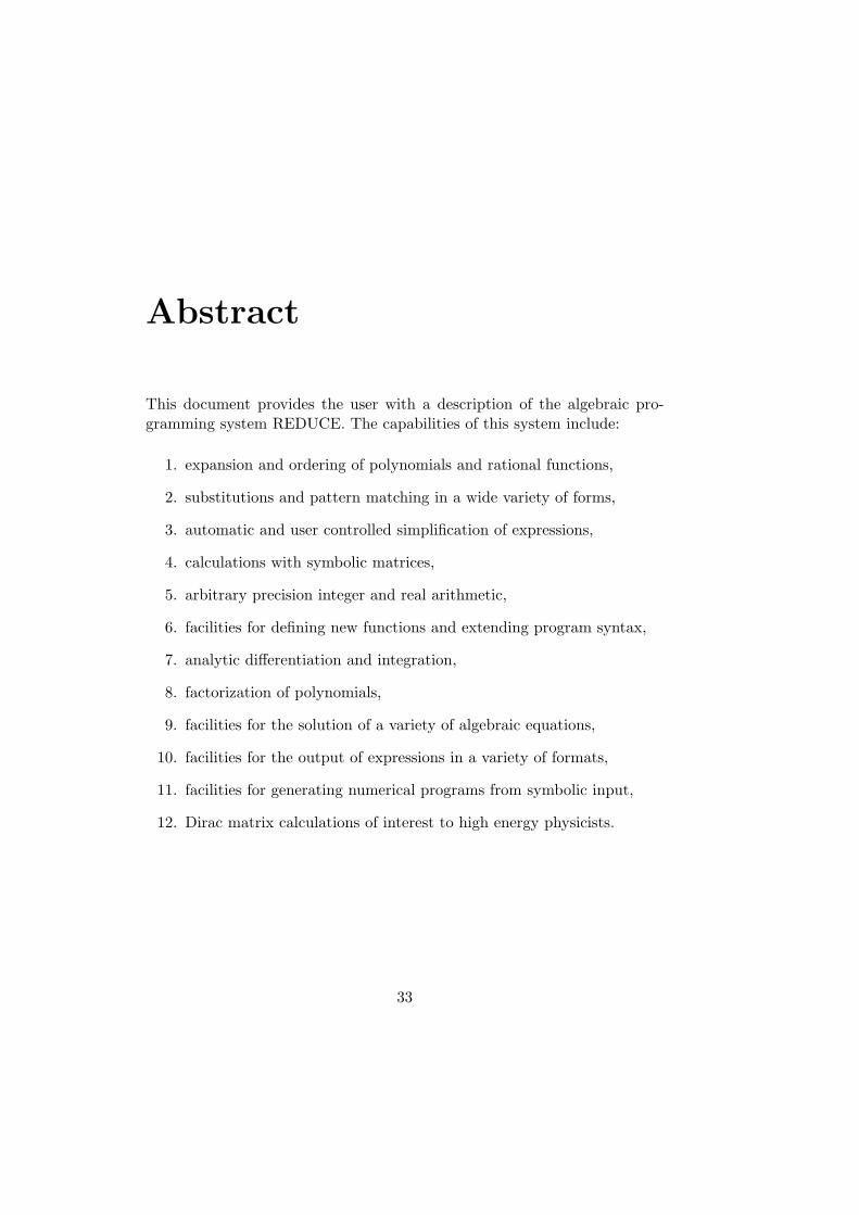
This document provides the user with a description of the algebraic pro-gramming system REDUCE. The capabilities of this system include:
1. expansion and ordering of polynomials and rational functions,
2. substitutions and pattern matching in a wide variety of forms,
3. automatic and user controlled simplification of expressions,
4. calculations with symbolic matrices,
5. arbitrary precision integer and real arithmetic,
6. facilities for defining new functions and extending program syntax,
7. analytic differentiation and integration,
8. factorization of polynomials,
9. facilities for the solution of a variety of algebraic equations,
10. facilities for the output of expressions in a variety of formats,
11. facilities for generating numerical programs from symbolic input,
12. Dirac matrix calculations of interest to high energy physicists.
33

34

Acknowledgment
The production of this version of the manual has been the result of thecontributions of a large number of individuals who have taken the time andeffort to suggest improvements to previous versions, and to draft new sec-tions. Particular thanks are due to Gerry Rayna, who provided a draftrewrite of most of the first half of the manual. Other people who have madesignificant contributions have included John Fitch, Martin Griss, Stan Ka-meny, Jed Marti, Herbert Melenk, Don Morrison, Arthur Norman, EberhardSchrufer, Larry Seward and Walter Tietze. Finally, Richard Hitt produceda TEX version of the REDUCE 3.3 manual, which has been a useful guidefor the production of the LATEX version of this manual.
35

36

Chapter 1
Introductory Information
REDUCE is a system for carrying out algebraic operations accurately, nomatter how complicated the expressions become. It can manipulate poly-nomials in a variety of forms, both expanding and factoring them, and ex-tract various parts of them as required. REDUCE can also do differenti-ation and integration, but we shall only show trivial examples of this inthis introduction. Other topics not considered include the use of arrays, thedefinition of procedures and operators, the specific routines for high energyphysics calculations, the use of files to eliminate repetitious typing and forsaving results, and the editing of the input text.
Also not considered in any detail in this introduction are the many opt-ions that are available for varying computational procedures, output forms,number systems used, and so on.
REDUCE is designed to be an interactive system, so that the user caninput an algebraic expression and see its value before moving on to the nextcalculation. For those systems that do not support interactive use, or forthose calculations, especially long ones, for which a standard script can bedefined, REDUCE can also be used in batch mode. In this case, a sequenceof commands can be given to REDUCE and results obtained without anyuser interaction during the computation.
In this introduction, we shall limit ourselves to the interactive use of RE-DUCE, since this illustrates most completely the capabilities of the system.When REDUCE is called, it begins by printing a banner message like:
REDUCE 3.8, 15-Jul-2003 ...
37
38 CHAPTER 1. INTRODUCTORY INFORMATION
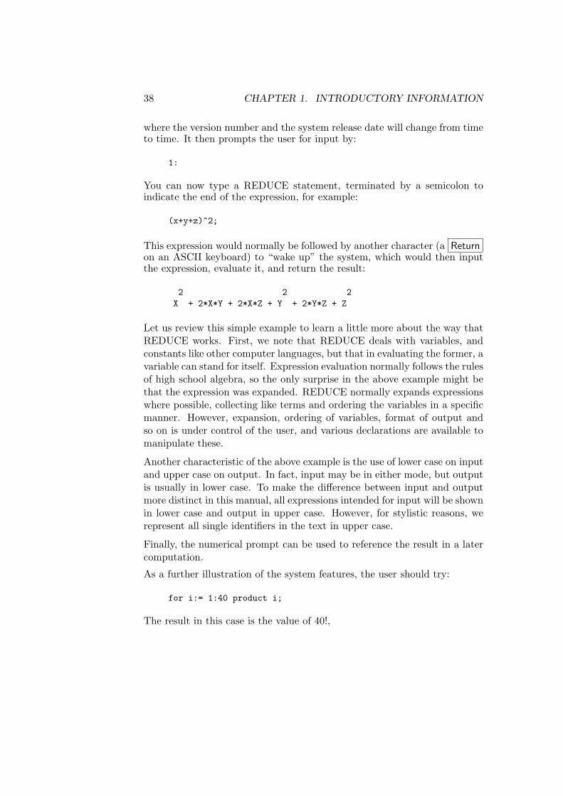
where the version number and the system release date will change from timeto time. It then prompts the user for input by:
1:
You can now type a REDUCE statement, terminated by a semicolon toindicate the end of the expression, for example:
(x+y+z)^2;
This expression would normally be followed by another character (a Returnon an ASCII keyboard) to “wake up” the system, which would then inputthe expression, evaluate it, and return the result:
2 2 2X + 2*X*Y + 2*X*Z + Y + 2*Y*Z + Z
Let us review this simple example to learn a little more about the way thatREDUCE works. First, we note that REDUCE deals with variables, andconstants like other computer languages, but that in evaluating the former, avariable can stand for itself. Expression evaluation normally follows the rulesof high school algebra, so the only surprise in the above example might bethat the expression was expanded. REDUCE normally expands expressionswhere possible, collecting like terms and ordering the variables in a specificmanner. However, expansion, ordering of variables, format of output andso on is under control of the user, and various declarations are available tomanipulate these.
Another characteristic of the above example is the use of lower case on inputand upper case on output. In fact, input may be in either mode, but outputis usually in lower case. To make the difference between input and outputmore distinct in this manual, all expressions intended for input will be shownin lower case and output in upper case. However, for stylistic reasons, werepresent all single identifiers in the text in upper case.
Finally, the numerical prompt can be used to reference the result in a latercomputation.
As a further illustration of the system features, the user should try:
for i:= 1:40 product i;
The result in this case is the value of 40!,

39
815915283247897734345611269596115894272000000000
You can also get the same result by saying
factorial 40;
Since we want exact results in algebraic calculations, it is essential that inte-ger arithmetic be performed to arbitrary precision, as in the above example.Furthermore, the FOR statement in the above is illustrative of a whole rangeof combining forms that REDUCE supports for the convenience of the user.
Among the many options in REDUCE is the use of other number systems,such as multiple precision floating point with any specified number of digits— of use if roundoff in, say, the 100th digit is all that can be tolerated.
In many cases, it is necessary to use the results of one calculation in suc-ceeding calculations. One way to do this is via an assignment for a variable,such as
u := (x+y+z)^2;
If we now use U in later calculations, the value of the right-hand side of theabove will be used.
The results of a given calculation are also saved in the variable WS (forWorkSpace), so this can be used in the next calculation for further process-ing.
For example, the expression
df(ws,x);
following the previous evaluation will calculate the derivative of (x+y+z)^2with respect to X. Alternatively,
int(ws,y);
would calculate the integral of the same expression with respect to y.
REDUCE is also capable of handling symbolic matrices. For example,
matrix m(2,2);
declares m to be a two by two matrix, and

40 CHAPTER 1. INTRODUCTORY INFORMATION
m := mat((a,b),(c,d));
gives its elements values. Expressions that include M and make algebraicsense may now be evaluated, such as 1/m to give the inverse, 2*m - u*m^2to give us another matrix and det(m) to give us the determinant of M.
REDUCE has a wide range of substitution capabilities. The system knowsabout elementary functions, but does not automatically invoke many of theirwell-known properties. For example, products of trigonometrical functionsare not converted automatically into multiple angle expressions, but if theuser wants this, he can say, for example:
(sin(a+b)+cos(a+b))*(sin(a-b)-cos(a-b))where cos(~x)*cos(~y) = (cos(x+y)+cos(x-y))/2,
cos(~x)*sin(~y) = (sin(x+y)-sin(x-y))/2,sin(~x)*sin(~y) = (cos(x-y)-cos(x+y))/2;
where the tilde in front of the variables X and Y indicates that the rulesapply for all values of those variables. The result of this calculation is
-(COS(2*A) + SIN(2*B))
See also the user-contributed packages ASSIST (chapter 23), CAMAL (chap-ter 28) and TRIGSIMP (chapter 85).
Another very commonly used capability of the system, and an illustrationof one of the many output modes of REDUCE, is the ability to outputresults in a FORTRAN compatible form. Such results can then be used ina FORTRAN based numerical calculation. This is particularly useful as away of generating algebraic formulas to be used as the basis of extensivenumerical calculations.
For example, the statements
on fort;df(log(x)*(sin(x)+cos(x))/sqrt(x),x,2);
will result in the output
ANS=(-4.*LOG(X)*COS(X)*X**2-4.*LOG(X)*COS(X)*X+3.*. LOG(X)*COS(X)-4.*LOG(X)*SIN(X)*X**2+4.*LOG(X)*. SIN(X)*X+3.*LOG(X)*SIN(X)+8.*COS(X)*X-8.*COS(X)-8.. *SIN(X)*X-8.*SIN(X))/(4.*SQRT(X)*X**2)

41
These algebraic manipulations illustrate the algebraic mode of REDUCE.REDUCE is based on Standard Lisp. A symbolic mode is also available forexecuting Lisp statements. These statements follow the syntax of Lisp, e.g.
symbolic car ’(a);
Communication between the two modes is possible.
With this simple introduction, you are now in a position to study the ma-terial in the full REDUCE manual in order to learn just how extensive therange of facilities really is. If further tutorial material is desired, the sevenREDUCE Interactive Lessons by David R. Stoutemyer are recommended.These are normally distributed with the system.

42 CHAPTER 1. INTRODUCTORY INFORMATION

Chapter 2
Structure of Programs
A REDUCE program consists of a set of functional commands which areevaluated sequentially by the computer. These commands are built up fromdeclarations, statements and expressions. Such entities are composed ofsequences of numbers, variables, operators, strings, reserved words and de-limiters (such as commas and parentheses), which in turn are sequences ofbasic characters.
2.1 The REDUCE Standard Character Set
The basic characters which are used to build REDUCE symbols are thefollowing:
1. The 26 letters a through z
2. The 10 decimal digits 0 through 9
3. The special characters ! ” $ % ’ ( ) * + , - . / : ; < > = <blank>
With the exception of strings and characters preceded by an exclamationmark, the case of characters is ignored: depending of the underlying LISPthey will all be converted internally into lower case or upper case: ALPHA,Alpha and alpha represent the same symbol. Most implementations allowyou to switch this conversion off. The operating instructions for a particularimplementation should be consulted on this point. For portability, we shalllimit ourselves to the standard character set in this exposition.
43

44 CHAPTER 2. STRUCTURE OF PROGRAMS
2.2 Numbers
There are several different types of numbers available in REDUCE. Integersconsist of a signed or unsigned sequence of decimal digits written without adecimal point, for example:
-2, 5396, +32
In principle, there is no practical limit on the number of digits permittedas exact arithmetic is used in most implementations. (You should howevercheck the specific instructions for your particular system implementation tomake sure that this is true.) For example, if you ask for the value of 22000
you get it displayed as a number of 603 decimal digits, taking up nine linesof output on an interactive display. It should be borne in mind of coursethat computations with such long numbers can be quite slow.
Numbers that aren’t integers are usually represented as the quotient of twointegers, in lowest terms: that is, as rational numbers.
In essentially all versions of REDUCE it is also possible (but not alwaysdesirable!) to ask REDUCE to work with floating point approximations tonumbers again, to any precision. Such numbers are called real. They canbe input in two ways:
1. as a signed or unsigned sequence of any number of decimal digits withan embedded or trailing decimal point.
2. as in 1. followed by a decimal exponent which is written as the letterE followed by a signed or unsigned integer.
e.g. 32. +32.0 0.32E2 and 320.E-1 are all representations of 32.
The declaration SCIENTIFIC NOTATION controls the output format of float-ing point numbers. At the default settings, any number with five or lessdigits before the decimal point is printed in a fixed-point notation, e.g.,12345.6. Numbers with more than five digits are printed in scientific no-tation, e.g., 1.234567E+5. Similarly, by default, any number with elevenor more zeros after the decimal point is printed in scientific notation. Tochange these defaults, SCIENTIFIC NOTATION can be used in one of two ways.SCIENTIFIC NOTATION m;, where m is a positive integer, sets the printingformat so that a number with more than m digits before the decimal point,or m or more zeros after the decimal point, is printed in scientific notation.

2.3. IDENTIFIERS 45
SCIENTIFIC NOTATION m,n, with m and n both positive integers, sets theformat so that a number with more than m digits before the decimal point,or n or more zeros after the decimal point is printed in scientific notation.
CAUTION: The unsigned part of any number may not begin with a dec-imal point, as this causes confusion with the CONS (.) operator, i.e., NOTALLOWED: .5 -.23 +.12; use 0.5 -0.23 +0.12 instead.
2.3 Identifiers
Identifiers in REDUCE consist of one or more alphanumeric characters (i.e.alphabetic letters or decimal digits) the first of which must be alphabetic.The maximum number of characters allowed is implementation dependent,although twenty-four is permitted in most implementations. In addition,the underscore character ( ) is considered a letter if it is within an identifier.For example,
a az p1 q23p a_very_long_variable
are all identifiers, whereas
_a
is not.
A sequence of alphanumeric characters in which the first is a digit is inter-preted as a product. For example, 2ab3c is interpreted as 2*ab3c. Thereis one exception to this: If the first letter after a digit is E, the system willtry to interpret that part of the sequence as a real number, which may failin some cases. For example, 2E12 is the real number 2.0 ∗ 1012, 2e3c is2000.0*C, and 2ebc gives an error.
Special characters, such as −, *, and blank, may be used in identifiers too,even as the first character, but each must be preceded by an exclamationmark in input. For example:
light!-years d!*!*n good! morning!$sign !5goldrings
CAUTION: Many system identifiers have such special characters in theirnames (especially * and =). If the user accidentally picks the name of oneof them for his own purposes it may have catastrophic consequences for his
46 CHAPTER 2. STRUCTURE OF PROGRAMS
REDUCE run. Users are therefore advised to avoid such names.
Identifiers are used as variables, labels and to name arrays, operators andprocedures.
Restrictions
The reserved words listed in another section may not be used as identifiers.No spaces may appear within an identifier, and an identifier may not extendover a line of text. (Hyphenation of an identifier, by using a reserved char-acter as a hyphen before an end-of-line character is possible in some versionsof REDUCE).
2.4 Variables
Every variable is named by an identifier, and is given a specific type. Thetype is of no concern to the ordinary user. Most variables are allowed tohave the default type, called scalar. These can receive, as values, the rep-resentation of any ordinary algebraic expression. In the absence of such avalue, they stand for themselves.
Reserved Variables
Several variables in REDUCE have particular properties which should notbe changed by the user. These variables include:
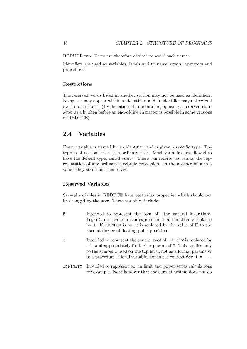
E Intended to represent the base of the natural logarithms.log(e), if it occurs in an expression, is automatically replacedby 1. If ROUNDED is on, E is replaced by the value of E to thecurrent degree of floating point precision.
I Intended to represent the square root of −1. i^2 is replaced by−1, and appropriately for higher powers of I. This applies onlyto the symbol I used on the top level, not as a formal parameterin a procedure, a local variable, nor in the context for i:= ...
INFINITY Intended to represent ∞ in limit and power series calculationsfor example. Note however that the current system does not do
2.5. STRINGS 47
proper arithmetic on ∞. For example, infinity + infinityis 2*infinity.
NIL In REDUCE (algebraic mode only) taken as a synonym for zero.Therefore NIL cannot be used as a variable.
PI Intended to represent the circular constant. With ROUNDED on,it is replaced by the value of π to the current degree of floatingpoint precision.
T Should not be used as a formal parameter or local variable inprocedures, since conflict arises with the symbolic mode meaningof T as true.
Other reserved variables, such as LOW POW, described in other sections, arelisted in Appendix A.
Using these reserved variables inappropriately will lead to errors.
There are also internal variables used by REDUCE that have similar re-strictions. These usually have an asterisk in their names, so it is unlikely acasual user would use one. An example of such a variable is K!* used in theasymptotic command package.
Certain words are reserved in REDUCE. They may only be used in the man-ner intended. A list of these is given in the section “Reserved Identifiers”.There are, of course, an impossibly large number of such names to keep inmind. The reader may therefore want to make himself a copy of the list,deleting the names he doesn’t think he is likely to use by mistake.
2.5 Strings
Strings are used in WRITE statements, in other output statements (such aserror messages), and to name files. A string consists of any number ofcharacters enclosed in double quotes. For example:
"A String".
Lower case characters within a string are not converted to upper case.
The string "" represents the empty string. A double quote may be includedin a string by preceding it by another double quote. Thus "a""b" is thestring a"b, and """" is the string ".

48 CHAPTER 2. STRUCTURE OF PROGRAMS
2.6 Comments
Text can be included in program listings for the convenience of human read-ers, in such a way that REDUCE pays no attention to it. There are twoways to do this:
1. Everything from the word COMMENT to the next statement terminator,normally ; or $, is ignored. Such comments can be placed anywhere ablank could properly appear. (Note that END and >> are not treatedas COMMENT delimiters!)
2. Everything from the symbol % to the end of the line on which it appearsis ignored. Such comments can be placed as the last part of any line.Statement terminators have no special meaning in such comments.Remember to put a semicolon before the % if the earlier part of theline is intended to be so terminated. Remember also to begin each lineof a multi-line % comment with a % sign.
2.7 Operators
Operators in REDUCE are specified by name and type. There are twotypes, infix and prefix. Operators can be purely abstract, just symbolswith no properties; they can have values assigned (using := or simple LETdeclarations) for specific arguments; they can have properties declared forsome collection of arguments (using more general LET declarations); or theycan be fully defined (usually by a procedure declaration).
Infix operators have a definite precedence with respect to one another, andnormally occur between their arguments. For example:
a + b - c (spaces optional)x<y and y=z (spaces required where shown)
Spaces can be freely inserted between operators and variables or operatorsand operators. They are required only where operator names are spelled outwith letters (such as the AND in the example) and must be unambiguouslyseparated from another such or from a variable (like Y). Wherever one spacecan be used, so can any larger number.
2.7. OPERATORS 49
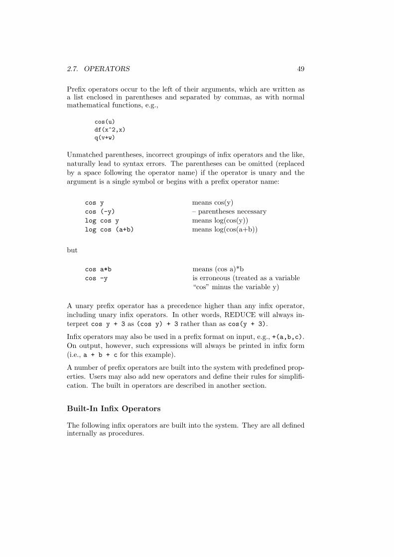
Prefix operators occur to the left of their arguments, which are written asa list enclosed in parentheses and separated by commas, as with normalmathematical functions, e.g.,
cos(u)df(x^2,x)q(v+w)
Unmatched parentheses, incorrect groupings of infix operators and the like,naturally lead to syntax errors. The parentheses can be omitted (replacedby a space following the operator name) if the operator is unary and theargument is a single symbol or begins with a prefix operator name:
cos y means cos(y)cos (-y) – parentheses necessarylog cos y means log(cos(y))log cos (a+b) means log(cos(a+b))
but
cos a*b means (cos a)*bcos -y is erroneous (treated as a variable
“cos” minus the variable y)
A unary prefix operator has a precedence higher than any infix operator,including unary infix operators. In other words, REDUCE will always in-terpret cos y + 3 as (cos y) + 3 rather than as cos(y + 3).
Infix operators may also be used in a prefix format on input, e.g., +(a,b,c).On output, however, such expressions will always be printed in infix form(i.e., a + b + c for this example).
A number of prefix operators are built into the system with predefined prop-erties. Users may also add new operators and define their rules for simplifi-cation. The built in operators are described in another section.
Built-In Infix Operators
The following infix operators are built into the system. They are all definedinternally as procedures.
50 CHAPTER 2. STRUCTURE OF PROGRAMS
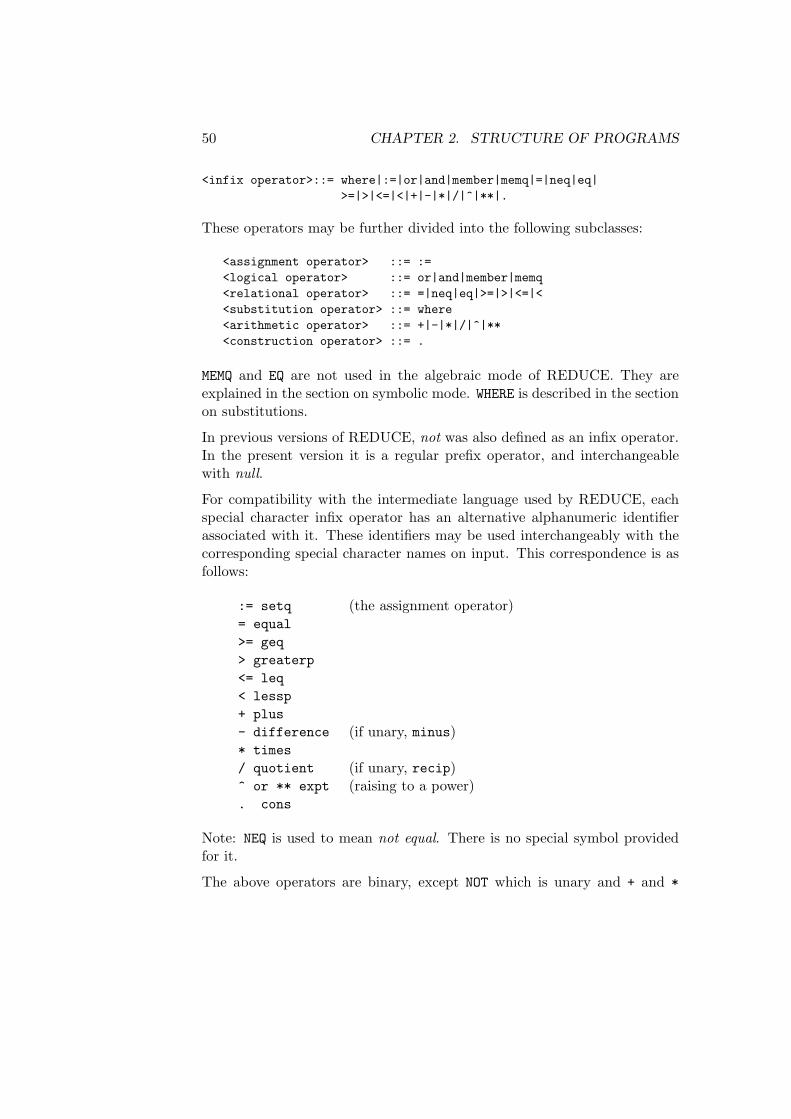
<infix operator>::= where|:=|or|and|member|memq|=|neq|eq|>=|>|<=|<|+|-|*|/|^|**|.
These operators may be further divided into the following subclasses:
<assignment operator> ::= :=<logical operator> ::= or|and|member|memq<relational operator> ::= =|neq|eq|>=|>|<=|<<substitution operator> ::= where<arithmetic operator> ::= +|-|*|/|^|**<construction operator> ::= .
MEMQ and EQ are not used in the algebraic mode of REDUCE. They areexplained in the section on symbolic mode. WHERE is described in the sectionon substitutions.
In previous versions of REDUCE, not was also defined as an infix operator.In the present version it is a regular prefix operator, and interchangeablewith null.
For compatibility with the intermediate language used by REDUCE, eachspecial character infix operator has an alternative alphanumeric identifierassociated with it. These identifiers may be used interchangeably with thecorresponding special character names on input. This correspondence is asfollows:
:= setq (the assignment operator)= equal>= geq> greaterp<= leq< lessp+ plus- difference (if unary, minus)* times/ quotient (if unary, recip)^ or ** expt (raising to a power). cons
Note: NEQ is used to mean not equal. There is no special symbol providedfor it.
The above operators are binary, except NOT which is unary and + and *

2.7. OPERATORS 51
which are nary (i.e., taking an arbitrary number of arguments). In addition,- and / may be used as unary operators, e.g., /2 means the same as 1/2.Any other operator is parsed as a binary operator using a left associationrule. Thus a/b/c is interpreted as (a/b)/c. There are two exceptions tothis rule: := and . are right associative. Example: a:=b:=c is interpretedas a:=(b:=c). Unlike ALGOL and PASCAL, ^ is left associative. In otherwords, a^b^c is interpreted as (a^b)^c.
The operators <, <=, >, >= can only be used for making comparisons be-tween numbers. No meaning is currently assigned to this kind of comparisonbetween general expressions.
Parentheses may be used to specify the order of combination. If parenthesesare omitted then this order is by the ordering of the precedence list definedby the right-hand side of the <infix operator> table at the beginning ofthis section, from lowest to highest. In other words, WHERE has the lowestprecedence, and . (the dot operator) the highest.

52 CHAPTER 2. STRUCTURE OF PROGRAMS

Chapter 3
Expressions
REDUCE expressions may be of several types and consist of sequences ofnumbers, variables, operators, left and right parentheses and commas. Themost common types are as follows:
3.1 Scalar Expressions
Using the arithmetic operations + - * / ^ (power) and parentheses, scalarexpressions are composed from numbers, ordinary “scalar” variables (iden-tifiers), array names with subscripts, operator or procedure names with ar-guments and statement expressions.
Examples:
xx^3 - 2*y/(2*z^2 - df(x,z))(p^2 + m^2)^(1/2)*log (y/m)a(5) + b(i,q)
The symbol ** may be used as an alternative to the caret symbol (^) forforming powers, particularly in those systems that do not support a caretsymbol.
Statement expressions, usually in parentheses, can also form part of a scalarexpression, as in the example
w + (c:=x+y) + z .
53

54 CHAPTER 3. EXPRESSIONS
When the algebraic value of an expression is needed, REDUCE determinesit, starting with the algebraic values of the parts, roughly as follows:
Variables and operator symbols with an argument list have the algebraicvalues they were last assigned, or if never assigned stand for themselves.However, array elements have the algebraic values they were last assigned,or, if never assigned, are taken to be 0.
Procedures are evaluated with the values of their actual parameters.
In evaluating expressions, the standard rules of algebra are applied. Unfor-tunately, this algebraic evaluation of an expression is not as unambiguousas is numerical evaluation. This process is generally referred to as “simpli-fication” in the sense that the evaluation usually but not always produces asimplified form for the expression.
There are many options available to the user for carrying out such simplifi-cation. If the user doesn’t specify any method, the default method is used.The default evaluation of an expression involves expansion of the expressionand collection of like terms, ordering of the terms, evaluation of derivativesand other functions and substitution for any expressions which have valuesassigned or declared (see assignments and LET statements). In many cases,this is all that the user needs.
The declarations by which the user can exercise some control over the wayin which the evaluation is performed are explained in other sections. Forexample, if a real (floating point) number is encountered during evaluation,the system will normally convert it into a ratio of two integers. If theuser wants to use real arithmetic, he can effect this by the command onrounded;. Other modes for coefficient arithmetic are described elsewhere.
If an illegal action occurs during evaluation (such as division by zero) orfunctions are called with the wrong number of arguments, and so on, anappropriate error message is generated.
3.2 Integer Expressions
These are expressions which, because of the values of the constants andvariables in them, evaluate to whole numbers.
Examples:
2, 37 * 999, (x + 3)^2 - x^2 - 6*x
3.3. BOOLEAN EXPRESSIONS 55
are obviously integer expressions.
j + k - 2 * j^2
is an integer expression when J and K have values that are integers, or if notintegers are such that “the variables and fractions cancel out”, as in
k - 7/3 - j + 2/3 + 2*j^2.
3.3 Boolean Expressions
A boolean expression returns a truth value. In the algebraic mode of RE-DUCE, boolean expressions have the syntactical form:
<expression> <relational operator> <expression>
or
<boolean operator> (<arguments>)
or
<boolean expression> <logical operator><boolean expression>.
Parentheses can also be used to control the precedence of expressions.
In addition to the logical and relational operators defined earlier as infixoperators, the following boolean operators are also defined:

56 CHAPTER 3. EXPRESSIONS
EVENP(U) determines if the number U is even or not;
FIXP(U) determines if the expression U is integer or not;
FREEOF(U,V) determines if the expression U does not contain thekernel V anywhere in its structure;
NUMBERP(U) determines if U is a number or not;
ORDP(U,V) determines if U is ordered ahead of V by some canon-ical ordering (based on the expression structure andan internal ordering of identifiers);
PRIMEP(U) true if U is a prime object, i.e., any object other than0 and plus or minus 1 which is only exactly divisibleby itself or a unit.
Examples:
j<1x>0 or x=-2numberp xfixp x and evenp xnumberp x and x neq 0
Boolean expressions can only appear directly within IF, FOR, WHILE, andUNTIL statements, as described in other sections. Such expressions cannotbe used in place of ordinary algebraic expressions, or assigned to a variable.
NB: For those familiar with symbolic mode, the meaning of some of theseoperators is different in that mode. For example, NUMBERP is true only forintegers and reals in symbolic mode.
When two or more boolean expressions are combined with AND, they areevaluated one by one until a false expression is found. The rest are notevaluated. Thus
numberp x and numberp y and x>y
does not attempt to make the x>y comparison unless X and Y are both
3.4. EQUATIONS 57
verified to be numbers.
Similarly, evaluation of a sequence of boolean expressions connected by ORstops as soon as a true expression is found.
NB: In a boolean expression, and in a place where a boolean expressionis expected, the algebraic value 0 is interpreted as false, while all otheralgebraic values are converted to true. So in algebraic mode a procedurecan be written for direct usage in boolean expressions, returning say 1 or 0as its value as in
procedure polynomialp(u,x);if den(u)=1 and deg(u,x)>=1 then 1 else 0;
One can then use this in a boolean construct, such as
if polynomialp(q,z) and not polynomialp(q,y) then ...
In addition, any procedure that does not have a defined return value (forexample, a block without a RETURN statement in it) has the boolean valuefalse.
3.4 Equations
Equations are a particular type of expression with the syntax
<expression> = <expression>.
In addition to their role as boolean expressions, they can also be used asarguments to several operators (e.g., SOLVE), and can be returned as values.
Under normal circumstances, the right-hand-side of the equation is evaluatedbut not the left-hand-side. This also applies to any substitutions made bythe SUB operator. If both sides are to be evaluated, the switch EVALLHSEQPshould be turned on.
To facilitate the handling of equations, two selectors, LHS and RHS, whichreturn the left- and right-hand sides of a equation respectively, are provided.For example,
lhs(a+b=c) -> a+band

58 CHAPTER 3. EXPRESSIONS
rhs(a+b=c) -> c.
3.5 Proper Statements as Expressions
Several kinds of proper statements deliver an algebraic or numerical resultof some kind, which can in turn be used as an expression or part of anexpression. For example, an assignment statement itself has a value, namelythe value assigned. So
2 * (x := a+b)
is equal to 2*(a+b), as well as having the “side-effect” of assigning the valuea+b to X. In context,
y := 2 * (x := a+b);
sets X to a+b and Y to 2*(a+b).
The sections on the various proper statement types indicate which of thesestatements are also useful as expressions.

Chapter 4
Lists
A list is an object consisting of a sequence of other objects (including liststhemselves), separated by commas and surrounded by braces. Examples oflists are:
a,b,c
1,a-b,c=d
a,b,c,d,e.
The empty list is represented as
.
4.1 Operations on Lists
Several operators in the system return their results as lists, and a user cancreate new lists using braces and commas. Alternatively, one can use theoperator LIST to construct a list. An important class of operations on listsare MAP and SELECT operations. For details, please refer to the chapterson MAP, SELECT and the FOR command. See also the documentation onthe ASSIST package.
To facilitate the use of lists, a number of operators are also available formanipulating them. PART(<list>,n) for example will return the nth ele-ment of a list. LENGTH will return the length of a list. Several operators are
59

60 CHAPTER 4. LISTS
also defined uniquely for lists. For those familiar with them, these operatorsin fact mirror the operations defined for Lisp lists. These operators are asfollows:
4.1.1 LIST
The operator LIST is an alternative to the usage of curly brackets. LISTaccepts an arbitrary number of arguments and returns a list of its argu-ments. This operator is useful in cases where operators have to be passedas arguments. E.g.,
list(a,list(list(b,c),d),e); -> a,b,c,d,e
4.1.2 FIRST
This operator returns the first member of a list. An error occurs if theargument is not a list, or the list is empty.
4.1.3 SECOND
SECOND returns the second member of a list. An error occurs if the argumentis not a list or has no second element.
4.1.4 THIRD
This operator returns the third member of a list. An error occurs if theargument is not a list or has no third element.
4.1.5 REST
REST returns its argument with the first element removed. An error occursif the argument is not a list, or is empty.
4.1.6 . (Cons) Operator
This operator adds (“conses”) an expression to the front of a list. Forexample:

4.1. OPERATIONS ON LISTS 61
a . b,c -> a,b,c.
4.1.7 APPEND
This operator appends its first argument to its second to form a new list.Examples:
append(a,b,c,d) -> a,b,c,dappend(a,b,c,d) -> a,b,c,d.
4.1.8 REVERSE
The operator REVERSE returns its argument with the elements in the reverseorder. It only applies to the top level list, not any lower level lists that mayoccur. Examples are:
reverse(a,b,c) -> c,b,areverse(a,b,c,d) -> d,a,b,c.
4.1.9 List Arguments of Other Operators
If an operator other than those specifically defined for lists is given a singleargument that is a list, then the result of this operation will be a list in whichthat operator is applied to each element of the list. For example, the resultof evaluating loga,b,c is the expression LOG(A),LOG(B),LOG(C).There are two ways to inhibit this operator distribution. Firstly, the switchLISTARGS, if on, will globally inhibit such distribution. Secondly, one caninhibit this distribution for a specific operator by the declaration LISTARGP.For example, with the declaration listargp log, loga,b,c would eval-uate to LOG(A,B,C).If an operator has more than one argument, no such distribution occurs.
4.1.10 Caveats and Examples
Some of the natural list operations such as member or delete are availableonly after loading the package ASSIST.
Please note that a non-list as second argument to CONS (a ”dotted pair”in LISP terms) is not allowed and causes an ”invalid as list” error.

62 CHAPTER 4. LISTS
a := 17 . 4;
***** 17 4 invalid as list
Also, the initialization of a scalar variable is not the empty list – one has toset list type variables explicitly, as in the following example:
load_package assist;
procedure lotto (n,m);begin scalar list_1_n, luckies, hit;
list_1_n := ;luckies := ;for k:=1:n do list_1_n := k . list_1_n;for k:=1:m do
<< hit := part(list_1_n,random(n-k+1) + 1);list_1_n := delete(hit,list_1_n);luckies := hit . luckies >>;
return luckies;end; % In Germany, try lotto (49,6);
Another example: Find all coefficients of a multivariate polynomial withrespect to a list of variables:
procedure allcoeffs(q,lis); % q : polynomial, lis: list of varsallcoeffs1 (list q,lis);
procedure allcoeffs1(q,lis);if lis= then q elseallcoeffs1(foreach qq in q join coeff(qq,first lis),rest lis);

Chapter 5
Statements
A statement is any combination of reserved words and expressions, and hasthe syntax
<statement> ::= <expression>|<proper statement>
A REDUCE program consists of a series of commands which are statementsfollowed by a terminator:
<terminator> ::= ;|$
The division of the program into lines is arbitrary. Several statements can beon one line, or one statement can be freely broken onto several lines. If theprogram is run interactively, statements ending with ; or $ are not processeduntil an end-of-line character is encountered. This character can vary fromsystem to system, but is normally the Return key on an ASCII terminal.Specific systems may also use additional keys as statement terminators.
If a statement is a proper statement, the appropriate action takes place.
Depending on the nature of the proper statement some result or responsemay or may not be printed out, and the response may or may not dependon the terminator used.
If a statement is an expression, it is evaluated. If the terminator is a semi-colon, the result is printed. If the terminator is a dollar sign, the result isnot printed. Because it is not usually possible to know in advance how largean expression will be, no explicit format statements are offered to the user.However, a variety of output declarations are available so that the output
63

64 CHAPTER 5. STATEMENTS
can be produced in different forms. These output declarations are explainedin Section 8.3.3.
The following sub-sections describe the types of proper statements in RE-DUCE.
5.1 Assignment Statements
These statements have the syntax
<assignment statement> ::= <expression> := <expression>
The <expression> on the left side is normally the name of a variable, anoperator symbol with its list of arguments filled in, or an array name withthe proper number of integer subscript values within the array bounds. Forexample:
a1 := b + ch(l,m) := x-2*y (where h is an operator)k(3,5) := x-2*y (where k is a 2-dim. array)
More general assignments such as a+b := c are also allowed. The effect ofthese is explained in Section 10.2.5.
An assignment statement causes the expression on the right-hand-side to beevaluated. If the left-hand-side is a variable, the value of the right-hand-side is assigned to that unevaluated variable. If the left-hand-side is anoperator or array expression, the arguments of that operator or array areevaluated, but no other simplification done. The evaluated right-hand-sideis then assigned to the resulting expression. For example, if A is a single-dimensional array, a(1+1) := b assigns the value B to the array elementa(2).
If a semicolon is used as the terminator when an assignment is issued as acommand (i.e. not as a part of a group statement or procedure or othersimilar construct), the left-hand side symbol of the assignment statement isprinted out, followed by a “:=”, followed by the value of the expression onthe right.
It is also possible to write a multiple assignment statement:
<expression> := ... := <expression> := <expression>

5.2. GROUP STATEMENTS 65
In this form, each <expression> but the last is set to the value of thelast <expression>. If a semicolon is used as a terminator, each expressionexcept the last is printed followed by a “:=” ending with the value of thelast expression.
5.1.1 Set Statement
In some cases, it is desirable to perform an assignment in which both theleft- and right-hand sides of an assignment are evaluated. In this case, theSET statement can be used with the syntax:
SET(<expression>,<expression>);
For example, the statements
j := 23;set(mkid(a,j),x);
assigns the value X to A23.
5.2 Group Statements
The group statement is a construct used where REDUCE expects a singlestatement, but a series of actions needs to be performed. It is formed byenclosing one or more statements (of any kind) between the symbols <<and >>, separated by semicolons or dollar signs – it doesn’t matter which.The statements are executed one after another.
Examples will be given in the sections on IF and other types of statementsin which the << . . .>> construct is useful.
If the last statement in the enclosed group has a value, then that is also thevalue of the group statement. Care must be taken not to have a semicolonor dollar sign after the last grouped statement, if the value of the group isrelevant: such an extra terminator causes the group to have the value NILor zero.

66 CHAPTER 5. STATEMENTS
5.3 Conditional Statements
The conditional statement has the following syntax:
<conditional statement> ::=IF <boolean expression> THEN <statement> [ELSE <statement>]
The boolean expression is evaluated. If this is true, the first <statement>is executed. If it is false, the second is.
Examples:
if x=5 then a:=b+c else d:=e+f
if x=5 and numberp ythen <<ff:=q1; a:=b+c>>else <<ff:=q2; d:=e+f>>
Note the use of the group statement.Conditional statements associate to the right; i.e.,
IF <a> THEN <b> ELSE IF <c> THEN <d> ELSE <e>
is equivalent to:
IF <a> THEN <b> ELSE (IF <c> THEN <d> ELSE <e>)
In addition, the construction
IF <a> THEN IF <b> THEN <c> ELSE <d>
parses as
IF <a> THEN (IF <b> THEN <c> ELSE <d>).
If the value of the conditional statement is of primary interest, it is oftencalled a conditional expression instead. Its value is the value of whicheverstatement was executed. (If the executed statement has no value, the condi-tional expression has no value or the value 0, depending on how it is used.)
Examples:
a:=if x<5 then 123 else 456;

5.4. FOR STATEMENTS 67
b:=u + v^(if numberp z then 10*z else 1) + w;
If the value is of no concern, the ELSE clause may be omitted if no action isrequired in the false case.
if x=5 then a:=b+c;
Note: As explained in Section 3.3,a if a scalar or numerical expression isused in place of the boolean expression – for example, a variable is writtenthere – the true alternative is followed unless the expression has the value0.
5.4 FOR Statements
The FOR statement is used to define a variety of program loops. Its generalsyntax is as follows:
FOR
〈var〉 := 〈number〉STEP 〈number〉 UNTIL
:
〈number〉
EACH 〈var〉INON
〈list〉
〈action〉 〈exprn〉
where
〈action〉 ::= do|product|sum|collect|join.
The assignment form of the FOR statement defines an iteration over theindicated numerical range. If expressions that do not evaluate to numbersare used in the designated places, an error will result.
The FOR EACH form of the FOR statement is designed to iterate down a list.Again, an error will occur if a list is not used.
The action DO means that <exprn> is simply evaluated and no value kept;the statement returning 0 in this case (or no value at the top level). COLLECTmeans that the results of evaluating <exprn> each time are linked togetherto make a list, and JOIN means that the values of <exprn> are themselveslists that are joined to make one list (similar to CONC in Lisp). Finally,PRODUCT and SUM form the respective combined value out of the values of<exprn>.
In all cases, <exprn> is evaluated algebraically within the scope of the cur-rent value of <var>. If <action> is DO, then nothing else happens. In other

68 CHAPTER 5. STATEMENTS
cases, <action> is a binary operator that causes a result to be built up andreturned by FOR. In those cases, the loop is initialized to a default value (0for SUM, 1 for PRODUCT, and an empty list for the other actions). The testfor the end condition is made before any action is taken. As in Pascal, ifthe variable is out of range in the assignment case, or the <list> is emptyin the FOR EACH case, <exprn> is not evaluated at all.
Examples:
1. If A, B have been declared to be arrays, the following stores 52 through102 in A(5) through A(10), and at the same time stores the cubes inthe B array:
for i := 5 step 1 until 10 do <<a(i):=i^2; b(i):=i^3>>
2. As a convenience, the common construction
STEP 1 UNTIL
may be abbreviated to a colon. Thus, instead of the above we couldwrite:
for i := 5:10 do <<a(i):=i^2; b(i):=i^3>>
3. The following sets C to the sum of the squares of 1,3,5,7,9; and D tothe expression x*(x+1)*(x+2)*(x+3)*(x+4):
c := for j:=1 step 2 until 9 sum j^2;d := for k:=0 step 1 until 4 product (x+k);
4. The following forms a list of the squares of the elements of the lista,b,c:
for each x in a,b,c collect x^2;
5. The following forms a list of the listed squares of the elements of thelist a,b,c (i.e., A^2,B^2,C^2):
for each x in a,b,c collect x^2;
6. The following also forms a list of the squares of the elements of thelist a,b,c, since the JOIN operation joins the individual lists intoone list:
5.5. WHILE . . . DO 69
for each x in a,b,c join x^2;
The control variable used in the FOR statement is actually a new variable,not related to the variable of the same name outside the FOR statement. Inother words, executing a statement for i:= . . . doesn’t change the system’sassumption that i2 = −1. Furthermore, in algebraic mode, the value of thecontrol variable is substituted in <exprn> only if it occurs explicitly in thatexpression. It will not replace a variable of the same name in the value ofthat expression. For example:
b := a; for a := 1:2 do write b;
prints A twice, not 1 followed by 2.
5.5 WHILE . . . DO
The FOR ...DO feature allows easy coding of a repeated operation in whichthe number of repetitions is known in advance. If the criterion for repetitionis more complicated, WHILE ...DO can often be used. Its syntax is:
WHILE <boolean expression> DO <statement>
The WHILE ...DO controls the single statement following DO. If several state-ments are to be repeated, as is almost always the case, they must be groupedusing the << . . .>> or BEGIN ...END as in the example below.
The WHILE condition is tested each time before the action following the DO isattempted. If the condition is false to begin with, the action is not performedat all. Make sure that what is to be tested has an appropriate value initially.
Example:
Suppose we want to add up a series of terms, generated one by one, until wereach a term which is less than 1/1000 in value. For our simple example, letus suppose the first term equals 1 and each term is obtained from the onebefore by taking one third of it and adding one third its square. We wouldwrite:
ex:=0; term:=1;while num(term - 1/1000) >= 0 do
<<ex := ex+term; term:=(term + term^2)/3>>;ex;

70 CHAPTER 5. STATEMENTS
As long as TERM is greater than or equal to (>=) 1/1000 it will be added toEX and the next TERM calculated. As soon as TERM becomes less than 1/1000the WHILE test fails and the TERM will not be added.
5.6 REPEAT . . . UNTIL
REPEAT ...UNTIL is very similar in purpose to WHILE ...DO. Its syntax is:
REPEAT <statement> UNTIL <boolean expression>
(PASCAL users note: Only a single statement – usually a group statement– is allowed between the REPEAT and the UNTIL.)
There are two essential differences:
1. The test is performed after the controlled statement (or group of state-ments) is executed, so the controlled statement is always executed atleast once.
2. The test is a test for when to stop rather than when to continue, soits “polarity” is the opposite of that in WHILE ...DO.
As an example, we rewrite the example from the WHILE ...DO section:
ex:=0; term:=1;repeat <<ex := ex+term; term := (term + term^2)/3>>
until num(term - 1/1000) < 0;ex;
In this case, the answer will be the same as before, because in neither caseis a term added to EX which is less than 1/1000.
5.7 Compound Statements
Often the desired process can best (or only) be described as a series ofsteps to be carried out one after the other. In many cases, this can beachieved by use of the group statement. However, each step often providessome intermediate result, until at the end we have the final result wanted.Alternatively, iterations on the steps are needed that are not possible with

5.7. COMPOUND STATEMENTS 71
constructs such as WHILE or REPEAT statements. In such cases the stepsof the process must be enclosed between the words BEGIN and END formingwhat is technically called a block or compound statement. Such a compoundstatement can in fact be used wherever a group statement appears. Theconverse is not true: BEGIN ...END can be used in ways that << . . .>>cannot.
If intermediate results must be formed, local variables must be provided inwhich to store them. Local means that their values are deleted as soon asthe block’s operations are complete, and there is no conflict with variablesoutside the block that happen to have the same name. Local variables arecreated by a SCALAR declaration immediately after the BEGIN:
scalar a,b,c,z;
If more convenient, several SCALAR declarations can be given one after an-other:
scalar a,b,c;scalar z;
In place of SCALAR one can also use the declarations INTEGER or REAL. Inthe present version of REDUCE variables declared INTEGER are expectedto have only integer values, and are initialized to 0. REAL variables on theother hand are currently treated as algebraic mode SCALARs.
CAUTION: INTEGER, REAL and SCALAR declarations can only be given im-mediately after a BEGIN. An error will result if they are used after otherstatements in a block (including ARRAY and OPERATOR declarations, whichare global in scope), or outside the top-most block (e.g., at the top level). Allvariables declared SCALAR are automatically initialized to zero in algebraicmode (NIL in symbolic mode).
Any symbols not declared as local variables in a block refer to the variables ofthe same name in the current calling environment. In particular, if they arenot so declared at a higher level (e.g., in a surrounding block or as parametersin a calling procedure), their values can be permanently changed.
Following the SCALAR declaration(s), if any, write the statements to be exe-cuted, one after the other, separated by delimiters (e.g., ; or $) (it doesn’tmatter which). However, from a stylistic point of view, ; is preferred.
The last statement in the body, just before END, need not have a terminator(since the BEGIN ...END are in a sense brackets confining the block state-

72 CHAPTER 5. STATEMENTS
ments). The last statement must also be the command RETURN followed bythe variable or expression whose value is to be the value returned by theprocedure. If the RETURN is omitted (or nothing is written after the wordRETURN) the procedure will have no value or the value zero, depending onhow it is used (and NIL in symbolic mode). Remember to put a terminatorafter the END.
Example:
Given a previously assigned integer value for N, the following block willcompute the Legendre polynomial of degree N in the variable X:
begin scalar seed,deriv,top,fact;seed:=1/(y^2 - 2*x*y +1)^(1/2);deriv:=df(seed,y,n);top:=sub(y=0,deriv);fact:=for i:=1:n product i;return top/fact
end;
5.7.1 Compound Statements with GO TO
It is possible to have more complicated structures inside the BEGIN ...ENDbrackets than indicated in the previous example. That the individual linesof the program need not be assignment statements, but could be almostany other kind of statement or command, needs no explanation. For exam-ple, conditional statements, and WHILE and REPEAT constructions, have anobvious role in defining more intricate blocks.
If these structured constructs don’t suffice, it is possible to use labels andGO TOs within a compound statement, and also to use RETURN in placeswithin the block other than just before the END. The following subsectionsdiscuss these matters in detail. For many readers the following example,presenting one possible definition of a process to calculate the factorial of Nfor preassigned N will suffice:
Example:
begin scalar m;m:=1;
l: if n=0 then return m;m:=m*n;n:=n-1;

5.7. COMPOUND STATEMENTS 73
go to lend;
5.7.2 Labels and GO TO Statements
Within a BEGIN ...END compound statement it is possible to label state-ments, and transfer to them out of sequence using GO TO statements. Onlystatements on the top level inside compound statements can be labeled, notones inside subsidiary constructions like << . . .>>, IF . . . THEN . . . , WHILE. . . DO . . . , etc.
Labels and GO TO statements have the syntax:
<go to statement> ::= GO TO <label> | GOTO <label><label> ::= <identifier><labeled statement> ::= <label>:<statement>
Note that statement names cannot be used as labels.
While GO TO is an unconditional transfer, it is frequently used in conditionalstatements such as
if x>5 then go to abcd;
giving the effect of a conditional transfer.
Transfers using GO TOs can only occur within the block in which the GOTO is used. In other words, you cannot transfer from an inner block to anouter block using a GO TO. However, if a group statement occurs within acompound statement, it is possible to jump out of that group statement toa point within the compound statement using a GO TO.
5.7.3 RETURN Statements
The value corresponding to a BEGIN ...END compound statement, such asa procedure body, is normally 0 (NIL in symbolic mode). By executing aRETURN statement in the compound statement a different value can be re-turned. After a RETURN statement is executed, no further statements withinthe compound statement are executed.
Examples:

74 CHAPTER 5. STATEMENTS
return x+y;return m;return;
Note that parentheses are not required around the x+y, although they arepermitted. The last example is equivalent to return 0 or return nil,depending on whether the block is used as part of an expression or not.
Since RETURN actually moves up only one block level, in a sense the casualuser is not expected to understand, we tabulate some cautions concerningits use.
1. RETURN can be used on the top level inside the compound statement,i.e. as one of the statements bracketed together by the BEGIN ...END
2. RETURN can be used within a top level << . . .>> construction withinthe compound statement. In this case, the RETURN transfers controlout of both the group statement and the compound statement.
3. RETURN can be used within an IF . . . THEN . . . ELSE . . . on the top levelwithin the compound statement.
NOTE: At present, there is no construct provided to permit early termina-tion of a FOR, WHILE, or REPEAT statement. In particular, the use of RETURNin such cases results in a syntax error. For example,
begin scalar y;y := for i:=0:99 do if a(i)=x then return b(i);...
will lead to an error.

Chapter 6
Commands and Declarations
A command is an order to the system to do something. Some commandscause visible results (such as calling for input or output); others, usuallycalled declarations, set options, define properties of variables, or define pro-cedures. Commands are formally defined as a statement followed by a ter-minator
<command> ::= <statement> <terminator><terminator> ::= ;|$
Some REDUCE commands and declarations are described in the followingsub-sections.
6.1 Array Declarations
Array declarations in REDUCE are similar to FORTRAN dimension state-ments. For example:
array a(10),b(2,3,4);
Array indices each range from 0 to the value declared. An element of anarray is referred to in standard FORTRAN notation, e.g. A(2).
We can also use an expression for defining an array bound, provided thevalue of the expression is a positive integer. For example, if X has the value10 and Y the value 7 then array c(5*x+y) is the same as array c(57).
If an array is referenced by an index outside its range, an error occurs. If
75

76 CHAPTER 6. COMMANDS AND DECLARATIONS
the array is to be one-dimensional, and the bound a number or a variable(not a more general expression) the parentheses may be omitted:
array a 10, c 57;
The operator LENGTH applied to an array name returns a list of its dimen-sions.
All array elements are initialized to 0 at declaration time. In other words,an array element has an instant evaluation property and cannot stand foritself. If this is required, then an operator should be used instead.
Array declarations can appear anywhere in a program. Once a symbol isdeclared to name an array, it can not also be used as a variable, or to namean operator or a procedure. It can however be re-declared to be an array,and its size may be changed at that time. An array name can also continueto be used as a parameter in a procedure, or a local variable in a compoundstatement, although this use is not recommended, since it can lead to userconfusion over the type of the variable.
Arrays once declared are global in scope, and so can then be referenced any-where in the program. In other words, unlike arrays in most other languages,a declaration within a block (or a procedure) does not limit the scope of thearray to that block, nor does the array go away on exiting the block (useCLEAR instead for this purpose).
6.2 Mode Handling Declarations
The ON and OFF declarations are available to the user for controlling varioussystem options. Each option is represented by a switch name. ON andOFF take a list of switch names as argument and turn them on and offrespectively, e.g.,
on time;
causes the system to print a message after each command giving the elapsedCPU time since the last command, or since TIME was last turned off, or thesession began. Another useful switch with interactive use is DEMO, whichcauses the system to pause after each command in a file (with the exceptionof comments) until a Return is typed on the terminal. This enables a userto set up a demonstration file and step through it command by command.

6.3. END 77
As with most declarations, arguments to ON and OFF may be strung togetherseparated by commas. For example,
off time,demo;
will turn off both the time messages and the demonstration switch.
We note here that while most ON and OFF commands are obeyed almostinstantaneously, some trigger time-consuming actions such as reading innecessary modules from secondary storage.
A diagnostic message is printed if ON or OFF are used with a switch that isnot known to the system. For example, if you misspell DEMO and type
on demq;
you will get the message
***** DEMQ not defined as switch.
6.3 END
The identifier END has two separate uses.
1) Its use in a BEGIN ...END bracket has been discussed in connection withcompound statements.
2) Files to be read using IN should end with an extra END; command. Thereason for this is explained in the section on the IN command. This useof END does not allow an immediately preceding END (such as the END of aprocedure definition), so we advise using ;END; there.
6.4 BYE Command
The command BYE; (or alternatively QUIT;) stops the execution of REDUCE,closes all open output files, and returns you to the calling program (usuallythe operating system). Your REDUCE session is normally destroyed.

78 CHAPTER 6. COMMANDS AND DECLARATIONS
6.5 SHOWTIME Command
SHOWTIME; prints the elapsed time since the last call of this command or, onits first call, since the current REDUCE session began. The time is normallygiven in milliseconds and gives the time as measured by a system clock. Theoperations covered by this measure are system dependent.
6.6 DEFINE Command
The command DEFINE allows a user to supply a new name for any identi-fier or replace it by any well-formed expression. Its argument is a list ofexpressions of the form
<identifier> = <number>|<identifier>|<operator>|<reserved word>|<expression>
Example:
define be==,x=y+z;
means that BE will be interpreted as an equal sign, and X as the expressiony+z from then on. This renaming is done at parse time, and therefore takesprecedence over any other replacement declared for the same identifier. Itstays in effect until the end of the REDUCE run.
The identifiers ALGEBRAIC and SYMBOLIC have properties which preventDEFINE from being used on them. To define ALG to be a synonym forALGEBRAIC, use the more complicated construction
put(’alg,’newnam,’algebraic);

Chapter 7
Built-in Prefix Operators
In the following subsections are descriptions of the most useful prefix oper-ators built into REDUCE that are not defined in other sections (such assubstitution operators). Some are fully defined internally as procedures;others are more nearly abstract operators, with only some of their proper-ties known to the system.
In many cases, an operator is described by a prototypical header line asfollows. Each formal parameter is given a name and followed by its allowedtype. The names of classes referred to in the definition are printed in lowercase, and parameter names in upper case. If a parameter type is not com-monly used, it may be a specific set enclosed in brackets . . . . Operatorsthat accept formal parameter lists of arbitrary length have the parameterand type class enclosed in square brackets indicating that zero or more oc-currences of that argument are permitted. Optional parameters and theirtype classes are enclosed in angle brackets.
7.1 Numerical Operators
REDUCE includes a number of functions that are analogs of those found inmost numerical systems. With numerical arguments, such functions returnthe expected result. However, they may also be called with non-numericalarguments. In such cases, except where noted, the system attempts tosimplify the expression as far as it can. In such cases, a residual expressioninvolving the original operator usually remains. These operators are as
79

80 CHAPTER 7. BUILT-IN PREFIX OPERATORS
follows:
7.1.1 ABS
ABS returns the absolute value of its single argument, if that argument hasa numerical value. A non-numerical argument is returned as an absolutevalue, with an overall numerical coefficient taken outside the absolute valueoperator. For example:
abs(-3/4) -> 3/4abs(2a) -> 2*ABS(A)abs(i) -> 1abs(-x) -> ABS(X)
7.1.2 CEILING
This operator returns the ceiling (i.e., the least integer greater than the givenargument) if its single argument has a numerical value. A non-numericalargument is returned as an expression in the original operator. For example:
ceiling(-5/4) -> -1ceiling(-a) -> CEILING(-A)
7.1.3 CONJ
This returns the complex conjugate of an expression, if that argument hasan numerical value. A non-numerical argument is returned as an expressionin the operators REPART and IMPART. For example:
conj(1+i) -> 1-Iconj(a+i*b) -> REPART(A) - REPART(B)*I - IMPART(A)*I
- IMPART(B)
7.1.4 FACTORIAL
If the single argument of FACTORIAL evaluates to a non-negative integer,its factorial is returned. Otherwise an expression involving FACTORIAL isreturned. For example:
factorial(5) -> 120

7.1. NUMERICAL OPERATORS 81
factorial(a) -> FACTORIAL(A)
7.1.5 FIX
This operator returns the fixed value (i.e., the integer part of the givenargument) if its single argument has a numerical value. A non-numericalargument is returned as an expression in the original operator. For example:
fix(-5/4) -> -1fix(a) -> FIX(A)
7.1.6 FLOOR
This operator returns the floor (i.e., the greatest integer less than the givenargument) if its single argument has a numerical value. A non-numericalargument is returned as an expression in the original operator. For example:
floor(-5/4) -> -2floor(a) -> FLOOR(A)
7.1.7 IMPART
This operator returns the imaginary part of an expression, if that argu-ment has an numerical value. A non-numerical argument is returned as anexpression in the operators REPART and IMPART. For example:
impart(1+i) -> 1impart(a+i*b) -> REPART(B) + IMPART(A)
7.1.8 MAX/MIN
MAX and MIN can take an arbitrary number of expressions as their arguments.If all arguments evaluate to numerical values, the maximum or minimum ofthe argument list is returned. If any argument is non-numeric, an appropri-ately reduced expression is returned. For example:
max(2,-3,4,5) -> 5min(2,-2) -> -2.max(a,2,3) -> MAX(A,3)

82 CHAPTER 7. BUILT-IN PREFIX OPERATORS
min(x) -> X
MAX or MIN of an empty list returns 0.
7.1.9 NEXTPRIME
NEXTPRIME returns the next prime greater than its integer argument, usinga probabilistic algorithm. A type error occurs if the value of the argumentis not an integer. For example:
nextprime(5) -> 7nextprime(-2) -> 2nextprime(-7) -> -5nextprime 1000000 -> 1000003
whereas nextprime(a) gives a type error.
7.1.10 RANDOM
random(n) returns a random number r in the range 0 ≤ r < n. A type erroroccurs if the value of the argument is not a positive integer in algebraic mode,or positive number in symbolic mode. For example:
random(5) -> 3random(1000) -> 191
whereas random(a) gives a type error.
7.1.11 RANDOM NEW SEED
random new seed(n) reseeds the random number generator to a sequencedetermined by the integer argument n. It can be used to ensure that arepeatable pseudo-random sequence will be delivered regardless of any pre-vious use of RANDOM, or can be called early in a run with an argument derivedfrom something variable (such as the time of day) to arrange that differentruns of a REDUCE program will use different random sequences. When afresh copy of REDUCE is first created it is as if random new seed(1) hasbeen obeyed.
A type error occurs if the value of the argument is not a positive integer.
7.2. MATHEMATICAL FUNCTIONS 83
7.1.12 REPART
This returns the real part of an expression, if that argument has an numer-ical value. A non-numerical argument is returned as an expression in theoperators REPART and IMPART. For example:
repart(1+i) -> 1repart(a+i*b) -> REPART(A) - IMPART(B)
7.1.13 ROUND
This operator returns the rounded value (i.e, the nearest integer) of its singleargument if that argument has a numerical value. A non-numeric argumentis returned as an expression in the original operator. For example:
round(-5/4) -> -1round(a) -> ROUND(A)
7.1.14 SIGN
SIGN tries to evaluate the sign of its argument. If this is possible SIGNreturns one of 1, 0 or -1. Otherwise, the result is the original form or asimplified variant. For example:
sign(-5) -> -1sign(-a^2*b) -> -SIGN(B)
Note that even powers of formal expressions are assumed to be positive onlyas long as the switch COMPLEX is off.
7.2 Mathematical Functions
REDUCE knows that the following represent mathematical functions thatcan take arbitrary scalar expressions as their single argument:
ACOS ACOSH ACOT ACOTH ACSC ACSCH ASEC ASECH ASIN ASINHATAN ATANH ATAN2 COS COSH COT COTH CSC CSCH DILOG EI EXPHYPOT LN LOG LOGB LOG10 SEC SECH SIN SINH SQRT TAN TANH
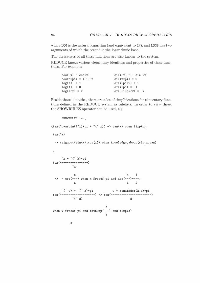
84 CHAPTER 7. BUILT-IN PREFIX OPERATORS
where LOG is the natural logarithm (and equivalent to LN), and LOGB has twoarguments of which the second is the logarithmic base.
The derivatives of all these functions are also known to the system.
REDUCE knows various elementary identities and properties of these func-tions. For example:
cos(-x) = cos(x) sin(-x) = - sin (x)cos(n*pi) = (-1)^n sin(n*pi) = 0log(e) = 1 e^(i*pi/2) = ilog(1) = 0 e^(i*pi) = -1log(e^x) = x e^(3*i*pi/2) = -i
Beside these identities, there are a lot of simplifications for elementary func-tions defined in the REDUCE system as rulelists. In order to view these,the SHOWRULES operator can be used, e.g.
SHOWRULES tan;
tan(~n*arbint(~i)*pi + ~(~ x)) => tan(x) when fixp(n),
tan(~x)
=> trigquot(sin(x),cos(x)) when knowledge_about(sin,x,tan)
,
~x + ~(~ k)*pitan(----------------)
~d
x k 1=> - cot(---) when x freeof pi and abs(---)=---,
d d 2
~(~ w) + ~(~ k)*pi w + remainder(k,d)*pitan(--------------------) => tan(-----------------------)
~(~ d) d
kwhen w freeof pi and ratnump(---) and fixp(k)
d
k

7.2. MATHEMATICAL FUNCTIONS 85
and abs(---)>=1,d
tan(atan(~x)) => x,
2df(tan(~x),~x) => 1 + tan(x)
For further simplification, especially of expressions involving trigonometricfunctions, see the TRIGSIMP package documentation.
Functions not listed above may be defined in the special functions packageSPECFN.
The user can add further rules for the reduction of expressions involvingthese operators by using the LET command.
In many cases it is desirable to expand product arguments of logarithms, orcollect a sum of logarithms into a single logarithm. Since these are inverseoperations, it is not possible to provide rules for doing both at the sametime and preserve the REDUCE concept of idempotent evaluation. As analternative, REDUCE provides two switches EXPANDLOGS and COMBINELOGSto carry out these operations. Both are off by default. Thus to expandLOG(X*Y) into a sum of logs, one can say
ON EXPANDLOGS; LOG(X*Y);
and to combine this sum into a single log:
ON COMBINELOGS; LOG(X) + LOG(Y);
At the present time, it is possible to have both switches on at once, whichcould lead to infinite recursion. However, an expression is switched fromone form to the other in this case. Users should not rely on this behavior,since it may change in the next release.
The current version of REDUCE does a poor job of simplifying surds. In par-ticular, expressions involving the product of variables raised to non-integerpowers do not usually have their powers combined internally, even thoughthey are printed as if those powers were combined. For example, the expres-sion
x^(1/3)*x^(1/6);

86 CHAPTER 7. BUILT-IN PREFIX OPERATORS
will print as
SQRT(X)
but will have an internal form containing the two exponentiated terms. Ifyou now subtract sqrt(x) from this expression, you will not get zero. In-stead, the confusing form
SQRT(X) - SQRT(X)
will result. To combine such exponentiated terms, the switch COMBINEEXPTshould be turned on.
The square root function can be input using the name SQRT, or the poweroperation ^(1/2). On output, unsimplified square roots are normally rep-resented by the operator SQRT rather than a fractional power. With thedefault system switch settings, the argument of a square root is first sim-plified, and any divisors of the expression that are perfect squares takenoutside the square root argument. The remaining expression is left underthe square root. Thus the expression
sqrt(-8a^2*b)
becomes
2*a*sqrt(-2*b).
Note that such simplifications can cause trouble if A is eventually given avalue that is a negative number. If it is important that the positive propertyof the square root and higher even roots always be preserved, the switchPRECISE should be set on (the default value). This causes any non-numericalfactors taken out of surds to be represented by their absolute value form.With PRECISE on then, the above example would become
2*abs(a)*sqrt(-2*b).
The statement that REDUCE knows very little about these functions appliesonly in the mathematically exact off rounded mode. If ROUNDED is on, anyof the functions
ACOS ACOSH ACOT ACOTH ACSC ACSCH ASEC ASECH ASIN ASINHATAN ATANH ATAN2 COS COSH COT COTH CSC CSCH EXP HYPOTLN LOG LOGB LOG10 SEC SECH SIN SINH SQRT TAN TANH

7.3. DF OPERATOR 87
when given a numerical argument has its value calculated to the currentdegree of floating point precision. In addition, real (non-integer valued)powers of numbers will also be evaluated.
If the COMPLEX switch is turned on in addition to ROUNDED, these functionswill also calculate a real or complex result, again to the current degree offloating point precision, if given complex arguments. For example, with onrounded,complex;
2.3^(5.6i) -> -0.0480793490914 - 0.998843519372*Icos(2+3i) -> -4.18962569097 - 9.10922789376*I
7.3 DF Operator
The operator DF is used to represent partial differentiation with respect toone or more variables. It is used with the syntax:
DF(EXPRN:algebraic[,VAR:kernel<,NUM:integer>]):algebraic.
The first argument is the expression to be differentiated. The remainingarguments specify the differentiation variables and the number of times theyare applied.
The number NUM may be omitted if it is 1. For example,
df(y,x) = ∂y/∂xdf(y,x,2) = ∂2y/∂x2
df(y,x1,2,x2,x3,2) = ∂5y/∂x21 ∂x2∂x
23.
The evaluation of df(y,x) proceeds as follows: first, the values of Y and Xare found. Let us assume that X has no assigned value, so its value is X.Each term or other part of the value of Y that contains the variable X isdifferentiated by the standard rules. If Z is another variable, not X itself,then its derivative with respect to X is taken to be 0, unless Z has previouslybeen declared to DEPEND on X, in which case the derivative is reported asthe symbol df(z,x).
7.3.1 Adding Differentiation Rules
The LET statement can be used to introduce rules for differentiation of user-defined operators. Its general form is
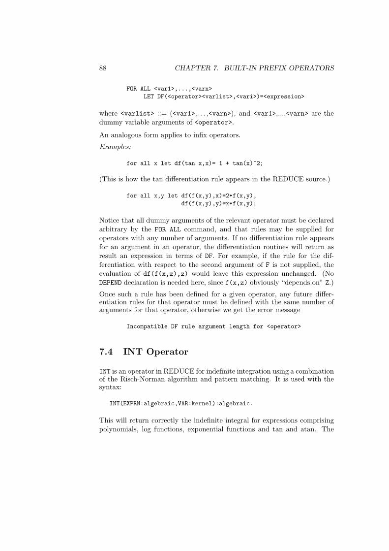
88 CHAPTER 7. BUILT-IN PREFIX OPERATORS
FOR ALL <var1>,...,<varn>LET DF(<operator><varlist>,<vari>)=<expression>
where <varlist> ::= (<var1>,. . . ,<varn>), and <var1>,...,<varn> are thedummy variable arguments of <operator>.
An analogous form applies to infix operators.
Examples:
for all x let df(tan x,x)= 1 + tan(x)^2;
(This is how the tan differentiation rule appears in the REDUCE source.)
for all x,y let df(f(x,y),x)=2*f(x,y),df(f(x,y),y)=x*f(x,y);
Notice that all dummy arguments of the relevant operator must be declaredarbitrary by the FOR ALL command, and that rules may be supplied foroperators with any number of arguments. If no differentiation rule appearsfor an argument in an operator, the differentiation routines will return asresult an expression in terms of DF. For example, if the rule for the dif-ferentiation with respect to the second argument of F is not supplied, theevaluation of df(f(x,z),z) would leave this expression unchanged. (NoDEPEND declaration is needed here, since f(x,z) obviously “depends on” Z.)
Once such a rule has been defined for a given operator, any future differ-entiation rules for that operator must be defined with the same number ofarguments for that operator, otherwise we get the error message
Incompatible DF rule argument length for <operator>
7.4 INT Operator
INT is an operator in REDUCE for indefinite integration using a combinationof the Risch-Norman algorithm and pattern matching. It is used with thesyntax:
INT(EXPRN:algebraic,VAR:kernel):algebraic.
This will return correctly the indefinite integral for expressions comprisingpolynomials, log functions, exponential functions and tan and atan. The
7.4. INT OPERATOR 89
arbitrary constant is not represented. If the integral cannot be done inclosed terms, it returns a formal integral for the answer in one of two ways:
1. It returns the input, INT(...,...) unchanged.
2. It returns an expression involving INTs of some other functions (some-times more complicated than the original one, unfortunately).
Rational functions can be integrated when the denominator is factorizable bythe program. In addition it will attempt to integrate expressions involvingerror functions, dilogarithms and other trigonometric expressions. In thesecases it might not always succeed in finding the solution, even if one exists.
Examples:
int(log(x),x) -> X*(LOG(X) - 1),int(e^x,x) -> E**X.
The program checks that the second argument is a variable and gives anerror if it is not.
Note: If the int operator is called with 4 arguments, REDUCE will im-plicitly call the definite integration package (DEFINT) and this packagewill interpret the third and fourth arguments as the lower and upper limitof integration, respectively. For details, consult the documentation on theDEFINT package.
7.4.1 Options
The switch TRINT when on will trace the operation of the algorithm. Itproduces a great deal of output in a somewhat illegible form, and is not ofmuch interest to the general user. It is normally off.
If the switch FAILHARD is on the algorithm will terminate with an error ifthe integral cannot be done in closed terms, rather than return a formalintegration form. FAILHARD is normally off.
The switch NOLNR suppresses the use of the linear properties of integrationin cases when the integral cannot be found in closed terms. It is normallyoff.
90 CHAPTER 7. BUILT-IN PREFIX OPERATORS
7.4.2 Advanced Use
If a function appears in the integrand that is not one of the functions EXP,ERF, TAN, ATAN, LOG, DILOG then the algorithm will make an attempt tointegrate the argument if it can, differentiate it and reach a known function.However the answer cannot be guaranteed in this case. If a function is knownto be algebraically independent of this set it can be flagged transcendentalby
flag(’(trilog),’transcendental);
in which case this function will be added to the permitted field descriptorsfor a genuine decision procedure. If this is done the user is responsible forthe mathematical correctness of his actions.
The standard version does not deal with algebraic extensions. Thus inte-gration of expressions involving square roots and other like things can leadto trouble. A contributed package that supports integration of functionsinvolving square roots is available, however (ALGINT, chapter 20). In ad-dition there is a definite integration package, DEFINT( chapter 34).
7.4.3 References
A. C. Norman & P. M. A. Moore, “Implementing the New Risch Algorithm”,Proc. 4th International Symposium on Advanced Comp. Methods in Theor.Phys., CNRS, Marseilles, 1977.
S. J. Harrington, “A New Symbolic Integration System in Reduce”, Comp.Journ. 22 (1979) 2.
A. C. Norman & J. H. Davenport, “Symbolic Integration — The DustSettles?”, Proc. EUROSAM 79, Lecture Notes in Computer Science 72,Springer-Verlag, Berlin Heidelberg New York (1979) 398-407.
7.5 LENGTH Operator
LENGTH is a generic operator for finding the length of various objects in thesystem. The meaning depends on the type of the object. In particular, thelength of an algebraic expression is the number of additive top-level termsits expanded representation.

7.6. MAP OPERATOR 91
Examples:
length(a+b) -> 2length(2) -> 1.
Other objects that support a length operator include arrays, lists and ma-trices. The explicit meaning in these cases is included in the description ofthese objects.
7.6 MAP Operator
The MAP operator applies a uniform evaluation pattern to all members ofa composite structure: a matrix, a list, or the arguments of an operatorexpression. The evaluation pattern can be a unary procedure, an operator,or an algebraic expression with one free variable.
It is used with the syntax:
MAP(U:function,V:object)
Here object is a list, a matrix or an operator expression. Function can beone of the following:
1. the name of an operator for a single argument: the operator is evalu-ated once with each element of object as its single argument;
2. an algebraic expression with exactly one free variable, that is a vari-able preceded by the tilde symbol. The expression is evaluated foreach element of object, where the element is substituted for the freevariable;
3. a replacement rule of the form var => rep where var is a variable(a kernel without a subscript) and rep is an expression that containsvar. Rep is evaluated for each element of object where the elementis substituted for var. Var may be optionally preceded by a tilde.
The rule form for function is needed when more than one free variableoccurs.
Examples:

92 CHAPTER 7. BUILT-IN PREFIX OPERATORS
map(abs,1,-2,a,-a) -> 1,2,ABS(A),ABS(A)map(int(~w,x), mat((x^2,x^5),(x^4,x^5))) ->
[ 3 6 ][ x x ][---- ----][ 3 6 ][ ][ 5 6 ][ x x ][---- ----][ 5 6 ]
map(~w*6, x^2/3 = y^3/2 -1) -> 2*X^2=3*(Y^3-2)
You can use MAP in nested expressions. However, you cannot apply MAP toa non-composed object, e.g. an identifier or a number.
7.7 MKID Operator
In many applications, it is useful to create a set of identifiers for namingobjects in a consistent manner. In most cases, it is sufficient to createsuch names from two components. The operator MKID is provided for thispurpose. Its syntax is:
MKID(U:id,V:id|non-negative integer):id
for example
mkid(a,3) -> A3mkid(apple,s) -> APPLES
while mkid(a+b,2) gives an error.
The SET operator can be used to give a value to the identifiers created byMKID, for example
set(mkid(a,3),3);
will give A3 the value 2.

7.8. PF OPERATOR 93
7.8 PF Operator
PF(<exp>,<var>) transforms the expression <exp> into a list of partial frac-tions with respect to the main variable, <var>. PF does a complete partialfraction decomposition, and as the algorithms used are fairly unsophisti-cated (factorization and the extended Euclidean algorithm), the code maybe unacceptably slow in complicated cases.
Example: Given 2/((x+1)^2*(x+2)) in the workspace, pf(ws,x); gives theresult
2 - 2 2-------,-------,-------------- .
X + 2 X + 1 2X + 2*X + 1
If you want the denominators in factored form, use off exp;. Thus, with2/((x+1)^2*(x+2)) in the workspace, the commands off exp; pf(ws,x);give the result
2 - 2 2-------,-------,---------- .
X + 2 X + 1 2(X + 1)
To recombine the terms, FOR EACH ...SUM can be used. So with the abovelist in the workspace, for each j in ws sum j; returns the result
2------------------
2(X + 2)*(X + 1)
Alternatively, one can use the operations on lists to extract any desired term.
7.9 SELECT Operator
The SELECT operator extracts from a list, or from the arguments of an n–aryoperator, elements corresponding to a boolean predicate. It is used with thesyntax:
SELECT(U:function,V:list)
94 CHAPTER 7. BUILT-IN PREFIX OPERATORS
Function can be one of the following forms:
1. the name of an operator for a single argument: the operator is evalu-ated once with each element of object as its single argument;
2. an algebraic expression with exactly one free variable, that is a vari-able preceded by the tilde symbol. The expression is evaluated foreach element of 〈object〉, where the element is substituted for the freevariable;
3. a replacement rule of the form 〈var => rep〉 where var is a variable(a kernel without subscript) and rep is an expression that containsvar. Rep is evaluated for each element of object where the elementis substituted for var. var may be optionally preceded by a tilde.
The rule form for function is needed when more than one free variableoccurs.
The result of evaluating function is interpreted as a boolean value corre-sponding to the conventions of REDUCE. These values are composed withthe leading operator of the input expression.
Examples:
select( ~w>0 , 1,-1,2,-3,3) -> 1,2,3select(evenp deg(~w,y),part((x+y)^5,0):=list)
-> X^5 ,10*X^3*Y^2 ,5*X*Y^4select(evenp deg(~w,x),2x^2+3x^3+4x^4) -> 4X^4 + 2X^2
7.10 SOLVE Operator
SOLVE is an operator for solving one or more simultaneous algebraic equat-ions. It is used with the syntax:
SOLVE(EXPRN:algebraic[,VAR:kernel|,VARLIST:list of kernels]):list.
EXPRN is of the form <expression> or <expression1>,<expression2>,. . . . Each expression is an algebraic equation, or is the difference of thetwo sides of the equation. The second argument is either a kernel or a listof kernels representing the unknowns in the system. This argument may beomitted if the number of distinct, non-constant, top-level kernels equals the

7.10. SOLVE OPERATOR 95
number of unknowns, in which case these kernels are presumed to be theunknowns.
For one equation, SOLVE recursively uses factorization and decomposition,together with the known inverses of LOG, SIN, COS, ^, ACOS, ASIN, and linear,quadratic, cubic, quartic, or binomial factors. Solutions of equations builtwith exponentials or logarithms are often expressed in terms of Lambert’s Wfunction. This function is (partially) implemented in the special functionspackage.
Linear equations are solved by the multi-step elimination method due toBareiss, unless the switch CRAMER is on, in which case Cramer’s method isused. The Bareiss method is usually more efficient unless the system is largeand dense.
Non-linear equations are solved using the Groebner basis package. Usersshould note that this can be quite a time consuming process.
Examples:
solve(log(sin(x+3))^5 = 8,x);solve(a*log(sin(x+3))^5 - b, sin(x+3));solve(a*x+y=3,y=-2,x,y);
SOLVE returns a list of solutions. If there is one unknown, each solution is anequation for the unknown. If a complete solution was found, the unknownwill appear by itself on the left-hand side of the equation. On the otherhand, if the solve package could not find a solution, the “solution” will bean equation for the unknown in terms of the operator ROOT OF. If there areseveral unknowns, each solution will be a list of equations for the unknowns.For example,
solve(x^2=1,x); -> X=-1,X=1
solve(x^7-x^6+x^2=1,x)6
-> X=ROOT_OF(X_ + X_ + 1,X_,TAG_1),X=1
solve(x+3y=7,y-x=1,x,y) -> X=1,Y=2.
The TAG argument is used to uniquely identify those particular solutions.Solution multiplicities are stored in the global variable ROOT MULTIPLICITIESrather than the solution list. The value of this variable is a list of the mul-tiplicities of the solutions for the last call of SOLVE. For example,

96 CHAPTER 7. BUILT-IN PREFIX OPERATORS
solve(x^2=2x-1,x); root_multiplicities;
gives the results
X=1
2
If you want the multiplicities explicitly displayed, the switch MULTIPLICITIEScan be turned on. For example
on multiplicities; solve(x^2=2x-1,x);
yields the result
X=1,X=1
7.10.1 Handling of Undetermined Solutions
When SOLVE cannot find a solution to an equation, it normally returns anequation for the relevant indeterminates in terms of the operator ROOT OF.For example, the expression
solve(cos(x) + log(x),x);
returns the result
X=ROOT_OF(COS(X_) + LOG(X_),X_,TAG_1) .
An expression with a top-level ROOT OF operator is implicitly a list withan unknown number of elements (since we don’t always know how manysolutions an equation has). If a substitution is made into such an expression,closed form solutions can emerge. If this occurs, the ROOT OF construct isreplaced by an operator ONE OF. At this point it is of course possible totransform the result of the original SOLVE operator expression into a standardSOLVE solution. To effect this, the operator EXPAND CASES can be used.
The following example shows the use of these facilities:

7.10. SOLVE OPERATOR 97
solve(-a*x^3+a*x^2+x^4-x^3-4*x^2+4,x);2 3
X=ROOT_OF(A*X_ - X_ + 4*X_ + 4,X_,TAG_2),X=1
sub(a=-1,ws);
X=ONE_OF(2,-1,-2,TAG_2),X=1
expand_cases ws;
X=2,X=-1,X=-2,X=1
7.10.2 Solutions of Equations Involving Cubics and Quartics
Since roots of cubics and quartics can often be very messy, a switchFULLROOTS is available, that, when off (the default), will prevent the pro-duction of a result in closed form. The ROOT OF construct will be used inthis case instead.
In constructing the solutions of cubics and quartics, trigonometrical formsare used where appropriate. This option is under the control of a switchTRIGFORM, which is normally on.
The following example illustrates the use of these facilities:
let xx = solve(x^3+x+1,x);
xx;3
X=ROOT_OF(X_ + X_ + 1,X_)
on fullroots;
xx;
- SQRT(31)*IATAN(---------------)
3*SQRT(3)X=(I*(SQRT(3)*SIN(-----------------------)
3

98 CHAPTER 7. BUILT-IN PREFIX OPERATORS
- SQRT(31)*IATAN(---------------)
3*SQRT(3)- COS(-----------------------)))/SQRT(3),
3
- SQRT(31)*IATAN(---------------)
3*SQRT(3)X=( - I*(SQRT(3)*SIN(-----------------------)
3
- SQRT(31)*IATAN(---------------)
3*SQRT(3)+ COS(-----------------------)))/SQRT(
3
3),
- SQRT(31)*IATAN(---------------)
3*SQRT(3)2*COS(-----------------------)*I
3X=----------------------------------
SQRT(3)
off trigform;
xx;2/3
X=( - (SQRT(31) - 3*SQRT(3)) *SQRT(3)*I
2/3 2/3- (SQRT(31) - 3*SQRT(3)) - 2 *SQRT(3)*I
2/3 1/3 1/3+ 2 )/(2*(SQRT(31) - 3*SQRT(3)) *6
1/6*3 ),
2/3X=((SQRT(31) - 3*SQRT(3)) *SQRT(3)*I

7.10. SOLVE OPERATOR 99
2/3 2/3- (SQRT(31) - 3*SQRT(3)) + 2 *SQRT(3)*I
2/3 1/3 1/3+ 2 )/(2*(SQRT(31) - 3*SQRT(3)) *6
1/6*3 ),
2/3 2/3(SQRT(31) - 3*SQRT(3)) - 2
X=-------------------------------------1/3 1/3 1/6
(SQRT(31) - 3*SQRT(3)) *6 *3
7.10.3 Other Options
If SOLVESINGULAR is on (the default setting), degenerate systems such asx+y=0, 2x+2y=0 will be solved by introducing appropriate arbitrary con-stants. The consistent singular equation 0=0 or equations involving func-tions with multiple inverses may introduce unique new indeterminant ker-nels ARBCOMPLEX(j), or ARBINT(j), (j=1,2,...), representing arbitrary com-plex or integer numbers respectively. To automatically select the principalbranches, do off allbranch; . To avoid the introduction of new inde-terminant kernels do OFF ARBVARS – then no equations are generated forthe free variables and their original names are used to express the solu-tion forms. To suppress solutions of consistent singular equations do OFFSOLVESINGULAR.
To incorporate additional inverse functions do, for example:
put(’sinh,’inverse,’asinh);put(’asinh,’inverse,’sinh);
together with any desired simplification rules such as
for all x let sinh(asinh(x))=x, asinh(sinh(x))=x;
For completeness, functions with non-unique inverses should be treated as^, SIN, and COS are in the SOLVE module source.
Arguments of ASIN and ACOS are not checked to ensure that the absolute

100 CHAPTER 7. BUILT-IN PREFIX OPERATORS
value of the real part does not exceed 1; and arguments of LOG are notchecked to ensure that the absolute value of the imaginary part does notexceed π; but checks (perhaps involving user response for non-numericalarguments) could be introduced using LET statements for these operators.
7.10.4 Parameters and Variable Dependency
The proper design of a variable sequence supplied as a second argument toSOLVE is important for the structure of the solution of an equation system.Any unknown in the system not in this list is considered totally free. E.g.the call
solve(x=2*z,z=2*y,z);
produces an empty list as a result because there is no function z = z(x, y)which fulfills both equations for arbitrary x and y values. In such a case theshare variable requirements displays a set of restrictions for the parametersof the system:
requirements;
x - 4*y
The non-existence of a formal solution is caused by a contradiction whichdisappears only if the parameters of the initial system are set such that allmembers of the requirements list take the value zero. For a linear system theset is complete: a solution of the requirements list makes the initial systemsolvable. E.g. in the above case a substitution x = 4y makes the equationset consistent. For a non-linear system only one inconsistency is detected.If such a system has more than one inconsistency, you must reduce themone after the other. 1 The set shows you also the dependency among theparameters: here one of x and y is free and a formal solution of the systemcan be computed by adding it to the variable list of solve. The requirementset is not unique – there may be other such sets.
A system with parameters may have a formal solution, e.g.
solve(x=a*z+1,0=b*z-y,z,x);
1 The difference between linear and non–linear inconsistent systems is based on thealgorithms which produce this information as a side effect when attempting to find aformal solution; example: solve(x = a, x = b, y = c, y = d, x, y gives a set a−b, c−dwhile solve(x2 = a, x2 = b, y2 = c, y2 = d, x, y leads to a− b.

7.10. SOLVE OPERATOR 101
y a*y + bz=---,x=---------
b b
which is not valid for all possible values of the parameters. The variableassumptions contains then a list of restrictions: the solutions are valid onlyas long as none of these expressions vanishes. Any zero of one of themrepresents a special case that is not covered by the formal solution. In theabove case the value is

102 CHAPTER 7. BUILT-IN PREFIX OPERATORS
assumptions;
b
which excludes formally the case b = 0; obviously this special parametervalue makes the system singular. The set of assumptions is complete forboth, linear and non–linear systems.
SOLVE rearranges the variable sequence to reduce the (expected) computingtime. This behavior is controlled by the switch VAROPT, which is on bydefault. If it is turned off, the supplied variable sequence is used or thesystem kernel ordering is taken if the variable list is omitted. The effect isdemonstrated by an example:
s:= y^3+3x=0,x^2+y^2=1;
solve(s,y,x);
6 2y=root_of(y_ + 9*y_ - 9,y_),
3- y
x=-------3
off varopt; solve(s,y,x);
6 4 2x=root_of(x_ - 3*x_ + 12*x_ - 1,x_),
4 2x*( - x + 2*x - 10)
y=-----------------------3
In the first case, solve forms the solution as a set of pairs (yi, x(yi)) be-cause the degree of x is higher – such a rearrangement makes the internalcomputation of the Grobner basis generally faster. For the second case theexplicitly given variable sequence is used such that the solution has now theform (xi, y(xi)). Controlling the variable sequence is especially important ifthe system has one or more free variables. As an alternative to turning offvaropt, a partial dependency among the variables can be declared using the

7.10. SOLVE OPERATOR 103
depend statement: solve then rearranges the variable sequence but keepsany variable ahead of those on which it depends.

104 CHAPTER 7. BUILT-IN PREFIX OPERATORS
on varopt;s:=a^3+b,b^2+c$solve(s,a,b,c);
3 6a=arbcomplex(1),b= - a ,c= - a
depend a,c; depend b,c; solve(s,a,b,c);
c=arbcomplex(2),
6a=root_of(a_ + c,a_),
3b= - a
Here solve is forced to put c after a and after b, but there is no obstacle tointerchanging a and b.
7.11 Even and Odd Operators
An operator can be declared to be even or odd in its first argument by thedeclarations EVEN and ODD respectively. Expressions involving an operatordeclared in this manner are transformed if the first argument contains aminus sign. Any other arguments are not affected. In addition, if say F isdeclared odd, then f(0) is replaced by zero unless F is also declared nonzero by the declaration NONZERO. For example, the declarations
even f1; odd f2;
mean that
f1(-a) -> F1(A)f2(-a) -> -F2(A)f1(-a,-b) -> F1(A,-B)f2(0) -> 0.
To inhibit the last transformation, say nonzero f2;.

7.12. LINEAR OPERATORS 105
7.12 Linear Operators
An operator can be declared to be linear in its first argument over powers ofits second argument. If an operator F is so declared, F of any sum is brokenup into sums of Fs, and any factors that are not powers of the variable aretaken outside. This means that F must have (at least) two arguments. Inaddition, the second argument must be an identifier (or more generally akernel), not an expression.
Example:
If F were declared linear, then
5f(a*x^5+b*x+c,x) -> F(X ,X)*A + F(X,X)*B + F(1,X)*C
More precisely, not only will the variable and its powers remain within thescope of the F operator, but so will any variable and its powers that hadbeen declared to DEPEND on the prescribed variable; and so would any ex-pression that contains that variable or a dependent variable on any level,e.g. cos(sin(x)).
To declare operators F and G to be linear operators, use:
linear f,g;
The analysis is done of the first argument with respect to the second; anyother arguments are ignored. It uses the following rules of evaluation:
f(0) -> 0f(-y,x) -> -F(Y,X)f(y+z,x) -> F(Y,X)+F(Z,X)f(y*z,x) -> Z*F(Y,X) if Z does not depend on Xf(y/z,x) -> F(Y,X)/Z if Z does not depend on X
To summarize, Y “depends” on the indeterminate X in the above if either ofthe following hold:
1. Y is an expression that contains X at any level as a variable, e.g.:cos(sin(x))
2. Any variable in the expression Y has been declared dependent on X byuse of the declaration DEPEND.

106 CHAPTER 7. BUILT-IN PREFIX OPERATORS
The use of such linear operators can be seen in the paper Fox, J.A. and A. C.Hearn, “Analytic Computation of Some Integrals in Fourth Order QuantumElectrodynamics” Journ. Comp. Phys. 14 (1974) 301-317, which containsa complete listing of a program for definite integration of some expressionsthat arise in fourth order quantum electrodynamics.
7.13 Non-Commuting Operators
An operator can be declared to be non-commutative under multiplicationby the declaration NONCOM.
Example:
After the declarationnoncom u,v;the expressions u(x)*u(y)-u(y)*u(x) and u(x)*v(y)-v(y)*u(x) will re-main unchanged on simplification, and in particular will not simplify tozero.
Note that it is the operator (U and V in the above example) and not thevariable that has the non-commutative property.
The LET statement may be used to introduce rules of evaluation for suchoperators. In particular, the boolean operator ORDP is useful for introducingan ordering on such expressions.
Example:
The rule
for all x,y such that x neq y and ordp(x,y)let u(x)*u(y)= u(y)*u(x)+comm(x,y);
would introduce the commutator of u(x) and u(y) for all X and Y. Note thatsince ordp(x,x) is true, the equality check is necessary in the degeneratecase to avoid a circular loop in the rule.
7.14 Symmetric and Antisymmetric Operators
An operator can be declared to be symmetric with respect to its argumentsby the declaration SYMMETRIC. For example

7.15. DECLARING NEW PREFIX OPERATORS 107
symmetric u,v;
means that any expression involving the top level operators U or V will haveits arguments reordered to conform to the internal order used by REDUCE.The user can change this order for kernels by the command KORDER.
For example, u(x,v(1,2)) would become u(v(2,1),x), since numbers areordered in decreasing order, and expressions are ordered in decreasing orderof complexity.
Similarly the declaration ANTISYMMETRIC declares an operator antisymmet-ric. For example,
antisymmetric l,m;
means that any expression involving the top level operators L or M will haveits arguments reordered to conform to the internal order of the system, andthe sign of the expression changed if there are an odd number of argumentinterchanges necessary to bring about the new order.
For example, l(x,m(1,2)) would become -l(-m(2,1),x) since one inter-change occurs with each operator. An expression like l(x,x) would also bereplaced by 0.
7.15 Declaring New Prefix Operators
The user may add new prefix operators to the system by using the declara-tion OPERATOR. For example:
operator h,g1,arctan;
adds the prefix operators H, G1 and ARCTAN to the system.
This allows symbols like h(w), h(x,y,z), g1(p+q), arctan(u/v) to beused in expressions, but no meaning or properties of the operator are implied.The same operator symbol can be used equally well as a 0-, 1-, 2-, 3-, etc.-place operator.
To give a meaning to an operator symbol, or express some of its properties,LET statements can be used, or the operator can be given a definition as aprocedure.
If the user forgets to declare an identifier as an operator, the system will

108 CHAPTER 7. BUILT-IN PREFIX OPERATORS
prompt the user to do so in interactive mode, or do it automatically in non-interactive mode. A diagnostic message will also be printed if an identifieris declared OPERATOR more than once.
Operators once declared are global in scope, and so can then be referencedanywhere in the program. In other words, a declaration within a block (ora procedure) does not limit the scope of the operator to that block, nordoes the operator go away on exiting the block (use CLEAR instead for thispurpose).
7.16 Declaring New Infix Operators
Users can add new infix operators by using the declarations INFIX andPRECEDENCE. For example,
infix mm;precedence mm,-;
The declaration infix mm; would allow one to use the symbol MM as an infixoperator:
a mm b instead of mm(a,b).
The declaration precedence mm,-; says that MM should be inserted into theinfix operator precedence list just after the − operator. This gives it higherprecedence than − and lower precedence than * . Thus
a - b mm c - d means a - (b mm c) - d,
while
a * b mm c * d means (a * b) mm (c * d).
Both infix and prefix operators have no transformation properties unless LETstatements or procedure declarations are used to assign a meaning.
We should note here that infix operators so defined are always binary:
a mm b mm c means (a mm b) mm c.

7.17. CREATING/REMOVING VARIABLE DEPENDENCY 109
7.17 Creating/Removing Variable Dependency
There are several facilities in REDUCE, such as the differentiation operatorand the linear operator facility, that can utilize knowledge of the dependencybetween various variables, or kernels. Such dependency may be expressedby the command DEPEND. This takes an arbitrary number of arguments andsets up a dependency of the first argument on the remaining arguments. Forexample,
depend x,y,z;
says that X is dependent on both Y and Z.
depend z,cos(x),y;
says that Z is dependent on COS(X) and Y.
Dependencies introduced by DEPEND can be removed by NODEPEND. Thearguments of this are the same as for DEPEND. For example, given the abovedependencies,
nodepend z,cos(x);
says that Z is no longer dependent on COS(X), although it remains dependenton Y.

110 CHAPTER 7. BUILT-IN PREFIX OPERATORS

Chapter 8
Display and Structuring ofExpressions
In this section, we consider a variety of commands and operators that permitthe user to obtain various parts of algebraic expressions and also display theirstructure in a variety of forms. Also presented are some additional conceptsin the REDUCE design that help the user gain a better understanding ofthe structure of the system.
8.1 Kernels
REDUCE is designed so that each operator in the system has an evaluation(or simplification) function associated with it that transforms the expressioninto an internal canonical form. This form, which bears little resemblanceto the original expression, is described in detail in Hearn, A. C., “REDUCE2: A System and Language for Algebraic Manipulation,” Proc. of the Sec-ond Symposium on Symbolic and Algebraic Manipulation, ACM, New York(1971) 128-133.
The evaluation function may transform its arguments in one of two alter-native ways. First, it may convert the expression into other operators inthe system, leaving no functions of the original operator for further manip-ulation. This is in a sense true of the evaluation functions associated withthe operators +, * and / , for example, because the canonical form doesnot include these operators explicitly. It is also true of an operator such
111

112 CHAPTER 8. DISPLAY AND STRUCTURING OF EXPRESSIONS
as the determinant operator DET because the relevant evaluation functioncalculates the appropriate determinant, and the operator DET no longer ap-pears. On the other hand, the evaluation process may leave some residualfunctions of the relevant operator. For example, with the operator COS, aresidual expression like COS(X) may remain after evaluation unless a rulefor the reduction of cosines into exponentials, for example, were introduced.These residual functions of an operator are termed kernels and are storeduniquely like variables. Subsequently, the kernel is carried through the cal-culation as a variable unless transformations are introduced for the operatorat a later stage.
In those cases where the evaluation process leaves an operator expressionwith non-trivial arguments, the form of the argument can vary dependingon the state of the system at the point of evaluation. Such arguments arenormally produced in expanded form with no terms factored or groupedin any way. For example, the expression cos(2*x+2*y) will normally bereturned in the same form. If the argument 2*x+2*y were evaluated at thetop level, however, it would be printed as 2*(X+Y). If it is desirable to havethe arguments themselves in a similar form, the switch INTSTR (for “internalstructure”), if on, will cause this to happen.
In cases where the arguments of the kernel operators may be reordered,the system puts them in a canonical order, based on an internal intrinsicordering of the variables. However, some commands allow arguments in theform of kernels, and the user has no way of telling what internal order thesystem will assign to these arguments. To resolve this difficulty, we introducethe notion of a kernel form as an expression that transforms to a kernel onevaluation.
Examples of kernel forms are:
acos(x*y)log(sin(x))
whereas
a*b(a+b)^4
are not.
We see that kernel forms can usually be used as generalized variables, and

8.2. THE EXPRESSION WORKSPACE 113
most algebraic properties associated with variables may also be associatedwith kernels.
8.2 The Expression Workspace
Several mechanisms are available for saving and retrieving previously evalu-ated expressions. The simplest of these refers to the last algebraic expressionsimplified. When an assignment of an algebraic expression is made, or anexpression is evaluated at the top level, (i.e., not inside a compound state-ment or procedure) the results of the evaluation are automatically saved ina variable WS that we shall refer to as the workspace. (More precisely, theexpression is assigned to the variable WS that is then available for furthermanipulation.)
Example:
If we evaluate the expression (x+y)^2 at the top level and next wish todifferentiate it with respect to Y, we can simply say
df(ws,y);
to get the desired answer.
If the user wishes to assign the workspace to a variable or expression forlater use, the SAVEAS statement can be used. It has the syntax
SAVEAS <expression>
For example, after the differentiation in the last example, the workspaceholds the expression 2*x+2*y. If we wish to assign this to the variable Z wecan now say
saveas z;
If the user wishes to save the expression in a form that allows him to usesome of its variables as arbitrary parameters, the FOR ALL command can beused.
Example:
for all x saveas h(x);

114 CHAPTER 8. DISPLAY AND STRUCTURING OF EXPRESSIONS
with the above expression would mean that h(z) evaluates to 2*Y+2*Z.
A further method for referencing more than the last expression is describedin the section on interactive use of REDUCE.
8.3 Output of Expressions
A considerable degree of flexibility is available in REDUCE in the printingof expressions generated during calculations. No explicit format statementsare supplied, as these are in most cases of little use in algebraic calculations,where the size of output or its composition is not generally known in advance.Instead, REDUCE provides a series of mode options to the user that shouldenable him to produce his output in a comprehensible and possibly pleasingform.
The most extreme option offered is to suppress the output entirely from anytop level evaluation. This is accomplished by turning off the switch OUTPUTwhich is normally on. It is useful for limiting output when loading large filesor producing “clean” output from the prettyprint programs.
In most circumstances, however, we wish to view the output, so we need toknow how to format it appropriately. As we mentioned earlier, an algebraicexpression is normally printed in an expanded form, filling the whole outputline with terms. Certain output declarations, however, can be used to affectthis format. To begin with, we look at an operator for changing the lengthof the output line.
8.3.1 LINELENGTH Operator
This operator is used with the syntax
LINELENGTH(NUM:integer):integer
and sets the output line length to the integer NUM. It returns the previousoutput line length (so that it can be stored for later resetting of the outputline if needed).
8.3. OUTPUT OF EXPRESSIONS 115
8.3.2 Output Declarations
We now describe a number of switches and declarations that are availablefor controlling output formats. It should be noted, however, that the trans-formation of large expressions to produce these varied output formats cantake a lot of computing time and space. If a user wishes to speed up theprinting of the output in such cases, he can turn off the switch PRI. If this isdone, then output is produced in one fixed format, which basically reflectsthe internal form of the expression, and none of the options below apply.PRI is normally on.
With PRI on, the output declarations and switches available are as follows:
ORDER Declaration
The declaration ORDER may be used to order variables on output. The syntaxis:
order v1,...vn;
where the vi are kernels. Thus,
order x,y,z;
orders X ahead of Y, Y ahead of Z and all three ahead of other variables notgiven an order. order nil; resets the output order to the system default.The order of variables may be changed by further calls of ORDER, but thenthe reordered variables would have an order lower than those in earlier ORDERcalls. Thus,
order x,y,z;order y,x;
would order Z ahead of Y and X. The default ordering is usually alphabetic.
FACTOR Declaration
This declaration takes a list of identifiers or kernels as argument. FACTORis not a factoring command (use FACTORIZE or the FACTOR switch for thispurpose); rather it is a separation command. All terms involving fixedpowers of the declared expressions are printed as a product of the fixed

116 CHAPTER 8. DISPLAY AND STRUCTURING OF EXPRESSIONS
powers and a sum of the rest of the terms.
All expressions involving a given prefix operator may also be factored byputting the operator name in the list of factored identifiers. For example:
factor x,cos,sin(x);
causes all powers of X and SIN(X) and all functions of COS to be factored.
Note that FACTOR does not affect the order of its arguments. You shouldalso use ORDER if this is important.
The declaration remfac v1,...,vn; removes the factoring flag from theexpressions v1 through vn.
8.3.3 Output Control Switches
In addition to these declarations, the form of the output can be modifiedby switching various output control switches using the declarations ON andOFF. We shall illustrate the use of these switches by an example, namely theprinting of the expression
x^2*(y^2+2*y)+x*(y^2+z)/(2*a) .
The relevant switches are as follows:
ALLFAC Switch
This switch will cause the system to search the whole expression, or anysub-expression enclosed in parentheses, for simple multiplicative factors andprint them outside the parentheses. Thus our expression with ALLFAC offwill print as
2 2 2 2(2*X *Y *A + 4*X *Y*A + X*Y + X*Z)/(2*A)
and with ALLFAC on as
2 2X*(2*X*Y *A + 4*X*Y*A + Y + Z)/(2*A) .
ALLFAC is normally on, and is on in the following examples, except whereotherwise stated.

8.3. OUTPUT OF EXPRESSIONS 117
DIV Switch
This switch makes the system search the denominator of an expression forsimple factors that it divides into the numerator, so that rational fractionsand negative powers appear in the output. With DIV on, our expressionwould print as
2 2 (-1) (-1)X*(X*Y + 2*X*Y + 1/2*Y *A + 1/2*A *Z) .
DIV is normally off.
LIST Switch
This switch causes the system to print each term in any sum on a separateline. With LIST on, our expression prints as
2X*(2*X*Y *A
+ 4*X*Y*A
2+ Y
+ Z)/(2*A) .
LIST is normally off.
NOSPLIT Switch
Under normal circumstances, the printing routines try to break an expres-sion across lines at a natural point. This is a fairly expensive process. Ifyou are not overly concerned about where the end-of-line breaks come, youcan speed up the printing of expressions by turning off the switch NOSPLIT.This switch is normally on.
RAT Switch
This switch is only useful with expressions in which variables are factoredwith FACTOR. With this mode, the overall denominator of the expression is

118 CHAPTER 8. DISPLAY AND STRUCTURING OF EXPRESSIONS
printed with each factored sub-expression. We assume a prior declarationfactor x; in the following output. We first print the expression with RAToff:
2 2(2*X *Y*A*(Y + 2) + X*(Y + Z))/(2*A) .
With RAT on the output becomes:
8.3. OUTPUT OF EXPRESSIONS 119
2 2X *Y*(Y + 2) + X*(Y + Z)/(2*A) .
RAT is normally off.
Next, if we leave X factored, and turn on both DIV and RAT, the resultbecomes
2 (-1) 2X *Y*(Y + 2) + 1/2*X*A *(Y + Z) .
Finally, with X factored, RAT on and ALLFAC off we retrieve the originalstructure
2 2 2X *(Y + 2*Y) + X*(Y + Z)/(2*A) .
RATPRI Switch
If the numerator and denominator of an expression can each be printed inone line, the output routines will print them in a two dimensional notation,with numerator and denominator on separate lines and a line of dashes inbetween. For example, (a+b)/2 will print as
A + B-----
2
Turning this switch off causes such expressions to be output in a linear form.
REVPRI Switch
The normal ordering of terms in output is from highest to lowest power. Insome situations (e.g., when a power series is output), the opposite orderingis more convenient. The switch REVPRI if on causes such a reverse orderingof terms. For example, the expression y*(x+1)^2+(y+3)^2 will normallyprint as
2 2X *Y + 2*X*Y + Y + 7*Y + 9
whereas with REVPRI on, it will print as

120 CHAPTER 8. DISPLAY AND STRUCTURING OF EXPRESSIONS
2 29 + 7*Y + Y + 2*X*Y + X *Y.
8.3.4 WRITE Command
In simple cases no explicit output command is necessary in REDUCE, sincethe value of any expression is automatically printed if a semicolon is used asa delimiter. There are, however, several situations in which such a commandis useful.
In a FOR, WHILE, or REPEAT statement it may be desired to output somethingeach time the statement within the loop construct is repeated.
It may be desired for a procedure to output intermediate results or otherinformation while it is running. It may be desired to have results labeledin special ways, especially if the output is directed to a file or device otherthan the terminal.
The WRITE command consists of the word WRITE followed by one or moreitems separated by commas, and followed by a terminator. There are threekinds of items that can be used:
1. Expressions (including variables and constants). The expression isevaluated, and the result is printed out.
2. Assignments. The expression on the right side of the := operator isevaluated, and is assigned to the variable on the left; then the symbolon the left is printed, followed by a “:=”, followed by the value ofthe expression on the right – almost exactly the way an assignmentfollowed by a semicolon prints out normally. (The difference is that ifthe WRITE is in a FOR statement and the left-hand side of the assign-ment is an array position or something similar containing the variableof the FOR iteration, then the value of that variable is inserted in theprintout.)
3. Arbitrary strings of characters, preceded and followed by double-quotemarks (e.g., "string").
The items specified by a single WRITE statement print side by side on oneline. (The line is broken automatically if it is too long.) Strings print exactlyas quoted. The WRITE command itself however does not return a value.

8.3. OUTPUT OF EXPRESSIONS 121
The print line is closed at the end of a WRITE command evaluation. Thereforethe command WRITE ""; (specifying nothing to be printed except the emptystring) causes a line to be skipped.
Examples:
1. If A is X+5, B is itself, C is 123, M is an array, and Q=3, then
write m(q):=a," ",b/c," THANK YOU";
will set M(3) to x+5 and print
M(Q) := X + 5 B/123 THANK YOU
The blanks between the 5 and B, and the 3 and T, come from theblanks in the quoted strings.
2. To print a table of the squares of the integers from 1 to 20:
for i:=1:20 do write i," ",i^2;
3. To print a table of the squares of the integers from 1 to 20, and at thesame time store them in positions 1 to 20 of an array A:
for i:=1:20 do <<a(i):=i^2; write i," ",a(i)>>;
This will give us two columns of numbers. If we had used
for i:=1:20 do write i," ",a(i):=i^2;
we would also get A(i) := repeated on each line.
4. The following more complete example calculates the famous f and gseries, first reported in Sconzo, P., LeSchack, A. R., and Tobey, R.,“Symbolic Computation of f and g Series by Computer”, AstronomicalJournal 70 (May 1965).
x1:= -sig*(mu+2*eps)$x2:= eps - 2*sig^2$x3:= -3*mu*sig$f:= 1$g:= 0$for i:= 1 step 1 until 10 do begin
f1:= -mu*g+x1*df(f,eps)+x2*df(f,sig)+x3*df(f,mu);

122 CHAPTER 8. DISPLAY AND STRUCTURING OF EXPRESSIONS
write "f(",i,") := ",f1;g1:= f+x1*df(g,eps)+x2*df(g,sig)+x3*df(g,mu);write "g(",i,") := ",g1;f:=f1$g:=g1$
end;
A portion of the output, to illustrate the printout from the WRITEcommand, is as follows:
... <prior output> ...
2F(4) := MU*(3*EPS - 15*SIG + MU)
G(4) := 6*SIG*MU
2F(5) := 15*SIG*MU*( - 3*EPS + 7*SIG - MU)
2G(5) := MU*(9*EPS - 45*SIG + MU)
... <more output> ...
8.3.5 Suppression of Zeros
It is sometimes annoying to have zero assignments (i.e. assignments of theform <expression> := 0) printed, especially in printing large arrays withmany zero elements. The output from such assignments can be suppressedby turning on the switch NERO.
8.3.6 FORTRAN Style Output Of Expressions
It is naturally possible to evaluate expressions numerically in REDUCE bygiving all variables and sub-expressions numerical values. However, as wepointed out elsewhere the user must declare real arithmetical operation byturning on the switch ROUNDED. However, it should be remembered thatarithmetic in REDUCE is not particularly fast, since results are interpretedrather than evaluated in a compiled form. The user with a large amount

8.3. OUTPUT OF EXPRESSIONS 123
of numerical computation after all necessary algebraic manipulations havebeen performed is therefore well advised to perform these calculations in aFORTRAN or similar system. For this purpose, REDUCE offers facilitiesfor users to produce FORTRAN compatible files for numerical processing.
First, when the switch FORT is on, the system will print expressions in aFORTRAN notation. Expressions begin in column seven. If an expressionextends over one line, a continuation mark (.) followed by a blank appearson subsequent cards. After a certain number of lines have been produced(according to the value of the variable CARD NO), a new expression is started.If the expression printed arises from an assignment to a variable, the variableis printed as the name of the expression. Otherwise the expression is giventhe default name ANS. An error occurs if identifiers or numbers are outsidethe bounds permitted by FORTRAN.
A second option is to use the WRITE command to produce other programs.
Example:
The following REDUCE statements
on fort;out "forfil";write "C this is a fortran program";write " 1 format(e13.5)";write " u=1.23";write " v=2.17";write " w=5.2";x:=(u+v+w)^11;write "C it was foolish to expand this expression";write " print 1,x";write " end";shut "forfil";off fort;
will generate a file forfil that contains:
c this is a fortran program1 format(e13.5)
u=1.23v=2.17w=5.2ans1=1320.*u**3*v*w**7+165.*u**3*w**8+55.*u**2*v**9+495.*u
. **2*v**8*w+1980.*u**2*v**7*w**2+4620.*u**2*v**6*w**3+

124 CHAPTER 8. DISPLAY AND STRUCTURING OF EXPRESSIONS
. 6930.*u**2*v**5*w**4+6930.*u**2*v**4*w**5+4620.*u**2*v**3*
. w**6+1980.*u**2*v**2*w**7+495.*u**2*v*w**8+55.*u**2*w**9+
. 11.*u*v**10+110.*u*v**9*w+495.*u*v**8*w**2+1320.*u*v**7*w
. **3+2310.*u*v**6*w**4+2772.*u*v**5*w**5+2310.*u*v**4*w**6
. +1320.*u*v**3*w**7+495.*u*v**2*w**8+110.*u*v*w**9+11.*u*w
. **10+v**11+11.*v**10*w+55.*v**9*w**2+165.*v**8*w**3+330.*
. v**7*w**4+462.*v**6*w**5+462.*v**5*w**6+330.*v**4*w**7+
. 165.*v**3*w**8+55.*v**2*w**9+11.*v*w**10+w**11x=u**11+11.*u**10*v+11.*u**10*w+55.*u**9*v**2+110.*u**9*v*
. w+55.*u**9*w**2+165.*u**8*v**3+495.*u**8*v**2*w+495.*u**8
. *v*w**2+165.*u**8*w**3+330.*u**7*v**4+1320.*u**7*v**3*w+
. 1980.*u**7*v**2*w**2+1320.*u**7*v*w**3+330.*u**7*w**4+462.
. *u**6*v**5+2310.*u**6*v**4*w+4620.*u**6*v**3*w**2+4620.*u
. **6*v**2*w**3+2310.*u**6*v*w**4+462.*u**6*w**5+462.*u**5*
. v**6+2772.*u**5*v**5*w+6930.*u**5*v**4*w**2+9240.*u**5*v
. **3*w**3+6930.*u**5*v**2*w**4+2772.*u**5*v*w**5+462.*u**5
. *w**6+330.*u**4*v**7+2310.*u**4*v**6*w+6930.*u**4*v**5*w
. **2+11550.*u**4*v**4*w**3+11550.*u**4*v**3*w**4+6930.*u**
. 4*v**2*w**5+2310.*u**4*v*w**6+330.*u**4*w**7+165.*u**3*v
. **8+1320.*u**3*v**7*w+4620.*u**3*v**6*w**2+9240.*u**3*v**
. 5*w**3+11550.*u**3*v**4*w**4+9240.*u**3*v**3*w**5+4620.*u
. **3*v**2*w**6+ans1c it was foolish to expand this expression
print 1,xend
If the arguments of a WRITE statement include an expression that requirescontinuation records, the output will need editing, since the output routineprints the arguments of WRITE sequentially, and the continuation mechanismtherefore generates its auxiliary variables after the preceding expression hasbeen printed.
Finally, since there is no direct analog of list in FORTRAN, a comment lineof the form
c ***** invalid fortran construct (list) not printed
will be printed if you try to print a list with FORT on.
FORTRAN Output Options
There are a number of methods available to change the default format ofthe FORTRAN output.

8.3. OUTPUT OF EXPRESSIONS 125
The breakup of the expression into subparts is such that the number ofcontinuation lines produced is less than a given number. This number canbe modified by the assignment
card_no := <number>;
where <number> is the total number of cards allowed in a statement. Thedefault value of CARD NO is 20.
The width of the output expression is also adjustable by the assignment
fort_width := <integer>;
which sets the total width of a given line to <integer>. The initial FOR-TRAN output width is 70.
REDUCE automatically inserts a decimal point after each isolated integercoefficient in a FORTRAN expression (so that, for example, 4 becomes 4.). To prevent this, set the PERIOD mode switch to OFF.
FORTRAN output is normally produced in lower case. If upper case isdesired, the switch FORTUPPER should be turned on.
Finally, the default name ANS assigned to an unnamed expression and itssubparts can be changed by the operator VARNAME. This takes a singleidentifier as argument, which then replaces ANS as the expression name.The value of VARNAME is its argument.
Further facilities for the production of FORTRAN and other language out-put are provided by the SCOPE and GENTRAN packagesdescribed in chap-ters 42 and 73.
8.3.7 Saving Expressions for Later Use as Input
It is often useful to save an expression on an external file for use later asinput in further calculations. The commands for opening and closing outputfiles are explained elsewhere. However, we see in the examples on outputof expressions that the standard “natural” method of printing expressionsis not compatible with the input syntax. So to print the expression in aninput compatible form we must inhibit this natural style by turning off theswitch NAT. If this is done, a dollar sign will also be printed at the end ofthe expression.
126 CHAPTER 8. DISPLAY AND STRUCTURING OF EXPRESSIONS
Example:
The following sequence of commands
off nat; out "out"; x := (y+z)^2; write "end";shut "out"; on nat;
will generate a file out that contains
X := Y**2 + 2*Y*Z + Z**2$END$
8.3.8 Displaying Expression Structure
In those cases where the final result has a complicated form, it is oftenconvenient to display the skeletal structure of the answer. The operatorSTRUCTR, that takes a single expression as argument, will do this for you.Its syntax is:
STRUCTR(EXPRN:algebraic[,ID1:identifier[,ID2:identifier]]);
The structure is printed effectively as a tree, in which the subparts are laidout with auxiliary names. If the optional ID1 is absent, the auxiliary namesare prefixed by the root ANS. This root may be changed by the operatorVARNAME. If the optional ID1 is present, and is an array name, the subpartsare named as elements of that array, otherwise ID1 is used as the root prefix.(The second optional argument ID2 is explained later.)
The EXPRN can be either a scalar or a matrix expression. Use of any otherwill result in an error.
Example:
Let us suppose that the workspace contains ((A+B)^2+C)^3+D. Then theinput STRUCTR WS; will (with EXP off) result in the output:

8.3. OUTPUT OF EXPRESSIONS 127
ANS3
where
3ANS3 := ANS2 + D
2ANS2 := ANS1 + C
ANS1 := A + B
The workspace remains unchanged after this operation, since STRUCTR inthe default situation returns no value (if STRUCTR is used as a sub-expression,its value is taken to be 0). In addition, the sub-expressions are normally onlydisplayed and not retained. If you wish to access the sub-expressions withtheir displayed names, the switch SAVESTRUCTR should be turned on. In thiscase, STRUCTR returns a list whose first element is a representation for theexpression, and subsequent elements are the sub-expression relations. Thus,with SAVESTRUCTR on, STRUCTR WS in the above example would return
3 2ANS3,ANS3=ANS2 + D,ANS2=ANS1 + C,ANS1=A + B
The PART operator can be used to retrieve the required parts of the ex-pression. For example, to get the value of ANS2 in the above, one couldsay:
part(ws,3,2);
If FORT is on, then the results are printed in the reverse order; the algorithmin fact guaranteeing that no sub-expression will be referenced before it isdefined. The second optional argument ID2 may also be used in this case toname the actual expression (or expressions in the case of a matrix argument).
Example:
Let us suppose that M, a 2 by 1 matrix, contains the elements ((a+b)^2+ c)^3 + d and (a + b)*(c + d) respectively, and that V has beendeclared to be an array. With EXP off and FORT on, the statementstructr(2*m,v,k); will result in the output
V(1)=A+BV(2)=V(1)**2+CV(3)=V(2)**3+D
128 CHAPTER 8. DISPLAY AND STRUCTURING OF EXPRESSIONS
V(4)=C+DK(1,1)=2.*V(3)K(2,1)=2.*V(1)*V(4)
8.4 Changing the Internal Order of Variables
The internal ordering of variables (more specifically kernels) can have asignificant effect on the space and time associated with a calculation. Inits default state, REDUCE uses a specific order for this which may varybetween sessions. However, it is possible for the user to change this internalorder by means of the declaration KORDER. The syntax for this is:
korder v1,...,vn;
where the Vi are kernels. With this declaration, the Vi are ordered internallyahead of any other kernels in the system. V1 has the highest order, V2 thenext highest, and so on. A further call of KORDER replaces a previous one.KORDER NIL; resets the internal order to the system default.
Unlike the ORDER declaration, that has a purely cosmetic effect on the wayresults are printed, the use of KORDER can have a significant effect on compu-tation time. In critical cases then, the user can experiment with the orderingof the variables used to determine the optimum set for a given problem.
8.5 Obtaining Parts of Algebraic Expressions
There are many occasions where it is desirable to obtain a specific partof an expression, or even change such a part to another expression. Anumber of operators are available in REDUCE for this purpose, and will bedescribed in this section. In addition, operators for obtaining specific partsof polynomials and rational functions (such as a denominator) are describedin another section.
8.5.1 COEFF Operator
Syntax:
COEFF(EXPRN:polynomial,VAR:kernel)

8.5. OBTAINING PARTS OF ALGEBRAIC EXPRESSIONS 129
COEFF is an operator that partitions EXPRN into its various coefficients withrespect to VAR and returns them as a list, with the coefficient independentof VAR first.
Under normal circumstances, an error results if EXPRN is not a polynomialin VAR, although the coefficients themselves can be rational as long as theydo not depend on VAR. However, if the switch RATARG is on, denominatorsare not checked for dependence on VAR, and are taken to be part of thecoefficients.
Example:
coeff((y^2+z)^3/z,y);
returns the result
2Z ,0,3*Z,0,3,0,1/Z.
whereas
coeff((y^2+z)^3/y,y);
gives an error if RATARG is off, and the result
3 2Z /Y,0,3*Z /Y,0,3*Z/Y,0,1/Y
if RATARG is on.
The length of the result of COEFF is the highest power of VAR encounteredplus 1. In the above examples it is 7. In addition, the variable HIGH POW isset to the highest non-zero power found in EXPRN during the evaluation, andLOW POW to the lowest non-zero power, or zero if there is a constant term.If EXPRN is a constant, then HIGH POW and LOW POW are both set to zero.
8.5.2 COEFFN Operator
The COEFFN operator is designed to give the user a particular coefficient ofa variable in a polynomial, as opposed to COEFF that returns all coefficients.COEFFN is used with the syntax
COEFFN(EXPRN:polynomial,VAR:kernel,N:integer)

130 CHAPTER 8. DISPLAY AND STRUCTURING OF EXPRESSIONS
It returns the nth coefficient of VAR in the polynomial EXPRN.
8.5.3 PART Operator
Syntax:
PART(EXPRN:algebraic[,INTEXP:integer])
This operator works on the form of the expression as printed or as it wouldhave been printed at that point in the calculation bearing in mind all therelevant switch settings at that point. The reader therefore needs somefamiliarity with the way that expressions are represented in prefix form inREDUCE to use these operators effectively. Furthermore, it is assumedthat PRI is ON at that point in the calculation. The reason for this is thatwith PRI off, an expression is printed by walking the tree representing theexpression internally. To save space, it is never actually transformed intothe equivalent prefix expression as occurs when PRI is on. However, theoperations on polynomials described elsewhere can be equally well used inthis case to obtain the relevant parts.
The evaluation proceeds recursively down the integer expression list. Inother words,
PART(<expression>,<integer1>,<integer2>)-> PART(PART(<expression>,<integer1>),<integer2>)
and so on, and
PART(<expression>) -> <expression>.
INTEXP can be any expression that evaluates to an integer. If the integer ispositive, then that term of the expression is found. If the integer is 0, theoperator is returned. Finally, if the integer is negative, the counting is fromthe tail of the expression rather than the head.
For example, if the expression a+b is printed as A+B (i.e., the ordering of thevariables is alphabetical), then
part(a+b,2) -> Bpart(a+b,-1) -> B
andpart(a+b,0) -> PLUS

8.5. OBTAINING PARTS OF ALGEBRAIC EXPRESSIONS 131
An operator ARGLENGTH is available to determine the number of argumentsof the top level operator in an expression. If the expression does not containa top level operator, then −1 is returned. For example,
arglength(a+b+c) -> 3arglength(f()) -> 0arglength(a) -> -1
8.5.4 Substituting for Parts of Expressions
PART may also be used to substitute for a given part of an expression. Inthis case, the PART construct appears on the left-hand side of an assignmentstatement, and the expression to replace the given part on the right-handside.
For example, with the normal settings of the REDUCE switches:
xx := a+b;part(xx,2) := c; -> A+Cpart(c+d,0) := -; -> C-D
Note that xx in the above is not changed by this substitution. In addition,unlike expressions such as array and matrix elements that have an instantevaluation property, the values of part(xx,2) and part(c+d,0) are alsonot changed.

132 CHAPTER 8. DISPLAY AND STRUCTURING OF EXPRESSIONS

Chapter 9
Polynomials and Rationals
Many operations in computer algebra are concerned with polynomials andrational functions. In this section, we review some of the switches andoperators available for this purpose. These are in addition to those thatwork on general expressions (such as DF and INT) described elsewhere. Inthe case of operators, the arguments are first simplified before the operationsare applied. In addition, they operate only on arguments of prescribedtypes, and produce a type mismatch error if given arguments which cannotbe interpreted in the required mode with the current switch settings. Forexample, if an argument is required to be a kernel and a/2 is used (with noother rules for A), an error
A/2 invalid as kernel
will result.
With the exception of those that select various parts of a polynomial orrational function, these operations have potentially significant effects on thespace and time associated with a given calculation. The user should there-fore experiment with their use in a given calculation in order to determinethe optimum set for a given problem.
One such operation provided by the system is an operator LENGTH whichreturns the number of top level terms in the numerator of its argument. Forexample,
length ((a+b+c)^3/(c+d));
has the value 10. To get the number of terms in the denominator, one would
133

134 CHAPTER 9. POLYNOMIALS AND RATIONALS
first select the denominator by the operator DEN and then call LENGTH, as in
length den ((a+b+c)^3/(c+d));
Other operations currently supported, the relevant switches and operators,and the required argument and value modes of the latter, follow.
9.1 Controlling the Expansion of Expressions
The switch EXP controls the expansion of expressions. If it is off, no expan-sion of powers or products of expressions occurs. Users should note howeverthat in this case results come out in a normal but not necessarily canoni-cal form. This means that zero expressions simplify to zero, but that twoequivalent expressions need not necessarily simplify to the same form.
Example: With EXP on, the two expressions
(a+b)*(a+2*b)
and
a^2+3*a*b+2*b^2
will both simplify to the latter form. With EXP off, they would remainunchanged, unless the complete factoring (ALLFAC) option were in force.EXP is normally on.
Several operators that expect a polynomial as an argument behave differ-ently when EXP is off, since there is often only one term at the top level. Forexample, with EXP off
length((a+b+c)^3/(c+d));
returns the value 1.
9.2 Factorization of Polynomials
REDUCE is capable of factorizing univariate and multivariate polynomialsthat have integer coefficients, finding all factors that also have integer coef-ficients. The package for doing this was written by Dr. Arthur C. Norman
9.2. FACTORIZATION OF POLYNOMIALS 135
and Ms. P. Mary Ann Moore at The University of Cambridge. It is de-scribed in P. M. A. Moore and A. C. Norman, “Implementing a PolynomialFactorization and GCD Package”, Proc. SYMSAC ’81, ACM (New York)(1981), 109-116.
The easiest way to use this facility is to turn on the switch FACTOR, whichcauses all expressions to be output in a factored form. For example, withFACTOR on, the expression A^2-B^2 is returned as (A+B)*(A-B).
It is also possible to factorize a given expression explicitly. The operatorFACTORIZE that invokes this facility is used with the syntax
FACTORIZE(EXPRN:polynomial[,INTEXP:prime integer]):list,
the optional argument of which will be described later. Thus to find anddisplay all factors of the cyclotomic polynomial x105 − 1, one could write:
factorize(x^105-1);
The result is a list of factor,exponent pairs. In the above example, there isno overall numerical factor in the result, so the results will consist only ofpolynomials in x. The number of such polynomials can be found by using theoperator LENGTH. If there is a numerical factor, as in factorizing 12x2 − 12,that factor will appear as the first member of the result. It will however notbe factored further. Prime factors of such numbers can be found, using aprobabilistic algorithm, by turning on the switch IFACTOR. For example,
on ifactor; factorize(12x^2-12);
would result in the output
2,2,3,1,X + 1,1,X - 1,1.
If the first argument of FACTORIZE is an integer, it will be decomposed intoits prime components, whether or not IFACTOR is on.
Note that the IFACTOR switch only affects the result of FACTORIZE. It hasno effect if the FACTOR switch is also on.
The order in which the factors occur in the result (with the exception ofa possible overall numerical coefficient which comes first) can be systemdependent and should not be relied on. Similarly it should be noted thatany pair of individual factors can be negated without altering their product,and that REDUCE may sometimes do that.

136 CHAPTER 9. POLYNOMIALS AND RATIONALS
The factorizer works by first reducing multivariate problems to univariateones and then solving the univariate ones modulo small primes. It normallyselects both evaluation points and primes using a random number genera-tor that should lead to different detailed behavior each time any particularproblem is tackled. If, for some reason, it is known that a certain (probablyunivariate) factorization can be performed effectively with a known prime,P say, this value of P can be handed to FACTORIZE as a second argument.An error will occur if a non-prime is provided to FACTORIZE in this manner.It is also an error to specify a prime that divides the discriminant of thepolynomial being factored, but users should note that this condition is notchecked by the program, so this capability should be used with care.
Factorization can be performed over a number of polynomial coefficient do-mains in addition to integers. The particular description of the relevantdomain should be consulted to see if factorization is supported. For exam-ple, the following statements will factorize x4 + 1 modulo 7:
setmod 7;on modular;factorize(x^4+1);
The factorization module is provided with a trace facility that may be usefulas a way of monitoring progress on large problems, and of satisfying curios-ity about the internal workings of the package. The most simple use of thisis enabled by issuing the REDUCE command on trfac; . Following this,all calls to the factorizer will generate informative messages reporting onsuch things as the reduction of multivariate to univariate cases, the choiceof a prime and the reconstruction of full factors from their images. Furtherlevels of detail in the trace are intended mainly for system tuners and for theinvestigation of suspected bugs. For example, TRALLFAC gives tracing infor-mation at all levels of detail. The switch that can be set by on timings;makes it possible for one who is familiar with the algorithms used to deter-mine what part of the factorization code is consuming the most resources.on overview; reduces the amount of detail presented in other forms of trace.Other forms of trace output are enabled by directives of the form
symbolic set!-trace!-factor(<number>,<filename>);
where useful numbers are 1, 2, 3 and 100, 101, ... . This facility is intendedto make it possible to discover in fairly great detail what just some smallpart of the code has been doing — the numbers refer mainly to depths ofrecursion when the factorizer calls itself, and to the split between its workforming and factorizing images and reconstructing full factors from these.If NIL is used in place of a filename the trace output requested is directed

9.3. CANCELLATION OF COMMON FACTORS 137
to the standard output stream. After use of this trace facility the generatedtrace files should be closed by calling
symbolic close!-trace!-files();
NOTE: Using the factorizer with MCD off will result in an error.
9.3 Cancellation of Common Factors
Facilities are available in REDUCE for cancelling common factors in thenumerators and denominators of expressions, at the option of the user. Thesystem will perform this greatest common divisor computation if the switchGCD is on. (GCD is normally off.)
A check is automatically made, however, for common variable and numer-ical products in the numerators and denominators of expressions, and theappropriate cancellations made.
When GCD is on, and EXP is off, a check is made for square free factors inan expression. This includes separating out and independently checking thecontent of a given polynomial where appropriate. (For an explanation ofthese terms, see Anthony C. Hearn, “Non-Modular Computation of Poly-nomial GCDs Using Trial Division”, Proc. EUROSAM 79, published asLecture Notes on Comp. Science, Springer-Verlag, Berlin, No 72 (1979)227-239.)
Example: With EXP off and GCD on, the polynomial a*c+a*d+b*c+b*d wouldbe returned as (A+B)*(C+D).
Under normal circumstances, GCDs are computed using an algorithm de-scribed in the above paper. It is also possible in REDUCE to computeGCDs using an alternative algorithm, called the EZGCD Algorithm, whichuses modular arithmetic. The switch EZGCD, if on in addition to GCD, makesthis happen.
In non-trivial cases, the EZGCD algorithm is almost always better than thebasic algorithm, often by orders of magnitude. We therefore strongly adviseusers to use the EZGCD switch where they have the resources available forsupporting the package.
For a description of the EZGCD algorithm, see J. Moses and D.Y.Y. Yun,“The EZ GCD Algorithm”, Proc. ACM 1973, ACM, New York (1973) 159-

138 CHAPTER 9. POLYNOMIALS AND RATIONALS
166.
NOTE: This package shares code with the factorizer, so a certain amountof trace information can be produced using the factorizer trace switches.
9.3.1 Determining the GCD of Two Polynomials
This operator, used with the syntax
GCD(EXPRN1:polynomial,EXPRN2:polynomial):polynomial,
returns the greatest common divisor of the two polynomials EXPRN1 andEXPRN2.
Examples:
gcd(x^2+2*x+1,x^2+3*x+2) -> X+1gcd(2*x^2-2*y^2,4*x+4*y) -> 2*X+2*Ygcd(x^2+y^2,x-y) -> 1.
9.4 Working with Least Common Multiples
Greatest common divisor calculations can often become expensive if exten-sive work with large rational expressions is required. However, in manycases, the only significant cancellations arise from the fact that there are of-ten common factors in the various denominators which are combined whentwo rationals are added. Since these denominators tend to be smaller andmore regular in structure than the numerators, considerable savings in bothtime and space can occur if a full GCD check is made when the denominatorsare combined and only a partial check when numerators are constructed. Inother words, the true least common multiple of the denominators is com-puted at each step. The switch LCM is available for this purpose, and isnormally on.
In addition, the operator LCM, used with the syntax
LCM(EXPRN1:polynomial,EXPRN2:polynomial):polynomial,
returns the least common multiple of the two polynomials EXPRN1 andEXPRN2.

9.5. CONTROLLING USE OF COMMON DENOMINATORS 139
Examples:
lcm(x^2+2*x+1,x^2+3*x+2) -> X**3 + 4*X**2 + 5*X + 2lcm(2*x^2-2*y^2,4*x+4*y) -> 4*(X**2 - Y**2)
9.5 Controlling Use of Common Denominators
When two rational functions are added, REDUCE normally produces anexpression over a common denominator. However, if the user does not wantdenominators combined, he or she can turn off the switch MCD which controlsthis process. The latter switch is particularly useful if no greatest commondivisor calculations are desired, or excessive differentiation of rational func-tions is required.
CAUTION: With MCD off, results are not guaranteed to come out in eithernormal or canonical form. In other words, an expression equivalent to zeromay in fact not be simplified to zero. This option is therefore most usefulfor avoiding expression swell during intermediate parts of a calculation.
MCD is normally on.
9.6 REMAINDER Operator
This operator is used with the syntax
REMAINDER(EXPRN1:polynomial,EXPRN2:polynomial):polynomial.
It returns the remainder when EXPRN1 is divided by EXPRN2. This is thetrue remainder based on the internal ordering of the variables, and not thepseudo-remainder. The pseudo-remainder and in general pseudo-divisionof polynomials can be calculated after loading the polydiv package. Pleaserefer to the documentation of this package for details.
Examples:
remainder((x+y)*(x+2*y),x+3*y) -> 2*Y**2remainder(2*x+y,2) -> Y.
CAUTION: In the default case, remainders are calculated over the inte-gers. If you need the remainder with respect to another domain, it must be

140 CHAPTER 9. POLYNOMIALS AND RATIONALS
declared explicitly.
Example:
remainder(x^2-2,x+sqrt(2)); -> X^2 - 2load_package arnum;defpoly sqrt2**2-2;remainder(x^2-2,x+sqrt2); -> 0
9.7 RESULTANT Operator
This is used with the syntax
RESULTANT(EXPRN1:polynomial,EXPRN2:polynomial,VAR:kernel):polynomial.
It computes the resultant of the two given polynomials with respect to thegiven variable, the coefficients of the polynomials can be taken from anydomain. The result can be identified as the determinant of a Sylvestermatrix, but can often also be thought of informally as the result obtainedwhen the given variable is eliminated between the two input polynomials. Ifthe two input polynomials have a non-trivial GCD their resultant vanishes.
The switch BEZOUT controls the computation of the resultants. It is off bydefault. In this case a subresultant algorithm is used. If the switch Bezoutis turned on, the resultant is computed via the Bezout Matrix. However, inthe latter case, only polynomial coefficients are permitted.

9.8. DECOMPOSE OPERATOR 141
The sign conventions used by the resultant function follow those in R. Loos,“Computing in Algebraic Extensions” in “Computer Algebra — Symbolicand Algebraic Computation”, Second Ed., Edited by B. Buchberger, G.E.Collins and R. Loos, Springer-Verlag, 1983. Namely, with A and B notdependent on X:
deg(p)*deg(q)resultant(p(x),q(x),x)= (-1) *resultant(q,p,x)
deg(p)resultant(a,p(x),x) = a
resultant(a,b,x) = 1
Examples:
2resultant(x/r*u+y,u*y,u) -> - y
calculation in an algebraic extension:
load arnum;defpoly sqrt2**2 - 2;
resultant(x + sqrt2,sqrt2 * x +1,x) -> -1
or in a modular domain:
setmod 17;on modular;
resultant(2x+1,3x+4,x) -> 5
9.8 DECOMPOSE Operator
The DECOMPOSE operator takes a multivariate polynomial as argument, andreturns an expression and a list of equations from which the original poly-nomial can be found by composition. Its syntax is:
DECOMPOSE(EXPRN:polynomial):list.

142 CHAPTER 9. POLYNOMIALS AND RATIONALS
For example:
decompose(x^8-88*x^7+2924*x^6-43912*x^5+263431*x^4-218900*x^3+65690*x^2-7700*x+234)
2 2 2-> U + 35*U + 234, U=V + 10*V, V=X - 22*X
2decompose(u^2+v^2+2u*v+1) -> W + 1, W=U + V
Users should note however that, unlike factorization, this decomposition isnot unique.
9.9 INTERPOL operator
Syntax:
INTERPOL(<values>,<variable>,<points>);
where <values> and <points> are lists of equal length and <variable> isan algebraic expression (preferably a kernel).
INTERPOL generates an interpolation polynomial f in the given variable ofdegree length(<values>)-1. The unique polynomial f is defined by the prop-erty that for corresponding elements v of <values> and p of <points> therelation f(p) = v holds.
The Aitken-Neville interpolation algorithm is used which guarantees a stableresult even with rounded numbers and an ill-conditioned problem.
9.10 Obtaining Parts of Polynomials and Ratio-nals
These operators select various parts of a polynomial or rational functionstructure. Except for the cost of rearrangement of the structure, these op-erations take very little time to perform.
For those operators in this section that take a kernel VAR as their secondargument, an error results if the first expression is not a polynomial in VAR,although the coefficients themselves can be rational as long as they do notdepend on VAR. However, if the switch RATARG is on, denominators are not

9.10. OBTAINING PARTS OF POLYNOMIALS AND RATIONALS 143
checked for dependence on VAR, and are taken to be part of the coefficients.
9.10.1 DEG Operator
This operator is used with the syntax
DEG(EXPRN:polynomial,VAR:kernel):integer.
It returns the leading degree of the polynomial EXPRN in the variable VAR.If VAR does not occur as a variable in EXPRN, 0 is returned.
Examples:
deg((a+b)*(c+2*d)^2,a) -> 1deg((a+b)*(c+2*d)^2,d) -> 2deg((a+b)*(c+2*d)^2,e) -> 0.
Note also that if RATARG is on,
deg((a+b)^3/a,a) -> 3
since in this case, the denominator A is considered part of the coefficients ofthe numerator in A. With RATARG off, however, an error would result in thiscase.
9.10.2 DEN Operator
This is used with the syntax:
DEN(EXPRN:rational):polynomial.
It returns the denominator of the rational expression EXPRN. If EXPRN is apolynomial, 1 is returned.
Examples:
den(x/y^2) -> Y**2den(100/6) -> 3
[since 100/6 is first simplified to 50/3]den(a/4+b/6) -> 12den(a+b) -> 1

144 CHAPTER 9. POLYNOMIALS AND RATIONALS
9.10.3 LCOF Operator
LCOF is used with the syntax
LCOF(EXPRN:polynomial,VAR:kernel):polynomial.
It returns the leading coefficient of the polynomial EXPRN in the variableVAR. If VAR does not occur as a variable in EXPRN, EXPRN is returned.

9.10. OBTAINING PARTS OF POLYNOMIALS AND RATIONALS 145
Examples:
lcof((a+b)*(c+2*d)^2,a) -> C**2+4*C*D+4*D**2lcof((a+b)*(c+2*d)^2,d) -> 4*(A+B)lcof((a+b)*(c+2*d),e) -> A*C+2*A*D+B*C+2*B*D
9.10.4 LPOWER Operator
Syntax:
LPOWER(EXPRN:polynomial,VAR:kernel):polynomial.
LPOWER returns the leading power of EXPRN with respect to VAR. If EXPRNdoes not depend on VAR, 1 is returned.
Examples:
lpower((a+b)*(c+2*d)^2,a) -> Alpower((a+b)*(c+2*d)^2,d) -> D**2lpower((a+b)*(c+2*d),e) -> 1
9.10.5 LTERM Operator
Syntax:
LTERM(EXPRN:polynomial,VAR:kernel):polynomial.
LTERM returns the leading term of EXPRN with respect to VAR. If EXPRNdoes not depend on VAR, EXPRN is returned.
Examples:
lterm((a+b)*(c+2*d)^2,a) -> A*(C**2+4*C*D+4*D**2)lterm((a+b)*(c+2*d)^2,d) -> 4*D**2*(A+B)lterm((a+b)*(c+2*d),e) -> A*C+2*A*D+B*C+2*B*D
Compatibility Note: In some earlier versions of REDUCE, LTERM returned 0if the EXPRN did not depend on VAR. In the present version, EXPRN is alwaysequal to LTERM(EXPRN,VAR) + REDUCT(EXPRN,VAR).

146 CHAPTER 9. POLYNOMIALS AND RATIONALS
9.10.6 MAINVAR Operator
Syntax:
MAINVAR(EXPRN:polynomial):expression.
Returns the main variable (based on the internal polynomial representation)of EXPRN. If EXPRN is a domain element, 0 is returned.
Examples:
Assuming A has higher kernel order than B, C, or D:
mainvar((a+b)*(c+2*d)^2) -> Amainvar(2) -> 0
9.10.7 NUM Operator
Syntax:
NUM(EXPRN:rational):polynomial.
Returns the numerator of the rational expression EXPRN. If EXPRN is a poly-nomial, that polynomial is returned.
Examples:
num(x/y^2) -> Xnum(100/6) -> 50num(a/4+b/6) -> 3*A+2*Bnum(a+b) -> A+B
9.10.8 REDUCT Operator
Syntax:
REDUCT(EXPRN:polynomial,VAR:kernel):polynomial.
Returns the reductum of EXPRN with respect to VAR (i.e., the part of EXPRNleft after the leading term is removed). If EXPRN does not depend on thevariable VAR, 0 is returned.
Examples:

9.11. POLYNOMIAL COEFFICIENT ARITHMETIC 147
reduct((a+b)*(c+2*d),a) -> B*(C + 2*D)reduct((a+b)*(c+2*d),d) -> C*(A + B)reduct((a+b)*(c+2*d),e) -> 0
Compatibility Note: In some earlier versions of REDUCE, REDUCT returnedEXPRN if it did not depend on VAR. In the present version, EXPRN is alwaysequal to LTERM(EXPRN,VAR) + REDUCT(EXPRN,VAR).
9.11 Polynomial Coefficient Arithmetic
REDUCE allows for a variety of numerical domains for the numerical co-efficients of polynomials used in calculations. The default mode is integerarithmetic, although the possibility of using real coefficients has been dis-cussed elsewhere. Rational coefficients have also been available by using in-teger coefficients in both the numerator and denominator of an expression,using the ON DIV option to print the coefficients as rationals. However, RE-DUCE includes several other coefficient options in its basic version whichwe shall describe in this section. All such coefficient modes are supportedin a table-driven manner so that it is straightforward to extend the range ofpossibilities. A description of how to do this is given in R.J. Bradford, A.C.Hearn, J.A. Padget and E. Schrufer, “Enlarging the REDUCE Domain ofComputation,” Proc. of SYMSAC ’86, ACM, New York (1986), 100–106.
9.11.1 Rational Coefficients in Polynomials
Instead of treating rational numbers as the numerator and denominator of arational expression, it is also possible to use them as polynomial coefficientsdirectly. This is accomplished by turning on the switch RATIONAL.
Example: With RATIONAL off, the input expression a/2 would be convertedinto a rational expression, whose numerator was A and denominator 2. WithRATIONAL on, the same input would become a rational expression with nu-merator 1/2*A and denominator 1. Thus the latter can be used in operationsthat require polynomial input whereas the former could not.
148 CHAPTER 9. POLYNOMIALS AND RATIONALS
9.11.2 Real Coefficients in Polynomials
The switch ROUNDED permits the use of arbitrary sized real coefficients inpolynomial expressions. The actual precision of these coefficients can be setby the operator PRECISION. For example, precision 50; sets the precisionto fifty decimal digits. The default precision is system dependent and canbe found by precision 0;. In this mode, denominators are automaticallymade monic, and an appropriate adjustment is made to the numerator.
Example: With ROUNDED on, the input expression a/2 would be convertedinto a rational expression whose numerator is 0.5*A and denominator 1.
Internally, REDUCE uses floating point numbers up to the precision sup-ported by the underlying machine hardware, and so-called bigfloats for higherprecision or whenever necessary to represent numbers whose value cannotbe represented in floating point. The internal precision is two decimal digitsgreater than the external precision to guard against roundoff inaccuracies.Bigfloats represent the fraction and exponent parts of a floating-point num-ber by means of (arbitrary precision) integers, which is a more precise rep-resentation in many cases than the machine floating point arithmetic, butnot as efficient. If a case arises where use of the machine arithmetic leadsto problems, a user can force REDUCE to use the bigfloat representation atall precisions by turning on the switch ROUNDBF. In rare cases, this switch isturned on by the system, and the user informed by the message
ROUNDBF turned on to increase accuracy
Rounded numbers are normally printed to the specified precision. How-ever, if the user wishes to print such numbers with less precision, the print-ing precision can be set by the command PRINT PRECISION. For example,print precision 5; will cause such numbers to be printed with five digitsmaximum.
Under normal circumstances when ROUNDED is on, REDUCE converts thenumber 1.0 to the integer 1. If this is not desired, the switch NOCONVERT canbe turned on.
Numbers that are stored internally as bigfloats are normally printed with aspace between every five digits to improve readability. If this feature is notrequired, it can be suppressed by turning off the switch BFSPACE.
Further information on the bigfloat arithmetic may be found in T. Sasaki,“Manual for Arbitrary Precision Real Arithmetic System in REDUCE”,Department of Computer Science, University of Utah, Technical Note No.

9.11. POLYNOMIAL COEFFICIENT ARITHMETIC 149
TR-8 (1979).
When a real number is input, it is normally truncated to the precisionin effect at the time the number is read. If it is desired to keep the fullprecision of all numbers input, the switch ADJPREC (for adjust precision) canbe turned on. While on, ADJPREC will automatically increase the precision,when necessary, to match that of any integer or real input, and a messageprinted to inform the user of the precision increase.
When ROUNDED is on, rational numbers are normally converted to roundedrepresentation. However, if a user wishes to keep such numbers in a rationalform until used in an operation that returns a real number, the switchROUNDALL can be turned off. This switch is normally on.
Results from rounded calculations are returned in rounded form with twoexceptions: if the result is recognized as 0 or 1 to the current precision, theinteger result is returned.
9.11.3 Modular Number Coefficients in Polynomials
REDUCE includes facilities for manipulating polynomials whose coefficientsare computed modulo a given base. To use this option, two commands mustbe used; SETMOD <integer>, to set the prime modulus, and ON MODULAR tocause the actual modular calculations to occur. For example, with setmod3; and on modular;, the polynomial (a+2*b)^3 would become A^3+2*B^3.
The argument of SETMOD is evaluated algebraically, except that non-modular(integer) arithmetic is used. Thus the sequence
setmod 3; on modular; setmod 7;
will correctly set the modulus to 7.
Modular numbers are by default represented by integers in the interval [0,p-1] where p is the current modulus. Sometimes it is more convenient to use anequivalent symmetric representation in the interval [-p/2+1,p/2], or moreprecisely [-floor((p-1)/2), ceiling((p-1)/2)], especially if the modular num-bers map objects that include negative quantities. The switch BALANCED MODallows you to select the symmetric representation for output.
Users should note that the modular calculations are on the polynomial co-efficients only. It is not currently possible to reduce the exponents since nocheck for a prime modulus is made (which would allow xp−1 to be reduced

150 CHAPTER 9. POLYNOMIALS AND RATIONALS
to 1 mod p). Note also that any division by a number not co-prime withthe modulus will result in the error “Invalid modular division”.
9.11.4 Complex Number Coefficients in Polynomials
Although REDUCE routinely treats the square of the variable i as equivalentto −1, this is not sufficient to reduce expressions involving i to lowest terms,or to factor such expressions over the complex numbers. For example, inthe default case,
factorize(a^2+1);
gives the result
A**2+1,1
and
(a^2+b^2)/(a+i*b)
is not reduced further. However, if the switch COMPLEX is turned on, fullcomplex arithmetic is then carried out. In other words, the above factoriza-tion will give the result
A + I,1,A - I,1
and the quotient will be reduced to A-I*B.
The switch COMPLEX may be combined with ROUNDED to give complex realnumbers; the appropriate arithmetic is performed in this case.
Complex conjugation is used to remove complex numbers from denomina-tors of expressions. To do this if COMPLEX is off, you must turn the switchRATIONALIZE on.

Chapter 10
Substitution Commands
An important class of commands in REDUCE define substitutions for vari-ables and expressions to be made during the evaluation of expressions. Suchsubstitutions use the prefix operator SUB, various forms of the commandLET, and rule sets.
10.1 SUB Operator
Syntax:
SUB(<substitution_list>,EXPRN1:algebraic):algebraic
where <substitution list> is a list of one or more equations of the form
VAR:kernel=EXPRN:algebraic
or a kernel that evaluates to such a list.
The SUB operator gives the algebraic result of replacing every occurrence ofthe variable VAR in the expression EXPRN1 by the expression EXPRN. Specif-ically, EXPRN1 is first evaluated using all available rules. Next the substitu-tions are made, and finally the substituted expression is reevaluated. Whenmore than one variable occurs in the substitution list, the substitution isperformed by recursively walking down the tree representing EXPRN1, andreplacing every VAR found by the appropriate EXPRN. The EXPRN are notthemselves searched for any occurrences of the various VARs. The trivial
151

152 CHAPTER 10. SUBSTITUTION COMMANDS
case SUB(EXPRN1) returns the algebraic value of EXPRN1.
Examples:
2 2sub(x=a+y,y=y+1,x^2+y^2) -> A + 2*A*Y + 2*Y + 2*Y + 1
and with s := x=a+y,y=y+1,
2 2sub(s,x^2+y^2) -> A + 2*A*Y + 2*Y + 2*Y + 1
Note that the global assignments x:=a+y, etc., do not take place.
EXPRN1 can be any valid algebraic expression whose type is such that a sub-stitution process is defined for it (e.g., scalar expressions, lists and matrices).An error will occur if an expression of an invalid type for substitution occurseither in EXPRN or EXPRN1.
The braces around the substitution list may also be omitted, as in:
2 2sub(x=a+y,y=y+1,x^2+y^2) -> A + 2*A*Y + 2*Y + 2*Y + 1
10.2 LET Rules
Unlike substitutions introduced via SUB, LET rules are global in scope andstay in effect until replaced or CLEARed.
The simplest use of the LET statement is in the form
LET <substitution list>
where <substitution list> is a list of rules separated by commas, each ofthe form:
<variable> = <expression>
or
<prefix operator>(<argument>,...,<argument>) = <expression>
or

10.2. LET RULES 153
<argument> <infix operator>,..., <argument> = <expression>
For example,
let x => y^2,h(u,v) => u - v,cos(pi/3) => 1/2,a*b => c,l+m => n,w^3 => 2*z - 3,z^10 => 0
The list brackets can be left out if preferred. The above rules could alsohave been entered as seven separate LET statements.
After such LET rules have been input, X will always be evaluated as thesquare of Y, and so on. This is so even if at the time the LET rule was input,the variable Y had a value other than Y. (In contrast, the assignment x:=y^2will set X equal to the square of the current value of Y, which could be quitedifferent.)
The rule let a*b=c means that whenever A and B are both factors in anexpression their product will be replaced by C. For example, a^5*b^7*wwould be replaced by c^5*b^2*w.
The rule for l+m will not only replace all occurrences of l+m by N, but will alsonormally replace L by n-m, but not M by n-l. A more complete descriptionof this case is given in Section 10.2.5.
The rule pertaining to w^3 will apply to any power of W greater than or equalto the third.
Note especially the last example, let z^10=0. This declaration means, ineffect: ignore the tenth or any higher power of Z. Such declarations, whenappropriate, often speed up a computation to a considerable degree. (SeeSection 10.4 for more details.)
Any new operators occurring in such LET rules will be automatically declaredOPERATOR by the system, if the rules are being read from a file. If they arebeing entered interactively, the system will ask DECLARE ... OPERATOR? .Answer Y or N and hit Return .
In each of these examples, substitutions are only made for the explicit ex-pressions given; i.e., none of the variables may be considered arbitrary inany sense. For example, the command

154 CHAPTER 10. SUBSTITUTION COMMANDS
let h(u,v) = u - v;
will cause h(u,v) to evaluate to U - V, but will not affect h(u,z) or H withany arguments other than precisely the symbols U,V.
These simple LET rules are on the same logical level as assignments madewith the := operator. An assignment x := p+q cancels a rule let x = y^2made earlier, and vice versa.
CAUTION: A recursive rule such as
let x = x + 1;
is erroneous, since any subsequent evaluation of X would lead to a non-terminating chain of substitutions:
x -> x + 1 -> (x + 1) + 1 -> ((x + 1) + 1) + 1 -> ...
Similarly, coupled substitutions such as
let l = m + n, n = l + r;
would lead to the same error. As a result, if you try to evaluate an X, L orN defined as above, you will get an error such as
X improperly defined in terms of itself
Array and matrix elements can appear on the left-hand side of a LET state-ment. However, because of their instant evaluation property, it is the valueof the element that is substituted for, rather than the element itself. E.g.,
array a(5);a(2) := b;let a(2) = c;
results in B being substituted by C; the assignment for a(2) does not change.
Finally, if an error occurs in any equation in a LET statement (includinggeneralized statements involving FOR ALL and SUCH THAT), the remainingrules are not evaluated.
10.2. LET RULES 155
10.2.1 FOR ALL . . . LET
If a substitution for all possible values of a given argument of an operatoris required, the declaration FOR ALL may be used. The syntax of such acommand is
FOR ALL <variable>,...,<variable><LET statement> <terminator>
e.g.,
for all x,y let h(x,y) = x-y;for all x let k(x,y) = x^y;
The first of these declarations would cause h(a,b) to be evaluated as A-B,h(u+v,u+w) to be V-W, etc. If the operator symbol H is used with more orfewer argument places, not two, the LET would have no effect, and no errorwould result.
The second declaration would cause k(a,y) to be evaluated as a^y, butwould have no effect on k(a,z) since the rule didn’t say FOR ALL Y ... .
Where we used X and Y in the examples, any variables could have beenused. This use of a variable doesn’t affect the value it may have outside theLET statement. However, you should remember what variables you actuallyused. If you want to delete the rule subsequently, you must use the samevariables in the CLEAR command.
It is possible to use more complicated expressions as a template for a LETstatement, as explained in the section on substitutions for general expres-sions. In nearly all cases, the rule will be accepted, and a consistent appli-cation made by the system. However, if there is a sole constant or a solefree variable on the left-hand side of a rule (e.g., let 2=3 or for all x letx=2), then the system is unable to handle the rule, and the error message
Substitution for ... not allowed
will be issued. Any variable listed in the FOR ALL part will have its symbolpreceded by an equal sign: X in the above example will appear as =X. Anerror will also occur if a variable in the FOR ALL part is not properly matchedon both sides of the LET equation.

156 CHAPTER 10. SUBSTITUTION COMMANDS
10.2.2 FOR ALL . . . SUCH THAT . . . LET
If a substitution is desired for more than a single value of a variable in anoperator or other expression, but not all values, a conditional form of theFOR ALL ...LET declaration can be used.
Example:
for all x such that numberp x and x<0 let h(x)=0;
will cause h(-5) to be evaluated as 0, but H of a positive integer, or of anargument that is not an integer at all, would not be affected. Any booleanexpression can follow the SUCH THAT keywords.
10.2.3 Removing Assignments and Substitution Rules
The user may remove all assignments and substitution rules from any ex-pression by the command CLEAR, in the form
CLEAR <expression>,...,<expression><terminator>
e.g.
clear x, h(x,y);
Because of their instant evaluation property, array and matrix elementscannot be cleared with CLEAR. For example, if A is an array, you must say
a(3) := 0;
rather than
clear a(3);
to “clear” element a(3).
On the other hand, a whole array (or matrix) A can be cleared by the com-mand clear a; This means much more than resetting to 0 all the elementsof A. The fact that A is an array, and what its dimensions are, are forgotten,so A can be redefined as another type of object, for example an operator.
The more general types of LET declarations can also be deleted by usingCLEAR. Simply repeat the LET rule to be deleted, using CLEAR in place of

10.2. LET RULES 157
LET, and omitting the equal sign and right-hand part. The same dummyvariables must be used in the FOR ALL part, and the boolean expression inthe SUCH THAT part must be written the same way. (The placing of blanksdoesn’t have to be identical.)
Example: The LET rule
for all x such that numberp x and x<0 let h(x)=0;
can be erased by the command
for all x such that numberp x and x<0 clear h(x);
10.2.4 Overlapping LET Rules
CLEAR is not the only way to delete a LET rule. A new LET rule identicalto the first, but with a different expression after the equal sign, replacesthe first. Replacements are also made in other cases where the existing rulewould be in conflict with the new rule. For example, a rule for x^4 wouldreplace a rule for x^5. The user should however be cautioned against havingseveral LET rules in effect that relate to the same expression. No guaranteecan be given as to which rules will be applied by REDUCE or in what order.It is best to CLEAR an old rule before entering a new related LET rule.
10.2.5 Substitutions for General Expressions
The examples of substitutions discussed in other sections have involved verysimple rules. However, the substitution mechanism used in REDUCE is verygeneral, and can handle arbitrarily complicated rules without difficulty.
The general substitution mechanism used in REDUCE is discussed in Hearn,A. C., “REDUCE, A User-Oriented Interactive System for Algebraic Sim-plification,” Interactive Systems for Experimental Applied Mathematics,(edited by M. Klerer and J. Reinfelds), Academic Press, New York (1968),79-90, and Hearn. A. C., “The Problem of Substitution,” Proc. 1968 Sum-mer Institute on Symbolic Mathematical Computation, IBM ProgrammingLaboratory Report FSC 69-0312 (1969). For the reasons given in these refer-ences, REDUCE does not attempt to implement a general pattern matchingalgorithm. However, the present system uses far more sophisticated tech-niques than those discussed in the above papers. It is now possible for therules appearing in arguments of LET to have the form

158 CHAPTER 10. SUBSTITUTION COMMANDS
<substitution expression> = <expression>
where any rule to which a sensible meaning can be assigned is permitted.However, this meaning can vary according to the form of <substitutionexpression>. The semantic rules associated with the application of thesubstitution are completely consistent, but somewhat complicated by thepragmatic need to perform such substitutions as efficiently as possible. Thefollowing rules explain how the majority of the cases are handled.
To begin with, the <substitution expression> is first partly simplified bycollecting like terms and putting identifiers (and kernels) in the system order.However, no substitutions are performed on any part of the expression withthe exception of expressions with the instant evaluation property, such asarray and matrix elements, whose actual values are used. It should also benoted that the system order used is not changeable by the user, even withthe KORDER command. Specific cases are then handled as follows:
1. If the resulting simplified rule has a left-hand side that is an identifier,an expression with a top-level algebraic operator or a power, then therule is added without further change to the appropriate table.
2. If the operator * appears at the top level of the simplified left-handside, then any constant arguments in that expression are moved to theright-hand side of the rule. The remaining left-hand side is then addedto the appropriate table. For example,
let 2*x*y=3
becomes
let x*y=3/2
so that x*y is added to the product substitution table, and whenthis rule is applied, the expression x*y becomes 3/2, but X or Y bythemselves are not replaced.
3. If the operators +, - or / appear at the top level of the simplified left-hand side, all but the first term is moved to the right-hand side of therule. Thus the rules
let l+m=n, x/2=y, a-b=c
become
10.2. LET RULES 159
let l=n-m, x=2*y, a=c+b.
One problem that can occur in this case is that if a quantified expression ismoved to the right-hand side, a given free variable might no longer appearon the left-hand side, resulting in an error because of the unmatched freevariable. E.g.,
for all x,y let f(x)+f(y)=x*y
would become
for all x,y let f(x)=x*y-f(y)
which no longer has Y on both sides.
The fact that array and matrix elements are evaluated in the left-hand sideof rules can lead to confusion at times. Consider for example the statements
array a(5); let x+a(2)=3; let a(3)=4;
The left-hand side of the first rule will become X, and the second 0. Thusthe first rule will be instantiated as a substitution for X, and the second willresult in an error.
The order in which a list of rules is applied is not easily understandablewithout a detailed knowledge of the system simplification protocol. It isalso possible for this order to change from release to release, as improvedsubstitution techniques are implemented. Users should therefore assumethat the order of application of rules is arbitrary, and program accordingly.
After a substitution has been made, the expression being evaluated is reex-amined in case a new allowed substitution has been generated. This processis continued until no more substitutions can be made.
As mentioned elsewhere, when a substitution expression appears in a prod-uct, the substitution is made if that expression divides the product. Forexample, the rule
let a^2*c = 3*z;
would cause a^2*c*x to be replaced by 3*Z*X and a^2*c^2 by 3*Z*C. If thesubstitution is desired only when the substitution expression appears in aproduct with the explicit powers supplied in the rule, the command MATCHshould be used instead.

160 CHAPTER 10. SUBSTITUTION COMMANDS
For example,
match a^2*c = 3*z;
would cause a^2*c*x to be replaced by 3*Z*X, but a^2*c^2 would not bereplaced. MATCH can also be used with the FOR ALL constructions describedabove.
To remove substitution rules of the type discussed in this section, the CLEARcommand can be used, combined, if necessary, with the same FOR ALL clausewith which the rule was defined, for example:
for all x clear log(e^x),e^log(x),cos(w*t+theta(x));
Note, however, that the arbitrary variable names in this case must be thesame as those used in defining the substitution.
10.3 Rule Lists
Rule lists offer an alternative approach to defining substitutions that is dif-ferent from either SUB or LET. In fact, they provide the best features of both,since they have all the capabilities of LET, but the rules can also be appliedlocally as is possible with SUB. In time, they will be used more and more inREDUCE. However, since they are relatively new, much of the REDUCEcode you see uses the older constructs.
A rule list is a list of rules that have the syntax
<expression> => <expression> (WHEN <boolean expression>)
For example,
cos(~x)*cos(~y) => (cos(x+y)+cos(x-y))/2,cos(~n*pi) => (-1)^n when remainder(n,2)=0
The tilde preceding a variable marks that variable as free for that rule, muchas a variable in a FOR ALL clause in a LET statement. The first occurrenceof that variable in each relevant rule must be so marked on input, otherwiseinconsistent results can occur. For example, the rule list
cos(~x)*cos(~y) => (cos(x+y)+cos(x-y))/2,cos(x)^2 => (1+cos(2x))/2

10.3. RULE LISTS 161
designed to replace products of cosines, would not be correct, since thesecond rule would only apply to the explicit argument X. Later occurrencesin the same rule may also be marked, but this is optional (internally, allsuch rules are stored with each relevant variable explicitly marked). Theoptional WHEN clause allows constraints to be placed on the application ofthe rule, much as the SUCH THAT clause in a LET statement.
A rule list may be named, for example
trig1 := cos(~x)*cos(~y) => (cos(x+y)+cos(x-y))/2,cos(~x)*sin(~y) => (sin(x+y)-sin(x-y))/2,sin(~x)*sin(~y) => (cos(x-y)-cos(x+y))/2,cos(~x)^2 => (1+cos(2*x))/2,sin(~x)^2 => (1-cos(2*x))/2;
Such named rule lists may be inspected as needed. E.g., the commandtrig1; would cause the above list to be printed.
Rule lists may be used in two ways. They can be globally instantiated bymeans of the command LET. For example,
let trig1;
would cause the above list of rules to be globally active from then on untilcancelled by the command CLEARRULES, as in
clearrules trig1;
CLEARRULES has the syntax
CLEARRULES <rule list>|<name of rule list>(,...) .
The second way to use rule lists is to invoke them locally by means of aWHERE clause. For example
cos(a)*cos(b+c)where cos(~x)*cos(~y) => (cos(x+y)+cos(x-y))/2;
or
cos(a)*sin(b) where trigrules;
The syntax of an expression with a WHERE clause is:

162 CHAPTER 10. SUBSTITUTION COMMANDS
<expression>WHERE <rule>|<rule list>(,<rule>|<rule list> ...)
so the first example above could also be written
cos(a)*cos(b+c)where cos(~x)*cos(~y) => (cos(x+y)+cos(x-y))/2;
The effect of this construct is that the rule list(s) in the WHERE clause onlyapply to the expression on the left of WHERE. They have no effect outsidethe expression. In particular, they do not affect previously defined WHEREclauses or LET statements. For example, the sequence
let a=2;a where a=>4;a;
would result in the output
4
2
Although WHERE has a precedence less than any other infix operator, it stillbinds higher than keywords such as ELSE, THEN, DO, REPEAT and so on. Thusthe expression
if a=2 then 3 else a+2 where a=3
will parse as
if a=2 then 3 else (a+2 where a=3)
WHERE may be used to introduce auxiliary variables in symbolic mode ex-pressions, as described in Section 16.4. However, the symbolic mode use hasdifferent semantics, so expressions do not carry from one mode to the other.
Compatibility Note: In order to provide compatibility with older versionsof rule lists released through the Network Library, it is currently possibleto use an equal sign interchangeably with the replacement sign => in rulesand LET statements. However, since this will change in future versions, thereplacement sign is preferable in rules and the equal sign in non-rule-basedLET statements.

10.3. RULE LISTS 163
Advanced Use of Rule Lists
Some advanced features of the rule list mechanism make it possible to writemore complicated rules than those discussed so far, and in many cases towrite more compact rule lists. These features are:
• Free operators
• Double slash operator
• Double tilde variables.
A free operator in the left hand side of a pattern will match any operatorwith the same number of arguments. The free operator is written in thesame style as a variable. For example, the implementation of the productrule of differentiation can be written as:
operator diff, !~f, !~g;
prule := diff(~f(~x) * ~g(~x),x) =>diff(f(x),x) * g(x) + diff(g(x),x) * f(x);
let prule;
diff(sin(z)*cos(z),z);
cos(z)*diff(sin(z),z) + diff(cos(z),z)*sin(z)
The double slash operator may be used as an alternative to a single slash(quotient) in order to match quotients properly. E.g., in the example of theGamma function above, one can use:
gammarule :=gamma(~z)//(~c*gamma(~zz)) => gamma(z)/(c*gamma(zz-1)*zz)
when fixp(zz -z) and (zz -z) >0,gamma(~z)//gamma(~zz) => gamma(z)/(gamma(zz-1)*zz)
when fixp(zz -z) and (zz -z) >0;
let gammarule;
gamma(z)/gamma(z+3);
1----------------------

164 CHAPTER 10. SUBSTITUTION COMMANDS
3 2z + 6*z + 11*z + 6
The above example suffers from the fact that two rules had to be written inorder to perform the required operation. This can be simplified by the useof double tilde variables. E.g. the rule list
GGrule := gamma(~z)//(~~c*gamma(~zz)) => gamma(z)/(c*gamma(zz-1)*zz)when fixp(zz -z) and (zz -z) >0;
will implement the same operation in a much more compact way. In general,double tilde variables are bound to the neutral element with respect to theoperation in which they are used.
Pattern given Argument used Binding
˜z + ˜˜y x z=x; y=0˜z + ˜˜y x+3 z=x; y=3 or z=3; y=x
˜z * ˜˜y x z=x; y=1˜z * ˜˜y x*3 z=x; y=3 or z=3; y=x
˜z / ˜˜y x z=x; y=1˜z / ˜˜y x/3 z=x; y=3
Remarks: A double tilde variable as the numerator of a pattern is not al-lowed. Also, using double tilde variables may lead to recursion errors whenthe zero case is not handled properly.
let f(~~a * ~x,x) => a * f(x,x) when freeof (a,x);
f(z,z);
***** f(z,z) improperly defined in terms of itself
% BUT:
let ff(~~a * ~x,x)=> a * ff(x,x) when freeof (a,x) and a neq 1;
ff(z,z);ff(z,z)

10.3. RULE LISTS 165
ff(3*z,z);3*ff(z,z)
Displaying Rules Associated with an Operator
The operator SHOWRULES takes a single identifier as argument, and returnsin rule-list form the operator rules associated with that argument. Forexample:
showrules log;
LOG(E) => 1,
LOG(1) => 0,
~XLOG(E ) => ~X,
1DF(LOG(~X),~X) => ----
~X
Such rules can then be manipulated further as with any list. For examplerhs first ws; has the value 1. Note that an operator may have otherproperties that cannot be displayed in such a form, such as the fact it is anodd function, or has a definition defined as a procedure.
Order of Application of Rules
If rules have overlapping domains, their order of application is important.In general, it is very difficult to specify this order precisely, so that it isbest to assume that the order is arbitrary. However, if only one operatoris involved, the order of application of the rules for this operator can bedetermined from the following:
1. Rules containing at least one free variable apply before all rules withoutfree variables.
2. Rules activated in the most recent LET command are applied first.

166 CHAPTER 10. SUBSTITUTION COMMANDS
3. LET with several entries generate the same order of application as acorresponding sequence of commands with one rule or rule set each.
4. Within a rule set, the rules containing at least one free variable areapplied in their given order. In other words, the first member of thelist is applied first.
5. Consistent with the first item, any rule in a rule list that contains nofree variables is applied after all rules containing free variables.
Example: The following rule set enables the computation of exact values ofthe Gamma function:
operator gamma,gamma_error;gamma_rules :=gamma(~x)=>sqrt(pi)/2 when x=1/2,gamma(~n)=>factorial(n-1) when fixp n and n>0,gamma(~n)=>gamma_error(n) when fixp n,gamma(~x)=>(x-1)*gamma(x-1) when fixp(2*x) and x>1,gamma(~x)=>gamma(x+1)/x when fixp(2*x);
Here, rule by rule, cases of known or definitely uncomputable values aresorted out; e.g. the rule leading to the error expression will be applied fornegative integers only, since the positive integers are caught by the precedingrule, and the last rule will apply for negative odd multiples of 1/2 only.Alternatively the first rule could have been written as
gamma(1/2) => sqrt(pi)/2,
but then the case x = 1/2 should be excluded in the WHEN part of the lastrule explicitly because a rule without free variables cannot take precedenceover the other rules.
10.4 Asymptotic Commands
In expansions of polynomials involving variables that are known to be small,it is often desirable to throw away all powers of these variables beyond acertain point to avoid unnecessary computation. The command LET may beused to do this. For example, if only powers of X up to x^7 are needed, thecommand
let x^8 = 0;

10.4. ASYMPTOTIC COMMANDS 167
will cause the system to delete all powers of X higher than 7.
CAUTION: This particular simplification works differently from most sub-stitution mechanisms in REDUCE in that it is applied during polynomialmanipulation rather than to the whole evaluated expression. Thus, with theabove rule in effect, x^10/x^5 would give the result zero, since the numera-tor would simplify to zero. Similarly x^20/x^10 would give a Zero divisorerror message, since both numerator and denominator would first simplifyto zero.
The method just described is not adequate when expressions involve severalvariables having different degrees of smallness. In this case, it is necessaryto supply an asymptotic weight to each variable and count up the totalweight of each product in an expanded expression before deciding whetherto keep the term or not. There are two associated commands in the systemto permit this type of asymptotic constraint. The command WEIGHT takesa list of equations of the form
<kernel form> = <number>
where <number> must be a positive integer (not just evaluate to a positiveinteger). This command assigns the weight <number> to the relevant kernelform. A check is then made in all algebraic evaluations to see if the totalweight of the term is greater than the weight level assigned to the calculation.If it is, the term is deleted. To compute the total weight of a product, theindividual weights of each kernel form are multiplied by their correspondingpowers and then added.
The weight level of the system is initially set to 1. The user may changethis setting by the command
wtlevel <number>;
which sets <number> as the new weight level of the system. <number> mustevaluate to a positive integer. WTLEVEL will also allow NIL as an argu-ment, in which case the current weight level is returned.

168 CHAPTER 10. SUBSTITUTION COMMANDS

Chapter 11
File Handling Commands
In many applications, it is desirable to load previously prepared REDUCEfiles into the system, or to write output on other files. REDUCE offers fourcommands for this purpose, namely, IN, OUT, SHUT, LOAD, and LOAD PACKAGE.The first three operators are described here; LOAD and LOAD PACKAGE arediscussed in Section 18.2.
11.1 IN Command
This command takes a list of file names as argument and directs the systemto input each file (that should contain REDUCE statements and commands)into the system. File names can either be an identifier or a string. Theexplicit format of these will be system dependent and, in many cases, sitedependent. The explicit instructions for the implementation being usedshould therefore be consulted for further details. For example:
in f1,"ggg.rr.s";
will first load file F1, then ggg.rr.s. When a semicolon is used as theterminator of the IN statement, the statements in the file are echoed on theterminal or written on the current output file. If $ is used as the terminator,the input is not shown. Echoing of all or part of the input file can beprevented, even if a semicolon was used, by placing an off echo; commandin the input file.
Files to be read using IN should end with ;END;. Note the two semicolons!
169

170 CHAPTER 11. FILE HANDLING COMMANDS
First of all, this is protection against obscure difficulties the user will have ifthere are, by mistake, more BEGINs than ENDs on the file. Secondly, it triggerssome file control book-keeping which may improve system efficiency. If ENDis omitted, an error message "End-of-file read" will occur.
11.2 OUT Command
This command takes a single file name as argument, and directs output tothat file from then on, until another OUT changes the output file, or SHUTcloses it. Output can go to only one file at a time, although many can beopen. If the file has previously been used for output during the currentjob, and not SHUT, the new output is appended to the end of the file. Anyexisting file is erased before its first use for output in a job, or if it had beenSHUT before the new OUT.
To output on the terminal without closing the output file, the reserved filename T (for terminal) may be used. For example, out ofile; will directoutput to the file OFILE and out t; will direct output to the user’s terminal.
The output sent to the file will be in the same form that it would have onthe terminal. In particular x^2 would appear on two lines, an X on the lowerline and a 2 on the line above. If the purpose of the output file is to saveresults to be read in later, this is not an appropriate form. We first mustturn off the NAT switch that specifies that output should be in standardmathematical notation.
Example: To create a file ABCD from which it will be possible to read – usingIN – the value of the expression XYZ:
off echo$ % needed if your input is from a file.off nat$ % output in IN-readable form. Each expression
% printed will end with a $ .out abcd$ % output to new filelinelength 72$ % for systems with fixed input line length.xyz:=xyz; % will output "XYZ := " followed by the value
% of XYZwrite ";end"$ % standard for ending files for INshut abcd$ % save ABCD, return to terminal outputon nat$ % restore usual output form

11.3. SHUT COMMAND 171
11.3 SHUT Command
This command takes a list of names of files that have been previously openedvia an OUT statement and closes them. Most systems require this action bythe user before he ends the REDUCE job (if not sooner), otherwise theoutput may be lost. If a file is shut and a further OUT command issued forthe same file, the file is erased before the new output is written.
If it is the current output file that is shut, output will switch to the terminal.Attempts to shut files that have not been opened by OUT, or an input file,will lead to errors.

172 CHAPTER 11. FILE HANDLING COMMANDS
Chapter 12
Commands for InteractiveUse
REDUCE is designed as an interactive system, but naturally it can also oper-ate in a batch processing or background mode by taking its input commandby command from the relevant input stream. There is a basic difference,however, between interactive and batch use of the system. In the formercase, whenever the system discovers an ambiguity at some point in a cal-culation, such as a forgotten type assignment for instance, it asks the userfor the correct interpretation. In batch operation, it is not practical to ter-minate the calculation at such points and require resubmission of the job,so the system makes the most obvious guess of the user’s intentions andcontinues the calculation.
There is also a difference in the handling of errors. In the former case, thecomputation can continue since the user has the opportunity to correct themistake. In batch mode, the error may lead to consequent erroneous (andpossibly time consuming) computations. So in the default case, no furtherevaluation occurs, although the remainder of the input is checked for syntaxerrors. A message "Continuing with parsing only" informs the user thatthis is happening. On the other hand, the switch ERRCONT, if on, will causethe system to continue evaluating expressions after such errors occur.
When a syntactical error occurs, the place where the system detected theerror is marked with three dollar signs ($$$). In interactive mode, the usercan then use ED to correct the error, or retype the command. When a non-syntactical error occurs in interactive mode, the command being evaluated
173

174 CHAPTER 12. COMMANDS FOR INTERACTIVE USE
at the time the last error occurred is saved, and may later be reevaluatedby the command RETRY.
12.1 Referencing Previous Results
It is often useful to be able to reference results of previous computationsduring a REDUCE session. For this purpose, REDUCE maintains a historyof all interactive inputs and the results of all interactive computations duringa given session. These results are referenced by the command number thatREDUCE prints automatically in interactive mode. To use an input expres-sion in a new computation, one writes input(n), where n is the commandnumber. To use an output expression, one writes WS(n). WS references theprevious command. E.g., if command number 1 was INT(X-1,X); and theresult of command number 7 was X-1, then
2*input(1)-ws(7)^2;
would give the result -1, whereas
2*ws(1)-ws(7)^2;
would yield the same result, but without a recomputation of the integral.
The operator DISPLAY is available to display previous inputs. If its argumentis a positive integer, n say, then the previous n inputs are displayed. If itsargument is ALL (or in fact any non-numerical expression), then all previousinputs are displayed.
12.2 Interactive Editing
It is possible when working interactively to edit any REDUCE input thatcomes from the user’s terminal, and also some user-defined procedure defini-tions. At the top level, one can access any previous command string by thecommand ed(n), where n is the desired command number as prompted bythe system in interactive mode. ED; (i.e. no argument) accesses the previouscommand.
After ED has been called, you can now edit the displayed string using a stringeditor with the following commands:

12.2. INTERACTIVE EDITING 175
B move pointer to beginningC<character> replace next character by characterD delete next characterE end editing and reread textF<character> move pointer to next occurrence of
characterI<string><escape> insert string in front of pointerK<character> delete all characters until characterP print string from current pointerQ give up with error exitS<string><escape> search for first occurrence of string, po-
sitioning pointer just before itspace or X move pointer right one character.
The above table can be displayed online by typing a question mark followedby a carriage return to the editor. The editor prompts with an angle bracket.Commands can be combined on a single line, and all command sequencesmust be followed by a carriage return to become effective.
Thus, to change the command x := a+1; to x := a+2; and cause it to beexecuted, the following edit command sequence could be used:
f1c2e<return>.
The interactive editor may also be used to edit a user-defined procedure thathas not been compiled. To do this, one says:
editdef <id>;
where <id> is the name of the procedure. The procedure definition willthen be displayed in editing mode, and may then be edited and redefinedon exiting from the editor.
Some versions of REDUCE now include input editing that uses the capa-bilities of modern window systems. Please consult your system dependentdocumentation to see if this is possible. Such editing techniques are usuallymuch easier to use then ED or EDITDEF.

176 CHAPTER 12. COMMANDS FOR INTERACTIVE USE
12.3 Interactive File Control
If input is coming from an external file, the system treats it as a batchprocessed calculation. If the user desires interactive response in this case,he can include the command ON INT; in the file. Likewise, he can issue thecommand off int; in the main program if he does not desire continual ques-tioning from the system. Regardless of the setting of INT, input commandsfrom a file are not kept in the system, and so cannot be edited using ED.However, many implementations of REDUCE provide a link to an externalsystem editor that can be used for such editing. The specific instructions forthe particular implementation should be consulted for information on this.
Two commands are available in REDUCE for interactive use of files. PAUSE;may be inserted at any point in an input file. When this command is encoun-tered on input, the system prints the message CONT? on the user’s terminaland halts. If the user responds Y (for yes), the calculation continues fromthat point in the file. If the user responds N (for no), control is returnedto the terminal, and the user can input further statements and commands.Later on he can use the command cont; to transfer control back to thepoint in the file following the last PAUSE encountered. A top-level pause;from the user’s terminal has no effect.
Chapter 13
Matrix Calculations
A very powerful feature of REDUCE is the ease with which matrix calcula-tions can be performed. To extend our syntax to this class of calculationswe need to add another prefix operator, MAT, and a further variable andexpression type as follows:
13.1 MAT Operator
This prefix operator is used to represent n×mmatrices. MAT has n argumentsinterpreted as rows of the matrix, each of which is a list of m expressionsrepresenting elements in that row. For example, the matrix
(a b cd e f
)
would be written as mat((a,b,c),(d,e,f)).
Note that the single column matrix(xy
)
becomes mat((x),(y)). The inside parentheses are required to distinguishit from the single row matrix
(x y
)
that would be written as mat((x,y)).
177

178 CHAPTER 13. MATRIX CALCULATIONS
13.2 Matrix Variables
An identifier may be declared a matrix variable by the declaration MATRIX.The size of the matrix may be declared explicitly in the matrix declara-tion, or by default in assigning such a variable to a matrix expression. Forexample,
matrix x(2,1),y(3,4),z;
declares X to be a 2 x 1 (column) matrix, Y to be a 3 x 4 matrix and Z amatrix whose size is to be declared later.
Matrix declarations can appear anywhere in a program. Once a symbolis declared to name a matrix, it can not also be used to name an array,operator or a procedure, or used as an ordinary variable. It can howeverbe redeclared to be a matrix, and its size may be changed at that time.Note however that matrices once declared are global in scope, and so canthen be referenced anywhere in the program. In other words, a declarationwithin a block (or a procedure) does not limit the scope of the matrix to thatblock, nor does the matrix go away on exiting the block (use CLEAR insteadfor this purpose). An element of a matrix is referred to in the expectedmanner; thus x(1,1) gives the first element of the matrix X defined above.References to elements of a matrix whose size has not yet been declared leadsto an error. All elements of a matrix whose size is declared are initializedto 0. As a result, a matrix element has an instant evaluation property andcannot stand for itself. If this is required, then an operator should be usedto name the matrix elements as in:
matrix m; operator x; m := mat((x(1,1),x(1,2));
13.3 Matrix Expressions
These follow the normal rules of matrix algebra as defined by the followingsyntax:
<matrix expression> ::=MAT<matrix description>|<matrix variable>|<scalar expression>*<matrix expression>|<matrix expression>*<matrix expression><matrix expression>+<matrix expression>|<matrix expression>^<integer>|<matrix expression>/<matrix expression>

13.4. OPERATORS WITH MATRIX ARGUMENTS 179
Sums and products of matrix expressions must be of compatible size; oth-erwise an error will result during their evaluation. Similarly, only squarematrices may be raised to a power. A negative power is computed as theinverse of the matrix raised to the corresponding positive power. a/b isinterpreted as a*b^(-1).
Examples:
Assuming X and Y have been declared as matrices, the following are matrixexpressions
yy^2*x-3*y^(-2)*xy + mat((1,a),(b,c))/2
The computation of the quotient of two matrices normally uses a two-stepelimination method due to Bareiss. An alternative method using Cramer’smethod is also available. This is usually less efficient than the Bareissmethod unless the matrices are large and dense, although we have no solidstatistics on this as yet. To use Cramer’s method instead, the switch CRAMERshould be turned on.
13.4 Operators with Matrix Arguments
The operator LENGTH applied to a matrix returns a list of the number of rowsand columns in the matrix. Other operators useful in matrix calculations aredefined in the following subsections. Attention is also drawn to the LINALG(chapter 52) and NORMFORM (chapter 57) packages.
13.4.1 DET Operator
Syntax:
DET(EXPRN:matrix_expression):algebraic.
The operator DET is used to represent the determinant of a square matrixexpression. E.g.,
det(y^2)
is a scalar expression whose value is the determinant of the square of the

180 CHAPTER 13. MATRIX CALCULATIONS
matrix Y, and
det mat((a,b,c),(d,e,f),(g,h,j));
is a scalar expression whose value is the determinant of the matrixa b cd e fg h j
Determinant expressions have the instant evaluation property. In otherwords, the statement
let det mat((a,b),(c,d)) = 2;
sets the value of the determinant to 2, and does not set up a rule for thedeterminant itself.
13.4.2 MATEIGEN Operator
Syntax:
MATEIGEN(EXPRN:matrix_expression,ID):list.
MATEIGEN calculates the eigenvalue equation and the corresponding eigen-vectors of a matrix, using the variable ID to denote the eigenvalue. A squarefree decomposition of the characteristic polynomial is carried out. The re-sult is a list of lists of 3 elements, where the first element is a square freefactor of the characteristic polynomial, the second its multiplicity and thethird the corresponding eigenvector (as an n by 1 matrix). If the square freedecomposition was successful, the product of the first elements in the lists isthe minimal polynomial. In the case of degeneracy, several eigenvectors canexist for the same eigenvalue, which manifests itself in the appearance ofmore than one arbitrary variable in the eigenvector. To extract the variousparts of the result use the operations defined on lists.
Example: The command
mateigen(mat((2,-1,1),(0,1,1),(-1,1,1)),eta);
gives the output
13.4. OPERATORS WITH MATRIX ARGUMENTS 181
ETA - 1,2,
[ARBCOMPLEX(1)][ ][ARBCOMPLEX(1)][ ][ 0 ]
,
ETA - 2,1,
[ 0 ][ ][ARBCOMPLEX(2)][ ][ARBCOMPLEX(2)]
13.4.3 TP Operator
Syntax:
TP(EXPRN:matrix_expression):matrix.
This operator takes a single matrix argument and returns its transpose.
13.4.4 Trace Operator
Syntax:
TRACE(EXPRN:matrix_expression):algebraic.
The operator TRACE is used to represent the trace of a square matrix.
13.4.5 Matrix Cofactors
Syntax:
COFACTOR(EXPRN:matrix_expression,ROW:integer,COLUMN:integer):

182 CHAPTER 13. MATRIX CALCULATIONS
algebraic
The operator COFACTOR returns the cofactor of the element in row ROW andcolumn COLUMN of the matrix MATRIX. Errors occur if ROW or COLUMN do notsimplify to integer expressions or if MATRIX is not square.
13.4.6 NULLSPACE Operator
Syntax:
NULLSPACE(EXPRN:matrix_expression):list
NULLSPACE calculates for a matrix A a list of linear independent vectors (abasis) whose linear combinations satisfy the equation Ax = 0. The basisis provided in a form such that as many upper components as possible areisolated.
Note that with b := nullspace a the expression length b is the nullity ofA, and that second length a - length b calculates the rank of A. Therank of a matrix expression can also be found more directly by the RANKoperator described below.
Example: The command
nullspace mat((1,2,3,4),(5,6,7,8));
gives the output
[ 1 ][ ][ 0 ][ ][ - 3][ ][ 2 ],[ 0 ][ ][ 1 ][ ][ - 2][ ]
13.5. MATRIX ASSIGNMENTS 183
[ 1 ]
In addition to the REDUCE matrix form, NULLSPACE accepts as input amatrix given as a list of lists, that is interpreted as a row matrix. If thatform of input is chosen, the vectors in the result will be represented by listsas well. This additional input syntax facilitates the use of NULLSPACE inapplications different from classical linear algebra.
13.4.7 RANK Operator
Syntax:
RANK(EXPRN:matrix_expression):integer
RANK calculates the rank of its argument, that, like NULLSPACE can eitherbe a standard matrix expression, or a list of lists, that can be interpretedeither as a row matrix or a set of equations.
Example:
rank mat((a,b,c),(d,e,f));
returns the value 2.
13.5 Matrix Assignments
Matrix expressions may appear in the right-hand side of assignment state-ments. If the left-hand side of the assignment, which must be a variable, hasnot already been declared a matrix, it is declared by default to the size ofthe right-hand side. The variable is then set to the value of the right-handside.
Such an assignment may be used very conveniently to find the solution ofa set of linear equations. For example, to find the solution of the followingset of equations
a11*x(1) + a12*x(2) = y1a21*x(1) + a22*x(2) = y2

184 CHAPTER 13. MATRIX CALCULATIONS
we simply write
x := 1/mat((a11,a12),(a21,a22))*mat((y1),(y2));
13.6 Evaluating Matrix Elements
Once an element of a matrix has been assigned, it may be referred to instandard array element notation. Thus y(2,1) refers to the element in thesecond row and first column of the matrix Y.

Chapter 14
Procedures
It is often useful to name a statement for repeated use in calculations withvarying parameters, or to define a complete evaluation procedure for anoperator. REDUCE offers a procedural declaration for this purpose. Itsgeneral syntax is:
[<procedural type>] PROCEDURE <name>[<varlist>];<statement>;
where
<varlist> ::= (<variable>,...,<variable>)
This will be explained more fully in the following sections.
In the algebraic mode of REDUCE the <procedure type> can be omitted,since the default is ALGEBRAIC. Procedures of type INTEGER or REAL mayalso be used. In the former case, the system checks that the value of theprocedure is an integer. At present, such checking is not done for a realprocedure, although this will change in the future when a more completetype checking mechanism is installed. Users should therefore only use thesetypes when appropriate. An empty variable list may also be omitted.
All user-defined procedures are automatically declared to be operators.
In order to allow users relatively easy access to the whole REDUCE sourceprogram, system procedures are not protected against user redefinition. Ifa procedure is redefined, a message
*** <procedure name> REDEFINED
185
186 CHAPTER 14. PROCEDURES
is printed. If this occurs, and the user is not redefining his own procedure,he is well advised to rename it, and possibly start over (because he hasalready redefined some internal procedure whose correct functioning may berequired for his job!)
All required procedures should be defined at the top level, since they haveglobal scope throughout a program. In particular, an attempt to define aprocedure within a procedure will cause an error to occur.
14.1 Procedure Heading
Each procedure has a heading consisting of the word PROCEDURE (optionallypreceded by the word ALGEBRAIC), followed by the name of the procedureto be defined, and followed by its formal parameters – the symbols that willbe used in the body of the definition to illustrate what is to be done. Thereare three cases:
1. No parameters. Simply follow the procedure name with a terminator(semicolon or dollar sign).
procedure abc;
When such a procedure is used in an expression or command, abc(),with empty parentheses, must be written.
2. One parameter. Enclose it in parentheses or just leave at least onespace, then follow with a terminator.
procedure abc(x);
or
procedure abc x;
3. More than one parameter. Enclose them in parentheses, separated bycommas, then follow with a terminator.
procedure abc(x,y,z);

14.2. PROCEDURE BODY 187
Referring to the last example, if later in some expression being evaluatedthe symbols abc(u,p*q,123) appear, the operations of the procedure bodywill be carried out as if X had the same value as U does, Y the same valueas p*q does, and Z the value 123. The values of X, Y, Z, after the procedurebody operations are completed are unchanged. So, normally, are the valuesof U, P, Q, and (of course) 123. (This is technically referred to as call byvalue.)
The reader will have noted the word normally a few lines earlier. The callby value protections can be bypassed if necessary, as described elsewhere.
14.2 Procedure Body
Following the delimiter that ends the procedure heading must be a singlestatement defining the action to be performed or the value to be delivered.A terminator must follow the statement. If it is a semicolon, the name ofthe procedure just defined is printed. It is not printed if a dollar sign isused.
If the result wanted is given by a formula of some kind, the body is just thatformula, using the variables in the procedure heading.
Simple Example:
If f(x) is to mean (x+5)*(x+6)/(x+7), the entire procedure definition couldread
procedure f x; (x+5)*(x+6)/(x+7);
Then f(10) would evaluate to 240/17, f(a-6) to A*(A-1)/(A+1), and soon.
More Complicated Example:
Suppose we need a function p(n,x) that, for any positive integer N, is theLegendre polynomial of order n. We can define this operator using thetextbook formula defining these functions:
pn(x) =1n!
dn
dyn
1
(y2 − 2xy + 1)12
∣∣∣y=0
Put into words, the Legendre polynomial pn(x) is the result of substitutingy = 0 in the nth partial derivative with respect to y of a certain fraction
188 CHAPTER 14. PROCEDURES
involving x and y, then dividing that by n!.
This verbal formula can easily be written in REDUCE:
procedure p(n,x);sub(y=0,df(1/(y^2-2*x*y+1)^(1/2),y,n))
/(for i:=1:n product i);
Having input this definition, the expression evaluation
2p(2,w);
would result in the output
23*W - 1 .
If the desired process is best described as a series of steps, then a group orcompound statement can be used.

14.3. USING LET INSIDE PROCEDURES 189
Example:
The above Legendre polynomial example can be rewritten as a series of stepsinstead of a single formula as follows:
procedure p(n,x);begin scalar seed,deriv,top,fact;
seed:=1/(y^2 - 2*x*y +1)^(1/2);deriv:=df(seed,y,n);top:=sub(y=0,deriv);fact:=for i:=1:n product i;return top/fact
end;
Procedures may also be defined recursively. In other words, the procedurebody can include references to the procedure name itself, or to other proce-dures that themselves reference the given procedure. As an example, we candefine the Legendre polynomial through its standard recurrence relation:
procedure p(n,x);if n<0 then rederr "Invalid argument to P(N,X)"else if n=0 then 1else if n=1 then xelse ((2*n-1)*x*p(n-1,x)-(n-1)*p(n-2,x))/n;
The operator REDERR in the above example provides for a simple error exitfrom an algebraic procedure (and also a block). It can take a string asargument.
It should be noted however that all the above definitions of p(n,x) are quiteinefficient if extensive use is to be made of such polynomials, since each calleffectively recomputes all lower order polynomials. It would be better tostore these expressions in an array, and then use say the recurrence relationto compute only those polynomials that have not already been derived. Weleave it as an exercise for the reader to write such a definition.
14.3 Using LET Inside Procedures
By using LET instead of an assignment in the procedure body it is possibleto bypass the call-by-value protection. If X is a formal parameter or localvariable of the procedure (i.e. is in the heading or in a local declaration),and LET is used instead of := to make an assignment to X, e.g.
190 CHAPTER 14. PROCEDURES
let x = 123;
then it is the variable that is the value of X that is changed. This effectalso occurs with local variables defined in a block. If the value of X is nota variable, but a more general expression, then it is that expression that isused on the left-hand side of the LET statement. For example, if X had thevalue p*q, it is as if let p*q = 123 had been executed.
14.4 LET Rules as Procedures
The LET statement offers an alternative syntax and semantics for proceduredefinition.
In place of
procedure abc(x,y,z); <procedure body>;
one can write
for all x,y,z let abc(x,y,z) = <procedure body>;
There are several differences to note.
If the procedure body contains an assignment to one of the formal parame-ters, e.g.
x := 123;
in the PROCEDURE case it is a variable holding a copy of the first actualargument that is changed. The actual argument is not changed.
In the LET case, the actual argument is changed. Thus, if ABC is defined usingLET, and abc(u,v,w) is evaluated, the value of U changes to 123. That is,the LET form of definition allows the user to bypass the protections that areenforced by the call by value conventions of standard PROCEDURE definitions.
Example: We take our earlier FACTORIAL procedure and write it as a LETstatement.
for all n let factorial n =begin scalar m,s;m:=1; s:=n;

14.4. LET RULES AS PROCEDURES 191
l1: if s=0 then return m;m:=m*s;s:=s-1;go to l1
end;
The reader will notice that we introduced a new local variable, S, and setit equal to N. The original form of the procedure contained the statementn:=n-1;. If the user asked for the value of factorial(5) then N wouldcorrespond to, not just have the value of, 5, and REDUCE would object totrying to execute the statement 5 := 5− 1.
If PQR is a procedure with no parameters,
procedure pqr;<procedure body>;
it can be written as a LET statement quite simply:
let pqr = <procedure body>;
To call procedure PQR, if defined in the latter form, the empty parentheseswould not be used: use PQR not PQR() where a call on the procedure isneeded.
The two notations for a procedure with no arguments can be combined. PQRcan be defined in the standard PROCEDURE form. Then a LET statement
let pqr = pqr();
would allow a user to use PQR instead of PQR() in calling the procedure.
A feature available with LET-defined procedures and not with proceduresdefined in the standard way is the possibility of defining partial functions.
for all x such that numberp x let uvw(x)=<procedure body>;
Now UVW of an integer would be calculated as prescribed by the procedurebody, while UVW of a general argument, such as Z or p+q (assuming theseevaluate to themselves) would simply stay uvw(z) or uvw(p+q) as the casemay be.

192 CHAPTER 14. PROCEDURES
14.5 REMEMBER Statement
Setting the remember option for an algebraic procedure by
REMEMBER (PROCNAME:procedure);
saves all intermediate results of such procedure evaluations, including recur-sive calls. Subsequent calls to the procedure can then be determined fromthe saved results, and thus the number of evaluations (or the complexity)can be reduced. This mode of evalation costs extra memory, of course. Inaddition, the procedure must be free of side–effects.
The following examples show the effect of the remember statement on twowell–known examples.
procedure H(n); % Hofstadter’s functionif numberp n then<< cnn := cnn +1; % counts the callsif n < 3 then 1 else H(n-H(n-1))+H(n-H(n-2))>>;
remember h;
> << cnn := 0; H(100); cnn>>;
100
% H has been called 100 times only.
procedure A(m,n); % Ackermann function
if m=0 then n+1 elseif n=0 then A(m-1,1) elseA(m-1,A(m,n-1));
remember a;
A(3,3);

Chapter 15
User Contributed Packages
The complete REDUCE system includes a number of packages contributedby users that are provided as a service to the user community. Questionsregarding these packages should be directed to their individual authors.
All such packages have been precompiled as part of the installation process.However, many must be specifically loaded before they can be used. (Thosethat are loaded automatically are so noted in their description.) You shouldalso consult the user notes for your particular implementation for furtherinformation on whether this is necessary. If it is, the relevant command isLOAD PACKAGE, which takes a list of one or more package names as argument,for example:
load_package algint;
although this syntax may vary from implementation to implementation.
Nearly all these packages come with separate documentation and test files(except those noted here that have no additional documentation), whichis included, along with the source of the package, in the REDUCE systemdistribution. These items should be studied for any additional details onthe use of a particular package.
Part 2 of this manual contains short documentation for the packages
• ALGINT: Integration of square roots (chapter 20);
• APPLYSYM: Infinitesimal symmetries of differential equations (chap-
193

194 CHAPTER 15. USER CONTRIBUTED PACKAGES
ter 21);
• ARNUM: An algebraic number package (chapter 22);
• ASSIST: Useful utilities for various applications (chapter 23);
• AVECTOR: A vector algebra and calculus package (chapter 25);
• BOOLEAN: A package for boolean algebra (chapter 26);
• CALI: A package for computational commutative algebra (chapter 27);
• CAMAL: Calculations in celestial mechanics (chapter 28);
• CHANGEVR: Change of Independent Variable(s) in DEs (chapter 30);
• COMPACT: Package for compacting expressions (chapter 31);
• CONTFR: Approximation of a number by continued fractions (chap-ter ??);
• CRACK: Solving overdetermined systems of PDEs or ODEs (chap-ter 32);
• CVIT: Fast calculation of Dirac gamma matrix traces (chapter 33);
• DEFINT: A definite integration interface for REDUCE (chapter 34);
• DESIR: Differential linear homogeneous equation solutions in theneighborhood of irregular and regular singular points (chapter 35);
• DFPART: Derivatives of generic functions (chapter 36);
• DUMMY: Canonical form of expressions with dummy variables (chap-ter 37);
• EXCALC: A differential geometry package (chapter 39);
• FPS: Automatic calculation of formal power series (chapter 41);
• FIDE: Finite difference method for partial differential equations (chap-ter 40);
• GENTRAN: A code generation package (chapter 42);
• GNUPLOT: Display of functions and surfaces (chapter 44);

195
• GROEBNER: A Grobner basis package (chapter 45);
• IDEALS: Arithmetic for polynomial ideals (chapter 46);
• INEQ: Support for solving inequalities (chapter 47);
• INVBASE: A package for computing involutive bases (chapter 48);
• LAPLACE: Laplace and inverse Laplace transforms (chapter 49);
• LIE: Functions for the classification of real n-dimensional Lie algebras(chapter 50);
• LIMITS: A package for finding limits (chapter 51);
• LINALG: Linear algebra package (chapter 52);
• MODSR: Modular solve and roots (chapter 54);
• NCPOLY: Non–commutative polynomial ideals (chapter 56);
• NORMFORM: Computation of matrix normal forms (chapter 57);
• NUMERIC: Solving numerical problems (chapter 58);
• ODESOLVE: Ordinary differential equations solver (chapter 59);
• ORTHOVEC: Manipulation of scalars and vectors (chapter 60);
• PHYSOP: Operator calculus in quantum theory (chapter 61);
• PM: A REDUCE pattern matcher (chapter 62);
• RANDPOLY: A random polynomial generator (chapter 64);
• REACTEQN: Support for chemical reaction equation systems (chap-ter 66);
• RESET: Code to reset REDUCE to its initial state (chapter 68);
• RESIDUE: A residue package (chapter 69);
• RLFI: REDUCE LaTeX formula interface (chapter 70);
• RSOLVE: Rational/integer polynomial solvers (chapter 72);
• ROOTS: A REDUCE root finding package (chapter 71);
196 CHAPTER 15. USER CONTRIBUTED PACKAGES
• SCOPE: REDUCE source code optimization package (chapter 73);
• SETS: A basic set theory package (chapter 74);
• SPDE: A package for finding symmetry groups of PDE’s (chapter 76);
• SPECFN: Package for special functions (chapter 77);
• SPECFN2: Package for special special functions (chapter 78);
• SUM: A package for series summation (chapter 79);
• SYMMETRY: Operations on symmetric matrices (chapter 81);
• TAYLOR: Manipulation of Taylor series (chapter 82);
• TPS: A truncated power series package (chapter 83);
• TRI: TeX REDUCE interface (chapter 84);
• TRIGSIMP: Simplification and factorization of trigonometric and hy-perbolic functions (chapter 85);
• XCOLOR: Calculation of the color factor in non-abelian gauge fieldtheories (chapter 87);
• XIDEAL: Grobner Bases for exterior algebra (chapter 88);
• WU: Wu algorithm for polynomial systems (chapter 86);
• ZEILBERG: A package for indefinite and definite summation (chap-ter 89);
• ZTRANS: Z-transform package (chapter 90);

Chapter 16
Symbolic Mode
At the system level, REDUCE is based on a version of the programming lan-guage Lisp known as Standard Lisp which is described in J. Marti, Hearn,A. C., Griss, M. L. and Griss, C., “Standard LISP Report” SIGPLAN No-tices, ACM, New York, 14, No 10 (1979) 48-68. We shall assume in thissection that the reader is familiar with the material in that paper. This alsoassumes implicitly that the reader has a reasonable knowledge about Lisp ingeneral, say at the level of the LISP 1.5 Programmer’s Manual (McCarthy,J., Abrahams, P. W., Edwards, D. J., Hart, T. P. and Levin, M. I., “LISP1.5 Programmer’s Manual”, M.I.T. Press, 1965) or any of the books men-tioned at the end of this section. Persons unfamiliar with this material willhave some difficulty understanding this section.
Although REDUCE is designed primarily for algebraic calculations, itssource language is general enough to allow for a full range of Lisp-like symb-olic calculations. To achieve this generality, however, it is necessary to pro-vide the user with two modes of evaluation, namely an algebraic mode anda symbolic mode. To enter symbolic mode, the user types symbolic; (orlisp;) and to return to algebraic mode one types algebraic;. Evaluationsproceed differently in each mode so the user is advised to check what modehe is in if a puzzling error arises. He can find his mode by typing
eval_mode;
The current mode will then be printed as ALGEBRAIC or SYMBOLIC.
Expression evaluation may proceed in either mode at any level of a calcu-
197

198 CHAPTER 16. SYMBOLIC MODE
lation, provided the results are passed from mode to mode in a compatiblemanner. One simply prefixes the relevant expression by the appropriatemode. If the mode name prefixes an expression at the top level, it will thenbe handled as if the global system mode had been changed for the scope ofthat particular calculation.
For example, if the current mode is ALGEBRAIC, then the commands

199
symbolic car ’(a);x+y;
will cause the first expression to be evaluated and printed in symbolic modeand the second in algebraic mode. Only the second evaluation will thusaffect the expression workspace. On the other hand, the statement
x + symbolic car ’(12);
will result in the algebraic value X+12.
The use of SYMBOLIC (and equivalently ALGEBRAIC) in this manner is thesame as any operator. That means that parentheses could be omitted in theabove examples since the meaning is obvious. In other cases, parenthesesmust be used, as in
symbolic(x := ’a);
Omitting the parentheses, as in
symbolic x := a;
would be wrong, since it would parse as
symbolic(x) := a;
For convenience, it is assumed that any operator whose first argument isquoted is being evaluated in symbolic mode, regardless of the mode in effectat that time. Thus, the first example above could be equally well written:
car ’(a);
Except where explicit limitations have been made, most REDUCE algebraicconstructions carry over into symbolic mode. However, there are some differ-ences. First, expression evaluation now becomes Lisp evaluation. Secondly,assignment statements are handled differently, as we shall discuss shortly.Thirdly, local variables and array elements are initialized to NIL rather than0. (In fact, any variables not explicitly declared INTEGER are also initializedto NIL in algebraic mode, but the algebraic evaluator recognizes NIL as 0.)Finally, function definitions follow the conventions of Standard Lisp.
To begin with, we mention a few extensions to our basic syntax which are

200 CHAPTER 16. SYMBOLIC MODE
designed primarily if not exclusively for symbolic mode.
16.1 Symbolic Infix Operators
There are three binary infix operators in REDUCE intended for use in symb-olic mode, namely . (CONS), EQ and MEMQ. The precedence of these oper-ators was given in another section.
16.2 Symbolic Expressions
These consist of scalar variables and operators and follow the normal rulesof the Lisp meta language.
Examples:
xcar u . reverse vsimp (u+v^2)
16.3 Quoted Expressions
Because symbolic evaluation requires that each variable or expression has avalue, it is necessary to add to REDUCE the concept of a quoted expressionby analogy with the Lisp QUOTE function. This is provided by the singlequote mark ’. For example,
’a represents the Lisp S-expression (quote a)’(a b c) represents the Lisp S-expression (quote (a b c))
Note, however, that strings are constants and therefore evaluate to them-selves in symbolic mode. Thus, to print the string "A String", one wouldwrite
prin2 "A String";
Within a quoted expression, identifier syntax rules are those of REDUCE.Thus (A !. B) is the list consisting of the three elements A, ., and B,whereas (A . B) is the dotted pair of A and B.

16.4. LAMBDA EXPRESSIONS 201
16.4 Lambda Expressions
LAMBDA expressions provide the means for constructing Lisp LAMBDA expres-sions in symbolic mode. They may not be used in algebraic mode.
Syntax:
<LAMBDA expression> ::=LAMBDA <varlist><terminator><statement>
where
<varlist> ::= (<variable>,...,<variable>)
e.g.,
lambda (x,y); car x . cdr y;
is equivalent to the Lisp LAMBDA expression
(lambda (x y) (cons (car x) (cdr y)))
The parentheses may be omitted in specifying the variable list if desired.
LAMBDA expressions may be used in symbolic mode in place of prefix oper-ators, or as an argument of the reserved word FUNCTION.
In those cases where a LAMBDA expression is used to introduce local variablesto avoid recomputation, a WHERE statement can also be used. For example,the expression
(lambda (x,y); list(car x,cdr x,car y,cdr y))(reverse u,reverse v)
can also be written
car x,cdr x,car y,cdr y where x=reverse u,y=reverse v
Where possible, WHERE syntax is preferred to LAMBDA syntax, since it is morenatural.

202 CHAPTER 16. SYMBOLIC MODE
16.5 Symbolic Assignment Statements
In symbolic mode, if the left side of an assignment statement is a variable,a SETQ of the right-hand side to that variable occurs. If the left-hand side isan expression, it must be of the form of an array element, otherwise an errorwill result. For example, x:=y translates into (SETQ X Y) whereas a(3) :=3 will be valid if A has been previously declared a single dimensioned arrayof at least four elements.
16.6 FOR EACH Statement
The FOR EACH form of the FOR statement, designed for iteration down a list,is more general in symbolic mode. Its syntax is:
FOR EACH ID:identifier IN|ON LST:listDO|COLLECT|JOIN|PRODUCT|SUM EXPRN:S-expr
As in algebraic mode, if the keyword IN is used, iteration is on each elementof the list. With ON, iteration is on the whole list remaining at each point inthe iteration. As a result, we have the following equivalence between eachform of FOR EACH and the various mapping functions in Lisp:
DO COLLECT JOININ MAPC MAPCAR MAPCANON MAP MAPLIST MAPCON
Example: To list each element of the list (a b c):
for each x in ’(a b c) collect list x;
16.7 Symbolic Procedures
All the functions described in the Standard Lisp Report are available to usersin symbolic mode. Additional functions may also be defined as symbolicprocedures. For example, to define the Lisp function ASSOC, the followingcould be used:
symbolic procedure assoc(u,v);

16.8. STANDARD LISP EQUIVALENT OF REDUCE INPUT 203
if null v then nilelse if u = caar v then car velse assoc(u, cdr v);
If the default mode were symbolic, then SYMBOLIC could be omitted inthe above definition. MACROs may be defined by prefixing the keywordPROCEDURE by the word MACRO. (In fact, ordinary functions may be definedwith the keyword EXPR prefixing PROCEDURE as was used in the StandardLisp Report.) For example, we could define a MACRO CONSCONS by
symbolic macro procedure conscons l;expand(cdr l,’cons);
Another form of macro, the SMACRO is also available. These are described inthe Standard Lisp Report. The Report also defines a function type FEXPR.However, its use is discouraged since it is hard to implement efficiently, andmost uses can be replaced by macros. At the present time, there are noFEXPRs in the core REDUCE system.
16.8 Standard Lisp Equivalent of Reduce Input
A user can obtain the Standard Lisp equivalent of his REDUCE input byturning on the switch DEFN (for definition). The system then prints theLisp translation of his input but does not evaluate it. Normal operation isresumed when DEFN is turned off.
16.9 Communicating with Algebraic Mode
One of the principal motivations for a user of the algebraic facilities of RE-DUCE to learn about symbolic mode is that it gives one access to a widerrange of techniques than is possible in algebraic mode alone. For example,if a user wishes to use parts of the system defined in the basic system sourcecode, or refine their algebraic code definitions to make them more efficient,then it is necessary to understand the source language in fairly completedetail. Moreover, it is also necessary to know a little more about the wayREDUCE operates internally. Basically, REDUCE considers expressionsin two forms: prefix form, which follow the normal Lisp rules of functioncomposition, and so-called canonical form, which uses a completely different

204 CHAPTER 16. SYMBOLIC MODE
syntax.
Once these details are understood, the most critical problem faced by a useris how to make expressions and procedures communicate between symbolicand algebraic mode. The purpose of this section is to teach a user the basicprinciples for this.
If one wants to evaluate an expression in algebraic mode, and then use thatexpression in symbolic mode calculations, or vice versa, the easiest way to dothis is to assign a variable to that expression whose value is easily obtainablein both modes. To facilitate this, a declaration SHARE is available. SHAREtakes a list of identifiers as argument, and marks these variables as havingrecognizable values in both modes. The declaration may be used in eithermode.
E.g.,
share x,y;
says that X and Y will receive values to be used in both modes.
If a SHARE declaration is made for a variable with a previously assignedalgebraic value, that value is also made available in symbolic mode.
16.9.1 Passing Algebraic Mode Values to Symbolic Mode
If one wishes to work with parts of an algebraic mode expression in symbolicmode, one simply makes an assignment of a shared variable to the relevantexpression in algebraic mode. For example, if one wishes to work with(a+b)^2, one would say, in algebraic mode:
x := (a+b)^2;
assuming that X was declared shared as above. If we now change to symbolicmode and say
x;
its value will be printed as a prefix form with the syntax:
(*SQ <standard quotient> T)
This particular format reflects the fact that the algebraic mode processor

16.9. COMMUNICATING WITH ALGEBRAIC MODE 205
currently likes to transfer prefix forms from command to command, butdoesn’t like to reconvert standard forms (which represent polynomials) andstandard quotients back to a true Lisp prefix form for the expression (whichwould result in excessive computation). So *SQ is used to tell the algebraicprocessor that it is dealing with a prefix form which is really a standardquotient and the second argument (T or NIL) tells it whether it needs furtherprocessing (essentially, an already simplified flag).
So to get the true standard quotient form in symbolic mode, one needs CADRof the variable. E.g.,
z := cadr x;
would store in Z the standard quotient form for (a+b)^2.
Once you have this expression, you can now manipulate it as you wish. Tofacilitate this, a standard set of selectors and constructors are available forgetting at parts of the form. Those presently defined are as follows:

206 CHAPTER 16. SYMBOLIC MODE
REDUCE Selectors
DENR denominator of standard quotient
LC leading coefficient of polynomial
LDEG leading degree of polynomial
LPOW leading power of polynomial
LT leading term of polynomial
MVAR main variable of polynomial
NUMR numerator (of standard quotient)
PDEG degree of a power
RED reductum of polynomial
TC coefficient of a term
TDEG degree of a term
TPOW power of a term
REDUCE Constructors
.+ add a term to a polynomial
./ divide (two polynomials to get quotient)
.* multiply power by coefficient to produce term
.^ raise a variable to a power
For example, to find the numerator of the standard quotient above, onecould say:
numr z;
or to find the leading term of the numerator:
lt numr z;
Conversion between various data structures is facilitated by the use of a setof functions defined for this purpose. Those currently implemented include:

16.9. COMMUNICATING WITH ALGEBRAIC MODE 207
!*A2F convert an algebraic expression to a standard form. If resultis rational, an error results;
!*A2K converts an algebraic expression to a kernel. If this is notpossible, an error results;
!*F2A converts a standard form to an algebraic expression;
!*F2Q convert a standard form to a standard quotient;
!*K2F convert a kernel to a standard form;
!*K2Q convert a kernel to a standard quotient;
!*P2F convert a standard power to a standard form;
!*P2Q convert a standard power to a standard quotient;
!*Q2F convert a standard quotient to a standard form. If the quo-tient denominator is not 1, an error results;
!*Q2K convert a standard quotient to a kernel. If this is not possible,an error results;
!*T2F convert a standard term to a standard form
!*T2Q convert a standard term to a standard quotient.
16.9.2 Passing Symbolic Mode Values to Algebraic Mode
In order to pass the value of a shared variable from symbolic mode to alge-braic mode, the only thing to do is make sure that the value in symbolic modeis a prefix expression. E.g., one uses (expt (plus a b) 2) for (a+b)^2, orthe format (*sq <standard quotient> t) as described above. However, ifyou have been working with parts of a standard form they will probably notbe in this form. In that case, you can do the following:
1. If it is a standard quotient, call PREPSQ on it. This takes a stand-ard quotient as argument, and returns a prefix expression. Alterna-tively, you can call MK!*SQ on it, which returns a prefix form like(*SQ <standard quotient> T) and avoids translation of the expres-sion into a true prefix form.
2. If it is a standard form, call PREPF on it. This takes a standard form asargument, and returns the equivalent prefix expression. Alternatively,
208 CHAPTER 16. SYMBOLIC MODE
you can convert it to a standard quotient and then call MK!*SQ.
3. If it is a part of a standard form, you must usually first build upa standard form out of it, and then go to step 2. The conversionfunctions described earlier may be used for this purpose. For example,
(a) If Z is an expression which is a term, !*T2F Z is a standard form.
(b) If Z is a standard power, !*P2F Z is a standard form.
(c) If Z is a variable, you can pass it direct to algebraic mode.
For example, to pass the leading term of (a+b)^2 back to algebraic mode,one could say:
y:= mk!*sq !*t2q lt numr z;
where Y has been declared shared as above. If you now go back to algebraicmode, you can work with Y in the usual way.
16.9.3 Complete Example
The following is the complete code for doing the above steps. The end resultwill be that the square of the leading term of (a+ b)2 is calculated.
share x,y; % declare X and Y as sharedx := (a+b)^2; % store (a+b)^2 in Xsymbolic; % transfer to symbolic modez := cadr x; % store a true standard quotient in Zlt numr z; % print the leading term of the
% numerator of Zy := mk!*sq !*t2q lt numr z; % store the prefix form of this
% leading term in Yalgebraic; % return to algebraic modey^2; % evaluate square of the leading term
% of (a+b)^2
16.9.4 Defining Procedures for Intermode Communication
If one wishes to define a procedure in symbolic mode for use as an operatorin algebraic mode, it is necessary to declare this fact to the system by usingthe declaration OPERATOR in symbolic mode. Thus
16.10. RLISP ’88 209
symbolic operator leadterm;
would declare the procedure LEADTERM as an algebraic operator. This dec-laration must be made in symbolic mode as the effect in algebraic mode isdifferent. The value of such a procedure must be a prefix form.
The algebraic processor will pass arguments to such procedures in prefixform. Therefore if you want to work with the arguments as standard quo-tients you must first convert them to that form by using the function SIMP!*.This function takes a prefix form as argument and returns the evaluatedstandard quotient.
For example, if you want to define a procedure LEADTERM which gives theleading term of an algebraic expression, one could do this as follows:
symbolic operator leadterm; % Declare LEADTERM as a symbolic% mode procedure to be used in% algebraic mode.
symbolic procedure leadterm u; % Define LEADTERM.mk!*sq !*t2q lt numr simp!* u;
Note that this operator has a different effect than the operator LTERM . Inthe latter case, the calculation is done with respect to the second argumentof the operator. In the example here, we simply extract the leading termwith respect to the system’s choice of main variable.
Finally, if you wish to use the algebraic evaluator on an argument in a symb-olic mode definition, the function REVAL can be used. The one argument ofREVAL must be the prefix form of an expression. REVAL returns the evaluatedexpression as a true Lisp prefix form.
16.10 Rlisp ’88
Rlisp ’88 is a superset of the Rlisp that has been traditionally used forthe support of REDUCE. It is fully documented in the book Marti, J.B.,“RLISP ’88: An Evolutionary Approach to Program Design and Reuse”,World Scientific, Singapore (1993). Rlisp ’88 adds to the traditional Rlispthe following facilities:
1. more general versions of the looping constructs for, repeat and while;
210 CHAPTER 16. SYMBOLIC MODE
2. support for a backquote construct;
3. support for active comments;
4. support for vectors of the form name[index];
5. support for simple structures;
6. support for records.
In addition, “–” is a letter in Rlisp ’88. In other words, A-B is an identi-fier, not the difference of the identifiers A and B. If the latter construct isrequired, it is necessary to put spaces around the - character. For compati-bility between the two versions of Rlisp, we recommend this convention beused in all symbolic mode programs.
To use Rlisp ’88, type on rlisp88;. This switches to symbolic mode withthe Rlisp ’88 syntax and extensions. While in this environment, it is im-possible to switch to algebraic mode, or prefix expressions by “algebraic”.However, symbolic mode programs written in Rlisp ’88 may be run in alge-braic mode provided the rlisp88 package has been loaded. We also expectthat many of the extensions defined in Rlisp ’88 will migrate to the basicRlisp over time. To return to traditional Rlisp or to switch to algebraicmode, say “off rlisp88”.
16.11 References
There are a number of useful books which can give you further informationabout LISP. Here is a selection:
Allen, J.R., “The Anatomy of LISP”, McGraw Hill, New York, 1978.
McCarthy J., P.W. Abrahams, J. Edwards, T.P. Hart and M.I. Levin, “LISP1.5 Programmer’s Manual”, M.I.T. Press, 1965.
Touretzky, D.S, “LISP: A Gentle Introduction to Symbolic Computation”,Harper & Row, New York, 1984.
Winston, P.H. and Horn, B.K.P., “LISP”, Addison-Wesley, 1981.

Chapter 17
Calculations in High EnergyPhysics
A set of REDUCE commands is provided for users interested in symboliccalculations in high energy physics. Several extensions to our basic syntaxare necessary, however, to allow for the different data structures encountered.
17.1 High Energy Physics Operators
We begin by introducing three new operators required in these calculations.
17.1.1 . (Cons) Operator
Syntax:
(EXPRN1:vector_expression). (EXPRN2:vector_expression):algebraic.
The binary . operator, which is normally used to denote the addition of anelement to the front of a list, can also be used in algebraic mode to denotethe scalar product of two Lorentz four-vectors. For this to happen, thesecond argument must be recognizable as a vector expression at the timeof evaluation. With this meaning, this operator is often referred to as thedot operator. In the present system, the index handling routines all assumethat Lorentz four-vectors are used, but these routines could be rewritten to
211

212 CHAPTER 17. CALCULATIONS IN HIGH ENERGY PHYSICS
handle other cases.
Components of vectors can be represented by including representations ofunit vectors in the system. Thus if EO represents the unit vector (1,0,0,0),(p.eo) represents the zeroth component of the four-vector P. Our metricand notation follows Bjorken and Drell “Relativistic Quantum Mechanics”(McGraw-Hill, New York, 1965). Similarly, an arbitrary component P maybe represented by (p.u). If contraction over components of vectors is re-quired, then the declaration INDEX must be used. Thus
index u;
declares U as an index, and the simplification of
p.u * q.u
would result in
P.Q
The metric tensor gµν may be represented by (u.v). If contraction over Uand V is required, then they should be declared as indices.
Errors occur if indices are not properly matched in expressions.
If a user later wishes to remove the index property from specific vectors,he can do it with the declaration REMIND. Thus remind v1...vn; removesthe index flags from the variables V1 through Vn. However, these variablesremain vectors in the system.
17.1.2 G Operator for Gamma Matrices
Syntax:
G(ID:identifier[,EXPRN:vector_expression]):gamma_matrix_expression.
G is an n-ary operator used to denote a product of γ matrices contracted withLorentz four-vectors. Gamma matrices are associated with fermion lines ina Feynman diagram. If more than one such line occurs, then a different setof γ matrices (operating in independent spin spaces) is required to representeach line. To facilitate this, the first argument of G is a line identificationidentifier (not a number) used to distinguish different lines.
17.1. HIGH ENERGY PHYSICS OPERATORS 213
Thus
g(l1,p) * g(l2,q)
denotes the product of γ.p associated with a fermion line identified as L1,and γ.q associated with another line identified as L2 and where p and q areLorentz four-vectors. A product of γ matrices associated with the same linemay be written in a contracted form.
Thus
g(l1,p1,p2,...,p3) = g(l1,p1)*g(l1,p2)*...*g(l1,p3) .
The vector A is reserved in arguments of G to denote the special γ matrixγ5. Thus
g(l,a) = γ5 associated with the line L
g(l,p,a) = γ.p ×γ5 associated with the line L.
γµ (associated with the line L) may be written as g(l,u), with U flagged asan index if contraction over U is required.
The notation of Bjorken and Drell is assumed in all operations involving γmatrices.
17.1.3 EPS Operator
Syntax:
EPS(EXPRN1:vector_expression,...,EXPRN4:vector_exp):vector_exp.
The operator EPS has four arguments, and is used only to denote the com-pletely antisymmetric tensor of order 4 and its contraction with Lorentzfour-vectors. Thus
εijkl =
+1 if i, j, k, l is an even permutation of 0,1,2,3−1 if an odd permutation0 otherwise
A contraction of the form εijµνpµqν may be written as eps(i,j,p,q), withI and J flagged as indices, and so on.

214 CHAPTER 17. CALCULATIONS IN HIGH ENERGY PHYSICS
17.2 Vector Variables
Apart from the line identification identifier in the G operator, all other ar-guments of the operators in this section are vectors. Variables used as suchmust be declared so by the type declaration VECTOR, for example:
vector p1,p2;
declares P1 and P2 to be vectors. Variables declared as indices or given amass are automatically declared vector by these declarations.
17.3 Additional Expression Types
Two additional expression types are necessary for high energy calculations,namely
17.3.1 Vector Expressions
These follow the normal rules of vector combination. Thus the product ofa scalar or numerical expression and a vector expression is a vector, as arethe sum and difference of vector expressions. If these rules are not followed,error messages are printed. Furthermore, if the system finds an undeclaredvariable where it expects a vector variable, it will ask the user in interactivemode whether to make that variable a vector or not. In batch mode, thedeclaration will be made automatically and the user informed of this by amessage.
Examples:
Assuming P and Q have been declared vectors, the following are vector ex-pressions
p2*q/32*x*y*p - p.q*q/(3*q.q)
whereas p*q and p/q are not.

17.4. TRACE CALCULATIONS 215
17.3.2 Dirac Expressions
These denote those expressions which involve γ matrices. A γ matrix isimplicitly a 4 × 4 matrix, and so the product, sum and difference of suchexpressions, or the product of a scalar and Dirac expression is again a Diracexpression. There are no Dirac variables in the system, so whenever a scalarvariable appears in a Dirac expression without an associated γ matrix ex-pression, an implicit unit 4 by 4 matrix is assumed. For example, g(l,p)+ m denotes g(l,p) + m*<unit 4 by 4 matrix>. Multiplication of Diracexpressions, as for matrix expressions, is of course non-commutative.
17.4 Trace Calculations
When a Dirac expression is evaluated, the system computes one quarterof the trace of each γ matrix product in the expansion of the expression.One quarter of each trace is taken in order to avoid confusion between thetrace of the scalar M, say, and M representing M * <unit 4 by 4 matrix>.Contraction over indices occurring in such expressions is also performed. Ifan unmatched index is found in such an expression, an error occurs.
The algorithms used for trace calculations are the best available at the timethis system was produced. For example, in addition to the algorithm devel-oped by Chisholm for contracting indices in products of traces, REDUCEuses the elegant algorithm of Kahane for contracting indices in γ matrixproducts. These algorithms are described in Chisholm, J. S. R., Il NuovoCimento X, 30, 426 (1963) and Kahane, J., Journal Math. Phys. 9, 1732(1968).
It is possible to prevent the trace calculation over any line identifier by thedeclaration NOSPUR. For example,
nospur l1,l2;
will mean that no traces are taken of γ matrix terms involving the linenumbers L1 and L2. However, in some calculations involving more than oneline, a catastrophic error
This NOSPUR option not implemented
can occur (for the reason stated!) If you encounter this error, please let usknow!
216 CHAPTER 17. CALCULATIONS IN HIGH ENERGY PHYSICS
A trace of a γ matrix expression involving a line identifier which has beendeclared NOSPUR may be later taken by making the declaration SPUR.
See also the CVIT package for an alternative mechanism (chapter 33).
17.5 Mass Declarations
It is often necessary to put a particle “on the mass shell” in a calculation.This can, of course, be accomplished with a LET command such as
let p.p= m^2;
but an alternative method is provided by two commands MASS and MSHELL.MASS takes a list of equations of the form:
<vector variable> = <scalar variable>
for example,
mass p1=m, q1=mu;
The only effect of this command is to associate the relevant scalar variableas a mass with the corresponding vector. If we now say
mshell <vector variable>,...,<vector variable>;
and a mass has been associated with these arguments, a substitution of theform
<vector variable>.<vector variable> = <mass>^2
is set up. An error results if the variable has no preassigned mass.
17.6 Example
We give here as an example of a simple calculation in high energy physicsthe computation of the Compton scattering cross-section as given in Bjorkenand Drell Eqs. (7.72) through (7.74). We wish to compute the trace of

17.6. EXAMPLE 217
α2
2
(k′
k
)2 (γ.pf +m
2m
) (γ.e′γ.eγ.ki
2k.pi+γ.eγ.e′γ.kf
2k′.pi
) (γ.pi +m
2m
)
(γ.kiγ.eγ.e
′
2k.pi+γ.kfγ.e
′γ.e2k′.pi
)
where ki and kf are the four-momenta of incoming and outgoing photons(with polarization vectors e and e′ and laboratory energies k and k′ respec-tively) and pi, pf are incident and final electron four-momenta.
Omitting therefore an overall factor α2
2m2
(k′k
)2we need to find one quarter
of the trace of
(γ.pf +m)(γ.e′γ.eγ.ki
2k.pi+γ.eγ.e′γ.kf
2k′.pi
)(γ.pi +m)
(γ.kiγ.eγ.e
′
2k.pi+γ.kfγ.e
′γ.e2k′.pi
)
A straightforward REDUCE program for this, with appropriate substitu-tions (using P1 for pi, PF for pf , KI for ki and KF for kf ) is
on div; % this gives output in same form as Bjorken and Drell.mass ki= 0, kf= 0, p1= m, pf= m; vector e,ep;% if e is used as a vector, it loses its scalar identity as% the base of natural logarithms.mshell ki,kf,p1,pf;let p1.e= 0, p1.ep= 0, p1.pf= m^2+ki.kf, p1.ki= m*k,p1.kf=
m*kp, pf.e= -kf.e, pf.ep= ki.ep, pf.ki= m*kp, pf.kf=m*k, ki.e= 0, ki.kf= m*(k-kp), kf.ep= 0, e.e= -1,ep.ep=-1;
for all p let gp(p)= g(l,p)+m;comment this is just to save us a lot of writing;gp(pf)*(g(l,ep,e,ki)/(2*ki.p1) + g(l,e,ep,kf)/(2*kf.p1))
* gp(p1)*(g(l,ki,e,ep)/(2*ki.p1) + g(l,kf,ep,e)/(2*kf.p1))$
write "The Compton cxn is",ws;
(We use P1 instead of PI in the above to avoid confusion with the reservedvariable PI).
This program will print the following result
(-1) (-1) 2The Compton cxn is 1/2*K*KP + 1/2*K *KP + 2*E.EP - 1

218 CHAPTER 17. CALCULATIONS IN HIGH ENERGY PHYSICS
17.7 Extensions to More Than Four Dimensions
In our discussion so far, we have assumed that we are working in the normalfour dimensions of QED calculations. However, in most cases, the programswill also work in an arbitrary number of dimensions. The command
vecdim <expression>;
sets the appropriate dimension. The dimension can be symbolic as well asnumerical. Users should note however, that the EPS operator and the γ5
symbol (A) are not properly defined in other than four dimensions and willlead to an error if used.

Chapter 18
REDUCE and Rlisp Utilities
REDUCE and its associated support language system Rlisp include a num-ber of utilities which have proved useful for program development over theyears. The following are supported in most of the implementations of RE-DUCE currently available.
18.1 The Standard Lisp Compiler
Many versions of REDUCE include a Standard Lisp compiler that is auto-matically loaded on demand. You should check your system specific userguide to make sure you have such a compiler. To make the compiler active,the switch COMP should be turned on. Any further definitions input afterthis will be compiled automatically. If the compiler used is a derivativeversion of the original Griss-Hearn compiler, (M. L. Griss and A. C. Hearn,“A Portable LISP Compiler”, SOFTWARE — Practice and Experience 11(1981) 541-605), there are other switches that might also be used in this re-gard. However, these additional switches are not supported in all compilers.They are as follows:
219

220 CHAPTER 18. REDUCE AND RLISP UTILITIES
PLAP If ON, causes the printing of the portable macros producedby the compiler;
PGWD If ON, causes the printing of the actual assembly languageinstructions generated from the macros;
PWRDS If ON, causes a statistic message of the form<function> COMPILED, <words> WORDS, <words> LEFTto be printed. The first number is the number of words ofbinary program space the compiled function took, and thesecond number the number of words left unused in binaryprogram space.
18.2 Fast Loading Code Generation Program
In most versions of REDUCE, it is possible to take any set of Lisp, Rlisp orREDUCE commands and build a fast loading version of them. In Rlisp orREDUCE, one does the following:
faslout <filename>;<commands or IN statements>faslend;
To load such a file, one uses the command LOAD, e.g. load foo; or loadfoo,bah;
This process produces a fast-loading version of the original file. In someimplementations, this means another file is created with the same name buta different extension. For example, in PSL-based systems, the extensionis b (for binary). In CSL-based systems, however, this process adds thefast-loading code to a single file in which all such code is stored. Particularfunctions are provided by CSL for managing this file, and described in theCSL user documentation.
In doing this build, as with the production of a Standard Lisp form of suchstatements, it is important to remember that some of the commands mustbe instantiated during the building process. For example, macros must beexpanded, and some property list operations must happen. The REDUCEsources should be consulted for further details on this.

18.3. THE STANDARD LISP CROSS REFERENCE PROGRAM 221
To avoid excessive printout, input statements should be followed by a $instead of the semicolon. With LOAD however, the input doesn’t print outregardless of which terminator is used with the command.
If you subsequently change the source files used in producing a fast loadingfile, don’t forget to repeat the above process in order to update the fastloading file correspondingly. Remember also that the text which is read induring the creation of the fast load file, in the compiling process describedabove, is not stored in your REDUCE environment, but only translated andoutput. If you want to use the file just created, you must then use LOAD toload the output of the fast-loading file generation program.
When the file to be loaded contains a complete package for a given appli-cation, LOAD PACKAGE rather than LOAD should be used. The syntax is thesame. However, LOAD PACKAGE does some additional bookkeeping such asrecording that this package has now been loaded, that is required for thecorrect operation of the system.
18.3 The Standard Lisp Cross Reference Program
CREF is a Standard Lisp program for processing a set of Standard LISPfunction definitions to produce:
1. A “summary” showing:
(a) A list of files processed;
(b) A list of “entry points” (functions which are not called or areonly called by themselves);
(c) A list of undefined functions (functions called but not defined inthis set of functions);
(d) A list of variables that were used non-locally but not declaredGLOBAL or FLUID before their use;
(e) A list of variables that were declared GLOBAL but not used asFLUIDs, i.e., bound in a function;
(f) A list of FLUID variables that were not bound in a function sothat one might consider declaring them GLOBALs;
(g) A list of all GLOBAL variables present;
(h) A list of all FLUID variables present;

222 CHAPTER 18. REDUCE AND RLISP UTILITIES
(i) A list of all functions present.
2. A “global variable usage” table, showing for each non-local variable:
(a) Functions in which it is used as a declared FLUID or GLOBAL;
(b) Functions in which it is used but not declared;
(c) Functions in which it is bound;
(d) Functions in which it is changed by SETQ.
3. A “function usage” table showing for each function:
(a) Where it is defined;
(b) Functions which call this function;
(c) Functions called by it;
(d) Non-local variables used.
The program will also check that functions are called with the correct num-ber of arguments, and print a diagnostic message otherwise.
The output is alphabetized on the first seven characters of each functionname.
18.3.1 Restrictions
Algebraic procedures in REDUCE are treated as if they were symbolic, sothat algebraic constructs will actually appear as calls to symbolic functions,such as AEVAL.
18.3.2 Usage
To invoke the cross reference program, the switch CREF is used. on crefcauses the cref program to load and the cross-referencing process to begin.After all the required definitions are loaded, off cref will cause the cross-reference listing to be produced. For example, if you wish to cross-referenceall functions in the file tst.red, and produce the cross-reference listing inthe file tst.crf, the following sequence can be used:
out "tst.crf";on cref;in "tst.red"$

18.4. PRETTYPRINTING REDUCE EXPRESSIONS 223
off cref;shut "tst.crf";
To process more than one file, more IN statements may be added before thecall of off cref, or the IN statement changed to include a list of files.
18.3.3 Options
Functions with the flag NOLIST will not be examined or output. Initially,all Standard Lisp functions are so flagged. (In fact, they are kept on a listNOLIST!*, so if you wish to see references to all functions, then CREF shouldbe first loaded with the command load cref, and this variable then set toNIL).
It should also be remembered that any macros with the property list flagEXPAND, or, if the switch FORCE is on, without the property list flag NOEXPAND,will be expanded before the definition is seen by the cross-reference program,so this flag can also be used to select those macros you require expandedand those you do not.
18.4 Prettyprinting Reduce Expressions
REDUCE includes a module for printing REDUCE syntax in a standardformat. This module is activated by the switch PRET, which is normally off.
Since the system converts algebraic input into an equivalent symbolic form,the printing program tries to interpret this as an algebraic expression beforeprinting it. In most cases, this can be done successfully. However, therewill be occasional instances where results are printed in symbolic mode formthat bears little resemblance to the original input, even though it is formallyequivalent.
If you want to prettyprint a whole file, say off output,msg; and (hope-fully) only clean output will result. Unlike DEFN, input is also evaluated withPRET on.

224 CHAPTER 18. REDUCE AND RLISP UTILITIES
18.5 Prettyprinting Standard Lisp S-Expressions
REDUCE includes a module for printing S-expressions in a standard format.The Standard Lisp function for this purpose is PRETTYPRINT which takes aLisp expression and prints the formatted equivalent.
Users can also have their REDUCE input printed in this form by use ofthe switch DEFN. This is in fact a convenient way to convert REDUCE (orRlisp) syntax into Lisp. off msg; will prevent warning messages from beingprinted.
NOTE: When DEFN is on, input is not evaluated.

Chapter 19
Maintaining REDUCE
Since January 1, 2009 REDUCE is Open Source Software. It is hosted at
http://reduce-algebra.sourceforge.net/
We mention here three ways in which REDUCE is maintained. The firstis the collection of queries, observations and bug-reports. All users areencouraged to subscribe to the mailing list that Sourceforge.net providesso that they will receive information about updates and concerns. Also onSourceForge there is a bug tracker and a forum. The expectation is thatthe maintainers and keen users of REDUCE will monitor those and try torespond to issues. However these resources are not there to seek answers toMaths homework problems - they are intended specifically for issues to dowith the use and support of REDUCE.
The second level of support is provided by the fact that all the sources ofREDUCE are available, so any user who is having difficulty either with abug or understanding system behaviour can consult the code to see if (forinstance) comments in it clarify something that was unclear from the regulardocumentation.
The source files for REDUCE are available on SourceForge in the Subversionrepository. Check the ”code/SVN” tab on the SourceForge page to findinstructions for using a Subversion client to fetch the most up to date copy ofeverything. From time to time there may be one-file archives of a snapshot ofthe sources placed in the download area on SourceForge, and eventually someof these mat be marked as “stable” releases, but at present it is recommendedthat developers use a copy from the Subversion repository.
225

226 CHAPTER 19. MAINTAINING REDUCE
The files fetched there come with a directory called “trunk” that holds themain current REDUCE, and one called “branches” that is reserved for futureexperimental versions. All the files that we have for creating help files andmanuals should also be present in the files you fetch.
The packages that make up the source for the algebraic capabilities of RE-DUCE are in the “packages” sub-directory, and often there are test files fora package present there and especially for contributed packages there will bedocumentation in the form of a LATEX file. Although REDUCE is coded inits own language many people in the past have found that it does not taketoo long to start to get used to it.
In various cases even fairly “ordinary end users” may wish to fetch thesource version of REDUCE and compile it all for themselves. This mayeither be because they need the benefit of a bug-fix only recently checkedinto the subversion repository or because no pre-compiled binary is availablefor the particular computer and operating system they use. This latter isto some extent unavoidable since REDUCE can run on both 32 and 64-bit Windows, the various MacOSX options (eg Intel and Powerpc), manydifferent distributions of Linux, some BSD variants and Solaris (at least). Itis not practically feasible for us to provide a constant stream of up to dateready-built binaries for all these.
There are instructions for compiling REDUCE present at the top of thetrunk source tree. Usually the hardest issue seems to be encuring that yourcomputer has an adequate set of development tools and libraries installledbefore you start, but once that is sorted out the hope is that the compilationof REDUCE should proceed uneventfully if sometimes tediously.
In a typical Open Source way the hope is that some of those who buildREDUCE from source or explore the source (out of general interest or topursue an understanding of some bug or detail) will transform themselvesinto contributors or developers which moves on to the third level of support.
At this third level any user can contribute proposals for bug fixes or exten-sions to REDUCE or its documentation. It might be valuable to collect alibrary of additional user-contributed examples illustrating the use of thesystem too. To do this first ensure that you have a fully up to date copy ofthe sources from Subversion, and then depending on just what sort of changeis being proposed provide the updates to the developers via the SourceForgebug tracker or other route. In time we may give more concrete guidanceabout the format of changes that will be easiest to handle. It is obviously

227
important that proposed changes have been properly tested and that theyare accompanied with a clear explanation of why they are of benefit. A spe-cific concern here is that in the past fixes to a bug in one part of REDUCEhave had bad effects on some other applications and packages, so some de-gree of caution is called for. Anybody who develops a significant whole newpackage for REDUCE is encouraged to make the developers aware so thatit can be considered for inclusion.
So the short form explanation about Support and Maintenance is that it ismainly focussed around the SourceForge system. That if discussions aboutbugs, requirements or issues are conducted there then all users and potentialusers of REDUCE will be able to benefit from reviewing them, and theSourceforge mailing lists, tracker, forums and wiki will grow to be both astatic repository of answers to common questions, an active set of locationsto to get new issues looked at and a focus for guiding future development.

228 CHAPTER 19. MAINTAINING REDUCE

Part II
Additional REDUCEDocumentation
229


231
The documentation in this section was written using to a large part theLATEX files provided by the authors, and distributed with REDUCE. Therehas been extensive editing and much rewriting, so the responsibility forthis part of the manual rests with the editor, John Fitch. It is hoped thatthis version of the documentation contains sufficient information about thefacilities available that a user may be able to progress. It deliberately avoidsdiscussions of algorithms or advanced use; for these the package author’s owndocumentation should be consulted. In general the package documentationwill contain more examples and in some cases additional facilities such astracing.

232

Chapter 20
ALGINT: Integration ofsquare roots
James DavenportSchool of Mathematical Sciences
University of BathBath BA2 7AY
England
e–mail: [email protected]
The package supplies no new functions, but extends the INT operator forindefinite integration so it can handle a wider range of expressions involvingsquare roots. When it is loaded the controlling switch ALGINT is turnedon. If it is desired to revert to the standard integrator, then it may beturned off. The normal integrator can deal with some square roots but inan unsystematic fashion.
1: load_package algint;
2: int(sqrt(sqrt(a^2+x^2)+x)/x,x);
2 2sqrt(a)*atan((sqrt(a)*sqrt(sqrt(a + x ) + x)
2 2*sqrt(a + x )
2 2
233

234 CHAPTER 20. ALGINT: INTEGRATION OF SQUARE ROOTS
- sqrt(a)*sqrt(sqrt(a + x ) + x)*a
2 2- sqrt(a)*sqrt(sqrt(a + x ) + x)*x)/(2

235
2 2 2*a )) + 2*sqrt(sqrt(a + x ) + x)
2 2+ sqrt(a)*log(sqrt(sqrt(a + x ) + x) - sqrt(a))
2 2- sqrt(a)*log(sqrt(sqrt(a + x ) + x) + sqrt(a))
3: off algint;
4: int(sqrt(sqrt(a^2+x^2)+x)/x,x);
2 2sqrt(sqrt(a + x ) + x)
int(-------------------------,x)x
There is also a switch TRA, which may be set on to provide detailed tracingof the algorithm used. This is not recommended for casual use.

236 CHAPTER 20. ALGINT: INTEGRATION OF SQUARE ROOTS

Chapter 21
APPLYSYM: Infinitesimalsymmetries of differentialequations
Thomas WolfSchool of Mathematical Sciences, Queen Mary and Westfield College
University of LondonLondon E1 4NS, England
e–mail: [email protected]
The investigation of infinitesimal symmetries of differential equations (DEs)with computer algebra programs attracted considerable attention over thelast years. The package APPLYSYM concentrates on the implementation ofapplying symmetries for calculating similarity variables to perform a pointtransformation which lowers the order of an ODE or effectively reduces thenumber of explicitly occuring independent variables of a PDE(-system) andfor generalising given special solutions of ODEs/PDEs with new constantparameters.
A prerequisite for applying symmetries is the solution of first order quasi-linear PDEs. The corresponding program QUASILINPDE can as well be usedwithout APPLYSYM for solving first order PDEs which are linear in theirfirst order derivative and otherwise at most rationally non-linear. The fol-lowing two PDEs are equations (2.40) and (3.12) taken from E. Kamke,”Loesungsmethoden und Loesungen von Differential- gleichungen, PartielleDifferentialgleichungen erster Ordnung”, B.G. Teubner, Stuttgart (1979).
237

238 CHAPTER 21. APPLYSYM: INFINITESIMAL SYMMETRIES
------------------------ Equation 2.40 ------------------------
2 3 4The quasilinear PDE: 0 = df(z,x)*x*y + 2*df(z,y)*y - 2*x
2 2 2+ 4*x *y*z - 2*y *z .
The equivalent characteristic system:
3 4 2 2 20=2*(df(z,y)*y - x + 2*x *y*z - y *z )
20=y *(2*df(x,y)*y - x)
for the functions: x(y) z(y) .The general solution of the PDE is given through
4 2 2log(y)*x - log(y)*x *y*z - y *z sqrt(y)*x
0 = ff(----------------------------------,-----------)4 2 y
x - x *y*z
with arbitrary function ff(..).
------------------------ Equation 3.12 ------------------------
The quasilinear PDE: 0 = df(w,x)*x + df(w,y)*a*x + df(w,y)*b*y
+ df(w,z)*c*x + df(w,z)*d*y + df(w,z)*f*z.The equivalent characteristic system:
0=df(w,x)*x
0=df(z,x)*x - c*x - d*y - f*z
0=df(y,x)*x - a*x - b*y
for the functions: z(x) y(x) w(x) .The general solution of the PDE is given through
a*x + b*y - y

239
0 = ff(---------------,( - a*d*x + b*c*x + b*f*z - b*z - c*f*xb b
x *b - x
2 f f f 2 f- d*f*y + d*y - f *z + f*z)/(x *b*f - x *b - x *f + x *f)
,w)
with arbitrary function ff(..).
The program DETRAFO can be used to perform point transformations ofODEs/PDEs (and -systems).
For detailed explanations the user is referred to the paper Programs forApplying Symmetries of PDEs by Thomas Wolf, supplied as part of theReduce documentation as applysym.tex and published in the Proceedingsof ISSAC’95 - 7/95 Montreal, Canada, ACM Press (1995).

240 CHAPTER 21. APPLYSYM: INFINITESIMAL SYMMETRIES

Chapter 22
ARNUM: An algebraicnumber package
Eberhard SchruferInstitute SCAI.Alg
German National Research Center for Information Technology (GMD)Schloss Birlinghoven
D-53754 Sankt Augustin, Germany
e–mail: [email protected]
Algebraic numbers are the solutions of an irreducible polynomial over someground domain. The algebraic number i (imaginary unit), for example,would be defined by the polynomial i2 + 1. The arithmetic of algebraicnumber s can be viewed as a polynomial arithmetic modulo the definingpolynomial.
The ARNUM package provides a mechanism to define other algebraic numbers,and compute with them.
22.1 DEFPOLY
DEFPOLY takes as its argument the defining polynomial for an algebraic num-ber, or a number of defining polynomials for different algebraic numbers,and arranges that arithmetic with the new symbol(s) is performed relativeto these polynomials.
241

242 CHAPTER 22. ARNUM: AN ALGEBRAIC NUMBER PACKAGE
load_package arnum;
defpoly sqrt2**2-2;
1/(sqrt2+1);
SQRT2 - 1
(x**2+2*sqrt2*x+2)/(x+sqrt2);
X + SQRT2
on gcd;
(x**3+(sqrt2-2)*x**2-(2*sqrt2+3)*x-3*sqrt2)/(x**2-2);
2X - 2*X - 3
--------------X - SQRT2
off gcd;
sqrt(x**2-2*sqrt2*x*y+2*y**2);
ABS(X - SQRT2*Y)
The following example introduces both√
2 and 513 :
defpoly sqrt2**2-2,cbrt5**3-5;
*** defining polynomial for primitive element:
6 4 3 2A1 - 6*A1 - 10*A1 + 12*A1 - 60*A1 + 17
sqrt2;
5 4 3 248/1187*A1 + 45/1187*A1 - 320/1187*A1 - 780/1187*A1 +
735/1187*A1 - 1820/1187

22.2. SPLIT FIELD 243
sqrt2**2;
2
22.2 SPLIT FIELD
The function SPLIT FIELD calculates a primitive element of minimal degreefor which a given polynomial splits into linear factors.
split_field(x**3-3*x+7);
*** Splitting field is generated by:
6 4 2A5 - 18*A5 + 81*A5 + 1215
4 21/126*A5 - 5/42*A5 - 1/2*A5 + 2/7,
4 2- (1/63*A5 - 5/21*A5 + 4/7),
4 21/126*A5 - 5/42*A5 + 1/2*A5 + 2/7
for each j in ws product (x-j);
3X - 3*X + 7

244 CHAPTER 22. ARNUM: AN ALGEBRAIC NUMBER PACKAGE

Chapter 23
ASSIST: Various UsefulUtilities
Hubert CaprasseDepartement d’Astronomie et d’Astrophysique
Institut de Physique, B–5, Sart TilmanB–4000 LIEGE 1, Belgium
e–mail: [email protected]
The ASSIST package provides a number of general purpose functions whichadapt REDUCE to various calculational strategies. All the examples in thissection require the ASSIST package to be loaded.
23.1 Control of Switches
The two functions SWITCHES, SWITCHORG have no argument and are calledas if they were mere identifiers.
SWITCHES displays the current status of the most often used switches whenmanipulating rational functions; EXP, DIV, MCD, GCD, ALLFAC, INTSTR, RAT,RATIONAL, FACTOR. The switch DISTRIBUTE which controls the handling ofdistributed polynomials is included as well (see section 23.8).
SWITCHORG resets (almost) all switches in the status they have when en-tering into REDUCE. (See also RESET, chapter 68). The new switchDISTRIBUTE facilitates changing polynomials to a distributed form.
245
246 CHAPTER 23. ASSIST: VARIOUS USEFUL UTILITIES
23.2 Manipulation of the List Structure
Functions for list manipulation are provided and are generalised to deal withthe new structure BAG.
i. Generation of a list of length n with its elements initialised to 0 andalso to append to a list l sufficient zeros to make it of length n:
MKLIST n; %% n is an INTEGERMKLIST(l,n); %% l is List-like, n is an INTEGER
ii. Generation of a list of sublists of length n containing p elements equalto 0 and n− p elements equal to 1.
SEQUENCES 2; ==> 0,0,0,1,1,0,1,1
The function KERNLIST transforms any prefix of a kernel into the listprefix. The output list is a copy:
KERNLIST (<kernel>); ==> <kernel arguments>
There are four functions to delete elements from lists. The DELETEfunction deletes the first occurrence of its first argument from thesecond, while REMOVE removes a numbered element. DELETE ALL elim-inates from a list all elements equal to its first argument. DELPAIRacts on list of pairs and eliminates from it the first pair whose firstelement is equal to its first argument:
DELETE(x,a,b,x,f,x); ==> a,b,f,xREMOVE(a,b,x,f,x,3); ==> a,b,f,xDELETE_ALL(x,a,b,x,f,x); ==> a,b,fDELPAIR(a,a,1,b,2,c,3; ==> b,2,c,3
iv. The function ELMULT returns an integer which is the multiplicity of itsfirst argument in the list which is its second argument. The functionFREQUENCY gives a list of pairs whose second element indicates thenumber of times the first element appears inside the original list:
ELMULT(x,a,b,x,f,x) ==> 2FREQUENCY(a,b,c,a); ==> a,2,b,1,c,1
v. The function INSERT inserts a given object into a list at the wantedposition. The functions INSERT KEEP ORDER and MERGE LIST keep agiven ordering when inserting one element inside a list or when mergingtwo lists. Both have 3 arguments. The last one is the name of a binaryboolean ordering function:

23.2. MANIPULATION OF THE LIST STRUCTURE 247
ll:=1,2,3$INSERT(x,ll,3); ==> 1,2,x,3INSERT_KEEP_ORDER(5,ll,lessp); ==> 1,2,3,5MERGE_LIST(ll,ll,lessp); ==> 1,1,2,2,3,3
vi. Algebraic lists can be read from right to left or left to right. Theylook symmetrical. It is sometimes convenient to have functions whichreflect this. So, as well as FIRST and REST this package provides thefunctions LAST and BELAST. LAST gives the last element of the list whileBELAST gives the list without its last element.Various additional functions are provided. They are: CONS, (.),POSITION, DEPTH, PAIR, APPENDN, REPFIRST, REPLAST The token“dot” needs a special comment. It corresponds to several differentoperations.
1. If one applies it on the left of a list, it acts as the CONS function.Note however that blank spaces are required around the dot:
4 . a,b; ==> 4,a,b
2. If one applies it on the right of a list, it has the same effect asthe PART operator:
a,b,c.2; ==> b
3. If one applies it on 4–dimensional vectors, it acts as in the HEP-HYS package (chapter 17.1
POSITION returns the position of the first occurrence of x in a list or amessage if x is not present in it. DEPTH returns an integer equal to thenumber of levels where a list is found if and only if this number is thesame for each element of the list otherwise it returns a message tellingthe user that list is of unequal depth. PAIR has two arguments whichmust be lists. It returns a list whose elements are lists of two elements.The nth sublist contains the nth element of the first list and the nth
element of the second list. These types of lists are called associationlists or ALISTS in the following. APPENDN has any number of lists asarguments, and appends them all. REPFIRST has two arguments. Thefirst one is any object, the second one is a list. It replaces the firstelement of the list by the object. REPREST has also two arguments. Itreplaces the rest of the list by its first argument and returns the newlist without destroying the original list.
ll:=a,b$ll1:=ll.1; ==> a,bll.0; ==> list

248 CHAPTER 23. ASSIST: VARIOUS USEFUL UTILITIES
0 . ll; ==> 0,a,bDEPTH ll; ==> 2PAIR(ll1,ll1); ==> a,a,b,bREPFIRSTnew,ll); ==> newll3:=APPENDN(ll1,ll1,ll1); ==> a,b,a,b,a,bPOSITION(b,ll3); ==> 2REPREST(new,ll3); ==> a,new
vii. The functions ASFIRST, ASLAST, ASREST, ASFLIST, ASSLIST, andRESTASLIST act on ALISTS or on list of lists of well defined depthsand have two arguments. The first is the key object which one seeksto associate in some way to an element of the association list which isthe second argument. ASFIRST returns the pair whose first element isequal to the first argument. ASLAST returns the pair whose last elementis equal to the first argument. ASREST needs a list as its first argument.The function seeks the first sublist of a list of lists (which is its secondargument) equal to its first argument and returns it. RESTASLIST hasa list of keys as its first arguments. It returns the collection of pairswhich meet the criterion of ASREST. ASFLIST returns a list containingall pairs which satisfy to the criteria of the function ASFIRST. So theoutput is also an ALIST or a list of lists. ASSLIST returns a list whichcontains all pairs which have their second element equal to the firstargument.
lp:=a,1,b,2,c,3$ASFIRST(a,lp); ==> a,1ASLAST(1,lp); ==> a,1ASREST(1,lp); ==> a,1RESTASLIST(a,b,lp); ==> 1,2lpp:=APPEND(lp,lp)$ASFLIST(a,lpp); ==> a,1,a,1ASSLIST(1,lpp); ==> a,1,a,1
23.3 The Bag Structure and its Associated Func-tions
The LIST structure of REDUCE is very convenient for manipulating groupsof objects which are, a priori, unknown. This structure is endowed withother properties such as “mapping” i.e. the fact that if OP is an operatorone gets, by default,
OP(x,y); ==> OP(x),OP(y)

23.3. THE BAG STRUCTURE AND ITS ASSOCIATED FUNCTIONS249
It is not permitted to submit lists to the operations valid on rings so thatlists cannot be indeterminates of polynomials. Frequently procedure argu-ments cannot be lists. At the other extreme, so to say, one has the KERNELstructure associated to the algebraic declaration operator. This structurebehaves as an “unbreakable” one and, for that reason, behaves like an or-dinary identifier. It may generally be bound to all non-numeric procedureparameters and it may appear as an ordinary indeterminate inside polynom-ials.The BAG structure is intermediate between a list and an operator. Fromthe operator it borrows the property to be a KERNEL and, therefore, may bean indeterminate of a polynomial. From the list structure it borrows theproperty to be a composite object.
Definition:
A bag is an object endowed with the following properties:
1. It is a KERNEL composed of an atomic prefix (its envelope) and itscontent (miscellaneous objects).
2. Its content may be changed in an analogous way as the content of alist. During these manipulations the name of the bag is conserved.
3. Properties may be given to the envelope. For instance, one may declareit NONCOM or SYMMETRIC etc. . . .
Available Functions:
i. A default bag envelope BAG is defined. It is a reserved identifier. Anidentifier other than LIST or one which is already associated with aboolean function may be defined as a bag envelope through the com-mand PUTBAG. In particular, any operator may also be declared to bea bag. When and only when the identifier is not an already de-fined function does PUTBAG puts on it the property of an OPERATORPREFIX. The command:
PUTBAG id1,id2,....idn;
declares id1,.....,idn as bag envelopes. Analogously, the command
CLEARBAG id1,...idn;
eliminates the bag property on id1,...,idn.

250 CHAPTER 23. ASSIST: VARIOUS USEFUL UTILITIES
ii. The boolean function BAGP detects the bag property.
aa:=bag(x,y,z)$if BAGP aa then "ok"; ==> ok
iii. Most functions defined above for lists do also work for bags. More-over functions subsequently defined for SETS (see section 23.4) alsowork. However, because of the conservation of the envelope, they actsomewhat differently.
PUTBAG op; ==> Taa:=op(x,y,z)$FIRST op(x,y,z); ==> op(x)REST op(x,y,z); ==> op(y,z)BELAST op(x,y,z); ==> op(x,y)APPEND(aa,aa); ==> op(x,y,z,x,y,z)LENGTH aa; ==> 3DEPTH aa; ==> 1
When “appending” two bags with different envelopes, the resultingbag gets the name of the one bound to the first parameter of APPEND.The function LENGTH gives the actual number of variables on which theoperator (or the function) depends. The NAME of the ENVELOPEis kept by the functions FIRST, SECOND, LAST and BELAST.
iv. The connection between the list and the bag structures is made easythanks to KERNLIST which transforms a bag into a list and thanks tothe coercion function LISTBAG. This function has 2 arguments and isused as follows:
LISTBAG(<list>,<id>); ==> <id>(<arg_list>)
The identifier <id> if allowed is automatically declared as a bag enve-lope or an error message is generated.
Finally, two boolean functions which work both for bags and lists areprovided. They are BAGLISTP and ABAGLISTP. They return T or NIL(in a conditional statement) if their argument is a bag or a list for thefirst one, if their argument is a list of sublists or a bag containing bagsfor the second one.
23.4. SETS AND THEIR MANIPULATION FUNCTIONS 251
23.4 Sets and their Manipulation Functions
The ASSIST package makes the Standard LISP set functions available inalgebraic mode and also generalises them so that they can be applied onbag–like objects as well.
i. The constructor MKSET transforms a list or bag into a set by eliminatingduplicates.
MKSET(1,a,a1); ==> 1,aMKSET bag(1,a,a1); ==> bag(1,a)
SETP is a boolean function which recognises set–like objects.
ii. The standard functions are UNION, INTERSECT, DIFFSET and SYMDIFF.They have two arguments which must be sets; otherwise an error mes-sage is issued.
23.5 General Purpose Utility Functions
i. The functions MKIDNEW, DELLASTDIGIT, DETIDNUM, LIST TO IDS han-dle identifiers. MKIDNEW is a variant of MKID.MKIDNEW has either 0 or 1 argument. It generates an identifier whichhas not yet been used before.
MKIDNEW(); ==> g0001MKIDNEW(a); ==> ag0002
DELLASTDIGIT takes an integer as argument, it strips it from its lastdigit.
DELLASTDIGIT 45; ==> 4
DETIDNUM, determines the trailing integer from an identifier. It is con-venient when one wants to make a do loop starting from a set of indicesa1, . . . , an.
DETIDNUM a23; ==> 23
LIST to IDS generalises the function MKID to a list of atoms. It createsand interns an identifier from the concatenation of the atoms. The firstatom cannot be an integer.
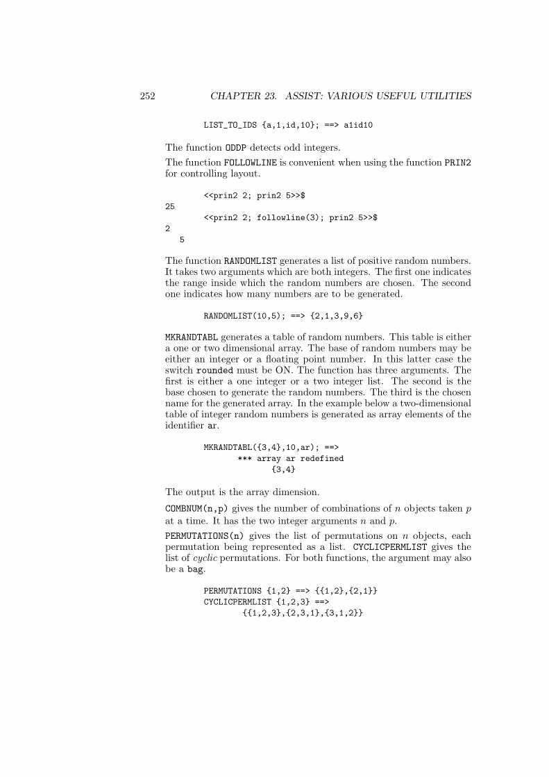
252 CHAPTER 23. ASSIST: VARIOUS USEFUL UTILITIES
LIST_TO_IDS a,1,id,10; ==> a1id10
The function ODDP detects odd integers.The function FOLLOWLINE is convenient when using the function PRIN2for controlling layout.
<<prin2 2; prin2 5>>$25
<<prin2 2; followline(3); prin2 5>>$2
5
The function RANDOMLIST generates a list of positive random numbers.It takes two arguments which are both integers. The first one indicatesthe range inside which the random numbers are chosen. The secondone indicates how many numbers are to be generated.
RANDOMLIST(10,5); ==> 2,1,3,9,6
MKRANDTABL generates a table of random numbers. This table is eithera one or two dimensional array. The base of random numbers may beeither an integer or a floating point number. In this latter case theswitch rounded must be ON. The function has three arguments. Thefirst is either a one integer or a two integer list. The second is thebase chosen to generate the random numbers. The third is the chosenname for the generated array. In the example below a two-dimensionaltable of integer random numbers is generated as array elements of theidentifier ar.
MKRANDTABL(3,4,10,ar); ==>*** array ar redefined
3,4
The output is the array dimension.
COMBNUM(n,p) gives the number of combinations of n objects taken pat a time. It has the two integer arguments n and p.PERMUTATIONS(n) gives the list of permutations on n objects, eachpermutation being represented as a list. CYCLICPERMLIST gives thelist of cyclic permutations. For both functions, the argument may alsobe a bag.
PERMUTATIONS 1,2 ==> 1,2,2,1CYCLICPERMLIST 1,2,3 ==>
1,2,3,2,3,1,3,1,2

23.5. GENERAL PURPOSE UTILITY FUNCTIONS 253
COMBINATIONS gives a list of combinations on n objects taken p at atime. The first argument is a list (or a bag) and the second is theinteger p.
COMBINATIONS(1,2,3,2) ==> 2,3,1,3,1,2
REMSYM is a command that erases the REDUCE commands symmetricor antisymmetric.SYMMETRIZE is a powerful function which generate a symmetric expres-sion. It has 3 arguments. The first is a list (or a list of lists) containingthe expressions which will appear as variables for a kernel. The secondargument is the kernel-name and the third is a permutation functionwhich either exist in the algebraic or in the symbolic mode. This func-tion may have been constructed by the user. Within this package thetwo functions PERMUTATIONS and CYCLICPERMLIST may be used.
ll:=a,b,c$SYMMETRIZE(ll,op,cyclicpermlist); ==>
OP(A,B,C) + OP(B,C,A) + OP(C,A,B)SYMMETRIZE(list ll,op,cyclicpermlist); ==>
OP(A,B,C) + OP(B,C,A) + OP(C,A,B)
Notice that taking for the first argument a list of lists gives rise to anexpression where each kernel has a list as argument. Another pecu-liarity of this function is that, unless a pattern matching is made onthe operator OP, it needs to be reevaluated. Here is an illustration:
op(a,b,c):=a*b*c$SYMMETRIZE(ll,op,cyclicpermlist); ==>
OP(A,B,C) + OP(B,C,A) + OP(C,A,B)for all x let op(x,a,b)=sin(x*a*b);SYMMETRIZE(ll,op,cyclicpermlist); ==>
OP(B,C,A) + SIN(A*B*C) + OP(A,B,C)
The functions SORTNUMLIST and SORTLIST are functions which sortlists. They use bubblesort and quicksort algorithms.
SORTNUMLIST takes as argument a list of numbers. It sorts it in in-creasing order.SORTLIST is a generalisation of the above function. It sorts the listaccording to any well defined ordering. Its first argument is the listand its second argument is the ordering function. The content ofthe list is not necessary numbers but must be such that the orderingfunction has a meaning.

254 CHAPTER 23. ASSIST: VARIOUS USEFUL UTILITIES
l:=1,3,4,0$ SORTNUMLIST l; ==> 0,1,3,4ll:=1,a,tt,z$ SORTLIST(ll,ordp); ==> a,z,tt,1
Note: using these functions for kernels or bags may be dangerous sincethey are destructive. If it is needed, it is recommended first to applyKERNLIST on them.The function EXTREMUM is a generalisation of the functions MIN andMAX to include general orderings. It is a 2 arguments function. Thefirst is the list and the second is the ordering function. With the listll defined in the last example, one gets
EXTREMUM(ll,ordp); ==> 1
iii. There are four functions to identify dependencies. FUNCVAR takes anyexpression as argument and returns the set of variables on which itdepends. Constants are eliminated.
FUNCVAR(e+pi+sin(log(y)); ==> y
DEPATOM has an atom as argument. It returns its argument if it is anumber or if no dependency has previously been declared. Otherwise,it returns the list of variables on which in depends as declared invarious DEPEND declarations.
DEPEND a,x,y;DEPATOM a; ==> x,y
The functions EXPLICIT and IMPLICIT make explicit or implicit thedependencies.
depend a,x; depend x,y,z;EXPLICIT a; ==> a(x(y,z))IMPLICIT ws; ==> a
These are useful when one does not know the names of the variablesand (or) the nature of the dependencies.KORDERLIST is a zero argument function which display the actual or-dering.
KORDER x,y,z;KORDERLIST; ==> (x,y,z)

23.6. PROPERTIES AND FLAGS 255
iv. A function SIMPLIFY which takes an arbitrary expression is availablewhich forces down-to-the-bottom simplification of an expression. Itis useful with SYMMETRIZE. It has also proved useful to simplify someoutput expressions of the package EXCALC (chapter 39).
l:=op(x,y,z)$op(x,y,z):=x*y*z$SYMMETRIZE(l,op,cyclicpermlist); ==>
op(x,y,z)+op(y,z,x)+op(z,x,y)SIMPLIFY ws; ==> op(y,z,x)+op(z,x,y)+x*y*z
v. Filtering functions for lists.
CHECKPROLIST is a boolean function which checks if the elements of alist have a definite property. Its first argument is the list, and its secondargument is a boolean function (FIXP NUMBERP . . .) or an orderingfunction (as ORDP).EXTRACTLIST extracts from the list given as its first argument the ele-ments which satisfy the boolean function given as its second argument.
l:=1,a,b,"st")$EXTRACTLIST(l,fixp); ==> 1EXTRACTLIST(l,stringp); ==> st
23.6 Properties and Flags
It may be useful to provide analogous functions in algebraic mode to theproperties and flags of LISP. Just using the symbolic mode functions toalter property lists of objects may easily destroy the integrity of the system.The functions which are here described do ignore the property list andflags already defined by the system itself. They generate and track theadditional properties and flags that the user issues using them. They offerthe possibility of working on property lists in an algebraic context.
i. Flags To a given identifier, one may associates another one linked to it“in the background”. The three functions PUTFLAG, DISPLAYFLAG andCLEARFLAG handle them.PUTFLAG has 3 arguments. The first is the identifier or a list of iden-tifiers, the second is the name of the flag, the third is T (true) or 0(zero). When the third argument is T, it creates the flag, when it is 0it destroys it.

256 CHAPTER 23. ASSIST: VARIOUS USEFUL UTILITIES
PUTFLAG(z1,flag_name,t); ==> flag_namePUTFLAG(z1,z2,flag1_name,t); ==> tPUTFLAG(z2,flag1_name,0); ==>
DISPLAYFLAG allows to extract flags. Continuing the example:
DISPLAYFLAG z1; ==> flag_name,flag1_nameDISPLAYFLAG z2; ==>
CLEARFLAG is a command which clears all flags associated to the iden-tifiers id1, . . . , idn.
ii. Properties PUTPROP has four arguments. The second argument is theindicator of the property. The third argument may be any valid ex-pression. The fourth one is also T or 0.
PUTPROP(z1,property,x^2,t); ==> z1
In general, one enter
PUTPROP(LIST(idp1,idp2,..),<propname>,<value>,T);
If the last argument is 0 then the property is removed. To display aspecific property, one uses DISPLAYPROP which takes two arguments.The first is the name of the identifier, the second is the indicator ofthe property.
2DISPLAYPROP(z1,property); ==> property,x
Finally, CLEARPROP is a nary commmand which clears all properties ofthe identifiers which appear as arguments.
23.7 Control Functions
The ASSIST package also provides additional functions which improve theuser control of the environment.
i. The first set of functions is composed of unary and binary booleanfunctions. They are:

23.7. CONTROL FUNCTIONS 257
ALATOMP x; x is anything.ALKERNP x; x is anything.DEPVARP(x,v); x is anything.
(v is an atom or a kernel)
ALATOMP has the value T iff x is an integer or an identifier after it hasbeen evaluated down to the bottom.
ALKERNP has the value T iff x is a kernel after it has been evaluateddown to the bottom.
DEPVARP returns T iff the expression x depends on v at any level.
The above functions together with PRECP have been declared operatorfunctions to ease the verification of their value.
NORDP is essentially equivalent to notORDP when inside a conditionalstatement. Otherwise, it can be used while notORDP cannot.
ii. The next functions allow one to analyse and to clean the environmentof REDUCE which is created by the user while working interactively.Two functions are provided:SHOW allows to get the various identifiers already assigned and to seetheir type. SUPPRESS selectively clears the used identifiers or clearsthem all. It is to be stressed that identifiers assigned from the inputof files are ignored. Both functions have one argument and the sameoptions for this argument:
SHOW (SUPPRESS) allSHOW (SUPPRESS) scalarsSHOW (SUPPRESS) listsSHOW (SUPPRESS) saveids (for saved expressions)SHOW (SUPPRESS) matricesSHOW (SUPPRESS) arraysSHOW (SUPPRESS) vectors
(contains vector, index and tvector)SHOW (SUPPRESS) forms
The option all is the most convenient for SHOW but it may takes timeto get the answer after one has worked several hours. When enteringREDUCE the option all for SHOW gives:
SHOW all; ==> scalars are: NILarrays are: NILlists are: NILmatrices are: NILvectors are: NILforms are: NIL
258 CHAPTER 23. ASSIST: VARIOUS USEFUL UTILITIES
It is a convenient way to remember the various options. Starting froma fresh environment
a:=b:=1$SHOW scalars; ==> scalars are: (A B)SUPPRESS scalars; ==> tSHOW scalars; ==> scalars are: NIL
iii. The CLEAR function of the system does not do a complete cleaningof OPERATORS and FUNCTIONS. The following two functions do a morecomplete cleaning and, also automatically takes into account the userflag and properties that the functions PUTFLAG and PUTPROP may haveintroduced.Their names are CLEAROP and CLEARFUNCTIONS. CLEAROP takes oneoperator as its argument. CLEARFUNCTIONS is a nary command. If oneissues
CLEARFUNCTIONS a1,a2, ... , an $
The functions with names a1,a2, ... ,an are cleared. One shouldbe careful when using this facility since the only functions which cannotbe erased are those which are protected with the lose flag.
23.8 Handling of Polynomials
The module contains some utility functions to handle standard quotientsand several new facilities to manipulate polynomials.
i. Two functions ALG TO SYMB and SYMB TO ALG allow the changing ofan expression which is in the algebraic standard quotient form intoa prefix lisp form and vice-versa. This is made in such a way thatthe symbol list which appears in the algebraic mode disappear inthe symbolic form (there it becomes a parenthesis “()” ) and it isreintroduced in the translation from a symbolic prefix lisp expressionto an algebraic one. The following example shows how the well-knownlisp function FLATTENS can be trivially transportd into algebraic mode:
algebraic procedure ecrase x;lisp symb_to_alg flattens1 alg_to_symb algebraic x;
symbolic procedure flattens1 x;

23.8. HANDLING OF POLYNOMIALS 259
% ll; ==> ((A B) ((C D) E))% flattens1 ll; (A B C D E)
if atom x then list x elseif cdr x then
append(flattens1 car x, flattens1 cdr x)else flattens1 car x;
gives, for instance,
ll:=a,b,c,d,e,z$ECRASE ll; ==> A, B, C, D, E, Z
ii. LEADTERM and REDEXPR are the algebraic equivalent of the symbolicfunctions LT and RED. They give the leading term and the reductumof a polynomial. They also work for rational functions. Their interestlies in the fact that they do not require to extract the main variable.They work according to the current ordering of the system:
pol:=x+y+z$LEADTERM pol; ==> xkorder y,x,z;LEADTERM pol; ==> yREDEXPR pol; ==> x + z
By default, the representation of multivariate polynomials is recur-sive. With such a representation, the function LEADTERM does notnecessarily extract a true monom. It extracts a monom in the leadingindeterminate multiplied by a polynomial in the other indeterminates.However, very often one needs to handle true monoms separately. Inthat case, one needs a polynomial in distributive form. Such a formis provided by the package GROEBNER (chapter 45). The facilitythere may be too involved and the need to load an additional packagecan be a problem. So, a new switch is created to handle distributedpolynomials. It is called DISTRIBUTE and a new function DISTRIBUTEputs a polynomial in distributive form. With the switch on, LEADTERMgives true monoms.
MONOM transforms a polynomial into a list of monoms. It works what-ever the setting of the switch DISTRIBUTE.
SPLITTERMS is analoguous to MONOM except that it gives a list of twolists. The first sublist contains the positive terms while the secondsublist contains the negative terms.

260 CHAPTER 23. ASSIST: VARIOUS USEFUL UTILITIES
SPLITPLUSMINUS gives a list whose first element is an expression of thepositive part of the polynomial and its second element is its negativepart.
iii. Two complementary functions LOWESTDEG and DIVPOL are provided.The first takes a polynomial as its first argument and the name of anindeterminate as its second argument. It returns the lowest degree inthat indeterminate. The second function takes two polynomials andreturns both the quotient and its remainder.
23.9 Handling of Transcendental Functions
The functions TRIGREDUCE and TRIGEXPAND and the equivalent ones for hy-perbolic functions HYPREDUCE and HYPEXPAND make the transformations tomultiple arguments and from multiple arguments to elementary arguments.
aa:=sin(x+y)$TRIGEXPAND aa; ==> SIN(X)*COS(Y) + SIN(Y)*COS(X)TRIGREDUCE ws; ==> SIN(Y + X)
When a trigonometric or hyperbolic expression is symmetric with respectto the interchange of SIN (SINH) and COS (COSH), the application ofTRIG(HYP)REDUCE may often lead to great simplifications. However, if it ishighly asymmetric, the repeated application of TRIG(HYP)REDUCE followedby the use of TRIG(HYP)EXPAND will lead to more complicated but moresymmetric expressions:
aa:=(sin(x)^2+cos(x)^2)^3$TRIGREDUCE aa; ==> 1bb:=1+sin(x)^3$TRIGREDUCE bb; ==>
- SIN(3*X) + 3*SIN(X) + 4---------------------------
4
TRIGEXPAND ws; ==>3 2
SIN(X) - 3*SIN(X)*COS(X) + 3*SIN(X) + 4-------------------------------------------
4
See also the TRIGSIMP package (chapter 85).
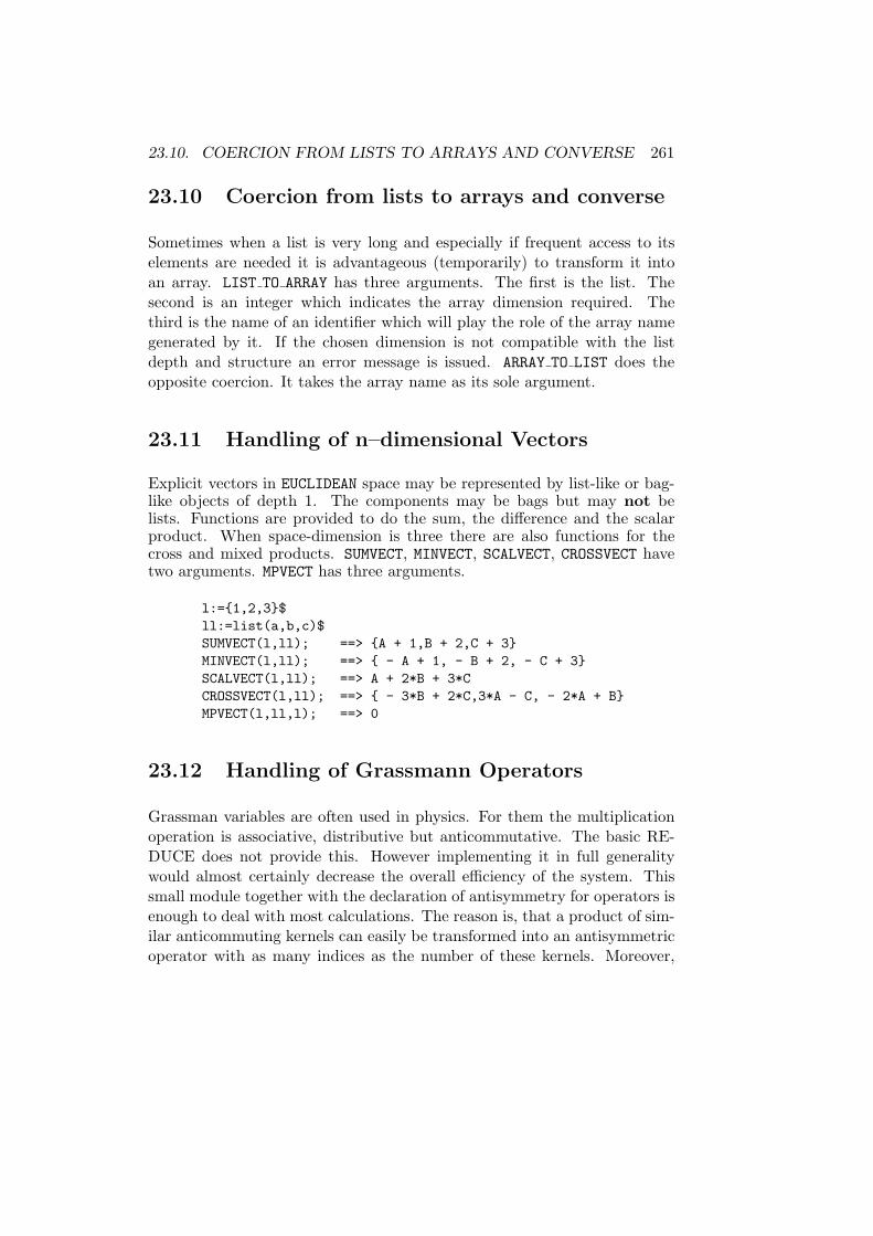
23.10. COERCION FROM LISTS TO ARRAYS AND CONVERSE 261
23.10 Coercion from lists to arrays and converse
Sometimes when a list is very long and especially if frequent access to itselements are needed it is advantageous (temporarily) to transform it intoan array. LIST TO ARRAY has three arguments. The first is the list. Thesecond is an integer which indicates the array dimension required. Thethird is the name of an identifier which will play the role of the array namegenerated by it. If the chosen dimension is not compatible with the listdepth and structure an error message is issued. ARRAY TO LIST does theopposite coercion. It takes the array name as its sole argument.
23.11 Handling of n–dimensional Vectors
Explicit vectors in EUCLIDEAN space may be represented by list-like or bag-like objects of depth 1. The components may be bags but may not belists. Functions are provided to do the sum, the difference and the scalarproduct. When space-dimension is three there are also functions for thecross and mixed products. SUMVECT, MINVECT, SCALVECT, CROSSVECT havetwo arguments. MPVECT has three arguments.
l:=1,2,3$ll:=list(a,b,c)$SUMVECT(l,ll); ==> A + 1,B + 2,C + 3MINVECT(l,ll); ==> - A + 1, - B + 2, - C + 3SCALVECT(l,ll); ==> A + 2*B + 3*CCROSSVECT(l,ll); ==> - 3*B + 2*C,3*A - C, - 2*A + BMPVECT(l,ll,l); ==> 0
23.12 Handling of Grassmann Operators
Grassman variables are often used in physics. For them the multiplicationoperation is associative, distributive but anticommutative. The basic RE-DUCE does not provide this. However implementing it in full generalitywould almost certainly decrease the overall efficiency of the system. Thissmall module together with the declaration of antisymmetry for operators isenough to deal with most calculations. The reason is, that a product of sim-ilar anticommuting kernels can easily be transformed into an antisymmetricoperator with as many indices as the number of these kernels. Moreover,

262 CHAPTER 23. ASSIST: VARIOUS USEFUL UTILITIES
one may also issue pattern matching rules to implement the anticommuta-tivity of the product. The functions in this module represent the minimumfunctionality required to identify them and to handle their specific features.
PUTGRASS is a (nary) command which give identifiers the property to be thenames of Grassmann kernels. REMGRASS removes this property.
GRASSP is a boolean function which detects Grassmann kernels.
GRASSPARITY takes a monom as argument and gives its parity. If themonom is a simple Grassmann kernel it returns 1.
GHOSTFACTOR has two arguments. Each one is a monom. It is equal to
(-1)**(GRASSPARITY u * GRASSPARITY v)
Here is an illustration to show how the above functions work:
PUTGRASS eta;if GRASSP eta(1) then "Grassmann kernel"; ==>
Grassmann kernelaa:=eta(1)*eta(2)-eta(2)*eta(1); ==>
AA := - ETA(2)*ETA(1) + ETA(1)*ETA(2)GRASSPARITY eta(1); ==> 1GRASSPARITY (eta(1)*eta(2)); ==> 0GHOSTFACTOR(eta(1),eta(2)); ==> -1grasskernel:=
eta(~x)*eta(~y) => -eta y * eta x when nordp(x,y),(~x)*(~x) => 0 when grassp x$
exp:=eta(1)^2$exp where grasskernel; ==> 0aa where grasskernel; ==> - 2*ETA(2)*ETA(1)
23.13 Handling of Matrices
There are additional facilities for matrices.
i. Often one needs to construct some UNIT matrix of a given dimension.This construction is performed by the function UNITMAT. It is a naryfunction. The command is
UNITMAT M1(n1), M2(n2), .....Mi(ni) ;
where M1,...Mi are names of matrices and n1, n2, ..., ni are

23.13. HANDLING OF MATRICES 263
integers.MKIDM is a generalisation of MKID. It allows the indexing of matrixnames. If u and u1 are two matrices, one can go from one to theother:
matrix u(2,2);$ unitmat u1(2)$u1; ==>
[1 0][ ][0 1]
mkidm(u,1); ==>[1 0][ ][0 1]
Note: MKIDM(V,1) will fail even if the matrix V1 exists, unless V isalso a matrix.This function allows to make loops on matrices like the following. IfU, U1, U2,.., U5 are matrices:
FOR I:=1:5 DO U:=U-MKIDM(U,I);
ii. The next functions map matrices onto bag-like or list-like objects andconversely they generate matrices from bags or lists.COERCEMAT transforms the matrix first argument into a list of lists.
COERCEMAT(U,id)
When id is list the matrix is transformed into a list of lists. Oth-erwise it transforms it into a bag of bags whose envelope is equal toid.BAGLMAT does the inverse. The first argument is the bag-like or list-likeobject while the second argument is the matrix identifier.
BAGLMAT(bgl,U)
bgl becomes the matrix U. The transformation is not done if U isalready the name of a previously defined matrix, to avoid accidentalredefinition of that matrix.

264 CHAPTER 23. ASSIST: VARIOUS USEFUL UTILITIES
ii. The functions SUBMAT, MATEXTR, MATEXTC take parts of a given matrix.SUBMAT has three arguments.
SUBMAT(U,nr,nc)
The first is the matrix name, and the other two are the row and columnnumbers. It gives the submatrix obtained from U deleting the row nrand the column nc. When one of them is equal to zero only columnnc or row nr is deleted.MATEXTR and MATEXTC extract a row or a column and place it into alist-like or bag-like object.
MATEXTR(U,VN,nr)MATEXTC(U,VN,nc)
where U is the matrix, VN is the “vector name”, nr and nc are integers.If VN is equal to list the vector is given as a list otherwise it is givenas a bag.
iii. Functions which manipulate matrices: MATSUBR, MATSUBC, HCONCMAT,VCONCMAT, TPMAT, HERMAT.MATSUBR and MATSUBC substitute rows and columns. They have threearguments.
MATSUBR(U,bgl,nr)MATSUBC(U,bgl,nc)
The meaning of the variables U, nr, nc is the same as above whilebgl is a list-like or bag-like vector. Its length should be compatiblewith the dimensions of the matrix.HCONCMAT and VCONCMAT concatenate two matrices.
HCONCMAT(U,V)VCONCMAT(U,V)
The first function concatenates horizontally, the second one concate-nates vertically. The dimensions must match.TPMAT makes the tensor product of two matrices. It is also an infixfunction.
TPMAT(U,V) or U TPMAT V

23.13. HANDLING OF MATRICES 265
HERMAT takes the hermitian conjugate of a matrix
HERMAT(U,HU)
where HU is the identifier for the hermitian matrix of U. It shouldunassigned for this function to work successfully. This is done onpurpose to prevent accidental redefinition of an already used identifier.
iv. SETELMAT and GETELMAT are functions of two integers. The first onereset the element (i,j) while the second one extract an element iden-tified by (i,j). They may be useful when dealing with matrices insideprocedures.

266 CHAPTER 23. ASSIST: VARIOUS USEFUL UTILITIES

Chapter 24
ATENSOR: Package forTensor Simplification
V. A. Ilyin and A. P. Kryukov
Tensors are classical examples for Objects often used in mathematics andphysics. Indexed objects can have very complicated and intricated proper-ties. For example the Riemann tensor has symmetry properties with respectto permutation of indices. Moreover it satisfies the cyclic identity. Thereare a number of linear identities with many terms in the case of Riemann-Cartan geometry with torsion. From the user’s point of view, there are threegroups of tensor properties:
• S - symmetry with respect to index permutation;
• I - linear identities;
• D - invariance with respect to renamings of dummy indices;
The problem under investigation can be formulated as whether two tensorexpressions are equal or not by taking into account S-I-D properties.
24.1 Basic tensors and tensor expressions
Under basic tensors we understand the object with finite number of indiceswhich can have such properties as symmetry and multiterm linear identities
267

268 CHAPTER 24. ATENSOR: TENSOR SIMPLIFICATION
(including the symmetry relations).Under tensor expression we understand any expression which can be ob-tained from basic tensors by summation with integer coefficients and multi-plication (commutative) of basic tensors.It is assumed that all terms in the tensor expression have the same numberof indices. Some pairs of them are marked as dummy ones. The set of non-dummy names have to be the same for each term in the tensor expression.The names of dummies can be arbitrary.
24.2 Operators for tensors
Use TENSOR to declare tensors and TCLEAR to remove them. The commandTSYM defines symmetry relations of basic tensors and KBASIS determines theK-Basis, which is the general name for a “triangle” set of linear independentvectors for a basic tensor considered as a separate tensor expression. It ispossible to build the sum, the difference and the multiplication for tensors.It is assumed that indices with identical names means the summation overtheir values.
Example:
1: load atensor;
2: tensor s2,a3;
3: tsym s2(i,j) - s2(j,i), % Symmetric3: a3(i,j,k) + a3(j,i,k), % Antisymm.3: a3(i,j,k) - a3(j,k,i);
4: kbasis s2,a3;
s2(j,i) + (-1)*s2(i,j)1a3(k,i,j) + a3(j,i,k)a3(k,j,i) + (-1)*a3(j,i,k)a3(i,k,j) + (-1)*a3(j,i,k)a3(i,j,k) + a3(j,i,k)a3(j,k,i) + a3(j,i,k)5

24.3. SWITCHES 269
24.3 Switches
There are two switches defined. The switch DUMMYPRI prints dummy indiceswith internal names and numbers. It’s default value is OFF. The other switchcalled SHORTEST prints tensor expressions in shortest form that was producedduring evaluation. The default value is OFF.
For further information refer to the documentation which comes with thispackage.

270 CHAPTER 24. ATENSOR: TENSOR SIMPLIFICATION

Chapter 25
AVECTOR: A vector algebraand calculus package
David HarperAstronomy Unit, Queen Mary and Westfield College
University of LondonMile End Road
London E1 4NS, England
e–mail: [email protected]
This package provides REDUCE with the ability to perform vector algebrausing the same notation as scalar algebra. The basic algebraic operationsare supported, as are differentiation and integration of vectors with respectto scalar variables, cross product and dot product, component manipulationand application of scalar functions (e.g. cosine) to a vector to yield a vectorresult.
25.1 Vector declaration and initialisation
To declare a list of names to be vectors use the VEC command:
VEC A,B,C;
declares the variables A, B and C to be vectors. If they have already beenassigned (scalar) values, these will be lost.
271

272 CHAPTER 25. AVECTOR: VECTOR ALGEBRA
When a vector is declared using the VEC command, it does not have aninitial value.
If a vector value is assigned to a scalar variable, then that variable willautomatically be declared as a vector and the user will be notified that thishas happened.
A vector may be initialised using the AVEC function which takes three scalararguments and returns a vector made up from those scalars. For example
A := AVEC(A1, A2, A3);
sets the components of the vector A to A1, A2 and A3.
25.2 Vector algebra
(In the examples which follow, V, V1, V2 etc are assumed to be vectors whileS, S1, S2 etc are scalars.)
The scalar algebra operators +,-,* and / may be used with vector operandsaccording to the rules of vector algebra. Thus multiplication and division ofa vector by a scalar are both allowed, but it is an error to multiply or divideone vector by another.
V := V1 + V2 - V3; Addition and subtractionV := S1*3*V1; Scalar multiplicationV := V1/S; Scalar divisionV := -V1; Negation
Vector multiplication is carried out using the infix operators DOT and CROSS.These are defined to have higher precedence than scalar multiplication anddivision.V := V1 CROSS V2; Cross productS := V1 DOT V2; Dot productV := V1 CROSS V2 + V3;V := (V1 CROSS V2) + V3;
The last two expressions are equivalent due to the precedence of the CROSSoperator.
The modulus of a vector may be calculated using the VMOD operator.
S := VMOD V;

25.3. VECTOR CALCULUS 273
A unit vector may be generated from any vector using the VMOD operator.
V1 := V/(VMOD V);
Components may be extracted from any vector using index notation in thesame way as an array.
V := AVEC(AX, AY, AZ);V(0); yields AXV(1); yields AYV(2); yields AZ
It is also possible to set values of individual components. Following fromabove:
V(1) := B;
The vector V now has components AX, B, AZ.
Vectors may be used as arguments in the differentiation and integrationroutines in place of the dependent expression.
V := AVEC(X**2, SIN(X), Y);DF(V,X); yields (2*X, COS(X), 0)INT(V,X); yields (X**3/3, -COS(X), Y*X)
Vectors may be given as arguments to monomial functions such as SIN, LOGand TAN. The result is a vector obtained by applying the function component-wise to the argument vector.
V := AVEC(A1, A2, A3);SIN(V); yields (SIN(A1), SIN(A2), SIN(A3))
25.3 Vector calculus
The vector calculus operators div, grad and curl are recognised. The Lapla-cian operator is also available and may be applied to scalar and vectorarguments.

274 CHAPTER 25. AVECTOR: VECTOR ALGEBRA
V := GRAD S; Gradient of a scalar fieldS := DIV V; Divergence of a vector fieldV := CURL V1; Curl of a vector fieldS := DELSQ S1; Laplacian of a scalar fieldV := DELSQ V1; Laplacian of a vector field
These operators may be used in any orthogonal curvilinear coordinate sys-tem. The user may alter the names of the coordinates and the values of thescale factors. Initially the coordinates are X, Y and Z and the scale factorsare all unity.
There are two special vectors : COORDS contains the names of the coordinatesin the current system and HFACTORS contains the values of the scale factors.
The coordinate names may be changed using the COORDINATES operator.
COORDINATES R,THETA,PHI;
This command changes the coordinate names to R, THETA and PHI.
The scale factors may be altered using the SCALEFACTORS operator.
SCALEFACTORS(1,R,R*SIN(THETA));
This command changes the scale factors to 1, R and R SIN(THETA).
Note that the arguments of SCALEFACTORS must be enclosed in parentheses.This is not necessary with COORDINATES.
When vector differential operators are applied to an expression, the currentset of coordinates are used as the independent variables and the scale factorsare employed in the calculation.
Several coordinate systems are pre-defined and may be invoked by name.To see a list of valid names enter
SYMBOLIC !*CSYSTEMS;
and REDUCE will respond with something like
(CARTESIAN SPHERICAL CYLINDRICAL)
To choose a coordinate system by name, use the command GETCSYSTEM.

25.3. VECTOR CALCULUS 275
To choose the Cartesian coordinate system :
GETCSYSTEM ’CARTESIAN;
Note the quote which prefixes the name of the coordinate system. This is re-quired because GETCSYSTEM (and its complement PUTCSYSTEM) is a SYMBOLICprocedure which requires a literal argument.
REDUCE responds by typing a list of the coordinate names in that coordi-nate system. The example above would produce the response
(X Y Z)
whilst
GETCSYSTEM ’SPHERICAL;
would produce
(R THETA PHI)
Note that any attempt to invoke a coordinate system is subject to the samerestrictions as the implied calls to COORDINATES and SCALEFACTORS. In par-ticular, GETCSYSTEM fails if any of the coordinate names has been assigneda value and the previous coordinate system remains in effect.
A user-defined coordinate system can be assigned a name using the commandPUTCSYSTEM. It may then be re-invoked at a later stage using GETCSYSTEM.
Example 1
We define a general coordinate system with coordinate names X,Y,Z and scalefactors H1,H2,H3 :
COORDINATES X,Y,Z;SCALEFACTORS(H1,H2,H3);PUTCSYSTEM ’GENERAL;
This system may later be invoked by entering
GETCSYSTEM ’GENERAL;

276 CHAPTER 25. AVECTOR: VECTOR ALGEBRA
25.4 Volume and Line Integration
Several functions are provided to perform volume and line integrals. Theseoperate in any orthogonal curvilinear coordinate system and make use ofthe scale factors described in the previous section.
Definite integrals of scalar and vector expressions may be calculated usingthe DEFINT function1.
Example 2
To calculate the definite integral of sin(x)2 between 0 and 2π we enter
DEFINT(SIN(X)**2,X,0,2*PI);
This function is a simple extension of the INT function taking two extraarguments, the lower and upper bounds of integration respectively.
Definite volume integrals may be calculated using the VOLINTEGRAL functionwhose syntax is as follows :
VOLINTEGRAL(integrand, vector lower-bound, vector upper-bound);
Example 3
In spherical polar coordinates we may calculate the volume of a sphere byintegrating unity over the range r=0 to RR, θ=0 to PI, φ=0 to 2*π as follows:VLB := AVEC(0,0,0); Lower boundVUB := AVEC(RR,PI,2*PI); Upper bound in r, θ, φ respectivelyVOLINTORDER := (0,1,2); The order of integrationVOLINTEGRAL(1,VLB,VUB);
Note the use of the special vector VOLINTORDER which controls the orderin which the integrations are carried out. This vector should be set tocontain the number 0, 1 and 2 in the required order. The first component ofVOLINTORDER contains the index of the first integration variable, the secondcomponent is the index of the second integration variable and the thirdcomponent is the index of the third integration variable.
Example 4
Suppose we wish to calculate the volume of a right circular cone. This is1Not to be confused with the DEFINT package described in chapter 34

25.4. VOLUME AND LINE INTEGRATION 277
equivalent to integrating unity over a conical region with the bounds:
z = 0 to H (H = the height of the cone)r = 0 to pZ (p = ratio of base diameter to height)phi = 0 to 2*PI
We evaluate the volume by integrating a series of infinitesimally thin circulardisks of constant z-value. The integration is thus performed in the order :d(φ) from 0 to 2π, dr from 0 to p*Z, dz from 0 to H. The order of the indicesis thus 2, 0, 1.
VOLINTORDER := AVEC(2,0,1);VLB := AVEC(0,0,0);VUB := AVEC(P*Z,H,2*PI);VOLINTEGRAL(1,VLB,VUB);
Line integrals may be calculated using the LINEINT and DEFLINEINT funct-ions. Their general syntax is
LINEINT(vector-fnct, vector-curve, variable);
DEFLINENINT(vector-fnct, vector-curve, variable,lower-bnd, upper-bnd);
where
vector-fnct is any vector-valued expression;
vector-curve is a vector expression which describes the path of integrationin terms of the independent variable;
variable is the independent variable;
lower-bnd
upper-bnd are the bounds of integration in terms of the independent vari-able.
Example 5
In spherical polar coordinates, we may integrate round a line of constanttheta (‘latitude’) to find the length of such a line. The vector function isthus the tangent to the ‘line of latitude’, (0,0,1) and the path is (0,LAT,PHI)where PHI is the independent variable. We show how to obtain the definiteintegral i.e. from φ = 0 to 2π :

278 CHAPTER 25. AVECTOR: VECTOR ALGEBRA
DEFLINEINT(AVEC(0,0,1),AVEC(0,LAT,PHI),PHI,0,2*PI);

Chapter 26
BOOLEAN: A package forboolean algebra
Herbert MelenkKonrad–Zuse–Zentrum fur Informationstechnik Berlin
Takustrase 7D–14195 Berlin–Dahlem, Germany
e–mail: [email protected]
The package Boolean supports the computation with boolean expressionsin the propositional calculus. The data objects are composed from algebraicexpressions (“atomic parts”, “leafs”) connected by the infix boolean oper-ators and, or, implies, equiv, and the unary prefix operator not. Booleanallows simplification of expressions built from these operators, and to testproperties like equivalence, subset property etc. Also the reduction of aboolean expression by a partial evaluation and combination of its atomicparts is supported.
26.1 Entering boolean expressions
In order to distinguish boolean data expressions from boolean expressionsin the REDUCE programming language (e.g. in an if statement), eachexpression must be tagged explicitly by an operator boolean. Otherwisethe boolean operators are not accepted in the REDUCE algebraic modeinput. The first argument of boolean can be any boolean expression, whichmay contain references to other boolean values.
279

280CHAPTER 26. BOOLEAN: A PACKAGE FOR BOOLEAN ALGEBRA
load_package boolean;boolean (a and b or c);q := boolean(a and b implies c);boolean(q or not c);
Brackets are used to override the operator precedence as usual. The leafsor atoms of a boolean expression are those parts which do not contain aleading boolean operator. These are considered as constants during theboolean evaluation. There are two pre-defined values:
• true, t or 1
• false, nil or 0
These represent the boolean constants. In a result form they are used onlyas 1 and 0.
By default, a boolean expression is converted to a disjunctive normal form.
On output, the operators and and or are represented as /\ and \/, respec-tively.
boolean(true and false); -> 0boolean(a or not(b and c)); -> boolean(not(b) \/ not(c) \/ a)boolean(a equiv not c); -> boolean(not(a)/\c \/ a/\not(c))
26.2 Normal forms
The disjunctive normal form is used by default. Alternatively a conjunc-tive normal form can be selected as simplification target, which is a formwith leading operator and. To produce that form add the keyword and asan additional argument to a call of boolean.
boolean (a or b implies c);->
boolean(not(a)/\not(b) \/ c)
boolean (a or b implies c, and);->
boolean((not(a) \/ c)/\(not(b) \/ c))
Usually the result is a fully reduced disjunctive or conjuntive normal form,where all redundant elements have been eliminated following the rules

26.2. NORMAL FORMS 281
a ∧ b ∨ ¬a ∧ b←→ b
a ∨ b ∧ ¬a ∨ b←→ b
Internally the full normal forms are computed as intermediate result; inthese forms each term contains all leaf expressions, each one exactly once.This unreduced form is returned when the additional keyword full is set:
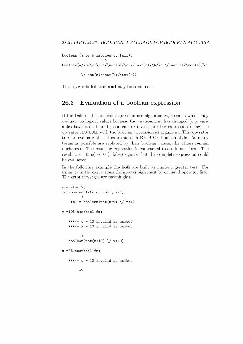
282CHAPTER 26. BOOLEAN: A PACKAGE FOR BOOLEAN ALGEBRA
boolean (a or b implies c, full);->
boolean(a/\b/\c \/ a/\not(b)/\c \/ not(a)/\b/\c \/ not(a)/\not(b)/\c
\/ not(a)/\not(b)/\not(c))
The keywords full and and may be combined.
26.3 Evaluation of a boolean expression
If the leafs of the boolean expression are algebraic expressions which mayevaluate to logical values because the environment has changed (e.g. vari-ables have been bound), one can re–investigate the expression using theoperator TESTBOOL with the boolean expression as argument. This operatortries to evaluate all leaf expressions in REDUCE boolean style. As manyterms as possible are replaced by their boolean values; the others remainunchanged. The resulting expression is contracted to a minimal form. Theresult 1 (= true) or 0 (=false) signals that the complete expression couldbe evaluated.
In the following example the leafs are built as numeric greater test. Forusing > in the expressions the greater sign must be declared operator first.The error messages are meaningless.
operator >;fm:=boolean(x>v or not (u>v));
->fm := boolean(not(u>v) \/ x>v)
v:=10$ testbool fm;
***** u - 10 invalid as number***** x - 10 invalid as number
->boolean(not(u>10) \/ x>10)
x:=3$ testbool fm;
***** u - 10 invalid as number
->

26.3. EVALUATION OF A BOOLEAN EXPRESSION 283
boolean(not(u>10))
x:=17$ testbool fm;
***** u - 10 invalid as number
->1

284CHAPTER 26. BOOLEAN: A PACKAGE FOR BOOLEAN ALGEBRA

Chapter 27
CALI: ComputationalCommutative Algebra
Hans-Gert GrabeInstitut fur Informatik, Universitat Leipzig
Augustusplatz 10 – 1104109 Leipzig, Germany
e–mail: [email protected]
This package contains algorithms for computations in commutative algebraclosely related to the Grobner algorithm for ideals and modules. Its heartis a new implementation of the Grobner algorithm that also allows for thecomputation of syzygies. This implementation is also applicable to submod-ules of free modules with generators represented as rows of a matrix. Asmain topics CALI contains facilities for
• defining rings, ideals and modules,
• computing Grobner bases and local standard bases,
• computing syzygies, resolutions and (graded) Betti numbers,
• computing (now also weighted) Hilbert series, multiplicities, indepen-dent sets, and dimensions,
• computing normal forms and representations,
• computing sums, products, intersections, quotients, stable quotients,elimination ideals etc.,
285

286 CHAPTER 27. CALI: COMMUTATIVE ALGEBRA
• primality tests, computation of radicals, unmixed radicals, equidimen-sional parts, primary decompositions etc. of ideals and modules,
• advanced applications of Grobner bases (blowup, associated gradedring, analytic spread, symmetric algebra, monomial curves etc.),
• applications of linear algebra techniques to zero dimensional ideals,as e.g. the FGLM change of term orders, border bases and affine andprojective ideals of sets of points,
• splitting polynomial systems of equations mixing factorisation and theGrobner algorithm, triangular systems, and different versions of theextended Grobner factoriser.
There is more extended documentation on this package elsewhere, whichincludes facilities for tracing and switches to control its behaviour.

Chapter 28
CAMAL: Calculations inCelestial Mechanics
J. P. FitchSchool of Mathematical Sciences, University of Bath
BATH BA2 7AY, England
e–mail: [email protected]
The CAMAL package provides facilities for calculations in Fourier seriessimilar to those in the specialist Celestial Mechanics system of the 1970s,and the Cambridge Algebra system in particular.
28.1 Operators for Fourier Series
HARMONIC
The celestial mechanics system distinguish between polynomial variables andangular variables. All angles must be declared before use with the HARMONICfunction.
harmonic theta, phi;
287

288 CHAPTER 28. CAMAL: CELESTIAL MECHANICS
FOURIER
The FOURIER function coerces its argument into the domain of a FourierSeries. The expression may contain sine and cosine terms of linear sums ofharmonic variables.
fourier sin(theta)
Fourier series expressions may be added, subtracted multiplies and differen-tiated in the usual REDUCE fashion. Multiplications involve the automaticlinearisation of products of angular functions.
There are three other functions which correspond to the usual restrictiveharmonic differentiation and integration, and harmonic substitution.
HDIFF and HINT
Differentiate or integrate a Fourier expression with respect to an angularvariable. Any secular terms in the integration are disregarded without com-ment.
load_package camal;harmonic u;bige := fourier (sin(u) + cos(2*u));aa := fourier 1+hdiff(bige,u);ff := hint(aa*aa*fourier cc,u);
HSUB
The operation of substituting an angle plus a Fourier expression for anangles and expanding to some degree is called harmonic substitution. Thefunction takes 5 arguments; the basic expression, the angle being replaced,the angular part of the replacement, the fourier part of the replacement anda degree to which to expand.
harmonic u,v,w,x,y,z;xx:=hsub(fourier((1-d*d)*cos(u)),u,u-v+w-x-y+z,yy,n);

28.2. A SHORT EXAMPLE 289
28.2 A Short Example
The following program solves Kepler’s Equation as a Fourier series to thedegree n.
bige := fourier 0;for k:=1:n do <<
wtlevel k;bige:=fourier e * hsub(fourier(sin u), u, u, bige, k);
>>;write "Kepler Eqn solution:", bige$

290 CHAPTER 28. CAMAL: CELESTIAL MECHANICS

Chapter 29
CGB: ComprehensiveGrobner Bases
Andreas Dolzmann & Thomas SturmDepartment of Mathematics and Computer Science
University of PassauD-94030 Passau, Germany
e-mail: [email protected], [email protected]
29.1 Introduction
Consider the ideal basis F = ax, x + y. Treating a as a parameter, thecalling sequence
torder(x,y,lex)$groebnera*x,x+y;
x,y
yields x, y as reduced Grobner basis. This is, however, not correct underthe specialization a = 0. The reduced Grobner basis would then be x+ y.Taking these results together, we obtain C = x+y, ax, ay, which is correctwrt. all specializations for a including zero specializations. We call this setC a comprehensive Grobner basis (cgb).
The notion of a cgb and a corresponding algorithm has been introduced
291

292 CHAPTER 29. CGB: COMPREHENSIVE GROBNER BASES
bei Weispfenning [17]. This algorithm works by performing case distinc-tions wrt. parametric coefficient polynomials in order to find out what thehead monomials are under all possible specializations. It does thus not onlydetermine a cgb, but even classifies the contained polynomials wrt. the spe-cializations they are relevant for. If we keep the Grobner bases for all casesseparate and associate information on the respective specializations withthem, we obtain a Grobner system. For our example, the Grobner systemis the following; [
a 6= 0 x+ y, ax, aya = 0 x+ y
].
A cgb is obtained as the union of the single Grobner bases in a Grobnersystem. It has also been shown that, on the other hand, a Grobner systemcan easily be reconstructed from a given cgb [17].
The CGB package provides functions for computing both cgb’s and Grobnersystems, and for turning Grobner systems into cgb’s.
29.2 Using the REDLOG Package
For managing the conditions occurring with the cgb computations, the CGBpackage uses the package REDLOG implementing first-order formulas, [?, ?],which is also part of the reduce distribution.
29.3 Term Ordering Mode
The CGB package uses the settings made with the function TORDER ofthe GROEBNER package. This includes in particular the choice of themain variables. All variables not mentioned in the variable list argument ofTORDER are parameters. The only term ordering modes recognized by cgbare LEX and REVGRADLEX.
29.4 CGB: Comprehensive Grobner Basis
The function CGB expects a list F of expressions. It returns a cgb of Fwrt. the current TORDER setting.

29.5. GSYS: GROBNER SYSTEM 293
Example:
torder(x,y,lex)$cgba*x+y,x+b*y;
x + b*y,a*x + y,(a*b - 1)*y
ws;
b*y + x,
a*x + y,
y*(a*b - 1)
Note that the basis returned by the CGB call has not undergone the standardevaluation process: The returned polynomials are ordered wrt. the chosenterm order. Reevaluation changes this as can be seen with the output of WS.
29.5 GSYS: Grobner System
The function GSYS follows the same calling conventions as CGB. It returnsthe complete Grobner system represented as a nested list
c1, g11, . . . , g1n1, . . . , cm, gm1, . . . , g1nm.
The ci are conditions in the parameters represented as quantifier-free RED-LOG formulas. Each choice of parameters will obey at least one of theci. Whenever a choice of parameters obeys some ci, the correspondinggi1, . . . , gini is a Grobner basis for this choice.
Example:
torder(x,y,lex)$gsys a*x+y,x+b*y;
a*b - 1 <> 0 and a <> 0,
a*x + y,x + b*y,(a*b - 1)*y,

294 CHAPTER 29. CGB: COMPREHENSIVE GROBNER BASES
a <> 0 and a*b - 1 = 0,
a*x + y,x + b*y,
a = 0,a*x + y,x + b*y
As with the function CGB, the contained polynomials remain unevaluated.
Computing a Grobner system is not harder than computing a cgb. In fact,CGB also computes a Grobner system and then turns it into a cgb.
29.5.1 Switch CGBGEN: Only the Generic Case
If the switch CGBGEN is turned on, both GSYS and CGB will assume all para-metric coefficients to be non-zero ignoring the other cases. For CGB thismeans that the result equals—up to auto-reduction—that of GROEBNER. Acall to GSYS will return this result as a single case including the assumptionsmade during the computation:
Example:
torder(x,y,lex)$on cgbgen;gsysa*x+y,x+b*y;
a*b - 1 <> 0 and a <> 0,
a*x + y,x + b*y,(a*b - 1)*y
off cgbgen;
29.6 GSYS2CGB: Grobner System to CGB
The call GSYS2CGB turns a given Grobner system into a cgb by constructingthe union of the Grobner bases of the single cases.
Example:
torder(x,y,lex)$

29.7. SWITCH CGBREAL: COMPUTING OVER THE REAL NUMBERS295
gsysa*x+y,x+b*y$gsys2cgb ws;
x + b*y,a*x + y,(a*b - 1)*y
29.7 Switch CGBREAL: Computing over the RealNumbers
All computations considered so far have taken place over the complex num-bers, more precisely, over algebraically closed fields. Over the real numbers,certain branches of the cgb computation can become inconsitent thoughthey are not inconsistent over the complex numbers. Consider, e.g., a con-dition a2 + 1 = 0.
When turning on the switch CGBREAL, all simplifications of conditions areperformed over the real numbers. The methods used for this are describedin [?].
Example:
torder(x,y,lex)$off cgbreal;gsys a*x+y,x-a*y;
2a + 1 <> 0 and a <> 0,
2a*x + y,x - a*y,(a + 1)*y,
2a <> 0 and a + 1 = 0,a*x + y,x - a*y,
a = 0,a*x + y,x - a*y
on cgbreal;gsys(a*x+y,x-a*y);
a <> 0,
2

296 CHAPTER 29. CGB: COMPREHENSIVE GROBNER BASES
a*x + y,x - a*y,(a + 1)*y,
a = 0,a*x + y,x - a*y
29.8 Switches
CGBREAL Compute over the real numbers. See Section 29.7 for details.
CGBGS Grobner simplification of the condition. The switch CGBGS can beturned on for applying advanced algebraic simplification techniques tothe conditions. This will, in general, slow down the computation, butlead to a simpler Grobner system.
CGBSTAT Statistics of the CGB run. The switch CGBSTAT toggles the creationand output of statistical information on the CGB run. The statisticalinformation is printed at the end of the run.
CGBFULLRED Full reduction. By default, the CGB functions perform fullreductions in contrast to pure top reductions. By turning off the switchCGBFULLRED, reduction can be restricted to top reductions.
Chapter 30
CHANGEVR: Change ofIndependent Variables inDEs
G. UcolukDepartment of Physics, Middle East Technical University
Ankara, Turkey
e–mail: [email protected]
The function CHANGEVAR has (at least) four different arguments.
• FIRST ARGUMENTis a list of the dependent variables of the differential equation. If thereis only one dependent variable it can be given directly, not as a list.
• SECOND ARGUMENTis a list of the new independent variables, or in the case of only one,the variable.
• THIRD ARGUMENT, FOURTH etc.are equations is of the form
old variable = a function in new variables
The left hand side cannot be a non-kernel structure. These give theold variables in terms of the new ones.
297

298 CHAPTER 30. CHANGEVR: CHANGE OF VARIABLES IN DES
• LAST ARGUMENTis a list of algebraic expressions which evaluates to differential equat-ions in the usual list notation. Again it is possible to omit the listform if there is only one differential equation.
If the last argument is a list then the result of CHANGEVAR is a list too.
It is possible to display the entries of the inverse Jacobian. To do so, turnON the flag DISPJACOBIAN.
30.1 An example: the 2-D Laplace Equation
The 2-dimensional Laplace equation in Cartesian coordinates is:
∂2u
∂x2+∂2u
∂y2= 0
Now assume we want to obtain the polar coordinate form of Laplace equat-ion. The change of variables is:
x = r cos θ, y = r sin θ
The solution using CHANGEVAR is
CHANGEVAR(u,r,theta,x=r*cos theta,y=r*sin theta,df(u(x,y),x,2)+df(u(x,y),y,2) );
Here we could omit the curly braces in the first and last arguments (becausethose lists have only one member) and the curly braces in the third argument(because they are optional), but not in the second. So one could equivalentlywrite
CHANGEVAR(u,r,theta,x=r*cos theta,y=r*sin theta,df(u(x,y),x,2)+df(u(x,y),y,2) );
The u(x,y) operator will be changed to u(r,theta) in the result as onewould do with pencil and paper. u(r,theta) represents the the transformeddependent variable.

Chapter 31
COMPACT: Package forcompacting expressions
Anthony C. HearnRAND
Santa MonicaCA 90407-2138, U.S.A.
e–mail: [email protected]
COMPACT is a package of functions for the reduction of a polynomial inthe presence of side relations. The package defines one operator COMPACTwhose syntax is:
COMPACT(<expression>, <list>):<expression>
<expression> can be any well-formed algebraic expression, and <list> anexpression whose value is a list of either expressions or equations. For ex-ample
compact(x**2+y**3*x-5y,x+y-z,x-y-z1);compact(sin(x)**10*cos(x)**3+sin(x)**8*cos(x)**5,
cos(x)**2+sin(x)**2=1);let y = cos(x)**2+sin(x)**2-1;compact(sin(x)**10*cos(x)**3+sin(x)**8*cos(x)**5,y);
COMPACT applies the relations to the expression so that an equivalent
299
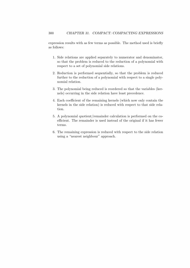
300 CHAPTER 31. COMPACT: COMPACTING EXPRESSIONS
expression results with as few terms as possible. The method used is brieflyas follows:
1. Side relations are applied separately to numerator and denominator,so that the problem is reduced to the reduction of a polynomial withrespect to a set of polynomial side relations.
2. Reduction is performed sequentially, so that the problem is reducedfurther to the reduction of a polynomial with respect to a single poly-nomial relation.
3. The polynomial being reduced is reordered so that the variables (ker-nels) occurring in the side relation have least precedence.
4. Each coefficient of the remaining kernels (which now only contain thekernels in the side relation) is reduced with respect to that side rela-tion.
5. A polynomial quotient/remainder calculation is performed on the co-efficient. The remainder is used instead of the original if it has fewerterms.
6. The remaining expression is reduced with respect to the side relationusing a “nearest neighbour” approach.

Chapter 32
CRACK: Solvingoverdetermined systems ofPDEs or ODEs
Thomas WolfSchool of Mathematical Sciences, Queen Mary and Westfield College
University of LondonLondon E1 4NS, England
e–mail: [email protected]
Andreas BrandInstitut fur Informatik
Friedrich Schiller Universitat Jena07740 Jena, Germany
e–mail: [email protected]
The package CRACK aims at solving or at least partially integrat-ing single ordinary differential equations or partial differential equations(ODEs/PDEs), and systems of them, exactly and in full generality. Calcu-lations done with input DEs include the
• integration of exact DEs and generalised exact DEs
• determination of monomial integrating factors
• direct and indirect separation of DEs
• systematic application of integrability conditions
301

302 CHAPTER 32. CRACK: OVERDETERMINED SYSTEMS OF DES
• solution of single elementary ODEs by using the REDUCE packageODESOLVE (chapter 59).
Input DEs may be polynomially non-linear in the unknown functions andtheir derivatives and may depend arbitrarily on the independent variables.
Suitable applications of CRACK are the solution of
• overdetermined ODE/PDE-systems (overdetermined here just meansthat the number of unknown functions of all independent variables isless than the number of given equations for these functions).
• simple non-overdetermined DE-systems (such as characteristic ODE-systems of first order quasilinear PDEs).
The strategy is to have one universal program (CRACK) which is as effectiveas possible for solving overdetermined PDE-systems and many applicationprograms (such as LIEPDE) which merely generate an overdetermined PDE-system depending on what is to be investigated (for example, symmetriesor conservation laws).
Examples are:
• the investigation of infinitesimal symmetries of DEs (LIEPDE),
• the determination of an equivalent Lagrangian for second order ODEs(LAGRAN)
• the investigation of first integrals of ODEs which are polynomial intheir highest derivative (FIRINT)
• the splitting of an nth order ODE into a first order ODE and an (n−1)th order problem (DECOMP)
Other applications where non-overdetermined problems are treated are
• the application of infinitesimal symmetries (e.g. calculated by LIEPDE)in the package APPLYSYM (chapter 21),
• the program QUASILINPDE (also in the package APPLYSYM) forsolving single first order quasilinear PDEs.

303
The kernel package for solving overdetermined or simple non-overdeterminedDE-systems is accessible through a call to the program CRACK in the pack-age CRACK. All the application programs (LIEPDE, LAGRAN, FIRINT,DECOMP except APPLYSYM) are contained in the package CRACKAPP.The programs APPLYSYM and QUASILINPDE are contained in the pack-age APPLYSYM (described in chapter 21).
Details of the CRACK applications can be found in the example file.
CRACK is called by
CRACK(equ1, equ2, . . . , equm,ineq1, ineq2, . . . , ineqn,fun1, fun2, . . . , funp,var1, var2, . . . , varq);
m,n, p, q are arbitrary.
• The equi are identically vanishing partial differential expressions, i.e.they represent equations 0 = equi, which are to be solved for the funct-ions funj as far as possible, thereby drawing only necessary conclusionsand not restricting the general solution.
• The ineqi are expressions which must not vanish identically for anysolution to be determined, i.e. only such solutions are computed forwhich none of the ineqi vanishes identically in all independent vari-ables.
• The dependence of the (scalar) functions funj on possibly a numberof variables is assumed to have been defined with DEPEND ratherthan declaring these functions as operators. Their arguments maythemselves only be independent variables and not expressions.
• The functions funj and their derivatives may only occur polynomially.Other unknown functions in equi may be represented as operators.
• The vark are further independent variables, which are not alreadyarguments of any of the funj . If there are none then the third argumentis the empty list .• The dependence of the equi on the independent variables and on con-
stants and functions other than funj is arbitrary.

304 CHAPTER 32. CRACK: OVERDETERMINED SYSTEMS OF DES
The result is a list of solutions
sol1, . . .
where each solution is a list of 3 lists:
con1, con2, . . . , conq,funa = exa, funb = ex b, . . . , funp = ex p,func, fund, . . . , funr
with integer a, b, c, d, p, q, r. If CRACK finds a contradiction as 0 = 1 thenthere exists no solution and it returns the empty list . The empty listis also returned if no solution exists which does not violate the inequalitiesineqi 6= 0. For example, in the case of a linear system as input, there is atmost one solution sol1.
The expressions coni (if there are any), are the remaining necessary andsufficient conditions for the functions func, . . . , funr in the third list. Thosefunctions can be original functions from the equations to be solved (of thesecond argument of the call of CRACK) or new functions or constants whicharose from integrations. The dependence of new functions on variables isdeclared with DEPEND and to visualise this dependence the algebraic modefunction FARGS(funi) can be used. If there are no coni then all equationsare solved and the functions in the third list are unconstrained.
The second list contains equations funi = ex i where each funi is an originalfunction and ex i is the computed expression for funi.
The exact behaviour of CRACK can be modified by internal variables, andthere is a help system particularly associated with CRACK. Users are referredto the detailed documentation for more information.

Chapter 33
CVIT: Fast calculation ofDirac gamma matrix traces
V. Ilyin, A. Kryukov, A. Rodionov and A. TaranovInstitute for Nuclear Physics
Moscow State UniversityMoscow, 119899 Russia
The package consists of 5 sections, and provides an alternative to the RE-DUCE high-energy physics system. Instead of being based on Γ-matricesas a basis for a Clifford algebra, it is based on treating Γ-matrices as 3-jsymbols, as described by Cvitanovic.
The functions it provides are the same as those of the standard package. Itdoes have four switches which control its behaviour.
CVIT
If it is on then use Kennedy-Cvitanovic algorithm else use standard facilities.
CVITOP
Switches on Fierz optimisation. Default is off;
CVITBTR
Switches on the bubbles and triangles factorisation. The default is on.
CVITRACE
Controls internal tracing of the CVIT package. Default is off.
305

306 CHAPTER 33. CVIT:DIRAC GAMMA MATRIX TRACES
index j1,j2,j3,;
vecdim n$
g(l,j1,j2,j2,j1);
2n
g(l,j1,j2)*g(l1,j3,j1,j2,j3);
2n
g(l,j1,j2)*g(l1,j3,j1,j3,j2);
n*( - n + 2)
Chapter 34
DEFINT: DefiniteIntegration for REDUCE
Kerry Gaskell and Winfried NeunKonrad–Zuse–Zentrum fur Informationstechnik Berlin
Takustrase 7D–14195 Berlin–Dahlem, Germany
e–mail: [email protected]
Stanley L. KamenyLos Angeles, U.S.A.
REDUCE’s definite integration package is able to calculate the definite inte-grals of many functions, including several special functions. There are anumber of parts of this package, including contour integration. The innova-tive integration process is to represent each function as a Meijer G-function,and then calculating the integral by using the following Meijer G integrationformula.
∫ ∞
0xα−1Gst
uv
(σx
∣∣∣∣∣(cu)(dv)
)Gmn
pq
(ωxl/k
∣∣∣∣∣(ap)(bq)
)dx = kGij
kl
(ξ
∣∣∣∣∣(gk)(hl)
)(1)
The resulting Meijer G-function is then retransformed, either directly or viaa hypergeometric function simplification, to give the answer.
The user interface is via a four argument version of the INT operator, withthe lower and upper limits added.
307

308CHAPTER 34. DEFINT: DEFINITE INTEGRATION FOR REDUCE
load_package defint;
int(sin x,x,0,pi/2);
1

309
int(log(x),x,1,5);
5*log(5) - 4
int(x*e^(-1/2x),x,0,infinity);
4
int(x^2*cos(x)*e^(-2*x),x,0,infinity);
4-----125
int(x^(-1)*besselj(2,sqrt(x)),x,0,infinity);
1
int(si(x),x,0,y);
cos(y) + si(y)*y - 1
int(besselj(2,x^(1/4)),x,0,y);
1/44*besselj(3,y )*y---------------------
1/4y
The DEFINT package also defines a number of additional transforms, suchas the Laplace transform1, the Hankel transform, the Y-transform, theK-transform, the StruveH transform, the Fourier sine transform, and theFourier cosine transform.
laplace_transform(cosh(a*x),x);
- s---------
2 2a - s
1See Chapter 49 for an alternative Laplace transform with inverse Laplace transform
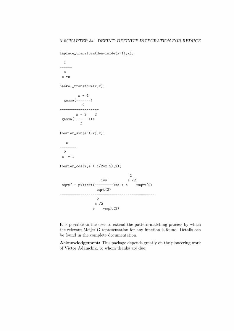
310CHAPTER 34. DEFINT: DEFINITE INTEGRATION FOR REDUCE
laplace_transform(Heaviside(x-1),x);
1------
se *s
hankel_transform(x,x);
n + 4gamma(-------)
2-------------------
n - 2 2gamma(-------)*s
2
fourier_sin(e^(-x),x);
s--------
2s + 1
fourier_cos(x,e^(-1/2*x^2),x);
2i*s s /2
sqrt( - pi)*erf(---------)*s + e *sqrt(2)sqrt(2)
----------------------------------------------2
s /2e *sqrt(2)
It is possible to the user to extend the pattern-matching process by whichthe relevant Meijer G representation for any function is found. Details canbe found in the complete documentation.
Acknowledgement: This package depends greatly on the pioneering workof Victor Adamchik, to whom thanks are due.

Chapter 35
DESIR: Differential linearhomogeneous equationsolutions in theneighbourhood of irregularand regular singular points
C. Dicrescenzo, F. Richard–Jung, E. TournierGroupe de Calcul Formel de Grenoble
laboratoire TIM3France
e–mail: [email protected]
This software enables the basis of formal solutions to be computed for anordinary homogeneous differential equation with polynomial coefficients overQ of any order, in the neighbourhood of zero (regular or irregular singularpoint, or ordinary point).
This software can be used in two ways, directly via the DELIRE procedure, orinteractively with the DESIR procedure. The basic procedure is the fDELIREprocedure which enables the solutions of a linear homogeneous differentialequation to be computed in the neighbourhood of zero.
The DESIR procedure is a procedure without argument whereby DELIRE canbe called without preliminary treatment to the data, that is to say, in an
311

312 CHAPTER 35. DESIR: LINEAR HOMOGENEOUS DES
interactive autonomous way. This procedure also proposes some transfor-mations on the initial equation. This allows one to start comfortably withan equation which has a non zero singular point, a polynomial right-handside and parameters.
delire(x,k,grille,lcoeff,param)
This procedure computes formal solutions of a linear homogeneous differen-tial equation with polynomial coefficients over Q and of any order, in theneighbourhood of zero, regular or irregular singular point. x is the variable,k is the number of desired terms (that is for each formal series in xt appear-ing in polysol, a0 + a1xt + a2x
2t + . . . + anx
nt + . . . we compute the k + 1
first coefficients a0, a1 to ak. The coefficients of the differential operator aspolynomial in xgrille. In general grille is 1. The argument lcoeff is a list ofcoefficients of the differential operator (in increasing order of differentiation)and param is a list of parameters. The procedure returns the list of generalsolutions.
lcoeff:=1,x,x,x**6;
6lcoeff := 1,x,x,x
param:=;
param :=
sol:=delire(x,4,1,lcoeff,param);
4 3 2xt - 4*xt + 12*xt - 24*xt + 24
sol := 0,1,-----------------------------------,1,12
,
4 30,1,(6*log(xt)*xt - 18*log(xt)*xt
2+ 36*log(xt)*xt - 36*log(xt)*xt
4 3- 5*xt + 9*xt - 36*xt + 36)/36,0,

313
,
1-------,1,
44*xt
4 3 2361*xt + 4*xt + 12*xt + 24*xt + 24
---------------------------------------,10,24

314 CHAPTER 35. DESIR: LINEAR HOMOGENEOUS DES

Chapter 36
DFPART: Derivatives ofgeneric functions
Herbert MelenkKonrad–Zuse–Zentrum fur Informationstechnik Berlin
Takustrase 7D–14195 Berlin–Dahlem, Germany
e–mail: [email protected]
The package DFPART supports computations with total and partial deriva-tives of formal function objects. Such computations can be useful in thecontext of differential equations or power series expansions.
36.1 Generic Functions
A generic function is a symbol which represents a mathematical function.The minimal information about a generic function function is the numberof its arguments. In order to facilitate the programming and for a betterreadable output this package assumes that the arguments of a generic func-tion have default names such as f(x, y), q(rho, phi). A generic function isdeclared by prototype form in a statement
GENERIC FUNCTION fname(arg1, arg2 · · · argn);
where fname is the (new) name of a function and argi are symbols for its for-
315

316CHAPTER 36. DFPART: DERIVATIVES OF GENERIC FUNCTIONS
mal arguments. In the following fname is referred to as “generic function”,arg1, arg2 · · · argn as “generic arguments” and fname(arg1, arg2 · · · argn) as“generic form”.
Examples:
generic_function f(x,y);generic_function g(z);
After this declaration REDUCE knows that
• there are formal partial derivatives ∂f∂x , ∂f
∂y∂g∂z and higher ones, while
partial derivatives of f and g with respect to other variables are as-sumed as zero,
• expressions of the type f(), g() are abbreviations for f(x, y), g(z),
• expressions of the type f(u, v) are abbreviations forsub(x = u, y = v, f(x, y))
• a total derivative df(u,v)dw has to be computed as ∂f
∂xdudw + ∂f
∂ydvdw
36.2 Partial Derivatives
The operator DFP represents a partial derivative:
DFP(expr, dfarg1, dfarg2 · · · dfargn);
where expr is a function expression and dfargi are the differentiation vari-ables. Examples:
dfp(f(),x,y);
means ∂2f∂x∂y and
dfp(f(u,v),x,y);
stands for ∂2f∂x∂y (u, v). For compatibility with the DF operator the differen-
tiation variables need not be entered in list form; instead the syntax of DFcan be used, where the function expression is followed by the differentiation

36.2. PARTIAL DERIVATIVES 317
variables, eventually with repetition numbers. Such forms are internallyconverted to the above form with a list as second parameter.
The expression expr can be a generic function with or without arguments,or an arithmetic expression built from generic functions and other algebraicparts. In the second case the standard differentiation rules are applied inorder to reduce each derivative expressions to a minimal form.
When the switch NAT is on partial derivatives of generic functions are printedin standard index notation, that is fxy for ∂2f
∂x∂y and fxy(u, v) for ∂2f∂x∂y (u, v).
Therefore single characters should be used for the arguments whenever pos-sible. Examples:
generic_function f(x,y);generic_function g(y);dfp(f(),x,2);
FXX
dfp(f()*g(),x,2);
F *G()XX
dfp(f()*g(),x,y);
F *G() + F *GXY X Y
The difference between partial and total derivatives is illustrated by thefollowing example:
generic_function h(x);dfp(f(x,h(x))*g(h(x)),x);
F (X,H(X))*G(H(X))X
df(f(x,h(x))*g(h(x)),x);

318CHAPTER 36. DFPART: DERIVATIVES OF GENERIC FUNCTIONS
F (X,H(X))*G(H(X)) + F (X,H(X))*H (X)*G(H(X))X Y X
+ G (H(X))*H (X)*F(X,H(X))Y X
Normally partial differentials are assumed as non-commutative
dfp(f(),x,y)-dfp(f(),y,x);
F - FXY YX
However, a generic function can be declared to have globally interchange-able partial derivatives using the declaration DFP COMMUTE which takes thename of a generic function or a generic function form as argument. Forsuch a function differentiation variables are rearranged corresponding to thesequence of the generic variables.
generic_function q(x,y);dfp_commute q(x,y);dfp(q(),x,y,y) + dfp(q(),y,x,y) + dfp(q(),y,y,x);
3*QXYY
If only a part of the derivatives commute, this has to be declared using thestandard REDUCE rule mechanism. Please note that then the derivativevariables must be written as list.
36.3 Substitutions
When a generic form or a DFP expression takes part in a substitution thefollowing steps are performed:
1. The substitutions are performed for the arguments. If the argumentlist is empty the substitution is applied to the generic arguments ofthe function; if these change, the resulting forms are used as newactual arguments. If the generic function itself is not affected by thesubstitution, the process stops here.

36.3. SUBSTITUTIONS 319
2. If the function name or the generic function form occurs as a left handside in the substitution list, it is replaced by the corresponding righthand side.
3. The new form is partially differentiated according to the list of partialderivative variables.
4. The (eventually modified) actual parameters are substituted into theform for their corresponding generic variables. This substitution isdone by name.
Examples:
generic_function f(x,y);sub(y=10,f());
F(X,10)
sub(y=10,dfp(f(),x,2));
F (X,10)XX
sub(y=10,dfp(f(y,y),x,2));
F (10,10)XX
sub(f=x**3*y**3,dfp(f(),x,2));
36*X*Y
generic_function ff(y,z);sub(f=ff,f(a,b));
FF(B,Z)

320CHAPTER 36. DFPART: DERIVATIVES OF GENERIC FUNCTIONS

Chapter 37
DUMMY: Canonical form ofexpressions with dummyvariables
Alain DresseUniversite Libre de Bruxelles
Boulevard du Triomphe, CP 210/01B–1050 BRUXELLES, Belgium
e–mail: [email protected]
An expression of the typen∑
a=1
f(a)
for any n is simply written asf(a)
and a is a dummy index. If the previous expression is written as
n∑
b=1
f(b)
b is also a dummy index and, obviously we should be able to get the equality
f(a)− f(b); → 0
To declare dummy variables, two declarations are available:
321

322 CHAPTER 37. DUMMY: EXPRESSIONS WITH DUMMY VARS
i. dummy_base <idp>;
where idp is the name of any unassigned identifier.
ii. dummy_names <d>,<dp>,<dpp> ....;
The first declares idp1,· · ·, idpn as dummy variables i.e. all variables ofthe form “idxxx” where xxx is a number will be dummy variables, suchas id1, id2, ... , id23. The second gives special names for dummyvariables. All other arguments are assumed to be free.An example:
dummy_base dv; ==> dv
% dummy indices are dv1, dv2, dv3, ...
dummy_names i,j,k; ==> t
% dummy names are i,j,k.
When this is done, an expression like
op(dv1)*sin(dv2)*abs(x)*op(i)^3*op(dv2)$
is allowed. Notice that, dummy indices may not be repeated (it is notlimited to tensor calculus) or that they be repeated many times inside theexpression.
By default all operators with dummy arguments are assumed to be commu-tative and without symmetry properties. This can be varied by declarationsNONCOM, SYMMETRIC and ANTISYMMETRIC may be used on the operators. Theycan also be declared anticommutative.
anticom ao1, ao2;
More complex symmetries can be handled with SYMTREE. The correspondingdeclaration for the Riemann tensor is
symtree (r, !+, !-, 1, 2, !-, 3, 4);
The symbols !*, !+ and !- at the beginning of each list mean that the operatorhas no symmetry, is symmetric and is antisymmetric with respect to theindices inside the list. Notice that the indices are not designated by theirnames but merely by their natural order of appearance. 1 means the first

323
written argument of r, 2 its second argument etc. In the example above ris symmetric with respect to interchange of the pairs of indices 1,2 and 3,4respectively.

324 CHAPTER 37. DUMMY: EXPRESSIONS WITH DUMMY VARS

Chapter 38
EDS: Exterior differentialsystems
David HartleyPhysics and Mathematical Physics
University of Adelaide SA 5005, Australiae-mail: [email protected]
38.1 Introduction
Exterior differential systems give a geometrical framework for partial differ-ential equations and more general differential geometric problems. The geo-metrical formulation has several advantages stemming from its coordinate-independence, including superior treatment of nonlinear and global prob-lems. EDS provides a number of tools for setting up and manipulating ex-terior differential systems and implements many features of the theory. Itsmain strengths are the ability to use anholonomic or moving frames and thecare taken with nonlinear problems.
The package is loaded by typing load eds;
Reading the full documentation, which comes with this package, is stronglyrecommended. The test file eds.tst, which is also in the package, providesthree inspiring examples on the subject.EDS uses E. Schrufer’s EXCALC package for the underlying exterior calcu-lus operations.
325

326 CHAPTER 38. EDS: EXTERIOR DIFFERENTIAL SYSTEMS
38.2 Data Structures and Concepts
38.2.1 EDS
A simple 〈EDS 〉, or exterior differential system, is a triple (S,Ω,M), whereM is a coframing, S is a system on M, and Ω is an independence condi-tion. Exterior differential equations without independence condition are nottreated by EDS. Ω should be either a decomposable 〈p-form〉 or a 〈system〉of 1-forms on M.More generally an 〈EDS 〉 is a list of simple 〈EDS 〉 objects where the variouscoframings are all disjoint.The solutions of (S,Ω,M) are integral manifolds, or immersions on whichS vanishes and the rank of Ω is preserved. Solutions at a single point aredescribed by integral elements.
38.2.2 Coframing
Within the context of EDS, a coframing means a real finite-dimensional dif-ferentiable manifold with a given global cobasis. The information about acoframing required by EDS is kept in a 〈coframing〉 object. The cobasis is theidentifying element of an EDS. In addition to the cobasis, there can be givencoordinates, structure equations and restrictions. In addition to the cobasis,coordinates, structure equations and restrictions can be given. The coordi-nates may be an incomplete or overcomplete set. The structure equationsexpress the exterior derivative of the coordinates and cobasis elements asneeded. All coordinate differentials must be expressed in terms of the givencobasis, but not all cobasis derivatives need be known. The restrictions area set of inequalities describing point sets not in the manifold.Please note that the 〈coframing〉 object is by no means a full descriptionof a differentiable manifold. However, the 〈coframing〉 object carries suffi-cient information about the underlying manifold to allow a range of exteriorsystems calculations to be carried out.
38.2.3 Systems and background coframing
The label 〈system〉 refers to a list <p-form expr>, . . . of differential forms.If an EDS operator also accepts a 〈system〉 as argument, then any extrainformation which is required is taken from the background coframing.

38.2. DATA STRUCTURES AND CONCEPTS 327
It is possible to activate the rules and orderings of a COFRAMING operatorglobally, by making it the background coframing. All subsequent EXCALCoperations will be governed by those rules. Operations on 〈EDS 〉 objectsare unaffected, since their coframings are still activated locally.
38.2.4 Integral elements
An 〈integral element〉 of an exterior system (S,Ω,M) is a subspace P ⊂ TpMof the tangent space at some point p ∈ M . This integral element can berepresented by its annihilator P⊥ ⊂ T ∗pM , comprising those 1-forms atp which annihilate every vector in P . This can also be understood as amaximal set of 1-forms at p such that S ' 0 (mod P⊥) and the rank of Ωis preserved modulo P⊥.An 〈integral element〉 in EDS is a distribution of 1-forms on M , specified asa 〈system〉 of 1-forms.
38.2.5 Properties and normal form
For large problems, it can require a great deal of computation to establishwhether, for example, a system is closed or not. In order to save recomputingsuch properties, an 〈EDS 〉 object carries a list of 〈properties〉 of the form
〈keyword〉 = 〈value〉,· · ·where 〈keyword〉 is one of closed, quasilinear, pfaffian or involutive,and 〈value〉 is either 0 (false) or 1 (true). These properties are suppressedwhen an 〈EDS 〉 is printed, unless the nat switch is off. They can beexamined using the PROPERTIES operator.Parts of the theory of exterior differential systems apply only at points onthe underlying manifold where the system is in some sense non-singular.To ensure the theory applies, EDS automatically works all exterior systems(S,Ω,M) into a normal form. This means that the Pfaffian component of Sand the independence condition Ω are in solved forms, distinguished termsfrom the 1-forms in S have been eliminated from the rest of S and from Ωand any 1-forms in S which vanish modulo the independence condition areremoved from the system and their coefficients are appended as 0-forms.

328 CHAPTER 38. EDS: EXTERIOR DIFFERENTIAL SYSTEMS
38.3 The EDS Package
In the descriptions of the various operators we define the following abbrevi-ations for function parameters:
E, E′ 〈EDS 〉S 〈system〉M , N 〈coframing〉, or a 〈system〉 specifying a 〈coframing〉r 〈integer〉Ω 〈p-form〉f 〈map〉rsx 〈list of inequalities〉cob 〈list of 1-form variables〉crd, dep, ind 〈list of 0-form variables〉drv 〈list of rules for exterior derivatives〉pde 〈list of expressions or equations〉X 〈transform〉T 〈tableau〉P 〈integral element〉
38.3.1 Constructing EDS objects
An EDS 〈coframing〉 is constructed using the COFRAMING operator. In oneform it examines the argument for 0-form and 1-form variables. The morebasic syntax takes the 〈cobasis〉 as a list of 1-forms, 〈coordinates〉 as a list of0-forms, 〈restrictions〉 as a list of inequalities and 〈structure equations〉 as alist giving the exterior derivatives of the coordinates and cobasis elements.All arguments except the cobasis are optional.A simple 〈EDS 〉 is constructed using the EDS operator where the 〈indep. condition〉can be either a decomposable 〈p-form〉 or a 〈system〉 of 1-forms. The〈coframing〉 and the 〈properties〉 arguments can be omitted. The EDS isput into normal form before being returned. With SET COFRAMING the back-ground coframing is set.The operator PDS2EDS encodes a PDE system into an 〈EDS 〉 object.
COFRAMING(cob,crd,rsx,drv) COFRAMING(S) EDS(S,Ω,M)CONTACT(r,M,N) PDE2EDS(pde,dep,ind) SET COFRAMING(M)SET COFRAMING(E) SET COFRAMING()

38.3. THE EDS PACKAGE 329
Example:
1: load eds;
2: pform x,y,z,p,q=0,e(i),w(i,j)=1;
3: indexrange i,j,k=1,2,a,b,c=3;
4: eds(d z - p*d x - q*d y, d p^d q,d x,d y);
EDS(d z - p*d x - q*d y,d p^d q,d x^d y)
5: OMrules:=index_expand d e(i)=>-w(i,-j)^e(j),w(i,-j)+w(j,-i)=>0$
6: eds(e(a),e(i)) where OMrules;
3 1 2EDS(e ,e ,e )
7: coframing ws;3 2 1 2 1 2 2
coframing(e ,w ,e ,e ,,d e => - e ^w ,1 1
2 1 2d e => e ^w ,)
1
38.3.2 Inspecting EDS objects
Using these operators you can get parts of your 〈EDS 〉 object. ThePROPERTIES(E) operator for example returns a list of properties which arenormally not printed out, unless the NAT switch is off.
COFRAMING(E) COFRAMING() COBASIS(M)COBASIS(E) COORDINATES(M) COORDINATES(E)STRUCTURE EQUATIONS(M) STRUCTURE EQUATIONS(E) RESTRICTIONS(M)RESTRICTIONS(E) SYSTEM(E) INDEPENDENCE(E)PROPERTIES(E) ONE FORMS(E) ONE FORMS(S)ZERO FORMS(E) ZERO FORMS(S)
Example:

330 CHAPTER 38. EDS: EXTERIOR DIFFERENTIAL SYSTEMS
8: depend u,x,y; depend v,x,y;
9: pde2eds(df(u,y,y)=df(v,x),df(v,y)=y*df(v,x));
EDS(d u - u *d x - u *d y, d u - u *d x - u *d y,x y x x x y x
d u - u *d x - v *d y, d v - v *d x - v *y*d y,d x^d y)y y x x x x
10: dependencies;
u,y,x,v,y,x
11: coordinates contact(3,x,u);
x,u,u ,u ,u x x x x x x
12: fdomain u=u(x);
13: coordinates d u+d y;
x,y
38.3.3 Manipulating EDS objects
These operators allow you to manipulate your 〈EDS 〉 objects. TheAUGMENT(E,S) operator, see example below, appends the extra forms in thesecond argument to the system part of the first. The original 〈EDS 〉 re-mains unchanged. As another example by using the TRANSFORM operator achange of the cobasis is made, where the argument 〈transform〉 is a list ofsubstitutions.
AUGMENT(E,S) M CROSS N E CROSS N PULLBACK(E,f)PULLBACK(S,f) PULLBACK(Ω,f) PULLBACK(M,f) RESTRICT(E,f)RESTRICT(S,f) RESTRICT(Ω,f) RESTRICT(M,f) TRANSFORM(M,X)TRANSFORM(E,X) TRANSFORM(S,X) TRANSFORM(Ω,X) LIFT(E)
Example:

38.3. THE EDS PACKAGE 331
% Non-Pfaffian system for a Monge-Ampere equation
14: PFORM x,y,z=0$
15: S := CONTACT(1,x,y,z);
s := EDS(d z - z *d x - z *d y,d x^d y)x y
16: S:= AUGMENT(S,d z(-x)^d z(-y));
s := EDS(d z - z *d x - z *d y,x y
d z ^d z ,d x^d y)x y
38.3.4 Analysing and Testing exterior systems
Analysing exterior systems
This section introduces higher level operators for extracting informationabout exterior systems. Many of them require a 〈EDS 〉 in normal form gen-erated in positive degree as input, but some can also analyse a 〈system〉 ora single 〈p-form〉.
CARTAN SYSTEM(E) CARTAN SYSTEM(S) CARTAN SYSTEM(Ω)CAUCHY SYSTEM(E) CAUCHY SYSTEM(S) CAUCHY SYSTEM(Ω)CHARACTERS(E) CHARACTERS(T) CHARACTERS(E,P)CLOSURE(E) DERIVED SYSTEM(E) DERIVED SYSTEM(S)DIM GRASSMANN VARIETY(E) DIM GRASSMANN VARIETY(E,P) DIM(M)DIM(E) INVOLUTION(E) LINEARISE(E,P)INTEGRAL ELEMENT(E) PROLONG(E) TABLEAU(E)TORSION(E) GRASSMANN VARIETY(E)
Testing exterior systems
The following operators allow various properties of an 〈EDS 〉 to be checked.The result is either a 1 or a 0, so these operators can be used in booleanexpressions. Since checking these properties is very time-consuming, theresult of the first test is stored on the 〈properties〉 record of an 〈EDS 〉 toavoid re-checking. This memory can be cleared using the CLEANUP opearator.

332 CHAPTER 38. EDS: EXTERIOR DIFFERENTIAL SYSTEMS
CLOSED(E) CLOSED(S) CLOSED(Ω) INVOLUTIVE(E)PFAFFIAN(E) QUASILINEAR(E) SEMILINEAR(E) E EQUIV E′
38.3.5 Switches
EDS provides several switches to govern the display of information and en-hance the speed or reliability of the calculations. For example the switchEDSVERBOSE if ON will display additional information as the calculation pro-gresses, which might generate too much output for larger problems.All switches are OFF by default.
EDSVERBOSE EDSDEBUG EDSSLOPPY EDSDISJOINT RANPOS GENPOS
38.3.6 Auxilliary functions
The operators of this section are designed to ease working with exteriorforms and exterior systems in REDUCE .
COORDINATES(S) INVERT(X) STRUCTURE EQUATIONS(X)STRUCTURE EQUATIONS(X,X−1) LINEAR DIVISORS(Ω) EXFACTORS(Ω)INDEX EXPAND(ANY) PDE2JET(pde,dep,ind) MKDEPEND(list)DISJOIN(f,g,...) CLEANUP(E) CLEANUP(M)REORDER(E) REORDER(M)
38.3.7 Experimental Functions
The following operators are experimental facilities since, they are either al-gorithmically not well-founded, or their implementation is very unstable, orthey have known bugs.
POINCARE(Ω) INVARIANTS(E,crd) INVARIANTS(S,crd)SYMBOL RELATIONS(E,π) SYMBOL MATRIX(E,ξ) CHARACTERISTIC VARIETY(E,ξ)
Example:

38.3. THE EDS PACKAGE 333
17: % Riemann invariants for Euler-Poisson-Darboux equation.17: % Set up the EDS for the equation, and examine tableau.17: depend u,x,y; EPD :=PDE2EDSDF(u,x,y)=-(df(u,x)+df(u,y))/(x+y)$
19: tableau EPD;
[d u 0 ][ x x ][ ][ 0 d u ][ y y]
20: % 1-form dx is characteristic: construct characteristic EDS.20: xvars ; C := cartan_system select(~f^d x=0,system closure epd)$
22: S := augment(eds(system EPD,d y),C)$
23: % Compute derived flag23: while not equiv(S,S1 := derived_system S) do S := S1;
24: % Stabilised. Find the Riemann invariants.24: invariants(S,reverse coordinates S);
x,
u *x + u *y + u,x x
- u *x - u *y - 2*u x x x x x

334 CHAPTER 38. EDS: EXTERIOR DIFFERENTIAL SYSTEMS

Chapter 39
EXCALC: A differentialgeometry package
Eberhard SchruferGMD, Institut I1
Postfach 131653757 St. Augustin, GERMANY
e–mail: [email protected]
EXCALC is designed for easy use by all who are familiar with the calculusof Modern Differential Geometry. Its syntax is kept as close as possibleto standard textbook notations. Therefore, no great experience in writingcomputer algebra programs is required. It is almost possible to input tothe computer the same as what would have been written down for a hand-calculation. For example, the statement
f*x^y + u _| (y^z^x)
would be recognized by the program as a formula involving exterior productsand an inner product. The program is currently able to handle scalar-valuedexterior forms, vectors and operations between them, as well as non-scalarvalued forms (indexed forms). With this, it should be an ideal tool forstudying differential equations, doing calculations in general relativity andfield theories, or doing such simple things as calculating the Laplacian of atensor field for an arbitrary given frame. With the increasing popularity ofthis calculus, this program should have an application in almost any field of
335

336 CHAPTER 39. EXCALC: DIFFERENTIAL GEOMETRY
physics and mathematics.
39.1 Declarations
Geometrical objects like exterior forms or vectors are introduced to thesystem by declaration commands. The declarations can appear anywherein a program, but must, of course, be made prior to the use of the object.Everything that has no declaration is treated as a constant; therefore zero-forms must also be declared.
An exterior form is introduced by
PFORM <declaration1>, <declaration2>, . . . ;
where
<declaration> ::= <name> | <list of names>=<number> | <identifier> |<expression><name> ::= <identifier> | <identifier>(<arguments>)
For example
pform u=k,v=4,f=0,w=dim-1;
declares U to be an exterior form of degree K, V to be a form of degree 4, Fto be a form of degree 0 (a function), and W to be a form of degree DIM-1.
The declaration of vectors is similar. The command TVECTOR takes a list ofnames.
TVECTOR <name1>, <name2>, . . . ;
For example, to declare X as a vector and COMM as a vector with two indices,one would say
tvector x,comm(a,b);
The exterior degree of a symbol or a general expression can be obtainedwith the function
EXDEGREE <expression>;
Example:

39.2. EXTERIOR MULTIPLICATION 337
exdegree(u + 3*chris(k,-k));
1
39.2 Exterior Multiplication
Exterior multiplication between exterior forms is carried out with the naryinfix operator ˆ (wedge). Factors are ordered according to the usual orderingin REDUCE using the commutation rule for exterior products.
pform u=1,v=1,w=k;
u^v;
U^V
v^u;
- U^V
u^u;
0
w^u^v;
K( - 1) *U^V^W
(3*u-a*w)^(w+5*v)^u;
A*(5*U^V^W - U^W^W)
It is possible to declare the dimension of the underlying space by
SPACEDIM <number> | <identifier>;
If an exterior product has a degree higher than the dimension of the space,it is replaced by 0:

338 CHAPTER 39. EXCALC: DIFFERENTIAL GEOMETRY
39.3 Partial Differentiation
Partial differentiation is denoted by the operator @. Its capability is thesame as the REDUCE DF operator.
Example 6
@(sin x,x);
COS(X)
@(f,x);
0
An identifier can be declared to be a function of certain variables. Thisis done with the command FDOMAIN. The following would tell the partialdifferentiation operator that F is a function of the variables X and Y andthat H is a function of X.
fdomain f=f(x,y),h=h(x);
Applying @ to F and H would result in
@(x*f,x);
F + X*@ FX
@(h,y);
0
The partial derivative symbol can also be an operator with a single argu-ment. It then represents a natural base element of a tangent vector.
39.4 Exterior Differentiation
Exterior differentiation of exterior forms is carried out by the operator d.Products are normally differentiated out,

39.5. INNER PRODUCT 339
pform x=0,y=k,z=m;
d(x * y);
X*d Y + d X^Y
This expansion can be suppressed by the command NOXPND D. Expansion isperformed again when the command XPND D is executed.
If an argument of an implicitly defined function has further dependenciesthe chain rule will be applied e.g.
fdomain y=y(z);
d f;
@ F*d X + @ F*@ Y*d ZX Y Z
Expansion into partial derivatives can be inhibited by NOXPND @ and enabledagain by XPND @.
39.5 Inner Product
The inner product between a vector and an exterior form is representedby the diphthong | (underscore or-bar), which is the notation of manytextbooks. If the exterior form is an exterior product, the inner product iscarried through any factor.
Example 7
pform x=0,y=k,z=m;
tvector u,v;
u _| (x*y^z);
KX*(( - 1) *Y^U _| Z + U _| Y^Z)
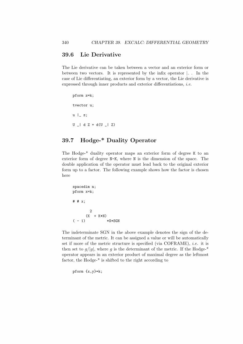
340 CHAPTER 39. EXCALC: DIFFERENTIAL GEOMETRY
39.6 Lie Derivative
The Lie derivative can be taken between a vector and an exterior form orbetween two vectors. It is represented by the infix operator | . In thecase of Lie differentiating, an exterior form by a vector, the Lie derivative isexpressed through inner products and exterior differentiations, i.e.
pform z=k;
tvector u;
u |_ z;
U _| d Z + d(U _| Z)
39.7 Hodge-* Duality Operator
The Hodge-* duality operator maps an exterior form of degree K to anexterior form of degree N-K, where N is the dimension of the space. Thedouble application of the operator must lead back to the original exteriorform up to a factor. The following example shows how the factor is chosenhere
spacedim n;pform x=k;
# # x;
2(K + K*N)
( - 1) *X*SGN
The indeterminate SGN in the above example denotes the sign of the de-terminant of the metric. It can be assigned a value or will be automaticallyset if more of the metric structure is specified (via COFRAME), i.e. it isthen set to g/|g|, where g is the determinant of the metric. If the Hodge-*operator appears in an exterior product of maximal degree as the leftmostfactor, the Hodge-* is shifted to the right according to
pform x,y=k;

39.8. VARIATIONAL DERIVATIVE 341
# x ^ y;
2(K + K*N)
( - 1) *X^# Y
39.8 Variational Derivative
The function VARDF returns as its value the variation of a given Lagrangiann-form with respect to a specified exterior form (a field of the Lagrangian).In the shared variable BNDEQ!*, the expression is stored that has to yieldzero if integrated over the boundary.
Syntax:
VARDF(<Lagrangian n-form>,<exterior form>)
Example 8
spacedim 4;
pform l=4,a=1,j=3;
l:=-1/2*d a ^ # d a - a^# j$ %Lagrangian of the e.m. field
vardf(l,a);
- (# J + d # d A) %Maxwell’s equations
bndeq!*;
- ’A^# d A %Equation at the boundary
For the calculation of the conserved currents induced by symmetry operators(vector fields), the function NOETHER is provided. It has the syntax:
NOETHER(<Lagrangian n-form>,<field>,<symmetry generator>)
Example 9
pform l=4,a=1,f=2;

342 CHAPTER 39. EXCALC: DIFFERENTIAL GEOMETRY
spacedim 4;
l:= -1/2*d a^#d a; %Free Maxwell field;
tvector x(k); %An unspecified generator;
noether(l,a,x(-k));
( - 2*d(X _|A)^# d A - (X _|d A)^# d A + d A^(X _|# d A))/2K K K
39.9 Handling of Indices
Exterior forms and vectors may have indices. On input, the indices are givenas arguments of the object. A positive argument denotes a superscript and anegative argument a subscript. On output, the indexed quantity is displayedtwo dimensionally if NAT is on. Indices may be identifiers or numbers.
Example 10
pform om(k,l)=m,e(k)=1;e(k)^e(-l);
KE ^E
L
om(4,-2);
4OM
2
In certain cases, one would like to inhibit the summation over specified indexnames, or at all. For this the command
NOSUM <indexname1>, . . . ;
and the switch NOSUM are available. The command NOSUM has the effectthat summation is not performed over those indices which had been listed.The command RENOSUM enables summation again. The switch NOSUM, if on,inhibits any summation.

39.10. METRIC STRUCTURES 343
It is possible to declare symmetry properties for an indexed quantity by thecommand INDEX SYMMETRIES. A prototypical example is as follows
index_symmetries u(k,l,m,n): symmetric in k,l,m,nantisymmetric in k,l,m,n,
g(k,l),h(k,l): symmetric;
It declares the object u symmetric in the first two and last two indices andantisymmetric with respect to commutation of the given index pairs. If anobject is completely symmetric or antisymmetric, the indices need not to begiven after the corresponding keyword as shown above for g and h.
39.10 Metric Structures
A metric structure is defined in EXCALC by specifying a set of basis one-forms (the coframe) together with the metric.
Syntax:
COFRAME <identifier><(index1)>=<expression1>,<identifier><(index2)>=<expression2>,...<identifier><(indexn)>=<expressionn>
WITH METRIC <name>=<expression>;
This statement automatically sets the dimension of the space and the indexrange. The clause WITH METRIC can be omitted if the metric is Euclideanand the shorthand WITH SIGNATURE <diagonal elements> can be used inthe case of a pseudo-Euclidean metric. The splitting of a metric structurein its metric tensor coefficients and basis one-forms is completely arbitraryincluding the extremes of an orthonormal frame and a coordinate frame.

344 CHAPTER 39. EXCALC: DIFFERENTIAL GEOMETRY
Example 11
coframe e r=d r, e(ph)=r*d phwith metric g=e(r)*e(r)+e(ph)*e(ph); %Polar coframe
The frame dual to the frame defined by the COFRAME command can be in-troduced by FRAME command.
FRAME <identifier>;
This command causes the dual property to be recognised, and the tangentvectors of the coordinate functions are replaced by the frame basis vectors.
Example 12
coframe b r=d r,b ph=r*d ph,e z=d z; %Cylindrical coframe;
frame x; on nero;
x(-k) _| b(l);
RNS := 1R
PHNS := 1PH
ZNS := 1Z
x(-k) |_ x(-l); %The commutator of the dual frame;
NS := X /RPH R PH
NS := ( - X )/R %i.e. it is not a coordinate base;R PH PH

39.11. RIEMANNIAN CONNECTIONS 345
As a convenience, the frames can be displayed at any point in a program bythe command DISPLAYFRAME;.
The Hodge-* duality operator returns the explicitly constructed dual ele-ment if applied to coframe base elements. The metric is properly taken intoaccount.
The total antisymmetric Levi-Cevita tensor EPS is also available. The valueof EPS with an even permutation of the indices in a covariant position istaken to be +1.
39.11 Riemannian Connections
The command RIEMANNCONX is provided for calculating the connection 1forms. The values are stored on the name given to RIEMANNCONX. Thiscommand is far more efficient than calculating the connection from the dif-ferential of the basis one-forms and using inner products.
39.12 Ordering and Structuring
The ordering of an exterior form or vector can be changed by the commandFORDER. In an expression, the first identifier or kernel in the arguments ofFORDER is ordered ahead of the second, and so on, and ordered ahead ofall not appearing as arguments. This ordering is done on the internal leveland not only on output. The execution of this statement can thereforehave tremendous effects on computation time and memory requirements.REMFORDER brings back standard ordering for those elements that are listedas arguments.
An expression can be put in a more structured form by renaming a subex-pression. This is done with the command KEEP which has the syntax
KEEP <name1>=<expression1>,<name2>=<expression2>, . . .
The capabilities of KEEP are currently very limited. Only exterior productsshould occur as righthand sides in KEEP.
Note: This is just an introduction to the full power of EXCALC. The readerif referred to the full documentation.

346 CHAPTER 39. EXCALC: DIFFERENTIAL GEOMETRY

Chapter 40
FIDE: Finite differencemethod for partialdifferential equations
Richard LiskaFaculty of Nuclear Science and Physical Engineering
Technical University of PragueBrehova 7, 115 19 Prague 1, Czech Republic
e–mail: [email protected]
The FIDE package performs automation of the process of numerical solvingpartial differential equations systems (PDES) by generating finite differencemethods. In the process one can find several stages in which computer al-gebra can be used for performing routine analytical calculations, namely:transforming differential equations into different coordinate systems, dis-cretisation of differential equations, analysis of difference schemes and gen-eration of numerical programs. The FIDE package consists of the followingmodules:
EXPRES for transforming PDES into any orthogonal coordinate system.
IIMET for discretisation of PDES by integro-interpolation method.
APPROX for determining the order of approximation of difference scheme.
CHARPOL for calculation of amplification matrix and characteristic poly-
347

348 CHAPTER 40. FIDE: FINITE DIFFERENCES FOR PDES
nomial of difference scheme, which are needed in Fourier stability anal-ysis.
HURWP for polynomial roots locating necessary in verifying the von Neu-mann stability condition.
LINBAND for generating the block of FORTRAN code, which solves asystem of linear algebraic equations with band matrix appearing quiteoften in difference schemes.
For more details on this package are given in the FIDE documentation, andin the examples. A flavour of its capabilities can be seen from the followingsimple example.
off exp;
factor diff;
on rat,eqfu;
% Declare which indexes will be given to coordinatescoordinates x,t into j,m;
% Declares uniform grid in x coordinategrid uniform,x;
% Declares dependencies of functions on coordinatesdependence eta(t,x),v(t,x),eps(t,x),p(t,x);
% Declares p as known functiongiven p;
same eta,v,p;
iim a, eta,diff(eta,t)-eta*diff(v,x)=0,v,diff(v,t)+eta/ro*diff(p,x)=0,eps,diff(eps,t)+eta*p/ro*diff(v,x)=0;
********************************** Program ***** IIMET Ver 1.1.2*****************************
Partial Differential Equations

349
==============================
diff(eta,t) - diff(v,x)*eta = 0
diff(p,x)*eta--------------- + diff(v,t) = 0
ro
diff(v,x)*eta*pdiff(eps,t) + ----------------- = 0
ro
Backtracking needed in grid optimalization0 interpolations are needed in x coordinate
Equation for eta variable is integrated in half grid pointEquation for v variable is integrated in half grid pointEquation for eps variable is integrated in half grid point
0 interpolations are needed in t coordinateEquation for eta variable is integrated in half grid pointEquation for v variable is integrated in half grid pointEquation for eps variable is integrated in half grid point
Equations after Discretization Using IIM :==========================================
(4*(eta(j,m + 1) - eta(j,m) - eta(j + 1,m)
+ eta(j + 1,m + 1))*hx - (
(eta(j + 1,m + 1) + eta(j,m + 1))
*(v(j + 1,m + 1) - v(j,m + 1))
+ (eta(j + 1,m) + eta(j,m))*(v(j + 1,m) - v(j,m)))
*(ht(m + 1) + ht(m)))/(4*(ht(m + 1) + ht(m))*hx) = 0
(4*(v(j,m + 1) - v(j,m) - v(j + 1,m) + v(j + 1,m + 1))*hx*ro
+ ((eta(j + 1,m + 1) + eta(j,m + 1))
*(p(j + 1,m + 1) - p(j,m + 1))

350 CHAPTER 40. FIDE: FINITE DIFFERENCES FOR PDES
+ (eta(j + 1,m) + eta(j,m))*(p(j + 1,m) - p(j,m)))
*(ht(m + 1) + ht(m)))/(4*(ht(m + 1) + ht(m))*hx*ro) = 0
(4*(eps(j,m + 1) - eps(j,m) - eps(j + 1,m)
+ eps(j + 1,m + 1))*hx*ro + ((
eta(j + 1,m + 1)*p(j + 1,m + 1)
+ eta(j,m + 1)*p(j,m + 1))
*(v(j + 1,m + 1) - v(j,m + 1)) +
(eta(j + 1,m)*p(j + 1,m) + eta(j,m)*p(j,m))
*(v(j + 1,m) - v(j,m)))*(ht(m + 1) + ht(m)))/(4
*(ht(m + 1) + ht(m))*hx*ro) = 0
clear a;
clearsame;
cleargiven;
Chapter 41
FPS: Automatic calculationof formal power series
Wolfram Koepf and Winfried NeunKonrad–Zuse–Zentrum fur Informationstechnik Berlin
Takustrase 7D–14195 Berlin–Dahlem, Germany
e–mail: [email protected] and [email protected]
This package can expand functions of certain type into their correspondingLaurent-Puiseux series as a sum of terms of the form
∞∑
k=0
ak(x− x0)k/n+s
where s is the ‘shift number’, n is the ‘Puiseux number’, and x0 is the ‘pointof development’. The following types are supported:
• functions of ‘rational type’, which are either rational or have arational derivative of some order;
• functions of ‘hypergeometric type’ where ak+m/ak is a rationalfunction for some integer m, the ‘symmetry number’;
• functions of ‘exp-like type’ which satisfy a linear homogeneousdifferential equation with constant coefficients.
FPS(f,x,x0) tries to find a formal power series expansion for f with respectto the variable x at the point of development x0. It also works for formal
351

352 CHAPTER 41. FPS: FORMAL POWER SERIES
Laurent (negative exponents) and Puiseux series (fractional exponents). Ifthe third argument is omitted, then x0:=0 is assumed.
Example: FPS(asin(x)^2,x) results in
2*k 2*k 2 2x *2 *factorial(k) *x
infsum(----------------------------,k,0,infinity)factorial(2*k + 1)*(k + 1)
If possible, the output is given using factorials. In some cases, the use of thePochhammer symbol pochhammer(a,k):= a(a+1) · · · (a+k−1) is necessary.
SimpleDE(f,x) tries to find a homogeneous linear differential equation withpolynomial coefficients for f with respect to x. Make sure that y is not aused variable. The setting factor df; is recommended to receive a niceroutput form.
Examples: SimpleDE(asin(x)^2,x) then results in
2df(y,x,3)*(x - 1) + 3*df(y,x,2)*x + df(y,x)
The depth for the search of a differential equation for f is controlled by thevariable fps_search_depth; higher values for fps_search_depth will in-crease the chance to find the solution, but increases the complexity as well.The default value for fps_search_depth is 5. For FPS(sin(x^(1/3)),x),or SimpleDE(sin(x^(1/3)),x) e.g., a setting fps_search_depth:=6 is nec-essary.
The output of the FPS package can be influenced by the switch tracefps.Setting on tracefps causes various prints of intermediate results.

Chapter 42
GENTRAN: A codegeneration package
Barbara L. GatesRAND
Santa Monica CA 90407-2138U.S.A.
Michael C. DewarSchool of Mathematical Sciences, The University of Bath
Bath BA2 7AY, England
e–mail: [email protected]
GENTRAN is an automatic code GENerator and TRANslator which runsunder REDUCE. It constructs complete numerical programs based on setsof algorithmic specifications and symbolic expressions. Formatted FOR-TRAN, RATFOR, PASCAL or C code can be generated through a series ofinteractive commands or under the control of a template processing routine.Large expressions can be automatically segmented into subexpressions ofmanageable size, and a special file-handling mechanism maintains stacks ofopen I/O channels to allow output to be sent to any number of files simul-taneously and to facilitate recursive invocation of the whole code generationprocess. GENTRAN provides the flexibility necessary to handle most codegeneration applications. It is designed to work with the SCOPE code opti-miser.
GENTRAN is a large system with a great many options. This section willonly describe the FORTRAN generation facilities, and in broad outline only.
353

354 CHAPTER 42. GENTRAN: A CODE GENERATION PACKAGE
The full manual is available as part of the REDUCE documentation.
42.1 Simple Use
A substantial subset of all expressions and statements in the REDUCE pro-gramming language can be translated directly into numerical code. TheGENTRAN command takes a REDUCE expression, statement, or proce-dure definition, and translates it into code in the target language.
Syntax:
GENTRAN stmt [ OUT f1,f2,. . . ,fn ];
stmt is any REDUCE expression, statement (simple, compound, or group),or procedure definition that can be translated by GENTRAN into the targetlanguage. stmt may contain any number of calls to the special functionsEVAL, DECLARE, and LITERAL. f1,f2,. . . ,fn is an optional argumentlist containing one or more f’s, where each f is one of:
an atom = an output fileT = the terminalNIL = the current output file(s)ALL!* = all files currently open for output
by GENTRAN (see section 42.6)
If the optional part of the command is not given, generated code is simplywritten to the current output file. However, if it is given, then the currentoutput file is temporarily overridden. Generated code is written to each filerepresented by f1,f2,. . . ,fn for this command only. Files which were openprior to the call to GENTRAN will remain open after the call, and fileswhich did not exist prior to the call will be created, opened, written to, andclosed. The output stack will be exactly the same both before and after thecall.
GENTRAN returns the name(s) of the file(s) to which code was written.
1: GENTRANLANG!* := ’FORTRAN$
2: GENTRAN2: FOR I:=1:N DO2: V(I) := 0$

42.2. PRECISION 355
DO 25001 I=1,NV(I)=0.0
25001 CONTINUE
42.2 Precision
By default GENTRAN generates constants and type declarations in singleprecision form. If the user requires double precision output then the switchDOUBLE must be set ON.
To ensure the correct number of floating point digits are generated it maybe necessary to use either the PRECISION or PRINT!-PRECISIONcommands. The former alters the number of digits REDUCE calculates,the latter only the number of digits REDUCE prints. Each takes an integerargument. It is not possible to set the printed precision higher than theactual precision. Calling PRINT!-PRECISION with a negative argumentcauses the printed precision to revert to the actual precision.
42.2.1 The EVAL Function
Syntax:
EVAL exp
Argument:
exp is any REDUCE expression or statement which, after evalua-tion by REDUCE, results in an expression that can be translatedby GENTRAN into the target language.
When EVAL is called on an expression which is to be translated, it tellsGENTRAN to give the expression to REDUCE for evaluation first, andthen to translate the result of that evaluation.
f;
22*X - 5*X + 6
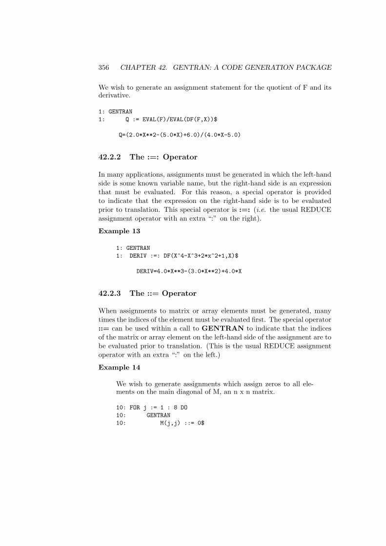
356 CHAPTER 42. GENTRAN: A CODE GENERATION PACKAGE
We wish to generate an assignment statement for the quotient of F and itsderivative.
1: GENTRAN1: Q := EVAL(F)/EVAL(DF(F,X))$
Q=(2.0*X**2-(5.0*X)+6.0)/(4.0*X-5.0)
42.2.2 The :=: Operator
In many applications, assignments must be generated in which the left-handside is some known variable name, but the right-hand side is an expressionthat must be evaluated. For this reason, a special operator is providedto indicate that the expression on the right-hand side is to be evaluatedprior to translation. This special operator is :=: (i.e. the usual REDUCEassignment operator with an extra “:” on the right).
Example 13
1: GENTRAN1: DERIV :=: DF(X^4-X^3+2*x^2+1,X)$
DERIV=4.0*X**3-(3.0*X**2)+4.0*X
42.2.3 The ::= Operator
When assignments to matrix or array elements must be generated, manytimes the indices of the element must be evaluated first. The special operator::= can be used within a call to GENTRAN to indicate that the indicesof the matrix or array element on the left-hand side of the assignment are tobe evaluated prior to translation. (This is the usual REDUCE assignmentoperator with an extra “:” on the left.)
Example 14
We wish to generate assignments which assign zeros to all ele-ments on the main diagonal of M, an n x n matrix.
10: FOR j := 1 : 8 DO10: GENTRAN10: M(j,j) ::= 0$

42.2. PRECISION 357
M(1,1)=0.0M(2,2)=0.0::M(8,8)=0.0
LSETQ may be used interchangeably with ::= on input.
42.2.4 The ::=: Operator
In applications in which evaluated expressions are to be assigned to arrayelements with evaluated subscripts, the ::=: operator can be used. It is acombination of the ::= and :=: operators described in sections 42.2.2 and42.2.3.
Example 15
The following matrix, M, has been derived symbolically:

358 CHAPTER 42. GENTRAN: A CODE GENERATION PACKAGE
( A 0 -1 1)( )( 0 B 0 0)( )( -1 0 C -1)( )( 1 0 -1 D)
We wish to generate assignment statements for those elementson the main diagonal of the matrix.
10: FOR j := 1 : 4 DO10: GENTRAN10: M(j,j) ::=: M(j,j)$
M(1,1)=AM(2,2)=BM(3,3)=CM(4,4)=D
The alternative alphanumeric identifier associated with ::=: is LRSETQ.
42.3 Explicit Type Declarations
Type declarations are automatically generated each time a subprogramheading is generated. Type declarations are constructed from informationstored in the GENTRAN symbol table. The user can place entries intothe symbol table explicitly through calls to the special GENTRAN functionDECLARE.
Syntax:
DECLARE v1,v2,. . . ,vn : type;
orDECLARE<<
v11,v12,. . . ,v1n : type1;v21,v22,. . . ,v2n : type2;::vn1,vnn,. . . ,vnn : typen;
>>;

42.4. EXPRESSION SEGMENTATION 359
Arguments:
Each v1,v2,. . . ,vn is a list of one or more variables (optionallysubscripted to indicate array dimensions), or variable ranges (twoletters separated by a “-”). v’s are not evaluated unless given asarguments to EVAL.
Each type is a variable type in the target language. Each must bean atom, optionally preceded by the atom IMPLICIT. type’sare not evaluated unless given as arguments to EVAL.
The DECLARE statement can also be used to declare subprogram types(i.e. SUBROUTINE or FUNCTION) for FORTRAN and RATFORcode, and function types for all four languages.
42.4 Expression Segmentation
Symbolic derivations can easily produce formulas that can be anywhere froma few lines to several pages in length. Such formulas can be translated intonumerical assignment statements, but unless they are broken into smallerpieces they may be too long for a compiler to handle. (The maximumnumber of continuation lines for one statement allowed by most FORTRANcompilers is only 19.) Therefore GENTRAN contains a segmentation facilitywhich automatically segments, or breaks down unreasonably large expres-sions.
The segmentation facility generates a sequence of assignment statements,each of which assigns a subexpression to an automatically generated tem-porary variable. This sequence is generated in such a way that temporaryvariables are re-used as soon as possible, thereby keeping the number of au-tomatically generated variables to a minimum. The facility can be turnedon or off by setting the mode switch GENTRANSEG accordingly (i.e.by calling the REDUCE function ON or OFF on it). The user can con-trol the maximum allowable expression size by setting the variable MAX-EXPPRINTLEN!* to the maximum number of characters allowed in anexpression printed in the target language (excluding spaces automaticallyprinted by the formatter). The GENTRANSEG switch is on initially,and MAXEXPPRINTLEN!* is initialised to 800.

360 CHAPTER 42. GENTRAN: A CODE GENERATION PACKAGE
42.5 Template Processing
In some code generation applications pieces of the target numerical pro-gram are known in advance. A template file containing a program outlineis supplied by the user, and formulas are derived in REDUCE, convertedto numerical code, and inserted in the corresponding places in the programoutline to form a complete numerical program. A template processor isprovided by GENTRAN for use in these applications.
Syntax:
GENTRANIN f1,f2,. . . ,fm [OUT f1,f2,. . . ,fn];
Arguments:
f1,f2,. . . ,fm is an argument list containing one or more f ’s,where each f is one of:
an atom = a template (input) fileT = the terminal
f1,f2,. . . ,fn is an optional argument list containing one or moref ’s, where each f is one of:
an atom = an output fileT = the terminalNIL = the current output file(s)ALL!* = all files currently open for output
by GENTRAN (see section 42.6)
GENTRANIN processes each template file f1,f2,. . . ,fm sequentially.
A template file may contain any number of parts, each of which is either anactive or an inactive part. All active parts start with the character sequence;BEGIN; and end with ;END;. The end of the template file is indicatedby an extra ;END; character sequence.
Inactive parts of template files are assumed to contain code in the targetlanguage. All inactive parts are copied to the output.
Active parts may contain any number of REDUCE expressions, statements,and commands. They are not copied directly to the output. Instead, they

42.5. TEMPLATE PROCESSING 361
are given to REDUCE for evaluation in algebraic mode. All output gener-ated by each evaluation is sent to the output file(s). Returned values areonly printed on the terminal.
Active parts will most likely contain calls to GENTRAN to generate code.This means that the result of processing a template file will be the originaltemplate file with all active parts replaced by generated code.
If OUT f1,f2,. . . ,fn is not given, generated code is simply written to thecurrent-output file.
However, if OUT f1,f2,. . . ,fn is given, then the current-output file is tem-porarily overridden. Generated code is written to each file represented byf1,f2,. . . ,fn for this command only. Files which were open prior to the callto GENTRANIN will remain open after the call, and files which did notexist prior to the call will be created, opened, written to, and closed. Theoutput-stack will be exactly the same both before and after the call.
GENTRANIN returns the names of all files written to by this command.

362 CHAPTER 42. GENTRAN: A CODE GENERATION PACKAGE
Example 16
Suppose we wish to generate a FORTRAN subprogram to com-pute the determinant of a 3 x 3 matrix. We can construct atemplate file with an outline of the FORTRAN subprogram andREDUCE and GENTRAN commands to fill it in:
Contents of file det.tem:
REAL FUNCTION DET(M)REAL M(3,3)
;BEGIN;OPERATOR M$MATRIX MM(3,3)$MM := MAT( (M(1,1),M(1,2),M(1,3)),
(M(2,1),M(2,2),M(2,3)),(M(3,1),M(3,2),M(3,3)) )$
GENTRAN DET :=: DET(MM)$;END;
RETURNEND
;END;
Now we can generate a FORTRAN subprogram with the follow-ing REDUCE session:
1: GENTRANLANG!* := ’FORTRAN$
2: GENTRANIN2: "det.tem"2: OUT "det.f"$
Contents of file det.f:
REAL FUNCTION DET(M)REAL M(3,3)DET=M(3,3)*M(2,2)*M(1,1)-(M(3,3)*M(2,1)*M(1,2))-(M(3,2)
. *M(2,3)*M(1,1))+M(3,2)*M(2,1)*M(1,3)+M(3,1)*M(2,3)*M(1
. ,2)-(M(3,1)*M(2,2)*M(1,3))RETURNEND

42.6. OUTPUT REDIRECTION 363
42.6 Output Redirection
The GENTRANOUT and GENTRANSHUT commands are identicalto the REDUCE OUT and SHUT commands with the following exceptions:
• GENTRANOUT and GENTRANSHUT redirect only code whichis printed as a side effect of GENTRAN commands.
• GENTRANOUT allows more than one file name to be given toindicate that generated code is to be sent to two or more files. (It isparticularly convenient to be able to have generated code sent to theterminal screen and one or more file simultaneously.)
• GENTRANOUT does not automatically erase existing files; itprints a warning message on the terminal and asks the user whetherthe existing file should be erased or the whole command be aborted.

364 CHAPTER 42. GENTRAN: A CODE GENERATION PACKAGE

Chapter 43
GEOMETRY: Mechanized(Plane) GeometryManipulations
Hans-Gert GrabeUniversitat Leipzig, Germany
e-mail: [email protected]
43.1 Introduction
This package provides tools for formulation and mechanized proofs of geom-etry statements in the spirit of the “Chinese Prover” of W.-T. Wu [20] andthe fundamental book [5] of S.-C. Chou who proved 512 geometry theoremswith this mechanized method, see also [4], [3], [18], [19].
The general idea behind this approach is an algebraic reformulation of ge-ometric conditions using generic coordinates. A (mathematically strong)proof of the geometry statement then may be obtained from appropriatemanipulations of these algebraic expressions. A CAS as, e.g., Reduce is wellsuited to mechanize these manipulations.
For a more detailed introduction to the topic see the accompanying filegeometry.tex in $REDUCEPATH/packages/geometry/.
365

366 CHAPTER 43. GEOMETRY: PLANE GEOMETRY
43.2 Basic Data Types and Constructors
The basic data types in this package are Scalar, Point, Line, Circle1and Circle.The function POINT(a, b) creates a Point in the plane with the (x, y)-coordinates (a, b). A Line is created with the function LINE(a, b, c) andfulfills the equation ax+ by + c = 0. For circles there are two constructors.You can use CIRCLE(c1, c2, c3, c4) to create a Circle where the scalar vari-ables solve the equation c1(x2 + y2) + c2x + c3y + c4 = 0. Note that linesare a subset of the circles with c1 = 0. The other way to create a Circle isthe function CIRCLE1(M, s). The variable M here denotes a Point and sthe squared radius. Please note that this package mostly uses the squareddistances and radiuses.
There are various functions whose return type is Scalar. Booleans arerepresented as extended booleans, i.e. the procedure returns a Scalarthat is zero iff the condition is fulfilled. For example, the function callPOINT ON CIRCLE(P,c) returns zero if the Point P is on the circle, oth-erwise P is not on the circle. In some cases also a non zero result has ageometric meaning. For example, COLLINEAR(A,B,C) returns the signedarea of the corresponding parallelogram.
43.3 Procedures
This section contains a short description of all procedures available in Ge-ometry. Per convention distances and radiuses of circles are squared.
ANGLE SUM(a,b:Scalar):ScalarReturns tan(α+ β), if a = tan(α), b = tan(β).
ALTITUDE(A,B,C:Point):LineThe altitude from A onto g(BC).
C1 CIRCLE(M:Point,sqr:Scalar):CircleThe circle with given center and sqradius.
CC TANGENT(c1,c2:Circle):ScalarZero iff c1 and c2 are tangent.
CHOOSE PC(M:Point,r,u):Point

43.3. PROCEDURES 367
Chooses a point on the circle around M with radius rusing its rational parametrization with parameter u.
CHOOSE PL(a:Line,u):PointChooses a point on a using parameter u.
CIRCLE(c1,c2,c3,c4:Scalar):CircleThe Circle constructor.
CIRCLE1(M:Point,sqr:Scalar):Circle1The Circle1 constructor.
CIRCLE CENTER(c:Circle):PointThe center of c.
CIRCLE SQRADIUS(c:Circle):ScalarThe sqradius of c.
CL TANGENT(c:Circle,l:Line):ScalarZero iff l is tangent to c.
COLLINEAR(A,B,C:Point):ScalarZero iff A,B,C are on a common line. In general thesigned area of the parallelogram spanned by ~AB and~AC.
CONCURRENT(a,b,c:Line):ScalarZero iff a, b, c have a common point.
INTERSECTION POINT(a,b:Line):PointThe intersection point of the lines a, b.
L2 ANGLE(a,b:Line):ScalarTangens of the angle between a and b.
LINE(a,b,c:Scalar):LineThe Line constructor.
LOT(P:Point,a:Line):LineThe perpendicular from P onto a.
MEDIAN(A,B,C:Point):LineThe median line from A to BC.
MIDPOINT(A,B:Point):PointThe midpoint of AB.
MP(B,C:Point):Line

368 CHAPTER 43. GEOMETRY: PLANE GEOMETRY
The midpoint perpendicular of BC.
ORTHOGONAL(a,b:Line):Scalarzero iff the lines a, b are orthogonal.
OTHER CC POINT(P:Point,c1,c2:Circle):Pointc1 and c2 intersect at P . The procedure returns thesecond intersection point.
OTHER CL POINT(P:Point,c:Circle,l:Line):Pointc and l intersect at P . The procedure returns thesecond intersection point.
P3 ANGLE(A,B,C:Point):ScalarTangens of the angle between ~BA and ~BC.
P3 CIRCLE(A,B,C:Point):Circle orP3 CIRCLE1(A,B,C:Point):Circle1
The circle through 3 given points.
P4 CIRCLE(A,B,C,D:Point):ScalarZero iff four given points are on a common circle.
PAR(P:Point,a:Line):LineThe line through P parallel to a.
PARALLEL(a,b:Line):ScalarZero iff the lines a, b are parallel.
PEDALPOINT(P:Point,a:Line):PointThe pedal point of the perpendicular from P onto a.
POINT(a,b:Scalar):PointThe Point constructor.
POINT ON BISECTOR(P,A,B,C:Point):ScalarZero iff P is a point on the (inner or outer) bisector ofthe angle 6 ABC.
POINT ON CIRCLE(P:Point,c:Circle):Scalar orPOINT ON CIRCLE1(P:Point,c:Circle1):Scalar
Zero iff P is on the circle c.
POINT ON LINE(P:Point,a:Line):ScalarZero iff P is on the line a.
PP LINE(A,B:Point):LineThe line through A and B.

43.3. PROCEDURES 369
SQRDIST(A,B:Point):ScalarSquare of the distance between A and B.
SYMPOINT(P:Point,l:Line):PointThe point symmetric to P wrt. the line l.
SYMLINE(a:Line,l:Line):LineThe line symmetric to a wrt. the line l.
VARPOINT(A,B:Point,u):PointThe point D = u ·A+ (1− u) ·B.
Geometry supplies as additional tools the functions
EXTRACTMAT(polys,vars)Returns the coefficient matrix of the list of equationspolys that are linear in the variables vars.
RED HOM COORDS(u:Line,Circle)Returns the reduced homogeneous coordinates of u,i.e., divides out the content.
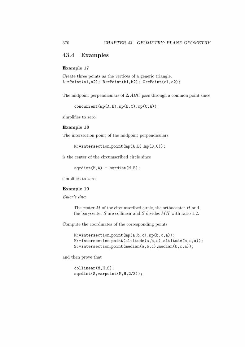
370 CHAPTER 43. GEOMETRY: PLANE GEOMETRY
43.4 Examples
Example 17
Create three points as the vertices of a generic triangle.A:=Point(a1,a2); B:=Point(b1,b2); C:=Point(c1,c2);
The midpoint perpendiculars of ∆ABC pass through a common point since
concurrent(mp(A,B),mp(B,C),mp(C,A));
simplifies to zero.
Example 18
The intersection point of the midpoint perpendiculars
M:=intersection point(mp(A,B),mp(B,C));
is the center of the circumscribed circle since
sqrdist(M,A) - sqrdist(M,B);
simplifies to zero.
Example 19
Euler’s line:
The center M of the circumscribed circle, the orthocenter H andthe barycenter S are collinear and S divides MH with ratio 1:2.
Compute the coordinates of the corresponding points
M:=intersection point(mp(a,b,c),mp(b,c,a));H:=intersection point(altitude(a,b,c),altitude(b,c,a));S:=intersection point(median(a,b,c),median(b,c,a));
and then prove that
collinear(M,H,S);sqrdist(S,varpoint(M,H,2/3));

43.4. EXAMPLES 371
both simplify to zero.

372 CHAPTER 43. GEOMETRY: PLANE GEOMETRY

Chapter 44
GNUPLOT: Display offunctions and surfaces
Herbert MelenkKonrad–Zuse–Zentrum fur Informationstechnik Berlin
Takustrase 7D–14195 Berlin–Dahlem, Germany
e–mail: [email protected]
The gnuplot system provides easy to use graphics output for curves orsurfaces which are defined by formulas and/or data sets. The REDUCEGNUPLOT package lets one use the GNUPLOT graphical output directlyfrom inside REDUCE, either for the interactive display of curves/surfacesor for the production of pictures on paper.
For a full understanding of use of the REDUCE GNUPLOT package it isbest to be familiar with gnuplot.
The main command is PLOT. It accepts an arbitrary list of arguments whichare either an expression to be plotted, a range expressions or an option.
load_package gnuplot;plot(w=sin(a),a=(0 .. 10),xlabel="angle",ylabel="sine");
The expression can be in one or two unknowns, or a list of two functionsfor the x and y values. It can also be an implicit equation in 2-dimensionalspace.
373

374 CHAPTER 44. GNUPLOT: PLOTTING FUNCTIONS
plot(x**3+x*y**3-9x=0);
The dependent and independent variables can be limited to a range withthe syntax shown in the first example. If omitted the independent variablesrange from -10 to 10 and the dependent variable is limited only by theprecision of the IEEE floating point arithmetic.
There are a great deal of options, either as keywords or as variable=string.Options include:
title: assign a heading (default: empty)
xlabel: set label for the x axis
ylabel: set label for the y axis
zlabel: set label for the z axis
terminal: select an output device
size: rescale the picture
view: set a viewpoint
(no)contour: 3d: add contour lines
(no)surface: 3d: draw surface (default: yes)
(no)hidden3d: 3d: remove hidden lines (default: no)
The command PLOTRESET closes the current GNUPLOT windows. The nextcall to PLOT will create a new one.
GNUPLOT is controlled by a number of switches.
Normally all intermediate data sets are deleted after terminating a plotsession. If the switch PLOTKEEP is set on, the data sets are kept for eventualpost processing independent of REDUCE.
In general PLOT tries to generate smooth pictures by evaluating the functionsat interior points until the distances are fine enough. This can require alot of computing time if the single function evaluation is expensive. Therefinement is controlled by the switch PLOTREFINE which is on by default.When you turn it off the functions will be evaluated only at the basic points.
The integer value of the global variable PLOT XMESH defines the number ofinitial function evaluations in x direction for PLOT. For 2d graphs additionalpoints will be used as long as plotrefine is on. For 3d graphs this number

375
defines also the number of mesh lines orthogonal to the x axis. PLOT YMESHdefines for 3d plots the number of function evaluations in the y directionand the number of mesh lines orthogonal to the y axis.
The grid for localising an implicitly defined curve in PLOT consists of tri-angles. These are computed initially equally distributed over the x-y planecontrolled by PLOT XMESH. The grid is refined adaptively in several levels.The final grid can be visualised by setting on the switch SHOW GRID.

376 CHAPTER 44. GNUPLOT: PLOTTING FUNCTIONS

Chapter 45
GROEBNER: A Grobnerbasis package
Herbert Melenk & Winfried NeunKonrad–Zuse–Zentrum fur Informationstechnik Berlin
Takustrase 7D–14195 Berlin–Dahlem, Germany
e–mail: [email protected]
and
H.M. MollerFernuniversitat Hagen FB Math und Informatik
Postfach 940D–58084 Hagen, Germany
e–mail: [email protected]
Grobner bases are a valuable tool for solving problems in connection withmultivariate polynomials, such as solving systems of algebraic equations andanalysing polynomial ideals.
The GROEBNER package calculates Grobner bases using the Buchbergeralgorithm. It can be used over a variety of different coefficient domains, andfor different variable and term orderings.
377

378 CHAPTER 45. GROEBNER: A GROBNER BASIS PACKAGE
45.1
45.1.1 Term Ordering
In the theory of Grobner bases, the terms of polynomials are considered asordered. Several order modes are available in the current package, includingthe basic modes:
LEX, GRADLEX, REVGRADLEX
All orderings are based on an ordering among the variables. For each pairof variables (a, b) an order relation must be defined, e.g. “a À b”. Thegreater signÀ does not represent a numerical relation among the variables;it can be interpreted only in terms of formula representation: “a” will beplaced in front of “b” or “a” is more complicated than “b”.
The sequence of variables constitutes this order base. So the notion of
x1, x2, x3
as a list of variables at the same time means
x1À x2À x3
with respect to the term order.
If terms (products of powers of variables) are compared with LEX, thatterm is chosen which has a greater variable or a higher degree if the greatestvariable is the first in both. With GRADLEX the sum of all exponents (thetotal degree) is compared first, and if that does not lead to a decision, theLEX method is taken for the final decision. The REVGRADLEX methodalso compares the total degree first, but afterward it uses the LEX methodin the reverse direction; this is the method originally used by Buchberger.Note that the LEX ordering is identical to the standard REDUCE kernelordering, when KORDER is set explicitly to the sequence of variables.
LEX is the default term order mode in the GROEBNER package.

45.2. THE BASIC OPERATORS 379
45.2 The Basic Operators
45.2.1 Term Ordering Mode
TORDER (vl,m,[p1, p2, . . .]);
where vl is a variable list (or the empty list if no variables are declaredexplicitly), m is the name of a term ordering mode LEX, GRADLEX,REVGRADLEX (or another implemented mode) and [p1, p2, . . .] areadditional parameters for the term ordering mode (not needed for thebasic modes).
TORDER sets variable set and the term ordering mode. The de-fault mode is LEX. The previous description is returned as a list withcorresponding elements. Such a list can alternatively passed as soleargument to TORDER.
If the variable list is empty or if the TORDER declaration is omitted,the automatic variable extraction is activated.
GVARS (exp1, exp2, . . ., expn);where exp1, exp2, . . . , expn is a list of expressions or equations.
GVARS extracts from the expressions exp1, exp2, . . . , expn the ker-nels, which can play the role of variables for a Grobner calculation.This can be used e.g. in a TORDER declaration.
45.2.2 GROEBNER: Calculation of a Grobner Basis
GROEBNER exp1, exp2, . . . , expm;where exp1, exp2, . . . , expm is a list of expressions or equations.
GROEBNER calculates the Grobner basis of the given set of expres-sions with respect to the current TORDER setting.
The Grobner basis 1 means that the ideal generated by the inputpolynomials is the whole polynomial ring, or equivalently, that theinput polynomials have no zeros in common.
As a side effect, the sequence of variables is stored as a REDUCE listin the shared variable gvarslast.
Example 20

380 CHAPTER 45. GROEBNER: A GROBNER BASIS PACKAGE
torder(,lex)$groebner3*x**2*y + 2*x*y + y + 9*x**2 + 5*x - 3,2*x**3*y - x*y - y + 6*x**3 - 2*x**2 - 3*x + 3,x**3*y + x**2*y + 3*x**3 + 2*x**2 ;
28*X - 2*Y + 5*Y + 3,
3 22*Y - 3*Y - 16*Y + 21
The operation of GROEBNER can be controlled by the following switches:
GROEBOPT – If set ON, the sequence of variables is optimized with re-spect to execution speed; note that the final list of variables is availablein GVARSLAST.
An explicitly declared dependency supersedes the variable optimiza-tion. By default GROEBOPT is off, conserving the original variablesequence.
GROEBFULLREDUCTION – If set off, the reduction steps during theGROEBNER operation are limited to the pure head term reduc-tion; subsequent terms are reduced otherwise. By default GROEB-FULLREDUCTION is on.
GLTBASIS – If set on, the leading terms of the result basis are extracted.They are collected in a basis of monomials, which is available as valueof the global variable with the name GLTB.
45.2.3 GZERODIM?: Test of dim = 0
GZERODIM!? baswhere bas is a Grobner basis in the current setting. The result is NIL, ifbas is the basis of an ideal of polynomials with more than finitely manycommon zeros. If the ideal is zero dimensional, i.e. the polynomialsof the ideal have only finitely many zeros in common, the result is aninteger k which is the number of these common zeros (counted withmultiplicities).

45.2. THE BASIC OPERATORS 381
45.2.4 GDIMENSION, GINDEPENDENT SETS
The following operators can be used to compute the dimension and theindependent variable sets of an ideal which has the Grobner basis bas witharbitrary term order:
Gdimension bas
Gindependent sets bas Gindependent sets computes the maximal left in-dependent variable sets of the ideal, that are the variable sets whichplay the role of free parameters in the current ideal basis. Each set isa list which is a subset of the variable list. The result is a list of thesesets. For an ideal with dimension zero the list is empty. GDimensioncomputes the dimension of the ideal, which is the maximum length ofthe independent sets.
45.2.5 GLEXCONVERT: Conversion to a Lexical Base
GLEXCONVERT (exp, . . . , expm [, var1 . . . , varn][,MAXDEG = mx] [, NEWV ARS = nv1, . . . , nvk])where exp1, . . . , expm is a Grobner basis with var1, . . . , varn asvariables in the current term order mode, mx is an integer, andnv1, . . . , nvk is a subset of the basis variables. For this operatorthe source and target variable sets must be specified explicitly.
GLEXCONVERT converts a basis of a zero-dimensional ideal (finite numberof isolated solutions) from arbitrary ordering into a basis under lex ordering.During the call of GLEXCONVERT the original ordering of the input basismust be still active.
NEWVARS defines the new variable sequence. If omitted, the original vari-able sequence is used. If only a subset of variables is specified here, thepartial ideal basis is evaluated. For the calculation of a univariate polyno-mial, NEWVARS should be a list with one element.
MAXDEG is an upper limit for the degrees. The algorithm stops with anerror message, if this limit is reached.
A warning occurs if the ideal is not zero dimensional.
GLEXCONVERT is an implementation of the FLGM algorithm. Often, thecalculation of a Grobner basis with a graded ordering and subsequent conver-

382 CHAPTER 45. GROEBNER: A GROBNER BASIS PACKAGE
sion to lex is faster than a direct lex calculation. Additionally, GLEXCON-VERT can be used to transform a lex basis into one with different variablesequence, and it supports the calculation of a univariate polynomial. If thelatter exists, the algorithm is even applicable in the non zero-dimensionalcase, if such a polynomial exists.
torder(w,p,z,t,s,b,gradlex)
g := groebner f1 := 45*p + 35*s -165*b -36,35*p + 40*z + 25*t - 27*s, 15*w + 25*p*s +30*z -18*t
-165*b**2, -9*w + 15*p*t + 20*z*s,w*p + 2*z*t - 11*b**3, 99*w - 11*s*b +3*b**2,b**2 + 33/50*b + 2673/10000;
G := 60000*W + 9500*B + 3969,
1800*P - 3100*B - 1377,
18000*Z + 24500*B + 10287,
750*T - 1850*B + 81,
200*S - 500*B - 9,2
10000*B + 6600*B + 2673
glexconvert(g,w,p,z,t,s,b,maxdeg=5,newvars=w);
2100000000*W + 2780000*W + 416421
glexconvert(g,w,p,z,t,s,b,maxdeg=5,newvars=p);
26000*P - 2360*P + 3051
45.2.6 GROEBNERF: Factorizing Grobner Bases
If Grobner bases are computed in order to solve systems of equations or tofind the common roots of systems of polynomials, the factorizing versionof the Buchberger algorithm can be used. The theoretical background is

45.2. THE BASIC OPERATORS 383
simple: if a polynomial p can be represented as a product of two (or more)polynomials, e.g. h = f ∗ g, then h vanishes if and only if one of the factorsvanishes. So if during the calculation of a Grobner basis h of the aboveform is detected, the whole problem can be split into two (or more) disjointbranches. Each of the branches is simpler than the complete problem; thissaves computing time and space. The result of this type of computation isa list of (partial) Grobner bases; the solution set of the original problem isthe union of the solutions of the partial problems, ignoring the multiplicityof an individual solution. If a branch results in a basis 1, then thereis no common zero, i.e. no additional solution for the original problem,contributed by this branch.
GROEBNERF Call
The syntax of GROEBNERF is the same as for GROEBNER.
GROEBNERF(exp1, exp2, . . . , expm[, , nz1, . . . nzk);
where exp1, exp2, . . . , expm is a given list of expressions or equations, andnz1, . . . nzk is an optional list of polynomials known to be non-zero.
GROEBNERF tries to separate polynomials into individual factors and tobranch the computation in a recursive manner (factorisation tree). Theresult is a list of partial Grobner bases. If no factorisation can be found orif all branches but one lead to the trivial basis 1, the result has only onebasis; nevertheless it is a list of lists of polynomials. If no solution is found,the result will be 1. Multiplicities (one factor with a higher power, thesame partial basis twice) are deleted as early as possible in order to speedup the calculation. The factorising is controlled by some switches.
As a side effect, the sequence of variables is stored as a REDUCE list in theshared variable
gvarslast .
If GLTBASIS is on, a corresponding list of leading term bases is also pro-duced and is available in the variable GLTB.
The third parameter of GROEBNERF allows one to declare some polynom-ials nonzero. If any of these is found in a branch of the calculation the branchis cancelled. This can be used to save a substantial amount of computing
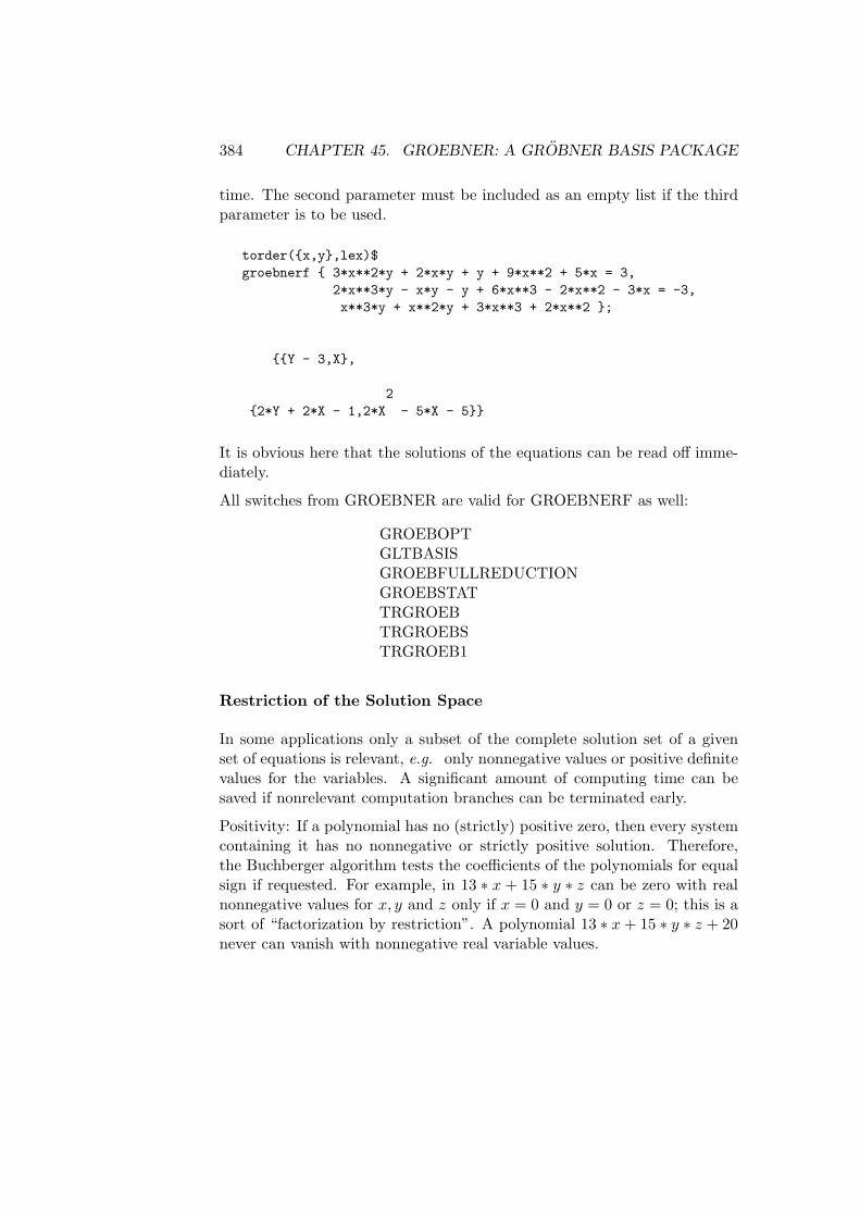
384 CHAPTER 45. GROEBNER: A GROBNER BASIS PACKAGE
time. The second parameter must be included as an empty list if the thirdparameter is to be used.
torder(x,y,lex)$groebnerf 3*x**2*y + 2*x*y + y + 9*x**2 + 5*x = 3,
2*x**3*y - x*y - y + 6*x**3 - 2*x**2 - 3*x = -3,x**3*y + x**2*y + 3*x**3 + 2*x**2 ;
Y - 3,X,
22*Y + 2*X - 1,2*X - 5*X - 5
It is obvious here that the solutions of the equations can be read off imme-diately.
All switches from GROEBNER are valid for GROEBNERF as well:
GROEBOPTGLTBASISGROEBFULLREDUCTIONGROEBSTATTRGROEBTRGROEBSTRGROEB1
Restriction of the Solution Space
In some applications only a subset of the complete solution set of a givenset of equations is relevant, e.g. only nonnegative values or positive definitevalues for the variables. A significant amount of computing time can besaved if nonrelevant computation branches can be terminated early.
Positivity: If a polynomial has no (strictly) positive zero, then every systemcontaining it has no nonnegative or strictly positive solution. Therefore,the Buchberger algorithm tests the coefficients of the polynomials for equalsign if requested. For example, in 13 ∗ x + 15 ∗ y ∗ z can be zero with realnonnegative values for x, y and z only if x = 0 and y = 0 or z = 0; this is asort of “factorization by restriction”. A polynomial 13 ∗ x+ 15 ∗ y ∗ z + 20never can vanish with nonnegative real variable values.

45.2. THE BASIC OPERATORS 385
Zero point: If any polynomial in an ideal has an absolute term, the idealcannot have the origin point as a common solution.
By setting the shared variable
GROEBRESTRICTION
GROEBNERF is informed of the type of restriction the user wants to imposeon the solutions:
GROEBRESTRICTION:=NONEGATIVE;only nonnegative real solutions are of interest
GROEBRESTRICTION:=POSITIVE;only nonnegative and nonzero solutions are of interest
GROEBRESTRICTION:=ZEROPOINT;only solution sets which contain the point 0, 0, . . . , 0 are or interest.
If GROEBNERF detects a polynomial which formally conflicts with therestriction, it either splits the calculation into separate branches, or, if aviolation of the restriction is determined, it cancels the actual calculationbranch.
45.2.7 GREDUCE, PREDUCE: Reduction of Polynomials
Background
Reduction of a polynomial “p” modulo a given sets of polynomials “B” isdone by the reduction algorithm incorporated in the Buchberger algorithm.
Reduction via Grobner Basis Calculation
GREDUCE(exp, exp1, exp2, . . . , expm]);where exp is an expression, and exp1, exp2, . . . , expm is a list of any num-ber of expressions or equations.
GREDUCE first converts the list of expressions exp1, . . . , expn to aGrobner basis, and then reduces the given expression modulo that basis.

386 CHAPTER 45. GROEBNER: A GROBNER BASIS PACKAGE
An error results if the list of expressions is inconsistent. The returned valueis an expression representing the reduced polynomial. As a side effect, GRE-DUCE sets the variable gvarslast in the same manner as GROEBNER does.
Reduction with Respect to Arbitrary Polynomials
PREDUCE(exp, exp1, exp2, . . . , expm);where exp is an expression, and exp1, exp2, . . . , expm is a list of any num-ber of expressions or equations.
PREDUCE reduces the given expression modulo the set exp1, . . . , expm.If this set is a Grobner basis, the obtained reduced expression is uniquelydetermined. If not, then it depends on the subsequence of the sin-gle reduction steps (see 45.2.7). PREDUCE does not check whetherexp1, exp2, . . . , expm is a Grobner basis in the actual order. Therefore,if the expressions are a Grobner basis calculated earlier with a variablesequence given explicitly or modified by optimisation, the proper variablesequence and term order must be activated first.
Example 21(PREDUCE called with a Grobner basis):
torder(x,y,lex);gb:=groebner3*x**2*y + 2*x*y + y + 9*x**2 + 5*x - 3,
2*x**3*y - x*y - y + 6*x**3 - 2*x**2 - 3*x + 3,x**3*y + x**2*y + 3*x**3 + 2*x**2$
preduce (5*y**2 + 2*x**2*y + 5/2*x*y + 3/2*y+ 8*x**2 + 3/2*x - 9/2, gb);
2Y
45.3 Ideal Decomposition & Equation System Solv-ing
Based on the elementary Grobner operations, the GROEBNER packageoffers additional operators, which allow the decomposition of an ideal orof a system of equations down to the individual solutions. Details of theoperators GROESOLVE, GROEBNERF and IDEALQUOTIENT can befound in the full documentation, with associated functions.

Chapter 46
IDEALS: Arithmetic forpolynomial ideals
Herbert MelenkKonrad–Zuse–Zentrum fur Informationstechnik Berlin
Takustrase 7D–14195 Berlin–Dahlem, Germany
e–mail: [email protected]
This package implements the basic arithmetic for polynomial ideals by ex-ploiting the Grobner bases package of REDUCE. In order to save computingtime all intermediate Grobner bases are stored internally such that time con-suming repetitions are inhibited. A uniform setting facilitates the access.
46.1 Initialization
Prior to any computation the set of variables has to be declared by callingthe operator I setting . For example in order to initiate computations inthe polynomial ring Q[x, y, z] call
I_setting(x,y,z);
A subsequent call to I setting allows one to select another set of variables;at the same time the internal data structures are cleared in order to freememory resources.
387

388CHAPTER 46. IDEALS: ARITHMETIC FOR POLYNOMIAL IDEALS
46.2 Bases
An ideal is represented by a basis (set of polynomials) tagged with thesymbol I, e.g.
u := I(x*z-y**2, x**3-y*z);
Alternatively a list of polynomials can be used as input basis; however,all arithmetic results will be presented in the above form. The operatorideal2list allows one to convert an ideal basis into a conventional REDUCElist.
46.2.1 Operators
Because of syntactical restrictions in REDUCE, special operators have tobe used for ideal arithmetic:
.+ ideal sum (infix)
.* ideal product (infix)
.: ideal quotient (infix)
./ ideal quotient (infix)
.= ideal equality test (infix)subset ideal inclusion test (infix)intersection ideal intersection (prefix,binary)member test for membership in an ideal
(infix: polynomial and ideal)gb Groebner basis of an ideal (prefix, unary)ideal2list convert ideal basis to polynomial list
(prefix,unary)
Example:
I(x+y,x^2) .* I(x-z);
2 2 2I(X + X*Y - X*Z - Y*Z,X*Y - Y *Z)
Note that ideal equality cannot be tested with the REDUCE equal sign:
I(x,y) = I(y,x) is falseI(x,y) .= I(y,x) is true

Chapter 47
INEQ: Support for solvinginequalities
Herbert MelenkKonrad–Zuse–Zentrum fur Informationstechnik Berlin
Takustrase 7D–14195 Berlin–Dahlem, Germany
e–mail: [email protected]
This package supports the operator ineq solve that tries to solves singleinequalities and sets of coupled inequalities. The following types of systemsare supported 1:
• only numeric coefficients (no parametric system),
• a linear system of mixed equations and <= – >= inequalities, applyingthe method of Fourier and Motzkin,
• a univariate inequality with <=, >=, > or < operator and polyno-mial or rational left–hand and right–hand sides, or a system of suchinequalities with only one variable.
Syntax:
INEQ SOLVE(<expr> [,<vl>])
1For linear optimization problems please use the operator simplex of the linalg pack-age (section 52.5
389

390 CHAPTER 47. INEQ: SUPPORT FOR SOLVING INEQUALITIES
where <expr> is an inequality or a list of coupled inequalities and equat-ions, and the optional argument <vl> is a single variable (kernel) or a listof variables (kernels). If not specified, they are extracted automaticallyfrom <expr>. For multivariate input an explicit variable list specifies theelimination sequence: the last member is the most specific one.
An error message occurs if the input cannot be processed by the currentalgorithms.
The result is a list. It is empty if the system has no feasible solution.Otherwise the result presents the admissible ranges as set of equations whereeach variable is equated to one expression or to an interval. The mostspecific variable is the first one in the result list and each form contains onlypreceding variables (resolved form). The interval limits can be formal maxor min expressions. Algebraic numbers are encoded as rounded numberapproximations.
Examples:
ineq_solve((2*x^2+x-1)/(x-1) >= (x+1/2)^2, x>0);
x=(0 .. 0.326583),x=(1 .. 2.56777)
reg:=a + b - c>=0, a - b + c>=0, - a + b + c>=0, 0>=0, 2>=0,2*c - 2>=0, a - b + c>=0, a + b - c>=0, - a + b + c - 2>=0,2>=0, 0>=0, 2*b - 2>=0, k + 1>=0, - a - b - c + k>=0,- a - b - c + k + 2>=0, - 2*b + k>=0,- 2*c + k>=0, a + b + c - k>=0,
2*b + 2*c - k - 2>=0, a + b + c - k>=0$
ineq_solve (reg,k,a,b,c);
c=(1 .. infinity),
b=(1 .. infinity),
a=(max( - b + c,b - c) .. b + c - 2),
k=a + b + c
Chapter 48
INVBASE: A package forcomputing involutive bases
A.Yu.Zharkov, Yu.A.BlinkovSaratov UniversityAstrakhanskaya 83
410071 Saratov, Russia
e–mail: [email protected]
Involutive bases are a new tool for solving problems in connection withmultivariate polynomials, such as solving systems of polynomial equationsand analysing polynomial ideals. An involutive basis of polynomial ideal isa special form of a redundant Grobner basis. The construction of involutivebases reduces the problem of solving polynomial systems to simple linearalgebra.
The INVBASE package can be seen as an alternative to Buchberger’s algo-rithm.
48.1 The Basic Operators
48.1.1 Term Ordering
The term order modes available are REVGRADLEX, GRADLEX and LEX. Thesemodes have the same meaning as for the GROEBNER package.
391

392 CHAPTER 48. INVBASE: INVOLUTIVE BASES
All orderings are based on an ordering among the variables. For eachpair of variables an order relation À must be defined. The term order-ing mode as well as the order of variables are set by the operator INVTORDERmode,x1, ..., xn where mode is one of the term order modes listed above.The notion of x1, ..., xn as a list of variables at the same time meansx1 À . . .À xn.
48.1.2 Computing Involutive Bases
To compute the involutive basis of ideal generated by the set of polynomialsp1, ..., pm one should type the command
INVBASE p1, ..., pmwhere pi are polynomials in variables listed in the INVTORDER operator. Ifsome kernels in pi were not listed previously in the INVTORDER operator theyare considered as parameters, i.e. they are considered part of the coefficientsof polynomials. If INVTORDER was omitted, all the kernels in pi are consideredas variables with the default REDUCE kernel order.
The coefficients of polynomials pi may be integers as well as rational num-bers (or, accordingly, polynomials and rational functions in the parametriccase). The computations modulo prime numbers are also available. For thispurpose one should type the REDUCE commands
ON MODULAR; SETMOD p;
where p is a prime number. The value of the INVBASE function is a list ofinteger polynomials g1, ..., gn representing an involutive basis of a givenideal.
INVTORDER REVGRADLEX, x,y,z;
g:= INVBASE 4*x**2 + x*y**2 - z + 1/4,2*x + y**2*z + 1/2,x**2*z - 1/2*x - y**2;
3 2 3 2g := 8*x*y*z - 2*x*y*z + 4*y - 4*y*z + 16*x*y + 17*y*z - 4*y,
4 2 2 28*y - 8*x*z - 256*y + 2*x*z + 64*z - 96*x + 20*z - 9,

48.1. THE BASIC OPERATORS 393
32*y *z + 4*x*y + y,
3 2 2 28*x*z - 2*x*z + 4*y - 4*z + 16*x + 17*z - 4,
3 3 2- 4*y*z - 8*y + 6*x*y*z + y*z - 36*x*y - 8*y,
2 2 24*x*y + 32*y - 8*z + 12*x - 2*z + 1,
22*y *z + 4*x + 1,
3 2 2- 4*z - 8*y + 6*x*z + z - 36*x - 8,
2 2 28*x - 16*y + 4*z - 6*x - z
To convert it into a lexicographical Grobner basis one should type
h := INVLEX g;
6 5 4 3h := 3976*x + 37104*z - 600*z + 2111*z + 122062*z
2+ 232833*z - 680336*z + 288814,
2 6 5 4 31988*y - 76752*z + 1272*z - 4197*z - 251555*z
2- 481837*z + 1407741*z - 595666,
7 6 5 4 3 216*z - 8*z + z + 52*z + 75*z - 342*z + 266*z
- 60

394 CHAPTER 48. INVBASE: INVOLUTIVE BASES

Chapter 49
LAPLACE: Laplace andinverse Laplace transforms
C. Kazasov, M. Spiridonova, V. TomovSofia, Bulgaria
The LAPLACE package provides both Laplace Transforms and InverseLaplace Transforms, with the two operators
LAPLACE(exp, s var, t var)INVLAP(exp, s var, t var)
The action is to transform the expression from the s var or source variableinto the t var or target variable. If t var is omitted, the package uses aninternal variable lp!& or il!& respectively.
Three switches control the transformations. If lmon is on then sine, cosine,hyperbolic sine and hyperbolic cosines are converted by LAPLACE intoexponentials. If lhyp is on then exponential functions are converted intohyperbolic form. The last switch ltrig has the same effect except it usestrigonometric functions.
The system can be extended by adding Laplace transformation rules forsingle functions by rules or rule sets. In such a rule the source variablemust be free, the target variable must be il!& for LAPLACE and lp!&for INVLAP, with the third parameter omitted. Also rules for transformingderivatives are entered in such a form. For example
let laplace(log(~x),x) => -log(gam * il!&)/il!&,
395

396 CHAPTER 49. LAPLACE: LAPLACE TRANSFORMS ETC.
invlap(log(gam * ~x)/x,x) => -log(lp!&);operator f;let
laplace(df(f(~x),x),x) => il!&*laplace(f(x),x) - sub(x=0,f(x)),
laplace(df(f(~x),x,~n),x) => il!&**n*laplace(f(x),x) -for i:=n-1 step -1 until 0 sum
sub(x=0, df(f(x),x,n-1-i)) * il!&**iwhen fixp n,
laplace(f(~x),x) = f(il!&);
The LAPLACE system knows about the functions DELTA and GAMMA, andused the operator ONE for the unit step function and INTL stands for theparameterised integral function, for instance intl(2*y**2,y,0,x) standsfor
∫ x0 2y2dx.
load_package laplace;
laplace(sin(17*x),x,p);
17----------
2p + 289
on lmon;
laplace(-1/4*e**(a*x)*(x-k)**(-1/2), x, p);
1 a*k- ---*sqrt(pi)*e
4----------------------
k*pe *sqrt( - a + p)
invlap(c/((p-a)*(p-b)), p, t);
a*t b*tc*(e - e )
-----------------a - b

397
invlap(p**(-7/3), p, t);
1/3t *t
------------7
gamma(---)3

398 CHAPTER 49. LAPLACE: LAPLACE TRANSFORMS ETC.

Chapter 50
LIE: Functions for theclassification of realn-dimensional Lie algebras
Carsten and Franziska SchobelThe Leipzig University, Computer Science Department
Augustusplatz 10/11,O-7010 Leipzig, Germany
e–mail: [email protected]
LIE is a package of functions for the classification of real n-dimensional Liealgebras. It consists of two modules: liendmc1 and lie1234.
50.1 liendmc1
With the help of the functions in this module real n-dimensional Lie algebrasL with a derived algebra L(1) of dimension 1 can be classified. L has tobe defined by its structure constants ckij in the basis X1, . . . , Xn with[Xi, Xj ] = ckijXk. The user must define an ARRAY LIENSTRUCIN(n, n, n)with n being the dimension of the Lie algebra L. The structure constantsLIENSTRUCIN(i, j, k):=ckij for i < j should be given. Then the procedureLIENDIMCOM1 can be called. Its syntax is:
LIENDIMCOM1(<number>).
399

400 CHAPTER 50. LIE: CLASSIFICATION OF LIE ALGEBRAS
<number> corresponds to the dimension n. The procedure simplifies thestructure of L performing real linear transformations. The returned valueis a list of the form
(i) LIE_ALGEBRA(2),COMMUTATIVE(n-2) or(ii) HEISENBERG(k),COMMUTATIVE(n-k)
with 3 ≤ k ≤ n, k odd.
The returned list is also stored asLIE LIST. The matrix LIENTRANS givesthe transformation from the given basis X1, . . . , Xn into the standard basisY1, . . . , Yn: Yj = (LIENTRANS)kjXk.
50.2 lie1234
This part of the package classifies real low-dimensional Lie algebras L ofthe dimension n := dimL = 1, 2, 3, 4. L is also given by its structureconstants ckij in the basis X1, . . . , Xn with [Xi, Xj ] = ckijXk. An ARRAYLIESTRIN(n, n, n) has to be defined and LIESTRIN(i, j, k):=ckij for i < jshould be given. Then the procedure LIECLASS can be performed whosesyntax is:
LIECLASS(<number>).
<number> should be the dimension of the Lie algebra L. The procedurestepwise simplifies the commutator relations of L using properties of invari-ance like the dimension of the centre, of the derived algebra, unimodularityetc. The returned value has the form:
LIEALG(n),COMTAB(m),
where the value m corresponds to the number of the standard form (basis:Y1, . . . , Yn) in an enumeration scheme.
This returned value is also stored as LIE CLASS. The linear transformationfrom the basis X1, . . . , Xn into the basis of the standard form Y1, . . . , Ynis given by the matrix LIEMAT: Yj = (LIEMAT)kjXk.

Chapter 51
LIMITS: A package forfinding limits
Stanley L. KamenyLos Angeles, U.S.A.
LIMITS is a fast limit package for REDUCE for functions which are con-tinuous except for computable poles and singularities, based on some earlierwork by Ian Cohen and John P. Fitch. The Truncated Power Series pack-age is used for non-critical points, at which the value of the function is theconstant term in the expansion around that point. l’Hopital’s rule is used incritical cases, with preprocessing of∞−∞ forms and reformatting of prod-uct forms in order to apply l’Hopital’s rule. A limited amount of boundedarithmetic is also employed where applicable.
51.1 Normal entry points
LIMIT(EXPRN:algebraic, VAR:kernel, LIMPOINT:algebraic):algebraic
This is the standard way of calling limit, applying all of the methods. Theresult is the limit of EXPRN as VAR approaches LIMPOINT.
401

402 CHAPTER 51. LIMITS: A PACKAGE FOR FINDING LIMITS
51.2 Direction-dependent limits
LIMIT!+(EXPRN:algebraic, VAR:kernel, LIMPOINT:algebraic):algebraicLIMIT!-(EXPRN:algebraic, VAR:kernel, LIMPOINT:algebraic):algebraic
If the limit depends upon the direction of approach to the LIMPOINT, thefunctions LIMIT!+ and LIMIT!- may be used. They are defined by:
LIMIT!+ (EXP,VAR,LIMPOINT) → LIMIT(EXP*,ε,0)where EXP* = sub(VAR=VAR+ε2,EXP)
and
LIMIT!- (EXP,VAR,LIMPOINT) → LIMIT(EXP*,ε,0)where EXP* = sub(VAR=VAR-ε2,EXP)
Examples:
load_package misc;
limit(sin(x)/x,x,0);
1
limit((a^x-b^x)/x,x,0);
log(a) - log(b)
limit(x/(e**x-1), x, 0);
1
limit!-(sin x/cos x,x,pi/2);
infinity
limit!+(sin x/cos x,x,pi/2);
- infinity
limit(x^log(1/x),x,infinity);
0

51.2. DIRECTION-DEPENDENT LIMITS 403
limit((x^(1/5) + 3*x^(1/4))^2/(7*(sqrt(x + 9) - 3 - x/6))^(1/5),x,0);
3/5- 6
---------1/5
7

404 CHAPTER 51. LIMITS: A PACKAGE FOR FINDING LIMITS

Chapter 52
LINALG: Linear algebrapackage
Matt RebbeckKonrad–Zuse–Zentrum fur Informationstechnik Berlin
Takustrase 7D–14195 Berlin–Dahlem, Germany
52.1 Introduction
This package provides a selection of functions that are useful in the worldof linear algebra. They can be classified into four sections:
52.1.1 Basic matrix handling
add columns add rows add to columns add to rowsaugment columns char poly column dim copy intodiagonal extend find companion get columnsget rows hermitian tp matrix augment matrix stackminor mult columns mult rows pivotremove columns remove rows row dim rows pivotstack rows sub matrix swap columns swap entriesswap rows
405

406 CHAPTER 52. LINALG: LINEAR ALGEBRA PACKAGE
52.1.2 Constructors
Functions that create matrices.
band matrix block matrix char matrix coeff matrixcompanion hessian hilbert jacobianjordan block make identity random matrix toeplitzvandermonde Kronecker Product
52.1.3 High level algorithms
char poly cholesky gram schmidt lu decompseudo inverse simplex svd triang adjoint
There is a separate NORMFORM package (chapter 57) for computing thematrix normal forms smithex, smithex int, frobenius, ratjordan, jordansym-bolic and jordan in REDUCE.
52.1.4 Predicates
matrixp squarep symmetricp
52.2 Explanations
In the examples the matrix A will be
A =
1 2 34 5 67 8 9
Throughout I is used to indicate the identity matrix and AT to indicate thetranspose of the matrix A.
Many of the functions have a fairly obvious meaning. Others need a littleexplanation.

52.3. BASIC MATRIX HANDLING 407
52.3 Basic matrix handling
The functions ADD COLUMNS and ADD ROWS provide basic operations betweenrows and columns. The form is
add columns(A,c1,c2,expr);and it replaces column c2 of the matix by expr ∗ column(A,c1) +column(A,c2).
ADD TO COLUMNS and ADD TO ROWS do a similar task, adding an expressionto each of a number of columns (or rows) specified by a list.
add to columns(A, 1, 2, 10) =
11 12 314 15 617 18 9
The functions MULT COLUMNS and MULT ROW are equivalent to multiplycolumns and rows.
COLUMN DIM and ROW DIM find the column dimension and row dimension oftheir argument.
Parts of a matrix can be replaced from another by using COPY INTO; thelast two arguments are row and column counters for to where to copy thematrix.
G =
0 0 0 00 0 0 00 0 0 00 0 0 0
copy into(A,G, 1, 2) =
0 1 2 30 4 5 60 7 8 90 0 0 0
A diagonal matrix can be created with DIAGONAL. The argument is a list ofexpressions of matrices which form the diagonal.
An existing matrix can be extended; the call EXTEND(A,r,c,exp) returns thematrix A extended by r rows and c columns, with the new entries all exp.
The function GET COLUMNS extracts from a matrix a list of the specified

408 CHAPTER 52. LINALG: LINEAR ALGEBRA PACKAGE
columns as matrices. GET ROWS does the equivalent for rows.
get columns(A, 1, 3) =
147
,
369
The Hermitian transpose, that is a matrix in which the (i, j) entry is theconjugate of the (j, i) entry of the input is returned by HERMITIAN TP.
MATRIX AUGMENT(mat1,mat2, . . . ,matn) produces a new matrix from thelist joined as new columns. MATRIX STACK joins a list of matrices by stackingthem.
matrix stack(A,A) =
1 2 34 5 67 8 91 2 34 5 67 8 9
MINOR(A,r,c) calculates the (r,c) minor of A.
PIVOT pivots a matrix about its (r,c) entry. To do this, multiples of the rth
row are added to every other row in the matrix. This means that the cth
column will be 0 except for the (r,c) entry.
A variant on this operation is provided by ROWS PIVOT. It applies the pivotonly to the rows specified as the last argument.
A sub matrix can be extracted, giving a list or the rows and columns tokeep.
sub matrix(A, 1, 3, 2, 3) =
(2 38 9
)
The basic operation of swapping rows or columns is provided by SWAP ROWSand SWAP COLUMNS. Individual entries can be swapped with SWAP ENTRIES.
swap columns(A, 2, 3) =
1 3 24 6 57 9 8

52.4. CONSTRUCTORS 409
swap entries(A, 1, 1, 3, 3) =
9 2 34 5 67 8 1
52.4 Constructors
AUGMENT COLUMNS allows just specified columns to be selected; STACK ROWSdoes a similar job for rows.
stack rows(A, 1, 3) =
(1 2 37 8 9
)
Rows or columns can be removed with REMOVE COLUMNS and REMOVE ROWS.
remove columns(A, 2) =
1 34 67 9
BAND MATRIX creates a square matrix of dimension its second argument. Thediagonal consists of the middle expressions of the first argument, which is anexpression list. The expressions to the left of this fill the required numberof sub diagonals and the expressions to the right the super diagonals.
band matrix(x, y, z, 6) =
y z 0 0 0 0x y z 0 0 00 x y z 0 00 0 x y z 00 0 0 x y z0 0 0 0 x y
Related to the band matrix is a block matrix, which can be created by
BLOCK MATRIX(r,c,matrix list).
The resulting matrix consists of r by c matrices filled from the matrix listrow wise.
B =
(1 00 1
), C =
(55
), D =
(22 3344 55
)

410 CHAPTER 52. LINALG: LINEAR ALGEBRA PACKAGE
block matrix(2, 3, B, C,D,D, C,B) =
1 0 5 22 330 1 5 44 5522 33 5 1 044 55 5 0 1
Characteristic polynomials and characteristic matrices are created by thefunctions CHAR POLY and CHAR MATRIX.
A set of linear equations can be turned into the associated coefficient matrixand vector of unknowns and the righthandside. COEFF MATRIX returns a listC,X ,B such that CX = B.
coeff matrix(x+ y + 4 ∗ z = 10, y + x− z = 20, x+ y + 4) =
4 1 1−1 1 10 1 1
,
zyx
,
1020−4
COMPANION(poly,x) creates the companion matrix C of a polynomial. Thatis the square matrix of dimension n, where n is the degree of polynomialwith respect to x, and the entries of C are: C(i,n) = -coeffn(poly,x,i-1) for i= 1 . . . n, C(i,i-1) = 1 for i = 2 . . . n and the rest are 0.
companion(x4 + 17 ∗ x3 − 9 ∗ x2 + 11, x) =
0 0 0 −111 0 0 00 1 0 90 0 1 −17
The polynomial associated with a companion matrix can be recovered bycalling FIND COMPANION.
HESSIAN(expr, var list) calculates the Hessian matrix of the expressions withrespect to the variables in the list, or the single variable. That is the matrixwith the (i, j) element the jth derivative of the expressions with respect tothe ith variable.
hessian(x ∗ y ∗ z + x2, w, x, y, z) =
0 0 0 00 2 z y0 z 0 x0 y x 0
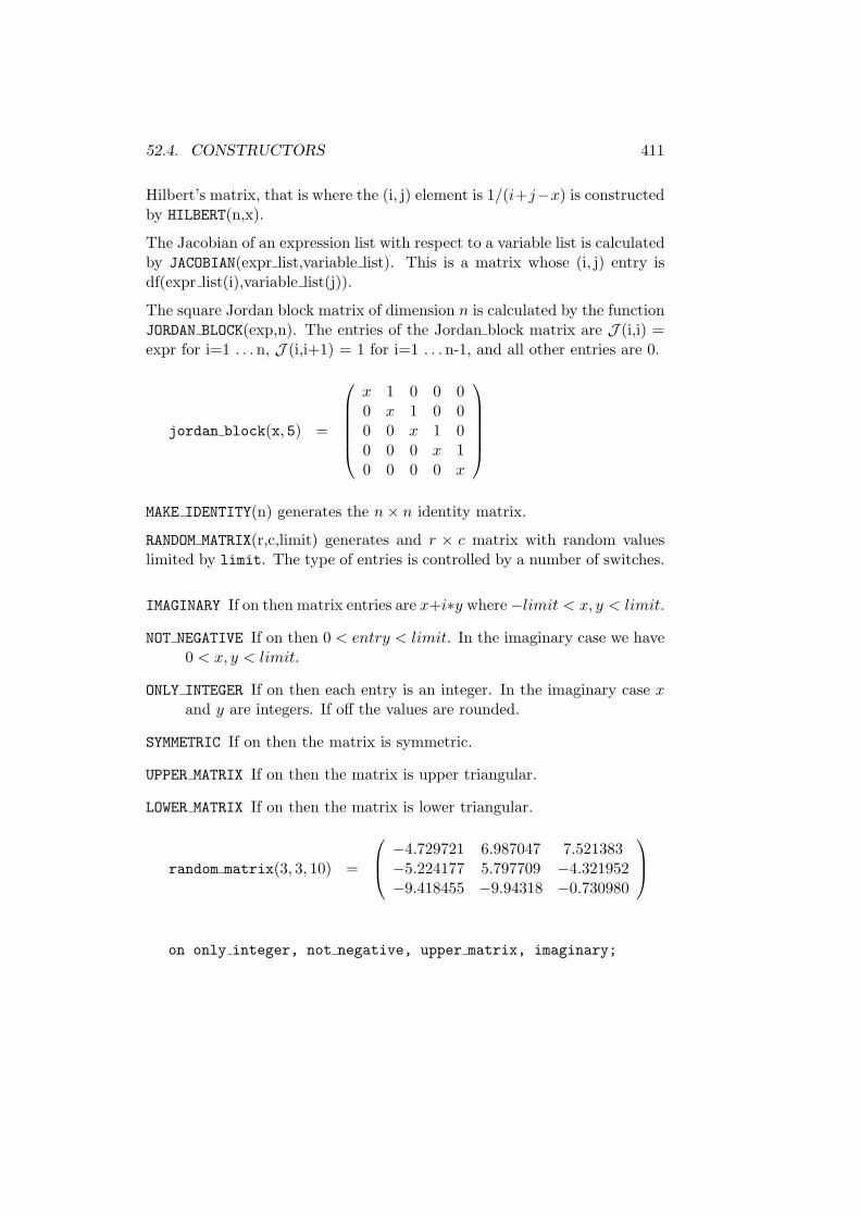
52.4. CONSTRUCTORS 411
Hilbert’s matrix, that is where the (i, j) element is 1/(i+j−x) is constructedby HILBERT(n,x).
The Jacobian of an expression list with respect to a variable list is calculatedby JACOBIAN(expr list,variable list). This is a matrix whose (i, j) entry isdf(expr list(i),variable list(j)).
The square Jordan block matrix of dimension n is calculated by the functionJORDAN BLOCK(exp,n). The entries of the Jordan block matrix are J (i,i) =expr for i=1 . . . n, J (i,i+1) = 1 for i=1 . . . n-1, and all other entries are 0.
jordan block(x, 5) =
x 1 0 0 00 x 1 0 00 0 x 1 00 0 0 x 10 0 0 0 x
MAKE IDENTITY(n) generates the n× n identity matrix.
RANDOM MATRIX(r,c,limit) generates and r × c matrix with random valueslimited by limit. The type of entries is controlled by a number of switches.
IMAGINARY If on then matrix entries are x+i∗y where−limit < x, y < limit.
NOT NEGATIVE If on then 0 < entry < limit. In the imaginary case we have0 < x, y < limit.
ONLY INTEGER If on then each entry is an integer. In the imaginary case xand y are integers. If off the values are rounded.
SYMMETRIC If on then the matrix is symmetric.
UPPER MATRIX If on then the matrix is upper triangular.
LOWER MATRIX If on then the matrix is lower triangular.
random matrix(3, 3, 10) =
−4.729721 6.987047 7.521383−5.224177 5.797709 −4.321952−9.418455 −9.94318 −0.730980
on only integer, not negative, upper matrix, imaginary;

412 CHAPTER 52. LINALG: LINEAR ALGEBRA PACKAGE
random matrix(4, 4, 10) =
2 ∗ i+ 5 3 ∗ i+ 7 7 ∗ i+ 3 60 2 ∗ i+ 5 5 ∗ i+ 1 2 ∗ i+ 10 0 8 i0 0 0 5 ∗ i+ 9
TOEPLITZ creates the Toeplitz matrix from the given expression list. Thisis a square symmetric matrix in which the first expression is placed on thediagonal and the ith expression is placed on the (i − 1)th sub- and super-diagonals. It has dimension equal to the number of expressions.
toeplitz(w, x, y, z) =
w x y zx w x yy x w xz y x w
VANDERMONDE creates the Vandermonde matrix from the expression list; thesquare matrix in which the (i, j) entry is expr list(i) (j−1).
vandermonde(x, 2 ∗ y, 3 ∗ z) =
1 x x2
1 2 ∗ y 4 ∗ y2
1 3 ∗ z 9 ∗ z2
The direct product (or tensor product) is created by the KRONECKER PRODUCTfunction.
a1 := mat((1,2),(3,4),(5,6))$a2 := mat((1,1,1),(2,z,2),(3,3,3))$kronecker_product(a1,a2);
1 1 1 2 2 22 z 2 4 2 ∗ z 43 3 3 6 6 63 3 3 4 4 46 3 ∗ z 6 8 4 ∗ z 89 9 9 12 12 125 5 5 6 6 610 5 ∗ z 10 12 6 ∗ z 1215 15 15 18 18 18

52.5. HIGHER ALGORITHMS 413
52.5 Higher Algorithms
The Cholesky decomposition of a matrix can be calculated with the functionCHOLESKY. It returns L,U where L is a lower matrix, U is an upper matrix,and A = LU , and U = LT .
Gram–Schmidt orthonormalisation can be calculated by GRAM SCHMIDT. Itaccepts a list of linearly independent vectors, written as lists, and returns alist of orthogonal normalised vectors.
gram_schmidt(1,0,0,1,1,0,1,1,1);
1,0,0,0,1,0,0,0,1
gram_schmidt(1,2,3,4);
1 2 2*sqrt(5) - sqrt(5)---------,---------,-----------,------------
sqrt(5) sqrt(5) 5 5
The LU decomposition of a real or imaginary matrix with numeric entries isperformed by LU DECOM(A). It returns L,U where L is a lower diagonalmatrix, U an upper diagonal matrix and A = LU .
Note: the algorithm used can swap the rows of A during the calculation.This means that LU does not equal A but a row equivalent of it. Due tothis, lu decom returns L,U ,vec. The call CONVERT(A,vec) will returnthe matrix that has been decomposed, i.e. LU = convert(A,vec).
K =
1 3 5−4 3 78 6 4
lu decom(K) =
8 0 0−4 6 01 2.25 1.1251
,
1 0.75 0.50 1 1.50 0 1
, [ 3 2 3 ]
PSEUDO INVERSE, also known as the Moore–Penrose inverse, computes thepseudo inverse of A. Given the singular value decomposition of A, i.e.A = U∑VT , then the pseudo inverse A−1 is defined by A−1 = VT ∑−1 U .

414 CHAPTER 52. LINALG: LINEAR ALGEBRA PACKAGE
Thus A ∗ pseudo inverse(A) = I.
pseudo inverse(A) =
−0.2 0.1−0.05 0.050.1 00.25 −0.05
The simplex linear programming algorithm for maximising or minimising afunction subject to lineal inequalities can be used with the function SIMPLEX.It requires three arguments, the first indicates where the action is to max-imising or minimising, the second is the test expressions, and the last is a listof linear inequalities. It returns optimal value, values of variables at thisoptimal. The algorithm implies that all the variables are non-negative.
simplex(max, x+ y, x >= 10, y >= 20, x+ y <= 25);***** Error in simplex: Problem has no feasible solution.
simplex(max, 10x+ 5y+ 5.5z, 5x+ 3z <= 200, x+ 0.1y+ 0.5z <= 12,0.1x+ 0.2y + 0.3z <= 9, 30x+ 10y + 50z <= 1500);
525.0, x = 40.0, y = 25.0, z = 0SVD computes the singular value decomposition of A with numeric entries.It returns U ,∑,V where A = U∑VT and
∑= diag(σ1, . . . , σn). σi for
i = (1 . . . n) are the singular values of A. The singular values of A are thenon-negative square roots of the eigenvalues of ATA.
U and V are such that UUT = VVT = VTV = In.
Q =
(1 3−4 3
)
svd(Q) =
(0.289784 0.957092−0.957092 0.289784
),
(5.149162 0
0 2.913094
),
(−0.687215 0.726453−0.726453 −0.687215
)
TRIANG ADJOINT computes the trianglarizing adjoint of the given matrix.The triangularizing adjoint is a lower triangular matrix. The multiplication

52.6. FAST LINEAR ALGEBRA 415
of the triangularizing adjoint with the given matrix results in an upper trian-gular matrix. The i-th entry in the diagonal of this matrix is the determinantof the principal i-th minor of the given matrix.
triang adjoint(A) =
1 0 0−4 1 0−3 6 −3
The multiplication of this matrix with A results in an upper triangularmatrix.
1 0 0−4 1 0−3 6 −3
1 2 34 5 67 8 9
=
1 2 30 −3 −60 0 0
52.6 Fast Linear Algebra
By turning the FAST LA switch on, the speed of the following functions willbe increased:add columns add rows augment columns column dimcopy into make identity matrix augment matrix stackminor mult column mult row pivotremove columns remove rows rows pivot squarepstack rows sub matrix swap columns swap entriesswap rows symmetricp
The increase in speed will be insignificant unless you are making a thousandsof calls. When using this switch, error checking is minimised, and thus illegalinput may give strange error messages.

416 CHAPTER 52. LINALG: LINEAR ALGEBRA PACKAGE

Chapter 53
MATHML : MathMLInterface for REDUCE
Luis Alvarez-SobrevielaKonrad-Zuse-Zentrum fur Informationstechnik Berlin
Takustrase 7D-14195 Berlin-Dahlem, Germany
MathML is intended to facilitate the use and re-use of mathematical andscientific content on the Web, and for other applications such as computeralgebra systems.This package contains the MathML-REDUCE interface. This interface pro-vides an easy to use series of commands, allowing to evaluate and outputMathML.
The principal features of this package can be resumed as:
• Evaluation of MathML code. Allows REDUCE to parse MathMLexpressions and evaluate them.
• Generation of MathML compliant code. Provides the printing of RE-DUCE expressions in MathML source code, to be used directly in webpage production.
We assume that the reader is familiar with MathML. If not, the specifica-tion1 is available at: http://www.w3.org/TR/WD-math/
1This specification is subject to change, since it is not yet a final draft. During the
417
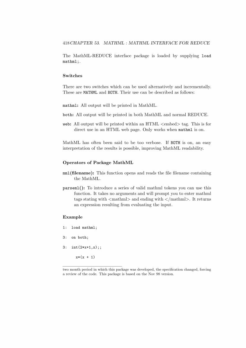
418CHAPTER 53. MATHML : MATHML INTERFACE FOR REDUCE
The MathML-REDUCE interface package is loaded by supplying loadmathml;.
Switches
There are two switches which can be used alternatively and incrementally.These are MATHML and BOTH. Their use can be described as follows:
mathml: All output will be printed in MathML.
both: All output will be printed in both MathML and normal REDUCE.
web: All output will be printed within an HTML <embed> tag. This is fordirect use in an HTML web page. Only works when mathml is on.
MathML has often been said to be too verbose. If BOTH is on, an easyinterpretation of the results is possible, improving MathML readability.
Operators of Package MathML
mml(filename): This function opens and reads the file filename containingthe MathML.
parseml(): To introduce a series of valid mathml tokens you can use thisfunction. It takes no arguments and will prompt you to enter mathmltags stating with <mathml> and ending with </mathml>. It returnsan expression resulting from evaluating the input.
Example
1: load mathml;
3: on both;
3: int(2*x+1,x);;
x*(x + 1)
two month period in which this package was developed, the specification changed, forcinga review of the code. This package is based on the Nov 98 version.

419
<mathml><apply><plus/>
<apply><power/><ci>x</ci><cn type="integer">2</cn>
</apply><ci>x</ci>
</apply></mathml>
4:

420CHAPTER 53. MATHML : MATHML INTERFACE FOR REDUCE

Chapter 54
MODSR: Modular solve androots
Herbert MelenkKonrad–Zuse–Zentrum fur Informationstechnik Berlin
Takustrase 7D–14195 Berlin–Dahlem, Germany
e–mail: [email protected]
This package supports solve (M SOLVE) and roots (M ROOTS) operators formodular polynomials and modular polynomial systems. The moduli neednot be primes. M SOLVE requires a modulus to be set. M ROOTS takes themodulus as a second argument. For example:
on modular; setmod 8;m_solve(2x=4); -> X=2,X=6m_solve(x^2-y^3=3);
-> X=0,Y=5, X=2,Y=1, X=4,Y=5, X=6,Y=1m_solve(x=2,x^2-y^3=3); -> X=2,Y=1off modular;m_roots(x^2-1,8); -> 1,3,5,7m_roots(x^3-x,7); -> 0,1,6
421

422 CHAPTER 54. MODSR: MODULAR SOLVE AND ROOTS

Chapter 55
MRVLIMIT: Package forComputing Limits of”Exp-Log” Functions
Neil LangmeadKonrad-Zuse-Zentrum fur Informationstechnik Berlin (ZIB)
Takustrase 7D - 14195 Berlin-Dahlem, Germany
Using the LIMITS package to compute the limits of functions containingexponential and logarithmic expressions may raise a problem. For the com-putation of indefinite forms (such as 0/0,or ∞∞) L’Hospital’s rule may only beapplied a finite number of times in a CAS. In REDUCE it is applied 3 times.This algorithm of Dominik Gruntz of the ETH Zurich solves this particularproblem, and enables the computation of many more limit calculations inREDUCE.
1: load limits;
2: limit(x^7/e^x,x,infinity);
7x
limit(----,x,infinity)x
e
423

424 CHAPTER 55. MRVLIMIT: LIMITS OF “EXP-LOG” FUNCTIONS
3: load mrvlimit;
4: mrv_limit(x^7/e^x,x,infinity);
0
For this example, the MRVLIMIT package is able to compute the correctlimit.MRV LIMIT(EXPRN:algebraic, VAR:kernel, LIMPOINT:algebraic):algebraic
The result is the limit of EXPRN as VAR approaches LIMPOINT.
A switch TRACELIMIT is available to inform the user about the computedTaylor expansion, all recursive calls and the return value of the internallycalled function MRV.
Examples:
5: b:=e^x*(e^(1/x-e^-x)-e^(1/x));
-1 - xx + x - e
b:= e *(e - 1)
6: mrv_limit(b,x,infinity);
-1
-17: ex:= - log(log(log(log(x))) + log(x)) *log(x)
*(log(log(x)) - log(log(log(x)) + log(x)));
- log(x)*(log(log(x)) - log(log(log(x)) + log(x)))ex:= -----------------------------------------------------
log(log(log(log(x))) + log(x))
8: off mcd;

425
9: mrv_limit(ex,x,infinity);
1

426 CHAPTER 55. MRVLIMIT: LIMITS OF “EXP-LOG” FUNCTIONS

Chapter 56
NCPOLY: Non–commutativepolynomial ideals
Herbert MelenkKonrad–Zuse–Zentrum fur Informationstechnik Berlin
Takustrase 7D–14195 Berlin–Dahlem, Germany
e–mail: [email protected]
Joachim ApelInstitut fur Informatik, Universitat Leipzig
Augustusplatz 10–11D–04109 Leipzig, Germany
e–mail: [email protected]–leipzig.de
REDUCE supports a very general mechanism for computing with objectsunder a non–commutative multiplication, where commutator relations mustbe introduced explicitly by rule sets when needed. The package NCPOLYallows the user to set up automatically a consistent environment for com-puting in an algebra where the non–commutativity is defined by Lie-bracketcommutators. The package uses the REDUCE noncom mechanism for el-ementary polynomial arithmetic; the commutator rules are automaticallycomputed from the Lie brackets. Polynomial arithmetic may be performeddirectly, including division and factorisation. Additionally NCPOLYsupports computations in a one sided ideal (left or right), especially onesided Grobner bases and polynomial reduction.
427

428 CHAPTER 56. NCPOLY: IDEALS IN NON–COMM CASE
56.1 Setup, Cleanup
Before the computations can start the environment for a non–commutativecomputation must be defined by a call to nc setup:
nc_setup(<vars>[,<comms>][,<dir>]);
where
< vars > is a list of variables; these must include the non–commutativequantities.
< comms > is a list of equations <u>*<v> - <v>*<u>=<rh> where < u >and < v > are members of < vars >, and < rh > is a polynomial.
< dir > is either left or right selecting a left or a right one sided ideal. Theinitial direction is left.
nc setup generates from < comms > the necessary rules to support an al-gebra where all monomials are ordered corresponding to the given variablesequence. All pairs of variables which are not explicitly covered in the com-mutator set are considered as commutative and the corresponding rules arealso activated.
The second parameter in nc setup may be omitted if the operator is calledfor the second time, e.g. with a reordered variable sequence. In such a casethe last commutator set is used again.
Remarks:
• The variables need not be declared noncom - nc setup performs allnecessary declarations.
• The variables need not be formal operator expressions; nc setup en-capsulates a variable x internally as nc!*(!_x) expressions anywaywhere the operator nc!∗ keeps the noncom property.
• The commands order and korder should be avoided because nc setupsets these such that the computation results are printed in the correctterm order.
Example:
nc_setup(KK,NN,k,n,

56.2. LEFT AND RIGHT IDEALS 429
NN*n-n*NN= NN, KK*k-k*KK= KK);
NN*N; -> NN*NN*NN; -> NN*N - NNnc_setup(k,n,KK,NN);NN*N - NN -> N*NN;
Here KK,NN, k, n are non–commutative variables where the commutatorsare described as [NN,n] = NN , [KK, k] = KK.
The current term order must be compatible with the commutators: theproduct < u > ∗ < v > must precede all terms on the right hand side< rh > under the current term order. Consequently
• the maximal degree of < u > or < v > in < rh > is 1,
• in a total degree ordering the total degree of < rh > may be not higherthan 1,
• in an elimination degree order (e.g. lex) all variables in < rh > mustbe below the minimum of < u > and < v >.
• If < rh > does not contain any variables or has at most < u > or< v >, any term order can be selected.
To use the non–commutative variables or results from non–commutativecomputations later in commutative operations it might be necessary toswitch off the non–commutative evaluation mode because not all operatorsin REDUCE are prepared for that environment. In such a case use thecommand
nc_cleanup;
without parameters. It removes all internal rules and definitions whichnc setup had introduced. To reactive non–commutative call nc setupagain.
56.2 Left and right ideals
A (polynomial) left ideal L is defined by the axioms
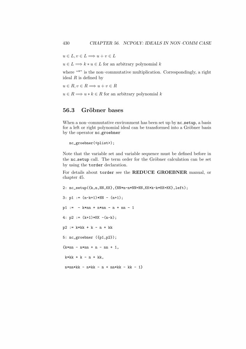
430 CHAPTER 56. NCPOLY: IDEALS IN NON–COMM CASE
u ∈ L, v ∈ L =⇒ u+ v ∈ Lu ∈ L =⇒ k ∗ u ∈ L for an arbitrary polynomial k
where “*” is the non–commutative multiplication. Correspondingly, a rightideal R is defined by
u ∈ R, v ∈ R =⇒ u+ v ∈ Ru ∈ R =⇒ u ∗ k ∈ R for an arbitrary polynomial k
56.3 Grobner bases
When a non–commutative environment has been set up by nc setup, a basisfor a left or right polynomial ideal can be transformed into a Grobner basisby the operator nc groebner
nc_groebner(<plist>);
Note that the variable set and variable sequence must be defined before inthe nc setup call. The term order for the Grobner calculation can be setby using the torder declaration.
For details about torder see the REDUCE GROEBNER manual, orchapter 45.
2: nc_setup(k,n,NN,KK,NN*n-n*NN=NN,KK*k-k*KK=KK,left);
3: p1 := (n-k+1)*NN - (n+1);
p1 := - k*nn + n*nn - n + nn - 1
4: p2 := (k+1)*KK -(n-k);
p2 := k*kk + k - n + kk
5: nc_groebner (p1,p2);
k*nn - n*nn + n - nn + 1,
k*kk + k - n + kk,
n*nn*kk - n*kk - n + nn*kk - kk - 1
56.4. LEFT OR RIGHT POLYNOMIAL DIVISION 431
Important: Do not use the operators of the GROEBNER package directlyas they would not consider the non–commutative multiplication.
56.4 Left or right polynomial division
The operator nc divide computes the one sided quotient and remainder oftwo polynomials:
nc_divide(<p1>,<p2>);
The result is a list with quotient and remainder. The division is performedas a pseudo–division, multiplying < p1 > by coefficients if necessary. Theresult < q >,< r > is defined by the relation
< c > ∗ < p1 >=< q > ∗ < p2 > + < r > for direction left and
< c > ∗ < p1 >=< p2 > ∗ < q > + < r > for direction right,
where < c > is an expression that does not contain any of the ideal variables,and the leading term of < r > is lower than the leading term of < p2 >according to the actual term order.
56.5 Left or right polynomial reduction
For the computation of the one sided remainder of a polynomial modulo agiven set of other polynomials the operator nc preduce may be used:
nc_preduce(<polynomial>,<plist>);
The result of the reduction is unique (canonical) if and only if < plist > isa one sided Grobner basis. Then the computation is at the same time anideal membership test: if the result is zero, the polynomial is member of theideal, otherwise not.
56.6 Factorisation
Polynomials in a non–commutative ring cannot be factored using the ordi-nary factorize command of REDUCE. Instead one of the operators of thissection must be used:

432 CHAPTER 56. NCPOLY: IDEALS IN NON–COMM CASE
nc_factorize(<polynomial>);
The result is a list of factors of < polynomial >. A list with the inputexpression is returned if it is irreducible.
As non–commutative factorisation is not unique, there is an additional op-erator which computes all possible factorisations
nc_factorize_all(<polynomial>);
The result is a list of factor decompositions of < polynomial >. If there areno factors at all the result list has only one member which is a list containingthe input polynomial.
56.7 Output of expressions
It is often desirable to have the commutative parts (coefficients) in a non–commutative operation condensed by factorisation. The operator
nc_compact(<polynomial>)
collects the coefficients to the powers of the lowest possible non-commutativevariable.
load_package ncpoly;
nc_setup(n,NN,NN*n-n*NN=NN)$p1 := n**4 + n**2*nn + 4*n**2 + 4*n*nn + 4*nn + 4;
4 2 2p1 := n + n *nn + 4*n + 4*n*nn + 4*nn + 4
nc_compact p1;
2 2 2(n + 2) + (n + 2) *nn

Chapter 57
NORMFORM: Computationof matrix normal forms
Matt RebbeckKonrad–Zuse–Zentrum fur Informationstechnik Berlin
Takustrase 7D–14195 Berlin–Dahlem, Germany
This package contains routines for computing the following normal forms ofmatrices:
• smithex int
• smithex
• frobenius
• ratjordan
• jordansymbolic
• jordan.
By default all calculations are carried out in Q (the rational numbers). Forsmithex, frobenius, ratjordan, jordansymbolic, and jordan, this fieldcan be extended to an algebraic number field using ARNUM (chapter 22).The frobenius, ratjordan, and jordansymbolic normal forms can also becomputed in a modular base.
433

434 CHAPTER 57. NORMFORM: MATRIX NORMAL FORMS
57.1 Smithex
Smithex(A, x) computes the Smith normal form S of the matrix A.
It returns S,P,P−1 where S,P, and P−1 are such that PSP−1 = A.
A is a rectangular matrix of univariate polynomials in x where x is thevariable name.
load package normform;
A =
(x x+ 10 3 ∗ x2
)
smithex(A, x) =
(1 00 x3
),
(1 0
3 ∗ x2 1
),
(x x+ 1−3 −3
)
57.2 Smithex int
Given an n by m rectangular matrix A that contains only integer entries,smithex int(A) computes the Smith normal form S of A.
It returns S,P,P−1 where S,P, and P−1 are such that PSP−1 = A.
load package normform;
A =
9 −36 30−36 192 −18030 −180 180
smithex int(A) =
3 0 00 12 00 0 60
,
−17 −5 −464 19 15−50 −15 −12
,
1 −24 30−1 25 −300 −1 1
57.3 Frobenius
Frobenius(A) computes the Frobenius normal form F of the matrix A.
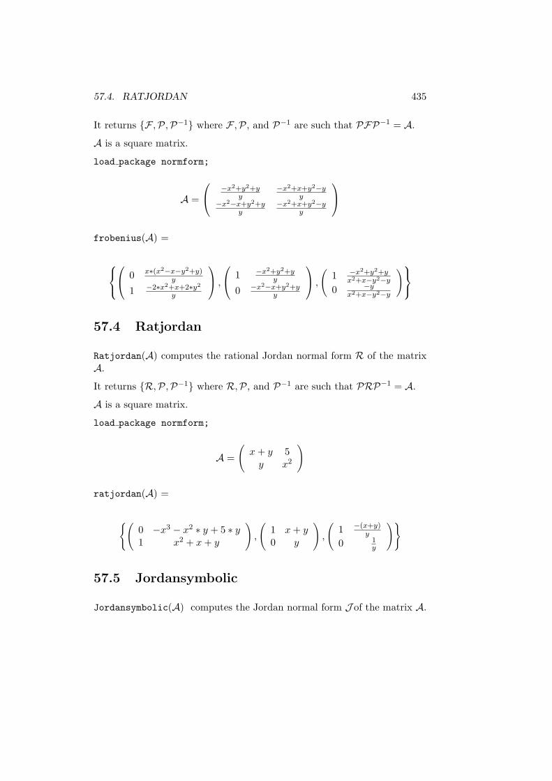
57.4. RATJORDAN 435
It returns F ,P,P−1 where F ,P, and P−1 are such that PFP−1 = A.
A is a square matrix.
load package normform;
A =
−x2+y2+yy
−x2+x+y2−yy
−x2−x+y2+yy
−x2+x+y2−yy
frobenius(A) =
0 x∗(x2−x−y2+y)
y
1 −2∗x2+x+2∗y2
y
,
1 −x2+y2+y
y
0 −x2−x+y2+yy
,
(1 −x2+y2+y
x2+x−y2−y
0 −yx2+x−y2−y
)
57.4 Ratjordan
Ratjordan(A) computes the rational Jordan normal form R of the matrixA.
It returns R,P,P−1 where R,P, and P−1 are such that PRP−1 = A.
A is a square matrix.
load package normform;
A =
(x+ y 5y x2
)
ratjordan(A) =
(0 −x3 − x2 ∗ y + 5 ∗ y1 x2 + x+ y
),
(1 x+ y0 y
),
(1 −(x+y)
y
0 1y
)
57.5 Jordansymbolic
Jordansymbolic(A) computes the Jordan normal form J of the matrix A.

436 CHAPTER 57. NORMFORM: MATRIX NORMAL FORMS
It returns J ,L,P,P−1, where J ,P, and P−1 are such that PJP−1 = A.L = ll, ξ , where ξ is a name and ll is a list of irreducible factors of p(ξ).
A is a square matrix.
load package normform;
A =
(1 yy2 3
)
jordansymbolic(A) =(
ξ11 00 ξ12
),−y3 + ξ2 − 4 ∗ ξ + 3
, ξ
,
(ξ11 − 3 ξ12 − 3y2 y2
),
ξ11−22∗(y3−1)
ξ11+y3−12∗y2∗(y3+1)
ξ12−22∗(y3−1)
ξ12+y3−12∗y2∗(y3+1)
solve(−y3 + xi2 − 4 ∗ xi + 3, xi);
ξ =√y3 + 1 + 2, ξ = −√
y3 + 1 + 2
J = sub(xi(1, 1) = sqrt(y3 + 1) + 2, xi(1, 2) = −sqrt(y3 + 1) + 2,first jordansymbolic (A));
J =
( √y3 + 1 + 2 0
0 −√y3 + 1 + 2
)
57.6 Jordan
Jordan(A) computes the Jordan normal form J of the matrix A.
It returns J ,P,P−1, where J ,P, and P−1 are such that PJP−1 = A.
A is a square matrix.

57.6. JORDAN 437
load package normform;
A =
−9 −21 −15 4 2 0−10 21 −14 4 2 0−8 16 −11 4 2 0−6 12 −9 3 3 0−4 8 −6 0 5 0−2 4 −3 0 1 3
J = first jordan(A);
J =
3 0 0 0 0 00 3 0 0 0 00 0 1 1 0 00 0 0 1 0 00 0 0 0 i+ 2 00 0 0 0 0 −i+ 2

438 CHAPTER 57. NORMFORM: MATRIX NORMAL FORMS
Chapter 58
NUMERIC: Solvingnumerical problems
Herbert MelenkKonrad–Zuse–Zentrum fur Informationstechnik Berlin
Takustrase 7D–14195 Berlin–Dahlem, Germany
e–mail: [email protected]
The NUMERIC package implements some numerical (approximative) algo-rithms for REDUCE based on the REDUCE rounded mode arithmetic.These algorithms are implemented for standard cases. They should notbe called for ill-conditioned problems; please use standard mathematicallibraries for these.
58.1 Syntax
58.1.1 Intervals, Starting Points
Intervals are generally coded as lower bound and upper bound connected bythe operator ‘..’, usually associated to a variable in an equation.
x= (2.5 .. 3.5)
means that the variable x is taken in the range from 2.5 up to 3.5. Note,
439

440 CHAPTER 58. NUMERIC: SOLVING NUMERICAL PROBLEMS
that the bounds can be algebraic expressions, which, however, must evaluateto numeric results. In cases where an interval is returned as the result, thelower and upper bounds can be extracted by the PART operator as the firstand second part respectively. A starting point is specified by an equationwith a numeric righthand side,
x=3.0
If for multivariate applications several coordinates must be specified by in-tervals or as a starting point, these specifications can be collected in oneparameter (which is then a list) or they can be given as separate parametersalternatively. The list form is more appropriate when the parameters arebuilt from other REDUCE calculations in an automatic style, while the flatform is more convenient for direct interactive input.
58.1.2 Accuracy Control
The keyword parameters accuracy = a and iterations = i, where a andi must be positive integer numbers, control the iterative algorithms: theiteration is continued until the local error is below 10−a; if that is impossiblewithin i steps, the iteration is terminated with an error message. The valuesreached so far are then returned as the result.
58.2 Minima
The function to be minimised must have continuous partial derivatives withrespect to all variables. The starting point of the search can be specified; ifnot, random values are taken instead. The steepest descent algorithms ingeneral find only local minima.
Syntax:
NUM MIN (exp, var1[= val1][, var2[= val2] . . .]
[, accuracy = a][, iterations = i])
or
NUM MIN (exp, var1[= val1][, var2[= val2] . . .][, accuracy = a][, iterations = i])

58.3. ROOTS OF FUNCTIONS/ SOLUTIONS OF EQUATIONS 441
where exp is a function expression,
var1, var2, . . . are the variables in exp and val1, val2, . . . are the (op-tional) start values.
NUM MIN tries to find the next local minimum along the descendingpath starting at the given point. The result is a list with the minimumfunction value as first element followed by a list of equations, wherethe variables are equated to the coordinates of the result point.
Examples:
num_min(sin(x)+x/5, x);
4.9489585606,X=29.643767785
num_min(sin(x)+x/5, x=0);
- 1.3342267466,X= - 1.7721582671
% Rosenbrock function (well known as hard to minimize).fktn := 100*(x1**2-x2)**2 + (1-x1)**2;num_min(fktn, x1=-1.2, x2=1, iterations=200);
0.00000021870228295,X1=0.99953284494,X2=0.99906807238
58.3 Roots of Functions/ Solutions of Equations
An adaptively damped Newton iteration is used to find an approximativezero of a function, a function vector or the solution of an equation or anequation system. The expressions must have continuous derivatives for allvariables. A starting point for the iteration can be given. If not given,random values are taken instead. If the number of forms is not equal tothe number of variables, the Newton method cannot be applied. Then theminimum of the sum of absolute squares is located instead.
With ON COMPLEX solutions with imaginary parts can be found, if either theexpression(s) or the starting point contain a nonzero imaginary part.
Syntax:
NUM SOLVE (exp1, var1[= val1][, accuracy = a][, iterations = i])

442 CHAPTER 58. NUMERIC: SOLVING NUMERICAL PROBLEMS
or
NUM SOLVE (exp1, . . . , expn, var1[= val1], . . . , var1[= valn]
[, accuracy = a][, iterations = i])
or
NUM SOLVE (exp1, . . . , expn, var1[= val1], . . . , var1[= valn][, accuracy = a][, iterations = i])
where exp1, . . . , expn are function expressions,
var1, . . . , varn are the variables,
val1, . . . , valn are optional start values.
NUM SOLVE tries to find a zero/solution of the expression(s). Resultis a list of equations, where the variables are equated to the coordinatesof the result point.
The Jacobian matrix is stored as a side effect in the shared variableJACOBIAN.
Example:
num_solve(sin x=cos y, x + y = 1,x=1,y=2);
X= - 1.8561957251,Y=2.856195584
jacobian;
[COS(X) SIN(Y)][ ][ 1 1 ]
58.4 Integrals
Numerical integration uses a polyalgorithm, explained in the full documen-tation.
NUM INT (exp, var1 = (l1..u1)[, var2 = (l2..u2) . . .]

58.5. ORDINARY DIFFERENTIAL EQUATIONS 443
[, accuracy = a][, iterations = i])
where exp is the function to be integrated,
var1, var2, . . . are the integration variables,
l1, l2, . . . are the lower bounds,
u1, u2, . . . are the upper bounds.
Result is the value of the integral.
Example:
num_int(sin x,x=(0 .. pi));
2.0000010334
58.5 Ordinary Differential Equations
A Runge-Kutta method of order 3 finds an approximate graph for the solu-tion of a ordinary differential equation real initial value problem.
Syntax:
NUM ODESOLVE (exp,depvar = dv,indepvar=(from..to)
[, accuracy = a][, iterations = i])
where
exp is the differential expression/equation,
depvar is an identifier representing the dependent variable (functionto be found),
indepvar is an identifier representing the independent variable,
exp is an equation (or an expression implicitly set to zero) which con-tains the first derivative of depvar wrt indepvar,
from is the starting point of integration,
to is the endpoint of integration (allowed to be below from),
dv is the initial value of depvar in the point indepvar = from.
The ODE exp is converted into an explicit form, which then is used fora Runge-Kutta iteration over the given range. The number of steps is
444 CHAPTER 58. NUMERIC: SOLVING NUMERICAL PROBLEMS
controlled by the value of i (default: 20). If the steps are too coarse toreach the desired accuracy in the neighbourhood of the starting point,the number is increased automatically.
Result is a list of pairs, each representing a point of the approximatesolution of the ODE problem.
Example:
num_odesolve(df(y,x)=y,y=1,x=(0 .. 1), iterations=5);
0.0,1.0,0.2,1.2214,0.4,1.49181796,0.6,1.8221064563,
0.8,2.2255208258,1.0,2.7182511366
58.6 Bounds of a Function
Upper and lower bounds of a real valued function over an interval or a rect-angular multivariate domain are computed by the operator BOUNDS. Someknowledge about the behaviour of special functions like ABS, SIN, COS,EXP, LOG, fractional exponentials etc. is integrated and can be evaluatedif the operator BOUNDS is called with rounded mode on (otherwise onlyalgebraic evaluation rules are available).
If BOUNDS finds a singularity within an interval, the evaluation is stoppedwith an error message indicating the problem part of the expression.

58.7. CHEBYSHEV CURVE FITTING 445
Syntax:
BOUNDS (exp, var1 = (l1..u1)[, var2 = (l2..u2) . . .])
BOUNDS (exp, var1 = (l1..u1)[, var2 = (l2..u2) . . .])where exp is the function to be investigated,
var1, var2, . . . are the variables of exp,
l1, l2, . . . and u1, u2, . . . specify the area (intervals).
BOUNDS computes upper and lower bounds for the expression in thegiven area. An interval is returned.
Example:
bounds(sin x,x=(1 .. 2));
-1,1
on rounded;bounds(sin x,x=(1 .. 2));
0.84147098481 .. 1
bounds(x**2+x,x=(-0.5 .. 0.5));
- 0.25 .. 0.75
58.7 Chebyshev Curve Fitting
The operator family Chebyshev . . . implements approximation and evalua-tion of functions by the Chebyshev method.
The operator Chebyshev fit computes this approximation and returns alist, which has as first element the sum expressed as a polynomial and assecond element the sequence of Chebyshev coefficients ci. Chebyshev df andChebyshev int transform a Chebyshev coefficient list into the coefficientsof the corresponding derivative or integral respectively. For evaluating aChebyshev approximation at a given point in the basic interval the operator

446 CHAPTER 58. NUMERIC: SOLVING NUMERICAL PROBLEMS
Chebyshev eval can be used. Note that Chebyshev eval is based on arecurrence relation which is in general more stable than a direct evaluationof the complete polynomial.
CHEBYSHEV FIT (fcn, var = (lo..hi), n)
CHEBYSHEV EVAL (coeffs, var = (lo..hi), var = pt)
CHEBYSHEV DF (coeffs, var = (lo..hi))
CHEBYSHEV INT (coeffs, var = (lo..hi))
where fcn is an algebraic expression (the function to be fitted), varis the variable of fcn, lo and hi are numerical real values which de-scribe an interval (lo < hi), n is the approximation order,an inte-ger > 0, set to 20 if missing, pt is a numerical value in the intervaland coeffs is a series of Chebyshev coefficients, computed by one ofCHEBY SHEV COEFF , DF or INT .
Example:
on rounded;
w:=chebyshev_fit(sin x/x,x=(1 .. 3),5);
3 2w := 0.03824*x - 0.2398*x + 0.06514*x + 0.9778,
0.8991,-0.4066,-0.005198,0.009464,-0.00009511
chebyshev_eval(second w, x=(1 .. 3), x=2.1);
0.4111
58.8 General Curve Fitting
The operator NUM FIT finds for a set of points the linear combination of agiven set of functions (function basis) which approximates the points bestunder the objective of the least squares criterion (minimum of the sum of

58.8. GENERAL CURVE FITTING 447
the squares of the deviation). The solution is found as zero of the gradientvector of the sum of squared errors.
Syntax:
NUM FIT (vals, basis, var = pts)
where vals is a list of numeric values,
var is a variable used for the approximation,
pts is a list of coordinate values which correspond to var,
basis is a set of functions varying in var which is used for the approx-imation.
The result is a list containing as first element the function which approx-imates the given values, and as second element a list of coefficients whichwere used to build this function from the basis.
Example:
% approximate a set of factorials by a polynomialpts:=for i:=1 step 1 until 5 collect i$vals:=for i:=1 step 1 until 5 collect
for j:=1:i product j$
num_fit(vals,1,x,x**2,x=pts);
214.571428571*X - 61.428571429*X + 54.6,54.6,
- 61.428571429,14.571428571
num_fit(vals,1,x,x**2,x**3,x**4,x=pts);
4 32.2083333234*X - 20.249999879*X
2+ 67.791666154*X - 93.749999133*X
+ 44.999999525,
44.999999525, - 93.749999133,67.791666154,

448 CHAPTER 58. NUMERIC: SOLVING NUMERICAL PROBLEMS
- 20.249999879,2.2083333234
58.9 Function Bases
The following procedures compute sets of functions for example to be usedfor approximation. All procedures have two parameters, the expression tobe used as variable (an identifier in most cases) and the order of the desiredsystem. The functions are not scaled to a specific interval, but the variablecan be accompanied by a scale factor and/or a translation in order to mapthe generic interval of orthogonality to another (e.g. (x − 1/2) ∗ 2pi). Theresult is a function list with ascending order, such that the first element isthe function of order zero and (for the polynomial systems) the function oforder n is the n+ 1-th element.
monomial_base(x,n) 1,x,...,x**ntrigonometric_base(x,n) 1,sin x,cos x,sin(2x),cos(2x)...Bernstein_base(x,n) Bernstein polynomialsLegendre_base(x,n) Legendre polynomialsLaguerre_base(x,n) Laguerre polynomialsHermite_base(x,n) Hermite polynomialsChebyshev_base_T(x,n) Chebyshev polynomials first kindChebyshev_base_U(x,n) Chebyshev polynomials second kind
Example:
Bernstein_base(x,5);
5 4 3 2 - X + 5*X - 10*X + 10*X - 5*X + 1,
4 3 25*X*(X - 4*X + 6*X - 4*X + 1),
2 3 210*X *( - X + 3*X - 3*X + 1),

58.9. FUNCTION BASES 449
3 210*X *(X - 2*X + 1),
45*X *( - X + 1),
5X

450 CHAPTER 58. NUMERIC: SOLVING NUMERICAL PROBLEMS

Chapter 59
ODESOLVE:Ordinary differentialequations solver
Malcolm A.H. MacCallumSchool of Mathematical Sciences, Queen Mary and Westfield College
University of LondonMile End Road
London E1 4NS, England
e–mail: [email protected]
The ODESOLVE package is a solver for ordinary differential equations. Atthe present time it has very limited capabilities,
1. it can handle only a single scalar equation presented as an algebraicexpression or equation, and
2. it can solve only first-order equations of simple types, linear equationswith constant coefficients and Euler equations.
These solvable types are exactly those for which Lie symmetry techniquesgive no useful information.
451
452 CHAPTER 59. ODESOLVE: ORDINARY DIFFERENTIAL EQNS
59.1 Use
The only top-level function the user should normally invoke is:
ODESOLVE(EXPRN:expression, equation,VAR1:variable,VAR2:variable):list-algebraic
ODESOLVE returns a list containing an equation (like solve):
EXPRN is a single scalar expression such that EXPRN = 0 is the ordinarydifferential equation (ODE for short) to be solved, or is an equivalentequation.
VAR1 is the name of the dependent variable.
VAR2 is the name of the independent variable
(For simplicity these will be called y and x in the sequel) The returned valueis a list containing the equation giving the general solution of the ODE (forsimultaneous equations this will be a list of equations eventually). It willcontain occurrences of the operator ARBCONST for the arbitrary constantsin the general solution. The arguments of ARBCONST should be new, aswith ARBINT etc. in SOLVE. A counter !!ARBCONST is used to arrange this(similar to the way ARBINT is implemented).
Some other top-level functions may be of use elsewhere, especially:
SORTOUTODE(EXPRN:algebraic, Y:var, X:var): expression
which finds the order and degree of the EXPRN as a differential equation forY with respect to Y and sets the linearity and highest derivative occurringin reserved variables ODEORDER, ODEDEGREE,ODELINEARITY andHIGHESTDERIV. An expression equivalent to the ODE is returned, or zeroif EXPRN (equated to 0) is not an ODE in the given variables.

59.2. COMMENTARY 453
59.2 Commentary
The methods used by this package are described in detail in the full docu-mentation, which should be inspected together with the examples file.

454 CHAPTER 59. ODESOLVE: ORDINARY DIFFERENTIAL EQNS
Chapter 60
ORTHOVEC:Three-dimensional vectoranalysis
James W. EastwoodAEA Technology, Culham Laboratory
AbingdonOxon OX14 3DB, England
e–mail: jim [email protected]
The ORTHOVEC package is a collection of REDUCE procedures and op-erations which provide a simple to use environment for the manipulationof scalars and vectors. Operations include addition, subtraction, dot andcross products, division, modulus, div, grad, curl, laplacian, differentiation,integration, a · ∇ and Taylor expansion.
60.1 Initialisation
The procedure START initialises ORTHOVEC. VSTART provides a menu ofstandard coordinate systems:-
1. cartesian (x, y, z) = (x, y, z)
2. cylindrical (r, θ, z) = (r, th, z)
455

456 CHAPTER 60. ORTHOVEC: SCALARS AND VECTORS
3. spherical (r, θ, φ) = (r, th, ph)
4. general (u1, u2, u3) = (u1, u2, u3)
5. others
which the user selects by number. Selecting options (1)-(4) automaticallysets up the coordinates and scale factors. Selection option (5) shows the userhow to select another coordinate system. If VSTART is not called, then thedefault cartesian coordinates are used. ORTHOVEC may be re-initialisedto a new coordinate system at any time during a given REDUCE session bytyping
VSTART $.
60.2 Input-Output
ORTHOVEC assumes all quantities are either scalars or 3 component vec-tors. To define a vector a with components (c1, c2, c3) use the procedureSVEC:
a := svec(c1, c2, c3);
The procedure VOUT (which returns the value of its argument) can be usedto give labelled output of components in algebraic form:
b := svec (sin(x)**2, y**2, z)$vout(b)$
The operator can be used to select a particular component (1, 2 or 3) foroutput e.g.
b_1 ;
60.3 Algebraic Operations
Six infix operators, sum, difference, quotient, times, exponentiation andcross product, and four prefix operators, plus, minus, reciprocal and modulusare defined in ORTHOVEC. These operators can take suitable combinationsof scalar and vector arguments, and in the case of scalar arguments reduceto the usual definitions of +,−, ∗, /, etc.

60.3. ALGEBRAIC OPERATIONS 457
The operators are represented by symbols
+, -, /, *, ^, ><
The composite >< is an attempt to represent the cross product symbol ×in ASCII characters. If we let v be a vector and s be a scalar, then validcombinations of arguments of the procedures and operators and the type ofthe result are as summarised below. The notation used isresult :=procedure(left argument, right argument) orresult :=(left operand) operator (right operand) .
Vector Additionv := VECTORPLUS(v) or v := + vs := VECTORPLUS(s) or s := + sv := VECTORADD(v,v) or v := v + vs := VECTORADD(s,s) or s := s + s
Vector Subtractionv := VECTORMINUS(v) or v := - vs := VECTORMINUS(s) or s := - sv := VECTORDIFFERENCE(v,v) or v := v - vs := VECTORDIFFERENCE(s,s) or s := s - s
Vector Divisionv := VECTORRECIP(v) or v := / vs := VECTORRECIP(s) or s := / sv := VECTORQUOTIENT(v,v) or v := v / vv := VECTORQUOTIENT(v, s ) or v := v / sv := VECTORQUOTIENT( s ,v) or v := s / vs := VECTORQUOTIENT(s,s) or s := s / s
Vector Multiplicationv := VECTORTIMES( s ,v) or v := s * vv := VECTORTIMES(v, s ) or v := v * ss := VECTORTIMES(v,v) or s := v * vs := VECTORTIMES( s , s ) or s := s * s
Vector Cross Productv := VECTORCROSS(v,v) or v := v × v

458 CHAPTER 60. ORTHOVEC: SCALARS AND VECTORS
Vector Exponentiations := VECTOREXPT (v, s ) or s := v ˆ ss := VECTOREXPT ( s , s ) or s := s ˆ s
Vector Moduluss := VMOD (s)s := VMOD (v)
All other combinations of operands for these operators lead to error messagesbeing issued. The first two instances of vector multiplication are scalarmultiplication of vectors, the third is the product of two scalars and thelast is the inner (dot) product. The prefix operators +, -, / can takeeither scalar or vector arguments and return results of the same type astheir arguments. VMOD returns a scalar.
In compound expressions, parentheses may be used to specify the order ofcombination. If parentheses are omitted the ordering of the operators, inincreasing order of precedence is
+ | - | dotgrad | * | >< | ^ | _
and these are placed in the precedence list defined in REDUCE after <.
Vector divisions are defined as follows: If a and b are vectors and c is ascalar, then
a/b =a · b| b |2
c/a =ca| a |2
Both scalar multiplication and dot products are given by the same symbol,braces are advisable to ensure the correct precedences in expressions suchas (a · b)(c · d).
Vector exponentiation is defined as the power of the modulus:an ≡ VMOD(a)n =| a |n
60.4 Differential Operations
Differential operators provided are div, grad, curl, delsq, and dotgrad.All but the last of these are prefix operators having a single vector or scalar

60.4. DIFFERENTIAL OPERATIONS 459
s := div (v)v := grad(s)v := curl(v)v := delsq(v)s := delsq(s)v := v dotgrad vs := v dotgrad s
Table 60.1: ORTHOVEC valid combinations of operator and argument
argument as appropriate. Valid combinations of operator and argument,and the type of the result are shown in table 60.1.
All other combinations of operator and argument type cause error messagesto be issued. The differential operators have their usual meanings. Thecoordinate system used by these operators is set by invoking VSTART (cf.Sec. 60.1). The names h1, h2 and h3 are reserved for the scale factors, andu1, u2 and u3 are used for the coordinates.
A vector extension, VDF, of the REDUCE procedure DF allows the dif-ferentiation of a vector (scalar) with respect to a scalar to be performed.Allowed forms are VDF(v, s) → v and VDF(s, s) → s , where, for example
vdf(B, x) ≡ ∂B∂x
The standard REDUCE procedures DEPEND and NODEPEND have beenredefined to allow dependences of vectors to be compactly defined. Forexample
a := svec(a1,a2,a3)$;depend a,x,y;
causes all three components a1,a2 and a3 of a to be treated as functions ofx and y. Individual component dependences can still be defined if desired.
depend a3,z;
The procedure VTAYLOR gives truncated Taylor series expansions of scalaror vector functions:-
vtaylor(vex,vx,vpt,vorder);

460 CHAPTER 60. ORTHOVEC: SCALARS AND VECTORS
VEX VX VPT VORDER
v v v vv v v sv s s ss v v vs v v ss s s s
Table 60.2: ORTHOVEC valid combination of argument types.
returns the series expansion of the expression VEX with respect to variableVX about point VPT to order VORDER. Valid combinations of argumenttypes are shown in table 60.2.
Any other combinations cause error messages to be issued. Elements ofVORDER must be non-negative integers, otherwise error messages are is-sued. If scalar VORDER is given for a vector expansion, expansions in eachcomponent are truncated at the same order, VORDER.
The new version of Taylor expansion applies l’Hopital’s rule in evaluatingcoefficients, so handle cases such as sin(x)/(x) , etc. which the originalversion of ORTHOVEC could not. The procedure used for this is LIMIT,which can be used directly to find the limit of a scalar function ex of variablex at point pt:-
ans := limit(ex,x,pt);
60.5 Integral Operations
Definite and indefinite vector, volume and scalar line integration proceduresare included in ORTHOVEC. They are defined as follows:
VINT(v, x) =∫
v(x)dx
DVINT(v, x, a, b) =∫ b
av(x)dx
VOLINT(v) =∫
vh1h2h3du1du2du3

60.5. INTEGRAL OPERATIONS 461
DVOLINT(v, l,u, n) =∫ u
lvh1h2h3du1du2du3
LINEINT(v, ω, t) =∫
v · dr ≡∫vihi
∂ωi
∂tdt
DLINEINT(v, ωt, a, b) =∫ b
avihi
∂ωi
∂tdt
In the vector and volume integrals, v are vector or scalar, a, b, x and n arescalar. Vectors l and u contain expressions for lower and upper bounds to theintegrals. The integer index n defines the order in which the integrals overu1, u2 and u3 are performed in order to allow for functional dependencies inthe integral bounds:
n order1 u1 u2 u3
2 u3 u1 u2
3 u2 u3 u1
4 u1 u3 u2
5 u2 u1 u3
otherwise u3 u2 u1
The vector ω in the line integral’s arguments contain explicit parameterisa-tion of the coordinates u1, u2, u3 of the line u(t) along which the integral istaken.

462 CHAPTER 60. ORTHOVEC: SCALARS AND VECTORS

Chapter 61
PHYSOP: Operator calculusin quantum theory
Mathias WarnsPhysikalisches Institut der Universitat Bonn
Endenicher Allee 11–13D–5300 BONN 1, Germany
e–mail: [email protected]
The package PHYSOP has been designed to meet the requirements of the-oretical physicists looking for a computer algebra tool to perform compli-cated calculations in quantum theory with expressions containing operators.These operations consist mainly in the calculation of commutators betweenoperator expressions and in the evaluations of operator matrix elements insome abstract space.
61.1 The NONCOM2 Package
The package NONCOM2 redefines some standard REDUCE routines in or-der to modify the way noncommutative operators are handled by the system.It redefines the NONCOM statement in a way more suitable for calculations inphysics. Operators have now to be declared noncommutative pairwise, i.e.coding:
463
464 CHAPTER 61. PHYSOP: OPERATOR CALCULUS
NONCOM A,B;
declares the operators A and B to be noncommutative but allows them tocommute with any other (noncommutative or not) operator present in theexpression. In a similar way if one wants e.g. A(X) and A(Y) not to commute,one has now to code:
NONCOM A,A;
A final example should make the use of the redefined NONCOM statementclear:
NONCOM A,B,C;
declares A to be noncommutative with B and C, B to be noncommutativewith A and C and C to be noncommutative with A and B. Note that afterthese declaration e.g. A(X) and A(Y) are still commuting kernels.
Finally to keep the compatibility with standard REDUCE declaring a singleidentifier using the NONCOM statement has the same effect as in standardREDUCE.
From the user’s point of view there are no other new commands implementedby the package.
61.2 The PHYSOP package
The package PHYSOP implements a new REDUCE data type to performcalculations with physical operators. The noncommutativity of operatorsis implemented using the NONCOM2 package so this file should be loadedprior to the use of PHYSOP.
61.2.1 Type declaration commands
The new REDUCE data type PHYSOP implemented by the package allowsthe definition of a new kind of operators (i.e. kernels carrying an arbitrarynumber of arguments). Throughout this manual, the name “operator” willrefer, unless explicitly stated otherwise, to this new data type. This data

61.2. THE PHYSOP PACKAGE 465
type is in turn divided into 5 subtypes. For each of this subtype, a declara-tion command has been defined:
SCALOP A; declares A to be a scalar operator. This operator may carryan arbitrary number of arguments; after the declaration: SCALOPA; all kernels of the form A(J), A(1,N), A(N,L,M) are recognisedby the system as being scalar operators.
VECOP V; declares V to be a vector operator. As for scalar operators, thevector operators may carry an arbitrary number of arguments. Forexample V(3) can be used to represent the vector operator ~V3. Notethat the dimension of space in which this operator lives is arbitrary.One can however address a specific component of the vector operatorby using a special index declared as PHYSINDEX (see below). This indexmust then be the first in the argument list of the vector operator.
TENSOP C(3); declares C to be a tensor operator of rank 3. Tensor oper-ators of any fixed integer rank larger than 1 can be declared. Again thisoperator may carry an arbitrary number of arguments and the spacedimension is not fixed. The tensor components can be addressed byusing special PHYSINDEX indices (see below) which have to be placedin front of all other arguments in the argument list.
STATE U; declares U to be a state, i.e. an object on which operators havea certain action. The state U can also carry an arbitrary number ofarguments.
PHYSINDEX X; declares X to be a special index which will be used to addresscomponents of vector and tensor operators.
A command CLEARPHYSOP removes the PHYSOP type from an identifier inorder to use it for subsequent calculations. However it should be rememberedthat no substitution rule is cleared by this function. It is therefore left tothe user’s responsibility to clear previously all substitution rules involvingthe identifier from which the PHYSOP type is removed.
61.2.2 Ordering of operators in an expression
The ordering of kernels in an expression is performed according to the fol-lowing rules:

466 CHAPTER 61. PHYSOP: OPERATOR CALCULUS
1. Scalars are always ordered ahead of PHYSOP operators in an expres-sion. The REDUCE statement KORDER can be used to control the orderingof scalars but has no effect on the ordering of operators.
2. The default ordering of operators follows the order in which they havebeen declared (not the alphabetical one). This ordering scheme can bechanged using the command OPORDER. Its syntax is similar to the KORDERstatement, i.e. coding: OPORDER A,V,F; means that all occurrences of theoperator A are ordered ahead of those of V etc. It is also possible to includeoperators carrying indices (both normal and special ones) in the argumentlist of OPORDER. However including objects not defined as operators (i.e.scalars or indices) in the argument list of the OPORDER command leads to anerror.
3. Adjoint operators are placed by the declaration commands just after theoriginal operators on the OPORDER list. Changing the place of an operatoron this list means not that the adjoint operator is moved accordingly. Thisadjoint operator can be moved freely by including it in the argument list ofthe OPORDER command.
61.2.3 Arithmetic operations on operators
The following arithmetic operations are possible with operator expressions:
1. Multiplication or division of an operator by a scalar.
2. Addition and subtraction of operators of the same type.
3. Multiplication of operators is only defined between two scalar operators.
4. The scalar product of two VECTOR operators is implemented with anew function DOT. The system expands the product of two vector operatorsinto an ordinary product of the components of these operators by insertinga special index generated by the program. To give an example, if one codes:
VECOP V,W;V DOT W;
the system will transform the product into:
V(IDX1) * W(IDX1)
where IDX1 is a PHYSINDEX generated by the system (called a DUMMY

61.2. THE PHYSOP PACKAGE 467
INDEX in the following) to express the summation over the components.The identifiers IDXn (n is a nonzero integer) are reserved variables for thispurpose and should not be used for other applications. The arithmeticoperator DOT can be used both in infix and prefix form with two arguments.
5. Operators (but not states) can only be raised to an integer power. Thesystem expands this power expression into a product of the correspondingnumber of terms inserting dummy indices if necessary. The following ex-amples explain the transformations occurring on power expressions (systemoutput is indicated with an -->):
SCALOP A; A**2;--> A*A
VECOP V; V**4;--> V(IDX1)*V(IDX1)*V(IDX2)*V(IDX2)
TENSOP C(2); C**2;--> C(IDX3,IDX4)*C(IDX3,IDX4)
Note in particular the way how the system interprets powers of tensor oper-ators which is different from the notation used in matrix algebra.
6. Quotients of operators are only defined between scalar operator expres-sions. The system transforms the quotient of 2 scalar operators into theproduct of the first operator times the inverse of the second one.
SCALOP A,B; A / B;-1
A *( B )
7. Combining the last 2 rules explains the way how the system handlesnegative powers of operators:
SCALOP B;B**(-3);
-1 -1 -1--> (B )*(B )*(B )
The method of inserting dummy indices and expanding powers of operatorshas been chosen to facilitate the handling of complicated operator expres-sions and particularly their application on states. However it may be usefulto get rid of these dummy indices in order to enhance the readability ofthe system’s final output. For this purpose the switch CONTRACT has to beturned on (CONTRACT is normally set to OFF). The system in this case con-
468 CHAPTER 61. PHYSOP: OPERATOR CALCULUS
tracts over dummy indices reinserting the DOT operator and reassemblingthe expanded powers. However due to the predefined operator ordering thesystem may not remove all the dummy indices introduced previously.
61.2.4 Special functions
Commutation relations
If two PHYSOPs have been declared noncommutative using the (redefined)NONCOM statement, it is possible to introduce in the environment elementary(anti-) commutation relations between them. For this purpose, two scalaroperators COMM and ANTICOMM are available. These operators are used inconjunction with LET statements. Example:
SCALOP A,B,C,D;LET COMM(A,B)=C;FOR ALL N,M LET ANTICOMM(A(N),B(M))=D;VECOP U,V,W; PHYSINDEX X,Y,Z;FOR ALL X,Y LET COMM(V(X),W(Y))=U(Z);
Note that if special indices are used as dummy variables in FOR ALL ...LET constructs then these indices should have been declared previously usingthe PHYSINDEX command.
Every time the system encounters a product term involving two noncommu-tative operators which have to be reordered on account of the given operatorordering, the list of available (anti-) commutators is checked in the follow-ing way: First the system looks for a commutation relation which matchesthe product term. If it fails then the defined anticommutation relations arechecked. If there is no successful match the product term A*B is replaced by:
A*B;--> COMM(A,B) + B*A
so that the user may introduce the commutation relation later on.
The user may want to force the system to look for anticommutators only;for this purpose a switch ANTICOM is defined which has to be turned on (ANTICOM is normally set to OFF). In this case, the above example is replacedby:

61.2. THE PHYSOP PACKAGE 469
ON ANTICOM;A*B;--> ANTICOMM(A,B) - B*A
For the calculation of (anti-) commutators between complex operator ex-pressions, the functions COMMUTE and ANTICOMMUTE have been defined.
VECOP P,A,K;PHYSINDEX X,Y;FOR ALL X,Y LET COMM(P(X),A(Y))=K(X)*A(Y);COMMUTE(P**2,P DOT A);
Adjoint expressions
As has been already mentioned, for each operator and state defined usingthe declaration commands, the system generates automatically the corre-sponding adjoint operator. For the calculation of the adjoint representationof a complicated operator expression, a function ADJ has been defined.
SCALOP A,B;ADJ(A*B);
+ +--> (A )*(B )
Application of operators on states
A function OPAPPLY has been defined for the application of operators tostates. It has two arguments and is used in the following combinations:
(i) LET OPAPPLY(operator, state) = state; This is to define a elementary ac-tion of an operator on a state in analogy to the way elementary commutationrelations are introduced to the system.
SCALOP A; STATE U;FOR ALL N,P LET OPAPPLY((A(N),U(P))= EXP(I*N*P)*U(P);
(ii) LET OPAPPLY(state, state) = scalar exp.; This form is to define scalarproducts between states and normalisation conditions.
STATE U;

470 CHAPTER 61. PHYSOP: OPERATOR CALCULUS
FOR ALL N,M LET OPAPPLY(U(N),U(M)) = IF N=M THEN 1 ELSE 0;
(iii) state := OPAPPLY(operator expression, state); In this way, the actionof an operator expression on a given state is calculated using elementary re-lations defined as explained in (i). The result may be assigned to a differentstate vector.
(iv) OPAPPLY(state, OPAPPLY(operator expression, state)); This is the wayhow to calculate matrix elements of operator expressions. The system pro-ceeds in the following way: first the rightmost operator is applied on theright state, which means that the system tries to find an elementary rela-tion which match the application of the operator on the state. If it fails thesystem tries to apply the leftmost operator of the expression on the left stateusing the adjoint representations. If this fails also, the system prints out awarning message and stops the evaluation. Otherwise the next operator oc-curing in the expression is taken and so on until the complete expression isapplied. Then the system looks for a relation expressing the scalar productof the two resulting states and prints out the final result. An example ofsuch a calculation is given in the test file.
The infix version of the OPAPPLY function is the vertical bar |. It is rightassociative and placed in the precedence list just above the minus (−) op-erator.
Chapter 62
PM: A REDUCE patternmatcher
Kevin McIsaacThe University of Western Australia
Australia
e–mail: [email protected]
PM is a general pattern matcher similar in style to those found in systemssuch as SMP and Mathematica.
A template is any expression composed of literal elements (e.g. 5, a or a+1)and specially denoted pattern variables (e.g. ?a or ??b). Atoms beginningwith ‘?’ are called generic variables and match any expression. Atoms begin-ning with ‘??’ are called multi-generic variables and match any expressionor any sequence of expressions including the null or empty sequence. A se-quence is an expression of the form ‘[a1, a2,...]’. When placed in a functionargument list the brackets are removed, i.e. f([a,1]) → f(a,1) and f(a,[1,2],b)→ f(a,1,2,b).
A template is said to match an expression if the template is literally equal tothe expression or if by replacing any of the generic or multi-generic symbolsoccurring in the template, the template can be made to be literally equal tothe expression. These replacements are called the bindings for the genericvariables. A replacement is an expression of the form exp1 -> exp2, whichmeans exp1 is replaced by exp2, or exp1 --> exp2, which is the same ex-cept exp2 is not simplified until after the substitution for exp1 is made. If
471
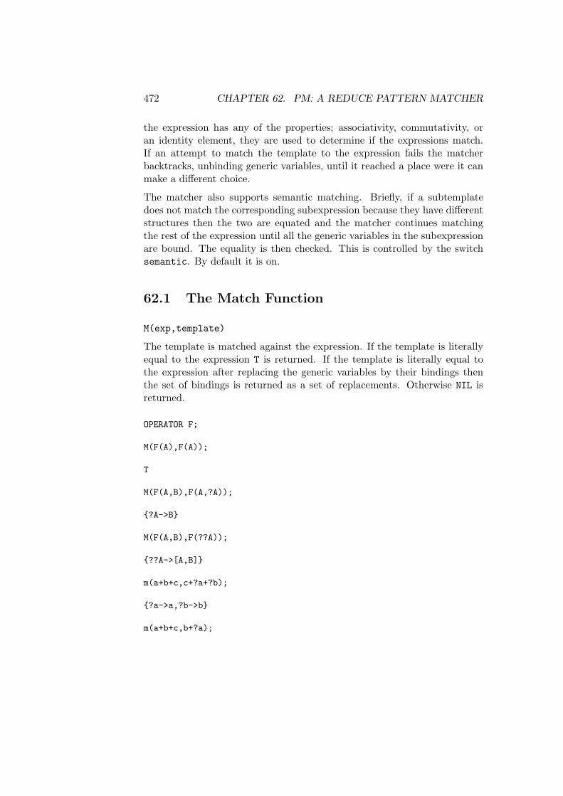
472 CHAPTER 62. PM: A REDUCE PATTERN MATCHER
the expression has any of the properties; associativity, commutativity, oran identity element, they are used to determine if the expressions match.If an attempt to match the template to the expression fails the matcherbacktracks, unbinding generic variables, until it reached a place were it canmake a different choice.
The matcher also supports semantic matching. Briefly, if a subtemplatedoes not match the corresponding subexpression because they have differentstructures then the two are equated and the matcher continues matchingthe rest of the expression until all the generic variables in the subexpressionare bound. The equality is then checked. This is controlled by the switchsemantic. By default it is on.
62.1 The Match Function
M(exp,template)
The template is matched against the expression. If the template is literallyequal to the expression T is returned. If the template is literally equal tothe expression after replacing the generic variables by their bindings thenthe set of bindings is returned as a set of replacements. Otherwise NIL isreturned.
OPERATOR F;
M(F(A),F(A));
T
M(F(A,B),F(A,?A));
?A->B
M(F(A,B),F(??A));
??A->[A,B]
m(a+b+c,c+?a+?b);
?a->a,?b->b
m(a+b+c,b+?a);

62.2. QUALIFIED MATCHING 473
?a->a + c
This example shows the effects of semantic matching, using the associativityand commutativity of +.
62.2 Qualified Matching
A template may be qualified by the use of the conditional operator =’,standing for such that. When a such-that condition is encountered in atemplate it is held until all generic variables appearing in logical-exp arebound. On the binding of the last generic variable logical-exp is simpli-fied and if the result is not T the condition fails and the pattern matcherbacktracks. When the template has been fully parsed any remaining heldsuch-that conditions are evaluated and compared to T.
load_package pm;
operator f;
if (m(f(a,b),f(?a,?b_=(?a=?b)))) then write "yes" else write"no";
no
m(f(a,a),f(?a,?b_=(?a=?b)));
?B->A,?A->A
62.3 Substituting for replacements
The operator S substitutes the replacements in an expression.
S(exp,temp1->sub1,temp2->sub2,...,rept, depth);
will do the substitutions for a maximum of rept and to a depth of depth,using a breadth-first search and replace. rept and depth may be omittedwhen they default to 1 and infinity.
SI(exp,temp1->sub1,temp2->sub2,..., depth)
will substitute infinitely many times until expression stops changing.

474 CHAPTER 62. PM: A REDUCE PATTERN MATCHER
SD(exp,temp1->sub1,temp2->sub2,...,rept, depth)
is a depth-first version of S.
s(f(a,b),f(a,?b)->?b^2);
2b
s(a+b,a+b->a*b);
a*b
operator nfac;
s(nfac(3),nfac(0)->1,nfac(?x)->?x*nfac(?x-1));
3*nfac(2)
s(nfac(3),nfac(0)->1,nfac(?x)->?x*nfac(?x-1),2);
6*nfac(1)
si(nfac(4),nfac(0)->1,nfac(?x)->?x*nfac(?x-1));
24
s(a+b+f(a+b),a+b->a*b,inf,0);
f(a + b) + a*b
62.4 Programming with Patterns
There are also facilities to use this pattern-matcher as a programming lan-guage. The operator :- can be used to declare that while simplifying allmatches of a template should be replaced by some expression. The operator::- is the same except that the left hand side is not simplified.
operator fac, gamma;

62.4. PROGRAMMING WITH PATTERNS 475
fac(?x_=Natp(?x)) ::- ?x*fac(?x-1);
HOLD(FAC(?X-1)*?X)
fac(0) :- 1;
1
fac(?x) :- Gamma(?x+1);
GAMMA(?X + 1)
fac(3);
6
fac(3/2);
GAMMA(5/2)

476 CHAPTER 62. PM: A REDUCE PATTERN MATCHER

Chapter 63
QSUM : Package forq-hypergeometric sums
Harald BoingWolfram Koepf
Konrad-Zuse-Zentrum fur Informationstechnik BerlinTakustrase 7
D-14195 Berlin-Dahleme-mail: [email protected]
This package is an implementation of the q-analogues of Gosper’s and Zeil-berger’s 1 algorithm for indefinite and definite summation of q-hypergeometricterms, respectively.
An expression ak is called a q-hypergeometric term, if ak/ak−1 is a rationalfunction with respect to qk. Most q-terms are based on the q-shifted fac-torial or qpochhammer. Other typical q-hypergeometric terms are ratios ofproducts of powers, q-factorials, q-binomial coefficients, and q-shifted facto-rials that are integer-linear in their arguments.The package is loaded with load package qsum.
63.1 Elementary q-Functions
The package supports the input of the following elementary q-functions:1The ZEILBERG package (Chap. 89 p. 601, see also [10]) contains the hypergeometric
versions.
477
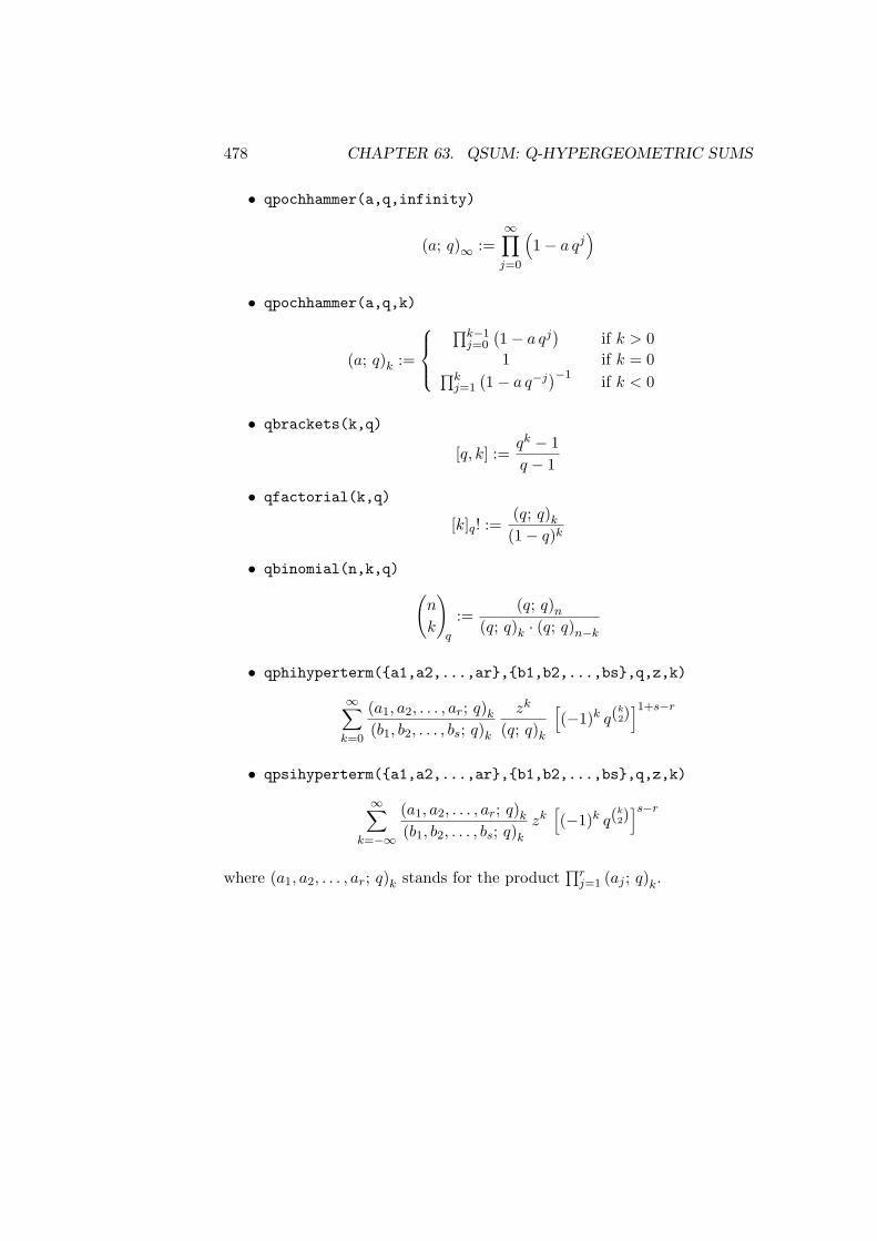
478 CHAPTER 63. QSUM: Q-HYPERGEOMETRIC SUMS
• qpochhammer(a,q,infinity)
(a; q)∞ :=∞∏
j=0
(1− a qj
)
• qpochhammer(a,q,k)
(a; q)k :=
∏k−1j=0
(1− a qj
)if k > 0
1 if k = 0∏kj=1
(1− a q−j
)−1 if k < 0
• qbrackets(k,q)
[q, k] :=qk − 1q − 1
• qfactorial(k,q)
[k]q! :=(q; q)k
(1− q)k
• qbinomial(n,k,q)
(n
k
)
q
:=(q; q)n
(q; q)k · (q; q)n−k
• qphihyperterm(a1,a2,...,ar,b1,b2,...,bs,q,z,k)
∞∑
k=0
(a1, a2, . . . , ar; q)k
(b1, b2, . . . , bs; q)k
zk
(q; q)k
[(−1)k q(
k2)
]1+s−r
• qpsihyperterm(a1,a2,...,ar,b1,b2,...,bs,q,z,k)
∞∑
k=−∞
(a1, a2, . . . , ar; q)k
(b1, b2, . . . , bs; q)k
zk[(−1)k q(
k2)
]s−r
where (a1, a2, . . . , ar; q)k stands for the product∏r
j=1 (aj ; q)k.
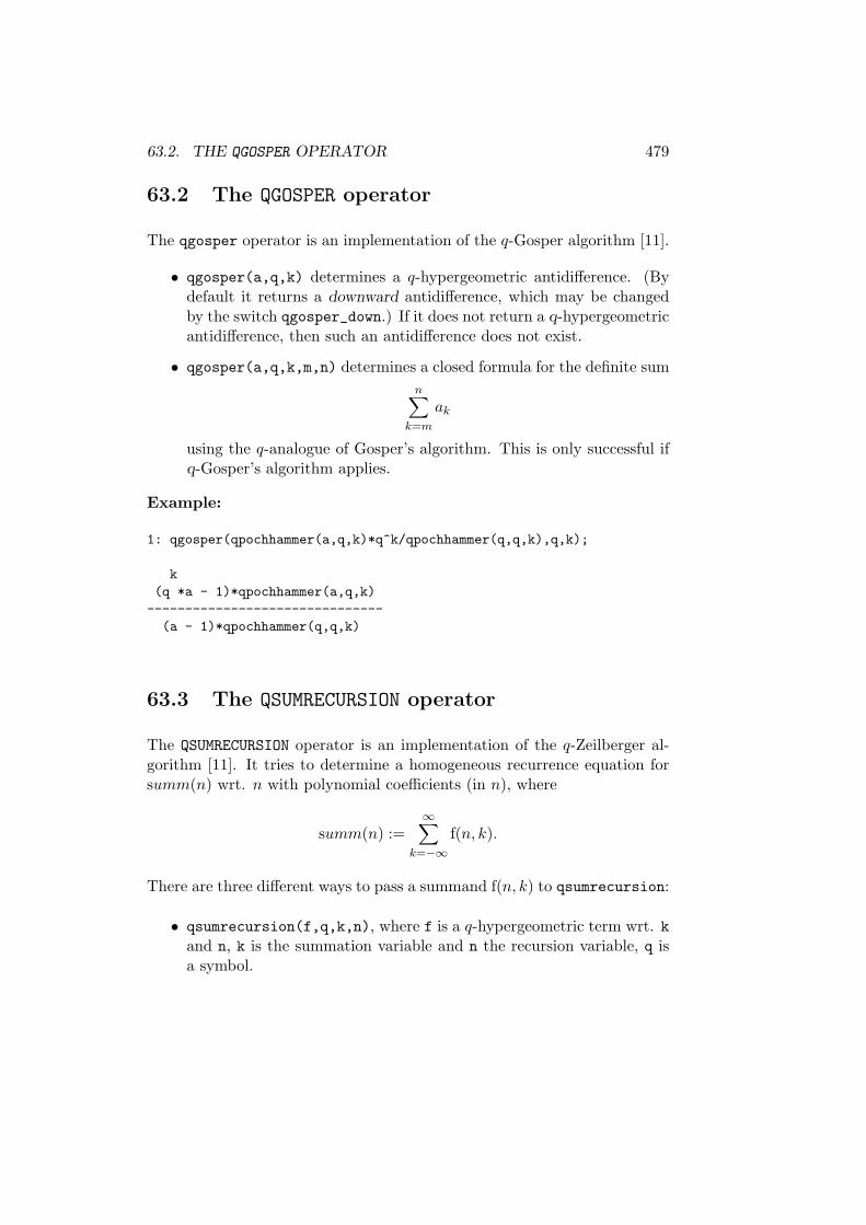
63.2. THE QGOSPER OPERATOR 479
63.2 The QGOSPER operator
The qgosper operator is an implementation of the q-Gosper algorithm [11].
• qgosper(a,q,k) determines a q-hypergeometric antidifference. (Bydefault it returns a downward antidifference, which may be changedby the switch qgosper_down.) If it does not return a q-hypergeometricantidifference, then such an antidifference does not exist.
• qgosper(a,q,k,m,n) determines a closed formula for the definite sumn∑
k=m
ak
using the q-analogue of Gosper’s algorithm. This is only successful ifq-Gosper’s algorithm applies.
Example:
1: qgosper(qpochhammer(a,q,k)*q^k/qpochhammer(q,q,k),q,k);
k(q *a - 1)*qpochhammer(a,q,k)
-------------------------------(a - 1)*qpochhammer(q,q,k)
63.3 The QSUMRECURSION operator
The QSUMRECURSION operator is an implementation of the q-Zeilberger al-gorithm [11]. It tries to determine a homogeneous recurrence equation forsumm(n) wrt. n with polynomial coefficients (in n), where
summ(n) :=∞∑
k=−∞f(n, k).
There are three different ways to pass a summand f(n, k) to qsumrecursion:
• qsumrecursion(f,q,k,n), where f is a q-hypergeometric term wrt. kand n, k is the summation variable and n the recursion variable, q isa symbol.

480 CHAPTER 63. QSUM: Q-HYPERGEOMETRIC SUMS
• qsumrecursion(upper,lower,q,z,n) is a shortcut forqsumrecursion(qphihyperterm(upper,lower,q,z,k),q,k,n)
• qsumrecursion(f,upper,lower,q,z,n) is a similar shortcut forqsumrecursion(f*qphihyperterm(upper,lower,q,z,k),q,k,n),
i. e. upper and lower are lists of upper and lower parameters of the gener-alized q-hypergeometric function. The third form is handy if you have anyadditional factors.
For all three instances it is possible to pass the order, if known in advance,as additional argument at the end of the parameter sequence. You can alsospecifiy a range by a list of two positive integers, the first one specifying thelowest and the second one the highest order. By default QSUMRECURSION willsearch for recurrences of order from 1 to 5. Usually it uses summ as namefor the summ-function. If you want to change this behaviour then use thefollowing syntax: QSUMRECURSION(f,q,k,s(n)).
2: qsumrecursion(qpochhammer(q^(-n),q,k)*z^k /qpochhammer(q,q,k),q,k,n);
n n- ((q - z)*summ(n - 1) - q *summ(n))
63.4 Global Variables and Switches
There are several switches defined in the QSUM package. Please takea look in the accompanying documentation file qsum.tex in $REDU-CEPATH/packages/.
The most important switches are:
• qgosper_down, default setting is on. It determines whether qgosperreturns a downward or an upward antidifference gk for the input termak, . e. ak = gk − gk−1 or ak = gk+1 − gk respectively.
• qsumrecursion_certificate, default off. As Zeilberger’s algorithmdelivers a recurrence equation for a q-hypergeometric term f(n, k) thisswitch is used to get all necessary informations for proving this recur-rence equation.

63.4. GLOBAL VARIABLES AND SWITCHES 481
If it is set on, instead of simply returning the resulting recurrenceequation (for the sum)—if one exists—qsumrecursion returns a listrec,cert,f,k,dir with five items: The first entry contains therecurrence equation, while the other items enable you to prove therecurrence a posteriori by rational arithmetic.
If we denote by r the recurrence rec where we substituted the summ-function by the input term f (with the corresponding shifts in n) thenthe following equation is valid:
r = cert*f - sub(k=k-1,cert*f)
orr = sub(k=k+1,cert*f) - cert*f
if dir=downward_antidifference or dir=upward_antidifferencerespectively.
There is one global variable:
• qsumrecursion_recrange!* controls for which recursion orders theprocedure qsumrecursion looks. It has to be a list with two entries,the first one representing the lowest and the second one the highestorder of a recursion to search for. By default it is set to 1,5.

482 CHAPTER 63. QSUM: Q-HYPERGEOMETRIC SUMS

Chapter 64
RANDPOLY: A randompolynomial generator
Francis J. WrightSchool of Mathematical Sciences, Queen Mary and Westfield College
University of LondonMile End Road
London E1 4NS, England
e–mail: [email protected]
The operator RANDPOLY requires at least one argument corresponding to thepolynomial variable or variables, which must be either a single expressionor a list of expressions. In effect, RANDPOLY replaces each input expressionby an internal variable and then substitutes the input expression for theinternal variable in the generated polynomial (and by default expands theresult as usual). The rest of this document uses the term “variable” torefer to a general input expression or the internal variable used to representit, and all references to the polynomial structure, such as its degree, arewith respect to these internal variables. The actual degree of a generatedpolynomial might be different from its degree in the internal variables.
By default, the polynomial generated has degree 5 and contains 6 terms.Therefore, if it is univariate it is dense whereas if it is multivariate it issparse.
483

484 CHAPTER 64. RANDPOLY: RANDOM POLYNOMIALS
64.1 Optional arguments
Other arguments can optionally be specified, in any order, after the firstcompulsory variable argument. All arguments receive full algebraic evalua-tion, subject to the current switch settings etc. The arguments are processedin the order given, so that if more than one argument relates to the sameproperty then the last one specified takes effect. Optional arguments areeither keywords or equations with keywords on the left.
In general, the polynomial is sparse by default, unless the keyword dense isspecified as an optional argument. (The keyword sparse is also accepted,but is the default.) The default degree can be changed by specifying anoptional argument of the form
degree = natural number.
In the multivariate case this is the total degree, i.e. the sum of the degreeswith respect to the individual variables. More complicated monomial de-gree bounds can be constructed by using the coefficient function describedbelow to return a monomial or polynomial coefficient expression. More-over, randpoly respects internally the REDUCE “asymptotic” commandslet, weight etc. described in section 10.4, which can be used to exerciseadditional control over the polynomial generated.
In the sparse case (only), the default maximum number of terms generatedcan be changed by specifying an optional argument of the form
terms = natural number.
The actual number of terms generated will be the minimum of the valueof terms and the number of terms in a dense polynomial of the specifieddegree, number of variables, etc.
64.2 Advanced use of RANDPOLY
The default order (or minimum or trailing degree) can be changed by spec-ifying an optional argument of the form
ord = natural number.

64.2. ADVANCED USE OF RANDPOLY 485
The order normally defaults to 0.
The input expressions to randpoly can also be equations, in which casethe order defaults to 1 rather than 0. Input equations are converted tothe difference of their two sides before being substituted into the generatedpolynomial. This makes it easy to generate polynomials with a specifiedzero – for example
randpoly(x = a);
generates a polynomial that is guaranteed to vanish at x = a, but is other-wise random.
The operator randpoly accepts two further optional arguments in the formof equations with the keywords coeffs and expons on the left. The rightsides of each of these equations must evaluate to objects that can be appliedas functions of no variables. These functions should be normal algebraicprocedures; the coeffs procedure may return any algebraic expression, butthe expons procedure must return an integer. The values returned by thefunctions should normally be random, because it is the randomness of thecoefficients and, in the sparse case, of the exponents that makes the con-structed polynomial random.
A convenient special case is to use the function rand on the right of one orboth of these equations; when called with a single argument rand returns ananonymous function of no variables that generates a random integer. Thesingle argument of rand should normally be an integer range in the forma .. b, where a, b are integers such that a < b. For example, the exponsargument might take the form
expons = rand(0 .. n)
where n will be the maximum degree with respect to each variable inde-pendently. In the case of coeffs the lower limit will often be the negativeof the upper limit to give a balanced coefficient range, so that the coeffsargument might take the form
coeffs = rand(-n .. n)
which will generate random integer coefficients in the range [−n, n].

486 CHAPTER 64. RANDPOLY: RANDOM POLYNOMIALS
Further information on the the auxiliary functions of RANDPOLY can befound in the extended documentation and examples.
64.3 Examples
randpoly(x);
5 4 3 2- 54*x - 92*x - 30*x + 73*x - 69*x - 67
randpoly(x, y, terms = 20);
5 4 4 3 2 3 331*x - 17*x *y - 48*x - 15*x *y + 80*x *y + 92*x
2 3 2 2 4 3 2+ 86*x *y + 2*x *y - 44*x + 83*x*y + 85*x*y + 55*x*y
5 4 3 2- 27*x*y + 33*x - 98*y + 51*y - 2*y + 70*y - 60*y - 10

64.3. EXAMPLES 487
randpoly(x, sin(x), cos(x));
4 3 3sin(x)*( - 4*cos(x) - 85*cos(x) *x + 50*sin(x)
2- 20*sin(x) *x + 76*sin(x)*x + 96*sin(x))

488 CHAPTER 64. RANDPOLY: RANDOM POLYNOMIALS

Chapter 65
RATAPRX : RationalApproximations Package
Lisa TemmeWolfram Koepf
Konrad-Zuse-Zentrum fur Informationstechnik BerlinTakustrase 7
D-14195 Berlin-Dahlem, Germanye-mail: [email protected]
This package provides functions to
• convert rational numbers in their periodic representation and viceversa,
• to compute continued fractions and
• to compute the Pade approximant of a function.
The package can be loaded using load package rataprx; it supersedes thecontfr package.
489

490 CHAPTER 65. RATAPRX: RATIONAL APPROXIMATIONS
65.1
65.1.1 Periodic Representation
The function rational2periodic(n) converts a rational number n in itsperiodic representation. For example 59/70 is converted to 0.8428571.Depending on the print function of your REDUCE system, calling thefunction rational2periodic might result in an expression of the formperiodic(a,b,c1,...,cn). a and b is the non-periodic part of therational number n and c1,...,cn are the digits of the periodic part. In thiscase 59/70 would result in periodic(8,10,4,2,8,5,7,1).The function periodic2rational(periodic(a,b,c1,...,cn)) is theinverse function and computes the rational expression for a periodic one.Note that b is 1,-1 or a integer multiple of 10. If a is zero, then the in-put number b indicates how many places after the decimal point the periodoccurs.
rational2periodic(6/17);
periodic(0,1,3,5,2,9,4,1,1,7,6,4,7,0,5,8,8,2)
periodic2rational(ws);
6----17
65.1.2 Continued Fractions
A continued fraction (see [1] §4.2) has the general form
b0 +a1
b1 + a2
b2+a3
b3+...
.
A more compact way of writing this is as
b0 +a1||b1 +
a2||b2 +
a3||b3 + . . . .

65.1. 491
This is represented in REDUCE as
contfrac(Rational approximant, b0, a1, b1, a2, b2, .....).
There are four different functions to determine the continued fractions forreal numbers and functions f in the variable var:
cfrac(number); cfrac(number,length);cfrac(f, var); cfrac(f, var, length);
The length argument is optional and specifies the number of ordered pairsai, bi to be returned. It’s default value is five.
cfrac pi;
1146408contfrac(---------),
364913
3,1,7,1,15,1,1,1,292,1,1,1,1,1,1,1,2,1,1)

492 CHAPTER 65. RATAPRX: RATIONAL APPROXIMATIONS
cfrac((x+2/3)^2/(6*x-5),x);
29*x + 12*x + 4 6*x + 13 24*x - 20
contfrac(-----------------,----------,1,-----------)54*x - 45 36 9
cfrac(e^x,x);
3 2x + 9*x + 36*x + 60
contfrac(-----------------------,2
3*x - 24*x + 60
1,x,1, - x,2,x,3, - x,2,x,5)
65.1.3 Pade Approximation
The Pade approximant represents a function by the ratio of two polynomials.The coefficients of the powers occuring in the polynomials are determinedby the coefficients in the Taylor series expansion of the function (see [1]).Given a power series
f(x) = c0 + c1(x− h) + c2(x− h)2 . . .
and the degree of numerator, n, and of the denominator, d, the pade functionfinds the unique coefficients ai, bi in the Pade approximant
a0 + a1x+ · · ·+ anxn
b0 + b1x+ · · ·+ bdxd.
The function pade(f, x, h ,n ,d) takes as input the function f in thevariable x to be approximated , where h is the point at which the approxi-mation is evaluated. n and d are the (specified) degrees of the numerator andthe denominator. It returns the Pade Approximant, ie. a rational function.
Error Messages may occur in the following different cases:
• The Taylor series expansion for the function f has not yet been imple-mented in the REDUCE Taylor Package.
• A Pade Approximant of this function does not exist.

65.1. 493
• A Pade Approximant of this order (ie. the specified numerator anddenominator orders) does not exist. Please note, there might exist anapproximant of a different order.

494 CHAPTER 65. RATAPRX: RATIONAL APPROXIMATIONS
pade(sin(x),x,0,3,3);
2x*( - 7*x + 60)
------------------2
3*(x + 20)
pade(tanh(x),x,0,5,5);
4 2x*(x + 105*x + 945)
-----------------------4 2
15*(x + 28*x + 63)
pade(exp(1/x),x,0,5,5);
***** no Pade Approximation exists
pade(factorial(x),x,1,3,3);
***** not yet implemented
30: pade(sin(x)/x^2,x,0,10,0);
***** Pade Approximation of this order does not exist
31: pade(sin(x)/x^2,x,0,10,2);
10 8 6 4 2- x + 110*x - 7920*x + 332640*x - 6652800*x + 39916800
--------------------------------------------------------------39916800*x

Chapter 66
REACTEQN: Support forchemical reaction equations
Herbert MelenkKonrad–Zuse–Zentrum fur Informationstechnik Berlin
Takustrase 7D–14195 Berlin–Dahlem, Germany
e–mail: [email protected]
The REDUCE package REACTEQN allows one to transform chemical re-action systems into ordinary differential equation systems corresponding tothe laws of pure mass action.
It provides the single function
reac2ode <reaction> [,<rate> [,<rate>]][,<reaction> [,<rate> [,<rate>]]]
....;
A rate is any REDUCE expression, and two rates are applicable only forforward and backward reactions. A reaction is coded as a linear sum of theseries variables, with the operator − > for forward reactions and <> fortwo-way reactions.
The result is a system of explicit ordinary differential equations with poly-nomial righthand sides. As side effect the following variables are set:
495

496CHAPTER 66. REACTEQN: CHEMICAL REACTION EQUATIONS
rates A list of the rates in the system.
species A list of the species in the system.
inputmat A matrix of the input coefficients.
outputmat A matrix of the output coefficients.
In the matrices the row number corresponds to the input reaction number,while the column number corresponds to the species index.
If the rates are numerical values, it will be in most cases appropriate toselect a REDUCE evaluation mode for floating point numbers.
Inputmat and outputmat can be used for linear algebra type investigationsof the reaction system. The classical reaction matrix is the difference ofthese matrices; however, the two matrices contain more information thantheir differences because the appearance of a species on both sides is notreflected by the reaction matrix.

Chapter 67
REDLOG: Logic System
Andreas DolzmannThomas Sturm
University of Passau, Germanye-mail: [email protected], [email protected]
67.1 Introduction
This package extends REDUCE to a computer logic system implementingsymbolic algorithms on first-order formulas wrt. temporarily fixed first-orderlanguages and theories.
67.1.1 Contexts
REDLOG is designed for working with several languages and theories in thesense of first-order logic. Both a language and a theory make up a context.There are the following contexts available:
OFSF OF stands for ordered fields, which is a little imprecise. The quanti-fier elimination actually requires the more restricted class of real closedfields, while most of the tool-like algorithms are generally correct forordered fields. One usually has in mind real numbers with orderingwhen using OFSF.
DVFSF Discretely valued fields. This is for computing with formulas over
497

498 CHAPTER 67. REDLOG: LOGIC SYSTEM
classes of p-adic valued extension fields of the rationals, usually thefields of p-adic numbers for some prime p.
ACFSF Algebraically closed fields such as the complex numbers.
67.1.2 Overview
REDLOG origins from the implementation of quantifier elimination proce-dures. Successfully applying such methods to both academic and real-worldproblems, the authors have developed over the time a large set of formula-manipulating tools, many of which are meanwhile interesting in their ownright:
• Numerous tools for comfortably inputing, decomposing, and analyzingformulas.
• Several techniques for the simplification of formulas.
• Various normal form computations. The CNF/DNF computationincludes both Boolean and algebraic simplification strategies. Theprenex normal form computation minimizes the number of quantifierchanges.
• Quantifier elimination computes quantifier-free equivalents for givenfirst-order formulas. For OFSF and DVFSF the formulas have toobey certain degree restrictions.
• The context OFSF allows a variant of quantifier elimination calledgeneric quantifier elimination: There are certain non-degeneracy as-sumptions made on the parameters, which considerably speeds up theelimination.
• The contexts OFSF and DVFSF provide variants of (generic) quan-tifier elimination that additionally compute answers such as satisfyingsample points for existentially quantified formulas.
• OFSF includes linear optimization techniques based on quantifierelimination.
To avoid ambiguities with other packages, all REDLOG functions andswitches are prefixed by “RL”.

67.2. CONTEXT SELECTION 499
The package is loaded by typing: load package redlog;
It is recommended to read the documentation which comes with this pack-age. This manual chapter gives an overview on the features of REDLOG,which is by no means complete.
67.2 Context Selection
The context to be used has to be selected explicitly. One way to do thisis using the command RLSET. As argument it takes one of the valid choicesACFSF (algebraically closed fields standard form), OFSF (ordered fields stand-ard form), and DVFSF (discretely valued fields standard form). By default,DVFSF computes uniformly over the class of all p-adic valued fields. Forthe sake of efficiency, this can be restricted by means of an extra RLSETargument. RLSET returns the old setting as a list.
67.3 Format and Handling of Formulas
67.3.1 First-order Operators
REDLOG knows the following operators for constructing Boolean combina-tions and quantifications of atomic formulas:
NOT: Unary AND: N-ary Infix OR: N-ary Infix IMPL: Binary InfixREPL: Binary Infix EQUIV: Binary Infix EX: BinaryALL: Binary TRUE: Variable FALSE: Variable
The EX and the ALL operators are the quantifiers. Their first argument isthe quantified variable, the second one a matrix formula.
There are operators MKAND and MKOR for the construction of large systematicconjunctions/disjunctions via for loops available. They are used in the styleof SUM and COLLECT.
Example:

500 CHAPTER 67. REDLOG: LOGIC SYSTEM
1: load_package redlog;
2: rlset ofsf;
3: g := for i:=1:3 mkand
for j:=1:3 mkor
if j<>i then mkid(x,i) + mkid(x,j)=0;
true and (false or false or x1 + x2 = 0 or x1 + x3 = 0)
and (false or x1 + x2 = 0 or false or x2 + x3 = 0)
and (false or x1 + x3 = 0 or x2 + x3 = 0 or false)
67.3.2 OFSF Operators
The OFSF context implements ordered fields over the language of orderedrings. There are the following binary operators available:
EQUAL NEQ LEQ GEQ LESSP GREATERP
They can also be written as =, <>, <=, >=, <, and >. For OFSF there isspecified that all right hand sides must be zero. Non-zero right hand sidesare immediately subtracted.
67.3.3 DVFSF Operators
Discretely valued fields are implemented as a one-sorted language using inaddition to = and <> the binary operators |, ||, ~, and /~, which encode ≤,<, =, and 6= in the value group, respectively.
EQUAL NEQ DIV SDIV ASSOC NASSOC

67.4. SIMPLIFICATION 501
67.3.4 ACFSF Operators
For algebraically closed fields there are only equations and inequalities al-lowed:
EQUAL NEQ
As in OFSF, they can be conveniently written as = and <>, respectively.All right hand sides are zero.
67.3.5 Extended Built-in Commands
The operators SUB, PART, and LENGTH work on formulas in a reasonable way.
67.3.6 Global Switches
The switch RLSIMPL causes the function RLSIMPL to be automatically appliedat the expression evaluation stage.
The switch RLREALTIME protocols the wall clock time needed for REDLOGcommands in seconds.
The switch RLVERBOSE toggles verbosity output with some REDLOG pro-cedures.
67.4 Simplification
REDLOG knows three types of simplifiers to reduce the size of a givenfirst-order formula: the standard simplifier, tableau simplifiers, and Grobnersimplifiers.
67.4.1 Standard Simplifier
The standard simplifier RLSIMPL returns a simplified equivalent of its argu-ment formula. It is much faster though less powerful than the other simpli-fiers.

502 CHAPTER 67. REDLOG: LOGIC SYSTEM
As an optional argument there can be a theory passed. This is a list ofatomic formulas assumed to hold. Simplification is then performed on thebasis of these assumptions.
Example:
4: rlsimpl g;
(x1 + x2 = 0 or x1 + x3 = 0) and (x1 + x2 = 0 or x2 + x3 = 0)
and (x1 + x3 = 0 or x2 + x3 = 0)
67.4.2 Tableau Simplifier
The standard simplifier preserves the basic Boolean structure of a formula.The tableau methods, in contrast, provide a technique for changing theBoolean structure of a formula by constructing case distinctions.
The function RLATAB automatically finds a suitable case distinction. Basedon RLATAB, the function RLITAB iterates this process until no further sim-plification can be detected. There is a more fundamental entry point RLTABfor manually entering case distinctions.
67.4.3 Grobner Simplifier
The Grobner simplifier considers algebraic simplification rules between theatomic formulas of the input formula. The usual procedure called forGrobner simplification is RLGSN. Similar to the standard simplifier, thereis an optional theory argument.
Example:
5: rlgsn(x*y+1<>0 or y*z+1<>0 or x-z=0);
true

67.5. NORMAL FORMS 503
67.5 Normal Forms
67.5.1 Boolean Normal Forms
RLCNF and RLDNF compute conjunctive resp. disjunctive normal forms oftheir formula arguments. Subsumption and cut strategies are applied todecrease the number of clauses.
67.5.2 Miscellaneous Normal Forms
RLNNF computes a negation normal form. This is an and-or-combination ofatomic formulas.
RLPNF computes a prenex normal form of its argument. That is, all quanti-fiers are moved outside such that they form a block in front of a quantifier-free matrix formula.
67.6 Quantifier Elimination and Variants
Quantifier elimination computes quantifier-free equivalents for given first-order formulas. For OFSF and DVFSF, REDLOG uses a technique basedon elimination set ideas. The OFSF implementation is restricted to atmost quadratic occurrences of the quantified variables, but includes nu-merous heuristic strategies for coping with higher degrees. The DVFSFimplementation is restricted to formulas that are linear in the quantifiedvariables. The ACFSF quantifier elimination is based on comprehensiveGrobner basis computation; there are no degree restrictions for this context
67.6.1 Quantifier Elimination
RLQE performs quantifier elimination on its argument formula. There is anoptional theory argument in the style of RLSIMPL supported.

504 CHAPTER 67. REDLOG: LOGIC SYSTEM
Example:
6: rlqe(ex(x,a*x**2+b*x+c>0),a<0);
24*a*c - b < 0
For OFSF and DVFSF there is a variant RLQEA available. It returns insteadof a quantifier-free equivalent, a list of condition-solution pairs containing,e.g., satisfying sample points for outermost existential quantifier blocks.
Example:
7: rlqea(ex(x,a*x**2+b*x+c>0),a<0);
24*a*c - b < 0,
2- sqrt( - 4*a*c + b ) - 2*a*epsilon1 - b
x = -------------------------------------------2*a
67.6.2 Generic Quantifier Elimination
OFSF allows generic quantifier elimination RLGQE, which enlarges the theoryby disequations, i.e. <>-atomic formulas, wherever this supports the quan-tifier elimination. There is also generic quantifier elimination with answeravailable: RLGQEA.
Example:
8: rlgqe ex(x,a*x**2+b*x+c>0);
a <> 0,
24*a*c - b < 0 or a >= 0

67.6. QUANTIFIER ELIMINATION AND VARIANTS 505
67.6.3 Linear Optimization
RLOPT uses quantifier elimination for linear optimization. It takes as argu-ments a list of constraints and the target function. The target function isminimized subject to the constraints.

506 CHAPTER 67. REDLOG: LOGIC SYSTEM
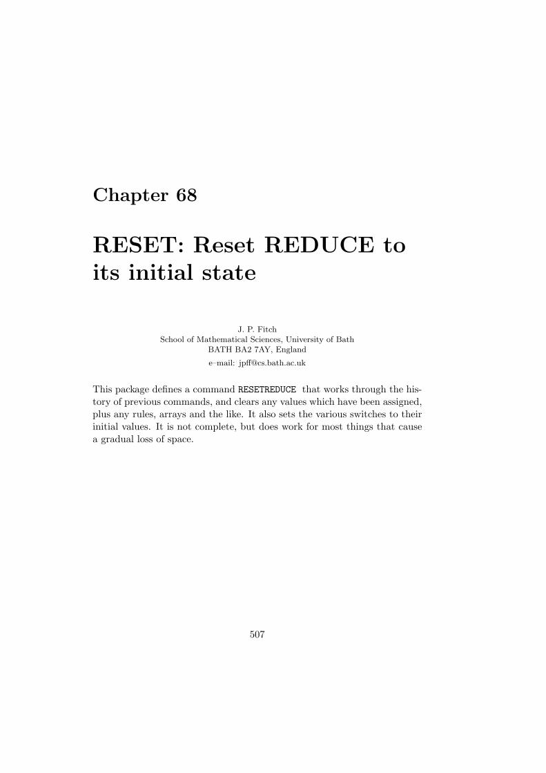
Chapter 68
RESET: Reset REDUCE toits initial state
J. P. FitchSchool of Mathematical Sciences, University of Bath
BATH BA2 7AY, England
e–mail: [email protected]
This package defines a command RESETREDUCE that works through the his-tory of previous commands, and clears any values which have been assigned,plus any rules, arrays and the like. It also sets the various switches to theirinitial values. It is not complete, but does work for most things that causea gradual loss of space.
507

508 CHAPTER 68. RESET: RESET REDUCE TO ITS INITIAL STATE

Chapter 69
RESIDUE: A residuepackage
Wolfram KoepfKonrad–Zuse–Zentrum fur Informationstechnik Berlin
Takustrase 7D–14195 Berlin–Dahlem, Germany
e–mail: [email protected]
This package supports the calculation of residues. The residue Resz=a
f(z) ofa function f(z) at the point a ∈ C is defined as
Resz=a
f(z) =1
2πi
∮f(z) dz ,
with integration along a closed curve around z = a with winding number 1.
It contains two REDUCE operators:
• residue(f,z,a) determines the residue of f at the point z = a iff is meromorphic at z = a. The calculation of residues at essentialsingularities of f is not supported.
• poleorder(f,z,a) determines the pole order of f at the point z = aif f is meromorphic at z = a.
Note that both functions use the TAYLOR package (chapter 82).
509

510 CHAPTER 69. RESIDUE: A RESIDUE PACKAGE
load_package residue;
residue(x/(x^2-2),x,sqrt(2));
1---2
poleorder(x/(x^2-2),x,sqrt(2));
1
residue(sin(x)/(x^2-2),x,sqrt(2));
sqrt(2)*sin(sqrt(2))----------------------
4
poleorder(sin(x)/(x^2-2),x,sqrt(2));
1
residue((x^n-y^n)/(x-y)^2,x,y);
ny *n
------y
poleorder((x^n-y^n)/(x-y)^2,x,y);
1

Chapter 70
RLFI: REDUCE LaTeXformula interface
Richard Liska, Ladislav DrskaComputational Physics Group
Faculty of Nuclear Sciences and Physical EngineeringCzech Technical University in Prague, Brehova 7, 115 19 Prague 1
Czech Republic
e–mail: [email protected]
The RLFI package provides the printing of REDUCE expressions in LATEXformat, so it can be used directly for document production. Various math-ematical constructions are supported by the interface including subscripts,superscripts, font changing, Greek letters, divide-bars, integral and sumsigns, derivatives etc.
The interface is connected to REDUCE by three new switches and severalstatements. To activate the LATEX output mode the switch latex must beset on. This switch causes all outputs to be written in the LATEX syntax offormulas. The switch VERBATIM is used for input printing control. If it is oninput to REDUCE system is typeset in LATEX verbatim environment afterthe line containing the string REDUCE Input:.
The switch lasimp controls the algebraic evaluation of input formulas. Ifit is on every formula is evaluated, simplified and written in the form givenby ordinary REDUCE statements and switches such as factor, order, ratetc. In the case when the lasimp switch is off evaluation, simplification orreordering of formulas is not performed and REDUCE acts only as a formula
511

512 CHAPTER 70. RLFI: REDUCE LATEX FORMULA INTERFACE
parser and the form of the formula output is exactly the same as that ofthe input, the only difference remains in the syntax. The mode off lasimpis designed especially for typesetting of formulas for which the user needspreservation of their structure. This switch has no meaning if the switchLatex is off and thus is working only for LATEX output.
For every identifier used in the typeset REDUCE formula the followingproperties can be defined by the statement defid:
• its printing symbol (Greek letters can be used).
• the font in which the symbol will be typeset.
• accent which will be typeset above the symbol.
Symbols with indexes are treated in REDUCE as operators. Each indexcorresponds to an argument of the operator. The meaning of operator ar-guments (where one wants to typeset them) is declared by the statementdefindex. This statement causes the arguments to be typeset as subscriptsor superscripts (on left or right-hand side of the operator) or as argumentsof the operator.
The statement mathstyle defines the style of formula typesetting. Thevariable laline!* defines the length of output lines.
The fractions with horizontal divide bars are typeset by using the new RE-DUCE infix operator \. This operator is not algebraically simplified. Duringtypesetting of powers the checking on the form of the power base and expo-nent is performed to determine the form of the typeset expression (e.g. sqrtsymbol, using parentheses).
Some special forms can be typeset by using REDUCE prefix operators.These are as follows:
• int - integral of an expression.
• dint - definite integral of an expression.
• df - derivative of an expression.
• pdf - partial derivative of an expression.
• sum - sum of expressions.
• product - product of expressions.

513
• sqrt - square root of expression.
There are still some problems unsolved in the present version of the interfaceas follows:
• breaking the formulas which do not fit on one line.
• automatic decision where to use divide bars in fractions.
• distinction of two- or more-character identifiers from the product ofone-character symbols.
• typesetting of matrices.

514 CHAPTER 70. RLFI: REDUCE LATEX FORMULA INTERFACE

Chapter 71
ROOTS: A REDUCE rootfinding package
Stanley L. KamenyLos Angeles, U.S.A.
The root finding package is designed so that it can be used as an independentpackage, or it can be integrated with and called by SOLVE.
71.1 Top Level Functions
The top level functions can be called either as symbolic operators fromalgebraic mode, or they can be called directly from symbolic mode withsymbolic mode arguments. Outputs are expressed in forms that print outcorrectly in algebraic mode.
71.1.1 Functions that refer to real roots only
The three functions REALROOTS, ISOLATER and RLROOTNO can receive 1, 2 or3 arguments.
The first argument is the polynomial p, that can be complex and can havemultiple or zero roots. If arg2 and arg3 are not present, all real roots arefound. If the additional arguments are present, they restrict the region ofconsideration.
515

516 CHAPTER 71. ROOTS: A REDUCE ROOT FINDING PACKAGE
• If there are two arguments the second is either POSITIVE or NEGA-TIVE. The function will only find positive or negative roots
• If arguments are (p,arg2,arg3) then Arg2 and Arg3 must be r (areal number) or EXCLUDE r, or a member of the list POSITIVE,NEGATIVE, INFINITY, -INFINITY. EXCLUDE r causes the value rto be excluded from the region. The order of the sequence arg2, arg3is unimportant. Assuming that arg2 ≤ arg3 when both are numeric,then-INFINITY,INFINITY (or ) all roots;arg2,NEGATIVE represents −∞ < r < arg2;arg2,POSITIVE represents arg2 < r <∞;
In each of the following, replacing an arg with EXCLUDE arg convertsthe corresponding inclusive ≤ to the exclusive <
arg2,-INFINITY represents −∞ < r ≤ arg2;arg2,INFINITY represents arg2 ≤ r <∞;arg2,arg3 represents arg2 ≤ r ≤ arg3;
• If zero is in the interval the zero root is included.
REALROOTS finds the real roots of the polynomial p. Precision of com-putation is guaranteed to be sufficient to separate all real roots in thespecified region. (cf. MULTIROOT for treatment of multiple roots.)
ISOLATER produces a list of rational intervals, each containing a singlereal root of the polynomial p, within the specified region, but does notfind the roots.
RLROOTNO computes the number of real roots of p in the specifiedregion, but does not find the roots.
71.1.2 Functions that return both real and complex roots
ROOTS p; This is the main top level function of the roots package. Itwill find all roots, real and complex, of the polynomial p to an accu-racy that is sufficient to separate them and which is a minimum of6 decimal places. The value returned by ROOTS is a list of equat-ions for all roots. In addition, ROOTS stores separate lists of real
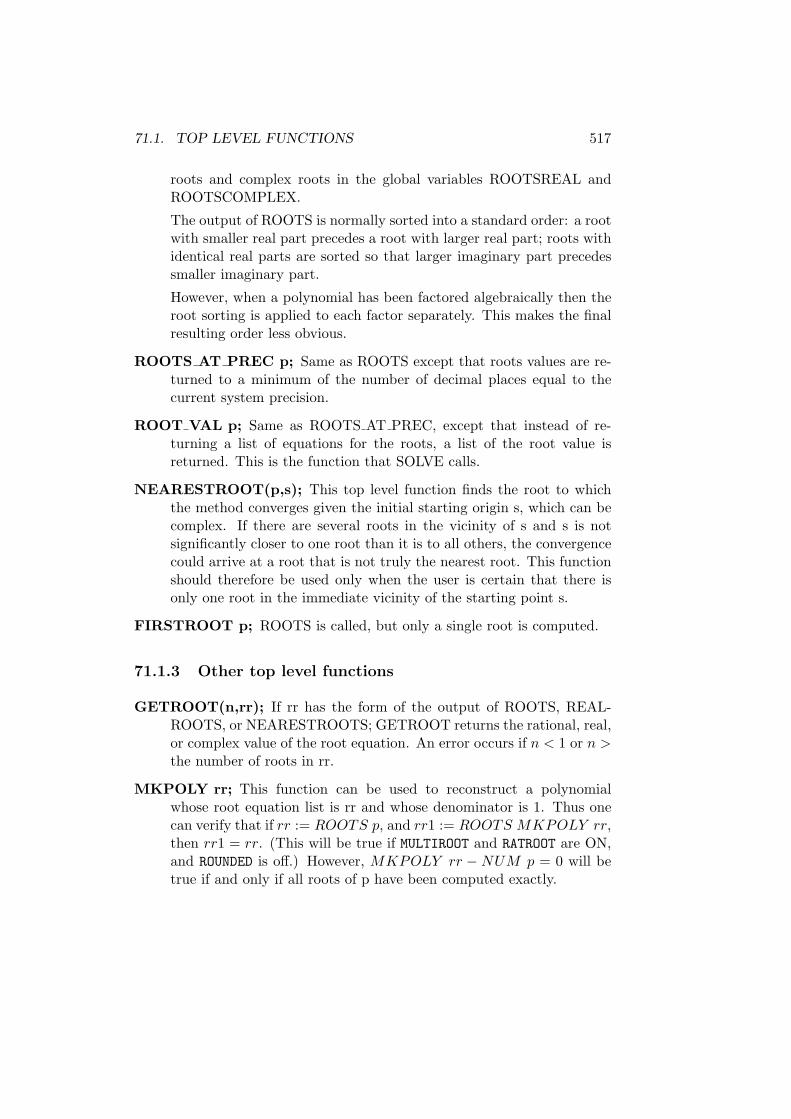
71.1. TOP LEVEL FUNCTIONS 517
roots and complex roots in the global variables ROOTSREAL andROOTSCOMPLEX.
The output of ROOTS is normally sorted into a standard order: a rootwith smaller real part precedes a root with larger real part; roots withidentical real parts are sorted so that larger imaginary part precedessmaller imaginary part.
However, when a polynomial has been factored algebraically then theroot sorting is applied to each factor separately. This makes the finalresulting order less obvious.
ROOTS AT PREC p; Same as ROOTS except that roots values are re-turned to a minimum of the number of decimal places equal to thecurrent system precision.
ROOT VAL p; Same as ROOTS AT PREC, except that instead of re-turning a list of equations for the roots, a list of the root value isreturned. This is the function that SOLVE calls.
NEARESTROOT(p,s); This top level function finds the root to whichthe method converges given the initial starting origin s, which can becomplex. If there are several roots in the vicinity of s and s is notsignificantly closer to one root than it is to all others, the convergencecould arrive at a root that is not truly the nearest root. This functionshould therefore be used only when the user is certain that there isonly one root in the immediate vicinity of the starting point s.
FIRSTROOT p; ROOTS is called, but only a single root is computed.
71.1.3 Other top level functions
GETROOT(n,rr); If rr has the form of the output of ROOTS, REAL-ROOTS, or NEARESTROOTS; GETROOT returns the rational, real,or complex value of the root equation. An error occurs if n < 1 or n >the number of roots in rr.
MKPOLY rr; This function can be used to reconstruct a polynomialwhose root equation list is rr and whose denominator is 1. Thus onecan verify that if rr := ROOTS p, and rr1 := ROOTS MKPOLY rr,then rr1 = rr. (This will be true if MULTIROOT and RATROOT are ON,and ROUNDED is off.) However, MKPOLY rr − NUM p = 0 will betrue if and only if all roots of p have been computed exactly.

518 CHAPTER 71. ROOTS: A REDUCE ROOT FINDING PACKAGE
71.2 Switches Used in Input
The input of polynomials in algebraic mode is sensitive to the switchesCOMPLEX, ROUNDED, and ADJPREC. The correct choice of input method isimportant since incorrect choices will result in undesirable truncation orrounding of the input coefficients.
Truncation or rounding may occur if ROUNDED is on and one of the followingis true:
1. a coefficient is entered in floating point form or rational form.
2. COMPLEX is on and a coefficient is imaginary or complex.
Therefore, to avoid undesirable truncation or rounding, then:
1. ROUNDED should be off and input should be in integer or rational form;or
2. ROUNDED can be on if it is acceptable to truncate or round input to thecurrent value of system precision; or both ROUNDED and ADJPREC canbe on, in which case system precision will be adjusted to accommodatethe largest coefficient which is input; or
3. if the input contains complex coefficients with very different magnitudefor the real and imaginary parts, then all three switches ROUNDED,ADJPREC and COMPLEX must be on.
integer and complex modes (off ROUNDED) any real polynomial can beinput using integer coefficients of any size; integer or rational coeffi-cients can be used to input any real or complex polynomial, indepen-dent of the setting of the switch COMPLEX. These are the most versatileinput modes, since any real or complex polynomial can be input ex-actly.
modes rounded and complex-rounded (on ROUNDED) polynomials canbe input using integer coefficients of any size. Floating point coef-ficients will be truncated or rounded, to a size dependent upon thesystem. If complex is on, real coefficients can be input to any preci-sion using integer form, but coefficients of imaginary parts of complexcoefficients will be rounded or truncated.

71.3. ROOT PACKAGE SWITCHES 519
71.3 Root Package Switches
RATROOT (Default OFF) If RATROOT is on all root equations are outputin rational form. Assuming that the mode is COMPLEX (i.e. ROUNDEDis off,) the root equations are guaranteed to be able to be input intoREDUCE without truncation or rounding errors. (Cf. the functionMKPOLY described above.)
MULTIROOT (Default ON) Whenever the polynomial has complex coef-ficients or has real coefficients and has multiple roots, as determinedby the Sturm function, the function SQFRF is called automatically tofactor the polynomial into square-free factors. If MULTIROOT is on, themultiplicity of the roots will be indicated in the output of ROOTS orREALROOTS by printing the root output repeatedly, according to itsmultiplicity. If MULTIROOT is off, each root will be printed once, andall roots should be normally be distinct. (Two identical roots shouldnot appear. If the initial precision of the computation or the accuracyof the output was insufficient to separate two closely-spaced roots, theprogram attempts to increase accuracy and/or precision if it detectsequal roots. If, however, the initial accuracy specified was too low,and it was not possible to separate the roots, the program will abort.)

520 CHAPTER 71. ROOTS: A REDUCE ROOT FINDING PACKAGE

Chapter 72
RSOLVE:Rational/integer polynomialsolvers
Francis J. WrightSchool of Mathematical Sciences, Queen Mary and Westfield College
University of LondonMile End Road
London E1 4NS, England
e–mail: [email protected]
The exact rational zeros of a single univariate polynomial using fast modularmethods can be calculated. The operator r_solve computes all rationalzeros and the operator i_solve computes only integer zeros in a way thatis slightly more efficient than extracting them from the rational zeros.
The first argument is either a univariate polynomial expression or equationwith integer, rational or rounded coefficients. Symbolic coefficients are notallowed. The argument is simplified to a quotient of integer polynomialsand the denominator is silently ignored.
Subsequent arguments are optional. If the polynomial variable is to bespecified then it must be the first optional argument. However, since thevariable in a non-constant univariate polynomial can be deduced from thepolynomial it is unnecessary to specify it separately, except in the degeneratecase that the first argument simplifies to either 0 or 0 = 0. In this casethe result is returned by i_solve in terms of the operator arbint and by
521

522 CHAPTER 72. RSOLVE: RATIONAL POLYNOMIAL SOLVER
r_solve in terms of the (new) analogous operator arbrat. The operatori_solve will generally run slightly faster than r_solve.
The (rational or integer) zeros of the first argument are returned as a listand the default output format is the same as that used by solve. Eachdistinct zero is returned in the form of an equation with the variable onthe left and the multiplicities of the zeros are assigned to the variableroot_multiplicities as a list. However, if the switch multiplicitiesis turned on then each zero is explicitly included in the solution list theappropriate number of times (and root_multiplicities has no value).
Optional keyword arguments acting as local switches allow other outputformats. They have the following meanings:
separate: assign the multiplicity list to the global variableroot_multiplicities (the default);
expand or multiplicities: expand the solution list to include multiplezeros multiple times (the default if the multiplicities switch is on);
together: return each solution as a list whose second element is the multi-plicity;
nomul: do not compute multiplicities (thereby saving some time);
noeqs: do not return univariate zeros as equations but just as values.
72.1 Examples
r_solve((9x^2 - 16)*(x^2 - 9), x);
x =
−43, x = 3, x = −3, x =
43
i_solve((9x^2 - 16)*(x^2 - 9), x);
x = 3, x = −3

Chapter 73
SCOPE: REDUCE sourcecode optimisation package
J.A. van HulzenUniversity of Twente, Department of Computer Science
P.O. Box 217, 7500 AE EnschedeThe Netherlands
e–mail: [email protected]
SCOPE is a package to produce optimised versions of algebraic expressions.It can be used in two distinct fashions, as an adjunct to numerical codegeneration (using GENTRAN, described in chapter 42) or as a stand aloneway of investigating structure in an expression.
When used with GENTRAN it is sufficient to set the switch GENTRANOPTon, and GENTRAN will then use SCOPE internally. This is described in itsinternal detail in the GENTRAN manual and the SCOPE documentation.
As a stand-alone package SCOPE provides the operator OPTIMIZE.
A SCOPE application is easily performed and based on the use of the fol-lowing syntax:
523

524CHAPTER 73. SCOPE: SOURCE CODE OPTIMISATION PACKAGE
<SCOPE application> ⇒ OPTIMIZE <object seq> [INAME <cse prefix>]<object seq> ⇒ <object>[,<object seq>]<object> ⇒ <stat> | <alglist> | <alglist production><stat> ⇒ <name> <assignment operator> <expression><assignment operator> ⇒ := | ::= | ::=: | :=:<alglist> ⇒ <eq seq><eq seq> ⇒ <name> = <expression>[,<eq seq>]<alglist production> ⇒ <name> | <function application><name> ⇒ <id> | <id> (<a subscript seq>)<a subscript seq> ⇒ <a subscript>[,<a subscript seq>]<a subscript> ⇒ <integer> | <integer infix expression><cse prefix> ⇒ <id>
A SCOPE action can be applied on one assignment statement, or to a se-quence of such statements, separated by commas, or a list of expressions.
The optional use of the INAME extension in an OPTIMIZE command is in-troduced to allow the user to influence the generation of cse-names. Thecse prefix is an identifier, used to generate cse-names, by extending it withan integer part. If the cse prefix consists of letters only, the initially selectedinteger part is 0. If the user-supplied cse prefix ends with an integer its valuefunctions as initial integer part.
z:=a^2*b^2+10*a^2*m^6+a^2*m^2+2*a*b*m^4+2*b^2*m^6+b^2*m^2;
2 2 2 6 2 2 4 2 6 2 2z := a *b + 10*a *m + a *m + 2*a*b*m + 2*b *m + b *m
OPTIMIZE z:=:z ;
G0 := b*aG4 := m*mG1 := G4*b*bG2 := G4*a*aG3 := G4*G4z := G1 + G2 + G0*(2*G3 + G0) + G3*(2*G1 + 10*G2)
it can be desirable to rerun an optimisation request with a restriction on theminimal size of the righthandsides. The command
SETLENGTH <integer>$

525
can be used to produce rhs’s with a minimal arithmetic complexity, dictatedby the value of its integer argument. Statements, used to rename functionapplications, are not affected by the SETLENGTH command. The defaultsetting is restored with the command
RESETLENGTH$
Example:
SETLENGTH 2$
OPTIMIZE z:=:z INAME s$
2 2s1 := b *m
2 2s2 := a *m
4 4z := (a*b + 2*m )*a*b + 2*(s1 + 5*s2)*m + s1 + s2
Details of the algorithm used is given in the Scope User’s Manual.

526CHAPTER 73. SCOPE: SOURCE CODE OPTIMISATION PACKAGE
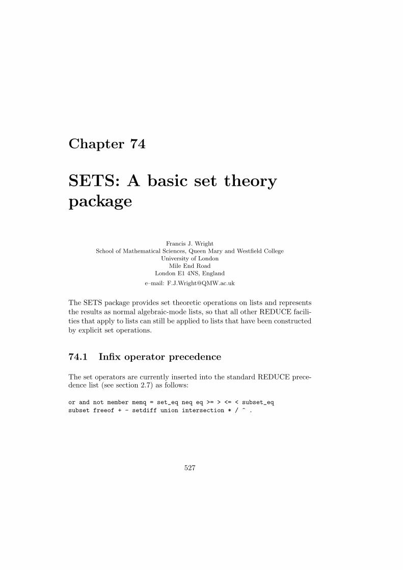
Chapter 74
SETS: A basic set theorypackage
Francis J. WrightSchool of Mathematical Sciences, Queen Mary and Westfield College
University of LondonMile End Road
London E1 4NS, England
e–mail: [email protected]
The SETS package provides set theoretic operations on lists and representsthe results as normal algebraic-mode lists, so that all other REDUCE facili-ties that apply to lists can still be applied to lists that have been constructedby explicit set operations.
74.1 Infix operator precedence
The set operators are currently inserted into the standard REDUCE prece-dence list (see section 2.7) as follows:
or and not member memq = set_eq neq eq >= > <= < subset_eqsubset freeof + - setdiff union intersection * / ^ .
527

528 CHAPTER 74. SETS: A BASIC SET THEORY PACKAGE
74.2 Explicit set representation and MKSET
Explicit sets are represented by lists, and there is a need to convert standardREDUCE lists into a set by removing duplicates. The package also ordersthe members of the set so the standard = predicate will provide set equality.
mkset 1,2,y,x*y,x+y;
x + y,x*y,y,1,2
The empty set is represented by the empty list .
74.3 Union and intersection
The intersection operator has the name intersect, and set union is denotesbyunion. These operators will probably most commonly be used as binaryinfix operators applied to explicit sets,
1,2,3 union 2,3,4;
1,2,3,4
1,2,3 intersect 2,3,4;
2,3
74.4 Symbolic set expressions
If one or more of the arguments evaluates to an unbound identifier thenit is regarded as representing a symbolic implicit set, and the union or in-tersection will evaluate to an expression that still contains the union orintersection operator. These two operators are symmetric, and so if theyremain symbolic their arguments will be sorted as for any symmetric opera-tor. Such symbolic set expressions are simplified, but the simplification maynot be complete in non-trivial cases. For example:
a union b union union b union 7,3;
3,7 union a union b

74.5. SET DIFFERENCE 529
a intersect ;
Intersection distributes over union, which is not applied by default but isimplemented as a rule list assigned to the variable set distribution rule,e.g.
a intersect (b union c);
(b union c) intersection a
a intersect (b union c) where set_distribution_rule;
a intersection b union a intersection c
74.5 Set difference
The set difference operator is represented by the symbol \ and is alwaysoutput using this symbol, although it can also be input using setdiff. Itis a binary operator.
1,2,3 \ 2,4;
1,3
a \ 1,2;
a\1,2
a \ a;
74.6 Predicates on sets
Set membership, inclusion or equality are all binary infix operators. Theycan only be used within conditional statements or within the argument of theevalb operator provided by this package, and they cannot remain symbolic

530 CHAPTER 74. SETS: A BASIC SET THEORY PACKAGE
– a predicate that cannot be evaluated to a Boolean value causes a normalREDUCE error.
The evalb operator provides a convenient shorthand for an if statementdesigned purely to display the value of any Boolean expression (not onlypredicates defined in this package).
if a = a then true else false;
true
evalb(a = a);
true
if a = b then true else false;
false
74.6.1 Set membership
Set membership is tested by the predicate member. Its left operand is re-garded as a potential set element and its right operand must evaluate to anexplicit set. There is currently no sense in which the right operand could bean implicit set.
evalb(1 member 1,2,3);
true
evalb(2 member 1,2 intersect 2,3);
true
evalb(a member b);
***** b invalid as list
74.6.2 Set inclusion
Set inclusion is tested by the predicate subset eq where a subset eq b istrue if the set a is either a subset of or equal to the set b; strict inclusionis tested by the predicate subset where a subset b is true if the set a is

74.6. PREDICATES ON SETS 531
strictly a subset of the set b and is false is a is equal to b. These predicatesprovide some support for symbolic set expressions, but is incomplete.
evalb(1,2 subset_eq 1,2,3);
true
evalb(1,2 subset_eq 1,2);
true
evalb(1,2 subset 1,2);
false
evalb(a subset a union b);
true

532 CHAPTER 74. SETS: A BASIC SET THEORY PACKAGE
evalb(a\b subset a);
true
An undecidable predicate causes a normal REDUCE error, e.g.
evalb(a subset_eq b);
***** Cannot evaluate a subset_eq b as Boolean-valued setexpression
74.6.3 Set equality
As explained above, equality of two sets in canonical form can be reliablytested by the standard REDUCE equality predicate (=).

Chapter 75
SPARSE: Sparse Matrices
Stephen ScowcroftKonrad-Zuse-Zentrum fur Informationstechnik Berlin
Takustrase 7D-14195 Berlin-Dahlem, Germany
75.1 Introduction
This package extends the available matrix feature to enable calculations withsparse matrices. It also provides a selection of functions that are useful inthe world of linear algebra with respect to sparse matrices.The package is loaded by: load package sparse;
75.2 Sparse Matrix Calculations
To extend the syntax of this class of calculations an expression type sparseis added. An identifier may be declared a sparse variable by the declarationsparse. The size of the sparse matrix must be declared explicitly in thematrix declaration. This declaration SPARSE is similar to the declarationMATRIX. Once a matrix has been declared a sparse matrix all elements ofthe matrix are treated as if they were initialized to 0. When printing outa sparse matrix only the non-zero elements are printed due to the fact thatonly the non-zero elements of the matrix are stored. To assign values tothe elements of the declared sparse matrix we use the same syntax as for
533

534 CHAPTER 75. SPARSE: SPARSE MATRICES
matrices.
sparse aa(10,1),bb(200,200);aa(1,1):=10;bb(100,150):=a;
75.3 Linear Algebra Package for Sparse Matrices
Most of the functions of this package are related to the functions of thelinear algebra package LINALG. For further explanation and examples of thevarious functions please refer to the LINALG package.
75.3.1 Basic matrix handling
spadd columns spadd rows spadd to columns spadd to rowsspaugment columns spchar poly spcol dim spcopy intospdiagonal spextend spfind companion spget columnsspget rows sphermitian tp spmatrix augment spmatrix stackspminor spmult columns spmult rows sppivotspremove columns spremove rows sprow dim sprows pivotspstack rows spsub matrix spswap columns spswap entriesspswap rows
75.3.2 Constructors
Functions that create sparse matrices.
spband matrix spblock matrix spchar matrix spcoeff matrixspcompanion sphessian spjacobian spjordan blockspmake identity
75.3.3 High level algorithms
spchar poly spcholesky spgram schmidt splu decomsppseudo inverse svd

75.3. LINEAR ALGEBRA PACKAGE FOR SPARSE MATRICES 535
75.3.4 Predicates
matrixp sparsematp squarep symmetricp

536 CHAPTER 75. SPARSE: SPARSE MATRICES

Chapter 76
SPDE: A package for findingsymmetry groups of PDE’s
Fritz SchwarzGMD, Institut F1
Postfach 12405205 St. Augustin, Germany
e–mail: [email protected]
The package SPDE provides a set of functions which may be applied to de-termine the symmetry group of Lie- or point-symmetries of a given systemof partial differential equations. Preferably it is used interactively on a com-puter terminal. In many cases the determining system is solved completelyautomatically. In some other cases the user has to provide some additionalinput information for the solution algorithm to terminate.
76.1 System Functions and Variables
The symmetry analysis of partial differential equations logically falls intothree parts. Accordingly the most important functions provided by thepackage are:
Some other useful functions for obtaining various kinds of output are:
SPDE expects a system of differential equations to be defined as the valuesof the operator deq and other operators. A simple example follows.
537

538 CHAPTER 76. SPDE: SYMMETRY GROUPS OF PDE’S
Function name OperationCRESYS(<arguments>) Constructs determining system
SIMPSYS() Solves determining systemRESULT() Prints infinitesimal generators
and commutator table
Table 76.1: SPDE Functions
Function name OperationPRSYS() Prints determining systemPRGEN() Prints infinitesimal generators
COMM(U,V) Prints commutator of generators U and V
Table 76.2: SPDE Useful Output Functions
load_package spde;
deq 1:=u(1,1)+u(1,2,2);
deq(1) := u(1,2,2) + u(1,1)
CRESYS deq 1;
PRSYS();
GL(1):=2*df(eta(1),u(1),x(2)) - df(xi(2),x(2),2) - df(xi(2),x(1))
GL(2):=df(eta(1),u(1),2) - 2*df(xi(2),u(1),x(2))
GL(3):=df(eta(1),x(2),2) + df(eta(1),x(1))
GL(4):=df(xi(2),u(1),2)
GL(5):=df(xi(2),u(1)) - df(xi(1),u(1),x(2))
GL(6):=2*df(xi(2),x(2)) - df(xi(1),x(2),2) - df(xi(1),x(1))
GL(7):=df(xi(1),u(1),2)
GL(8):=df(xi(1),u(1))

76.1. SYSTEM FUNCTIONS AND VARIABLES 539
GL(9):=df(xi(1),x(2))
The remaining dependencies
xi(2) depends on u(1),x(2),x(1)
xi(1) depends on u(1),x(2),x(1)
eta(1) depends on u(1),x(2),x(1)
A detailed description can be found in the SPDE documentation and exam-ples.

540 CHAPTER 76. SPDE: SYMMETRY GROUPS OF PDE’S

Chapter 77
SPECFN: Package for specialfunctions
Chris Cannam & Winfried NeunKonrad–Zuse–Zentrum fur Informationstechnik Berlin
Takustrase 7D–14195 Berlin–Dahlem, Germany
e–mail: [email protected]
This package is designed to provide algebraic and numeric manipulations ofseveral common special functions, namely:
• Bernoulli Numbers and Polynomials;
• Euler numbers and Polynomials;
• Fibonacci numbers and Polynomials;
• Stirling Numbers;
• Binomial Coefficients;
• Pochhammer notation;
• The Gamma function;
• The Psi function and its derivatives;
• The Riemann Zeta function;
541

542 CHAPTER 77. SPECFN: PACKAGE FOR SPECIAL FUNCTIONS
• The Bessel functions J and Y of the first and second kinds;
• The modified Bessel functions I and K;
• The Hankel functions H1 and H2;
• The Kummer hypergeometric functions M and U;
• The Beta function, and Struve, Lommel and Whittaker functions;
• The Airy functions;
• The Exponential Integral, the Sine and Cosine Integrals;
• The Hyperbolic Sine and Cosine Integrals;
• The Fresnel Integrals and the Error function;
• The Dilog function;
• The Polylogarithm and Lerch Phi function;
• Hermite Polynomials;
• Jacobi Polynomials;
• Legendre Polynomials;
• Associated Legendre Functions (Spherical and Solid Harmonics);
• Laguerre Polynomials;
• Chebyshev Polynomials;
• Gegenbauer Polynomials;
• Lambert’s ω function;
• Jacobi Elliptic Functions and Integrals;
• 3j symbols, 6j symbols and Clebsch Gordan coefficients;
• and some well-known constants.
77.1. SIMPLIFICATION AND APPROXIMATION 543
77.1 Simplification and Approximation
All of the operators supported by this package have certain algebraic sim-plification rules to handle special cases, poles, derivatives and so on. Suchrules are applied whenever they are appropriate. However, if the ROUNDEDswitch is on, numeric evaluation is also carried out. Unless otherwise statedbelow, the result of an application of a special function operator to real orcomplex numeric arguments in rounded mode will be approximated numeri-cally whenever it is possible to do so. All approximations are to the currentprecision.
77.2 Constants
Some well-known constants are defined in the special function package. Im-portant properties of these constants which can be used to define them arealso known. Numerical values are computed at arbitrary precision if theswitch ROUNDED is on.
• Euler Gamma : Euler’s constants, also available as -ψ(1);
• Catalan : Catalan’s constant;
• Khinchin : Khinchin’s constant;
• Golden Ratio : 1+√
52
77.3 Functions
The functions provided by this package are given in the following tables.

544 CHAPTER 77. SPECFN: PACKAGE FOR SPECIAL FUNCTIONS
Function Operator
( nm
)Binomial(n,m)
Motzkin(n) Motzkin(n)Bernoulli(n) or Bn Bernoulli(n)
Euler(n) or En Euler(n)Fibonacci(n) or Fn Fibonacci(n)
S(m)n Stirling1(n,m)
S(m)n Stirling2(n,m)
B(z, w) Beta(z,w)Γ(z) Gamma(z)
incomplete Beta Bx(a, b) iBeta(a,b,x)incomplete Gamma Γ(a, z) iGamma(a,z)
(a)k Pochhammer(a,k)ψ(z) Psi(z)
ψ(n)(z) Polygamma(n,z)Riemann’s ζ(z) Zeta(z)
Jν(z) BesselJ(nu,z)Yν(z) BesselY(nu,z)Iν(z) BesselI(nu,z)Kν(z) BesselK(nu,z)
H(1)ν (z) Hankel1(nu,z)
H(2)ν (z) Hankel2(nu,z)
B(z, w) Beta(z,w)

77.3. FUNCTIONS 545
Function Operator
Hν(z) StruveH(nu,z)Lν(z) StruveL(nu,z)sa,b(z) Lommel1(a,b,z)Sa,b(z) Lommel2(a,b,z)Ai(z) Airy Ai(z)Bi(z) Airy Bi(z)Ai′(z) Airy Aiprime(z)Bi′(z) Airy Biprime(z)
M(a, b, z) or 1F1(a, b; z) or Φ(a, b; z) KummerM(a,b,z)U(a, b, z) or z−a
2F0(a, b; z) or Ψ(a, b; z) KummerU(a,b,z)Mκ,µ(z) WhittakerM(kappa,mu,z)Wκ,µ(z) WhittakerW(kappa,mu,z)Bn(x) BernoulliP(n,x)En(x) EulerP(n,x)
Fibonacci Polynomials Fn(x) FibonacciP(n,x)
C(α)n (x) GegenbauerP(n,alpha,x)Hn(x) HermiteP(n,x)Ln(x) LaguerreP(n,x)
L(m)n (x) LaguerreP(n,m,x)Pn(x) LegendreP(n,x)
P(m)n (x) LegendreP(n,m,x)
P(α,β)n (x) JacobiP(n,alpha,beta,x)Un(x) ChebyshevU(n,x)Tn(x) ChebyshevT(n,x)
Function Operator
Y mn (x, y, z, r2) SolidHarmonicY(n,m,x,y,z,r2)
Y mn (θ, φ) SphericalHarmonicY(n,m,theta,phi)(
j1m1
j2m2
j3m3
)ThreeJSymbol(j1,m1,j2,m2,j3,m3)
(j1m1j2m2|j1j2j3 −m3) Clebsch Gordan(j1,m1,j2,m2,j3,m3)j1l1
j2l2
j3l3
SixJSymbol(j1,j2,j3,l1,l2,l3)

546 CHAPTER 77. SPECFN: PACKAGE FOR SPECIAL FUNCTIONS
Function Operator
Si(z) Si(z)si(z) s i(z)Ci(z) Ci(z)Shi(z) Shi(z)Chi(z) Chi(z)erf(z) erf(z)erfc(z) erfc(z)Ei(z) Ei(z)li(z) li(z)C(x) Fresnel C(x)S(x) Fresnel S(x)
dilog(z) dilog(z)Lin(z) Polylog(n,z)
Lerch Φ(z, s, a) Lerch Phi(z,s,a)
sn(u|m) Jacobisn(u,m)dn(u|m) Jacobidn(u,m)cn(u|m) Jacobicn(u,m)cd(u|m) Jacobicd(u,m)sd(u|m) Jacobisd(u,m)nd(u|m) Jacobind(u,m)dc(u|m) Jacobidc(u,m)nc(u|m) Jacobinc(u,m)sc(u|m) Jacobisc(u,m)ns(u|m) Jacobins(u,m)ds(u|m) Jacobids(u,m)cs(u|m) Jacobics(u,m)F (φ|m) EllipticF(phi,m)K(m) EllipticK(m)
E(φ|m)orE(m) EllipticE(phi,m) orEllipticE(m)
H(u|m),H1(u|m),Θ1(u|m),Θ(u|m) EllipticTheta(a,u,m)θ1(u|m), θ2(u|m), θ3(u|m), θ4(u|m) EllipticTheta(a,u,m)
Z(u|m) Zeta function(u,m)
Lambert ω(z) Lambert W(z)

Chapter 78
SPECFN2: Special specialfunctions
Victor S. AdamchikByelorussian University
Minsk, Belorus
and
Winfried NeunKonrad–Zuse–Zentrum fur Informationstechnik Berlin
Takustrase 7D–14195 Berlin–Dahlem, Germany
e–mail: [email protected]
The (generalised) hypergeometric functions
pFq
(a1, . . . , ap
b1, . . . , bq
∣∣∣∣∣z)
are defined in textbooks on special functions.
78.1 REDUCE operator HYPERGEOMETRIC
The operator hypergeometric expects 3 arguments, namely the list of upperparameters (which may be empty), the list of lower parameters (which maybe empty too), and the argument, e.g:
547

548 CHAPTER 78. SPECFN2: SPECIAL SPECIAL FUNCTIONS
hypergeometric (,,z);
ZE
hypergeometric (1/2,1,3/2,-x^2);
ATAN(X)---------
X
78.2 Enlarging the HYPERGEOMETRIC opera-tor
Since hundreds of particular cases for the generalised hypergeometric func-tions can be found in the literature, one cannot expect that all cases areknown to the hypergeometric operator. Nevertheless the set of specialcases can be augmented by adding rules to the REDUCE system, e.g.
let hypergeometric(1/2,1/2,3/2,-(~x)^2) => asinh(x)/x;

Chapter 79
SUM: A package for seriessummation
Fujio KakoDepartment of Mathematics, Faculty of Science
Hiroshima UniversityHiroshima 730, JAPAN
e–mail: [email protected]
This package implements the Gosper algorithm for the summation of series.It defines operators SUM and PROD. The operator SUM returns the indef-inite or definite summation of a given expression, and the operator PRODreturns the product of the given expression. These are used with the syntax:
SUM(EXPR:expression, K:kernel, [LOLIM:expression [, UPLIM:expression]])PROD(EXPR:expression, K:kernel, [LOLIM:expression [, UPLIM:expression]])
If there is no closed form solution, these operators return the input un-changed. UPLIM and LOLIM are optional parameters specifying the lowerlimit and upper limit of the summation (or product), respectively. If UP-LIM is not supplied, the upper limit is taken as K (the summation variableitself).
For example:
sum(n**3,n);
sum(a+k*r,k,0,n-1);
549

550 CHAPTER 79. SUM: A PACKAGE FOR SERIES SUMMATION
sum(1/((p+(k-1)*q)*(p+k*q)),k,1,n+1);
prod(k/(k-2),k);
Gosper’s algorithm succeeds whenever the ratio
∑nk=n0
f(k)∑n−1
k=n0f(k)
is a rational function of n. The function SUM!-SQ handles basic functionssuch as polynomials, rational functions and exponentials.
The trigonometric functions sin, cos, etc. are converted to exponentials andthen Gosper’s algorithm is applied. The result is converted back into sin,cos, sinh and cosh.
Summations of logarithms or products of exponentials are treated by theformula:
n∑
k=n0
log f(k) = logn∏
k=n0
f(k)
n∏
k=n0
exp f(k) = expn∑
k=n0
f(k)
Other functions can be summed by providing LET rules which must relatethe functions evaluated at k and k − 1 (k being the summation variable).
operator f,gg; % gg used to avoid possible conflict with high energy% physics operator.
for all n,m such that fixp m letf(n+m)=if m > 0 then f(n+m-1)*(b*(n+m)**2+c*(n+m)+d)
else f(n+m+1)/(b*(n+m+1)**2+c*(n+m+1)+d);
for all n,m such that fixp m letgg(n+m)=if m > 0 then gg(n+m-1)*(b*(n+m)**2+c*(n+m)+e)
else gg(n+m+1)/(b*(n+m+1)**2+c*(n+m+1)+e);

551
sum(f(n-1)/gg(n),n);
f(n)---------------gg(n)*(d - e)

552 CHAPTER 79. SUM: A PACKAGE FOR SERIES SUMMATION
Chapter 80
SUSY2: Super Symmetry
Ziemowit PopowiczInstitute of Theoretical Physics, University of Wroclaw
pl. M. Borna 9 50-205 Wroclaw, Polande-mail: [email protected]
This package deals with supersymmetric functions and with algebra of su-persymmetric operators in the extended N=2 as well as in the nonextendedN=1 supersymmetry. It allows us to make the realization of SuSy algebraof differential operators, compute the gradients of given SuSy Hamiltoniansand to obtain SuSy version of soliton equations using the SuSy Lax ap-proach. There are also many additional procedures encountered in the SuSysoliton approach, as for example: conjugation of a given SuSy operator,computation of general form of SuSy Hamiltonians (up to SuSy-divergenceequivalence), checking of the validity of the Jacobi identity for some SuSyHamiltonian operators.
To load the package, type load susy2;
For full explanation and further examples, please refer to the detailed doc-umentation and the susy2.tst which comes with this package.
553

554 CHAPTER 80. SUSY2: SUPER SYMMETRY
80.1 Operators
80.1.1 Operators for constructing Objects
The superfunctions are represented in this package by BOS(f,n,m) for super-bosons and FER(f,n,m) for superfermions. The first index denotes the nameof the given superobject, the second denotes the value of SuSy derivatives,and the last gives the value of usual derivative.In addition to the definitions of the superfunctions, also the inverse and theexponential of superbosons can be defined (where the inverse is defined asBOS(f,n,m,-1) with the property bos(f,n,m,-1)*bos(f,n,m,1)=1). The expo-nential of the superboson function is AXP(BOS(f,0,0)).The operator FUN and GRAS denote the classical and the Grassmann func-tion.Three different realizations of supersymmetric derivatives are implemented.To select traditional realization declare LET TRAD. In order to select chiralor chiral1 algebra declare LET CHIRAL or LET CHIRAL1. For usual differen-tiation the operator D(1) stands for right and D(2) for left differentiation.SuSy derivatives are denoted as der and del. DER and DEL are one compo-nent argument operations and represent the left and right operators. Theaction of these operators on the superfunctions depends on the choice of thesupersymmetry algebra.
BOS(f,n,m) BOS(f,n,m,k) FER(f,n,m) AXP(f) FUN(f,n) FUN(f,n,m)GRAS(f,n) AXX(f) D(1) D(2) D(3) D(-1)D(-2) D(-3) D(-4) DR(-n) DER(1) DER(2)DEL(1) DEL(2)
Example:
1: load susy2;
2: bos(f,0,2,-2)*axp(fer(k,1,2))*del(1); %first susy derivative
2*fer(f,1,2)*bos(f,0,2,-3)*axp(fer(k,1,2))
- bos(k,0,3)*bos(f,0,2,-2)*axp(fer(k,1,2))
+ del(1)*bos(f,0,2,-2)*axp(fer(k,1,2))

80.1. OPERATORS 555
3: sub(del=der,ws);
bos(f,0,2,-2)*axp(fer(k,1,2))*der(1)
80.1.2 Commands
There are plenty of operators on superfunction objects. Some of them areintroduced here briefly.
• By using the operators FPART, BPART, BFPART and BF PART it ispossible to compute the coordinates of the arbitrary SuSyexpressions.
• With W COMB, FCOMB and PSE ELE there are three operators to be ableto construct different possible combinations of superfunctions andsuper-pseudo-differential elements with the given conformaldimensions .
• The three operators S PART, D PART and SD PART are implemented toobtain the components of the (pseudo)-SuSy element.
• RZUT is used to obtain the projection onto the invariant subspace(with respect to commutator) of algebra of pseudo-SuSy-differentialalgebra.
• To obtain the list of the same combinations of some superfunctionsand (SuSy) derivatives from some given operator-valued expression,the operators LYST, LYST1 and LYST2 are constructed.

556 CHAPTER 80. SUSY2: SUPER SYMMETRY
FPART(expression) BPART(expression)BF PART(expression,n) B PART(expression,n)PR(n,expression) PG(n,expression)W COMB(f,n,x,...,m,z,y) FCOMB(f,n,x,...,m,z,y)PSE ELE(n,f,n,...,z)S PART(expression,n) D PART(expression,n)SD PART(expression,n,m) CP(expression)RZUT(expression,n) LYST(expression)LYST1(expression) LYST2(expression)CHAN(expression) ODWA(expression)GRA(expression,f) DYW(expression,f)WAR(expression,f) DOT HAM(equations,expression)N GAT(operator,list) FJACOB(operator,list)JACOB(operator,list,α, β, γ) MACIERZ(expression,x,y)S INT(number,expression,list)
Example:
4: xxx:=fer(f,2,3);
xxx := fer(f,2,3)
5: fpart(xxx); % all components
- fun(f0,4) + 2*fun(f1,3) gras(ff2,4)gras(ff2,3), ----------------------------,0, -------------
2 26: bpart(xxx); % bosonic sector
- fun(f0,4) + 2*fun(f1,3)0,----------------------------,0,0
2
9: b_part(xxx,1); %the given component in the bosonic sector
- fun(f0,4) + 2*fun(f1,3)----------------------------
2

80.2. OPTIONS 557
80.2 Options
The are several options defined in this package. Please note that they areactivated by typing let <option>. See also above.The TRAD, CHIRAL and CHIRAL1 select the different realizations of thesupersymmetric derivatives. By default traditional algebra is selected.If the command LET INVERSE is used, then three indices bos objects aretransformed onto four indices objects.
TRAD CHIRAL CHIRAL1 INVERSE DRR NODRR
Example:
10: let inverse;
11: bos(f,0,3)**3*bos(k,3,1)**40*bos(f,0,3,-2);
bos(k,3,1,40)*bos(f,0,3,1);
12: clearrules inverse;
13: xxx:=fer(f,1,2)*bos(k,0,2,-2);
xxx := fer(f,1,2)*bos(k,0,2,-2)
14: pr(1,xxx); % first susy derivative
- 2*fer(k,1,2)*fer(f,1,2)*bos(k,0,2,-3) + bos(k,0,2,-2)*bos(f,0,3)
15: pr(2,xxx); %second susy derivative
- 2*fer(k,2,2)*fer(f,1,2)*bos(k,0,2,-3) - bos(k,0,2,-2)*bos(f,3,2)
16: clearrules trad;
17: let chiral; % changing to chiral algebra
18: pr(1,xxx);
- 2*fer(k,1,2)*fer(f,1,2)*bos(k,0,2,-3)

558 CHAPTER 80. SUSY2: SUPER SYMMETRY

Chapter 81
SYMMETRY: Symmetricmatrices
Karin GatermannKonrad–Zuse–Zentrum fur Informationstechnik Berlin
Takustrase 7D–14195 Berlin–Dahlem, Germany
e–mail: [email protected]
The SYMMETRY package provides procedures that computesymmetry-adapted bases and block diagonal forms of matrices which havethe symmetry of a group.
81.1 Operators for linear representations
The data structure for a linear representation, a representation, is a listconsisting of the group identifier and equations which assign matrices tothe generators of the group.
Example:
rr:=mat((0,1,0,0),(0,0,1,0),(0,0,0,1),(1,0,0,0));
sp:=mat((0,1,0,0),
559
560 CHAPTER 81. SYMMETRY: SYMMETRIC MATRICES
(1,0,0,0),(0,0,0,1),(0,0,1,0));
representation:=D4,rD4=rr,sD4=sp;
For orthogonal (unitarian) representations the following operators areavailable.
canonicaldecomposition(representation);
returns an equation giving the canonical decomposition of the linearrepresentation.
character(representation);
computes the character of the linear representation. The result is a list ofthe group identifier and of lists consisting of a list of group elements in oneequivalence class and a real or complex number.
symmetrybasis(representation,nr);
computes the basis of the isotypic component corresponding to theirreducible representation of type nr. If the nr-th irreducible representationis multidimensional, the basis is symmetry adapted. The output is amatrix.
symmetrybasispart(representation,nr);
is similar as symmetrybasis, but for multidimensional irreduciblerepresentations only the first part of the symmetry adapted basis iscomputed.
allsymmetrybases(representation);
is similar as symmetrybasis and symmetrybasispart, but the bases of allisotypic components are computed and thus a complete coordinatetransformation is returned.
diagonalize(matrix,representation);
returns the block diagonal form of matrix which has the symmetry of thegiven linear representation. Otherwise an error message occurs.
81.2. DISPLAY OPERATORS 561
81.2 Display Operators
Access is provided to the information for a group, and for addingknowledge for other groups. This is explained in detail in the Symmetryon-line documentation.

562 CHAPTER 81. SYMMETRY: SYMMETRIC MATRICES

Chapter 82
TAYLOR: Manipulation ofTaylor series
Rainer SchopfZentrum fur Datenverarbeitung der Universitat Mainz
Anselm-Franz-von-Bentzel-Weg 12D-55055 Mainz, Germany
e–mail: [email protected]
The TAYLOR package of REDUCE allow Taylor expansion in one orseveral variables, and efficient manipulation of the resulting Taylor series.Capabilities include basic operations (addition, subtraction, multiplicationand division), and also application of certain algebraic and transcendentalfunctions. To a certain extent, Laurent and Puiseux expansions can beperformed as well. In many cases, separable singularities are detected andfactored out.
TAYLOR(EXP:exprn[,VAR:kernel, VAR0:exprn,ORDER:integer]. . . ):exprn
where EXP is the expression to be expanded. It can be any REDUCEobject, even an expression containing other Taylor kernels. VAR is thekernel with respect to which EXP is to be expanded. VAR0 denotes thepoint about which and ORDER the order up to which expansion is to takeplace. If more than one (VAR, VAR0, ORDER) triple is specified TAYLORwill expand its first argument independently with respect to each variablein turn. For example,
taylor(e^(x^2+y^2),x,0,2,y,0,2);
563

564 CHAPTER 82. TAYLOR: MANIPULATION OF TAYLOR SERIES
will calculate the Taylor expansion up to order X2 ∗ Y 2. Note that oncethe expansion has been done it is not possible to calculate higher orders.Instead of a kernel, VAR may also be a list of kernels. In this caseexpansion will take place in a way so that the sum of the degrees of thekernels does not exceed ORDER. If VAR0 evaluates to the specialidentifier INFINITY TAYLOR tries to expand EXP in a series in 1/VAR.
The expansion is performed variable per variable, i.e. in the example aboveby first expanding exp(x2 + y2) with respect to x and then expandingevery coefficient with respect to y.
There are two extra operators to compute the Taylor expansions ofimplicit and inverse functions:
IMPLICIT TAYLOR(F:exprn,VAR1,VAR2:kernel,
VAR10,VAR20:exprn, ORDER:integer):exprn
takes a function F depending on two variables VAR1 and VAR2 andcomputes the Taylor series of the implicit function VAR2(VAR1) given bythe equation F(VAR1,VAR2) = 0. For example,
implicit_taylor(x^2 + y^2 - 1,x,y,0,1,5);
INVERSE TAYLOR(F:exprn,VAR1,VAR2:kernel,
VAR10:exprn, ORDER:integer):exprn
takes a function F depending on VAR1 and computes the Taylor series ofthe inverse of F with respect to VAR2. For example,
inverse_taylor(exp(x)-1,x,y,0,8);
When a Taylor kernel is printed, only a certain number of (non-zero)coefficients are shown. If there are more, an expression of the form(n terms) is printed to indicate how many non-zero terms have beensuppressed. The number of terms printed is given by the value of theshared algebraic variable TAYLORPRINTTERMS. Allowed values are integersand the special identifier ALL. The latter setting specifies that all terms areto be printed. The default setting is 5.
If the switch TAYLORKEEPORIGINAL is set to ON the original expression EXPis kept for later reference. It can be recovered by means of the operator
565
TAYLORORIGINAL(EXP:exprn):exprn
An error is signalled if EXP is not a Taylor kernel or if the originalexpression was not kept, i.e. if TAYLORKEEPORIGINAL was OFF duringexpansion. The template of a Taylor kernel, i.e. the list of all variableswith respect to which expansion took place together with expansion pointand order can be extracted using
TAYLORTEMPLATE(EXP:exprn):list
This returns a list of lists with the three elements (VAR,VAR0,ORDER).As with TAYLORORIGINAL, an error is signalled if EXP is not a Taylorkernel.
TAYLORTOSTANDARD(EXP:exprn):exprn
converts all Taylor kernels in EXP into standard form and resimplifies theresult.
TAYLORSERIESP(EXP:exprn):boolean
may be used to determine if EXP is a Taylor kernel. Note that thisoperator is subject to the same restrictions as, e.g., ORDP or NUMBERP,i.e. it may only be used in boolean expressions in IF or LET statements.Finally there is
TAYLORCOMBINE(EXP:exprn):exprn
which tries to combine all Taylor kernels found in EXP into one.Operations currently possible are:
• Addition, subtraction, multiplication, and division.
• Roots, exponentials, and logarithms.
• Trigonometric and hyperbolic functions and their inverses.
Application of unary operators like LOG and ATAN will nearly alwayssucceed. For binary operations their arguments have to be Taylor kernelswith the same template. This means that the expansion variable and theexpansion point must match. Expansion order is not so important,different order usually means that one of them is truncated before doingthe operation.
If TAYLORKEEPORIGINAL is set to ON and if all Taylor kernels in exp havetheir original expressions kept TAYLORCOMBINE will also combine these and

566 CHAPTER 82. TAYLOR: MANIPULATION OF TAYLOR SERIES
store the result as the original expression of the resulting Taylor kernel.There is also the switch TAYLORAUTOEXPAND (see below).
There are a few restrictions to avoid mathematically undefined expressions:it is not possible to take the logarithm of a Taylor kernel which has noterms (i.e. is zero), or to divide by such a beast. There are some provisionsmade to detect singularities during expansion: poles that arise because thedenominator has zeros at the expansion point are detected and properlytreated, i.e. the Taylor kernel will start with a negative power. (This isaccomplished by expanding numerator and denominator separately andcombining the results.) Essential singularities of the known functions (seeabove) are handled correctly.
Differentiation of a Taylor expression is possible. Differentiating withrespect to one of the Taylor variables will decrease the order by one.
Substitution is a bit restricted: Taylor variables can only be replaced byother kernels. There is one exception to this rule: one can alwayssubstitute a Taylor variable by an expression that evaluates to a constant.Note that REDUCE will not always be able to determine that anexpression is constant.
Only simple Taylor kernels can be integrated. More complicatedexpressions that contain Taylor kernels as parts of themselves areautomatically converted into a standard representation by means of theTAYLORTOSTANDARD operator. In this case a suitable warning isprinted.
It is possible to revert a Taylor series of a function f , i.e., to compute thefirst terms of the expansion of the inverse of f from the expansion of f .This is done by the operator
TAYLORREVERT(EXP:exprn,OLDVAR:kernel, NEWVAR:kernel):exprn
EXP must evaluate to a Taylor kernel with OLDVAR being one of itsexpansion variables. Example:
taylor (u - u**2, u, 0, 5);taylorrevert (ws, u, x);
This package introduces a number of new switches:
• If TAYLORAUTOCOMBINE is set to ON REDUCE automatically combinesTaylor expressions during the simplification process. This is

567
equivalent to applying TAYLORCOMBINE to every expression thatcontains Taylor kernels. Default is ON.
• TAYLORAUTOEXPAND makes Taylor expressions “contagious” in thesense that TAYLORCOMBINE tries to Taylor expand all non-Taylorsubexpressions and to combine the result with the rest. Default isOFF.
• TAYLORKEEPORIGINAL, if set to ON, forces the package to keep theoriginal expression, i.e. the expression that was Taylor expanded. Alloperations performed on the Taylor kernels are also applied to thisexpression which can be recovered using the operatorTAYLORORIGINAL. Default is OFF.
• TAYLORPRINTORDER, if set to ON, causes the remainder to be printedin big-O notation. Otherwise, three dots are printed. Default is ON.

568 CHAPTER 82. TAYLOR: MANIPULATION OF TAYLOR SERIES

Chapter 83
TPS: A truncated powerseries package
Alan BarnesDept. of Computer Science and Applied Mathematics
Aston University, Aston Triangle,Birmingham B4 7ET, England
e–mail: [email protected]
and
Julian PadgetSchool of Mathematics, University of Bath
Bath, BA2 7AY, England
e–mail: [email protected]
This package implements formal Laurent series expansions in one variableusing the domain mechanism of REDUCE. This means that power seriesobjects can be added, multiplied, differentiated etc. like other first classobjects in the system. A lazy evaluation scheme is used in the package andthus terms of the series are not evaluated until they are required forprinting or for use in calculating terms in other power series. The seriesare extendible giving the user the impression that the full infinite series isbeing manipulated. The errors that can sometimes occur using series thatare truncated at some fixed depth (for example when a term in therequired series depends on terms of an intermediate series beyond thetruncation depth) are thus avoided.
569

570 CHAPTER 83. TPS: A TRUNCATED POWER SERIES PACKAGE
83.1 Basic Truncated Power Series
83.1.1 PS Operator
Syntax:
PS(EXPRN:algebraic,DEPVAR:kernel,ABOUT:algebraic):ps object
The PS operator returns a power series object representing the univariateformal power series expansion of EXPRN with respect to the dependentvariable DEPVAR about the expansion point ABOUT. EXPRN may itselfcontain power series objects.
The algebraic expression ABOUT should simplify to an expression which isindependent of the dependent variable DEPVAR, otherwise an error willresult. If ABOUT is the identifier INFINITY then the power seriesexpansion about DEPVAR = ∞ is obtained in ascending powers of1/DEPVAR.
The power series object representing EXPRN is compiled and then anumber of terms of the power series expansion are evaluated. Theexpansion is carried out as far as the value specified by PSEXPLIM. If,subsequently, the value of PSEXPLIM is increased, sufficient information isstored in the power series object to enable the additional terms to becalculated without recalculating the terms already obtained.
If the function has a pole at the expansion point then the correct Laurentseries expansion will be produced.
The following examples are valid uses of PS:
psexplim 6;ps(log x,x,1);ps(e**(sin x),x,0);ps(x/(1+x),x,infinity);ps(sin x/(1-cos x),x,0);
New user-defined functions may be expanded provided the user providesLET rules giving
1. the value of the function at the expansion point
2. a differentiation rule for the new function.

83.1. BASIC TRUNCATED POWER SERIES 571
For example
operator sech;forall x let df(sech x,x)= - sech x * tanh x;let sech 0 = 1;ps(sech(x**2),x,0);
The power series expansion of an integral may also be obtained (even ifREDUCE cannot evaluate the integral in closed form). An example of thisis
ps(int(e**x/x,x),x,1);
Note that if the integration variable is the same as the expansion variablethen REDUCE’s integration package is not called; if on the other hand thetwo variables are different then the integrator is called to integrate each ofthe coefficients in the power series expansion of the integrand. Theconstant of integration is zero by default. If another value is desired, thenthe shared variable PSINTCONST should be set to required value.
83.1.2 PSORDLIM Operator
Syntax:
PSORDLIM(UPTO:integer):integer
or
PSORDLIM():integer
An internal variable is set to the value of UPTO (which should evaluate toan integer). The value returned is the previous value of the variable. Thedefault value is 15.
If PSORDLIM is called with no argument, the current value is returned.
The significance of this control is that the system attempts to find theorder of the power series required, that is the order is the degree of thefirst non-zero term in the power series. If the order is greater than thevalue of this variable an error message is given and the computationaborts. This prevents infinite loops in examples such as
ps(1 - (sin x)**2 - (cos x)**2,x,0);

572 CHAPTER 83. TPS: A TRUNCATED POWER SERIES PACKAGE
where the expression being expanded is identically zero, but is notrecognised as such by REDUCE.
83.2 Controlling Power Series
83.2.1 PSTERM Operator
Syntax:
PSTERM(TPS:power series object,NTH:integer):algebraic
The operator PSTERM returns the NTH term of the existing power seriesobject TPS. If NTH does not evaluate to an integer or TPS to a powerseries object an error results. It should be noted that an integer is treatedas a power series.
83.2.2 PSORDER Operator
Syntax:
PSORDER(TPS:power series object):integer
The operator PSORDER returns the order, that is the degree of the firstnon-zero term, of the power series object TPS. TPS should evaluate to apower series object or an error results. If TPS is zero, the identifierUNDEFINED is returned.
83.2.3 PSSETORDER Operator
Syntax:
PSSETORDER(TPS:power series object, ORD:integer):integer
The operator PSSETORDER sets the order of the power series TPS to thevalue ORD, which should evaluate to an integer. If TPS does not evaluateto a power series object, then an error occurs. The value returned by thisoperator is the previous order of TPS, or 0 if the order of TPS wasundefined. This operator is useful for setting the order of the power seriesof a function defined by a differential equation in cases where the powerseries package is inadequate to determine the order automatically.

83.2. CONTROLLING POWER SERIES 573
83.2.4 PSDEPVAR Operator
Syntax:
PSDEPVAR(TPS:power series object):identifier
The operator PSDEPVAR returns the expansion variable of the power seriesobject TPS. TPS should evaluate to a power series object or an integer,otherwise an error results. If TPS is an integer, the identifier UNDEFINED isreturned.
83.2.5 PSEXPANSIONPT operator
Syntax:
PSEXPANSIONPT(TPS:power series object):algebraic
The operator PSEXPANSIONPT returns the expansion point of the powerseries object TPS. TPS should evaluate to a power series object or aninteger, otherwise an error results. If TPS is integer, the identifierUNDEFINED is returned. If the expansion is about infinity, the identifierINFINITY is returned.
83.2.6 PSFUNCTION Operator
Syntax:
PSFUNCTION(TPS:power series object):algebraic
The operator PSFUNCTION returns the function whose expansion gave riseto the power series object TPS. TPS should evaluate to a power seriesobject or an integer, otherwise an error results.
83.2.7 PSCHANGEVAR Operator
Syntax:
PSCHANGEVAR(TPS:power series object, X:kernel):power series object
The operator PSCHANGEVAR changes the dependent variable of the powerseries object TPS to the variable X. TPS should evaluate to a power seriesobject and X to a kernel, otherwise an error results. Also X should not

574 CHAPTER 83. TPS: A TRUNCATED POWER SERIES PACKAGE
appear as a parameter in TPS. The power series with the new dependentvariable is returned.
83.2.8 PSREVERSE Operator
Syntax:
PSREVERSE(TPS:power series object):power series
Power series reversion. The power series TPS is functionally inverted. Fourcases arise:
1. If the order of the series is 1, then the expansion point of theinverted series is 0.
2. If the order is 0 and if the first order term in TPS is non-zero, thenthe expansion point of the inverted series is taken to be thecoefficient of the zeroth order term in TPS.
3. If the order is -1 the expansion point of the inverted series is thepoint at infinity. In all other cases a REDUCE error is reportedbecause the series cannot be inverted as a power series. Puiseuxexpansion would be required to handle these cases.
4. If the expansion point of TPS is finite it becomes the zeroth orderterm in the inverted series. For expansion about 0 or the point atinfinity the order of the inverted series is one.
If TPS is not a power series object after evaluation an error results.
Here are some examples:
ps(sin x,x,0);psreverse(ws); % produces series for asin x about x=0.ps(exp x,x,0);psreverse ws; % produces series for log x about x=1.ps(sin(1/x),x,infinity);psreverse(ws); % produces series for 1/asin(x) about x=0.
83.2.9 PSCOMPOSE Operator
Syntax:

83.2. CONTROLLING POWER SERIES 575
PSCOMPOSE(TPS1:power series, TPS2:power series):power series
PSCOMPOSE performs power series composition. The power series TPS1 andTPS2 are functionally composed. That is to say that TPS2 is substitutedfor the expansion variable in TPS1 and the result expressed as a powerseries. The dependent variable and expansion point of the result coincidewith those of TPS2. The following conditions apply to power seriescomposition:
1. If the expansion point of TPS1 is 0 then the order of the TPS2 mustbe at least 1.
2. If the expansion point of TPS1 is finite, it should coincide with thecoefficient of the zeroth order term in TPS2. The order of TPS2should also be non-negative in this case.
3. If the expansion point of TPS1 is the point at infinity then the orderof TPS2 must be less than or equal to -1.
If these conditions do not hold the series cannot be composed (with thecurrent algorithm terms of the inverted series would involve infinite sums)and a REDUCE error occurs.
Examples of power series composition include the following.
a:=ps(exp y,y,0); b:=ps(sin x,x,0);pscompose(a,b);% Produces the power series expansion of exp(sin x)% about x=0.
a:=ps(exp z,z,1); b:=ps(cos x,x,0);pscompose(a,b);% Produces the power series expansion of exp(cos x)% about x=0.
a:=ps(cos(1/x),x,infinity); b:=ps(1/sin x,x,0);pscompose(a,b);% Produces the power series expansion of cos(sin x)% about x=0.
83.2.10 PSSUM Operator
Syntax:

576 CHAPTER 83. TPS: A TRUNCATED POWER SERIES PACKAGE
PSSUM(J:kernel = LOWLIM:integer, COEFF:algebraic, X:kernel,ABOUT:algebraic, POWER:algebraic):power series
The formal power series sum for J from LOWLIM to INFINITY of
COEFF*(X-ABOUT)**POWER
or if ABOUT is given as INFINITY
COEFF*(1/X)**POWER
is constructed and returned. This enables power series whose general termis known to be constructed and manipulated using the other procedures ofthe power series package.
J and X should be distinct simple kernels. The algebraics ABOUT,COEFF and POWER should not depend on the expansion variable X,similarly the algebraic ABOUT should not depend on the summationvariable J. The algebraic POWER should be a strictly increasing integervalued function of J for J in the range LOWLIM to INFINITY.
pssum(n=0,1,x,0,n*n);% Produces the power series summation for n=0 to% infinity of x**(n*n).
pssum(m=1,(-1)**(m-1)/(2m-1),y,1,2m-1);% Produces the power series expansion of atan(y-1)% about y=1.
pssum(j=1,-1/j,x,infinity,j);% Produces the power series expansion of log(1-1/x)% about the point at infinity.
pssum(n=0,1,x,0,2n**2+3n) + pssum(n=1,1,x,0,2n**2-3n);% Produces the power series summation for n=-infinity% to +infinity of x**(2n**2+3n).
83.2.11 Arithmetic Operations
As power series objects are domain elements they may be combinedtogether in algebraic expressions in algebraic mode of REDUCE in the

83.3. RESTRICTIONS AND KNOWN BUGS 577
normal way.
For example if A and B are power series objects then the commands suchas:
a*b;a**2+b**2;
will produce power series objects representing the product and the sum ofthe squares of the power series objects A and B respectively.
83.2.12 Differentiation
If A is a power series object depending on X then the input df(a,x); willproduce the power series expansion of the derivative of A with respect toX.
83.3 Restrictions and Known Bugs
If A and B are power series objects and X is a variable which evaluates toitself then currently expressions such as a/b and a*x do not evaluate to asingle power series object (although the results are in each case formallyvalid). Instead use ps(a/b,x,0) and ps(a*x,x,0) etc..

578 CHAPTER 83. TPS: A TRUNCATED POWER SERIES PACKAGE

Chapter 84
TRI: TeX REDUCEinterface
Werner Antweiler, Andreas Strotmann and Volker WinkelmannUniversity of Cologne Computer Center, Abt. Anwendungssoftware, Robert-Koch-Straße
105000 K”oln 41, Germany
e–mail: [email protected] [email protected]@rrz.uni-koeln.de
The REDUCE-TEX-Interface incorporates three levels of TEX output:without line breaking, with line breaking, and with line breaking plusindentation.
During loading the package some default initialisations are performed. Thedefault page width is set to 15 centimetres, the tolerance for page breakingis set to 20 by default. Moreover, TRI is enabled to translate Greek names,e.g. TAU or PSI, into equivalent TEX symbols, e.g. τ or ψ, respectively.Letters are printed lowercase as defined through assertion of the setLOWERCASE.
84.1 Switches for TRI
The three TRI modes can be selected by switches, which can be usedalternatively and incrementally. Switching TEX on gives standardTEX-output; switching TEXBREAK gives broken TEX-output, and TEXINDENTto give broken TEX-output plus indentation. Thus the three levels of TRI
579
580 CHAPTER 84. TRI: TEX REDUCE INTERFACE
are enabled or disabled according to:
On TeX; % switch TeX is onOn TeXBreak; % switches TeX and TeXBreak are onOn TeXIndent; % switches TeX, TeXBreak and TeXIndent are onOff TeXIndent; % switch TeXIndent is offOff TeXBreak; % switches TeXBreak and TeXIndent are offOff TeX; % all three switches are off
How TRI breaks multiple lines of TEX-code may be controlled by settingvalues for page width and tolerance
TeXsetbreak(page_width, tolerance);
Page width is measured in millimetres, and tolerance is a positive integerin the closed interval [0 . . . 10000]. The higher the tolerance, the morebreakpoints become feasible. A tolerance of 0 means that actually nobreakpoint will be considered feasible, while a value of 10000 allows anybreakpoint to be considered feasible. For line-breaking withoutindentation, suitable values for the tolerance lie between 10 and 100. As arule of thumb, use higher values the deeper the term is nested. If usingindentation, use much higher tolerance values; reasonable values fortolerance here lie between 700 and 1500.
84.1.1 Adding Translations
Sometimes it is desirable to add special REDUCE-symbol-to-TEX-itemtranslations. For such a task TRI provides a function TeXlet which bindsany REDUCE-symbol to one of the predefined TEX-items. A call to thisfunction has the following syntax:
TeXlet(REDUCE-symbol, TEX-item);
For example
TeXlet(’velocity,’!v);TeXlet(’gamma,\verb|’!\!G!a!m!m!a! |);TeXlet(’acceleration,\verb|’!\!v!a!r!t!h!e!t!a! |);
Besides this method of single assertions one can assert one of (currently)two standard sets providing substitutions for lowercase and Greek letters.These sets are loaded by default. These sets can be switched on or off

84.2. EXAMPLES OF USE 581
using the functions
TeXassertset setname;TeXretractset setname;
where the setnames currently defined are ’GREEK and ’LOWERCASE.
There are facilities for creating other sets of substitutions, using thefunction TeXitem.
84.2 Examples of Use
Some representative examples demonstrate the capabilities of TRI.
load_package tri;% TeX-REDUCE-Interface 0.50% set greek asserted% set lowercase asserted% \tolerance 10% \hsize=150mm
TeXsetbreak(150,250);% \tolerance 250% \hsize=150mm
on TeXindent;
(x+y)^16/(v-w)^16;$$\displaylines\qdd\(x^16
+16\cdot x^15\cdot y+120\cdot x^14\cdot y^2+560\cdot x^13\cdot y^3+1820\cdot x^12\cdot y^4+4368\cdot x^11\cdot y^5\nl\off327680+8008\cdot x^10\cdot y^6+11440\cdot x^9\cdot y^7+12870\cdot x^8\cdot y^8+11440\cdot x^7\cdot y^9+8008\cdot x^6\cdot y^10\nl\off327680+4368\cdot x^5\cdot y^11
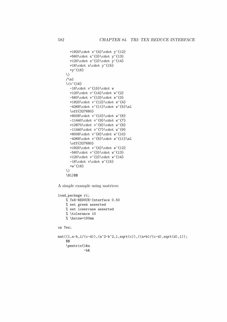
582 CHAPTER 84. TRI: TEX REDUCE INTERFACE
+1820\cdot x^4\cdot y^12+560\cdot x^3\cdot y^13+120\cdot x^2\cdot y^14+16\cdot x\cdot y^15+y^16
\)/\nl\(v^16
-16\cdot v^15\cdot w+120\cdot v^14\cdot w^2-560\cdot v^13\cdot w^3+1820\cdot v^12\cdot w^4-4368\cdot v^11\cdot w^5\nl\off327680+8008\cdot v^10\cdot w^6-11440\cdot v^9\cdot w^7+12870\cdot v^8\cdot w^8-11440\cdot v^7\cdot w^9+8008\cdot v^6\cdot w^10-4368\cdot v^5\cdot w^11\nl\off327680+1820\cdot v^4\cdot w^12-560\cdot v^3\cdot w^13+120\cdot v^2\cdot w^14-16\cdot v\cdot w^15+w^16
\)\Nl$$
A simple example using matrices:
load_package ri;% TeX-REDUCE-Interface 0.50% set greek asserted% set lowercase asserted% \tolerance 10% \hsize=150mm
on Tex;
mat((1,a-b,1/(c-d)),(a^2-b^2,1,sqrt(c)),((a+b)/(c-d),sqrt(d),1));$$\pmatrix1&a
-b&

84.2. EXAMPLES OF USE 583
\frac1c-d\cr
a^2-b^2&1&\sqrtc\cr\fraca
+bc-d&
\sqrtd&1\cr
$$
Note that the resulting output uses a number of TEX macros which aredefined in the file tridefs.tex which is distributed with the example file.

584 CHAPTER 84. TRI: TEX REDUCE INTERFACE

Chapter 85
TRIGSIMP: Simplificationand factorisation oftrigonometric and hyperbolicfunctions
Wolfram Koepf, Andreas Bernig and Herbert MelenkKonrad–Zuse–Zentrum fur Informationstechnik Berlin
Takustrase 7D–14195 Berlin–Dahlem, Germany
e–mail: [email protected]
There are three procedures included in TRIGSIMP: trigsimp, trigfactorizeand triggcd. The first is for finding simplifications of trigonometric orhyperbolic expressions with many options, the second for factorising themand the third for finding the greatest common divisor of two trigonometricor hyperbolic polynomials.
85.1 Simplifiying trigonometric expressions
As there is no normal form for trigonometric and hyperbolic functions, thesame function can convert in many different directions, e.g.sin(2x)↔ 2 sin(x) cos(x). The user has the possibility to give severalparameters to the procedure trigsimp in order to influence the direction
585

586 CHAPTER 85. TRIGSIMP: TRIGONOMETRIC SIMPLIFICATION
of transformations. The decision whether a rational expression intrigonometric and hyperbolic functions vanishes or not is possible.
To simplify a function f, one uses trigsimp(f[,options]). Example:
2: trigsimp(sin(x)^2+cos(x)^2);
1
Possible options are (* denotes the default):
1. sin (*) or cos
2. sinh (*) or cosh
3. expand (*) or combine or compact
4. hyp or trig or expon
5. keepalltrig
From each group one can use at most one option, otherwise an errormessage will occur. The first group fixes the preference used whiletransforming a trigonometric expression. The second group is theequivalent for the hyperbolic functions. The third group determines thetype of transformations. With the default expand, an expression is writtenin a form only using single arguments and no sums of arguments. Withcombine, products of trigonometric functions are transformed totrigonometric functions involving sums of arguments.
trigsimp(sin(x)^2,cos);
2- cos(x) + 1
trigsimp(sin(x)*cos(y),combine);
sin(x - y) + sin(x + y)-------------------------
2

85.2. FACTORISING TRIGONOMETRIC EXPRESSIONS 587
With compact, the REDUCE operator compact (see chapter 31) is appliedto f. This leads often to a simple form, but in contrast to expand onedoesn’t get a normal form.
trigsimp((1-sin(x)**2)**20*(1-cos(x)**2)**20,compact);
40 40cos(x) *sin(x)
With the fourth group each expression is transformed to a trigonometric,hyperbolic or exponential form:
trigsimp(sin(x),hyp);
- sinh(i*x)*i
trigsimp(e^x,trig);
x xcos(---) + sin(---)*i
i i
Usually, tan, cot, sec, csc are expressed in terms of sin and cos. It canbe sometimes useful to avoid this, which is handled by the optionkeepalltrig:
trigsimp(tan(x+y),keepalltrig);
- (tan(x) + tan(y))----------------------
tan(x)*tan(y) - 1
It is possible to use the options of different groups simultaneously.
85.2 Factorising trigonometric expressions
With trigfactorize(p,x) one can factorise the trigonometric orhyperbolic polynomial p with respect to the argument x. Example:
trigfactorize(sin(x),x/2);

588 CHAPTER 85. TRIGSIMP: TRIGONOMETRIC SIMPLIFICATION
x x2,cos(---),sin(---)
2 2
If the polynomial is not coordinated or balanced the output will equal theinput. In this case, changing the value for x can help to find a factorisation:
trigfactorize(1+cos(x),x);
cos(x) + 1
trigfactorize(1+cos(x),x/2);
x x2,cos(---),cos(---)
2 2
85.3 GCDs of trigonometric expressions
The operator triggcd is an application of trigfactorize. With its helpthe user can find the greatest common divisor of two trigonometric orhyperbolic polynomials. The syntax is: triggcd(p,q,x), where p and qare the polynomials and x is the smallest unit to use. Example:
triggcd(sin(x),1+cos(x),x/2);
xcos(---)
2
triggcd(sin(x),1+cos(x),x);
1
See also the ASSIST package (chapter 23).

Chapter 86
WU: Wu algorithm for polysystems
Russell BradfordSchool of Mathematical Sciences, University of Bath,
Bath, BA2 7AY, England
e–mail: [email protected]
The interface:
wu( x^2+y^2+z^2-r^2, x*y+z^2-1, x*y*z-x^2-y^2-z+1, x,y,z);
calls wu with the named polynomials, and with the variable orderingx > y > z. In this example, r is a parameter.
The result is
2 3 2r + z - z - 1,
2 2 2 2 4 2 2 2r *y + r *z + r - y - y *z + z - z - 2,
2x*y + z - 1,
y,
6 4 6 2 6 4 7 4 6 4 5 4 4
589
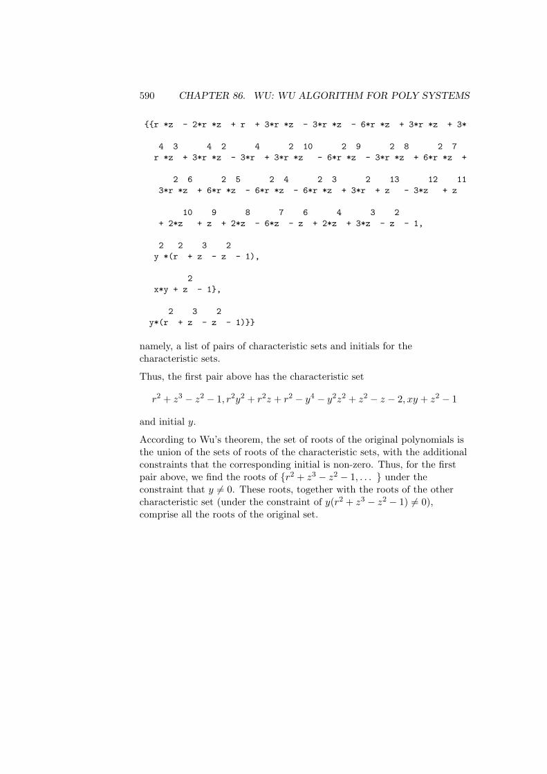
590 CHAPTER 86. WU: WU ALGORITHM FOR POLY SYSTEMS
r *z - 2*r *z + r + 3*r *z - 3*r *z - 6*r *z + 3*r *z + 3*
4 3 4 2 4 2 10 2 9 2 8 2 7r *z + 3*r *z - 3*r + 3*r *z - 6*r *z - 3*r *z + 6*r *z +
2 6 2 5 2 4 2 3 2 13 12 113*r *z + 6*r *z - 6*r *z - 6*r *z + 3*r + z - 3*z + z
10 9 8 7 6 4 3 2+ 2*z + z + 2*z - 6*z - z + 2*z + 3*z - z - 1,
2 2 3 2y *(r + z - z - 1),
2x*y + z - 1,
2 3 2y*(r + z - z - 1)
namely, a list of pairs of characteristic sets and initials for thecharacteristic sets.
Thus, the first pair above has the characteristic set
r2 + z3 − z2 − 1, r2y2 + r2z + r2 − y4 − y2z2 + z2 − z − 2, xy + z2 − 1
and initial y.
According to Wu’s theorem, the set of roots of the original polynomials isthe union of the sets of roots of the characteristic sets, with the additionalconstraints that the corresponding initial is non-zero. Thus, for the firstpair above, we find the roots of r2 + z3 − z2 − 1, . . . under theconstraint that y 6= 0. These roots, together with the roots of the othercharacteristic set (under the constraint of y(r2 + z3 − z2 − 1) 6= 0),comprise all the roots of the original set.

Chapter 87
XCOLOR: Calculation of thecolor factor in non-abeliangauge field theories
A. KryukovInstitute for Nuclear Physics, Moscow State University
119899, Moscow, Russia
e–mail: [email protected]
XCOLOR calculates the colour factor in non-abelian gauge field theories.It provides two commands and two operators.
SUdim integer
Sets the order of the SU group. The default value is 3.
SpTT expression
Sets the normalisation coefficient A in the equation Sp(TiTj) = A∆(i, j).The default value is 1/2.
QG(inQuark, outQuark, Gluon)
Describes the quark-gluon vertex. The parameters may be any identifiers.The first and second of then must be in- and out- quarks correspondingly.Third one is a gluon.
G3(Gluon1, Gluon2, Gluon3)
591

592 CHAPTER 87. XCOLOR: COLOR FACTOR IN GAUGE THEORY
Describes the three-gluon vertex. The parameters may be any identifiers.The order of gluons must be clockwise.
In terms of QG and G3 operators one can input a diagram in “color” spaceas a product of these operators. For example

593
e1---->---
/ \/ \
| e2 |v1*............*v2
| |\ /\ e3 /----<---
where --->--- is a quark and ....... is a gluon.
The related REDUCE expression is QG(e3,e1,e2)*QG(e1,e3,e2).

594 CHAPTER 87. XCOLOR: COLOR FACTOR IN GAUGE THEORY

Chapter 88
XIDEAL: Grobner forexterior algebra
David HartleyGMD, Institute I1, Schloss Birlinghoven
D–53757 St. Augustin, Germany
e–mail: [email protected]
andPhilip A. Tuckey
Max Planck Institute for PhysicsFoehringer Ring 6
D–80805 Munich, Germany
e–mail: [email protected]
XIDEAL extends the Grobner base method to exterior algebras.
XIDEAL constructs Grobner bases for solving the left ideal membershipproblem: Grobner left ideal bases or GLIBs. For graded ideals, where eachform is homogeneous in degree, the distinction between left and rightideals vanishes. Furthermore, if the generating forms are all homogeneous,then the Grobner bases for the non-graded and graded ideals are identical.In this case, XIDEAL is able to save time by truncating the Grobner basisat some maximum degree if desired. XIDEAL uses the EXCALC package(chapter 39).
595

596 CHAPTER 88. XIDEAL: GROBNER FOR EXTERIOR ALGEBRA
88.1 Operators
XIDEAL
XIDEAL calculates a Grobner left ideal basis in an exterior algebra. Thesyntax is
XIDEAL(S:list of forms[,R:integer]):list of forms.
XIDEAL calculates the Grobner left ideal basis for the left ideal generatedby S using graded lexicographical ordering based on the current kernelordering. The resulting list can be used for subsequent reductions withXMODULOP as long as the kernel ordering is not changed. If the set ofgenerators S is graded, an optional parameter R can be given, and XIDEALproduces a truncated basis suitable for reducing exterior forms of degreeless than or equal to R in the left ideal. This can save time and space withlarge expressions, but the result cannot be used for exterior forms ofdegree greater than R. See also the switches XSTATS and XFULLREDUCTION.
XMODULO
XMODULO reduces exterior forms to their (unique) normal forms modulo aleft ideal. The syntax is
XMODULO(F:form, S:list of forms):form
or
XMODULO(F:list of forms, S:list of forms):list of forms.
An alternative infix syntax is also available:
F XMODULO S.
XMODULO(F,S) first calculates a Grobner basis for the left ideal generatedby S, and then reduces F. F may be either a single exterior form, or a list offorms, and S is a list of forms. If F is a list of forms, each element isreduced, and any which vanish are deleted from the result. If this operatoris used more than once, and S does not change between calls, then theGrobner basis is not recalculated. If the set of generators S is graded, then

88.2. SWITCHES 597
a truncated Grobner basis is calculated using the degree of F (or themaximal degree in F).
XMODULOP
XMODULOP reduces exterior forms to their (not necessarily unique) normalforms modulo a set of exterior polynomials. The syntax is
XMODULOP(F:form, S:list of forms):form
or
XMODULOP(F:list of forms, S:list of forms):list of forms.
An alternative infix syntax is also available:
F XMODULOP S.
XMODULOP(F,S) reduces F with respect to the set of exterior polynomials S,which is not necessarily a Grobner basis. F may be either a single exteriorform, or a list of forms, and S is a list of forms. This operator can be usedin conjunction with XIDEAL to produce the same effect as XMODULO: for asingle form F in an ideal generated by the graded set S, F XMODULO S isequivalent to F XMODULOP XIDEAL(S,EXDEGREE F).
88.2 Switches
XFULLREDUCE
ON XFULLREDUCE allows XIDEAL and XMODULO to calculate reduced (but notnecessarily normed) Grobner bases, which speeds up subsequentreductions, and guarantees a unique form (up to scaling) for the Grobnerbasis. OFF XFULLREDUCE turns of this feature, which may speed upcalculation of the Grobner basis. XFULLREDUCE is ON by default.
XSTATS
ON XSTATS produces counting and timing information. As XIDEAL isrunning, a hash mark (#) is printed for each form taken from the input list,

598 CHAPTER 88. XIDEAL: GROBNER FOR EXTERIOR ALGEBRA
followed by a sequences of carets (^) and dollar signs ($). Each caretrepresents a new basis element obtained by a simple wedge product, andeach dollar sign represents a new basis element obtained from anS-polynomial. At the end, a table is printed summarising the calculation.XSTATS is OFF by default.
88.3 Examples
Suppose EXCALC and XIDEAL have been loaded, the switches are attheir default settings, and the following exterior variables have beendeclared:
pform x=0,y=0,z=0,t=0,f(i)=1,h=0,hx=0,ht=0;
In a commutative polynomial ring, a single polynomial is its own Grobnerbasis. This is no longer true for exterior algebras because of the presenceof zero divisors, and can lead to some surprising reductions:
xideal d x^d y - d z^d t;
d T^d Z + d X^d Y,
d X^d Y^d Z,
d T^d X^d Y
f(3)^f(4)^f(5)^f(6)xmodulo f(1)^f(2) + f(3)^f(4) + f(5)^f(6);
0
The heat equation, hxx = ht can be represented by the following exteriordifferential system.
S := d h - ht*d t - hx*d x,d ht^d t + d hx^d x,d hx^d t - ht*d x^d t;
XMODULO can be used to check that the exterior differential system is closedunder exterior differentiation.

88.3. EXAMPLES 599
d S xmodulo S;
Non-graded left and right ideals are no longer the same:
d t^(d z+d x^d y) xmodulo d z+d x^d y;
0
(d z+d x^d y)^d t xmodulo d z+d x^d y;
- 2*d t^d z
Higher order forms can now reduce lower order ones:
d x xmodulo d y^d z + d x,d x^d y + d z;
0
Any form containing a 0-form term generates the whole ideal:
xideal 1 + f(1) + f(1)^f(2) + f(2)^f(3)^f(4);
1

600 CHAPTER 88. XIDEAL: GROBNER FOR EXTERIOR ALGEBRA

Chapter 89
ZEILBERG: A package forindefinite and definitesummation
Wolfram Koepf and Gregor StoltingKonrad–Zuse–Zentrum fur Informationstechnik Berlin
Takustrase 7D–14195 Berlin–Dahlem, Germany
e–mail: [email protected]
The ZEILBERG package provides an implementation of the Gosper andZeilberger algorithms for indefinite, and definite summation ofhypergeometric terms, respectively, with extensions for ratios of productsof powers, factorials, Γ function terms, binomial coefficients, and shiftedfactorials that are rational-linear in their arguments.
89.1 The GOSPER summation operator
The gosper operator is an implementation of the Gosper algorithm.
• gosper(a,k) determines a closed form antidifference. If it does notreturn a closed form solution, then a closed form solution does notexist.
601

602 CHAPTER 89. ZEILBERG: INDEF & DEFINITE SUMMATION
• gosper(a,k,m,n) determines
n∑
k=m
ak
using Gosper’s algorithm. This is only successful if Gosper’salgorithm applies.
Example:
gosper((-1)^(k+1)*(4*k+1)*factorial(2*k)/(factorial(k)*4^k*(2*k-1)*factorial(k+1)),k);
k- ( - 1) *factorial(2*k)
------------------------------------2*k
2 *factorial(k + 1)*factorial(k)
gosper(binomial(k,n),k);
(k + 1)*binomial(k,n)-----------------------
n + 1
89.2 EXTENDED GOSPER operator
The extended gosper operator is an implementation of an extendedversion of Gosper’s algorithm.
• extended gosper(a,k) determines an antidifference gk of ak
whenever there is a number m such that hk − hk−m = ak, and hk isan m-fold hypergeometric term, i. e.
hk/hk−m is a rational function with respect to k.
If it does not return a solution, then such a solution does not exist.
• extended gosper(a,k,m) determines an m-fold antidifference hk ofak, i. e. hk − hk−m = ak, if it is an m-fold hypergeometric term.

89.3. SUMRECURSION OPERATOR 603
Examples:
extended_gosper(binomial(k/2,n),k);
k k - 1(k + 2)*binomial(---,n) + (k + 1)*binomial(-------,n)
2 2-------------------------------------------------------
2*(n + 1)
extended_gosper(k*factorial(k/7),k,7);
k(k + 7)*factorial(---)
7
89.3 SUMRECURSION operator
The sumrecursion operator is an implementation of the (fast) Zeilbergeralgorithm.
• sumrecursion(f,k,n) determines a holonomic recurrence equationfor
sum(n) =∞∑
k=−∞f(n, k)
with respect to n. The resulting expression equals zero.
• sumrecursion(f,k,n,j) searches for a holonomic recurrenceequation of order j.Note that if j is too large, the recurrence equationmay not be unique, and only one particular solution is returned.
sumrecursion(binomial(n,k),k,n);
2*sum(n - 1) - sum(n)
89.4 HYPERRECURSION operator
If a recursion for a generalised hypergeometric function is to beestablished, one can use

604 CHAPTER 89. ZEILBERG: INDEF & DEFINITE SUMMATION
• hyperrecursion(upper,lower,x,n) determines a holonomicrecurrence equation with respect to n for
pFq
(a1, a2, · · · , ap
b1, b2, · · · , bq
∣∣∣∣∣x),
where upper= a1, a2, . . . , ap is the list of upper parameters, andlower= b1, b2, . . . , bq is the list of lower parameters depending on n.
• hyperrecursion(upper,lower,x,n,j) (j ∈ IN) searches only for aholonomic recurrence equation of order j. This operator does notautomatically use extended sumrecursion.
hyperrecursion(-n,b,c,1,n);
(b - c - n + 1)*sum(n - 1) + (c + n - 1)*sum(n)
If a hypergeometric expression is given in hypergeometric notation, thenthe use of hyperrecursion is more natural than the use of sumrecursion.
Moreover the REDUCE operator
• hyperterm(upper,lower,x,k) yields the hypergeometric term
(a1)k · (a2)k · · · (ap)k
(b1)k · (b2)k · · · (bq)k k!xk
with upper parameters upper= a1, a2, . . . , ap, and lowerparameters lower= b1, b2, . . . , bq
in connection with hypergeometric terms.
89.5 HYPERSUM operator
With the operator hypersum, hypergeometric sums are directly evaluatedin closed form whenever the extended Zeilberger algorithm leads to arecurrence equation containing only two terms:
• hypersum(upper,lower,x,n) determines a closed formrepresentation for

89.6. SUMTOHYPER OPERATOR 605
pFq
(a1, a2, · · · , ap
b1, b2, · · · , bq
∣∣∣∣∣x)
, where upper= a1, a2, . . . , ap is the
list of upper parameters, and lower= b1, b2, . . . , bq is the list oflower parameters depending on n. The result is given as ahypergeometric term with respect to n.
If the result is a list of length m, we call it m-fold symmetric, whichis to be interpreted as follows: Its jth part is the solution valid for alln of the form n = mk + j − 1 (k ∈ IN0). In particular, if the resultinglist contains two terms, then the first part is the solution for even n,and the second part is the solution for odd n.
hypersum(a,1+a/2,c,d,-n,a/2,1+a-c,1+a-d,1+a+n,1,n);
pochhammer(a - c - d + 1,n)*pochhammer(a + 1,n)-------------------------------------------------pochhammer(a - c + 1,n)*pochhammer(a - d + 1,n)
hypersum(a,1+a/2,d,-n,a/2,1+a-d,1+a+n,-1,n);
pochhammer(a + 1,n)-------------------------pochhammer(a - d + 1,n)
Note that the operator togamma converts expressions given infactorial-Γ-binomial-Pochhammer notation into a pure Γ functionrepresentation:
togamma(hypersum(a,1+a/2,d,-n,a/2,1+a-d,1+a+n,-1,n));
gamma(a - d + 1)*gamma(a + n + 1)-----------------------------------gamma(a - d + n + 1)*gamma(a + 1)
89.6 SUMTOHYPER operator
With the operator sumtohyper, sums given infactorial-Γ-binomial-Pochhammer notation are converted intohypergeometric notation.

606 CHAPTER 89. ZEILBERG: INDEF & DEFINITE SUMMATION
• sumtohyper(f,k) determines the hypergeometric representation of∞∑
k=−∞fk, i.e. its output is c*hypergeometric(upper,lower,x),
corresponding to the representation
∞∑
k=−∞fk = c · pFq
(a1, a2, · · · , ap
b1, b2, · · · , bq
∣∣∣∣∣x),
where upper= a1, a2, . . . , ap and lower= b1, b2, . . . , bq are thelists of upper and lower parameters.
Examples:
sumtohyper(binomial(n,k)^3,k);
hypergeometric( - n, - n, - n,1,1,-1)
89.7 Simplification Operators
For the decision that an expression ak is a hypergeometric term, it isnecessary to find out whether or not ak/ak−1 is a rational function withrespect to k. For the purpose to decide whether or not an expressioninvolving powers, factorials, Γ function terms, binomial coefficients, andPochhammer symbols is a hypergeometric term, the followingsimplification operators can be used:
• simplify gamma(f) simplifies an expression f involving onlyrational, powers and Γ function terms.
• simplify combinatorial(f) simplifies an expression f involvingpowers, factorials, Γ function terms, binomial coefficients, andPochhammer symbols by converting factorials, binomial coefficients,and Pochhammer symbols into Γ function terms, and applyingsimplify gamma to its result. If the output is not rational, it is givenin terms of Γ functions. If factorials are preferred use
• gammatofactorial (rule) converting Γ function terms into factorialsusing Γ (x)→ (x− 1)!.
• simplify gamma2(f) uses the duplication formula of the Γ functionto simplify f .

89.7. SIMPLIFICATION OPERATORS 607
• simplify gamman(f,n) uses the multiplication formula of the Γfunction to simplify f .
The use of simplify combinatorial(f) is a safe way to decide therationality for any ratio of products of powers, factorials, Γ function terms,binomial coefficients, and Pochhammer symbols.
Example:
simplify_gamma2(gamma(2*n)/gamma(n));
2*n 2*n + 12 *gamma(---------)
2-----------------------
2*sqrt(pi)

608 CHAPTER 89. ZEILBERG: INDEF & DEFINITE SUMMATION
Chapter 90
ZTRANS: Z-transformpackage
Wolfram Koepf and Lisa TemmeKonrad–Zuse–Zentrum fur Informationstechnik Berlin
Takustrase 7D–14195 Berlin–Dahlem, Germany
e–mail: [email protected]
The Z-Transform of a sequence fn is the discrete analogue of theLaplace Transform, and
Zfn = F (z) =∞∑
n=0
fnz−n .
This series converges in the region outside the circle|z| = |z0| = lim sup
n→∞n√|fn| . In the same way that a Laplace Transform can
be used to solve differential equations, so Z-Transforms can be used tosolve difference equations.
SYNTAX: ztrans(fn, n, z) where fn is an expression, and n,zare identifiers.
This package can compute the Z-Transforms of the following list of fn, andcertain combinations thereof.
609

610 CHAPTER 90. ZTRANS: Z-TRANSFORM PACKAGE
1 eαn 1(n+k)
1n!
1(2n)!
1(2n+1)!
sin(βn)n! sin(αn+ φ) eαn sin(βn)
cos(βn)n! cos(αn+ φ) eαn cos(βn)
sin(β(n+1))n+1 sinh(αn+ φ) cos(β(n+1))
n+1
cosh(αn+ φ)(n+k
m
)
Other Combinations
Linearity Zafn + bgn = aZfn+ bZgn
Multiplication by n Znk · fn = −z ddz
(Znk−1 · fn, n, z
)
Multiplication by λn Zλn · fn = F(
zλ
)
Shift Equation Zfn+k = zk
(F (z)−
k−1∑j=0
fjz−j
)
Symbolic Sums Z
n∑k=0
fk
= z
z−1 · Zfn
Z
n+q∑k=p
fk
combination of the above
where k,λ ∈ N−0; and a,b are variables or fractions; and p,q ∈ Z orare functions of n; and α, β and φ are angles in radians.
The calculation of the Laurent coefficients of a regular function results inthe following inverse formula for the Z-Transform:
If F (z) is a regular function in the region |z| > ρ then ∃ a sequence fn

611
with Zfn = F (z) given by
fn =1
2πi
∮F (z)zn−1dz
SYNTAX: invztrans(F (z), z, n) where F (z) is an expression,and z,n are identifiers.
This package can compute the Inverse Z-Transforms of any rational function,whose denominator can be factored over Q, in addition to the following listof F (z).
sin(
sin(β)z
)e(
cos(β)z
)cos
(sin(β)
z
)e(
cos(β)z
)
√zA sin
(√zA
)cos
(√zA
)
√zA sinh
(√zA
)cosh
(√zA
)
z log(
z√z2−Az+B
)z log
(√z2+Az+B
z
)
arctan(
sin(β)z+cos(β)
)
here k,λ ∈ N−0 and A,B are fractions or variables (B > 0) and α,β, &φ are angles in radians.
Examples:
ztrans(sum(1/factorial(k),k,0,n),n,z);
1/ze *z
--------z - 1
invztrans(z/((z-a)*(z-b)),z,n);
n na - b
---------

612 CHAPTER 90. ZTRANS: Z-TRANSFORM PACKAGE
a - b

Part III
Standard Lisp Report
613


Chapter 91
The Standard Lisp Report
Jed MartiA. C. HearnM. L. Griss
C. Griss
91.1 Introduction
Although the programming language LISP was first formulated in1960 [13], a widely accepted standard has never appeared. As a result,various dialects of LISP were produced [2, 6, 12, 16, 14, 15] in some casesseveral on the same machine! Consequently, a user often faces considerabledifficulty in moving programs from one system to another. In addition, itis difficult to write and use programs which depend on the structure of thesource code such as translators, editors and cross-reference programs.
In 1969, a model for such a standard was produced [9] as part of a generaleffort to make a large LISP based algebraic manipulation program,REDUCE [8], as portable as possible. The goal of this work was to definea uniform subset of LISP 1.5 and its variants so that programs written inthis subset could run on any reasonable LISP system.
In the intervening years, two deficiencies in the approach taken in Ref. [9]have emerged. First in order to be as general as possible, the specificsemantics and values of several key functions were left undefined.Consequently, programs built on this subset could not make any
615
616 CHAPTER 91. THE STANDARD LISP REPORT
assumptions about the form of the values of such functions. The seconddeficiency related to the proposed method of implementation of thislanguage. The model considered in effect two versions of LISP on anygiven machine, namely Standard LISP and the LISP of the host machine(which we shall refer to as Target LISP). This meant that if any definitionwas stored in interpretive form, it would vary from implementation toimplementation, and consequently one could not write programs inStandard LISP which needed to assume any knowledge about the structureof such forms. This deficiency became apparent during recent work on thedevelopment of a portable compiler for LISP [7]. Clearly a compiler has toknow precisely the structure of its source code; we concluded that theappropriate source was Standard LISP and not Target LISP.
With these thoughts in mind we decided to attempt again a definition ofStandard LISP. However, our approach this time is more aggressive. Inthis document we define a standard for a reasonably large subset of LISPwith as precise as possible a statement about the semantics of eachfunction. Secondly, we now require that the target machine interpreter bemodified or written to support this standard, rather than mappingStandard LISP onto Target LISP as previously.
We have spent countless hours in discussion over many of the definitionsgiven in this report. We have also drawn on the help and advice of a lot offriends whose names are given in the Acknowledgements. Whereverpossible, we have used the definition of a function as given in the LISP 1.5Programmer’s Manual [13] and have only deviated where we felt itdesirable in the light of LISP programming experience since that time. Inparticular, we have given considerable thought to the question of variablebindings and the definition of the evaluator functions EVAL and APPLY.We have also abandoned the previous definition of LISP arrays in favor ofthe more accepted idea of a vector which most modern LISP systemssupport. These are the places where we have strayed furthest from theconventional definitions, but we feel that the consistency which resultsfrom our approach is worth the redefinition.
We have avoided entirely in this report problems which arise fromenvironment passing, such as those represented by the FUNARG problem.We do not necessarily exclude these considerations from our standard, butin this report have decided to avoid the controversy which they create.The semantic differences between compiled and interpreted functions is thetopic of another paper [7]. Only functions which affect the compiler in a

91.2. PRELIMINARIES 617
general way make reference to it.
This document is not intended as an introduction to LISP rather it isassumed that the reader is already familiar with some version. Thedocument is thus intended as an arbiter of the syntax and semantics ofStandard LISP. However, since it is not intended as an implementationdescription, we deliberately leave unspecified many of the details on whichan actual implementation depends. For example, while we assume theexistence of a symbol table for atoms (the ”object list” in LISPterminology), we do not specify its structure, since conventional LISPprogramming does not require this information. Our ultimate goal,however, is to remedy this by defining an interpreter for Standard LISPwhich is sufficiently complete that its implementation on any givencomputer will be straightforward and precise. At that time, we shallproduce an implementation level specification for Standard LISP whichwill extend the description of the primitive functions defined herein byintroducing a new set of lower level primitive functions in which thestructure of the symbol table, heap and so on may be defined.
The plan of this chapter is as follows. In Section 91.2 we describe thevarious data types used in Standard LISP. In Section 91.3, a description ofall Standard LISP functions is presented, organized by type. Thesefunctions are defined in an RLISP syntax which is easier to read thanLISP S-expressions. Section 91.4 describes global variables which controlthe operation of Standard LISP.
91.2 Preliminaries
91.2.1 Primitive Data Types
integer Integers are also called ”fixed” numbers. The magnitude of aninteger is unrestricted. Integers in the LISP input stream arerecognized by the grammar:
<digit> ::= 0|1|2|3|4|5|6|7|8|9<unsigned-integer> ::= <digit>|<unsigned-integer><digit><integer> ::= <unsigned-integer> |
+<unsigned-integer> |—<unsigned-integer>

618 CHAPTER 91. THE STANDARD LISP REPORT
floating - Any floating point number. The precision of floating pointnumbers is determined solely by the implementation. In BNFfloating point numbers are recognized by the grammar:
<base> ::= <unsigned-integer>.|.<unsigned-integer>|<unsigned-integer>.<unsigned-integer><unsigned-floating> ::= <base>|<base>E<unsigned-integer>|<base>E-<unsigned-integer>|<base>E+<unsigned-integer>
<floating> ::= <unsigned-floating>|+<unsigned-floating>|-<unsigned-floating>
id An identifier is a string of characters which may have the followingitems associated with it.
print name The characters of the identifier.
flags An identifier may be tagged with a flag. Access is by theFLAG, REMFLAG, and FLAGP functions defined insection 91.3.4 on page 631.
properties An identifier may have an indicator-value pairassociated with it. Access is by the PUT, GET, andREMPROP functions defined in section 91.3.4 on page 631.
values/functions An identifier may have a value associated withit. Access to values is by SET and SETQ defined insection 91.3.6 on page 635. The method by which the value isattached to the identifier is known as the binding type, beingone of LOCAL, GLOBAL, or FLUID. Access to the bindingtype is by the GLOBAL, GLOBALP, FLUID, FLUIDP, andUNFLUID functions.An identifier may have a function or macro associated with it.Access is by the PUTD, GETD, and REMD functions (see“Function Definition”, section 91.3.5, on page 633). Anidentifier may not have both a function and a value associatedwith it.
OBLIST entry An identifier may be entered and removed from astructure called the OBLIST. Its presence on the OBLIST doesnot directly affect the other properties. Access to the OBLISTis by the INTERN, REMOB, and READ functions.

91.2. PRELIMINARIES 619
The maximum length of a Standard LISP identifier is 24 characters(excluding occurrences of the escape character !) but animplementation may allow more. Special characters (digits in thefirst position and punctuation) must be prefixed with an escapecharacter, an ! in Standard LISP. In BNF identifiers are recognizedby the grammar:
<special-character> ::= !<any-character><alphabetic> ::=
A|B|C|D|E|F|G|H|I|J|K|L|M|N|O|P|Q|R|S|T|U|V|W|X|Y|Z|a|b|c|d|e|f|g|h|i|j|k|l|m|n|o|p|q|r|s|t|u|v|w|x|y|z
<lead-character> ::= <special-character>|<alphabetic><regular-character> ::= <lead-character>|<digit><last-part> ::= <regular-character> |
<last-part><regular-character><id> ::= <lead-character>|<lead-character><last-part>
Note: Using lower case letters in identifiers may cause portabilityproblems. Lower case letters are automatically converted to uppercase when the !*RAISE flag is T.
string A set of characters enclosed in double quotes as in ”THIS IS ASTRING”. A quote is included by doubling it as in ”HE SAID,””LISP”””. The maximum size of strings is 80 characters but animplementation may allow more. Strings are not part of the OBLISTand are considered constants like numbers, vectors, andfunction-pointers.
dotted-pair A primitive structure which has a left and right part. Anotation called dot-notation is used for dotted pairs and takes theform:
(<left-part> . <right-part>)
The <left-part> is known as the CAR portion and the <right-part>as the CDR portion. The left and right parts may be of any type.Spaces are used to resolve ambiguity with floating point numbers.
vector A primitive uniform structure in which an integer index is used toaccess random values in the structure. The individual elements of a
620 CHAPTER 91. THE STANDARD LISP REPORT
vector may be of any type. Access to vectors is restricted tofunctions defined in “Vectors” section 91.3.9 on page 641. A notationfor vectors, vector-notation, has the elements of a vector surroundedby square brackets1
<elements> ::= <any>|<any> <elements><vector> ::= [<elements>]
function-pointer An implementation may have functions which dealwith specific data types other than those listed. The use of theseentities is to be avoided with the exception of a restricted use of thefunction-pointer, an access method to compiled EXPRs andFEXPRs. A particular function-pointer must remain validthroughout execution. Systems which change the location of afunction must use either an indirect reference or change alloccurrences of the associated value. There are two classes of use offunction-pointers, those which are supported by Standard LISP butare not well defined, and those which are well defined.
Not well defined Function pointers may be displayed by the printfunctions or expanded by EXPLODE. The value appears in theconvention of the implementation site. The value is not definedin Standard LISP. Function pointers may be created byCOMPRESS in the format used for printing but the value usedis not defined in Standard LISP. Function pointers may becreated by functions which deal with compiled function loading.Again, the values created are not well defined in Standard LISP.
Well defined The function pointer associated with an EXPR orFEXPR may be retrieved by GETD and is valid as long asStandard LISP is in execution. Function pointers may be storedusing PUTD, PUT, SETQ and the like or by being bound tovariables. Function pointers may be checked for equivalence byEQ. The value may be checked for being a function pointer bythe CODEP function.
1Vector elements are not separated by commas as in the published version of thisdocument.

91.2. PRELIMINARIES 621
91.2.2 Classes of Primitive Data Types
The classes of primitive types are a notational convenience for describingthe properties of functions.
boolean The set of global variables T,NIL, or their respective values,T, NIL.
extra-boolean Any value in the system. Anything that is not NIL hasthe boolean interpretation T.
ftype The class of definable function types. The set of ids EXPR,FEXPR, MACRO.
number The set of integer, floating.constant The set of integer, floating, string, vector, function-pointer.
Constants evaluate to themselves (see the definition of EVAL in“The Interpreter”, section 91.3.14 on page 655).
any The set of integer, floating, string, id, dotted-pair, vector,function-pointer. An S-expression is another term for any. AllStandard LISP entities have some value unless an ERROR occursduring evaluation or the function causes transfer of control (such asGO and RETURN).
atom The set any-dotted-pair.
91.2.3 Structures
Structures are entities created out of the primitive types by the use ofdotted-pairs. Lists are structures very commonly required as actualparameters to functions. Where a list of homogeneous entities is requiredby a function this class will be denoted by <xxx-list> where xxx is thename of a class of primitives or structures. Thus a list of ids is an id-list, alist of integers an integer-list and so on.
list A list is recursively defined as NIL or the dotted-pair (any . list). Aspecial notation called list-notation is used to represent lists.List-notation eliminates extra parentheses and dots. The list (a . (b .(c . NIL))) in list notation is (a b c). List-notation and dot-notation

622 CHAPTER 91. THE STANDARD LISP REPORT
may be mixed as in (a b . c) or (a (b . c) d) which are (a . (b . c))and (a . ((b . c) . (d . NIL))). In BNF lists are recognized by thegrammar:
<left-part> ::= ( | <left-part> <any><list> ::= <left-part>) | <left-part> . <any>)
Note: () is an alternate input representation of NIL.
alist An association list; each element of the list is a dotted-pair, the CARpart being a key associated with the value in the CDR part.
cond-form A cond-form is a list of 2 element lists of the form:
(ANTECEDENT:any CONSEQUENT:any)
The first element will henceforth be known as the antecedent andthe second as the consequent. The antecedent must have a value.The consequent may have a value or an occurrence of GO orRETURN as described in the “Program Feature Functions”,section 91.3.7 on page 637.
lambda A LAMBDA expression which must have the form (in listnotation): (LAMBDA parameters body). “parameters” is a list offormal parameters for “body” an S-expression to be evaluated. Thesemantics of the evaluation are defined with the EVAL function (see“The Interpreter”, section 91.3.14 on page 655).
function A LAMBDA expression or a function-pointer to a function. Afunction is always evaluated as an EVAL, SPREAD form.
91.2.4 Function Descriptions
Each function is provided with a prototypical header line. Each formalparameter is given a name and suffixed with its allowed type. Lower case,italic tokens are names of classes and upper case, bold face, tokens areparameter names referred to in the definition. The type of the valuereturned by the function (if any) is suffixed to the parameter list. If it isnot commonly used the parameter type may be a specific set enclosed inbrackets . . . . For example:
PUTD(FNAME:id, TYPE:ftype, BODY:lambda, function-pointer):id
91.2. PRELIMINARIES 623
PUTD is a function with three parameters. The parameter FNAME is anid to be the name of the function being defined. TYPE is the type of thefunction being defined and BODY is a lambda expression or afunction-pointer. PUTD returns the name of the function being defined.
Functions which accept formal parameter lists of arbitrary length have thetype class and parameter enclosed in square brackets indicating that zeroor more occurrences of that argument are permitted. For example:
AND([U:any]):extra-boolean
AND is a function which accepts zero or more arguments which may be ofany type.
91.2.5 Function Types
EVAL type functions are those which are invoked with evaluatedarguments. NOEVAL functions are invoked with unevaluated arguments.SPREAD type functions have their arguments passed in one-to-onecorrespondence with their formal parameters. NOSPREAD functionsreceive their arguments as a single list. EVAL, SPREAD functions areassociated with EXPRs and NOEVAL, NOSPREAD functions withFEXPRs. EVAL, NOSPREAD and NOEVAL, SPREAD functions can besimulated using NOEVAL, NOSPREAD functions or MACROs.
EVAL, SPREAD type functions may have a maximum of 15 parameters.There is no limit on the number of parameters a NOEVAL, NOSPREADfunction or MACRO may have.
In the context of the description of an EVAL, SPREAD function, then wespeak of the formal parameters we mean their actual values. However, in aNOEVAL, NOSPREAD function it is the unevaluated actual parameters.
A third function type, the MACRO, implements functions which createS-expressions based on actual parameters. When a macro invocation isencountered, the body of the macro, a lambda expression, is invoked as aNOEVAL, NOSPREAD function with the macro’s invocation bound as alist to the macros single formal parameter. When the macro has beenevaluated the resulting S-expression is reevaluated. The description of theEVAL and EXPAND functions provide precise details.
624 CHAPTER 91. THE STANDARD LISP REPORT
91.2.6 Error and Warning Messages
Many functions detect errors. The description of such functions willinclude these error conditions and suggested formats for display of thegenerated error messages. A call on the ERROR function is implied butthe error number is not specified by Standard LISP. In some cases awarning message is sufficient. To distinguish between errors and warnings,errors are prefixed with five asterisks and warnings with only three.
Primitive functions check arguments that must be of a certain primitivetype for being of that type and display an error message if the argument isnot correct. The type mismatch error always takes the form:
***** PARAMETER not TYPE for FN
Here PARAMETER is the unacceptable actual parameter, TYPE is thetype that PARAMETER was supposed to be. FN is the name of thefunction that detected the error.
91.2.7 Comments
The character % signals the start of a comment, text to be ignored duringparsing. A comment is terminated by the end of the line it is on. Thefunction READCH must be able to read a comment one character at atime. Comments are transparent to the function READ. % may occur as acharacter in identifiers by preceding it with the escape character !.
91.3 Functions
91.3.1 Elementary Predicates
Functions in this section return T when the condition defined is met andNIL when it is not. Defined are type checking functions and elementarycomparisons.

91.3. FUNCTIONS 625
ATOM(U:any):boolean eval, spreadReturns T if U is not a pair.
EXPR PROCEDURE ATOM(U);NULL PAIRP U;
CODEP(U:any):boolean eval, spreadReturns T if U is a function-pointer.
CONSTANTP(U:any):boolean eval, spreadReturns T if U is a constant (a number, string, function-pointer, orvector).
EXPR PROCEDURE CONSTANTP(U);NULL OR(PAIRP U, IDP U);
EQ(U:any, V:any):boolean eval, spreadReturns T if U points to the same object as V. EQ is not a reliablecomparison between numeric arguments.
EQN(U:any, V:any):boolean eval, spreadReturns T if U and V are EQ or if U and V are numbers and havethe same value and type.
EQUAL(U:any, V:any):boolean eval, spreadReturns T if U and V are the same. Dotted-pairs are comparedrecursively to the bottom levels of their trees. Vectors must haveidentical dimensions and EQUAL values in all positions. Stringsmust have identical characters. Function pointers must have EQvalues. Other atoms must be EQN equal.

626 CHAPTER 91. THE STANDARD LISP REPORT
FIXP(U:any):boolean eval, spreadReturns T if U is an integer (a fixed number).
FLOATP(U:any):boolean eval, spreadReturns T if U is a floating point number.
IDP(U:any):boolean eval, spreadReturns T if U is an id.
MINUSP(U:any):boolean eval, spreadReturns T if U is a number and less than 0. If U is not a number oris a positive number, NIL is returned.
EXPR PROCEDURE MINUSP(U);IF NUMBERP U THEN LESSP(U, 0) ELSE NIL;
NULL(U:any):boolean eval, spreadReturns T if U is NIL.
EXPR PROCEDURE NULL(U);U EQ NIL;
NUMBERP(U:any):boolean eval, spreadReturns T if U is a number (integer or floating).
EXPR PROCEDURE NUMBERP(U);IF OR(FIXP U, FLOATP U) THEN T ELSE NIL;
91.3. FUNCTIONS 627
ONEP(U:any):boolean eval, spread.Returns T if U is a number and has the value 1 or 1.0. Returns NILotherwise. a
EXPR PROCEDURE ONEP(U);OR(EQN(U, 1), EQN(U, 1.0));
aThe definition in the published report is incorrect as it does not return T forU of 1.0.
PAIRP(U:any):boolean eval, spreadReturns T if U is a dotted-pair.
STRINGP(U:any):boolean eval, spreadReturns T if U is a string.
VECTORP(U:any):boolean eval, spreadReturns T if U is a vector.
ZEROP(U:any):boolean eval, spread.Returns T if U is a number and has the value 0 or 0.0. Returns NILotherwise.a
EXPR PROCEDURE ZEROP(U);OR(EQN(U, 0), EQN(U, 0.0));
aThe definition in the published report is incorrect as it does not return T forU of 0.0.
91.3.2 Functions on Dotted-Pairs
The following are elementary functions on dotted-pairs. All functions inthis section which require dotted-pairs as parameters detect a type

628 CHAPTER 91. THE STANDARD LISP REPORT
mismatch error if the actual parameter is not a dotted-pair.
CAR(U:dotted-pair):any eval, spreadCAR(CONS(a, b)) → a. The left part of U is returned. The typemismatch error occurs if U is not a dotted-pair.
CDR(U:dotted-pair):any eval, spreadCDR(CONS(a, b)) → b. The right part of U is returned. The typemismatch error occurs if U is not a dotted-pair.
The composites of CAR and CDR are supported up to 4 levels, namely:
CAAAAR CAAAR CAARCAAADR CAADR CADRCAADAR CADAR CDARCAADDR CADDR CDDRCADAAR CDAARCADADR CDADRCADDAR CDDARCADDDR CDDDRCDAAARCDAADRCDADARCDADDRCDDAARCDDADRCDDDARCDDDDR
CONS(U:any, V:any):dotted-pair eval, spreadReturns a dotted-pair which is not EQ to anything and has U as itsCAR part and V as its CDR part.
91.3. FUNCTIONS 629
LIST([U:any]):list noeval, nospread, or macroA list of the evaluation of each element of U is returned. The order ofevaluation need not be first to last as the following definition implies.a
FEXPR PROCEDURE LIST(U);EVLIS U;
aThe published report’s definition implies a specific ordering.
RPLACA(U:dotted-pair, V:any):dotted-pair eval, spreadThe CAR portion of the dotted-pair U is replaced by V. If dotted-pair U is (a . b) then (V . b) is returned. The type mismatch erroroccurs if U is not a dotted-pair.
RPLACD(U:dotted-pair, V:any):dotted-pair eval, spreadThe CDR portion of the dotted-pair U is replaced by V. If dotted-pair U is (a . b) then (a . V) is returned. The type mismatch erroroccurs if U is not a dotted-pair.
91.3.3 Identifiers
The following functions deal with identifiers and the OBLIST, thestructure of which is not defined. The function of the OBLIST is toprovide a symbol table for identifiers created during input. Identifierscreated by READ which have the same characters will therefore refer tothe same object (see the EQ function in “Elementary Predicates”,section 91.3.1 on page 624).

630 CHAPTER 91. THE STANDARD LISP REPORT
COMPRESS(U:id-list):atom-vector eval, spreadU is a list of single character identifiers which is built into a Stand-ard LISP entity and returned. Recognized are numbers, strings,and identifiers with the escape character prefixing special charac-ters. The formats of these items appear in “Primitive Data Types”section 91.2.1 on page 617. Identifiers are not interned on the OB-LIST. Function pointers may be compressed but this is an undefineduse. If an entity cannot be parsed out of U or characters are left overafter parsing an error occurs:
***** Poorly formed atom in COMPRESS
EXPLODE(U:atom-vector):id-list eval, spreadReturned is a list of interned characters representing the characters toprint of the value of U. The primitive data types have these formats:
integer Leading zeroes are suppressed and a minus sign prefixes thedigits if the integer is negative.
floating The value appears in the format [-]0.nn...nnE[-]mm if themagnitude of the number is too large or small to display in[-]nnnn.nnnn format. The crossover point is determined by theimplementation.
id The characters of the print name of the identifier are producedwith special characters prefixed with the escape character.
string The characters of the string are produced surrounded by dou-ble quotes ”. . . ”.
function-pointer The value of the function-pointer is created as alist of characters conforming to the conventions of the systemsite.
The type mismatch error occurs if U is not a number, identifier,string, or function-pointer.

91.3. FUNCTIONS 631
GENSYM():identifier eval, spreadCreates an identifier which is not interned on the OBLIST and con-sequently not EQ to anything else.
INTERN(U:id,string):id eval, spreadINTERN searches the OBLIST for an identifier with the same printname as U and returns the identifier on the OBLIST if a matchis found. Any properties and global values associated with U maybe lost. If U does not match any entry, a new one is created andreturned. If U has more than the maximum number of characterspermitted by the implementation (the minimum number is 24) anerror occurs:
***** Too many characters to INTERN
REMOB(U:id):id eval, spreadIf U is present on the OBLIST it is removed. This does not affect Uhaving properties, flags, functions and the like. U is returned.
91.3.4 Property List Functions
With each id in the system is a “property list”, a set of entities which areassociated with the id for fast access. These entities are called “flags” iftheir use gives the id a single valued property, and “properties” if the id isto have a multivalued attribute: an indicator with a property.
Flags and indicators may clash, consequently care should be taken to avoidthis occurrence. Flagging X with an id which already is an indicator for Xmay result in that indicator and associated property being lost. Likewise,adding an indicator which is the same id as a flag may result in the flagbeing destroyed.
632 CHAPTER 91. THE STANDARD LISP REPORT
FLAG(U:id-list, V:id):NIL eval, spreadU is a list of ids which are flagged with V. The effect of FLAG isthat FLAGP will have the value T for those ids of U which wereflagged. Both V and all the elements of U must be identifiers or thetype mismatch error occurs.
FLAGP(U:any, V:any):boolean eval, spreadReturns T if U has been previously flagged with V, else NIL. ReturnsNIL if either U or V is not an id.
GET(U:any, IND:any):any eval, spreadReturns the property associated with indicator IND from the prop-erty list of U. If U does not have indicator IND, NIL is returned.GET cannot be used to access functions (use GETD instead).
PUT(U:id, IND:id, PROP:any):any eval, spreadThe indicator IND with the property PROP is placed on the propertylist of the id U. If the action of PUT occurs, the value of PROP isreturned. If either of U and IND are not ids the type mismatch errorwill occur and no property will be placed. PUT cannot be used todefine functions (use PUTD instead).
REMFLAG(U:any-list, V:id):NIL eval, spreadRemoves the flag V from the property list of each member of thelist U. Both V and all the elements of U must be ids or the typemismatch error will occur.
REMPROP(U:any, IND:any):any eval, spreadRemoves the property with indicator IND from the property list of U.Returns the removed property or NIL if there was no such indicator.
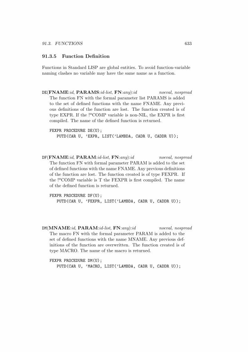
91.3. FUNCTIONS 633
91.3.5 Function Definition
Functions in Standard LISP are global entities. To avoid function-variablenaming clashes no variable may have the same name as a function.
DE(FNAME:id, PARAMS:id-list, FN:any):id noeval, nospreadThe function FN with the formal parameter list PARAMS is addedto the set of defined functions with the name FNAME. Any previ-ous definitions of the function are lost. The function created is oftype EXPR. If the !*COMP variable is non-NIL, the EXPR is firstcompiled. The name of the defined function is returned.
FEXPR PROCEDURE DE(U);PUTD(CAR U, ’EXPR, LIST(’LAMBDA, CADR U, CADDR U));
DF(FNAME:id, PARAM:id-list, FN:any):id noeval, nospreadThe function FN with formal parameter PARAM is added to the setof defined functions with the name FNAME. Any previous definitionsof the function are lost. The function created is of type FEXPR. Ifthe !*COMP variable is T the FEXPR is first compiled. The nameof the defined function is returned.
FEXPR PROCEDURE DF(U);PUTD(CAR U, ’FEXPR, LIST(’LAMBDA, CADR U, CADDR U));
DM(MNAME:id, PARAM:id-list, FN:any):id noeval, nospreadThe macro FN with the formal parameter PARAM is added to theset of defined functions with the name MNAME. Any previous def-initions of the function are overwritten. The function created is oftype MACRO. The name of the macro is returned.
FEXPR PROCEDURE DM(U);PUTD(CAR U, ’MACRO, LIST(’LAMBDA, CADR U, CADDR U));

634 CHAPTER 91. THE STANDARD LISP REPORT
GETD(FNAME:any):NIL, dotted-pair eval, spreadIf FNAME is not the name of a defined function, NIL is returned. IfFNAME is a defined function then the dotted-pair
(TYPE:ftype . DEF:function-pointer, lambda)
is returned.
PUTD(FNAME:id, TYPE:ftype, BODY:function):id eval, spreadCreates a function with name FNAME and definition BODY of typeTYPE. If PUTD succeeds the name of the defined function is re-turned. The effect of PUTD is that GETD will return a dotted-pair with the functions type and definition. Likewise the GLOBALPpredicate will return T when queried with the function name.If the function FNAME has already been declared as a GLOBAL orFLUID variable the error:
***** FNAME is a non-local variable
occurs and the function will not be defined. If function FNAMEalready exists a warning message will appear:
*** FNAME redefined
The function defined by PUTD will be compiled before definition ifthe !*COMP global variable is non-NIL.
REMD(FNAME:id):NIL, dotted-pair eval, spreadRemoves the function named FNAME from the set of defined func-tions. Returns the (ftype . function) dotted-pair or NIL as doesGETD. The global/function attribute of FNAME is removed andthe name may be used subsequently as a variable.

91.3. FUNCTIONS 635
91.3.6 Variables and Bindings
A variable is a place holder for a Standard LISP entity which is said to bebound to the variable. The scope of a variable is the range over which thevariable has a defined value. There are three different binding mechanismsin Standard LISP.
Local Binding This type of binding occurs only in compiled functions.Local variables occur as formal parameters in lambda expressionsand as PROG form variables. The binding occurs when a lambdaexpression is evaluated or when a PROG form is executed. The scopeof a local variable is the body of the function in which it is defined.
Global Binding Only one binding of a global variable exists at any timeallowing direct access to the value bound to the variable. The scopeof a global variable is universal. Variables declared GLOBAL maynot appear as parameters in lambda expressions or as PROG formvariables. A variable must be declared GLOBAL prior to its use as aglobal variable since the default type for undeclared variables isFLUID.
Fluid Binding Fluid variables are global in scope but may occur asformal parameters or PROG form variables. In interpreted functionsall formal parameters and PROG form variables are considered tohave fluid binding until changed to local binding by compilation.When fluid variables are used as parameters they are rebound insuch a way that the previous binding may be restored. All referencesto fluid variables are to the currently active binding.
FLUID(IDLIST:id-list):NIL eval, spreadThe ids in IDLIST are declared as FLUID type variables (ids notpreviously declared are initialized to NIL). Variables in IDLIST al-ready declared FLUID are ignored. Changing a variable’s type fromGLOBAL to FLUID is not permissible and results in the error:
***** ID cannot be changed to FLUID

636 CHAPTER 91. THE STANDARD LISP REPORT
FLUIDP(U:any):boolean eval, spreadIf U has been declared FLUID (by declaration only) T is returned,otherwise NIL is returned.
GLOBAL(IDLIST:id-list):NIL eval, spreadThe ids of IDLIST are declared global type variables. If an id has notbeen declared previously it is initialized to NIL. Variables already de-clared GLOBAL are ignored. Changing a variables type from FLUIDto GLOBAL is not permissible and results in the error:
***** ID cannot be changed to GLOBAL
GLOBALP(U:any):boolean eval, spreadIf U has been declared GLOBAL or is the name of a defined function,T is returned, else NIL is returned.
SET(EXP:id, VALUE:any):any eval, spreadEXP must be an identifier or a type mismatch error occurs. Theeffect of SET is replacement of the item bound to the identifier byVALUE. If the identifier is not a local variable or has not been de-clared GLOBAL it is automatically declared FLUID with the result-ing warning message:
*** EXP declared FLUID
EXP must not evaluate to T or NIL or an error occurs:
***** Cannot change T or NIL

91.3. FUNCTIONS 637
SETQ(VARIABLE:id, VALUE:any):any noeval, nospreadIf VARIABLE is not local or GLOBAL it is by default declaredFLUID and the warning message:
*** VARIABLE declared FLUID
appears. The value of the current binding of VARIABLE is replacedby the value of VALUE. VARIABLE must not be T or NIL or anerror occurs:
***** Cannot change T or NIL
MACRO PROCEDURE SETQ(X);LIST(’SET, LIST(’QUOTE, CADR X), CADDR X);
UNFLUID(IDLIST:id-list):NIL eval, spreadThe variables in IDLIST that have been declared as FLUID vari-ables are no longer considered as fluid variables. Others are ignored.This affects only compiled functions as free variables in interpretedfunctions are automatically considered fluid [7].
91.3.7 Program Feature Functions
These functions provide for explicit control sequencing, and the definitionof blocks altering the scope of local variables.
638 CHAPTER 91. THE STANDARD LISP REPORT
GO(LABEL:id) noeval, nospreadGO alters the normal flow of control within a PROG function. Thenext statement of a PROG function to be evaluated is immediatelypreceded by LABEL. A GO may only appear in the following situa-tions:
1. At the top level of a PROG referencing a label which also ap-pears at the top level of the same PROG.
2. As the consequent of a COND item of a COND appearing onthe top level of a PROG.
3. As the consequent of a COND item which appears as the con-sequent of a COND item to any level.
4. As the last statement of a PROGN which appears at the toplevel of a PROG or in a PROGN appearing in the consequentof a COND to any level subject to the restrictions of 2 and 3.
5. As the last statement of a PROGN within a PROGN or as theconsequent of a COND in a PROGN to any level subject tothe restrictions of 2, 3 and 4.
If LABEL does not appear at the top level of the PROG in whichthe GO appears, an error occurs:
***** LABEL is not a known label
If the GO has been placed in a position not defined by rules 1-5,another error is detected:
***** Illegal use of GO to LABEL

91.3. FUNCTIONS 639
PROG(VARS:id-list, [PROGRAM:id, any]):any noeval, nospreadVARS is a list of ids which are considered fluid when the PROG isinterpreted and local when compiled (see “Variables and Bindings”,section 91.3.6 on page 635). The PROGs variables are allocatedspace when the PROG form is invoked and are deallocated whenthe PROG is exited. PROG variables are initialized to NIL. ThePROGRAM is a set of expressions to be evaluated in order of theirappearance in the PROG function. Identifiers appearing in the toplevel of the PROGRAM are labels which can be referenced by GO.The value returned by the PROG function is determined by a RE-TURN function or NIL if the PROG “falls through”.
PROGN([U:any]):any noeval, nospreadU is a set of expressions which are executed sequentially. The valuereturned is the value of the last expression.
PROG2(A:any, B:any)any eval, spreadReturns the value of B.
EXPR PROCEDURE PROG2(A, B);B;
RETURN(U:any) eval, spreadWithin a PROG, RETURN terminates the evaluation of a PROGand returns U as the value of the PROG. The restrictions on theplacement of RETURN are exactly those of GO. Improper placementof RETURN results in the error:
***** Illegal use of RETURN

640 CHAPTER 91. THE STANDARD LISP REPORT
91.3.8 Error Handling
ERROR(NUMBER:integer, MESSAGE:any) eval, spreadNUMBER and MESSAGE are passed back to a surrounding ER-RORSET (the Standard LISP reader has an ERRORSET). MES-SAGE is placed in the global variable EMSG!* and the error numberbecomes the value of the surrounding ERRORSET. FLUID variablesand local bindings are unbound to return to the environment of theERRORSET. Global variables are not affected by the process.
ERRORSET(U:any, MSGP:boolean, TR:boolean):any eval, spreadIf an error occurs during the evaluation of U, the value of NUMBERfrom the ERROR call is returned as the value of ERRORSET. Inaddition, if the value of MSGP is non-NIL, the MESSAGE from theERROR call is displayed upon both the standard output device andthe currently selected output device unless the standard output de-vice is not open. The message appears prefixed with 5 asterisks. TheMESSAGE list is displayed without top level parentheses. The MES-SAGE from the ERROR call will be available in the global variableEMSG!*. The exact format of error messages generated by StandardLISP functions described in this document are not fixed and shouldnot be relied upon to be in any particular form. Likewise, errornumbers generated by Standard LISP functions are implementationdependent.If no error occurs during the evaluation of U, the value of (LIST(EVAL U)) is returned.If an error has been signaled and the value of TR is non-NIL a trace-back sequence will be initiated on the selected output device. Thetraceback will display information such as unbindings of FLUID vari-ables, argument lists and so on in an implementation dependent for-mat.
91.3. FUNCTIONS 641
91.3.9 Vectors
Vectors are structured entities in which random elements may be accessedwith an integer index. A vector has a single dimension. Its maximum sizeis determined by the implementation and available space. A suggestedinput “vector notation” is defined in “Classes of Primitive Data Types”,section 91.2.2 on page 621 and output with EXPLODE, “Identifiers”section 91.3.3 on page 629.
GETV(V:vector, INDEX:integer):any eval, spreadReturns the value stored at position INDEX of the vector V. Thetype mismatch error may occur. An error occurs if the INDEX doesnot lie within 0. . . UPBV(V) inclusive:
***** INDEX subscript is out of range
MKVECT(UPLIM:integer):vector eval, spreadDefines and allocates space for a vector with UPLIM+1 elementsaccessed as 0. . . UPLIM. Each element is initialized to NIL. An errorwill occur if UPLIM is < 0 or there is not enough space for a vectorof this size:
***** A vector of size UPLIM cannot be allocated
PUTV(V:vector, INDEX:integer, VALUE:any):any eval, spreadStores VALUE into the vector V at position INDEX. VALUE is re-turned. The type mismatch error may occur. If INDEX does not liein 0. . . UPBV(V) an error occurs:
***** INDEX subscript is out of range

642 CHAPTER 91. THE STANDARD LISP REPORT
UPBV(U:any):NIL,integer eval, spreadReturns the upper limit of U if U is a vector, or NIL if it is not.
91.3.10 Boolean Functions and Conditionals
AND([U:any]):extra-boolean noeval, nospreadAND evaluates each U until a value of NIL is found or the end of thelist is encountered. If a non-NIL value is the last value it is returned,or NIL is returned.
FEXPR PROCEDURE AND(U);BEGIN
IF NULL U THEN RETURN NIL;LOOP: IF NULL CDR U THEN RETURN EVAL CAR U
ELSE IF NULL EVAL CAR U THEN RETURN NIL;U := CDR U;GO LOOP
END;
COND([U:cond-form]):any noeval, nospreadThe antecedents of all U’s are evaluated in order of their appearanceuntil a non-NIL value is encountered. The consequent of the selectedU is evaluated and becomes the value of the COND. The consequentmay also contain the special functions GO and RETURN subject tothe restraints given for these functions in “Program Feature Funct-ions”, section 91.3.7 on page 637. In these cases COND does nothave a defined value, but rather an effect. If no antecedent is non-NILthe value of COND is NIL. An error is detected if a U is improperlyformed:
***** Improper cond-form as argument of COND

91.3. FUNCTIONS 643
NOT(U:any):boolean eval, spreadIf U is NIL, return T else return NIL (same as function NULL).
EXPR PROCEDURE NOT(U);U EQ NIL;
OR([U:any]):extra-boolean noeval, nospreadU is any number of expressions which are evaluated in order of theirappearance. When one is found to be non-NIL it is returned as thevalue of OR. If all are NIL, NIL is returned.
FEXPR PROCEDURE OR(U);BEGIN SCALAR X;LOOP: IF NULL U THEN RETURN NIL
ELSE IF (X := EVAL CAR U) THEN RETURN X;U := CDR U;GO LOOP
END;
91.3.11 Arithmetic Functions
Conversions between numeric types are provided explicitly by the FIXand FLOAT functions and implicitly by any multi-parameter arithmeticfunction which receives mixed types of arguments. A conversion from fixedto floating point numbers may result in a loss of precision without awarning message being generated. Since integers may have a greatermagnitude that that permitted for floating numbers, an error may besignaled when the attempted conversion cannot be done. Because themagnitude of integers is unlimited the conversion of a floating pointnumber to a fixed number is always possible, the only loss of precisionbeing the digits to the right of the decimal point which are truncated. If afunction receives mixed types of arguments the general rule will have thefixed numbers converted to floating before arithmetic operations areperformed. In all cases an error occurs if the parameter to an arithmeticfunction is not a number:
***** XXX parameter to FUNCTION is not a number

644 CHAPTER 91. THE STANDARD LISP REPORT
XXX is the value of the parameter at fault and FUNCTION is the name ofthe function that detected the error. Exceptions to the rule are notedwhere they occur.
ABS(U:number):number eval, spreadReturns the absolute value of its argument.
EXPR PROCEDURE ABS(U);IF LESSP(U, 0) THEN MINUS(U) ELSE U;
ADD1(U:number):number eval, spreadReturns the value of U plus 1 of the same type as U (fixed or floating).
EXPR PROCEDURE ADD1(U);PLUS2(U, 1);
DIFFERENCE(U:number, V:number):number eval, spreadThe value U - V is returned.
DIVIDE(U:number, V:number):dotted-pair eval, spreadThe dotted-pair (quotient . remainder) is returned. The quotientpart is computed the same as by QUOTIENT and the remainderthe same as by REMAINDER. An error occurs if division by zero isattempted:
***** Attempt to divide by 0 in DIVIDE
EXPR PROCEDURE DIVIDE(U, V);(QUOTIENT(U, V) . REMAINDER(U, V));

91.3. FUNCTIONS 645
EXPT(U:number, V:integer):number eval, spreadReturns U raised to the V power. A floating point U to an inte-ger power V does not have V changed to a floating number beforeexponentiation.
FIX(U:number):integer eval, spreadReturns an integer which corresponds to the truncated value of U.The result of conversion must retain all significant portions of U. IfU is an integer it is returned unchanged.
FLOAT(U:number):floating eval, spreadThe floating point number corresponding to the value of the argu-ment U is returned. Some of the least significant digits of an integermay be lost do to the implementation of floating point numbers.FLOAT of a floating point number returns the number unchanged.If U is too large to represent in floating point an error occurs:
***** Argument to FLOAT is too large
GREATERP(U:number, V:number):boolean eval, spreadReturns T if U is strictly greater than V, otherwise returns NIL.
LESSP(U:number, V:number):boolean eval, spreadReturns T if U is strictly less than V, otherwise returns NIL.

646 CHAPTER 91. THE STANDARD LISP REPORT
MAX([U:number]):number noeval, nospread, or macroReturns the largest of the values in U. If two or more values are thesame the first is returned.
MACRO PROCEDURE MAX(U);EXPAND(CDR U, ’MAX2);
MAX2(U:number, V:number):number eval, spreadReturns the larger of U and V. If U and V are the same value U isreturned (U and V might be of different types).
EXPR PROCEDURE MAX2(U, V);IF LESSP(U, V) THEN V ELSE U;
MIN([U:number]):number noeval, nospread, or macroReturns the smallest of the values in U. If two or more values are thesame the first of these is returned.
MACRO PROCEDURE MIN(U);EXPAND(CDR U, ’MIN2);
MIN2(U:number, V:number):number eval, spreadReturns the smaller of its arguments. If U and V are the same value,U is returned (U and V might be of different types).
EXPR PROCEDURE MIN2(U, V);IF GREATERP(U, V) THEN V ELSE U;
MINUS(U:number):number eval, spreadReturns -U.
EXPR PROCEDURE MINUS(U);DIFFERENCE(0, U);

91.3. FUNCTIONS 647
PLUS([U:number]):number noeval, nospread, or macroForms the sum of all its arguments.
MACRO PROCEDURE PLUS(U);EXPAND(CDR U, ’PLUS2);
PLUS2(U:number, V:number):number eval, spreadReturns the sum of U and V.
QUOTIENT(U:number, V:number):number eval, spreadThe quotient of U divided by V is returned. Division of two positiveor two negative integers is conventional. When both U and V areintegers and exactly one of them is negative the value returned isthe negative truncation of the absolute value of U divided by theabsolute value of V. An error occurs if division by zero is attempted:
***** Attempt to divide by 0 in QUOTIENT
REMAINDER(U:number, V:number):number eval, spreadIf both U and V are integers the result is the integer remainder ofU divided by V. If either parameter is floating point, the result isthe difference between U and V*(U/V) all in floating point. If eithernumber is negative the remainder is negative. If both are positive orboth are negative the remainder is positive. An error occurs if V iszero:
***** Attempt to divide by 0 in REMAINDER
EXPR PROCEDURE REMAINDER(U, V);DIFFERENCE(U, TIMES2(QUOTIENT(U, V), V));

648 CHAPTER 91. THE STANDARD LISP REPORT
SUB1(U:number):number eval, spreadReturns the value of U less 1. If U is a FLOAT type number, thevalue returned is U less 1.0.
EXPR PROCEDURE SUB1(U);DIFFERENCE(U, 1);
TIMES([U:number]):number noeval, nospread, or macroReturns the product of all its arguments.
MACRO PROCEDURE TIMES(U);EXPAND(CDR U, ’TIMES2);
TIMES2(U:number, V:number):number eval, spreadReturns the product of U and V.
91.3.12 MAP Composite Functions
MAP(X:list, FN:function):any eval, spreadApplies FN to successive CDR segments of X. NIL is returned.
EXPR PROCEDURE MAP(X, FN);WHILE X DO << FN X; X := CDR X >>;
MAPC(X:list, FN:function):any eval, spreadFN is applied to successive CAR segments of list X. NIL is returned.
EXPR PROCEDURE MAPC(X, FN);WHILE X DO << FN CAR X; X := CDR X >>;

91.3. FUNCTIONS 649
MAPCAN(X:list, FN:function):any eval, spreadA concatenated list of FN applied to successive CAR elements of Xis returned.
EXPR PROCEDURE MAPCAN(X, FN);IFNULL X THEN NILELSE NCONC(FN CAR X, MAPCAN(CDR X, FN));
MAPCAR(X:list, FN:function):any eval, spreadReturned is a constructed list of FN applied to each CAR of list X.
EXPR PROCEDURE MAPCAR(X, FN);IFNULL X THEN NILELSE FN CAR X . MAPCAR(CDR X, FN);
MAPCON(X:list, FN:function):any eval, spreadReturned is a concatenated list of FN applied to successive CDRsegments of X.
EXPR PROCEDURE MAPCON(X, FN);IFNULL X THEN NILELSE NCONC(FN X, MAPCON(CDR X, FN));
MAPLIST(X:list, FN:function):any eval, spreadReturns a constructed list of FN applied to successive CDR segmentsof X.
EXPR PROCEDURE MAPLIST(X, FN);IFNULL X THEN NILELSE FN X . MAPLIST(CDR X, FN);

650 CHAPTER 91. THE STANDARD LISP REPORT
91.3.13 Composite Functions
APPEND(U:list, V:list):list eval, spreadReturns a constructed list in which the last element of U is followedby the first element of V. The list U is copied, V is not.
EXPR PROCEDURE APPEND(U, V);IFNULL U THEN VELSE CAR U . APPEND(CDR U, V);
ASSOC(U:any, V:alist):dotted-pair, NIL eval, spreadIf U occurs as the CAR portion of an element of the alist V, thedotted-pair in which U occurred is returned, else NIL is returned.ASSOC might not detect a poorly formed alist so an invalid con-struction may be detected by CAR or CDR.
EXPR PROCEDURE ASSOC(U, V);IF NULL V THEN NIL
ELSE IF ATOM CAR V THENERROR(000, LIST(V, "is a poorly formed alist"))
ELSE IF U = CAAR V THEN CAR VELSE ASSOC(U, CDR V);
DEFLIST(U:dlist, IND:id):list eval, spreadA ”dlist” is a list in which each element is a two element list: (ID:idPROP:any). Each ID in U has the indicator IND with propertyPROP placed on its property list by the PUT function. The valueof DEFLIST is a list of the first elements of each two element list.Like PUT, DEFLIST may not be used to define functions.
EXPR PROCEDURE DEFLIST(U, IND);IF NULL U THEN NILELSE << PUT(CAAR U, IND, CADAR U);
CAAR U >> . DEFLIST(CDR U, IND);
91.3. FUNCTIONS 651
DELETE(U:any, V:list):list eval, spreadReturns V with the first top level occurrence of U removed from it.
EXPR PROCEDURE DELETE(U, V);IF NULL V THEN NILELSE IF CAR V = U THEN CDR VELSE CAR V . DELETE(U, CDR V);
DIGIT(U:any):boolean eval, spreadReturns T if U is a digit, otherwise NIL.
EXPR PROCEDURE DIGIT(U);IF MEMQ(U, ’(!0 !1 !2 !3 !4 !5 !6 !7 !8 !9))THEN T ELSE NIL;
LENGTH(X:any):integer eval, spreadThe top level length of the list X is returned.
EXPR PROCEDURE LENGTH(X);IF ATOM X THEN 0ELSE PLUS(1, LENGTH CDR X);
LITER(U:any):boolean eval, spreadReturns T if U is a character of the alphabet, NIL otherwise.a
EXPR PROCEDURE LITER(U);IF MEMQ(U, ’(!A !B !C !D !E !F !G !H !I !J !K !L !M
!N !O !P !Q !R !S !T !U !V !W !X !Y !Z!a !b !c !d !e !f !g !h !i !j !k !l !m!n !o !p !q !r !s !t !u !v !w !x !y !z))
THEN T ELSE NIL;
aThe published report omits escape characters. These are required for bothupper and lower case as some systems default to lower.

652 CHAPTER 91. THE STANDARD LISP REPORT
MEMBER(A:any, B:list):extra-boolean eval, spreadReturns NIL if A is not a member of list B, returns the remainder ofB whose first element is A.
EXPR PROCEDURE MEMBER(A, B);IF NULL B THEN NILELSE IF A = CAR B THEN BELSE MEMBER(A, CDR B);
MEMQ(A:any, B:list):extra-boolean eval, spreadSame as MEMBER but an EQ check is used for comparison.
EXPR PROCEDURE MEMQ(A, B);IF NULL B THEN NIL
ELSE IF A EQ CAR B THEN BELSE MEMQ(A, CDR B);
NCONC(U:list, V:list):list eval, spreadConcatenates V to U without copying U. The last CDR of U ismodified to point to V.
EXPR PROCEDURE NCONC(U, V);BEGIN SCALAR W;
IF NULL U THEN RETURN V;W := U;WHILE CDR W DO W := CDR W;RPLACD(W, V);RETURN U
END;

91.3. FUNCTIONS 653
PAIR(U:list, V:list):alist eval, spreadU and V are lists which must have an identical number of elements.If not, an error occurs (the 000 used in the ERROR call is arbitraryand need not be adhered to). Returned is a list where each elementis a dotted-pair, the CAR of the pair being from U, and the CDRthe corresponding element from V.
EXPR PROCEDURE PAIR(U, V);IF AND(U, V) THEN (CAR U . CAR V) . PAIR(CDR U, CDR V)ELSE IF OR(U, V) THEN ERROR(000,
"Different length lists in PAIR")ELSE NIL;
REVERSE(U:list):list eval, spreadReturns a copy of the top level of U in reverse order.
EXPR PROCEDURE REVERSE(U);BEGIN SCALAR W;
WHILE U DO << W := CAR U . W;U := CDR U >>;
RETURN WEND;
SASSOC(U:any, V:alist, FN:function):any eval, spreadSearches the alist V for an occurrence of U. If U is not in the alistthe evaluation of function FN is returned.
EXPR PROCEDURE SASSOC(U, V, FN);IF NULL V THEN FN()ELSE IF U = CAAR V THEN CAR VELSE SASSOC(U, CDR V, FN);

654 CHAPTER 91. THE STANDARD LISP REPORT
SUBLIS(X:alist, Y:any):any eval, spreadThe value returned is the result of substituting the CDR of eachelement of the alist X for every occurrence of the CAR part of thatelement in Y.
EXPR PROCEDURE SUBLIS(X, Y);IF NULL X THEN Y
ELSE BEGIN SCALAR U;U := ASSOC(Y, X);RETURN IF U THEN CDR U
ELSE IF ATOM Y THEN YELSE SUBLIS(X, CAR Y) .
SUBLIS(X, CDR Y)END;
SUBST(U:any, V:any, W:any):any eval, spreadThe value returned is the result of substituting U for all occurrencesof V in W.
EXPR PROCEDURE SUBST(U, V, W);IF NULL W THEN NILELSE IF V = W THEN UELSE IF ATOM W THEN WELSE SUBST(U, V, CAR W) . SUBST(U, V, CDR W);

91.3. FUNCTIONS 655
91.3.14 The Interpreter
APPLY(FN:id,function, ARGS:any-list):any eval, spreadAPPLY returns the value of FN with actual parameters ARGS. Theactual parameters in ARGS are already in the form required forbinding to the formal parameters of FN. Implementation specificportions described in English are enclosed in boxes.
EXPR PROCEDURE APPLY(FN, ARGS);BEGIN SCALAR DEFN;
IF CODEP FN THEN RETURN
Spread the actual parameters in ARGSfollowing the conventions: for callingfunctions, transfer to the entry pointof the function, and return the valuereturned by the function.
;
IF IDP FN THEN RETURNIF NULL(DEFN := GETD FN) THEN
ERROR(000, LIST(FN, "is an undefined function"))ELSE IF CAR DEFN EQ ’EXPR THEN
APPLY(CDR DEFN, ARGS)ELSE ERROR(000,
LIST(FN, "cannot be evaluated by APPLY"));IF OR(ATOM FN, NOT(CAR FN EQ ’LAMBDA)) THEN
ERROR(000,LIST(FN, "cannot be evaluated by APPLY"));
RETURNBind the actual parameters in ARGS tothe formal parameters of the lambdaexpression. If the two lists are notof equal length then ERROR(000, "Numberof parameters do not match"); The valuereturned is EVAL CADDR FN.
END;
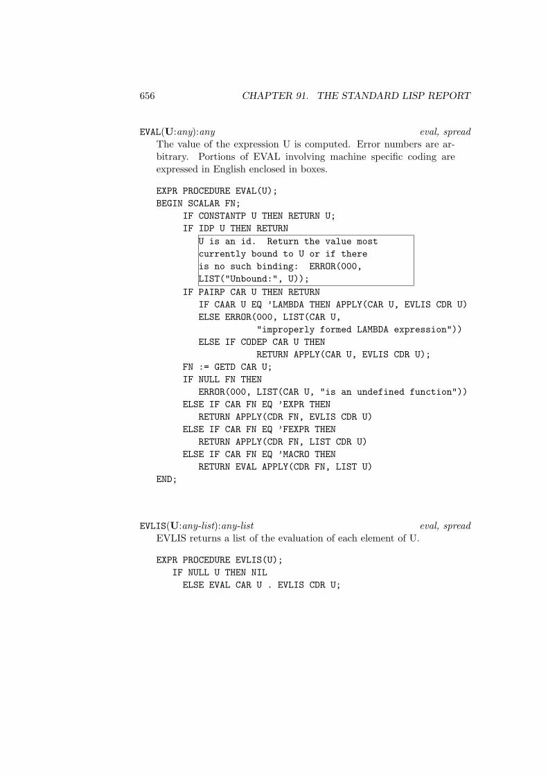
656 CHAPTER 91. THE STANDARD LISP REPORT
EVAL(U:any):any eval, spreadThe value of the expression U is computed. Error numbers are ar-bitrary. Portions of EVAL involving machine specific coding areexpressed in English enclosed in boxes.
EXPR PROCEDURE EVAL(U);BEGIN SCALAR FN;
IF CONSTANTP U THEN RETURN U;IF IDP U THEN RETURN
U is an id. Return the value mostcurrently bound to U or if thereis no such binding: ERROR(000,LIST("Unbound:", U));
IF PAIRP CAR U THEN RETURNIF CAAR U EQ ’LAMBDA THEN APPLY(CAR U, EVLIS CDR U)ELSE ERROR(000, LIST(CAR U,
"improperly formed LAMBDA expression"))ELSE IF CODEP CAR U THEN
RETURN APPLY(CAR U, EVLIS CDR U);FN := GETD CAR U;IF NULL FN THEN
ERROR(000, LIST(CAR U, "is an undefined function"))ELSE IF CAR FN EQ ’EXPR THEN
RETURN APPLY(CDR FN, EVLIS CDR U)ELSE IF CAR FN EQ ’FEXPR THEN
RETURN APPLY(CDR FN, LIST CDR U)ELSE IF CAR FN EQ ’MACRO THEN
RETURN EVAL APPLY(CDR FN, LIST U)END;
EVLIS(U:any-list):any-list eval, spreadEVLIS returns a list of the evaluation of each element of U.
EXPR PROCEDURE EVLIS(U);IF NULL U THEN NILELSE EVAL CAR U . EVLIS CDR U;

91.3. FUNCTIONS 657
EXPAND(L:list, FN:function):list eval, spreadFN is a defined function of two arguments to be used in the expansionof a MACRO. EXPAND returns a list in the form:
(FN L0 (FN L1 . . . (FN Ln−1 Ln) . . . ))
where n is the number of elements in L, Li is the ith element of L.
EXPR PROCEDURE EXPAND(L,FN);IF NULL CDR L THEN CAR LELSE LIST(FN, CAR L, EXPAND(CDR L, FN));
FUNCTION(FN:function):function noeval, nospreadThe function FN is to be passed to another function. If FN is to haveside effects its free variables must be fluid or global. FUNCTION islike QUOTE but its argument may be affected by compilation. Wedo not consider FUNARGs in this report.
QUOTE(U:any):any noeval, nospreadStops evaluation and returns U unevaluated.
FEXPR PROCEDURE QUOTE(U);CAR U;
91.3.15 Input and Output
The user normally communicates with Standard LISP through “standarddevices”. The default devices are selected in accordance with theconventions of the implementation site. Other input and output devices orfiles may be selected for reading and writing using the functions describedherein.
658 CHAPTER 91. THE STANDARD LISP REPORT
CLOSE(FILEHANDLE:any):any eval, spreadCloses the file with the internal name FILEHANDLE writing anynecessary end of file marks and such. The value of FILEHANDLEis that returned by the corresponding OPEN. The value returned isthe value of FILEHANDLE. An error occurs if the file can not beclosed.
***** FILEHANDLE could not be closed
EJECT():NIL eval, spreadSkip to the top of the next output page. Automatic EJECTs areexecuted by the print functions when the length set by the PAGE-LENGTH function is exceeded.
LINELENGTH(LEN:integer, NIL):integer eval, spreadIf LEN is an integer the maximum line length to be printed beforethe print functions initiate an automatic TERPRI is set to the valueLEN. No initial Standard LISP line length is assumed. The previousline length is returned except when LEN is NIL. This special casereturns the current line length and does not cause it to be reset. Anerror occurs if the requested line length is too large for the currentlyselected output file or LEN is negative or zero.
***** LEN is an invalid line length
LPOSN():integer eval, spreadReturns the number of lines printed on the current page. At the topof a page, 0 is returned.

91.3. FUNCTIONS 659
OPEN(FILE:any, HOW:id):any eval, spreadOpen the file with the system dependent name FILE for output ifHOW is EQ to OUTPUT, or input if HOW is EQ to INPUT. If thefile is opened successfully, a value which is internally associatedwith the file is returned. This value must be saved for use by RDSand WRS. An error occurs if HOW is something other than INPUTor OUTPUT or the file can’t be opened.
***** HOW is not option for OPEN***** FILE could not be opened
PAGELENGTH(LEN:integer, NIL):integer eval, spreadSets the vertical length (in lines) of an output page. Automatic pageEJECTs are executed by the print functions when this length isreached. The initial vertical length is implementation specific. Theprevious page length is returned. If LEN is 0, no automatic pageejects will occur.
POSN():integer eval, spreadReturns the number of characters in the output buffer. When thebuffer is empty, 0 is returned.
PRINC(U:id):id eval, spreadU must be a single character id such as produced by EXPLODE orread by READCH or the value of !$EOL!$. The effect is the characterU displayed upon the currently selected output device. The value of!$EOL!$ causes termination of the current line like a call to TERPRI.

660 CHAPTER 91. THE STANDARD LISP REPORT
PRINT(U:any):any eval, spreadDisplays U in READ readable format and terminates the print line.The value of U is returned.
EXPR PROCEDURE PRINT(U);<< PRIN1 U; TERPRI(); U >>;
PRIN1(U:any):any eval, spreadU is displayed in a READ readable form. The format of display isthe result of EXPLODE expansion; special characters are prefixedwith the escape character !, and strings are enclosed in ”. . . ”. Listsare displayed in list-notation and vectors in vector-notation.
PRIN2(U:any):any eval, spreadU is displayed upon the currently selected print device but output isnot READ readable. The value of U is returned. Items are displayedas described in the EXPLODE function with the exceptions thatthe escape character does not prefix special characters and stringsare not enclosed in ”. . . ”. Lists are displayed in list-notation andvectors in vector-notation. The value of U is returned.
RDS(FILEHANDLE:any):any eval, spreadInput from the currently selected input file is suspended and fur-ther input comes from the file named. FILEHANDLE is a systemdependent internal name which is a value returned by OPEN. IfFILEHANDLE is NIL the standard input device is selected. Whenend of file is reached on a non-standard input device, the standardinput device is reselected. When end of file occurs on the standardinput device the Standard LISP reader terminates. RDS returns theinternal name of the previously selected input file.
***** FILEHANDLE could not be selected for input
91.3. FUNCTIONS 661
READ():anyThe next expression from the file currently selected for input. Validinput forms are: vector-notation, dot-notation, list-notation, num-bers, function-pointers, strings, and identifiers with escape charac-ters. Identifiers are interned onW the OBLIST (see the INTERNfunction in ”Identifiers”, section 91.3.3 on page 629). READ returnsthe value of !$EOF!$ when the end of the currently selected inputfile is reached.
READCH():idReturns the next interned character from the file currently selectedfor input. Two special cases occur. If all the characters in an inputrecord have been read, the value of !$EOL!$ is returned. If the file
selected for input has all been read the value of !$EOF!$ is returned.Comments delimited by % and end-of-line are not transparent toREADCH.
TERPRI():NILThe current print line is terminated.
WRS(FILEHANDLE:any):any eval, spreadOutput to the currently active output file is suspended and furtheroutput is directed to the file named. FILEHANDLE is an internalname which is returned by OPEN. The file named must have beenopened for output. If FILEHANDLE is NIL the standard outputdevice is selected. WRS returns the internal name of the previouslyselected output file.
***** FILEHANDLE could not be selected for output

662 CHAPTER 91. THE STANDARD LISP REPORT
91.3.16 LISP Reader
An EVAL read loop has been chosen to drive a Standard LISP system toprovide a continuity in functional syntax. Choices of messages and theamount of extra information displayed are decisions left to theimplementor.
EXPR PROCEDURE STANDARD!-LISP();BEGIN SCALAR VALUE;
RDS NIL; WRS NIL;PRIN2 "Standard LISP"; TERPRI();WHILE T DO
<< PRIN2 "EVAL:"; TERPRI();VALUE := ERRORSET(QUOTE EVAL READ(), T, T);IF NOT ATOM VALUE THEN PRINT CAR VALUE;TERPRI() >>;
END;
QUIT()Causes termination of the LISP reader and control to be transferredto the operating system.
91.4 System GLOBAL Variables
These variables provide global control of the LISP system, or implementvalues which are constant throughout execution.2
*COMP = NIL globalThe value of !*COMP controls whether or not PUTD compiles thefunction defined in its arguments before defining it. If !*COMP isNIL the function is defined as an xEXPR. If !*COMP is somethingelse the function is first compiled. Compilation will produce certainchanges in the semantics of functions particularly FLUID type access.
2The published document does not specify that all these are GLOBAL.

91.4. SYSTEM GLOBAL VARIABLES 663
EMSG* = NIL globalWill contain the MESSAGE generated by the last ERROR call (see“Error Handling” section 91.3.8 on page 640).
$EOF$ = <an uninterned identifier> globalThe value of !$EOF!$ is returned by all input functions when the endof the currently selected input file is reached.
$EOL$ = <an uninterned identifier> globalThe value of !$EOL!$ is returned by READCH when it reaches theend of a logical input record. Likewise PRINC will terminate itscurrent line (like a call to TERPRI) when !$EOL!$ is its argument.
*GC = NIL global!*GC controls the printing of garbage collector messages. If NILno indication of garbage collection may occur. If non-NIL varioussystem dependent messages may be displayed.
NIL = NIL globalNIL is a special global variable. It is protected from being modifiedby SET or SETQ.
*RAISE = NIL globalIf !*RAISE is non-NIL all characters input through Standard LISPinput/output functions will be raised to upper case. If !*RAISE isNIL characters will be input as is.
T = T globalT is a special global variable. It is protected from being modified bySET or SETQ.
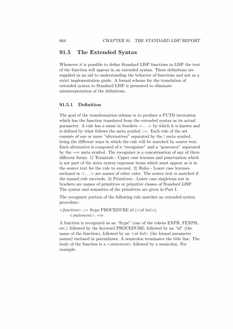
664 CHAPTER 91. THE STANDARD LISP REPORT
91.5 The Extended Syntax
Whenever it is possible to define Standard LISP functions in LISP the textof the function will appear in an extended syntax. These definitions aresupplied as an aid to understanding the behavior of functions and not as astrict implementation guide. A formal scheme for the translation ofextended syntax to Standard LISP is presented to eliminatemisinterpretation of the definitions.
91.5.1 Definition
The goal of the transformation scheme is to produce a PUTD invocationwhich has the function translated from the extended syntax as its actualparameter. A rule has a name in brackets <. . .> by which it is known andis defined by what follows the meta symbol ::=. Each rule of the setconsists of one or more “alternatives” separated by the | meta symbol,being the different ways in which the rule will be matched by source text.Each alternative is composed of a “recognizer” and a “generator” separatedby the =⇒ meta symbol. The recognizer is a concatenation of any of threedifferent forms. 1) Terminals - Upper case lexemes and punctuation whichis not part of the meta syntax represent items which must appear as is inthe source text for the rule to succeed. 2) Rules - Lower case lexemesenclosed in <. . .> are names of other rules. The source text is matched ifthe named rule succeeds. 3) Primitives - Lower case singletons not inbrackets are names of primitives or primitive classes of Standard LISP.The syntax and semantics of the primitives are given in Part I.
The recognizer portion of the following rule matches an extended syntaxprocedure:
<function> ::= ftype PROCEDURE id (<id list>);<statement>; =⇒
A function is recognized as an “ftype” (one of the tokens EXPR, FEXPR,etc.) followed by the keyword PROCEDURE, followed by an “id” (thename of the function), followed by an <id list> (the formal parameternames) enclosed in parentheses. A semicolon terminates the title line. Thebody of the function is a <statement> followed by a semicolon. Forexample:
91.5. THE EXTENDED SYNTAX 665
EXPR PROCEDURE NULL(X); EQ(X, NIL);
satisfies the recognizer, causes the generator to be activated and the rule tobe matched successfully.
The generator is a template into which generated items are substituted.The three syntactic entities have corresponding meanings when theyappear in the generator portion. 1) Terminals - These lexemes are copiedas is to the generated text. 2) Rules - If a rule has succeeded in therecognizer section then the value of the rule is the result of the generatorportion of that rule. 3) Primitives - When primitives are matched theprimitive lexeme replaces its occurrence in the generator.
If more than one occurrence of an item would cause ambiguity in thegenerator portion this entity appears with a bracketed subscript. Thus:
<conditional> ::=IF <expression> THEN <statement1>
ELSE <statement2> . . .
has occurrences of two different <statement>s. The generator portion usesthe subscripted entities to reference the proper generated value.
The <function> rule appears in its entirety as:
<function> ::= ftype PROCEDURE id (<id list>);<statement>; =⇒(PUTD (QUOTE id)
(QUOTE ftype)(QUOTE (LAMBDA (<id list>) <statement>)))
If the recognizer succeeds (as it would in the case of the NULL procedureexample) the generator returns:
(PUTD (QUOTE NULL) (QUOTE EXPR) (QUOTE (LAMBDA (X) (EQ X NIL))))
The identifier in the template is replaced by the procedure name NULL,<id list> by the single formal parameter X, the <statement> by (EQ XNIL) which is the result of the <statement> generator. EXPR replacesftype, the type of the defined procedure.

666 CHAPTER 91. THE STANDARD LISP REPORT
91.5.2 The Extended Syntax Rules
<function> ::= ftype PROCEDURE id (<id list>); <statement>; =⇒(PUTD (QUOTE id)
(QUOTE ftype)(QUOTE (LAMBDA (<id list>) <statement>)))
<id list> ::= id =⇒ id |id, <id list> =⇒ id <id list> |=⇒ NIL
<statement> ::= <expression> =⇒ <expression> |<proper statement> =⇒ <proper statement>
<proper statement> ::=<assignment statement> =⇒ <assignment statement> |<conditional statement> =⇒ <conditional statement> |<while statement> =⇒ <while statement> |<compound statement> =⇒ <compound statement>
<assignment statement> ::= id := <expression> =⇒(SETQ id <expression>)
<conditional statement> ::=IF <expression> THEN <statement1> ELSE <statement2> =⇒
(COND (<expression> <statement1>)(T <statement2>)) |IF <expression> THEN <statement> =⇒
(COND (<expression> <statement>))
<while statement> ::= WHILE <expression> DO <statement> =⇒(PROG NILLBL (COND ((NULL <expression>) (RETURN NIL)))
<statement>(GO LBL))
<compound statement> ::=BEGIN SCALAR <id list>; <program list> END =⇒
(PROG (<id list>) <program list>) |BEGIN <program list> END =⇒
(PROG NIL <program list>) |<< <statement list> >> =⇒ (PROGN <statement list>)

91.5. THE EXTENDED SYNTAX 667
<program list> ::= <full statement> =⇒ <full statement> |<full statement> <program list> =⇒
<full statement> <program list>
<full statement> ::= <statement> =⇒ <statement> | id: =⇒ id
<statement list> ::= <statement> =⇒ <statement> |<statement>; <statement list> =⇒
<statement> <statement list>
<expression> ::=<expression1> . <expression2> =⇒
(CONS <expression1> <expression2> |<expression1> = <expression2> =⇒
(EQUAL <expression1> <expression2>) |<expression1> EQ <expression2> =⇒
(EQ <expression1> <expression2>) |’<expression> =⇒ (QUOTE <expression>) |function <expression> =⇒ (function <expression>) |function(<argument list>) =⇒ (function <argument list>) |number =⇒ number |id =⇒ id
<argument list> ::= () =⇒ |<expression> =⇒ <expression> |<expression>, <argument list> =⇒ <expression> <argument list>
Notice the three infix operators . EQ and = which are translated into callson CONS, EQ, and EQUAL respectively. Note also that a call on afunction which has no formal parameters must have () as an argument list.The QUOTE function is abbreviated by ’.

668 CHAPTER 91. THE STANDARD LISP REPORT

Part IV
Appendix
669


Appendix A
Reserved Identifiers
We list here all identifiers that are normally reserved in REDUCEincluding names of commands, operators and switches initially in thesystem. Excluded are words that are reserved in specific implementationsof the system.
Commands ALGEBRAIC ANTISYMMETRIC ARRAY BYE CLEARCLEARRULES COMMENT CONT DECOMPOSE DEFINEDEPEND DISPLAY ED EDITDEF END EVEN FACTOR FORFORALL FOREACH GO GOTO IF IN INDEX INFIX INPUTINTEGER KORDER LET LINEAR LISP LISTARGP LOADLOAD PACKAGE MASS MATCH MATRIX MSHELLNODEPEND NONCOM NONZERO NOSPUR ODD OFF ONOPERATOR ORDER OUT PAUSE PRECEDENCEPRINT PRECISION PROCEDURE QUIT REAL REMFACREMIND RETRY RETURN SAVEAS SCALAR SETMODSHARE SHOWTIME SHUT SPUR SYMBOLIC SYMMETRICVECDIM VECTOR WEIGHT WRITE WTLEVEL
Boolean Operators EVENP FIXP FREEOF NUMBERP ORDP PRIMEP
Infix Operators := = >= > <= < => + - * / ^ ** . WHERE SETQ ORAND MEMBER MEMQ EQUAL NEQ EQ GEQ GREATERP LEQLESSP PLUS DIFFERENCE MINUS TIMES QUOTIENTEXPT CONS
671

672 APPENDIX A. RESERVED IDENTIFIERS
Numerical Operators ABS ACOS ACOSH ACOT ACOTH ACSC ACSCH ASECASECH ASIN ASINH ATAN ATANH ATAN2 COS COSH COTCOTH CSC CSCH EXP FACTORIAL FIX FLOOR HYPOT LNLOG LOGB LOG10 NEXTPRIME ROUND SEC SECH SINSINH SQRT TAN TANH
Prefix Operators APPEND ARGLENGTH CEILING COEFF COEFFNCOFACTOR CONJ DEG DEN DET DF DILOG EI EPS ERFFACTORIZE FIRST GCD G IMPART INT INTERPOL LCMLCOF LENGTH LHS LINELENGTH LTERM MAINVAR MATMATEIGEN MAX MIN MKID NULLSPACE NUM PART PFPRECISION PROD RANDOM RANDOM NEW SEED RANKREDERR REDUCT REMAINDER REPART REST RESULTANTREVERSE RHS SECOND SET SHOWRULES SIGN SOLVESTRUCTR SUB SUM THIRD TP TRACE VARNAME
Reserved Variables CARD NO E EVAL MODE FORT WIDTH HIGH POW IINFINITY K!* LOW POW NIL PIROOT MULTIPLICITIES T
Switches ADJPREC ALGINT ALLBRANCH ALLFAC BALANCE MODBFSPACE COMBINEEXPT COMBINELOGS COMP COMPLEXCRAMER CREF DEFN DEMO DIV ECHO ERRCONTEVALLHSEQP EXP EXPANDLOGS EZGCD FACTOR FORTFULLROOTS GCD IFACTOR INT INTSTR LCM LISTLISTARGS MCD MODULAR MSG MULTIPLICITIES NATNERO NOSPLIT OUTPUT PERIOD PRECISE PRET PRIRAT RATARG RATIONAL RATIONALIZE RATPRI REVPRIRLISP88 ROUNDALL ROUNDBF ROUNDED SAVESTRUCTRSOLVESINGULAR TIME TRA TRFAC TRIGFORM TRINT
Other Reserved Ids BEGIN DO EXPR FEXPR INPUT LAMBDA LISP MACROPRODUCT REPEAT SMACRO SUM UNTIL WHEN WHILE WS

Bibliography
[1] G. A. Baker, L. P. Benofy, M. Fortes, M. de Llano, S. M. Peltier, andA. Plastino. Hard-core square-well fermion. Phys. Rev. A,26(6):3575–3588, 1982.
[2] Computation Center. LISP Reference Manual, CDC-6000. TheUniversity of Texas at Austin.
[3] S.-C. Chou. Automated reasoning in geometries using thecharacteristic set method and Grobner basis method. In ISSAC ’90:Proceedings of the international symposium on Symbolic and algebraiccomputation, pages 255–260, New York, NY, USA. ACM.
[4] S.-C. Chou. Proving elementary geometry theorems using Wu’salgorithm. In Contemp. Math., volume 19, pages 243 – 286. AMS,Providence, Rhode Island, 1984.
[5] S.-C. Chou. Mechanical geometry theorem proving. Reidel, Dortrecht,1988.
[6] Stanford Center for Information Processing. LISP/360 ReferenceManual. Stanford University.
[7] M. L. Griss and A. C. Hearn. A portable LISP compiler.Software—Practice and Experience, 11:541–605, June 1981.
[8] A. C. Hearn. REDUCE user’s manual: Version 3.3. Publication CP78(Rev 1/88), RAND, 1988.
[9] A. C. Hearn, P. K. Kuo, and D. R. Yennie. Radiative corrections toan electron-positron scattering experiment. Phys. Rev.,187(5):2088–2096, 1969.
673

674 BIBLIOGRAPHY
[10] Wolfram Koepf. REDUCE package for the indefinite and definitesummation. SIGSAM Bulletin, 29(1):14–30, January 1995.
[11] T. H. Koornwinder. On Zeilberger’s algorithm and its q-analogue: arigorous description. J. of Comput. and Appl. Math., 48(1-2):91–111,October 1993.
[12] MACLISP Reference Manual, March 1976.
[13] John McCarthy, Paul W. Abrahams, Daniel J. Edwards, Timothy P.Hart, and Michael I. Levin. LISP 1.5 Programmers Manual. TheM.I.T. Press, Cambridge, Massachusettes, 1965.
[14] Mats Nordstrom, Erik Sandewall, and Diz Breslow. LISP F1: AFORTRAN Implementation of LISP 1.5. Uppsala University,Department of Computer Sciences.
[15] Lynn H. Quam and Whitfield Diffie. Stanford LISP 1.6 Manual.Stanford Artificial Intelligence Laboratory, operating note 28.7 edition.
[16] Warren Teitelman. INTERLISP Reference Manual. XEROX, PaloAlto Research Centers, 3333 Coyote Road, Palo Alto, California94304, 1978.
[17] Volker Weispfenning. Comprehensive Grobner bases. Journal ofSymbolic Computation, 14(1):1–29, July 1992.
[18] W.-T. Wu. On the decision problem and the mechanization oftheorem-proving in elementary geometry. In W. W. Bledsoe andD. W. Loveland, editors, Automated Theorem Proving: After 25Years, volume 29 of Contemporary Mathematics, pages 213–234. AMS,Providence, Rhode Island, 1984.
[19] W.-T. Wu. Some recent advances in mechanical theorem proving ofgeometry. In W. W. Bledsoe and D. W. Loveland, editors, AutomatedTheorem Proving: After 25 Years, volume 29 of ContemporaryMathematics, pages 235–241. AMS, Providence, Rhode Island, 1984.
[20] W.-T. Wu. Mechanical Theorem Proving in Geometries. Number 1 inTexts and Monographs in Symbolic Computation. Springer, Wien,1994.

Index
!*CSYSTEMS global (AVECTOR),274
><3-D vector, 457diphthong, 457
| operator, 340(), 622*
3-D vector, 457power series, 577vector, 272
**power series, 577
*** (warning message), 624***** (error message), 624, 640*COMP (fluid), 633, 634*COMP (global), 662*COMP variable, 633*GC (global), 663*RAISE (global), 619, 663+
3-D vector, 457power series, 577vector, 272
-3-D vector, 457power series, 577vector, 272
-list, 621., 247. (CONS), 60/
3-D vector, 457power series, 577vector, 272
:-, 474::=, 356::=:, 357:=:, 356;BEGIN; marker, 360;END; marker, 360@ operator, 338[. . . ] syntax, 623#
Hodge-* operator, 340$EOF$ (global), 661, 663$EOL$ (global), 659, 661, 663%, 624%
read by READCH, 661ˆ
3-D vector, 457exterior multiplication, 337
| operator, 339=, 473. . .
as syntax, 6223j and 6j symbols, 545
ABAGLISTP, 250ABS, 644ABS, 80ACFSF, 499, 501ACOS, 83, 86
675

676 INDEX
ACOSH, 83, 86ACOT, 83, 86ACOTH, 83, 86ACSC, 83, 86ACSCH, 83, 86ADD1, 644ADD COLUMNS, 405, 407ADD ROWS, 405ADD TO COLUMNS, 405, 407ADD TO ROWS, 405, 407ADJ, 469ADJPREC, 149Airy functions, 545Airy Ai, 545Airy Aiprime, 545Airy Bi, 545Airy Biprime, 545ALATOMP, 257ALG TO SYMB, 258ALGEBRAIC, 197Algebraic mode, 197, 203, 204ALGINT, 193, 233alist, 622alist
in ASSOC, 650in SASSOC, 653in SUBLIS, 654
ALKERNP, 257ALL, 499ALL!*, 354ALLBRANCH, 99ALLFAC, 116, 119allsymmetrybases, 560ALTITUDE, 366AND, 642AND, 499ANGLE SUM, 366antecedent (cond-form), 622ANTICOM, 322, 468ANTICOMM, 468
ANTICOMMUTE, 469ANTISYMMETRIC, 107, 322any, 621APPEND, 650APPEND, 61APPENDN, 247APPLY, 655APPLYSYM, 194, 237ARBCONST operator, 452ARBVARS, 99ARGLENGTH, 131ARNUM, 194, 241ARRAY, 75ARRAY TO LIST, 261ASEC, 83, 86ASECH, 83, 86ASFIRST, 248ASFLIST, 248ASIN, 83, 86ASINH, 83, 86ASLAST, 248ASREST, 248Assignment, 64, 65, 67, 72, 202, 204ASSIST, 194, 245ASSLIST, 248ASSOC, 650ASSOC, 500association list, 622assumptions, 101Asymptotic command, 153, 166ATAN, 83, 86, 90ATAN2, 83, 86ATANH, 83, 86ATENSOR, 267ATOM, 625atom, 621AUGMENT, 330AUGMENT COLUMNS, 405, 409AVEC function, 272AVECTOR, 194, 271

INDEX 677
AVECTOR packageexample, 275–277
AXP, 554AXX, 554
B PART, 556BAG, 249BAGLISTP, 250BAGLMAT, 263BAGP, 250BALANCED MOD, 149BAND MATRIX, 406, 409BEGIN ...END, 71–74BELAST, 247Bernoulli, 544Bernoulli numbers, 544Bernoulli polynomials, 545BernoulliP, 545Bernstein base, 448Bessel functions, 544BesselI, 544BesselJ, 544BesselK, 544BesselY, 544Beta, 544Beta function, 544BEZOUT, 140BF PART, 556BFSPACE, 148Binomial, 544Binomial coefficients, 544Block, 71, 74BLOCK MATRIX, 406, 409BNDEQ!*, 341BOOLEAN, 194, 279Boolean, 55boolean, 621BOS, 554BOTH, 418BOUNDS, 439, 445
BPART, 556Buchberger’s Algorithm, 377BYE, 77
C1 CIRCLE, 366CALI, 194, 285Call by value, 187, 189CAMAL, 287CAMAL, 194, 287Canonical form, 111canonicaldecomposition, 560CAR, 628CAR
composite forms, 628CARD NO, 123CARTAN SYSTEM, 331cartesian coordinates, 455Catalan, 543CAUCHY SYSTEM, 331CC TANGENT, 366CDR, 628CDR
composite forms, 628CEILING, 80Celestial Mechanics, 287CFRAC, 491CGB, 292CGBFULLRED, 296CGBGEN, 294CGBGS, 296CGBREAL, 295CGBSTAT, 296chain rule, 339CHAN, 556CHANGEVAR, 297CHANGEVR, 194CHAR MATRIX, 406, 410CHAR POLY, 405, 406, 410character, 560Character set, 43
678 INDEX
CHARACTERISTIC VARIETY, 332CHARACTERS, 331Chebyshev fit, 439Chebyshev polynomials, 545Chebyshev base T, 448Chebyshev base U, 448Chebyshev df, 445Chebyshev eval, 446Chebyshev fit, 445Chebyshev int, 445ChebyshevT, 545ChebyshevU, 545CHECKPROLIST, 255Chi, 546CHIRAL, 557CHIRAL1, 557CHOLESKY, 406CHOOSE PC, 366CHOOSE PL, 367Ci, 546CIRCLE, 367CIRCLE1, 367CIRCLE CENTER, 367CIRCLE SQRADIUS, 367CL TANGENT, 367CLEANUP, 331, 332CLEAR, 156, 160, 258CLEARBAG, 249CLEARFLAG, 255CLEARFUNCTIONS, 258CLEAROP, 258CLEARPHYSOP, 465CLEARRULES, 161Clebsch Gordan coefficients, 545Clebsch Gordan, 545CLOSE, 658CLOSED, 332CLOSURE, 331COBASIS, 329code templates, 360
CODEP, 620, 625COEFF, 128COEFF MATRIX, 406Coefficient, 147–150COEFFN, 129COERCEMAT, 263COFACTOR, 181coframe, 340, 343COFRAME
WITH METRIC, 343WITH SIGNATURE, 343
COFRAMING, 328, 329COLLECT, 67COLLINEAR, 367COLUMN DIM, 405, 407COMBINATIONS, 253COMBINEEXPT, 86COMBINELOGS, 85COMBNUM, 252COMM, 468, 538Command, 75Command terminator, 169COMMENT, 48comments, 624COMMUTE, 469COMP, 219COMPACT, 194, 299COMPACT operator, 299COMPACT package, 299COMPANION, 406Compiler, 219COMPLEX, 150Complex coefficient, 150Compound statement, 70, 72COMPRESS, 620, 630CONCURRENT, 367COND, 642cond-form, 622Conditional statement, 66CONJ, 80

INDEX 679
CONS, 628CONS, 247consequent (cond-form), 622constant, 621CONSTANTP, 625Constructor, 205CONT, 176CONTACT, 328CONTFR, 194CONTFRAC, 491continuation lines, 359contour, 374CONTRACT, 467CONVERT, 413COORDINATES, 329, 332COORDINATES operator, 274COORDS vector, 274COPY INTO, 405, 407COS, 83, 86COSH, 83, 86COT, 83, 86COTH, 83, 86CP, 556CRACK, 194, 301CRAMER, 95, 179CREF, 221, 222CRESYS, 538CROSS, 330CROSS
vector, 272cross product, 272, 457Cross reference, 221CROSSVECT, 261CSC, 83, 86CSCH, 83, 86CURL
operator, 273curl
vector field, 273curl operator, 458
CVIT, 194, 305CVITBTR, 305CVITOP, 305CVITRACE, 305CYCLICPERMLIST, 252cylindrical coordinates, 455
D, 554D PART, 556data structures, 621DE, 633Declaration, 75DECLARE function, 358DECOMPOSE, 141default
term order, 378defid, 512defindex, 512DEFINE, 78definite integration (simple), 276DEFINT, 194, 307DEFINT function, 276DEFLINEINT function, 277DEFLIST, 650DEFN, 203, 223, 224DEFPOLY, 241DEG, 143Degree, 143DEL, 554DELETE, 651DELETE, 246DELETE ALL, 246DELLASTDIGIT, 251DELPAIR, 246DELSQ
operator, 273delsq operator, 458DEMO, 76DEN, 134, 143DEPATOM, 254

680 INDEX
DEPEND, 103, 109DEPEND statement, 459DEPTH, 247DEPVARP, 257DER, 554derivative
variational, 341derivatives, 315DERIVED SYSTEMS, 331DESIR, 194, 311DET, 112, 179DETIDNUM, 251DETRAFO, 239DF, 633DF, 87, 88DFP, 316DFP COMMUTE, 318DFPART, 194, 315DIAGONAL, 405, 407diagonalize, 560DIFFERENCE, 644Differentiation, 87, 88, 109differentiation
partial, 338vector, 273
DIFFSET, 251DIGIT, 651DILOG, 83, 90dilog, 546Dilogarithm function, 546DIM, 331DIM GRASSMANN VARIETY, 331dimension, 337Dirac γ matrix, 212direct product, 412DISJOIN, 332DISPJACOBIAN, 298DISPLAY, 174Display, 111DISPLAYFLAG, 255
DISPLAYFRAME command, 344Displaying structure, 126DISTRIBUTE, 259DIV, 117, 147, 500DIV
operator, 273div operator, 458divergence
vector field, 273DIVIDE, 644division by zero, 644, 647DIVPOL, 260DLINEINT, 460dlist, 650DM, 633DO, 67, 69Dollar sign, 63DOT, 466DOT
vector, 272Dot product, 211, 272dot product, 458dot-notation, 619, 621DOT HAM, 556dotgrad operator, 458dotted-pair, 619, 627, 628DOUBLE switch, 355DR, 554DRR, 557DUMMY, 194, 321DUMMY BASE, 321dummy names, 322DUMMYPRI, 269DVFSF, 499, 500DVINT, 460DVOLINT, 460DYW, 556
E, 46ECHO, 169

INDEX 681
ED, 173, 174EDITDEF, 175EDS, 325, 328EDS: Exterior differential
dystems, 325EDSDEBUG, 332EDSDISJOINT, 332EDSSLOPPY, 332EDSVERBOSE, 332Ei, 83, 546EJECT, 658, 659EllipticE, 546EllipticF, 546EllipticK, 546EllipticTheta, 546ELMULT, 246EMSG* (global), 640, 663END, 77end of file, 663end of line, 663EPS, 213, 345EQ, 625EQ
in MEMQ, 652of dotted-pairs, 628of function-pointers, 620, 625of GENSYMs, 631of identifiers, 629
EQN, 625EQUAL, 625EQUAL, 500, 501EQUAL
in ASSOC, 650in DELETE, 651in MEMBER, 652in SASSOC, 653in SUBST, 654
Equation, 57EQUIV, 332, 499ERF, 90
erf, 546erfc, 546ERRCONT, 173ERROR, 624, 640, 663error
type mismatch error, 624error messages, 624ERRORSET, 640escape character, 624Euclidean metric, 343Euler, 544Euler polynomials, 544Euler Gamma, 543EulerP, 545EVAL, 656EVAL, 355EVAL
function, 622function type, 623lambda expressions, 622MACRO functions, 623of constants, 621
EVAL MODE, 197evalb, 529EVALLHSEQP, 57EVEN, 104Even operator, 104EVENP, 56EVLIS, 656EX, 499EXCALC, 194, 327, 335EXCALC package
example, 338, 339, 341, 342, 344Exclamation mark, 43EXCLUDE, 516EXDEGREE command, 336EXFACTORS, 332EXP, 83, 86, 90, 134, 137EXPAND, 657EXPAND CASES, 96

682 INDEX
EXPANDLOGS, 85EXPLICIT, 254EXPLODE, 620, 630, 641EXPR, 620, 621, 633EXPR, 203Expression, 53EXPT, 645EXTEND, 405, 407extended gosper, 602exterior calculus, 335exterior differentiation, 338exterior form
declaration, 336vector, 336with indices, 342
exterior product, 337, 345extra-boolean, 621EXTRACTLIST, 255EXTRACTMAT, 369EXTREMUM, 254EZGCD, 137
FACTOR, 115, 135FACTORIAL, 80, 190Factorization, 134FACTORIZE, 135, 136FALSE, 499Fast loading of code, 220FAST LA, 415FCOMB, 556FDOMAIN command, 338FER, 554FEXPR, 620, 621, 623, 633FEXPR, 203Fibonacci, 544Fibonacci, 544Fibonacci polynomials, 545FibonacciP, 545FIDE, 194, 347file handle, 658–661
File handling, 169files, 658, 659FIND COMPANION, 405, 410FIRST, 60FIRSTROOT, 517FIX, 643, 645FIX, 81FIXP, 626FIXP, 56FJACOB, 556FLAG, 618, 632FLAGP, 618, 632flags, 631FLOAT, 643, 645floating
input, 618output, 630
FLOATP, 626FLOOR, 81FLUID, 618, 635fluid
in traceback, 640unbinding by ERROR, 640
fluid binding, 635fluid binding
as default, 635FLUIDP, 636FOLLOWLINE, 252FOR, 74FOR ALL, 155, 156FOR EACH, 67, 68, 202FORDER command, 345formal parameter limit, 623FORT, 123FORT WIDTH, 125FORTRAN, 123, 124FORTUPPER, 125FOURIER, 288Fourier cosine transform, 309Fourier Series, 287

INDEX 683
Fourier sine transform, 309FPART, 556FPS, 194, 351fps search depth, 352FRAME command, 344FREEOF, 56FREQUENCY, 246Fresnel C, 546Fresnel S, 546frobenius, 434ftype, 621FUIDP, 618FULLROOTS, 97FUN, 554FUNARGs not supported, 657FUNCTION, 359, 657Function, 191function, 622function
as GLOBAL, 633as global, 634
function-pointer, 620function-pointer
output, 630functions, 618FUNCVAR, 254
G, 212G3, 591Gamma, 544Gamma function, 544gammatofactorial, 606garbage collector, 663GCD, 137GDIMENSION, 381Gegenbauer polynomials, 545GegenbauerP, 545Generalised Hypergeometric
functions, 547generic function, 315
GENERIC FUNCTION, 315GENPOS, 332GENSYM, 631GENTRAN, 194, 353, 523GENTRAN
file output, 363preevaluation, 356, 361templates, 360
GENTRAN packageexample, 354
GENTRANIN command, 360GENTRANOPT, 523GENTRANOUT command, 363GENTRANSEG switch, 359GENTRANSHUT command, 363GEOMETRY, 365GEQ, 500GET, 618, 632GET
not for functions, 632GET COLUMNS, 405, 407GET ROWS, 405, 408GETCSYSTEM command, 274GETD, 618, 620, 634GETROOT, 517GETV, 641GHOSTFACTOR, 262GINDEPENDENT SETS, 381GLEXCONVERT, 381GLOBAL, 618, 636global binding, 635GLOBALP, 618, 634, 636GLTBASIS, 380, 384GNUPLOT, 194, 373GO, 622, 638GO
in COND, 638, 642GO TO, 72, 73Golden Ratio, 543gosper, 601

684 INDEX
Gosper’s Algorithm, 549GRA, 556GRAD
operator, 273grad operator, 458gradient
vector field, 273GRADLEX, 391GRADLEX
term order, 378GRAM SCHMIDT, 406, 413GRAS, 554Grassmann Operators, 261GRASSMANN VARIETY, 331GRASSP, 262GRASSPARITY, 262GREATERP, 645GREATERP, 500GREDUCE, 385GROEBFULLREDUCTION, 380, 384GROEBNER, 195, 377, 379Groebner, 95Groebner Bases, 427GROEBNER package, 377GROEBNER package
example, 379GROEBNERF, 383, 386GROEBOPT, 380, 384GROEBRESTRICTION, 385GROEBSTAT, 384GROESOLVE, 386Group statement, 65, 66, 70GSYS, 293GSYS2CGB, 294GVARS, 379GVARSLAST, 380gvarslast, 379GZERODIM?, 380
Hankel functions, 544
Hankel transform, 309Hankel1, 544Hankel2, 544HARMONIC, 287HCONCMAT, 264HDIFF, 288HERMAT, 264Hermite polynomials, 545Hermite base, 448HermiteP, 545HERMITIAN TP, 405, 408HESSIAN, 406, 410HFACTORS scale factors, 274hidden3d, 374High energy trace, 215High energy vector expression, 211,
214HIGH POW, 129HIGHESTDERIV, 452HILBERT, 406, 411HINT, 288History, 174Hodge-* duality operator, 340, 345HSUB, 288hyperrecursion, 604hypersum, 604hyperterm, 604HYPEXPAND, 260HYPOT, 83, 86HYPREDUCE, 260
I, 46i, 241I SOLVE, 521iBeta, 544id
escape character, 619input, 618maximum length, 619minimum size, 631

INDEX 685
output, 630id-list, 621ideal dimension, 381IDEALQUOTIENT, 386IDEALS, 195, 387Identifier, 45identifier (see id), 618IDP, 626IF, 65, 66IFACTOR, 135iGamma, 544IMAGINARY, 411imaginary unit, 241IMPART, 80, 81, 83IMPL, 499IMPLICIT, 254IMPLICIT option, 359IMPLICIT TAYLOR operator, 564IN, 169incomplete Beta function, 544incomplete Gamma function, 544Indefinite integration, 88INDEPENDENCE, 329independent sets, 381INDEX, 212INDEX EXPAND, 332INDEXSYMMETRIES command,
342INEQ, 195, 389INFINITY, 46, 516INFIX, 108Infix operator, 48–51inner product, 458inner product
exterior form, 339INPUT, 659INPUT, 174Input, 169INSERT, 246INSERT KEEP ORDER, 246
Instant evaluation, 76, 131, 154,178, 180
INT, 88, 176, 233, 307INTEGER, 71Integer, 54integer
input, 617magnitude, 617, 643output, 630
integer-list, 621INTEGRAL ELEMENT, 331Integration, 88, 106integration
definite (simple), 276line, 277volume, 276
Interactive use, 173, 176INTERN, 618, 631, 661INTERPOL, 142INTERSECT, 251intersect, 528INTERSECTION POINT, 367Interval, 439Introduction, 37INTSTR, 112INVARIANTS, 332INVBASE, 195, 391, 392INVERSE, 557INVERSE TAYLOR, 564INVERT, 332INVLAP, 395INVOLUTION, 331INVOLUTIVE, 332INVTORDER, 392invztrans, 611ISOLATER, 516
JACOB, 556Jacobi Elliptic Functions and
Integrals, 546

686 INDEX
Jacobi’s polynomials, 545JACOBIAN, 406, 411, 442Jacobicd, 546Jacobicn, 546Jacobics, 546Jacobidc, 546Jacobidn, 546Jacobids, 546Jacobinc, 546Jacobind, 546Jacobins, 546JacobiP, 545Jacobisc, 546Jacobisd, 546Jacobisn, 546JOIN, 67jordan, 436JORDAN BLOCK, 406, 411jordansymbolic, 435
K-transform, 309KBASIS, 268KEEP command, 345Kernel, 111, 112, 115, 128kernel form, 112KERNLIST, 246Khinchin, 543KORDER, 128, 466KORDERLIST, 254KRONECKER PRODUCT, 406, 412Kummer functions, 545KummerM, 545KummerU, 545
l’Hopital’s rule, 401, 460L2 ANGLE, 367Label, 72, 73Laguerre polynomials, 545Laguerre base, 448LaguerreP, 545
laline!*, 512LAMBDA, 622LAMBDA, 201lambda expression, 622Lambert ω function, 546Lambert’s W, 95Lambert W, 546LAPLACE, 195, 395Laplace transform, 309Laplacian
vector field, 273lasimp, 511LAST, 247latex, 511Laurent series, 563Laurent series expansions, 569LCM, 138LCOF, 144Leading coefficient, 144LEADTERM, 259Legendre polynomials, 187, 545Legendre base, 448LegendreP, 545LENGTH, 651LENGTH, 59, 76, 90, 133, 135, 179,
501LEQ, 500Lerch Phi function, 546Lerch Phi, 546LESSP, 645LESSP, 500LET, 85, 87, 100, 106–108, 152, 161,
189, 190Levi-Cevita tensor, 345LEX, 391LEX
term order, 378LHS, 57li, 546LIE, 195, 399

INDEX 687
Lie Derivative, 340LIE LIST, 400LIECLASS, 400LIENDIMCOM1, 399LIFT, 330LIMIT, 401, 460LIMIT+, 402LIMIT-, 402LIMITS, 195, 401LINALG, 195, 405LINE, 367line integrals, 277LINEAR, 105Linear operator, 105, 106, 109LINEAR DIVISORS, 332LINEARISE, 331LINEINT, 460LINEINT function, 277LINELENGTH, 658LINELENGTH, 114LISP, 197Lisp, 197LIST, 629LIST, 117List, 59list, 621list, 93List operation, 59, 61list-notation, 621LIST TO ARRAY, 261LIST TO IDS, 251LISTARGP, 61LISTARGS, 61LISTBAG, 250LITER, 651LN, 83, 86LOAD, 220LOAD PACKAGE, 193, 221local binding, 635LOG, 83, 86, 90
LOG10, 83, 86LOGB, 83, 86Lommel functions, 545Lommel1, 545Lommel2, 545Loop, 67, 68LOT, 367LOW POW, 129LOWER MATRIX, 411LOWESTDEG, 260lpon, 395LPOSN, 658LPOWER, 145LRSETQ, 358lrsetq operator, 357LSETQ, 357lsetq operator, 356LTERM, 145, 209ltrig, 395LU DECOM, 406, 413LYST, 556LYST1, 556LYST2, 556
M, 472M ROOTS, 421M SOLVE, 421MACIERZ, 556MACRO, 621, 623, 633MACRO, 203MAINVAR, 146MAKE IDENTITY, 406, 411MAP, 648MAP, 91map, 93MAPC, 648MAPCAN, 649MAPCAR, 649MAPCON, 649MAPLIST, 649

688 INDEX
MASS, 214, 216MAT, 177, 178MATCH, 159MATEIGEN, 180MATEXTC, 264MATEXTR, 264Mathematical function, 83MATHML, 417, 418mathstyle, 512matrices
in GENTRAN, 356, 357, 362MATRIX, 178Matrix assignment, 183Matrix calculations, 177MATRIX, see also SPARSE, 533MATRIX AUGMENT, 405, 408MATRIX STACK, 405, 408MATRIXP, 406, 535MATSUBC, 264MATSUBR, 264MAX, 646MAX, 81MAX2, 646MAXEXPPRINTLEN!*, 359MCD, 137, 139MEDIAN, 367Meijer’s G function, 547MEMBER, 652member, 530MEMQ, 652MERGE LIST, 246metric structure, 343MIDPOINT, 367MIN, 646MIN, 81MIN2, 646Minimum, 439MINOR, 405, 408MINUS, 646MINUSP, 626
MINVECT, 261mixed-mode arithmetic, 643MKAND, 499MKDEPEND, 332MKID, 92, 263MKIDM, 263MKIDNEW, 251MKLIST, 246MKOR, 499MKPOLY, 517MKRANDTABL, 252MKSET, 251, 528MKVECT, 641MML, 418Mode, 76Mode communication, 203MODSR, 195, 421MODULAR, 149Modular coefficient, 149MONOM, 259monomial base, 448Moore–Penrose inverse, 413Motzkin, 544Motzkin, 544MP, 367MPVECT, 261MRV LIMIT, 424MRVLIMIT, 423MSG, 223MSHELL, 216MULT COLUMNS, 405, 407MULT ROW, 407MULT ROWS, 405Multiple assignment statement, 64MULTIPLICITIES, 96MULTIROOT, 519
N GAT, 556NASSOC, 500NAT, 125, 329

INDEX 689
NAT flag, 342nc cleanup, 429nc compact, 432nc divide, 431nc factorize, 431nc factorize all, 432nc groebner, 430nc preduce, 431nc setup, 428NCONC, 652NCPOLY, 195, 427NEARESTROOT, 517NEARESTROOTS, 517NEGATIVE, 516NEQ, 500, 501NERO, 122Newton’s method, 439NEXTPRIME, 82NIL
cannot be changed, 636, 637,663
NIL (global), 621, 624, 663NOCONVERT, 148NODEPEND, 109NODEPEND statement, 459NODRR, 557NOETHER function, 341NOEVAL
function type, 623Non-commuting operator, 106NONCOM, 106, 322, 463, 468NONZERO, 104NORDP, 257NORMFORM, 195, 433NOSPLIT, 117NOSPREAD
function type, 623NOSPUR, 215NOSUM command, 342NOSUM switch, 342
NOT, 643NOT, 499NOT NEGATIVE, 411NOXPND
@, 339D, 339
NULL, 626NULLSPACE, 182NUM, 146NUM FIT, 446NUM INT, 439, 442NUM MIN, 439, 440NUM ODESOLVE, 439, 443NUM SOLVE, 439, 441Number, 44, 45number, 621NUMBERP, 626NUMBERP, 56NUMERIC, 195, 439Numerical operator, 79Numerical precision, 46
OBLIST, 629OBLIST entry, 618, 631, 661ODD, 104Odd operator, 104ODDP, 252ODEDEGREE, 452ODELINEARITY, 452ODEORDER, 452ODESOLVE, 195, 451, 452ODWA, 556OFF, 76, 77OFSF, 499, 500ON, 76, 77ONE FORMS, 329ONE OF, 96ONEP, 627ONLY INTEGER, 411OPAPPLY, 469

690 INDEX
OPEN, 658, 659OPERATOR, 208Operator, 48–51Operator precedence, 49, 51OPORDER, 466OPTIMIZE, 523OR, 643OR, 499ORDER, 115, 128ordering
exterior form, 345ordinary differential equations, 451ORDP, 56, 106ORTHOGONAL, 368Orthogonal polynomials, 541ORTHOVEC, 195, 455OTHER CC POINT, 368OTHER CL POINT, 368OUT, 169, 170OUTPUT, 659OUTPUT, 114Output, 120, 124Output declaration, 114, 115
P3 ANGLE, 368P3 CIRCLE, 368P3 CIRCLE1, 368P4 CIRCLE, 368PADE, 492PAGELENGTH, 658, 659PAIR, 653PAIR, 247PAIRP, 627PAR, 368PARALLEL, 368PARSEML, 418PART, 59, 127, 130, 501partial derivatives, 315partial differentiation, 338PAUSE, 176
PDE2EDS, 328PDE2JET, 332PEDALPOINT, 368Percent sign, 48PERIOD, 125PERIODIC, 490PERIODIC2RATIONAL, 490PERMUTATIONS, 252PF, 93PFAFFIAN, 332PFORM statement, 336PG, 556PHYSINDEX, 465, 468PHYSOP, 195, 463PI, 47PIVOT, 405, 408PLOT, 194, 373PLOT XMESH, 374PLOT YMESH, 375PLOTKEEP, 374PLOTREFINE, 374plotrefine, 374PLOTRESET, 374PLUS, 647PLUS2, 647PM, 195, 471Pochhammer, 544Pochhammer’s symbol, 544POINCARE, 332POINT, 368POINT ON BISECTOR, 368POINT ON CIRCLE, 368POINT ON CIRCLE1, 368POINT ON LINE, 368poleorder, 509Polygamma, 544Polygamma functions, 544Polylog, 546Polylogarithm function, 546Polynomial, 133

INDEX 691
POSITION, 247POSITIVE, 516POSN, 659power series, 569power series
arithmetic, 576composition, 575differentiation, 577of integral, 571of user defined function, 570
PP LINE, 368PR, 556PRECEDENCE, 108PRECISE, 86PRECISION, 148precision, 355PRECISION command, 355PRECP, 257predicate , 624PREDUCE, 386Prefix, 79, 107, 108Prefix operator, 48, 49PRET, 223PRETTYPRINT, 224Prettyprinting, 223, 224PRGEN, 538PRI, 115PRIMEP, 56PRIN1, 660PRIN2, 660PRINC, 659, 663PRINT, 660print name, 618PRINT!-PRECISION command,
355PRINT PRECISION, 148PROCEDURE, 185Procedure body, 187, 189Procedure heading, 186PROD operator, 549
PRODUCT, 67, 68PROG, 639PROG
default value, 639variables, 639
PROG2, 639PROGN, 639Program, 48Program structure, 43PROLONG, 331Proper statement, 58, 63, 64PROPERTIES, 329properties, 618, 631property list, 631PRSYS, 538PS, 196, 569PS operator, 570PSCHANGEVAR operator, 573PSCOMPOSE operator, 574PSDEPVAR operator, 573PSE ELE, 556PSEUDO DIVIDE, 139PSEUDO INVERSE, 406, 413PSEUDO REMAINDER, 139PSEXPANSIONPT operator, 573PSEXPLIM operator, 570PSFUNCTION operator, 573Psi, 544Psi function, 544PSINTCONST (shared), 571PSORDER operator, 572PSORDLIM operator, 571PSREVERSE operator, 574PSSETORDER operator, 572PSSUM operator, 575PSTERM operator, 572Puiseux expansion, 574PULLBACK, 330PUT, 618, 620, 632PUT

692 INDEX
not for functions, 632PUTBAG, 249PUTCSYSTEM command, 275PUTD, 618, 620, 634PUTFLAG, 255PUTGRASS, 262PUTPROP, 256PUTV, 641
QBINOMIAL, 478QBRACKETS, 478QFACTORIAL, 478QG, 591QPHIHYPERTERM, 478QPOCHHAMMER, 478QPSIHYPERTERM, 478QSUM, 477QSUMRECURSION, 479Quadrature, 439QUASILINEAR, 332QUASILINPDE, 237QUIT, 662QUIT, 77QUOTE, 657QUOTE, 200QUOTIENT, 647
R SOLVE, 521RANDOM, 82RANDOM MATRIX, 406, 411RANDOM NEW SEED, 82RANDOMLIST, 252RANDPOLY, 195, 483randpoly
coeffs, 485degree, 484dense, 484expons, 485ord, 484sparse, 484
terms, 484RANK, 183RANPOS, 332RAT, 117RATAPRX, 489RATARG, 129, 142RATIONAL, 147Rational coefficient, 147Rational function, 133RATIONAL2PERIODIC, 490RATIONALIZE, 150ratjordan, 435RATPRI, 119RATROOT, 519RDS, 660REACTEQN, 195, 495reacteqn
inputmat, 496outputmat, 496rates, 496species, 496
READ, 618, 624, 629, 661READCH, 624, 661, 663REAL, 71Real, 44, 45Real coefficient, 147, 148REALROOTS, 516, 517RED HOM COORDS, 369REDERR, 189REDEXPR, 259REDLOG, 291, 497REDUCT, 146relations
side, 299REMAINDER, 647REMAINDER, 139REMD, 618, 634REMEMBER, 192REMFAC, 116REMFLAG, 618, 632

INDEX 693
REMFORDER command, 345REMGRASS, 262REMIND, 212REMOB, 618, 631REMOVE, 246REMOVE COLUMNS, 405, 409REMOVE ROWS, 405, 409REMPROP, 618, 632REMSYM, 253RENOSUM command, 342REORDER, 332REPART, 80, 81, 83REPEAT, 70–72, 74REPL, 499REPLAST, 247requirements, 100Reserved variable, 46, 47RESET, 195, 245, 507RESETREDUCE, 507RESIDUE, 195, 509residue, 509REST, 60RESTASLIST, 248RESTRICT, 330RESTRICTIONS, 329RESULT, 538RESULTANT, 140RETRY, 174RETUNR
in CODE, 642RETURN, 622, 639RETURN, 72–74RETURN
in COND, 638REVERSE, 653REVERSE, 61REVGRADLEX, 391REVGRADLEX
term order, 378REVPRI, 119
RHS, 57RIEMANNCONX command, 345Riemannian Connections, 345RLATAB, 502RLCNF, 503RLDNF, 503RLFI, 195, 511RLGQE, 504RLGQEA, 504RLGSN, 502Rlisp, 219RLISP88, 210RLITAB, 502RLNNF, 503RLOPT, 505RLPNF, 503RLQE, 503RLQEA, 504RLREALTIME, 501RLROOTNO, 516RLSET, 499RLSIMPL, 501RLTAB, 502RLVERBOSE, 501ROOT OF, 95, 96ROOT VAL, 517ROOTS, 195, 515–517ROOTS AT PREC, 517ROOTSCOMPLEX, 517ROOTSREAL, 517ROUND, 83ROUNDALL, 149ROUNDBF, 148ROUNDED, 46, 54, 86, 122, 148ROW DIM, 405, 407ROWS PIVOT, 405, 408RPLACA, 629RPLACD, 629rsetq operator, 356RSOLVE, 195, 521

694 INDEX
Rule lists, 160RZUT, 556
S, 473s i, 546S INT, 556S PART, 556SASSOC, 653SAVEAS, 113SAVESTRUCTR, 127Saving an expression, 125SCALAR, 71Scalar, 53SCALEFACTORS operator, 274SCALOP, 465SCALVECT, 261SCIENTIFIC NOTATION, 44SCOPE, 196scope, 635scope
fluid, 635fluid and compiled, 637global, 635local, 635
SCOPE functionRESETLENGTH, 525SETLENGTH, 524
SCOPE optionINAME, 524
SD, 474SD PART, 556SDIV, 500SEC, 83, 86SECH, 83, 86SECOND, 60segmenting expressions, 359SELECT, 93Selector, 205SEMANTIC, 472Semicolon, 63
SEMILINEAR, 332SET, 618, 636SET, 65, 92SET COFRAMING, 328setdiff, 529SETMOD, 149SETP, 251SETQ, 618, 620, 637SETS, 196, 527SGN
indeterminate sign, 340SHARE, 204Shi, 546SHORTEST, 269SHOW, 257SHOW GRID, 375SHOWRULES, 165SHOWTIME, 78SHUT, 169–171SI, 473Si, 546Side effect, 58side relations, 299SIGN, 83SIMPLEX, 406, 414Simplex Algorithm, 414Simplification, 54, 111SIMPLIFY, 255simplify combinatorial, 606simplify gamma, 606simplify gamma2, 606simplify gamman, 607SIMPSYS, 538SIN, 83, 86SINH, 83, 86SixJSymbol, 545size, 374SMACRO, 203smithex, 434smithex int, 434

INDEX 695
SolidHarmonicY, 545SOLVE, 94, 95, 99SOLVE package
with ROOTS package, 515SOLVESINGULAR, 99SORTLIST, 253SORTNUMLIST, 253SORTOUTODE, 452SPACEDIM command, 337SPADD COLUMNS, 534SPADD ROWS, 534SPADD TO COLUMNS, 534SPADD TO ROWS, 534SPARSE, 533SPARSE, Sparse matrices, 533SPARSEMATP, 535SPAUGMENT COLUMNS, 534SPBAND MATRIX, 534SPBLOCK MATRIX, 534SPCHAR MATRIX, 534SPCHAR POLY, 534SPCHOLESKY, 534SPCOEFF MATRIX, 534SPCOL DIM, 534SPCOMPANION, 534SPCOPY INTO, 534SPDE, 196, 537SPDIAGONAL, 534SPECFN, 85, 196, 541SPECFN2, 196, 547SPEXTEND, 534SPFIND COMPANION, 534SPGET COLUMNS, 534SPGET ROWS, 534SPGRAM SCHMIDT, 534spherical coordinates, 455SphericalHarmonicY, 545SPHERMITIAN TP, 534SPHESSIAN, 534SPJACOBIAN, 534
SPJORDAN BLOCK, 534SPLIT FIELD, 243SPLITPLUSMINUS, 260SPLITTERMS, 259SPLU DECOM, 534SPMAKE IDENTITY, 534SPMATRIX AUGMENT, 534SPMATRIX STACK, 534SPMINOR, 534SPMULT COLUMNS, 534SPMULT ROWS, 534SPPIVOT, 534SPPSEUDO INVERSE, 534SPREAD
function type, 623SPREMOVE COLUMNS, 534SPREMOVE ROWS, 534SPROW DIM, 534SPROWS PIVOT, 534SPSTACK ROWS, 534SPSUB MATRIX, 534SPSWAP COLUMNS, 534SPSWAP ENTRIES, 534SPSWAP ROWS, 534SpTT, 591SPUR, 216SQFRF, 519SQRDIST, 369SQRT, 83, 86SQUAREP, 406, 535STACK ROWS, 405, 409standard devices, 657Standard form, 205standard input, 660Standard Lisp Report, 615standard output, 661Standard quotient, 205STANDARD-LISP, 662STATE, 465Statement, 63

696 INDEX
Stirling numbers, 544Stirling1, 544Stirling2, 544String, 47string, 619string
output, 630STRINGP, 627STRUCTR, 126, 127STRUCTURE EQUATIONS, 329, 332structures, 621Structuring, 111Struve functions, 545StruveH, 545StruveH transform, 309StruveL, 545SUB, 57, 151, 501SUB1, 648SUB MATRIX, 405SUBLIS, 654SUBMAT, 264SUBROUTINE, 359subset, 530subset eq, 530SUBST, 654Substitution, 151SUCH THAT, 156SUdim, 591SUM, 67, 68, 196, 549SUM operator, 549SUM-SQ, 550sumrecursion, 603sumtohyper, 605SUMVECT, 261SUPPRESS, 257surface, 374SUSY2, 553SVD, 406, 414, 534SVEC, 456SWAP COLUMNS, 405, 408
SWAP ENTRIES, 405, 408SWAP ROWS, 405, 408Switch, 76, 77SWITCHES, 245SWITCHORG, 245SYMB TO ALG, 258SYMBOL MATRIX, 332SYMBOL RELATIONS, 332SYMBOLIC, 197Symbolic mode, 197, 199, 203, 204Symbolic procedure, 202SYMDIFF, 251SYMLINE, 369SYMMETRIC, 106, 322, 411SYMMETRICP, 406, 535SYMMETRIZE, 253SYMMETRY, 196, 559symmetrybasis, 560symmetrybasispart, 560SYMPOINT, 369SYMTREE, 322SYSTEM, 329
T, 47T
cannot be changed, 636, 637,663
T (global), 621, 624, 663TABLEAU, 331TAN, 83, 86, 90tangent vector, 338TANH, 83, 86TAYLOR, 196, 563TAYLOR package, 563Taylor Series, 563Taylor series
arithmetic, 565differentiation, 566integration, 566reversion, 566

INDEX 697
substitution, 566TAYLORAUTOCOMBINE switch,
566TAYLORAUTOEXPAND switch,
566, 567TAYLORCOMBINE, 565TAYLORKEEPORIGINAL, 565TAYLORKEEPORIGINAL switch,
564, 567TAYLORPRINTORDER switch,
567TAYLORPRINTTERMS variable,
564TAYLORSERIESP, 565TAYLORTEMPLATE, 565TAYLORTOSTANDARD, 565TCLEAR, 268templates, 360TENSOP, 465TENSOR, 268tensor product, 412terminal, 374Terminator, 63TERPRI, 658, 661TESTBOOL, 282TEX, 579TEXBREAK, 579TEXINDENT, 579TeXitem, 581TeXlet, 580TeXsetbreak, 580THIRD, 60ThreeJSymbol, 545TIME, 76TIMES, 648TIMES2, 648title, 374TOEPLITZ, 406, 412togamma, 605TORDER, 379
TORSION, 331TP, 181TPMAT, 264TPS, 196, 569TRA, 235TRACE, 181TRACEFPS, 352tracing
EXCALC, 344TRAD, 557TRANSFORM, 330TRFAC, 136TRGROEB, 384TRGROEB1, 384TRGROEBS, 384TRI, 196, 579TRI
page-width, 580tolerance, 580
TRIANG ADJOINT, 406, 414TRIGEXPAND, 260trigfactorize, 587TRIGFORM, 97triggcd, 588trigonometric base, 448TRIGREDUCE, 260TRIGSIMP, 85, 196, 585trigsimp, 586trigsimp
combine, 586compact, 586cos, 586cosh, 586expand, 586expon, 586hyp, 586keepalltrig, 586sin, 586sinh, 586trig, 586
698 INDEX
TRUE, 499truncated power series, 569TSYM, 268TVECTOR command, 336
UNFLUID, 618, 637UNION, 251union, 528UNITMAT, 262UNTIL, 67UPBV, 642UPPER MATRIX, 411User packages, 193
values, 618VANDERMONDE, 406, 412VARDF, 341Variable, 46variable scope, 635variational derivative, 341VARNAME, 125, 126VAROPT, 102VARPOINT, 369VCONCMAT, 264VDF, 459VEC command, 271VECDIM, 218VECOP, 465VECTOR, 214vector, 619, 641vector
addition, 457cross product, 457differentiation, 273division, 457dot product, 458exponentiation, 458inner product, 458integration, 273modulus, 458
multiplication, 457subtraction, 457
vector-notation, 620VECTORADD, 457VECTORCROSS, 457VECTORDIFFERENCE, 457VECTOREXPT, 458VECTORMINUS, 457VECTORP, 627VECTORPLUS, 457VECTORQUOTIENT, 457VECTORRECIP, 457VECTORTIMES, 457VERBATIM, 511view, 374VINT, 460VMOD, 458VMOD operator, 272VOLINT, 460VOLINTEGRAL function, 276VOLINTORDER vector, 276VORDER, 460VOUT, 456VSTART, 455VTAYLOR, 459
W COMB, 556WAR, 556warning messages, 624WEB, 418WEIGHT, 167WHEN, 161WHERE, 161WHILE, 69, 71, 72, 74Whittaker functions, 545WhittakerM, 545WhittakerW, 545Workspace, 113WRITE, 120WRS, 661

INDEX 699
WS, 39, 174WTLEVEL, 167WU, 196, 589
XCOLOR, 196, 591XFULLREDUCE, 597XIDEAL, 196, 595, 596xlabel, 374XMODULO, 596XMODULOP, 597XPND
@, 339D, 339
XSTATS, 597
Y-transform, 309ylabel, 374
ZEILBERG, 196, 601ZERO FORMS, 329ZEROP, 627Zeta, 544Zeta function (Riemann’s), 544Zeta function, 546zlabel, 374ZTRANS, 196, 609ztrans, 609


