Recurrent Bayesian Reasoning in Probabilistic Neural Networks

Recurrent Bayesian Reasoningin Probabilistic Neural Networks

Jirı Grim and Jan Hora

1 Institute of Information Theory and Automationof the Czech Academy of Sciences,

P.O. Box 18, 18208 Prague 8, Czech Republic2 Faculty of Nuclear Science and Physical Engineering

Czech Technical University,Trojanova 13, CZ-120 00 Prague 2, Czech Republic

Abstract. Considering the probabilistic approach to neural networksin the framework of statistical pattern recognition we assume approxi-mation of class-conditional probability distributions by finite mixturesof product components. The mixture components can be interpreted asprobabilistic neurons in neurophysiological terms and, in this respect, thefixed probabilistic description becomes conflicting with the well knownshort-term dynamic properties of biological neurons. We show that someparameters of PNN can be “released” for the sake of dynamic processeswithout destroying the statistically correct decision making. In particu-lar, we can iteratively adapt the mixture component weights or modifythe input pattern in order to facilitate the correct recognition.

1 Introduction

The concept of probabilistic neural networks (PNN) relates to the early workof Specht [18] and others (cf. [13], [19], [15]). In this paper we consider theprobabilistic approach to neural networks based on distribution mixtures withproduct components in the framework of statistical pattern recognition. We refermainly to our papers on PNN published in the last years (cf. [3] - [12]).

Let us recall that, given the class-conditional probability distributions, theBayes decision function minimizes the classification error. For this reason, inorder to design PNN for pattern recognition, we approximate the unknown class-conditional distributions by finite mixtures of product components. In particular,given a training data set for each class, we compute the estimates of mixtureparameters by means of the well known EM algorithm [17,2,16]. The main ideaof the considered PNN is to view the components of mixtures as formal neurons.In this way there is a possibility to explain the properties of biological neuronsin terms of the component parameters. The mixture-based PNN do not providea new technique of statistical pattern recognition but, on the other hand, theinterpretation of a theoretically well justified statistical method is probably theonly way to better understanding of the functional principles of biological neuralnetworks.

J. Marques de Sa et al. (Eds.): ICANN, Part I, LNCS 4668, pp. 129–138, 2007.c© Springer-Verlag Berlin Heidelberg 2007

130 J. Grim and J. Hora

The primary motivation of our previous research has been to demonstrate dif-ferent neuromorphic features of PNN. Simultaneously the underlying statisticalmethod has been modified in order to improve the compatibility with biologicalneural networks. We have shown that the estimated mixture parameters can beused to define information preserving transform with the aim to design multi-layer PNN sequentially [3,4,20]. In case of long training data sequences the EMalgorithm can be realized as a sequential procedure which corresponds to one“infinite” iteration of EM algorithm including periodical updating of the esti-mated parameters [5,8]. In pattern recognition the classification accuracy canbe improved by parallel combination of independently trained PNN [9,10]. Theprobabilistic neuron can be interpreted in neurophysiological terms at the levelof functional properties of a biological neuron [10,8] and the resulting synapticalweights can be viewed as a theoretical counterpart of the well known Hebbianprinciple of learning [14]. The PNN can be trained sequentially while assumingstrictly modular properties of the probabilistic neurons [8]. Weighting of trainingdata in PNN is compatible with the technique of boosting which is widely usedin pattern recognition [12]. In this sense the importance of training data vectorsmay be evaluated selectively as it is assumed e.g. in connection with “emotional”learning.

One of the most apparent limitations of the probabilistic approach to neu-ral networks has been the biologically unnatural complete interconnection ofneurons with all input variables. The complete interconnection property followsfrom the basic paradigms of probability theory. For the sake of Bayes formulaall class-conditional probability distributions must be defined on the same spaceand therefore each neuron must be connected with the same (complete) set ofinput variables. We have proposed a structural mixture model which avoids thebiologically unnatural condition of complete interconnection of neurons. The re-sulting subspace approach to PNN is compatible with the statistically correctdecision making and, simultaneously, optimization of the interconnection struc-ture of PNN can be included into the EM algorithm [11,10].

Another serious limitation of PNN arises from the conflicting properties ofthe estimated mixture parameters and of the well known short-term dynamicprocesses in biological neural networks. The mixture parameters computed bymeans of EM algorithm reflect the statistical properties of training data anduniquely determine the performance of PNN. Unfortunately the “static” role ofmixture parameters is sharply contrasting with the short-term dynamic proper-ties of biological neurons. Motivated by this contradiction we apply in this paperthe recurrent Bayesian reasoning originally proposed in the framework of prob-abilistic expert systems [7]. The statistical decision-making based on recurrentBayesian reasoning is invariant with respect to the a priori component weightsand makes PNN more compatible with the short-term dynamic properties of bi-ological neural networks. In the following we first summarize basic properties ofPNN (Sec. 2) and discuss the biological interpretation of the probabilistic neuron(Sec.3). Sec.4 describes the proposed principles of recurrent Bayesian reasoningand in Sec.5 we apply the proposed PNN to recognition of handwritten numerals.

Recurrent Bayesian Reasoning in Probabilistic Neural Networks 131

2 Subspace Approach to Statistical Pattern Recognition

In the following sections we confine ourselves to the problem of statistical recog-nition of binary data vectors

x = (x1, x2, . . . , xN ) ∈ X , X = {0, 1}N

to be classified according to a finite set of classes Ω = {ω1, ω2, . . . , ωK}. Assum-ing probabilistic description of classes we reduce the final decision-making to theBayes formula

p(ω|x) =P (x|ω)p(ω)

P (x), P (x) =

∑

ω∈Ω

P (x|ω)p(ω), x ∈ X . (1)

where P (x|ω) represent the conditional probability distributions and p(ω), ω ∈ Ωdenote the related a priori probabilities of classes.

Considering PNN we approximate the conditional distributions P (x|ω) byfinite mixtures of product components

P (x|ω) =∑

m∈Mω

F (x|m)f(m) =∑

m∈Mω

f(m)∏

n∈Nfn(xn|m). (2)

Here f(m) ≥ 0 are probabilistic weights, F (x|m) denote the component specificproduct distributions, Mω are the component index sets of different classes andN is the index set of variables. In case of binary data vectors we assume thecomponents F (x|m) to be multivariate Bernoulli distributions, i.e. we have

fn(xn|m) = θxnmn(1 − θmn)1−xn , n ∈ N , N = {1, . . . , N}, (3)

F (x|m) =∏

n∈Nfn(xn|m) =

∏

n∈Nθxn

mn(1 − θmn)1−xn , m ∈ Mω. (4)

In order to simplify notation we assume consecutive indexing of components.Hence, for each component index m ∈ Mω the related class ω ∈ Ω is uniquelydetermined and therefore the parameter ω can be partly omitted in Eq. (2).

The basic idea of PNN is to view the component distributions in Eq. (2) as for-mal neurons. If we define the output of the m-th neuron in terms of the mixturecomponent F (x|m)f(m) then the posterior probabilities p(ω|x) are proportionalto partial sums of the neural outputs (cf. (1),(2)):

p(ω|x) =p(ω)P (x)

∑

m∈Mω

F (x|m)f(m). (5)

The well known “beauty defect” of the probabilistic approach to neural net-works is the biologically unnatural complete interconnection of neurons withall input variables. In order to avoid the undesirable complete interconnectioncondition we have introduced the structural mixture model [5]. In particular wemake substitution


F (x|m) = F (x|0)G(x|m, φm)f(m), m ∈ Mω (6)

where F (x|0) is a “background” probability distribution usually defined as afixed product of global marginals

F (x|0) =∏

n∈Nfn(xn|0) =

∏

n∈Nθxn0n (1 − θ0n)1−xn , (θ0n = P{xn = 1}) (7)

and the component functions G(x|m, φm) include additional binary structuralparameters φmn ∈ {0, 1}

G(x|m, φm) =∏

n∈N

[fn(xn|m)fn(xn|0)

]φmn

=∏

n∈N

[(θmn

θ0n

)xn(

1 − θmn

1 − θ0n

)1−xn]φmn

.

(8)An important feature of PNN is the possibility to optimize the mixture param-

eters f(m), θmn, and the structural parameters φmn simultaneously by means ofEM algorithm (cf. [17,5,11,10,16]). Given a training set of independent observa-tions from the class ω ∈ Ω

Sω = {x(1), . . . , x(Kω)}, x(k) ∈ X ,

we obtain the maximum-likelihood estimates of the mixture (6) by maximizingthe log-likelihood function

L =1

|Sω |∑

x∈Sω

log

[∑

m∈Mω

F (x|0)G(x|m, φm)f(m)

]. (9)

For this purpose the EM algorithm can be modified as follows:

f(m| x) =G(x| m, φm)f(m)∑j∈Mω

G(x|j, φj)f(j), m ∈ Mω, x ∈ Sω, (10)

f′(m) =

1|Sω|

∑

x∈Sω

f(m| x), θ′

mn =1

|Sω |f ′(m)

∑

x∈Sω

xnf(m|x), n ∈ N (11)

γ′

mn = f′(m)

[θ

′

mn logθ

′

mn

θ0n+ (1 − θ

′

mn) log(1 − θ

′

mn)(1 − θ0n)

], (12)

φ′

mn ={

1, γ′

mn ∈ Γ′,

0, γ′

mn �∈ Γ′,

, Γ′ ⊂ {γ

′

mn}m∈Mω n∈N , |Γ ′ | = r. (13)

Here f′(m), θ

′

mn, and φ′

mn are the new iteration values of mixture parametersand Γ

′is the set of a given number of highest quantities γ

′

mn. The iterativeequations (10)-(13) generate a nondecreasing sequence {L(t)}∞0 converging to apossibly local maximum of the log-likelihood function (9).


3 Structural Probabilistic Neural Networks

The main advantage of the structural mixture model is the possibility to cancelthe background probability density F (x|0) in the Bayes formula since then thedecision making may be confined only to “relevant” variables. In particular,making substitution (6) in (2) and introducing notation wm = p(ω)f(m) we canexpress the unconditional probability distribution P (x) in the form

P (x) =∑

ω∈Ω

∑

m∈Mω

F (x|m)wm =∑

m∈MF (x|0)G(x|m, φm)wm (14)

Further denoting

q(m|x) =F (x|m)wm

P (x)=

G(x|m, φm)wm∑j∈M G(x|j, φj)wj

, m ∈ M, x ∈ X (15)

the conditional component weights, we can write

p(ω|x) =

∑m∈Mω

G(x|m, φm)wm∑j∈M G(x|j, φj)wj

=∑

m∈Mω

q(m|x). (16)

Thus the posterior probability p(ω|x) becomes proportional to a weighted sum ofthe component functions G(x|m, φm) each of which can be defined on a differentsubspace. In other words the input connections of a neuron can be confined toan arbitrary subset of input neurons. In this sense the structural mixture modelrepresents a statistically correct subspace approach to Bayesian decision-makingwhich is directly applicable to the input space without any feature selection ordimensionality reduction [10].

In multilayer neural networks each neuron of a hidden layer plays the role ofa coordinate function of a vector transform T mapping the input space X intothe space of output variables Y. We denote

T : X → Y , Y ⊂ RM , y = T (x) = (T 1(x),T2(x), . . . ,TM (x)) ∈ Y. (17)

It has been shown (cf. [4], [20]) that the transform defined in terms of the pos-terior probabilities f(m|x):

ym = Tm(x) = log q(m|x), x ∈ X , m ∈ M (18)

preserves the statistical decision information and minimizes the entropy of theoutput space Y.

From the neurophysiological point of view the conditional probability q(m|x)can be naturally interpreted as a measure of excitation or probability of firing ofthe m-th neuron given the input pattern x ∈ X . The output signal ym (cf. (18))is defined as logarithm of the excitation q(m|x) and therefore logarithm playsthe role of activation function of probabilistic neurons. In view of Eqs. (8), (16)we can write


ym = Tm(x) = log q(m|x) =

= log wm +∑

n∈Nφmn log

fn(xn|m)fn(xn|0)

− log[∑

j∈MG(x|j, φj)f(j)]. (19)

Consequently, we may assume the first term on the right-hand side of Eq. (19)to be responsible for the spontaneous activity of the m-th neuron. The secondterm in Eq. (19) summarizes contributions of input variables xn (input neurons)chosen by means of binary structural parameters φmn = 1. In this sense, theterm

gmn(xn) = log fn(xn|m) − log fn(xn|0) (20)

can be viewed as the current synaptic weight of the n-th neuron at input ofthe m-th neuron - as a function of the input value xn. The effectiveness of thesynaptic transmission, as expressed by the formula (20), combines the statisti-cal properties of the input variable xn with the activity of the “postsynaptic”neuron “m”. In words, the synaptic weight (20) is high when the input signalxn frequently takes part in excitation of the m-th neuron and, in turn, it is lowwhen the input signal xn usually doesn’t contribute to the excitation of the m-thneuron. This formulation resembles the classical Hebb’s postulate of learning (cf.[14], p.62):

“When an axon of cell A is near enough to excite a cell B and repeatedly orpersistently takes part in firing it, some growth process or metabolic changes takeplace in one or both cells such that A’s efficiency as one of the cells firing B, isincreased.”

Note that the synaptic weight (20) is defined generally as a function of theinput variable and separates the weight gmn from the particular input values xn.The last term in (19) includes the norming coefficient responsible for competitiveproperties of neurons and therefore it can be interpreted as a cumulative effectof special neural structures performing lateral inhibition. This term is identicalfor all components of the underlying mixture and, for this reason, the Bayesiandecision-making would not be influenced by its accuracy.

Let us recall finally that the estimation of mixture parameters in Eq. (19) isa long-term process reflecting the global statistical properties of training data.Obviously, any modification of mixture parameters may strongly influence theoutputs of hidden layer neurons (19) and change the Bayes probabilities (16) withthe resulting unavoidable loss of decision-making optimality. Unfortunately the“static” nature of the considered PNN strongly contradicts with the well knownshort-term dynamic processes in biological neural networks related e.g. to short-term synaptic plasticity or to complex transient states of neural assemblies.

In the next section we show that, in case of recurrent use of Bayes formula,some parameters of PNN can be “released” for the sake of short-term processeswithout destroying the statistically correct decision making. In particular, wecan adapt the component weights to a specific data vector on input or the inputpattern can be iteratively adapted in order to facilitate the correct recognition.


4 Recurrent Bayesian Reasoning

Let us recall that the conditional distributions P (x|ω) in the form of mixturesimplicitly introduce an additional low-level “descriptive” decision problem [3]with the mixture components F (x|m) corresponding to features, properties orsituations. Given a vector x ∈ X , the implicit presence of these “elementary”properties can be characterized by the conditional probabilities q(m|x) relatedto the a posteriori probabilities of classes by (16).

In Eq. (14) the component weights wm represent a priori knowledge of thedecision problem. Given a particular input vector x ∈ X , they could be replacedby the more specific conditional weights q(m|x). In this way we obtain a recurrentBayes formula

q(t+1)(m|x) =G(x|m, φm)q(t)(m|x)∑j∈M G(x|j, φj)q(t)(j|x)

, q(0)(m|x) = wm, m ∈ M. (21)

The recurrent computation of the conditional weights q(t)(m|x) resembles nat-ural process of cognition as iteratively improving understanding of input infor-mation. Formally it is related to the original convergence proof of EM algorithmby Schlesinger [17]. Eq. (21) is a special case of the iterative inference mecha-nism originally proposed in probabilistic expert systems [7]. In a simple formrestricted to two components the iterative weighting has been also considered inpattern recognition [1].

It can be easily verified that the iterative procedure defined by (21) converges[7]. In particular, considering a simple log-likelihood function corresponding toa data vector x ∈ X

L(w, x) = log[∑

m∈MF (x|0)G(x|m, φm)wm] (22)

we can view the formula (21) as the EM iteration equations to maximize (22)with respect to the component weights wm. If we set w

(t)m = q(t)(m|x) then

the sequence of values L(w(t), x) is known to be nondecreasing and convergingto a unique limit L(w∗, x) since (22) is strictly concave as a function of w(for details cf. [7]). Consequently, the limits of the conditional weights q∗(m|x)are independent with respect to the initial values q(0)(m|x). Simultaneously weremark that log-likelihood function L(w, x) achieves an obvious maximum bysetting the weight of the highest component function F (x|m0) to one, i.e. forwm0 = 1. We illustrate both aspects of the recurrent Bayes formula (21) innumerical experiments of Sec.5.

Let us note that, in a similar way, the log-likelihood criterion (22) can also bemaximized as a function of x by means of EM algorithm. If we denote

Q(t)n = log

θ0n

1 − θ0n+

∑

m∈Mφmnq(t)(m|x)log

θmn(1 − θ0n)θ0n(1 − θmn)

(23)

then, in connection with (21), we can compute a sequence of data vectors x(t) :


x(t+1)n =

{1, Q

(t)n ≥ 0,

0, Q(t)n < 0,

(24)

starting with an initial value x(0) and maximizing the criterion L(w, x). Inparticular, the sequence L(w, x(t)) is nondecreasing and converges to a localmaximum of P (x). In other words, given an initial value of x, we obtain asequence of data vectors x(t) which are more probable than the initial data vectorand therefore they should be more easily classified. In numerical experiments wehave obtained slightly better recognition accuracy than with the exact Bayesdecision formula. By printing the iteratively modified input pattern we can seethat atypically written numerals quickly adapt to a standard form.

5 Numerical Example

In evaluation experiments we have applied the proposed PNN to the NIST Spe-cial Database 19 (SD19) containing about 400000 handwritten digits. The SD19numerals have been widely used for benchmarking of classification algorithms.In our experiments we have normalized all digit patterns (about 40000 for eachnumeral) to a 16x16 binary raster. Unfortunately there is no generally acceptedpartition of SD19 into the training and testing data set. In order to guaranteethe same statistical properties of both data sets we have used the odd samplesof each class for training and the even samples for testing.

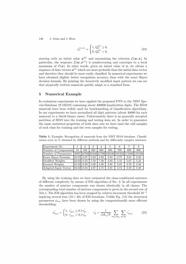
Table 1. Example: Recognition of numerals from the NIST SD19 database. Classifi-cation error in % obtained by different methods and for differently complex mixtures.

Experiment No. 1 2 3 4 5 6 7 8Number of Components 10 100 200 300 400 700 800 900Number of Parameters 2005 16700 38340 41700 100100 105350 115880 133100Exact Bayes Formula 16.55 6.87 5.02 4.80 3.84 3.77 3.61 3.50Modified Weights 22.63 9.22 7.50 7.30 4.93 5.55 5.67 5.24Iterated Weights 16.50 6.99 5.09 4.88 3.88 3.85 3.70 3.56Adapted Input Vector 16.62 6.84 4.97 4.75 3.81 3.74 3.58 3.48

By using the training data we have estimated the class-conditional mixturesof different complexity by means of EM algorithm of Sec. 2. In all experimentsthe number of mixture components was chosen identically in all classes. Thecorresponding total number of mixture components is given in the second row ofTab.1. The EM algorithm has been stopped by relative increment threshold 10−5

implying several tens (10 ÷ 40) of EM iterations. Unlike Eq. (13) the structuralparameters φmn have been chosen by using the computationally more efficientthresholding:

φ′

mn ={

1, γ′

mn ≥ 0.1γ′

0,

0, γ′

mn < 0.1γ′

0,, γ

′

0 =1

|Mω|N∑

m∈Mω

∑

n∈Nγ

′

mn. (25)


Here γ′

0 is the mean value of the individual informativity of variables γ′

mn. Thecoefficient 0.1 is chosen relatively low because all variables are rather informativeand the training data set is large enough to get reliable estimates of all param-eters. Hence, the threshold value 0.1γ

′

0 actually suppresses in each componentonly the really superfluous variables. For each experiment the resulting totalnumber of component specific variables (

∑m

∑n φmn) is given in the third row

of Tab.1.We have used four different versions of Bayes decision rule. The fourth row

correspond to the Bayes rule based on the estimated class-conditional mixtures.The fifth row illustrates the influence of altered component weights. In particular,approximately one half of weights (randomly chosen) has been almost suppressedby setting wm = 10−8 with the remaining weights being equal to wm = 10without any norming. Expectedly, the resulting classification accuracy is muchworse than the standard Bayes rule. The sixth row shows how the “spoiled”weights can be repaired by using the iterative weighting (21). The achievedaccuracy illustrates that the classification based on iterated weights is actuallyindependent with respect to the initial weights. The last row illustrates theperformance of classification based on iteratively modified input vector. Theconvergence of the iteration equations (21), (23) is achieved in three or foursteps. The classification accuracy of Bayes formula applied to the modified inputpattern is even slightly better that in the standard form.

6 Conclusion

Considering PNN in the framework of statistical pattern recognition we obtainformal neurons strictly defined by means of parameters of the estimated class-conditional mixtures. In this respect a serious disadvantage of PNN is the fixedprobabilistic description of the underlying decision problem which is not com-patible with the well known short-term dynamic processes in biological neuralnetworks. We have shown that if we use the Bayes formula in a recurrent waythen some mixture parameters may take part in short term dynamic processeswithout destroying the statistically correct decision making. In particular, themixture component weights can be iteratively adapted to a specific input patternor the input pattern can be iteratively modified in order to facilitate the correctrecognition.

Acknowledgement. This research was supported by the project GACR No.102/07/1594 of Czech Grant Agency, by the EC project FP6-507752 MUSCLE,and partially by the projects 2C06019 ZIMOLEZ and MSMT 1M0572 DAR.

References

1. Baram, Y.: Bayesian classification by iterated weighting. Neurocomputing 25, 73–79 (1999)

2. Grim, J.: On numerical evaluation of maximum - likelihood estimates for finitemixtures of distributions. Kybernetika 18, 173–190 (1982)


3. Grim, J.: Maximum-likelihood design of layered neural networks. In: InternationalConference on Pattern Recognition. Proceedings, pp. 85–89. IEEE Computer So-ciety Press, Los Alamitos (1996)

4. Grim, J.: Design of multilayer neural networks by information preserving trans-forms. In: Pessa, E., Penna, M.P., Montesanto, A. (eds.) Third European Congresson Systems Science, pp. 977–982. Edizioni Kappa, Roma (1996)

5. Grim, J.: Information approach to structural optimization of probabilistic neuralnetworks. In: Ferrer, L., Caselles, A. (eds.) Fourth European Congress on SystemsScience, pp. 527–539. SESGE, Valencia (1999)

6. Grim, J.: A sequential modification of EM algorithm. In: Gaul, W., Locarek-Junge,H. (eds.) Classification in the Information Age. Studies in Classif., Data Anal., andKnowl. Organization, pp. 163–170. Springer, Berlin (1999)

7. Grim, J., Vejvalkova, J.: An iterative inference mechanism for the probabilisticexpert system PES. International Journal of General Systems 27, 373–396 (1999)

8. Grim, J., Just, P., Pudil, P.: Strictly modular probabilistic neural networks forpattern recognition. Neural Network World 13, 599–615 (2003)

9. Grim, J., Kittler, J., Pudil, P., Somol, P.: Combining multiple classifiers in proba-bilistic neural networks. In: Kittler, J., Roli, F. (eds.) MCS 2000. LNCS, vol. 1857,pp. 157–166. Springer, Heidelberg (2000)

10. Grim, J., Kittler, J., Pudil, P., Somol, P.: Multiple classifier fusion in probabilisticneural networks. Pattern Analysis & Applications 5, 221–233 (2002)

11. Grim, J., Pudil, P., Somol, P.: Recognition of handwritten numerals by structuralprobabilistic neural networks. In: Bothe, H., Rojas, R. (eds.) Proceedings of theSecond ICSC Symposium on Neural Computation, pp. 528–534. ICSC, Wetaskiwin(2000)

12. Grim, J., Pudil, P., Somol, P.: Boosting in probabilistic neural networks. In: Kas-turi, R., Laurendeau, D., Suen, C. (eds.) Proc. 16th International Conference onPattern Recognition, pp. 136–139. IEEE Comp. Soc, Los Alamitos (2002)

13. Haykin, S.: Neural Networks: a comprehensive foundation. Morgan Kaufman, SanMateo, CA (1993)

14. Hebb, D.O.: The Organization of Behavior: A Neuropsychological Theory. Wiley,New York (1949)

15. Hertz, J., Krogh, A., Palmer, R.G.: Introduction to the Theory of Neural Com-putation. Addison-Wesley, New York, Menlo Park CA, Amsterdam (1991)

16. McLachlan, G.J., Peel, D.: Finite Mixture Models. John Wiley and Sons, NewYork, Toronto (2000)

17. Schlesinger, M.I.: Relation between learning and self-learning in pattern recognition(in Russian). Kibernetika (Kiev) 6, 81–88 (1968)

18. Specht, D.F.: Probabilistic neural networks for classification, mapping or associa-tive memory. In: Proc. of the IEEE Intternational Conference on Neural Networks,vol. I, pp. 525–532. IEEE Computer Society Press, Los Alamitos (1988)

19. Streit, L.R., Luginbuhl, T.E.: Maximum-likelihood training of probabilistic neuralnetworks. IEEE Trans. on Neural Networks 5, 764–783 (1994)

20. Vajda, I., Grim, J.: About the maximum information and maximum likelihoodprinciples in neural networks. Kybernetika 34, 485–494 (1998)

Documents

Recurrent Bayesian Reasoning in Probabilistic Neural Networks