Real World Verification - avacs.org

AVACS – Automatic Verification and Analysis ofComplex Systems

REPORTSof SFB/TR 14 AVACS

Editors: Board of SFB/TR 14 AVACS

Real World Verification

byAndre Platzer Jan-David Quesel Philipp Rummer

AVACS Technical Report No. 52June 2009

ISSN: 1860-9821

Publisher: Sonderforschungsbereich/Transregio 14 AVACS(Automatic Verification and Analysis of Complex Systems)

Editors: Bernd Becker, Werner Damm, Martin Franzle, Ernst-Rudiger Olderog,Andreas Podelski, Reinhard Wilhelm

ATRs (AVACS Technical Reports) are freely downloadable from www.avacs.org

Copyright c© June 2009 by the author(s)

Author(s) contact: Jan-David Quesel ([email protected]).

Real World Verification

Andre Platzer1, Jan-David Quesel2, and Philipp Rummer3

1 Carnegie Mellon University, Pittsburgh, [email protected]

2 University of Oldenburg, [email protected]

3 Oxford University, Computing Laboratory, [email protected]

Abstract. Scalable handling of real arithmetic is a crucial part of theverification of hybrid systems, mathematical algorithms, and mixed ana-log/digital circuits. Despite substantial advances in verification tech-nology, complexity issues with classical decision procedures are still amajor obstacle for formal verification of real-world applications, e.g.,in automotive and avionic industries. To identify strengths and weak-nesses, we examine state of the art symbolic techniques and implemen-tations for the universal fragment of real-closed fields: approaches basedon quantifier elimination, Grobner Bases, and semidefinite programmingfor the Positivstellensatz. Within a uniform context of the verificationtool KeYmaera, we compare these approaches qualitatively and quanti-tatively on verification benchmarks from hybrid systems, textbook algo-rithms, and on geometric problems. Finally, we introduce a new decisionprocedure combining Grobner Bases and semidefinite programming forthe real Nullstellensatz that outperforms the individual approaches onan interesting set of problems.

Keywords: real-closed fields, decision procedures, hybrid systems, soft-ware verification

1 Introduction

The field of formal verification has the important ambition to check the behaviorof systems by either proving the correct functioning of the system or finding bugsin its design. For several classes of systems that come from real-world domains,reasoning about real quantities is an inherent aspect of the problem. This in-cludes (i) embedded systems or complex physical systems, (ii) formal analysisof mixed discrete/analog effects in chip design, or (iii) mathematical textbookalgorithms, numerical algorithms or floating point arithmetic in standard pro-grams. For domains (i)–(ii), hybrid systems are a common model, i.e., systemsgoverned by interacting discrete and continuous transitions in the state space. Inthese domains, the need for real arithmetic reasoning comes from the temporalevolution of the continuous part of the state space, e.g., positions, velocities, ana-log signals. For case (iii), real arithmetic occurs in the computations on programdata or are used as a first approximation for floating-point arithmetic.

2 Andre Platzer, Jan-David Quesel, and Philipp Rummer

By a famous result due to Tarski [1], real arithmetic is decidable in thesense that (the first-order theory of) real arithmetic is equivalent to the first-order theory of real-closed fields, which is decidable by quantifier elimination(i.e., the process of replacing quantified formulas equivalently by quantifier-freeformulas). Numerous algorithmic improvements have been made both for thehandling of basic real arithmetic and for specific verification procedures for theproblem domains (i)–(iii). However, for a large number of real-world systems,the underlying problems in real arithmetic still have a prohibitive complexity forquantifier elimination. Even numerical procedures for real arithmetic [2] sufferfrom the curse of dimensionality limiting their scalability.

In this paper we compare three state of the art approaches to reasoning aboutreal-arithmetic in real-closed fields based on: quantifier elimination [3, 4] GrobnerBases [5], and semidefinite programming [6] for the Positivstellensatz [7]. Quan-tifier elimination is defined for full quantified (polynomial) nonlinear real arith-metic. The other approaches are for the universal fragment, i.e., formulas witha universal quantifier prefix. We discuss strengths and weaknesses of these ap-proaches for formal verification and compare multiple algorithms and imple-mentations on a set of benchmarks originating from real verification problems orinteresting instances of real arithmetic. To obtain representative experimentalresults, we integrate all these approaches within a single uniform framework ofthe automated theorem prover KeYmaera for hybrid systems [8].

Finally, we introduce a new decision procedure for the universal fragment ofreal-closed fields that combines Grobner Basis computations with semidefiniteprogramming for the real Nullstellensatz [7] to avoid the scalability issues withsemidefinite programming for the Positivstellensatz. Our algorithm outperformsthe other algorithms on an interesting set of benchmarks.

With the goal of finding out which approaches are most suitable for realworld verification problems, we provide an experimental evaluation for a widerange of techniques for real arithmetic. We contrast multiple state of the artapproaches and different implementations:

1. Quantifier elimination for real-closed fields in Mathematica, QEPCAD B [9],Redlog [10], and HOL Light [11];

2. Real arithmetic handling with Grobner Bases using external procedures inMathematica, the Orbital library, and internally with KeYmaera proof rules;

3. Semidefinite programming relaxations [6] for the Positivstellensatz [7] usingthe CSDP solver [12] in our own implementation and in HOL Light [13];

4. Our new algorithm combining Grobner Bases and semidefinite programmingfor the real Nulstellensatz [7] using CSDP [12] and the Orbital library.

In this paper, we consider problems in the continuous world of reals thatarise in real world verification problems, including hybrid systems analysis andprogram verification. Our contributions are a systematic quantitative and qual-itative comparison of multiple techniques for handling real arithmetic within auniform verification framework and the introduction of a novel decision proce-dure for universal real arithmetic that combines Grobner Bases with semidefiniteprogramming for the real Nullstellensatz. We further address the question how

Real World Verification 3

expensive various levels of confidence in real verification are in real examples: ex-ternal (unverified) blackboxes, external blackboxes producing formally checkablecertificates, and internal formal reasoning within a proof system.

2 Overall Verification Approach

We briefly discuss our formal verification approach for hybrid systems and math-ematical algorithms within the automated theorem prover KeYmaera [8]. It is animplementation of a Gentzen-style sequent proof calculus for hybrid systems [14]that uses deduction modulo decision procedures for handling real arithmetic. Thecalculus works on sequents of the form φ1, . . . , φn ` ψ1, . . . , ψm with the seman-tics of the formula

∧ni=1 φi →

∨mi=1 ψi. Among several other rules, the calculus

transforms the propositional structure into a sequent representation.The deduction modulo calculus of KeYmaera gives us a uniform context for

comparing the performance of multiple approaches and implementations for realarithmetic. The input for KeYmaera is a formula given in differential dynamiclogic [14]. This logic extends first-order logic over real arithmetic by constructsfor reasoning about hybrid systems as well as real-valued mathematical algo-rithms. For the verification task, the proof calculus transforms the input for-mulas into first-order formulas over real-arithmetic. For details about the proofrules of this transformation we refer to [14].

In this paper we address the question of handling the resulting real arith-metic formulas. Although first-order logic over real arithmetic is decidable byquantifier elimination [1] its complexity is doubly exponential in theory and canbe high in practice. The central point of this work is to examine the questionwhich approach to handling real arithmetic is best for which class of real worldexamples. We further want to determine the computational cost for techniquesthat provide formal proof certificates.

3 Methods for Handling Real Arithmetic

We survey different approaches to handling real arithmetic in background proversfor verification. We phrase these approaches in terms of reals for simplicity. Yet,all subsequent theory in Sections 3–4 generalizes from R to real-closed fields.

In the sequel we assume the presence of standard rules for propositionalconnectives. Such rules are not presented here, as propositional reasoning is or-thogonal to the handling of arithmetic. The KeYmaera system uses classicalpropositional sequent calculus rules; see [14, 15] for details. To simplify the pre-sentation, we further assume simple rules to normalise sequents that translate,e.g., g ≤ f to f ≥ g, f 6= g to ¬(f = g) and ` f > g to f ≤ g ` respectively.We assume all inequalities to be moved to the antecedent in this way.

3.1 Grobner Bases for Real Arithmetic

Grobner bases [5] provide a sound but incomplete procedure for proving validityof formulas in the universal fragment of equational first-order real arithmetic.


Preliminaries. Let Q[X1, . . . , Xn] be the set of multivariate polynomials over theindeterminates X1, . . . , Xn with coefficients in Q. A subset I ⊆ Q[X1, . . . , Xn]is an ideal, iff I is a subgroup with respect to addition and

rx ∈ I, for all x ∈ I, r ∈ Q[X1, . . . , Xn] .

The ideal generated by a set G ⊆ Q[X1, . . . , Xn] is the smallest ideal I contain-ing G, and is denoted by (G).

The notions of Grobner bases and polynomial reductions are relative to anadmissible monomial order ≺, which is a strict well-order on monomials suchthat uw ≺ vw whenever u ≺ v for arbitrary monomials u, v, w. Admissible ordersextend canonically to Q[X1, . . . , Xn] as a multiset order; see [5] for details. Themonomial order determines the leading term in multivariate polynomials, i.e.,the maximal monomial with respect to ≺.

Definition 1 (Reduction). Let f, g ∈ Q[X1, . . . , Xn]. We say that f reduces tog with respect to G ⊂ Q[X1, . . . , Xn] iff for some m ∈ N there are f0, f1, . . . , fm

in Q[X1, . . . , Xn] with f0 = f, fm = g such that, for all i, fi+1 = fi − higi

for some hi ∈ Q[X1, . . . , Xn], gi ∈ G, and fi+1 ≺ fi. We write g = redG f if, inaddition, g cannot be reduced further, i.e., there is no hm+1 ∈ Q[X1, . . . , Xn] andgm+1 ∈ G with g − hm+1 gm+1 ≺ q.

Definition 2 (Grobner basis). A finite subset G of an ideal I of Q[X1, .., Xn],is called Grobner basis iff I = (G) and redG f is unique for all polynomials f .Further G is reduced if no g ∈ G can be reduced further with respect to G \ {g}.

There are several equivalent alternative formulations of this definition, for in-stance that redG f = 0 iff f ∈ I. This means that Grobner bases solve the idealmembership problem and can, thus, directly be used as an (incomplete) proofrule for equational arithmetic.

Grobner Basis Eliminations. The most naive use of Grobner bases for real arith-metic is described by the rules A1, A2 in Fig. 1. The rule A1 closes a goal if theideal G generated by equations in the antecedent contains 1, which (by Hilbert’sNullstellensatz) implies that the equations do not have common solutions (i.e.,are contradictory). Similarly, A2 can be applied if the sides f, g of an equationin the succedent have the same remainder modulo G, which means f − g ∈ (G).

The scope of the rules can be extended by testing for radical membershipinstead of ideal membership, which can prove problems like x2 = 0 ` x = 0 thatA2 cannot prove. The radical of an ideal I is the set

√I =

∞⋃i=1

{g ∈ Q[X1, . . . , Xn] : gi ∈ I} ⊇ I

Because the inclusion I ⊆√I can be strict (e.g.,

√(x2) = (x)), testing for radical

membership is more liberal than ideal membership, while still being sound.


(A1)∗

Γ, g1 = g1, . . . , gn = gn ` ∆

(A2)∗

Γ, g1 = g1, . . . , gn = gn ` f = h,∆

(A3)Γ, (f − g)z = 1 ` ∆

Γ ` f = g,∆

(A4)Γ, f − g = z2 ` ∆Γ, f ≥ g ` ∆

(A5)Γ, (f − g)z2 = 1 ` ∆

Γ, f > g ` ∆

(A6)Γ ` 1 + s21 + · · ·+ s2n = 0,∆

Γ ` ∆

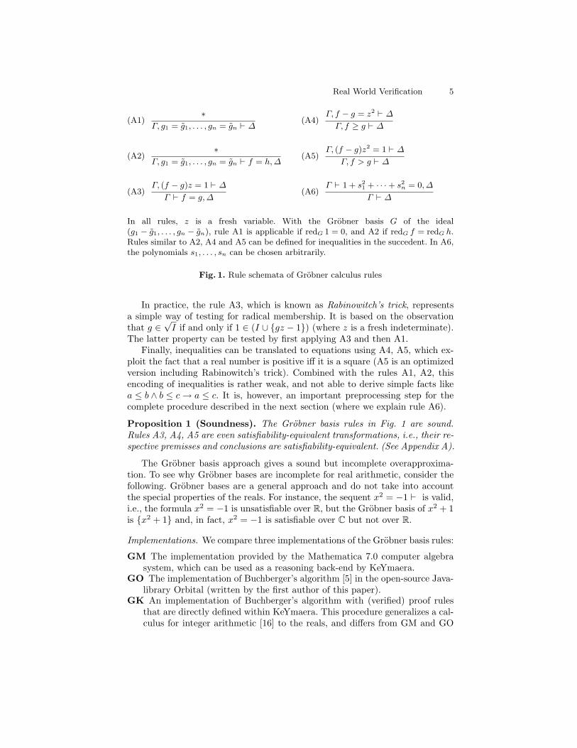
In all rules, z is a fresh variable. With the Grobner basis G of the ideal(g1 − g1, . . . , gn − gn), rule A1 is applicable if redG 1 = 0, and A2 if redG f = redG h.Rules similar to A2, A4 and A5 can be defined for inequalities in the succedent. In A6,the polynomials s1, . . . , sn can be chosen arbitrarily.

Fig. 1. Rule schemata of Grobner calculus rules

In practice, the rule A3, which is known as Rabinowitch’s trick, representsa simple way of testing for radical membership. It is based on the observationthat g ∈

√I if and only if 1 ∈ (I ∪ {gz − 1}) (where z is a fresh indeterminate).

The latter property can be tested by first applying A3 and then A1.Finally, inequalities can be translated to equations using A4, A5, which ex-

ploit the fact that a real number is positive iff it is a square (A5 is an optimizedversion including Rabinowitch’s trick). Combined with the rules A1, A2, thisencoding of inequalities is rather weak, and not able to derive simple facts likea ≤ b ∧ b ≤ c→ a ≤ c. It is, however, an important preprocessing step for thecomplete procedure described in the next section (where we explain rule A6).

Proposition 1 (Soundness). The Grobner basis rules in Fig. 1 are sound.Rules A3, A4, A5 are even satisfiability-equivalent transformations, i.e., their re-spective premisses and conclusions are satisfiability-equivalent. (See Appendix A).

The Grobner basis approach gives a sound but incomplete overapproxima-tion. To see why Grobner bases are incomplete for real arithmetic, consider thefollowing. Grobner bases are a general approach and do not take into accountthe special properties of the reals. For instance, the sequent x2 = −1 ` is valid,i.e., the formula x2 = −1 is unsatisfiable over R, but the Grobner basis of x2 + 1is {x2 + 1} and, in fact, x2 = −1 is satisfiable over C but not over R.

Implementations. We compare three implementations of the Grobner basis rules:

GM The implementation provided by the Mathematica 7.0 computer algebrasystem, which can be used as a reasoning back-end by KeYmaera.

GO The implementation of Buchberger’s algorithm [5] in the open-source Java-library Orbital (written by the first author of this paper).

GK An implementation of Buchberger’s algorithm with (verified) proof rulesthat are directly defined within KeYmaera. This procedure generalizes a cal-culus for integer arithmetic [16] to the reals, and differs from GM and GO


in that it does not use the rules A3, A4, A5, but instead integrates theFourier-Motzkin variable elimination rule [17] to handle inequalities (whichis complete for linear arithmetic). This tight integration of the two proce-dures can simplify terms in inequalities using Grobner bases, and can feedequations derived by the Fourier-Motzkin procedure back to Buchberger’salgorithm. We evaluate the benefits of this cooperation in Sect. 5. Sinceour domain are the reals, we do not use the heuristic approach tailored tononlinear integer inequalities from [16].

3.2 A Complete Rule using the Real Nullstellensatz

While the rules A1, A2, A3, A4, A5 only form an incomplete calculus for prob-lems in real arithmetic, the situation is different over the complex numbers:Hilbert’s Nullstellensatz tells that A1, A3 together yield a decision procedurefor universal equational problems in C. A corresponding result for real-closedfields is Stengle’s real Nullstellensatz [7]; also see [13]:

Theorem 1 (Nullstellensatz [7] for real-closed fields). Let R be a real-closed field (e.g., R = R) and G be a finite subset of R[X1, . . . , Xn]. Then the set{x ∈ Rn : g(x) = 0 for all g ∈ G} is empty if and only if there are polynomi-als s1, . . . , sm ∈ R[X1, . . . , Xn] such that 1 + s21 + · · ·+ s2m ∈ (G). If, moreover,G ⊆ Q[X1, . . . , Xn], then also the polynomials s1, . . . , sm can be chosen amongthe elements of Q[X1, . . . , Xn].

This theorem leads to an extremely simple, yet complete, proof methodfor the universal fragment of real arithmetic: in addition to the rules thatwe have already discussed, we add rule A6 in Fig. 1 for injecting the equa-tion 1 + s21 + · · ·+ s2m = 0 into a proof goal. Any valid proof goal can then beclosed in the following way: (i) inequalities and equations in the succedent areturned into equations in the antecedent with the help of A3, A4, A5, (ii) thewitness 1 + s21 + · · ·+ s2m due to the real Nullstellensatz is generated using A6,and (iii) the goal is closed by the Grobner Basis computations with A2.

Corollary 1 (Completeness). Along with propositional rules, the rules inFig. 1 are complete for the universal fragment of real arithmetic.

Proof. Completeness follows from Theorem 1 using the satisfiability-equivalenceproperties for the transformation by A3, A4, A5 according to Proposition 1. ut

The main difficulty with this calculus is obvious: it does not provide anyguidance for choosing the witness 1 + s21 + · · ·+ s2m = 0. One technique to tacklethe required search is semidefinite programming, following the work based onStengle’s Positivstellensatz (Sect. 3.4) in [6, 13]. We describe a new approachthat combines semidefinite programming with Grobner bases in Sect. 4.

Example 1. In Fig. 2, we show a proof for the following implication (leaving outpropositional reasoning):

x ≥ y ∧ z ≥ 0→ xz ≥ yz. (1)


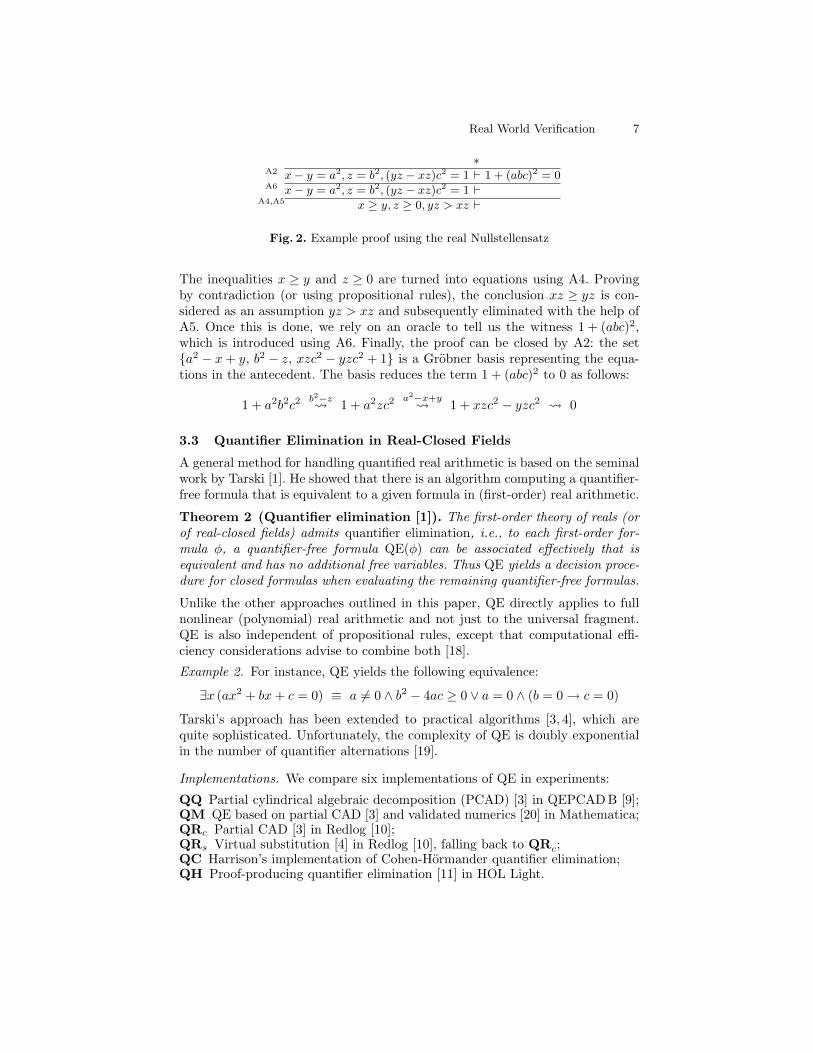
∗A2 x− y = a2, z = b2, (yz − xz)c2 = 1 ` 1 + (abc)2 = 0A6 x− y = a2, z = b2, (yz − xz)c2 = 1 `

A4,A5 x ≥ y, z ≥ 0, yz > xz `

Fig. 2. Example proof using the real Nullstellensatz

The inequalities x ≥ y and z ≥ 0 are turned into equations using A4. Provingby contradiction (or using propositional rules), the conclusion xz ≥ yz is con-sidered as an assumption yz > xz and subsequently eliminated with the help ofA5. Once this is done, we rely on an oracle to tell us the witness 1 + (abc)2,which is introduced using A6. Finally, the proof can be closed by A2: the set{a2 − x+ y, b2 − z, xzc2 − yzc2 + 1} is a Grobner basis representing the equa-tions in the antecedent. The basis reduces the term 1 + (abc)2 to 0 as follows:

1 + a2b2c2b2−z 1 + a2zc2

a2−x+y 1 + xzc2 − yzc2 0

3.3 Quantifier Elimination in Real-Closed Fields

A general method for handling quantified real arithmetic is based on the seminalwork by Tarski [1]. He showed that there is an algorithm computing a quantifier-free formula that is equivalent to a given formula in (first-order) real arithmetic.

Theorem 2 (Quantifier elimination [1]). The first-order theory of reals (orof real-closed fields) admits quantifier elimination, i.e., to each first-order for-mula φ, a quantifier-free formula QE(φ) can be associated effectively that isequivalent and has no additional free variables. Thus QE yields a decision proce-dure for closed formulas when evaluating the remaining quantifier-free formulas.

Unlike the other approaches outlined in this paper, QE directly applies to fullnonlinear (polynomial) real arithmetic and not just to the universal fragment.QE is also independent of propositional rules, except that computational effi-ciency considerations advise to combine both [18].

Example 2. For instance, QE yields the following equivalence:

∃x (ax2 + bx+ c = 0) ≡ a 6= 0 ∧ b2 − 4ac ≥ 0 ∨ a = 0 ∧ (b = 0→ c = 0)

Tarski’s approach has been extended to practical algorithms [3, 4], which arequite sophisticated. Unfortunately, the complexity of QE is doubly exponentialin the number of quantifier alternations [19].

Implementations. We compare six implementations of QE in experiments:

QQ Partial cylindrical algebraic decomposition (PCAD) [3] in QEPCAD B [9];QM QE based on partial CAD [3] and validated numerics [20] in Mathematica;QRc Partial CAD [3] in Redlog [10];QRs Virtual substitution [4] in Redlog [10], falling back to QRc;QC Harrison’s implementation of Cohen-Hormander quantifier elimination;QH Proof-producing quantifier elimination [11] in HOL Light.


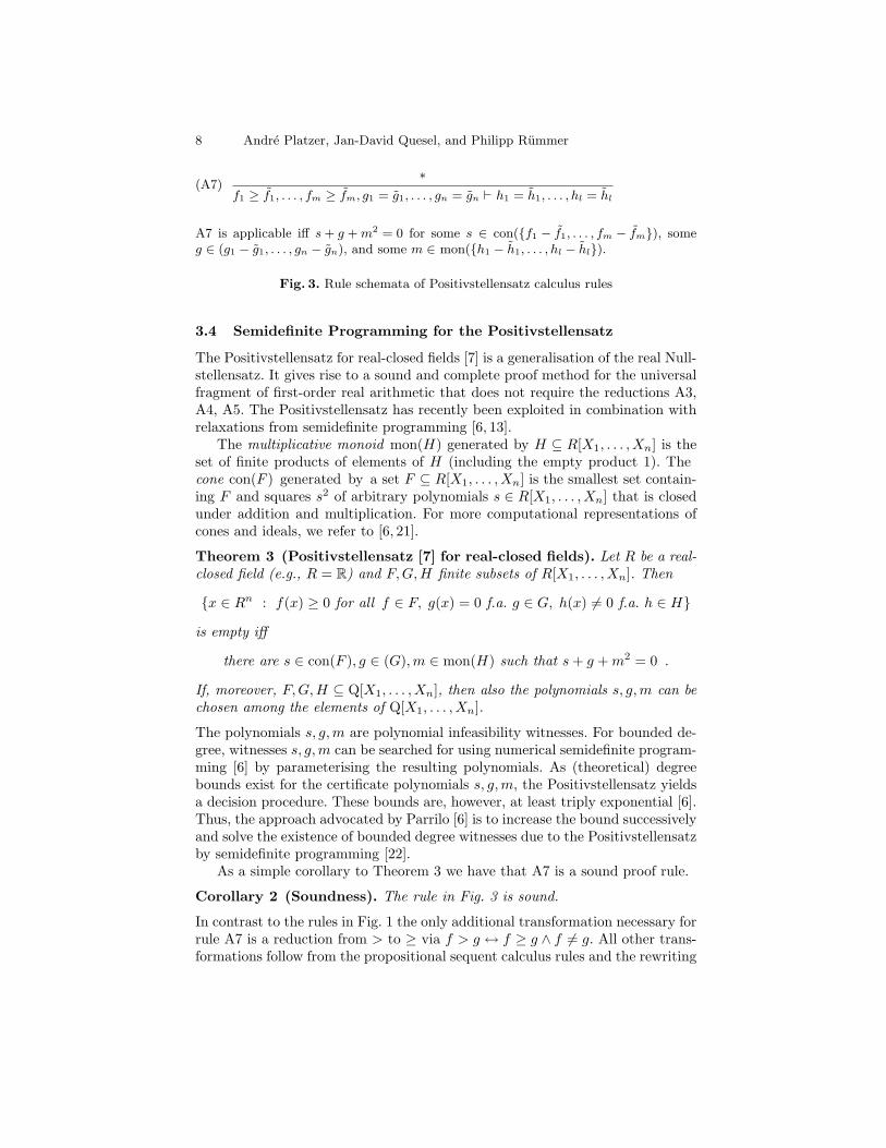
(A7)∗

f1 ≥ f1, . . . , fm ≥ fm, g1 = g1, . . . , gn = gn ` h1 = h1, . . . , hl = hl

A7 is applicable iff s+ g +m2 = 0 for some s ∈ con({f1 − f1, . . . , fm − fm}), someg ∈ (g1 − g1, . . . , gn − gn), and some m ∈ mon({h1 − h1, . . . , hl − hl}).

Fig. 3. Rule schemata of Positivstellensatz calculus rules

3.4 Semidefinite Programming for the Positivstellensatz

The Positivstellensatz for real-closed fields [7] is a generalisation of the real Null-stellensatz. It gives rise to a sound and complete proof method for the universalfragment of first-order real arithmetic that does not require the reductions A3,A4, A5. The Positivstellensatz has recently been exploited in combination withrelaxations from semidefinite programming [6, 13].

The multiplicative monoid mon(H) generated by H ⊆ R[X1, . . . , Xn] is theset of finite products of elements of H (including the empty product 1). Thecone con(F ) generated by a set F ⊆ R[X1, . . . , Xn] is the smallest set contain-ing F and squares s2 of arbitrary polynomials s ∈ R[X1, . . . , Xn] that is closedunder addition and multiplication. For more computational representations ofcones and ideals, we refer to [6, 21].

Theorem 3 (Positivstellensatz [7] for real-closed fields). Let R be a real-closed field (e.g., R = R) and F,G,H finite subsets of R[X1, . . . , Xn]. Then

{x ∈ Rn : f(x) ≥ 0 for all f ∈ F, g(x) = 0 f.a. g ∈ G, h(x) 6= 0 f.a. h ∈ H}

is empty iff

there are s ∈ con(F ), g ∈ (G),m ∈ mon(H) such that s+ g +m2 = 0 .

If, moreover, F,G,H ⊆ Q[X1, . . . , Xn], then also the polynomials s, g,m can bechosen among the elements of Q[X1, . . . , Xn].

The polynomials s, g,m are polynomial infeasibility witnesses. For bounded de-gree, witnesses s, g,m can be searched for using numerical semidefinite program-ming [6] by parameterising the resulting polynomials. As (theoretical) degreebounds exist for the certificate polynomials s, g,m, the Positivstellensatz yieldsa decision procedure. These bounds are, however, at least triply exponential [6].Thus, the approach advocated by Parrilo [6] is to increase the bound successivelyand solve the existence of bounded degree witnesses due to the Positivstellensatzby semidefinite programming [22].

As a simple corollary to Theorem 3 we have that A7 is a sound proof rule.

Corollary 2 (Soundness). The rule in Fig. 3 is sound.

In contrast to the rules in Fig. 1 the only additional transformation necessary forrule A7 is a reduction from > to ≥ via f > g ↔ f ≥ g ∧ f 6= g. All other trans-formations follow from the propositional sequent calculus rules and the rewriting


rules described in the beginning of Sect. 3. Therefore, this approach does not in-troduce new variables, as it does not need the rules A3 – A5. Alternatively, A5can be used in place of the f > g axiomatisation as we show in the sequel.

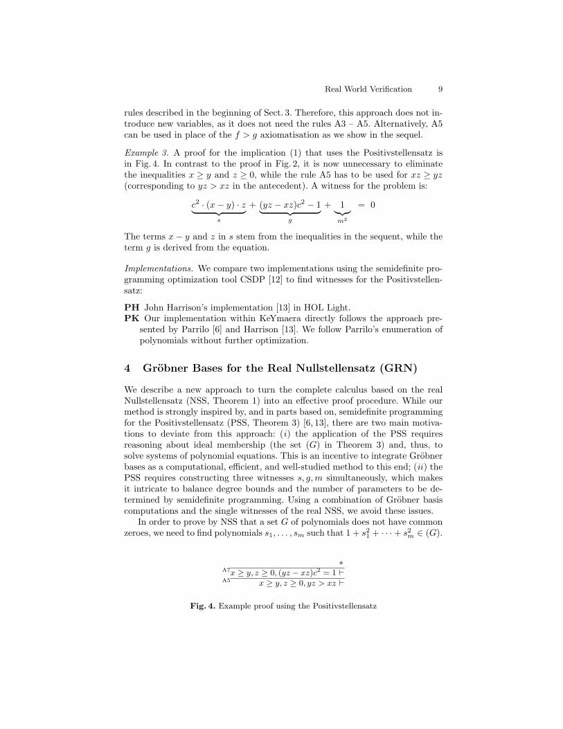
Example 3. A proof for the implication (1) that uses the Positivstellensatz isin Fig. 4. In contrast to the proof in Fig. 2, it is now unnecessary to eliminatethe inequalities x ≥ y and z ≥ 0, while the rule A5 has to be used for xz ≥ yz(corresponding to yz > xz in the antecedent). A witness for the problem is:

c2 · (x− y) · z︸︷︷︸s

+ (yz − xz)c2 − 1︸︷︷︸g

+ 1︸︷︷︸m2

= 0

The terms x− y and z in s stem from the inequalities in the sequent, while theterm g is derived from the equation.

Implementations. We compare two implementations using the semidefinite pro-gramming optimization tool CSDP [12] to find witnesses for the Positivstellen-satz:

PH John Harrison’s implementation [13] in HOL Light.PK Our implementation within KeYmaera directly follows the approach pre-

sented by Parrilo [6] and Harrison [13]. We follow Parrilo’s enumeration ofpolynomials without further optimization.

4 Grobner Bases for the Real Nullstellensatz (GRN)

We describe a new approach to turn the complete calculus based on the realNullstellensatz (NSS, Theorem 1) into an effective proof procedure. While ourmethod is strongly inspired by, and in parts based on, semidefinite programmingfor the Positivstellensatz (PSS, Theorem 3) [6, 13], there are two main motiva-tions to deviate from this approach: (i) the application of the PSS requiresreasoning about ideal membership (the set (G) in Theorem 3) and, thus, tosolve systems of polynomial equations. This is an incentive to integrate Grobnerbases as a computational, efficient, and well-studied method to this end; (ii) thePSS requires constructing three witnesses s, g,m simultaneously, which makesit intricate to balance degree bounds and the number of parameters to be de-termined by semidefinite programming. Using a combination of Grobner basiscomputations and the single witnesses of the real NSS, we avoid these issues.

In order to prove by NSS that a set G of polynomials does not have commonzeroes, we need to find polynomials s1, . . . , sm such that 1 + s21 + · · ·+ s2m ∈ (G).

∗A7x ≥ y, z ≥ 0, (yz − xz)c2 = 1 `A5 x ≥ y, z ≥ 0, yz > xz `

Fig. 4. Example proof using the Positivstellensatz


We reduce this problem to a search for positive semidefinite matrices with thehelp of the following lemma. A matrix X ∈ Rk×k is called positive semidefinite(PSD) if it is symmetric, and if xtXx ≥ 0 for each vector x ∈ Rk. There is asimple correspondence between PSD matrices and sums of squares:

Lemma 1. Suppose p ∈ Q[X1, . . . , Xn]k is a vector of rational polynomials. Thefollowing identities hold (see the proof in Appendix A):{

l∑i=1

(cip)2 : l ∈ N, ci ∈ Qk

}

=

{l∑

i=1

αi(cip)2 : l ∈ N, αi ∈ Q, αi ≥ 0, ci ∈ Qk

}={ptXp : X ∈ Qk×k positive semidefinite

}By combining Lemma 1 with the NSS, we see that a set G of polynomials

does not have any common zeroes if and only if there is a vector p of polynomialsand a PSD matrix X ∈ Rk×k such that 1 + ptXp ∈ (G). As the vector space ofpolynomials is generated by monomials, it is sufficient to consider vectors p ofmonomials.

Semidefinite programming [22] provides a simple method to determine suchmatrices X. A semidefinite program (SDP) is an optimisation problem in termsof traces (tr) of matrices:

maximise tr(CX)subject to tr(AiX) = bi (for i ∈ {1, . . . , n}),where X positive semidefinite

where Ai, C ∈ Rk×k are symmetric matrices and bi ∈ R. Such optimisation prob-lems can be solved efficiently using numerical convex optimization [22].

The key insight underlying our method is the following: by computing aGrobner basis B for the ideal (G), the NSS condition 1 + ptXp ∈ (G) can be en-coded as the linear side constraints tr(AiX) = bi (i ∈ {1, . . . , n}) of a semidefiniteprogram searching for X. To see this, note that both the expression 1 + ptXpand the reduction redB(1 + ptXp) are linear in X. Because Grobner bases de-termine unique remainders, we therefore have 1 + ptXp ∈ (G) if and only ifredB(1 + ptXp) = 0. This equation is a linear constraint on X suitable for SDP.

To capture this observation formally, let Q be a symmetric k × k matrix ofparameters:

Q =

q1,1 q1,2 . . . q1,k

q1,2 q2,2 . . . q2,k

. . . . . . . . . . .q1,k q2,k . . . qk,k

The polynomial 1 + ptQp is linear in Q and can be represented in the form1 + ptQp = qtCm, where q = (q1,1, q1,2, . . . , qk,k)t is the vector of all the Q-parameters, m = (m1, . . . ,ms)t is a vector of monomials over X1, . . . , Xn (con-taining, at least, 1 and all products pipj of components of p), and C ∈ Qk2×s


is a matrix. By computing the remainder qtDm = redB(qtCm) of this term fora Grobner basis B over Q[X1, . . . , Xn], we can construct the required side con-straints:

Lemma 2. Suppose that the components of m are pairwise distinct, and thatqtCm and qtDm are two polynomials over Q[q1,1, q1,2, . . . , qk,k][X1, . . . , Xn] de-fined by the matrices C,D ∈ Qk2×s, such that qtDm = redB(qtCm). Then thefollowing equation holds (see Appendix B for a proof):

{x ∈ Rk : redB(xtCm) = 0} = {x ∈ Rk : xtD = 0} (2)

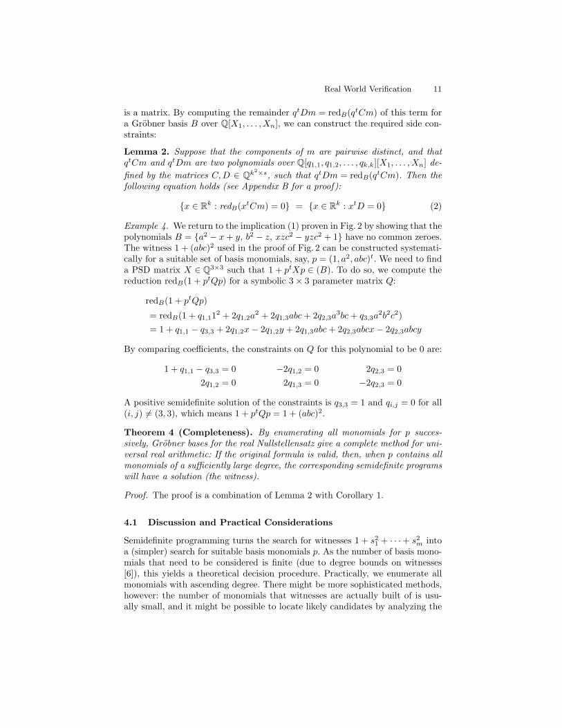
Example 4. We return to the implication (1) proven in Fig. 2 by showing that thepolynomials B = {a2 − x+ y, b2 − z, xzc2 − yzc2 + 1} have no common zeroes.The witness 1 + (abc)2 used in the proof of Fig. 2 can be constructed systemati-cally for a suitable set of basis monomials, say, p = (1, a2, abc)t. We need to finda PSD matrix X ∈ Q3×3 such that 1 + ptXp ∈ (B). To do so, we compute thereduction redB(1 + ptQp) for a symbolic 3× 3 parameter matrix Q:

redB(1 + ptQp)

= redB(1 + q1,112 + 2q1,2a2 + 2q1,3abc+ 2q2,3a

3bc+ q3,3a2b2c2)

= 1 + q1,1 − q3,3 + 2q1,2x− 2q1,2y + 2q1,3abc+ 2q2,3abcx− 2q2,3abcy

By comparing coefficients, the constraints on Q for this polynomial to be 0 are:

1 + q1,1 − q3,3 = 0 −2q1,2 = 0 2q2,3 = 02q1,2 = 0 2q1,3 = 0 −2q2,3 = 0

A positive semidefinite solution of the constraints is q3,3 = 1 and qi,j = 0 for all(i, j) 6= (3, 3), which means 1 + ptQp = 1 + (abc)2.

Theorem 4 (Completeness). By enumerating all monomials for p succes-sively, Grobner bases for the real Nullstellensatz give a complete method for uni-versal real arithmetic: If the original formula is valid, then, when p contains allmonomials of a sufficiently large degree, the corresponding semidefinite programswill have a solution (the witness).

Proof. The proof is a combination of Lemma 2 with Corollary 1.

4.1 Discussion and Practical Considerations

Semidefinite programming turns the search for witnesses 1 + s21 + · · ·+ s2m intoa (simpler) search for suitable basis monomials p. As the number of basis mono-mials that need to be considered is finite (due to degree bounds on witnesses[6]), this yields a theoretical decision procedure. Practically, we enumerate allmonomials with ascending degree. There might be more sophisticated methods,however: the number of monomials that witnesses are actually built of is usu-ally small, and it might be possible to locate likely candidates by analyzing the


Grobner basis B. In our experience, the number of basis monomials that areconsidered before a solution is found (and thus the difficulty of a problem) de-pends on (i) the number of variables in the polynomial ring, and (ii) the degreeof the leading monomials in the Grobner basis.

Another issue is that implementations for semidefinite programming (like theCSDP solver [12] used by us) are numerical and produce answers in floating pointarithmetic. To recover precise solutions in Q from such answers, we use a similarapproach as in [13]: We approximate floating point numbers to a certain preci-sion by rationals (with the help of Stern-Brocot trees [23]), and check resultingsolution candidate for semidefiniteness. We increase the precision successively aslong as the solution candidate remains indefinite.

Optimizations. We found it essential to use preprocessing steps to reduce thenumber of variables in a problem, such that the number of potential basis mono-mials becomes tractable. Some heuristics are:

– If the Grobner basis B contains a polynomial x+ t such that x does notoccur in t, then x and the polynomial can be eliminated by simple rewriting.

– If B contains polynomials xy − 1 and xn + t such that xn does not dividet, then x and the polynomial xy − 1 can be eliminated by multiplying eachpolynomial in B (except xy − 1) with a power of y and reducing w.r.t. xy − 1.

– Polynomials α1m21 + · · ·+ αnm

2n ∈ B such that αi > 0 for i ∈ {1, . . . , n} can

be replaced by the monomials m1, . . . ,mn.– If B contains a polynomial α0x

2 − α1m21 − · · · − αnm

2n such that αi > 0 for

i ∈ {0, . . . , n} where x only occurs with even degree in B, then x can beeliminated by rewriting and the polynomial can be removed.

The last two cases are surprisingly common, due to the encoding of inequalitiesby quadratic terms performed by A4 and A5.

5 Experimental Results

We have integrated the techniques presented in Sect. 3–4 into KeYmaera. Withthe various methods for real arithmetic integrated into a common framework andreal arithmetic examples from different domains, we have a solid base for ourexperiments. The benchmarks4 are a collection of challenging arithmetic prob-lems from the hybrid system world [24], the verification of invariant propertiesfor mathematical algorithms [25, 26] and algebraic geometry [27], as well as asmaller number of synthetic problems. For the examples with mixed quantifiers,our setting applies QM to the existential quantifiers such that we can still gaininsight into the scalability of the approaches that are restricted to the universalfragment on these examples. We run our experiments on a dual Intel Xeon E5430(quad core with 2.66 GHz) and 32 gigabytes RAM.

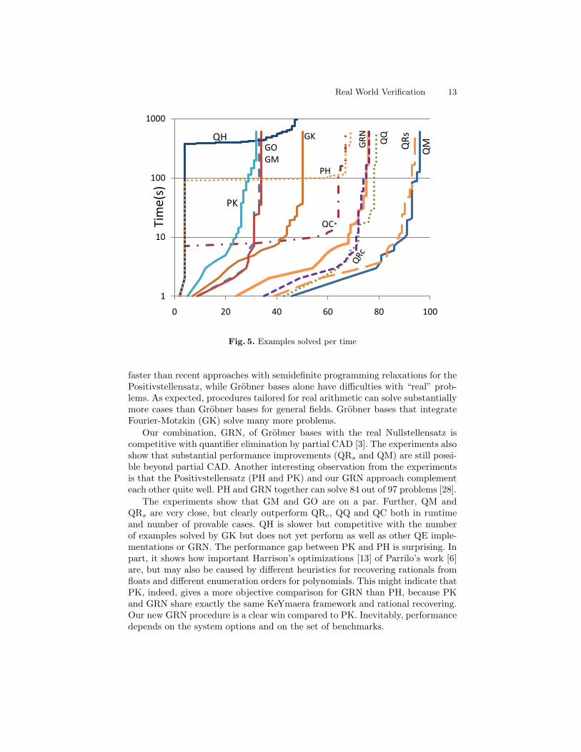
The experimental results (see Appendix C) summarized in Fig. 5 show that,for our particular mix of examples, quantifier elimination procedures are still4 Available along with KeYmaera from http://symbolaris.com/info/KeYmaera.html


Fig. 5. Examples solved per time

faster than recent approaches with semidefinite programming relaxations for thePositivstellensatz, while Grobner bases alone have difficulties with “real” prob-lems. As expected, procedures tailored for real arithmetic can solve substantiallymore cases than Grobner bases for general fields. Grobner bases that integrateFourier-Motzkin (GK) solve many more problems.

Our combination, GRN, of Grobner bases with the real Nullstellensatz iscompetitive with quantifier elimination by partial CAD [3]. The experiments alsoshow that substantial performance improvements (QRs and QM) are still possi-ble beyond partial CAD. Another interesting observation from the experimentsis that the Positivstellensatz (PH and PK) and our GRN approach complementeach other quite well. PH and GRN together can solve 84 out of 97 problems [28].

The experiments show that GM and GO are on a par. Further, QM andQRs are very close, but clearly outperform QRc, QQ and QC both in runtimeand number of provable cases. QH is slower but competitive with the numberof examples solved by GK but does not yet perform as well as other QE imple-mentations or GRN. The performance gap between PK and PH is surprising. Inpart, it shows how important Harrison’s optimizations [13] of Parrilo’s work [6]are, but may also be caused by different heuristics for recovering rationals fromfloats and different enumeration orders for polynomials. This might indicate thatPK, indeed, gives a more objective comparison for GRN than PH, because PKand GRN share exactly the same KeYmaera framework and rational recovering.Our new GRN procedure is a clear win compared to PK. Inevitably, performancedepends on the system options and on the set of benchmarks.


6 Related Work

Nipkow [29] presented a formally verified implementations of quantifier elimina-tion in an executable fragment of Isabelle/HOL, currently for linear real arith-metic only. McLaughlin and Harrison [11] presented a nonverified but proof-producing implementation of general quantifier elimination, so that the result ofthe procedure can be checked independently.

The sum of squares approach has been pioneered by Parrilo [6] and Harri-son [13]. Harrison also gives optimizations for the univariate case.

Tiwari [30] presents an approach using Grobner bases and sign conditionson variables to produce unsatisfiability witnesses for nonlinear constraints. Theapproach depends on appropriate heuristic variable orderings that are formedby successively introducing new variables for polynomial expressions followingcertain heuristics (which may not terminate). Our work and that of Tiwari sharethe combination of Grobner bases with witness generation. Yet we follow semi-definite programming for the real Nullstellensatz, whereas [30] uses heuristicgeneration of polynomial witness expressions. Tiwari uses the Positivstellensatzto prove refutational completeness but not as part of his technique.

RSolver [2] is a numerical approach for deciding validity of (robust instancesof) first-order formulas over real arithmetic extended with transcendental func-tions. Unlike our work, this relies on numerical stability of the input formula.

MetiTarski [31] is an interesting approach for handling special functions usinga combination of resolution proving with simple QE procedures. Their focus ison handling special functions not on handling real arithmetic.

Hunt et al. [32] describe the handling of nonlinear arithmetic in ACL2, whichis based on heuristic multiplication of inequalities in the style of (1) and yields anincomplete method. The method is claimed to be empirically successful, though,and can also be applied to nonlinear integer arithmetic.

7 Discussion and Conclusions

The respective approaches from Sect. 3–4 have different advantages and weak-nesses for formal verification of real world problems in real arithmetic. We draw aqualitative comparison complementing the quantitative comparison from Sect. 5.

Quantifier Elimination. Quantifier elimination procedures [3] can handle fullnonlinear real arithmetic, including existential quantifiers. Their implementa-tions are quite intricate algorithms for which correctness is not easily establishedformally. Unfortunately, QE does not produce simple checkable certificates.

Proof-producing [11] or verified [29] QE procedures may be interesting im-provements on the formal traceability of QE. Unfortunately, their performanceis not yet fully competitive with other quantifier elimination implementations orour new proof-producing GRN procedure.

A compromise is reverification: Proof search [33, 18] in KeYmaera generatesseveral problems of real arithmetic to find a proof, but only those in the fi-nal proof are soundness-critical. For soundness, it is sufficient to use a fast or


untrusted implementation of QE during the proof search and to reverify thefinal proof in a proof checker with a verified or proof-producing QE implemen-tation [11, 29]. For this purpose, KeYmaera strategies are especially useful thatidentify the sweetspot for applying QE iteratively during the proof search [18].

Positivstellensatz. In the context of verification, a useful property of the Posi-tivstellensatz is that it produces a witness (s+ g +m2 = 0) for the validity of aformula. Once the witness has been found, it is checkable by simple computationsin the polynomial ring to determine whether the polynomial identity holds bycomparing the coefficients. Similarly, the well-formedness of the witness can bedetermined by checking whether s is build from sums of squares using an exten-sion of “completing the square” [13]. Thus, complicated numerical semidefiniteprogramming tools [22] do not need to be part of the trusted computing baseconcerning soundness. Due to its enumerative nature with a large number ofextra parameters, scalability with the number of variables is still limited.

Grobner Bases. The Grobner Basis approach does not have simple witnesses likePositivstellensatz approaches. Their working principle, however, is strictly basedon symbolic computations, which can be carried out from a small set of rewriterules within a logic. This corresponds to our built-in Grobner basis approachGK, which is almost as efficient as external Grobner basis implementations. Ourexperimental results indicate that, due to the partial ignorance of real-closedfield properties, the capabilities of Grobner bases alone are not sufficient, evenin combination with Fourier-Motzkin elimination.

Real Nullstellensatz. Our new decision procedure based on Grobner basis com-putations and the real Nullstellensatz share the presence of checkable witnesseswith approaches based on the Positivstellensatz. Once a witness 1 +

∑i s

2i = 0

has been found, the polynomial equality check can be performed easily within aproof system using the GK rules, giving a fully formal proof. The performance inour experiments show that this new approach is promising. It outperforms mostother approaches, except for highly tuned QE procedures, which lack supportfor formal traceability. We believe that further research in this area is likely toproduce competitive but traceable solutions for real arithmetic.

Acknowledgments. We like to thank Leonardo de Moura, Nikolaj Bjørner, andJohn Harrison for providing benchmarks and fruitful discussions. Additionally,we like to thank Sean McLaughlin for his support in the integration of QH, PH,and QC as well as the anonymous referees for their useful comments. We alsolike to thank Arnold Neumaier for discussions.

References

1. Tarski, A.: A Decision Method for Elementary Algebra and Geometry. 2nd edn.University of California Press, Berkeley (1951)


2. Ratschan, S.: Efficient solving of quantified inequality constraints over the realnumbers. ACM Trans. Comput. Log. 7(4) (2006) 723–748

3. Collins, G.E., Hong, H.: Partial cylindrical algebraic decomposition for quantifierelimination. J. Symb. Comput. 12(3) (1991) 299–328

4. Weispfenning, V.: Quantifier elimination for real algebra - the quadratic case andbeyond. Appl. Algebra Eng. Commun. Comput. 8(2) (1997) 85–101

5. Buchberger, B.: An Algorithm for Finding the Basis Elements of the Residue ClassRing of a Zero Dimensional Polynomial Ideal. PhD thesis, University of Innsbruck(1965)

6. Parrilo, P.A.: Semidefinite programming relaxations for semialgebraic problems.Math. Program. 96(2) (2003) 293–320

7. Stengle, G.: A Nullstellensatz and a Positivstellensatz in semialgebraic geometry.Math. Ann. 207(2) (1973) 87–97

8. Platzer, A., Quesel, J.D.: KeYmaera: A hybrid theorem prover for hybrid systems.In: IJCAR. Volume 5195 of LNCS., Springer (2008) 171–178

9. Brown, C.W.: QEPCAD B: A program for computing with semi-algebraic setsusing CADs. SIGSAM Bull. 37(4) (2003) 97–108

10. Dolzmann, A., Sturm, T.: Redlog: Computer algebra meets computer logic. ACMSIGSAM Bull. 31 (1997) 2–9

11. McLaughlin, S., Harrison, J.: A proof-producing decision procedure for real arith-metic. In Nieuwenhuis, R., ed.: CADE. Volume 3632 of LNCS., Springer (2005)

12. Borchers, B.: CSDP, a C library for semidefinite programming. OptimizationMethods and Software 11(1-4) (1999) 613–623

13. Harrison, J.: Verifying nonlinear real formulas via sums of squares. In Schneider,K., Brandt, J., eds.: TPHOLs. Volume 4732 of LNCS., Springer (2007) 102–118

14. Platzer, A.: Differential dynamic logic for hybrid systems. J. Autom. Reasoning41(2) (2008) 143–189

15. Beckert, B., Hahnle, R., Schmitt, P.H., eds.: Verification of Object-Oriented Soft-ware: The KeY Approach. Volume 4334 of LNCS. Springer (2007)

16. Rummer, P.: A sequent calculus for integer arithmetic with counterexample gener-ation. In Beckert, B., ed.: VERIFY’07 at CADE, Bremen, Germany. Volume 259of CEUR-WS.org. (2007)

17. Schrijver, A.: Theory of Linear and Integer Programming. Wiley (1986)18. Platzer, A.: Combining deduction and algebraic constraints for hybrid system

analysis. In Beckert, B., ed.: VERIFY’07 at CADE, Bremen, Germany. Volume259 of CEUR Workshop Proceedings., CEUR-WS.org (2007) 164–178

19. Davenport, J.H., Heintz, J.: Real quantifier elimination is doubly exponential. J.Symb. Comput. 5(1/2) (1988) 29–35

20. Strzebonski, A.W.: Cylindrical algebraic decomposition using validated numerics.J. Symb. Comput. 41(9) (2006) 1021–1038

21. Bochnak, J., Coste, M., Roy, M.F.: Real Algebraic Geometry. Volume 36 of Ergeb-nisse der Mathematik und ihrer Grenzgebiete. Springer (1998)

22. Boyd, S., Vandenberghe, L.: Convex Optimization. Cambridge Univ. Press (2004)23. Graham, R.L., Knuth, D.E., Patashnik, O.: Concrete Mathematics: A Foundation

for Computer Science. Addison-Wesley Longman (1994)24. Platzer, A., Quesel, J.D.: Logical verification and systematic parametric analysis

in train control. In Egerstedt, M., Mishra, B., eds.: HSCC. LNCS, Springer (2008)25. Kovacs, L.: Aligator: A mathematica package for invariant generation (system

description). In: IJCAR. Volume 5195 of LNCS., Springer (2008) 275–28226. de Moura, L.M., Bjørner, N.: Z3: An efficient SMT solver. In Ramakrishnan, C.R.,

Rehof, J., eds.: TACAS. Volume 4963 of LNCS., Springer (2008) 337–340


27. Dolzmann, A., Sturm, T., Weispfenning, V.: A new approach for automatic theo-rem proving in real geometry. J. Autom. Reason. 21(3) (1998) 357–380

28. Platzer, A., Quesel, J.D., Rummer, P.: Real world verification. Reports of SFB/TR14 AVACS 52, SFB/TR 14 AVACS (2009) ISSN: 1860-9821, http://www.avacs.org.

29. Nipkow, T.: Linear quantifier elimination. In: IJCAR. Volume 5195 of LNCS.,Springer (2008)

30. Tiwari, A.: An algebraic approach for the unsatisfiability of nonlinear constraints.In Ong, C.H.L., ed.: CSL. Volume 3634 of LNCS., Springer (2005) 248–262

31. Akbarpour, B., Paulson, L.C.: Extending a resolution prover for inequalities onelementary functions. In Dershowitz, N., Voronkov, A., eds.: LPAR. Volume 4790of LNCS., Springer (2007) 47–61

32. Warren A. Hunt, J., Krug, R.B., Moore, J.S.: Linear and nonlinear arithmetic inACL2. In: Proceedings, Correct Hardware Design and Verification Methods, 12thIFIP Conference. Volume 2860 of LNCS., Springer (2003) 319–333

33. Platzer, A., Clarke, E.M.: Computing differential invariants of hybrid systems asfixedpoints. In Gupta, A., Malik, S., eds.: CAV. Volume 5123 of LNCS., Springer(2008) 176–189


A Soundness Proof for Grobner Basis Rules

Proof (Proposition 1). The rules in Fig. 1 are sound. As usual for the soundnessproofs we assume Γ to be true in an interpretation ν and ∆ to be false as thereis nothing to show otherwise. For A3, A4,A5, we show equivalence of premissand conclusion, which implies soundness.

A2 Suppose the conclusion was false in ν, i.e., ν |= g1 = g1 ∧ · · · ∧ gn = gn ∧ f 6= h.Thus, ν |= g = 0 for all g ∈ G. Consequently, ν |= g = 0 for all polynomials gin the ideal (G) of G. As a consequence of the applicability condition, wehave redG(f − h) = 0, which, by Def. 2, implies that f − h is in the idealof G. In combination, we have ν |= f − h = 0, hence ν |= f = h, which is acontradiction. ut

A1 The soundness of A1 is a special case of the soundness of A2 when assumingthe false formula 1 = 0 for the succedent f = h.

A3 Satisfiability-equivalence of A3 is a consequence of the Rabinowitchtrick equivalence x 6= 0↔ ∃z (xz = 1), using f − g for x. More generally,this holds in fields where non-zero elements are exactly the elements thathave some inverse z. By introducing a free new variable z, we obtain thatthe premiss is satisfiable if and only if the conclusion is satisfiable.

A4 Satisfiability-equivalence follows from the equivalence f ≥ g ↔ ∃z (f − g = z2)in the domain of reals. More generally, this holds in real-closed fields wheresquares are exactly the positive numbers. By introducing a free new vari-able z in the rule, this equivalence we obtain that the premiss and conclusionare satisfiability-equivalent, i.e., the premiss is satisfiable if and only if theconclusion is satisfiable.

A5 Satisfiability-equivalence follows from the equivalence x > 0↔ ∃z (xz2 = 1)in the reals, using f − g for x.

A6 Since a sum of squares is nonnegative over R, the value of 1 + s21 + · · ·+ s2nis strictly positive and 1 + s21 + · · ·+ s2n = 0 is a contradiction over the reals.Consequently, if the premiss is valid, then so is the conclusion.

Proof (Lemma 1). The first equation holds because each non-negative rationalnumber αi can be written as a sum of four rational squares by Lagrange’s four-square theorem.

We consider the two directions of the second equation:“⊇”: This is shown (constructively) by [13, Theorem 1].“⊆”: Let

∑li=1 αi(cip)2 be a sum of squares with αi ≥ 0. We define the

matrices

C =

ct1ct2...ctl

, D =

α1

α2

. . .αl

and thus obtain the identity:

l∑i=1

αi(cip)2 = (Cp)tD(Cp) = pt(CtDC)p


The matrix CtDC = Q ∈ Qk×k is positive semidefinite because of:

xt(CtDC)x =l∑

i=1

αi(cix)2 ≥ 0.

B Completeness of Grobner Bases for the RealNullstellensatz

Proof (Lemma 2). First, observe that for all x ∈ Rn:

xtCm− xtDm ∈ (B) (3)

The proof of the lemma is as follows:

– “⊇”: Suppose xtD = 0. Then also xtDm = 0 and, by (3), xtCm− xtDm =xtCm ∈ (B). This implies redB(xtCm) = 0 because B is a Grobner basis.

– “⊆”: Suppose redB(xtCm) = 0, i.e., xtCm ∈ (B). By (3), this impliesxtDm ∈ (B).Now, observe that also the instance xtDm is irreducible w.r.t. B: becausethe parametrised polynomial qtDm is irreducible w.r.t. B, it has to be thecase that the i’th component of btD is zero whenever the monomial mi isreducible w.r.t. B. This means that, in this case, the i’th column of D onlycontains zeroes. Then also the i’th component of xtD is zero and xtDmcannot contain any reducible terms.Because B is a Grobner basis, 0 is the only member of (B) that is irreduciblew.r.t. B, which implies xtDm = 0. Finally, because the elements of m arepairwise distinct and thus linearly independent, this is only possible if xtD =0.

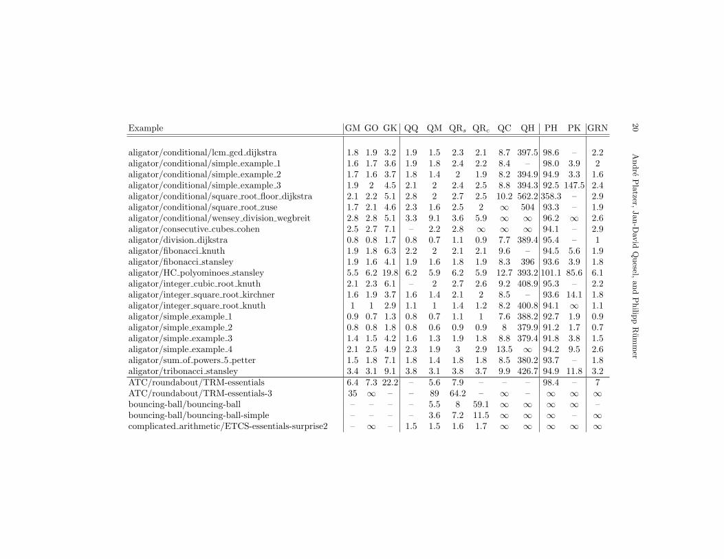
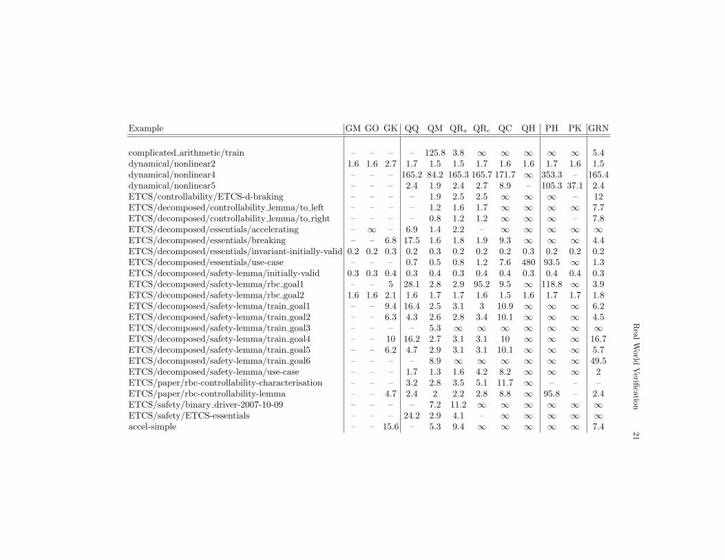
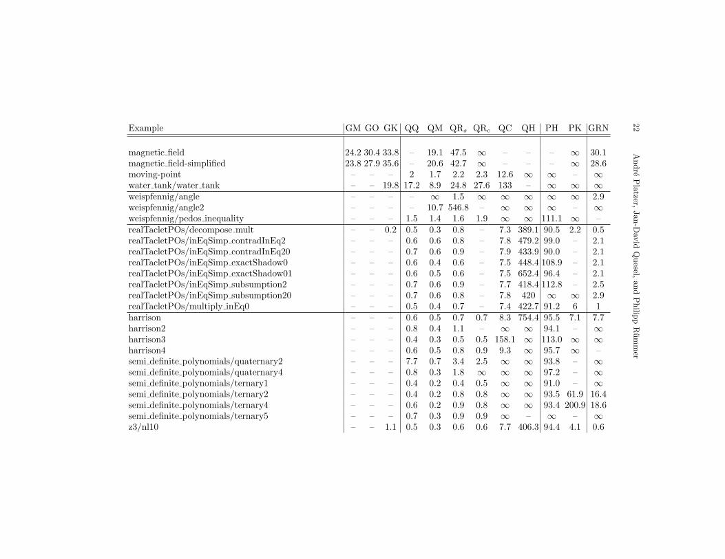
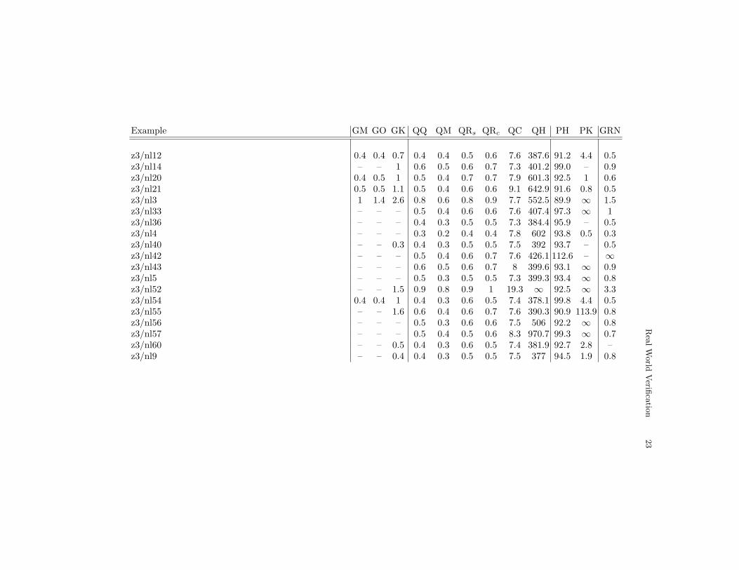
C Full Details Experimental Results

In this section we present a table containing all experimental results produced forour evaluation of the different techniques. To get comparability, we did neitheruse the invariant generation techniques described in [33] but instead providedthe invariants necessary a priori nor did we use our iterative background closureprocedure [18].

All times are given in seconds. We write∞ if the computation did not termi-nate within 600 seconds (1000 seconds for QH, because it needs ≈ 400 secondsfor startup). If the solver terminates unsuccessfully before this timeout we markthis with –.

20

Andre

Pla

tzer,Jan-D

avid

Quesel,

and

Philip

pR

um

mer

Example GM GO GK QQ QM QRs QRc QC QH PH PK GRN

aligator/conditional/lcm gcd dijkstra 1.8 1.9 3.2 1.9 1.5 2.3 2.1 8.7 397.5 98.6 – 2.2aligator/conditional/simple example 1 1.6 1.7 3.6 1.9 1.8 2.4 2.2 8.4 – 98.0 3.9 2aligator/conditional/simple example 2 1.7 1.6 3.7 1.8 1.4 2 1.9 8.2 394.9 94.9 3.3 1.6aligator/conditional/simple example 3 1.9 2 4.5 2.1 2 2.4 2.5 8.8 394.3 92.5 147.5 2.4aligator/conditional/square root floor dijkstra 2.1 2.2 5.1 2.8 2 2.7 2.5 10.2 562.2 358.3 – 2.9aligator/conditional/square root zuse 1.7 2.1 4.6 2.3 1.6 2.5 2 ∞ 504 93.3 – 1.9aligator/conditional/wensey division wegbreit 2.8 2.8 5.1 3.3 9.1 3.6 5.9 ∞ ∞ 96.2 ∞ 2.6aligator/consecutive cubes cohen 2.5 2.7 7.1 – 2.2 2.8 ∞ ∞ ∞ 94.1 – 2.9aligator/division dijkstra 0.8 0.8 1.7 0.8 0.7 1.1 0.9 7.7 389.4 95.4 – 1aligator/fibonacci knuth 1.9 1.8 6.3 2.2 2 2.1 2.1 9.6 – 94.5 5.6 1.9aligator/fibonacci stansley 1.9 1.6 4.1 1.9 1.6 1.8 1.9 8.3 396 93.6 3.9 1.8aligator/HC polyominoes stansley 5.5 6.2 19.8 6.2 5.9 6.2 5.9 12.7 393.2 101.1 85.6 6.1aligator/integer cubic root knuth 2.1 2.3 6.1 – 2 2.7 2.6 9.2 408.9 95.3 – 2.2aligator/integer square root kirchner 1.6 1.9 3.7 1.6 1.4 2.1 2 8.5 – 93.6 14.1 1.8aligator/integer square root knuth 1 1 2.9 1.1 1 1.4 1.2 8.2 400.8 94.1 ∞ 1.1aligator/simple example 1 0.9 0.7 1.3 0.8 0.7 1.1 1 7.6 388.2 92.7 1.9 0.9aligator/simple example 2 0.8 0.8 1.8 0.8 0.6 0.9 0.9 8 379.9 91.2 1.7 0.7aligator/simple example 3 1.4 1.5 4.2 1.6 1.3 1.9 1.8 8.8 379.4 91.8 3.8 1.5aligator/simple example 4 2.1 2.5 4.9 2.3 1.9 3 2.9 13.5 ∞ 94.2 9.5 2.6aligator/sum of powers 5 petter 1.5 1.8 7.1 1.8 1.4 1.8 1.8 8.5 380.2 93.7 – 1.8aligator/tribonacci stansley 3.4 3.1 9.1 3.8 3.1 3.8 3.7 9.9 426.7 94.9 11.8 3.2ATC/roundabout/TRM-essentials 6.4 7.3 22.2 – 5.6 7.9 – – – 98.4 – 7ATC/roundabout/TRM-essentials-3 35 ∞ – – 89 64.2 – ∞ – ∞ ∞ ∞bouncing-ball/bouncing-ball – – – – 5.5 8 59.1 ∞ ∞ ∞ ∞ –bouncing-ball/bouncing-ball-simple – – – – 3.6 7.2 11.5 ∞ ∞ ∞ – ∞complicated arithmetic/ETCS-essentials-surprise2 – ∞ – 1.5 1.5 1.6 1.7 ∞ ∞ ∞ ∞ ∞

Rea

lW

orld

Verifi

catio

n21


complicated arithmetic/train – – – – 125.8 3.8 ∞ ∞ ∞ ∞ ∞ 5.4dynamical/nonlinear2 1.6 1.6 2.7 1.7 1.5 1.5 1.7 1.6 1.6 1.7 1.6 1.5dynamical/nonlinear4 – – – 165.2 84.2 165.3 165.7 171.7 ∞ 353.3 – 165.4dynamical/nonlinear5 – – – 2.4 1.9 2.4 2.7 8.9 – 105.3 37.1 2.4ETCS/controllability/ETCS-d-braking – – – – 1.9 2.5 2.5 ∞ ∞ ∞ – 12ETCS/decomposed/controllability lemma/to left – – – – 1.2 1.6 1.7 ∞ ∞ ∞ ∞ 7.7ETCS/decomposed/controllability lemma/to right – – – – 0.8 1.2 1.2 ∞ ∞ ∞ – 7.8ETCS/decomposed/essentials/accelerating – ∞ – 6.9 1.4 2.2 – ∞ ∞ ∞ ∞ ∞ETCS/decomposed/essentials/breaking – – 6.8 17.5 1.6 1.8 1.9 9.3 ∞ ∞ ∞ 4.4ETCS/decomposed/essentials/invariant-initially-valid 0.2 0.2 0.3 0.2 0.3 0.2 0.2 0.2 0.3 0.2 0.2 0.2ETCS/decomposed/essentials/use-case – – – 0.7 0.5 0.8 1.2 7.6 480 93.5 ∞ 1.3ETCS/decomposed/safety-lemma/initially-valid 0.3 0.3 0.4 0.3 0.4 0.3 0.4 0.4 0.3 0.4 0.4 0.3ETCS/decomposed/safety-lemma/rbc goal1 – – 5 28.1 2.8 2.9 95.2 9.5 ∞ 118.8 ∞ 3.9ETCS/decomposed/safety-lemma/rbc goal2 1.6 1.6 2.1 1.6 1.7 1.7 1.6 1.5 1.6 1.7 1.7 1.8ETCS/decomposed/safety-lemma/train goal1 – – 9.4 16.4 2.5 3.1 3 10.9 ∞ ∞ ∞ 6.2ETCS/decomposed/safety-lemma/train goal2 – – 6.3 4.3 2.6 2.8 3.4 10.1 ∞ ∞ ∞ 4.5ETCS/decomposed/safety-lemma/train goal3 – – – – 5.3 ∞ ∞ ∞ ∞ ∞ ∞ ∞ETCS/decomposed/safety-lemma/train goal4 – – 10 16.2 2.7 3.1 3.1 10 ∞ ∞ ∞ 16.7ETCS/decomposed/safety-lemma/train goal5 – – 6.2 4.7 2.9 3.1 3.1 10.1 ∞ ∞ ∞ 5.7ETCS/decomposed/safety-lemma/train goal6 – – – – 8.9 ∞ ∞ ∞ ∞ ∞ ∞ 49.5ETCS/decomposed/safety-lemma/use-case – – – 1.7 1.3 1.6 4.2 8.2 ∞ ∞ ∞ 2ETCS/paper/rbc-controllability-characterisation – – – 3.2 2.8 3.5 5.1 11.7 ∞ – – –ETCS/paper/rbc-controllability-lemma – – 4.7 2.4 2 2.2 2.8 8.8 ∞ 95.8 – 2.4ETCS/safety/binary driver-2007-10-09 – – – – 7.2 11.2 ∞ ∞ ∞ ∞ ∞ ∞ETCS/safety/ETCS-essentials – – – 24.2 2.9 4.1 – ∞ ∞ ∞ ∞ ∞accel-simple – – 15.6 – 5.3 9.4 ∞ ∞ ∞ ∞ ∞ 7.4

22

Andre

Pla

tzer,Jan-D

avid

Quesel,

and

Philip

pR

um

mer


magnetic field 24.2 30.4 33.8 – 19.1 47.5 ∞ – – – ∞ 30.1magnetic field-simplified 23.8 27.9 35.6 – 20.6 42.7 ∞ – – – ∞ 28.6moving-point – – – 2 1.7 2.2 2.3 12.6 ∞ ∞ – ∞water tank/water tank – – 19.8 17.2 8.9 24.8 27.6 133 – ∞ ∞ ∞weispfennig/angle – – – – ∞ 1.5 ∞ ∞ ∞ ∞ ∞ 2.9weispfennig/angle2 – – – – 10.7 546.8 – ∞ ∞ ∞ – ∞weispfennig/pedos inequality – – – 1.5 1.4 1.6 1.9 ∞ ∞ 111.1 ∞ –realTacletPOs/decompose mult – – 0.2 0.5 0.3 0.8 – 7.3 389.1 90.5 2.2 0.5realTacletPOs/inEqSimp contradInEq2 – – – 0.6 0.6 0.8 – 7.8 479.2 99.0 – 2.1realTacletPOs/inEqSimp contradInEq20 – – – 0.7 0.6 0.9 – 7.9 433.9 90.0 – 2.1realTacletPOs/inEqSimp exactShadow0 – – – 0.6 0.4 0.6 – 7.5 448.4 108.9 – 2.1realTacletPOs/inEqSimp exactShadow01 – – – 0.6 0.5 0.6 – 7.5 652.4 96.4 – 2.1realTacletPOs/inEqSimp subsumption2 – – – 0.7 0.6 0.9 – 7.7 418.4 112.8 – 2.5realTacletPOs/inEqSimp subsumption20 – – – 0.7 0.6 0.8 – 7.8 420 ∞ ∞ 2.9realTacletPOs/multiply inEq0 – – – 0.5 0.4 0.7 – 7.4 422.7 91.2 6 1harrison – – – 0.6 0.5 0.7 0.7 8.3 754.4 95.5 7.1 7.7harrison2 – – – 0.8 0.4 1.1 – ∞ ∞ 94.1 – ∞harrison3 – – – 0.4 0.3 0.5 0.5 158.1 ∞ 113.0 ∞ ∞harrison4 – – – 0.6 0.5 0.8 0.9 9.3 ∞ 95.7 ∞ –semi definite polynomials/quaternary2 – – – 7.7 0.7 3.4 2.5 ∞ ∞ 93.8 – ∞semi definite polynomials/quaternary4 – – – 0.8 0.3 1.8 ∞ ∞ ∞ 97.2 – ∞semi definite polynomials/ternary1 – – – 0.4 0.2 0.4 0.5 ∞ ∞ 91.0 – ∞semi definite polynomials/ternary2 – – – 0.4 0.2 0.8 0.8 ∞ ∞ 93.5 61.9 16.4semi definite polynomials/ternary4 – – – 0.6 0.2 0.9 0.8 ∞ ∞ 93.4 200.9 18.6semi definite polynomials/ternary5 – – – 0.7 0.3 0.9 0.9 ∞ – ∞ – ∞z3/nl10 – – 1.1 0.5 0.3 0.6 0.6 7.7 406.3 94.4 4.1 0.6

Rea

lW

orld

Verifi

catio

n23


z3/nl12 0.4 0.4 0.7 0.4 0.4 0.5 0.6 7.6 387.6 91.2 4.4 0.5z3/nl14 – – 1 0.6 0.5 0.6 0.7 7.3 401.2 99.0 – 0.9z3/nl20 0.4 0.5 1 0.5 0.4 0.7 0.7 7.9 601.3 92.5 1 0.6z3/nl21 0.5 0.5 1.1 0.5 0.4 0.6 0.6 9.1 642.9 91.6 0.8 0.5z3/nl3 1 1.4 2.6 0.8 0.6 0.8 0.9 7.7 552.5 89.9 ∞ 1.5z3/nl33 – – – 0.5 0.4 0.6 0.6 7.6 407.4 97.3 ∞ 1z3/nl36 – – – 0.4 0.3 0.5 0.5 7.3 384.4 95.9 – 0.5z3/nl4 – – – 0.3 0.2 0.4 0.4 7.8 602 93.8 0.5 0.3z3/nl40 – – 0.3 0.4 0.3 0.5 0.5 7.5 392 93.7 – 0.5z3/nl42 – – – 0.5 0.4 0.6 0.7 7.6 426.1 112.6 – ∞z3/nl43 – – – 0.6 0.5 0.6 0.7 8 399.6 93.1 ∞ 0.9z3/nl5 – – – 0.5 0.3 0.5 0.5 7.3 399.3 93.4 ∞ 0.8z3/nl52 – – 1.5 0.9 0.8 0.9 1 19.3 ∞ 92.5 ∞ 3.3z3/nl54 0.4 0.4 1 0.4 0.3 0.6 0.5 7.4 378.1 99.8 4.4 0.5z3/nl55 – – 1.6 0.6 0.4 0.6 0.7 7.6 390.3 90.9 113.9 0.8z3/nl56 – – – 0.5 0.3 0.6 0.6 7.5 506 92.2 ∞ 0.8z3/nl57 – – – 0.5 0.4 0.5 0.6 8.3 970.7 99.3 ∞ 0.7z3/nl60 – – 0.5 0.4 0.3 0.6 0.5 7.4 381.9 92.7 2.8 –z3/nl9 – – 0.4 0.4 0.3 0.5 0.5 7.5 377 94.5 1.9 0.8

Documents

Real World Verification - avacs.org