Real Exchange Rates and Growth Surges

Fordham University Department of Economics Discussion Paper Series

Real Exchange Rates and Productivity

Growth

Darryl McLeod Fordham University, Department of Economics

Elitza Mileva European Central Bank

Discussion Paper No: 2011-04 July 2011

Department of Economics

Fordham University 441 E Fordham Rd, Dealy Hall

Bronx, NY 10458 (718) 817-4048

Real Exchange Rates and Productivity Growth

Darryl McLeod∗ and Elitza Mileva†

July 18, 2011

Abstract

Maintaining a weak real exchange rate is a widely emulated growth strategy, in

part because of the success of Asian exporters, most recently China. Simulations of

a simple two-sector open economy growth model based on Matsuyama (1992) sug-

gest that a weaker real exchange rate can lead to a ”growth surge”, as workers move

into traded goods industries with more ”learning by doing” and exit non-traded goods

sectors with slower productivity growth. Using the updated total factor productivity

(TFP) estimates from Bosworth and Collins (2003), panel estimates for 58 countries

reveal the anticipated non-linear relationship between the real exchange rate and TFP

growth: real currency depreciation raises TFP and GDP growth up to a point. Man-

ufacturing exports appear to be one channel via which the real exchange rate affects

TFP growth. Fears that a weaker real exchange rate might reduce investment and pro-

ductivity growth by making imported equipment more expensive are not supported.

∗Corresponding author, Economics Department, Fordham University, 441 East Fordham Road,Bronx, NY 10458, Phone (718) 817-4063/45, Fax(718) 817-3518, E-mail: [email protected],http://www.fordham.edu/economics/mcleod/.†European Central Bank, Kaiserstrasse 29, 60311 Frankfurt am Main, Germany, E-mail:

[email protected]

1

Keywords: economic growth, total factor productivity growth, exchange rate pol-

icy

JEL Classification: O14, O41, O47 and O57

1 Introduction

Maintaining a weak real exchange rate (RER) has become a widely recommended growth

strategy, partly due to the success of Asian exporters. Rodrik (2010) argues that ”poor

nations” can replicate the ”essentials of the Chinese model” by actively using ”exchange

rates... to stimulate industrialization and growth”. Johnson, Ostry and Subramanian (2006)

argue that exchange rate policy is a ”lever for growth” even in countries with relatively

weak institutions. This paper explores how a weak real exchange rate (RER) stimulates

economic growth, especially surges in productivity growth. Simulations using a model similar

to Matsuyama’s (1992) two-sector open economy growth model show that a combination

of ”learning by doing” in the traded goods sector and a policy lever, such as the RER,

which moves workers into traded goods production faster, can lead to a surge in total factor

productivity (TFP) growth. Eventually diminishing returns raise wages in the non-traded

goods sector and growth slows.

Panel estimates for 58 countries support the non-linear relationship between the real

exchange rate and GDP growth anticipated by the model. Moreover, dynamic panel esti-

mation with a parsimonious use of instruments suggests that causality runs from the real

exchange rate to productivity growth.1 Our findings suggest that a 10% real depreciation of

1The Balassa-Samuelson effect posits reverse causality: faster productivity growth in the traded goodssector leads to long run RER appreciation. A weaker real exchange rate creates a surge in TFP andGDP growth which over time raises wages in the non-traded sector, leading to an appreciation of the realexchange rate. In the scenario explored by this paper the government attempts to counteract the effect offaster productivity growth in the traded goods sector using policy intervention to slow the RER appreciation.

2

the exchange rate leads to about 0.2% increase in the average annual TFP growth rate. If

TFP growth starts at 1.5%, a 10% real depreciation can raise productivity growth to 1.7%.

However, our dynamic panel estimates show that the impact can be twice as large, in the

range of 0.3% to 0.5%. These results are of interest because Krugman (1994) and Young

(1995) questioned how miraculous Asian growth was in the 1980s as rapid factor accumu-

lation accounted for most of the rise in per capita incomes. However, since 1990 a number

of Asian countries, notably China, have enjoyed rapid TFP growth. If China’s currency

is currently undervalued by 20-30%, as some argue, then fully a third of China’s 3% TFP

growth can be attributed to its exchange rate policy.2

We find some evidence that traded goods production is a key driver of overall productivity

growth: holding manufacturing activity constant greatly reduces the effects of the exchange

rate policy. Rodrik (2008) finds that weaker real exchange rates are associated with faster

per capita GDP growth but his growth drivers are weak institutions and imperfect markets

not learning by doing in traded goods production. He does not examine the effects of the

real exchange rate on TFP growth, the main focus of this paper.

Kose, Prasad and Terrones (2009) explore the links between financial openness and TFP

growth. Using their own TFP estimates over the period 1966-2005, they find that capital

account liberalization accelerates TFP growth. To the extent capital inflows also result in

RER appreciation, capital account liberalization might lead to a negative association between

RER depreciation and TFP growth, but this correlation is not evident in our data.

The next section reviews the literature on exchange rates and growth. Section 3 presents

Both effects are evident in China today: rapid growth of tradable output driving a large trade surplus, butrising real wages leading to a drop in China’s PPP to market exchange rate ratio (which fell sharply withthe release of the new 2005 PPP GDP estimates).

2Estimates of China’s TFP growth vary; 3% annually is in line with estimates by Bosworth and Collins(2008).

3

a simple version of the Matsuyama (1992) model modified to replace agriculture and industry

with traded and non-traded goods. Finally, Section 4 presents panel data evidence on the

relationship between real exchange rate depreciation and total factor productivity growth.

2 Real Exchange Rates and Productivity Growth

Initially productivity growth was considered central to the Asian growth miracle. In ”Making

a Miracle”, Lucas (1993) stays ”sharply focused on neoclassical theories that view the growth

miracles as productivity miracles. What happened over the last 30 years that enabled the

typical Korean or overseas Chinese worker to produce 6 times the goods and services he

could produce in 1960?” However, Young’s (1995) ”Tyranny of Numbers” growth accounting

seemed to show the opposite: high Asian growth rates were almost all factor accumulation;

productivity growth was unusually low, leading Krugman (1994) to declare the Asian growth

miracle ”a myth”. China and India appear to be more conventional Asian miracles, however,

as they have recently had both rapid TFP and economic growth. Bosworth and Collins (2008)

also find that sectoral labor shifts accounted for about 1.2% of per capita growth in both

countries, in line with the simulations discussed in the next section.

Though relatively few papers focus on TFP growth, there is a considerable literature

linking real exchange rates and per capita GDP growth. Dollar (1992) uses PPP based

real exchange rate estimates to show that overvaluation harms growth, while Razin and

Collins (1997) and Aguirre and Calderon (2006) find that large over- and under-valuation

hurt growth, while modest undervaluation enhances growth. Similarly, Hausmann, Pritchett

and Rodrik (2005) demonstrate that rapid growth accelerations are often correlated with real

exchange rate depreciations. Rodrik (2008) finds that the growth acceleration takes place, on

4

average, after ten years of steady increase in undervaluation in developing countries.3 Rodrik

argues that a weak real exchange rate compensates for institutional weaknesses and market

failures (e.g. knowledge spillovers, credit market imperfections, etc.) which lead to underin-

vestment in the traded goods sector in developing countries. An undervalued exchange rate

raises the profitability of traded goods production and generates faster growth.4

Most papers on exchange rate policy focus on per capita GDP growth or investment. An

exception is Kose, Prasad and Terrones (2009): using their own TFP growth estimates, they

find mixed evidence regarding the impact of financial liberalization on productivity growth.

De jure liberalization seems to raise TFP growth but de facto liberalization (capital inflows)

does not; instead, FDI and portfolio equity flows increase TFP growth but external debt

does not. To the extent that capital inflows lead to exchange rate appreciation (unless they

are sterilized), their findings suggest that exchange rate appreciation might be positively

correlated with economic growth.

3 Open Economy Growth with Traded and Non-traded

Goods Sectors

Matsuyama’s (1992) two-sector open economy model has ”learning by doing” in manufac-

turing but not agriculture. Our use of Matsuyama’s model is similar to that of Rodriguez

3In Asia, Rodrik (2008) argues that currencies were undervalued by 20%, on average, before the growthspurt and remained undervalued as growth accelerated. In addition, Rodrik (2008) provides panel dataevidence that undervaluation leads to an increase in the relative size of the traded goods sector and that theincrease in the size of the traded goods sector, caused by undervaluation, promotes economic growth.

4Another strand of the literature focuses on real exchange rate volatility. Exchange rate volatility maydiscourage trade and investment which are important drivers of growth. However, the empirical evidence ofthe relationship between real exchange rate volatility and growth is inconclusive. See Eichengreen (2008) fora review of the relevant studies.

5

and Rodrik’s (2001): they study how an import tariff can accelerate growth by increasing

the share the work force in industry. Similarly, a weaker real exchange rate can raise wages

in the traded goods production leading to a more rapid shift of workers out of the traditional

or non-traded goods sector (where there is less learning by doing). An important difference

between tariffs and the real exchange rate is that the government does not have to decide

which sector to protect; a weaker real exchange rate automatically benefits all exporters and

import competing industries. Aizenman and Lee (2008) present a more elaborate model,

in which the learning by doing externality assumed by Matsuyama (1992) may be linked

either to production or investment. They argue that, if this externality happens to be linked

to investment, undervaluation may decrease (not increase) productivity growth by raising

the cost of imported investment goods.5 We explore this argument empirically in the next

section.

Whereas Matsuyama models agriculture and industry, we focus on employment shifts

between a traded or manufacturing goods sector (T ) and a non-traded goods sector (N).

The real exchange rate is the relative price of traded goods. The RER, qt, depends on the

nominal exchange rate, et, the exogenous price of traded goods set in international markets,

p∗t , and the domestic price of non-traded goods, pNt :

qt =etp

∗t

pNt. (1)

Governments influence the real exchange rate by managing the nominal exchange, et, or

by using monetary policy to influence the domestic price of non-traded goods, pNt .

Labor is the only mobile factor of production. The total labor supply is assumed to

5Aizenman and Lee (2008) also point out that there is no clear empirical evidence that supports an”aggregate investment” externality as opposed to an ”aggregate production” externality.

6

be constant and set to one, L = 1. Assuming identical diminishing returns technologies,

0 < α < 1, and defining lt as the share of the labor force in manufacturing, the production

functions for traded and non-traded goods are

QTt = Atl

αt (2)

QNt = B(1− lt)α. (3)

The key difference between the two sectors is the productivity level: B in the non-traded

goods sector is assumed to be constant, whereas traded goods sector productivity At is

subject to ”learning by doing” in the tradition of Kenneth Arrow. Traded goods sector

productivity increases with the level of output, QTt , but is not affected by changes in non-

traded output, QNt .

Learning by doing is external to the individual firm but internal to the sector as a whole,

so that manufacturing productivity evolves over time according to

At = δQTt , (4)

in which δ > 0 is the exogenous rate of learning by doing.

Competition and the mobility of labor between the two sectors equalize the marginal

products of labor in the two sectors:

B(1− lt)α−1 = qtAtlα−1t , (5)

in which qt is the real exchange rate defined in Equation (1). The real exchange rate

affects the allocation of labor between the two sectors: a weaker RER (a higher qt) raises the

7

marginal product of labor in the traded goods sector, increasing real wages in that sector

until movement of labor out of the nontraded goods sector equalizes the marginal product

of labor (real wage) economy wide.

Substituting (2) into (4) yields the growth rate of productivity in the traded goods

sector as a function of the share of labor employed in that sector and the learning-by-doing

externality:

AtAt

= δlαt . (6)

Equation (5) implicitly defines lt as a function of qt, and differentiation ( ∂lt∂qt> 0) shows

that an increase in the domestic relative price of the traded good leads to an increase in

the share of labor employed in the traded goods sector, which then raises productivity via

Equation (6).

Total output, Yt, in foreign prices is

Yt = B(1− lt)α + Atlαt (7)

The time derivative of Equation (7) and Equations (2), (4) and (5) yields the instanta-

neous rate of growth of output:

YtYt

= (λt +α(λt − lt)

1− α)δlαt , (8)

in whichQTtYt

= λt represents the manufacturing share of output in foreign prices.

Since learning by doing in the traded goods sector is the only source of productivity

growth over the longer term, overall (economy-wide) productivity growth depends only on

the share of labor, lt, in that sector. This implies a steady state overall TFP growth of

8

ˆTFP t = δl1+αt . (9)

However, during the transition changing the RER changes the labor share lt, so overall

productivity growth also depends on the rate at which lt changes over time (i.e. how fast

changes in the RER, qt, move labor out of the non-traded goods sector with fixed productivity

level B into the dynamic traded goods sector). The instantaneous rate of growth of overall

TFP is given by

˙TFP t

TFPt=

(At −B)lt + ltAtltAt + (1− lt)B

, (10)

where TFPt = ltAt + (1− lt)B.

The relationship between output growth, TFP growth and the RER described by Equa-

tions (8) and (10) is nonlinear as illustrated in Figure 1 using plausible parameters. The

surge in TFP and GDP growth occurs because, initially, depreciation of the RER leads to

rapid reallocation of labor into the traded goods sector, accelerating learning by doing. For

this particular calibration of the model parameters overall productivity growth converges to

about 3%, the rate observed in China today. Diminishing returns in the non-traded goods

sector (α < 1) eventually offset the weak RER driven growth enhancing effect of transfering

workers to higher productivity in traded goods sector employment so growth settles to it’s

long run trend.

9

0.2 0.3 0.4 0.5 0.6 0.7 0.8 0.90

0.5

1

1.5

2

2.5

3

3.5

4

4.5

Real exchange rate level (qt)

Gro

wth

rat

e (%

)

Traded goods sector TFP growthGDP growth per workerTotal TFP growth (labor-weighted)

Figure 1: A real exchange rate driven shift of labor into traded goods creates a surge in TFPand GDP growth. (Parameter values: α = 0.8; δ = 0.03;A0 = 3;B = 1)

10

4 Empirical Results

This section provides estimates of the impact of real exchange rate changes on TFP growth

using a panel of 58 developing countries for the period 1975 - 2004. The TFP growth rates

are from an updated version of the Bosworth and Collins (2003) dataset.6 The data on real

exchange rates is based on our own trade-weighted estimates as explained in the appendix.7

The remaining variables are from the World Development Indicators (WDI) database (World

Bank, 2010). Following standard practice five-year averages are used to capture long-term

as opposed to transitory and business cycle fluctuations.

Table 1 reports regressions of TFP growth on the real effective exchange rate and several

standard control variables. According to the country fixed effects panel data estimates

reported in Column 1.1, 10% depreciation of the real exchange rate (i.e. an increase in the

variable Log of RER) is associated with a 0.2% increase in the average annual TFP growth

rate, confirming the predictions of the model. The control variables openness and secondary

6The Bosworth and Collins (2003) dataset includes 62 developing countries, we exclude four of these fromour sample: Nigeria, Singapore and Taiwan due to lack of data (on government consumption, secondaryschool enrollment and trade-weighted exchange rates, respectively) and Nicaragua, which is an outlier dueto a brush with hyperinflation. The countries included are Algeria, Argentina, Bangladesh, Bolivia, Brazil,Cameroon, Chile, China, Colombia, Costa Rica, Cote d’Ivoire, Cyprus, Dominican Republic, Ecuador,Egypt, Arab Rep., El Salvador, Ethiopia, Ghana, Guatemala, Guyana, Haiti, Honduras, India, Indone-sia, Iran, Islamic Rep., Israel, Jamaica, Jordan, Kenya, Korea, Rep., Madagascar, Malawi, Malaysia, Mali,Mauritius, Mexico, Morocco, Mozambique, Nicaragua, Nigeria, Pakistan, Panama, Paraguay, Peru, Philip-pines, Rwanda, Senegal, Sierra Leone, Singapore, South Africa, Sri Lanka, Tanzania, Thailand, Trinidadand Tobago, Tunisia, Turkey, Uganda, Uruguay, Venezuela, RB, Zambia, Zimbabwe, Algeria, Argentina,Bangladesh, Bolivia, Brazil, Cameroon, Chile, China, Colombia, Costa Rica, Cote d’Ivoire, Cyprus, Do-minican Republic, Ecuador, Egypt, Arab Rep., El Salvador, Ethiopia, Ghana, Guatemala, Guyana, Haiti,Honduras, India, Indonesia, Iran, Islamic Rep., Israel, Jamaica, Jordan, Kenya, Korea, Rep., Madagascar,Malawi, Malaysia, Mali, Mauritius, Mexico, Morocco, Mozambique, Nicaragua, Nigeria, Pakistan, Panama,Paraguay, Peru, Philippines, Rwanda, Senegal, Sierra Leone, Singapore, South Africa, Sri Lanka, Tanzania,Thailand, Trinidad and Tobago, Tunisia, Turkey, Uganda, Uruguay, Venezuela, RB, Zambia, Zimbabwe.

7The real exchange rate data used in this paper are available at http://www.fordham.edu/economics/mcleod/TradeWeightedRER.xlsx. We have reproduced all regressions using the REER data from the WorldBank WDI but the WDI only provides RER estimates for 29 countries. These estimates are available uponrequest from the authors.

11

school enrolment have a positive impact, whereas government consumption reduces TFP

growth. Initial real PPP GDP per capita (defined as the real PPP GDP per capita in the

first year of each five-year period) is a proxy for structural development and the coefficient on

this variable shows that countries at a lower stage of development tend to have, on average,

higher TFP growth rates (Column 1.3). The results are similar if the lagged real PPP GDP

per capita is used (Column 1.4).8

Table 2 explores the interaction of trade and the RER and provides alternate estimates

of the equations in Table 1. The first column of Table 2 reports the same regression as in

Column 1.3 of Table 1. The equation reported in Column 2.2 includes the change in the share

of manufactures exports in PPP GDP. A one-percent increase in the share of manufactures

exports is associated with a 0.11% increase in the average TFP growth rate. The coefficient

on the RER is no longer significant, pointing to interaction between the two variables. This

result seems to suggest that the RER affects TFP growth through the change in manufactures

exports. As a robustness check, Columns 2.3 and 2.4 report regressions based on the same

specifications and estimated in first differences. The results are very similar to the levels

equations.

Table 2 also presents dynamic panel estimates using the generalized method of moments

(GMM) and various instruments. These estimates allow us to test the direction of causality

between TFP growth and the RER. Recall that the Balassa - Samuelson effect implies

causality running from exogenous rapid productivity growth in the traded goods sector to

a real exchange rate appreciation driven by higher wages in both sectors. Columns 2.1

through 2.4 indicate a positive correlation between TFP growth and the RER, contrary to

the correlation predicted by the Balassa - Samuelson effect. Columns 2.5-2.8 present four

8We prefer initial real PPP GDP per capita to lagged real PPP GDP per capita to economize on obser-vations lost due to using one lag.

12

Table 1: TFP growth and the real exchange rate, five-year averages (1975 - 2004)

Dependent Variable: TFP growth

(Robust standard errors in parentheses) 1.1 1.2 1.3 1.4

Log of RER 0.02*** 0.018*** 0.022*** 0.018***(0.007) (0.007) (0.005) (0.006)

Openness 0.005 0.016*** 0.011**(0.006) (0.005) (0.006)

Government consumption (share of GDP) -0.18** -0.20*** -0.19***(0.09) (0.07) (0.07)

Secondary school enrollment 0.001 0.04*** 0.07***(0.01) (0.02) (0.02)

Log of initial real PPP GDP per capita -0.047***(0.012)

Lagged log of real PPP GDP per capita -0.055***(0.014)

Constant -0.1*** -0.05 0.31*** 0.36***(0.03) (0.03) (0.1) (0.11)

Number of observations 334 312 310 267Number of countries 58 58 58 58R2 0.04 0.06 0.18 0.21Estimation method Country fixed effects

*** indicates statistical significance at the 1%; ** at the 5%; and * at the 10% level.

Data sources: The TFP estimates are from an updated version of estimates presented in Bosworth and

Collins (2003) that end in 2003. All other variables are obtained from the World Development Indicators

as downloaded in August 2009. Computation of trade-weighted RERs is described in the appendix. The

estimates use five-year averages, so that T = 6: 75-79, 80-84, 85-89, 90-94, 95-99 and 00-04, except for

TFP, which is the average of 2000-03. Openness is defined as the ratio of the sum of exports and imports

to PPP GDP. Using international prices reduces the effect of exchange rate fluctuations on the trade shares.

Initial real GDP per capita is the natural log of real PPP GDP per capita in the first year of each five-year

period (following Prasad et al., 2006).

13

estimates computed using the Arellano - Bond (1991) difference GMM and the Blundell -

Bond (1998) system GMM estimator.

For the difference GMM estimates all variables are differenced and the first difference of

the RER is instrumented by its own second or third (or both) lags in levels, one excluded

exogenous instrument - the real interest rate in the US, and all exogenous variables included

in the regression equation. For the system GMM estimates, the equation in levels and the

equation in first differences are estimated as a system, with the RER level instrumented by

the second and third lag of its first difference.9 Similarly, the PPP GDP share of manufac-

tures exports is instrumented either by its own lagged differences in Column 2.6 or by both

lagged levels and differences in equation 2.8. An additional excluded exogenous instrument

for each country’s manufacturing export share is the total world manufacturing export share

of world GDP. The dynamic GMM regressions include the logarithm of initial TFP growth,

i.e. the TFP level in the first year of each five-year period.10

Longer lags of the endogenous variables turn out to be good exogenous instruments. The

Hansen J test of the overidentifying restrictions indicates that the instruments as a group are

exogenous (the Hansen J test is equivalent to the Sargan statistic if the errors are normally

distributed). Tests for second-order autocorrelation in the differenced equation (which is

equivalent to testing for first-order autocorrelation in the equation in levels) does not reject

the null hypothesis of no autocorrelation.

9Limiting the number of lags used as instruments in the GMM regressions keeps the instrument count lowand improves the performance of the Hansen J test for joint validity of those instruments. Using too manyinstruments can overfit the endogenous variables and bias the coefficient estimates (see Roodman 2007).

10Kose, Prasad and Terrones (2009) interpret this as convergence to a common technological frontier.

14

Tab

le2:

TF

Pgro

wth

and

the

real

exch

ange

rate

,five-y

ear

avera

ges

(1975-2

004)

Dep

end

ent

Var

iab

le:

TF

Pgro

wth

(Rob

ust

stan

dar

der

rors

inp

aren

thes

es)

2.1

2.2

2.3

2.4

2.5

2.6

2.7

2.8

Log

ofR

ER

0.022***

0.0

13

0.0

16**

0.0

16

0.0

31**

0.0

28

0.0

54**

0.0

27

(0.0

05)

(0.0

09)

(0.0

07)

(0.0

12)

(0.0

14)

(0.0

24)

(0.0

22)

(0.0

17)

Op

enn

ess

0.016***

0.0

17**

0.0

16***

0.0

19**

0.0

18***

0.0

33***

0.007*

0.0

06

(0.0

05)

(0.0

07)

(0.0

06)

(0.0

09)

(0.0

07)

(0.0

12)

(0.0

04)

(0.0

04)

Gov

ern

men

tco

nsu

mp

tion

(sh

are

ofG

DP

)-0

.20***

-0.2

3***

-0.2

9***

-0.2

5***

-0.3

1***

-0.3

2***

-0.0

7-0

.08

(0.0

7)

(0.0

6)

(0.0

6)

(0.0

7)

(0.0

8)

(0.0

9)

(0.0

5)

(0.0

5)

Sec

ond

ary

school

enro

llm

ent

0.04***

0.0

3**

-0.0

04

-0.0

05

0.0

2-0

.02

0.03**

0.0

3***

(0.0

2)

(0.0

1)

(0.0

23)

(0.0

25)

(0.0

3)

(0.0

3)

(0.0

2)

(0.0

1)

Log

ofin

itia

lre

alP

PP

GD

Pp

erca

pit

a-0

.047***

-0.0

38***

-0.0

94***

-0.0

78***

-0.0

42

-0.0

05

-0.0

26***

-0.0

21***

(0.0

12)

(0.0

1)

(0.0

14)

(0.0

13)

(0.0

32)

(0.0

40)

(0.0

07)

(0.0

06)

Man

ufa

ctu

res

exp

orts

0.1

1**

0.1

1**

0.4

9**

0.2

3*

(Ch

ange

inP

PP

GD

Psh

are)

(0.0

5)

(0.0

5)

(0.2

3)

(0.1

2)

Log

arit

hm

ofin

itia

lT

FP

-0.0

7*

-0.0

80.0

4**

0.0

3**

(0.0

4)

(0.0

5)

(0.0

2)

(0.0

1)

Con

stan

t0.

31***

0.2

9***

0.0

1**

0.0

04

-0.0

40.0

4(0

.1)

(0.0

8)

(0.0

03)

(0.0

03)

(0.1

)(0

.06)

Nu

mb

erof

obse

rvat

ion

s310

260

247

195

247

195

310

260

Nu

mb

erof

cou

ntr

ies

58

55

58

54

58

54

58

55

Nu

mb

erof

inst

rum

ents

26

30

14

42

AR

2te

stp

-val

ue

0.2

00.8

40.4

40.1

9H

anse

nJ

stat

isti

c(r

obu

st)

p-v

alu

e0.3

90.2

90.2

00.2

2R

20.1

80.1

80.2

70.2

5E

stim

atio

nm

eth

od

Cou

ntr

yfi

xed

effec

tsF

irst

diff

eren

ces

Diff

eren

ceG

MM

1/

Syst

emG

MM

2/

**

*in

dic

ate

sst

ati

stic

al

sign

ifica

nce

at

the

1%

;*

*a

tth

e5

%;

an

d*

at

the

10

%le

vel.

1/

Are

lla

no

-B

on

d(1

99

1)

diff

eren

ceG

MM

;2

/B

lun

del

l-

Bo

nd

(19

98

)sy

stem

GM

M,

two

-ste

pes

tim

ati

on

usi

ng

the

Sta

tap

rogr

am

xta

bon

d2

wri

tten

byR

ood

ma

n(2

00

6).

Data

sources:

See

da

taso

urc

esa

nd

no

tes

inth

efo

otn

ote

toT

abl

e1

.T

he

sam

ple

use

din

regr

essi

on

s2

.2a

nd

2.4

excl

ud

esS

ierr

aL

eon

e,fo

rw

hic

hth

ere

are

no

da

tao

nm

an

ufa

ctu

rin

gex

port

s,a

nd

two

ou

tlie

rs,

the

Do

min

ica

nR

epu

blic

an

dG

ha

na

.R

egre

ssio

n2

.4a

lso

excl

ud

esT

an

zan

ia,

for

wh

ich

ther

ea

ren

ot

eno

ugh

obs

erva

tio

ns

on

ma

nu

fact

uri

ng

expo

rts

for

firs

td

iffer

ence

ses

tim

ati

on

.In

itia

lT

FP

isth

eT

FP

leve

lin

the

firs

tyea

ro

fea

chfi

ve-y

ear

peri

od.

Wo

rld

ma

nu

fact

ure

sex

port

sa

sa

sha

reo

fG

DP

isu

sed

as

an

excl

ud

edex

ogen

ou

sin

stru

men

tin

regr

essi

on

s2

.6a

nd

2.8

an

dth

eU

Sre

al

inte

rest

rate

isu

sed

inre

gres

sio

ns

2.5

-2.8

.

15

The GMM estimates confirm the fixed effects and first difference regressions. We cannot

reject the hypothesis that causality runs from the RER to TFP growth and from manufac-

turing exports to TFP growth, in line with the model discussed in Section 3. Controlling

for possible endogeneity, the positive impact of RER depreciation on TFP growth is even

stronger: a 10% real depreciation leads to an increase in average TFP growth of 0.3% - 0.5%

(Columns 2.5 and 2.7). Raising the share of manufactures exports in PPP GDP by 1% leads

to an increase in the average TFP growth of 0.2% - 0.5%. As in Regressions 2.2 and 2.4,

in the GMM regressions including manufactures exports the coefficient on the RER is not

statistically significant (Columns 2.6 and 2.8).

The model predicts a gradual decline in the impact of a weaker RER on TFP growth

to the point that more depreciation leads to slower economy-wide TFP growth and slower

output growth. Table 3 reports the results of country fixed effects and first differences panel

regressions of TFP growth and real per capita PPP GDP growth on the RER, the RER

squared and the same control variables as above. The coefficient on the RER is statistically

significant and positive in all regressions, whereas the coefficient on the squared term is

significant and negative, thus confirming the pattern predicted in Figure 1 above.

The nonlinear effect of the RER on TFP growth suggests that there is some level of the

RER at which TFP growth stops increasing. Using the estimates shown in Columns 3.1

and 3.2, economy-wide TFP growth is fastest when the level of the RER is at 180 - 205.

Similarly, the estimates reported as Columns 3.3 and 3.4 show that the GDP growth rate is

maximized when the RER index is in the range 185 - 265 (at base year 2000).

Following Rodrik (2008), there is some evidence that the effect of the RER on TFP growth

operates (at least partially) through its impact on the sectoral composition of output. Rodrik

regresses the shares of industry and agriculture in GDP and in employment, respectively,

16

Table 3: TFP growth and the real exchange rate - tests for non-linear relationship,five-year averages (1975 - 2004)

Dependent Variable: TFP growth Real per capita GDPgrowth


Log of RER 0.24*** 0.102** 0.29*** 0.103**(0.08) (0.048) (0.1) (0.041)

Log of RER Squared -0.02*** -0.01* -0.03*** -0.01*(0.01) (0.006) (0.01) (0.005)

Openness 0.017*** -0.001 0.031*** 0.015*(0.006) (0.008) (0.008) (0.009)

Government consumption (share of GDP) -0.19*** -0.39*** -0.24*** -0.38***(0.07) (0.08) (0.08) (0.08)

Secondary school enrollment 0.03* -0.04 0.027 -0.06**(0.02) (0.03) (0.019) (0.03)

Log of initial real PPP GDP per capita -0.046*** -0.054***(0.013) (0.012)

Constant -0.21 0.0 -0.23 0.002(0.21) (0.003) (0.26) (0.003)

Number of observations 304 249 304 248Number of countries 57 58 57 58R2 0.19 0.12 0.23 0.14Estimation method1/ FE FD FE FDGrowth maximizing RER 182 206 184 265

*** indicates statistical significance at the 1%; ** at the 5%; and * at the 10% level. 1/ FE is country fixedeffects and FD are first differences that eliminate country fixed effects.Data sources: See data sources in the footnote to Table 1. Log of initial real PPP GDP per capita isdropped from regressions 2.2 and 2.4 as a robustness test, becasue when differenced it becomes too similar toGDP growth.

17

reporting four regressions on the RER and other independent variables. Table 4 reports

four country fixed effects panel regressions in which the dependent variables are the value

added of manufacturing, industry, agriculture or services in percent of GDP. The data are

from the WDI and are averaged over five years. The explanatory variables are the RER and

real PPP GDP per capita, the latter serving as a proxy for convergence. RER depreciation

is associated with an increase in the manufacturing and industry shares of GDP11 and a

decrease (albeit not statistically significant in the latter case) in the agriculture and services

shares of GDP. As expected given Engel’s law, higher GDP per capita is associated with

larger industrial and services sectors and smaller agricultural sector.

Table 4: Sectoral shares of GDP and the real exchange rate, five-year averages(1975 - 2004)

Shares of GDPDependent Variable: Manufacturing Industry Agriculture Services


Log of RER 0.03*** 0.06*** -0.03* -0.03(0.01) (0.01) (0.02) (0.02)

Log of real PPP GDP per capita 0.01 0.03* -0.14*** 0.10***(0.02) (0.02) (0.01) (0.02)

Constant -0.1 -0.24* 1.43*** -0.19(0.16) (0.14) (0.14) (0.16)

Number of observations 295 298 298 298Number of countries 55 55 55 55R2 0.08 0.19 0.47 0.21Estimation method Country fixed effects

*** indicates statistical significance at the 1%; ** at the 5%; and * at the 10% level.Data sources: See data sources in the footnote to Table 1.

The results in Table 4 are similar to Rodrik’s (2008): a weaker RER is associated with

an increase in the share of industry and a smaller agricultural sector (columns 4.2 and 4.3).

11Manufacturing is a subset of the industrial sector.

18

Since both industrial and agricultural goods are tradable goods, the negative impact of

the RER on agriculture is unexpected, as Rodrik notes as well. However, to the extent

that the RER and TFP growth raise per capita income, Engel’s law may dominate the

effects of productivity growth in agriculture, leading to an overall decline in agriculture’s

GDP share despite productivity growth in that sector. Trade in agricultural commodities

is also managed with extensive quotas and tariffs, so that trade barriers may thwart the

opportunity for expanded exports driven by a more competitive exchange rate. Indeed, this

is the argument of many less developed countries in the Doha Round.

Following Rodrik (2008), we also run a two-stage least squares regression of TFP growth

on the manufacturing share of GDP and the logarithm of real per capital PPP GDP, in the

first stage of which the manufacturing share of GDP is regressed on the logarithm of the

RER.12 The coefficient on the manufacturing share of GDP is significant at the 1% level and

is equal to 0.7, indicating that the variation in the manufacturing share of GDP directly

caused by the RER, controlling for real per capita GDP, is associated positively with TFP

growth. This result shows that depreciation leads to manufacturing sector growth, which in

turns leads to higher productivity growth.

Finally, we address the concern of Aizenman and Lee (2008) that a weak real exchange

rate might slow productivity growth by reducing investment, via the higher cost of imported

machinery and equipment. Table 5 reports Arellano-Bond difference and system GMM

regressions, in which the dependent variable is the GDP share of domestic investment. In

12This regression was performed using the xtivreg2 program in Stata written by Schaffer (2007). Theequation is exactly identified. The Angrist-Pischke (AP) first-stage chi-squared Wald statistic rejects thenull hypothesis that the endogenous regressor, the manufacturing share in GDP, is unidentified. The first-stage F statistic (15.32) exceeds the rule of thumb, suggested by Staiger and Stock (1997), that the F statisticbe larger than 10, which means that the IV specification does not suffer from weak identification. In addition,the Stock and Yogo (2005) weak identification test indicates that the maximum size distortion of a 5% Waldtest is 15%.

19

addition to the logarithm of the RER, the regressions include a lagged dependent variable

and three standard control variables: lagged real GDP growth, to capture the conventional

accelerator effect; the change in the GDP share of domestic credit to the private sector, which

is a proxy for the availability of capital; and a measure of uncertainty computed as the one-

step ahead absolute forecast error of real GDP growth from a univariate autoregressive model

of order one (AR1), estimated recursively for each country and averaged over the current

and previous two years, as in Serven (1998). Lagged investment and domestic credit are

treated as predetermined and endogenous, respectively, and are instrumented by up to three

available lags of their levels in the difference GMM and of their levels and first differences in

the system GMM, again limiting the instrument count.

The coefficient on the lagged dependent variable is positive, statistically significant and

large in all regressions, pointing to considerable persistence in domestic investment. Accord-

ing to the results presented in Column 5.1, the real exchange rate is positively associated

with domestic investment. In Column 5.2 the coefficients on domestic credit and lagged

growth have the expected positive signs, whereas the coefficient on uncertainty is not statis-

tically significant. The system GMM estimates are similar, although the coefficient on the

real exchange rate is statistically significant only in the regression with control variables.

Overall, the regression results reported in Table 5 suggest that, if anything, the relationship

between real depreciation and domestic investment is positive.13

13Using the same dataset, Mileva (2011) provides some evidence that, for the countries with relatively un-derdeveloped financial markets, higher real exchange rate volatility reduces investment, as firms have limitedaccess to instruments hedging against currency risk. The author concludes that both RER depreciation and,to a lesser extent, lower RER volatility can be associated with higher domestic investment in developingcountries.

20

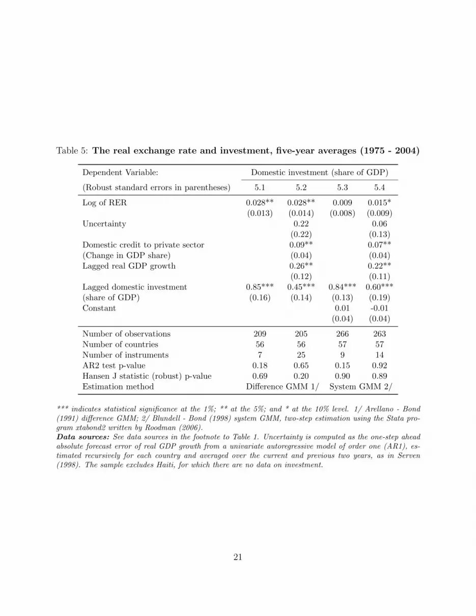
Table 5: The real exchange rate and investment, five-year averages (1975 - 2004)

Dependent Variable: Domestic investment (share of GDP)


Log of RER 0.028** 0.028** 0.009 0.015*(0.013) (0.014) (0.008) (0.009)

Uncertainty 0.22 0.06(0.22) (0.13)

Domestic credit to private sector 0.09** 0.07**(Change in GDP share) (0.04) (0.04)Lagged real GDP growth 0.26** 0.22**

(0.12) (0.11)Lagged domestic investment 0.85*** 0.45*** 0.84*** 0.60***(share of GDP) (0.16) (0.14) (0.13) (0.19)Constant 0.01 -0.01

(0.04) (0.04)

Number of observations 209 205 266 263Number of countries 56 56 57 57Number of instruments 7 25 9 14AR2 test p-value 0.18 0.65 0.15 0.92Hansen J statistic (robust) p-value 0.69 0.20 0.90 0.89Estimation method Difference GMM 1/ System GMM 2/

*** indicates statistical significance at the 1%; ** at the 5%; and * at the 10% level. 1/ Arellano - Bond(1991) difference GMM; 2/ Blundell - Bond (1998) system GMM, two-step estimation using the Stata pro-gram xtabond2 written by Roodman (2006).Data sources: See data sources in the footnote to Table 1. Uncertainty is computed as the one-step aheadabsolute forecast error of real GDP growth from a univariate autoregressive model of order one (AR1), es-timated recursively for each country and averaged over the current and previous two years, as in Serven(1998). The sample excludes Haiti, for which there are no data on investment.

21

5 Conclusions

Using the well-known TFP estimates of Bosworth and Collin (2003, 2008) and real exchange

rate estimates consistent with a traded-non-traded goods variation of Matsuyama’s (1992)

growth model, we find a robust and causal relationship between a weak real exchange rate

and faster TFP growth. This relationship is nonlinear as suggested by our two sector model

with diminishing returns: the acceleration of TFP growth created by a weak real exchange

rate diminishes as the trade good sector dominates GDP. There is also some evidence that

the traded goods sector, as represented by manufacturing exports, is a key TFP transmission

mechanism.

These estimates suggest that the growth impact of an undervalued exchange rate can

be substantial. If China’s real exchange rate is undervalued by 20-30%, as some recent

estimates suggest14, our results show that 20% and perhaps as much as a third of China’s

3% TFP growth may be attributable to its exchange rate policy. Rapid expansion of the

traded goods sector has two effects on overall productivity growth: one is the movement

of workers from low- to higher-productivity growth sectors, the other is faster ”learning

by doing” productivity growth in the traded goods sector. Early on, these two effects can

combine to create an impressive, if not miraculous, surge in per capita growth.

References

Aghion P, Bacchetta P, Ranciere R, Rogoff K. Exchange rate volatility and productivity

growth: The role of financial development. NBER Working Paper No. 12117; 2006.

14See Table 1 of Siregar and Rajan (2006) for a number of estimates of exchange rate misalignment inChina.

22

Aguirre A, Calderon C. Real exchange rate misalignments and economic performance. Cen-

tral Bank of Chile Working Papers No. 315; 2006.

Arellano M, Bond S. Some tests of specification for panel data: Monte Carlo evidence and

an application to employment equations. The Review of Economic Studies 1991; 58; 277

- 297.

Aizenman J, Lee J. The real exchange rate, mercantilism and the learning by doing exter-

nality. NBER Working Paper 13853; 2008.

Baum CF, Schaffer ME, Stillman S. Instrumental variables and GMM: Estimation and test-

ing. The Stata Journal 2003; 3(1); 1 - 31.

Blundell R, Bond S. Initial conditions and moment restrictions in dynamic panel data models.

Journal of Econometrics 1998; 87(1); 115 - 143.

Bosworth B, Collins S. The empirics of growth: An update. The Brookings

Institution 2003. http://www.brookings.edu/papers/2003/0922globaleconomics_

bosworth.aspx. Accessed 20 September 2010.

Bosworth B, Collins S. Accounting for growth: Comparing China and India. Journal of

Economic Perspectives 2008; 22(1); 45 - 66.

Dollar D. Outward-oriented developing economies really do grow more rapidly: evidence

from 95 LDCs, 1976-1985. Economic Development and Cultural Change 1992; 40(3);

523 - 544.

Eichengreen B. The real exchange rate and economic growth. Commission on Growth and

Development Working Paper No. 4; 2008.

23

Hausmann R, Pritchett L, Rodrik D. Growth accelerations. Journal of Economic Growth

2005; 10; 303 - 329.

International Monetary Fund. Direction of Trade Statistics database 2010.

Johnson S, Ostry JD, Subramanian A. Levers for growth. Finance and Development 2006;

43(1).

Kose MA, Prasad ES, Terrones ME. Does openness to international financial flows raise

productivity growth? Journal of International Money and Finance 2009; 28; 554 - 580.

Krugman P. The Myth of Asia’s miracle, Foreign Affairs 1994; 73(6); 62 - 78.

Matsuyama K. Agricultural productivity, comparative advantage and economic growth.

Journal of Economic Theory 1992; 58; 317 - 334.

Mileva E. Current account surpluses and growth: the role of foreign exchange reserves.

Fordham University 2011; ProQuest Dissertations and Theses.

Razin O, Collins SM. Real exchange rate misalignments and growth. In: Razin A, Sadka

E (Eds), The economics of globalization: Policy perspectives from public economics.

University Press: Cambridge, New York and Melbourne; 1997. p. 59 - 81.

Rodriguez F, Rodrik D. Trade policy and economic growth: a skeptic’s guide to the cross-

national evidence. NBER Macroeconomics Annual 2000; vol. 15; 261 - 338.

Rodrik D. The real exchange rate and economic growth. Brookings Papers on Economic

Activity 2008; 2; 365 - 412.

24

Rodrik D. Is Chinese mercantilism good or bad for poor countries? Project Syndicate 2010.

http://www.project-syndicate.org/commentary/rodrik47/English. Accessed 20

September 2010.

Roodman D. How to do xtabond2: an introduction to ”Difference” and ”System” GMM in

Stata. Center for Global Development Working Paper Number 103; 2006.

Roodman D. A short note on the theme of too many instruments. Center for Global Devel-

opment Working Paper Number 125; 2007.

Siregar R, Rajan R. S. Models Of Equilibrium Real Exchange Rates Revisited: A Selective

Review Of The Literature. Center for International Economic Studies Discussion Paper

No. 0604; 2006.

Staiger D, Stock JH. Instrumental variables regression with weak instruments. Econometrica

1997; 65; 557 - 586.

Stock JH, Yogo M. Testing for weak instruments in linear IV regression. NBER Technical

Working Paper 284; 2002.

World Bank. World Development Indicators 2010.

Young A. Learning by Doing and the Dynamic Effects of International Trade. Quarterly

Journal of Economics 1991; 106; 369 - 406.

Young A. The tyranny of numbers: Confronting the statistical realities of the East Asian

growth experience. The Quarterly Journal of Economics 1995; 110(3); 641 - 680.

25

Appendix Trade-weighted real exchange rates

The World Bank and the IMF provide trade-weighted real effective exchange rates, or

REERs, for about half of the countries in the Bosworth and Collins (2006) TFP sample.

Both sets of real exchange rates follow the PPP tradition of having the CPI in both the

numerator and the denominator. To get closer to the traded - non-traded goods view of

the real exchange rate developed in this paper, and to fill in the missing REER series, we

computed trade-weighted real exchange rates with producer or wholesale prices in the nu-

merator. Trade weights for 1985, 1995 and 2005 were computed using trade flows from the

IMF Direction of Trade Statistics database:

ωi =(X +M)i,jn∑j=1

(X +M)i,j

,

in which the numerator reflects the amount of trade country i has with trading partner j,

and the denominator reflects the total value of trade of country i with its 56 largest trading

partners. These weights were used to compute a weighted-average of dollar wholesale prices

for trading partners15:

P ∗i,t =

∑ni=1 ωiP

wi,t.

These weighted-average dollar WPI, or traded goods prices, were used to compute the

real exchange rates:

15Wholesale price indices, obtained from the IMF’s International Financial Statistics (IFS) database, wereused to quantify general price levels in each of these countries. Consumer prices were obtained mainly fromIFS and the WDI. Where no wholesale price series were available, GDP price deflators were used. Thedetails and sources of these price data are available from the authors upon request. Price data from theWorld Bank and the IMF were indexed to the year 2000, while price data from the United Nations (from thedatabase on national accounts) were indexed to 1990. All price indices were rebased to 2000. Internationalprices were expressed in terms of an index in US dollars. The official average annual exchange rates (localcurrency units to US dollars) from 1970 to 2006 were obtained from the WDI and indexed to the year 2000.For the euro area countries, the entire exchange rate series in euros were back-casted using the growth ratesof the old local currency unit series.

26

q∗i,t =ei,tP

∗i,t

Pi,t,

in which ei,t is the nominal (rf) exchange rate, and Pi,t is the local consumer price index.16

16We also tried geometric averages, ln qi,t = lnP ∗i,t + ln ei,t − lnPi,t, in which lnP ∗i,t = ωi lnPwi,t, but the

arithmetic averages seemed to be closest to the WDI and IMF series, which we also tested as discussed inthe paper.

27

Documents

Real Exchange Rates and Growth Surges