Embed Size (px)
Citation preview
NBER WORKING PAPER SERIES
REAL BUSINESS CYCLE MODELS
Bennett T. McCallum
Working Paper No. 2480
NATIONAL BUREAU OF ECONOMIC RESEARCH1050 Massachusetts Avenue
Cambridge, MA 02138
January 1988
This paper has been prepared for the Handbook of Modern Business CycleTheory, edited by Robert J. Barro. The author is indebted to MartinEichenbaum, Marvin Goodfriend, Robert King, Finn Kydland, Allan Meltzer, andKenneth Singleton for helpful discussions. In addition, he has benefittedfrom a generous quantity of criticism furnished by the Rochester RBC Group ofTen and the following individuals: Robert Barro, William Brock, LarryChristiano, and Edward Prescott. Partial financial support was provided bythe National Science Foundation. The research reported here is part of theNBER's research programs in Economic Fluctuations and Financial Markets andMonetary Economics. Any opinions expressed are those of the author and notthose of the National Bureau of Economic Research. Support from the Lynde
and Harry Bradley Foundation is gratefully acknowledged.
NBER Working Paper #2480January 1988
Real Business Cycle Models
ABSTRACT
This paper attempts to provide an evaluation of both strengths and
weaknesses of the real business cycle (RBC) approach to the analysis of
macroeconomic fluctuations. It begins with a description of the basicanalytical structure typically employed, one in which individual households
make consumption and labor supply decisions while producing output from
capital and labor inputs, hired on competitive markets, according to a
technology that is subject to stochastic shocks. It then explores conditions
on parameter values that are needed for a model of this type to yieldfluctuations that provide a good quantitative match to those observed in the
postwar U.S. quarterly data. The plausibility of the hypothesis that(unobservable) aggregate technology shocks have the requisite variability is
considered and problems with certain cross correlations are noted. Relevantevidence obtained by formal econometric methods is summarized and a fewtentative conclusions regarding business cycle research are suggested.
Bennett T. McCallumGS IA
Carnegie—Mellon UniversityPittsburgh, Pennsylvania 15213(412)268—2347
I. Introduction
One of the most striking developments in macroeconomics during the early
1980s was the emergence of a substantial body of literature devoted to the
"real business cycle" approach to the analysis of macroeconomic fluctuations.
Particularly prominent papers have been contributed by Kydland and Prescott
(1982), Long and Plosser (1983), and King and Plosser (1984) while many others
of interest have been written' and a number of critical or skeptical pieces
have begun to appear.2 This literature's implied point of view is an
outgrowth of the equilibrium strategy for business cycle analysis that was
initiated by Lucas (1972) (1973) (1975) and extended by Barro (1976) (1981),
but differs from that of the earlier work in two critical respects. First,
the real business cycle (or "RBC") models place much more emphasis than did
the previous equilibrium—approach literature on mechanisms involving cycle
propagation, i.e., the spreading over time of the effects of shocks. Second,
as the name implies, RBC models emphasize the extent to which shocks that
initiate cycles are real——as opposed to "monetary"——in origin. In particular,
the primary driving force is taken to be shocks to technology,3 rather than
the monetary and fiscal policy disturbances that are emphasized in the earlier
equilibrium—approach writings.
It will be noted that these two features of the RBC approach are quite
different from each other in terms of their relationship to alternative
business cycle theories. Specifically, the RBC propagation analysis is
entirely compatible with the Lucas—Barro monetary—misperceptions variant of
the equilibrium approach and could logically be viewed as an attempt to
elaborate and improve upon models of the Lucas—Barro type. Indeed, the point
can be taken further by noting that the propagation phenomena stressed by RBC
analysis could be relevant and important even in non-equilibrium4 models that
—1—
feature nominal wage and/or price stickiness.
With regard to initiating shocks, by contrast, the RBC viewpoint reflects
much more of a departure from other theories. In this regard, two positions
can usefully be identified. The weaker of the two is that technology shocks
are quantitatively more important than monetary disturbances as initiators of
business cycle movements, while the stronger is that monetary disturbances are
of negligible consequence. The former position is compatible with
monetary—misperception variants of equilibrium theory, as these have not
involved denials of the role of supply shocks. The stronger RBC position,
however——the hypothesis that monetary disturbances are an insignificant source
of cyclical fluctuations——is clearly inconsistent with most alternative
theories. In this form, the RBC approach presents a distinct challenge to
mainstream macroeconomic analysis.
In the discussion that follows, most of the emphasis will be implicitly
given to the weaker version of the RBC hypothesis, as it is more clearly
representative of the position taken in print by RBC proponents. The strong
version will be accorded some attention, however, for two reasons. The more
basic of these is that while the main topic of the present survey is RBC
theory itself, a secondary topic is the contrast provided by RBC models with
theories that rely upon monetary disturbances. Thus the sharp distinction
provided by the strong RBC hypothesis is expositionally natural and
convenient. But, in addition, it is this strong hypothesis that provides the
RBC approach with a truly distinctive identity. As monetary-misperception
variants of equilibrium theory do not deny the existence of supply shocks or
propagation mechanisms, it is difficult to see how the RBC approach could be
distinguished from the more general category of equilibrium analysis without
• reliance on the strong hypothesis. It is evidently the latter that
—2—

constitutes the approach's distinguishing characteristic.
The present paper's organization is as follows. In Section II the main
features of the RBC approach are introduced by means of a simple prototype
model. While this discussion touches upon certain qualitative properties of
the model and their relation to actual U.S. data, the main quantitative
comparison between theory and evidence appears in Section III. There more
elaborate versions of the model are recognized and a fairly detailed review of
evidence of the type emphasized by Kydland and Prescott (1982) (1986) is
provided. Then in Section IV other types of evidence and several matters of
controversy are reviewed. Finally, some conclusions are tentatively put forth
in Section V.
—3—
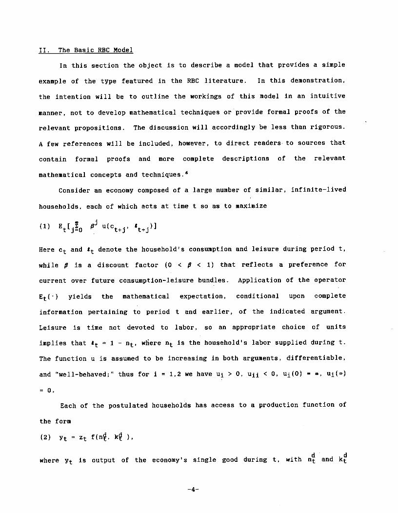
II. The Basic RBC Model
In this section the object is to describe a model that provides a simple
example of the type featured in the RBC literature. In this demonstration,
the intention will be to outline the workings of this model in an intuitive
manner, not to develop mathematical techniques or provide formal proofs of the
relevant propositions. The discussion will accordingly be less than rigorous.
A few references will be Included, however, to direct readers to sources that
contain formal proofs and more complete descriptions of the relevant
mathematical concepts and techniques.6
Consider an economy composed of a large number of similar, infinite—lived
households, each of which acts at time t so as to maximize
(1) Et(jo u(c, tt+j
Here Ct and 1t denote the household's consumption and leisure during period t,
while is a discount factor (0 < < 1) that reflects a preference for
current over future consumption—leisure bundles. Application of the operator
Et() yields the mathematical expectation, conditional upon complete
information pertaining to period t and earlier, of the indicated argument.
Leisure is time not devoted to labor, so an appropriate choice of units
implies that tt = 1 — where t is the household's labor supplied during t.
The function u is assumed to be Increasing in both arguments, differentiable,
and "well—behaved;" thus for i = 1,2 we have u > 0, uij < 0, u1(O) = =, u(o')
= 0.
Each of the postulated households has access to a production function of
the form
(2) Yt = zt f(n, k ),
where Yt is output of the economy's single good during t, with n and k
—4—
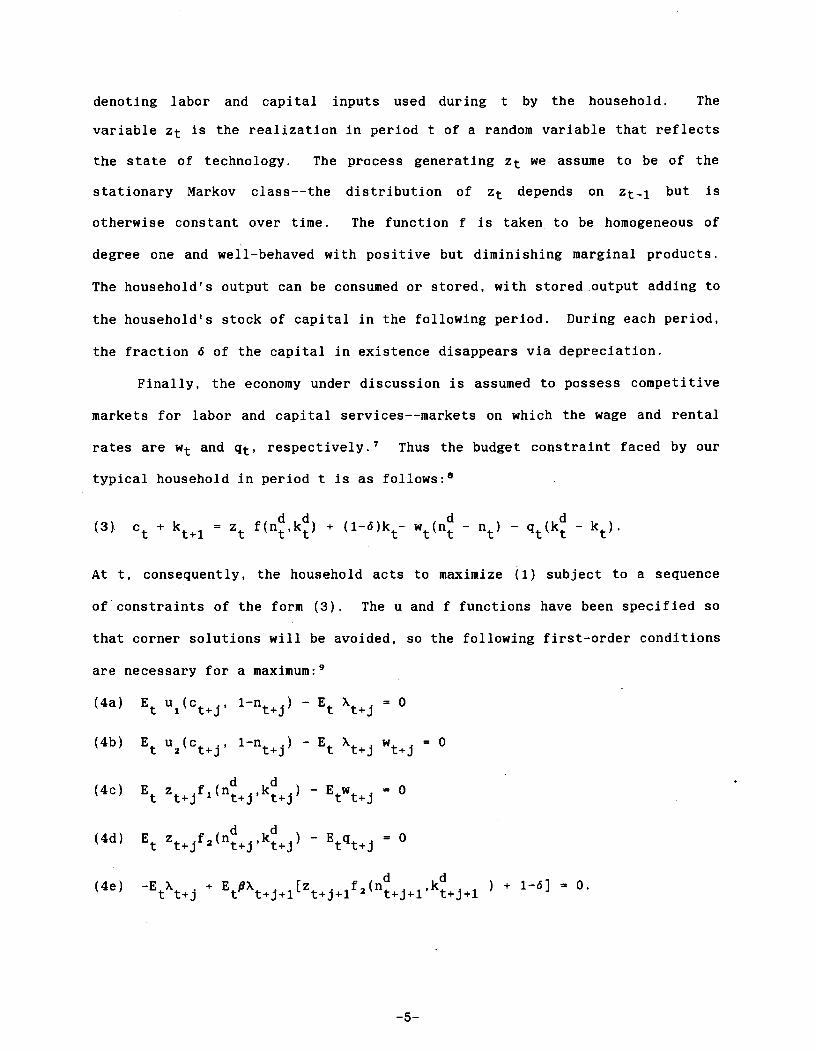
denoting labor and capital inputs used during t by the household. The
variable zt is the realization in period t of a random variable that reflects
the state of technology. The process generating zt we assume to be of the
stationary Markov class—-the distribution of zt depends on zt_l but is
otherwise constant over time. The function f is taken to be homogeneous of
degree one and well—behaved with positive but diminishing marginal products.
The household's output can be consumed or stored, with stored output adding to
the household's stock of capital in the following period. During each period,
the fraction 6 of the capital in existence disappears via depreciation.
Finally, the economy under discussion is assumed to possess competitive
markets for labor and capital services——markets on which the wage and rental
rates are wt and respectively.7 Thus the budget constraint faced by our
typical household in period t is as follows:8
(3). c + kt+1= z f(,1) + (l.6)kt- w(n — — — kt).
At t, consequently, the household acts to maximize (1) subject to a sequence
of constraints of the form (3). The u and f functions have been specified so
that corner solutions will be avoided, so the following first—order conditions
are necessary for a maximum:9
(4a) Et u1(c+ l—nt+) — Et = 0
(4b) E u(c .,l—n .)—E X w .=0t 2 t+j t+.j t t+j t+j
d d(4c) E z .f (n .,k .) — E w = 0t t+j t+j t+j t t+j
d d(4d) Et zt+jf2(nt+j.kt+j) —
= 0
(4e) _EtXt. + ) + l-J = 0.
-5—
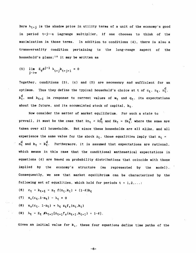
Here is the shadow price in utility terms of a unit of the economy's good
in period t÷j——a Lagrange multiplier, if one chooses to think of the
maximization in those terms. In addition to conditions (4), there is also a
transversality condition pertaining to the long—range aspect of the
household's plans;1° it may be written as
(5) Urn EtJ Xt ikt.1 = 0
Together, conditions (3), (4) and (5) are necessary and sufficient for an
optimum. Thus they define the typical household's choice at t of Ct,
and kt÷i in response to current values of wt and qt its expectations
about the future, and its accumulated stock of capital, kt.
Now consider the matter of market equilibrium. For such a state to
d dprevail, it must be the case that Eflt = Eflt and Ekt = Ekt, where the sums are
taken over all households. But since these households are all alike, and all
experience the same value for the shock Zt, those equalities imply that t =
and kt = k. Furthermore, it is assumed that expectations are rational,
which means in this case that the conditional mathematical expectations in
equations (4) are based on probability distributions that coincide with those
implied by the economy's structure (as represented by the model)..
Consequently, we see that market equilibrium can be characterized by the
following set of equalities, which hold for periods t =
(6) Ct + kt+i = Zt f(nt,kt) + (1—6)kt
(7) Ui(Ct,1—rlt) — xt = 0
(8) u2(ct, 1—nt) = X. ztf1(nt,kt)
(9) At = Et + 1—6].
Given an initial value for k1, these four equations define time paths of the
-6—
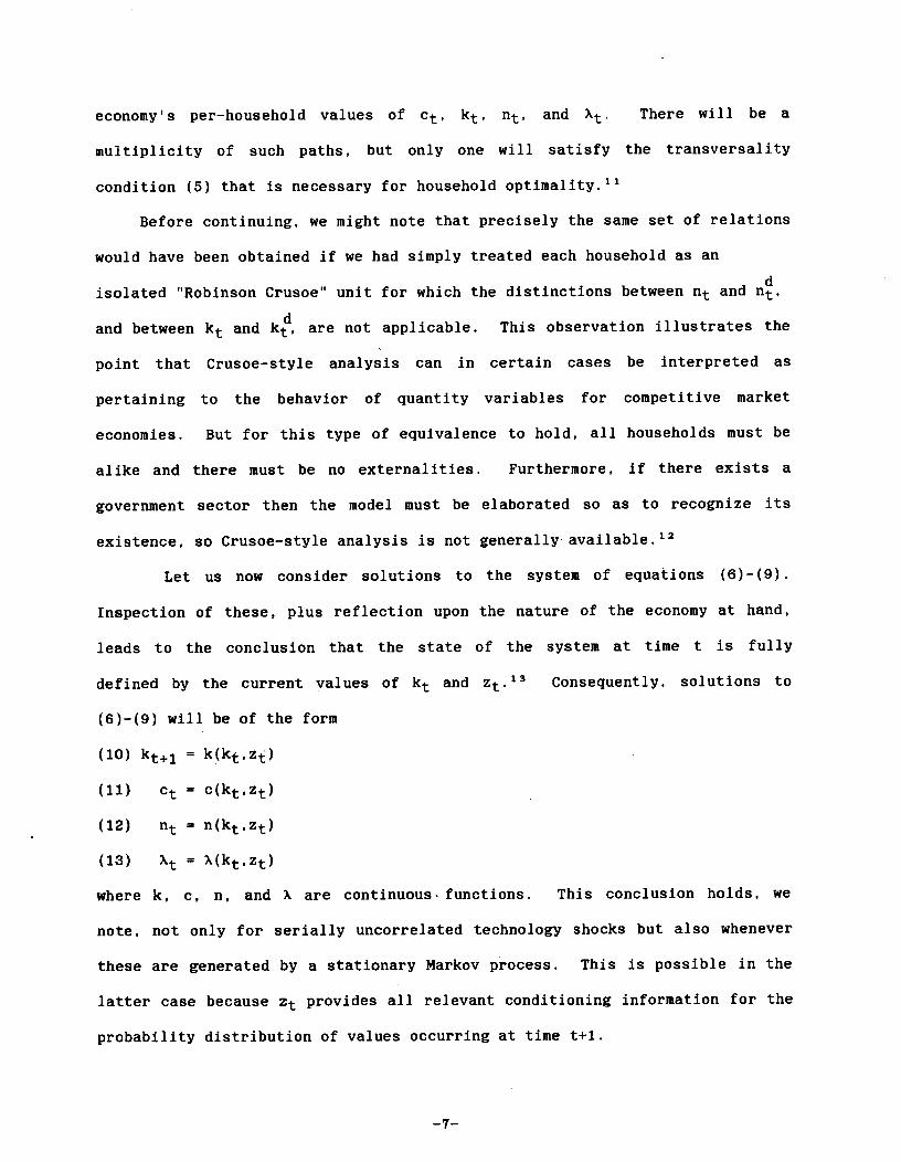
economy's per—household values of Ct, kt, and At. There will be a
multiplicity of such paths, but only one will satisfy the transversality
condition (5) that Is necessary for household optimality.''
Before continuing, we might note that precisely the same set of relations
would have been obtained if we had simply treated each household as an
isolated "Robinson Crusoe" unit for which the distinctions between nt and n,
and between kt and k1,, are not applicable. This observation illustrates the
point that Crusoe—style analysis can in certain cases be interpreted as
pertaining to the behavior of quantity variables for competitive market
economies. But for this type of equivalence to hold, all households must be
alike and there must be no externalities. Furthermore, If there exists a
government sector then the model must be elaborated so as to recognize its
existence, so Crusoe—style analysis is not generally available.'2
Let us now consider solutions to the system of equations (6)—(9).
Inspection of these, plus reflection upon the nature of the economy at hand,
leads to the conclusion that the state of the system at time t is fully
defined by the current values of kt and zt.'3 Consequently, solutions to
(6)—(9) will be of the form
(10) kt+i = k(kt,zt)(11) Ct = c(kt,zt)(12) t = fl(kt,Zt)
(13) At = X(kt,zt)where k, c, n, and A are continuous- functions. This conclusion holds, we
note, not only for serially uncorrelated technology shocks but also whenever
these are generated by a stationary Markov process. This is possible in the
latter case because zt provides all relevant conditioning information for the
probability distribution of values occurring at time t+1.
—7—
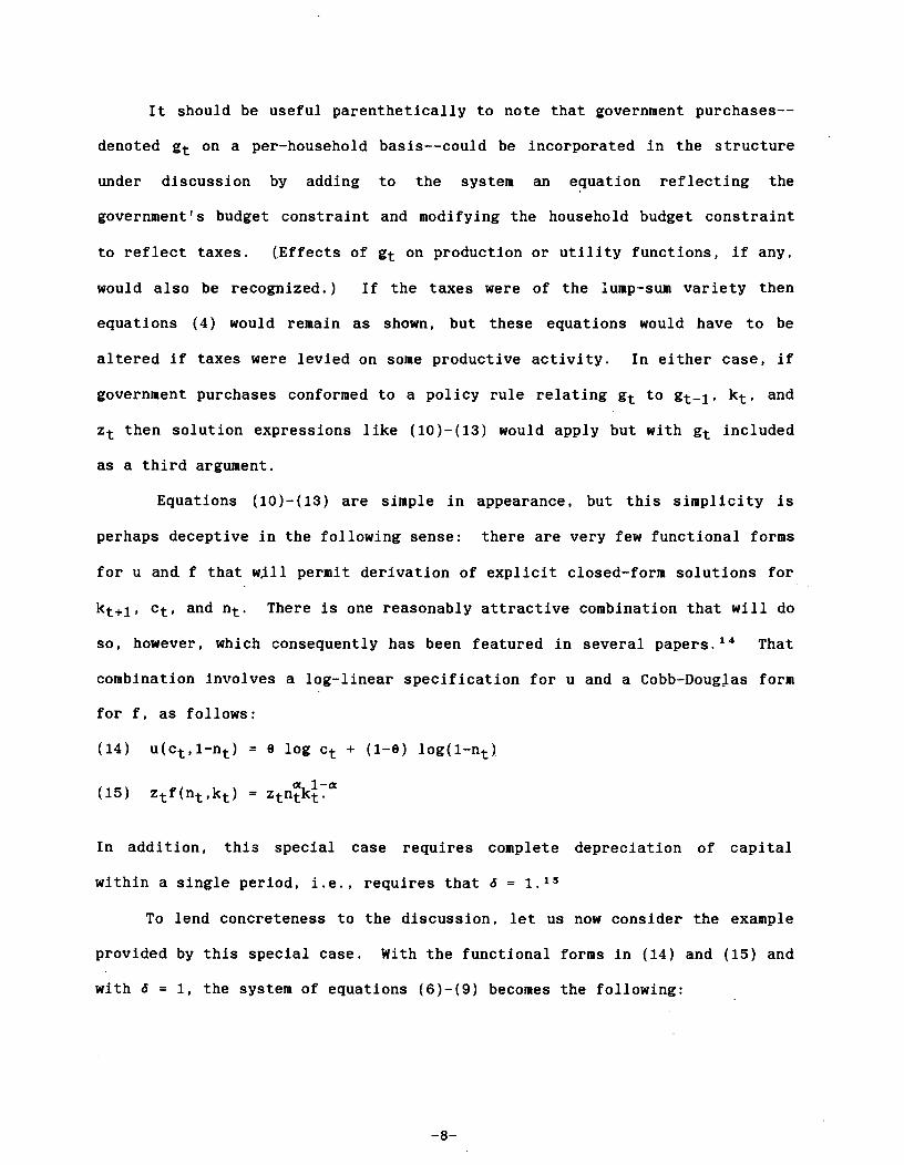
It should be useful parenthetically to note that government purchases——
denoted gt on a per—household basis——could be incorporated in the structure
under discussion by adding to the system an equation reflecting the
governments budget constraint and modifying the household budget constraint
to reflect taxes. (Effects of gt on production or utility functions, if any,
would also be recognized.) If the taxes were of the lump—sum variety then
equations (4) would remain as shown, but these equations would have to be
altered if taxes were levied on some productive activity. In either case, if
government purchases conformed to a policy rule relating g to gt—i kt, and
zt then solution expressions like (1O)—(13) would apply but with gt included
as a third argument.
Equations (1O)—(13) are simple in appearance, but this simplicity is
perhaps deceptive in the following sense: there are very few functional forms
for u and f that w.jll permit derivation of explicit closed—form solutions for
kt+i, ct, and nt. There is one reasonably attractive combination that will do
so, however, which consequently has been featured in several papers.'4 That
combination involves a log—linear specification for u and a Cobb—Doug1as form
for f, as follows:
(14) u(ct,l—nt) = 8 log ct + (1—8) log(1—n)
'x l-x(15) ztf(nt,kt) = ztntkt.
In addition, this special case requires complete depreciation of capital
within a single period, i.e., requires that 6 = 1.15
To lend concreteness to the discussion, let us now consider the example
provided by this special case. With the functional forms in (14) and (15) and
with 6 = 1, the system of equations (6)—(9) becomes the following:
—8—
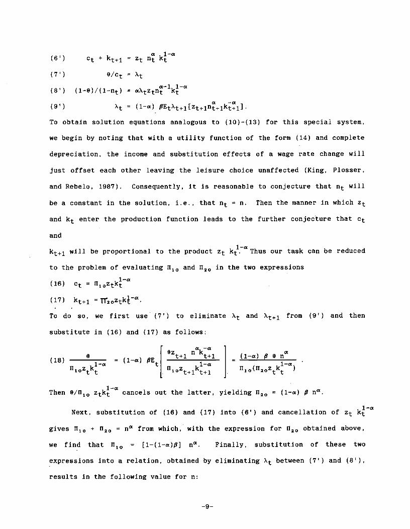
a 1-a1. —kU J Ct + 'Vt÷l — Zt t 'Vt
(7') e/ct =
a-i i-a(8 ) (1—e)/(1—nt) = aXtztnt kt
(9') = (1—a)EtXt+i[zt+in+iktij.To obtain solution equations analogous to (lO)—(13) for this special system,
we begin by noting that with a utility function of the form (14) and complete
depreciation, the income and substitution effects of a wage rate change will
just offset each other leaving the leisure choice unaffected (King, Plosser,
and Rebelo, 1987). Consequently, it is reasonable to conjecture that t will
be a constant in the solution, i.e., that t = n. Then the manner in which zt
and kt enter the production function leads to the further conjecture that Ct
and
kt+i will be proportional to the product zt k.a Thus our task can be reduced
to the problem of evaluating ri, and fl20 in the two expressions
1—a(16) Ct = fl10ztkt
(17) kt+i =rr20ztka.
To do so, we first use (7') to eliminate X and X÷ from (9') and then
substitute in (16) and (17) as follows:
(18) = = (1—a) 0 n
fllO(ffZOzka)
Then 0/fl10 Zka cancels out the latter, yielding fl20 = (1—a) nix.
Next, substitution of (16) and (17) into (6') and cancellation of zt
gives fl ÷ = a from which, with the expression for fl20 obtained above,
we find that fl10 = [1—(1—a)] Finally, substitution of these two
expressions into a relation, obtained by eliminating X. between (7') and (8'),
results in the following value for n:
-9—
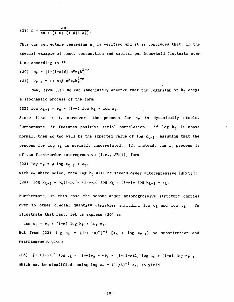
(19) fl+ (1—8) [1—(1—)]
Thus our conjecture regarding nt is verified and it is concluded that, in the
special example at hand, consumption and capital per household fluctuate over
time according to 16
(20) ct = [1—(1—x)]
(21) kt÷i = (1-cc) flaztkt
Now, from (21) we can immediately observe that the logarithm of kt obeys
a stochastic process of the form
(22) log kt+1 = + (1—x) log kt ÷ log zt.
Since I1—I < 1, moreover, the process for kt is dynamically stable.
Furthermore, it features positive serial correlation: if log kt is above
normal, then so too will be the expected value of log kt÷i, assuming that the
process for log zt is serially uncorrelated. If, instead, the zt process is
of the first—order autoregressive [i.e., AR(i)] form
(23) log zt = log zt_1 +
with white noise, then log kt will be second—order autoregressive [AR(2)]:
(24) log kt÷i = •0(1—p) + (1—+p) log kt — (1—cx)p log kt_i +
Furthermore, in this case the second—order autoregressive structure carries
over to other crucial quantity variables including log Ct and log yt. To
illustrate that fact, let us express (20) as
log ct = ÷ (1—a) log kt + log zt.
But from (22) log kt = [1—(1—a)L] [o + log zt_1] so substitution and
rearrangement gives
(25) [1—(1—a)L] log Ct = (1—a),0 ÷ a•1 + [1—(1—a)L] log zt + (1—a) log zt....l
which may be simplified, using log zt = (1—pL) ii,, to yield
—10—
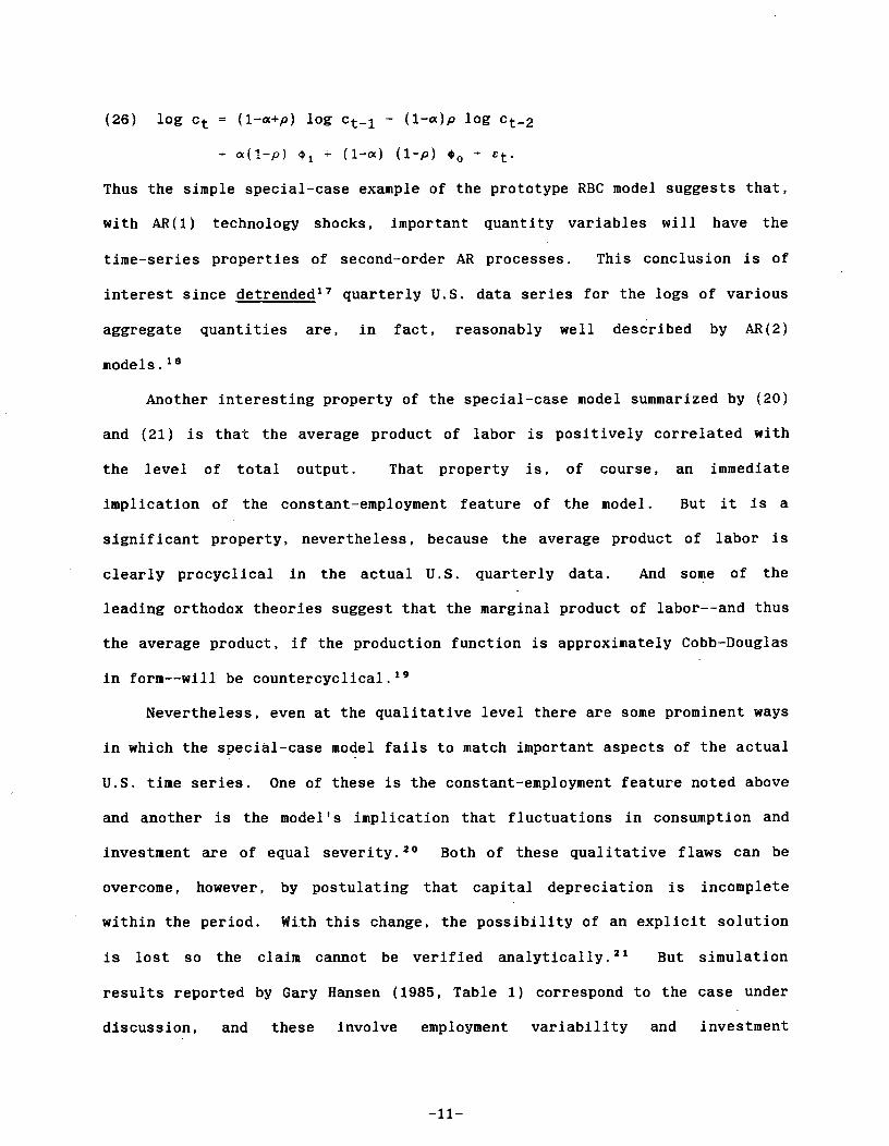
(26) log Ct = (1—cc+p) log Ct_i — (l—a)p log ct_2
+ cx(1—p) + (l—x) (1—p) 00 +
Thus the simple special—case example of the prototype RBC model suggests that,
with AR(1) technology shocks, important quantity variables will have the
time—series properties of second—order AR processes. This conclusion is of
interest since detrended'7 quarterly U.S. data series for the logs of various
aggregate quantities are, in fact, reasonably well described by AR(2)
models. 18
Another interesting property of the special—case model summarized by (20)
and (21) is that the average product of labor is positively correlated with
the level of total output. That property is, of course, an immediate
implication of the constant—employment feature of the model. But it is a
significant property, nevertheless, because the average product of labor is
clearly procyclical in the actual U.S. quarterly data. And some of the
leading orthodox theories suggest that the marginal product of labor-—and thus
the average product, if the production function is approximately Cobb—Douglas
in form——will be countercyclical.'9
Nevertheless, even at the qualitative level there are some prominent ways
in which the special—case model fails to match important aspects of the actual
U.S. time series. One of these is the constant-employment feature noted above
and another is the model's implication that fluctuations in consumption and
investment are of equal severity.20 Both of these qualitative flaws can be
overcome, however, by postulating that capital depreciation is incomplete
within the period. With this change, the possibility of an explicit solution
is lost so the claim cannot be verified analytically.21 But simulation
results reported by Gary Hansen (1985, Table 1) correspond to the case under
discussion, and these involve employment variability and investment
—11—

fluctuations that are several times as severe (in terms of percentage standard
deviations from trend) as those of consumption. So even with the special
assumptions (14) and (15) regarding utility and production functions, the
prototype RBC model provides a reasonable match to important features of
actual business cycle data. It is time, consequently, to turn to quantitative
aspects of the match. This will be done in the next section.
—12—
III. Quantitative Aspects of RBC Models
Perhaps the strongest single stimulus to analysis with RBC models was
provided by the innovative Time to Build' paper of Kydland and Prescott
(1982), which first demonstrated the possibility of obtaining a good
quantitative match between RBC model implications and actual business cycle
fluctuations. The model developed and simulated by Kydland and Prescott is
basically of the type described in the previous section, but includes several
additional features that were intended to improve its performance—-i.e., its
agreement with cyclical characteristics of the postwar U.S. data. Four such
features are as follows.
(i) Leisure "services" in each period (i.e., quarter) are represented
by a distributed lag of current and past leisure hours.
(ii) Investment projects begun in period t require additional
expenditures in periods, t÷1, t+2, and t÷3 before becoming productive in
period t+4.
(iii) Producers hold inventories of finished goods that serve as an
additional factor of production.
(iv) The technology shock is composed of transitory and
highly-persistent components that cannot be directly distinguished by
producers or consumers.
Needless to say, with these features and incomplete depreciation, the
Kydland—Prescott model does not admit an analytical solution. But an
approximation can be obtained, parameter values assigned, and simulations
conducted. Kydland and Prescott's approach was to follow that strategy, with
the average results of a number of stochastic simulations serving to
characterize the model's cyclical properties. And the same kind of procedure
can be applied to the basic model (with 5 < 1) of the previous section, or
—13—
other structures of the same general type.
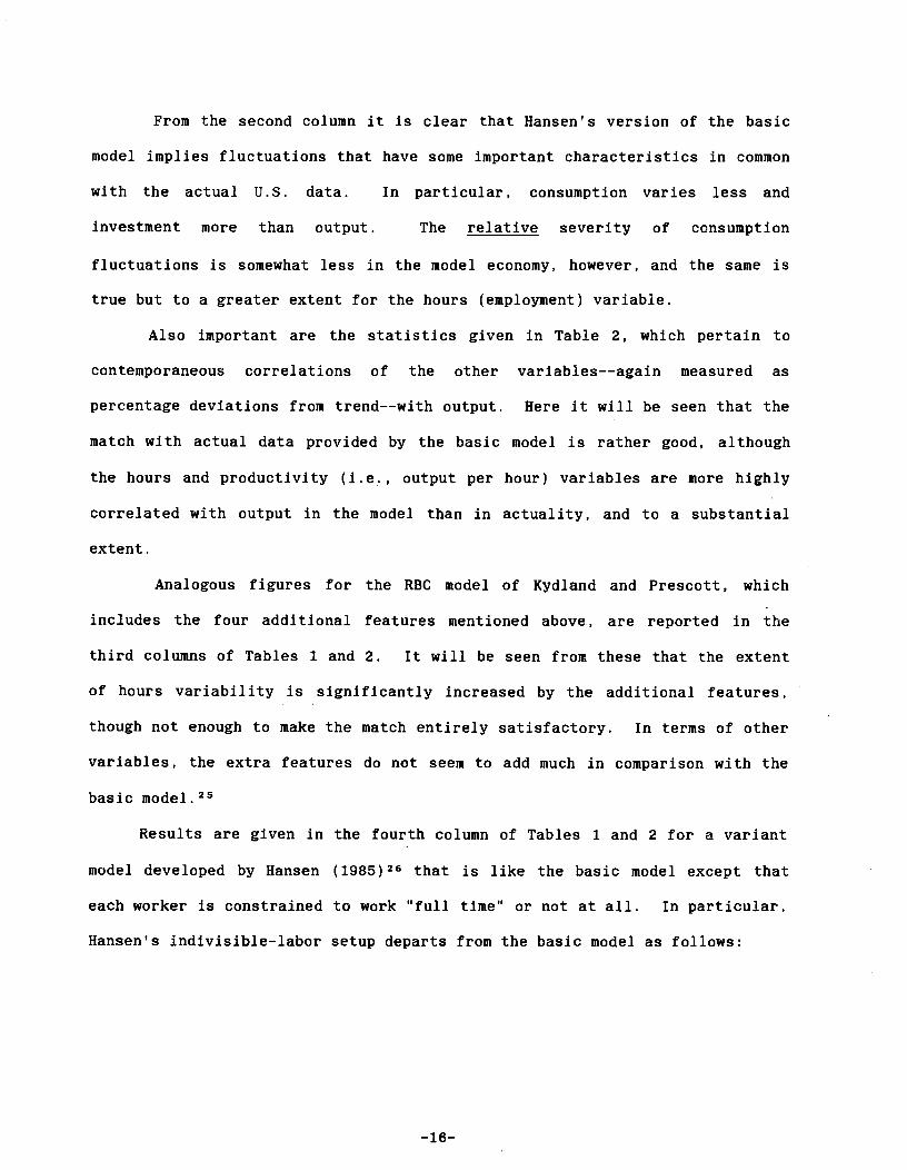
To see how well the basic and Kydland-Prescott structures do in mimicking
actual U.S. fluctuations, we begin by examining the figures presented in Table
1. Here the first column reports, for several important quantity variables,
the magnitude of cyclical fluctuations in the actual quarterly U.S. data,
1955.3—1984.1. These magnitudes are standard deviations of the quarterly
observations measured relative to trend values, with the departures from trend
expressed in percentage form. The trend values themselves are generated by
smoothing tire raw series in accordance with a procedure developed by Hodrick
and Prescott (1981).22 From this first column it is apparent that actual
consumption fluctuates less, and investment much more, than total output (in
percentage terms, that is). Also, the extent of fluctuations in total
manhours employed in production (designated "hours") is almost as great as
that of total output.
In column two, comparable figures are reported for a version of the basic
model that has been specified and simulated by Hansen (1985).23 Here the
standard deviations actually reported by Hansen have all been scaled up,
multiplied by the factor 1.31, so that the reported standard deviation for
output is the same as in the U.S. data.24 Thus the values in Table 1 are
designed to reflect only the relative extent of fluctuations of other
variables in comparison with output. The magnitude of output fluctuations is
governed, for each model, by the variance of the technology shock zt that is
assumed and used in the simulations; independent evidence concerning the
plausibility of these shock—variance magnitudes will be considered below.
—14—
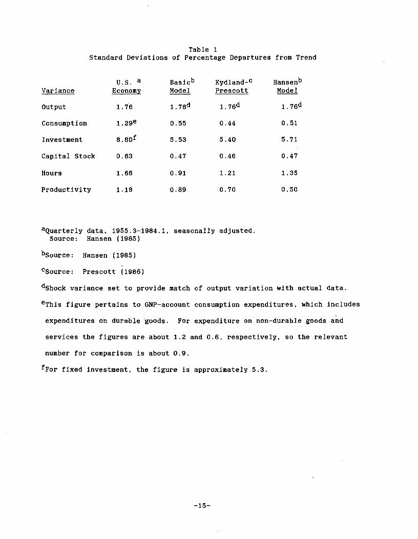
Table 1Standard Deviations of Percentage Departures from Trend
u.s. a Basicb Kydland_C HansenbVariance Economy Model Prescott Model
Output 1.76 176d 176d 176d
Consumption 129e 0.55 0.44 0.51
Investment 8.6of 5.53 5.40 5.71
Capital Stock 0.63 0.47 0.46 0.47
Hours 1.66 0.91 1.21 1.35
Productivity 1.18 0.89 0.70 0.50
aQuarterly data, 1955.3—1984.1, seasonally adjusted.Source: Hansen (1985)
bSource: Hansen (1985)
CSource: Prescott (1986)
dshock variance set to provide match of output variation with actual data.
eThis figure pertains to GNP—account consumption expenditures, which includes
expenditures on durable goods. For expenditure on non—durable goods and
services the figures are about 1.2 and 0.6, respectively, so the relevant
number for comparison is about 0.9.
For fixed investment, the figure is approximately 5.3.
—15—
From the second column it is clear that Hansen's version of the basic
model implies fluctuations that have some important characteristics in common
with the actual U.S. data. In particular, consumption varies less and
investment more than output. The relative severity of consumption
fluctuations is somewhat less in the model economy, however, and the same is
true but to a greater extent for the hours (employment) variable.
Also important are the statistics given in Table 2, which pertain to
contemporaneous correlations of the other variables——again measured as
percentage deviations from trend——with output. Here it will be seen that the
match with actual data provided by the basic model is rather good, although
the hours and productivity (i.e., output per hour) variables are more highly
correlated with output in the model than in actuality, and to a substantial
extent.
Analogous figures for the RBC model of Kydland and Prescott, which
includes the four additional features mentioned above., are reported in the
third columns of Tables 1 and 2. It will be seen from these that the extent
of hours variability is significantly increased by the additional features,
though not enough to make the match entirely satisfactory. In terms of other
variables, the extra features do not seem to add much in comparison with the
basic model.25
Results are given in the fourth column of Tables 1 and 2 for a variant
model developed by Hansen (1985)26 that is like the basic model except that
each worker is constrained to work "full time" or not at all. In particular,
Hansen's indivisible—labor setup departs from the basic model as follows:
—16—
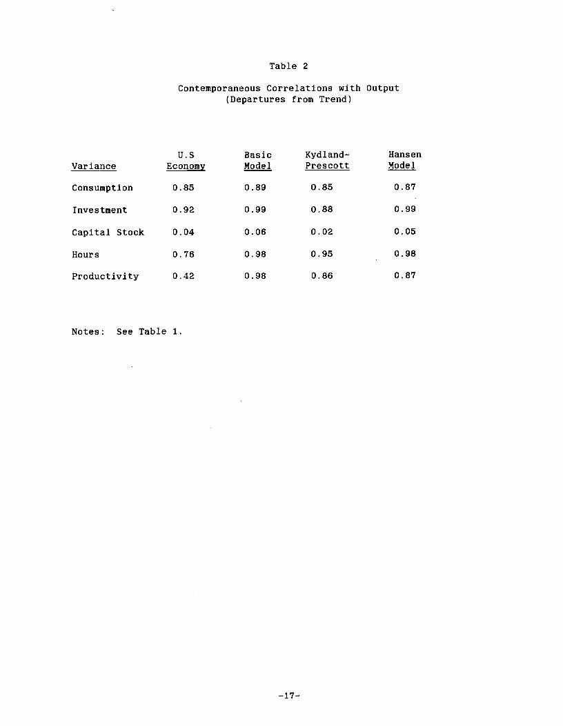
Table 2
Contemporaneous Correlations with Output(Departures from Trend)
U.S Basic Kydland— HansenVariance Economy Model Prescott Model
Consumption 0.85 0.89 0.85 0.87
Investment 0.92 0.99 0.88 0.99
Capital Stock 0.04 0.06 0.02 0.05
Hours 0.76 0.98 0.95 0.98
Productivity 0.42 0.98 0.86 0.87
Notes: See Table 1.
—17—
The new commodity being introduced is a contract between thefirm and a household that commits the household to work h0hours {full time] with probability . The contract itself isbeing traded, so the household gets paid whether it works ornot. Therefore, the firm is providing complete unemploymentinsurance to the workers. Since all households are identical,all will choose the same ... cx. However, although householdsare ex ante identical, they will differ ex post depending onthe outcome of the lottery: a fraction of the continuum ofhouseholds will work and the rest will not. (Hansen, 1985, p.316).
It Is apparent from Table 1 that this model generates considerably more
variability in manhours employment, relative to output, than the basic model
(but at the cost of a poorer match for productivity). Something that is not
apparent from the table is that the assumed variance of zt, needed to generate
output variability equal to that of the U.S. economy, is smaller than that of
the basic model. Specifically, the standard deviation of zt required for the
column four values is only 0.767 as great as that for column two.27
Kydland (1984) and Kydland and Prescott (1986) have explored other
specificational modifications that are designed to improve the match between
model and actuality. Kydland (1984) postulates two types of labor, of
differing effectiveness in production, and finds that this modification
increases the variability of hours relative to output. Kydland and Prescott
(1986) incorporates a variable rate of capital utilization and shows that a
smaller variance for zt is needed, with this elaboration, to yield output
variability that matches actuality. In each of these two cases the magnitude
of the improvement is about 20% and in each case the overall pattern of
correlations is not substantially altered.
In all of these numerical investigations, it should be emphasized, the
model's's parameter values are not obtained In a manner that provides the best
fit to the quarterly time series data. Instead, values for parameters——
analogous to those designated , fi, 6, 0, and p in Section II above——are
—18—
assigned so as to agree with panel studies of individual households or with
stylized facts relating to such magnitudes as labor's share of national income
(suggesting a = 0.64), the fraction of time spent in market employment (9 =
0.33), etc.28 This procedure guarantees that certain properties of the model
will be "sensible," in the judgement of the model builders, a situation that
might not obtain if the parameters were estimated in a more orthodox manner.
In this regard it is important to note that Kydland—Prescott and Hansen choose
the value 0.95 for the counterpart of the parameter p. In the context of
their model, the high implied degree of serial correlation for the technology
shock tends to impart a high degree of serial correlation to endogenous
variables such as employment and output.29
One of the main issues considered in the literature is whether the
required magnitude of technology shocks is plausible, i.e., whether the
variance of zt needed to generate fluctuations of the amplitude reported in
Table 1 could plausibly apply to actual aggregate technology shocks.3° This
issue is addressed by Prescott (1986), who initially estimates the variance of
t (not Zt) as the sample variance of the residuals from an aggregate
Cobb—Douglas production function, fitted in first differenced form.31
Prescott then goes on to revise downward this straightforward estimate by
attempting to take account of measurement error in the labor input series.
His final estimate of the standard deviation in 0.00763, which can be compared
with the values needed in different models to generate output fluctuations
that match (as in Table 1) those of the U.S. economy. The needed value with
the basic model is 0.0093, according to Hansen's (1985) results,32 while the
figure with his indivisible—labor setup is only 0.00712. In the
Kydland—Prescott model there are two technology shocks, as mentioned above.
But the contribution of the purely transitory shock is very small, so we can
—19—
focus on the highly—persistent shock. Its standard deviation is reported in
Kydland—Prescott (1986) as 0.0091. Given the relationship zt = O.95Zt_i +
this last figure implies a standard deviation for Zt of the value 0.0291.
These numerical results may be viewed as giving some support to the idea
that technology shocks are in fact large enough to give rise to business cycle
fluctuations of the magnitude experienced by the postwar U.S. economy. There
are reasons, however, for skepticism. The first of these involves the type of
procedure used by Prescott to estimate the shock variance. His procedure, to
some extent based on Solow (1957), relies crucially on the assumption that
current capital and labor are the only relevant inputs. If, however, there
are in fact adjustment costs, so that previous levels of (say) labor usage are
relevant for current output, then the Solow—Prescott procedure will be likely
to overestimate the shock variance.33. In this regard it is worthy of note
that the literature on technical progress that followed Solow's 1957
contribution indicated that the magnitude of technical change would be
strongly overstated by the Solow procedure unless steps were taken to correct
for certain neglected effects. Jorgenson and Griliches (1967), for example,
summarize their findings for the U.S. economy over 1945—65 as follows: "The
rate of growth of [total factor] input initially explains 52.4 percent of the
rate of growth of output. After elimination of aggregation errors and
correction for changes in rates of utilization of labor and capital stock the
rate of growth of input explains 96.7 percent of the rate of growth of output;
change in total factor productivity explains the rest." Thus, in this
example, the Jorgenson—Griliches adjustments reduce the average contribution
to growth provided by the residual to only 7% of the initial Solow—type
estimate.3' Finally, it should be noted without prejudice that Prescott's
procedure is actually not the same as Solow's. Specifically, Prescott's
—20—

procedure uses the same labor—share parameter for each period while Solow's
treats the labor share as a variable. Thus Prescott's procedure is likely to
fit the observations less closely and leave more variation to be accounted for
by the residual, thereby yielding——perhaps appropriately——a larger estimate of
its variance.
A second problem is related to the nature of the unobserved random
components that the RBC literature refers to as "technology shocks." If this
term is taken literally to refer to shifts in the state—of—knowledge
technological, relationship between inputs and outputs, then it seems highly
unlikely that there could exist any substantial aggregate variability. Here
the point is that highly distinctive technologies involving entirely different
types of machines (and other sorts of capital) are used in different
industries——and for different products within any single industry.
Accordingly, any specific technological discovery can impact on the production
function for only a few products. According to this perspective, RBC models
should be formulated so as to recognize that there are many different
productive sectors whose technology shocks should presumably be nearly
independent. Averaging across industries, then, the economy—wide technology
shock would have a variance that is small in relation to the variance for each
industry, much as the mean of a random sample of size n has a variance that is
only 1/n times the variance of each observation.35
There is one prominent type of "supply side" disturbance that has effects
across a very wide category of industries, namely, a change in the real price
that must be paid for imported raw materials-—especially, energy. The oil—
price shocks of 1974, 1979, and 1986 clearly have had significant impact on
the U.S. economy at the aggregate level (Hamilton, 1983). And since the
Kydland—Prescott and Hansen models have rio foreign sector, such effects are
—21—

treated by their analyses as "residuals"——shifts in the production function.36
Such a treatment is, however, avoidable since these price changes may be
observed and are documented in basic aggregate data sources. It is also
analytically undesirable: to lump input price changes together with
production—function shifts is to blur an important distinction. Presumably
future RBC studies will explicitly model these terms—of—trade effects and
thereby reduce their reliance on unobserved technology shocks.
A good bit of relevant research has been prompted by the contribution of
Lilien (1982), who suggested that unusually large shifts in the sectoral
composition of output would necessitate unusually large employment
reallocations which, being costly, tend to reduce aggregate employment and
output. While Lilien emphasized relative demand shifts as a source of sectoral
imbalance, sector—specific technology shocks would likewise call for
reallocations. Some evidence in support ofthe sectoral shift hypothesis is
presented by Lilien (1982), who shows that a measure of the dispersion of
employment growth across two—digit industries has considerable explanatory
power for the aggregate unemployment rate. A pair of subsequent
studies——succinctly described by Barro (1986)——are, however, largely
unsupportive of Lilien's hypothesis. In particular, Abraham and Katz (1986)
find evidence to be inconsistent with the implication that job—vacancy rates
should be positively related to the employment—growth dispersion measure,
while Loungani (1986, p.536) finds that 'once the dispersion in employment
growth due to oil shocks is accounted for, the residual dispersion has no
explanatory power for unemployment." More recently, Davis (1987) has
challenged the Abraham—Katz conclusion, on the basis of the stock—flow
distinction as applied to vacancies, and has developed a reallocation timing
hypothesis that stresses cyclical variations in the cost of unemployment that
—22—
accompanies sectoral reallocations. In addition, Davis (1987) presents
various bits of evidence in support of the idea that sectoral shifts and
reallocation timing are important determinants of aggregate unemployment;
useful observations and caveats are provided by Oi (1987). Conclusions
regarding the significance of this line of research for RBC models would seem
to be as yet premature.
While considerable attention has been devoted in the literature to
questions regarding (a) technology shocks and (b) the variability of hours
relative to output, other important aspects of the Kydland—Prescott results
have been neglected. One example is provided by the excessively strong
correlation between productivity and output that is implied by the models. A
related problem——noted by Kydland and Prescott (1982, p. 1366)—— that is
potentially crucial concerns productivity—output correlations at various lags
and leads. In this regard, Table 3 compares a few of these autocorrelations
for the Kydland—Prescott model with those that pertain to the U.S. data.
Evidently, the pattern implied by the model is markedly different from that
existing in actuality, productivity being positively correlated with past
output in the model but negatively correlated in reality. As the actual
pattern is rather like that which would exist if the bivariate relationship
were dominated by exogenous (demand—induced?) output movements and "labor
hoarding,"37 this discrepancy would seem to warrant particular attention by
RBC proponents and critics.
Another significant topic that has been neglected in the main RBC
literature is the cyclical behavior of relative price variables, including the
real wage and the real interest rate. Their models' implications for the
latter have been reported by Kydland and Prescott (1982) (1986), but not the
—23—
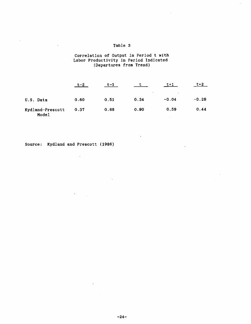
Table 3
Correlation of Output in Period t withLabor Productivity in Period Indicated
(Departures from Trend)
t—2 t—1 t t+l t+2
U.S. Data 0.60 0.51 0.34 —0.04 -0.28
Kydland—Prescott 0.37 0.68 0.90 0.59 0.44
Model
Source: Kydland and Prescott (1986)
—24—
counterpart 9tatistics for the U.S. data. One reason for this omission,
presumably, is that the ex—aifte real rate is the relevant variable while only
ex—post values are directly observable. Attempts to estimate ex—ante real
rates have been made, however, by Hamilton (1985) and Mishkin (1983). The
impression that one gets from examination of their charts is that the ex—ante
real rate is not nearly as strongly procyclical as the Kydland-Prescott model
implies.38 But numerical analysis is needed to be confident on this point.
In the case of the real wage, Kydland and Prescott report neither actual
nor model—implied results. But with a production function that is basically
Cobb-Douglas in specification, the marginal product of labor will fluctuate
closely with the average product of labor-—which is the "productivity"
variable that appears in Tables 1—3. Many investigators including Bils
(1985), and Geary and Kennan (1982) (1984) have found the real wage to be
positively correlated with output. But the magnitude of the contemporaneous
correlation in these studies is quite small39 a far cry from the 0.86—0.98
values implied by the Kydland—Prescott and Hansen models.
Let us now turn to relevant evidence obtained by other empirical methods.
Incomplete models with specifications that are compatible with the RBC
approach have been studied by means of econometric techniques that are quite
different from those utilized by Kydland—Prescott and Hansen. Most notably,
there area a number of papers that estimate, using aggregate time series
observations, household optiinality conditions analogous to equations (6)—(9)
above--but with the typical household viewed as facing market-determined wage
and interest rates rather than operating its own production facility. Leading
examples in this genre are provided by Lars Hansen and Singleton (1982),
Eichenbaum, Hansen, and Singleton (1986), and Mankiw, Rotemberg, and Summers
(1984).
-25-

Because these studies are designed to utilize models in which the
production sector is left unspecified, it is not possible to obtain
implications concerning fluctuations of the type that are emphasized by
Kydland and Prescott. There are certain results obtained that have some
relevance, however, for the RBC type of model. In particular, the models'
assumptions (including rational expectations) imply that certain variables
should be orthogonal to composite "disturbances" that are •involved in the
instrumental—variable (or "method of moments") estimation procedure. This in
turn implies that certain test statistics developed by Hansen (1982) have,
under the hypothesis that the model is well—specified, asymptotic chi-square
distributions with known degrees of freedom. Computed values that are
improbable under this hypothesis therefore constitute formal evidence against
the model at hand. In the recent study by Eichenbaum, Hansen, and Singleton
(1986), five of the six such statistics computed for a model composed of
equations similar to (6)—(9) above40 call for rejection at significance levels
below O.O1.' In addition, Eichenbaum, Hansen, and Singleton report that
"estimated values of key parameters differ significantly from the values
assumed in several studies," i.e., those of Kydland and Prescott. It is not
clear, however, that these results are unfavorable for RBC models in general,
as opposed to the Kydland—Prescott specification in particular.
Finally, mention should be made of an ambitious study conducted by Altug
(1985) who has obtained maximum likelihood estimates of a model that is fairly
close in specification to that of Kydland and Prescott (1982). No single test
statistic for the Kydland—Prescott parameter values is reported by Altug, but
the impression obtained from her various tables and charts is that agreement
with the data is not very good. Also, Altug's estimated version of the model
has properties that fail to match actuality in several respects. For example,
-26-

spectra of individual series implied by the model have shapes that are quite
different from the unrestricted estimates of these spectra.
It can be argued that the value of formal econometric test results is
small in the present context, i.e., in indicating whether models like that of
Kydland and Prescott (1982) do a good job of matching the actual data.
model that is both manageable and theoretically coherent will necessarily be
too simple to closely match the data in all respects, so with the number of
quarterly observations available such models will inevitably be rejected at
low significance levels in formal tests against generalized alternatives.
There is considerable merit to this argument, in my opinion, as a general
matter. It is unclear, however, that the particular models mentioned in
Tables 1—3 provide good data matches according to the builders' own criteria.
To some extent, this may be due to the äurrent models' simplicity, rather than
to any basic flaw in the RBC strategy. Future work on the topic should be
designed with that consideration in mind.
—27—

IV. Additional Issues
There are numerous additional matters of controversy——both substantive
and methodological——pertaining to RBC analysis that could be discussed. A few
of the more important ones will be taken up in the present section.
The first of these topics concerns the issue of social optimality. In
the models of Kydland and Prescott (1982) (1986) and Hansen (1985) there are
by construction no externalities, taxes, government consumption, or monetary
variables. Furthermore, all households are alike and each is effectively
infinite—lived. Consequently, competitive equilibria in these particular
models have the property of Pareto optimality.42 One message that should be
taken from that fact is that the mere existence of cyclical fluctuations is
not sufficient for a conclusion that interventionist government policy is
warranted. These models provide no basis, on the other hand, for concluding
that the solutions generated by actual economies are Pareto optimal. To
overturn that notion it should be sufficient to recall that in the U.S.
economy, to take one example, about 20% of total output is absorbed by
government purchases. Therefore, unless government services are precisely
chosen to reflect indIviduals' preferences, some departure from Pareto
optimality will result. In addition, taxes used to finance these purchases
are likely to have distorting allocational effects. As the RBC models in
question do not recognize the existence of government activities, they simply
have nothing to say on this matter.
Another particularly prominent omission pertains to money. It is not
true, as Eichenbaum and Singleton (1986) have pointed out, that the models
must be interpreted as implying the literal absence of money. Indeed, it is
doubtful that RBC proponents intend to advance the proposition that no less
output would be produced in the U.S. (with the existing capital stock) if
—28--
there were no medium of exchange——i.e., if all transactions had to be carried
out by crude or sophisticated barter. But the models do imply that, to a good
approximation, policy-induced fluctuations in monetary variables have no
effect on the real variables listed in Table 1——at least for fluctuations of
the magnitude experienced since World War II. Of course, RBC proponents do
not deny that there exist correlations between monetary and real variables,
but they claim that these reflect responses by the monetary system to
fluctuations induced by technology shocks——"reverse causation," in the words
of King and Plosser (1984).
It is somewhat ironic that the reverse-causation viewpoint should be
featured in a body of analysis that is a direct outgrowth of the
monetary-misperception class of equilibrium business cycle models. For the
problem that Lucas set out to solve, in his papers (1972) (1973) that created
this class, was to construct a competitive equilibrium model that incorporates
a Phillips—type money—to—income relationship although the modelled economy is
populated with rational agents——i.e., agents devoid of money illusion and
expectational irrationality. In his words, Lucas's JET paper was designed to
provide a model "of an economy in which equilibrium prices and quantities
exhibit what may be the central feature of the modern business cycle: a
systematic relation between the rate of change in nominal prices and the level
of real output" (Lucas, 1972a, p. 1O3).
It is important, then, to reflect on the process by which the equilibrium
business cycle program was transformed into one in which monetary impulses
play no significant role. In that regard, there are both theoretical and
empirical findings that have been important. Little needs to be said here
about the former, for the basic objection to monetary misperception models has
become widely understood.44 Some space must be devoted, however, to the
—29-
empirical findings.
Chronologically the first major empirical development was provided by
Simss (1980) (1982) demonstration that money stock innovations, in small VAR
systems, have little explanatory power for output fluctuations when a nominal
interest rate variable is included in the system.45 The interpretation
offered by Sims is that money stock innovations represent surprise policy
actions by the monetary authority——i.e., the Fed——so the finding is indicative
of the unimportance of monetary policy actions. But this interpretation is
open to objection. Suppose that the monetary authority implements its actions
by manipulating, on a quarter—to—quarter or month—to—month basis, the nominal
interest rate. Then interest rate innovations would reflect monetary policy
surprises, with money stock innovations representing linear combinations of
disturbances afflicting money demand, saving—investment, and production
relations as well as policy behavior. In this case, interest rate innovations
would measure monetary policy surprises better than would money stock
innovations. And in fact, U.S. monetary policy has been implemented
throughout the postwar period by means of interest rate instruments, even
during the period 1979_82.46 So the finding that money stock innovations
provide little explanatory power for output or employment movements simply
does not imply that monetary policy has been unimportant.47 On the contrary,
the considerable explanatory power provided by interest rate innovations in
Sims's studies suggests just the opposite.
For analogous reasons, moreover, it is incorrect to presume that
movements in the monetary base are accurate reflections of U.S. monetary
policy behavior. While the Fed could use the base as its operating instrument
if it chose to do so, in fact it never has. Consequently, empirical analyses
that treat the base as the Fed's instrument involve a serious misspecification
-30—
that must be accounted for in interpreting their findings.
These particular difficulties concerning the monetary authority's
operating procedures can in principle be partially circumvented by noting
that, in a system that includes all variables of macroeconomic importance to
agents, output, employment, and other real variables will be block exogenous
to all nominal variables——prices and interest rates, for example, as well as
monetary aggregates. It would then appear that this property of RBC models
could be used as the basis of a statistical test; if the RBC hypothesis were
true, then output, employment, etc. should not be Granger-caused by any
nominal variable or variables.48 Unfortunately, further analysis indicates
that in practice the presence of Granger causality from nominal to real
variables is neither necessary nor sufficient for rejection of the RBC
hypothesis. It is not necessary because a Lucas-style monetary misperceptions
model, in which monetary policy actions affect output but only if they are
unanticipated, will not imply Granger—causality from nominal to real
variables.49 Conversly, a finding of such causality is not sufficient for RBC
rejection if variables that are important to private agents are not observed
by the econometrician. In such cases, as Litterman and Weiss (1985), King
(1986), and Eichenbaum and Singleton (1986) have shown, monetary variables may
move in response to real shocks in a manner that has predictive content for
real variables even though the latter would be block exogenous in a wider
system that included the (practically unobserved) variables.
Furthermore, it is unclear whether or not significant nominal—to—real
Granger causality prevails in the available data. Some studies report test
statistics that imply strong rejections of non—causality null hypotheses; see,
e.g., Geary and Kennan (1984, Table 2) or Litterman and Weiss (1985), (Table
VII, line 18). But Eichenbaum and Singleton (1986) have documented a marked
—31—
tendency for nominal-to—real causality to become insignificant when the data
series are rendered stationary, prior to analysis, be means of first
differencing rather than removal of deterministic trend components. Despite
much recent research, it is not entirely clear what conclusion should be drawn
regarding the presence of causality when results differ in this fashion.50
The subject of first—differencing leads naturally to a relevant argument
put forth by Nelson and Plosser (1982) that has recently attracted
considerable attention. This argument begins with the presumption that
monetary impulses can have no effects on the trend component of output (or
employment) and continues with the claim that, in fact, output fluctuations
are dominated by trend (as opposed to cyclical) movements. The argument's
conclusion, then, is that output movements must be primarily induced by real
rather than monetary impulses-—a notion that is clearly pertinent for the RBC
hypothesis.
The Nelson—Plosser argument is related to the first differencing of data
because Its contention that output fluctuations are trend—dominated relies
critically upon the analysis of output (etc.) measures that have been first
differenced to remove the non-stationary trend component. For most aggregate
U.S. data series It is the case that the variability that is left to be
studied, or classified as "cyclical," is much smaller after differencing than
after removal of deterministic trends.
With regard to the Nelson—Plosser line of argument, McCallum (1986) has
objected that the empirical evidence does not warrant the conclusion that
first—differenclng is appropriate (and deterministic trend removal
inappropriate) as a method for rendering the series stationary. Such would be
the case if the series in question were generated by ARMA processes in which
the AR polynomial possesses a root precisely equal to 1.0. That is, if the
—32—
process for the variably Yt is expressed as
8 +eL+...÷eLl(27) y4 =
8(L) = 0 1 q*
01 p
with the white—noise innovation, then differencing would be required if the
solutions to the equation 'fi, + '',z + 2z2 +. . . + ''pZ = 0 include one root that
equals 1.0 precisely. The Nelson—Plosser evidence only shows, however, that
the hypothesis that such a root exists cannot be rejected at conventional
significance levels. But such test results are entirely consistent with the
possibility that the root in question is close to but not precisely equal to
unity; power against alternative hypotheses that the true value is 0.98 or
0.96 (for example) is extremely low. Thus the variables' ARMA processes may
easily be of a form such that deterministic detreziding would be entirely
appropriate.
The foregoing objection the Nelson—Plosser position does not constitute a
claim that output (employment, etc.) series can be firmly shown to be
trend—stationary, but rather that the Nelson—Plosser tests are incapable of
establishing their contention, i.e., that the data series are such that
differencing is necessary to induce stationarity. But without that
contention, the Nelson—Plosser evidence does not provide support for the RBC
hypothesis. '
The final matter to be taken up in this section concerns the connection
between business cycles and economic growth. Traditionally, of course,
macroeconomic analysis has typically proceeded under the maintained assumption
that these two types of phenomena can without serious loss be studied
separately——that the latter basically involves capital accumulation and
technical progress while the former concerns the extent to which existing
capital and labor are utilized. More recently, however, support has grown for
-33—
the idea that if technology shocks are the principle driving force behind
cyclical movements, as the RBC models presume, then the two types of phenomena
may be simply different manifestations of the same basic process.
Partly for the reason, perhaps, Prescott (1986, pp. 12—13) has emphasized
the desirability of simultaneously accounting for both growth and cycles. In
practice, however, the Kydland and Prescott (1982) (1986) studies have not
provided an integration at either the theoretical or empirical level. Thus
their theoretical specification pertains to an economy in which there is no
growth, either in total or per—capita terms.52 And the Kydland—Prescott
empirical procedure involves detrending of the data series prior to analysis,
so the economy's growth is abstracted from before the study of cycles is
begun. This latter aspect of the Kydland—Prescott procedure has been
criticised by Singleton (1986), who emphasizes that maximizing behavior
implies certain restrictions relating to the trend or growth components of
different variables. When such restrictions are ignored, parameter estimation
will be inefficient and some opportunities for model testing will go
unexploited.
It is possible, depending on the extent to which technical progress can
be appropriately viewed as exogenous, that the current emphasis on integration
of growth and cycle analysis may be misplaced or excessive. The point is
this: if technical progress were exogenous, then even if RBC views were
correct there would be little necessary relation between the magnitude of
growth and the extent of cycles, as they depend upon two different aspects of
the technical—progress process. Specifically, if the stochastic process for
zt is log zt = + 71t + 2 log ztl + with 1721 < 1, then growth will
depend upon 7 while cyclical properties will be related to the independent
parameter If = 0, the system would be one that features cycles but
-34-
no growth.54 In this case the Kydland—Prescott practice——as opposed to
rhetoric——would be largely appropriate.
On the other hand, it may be that growth results not from exogenous
technical progress but from endogenous forces. Quite recently, King and
Rebelo (1986) have——following some leads provided by Romer (1986)——begun an
investigation of the idea that growth may be the consequence of human—capital
accumulation with the latter determined endogenously. In the particular
example described by King, Plosser, and Rebelo (1987), the economy's rate of
steady growth per capita depends upon the ratio of human to physical capital
and the fraction of resources that are devoted to human capital formation and
maintenance, all of which are determined endogenously. There is in this model
no parameter, analogous to 7 in the previous paragraph, for which a special
value would imply zero growth without affecting cyclical properties. The link
between growth and cycles is, therefore, more intimate.
Some versions of the endogenous growth model have been formulated in a
manner that could lead readers to believe that steady—state growth, as opposed
to growth at ever increasing or decreasing rates, is possible only with a
production function for human capital that is excessively special. King,
Plosser, and Rebelo (1987) show, however, that the situation is essentially
the same as in the standard competitive growth model: steady growth requires
constant returns to scale in production: labor—argumenting technical change,
and utility functions of a certain class. Thus criticism on this basis is
unwarranted; these requirements for steady growth apply quite generally.
The discussion in King, Plosser, and Rebelo (1987) suggests that the
endogenous growth approach can account for the presence of autoregressive unit
roots in the univariate time series processes for capital stock and other real
variables. But while their analysis is promising in this regard, it
—35—

apparently implies roots precisely equal to unity only when production
functions are homogenous of degree precisely one. While many analysts would
accept constant returns as a good approximation, the implication for
autoregressive roots is only that values close to unity will be found.
-36--
V. Concluding Remarks
As an identifiable topic of study, RBC analysis is only a few years old.
Accordingly, it is perhaps too early for any reliable conclusions to be drawn.
But the arguments presented above can be summarized and a few judgements
attempted, even though the latter should be regarded as highly preliminary and
more of the nature of predictions than settled opinions.
Basically, we have seen in our discussion that a model of a competitive
market economy, in which an aggregate technology shock affects the quantity of
output producible from capital and labor inputs, will experience fluctuations
in per—capita quantities of consumption, investment, and total product. Under
most functional specifications for preferences and technology, the quantity of
labor employed will also fluctuate and investment variability will exceed that
of consumption. If the technology shock process. is strongly autoregressive—-
close to a random walk——so too will be the model's quantity variables, and the
contemporaneous correlations among these variables will in several ways be
notably similar to those that appear in detrended postwar quarterly data for
the U.S. economy. Furthermore, if the technology shock has a standard
deviation of about 3% of its mean value——about 1% for the surprise component
of this shock——then the magnitude of the model's output fluctuations will
match those of quarterly postwar real GNP, with a fairly good variability
match for other key variables as well.
Of course there are ways in which the model's stochastic properties do
not closely match actual data. For example, the correlations with output of
hours worked and productivity are much higher in the model than in reality,
and the correlation of productivity with lagged output provides a serious
mismatch. It is possible that such discrepancies are simply due to the
model's simplicity, however, rather than to any fundamental flaw in the RBC
-37—

approach. Until 3tudies have been conducted that convincingly distinguish
between sources f fluctuations, it will be possible for responsible
researchers to maintain sharply differing beliefs in this regard. An
important gap in the RBC analysis has been a clear and convincing story
concerning the nature of the postulated aggregate shock variable. If the
latter were actually a proxy for observable variables that have been omitted
from the models——fiscal policy and/or import prices, for example——then the
interpretation and conclusions of the work would be quite different than if
the shocks were of a strictly technological nature.
As for the notion that monetary policy irregularity has been an
unimportant source of output fluctuations, at least during the postwar era, it
is too early to reach any firm conclusion. RBC proponents have pointed to
empirical findings that are suggestive of that hypothesis, but there are
significant problems with the evidence that has been developed to date.
It would seem to be virtually indisputable that the RBC literature has
provided a substantial number of innovative and constructive technical
developments that will be of lasting benefit in macroeconomic analysis. In
particular, the example of Kydland and Prescott (1982) has suggested one route
toward the goal of a dynamic equilibrium model with optimizing agents that can
be used for quantitative macroeconomic analysis. The type of model employed
does not, it should be emphasized, require a belief that the workings of the
economy are socially optimal. In addition, the literature has spurred
interest in several purely methodological topics, including alternative
methods for the investigation of the dynamic properties of non—linear general
equilibrium models and for the detrending of time series data. Also, issues
concerning the practical reliability of Granger—causality tests have been
highlighted by controversies initiated by RBC analysis.
—38—
From a substantive perspective, the RBC studies have provided a healthy
reminder that a sizeable portion of the output and employment variability that
is observed in actual economies is probably the consequence of various
unavoidable shocks, i.e., disturbances not generated by erratic monetary or
fiscal policy makers. Thus it is unlikely that many scholars today would
subscribe to the proposition that all or most of the postwar fluctuation in
U.S. output has been attributable to actions of the Federal Open Market
Committee. Whether a substantial fraction can be so attributed remains a
topic of interest and importance.
—39—
Footnotes
1. An incomp1ete list of other notable items includes Black (1982), Kydland
and Prescott (1980) (1986), Kydland (1984), King (1986), King, Plosser, and
Rebelo (1987), King, Plosser, Stock, and Watson (1987), Hansen (1985), and
Prescott (1986).
2. To date, these include critical pieces by Fischer (1987), McCallum (1986),
and Summers (1986) plus sympathetic but skeptical discussions by Barro (1986),
Eichenbaum and Singleton (1986), King and Dotsey (1987), Lucas (1985), and
Mankiw (1986). A guide to the Prescott-Summers exchange is provided by
Manuelli (1986) and expository articles have been prepared by Rush (1987) and
Walsh (1986).
3. Clearly, real shocks could in principle pertain as well to individuals'
preferences, but in fact the literature has emphasized technology
disturbances.
4. Here the term "equilibrium" is being used as a shorthand for the more
precise term, "flexible—price equilibrium." McCalluin (1982) suggests that
there is no Inherent reason why equilibrium models could not accommodate
sluggish price adjustments.
5. That such a challenge is intended by some of the leaders of RBC analysis
is suggested by King and Plosser's (1984, p. 363) statement that "there are
good reasons for dissatisfaction with existing macro economic theories" in
conjunction with a reference to "alternative hypotheses."
6. A basic reference in this regard is Brock and Mirman (1972), which
provides formal analysis of a social planner's problem in the context of a
related stochastic growth model. Brock (1974) indicated how the mathematics
could be re—interpreted so as to constitute a descriptive model of a
competitive economy with a large number of similar households. The only
significant differences between the re—interpreted Brock—Mirman model and the
one with which we begin is the non-recognition of leisure in the former—-a
difference that is of very little importance on the design of proofs——and the
formerts assumption of serially—independent technology shocks. This latter
limitation was removed by Donaldson and Mehra (1983).
7. Alternatively, we could proceed under the assumption that there is a
market for one—period bonds instead of one for capital services. Suppose that
a bond purchased in t for 1/(l+rt) is a claim to one unit of output in t÷1.
Then the household's net expenditure on bonds during t could be denoted
(l+rt) bt÷i—bt, with bt+i the number of bonds purchased in t. The price
(l÷rt) would be determined by the market—clearing condition, implied by the
similarity of all households, that bt÷i = 0. Equilibrium values of Ct,
and kt÷i would be precisely the same as with the market structure implied by
equation (3).
8. Obviously, the equality in (6) should properly be written as the
inequality "�.." But our assumptions are such that the equality will in fact
hold. This type of notational shortcut is used extensively in what follows.
9. If we neglect the variable—leisure aspect of our model, then proofs can be
found in Brock (1982) and Donaldson and Mehra (1983).
10. Since is the utility value of a unit of capital acquired in period
t+j, j1 is the present value in t of capital held by the
household at the end of period t÷j. Condition (5) serves to rule out the
possibility that the household would forever accumulate capital at an
excessive rate, something that is not precluded by any of conditions (4).
11. On this, see Brock (1982).
12. Some readers have objected to the way in which the optimization analysis
is here described, suggesting that instead it be expressed in terms of the
identity between Pareto-optimality and competitive equilibrium that has been
used in several of the key RBC papers. I have quite deliberately chosen not
to proceed in that manner so as to avoid portraying RBC analysis in a overly
restrictive manner. An approach that is applicable only to economies known to
be Pareto optimal would be of quite limited usefulness, but such is in fact
not the case for RBC analysis. The latter point is recognized by King,
Plosser, and Rebelo (1987).
13. For a more complete discussion, see Lucas (1987). Strictly speaking, our
statement presumes that interest is limited to minimal sets of state
variables, a limitation that rules out "bubbles.' But since any bubble path
would in the present model be inconsistent with the transversality condition
(5), this limitation is not significant.
14. These include Long and Plosser (1983).
15. Very recently Hercovitz and Sampson (1986) have developed a different
special case that does not require complete depreciation yet results in
explicit log-linear solutions that feature variable employment. These
attractive features are obtained at the price of adopting unfamiliar
specifications for utility and depreciation functions. Specifically, the
within—period utility function is u(ct, l—flt) = log(c — a n.') with a > 0 and
7 > 1, a form that makes the marginal rate of substitution between consumption
and leisure independent of Ct. Ignoring complications involving human capital
that are stressed by Hercovitz and Sampson, let technology continue to be Yt
1—x . .= zt nt kt as in (15) and maintain the usual concept of gross investment,
= Yt — ct. Regarding depreciation, however, assume that kt+i = i4 iwhere • > 0 and 1 > a > 0. One can think of this log—linear expression as
departing from the usual linear form for adjustment—cost reasons as in Lucas
and Prescott (1971), or alternatively as an approximation adopted for
analytical convenience. In any event, with this specification the model
yields solutions of the form
$12 $13 $22 033 $32 $33Ct - •ijzt kt nt = •21zt kt , kt÷i = 031 zt kt
16. The shadow price Xt obviously obeys Xt = e[l—(1—x)]' n—z' k-'.
17. Whether it is appropriate to use detrended data is an important issue
that will be briefly discussed below, in Section IV.
18. For output this is well known. For consumption we have log Ct = .06 +
1.21 log ct_i — .24 log ct_i + .00024t, o = .007, DW = 2.08.
19. In these models, positive demand shocks result in high output because
they induce high employment in response to low real wages.
20. To obtain this implication, note that with 6 = 1 investment during period
t is identically the same as kt+i. Then recall that the stochastic processes
for kt and Ct have the same autoregressive components and the same forcing
variable, t•-
21. More precisely, the claim cannot be verified without resort to some sort
of approximation procedure. Using one, King, Plosser, and Rebelo (1987) are
able to show that, in aversion with no labor—leisure decision, consumption
variability is greater than for investment.
22. The smoothing procedure for measuring the trend component of the various
series is somewhat unorthodox. If xt is the variable to be smoothed and St
the smoothed value for period t, the method entails minimizing the sum of
2 1T 2
T I(xt—st) and pT E((st÷i—st)s1_1J, where i is a weighting factor
t=1 t=2
that is chosen to provide the desired degree of smoothness. Use of this
particular method of detrending the data has not attracted much discussion or
criticism to date, but inspection of material in King, Plosser, and Rebelo
(1987) suggests that cross—variable correlations may be sensitive to the
method. Some issues concerning detrending (by any method) will be briefly
considered in Section IV.
23. The parameter values utilized by Hansen are 9 = 0.33, = 0.64, = 0.99,
and 6 = 0.025. Also, the counterpart of p is taken to be 0.95. It is
necessary to refer to "the counterpart of p" rather than to p itself because
Hansen's specification (like that of Kydland and Prescott) is of the form zt =
0.95 zt...l + , with t log—normal, rather than log zt = log zt...l +
24. Since the model is not linear in logs of the variables, this scaling is
not strictly legitimate; an increase in the variance of the technology shock
would change the relative standard deviations to a small extent. It is my
belief that such an effect would be negligible in the case at hand.
25. It is possible that serial correlation properties are enhanced, however.
Statistics relating to this dimension of performance are not reported by
Hansen (1985).
26. As Hansen (1985) emphasizes, his specification is based on theoretical
analysis originally developed by Rogerson (1985).
27. Again, this magnitude is (because of ignored nonlinearities) only
approximate. The correct statement is that in Hansen's simulations the basic
model has output variability only 0.134/0.176 = 0.767 as large as that for the
indivisible labor model when the same zt variance is used for both.
28. As previously mentioned, other typical values are fi = 0.99 and 6 = 0.025
(quarterly data). There is room for dispute regarding some of these
magnitudes. Significantly, Summers (1986) has questioned the Kydland—
Prescott—Hansen choice for fi, which implies a steady—state real rate of return
of 4% per year, and the 9 value that implies that about a third of the typical
household's time is spent in employment. Summers notes that the actual figure
is closer to one—sixth, a magnitude that is borne out by estimates obtained by

Eichenbaum, Hansen, and Singleton (1986).
29. A sensitivity of this type has been mentioned by Christiano (1987a, p.
341). Some related facts are brought out by King, Plosser, and Rebelo (1987).
30. The issue has been raised by Barro (1986), Lucas (1987), and Summers
(1986), among others.
31. Thus this estimate pretends that p = 1. While this is inconsistent with
0.95 value used by Kydland and Prescott (1982) (1986), the resulting effect is
probably small in the present context (i.e., obtaining an estimate of the
variance of Et). Prescott's procedure involves a weighted manhours series and
imposes the restriction = 0.75.
32. Actually, this number is here inf erred, in the manner described in
footnote 27, from Hansen's reported level of output fluctuations.
33. By failing to take account of quarter—to—quarter dynamics, the procedure
throws into the residual fluctuations that which would properly be attributed
to this source of dynamics (if the adjustment—cost hypothesis were true).
This problem, it might be said, concerns misspecification of the (dynamic)
production—employment relation, not measurement error. The omission of
relevant lagged variables is only likely (rather than certain) to lead to
over—estimation of the shock variance because the procedure uses factor shares
as parameters rather than estimating the latter in a regression designed to
yield zt residuals.
34. This calculation, it should be said, pertains to the mean level of
productivity change, not its variance.
35. Long and Plosser (1983) includes an interesting discussion of a
multisector RBC framework. From their Figure 3 it would appear that the
magnitude of aggregate fluctuations is smaller than for individual sectors,
but numerical statistics relating to this particular point are not included.
The discrepancy between sectoral and aggregate magnitudes would be heightened,
of course, by recognition of more sectors; the Long and Plosser example has
only six.
36. An increase in the price of imported materials will lead to a decline in
their quantity utilized, relative to the quantities of domestic factors. That
will reduce the quantity of output for any given usage of domestic factors,
i.e., will shift downward the production schedule relating output to domestic
factors alone.
37. Labor hoarding is mentioned by Summers (1986). What I understand by the
term is that costs of hiring and firing lead firms to adjust their workforce
much more slowly than if no such costs existed. To see that the lag
correlation pattern could easily be as claimed, consider an example in which
= byt_i + et and nt = ayt + (l—a)yt_i, where Yt and nt denote logs of
output and hours so that the log of productivity is xt = Yt - Then it is
easy to show that Eytxt+i < 0 while Eytxt_i > 0 and EytXt > 0. An interesting
recent attempt to discriminate between the supply—shock and labor—hoarding
hypotheses has been made by Shapiro (1987), whose results are supportive of
the former. Some apparent inconsistencies with other wage—productivity
studies may be due to Shapiros use of annual data.
38. The Kydland—Prescott correlations with output analogous to those of Table
3 are as follows: 0.46, 0.68, 0.84, 0.56, 0.42.
39. The U.S. correlation in Geary and Kennan (1984), for example, is 0.20.
40. The model is less restrictive than (6)—(9) as it permits current utility
to be affected by a distributed lag of leisure hours.
41. Eichenbaum, Hansen, and Singleton (1986) develop evidence which suggests
that the model's rejection stems primarily from a failure to satisfy the
intratemporal, as opposed to intertemporal, optimality conditions.
42. In fact, the competitive equilibria are computed in these papers by
solving Pareto optimality problems for a fictitious social planner.
43. From its context, it is clear that Lucas presumed the causal relation to
be from money to income.
44. The point is that in actual developed economies data is available on
monetary aggregates too promptly to be consistent with the assumption——
critical in the Lucas-Barro models——that individuals are ignorant of
contemporaneous monetary magnitudes. A key item in the literature is King's
(1981) demonstration that this problem is not circumvented by measurement
error on the 'true" aggregate.
45. This statement pertains to the postwar U.S. data, quarterly and monthly.
46. Relevant discussion of the 1979—82 episode appears in McCallum (1985).
47. For an elaboration on this argument, see McCallum (1986) and references
cited therein.
48. Block exogeneity of xt of course implies that xt is not Granger—caused by
any variable not included In the vector x.
49. See Sargent (1976) and the comments on this paper that appeared in April
1979 issue of the Journal of Political Economy.
50. Christiano (1987b) has provided some simulation results that suggest (but
do not establish) that the results with undifferenced data are more reliable
in this particular context. On the other hand, it might be noted that only a
small fraction of the predictive power for output movements can be attributed
to nominal variables even in those studies that feature strong rejections of
the no—causality hypothesis; most of the explanatory power lies in past
movements of output itself. But this type of finding appears so frequently in
Granger—causality studies of other, entirely unrelated, issues that one is led
to suspect that the basic procedure is seriously flawed in some
respect——possibly involving measurement error——that has thus far eluded formal
analysis.
51. Some support for the foregoing argument is provided by interesting recent
studies by Cochrane (1986), Watson- (1986), and Evans (1986). A contrary
position is taken in a notable paper by Campbell and Mankiw (1986).
52. Exogenous technical progress can be added to the model, of course, but
that step does not constitute much of an integration.
53. This fact is not invalidated by the dependence of both growth and cycle
magnitudes on
54. If the log zt process' were a random walk with drift, the definition of
"cycles' would become problematical. But it would remain reasonable to say
that zero drift implies zero growth while leaving scope for cycles.
References
Abraham, Katharine G., and Lawrence F. Katz, "Cyclical Unemployment: Sectoral
Shifts or Aggregate Disturbances?" Journal of Political Economy 94
(November 1986), 507—522.
Altug, Sumru G., "Essays in the Equilibrium Approach to Aggregate Fluctuations
and Asset Pricing," Ph.D. dissertation, Carnegie Mellon University, 1985.
Barro, Robert, J., "Rational Expectations and the Role of Monetary Policy,"
Journal of Monetary Economics 2 (January 1976), 1—32.
Barro, Robert, J., "The Equilibrium Approach to Business Cycles," in Money,
Expectations, and Business Cycles. New York: Academic Press, 1981.
Barro, Robert, J., "Comments," NBER Macroeconomics Annual 1986. Cambridge:
MIT press, 1986.
Bus, Mark J., "Real Wages over the Business Cycle: Evidence from Panel Data."
Journal of Political Economy 93 (August 1985), 666-89.
Black, Fischer, "General Equilibrium and Business Cycles," NBER Working Paper
No. 950, August 1982.
Brock, William A., "Comments," in Frontiers of Quantitative Economics, Vol.
II, ed. by M.D. Intriligator. and D.A. Kendrick. Amsterdam: North—Holland
Publishing Co., 1974.
Brock, William A., "Asset Prices in a Production Economy," in The Economics of
Information and Uncertainty, ed. by J.J. McCall. Chicago: University of
Chicago press, 1982.
Brock, William, A., and Leonard J. Mirman, "Optimal Economic Growth and
Uncertainty: The Discounted Case," Journal of Economic Theory 4: (1972),
479—515.
Campbell, John Y.. and N. Gregory Mankiw, "Are Output fluctuations Transitory?"
NBER Working Paper No. 1916, January 1986.
Christiano, Lawrence, J., "Is Consumption Insufficiently Sensitive to
Innovations in Income?" American Economic Review 77 (May 1987), 337—341. (a)
Christiano, Lawrence, J., "Money Does Granger—Cause Output in the Bivariate
Output-Money Relation," Working Paper, Federal Reserve Bank of Minneapolis,
February 1987. (b)
Cochrane, John H., "How Big is the Random Walk in GNP?" Working Paper,
University of Chicago, April 1986.
Davis, Steven J., "Fluctuations in the Pace of Labor Reallocation," Carnegie-
Rochester Conference Series on Public Policy 27 (Autumn 1987), forthcoming.
Donaldson, John B., and Rajnish Mehra, "Stochastic Growth with Correlated
Production Shocks," Journal of Economic Theory 29 (1983), 282—312.
Eichenbaum, Martin, and Kenneth J. Singleton," Do Equilibrium Real Business
Cycle Theories Explain Postwar U.S. Business Cycles?" NBER Macroeconomics
Annual 1986. Cambridge: MIT Press, 1986.
Eichenbaum, Martin S., Lars P. Hansen, and Kenneth J. Singleton, "A Time
Series Analysis of Representative Agent Models of Consumption and
Leisure Choice Under Uncertainty," NBER Working Paper No. 1981, July 1986.
Evans, George W., "Output and Unemployment Dynamics in the United States:
1950—1985," Working Paper, Stanford University, October 1986.
Fischer, Stanley, "New Classical Macroeconomics," The New Palgrave: A
Dictionary of Economics. New York: Stockton Press, 1987.
Geary, Patrick T., and John Kennan, "The Employment-Real Wage Relationship:
An International Study," Journal of Political Economy 90 (August 1982),
854—871.
Geary, Patrick T., and John Kennan, "Intertemporal Substitution and the
Phillips Curve: International Evidence," Working Paper No. 84—35,
University of Iowa, December 1984.
Hansen, Gary D., "Indivisible Labor and the Business Cycle," Journal of
Monetary Economics 16 (November 1985), 309—327.
Hansen, Lars P., "Large Sample Properties of Generalized Method of Moments
Estimators," Econometrica 50 (July 1982), 1029—1054.
Hansen, Lars P., and Kenneth J. Singleton, "Generalized Instrumental Variables
Estimation of Nonlinear Rational Expectations Models," Econometrica 50
(September 1982), 1269—1286.
Hamilton, James D., "Oil and the Macroeconomy since World War II," Journal of
Political Economy 91 (April 1983), 228—248.
Hamilton, James D., "Uncovering Financial Market Expectations of Inflation,"
Journal of Political Economy 93 (December 1985), 1224—1241.
Hercowitz, Zvi, and Michael Sampson, "Growth and Employment Fluctuations,"
Working Paper, July 1986.
Hodrick, Robert J., and Edward C. Prescott, "Post—War U.S. Business Cycles:
An Empirical Investigation," Working Paper, Carnegie Mellon University,
1980.
Jorgensen, Dale W., and Zvi Griliches, "The Explanation of Productivity
Change," Review of Economic Studies 34 (April 1967), 249—283.
King, Robert 6., "Monetary Information and Monetary Neutrality," Journal of
Monetary Economics 7 (March 1981), 195—206.
King, Robert 6., "Money and Business Cycles: Comments on Bernanke and Related
Literature," Carnegie—Rochester Conference Series on Public Policy 25
(Autumn 1986), 101—116.
King, Robert G., and Michael Dotsey, "Rational Expectations and the Business
Cycle," The New Paigrave: A Dictionary of Economics. New York: 'Stockton
Press, 1987.
King, Robert G., and Charles I. Plosser, "Money, Credit, and Prices in a Real
Business Cycle," American Economic Review 74 (June 1984), 363-80.
King, Robert G., Charles I. Plosser, and Sergio T. Rebelo, "Production,
Growth, and Business Cycles," Working Paper, University of Rochester, July
1987.
King, Robert, G., and Sergio T. Rebelo, "Business Cycles with Endogenous
Growth," Working Paper, University of Rochester, July 1986.
Kydland, Finn E., "Labor Force Heterogeneity and the Business Cycle,"
Carne2ie—Rochester Conference Series on Public Policy 21 (Autumn 1984),
173-208.
Kydland, Finn E., and Edward C. Prescott, "A Competitive Theory of
Fluctuations and the Feasibility and Desirability of Stabilization Policy,"
in Rational Expectations and Economic Policy, ed. by S. Fischer. Chicago:
University of Chicago Press, 1980.
Kydland, Finn E., and Edward C. Prescott, "Time to Build and Aggregate
Fluctuations," Econometrica 50 (November 1982), 1345—1370.
Kydland, Finn E., and Edward C. Prescott, "The Workweek of Capital and its
Cyclical Implications," Working Paper, Federal Reserve Bank of Minneapolis,
October 1986.
Lilien, David M., "Sectoral Shifts and Cyclical Unemployment," Journal of
Political Economy 90 (August 1982), 777—793.
Litterman, Robert B., and Lawrence Weiss, "Money, Real Interest Rates, and
Output: A Reinterpretation of Postwar U.S. Data," Econometrica 53 (January
1985), 129—56.
Long, John B., and Charles I. Plosser, "Real Business Cycles," Journal of
Political Economy 91 (February 1983), 39—69.
Loungani, Prakash, "Oil Price Shocks and the Dispersion Hypothesis," Review of
Economics and Statistics 68 (August 1986), 536—539.
Lucas, Robert E., Jr., "Expectations and the Neutrality of Money," Journal of
Economic Theory 4 (April 1972), 103—24.
Lucas, Robert E., Jr., "Some International Evidence on Output—Inflation
Tradeoffs," American Economic Review 63 (June 1973), 326—334.
Lucas, Robert E., Jr., "An Equilibrium Model of the Business Cycle," Journal
of Political Economy 83 (December 1975), 1113—1144.
Lucas, Robert E., Jr., Models of Business Cycles. Oxford: Basil Blackwell,
1987.
Lucas, Robert E., Jr., and Edward C. Prescott, "Investment Under Uncertainty,"
Econometrica 39 (September 1971), 659-682.
Mankiw, N. Gregory, "Comments," NBER Macroeconomics Annual 1986. Cambridge:
MIT Press, 1986.
Mankiw, N. Gregory, Julio J. Rotemberg, and Lawrence H. Summers,
"Intertemporal Substitution in Macroeconomics," Q!rterly Journal of
Economics 100 (February 1985), 225—251.
McCallum, Bennett T., "Macroeconomics After a Decade of Rational Expectations:
Some Critical Issues," Federal Reserve Bank of Richmond Economic Review 68
(November/December 1982), 3—12.
McCallum, Bennett T., "On Consequences and Criticisms of Monetary Targeting,"
Journal of Money, Credit, and Banking 17 (November 1985, Part 2), 570—97.
McCallum, Bennett T., "On 'Real' and 'Sticky Price' Theories of the Business
Cycle," Journal of Money, Credit, and Banking 18 (November 1986), 397—414.
Mishkin, Frederick S., "The Real Interest Rate: An Empirical Investigation,"
Carnegie—Rochester Conference Series on Public Policy 15 (Autumn 1981),
151—200.

Nelson, Charles R., and Charles I. Plosser, "Trends and Random Walks in
Macroeconomic Time Series,' Journal of Monetary Economics 10 (September
1982), 139—62.
Oi, Walter Y., 'Comment on the Relation Between Unemployment and Sectoral
Shifts," Carngj—Rochester Conference Series on Public Policy 27 (Autumn
1987), forthcoming.
Prescott, Edward C., "Theory Ahead of Business Cycle Measurement,"
Carnegie—Rochester Conference Series on Public Policy 25 (Autumn 1986),
11—44.
Rogerson, Richard D., "Indivisible Labor, Lotteries, and Equilibrium," Working
Paper, University of Rochester, 1985.
Romer, Paul M., "Increasing Returns and Long—Run Growth, Journal of Political
Economy 94 (October 1986), 1002—1037.
Rush, Mark, "Real Business Cycles, Federal Reserve Bank of Kansas City
Economic Review 72 (February 1987), 20—32.
Sargent, Thomas J., "The Observational Equivalence of Natural and Unnatural
Rate Theories of Macroeconomics," Journal of Political Economy 84 (August
197à), 631—640.
Sargent, Thomas J., Macroeconomic Theory. New York: Academic Press, 1979.
Shapiro, Matthew D., "Are Cyclical Fluctuations in Produclivity Due More to
Supply Shocks or Demand Shocks?" NBER Working Paper No. 2147, February
1987.
Sims, Christopher A., "Comparison of Interwar and Postwar Business Cycles:
Monetarism Reconsidered," American Economic Review 73 (May 1983), 250—7.
Sims, Christopher A., "Policy Analysis with Econometric Models," Brookings
Papers on Economic Activity (1982, No. 1), 107—52.
Singleton, Kenneth J., "Econometric Issues in the Analysis of Equilibrium
Business Cycle Models" Working Paper, Carnegie Mellon University, July
1986.
Solow, Robert M., "Technical Change and the Aggregate Production Function,"
Review of Economics and Statistics 39 (May 1957), 312—320.
Summers, Lawrence H., "Some Skeptical Observations on Real Business Cycle
Theory," Federal Reserve Bank of Minneapolis Quarterly Review 10 (Fall
1986), 23—27.
Walsh, Carl E., "New Views of the Business Cycle: Has the Past Emphasis on
Money been Misplaced?" Federal Reserve Bank of Philadelphia Business Review
(January—February 1986), 3—13.
Watson, Mark W., "Univariate Detrending Methods with Stochastic Trends,"
Journal of Monetary Economics 18 (July 1986), 49—75.


