Embed Size (px)
Citation preview
arX
iv:1
010.
0429
v2 [
mat
h.N
T]
9 D
ec 2
010
RATIONAL APPROXIMATIONS FOR THE QUOTIENT OF
GAMMA VALUES
KH. HESSAMI PILEHROOD1 AND T. HESSAMI PILEHROOD2
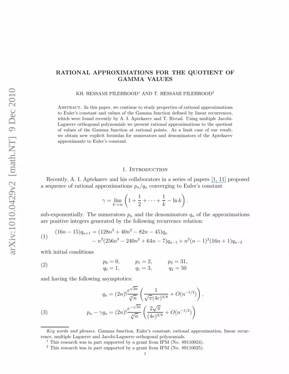
Abstract. In this paper, we continue to study properties of rational approximationsto Euler’s constant and values of the Gamma function defined by linear recurrences,which were found recently by A. I. Aptekarev and T. Rivoal. Using multiple Jacobi-Laguerre orthogonal polynomials we present rational approximations to the quotientof values of the Gamma function at rational points. As a limit case of our result,we obtain new explicit formulas for numerators and denominators of the Aptekarevapproximants to Euler’s constant.
1. Introduction
Recently, A. I. Aptekarev and his collaborators in a series of papers [1, 11] proposeda sequence of rational approximations pn/qn converging to Euler’s constant
γ = limk→∞
(
1 +1
2+ · · ·+ 1
k− ln k
)
.
sub-exponentially. The numerators pn and the denominators qn of the approximationsare positive integers generated by the following recurrence relation:
(16n− 15)qn+1 = (128n3 + 40n2 − 82n− 45)qn
− n2(256n3 − 240n2 + 64n− 7)qn−1 + n2(n− 1)2(16n+ 1)qn−2
(1)
with initial conditions
(2)p0 = 0, p1 = 2, p2 = 31,q0 = 1, q1 = 3, q2 = 50
and having the following asymptotics:
qn = (2n)!e√2n
4√n
(
1√π(4e)3/8
+O(n−1/2)
)
,
pn − γqn = (2n)!e−
√2n
4√n
(
2√π
(4e)3/8+ O(n−1/2)
)
(3)
Key words and phrases. Gamma function, Euler’s constant, rational approximation, linear recur-rence, multiple Laguerre and Jacobi-Laguerre orthogonal polynomials.
1 This research was in part supported by a grant from IPM (No. 89110024).2 This research was in part supported by a grant from IPM (No. 89110025).
1

In [6], explicit formulas for the sequences pn and qn were given in terms of hypergeo-metric sums
(4) qn =n
∑
k=0
(
n
k
)2
(n+ k)!,
pn =
n∑
k=0
(
n
k
)2
(n+k)!Hn+k−2
n∑
k=1
k∑
m=0
n−k∑
l=0
(−1)m+k
k
(
n
k + l
)(
k
m
)(
n− k
l
)
(m+n+ l)!,
where Hn is an n-th harmonic number defined by
Hn(α) =n
∑
k=1
1
k + α, n ≥ 1, H0(α) = 0, Hn = Hn(0).
These representations provide a more profound insight on arithmetical properties ofthese sequences that can not be deduced from the recurrence equation (1). From (4) itfollows that qn and pn are integers divisible by n! and n!/Dn respectively, where Dn isthe least common multiple of the numbers 1, 2, . . . , n. This implies that the coefficientsof the linear form (3) can be canceled out by the big common factor n!
Dn, but it is still
not sufficient to prove the irrationality of γ. The remainder of the above approximationis given by the integral [3]
∫ ∞
0
Q(0,0,1)n (x) e−x ln(x) dx = pn − γqn,
where for a1, a2 > −1, b > 0,
(5) Q(a1,a2,b)n (x) =
1
n!2
2∏
j=1
[
w−1j
dn
dxnwjx
n]
(1− x)2n
is a multiple Jacobi-Laguerre orthogonal polynomial on ∆1 = [0, 1] and ∆2 = [1,+∞)with respect to the two weight functions
w1(x) = xa1(1− x)e−bx, w2(x) = xa2(1− x)e−bx
satisfying the following orthogonality conditions [2]:
(6)
∫
∆j
xνQ(a1,a2,b)n (x)wk(x) dx = 0, j, k = 1, 2, ν = 0, 1, . . . , n− 1.
Note that, as the values of the parameters a1, a2 tend to 0 and b = 1, the limit values of
Q(0,0,1)n (x) satisfy the orthogonality relations (6) with the weights w1(x) = (1 − x)e−x,
w2(x) = (1− x) ln(x)e−x.In [6], the authors showed that for a, b ∈ Q, a > −1, b > 0 the integrals
(7)b2n+a+1
Γ(a+ 1)
∫ ∞
0
Q(a,a,b)n (x)xa ln(x)e−bx dx = pn(a, b)− (ln(b)− ψ(a + 1))qn(a, b),
where ψ(z) = Γ′(z)/Γ(z) defines the logarithmic derivative of the gamma function, pro-vide good rational approximations for ln(b)−ψ(a+1), which converge sub-exponentially
2

to this number
(8)pn(a, b)
qn(a, b)− (ln(b)− ψ(a + 1)) = 2πe−2
√2bn(1 +O(n−1/2)) as n→ ∞,
and gave explicit formulas for the denominators and numerators of the approximations
qn(a, b) =
n∑
k=0
(
n
k
)2
(a + 1)n+k bn−k,
pn(a, b) =
n∑
k=0
(
n
k
)2
(a + 1)n+k bn−kHn+k(a)
− 2n
∑
k=1
k∑
m=0
n−k∑
l=0
(−1)m+k
k
(
n
k + l
)(
k
m
)(
n− k
l
)
(a+ 1)m+n+l bn−m−l,
(9)
here (a)n is the Pochhammer symbol defined by (a)0 = 1 and (a)n = a(a + 1) · · · (a +n− 1), n ≥ 1.
Recently, T. Rivoal [9] found another example of rational approximations to thenumber γ + ln(x), x ∈ Q, x > 0, by using multiple Laguerre polynomials
An(x) =ex
n!2(xn(xne−x)(n))(n) = ex · 2F2
(
n+ 1, n+ 1
1, 1
∣
∣
∣
∣
− x
)
(for the validity of the last equality see [7, §4.3]). Here pFq is the generalized hyperge-ometric function defined by the series
pFq
(
α1, . . . , αp
β1, . . . βq
∣
∣
∣
∣
z
)
=
∞∑
k=0
(α1)k · · · (αp)k(β1)k · · · (βq)k
zk
k!,
which converges for all finite z if p ≤ q, converges for |z| < 1 if p = q + 1, and divergesfor all z, z 6= 0 if p > q+1. The series pFq terminates and, therefore, is a polynomial inz if a numerator parameter is a negative integer or zero, provided that no denominatorparameter is a negative integer or zero.
The polynomial An(x) as well as the hypergeometric function 2F2
(
n+1,n+11, 1
∣
∣− x)
sat-
isfies a certain third-order linear recurrence relation with polynomial coefficients in nand x. The polynomials An(x) are orthogonal with respect to the weight functionsω1(x) = e−x, ω2(x) = e−x ln(x) on [0,+∞), so that
(10)
∫ ∞
0
xνAn(x)ωk(x) dx = 0, k = 1, 2, ν = 0, 1, . . . , n− 1.
This implies that An(x) is a common denominator in type II Hermite-Pade approxima-tion for the two Stieltjes functions
E1(x) =∫ ∞
0
e−t
x− tdt, E2(x) =
∫ ∞
0
e−t ln(t)
x− tdt
3
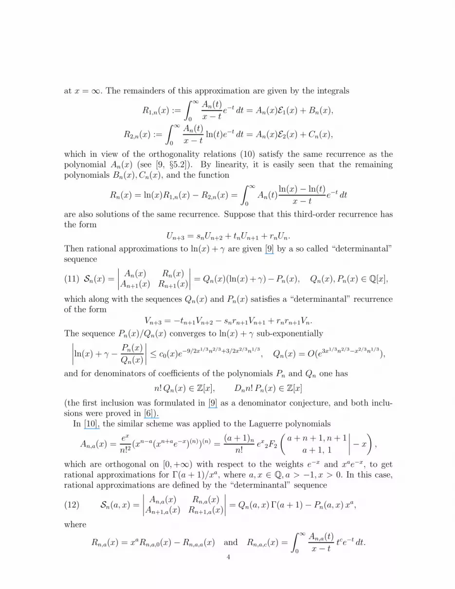
at x = ∞. The remainders of this approximation are given by the integrals
R1,n(x) :=
∫ ∞
0
An(t)
x− te−t dt = An(x)E1(x) +Bn(x),
R2,n(x) :=
∫ ∞
0
An(t)
x− tln(t)e−t dt = An(x)E2(x) + Cn(x),
which in view of the orthogonality relations (10) satisfy the same recurrence as thepolynomial An(x) (see [9, §5.2]). By linearity, it is easily seen that the remainingpolynomials Bn(x), Cn(x), and the function
Rn(x) = ln(x)R1,n(x)− R2,n(x) =
∫ ∞
0
An(t)ln(x)− ln(t)
x− te−t dt
are also solutions of the same recurrence. Suppose that this third-order recurrence hasthe form
Un+3 = snUn+2 + tnUn+1 + rnUn.
Then rational approximations to ln(x) + γ are given [9] by a so called “determinantal”sequence
(11) Sn(x) =
∣
∣
∣
∣
An(x) Rn(x)An+1(x) Rn+1(x)
∣
∣
∣
∣
= Qn(x)(ln(x)+ γ)−Pn(x), Qn(x), Pn(x) ∈ Q[x],
which along with the sequences Qn(x) and Pn(x) satisfies a “determinantal” recurrenceof the form
Vn+3 = −tn+1Vn+2 − snrn+1Vn+1 + rnrn+1Vn.
The sequence Pn(x)/Qn(x) converges to ln(x) + γ sub-exponentially∣
∣
∣
∣
ln(x) + γ − Pn(x)
Qn(x)
∣
∣
∣
∣
≤ c0(x)e−9/2x1/3n2/3+3/2x2/3n1/3
, Qn(x) = O(e3x1/3n2/3−x2/3n1/3
),
and for denominators of coefficients of the polynomials Pn and Qn one has
n!Qn(x) ∈ Z[x], Dnn!Pn(x) ∈ Z[x]
(the first inclusion was formulated in [9] as a denominator conjecture, and both inclu-sions were proved in [6]).
In [10], the similar scheme was applied to the Laguerre polynomials
An,a(x) =ex
n!2(xn−a(xn+ae−x)(n))(n) =
(a + 1)nn!
ex2F2
(
a+ n + 1, n+ 1
a+ 1, 1
∣
∣
∣
∣
− x
)
,
which are orthogonal on [0,+∞) with respect to the weights e−x and xae−x, to getrational approximations for Γ(a + 1)/xa, where a, x ∈ Q, a > −1, x > 0. In this case,rational approximations are defined by the “determinantal” sequence
(12) Sn(a, x) =
∣
∣
∣
∣
An,a(x) Rn,a(x)An+1,a(x) Rn+1,a(x)
∣
∣
∣
∣
= Qn(a, x) Γ(a + 1)− Pn(a, x) xa,
where
Rn,a(x) = xaRn,a,0(x)−Rn,a,a(x) and Rn,a,c(x) =
∫ ∞
0
An,a(t)
x− ttce−t dt.
4

The sequences Pn(a, x), Qn(a, x),Sn(a, x) are solutions of the third-order recurrence
C3(n, a, x)Vn+3 + C2(n, a, x)Vn+2 + C1(n, a, x)Vn+1 + C0(n, a, x)Vn = 0,
where the coefficients Cj(n, a, x), j = 0, 1, 2, 3 are polynomials with integer coefficientsin n, a, x of degree 16 in n. Moreover, one has [10]
|Qn(a, x)Γ(a+ 1)− Pn(a, x)xa| ≤ c1(a, x) e
−3/2x1/3n2/3+1/2x2/3n1/3
n2a/3−2,
Qn(a, x) = O(e3x1/3n2/3−x2/3n1/3
n2a/3−2)
with the following inclusions proved in [6]:
(n+ 1)2 · n!µ2n+1a (den x)n+1Pn(a, x), (n + 1)2 · n!µ3n+1
a (den x)n+1Qn(a, x) ∈ Z,
where
(13) µna = (den a)n ·
∏
p|dena
p[n
p−1]
and den a ∈ N is the denominator of a simplified fraction a.In this paper, we continue to study properties of the above constructions and get
rational approximations for the quotient of values of the Gamma function at rationalpoints. The main result of this paper is as follows.
Theorem 1. Let a1, a2, b ∈ Q, a1 − a2 6∈ Z, a1, a2 > −1, b > 0. For n = 0, 1, 2, . . . ,define a sequence of rational numbers
qn(a1, a2, b) =n
∑
k=0
(
n + a1 − a2k
)(
n+ a2 − a1n− k
)
(a2 + 1)n+kbn−k,
Then
µna2−a1µ
2na2 qn(a1, a2, b) ∈ n!Z[b],
where µna is defined in (13), and the following asymptotic formulas are valid:
(14) qn(a1, a2, b)Γ(a2 + 1)/ba2
Γ(a1 + 1)/ba1− qn(a2, a1, b) = (2n)!
e−√2bn
n1/4−(a1+a2)/2(c1 +O(n−1/2)),
qn(a1, a2, b) = (2n)!e√2bn
n1/4−(a1+a2)/2(c2 +O(n−1/2)) as n→ ∞
with
(15) c1 =2 sin(π(a2 − a1))Γ(a2 + 1)
ba2−a1Γ(a1 + 1)c2, c2 =
2(a1+a2)/2−3/4
b1/4+(a1−a2)/2e3b/8√πΓ(a2 + 1)
.
The linear forms (14) do not allow one to prove the irrationality of the quotientΓ(a2 +1)/(Γ(a1+1)ba2−a1), however they present good rational approximations to thisnumber
Γ(a2 + 1)/ba2
Γ(a1 + 1)/ba1− qn(a2, a1, b)
qn(a1, a2, b)=c1c2e−2
√2bn
(
1 +O(n−1/2))
.
For an overview of known results on arithmetical nature of Gamma values, see [10] andthe references given there.
5
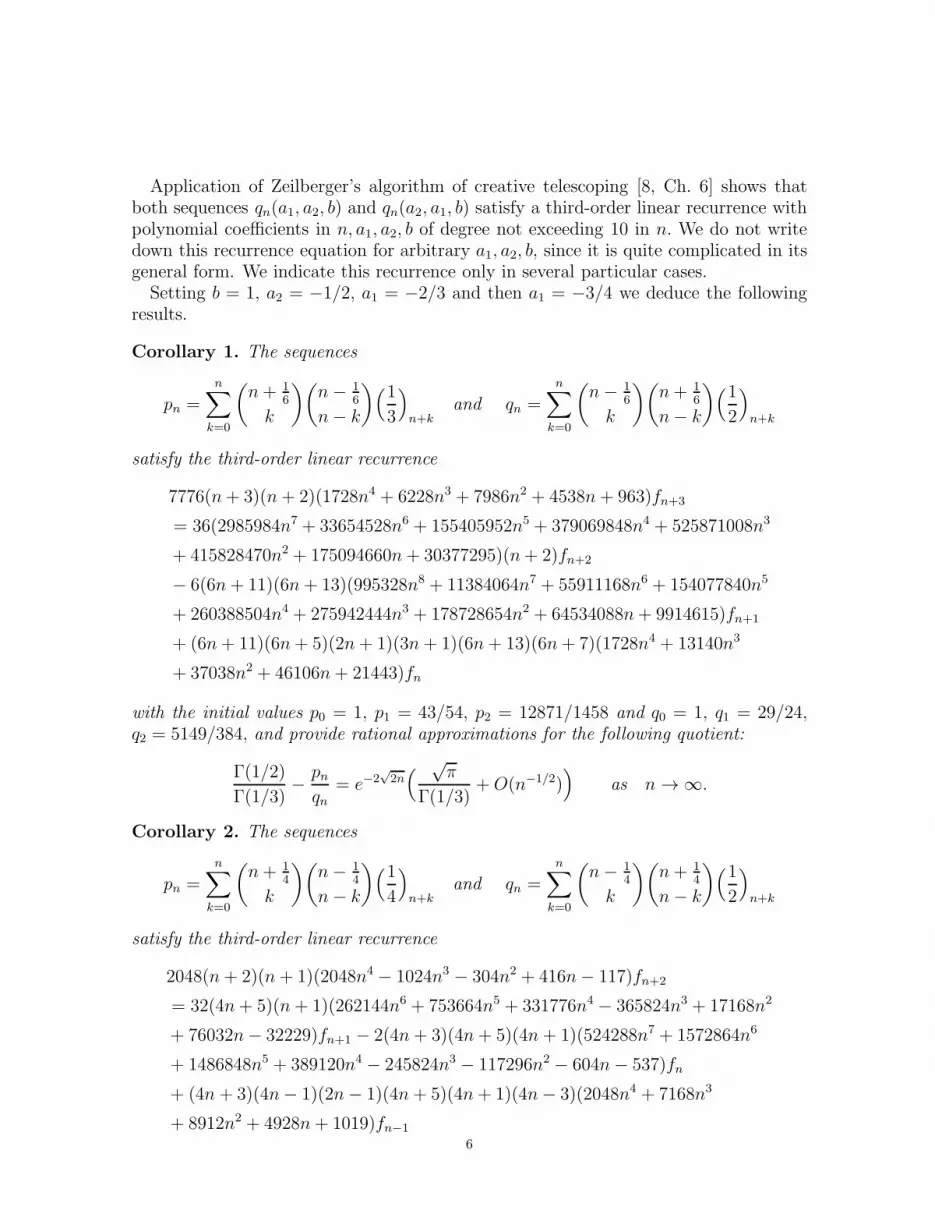
Application of Zeilberger’s algorithm of creative telescoping [8, Ch. 6] shows thatboth sequences qn(a1, a2, b) and qn(a2, a1, b) satisfy a third-order linear recurrence withpolynomial coefficients in n, a1, a2, b of degree not exceeding 10 in n. We do not writedown this recurrence equation for arbitrary a1, a2, b, since it is quite complicated in itsgeneral form. We indicate this recurrence only in several particular cases.
Setting b = 1, a2 = −1/2, a1 = −2/3 and then a1 = −3/4 we deduce the followingresults.
Corollary 1. The sequences
pn =
n∑
k=0
(
n+ 16
k
)(
n− 16
n− k
)
(1
3
)
n+kand qn =
n∑
k=0
(
n− 16
k
)(
n+ 16
n− k
)
(1
2
)
n+k
satisfy the third-order linear recurrence
7776(n+ 3)(n+ 2)(1728n4 + 6228n3 + 7986n2 + 4538n+ 963)fn+3
= 36(2985984n7 + 33654528n6 + 155405952n5 + 379069848n4 + 525871008n3
+ 415828470n2 + 175094660n+ 30377295)(n+ 2)fn+2
− 6(6n+ 11)(6n+ 13)(995328n8 + 11384064n7 + 55911168n6 + 154077840n5
+ 260388504n4 + 275942444n3 + 178728654n2 + 64534088n+ 9914615)fn+1
+ (6n+ 11)(6n+ 5)(2n+ 1)(3n+ 1)(6n+ 13)(6n+ 7)(1728n4 + 13140n3
+ 37038n2 + 46106n+ 21443)fn
with the initial values p0 = 1, p1 = 43/54, p2 = 12871/1458 and q0 = 1, q1 = 29/24,q2 = 5149/384, and provide rational approximations for the following quotient:
Γ(1/2)
Γ(1/3)− pnqn
= e−2√2n(
√π
Γ(1/3)+O(n−1/2)
)
as n→ ∞.
Corollary 2. The sequences
pn =n
∑
k=0
(
n+ 14
k
)(
n− 14
n− k
)
(1
4
)
n+kand qn =
n∑
k=0
(
n− 14
k
)(
n+ 14
n− k
)
(1
2
)
n+k
satisfy the third-order linear recurrence
2048(n+ 2)(n+ 1)(2048n4 − 1024n3 − 304n2 + 416n− 117)fn+2
= 32(4n+ 5)(n+ 1)(262144n6 + 753664n5 + 331776n4 − 365824n3 + 17168n2
+ 76032n− 32229)fn+1 − 2(4n+ 3)(4n+ 5)(4n+ 1)(524288n7 + 1572864n6
+ 1486848n5 + 389120n4 − 245824n3 − 117296n2 − 604n− 537)fn
+ (4n+ 3)(4n− 1)(2n− 1)(4n+ 5)(4n+ 1)(4n− 3)(2048n4 + 7168n3
+ 8912n2 + 4928n+ 1019)fn−1
6

with the initial values p0 = 1, p1 = 37/64, p2 = 50685/8192 and q0 = 1, q1 = 19/16,q2 = 6525/512, and provide rational approximations for the following quotient:
Γ(1/2)
Γ(1/4)− pnqn
= e−2√2n(
√2π
Γ(1/4)+O(n−1/2)
)
as n→ ∞.
Setting a1 = 0, a2 = a, b = 1 in Theorem 1 we get rational approximations for valuesof the Gamma function.
Corollary 3. Let a ∈ Q \ Z, a > −1. Then the sequences
pn =
n∑
k=0
(
n+ a
k
)(
n− a
n− k
)
(n + k)! and qn =
n∑
k=0
(
n− a
k
)(
n+ a
n− k
)
(a + 1)n+k
satisfy the third-order recurrence
λ2(n, a)fn+2 + λ1(n, a)fn+1 + λ0(n, a)fn + λ−1(n, a)fn−1 = 0,
where
λ2(n, a) = (n+ 2)(16n3 + 20n2a + 10na2 + 2a3 + 17n2 + 14na+ 3a2 + n− a),
λ1(n, a) = −128n6 − 224n5a− 112n4a2 + 20n3a3 + 42n2a4 + 16na5 + 2a6 − 808n5
− 1228n4a− 601n3a2 − 45n2a3 + 47na4 + 11a5 − 1910n4 − 2446n3a
− 1085n2a2 − 176na3 − 3a4 − 2035n3 − 2063n2a− 715na2 − 91a3 − 887n2
− 592na− 113a2 − 82n+ 14a,
λ0(n, a) = (n− a+ 1)(n+ a + 1)(256n6 + 576n5a + 544n4a2 + 272n3a3 + 72n2a4
+ 8na5 + 1296n5 + 2384n4a + 1724n3a2 + 596n2a3 + 92na4 + 4a5 + 2448n4
+ 3518n3a+ 1840n2a2 + 404na3 + 30a4 + 2185n3 + 2333n2a+ 817na2 + 93a3
+ 923n2 + 668na+ 125a2 + 146n+ 58a),
λ−1(n, a) = −(n− a)(n− a + 1)(n+ a+ 1)(16n3 + 20n2a + 10na2 + 2a3 + 65n2
+ 54na+ 13a2 + 83n+ 33a+ 34)(n+ a)2,
with the initial conditions
p0 = 1, p1 = 3 + a, p2 = 50 + 33a+ 7a2,q0 = 1, q1 = (a+ 1)(3− a2), q2 = (a+ 1)(a+ 2)(a4 + 2a3 − 12a2 − 11a+ 50)/2,
and provide rational approximations for the following value of the Gamma function:
Γ(a + 1)− pnqn
= e−2√2n( 2πa
Γ(1− a)+O(n−1/2)
)
as n→ ∞.
Another positive feature of our considerations is the fact that we can prove a simplerformula for the numerator pn(a, b) of rational approximations (8) than a representationgiven by (9).
7

Theorem 2. For the sequence pn(a, b), n = 0, 1, 2, . . . , defined by (9), a more compact
formula is valid
pn(a, b) =n
∑
k=0
(
n
k
)2
(a+ 1)n+k bn−k(Hn+k(a) + 2Hn−k − 2Hk).
As a consequence, we get a simple formula for the numerator pn of rational approxi-mations (3) to Euler’s constant.
Corollary 4. The sequences pn and qn, n = 0, 1, 2, . . . , defined by the recurrence (1)with initial conditions (2) are given by the formulas
qn =n
∑
k=0
(
n
k
)2
(n+ k)!,
pn =n
∑
k=0
(
n
k
)2
(n+ k)!(Hn+k + 2Hn−k − 2Hk).
2. Analytical construction
Let a1, a2, b be arbitrary rational numbers such that a1 − a2 6∈ Z, a1, a2 > −1, b > 0.The construction of rational approximations to the numbers Γ(a2+1)/(Γ(a1+1)ba2−a1)is based on the integral
(16) Rn := Rn(a1, a2, b) = b2n+1
∫ ∞
0
(xa2 − xa1)Q(a1,a2,b)n (x)e−bx dx,
where the polynomial Q(a1,a2,b)n (x) is defined in (5).
Lemma 1. Let a1, a2, b ∈ Q, a1 − a2 6∈ Z, a1, a2 > −1, b > 0. Then we have
Rn(a1, a2, b) = qn(a1, a2, b)Γ(a2 + 1)
ba2− qn(a2, a1, b)
Γ(a1 + 1)
ba1,
where qn(a1, a2, b) is defined in Theorem 1,
(17) qn(a1, a2, b) =b2n+a2+1
Γ(a2 + 1)
∫ ∞
0
xa2Q(a1,a2,b)n e−bx dx
and µna2−a1
µ2na2qn(a1, a2, b) ∈ n!Z[b].
Proof. Substituting (5) into (16) we get
Rn(a1, a2, b) =b2n+1
n!2
∫ ∞
0
(xn+a2−a1(xn+a1(1− x)2n+1e−bx)(n))(n)
1− xdx
− b2n+1
n!2
∫ ∞
0
xa1−a2
1− x(xn+a2−a1(xn+a1(1− x)2n+1e−bx)(n))(n) dx.
(18)
8

Denoting the first integral on the right-hand side of (18) by I1 and applying n-integrationsby parts, we have
I1 =(−1)nb2n+1
n!
∫ ∞
0
xn+a2−a1
(1− x)n+1
(
xn+a1(1− x)2n+1e−bx)(n)
dx
=b2n+1
n!
∫ ∞
0
(
xn+a2−a1
(1− x)n+1
)(n)
xn+a1(1− x)2n+1e−bx dx.
Now using the following relation for hypergeometric functions (see [7, §3.4, (11)]):(19)dn
dxn[xα(1− x)β ] = (α− n+1)nx
α−n(1− x)β−n2F1
(−n, α + 1 + β − n
α + 1− n
∣
∣
∣
∣
x
)
, n−α 6∈ N,
with α = n + a2 − a1, β = −n− 1, we get(
xn+a2−a1
(1− x)n+1
)(n)
= (a2 − a1 + 1)nxa2−a1(1− x)−2n−1
2F1
(−n, a2 − a1 − n
a2 − a1 + 1
∣
∣
∣
∣
x
)
and therefore,
I1 =b2n+1(1 + a2 − a1)n
n!
∫ ∞
0
xn+a22F1
(−n, a2 − a1 − n
a2 − a1 + 1
∣
∣
∣
∣
x
)
e−bx dx
=b2n+1(1 + a2 − a1)n
n!
n∑
k=0
(−n)k(a2 − a1 − n)kk! (1 + a2 − a1)k
∫ ∞
0
xn+a2+ke−bx dx
= b2n+1
n∑
k=0
(
n + a1 − a2k
)(
n+ a2 − a1n− k
)
Γ(n + a2 + k + 1)
bn+a2+k+1.
(20)
Thus we have
I1 = qn(a1, a2, b)Γ(a2 + 1)
ba2,
which implies (17). Similarly, denoting the second integral on the right-hand side of(18) by I2 and integrating by parts, we have
(21) I2 =(−1)nb2n+1
n!2
∫ ∞
0
(
xa1−a2
1− x
)(n)
xn+a2−a1(xn+a1(1− x)2n+1e−bx)(n) dx.
Applying formula (19) with α = a1 − a2, β = −1 we get(
xa1−a2
1− x
)(n)
= (a1 − a2 − n + 1)nxa1−a2−n(1− x)−n−1
2F1
(−n, a1 − a2 − n
a1 − a2 − n + 1
∣
∣
∣
∣
x
)
.
Substituting the n-th derivative into the integral (21) and integrating by parts we obtain
I2 =b2n+1(a1 − a2 − n + 1)n
n!2
×∫ ∞
0
(
(1− x)−n−12F1
(−n, a1 − a2 − n
a1 − a2 − n+ 1
∣
∣
∣
∣
x
))(n)
xn+a1(1− x)2n+1e−bx dx.
9

Using the following relation (see [7, §3.4, (10)]):dn
dxn
[
(1− x)α+β−δ2F1
(
α, β
δ
∣
∣
∣
∣
x
)]
=(δ − α)n(δ − β)n
(δ)n(1− x)α+β−δ−n
2F1
(
α, β
δ + n
∣
∣
∣
∣
x
)
with α = −n, β = a1 − a2 − n, δ = a1 − a2 − n+ 1 we can compute the n-th derivativein the last integral
(
(1− x)−n−12F1
(−n, a1 − a2 − n
a1 − a2 − n+ 1
∣
∣
∣
∣
x
))(n)
=(a1 − a2 + 1)n n!
(a1 − a2 − n+ 1)n(1− x)−2n−1
× 2F1
(−n, a1 − a2 − n
a1 − a2 + 1
∣
∣
∣
∣
x
)
to get
I2 =b2n+1(a1 − a2 + 1)n
n!
∫ ∞
0
xn+a12F1
(−n, a1 − a2 − n
a1 − a2 + 1
∣
∣
∣
∣
x
)
e−bx dx.
Comparing this integral with (20) we obtain
I2 = qn(a2, a1, b)Γ(a1 + 1)
ba1,
and the desired expansion of Rn(a1, a2, b) is proved.From the definition of the sequence qn(a1, a2, b) it follows that qn(a1, a2, b) ∈ Q[b]. To
estimate its denominators we need the following property of binomial coefficients (see[5, lemma 4.1]):
(22) µka ·
(a)kk!
∈ Z if a ∈ Q.
Then according to (22), the numbers
µ2na2µna2−a1
(
n + a2 − a1n− k
)(
n+ a1 − a2k
)
(a2 + 1)n+k
(n + k)!
are integers for k = 0, 1, . . . , n. This proves the lemma. �
Remark 1. From Lemma 1 it follows that Rn(a1, a2, b) = −Rn(a2, a1, b). Note that this
symmetry property can be obtained directly from (16), since we have Q(a1,a2,b)n (x) =
Q(a2,a1,b)n (x). The last equality follows easily from the Rodrigues formula (5) and the
fact (see [2, Ex.]) that the Rodrigues operators corresponding to the weights w1 andw2 in (5) commute.
Note that by the analogous arguments, the Rivoal construction (12) and therefore,the polynomials Pn(a, x), Qn(a, x) possess a similar symmetry. Indeed, if we define thegeneralized Laguerre polynomial (see [2, §3.2])
An,a1,a2(x) =x−a2ex
n!2(xn+a2−a1(xn+a1e−x)(n))(n)
=(a1 + 1)n(a2 + 1)n
n!2ex2F2
(
a1 + n+ 1, a2 + n+ 1
a1 + 1, a2 + 1
∣
∣
∣
∣
− x
)
10
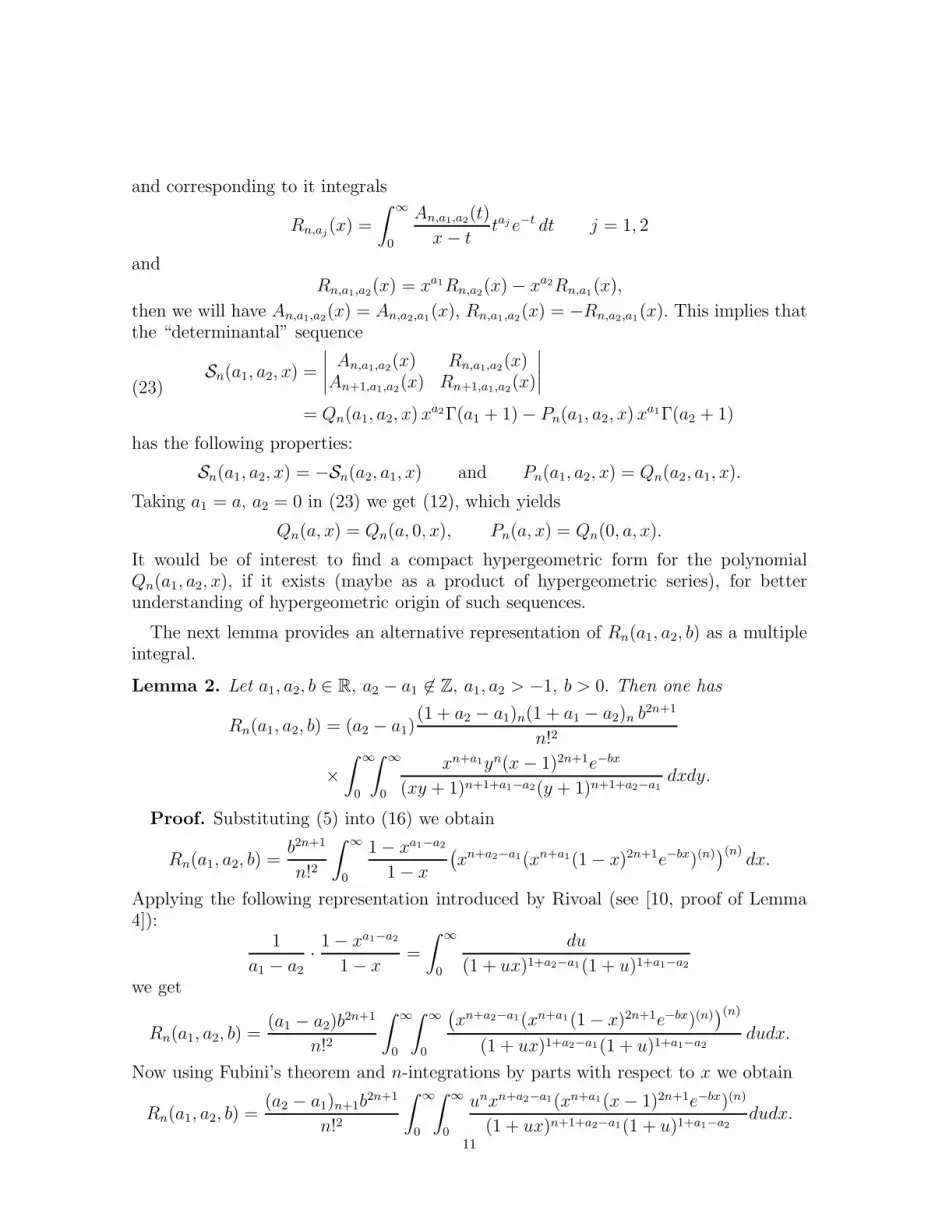
and corresponding to it integrals
Rn,aj(x) =
∫ ∞
0
An,a1,a2(t)
x− ttaje−t dt j = 1, 2
andRn,a1,a2(x) = xa1Rn,a2(x)− xa2Rn,a1(x),
then we will have An,a1,a2(x) = An,a2,a1(x), Rn,a1,a2(x) = −Rn,a2,a1(x). This implies thatthe “determinantal” sequence
Sn(a1, a2, x) =
∣
∣
∣
∣
An,a1,a2(x) Rn,a1,a2(x)An+1,a1,a2(x) Rn+1,a1,a2(x)
∣
∣
∣
∣
= Qn(a1, a2, x) xa2Γ(a1 + 1)− Pn(a1, a2, x) x
a1Γ(a2 + 1)
(23)
has the following properties:
Sn(a1, a2, x) = −Sn(a2, a1, x) and Pn(a1, a2, x) = Qn(a2, a1, x).
Taking a1 = a, a2 = 0 in (23) we get (12), which yields
Qn(a, x) = Qn(a, 0, x), Pn(a, x) = Qn(0, a, x).
It would be of interest to find a compact hypergeometric form for the polynomialQn(a1, a2, x), if it exists (maybe as a product of hypergeometric series), for betterunderstanding of hypergeometric origin of such sequences.
The next lemma provides an alternative representation of Rn(a1, a2, b) as a multipleintegral.
Lemma 2. Let a1, a2, b ∈ R, a2 − a1 6∈ Z, a1, a2 > −1, b > 0. Then one has
Rn(a1, a2, b) = (a2 − a1)(1 + a2 − a1)n(1 + a1 − a2)n b
2n+1
n!2
×∫ ∞
0
∫ ∞
0
xn+a1yn(x− 1)2n+1e−bx
(xy + 1)n+1+a1−a2(y + 1)n+1+a2−a1dxdy.
Proof. Substituting (5) into (16) we obtain
Rn(a1, a2, b) =b2n+1
n!2
∫ ∞
0
1− xa1−a2
1− x
(
xn+a2−a1(xn+a1(1− x)2n+1e−bx)(n))(n)
dx.
Applying the following representation introduced by Rivoal (see [10, proof of Lemma4]):
1
a1 − a2· 1− xa1−a2
1− x=
∫ ∞
0
du
(1 + ux)1+a2−a1(1 + u)1+a1−a2
we get
Rn(a1, a2, b) =(a1 − a2)b
2n+1
n!2
∫ ∞
0
∫ ∞
0
(
xn+a2−a1(xn+a1(1− x)2n+1e−bx)(n))(n)
(1 + ux)1+a2−a1(1 + u)1+a1−a2dudx.
Now using Fubini’s theorem and n-integrations by parts with respect to x we obtain
Rn(a1, a2, b) =(a2 − a1)n+1b
2n+1
n!2
∫ ∞
0
∫ ∞
0
unxn+a2−a1(xn+a1(x− 1)2n+1e−bx)(n)
(1 + ux)n+1+a2−a1(1 + u)1+a1−a2dudx.
11

Making the change of variable u = 1/(xy) or y = 1/(xu) in the last integral we get
Rn(a1, a2, b) =(a2 − a1)n+1b
2n+1
n!2
∫ ∞
0
∫ ∞
0
(xn+a1(x− 1)2n+1e−bx)(n)
(y + 1)n+1+a2−a1(xy + 1)1+a1−a2dxdy.
Finally, integrating by parts with respect to x we obtain the desired representation andthe lemma is proved. �
Our next concern will be the asymptotic behavior of the sequences qn(a1, a2, b) andRn(a1, a2, b).
Lemma 3. Let a1, a2, b ∈ R, a2 − a1 6∈ Z, a1, a2 > −1, b > 0. Then the following
asymptotic formulas are valid:
Rn(a1, a2, b) = (2n)!e−
√2bn
n1/4−(a1+a2)/2
(
2 sin(π(a2 − a1))Γ(a2 + 1)
ba2c2 +O(n−1/2)
)
,
qn(a1, a2, b) = (2n)!e√2bn
n1/4−(a1+a2)/2
(
c2 +O(n−1/2))
as n→ ∞,
where the constant c2 is defined in Theorem 1.
Proof. To obtain the asymptotic behavior of the above sequences, we proceed anal-ogously to the proof of Lemma 5 in [6]. Substituting (5) into (17) and integrating byparts we have
qn(a1, a2, b) =(−1)n
n!
b2n+a2+1
Γ(a2 + 1)
∫ ∞
0
xn+a1(x− 1)2n+1e−bx
(
xn+a2−a1
(x− 1)n+1
)(n)
dx.
Further, repeating the arguments such as those used in [4, p.56-59] we get
qn(a1, a2, b) =b2n+a2+1
Γ(a2 + 1)
n2n+(a1+a2)/2+3/4
2√π
∫ ∞
0
enϕ1(y)ψ1(y) dy · (1 +O(n−1/2)),
where
ϕ1(y) = 2 ln(√y + 1/
√n) + ln y − by, ψ1(y) = (
√y + 1/
√n)y(a1+a2)/2−1/4.
The last integral coincides with the corresponding integral from [6, Lemma 5] andlikewise, by the Laplace method, we obtain
qn(a1, a2, b) =(2n)2n+(a1+a2)/2+1/4
Γ(a2 + 1)b1/4+(a1−a2)/2e−2n+
√2bn−3b/8
(
1 +O(n−1/2))
= (2n)!n(a1+a2)/2−1/4e√2bn
(
c2 +O(n−1/2))
,
where the constant c2 = c2(a1, a2, b) is defined in Theorem 1.Making the change of variables x = nu, y = v/
√nu in the double integral of Lemma 2
we get
Rn =Γ(n+ 1 + a2 − a1)Γ(n+ 1 + a1 − a2)
n!2Γ(a2 − a1)Γ(1 + a1 − a2)b2n+1n3n+2+(a1+a2)/2
∫ ∞
0
g(u, v)fn(u, v) dudv,
where
f(u, v) =uv(u− 1/n)2e−bu
(v +√nu)(v
√nu+ 1)
, g(u, v) =u(a1+a2)/2(u− 1/n)
(v +√nu)1+a2−a1(v
√nu+ 1)1+a1−a2
.
12

Using the reflection formula
Γ(a2 − a1) · Γ(1 + a1 − a2) =π
sin(π(a2 − a1))
and Stirling’s formula for the gamma function
Γ(n+ 1 + a2 − a1) = na2−a1n!(
1 +O(n−1/2))
as n→ ∞we get
Rn =sin(π(a2 − a1))
πb2n+1n3n+2+(a1+a2)/2
∫ ∞
0
g(u, v)fn(u, v) dudv ·(
1 +O(n−1))
.
Now applying the Laplace method for multiple integrals by the same way as in theproof of Lemma 5 [6] with the only difference that in our case
g(u0, v0) =1
n
(
2
b
)
a1+a22
(
1 +O(n−1/2))
,
we obtain
Rn = 2 sin(π(a2 − a1))(2n)2n+1/4+(a1+a2)/2
b1/4+(a1+a2)/2e−2n−
√2bn−3b/8
(
1 +O(n−1/2))
= (2n)!e−√2bnn(a1+a2)/2−1/4
(
2 sin(π(a2 − a1))Γ(a2 + 1)
ba2c2 +O(n−1/2)
)
and the lemma is proved. �
Now Theorem 1 follows easily from Lemmas 1–3.
3. Proof of Theorem 2.
It is readily seen that the construction (7) is a limiting case of Theorem 1. Indeed,comparing Lemma 2 with Lemmas 3, 4 from [6] we get
(24) lima2→a1
ba1
Γ(a1 + 1)
Rn(a1, a2, b)
a2 − a1= pn(a1, b)− (ln b− ψ(a1 + 1))qn(a1, b).
On the other hand, by Lemma 1, we have
lima2→a1
ba1
Γ(a1 + 1)
Rn(a1, a2, b)
a2 − a1= lim
a2→a1
1
a2 − a1
(
qn(a1, a2, b)Γ(a2 + 1)/ba2
Γ(a1 + 1)/ba1− qn(a2, a1, b)
)
= lima2→a1
qn(a1, a2, b)
Γ(a1 + 1)·
Γ(a2+1)ba2−a1
− Γ(a1 + 1)
a2 − a1+ lim
a2→a1
qn(a1, a2, b)− qn(a2, a1, b)
a2 − a1
=qn(a1, a1, b)
Γ(a1 + 1)· d
da2
(
Γ(a2 + 1)
ba2−a1
)∣
∣
∣
∣
a2=a1
+ lima2→a1
qn(a1, a2, b)− qn(a2, a1, b)
a2 − a1.
Taking into account that
d
da2
(
Γ(a2 + 1)
ba2−a1
)
=Γ(a2 + 1)
ba2−a1(ψ(a2 + 1)− ln b),
13

we obtain(25)
lima2→a1
ba1
Γ(a1 + 1)
Rn(a1, a2, b)
a2 − a1= qn(a1, b)(ψ(a1+1)−ln b)+ lim
a2→a1
qn(a1, a2, b)− qn(a2, a1, b)
a2 − a1.
Comparing the right-hand sides of (24) and (25) we conclude that
pn(a1, b) = lima2→a1
qn(a1, a2, b)− qn(a2, a1, b)
a2 − a1.
To evaluate the above limit, we need the following expansions:(
n+ a1 − a2k
)
=
(
n
k
)
−(
n
k
)
(Hn −Hn−k)(a2 − a1) +O(
(a2 − a1)2)
,
(
n+ a2 − a1n− k
)
=
(
n
k
)
+
(
n
k
)
(Hn −Hk)(a2 − a1) +O(
(a2 − a1)2)
,
(a2 + 1)n+k = (a1 + 1)n+k + (a1 + 1)n+kHn+k(a1)(a2 − a1) +O(
(a2 − a1)2)
.
Then a straightforward verification shows that
pn(a1, b) =
n∑
k=0
bn−k
(
n
k
)2
(a1 + 1)n+k(Hn+k(a1) + 2Hn−k − 2Hk),
and this is precisely the assertion of Theorem 2. �
Setting a1 = 0, b = 1 yields Corollary 4.
Remark 2. Note that an analogous conclusion can be drawn for the polynomialsPn(x), Qn(x) from (11). Comparing [9, Lemma 1] with [10, Lemma 4] gives
Sn(x) = lima→0
−1
a xa· Sn(a, x).
Then analysis similar to that in the proof of Theorem 2 shows that Qn(x) = Qn(0, x) =Qn(0, 0, x) and
Pn(x) = lima→0
Qn(a, x)− Pn(a, x)
a= lim
a→0
Qn(a, 0, x)−Qn(0, a, x)
a,
where the polynomial Qn(a1, a2, x) is defined in Remark 1.
References
[1] A. I. Aptekarev (ed.), Rational approximation of Euler’s constant and recurrence relations, CurrentProblems in Math., (2007), vol. 9, Steklov Math. Inst. RAN. (Russian)
[2] A. I. Aptekarev, A. Branquinho, and W. Van Assche, Multiple orthogonal polynomials for classical
weights, Trans. Amer. Math. Soc. 355 (2003), 3887–3914.[3] A. I. Aptekarev, D. N. Tulyakov, Four-term recurrence relations for γ-forms, in [1], p.37–43.[4] A. I. Aptekarev, V. G. Lysov, Asymptotics of γ-forms jointly generated by orthogonal polynomials,
in [1], p.55–62.[5] G. V. Chudnovsky, On the method of Thue-Siegel, Ann. of Math. (2) 117 (1983), no. 2, 325–382.[6] Kh. Hessami Pilehrood, T. Hessami Pilehrood, Rational approximations for values of the digamma
function and a denominators conjecture, arXiv:1004.0578v1[math.NT][7] Yu. L. Luke, The special functions and their approximations, Vol. 1, Academic Press, 1969.[8] M. Petkovsek, H. Wilf, D. Zeilberger, A=B, A. K. Peters. Ltd, 1997.
14

[9] T. Rivoal, Rational approximations for values of derivatives of the Gamma function, Trans. Amer.Math. Soc. 361 (2009), 6115–6149.
[10] T. Rivoal, Approximations rationnelles des valeurs de la fonction Gamma aux rationneels, J. Num-ber Theory, 130 (2010), 944–955.
[11] D. N. Tulyakov, A system of recurrence relations for rational approximations of the Euler constant,
Math. Notes 85 (2009), no. 5, 746–750.
Mathematics Department, Faculty of Basic Sciences, Shahrekord University,Shahrekord, P.O. Box 115, Iran.
School of Mathematics, Institute for Research in Fundamental Sciences (IPM),P.O.Box 19395-5746, Tehran, Iran
E-mail address : [email protected], [email protected], [email protected]
15


