QUASI-GEOMETRIC DISCOUNTING: A CLOSED-FORM

SOLUTION UNDER THE EXPONENTIAL UTILITY FUNCTION*

Lilia Maliar and Serguei Maliar**

WP-AD 2003-16

Correspondence to: Universidad de Alicante, Departamento de Fundamentos del Análisis Económico, Campus San Vicente del Raspeig, Ap. Correos, 99, 03080 Alicante (Spain). E-mails: maliarl@merlin.fae.ua.es, maliars@merlin.fae.ua.es. Editor: Instituto Valenciano de Investigaciones Económicas, S.A. Primera Edición Abril 2003 Depósito Legal: V-1907-2003 IVIE working papers offer in advance the results of economic research under way in order to encourage a discussion process before sending them to scientific journals for their final publication.

* We have benefited from the comments of an anonymous referee and managing editor, Gianni De Fraja. All errors are ours. This research was partially supported by the Instituto Valenciano de Investigaciones Económicas and the Ministerio de Ciencia y Tecnología de España, BEC 2001-0535. ** Universidad de Alicante.

2

QUASI-GEOMETRIC DISCOUNTING: A CLOSED-FORM SOLUTION UNDER THE EXPONENTIAL UTILITY FUNCTION

Lilia Maliar and Serguei Maliar

ABSTRACT

This paper studies a discrete-time utility maximization problem of an infinitely-lived quasi-geometric consumer whose labor income is subject to uninsurable idiosyncratic productivity shocks. We restrict attention to a first-order Markov recursive solution. We show that under the assumption of the exponential utility function, the problem of the quasi-geometric consumer admits a closed-form solution. Keywords: quasi-geometric (quasi-hyperbolic) discounting, idiosyncratic shocks, closed-form solution. JEL Classification: D91, E21, G11

A large body of recent literature investigates the consumption-savings be-

havior of agents under the assumption of quasi-geometric (quasi-hyperbolic)

discounting, e.g., Laibson (1997), Barro (1999), Harris and Laibson (2001),

Krusell, Kurusçu and Smith (2002), Krusell and Smith (2003), Luttmer and

Mariotti (2003). Krusell and Smith (2003) incorporate quasi-geometric dis-

counting into a deterministic version of the standard infinite-horizon neo-

classical growth model. In particular, they show that under the assumptions

of logarithmic utility function, Cobb-Douglas production function and full

depreciation of capital, the model allows for a closed-form solution.

This paper describes another model with quasi-geometric discounting that

can be solved analytically. We study a discrete-time utility maximization

problem of an infinitely-lived quasi-geometric consumer whose labor income

is subject to uninsurable idiosyncratic productivity shocks. We restrict at-

tention to a first-order Markov recursive solution. We show that under the

assumption of the exponential utility function, the problem of such a con-

sumer admits a closed-form solution. Our results can be viewed as an exten-

sion of the work of Caballero (1990), who derived a closed-form solution for

the standard geometric-discounting case.

3

At each date t ∈ {0, 1, 2, ...}, an agent solves the following problem

max{cτ ,aτ+1}∞τ=t

u (ct) +Et

∞

τ=t

βδτ+1−tu (cτ+1) (1)

subject to

cτ + aτ+1 = wsτ + (1 + r) aτ , (2)

where initial condition (at, st) is given. Here, β > 0 and δ ∈ (0, 1) are the dis-

counting parameters; cτ and aτ are consumption and asset holdings, respec-

tively; sτ is an idiosyncratic productivity shock following a first-order Markov

process; r and w are the interest rate and wage per unit of efficiency labor,

respectively; Eτ is the expectation, conditional on all information about the

agent’s idiosyncratic shocks available at τ .

It is typically assumed in the literature on quasi-geometric discounting

that a discount factor, applied between today and tomorrow, is lower than

the one, used on all dates advanced further in the future, β < 1. This

leads to the following form of time-inconsistency in preferences: the agent

systematically plans to be patient (to save much) tomorrow, but as tomorrow

arrives, she always changes her mind and behaves impatiently (saves little).

One can also consider the opposite case, β > 1, when the agent always

behaves more patiently than she originally planned. The parameterization

4

β = 1 corresponds to the standard geometric-discounting case, when the

agent is equally patient in both the short-run and the long-run.

We consider a recursive Markov solution to the problem (1) , (2), such

that in all periods, the agent decides on consumption according to the same

decision rule ct = C (at, st). Then, without time subscripts, the recursive

formulation of the individual problem is as follows:

W (a, s) = maxc{u (c) + βδE [V (a , s ) | s]} , (3)

where given a, s, the value function V solves the functional equation

V (a, s) = u [C (a, s)] + δE {V [ws+ (1 + r) a− C (a, s) ; s ] | s} (4)

subject to the budget constraint

a = ws+ (1 + r) a− c. (5)

The problem (3) − (5) is to be solved for the unknown value functions

W (a, s) , V (a, s) and the decision rule C (a, s).

We shall assume that the agent has the exponential momentary utility

function

u (ct) = −1θexp (−θct) , θ > 0. (6)

5

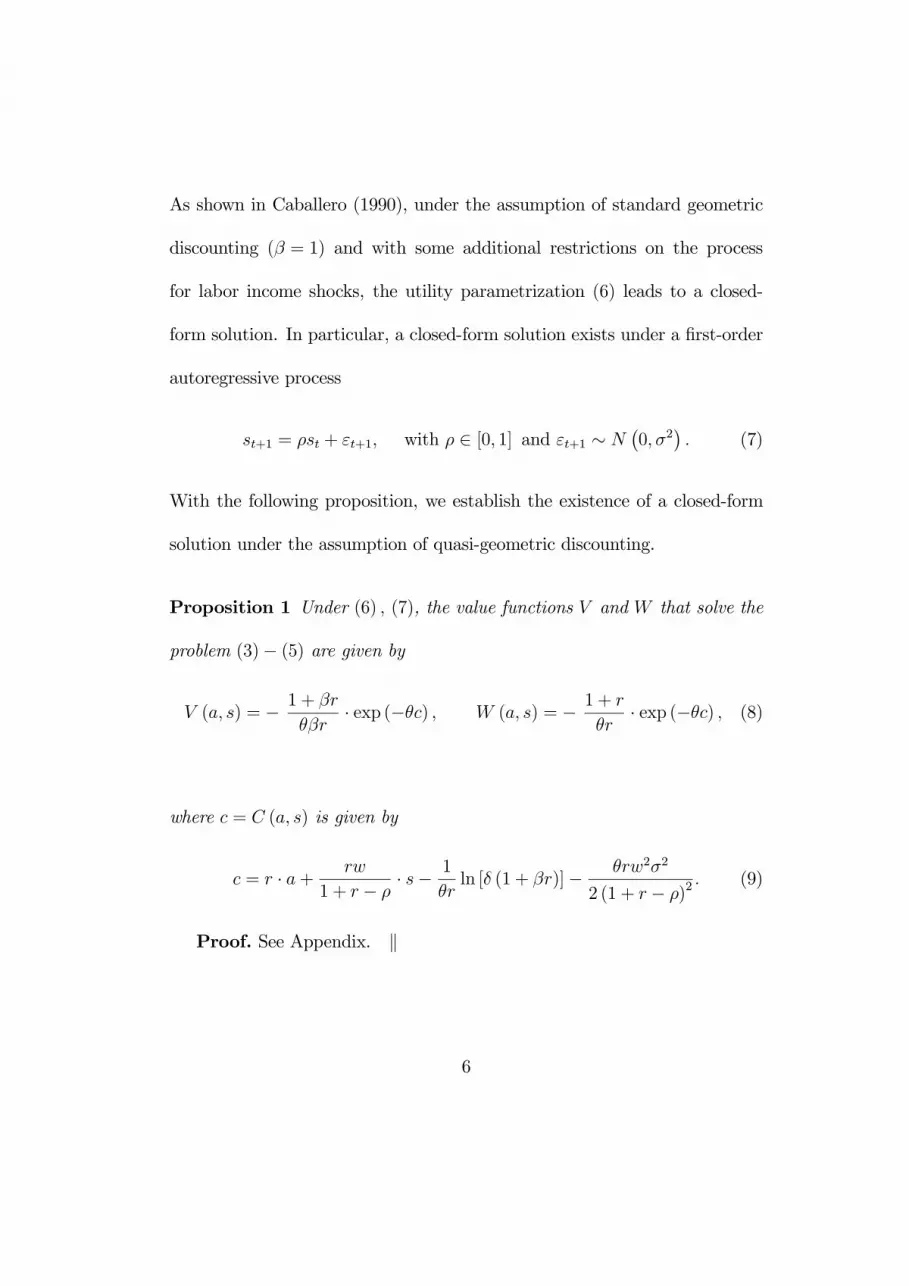
As shown in Caballero (1990), under the assumption of standard geometric

discounting (β = 1) and with some additional restrictions on the process

for labor income shocks, the utility parametrization (6) leads to a closed-

form solution. In particular, a closed-form solution exists under a first-order

autoregressive process

st+1 = ρst + εt+1, with ρ ∈ [0, 1] and εt+1 ∼ N 0,σ2 . (7)

With the following proposition, we establish the existence of a closed-form

solution under the assumption of quasi-geometric discounting.

Proposition 1 Under (6) , (7), the value functions V and W that solve the

problem (3)− (5) are given by

V (a, s) = − 1 + βr

θβr· exp (−θc) , W (a, s) = − 1 + r

θr· exp (−θc) , (8)

where c = C (a, s) is given by

c = r · a+ rw

1 + r − ρ· s− 1

θrln [δ (1 + βr)]− θrw2σ2

2 (1 + r − ρ)2. (9)

Proof. See Appendix.

6

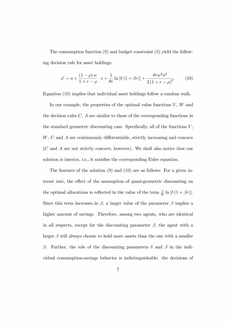
The consumption function (9) and budget constraint (5) yield the follow-

ing decision rule for asset holdings:

a = a+(1− ρ)w

1 + r − ρ· s+ 1

θrln [δ (1 + βr)] +

θrw2σ2

2 (1 + r − ρ)2. (10)

Equation (10) implies that individual asset holdings follow a random walk.

In our example, the properties of the optimal value functions V , W and

the decision rules C, A are similar to those of the corresponding functions in

the standard geometric discounting case. Specifically, all of the functions V ,

W , C and A are continuously differentiable, strictly increasing and concave

(C and A are not strictly concave, however). We shall also notice that our

solution is interior, i.e., it satisfies the corresponding Euler equation.

The features of the solution (9) and (10) are as follows: For a given in-

terest rate, the effect of the assumption of quasi-geometric discounting on

the optimal allocations is reflected in the value of the term 1θrln [δ (1 + βr)].

Since this term increases in β, a larger value of the parameter β implies a

higher amount of savings. Therefore, among two agents, who are identical

in all respects, except for the discounting parameter β, the agent with a

larger β will always choose to hold more assets than the one with a smaller

β. Further, the role of the discounting parameters δ and β in the indi-

vidual consumption-savings behavior is indistinguishable: the decisions of

7

a quasi-geometric consumer with the parameters δ and β = 1 are identi-

cal to those of a standard geometric consumer, β = 1, with the parameter

δ = δ(1+βr)1+r

. Finally, the assumption of quasi-geometric discounting does not

affect the amount of savings for precautionary motives, which are defined

as the difference between the agent’s asset holdings with and without un-

certainty. Indeed, according to (10), precautionary savings are given by the

term θrw2σ2

2(1+r−ρ)2 , which is independent of the discounting parameter β.

References

[1] Barro, R., 1999, Ramsey meets Laibson in the neoclassical growth model,

Quarterly Journal of Economics 114 (4), 1125-1152.

[2] Caballero, R., 1990, Consumption puzzles and precautionary savings,

Journal of Monetary Economics 25, 113-136.

[3] Harris, C. and D. Laibson, 2001, Dynamic choices of hyperbolic con-

sumers, Econometrica 69, 935-959.

[4] Krusell, P. and A. Smith, 2003, Consumption-savings decisions with

quasi-geometric discounting, Manuscript, Econometrica 71, 365-375.

8

[5] Krusell, P., Kurusçu, B. and A. Smith, 2002, Equilibrium welfare and

government policy with quasi-geometric discounting, Journal of Economic

Theory 105, 42-72.

[6] Laibson, D., 1997, Golden eggs and hyperbolic discounting, Quarterly

Journal of Economics 112, 443-477.

[7] Luttmer, E. and T. Mariotti, 2003, Subjective discounting in an exchange

economy, Journal of Political Economy (forthcoming).

Appendix

Proof to Proposition 1. Guess that the value function V has the

following functional form

V (a , s ) = µ0 exp (µ1a + µ2s + µ3) , (11)

where µ0, µ1, µ2, µ3 are some constant coefficients. Substitution (5) and (11)

into equation (3) and the updated version of (4) yields

W (a, s) = maxa

−1θexp [−θ ((1 + r) a+ ws− a )] + βδE [µ0 exp (µ1a + µ2s + µ3)] ,

(12)

9

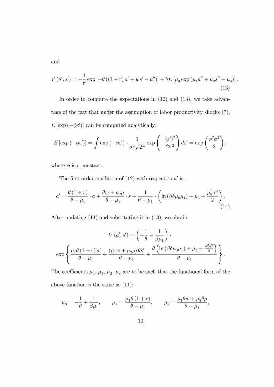
and

V (a , s ) = −1θexp [−θ ((1 + r) a + ws − a )] + δE [µ0 exp (µ1a + µ2s + µ3)] .

(13)

In order to compute the expectations in (12) and (13), we take advan-

tage of the fact that under the assumption of labor productivity shocks (7),

E [exp (−φε )] can be computed analytically:

E [exp (−φε )] = exp (−φε ) · 1

σ2√2πexp −(ε )

2

2σ2dε = exp

φ2σ2

2,

where φ is a constant.

The first-order condition of (12) with respect to a is

a =θ (1 + r)

θ − µ1· a+ θw + µ2ρ

θ − µ1· s+ 1

θ − µ1· ln (βδµ0µ1) + µ3 +

µ22σ2

2.

(14)

After updating (14) and substituting it in (13), we obtain

V (a , s ) = −1θ+

1

βµ1·

exp

µ1θ (1 + r) aθ − µ1+(µ1w + µ2ρ) θs

θ − µ1+

θ ln (βδµ0µ1) + µ3 +µ22σ

2

2

θ − µ1

.The coefficients µ0, µ1, µ2, µ3 are to be such that the functional form of the

above function is the same as (11):

µ0 = −1

θ+

1

βµ1, µ1 =

µ1θ (1 + r)

θ − µ1, µ2 =

µ1θw + µ2θρ

θ − µ1,

10

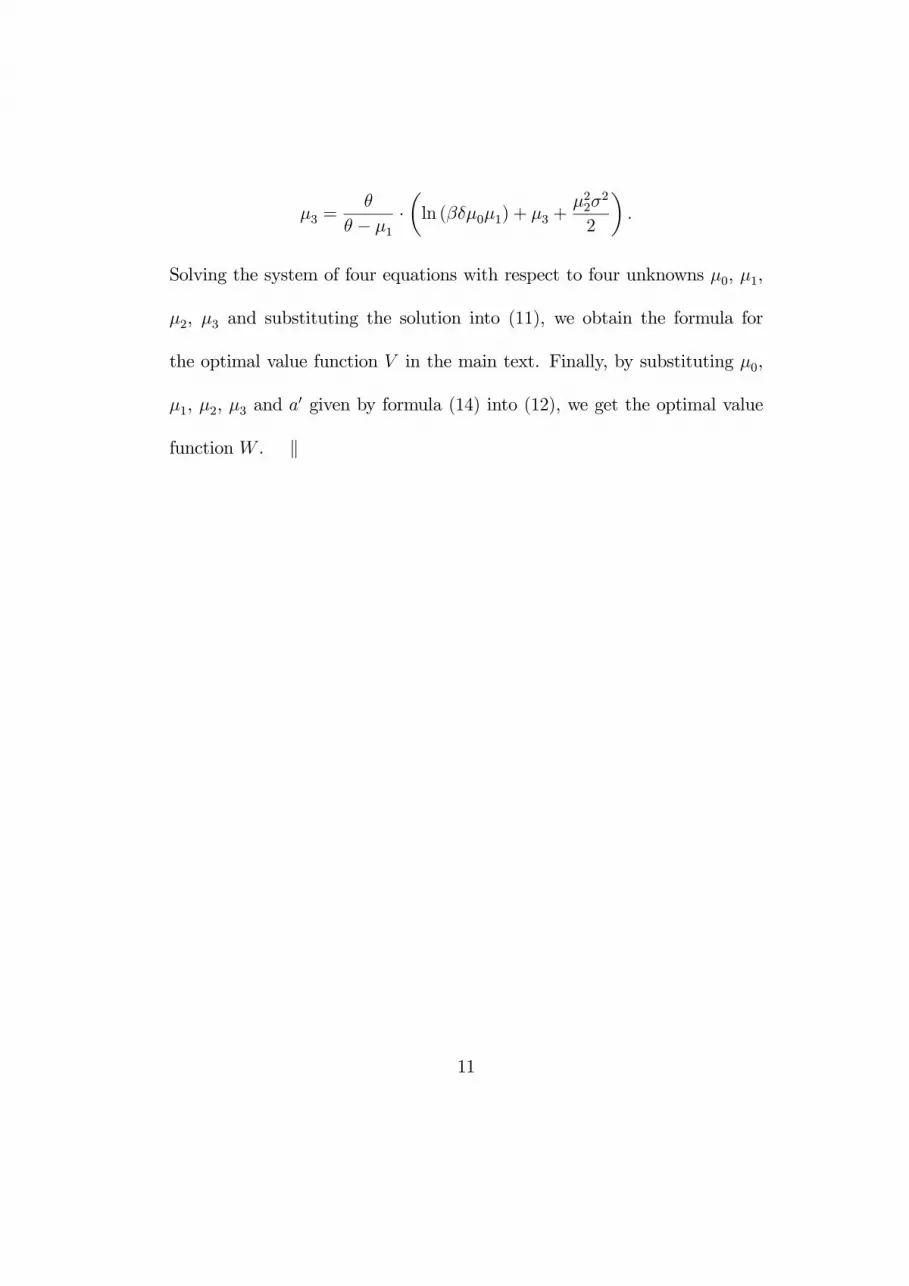
µ3 =θ

θ − µ1· ln (βδµ0µ1) + µ3 +

µ22σ2

2.

Solving the system of four equations with respect to four unknowns µ0, µ1,

µ2, µ3 and substituting the solution into (11), we obtain the formula for

the optimal value function V in the main text. Finally, by substituting µ0,

µ1, µ2, µ3 and a given by formula (14) into (12), we get the optimal value

function W .

11