Stability for multivariate exponential familiesAugust A. Balkema Claudia Kl�uppelberg� Sidney I. ResnickJanuary 18, 2000AbstractA random vector X generates a natural exponential family of vectors X�, � 2 �, where �is the set where the moment generating function (mgf) K(�) = Ee�X is �nite. Assume that �is open and X non-degenerate. Suppose there exist a�ne transformations ��(x) = A�x+a�depending continuously on the parameter � and a non-degenerate vector Y so that��1� (X�)) Ywhen � diverges. In this paper it will be shown that the limit vector satis�es a stabilityrelation. Some examples of this limit relation are presented.

AMS Subject Classi�cations: Primary 60F05; secondary 60E05,44A10Keywords: Esscher, exponential family, Laplace transform, multivariate, stability�Author for correspondence. 1

1 IntroductionExponential group families are of special interest to statisticians. Recently there has also beeninterest in this subject from the quarter of mathematical physics. The book Faraut and Kor�anyi[1994] gives a complete classi�cation of all exponential families which are generated by Lebesguemeasure on proper open symmetric cones invariant under a group of linear transformations.Exponential families are useful tools in the theory of Laplace transformations.In this paper we consider multivariate exponential families which can be normalised to con-verge to a non-degenerate limit. The limit vector generates an exponential family which is stablein the sense that all members of the family are of the same type. In the univariate case the limitdistributions are normal or gamma. The signi�cance of such a limit theorem for the theory ofLaplace transforms was perceived by Feigin and Yashchin [1976]. Nagaev treated the univariatecase in a series of papers dating back to the early sixties. A general univariate theory can befound in two papers by Balkema, Kl�uppelberg and Resnick. These will be referred to as BKR[1999a] and BKR [1999b] in the sequel. The statistical theory for densities in the strong domainof attraction of the multivariate normal distribution has been treated in Barndor�-Nielsen andKl�uppelberg [1999]. The present paper presents a number of general results for the multivariatecase. We shall give concrete results for two multivariate generalisations of the gamma distribu-tion: The uniform distribution on the unit ball, and the multivariate Laplace distribution e�r=c.The latter distribution and its generalisations have also been considered by Nagaev and Zaigraev[1999].Let us now be more speci�c. With a non-degenerate random vector Z is associated an openconvex set D, the convex domain of Z. The closure of D is the smallest closed convex set whichcontains almost every realisation of Z. In this paper we assume that PfZ 2 Dg = 1. Let themgf K of Z converge on a neighbourhood of the origin. The domain of K is the convex set� = f� j K(�) = e�X <1g. In this paper we assume that � is open.Let Z�, � 2 �, be the exponential family generated by Z. We are interested in the asymptoticbehaviour of the distribution of X� as � tends to the boundary of � or to 1. The Ansatz ofthis paper is that there exists a non-degenerate limit vector W . SoW� := ��1� (Z�))W �! @: (1.1)This paper then addresses two questions: What can one say about the limit distribution? Giventhe limit law, what can one say about its domain of attraction?1

Similar questions have been asked about limit laws for sums, giving rise to the concept ofstable distributions, and about limit laws for maxima and residual life times. In all these caseswe start with a family of variables which diverges. By a proper choice of norming constantssuch a family may be stabilised to converge to a non-degenerate limit law. The limit variable Wexhibits a certain stability property. The main result of this paper is a similar stability propertyfor the limit vector in (1.1).The paper is organised as follows. The �rst part, sections 2 to 4, treats basics and provesstability of the limit family in (1.1). The middle part, sections 5 to 9, develops some ideas aboutthe limit relation. In the last part we treat some special cases.Notation This paper is concerned with probability distributions rather than random variables.The vectors Z� are only introduced as a notational convenience. We use the notation X � Yor X = Y to express equality of distribution and Yn ) Y to denote weak convergence of theassociated probability distributions.The basic set-up is a natural exponential family of probability distributions ��, � 2 �, on aeuclidean space E. Here d��(z) = e�zd�(z)=K(�) is the distribution of Z�. The convex domainD of Z is a subset of E, the domain � of the mgf K is a subset of the dual space ET .The group of all a�ne transformations on the d-dimensional space E�(x) = Ax+ a detA 6= 0; a 2 E (1.2)is denoted by A = A(d), and AT denotes the group of a�ne transformations � 7! �A + aT onthe dual space ET . A�ne transformations on E may be represented by square matrices of sized+ 1 with top row (1; 0; : : : ; 0). The transpose matrix represents an element of AT .The set A is an open subset of a euclidean space. Let K be a compact subgroup of A. Thenthere exists a continuous function N : A ! [0;1) with the properties:1) fN = 0g = K;2) fN � cg is compact for each c;3) N(�) = N(��1).The number N(�) is not a norm but N(�; �) = N(��1�) measures the \distance" between� and � modulo K. If the distance is large then one of the terms is large:Lemma 1.1 For each c0 > 0 there exists c1 so thatN(�; �) > c1 ) N(�) > c0 or N(�) > c0:2

Proof The set fN � c0g is compact and the product is continuous so N(�; �) � c1 ifN(�); N(�) � c0. {For a sequence (!n) of points in an open convex set we write !n ! @ or !n ! @ if anycompact subset of contains only �nitely many terms of the sequence. Similarly for f : !Mand a a point in the metric space M we writef(!)! a ! ! @ (1.3)if for each � > 0 there exists a compact set F in so that d(f(!); a) < � for ! 2 n F . (Thespace [ f@g is the Alexandrov one point compacti�cation of the locally compact space .)2 Exponential familiesGiven a non-zero Radon measure � on the �nite dimensional vector space E de�ne measures ��by d��(x) = e�xd�(x) � 2 ET :Set K(�) = ��(E) = R e�xd�(x) � 1. The domain of K is the set � where K is �nite. For any� 2 � introduce a random vector Z� with probability distribution �� = ��=K(�). The family ofvectors Z�, � 2 �, is called the natural exponential family generated by �. If � is the distributionof a vector Z we speak of the exponential family generated by Z.The measures c��, c > 0 and � 2 ET , all generate the same exponential family apart froma trivial translation. So we may always assume that the exponential family is generated by arandom vector Z = Z0. Then � contains the origin. The vectors Z and Z� p generate the sameexponential family apart from a trivial translation of the convex set D. So we may assume thatEX = 0 2 D if we wish.It is well known that � is convex. The mgf K is lower semi-continuous (by Fatou's Lemma).If � is open then K(�) ! 1 when � tends to a point in @�. If the origin lies in the convexdomain D of Z then K(�)!1 for �!1. This gives:Proposition 2.1 Suppose the domain � of the mgf K is open and the origin lies in the convexdomain D of the exponential family. Then K(�)!1 for �! @.The mgf K is C1 (even analytic) on the interior of �. For interior points � of � the momentsof Z� are �nite and may be computed by di�erentiation EZ�i1 � � �X�in = @i1 � � � @inK(�). The3

cumulant generating function (cgf) � = logK yields the reduced moments:�0(�) := EZ� �00(�) = var(Z�): (2.1)So if Z is non-degenerate and � is open then � is a strictly convex C1 function on �. Therelations (2.1) are well known for � = 0 and they follow for arbitrary � by observing thatK�(�) = Ee�Z� = R e�xe�xd�(x) = K(�+ �)=K(�) and hence��(�) = �(�+ �)� �(�) �; �+ � 2 �: (2.2)Introduce the Esscher transforms E�, writing Z� = E�Z. ThenE�E� = E�+� �; �+ � 2 �:For future use note:Lemma 2.2 Let Z have cgf �. Then the vector �(Z�) = BZ� + b has cgf�(�+ �B)� �(�) + �b:Lemma 2.3 Let X in E have cgf � with domain � � ET . Let �(x) = Bx+ b where B : E ! Fis a linear surjection and b 2 F . Then BT : F T ! ET is a linear injection. For �B = BT (�) 2 ��(E�BX) � E�(�(X)):If � is a non-degenerate probability measure on E and the domain � of the exponential family[�] := f�� j R e�xd�(x) <1g is open then [�] is a closed subset of the space of all non-degeneratedistributions on E and is homeomorphic to �. See Theorem 8.3 in Barndor�-Nielsen [1978]. Acorresponding result holds for general �.Proposition 2.4 Let � be a non-degenerate probability measure on E with cgf �. Let � be thedomain of � and let [�] = f�� j � 2 �g be the exponential family. Then1) [�] is homeomorphic to the graph of � in ��R;2) [�] is a closed set in the space of non-degenerate probability measures on E.Corollary 2.5 If �n ! @ and ��1n (Z�n))W with W non-degenerate then �n diverges in A.We end this section with a few remarks on the limit relation (1.1).4

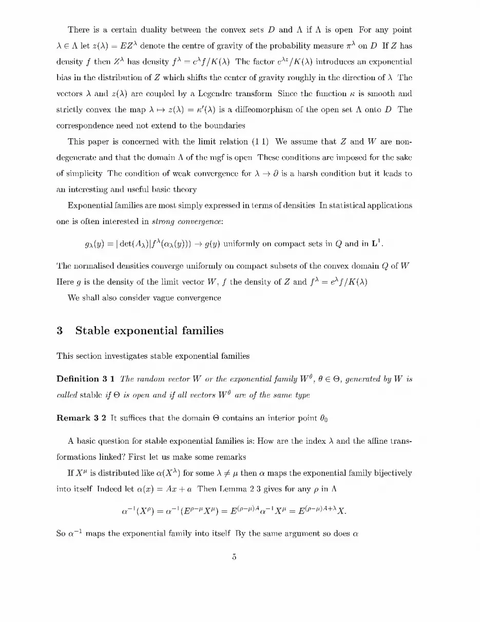
There is a certain duality between the convex sets D and � if � is open. For any point� 2 � let z(�) = EZ� denote the centre of gravity of the probability measure �� on D. If Z hasdensity f then Z� has density f� = e�f=K(�). The factor e�z=K(�) introduces an exponentialbias in the distribution of Z which shifts the center of gravity roughly in the direction of �. Thevectors � and z(�) are coupled by a Legendre transform. Since the function � is smooth andstrictly convex the map � 7! z(�) = �0(�) is a di�eomorphism of the open set � onto D. Thecorrespondence need not extend to the boundaries.This paper is concerned with the limit relation (1.1). We assume that Z and W are non-degenerate and that the domain � of the mgf is open. These conditions are imposed for the sakeof simplicity. The condition of weak convergence for � ! @ is a harsh condition but it leads toan interesting and useful basic theory.Exponential families are most simply expressed in terms of densities. In statistical applicationsone is often interested in strong convergence:g�(y) = jdet(A�)jf�(��(y)))! g(y) uniformly on compact sets in Q and in L1:The normalised densities converge uniformly on compact subsets of the convex domain Q of W .Here g is the density of the limit vector W , f the density of Z and f� = e�f=K(�).We shall also consider vague convergence.3 Stable exponential familiesThis section investigates stable exponential families.De�nition 3.1 The random vector W or the exponential family W �, � 2 �, generated by W iscalled stable if � is open and if all vectors W � are of the same type.Remark 3.2 It su�ces that the domain � contains an interior point �0.A basic question for stable exponential families is: How are the index � and the a�ne trans-formations linked? First let us make some remarks.If X� is distributed like �(X�) for some � 6= � then � maps the exponential family bijectivelyinto itself. Indeed let �(x) = Ax+ a. Then Lemma 2.3 gives for any � in ���1(X�) = ��1(E���X�) = E(���)A��1X� = E(���)A+�X:So ��1 maps the exponential family into itself. By the same argument so does �.5

De�nition 3.3 An element � 2 A is a symmetry of the non-degenerate random vector X if�X � X. The set of all symmetries is a closed compact group K, the symmetry group of therandom vector X. Let [X] = fX� j � 2 �g denote the exponential family generated by X. Thesymmetry group of the exponential family [X] is the setG = f� 2 A j [�X] = [X]g: (3.1)The map �(x) = Ax + b 7! A from A(d) to GL(d) is a homomorphism. For any subgroup G ofthe a�ne group A we de�ne the linear group G0 as the corresponding subgroup of GL.Proposition 3.4 The set G in (3.1) is a closed subgroup of A which contains the compactsymmetry group K of Y .There is a simple condition for stability of an exponential family in terms of the groupsintroduced above.De�ne ' : G ! ET by the relation X'(�) � �X. Casalis [1990] has shown that'(��) = '(�)B + '(�) �; � 2 G; �(x) = Bx+ b:This implies that the map � � 1 0a A! 7! �� � 1 '(�)0 A !is a homomorphism from G onto some group G� in AT which extends the canonical isomorphismA 7! AT from the linear group G0 introduced in de�nition 3.3 above. We shall call G� the Casalisgroup associated with the exponential family [X] and the homonorphism � 7! �� the Casalismap. Note that the Casalis map is continuous. So the Casalis group G� is a Lie group and theCasalis map is C1. Since the symmetry group K is a subgroup of the linear group G0 the Casalismap is injective. By de�nition it is onto. So it is an isomorphism. We obtain the following result.Theorem 3.5 If W is stable the domain � of the cgf � of W is an orbit of the Casalis groupG� of the exponential family W �, � 2 �.This impliesTheorem 3.6 Let W be a non-degenerate random vector in Rd with symmetry group K. Let Gbe the symmetry group of the exponential family [W ] = fW � j � 2 �g. Here � is the domain ofthe mgf of W . If dimG = dimK + d then W is stable.6

Corollary 3.7 If there exist independent vectors �1; : : : ; �d in � so that the vectors W t�i, t 2[0; 1], i = 1; : : : ; d, are all of the same type then W is stable.4 Stability of the limitThis section contains our main result.Theorem 4.1 Suppose n ! 0, Un ) U0 and Vn ) V0 where U0 and V0 are non-degenerate.Let Kn be the mgf of Un for n � 0. Assume that Kn( n) is �nite and Vn = U nn for n � 1. ThenV0 = U 00 and Kn( n)! K0( 0) <1.Proof Let �n denote the probability distribution of Un and �n the distribution of Vn for n � 0.Then e nxd�n(x) = and�n(x) for n � 1 where an = Kn( n). Observe thatand�n(x) = e nxd�n(x)! e 0xd�0(x) =: d�(x) vaguely:Since �n ! �0 vaguely and �0 and � do not vanish we conclude that an converges to a constanta0 2 (0;1) and d� = a0d�0. Then R e 0xd�0(x) = a0 < 1 and d�0(x) = e 0xd�0(x)=a0 since�0E = 1. {Now return to the basic relation (1.1). The Esscher transform E�Y� exists if � is small. Itsatis�es Y �� � �Y� � = ��1� ��; � = �+ �A�1� (4.1)provided � is chosen so that � lies in �.Theorem 4.2 Let Z and W be non-degenerate vectors. Let Z�, � 2 �, be the exponentialfamily generated by Z. Assume that � is open. Let � : �! A be a continuous normalisation sothat (1.1) holds. Then the exponential family generated by W is stable.Proof We shall prove that for each � 2 ET there exists a t0 > 0 so that the vectors W t�,0 � t � t0, all are of the same type. This implies that the exponential family W �, � 2 �,generated by W is stable by Corollary 3.7.Let � 2 ET and let �n ! @. Fix n � 1. For t � 0 relation (4.1) givesW t��n = �n(t)W�n(t) �n(t) = �n + t�A�1�n7

provided �n(t) 2 �. Since � is convex and open this will be the case for t 2 [0; cn) for somemaximal cn �1. Note that �n(0) = id and N(�n(t))!1 for t! cn by Corollary 2.5. Choosetn 2 (0; cn) so that N(�n(tn)) = 1. If tn > 1 then take tn = 1.Now assume �n = �n(tn) ! @. Take a subsequence so that �n(tn) ! � for some � 2 Aand tn ! t 2 [0; 1]. Then W�n ) W , tn� ! t� and W tn��n � �n(tn)W�n(tn) ) �W implyW t� � �W by Proposition 2.4. If �n ! � 2 � for some subsequence then N(��n) ! N(��)and N(�n(tn))!1 by Lemma 1.1. This contradicts our choice of tn. {Remark 4.3 We may replace the continuity condition by a weaker condition. Suppose the limitvector in (1.1) has symmetry group K. Let A=K be the symmetric space of cosets [�] = �K,� 2 A. It su�ces that there exists a compact convex set C � � so that � is continuous moduloK on � n C, i.e. [�] : �! A=K is continuous on � n C.We have now established our main result.Lemma 4.4 Suppose (1.1) holds. Let � be the domain of the mgf of the limit vector. Write��(x) = A�x+ a�. Let �n ! @ and let �n ! � 2 �. De�ne�n(t) = �n + t�nA�1�n �n(t) = ��1�n��n(t) t � 0:Then the sequence (�n(tn)) in A is bounded for any sequence (tn) in [0; 1] and �n(tn)! @.Proof Let c0 be the maximum of N over the compact set of all � 2 A for which there existst 2 [0; 1] such that W t� � �W . Let c1 = c0+1. Suppose �n(tn) is unbounded for some sequence(tn) in [0; 1]. Choose a subsequence so that N(�n(tn))!1. By continuity there exist rn 2 (0; tn)so that N(�n(rn)) ! c1. Take a subsequence so that �n(rn)! � and rn ! r. Then N(�) = c1and W r� � �W as in the proof of Theorem 4.2. By de�nition N(�) � c0. Contradiction. {Weak convergence in (1.1) implies convergence of the cgf's.Theorem 4.5 Suppose (1.1) holds. Let �� denote the cgf of the normalised variable W� =��1� (Z�) and let � be the domain of the cgf � of the limit variable W . Then �� ! � uniformlyon compact subsets of � for �! @.Proof Let �n ! � 2 �, �n ! @. The sequence (�n(1)) in Lemma 4.4 is relatively compact andall limit points � satisfy W � � �W and W �n�n )W �. Theorem 4.1 gives ��n(�n)! �(�). {8

5 The support of a stable familyThe support of a stable exponential family with symmetry group G is an atom in the �-�eld ofG invariant sets. This explains why the multivariate theory for exponential families is similar tothe univariate theory for limits of sums and maxima rather than the multivariate theory. SeeBalkema and Qi [1997] for related results on multivariate limit laws of residual life times.Given a closed subgroup G of A introduce the �-algebra E = E(G) of invariant Borel sets ofthe space E. It is generated by the setsGK = f�(x) j � 2 G; x 2 Kg K � E;Kcompact:Theorem 5.1 Let the exponential family W �, � 2 �, be invariant under the closed subgroup G.Then the support S of W is an atom of E.Proof First note that S is the support of W � for every � 2 �. So �W � W � implies that S = S. The support is invariant. Since it is �-compact it is a set in E .Suppose there exists a set S0 2 E so that PfW 2 S0g = p0 2 (0; 1). Then PfW 2 S1g =p1 = 1� p0 for S1 = S n S0. Note thatEe�W 1fW2S0g +Ee�W 1fW2S1g = Ee�W = K(�):Let W � � �W . Then for i = 0; 1pi = Pf�W 2 Sig = PfW � 2 Sig = Ee�W 1fW2Sig=K(�):So K(�) is the mgf of the conditional distribution of W given W 2 Si for i = 0 and i = 1. Hencethese conditional distributions agree. Contradiction. {6 Domains of attractionAs in the limit theory for sums and maxima one is not only interested in the limit laws, buteven more in a description of their domains of attraction.De�nition 6.1 Let W be a non-degenerate random vector which generates a stable exponentialfamily W �, � 2 �. The exponential family Z�, � 2 �, belongs to the domain of attraction of theexponential family W � and we write Z 2 D(W ) if � is open and if (1.1) holds for some family9

of normalisations �� 2 A. (We do not assume continuous dependence on � here.) Similarly wesay that a random vector, a measure, a density, a mgf or cgf belongs to the domain of attractionif this holds for the exponential families generated by these objects.Two measures which are asymptotically equal belong to the same domains of attraction.Theorem 6.2 Suppose (1.1) holds for the random vector Z with mgf K with domain �. Let ~Zhave mgf ~K with domain � and suppose ~K(�) � K(�) for �! @. Then ��1� ( ~Z�))W .Proof Let the limit vector W have cgf � with domain �. The vector W� = ��1� (Z�) has cgf��(�) := �(�+ �B�)� �(�) + �b� ��1� (y) = B�y + b�by Lemma 2.2. The vector ~W� has cgf ~�� with � replaced by ~� in the formula above. Byassumption (~� � �)(�) ! 0 for � ! @. This implies (~��n � ��n)(�n) ! 0 for � 2 � and�n ! @ by Lemma 4.4. So �� ! � on � implies ~�� ! ~� on �. Convergence of the mgfs impliesconvergence in law. {The asymptotic behaviour of the mgf K(�) for � ! @ is determined by the asymptoticbehaviour of the distribution of Z for z ! @D.Lemma 6.3 Let � be a �nite measure with convex support C. Let H = f�0 � c0g be a half spaceso that C nH is bounded and non-empty. Then there exists an open cone � � � containing �0so that � H=� C ! 0 2 �; !1:Lemma 6.4 Let � be a �nite measure with convex support C and � a �nite measure with convexsupport A contained in the interior of C. Let the domain � of the mgf K� be open. ThenK�(�)=K�(�)! 0 �! @�:Theorem 6.5 Let � be a �nite measures with convex domain D. Assume that � lives on D andthat the domain � of the mgf K of � is open. Let h : D ! [0;1) be a Borel function such thatR hd� is �nite and h(x)! 1 for x! @D. Then the mgf K0 of d�0 = hd� has domain � and K0and K are asymptotically equal for �! @.Proof Let � > 0. There is a compact convex set A � D so that j log h(x)j < � for x 2 D n A.Let �� agree with � on A and with �0 on D nA. Then the cgfs satisfy j��(�)� �(�)j < � for all� 2 � and j��(�)� �0(�)j < � eventually. So j�0(�)� �(�)j < 2� eventually. {10

7 The construction of stable exponential familiesGiven a group G in A how does one construct a measure such that the natural exponentialfamily associated with this measure is invariant under G?We give an example to describe a procedure.Example 7.1 The two-dimensional commutative group of diagonal matrices with positive el-ements gives rise to the exponential families generated by the bivariate gamma densities on(0;1)2. There is one other two-dimensional commuatative group G of linear transformations,with matrices A = a 0b a! a > 0; b 2 R:The right half plane is invariant and G is transitive on this half plane since A(1; 0) = (a; b).Assume there exists a density f = e�' such that f � A = f� for some vector � depending on aand b. This means that '(x; y) +L(x; y) = '(ax; bx+ ay) for some linear function L dependingon a and b. Taking derivatives with respect to x and y and writing 'ij for @i@j'(ax; bx + ay)we �nd 'xx = a2'11 + 2ab'12 + b2'22'xy = a2'12 + ab'22'xx = a2'22:Now given x and y choose a and b so that (ax; bx + ay) = (1; 0). This gives a = 1=x andb = �y=x2: The three quantities ci+j = 'ij(1; 0) are constant. So we obtain'xx = c2x2 � 2c3yx3 + c4y2x4'xy = c3x2 � c4yx3'xx = c4x2 :These functions have to satisfy the integrability conditions 'xxy = 'xyx and 'xyy = 'yyx: Thisyields the solution'(x; y) = a0 + a1x+ a2y + a3 log x+ a4y=x f(x; y) = c0xa3ea1x+a2yea4y=x:The corresponding measures on (0;1)�R are invariant. However none of them is �nite.11

8 Vague convergence and continuationSuppose (1.1) holds. There is a �nite measure � with convex domain D and a �nite measure �with convex domain Q so that��1� (��)=K(�)! � weakly �! @:Here K(�) = ��(E) and d��(x) = e�xd�. So � is a probability measure.Let d~� = hd� for a Borel function h on D and d~� = h0d� for a continuous strictly positivefunction h0 on Q, and assume that there exist positive constants C(�) so that��1� (~��)=C(�)! ~� vaguely �! @: (8.1)This will be the case ifh(��(y))=c(�) ! h0 uniformly on compact sets in Q: (8.2)Note that c(�) � jdetA�j=C(�) � h(p�)=h0(q) �! @for p� = ��(q) and any q 2 Q. So we �ndProposition 8.1 Suppose (8.2) holds. Let the corresponding measures d~� = hd� and d~� = h0d�be �nite. Weak convergence holds in (8.1) if and only if the mgf ~K(�) = ~��(D) of ~� satis�es theasymptotic equality ~K(�) � ~�(Q)h(p�)=(h0(q)jdetA�j) �! @:Vague convergence in (8.1) implies vague convergence on any open subset of Q. Converselyif (8.1) holds on any non-empty open subset of Q then it holds on Q. This is the main result ofthe present section.Suppose �n ! � vaguely on the open set W and �W > 0. If cn�n ! � vaguely on W thencn ! c � 0 and � = c�. This impliesLemma 8.2 Suppose �n ! � 2 A, �n ! � vaguely on the open set U and cn�n�n ! � vaguelyon U . If �(U \ �U) > 0 then cn ! c � 0 and � = c�� on U \ �U .Now suppose (8.1) holds on the non-empty open set U � Q. Let�n ! @ �n ! � 2 � �n = �n + �nA�1�n �n = ��1�n��n :12

Since we assume that (1.1) holds we �nd �n ! @ and [�n]! [�]. Then�n��n = ��1�n (��n=C(�n) = ��1�n (E�nA�1�n��n)=C(�n) = E�n��nC(�n)=C(�n):So E�n��n ! E�� vaguely on U and �n��n ! �� vaguely on �U . If �(U \ �U) is positive thenC(�n)=C(�n)! c � 0 and �� = cE�� on U \ �U .Theorem 8.3 Suppose (1.1) holds. Let � be a Radon measure on D and � a �nite measure ona relatively compact open U in Q. Suppose �� = ��1� (��)=C(�) ! � vaguely on U for � ! @.Then � extends to a unique Radon measure �� on Q such that �� ! �� vaguely on Q.Corollary 8.4 Let h : D ! [0;1) be a Borel function and h0 : U ! (0;1) continuous.If h � ��1� ! h0 uniformly on U then h0 extends to a continuous function �h0 on Q so thath � ��1� ! �h0 uniformly on compact subsets of Q. The function �h0 is a quasi-multiplieer for thesymmetry group G of W �, � 2 �.Given convergence in (1.1) for a density f it is fairly easy to adapt f or the underlyingLebesgue measure so that vague convergence holds on some relativley compact open subset ofQ. All that then remains to be done is to prove weak convergence!9 The geometryA geometry on D is a collection E of ellipsoids Ep, p 2 D. A geometry on D determines a metricon D, the collection of at functions, and the collection of measures which are asymptoticallyLebesgue. Suppose (1.1) holds. There are three ways to generate the geometry E .1) Any non-degenerate random vector X in E determines a family of ellipsoids centered inEX. These are the level curves of the density of a gaussian variable with the same �rst twomoments and can be represented as Er = fEX + u j ��1(u; u) � r2g where � is the covariance.Fix r > 0 and let E be the collection of the ellipsoids Er� associated with the vectors Z�.2) The cgf � of Z is convex and analytic. It determines a quadratic form �00(�) in each point�0(�) of D and hence as in 1) a collection E of ellipsoids on D.3) Let Q be the convex domain of the limit vector W in (1.1). Assume that W is centeredand has unit variance. Let B = Br(0) be the closed ball of radius r. De�ne E to be the set of allellipsoids ��(B). 13

Proposition 9.1 Suppose (1.1) holds. For any compact convex sets B � Q and C � D thereis a compact convex set A � � so that ��(B) � D n C for � 2 � n A.The third method may be generalised. The set B may be any compact convex set in Q whichis invariant under the symmetry group K of W . Thus if D = (0;1)d, Q = (�1; 1)d and W isthe vector with independent gamma components it is convenient to take B the cube [1=2; 3=2]d .In (1.1) we may replace �� by ~�� = ���� provided any sequence �n ! @ contains a subse-quence �0n so that ��0n ! � 2 K, where K is the symmetry group of W . If B is invariant underK the ellipsoids ~E� and E� are asymptotic in the sense that for any r > 1 the ellipsoid ~E� iseventually enclosed between two concentric scalings E�(1=r) and E�(r) of E�.We shall assume that the collection E has the property of Proposition 9.1. Collections whichare asymptotically equal for p = �0(�)! @ de�ne the same geometry.Theorem 9.2 The geometry depends only on the normalisations ��, � 2 �, and not on thedistribution of Z or W .De�nition 9.3 A function h : D ! [0;1) is at if it is positive outside some compact convexsubset C of D and if it is asymptotically constant on the ellipsoids in the geometry E: If pn !@D then supfh(x)=h(y) j x; y 2 Epng ! 1. A measure � on D is asymptotically Lebesgue if1B��1� (�)=jdetA�j converges weakly to the uniform distribution on B. In particular �(E�) �jE�j = jBjjdetA�j.Suppose (1.1) holds. Let f : D ! [0;1) be a Borel function and g : Q! [0;1) be continuouswith g(q) > 0 for some q 2 Q. Set g� = jdetA�j(e�f) � ��. Supposeg�=c(�)! g uniformly on compact sets in Q: (9.1)Then c(�) � g�(q)=g(q). Let ~f = hf with h at. Then (9.1) holds for ~g with the normalisation~c(�) = ~g�(q)=g(q). If (9.1) holds in L1 then g�=K(�) ! g= R gdz where K(�) = R e�fdz is themgf of the density f . HenceK(�) � g�(q) Z gdz=g(q) = (jdetA�j Z gdz=g(q))(e�f)(��(q)) �! @:If (9.1) also holds in L1 for ~f then ~K(�) � K(�)h(��(q)): (9.2)14

In some cases the geometry is determined by the form of the setD or �. We give four examples1) If D = Q is a symmetric cone with symmetry group G and if the limit vector W has thecharacteristic function of Q as density or a gamma function then E = f (B) j 2 Gg where Bis a symmetric compact body in Q. See Faraut and Kor�anyi [1994].2) IfD is an open body which contains the origin then each point p 2 D has the representationp = (1 � t)b with t 2 (0; 1] and b 2 @D. Call D rotund if the boundary is C2 and has positivecurvature. See Section 10 for details. Then for p 6= 0 there exists a unique ellipsoid E�p . whichosculates @D in b. Take Ep to be the ellipsoid concentric to E�p scaled down by a factor 1=2.This yields the geometry associated with the uniform distribution on D.3) If � is a rotund body which contains the origin then so is the interior of the polar set�o. For p = tb, b 2 �o, t > 0, let E�p be the ellipsoid centered in p which osculates the convexset b� �o in the origin, and de�ne Ep to be concentric to E�p and scaled by a factor 1=2. Thisgeometry is associated with the vector Z with the Laplace density e�r=c where r is the normfunction of �o.4) The geometry on D is asymptotically euclidean if the map p 7! Qp is at. Here Qp is thequadratic function associated with the ellipsoid Ep 2 E . SoQp0 [x; x]=Qp[x; x]! 1 uniformly in x 6= 0 pn ! @D; p0n 2 Epn :See Barndor�-Nielsen and Kl�uppelberg [1999]. This characterises the domain of attraction ofthe normal distribution.On the unit disk there is the geometry associated with the uniform distribution, but therealso is a host of distinct geometries on D associated with a normal limit, even if we restrictourselves to densities with circular symmetry.A geometry E determines a rough integer valued distance: Count the number of ellipsoidsneeded to form a chain from p1 to p2. This metric can be re�ned by using smaller ellipsoids. Inthe limit we obtain the Riemannian metric induced by the quadratic functions associated withthe ellipsoids.De�ne the cumulant metric on D as the Riemannian metric with the quadratic functionsQp = �00(�) for p = �0(�). In the cumulant metric bounded sets are relatively compact.Theorem 9.4 Let d be the Riemannian metric on � induced by the quadratic forms �00(�)�1,and let dc be the cumulant metric on D. Then the Legendre transform is an isometry.15

The geometry does not distinguish metrics which are asymptotic to the cumulant metric. Interms of the random vector Z this means that we do not distinguish between the vectors Z and~Z if ~�00(�) � �00(�) for �! @. Often it su�ces for the metric d to be equivalent to the cumulantmetric dc in the sense that the quotient d(p; p0)=dc(p; p0) is bounded and bounded away fromzero.On the unit sphere the distance between two points is equal to the angle between two rays.On the surface of a rotund body there is an intrinsic Riemannian metric d0 de�ned in terms ofthe curvature. It is invariant under a�ne transformations. Assume that D is rotund and containsthe origin. Each point has the form p = (1 � t)b with t 2 (0; 1) and b 2 @D. The geometry inthe second example above determines a metric on D. If pi = (1� ti)b lie on the same ray thend(p1; p2) = j log(t1=t2)j, if pi = (1 � t)bi lie on the same surface then d(p1; p2) = d0(b1; b2)=pt.Similarly in the third example d(t1b; t2b) = j log(t1=t2)j and the distance between two pointspi = tbi 2 t@�o is d0(b1; b2)pt where d0 is the intrinsic metric on the surface of �o. This metricis equivalent to the metric with �o replaced by the unit ball.If D or � is a rotund body we may extend the natural conjugation between the boundary ofthe body and the boundary of the polar body. Thus if � is rotund and ! 2 @� then !o = b 2 @�0satis�es !b = 1 and �b < 1 for � 2 �. For � = (1 � 1=t)! with 0 < t < 1 set �o = tb. A similarconjugation exists for the uniform distribution on D. This conjugation mimicks the Legendretransform.Proposition 9.5 Let D be a rotund body and d a metric equivalent to the metric describedabove. Then there exists a constant M � 1 so thatd(p0; p) �M(j log(t=t0)j+q1 + j�0(p0 � p)j) p; p0 2 D:Here �0 = po0, t; t0 2 (0; 1) satisfy p = (1� t)b and p0 = (1� t0)b0 with b; b0 2 @D.Corollary 9.6 If h : D ! (0;1) is at then for any � > 0 there is a compact convex set A � Dand a constant M � 1 so thath(p)=h(p0) �Me�j log(t=t0)je�j�0(p0�p)j p; p0 2 D n A:Proposition 9.7 Let � be a rotund body and d equivalent to the associated metric. There existsa constant M � 1 so thatd(z; z0) �M(j log(r=r0)j+ 1 +qr � �0(z)) z; z0 2 E:16

Here r; r0 is the value of the norm function of �o in z; z0 and �0 = zo0 is the conjugate of z0.Corollary 9.8 If h : E ! (0;1) is at then for any � > 0 there is a compact set A � E and aconstant M � 1 so thath(z)=h(z0) �Me�j log(r=r0)je�jr��0(z)j z; z0 2 Ac:These bounds make it possilbe to insert a at function into the density of Z without a�ectingthe weak convergence of ��1� (Z�).10 Uniform distribution on the unit ballLet Z = (X;Y ) be uniformly distributed on the open diskD = f(x; y) j (x� 1)2 + y2 < 1g:The density is f = 1D=�. Let � = (0;��) with � > 0. Then Z� has density f�(x; y) =c(�)e��y1D(x; y). For � large the mass concentrates in a thin region close to the origin. Sowe blow up the disk into a long vertical ellipse E� centered in (0; �) and passing through theorigin. Then the random vector has density c(�)e�y1E� . In order to obtain a limit for � !1 wehave to ensure that the curvature in the origin does not blow up. This can be achieved by alsoexpanding the ellipse in the horizontal direction, by a factor p� . The limit of these ellipses for� !1 is the open parabola Q = fy > x2=2g. The limit vector has density g(x; y) = e�y=p2�.The disk and its boundary are invariant under rotations. There is a corresponding one pa-rameter group of skew translations (x; y) 7! (x+ t; y+xt+ t2=2) which leave Q and its boundaryinvariant. In addition there is the group of expansions (x; y) 7! (rx; r2y) which were used totransform the circle into a parabola. These also leave the limit set Q invariant. They add a mul-tiplicative constant to Lebesgue measure which drops out when we normalise. Lebesgue measureon Q is quasi-invariant under a two-dimensional group G in A. It generates a stable exponentialfamily.Now start with a unit ball in Rd�R centered in (0; 1). The procedure above yields the openconvex set Q = fv > 0g v = y � xTx=2; (x; y) 2 Rd �R (10.1)17

which is invariant under the d+ 1 dimensional group G of a�ne transformations generated by�p � 0BB@ 1 0T 0p I 0pT p=2 pT 11CCA �r � 0BB@ 1 0T 00 rI 00 0T 11CCA p 2 Rd; r > 0:The skew translations �p leave Lebesgue measure invariant, the diagonal linear transformations�r only add an innocuous factor.So let � be Lebesgue measure restricted to Q. The measure �� has density e�z (by de�nition)and is �nite if and only if � lies in � = Rd � (0;1). The Casalis isomorphism maps �p into ��pand �r into ��r where��p � 0BB@ 1 pT 00 I 00 pT 11CCA ��r � 0BB@ 1 0T 00 rI 00 0T 11CCA p 2 Rd; r > 0:This is the basic construction.Now start with the uniform distribution on the surface of the unit ball. This distribution gen-erates the Von Mises-Fisher exponential family. The arguments above yield a stable exponentialfamily on the paraboloid @Q = fy = xTx=2g. It is generated by the measure � which is the im-age of Lebesgue measure on the horizontal hyperplane Rd�f0g under the map x 7! (x; xTx=2).The measure �� is �nite for � 2 Rd � (�1; 0). For � = (0;�1) it projects onto a multiple ofthe standard normal distribution on the horizontal plane fy = 0g.Theorem 10.1 Let Q and v be de�ned by (10.1). For s > 0 let Ws have densityhs(x; y) = ws�1e�y1Q(x; y)=(2�)d=2�(s)and for s = 0 let W0 be the vector (X0;XT0 X0=2) where X0 has a standard normal distribution onRd. Each vector Ws, s � 0, generates a stable exponential family W �s , � 2 � = Rd � (�1;�1).What can one say about the domains of attraction? Note that the examples above give aglobal result which depends only on the local behaviour of the original distribution of Z.Let D be a convex bounded open set in Rd+1 whose boundary can locally be described bya C2 function with a positive de�nite second derivative. Let U be uniformly distributed on D.Then U lies in the domain of attraction of W1. If U is uniformly distributed on the surface @Dit lies in the domain of attraction of W0. These two results remain true if we replace the uniformdistribution by a density which is continuous on the closure of D and positive on the boundary.18

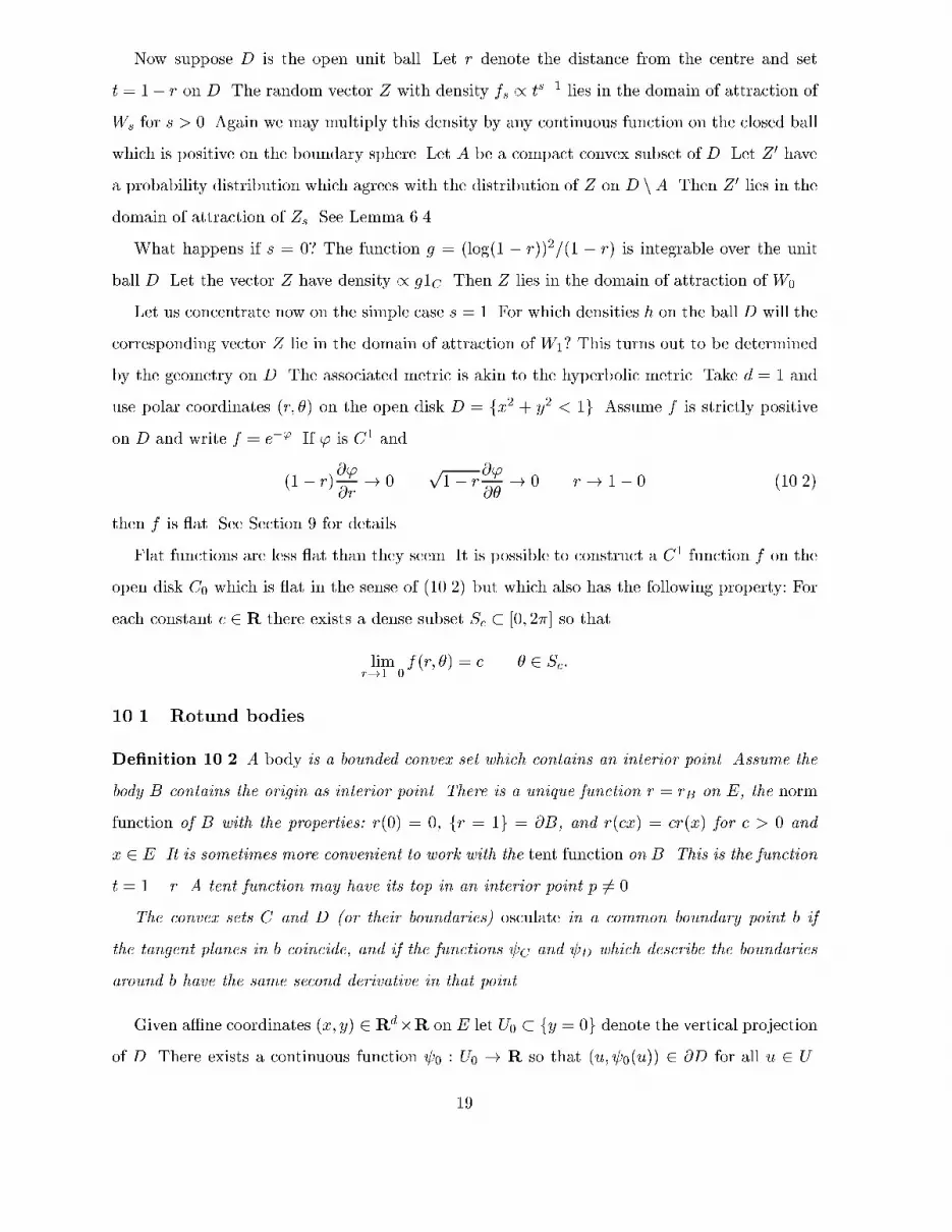
Now suppose D is the open unit ball. Let r denote the distance from the centre and sett = 1� r on D. The random vector Z with density fs / ts�1 lies in the domain of attraction ofWs for s > 0. Again we may multiply this density by any continuous function on the closed ballwhich is positive on the boundary sphere. Let A be a compact convex subset of D. Let Z 0 havea probability distribution which agrees with the distribution of Z on D nA. Then Z 0 lies in thedomain of attraction of Zs. See Lemma 6.4.What happens if s = 0? The function g = (log(1 � r))2=(1 � r) is integrable over the unitball D. Let the vector Z have density / g1C . Then Z lies in the domain of attraction of W0.Let us concentrate now on the simple case s = 1. For which densities h on the ball D will thecorresponding vector Z lie in the domain of attraction of W1? This turns out to be determinedby the geometry on D. The associated metric is akin to the hyperbolic metric. Take d = 1 anduse polar coordinates (r; �) on the open disk D = fx2 + y2 < 1g. Assume f is strictly positiveon D and write f = e�'. If ' is C1 and(1� r)@'@r ! 0 p1� r@'@� ! 0 r ! 1� 0 (10.2)then f is at. See Section 9 for details.Flat functions are less at than they seem. It is possible to construct a C1 function f on theopen disk C0 which is at in the sense of (10.2) but which also has the following property: Foreach constant c 2 R there exists a dense subset Sc � [0; 2�] so thatlimr!1�0 f(r; �) = c � 2 Sc:10.1 Rotund bodiesDe�nition 10.2 A body is a bounded convex set which contains an interior point. Assume thebody B contains the origin as interior point. There is a unique function r = rB on E, the normfunction of B with the properties: r(0) = 0, fr = 1g = @B, and r(cx) = cr(x) for c > 0 andx 2 E. It is sometimes more convenient to work with the tent function on B. This is the functiont = 1� r. A tent function may have its top in an interior point p 6= 0.The convex sets C and D (or their boundaries) osculate in a common boundary point b ifthe tangent planes in b coincide, and if the functions C and D which describe the boundariesaround b have the same second derivative in that point.Given a�ne coordinates (x; y) 2 Rd�R on E let U0 � fy = 0g denote the vertical projectionof D. There exists a continuous function 0 : U0 ! R so that (u; 0(u)) 2 @D for all u 2 U .19

In fact there exist two such functions. We choose the convex function. It describes the lowerboundary of D.The following are equivalent for any k � 1:1) @D is a Ck manifold;2) The norm function r is Ck on E n f0g;3) The functions 0 : U0 ! R above are Ck.Let b 2 @D be a boundary point of D. Assume there is a unique supporting plane Tb to Din b, the tangent plane. We regard Tb as a hyperplane in E. It becomes a vector space T 0b bydeclaring b to be the origin. So a point a 2 Tb � E corresponds to the vector w = a� b 2 T 0b .Choose new coordinates (x; y) 2 Rd �R on E so that b = (0; 0) and D � fy > 0g. Then Tb isthe horizontal plane fy = 0g.Let Ub � Tb be the vertical projection of D. Set Wb = Ub � b � T 0b , and let b : Wb ! Rdescribe the lower boundary of D. Then b(0) = 0 and 0b(0) = 0. Suppose 00b (0) exists andis positive de�nite. Then there are two euclidean structures on T 0b , the euclidean structure onTb � E inherited from E, and the intrinsic euclidean structure determined by the symmetricpositive de�nite bilinear form 00b (0). We endow T with the intrinsic structure. One may choosea�ne coordinates on E so that the unit sphere in E centered in (0; 1) osculates @D in b. Thenthe two structures coincide in b.De�nition 10.3 The body D is rotund if D is open, @D is a C2 manifold and if the curvature 00b (0) is positive de�nite for each b 2 @D.Let D be a rotund body, p 2 D. For each boundary point b there exists a unique ellipsoidEb(p) centered in p which osculates D in b. These ellipsoids vary continuously with b.Let T denote the tangent bundle to @D. We may identify T with the set of pairs f(b; w) jb 2 @D; b + w 2 Tb � Eg. The set W = f(b; w) j b 2 @D;w 2 Wb � T 0b g is open in T . De�ne : W ! R by (b; w) = b(w), and similarly de�ne the partial derivatives w(b; w) = 0b(w)and ww(b; w) = 00b (w).Proposition 10.4 The functions and w are C1 on W .The set A� = f(b; w) j b(0)[w;w] � �2g is a compact subset of T which is contained in Wfor some � > 0. Uniform continuity of on A� implies20

Lemma 10.5 Let bn 2 @D and wn 2 T 0bn . Suppose bn ! b and wn ! w. Let �n !1. Then�n bn(wn=p�n)! wTw=2:10.2 Weak convergence for strictly smooth convex bodiesProposition 10.6 Let t be the tent function on the rotund body D in d+ 1-dimensional spaceE for some d � 1. For s > 0 the density ts�11D lies in the domain of attraction of the stableexponential family generated by the densityg = vs�1e�y1Q Q = fv > 0g; v = y = x2=2:The normalised densities converge uniformly on compact subsets of Q.Proof The proof consists of two steps: We �rst prove vague convergence, then weak convergence.The domain � of the mgf of � is the whole space ET , hence is open. Take � 6= 0 and let b 2 @Dbe the point where � = �b is maximal. Then f� = �g is the tangent plane to @D in b. We assumethat the center of gravity of D is the origin.De�ne �� = �bB� where �b is an initial transformation to bring the convex body into theright position. Choose �� so that Db = ��1b (D) � Rd �R lies in the upper half space fy > 0g,with center of gravity (0; 1), and so that ��1b (b) = (0; 0). Then the horizontal coordinate planefy = 0g is the tangent plane and the function e� on D transforms into the function e� e��y onDb. We also choose �b so that the unit sphere centered in (0; 1) osculated Db in (0; 0).Now treat Db as we did the unit ball. Blow it up by a factor � in the vertical direction andby the factor p� in the horizontal directions. SetQ� = B�1� (Db) = ��1� (D) B�1t (x; y) = (p�x; �y):Then ��(0; 1) = p = (1� 1=�)b and the lower boundary of Q� is given by the function p(x) = � b(x=p� )! x2=2 uniformly in b 2 @D: (10.3)The function e��y on Db transforms into the function e�y on Q�, and the tent function t on Dinto the tent function t� on Q�. Since the center of gravity of Q� is (0; �) the limit relation (10.3)gives �t�(x; y)! y � x2=2 � !1; (x; y) 2 Q:21

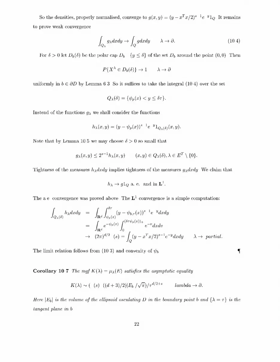
So the densities, properly normalised, converge to g(x; y) = (y�xTx=2)s�1e�y1Q. It remainsto prove weak convergence ZQ� g�dxdy ! ZQ gdxdy �! @: (10.4)For � > 0 let Db(�) be the polar cap Db\fy � �g of the set Db around the point (0; 0). ThenPfX� 2 Db(�)g ! 1 �! @uniformly in b 2 @D by Lemma 6.3. So it su�ces to take the integral (10.4) over the setQ�(�) = f p(x) < y � ��g:Instead of the functions g� we shall consider the functionsh�(x; y) = (y � p(x))s�1e�y1Q�(�)(x; y):Note that by Lemma 10.5 we may choose � > 0 so small thatg�(x; y) � 2s�1h�(x; y) (x; y) 2 Q�(�); � 2 ET n f0g:Tightness of the measures h�dxdy implies tightness of the measures g�dxdy. We claim thath� ! g1Q a: e: and in L1:The a.e. convergence was proved above. The L1 convergence is a simple computation:ZQ�(�) h�dxdy = ZRd Z �� p(x)(y � b;� (x))s�1e�ydxdy= ZRd e� p(x) Z (�� p(x))+0 e�vdxdv! (2�)d=2�(s) = ZQ(y � xTx=2)s�1e�ydxdy �! partial:The limit relation follows from (10.3) and convexity of b. {Corollary 10.7 The mgf K(�) = ��(E) satis�es the asymptotic equalityK(�) � (�(s)�((d + 3)=2)jEbj=p�)=�d=2+s lambda! @:Here jEbj is the volume of the ellipsoid osculating D in the boundary point b and f� = �g is thetangent plane in b. 22

We may insert a at function h into the density without harming the weak convergence, seeSection 9. It is also possible to replace Lebesgue measure by any measure � which is asymptot-ically Lebesgue. This can be done by de�ning suitable partitions and showing that the changein the integral is managable if one rede�nes the measure of the atoms of the partition withoutchanging the total mass of the atom.Theorem 10.8 Let D be a rotund body in d+1-dimensional euclidean space with d � 1. Let Zbe a random vector with distribution d� = ts�1hd� (10.5)where t is a tent function on D, s a positive parameter, h a at function and � a �nite measurewhich is asymptotically Lebesgue. Then Z lies in the domain of attraction of the stable exponentialfamily generated by the random vector Wsin Theorem 10.1. Conversely any random vector Zwith convex domain D which is attracted to Ws has a distribution of the form (10.5).10.3 Spherically symmetric distributionsLet � be a probability measure on the unit disk which is concentrated on a sequence of concentriccircles with radii rn ! 1. Assume that � is uniformly distributed over each of these circles. Canone choose the sequence rn so that � is in the domain of attraction of W1?Let D be the unit ball in Rd � R centered in q = (0; 1). Let t denote the tent functionon D with top in q and ! = !(p) the angle in q between the point p 2 D and (0; 0). Theny � 1 = (s� 1) cos j!j and for j!j < �=4 and � > 0e��te�� j!j2=2 � e��y � e��t=2e�j!j2=4:Let � = � � �0 be a product measure on Sd � (0; 1] where � is the uniform distribution.The map (!; s)! (p�!; �s) maps � into a product measure �� on p�Sd � (0; � ]. Now suppose�� = ��=c(�)! � vaguely. Thene��2=2e�yd�� (�; y)! e�x2=2e�yd�(x; y) vaguely:Suppose that Z e��2=4e�y=2d�� (�; y)! Z e�x2=4e�yd�(x; y):Then e�y cos(�=�)e�(1�cos �=�)d�� (�; y)! e�ye�x2=2d�(x; y)23

weakly for � ! 1. The latter is equivalent to convergence ��1� (Z�) ) W for � = (0;��) andW = f(V ) where the vector V has distribution ce�ye�x2=2d� for some c > 0 and f(x; y) =(x; y + x2=2) maps the half space y > 0 onto the paraboloid Q.Convergence ��1� (Z) ) W for a vector Z on the unit ball with the symmetric probabilitydistribution corresponding to � is equivalent to convergence of the univariate exponential familygenerated by the probability measure �0 on (0; 1]. This is equivalent to regular variation of thedistribution function M0(t) = �0(0; t] for t! 0. See BKR [1999b].Theorem 10.9 Let the random vector Z have the open unit ball D as convex domain. Supposethat Z is spherically symmetric. De�neM(t) = PfkXk � 1� tg t 2 (0; 1]:Let s > 0. The vector Z lies in the domain of attraction of Ws in Theorem 10.1 if and only ifM varies regularly in t = 0 with exponent s.11 The Laplace distributionThe function f = e�r=c c = 2�d=2�(d)=�(d=2); r = kxk2 (11.1)is a probability density on Rd+1.Proposition 11.1 For s > �(1 + d=2) the functiongs(x; y) = yse�(y+xT x=2y)=2�d�1�(s+ d=2 + 1)is the density of a vector Ws on D = Rd � (0;1) which generates a stable exponential family.Proposition 11.2 The density f in (11.1) lies in the domain of attraction of the density g0.More generally one can showTheorem 11.3 Let � be a rotund body in Rd+1 which contains the origin and let r be the normfunction of the polar set �o. Let h be a at function for the geometry associated with this normfunction. Let s + d=2 + 1 > 0. Then the vector Z with density f = he�rrs is attracted to thevector Ws in Proposition 11.1. 24

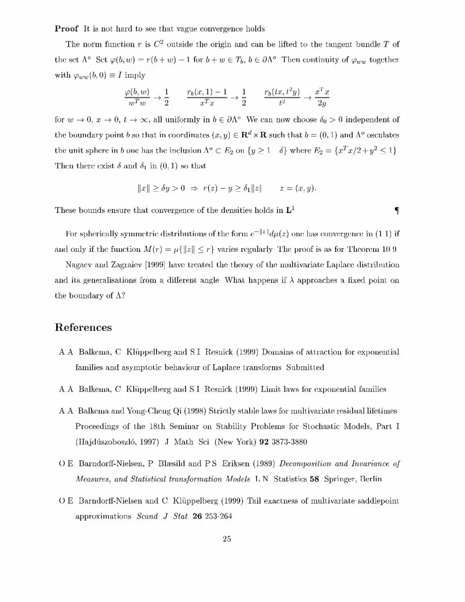
Proof It is not hard to see that vague convergence holds.The norm function r is C2 outside the origin and can be lifted to the tangent bundle T ofthe set �o. Set '(b; w) = r(b+w)� 1 for b+w 2 Tb, b 2 @�o. Then continuity of 'ww togetherwith 'ww(b; 0) � I imply'(b; w)wTw ! 12 rb(x; 1)� 1xTx ! 12 rb(tx; t2y)t2 ! xTx2yfor w ! 0, x ! 0, t! 1, all uniformly in b 2 @�o. We can now choose �0 > 0 independent ofthe boundary point b so that in coordinates (x; y) 2 Rd�R such that b = (0; 1) and �o osculatesthe unit sphere in b one has the inclusion �o � E2 on fy � 1��g where E2 = fxTx=2+y2 � 1g.Then there exist � and �1 in (0; 1) so thatkxk � �y > 0 ) r(z)� y � �1kzk z = (x; y):These bounds ensure that convergence of the densities holds in L1. {For spherically symmetric distributions of the form e�kzkd�(z) one has convergence in (1.1) ifand only if the function M(r) = �fkzk � rg varies regularly. The proof is as for Theorem 10.9.Nagaev and Zagraiev [1999] have treated the theory of the multivariate Laplace distributionand its generalisations from a di�erent angle. What happens if � approaches a �xed point onthe boundary of �?ReferencesA.A. Balkema, C. Kl�uppelberg and S.I. Resnick (1999) Domains of attraction for exponentialfamilies and asymptotic behaviour of Laplace transforms. Submitted.A.A. Balkema, C. Kl�uppelberg and S.I. Resnick (1999) Limit laws for exponential families.A.A. Balkema and Yong-Cheng Qi (1998) Strictly stable laws for multivariate residual lifetimes.Proceedings of the 18th Seminar on Stability Problems for Stochastic Models, Part I(Hajd�uszoboszl�o, 1997). J. Math. Sci. (New York) 92 3873-3880.O.E. Barndor�-Nielsen, P. Bl�sild and P.S. Eriksen (1989) Decomposition and Invariance ofMeasures, and Statistical transformation Models. L.N. Statistics 58. Springer, Berlin.O.E. Barndor�-Nielsen and C. Kl�uppelberg (1999) Tail exactness of multivariate saddlepointapproximations. Scand. J. Stat. 26 253-264.25

M. Casalis (1991) Familles exponentielles naturelles sur IRd invariantes par un groupe. Internat.Statist. Review 59 241-262.J. Faraut and A. Kor�anyi (1994) Analysis on symmetric cones. Clarendon Press, Oxford.P. Feigin and E. Yashchin (1983). On a strong Tauberian result. Z. Wahrsch. verw. Gebiete 6535-48.A. Nagaev and A. Zaigraev (1999) Abelian theorems for a class of probability distributions inIRd and their application. Preprint.August A. Balkema Claudia Kl�uppelberg Sidney I. ResnickDepartment of Mathematics Center of Mathematical Sciences ORIEUniversity of Amsterdam Munich University of Technology Cornell UniversityNL-1018TV Amsterdam D-80290 Munich Ithaca, NY 14853-7501Holland Germany USAguus@wins.uva.nl cklu@ma.tum.de sid@orie.cornell.eduwww.ma.tum.de/stat/

26