Quantitative Kleene coalgebras

Filippo Bonchia, Marcello Bonsanguec,b, Jan Ruttenb,e,d, Alexandra Silvab

aINRIA-SaclaybCentrum voor Wiskunde en Informatica

cLeiden Institute Advanced Computer SciencedRadboud Universiteit Nijmegen

eVrije Universiteit Amsterdam

Abstract

We present a systematic way to generate (1) languages of (generalised) regular expressions, and(2) sound and complete axiomatizations thereof, for a wide variety of quantitative systems. Ourquantitative systems include weighted versions of automata and transition systems, in which tran-sitions are assigned a value in a monoid that represents cost, duration, probability, etc. Suchsystems are represented as coalgebras and (1) and (2) above are derived in a modular fashionfrom the underlying (functor) type of these coalgebras.

In previous work, we applied a similar approach to a class of systems (without weights) thatgeneralizes both the results of Kleene (on rational languages and DFA’s) and Milner (on regularbehaviours and finite LTS’s), and includes many other systems such as Mealy and Moore machines.

In the present paper, we extend this framework to deal with quantitative systems. As a conse-quence, our results now include languages and axiomatizations, both existing and new ones, formany different kinds of probabilistic systems.

1. Introduction

Kleene’s Theorem [25] gives a fundamental correspondence between regular expressions anddeterministic finite automata (DFA’s): each regular expression denotes a language that can be rec-ognized by a DFA and, vice-versa, the language accepted by a DFA can be specified by a regularexpression. Languages denoted by regular expressions are called regular. Two regular expressionsare called (language) equivalent if they denote the same regular language. Salomaa [37] pre-sented a sound and complete axiomatization for proving the equivalence of regular expressions,which was later refined by Kozen [27].

The above programme was applied by Milner in [31] to process behaviours and labelled transi-tion systems (LTS’s). Milner introduced a set of expressions for finite LTS’s and proved an analogueof Kleene’s Theorem: each expression denotes the behaviour of a finite LTS and, conversely, thebehaviour of a finite LTS can be specified by an expression (modulo bisimilarity). Milner also pro-vided an axiomatization for his expressions, with the property that two expressions are provablyequivalent if and only if they are bisimilar.

Coalgebras provide a general framework for the study of dynamical systems such as DFA’s andLTS’s. For a functor F : Set→ Set, an F-coalgebra or F-system is a pair (S, f ), consisting of a setS of states and a function f : S→ F(S) defining the “transitions” of the states. We call the functorF the type of the system. For instance, DFA’s can be readily seen to correspond to coalgebras ofthe functor F(S) = 2× SA and image-finite LTS’s are obtained by F(S) = Pω(S)

A, where Pω is finitepowerset.

Under mild conditions, functors F have a final coalgebra (unique up to isomorphism) intowhich every F-coalgebra can be mapped via a unique so-called F-homomorphism. The final coal-gebra can be viewed as the universe of all possible F-behaviours: the unique homomorphism intothe final coalgebra maps every state of a coalgebra to a canonical representative of its behaviour.This gives a general notion of behavioural equivalence: two states are equivalent iff they are

Preprint submitted to Elsevier July 22, 2010

mapped to the same element of the final coalgebra. In the case of DFA’s, two states are equiva-lent when they accept the same language; for LTS’s, behavioural equivalence coincides with theordinary notion of bisimilarity.

In a previous paper [8], we introduced for coalgebras of a large but restricted class of functors,a language of regular expressions; a corresponding generalisation of Kleene’s Theorem; and asound and complete axiomatization with respect to bisimilarity. We derived both the language ofexpressions and their axiomatization, in a modular fashion, from the functor defining the type ofthe system, by induction on the structure of the functors.

In recent years, much attention has been devoted to the analysis of probabilistic behaviours,which occur for instance in randomized, fault-tolerant systems. Several different types of systemswere proposed: reactive [34, 28], generative [19], stratified [41, 45], alternating [23, 46], (sim-ple) Segala systems [40, 39], bundle [15] and Pnueli-Zuck [33], among others. For some of thesesystems, expressions were defined for the specification of their behaviours, as well as axioms toreason about their behavioural equivalence. Examples include [24, 29, 2, 42, 1, 4, 32, 16, 17].

The results in [8] apply to the class of non-deterministic functors, which is general enough toinclude the examples of deterministic automata and labelled transition systems, as well as manyother systems such as Mealy and Moore machines. However, probabilistic systems, weightedautomata [38, 18] etc. cannot be described by non-deterministic functors. It is aim of the presentpaper to identify a class of functors (a) that is general enough to include these and more generallya large class of quantitative systems; and (b) to which the methodology developed in [8] can beextended.

To this end, we give a non-trivial extension of the class of non-deterministic functors by addinga functor type that allows the transitions of our systems to take values in a monoid structure ofquantitative values. This new class, which we shall call quantitative functors, now includes all thetypes of probabilistic systems mentioned above.

At the same time, we show how to extend our earlier approach to the new setting. As it turnsout, the main technical challenge is due to the fact that the behaviour of quantitative systems isinherently non-idempotent. As an example consider the expression 1/2 · ǫ⊕ 1/2 · ǫ′ representing aprobabilistic system that either behaves as ǫ with probability 1/2 or behaves as ǫ′ with the sameprobability. When ǫ is equivalent to ǫ′, then the system is equivalent to 1 · ǫ rather than 1/2 · ǫ.This is problematic because idempotency played a crucial role in our previous results to ensurethat expressions denote finite-state behaviours.

We will show how the lack of idempotency in the extended class of functors can be circum-vented by a clever use of the monoid structure. This will allow us to derive for each functor in ournew extended class everything we were after: a language of regular expressions; a correspond-ing Kleene’s Theorem; and a sound and complete axiomatization for the corresponding notion ofbehavioural equivalence.

In order to show the effectiveness and the generality of our approach, we apply it to four typesof systems: weighted automata; simple Segala, stratified and Pnueli-Zuck systems. For simpleSegala systems, we recover the language and axiomatization presented in [17]. For weightedautomata and stratified systems, languages have been defined in [12] and [45] but, to the bestof our knowledge, no axiomatization was ever given. Applying our method, we obtain the samelanguages and, more interestingly, we obtain novel axiomatizations. We also present a completelynew framework to reason about Pnueli-Zuck systems. Table 1 summarizes the main results of thispaper: the languages and axiomatizations derived for several quantitative systems.

This paper is an extended version of our CONCUR paper [6]. In comparison to [6], thispaper includes more details in the examples, contains all the proofs of new results, provides adetailed explanation of the soundness and completeness of the axiomatization and it includes thedescription of an alternative definition of a functor to model quantitative systems (Section 7).

Organization of the paper. Section 2 gives preliminaries on coalgebras and non-deterministicfunctors and recalls the main results of [8]. In Section 3 we introduce the functor that will allowus to model quantitative systems: the monoidal exponentiation functor. Section 4 shows how toextend the framework presented in the previous chapter to quantitative systems: we associate with

2

every quantitative functor H a language of expressions ExpH, we prove a Kleene like theorem andwe introduce a sound and complete axiomatization with respect to behavioural equivalence of H.Section 5 paves the way for the derivation of expressions and axioms for probabilistic systems,which we present in Section 6. Section 7 shows a variation on the definition of the monoidalexponentiation functor and the consequences it would have in the framework. We conclude andpresent pointers for future work in Section 8.

Weighted automata – H(S) = S× (SS)A

ǫ::= ; | ǫ⊕ ǫ | µx .ǫ | x | s | a(s · ǫ) where s ∈ S and a ∈ A

(ǫ1 ⊕ ǫ2)⊕ ǫ3 ≡ ǫ1 ⊕ (ǫ2 ⊕ ǫ3) ǫ1 ⊕ ǫ2 ≡ ǫ2 ⊕ ǫ1 ǫ⊕; ≡ ǫ

a(s · ǫ)⊕ a(s′ · ǫ)≡ a((s+ s′) · ǫ) s⊕ s′ ≡ s+ s′ a(0 · ǫ)≡ ; 0≡ ;ǫ[µx .ǫ/x]≡ µx .ǫ γ[ǫ/x]≡ ǫ⇒ µx .γ≡ ǫ

Segala systems – H(S) = Pω(Dω(S))A

ǫ::= ; | ǫ⊞ ǫ | µx .ǫ | x | a(ǫ′) where a ∈ A, pi ∈ (0, 1] and∑

i∈1...npi = 1

ǫ′::=⊕

i∈1···npi · ǫi

(ǫ1 ⊞ ǫ2)⊞ ǫ3 ≡ ǫ1 ⊞ (ǫ2 ⊞ ǫ3) ǫ1 ⊞ ǫ2 ≡ ǫ2 ⊞ ǫ1 ǫ⊞ ; ≡ ǫ ǫ⊞ ǫ ≡ ǫ

(ǫ′1 ⊕ ǫ′2)⊕ ǫ

′3 ≡ ǫ

′1 ⊕ (ǫ

′2 ⊕ ǫ

′3) ǫ′1 ⊕ ǫ

′2 ≡ ǫ

′2 ⊕ ǫ

′1 (p1 · ǫ)⊕ (p2 · ǫ)≡ (p1 + p2) · ǫ

ǫ[µx .ǫ/x]≡ µx .ǫ γ[ǫ/x]≡ ǫ⇒ µx .γ≡ ǫ

Stratified systems – H(S) =Dω(S) + (B× S) + 1

ǫ::= µx .ǫ | x | ⟨b,ǫ⟩ |⊕

i∈1···npi · ǫi | ↓ where b ∈ B, pi ∈ (0, 1] and

∑

i∈1...npi = 1

(ǫ1 ⊕ ǫ2)⊕ ǫ3 ≡ ǫ1 ⊕ (ǫ2 ⊕ ǫ3) ǫ1 ⊕ ǫ2 ≡ ǫ2 ⊕ ǫ1 (p1 · ǫ)⊕ (p2 · ǫ)≡ (p1 + p2) · ǫ

ǫ[µx .ǫ/x]≡ µx .ǫ γ[ǫ/x]≡ ǫ⇒ µx .γ≡ ǫ

Pnueli-Zuck systems – H(S) = PωDω(Pω(S)A)

ǫ::= ; | ǫ⊞ ǫ | µx .ǫ | x | ǫ′ where a ∈ A, pi ∈ (0, 1] and∑

i∈1...npi = 1

ǫ′::=⊕

i∈1···npi · ǫ

′′i

ǫ′′::= ; | ǫ′′ ⊞ ǫ′′ | a(ǫ)

(ǫ1 ⊞ ǫ2)⊞ ǫ3 ≡ ǫ1 ⊞ (ǫ2 ⊞ ǫ3) ǫ1 ⊞ ǫ2 ≡ ǫ2 ⊞ ǫ1 ǫ⊞ ; ≡ ǫ ǫ⊞ ǫ ≡ ǫ

(ǫ′1 ⊕ ǫ′2)⊕ ǫ

′3 ≡ ǫ

′1 ⊕ (ǫ

′2 ⊕ ǫ

′3) ǫ′1 ⊕ ǫ

′2 ≡ ǫ

′2 ⊕ ǫ

′1 (p1 · ǫ

′′)⊕ (p2 · ǫ′′)≡ (p1 + p2) · ǫ

′′

(ǫ′′1 ⊞ ǫ′′2 )⊞ ǫ

′′3 ≡ ǫ

′′1 ⊞ (ǫ

′′2 ⊞ ǫ

′′3 ) ǫ′′1 ⊞ ǫ

′′2 ≡ ǫ

′′2 ⊞ ǫ

′′1 ǫ′′ ⊞ ; ≡ ǫ′′ ǫ′′ ⊞ ǫ′′ ≡ ǫ′′

ǫ[µx .ǫ/x]≡ µx .ǫ γ[ǫ/x]≡ ǫ⇒ µx .γ≡ ǫ

Table 1: All the (valid) expressions are closed and guarded. The congruence and the α-equivalence axiomsare implicitly assumed for all the systems. The symbols 0 and + denote, in the case of weighted automata,the empty element and the binary operator of the commutative monoid S while, for the other systems, theydenote the ordinary 0 and sum of real numbers. We write

⊕

i∈1···npi · ǫi for p1 · ǫ1 ⊕ · · · ⊕ pn · ǫn.

2. Preliminaries

We give the basic definitions on non-deterministic functors and coalgebras and introduce thenotion of bisimulation.

3

First we fix notation on sets and operations on them. Let Set be the category of sets and functions.Sets are denoted by capital letters X , Y, . . . and functions by lower case f , g, . . .. We write for theempty set and the collection of all finite subsets of a set X is defined as Pω(X ) = Y ⊆ X | Y finite.The collection of functions from a set X to a set Y is denoted by Y X . We write idX for the identityfunction on set X . Given functions f : X → Y and g : Y → Z we write their composition as g f .

The product of two sets X , Y is written as X×Y , with projection functions X X × Yπ1 π2

Y .The set 1 is a singleton set typically written as 1= ∗ and it can be regarded as the empty product.We define

X 3+ Y = X ⊎ Y ⊎ ⊥,⊤

where ⊎ is the disjoint union of sets, with injections Xκ1

X ⊎ Y Yκ2 . Note that the set

X 3+ Y is different from the classical coproduct of X and Y (which we shall denote by X + Y ),because of the two extra elements ⊥ and ⊤. These extra elements will later be used to represent,respectively, underspecification and inconsistency in the specification of some systems.

For each of the operations defined above on sets, there are analogous ones on functions. Letf1 : X → Y and f2 : Z →W . We define the following operations:

f1 × f2 : X × Z → Y ×W f1 3+ f2 : X 3+ Z → Y 3+W

( f1 × f2)(⟨x , z⟩) = ⟨ f1(x), f2(z)⟩ ( f 3+ f2)(c) = c, c ∈ ⊥,⊤( f1 3+ f2)(κi(x)) = κi( fi(x)), i ∈ 1,2

f A1 : X A→ Y A Pω( f1): Pω(X )→ Pω(Y )

f A1 (g) = λa. f1(g(a)) Pω( f1)(S) = f1(x) | x ∈ S

Note that here we are using the same symbols that we defined above for the operations on sets. Itwill always be clear from the context which operation is being used.

A functor F : Set→ Set is a mapping of sets to sets and functions to functions satisfying:

1. F(g f ) = F(g) F( f )

2. F(idX ) = idF(X )

The operations we defined above on sets and functions actually form functors, as we will use laterin this paper when defining the class of quantitative functors.

In our definition of quantitative functors we will use constant sets equipped with an informa-tion order. In particular, we will use join-semilattices. A (bounded) join-semilattice is a set B

equipped with a binary operation ∨B and a constant ⊥B ∈ B, such that ∨B is commutative, asso-ciative and idempotent. The element ⊥B is neutral w.r.t. ∨B. As usual, ∨B gives rise to a partialordering ≤B on the elements of B: b1 ≤B b2⇔ b1 ∨B b2 = b2. Every set S can be mapped into ajoin-semilattice by taking B to be the set of all finite subsets of S with union as join.

Coalgebras. A coalgebra is a pair (S, f : S → F(S)), where S is a set of states and F : Set → Set

is a functor. The functor F, together with the function f , determines the transition structure (ordynamics) of the F-coalgebra [35].

An F-homomorphism from an F-coalgebra (S, f ) to an F-coalgebra (T, g) is a function h: S→ T

preserving the transition structure, i.e., such that g h= F(h) f .

2.1 DEFINITION. An F-coalgebra (Ω,ω) is said to be final if for any F-coalgebra (S, f ) there existsa unique F-homomorphism behS : S→ Ω. ♣

The notion of finality will play a key role later in providing a semantics to expressions.For every bounded functor there exists a final F-coalgebra (ΩF,ωF) [35, 22]. A functor is said

to be bounded [22, Theorem 4.7] if there exists a natural surjection η from a functor B × (−)A toF, for some sets B and A.

4

Given an F-coalgebra (S, f ) and a subset V of S with inclusion map i : V → S we say that V isa subcoalgebra of S if there exists g : V → F(V ) such that i is an F-homomorphism. Given s ∈ S,⟨s⟩= (T, t) denotes the smallest subcoalgebra generated by s, with T given by

T =⋂

V | V is a subcoalgebra of S and s ∈ V (1)

If the functor F preserves arbitrary intersections, then the subcoalgebra ⟨s⟩ exists. This will be thecase for every functor considered in this paper.

We will write Coalg(F) for the category of F-coalgebras together with coalgebra homomor-phisms. We also write CoalgLF(F) for the category of F-coalgebras that are locally finite: F-coalgebras (S, f ) such that for each state s ∈ S the generated subcoalgebra ⟨s⟩ is finite.

Let (S, f ) and (T, g) be two F-coalgebras. We call a relation R⊆ S × T a bisimulation iff

⟨s, t⟩ ∈ R⇒ ⟨ f (s), g(t)⟩ ∈ F(R)

where F(R) is defined as F(R) = ⟨F(π1)(x),F(π2)(x)⟩ | x ∈ F(R).We write s ∼F t whenever there exists a bisimulation relation containing (s, t) and we call ∼F

the bisimilarity relation. We shall drop the subscript F whenever the functor F is clear from thecontext.

We say that the states s ∈ S and t ∈ T are behaviourally equivalent, written s ∼b t, if and only ifthey are mapped into the same element in the final coalgebra, that is behS(s) = behT (t).

If two states are bisimilar then they are always behaviourally equivalent (s ∼ t ⇒ s ∼b t). Theconverse implication is only true for certain classes of functors. For instance, if the functor F pre-serves weak-pullbacks then we also have s ∼b t ⇒ s ∼ t. The class of non-deterministic functors,which we will recall next, satisfies this property, whereas the class of quantitative functors, whichwe shall introduce later in this paper does not.

Non-deterministic functors. Non-deterministic functors are functors G: Set → Set, built induc-tively from the identity and constants, using ×, 3+, (−)A and Pω.

2.2 DEFINITION. The class NDF of non-deterministic functors on Set is inductively defined by:

NDF ∋ G::= Id | B | G×G | G 3+ G | GA | PωG

where B is a finite join-semilattice and A is a finite set. ♣

Since we only consider finite exponents A= a1, . . . , an, the functor (−)A is not really needed,since it is subsumed by a product with n components. However, to simplify the presentation, wedecided to include it.

We now show the explicit definition of the functors above on a set X and on a morphismf : X → Y (note that G( f ): G(X )→ G(Y )).

Id(X ) = X B(X ) = B (G1 3+ G2)(X ) = G1(X )3+ G2(X )

Id( f ) = f B( f ) = idB (G1 3+ G2)( f ) = G1( f )3+ G2( f )

(GA)(X ) = G(X )A (PωG)(X ) = Pω(G(X )) (G1 ×G2)(X ) = G1(X )×G2(X )

(GA)( f ) = G( f )A (PωG)( f ) = Pω(G( f )) (G1 ×G2)( f ) = G1( f )×G2( f )

Typical examples of non-deterministic functors include M = (B× Id)A, D = 2× IdA, Q = (1 3+ Id)A

and N = 2 × (Pω(Id))A. These functors represent, respectively, the type of Mealy, deterministic,

partial deterministic and non-deterministic automata. In [7], we have studied in detail regularexpressions for Mealy automata. Similarly to what happened there, we impose a join-semilatticestructure on the constant functor G(X ) = B. The product, exponentiation and powerset functorspreserve the join-semilattice structure and thus need not to be changed. This is not the case forthe classical coproduct and thus we use 3+ instead, which also guarantees that the join semilatticestructure is preserved.

We remark that every non-deterministic functor is bounded (and thus has a final coalgebra).

5

Next, we give the definition of the ingredient relation, which relates a non-deterministic func-tor G with its ingredients, i.e. the functors used in its inductive construction. We shall use thisrelation later for typing our expressions.

2.3 DEFINITION. Let Ã⊆ NDF×NDF be the least reflexive and transitive relation on non-determi-nistic functors such that

G1 ⊳G1 ×G2, G2 Ã G1 ×G2, G1 Ã G1 3+ G2, G2 Ã G1 3+ G2, GÃ GA, GÃ PωG

♣

Here and throughout this paper we use F Ã G as a shorthand for ⟨F,G⟩ ∈Ã. If F Ã G, then F

is said to be an ingredient of G. For example, 2, Id, IdA and D itself are all the ingredients of thedeterministic automata functor D.

2.1. A language of expressions for non-deterministic coalgebras

In this section, we recall the main definitions and results concerning the language of expres-sions associated with a non-deterministic functor [8]. We start by introducing an untyped lan-guage of expressions and then we single out the well-typed ones via an appropriate typing system,thereby associating expressions to non-deterministic functors.

2.4 DEFINITION (Expressions). Let A be a finite set, B a finite join-semilattice and X a set of fixed-point variables. The set Exp of all expressions is given by the following grammar, where a ∈ A,b ∈ B and x ∈ X :

ǫ ::= ; | x | ǫ⊕ ǫ | µx .γ | b | l⟨ǫ⟩ | r⟨ǫ⟩ | l[ǫ] | r[ǫ] | a(ǫ) | ǫ

where γ is a guarded expression given by:

γ ::= ; | γ⊕ γ | µx .γ | b | l⟨ǫ⟩ | r⟨ǫ⟩ | l[ǫ] | r[ǫ] | a(ǫ) | ǫ

♣

In the expression µx .γ, µ is a binder for all the occurrences of x in γ. Variables that arenot bound are free. A closed expression is an expression without free occurrences of fixed-pointvariables x . We denote the set of closed expressions by Expc.

Intuitively, expressions denote elements of the final coalgebra. The expressions ;, ǫ1 ⊕ ǫ2 andµx .ǫ will play a similar role to, respectively, the empty language, the union of languages and theKleene star in classical regular expressions for deterministic automata. The expressions l⟨ǫ⟩ andr⟨ǫ⟩ refer to the left and right hand-side of products. Similarly, l[ǫ] and r[ǫ] refer to the left andright hand-side of sums. The expressions a(ǫ) and ǫ denote function application and a singletonset, respectively.

Next, we present a typing assignment system for associating expressions to non-deterministicfunctors. This will associate with each functor G the expressions ǫ ∈ Exp that are valid specifi-cations of G-coalgebras. The typing proceeds following the structure of the expressions and theingredients of the functors.

2.5 DEFINITION (Type system). We now define a typing relation ⊢⊆ Exp× NDF × NDF that willassociate an expression ǫ with two non-deterministic functors F and G, which are related by theingredient relation (F is an ingredient of G). We shall write ⊢ ǫ : F Ã G for ⟨ǫ,F,G⟩ ∈ ⊢. The rulesthat define ⊢ are the following:

⊢ ;: F Ã G ⊢ b : BÃ G ⊢ x : G Ã G

⊢ ǫ : G Ã G

⊢ µx .ǫ : G Ã G

⊢ ǫ1 : F Ã G ⊢ ǫ2 : F Ã G

⊢ ǫ1 ⊕ ǫ2 : F Ã G

⊢ ǫ : G Ã G

⊢ ǫ : Idà G

⊢ ǫ : F Ã G

⊢ ǫ: PωF Ã G

⊢ ǫ : F Ã G

⊢ a(ǫ): FAÃ G

⊢ ǫ : F1 Ã G

⊢ l⟨ǫ⟩: F1 ×F2 Ã G

⊢ ǫ : F2 Ã G

⊢ r⟨ǫ⟩: F1 ×F2 Ã G

⊢ ǫ : F1 Ã G

⊢ l[ǫ]: F1 3+F2 Ã G

⊢ ǫ : F2 Ã G

⊢ r[ǫ]: F1 3+F2 Ã G

6

♣

Intuitively, ⊢ ǫ : F à G (for a closed expression ǫ) means that ǫ denotes an element of F(ΩG),where ΩG is the final coalgebra of G. As expected, there is a rule for each expression construct.The extra rule involving Idà G reflects the isomorphism between the final coalgebra ΩG and G(ΩG)

(Lambek’s lemma, cf. [35]). Only fixed-points at the outermost level of the functor are allowed.This does not mean however that we disallow nested fixed-points. For instance, µx . a(x⊕µy. a(y))

would be a well-typed expression for the functor D of deterministic automata, as it will becomeclear below, when we will present more examples of well-typed and non-well-typed expressions.The presented type system is decidable (expressions are of finite length and the system is inductiveon the structure of ǫ ∈ Exp).

We can now formally define the set of G-expressions: well-typed expressions associated with anon-deterministic functor G.

2.6 DEFINITION (G-expressions). Let G be a non-deterministic functor and F an ingredient of G.We define ExpFÃG by:

ExpFÃG = ǫ ∈ Expc | ⊢ ǫ : F Ã G .

We define the set ExpG of well-typed G-expressions by ExpGÃG. ♣

Examples of well-typed expressions for the functor D= 2× IdA (with 2 = 0,1; recall that theingredients of D are 2, IdA and D itself) include r⟨a(;)⟩, l⟨1⟩ ⊕ r⟨a(l⟨0⟩)⟩ and µx .r⟨a(x)⟩ ⊕ l⟨1⟩.The expressions l[1], l⟨1⟩ ⊕ 1 and µx .1 are examples of non well-typed expressions, because thefunctor D does not involve 3+, the subexpressions in the sum have different types, and recursionis not at the outermost level (1 has type 2ÃD), respectively.

Let us instantiate the definition of G-expressions to the functors of deterministic automataD= 2× IdA.

2.7 EXAMPLE (Deterministic expressions). Let A be a finite set of input actions and let X be a setof (recursion or) fixed-point variables. The set ExpD of deterministic expressions is given by the setof closed and guarded expressions generated by the following BNF grammar. For a ∈ A and x ∈ X :

ǫ::= ; | ǫ⊕ ǫ | µx .ǫ | x | l⟨ǫ1⟩ | r⟨ǫ2⟩

ǫ1::= ; | 0 | 1 | ǫ1 ⊕ ǫ1

ǫ2::= ; | a(ǫ) | ǫ2 ⊕ ǫ2

♠

At this point, we should remark that the syntax of our expressions differs from the classicalregular expressions in the use of µ and action prefixing a(ǫ) instead of star and full concatena-tion. We shall show later that these two syntactically different formalisms are equally expressive(Theorem 2.12).

We have now defined a language of expressions which gives us an algebraic description ofsystems. The goal is now to present a generalization of Kleene’s theorem for non-deterministiccoalgebras (Theorem 2.12). Recall that, for regular languages, the theorem states that a languageis regular if and only if it is recognized by a finite automaton. In order to achieve our goal we willfirst show that the set ExpG of G-expressions carries a G-coalgebra structure. More precisely, weare going to define a function

δFÃG : ExpFÃG→ F(ExpG)

for every ingredient F of G, and then set δG = δGÃG. Our definition of the function δFÃG will makeuse of the following.

2.8 DEFINITION. For every G ∈ NDF and for every F with F Ã G:

(i) we define a constant EmptyFÃG ∈ F(ExpG) by induction on the syntactic structure of F:

EmptyIdÃG = ;

EmptyBÃG = ⊥B

EmptyF1×F2ÃG = ⟨EmptyF1ÃG,EmptyF2ÃG⟩

EmptyF13+F2ÃG = ⊥

EmptyFAÃG = λa.EmptyFÃG

EmptyPωFÃG =

7

(ii) we define a function PlusFÃG : F(ExpG)×F(ExpG)→ F(ExpG) by induction on the syntacticstructure of F:

PlusIdÃG(ǫ1,ǫ2) = ǫ1 ⊕ ǫ2

PlusBÃG(b1, b2) = b1 ∨B b2

PlusF1×F2ÃG(⟨ǫ1,ǫ2⟩, ⟨ǫ3,ǫ4⟩) = ⟨PlusF1ÃG(ǫ1,ǫ3),PlusF2ÃG(ǫ2,ǫ4)⟩PlusF13+F2ÃG(κi(ǫ1),κi(ǫ2)) = κi(PlusFiÃG(ǫ1,ǫ2)), i ∈ 1,2PlusF13+F2ÃG(κi(ǫ1),κ j(ǫ2)) = ⊤ i, j ∈ 1,2 and i 6= j

PlusF13+F2ÃG(x ,⊤) = PlusF13+F2ÃG(⊤, x) = ⊤

PlusF13+F2ÃG(x ,⊥) = PlusF13+F2ÃG(⊥, x) = x

PlusFAÃG( f , g) = λa. PlusFÃG( f (a), g(a))

PlusPωFÃG(s1, s2) = s1 ∪ s2

♣

Intuitively, one can think of the constant EmptyFÃG and the function PlusFÃG as liftings of ;and ⊕ to the level of F(ExpG).

We need two more things to define δFÃG. First, we define an order ¹ on the types of expres-sions. For F1, F2 and G non-deterministic functors such that F1 Ã G and F2 Ã G, we define

(F1 Ã G)¹ (F2 Ã G)⇔ F1 Ã F2

The order ¹ is a partial order (structure inherited from Ã). Note also that (F1 Ã G) = (F2 Ã G)⇔

F1 = F2. Second, we define a measure N(ǫ) based on the maximum number of nested unguardedoccurrences of µ-expressions in ǫ and unguarded occurrences of ⊕. We say that a subexpressionµx .ǫ1 of ǫ occurs unguarded if it is not in the scope of one of the operators l⟨−⟩, r⟨−⟩, l[−], r[−],a(−) or −.

2.9 DEFINITION. For every guarded expression ǫ, we define N(ǫ) as follows:

N(;) = N(b) = N(a(ǫ)) = N(l⟨ǫ⟩) = N(r⟨ǫ⟩) = N(l[ǫ]) = N(r[ǫ]) = N(ǫ) = 0

N(ǫ1 ⊕ ǫ2) = 1+maxN(ǫ1), N(ǫ2)

N(µx .ǫ) = 1+ N(ǫ)

♣

The measure N induces a partial order on the set of expressions: ǫ1≪ ǫ2⇔ N(ǫ1)≤ N(ǫ2), where≤ is just the ordinary inequality of natural numbers.

Now we have all we need to define δFÃG : ExpFÃG→ F(ExpG).

2.10 DEFINITION. For every ingredient F of a non-deterministic functor G and an expressionǫ ∈ ExpFÃG, we define δFÃG(ǫ) as follows:

δFÃG(;) = EmptyFÃG

δFÃG(ǫ1 ⊕ ǫ2) = PlusFÃG(δFÃG(ǫ1),δFÃG(ǫ2))

δGÃG(µx .ǫ) = δGÃG(ǫ[µx .ǫ/x])δIdÃG(ǫ) = ǫ for G 6= Id

δBÃG(b) = b

δF1×F2ÃG(l⟨ǫ⟩) = ⟨δF1ÃG(ǫ),EmptyF2ÃG⟩

δF1×F2ÃG(r⟨ǫ⟩) = ⟨EmptyF1ÃG,δF2ÃG(ǫ)⟩

δF13+F2ÃG(l[ǫ]) = κ1(δF1ÃG(ǫ))

δF13+F2ÃG(r[ǫ]) = κ2(δF2ÃG(ǫ))

δFAÃG(a(ǫ)) = λa′.

½

δFÃG(ǫ) if a = a′

EmptyFÃG otherwiseδPωFÃG(ǫ) = δFÃG(ǫ)

Here, ǫ[µx .ǫ/x] denotes syntactic substitution, replacing every free occurrence of x in ǫ by µx .ǫ.♣

8

In order to see that the definition of δFÃG is well-formed, we have to observe that δFÃG canbe seen as a function having two arguments: the type F Ã G and the expression ǫ. Then, we useinduction on the Cartesian product of types and expressions with orders ¹ and ≪, respectively.More precisely, given two pairs ⟨F1 Ã G,ǫ1⟩ and ⟨F2 Ã G,ǫ2⟩ we have an order

⟨F1 Ã G,ǫ1⟩ ≤ ⟨F2 Ã G,ǫ2⟩ ⇔ (i) (F1 Ã G)¹ (F2 Ã G)

or (ii) (F1 Ã G) = (F2 Ã G) and ǫ1≪ ǫ2(2)

Observe that in the definition above it is always true that ⟨F′ Ã G,ǫ′⟩ ≤ ⟨F Ã G,ǫ⟩, for all occur-rences of δF′ÃG(ǫ

′) occurring in the right hand side of the equation defining δFÃG(ǫ). In all cases,but the ones that ǫ is a fixed point or a sum expression, the inequality comes from point (i) above.For the case of the sum, note that ⟨F Ã G,ǫ1⟩ ≤ ⟨F Ã G,ǫ1⊕ǫ2⟩ and ⟨F Ã G,ǫ2⟩ ≤ ⟨F Ã G,ǫ1⊕ǫ2⟩ bypoint (ii), since N(ǫ1)< N(ǫ1 ⊕ ǫ2) and N(ǫ2)< N(ǫ1 ⊕ ǫ2). Similarly, in the case of µx .ǫ we havethat N(ǫ) = N(ǫ[µx .ǫ/x]), which can easily be proved by (standard) induction on the syntacticstructure of ǫ, since ǫ is guarded (in x), and this guarantees that N(ǫ[µx .ǫ/x])<N(µx .ǫ). Hence,⟨G Ã G,ǫ⟩ ≤ ⟨G Ã G,µx .ǫ⟩. Also note that clause 4 of the above definition overlaps with clauses1 and 2 (by taking F = Id). However, they give the same result and thus the function δFÃG iswell-defined.

2.11 DEFINITION. We can now define, for each non-deterministic functor G, a G-coalgebra

δG : ExpG→ G(ExpG)

by putting δG = δGÃG. ♣

We remark that δG is the generalization of the well-known notion of Brzozowski derivative [11]for regular expressions and, moreover, it provides an operational semantics for expressions. Wenow present the generalization of Kleene’s theorem.

2.12 THEOREM ([8, Theorem 4]). Let G be a non-deterministic functor.

1. For every locally finite G-coalgebra (S, g) and for any s ∈ S there exists an expression ǫs ∈ ExpG

such that ǫs ∼b s.

2. For every ǫ ∈ ExpG, we can construct a coalgebra (S, g) such that S is finite and there exists

sǫ ∈ S with ǫ ∼b sǫ.

Note that ǫs ∼b s means that the expression ǫs and the (system with initial) state s have thesame behaviour. For instance, for DFA’s, this would mean that they denote and accept the sameregular language. Similarly for ǫ and sǫ in item 2. above.

In [8], we presented a sound and complete axiomatization with respect to bisimilarity forExpG. We will not recall it here because this axiomatization can be recovered as an instance of theone presented in Section 4.

3. Monoidal exponentiation functor

In the previous section we introduced non-deterministic functors and a language of expressionsfor specifying coalgebras. Coalgebras for non-deterministic functors cover many interesting typesof systems, such as deterministic automata and Mealy machines, but not quantitative systems. Forthis reason, we recall the definition of the monoidal exponentiation functor [20], which will allowus to define coalgebras representing quantitative systems. In the next section, we will provideexpressions and an axiomatization for these.

A monoid ⟨M,+, 0⟩ is an algebraic structure consisting of a set with an associative binary op-eration + and a neutral element 0 for that operation. We will frequently refer to a monoid usingthe carrier set M. A commutative monoid is a monoid where + is also commutative. Examples ofcommutative monoids include 2, the two-element 0,1 Boolean algebra with logical “or”, and theset R of real numbers with addition.

9

A property that will play a crucial role in the rest of the paper is idempotency: a monoid isidempotent, if the associated binary operation + is idempotent. For example, the monoid 2 isidempotent, while R is not. Note that an idempotent commutative monoid is a join-semilattice.

For a function ϕ from a set S to a monoidM, we define support of ϕ as the set s ∈ S | ϕ(s) 6= 0.

3.1 DEFINITION (Monoidal exponentiation functor). Let ⟨M,+, 0⟩ be a commutative monoid. Themonoidal exponentiation functor M−ω : Set→ Set is defined as follows. For each set S, MS

ω is theset of functions from S toM with finite support. For each function h: S→ T ,Mh

ω :MSω→M

Tω is the

function mapping each ϕ ∈MSω into ϕh ∈MT

ω defined, for every t ∈ T , as

ϕh(t) =∑

s′∈h−1(t)

ϕ(s′)

♣

Throughout this paper we will omit the subscript ω and use M− to denote the monoidal ex-ponentiation functor. Note that the (finite) powerset functor Pω(−) coincides with 2−ω. This isoften used to represent non-deterministic systems. For example, LTS’s (with labels over A) arecoalgebras of the functor Pω(−)

A.

3.2 PROPOSITION. The functor M− is bounded.

PROOF. Using [22, Theorem 4.7] it is enough to prove that there exists a natural surjection η froma functor B× (−)A to M−, for some sets B and A.

We take A= N and B =MN, where N denotes the set of all natural numbers and we define forevery set X the function ηX :MN × XN→MX as

ηX (ϕ, f )(x) =∑

n∈ f −1(x)

ϕ(n)

The function ηX is surjective. It remains to prove that it is natural. Take h: X → Y . We shall provethat the following diagram commutes

MN × XN

ηX

id×hN

MN × Y N

ηY

MX

MhM

Y

that is Mh ηX = ηY (id× hN).

(Mh ηX )(ϕ, f ) =∑

x∈h−1(y)ηX (ϕ, f )(x) (def. Mh applied to ηX (ϕ, f ))

=∑

x∈h−1(y)

∑

n∈ f −1(x)ϕ(n) (def. ηX )

=∑

n∈(h f )−1(y)ϕ(n) ( f and h are functions)

= ηY (ϕ,h f ) (def. ηY )

= (ηY (id× hN))(ϕ, f )

3.3 COROLLARY. The functor M− has a final coalgebra.

PROOF. By [21, Theorem 7.2], the fact that M− is bounded is enough to guarantee the existenceof a final coalgebra.

Recall that M− does not preserve weak-pullbacks [20], but it preserves arbitrary intersec-tions [20, Corollary 5.4], which we need to define smallest subcoalgebras.

We finish this section with an example of quantitative systems–weighted automata–modelledas coalgebras of a functor which contains the monoidal exponentiation as a subfunctor.

10

Weighted Automata. Weighted automata [38, 18] are transition systems labelled over a set A

and with weights in a semiring S. Moreover, each state is equipped with an output value1 in S. Asemiring S is a tuple ⟨S,+,×, 0, 1⟩where ⟨S,+, 0⟩ is a commutative monoid and ⟨S,×, 1⟩ is a monoidsatisfying certain distributive laws. Examples of semirings include the real numbers R, with usualaddition and multiplication, and the Boolean semiring 2 with disjunction and conjunction.

From a coalgebraic perspective, weighted automata are coalgebras of the functor W = S ×

(SId)A, where we write again S to denote the commutative monoid of the semiring S. More con-cretely, a coalgebra for S × (SId)A is a pair (S, ⟨o, T ⟩), where S is a set of states, o : S → S is thefunction that associates an output weight to each state s ∈ S and T : S → (SS)A is the transitionrelation that associates a weight to each transition. We will use the following notation in therepresentation of weighted automata:

sa,w

s′

os os′

⇔ T (s)(a)(s′) = w and o(s) = os and o(s′) = os′

If the set of states S and the alphabet A are finite, weighted automata can be conveniently repre-sented in the following way. Let S = s1, . . . , sn be the set of states and A= a1, . . . , am the inputalphabet. The output function o can be seen as a vector with n entries

o =

o(s1)...

o(sn)

and the transition function T is a set of m matrices (of dimension n× n)

Tai=

t11 . . . t1n

......

tn1 . . . tnn

with t jk = T (s j)(ai)(sk)

This representation has advantages in the definition of homomorphism between two weightedautomata. Composition of homomorphisms can be expressed as matrix multiplication, making iteasier to check the commutativity of the diagram below. This will be useful in the proof of Proposi-tion 3.4, which states the coincidence between the coalgebraic notion of behavioural equivalencefor the weighted automata functor and the bisimilarity notion introduced in [12].

Let (S, ⟨o, T ⟩) and (S′, ⟨o′, T ′⟩) be two weighted automata. A homomorphism between theseautomata is a function h: S→ S′ which makes the following diagram commute

S

⟨o,T ⟩

hS′

⟨o′,T ′⟩

S× (SS)Aid×(Sh)A

S× (SS′

)A

Now, representing h: S→ S′, with S = s1, . . . , sn and S′ = s′1, . . . , s′m as a matrix with dimensions

n×m in the following way

h=

h11 . . . h1m

......

hn1 . . . hnm

with h jk =

¨

1 h(s j) = s′k

0 otherwise

1In the original formulation also an input value is considered. To simplify the presentation and following [13] we omitit.

11

one can formulate the commutativity condition of the diagram above – (id × (Sh)A) ⟨o, T ⟩ =

⟨o′, T ′⟩ h – as the following matrix equalities:

o = h× o′ and ∀a∈A Ta × h= h× T ′a

Here, we are using the same letters to denote the functions, on the left side of the equations,and their representation as matrices, on the right side. Note that (Sh Ta)(si)(s

′j) = (Ta × h)(i, j),

T ′a h= h× T ′

aand o′ h= h× o′.

For a concrete example, let S= R, let A= a and consider the two weighted automata depictedbelow.

s2

s1

a,1

a,1

0

0 s3

0

s′1a,2

s′2

0 0

o =

000

Ta =

0 1 10 0 00 0 0

o′ =

00

T ′a=

0 20 0

Now consider the morphism h: S → S′ which maps s1 to s′1 and both s2 and s3 to s′2, that is, itcorresponds to the matrix

h=

1 00 10 1

We now compute

h× o′ =

000

= o and Ta × h=

0 20 00 0

= h× T ′

a

and we can conclude that h is a coalgebra homomorphism.It is worth recalling that coalgebra homomorphisms always map states into bisimilar states

([35, Lemma 5.3]). Thus, since h is a R× (RId)A-homomorphism, s1 is bisimilar to s′1 and s2,s3 arebisimilar to s′2.

Note that the multiplicative monoid ⟨S,×, 1⟩ plays no role in the coalgebraic definition ofweighted automata. Also in [38, 18] it is used only to define the weight of a sequence of tran-sitions. Bisimilarity for weighted automata has been studied in [12] and it coincides with thecoalgebraic notion of behavioural equivalence.

3.4 PROPOSITION. Behavioural equivalence for S × (SId)A coincides with the weighted automata

bisimilarity defined in [12].

PROOF. The definition of homomorphism which we stated above using matrix multiplication co-incides with the definition of functional simulation [12, Definition 3.1]. Then, by [12, Corollary3.6], states s ∈ S and s′ ∈ S′ of two weighted automata (S, ⟨o, T ⟩) and (S′, ⟨o′, T ′⟩) are bisimilar(according to [12]) if and only if there exists a weighted automata ⟨Q, ⟨o1, T1⟩) such that thereexist surjective functional simulations h: S → Q and h′ : S′ → Q satisfying h(s) = h′(s′). In coalge-braic terms, h and h′ form a cospan of coalgebra homomorphisms, which we show in the following

12

commuting diagram:

S

⟨o,T ⟩

hQ

⟨o1,T1⟩

S′

⟨o′,T ′⟩

h′

S× (SS)A S× (SQ)A S× (SS′

)A

Thus, for any s ∈ S and s′ ∈ S′, if they are bisimilar accordding to [12], that is if h(s) = h′(s′), thenwe have that behQ(h(s)) = behQ(h

′(s′)) which, by uniqueness of the map into the final coalgebra,implies that behS(s) = behS′(s

′). Hence, the states s and s′ are behaviourally equivalent.For the converse implication, suppose that s and s′ are behaviourally equivalent, that is behS(s) =

behS′(s′). We set (S, ⟨o, T ⟩), (S′, ⟨o′, T ′⟩) and (Q, ⟨o1, T1⟩) in the diagram above to be the subcoal-

gebras ⟨s⟩, ⟨s′⟩ and behS(⟨s⟩). The key point is now to observe that behS(⟨s⟩) = behS′(⟨s′⟩) and

thus, by definition, we have two surjective homomorphisms h and h′ (the suitable restrictions ofbehS and behS′ to ⟨s⟩ and ⟨s′⟩, respectively) satisfying h(s) = h′(s′). Hence, s and s′ are bisimilaraccording to [12].

4. A non-idempotent algebra for quantitative regular behaviours

In this section, we will extend the framework presented in Section 2 in order to deal withquantitative systems, as described in the previous section. We will start by defining an appropriateclass of functors H, proceed with presenting the language ExpH of expressions associated withH together with a Kleene like theorem and finally we introduce an axiomatization of ExpH andprove it sound and complete with respect to behavioural equivalence.

4.1 DEFINITION. The set QF of quantitative functors on Set is defined inductively by putting:

QF ∋H::= G |MH | (MH)A |MH11 ×M

H22 |M

H11 3+M

H22

where G is a non-deterministic functor, M is a commutative monoid and A is a finite set. ♣

Note that the Pω functor is explicitly included in the syntax above, since it is a non-deterministicfunctor. Moreover, note that we do not allow mixed functors, such as G 3+MH or G×MH. Thereason for this restriction will become clear later in this section when we discuss the proof ofKleene’s theorem. In Section 5, we will show how to deal with such mixed functors.

We need now to extend several definitions presented in Section 2. The definition of the ingre-dient associated with a functor is extended in the expected way, as we show next.

4.2 DEFINITION. Let Ã⊆ QF × QF be the least reflexive and transitive relation on quantitativefunctors such that

H1 ÃH1 ×H2, H2 ÃH1 ×H2, H1 ÃH1 3+H2, H2 ÃH1 3+H2, H ÃHA, H Ã PωH, H ÃMH

♣

All the other definitions we presented in Section 2 need now to be extended to quantitativefunctors. We start by observing that taking the current definitions and replacing the subscriptF Ã G with F Ã H does most of the work. In fact, having that, we just need to extend all thedefinitions for the case MF

ÃH.We start by introducing a new expression m · ǫ, which we highlight in the definition, with

m ∈M, extending the set of untyped expressions.

4.3 DEFINITION (Expressions for quantitative functors). Let A be a finite set, B a finite join-semilattice,M a commutative monoid and X a set of fixed-point variables. The set of all expressions

is given by the following grammar, where a ∈ A, b ∈ B, m ∈M and x ∈ X :

ǫ ::= ; | x | ǫ⊕ ǫ | µx .γ | b | l⟨ǫ⟩ | r⟨ǫ⟩ | l[ǫ] | r[ǫ] | a(ǫ) | ǫ | m · ǫ

13

where γ is a guarded expression given by:

γ ::= ; | γ⊕ γ | µx .γ | b | l⟨ǫ⟩ | r⟨ǫ⟩ | l[ǫ] | r[ǫ] | a(ǫ) | ǫ | m · ǫ

♣

The intuition behind the new expression m · ǫ is that there is a transition between the currentstate and the state specified by ǫ with weight m.

The type system will have one extra rule, which we highlight in the definition.

4.4 DEFINITION (Type system). We now define a typing relation ⊢⊆ Exp×QF×QF that will asso-ciate an expression ǫ with two quantitative functors F and H, which are related by the ingredientrelation (F is an ingredient of H). We shall write ⊢ ǫ : F Ã H for ⟨ǫ,F,H⟩ ∈ ⊢. The rules thatdefine ⊢ are the following:

⊢ ;: F ÃH ⊢ b : BÃH ⊢ x : H ÃH

⊢ ǫ : H ÃH

⊢ µx .ǫ : H ÃH

⊢ ǫ1 : F ÃH ⊢ ǫ2 : F Ã H

⊢ ǫ1 ⊕ ǫ2 : F ÃH

⊢ ǫ : H ÃH

⊢ ǫ : IdÃH

⊢ ǫ : F ÃH

⊢ ǫ: PωF ÃH

⊢ ǫ : F ÃH

⊢ a(ǫ): FAÃH

⊢ ǫ : F1 ÃH

⊢ l⟨ǫ⟩: F1 ×F2 ÃH

⊢ ǫ : F2 ÃH

⊢ r⟨ǫ⟩: F1 ×F2 ÃH

⊢ ǫ : F1 ÃH

⊢ l[ǫ]: F1 3+F2 ÃH

⊢ ǫ : F2 ÃH

⊢ r[ǫ]: F1 3+F2 ÃH

⊢ ǫ : F ÃH

⊢ m · ǫ :MFÃH

♣

We define ExpFÃH by:ExpFÃH = ǫ ∈ Exp | ⊢ ǫ : F ÃH .

The set ExpH of well-typed H-expressions equals ExpHÃH.Next, we provide the set ExpH with a coalgebraic structure. Moer precisely, we define a func-

tion δFÃH : ExpFÃH → F(ExpH) and then set δH = δHÃH. We show the definition of δFÃH aswell as of the auxiliary constant EmptyFÃH and function PlusFÃH . As before we highlight the newpart of the definition when compared with the definition for non-deterministic functors.

4.5 DEFINITION. For every H ∈ QF and for every F with F ÃH:

(i) we define a constant EmptyFÃH ∈ F(ExpH) by induction on the syntactic structure of F:

EmptyIdÃH = ; EmptyF13+F2ÃH = ⊥

EmptyBÃH = ⊥B EmptyFAÃH = λa.EmptyFÃH

EmptyF1×F2ÃH = ⟨EmptyF1ÃH,EmptyF2ÃH⟩ EmptyPωFÃH =

EmptyMFÃH = λc.0

(ii) we define a function PlusFÃH : F(ExpH)×F(ExpH)→ F(ExpH) by induction on the syntacticstructure of F:

PlusIdÃH(ǫ1,ǫ2) = ǫ1 ⊕ ǫ2

PlusBÃH(b1, b2) = b1 ∨B b2

PlusF1×F2ÃH(⟨ǫ1,ǫ2⟩, ⟨ǫ3,ǫ4⟩) = ⟨PlusF1ÃH(ǫ1,ǫ3),PlusF2ÃH(ǫ2,ǫ4)⟩Plus

F13+F2ÃH(κi(ǫ1),κi(ǫ2)) = κi(PlusFiÃH(ǫ1,ǫ2)), i ∈ 1,2

PlusF13+F2ÃH

(κi(ǫ1),κ j(ǫ2)) = ⊤ i, j ∈ 1,2 and i 6= j

PlusF13+F2ÃH

(x ,⊤) = PlusF13+F2ÃH

(⊤, x) =⊤

PlusF13+F2ÃH

(x ,⊥) = PlusF13+F2ÃH

(⊥, x) = x

PlusFAÃH( f , g) = λa. PlusFÃH( f (a), g(a))

PlusPωFÃH(s1, s2) = s1 ∪ s2

PlusMFÃH( f , g) = λc. f (c) + g(c)

14

(iii) we define a function δFÃH : ExpFÃH→ F(ExpH), by induction on the product of types of ex-pressions and expressions (using the order defined in equation (2), extended with the clauseN(m · ǫ) = 0). For every ingredient F of a non-deterministic functor H and an expressionǫ ∈ ExpFÃH, we define δFÃH(ǫ) as follows:

δFÃH(;) = EmptyFÃH

δFÃH(ǫ1 ⊕ ǫ2) = PlusFÃH(δFÃH(ǫ1),δFÃH(ǫ2))

δHÃH(µx .ǫ) = δHÃH(ǫ[µx .ǫ/x])δIdÃH(ǫ) = ǫ for H 6= Id

δBÃH(b) = b

δF1×F2ÃH(l⟨ǫ⟩) = ⟨δF1ÃH(ǫ),EmptyF2ÃH⟩

δF1×F2ÃH(r⟨ǫ⟩) = ⟨EmptyF1ÃH,δF2ÃH(ǫ)⟩

δF13+F2ÃH(l[ǫ]) = κ1(δF1ÃH(ǫ))

δF13+F2ÃH(r[ǫ]) = κ2(δF2ÃH(ǫ))

δFAÃH(a(ǫ)) = λa′.

½

δFÃH(ǫ) if a = a′

EmptyFÃH otherwiseδPωFÃG(ǫ) = δFÃH(ǫ)

δMFÃH(m · ǫ) = λc.

¨

m if δFÃH(ǫ) = c

0 otherwise

♣

The function δH = δHÃH provides an operational semantics for the expressions. We will soonillustrate this for the case of expressions for weighted automata (Example 4.8).

Finally, we introduce an equational system for expressions of type F Ã H. We define the rela-tion ≡ ⊆ ExpFÃH ×ExpFÃH, written infix, as the least reflexive and transitive relation containingthe following identities:

ǫ⊕ ǫ ≡ ǫ, if ǫ ∈ ExpFÃG (Idempotency)

ǫ1 ⊕ ǫ2 ≡ ǫ2 ⊕ ǫ1 (Commutativity)

ǫ1 ⊕ (ǫ2 ⊕ ǫ3)≡ (ǫ1 ⊕ ǫ2)⊕ ǫ3 (Associativity)

;⊕ ǫ ≡ ǫ (Empty)

γ[µx .γ/x]≡ µx .γ (FP)

γ[ǫ/x]≡ ǫ⇒ µx .γ≡ ǫ (Unique)

; ≡ ⊥B (B−;) b1 ⊕ b2 ≡ b1 ∨B b2 (B−⊕)

l⟨;⟩ ≡ ; (×−;− L) l⟨ǫ1 ⊕ ǫ2⟩ ≡ l⟨ǫ1⟩ ⊕ l⟨ǫ2⟩ (×−⊕− L)

r⟨;⟩ ≡ ; (×−;− R) r⟨ǫ1 ⊕ ǫ2⟩ ≡ r⟨ǫ1⟩ ⊕ r⟨ǫ2⟩ (×−⊕− R)

a(;)≡ ; (−A−;) a(ǫ1 ⊕ ǫ2)≡ a(ǫ1)⊕ a(ǫ2) (−A−⊕)

(0 · ǫ)≡ ; (M− −;) (m · ǫ)⊕ (m′ · ǫ)≡ (m+m′) · ǫ (M− −⊕)

l[ǫ1 ⊕ ǫ2]≡ l[ǫ1]⊕ l[ǫ2] (+−⊕− L)

r[ǫ1 ⊕ ǫ2]≡ r[ǫ1]⊕ r[ǫ2] (+−⊕− R)

l[ǫ1]⊕ r[ǫ2]≡ l[;]⊕ r[;] (+−⊕−⊤)

ǫ1 ≡ ǫ2⇒ ǫ[ǫ1/x]≡ ǫ[ǫ2/x] if x is free in ǫ (Cong)

µx .γ≡ µy.γ[y/x] if y is not free in γ (α− equiv)

Note that (Idempotency) only holds for ǫ ∈ ExpFÃG. The reason why it cannot hold for theremaining functors comes from the fact that a monoid is, in general, not idempotent. Thus,(Idempotency) would conflict with the axiom (M− − ⊕), which allows us to derive, for instance,(2 · ;)⊕ (2 · ;) ≡ 4 · ;. In the case of an idempotent commutative monoid M, (Idempotency) followsfrom the axiom (M− −⊕).

4.6 LEMMA. Let M be an idempotent commutative monoid. For every expression ǫ ∈ ExpMFÃH, one

has ǫ⊕ ǫ ≡ ǫ.

15

PROOF. By induction on the product of types of expressions and expressions (using the orderdefined in equation (2)). Everything follows easily by induction. The most interesting case isǫ = p ·ǫ1. Then, by (M−⊕), (p ·ǫ1)⊕ (p ·ǫ1)≡ (p+ p) ·ǫ1 and, since the monoid is idempotent onehas (p+ p) · ǫ1 = p · ǫ1.

4.7 EXAMPLE (Expressions for Pω(Id) and 2Id). The functor Pω(Id), which we explicitly includein our syntax of quantitative functors (since it is a non-deterministic functor), is isomorphic tothe functor 2Id, an instance of the monoidal exponentiation functor. We shall now show that, asexpected, ExpPω(Id)

/≡∼= Exp2Id/≡.

The expressions for Pω(Id) are given by the closed and guarded expressions defined in thefollowing BNF

ǫ::= ; | ǫ⊕ ǫ | µx .ǫ | x | ǫ

The axioms which apply for these expressions are the axioms for fixed-points plus the axioms(Associativity), (Commutativity), (Idempotency) and (Empty).

For 2Id, the expressions are given by the closed and guarded expressions defined in the follow-ing BNF

ǫ::= ; | ǫ⊕ ǫ | µx .ǫ | x | 1 · ǫ | 0 · ǫ

The axiomatization consists of the axioms for fixed-points plus (Associativity), (Commutativity),(Empty), 0 · ǫ ≡ ; and p · ǫ⊕ p′ · ǫ ≡ (p+ p′) · ǫ. Because 2 is an idempotent monoid, the last axiomcan be replaced, for p = p′, by the (Idempotency) axiom (by Lemma 4.6). For p 6= p′ , note that0·ǫ ≡ ; applies and, using the fact that 1+0= 0, the axiom p ·ǫ⊕p′ ·ǫ ≡ (p+p)·ǫ can be completelyeliminated. This, together with the one but last axiom, yields that ExpPω(Id)

/≡∼= Exp2Id/≡. ♠

4.8 EXAMPLE (Expressions for weighted automata). The syntax canonically derived from our typ-ing system for the functor W= S× (SId)A 2 is given by the closed and guarded expressions definedby the following BNF:

ǫ ::= ; | ǫ⊕ ǫ | x | µx .ǫ | l⟨s⟩ | r⟨ǫ′⟩ǫ′ ::= ; | ǫ′ ⊕ ǫ′ | a(ǫ′′)ǫ′′ ::= ; | ǫ′′ ⊕ ǫ′′ | s · ǫ

where s ∈ S and a ∈ A. The operational semantics of these expressions is given by the functionδWÃW (hereafter denoted by δW) which is an instance of the general definition of δFÃH above.

2To be completely precise (in order for W to be a quantitative functor) here the leftmost S should be written as S∗.However, it is easy to see that Exp

S∗/≡∼= S and so we will omit this detail from now on.

16

It is given by:

δW(;) = ⟨0,λa.λǫ.0⟩δW(ǫ1 ⊕ ǫ2) = ⟨s1 + s2,λa.λǫ.( f (a)(ǫ) + g(s)(ǫ))

where ⟨s1, f ⟩= δW(ǫ1) and ⟨s2, g⟩= δW(ǫ2)

δW(µx .ǫ) = δW(ǫ[µx .ǫ/x])δW(l⟨s⟩) = ⟨s,λa.λǫ.0⟩δW(r⟨ǫ

′⟩) = ⟨0,δ(SId)AÃW(ǫ′)⟩

δ(SId)AÃW(;) = λa.λǫ.0δ(SId)AÃW(ǫ1 ⊕ ǫ2) = λa.λǫ.( f (a)(ǫ) + g(s)(ǫ))

where f = δ(SId)AÃW(ǫ1) and g = δ(SId)AÃW(ǫ2)

δ(SId)AÃW(a(ǫ′′)) = λa′.

½

δSIdÃW(ǫ′′) if a = a′

λǫ.0 otherwise

δ(SId)ÃW(;) = λǫ.0δ(SId)ÃW(ǫ1 ⊕ ǫ2) = λǫ.( f (ǫ) + g(ǫ))

where f = δ(SId)ÃW(ǫ1) and g = δ(SId)ÃW(ǫ2)

δ(SId)ÃW(s · ǫ) = λǫ′.

½

s if ǫ = ǫ′

0 otherwise

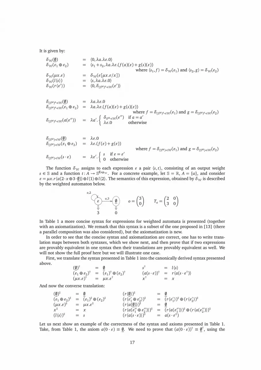
The function δW assigns to each expression ǫ a pair ⟨s, t⟩, consisting of an output weights ∈ S and a function t : A → SExpW . For a concrete example, let S = R, A = a, and considerǫ = µx .r⟨a(2 · x⊕3 ·;)⟩⊕ l⟨1⟩⊕ l⟨2⟩. The semantics of this expression, obtained by δW is describedby the weighted automaton below.

ǫ

a,2

a,3;

3 0

o =

30

Ta =

2 03 0

In Table 1 a more concise syntax for expressions for weighted automata is presented (togetherwith an axiomatization). We remark that this syntax is a subset of the one proposed in [13] (therea parallel composition was also considered), but the axiomatization is new.

In order to see that the concise syntax and axiomatization are correct, one has to write trans-lation maps between both syntaxes, which we show next, and then prove that if two expressionsare provably equivalent in one syntax then their translations are provably equivalent as well. Wewill not show the full proof here but we will illustrate one case.

First, we translate the syntax presented in Table 1 into the canonically derived syntax presentedabove.

(;)† = ;

(ǫ1 ⊕ ǫ2)† = (ǫ1)

† ⊕ (ǫ2)†

(µx .ǫ)† = µx .ǫ†

s† = l⟨s⟩

(a(s · ǫ))† = r⟨a(s · ǫ†)⟩

x† = x

And now the converse translation:

(;)‡ = ;

(ǫ1 ⊕ ǫ2)‡ = (ǫ1)

‡ ⊕ (ǫ2)‡

(µx .ǫ)‡ = µx .ǫ‡

x‡ = x

(l⟨s⟩)‡ = s

(r⟨;⟩)‡ = ;

(r⟨ǫ′1 ⊕ ǫ′2⟩)

‡ = (r⟨ǫ′1⟩)‡ ⊕ (r⟨ǫ′2⟩)

‡

(r⟨a(;)⟩)‡ = ;

(r⟨a(ǫ′′1 ⊕ ǫ′′2 )⟩)

‡ = (r⟨a(ǫ′′1 )⟩)‡ ⊕ (r⟨a(ǫ′′2 )⟩)

‡

(r⟨a(s · ǫ)⟩)‡ = a(s · ǫ‡)

Let us next show an example of the correctness of the syntax and axioms presented in Table 1.Take, from Table 1, the axiom a(0 · ǫ) ≡ ;. We need to prove that (a(0 · ǫ))† ≡ ;†, using the

17

canonically derived axioms for ExpW. The left expression would be translated to r⟨a(0 · ǫ†)⟩,whereas ; would just be translated to ;. Next, using the axioms of ExpW one derives r⟨a(0 · ǫ†)⟩ ≡

r⟨a(;)⟩ ≡ r⟨;⟩ ≡ ;, as expected. ♠

We are now ready to formulate the analogue of Kleene’s theorem for quantitative systems.

4.9 THEOREM (Kleene’s theorem for quantitative functors). Let H be a quantitative functor.

1. For every locally finite H-coalgebra (S,h) and for every s ∈ S there exists an expression ǫs ∈

ExpH such that s ∼b ǫs.

2. For every ǫ ∈ ExpH, there exists a finite H-coalgebra (S,h) with s ∈ S such that s ∼b ǫ.

PROOF. Let H be a quantitative functor.Proof of item 1. Let s ∈ S and let ⟨s⟩ = s1, . . . , sn with s1 = s. We construct, for every state

si ∈ ⟨s⟩, an expression ⟨⟨ si ⟩⟩ such that si ∼ ⟨⟨ si ⟩⟩ (and thus si ∼b ⟨⟨ si ⟩⟩).If H = Id, we set, for every i, ⟨⟨ si ⟩⟩ = ;. It is easy to see that ⟨si ,;⟩ | si ∈ ⟨s⟩ is a bisimulation

and, thus, we have that s ∼ ⟨⟨ s ⟩⟩.For H 6= Id, we proceed in the following way. Let, for every i, Ai = µx i .γ

Hh(si)

where, for F ÃH

and c ∈ F⟨s⟩, the expression γFc∈ ExpFÃH is defined by induction on the structure of F:

γIdsi= x i γB

b= b γ

F1×F2

⟨c,c′⟩ = l⟨γF1c⟩ ⊕ r⟨ǫ

F2

c′⟩ γFA

f=⊕

a∈A a(γFf (a))

γF13+F2

κ1(c)= l[γF1

c] γ

F13+F2

κ2(c)= r[γF2

c] γ

F13+F2

⊥= ; γ

F13+F2

⊤= l[;]⊕ r[;]

γPωF

C =

⊕

c∈C

γFc C 6=

; otherwiseγM

H1

f=⊕

c ∈H1(⟨s⟩)

f (c) 6= 0

f (c) · γH1c

Now, let A0i= Ai , define Ak+1

i= Ak

iAk

k+1/xk+1 and then set ⟨⟨ si ⟩⟩ = Ani. Here, AA′/x denotes

syntactic replacement (that is, substitution without renaming of bound variables in A which arealso free variables in A′).

Observe that the termAn

i= (µx i .γ

Hh(si))A0

1/x1 . . . An−1n/xn

is a closed term because, for every j = 1, . . . , n, the term Aj−1j

contains at most n− j free variablesin the set x j+1, . . . , xn.

It remains to prove that si ∼ ⟨⟨ si ⟩⟩. We show that R= ⟨si , ⟨⟨ si ⟩⟩⟩ | si ∈ ⟨s⟩ is a bisimulation. Forthat, we first define, for F ÃH and c ∈ F⟨s⟩, ξF

c= γF

cA0

1/x1 . . . An−1n/xn and the relation

RFÃH = ⟨c,δFÃH(ξFc)⟩ | c ∈ F⟨s⟩.

Then, we prove that 1 RFÃH = F(R) and 2 ⟨h(si),δH(⟨⟨ si ⟩⟩)⟩ ∈ RHÃH.

1 By induction on the structure of F. We will show here only the proof for the case F =MH1 .

⟨ f , g⟩ ∈MH1(R)

⇔ ∃ϕ : H1(R)→MM

H1(π1)(ϕ) = f and MH1(π2)(ϕ) = g (def. MH1(R))

⇔ f (u) =∑

⟨u,y⟩∈H1(R)

ϕ(⟨u, y⟩) and g(v) =∑

⟨x ,v⟩∈H1(R)

ϕ(⟨x , v⟩) (def. MH1 on arrows)

⇔ f (u) =∑

⟨u,y⟩∈RH1ÃH

ϕ(⟨u, y⟩) and g(v) =∑

⟨x ,v⟩∈RH1ÃH

ϕ(⟨x , v⟩) (ind. hyp.)

⇔ f (u) = ϕ(⟨u,δ(ξH1u)⟩) and g(v) =

∑

v=δ(ξH1x )

ϕ(⟨x ,δ(ξH1x)⟩) (def. RH1ÃH)

18

⇔ f (u) = ϕ(⟨u,δ(ξH1u)⟩) and g(v) =

∑

v=δ(ξH1x )

f (x) (def. f )

⇔ f ∈MH1(⟨s⟩) and g = δMH1ÃH(⊕

f (x) 6=0f (x) · ξH1

x) (def. δMH1ÃH)

⇔ f ∈MH1(⟨s⟩) and g = δMH1ÃH(ξM

H1

f) (def. ξM

H1

f)

⇔ ⟨ f , g⟩ ∈ RMH1ÃH

2 We want to prove that ⟨g(si),δH(⟨⟨ si ⟩⟩)⟩ ∈ RHÃH. For that, we must show that g(si) ∈H⟨s⟩

and δH(⟨⟨ si ⟩⟩) = δH(ξHg(si)). The latter follows by definition of ⟨s⟩, whereas for the former

we observe that:

δH(⟨⟨ si ⟩⟩)

= δH((µx i .γHg(si))A0

1/x1 . . . An−1n/xn) (def. of ⟨⟨ si ⟩⟩)

= δH(µx i .γHg(si)A0

1/x1 . . . Ai−2i−1/x i−1A

ii+1/x i+1 . . . A

n−1n/xn)

= δH(γHg(si)A0

1/x1 . . . Ai−2i−1/x i−1A

ii+1/x i+1 . . . A

n−1n/xn[A

ni/x i]) (def. of δH)

= δH(γHg(si)A0

1/x1 . . . Ai−2i−1/x i−1A

ii+1/x i+1 . . . A

n−1n/xnA

ni/x i) ([An

i/x i] = A

ni/x i)

= δH(γHg(si)A0

1/x1 . . . Ai−2i−1/x i−1A

ni/x iA

ii+1/x i+1 . . . A

n−1n/xn)

= δH(ξHg(si))

Here, note that [Ani/x i] = A

ni/x i, because An

ihas no free variables. The last two steps follow,

respectively, because x i is not free in Aii+1, . . . ,An−1

nand:

Ani/x iA

ii+1/x i+1 . . . A

n−1n/xn

= Ai−1iAi

i+1/x i+1 . . . An−1n/xn/x iA

ii+1/x i+1 . . . A

n−1n/xn

= Ai−1i/x iA

ii+1/x i+1 . . . A

n−1n/xn (3)

Equation (3) uses the syntactic identity

ABC/y/xC/y= AB/xC/y, y not free in C (4)

Proof of item 2. We want to show that for every expression ǫ ∈ ExpH there is a finite H-coalgebra(S, f ) with s ∈ S such that s ∼b ǫ. We construct such coalgebra in the following way.

Again, we only show the proof for H =MH1 . The case when H is a non-deterministic functoris covered by Theorem 2.12 and the other cases (MH×MH, (MH)A andMH

3+MH) follow directlyfrom the H =MH1 , which we shall prove next.

For ǫ ∈ ExpMH1ÃH, we set (S,h) = ⟨ǫ⟩ (recall that ǫ is the subcoalgebra generated by ǫ). Wenow just have to prove that S is finite. In fact we shall prove that S ⊆ cl(ǫ), where cl(ǫ) denotesthe smallest subset containing all subformulas of ǫ and the unfoldings of µ (sub)formulas, that is,the smallest subset satisfying:

cl(;) = ;

cl(ǫ1 ⊕ ǫ2) = ǫ1 ⊕ ǫ2 ∪ cl(ǫ1)∪ cl(ǫ2)

cl(µx .ǫ1) = µx .ǫ1 ∪ cl(ǫ1[µx .ǫ1/x])

cl(l⟨ǫ1⟩) = l⟨ǫ1⟩ ∪ cl(ǫ1)

cl(r⟨ǫ1⟩) = r⟨ǫ1⟩ ∪ cl(ǫ1)

cl(l[ǫ1]) = l[ǫ1] ∪ cl(ǫ1)

cl(r[ǫ1]) = r[ǫ1] ∪ cl(ǫ1)

cl(a(ǫ1)) = a(ǫ1) ∪ cl(ǫ1)

cl(ǫ1) = ǫ1 ∪ cl(ǫ1)

cl(m · ǫ1) = m · ǫ1 ∪ cl(ǫ1)

19

Note that the set cl(ǫ) is finite (the number of unfoldings is finite).To show that S ⊆ cl(ǫ) (S is the state space of ⟨ǫ⟩), it is enough to show that, for any c ∈

H1(ExpMH1ÃH), δMH1ÃH(ǫ)(c) 6= 0⇒ c ∈H1(cl(ǫ)).It is an easy proof by induction on the product of types of expressions and expressions (using

the order defined in equation (2)). We exemplify the cases ǫ = ǫ1 ⊕ ǫ2

δMH1ÃH(ǫ1 ⊕ ǫ2)(c) 6= 0⇔ δMH1ÃH(ǫ1)(c) 6= 0 or δMH1ÃH(ǫ2)(c) 6= 0 (def. δMH1ÃH)⇒ c ∈H1(cl(ǫ1)) or c ∈H1(cl(ǫ2)) (ind. hyp.)⇒ c ∈H1(cl(ǫ1 ⊕ ǫ2)) (def. cl)

and ǫ = µx .ǫ1

δMH1 (µx .ǫ1)(c) 6= 0⇔ δMH1 (ǫ1[µx .ǫ1/x])(c) 6= 0 (def. δMH1 (µx .ǫ1))⇒ c ∈H1(cl(ǫ1[µx .ǫ1/x])) (ind. hyp.)⇒ c ∈H1(cl(µx .ǫ1)) (H1(cl(ǫ1[µx .ǫ1/x]))⊆H1(cl(µx .ǫ1)))

We can now explain the technical reason why we consider in this section only functors that arenot mixed.

In the case of a non-deterministic functor G, the proof of item 2. above requires consideringsubcoalgebras modulo (Associativity), (Commutativity) and (Idempotency) (ACI). Consider for in-stance the expression ǫ = µx .r⟨a(x ⊕ x)⟩ of type D = 2× IdA. The subcoalgebras generated withand without applying ACI are the following:

ǫ

a

ǫa

ǫ⊕ ǫa

(ǫ⊕ ǫ)⊕ (ǫ⊕ ǫ)a . . .

In the case of MH (or MH ×MH, (MH)A and MH3+MH), the idempotency axiom does not hold

anymore. However, surprisingly enough, in these cases proving the finiteness of the subcoalgebra⟨ǫ⟩ is not problematic. The key observation is that the monoid structure will be able to avoid theinfinite scenario described above. What happens is concisely captured by the following example.Take the expression ǫ = µx .2 · (x ⊕ x) for the functor RId. Then, the subcoalgebra generated by ǫis depicted in the following picture:

ǫ2

ǫ⊕ ǫ

4

The syntactic restriction that excludes mixed functors is needed because of the following problem.Take as an example the functor MId × IdA. A well-typed expression for this functor would be ǫ =µx .r⟨a(x⊕ x⊕ l⟨2 · x⟩⊕ l⟨2 · x⟩)⟩. It is clear that we cannot apply idempotency in the subexpressionx ⊕ x ⊕ l⟨2 · x⟩ ⊕ l⟨2 · x⟩ and hence the subcoalgebra generated by ǫ will be infinite:

ǫa

ǫ′a

4 ǫ′ ⊕ ǫ′a

8

(ǫ′ ⊕ ǫ′)⊕ (ǫ′ ⊕ ǫ′)a

16

. . .

with ǫ′ = ǫ⊕ ǫ⊕ l⟨2 · ǫ⟩⊕ l⟨2 · ǫ⟩. We will show in the next section how to overcome this problem.Let us summarize what we have achieved so far: we have presented a framework that allows,

for each quantitative functor H ∈ QF, the derivation of a language ExpH. Moreover, Theorem 4.9guarantees that for each expression ǫ ∈ ExpH, there exists a finite H-coalgebra (S,h) that containsa state s ∈ S bisimilar to ǫ and, conversely, for each locally finite H-coalgebra (S,h) and for everystate in s there is an expression ǫs ∈ ExpH bisimilar to s.

Next, we show that the axiomatization is sound and complete with respect to behaviouralequivalence.

20

4.1. Soundness and Completeness

The proof of soundness and completeness follows exactly the same structure as the ones pre-sented in [8] for non-deterministic functors (with the difference that now we use behavioral equiv-alence ∼b instead of bisimilarity ∼). We will recall all the steps here, but will only show the proofof each theorem and lemma for the new case of the monoidal exponentiation functor.

The relation ≡ gives rise to the equivalence map [−]: ExpFÃH→ ExpFÃH/≡, defined by [ǫ] =ǫ′ | ǫ ≡ ǫ′. The following diagram summarizes the maps we have defined so far:

ExpFÃH

δFÃH

[−]ExpFÃH/≡

F(ExpH)F[−]

F(ExpH/≡)

In order to complete the diagram, we next prove that the relation ≡ is contained in the kernel ofF[−] δFÃH

3. This will guarantee the existence of a well-defined function ∂FÃH : ExpFÃH/≡ →

F(ExpH/≡) which, when F = H, provides ExpH/≡ with a coalgebraic structure ∂H : ExpH/≡ →

H(ExpH/≡) (as before we write ∂H for ∂HÃH) and which makes [−] a homomorphism of coalge-bras.

4.10 LEMMA. Let H and F be quantitative functors, with F Ã H. For all ǫ1,ǫ2 ∈ ExpFÃH with

ǫ1 ≡ ǫ2,

(F[−]) δFÃH(ǫ1) = (F[−]) δFÃH(ǫ2)

PROOF. By induction on the length of derivations of ≡.We just show the proof for the axioms 0 · ǫ = ; and (m · ǫ)⊕ (m′ · ǫ) = (m+m′) · ǫ.

δMH1ÃH(0 · ǫ) = λc.0 = δMH1ÃH(;)

δMH1ÃH((m · ǫ)⊕ (m′ · ǫ)) = λc.δMH1ÃH(m · ǫ)(c) +δMH1ÃH(m

′ · ǫ)(c)

= λc.

¨

m+m′ if δH1ÃH(ǫ) = c

0 otherwise= δMH1ÃH((m+m′) · ǫ)

Thus, we have now provided the set ExpH/≡ with a coalgebraic structure: we have defined afunction ∂H : ExpH/≡→ H(ExpH/≡), with ∂H([ǫ]) = (H[−]) δH(ǫ).

At this point we can prove soundness, since it is a direct consequence of the fact that theequivalence map [−] is a coalgebra homomorphism.

4.11 THEOREM (Soundness). Let H be a quantitative functor. For all ǫ1,ǫ2 ∈ ExpH,

ǫ1 ≡ ǫ2⇒ ǫ1 ∼b ǫ2

PROOF. Let H be a quantitative functor, let ǫ1,ǫ2 ∈ ExpH and suppose that ǫ1 ≡ ǫ2. Then, [ǫ1] =[ǫ2] and, thus

behExpH/≡([ǫ1]) = behExpH/≡

([ǫ2])

where behS denotes, for any H-coalgebra (S, f ), the unique map into the final coalgebra. Theuniqueness of the map into the final coalgebra and the fact that [−] is a coalgebra homomorphismimplies that

behExpH/≡ [−] = behExpH

(5)

3This is equivalent to proving that ExpFÃH/≡, together with [−], is the coequalizer of the projection morphisms from≡ to ExpFÃH .

21

which then yieldsbehExpH

(ǫ1) = behExpH(ǫ2)

Hence, ǫ1 ∼b ǫ2.For completeness a bit more of work is required. Let us explain upfront the key ingredients of

the proof. The goal is to prove that ǫ1 ∼b ǫ2⇒ ǫ1 ≡ ǫ2. First, note that, using equation (5) above,we have

ǫ1 ∼b ǫ2⇔ behExpH(ǫ1) = behExpH

(ǫ2)⇔ behExpH/≡([ǫ1]) = behExpH/≡

([ǫ2]) (6)

We then prove that behExpH/≡is injective, which is a sufficient condition to guarantee that ǫ1 ≡ ǫ2

(since it implies, together with (6), that [ǫ1] = [ǫ2]).We proceed as follows. First, we factorize behExpH/≡

into an epimorphism and a monomor-phism [35, Theorem 7.1] as shown in the following diagram (where I = behExpH/≡

(ExpH/≡)):

ExpH/≡

behExpH/≡

e

∂H

Im

ωH

ΩH

ωH

H(ExpH/≡) H(I) HΩH

(7)

Then, we prove that (1) (ExpH/≡,∂H) is a locally finite coalgebra (Lemma 4.12) and (2) bothcoalgebras (ExpH/≡,∂H) and (I ,ωH) are final in the category of locally finite H-coalgebras (Lem-mas 4.15 and 4.16, respectively). Since final coalgebras are unique up to isomorphism, it followsthat e : ExpH/≡→ I is in fact an isomorphism and therefore behExpH/≡

is injective, which will giveus completeness.

We now proceed with presenting and proving the extra lemmas needed in order to provecompleteness. We start by showing that the coalgebra (ExpH/≡,∂H) is locally finite (note that thisimplies that (I ,ωH) is also locally finite) and that ∂H is an isomorphism.

4.12 LEMMA. The coalgebra (ExpH/≡,∂H) is a locally finite coalgebra. Moreover, ∂H is an isomor-

phism.

PROOF. Locally finiteness is a direct consequence of the generalized Kleene’s theorem (Theo-rem 4.9). In the proof of Theorem 4.9 we showed that given ǫ ∈ ExpH, for H = MH1 , H =

MH1 ×MH2 , H = (MH1)A or H = MH1 3+MH2 , the subcoalgebra ⟨ǫ⟩ is finite. In case H is a non-

deterministic functor, we proved in [8] that the subcoalgebra ⟨[ǫ]ACIE⟩ is finite. Thus, the subcoal-gebra ⟨[ǫ]⟩ is always finite (since ExpH/≡ is a quotient of both ExpH and ExpH/≡ACIE

). Recall thatACIE abbreviates the axioms (Associativity), (Commutativity), (Idempotency) and (Empty).

To see that ∂H is an isomorphism, first define, for every F ÃH,

∂ −1FÃH

(c) = [γF

c] (8)

where γF

cis defined, for F 6= Id, as γF

cin the proof of Theorem 4.9, and for F = Id as γId

[ǫ] = ǫ. Then,

we prove that the function ∂ −1FÃH

has indeed the desired properties 1 ∂ −1FÃH ∂FÃH = idExpFÃH/≡

and 2 ∂FÃH ∂−1FÃH

= idF(ExpFÃH/≡). Instantiating F =H one derives that δH is an isomorphism.

It is enough to prove for 1 that γF

∂FÃH([ǫ])≡ ǫ and for 2 that ∂FÃH([γ

F

c]) = c. We just illustrate

the case F =MH1 .

1 By induction on the product of types of expressions and expressions (using the order definedin equation (2)).

γMH1

∂M

H1ÃH([m·ǫ])

=⊕

∂MH1ÃH([m · ǫ])(c) · γH1c| c ∈H1(ExpH/≡),∂MH1ÃH([m · ǫ])(c) 6= 0

= m · γH1

∂H1ÃH([ǫ])

≡ m · ǫ

22

In the last step, we used the induction hypothesis, whereas in the one but last step we used thefact that ∂MH1ÃH([m · ǫ])(c) 6= 0⇔ c = ∂H1ÃH([ǫ]).2 By induction on the structure of F.

∂MH1ÃH([γM

H1

f]) = ∂MH1ÃH([

⊕

f (c) · γH1c| c ∈H1(ExpH/≡), f (c) 6= 0])

= λc′.∑

f (c) | c ∈H1(ExpH/≡) and c′ = ∂H1ÃH(γH1c)

IH= λc′.∑

f (c) | c ∈H1(ExpH/≡) and c′ = c

= f

We now prove the analogue of the following useful and intuitive equality on regular expres-sions, which we will then make use of to prove that there exists a coalgebra homomorphismbetween any locally finite coalgebra (S,h) and (ExpH/≡,∂H).

Given a deterministic automaton ⟨o, t⟩: S → 2× SA and a state s ∈ S, the associated regularexpression rs can be written as

rs = o(s) +∑

a∈A

a · rt(s)(a) (9)

using the axioms of Kleene algebra [11, Theorem 4.4].

4.13 LEMMA. Let (S,h) be a locally finite H-coalgebra, with H 6= Id, and let s ∈ S, with ⟨s⟩ =

s1, . . . , sn (where s1 = s). Then:

⟨⟨ si ⟩⟩ ≡ γHg(si)⟨⟨ s1 ⟩⟩/x1 . . . ⟨⟨ sn ⟩⟩/xn (10)

PROOF. Let Aki, where i and k range from 1 to n, be the terms defined as in the proof of Theo-

rem 4.9. Recall that ⟨⟨ si ⟩⟩= Ani. We calculate:

⟨⟨ si ⟩⟩

= Ani

= (µx i .γG

g(si))A0

1/x1 . . . An−1n/xn

= µx i .(γG

g(si)A0

1/x1 . . . Ai−2i−1/x i−2A

ii+1/x i+1 . . . A

n−1n/xn)

≡ γG

g(si)A0

1/x1 . . . Ai−2i−1/x i−2A

ii+1/x i+1 . . . A

n−1n/xnA

ni/x i (fixed-point axiom4)

= γG

g(si)A0

1/x1 . . . An−1n/xn (by 3)

= γG

g(si)A0

1A12/x2 . . . A

n−1n/xn/x1 . . . A

n−1n/xn (by 4)

= γG

g(si)An

1/x1A12/x2 . . . A

n−1n/xn (def. An

1)

... (last 2 steps for A12, . . . ,An−2

n−1)

= γG

g(si)An

1/x1An2/x2 . . . A

nn/xn (An

n−1 = Ann)

= γG

g(si)[An

1/x1][An2/x2] . . . [A

nn/xn] (all An

iare closed)

Instantiating (10) for ⟨o, t⟩: S → 2× SA, one can easily spot the similarity with equation (9)above:

⟨⟨ s ⟩⟩ ≡ l⟨o(s)⟩ ⊕ rD⊕

a∈A

a

⟨⟨ t(s)(a) ⟩⟩

E

The above equality is used to prove that there exists a coalgebra homomorphism between anylocally finite coalgebra (S,h) and (ExpH/≡,∂H).

4Note that the fixed point axiom can be formulated using syntactic replacement rather than substitution – γµx .γ/x ≡µx .γ – since µx .γ is a closed term.

23

4.14 LEMMA. Let (S,h) be a locally finite H-coalgebra. There exists a coalgebra homomorphism

⌈−⌉: S→ ExpH/≡.

PROOF. We define ⌈−⌉ = [−] ⟨⟨−⟩⟩, where ⟨⟨−⟩⟩ is as in the proof of Theorem 4.9, associatingto a state s of a locally finite coalgebra an expression ⟨⟨ s ⟩⟩ with s ∼ ⟨⟨ s ⟩⟩. To prove that ⌈−⌉ is ahomomorphism we need to verify that (H⌈−⌉) h= ∂H ⌈−⌉.

If H = Id, then (H⌈−⌉) g(si) = [;] = ∂H(⌈ si ⌉). For H 6= Id we calculate, using Lemma 4.13:

∂H ⌈ si ⌉= ∂H([γHg(si)[⟨⟨ s1 ⟩⟩/x1] . . . [⟨⟨ sn ⟩⟩/xn]])

and we then prove the more general equality, for F ÃH and c ∈ F⟨s⟩:

∂FÃH([γFc[⟨⟨ s1 ⟩⟩/x1] . . . [⟨⟨ sn ⟩⟩/xn]]) = F⌈−⌉(c) (11)

The intended equality then follows by taking F =H and c = g(si). Let us prove the equation (11)by induction on F. We only show the case F =MH1 .

∂MH1ÃH([γM

H1

f[⟨⟨ s1 ⟩⟩/x1] . . . [⟨⟨ sn ⟩⟩/xn]])

= ∂MH1ÃH([⊕

f (c) · γH1c[⟨⟨ s1 ⟩⟩/x1] . . . [⟨⟨ sn ⟩⟩/xn] | c ∈H1(ExpH/≡), f (c) 6= 0])

= λc′.∑

f (c) | c ∈H1(ExpH/≡) and c′ = ∂H1ÃH(γH1c[⟨⟨ s1 ⟩⟩/x1] . . . [⟨⟨ sn ⟩⟩/xn])

IH= λc′.∑

f (c) | c ∈H1(ExpH/≡) and c′ = (H1⌈−⌉)(c)

= MH1(⌈−⌉)( f )

We can now prove that the coalgebras (ExpH/≡,∂H) and (I ,ωH) are both final in the categoryof locally finite H-coalgebras.

4.15 LEMMA. The coalgebra (I ,ωH) is final in the category Coalg(H)LF.

PROOF. We want to show that for any locally finite coalgebra (S,h), there exists a unique homomor-phism (S,h) → (I ,ωH). The existence is guaranteed by Lemma 4.14, where ⌈−⌉: S → ExpH/≡is defined. Postcomposing this homomorphism with e (defined above, in diagram 7) we get acoalgebra homomorphism e ⌈−⌉: S → I . If there is another homomorphism f : S → I , then bypostcomposition with the inclusion m: I ,→ Ω we get two homomorphisms (m f and m e ⌈−⌉)into the final H-coalgebra. Thus, f and e ⌈−⌉ must be equal.

4.16 LEMMA. The coalgebra (ExpH/≡,∂H) is final in the category Coalg(H)LF.

PROOF. We want to show that for any locally finite coalgebra (S,h), there exists a unique ho-momorphism (S,h) → (ExpH/≡,∂H). We only need to prove uniqueness, since the existence isguaranteed by Lemma 4.14, where ⌈−⌉: S→ ExpH/≡ is defined.

Suppose we have another homomorphism f : S→ ExpH/≡. Then, we shall prove that f = ⌈−⌉.First, observe that because f is a homomorphism the following holds for every s ∈ S (without anyrisk of confusion, in this proof that follows we denote equivalence classes [ǫ] by expressions ǫrepresenting them):

f (s) = ∂ −1HH f h(s) = [γH

g(s)[ f (s1)/x1] . . . [ f (sn)/xn]] (12)

where ⟨s⟩ = s1, . . . , sn, with s1 = s (recall that ∂ −1H

was defined in (8) and note that γH

H f h(s)=

γHh(s)[ f (si)/x i]).We now have to prove that f (si) = ⌈ si ⌉, for all i = 1, . . . n. The proof, which relies mainly on

uniqueness of fixed points, is exactly the same as in the analogue theorem for non-deterministicfunctors and we omit it here.

24

Because final objects are unique up-to isomorphism, we know that e : ExpH/≡→ I is an isomor-phism and hence we can conclude that the map behExpH/≡

is injective, since it factorizes into anisomorphism followed by a mono. This fact is the last ingredient we need to prove completeness.

4.17 THEOREM (Completeness). Let H be a quantitative functor. For all ǫ1,ǫ2 ∈ ExpH,

ǫ1 ∼b ǫ2⇒ ǫ1 ≡ ǫ2

PROOF. Let H be a quantitative functor, let ǫ1,ǫ2 ∈ ExpH and suppose that ǫ1 ∼b ǫ2, that is,behExpH

(ǫ1) = behExpH(ǫ2). Since the equivalence class map [−] is a homomorphism, it holds that

behExpH/≡([ǫ1]) = behExpH/≡

([ǫ2]). Now, because behExpH/≡is injective we have that [ǫ1] = [ǫ2].

Hence, ǫ1 ≡ ǫ2.

5. Extending the class of functors

In the previous section, we introduced regular expressions for the class of quantitative functors.In this section, by employing standard results from the theory of coalgebras, we show how to usesuch regular expressions to describe the coalgebras of many more functors, including the mixedfunctors we mentioned in Section 4.

Given F and G two endofunctors on Set, a natural transformation α: F ⇒ G is a family offunctions αS : F(S)→ G(S) (for all sets S), such that for all functions h: T → U , αUF(h) = G(h)αT .If all the αS are injective, then we say that α is injective.

5.1 PROPOSITION. An injective natural transformation α: F⇒ G induces a functor α(−): Coalg(F)LF→

Coalg(G)LF that preserves and reflects behavioural equivalence.

PROOF. It is well known from [35, 5] that, an injective α: F⇒ G induces a functor α(−): Coalg(F)→

Coalg(G) that preserves and reflects behavioural equivalence. Thus we have only to prove thatα (−) maps locally finite F-coalgebras into locally finite G-coalgebras.

Recall that α (−) maps each F-coalgebra (S, f ) into the G-coalgebra (S,α f ), and each F-homomorphism into itself. We prove that if (S, f ) is locally finite, then also (S,α f ) is locallyfinite.

An F-coalgebra (S, f ) is locally finite if for all s ∈ S, there exists a finite set Vs ⊆ S, such thats ∈ Vs and Vs is a subsystem of S. That is, there exists a function v : Vs → F(Vs), such that theinclusion i : Vs → S is an F-homomorphism between (Vs, v) and (S, f ). At this point, note that ifi : V → S is an F-homomorphism between (Vs, v) and (S, f ), then it is also a G-homomorphismbetween (Vs,α v) and (S,α f ). Thus, (S,α f ) is locally finite.

This result allows us to extend our framework to many other functors, as we shall explainnext. Consider a functor F which is not quantitative and suppose there exists an injective naturaltransformation α from F into some quantitative functor H. A (locally finite) F-coalgebra can betranslated into a (locally finite) H-coalgebra via the functor α(−) and then it can be characterizedby using expressions in ExpH. The axiomatization for ExpH is still sound and complete for F-coalgebras, since the functor α (−) preserves and reflects behavioural equivalence.

However, note that (half of) Kleene’s theorem does not hold anymore, because not all the ex-pressions in ExpH denote F-behaviours or, more precisely, not all expressions in ExpH are equiva-lent to H-coalgebras that are in the image of α (−). Thus, in order to retrieve Kleene’s theorem,one has to exclude such expressions. In many situations, this is feasible by simply imposing somesyntactic constraints on ExpH.

Let us illustrate this by means of an example. First, we recall the definition of the probabilityfunctor (which will play a key role in the next section).

5.2 DEFINITION (Probability functor). A probability distribution over a set S is a function d : S→

[0,1] such that∑

s∈S d(s) = 1. The probability functor Dω : Set→ Set is defined as follows. Forall sets S, Dω(S) is the set of probability distributions over S with finite support. For all functionsh: S→ T , Dω(h) maps each d ∈Dω(S) into dh (Definition 3.1). ♣

25

Note that for any set S, Dω(S) ⊆ RS since probability distributions are also functions from

S to R. Let ι be the family of inclusions ιS : Dω(S) → RS . It is easy to see that ι is a natural

transformation between Dω and RId (the two functors are defined in the same way on arrows).Thus, in order to specify Dω-coalgebras, we will use ǫ ∈ ExpRId . These are the closed and guardedexpressions given by the following BNF, where r ∈ R and x ∈ X (X a set of fixed-point variables)

ǫ ::= ; | ǫ⊕ ǫ | x | µx .ǫ | r · ǫ

This language is enough to specify all Dω-behaviours, but it also allows us to specify RId-behavioursthat are not Dω-behaviours, such as for example, µx .2·x and µx .0·x . In order to obtain a languageExpDω

that specifies all and only the regular Dω-behaviours, it suffices to change the BNF above asfollows:

ǫ ::= x | µx .ǫ |⊕

i∈1...n

pi · ǫi for pi ∈ (0,1] such that∑

i∈1...n

pi = 1 (13)

where⊕

i∈1...npi · ǫi denotes p1 · ǫ1 ⊕ · · · ⊕ pn · ǫn.

Next, we prove Kleene’s theorem for this restricted syntax. Note that the procedure of appro-priately restricting the syntax usually requires some ingenuity. We shall see that in many concretecases, as for instance Dω above, it is fairly intuitive which restriction to choose. Also, althoughwe cannot provide a uniform proof of Kleene’s theorem, the proof for each concrete example is aslight adaptation of the more general one (Theorem 4.9).

5.3 THEOREM (Kleene’s Theorem for the probability functor).

1. For every locally finite Dω-coalgebra (S, d) and for every s ∈ S there exists an expression ǫs ∈

ExpDωsuch that s ∼b ǫs.

2. For every ǫ ∈ ExpDω, there exists a finite Dω-coalgebra (S, d) with s ∈ S such that s ∼b ǫ.

PROOF. Let s ∈ S and let ⟨s⟩ = s1, . . . , sn with s1 = s. We construct, for every state si ∈ ⟨s⟩, anexpression ⟨⟨ si ⟩⟩ such that si ∼ ⟨⟨ si ⟩⟩ (and thus s ∼b ǫs) .

Let, for every i, Ai = µx i .⊕

d(si)(s j) 6=0d(si)(s j) · x j.

Now, let A0i= Ai, define Ak+1

i= Ak

iAk

k+1/xk+1 and then set ⟨⟨ si ⟩⟩= Ani. Observe that the term

Ani= (µx i .⊕

d(si)(s j) 6=0

d(si)(s j) · x j)A01/x1 . . . A

n−1n/xn

is a closed term and∑

d(si)(s j) 6=0d(si)(s j) = 1. Thus, An

i∈ ExpDω

.

It remains to prove that si ∼b ⟨⟨ si ⟩⟩. We show that R= ⟨si , ⟨⟨ si ⟩⟩⟩ | si ∈ ⟨s⟩ is a bisimulation.For that we define a function ξ: R → Dω(R) as ξ(⟨si ,−⟩)(⟨s j ,−⟩) = d(si)(s j) and we observe thatthe projection maps π1 and π2 are coalgebra homomorphisms, that is, the following diagramcommutes.

⟨s⟩

(1)d

Rπ1

(2)ξ

π2An

i| si ∈ ⟨s⟩

δExpDω

Dω(⟨s⟩) Dω(R)Dω(π1) Dω(π2)

Dω(Ani| si ∈ ⟨s⟩)

Dω(π1)(ξ(⟨si ,Ani⟩))(s j) =∑

⟨s j ,x⟩∈R

ξ(⟨si ,Ani⟩)(⟨s j , x⟩) = d(si)(s j) (1)

Dω(π2)(ξ(⟨si ,Ani⟩))(An

j) =∑

⟨x ,anj⟩∈R

ξ(⟨si ,Ani⟩)(⟨x ,An

j⟩) = d(si)(s j) = δExpDω

(Ani)(An

j) (2)

For the second part of the theorem, We need to show that for every expression ǫ ∈ ExpDωthere is

a finite Dω-coalgebra (S, d) with s ∈ S such that s ∼b ǫ. We take (S, d) = ⟨ǫ⟩ and we observe that S

is finite, because S ⊆ cl(ǫ) (the proof of this inclusion is as in Theorem 4.9).

26

•

a

ba

1/21/2 1/32/31

• • • • •

•1/2 1/2

•1/3 2/3

•

b

•

a

•

a

•

• •

•

1/3 2/31

aa abb

• • • • •

(i) (ii) (iii)

Figure 1: (i) A simple Segala system, (ii) a stratified system and (iii) a Pnueli-Zuck system

The axiomatization of ExpDωis a subset of the one for ExpRId , since some axioms, such as

; ≡ 0 · ǫ, have no meaning in the restricted syntax. In this case the axiomatization for ExpDω

would contain the axioms for the fixed-point, plus (Associativity), (Commutativity) and p · ǫ ⊕ p′ ·

ǫ = (p + p′) · ǫ. The soundness of this axiomatization comes for free from the soundness in RId,because behavioural equivalence in RId implies behavioural equivalence in Dω. Completenessneeds however a bit more of work: we need to prove that, for any two expressions in the newsyntax, if they are provably equivalent using all the axioms of ExpRId then they must be provablyequivalent using only the restricted set of axioms. Note that it is usually obvious which axiomsone needs to keep for the restricted syntax.

For another example, consider the functors Id and Pω(Id). Let τ be the family of functionsτS : S → Pω(S) mapping each s ∈ S in the singleton set s. It is easy to see that τ is an injectivenatural transformation. With the above observation, we can also get regular expressions for thefunctor MId × IdA which, as discussed in Section 4, does not belong to our class of quantitativefunctors. By extending τ, we can construct an injective natural transformation MId × IdA⇒MId ×

Pω(Id)A.

In the same way, we can construct an injective natural transformation from the functor Dω(Id)+

(A× Id) + 1 (which is the type of stratified systems, which we shall use as an example in thenext section) into RId + (A× Pω(Id)) + 1. Since the latter is a quantitative functor, we can useits expressions and axiomatization for stratified systems. But since not all its expressions definestratified behaviours, we again will have to restrict the syntax.

6. Probabilistic Systems

Many different types of probabilistic systems have been defined in literature: examples includereactive, generative, stratified, alternating, (simple) Segala, bundle and Pnueli-Zuck. Each typecorresponds to a functor, and the systems of a certain type are coalgebras of the correspondingfunctor. A systematic study of all these systems as coalgebras was made in [5]. In particular, Fig-ure 1 of [5] provides a full correspondence between types of systems and functors. By employingthis correspondence and the results of the previous section, we can use our framework in order toderive regular expressions and axiomatizations for all these types of probabilistic systems.

In order to show the effectiveness of our approach, we have derived expressions and axiomsfor three different types of probabilistic systems: simple Segala, stratified, and Pnueli-Zuck.

Simple Segala systems. Simple Segala systems are transition systems where both probability andnon determinism are present. They are coalgebras of the functor Pω(Dω(Id))

A. Each labelledtransition leads, non-deterministically, to a probability distribution of states instead of a singlestate. An example is shown in Figure 1(i).

We recall the expressions and axioms for simple Segala systems as shown in Table 1.

27

ǫ::= ; | ǫ⊞ ǫ | µx .ǫ | x | a(ǫ′) where a ∈ A, pi ∈ (0,1] and∑

i∈1...npi = 1

ǫ′::=⊕

i∈1···npi · ǫi

(ǫ1 ⊞ ǫ2)⊞ ǫ3 ≡ ǫ1 ⊞ (ǫ2 ⊞ ǫ3) ǫ1 ⊞ ǫ2 ≡ ǫ2 ⊞ ǫ1 ǫ⊞ ; ≡ ǫ ǫ⊞ ǫ ≡ ǫ

(ǫ′1 ⊕ ǫ′2)⊕ ǫ

′3 ≡ ǫ

′1 ⊕ (ǫ

′2 ⊕ ǫ

′3) ǫ′1 ⊕ ǫ

′2 ≡ ǫ

′2 ⊕ ǫ

′1 (p1 · ǫ)⊕ (p2 · ǫ)≡ (p1 + p2) · ǫ

ǫ[µx .ǫ/x]≡ µx .ǫ γ[ǫ/x]≡ ǫ⇒ µx .γ≡ ǫ

Here, in order to avoid confusion, we use ⊞ instead of ⊕ for the expressions at the top level, mak-ing a clear distinction between the idempotent (non-deterministic) and non-idempotent (proba-bilistic) sums. The syntax above was obtained from the canonically derived one by applying therestrictions arising from Dω and also some simplifications (syntactic sugar) which improve read-ability (in the spirit of what we showed before for ExpW, the expressions for weighted automata).

As we showed in section 5, to be completely formal we would have to prove Kleene’s Theoremand the completeness of the axiomatization for the restricted syntax (as well as the correctness ofthe simplifications). The proofs would be based on the ones we showed for the functor Dω (and theones for the simplifications similar to what we showed for ExpW). We omit them here and showinstead an example of application. The expression a(1/2·;⊕1/2·;)⊞a(1/3·;⊕2/3·;)⊞b(1·;)is bisimilar to the top-most state in the simple Segala system depicted in Figure 1(i). Using theaxiomatization, we can derive:

a(1/2 · ; ⊕ 1/2 · ;)⊞ a(1/3 · ; ⊕ 2/3 · ;)⊞ b(1 · ;)≡ a((1/2+ 1/2) · ;)⊞ a((1/3+ 2/3) · ;)⊞ b(1 · ;)≡ a(1 · ;)⊞ a(1 · ;)⊞ b(1 · ;)≡ a(1 · ;)⊞ b(1 · ;)

Thus, we can conclude that the system presented in Figure 1(i) is bisimilar to the following one:

•a b

1 1•

The language and axiomatization we presented above are the same as the one presented in [17](with the difference that in [17] a parallel composition operator was also considered). This isof course reassuring for the correctness of the general framework we presented. In the next twoexamples, we will present new results (that is syntax/axiomatizations which did not exist). This iswhere the generality starts paying off: not only one recovers known results but also derives newones, all of this inside the same uniform framework.

Stratified systems. Stratified systems are coalgebras of the functor Dω(Id)+(B×Id)+1. Each stateof these systems either performs unlabelled probabilistic transitions or one B-labelled transitionor it terminates. We first derive expressions and axioms for RId + (B× Pω(Id)) + 1 and then werestrict the syntax to characterize only Dω(Id) + (B× Id) + 1-behaviours. This, together with theintroduction of some syntactic sugar, leads to the following syntax and axioms.

ǫ::= µx .ǫ | x | ⟨b,ǫ⟩ |⊕

i∈1···npi · ǫi | ↓ where b ∈ B, pi ∈ (0,1] and

∑

i∈1...npi = 1

(ǫ1 ⊕ ǫ2)⊕ ǫ3 ≡ ǫ1 ⊕ (ǫ2 ⊕ ǫ3) ǫ1 ⊕ ǫ2 ≡ ǫ2 ⊕ ǫ1 (p1 · ǫ)⊕ (p2 · ǫ)≡ (p1 + p2) · ǫ

ǫ[µx .ǫ/x]≡ µx .ǫ γ[ǫ/x]≡ ǫ⇒ µx .γ≡ ǫ

Here ↓, which denotes termination, corresponds to the canonically derived expression r[r[1]],while ⟨b,ǫ⟩ corresponds to r[l[l⟨b⟩ ⊕ r⟨ǫ⟩]].

28

We can use these axioms (together with Kleene’s theorem) to reason about the system pre-sented in Figure 1(ii). The topmost state of this system is bisimilar to the expression

1/2 · (1/3 · ⟨a,↓⟩ ⊕ 2/3 · ⟨a,↓⟩)⊕ 1/2 · ⟨b,↓⟩

which in turn is provably equivalent to 1/2 · (1 · ⟨a,↓⟩)⊕ 1/2 · ⟨b,↓⟩. That leads us to conclude thatthe aforementioned system is equivalent to the following simpler one.

•1/2 1/2

•

1

•

b

•a

•

The language of expressions we propose for these systems is a subset of the language originallyproposed in [45] (there a parallel composition operator is also considered). More interestingly,there was no axiomatization of the language in [45] and thus the axiomatization we present hereis completely new.

Pnueli-Zuck systems. These systems are coalgebras of the functor PωDω(Pω(Id)A). Intuitively, the

ingredient Pω(Id)A denotes A-labelled transitions to other states. Then, Dω(Pω(Id))

A corresponds toa probability distribution of labelled transitions and then, each state of a PωDω(Pω(Id))

A-coalgebraperforms a non-deterministic choice amongst probability distributions of labelled transitions. Foran example, consider the system depicted in Figure 1(iii).

The expressions and axioms for these systems are the following.

ǫ::= ; | ǫ⊞ ǫ | µx .ǫ | x | ǫ′ where a ∈ A, pi ∈ (0,1] and∑

i∈1...npi = 1

ǫ′::=⊕

i∈1···npi · ǫ

′′i

ǫ′′::= ; | ǫ′′ ⊞ ǫ′′ | a(ǫ)

(ǫ1 ⊞ ǫ2)⊞ ǫ3 ≡ ǫ1 ⊞ (ǫ2 ⊞ ǫ3) ǫ1 ⊞ ǫ2 ≡ ǫ2 ⊞ ǫ1 ǫ⊞ ; ≡ ǫ ǫ⊞ ǫ ≡ ǫ

(ǫ′1 ⊕ ǫ′2)⊕ ǫ

′3 ≡ ǫ

′1 ⊕ (ǫ

′2 ⊕ ǫ

′3) ǫ′1 ⊕ ǫ

′2 ≡ ǫ

′2 ⊕ ǫ

′1 (p1 · ǫ

′′)⊕ (p2 · ǫ′′)≡ (p1 + p2) · ǫ

′′

(ǫ′′1 ⊞ ǫ′′2 )⊞ ǫ

′′3 ≡ ǫ

′′1 ⊞ (ǫ

′′2 ⊞ ǫ

′′3 ) ǫ

′′1 ⊞ ǫ

′′2 ≡ ǫ

′′2 ⊞ ǫ

′′1 ǫ′′ ⊞ ; ≡ ǫ′′ ǫ′′ ⊞ ǫ′′ ≡ ǫ′′

ǫ[µx .ǫ/x]≡ µx .ǫ γ[ǫ/x]≡ ǫ⇒ µx .γ≡ ǫ

The expression 1/3·(a(;)⊞a(;))⊕2/3·(b(;)⊞a(;))⊞1·b(;) specifies the Pnueli-Zucksystem in Figure 1(iii). Note that we use the same symbol ⊞ for denoting two different kinds ofnon-deterministic choice. This is safe, since they satisfy exactly the same axioms.

Both the syntax and the axioms we propose here for these systems are to the best of ourknowledge new. In the past, these systems were studied using a temporal logic [33].

7. A slight variation on the monoidal exponentiation functor

In this section we show a slight variation on the definition of the monoidal exponentiationfunctor which would allow for a cleaner derivation of syntax and axioms for certain functors,among which the probability functor.

In the spirit of [26], where this functor is defined, we shall call it constrained monoidal expo-nentiation functor.

7.1 DEFINITION (Constrained monoidal exponentiation functor). LetM be a commutative monoidand V ⊆M (V being the constraint). The constrained monoidal exponentiation functorM−

V: Set→

Set is defined on sets as MSV= f ∈MS

ω |∑

s∈S

f (s) ∈ V and on functions as M−ω. ♣

29

The probability functor Dω coincides now with (R+0 )−1 (R+0 denotes the monoid of positive real

numbers).The expressions associated with this functor are the closed and guarded expressions given by

the following BNF, where x ∈ X and mi ∈M,

ExpM−V ∋ ǫ ::= x | µx .ǫ |⊕

i∈I

mi · ǫi such that∑

i∈I

mi ∈ V

We note that instantiating this syntax for (R+0 )−1, one gets precisely the syntax we proposed in

equation (13) for Dω.Providing a Kleene like theorem and a sound and complete axiomatization goes precisely as

before (for the functor M−ω), with the minor difference that the axiom 0 · ǫ ≡ ; has to be replacedby 0 · ǫ⊕m · ǫ′ ≡ m · ǫ′, since ; is not a valid expression for this functor.

All of this seems to indicate that using the constrained monoidal exponentiation functor wouldhave made it easier to define expressions and axiomatizations for quantitative systems. Althoughthis would have been true for systems such as the simple Segala, it would not completely avoidthe use of the technique we described in Section 5, which allows us to deal with a large class offunctors: not only with Dω (embedded into RId) but also with mixed functors, such the one ofstratified systems. Moreover, using this functor would require extra care when dealing with themodularity of the axiomatization, which we will illustrate next by means of an example. For thesereasons, we decided to present the syntax and axiomatizations of all our running examples as aspecial instance of the general technique described in Section 5.

7.2 EXAMPLE (Reactive probabilistic automata). Let us consider a very simple version of reactiveprobabilistic automata, coalgebras for the functor Dω(−)

A = ((R+0 )Id1)

A.The syntax modularly derived for this functor would be

ǫ::= ; | ǫ⊕ ǫ | x | µx .ǫ | a(ǫ′)ǫ′::=⊕

i∈I

pi · ǫi such that∑

i∈I

pi = 1

In the axiomatization, we would (expect to) have the axiom a(ǫ1)⊕ a(ǫ2) ≡ a(ǫ1 ⊕ ǫ2). But nownote how this could lead to an inconsistent specification, since ǫ1⊕ǫ2 will not be a valid expressionanymore for Dω (if

∑

pi = 1 in both ǫ1 and ǫ2 then it will be 2 in ǫ1 ⊕ ǫ2!).In order to keep the axiomatization compositional we would have to require certain conditions

on the set V in the functorM−V

. For instance, one of the possible conditions would be that V wouldhave to be closed with respect to +, which would be a too strong condition to model Dω. ♠

8. Discussion

We presented a general framework to canonically derive expressions and axioms for quantita-tive regular behaviours. To illustrate the effectiveness and generality of our approach we derivedexpressions and equations for weighted automata, simple Segala, stratified and Pnueli-Zuck sys-tems. We recovered the syntaxes proposed in [13, 17, 45] for the first three models and the axiom-atization of [17]. For weighted automata and stratified systems we derived new axiomatizationsand for Pnueli-Zuck systems both a novel language of expressions and axioms. The process calculiin [13, 17, 45] also contained a parallel composition operator and thus they slightly differ fromour languages that are more in the spirit of Kleene and Milner’s expressions. In order to obtain alanguage, based on the one we defined in this chapter, which also includes other (user-defined)operators, such as parallel composition, we would like to study the connection with bialgebrasand GSOS.

In [42, 16, 4] expressions without parallel composition are studied for probabilistic systems.These provide syntax and axioms for generative systems, Segala systems and alternating systems,respectively. For Segala systems our approach will derive the same language of [16], while theexpressions in [42] differ from the ones resulting from our approach, since they use a probabilistic

30

choice operator +p. For alternating systems, our approach could bring some new insights, sincein [4] only expressions without recursion are considered.

The derivation of the syntax and axioms associated with each quantitative functor is in theprocess of being implemented in the coinductive prover CIRC [30]. For the non-deterministicfragment everything can be done automatically, whereas for the functors described in Section 5,such as the probability functor, some user input is required, in order to define the syntactic restric-tions. This will then allow for automatic reasoning about the equivalence of expressions specifyingsystems.

In this paper we studied coalgebras for Set functors. It is an interesting and challenging ques-tion to extend our results to other categories. In particular, it seems promising to study functorsover metric spaces [43, 44] or vector spaces [36, 9].

Acknowledgments. The authors are grateful for useful comments from several people, amongwhich Bartek Klin, Ana Sokolova, the anonymous reviewers of the conference version of thispaper, the (very participative) audience of CONCUR’09 and the two anonymous reviewers of thepresent paper for their detailed reports which greatly improved the presentation.

References

[1] Luca Aceto, Zoltán Ésik, and Anna Ingólfsdóttir. Equational axioms for probabilistic bisim-ilarity. In Hélène Kirchner and Christophe Ringeissen, editors, AMAST, volume 2422 ofLecture Notes in Computer Science, pages 239–253. Springer, 2002. pages 2

[2] Jos C. M. Baeten, Jan A. Bergstra, and Scott A. Smolka. Axiomization probabilistic processes:Acp with generative probabililties (extended abstract). In Cleaveland [14], pages 472–485.pages 2

[3] Jos C. M. Baeten and Jan Willem Klop, editors. CONCUR ’90, Theories of Concurrency: Unifi-

cation and Extension, Amsterdam, The Netherlands, August 27-30, 1990, Proceedings, volume458 of Lecture Notes in Computer Science. Springer, 1990. pages 32, 33

[4] Emanuele Bandini and Roberto Segala. Axiomatizations for probabilistic bisimulation. InFernando Orejas, Paul G. Spirakis, and Jan van Leeuwen, editors, ICALP, volume 2076 ofLecture Notes in Computer Science, pages 370–381. Springer, 2001. pages 2, 30, 31

[5] Falk Bartels, Ana Sokolova, and Erik P. de Vink. A hierarchy of probabilistic system types.Theor. Comput. Sci., 327(1-2):3–22, 2004. pages 25, 27

[6] Filippo Bonchi, Marcello M. Bonsangue, Jan J. M. M. Rutten, and Alexandra Silva. Derivingsyntax and axioms for quantitative regular behaviours. In Bravetti and Zavattaro [10], pages146–162. pages 2

[7] Marcello M. Bonsangue, Jan J. M. M. Rutten, and Alexandra Silva. Coalgebraic logic andsynthesis of Mealy machines. In Roberto M. Amadio, editor, FoSSaCS, volume 4962 of Lecture

Notes in Computer Science, pages 231–245. Springer, 2008. pages 5

[8] Marcello M. Bonsangue, Jan J. M. M. Rutten, and Alexandra Silva. An algebra for Kripkepolynomial coalgebras. In LICS, pages 49–58. IEEE Computer Society, 2009. pages 2, 6, 9,21, 22

[9] Michele Boreale. Weighted bisimulation in linear algebraic form. In Bravetti and Zavattaro[10], pages 163–177. pages 31

[10] Mario Bravetti and Gianluigi Zavattaro, editors. CONCUR 2009 - Concurrency Theory, 20th

International Conference, CONCUR 2009, Bologna, Italy, September 1-4, 2009. Proceedings,volume 5710 of Lecture Notes in Computer Science. Springer, 2009. pages 31

31

[11] Janusz A. Brzozowski. Derivatives of regular expressions. Journal of the ACM, 11(4):481–494, 1964. pages 9, 23

[12] Peter Buchholz. Bisimulation relations for weighted automata. Theor. Comput. Sci., 393(1-3):109–123, 2008. pages 2, 11, 12, 13

[13] Peter Buchholz and Peter Kemper. Quantifying the dynamic behavior of process algebras. InLuca de Alfaro and Stephen Gilmore, editors, PAPM-PROBMIV, volume 2165 of Lecture Notes

in Computer Science, pages 184–199. Springer, 2001. pages 11, 17, 30

[14] Rance Cleaveland, editor. CONCUR ’92, Third International Conference on Concurrency The-

ory, Stony Brook, NY, USA, August 24-27, 1992, Proceedings, volume 630 of Lecture Notes in

Computer Science. Springer, 1992. pages 31, 33

[15] Pedro R. D’Argenio, Holger Hermanns, and Joost-Pieter Katoen. On generative parallel com-position. Electr. Notes Theor. Comput. Sci., 22, 1999. pages 2

[16] Yuxin Deng and Catuscia Palamidessi. Axiomatizations for probabilistic finite-state behav-iors. In Vladimiro Sassone, editor, FoSSaCS, volume 3441 of Lecture Notes in Computer

Science, pages 110–124. Springer, 2005. pages 2, 30

[17] Yuxin Deng, Catuscia Palamidessi, and Jun Pang. Compositional reasoning for probabilisticfinite-state behaviors. In Aart Middeldorp, Vincent van Oostrom, Femke van Raamsdonk,and Roel C. de Vrijer, editors, Processes, Terms and Cycles, volume 3838 of Lecture Notes in

Computer Science, pages 309–337. Springer, 2005. pages 2, 28, 30

[18] Manfred Droste and Paul Gastin. Weighted automata and weighted logics. In Luís Caires,Giuseppe F. Italiano, Luís Monteiro, Catuscia Palamidessi, and Moti Yung, editors, ICALP,volume 3580 of Lecture Notes in Computer Science, pages 513–525. Springer, 2005. pages 2,11, 12

[19] Alessandro Giacalone, Chi-Chang Jou, and Scott A. Smolka. Algebraic reasoning for proba-bilistic concurrent systems. In M. Broy and C.B Jones, editors, Proc. of Working Conference

on Programming Concepts and Methods. IFIP TC 2, 1990. pages 2

[20] H. Peter Gumm and Tobias Schröder. Monoid-labeled transition systems. Electr. Notes Theor.

Comput. Sci., 44(1), 2001. pages 9, 10

[21] H. Peter Gumm and Tobias Schröder. Products of coalgebras. Algebra Universalis, 46:163–185, 2001. pages 10

[22] H. Peter Gumm and Tobias Schröder. Coalgebras of bounded type. Mathematical Structures

in Computer Science, 12(5):565–578, 2002. pages 4, 10

[23] Hans Hansson and Bengt Jonsson. A logic for reasoning about time and reliability. Formal

Asp. Comput., 6(5):512–535, 1994. pages 2

[24] Chi-Chang Jou and Scott A. Smolka. Equivalences, congruences, and complete axiomatiza-tions for probabilistic processes. In Baeten and Klop [3], pages 367–383. pages 2

[25] Stephen Kleene. Representation of events in nerve nets and finite automata. Automata

Studies, pages 3–42, 1956. pages 1

[26] Bartek Klin. Structural operational semantics for weighted transition systems. In Jens Pals-berg, editor, Semantics and Algebraic Specification, volume 5700 of Lecture Notes in Computer

Science, pages 121–139. Springer, 2009. pages 29

[27] Dexter Kozen. A completeness theorem for Kleene algebras and the algebra of regular events.In Logic in Computer Science, pages 214–225, 1991. pages 1

32

[28] Kim Guldstrand Larsen and Arne Skou. Bisimulation through probabilistic testing. Inf. Com-

put., 94(1):1–28, 1991. pages 2

[29] Kim Guldstrand Larsen and Arne Skou. Compositional verification of probabilistic processes.In Cleaveland [14], pages 456–471. pages 2

[30] Dorel Lucanu, Eugen-Ioan Goriac, Georgiana Caltais, and Grigore Rosu. Circ: A behavioralverification tool based on circular coinduction. In Alexander Kurz, Marina Lenisa, and An-drzej Tarlecki, editors, CALCO, volume 5728 of Lecture Notes in Computer Science, pages433–442. Springer, 2009. pages 31

[31] Robin Milner. A complete inference system for a class of regular behaviours. J. Comput. Syst.

Sci., 28(3):439–466, 1984. pages 1

[32] Michael W. Mislove, Joël Ouaknine, and James Worrell. Axioms for probability and nonde-terminism. Electr. Notes Theor. Comput. Sci., 96:7–28, 2004. pages 2

[33] Amir Pnueli and Lenore D. Zuck. Probabilistic verification by tableaux. In LICS, pages 322–331. IEEE Computer Society, 1986. pages 2, 29

[34] Michael O. Rabin. Probabilistic automata. Information and Control, 6(3):230–245, 1963.pages 2

[35] Jan J. M. M. Rutten. Universal coalgebra: a theory of systems. Theor. Comput. Sci., 249(1):3–80, 2000. pages 4, 7, 12, 22, 25

[36] Jan J. M. M. Rutten. Coalgebraic foundations of linear systems. In Till Mossakowski, UgoMontanari, and Magne Haveraaen, editors, CALCO, volume 4624 of Lecture Notes in Com-

puter Science, pages 425–446. Springer, 2007. pages 31

[37] Arto Salomaa. Two complete axiom systems for the algebra of regular events. J. ACM,13(1):158–169, 1966. pages 1

[38] Marcel Paul Schützenberger. On the definition of a family of automata. Information and

Control, 4(2-3):245–270, 1961. pages 2, 11, 12

[39] Roberto Segala. Modeling and verification of randomized distributed real-time systems. PhDthesis, MIT, Dept. of EECS, 1995. pages 2

[40] Roberto Segala and Nancy A. Lynch. Probabilistic simulations for probabilistic processes.In Bengt Jonsson and Joachim Parrow, editors, CONCUR, volume 836 of Lecture Notes in

Computer Science, pages 481–496. Springer, 1994. pages 2

[41] Scott A. Smolka and Bernhard Steffen. Priority as extremal probability. In Baeten and Klop[3], pages 456–466. pages 2

[42] Eugene W. Stark and Scott A. Smolka. A complete axiom system for finite-state probabilisticprocesses. In Gordon D. Plotkin, Colin Stirling, and Mads Tofte, editors, Proof, Language, and

Interaction, pages 571–596. The MIT Press, 2000. pages 2, 30

[43] Daniele Turi and Jan J. M. M. Rutten. On the foundations of final coalgebra semantics:non-well-founded sets, partial orders, metric spaces. Mathematical Structures in Computer

Science, 8(5):481–540, 1998. pages 31

[44] Franck van Breugel and James Worrell. Approximating and computing behavioural distancesin probabilistic transition systems. Theor. Comput. Sci., 360(1-3):373–385, 2006. pages 31

[45] Rob J. van Glabbeek, Scott A. Smolka, and Bernhard Steffen. Reactive, generative andstratified models of probabilistic processes. Inf. Comput., 121(1):59–80, 1995. pages 2, 29,30

33

[46] Moshe Y. Vardi. Automatic verification of probabilistic concurrent finite-state programs. InFOCS, pages 327–338. IEEE, 1985. pages 2

34