Embed Size (px)
Citation preview
arX
iv:2
111.
1067
1v1
[he
p-ph
] 2
0 N
ov 2
021
QCD resummation for high-pT jet
shapes at hadron colliders
A thesis submitted to the University of Manchester
for the degree of Doctor of Philosophy
in the Faculty of Engineering and Physical Sciences
2012
Kamel Khelifa-Kerfa
School of Physics and Astronomy

2
Contents
List of Figures 7
List of Tables 13
1 Introduction 25
2 QCD phenomenology 35
2.1 SU(Nc) colour . . . . . . . . . . . . . . . . . . . . . . . . . . . . . . . 36
2.1.1 Large Nc limit . . . . . . . . . . . . . . . . . . . . . . . . . . . 37
2.2 Lagrangian and gauge invariance . . . . . . . . . . . . . . . . . . . . 38
2.2.1 Perturbation theory and Feynman rules . . . . . . . . . . . . . 41
2.2.2 Optical theorem and cross-sections . . . . . . . . . . . . . . . 42
2.3 Running of αs . . . . . . . . . . . . . . . . . . . . . . . . . . . . . . . 44
2.3.1 Confinement and factorisation . . . . . . . . . . . . . . . . . . 45
3 Jet phenomenology 49
3.1 Jet clustering algorithms . . . . . . . . . . . . . . . . . . . . . . . . . 51
3.1.1 Cone algorithms . . . . . . . . . . . . . . . . . . . . . . . . . . 52
3.1.2 IRC safety of jet algorithms . . . . . . . . . . . . . . . . . . . 53
3.1.3 Sequential recombination algorithms . . . . . . . . . . . . . . 54
3.1.4 Jet grooming techniques . . . . . . . . . . . . . . . . . . . . . 56
3.2 Jet shapes . . . . . . . . . . . . . . . . . . . . . . . . . . . . . . . . . 57
3.2.1 Jet shape distributions . . . . . . . . . . . . . . . . . . . . . . 60
3.2.2 Non–global logarithms . . . . . . . . . . . . . . . . . . . . . . 61
3.2.3 Clustering logarithms . . . . . . . . . . . . . . . . . . . . . . . 63
3.2.4 Resummation . . . . . . . . . . . . . . . . . . . . . . . . . . . 65
3.2.5 Non-perturbative effects . . . . . . . . . . . . . . . . . . . . . 70
3.3 Summary . . . . . . . . . . . . . . . . . . . . . . . . . . . . . . . . . 71
4 Resummation of angularities in e+e− annihilation 73
4.1 Introduction . . . . . . . . . . . . . . . . . . . . . . . . . . . . . . . . 73
4.2 High-pT jet-shapes/energy-flow correlation . . . . . . . . . . . . . . . 76
4.2.1 Observable definition . . . . . . . . . . . . . . . . . . . . . . . 76
4.3 Soft limit calculations . . . . . . . . . . . . . . . . . . . . . . . . . . . 78
3
4 Contents
4.3.1 Two-gluon calculation and non-global logarithms . . . . . . . 80
4.4 Resummation . . . . . . . . . . . . . . . . . . . . . . . . . . . . . . . 84
4.4.1 Independent emission contribution . . . . . . . . . . . . . . . 84
4.4.2 Non-global component . . . . . . . . . . . . . . . . . . . . . . 86
4.4.3 Numerical studies . . . . . . . . . . . . . . . . . . . . . . . . . 87
4.5 Other jet algorithms . . . . . . . . . . . . . . . . . . . . . . . . . . . 90
4.5.1 Revisiting the anti-kT algorithm at two-gluons . . . . . . . . . 90
4.5.2 The kT algorithm and clustering logarithms . . . . . . . . . . 93
4.6 Conclusion . . . . . . . . . . . . . . . . . . . . . . . . . . . . . . . . . 95
5 Non-global structure of jet shapes beyond leading log accuracy 99
5.1 Introduction . . . . . . . . . . . . . . . . . . . . . . . . . . . . . . . . 99
5.2 Jet-thrust distribution at O(αs) . . . . . . . . . . . . . . . . . . . . . 100
5.2.1 Observable definition . . . . . . . . . . . . . . . . . . . . . . . 100
5.2.2 LO distribution . . . . . . . . . . . . . . . . . . . . . . . . . . 101
5.3 Jet-thrust distribution at O(α2s) . . . . . . . . . . . . . . . . . . . . . 102
5.3.1 The anti-kT algorithm . . . . . . . . . . . . . . . . . . . . . . 105
5.3.2 The C/A algorithm . . . . . . . . . . . . . . . . . . . . . . . . 113
5.4 Resummation . . . . . . . . . . . . . . . . . . . . . . . . . . . . . . . 120
5.4.1 The anti-kT algorithm . . . . . . . . . . . . . . . . . . . . . . 121
5.4.2 The C/A algorithm . . . . . . . . . . . . . . . . . . . . . . . . 122
5.4.3 All-orders numerical studies . . . . . . . . . . . . . . . . . . . 123
5.5 Comparison to event2 . . . . . . . . . . . . . . . . . . . . . . . . . . 126
5.6 Conclusion . . . . . . . . . . . . . . . . . . . . . . . . . . . . . . . . . 129
6 On the resummation of clustering logarithms 131
6.1 Introduction . . . . . . . . . . . . . . . . . . . . . . . . . . . . . . . . 131
6.2 The jet mass distribution and clustering algorithms . . . . . . . . . . 133
6.3 Two-gluon emission calculation . . . . . . . . . . . . . . . . . . . . . 134
6.3.1 Calculation in the kT algorithm . . . . . . . . . . . . . . . . . 134
6.3.2 Calculation in the C/A algorithm . . . . . . . . . . . . . . . . 137
6.4 Three and four-gluon emission . . . . . . . . . . . . . . . . . . . . . . 137
6.4.1 Three-gluon emission . . . . . . . . . . . . . . . . . . . . . . . 137
6.4.2 Four-gluon emission . . . . . . . . . . . . . . . . . . . . . . . . 139
6.5 All-orders result . . . . . . . . . . . . . . . . . . . . . . . . . . . . . . 139
6.6 Comparison to MC results . . . . . . . . . . . . . . . . . . . . . . . . 142
6.6.1 Non-global logs . . . . . . . . . . . . . . . . . . . . . . . . . . 143
6.7 Conclusion . . . . . . . . . . . . . . . . . . . . . . . . . . . . . . . . . 145
Contents 5
7 Resummation of jet mass at hadron colliders 147
7.1 Introduction . . . . . . . . . . . . . . . . . . . . . . . . . . . . . . . . 147
7.2 General framework . . . . . . . . . . . . . . . . . . . . . . . . . . . . 151
7.3 The eikonal approximation and resummation . . . . . . . . . . . . . . 155
7.3.1 Exponentiation: the Z+jet case . . . . . . . . . . . . . . . . . 156
7.3.2 Exponentiation: the dijet case . . . . . . . . . . . . . . . . . . 159
7.3.3 The constant term C1 . . . . . . . . . . . . . . . . . . . . . . 161
7.4 Non-global logarithms . . . . . . . . . . . . . . . . . . . . . . . . . . 162
7.4.1 Fixed order . . . . . . . . . . . . . . . . . . . . . . . . . . . . 162
7.4.2 All-orders treatment . . . . . . . . . . . . . . . . . . . . . . . 165
7.5 Z+jet at the LHC . . . . . . . . . . . . . . . . . . . . . . . . . . . . . 167
7.5.1 Different approximations to the resummed exponent . . . . . . 167
7.5.2 Matching to fixed order . . . . . . . . . . . . . . . . . . . . . 168
7.5.3 Numerical estimate of constant term C1 . . . . . . . . . . . . 170
7.5.4 Comparison to Monte Carlo event generators . . . . . . . . . . 171
7.6 Dijets at the LHC . . . . . . . . . . . . . . . . . . . . . . . . . . . . . 174
7.7 Conclusion . . . . . . . . . . . . . . . . . . . . . . . . . . . . . . . . . 174
8 Conclusions 177
A Colour algebra 181
A.1 Fierz identities . . . . . . . . . . . . . . . . . . . . . . . . . . . . . . 181
B Perturbative calculations in e+e− annihilation 185
B.1 Eikonal method . . . . . . . . . . . . . . . . . . . . . . . . . . . . . . 185
B.2 pQCD: e+e− → hadrons . . . . . . . . . . . . . . . . . . . . . . . . . 188
B.2.1 Generalities . . . . . . . . . . . . . . . . . . . . . . . . . . . . 188
B.2.2 Born cross-section . . . . . . . . . . . . . . . . . . . . . . . . . 191
B.2.3 O(αs) corrections . . . . . . . . . . . . . . . . . . . . . . . . . 193
B.2.4 O(α2s) corrections . . . . . . . . . . . . . . . . . . . . . . . . . 198
C Jet–thrust calculations 203
C.1 Derivation of the LO distribution . . . . . . . . . . . . . . . . . . . . 203
C.2 Gnm coefficients . . . . . . . . . . . . . . . . . . . . . . . . . . . . . . 205
C.3 Jet-thrust distribution in SCET . . . . . . . . . . . . . . . . . . . . . 206
C.3.1 Resummation . . . . . . . . . . . . . . . . . . . . . . . . . . . 207
C.4 Comparisons to event2 : single Rs plots . . . . . . . . . . . . . . . . 208
D Full R-dependence of clustering coefficients 213
6 Contents
E Radiators 217
E.1 Dipole calculations for the global part . . . . . . . . . . . . . . . . . . 217
E.1.1 In-in dipole . . . . . . . . . . . . . . . . . . . . . . . . . . . . 218
E.1.2 In-recoil dipoles . . . . . . . . . . . . . . . . . . . . . . . . . . 218
E.1.3 Jet-recoil dipole . . . . . . . . . . . . . . . . . . . . . . . . . . 219
E.1.4 In-jet dipoles . . . . . . . . . . . . . . . . . . . . . . . . . . . 220
E.2 Dipole calculations for the non-global contribution . . . . . . . . . . . 221
E.2.1 Dipoles involving the measured jet . . . . . . . . . . . . . . . 221
E.2.2 The remaining dipoles . . . . . . . . . . . . . . . . . . . . . . 221
E.3 Resummation formulae . . . . . . . . . . . . . . . . . . . . . . . . . . 224
References 227
Word count: 65,000
List of Figures
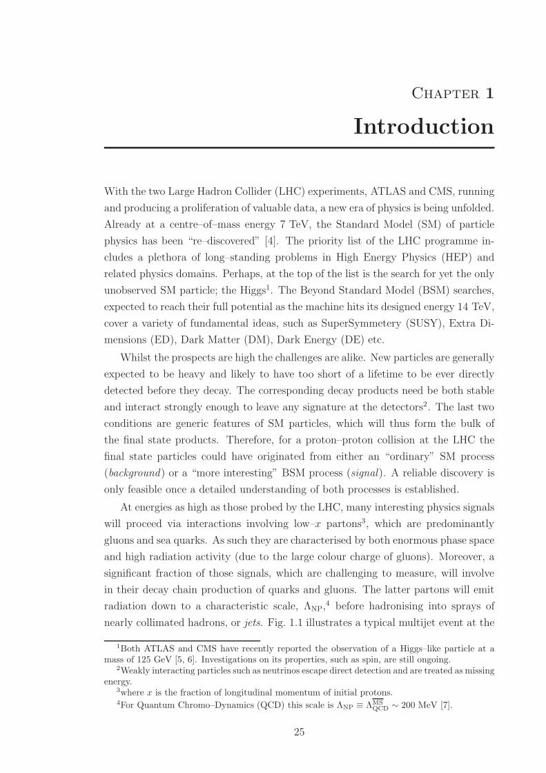
1.1 A typical LHC multijet event with associated various perturbative
and non–perturbative effects. Former effects include: hard scatter-
ing subprocess, soft and collinear radiation (resummation), soft and
wide–angle radiation, non-global logs (NGLs), effects of jet algorithms
(JetAlg) with jet radius R and recombination scheme E. Latter ef-
fects include: parton densities (f(x, µF )), underlying event (UE) and
hadronisation. This thesis concerns perturbative effects. . . . . . . . . 26
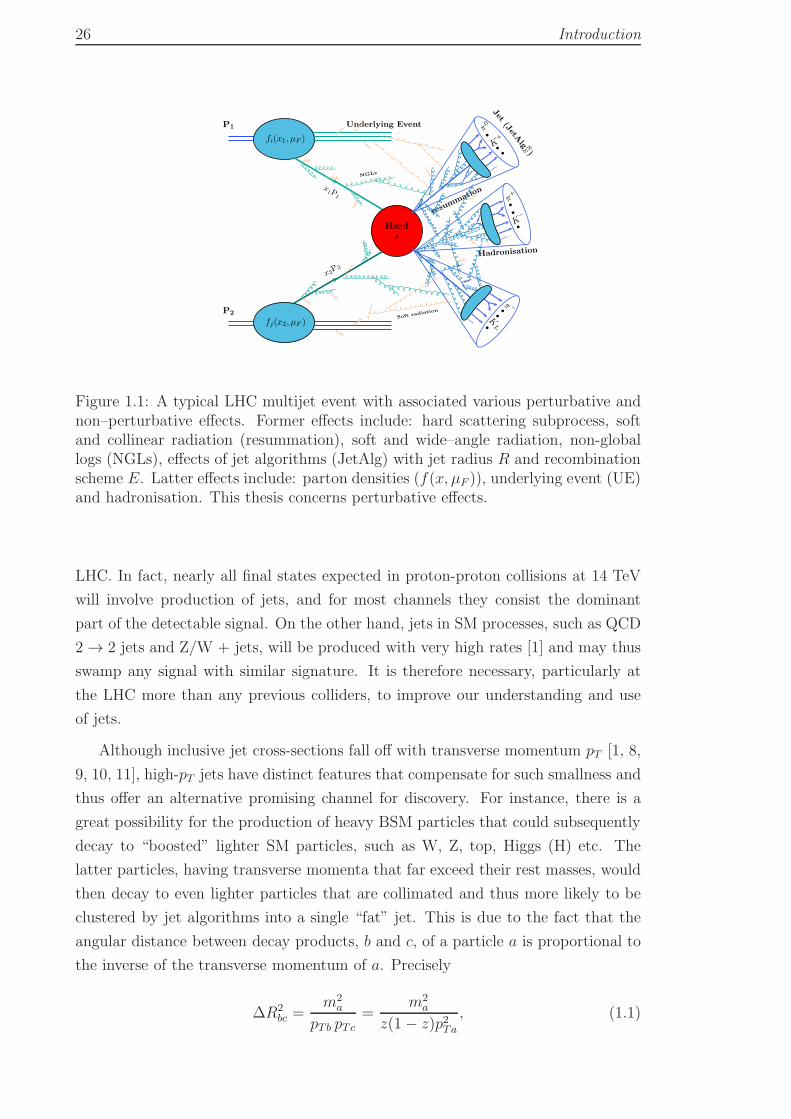
1.2 Jet mass distribution for an inclusive QCD jet sample generated for
the LHC with pT,min for the hard scattering of 2 TeV. Jets are defined
using different jet algorithms with jet radius of 0.7. The peak is
around 125 GeV (in natural units, c = ~ = 1) (figure from [1]). . . . . 27
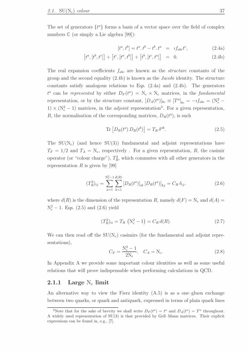
2.1 Graphical representation of the Fierz identity for a one–gluon ex-
change between a quark–antiquark pair (t–channel exchange). . . . . 38
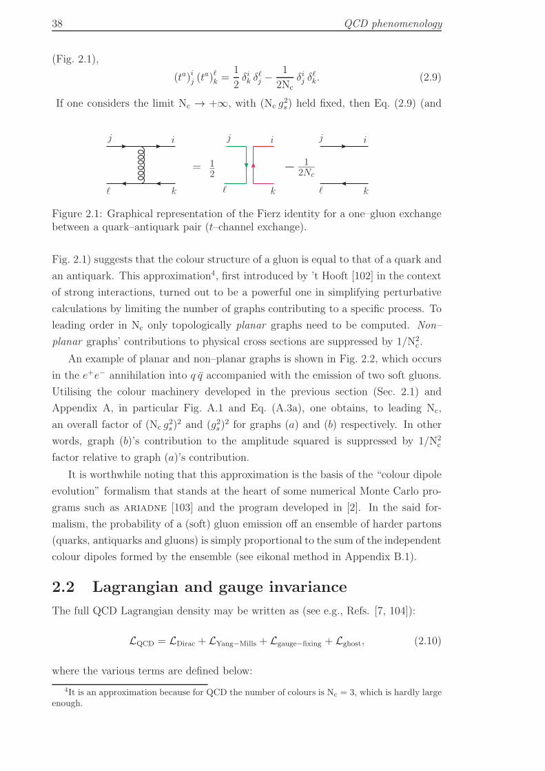
2.2 Graph (a) is an example of a planar graph which contributes at lead-
ing Nc. Graph (b) is an example of non–planar graph which con-
tributes at subleading Nc. The graphs represent Feynman diagrams
for the amplitude squared of e+e− anihilation into qqgg (to be dis-
cussed in Sec. 2.2 and Appendix B). . . . . . . . . . . . . . . . . . . . 39
2.3 Feynman rules for QCD in a covariant gauge: gluons (curly lines),
fermions (solid lines) and ghosts (dashed lines). . . . . . . . . . . . . 43
2.4 Feynman diagrams contributing to QCD β function. (top) fermion
self–energy diagrams, (middle) gluon self–energy diagrams and (bot-
tom) fermion–gluon vertex diagrams. . . . . . . . . . . . . . . . . . . 44
3.1 A schematic view of jet production at hadron colliders. The figure,
modified from [1], shows a proton–proton collision at the LHC. . . . . 50
3.2 Figures (a1), (a2) illustrate the output of a an IR unsafe cone algo-
rithm and figures (b1), (b2) illustrate the output of a collinear unsafe
cone algorithm. The plane (pt, y) is the 2D projection of the 3D
phase space (pt, y, φ). . . . . . . . . . . . . . . . . . . . . . . . . . . . 54
7
8 List of Figures
3.3 Sources of global (configuration 1) and non–global (configuration 2)
logarithms in dijet events at fixed–order. For configuration 2, we show
a real secondary emission (left) and its virtual correction (right). . . . 60
3.4 An into-jet J1 coherent radiation from an ensemble of soft large-angle
gluons (that are outside J1). Such configurations contribute to NGLs
at higher-orders. . . . . . . . . . . . . . . . . . . . . . . . . . . . . . . 62
3.5 Fixed–order vs (matched) resummed calculations and compar-
ison to experimental data for the total broadening shape
variable (left) without hadronisation effects and (right) with
hadronisation effects (figure from http://www.lpthe.jussieu.fr/
\protect\unhbox\voidb@x\protect\penalty\@M\salam/talks/). . 66
4.1 Diagrams representing the correlated emissions which give rise to the
lowest-order non-global logarithms. (A): the harder gluon k1 lies out-
side both jets and the softest one k2 is recombined with the measured
jet and contributes to the angularity distribution. (B): the harder
gluon is inside the unmeasured jet and emits a softer gluon into the
measured jet. (C): the harder gluon is inside the unmeasured jet
and emits a softer gluon outside both jets, which contributes to the
E0-distribution. . . . . . . . . . . . . . . . . . . . . . . . . . . . . . 81
4.2 The angularity distribution dΣ/ dτa for five values of the parameter
a given at Q = 500 GeV (about 250GeV or so at a hadron collider)
and different values of the jet radius and energy cut. The left column
is for quark jets, while the right is for gluon gets. As shown in the
legend, solid lines correspond to neglecting NGLs while dotted lines
take them into account. . . . . . . . . . . . . . . . . . . . . . . . . . . 88
4.3 Non global contribution 1 − S(t) from the measured jet (meas), the
unmeasured jet (unmeas) and overall (tot) as a function of E0 for
a = 0, τ0 = 5× 10⁻⁴ and R = 0.4. . . . . . . . . . . . . . . . . . . . . 89
4.4 Diagrams contributing to independent two-gluon emission from a
hard parton line. . . . . . . . . . . . . . . . . . . . . . . . . . . . . . 90
5.1 Schematic representation of gluonic arrangement giving rise to NGLs.
Here we assume that kt1 > kt2. (a): harder gluon k1 in interjet
region emits softer gluon k2 into pR–jet, thus giving rise to leading
NGLs contribution to the pR–jet mass distribution. (b): k1 inside
pR–jet emits k2 into interjet region, thus giving rise to leading NGLs
contribution to E0 distribution. (c): k1 inside pL–jet emits k2 into
pR–jet, thus leading to subleading NGLs contribution to pR–jet mass.
We have only shown the NGLs contributions to the pR–jet, identical
contributions apply to the pL–jet. . . . . . . . . . . . . . . . . . . . . 106
List of Figures 9
5.2 A schematic representation of a three–jet final state after applying
the C/A algorithm on real emission along with virtual correction di-
agrams. The two gluons are clustered in the E–Scheme (see Sec. 5.2).
Identical diagrams hold for the pL–jet. . . . . . . . . . . . . . . . . . 114
5.3 A schematic representation of a two-jet final state after applying the
C/A algorithm on real emission along with virtual correction dia-
grams. The two gluons are clustered in the E–Scheme (see Sec. 5.2).
Identical diagrams hold for the left (pL–) jet. . . . . . . . . . . . . . . 115
5.4 Leading non-global coefficient S22 in the anti-kT and C/A algorithms. 119
5.5 N3LL NGLs coefficients for both CFCA and CFTFnf colour chan-
nels in anti-kT (solid) and C/A (kT) (dashed). Note that Sa21 =
S(a)21 /CFCA, S
CA21 = SCA
21 /CFCA and Snf
21 = Snf
21 /CFTFnf . . . . . . . . . 120
5.6 Comparison of analytical resummed differential distribution dΣ/ dτE0
where the Sudakov, full anti-kT and full kT distributions are given,
respectively, in Eqs. (5.78), (5.77), and (5.81). The plots are shown
for a jet veto E0 = 60 GeV and a hard scale Q = 500 GeV. . . . . . . 125
5.7 Variation of 1−S(t) as E0 is varied for several jet radii. The smallest
value of E0 corresponds to the Emin0 = QτE0/(2Rs), derived from
(5.30) where e∆η ∼ 1/Rs. . . . . . . . . . . . . . . . . . . . . . . . . . 125
5.8 The difference between event2 and τE0 LO distribution for various
jet radii in both anti-kT (left) and C/A (right) algorithms. . . . . . . 127
5.9 The difference between event2 and τE0 NLO distribution for various
jet radii in both anti-kT (left) and C/A (right) algorithms. . . . . . . 128
6.1 Comparisons of the analytical result to the output of the Monte Carlo
program in the kT algorithm for two values of the jet radius. . . . . . 142
6.2 The output of the Monte Carlo program in the kT algorithm for var-
ious jet radii. . . . . . . . . . . . . . . . . . . . . . . . . . . . . . . . 143
6.3 Comparisons of the Sudakov result, the correct primary result and
the full result including non-global logarithms with and without clus-
tering, as detailed in the main text. . . . . . . . . . . . . . . . . . . . 144
7.1 Comparison between different approximations to the resummed ex-
ponent: jet functions (blue), with full resummation of the global con-
tribution (green) and with non-global logarithms as well (red). The
jet radius is R = 0.6. . . . . . . . . . . . . . . . . . . . . . . . . . . . 168
7.2 Comparison between different approximations to the resummed ex-
ponent: jet functions (blue), with full resummation of the global con-
tribution (green) and with non-global logarithms as well (red). The
jet radius is R = 1.0. . . . . . . . . . . . . . . . . . . . . . . . . . . . 169
10 List of Figures
7.3 Matching of the NLL resummed distribution to the LO one for R =
0.6 (on the left) and R = 1.0 (on the right). . . . . . . . . . . . . . . 169
7.4 The impact of the NLL constant C1, for R = 0.6 jets (on the left)
and R = 1.0 (on the right). The band is produced by suppressing the
real radiation contributions with a quark or gluon jet form factor, as
explained in the text. . . . . . . . . . . . . . . . . . . . . . . . . . . . 171
7.5 Comparison of our resummed and matched result NLL+LO (in red)
to standard Monte Carlo event generators, at the parton level. . . . . 173
7.6 Results for the ζ distributions obtained with standard Monte Carlo
parton showers, with hadronisation corrections (dashed lines) com-
pared to analytical resummation with non-perturbative shifts (shaded
bands) as explained in the main text. . . . . . . . . . . . . . . . . . . 173
7.7 The NLL+LO jet mass distribution for dijets, with different approx-
imation to the resummed exponent. . . . . . . . . . . . . . . . . . . . 175
A.1 Graphical representation of some important colour relations. . . . . . 182
A.2 Graphical representation of the Fierz identity. . . . . . . . . . . . . . 182
B.1 Eikonal Feynman rules for QCD: gluons are represented by curly lines
and fermions by solid lines. For triple vertices, the colour is read
clockwise. . . . . . . . . . . . . . . . . . . . . . . . . . . . . . . . . . 186
B.2 Feynman diagrams for (a) e+e− → q q, Born amplitude, (b) e+e− →qq, virtual corrections, and (c) e+e− → qqg, real emission. . . . . . . . 192
B.3 Dalitz plot for a three–body “decay” of a photon. All partons
are assumed on–shell. The edges xi = 1 correspond to two par-
tons being collinear and the corners xi = 0 correspond to one par-
ton being soft (pi → 0). The different kinematical regions are:
(1) x1 > x2 > x3, (2) x2 > x1 > x3, (3) x2 > x3 > x1, (4) x3 > x2 >
x1, (5) x3 > x1 > x2 and (6) x1 > x3 > x2. . . . . . . . . . . . . . . . . 195
B.4 Poles of the integrand of Eq. (B.48) in the complex plane. . . . . . . 197
B.5 Feynman diagrams for (a) e+e− → qqgg and (b) e+e− → qqq′q′. There
are three other diagrams corresponding to swapping the secondary
gluons g3, g4 in the top three diagrams. . . . . . . . . . . . . . . . . . 198
C.1 The difference between event2 and τE0 NLO distribution for various
jet radii in both anti-kT (left) and C/A (right) algorithms. Plots are
for C2F channel. . . . . . . . . . . . . . . . . . . . . . . . . . . . . . . 209
C.2 The difference between event2 and τE0 NLO distribution for various
jet radii in both anti-kT (left) and C/A (right) algorithms. Plots are
for CFCA channel. . . . . . . . . . . . . . . . . . . . . . . . . . . . . . 210

List of Figures 11
C.3 The difference between event2 and τE0 NLO distribution for various
jet radii in both anti-kT (left) and C/A (right) algorithms. Plots are
for CFTFnf channel. . . . . . . . . . . . . . . . . . . . . . . . . . . . 211
D.1 Full R-dependence of the two-gluon clustering coefficient F2. . . . . . 214

12
List of Tables
5.1 Full Rs numerical results for the leading and next-to-leading cluster-
ing logs’ coefficients. . . . . . . . . . . . . . . . . . . . . . . . . . . . 117
5.2 Fitting values of the parameters a, b and c for S(t) factor in both
anti-kT and kT . The coefficient I22 = S22/CFCA. . . . . . . . . . . . 124
5.3 Fitting values of the parameters a, b and c for CP factor. . . . . . . . 124
D.1 Estimates of the clustering coefficients Fn for n = 2, 3, 4 at different
values of the jet radius R in the kt and C/A algorithms. Recall that
FC/A2 = Fkt
2 (≡ F2) and that FC/A4 has not been computed. Note that
FC/A3 and F4 are more difficult to evaluate numerically than F3 (and
obviously F2). Thus their final answers are subjected to larger errors. 215
E.1 Numerical results for the coefficients that parametrize the resumma-
tion of non-global logarithms. . . . . . . . . . . . . . . . . . . . . . . 225
E.2 Numerical results for the coefficients that parametrize the resumma-
tion of non-global logarithms. Note that the above results are valid
in the case |∆y| = 2. . . . . . . . . . . . . . . . . . . . . . . . . . . . 225
13

14
Abstract
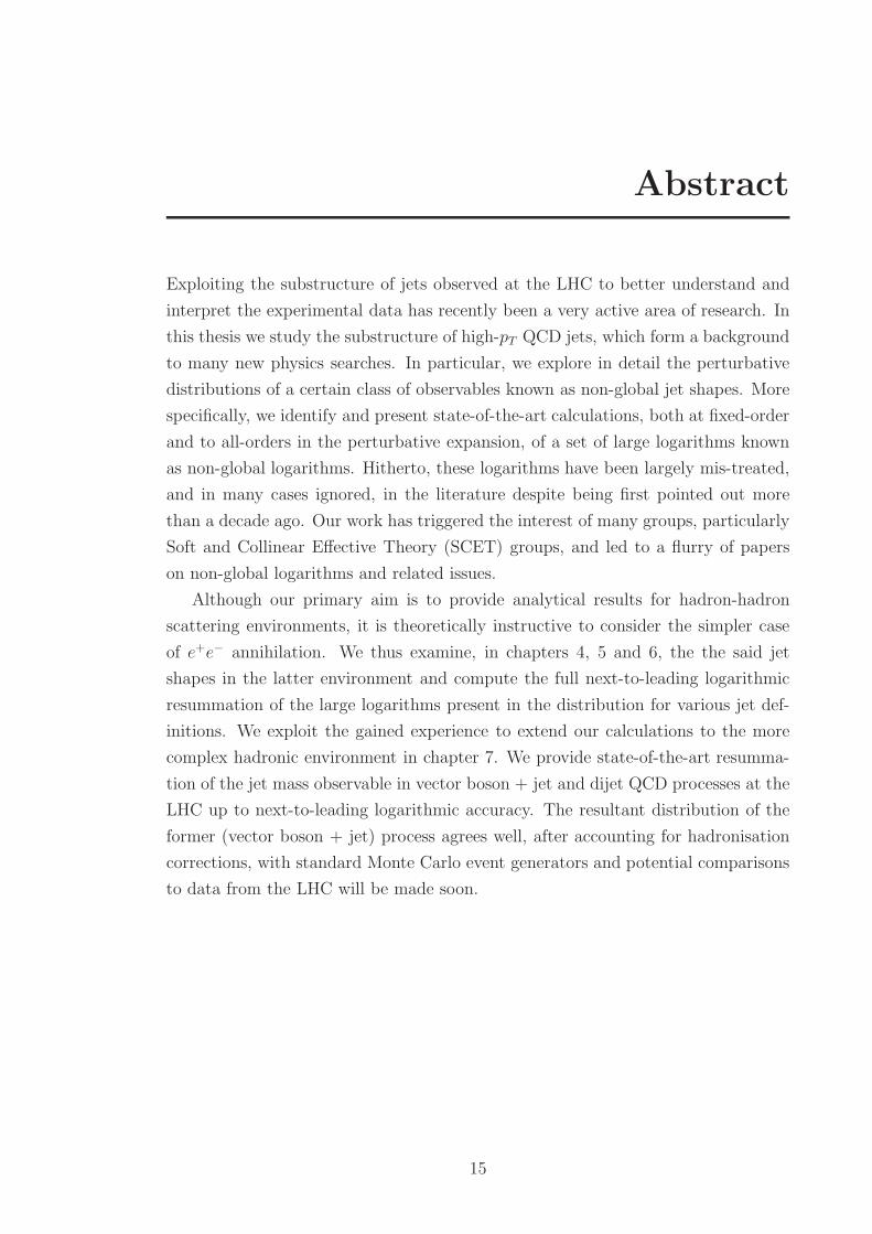
Exploiting the substructure of jets observed at the LHC to better understand and
interpret the experimental data has recently been a very active area of research. In
this thesis we study the substructure of high-pT QCD jets, which form a background
to many new physics searches. In particular, we explore in detail the perturbative
distributions of a certain class of observables known as non-global jet shapes. More
specifically, we identify and present state-of-the-art calculations, both at fixed-order
and to all-orders in the perturbative expansion, of a set of large logarithms known
as non-global logarithms. Hitherto, these logarithms have been largely mis-treated,
and in many cases ignored, in the literature despite being first pointed out more
than a decade ago. Our work has triggered the interest of many groups, particularly
Soft and Collinear Effective Theory (SCET) groups, and led to a flurry of papers
on non-global logarithms and related issues.
Although our primary aim is to provide analytical results for hadron-hadron
scattering environments, it is theoretically instructive to consider the simpler case
of e+e− annihilation. We thus examine, in chapters 4, 5 and 6, the the said jet
shapes in the latter environment and compute the full next-to-leading logarithmic
resummation of the large logarithms present in the distribution for various jet def-
initions. We exploit the gained experience to extend our calculations to the more
complex hadronic environment in chapter 7. We provide state-of-the-art resumma-
tion of the jet mass observable in vector boson + jet and dijet QCD processes at the
LHC up to next-to-leading logarithmic accuracy. The resultant distribution of the
former (vector boson + jet) process agrees well, after accounting for hadronisation
corrections, with standard Monte Carlo event generators and potential comparisons
to data from the LHC will be made soon.
15

16

Declaration
No portion of the work referred to in the thesis has been submitted in support of
an application for another degree or qualification of this or any other university or
other institute of learning.
17

18

Copyright Statement
i. The author of this thesis (including any appendices and/or schedules to this
thesis) owns certain copyright or related rights in it (the “Copyright”) and s/he
has given The University of Manchester certain rights to use such Copyright,
including for administrative purposes.
ii. Copies of this thesis, either in full or in extracts and whether in hard or
electronic copy, may be made only in accordance with the Copyright, Designs
and Patents Act 1988 (as amended) and regulations issued under it or, where
appropriate, in accordance with licensing agreements which the University has
from time to time. This page must form part of any such copies made.
iii. The ownership of certain Copyright, patents, designs, trade marks and other
intellectual property (the “Intellectual Property”) and any reproductions of
copyright works in the thesis, for example graphs and tables (“Reproduc-
tions”), which may be described in this thesis, may not be owned by the
author and may be owned by third parties. Such Intellectual Property and
Reproductions cannot and must not be made available for use without the
prior written permission of the owner(s) of the relevant Intellectual Property
and/or Reproductions.
iv. Further information on the conditions under which disclosure, publication and
commercialisation of this thesis, the Copyright and any Intellectual Property
and/or Reproductions described in it may take place is available in the Univer-
sity IP Policy (see http://documents.manchester.ac.uk/DocuInfo.aspx?
DocID=487), in any relevant Thesis restriction declarations deposited in the
University Library, The University Library’s regulations (see http://www.
manchester.ac.uk/library/aboutus/regulations) and in The University’s
policy on presentation of Theses.
19

20
Acknowledgements
First and foremost all praises are due to Almighty ALLAH.
I would like to thank my supervisor, Mrinal Dasgupta, for his support and con-
tinuous effort throughout the course of my PhD. I am indebted to Yazid Delenda
for intriguing discussions, particularly in chapter 6, reviewing and proofreading the
thesis, and to Simone Marzani for conceptual and technical discussions as well as
providing the numerical codes used in chapter 7. My thanks extend to Andrea Banfi
for assistance in chapter 5 and Mike Seymour for aid with the numerical program
event2 as well as helpful feedback on chapter 5. I would also like to thank Michael
Spannowsky for collaborating on the work presented in chapter 7, and in particular
for providing the results of the Monte Carlo event generators. The program of Ref.
[2] with the implementation of the kT clustering in [3], which has been heavily used
in this thesis, has not been made public yet and for that reason I would like to thank
the authors, Mrinal Dasgupta, Gavin P. Salam and Andrea Banfi, for approving its
usage in this thesis.
The encouragement of Apostolos Pilaftsis, my supervisor for the MPhys project,
is highly appreciated, and so is the help of Jeff Forshaw and Fred Loebinger regarding
administrative issues.
Moreover, I would like to express my gratitude to my brother Abdelkader for the
enormous support he offered me throughout my educational career.
The work presented in this thesis has been sponsored by both the University of
Manchester and the Algerian government. I would like to express my gratitude to
the Faculty of Engineering and Physical Sciences, the ministry of higher education
and scientific research and the Algerian consulate in London for their financial and
administrative support during my stay in the United Kingdom.
21

22
List of Publications
• Y. Delenda and K. Khelifa-Kerfa, On the resummation of clustering loga-
rithms for non-global observables, J. High Energy Phys. 09 (2012) 109 [hep-
ph/1207.4528].
• M. Dasgupta, K. Khelifa-Kerfa, S. Marzani, M. Spannowsky, On jet mass
distributions in Z+jet and dijet processes at the LHC, J. High Energy Phys.
10 (2012) 126 [hep-ph/1207.1640].
• K. Khelifa-Kerfa, Non-global logs and clustering impact on jet mass with a jet
veto distribution, J. High Energy Phys. 02 (2012) 072 [hep-ph/1111.2016]
• A. Banfi, M. Dasgupta, K. Khelifa-Kerfa and S. Marzani, Non-global loga-
rithms and jet algorithms in high-pT jet shapes, J. High Energy Phys. 08
(2010) 064 [hep-ph/1004.3483].
23

24
Chapter 1
Introduction
With the two Large Hadron Collider (LHC) experiments, ATLAS and CMS, running
and producing a proliferation of valuable data, a new era of physics is being unfolded.
Already at a centre–of–mass energy 7 TeV, the Standard Model (SM) of particle
physics has been “re–discovered” [4]. The priority list of the LHC programme in-
cludes a plethora of long–standing problems in High Energy Physics (HEP) and
related physics domains. Perhaps, at the top of the list is the search for yet the only
unobserved SM particle; the Higgs1. The Beyond Standard Model (BSM) searches,
expected to reach their full potential as the machine hits its designed energy 14 TeV,
cover a variety of fundamental ideas, such as SuperSymmetery (SUSY), Extra Di-
mensions (ED), Dark Matter (DM), Dark Energy (DE) etc.
Whilst the prospects are high the challenges are alike. New particles are generally
expected to be heavy and likely to have too short of a lifetime to be ever directly
detected before they decay. The corresponding decay products need be both stable
and interact strongly enough to leave any signature at the detectors2. The last two
conditions are generic features of SM particles, which will thus form the bulk of
the final state products. Therefore, for a proton–proton collision at the LHC the
final state particles could have originated from either an “ordinary” SM process
(background) or a “more interesting” BSM process (signal). A reliable discovery is
only feasible once a detailed understanding of both processes is established.
At energies as high as those probed by the LHC, many interesting physics signals
will proceed via interactions involving low–x partons3, which are predominantly
gluons and sea quarks. As such they are characterised by both enormous phase space
and high radiation activity (due to the large colour charge of gluons). Moreover, a
significant fraction of those signals, which are challenging to measure, will involve
in their decay chain production of quarks and gluons. The latter partons will emit
radiation down to a characteristic scale, ΛNP,4 before hadronising into sprays of
nearly collimated hadrons, or jets. Fig. 1.1 illustrates a typical multijet event at the
1Both ATLAS and CMS have recently reported the observation of a Higgs–like particle at amass of 125 GeV [5, 6]. Investigations on its properties, such as spin, are still ongoing.
2Weakly interacting particles such as neutrinos escape direct detection and are treated as missingenergy.
3where x is the fraction of longitudinal momentum of initial protons.4For Quantum Chromo–Dynamics (QCD) this scale is ΛNP ≡ ΛMS
QCD ∼ 200 MeV [7].
25
26 Introduction
P1
fi(x1, µF )
Underlying Event
x1P
1
NGLs
Hard
s
Jet(JetA
lg RE )
resum
mation
π0
b
K+
bb
Hadronisation
π+
b
b
K−
b
π −b
bKLb
x2P2
Softrad
iationP2
fj(x2, µF )
Figure 1.1: A typical LHC multijet event with associated various perturbative andnon–perturbative effects. Former effects include: hard scattering subprocess, softand collinear radiation (resummation), soft and wide–angle radiation, non-globallogs (NGLs), effects of jet algorithms (JetAlg) with jet radius R and recombinationscheme E. Latter effects include: parton densities (f(x, µF )), underlying event (UE)and hadronisation. This thesis concerns perturbative effects.
LHC. In fact, nearly all final states expected in proton-proton collisions at 14 TeV
will involve production of jets, and for most channels they consist the dominant
part of the detectable signal. On the other hand, jets in SM processes, such as QCD
2 → 2 jets and Z/W + jets, will be produced with very high rates [1] and may thus
swamp any signal with similar signature. It is therefore necessary, particularly at
the LHC more than any previous colliders, to improve our understanding and use
of jets.
Although inclusive jet cross-sections fall off with transverse momentum pT [1, 8,
9, 10, 11], high-pT jets have distinct features that compensate for such smallness and
thus offer an alternative promising channel for discovery. For instance, there is a
great possibility for the production of heavy BSM particles that could subsequently
decay to “boosted” lighter SM particles, such as W, Z, top, Higgs (H) etc. The
latter particles, having transverse momenta that far exceed their rest masses, would
then decay to even lighter particles that are collimated and thus more likely to be
clustered by jet algorithms into a single “fat” jet. This is due to the fact that the
angular distance between decay products, b and c, of a particle a is proportional to
the inverse of the transverse momentum of a. Precisely
∆R2bc =
m2a
pTb pTc=
m2a
z(1 − z)p2Ta
, (1.1)
Introduction 27
)2
Jet Mass (GeV/c
0 100 200 300 400 500 600
310×
Nu
mb
er
of
Jets
0
10
20
30
40
50
60
70Algorithms
MidPointJetCluCellJetFastJet InclusiveSISCone
Figure 1.2: Jet mass distribution for an inclusive QCD jet sample generated for theLHC with pT,min for the hard scattering of 2 TeV. Jets are defined using differentjet algorithms with jet radius of 0.7. The peak is around 125 GeV (in natural units,c = ~ = 1) (figure from [1]).
where z is the momentum fraction of, say, particle b. Thus for p2Ta ≫ m2a, and given
that the decay is not too asymmetric, i.e., z neither too close to 0 nor 1, ∆Rbc will
be small and bc will end up in a single jet. Moreover, owing to the fact that non–
perturbative corrections, particularly hadronisation, fall off with pT [12, 13], high-pT
jets are less sensitive to such corrections, making them ideal for clean perturbative
investigations.
The above mentioned high-pT (boosted) signal jets have shape and substructure
that are distinct from those of plain QCD jets initiated by light quarks and gluons.
Exploring such a rich substructure may prove very useful in situations such as that
depicted in Fig. 1.2, where QCD events may have jet mass distributions that peak
around 125 GeV (the current experimentally measured Higgs’ mass) and thus form
a strong background to Higgs searches based on the use of jet masses. Such very
high-pT jet events are not uncommon at the LHC given the high momentum probed
and hence pose a great challenge. Therefore new and more powerful jet substructure
techniques may offer an indispensable tool in boosted signal searches (see e.g [14,
15, 16, 17, 18, 19, 20, 21]). Note that the peak region in Fig. 1.2 is well within the
perturbative domain of QCD and analytical “resummation” calculations are very
efficient, as we shall be illustrating in this thesis. The aforementioned substructure
techniques may be divided into two broad classes: grooming techniques and jet
shapes.
Jets, the footprint of the underlying QCD partons, are not intrinsically well–
defined, and they thus ought to be “defined” before they can be used. A modern jet
definition consists of a jet algorithm and a recombination scheme [22, 23, 24, 25].
We discuss these in more details in Chapter 3. Grooming techniques, reviewed for
instance in [26, 27], are based on jet algorithms and primarily utilised to identify
subjets, within a fat jet, as well as to mitigate isolated diffuse soft radiation coming
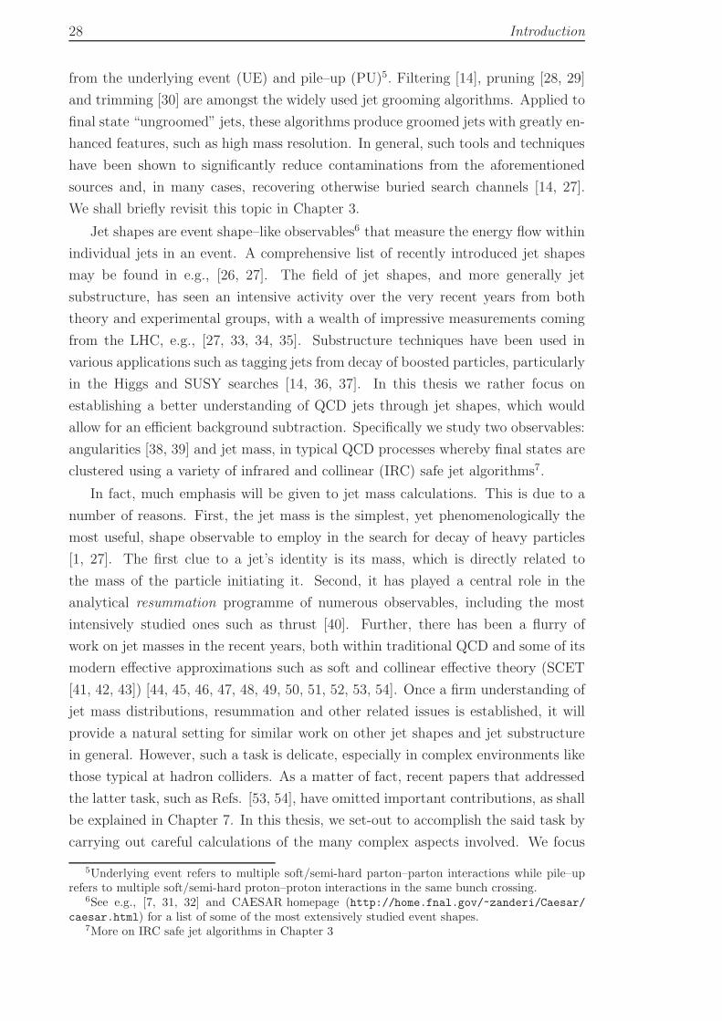
28 Introduction
from the underlying event (UE) and pile–up (PU)5. Filtering [14], pruning [28, 29]
and trimming [30] are amongst the widely used jet grooming algorithms. Applied to
final state “ungroomed” jets, these algorithms produce groomed jets with greatly en-
hanced features, such as high mass resolution. In general, such tools and techniques
have been shown to significantly reduce contaminations from the aforementioned
sources and, in many cases, recovering otherwise buried search channels [14, 27].
We shall briefly revisit this topic in Chapter 3.
Jet shapes are event shape–like observables6 that measure the energy flow within
individual jets in an event. A comprehensive list of recently introduced jet shapes
may be found in e.g., [26, 27]. The field of jet shapes, and more generally jet
substructure, has seen an intensive activity over the very recent years from both
theory and experimental groups, with a wealth of impressive measurements coming
from the LHC, e.g., [27, 33, 34, 35]. Substructure techniques have been used in
various applications such as tagging jets from decay of boosted particles, particularly
in the Higgs and SUSY searches [14, 36, 37]. In this thesis we rather focus on
establishing a better understanding of QCD jets through jet shapes, which would
allow for an efficient background subtraction. Specifically we study two observables:
angularities [38, 39] and jet mass, in typical QCD processes whereby final states are
clustered using a variety of infrared and collinear (IRC) safe jet algorithms7.
In fact, much emphasis will be given to jet mass calculations. This is due to a
number of reasons. First, the jet mass is the simplest, yet phenomenologically the
most useful, shape observable to employ in the search for decay of heavy particles
[1, 27]. The first clue to a jet’s identity is its mass, which is directly related to
the mass of the particle initiating it. Second, it has played a central role in the
analytical resummation programme of numerous observables, including the most
intensively studied ones such as thrust [40]. Further, there has been a flurry of
work on jet masses in the recent years, both within traditional QCD and some of its
modern effective approximations such as soft and collinear effective theory (SCET
[41, 42, 43]) [44, 45, 46, 47, 48, 49, 50, 51, 52, 53, 54]. Once a firm understanding of
jet mass distributions, resummation and other related issues is established, it will
provide a natural setting for similar work on other jet shapes and jet substructure
in general. However, such a task is delicate, especially in complex environments like
those typical at hadron colliders. As a matter of fact, recent papers that addressed
the latter task, such as Refs. [53, 54], have omitted important contributions, as shall
be explained in Chapter 7. In this thesis, we set-out to accomplish the said task by
carrying out careful calculations of the many complex aspects involved. We focus
5Underlying event refers to multiple soft/semi-hard parton–parton interactions while pile–uprefers to multiple soft/semi-hard proton–proton interactions in the same bunch crossing.
6See e.g., [7, 31, 32] and CAESAR homepage (http://home.fnal.gov/~zanderi/Caesar/caesar.html) for a list of some of the most extensively studied event shapes.
7More on IRC safe jet algorithms in Chapter 3
Introduction 29
on perturbative calculations of jet shape distributions in QCD.
There are two complementary theoretical tools to study shape distributions: an-
alytical calculations and numerical Monte Carlo (MC) simulations. The former are
inclusive over the final state and in most cases only deal with a single observable at
a time. The calculations are performed in the perturbative region of QCD and have
so far only treated a limited set of observables (see for instance [31, 55] and refer-
ences therein). Numerical simulations, on the other side, are completely exclusive
over the final state and thus any number of observables can be measured (simultane-
ously). In addition to the perturbative region, MC event generators (cf. fixed–order
Monte Carlos discussed below) probe the non–perturbative region8 of QCD through
phenomenological models that parametrise the effects of processes such as hadroni-
sation, UE and PU, in terms of a number tunable parameters. The state–of–the–art
is that analytical calculations, both at fixed– and all–orders (resummation), often
have higher precision than event generators9. As such, they can play a crucial role
in advancing the development of these generators as well as providing an indispens-
able tool for the interpretation of new physics signals, should they show up at the
LHC. Moreover, analytical calculations are cleaner, offer a deeper insight into the
dynamics of perturbative QCD and can systematically be improved. For these, and
other reasons, the central focus in this thesis is on analytical calculations of jet shape
distributions. Comparisons of the analytical findings to the output of various MCs
are, whenever possible, provided though.
Perturbative analytical calculations of a generic jet shape v of high–pT QCD
jets may be divided into two regimes: small v and large v. In the large v region,
v . 1, fixed–order calculations are sufficient to capture the full features of the
measured jet shape distribution. Fixed–order predictions for an arbitrary IRC safe
observable may be obtained with the aid of fixed–order Monte Carlos (FOMCs),
such as [56, 57, 58]. The small v region, v ≪ 1, on the other hand, receives large
enhancements (usually logarithmic) in ratios of the energy scales present in the
process. In an environment such that of the LHC (Fig. 1.1), the presence of many
scales is common for the majority of events. Such scales involve, for instance: jet
pT , the measured value of the jet shape, jet radius R and other parameters of the jet
algorithm, non–perturbative scale ΛQCD, and any other kinematical and selection
cuts. The said large logarithmic terms render fixed–order calculations unreliable
and, more seriously, threaten the validity of the perturbative expansion. To restore
the latter expansion, a summation of these logarithmic enhancements to all–orders
is inevitable. Such a task is dubbed resummation, which may be regarded as a
8The perturbative and non–perturbative regions of QCD correspond to kinematical regionswhere the strong coupling constant is small, αs ≪ 1, and large, αs ∼ 1, respectively.
9This stems from the fact that the formal precision of event generators is leading logarithm (LL)accuracy. No higher accuracy is guaranteed beyond that due to higher order and non–perturbativecontaminations.
30 Introduction
consequence of more profound characteristic features of QCD [59]. Namely coherence
[60, 61] (and factorisation [62, 63, 64]). The small v regime is of prime interest, in
this thesis, and will thus form the bulk of the discussion presented herein.
In perturbative QCD (pQCD), resummation of large logarithms that occur in
the distribution of sufficiently inclusive shape observables, or global observables,
has become a typical exercise in modern phenomenology [65, 66]. For many such
observables, the corresponding resummation has even been automated [31, 55]. Re-
summation is most effective when the logarithms exponentiate. This exponentiation,
of jet shapes, follows primarily from the corresponding (exponentiation) property of
QCD matrix–elements in the soft and collinear regions [40, 67, 68]. If we define the
jet shape fraction (or integrated shape cross-section) Σ(v) as
Σ(v) =
∫ v
0
dv′1
σ(0)
dσ
dv′, (1.2)
where σ(0) is the Born cross-section, then Σ(v) exponentiates10 precisely means that
it assumes the following form at small v
Σ(v) = C(αs) exp [Lg1(αsL) + g2(αsL) + αsg3(αsL) + · · · ] +D(αs, v), (1.3)
with L = ln(1/v), C(αs) sums the loop constants and the remainder function
D(αs, v) vanishes in the limit v → 0. The function g1(αsL) resums leading log-
arithms (LL), αns L
n+1, g2(αsL) resums next–to–leading logarithms (NLL), αns L
n,
g3(αsL) resums next–to–next–to–leading logarithms (NNLL), αns L
n−1, and so on.
Moreover, one must establish, in addition to the matrix elements, that the phase
space defining the shape fraction for a particular shape variable factorises (and hence
exponentiate), possibly after a suitable integral transformation [7]. We elaborate on
this in more detail in Chapter 3 (Sec. 3.2.4). For the aforementioned global ob-
servables, g1 is simply given by the exponentiation of the single soft gluon emission
result (known as “Sudakov” form factor). Further, the resummation of sublead-
ing logarithms. i.e., calculation of g2, g3, · · · can in principle be achieved through,
for example, inclusion of the running coupling at higher loops, proper treatment of
multiple emissions etc [31]. The current state–of–the–art is N3LL resummation for
thrust and other event/jet shapes [46, 49].
Nearly every measurement11 at the LHC will involve non–global observables [2,
70]. Such observables are sensitive only to specific regions of phase space. e.g., the
invariant jet mass is only sensitive to radiation into the jet region. Restricting the
jet mass observable in the latter region to be less than a specific value, say MJ,
10Not all shape observables exponentiate though. Examples of observables that have been proveninconsistent with exponentiation include the JADE jet–resolution thresholds [24]. For such typeof observables even an LL resummation does not exist [31, 69].
11Not all of them require resummation though. Often fixed–order calculations suffice.
Introduction 31
induces large non–global (single) logarithms (NGLs) in the ratio p2TR2/M2
J, with
R being the jet size determined by the jet algorithm used. The resummation of
these logarithms, which contribute to g2 and higher functions (g3, g4, etc) and start
at O(α2s) in the perturbative expansion, have not been possible analytically due to
the non–factorisation of the non–abelian part of the multiple gluon emission matrix–
element. Nonetheless, two alternative methods have been developed to resum NGLs.
Namely: a Monte Carlo program [2] and a non–linear evolution equation [71]. Their
formal accuracy is leading NGLs, which is NLL for the jet mass, and are only
valid in the large-Nc limit12. Neglected subleading colour corrections contribute
at the 10% level. Phenomenological impact of NGLs have been shown to lead
to a reduction in the peak of the corresponding Sudakov form factor that can be
significant for some observables [2, 70, 72]. Therefore, any reliable resummation
of non–global observables aiming at NLL accuracy, or beyond, should necessarily
account for NGLs.
Jet clustering algorithms, other than cone–type [22] and anti-kT [73] algorithms,
when applied to final state partons lead to a more complicated phase space due
to the non–trivial role of clustering amongst soft partons. Generally the resultant
phase space is not factorisable (into single particle phase space for each parton).
Performing the integral in Eq. (1.2) with modified phase space due to a jet algorithm
yields two effects. First, new large single logarithms in the abelian sector. These
are termed clustering logarithms (CLs) and were first pointed out in [74] for the
interjet energy flow distribution. Second, a reduction in the impact of NGLs, as was
shown in [75] for the same distribution. Since the phase space becomes increasingly
complex as the number of final state partons increases, analytical resummation of
CLs seems to be highly intricate. The MC program of Ref. [2] is at the moment
the only available method to resum both CLs and NGLs in the presence of a jet
algorithm. Nevertheless, it has been shown, through explicit fixed–order calculations
up to O(α4s) in the perturbative expansion for the interjet energy flow distribution
in e+e− annihilation, that CLs exponentiate [3]. The analytical results agreed well
with the output of the said MC program, indicating that the all–orders result is
dominated by the first few orders. We carry out analogous calculations for the jet
mass in Chapter 6.
As previously mentioned, resummation calculations are accurate for the domi-
nant part of the shape distribution, specifically in the small v (peak) region. For
phenomenological analyses, including comparison to measurements, other contribu-
tions and corrections ought to be taken into account. These include (a) fixed–order
calculations which can, as stated above, reliably reproduce the tail of the jet shape
distribution (large v region). Hence, a matching of the two, resummation and fixed–
12Nc is the number of colour degrees of freedom. For SU(3), the symmetry group of QCD,Nc = 3.
32 Introduction
order, calculations is necessary for an accurate prediction over the full kinematical
range of the jet shape v; (b) non–perturbative (NP) corrections, such as hadroni-
sation, UE and PU, which affect the small v region of the shape distribution. The
latter are non–calculable in pQCD and at present can only be quantified through
models, best implemented in Monte Carlo event generators (see [76] for a review).
Meanwhile, theoretical progress on estimating the impact of non–perturbative cor-
rections using perturbative methods such as renormalon–inspired techniques and
related approaches [12, 13, 77, 78] have yielded promising results [66, 79, 80, 81, 82].
Typically, these corrections, particularly hadronisation, may be included as a shift,
v → v+ 〈δv〉NP where 〈δv〉 is the mean of the change in v, in the jet shape distribu-
tion13 [70, 83].
This thesis is divided into three main parts: physics background, results from
e+e− annihilation and results from hadron-hadron collisions. The first part includes
Chapters 2 and 3. Chapter 2 surveys the theoretical basis of QCD and serves as
a background to the rest of the thesis. Important ingredients which are essential
to later discussions such as factorisation and matrix–elements are provided. Most
noticeably, the eikonal approximation is explained and the corresponding Feynman
rules explicitly given. Since our pivotal object in this thesis are jets, Chapter 3 is
devoted to theoretical exploration of jets, jet algorithms and jet shapes. A generic
formulation of the latter is presented and related topics such as IRC safety addressed.
At this point, the main conceptual basis is laid down and the computational ma-
chinery is set up.
The actual calculations are then carried out in the other two parts. Whilst our
aim is to produce analytical results that can be compared to present hadron collider
measurements, it is theoretically instructive to start with the simpler and cleaner
e+e− annihilation environment. Indeed, the latter calculations form a natural setting
for hadron collision calculations, as we shall see. Consequently, the second part,
which includes Chapters 4, 5 and 6, concerns jet shapes, specifically angularities, in
chapter 4, and the invariant jet mass, in the remaining two chapters 5 and 6, in e+e−
annihilation. Notice that Chapter 4 is similar in content to [84] but treats the more
general angularities shape observable. Chapter 5 largely expands [85] and Chapter
6 is simply drawn from [86]. The final part, which includes Chapter 7, extends
the e+e− annihilation findings to hadron-hadron collisions, particularly addressing
Z+jet and dijet processes at the LHC. Its content is essentially the same as [87].
Once a next-to-leading order matching is performed, the latter will represent the
state-of-the-art calculations for non–global observables at hadron colliders.
We consider final state clustering by various jet algorithms in e+e− annihilation,
and only one jet algorithm in hadron-hadron scattering. For each jet algorithm, we
13Strictly speaking, the shift is only valid to the right of the distribution peak, as shall bediscussed in Chapter 3.
Introduction 33
perform the following:
• Compute the full leading–order shape distribution accounting for soft wide–
angle radiation with full jet-radius and colour dependence in both e+e− and
hadron-hadron scattering.
• Compute the full next–to–leading order (two-gluon emission) shape distribu-
tion up to NNLL in the expansion (equivalent to α2s L
2), with full jet-radius
and colour dependence. The two-gluon emission calculations are generally per-
formed within the eikonal framework. The latter is sufficient to achieve the
said NNLL accuracy in both e+e− and hadron-hadron scattering.
• In e+e− annihilation, we additionally compute the full N3LL terms in the
expansion (equivalent to α2s L), for which a more accurate emission amplitude
is computed in Appendix B, and hence the only missing piece to obtain the full
two-gluon distribution is the two–loop constant C2. Our calculations represent
the state-of-the-art, with full jet-radius dependence of both NGLs and CLs
coefficients.
• Compute the full NLL resummation including numerical estimates of NGLs
and CLs (only in the e+e− case) to all–orders with full jet-radius dependence
in the large-Nc limit.
• In the hadron-hadron scattering case we perform matching to (leading) fixed–
order, estimate non–perturbative hadronisation corrections and compare to
MC event generators.
Finally, in Chapter 8 we draw our conclusions and highlight areas where more work
is needed in light of upcoming LHC measurements.
In the next chapter, we begin with a review of QCD phenomenology.

34
Chapter 2
QCD phenomenology
The contemporary Standard Model for elementary particles and forces encompasses
three, out of four, fundamental forces of nature: Electromagnetic, Weak and strong
forces. These interactions are elegantly described by the mathematically consis-
tent gauge field theory (GFT)1. Within this framework, Quantum Electrodynam-
ics (QED) describes electromagnetic interactions, Electro–Weak (EW) describes
the unified electromagnetic and weak interactions and Quantum Chromodynam-
ics (QCD) describes the strong interactions. In this thesis we are concerned with
QCD. The latter theory is formulated, at the Lagrangian level, in terms of quarks
and gluons. Quarks are described in GFT by the Dirac spinor fields and can ex-
ist in three different states of colour (usually referred to as red, green and blue)
and six flavours; up (u), down (d), strange (s), charm (c), bottom (b) and top (t).
Their electric charges are, in units of the electron charge (e): +2/3 (u,c,t) and −1/3
(d,s,b). One striking difference between QED and QCD is that quarks have never
been seen in isolation, i.e., as asymptotic states, as have electrons and photons. This
QCD phenomenon is known as confinement. What is instead observed at detectors
are hadrons, both baryons and mesons. The former are composites of three spin–12
quarks, qq′q′′, while the latter are composites of spin–12quark–antiquark, qq′, pairs2.
Gluons, in analogy to photons, are vector fields which arise as a result of de-
manding the quark Lagrangian be invariant under local, or gauge, rotations in the
colour space. The corresponding mathematical group of such rotations for QCD
is the special unitary group SU(3) (see below). Another sharp contrast between
QED and QCD is the fact that gluons, which mediate the strong interaction, are
colourful, i.e., they are charged. Consequently they can interact among themselves
(in addition to their interactions with quarks).
In this chapter, we begin by briefly reviewing the main features of the general
symmetry group SU(Nc), of which SU(3) is a special case, on the way recalling
some of the important relations and identities which will be useful in later sections
(and chapters). Most of the material presented in this section is based on the refer-
ences listed at the end of this introductory section. After that we write the general
1Quantum field theory with the requirement of gauge invariance.2The idea that hadrons are not themselves elementary but bound states of other more elemen-
tary states dates back to the early work of Fermi and Yang [88].
35
36 QCD phenomenology
form of the QCD Lagrangian and discuss the various terms in it. To make contact
with experiments, it is necessary that one is able to extract predictions from the
latter abstract Lagrangian. At small coupling, gs, this is achieved through pertur-
bation theory, equipped with some essential features of QCD such as factorisation,
to which we turn in Sec. 2.3. Calculations in perturbative QCD are carried out (in
the traditional method) via the use of Feynman diagrams and Feynman rules. An
important result of perturbation theory is the running of the coupling gs. Unlike
QED, the QCD strong coupling decreases as the energy scale at which it is measured
increases. Therefore at small and medium energies, the coupling approaches unity
and perturbation theory breaks down. Furthermore, when considering soft gluons
dynamics, one may utilise a practically simpler effective theory known as eikonal
theory [89]. We elaborate on this, including the eikonal version of Feynman rules,
in Appendix B.1. Finally, in Appendix B.2, we present detailed perturbative calcu-
lations of e+e− annihilation into hadrons which will form the backbone of Chapters
4, 5 and 6.
Further detailed discussions and in–depth treatment of QCD, and generally of
GFT, may be found in standard textbooks, e.g., [7, 90, 91, 92, 93, 94, 95]. Reviews
such as those in [96, 97, 98] are also useful. Other references specific to certain
sections will be given therein.
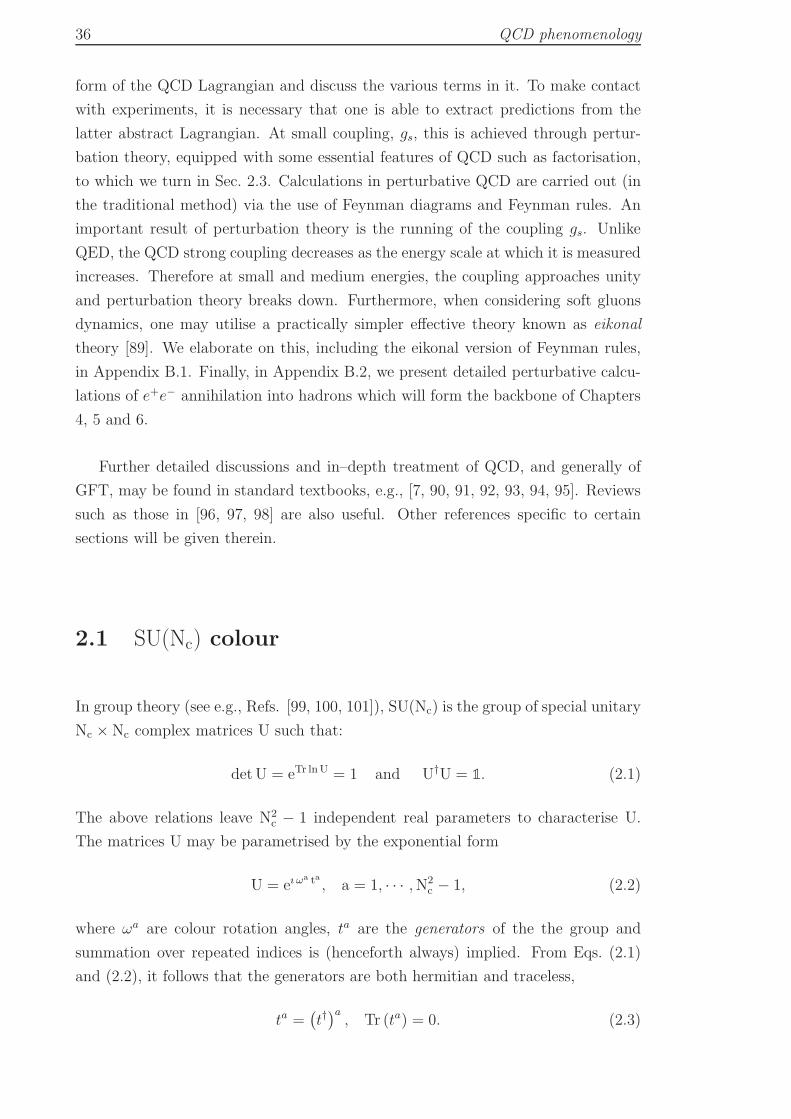
2.1 SU(Nc) colour
In group theory (see e.g., Refs. [99, 100, 101]), SU(Nc) is the group of special unitary
Nc × Nc complex matrices U such that:
det U = eTr lnU = 1 and U†U = 1. (2.1)
The above relations leave N2c − 1 independent real parameters to characterise U.
The matrices U may be parametrised by the exponential form
U = eı ωa ta , a = 1, · · · ,N2
c − 1, (2.2)
where ωa are colour rotation angles, ta are the generators of the the group and
summation over repeated indices is (henceforth always) implied. From Eqs. (2.1)
and (2.2), it follows that the generators are both hermitian and traceless,
ta =(t†)a
, Tr (ta) = 0. (2.3)
2.1. SU(Nc) colour 37
The set of generators ta forms a basis of a vector space over the field of complex
numbers C (or simply a Lie algebra [99]):
[ta, tb] = ta. tb − tb. ta = ıfabctc, (2.4a)
[ta, [tb, tc]
]+[tc, [ta, tb]
]+[tb, [tc, ta]
]= 0. (2.4b)
The real expansion coefficients fabc are known as the structure constants of the
group and the second equality (2.4b) is known as the Jacobi identity. The structure
constants satisfy analogous relations to Eqs. (2.4a) and (2.4b). The generators
ta can be represented by either DF (ta) = Nc × Nc matrices, in the fundamental
representation, or by the structure constant, [DA(ta)]bc ≡ [T a]bc = −ıfabc = (N2
c −1) × (N2
c − 1) matrices, in the adjoint representation3. For a given representation,
R, the normalisation of the corresponding matrices, DR(ta), is such
Tr[DR(t
a)DR(tb)]= TR δab. (2.5)
The SU(Nc) (and hence SU(3)) fundamental and adjoint representations have
TF = 1/2 and TA = Nc, respectively . For a given representation, R, the casimir
operator (or “colour charge”), T 2R, which commutes with all other generators in the
representation R is given by [99]
(T 2R)ij =
N2c−1∑
a=1
d(R)∑
k=1
[DR(ta)]ik [DR(t
a)]kj = CR δij, (2.6)
where d(R) is the dimension of the representation R, namely d(F ) = Nc and d(A) =
N2c − 1. Eqs. (2.5) and (2.6) yield
(T 2R)ii = TR
(N2
c − 1)= CR d(R). (2.7)
We can then read off the SU(Nc) casimirs (for the fundamental and adjoint repre-
sentations),
CF =N2
c − 1
2Nc, CA = Nc. (2.8)
In Appendix A we provide some important colour identities as well as some useful
relations that will prove indispensable when performing calculations in QCD.
2.1.1 Large Nc limit
An alternative way to view the Fierz identity (A.5) is as a one–gluon exchange
between two quarks, or quark and antiquark, expressed in terms of plain quark lines
3Note that for the sake of brevity we shall write DF (ta) = ta and DA(t
a) = T a throughout.A widely used representation of SU(3) is that provided by Gell–Mann matrices. Their explicitexpressions can be found in, e.g., [7].
38 QCD phenomenology
(Fig. 2.1),
(ta)ij (ta)ℓk =
1
2δik δ
ℓj −
1
2Ncδij δ
ℓk. (2.9)
If one considers the limit Nc → +∞, with (Nc g2s) held fixed, then Eq. (2.9) (and
= − 12Nc
12
ℓ
j i
k k
j i
ℓ
j i
kℓ
Figure 2.1: Graphical representation of the Fierz identity for a one–gluon exchangebetween a quark–antiquark pair (t–channel exchange).
Fig. 2.1) suggests that the colour structure of a gluon is equal to that of a quark and
an antiquark. This approximation4, first introduced by ’t Hooft [102] in the context
of strong interactions, turned out to be a powerful one in simplifying perturbative
calculations by limiting the number of graphs contributing to a specific process. To
leading order in Nc only topologically planar graphs need to be computed. Non–
planar graphs’ contributions to physical cross sections are suppressed by 1/N2c.
An example of planar and non–planar graphs is shown in Fig. 2.2, which occurs
in the e+e− annihilation into q q accompanied with the emission of two soft gluons.
Utilising the colour machinery developed in the previous section (Sec. 2.1) and
Appendix A, in particular Fig. A.1 and Eq. (A.3a), one obtains, to leading Nc,
an overall factor of (Nc g2s)
2 and (g2s)2 for graphs (a) and (b) respectively. In other
words, graph (b)’s contribution to the amplitude squared is suppressed by 1/N2c
factor relative to graph (a)’s contribution.
It is worthwhile noting that this approximation is the basis of the “colour dipole
evolution” formalism that stands at the heart of some numerical Monte Carlo pro-
grams such as ariadne [103] and the program developed in [2]. In the said for-
malism, the probability of a (soft) gluon emission off an ensemble of harder partons
(quarks, antiquarks and gluons) is simply proportional to the sum of the independent
colour dipoles formed by the ensemble (see eikonal method in Appendix B.1).
2.2 Lagrangian and gauge invariance
The full QCD Lagrangian density may be written as (see e.g., Refs. [7, 104]):
LQCD = LDirac + LYang−Mills + Lgauge−fixing + Lghost, (2.10)
where the various terms are defined below:
4It is an approximation because for QCD the number of colours is Nc = 3, which is hardly largeenough.
2.2. Lagrangian and gauge invariance 39
≃
(a)
≃
(b)
Figure 2.2: Graph (a) is an example of a planar graph which contributes at leadingNc. Graph (b) is an example of non–planar graph which contributes at subleadingNc. The graphs represent Feynman diagrams for the amplitude squared of e+e−
anihilation into qqgg (to be discussed in Sec. 2.2 and Appendix B).
• The quark content of QCD is described by the Dirac Lagrangian density
LDirac =
nf∑
f=1
qf (ı D/−mf)qf , (2.11)
where q labels a quark field of flavour f and mass mf . In QCD there are
nf = 6 flavours of quark fields and their conjugates, qf = q†f γ
0. The quark
field forms a three–vector in the colour space; q = (q1, q2, q3) with qa being
Dirac spinor fields5. The symbol D/ denotes the product γµDµ where γµ are
the traceless Dirac matrices satisfying the Clifford algebra γµ, γν = 2 gµν,
with the latter metric given by gµν = diag (+1,−1,−1,−1)6, and Dµ is the
covariant derivative given by
Dµ = ∂µ − ı gsAµ. (2.12)
The SU(3) gluon fields are given by Aµ =∑8
a=1 Aaµ t
a when Dµ is acting on
the quark field (colour triplet) and Aµ =∑8
a=1Aaµ T
a when acting on the
gluon field (colour octet), with ta and T a (≡ (T a)bc) being, respectively, the
generators of SU(3) in the fundamental and adjoint representations discussed
5The three values of the colour index a are usually referred to as red, blue and green, asmentioned in the introductory part.
6Especially useful representation of the Dirac γ matrices is the Weyl (or chiral) representation.Explicit expressions of the latter may be found in e.g., [93].
40 QCD phenomenology
previously. The strong coupling parameter, gs, measures the strength of the
strong interaction between quarks and gluons or gluons amongst themselves.
• The Yang–Mills Lagrangian density describes the free propagation of the gluon
field and reads
LYang−Mills = −1
2Tr[F 2µν(A)
]2, (2.13)
where the non–abelian, i.e., non–commutative, SU(3) field strength tensor,
Fµν = F aµν t
a, is defined by the commutator
[Dµ, Dν ] = −ı gsFµν . (2.14)
Explicitly written in terms of the gluon fields, Fµν = ∂µAν−∂νAµ−ı gs [Aµ, Aν ].
The sum of the Dirac and Yang–Mills Lagrangians is the classical QCD La-
grangian. The latter is invariant under the local gauge transformations (rep-
resented by the SU(3) matrix U given in Eq. (2.2)):
q(x) → q′(x) = U(x)q(x),
Aµ(x) → A′µ(x) = U(x)
[Aµ(x) +
ı
gs∂µ
]U†(x). (2.15)
The field strength tensor (2.14) thus transforms under the latter finite trans-
formations (2.15) as
Fµν → F ′µν = UFµν U
†. (2.16)
Considering infinitesimal gauge transformations, for which the U matrix may
be written as an expansion around the unit matrix; U = 1 + ı ωata, then it
follows from Eq. (2.16) that Fµν is not gauge invariant,
F aµν → F a ′
µν = F aµν − fabc F
bµν ω
c +O(ω2). (2.17)
This result is in contrast to the QED case where the photon field strength
tensor is gauge invariant. The immediate consequence of this is that gluons
are coloured and cannot thus be seen as asymptotic states. Notice also that
since a mass term AµAν breaks the gauge invariance then it cannot be included
in the Lagrangian density (2.13). It follows that gluons are massless.
• To eliminate the gauge freedom in the Yang–Mills Lagrangian one must fix a
gauge to work in. Without the gauge fixing term the gluon propagator is not
well defined (see e.g., Refs. [91, 105]). One possible class of gauge conditions
is that of covariant gauges, defined by
Lgauge−fixing = − 1
2 ξ(∂µ A
µ)2 , (2.18)
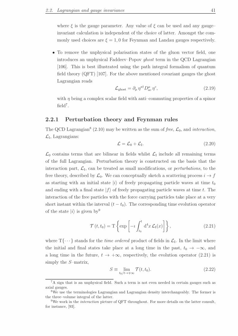
2.2. Lagrangian and gauge invariance 41
where ξ is the gauge parameter. Any value of ξ can be used and any gauge–
invariant calculation is independent of the choice of latter. Amongst the com-
monly used choices are ξ = 1, 0 for Feynman and Landau gauges respectively.
• To remove the unphysical polarisation states of the gluon vector field, one
introduces an unphysical Faddeev–Popov ghost term in the QCD Lagrangian
[106]. This is best illustrated using the path integral formalism of quantum
field theory (QFT) [107]. For the above mentioned covariant gauges the ghost
Lagrangian reads
Lghost = ∂µ ηa†Dµ
ac ηc, (2.19)
with η being a complex scalar field with anti–commuting properties of a spinor
field7.
2.2.1 Perturbation theory and Feynman rules
The QCD Lagrangian8 (2.10) may be written as the sum of free, L0, and interaction,
LI, Lagrangians:
L = L0 + LI. (2.20)
L0 contains terms that are bilinear in fields whilst LI include all remaining terms
of the full Lagrangian. Perturbation theory is constructed on the basis that the
interaction part, LI, can be treated as small modifications, or perturbations, to the
free theory, described by L0. We can conceptually sketch a scattering process i → f
as starting with an initial state |i〉 of freely propagating particle waves at time t0
and ending with a final state |f〉 of freely propagating particle waves at time t. The
interaction of the free particles with the force carrying particles take place at a very
short instant within the interval (t− t0). The corresponding time evolution operator
of the state |i〉 is given by9
T (t, t0) = T
exp
[−ı
∫ t
t0
d4xLI(x)
], (2.21)
where T· · · stands for the time ordered product of fields in LI. In the limit where
the initial and final states take place at a long time in the past, t0 → −∞, and
a long time in the future, t → +∞, respectively, the evolution operator (2.21) is
simply the S–matrix,
S ≡ limt0/t→∓∞
T (t, t0). (2.22)
7A sign that is an unphysical field. Such a term is not even needed in certain gauges such asaxial gauges.
8We use the terminologies Lagrangian and Lagrangian density interchangeably. The former isthe three–volume integral of the latter.
9We work in the interaction picture of QFT throughout. For more details on the latter consult,for instance, [93].
42 QCD phenomenology
The S–matrix encodes a plethora of information about the scattering process. The
entries of the S–matrix, or the matrix–elements Sfi, are related to the i → f tran-
sition amplitude (or invariant matrix elements) Mfi through,
Sfi = 〈f |S |i〉 = δfi − ıTfi, (2.23)
with the T–matrix elements given by
ıTfi = ı (2π)4 δ(4) (Pi − Pf) Mfi, (2.24)
where Pi(f) is the total four–momentum of initial (final) state particles. The delta
term δfi in (2.23) is the zeroth order in the expansion of (2.22) and describes the
state where no interaction happens. The transition amplitude ıTfi, or ıMfi, consists
of the timed–ordered expansion of S, starting at first order and adding an extra
interaction term LI(x) at each higher order.
To compute Mfi one employs a set of Feynman rules, along with a graphical
visualisation of the process via Feynman graphs, derived from the Lagrangian (2.10).
These rules are represented by external lines for incoming (initial) or outgoing (final)
particles, internal lines for propagators (that are neither initial nor final) and vertices
for the interaction terms. The set of Feynman rules for QCD are depicted in Fig. 2.3.
2.2.2 Optical theorem and cross-sections
An important feature of the S–matrix that is useful in checking the consistency of
Feynman amplitude calculations is unitarity. This follows from the fact that the
probability of producing a final state |f〉 given an initial state |i〉 is simply |Sfi|2.Summing over all possible final states, the total probability must be equal to unity.
Schematically ∑
f
|Sfi|2 = 1 ⇒ S†S = 1. (2.25)
Substituting for ıT from Eq. (2.23), the unitarity relation (2.25) implies
−ı (Ti′i − T ⋆i′i) =
∑
f
T ⋆fi′Tfi. (2.26)
In the special case of elastic, |i′〉 = |i〉, two–particle scattering, Eq. (2.26) leads to
the optical theorem:
Im (Mii) = λ1/2(s,m2a, m
2b) σtot (i → X) , (2.27)
which relates the forward scattering amplitude to the total cross section for pro-
duction of all possible final states X . The normalisation factor λ(s,m2a, m
2b) given
2.2. Lagrangian and gauge invariance 43
External lines :
u(p)p
u(p)p
v(p)p
v(p)p
µ, apǫaµ(λ,p)
µ, ap, a ǫ∗aµ (λ,p)
Internal lines (propagators) :
a p −ıδab
p2+ıǫ
(gµν − (1− ξ) p
µpν
p2+ıǫ
)
µ ν
b
ıδab
p2+ıǫpa b
ıγµpµ−m+ıǫ
p
Vertices :
aµ
bν
σdc
ρ
−ıg2s [fabcf cde(gµρgνσ − gµσgνρ)
+facef bde(gµνgρσ − gµσgνρ)+fadef bce(gµνgρσ − gµρgνσ)]
+ıgsγµta
aµ
−gsfabc pµ
aµ
b cp
−ıgsγµta
aµ
gsfabd[gµν(k1 − k2)
ρ + gνρ(k2 − k3)µ
a
µ
bν
cρ
k1 k2
k3+gρµs (k3 − k1)
ν ]
p
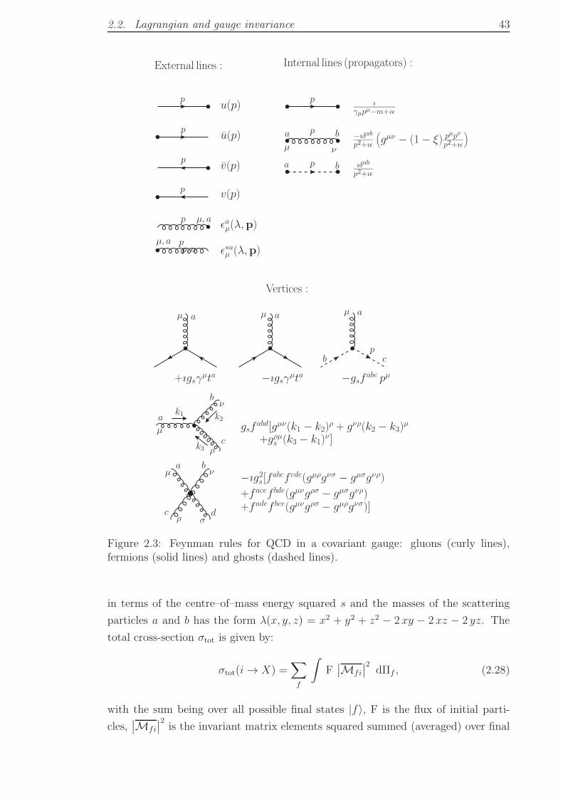
Figure 2.3: Feynman rules for QCD in a covariant gauge: gluons (curly lines),fermions (solid lines) and ghosts (dashed lines).
in terms of the centre–of–mass energy squared s and the masses of the scattering
particles a and b has the form λ(x, y, z) = x2 + y2 + z2 − 2 xy − 2 xz − 2 yz. The
total cross-section σtot is given by:
σtot(i → X) =∑
f
∫F∣∣Mfi
∣∣2 dΠf , (2.28)
with the sum being over all possible final states |f〉, F is the flux of initial parti-
cles,∣∣Mfi
∣∣2 is the invariant matrix elements squared summed (averaged) over final
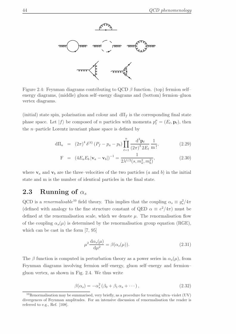
44 QCD phenomenology
Figure 2.4: Feynman diagrams contributing to QCD β function. (top) fermion self–energy diagrams, (middle) gluon self–energy diagrams and (bottom) fermion–gluonvertex diagrams.
(initial) state spin, polarisation and colour and dΠf is the corresponding final state
phase space. Let |f〉 be composed of n particles with momenta pµℓ = (Eℓ,pℓ), then
the n–particle Lorentz invariant phase space is defined by
dΠn = (2π)4 δ(4) (Pf − pa − pb)n∏
ℓ=1
d3pℓ
(2π)3 2Eℓ
1
m !, (2.29)
F = (4EaEb |va − vb|)−1 =1
2λ1/2(s,m2a, m
2b), (2.30)
where va and vb are the three–velocities of the two particles (a and b) in the initial
state and m is the number of identical particles in the final state.
2.3 Running of αs
QCD is a renormalisable10 field theory. This implies that the coupling αs ≡ g2s/4π
(defined with analogy to the fine structure constant of QED α ≡ e2/4π) must be
defined at the renormalisation scale, which we denote µ. The renormalisation flow
of the coupling αs(µ) is determined by the renormalisation group equation (RGE),
which can be cast in the form [7, 95]
µ2 dαs(µ)
dµ2= β(αs(µ)). (2.31)
The β function is computed in perturbation theory as a power series in αs(µ), from
Feynman diagrams involving fermion self–energy, gluon self–energy and fermion–
gluon vertex, as shown in Fig. 2.4. We thus write
β(αs) = −α2s (β0 + β1 αs + · · · ) , (2.32)
10Renormalisation may be summarised, very briefly, as a procedure for treating ultra–violet (UV)divergences of Feynman amplitudes. For an intensive discussion of renormalisation the reader isreferred to e.g., Ref. [108].
2.3. Running of αs 45
where β0 = (11CA − 2nf ) /12π, β1 =(17CA
2 − 5CAnf − 3CFnf
)/24π2 and the mi-
nus sign on the right–hand side of (2.32) distinguishes QCD from QED, for which
one has (see e.g., [109])
βQED(α) = +α2(βQED0 + βQED
1 α + · · ·), (2.33)
with βQED0 = nf/3π and βQED
1 = 1/4π2. The solution to Eq. (2.31) determines the
value of the coupling at a scale µ2 in terms of its value at another scale µ111. At
lowest order, one obtains for QCD an expression of the form
αs(µ2) =αs(µ1)
1 + β0 αs(µ1) ln (µ22/µ
21)
=1
β0 ln(µ22/Λ
2QCD
) , (2.34)
where the last equality follows from rewriting Eq. (2.31) as,
ln
(µ22
µ21
)=
∫ αs(µ2)
αs(µ1)
dαs
β(αs), (2.35)
and setting µ1 → ΛQCD. Provided the first coefficient β0 is positive, which is only
true if the number of flavours nf is less than about 16.5, then the coupling weakens
(diverges) logarithmically at larger (smaller) renormalisation masses µ. Indeed, αs
approaches zero in the limit µ → ∞ and blows up in the limit µ → ΛQCD, as can be
seen from Eq. (2.34). The former limit is known as asymptotic freedom [111, 112] and
justifies the validity of perturbation theory in this regime. The latter limit signals the
failure of the lowest–order approximation (2.34) where the theory becomes strongly
coupled and thus essentially non–perturbative. To the contrary, the QED coupling
α is small at low energies, α(µ = 0) ∼ 1/137, and grows logarithmically at high
energies, α(µ = mZ) ∼ 1/128.
2.3.1 Confinement and factorisation
Probed at sufficiently high energies, or momentum transfer ≫ ΛQCD, hadrons may
reliably be considered as “bags” of weakly interacting quarks and gluons. Conse-
quently, collisions between hadrons can effectively be regarded as scattering amongst
their “free” constituent partons (quarks and gluons). The hard scattering process, to
which mainly two partons, one from each of the colliding hadrons, participate with
the rest of the “spectator” partons interfering at lower energies and thus forming
hadron remnants, is fully calculable in perturbation theory. Such a hard scattering
occurs, by the uncertainty principle, at very short distances.
As the energy falls to ∼ ΛQCD or below, the quarks and gluons inside a hadron
become strongly coupled to the extent that it is impossible to knock an individual
11Usually the magnitude of αs in QCD is given at the mass of the Z boson: αs(µ = mZ) ∼ 0.118[110]. The magnitude at any other scale is then deduced from the solution of Eq. (2.31).
46 QCD phenomenology
quark out of the hadron. This phenomenon is know as confinement. Starting with a
meson (quark–antiquark bound state), if one attempts to pull apart its constituents
then instead of the meson breaking into two quarks it breaks into two mesons.
The new quark–antiquark pair is created from quantum mechanical fluctuations
once the energy in the “flux tube”12, formed between the original quark–antiquark
pair, becomes higher than the rest mass of the pair (recall that the masses of the
light quarks, O(5 MeV), are far below the QCD non–perturbative scale ΛQCD ∼200 MeV). Therefore at low energies, or equivalently long distances, individual
quarks cannot be observed as they immediately confine, or hadronise, into hadronic
bound states.
A typical event at the LHC proceeds as follows: First, two protons are made
to collide head–on at a high centre–of–mass energy. The actual hard scattering
occurs between the constituent partons, one from each proton. As the quarks travel
towards the outer parts of the detector they lose energy by emitting gluons, which in
turn radiate more gluons and/or split into quark–antiquark pairs. At each step the
energy falls and the number of quarks and gluons grows up leading to the formation
of a “shower” of partons. Eventually, at low energies, quarks and gluons undergo the
inevitable process of hadronisation (confinement) into mesons and baryons, which
are observed at detectors as collimated energy depositions, or equivalently “jets”.
The latter will be the pivotal subject of the next chapter (Chapter 3).
Two processes that take place at two disparately different scales, long and short
distances, are quantum mechanically incoherent. i.e., their interference vanishes,
up to inverse powers of the hard scale of the system, as shown in Eq. (2.36). This
allows for a separate treatment of each process. Such a separation is known as
factorisation. The general form of a factorised physical cross section for a process
initiated by two hadrons with momenta P1 and P2 is [62, 63, 97, 113]
σ (P1, P2) =∑
i,j
∫dx1 dx2 fi(x1, µF )fj(x2, µF ) σij (p1, p2, αs(µF ), Q/µF )+O(1/Qp),
(2.36)
where pi = xiPi is the momentum of parton i participating in the hard scattering,
as schematically depicted in Fig. 1.1. σ is a short distance, hard scattering partonic
cross section, which is infrared safe13 and calculable in perturbation theory, and f is
a long distance function that is not calculable in perturbation theory. It is however
“universal” and can be measured experimentally once and for all. In essence, the
function f describes the distribution (and dynamics) of partons in the colliding
12This concept arises in the investigation of QCD confinement from the point of view of a non–abelian analogue to the Meissner effect in superconductors [104].
13Infrared (and collinear) safety, which refers to the insensitivity to soft emissions and collinearsplittings, is crucial to the finiteness of perturbative calculations. This topic will be addressed inthe next chapter (Chapter 3).
2.3. Running of αs 47
hadrons. As such f is termed the parton distribution function (PDF)14, and the
subscripts i and j in Eq. (2.36) refer to the specific parton flavour (including gluons).
The symbols Q and µF denote, respectively, the partonic hard and factorisation
scales. The latter marks the boundary between short distance and long distance, or
equivalently between perturbative and non–perturbative, dynamics. Thus a parton
emitted at a scale less than µF will be absorbed into the parton distributions, while
a parton emitted at a scale larger than µF will be considered as part of σ. The more
orders included in σ the less dependence of σ on the scale µF . The last term in
Eq. (2.36), with p being a real number, is there to indicate that factorisation holds
up to corrections that behave as inverse powers of Q. It is worth noting that the
factorisation formula (2.36) has been proven for sufficiently inclusive observables in
a variety of processes, e.g., Drell–Yan process (hadron + hadron → mu+µ− + X)
and scattering of colourless hadrons (hadron + hadron → hadron + X), where X
denotes “anything else” in the final state [62, 63, 64, 114].
Since physical quantities, such as σ, cannot depend on the (arbitrary) factorisa-
tion scale µF then∂ lnσ
∂ lnµF= 0. (2.37)
Although parton distributions are not calculable from first principles of QCD, as
stated above, (2.37) allows for perturbative calculations of their dependence on the
scale µF . Substituting Eq. (2.36) into Eq. (2.37), we schematically have
∂ ln f
∂ lnµF∝ P, f = qi, g. (2.38)
where the function P can only depend on the shared variables between σ and f ;
the coupling and convolution variables. The solution of Eq. (2.38) describes the
“evolution” of the PDFs between two scales, say, µF and µ′F . Once measured ex-
perimentally at a scale µF , they can be perturbatively predicted at arbitrary high
scales, µ′F ≫ ΛQCD, (provided the coupling remains small over the evolution range).
The function P actually refers to the Altarelli-Parisi splitting functions (or evolution
kernels) and Eq. (2.38) is the Dokshitzer–Gribov–Lipatov–Altarelli–Parisi (DGLAP)
evolution equation [115, 116, 117, 118]. It is one of the fundamental equations in
pQCD (analogous to the β function equation (2.31)). Written in the standard form,
including explicit dependence on the partons’ (longitudinal) momentum fractions,
the latter evolution equation reads [7].
∂fi(x, µF )
∂ lnµF
=αs (µF )
2π
∑
j
∫ 1
x
dz
zfj(z, µF )Pij
(xz, αs(µF )
). (2.39)
14Considering final state hadrons, f may be taken to be the fragmentation function (usuallydenoted D) [7].
48 QCD phenomenology
The splitting functions Pij essentially correspond to the rate of production of parton
i from parton j as the process evolves in lnµF . They have the following perturbative
expansion in the running coupling:
Pij (z, αs) = P(0)ij (z) +
αs
2πP
(1)ij (z) + · · · , (2.40)
where the leading splitting functions are
P (0)qq (z) = CF
[1 + z2
(1− z)++
3
2δ(1− z)
],
P (0)qg (z) = TF
[z2 + (1− z)2
],
P (0)gq (z) = CF
[1 + (1− z)2
z
],
P (0)gg (z) = 2CA
[z
(1− z)++
1− z
z+ z(1− z)
]+
[11CA − 4nfTR
6
]δ (1− z) .
(2.41)
Additionally P(0)qq′ = P
(0)qq = 0. The “plus” distribution used in the above equations
is defined by ∫ 1
0
dxh(x)
(1− x)+=
∫ 1
0
dxh(x)− h(1)
(1− x), (2.42)
where h(x) is an arbitrary smooth function. The state–of–the–art of the splitting
kernels is up to O(α3s) [119, 120].
Lastly, notice that the DGLAP equation (2.39) can be solved numerically either
in x-space or in its conjugate Mellin space:
f(N, µ) =
∫ 1
0
dxxN−1f(x, µ). (2.43)
In the latter space it may be possible to solve the equation analytically. Inverting
back to the x–space is not, except in very special cases, however analytically possi-
ble. Throughout this thesis we shall adopt the standard choice µF = Q and thus do
not worry about the evolution of parton densities. There is a plethora of numerical
programs that straightforwardly handle such an evolution, see e.g., [121] (and refer-
ences therein). Lastly note that a conventional way of estimating PDF uncertainties
is to choose the renormalisation scale µR, which has so far been implicitly taken to
be equal to µF , to be µ2R = (xµµF )
2 and vary xµ in the range 1/2 < xµ < 2 (often
just takes the values xµ = 1/2, 1, 2) [122].
In the next chapter, we address more specific issues that are of direct concern in
the current thesis. Namely the phenomenology of “jets”.
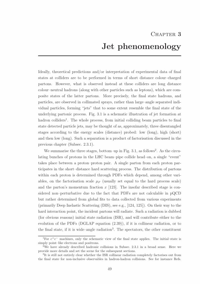
Chapter 3
Jet phenomenology
Ideally, theoretical predictions and/or interpretation of experimental data of final
states at colliders are to be performed in terms of short distance colour–charged
partons. However, what is observed instead at these colliders are long distance
colour–neutral hadrons (along with other particles such as leptons), which are com-
posite states of the latter partons. More precisely, the final state hadrons, and
particles, are observed in collimated sprays, rather than large–angle separated indi-
vidual particles, forming “jets” that to some extent resemble the final state of the
underlying partonic process. Fig. 3.1 is a schematic illustration of jet formation at
hadron colliders1. The whole process, from initial colliding beam particles to final
state detected particle jets, may be thought of as, approximately, three disentangled
stages according to the energy scales (distance) probed: low (long), high (short)
and then low (long). Such a separation is a product of factorisation discussed in the
previous chapter (Subsec. 2.3.1).
We summarise the three stages, bottom–up in Fig. 3.1, as follows2. As the circu-
lating bunches of protons in the LHC beam–pipe collide head–on, a single “event”
takes place between a proton–proton pair. A single parton from each proton par-
ticipates in the short–distance hard scattering process. The distribution of partons
within each proton is determined through PDFs which depend, among other vari-
ables, on the factorisation scale µF (usually set equal to the hard process scale)
and the parton’s momentum fraction x [123]. The insofar described stage is con-
sidered non–perturbative due to the fact that PDFs are not calculable in pQCD
but rather determined from global fits to data collected from various experiments
(primarily Deep Inelastic Scattering (DIS), see e.g., [124, 125]). On their way to the
hard interaction point, the incident partons will radiate. Such a radiation is dubbed
(for obvious reasons) initial state radiation (ISR), and will contribute either to the
evolution of the PDFs (DGLAP equation (2.39)), if it is collinear radiation, or to
the final state, if it is wide–angle radiation3. The spectators, the other constituent
1For e+e− machines, only the schematic view of the final state applies. The initial–state issimply point–like electrons and positrons.
2We have already described hadronic collisions in Subsec. 2.3.1 in a broad sense. Here weprovide more details and set the scene for the subsequent sections.
3It is still not entirely clear whether the ISR collinear radiation completely factorises out fromthe final state for non-inclusive observables in hadron-hadron collisions. See for instance Refs.
49
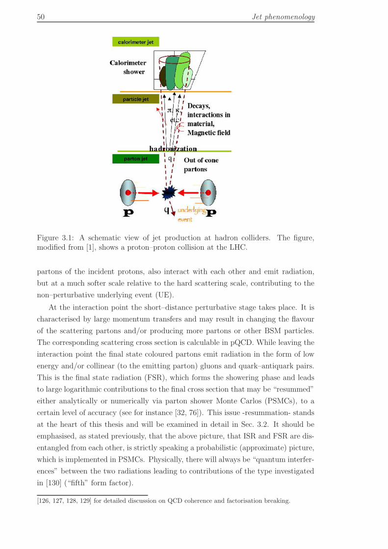
50 Jet phenomenology
Figure 3.1: A schematic view of jet production at hadron colliders. The figure,modified from [1], shows a proton–proton collision at the LHC.
partons of the incident protons, also interact with each other and emit radiation,
but at a much softer scale relative to the hard scattering scale, contributing to the
non–perturbative underlying event (UE).
At the interaction point the short–distance perturbative stage takes place. It is
characterised by large momentum transfers and may result in changing the flavour
of the scattering partons and/or producing more partons or other BSM particles.
The corresponding scattering cross section is calculable in pQCD. While leaving the
interaction point the final state coloured partons emit radiation in the form of low
energy and/or collinear (to the emitting parton) gluons and quark–antiquark pairs.
This is the final state radiation (FSR), which forms the showering phase and leads
to large logarithmic contributions to the final cross section that may be “resummed”
either analytically or numerically via parton shower Monte Carlos (PSMCs), to a
certain level of accuracy (see for instance [32, 76]). This issue -resummation- stands
at the heart of this thesis and will be examined in detail in Sec. 3.2. It should be
emphasised, as stated previously, that the above picture, that ISR and FSR are dis-
entangled from each other, is strictly speaking a probabilistic (approximate) picture,
which is implemented in PSMCs. Physically, there will always be “quantum interfer-
ences” between the two radiations leading to contributions of the type investigated
in [130] (“fifth” form factor).
[126, 127, 128, 129] for detailed discussion on QCD coherence and factorisation breaking.
3.1. Jet clustering algorithms 51
As the process evolves away from the hard interaction point towards lower en-
ergies (longer distances) the coloured partons resulting from the showering as well
as those coming from softer interactions, both from UE and PU4, undergo a non–
perturbative hadronisation phase yielding colour singlet hadrons. The latter (mas-
sive) hadrons are produced either at ground or excited state. The excited state
hadrons, or “resonances”, decay to lighter ones, at ground state, with high (low)
longitudinal (transverse) momentum, with respect to the direction of the outgoing
resonance. At high centre–of–mass energies,√s ≫ EW scale ∼ 90 GeV, massive
particles, both elementary and bound–state resonances in SM and BSM, decay into
lighter particles that are highly boosted in the lab frame. The resultant final jets
have a different topology to the unboosted case. This field has seen substantial
developments in the very recent years (see e.g., the boost11 review [26]).
At leading–order, parton jets are infinitely narrow and only start to build non–
vanishing width at next–to–leading order. The showering and hadronisation phases
contribute towards the increase of the latter width, thus smearing out the energy
distribution within the jet (a “splash–out” effect [1]). The UE and PU, on the
other hand, give rise to a “splash–in” effect whereby extra (soft) energy is added
to the jets. The final hadron (jets) eventually pass through the various layers of
the detector where they undergo some interactions resulting in -yet another level
of complexity- “calorimeter” jets, shown at the top of Fig. 3.1, which embodies the
detector response. The latter (detector-level jets) is beyond the scope of the present
thesis and we refer the interested reader to Ref. [1] for more information. Hitherto,
we have presented no formal definition of a jet that applies at all levels; parton,
shower, hadron and detector. We do so in Sec. 3.1. Once a jet is properly defined,
we then exploit its usage in understanding QCD through exploring its “internal”
and “external” properties in Sec. 3.2. We succinctly summarise the main points in
Sec. 3.3.
It is worth noting that the field of jets (and related topics) has seen a substan-
tial growth over the last few years, mainly due to the fact that the final state at
the LHC is predominantly jets. Different research groups tackled the issue from
different angles and with different aims (understanding QCD, background–signal
discrimination, · · · ). A sample of literature reviews on the topic may be found in
Refs. [1, 26, 27, 31, 80, 131, 132, 133, 134] (and references therein).
3.1 Jet clustering algorithms
The measured kinematics (four–vectors) of “jets” at the detector level (from energy
depositions into calorimeter cells and tracks of charged particles) provide a measure
of the kinematics of the underlying short–distance theory partons and/or decaying
4See definitions in introductory chapter 1.
52 Jet phenomenology
massive (boosted) particles5 [1, 135, 136, 137, 138]. Jets are not, however, intrinsi-
cally well–defined objects, just as partons are not well–defined due to their infinite
branching probabilities in pQCD, and thus a prescription for defining them is re-
quired. A wide variety of “jet definitions” have been proposed in the literature (for
a review see, for instance, Refs. [139, 133]). A typical jet definition consists of a
jet algorithm and a recombination scheme. A jet algorithm is essentially a set of
mathematical rules that details the procedure of merging (“daughter”) objects into
“protojets” (parent objects) based on a measure of their “closeness”. The objects,
described by their 4–vectors, refer to partons in perturbative final state, final state
hadrons in the simulated Monte Carlo events or calorimeter output at detectors.
The recombination scheme specifies how the kinematics of the parent protojets are
constructed from those of the daughters.
Different jet definitions implement different jet algorithms and/or recombination
schemes with different strengths and weaknesses. Some important general properties
that should be fulfilled by a jet definition for it to be practically useful were set out
by the “Snowmass accord” [140]. They include, along others, the crucial requirement
of infrared and collinear (IRC) safety of the jet algorithm. The presently available
jet algorithms may be divided into two main categories, depending on the manner
they operate: cone algorithms and sequential recombination algorithms. In what
follows below, we first provide a brief description of the first type and take it as an
example to address the issue of IRC safety. We then consider the second type of jet
algorithms. Notice that our calculations in this thesis are confined to the latter type
of algorithms and they are thus discussed in more detail (than cone algorithms).
3.1.1 Cone algorithms
The first appearance of a jet algorithm was in the pioneering work of Sterman and
Weinberg [141], wherein they calculated the (partial) cross section for e+e− hadronic
events, in which all but a fraction ǫ ≪ 1 of the total e+e− energy is emitted within
some pair of oppositely directed cones of half–angle δ ≪ 1. This was the first basic
definition of a cone algorithm in terms of two parameters; energy and angle.
A modern cone algorithm operates in two distinct steps. In the first step it
searches for stable cones6. In the second step it runs a split–merge procedure to
resolve any overlapping stable cones. The outcome of this procedure is that each
object, in the initial list, is assigned to a single jet in the final list. Insofar the
only IRC safe cone algorithm available is the seedless infrared safe cone (SISCone)
algorithm developed in Ref. [142]. A detailed description of various cone algorithms
may be found in the review [133].
5After effects of FSR, ISR, hadronisation, UE and PU are properly estimated and corrected forat a sufficiently reliable precision level.
6A stable cone is a cone whose axis coincides with the axis of the sum of all three–momenta ofparticles it contains.
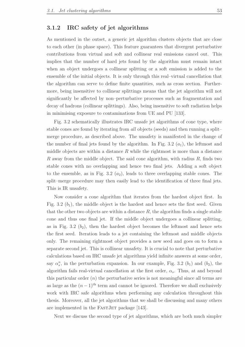
3.1. Jet clustering algorithms 53
3.1.2 IRC safety of jet algorithms
As mentioned in the outset, a generic jet algorithm clusters objects that are close
to each other (in phase space). This feature guarantees that divergent perturbative
contributions from virtual and soft and collinear real emissions cancel out. This
implies that the number of hard jets found by the algorithm must remain intact
when an object undergoes a collinear splitting or a soft emission is added to the
ensemble of the initial objects. It is only through this real–virtual cancellation that
the algorithm can serve to define finite quantities, such as cross section. Further-
more, being insensitive to collinear splittings means that the jet algorithm will not
significantly be affected by non–perturbative processes such as fragmentation and
decay of hadrons (collinear splittings). Also, being insensitive to soft radiation helps
in minimising exposure to contaminations from UE and PU [133].
Fig. 3.2 schematically illustrates IRC unsafe jet algorithms of cone type, where
stable cones are found by iterating from all objects (seeds) and then running a split–
merge procedure, as described above. The unsafety is manifested in the change of
the number of final jets found by the algorithm. In Fig. 3.2 (a1), the leftmost and
middle objects are within a distance R while the rightmost is more than a distance
R away from the middle object. The said cone algorithm, with radius R, finds two
stable cones with no overlapping and hence two final jets. Adding a soft object
to the ensemble, as in Fig. 3.2 (a2), leads to three overlapping stable cones. The
split–merge procedure may then easily lead to the identification of three final jets.
This is IR unsafety.
Now consider a cone algorithm that iterates from the hardest object first. In
Fig. 3.2 (b1), the middle object is the hardest and hence sets the first seed. Given
that the other two objects are within a distance R, the algorithm finds a single stable
cone and thus one final jet. If the middle object undergoes a collinear splitting,
as in Fig. 3.2 (b2), then the hardest object becomes the leftmost and hence sets
the first seed. Iteration leads to a jet containing the leftmost and middle objects
only. The remaining rightmost object provides a new seed and goes on to form a
separate second jet. This is collinear unsafety. It is crucial to note that perturbative
calculations based on IRC unsafe jet algorithms yield infinite answers at some order,
say αns , in the perturbation expansion. In our example, Fig. 3.2 (b1) and (b2), the
algorithm fails real-virtual cancellation at the first order, αs. Thus, at and beyond
this particular order (n) the perturbative series is not meaningful since all terms are
as large as the (n− 1)th term and cannot be ignored. Therefore we shall exclusively
work with IRC safe algorithms when performing any calculation throughout this
thesis. Moreover, all the jet algorithms that we shall be discussing and many others
are implemented in the FastJet package [143].
Next we discuss the second type of jet algorithms, which are both much simpler
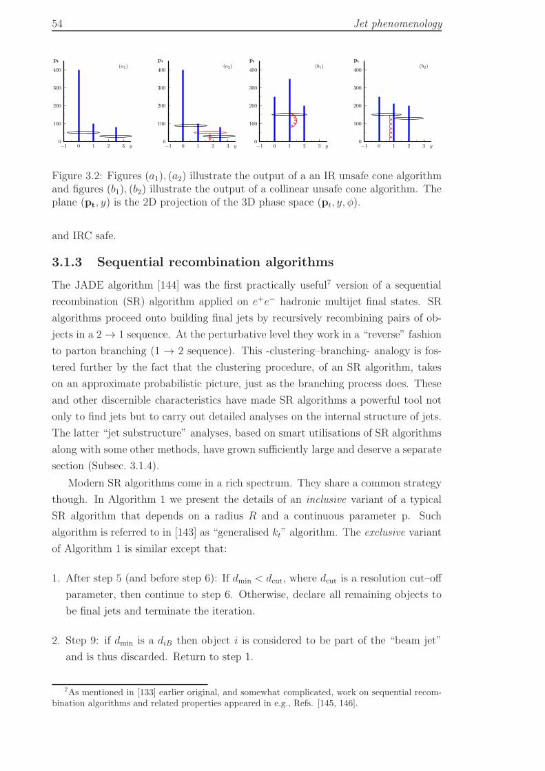
54 Jet phenomenology
0
100
200
300
400
−1 0 1 2 3 y
pt
(a1)
0
100
200
300
400
−1 0 1 2 3 y
pt
(a2)
0
100
200
300
400
−1 0 1 2 3 y
pt
(b1)
0
100
200
300
400
−1 0 1 2 3 y
pt
(b2)
Figure 3.2: Figures (a1), (a2) illustrate the output of a an IR unsafe cone algorithmand figures (b1), (b2) illustrate the output of a collinear unsafe cone algorithm. Theplane (pt, y) is the 2D projection of the 3D phase space (pt, y, φ).
and IRC safe.
3.1.3 Sequential recombination algorithms
The JADE algorithm [144] was the first practically useful7 version of a sequential
recombination (SR) algorithm applied on e+e− hadronic multijet final states. SR
algorithms proceed onto building final jets by recursively recombining pairs of ob-
jects in a 2 → 1 sequence. At the perturbative level they work in a “reverse” fashion
to parton branching (1 → 2 sequence). This -clustering–branching- analogy is fos-
tered further by the fact that the clustering procedure, of an SR algorithm, takes
on an approximate probabilistic picture, just as the branching process does. These
and other discernible characteristics have made SR algorithms a powerful tool not
only to find jets but to carry out detailed analyses on the internal structure of jets.
The latter “jet substructure” analyses, based on smart utilisations of SR algorithms
along with some other methods, have grown sufficiently large and deserve a separate
section (Subsec. 3.1.4).
Modern SR algorithms come in a rich spectrum. They share a common strategy
though. In Algorithm 1 we present the details of an inclusive variant of a typical
SR algorithm that depends on a radius R and a continuous parameter p. Such
algorithm is referred to in [143] as “generalised kt” algorithm. The exclusive variant
of Algorithm 1 is similar except that:
1. After step 5 (and before step 6): If dmin < dcut, where dcut is a resolution cut–off
parameter, then continue to step 6. Otherwise, declare all remaining objects to
be final jets and terminate the iteration.
2. Step 9: if dmin is a diB then object i is considered to be part of the “beam jet”
and is thus discarded. Return to step 1.
7As mentioned in [133] earlier original, and somewhat complicated, work on sequential recom-bination algorithms and related properties appeared in e.g., Refs. [145, 146].
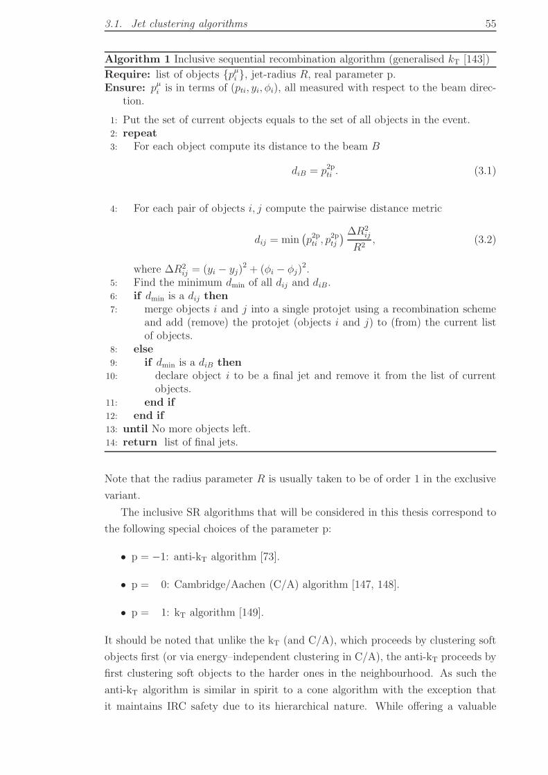
3.1. Jet clustering algorithms 55
Algorithm 1 Inclusive sequential recombination algorithm (generalised kT [143])
Require: list of objects pµi , jet-radius R, real parameter p.Ensure: pµi is in terms of (pti, yi, φi), all measured with respect to the beam direc-
tion.
1: Put the set of current objects equals to the set of all objects in the event.2: repeat3: For each object compute its distance to the beam B
diB = p2pti . (3.1)
4: For each pair of objects i, j compute the pairwise distance metric
dij = min(p2pti , p
2ptj
) ∆R2ij
R2, (3.2)
where ∆R2ij = (yi − yj)
2 + (φi − φj)2.
5: Find the minimum dmin of all dij and diB.6: if dmin is a dij then7: merge objects i and j into a single protojet using a recombination scheme
and add (remove) the protojet (objects i and j) to (from) the current listof objects.
8: else9: if dmin is a diB then10: declare object i to be a final jet and remove it from the list of current
objects.11: end if12: end if13: until No more objects left.14: return list of final jets.
Note that the radius parameter R is usually taken to be of order 1 in the exclusive
variant.
The inclusive SR algorithms that will be considered in this thesis correspond to
the following special choices of the parameter p:
• p = −1: anti-kT algorithm [73].
• p = 0: Cambridge/Aachen (C/A) algorithm [147, 148].
• p = 1: kT algorithm [149].
It should be noted that unlike the kT (and C/A), which proceeds by clustering soft
objects first (or via energy–independent clustering in C/A), the anti-kT proceeds by
first clustering soft objects to the harder ones in the neighbourhood. As such the
anti-kT algorithm is similar in spirit to a cone algorithm with the exception that
it maintains IRC safety due to its hierarchical nature. While offering a valuable
56 Jet phenomenology
replacement for the cone algorithm8, the substructure defined by the anti-kT algo-
rithm cannot be mapped onto that of QCD jets resulting from parton branching.
As a consequence of this, care should be exercised when carrying out substructure
studies using the anti-kT algorithm.
Each of the above listed algorithms has some strengths and weaknesses, which
are highlighted in [142], and using a variety of them for physics analyses is highly
desirable as concluded in [1]. Lastly it is worth mentioning that a flurry of variants
of SR algorithms9 have been developed over the past few years. These include,
for instance, flavoured kt algorithm [150], variable–R algorithm [151] and arclus
(3 → 2 clustering sequence) algorithm [152].
3.1.4 Jet grooming techniques
Jet grooming algorithms, which may be regarded as variants of SR algorithms,
were largely motivated by UE and PU investigations. Soft radiation coming from
the latter non–perturbative processes and which end up in jets may be “groomed”
(mitigated) away through modifying the substructure of the respective jets. Each
grooming algorithm operates on a single jet and produces a “groomed” jet. The
latter contains less junk–radiation and is thus of improved resolution, leading to
more accurate extractions of its properties. Popular jet grooming algorithms include:
filtering [14, 153], trimming [30] and pruning [29]. Although all three methods aid
in better identifying the origin of a particular jet, trimming was originally proposed
for use on jets from QCD light quarks while filtering and pruning have typically
been used on jets from decay of (boosted) heavy particles [26].
As mentioned earlier, jet grooming is one of the main jet substructure techniques
devised to boost new physics searches in a jetty environment such as that experienced
at LHC. Other substructure tools and methods, aside from jet shapes which we
address below, include: Y–splitter [20], various taggers [37, 154, 155, 156, 157, 158],
shower deconstruction [159], three–body kinematic variables [160] and many others
(see Refs. [26, 27]10). Most of these substructure tools have been incorporated
into the FastJet package11. This package, written in a “jet–oriented” manner,
has served as a framework for the development of a whole branch of study that is
primarily concerned with jets: “jetography”. The reader is referred to Ref. [133] for
more details.
8Note that calculations with cone algorithms are far simpler than with typical SR algorithms.The anti-kT retains the simplicity of the cone algorithms while dispelling their IRC culprit.
9Some with extra parameters that need, in most cases, to be tuned to the specific physicsanalysis being carried out.
10See also the boost12 page at “http://ific.uv.es/~boost2012/”.11SpartyJet [161] is another software/package built around FastJet and provides a variety of
other jet–oriented tools including measurements of some event and jet observables.
3.2. Jet shapes 57
3.2 Jet shapes
Event shape observables (or simply event shapes), such as thrust, characterise the
geometrical properties of the energy flow in QCD final state events. For example, a
pencil–like event produces a value of the (thrust) event shape that is different from
that produced by a sphere–like event. Event shapes are constructed by taking a
weighted sum of the four–momenta, transverse momenta, energies etc of final state
particles12. While imparting information on the global shape of an event, hence
dubbed global (event) shapes, event shapes convey no information regarding the jet
content of the event, such as energy distribution within individual jets.
Event shape–like observables that are sensitive to the properties of single jets in
an event are known as jet shapes13. They can serve to quantify a variety of topologies
in the final state, from pure QCD–like to EW bosons’ two–pronged decays to top
quark (and other proposed new particles) three–pronged decays14. Each of the latter
mentioned topologies yields a different value for the jet shape. Jet shapes are by
construction of non–global nature, as they only measure specific parts, rather than
the whole, of the the event. Such a non–global property, besides making jet shapes
more delicate, opens up the door for a better scrutiny of QCD dynamics.
A trend of jet observables, under the broader class of jet substructure, have been
devised in the recent years. These include, for instance: N–subjettiness [163], jet
width and jet eccentricity [164], jet pull [165] and many others, e.g., [166, 167, 168,
169, 170, 171, 172] (see Refs. [26, 27] for a review). To facilitate later discussions,
we concentrate in this introductory review on the jet shape named angularities
[45, 167] (originally introduced in [38, 39] for two-jets in e+e− annihilation), which
embodies a spectrum of other jet shapes through a continuous parameter a and has
the functional form:
τa =1
2EJ
∑
i∈ J
kti e−ηi(1−a), (3.3)
where kt = |kt| is the transverse momentum relative to the jet direction and η =
− ln tan(θ/2) is the (pseudo-)rapidity measured from the jet axis. EJ ∼ Q/2 is the
energy of the jet J (which will be replaced by the transverse momentum of the jet
in hadron–hadron scattering) and Q is the hard scale. The parameter a runs over
the range −∞ < a < 2 due to IRC safety (see below). For a = 0 the angularities
12Particles here refer, as previously discussed in Sec. 3.1, to: calorimeter towers, clusters orcharged tracks at the detector level, particles at hadronic level, many partons at the shower leveland few partons at perturbative level.
13The term “jet shapes” originally devised for the observable ψ(r;R) which measures the fractionof energy confined in an annulus of width dr = R− r [162].
14More information on two– and three–pronged decays may be found in [133].
58 Jet phenomenology
jet shape (3.3) reduces to the jet mass fraction, defined by
ρ =M2
J
Q2=
1
Q2
(∑
i∈ J
ki
)2
, (3.4)
where ki is the four–momentum of particle i. The case a = 1 corresponds to jet
broadening (B) [173]. It has been shown in [174] that recoil of the primary quarks
(in e+e− two-jet events)15 against soft gluons contributes to the B-distribution at
single logarithmic (SL) accuracy. As such for a = 1 in τa (3.3) recoil effects cannot
be neglected should we aim to compute the τa distribution at the said accuracy. In
fact, for this value of a (a = 1) τa is independent of η and contributions of hard
collinear radiation to the angularities jet shape are equal to contributions from soft
wide-angle radiation (both contribute at SL accuracy). For a > 1 the jet shape τa,
which becomes ∝ e+ηi , receives larger contributions from hard collinear radiation
than from soft wide-angle radiation. Since a full treatment of recoil effects is beyond
the scope of this thesis16, we restrict our analyses to the case a < 1 throughout.
A somewhat related general form of jet shapes was introduced in [31]:
V (p, k) = dℓ
(k(ℓ)t
Q
)aℓ
e−bℓη(ℓ)
gℓ(φ(ℓ)), (3.5)
where p represents the Born momenta after recoil against emission kµ, with trans-
verse momentum k(ℓ)t , (pseudo-)rapidity η(ℓ) and azimuthal angle φ(ℓ) measured
with respect to the emitting parton leg ℓ. IRC safety implies that aℓ > 0 and
aℓ + bℓ > 0 [31, 38, 175]17. The angularities (3.3) then corresponds to the specific
choice: aℓ = dℓ = gℓ(φ) = 1, Q = 2EJ and bℓ = 1− a with emissions restricted to be
within the jet reach. The said IRC conditions on V then translate into a < 2 for τa
eqrefeq:Jets:Angularities.
IRC and recursive IRC safety
In a similar fashion to IRC safety of a jet algorithm, discussed in Subsec. 3.1.2,
IRC safety of an observable means that [31] given an ensemble of partons then the
addition of a relatively much softer and/or collinear splitting of one (or more) of those
partons should not significantly change the value of the observable. Precisely, the
change should not be more than a positive power of the softness/collinearity of the
15Recall that the quark transverse momentum induced via recoil is (assuming the quark to bein the right hemisphere): pt = −∑i∈HR
kti/Q, where HR is the right hemisphere (ηi > 0).16We refer the reader to eg., [31, 174] for details on the treatment of recoil effects in event/jet
shape studies.17Clearly if aℓ < 0 then V ∝ Q/k
(ℓ)t and hence the jet shape is IR unsafe. Moreover, the contri-
bution of any particle to the jet shape behaves as k(ℓ)t e−bℓη
(ℓ)
= ω sin θ(ℓ)e−bℓη(ℓ) ∼ ωe−(aℓ+bℓ)η
(ℓ)
in the collinear limit. Collinear safety (V should stay finite as η(ℓ) → +∞) then implies thataℓ + bℓ > 0.
3.2. Jet shapes 59
splitting(s), normalised to the hard scale. Recursive IRC (rIRC) safety conditions
slightly, but crucially, extend those of “plain” IRC and may be formulated as in
Eqs. (3.3), (3.4) and (3.5) of Ref. [31]18. rIRC safety not only ensures the validity of
perturbative expansion of the corresponding jet shape distribution but also ensures
the “resummability”, or equivalently exponentiation, of the latter perturbative series
(see below, Subsec. 3.2.4).
Let us verify, for instance, that the angularities τa jet shape (3.3) is an rIRC safe
observable. If we introduce the variable
τa (p, k) =ktQe−η(1−a), (3.6)
and use Eq. (3.3) of [31], which states that τa(p, ki(λi)) = λi where ki(λi) are
momentum functions that depend on the parameters λi, then the angularities τa in
(3.3) reads:
τa ≡ τa (p, k1(ǫλ1), · · · , km(ǫλm)) =
m∑
i∈Jτa (p, ki(ǫλi)) = ǫ
m∑
i∈Jλi, (3.7)
where ǫ ≪ 1 is a small parameter. Applying the conditions of rIRC safety given in
Eqs. (3.4), (3.5a) and (3.5b) in [31] we find: (a) for the first condition given in (3.4)
we have
limǫ→0
1
ǫτa (p, k1(ǫλ1), · · · , km(ǫλm)) =
m∑
i∈Jλi, (3.8)
(b) for the second condition given in (3.5a) we have
limλm+1→0
limǫ→0
1
ǫτa (p, k1(ǫλ1), · · · , km+1(ǫλm+1)) = lim
λm+1→0
m+1∑
i∈Jλi =
m∑
i∈Jλi. (3.9)
and finally (c) for the third condition given in (3.5b) we have
limµ→0
limǫ→0
1
ǫτa (p, k1(ǫλ1), · · · , kaℓ, kbℓ(ǫλℓ, µ), · · · , km(ǫλm))
= limµ→0
[∑
i∈J,i 6=ℓ
λi + µλℓ + (1− µ)λℓ
]=∑
i∈Jλi, (3.10)
where µ2 = (kaℓ + kbℓ)2 /k2
tℓ and limµ→0 kaℓ + kbℓ = kℓ. Eqs. (3.8), (3.9), and (3.10)
proves that τa is an rIRC safe observable. Consequently the τa perturbative distri-
bution can be resummed into the form (1.3).
In the next section we first define the (integrated) jet shape distribution and
present an explicit calculation at one-gluon level. Then we elaborate on some of the
18Instead of rewriting the full expressions here we rather use them to carry out an explicitexample below.
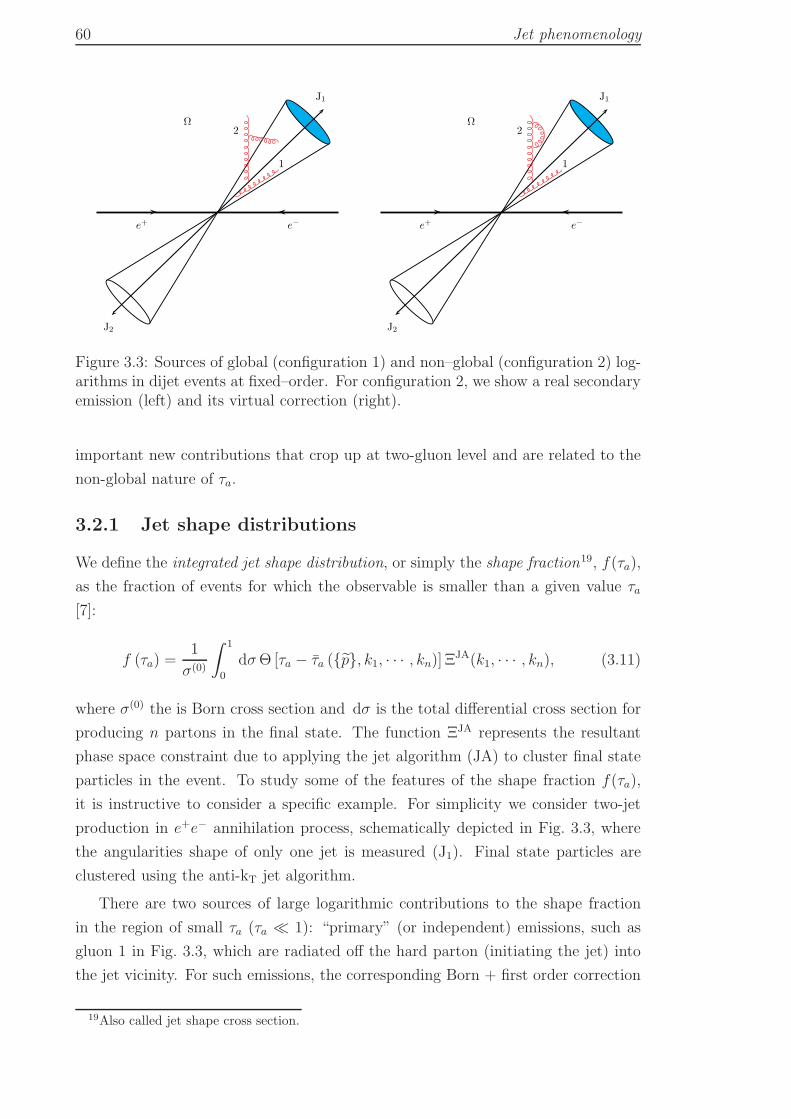
60 Jet phenomenology
e+ e−
J1
J2
Ω
1
2
e+ e−
J1
J2
Ω
1
2
Figure 3.3: Sources of global (configuration 1) and non–global (configuration 2) log-arithms in dijet events at fixed–order. For configuration 2, we show a real secondaryemission (left) and its virtual correction (right).
important new contributions that crop up at two-gluon level and are related to the
non-global nature of τa.
3.2.1 Jet shape distributions
We define the integrated jet shape distribution, or simply the shape fraction19, f(τa),
as the fraction of events for which the observable is smaller than a given value τa
[7]:
f (τa) =1
σ(0)
∫ 1
0
dσΘ [τa − τa (p, k1, · · · , kn)] ΞJA(k1, · · · , kn), (3.11)
where σ(0) the is Born cross section and dσ is the total differential cross section for
producing n partons in the final state. The function ΞJA represents the resultant
phase space constraint due to applying the jet algorithm (JA) to cluster final state
particles in the event. To study some of the features of the shape fraction f(τa),
it is instructive to consider a specific example. For simplicity we consider two-jet
production in e+e− annihilation process, schematically depicted in Fig. 3.3, where
the angularities shape of only one jet is measured (J1). Final state particles are
clustered using the anti-kT jet algorithm.
There are two sources of large logarithmic contributions to the shape fraction
in the region of small τa (τa ≪ 1): “primary” (or independent) emissions, such as
gluon 1 in Fig. 3.3, which are radiated off the hard parton (initiating the jet) into
the jet vicinity. For such emissions, the corresponding Born + first order correction
19Also called jet shape cross section.
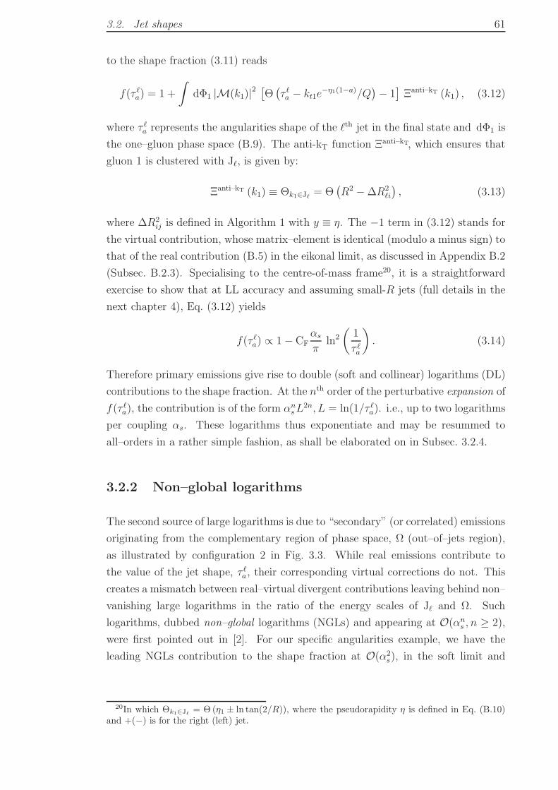
3.2. Jet shapes 61
to the shape fraction (3.11) reads
f(τ ℓa) = 1 +
∫dΦ1 |M(k1)|2
[Θ(τ ℓa − kt1e
−η1(1−a)/Q)− 1]Ξanti–kT (k1) , (3.12)
where τ ℓa represents the angularities shape of the ℓth jet in the final state and dΦ1 is
the one–gluon phase space (B.9). The anti-kT function Ξanti–kT, which ensures that
gluon 1 is clustered with Jℓ, is given by:
Ξanti–kT (k1) ≡ Θk1∈Jℓ = Θ(R2 −∆R2
ℓi
), (3.13)
where ∆R2ij is defined in Algorithm 1 with y ≡ η. The −1 term in (3.12) stands for
the virtual contribution, whose matrix–element is identical (modulo a minus sign) to
that of the real contribution (B.5) in the eikonal limit, as discussed in Appendix B.2
(Subsec. B.2.3). Specialising to the centre-of-mass frame20, it is a straightforward
exercise to show that at LL accuracy and assuming small-R jets (full details in the
next chapter 4), Eq. (3.12) yields
f(τ ℓa) ∝ 1− CFαs
πln2
(1
τ ℓa
). (3.14)
Therefore primary emissions give rise to double (soft and collinear) logarithms (DL)
contributions to the shape fraction. At the nth order of the perturbative expansion of
f(τ ℓa), the contribution is of the form αnsL
2n, L = ln(1/τ ℓa). i.e., up to two logarithms
per coupling αs. These logarithms thus exponentiate and may be resummed to
all–orders in a rather simple fashion, as shall be elaborated on in Subsec. 3.2.4.
3.2.2 Non–global logarithms
The second source of large logarithms is due to “secondary” (or correlated) emissions
originating from the complementary region of phase space, Ω (out–of–jets region),
as illustrated by configuration 2 in Fig. 3.3. While real emissions contribute to
the value of the jet shape, τ ℓa, their corresponding virtual corrections do not. This
creates a mismatch between real–virtual divergent contributions leaving behind non–
vanishing large logarithms in the ratio of the energy scales of Jℓ and Ω. Such
logarithms, dubbed non–global logarithms (NGLs) and appearing at O(αns , n ≥ 2),
were first pointed out in [2]. For our specific angularities example, we have the
leading NGLs contribution to the shape fraction at O(α2s), in the soft limit and
20In which Θk1∈Jℓ= Θ(η1 ± ln tan(2/R)), where the pseudorapidity η is defined in Eq. (B.10)
and +(−) is for the right (left) jet.
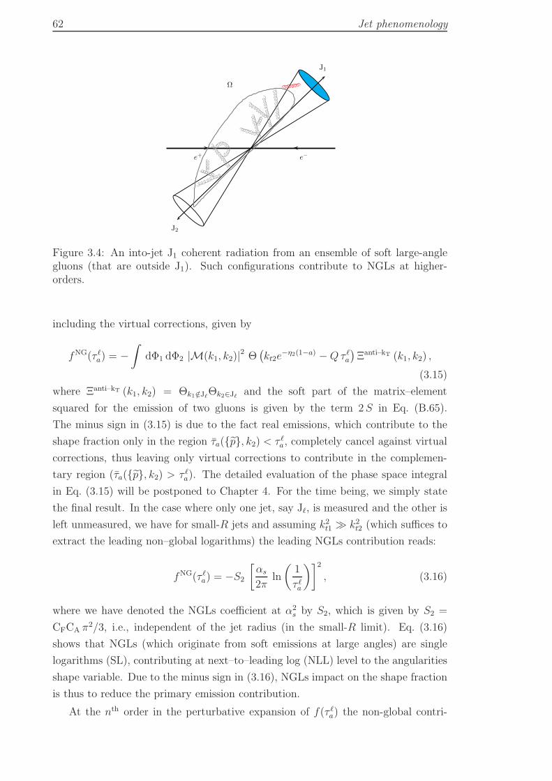
62 Jet phenomenology
e+ e−
J1
J2
Ω
Figure 3.4: An into-jet J1 coherent radiation from an ensemble of soft large-anglegluons (that are outside J1). Such configurations contribute to NGLs at higher-orders.
including the virtual corrections, given by
fNG(τ ℓa) = −∫
dΦ1 dΦ2 |M(k1, k2)|2 Θ(kt2e
−η2(1−a) −Qτ ℓa)Ξanti–kT (k1, k2) ,
(3.15)
where Ξanti–kT (k1, k2) = Θk1 /∈JℓΘk2∈Jℓ and the soft part of the matrix–element
squared for the emission of two gluons is given by the term 2S in Eq. (B.65).
The minus sign in (3.15) is due to the fact real emissions, which contribute to the
shape fraction only in the region τa(p, k2) < τ ℓa, completely cancel against virtual
corrections, thus leaving only virtual corrections to contribute in the complemen-
tary region (τa(p, k2) > τ ℓa). The detailed evaluation of the phase space integral
in Eq. (3.15) will be postponed to Chapter 4. For the time being, we simply state
the final result. In the case where only one jet, say Jℓ, is measured and the other is
left unmeasured, we have for small-R jets and assuming k2t1 ≫ k2
t2 (which suffices to
extract the leading non–global logarithms) the leading NGLs contribution reads:
fNG(τ ℓa) = −S2
[αs
2πln
(1
τ ℓa
)]2, (3.16)
where we have denoted the NGLs coefficient at α2s by S2, which is given by S2 =
CFCA π2/3, i.e., independent of the jet radius (in the small-R limit). Eq. (3.16)
shows that NGLs (which originate from soft emissions at large angles) are single
logarithms (SL), contributing at next–to–leading log (NLL) level to the angularities
shape variable. Due to the minus sign in (3.16), NGLs impact on the shape fraction
is thus to reduce the primary emission contribution.
At the nth order in the perturbative expansion of f(τ ℓa) the non-global contri-
3.2. Jet shapes 63
bution fNG(τ ℓa) corresponds to configurations where an ensemble of (n − 1) soft,
wide-angle particles21 outside the jet coherently emit a single softest gluon into the
jet, as depicted in Fig. 3.4. The ensemble may assume any complicated geometry.
As such it has not been possible [2, 176] to analytically resum these logs to all–
orders, as has the case been with primary (global) logs. However, employing the
large-Nc limit one can either write an evolution equation [71] or resort to a dipole
evolution code [2] to numerically compute the resummation. The solution to the
said all–orders evolution equation adheres a factorised form [71, 177]:
f(τ ℓa) = ΣP (τℓa)S(t) (3.17)
where the first term ΣP is the Sudakov form factor given by bremsstrahlung emission
from primary hard partons and is discussed below. The second factor arises from
successive soft secondary branchings (as described above). The parameter t is known
as the evolution parameter and is given by
t =
∫ 1
e−L
dx
x
αs(xQ)
2π, (3.18)
where x = 2 kt/Q and the logarithm L ∝ ln(1/τ ℓa) (with the exact formula of L
depending on the configuration under study). A widely used parametrisation of
S(t) is given in [2]
S(t) = exp
[−C2
A
2S2
(1 + (at)2
1 + (bt)c
)t2 +O(1/N2
c)
], (3.19)
where S2 is the O(α2s) coefficient and the parameters a, b and c are determined from
fitting (3.19) to the output of the MC program of Ref. [2]. Actually, for use in
phenomenology one replaces the large-Nc colour factor CA/2 by the corresponding
full colour factor such that when expanding (3.19) one recovers the full O(α2s) result.
Note that the neglected 1/N2c non-planar part contribute at the 10% level.
In–depth discussion of this and other related features of NGLs is presented in the
subsequent chapters. It is in fact one of the central aims of this thesis to compute,
as accurately as possible, NGLs at fixed–order and quantify their all–orders impact
on the total resummed jet shape distribution.
3.2.3 Clustering logarithms
So far we have only dealt with jet shape distributions where final state jets are
defined with the anti-kT algorithm. As emphasised earlier (see Sec. 3.1) the anti-kT
algorithm works, particularly in the soft limit, like a rigid cone. Soft partons are
21To extract the leading NGLs it suffices to consider these particles to be energy-ordered; ω1 ≫ω2 ≫ · · · ≫ ωn−1.
64 Jet phenomenology
clustered independently to their nearest hard neighbours. This simple picture is
spoiled by other SR algorithms such as kT, C/A as well as the SISCone algorithm,
where soft partons are iteratively clustered together, based on their closeness, and
may well form separate jets from hard partons’ jets. The impact of this on the final
form of the jet shape distribution is two fold:
• Significant reduction in the NGLs contribution due to tighter phase space
constraints. This was first shown in [75] for gaps–between–jets distribution.
• Breakdown of the naive single–gluon exponentiation (at NLL) associated with
primary emissions due to the appearance of a tower of large single logarithms.
This was first pointed out in [3, 74] for the same distribution (gaps–between–
jets). We refer to these logarithms as clustering logarithms (CLs). They are a
type of non–global logarithm as they only show–up for non–global observables.
As a result of this some authors, e.g., of Ref. [178], refer to them as abelian
NGLs.
Postponing the discussion of both effects at fixed–order and all–orders to later chap-
ters, we note that the leading CLs contribution to angularities shape fraction at
O(α2s) is, for the case of one measured jet Jℓ, of the form
f JA(τ ℓa) = CP,JA2 C2
F
(αs
2π
)2L2, (3.20)
where L = ln(1/τ ℓa) and CP,JA2 is the outcome of the phase space integral. For small
jet radii, R ≪ 1, CP,JA2 only depends on the geometry of the final state (and neither
R nor the jet shape). As R increases CP,JA2 dependence on R is restored as shall be
explicitly shown in Chapter 5. For the kT and C/A algorithms: CP,kT2 = C
P,C/A2 ≃
π2/27 = S2/N2c as R → 0. This relation between C
P,kT(C/A)2 and S2 further fosters
the non-global nature of CLs.
Just like NGLs, the SL clustering logs persist at every order in the perturbative
expansion of the non–global jet shape distribution and must be resummed for a
given phenomenological calculation to be meaningful. Although the all–orders result
can currently only be obtained via the MC program of [2], the situation is slightly
more satisfactory than with NGLs. It has been possible, for both gaps–between–
jets and jet mass as discussed in Chapter 6, to analytically compute the first few
orders in the corresponding g2 (see Eq. (1.3)) CLs–tower and evidently show, by
explicit comparison to the output of the said MC program, that they capture the
full behaviour of the all–orders result. Full details are presented in Chapter 6.
Below we outline the necessary steps for a typical resummation calculation of
primary global logarithms (GLs).
3.2. Jet shapes 65
3.2.4 Resummation
Fixed–order perturbative calculations usually involve a small number of additional
partons to the Born configuration and can produce accurate results at the large–
τa tail region of the jet shape distribution (τa . 1). Such regions of phase space
describe large departures from the Born–event energy flow pattern due to the ex-
tra partons being energetic and at large angles. Their contributions are free from
large logarithms, suppressed by powers of the coupling αs and comply with the
convergence of the perturbative series. Fixed–order calculations are usually carried
out with the help of Fixed–order Monte Carlos (FOMCs) such as event2 [179],
eerad3 [180, 181], for e+e− annihilation, and mcfm [182], nlojet++ [58], for
hadron-hadron scattering, to mention just a few. These programs are fully exclusive
over the final state and can produce predictions for arbitrary IRC observables. The
prevalent accuracy across the majority of the available FOMCs is next–to–leading
order (NLO), with the exception of eerad3 which reaches next–to–next–to–leading
order (NNLO) for observables in e+e− annihilation events.
In the small τa region, τa ≪ 1, in which departures from the Born energy–flow
configuration are small due to the extra partons being soft and/or collinear to the
initial hard Born partons, and which constitutes the bulk of final state configura-
tions, fixed–order perturbative calculations are unreliable, as illustrated in Fig. 3.5
(left). This is due to the fact that each power of the coupling αs is accompanied by
up to two powers of large logarithms associated with soft and collinear divergences,
as exemplified in the previous subsections. The all–orders perturbative series of the
shape fraction f(τa) (3.11) may be cast in the form
f(τa) = 1 +∞∑
n=1
[A(1)
n αns L
2n + A(2)n αn
s L2n−1 + A(3)
n αns L
2(n−1) + · · ·], τa ≪ 1,
(3.21)
where the coefficients A(m)n are determined from phase space integrals and L is
defined as before. In the above equation A(1)n is the LL coefficient, A
(2)n the NLL
coefficient and so on (in the expansion). For many jet shape observables, such as the
angularities τa, the dominant LL terms exponentiate. Similarly, the NLL terms fac-
torise and can be resummed to all–orders [71, 149] as shown above. However achiev-
ing this NLL accuracy is a delicate question and requires detailed understanding of
the observable’s analytical properties as well as the phase space integrals. We have
already illustrated how correlated emissions and jet algorithms can non-trivially give
rise to NLL contributions. The exponential form of f(τa) is given by
f(τa) ∝ exp [Lg1 (αs L) + g2 (αs L) + αs g3 (αs L) + · · · ] , (3.22)
where the gi functions were defined in Chapter 1. NmLL resummation precisely
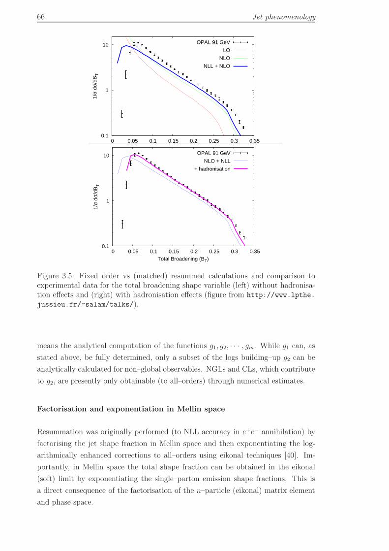
66 Jet phenomenology
0.1
1
10
0 0.05 0.1 0.15 0.2 0.25 0.3 0.35
1/σ
dσ/d
BT
Total Broadening (BT)
OPAL 91 GeV
LO
NLO
NLL + NLO
d
dB(αs ln
2 B + α2s ln
4 B + · · · )
0.1
1
10
0 0.05 0.1 0.15 0.2 0.25 0.3 0.35
1/σ
dσ/d
BT
Total Broadening (BT)
OPAL 91 GeV
NLO + NLL
+ hadronisation
d
dB(αs ln
2 B + α2s ln
4 B + · · · )
Figure 3.5: Fixed–order vs (matched) resummed calculations and comparison toexperimental data for the total broadening shape variable (left) without hadronisa-tion effects and (right) with hadronisation effects (figure from http://www.lpthe.
jussieu.fr/~salam/talks/).
means the analytical computation of the functions g1, g2, · · · , gm. While g1 can, as
stated above, be fully determined, only a subset of the logs building–up g2 can be
analytically calculated for non–global observables. NGLs and CLs, which contribute
to g2, are presently only obtainable (to all–orders) through numerical estimates.
Factorisation and exponentiation in Mellin space
Resummation was originally performed (to NLL accuracy in e+e− annihilation) by
factorising the jet shape fraction in Mellin space and then exponentiating the log-
arithmically enhanced corrections to all–orders using eikonal techniques [40]. Im-
portantly, in Mellin space the total shape fraction can be obtained in the eikonal
(soft) limit by exponentiating the single–parton emission shape fractions. This is
a direct consequence of the factorisation of the n–particle (eikonal) matrix element
and phase space.
3.2. Jet shapes 67
The jet shape fraction (3.11) may be rewritten explicitly to all–orders as
f(τa) =
∞∑
n=2
1
σ(0)
∫dσ(n)(k1, · · · , kn)Θ [τa − τa (p, k1, · · · , kn)] ΞJA(k1, · · · , kn),
(3.23)
where dσ(n) is the exclusive cross section for the production of n partons in the
final state. In the eikonal limit22, it reads for primary emissions, off a primary hard
quark–antiquark pair, (see Appendix B.1 and Refs. [61, 183])
dσ(n) = dΦm+n
⟨m+n
∣∣m+n⟩= dΦm
⟨m∣∣m⟩ 1
n!
n∏
i=1
dk2ti
k2ti
dηidφi
2π
αs(k2ti)
2πCF ωqq(ki),
(3.24)
where dΦm
⟨m∣∣m⟩is the differential Born cross section, which factors out of the
rest of the integrand and when integrated will cancel the denominator in Eq. (3.23),
and the factor 1/n! ensures that no phase space region is double counted when
the partons’ transverse momenta assume no particular ordering. Notice that the
argument of the running αs is the transverse momentum squared k2t [13, 115, 184].
The classical antenna function ωij(k) is defined in Eq. (B.7). Here we replace the
energy ω by the transverse momentum kt23;
ωij(k) =k2t (pi . pj)
(pi . k) (pj . k). (3.25)
To account for hard collinear emissions, we simply replace the antenna function ωqq
with the full q → qg splitting kernel
dηdφ
2πωqq(k) → dz Pgq(z), (3.26)
where Pgq(z) is defined in Eqs. (2.40) and (2.41) and for a gluon emitted sufficiently
collinear24 to leg ℓ (ℓ = q, q): k ≃ zpℓ + k⊥ = kt(cosh η, cosφ, sinφ, sinh η). Then, in
the qq dipole centre-of-mass system, with pℓ in the +z direction, we have z = kteη/Q.
The jet algorithm function is, for n partons contributing to the shape observable of
the ℓth jet,
ΞJA(k1, · · · , kn) =n∏
i=1
Θki∈Jℓ =n∏
i=1
Θ
(zi −
2ktiQR
), (3.27)
where the last equality follows, in the small-R limit, from the fact that, for the above
kinematic set-up, Θk∈Jℓ = Θ (η − ln tan(R/2)) ≃ Θ(η − ln(2/R)). It only remains
22Recall that the eikonal, or soft, limit corresponds to ki ≪ pq, pq, or equivalently (kipq), (kipq) ≪(pqpq). The latter is equivalent to ωi ≪ Eq ≃ Eq ≃ Q/2 where Eq, Eq and ωi are the energies inthe centre-of-mass of the dipole (qq) [183].
23Note that different definitions of the antenna function will appear in Chapters 5 and 7.Nonetheless, the corresponding calculations are, once a particular definition is chosen, consistent.
24Such that θℓk ≪ θℓℓ′ , with ℓ, ℓ′ = q, q.
68 Jet phenomenology
to write the jet shape step function in a factorised form. This is achieved through
Mellin transformation [185]
∫ ∞
0
dτ ℓa e−τℓa NℓΘ
(τ ℓa −
∑
i∈Jℓ
(kti/Q)2−a
z1−ai
)=∏
i=1
exp
[−Nℓ(kti/Q)2−a
z1−ai
], (3.28)
where Nℓ is the Mellin conjugate of τ ℓa. Therefore, taking the Mellin transform of the
shape fraction, f(Nℓ), and accounting for virtual corrections, we write the resummed
jet shape distribution in Mellin space as
ln f(Nℓ) = CF
∫dk2
t
k2t
αs(k2t )
2π
∫ 1
0
dz Pgq(z) Θ
(z − 2kt
QR
)[e−
Nℓ(kt/Q)2−a
z1−a − 1
].
(3.29)
To evaluate the above exponent to NLL accuracy we note that [40] both the coupling
and splitting kernel must be computed to two–loops order in the MS scheme, or
equivalently to one–loop order in the Catani-Marchesini-Webber (CMW) scheme25
[186], where
αCMWs = αMS
s
(1 +K
αMSs
2π
). (3.30)
The factor K is given in the MS scheme by26 [190, 191, 192]
K = CA
(67
18− π2
6
)− 5
9nf . (3.31)
We substitute for αs in (3.29) the relation (3.30) and evaluate the integral for αMSs at
two-loops. Moreover, at the said accuracy one can use the approximation [186, 193]
exp
[−Nℓ(kt/Q)2−a
z1−a
]− 1 ≃ −Θ
((kt/Q)2−a
z1−a−N
−1
ℓ
), (3.32)
where N ℓ = Nℓ e−γE and γE ≃ 0.577 · · · is the Euler gamma constant. To invert the
resultant expression back into the τ ℓa space we use the inverse Mellin transformation
[40]
f(τ ℓa) =1
2πı
∫
C
dNℓ
Nℓ
eτℓa Nℓ f(Nℓ) =
exp [R(αs, L)− γER′(αs, L)]
Γ(1 +R′(αs, L)), (3.33)
where the contour of integration C runs parallel to the imaginary axis, to the right
of all singularities of the integrand and Γ is the Euler Gamma function. The last
equality in Eq. (3.33) is valid at NLL accuracy [40] with R being analogous to
ln f(Nℓ) with Nℓ → 1/τ ℓa, R′ = ∂LR and L is as before equals to ln(1/τ ℓa). We
25It is sometimes referred to as “Monte Carlo” [186] or “physical” [13] scheme.26Note that the K factor is related to the cusp anomalous dimension Γcusp [187, 188, 189], which
has a perturbative expansion given by: Γcusp(αs) = CF (αs/π) +12CFK (αs/π)
2 + · · · .
3.2. Jet shapes 69
implement these techniques to arrive at the form reported in Chapter 4 (Eq. (4.26)).
Matching
To obtain predictions for the jet shape distribution that are accurate at both ends,
τa ≪ 1 and τa . 1, one combines resummed and fixed–order results with the aid of
a “matching” procedure. Various matching prescriptions have been proposed in the
literature (see e.g., [70, 149]). An NmLL + Nm′LO matching procedure should fulfil
the following requirements [32]:
• The matched result should be correct up to NmLL terms in the exponent
and the expanded matched result should be correct up to and including
O(αns L
2(n−m)).
• The expanded matched result should reproduce the fixed–order result up to
and including Nm′LO terms.
• The jet shape distribution should tend to one at the maximum allowed value
of the jet shape, τmaxa , while the corresponding differential distribution should
vanish:
f(τmaxa ) = 1,
df(τa)
dτa
∣∣∣τa=τmax
a
= 0. (3.34)
The matched resummed result will then be of the form stated in the introductory
chapter, Eq. (1.3). The current state–of–the–art is N3LL + N2LO, e.g., thrust and
heavy jet mass distributions [46, 49].
Owing to the considerable importance of resummed (and matched) results, spe-
cial efforts have been devoted over the last decade to alleviate some of the limitations
that are inherent in resummed calculations, for instance the need for considerable
understanding of the details of the observable being resummed, manually repeating
cumbersome calculations for each new observable etc. Notably the automation of
the resummation programme in a semi–analytical approach with state–of–the–art
resummation accuracy, clean separation between gi functions without spurious con-
tamination from uncontrolled higher–orders and more exclusiveness over the final
state. NumResum [55], DISresum [70] and caesar [31] are examples of numerical
programs developed specifically to achieve the aforementioned (automated resum-
mation) goal. Despite these remarkable achievements, the above–listed programs
can only treat global observables, which comprise a subset of the observables mea-
sured in real experiments. Including the other subset, non-global observables, into
the automation programme requires more effort. We hope that this thesis will be a
contribution to such effort.
70 Jet phenomenology
3.2.5 Non-perturbative effects
Analytical studies, based on the renormalon–inspired model [12] (and related ap-
proaches [13]), revealed that event shape distributions receive power corrections
of the order of 1/Q (more precisely 1/τQ for an event shape observable τ), e.g.,
[194, 195, 196, 197, 198, 199, 200, 201], in the small τa ≪ 1 region. The coefficient
of this correction is typically a product of two factors: the first is perturbatively cal-
culable and observable dependent, and the other is fundamentally non–perturbative
but universal across a range of processes. In effect, the correction leads to a shift in
the exponent of the resummed distribution (in other words it induces a change in the
logarithm of the observable, L → L), as indicated in Fig. 3.5 (right). Hadronisation,
as well as UE, corrections to jet observables have also been studied in [80] using a
variant of the aforementioned model.
The jet mass distribution, and more generally jet shape distributions, will have
to be corrected, in analogy with event shapes, by a non–perturbative shape function
in the endpoints M2J → 0 (τa → 0). A general relation between the perturbative
distribution f(τa) and the full distribution, ffull, including non-perturbative effects,
fNP, may be written as
ffull(τa) =
∫dxfNP(τa, x, αs(Q), Q)f (τa − x/Q) . (3.35)
In the two-jet region and for observables that are linear in the momenta of multiple
soft particles, 3.35 can be cast in a simpler form [198, 199, 200]
ffull(τa) ≃∫
dxfNP(x) f (τa − x/Q) . (3.36)
In other words the non-perturbative shape function is independent of τa and αs.
A physically interesting approximation to the latter shape function is a δ-function
[83, 198], which simply shifts the perturbative distribution
ffull(τa) = f(τa − 〈δτa,had〉), (3.37)
where 〈δτa,had〉 is the mean value of the hadronisation contribution to τa27 and f is
the resummed shape fraction (3.33). Note that the shift is strictly valid to the right
of the Sudakov peak. It should be emphasised that for more accurate estimations
of hadronisation care should be taken regarding the effect of hadron masses, which
are usually proportional to powers of lnQ (or precisely ln τQ), for event shapes,
and multiply the same perturbatively calculable factor as the 1/Q corrections [202].
In Chapter 7, when estimating hadronisation corrections to the total resummed
distribution we confine ourselves to the shift approximation.
27See for instance Ref. [70] for examples on how to calculate such means for event shapes.
3.3. Summary 71
Lastly it is worth mentioning that numerical Monte Carlo event generators
(MCEGs), which include all the necessary ingredients for a theory–data compar-
ison and whose predictions can be applied to any arbitrary observable, will continue
to play a central role in jet (and generally QCD) phenomenology. Popular present–
day general purpose MCEGs include: herwig [203, 204], pythia [146, 205, 206],
sherpa [207, 208] and ariadne [103]. A thorough review of the physics basis of
MCEGs, their main features and uses may be found in, e.g., [76]. In Chapter 7 we
compare our analytical results to the first three MCEGs (mentioned above).
3.3 Summary
In this chapter, and the previous one, we have outlined some of the concepts, tools
and methods applicable to QCD processes in general and to jet related studies in
specific. Asymptotic freedom and factorisation theorems of QCD equipped with
Feynman graphs, spin and colour combinatorics allow for the perturbation calcula-
tions of a wealth of QCD processes in e+e− annihilation, DIS and hadron–hadron
collisions. Final states in the said processes are not simple QCD partons, but rather
their footprints; jets. Jet algorithms not only provide a framework for defining jets
but constitute, with the aid of jet shape observables, an indispensable tool for de-
tailed understanding of jet substructure, which in turn allows for an optimal use
of jets in new physics searches. In the subsequent chapters we attempt to shed
some light on this very last issue from the perspective of exploring the structure of
QCD jets. We begin with a study of jet shapes in the theoretically favoured e+e−
annihilation processes and then use the experience gained there to address the theo-
retically more challenging, and presently more interesting, hadron-hadron scattering
processes.

72
Chapter 4
Resummation of angularities in
e+e− annihilation
4.1 Introduction
It has long been known that probing the shape and structure of high-pT jets is po-
tentially of great value in searches for new particles at collider experiments [209].
With the advent of the LHC and much activity in improving and developing jet
algorithms [73, 142, 147, 148, 149, 210], studies of this nature have received consid-
erable impetus. In particular, much recent attention has been focused on using jet
studies for the identification of boosted massive particles which decay to hadrons
forming a collimated jet, see for instance Refs. [14, 21, 28, 29, 154, 156, 160, 164,
167, 168, 211, 212, 213, 214, 215, 216, 217, 218, 219].
In the same context a method has been suggested to study the shapes of one
or more jets produced in multi-jet events at fixed jet multiplicity [44, 45]. The
precise details of the observable suggested in those references involve defining a jet
shape/energy flow correlation similar to that introduced in Ref. [175]. Specifically
the proposal was to measure the shapes of one or more jets in an event leaving
other jets unmeasured and introducing a cut on hadronic activity outside high–pT
(hard) jets, to hold the hard-jet multiplicity fixed. This is in contrast to for instance
hadronic event shapes [32, 55, 65, 66] which by construction are sensitive to the
shape of the overall event rather than an isolated jet.
In the present chapter we wish to use this observable as a case study to make
several points that we believe will be useful both within and outside the specific
context. The main points that we wish to address concern the resummation of soft
gluon effects that become important in describing the observable distribution for
small values of the shape variable τa and the energy cut E0.
In particular in this chapter we shall study the structure of non-global logarithms
(NGLs) [2, 176] as well as compute them for jets defined using various jet algorithms.
We remind the reader that observables that are sensitive to radiation in a limited
phase-space region such as the interior of a particular jet are non-global in the sense
that they receive logarithmic contributions from correlated soft emission, which
are highly non-trivial to treat to all-orders. Existing resummations of NGLs have
73
74 Resummation of angularities in e+e− annihilation
been confined to a few special cases [2, 70, 71, 153, 176] and to the large–Nc limit.
Given that the observable we study in the current chapter is non-global, it is worth
examining in detail the precise structure of NGLs, which by definition start at O(α2s)
in the perturbative expansion and are of the same size as the logarithms resummed
in Refs. [44, 45]. Thus they need to be taken into account in order to achieve
next–to–leading log accuracy.
We find non-global logarithms arise both in the ratio of the shape variable τa and
the energy cut-off E0 as well as in E0/Q where Q is the hard scale of the process,
which is naturally of the order of the hard jet pT1. We argue that in the limit of
narrow well-separated jets a simple picture emerges for NGLs. The simplicity in the
non-global structure is to do with the fact of QCD coherence [220]. Narrow well-
separated jets do not affect each other’s evolution even in the non-global component
which arises individually as an edge effect from the boundary of each jet, precisely as
the NGLs in the case of a hemisphere mass in e+e− annihilation arise from the edge
separating the observed and unobserved hemispheres [2]. Hence the resummation
of non-global logarithms arising at each jet boundary can simply be taken from the
existing result for a hemisphere2 up to corrections that vanish as powers of the jet
radius. This simple structure of non-global effects in turn provides us with an ansatz
that can be used for any jet event of arbitrary jet multiplicity.
We also assess here the numerical contribution of the non-global logarithms and
find that while limiting the value of E0 is of some use in diminishing their size the
effect is still of order twenty percent as far as the peak height of shape distributions
is concerned. In fact we find that changing the value of E0 is not particularly
useful as a means of reducing the non-global contribution. Specifically following the
original proposal in Ref. [38] it was suggested in Ref. [45] that one may take the
value of E0/Q to be of the same order as the jet shape variable τa, which we agree
eliminates the non-global contribution from the measured jet. However in this case
the contribution from the unmeasured jet becomes as significant as the contribution
we are attempting to eliminate and hence the overall effect of this choice turns out
to actually increase the overall non-global component. With the resummed results
of the current chapter however one does not have to be too concerned about the
precise choice of E0 as the non-global terms should be accounted for, at least within
the large-Nc approximation and up to corrections vanishing as powers of the jet
radius3.
Another point we wish to make is concerning the role of the different jet algo-
rithms. The computation of NGLs can actually be carried out in any jet algorithm,
1The potential presence of such logarithms was also mentioned in [44, 45].2This statement should be qualified as it is correct only for the case of the anti-kT jet algorithm
[73], which is the one we recommend for study of such observables.3These effects would amount to perhaps a ten percent change in the non-global term which we
do not expect to be of significant phenomenological consequence.
4.1. Introduction 75
analytically for the first non–trivial term in the perturbative expansion and by means
of the numerical Monte Carlo code developed in [2, 75, 153] in the leading–Nc limit.
Indeed it was found [75], in gaps–between–jets studies, that the use of certain se-
quential recombination algorithms (such as the kT or Cambridge–Aachen C/A) can
significantly reduce the non-global logarithms due to the soft gluon clustering in-
herent in such algorithms. It was however later demonstrated [3, 74] that one pays
a price for this reduction in the non-global component in the form of a more com-
plicated result for the independent emission terms. While independent emission is
commonly associated with the exponentiation of the single-gluon result, this associ-
ation is spoiled by the application of jet algorithms other than the anti-kT algorithm.
As we shall show in this chapter the results of soft gluon clustering in the kT and
C/A algorithms modify the independent emission (global term) which deviates from
the naive exponentiation of a single gluon at a relevant single logarithmic (SL) ac-
curacy. Moreover the effect of the clustering near the boundary of a collinear jet no
longer produces logarithms suppressed in the jet radius R as was the case for small
central rapidity gaps discussed in Refs. [3, 74] but rather pure single-logarithms.
We refer to these logarithms as clustering logs (CLs). These effects are absent for
the anti-kT algorithm as already pointed out in Ref. [73], since that algorithm clus-
ters soft gluons independently to the hard parton and hence produces circular jets
in the soft limit, i.e., it can be regarded in this limit as a rigid cone. Hence for
the present moment and postponing a resummation of the clustering logarithms to
Chapter 64 we confine our studies to the anti-kT algorithm. We do however pro-
vide an explicit fixed-order computation of the single-logarithmic corrections in the
independent emission piece, that arise in other algorithms as we believe this point
deserves some stress.
The chapter is organised as follows. In Sec. 4.2 we define our observable, choosing
the angularities shape variable in dijet events as an example of a jet-shape observ-
able, while imposing a cut E0 in the inter-jet energy flow. In Sec. 4.3 we perform
the leading and next-to leading order calculation of such observable in the soft limit,
which elucidates the structure of the logarithms arising from independent soft gluon
emissions as well as non-global logarithms from correlated emissions. We use these
results to construct an argument which culminates with the resummation of these
logarithms in Sec. 4.4. We also present a study which assesses the numerical sig-
nificance of the non-global logarithms as a function of the parameters τa and E0.
In Sec. 4.5 we highlight the fact that for algorithms other than the anti-kT expo-
nentiation of the single gluon result is not sufficient to capture the next-to–leading
logarithms even in the independent emission piece, let alone the non-global terms.
Finally we draw our conclusions in Sec. 4.6.
4We actually carry out the resummation for the jet mass. Results for the angularities τa shouldbe analogous.
76 Resummation of angularities in e+e− annihilation
4.2 High-pT jet-shapes/energy-flow correlation
We wish to examine a situation where one studies the shapes of one or more high-pT
jets in jet events with definite multiplicity. From the results we shall obtain below
for such events one can draw conclusions also about the jet shape distribution for
instance for the process pp → j + X , where one can demand the production of a
jet j setting a value for a particular jet-shape, while summing over everything else
denoted by X .
For the points we address in this chapter we can for illustrative purposes and
without loss of generality consider high–pT dijet events. In order to restrict the jet
multiplicity we can place a cut E0 whereby we veto the interjet activity such that the
sum of transverse energies of emissions outside the two high–pT jets is less than this
value. This was also the definition adopted in Refs. [44, 45] where the parameter Λ
indicated a cut on additional jet activity along the above lines.
Moreover, in this chapter we are interested in physics at the boundary of the
triggered hard jets and specifically in the non–global logarithms that arise at these
boundaries. Hence we can for our discussion ignore the effects of initial state ra-
diation which can simply be accommodated once the structure of the results is
understood. Since it is this structure that we focus on, it proves advantageous to
consider as an analogy the production of dijets in e+e− annihilation. Hence all our
points can be made in full generality by considering two hard jets in e+e− processes
where one measures the shape of one of the jets leaving the other jet unmeasured
as prescribed in Refs. [44, 45]. Our results should also then be directly comparable
to those obtained by other authors using soft-collinear effective theory [44, 45].
4.2.1 Observable definition
We shall pick the angularities, τa, introduced in [38, 39] and analysed in [44, 45]
with a mis–treatment of NGLs, as a specific simple example of a jet-shape variable.
We defined τa in the previous chapter (precisely Eq. (3.3)) in terms of the hadronic
variables: transverse momentum (kt), pseudorapidity (η) and azimuth (φ). An
equivalent definition in terms of e+e− variables5 is given by [39]
τa = τa(p, k1, · · · , kn) =n∑
i∈J
ωi
Qsina θi (1− cos θi)
1−a ; −∞ < a < 1, (4.1)
where θi is the polar angle of gluon i with respect to the jet axis, ωi is its energy
and EJ ∼ Q/2 is the jet energy with Q being the hard scale.
We study the integrated and normalised shape distribution (equivalently the
5See Eq. (B.10) for the relations between the two sets of variables.
4.2. High-pT jet-shapes/energy-flow correlation 77
shape cross–section or shape fraction) given by the general expression
Σ(τa, E0) =
∫ τa
0
dτ 1a
∫ E0
0
dE31
σ(0)
d4σ
dτ 1a dE3 dp1 dp2, (4.2)
where σ(0) is the Born cross-section and τ 1a denotes the angularity of the jet with
momentum p1. The above equation indicates that we are restricting the shape of
the jet with three momentum p1 to be less than τa leaving the shape of the other jet
with momentum p2 unmeasured. Likewise, the interjet energy flow E3 is restricted
to be less than E0 hence our observable definition above is in precise accordance
with the definition in Refs. [44, 45]. We shall in future leave the dependence on jet
momenta p1,p2 unspecified and to be understood.
We carry out a calculation for the above observable which includes a resummation
of large logarithms in R2−a/τa to next-to–leading logarithmic (equivalently single
logarithmic (SL)) accuracy in the exponent. We include a description of non-global
single logarithms in the leading-Nc limit. Additionally we resum the logarithmic
dependence on Q/E0 to single logarithmic accuracy again accounting for the non-
global contributions. Our main aim is to study the effect of the non-global logarithms
neglected for instance in previous calculations of jet shapes [44, 45, 167] on the shape
fraction Eq. (4.2). While resumming logarithms in τa and E0 we shall neglect those
logarithms that are suppressed by powers of the jet radius R which shall enable us
to treat non-global logarithms straightforwardly6. Hence our calculation addresses
the range of study where E0/Q ≫ τa and is valid in the limit of relatively small
jet radius R. We shall not however resum terms varying purely as αs lnR which
for the values of R we consider can safely be ignored from a phenomenological
viewpoint. We thus aim to resum large logarithms in τa and E0/Q in what one may
call the approximation of narrow well separated jets. According to our estimates this
approximation and our consequent resummation should enable relatively accurate
phenomenological studies of jet shapes.
The perturbative expansion of the shape fraction Σ (4.2) in terms of coupling αs
may be cast in the form
Σ = Σ(0) + Σ(1) + Σ(2) + · · · , (4.3)
where Σ(0) refers to the Born contribution and is equal to 1. In the next section we
shall carrying out a calculation of the logarithmic structure that emerges at the one
and two gluon levels, in the limit of soft gluon emission. These calculations will help
us to identify the full logarithmic structure and point the way towards a resummed
6More specifically we shall neglect corrections varying as R2/∆ij where ∆ij = 1 − cos θij isa measure of the angular separation between the hard jets. This parameter emerges naturallyin fixed–order computation of NGLs for energy flow outside jets [72] and it was also treated asnegligible in [44, 45].
78 Resummation of angularities in e+e− annihilation
treatment. We start below with a leading order calculation in the soft limit.
4.3 Soft limit calculations
We start by considering the effect of a single soft emission k by a hard qq pair,
produced in e+e− annihilation. At this level all infrared and collinear (IRC) safe jet
algorithms will yield the same result. We can write the parton momenta as
p1 =Q
2(1, 0, 0, 1),
p2 =Q
2(1, 0, 0,−1),
k = ω (1, sin θ cosφ, sin θ sinφ, cos θ) , (4.4)
where p1 and p2 are the hard partons and we have neglected recoil against the soft
gluon emission k, which is irrelevant at the logarithmic accuracy we seek. Let p1
corresponds to the measured jet. Then if the gluon is combined with the parton
p1 one restricts the angularity of the resulting jet to be below τa while if combined
with p2 the angularity is unrestricted. Likewise one can consider the parton p2 to
be in the measured jet direction, which will give an identical result. We thus have
Σ(1)(τa, E0) =1
σ(0)
∫ τmaxa
0
dτ 1adσ(1)
dτ 1aΘ(τa − τ 1a
)Θk∈J1+
+
∫ Q/2
0
dE3dσ(1)
dE3Θ (E0 −E3)Θk/∈J1,J2 (4.5)
Note that there is no constraint on the gluon energy when it is combined with the
jet J2. Moreover, one notices that (4.5) is actually a sum of two distributions. In
the limit E0 → Q/2, (4.5) corresponds purely to the angularity distribution. While
in the limit τa → τmaxa it reduces to the interjet energy flow (or gaps-between-jets)
distribution.
In all the commonly used IRC safe jet algorithms the soft gluon k will form a
jet with a hard parton if it is within a specified distance R of the hard parton. The
distance is measured for hadron collider processes in the (η, φ) plane as ∆η2 +∆φ2
where ∆η is the separation in rapidity and ∆φ is the separation in φ between the
hard parton and the gluon k. In the limit of small angles, relevant for small-R values
R ≪ 1, which we shall consider here, the distance measure reduces to θ2pk where θpk
is the angle between the gluon k and hard parton p. Thus k and p1 form a jet if
θ2p1k < R2. Otherwise the gluon is outside the jet formed by p1 which at this order
remains massless. If the gluon does not also combine with hard parton p2 to form
a jet, one restricts its energy to be less than E0 as required by the definition of the
observable. Differences between the various algorithms shall emerge in the following
section where we examine the emission of two soft gluons.
4.3. Soft limit calculations 79
Thus we can write for the contribution of the real soft gluon k with θ2p1k ≡ θ1 < R2
to the shape fraction
Σ(1)r =
CFαs
π
∫dω
ω
dθ21θ21
Θ(τa − τ 1a
). (4.6)
where the superscript r denotes the real emission piece. In this same soft region vir-
tual corrections are exactly minus the real contributions, but unconstrained; there-
fore we can cancel the real emission result above entirely against the virtual piece
and we are left with
Σ(1)in = −CFαs
π
∫ Q/2
0
dω
ω
∫ R2
0
dθ21θ21
Θ
(ω θ2−a
1
21−aQ− τa
), (4.7)
where we used the small-angle approximation to simplify the expression Eq. (4.1)
for a single gluon since θ2 < R2 ≪ 1. The suffix “in” denotes the contribution to
Σ(1) from the region where the gluon is in the measured jet. Performing the integral
over angles with the specified constraint results in
Σ(1)in = −CFαs
π
∫ Q/2
2τaQ
R2−a
dω
ωln
[R2
(ω
21−aτaQ
) 22−a
]
= −CFαs
π
1
2− aln2
((R/2)2−a
τa
)Θ
((R/2)2−a
τa− 1
). (4.8)
Notice that using η, kt variables one would find that the argument of the logarithm
is tan2−a(R/2), to which (R/2)2−a is the small-R approximation.
Next we consider the region where the soft emission flies outside either hard jets,
with the corresponding contribution Σ(1)out. Since here we are no longer confined
to the small angle approximation we use kt and η with respect to the jet axis
as integration variables where η is the gluon rapidity. In these variables one can
represent the contribution of the gluon k after real-virtual cancellation as
Σ(1)out = −2CFαs
π
∫ Q/2 dktkt
∫ ln 2/R
− ln 2/R
dηΘ (kt cosh η −E0) . (4.9)
where the limits on the rapidity integral reflect the out of jet region. Performing
the integrals one obtains, to the required single-logarithmic accuracy,
Σ(1)out = −2CFαs
πln
Q
E0
(2 ln
2
R
). (4.10)
The full soft result at leading order is Σ(1) = Σ(1)in + Σ
(1)out. We see that the
angularity distribution receives double logarithmic corrections which in the present
case are in the ratio R2−a/τa. Taking account of hard collinear emissions one would
80 Resummation of angularities in e+e− annihilation
obtain also single logarithms in R2−a/τa, which we shall account for in our final
results.
We shall now move to considering two-gluon emission and the structure of the
non-global logarithms that arise at this level.
4.3.1 Two-gluon calculation and non-global logarithms
Going beyond a single soft emission to the two gluon emission case the precise details
of the jet algorithm start to become important. In what follows below we shall
consider only the anti-kT algorithm since in the soft limit the algorithm functions
essentially as a perfect cone algorithm [73]. In particular this implies that soft
gluons are recombined with the hard partons independently of one another (one
can neglect soft gluon clustering effects) which considerably eases the path to a
resummed prediction. The logarithmic structure for other jet algorithms is also
interesting and we shall discuss it in a later section.
Here we carry out an explicit two-gluon calculation to obtain the structure
of NGLs for the observable at hand. Referring to the non-global contribution to
Σ(τa, E0) as S, we compute below S2 the first non-trivial term of S (see the previous
chapter, Eq. (3.16)). Our results shall indicate a way forward towards a resummed
result incorporating these effects. As in Refs. [2, 176] we shall consider the emission
of gluons k1 and k2 such that ω1 ≫ ω2, i.e., strong energy ordering7. In this limit
the squared matrix element can be split into an independent emission term ∝ C2F
and a correlated emission term ∝ CFCA. The former is incorporated in the standard
resummed results based on exponentiation of a single gluon, which we discuss later.
Let us concentrate on the CFCA term missed by the single gluon exponentiation,
and which generates the NGLs we wish to study and resum. Consider the following
kinematics:
p1 =Q
2(1, 0, 0, 1) ,
p2 =Q
2(1, 0, 0,−1) ,
k1 = ω1 (1, sin θ1, 0, cos θ1) ,
k2 = ω2 (1, sin θ2 cosφ, sin θ2 sinφ, cos θ2) , (4.11)
with ω1 ≫ ω2 as stated above.
Consider the situation where the harder gluon k1 is not recombined with either
jet but the softest emission k2 is recombined with J1 (initiated by hard parton
p1). This situation corresponds to the diagram (A) of Fig. 4.1. In the small-angle
limit, which applies for the case R ≪ 1, the condition for k2 to be recombined
7Working in this regime simplifies the calculations and is sufficient to extract the full leadingNGLs.
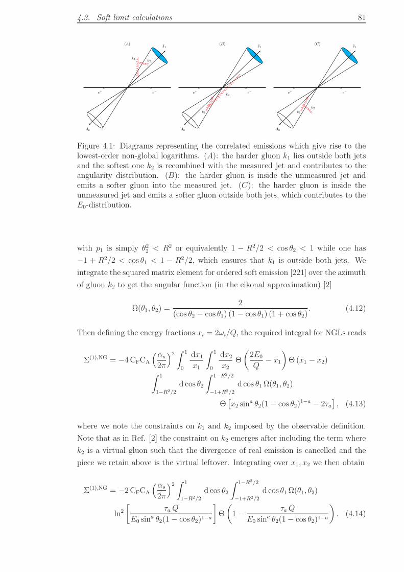
4.3. Soft limit calculations 81
e+ e−
J1
J2
(A)
k1 k2
e+ e−
J1
J2
(B)
k1
k2e+ e−
J1
J2
(C)
k1
k2
Figure 4.1: Diagrams representing the correlated emissions which give rise to thelowest-order non-global logarithms. (A): the harder gluon k1 lies outside both jetsand the softest one k2 is recombined with the measured jet and contributes to theangularity distribution. (B): the harder gluon is inside the unmeasured jet andemits a softer gluon into the measured jet. (C): the harder gluon is inside theunmeasured jet and emits a softer gluon outside both jets, which contributes to theE0-distribution.
with p1 is simply θ22 < R2 or equivalently 1 − R2/2 < cos θ2 < 1 while one has
−1 + R2/2 < cos θ1 < 1 − R2/2, which ensures that k1 is outside both jets. We
integrate the squared matrix element for ordered soft emission [221] over the azimuth
of gluon k2 to get the angular function (in the eikonal approximation) [2]
Ω(θ1, θ2) =2
(cos θ2 − cos θ1) (1− cos θ1) (1 + cos θ2). (4.12)
Then defining the energy fractions xi = 2ωi/Q, the required integral for NGLs reads
Σ(1),NG = −4CFCA
(αs
2π
)2 ∫ 1
0
dx1
x1
∫ 1
0
dx2
x2Θ
(2E0
Q− x1
)Θ (x1 − x2)
∫ 1
1−R2/2
d cos θ2
∫ 1−R2/2
−1+R2/2
d cos θ1Ω(θ1, θ2)
Θ[x2 sin
a θ2(1− cos θ2)1−a − 2τa
], (4.13)
where we note the constraints on k1 and k2 imposed by the observable definition.
Note that as in Ref. [2] the constraint on k2 emerges after including the term where
k2 is a virtual gluon such that the divergence of real emission is cancelled and the
piece we retain above is the virtual leftover. Integrating over x1, x2 we then obtain
Σ(1),NG = −2CFCA
(αs
2π
)2 ∫ 1
1−R2/2
d cos θ2
∫ 1−R2/2
−1+R2/2
d cos θ1Ω(θ1, θ2)
ln2
[τa Q
E0 sina θ2(1− cos θ2)1−a
]Θ
(1− τa Q
E0 sina θ2(1− cos θ2)1−a
). (4.14)
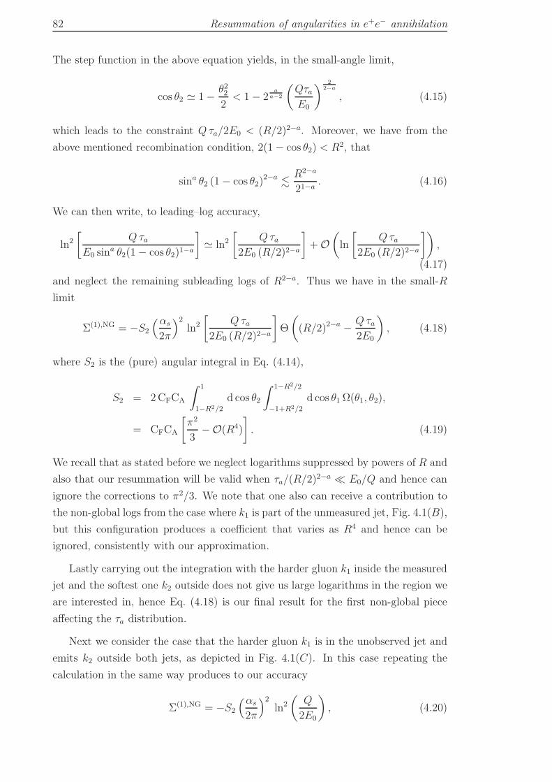
82 Resummation of angularities in e+e− annihilation
The step function in the above equation yields, in the small-angle limit,
cos θ2 ≃ 1− θ222
< 1− 2a
a−2
(QτaE0
) 22−a
, (4.15)
which leads to the constraint Qτa/2E0 < (R/2)2−a. Moreover, we have from the
above mentioned recombination condition, 2(1− cos θ2) < R2, that
sina θ2 (1− cos θ2)2−a
.R2−a
21−a. (4.16)
We can then write, to leading–log accuracy,
ln2
[Qτa
E0 sina θ2(1− cos θ2)1−a
]≃ ln2
[Qτa
2E0 (R/2)2−a
]+O
(ln
[Qτa
2E0 (R/2)2−a
]),
(4.17)
and neglect the remaining subleading logs of R2−a. Thus we have in the small-R
limit
Σ(1),NG = −S2
(αs
2π
)2ln2
[Qτa
2E0 (R/2)2−a
]Θ
((R/2)2−a − Qτa
2E0
), (4.18)
where S2 is the (pure) angular integral in Eq. (4.14),
S2 = 2CFCA
∫ 1
1−R2/2
d cos θ2
∫ 1−R2/2
−1+R2/2
d cos θ1 Ω(θ1, θ2),
= CFCA
[π2
3−O(R4)
]. (4.19)
We recall that as stated before we neglect logarithms suppressed by powers of R and
also that our resummation will be valid when τa/(R/2)2−a ≪ E0/Q and hence can
ignore the corrections to π2/3. We note that one also can receive a contribution to
the non-global logs from the case where k1 is part of the unmeasured jet, Fig. 4.1(B),
but this configuration produces a coefficient that varies as R4 and hence can be
ignored, consistently with our approximation.
Lastly carrying out the integration with the harder gluon k1 inside the measured
jet and the softest one k2 outside does not give us large logarithms in the region we
are interested in, hence Eq. (4.18) is our final result for the first non-global piece
affecting the τa distribution.
Next we consider the case that the harder gluon k1 is in the unobserved jet and
emits k2 outside both jets, as depicted in Fig. 4.1(C). In this case repeating the
calculation in the same way produces to our accuracy
Σ(1),NG = −S2
(αs
2π
)2ln2
(Q
2E0
), (4.20)
4.3. Soft limit calculations 83
where S2 is given above (Eq. (4.19)).
The above results are noteworthy in many respects. Note that the result (4.18)
corresponds, in the small-R limit, to the result already obtained for the hemisphere
jet-mass in Ref. [2] provided one replaces 1/τa in that result by 2E0
Qτa(R/2)2−a. This
is because the non-global evolution takes place from energies of order Qτa/(R/2)2−a
up to those of order E0, whereas for the hemisphere mass the relevant energy for the
harder gluon was of order Q. More interestingly the coefficient of S2 for small-R,
π2/3, is the same as was obtained there. The origin of this is the fact that the
collinear singularity between k1 and k2 dominates the angular integral. As has been
noted before [176] as one separates the gluons in rapidity the contribution to the
non-global term, which represents correlated gluon emission, falls exponentially as
gluons widely separated in rapidity are emitted essentially independently. Thus in
the small-R limit, and up to corrections suppressed by R4 the results for the τa
distribution arise from the edge of the measured jet independently of the evolution
of the unobserved jet. Likewise there are NGLs given by Eq. (4.20) which affect
purely the inter-jet energy flow E0 distribution. These arise, in the small-R limit,
purely from the edge of the unmeasured jets and are independent of the evolution of
the measured jet which is well separated in rapidity (similar results were obtained
in the work of Refs. [72, 153]).
Thus a simple picture arises for NGLs where each jet evolves independently and
the effects arise from the edges of the jet. For the measured jet, the non-global
logarithms involve the ratio of the shape variable (R/2)2−a/τa to the energy flow
variable E0/Q, while for the unmeasured jets, they involve the ratio Q/E0. The
coefficients of NGLs will be identical within our accuracy (small-R limit) to those
computed for the hemisphere mass (where the effect is again an edge effect coming
from the hemisphere boundary) and hence the resummation of the non-global effects
from each jet can simply be taken from the resummation carried out in Ref. [2]
simply modifying the evolution variable. This will be done in the next section.
To conclude we wish to draw attention to the fact that we have determined, with
a fixed order calculation, the precise non-global structure which was not included in
Refs. [44, 45] and knowledge of the nature of these logarithms should pave the way
for more accurate phenomenological studies. We remind the reader that our study
above is valid only for the case of the anti-kT algorithm. Other jet algorithms will
give different non-global pieces as discussed in Refs. [3, 74, 75]. In fact even the
resummation of independent emission terms will be different in other algorithms, a
fact that is not widely appreciated and that we shall stress in a later section.
In the following section we turn to resummed results and provide a simple ansatz
which will be valid for arbitrarily complex processes involving jet production.
84 Resummation of angularities in e+e− annihilation
4.4 Resummation
Having observed the key feature of the non-global logarithms (independent contri-
butions from each jet) that allow us to write a resummed result we shall now focus
on the resummation in more detail. The main point to note is that NGLs provide
a factor that corrects straightforward single-gluon exponentiation (as discussed in
Subsec. 3.2.2):
Σ
(R2−a
τa,Q
E0
)= Σind
(R2−a
τa,Q
E0
)Sng
(E0R
2−a
Qτa,Q
E0
). (4.21)
Thus we shall first provide the result for the single-gluon exponentiation taking
account of hard-collinear emission and the running coupling, which contains leading
and next-to–leading logarithms in R2−a/τa as well as leading logarithms in Q/E0.
4.4.1 Independent emission contribution
The resummation of independent emission contributions based on a squared matrix
element that has a factorized structure for multi-gluon emission is by now a standard
procedure and we shall avoid listing these details (see for instance [31] for a detailed
study of these techniques). We shall provide here only details of the final result
for independent emission valid for the anti-kT algorithm only. We stress once again
that even the independent emission piece will differ at next-to–leading logarithmic
accuracy from that reported below if using another jet algorithm.
The result for the independent emission contribution can be written in the usual
form (described in Subsec. 3.2.4, Eq. (3.33))
Σind
(R2−a
τa,Q
E0
)=
exp[−Rτa − γER′
τa
]
Γ(1 +R′
τa
) exp [−RE0 ] . (4.22)
Here Rτa and RE0 are functions of R2−a/τa and Q/E0 respectively, representing the
exponentiation of the one gluon result. They describe the resummation of large
(global) logarithms to next-to–leading logarithmic accuracy in R2−a/τa and leading
logarithmic accuracy in Q/E0. Note that the factorised form (4.22) can be proven
straightforwardly by following the steps outlined in Subsec. 3.2.4 for the specific
distribution
Σ(τa, E0) =∑
n,m
∫dτa dE0
1
σ(0)
d2σ
dτa dE0Θ
(τa −
n∑
i∈J1
ωi
Qsina θi (1− cos θi)
1−a
)
Θ
E0 −
m∑
i/∈J1,J2
ωi
. (4.23)
With inclusion of running coupling effects and the effects of hard collinear emis-
4.4. Resummation 85
sion the function Rτa can be written as (see Eqs. (3.29) and (3.32))
Rτa =CF
π
∫dk2
t
k2t
αs(k2t )F(k2
t ), (4.24)
where we defined
F(k2t ) =
∫ 1
0
dz Pgq(z) Θ
(z − 2kt
QR
)Θ
[(kt/Q)2−a
z1−a− τa
]. (4.25)
Carrying out the integration for the soft and hard phase space regions one obtains
F(k2t ) = ln
(QRe−
32
2kt
)Θ
(QR
2− kt
)Θ
[(ktQ
)2−a
− τa
]
+1
1− aln
(kt(R/2)1−a
Qτa
)Θ
[τa −
(ktQ
)2−a]Θ
(k2t
Q2− τ 2a
(R/2)2(1−a)
), (4.26)
where the factor e−3/2 in the argument of the logarithm in the first term above takes
account of the hard collinear region 2ω/Q → 1, for a primary hard quark8. For a
primary hard gluon one makes the changes: CF → CA and e−3/2 → e−2πβ0/CA , where
β0 is given below.
Carrying out the integral over kt one obtains the familiar [40] results
Rτa = −Lf1(λ)− f2(λ), (4.27a)
R′τa = − ∂
∂L(Lf1(λ)) . (4.27b)
The functions f1 and f2 are listed below:
f1(λ) = − CF
2πβ0(1− a)λ
[(1− 2λ) ln(1− 2λ)− (2− a− 2λ) ln
(2− a− 2λ
2− a
)],
(4.28a)
and
f2(λ) = − CFK
4π2β20(1− a)
[(2− a) ln
(2− a− 2λ
2− a
)− ln(1− 2λ)
]
−fcoll ln
(2− a− 2λ
2− a
)− CFβ1
2πβ30(1− a)
[ln (1− 2λ) +
1
2ln2(1− 2λ)
−2− a
2ln2
(2− a− 2λ
2− a
)− (2− a) ln
(2− a− 2λ
2− a
)], (4.28b)
8In order to obtain this one replaces as usual dx/x → dx[1 + (1− x)2
]/2x where x = 2ω/Q
in the integral over gluon energy, which is essentially introducing the full splitting function insteadof its soft singular term.
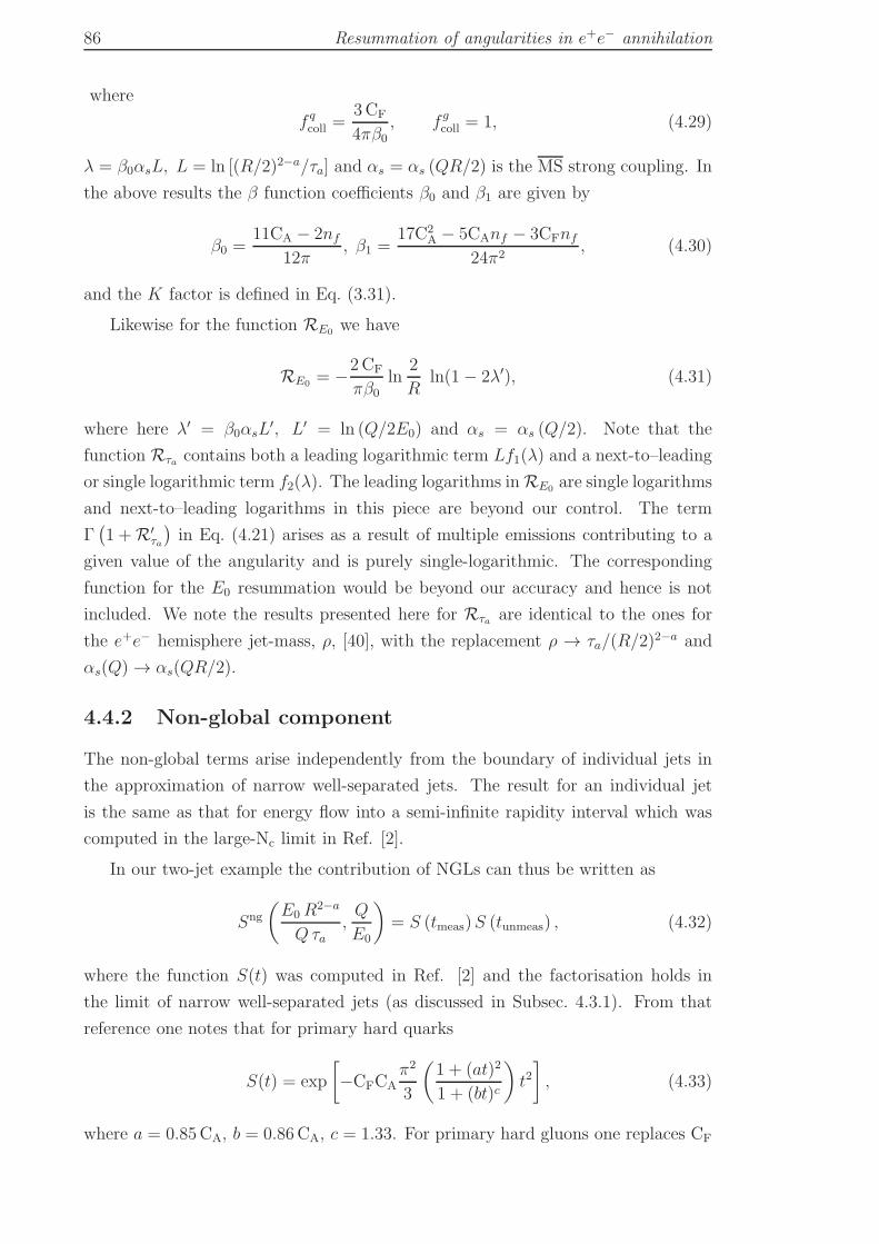
86 Resummation of angularities in e+e− annihilation
where
f qcoll =
3CF
4πβ0
, f gcoll = 1, (4.29)
λ = β0αsL, L = ln [(R/2)2−a/τa] and αs = αs (QR/2) is the MS strong coupling. In
the above results the β function coefficients β0 and β1 are given by
β0 =11CA − 2nf
12π, β1 =
17C2A − 5CAnf − 3CFnf
24π2, (4.30)
and the K factor is defined in Eq. (3.31).
Likewise for the function RE0 we have
RE0 = −2CF
πβ0ln
2
Rln(1− 2λ′), (4.31)
where here λ′ = β0αsL′, L′ = ln (Q/2E0) and αs = αs (Q/2). Note that the
function Rτa contains both a leading logarithmic term Lf1(λ) and a next-to–leading
or single logarithmic term f2(λ). The leading logarithms inRE0 are single logarithms
and next-to–leading logarithms in this piece are beyond our control. The term
Γ(1 +R′
τa
)in Eq. (4.21) arises as a result of multiple emissions contributing to a
given value of the angularity and is purely single-logarithmic. The corresponding
function for the E0 resummation would be beyond our accuracy and hence is not
included. We note the results presented here for Rτa are identical to the ones for
the e+e− hemisphere jet-mass, ρ, [40], with the replacement ρ → τa/(R/2)2−a and
αs(Q) → αs(QR/2).
4.4.2 Non-global component
The non-global terms arise independently from the boundary of individual jets in
the approximation of narrow well-separated jets. The result for an individual jet
is the same as that for energy flow into a semi-infinite rapidity interval which was
computed in the large-Nc limit in Ref. [2].
In our two-jet example the contribution of NGLs can thus be written as
Sng
(E0R
2−a
Qτa,Q
E0
)= S (tmeas)S (tunmeas) , (4.32)
where the function S(t) was computed in Ref. [2] and the factorisation holds in
the limit of narrow well-separated jets (as discussed in Subsec. 4.3.1). From that
reference one notes that for primary hard quarks
S(t) = exp
[−CFCA
π2
3
(1 + (at)2
1 + (bt)c
)t2], (4.33)
where a = 0.85CA, b = 0.86CA, c = 1.33. For primary hard gluons one replaces CF
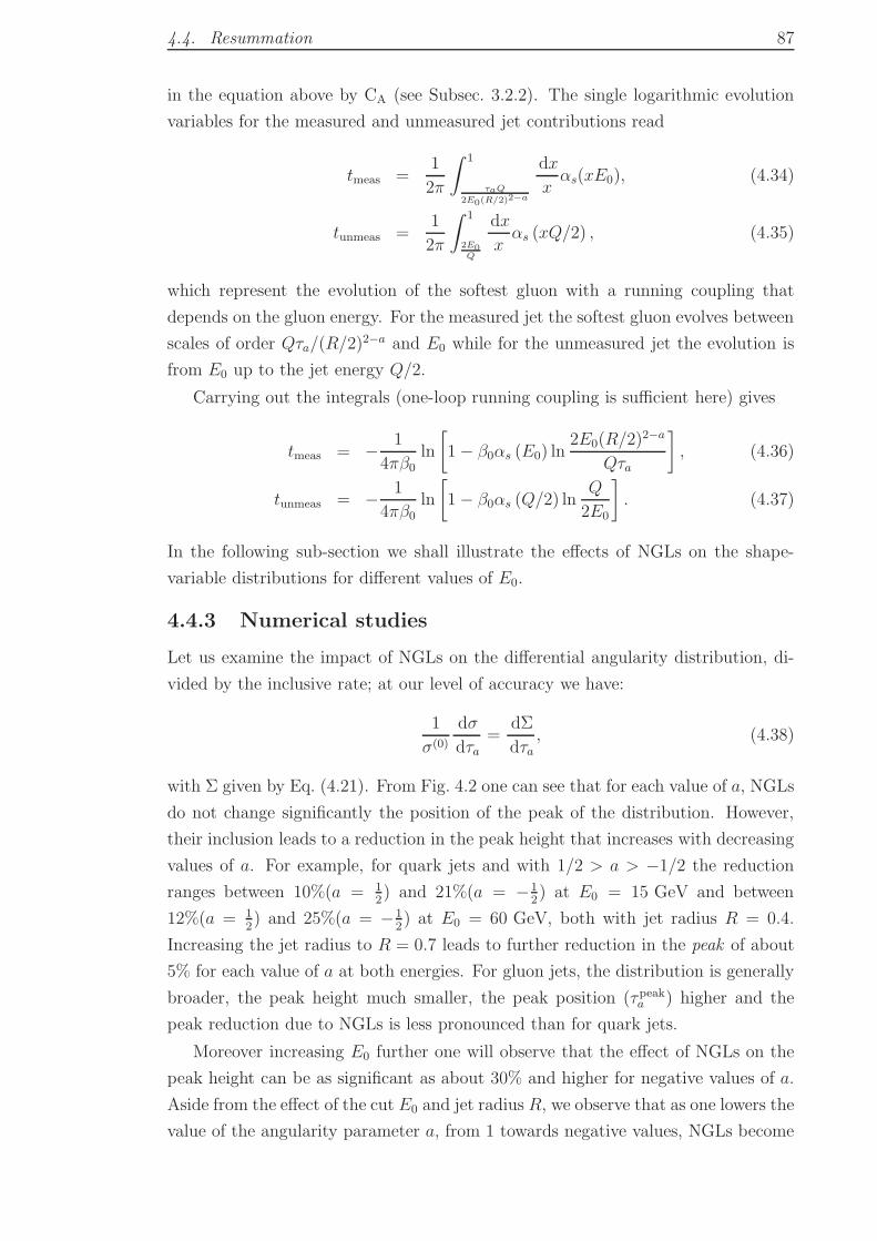
4.4. Resummation 87
in the equation above by CA (see Subsec. 3.2.2). The single logarithmic evolution
variables for the measured and unmeasured jet contributions read
tmeas =1
2π
∫ 1
τaQ
2E0(R/2)2−a
dx
xαs(xE0), (4.34)
tunmeas =1
2π
∫ 1
2E0Q
dx
xαs (xQ/2) , (4.35)
which represent the evolution of the softest gluon with a running coupling that
depends on the gluon energy. For the measured jet the softest gluon evolves between
scales of order Qτa/(R/2)2−a and E0 while for the unmeasured jet the evolution is
from E0 up to the jet energy Q/2.
Carrying out the integrals (one-loop running coupling is sufficient here) gives
tmeas = − 1
4πβ0ln
[1− β0αs (E0) ln
2E0(R/2)2−a
Qτa
], (4.36)
tunmeas = − 1
4πβ0ln
[1− β0αs (Q/2) ln
Q
2E0
]. (4.37)
In the following sub-section we shall illustrate the effects of NGLs on the shape-
variable distributions for different values of E0.
4.4.3 Numerical studies
Let us examine the impact of NGLs on the differential angularity distribution, di-
vided by the inclusive rate; at our level of accuracy we have:
1
σ(0)
dσ
dτa=
dΣ
dτa, (4.38)
with Σ given by Eq. (4.21). From Fig. 4.2 one can see that for each value of a, NGLs
do not change significantly the position of the peak of the distribution. However,
their inclusion leads to a reduction in the peak height that increases with decreasing
values of a. For example, for quark jets and with 1/2 > a > −1/2 the reduction
ranges between 10%(a = 12) and 21%(a = −1
2) at E0 = 15 GeV and between
12%(a = 12) and 25%(a = −1
2) at E0 = 60 GeV, both with jet radius R = 0.4.
Increasing the jet radius to R = 0.7 leads to further reduction in the peak of about
5% for each value of a at both energies. For gluon jets, the distribution is generally
broader, the peak height much smaller, the peak position (τpeaka ) higher and the
peak reduction due to NGLs is less pronounced than for quark jets.
Moreover increasing E0 further one will observe that the effect of NGLs on the
peak height can be as significant as about 30% and higher for negative values of a.
Aside from the effect of the cut E0 and jet radius R, we observe that as one lowers the
value of the angularity parameter a, from 1 towards negative values, NGLs become
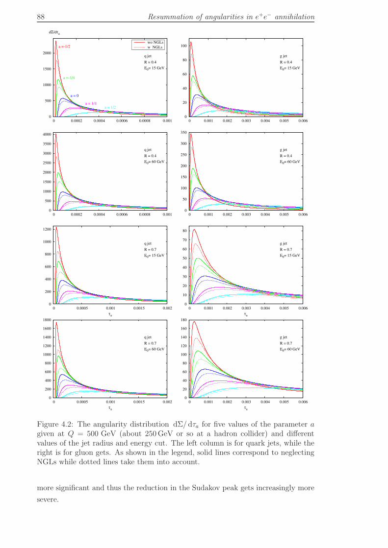
88 Resummation of angularities in e+e− annihilation
0
500
1000
1500
2000
0 0.0002 0.0004 0.0006 0.0008 0.001
dΣ/dτa
a =-1/2
a =-1/4
a = 0
a = 1/4a = 1/2
q jet
R = 0.4
E0= 15 GeV
wo NGLs
w NGLs
0
20
40
60
80
100
0 0.001 0.002 0.003 0.004 0.005 0.006
g jet
R = 0.4
E0= 15 GeV
0
500
1000
1500
2000
2500
3000
3500
4000
0 0.0002 0.0004 0.0006 0.0008 0.001
q jet
R = 0.4
E0= 60 GeV
0
50
100
150
200
250
300
350
0 0.001 0.002 0.003 0.004 0.005 0.006
g jet
R = 0.4
E0= 60 GeV
0
200
400
600
800
1000
1200
0 0.0005 0.001 0.0015 0.002
τa
q jet
R = 0.7
E0= 15 GeV
0
10
20
30
40
50
60
70
80
0 0.001 0.002 0.003 0.004 0.005 0.006
τa
g jet
R = 0.7
E0= 15 GeV
0
200
400
600
800
1000
1200
1400
1600
1800
0 0.0005 0.001 0.0015 0.002
τa
q jet
R = 0.7
E0= 60 GeV
0
20
40
60
80
100
120
140
160
180
0 0.001 0.002 0.003 0.004 0.005 0.006
τa
g jet
R = 0.7
E0= 60 GeV
Figure 4.2: The angularity distribution dΣ/ dτa for five values of the parameter agiven at Q = 500 GeV (about 250GeV or so at a hadron collider) and differentvalues of the jet radius and energy cut. The left column is for quark jets, while theright is for gluon gets. As shown in the legend, solid lines correspond to neglectingNGLs while dotted lines take them into account.
more significant and thus the reduction in the Sudakov peak gets increasingly more
severe.
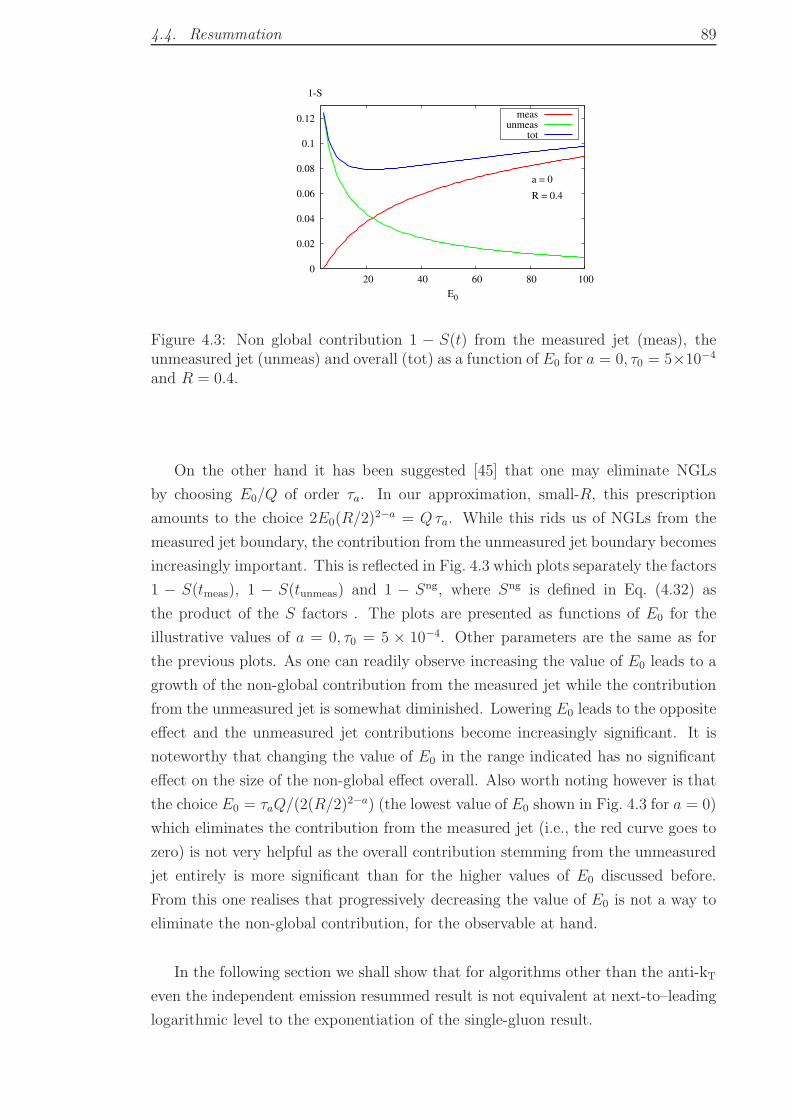
4.4. Resummation 89
0
0.02
0.04
0.06
0.08
0.1
0.12
20 40 60 80 100
E0
1-S
a = 0
R = 0.4
measunmeas
tot
Figure 4.3: Non global contribution 1 − S(t) from the measured jet (meas), theunmeasured jet (unmeas) and overall (tot) as a function of E0 for a = 0, τ0 = 5×10⁻⁴
and R = 0.4.
On the other hand it has been suggested [45] that one may eliminate NGLs
by choosing E0/Q of order τa. In our approximation, small-R, this prescription
amounts to the choice 2E0(R/2)2−a = Qτa. While this rids us of NGLs from the
measured jet boundary, the contribution from the unmeasured jet boundary becomes
increasingly important. This is reflected in Fig. 4.3 which plots separately the factors
1 − S(tmeas), 1 − S(tunmeas) and 1 − Sng, where Sng is defined in Eq. (4.32) as
the product of the S factors . The plots are presented as functions of E0 for the
illustrative values of a = 0, τ0 = 5 × 10⁻⁴. Other parameters are the same as for
the previous plots. As one can readily observe increasing the value of E0 leads to a
growth of the non-global contribution from the measured jet while the contribution
from the unmeasured jet is somewhat diminished. Lowering E0 leads to the opposite
effect and the unmeasured jet contributions become increasingly significant. It is
noteworthy that changing the value of E0 in the range indicated has no significant
effect on the size of the non-global effect overall. Also worth noting however is that
the choice E0 = τaQ/(2(R/2)2−a) (the lowest value of E0 shown in Fig. 4.3 for a = 0)
which eliminates the contribution from the measured jet (i.e., the red curve goes to
zero) is not very helpful as the overall contribution stemming from the unmeasured
jet entirely is more significant than for the higher values of E0 discussed before.
From this one realises that progressively decreasing the value of E0 is not a way to
eliminate the non-global contribution, for the observable at hand.
In the following section we shall show that for algorithms other than the anti-kT
even the independent emission resummed result is not equivalent at next-to–leading
logarithmic level to the exponentiation of the single-gluon result.
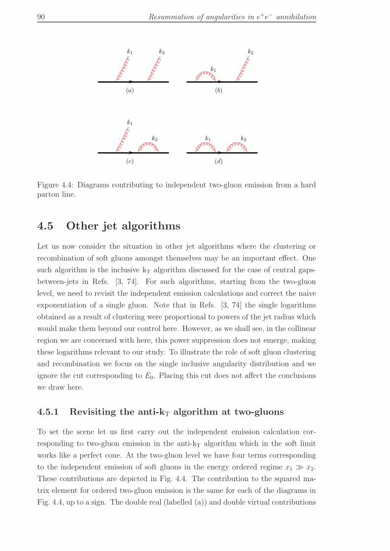
90 Resummation of angularities in e+e− annihilation
k1 k2
(a)
k1
k2
(b)
k1
k2
(c)
k1 k2
(d)
Figure 4.4: Diagrams contributing to independent two-gluon emission from a hardparton line.
4.5 Other jet algorithms
Let us now consider the situation in other jet algorithms where the clustering or
recombination of soft gluons amongst themselves may be an important effect. One
such algorithm is the inclusive kT algorithm discussed for the case of central gaps-
between-jets in Refs. [3, 74]. For such algorithms, starting from the two-gluon
level, we need to revisit the independent emission calculations and correct the naive
exponentiation of a single gluon. Note that in Refs. [3, 74] the single logarithms
obtained as a result of clustering were proportional to powers of the jet radius which
would make them beyond our control here. However, as we shall see, in the collinear
region we are concerned with here, this power suppression does not emerge, making
these logarithms relevant to our study. To illustrate the role of soft gluon clustering
and recombination we focus on the single inclusive angularity distribution and we
ignore the cut corresponding to E0. Placing this cut does not affect the conclusions
we draw here.
4.5.1 Revisiting the anti-kT algorithm at two-gluons
To set the scene let us first carry out the independent emission calculation cor-
responding to two-gluon emission in the anti-kT algorithm which in the soft limit
works like a perfect cone. At the two-gluon level we have four terms corresponding
to the independent emission of soft gluons in the energy ordered regime x1 ≫ x2.
These contributions are depicted in Fig. 4.4. The contribution to the squared ma-
trix element for ordered two-gluon emission is the same for each of the diagrams in
Fig. 4.4, up to a sign. The double real (labelled (a)) and double virtual contributions
4.5. Other jet algorithms 91
(labelled (d)) can be expressed as
W (k1, k2) = 4C2Fg
4s
(p1 . p2)2
(p1 . k1) (p1 . k2) (p2 . k1) (p2 . k2), (4.39)
which in terms of the energy fractions x1 and x2 introduced in Subsec. 4.3.1 becomes
simply
W (k1, k2) = 256 g4sC2
F
Q4
1
x21x
22
1
(1− cos2 θ1) (1− cos2 θ2). (4.40)
Since the calculation that follows below is intended for highly collimated jets, R ≪ 1,
we shall take the small angle limit of the above result, θ1, θ2 ≪ 1. A similar result
holds for the one-real one-virtual terms (b) and (c) in Fig. 4.4 with a relative minus
sign. We are now in a position to compute the angularity distribution at the two
gluon level for the independent emission C2F term.
We start by noting that the integration region for all graphs can be divided
according to whether the real gluons k1 and k2 are inside or outside the measured
jet. We have four distinct regions: k1, k2 both outside the measured jet, k1, k2 both
inside the measured jet or either of the gluons inside and the other outside the jet.
The condition for a given gluon to end up inside or outside the measured jet depends
on the jet algorithm we choose to employ. In the anti-kT algorithm the condition
is particularly simple when considering only soft emissions; such an emission k is
inside the jet if it is within an angle R of the hard parton initiating the jet, else it
is outside.
Given this fact let us consider how the various diagrams (a)–(d) in Fig. 4.4
combine in the different regions mentioned above. Since we are computing the
angularity distribution dΣ/ dτa for a fixed angularity τa, the pure virtual diagram
(d) makes no contribution and hence we shall omit all reference to it in what follows.
In the region where both emissions are in the jet we shall treat the sum of graphs
(a)–(c). Where the harder emission k1 is in the jet and k2 is out, graphs (a) and (c)
cancel since the real k2 does not contribute to the angularity exactly like the virtual
k2. This leaves diagram (b) which gives zero since the in-jet gluon k1 is virtual and
hence does not generate a value for the angularity. Hence the region with k1 in and
k2 out gives no contribution.
Now we consider k2 in and k1 out. The contributions with k2 real (a) and (b)
cancel as the graphs contribute in the same way to the angularity. The diagram with
k2 virtual (c) cannot contribute to the angularity as the real emission k1 lies outside
the jet. Hence we only need to treat the region with both gluons in and we shall
show that this calculation correctly reproduces the result based on exponentiation
of the single gluon result. The summed contribution of graphs (a) to (c) can be
92 Resummation of angularities in e+e− annihilation
represented as
dΣ2
dτa∼∫
dΦW
[δ
(τa −
x1θ2−a1
22−a− x2θ
2−a2
22−a
)− δ
(τa −
x1θ2−a1
22−a
)− δ
(τa −
x2θ2−a2
22−a
)],
(4.41)
where we wrote the contribution to the angularity from an emission with energy
fraction x and angle θ with respect to the hard parton as x sina θ (1− cos θ)1−a /2 ≈x(θ/2)2−a.
To compute the leading double-logarithmic contribution and show that it corre-
sponds to the exponentiation of the order αs double-logarithmic term one can write
δ (τa − x1(θ1/2)2−a − x2(θ2/2)
2−a) as ∂ [Θ (τa − x1(θ1/2)2−a − x2(θ2/2)
2−a)] /∂τa
and make the leading-logarithmic approximation
Θ(τa − x1(θ1/2)
2−a − x2(θ2/2)2−a)→ Θ
(τa − x1(θ1/2)
2−a)Θ(τa − x2(θ2/2)
2−a),
(4.42)
which allows us to make the replacement
δ(τa − x1(θ1/2)
2−a − x2(θ2/2)2−a)→ δ
(τa − x1(θ1/2)
2−a)Θ(τa − x2(θ2/2)
2−a)
+ 1 ↔ 2 . (4.43)
Doing so and using the explicit forms of W and the phase space dΦ in the small
angle limit we get
dΣ2
dτa= −4C2
F
(αs
2π
)2 ∫ dθ21θ21
dθ22θ22
dφ
2π
dx1
x1
dx2
x2
[δ(τa − x1(θ1/2)
2−a)
Θ(x2(θ2/2)
2−a − τa)+ 1 ↔ 2
]Θ(R2 − θ21
)Θ(R2 − θ22
)
Θ (x1 − x2)Θ(1− x1). (4.44)
Carrying out the integrals we straightforwardly obtain
dΣ2
dτa= −2
(CFαs
π(2− a)
)21
τaln3
((R/2)2−a
τa
), (4.45)
which is precisely the result obtained by expanding the exponentiated double-
logarithmic one-gluon result to order α2s and differentiating with respect to τa. Thus
the standard double-logarithmic result for the angularity distribution arises entirely
from the region with both gluons in the jet. Contributions from soft emission arising
from the other regions cancel in the sense that they produce no relevant logarithms.
4.5. Other jet algorithms 93
4.5.2 The kT algorithm and clustering logarithms
We shall now argue that for algorithms other than the anti-kT relevant single-
logarithmic contributions shall appear from the regions which cancelled in the ar-
gument above, although of course the leading double-logarithms are still precisely
the same as for the anti-kT case. An analysis of such miscancelling contributions
is therefore necessary for a resummation aiming at next-to–leading logarithmic ac-
curacy in the angularity. The logarithms we compute below correct the one-gluon
exponentiated result for the angularity distribution at the single-logarithmic level
starting from order α2s.
Let us consider the situation in, for instance, the kT algorithm (Algorithm 1 with
p = 1). When both k1 and k2 are within an angle R of the hard parton both soft
gluons get combined into the hard jet and this region produces precisely the same
result as the anti-kT algorithm, corresponding to exponentiation of the one-gluon
result. Moreover, when both k1 and k2 are beyond an angle R with respect to the
hard parton there is no contribution from either to the angularity. However, when
k1 is beyond an angle R and k2 is inside an angle R the situation changes from the
anti-kT case. This is because in the kT algorithm when the two soft partons are
separated by less than R in angle they can be clustered together. The resulting soft
jet has four-momentum k1 + k2, when we use the four-momentum recombination
scheme (E–scheme), and lies essentially along the harder gluon k1. Thus when k1 is
beyond an angle R it can pull k2 out of the hard jet since the soft jet k1 + k2 which
replaces k2 lies outside an angle R of the hard parton. Hence such a configuration
gives no contribution to the angularity distribution.
In precisely the same angular region the virtual k1, real k2 diagram (b) (obviously
unaffected by clustering) does however give a contribution whereas in the anti-kT
case it had cancelled the double real contribution (a). The graph with k1 real and k2
virtual gives no contribution as before. Thus a new uncancelled contribution arises
for the kT (and indeed the Cambridge–Aachen (C/A)) algorithm from the region
where the two real gluons k1 and k2 are clustered, which can be given by computing
the k1 virtual k2 real graph in the same angular region.
We now carry out this calculation explicitly. We consider the angles θ21, θ22 and
θ212 as the angles between k1 and the hard parton, k2 and the hard parton and k1 and
k2 respectively. Applying the kT algorithm (Algorithm 1, p = 1) in inclusive mode
means constructing the distances ω21θ
21, ω
22θ
22 and ω2
2θ212 along with the distances (from
the “beam”) ω21R
2, ω22R
2, where, for the e+e− case we consider here, the energy ω
plays the role of the kt with respect to the beam in a hadron collider event. Now
since θ21 > R2, θ22 < R2 the only quantities that can be a candidate for the smallest
distance are ω22θ
22 and ω2
2θ212. Thus the gluons are clustered and k2 is pulled out
of the jet if θ12 < θ2 < R. Otherwise k2 is in the jet and cancels against virtual
94 Resummation of angularities in e+e− annihilation
corrections. We write this as
Θclus(k1, k2) = Θ(θ21 −R2
)Θ(θ22 − θ212
)Θ(R2 − θ22
). (4.46)
Note that repeating the above discussion for the C/A algorithm yields an identical
expression to Eq. (4.46). We can then write the contribution of graph (b) of Fig. 4.4
in the clustering region
dΣclus
dτa= −4C2
F
(αs
2π
)2 ∫ dθ21θ21
dθ22θ22
dφ
2π
dx1
x1
dx2
x2δ[τa − x2(θ2/2)
2−a]
Θ(x1 − x2)Θclus(θ1, θ2). (4.47)
Using the fact that in the small-angle approximation relevant to our study
θ212 = θ21 + θ22 − 2θ1θ2 cosφ , (4.48)
integrating over x1 and x2 and using t = (θ2/2)2−a/τa one obtains
dΣclus
dτa= −4C2
F
(αs
2π
)2 2
(2− a)τa
∫dθ21θ21
dt
t
dφ
2πln t
Θ (t− 1)Θ(θ21 −R2
)Θ(4(τat)
2(2−a) cos2 φ− θ21
)Θ(R2−a/τa − t
). (4.49)
Carrying out the integral over θ21 results in
dΣclus
dτa= −4C2
F
(αs
2π
)2 2
(2− a)τa
∫dt
t
dφ
2πln
(4(τat)
22−a cos2 φ
R2
)ln t
Θ (t− 1)Θ(4(τat)
22−a cos2 φ− R2
)Θ(R2−a/τa − t
). (4.50)
Now we need to carry out the t integral for which we note t >
max[1, [R/(2 cosφ)]2−a /τa
]. In the region of large logarithms which we resum one
has however that R2−a ≫ τa and hence [R/(2 cosφ)]2−a /τa > 1. This condition is
reversed only when τa ∼ R2−a; a region not enhanced by large logarithms and hence
beyond our accuracy.
It is then straightforward to carry out the t integral and doing so and extracting
the leading singular behaviour in τa produces the result
dΣclus
dτa= −4C2
F
(αs
2π
)2 1
τaln
1
τa
∫dφ
πln2 (2 cosφ)Θ
(cosφ− 1
2
)
= −0.728C2F
(αs
2π
)2 1
τaln
1
τa. (4.51)
This behaviour in the distribution translates into a next-to–leading logarithmic
4.6. Conclusion 95
α2s ln
2(1/τa) behaviour in the integrated cross-section, which is relevant for resum-
mations aiming at this accuracy. We refer to the latter logarithms as clustering logs
(CLs). As we mentioned before the above finding of single logarithmic corrections
generated by clustering has also been reported before for the case of gaps-between-
jets studies [74]. Note however that the logarithms found there had coefficients that
depended on powers of the jet radius starting at the R3 level. In the present case
however the presence of collinear singularities near the boundary of a jet of small
radius R ensures that there is no power suppression in R and hence the logarithms
generated are formally comparable to those we aim to control here and indeed those
resummed in Refs. [44, 45]. Note also that at this logarithmic level, the CLs coeffi-
cient does not depend on the parameter a. The dependence on a, just like the shape
variable itself, τa, is confined to the argument of the logarithm. This is in-line with
our finding that the non-global coefficient, S2, is independent of a. Thus non-global
and clustering coefficients are only sensitive to the geometry of the final state (and
not to the shape variable or parameters that enter in its definition).
Likewise the clustering will also generate leading logarithms in the E0 variable,
which are again unsuppressed by any powers of R and hence ought to be controlled.
Lastly we point out that the logarithms generated by independent emission and
subsequent kT clustering were actually resummed in Ref. [3] and that possibility
also exists here. The explicit calculations will be presented to Chapter 6. Moreover,
we mention that calculations of NGLs and CLs contributions at two-gluon level in
the C/A algorithm produce results that are identical to the above kT algorithm
results reported here.
4.6 Conclusion
We would like to conclude by emphasising the main points of our study. Given
the current interest in the study of jet shapes and substructure for the purposes of
discovering new physics at the LHC, it is worth examining the theoretical state of
the art when it comes to looking at individual jet profiles in a multi-jet event. A
step in this direction was taken for instance in Refs. [44, 45]. In the present chapter
we have noted
• Observables where one picks out for study one or more jets in multi-jet events
are in principle non-global. The non-global logarithms will arise at next-to–
leading or single-logarithmic accuracy in the jet-shape distributions. If one
studies jet events with a fixed multiplicity by imposing a cut E0 on hadronic
activity outside the high-pT jets, there are non-global logarithms involving the
ratio of the shape variable τa and the energy flow E0, as was first anticipated
in [38]. Moreover, there are also non-global logarithms in E0/Q where Q
is the hard scale of the process. These logarithms are leading as far as the
96 Resummation of angularities in e+e− annihilation
distribution in E0 for a fixed τa is concerned.
• In the limit of narrow jets R → 0, one may naively expect the non-global
contributions to the jet-shape distributions to vanish with R due to the ap-
parently limited phase-space available for soft emission inside the jet. Here we
have pointed out that the non-global logarithms do not vanish in the small cone
approximation as mentioned for instance in Ref. [222]. One finds instead an
effect (at small-R) that is independent of R and arises from the edge of the jet.
However, in the limit of narrow well-separated jets R2 ≪ (1 − cos θij), where
θij is the inter-jet separation, one can simplify the non-global contribution.
In this limit, owing to QCD coherence and the nature of correlated multiple
soft emissions, one can regard the non-global logarithms to arise independently
from the boundary of each jet up to corrections that vanish as R2/ (1− cos θij).
For a measured jet one picks up logarithms in 2E0(R/2)2−a/(Qτa) while for
each unmeasured jet one has logarithms in 2E0/Q. The resummation of these
logarithms yields a factor Sj for each jet j, which is the factor computed, in
the large-Nc limit, for the hemisphere jet-mass in e+e− annihilation in Ref.
[2], again up to corrections vanishing as R2/ (1− cos θij).
• The overall size of non-global logarithms depends on the precise values one
chooses for E0/Q, R, a and τa. However, broadly speaking, we find the con-
tribution not to vary significantly with E0 and to yield corrections of order
10 − 25% in the peak region of the τa distribution. Choosing E0/Q of or-
der τa/(R/2)2−a eliminates the non-global contributions from the measured
jet but steeply enhances the contributions from the unmeasured jet and it is
not an optimal choice for reducing the overall non-global contribution to this
observable.
• We emphasise that the above observations are valid for the anti-kT algorithm
in which our ansatz for resummation of jet shapes in an arbitrarily complex
event is to correct the one-gluon exponentiation with a product of independent
non-global factors from each jet. We further have emphasised that switching
to algorithms other than the anti-kT gives relevant next-to–leading logarithms
in the shape distribution as well as leading logarithms in the E0 distribution,
even within the independent emission approximation. Thus predictions for
observables such as the one discussed in this chapter, in those algorithms are
prone to more uncertainty than our current study in the anti-kT algorithm at
least until such logarithms are also resummed.
We would like to stress that the general observations in this chapter are of ap-
plicability in a variety of other contexts. For instance, the issue of threshold re-
summation addresses limited energy flow outside hard jets, along the lines of the
4.6. Conclusion 97
E0 distribution here. The consequent non-global logarithms and the issue of the
jet algorithm have not been addressed to any extent in the existing literature. The
same issues crop up in the case of resummation in the central jet veto scale for the
important study of Higgs production in association with two jets.
We hope that an awareness of the nature and size of the non-global contributions,
the simplification that occurs in the small-R limit and our comments about the sit-
uation in other jet algorithms will help to generate more accurate phenomenological
studies for these important observables at the LHC. In particular we shall address
in more detail, in Chapter 7, the role of soft gluon effects and especially non-global
logarithms on QCD predictions relevant to new physics searches at the LHC.
In the next chapter we present “precision” calculations of both non-global and
clustering logarithms in various jet algorithms. The jet mass distribution in e+e−
annihilation will be taken as a generic example of non-global jet shape observables.

98
Chapter 5
Non-global structure of jet shapes
beyond leading log accuracy
5.1 Introduction
Within the same context of e+e− multijet events considered in the previous chapter,
we study in this chapter the jet-thrust τE0 , introduced in [50], where one measures
the mass of the two highest–energy jets with a veto E0 on energy flow into the
interjet region Ω. We shall compute the individual colour (C2F,CFCA and CFTFnf)
contributions to the total differential τE0 distribution (at O(α2s)) as well as the effect
of the C/A (and indeed the kT) algorithm clustering at N3LL (that is up to α2s L)
in the expansion. The work presented in the current chapter may be regarded as an
extension to that of the the previous chapter.
Such an extension includes: (a) computing the full R dependence of the leading
and next-to-leading NGLs coefficients in the ant-kT, C/A and kT algorithms, (b)
computing the full R dependence of the leading and next-to-leading CLs coefficients
in the C/A and kT algorithms, (c) providing a next-to-leading log (in the exponent)
resummation, including numerical estimates of all–orders NGLs and CLs in the
large-Nc limit, for both anti-kT and kT algorithms with full R dependence using the
Monte Carlo program developed in [2] with the clustering option added in [3] and
(d) checking our findings, and hence implicitly those of the previous chapter, for
a = 0, (which are valid in the small R limit) against the NLO program event2
[179]. The C/A and kT jet algorithms are actually identical for both NGLs and CLs
at O(α2s) as mentioned previously (Subsec. 4.5.2), and hence we shall only explicitly
discuss the C/A algorithm. However, owing to the fact that the said MC program
[2, 3] only implements the kT algorithm, all–orders treatment of NGLs and CLs shall
therefore be addressed in the kT algorithm.
The organisation of this chapter is as follows. In Sec. 5.2 we compute the full
logarithmic part of the LO jet-thrust distribution. We then consider, in Sec. 5.3, the
fixed–order NLO distribution in the eikonal limit and compute the NGLs coefficients
up to α2s L, in both anti-kT and C/A jet algorithms. In the same section we derive
an expression for the CLs leading and next-to-leading terms as well. Note that our
calculations in this section include full jet–radius dependence. Sec. 5.4 is devoted
99
100 Non-global structure of jet shapes beyond leading log accuracy
to NLL resummation of our jet shape including determination of the coefficients of
the logs in the exponent which will be used to compute the full N3LL fixed–order
differential distribution to be compared with the output of event2 . We additionally
investigate in the same section the impact of NGLs on the Sudakov resummation and
discuss various factors that play a role in enhancing or reducing the latter impact,
including clustering effects. Numerical distributions of the jet-thrust obtained using
the program event2 are compared to analytical results and the findings discussed
in Sec. 5.5. In light of this discussion, we draw our main conclusions in Sec. 5.6.
5.2 Jet-thrust distribution at O(αs)
After briefly reviewing the definition of the jet-thrust, or the jet mass with a jet
veto, observable presented in [50, 223], the e+e− version of the general formula for
sequential recombination jet algorithms (Algorithm 1) is presented. We then move
on to compute the LO integrated distribution of this shape variable. At this order,
all jet algorithms are identical. Note that partons (quarks and gluons) are assumed
on–mass shell throughout.
5.2.1 Observable definition
Consider e+e− annihilation into multijet events. First, one clusters events into jets
of size (radius) R with a jet algorithm. After clustering, one labels the momenta
of the two hardest jets pR and pL and the energy of the third hardest jet E3. The
jet-thrust is then given by the sum of the two leading jets’ masses after events with
E3 > E0 are vetoed [50],
τE0 =m2
R +m2L
Q2=
ρR + ρL4
, (5.1)
where ρR and ρL are the jet mass fractions, studied in the previous chapter (ρ = τ0),
for the two leading jets and Q is the hard scale.
A general form of sequential recombination algorithms at hadron colliders is
presented in Algorithm 1. The adopted version for e+e− machines corresponds
simply to the replacements: pti → Ei and ∆R2ij = 2(1 − cos θij), where Ei is the
energy of parton, or pseudojet, i and θij the polar angle between two partons i and
j. Recall that two partons, i and j, are merged together if
∆R2ij < R2. (5.2)
With regard to notation, we follow Ref. [50] and work with the jet radius Rs1, which
1The motivation for using Rs instead of R was to have results that can directly and straight-forwardly be compared to those found in [50], to which our paper [85] was a clarification regardingNGLs.
5.2. Jet-thrust distribution at O(αs) 101
is given in terms of the above R by:
Rs = R2/4. (5.3)
It is worth noting that the jet-thrust, defined in 5.1 is just the thrust in the
threshold (dijet) limit, hence the name. To verify this we begin with the general
formula of the thrust T (or rather 1− T ≡ τ),
τ = 1−maxn
∑i |pi.n|∑i |pi|
, (5.4)
where the sum is over all final state three–momenta pi and the maximum is over
directions (unit vectors) n. In the threshold limit, enforced by applying a jet veto
E0, e+e− annihilates into two back–to–back jets and the thrust axis, the maximum
n, coincides with jet directions. At LO, an emission of a single gluon, k, that is
close to, and hence clustered with, say pR, produces the following contribution to
the thrust
τ ≃ ERω
Q(1− cos θkpR) +
ELω
Q(1− cos θkpL) +
ω2
Q2(1− cos θkpR)(1− cos θkpL), (5.5)
where ER(L) is the energy of the hard leg pR(L), ω the gluon energy and we have
discarded O(τ 2) terms. Recalling that the first two terms in the RHS of Eq. (5.5)
are just the mass fractions ρR and ρL, respectively, at LO and neglecting the third
term (quadratic in ω) one concludes that
τ ≃ τE0 . (5.6)
This relation can straightforwardly be shown to hold to all–orders in the two-jet
limit.
5.2.2 LO distribution
In the previous chapter we computed the LO distribution of the jet mass fraction,
ρ = τ0, in the small R (hence small Rs) limit using the matrix–element squared
in the eikonal approximation (see Appendix B.1). In this section, we use the full
QCD matrix–element to restore the complete Rs dependence of the singular part of
the τE0 distribution. The general expression for the integrated and normalised τE0
distribution, or equivalently the τE0 shape fraction, is given by
Σ(τE0 , E0) =
∫ τE0
0
dτ ′E0
∫ E0
0
dE31
σ(0)
d2σ
dτ ′E0dE3
, (5.7)
where σ(0) is the Born cross-section. The perturbative expansion of the shape frac-
tion Σ in terms of QCD coupling αs may be cast in the form (4.3). The derivation
102 Non-global structure of jet shapes beyond leading log accuracy
of the first order correction, Σ(1), to the Born approximation is presented in Ap-
pendix C.1. The final result reads
Σ(1)(τE0 , E0) =CFαs
2π
[−2 ln2 τE0 +
(−3 + 4 ln
Rs
1− Rs
)ln τE0
]Θ(2 τmax
E0(Rs)− τE0
)
+CFαs
2π
[− 1 +
π2
3− 4 ln
Rs
1− Rs
ln2E0
Q+ fE0(Rs)
], (5.8)
where2
τmaxE0
(Rs) =2
Rs
(1−
√1−Rs
)− 1, (5.9)
and the function fE0(Rs) is given by
fE0(Rs) = −2 lnRs lnRs
1−Rs+ 2 Li2(Rs)− 2 Li2(1−Rs)+
8E0
Q
(1 +
3
4ln
Rs
1−Rs
)+O
(E2
0
Q2
). (5.10)
It is worthwhile to note that in the limit Rs → 1/2 the τE0 distribution (5.8) reduces,
as expected from (5.6), to the well-known thrust distribution [7, 40] with upper limit
τ < 1/3. For Rs < 1/2 the jet-thrust distribution includes, in addition to thrust
distribution and other single logarithms due to finite Rs jet size, the interjet energy
flow distribution [224] too,
Σ(1)E flow(E0) =
CFαs
2π
[−4 ln
Rs
1−Rsln
(2E0
Q
)+O
(E0
Q
)], (5.11)
Here the interjet region, or rapidity gap referred to in literature as ∆η, is defined
by the edges of the jets. Specifically, it is related to the jet–radius Rs by
∆η = − ln
(Rs
1− Rs
). (5.12)
The important features of the τE0 distribution that are of concern to the present
chapter are actually contained in the second order correction term Σ(2), which we
address in the next section.
5.3 Jet-thrust distribution at O(α2s)
The O(α2s) matrix–element squared for e+e− annihilation, which includes the pro-
cesses e+e− → q(pa)+q(pb)+g1(k1)+g2(k2) and e+e− → q(pa)+q(pb)+q1(k1)+q2(k2),
has been derived in the eikonal approximation3, Q ≫ (Q . ki) for i = 1, 2, in Ap-
2Notice that for a single gluon emission, if the gluon is clustered with, say, R–jet then m2L = 0
and τE0 < τmaxE0
(and not τE0 < 2τmaxE0
).3The recoil effects are negligible in this regime and are hence ignored throughout. This limit
also allows one to consider the produced jets to be back–to–back, hence the parametrisation (5.13).
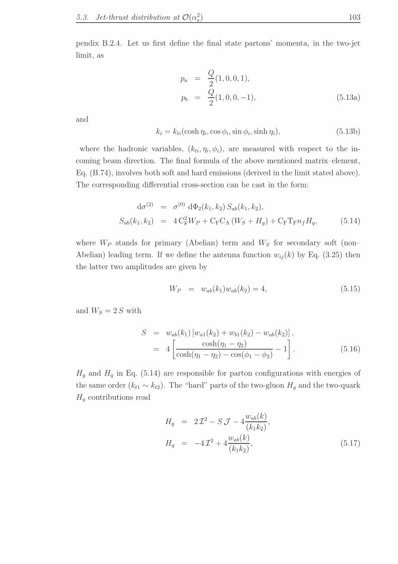
5.3. Jet-thrust distribution at O(α2s) 103
pendix B.2.4. Let us first define the final state partons’ momenta, in the two-jet
limit, as
pa =Q
2(1, 0, 0, 1),
pb =Q
2(1, 0, 0,−1), (5.13a)
and
ki = kti(cosh ηi, cosφi, sinφi, sinh ηi), (5.13b)
where the hadronic variables, (kti, ηi, φi), are measured with respect to the in-
coming beam direction. The final formula of the above mentioned matrix–element,
Eq. (B.74), involves both soft and hard emissions (derived in the limit stated above).
The corresponding differential cross-section can be cast in the form:
dσ(2) = σ(0) dΦ2(k1, k2)Sab(k1, k2),
Sab(k1, k2) = 4C2FWP + CFCA (WS +Hg) + CFTFnfHq, (5.14)
where WP stands for primary (Abelian) term and WS for secondary soft (non–
Abelian) leading term. If we define the antenna function wij(k) by Eq. (3.25) then
the latter two amplitudes are given by
WP = wab(k1)wab(k2) = 4, (5.15)
and WS = 2S with
S = wab(k1) [wa1(k2) + wb1(k2)− wab(k2)] ,
= 4
[cosh(η1 − η2)
cosh(η1 − η2)− cos(φ1 − φ2)− 1
]. (5.16)
Hg and Hq in Eq. (5.14) are responsible for parton configurations with energies of
the same order (kt1 ∼ kt2). The “hard” parts of the two-gluon Hg and the two-quark
Hq contributions read
Hg = 2 I2 − S J − 4wab(k)
(k1k2),
Hq = −4 I2 + 4wab(k)
(k1k2), (5.17)
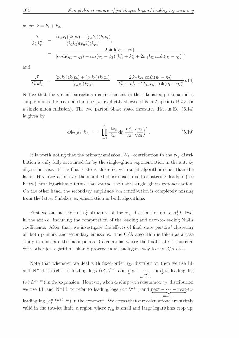
104 Non-global structure of jet shapes beyond leading log accuracy
where k = k1 + k2,
Ik2t1k
2t2
=(pak1)(k2pb)− (pak2)(k1pb)
(k1k2)(pak)(kpb),
=2 sinh(η1 − η2)
[cosh(η1 − η2)− cos(φ1 − φ2)][k2t1 + k2
t2 + 2kt1kt2 cosh(η1 − η2)],
and
Jk2t1k
2t2
=(pak1)(k2pb) + (pak2)(k1pb)
(pak)(kpb)=
2 kt1kt2 cosh(η1 − η2)
[k2t1 + k2
t2 + 2kt1kt2 cosh(η1 − η2)].(5.18)
Notice that the virtual correction matrix-element in the eikonal approximation is
simply minus the real emission one (we explicitly showed this in Appendix B.2.3 for
a single gluon emission). The two–parton phase space measure, dΦ2, in Eq. (5.14)
is given by
dΦ2(k1, k2) =
2∏
i=1
dktikti
dηidφi
2π
(αs
2π
)2. (5.19)
It is worth noting that the primary emission, WP , contribution to the τE0 distri-
bution is only fully accounted for by the single–gluon exponentiation in the anti-kT
algorithm case. If the final state is clustered with a jet algorithm other than the
latter, WP integration over the modified phase space, due to clustering, leads to (see
below) new logarithmic terms that escape the naive single–gluon exponentiation.
On the other hand, the secondary amplitude WS contribution is completely missing
from the latter Sudakov exponentiation in both algorithms.
First we outline the full α2s structure of the τE0 distribution up to α2
s L level
in the anti-kT including the computation of the leading and next-to-leading NGLs
coefficients. After that, we investigate the effects of final state partons’ clustering
on both primary and secondary emissions. The C/A algorithm is taken as a case
study to illustrate the main points. Calculations where the final state is clustered
with other jet algorithms should proceed in an analogous way to the C/A case.
Note that whenever we deal with fixed-order τE0 distribution then we use LL
and NmLL to refer to leading logs (αns L
2n) and next− · · · − next︸ ︷︷ ︸m=1,···
-to-leading log
(αns L
2n−m) in the expansion. However, when dealing with resummed τE0 distribution
we use LL and NmLL to refer to leading logs (αns L
n+1) and next− · · · − next︸ ︷︷ ︸m=1,···
-to-
leading log (αns L
n+1−m) in the exponent. We stress that our calculations are strictly
valid in the two-jet limit, a region where τE0 is small and large logarithms crop up.
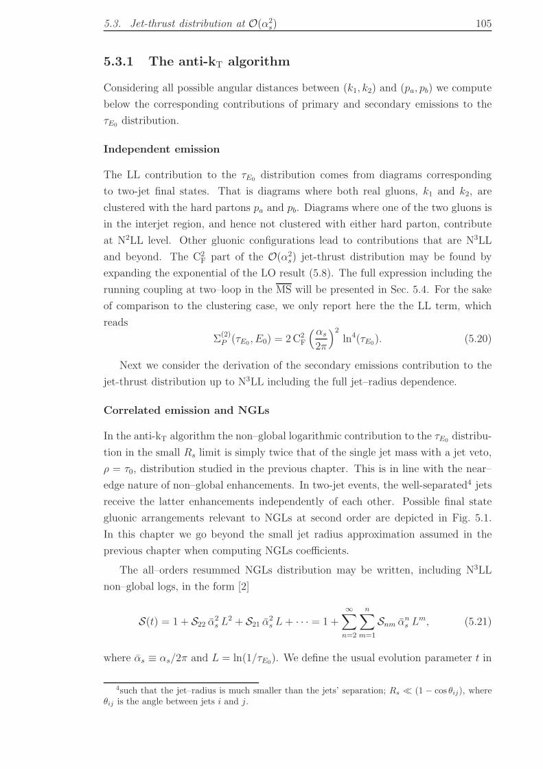
5.3. Jet-thrust distribution at O(α2s) 105
5.3.1 The anti-kT algorithm
Considering all possible angular distances between (k1, k2) and (pa, pb) we compute
below the corresponding contributions of primary and secondary emissions to the
τE0 distribution.
Independent emission
The LL contribution to the τE0 distribution comes from diagrams corresponding
to two-jet final states. That is diagrams where both real gluons, k1 and k2, are
clustered with the hard partons pa and pb. Diagrams where one of the two gluons is
in the interjet region, and hence not clustered with either hard parton, contribute
at N2LL level. Other gluonic configurations lead to contributions that are N3LL
and beyond. The C2F part of the O(α2
s) jet-thrust distribution may be found by
expanding the exponential of the LO result (5.8). The full expression including the
running coupling at two–loop in the MS will be presented in Sec. 5.4. For the sake
of comparison to the clustering case, we only report here the the LL term, which
reads
Σ(2)P (τE0 , E0) = 2C2
F
(αs
2π
)2ln4(τE0). (5.20)
Next we consider the derivation of the secondary emissions contribution to the
jet-thrust distribution up to N3LL including the full jet–radius dependence.
Correlated emission and NGLs
In the anti-kT algorithm the non–global logarithmic contribution to the τE0 distribu-
tion in the small Rs limit is simply twice that of the single jet mass with a jet veto,
ρ = τ0, distribution studied in the previous chapter. This is in line with the near–
edge nature of non–global enhancements. In two-jet events, the well-separated4 jets
receive the latter enhancements independently of each other. Possible final state
gluonic arrangements relevant to NGLs at second order are depicted in Fig. 5.1.
In this chapter we go beyond the small jet radius approximation assumed in the
previous chapter when computing NGLs coefficients.
The all–orders resummed NGLs distribution may be written, including N3LL
non–global logs, in the form [2]
S(t) = 1 + S22 α2s L
2 + S21 α2s L+ · · · = 1 +
∞∑
n=2
n∑
m=1
Snm αns L
m, (5.21)
where αs ≡ αs/2π and L = ln(1/τE0). We define the usual evolution parameter t in
4such that the jet–radius is much smaller than the jets’ separation; Rs ≪ (1 − cos θij), whereθij is the angle between jets i and j.
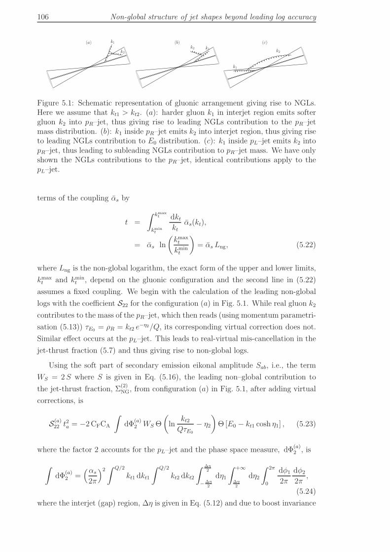
106 Non-global structure of jet shapes beyond leading log accuracy
(a)
k2
k1 (b)k2 k1
(c)
k2
k1
Figure 5.1: Schematic representation of gluonic arrangement giving rise to NGLs.Here we assume that kt1 > kt2. (a): harder gluon k1 in interjet region emits softergluon k2 into pR–jet, thus giving rise to leading NGLs contribution to the pR–jetmass distribution. (b): k1 inside pR–jet emits k2 into interjet region, thus giving riseto leading NGLs contribution to E0 distribution. (c): k1 inside pL–jet emits k2 intopR–jet, thus leading to subleading NGLs contribution to pR–jet mass. We have onlyshown the NGLs contributions to the pR–jet, identical contributions apply to thepL–jet.
terms of the coupling αs by
t =
∫ kmaxt
kmint
dktkt
αs(kt),
= αs ln
(kmaxt
kmint
)= αs Lng, (5.22)
where Lng is the non-global logarithm, the exact form of the upper and lower limits,
kmaxt and kmin
t , depend on the gluonic configuration and the second line in (5.22)
assumes a fixed coupling. We begin with the calculation of the leading non-global
logs with the coefficient S22 for the configuration (a) in Fig. 5.1. While real gluon k2
contributes to the mass of the pR–jet, which then reads (using momentum parametri-
sation (5.13)) τE0 = ρR = kt2 e−η2/Q, its corresponding virtual correction does not.
Similar effect occurs at the pL–jet. This leads to real-virtual mis-cancellation in the
jet-thrust fraction (5.7) and thus giving rise to non-global logs.
Using the soft part of secondary emission eikonal amplitude Sab, i.e., the term
WS = 2S where S is given in Eq. (5.16), the leading non–global contribution to
the jet-thrust fraction, Σ(2)NG, from configuration (a) in Fig. 5.1, after adding virtual
corrections, is
S(a)22 t2a = −2CFCA
∫dΦ
(a)2 WS Θ
(ln
kt2QτE0
− η2
)Θ [E0 − kt1 cosh η1] , (5.23)
where the factor 2 accounts for the pL–jet and the phase space measure, dΦ(a)2 , is
∫dΦ
(a)2 =
(αs
2π
)2 ∫ Q/2
kt1 dkt1
∫ Q/2
kt2 dkt2
∫ ∆η2
−∆η2
dη1
∫ +∞
∆η2
dη2
∫ 2π
0
dφ1
2π
dφ2
2π,
(5.24)
where the interjet (gap) region, ∆η is given in Eq. (5.12) and due to boost invariance
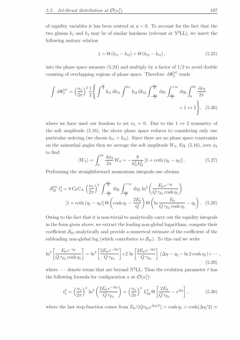
5.3. Jet-thrust distribution at O(α2s) 107
of rapidity variables it has been centred at η = 0. To account for the fact that the
two gluons k1 and k2 may be of similar hardness (relevant at N3LL), we insert the
following unitary relation
1 = Θ (kt1 − kt2) + Θ (kt2 − kt1) , (5.25)
into the phase space measure (5.24) and multiply by a factor of 1/2 to avoid double
counting of overlapping regions of phase space. Therefore dΦ(a)2 reads
∫dΦ
(a)2 =
(αs
2π
)2 12
∫ Q2
kt1 dkt1
∫ kt1
kt2 dkt2
∫ ∆η2
−∆η2
dη1
∫ +∞
∆η2
dη2
∫ 2π
0
dφ2
2π
+ 1 ↔ 2
, (5.26)
where we have used our freedom to set φ1 = 0. Due to the 1 ↔ 2 symmetry of
the soft amplitude (5.16), the above phase space reduces to considering only one
particular ordering (we choose kt1 > kt2). Since there are no phase space constraints
on the azimuthal angles then we average the soft amplitude WS, Eq. (5.16), over φ2
to find
〈WS〉 =∫ 2π
0
dφ2
2πWS = − 8
k2t1k
2t2
[1 + coth (η1 − η2)] . (5.27)
Performing the straightforward momentum integrals one obtains
S(a)22 t2a = 8CFCA
(αs
2π
)2 ∫ ∆η2
−∆η2
dη1
∫ +∞
∆η2
dη2 ln2
(E0 e
−η2
QτE0 cosh η1
)
[1 + coth (η1 − η2)] Θ
(cosh η1 −
2E0
Q
)Θ
(ln
E0
QτE0 cosh η1− η2
). (5.28)
Owing to the fact that it is non-trivial to analytically carry out the rapidity integrals
in the form given above, we extract the leading non-global logarithms, compute their
coefficient S22 analytically and provide a numerical estimate of the coefficient of the
subleading non-global log (which contributes to S21). To this end we write
ln2
[E0 e
−η2
QτE0 cosh η1
]= ln2
[2E0 e
−∆η
QτE0
]+2 ln
[2E0 e
−∆η
QτE0
](∆η − η2 − ln 2 cosh η1)+· · · ,
(5.29)
where · · · denote terms that are beyond N3LL. Thus the evolution parameter t has
the following formula for configuration a at O(α2s):
t2a =(αs
2π
)2ln2
(2E0 e
−∆η
QτE0
)=(αs
2π
)2L2ng Θ
[2E0
QτE0
− e∆η
], (5.30)
where the last step-function comes from E0/(QτE0e∆η/2) > cosh η1 > cosh(∆η/2) ≃
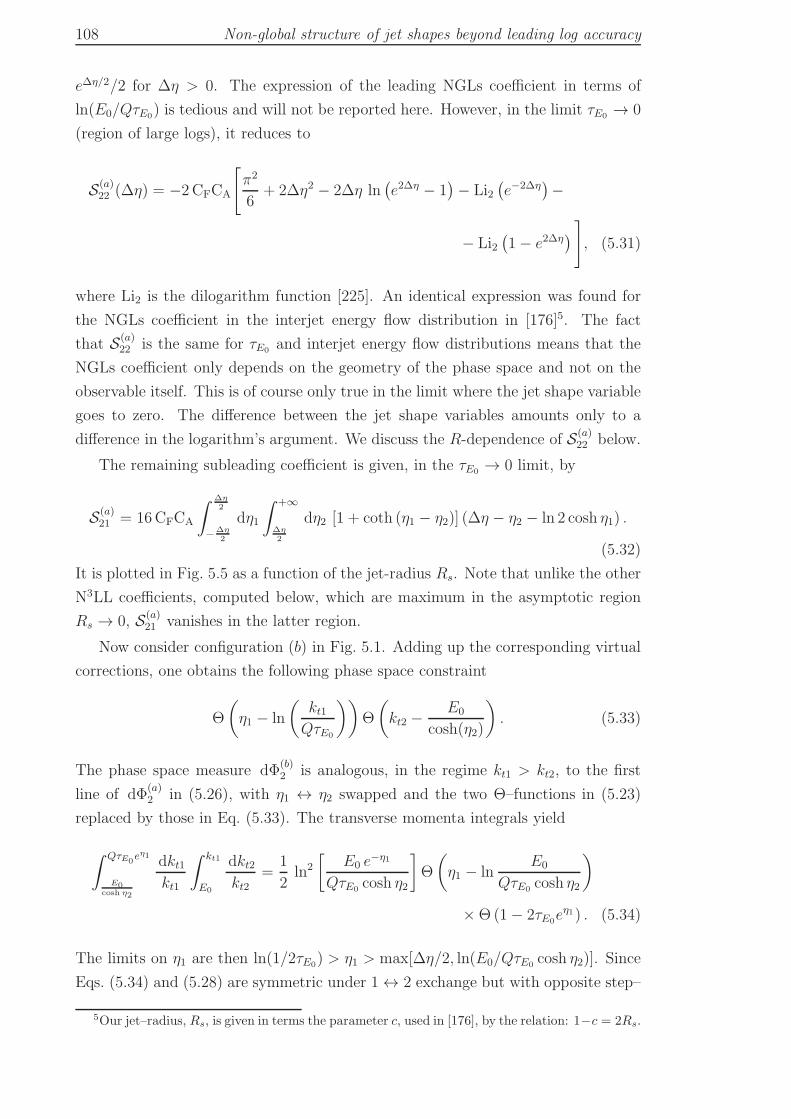
108 Non-global structure of jet shapes beyond leading log accuracy
e∆η/2/2 for ∆η > 0. The expression of the leading NGLs coefficient in terms of
ln(E0/QτE0) is tedious and will not be reported here. However, in the limit τE0 → 0
(region of large logs), it reduces to
S(a)22 (∆η) = −2CFCA
[π2
6+ 2∆η2 − 2∆η ln
(e2∆η − 1
)− Li2
(e−2∆η
)−
− Li2(1− e2∆η
)], (5.31)
where Li2 is the dilogarithm function [225]. An identical expression was found for
the NGLs coefficient in the interjet energy flow distribution in [176]5. The fact
that S(a)22 is the same for τE0 and interjet energy flow distributions means that the
NGLs coefficient only depends on the geometry of the phase space and not on the
observable itself. This is of course only true in the limit where the jet shape variable
goes to zero. The difference between the jet shape variables amounts only to a
difference in the logarithm’s argument. We discuss the R-dependence of S(a)22 below.
The remaining subleading coefficient is given, in the τE0 → 0 limit, by
S(a)21 = 16CFCA
∫ ∆η2
−∆η2
dη1
∫ +∞
∆η2
dη2 [1 + coth (η1 − η2)] (∆η − η2 − ln 2 cosh η1) .
(5.32)
It is plotted in Fig. 5.5 as a function of the jet-radius Rs. Note that unlike the other
N3LL coefficients, computed below, which are maximum in the asymptotic region
Rs → 0, S(a)21 vanishes in the latter region.
Now consider configuration (b) in Fig. 5.1. Adding up the corresponding virtual
corrections, one obtains the following phase space constraint
Θ
(η1 − ln
(kt1QτE0
))Θ
(kt2 −
E0
cosh(η2)
). (5.33)
The phase space measure dΦ(b)2 is analogous, in the regime kt1 > kt2, to the first
line of dΦ(a)2 in (5.26), with η1 ↔ η2 swapped and the two Θ–functions in (5.23)
replaced by those in Eq. (5.33). The transverse momenta integrals yield
∫ QτE0eη1
E0cosh η2
dkt1kt1
∫ kt1
E0
dkt2kt2
=1
2ln2
[E0 e
−η1
QτE0 cosh η2
]Θ
(η1 − ln
E0
QτE0 cosh η2
)
×Θ (1− 2τE0eη1) . (5.34)
The limits on η1 are then ln(1/2τE0) > η1 > max[∆η/2, ln(E0/QτE0 cosh η2)]. Since
Eqs. (5.34) and (5.28) are symmetric under 1 ↔ 2 exchange but with opposite step–
5Our jet–radius, Rs, is given in terms the parameter c, used in [176], by the relation: 1−c = 2Rs.
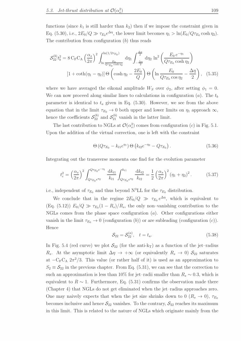
5.3. Jet-thrust distribution at O(α2s) 109
functions (since k1 is still harder than k2) then if we impose the constraint given in
Eq. (5.30), i.e., 2E0/Q ≫ τE0e∆η, the lower limit becomes η1 > ln(E0/QτE0 cosh η2).
The contribution from configuration (b) thus reads
S(b)22 t
2b = 8CFCA
(αs
2π
)2 ∫ ln(1/2τE0)
lnE0
QτE0cosh η2
dη1
∫ ∆η2
−∆η2
dη2 ln2
(E0 e
−η1
QτE0 cosh η2
)
[1 + coth(η1 − η2)]Θ
(cosh η2 −
2E0
Q
)Θ
(ln
E0
QτE0 cos η2− ∆η
2
), (5.35)
where we have averaged the eikonal amplitude WS over φ2, after setting φ1 = 0.
We can now proceed along similar lines to calculations in configuration (a). The tb
parameter is identical to ta given in Eq. (5.30). However, we see from the above
equation that in the limit τE0 → 0 both upper and lower limits on η1 approach ∞,
hence the coefficients S(b)22 and S(b)
21 vanish in the latter limit.
The last contribution to NGLs at O(α2s) comes from configuration (c) in Fig. 5.1.
Upon the addition of the virtual correction, one is left with the constraint
Θ (QτE0 − kt1eη1) Θ
(kt2e
−η2 −QτE0
). (5.36)
Integrating out the transverse momenta one find for the evolution parameter
t2c =(αs
2π
)2 ∫ QτE0e−η1
QτE0eη2
dkt1kt1
∫ kt1
QτE0eη2
dkt2kt2
=1
2
(αs
2π
)2(η1 + η2)
2 . (5.37)
i.e., independent of τE0 and thus beyond N3LL for the τE0 distribution.
We conclude that in the regime 2E0/Q ≫ τE0 e∆η, which is equivalent to
(Eq. (5.12)) E0/Q ≫ τE0(1 − Rs)/Rs, the only non–vanishing contribution to the
NGLs comes from the phase space configuration (a). Other configurations either
vanish in the limit τE0 → 0 (configuration (b)) or are subleading (configuration (c)).
Hence
S22 = S(a)22 , t = ta. (5.38)
In Fig. 5.4 (red curve) we plot S22 (for the anti-kT) as a function of the jet–radius
Rs. At the asymptotic limit ∆η → +∞ (or equivalently Rs → 0) S22 saturates
at −CFCA 2π2/3. This value (or rather half of it) is used as an approximation to
S2 ≡ S22 in the previous chapter. From Eq. (5.31), we can see that the correction to
such an approximation is less than 10% for jet–radii smaller than Rs ∼ 0.3, which is
equivalent to R ∼ 1. Furthermore, Eq. (5.31) confirms the observation made there
(Chapter 4) that NGLs do not get eliminated when the jet–radius approaches zero.
One may naively expects that when the jet size shrinks down to 0 (Rs → 0), τE0
becomes inclusive and hence S22 vanishes. To the contrary, S22 reaches its maximum
in this limit. This is related to the nature of NGLs which originate mainly from the
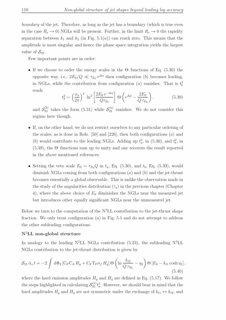
110 Non-global structure of jet shapes beyond leading log accuracy
boundary of the jet. Therefore, as long as the jet has a boundary (which is true even
in the case Rs → 0) NGLs will be present. Further, in the limit Rs → 0 the rapidity
separation between k1 and k2 (in Fig. 5.1(a)) can reach zero. This means that the
amplitude is most singular and hence the phase space integration yields the largest
value of S22.
Few important points are in order:
• If we choose to order the energy scales in the Θ–functions of Eq. (5.30) the
opposite way, i.e., 2E0/Q ≪ τE0 e∆η then configuration (b) becomes leading,
in NGLs, while the contribution from configuration (a) vanishes. That is t2breads
t2b =(αs
2π
)2ln2
[2E0 e
−∆η
QτE0
]Θ
(e∆η − 2E0
QτE0
). (5.39)
and S(b)22 takes the form (5.31) while S(a)
22 vanishes. We do not consider this
regime here though.
• If, on the other hand, we do not restrict ourselves to any particular ordering of
the scales, as is done in Refs. [50] and [226], then both configurations (a) and
(b) would contribute to the leading NGLs. Adding up t2a, in (5.30), and t2b , in
(5.39), the Θ–functions sum up to unity and one recovers the result reported
in the above mentioned references.
• Setting the veto scale E0 ∼ τE0Q in ta, Eq. (5.30), and tb, Eq. (5.39), would
diminish NGLs coming from both configurations (a) and (b) and the jet-thrust
becomes essentially a global observable. This is unlike the observation made in
the study of the angularities distribution (τa) in the previous chapter (Chapter
4), where the above choice of E0 diminishes the NGLs near the measured jet
but introduces other equally significant NGLs near the unmeasured jet.
Below we turn to the computation of the N3LL contribution to the jet-thrust shape
fraction. We only treat configuration (a) in Fig. 5.1 and do not attempt to address
the other subleading configurations.
N3LL non-global structure
In analogy to the leading N2LL NGLs contribution (5.23), the subleading N3LL
NGLs contribution to the jet-thrust distribution is given by
S21 αs t = −2
∫dΦ2 [CFCA Hg + CFTFnf Hq] Θ
(ln
kt2QτE0
− η2
)Θ [E0 − kt1 cosh η1] ,
(5.40)
where the hard emission amplitudes Hg and Hq are defined in Eq. (5.17). We follow
the steps highlighted in calculating S(a)22 t
2a. However, we should bear in mind that the
hard amplitudes Hg and Hq are not symmetric under the exchange of kt1 ↔ kt2, and
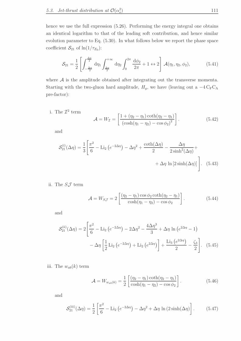
5.3. Jet-thrust distribution at O(α2s) 111
hence we use the full expression (5.26). Performing the energy integral one obtains
an identical logarithm to that of the leading soft contribution, and hence similar
evolution parameter to Eq. (5.30). In what follows below we report the phase space
coefficient S21 of ln(1/τE0):
S21 =1
2
[∫ ∆η2
−∆η2
dη1
∫ +∞
∆η2
dη2
∫ 2π
0
dφ2
2π+ 1 ↔ 2
]A(η1, η2, φ2), (5.41)
where A is the amplitude obtained after integrating out the transverse momenta.
Starting with the two-gluon hard amplitude, Hg, we have (leaving out a −4CFCA
pre-factor):
i. The I2 term
A = WI =
[1 + (η2 − η1) coth(η2 − η1)
(cosh(η1 − η2)− cosφ2)2
]. (5.42)
and
S(i)21 (∆η) =
1
3
[π2
6− Li2
(e−2∆η
)−∆η2 +
coth(∆η)
2− ∆η
2 sinh2(∆η)+
+ ∆η ln [2 sinh(∆η)]
]. (5.43)
ii. The SJ term
A = WSJ = 2
[(η2 − η1) cosφ2 coth(η2 − η1)
cosh(η1 − η2)− cosφ2
]. (5.44)
and
S(ii)21 (∆η) = 2
[π2
6− Li2
(e−2∆η
)− 2∆η2 − 4∆η3
3+ ∆η ln
(e2∆η − 1
)
−∆η
[1
2Li2(e−2∆η
)+ Li2
(e2∆η
)]+
Li3(e2∆η
)
2− ζ3
2
]. (5.45)
iii. The wab(k) term
A = Wwab(k) =1
2
[(η2 − η1) coth(η2 − η1)
cosh(η1 − η2)− cosφ2
]. (5.46)
and
S(iii)21 (∆η) =
1
2
[π2
6− Li2
(e−2∆η
)−∆η2 +∆η ln (2 sinh(∆η)
]. (5.47)
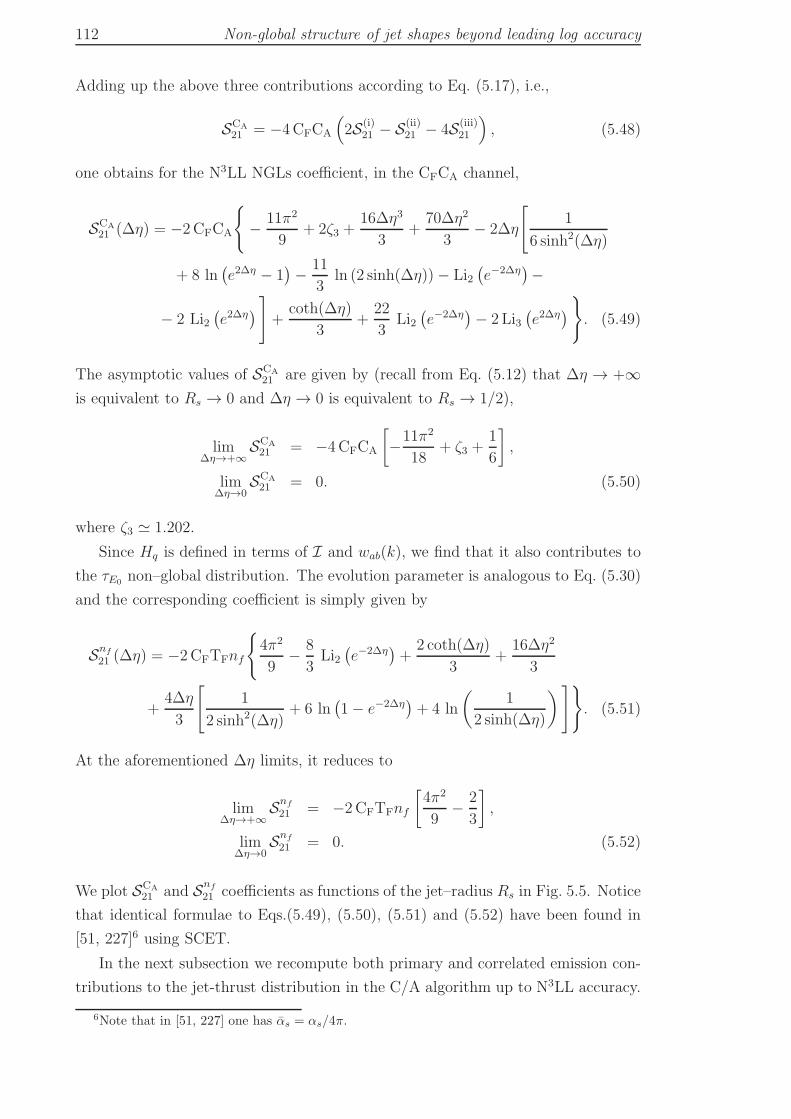
112 Non-global structure of jet shapes beyond leading log accuracy
Adding up the above three contributions according to Eq. (5.17), i.e.,
SCA21 = −4CFCA
(2S(i)
21 − S(ii)21 − 4S(iii)
21
), (5.48)
one obtains for the N3LL NGLs coefficient, in the CFCA channel,
SCA21 (∆η) = −2CFCA
− 11π2
9+ 2ζ3 +
16∆η3
3+
70∆η2
3− 2∆η
[1
6 sinh2(∆η)
+ 8 ln(e2∆η − 1
)− 11
3ln (2 sinh(∆η))− Li2
(e−2∆η
)−
− 2 Li2(e2∆η
)]+
coth(∆η)
3+
22
3Li2(e−2∆η
)− 2 Li3
(e2∆η
). (5.49)
The asymptotic values of SCA21 are given by (recall from Eq. (5.12) that ∆η → +∞
is equivalent to Rs → 0 and ∆η → 0 is equivalent to Rs → 1/2),
lim∆η→+∞
SCA21 = −4CFCA
[−11π2
18+ ζ3 +
1
6
],
lim∆η→0
SCA21 = 0. (5.50)
where ζ3 ≃ 1.202.
Since Hq is defined in terms of I and wab(k), we find that it also contributes to
the τE0 non–global distribution. The evolution parameter is analogous to Eq. (5.30)
and the corresponding coefficient is simply given by
Snf
21 (∆η) = −2CFTFnf
4π2
9− 8
3Li2(e−2∆η
)+
2 coth(∆η)
3+
16∆η2
3
+4∆η
3
[1
2 sinh2(∆η)+ 6 ln
(1− e−2∆η
)+ 4 ln
(1
2 sinh(∆η)
)]. (5.51)
At the aforementioned ∆η limits, it reduces to
lim∆η→+∞
Snf
21 = −2CFTFnf
[4π2
9− 2
3
],
lim∆η→0
Snf
21 = 0. (5.52)
We plot SCA21 and Snf
21 coefficients as functions of the jet–radius Rs in Fig. 5.5. Notice
that identical formulae to Eqs.(5.49), (5.50), (5.51) and (5.52) have been found in
[51, 227]6 using SCET.
In the next subsection we recompute both primary and correlated emission con-
tributions to the jet-thrust distribution in the C/A algorithm up to N3LL accuracy.
6Note that in [51, 227] one has αs = αs/4π.
5.3. Jet-thrust distribution at O(α2s) 113
5.3.2 The C/A algorithm
The definition of the C/A algorithm is given in Algorithm 1 with p = 0 and the
corresponding e+e− version is discussed in Subsec. 5.2.1. Unlike the anti-kT algo-
rithm, which successively merges soft gluons with the nearest hard parton, the C/A
algorithm proceeds by successively clustering soft gluons amongst themselves. Con-
sequently, a soft parton may in many occasions be dragged into (away from) a jet
region and hence contributing (not contributing) to the invariant mass of the latter.
The jet mass, and hence τE0, distribution is then modified. It is these modifications,
due to soft–gluons self–clustering, that we shall address below.
Any clustering–induced contribution to the τE0 distribution will only arise from
phase space configurations where the two soft gluons, k1 and k2, are initially (that
is, before applying the clustering) in different regions of phase space. Configurations
where both gluons are within the same jet region, gluon k1 is in one of the two jet
regions and gluon k2 is in the other, or both gluons are within the interjet region
are not altered by clustering and calculations of the corresponding contributions
will yield identical results to the anti-kT algorithm. We can therefore write the τE0
distribution in the C/A algorithm, at O(α2s), as
Σ(2)C/A(τE0, E0) = Σ
(2)anti–kT
(τE0 , E0) + Σ(2)clus(τE0 , E0). (5.53)
It is the last term in Eq. (5.53) that we compute in the present section.
Independent emission
Since we are aiming at N3LL accuracy we will be taking into account hard emis-
sion contributions through employing the full Altarelli–Parisi splitting kernel for
the emission of a gluon, with momentum fraction x, off a quark; Pgq(x) =
[1 + (1− x)2] /x, and integrating over the full phase space including regions with
x1 ∼ x2. We follow the steps outlined in the previous subsection, Subsec. 5.3.1 and
Eq. (5.25), to achieve this. Like WS (5.16), the independent emission amplitude
(5.15) is symmetric under the exchange of the two gluons and we simply consider
one ordering, say x1 > x2, and multiply the final answer by two, which cancels
against the factor 1/2 that was introduced to avoid double counting. In fact, in the
two-jet limit we can impose the stronger ordering x1 ≫ x2 and focus on phase space
regions that lead to large logarithms7.
Let the two gluons’ momenta, using the e+e− variables (E, θ, φ), be written as
k1 = ω1 (1, sin θ1 cos φ1, sin θ1 sin φ1, cos θ1) ,
k2 = ω2 (1, sin θ2 cos φ2, sin θ2 sin φ2, cos θ2) , (5.54)
7Comparisons to the NLO program event2 in Sec. 5.5 indicates that corrections to this ap-proximation, if any, are negligible.
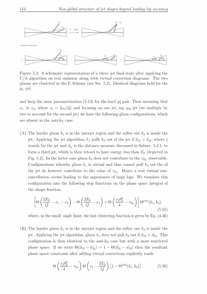
114 Non-global structure of jet shapes beyond leading log accuracy
C−Aalg
k1
k2
k1 + k2
k2k1
k1
k2 k1k2
virtual corrections
+ + +
Figure 5.2: A schematic representation of a three–jet final state after applying theC/A algorithm on real emission along with virtual correction diagrams. The twogluons are clustered in the E–Scheme (see Sec. 5.2). Identical diagrams hold for thepL–jet.
and keep the same parametrisation (5.13) for the hard qq pair. Then assuming that
x1 ≫ x2, where xi = 2ωi/Q, and focusing on one jet, say pR–jet (we multiply by
two to account for the second jet) we have the following gluon configurations, which
are absent in the anti-kT case:
(A) The harder gluon k1 is in the interjet region and the softer one k2 is inside the
jet. Applying the jet algorithm, k1 pulls k2 out of the jet if d12 < d2j , where j
stands for the jet and dij is the distance measure discussed in Subsec. 5.2.1, to
form a third jet, which is then vetoed to have energy less than E0 (depicted in
Fig. 5.2). In the latter case gluon k2 does not contribute to the τE0 observable.
Configurations whereby gluon k1 is virtual and thus cannot pull k2 out the of
the jet do however contribute to the value of τE0 . Hence a real–virtual mis-
cancellation occurs leading to the appearance of large logs. We translate this
configuration into the following step functions on the phase space integral of
the shape fraction,
[Θ
(2E0
Q− x1 − x2
)−Θ
(2E0
Q− x1
)+Θ
(x2θ
22
4− τE0
)]Θclus(k1, k2).
(5.55)
where, in the small–angle limit, the last clustering function is given by Eq. (4.46)
(B) The harder gluon k1 is in the interjet region and the softer one k2 is inside the
jet. Applying the jet algorithm, gluon k1 does not pull k2 out if d12 > d2j. This
configuration is then identical to the anti-kT case but with a more restricted
phase space. If we write Θ(d12 − d2j) = 1 − Θ(d2j − d12) then the resultant
phase space constraint after adding virtual corrections explicitly reads
Θ
(x2θ
22
4− τE0
)Θ
(x1 −
2E0
Q
)[1−Θclus(k1, k2)
]. (5.56)
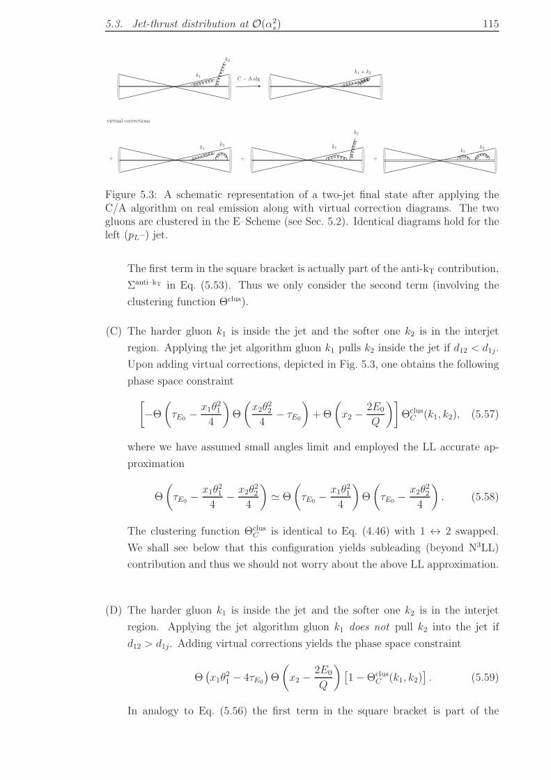
5.3. Jet-thrust distribution at O(α2s) 115
C−Aalgk1
k2
k1 + k2
k2
k1k1k2
k1k2
virtual corrections
+ + +
Figure 5.3: A schematic representation of a two-jet final state after applying theC/A algorithm on real emission along with virtual correction diagrams. The twogluons are clustered in the E–Scheme (see Sec. 5.2). Identical diagrams hold for theleft (pL–) jet.
The first term in the square bracket is actually part of the anti-kT contribution,
Σanti–kT in Eq. (5.53). Thus we only consider the second term (involving the
clustering function Θclus).
(C) The harder gluon k1 is inside the jet and the softer one k2 is in the interjet
region. Applying the jet algorithm gluon k1 pulls k2 inside the jet if d12 < d1j.
Upon adding virtual corrections, depicted in Fig. 5.3, one obtains the following
phase space constraint
[−Θ
(τE0 −
x1θ21
4
)Θ
(x2θ
22
4− τE0
)+Θ
(x2 −
2E0
Q
)]Θclus
C (k1, k2), (5.57)
where we have assumed small angles limit and employed the LL accurate ap-
proximation
Θ
(τE0 −
x1θ21
4− x2θ
22
4
)≃ Θ
(τE0 −
x1θ21
4
)Θ
(τE0 −
x2θ22
4
). (5.58)
The clustering function ΘclusC is identical to Eq. (4.46) with 1 ↔ 2 swapped.
We shall see below that this configuration yields subleading (beyond N3LL)
contribution and thus we should not worry about the above LL approximation.
(D) The harder gluon k1 is inside the jet and the softer one k2 is in the interjet
region. Applying the jet algorithm gluon k1 does not pull k2 into the jet if
d12 > d1j. Adding virtual corrections yields the phase space constraint
Θ(x1θ
21 − 4τE0
)Θ
(x2 −
2E0
Q
)[1−Θclus
C (k1, k2)]. (5.59)
In analogy to Eq. (5.56) the first term in the square bracket is part of the
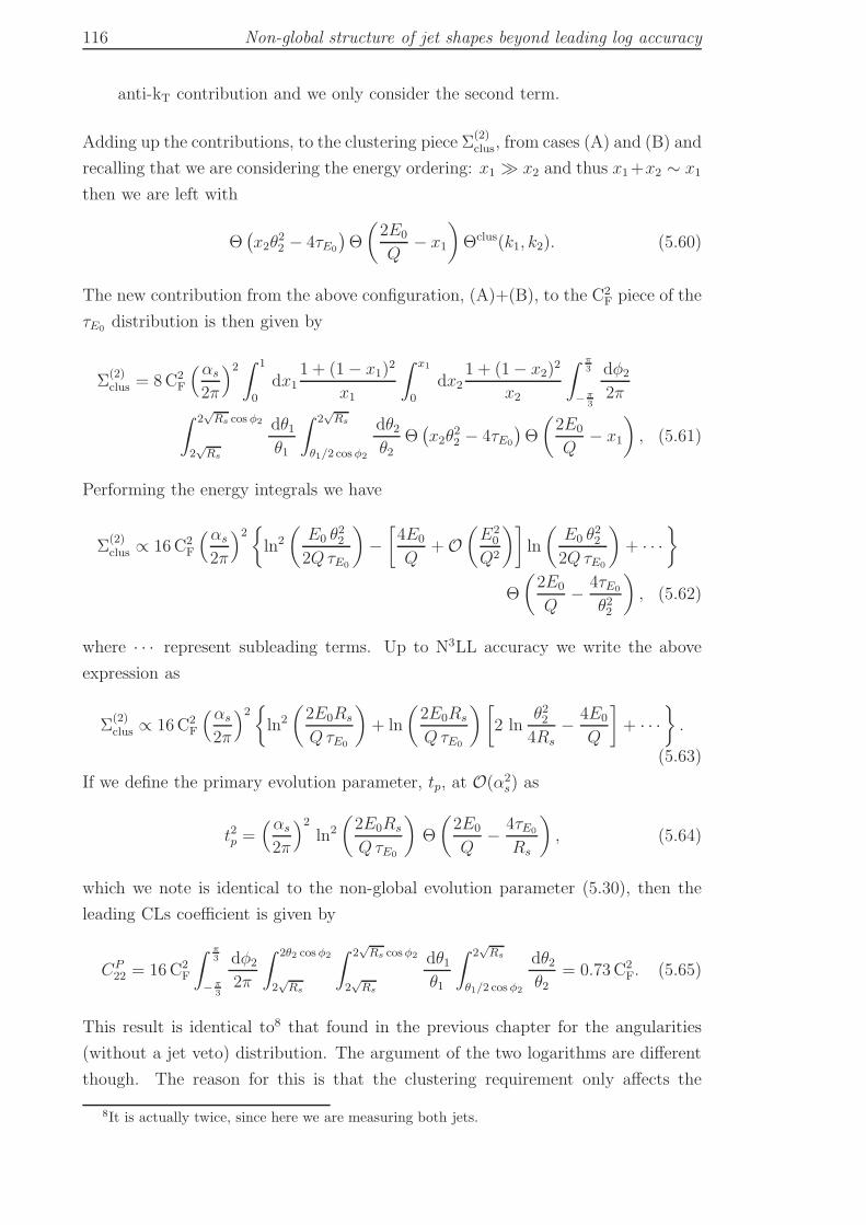
116 Non-global structure of jet shapes beyond leading log accuracy
anti-kT contribution and we only consider the second term.
Adding up the contributions, to the clustering piece Σ(2)clus, from cases (A) and (B) and
recalling that we are considering the energy ordering: x1 ≫ x2 and thus x1+x2 ∼ x1
then we are left with
Θ(x2θ
22 − 4τE0
)Θ
(2E0
Q− x1
)Θclus(k1, k2). (5.60)
The new contribution from the above configuration, (A)+(B), to the C2F piece of the
τE0 distribution is then given by
Σ(2)clus = 8C2
F
(αs
2π
)2 ∫ 1
0
dx11 + (1− x1)
2
x1
∫ x1
0
dx21 + (1− x2)
2
x2
∫ π3
−π3
dφ2
2π∫ 2
√Rs cos φ2
2√Rs
dθ1θ1
∫ 2√Rs
θ1/2 cosφ2
dθ2θ2
Θ(x2θ
22 − 4τE0
)Θ
(2E0
Q− x1
), (5.61)
Performing the energy integrals we have
Σ(2)clus ∝ 16C2
F
(αs
2π
)2ln2
(E0 θ
22
2QτE0
)−[4E0
Q+O
(E2
0
Q2
)]ln
(E0 θ
22
2QτE0
)+ · · ·
Θ
(2E0
Q− 4τE0
θ22
), (5.62)
where · · · represent subleading terms. Up to N3LL accuracy we write the above
expression as
Σ(2)clus ∝ 16C2
F
(αs
2π
)2ln2
(2E0Rs
QτE0
)+ ln
(2E0Rs
QτE0
)[2 ln
θ224Rs
− 4E0
Q
]+ · · ·
.
(5.63)
If we define the primary evolution parameter, tp, at O(α2s) as
t2p =(αs
2π
)2ln2
(2E0Rs
QτE0
)Θ
(2E0
Q− 4τE0
Rs
), (5.64)
which we note is identical to the non-global evolution parameter (5.30), then the
leading CLs coefficient is given by
CP22 = 16C2
F
∫ π3
−π3
dφ2
2π
∫ 2θ2 cosφ2
2√Rs
∫ 2√Rs cosφ2
2√Rs
dθ1θ1
∫ 2√Rs
θ1/2 cosφ2
dθ2θ2
= 0.73C2F. (5.65)
This result is identical to8 that found in the previous chapter for the angularities
(without a jet veto) distribution. The argument of the two logarithms are different
though. The reason for this is that the clustering requirement only affects the
8It is actually twice, since here we are measuring both jets.
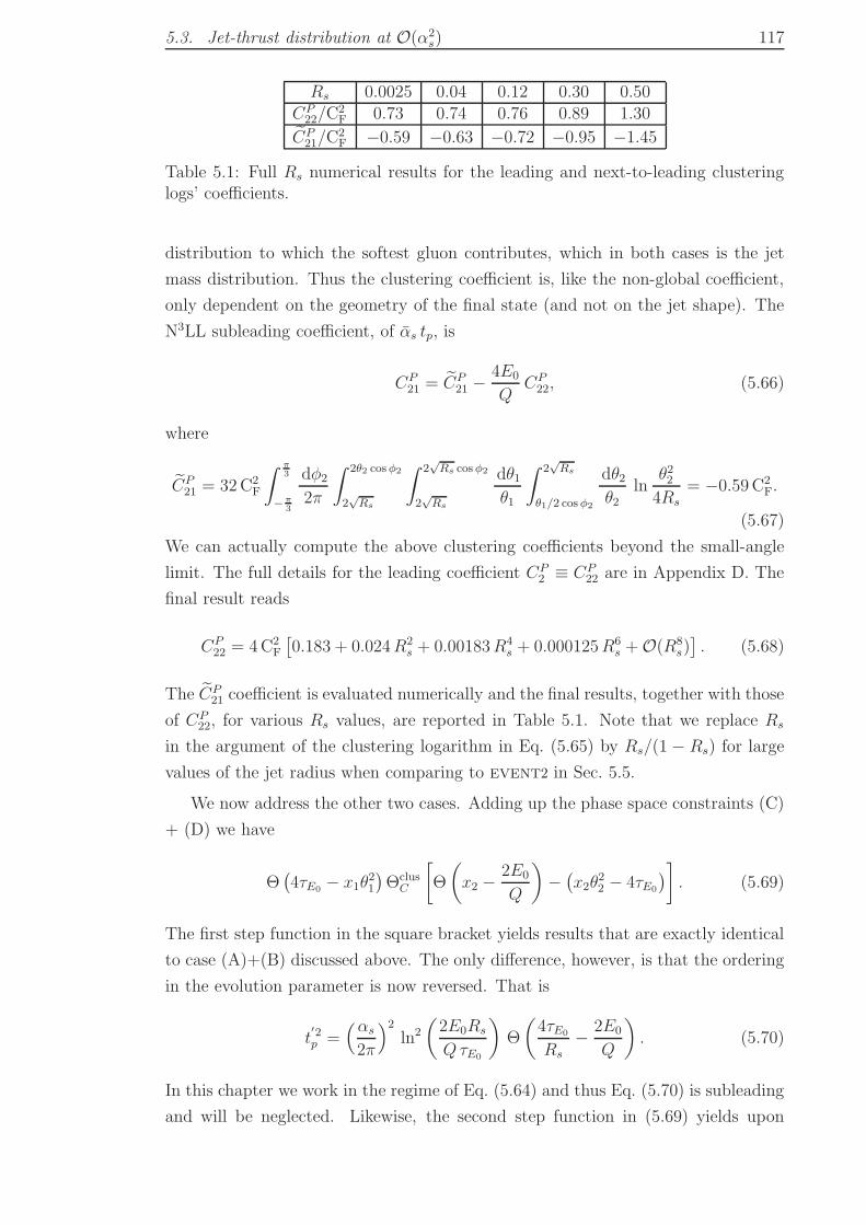
5.3. Jet-thrust distribution at O(α2s) 117
Rs 0.0025 0.04 0.12 0.30 0.50CP
22/C2F 0.73 0.74 0.76 0.89 1.30
CP21/C
2F −0.59 −0.63 −0.72 −0.95 −1.45
Table 5.1: Full Rs numerical results for the leading and next-to-leading clusteringlogs’ coefficients.
distribution to which the softest gluon contributes, which in both cases is the jet
mass distribution. Thus the clustering coefficient is, like the non-global coefficient,
only dependent on the geometry of the final state (and not on the jet shape). The
N3LL subleading coefficient, of αs tp, is
CP21 = CP
21 −4E0
QCP
22, (5.66)
where
CP21 = 32C2
F
∫ π3
−π3
dφ2
2π
∫ 2θ2 cosφ2
2√Rs
∫ 2√Rs cosφ2
2√Rs
dθ1θ1
∫ 2√Rs
θ1/2 cosφ2
dθ2θ2
lnθ224Rs
= −0.59C2F.
(5.67)
We can actually compute the above clustering coefficients beyond the small-angle
limit. The full details for the leading coefficient CP2 ≡ CP
22 are in Appendix D. The
final result reads
CP22 = 4C2
F
[0.183 + 0.024R2
s + 0.00183R4s + 0.000125R6
s +O(R8s)]. (5.68)
The CP21 coefficient is evaluated numerically and the final results, together with those
of CP22, for various Rs values, are reported in Table 5.1. Note that we replace Rs
in the argument of the clustering logarithm in Eq. (5.65) by Rs/(1 − Rs) for large
values of the jet radius when comparing to event2 in Sec. 5.5.
We now address the other two cases. Adding up the phase space constraints (C)
+ (D) we have
Θ(4τE0 − x1θ
21
)Θclus
C
[Θ
(x2 −
2E0
Q
)−(x2θ
22 − 4τE0
)]. (5.69)
The first step function in the square bracket yields results that are exactly identical
to case (A)+(B) discussed above. The only difference, however, is that the ordering
in the evolution parameter is now reversed. That is
t′2p =
(αs
2π
)2ln2
(2E0Rs
QτE0
)Θ
(4τE0
Rs
− 2E0
Q
). (5.70)
In this chapter we work in the regime of Eq. (5.64) and thus Eq. (5.70) is subleading
and will be neglected. Likewise, the second step function in (5.69) yields upon
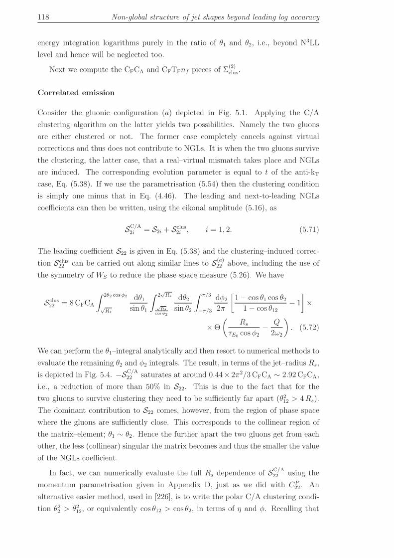
118 Non-global structure of jet shapes beyond leading log accuracy
energy integration logarithms purely in the ratio of θ1 and θ2, i.e., beyond N3LL
level and hence will be neglected too.
Next we compute the CFCA and CFTFnf pieces of Σ(2)clus.
Correlated emission
Consider the gluonic configuration (a) depicted in Fig. 5.1. Applying the C/A
clustering algorithm on the latter yields two possibilities. Namely the two gluons
are either clustered or not. The former case completely cancels against virtual
corrections and thus does not contribute to NGLs. It is when the two gluons survive
the clustering, the latter case, that a real–virtual mismatch takes place and NGLs
are induced. The corresponding evolution parameter is equal to t of the anti-kT
case, Eq. (5.38). If we use the parametrisation (5.54) then the clustering condition
is simply one minus that in Eq. (4.46). The leading and next-to-leading NGLs
coefficients can then be written, using the eikonal amplitude (5.16), as
SC/A2i = S2i + Sclus
2i , i = 1, 2. (5.71)
The leading coefficient S22 is given in Eq. (5.38) and the clustering–induced correc-
tion Sclus22 can be carried out along similar lines to S(a)
22 above, including the use of
the symmetry of WS to reduce the phase space measure (5.26). We have
Sclus22 = 8CFCA
∫ 2θ2 cosφ2
√Rs
dθ1sin θ1
∫ 2√Rs
√Rs
cosφ2
dθ2sin θ2
∫ π/3
−π/3
dφ2
2π
[1− cos θ1 cos θ2
1− cos θ12− 1
]×
×Θ
(Rs
τE0 cos φ2− Q
2ω2
). (5.72)
We can perform the θ1–integral analytically and then resort to numerical methods to
evaluate the remaining θ2 and φ2 integrals. The result, in terms of the jet–radius Rs,
is depicted in Fig. 5.4. −SC/A22 saturates at around 0.44×2π2/3CFCA ∼ 2.92CFCA,
i.e., a reduction of more than 50% in S22. This is due to the fact that for the
two gluons to survive clustering they need to be sufficiently far apart (θ212 > 4Rs).
The dominant contribution to S22 comes, however, from the region of phase space
where the gluons are sufficiently close. This corresponds to the collinear region of
the matrix–element; θ1 ∼ θ2. Hence the further apart the two gluons get from each
other, the less (collinear) singular the matrix becomes and thus the smaller the value
of the NGLs coefficient.
In fact, we can numerically evaluate the full Rs dependence of SC/A22 using the
momentum parametrisation given in Appendix D, just as we did with CP22. An
alternative easier method, used in [226], is to write the polar C/A clustering condi-
tion θ22 > θ212, or equivalently cos θ12 > cos θ2, in terms of η and φ. Recalling that
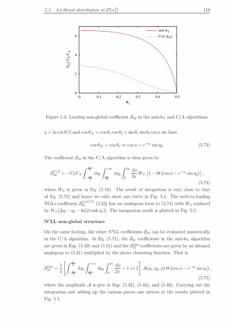
5.3. Jet-thrust distribution at O(α2s) 119
0
2
4
6
0 0.1 0.2 0.3 0.4 0.5
-S22/
CF C
A
Rs
anti-kT
C/A (kT)
Figure 5.4: Leading non-global coefficient S22 in the anti-kT and C/A algorithms.
η = ln cot θ/2 and cos θ12 = cos θ1 cos θ2 + sin θ1 sin θ2 cosφ we have
cos θ12 > cos θ2 ⇒ cos φ > e−η1 sin η2. (5.73)
The coefficient S22 in the C/A algorithm is then given by
SC/A22 = −CFCA
∫ ∆η2
−∆η2
dη1
∫ +∞
∆η2
dη2
∫ 2π
0
dφ
2πWS
[1−Θ
(cosφ− e−η1 sin η2
)],
(5.74)
where WS is given in Eq. (5.16). The result of integration is very close to that
of Eq. (5.72) and hence we only show one curve in Fig. 5.4. The next-to-leading
NGLs coefficient S(a),C/A21 (5.32) has an analogous form to (5.74) with WS replaced
by WS [∆η − η2 − ln(2 cosh η1)]. The integration result is plotted in Fig. 5.5.
N3LL non-global structure
On the same footing, the other N3LL coefficients S21 can be evaluated numerically
in the C/A algorithm. In Eq. (5.71), the S21 coefficients in the anti-kT algorithm
are given in Eqs. (5.49) and (5.51) and the Sclus21 coefficients are given by an integral
analogous to (5.41) multiplied by the above clustering function. That is
Sclus21 =
1
2
[∫ ∆η2
−∆η2
dη1
∫ +∞
∆η2
dη2
∫ 2π
0
dφ
2π+ 1 ↔ 2
]A(η1, η2, φ) Θ
(cosφ− e−η1 sin η2
),
(5.75)
where the amplitude A is give in Eqs. (5.42), (5.44), and (5.46). Carrying out the
integration and adding up the various pieces one arrives at the results plotted in
Fig. 5.5.
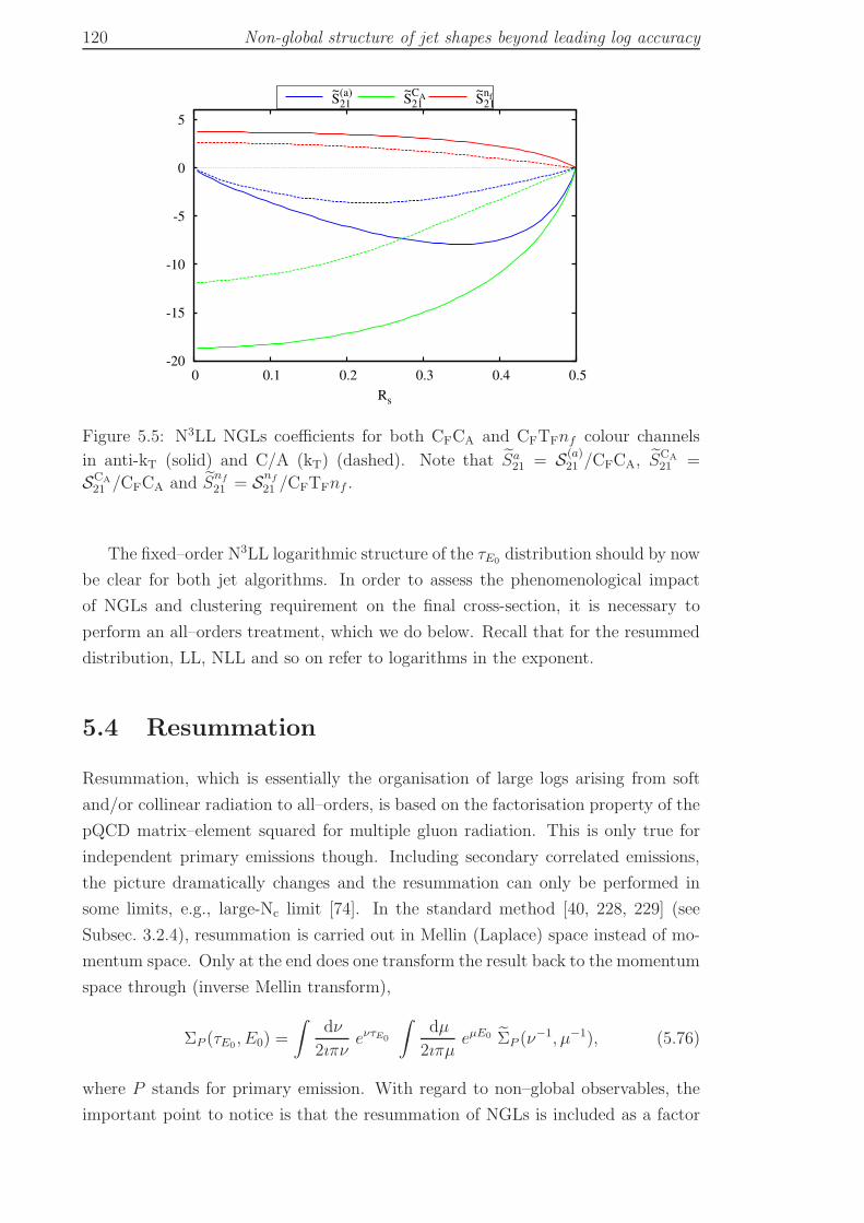
120 Non-global structure of jet shapes beyond leading log accuracy
-20
-15
-10
-5
0
5
0 0.1 0.2 0.3 0.4 0.5
Rs
S~(a)
21 S~CA
21 S~nf
21
Figure 5.5: N3LL NGLs coefficients for both CFCA and CFTFnf colour channels
in anti-kT (solid) and C/A (kT) (dashed). Note that Sa21 = S(a)
21 /CFCA, SCA21 =
SCA21 /CFCA and S
nf
21 = Snf
21 /CFTFnf .
The fixed–order N3LL logarithmic structure of the τE0 distribution should by now
be clear for both jet algorithms. In order to assess the phenomenological impact
of NGLs and clustering requirement on the final cross-section, it is necessary to
perform an all–orders treatment, which we do below. Recall that for the resummed
distribution, LL, NLL and so on refer to logarithms in the exponent.
5.4 Resummation
Resummation, which is essentially the organisation of large logs arising from soft
and/or collinear radiation to all–orders, is based on the factorisation property of the
pQCD matrix–element squared for multiple gluon radiation. This is only true for
independent primary emissions though. Including secondary correlated emissions,
the picture dramatically changes and the resummation can only be performed in
some limits, e.g., large-Nc limit [74]. In the standard method [40, 228, 229] (see
Subsec. 3.2.4), resummation is carried out in Mellin (Laplace) space instead of mo-
mentum space. Only at the end does one transform the result back to the momentum
space through (inverse Mellin transform),
ΣP (τE0 , E0) =
∫dν
2ıπνeντE0
∫dµ
2ıπµeµE0 ΣP (ν
−1, µ−1), (5.76)
where P stands for primary emission. With regard to non–global observables, the
important point to notice is that the resummation of NGLs is included as a factor
5.4. Resummation 121
multiplying the single–gluon Sudakov form factor ΣP (as described in Subsec. 3.2.2);
Σ (τE0 , E0) = ΣP (τE0 , E0) S (t) , (5.77)
In this section, we first consider resummation of τE0 distribution in events where
the final state jets are defined in the anti-kT algorithm and, second, discuss the
potential changes to the resummed result when the jets are defined in the C/A
algorithm instead.
5.4.1 The anti-kT algorithm
As stated in the introduction and proved in Sec. 5.2, the τE0 observable is simply
the sum of the invariant masses of the two highest–energy (or highest–pT for hadron
colliders) jets. Therefore the τE0 resummed Sudakov form factor is just double that
computed in Subsec. 4.4.1 for a = 0. That is, up to NLL level we have
ΣP (τE0 , E0) =exp
[−2(RτE0
(τE0) + γER′τE0
(τE0))]
Γ(1 + 2R′
τE0(τE0)
) exp [−RE0(E0)] . (5.78)
The full derivation of (5.78) as well as the resultant expressions of the various
radiators are presented in the small jet–radius limit in Chapter 4. To restore the
full Rs dependence we make the replacement R2/ρ → Rs/(τE0(1 − Rs)) such that
when expanded Eq. (5.78) reproduces at O(αs) the LO distribution (5.8).
To account for the NGLs at all–orders in αs, it is necessary to consider an arbi-
trary ensemble of energy–ordered, soft wide–angle gluons that coherently radiate a
softest gluon into the vetoed region of phase space [2]9. The analytical resummation
of NGLs is then plagued with mathematical problems coming from the geometric
and colour structure of the gluon ensemble. Two methods have been developed to
address this issue: A numerical Monte Carlo evaluation [2, 176] and a non–linear
evolution equation that resums single logs (SL) at all–orders [71]. Both methods are
only valid in the large-Nc limit. In the latter limit and for small values of the jet–
radius Rs, we argued in the previous chapter that the form of S(t) should be identical
to that found in the hemisphere jet mass case [2]. Since in the present chapter we
are not confined to the small Rs limit, we need to modify and re–run the Monte
Carlo algorithm of Ref. [2], for medium and large values of the jet–radius should
we seek to resum the τE0 NGLs distribution. We do this in Subsec. 5.4.3, where we
consider the all–orders distribution in the anti-kT and discuss modifications due to
clustering.
However when comparing the analytical results of Sec. 5.2 and Sec. 5.3 with
9In our case the vetoed region is the jet region. Due to symmetry, we can choose one jet regionand multiply the final answer by a factor of two.

122 Non-global structure of jet shapes beyond leading log accuracy
fixed–order NLO program event2 , it suffices to simply exponentiate the fixed–
order terms S22, Eq. (5.38), and S21, Eqs. (5.32) + (5.49) + (5.51),
S(t) = exp(S22 t
2 + S21 αs t). (5.79)
The distribution (5.77) is of the generic form given in Eq. (1.3). Explicitly, it
reads
Σ(τE0 , E0) =
(1 +
∞∑
k=1
Ck
(αs
2π
)k)exp
[ ∞∑
n=1
n+1∑
m=0
Gnm
(αs
2π
)nLm
]+Dfin(τE0),
(5.80)
where Ck is the kth loop–constant, L = ln(1/τE0) and Dfin ≡ D (where D is given
in (1.3)), which vanishes in the limit τE0 → 0. In order to determine the coefficients
Gnm at NLO and up to N3LL, we need to expand the radiators, as well as the Γ
function, in Eq. (5.78) up to second order in the fixed coupling αs. The results are
presented in Appendix C.2. The only missing piece in the N3LL coefficient, G21 in
Eq. (C.7), are the coefficients of L which are independent of ln(Rs/(1−Rs)) for all
colour channels. These can be borrowed from thrust distribution [194, 227, 230]10. It
is worthwhile mentioning that the two–loop constant C2 has also been computed for
the latter variable as well as the thrust [194, 227]. Moreover, to make contact with
SCET calculations, we provide in Appendix C.3 the full formula of the Sudakov form
factor for the τE0 primary distribution including determination of Gnm coefficients
in SCET up to N3LL.
Next we comment on the form of resummation when final state jets are defined
in the C/A algorithm.
5.4.2 The C/A algorithm
With regard to primary emission piece, resumming logs induced by clustering is
a cumbersome but doable task. It has been performed, for example, in [3] for
interjet energy flow distribution where final state jets are defined in the inclusive kT
algorithm. The final result of the resummed radiator was written as an expansion in
the jet–radius and the first three terms were determined. For secondary emissions,
the resummation of NGLs has only been possible numerically and in the large-Nc
limit. It has again been carried out for the above mentioned energy flow distribution
in [75]. We expect that analogous, to the interjet energy flow, analytical treatment
and numerical evaluation can be achieved for the resummation of CLs and NGLs,
respectively, for the τE0 variable. While we postpone the analytical resummation
of CLs to the next chapter (Chapter 6), we provide in this section the all–orders
numerical results for both logarithms.
10All Rs–dependent terms are captured as can be seen from comparison to the SCET result(C.3), which only contains the primary emission piece and is valid to N3LL.
5.4. Resummation 123
Due to the fact that logarithmic contributions induced by clustering arise mainly
from soft wide–angle gluons, we expect them, i.e., clustering–induced logs, to fac-
torise from the primary Sudakov form factor at all–orders. Therefore, the resummed
distribution, whereby clustering is imposed on the final state, may be written in the
following factorised form
Σ(τE0 , E0) = ΣP (τE0 , E0)SC/A (t) CP (t) , (5.81)
where we recall that the evolution parameter of CP , Eq. (5.64), is identical to that
of the non-global factor S, Eq. (5.30). We investigate the numerical impact of the
above resummed distribution in the next subsection, Subsec. 5.4.3. However, for the
sake of comparison to event2 , it is sufficient to simply consider the exponentiation
of the fixed–order terms SC/A22 ,SC/A
21 , CP22 and CP
21, just as we did with the anti-kT
algorithm case. In other words, we write SC/A in the form (5.79) with S22,S21
replaced by SC/A22 ,SC/A
21 and, in analogy with the NGLs factor (5.79), we write for
the τE0 CLs factor
CP (t) = exp(CP
22 t2 + CP
21αs t). (5.82)
The resultant Gnm coefficients in the exponent of Eq. (5.81) are presented in Ap-
pendix C.2 (Eqs. (C.7) and (C.10)).
5.4.3 All-orders numerical studies
As stated above, non-global logs have hitherto only been resummed numerically
using the program of [2, 3] in the large-Nc limit, both in anti-kT and other jet
algorithms. Although there have been analytical attempts to resum clustering logs
at all–orders, which we shall discuss in detail in the next chapter, in this subsection
we confine ourselves to only provide numerical estimates using the said program.
To this end, we parametrise the non-global factor S(t) in any given jet algorithm by
the formula [2]
S(t) = exp
[−CFCA I22(Rs)
(1 + (at)2
1 + (bt)c
)t2], (5.83)
where I22(Rs) = S22/CFCA. In Table 5.2 we provide the corresponding values of I22
along with a, b and c for several jet radii in both anti-kT and kT (instead of C/A since
it is currently the only available algorithm in the program besides the anti-kT as
stated at the outset) algorithms. Due to the similarity of CLs and NGLs; being only
present for non-global observables and first appear at O(α2s), we opt to parametrise
the all–orders factor CP (t), Eq. (5.81), by an analogous formula to Eq. (5.83),
CP (t) = exp
[C2
F CP22(Rs)
(1 + (at)2
1 + (bt)c
)t2]. (5.84)
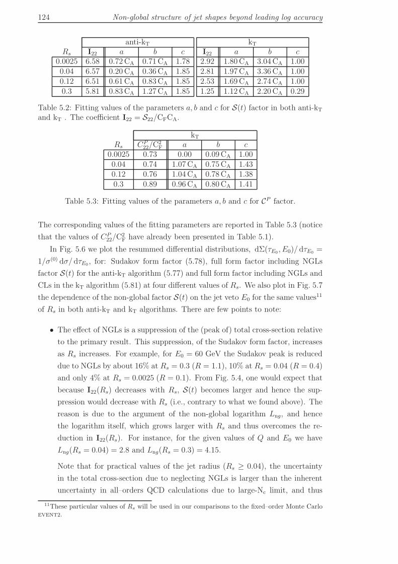
124 Non-global structure of jet shapes beyond leading log accuracy
anti-kTRs I22 a b c
0.0025 6.58 0.72CA 0.71CA 1.780.04 6.57 0.20CA 0.36CA 1.850.12 6.51 0.61CA 0.83CA 1.850.3 5.81 0.83CA 1.27CA 1.85
kTI22 a b c2.92 1.80CA 3.04CA 1.002.81 1.97CA 3.36CA 1.002.53 1.69CA 2.74CA 1.001.25 1.12CA 2.20CA 0.29
Table 5.2: Fitting values of the parameters a, b and c for S(t) factor in both anti-kTand kT . The coefficient I22 = S22/CFCA.
kTRs CP
22/C2F a b c
0.0025 0.73 0.00 0.09CA 1.000.04 0.74 1.07CA 0.75CA 1.430.12 0.76 1.04CA 0.78CA 1.380.3 0.89 0.96CA 0.80CA 1.41
Table 5.3: Fitting values of the parameters a, b and c for CP factor.
The corresponding values of the fitting parameters are reported in Table 5.3 (notice
that the values of CP22/C
2F have already been presented in Table 5.1).
In Fig. 5.6 we plot the resummed differential distributions, dΣ(τE0 , E0)/ dτE0 =
1/σ(0) dσ/ dτE0 , for: Sudakov form factor (5.78), full form factor including NGLs
factor S(t) for the anti-kT algorithm (5.77) and full form factor including NGLs and
CLs in the kT algorithm (5.81) at four different values of Rs. We also plot in Fig. 5.7
the dependence of the non-global factor S(t) on the jet veto E0 for the same values11
of Rs in both anti-kT and kT algorithms. There are few points to note:
• The effect of NGLs is a suppression of the (peak of) total cross-section relative
to the primary result. This suppression, of the Sudakov form factor, increases
as Rs increases. For example, for E0 = 60 GeV the Sudakov peak is reduced
due to NGLs by about 16% at Rs = 0.3 (R = 1.1), 10% at Rs = 0.04 (R = 0.4)
and only 4% at Rs = 0.0025 (R = 0.1). From Fig. 5.4, one would expect that
because I22(Rs) decreases with Rs, S(t) becomes larger and hence the sup-
pression would decrease with Rs (i.e., contrary to what we found above). The
reason is due to the argument of the non-global logarithm Lng, and hence
the logarithm itself, which grows larger with Rs and thus overcomes the re-
duction in I22(Rs). For instance, for the given values of Q and E0 we have
Lng(Rs = 0.04) = 2.8 and Lng(Rs = 0.3) = 4.15.
Note that for practical values of the jet radius (Rs ≥ 0.04), the uncertainty
in the total cross-section due to neglecting NGLs is larger than the inherent
uncertainty in all–orders QCD calculations due to large-Nc limit, and thus
11These particular values of Rs will be used in our comparisons to the fixed–order Monte Carloevent2.
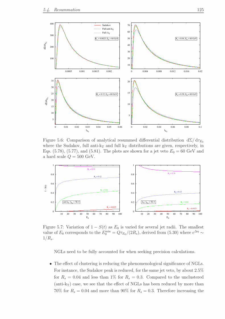
5.4. Resummation 125
100
200
300
400
0.0005 0.001 0.0015 0.002
dΣ/
dτ E
0
Sudakov
Full:anti-kT
Full: kT
Rs = 0.0025, E0 = 60 GeV
10
20
30
40
50
60
70
0 0.004 0.008 0.012 0.016 0.02
Rs = 0.04, E0 = 60 GeV
5
10
15
20
25
30
35
0 0.01 0.02 0.03 0.04 0.05 0.06
dΣ/
dτ E
0
τE0
Rs = 0.12, E0 = 60 GeV
5
10
15
20
0 0.02 0.04 0.06 0.08 0.1
τE0
Rs = 0.30, E0 = 60 GeV
Figure 5.6: Comparison of analytical resummed differential distribution dΣ/ dτE0
where the Sudakov, full anti-kT and full kT distributions are given, respectively, inEqs. (5.78), (5.77), and (5.81). The plots are shown for a jet veto E0 = 60 GeV anda hard scale Q = 500 GeV.
0
0.2
0.4
0.6
0.8
1
10 20 30 40 50 60 70 80 90 100
1 -
S(t
)
E0
Rs = 0.0025
Rs = 0.04
Rs = 0.12
Rs = 0.30
ant-kT: τE0 = 5E-4
0
0.2
0.4
0.6
0.8
1
10 20 30 40 50 60 70 80 90 100
E0
Rs = 0.0025
Rs = 0.04
Rs = 0.12
Rs = 0.30
kT: τE0 = 5E-4
Figure 5.7: Variation of 1 − S(t) as E0 is varied for several jet radii. The smallestvalue of E0 corresponds to the Emin
0 = QτE0/(2Rs), derived from (5.30) where e∆η ∼1/Rs.
NGLs need to be fully accounted for when seeking precision calculations.
• The effect of clustering is reducing the phenomenological significance of NGLs.
For instance, the Sudakov peak is reduced, for the same jet veto, by about 2.5%
for Rs = 0.04 and less than 1% for Rs = 0.3. Compared to the unclustered
(anti-kT) case, we see that the effect of NGLs has been reduced by more than
70% for Rs = 0.04 and more than 90% for Rs = 0.3. Therefore increasing the
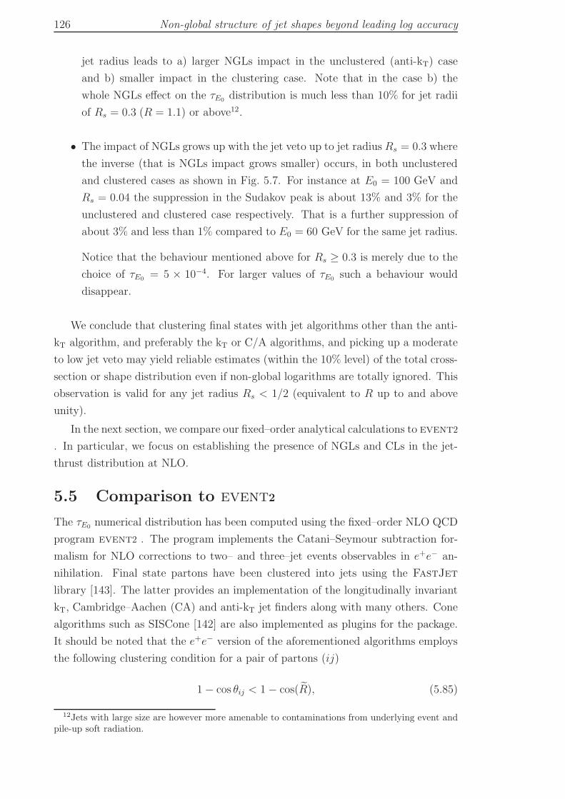
126 Non-global structure of jet shapes beyond leading log accuracy
jet radius leads to a) larger NGLs impact in the unclustered (anti-kT) case
and b) smaller impact in the clustering case. Note that in the case b) the
whole NGLs effect on the τE0 distribution is much less than 10% for jet radii
of Rs = 0.3 (R = 1.1) or above12.
• The impact of NGLs grows up with the jet veto up to jet radius Rs = 0.3 where
the inverse (that is NGLs impact grows smaller) occurs, in both unclustered
and clustered cases as shown in Fig. 5.7. For instance at E0 = 100 GeV and
Rs = 0.04 the suppression in the Sudakov peak is about 13% and 3% for the
unclustered and clustered case respectively. That is a further suppression of
about 3% and less than 1% compared to E0 = 60 GeV for the same jet radius.
Notice that the behaviour mentioned above for Rs ≥ 0.3 is merely due to the
choice of τE0 = 5 × 10⁻⁴. For larger values of τE0 such a behaviour would
disappear.
We conclude that clustering final states with jet algorithms other than the anti-
kT algorithm, and preferably the kT or C/A algorithms, and picking up a moderate
to low jet veto may yield reliable estimates (within the 10% level) of the total cross-
section or shape distribution even if non-global logarithms are totally ignored. This
observation is valid for any jet radius Rs < 1/2 (equivalent to R up to and above
unity).
In the next section, we compare our fixed–order analytical calculations to event2
. In particular, we focus on establishing the presence of NGLs and CLs in the jet-
thrust distribution at NLO.
5.5 Comparison to event2
The τE0 numerical distribution has been computed using the fixed–order NLO QCD
program event2 . The program implements the Catani–Seymour subtraction for-
malism for NLO corrections to two– and three–jet events observables in e+e− an-
nihilation. Final state partons have been clustered into jets using the FastJet
library [143]. The latter provides an implementation of the longitudinally invariant
kT, Cambridge–Aachen (CA) and anti-kT jet finders along with many others. Cone
algorithms such as SISCone [142] are also implemented as plugins for the package.
It should be noted that the e+e− version of the aforementioned algorithms employs
the following clustering condition for a pair of partons (ij)
1− cos θij < 1− cos(R), (5.85)
12Jets with large size are however more amenable to contaminations from underlying event andpile-up soft radiation.
5.5. Comparison to event2 127
-40
-20
0
20
40
-14 -12 -10 -8 -6 -4 -2 0
r(L
)
L = Ln(τE0)
Rs = 2.5E-3
Rs = 0.04
Rs = 0.12
Rs = 0.30
anti-kT: LO, E0 = 0.01 Q
-40
-20
0
20
40
-14 -12 -10 -8 -6 -4 -2 0
L = Ln(τE0)
C/A: LO, E0 = 0.01 Q
Figure 5.8: The difference between event2 and τE0 LO distribution for various jetradii in both anti-kT (left) and C/A (right) algorithms.
where R is the jet–radius parameter used in FastJet 13. Compared to Eqs. (5.2)
and (5.3), R = cos−1(1−2Rs). The exact numerical distributions (1/σ(0))( dσe/ dL),
with L = −L = ln(τE0), for the three colour channels, C2F,CFCA and CFTFnf , have
been obtained with 1011 events in the bin range −14 < L < 0. We have used four
values for the jet–radius: Rs = 0.30, Rs = 0.12, Rs = 0.04 and Rs = 0.0025, with an
energy veto E0 = 0.01Q. Standard deviations on individual bins range from 10−4%
to 10−2%.
We plot the difference between the numerical and analytical distributions at both
LO and NLO,
r(L) =dσe
σ(0) dL− dσr,2
σ(0) dL, (5.86)
where 1/σ(0) dσr,2/ dL is given in Eq. (C.13). Recall that at small values of the jet
shape, τE0 , the finite remainder function Dfin(τE0) in Eq. (5.80) is vanishingly small
and will thus be ignored. If our analytical calculations of the NGLs coefficients for
both anti-kT and C/A algorithms are correct then r(L) should asymptotically vanish
for all colour channels. We plot our results in Figs. 5.8, 5.9 and, for each radius
Rs separately, in Figs. C.1, C.2 and C.3. Overall, the cancellation in Eq. (5.86) is,
within statistical errors, reasonably good for all three colour channels and at most
values of the jet radius considered. Few comments are in order:
• At LO, the distribution is independent of the jet definition. The kinks in
Fig. 5.8 correspond to the maximum values of τE0 (τmaxE0
(Rs) given in Eq. (5.9))
that are kinematically allowed. Notice that the exact LO distribution vanishes
for τE0 > τmaxE0
and the straight lines for τE0 > τmaxE0
are simply the analytical
results.
• At NLO, the asymptotic region, i.e., the region where large logs are expected
to dominate over non–logarithmic contributions, corresponds to L less than
13In FastJet ’s manual R is allowed to go up to π. Since we are interested in two-jet eventsthe jet size cannot be wider than a hemisphere. Thus we restrict R to be less than π/2.
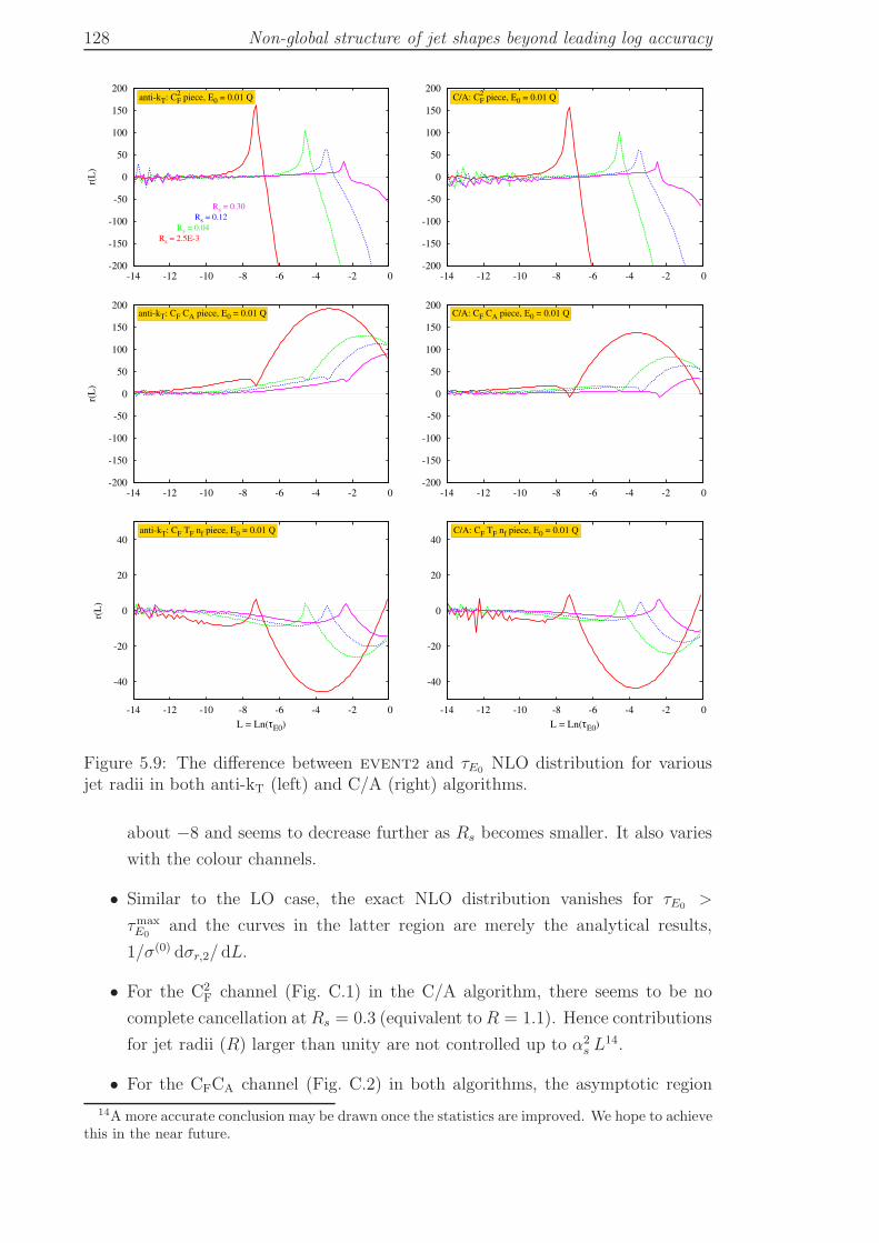
128 Non-global structure of jet shapes beyond leading log accuracy
-200
-150
-100
-50
0
50
100
150
200
-14 -12 -10 -8 -6 -4 -2 0
r(L
)
Rs = 2.5E-3
Rs = 0.04
Rs = 0.12
Rs = 0.30
anti-kT: C2F piece, E0 = 0.01 Q
-200
-150
-100
-50
0
50
100
150
200
-14 -12 -10 -8 -6 -4 -2 0
C/A: C2F piece, E0 = 0.01 Q
-200
-150
-100
-50
0
50
100
150
200
-14 -12 -10 -8 -6 -4 -2 0
r(L
)
anti-kT: CF CA piece, E0 = 0.01 Q
-200
-150
-100
-50
0
50
100
150
200
-14 -12 -10 -8 -6 -4 -2 0
C/A: CF CA piece, E0 = 0.01 Q
-40
-20
0
20
40
-14 -12 -10 -8 -6 -4 -2 0
r(L
)
L = Ln(τE0)
anti-kT: CF TF nf piece, E0 = 0.01 Q
-40
-20
0
20
40
-14 -12 -10 -8 -6 -4 -2 0
L = Ln(τE0)
C/A: CF TF nf piece, E0 = 0.01 Q
Figure 5.9: The difference between event2 and τE0 NLO distribution for variousjet radii in both anti-kT (left) and C/A (right) algorithms.
about −8 and seems to decrease further as Rs becomes smaller. It also varies
with the colour channels.
• Similar to the LO case, the exact NLO distribution vanishes for τE0 >
τmaxE0
and the curves in the latter region are merely the analytical results,
1/σ(0) dσr,2/ dL.
• For the C2F channel (Fig. C.1) in the C/A algorithm, there seems to be no
complete cancellation atRs = 0.3 (equivalent toR = 1.1). Hence contributions
for jet radii (R) larger than unity are not controlled up to α2s L
14.
• For the CFCA channel (Fig. C.2) in both algorithms, the asymptotic region
14A more accurate conclusion may be drawn once the statistics are improved. We hope to achievethis in the near future.
5.6. Conclusion 129
starts at values of L that are about or smaller than −14 for jet radii Rs < 0.04.
i.e., out of our reach. The shift of the asymptotic region towards smaller values
of L as Rs decreases is clear in the above mentioned figures (Fig. C.2).
• The results for the CFTFnf channel (Fig. C.3) in both algorithms are more
pronounced (than for the other channels), again with the observation that the
asymptotic region shifts towards smaller values of L as Rs decreases.
In summary, we have confirmed through explicit comparisons to exact numerical
distributions the existence of large NGLs and large CLs for the τE0 distribution
at N2LL and beyond (in the expansion). We have also shown that clustering the
final state partons with the C/A algorithm yielded a significant reduction in NGLs
impact, both at N2LL and beyond, albeit inducing large CLs, both at N2LL and
beyond, in the primary emission sector.
5.6 Conclusion
The jet mass with a jet veto, or simply the jet-thrust, is an example of a wider
class of non–global observables. These have the characteristic of being sensitive
to radiation into restricted regions of phase space, or sensitive to radiation into
the whole phase space but differently in different regions. For such observables
the universal Sudakov form factor fails to reproduce the full logarithmic structure
even at NLL (in the exponent) accuracy. New contributions that are dependent on
various variables such as the jet size and jet definition appear at this logarithmic
level and beyond. In this chapter, we have elaborated on these very contributions
for the aforementioned observable.
Considering secondary emissions, we have computed the full analytical expres-
sions of the first leading and next-to-leading terms, S22 and S21, in a series of missing
large non-global logarithms. The coefficients depend, as anticipated, on the jet size
and saturate at their maxima in the limit where the latter, i.e., jet size, vanishes.
The saturation value of S22 was used in Chapter 4 as an approximation to the full
value in the small Rs limit. It turns out that the approximation is valid for quite a
wide range of Rs. The formulae for S22 and S21 have been checked against full exact
numerical result obtained by the program event2 . The difference between the an-
alytical and numerical differential distributions was shown to asymptotically vanish
signalling a complete cancellation of singular terms up to N3LL (in the expansion)
level. This has all been done for final states defined in the cone–like anti-kT jet
algorithm.
To illustrate the dependence of N2LL (in the expansion) and beyond on the jet
definition, we have investigated the effects of applying the C/A algorithm on e+e−
final states. The impact of soft partons clustering is two–fold. On one side, it
reduces the size of NGLs through shrinking the phase space region where the latter
130 Non-global structure of jet shapes beyond leading log accuracy
dominantly come from. i.e., the region where the emitter and emitted soft partons
are just in and just out of the jet. On the other side, it gives rise to new N2LL, and
beyond, logarithmic contributions, CLs, in the primary emission sector. We have
computed the full Rs dependence of the corresponding coefficients, CP22 at N2LL
and CP21 at N3LL, at second order, which were then verified against event2 . With
regard to jet definitions, the kT and C/A algorithms behave identically at O(α2s)
with respect to non-global and clustering logs.
Furthermore, we have provided a resummation of the jet-thrust up to NLL (in
the exponent) accuracy with full jet radius dependence in both anti-kT and kT jet
algorithms in e+e− annihilation events. Non-global as well as clustering logs logs
in both algorithms have been obtained with the aid of the numerical program of
Ref. [2] (with clustering added in [3]), in the large-Nc limit. It has been observed
that the size, and hence the impact of non-global logarithms on the Sudakov form
factor for the jet-thrust is controlled by few factors, including: jet radius, jet veto
and jet definition. Within our accuracy we have been able to conclude that using
a jet definition other than the ant-kT, such as kT or C/A, with reasonably low to
medium jet vetos would diminish the effect of non-global logs for jet radii up to 1,
and above (such that the uncertainty from neglecting non-global logs is within the
10% uncertainty level inherent from large-Nc approximation).
Further, we note that the Monte Carlo program of [2] only provides the leading
non-global, and clustering, logs (which are next-to-leading logs in the jet-thrust).
Since we have fully outlined the N3LL structure of non-global, and clustering logs,
at fixed–order, it would be interesting to extend the above program to include them
at all–orders. i.e., resum non-global logs at NLL (in the exponent) accuracy (which
is N2LL accuracy for the jet-thrust). We investigate this more in future.
In the next chapter we present an attempt to analytically resum clustering log-
arithms that occur in the jet mass distribution at all–orders in both kT and C/A
algorithms.
Chapter 6
On the resummation of clustering
logarithms
6.1 Introduction
In the presence of a jet algorithm, other than anti-kT [73], non-global observables
suffer from large logs in the Abelian part of the emission amplitude, as we have seen
in the previous chapters. We referred to these as “clustering logs” (CLs). These
logs were first computed analytically at fixed order and numerically to all–orders
in Ref. [74] and subsequently partially analytically resummed in Ref. [3] for away-
from–jets energy (Et) flow. There, however, the resulting exponent of the resummed
distribution has been written as a power-series in the radius parameter1 of the jet
algorithm R starting from R3. Thus for a typical jet radius (R ∼ 1) it was sufficient,
for an accurate approximation, to compute the first couple of terms (O(R3) and
O(R5)), as the series rapidly converges. Excellent agreement was noticed when
compared to the output of the Monte Carlo program developed in [2].
Clustering logs arise due to mis-cancellation between real emissions and virtual
corrections. This mis-cancellation results from re-clustering of final-state configura-
tions of soft gluons. Unlike the single-log Et distribution, resummation of clustering
logs in the jet mass distribution cannot simply be written as a power-series in the jet
radius. Collinear singularities at the boundary of a small-R jet yields large logs in
the radius parameter, which appear to all–orders in αs (see Chapters 4 and 5). Note
that the jet veto distribution, studied in the latter chapters, disentangles from the
jet mass distribution to all–orders [177] and has a non-global structure analogous to
the Et distribution. That is, the coefficients of both non-global and clustering logs
are identical for the jet veto and Et distributions. The arguments of the logs are
different though, as explicitly shown in Chapter 5.
The clustering logs have recently been the subject of much study both at fixed
order and to all–orders. However there has been no full resummation to all–orders
and it was recently suggested that it is unlikely that such logs be fully resummed
even to their leading log level, which means NLL accuracy relative to leading double
1It is actually a series in t R where (at fixed–order) t = αs/2π ln(Q/Q0), with Q and Q0 beingthe hard and veto scales, and is typically in the range t ∈ [0, 0.25].
131
132 On the resummation of clustering logarithms
logs (in jet mass distribution) [178, 231]. In the SCET framework [41, 42, 232]
the authors of Ref. [178] confirmed the findings of Ref. [84] (Chapter 4 for a =
0), regarding CLs coefficient at O(α2s), and computed the full R-dependence of
the jet mass distribution at O(α2s). They also pointed out the unlikelihood of the
resummation of the clustering logs to all–orders.
In the preceding chapter (Chapter 5) the resummation of the jet mass distribu-
tion for e+e− annihilation, in the anti-kT and C/A (kT) algorithms, was performed
to all–orders including the non-global and clustering components in large-Nc limit.
Employing the anti-kT clustering algorithm meant that the observable definition
was linear in transverse momenta of soft emissions and therefore the resummation
involved no clustering logs. In the same chapter we also carried out a fixed-order
calculation for the jet mass distribution at O(α2s) employing the C/A (kT) algo-
rithm [149, 210] and provided a numerical estimate of the all–orders factor with full
R dependence.
We present here an expression for the all–orders resummed result of clustering
logs to NLL accuracy in the kT and C/A algorithms [147, 149] for the jet mass dis-
tribution. The logs that we control take the form Fn αns L
n (n ≥ 2) in the exponent
of the resummed distribution, and we only compute F2, F3 and F4 in this chapter.
By comparing our findings to the output of the Monte Carlo of Refs. [2, 3] we show
that missing higher-order terms are negligible. We also show that the impact of the
primary-emission single clustering logs is of maximum order 5% for typical jet radii.
Furthermore, we estimate the non-global (clustering-induced) contribution to the
jet mass distribution in the large-Nc limit using the said Monte Carlo in the case of
the kT algorithm.
This chapter is organised as follows. In the next section we define the jet mass
and show how different algorithms affect its distribution at NLL level. We then
start with the impact of kT and C/A algorithms on the jet mass distribution at
O(α2s), thus confirming the findings of Ref. [84] (Chapter 4 for a = 0). In Sec. 6.4
we compute higher-order clustering terms and notice that they exhibit a pattern
of exponentiation. By making an anstaz of higher-order clustering-log terms we
perform a resummation of the clustering logs to all–orders in Sec. 6.5 and compare
our findings to the output of the said Monte Carlo program in Sec. 6.6. We also
perform a numerical estimate of the non-global logs in the large-Nc limit for the
jet mass distribution in the kT algorithm in Subsec. 6.6.1. Finally we draw our
conclusions and point to future work in Sec. 6.7.
6.2. The jet mass distribution and clustering algorithms 133
6.2 The jet mass distribution and clustering algo-
rithms
Consider for simplicity the e+e− annihilation into two jets produced back-to-back
with high transverse momenta. We would like to study the single inclusive jet mass
distribution via measuring the invariant mass of one of the final-state jets, M2j , while
leaving the other jet unmeasured. One can restrict inter-jet activity by imposing a
cut Q0 on emissions in this region [44, 45]. For the purpose of this chapter we do
not worry about this issue because the effect of this cut has already been dealt with
in the previous chapters (as well as in [3]) and can be included straightforwardly.
The normalised invariant jet-mass–squared fraction, ρ, is defined by:
ρ =
(∑
i∈jpi
)2
/
(∑
i
Ei
)2
, (6.1)
where pi is the four-momentum of the ith particle and the sum in the numerator
runs over all particles in the measured jet, defined using an infrared and collinear
(IRC)-safe algorithm such as kT or C/A algorithm. At born level the jet mass has
the value zero and it departs from this value at higher orders.
A generic form of general sequential recombination algorithms [73, 143, 147, 149]
was discussed in Chapter 3 (Algorithm 1). For e+e− ahhihilation we employ the
changes discussed in Sec. 5.2. We may write 2(1− cos θij) ≈ θ2ij in the small-angles
limit where jets are narrow and well-separated to avoid correlations, and hence
contamination, between various jets.
In the kT algorithm, softest partons are clustered first according to the above-
mentioned procedure (Algorithm 1), while in the anti-kT algorithm clustering starts
with the hardest partons. In the C/A algorithm only angular separations between
partons matter so clustering starts with the geometrically closest partons. In effect,
clustering induces modifications to the mass of the measured jet due to reshuffling
of soft gluons. Only those gluons which end up in the jet region would contribute
to its mass. Different jet algorithms would then give different values of the jet mass
for the same event.
The global part of the integrated resummed jet mass distribution in the kT (C/A)
algorithm is related to that in the anti-kT algorithm by:
ΣkT(C/A)
(R2
ρ
)= Σanti–kT
(R2
ρ
)exp
[gkT(C/A)2,A
(R2
ρ
)], (6.2)
where Σanti–kT resums the leading double logs (DL) (due to soft and collinear poles
of the emission amplitude) as well as next-to–leading single logs (SL) in the anti–kT
algorithm. The reader is referred to Chapter 4 for further details about this piece.
134 On the resummation of clustering logarithms
The function g2,A contains the new large clustering single logs due to kT (C/A)
clustering.
In addition to the global part, each of the distributions Σanti–kT,kT,C/A receives
its own non-global NLL contribution factor S(R2/ρ). In the anti-kT algorithm the
resummation of the non-global logs in the large-Nc limit for the jet mass distribution
was estimated in Chapters 4 and 5. The result of Chapter 4 was actually shown to
coincide with that of the hemisphere jet mass case. The latter has been available for
quite a while [2, 176]. For kT clustering the effect of non-global logs has been dealt
with numerically in Chapter 5 and [75] and analytically, for example, in the case of
gaps-between–jets Et flow [3]. We expect the gross features of the latter to hold for
the jet mass observable. Essentially, the impact of kT clustering is in such a way as
to reduce the size of the anti-kT (non-clustering) non-global logs. Brief comments
on such a reduction will be given in Subsec. 6.6.1. In this chapter we are, however,
mainly interested in the function g2,A(R2/ρ).
6.3 Two-gluon emission calculation
The effect of kT and C/A clustering logs starts at O(α2s). At O(αs) there is indeed
a dependence on the jet radius but this dependence is also present for the anti-
kT algorithm and has been dealt with in Ref. [84]. In this regard we begin with
two-gluon emission case and study the effect of clustering using both the C/A and
kT algorithms. This calculation has already been performed in Ref. [84] for the kT
algorithm in the small-R limit. Here we perform a full-R calculation of the logs
coefficient.
6.3.1 Calculation in the kT algorithm
Consider the independent emission of two soft energy-ordered gluons k2t2 ≪ k2
t1 ≪Q2, where Q is the hard scale. This regime, i.e., strong energy ordering, is sufficient
to extract the leading clustering logs.
In the case of the anti-kT algorithm discussed in Ref. [84] the only contribution
from these gluons to the jet mass differential distribution is when both of them are
emitted within an angle R from the hard parton initiating the measured jet. This
is because the anti-kT algorithm works in the opposite sense of the kT algorithm:
clustering starts with the hardest particles. In this sense the algorithm essentially
works as a perfect cone around the hard initiating parton with no dragging-in or
dragging-out soft effect.
In the kT algorithm, on the other hand, the two gluons may be in one of the
following four configurations:
1. Both gluons k1 and k2 are initially, i.e., before applying the algorithm, in-
side2 the triggered jet. This configuration contributes to the jet shape (mass)
2We use inside, or simply “in”, to signify that the parton is within an angular separation of R
6.3. Two-gluon emission calculation 135
regardless of clustering. The corresponding contribution to the jet mass dis-
tribution is identical to that of the anti-kT case (accounted for by Σanti–kT –
see Eq. (6.4) below).
2. Both gluons are initially outside the triggered jet. This arrangement does not
contribute to the jet shape regardless of whether the two gluons are clustered
or not.
3. The harder gluon, k1, is initially inside the triggered jet and the softer gluon,
k2, is outside of it. The value of the jet shape (mass) is not changed even
if clustering takes place. This is due to the strong-ordering condition stated
above.
4. The harder gluon, k1, is initially outside the triggered jet and the softer gluon,
k2, is inside of it. Applying the algorithm one finds that a real-virtual mis-
cancellation occurs only if k2 is pulled-out of the triggered-jet vicinity by k1,
a situation which is only possible if k2 is “closer” (in terms of distances dij) to
k1 than to the axis of the jet.
We translate the latter configuration mathematically into the step function:
Ξ2 (k1, k2) = Θ(θ21 − R2)Θ(R2 − θ22)Θ(θ22 − θ212), (6.3)
where θi is the angle between gluon ki and the jet axis and θ12 is the relative
angle of the two gluons. The above condition is valid only in the small-R limit
and we extend this to the full R-dependence in appendix D. Hence Ξ2 = 1 when
configuration 4 above is satisfied and Ξ2 = 0 otherwise. While in the case where the
gluon k1 is virtual and k2 is real (meaning that k1 cannot pull k2 out) the particle
k2 contributes to the jet mass. To the contrary, when both k1 and k2 are real, then
k1 will not allow k2 to contribute to the jet mass as it pulls it out. Thus a real-
virtual mismatch occurs and a tower of large logarithms appears. To calculate these
large logarithms we insert the clustering condition Ξ2 above into the phase-space
of the O(α2s) integrated jet mass distribution. The latter, normalised to the Born
cross-section σ0 is given, in the soft and collinear approximation, by:
ΣkT2
(R2/ρ
)= Σanti–kT
2
(R2/ρ
)+ Σclus
2
(R2/ρ
),
Σclus2
(R2/ρ
)=
1
2!
(−CF
αs
π
)2 ∫dP1dP2 Ξ2 (k1, k2) , (6.4)
from the hard triggered parton (jet axis), and outside, or simply “out”, if it is more than R awayfrom it.
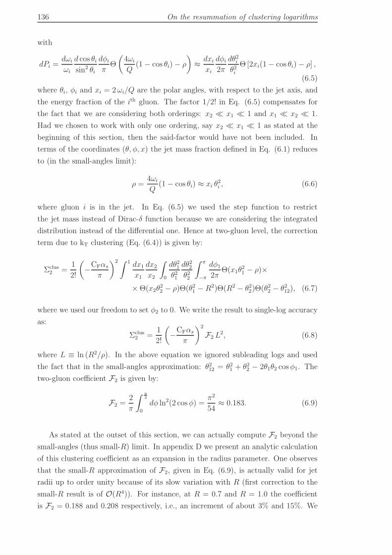
136 On the resummation of clustering logarithms
with
dPi =dωi
ωi
d cos θisin2 θi
dφi
πΘ
(4ωi
Q(1− cos θi)− ρ
)≈ dxi
xi
dφi
2π
dθ2iθ2i
Θ [2xi(1− cos θi)− ρ] ,
(6.5)
where θi, φi and xi = 2ωi/Q are the polar angles, with respect to the jet axis, and
the energy fraction of the ith gluon. The factor 1/2! in Eq. (6.5) compensates for
the fact that we are considering both orderings: x2 ≪ x1 ≪ 1 and x1 ≪ x2 ≪ 1.
Had we chosen to work with only one ordering, say x2 ≪ x1 ≪ 1 as stated at the
beginning of this section, then the said-factor would have not been included. In
terms of the coordinates (θ, φ, x) the jet mass fraction defined in Eq. (6.1) reduces
to (in the small-angles limit):
ρ =4ωi
Q(1− cos θi) ≈ xi θ
2i , (6.6)
where gluon i is in the jet. In Eq. (6.5) we used the step function to restrict
the jet mass instead of Dirac-δ function because we are considering the integrated
distribution instead of the differential one. Hence at two-gluon level, the correction
term due to kT clustering (Eq. (6.4)) is given by:
Σclus2 =
1
2!
(−CFαs
π
)2 ∫ 1 dx1
x1
dx2
x2
∫
0
dθ21θ21
dθ22θ22
∫ π
−π
dφ1
2πΘ(x1θ
21 − ρ)×
×Θ(x2θ22 − ρ)Θ(θ21 − R2)Θ(R2 − θ22)Θ(θ22 − θ212), (6.7)
where we used our freedom to set φ2 to 0. We write the result to single-log accuracy
as:
Σclus2 =
1
2!
(−CFαs
π
)2
F2L2, (6.8)
where L ≡ ln (R2/ρ). In the above equation we ignored subleading logs and used
the fact that in the small-angles approximation: θ212 = θ21 + θ22 − 2θ1θ2 cosφ1. The
two-gluon coefficient F2 is given by:
F2 =2
π
∫ π3
0
dφ ln2(2 cosφ) =π2
54≈ 0.183. (6.9)
As stated at the outset of this section, we can actually compute F2 beyond the
small-angles (thus small-R) limit. In appendix D we present an analytic calculation
of this clustering coefficient as an expansion in the radius parameter. One observes
that the small-R approximation of F2, given in Eq. (6.9), is actually valid for jet
radii up to order unity because of its slow variation with R (first correction to the
small-R result is of O(R4)). For instance, at R = 0.7 and R = 1.0 the coefficient
is F2 = 0.188 and 0.208 respectively, i.e., an increment of about 3% and 15%. We
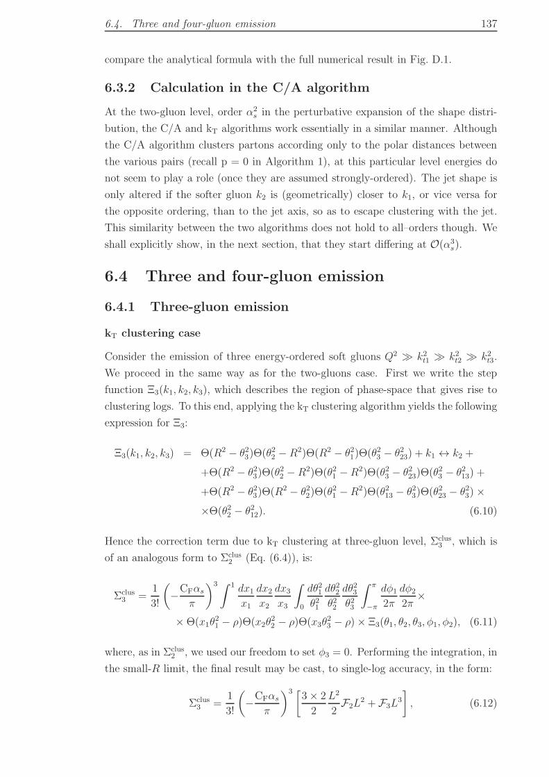
6.4. Three and four-gluon emission 137
compare the analytical formula with the full numerical result in Fig. D.1.
6.3.2 Calculation in the C/A algorithm
At the two-gluon level, order α2s in the perturbative expansion of the shape distri-
bution, the C/A and kT algorithms work essentially in a similar manner. Although
the C/A algorithm clusters partons according only to the polar distances between
the various pairs (recall p = 0 in Algorithm 1), at this particular level energies do
not seem to play a role (once they are assumed strongly-ordered). The jet shape is
only altered if the softer gluon k2 is (geometrically) closer to k1, or vice versa for
the opposite ordering, than to the jet axis, so as to escape clustering with the jet.
This similarity between the two algorithms does not hold to all–orders though. We
shall explicitly show, in the next section, that they start differing at O(α3s).
6.4 Three and four-gluon emission
6.4.1 Three-gluon emission
kT clustering case
Consider the emission of three energy-ordered soft gluons Q2 ≫ k2t1 ≫ k2
t2 ≫ k2t3.
We proceed in the same way as for the two-gluons case. First we write the step
function Ξ3(k1, k2, k3), which describes the region of phase-space that gives rise to
clustering logs. To this end, applying the kT clustering algorithm yields the following
expression for Ξ3:
Ξ3(k1, k2, k3) = Θ(R2 − θ23)Θ(θ22 − R2)Θ(R2 − θ21)Θ(θ23 − θ223) + k1 ↔ k2 +
+Θ(R2 − θ23)Θ(θ22 − R2)Θ(θ21 −R2)Θ(θ23 − θ223)Θ(θ23 − θ213) +
+Θ(R2 − θ23)Θ(R2 − θ22)Θ(θ21 −R2)Θ(θ213 − θ23)Θ(θ223 − θ23)××Θ(θ22 − θ212). (6.10)
Hence the correction term due to kT clustering at three-gluon level, Σclus3 , which is
of an analogous form to Σclus2 (Eq. (6.4)), is:
Σclus3 =
1
3!
(−CFαs
π
)3 ∫ 1 dx1
x1
dx2
x2
dx3
x3
∫
0
dθ21θ21
dθ22θ22
dθ23θ23
∫ π
−π
dφ1
2π
dφ2
2π×
×Θ(x1θ21 − ρ)Θ(x2θ
22 − ρ)Θ(x3θ
23 − ρ)× Ξ3(θ1, θ2, θ3, φ1, φ2), (6.11)
where, as in Σclus2 , we used our freedom to set φ3 = 0. Performing the integration, in
the small-R limit, the final result may be cast, to single-log accuracy, in the form:
Σclus3 =
1
3!
(−CFαs
π
)3 [3× 2
2
L2
2F2L
2 + F3L3
], (6.12)
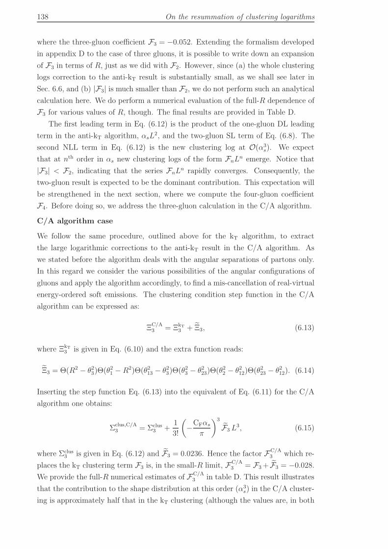
138 On the resummation of clustering logarithms
where the three-gluon coefficient F3 = −0.052. Extending the formalism developed
in appendix D to the case of three gluons, it is possible to write down an expansion
of F3 in terms of R, just as we did with F2. However, since (a) the whole clustering
logs correction to the anti-kT result is substantially small, as we shall see later in
Sec. 6.6, and (b) |F3| is much smaller than F2, we do not perform such an analytical
calculation here. We do perform a numerical evaluation of the full-R dependence of
F3 for various values of R, though. The final results are provided in Table D.
The first leading term in Eq. (6.12) is the product of the one-gluon DL leading
term in the anti-kT algorithm, αsL2, and the two-gluon SL term of Eq. (6.8). The
second NLL term in Eq. (6.12) is the new clustering log at O(α3s). We expect
that at nth order in αs new clustering logs of the form FnLn emerge. Notice that
|F3| < F2, indicating that the series FnLn rapidly converges. Consequently, the
two-gluon result is expected to be the dominant contribution. This expectation will
be strengthened in the next section, where we compute the four-gluon coefficient
F4. Before doing so, we address the three-gluon calculation in the C/A algorithm.
C/A algorithm case
We follow the same procedure, outlined above for the kT algorithm, to extract
the large logarithmic corrections to the anti-kT result in the C/A algorithm. As
we stated before the algorithm deals with the angular separations of partons only.
In this regard we consider the various possibilities of the angular configurations of
gluons and apply the algorithm accordingly, to find a mis-cancellation of real-virtual
energy-ordered soft emissions. The clustering condition step function in the C/A
algorithm can be expressed as:
ΞC/A3 = ΞkT
3 + Ξ3, (6.13)
where ΞkT3 is given in Eq. (6.10) and the extra function reads:
Ξ3 = Θ(R2 − θ23)Θ(θ21 − R2)Θ(θ213 − θ23)Θ(θ23 − θ223)Θ(θ22 − θ212)Θ(θ223 − θ212). (6.14)
Inserting the step function Eq. (6.13) into the equivalent of Eq. (6.11) for the C/A
algorithm one obtains:
Σclus,C/A3 = Σclus
3 +1
3!
(−CFαs
π
)3
F3 L3, (6.15)
where Σclus3 is given in Eq. (6.12) and F3 = 0.0236. Hence the factor FC/A
3 which re-
places the kT clustering term F3 is, in the small-R limit, FC/A3 = F3+ F3 = −0.028.
We provide the full-R numerical estimates of FC/A3 in table D. This result illustrates
that the contribution to the shape distribution at this order (α3s) in the C/A cluster-
ing is approximately half that in the kT clustering (although the values are, in both
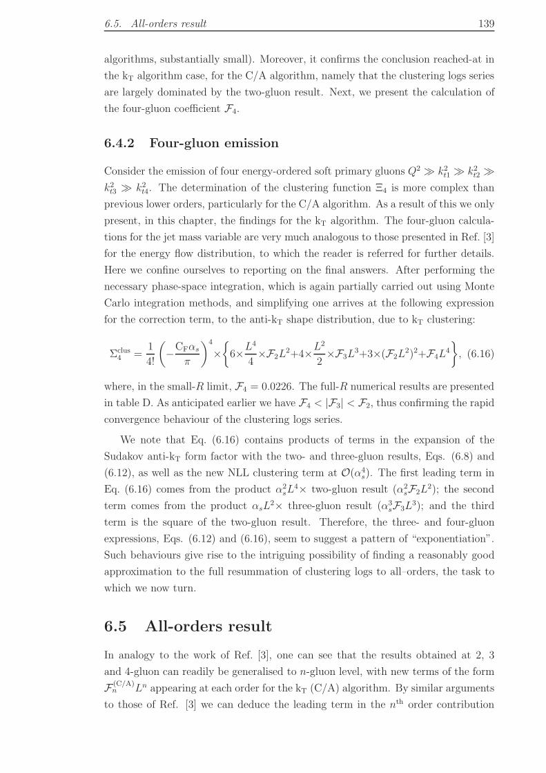
6.5. All-orders result 139
algorithms, substantially small). Moreover, it confirms the conclusion reached-at in
the kT algorithm case, for the C/A algorithm, namely that the clustering logs series
are largely dominated by the two-gluon result. Next, we present the calculation of
the four-gluon coefficient F4.
6.4.2 Four-gluon emission
Consider the emission of four energy-ordered soft primary gluons Q2 ≫ k2t1 ≫ k2
t2 ≫k2t3 ≫ k2
t4. The determination of the clustering function Ξ4 is more complex than
previous lower orders, particularly for the C/A algorithm. As a result of this we only
present, in this chapter, the findings for the kT algorithm. The four-gluon calcula-
tions for the jet mass variable are very much analogous to those presented in Ref. [3]
for the energy flow distribution, to which the reader is referred for further details.
Here we confine ourselves to reporting on the final answers. After performing the
necessary phase-space integration, which is again partially carried out using Monte
Carlo integration methods, and simplifying one arrives at the following expression
for the correction term, to the anti-kT shape distribution, due to kT clustering:
Σclus4 =
1
4!
(−CFαs
π
)4
×6×L4
4×F2L
2+4×L2
2×F3L
3+3×(F2L2)2+F4L
4
, (6.16)
where, in the small-R limit, F4 = 0.0226. The full-R numerical results are presented
in table D. As anticipated earlier we have F4 < |F3| < F2, thus confirming the rapid
convergence behaviour of the clustering logs series.
We note that Eq. (6.16) contains products of terms in the expansion of the
Sudakov anti-kT form factor with the two- and three-gluon results, Eqs. (6.8) and
(6.12), as well as the new NLL clustering term at O(α4s). The first leading term in
Eq. (6.16) comes from the product α2sL
4× two-gluon result (α2sF2L
2); the second
term comes from the product αsL2× three-gluon result (α3
sF3L3); and the third
term is the square of the two-gluon result. Therefore, the three- and four-gluon
expressions, Eqs. (6.12) and (6.16), seem to suggest a pattern of “exponentiation”.
Such behaviours give rise to the intriguing possibility of finding a reasonably good
approximation to the full resummation of clustering logs to all–orders, the task to
which we now turn.
6.5 All-orders result
In analogy to the work of Ref. [3], one can see that the results obtained at 2, 3
and 4-gluon can readily be generalised to n-gluon level, with new terms of the form
F (C/A)n Ln appearing at each order for the kT (C/A) algorithm. By similar arguments
to those of Ref. [3] we can deduce the leading term in the nth order contribution
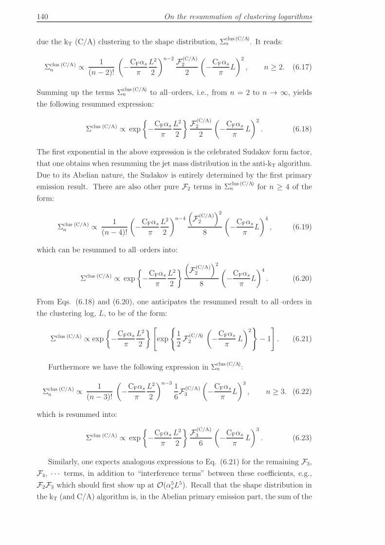
140 On the resummation of clustering logarithms
due the kT (C/A) clustering to the shape distribution, Σclus (C/A)n . It reads:
Σclus (C/A)n ∝ 1
(n− 2)!
(−CFαs
π
L2
2
)n−2 F (C/A)2
2
(−CFαs
πL
)2
, n ≥ 2. (6.17)
Summing up the terms Σclus (C/A)n to all–orders, i.e., from n = 2 to n → ∞, yields
the following resummed expression:
Σclus (C/A) ∝ exp
−CFαs
π
L2
2
F (C/A)2
2
(−CFαs
πL
)2
. (6.18)
The first exponential in the above expression is the celebrated Sudakov form factor,
that one obtains when resumming the jet mass distribution in the anti-kT algorithm.
Due to its Abelian nature, the Sudakov is entirely determined by the first primary
emission result. There are also other pure F2 terms in Σclus (C/A)n for n ≥ 4 of the
form:
Σclus (C/A)n ∝ 1
(n− 4)!
(−CFαs
π
L2
2
)n−4
(F (C/A)
2
)2
8
(−CFαs
πL
)4
, (6.19)
which can be resummed to all–orders into:
Σclus (C/A) ∝ exp
−CFαs
π
L2
2
(F (C/A)
2
)2
8
(−CFαs
πL
)4
. (6.20)
From Eqs. (6.18) and (6.20), one anticipates the resummed result to all–orders in
the clustering log, L, to be of the form:
Σclus (C/A) ∝ exp
−CFαs
π
L2
2
[exp
1
2F (C/A)
2
(−CFαs
πL
)2
− 1
]. (6.21)
Furthermore we have the following expression in Σclus (C/A)n :
Σclus (C/A)n ∝ 1
(n− 3)!
(−CFαs
π
L2
2
)n−31
6F (C/A)
3
(−CFαs
πL
)3
, n ≥ 3. (6.22)
which is resummed into:
Σclus (C/A) ∝ exp
−CFαs
π
L2
2
F (C/A)3
6
(−CFαs
πL
)3
. (6.23)
Similarly, one expects analogous expressions to Eq. (6.21) for the remaining F3,
F4, · · · terms, in addition to “interference terms” between these coefficients, e.g.,
F2F3 which should first show up at O(α5sL
5). Recall that the shape distribution in
the kT (and C/A) algorithm is, in the Abelian primary emission part, the sum of the
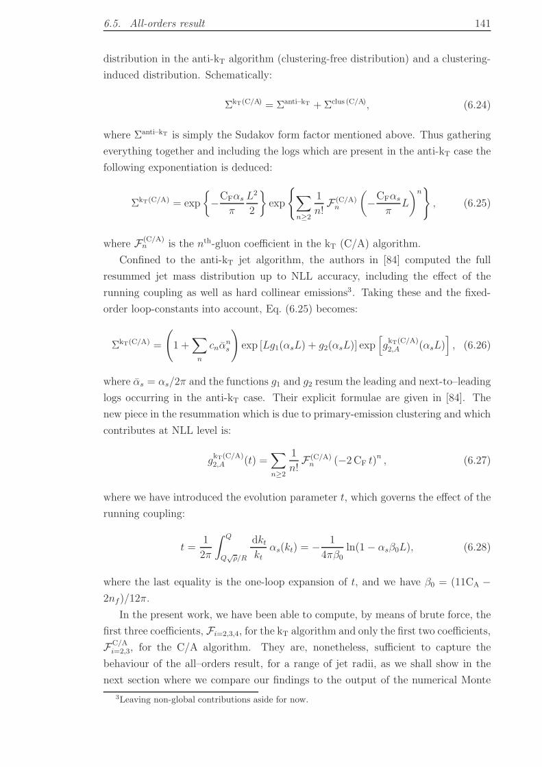
6.5. All-orders result 141
distribution in the anti-kT algorithm (clustering-free distribution) and a clustering-
induced distribution. Schematically:
ΣkT(C/A) = Σanti–kT + Σclus (C/A), (6.24)
where Σanti–kT is simply the Sudakov form factor mentioned above. Thus gathering
everything together and including the logs which are present in the anti-kT case the
following exponentiation is deduced:
ΣkT(C/A) = exp
−CFαs
π
L2
2
exp
∑
n≥2
1
n!F (C/A)
n
(−CFαs
πL
)n, (6.25)
where F (C/A)n is the nth-gluon coefficient in the kT (C/A) algorithm.
Confined to the anti-kT jet algorithm, the authors in [84] computed the full
resummed jet mass distribution up to NLL accuracy, including the effect of the
running coupling as well as hard collinear emissions3. Taking these and the fixed-
order loop-constants into account, Eq. (6.25) becomes:
ΣkT(C/A) =
(1 +
∑
n
cnαns
)exp [Lg1(αsL) + g2(αsL)] exp
[gkT(C/A)2,A (αsL)
], (6.26)
where αs = αs/2π and the functions g1 and g2 resum the leading and next-to–leading
logs occurring in the anti-kT case. Their explicit formulae are given in [84]. The
new piece in the resummation which is due to primary-emission clustering and which
contributes at NLL level is:
gkT(C/A)2,A (t) =
∑
n≥2
1
n!F (C/A)
n (−2CF t)n , (6.27)
where we have introduced the evolution parameter t, which governs the effect of the
running coupling:
t =1
2π
∫ Q
Q√ρ/R
dktkt
αs(kt) = − 1
4πβ0
ln(1− αsβ0L), (6.28)
where the last equality is the one-loop expansion of t, and we have β0 = (11CA −2nf)/12π.
In the present work, we have been able to compute, by means of brute force, the
first three coefficients, Fi=2,3,4, for the kT algorithm and only the first two coefficients,
FC/Ai=2,3, for the C/A algorithm. They are, nonetheless, sufficient to capture the
behaviour of the all–orders result, for a range of jet radii, as we shall show in the
next section where we compare our findings to the output of the numerical Monte
3Leaving non-global contributions aside for now.
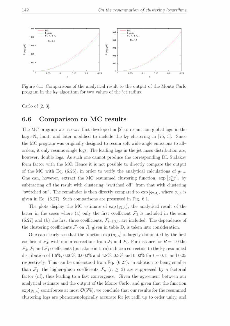
142 On the resummation of clustering logarithms
1
1.01
1.02
1.03
1.04
1.05
0 0.05 0.1 0.15 0.2 0.25
Exp
[g2,A
(t)]
t
R = 0.1
MCF2 onlyF2, F3 & F4
1
1.01
1.02
1.03
1.04
1.05
0 0.05 0.1 0.15 0.2 0.25
Exp
[g2,A
(t)]
t
R = 1.0
MCF2 onlyF2, F3 & F4
Figure 6.1: Comparisons of the analytical result to the output of the Monte Carloprogram in the kT algorithm for two values of the jet radius.
Carlo of [2, 3].
6.6 Comparison to MC results
The MC program we use was first developed in [2] to resum non-global logs in the
large-Nc limit, and later modified to include the kT clustering in [75, 3]. Since
the MC program was originally designed to resum soft wide-angle emissions to all–
orders, it only resums single logs. The leading logs in the jet mass distribution are,
however, double logs. As such one cannot produce the corresponding DL Sudakov
form factor with the MC. Hence it is not possible to directly compare the output
of the MC with Eq. (6.26), in order to verify the analytical calculations of g2,A.
One can, however, extract the MC resummed clustering function, exp[gMC2,A
], by
subtracting off the result with clustering “switched off” from that with clustering
“switched on”. The remainder is then directly compared to exp [g2,A], where g2,A is
given in Eq. (6.27). Such comparisons are presented in Fig. 6.1.
The plots display the MC estimate of exp (g2,A), the analytical result of the
latter in the cases where (a) only the first coefficient F2 is included in the sum
(6.27) and (b) the first three coefficients, Fi=2,3,4, are included. The dependence of
the clustering coefficients Fi on R, given in table D, is taken into consideration.
One can clearly see that the function exp (g2,A) is largely dominated by the first
coefficient F2, with minor corrections from F3 and F4. For instance for R = 1.0 the
F2, F3 and F4 coefficients (put alone in turn) induce a correction to the kT resummed
distribution of 1.6%, 0.06%, 0.002% and 4.8%, 0.3% and 0.02% for t = 0.15 and 0.25
respectively. This can be understood from Eq. (6.27): in addition to being smaller
than F2, the higher-gluon coefficients Fn (n ≥ 3) are suppressed by a factorial
factor (n!), thus leading to a fast convergence. Given the agreement between our
analytical estimate and the output of the Monte Carlo, and given that the function
exp(g2,A) contributes at most O(5%), we conclude that our results for the resummed
clustering logs are phenomenologically accurate for jet radii up to order unity, and

6.6. Comparison to MC results 143
1
1.02
1.04
1.06
1.08
1.1
1.12
1.14
0 0.05 0.1 0.15 0.2 0.25
Exp
[g2,
A(t
)]
t
R = 0.1R = 0.4R = 0.7R = 1.0
R = 1.1R = 1.2R = 1.3
Figure 6.2: The output of the Monte Carlo program in the kT algorithm for variousjet radii.
that missing higher-order coefficients Fn (n ≥ 5) are unimportant.
Lastly, we plot in Fig. 6.2, the MC results of the function exp(g2,A) for various
jet radii. The plots unequivocally indicate that for a fixed t, say 0.15, the function
g2,A varies very slowly with R for R ≤ 1 and grows relatively rapidly as R > 1. Such
a behaviour may be explained by the analytical formula of F2, Eq. (D.10), where
the first correction to the small-R result is proportional to R4.
6.6.1 Non-global logs
As a final task, we plot in Fig. 6.3 the full resummed jet mass distribution in the
kT algorithm, Eq. (6.2), including the non-global factor S(t) in the large-Nc limit,
for various jet radii. In the figure, “Sudakov” refers to the Sudakov anti-kT form
factor (Σanti–kT), “primary” refers to the primary form factor in the kT algorithm
containing the clustering logarithms (ΣkT) in Eq. (6.26), “Full: anti-kT ” refers to
the full anti-kT resummation, Σanti–kT Santi–kT(t) and “Full: kT ” refers to ΣkT SkT(t).
We notice that the inclusion of non-global logs leads to a noticeably large reduction
of the full resummed result for the anti-kT algorithm case, while in the kT algorithm
the reduction is moderate.
As is well-known by now (see Chapters 4 and 5 and Refs. [3, 75, 226]) clustering
reduces the impact of non-global logs through restricting the available phase-space
for their contribution. This is also the case with the jet mass distribution where
we note, for instance, that for t = 0.15 the impact of non-global logs in the kT
algorithm (for R = 0.1, 0.7 and 1.0) is a 24% reduction of the global part, while
in the kT clustering case this is merely 7% (for R = 0.1 and R = 0.7) and 4%
for R = 1.0. We further notice that for small values of the jet radius, S(t) is
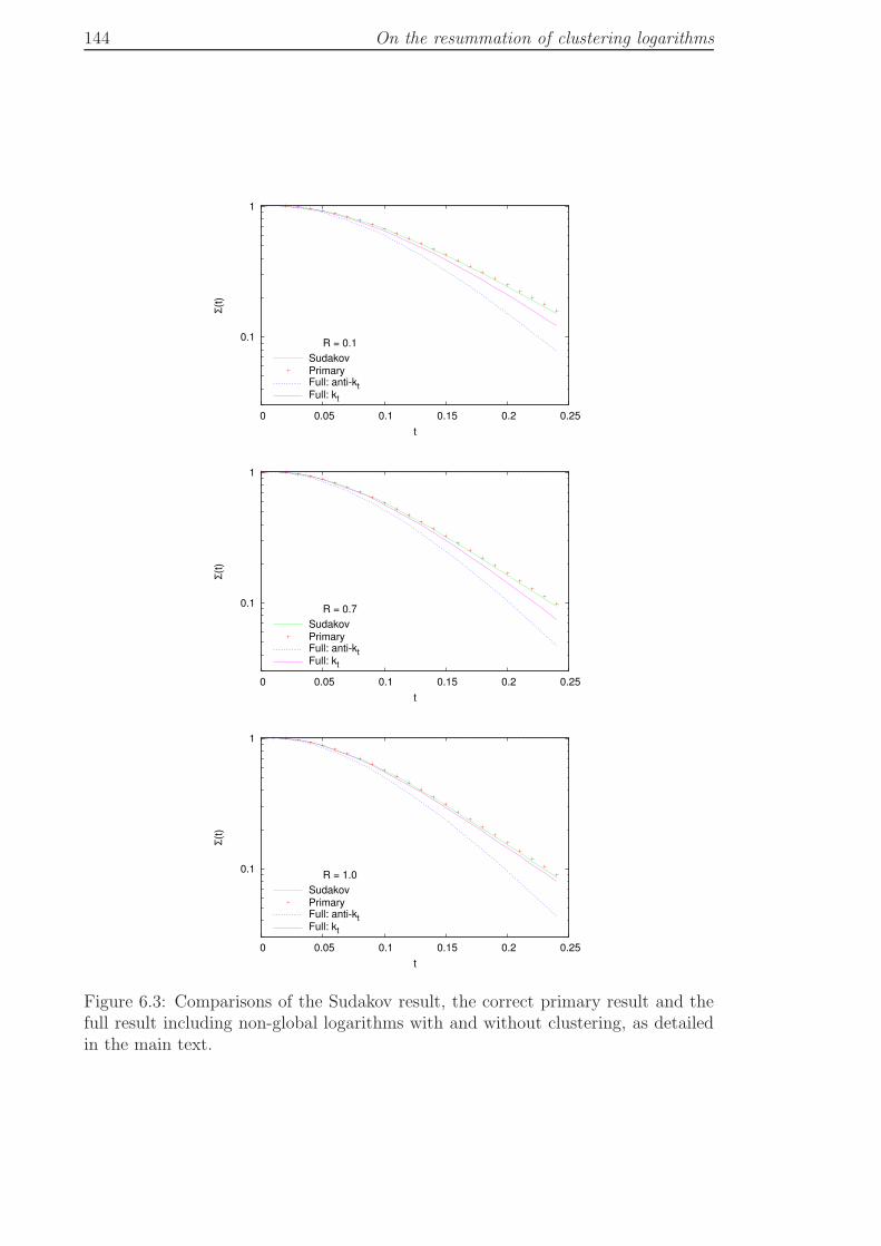
144 On the resummation of clustering logarithms
0.1
1
0 0.05 0.1 0.15 0.2 0.25
Σ(t)
t
R = 0.1
SudakovPrimaryFull: anti-ktFull: kt
0.1
1
0 0.05 0.1 0.15 0.2 0.25
Σ(t)
t
R = 0.7
SudakovPrimaryFull: anti-ktFull: kt
0.1
1
0 0.05 0.1 0.15 0.2 0.25
Σ(t)
t
R = 1.0
SudakovPrimaryFull: anti-ktFull: kt
Figure 6.3: Comparisons of the Sudakov result, the correct primary result and thefull result including non-global logarithms with and without clustering, as detailedin the main text.
6.7. Conclusion 145
independent of R. While this is true for all values of R in the anti-kT algorithm4, in
the kT algorithm S falls down as R becomes larger. This is evident in the R = 1.0
plot in Fig. 6.3.
6.7 Conclusion
In this chapter we have considered the possibility of exponentiation of clustering logs
in the kT and C/A algorithms. We have found, by explicit calculations of the first few
orders (up to O(α4s), and including, for the first time in literature, the full jet radius
dependence), that the perturbative expansion of the invariant jet mass distribution
exhibits a pattern of an expansion of an exponential. Consequently, we were able to
write an all–orders partially resummed expression for primary emission clustering
logs. We further checked our formula against the output of the numerical Monte
Carlo of [2] and found a good agreement, within the accuracy of our calculations. We
have therefore concluded that missing higher-order single-log terms in our resummed
distribution have a negligible impact on the total resummed distribution for typical
values of jet radii (up to order unity).
Furthermore, we have briefly discussed the impact of the inclusion of non-global
logs on the total resummed distribution. We confirmed previous observations con-
cerning the facts that (a) non-global logs reduce the Sudakov peak of the distribution
and that (b) such an impact is diminished when clustering is imposed on final-state
particles.
We note that the calculations we performed here can readily be generalised to a
large class of non-global observables defined using the kT or C/A algorithm, where
the observable is sensitive to soft emissions in a restricted region of phase space,
e.g., angularities discussed in Chapter 4. Since the calculations of the coefficients
Fn presented here are in fact independent of the jet shape and depend only on the
angular configurations introduced by the clustering algorithm, then the effect of
jet clustering can simply be included for any generic observable v (being sensitive
to soft and collinear emissions inside the jet only) by introducing the exponential
function exp[g2,A], with exactly the same coefficients Fn we computed here. The
only difference is the argument of the logarithm essentially becoming R2/v.
The end of this chapter closes the second part of this thesis, which has been
devoted to perturbative calculations of jet shape distributions in e+e− annihilation
processes. In the next chapter, which opens-up the third and final part, we extend
our perturbative calculational machinery to more complex processes that occur at
hadron colliders. We attempt at producing results that are competitive to Monte
Carlo event generators and ultimately ready for potential comparisons to real ex-
perimental data.
4Santi–kT(t) for our jet mass is identical to that for the hemisphere jet mass case considered inRef. [2].

146
Chapter 7
Resummation of jet mass at
hadron colliders
7.1 Introduction
Studies of jet substructure have become an area of great interest and much activity
in the context of LHC phenomenology [26, 27]. The primary reason for this rela-
tively recent explosion of interest has been the observation that massive particles
at the LHC can emerge with large boosts either due to the fact that one has an
unprecedentedly large centre-of–mass energy√s, which consequently enables ac-
cess to a large range of particle transverse momenta, or due to the possibility of
producing very heavy new BSM particles that could subsequently decay to lighter
SM particles which thus emerge highly boosted. Such particles with energies or,
equivalently, transverse momenta much greater than their masses pT ≫ m, would
decay to products that are collimated and a significant fraction of the time would be
recombined by jet algorithms into single jets. One is then faced with the problem
of disentangling more interesting signal jets from those that are purely QCD back-
ground jets. In this context, detailed studies of jet substructure had been proposed
some time ago [209] as having the potential to help separate signal jets (for instance,
those arising from hadronic Higgs decays) from QCD background. More recent and
detailed analyses [14, 36, 214] subsequently revealed the great potential offered by
substructure studies in the specific case of boosted Higgs searches and paved the
way for other substructure based studies in many different new physics contexts,
which continue to emerge.
However, one important issue that is a significant hindrance to the success of
studies that try to exploit detailed knowledge of jet substructure is the complexity
of the LHC as a physics environment, particularly in the context of strong interac-
tions. For example, while looking for signal mass-peaks in the vicinity of a certain
value of mass, m, one is inevitably led to consider the distribution of background
QCD jets around that value. In fact a precise knowledge of jet-mass distributions
and the related role of cuts on jet masses are extremely crucial for a wide variety of
substructure studies. At the LHC one faces formidable obstacles as far as an accu-
rate description of such spectra is concerned. Firstly, from the viewpoint of QCD
147
148 Resummation of jet mass at hadron colliders
perturbation theory, the most reliable tool at our disposal, one is confronted with
large logarithms due to the multi-scale nature of the distribution at hand, which
are as singular as αns ln
2n−1(pT/mJ)/mJ , i.e., double logarithmic, plus subleading
terms. For boosted studies involving values of pT ≫ mJ such logarithms dominate
the perturbative expansion and hence fixed-order tools like nlojet++ [233], which
are typically heavily relied upon for accurate QCD predictions, become at worst
invalid or at best of severely limited use. To make matters worse, there are non-
perturbative effects such as the underlying event and also the issue of pile-up, which
leads to a contamination of jets resulting in an often very significant worsening of
any perturbative description.
In light of the above discussion, it is clear that the tools one can most readily
use to estimate distributions of quantities such as jet masses are in fact Monte Carlo
event generators. The parton showers encoded in these event generators derive from
first principles of QCD and offer a partial resummation of the large logarithms we
mentioned before. They can be combined with fixed-order NLO results [57, 234, 235]
to yield descriptions that also describe accurately regions of phase space where
the logarithms in question may not be entirely dominant. Moreover, they include
hadronisation models as well as a model dependent treatment of other effects such
as the underlying event where the parameters of the model are extensively tuned
to various data sets, to render them more accurate descriptions. While such tools
are very general and hence of immense value in addressing the complexity of the
LHC environment, the level of precision they offer may be considered a still open
question.
On the perturbative side the accuracy of the logarithmic resummation repre-
sented by parton showers is not clear. While leading logarithms (double logarithms
in the present case) are understood to be guaranteed, at the level of next-to–leading
or single logarithms (NLL level) the showers are not expected to provide a complete
description. For example, it is well-known that parton showers work in the leading
colour (large-Nc) approximation as far as large-angle soft radiation is concerned,
while the jet mass distributions we discuss here receive single logarithmic contri-
butions from such effects which start already at leading order in αs and contain
subleading colour terms. As we shall show, single-logarithmic terms on the whole
have a large impact on the final result and thus it is a little disconcerting to note
that they will not be fully accommodated in current shower descriptions.
Moreover, the event generators we are considering have different models both
for parton showers as well as for non-perturbative effects such as the underlying
event (UE) and hadronisation. While it is always possible to tune the parameters
in each event generator to experimental data, a comparison of the separate physics
ingredients of each program often reveal large differences which, in certain cases,
does not inspire much confidence in the accuracy of the final description, as far
7.1. Introduction 149
as QCD predictions are concerned. As one example of such differences, we can
refer the reader to the studies of non-perturbative effects in jets at hadron colliders
[80], where large differences were pointed out between the herwig [236] and pythia
[205] underlying event estimates at Tevatron energies. A perhaps even more directly
relevant example is the recent comparison by the ATLAS collaboration of their data
on jet masses and shapes [33, 34, 237] to predictions from herwig++ [204] and
pythia which for the jet mass case, for example, do not agree very well with one
another, with pythia describing the data better. An understanding of the origin
of such differences is certainly an important issue in order to gain confidence in the
use of Monte Carlo tools for future LHC phenomenology.
Another avenue that can be explored in terms of theoretical predictions is the
possibility for analytical resummation of large logarithms. While the techniques
needed to achieve such resummation currently apply to a more limited number of
observables (cf. event generators are far more general purpose tools) where possible,
resummation alleviates some of the present difficulties inherent in an event generator
based approach. The typical accuracy of analytical resummation is usually at least
NLL with some results having been obtained even up to the N3LL level [46]. It is also
possible, and straightforward in principle, to match these resummed calculations to
NLO estimates so as to have an accurate prediction over a wide range of observable
values. Resummation has been a valuable tool in achieving high precision in several
QCD studies ranging from pioneering studies of LEP event shapes [40] to current
studies involving hadron collider event shapes [32]. In this chapter we carry out
such a resummation for the case of the jet mass in Z+jet and dijet processes at the
LHC.
If one takes the study of jet-mass distributions as a particular case of studying
shapes of jets produced in multi-jet events (see for instance Refs. [44, 45]) then it is
clear that for substructure studies, resummation of the kind that we perform here
for the jet mass, will be an important tool in achieving a precise description of the
internal structure of jets. For the same reason, all the issues one encounters in the
present study and the solutions we propose here to those problems, will also be
of general relevance in the wider context of resummed calculations as substructure
tools. There have in fact been several recent attempts to address the issue of re-
summation for jet masses and other substructure observables such as angularities
[44, 45, 53, 54]. In Refs. [44, 45] it was proposed to study angularities of one or
more jets produced in multijet events but calculations were only carried out for jets
produced in e+e− annihilation. The calculations carried out in these references also
omitted important contributions at single-logarithmic level, the so called non-global
logarithms [2, 176], as was explained in some detail in Chapter 4. Further calcu-
lations for jet-mass observable definitions in e+e− annihilation were carried out in
Chapter 5 and Refs. [50, 51].
150 Resummation of jet mass at hadron colliders
Refs. [53, 54], on the other hand, attempt to address the issue for the case of
hadron collisions but employ calculations that are not complete to next-to–leading
logarithmic accuracy, taking only into account the collinear branchings that generate
the so called process independent jet function approximation to the resummed result.
In this approach one does not treat the soft large-angle effects that arise from initial
state radiation (ISR) or address the important issue of non-global logarithms or the
dependence on the jet algorithm explained in Chapters 4 and 5, and hence cannot
be considered sufficient for a reasonable phenomenological description of data.
In our current chapter we address both issues of ISR and non-global contri-
butions and demonstrate their significance not just as formal NLL terms but also
from the perspective of numerics and the accuracy of the final description for po-
tential comparisons to data. We consider specifically the jet mass distribution of
jets produced in two different hard processes: Z+jet production where it will be a
background to the case of associated boosted Higgs production, with Higgs decay
to bb and the case of jet production in dijet LHC events. We carry out a resummed
calculation including the ISR contributions as a power series in jet radius R, while
the non-global logarithms are calculated exactly at leading order (i.e., order α2s)
and then resummed in the leading-Nc approximation as was the case for DIS single
hemisphere event shapes studied phenomenologically in Ref. [70].
We demonstrate that developing calculations for e+e− variables and carrying
them over to the LHC with neglect of process dependent ISR and non-global loga-
rithms can yield large differences with the full resummation which correctly includes
these effects. Moreover, our calculations have an advantage also over Monte Carlo
event generators in that we retain the full colour structure of the ISR terms re-
sorting to the leading-Nc approximation only for the non-global terms starting from
order α3s. The accuracy that we achieve in our resummed exponent should then be
comparable to that which yielded a good description of DIS event shape data [70].
We also match our results to leading order QCD predictions so as to account for
those terms which are not enhanced by large logarithms but may be important at
larger values of jet mass, i.e., away from the peak of the distribution. The calcu-
lations of this chapter are valid for jets defined in the anti-kT algorithm [73]. For
jets defined in other algorithms such as the kT [149, 210], and Cambridge–Aachen
(C/A) algorithms [147, 148] the role of gluon self-clustering effects greatly compli-
cates the single-logarithmic resummation (see e.g., the discussions in Chapter 5 and
Refs. [3, 74, 178, 231]). For this reason we postpone the task of resumming the jet
mass in such algorithms to future work.
The calculations in the present chapter also stop short of achieving the accuracy
that was obtained for single-hemisphere DIS event shapes in one aspect. While we
achieve the same accuracy as the DIS case for the resummed exponent, we do not
yet obtain the NNLL accuracy in the expansion of the resummation as is achieved
7.2. General framework 151
for most global event shapes in e+e− and DIS in the leading-Nc limit [66] as well
as in hadron collisions [32]. In other words, our current resummation would not
guarantee obtaining the α2sL
2 terms in the expansion, that arise from a cross-talk
between a constant coefficient function αsC1, which corrects the resummation off
just the Born configuration, and the αsL2 term of the Sudakov form factors one
obtains for jet masses. A proper treatment of such constant coefficients requires
further work. At that stage we will also be in a position to carry out an NLO
matching which, at least from the perturbative viewpoint, will give us an answer
that will represent the state-of-the-art for non-global observables. We do however
estimate in this chapter the possible effect of correcting for the coefficient function
on our present predictions for the case of Z+jet production. In order to proceed
to full NLL accuracy one would also need to understand non-global logarithms
beyond the leading-Nc approximation. This is however a much longer term goal.
In the meantime we believe that the predictions we obtain here and certainly after
forthcoming NLOmatching will be sufficiently accurate so as to render them valuable
for phenomenological studies. For the present moment we compare our resummed
results to results from shower Monte Carlos and comment on the interesting features
that emerge.
We organise this chapter as follows: in the following section we outline the
general framework for our resummed results indicating the separation between the
global piece and the non-global terms. Following this, we derive in more detail
the results for the global terms for both the case of Z+jet and dijet production.
In Sec. 7.4 we detail the results of our calculation for the non-global component at
fixed-order and at all orders in the large-Nc limit. In Sec. 7.5 we plot our final results
for the case of Z+jet production, having carried out a leading-order matching and
commented on the impact of various contributions to the resummed exponent such
as ISR and non-global logarithms. We also discuss the expected effect on our results
of a proper treatment of the coefficient C1, by treating its contribution in different
approximations. Lastly, for the Z+jet case we compare our results to Monte Carlo
estimates from a variety of event generators. In Sec. 7.6 we discuss final results
for the case of dijet production with matching to leading-order calculations. We
arrive at our conclusions in Sec. 7.7. Detailed calculations and explicit resummation
formulae are collected in the Appendices.
7.2 General framework
The purpose of this section is to outline the overall structure of the resummed results
that we have computed for both jet production in association with a vector boson
and dijet processes at hadron colliders. The notation we find most convenient to
adopt is the one developed and used in Refs [31, 32] for the case of global event
shape variables in hadron collisions. The extra ingredient specific to our calculation
152 Resummation of jet mass at hadron colliders
of jet masses is essentially that the observables we address are non-global, so that
certain specifics shall of course differ from the case of global event shapes, which we
shall highlight, where relevant.
For the case of jet production in association with a Z boson we shall thus examine
a distribution of the form1
σ
dσ
dm2J
(7.1)
where m2J is the jet-mass squared of the highest pT jet recoiling against the Z boson.
For dijet production we shall instead adopt a different observable definition and
study essentially the jet mass distribution averaged over the two-highest transverse
momentum jets:1
σ
(dσ
dm2J1
+dσ
dm2J2
)(7.2)
where m2J1 and m2
J2 are the squared masses of the highest and next-to-highest pT
jets, respectively.
At Born level, for the Z+jet case, we have a single parton recoiling against the
Z boson. If we restrict ourselves to a single-jet final state, then the jet-mass distri-
bution for small jet masses is generated by soft and collinear emission off the hard
Born configuration whose colour content is provided by the two incoming partons
and the final state parton that initiates the jet. In contrast, for the case of dijet
production soft and collinear emissions around the Born configuration, involve an
ensemble of four coloured particles, with two incoming partons and two outgoing
partons corresponding to the jets.
While for global observables, such as event shapes, resummation off the hard
Born configuration is all that matters, in the present case it is obvious that small
jet masses can be produced in events with any jet multiplicity, that represent higher
order corrections to the basic Born configurations we address. To restrict oneself
to addressing just the Born configuration one can, for example, impose a veto scale
pT0, as suggested in Ref. [44]. However, depending on the value of this scale one
may then need to also resum the consequent logarithms involving the veto scale
(see Refs. [44, 45] for a discussion). Even if one chooses to adopt this procedure,
the calculations we carry out and report in this chapter shall still form the basis
of the resummed answer, but will need to be modified to account additionally for
the imposition of a veto. In the present chapter, we do not impose a veto but
note that any additional production of non-soft, non-collinear particles ( e.g., the
Z+2 jet correction terms to the leading Z+jet process) will be associated with a
suppression factor of αs(pT ) relative to the Born term, for each additional jet, where
pT is the typical transverse momentum of the additional jet. This means that to
the accuracy of our present calculations (and indeed the accuracy of most current
resummed calculations) we shall need to account for only the order αs correction
7.2. General framework 153
to the Born term supported by a form factor involving only the double logarithmic
(soft and collinear) component of the jet mass resummation. Thus, we never have
to discuss, to our accuracy, the complex issue of soft wide-angle gluon resummation
off an ensemble other than the Born configuration. The role of correction terms
to the basic Born level resummation shall be discussed in more detail later in the
chapter.
Next, following the notation of Refs. [31, 32] and denoting the Born kinematical
configuration by B we write, for a fixed Born configuration, the cross-section for the
squared jet mass to be below some value vp2T , as
dΣ(δ)(v)
dB =
∫dm2
J
d2σ(δ)
dB dm2J
Θ(vp2T −m2J). (7.3)
The label δ corresponds to the relevant production channel at Born level, i.e., the
flavour structure of the underlying 2 → 2 Born process. We have also introduced
the dimensionless variable v = m2J/p
2T , with pT the transverse momentum of the
measured jet. One can integrate over the Born configuration with a set of kinematical
cuts denoted by H(B) to obtain the integrated cross-section
Σ(δ)(v) =
∫dB dΣ(δ)(v)
dB H(B), (7.4)
where, as should be clear from the notation, dΣ(δ)/ dB is the fully differential Born
cross-section (i.e., the leading order cross-section at fixed Born kinematics) for the
subprocess labelled by δ. We can then sum over Born channels δ to obtain Σ(v),
the integrated jet mass cross-section. However, the above result differs from the
case of global observables considered in Refs. [31, 32], in that it is correct only as
far as the resummation of logarithms off the Born configuration is concerned and
not at the level of constant terms which can arise from the higher jet topologies we
mentioned before, that are not related to the Born configuration. When addressing
the issue of constant corrections we shall thus need to account in addition to the
above, for jet production beyond the Born level. For the present we focus on the
basic resummation and hence work only with the Born level production channels as
detailed above.
Following Ref. [31] (for v ≪ 1) we then write
dΣ(δ)(v)
dB =dσ
(δ)0
dB f(δ)B (1 +O (αs)) . (7.5)
The resummation is included in the function f(δ)B and has the usual form [40]:
f(δ)B = exp [Lg1(αsL) + g2(αsL) + αsg3(αsL) + · · · ] , (7.6)
154 Resummation of jet mass at hadron colliders
where g1, g2 and g3 are leading, next-to–leading and next-to–next to leading logarith-
mic functions with further subleading terms indicated by the ellipses and L = ln 1/v.
For the observable we study here, namely non-global jet mass, the function g1 is
generated simply by the time-like soft and collinear branching of an outgoing parton
and depends only on the colour Casimir operator of the parton initiating the jet,
while being independent of the rest of the event. The function g2 is much more
complicated. It has a piece of pure hard-collinear origin, which, like the leading
logarithmic function g1, only depends on the colour charge of the parton initiating
the jet and factorises from the rest of the event. In the collinear approximation,
combining the soft-collinear terms of g1 and the hard-collinear terms included in
g2 we recover essentially the jet functions first computed for quark jets in e+e−
annihilation in [40]. However, for complete single logarithmic accuracy one has to
consider also the role of soft wide-angle radiation. The function g2 receives a pure
soft large-angle contribution also due to emissions from hard partons other than
the one initiating the jet. For the Z+jet case this piece would be generated by
coherent soft wide-angle emission from a three hard parton ensemble, consisting
of the incoming partons and the outgoing hard parton (jet). For the case of dijet
production, we have instead to consider an ensemble of four hard partons and the
consequent soft wide-angle radiation has a non-trivial colour matrix structure [238],
as for global hadronic dijet event shapes.
Other than the above effects, which are all present for global event shapes and
which are all generated by a single soft emission, the function g2 receives another
kind of soft contribution, starting from the level of two soft gluons. Since we are
looking into the interior of a jet rather than the whole of phase space, our observable
is sensitive to soft gluons outside the jet region emitting a much softer gluon into
the jet. While for a global observable such a much softer emission would cancel
against virtual corrections, in the present case it makes an essential contribution to
the jet mass, triggering single logarithms in the jet mass distribution. These single
logarithms (non-global logarithms) cannot be resummed by traditional methods
which are based essentially on single gluon exponentiation. In fact a resummation
of non-global terms, valid in the large-Nc limit, which corresponds to solving a non-
linear evolution equation [71], can be obtained by means of a dipole evolution code
[2]. We carry out such a resummation in this chapter but do not attempt to address
the issue of the subleading-Nc corrections which are as yet an unsolved problem.
Since non-global logarithms are next-to–leading and we are in fact able to obtain
the full colour structure for them up to order α2s, it is only single logarithmic terms
starting at order α3s where one needs to use the large-Nc approximation. One may
thus expect that for phenomenological purposes an adequate description of non-
global effects will be provided by our treatment here, as was the case for DIS event
shape variables studied in Ref. [70].
7.3. The eikonal approximation and resummation 155
In the next section we shall generate the entire result, except for the non-global
terms, which we shall correct for in a subsequent section, Sec. 7.4. The results of
the next section correspond to the answer that would be obtained if the observable
were a global observable and include process independent soft and hard-collinear
terms alluded to above, as well as a process dependent soft wide-angle piece, which
also depends on the jet radius R. This soft wide-angle piece, which starts at order
αs, is calculated with full colour structure whereas one would expect that in Monte
Carlo event generators only the leading-Nc terms are retained, thus implying higher
accuracy of the results we obtain here.
7.3 The eikonal approximation and resummation
In the current section we shall consider the emission of a soft gluon by an ensemble
of hard partons in the eikonal approximation (see Appendix B.1). In this limit
one can consider the radiation pattern to be a sum over dipole emission terms
[7]. Our strategy is to calculate the individual dipole contributions to the jet mass
distribution and then sum over dipoles to obtain results for both the Z+jet case
as well as the dijet case. While the sum over dipoles shall generate both the soft-
collinear and soft wide-angle terms we mentioned in the preceding section, we shall
need to extend our answer to include also the relevant hard-collinear terms. Once
this is done, the only remaining source of single logarithmic terms will be the non-
global contribution to the single-logarithmic function g2, which we shall address in
detail in the following section.
We shall consider the most general situation that we need to address with all
dipoles formed by two incoming partons and two outgoing hard partons. Clearly,
for the Z+jet case one would have only a single hard parton in the final state, with
the other parton replaced by a massive vector boson and hence for this case we will
exclude the dipole contributions involving the recoiling jet.
The squared matrix element for emission of a soft gluon k by a system of hard
dipoles is described, in the eikonal approximation, as a sum over contributions from
all possible colour dipoles:
|Mδ|2 = |MB,δ|2∑
(ij)∈δ
Cij Wij(k) , (7.7)
where the sum runs over all distinct pairs (ij) of hard partons present in the flavour
configuration δ, or equivalently, as stated before, over all dipoles. The quantity
|MB,δ|2 is the squared matrix element for the Born level hard scattering, which in
our case has to be computed for each separate partonic subprocess δ contributing
to the jet distribution and contains also the dependence on parton distribution
functions. The contribution of each dipole Wij is weighted by the colour factor Cij,
156 Resummation of jet mass at hadron colliders
which we shall specify later, while the kinematic factor Wij(k) is explicitly given by
the classical antenna function
Wij(k) =αs (κt,ij)
2π
pi · pj(pi · k)(pj · k)
. (7.8)
In the above equation αs is defined in the bremsstrahlung scheme [186], and its
argument is the invariant quantity κ2t,ij = 2(pi · k)(pj · k)/(pi · pj), which is just the
transverse momentum with respect to the dipole axis, in the dipole rest frame. We
note that in the eikonal approximation, as is well-known, the Born level production
of hard partons in the relevant subprocess δ, factorises from the production of soft
gluons described by the antenna functions W . The squared matrix element |MB,δ|2essentially produces the quantity dΣ
(δ)0 / dB while the W functions start to build up
the exponential resummation factor f(δ)B referred to in Eq. (7.5). In what follows
below we shall focus on the various components of the resummation in more detail
and in particular carry out the calculations for the individual dipole terms.
7.3.1 Exponentiation: the Z+jet case
We have mentioned above the antenna structure of soft gluon emission from a system
of hard emitting dipoles. It is well understood by now that if one ignores config-
urations corresponding to non-global logarithms (in other words those that stem
from emission regions where gluons are ordered in energy but not in angle), then
to single-logarithmic accuracy there is an exponentiation of the one-gluon emission
terms described in the preceding section, as well as the corresponding virtual cor-
rections that have the same colour and dynamical structure but contribute with an
opposite sign so as to cancel the divergences of real emission. We note that for
the case of Z+jet we are dealing with a hard parton ensemble with three partons,
two incoming and one corresponding to the triggered jet. In this case the colour
factors Cij = −2 (Ti.Tj) (with the Ti being SU(3) generators), that accompany
the dipole contributions, can be straightforwardly expressed in terms of quark and
gluon colour charges. Taking account of virtual corrections and the role of multiple
emissions generating the jet mass one can write the result in a form that is familiar
from the earliest studies of jet masses in e+e− annihilation [40]
f(δ)B,global =
exp[−Rδ − γER′δ]
Γ(1 +R′δ)
, (7.9)
where the subscript “global” above denotes that we are considering the global term
only i.e., ignoring all non-global corrections to f(δ)B .
The function (−R) represents the exponentiation of the single-gluon contribution
after cancellation of real-virtual divergences, while R′ is the logarithmic derivative
of R, ∂LR to be evaluated to our accuracy simply by accounting for the leading
7.3. The eikonal approximation and resummation 157
logarithmic terms in R. The terms involving R′ arise due to the fact that direct
exponentiation only occurs for the Mellin conjugate of the variable v. To single-
logarithmic accuracy one can invert the Mellin transform analytically by [40] per-
forming a Taylor expansion of the Mellin space result to first order and integrating
over the Mellin variable, resulting in the form written above.
We have for the δ–channel “radiator”, Rδ, the result:
Rδ =∑
(ij)∈δ
∫Cij dktkt dη
dφ
2πWij(k) Θ (v(k)− v) , (7.10)
where we have introduced the integral over the momentum of the emitted gluon k
and the step function accounts for the fact that real-virtual cancellations occur below
a value v of the normalised squared jet mass, while uncancelled virtual corrections
remain above v. The function v(k) is just the dependence of jet-mass on the emission
k. Letting the hard initiating parton have rapidity y and transverse momentum pt
and denoting by kt, η and φ the transverse momentum, rapidity and azimuth of the
soft gluon k, we have (when the hard parton and gluon are recombined to form a
massive jet)
v(k) =m2
J
|pt+ kt|2
=2ktpt
[cosh (η − y)− cosφ] +O(k2t
p2t
), (7.11)
where we neglect terms quadratic in the small quantity kt/pt.
It now remains to carry out the dipole calculations for the Z+jet case. We have
a hard process with two coloured fermions and a gluon or a three-hard–particle
antenna, irrespective of the Born channel δ. Let us call δ1 the Born subprocess
with an incoming quark (or anti-quark) and an incoming gluon, which results in a
final state coloured quark or antiquark recoiling against the Z boson. Labelling the
incoming partons as 1 (fermion) and 2 (gluon) and the measured jet as 3 we have
the following colour factors:
C12 = Nc, C23 = Nc, C13 = − 1
Nc
. (7.12)
For the remaining Born channel with an incoming qq pair we obtain the same set
of colour factors as above but with an interchange of 2 and 3, to correspond to the
fact that it is always the quark-(anti)quark dipole which is colour suppressed.
The calculation of individual dipole terms is carried out in Appendix E.1. We
use the results obtained there to construct the final answer. Let us focus on the
Born channel δ1 corresponding to an incoming gluon and quark with a measured
quark jet. In order to combine the various dipoles that contribute to the resummed
exponent, we combine the pieces Rij computed in the appendix weighting them
158 Resummation of jet mass at hadron colliders
appropriately by colour factors:
Rδ1 = C12R12 + C13
(Rsoft
13 +Rcoll.13
)+ C23
(Rsoft
23 +Rcoll23
). (7.13)
Using the appropriate dipole results generated by using the eikonal approxima-
tion, from Appendix E.1 and using the colour factors mentioned in Eq. (7.12) we
obtain
Rδ1 =N2
c − 1
Nc
Rcoll. +NcRsoft12 +
N2c − 1
Nc
Rsoft, (7.14)
where we used the fact that Rcoll.13 = Rcoll.
23 = Rcoll. andRsoft13 = Rsoft
23 = Rsoft. Writing
the result in terms of the colour factors CF and CA and the explicit results for the
various dipoles results in the following simple form:
Rδ1(v) = 2CF
∫αs (kt,J)
2π
dk2t,J
k2t,J
ln
(Rpte
−3/2
kt,J
)Θ
(k2t,J
p2t− v
)Θ
(R2 −
k2t,J
p2t
)
+ 2CF
∫αs (kt,J)
2π
dk2t,J
k2t,J
ln
(Rkt,Jvpt
)Θ
(v −
k2t,J
p2t
)Θ
(k2t,J
p2t− v2
R2
)
+R2
(CA +
CF
2
)∫ 1
v
dx
x
αs(xpt)
2π+
R4
144CF
∫ 1
v
dx
x
αs(xpt)
2π, (7.15)
where kt,J is the transverse momentum of the emitted gluon with respect to the jet.
The above result represents the decomposition of the resummed exponent into a
collinear piece contained in the first two lines of the above equation and a soft wide-
angle piece. We have included in the collinear piece a term e−3/2 in the argument of
the logarithm, which corrects the eikonal approximation for hard collinear splittings
of the final state quark jet. This correction term emerges from replacing the IR
singular (pole part) of the q → qg splitting function, treated by the eikonal approx-
imation, by the full splitting function. As one would expect this collinear piece,
which also contains the leading double logarithms, involves only the colour charge
CF of the parton that initiates the measured massive jet, in this case a quark. The
remaining part of the result above is a process dependent soft large angle piece that
has a power series expansion in jet radius R, which we truncated at the R4 term.
We note that the R4 term emerges with a numerically small coefficient and shall
make a negligible impact on our final results which can thus be essentially obtained
by considering the O(R2) corrections alone. We also note that the calculation of
the soft large-angle component of the result should mean that our results are more
accurate than those obtained from MC event generators, which would only treat
such pieces in a leading Nc approximation.
The case of the other subprocess, which generates a gluon jet in the final state,
7.3. The eikonal approximation and resummation 159
is totally analogous. The result for the resummed exponent is
Rδ2(v) = 2CA
∫αs (kt,J)
2π
dk2t,J
k2t,J
ln
(Rpte
−2πβ0/CA
kt,J
)Θ
(k2t,J
p2t− v
)Θ
(R2 −
k2t,J
p2t
)
+ 2CA
∫αs (kt,J)
2π
dk2t,J
k2t,J
ln
(Rkt,Jvpt
)Θ
(v −
k2t,J
p2t
)Θ
(k2t,J
p2t− v2
R2
)
+R2
(2CF − CA
2
)∫ 1
v
dx
x
αs(xpt)
2π+O(R4). (7.16)
In order to achieve NLL accuracy, the remaining integrals in Eq. (7.15) and Eq. (7.16)
must be performed with the two-loop expression for the running coupling. We
obtain:
Rδ1 = −CF (Lf1 + f2 + fcoll,q)− R2fl.a.
(CA +
CF
2
)+O(R4),
Rδ2 = −CA (Lf1 + f2 + fcoll,g)−R2fl.a.
(2CF − CA
2
)+O(R4),
(7.17)
with L = lnR2/v. Explicit expressions for the functions fi are collected in Ap-
pendix E.3.
7.3.2 Exponentiation: the dijet case
We now turn our attention to the process
p(P1) + p(P2) → J(p3) + J(p4) +X, (7.18)
where we want to measure the mass of the two leading jets. For convenience, we
fix the kinematics of the two (back-to-back, in the eikonal limit) leading jets, i.e.,
their transverse momentum pT and their rapidity separation |∆y|. The calculation
of the dipoles in the eikonal limit proceeds in the same way as in the Z+jet case that
we have previously analysed. The main difference is the more complicated colour
algebra, that leads to a matrix-structure of the resummed result. The formalism
to perform the resummation in the presence of more than three hard partons was
developed in [238]. For each partonic sub-process we need to fix a colour basis and
find the corresponding representations of the colour factors Ti.Tj. For each partonic
subprocess, the resummed exponent takes the form
f(δ)B,global =
1
trHδ
∑
J=3,4
tr
Hδe
−(Gδ,J+γEG′δ,J)
†
Sδ,Je−Gδ,J−γEG′
δ,J + (∆y ↔ −∆y)
Γ(1 + 2G ′
δ,J
)
.
(7.19)
160 Resummation of jet mass at hadron colliders
The matrices Hδ correspond to the different Born subprocesses and trHδ =
dσ(δ)0 / dB. We note that the resummed expression in Eq. (7.19) is written in terms
of exponentials that describe the colour evolution of the amplitude 1, rather than of
the cross-section as in the Z+jet case. We obtain
Gδ,3 = −T23
2(Lf1 + f2 + fcoll,3) +T1.T2fl.a.(2πi+R2)
+R2fl.a.
(1
4T3.T4 tanh
2 ∆y
2+
1
4(T1.T3 +T2.T3)
+1
2T1.T4
e∆y
1 + cosh∆y+
1
2T2.T4
e−∆y
1 + cosh∆y
)+O(R4),
Gδ,4 = −T24
2(Lf1 + f2 + fcoll,4) +T1.T2fl.a.(2πi+R2)
+R2fl.a.
(1
4T3.T4 tanh
2 ∆y
2+
1
4(T1.T4 +T2.T4)
+1
2T2.T3
e∆y
1 + cosh∆y+
1
2T1.T3
e−∆y
1 + cosh∆y
)+O(R4),
(7.20)
where the functions fi are reported in Appendix E.3 and, as before, L = lnR2/v,
G ′ = ∂LG. The collinear part of the result is diagonal in colour space, with a coef-
ficient that is the Casimir of the jet. Large-angle radiation is instead characterised
by a more complicated colour structure. We also note the presence of the imaginary
phase due to Coulomb gluon exchange. We choose to work in the set of orthonormal
bases specified in [239], to which we remind for the explicit expressions below. As
a result, all the colour matrices are symmetric and the soft matrix appearing in
Eq. (7.19) is the identity Sδ,J = 1.
As an example, we report explicit results for the scattering of quarks with dif-
ferent flavours q(i)q′(j) → q(k)q′(l). We work in a normalised singlet-octet basis:
c1 =1
Ncδikδjl ,
c2 =1√
Nc2 − 1
(δilδjk −
1
Ncδikδjl
). (7.21)
In the t channel (∆y > 0), the hard scattering matrix is given by
H(t, u) =4
Nc2
(0 0
0 u2+s2
t2
). (7.22)
1In the literature this resummed expression is written in terms of an anomalous dimension Γ,where G = Γξ and ξ is the appropriate evolution variable.
7.3. The eikonal approximation and resummation 161
We have that T23 = T2
4 = CF and the other colour matrices are
T1.T2 = T3.T4 =
0
√Nc
2−1
2Nc√Nc
2−1
2Nc− 1
Nc
,
T1.T3 = T2.T4 =
(−CF 0
0 12Nc
),
T2.T3 = T1.T4 =
0 −
√Nc
2−1
2Nc
−√
Nc2−1
2Nc
12Nc
− CF
. (7.23)
7.3.3 The constant term C1
In order to achieve the NNLL accuracy in the perturbative expansion, that is com-
mon for most resummation studies of event shape variables, one must consider also
the O(αs) corrections, which are not logarithmically enhanced in the small jet-mass
limit, and their cross-talk with double logarithmic terms arising from the Sudakov
form factors. The constant terms can be expressed as :
αsC(δ)1 = lim
v→0
[Σ
(δ)NLO(v)− Σ
(δ)NLL,αs
(v)]= lim
v→0
[∫ v
0
dσ(δ)
dvdv − Σ
(δ)NLL,αs
(v)
]
= limv→0
[σ(δ)NLO −
∫ vmax
v
dσ(δ)
dvdv − Σ
(δ)NLL,αs
(v)
]
= σ(δ)NLO + lim
v→0
[∫ v
vmax
dσ(δ)
dvdv − Σ
(δ)NLL,αs
(v)
]. (7.24)
If δ is a partonic channel that is also present at Born level, then we can recover the
usual definition of the constant term:
C(δ)1 =
C(δ)1
σ(δ)0
. (7.25)
The general kinematic, colour and flavour structure of C(δ)1 can be rather com-
plicated. However, as discussed for global event-shapes in Ref. [31, 32], one can
simply multiply together this constant and the appropriate resummed exponent f(δ)B
previously discussed, essentially because the only relevant terms at NLL originate
by the product of C(δ)1 times the double logarithms (soft and collinear) in the ex-
ponent, which do not depend on the colour flow in the hard scattering nor on the
parton distribution functions. This is also true in the case of the jet-mass we are
considering in this chapter, with the further complication that we need to specify
the flavour of the jet we are measuring, because quark and gluon jets will receive
different suppression factors. In particular, new channels open up at relative order
αs which are not related to the Born channels and hence obtaining the contribution
162 Resummation of jet mass at hadron colliders
of the constant terms separately for these channels is an involved exercise. While we
leave the complete determination of C1 in different experimental set-ups, as well as
an analysis of the dijet case, for future work, for the case of the jet mass in Z+jet,
where we measure the mass of the hardest jet, we shall provide later an estimate of
the contribution of the constant terms C1 to the resummed distribution.
7.4 Non-global logarithms
7.4.1 Fixed order
As we emphasised before, the jet mass that we study here, is a non-global observable
which means that the results presented in the previous section are not sufficient to
obtain the next-to–leading logarithmic accuracy that is common for event shape
variables in e+e− annihilation. One is also required to correct the results for the
effect of soft wide-angle emissions arising from gluon branching; in other words
correlated gluon emission as opposed to independent emission of soft gluons by the
hard particle ensemble. Calculations involving correlated gluon emission have been
carried out at fixed-order and all-orders (in the leading-Nc limit), in the simpler
cases of non-global event shapes in e+e− annihilation (such as the light jet-mass)
and DIS. Till date a full calculation even at fixed-order has not been carried out for
hadron collisions, which we shall do below, in the context of the jet-mass distribution.
We also note that in our previous work we carried out a calculation of non-global
logarithms for jet masses of jets produced in e+e− annihilation, both in the limit of
small jet radius R ≪ 1 in Chapter 4 and including the full R dependence in Chapter
5. In the current work we shall lift the approximation of small R, meaning that our
calculations should be useful for jets of any radius .
To address the correlated emission term at leading-order we need to consider
the case where one has two energy-ordered soft gluons k1 and k2 such that, for
instance, ω1 ≫ ω2, where ω1 and ω2 are the respective energies. In previous work
involving e+e− annihilation we have addressed this situation by using the fact that
the emission of such a two-gluon system off a hard qq dipole is described by an
independent emission term with colour factor C2F and a correlated emission term
with colour factor CFCA. However, in the present case of multiple hard partons, the
emission of a two-gluon system is in principle more involved, since there are several
emitting dipoles. In practice, the structure of two-parton emission for the cases
we study in this chapter (i.e., up to n = 4 hard legs) is known to be remarkably
simple [240, 241].
As an illustrative example, we consider again the Z+jet case, with three hard
legs and the Born channel δ1, with an outgoing quark jet. The squared matrix
element once again contains an independent emission piece, which contributes to
the exponentiation of the single gluon result, described by our function R. This
7.4. Non-global logarithms 163
leaves the correlated parton emission term which has the structure
W corr.(k1, k2) =Nc
2w
(2)12 +
Nc
2w
(2)23 − 1
2Ncw
(2)13 , (7.26)
where w(2)ij is the correlated two-gluon emission by a dipole ij, and which is the
same as for the qq case studied in e+e− annihilation. Hence the dipole emission and
associated colour structure for a correlated two-parton system is precisely the same
as for a single gluon emission [241].
Next we note that, as described for example in Ref. [241], a piece of the correlated
two-parton emission contribution actually goes to build up the running coupling
(which we have already considered in the exponentiated single gluon contribution
R). This piece comprises of gluon splittings into equally hard gluons or into a qq
pair, which together produce the leading term of the QCD β function 2. This leaves
us to consider only the soft part of the correlated emission S [242], which describes
the production of an energy-ordered two-gluon system. For a global observable, as
is well-known, this term produces no effect at single-logarithmic accuracy whereas
in the present case it provides us with the first term of the non-global contribution.
For a general dipole ij we can explicitly write
Sij = 2CATi.Tj (Aab + Aba − AaAb) , (7.27)
where
Aab =(ij)
(ika)(kakb)(kbj), Aa =
(ij)
(ika)(jka). (7.28)
We note that this term is free of collinear singularities along the hard legs a and b
due to cancellation between the various terms of Eq. (7.27). The remaining collinear
singularity from the 1/ (k1.k2) , involving the soft gluons, shall turn out to be in-
tegrable for the non-global configurations considered below. Thus to obtain the
leading non-global term for the jet mass under consideration, it suffices to carry out
dipole calculations using the Eqs. (7.27) and (7.28), for each of the hard emitting
dipoles, just as we did for the single gluon emission case. The results we obtain
are mentioned and commented on below with the details on the calculation in Ap-
pendix E.2. We report below the coefficients Iij of the non-global single logarithms:
∫[ dk1][ dk2]SijΘk1 /∈JΘk2∈J ≡ CATi.Tj Iij ln
2 1
v. (7.29)
• dipoles involving the measured jet
As was demonstrated in our previous work (Chapters 4 and 5), for such dipoles
2For a non-global observable, such hard splittings will also give rise to non-global logarithmsbelow the single logarithmic level, as shown in Chapter 5, which are subleading from our point ofview.
164 Resummation of jet mass at hadron colliders
one obtains3:
I13 = I23 ≃ I34 =π2
3+O(R4). (7.30)
The dipole I34, which is relevant for the dijet calculation, depends, in prin-
ciple, on the rapidity separation ∆y between the leading jets. However any
∆y dependence will be associated with powers of R that appear to make a
negligible contribution.
We note that the result π2/3 is exact for e+e− collisions, where one defines
the jet in terms of a polar angle. This result is precisely the same as was
obtained for hemisphere jet masses in e+e− annihilation and implies that the
result obtained does not depend on the position of the jet boundary, a feature
that has also been observed in [226].
• in-in dipole
Here we are considering a situation where the emitting dipole legs are away
from the interior of the jet region into which the softest gluon k2 is emitted.
This situation is reminiscent of the much studied case of non-global logarithms
in energy flow into gaps between jets [71, 176]. In Ref. [176] for instance, energy
flow into an inter-jet region (i.e., a region between but away from the hard
legs of an emitting dipole) was considered for specific choices of the geometry
of this region, such as a rapidity slice and a patch in rapidity and azimuth. In
the present case we are certainly studying the same problem but the region
being considered here is a circle (η − y)2 + φ2, centred on the measured jet.
The result we obtain for the non-global contribution due to the in-in dipole
has, in the small-R limit, the analytical form
I12 ≈ 4[1.17R2 −R2 ln 2R +O
(R4)]
. (7.31)
We note that the R2 behaviour arises simply from integrating the emitted
softest gluon k2 over the interior of the jet region while the lnR behaviour is
a reflection of the collinear singularity we mentioned above, between the two
soft gluons k1 and k2. In practice the above small R approximation is not a
good approximation to the full result obtained numerically, for larger values
of R (R & 1), hence eventually we use the numerical answer rather than the
form above.
• in-recoil dipole
Here again the situation is similar to the case of the interjet energy flow with
the only difference from the previous dipole being the geometry of the hard
dipole legs, which are now formed by an incoming parton and an outgoing
3Notice that Eqs. (7.30) and (4.19) differ in the sign of the R4 coefficient.
7.4. Non-global logarithms 165
parton at a finite rapidity with respect to the beam. The analytical result we
find reads
I14 ≈(1 + e∆y
)2
(1 + cosh∆y)2(1.17R2 −R2 ln 2R
)+
(1 + e∆y)
1 + cosh∆yκ(∆y)R2. (7.32)
where κ depends on rapidity difference ∆y = y − yr and is evaluated numer-
ically. In the limit ∆y → ∞, κ(∆y) → 0 and one recovers the previous case.
The dipole I24 is easily obtained as
I24 = I14(−∆y). (7.33)
Note that here too we use the numerical result instead of the formula given
above.
7.4.2 All-orders treatment
In order to perform a complete (NLL) resummation of non-global logarithms, one
would need to consider the emission of a soft gluon from an ensemble of any number
of gluons. This problem can be treated only in the large-Nc limit [2, 71]4. For
this study, we have adapted the dipole-evolution code used in [2] to perform the
resummation in the case of jet-masses.
The code developed in Ref. [2] handled the case of evolution off a hard primary
dipole in the leading-Nc limit. The result for the non-global contribution S(t) was
obtained by dividing the resummed result by the contribution of primary emissions
alone, off the hard emitting dipole. For our work here we have a situation with
several possible emitting dipoles. In this situation one has to resort to the large-
Nc limit in which one can treat the problem as independent evolution of only the
leading colour-connected dipoles in the hard process . Detailed formulae can be found
in Ref. [71].
In the Z+jet case, which is simpler, we have noted that there is no visible differ-
ence arising from considering just the leading colour-connected dipoles in the hard
process relative to the case where one evolves all hard dipoles using the evolution
code. We choose the latter option here hence write the full resummed expression,
with the exception of the contributions coming from the constant terms C1, as
Σ(v) =∑
δ
∫dBdσ
(δ)0
dB f(δ)B,globalf
(δ)B,non−globalH(B). (7.34)
The resummation of non-global logarithms, including contributions from the colour
4An alternative approach that can be found in the literature consists of an expansion in thenumber of out-of-jet (in this case), gluons, keeping the full colour structure, see for instance [239,243, 244, 245].
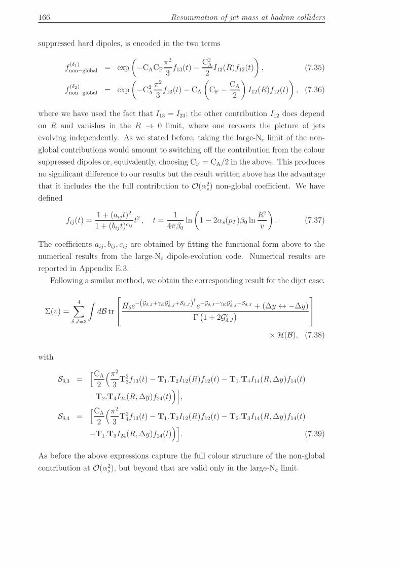
166 Resummation of jet mass at hadron colliders
suppressed hard dipoles, is encoded in the two terms
f(δ1)non−global = exp
(−CACF
π2
3f13(t)−
C2A
2I12(R)f12(t)
), (7.35)
f(δ2)non−global = exp
(−C2
A
π2
3f13(t)− CA
(CF − CA
2
)I12(R)f12(t)
), (7.36)
where we have used the fact that I13 = I23; the other contribution I12 does depend
on R and vanishes in the R → 0 limit, where one recovers the picture of jets
evolving independently. As we stated before, taking the large-Nc limit of the non-
global contributions would amount to switching off the contribution from the colour
suppressed dipoles or, equivalently, choosing CF = CA/2 in the above. This produces
no significant difference to our results but the result written above has the advantage
that it includes the the full contribution to O(α2s) non-global coefficient. We have
defined
fij(t) =1 + (aijt)
2
1 + (bijt)cijt2 , t =
1
4πβ0
ln
(1− 2αs(pT )β0 ln
R2
v
). (7.37)
The coefficients aij , bij , cij are obtained by fitting the functional form above to the
numerical results from the large-Nc dipole-evolution code. Numerical results are
reported in Appendix E.3.
Following a similar method, we obtain the corresponding result for the dijet case:
Σ(v) =4∑
δ,J=3
∫dB tr
Hδe−(Gδ,J+γEG′
δ,J+Sδ,J)†
e−Gδ,J−γEG′δ,J−Sδ,J + (∆y ↔ −∆y)
Γ(1 + 2G ′
δ,J
)
×H(B), (7.38)
with
Sδ,3 =[CA
2
(π2
3T2
3f13(t)−T1.T2I12(R)f12(t)−T1.T4I14(R,∆y)f14(t)
−T2.T4I24(R,∆y)f24(t))]
,
Sδ,4 =[CA
2
(π2
3T2
4f13(t)−T1.T2I12(R)f12(t)−T2.T3I14(R,∆y)f14(t)
−T1.T3I24(R,∆y)f24(t))]
. (7.39)
As before the above expressions capture the full colour structure of the non-global
contribution at O(α2s), but beyond that are valid only in the large-Nc limit.
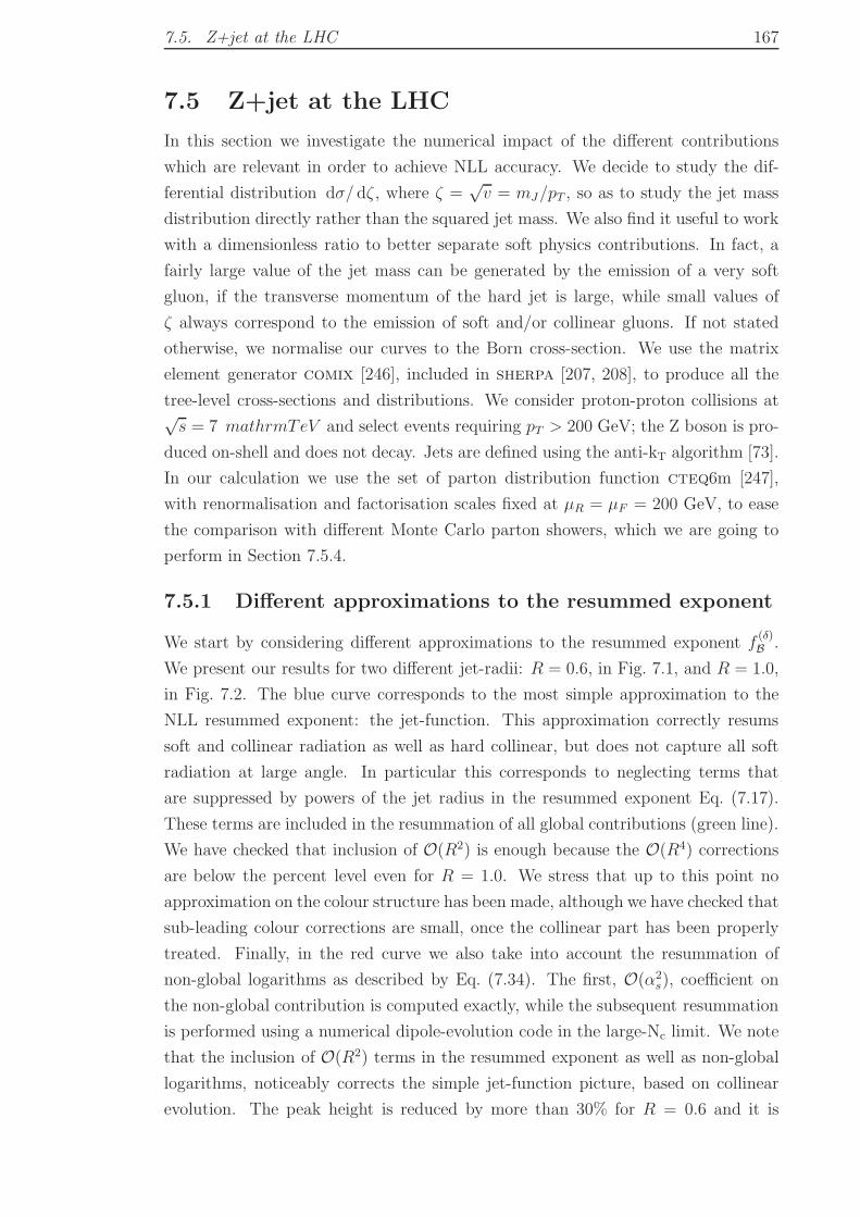
7.5. Z+jet at the LHC 167
7.5 Z+jet at the LHC
In this section we investigate the numerical impact of the different contributions
which are relevant in order to achieve NLL accuracy. We decide to study the dif-
ferential distribution dσ/ dζ , where ζ =√v = mJ/pT , so as to study the jet mass
distribution directly rather than the squared jet mass. We also find it useful to work
with a dimensionless ratio to better separate soft physics contributions. In fact, a
fairly large value of the jet mass can be generated by the emission of a very soft
gluon, if the transverse momentum of the hard jet is large, while small values of
ζ always correspond to the emission of soft and/or collinear gluons. If not stated
otherwise, we normalise our curves to the Born cross-section. We use the matrix
element generator comix [246], included in sherpa [207, 208], to produce all the
tree-level cross-sections and distributions. We consider proton-proton collisions at√s = 7 mathrmTeV and select events requiring pT > 200 GeV; the Z boson is pro-
duced on-shell and does not decay. Jets are defined using the anti-kT algorithm [73].
In our calculation we use the set of parton distribution function cteq6m [247],
with renormalisation and factorisation scales fixed at µR = µF = 200 GeV, to ease
the comparison with different Monte Carlo parton showers, which we are going to
perform in Section 7.5.4.
7.5.1 Different approximations to the resummed exponent
We start by considering different approximations to the resummed exponent f(δ)B .
We present our results for two different jet-radii: R = 0.6, in Fig. 7.1, and R = 1.0,
in Fig. 7.2. The blue curve corresponds to the most simple approximation to the
NLL resummed exponent: the jet-function. This approximation correctly resums
soft and collinear radiation as well as hard collinear, but does not capture all soft
radiation at large angle. In particular this corresponds to neglecting terms that
are suppressed by powers of the jet radius in the resummed exponent Eq. (7.17).
These terms are included in the resummation of all global contributions (green line).
We have checked that inclusion of O(R2) is enough because the O(R4) corrections
are below the percent level even for R = 1.0. We stress that up to this point no
approximation on the colour structure has been made, although we have checked that
sub-leading colour corrections are small, once the collinear part has been properly
treated. Finally, in the red curve we also take into account the resummation of
non-global logarithms as described by Eq. (7.34). The first, O(α2s), coefficient on
the non-global contribution is computed exactly, while the subsequent resummation
is performed using a numerical dipole-evolution code in the large-Nc limit. We note
that the inclusion of O(R2) terms in the resummed exponent as well as non-global
logarithms, noticeably corrects the simple jet-function picture, based on collinear
evolution. The peak height is reduced by more than 30% for R = 0.6 and it is
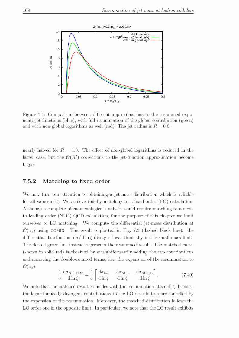
168 Resummation of jet mass at hadron colliders
0
2
4
6
8
10
12
14
0 0.05 0.1 0.15 0.2 0.25 0.3
1/σ
dσ /
dζ
ζ = mJ/pTJ
Z+jet, R=0.6, pTJ > 200 GeV
Jet Functionswith O(R2) terms (global only)
with non-global logs
Figure 7.1: Comparison between different approximations to the resummed expo-nent: jet functions (blue), with full resummation of the global contribution (green)and with non-global logarithms as well (red). The jet radius is R = 0.6.
nearly halved for R = 1.0. The effect of non-global logarithms is reduced in the
latter case, but the O(R2) corrections to the jet-function approximation become
bigger.
7.5.2 Matching to fixed order
We now turn our attention to obtaining a jet-mass distribution which is reliable
for all values of ζ . We achieve this by matching to a fixed-order (FO) calculation.
Although a complete phenomenological analysis would require matching to a next-
to leading order (NLO) QCD calculation, for the purpose of this chapter we limit
ourselves to LO matching. We compute the differential jet-mass distribution at
O(αs) using comix. The result is plotted in Fig. 7.3 (dashed black line): the
differential distribution dσ/ d ln ζ diverges logarithmically in the small-mass limit.
The dotted green line instead represents the resummed result. The matched curve
(shown in solid red) is obtained by straightforwardly adding the two contributions
and removing the double-counted terms, i.e., the expansion of the resummation to
O(αs):1
σ
dσNLL+LO
d ln ζ=
1
σ
[dσLO
d ln ζ+
dσNLL
d ln ζ− dσNLL,αs
d ln ζ
]. (7.40)
We note that the matched result coincides with the resummation at small ζ , because
the logarithmically divergent contributions to the LO distribution are cancelled by
the expansion of the resummation. Moreover, the matched distribution follows the
LO order one in the opposite limit. In particular, we note that the LO result exhibits
7.5. Z+jet at the LHC 169
0
2
4
6
8
10
0 0.1 0.2 0.3 0.4 0.5
1/σ
dσ /
dζ
ζ = mJ/pTJ
Z+jet, R=1.0, pTJ > 200 GeV
Jet Functionswith O(R2) terms (global only)
with non-global logs
Figure 7.2: Comparison between different approximations to the resummed expo-nent: jet functions (blue), with full resummation of the global contribution (green)and with non-global logarithms as well (red). The jet radius is R = 1.0.
0
0.1
0.2
0.3
0.4
0.5
0.6
0.7
0.8
10-2 10-1 100
1/σ
dσ /
dζ
ζ = mJ/pTJ
Z+jet, R=0.6, pTJ > 200 GeV
LONLL
NLL+LO
0
0.1
0.2
0.3
0.4
0.5
0.6
0.7
0.8
10-2 10-1 100
1/σ
dσ /
dζ
ζ = mJ/pTJ
Z+jet, R=1.0, pTJ > 200 GeV
LONLL
NLL+LO
Figure 7.3: Matching of the NLL resummed distribution to the LO one for R = 0.6(on the left) and R = 1.0 (on the right).
an end-point:
ζ2 =m2
J
p2T=
2ptkt|p
t+ kt|2
(cosh y − cosφ) =2ptkt
p2t + k2t + 2ptkt cosφ
(cosh y − cosφ) ,
(7.41)
which leads to
ζmax =√
maxy2+φ2≤R2
ζ2 = tanR
2=
R
2+O(R3). (7.42)
This feature is not present in the resummed distribution, because the jet does not
recoil against the emission of the eikonal gluon, but it is restored thanks to matching.
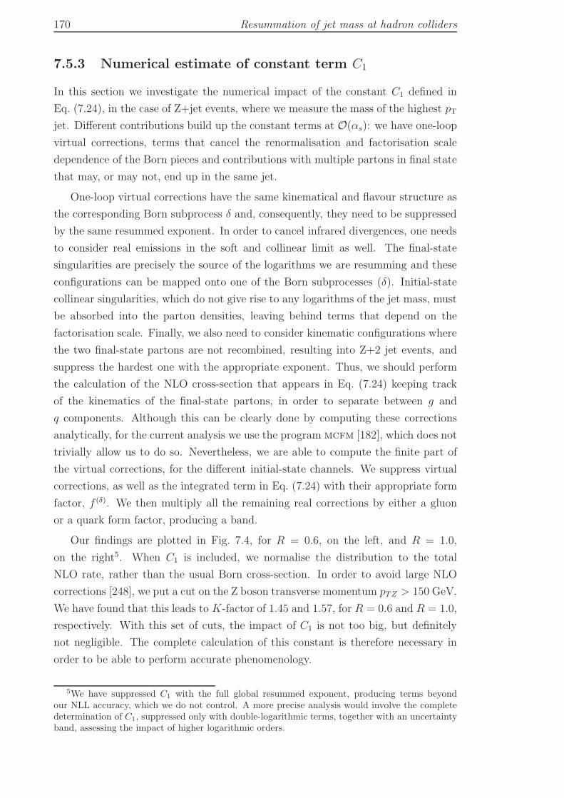
170 Resummation of jet mass at hadron colliders
7.5.3 Numerical estimate of constant term C1
In this section we investigate the numerical impact of the constant C1 defined in
Eq. (7.24), in the case of Z+jet events, where we measure the mass of the highest pT
jet. Different contributions build up the constant terms at O(αs): we have one-loop
virtual corrections, terms that cancel the renormalisation and factorisation scale
dependence of the Born pieces and contributions with multiple partons in final state
that may, or may not, end up in the same jet.
One-loop virtual corrections have the same kinematical and flavour structure as
the corresponding Born subprocess δ and, consequently, they need to be suppressed
by the same resummed exponent. In order to cancel infrared divergences, one needs
to consider real emissions in the soft and collinear limit as well. The final-state
singularities are precisely the source of the logarithms we are resumming and these
configurations can be mapped onto one of the Born subprocesses (δ). Initial-state
collinear singularities, which do not give rise to any logarithms of the jet mass, must
be absorbed into the parton densities, leaving behind terms that depend on the
factorisation scale. Finally, we also need to consider kinematic configurations where
the two final-state partons are not recombined, resulting into Z+2 jet events, and
suppress the hardest one with the appropriate exponent. Thus, we should perform
the calculation of the NLO cross-section that appears in Eq. (7.24) keeping track
of the kinematics of the final-state partons, in order to separate between g and
q components. Although this can be clearly done by computing these corrections
analytically, for the current analysis we use the program mcfm [182], which does not
trivially allow us to do so. Nevertheless, we are able to compute the finite part of
the virtual corrections, for the different initial-state channels. We suppress virtual
corrections, as well as the integrated term in Eq. (7.24) with their appropriate form
factor, f (δ). We then multiply all the remaining real corrections by either a gluon
or a quark form factor, producing a band.
Our findings are plotted in Fig. 7.4, for R = 0.6, on the left, and R = 1.0,
on the right5. When C1 is included, we normalise the distribution to the total
NLO rate, rather than the usual Born cross-section. In order to avoid large NLO
corrections [248], we put a cut on the Z boson transverse momentum pTZ > 150 GeV.
We have found that this leads to K-factor of 1.45 and 1.57, for R = 0.6 and R = 1.0,
respectively. With this set of cuts, the impact of C1 is not too big, but definitely
not negligible. The complete calculation of this constant is therefore necessary in
order to be able to perform accurate phenomenology.
5We have suppressed C1 with the full global resummed exponent, producing terms beyondour NLL accuracy, which we do not control. A more precise analysis would involve the completedetermination of C1, suppressed only with double-logarithmic terms, together with an uncertaintyband, assessing the impact of higher logarithmic orders.
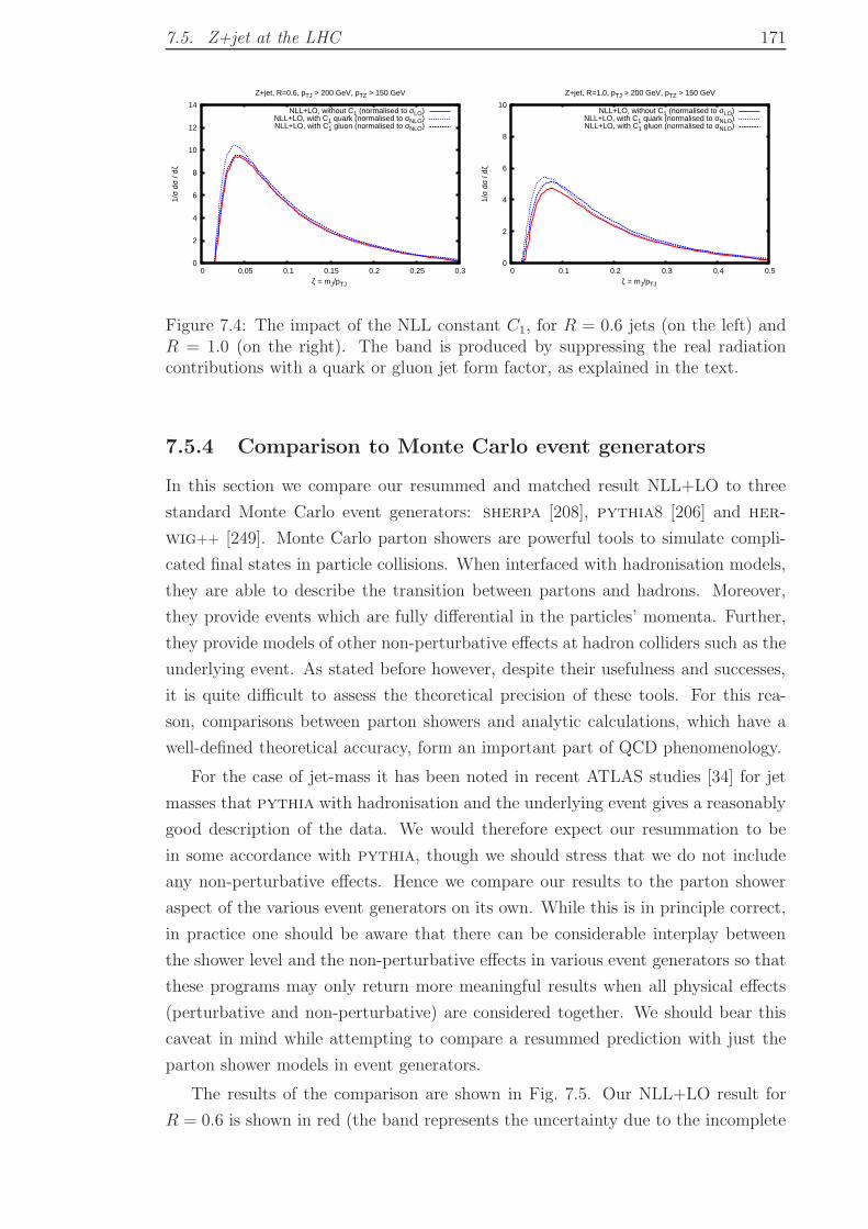
7.5. Z+jet at the LHC 171
0
2
4
6
8
10
12
14
0 0.05 0.1 0.15 0.2 0.25 0.3
1/σ
dσ /
dζ
ζ = mJ/pTJ
Z+jet, R=0.6, pTJ > 200 GeV, pTZ > 150 GeV
NLL+LO, without C1 (normalised to σLO)NLL+LO, with C1 quark (normalised to σNLO)NLL+LO, with C1 gluon (normalised to σNLO)
0
2
4
6
8
10
0 0.1 0.2 0.3 0.4 0.5
1/σ
dσ /
dζ
ζ = mJ/pTJ
Z+jet, R=1.0, pTJ > 200 GeV, pTZ > 150 GeV
NLL+LO, without C1 (normalised to σLO)NLL+LO, with C1 quark (normalised to σNLO)NLL+LO, with C1 gluon (normalised to σNLO)
Figure 7.4: The impact of the NLL constant C1, for R = 0.6 jets (on the left) andR = 1.0 (on the right). The band is produced by suppressing the real radiationcontributions with a quark or gluon jet form factor, as explained in the text.
7.5.4 Comparison to Monte Carlo event generators
In this section we compare our resummed and matched result NLL+LO to three
standard Monte Carlo event generators: sherpa [208], pythia8 [206] and her-
wig++ [249]. Monte Carlo parton showers are powerful tools to simulate compli-
cated final states in particle collisions. When interfaced with hadronisation models,
they are able to describe the transition between partons and hadrons. Moreover,
they provide events which are fully differential in the particles’ momenta. Further,
they provide models of other non-perturbative effects at hadron colliders such as the
underlying event. As stated before however, despite their usefulness and successes,
it is quite difficult to assess the theoretical precision of these tools. For this rea-
son, comparisons between parton showers and analytic calculations, which have a
well-defined theoretical accuracy, form an important part of QCD phenomenology.
For the case of jet-mass it has been noted in recent ATLAS studies [34] for jet
masses that pythia with hadronisation and the underlying event gives a reasonably
good description of the data. We would therefore expect our resummation to be
in some accordance with pythia, though we should stress that we do not include
any non-perturbative effects. Hence we compare our results to the parton shower
aspect of the various event generators on its own. While this is in principle correct,
in practice one should be aware that there can be considerable interplay between
the shower level and the non-perturbative effects in various event generators so that
these programs may only return more meaningful results when all physical effects
(perturbative and non-perturbative) are considered together. We should bear this
caveat in mind while attempting to compare a resummed prediction with just the
parton shower models in event generators.
The results of the comparison are shown in Fig. 7.5. Our NLL+LO result for
R = 0.6 is shown in red (the band represents the uncertainty due to the incomplete
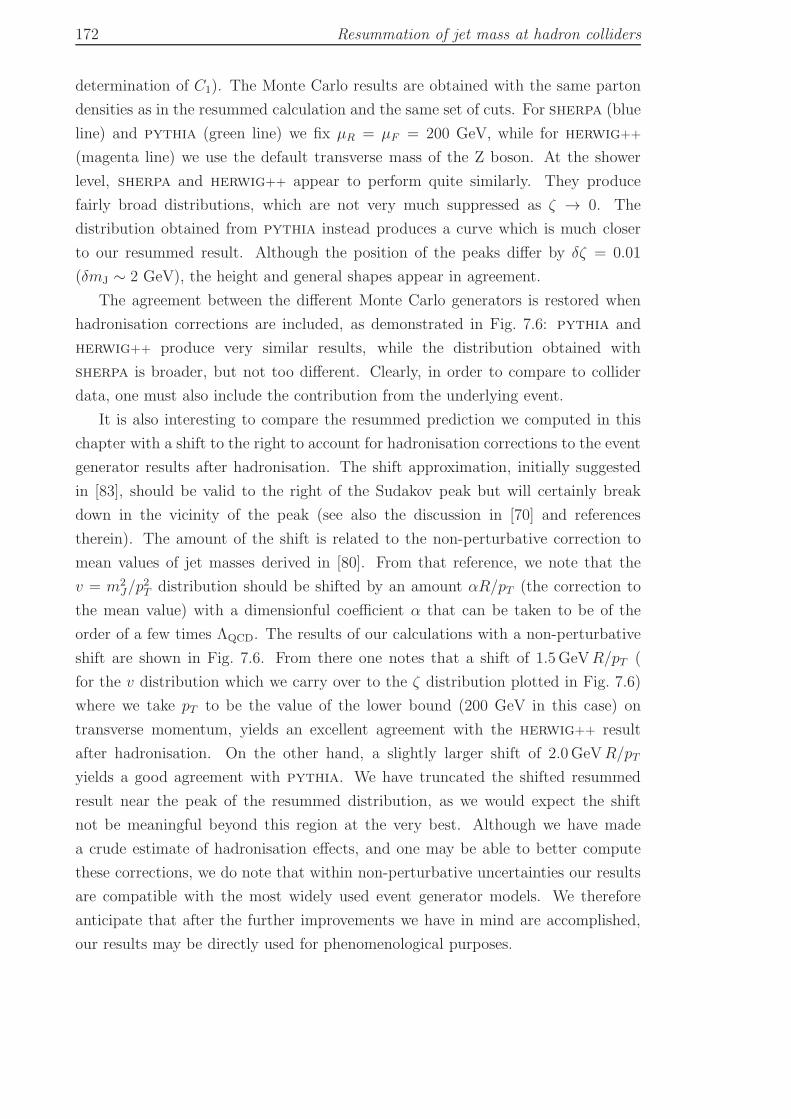
172 Resummation of jet mass at hadron colliders
determination of C1). The Monte Carlo results are obtained with the same parton
densities as in the resummed calculation and the same set of cuts. For sherpa (blue
line) and pythia (green line) we fix µR = µF = 200 GeV, while for herwig++
(magenta line) we use the default transverse mass of the Z boson. At the shower
level, sherpa and herwig++ appear to perform quite similarly. They produce
fairly broad distributions, which are not very much suppressed as ζ → 0. The
distribution obtained from pythia instead produces a curve which is much closer
to our resummed result. Although the position of the peaks differ by δζ = 0.01
(δmJ ∼ 2 GeV), the height and general shapes appear in agreement.
The agreement between the different Monte Carlo generators is restored when
hadronisation corrections are included, as demonstrated in Fig. 7.6: pythia and
herwig++ produce very similar results, while the distribution obtained with
sherpa is broader, but not too different. Clearly, in order to compare to collider
data, one must also include the contribution from the underlying event.
It is also interesting to compare the resummed prediction we computed in this
chapter with a shift to the right to account for hadronisation corrections to the event
generator results after hadronisation. The shift approximation, initially suggested
in [83], should be valid to the right of the Sudakov peak but will certainly break
down in the vicinity of the peak (see also the discussion in [70] and references
therein). The amount of the shift is related to the non-perturbative correction to
mean values of jet masses derived in [80]. From that reference, we note that the
v = m2J/p
2T distribution should be shifted by an amount αR/pT (the correction to
the mean value) with a dimensionful coefficient α that can be taken to be of the
order of a few times ΛQCD. The results of our calculations with a non-perturbative
shift are shown in Fig. 7.6. From there one notes that a shift of 1.5GeVR/pT (
for the v distribution which we carry over to the ζ distribution plotted in Fig. 7.6)
where we take pT to be the value of the lower bound (200 GeV in this case) on
transverse momentum, yields an excellent agreement with the herwig++ result
after hadronisation. On the other hand, a slightly larger shift of 2.0GeVR/pT
yields a good agreement with pythia. We have truncated the shifted resummed
result near the peak of the resummed distribution, as we would expect the shift
not be meaningful beyond this region at the very best. Although we have made
a crude estimate of hadronisation effects, and one may be able to better compute
these corrections, we do note that within non-perturbative uncertainties our results
are compatible with the most widely used event generator models. We therefore
anticipate that after the further improvements we have in mind are accomplished,
our results may be directly used for phenomenological purposes.
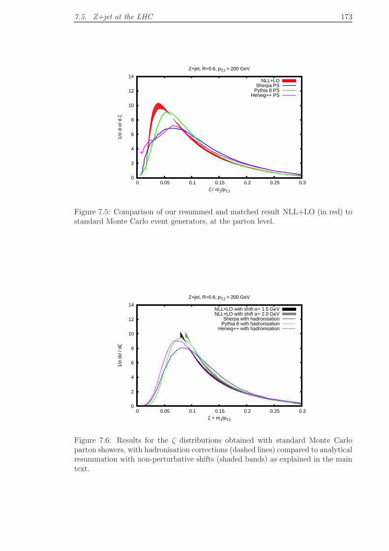
7.5. Z+jet at the LHC 173
0
2
4
6
8
10
12
14
0 0.05 0.1 0.15 0.2 0.25 0.3
1/σ
d σ/
d ζ
ζ= mJ/pTJ
Z+jet, R=0.6, pTJ > 200 GeV
NLL+LOSherpa PS
Pythia 8 PSHerwig++ PS
Figure 7.5: Comparison of our resummed and matched result NLL+LO (in red) tostandard Monte Carlo event generators, at the parton level.
0
2
4
6
8
10
12
14
0 0.05 0.1 0.15 0.2 0.25 0.3
1/σ
dσ /
dζ
ζ = mJ/pTJ
Z+jet, R=0.6, pTJ > 200 GeV
NLL+LO with shift α= 1.5 GeVNLL+LO with shift α= 2.0 GeV
Sherpa with hadronisationPythia 8 with hadronisation
Herwig++ with hadronisation
Figure 7.6: Results for the ζ distributions obtained with standard Monte Carloparton showers, with hadronisation corrections (dashed lines) compared to analyticalresummation with non-perturbative shifts (shaded bands) as explained in the maintext.
174 Resummation of jet mass at hadron colliders
7.6 Dijets at the LHC
In this section we provide numerical predictions for the jet mass distribution in
dijet events. As before, we consider proton-proton collision at√s = 7 TeV, with
jets defined according to the anti-kT algorithm [73]. The main complication with
respect to the Z+jet case previously discussed is a more complicated colour algebra,
which results into a matrix structure of large-angle soft gluon radiation. In order
to simplify our resummed calculation, we work at fixed kinematics, i.e., we demand
the jets’ transverse momentum pT to be 200 GeV and their rapidity separation to
be |∆y| = 2 (at Born level we only have two jets). We remind the reader that we
consider1
σ
dσ
dζ=
1
σ
(dσ
dζ1+
dσ
dζ2
)
ζ1=ζ2=ζ
. (7.43)
We match the resummation to a LO calculation of the jet mass distribution
obtained with nlojet++ [233], according to Eq (7.40). In Fig. 7.7 we plot our
NLL+LO result with different approximation for the resummed exponent Eq. (7.38):
jet-functions (blue), with the inclusion of O(R2) corrections (green) and non-global
logarithms (red), as explained in detail for the Z+jet case. Although the corrections
to the jet-function approximation are less pronounced than in the Z+jet case, they
are still sizeable and must be taken into account. In our understanding, the pertur-
bative part of the resummed result of Ref [53, 54] is precisely the one captured by
the jet-functions (plus an approximated treatment of the one-loop constant C1).
In order to obtain a more realistic prediction, one would need to integrate over the
appropriate cuts in transverse momentum and rapidity and match to NLO, which, in
principle, should not pose any difficulties. More delicate is instead the determination
of the constant C1, although this issue has been addressed in Ref. [31, 32] for the
case of global event-shapes.
7.7 Conclusion
In this chapter we have provided resummed expressions to NLL accuracy for jet-mass
distributions in hadron-hadron collisions, for jets of arbitrary radius and defined in
the anti-kT algorithm. In particular, we have considered Z boson production in
association with a jet and jet masses in dijet production. We have improved upon
existing studies of jet masses and shapes (many of which use e+e− annihilation as
a model for jets produced in hadron collision processes) by incorporating initial
state radiation effects as well as accounting for non-global logarithms in the large-
Nc limit. We have matched our results to leading-order predictions to account
for non-logarithmic terms to this order and have commented on the role of the
coefficient function C1αs (corrections of order αs to the basic resummation off the
Born configuration). Finally, we have compared our results to all the leading Monte

7.7. Conclusion 175
0
2
4
6
8
10
12
14
16
0 0.05 0.1 0.15 0.2 0.25 0.3
1/σ
dσ /
dζ
ζ = mJ/pTJ
Dijets R=0.6, pT = 200 GeV, ∆y = 2
Jet functions + LOwith O(R2) terms (global only) + LO
with non-global logs + LO
Figure 7.7: The NLL+LO jet mass distribution for dijets, with different approxima-tion to the resummed exponent.
Carlo event generators pythia, sherpa and herwig++, with and without non-
perturbative hadronisation corrections.
We have found that: first, ISR and non-global logarithms play an important role
even at relatively small values of jet radius such as R = 0.6 and hence cannot be
ignored while discussing inclusive jet shapes at hadron colliders. Our calculations
for non-global logarithms both at fixed-order and at all orders represent to our
knowledge the first attempt to calculate these terms beyond the simpler cases of
e+e− annihilation and DIS. Second, on comparing our results to event generators,
widely used for phenomenology, we find that at the purely perturbative level the best
agreement is with the pythia shower, with an apparent small shift accounting for
much of the difference between the analytical resummation and the parton shower
estimate. The differences with sherpa and herwig++ on the other hand are more
marked especially towards smaller jet masses as one approaches the peak of the
distributions. After hadronisation corrections are applied in the event generators
and also applying a shift to the analytical resummation to account for hadronisation,
we are able to obtain very good agreement with pythia and herwig++ with slightly
different shifts required in either case, for jet mass values to the right of the Sudakov
peak of the distribution. For smaller jet masses we do not expect a simple shift of
the analytical resummation to reproduce the correct result and we observe here
discrepancy with all Monte Carlo generators which is to be expected. However, this
region of very small jet masses of the order of a few GeV will not be of interest in
LHC phenomenology in any case. We may thus expect that our results should be
of direct phenomenological value even pending some of the improvements we intend
to make in the near future.
176 Resummation of jet mass at hadron colliders
For the immediate future we aim to improve our results chiefly by taking proper
account of the order αs coefficient function C1 and computing the various pieces of
C1 which originate from different regions and suppressing these by an appropriate
form factor rather than the cruder treatment reported in the text, which was aimed
at producing an uncertainty band associated to a lack of correct treatment of C1.
When this is done we will be in a position to carry out an NLO matching and
estimate the uncertainty of our theoretical calculations accurately, which will be
important in the context of phenomenology.
We have not taken directly into account non-perturbative effects in this chapter,
incorporating them as a simple shift of the perturbative spectra as for the case of
global event shapes [66]. We can study non-perturbative corrections in more detail
using the methods outlined in [80], but for the moment we note that the Monte
Carlo event generators we have studied, contain differences in their estimate of
hadronisation which should be explored further along with studying the underlying
event contributions. Since our predictions are valid for any value of jet radius R,
one can hope that phenomenological studies selecting a small value of R would
help in better isolating the perturbative contributions, since the hadronisation and
underlying event corrections for m2J/p
2T scale respectively as R and R4 [80]. On
the other hand moving to a larger R after pinning down the perturbative content
would help to more accurately constrain the non- perturbative models in various
approaches.
Chapter 8
Conclusions
Each chapter has its own conclusion section. In this chapter we tie together the
most important points to be learned from the study presented in this thesis.
Due to the complex environment present at hadron colliders, such as the LHC,
new physics discoveries are only feasible given a detailed understanding of the al-
ready established standard model, and QCD in particular as the strong interactions,
governed by the latter, constitute the bulk of all possible interactions. At the LHC,
the establishment of the latter understanding is best accessible via studies of jets,
which are the final product of the aforementioned strong interactions and which
populate the final state at the latter collider. High-pT jets, in particular, have some
discernible features that make them ideal for perturbative analyses. Such analyses
include exploration of the substructure of these jets, which is distinct from that of
moderate- and low-pT jets and which would aid in discriminating new physics signals
from QCD background.
Equipped with an infrared and collinear safe jet shape observable, angularities,
we probed in Chapter 4 the substructure of high-pT QCD jets in the simple process
of dijet production in e+e− annihilation, where only one jet is measured while the
other is left unmeasured. We identified large logarithms, non-global logs, that were
missed out by previous studies and argued that in the limit of narrow well-separated
jets their all–orders structure simplifies to that of the hemisphere jet mass. This
is mainly due to the observation that non-global logs arise predominantly near the
boundary of each jet and evolve independently of the other well-separated jets.
Moreover, we commented on their phenomenological impact on the primary emission
Sudakov form factor and put forward the ansatz that the above simplified picture
of non-global structure holds even at hadron collider environments.
Given the fact that experimental measurements generally employ large values of
the jet parameter R in their jet finding, it proved necessary to extend the work of
Chapter 4 to include the effects of large jet radii. We have performed this very task
in Chapter 5. Within the same context of dijet production in e+e− annihilation and
taking the jet mass as an example we computed the full logarithmic structure of the
latter shape distribution at O(α2s), i.e., up to α2
s L (N3LL accuracy in the expansion),
while retaining the full R dependence. The calculations were explicitly carried out
for both anti-kT and C/A jet algorithms and implicitly, through similarity to C/A,
177
178 Conclusions
for the kT algorithm, and represent one of the most accurate fixed-order calculations
for non-global observables. Further, the NLL (in the exponent) resummation of
Chapter 4 has been extended to full jet radius, in the large-Nc limit, for both the
anti-kT and kT algorithms. Very few non-global observables have been computed
at fixed-order and/or resummed to all–orders to such an accuracy (In fact, the only
observable the author is aware of is the energy flow in gaps-between-jets [3, 176, 81]).
Based on our resummed results, which include both non-global and clustering
logs, we concluded that it is recommended in jet phenomenological studies to use
a variety of jet algorithms. Further, we found that ignoring non-global logs all to-
gether in events where the final state is clustered with a sequential recombination
jet algorithm other than the anti-kT induces an uncertainty that is well below that
originated from the large-Nc approximation, for quite large jet radii. Our future
directions regarding non-global observables include: extending the numerical pro-
gram of Ref. [2] to next-to-leading non-global logs and as a long-term project, going
beyond the large-Nc approximation.
Following previous work on the energy flow in gaps-between-jets, we showed
in Chapter 6 that clustering logs occurring in jet mass calculations in kT and C/A
algorithms exponentiate. We explicitly computed the first few orders in the exponent
with full R dependence. Comparisons to the Monte Carlo program of [2] revealed
that the missing higher-order terms have negligible effect. Our findings settled the
issue, raised by other research groups, of whether such logs, with highly non-trivial
phase space, can exponentiate and hence resummed. The next obvious step is to
extend the resummation to next-to-leading clustering logs.
Finally, we have exploited the wealth of techniques and experience gained in
the work of the previous chapters to carry out, in the final chapter 7, a full NLL
resummation of jet mass at hadron colliders for the anti-kT jet algorithm. Explic-
itly studied were vector boson production in association with a single jet and dijet
production. Parts of the resummed exponent, such as the soft wide-angle piece in-
volves the full colour structure and thus exceeds the accuracy of standard Monte
Carlo event generators (which work in the large-Nc approximation). Our calculation
marks the first attempt in literature where non-global logs are computed at hadron
colliders and with full R dependence retained. Already with a simple shift in the
exponent to account for hadronisation corrections and only leading-order matching,
our results compared well to the output of the most widely used event generators,
and even hinted noticeable differences between them.
Additionally, although in the last chapter 7 we have treated a single variable,
the jet mass, it is actually straightforward to extend our treatment to the entire
range of angularities as for instance were explored for jets in e+e− annihilation in
Chapter 4 and Refs. [44, 45]. The basic calculations we carried out here can be
easily extended to include those variables as well as any variants of the jet mass
179
itself such as studying the jet mass with an additional jet veto. Once we have
accomplished an NLO matching we therefore intend to generalise our approach to
accommodate a range of substructure variables in different hard processes, including
final state clustering with other jet algorithms such as the kT, C/A and SISCone
algorithms. Moreover, the boost11 review [27] recommended, in addition to the
above two (vector boson + jet and dijets) processes, calculations for multijet events.
We hope to perform this in the near future as well as writing a semi-analytical
program for an automation of these calculations which will enable similar studies of
other non-global jet shapes. We hope that our work will eventually lead to improved
estimates of the accuracy and hence more confidence in a detailed understanding of
jet substructure than is the case presently, which could in turn be important for a
variety of substructure applications at the LHC.

180
Appendix A
Colour algebra
A.1 Fierz identities
A matrix M in SU(Nc) can be written as a linear combination of the basis matrices
va, a = 1, · · · ,N2c − 1. In the fundamental representation, va = ta, this reads
M = m0 1+
N2c−1∑
a=1
ma ta, (A.1)
where m0 and ma are real expansion coefficients. To determine the latter coefficients
one can make use of the traceless property of ta, Eq. (2.3), together with Eq. (2.5).
One can straightforwardly show that
m0 =1
NcTr (M) , ma = 2 Tr (M ta) . (A.2)
If one takes, for example, the matrixM to be the commutator and anti–commutator1
of the basis matrices then one obtains, using Eqs. (A.1) and (A.2),
ıfabc = 2 Tr([ta, tb]tc
), (A.3a)
ta, tb =δab
Nc1 + dabc t
c, dabc = 2 Tr(ta, tbtc
). (A.3b)
It is worthwhile noting that Eq. (A.3a) implies that the structure constants are
totally antisymmetric in all three indices, fabc = −facb, fabc = −fbac etc. Moreover,
Eq. (A.3b) defines, in analogy to (A.3a), the totally symmetric constants dabc, which
form a symmetric adjoint representation of SU(Nc)2. The corresponding casimir
operator can be deduced from Eq. (A.3b). It reads [250]: CAs = (N2c − 4)/Nc.
Adding up Eqs. (A.3a) and (A.3b) one obtains the following useful relation for
1For two matrices A and B, the anti–commutator is defined as A,B = A.B +B.A. Recallthat the commutator is just the Lie product defined in Eq. (2.4a).
2For SU(3), a system of three quarks (forming a baryon) can be in four representations. Theseare found using Young Tableaux techniques (see e.g., [100]): 3× 3× 3 = 1⊕ 8⊕ 8⊕ 10. 8 and 8 arerespectively the symmetric and antisymmetric representations. Employing the same techniquesone can also compute the dimension of a given representation.
181
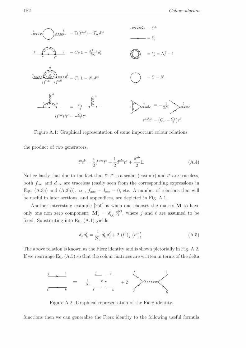
182 Colour algebra
= CF 1 = N2c−12Nc
δikk i
ta ta
= Tr(tatb) = TR δaba b
= −CA2
ıfabctbtc = −CA2ta
a
bc
a
= δik
= δab
= δaa = N2c − 1
= − 12Nc
tatbta =(CF − CA
2
)tb
ab b
a b
d
ıfadc ıf cdb= CA 1 = Nc δ
abc
= δii = Nc
Figure A.1: Graphical representation of some important colour relations.
the product of two generators,
tatb =ı
2fabctc +
1
2dabctc +
δab
21. (A.4)
Notice lastly that due to the fact that te. te is a scalar (casimir) and te are traceless,
both fabc and dabc are traceless (easily seen from the corresponding expressions in
Eqs. (A.3a) and (A.3b)). i.e., faac = daac = 0, etc. A number of relations that will
be useful in later sections, and appendices, are depicted in Fig. A.1.
Another interesting example [250] is when one chooses the matrix M to have
only one non–zero component; Mik = δi(j) δ
(ℓ)k , where j and ℓ are assumed to be
fixed. Substituting into Eq. (A.1) yields
δij δℓk =
1
Ncδik δ
ℓj + 2 (ta)ik (ta)ℓj . (A.5)
The above relation is known as the Fierz identity and is shown pictorially in Fig. A.2.
If we rearrange Eq. (A.5) so that the colour matrices are written in terms of the delta
=
j i
kℓ
j i
kℓ
1Nc
+ 2
j i
kℓ
Figure A.2: Graphical representation of the Fierz identity.
functions then we can generalise the Fierz identity to the following useful formula
A.1. Fierz identities 183
[251]
L taQta R =1
2Tr (Q)LR− 1
2NcLQR, (A.6)
where L,Q and R are any colour matrices. In the special case where both L and R
are unit matrices and Q = tb then
ta tb ta = − 1
2Nctb, (A.7)
or Q = tb tc then
ta tb tc ta =1
4δbc − 1
2Nctb tc. (A.8)
Finally, the calculation of the cross section involves, as we shall see later in Sec. 2.2,
products of traces of colour generators, with each colour summed over. It would
thus prove useful to provide the following trace identity [251]:
Tr (ta Q)Tr (ta R) =1
2Tr (QR)− 1
2NcTr (Q)Tr (R) . (A.9)

184
Appendix B
Perturbative calculations in e+e−
annihilation
In this appendix, we present detailed perturbative calculations of differential cross
sections for one of the main two QCD processes discussed in this thesis, namely e+e−
annihilation into hadrons. In addition to the classical Feynman diagrammatic ap-
proach of computing matrix elements, we consider the effective eikonal method. We
start, in Sec. B.1, by laying out the general structure of the latter method, encoun-
tering in the way some of the main definitions and relations that will be essential
to later calculations. We then compute the matrix element squared (and therefore
the differential cross section) at Born level, in Subsec. B.2.2. O(αs) corrections
stemming from both real emission and virtual loops are addressed in Subsecs. B.2.3
and B.2.3. Lastly we compute the more complicated O (α2s) real emission matrix
element, taking into account hard emission contributions.
B.1 Eikonal method
The eikonal method [89]1 provides a reliable approximation to the full theory at
high energies. The resultant all–orders eikonal matrix element may be written in a
closed form. This method is based on the propagator approximation
ı
(p± k)2 + ıǫ≃ ı
±2 p.k + ıǫ, (B.1)
where p is an external four–momentum, which is assumed to be on–shell (p2 = 0)2,
and k may be a partial sum of internal four–momenta3, thereby neglecting the k2
term relative to p . k (k2 ≪ p.k). The corresponding eikonal Feynman rules are
shown in Fig. B.1.
Consider the emission of a soft gluon k = (ω,k) off a system of m (harder)
partons, with momenta pi = (Ei,pi) , i = 1, · · ·m. One can write the corresponding
1The eikonal method was originally developed in the context of the non–relativistic theory ofpotential scattering [252, 253] (and references in [89]).
2The on–shell (or on mass shell) approximation will be used throughout unless stated otherwise.This approximation becomes almost exact when considering scattering at high energies, which arefar larger than the masses of the light quarks (i.e., excluding the top quark).
3In cases where k is the four–momentum of a single parton, which is soft relative to its emitter,this approximation may be referred to as the soft approximation.
185
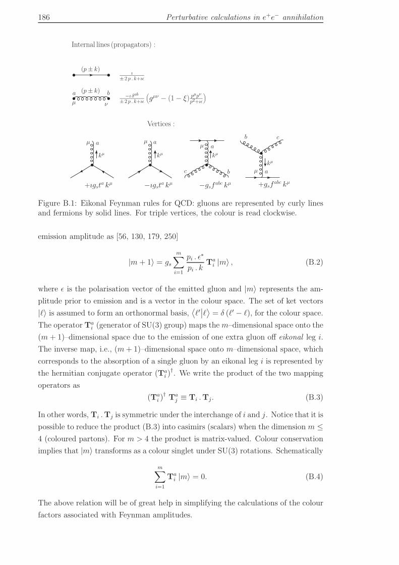
186 Perturbative calculations in e+e− annihilation
Internal lines (propagators) :
a (p± k)−ı δab
± 2 p . k+ıǫ
(gµν − (1− ξ) p
µpν
p2+ıǫ
)
µ ν
b
ı± 2 p . k+ıǫ
(p± k)
Vertices :
+ıgsta kµ
aµ
−ıgsta kµ
aµ
−gsfabc kµ
b
+gsfabc kµ
aµ
b c
aµ
c
kµ kµ kµ
kµ
Figure B.1: Eikonal Feynman rules for QCD: gluons are represented by curly linesand fermions by solid lines. For triple vertices, the colour is read clockwise.
emission amplitude as [56, 130, 179, 250]
|m+ 1〉 = gs
m∑
i=1
pi . ǫ∗
pi . kTa
i |m〉 , (B.2)
where ǫ is the polarisation vector of the emitted gluon and |m〉 represents the am-
plitude prior to emission and is a vector in the colour space. The set of ket vectors
|ℓ〉 is assumed to form an orthonormal basis,⟨ℓ′∣∣ℓ⟩= δ (ℓ′ − ℓ), for the colour space.
The operator Tai (generator of SU(3) group) maps them–dimensional space onto the
(m+ 1)–dimensional space due to the emission of one extra gluon off eikonal leg i.
The inverse map, i.e., (m+ 1)–dimensional space onto m–dimensional space, which
corresponds to the absorption of a single gluon by an eikonal leg i is represented by
the hermitian conjugate operator (Tai )
†. We write the product of the two mapping
operators as
(Tai )
† Taj ≡ Ti .Tj. (B.3)
In other words, Ti .Tj is symmetric under the interchange of i and j. Notice that it is
possible to reduce the product (B.3) into casimirs (scalars) when the dimension m ≤4 (coloured partons). For m > 4 the product is matrix-valued. Colour conservation
implies that |m〉 transforms as a colour singlet under SU(3) rotations. Schematically
m∑
i=1
Tai |m〉 = 0. (B.4)
The above relation will be of great help in simplifying the calculations of the colour
factors associated with Feynman amplitudes.
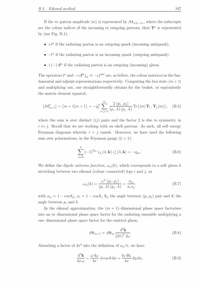
B.1. Eikonal method 187
If the m–parton amplitude |m〉 is represented by Mi1i2···im , where the subscripts
are the colour indices of the incoming or outgoing partons, then Ta is represented
by (see Fig. B.1):
• +ta if the radiating parton is an outgoing quark (incoming antiquark).
• −ta if the radiating parton is an incoming quark (outgoing antiquark).
• +(−) ıfa if the radiating parton is an outgoing (incoming) gluon.
The operators ta and −ı (fa)bc ≡ −ıfabc are, as before, the colour matrices in the fun-
damental and adjoint representations respectively. Computing the bra state 〈m+ 1|and multiplying out, one straightforwardly obtains for the braket, or equivalently
the matrix element squared,
∣∣M2m+1
∣∣ =⟨m+ 1
∣∣m+ 1⟩= −g2s
m∑
i<j=1
2 (pi . pj)
(pi . k) (pj . k)Tr (〈m|Ti .Tj |m〉) , (B.5)
where the sum is over distinct (ij) pairs and the factor 2 is due to symmetry in
i ↔ j. Recall that we are working with on–shell partons. As such, all self–energy
Feynman diagrams whereby i = j vanish. Moreover, we have used the following
sum over polarisations, in the Feynman gauge (ξ = 1):
3∑
λ=0
(−1)δλ0 ǫµ (λ,k) ǫ∗ν (λ,k) = −gµν . (B.6)
We define the dipole antenna function, ωij(k), which corresponds to a soft gluon k
stretching between two eikonal (colour–connected) legs i and j, as
ωij(k) =ω2 (pi . pj)
(pi . k) (pj . k)=
aijai aj
, (B.7)
with aij = 1 − cos θij , ai = 1 − cos θi, θij the angle between (pi, pj) pair and θi the
angle between pi and k.
In the eikonal approximation, the (m + 1)–dimensional phase space factorises
into an m–dimensional phase space factor for the radiating ensemble multiplying a
one–dimensional phase space factor for the emitted gluon,
dΦm+1 = dΦmd3k
(2π)3 2ω(B.8)
Absorbing a factor of 4π2 into the definition of αs/π, we have
d3k
4π ω=
ω dω
4πd cos θ dφ =
kt dkt4π
dη dφ, (B.9)
188 Perturbative calculations in e+e− annihilation
where (θ, φ) are the polar and azimuthal angles of the gluon with respect to (w.r.t.)
a chosen axis. The (pseudo)rapidity η and transverse momentum of the gluon kt are
related to its energy and angle, ω and θ, via
η = − ln tanθ
2, kt = ω sin θ. (B.10)
B.2 pQCD: e+e− → hadrons
The purpose of this section is to provide a detailed derivation of the full differential
cross section for the process e+e− annihilation into final state hadrons up to O (α2s)
real radiative corrections. That is, we consider the the emission of up to two real
gluons off the initial Born process e+e− → q q. We also consider the one–loop virtual
correction in the eikonal limit. The latter is to demonstrate that for the accuracy
sought in this thesis it is sufficient to simply take the virtual correction to be minus
the real one. Detailed calculations of the total cross–section up to NNLO (two–loop
corrections) can be found in, e.g., [254, 255].
The perturbative expansion of the cross section for the said process, up to the
nth order, may be cast in the form
σ e+e−→hadronsn = σ(0) + σ(1) + σ(2) + · · ·+ σ(n). (B.11)
Below, we first present a general form for the n gluon emission differential cross
section, dσ(n), including the form of the n–body phase space. Using the resul-
tant expressions, we then compute the Born term, σ(0), the O(αs) correction, σ(1),
including both real and virtual contributions and finally the O (α2s) real contribu-
tion, σ(2). To simplify the calculations, we shall work at a centre–of–mass energy
s < m2Z , so that contributions from the Z boson propagator can be neglected, and
in the centre–of–mass (cm) frame4, such that the photon propagator’s momentum
is q = (√s, 0).
B.2.1 Generalities
The general form of the total cross section is given in Eq. (2.28). At order αns in the
perturbative expansion, Eq. (B.11), it reads
σ(n) =1
2s
∫ ∣∣∣M(n)
∣∣∣2
dΠn. (B.12)
nth order matrix element squared
The invariant matrix element squared (averaged and summed over initial and final
state quantum numbers) may be split into a leptonic part, e+e− → γ∗, and a
4Recall that the whole problem is Lorentz invariant, and thus one can work at any chosen frame.
B.2. pQCD: e+e− → hadrons 189
hadronic part, γ∗ → qqg · · · :
∣∣∣M(n)
∣∣∣2
=1
s2Lµν H(n)
µν . (B.13)
The leptonic tensor, Lµν , is given by
Lµν =1
4
∑
s1,s2
Lµ (q1, s1; q2.s2) Lν† (q1, s1; q2, s2) ,
=e2
4
∑
s1,s2
[u (s1, q1) γµv (s2, q2)] [v (s2, q2) γ
νu (s1, q1)] ,
=e2
4Tr (q1/ γ
µ q2/ γν) = e2 (qµ1 q
ν2 + qν1q
µ2 − gµνq1 . q2) , (B.14)
where we have used the spinors completeness relations, for a four-momentum p,
∑
λ=±1
uλ(p)uλ(p) = p/,∑
λ=±1
vλ(p)vλ(p) = p/, (B.15)
along with the recursive relation for the trace of products of an even number, N , of
Dirac matrices
Tr (γµ1γµ2 · · · γµk · · · γµN ) = 4n∑
k=2
(−1)k gµ1µk Tr (γµ2 · · · γµk−1γµk+1 · · · γµN ) .
(B.16)
To simplify the calculations, particularly of H(n)µν , it is instructive to employ the
Ward identity [93], which states that if a matrix element M(p) = Mµ(p) ǫµ(p) then
upon the replacement ǫµ → pµ the matrix element vanishes. This implies, in our
case, that
qµ Lµν(e+e− → γ∗) = 0, qν Hµν (γ
∗ → qqg · · · ) = 0. (B.17)
The hadronic tensor is thus proportional to the projector (gµν − qµqν/q2)5. The
matrix element squared (B.13) can then be written as
∣∣∣M(n)
∣∣∣2
=1
s2Lµν
(gµν −
qµqνq2
)H(n),
=1
s2gµνL
µν H(n),
=1
s2gµνL
µν 1
3gρσH(n)
ρσ ,
=1
3 s2LH(n), (B.18)
where we made use of Eq. (B.17) to pass to the second line. We then multiplied both
sides in the expansion of the hadronic tensor H(n)µν in terms of the aforementioned
5So is the leptonic tensor. However since one will be integrating over final state phase spacethen one only needs to extract the tensor structure of the final state term. i.e., the hadronic tensor.
190 Perturbative calculations in e+e− annihilation
projector (H(n)µν = (gµν − qµqν/q
2)H(n)) by the metric gµν and used the fact that
gµνgµν = 4 (in four–dimensional spacetime) to pass to the third line. The last line
in Eq. (B.18) defines the scalars L and H(n):
L = gνν Lµν = −e2 s,
H(n) = gµν H(n)µν . (B.19)
Our task in the subsequent sections is simply to compute H(n).
n–body phase space
The general form of the final state phase space factor for n gluons emission is given
in Eq. (2.29). There are two ways of simplifying the n–body form (2.29). The first
is to proceed by integrating out pn then pn−1 and so on. The second method is to
exclusively integrate out p1 and p2 leaving the rest intact. As we shall see below, this
latter method results in an expression analogous to what would be found using the
eikonal method of Sec. B.1 (modulo a Jacobi factor). The first method is thoroughly
presented in [256]. We only explicitly derive the integrated two– and three–body
phase space factors for the on–shell case. The two–body phase space reads
∫dΠ2 =
∫d3p1
(2π)3 2E1
d3p2
(2π)3 2E2
(2π)4 δ(4) (q − p1 − p2) ,
=
∫d3p1
(2π)3 2E1
(2π)δ (
√s− E1 − E2)
2E2
∣∣∣p1=−p2
=1
32π2
∫d2Ω1,
(B.20)
Similarly the three–body phase space is given by
∫dΠ3 =
∫d3p1
(2π)3 2E1
d3p2
(2π)3 2E2
d3p3
(2π)3 2E3
(2π)4 δ(4) (q − p1 − p2 − p3) . (B.21)
Integrating p3 out and using the fact that6
δ (√s− E1 − E2 −E3)
2E3
= δ[(q − p1 − p2 − p3)
2] = δ (−s− 2p1 . p2 + 2q . p1 + 2q . p2)
=1
sδ [1− x1 − x2 + x1x2 a12/2] , (B.22)
where aij = 1− cos θij and the energy fraction xi is defined by
xi =2q . pis
=2Ei√
s. (B.23)
6This may be shown to hold by noting that δ(4)(p2) = δ(4)(p20 − |p|2) = 1/2 |p| δ(p0 − |p|) forp0 > 0.
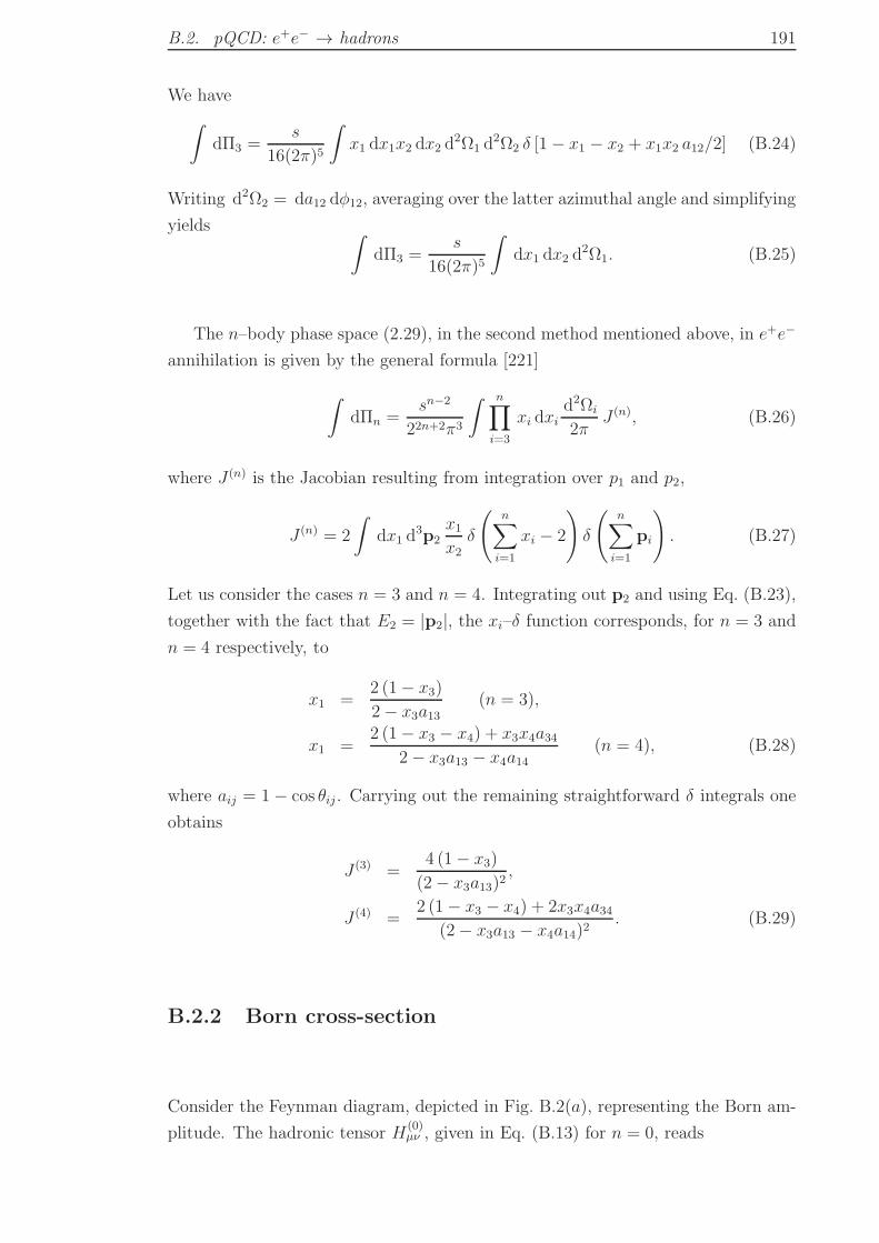
B.2. pQCD: e+e− → hadrons 191
We have
∫dΠ3 =
s
16(2π)5
∫x1 dx1x2 dx2 d
2Ω1 d2Ω2 δ [1− x1 − x2 + x1x2 a12/2] (B.24)
Writing d2Ω2 = da12 dφ12, averaging over the latter azimuthal angle and simplifying
yields ∫dΠ3 =
s
16(2π)5
∫dx1 dx2 d
2Ω1. (B.25)
The n–body phase space (2.29), in the second method mentioned above, in e+e−
annihilation is given by the general formula [221]
∫dΠn =
sn−2
22n+2π3
∫ n∏
i=3
xi dxid2Ωi
2πJ (n), (B.26)
where J (n) is the Jacobian resulting from integration over p1 and p2,
J (n) = 2
∫dx1 d
3p2x1
x2δ
(n∑
i=1
xi − 2
)δ
(n∑
i=1
pi
). (B.27)
Let us consider the cases n = 3 and n = 4. Integrating out p2 and using Eq. (B.23),
together with the fact that E2 = |p2|, the xi–δ function corresponds, for n = 3 and
n = 4 respectively, to
x1 =2 (1− x3)
2− x3a13(n = 3),
x1 =2 (1− x3 − x4) + x3x4a34
2− x3a13 − x4a14(n = 4), (B.28)
where aij = 1 − cos θij . Carrying out the remaining straightforward δ integrals one
obtains
J (3) =4 (1− x3)
(2− x3a13)2,
J (4) =2 (1− x3 − x4) + 2x3x4a34
(2− x3a13 − x4a14)2. (B.29)
B.2.2 Born cross-section
Consider the Feynman diagram, depicted in Fig. B.2(a), representing the Born am-
plitude. The hadronic tensor H(0)µν , given in Eq. (B.13) for n = 0, reads
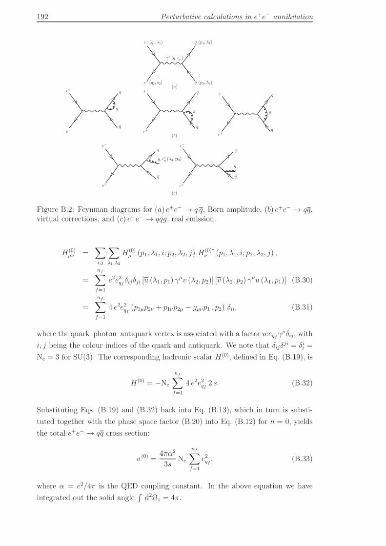
192 Perturbative calculations in e+e− annihilation
(b)
e+ (q2, s2) q (p2, λ2)
e− (q1, s1) q (p1, λ1)
γ∗ (q, ǫµ)
e− q
e+q
g
e− q
e+q
g
e− q
e+q
g
e−q
e+
q
g
(c)
e−q
e+
q
g, ǫ∗µ (λ3,p3)
(a)
Figure B.2: Feynman diagrams for (a) e+e− → q q, Born amplitude, (b) e+e− → qq,virtual corrections, and (c) e+e− → qqg, real emission.
H(0)µν =
∑
i,j
∑
λ1,λ2
H(0)µ (p1, λ1, i; p2, λ2, j) H
(0)†ν (p1, λ1, i; p2, λ2, j) ,
=
nf∑
f=1
e2e2qf δijδji [u (λ1, p1) γµv (λ2, p2)] [v (λ2, p2) γ
νu (λ1, p1)] (B.30)
=
nf∑
f=1
4 e2e2qf (p1µp2ν + p1νp2µ − gµνp1 . p2) δii, (B.31)
where the quark–photon–antiquark vertex is associated with a factor ıeeqfγµδij , with
i, j being the colour indices of the quark and antiquark. We note that δijδji = δii =
Nc = 3 for SU(3). The corresponding hadronic scalar H(0), defined in Eq. (B.19), is
H(0) = −Nc
nf∑
f=1
4 e2e2qf 2 s. (B.32)
Substituting Eqs. (B.19) and (B.32) back into Eq. (B.13), which in turn is substi-
tuted together with the phase space factor (B.20) into Eq. (B.12) for n = 0, yields
the total e+e− → qq cross section:
σ(0) =4πα2
3sNc
nf∑
f=1
e2qf , (B.33)
where α = e2/4π is the QED coupling constant. In the above equation we have
integrated out the solid angle∫d2Ω1 = 4π.
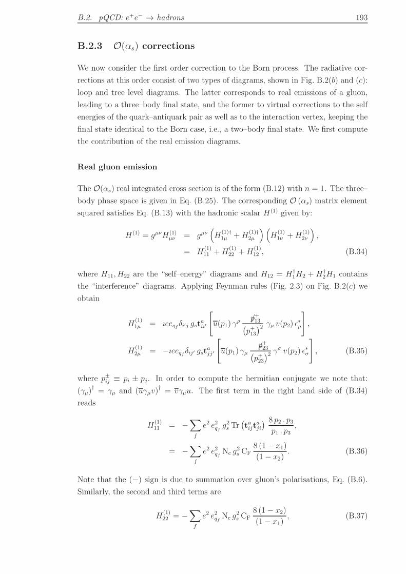
B.2. pQCD: e+e− → hadrons 193
B.2.3 O(αs) corrections
We now consider the first order correction to the Born process. The radiative cor-
rections at this order consist of two types of diagrams, shown in Fig. B.2(b) and (c):
loop and tree level diagrams. The latter corresponds to real emissions of a gluon,
leading to a three–body final state, and the former to virtual corrections to the self
energies of the quark–antiquark pair as well as to the interaction vertex, keeping the
final state identical to the Born case, i.e., a two–body final state. We first compute
the contribution of the real emission diagrams.
Real gluon emission
The O(αs) real integrated cross section is of the form (B.12) with n = 1. The three–
body phase space is given in Eq. (B.25). The corresponding O (αs) matrix element
squared satisfies Eq. (B.13) with the hadronic scalar H(1) given by:
H(1) = gµνH(1)µν = gµν
(H
(1)†1µ +H
(1)†2µ
)(H
(1)1ν +H
(1)2ν
),
= H(1)11 +H
(1)22 +H
(1)12 , (B.34)
where H11, H22 are the “self–energy” diagrams and H12 = H†1H2 + H†
2H1 contains
the “interference” diagrams. Applying Feynman rules (Fig. 2.3) on Fig. B.2(c) we
obtain
H(1)1µ = ıeeqf δi′j gst
aii′
[u(p1) γ
ρ p+13/(p+13)2 γµ v(p2) ǫ
∗ρ
],
H(1)2µ = −ıeeqf δij′ gst
ajj′
[u(p1) γµ
p+23/(p+23)2 γ
σ v(p2) ǫ∗σ
], (B.35)
where p±ij ≡ pi ± pj . In order to compute the hermitian conjugate we note that:
(γµ)† = γµ and (uγµv)
† = vγµu. The first term in the right hand side of (B.34)
reads
H(1)11 = −
∑
f
e2 e2qf g2s Tr
(taijt
aji
) 8 p2 . p3p1 . p3
,
= −∑
f
e2 e2qf Nc g2s CF
8 (1− x1)
(1− x2). (B.36)
Note that the (−) sign is due to summation over gluon’s polarisations, Eq. (B.6).
Similarly, the second and third terms are
H(1)22 = −
∑
f
e2 e2qf Nc g2s CF
8 (1− x2)
(1− x1), (B.37)
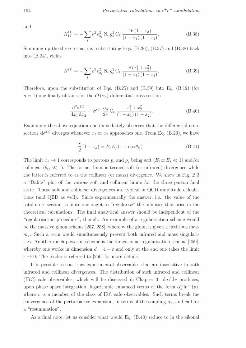
194 Perturbative calculations in e+e− annihilation
and
H(1)12 = −
∑
f
e2 e2qf Nc g2s CF
16 (1− x3)
(1− x1) (1− x2). (B.38)
Summing up the three terms, i.e., substituting Eqs. (B.36), (B.37) and (B.38) back
into (B.34), yields
H(1) = −∑
f
e2 e2qf Nc g2s CF
8 (x21 + x2
2)
(1− x1) (1− x2). (B.39)
Therefore, upon the substitution of Eqs. (B.25) and (B.39) into Eq. (B.12) (for
n = 1) one finally obtains for the O (αs) differential cross section
d2σ(1)
dx1 dx2= σ(0) αs
2πCF
x21 + x2
2
(1− x1) (1− x2). (B.40)
Examining the above equation one immediately observes that the differential cross
section dσ(1) diverges whenever x1 or x2 approaches one. From Eq. (B.23), we have
s
2(1− xk) = Ei Ej (1− cos θij) . (B.41)
The limit xk → 1 corresponds to partons pi and pj being soft (Ei orEj ≪ 1) and/or
collinear (θij ≪ 1). The former limit is termed soft (or infrared) divergence while
the latter is referred to as the collinear (or mass) divergence. We show in Fig. B.3
a “Dalitz” plot of the various soft and collinear limits for the three parton final
state. These soft and collinear divergences are typical in QCD amplitude calcula-
tions (and QED as well). Since experimentally the answer, i.e., the value of the
total cross section, is finite one ought to “regularise” the infinities that arise in the
theoretical calculations. The final analytical answer should be independent of the
“regularisation procedure”, though. An example of a regularisation scheme would
be the massive gluon scheme [257, 258], whereby the gluon is given a fictitious mass
mg. Such a term would simultaneously prevent both infrared and mass singulari-
ties. Another much powerful scheme is the dimensional regularisation scheme [259],
whereby one works in dimension d = 4 − ε and only at the end one takes the limit
ε → 0. The reader is referred to [260] for more details.
It is possible to construct experimental observables that are insensitive to both
infrared and collinear divergences. The distribution of such infrared and collinear
(IRC) safe observables, which will be discussed in Chapter 3, dσ/ dv produces,
upon phase space integration, logarithmic enhanced terms of the form αns ln
m (v),
where v is a member of the class of IRC safe observables. Such terms break the
convergence of the perturbative expansion, in terms of the coupling αs, and call for
a “resummation”.
As a final note, let us consider what would Eq. (B.40) reduce to in the eikonal
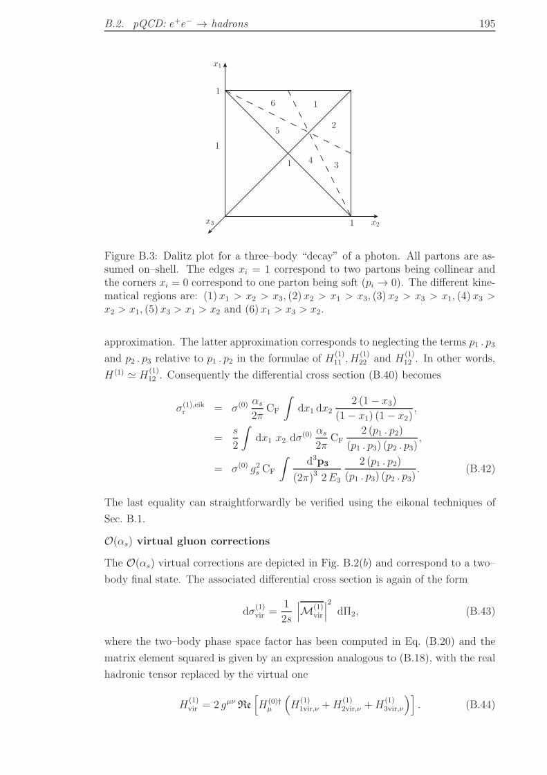
B.2. pQCD: e+e− → hadrons 195
x1
x2x3
1
1
1
16
5
43
2
1
Figure B.3: Dalitz plot for a three–body “decay” of a photon. All partons are as-sumed on–shell. The edges xi = 1 correspond to two partons being collinear andthe corners xi = 0 correspond to one parton being soft (pi → 0). The different kine-matical regions are: (1) x1 > x2 > x3, (2) x2 > x1 > x3, (3) x2 > x3 > x1, (4) x3 >x2 > x1, (5) x3 > x1 > x2 and (6) x1 > x3 > x2.
approximation. The latter approximation corresponds to neglecting the terms p1 . p3
and p2 . p3 relative to p1 . p2 in the formulae of H(1)11 , H
(1)22 and H
(1)12 . In other words,
H(1) ≃ H(1)12 . Consequently the differential cross section (B.40) becomes
σ(1),eikr = σ(0) αs
2πCF
∫dx1 dx2
2 (1− x3)
(1− x1) (1− x2),
=s
2
∫dx1 x2 dσ(0) αs
2πCF
2 (p1 . p2)
(p1 . p3) (p2 . p3),
= σ(0) g2s CF
∫d3p3
(2π)3 2E3
2 (p1 . p2)
(p1 . p3) (p2 . p3). (B.42)
The last equality can straightforwardly be verified using the eikonal techniques of
Sec. B.1.
O(αs) virtual gluon corrections
The O(αs) virtual corrections are depicted in Fig. B.2(b) and correspond to a two–
body final state. The associated differential cross section is again of the form
dσ(1)vir =
1
2s
∣∣∣M(1)vir
∣∣∣2
dΠ2, (B.43)
where the two–body phase space factor has been computed in Eq. (B.20) and the
matrix element squared is given by an expression analogous to (B.18), with the real
hadronic tensor replaced by the virtual one
H(1)vir = 2 gµν Re
[H(0)†
µ
(H
(1)1vir,ν +H
(1)2vir,ν +H
(1)3vir,ν
)]. (B.44)
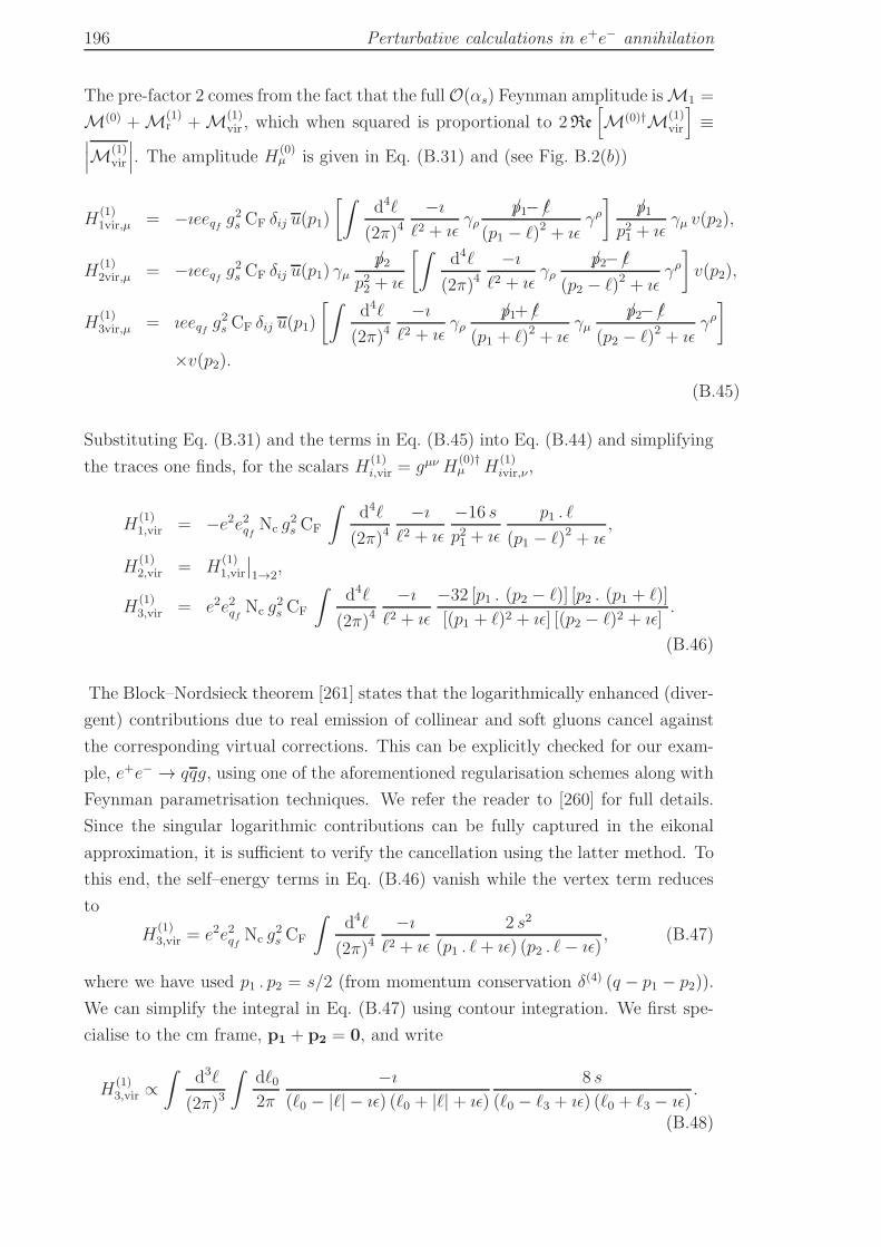
196 Perturbative calculations in e+e− annihilation
The pre-factor 2 comes from the fact that the fullO(αs) Feynman amplitude isM1 =
M(0) + M(1)r + M(1)
vir , which when squared is proportional to 2Re
[M(0)†M(1)
vir
]≡
∣∣∣M(1)vir
∣∣∣. The amplitude H(0)µ is given in Eq. (B.31) and (see Fig. B.2(b))
H(1)1vir,µ = −ıeeqf g
2s CF δij u(p1)
[∫d4ℓ
(2π)4−ı
ℓ2 + ıǫγρ
p1/− ℓ/
(p1 − ℓ)2 + ıǫγρ
]p1/
p21 + ıǫγµ v(p2),
H(1)2vir,µ = −ıeeqf g
2s CF δij u(p1) γµ
p2/
p22 + ıǫ
[∫d4ℓ
(2π)4−ı
ℓ2 + ıǫγρ
p2/− ℓ/
(p2 − ℓ)2 + ıǫγρ
]v(p2),
H(1)3vir,µ = ıeeqf g
2s CF δij u(p1)
[∫d4ℓ
(2π)4−ı
ℓ2 + ıǫγρ
p1/+ ℓ/
(p1 + ℓ)2 + ıǫγµ
p2/− ℓ/
(p2 − ℓ)2 + ıǫγρ
]
×v(p2).
(B.45)
Substituting Eq. (B.31) and the terms in Eq. (B.45) into Eq. (B.44) and simplifying
the traces one finds, for the scalars H(1)i,vir = gµν H
(0)†µ H
(1)ivir,ν ,
H(1)1,vir = −e2e2qf Nc g
2s CF
∫d4ℓ
(2π)4−ı
ℓ2 + ıǫ
−16 s
p21 + ıǫ
p1 . ℓ
(p1 − ℓ)2 + ıǫ,
H(1)2,vir = H
(1)1,vir
∣∣1→2
,
H(1)3,vir = e2e2qf Nc g
2s CF
∫d4ℓ
(2π)4−ı
ℓ2 + ıǫ
−32 [p1 . (p2 − ℓ)] [p2 . (p1 + ℓ)]
[(p1 + ℓ)2 + ıǫ] [(p2 − ℓ)2 + ıǫ].
(B.46)
The Block–Nordsieck theorem [261] states that the logarithmically enhanced (diver-
gent) contributions due to real emission of collinear and soft gluons cancel against
the corresponding virtual corrections. This can be explicitly checked for our exam-
ple, e+e− → qqg, using one of the aforementioned regularisation schemes along with
Feynman parametrisation techniques. We refer the reader to [260] for full details.
Since the singular logarithmic contributions can be fully captured in the eikonal
approximation, it is sufficient to verify the cancellation using the latter method. To
this end, the self–energy terms in Eq. (B.46) vanish while the vertex term reduces
to
H(1)3,vir = e2e2qf Nc g
2s CF
∫d4ℓ
(2π)4−ı
ℓ2 + ıǫ
2 s2
(p1 . ℓ+ ıǫ) (p2 . ℓ− ıǫ), (B.47)
where we have used p1 . p2 = s/2 (from momentum conservation δ(4) (q − p1 − p2)).
We can simplify the integral in Eq. (B.47) using contour integration. We first spe-
cialise to the cm frame, p1 + p2 = 0, and write
H(1)3,vir ∝
∫d3ℓ
(2π)3
∫dℓ02π
−ı
(ℓ0 − |ℓ| − ıǫ) (ℓ0 + |ℓ|+ ıǫ)
8 s
(ℓ0 − ℓ3 + ıǫ) (ℓ0 + ℓ3 − ıǫ).
(B.48)
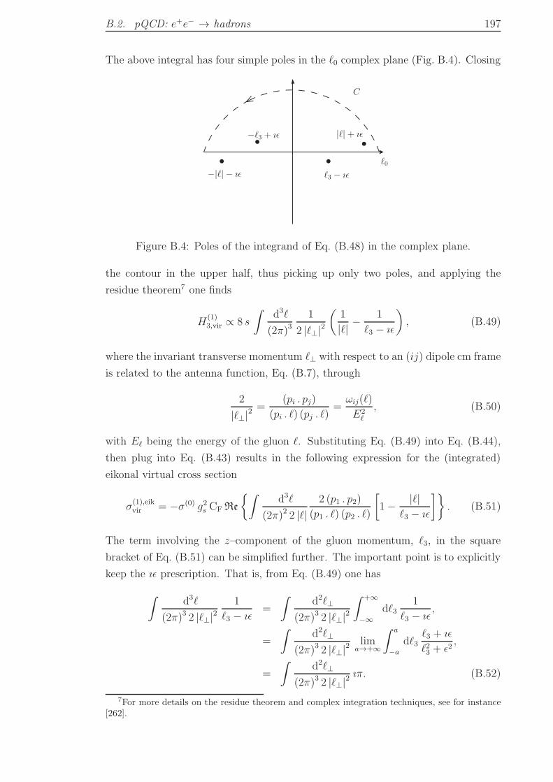
B.2. pQCD: e+e− → hadrons 197
The above integral has four simple poles in the ℓ0 complex plane (Fig. B.4). Closing
ℓ0
|ℓ|+ ıǫ
ℓ3 − ıǫ−|ℓ| − ıǫ
−ℓ3 + ıǫ
C
Figure B.4: Poles of the integrand of Eq. (B.48) in the complex plane.
the contour in the upper half, thus picking up only two poles, and applying the
residue theorem7 one finds
H(1)3,vir ∝ 8 s
∫d3ℓ
(2π)31
2 |ℓ⊥|2(
1
|ℓ| −1
ℓ3 − ıǫ
), (B.49)
where the invariant transverse momentum ℓ⊥ with respect to an (ij) dipole cm frame
is related to the antenna function, Eq. (B.7), through
2
|ℓ⊥|2=
(pi . pj)
(pi . ℓ) (pj . ℓ)=
ωij(ℓ)
E2ℓ
, (B.50)
with Eℓ being the energy of the gluon ℓ. Substituting Eq. (B.49) into Eq. (B.44),
then plug into Eq. (B.43) results in the following expression for the (integrated)
eikonal virtual cross section
σ(1),eikvir = −σ(0) g2s CF Re
∫d3ℓ
(2π)2 2 |ℓ|2 (p1 . p2)
(p1 . ℓ) (p2 . ℓ)
[1− |ℓ|
ℓ3 − ıǫ
]. (B.51)
The term involving the z–component of the gluon momentum, ℓ3, in the square
bracket of Eq. (B.51) can be simplified further. The important point is to explicitly
keep the ıǫ prescription. That is, from Eq. (B.49) one has
∫d3ℓ
(2π)3 2 |ℓ⊥|21
ℓ3 − ıǫ=
∫d2ℓ⊥
(2π)3 2 |ℓ⊥|2∫ +∞
−∞dℓ3
1
ℓ3 − ıǫ,
=
∫d2ℓ⊥
(2π)3 2 |ℓ⊥|2lim
a→+∞
∫ a
−a
dℓ3ℓ3 + ıǫ
ℓ23 + ǫ2,
=
∫d2ℓ⊥
(2π)3 2 |ℓ⊥|2ıπ. (B.52)
7For more details on the residue theorem and complex integration techniques, see for instance[262].
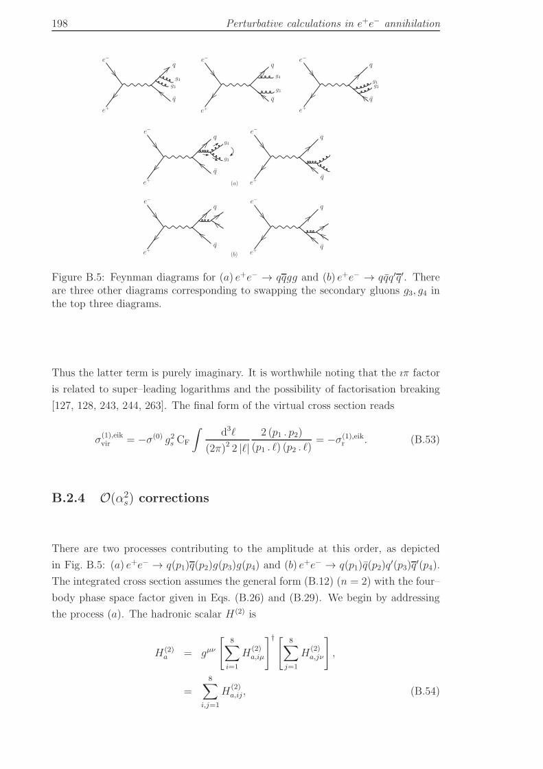
198 Perturbative calculations in e+e− annihilation
(b)
e−q
e+q
e−q
e+q
e−q
e+
q
e−q
e+
q
e−q
e+
q
g4g3
g4
g3
g4g3
e−q
e+q
e−q
e+
q
(a)
g4
g3
Figure B.5: Feynman diagrams for (a) e+e− → qqgg and (b) e+e− → qqq′q′. Thereare three other diagrams corresponding to swapping the secondary gluons g3, g4 inthe top three diagrams.
Thus the latter term is purely imaginary. It is worthwhile noting that the ıπ factor
is related to super–leading logarithms and the possibility of factorisation breaking
[127, 128, 243, 244, 263]. The final form of the virtual cross section reads
σ(1),eikvir = −σ(0) g2s CF
∫d3ℓ
(2π)2 2 |ℓ|2 (p1 . p2)
(p1 . ℓ) (p2 . ℓ)= −σ(1),eik
r . (B.53)
B.2.4 O(α2s) corrections
There are two processes contributing to the amplitude at this order, as depicted
in Fig. B.5: (a) e+e− → q(p1)q(p2)g(p3)g(p4) and (b) e+e− → q(p1)q(p2)q′(p3)q
′(p4).
The integrated cross section assumes the general form (B.12) (n = 2) with the four–
body phase space factor given in Eqs. (B.26) and (B.29). We begin by addressing
the process (a). The hadronic scalar H(2) is
H(2)a = gµν
[8∑
i=1
H(2)a,iµ
]† [ 8∑
j=1
H(2)a,jν
],
=
8∑
i,j=1
H(2)a,ij, (B.54)
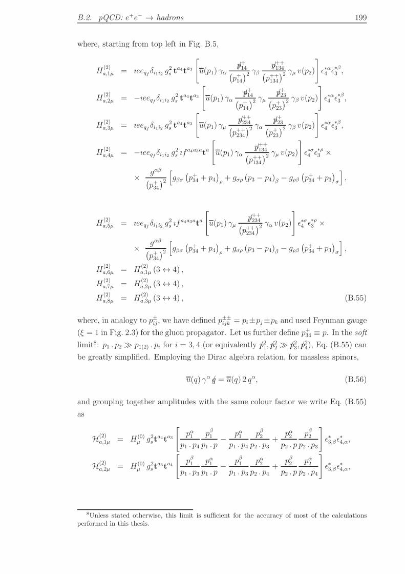
B.2. pQCD: e+e− → hadrons 199
where, starting from top left in Fig. B.5,
H(2)a,1µ = ıeeqf δi1i2 g
2s t
a4ta3
[u(p1) γα
p+14/(p+14)2 γβ
p++134/
(p++134
)2 γµ v(p2)]ǫ∗α4 ǫ∗β3 ,
H(2)a,2µ = −ıeeqf δi1i2 g
2s t
a4ta3
[u(p1) γα
p+14/(p+14)2 γµ
p+23/(p+23)2 γβ v(p2)
]ǫ∗α4 ǫ∗β3 ,
H(2)a,3µ = ıeeqf δi1i2 g
2s t
a4ta3
[u(p1) γµ
p++234/
(p++234
)2 γαp+23/
(p+23)2 γβ v(p2)
]ǫ∗α4 ǫ∗β3 ,
H(2)a,4µ = −ıeeqf δi1i2 g
2s ıf
a4a3ata
[u(p1) γα
p++134/
(p++134
)2 γµ v(p2)]ǫ∗σ4 ǫ∗ρ3 ×
× gαβ(p+34)2[gβσ(p+34 + p4
)ρ+ gσρ (p3 − p4)β − gρβ
(p+34 + p3
)σ
],
H(2)a,5µ = ıeeqf δi1i2 g
2s ıf
a4a3ata
[u(p1) γµ
p++234/
(p++234
)2 γα v(p2)]ǫ∗σ4 ǫ∗ρ3 ×
× gαβ(p+34)2[gβσ(p+34 + p4
)ρ+ gσρ (p3 − p4)β − gρβ
(p+34 + p3
)σ
],
H(2)a,6µ = H
(2)a,1µ (3 ↔ 4) ,
H(2)a,7µ = H
(2)a,2µ (3 ↔ 4) ,
H(2)a,8µ = H
(2)a,3µ (3 ↔ 4) , (B.55)
where, in analogy to p±ij , we have defined p±±ijk = pi±pj±pk and used Feynman gauge
(ξ = 1 in Fig. 2.3) for the gluon propagator. Let us further define p+34 ≡ p. In the soft
limit8: p1 . p2 ≫ p1(2) . pi for i = 3, 4 (or equivalently p/21, p/22 ≫ p/23, p/
24), Eq. (B.55) can
be greatly simplified. Employing the Dirac algebra relation, for massless spinors,
u(q) γα q/ = u(q) 2 qα, (B.56)
and grouping together amplitudes with the same colour factor we write Eq. (B.55)
as
H(2)a,1µ = H(0)
µ g2sta4ta3
[pα1
p1 . p4
pβ1p1 . p
− pα1p1 . p4
pβ2p2 . p3
+pα2
p2 . p
pβ2p2 . p3
]ǫ∗3,βǫ
∗4,α,
H(2)a,2µ = H(0)
µ g2sta3ta4
[pβ1
p1 . p3
pα1p1 . p
− pβ1p1 . p3
pα2p2 . p4
+pβ2
p2 . p
pα2p2 . p4
]ǫ∗3,βǫ
∗4,α,
8Unless stated otherwise, this limit is sufficient for the accuracy of most of the calculationsperformed in this thesis.
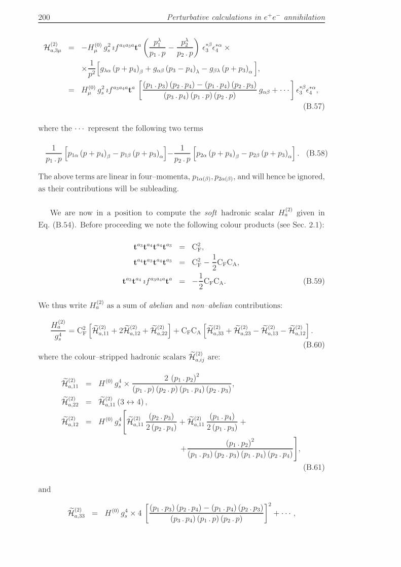
200 Perturbative calculations in e+e− annihilation
H(2)a,3µ = −H(0)
µ g2s ıfa4a3ata
(pλ1
p1 . p− pλ2
p2 . p
)ǫ∗β3 ǫ∗α4 ×
× 1
p2
[gλα (p+ p4)β + gαβ (p3 − p4)λ − gβλ (p+ p3)α
],
= H(0)µ g2s ıf
a3a4ata[(p1 . p3) (p2 . p4)− (p1 . p4) (p2 . p3)
(p3 . p4) (p1 . p) (p2 . p)gαβ + · · ·
]ǫ∗β3 ǫ∗α4 ,
(B.57)
where the · · · represent the following two terms
1
p1 . p
[p1α (p+ p4)β − p1β (p+ p3)α
]− 1
p2 . p
[p2α (p+ p4)β − p2β (p+ p3)α
]. (B.58)
The above terms are linear in four–momenta, p1α(β), p2α(β), and will hence be ignored,
as their contributions will be subleading.
We are now in a position to compute the soft hadronic scalar H(2)a given in
Eq. (B.54). Before proceeding we note the following colour products (see Sec. 2.1):
ta3ta4ta4ta3 = C2F,
ta4ta3ta4ta3 = C2F − 1
2CFCA,
ta3ta4 ıfa3a4ata = −1
2CFCA. (B.59)
We thus write H(2)a as a sum of abelian and non–abelian contributions:
H(2)a
g4s= C2
F
[H(2)
a,11 + 2H(2)a,12 + H(2)
a,22
]+ CFCA
[H(2)
a,33 + H(2)a,23 − H(2)
a,13 − H(2)a,12
].
(B.60)
where the colour–stripped hadronic scalars H(2)a,ij are:
H(2)a,11 = H(0) g4s ×
2 (p1 . p2)2
(p1 . p) (p2 . p) (p1 . p4) (p2 . p3),
H(2)a,22 = H(2)
a,11 (3 ↔ 4) ,
H(2)a,12 = H(0) g4s
[H(2)
a,11
(p2 . p3)
2 (p2 . p4)+ H(2)
a,11
(p1 . p4)
2 (p1 . p3)+
+(p1 . p2)
2
(p1 . p3) (p2 . p3) (p1 . p4) (p2 . p4)
],
(B.61)
and
H(2)a,33 = H(0) g4s × 4
[(p1 . p3) (p2 . p4)− (p1 . p4) (p2 . p3)
(p3 . p4) (p1 . p) (p2 . p)
]2+ · · · ,
B.2. pQCD: e+e− → hadrons 201
H(2)a,13 = −H(0) g4s
(p1 . p2)
(p1 . p4) (p2 . p3)
[(p1 . p3) (p2 . p4)− (p1 . p4) (p2 . p3)
(p3 . p4) (p1 . p) (p2 . p)
],
H(2)a,23 = −H(0) g4s
(p1 . p2)
(p1 . p3) (p2 . p4)
[(p1 . p3) (p2 . p4)− (p1 . p4) (p2 . p3)
(p3 . p4) (p1 . p) (p2 . p)
].
(B.62)
Note that a (−) sign has been absorbed into the Born hadronic tensor H(0). Sub-
stituting Eqs. (B.61) and (B.62) into Eq. (B.60), which is in turn substituted back
into Eq. (B.13), for n = 2 and process a, yields
∣∣∣M(2)a
∣∣∣2
=∣∣∣M(0)
∣∣∣2
g4s[4C2
FWP + CFCA (2S +Hg)], (B.63)
where the abelian (primary emission) amplitude is
WP =(p1 . p2)
(p1 . p3) (p2 . p3)
(p1 . p2)
(p1 . p4) (p2 . p4)=
ω12(p3)ω12(p4)
E23E
24
, (B.64)
and writing (pi . pj) = (ij) the non–abelian (secondary emission) amplitude is9 the
sum of the soft, S, and gluon hard, Hg, terms:
S =(12)
(13)(34)(42)+
(12)
(14)(43)(32)− (12)
(13)(32)
(12)
(14)(42),
=1
E23E
24
ω12(p3) [ω13(p4) + ω23(p4)− ω12(p4)] , (B.65)
and
Hg = 2 I2 − S J − 4ω12(p)
(34)E2p
, (B.66)
where
I =(13)(24)− (14)(23)
(34)(1p)(2p),
J =(13)(24) + (14)(23)
(1p)(2p). (B.67)
The other process at O(α2s), as stated above, is represented by the Feynman
diagrams in Fig. B.5(b). The corresponding hadronic scalar reads
H(2)b = gµν
[H
(2)b,1µ +H
(2)b,2µ
]† [H
(2)b,1ν +H
(2)b,2ν
], (B.68)
9The trick to simplify the non–abelian part of Eq. (B.60) to the form presented in Eq. (B.63)is to add and subtract a factor of 2 in the square brackets of Eqs. (B.61) and (B.62).
202 Perturbative calculations in e+e− annihilation
where
H(2)b,1µ = ıeeqf δi′1i2 g
2st
ai1i′1
taj3j4
[u(p1) γα
p++134/
(p++134
)2 γµ v(p2)]
1(p+34)2 [u(p4) γ
α v(p3)] ,
H(2)b,2µ = −ıeeqf δi1i′2 g
2st
ai′2i2
taj3j4
[u(p1) γµ
p++234/
(p++234
)2 γα v(p2)]
1(p+34)2 [u(p4) γ
α v(p3)] .
(B.69)
Similar to process (a), Eq. (B.69) simplifies significantly in the soft limit. Adding
up the two contributions (and using the above notation p = p+34) we have
H(2)b,µ = H(0)
µ g2s tai1i2t
aj3j4
(pα1
(p1 . p)− pα2
(p2 . p)
)1
p2[u(p4) γα v(p3)] . (B.70)
Squaring the above amplitude we find
H(2)b ≃ H(0) g4s t
ai1i2
Tr(taj3j4t
bj3j4
)tbi1i2 nf
(pα1(1p)
− pα2(2p)
)(pβ1(1p)
− pβ2(2p)
)×
Tr [p4/ γα p3/ γβ]
4 (p3 . p4)2 ,
≃ H(0) g4s CFTRnf2
[(34)(1p)(2p)]2[(12)(34)(1p)(2p)− ((13)(24)− (14)(23))2
].
(B.71)
Therefore the matrix element squared for process (b) can be written, following the
steps outlined previously for process (a), as
∣∣∣M(2)b
∣∣∣2
=∣∣∣M(0)
∣∣∣2
g4s CFTRnf Hq, (B.72)
where TR = TF = 1/2 and the quark hard term is
Hq = −4 I2 + 4ω12(p)
(34)E2p
. (B.73)
Adding up the contributions of both processes (a) and (b) the final expression of the
O(α2s) matrix element in the soft limit (which nonetheless includes the quark and
gluon hard terms) is given by
∣∣∣M(2)
∣∣∣2
=∣∣∣M(0)
∣∣∣2
g4s[4C2
FWP + CFCA (2S +Hg) + CFTFnf Hq
]. (B.74)
Notice that if one employs the eikonal method (described in Sec. B.1) then one
would find an identical formula to Eq. (B.74) without the hard terms Hg and Hq.
Appendix C
Jet–thrust calculations
C.1 Derivation of the LO distribution
In the present section we outline the necessary steps for the derivation of the full
logarithmic part of the LO τE0 integrated distribution, Eq. (5.7). For the emission of
a single gluon, i.e, e+e− → q q g, we define the kinematic variables, xi = 2pi . q/Q2 =
2Ei/Q and yij = 2pi . pj/Q2 = 1 − xk where i, j, k = 1(q), 2(q), 3(g) and q = p1 +
p2 + p3. The leading–order (qqg) matrix–element squared is given in Eq. (B.40). It
readsd2σ(1)
σ(0) dx1 dx2=
CFαs
2π
x21 + x2
2
(1− x1)(1− x2), (C.1)
where σ(0) is the Born cross–section. The integration region, which is originally
1 ≥ x1, x2, x3 ≥ 0 (recall that x1 + x2 + x3 = 2) and which leads to divergences,
gets modified by introducing the jet shape variable. For three partons in the final
state, τE0 is zero unless two partons are clustered together. That is, the τE0 shape
distribution receives, at this order, contributions from two–jet configurations only.
Three–jet final state configurations, which are also present at this order, do not
contribute to the latter distribution. They contribute to the E0 distribution instead,
as we shall see later.
It is a straightforward exercise to show that the thrust, or rather τ = 1 − T ,
is, for small values of τ , the sum of the masses of two hemisphere jets. Precisely
τ ≃ (p2J1+p2J2)/Q2 = 1−maxxi = τE0 where i = 1, 2, 3 1. The two distributions are
thus equal. However, here we are considering jets of size Rs < 1/2 and the following
(generic) jet algorithm condition for a pair (i, j) to be recombined together to form
a jet applies
Rs > 2(1− cos θij) =(1− xk)
xixj≃ (1− xk)
xj, k 6= i, j, (C.2)
where the last approximation follows from xk > xi > xj (we show in Sec. 5.2.2 that
in the limit Rs → 1/2 ⇔ θij → π/2 the latter approximation yields the exact τ
distribution).
1From conservation of momentum given above we have for a jet formed by a pair of partons(i, j): τE0 = (pi + pj)
2/Q2 = 2pi . pj/Q2 = (1− xk) where xk > xi, xj . i.e, τE0 = 1−maxxi.
203
204 Jet–thrust calculations
The phase space of the two–jet/three–jet boundary for the τE0(p1, p2) < τE0 is
given in terms of the energy fractions 2 as
1 > x1, x2 > 1− τE0, 1 + τE0 > x1 + x2, R2 >4(1− x2)
2− x1 − x3, (C.3)
where we have chosen to recombine the gluon, p3, with hard leg p1. The other
choice, i.e, recombining the gluon with hard leg p2, produces identical result. Hence
we multiply by a factor of two to account for the latter. Likewise, the phase space
boundary for the three–jet configuration whereby the third jet, chosen to be the
gluon jet, is vetoed to have energy less than a cut–off E0 is given by
2 > x1 + x2 > 2
(1− E0
Q
),
4(1− x2)
2− x1 − x3> R2,
4(1− x1)
2− x2 − x3> R2. (C.4)
Due to the soft and collinear singularities of the matrix–element (C.1), x1,2 → 1, we
use the following completion relation in order to integrate the τE0 and E0 differential
distributions
Σ(0) +[Σ
(1)in + Σ
(1)out
]= 1 +
∫ τE0
0
dτ ′E0
1
σ(0)
dσ(1)
dτ ′E0
+
∫ E0
0
dE31
σ(0)
dσ(1)
dE3
,
=σtot
σ(0)−∫ τmax
E0
τE0
dτ ′E0
1
σ(0)
dσ(1)
dτ ′E0
−∫ Q/2
E0
dE31
σ(0)
dσ(1)
dE3
,
(C.5)
where “in” and “out” refer to the regions (C.3) and (C.4), respectively, and the total
cross–section σtot, which includes both real (two–jet and three–jet contributions) and
virtual corrections, is related to the Born cross–section by [7]
σtot
σ(0)= 1 +
3CF
2
αs
2π+O(α2
s). (C.6)
Thus inverting the conditions in Eqs. (C.3) and (C.4), carrying out the integrals in
Eq. (C.5) separately and then adding up with the O(αs) of Eq. (C.6) one obtains
Eq. (5.8).
2Similar limits have been derived for the JADE variable y in [7], which were also used for τ inthe same reference.
C.2. Gnm coefficients 205
C.2 Gnm coefficients
The resultant coefficients from the expansion of the exponent in the resummed
integrated distribution, eq. (5.80), for the anti–kTalgorithm, are
G12 = −2CF,
G11 = CF (3− 4LRs) ,
G10 = CF
[−4LRsLE0 +
f0(Rs)
2
],
G23 = CF
(4
3TFnf −
11
3CA
),
G22 = −4π2
3C2
F + CFCA
(π2
3− I22(Rs)−
169
36− 22
3LRs
)+ CFTFnf
(11
9+
8
3LRs
),
G21 = −C2F
8π2
3LRs − CFCA
[2I22(Rs)LE0 − Ia21(Rs) + ICA
21 (Rs)−
−(2π2
3− 2I22(Rs)− 134
9− 11
3LRs
)LRs
]+
+ CFTFnf
[Inf
21 (Rs) +
(4
3LRs +
40
9
)LRs
]. (C.7)
where LRs = ln(Rs/(1−Rs)) and LE0 = ln(2E0/Q). The factor f0(Rs) only captures
the first term of f0 given in eq. (5.10). We simply replace f0 7→ f0 when comparing
to the numerical distribution. Moreover, we have
S22 = −CFCA I22(Rs), Sa21 = −CFCA Ia21(Rs),
SCA21 = −CFCA ICA
22 (Rs), Snf
21 = −CFCA Inf
22 (Rs). (C.8)
The one–loop constant is given by, eq. (5.8),
C1 = CF
(−1 +
π2
3
), (C.9)
For the C/A algorithm we have the following replacements in G22 and G21:
I2i → IC/A2i ,
G22 : −4π2
3C2
F → C2F
(CP
2 − 4π2
3
),
G21 : −C2F
8π2
3LRs → C2
F
(2CP
2 − 8π2
3
)LRs + CP
21. (C.10)
Expanding the total resummed distribution in eq. (5.80) to O(α2s) and up to
206 Jet–thrust calculations
NLL we have
Σr,2(L) = 1 +(αs
2π
)(H12L
2 +H11L+H10
)+(αs
2π
)2 (H24L
4 +H23L3 +H22L
2+
+H21L+H20
), (C.11)
where (recall that L = ln(1/τE0) ⇒ τE0 = e−L)
Dfin(e−L) =
(αs
2π
)d1(e
−L) +(αs
2π
)2d2(e
−L),
H12 = G12,
H11 = G11,
H10 = G10 + C1 + d1(τE0),
H24 =1
2G2
12.
H23 = G23 +G12G11,
H22 = G22 + (G10 + C1)G12 +1
2G2
11,
H21 = G21 + (G10 + C1)G11,
H20 = G20 +1
2G2
10 + C1G10 + C2 + d2(τE0). (C.12)
Differentiating (C.11) w.r.t. L, the NLO differential distribution reads
dΣr,2
dL=
1
σ0
dσr,2
dL= δ(L)Dδ +
(αs
2π
)DA(L) +
(αs
2π
)2DB(L), (C.13)
where the singular (logarithmic) terms are given by
Dδ = 1 +(αs
2π
)[G10 + C1] +
(αs
2π
)2 [G20 +
1
2G2
10 + C1G10 + C2
],
DA(L) = 2H12L+H11 +d
dLd1(e
−L),
DB(L) = 4H24L3 + 3H23L
2 + 2H22L+H21 +d
dLd2(e
−L). (C.14)
C.3 Jet-thrust distribution in SCET
The resummation of the jet-thrust in SCET is presented in the current section for
comparison with pQCD. We shall only present the final form of the resummed result
taken from Refs. [50, 223, 46]. For a full derivation and more in depth discussion
one should consult the latter references. The only task we have performed here is
the expansion of the full resummed distribution to O(α2s).
C.3. Jet-thrust distribution in SCET 207
C.3.1 Resummation
The general formula of the resummed distribution for the jet-thrust is given by [50,
46]
dΣSCET(τE0 , R)
dτE0
= exp[4S(µh, µj) + 4S(µs, µj)− 4AH(µh, µs) + 4AJ(µj, µs)
]
×(
Rs
1− Rs
)−2AΓ(µω ,µs)(Q2
µ2h
)−2AΓ(µh ,µj)
H(Q2, µh)
× SoutR (ω, µω)
[j
(ln
µsQ
µ2j
+ ∂η, µj
)]2sinτE0
(∂η, µs)
× 1
τE0
(τE0Q
µs
)ηe−γEη
Γ(η). (C.15)
See [50, 46] for full notation. In order to compute the fixed–order expansion of (C.15)
up to O(α2s), all scales should be set equal (µh = µj = µs = Q). In this limit, the
evolution factors S,AJ and AH vanish. The differentiation w.r.t. η is carried out
using the explicit form of j and sinτE0. The final result of the integrated distribution
may be cast in the generic form (5.80) with the constants and coefficients of the logs
given by
C1 = CF
(−1 +
π2
3
), (C.16)
C2 = C2F
(1− 3π2
8+
π4
72− 6ζ(3)
)+ CFCA
(493
324+
85π2
24− 73π4
360+
283ζ(3)
18
)+
+ CFTFnf
(7
81− 7π2
6− 22ζ(3)
9
)+ C in
2 + Cout2 , (C.17)
and
G12 = −2CF,
G11 = −CF (3− 4LRs) ,
G10 = CF
(−4LRsLE0 +
f02
),
G23 = CF
(11
3CA − 4
3TFnf
),
G22 = −4π2
3C2
F + CFCA
(π2
3− 169
36− 22
3LRs
)+ CFTFnf
(11
9+
8
3LRs
),
G21 = C2F
[−3
4− π2 + 4ζ(3) +
8π2
3LRs
]+ CFTFnf
[5−
(4
3LRs +
40
9
)LRs
]
+ CFCA
[− 57
4+ 6ζ(3)−
(2π2
3− 134
9− 11
3LRs
)LRs
].
208 Jet–thrust calculations
G20 = C2F
[− f 2
0
8+(2π2 − 16ζ(3)
)LRs −
(11π2
6+
f02
)L2Rs
− L2Rs
]+
+ CFCA
[11π2
9LRs −
11
6LRsL
2E0
− LE0
(11f012
+
[134
9− 2π2
3
]LRs +
+11
6L2Rs
)]+ CFTFnf
[− 4π2
9LRs +
2
3LRsL
2E0
+ LE0
(f0(Rs)
3+
+40
9LRs +
2
3L2Rs
)], (C.18)
where f0 ≡ fo(Rs). Considering primary emission, the only missing piece in the
distribution is the two–loop constants in the soft function, namely C in2 and Cout
2 .
C.4 Comparisons to event2 : single Rs plots
Below we provide plots for the difference between the analytical and numerical
(exact) jet-thrust τE0 distribution at NLO for each colour channel. The plots are
shown for each value of Rs separately.
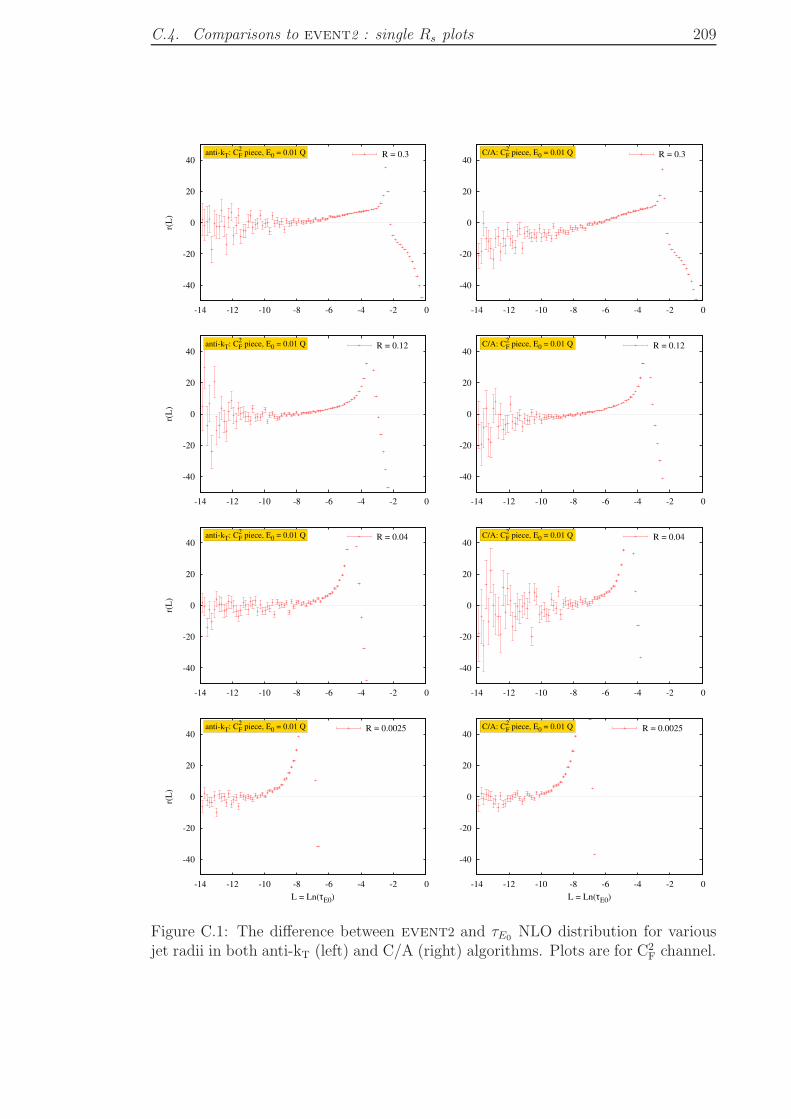
C.4. Comparisons to event2 : single Rs plots 209
-40
-20
0
20
40
-14 -12 -10 -8 -6 -4 -2 0
r(L
)
R = 0.3anti-kT: C2F piece, E0 = 0.01 Q
-40
-20
0
20
40
-14 -12 -10 -8 -6 -4 -2 0
R = 0.3C/A: C2F piece, E0 = 0.01 Q
-40
-20
0
20
40
-14 -12 -10 -8 -6 -4 -2 0
r(L
)
R = 0.12anti-kT: C2F piece, E0 = 0.01 Q
-40
-20
0
20
40
-14 -12 -10 -8 -6 -4 -2 0
R = 0.12C/A: C2F piece, E0 = 0.01 Q
-40
-20
0
20
40
-14 -12 -10 -8 -6 -4 -2 0
r(L
)
R = 0.04anti-kT: C2F piece, E0 = 0.01 Q
-40
-20
0
20
40
-14 -12 -10 -8 -6 -4 -2 0
R = 0.04C/A: C2F piece, E0 = 0.01 Q
-40
-20
0
20
40
-14 -12 -10 -8 -6 -4 -2 0
r(L
)
L = Ln(τE0)
R = 0.0025anti-kT: C2F piece, E0 = 0.01 Q
-40
-20
0
20
40
-14 -12 -10 -8 -6 -4 -2 0
L = Ln(τE0)
R = 0.0025C/A: C2F piece, E0 = 0.01 Q
Figure C.1: The difference between event2 and τE0 NLO distribution for variousjet radii in both anti-kT (left) and C/A (right) algorithms. Plots are for C2
F channel.
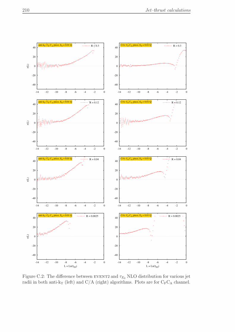
210 Jet–thrust calculations
-40
-20
0
20
40
-14 -12 -10 -8 -6 -4 -2 0
r(L
)
R = 0.3anti-kT: CF CA piece, E0 = 0.01 Q
-40
-20
0
20
40
-14 -12 -10 -8 -6 -4 -2 0
R = 0.3C/A: CF CA piece, E0 = 0.01 Q
-40
-20
0
20
40
-14 -12 -10 -8 -6 -4 -2 0
r(L
)
R = 0.12anti-kT: CF CA piece, E0 = 0.01 Q
-40
-20
0
20
40
-14 -12 -10 -8 -6 -4 -2 0
R = 0.12C/A: CF CA piece, E0 = 0.01 Q
-40
-20
0
20
40
-14 -12 -10 -8 -6 -4 -2 0
r(L
)
R = 0.04anti-kT: CF CA piece, E0 = 0.01 Q
-40
-20
0
20
40
-14 -12 -10 -8 -6 -4 -2 0
R = 0.04C/A: CF CA piece, E0 = 0.01 Q
-40
-20
0
20
40
-14 -12 -10 -8 -6 -4 -2 0
r(L
)
L = Ln(τE0)
R = 0.0025anti-kT: CF CA piece, E0 = 0.01 Q
-40
-20
0
20
40
-14 -12 -10 -8 -6 -4 -2 0
L = Ln(τE0)
R = 0.0025C/A: CF CA piece, E0 = 0.01 Q
Figure C.2: The difference between event2 and τE0 NLO distribution for various jetradii in both anti-kT (left) and C/A (right) algorithms. Plots are for CFCA channel.
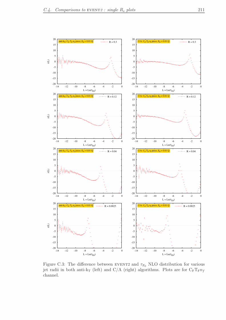
C.4. Comparisons to event2 : single Rs plots 211
-20
-15
-10
-5
0
5
10
15
20
-14 -12 -10 -8 -6 -4 -2 0
r(L
)
L = Ln(τE0)
R = 0.3anti-kT: CF TF nf piece, E0 = 0.01 Q
-20
-15
-10
-5
0
5
10
15
20
-14 -12 -10 -8 -6 -4 -2 0
L = Ln(τE0)
R = 0.3C/A: CF TF nf piece, E0 = 0.01 Q
-20
-15
-10
-5
0
5
10
15
20
-14 -12 -10 -8 -6 -4 -2 0
r(L
)
L = Ln(τE0)
R = 0.12anti-kT: CF TF nf piece, E0 = 0.01 Q
-20
-15
-10
-5
0
5
10
15
20
-14 -12 -10 -8 -6 -4 -2 0
L = Ln(τE0)
R = 0.12C/A: CF TF nf piece, E0 = 0.01 Q
-20
-15
-10
-5
0
5
10
15
20
-14 -12 -10 -8 -6 -4 -2 0
r(L
)
L = Ln(τE0)
R = 0.04anti-kT: CF TF nf piece, E0 = 0.01 Q
-20
-15
-10
-5
0
5
10
15
20
-14 -12 -10 -8 -6 -4 -2 0
L = Ln(τE0)
R = 0.04C/A: CF TF nf piece, E0 = 0.01 Q
-20
-15
-10
-5
0
5
10
15
20
-14 -12 -10 -8 -6 -4 -2 0
r(L
)
L = Ln(τE0)
R = 0.0025anti-kT: CF TF nf piece, E0 = 0.01 Q
-20
-15
-10
-5
0
5
10
15
20
-14 -12 -10 -8 -6 -4 -2 0
L = Ln(τE0)
R = 0.0025C/A: CF TF nf piece, E0 = 0.01 Q
Figure C.3: The difference between event2 and τE0 NLO distribution for variousjet radii in both anti-kT (left) and C/A (right) algorithms. Plots are for CFTFnf
channel.

212
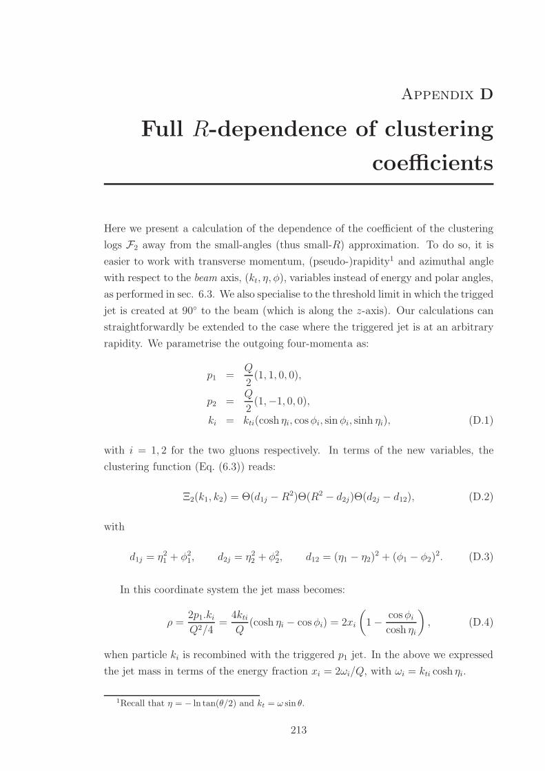
Appendix D
Full R-dependence of clustering
coefficients
Here we present a calculation of the dependence of the coefficient of the clustering
logs F2 away from the small-angles (thus small-R) approximation. To do so, it is
easier to work with transverse momentum, (pseudo-)rapidity1 and azimuthal angle
with respect to the beam axis, (kt, η, φ), variables instead of energy and polar angles,
as performed in sec. 6.3. We also specialise to the threshold limit in which the trigged
jet is created at 90 to the beam (which is along the z-axis). Our calculations can
straightforwardly be extended to the case where the triggered jet is at an arbitrary
rapidity. We parametrise the outgoing four-momenta as:
p1 =Q
2(1, 1, 0, 0),
p2 =Q
2(1,−1, 0, 0),
ki = kti(cosh ηi, cosφi, sinφi, sinh ηi), (D.1)
with i = 1, 2 for the two gluons respectively. In terms of the new variables, the
clustering function (Eq. (6.3)) reads:
Ξ2(k1, k2) = Θ(d1j − R2)Θ(R2 − d2j)Θ(d2j − d12), (D.2)
with
d1j = η21 + φ21, d2j = η22 + φ2
2, d12 = (η1 − η2)2 + (φ1 − φ2)
2. (D.3)
In this coordinate system the jet mass becomes:
ρ =2p1.kiQ2/4
=4ktiQ
(cosh ηi − cosφi) = 2xi
(1− cosφi
cosh ηi
), (D.4)
when particle ki is recombined with the triggered p1 jet. In the above we expressed
the jet mass in terms of the energy fraction xi = 2ωi/Q, with ωi = kti cosh ηi.
1Recall that η = − ln tan(θ/2) and kt = ω sin θ.
213
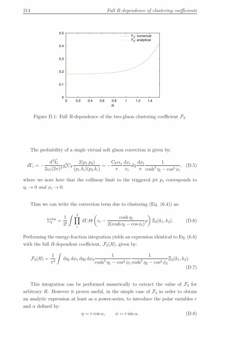
214 Full R-dependence of clustering coefficients
0
0.1
0.2
0.3
0.4
0.5
0 0.2 0.4 0.6 0.8 1 1.2 1.4
R
F2: numericalF2: analytical
Figure D.1: Full R-dependence of the two-gluon clustering coefficient F2.
The probability of a single virtual soft gluon correction is given by:
dΓi = − d3~ki2ωi(2π)3
g2sCF2(p1.p2)
(p1.ki)(p2.ki)= −CFαs
π
dxi
xidη
dφi
π
1
cosh2 ηi − cos2 φi
, (D.5)
where we note here that the collinear limit to the triggered jet p1 corresponds to
ηi → 0 and φi → 0.
Thus we can write the correction term due to clustering (Eq. (6.4)) as:
Σclus2 =
1
2!
∫ 2∏
i
dΓiΘ
(xi −
cosh ηi2(cosh ηi − cos φi)
ρ
)Ξ2(k1, k2). (D.6)
Performing the energy-fraction integration yields an expression identical to Eq. (6.8)
with the full R-dependent coefficient, F2(R), given by:
F2(R) =1
π2
∫dη1 dφ1 dη2 dφ2
1
cosh2 η1 − cos2 φ1
1
cosh2 η2 − cos2 φ2
Ξ2(k1, k2).
(D.7)
This integration can be performed numerically to extract the value of F2 for
arbitrary R. However it proves useful, in the simple case of F2 in order to obtain
an analytic expression at least as a power-series, to introduce the polar variables r
and α defined by:
η = r cosα, φ = r sinα. (D.8)
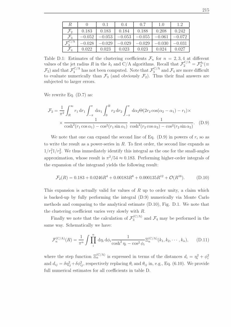
215
R 0 0.1 0.4 0.7 1.0 1.2
F2 0.183 0.183 0.184 0.188 0.208 0.242F3 −0.052 −0.053 −0.053 −0.055 −0.061 −0.072
FC/A3 −0.028 −0.029 −0.029 −0.029 −0.030 −0.031F4 0.022 0.023 0.023 0.023 0.024 0.027
Table D.1: Estimates of the clustering coefficients Fn for n = 2, 3, 4 at differentvalues of the jet radius R in the kt and C/A algorithms. Recall that FC/A
2 = Fkt2 (≡
F2) and that FC/A4 has not been computed. Note that FC/A
3 and F4 are more difficultto evaluate numerically than F3 (and obviously F2). Thus their final answers aresubjected to larger errors.
We rewrite Eq. (D.7) as:
F2 =1
π2
∫ ∞
R
r1 dr1
∫ π
−π
dα1
∫ R
0
r2 dr2
∫ π
−π
dα2Θ(2r2 cos(α2 − α1)− r1)×
× 1
cosh2(r1 cosα1)− cos2(r1 sinα1)
1
cosh2(r2 cosα2)− cos2(r2 sinα2). (D.9)
We note that one can expand the second line of Eq. (D.9) in powers of ri so as
to write the result as a power-series in R. To first order, the second line expands as
1/r211/r22. We thus immediately identify this integral as the one for the small-angles
approximation, whose result is π2/54 ≈ 0.183. Performing higher-order integrals of
the expansion of the integrand yields the following result:
F2(R) = 0.183 + 0.0246R4 + 0.00183R8 + 0.000135R12 +O(R16). (D.10)
This expansion is actually valid for values of R up to order unity, a claim which
is backed-up by fully performing the integral (D.9) numerically via Monte Carlo
methods and comparing to the analytical estimate (D.10), Fig. D.1. We note that
the clustering coefficient varies very slowly with R.
Finally we note that the calculation of F (C/A)3 and F4 may be performed in the
same way. Schematically we have:
F (C/A)n (R) =
1
πn
∫ n∏
i
dηi dφi1
cosh2 ηi − cos2 φi
Ξ(C/A)n (k1, k2, · · · , kn), (D.11)
where the step function Ξ(C/A)n is expressed in terms of the distances di = η2i + φ2
i
and dij = δη2ij+δφ2ij , respectively replacing θi and θij in, e.g., Eq. (6.10). We provide
full numerical estimates for all coefficients in table D.

216
Appendix E
Radiators
E.1 Dipole calculations for the global part
In order to carry out the calculations for the various dipole terms required for the
resummation detailed in the main text we shall make use of the following Born
kinematics for the hard incoming and outgoing particles,
p1 =
√s
2x1 (1, 0, 0, 1) ,
p2 =
√s
2x2 (1, 0, 0,−1) ,
p3 = pt (cosh y, 1, 0, sinh y) ,
p4 = pt (cosh yr,−1, 0, sinh yr) , (E.1)
where, as in the main, text p1 and p2 denote the four-momenta of the incoming hard
partons, p3 that of the jet whose mass is being considered and p4 the four-momentum
of a recoiling jet. In the case of a final state vector boson instead of a recoiling jet
the contribution from p4 to the dipole calculations is of course absent as the Z boson
is colour neutral. Further we have indicated by x1 and x2 the fractional momenta
of incoming partons relative to the colliding hadrons P1 and P2 respectively. Also
y denotes the rapidity of the measured jet, yr that of the recoiling jet and pt their
transverse momenta. One can, by ignoring recoil, use the Born kinematics outlined
above even in the presence of a soft emission, whose momentum can be expressed
as
k = kt (cosh η, cosφ, sinφ, sinh η) ; (E.2)
where transverse momentum kt, rapidity η and azimuth φ are all measured with
respect to the beam direction.
We shall now set up the various dipole contributions to the jet mass cross-
section. We recall from the main text that eventually these dipole contributions will
exponentiate with appropriate colour factors, so what follows below is in essence a
calculation of various components of the resummed exponent.
217
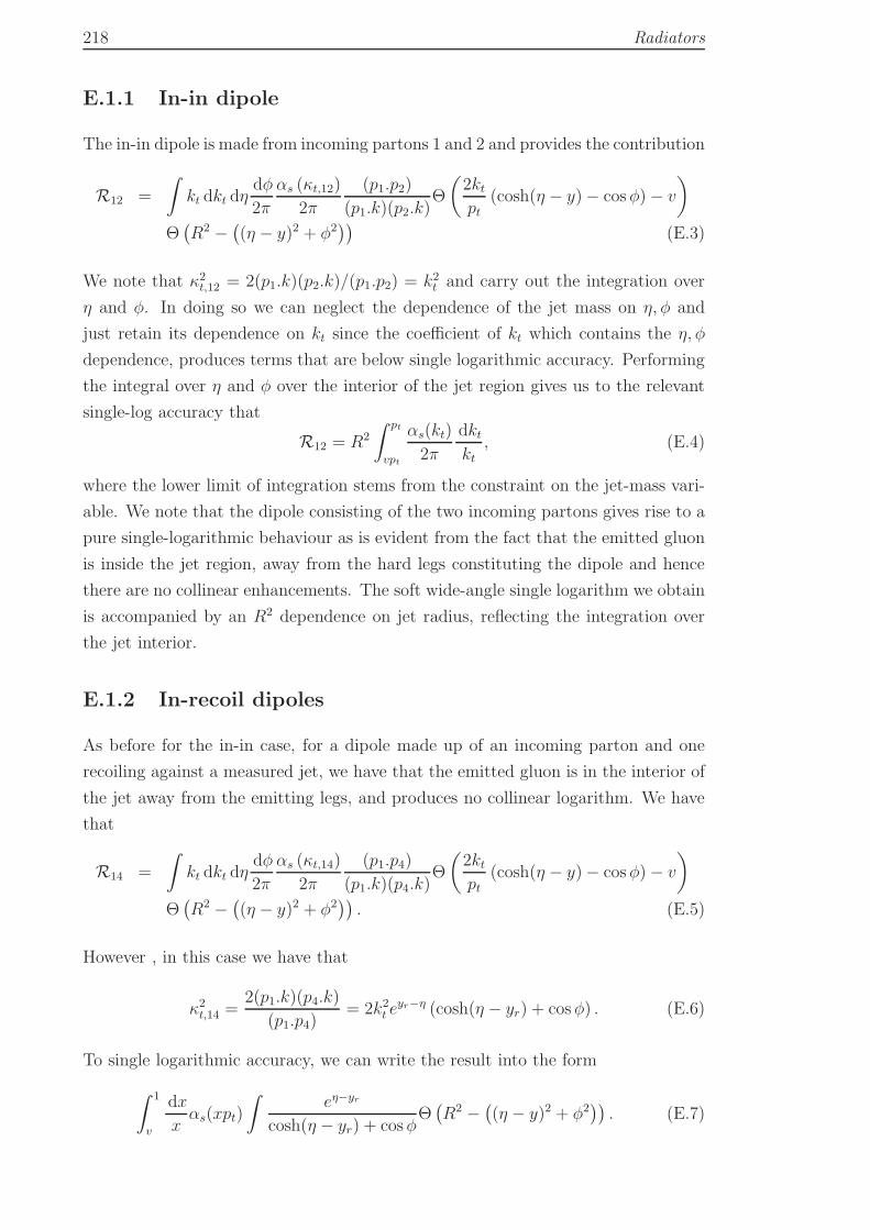
218 Radiators
E.1.1 In-in dipole
The in-in dipole is made from incoming partons 1 and 2 and provides the contribution
R12 =
∫kt dkt dη
dφ
2π
αs (κt,12)
2π
(p1.p2)
(p1.k)(p2.k)Θ
(2ktpt
(cosh(η − y)− cosφ)− v
)
Θ(R2 −
((η − y)2 + φ2
))(E.3)
We note that κ2t,12 = 2(p1.k)(p2.k)/(p1.p2) = k2
t and carry out the integration over
η and φ. In doing so we can neglect the dependence of the jet mass on η, φ and
just retain its dependence on kt since the coefficient of kt which contains the η, φ
dependence, produces terms that are below single logarithmic accuracy. Performing
the integral over η and φ over the interior of the jet region gives us to the relevant
single-log accuracy that
R12 = R2
∫ pt
vpt
αs(kt)
2π
dktkt
, (E.4)
where the lower limit of integration stems from the constraint on the jet-mass vari-
able. We note that the dipole consisting of the two incoming partons gives rise to a
pure single-logarithmic behaviour as is evident from the fact that the emitted gluon
is inside the jet region, away from the hard legs constituting the dipole and hence
there are no collinear enhancements. The soft wide-angle single logarithm we obtain
is accompanied by an R2 dependence on jet radius, reflecting the integration over
the jet interior.
E.1.2 In-recoil dipoles
As before for the in-in case, for a dipole made up of an incoming parton and one
recoiling against a measured jet, we have that the emitted gluon is in the interior of
the jet away from the emitting legs, and produces no collinear logarithm. We have
that
R14 =
∫kt dkt dη
dφ
2π
αs (κt,14)
2π
(p1.p4)
(p1.k)(p4.k)Θ
(2ktpt
(cosh(η − y)− cosφ)− v
)
Θ(R2 −
((η − y)2 + φ2
)). (E.5)
However , in this case we have that
κ2t,14 =
2(p1.k)(p4.k)
(p1.p4)= 2k2
t eyr−η (cosh(η − yr) + cosφ) . (E.6)
To single logarithmic accuracy, we can write the result into the form
∫ 1
v
dx
xαs(xpt)
∫eη−yr
cosh(η − yr) + cosφΘ(R2 −
((η − y)2 + φ2
)). (E.7)
E.1. Dipole calculations for the global part 219
It is possible to evaluate the integral over η, φ as a power series in R, such that the
overall result for this dipole reads
∫ 1
v
dx
x
αs(xpt)
2π
(R2
2
e∆y
(1 + cosh∆y)+
R4
32sech4∆y
2+O
(R6))
(E.8)
where ∆y = y − yr For the R24 dipole one obtains the same result as above, with
the replacement of ∆y by −∆y.
E.1.3 Jet-recoil dipole
For this dipole we have also an involvement of the parton that initiates the measured
jet as one of the hard emitting legs. The consequent collinear singularity, in addition
to the pole due to soft emission, gives rise to double-logarithmic contributions. In
this case one needs to evaluate the argument of the running coupling more carefully
whereas for soft wide-angle pieces, dealt with previously, all that is important at our
accuracy is that the argument of the running coupling is proportional to the energy
of the soft gluon being considered.
In the present case we start with the integral
R34 =
∫kt dkt dη
dφ
2π
αs (κt,34)
2π
(p3.p4)
(p3.k)(p4.k)Θ
(2ktpt
(cosh(η − y)− cos φ)− v
)
Θ(R2 −
((η − y)2 + φ2
))(E.9)
where
κ2t,34 =
2(p3.k)(p4.k)
(p3.p4)= 2k2
t
(cosh (yr − η) + cosφ) (cosh (y − η) + cosφ))
1 + cosh∆y. (E.10)
Next we introduce the variables r and θ such that y−η = r cos θ and φ = r sin θ such
that the in jet condition (y − η)2 + φ2 < R2, simply produces r < R, while θ takes
values between 0 and 2π. Thinking of Eq. (E.9) as a power series in r we can isolate
the collinear-enhanced terms which produces double logarithms and separate it from
terms that are finite as r → 0, which upon integration produce terms that behave
as powers of R corresponding to soft wide-angle contributions. The contribution
R34 can thus be broken into terms that contain collinear enhancements (and hence
leading double logarithms) and pure soft single-logarithmic pieces:
R34 = Rcoll.34 +Rsoft
34 , (E.11)
where the pure soft terms can be expressed as a power series in R:
Rsoft34 =
∫ 1
v
αs(xpt)
2π
dx
x
(R2
4tanh2 ∆y
2+
R4
1152sech4∆y
2(−5 + cosh∆y)2 +O(R6)
),
(E.12)
220 Radiators
where we have neglected terms that vanish as v → 0.
The collinear contributions require us to be more precise in treating the argument
of the running coupling. In particular, in the limit of small r, which is the collinear
region, we obtain
Rcoll.34 =
∫ R2
v
dr2
r2dθ
2π
∫ 1
vR2
dx
x
αs
2π(xrpt) (E.13)
where we have written the result in terms of a dimensionless energy fraction x such
that in the collinear limit r ≪ 1, one has that κt,34/(rpt) = x. The lower limits of
the energy and angular integrals follow from the restriction on the jet mass to be
greater than v, while the upper limit of the angular integral over r2 corresponds to
the jet boundary.
It is straightforward to obtain the result corresponding to the fixed-coupling limit
from Eq. (E.13), which gives:
Rcoll.34 =
αs
2π
1
2ln2 R
2
v. (E.14)
The running coupling result can be compared directly to that obtained in the
e+e− case in our previous work [84]. In order to do this we introduce the transverse
momentum with respect to the emitting jet kt,J = xrpt, and changing variable we
obtain
Rcoll.34 =
∫dkt,Jkt,J
αs (kt,J)
2π
dr2
r2Θ(R2 − r2
)Θ(r2 − v
)Θ
(r2 −
k2t,J
p2t
)Θ
(r2 − v2p2t
k2t,J
)
(E.15)
Carrying out the integral over r, we are left to evaluate the integral over kt,J
which reads
Rcoll.34 =
∫dk2
t,J
k2t,J
αs (kt,J)
2πln
(Rptkt,J
)Θ
(k2t,J
p2t− v
)Θ
(R2 −
k2t,J
p2t
)
+
∫dk2
t,J
k2t,J
αs
(k2t,J
)
2πln
(Rkt,Jvpt
)Θ
(v −
k2t,J
p2t
)Θ
(k2t,J
p2t− v2
R2
)(E.16)
E.1.4 In-jet dipoles
Now we consider the dipole formed by the triggered jet and one of the incoming
partons. Since here too the measured jet is involved as one of the legs of the hard
dipoles, we can carry out precisely the same manipulations as for the R34 dipole
immediately above. Doing so yields the same soft-collinear piece as before
Rcoll.13 = Rcoll.
23 = Rcoll.34 , (E.17)
E.2. Dipole calculations for the non-global contribution 221
while the soft wide-angle piece reads
Rsoft13 = Rsoft
23 =
∫ 1
v
αs(xpt)
2π
dx
x
(R2
4+
R4
288+O
(R6))
. (E.18)
E.2 Dipole calculations for the non-global contri-
bution
We now turn our attention to the evaluation of the different contributions arising
from correlated-gluon emissions.
E.2.1 Dipoles involving the measured jet
We start by considering the the three dipoles involving the triggered jet I13, I23:
I13 = 4
∫dη1
dφ1
2π
∫dη2
dφ2
2π
1− eη1 cosφ1 − eη2 cosφ2 + eη1+η2 cos(φ1 − φ2)
(cosh(η1 − η2)− cos(φ1 − φ2)) (cosh η1 − cosφ1) (cosh η2 − cosφ2)
Θ[R2 − (η22 + φ2
2)]Θ[η21 + φ2
1 − R2]. (E.19)
We evaluate the above integral in powers of the jet radius R. We find
I13 = I23 =π2
3+ αR4 +O(R6). (E.20)
As expected the O(R0) term is the same result as in the hemisphere case. Moreover,
we find that the O(R2) is zero and the first non-vanishing correction to π2/3 is
O(R4). A numerical evaluation of the integral leads to a small coefficient α = 0.013.
The dipole I34, which is relevant for the dijet calculation, depends, in principle, on
the rapidity separation ∆y between the leading jets. However, any such dependence
will be multiplied by, at least, O(R4) and hence makes no significance contribution.
Therefore I34 assumes an analogous result to Eq. (E.20).
E.2.2 The remaining dipoles
Let us consider the dipole from 2 incoming legs I12.
We have to evaluate
I12 = 4
∫dη1
dφ1
2π
∫dη2
dφ2
2π
cos(φ1 − φ2)
cosh(η1 − η2)− cos(φ1 − φ2)Θ(R2 − (η22 + φ2
2))
Θ(η21 + φ2
1 − R2). (E.21)
222 Radiators
Let us change the variables to
η1 − η2 = λ cos β , φ1 − φ2 = λ sin β
η2 = ρ cosα , φ2 = ρ sinα. (E.22)
Doing so and taking care of the fact that −π < φ1 < π we get
∫cos (λ sinβ)
cosh (λ cosβ)− cos (λ sin β)Θ[ρ2 + λ2 + 2ρλ cos(α− β)−R2
]Θ[R2 − ρ2
]
Θ [π − (ρ sinα + λ sinβ)] Θ [π + (ρ sinα+ λ sin β)] ρdρdα
2πλdλ
dβ
2π(E.23)
The step function implies
cos(α− β) >R2 − ρ2 − λ2
2ρλ(E.24)
This is automatically satisfied if (R2 − ρ2 − λ2)/(2ρλ) < −1. It is never satisfied if
(R2 − ρ2 − λ2)/(2ρλ) > 1. Hence, the step function in question is only active when
−1 < (R2−ρ2−λ2)/(2ρλ) < 1. For a non-zero result we must then have ρ+λ > R.
Let us consider first the region of integration where the first step function is
active. We have two integrals
∫ R
0
λdλcos(λ sin β)
cosh(λ cos β)− cos(λ sinβ)
dβ
2π
∫ R
R−λ
ρdρdα
2π×
×Θ(ρ2 + λ2 + 2ρλ cos(α− β)− R2
)+
+
∫ 2R
R
λdλcos(λ sinβ)
cosh(λ cos β)− cos(λ sin β)
dβ
2π
∫ R
λ−R
ρdρdα
2π×
×Θ(ρ2 + λ2 + 2ρλ cos(α− β)− R2
), (E.25)
where we have not written the other step functions that are automatically satisfied
since λ and ρ are small here. The first integral yields ≈ 0.61R2 while the second
one is ≈ 0.37R2.
When the cosine condition is automatically satisfied we have the following range
of values
R < λ < 2R, 0 < ρ < λ− R (E.26)
and
λ > 2R, 0 < ρ < R. (E.27)
The first integral is
∫ 2R
R
λdλcos(λ sin β)
cosh(λ cos β)− cos(λ sin β)
dβ
2π
∫ λ−R
0
ρdρdα
2π(E.28)
E.2. Dipole calculations for the non-global contribution 223
Note that for small R and the above range of values of ρ all other theta functions
are also satisfied as e.g it is always true that π > ρ sinα+ λ sin β. One can evaluate
the integral above easily and the result is ≈ 0.19R2.
The remaining integral is
∫ ∞
2R
λdλcos(λ sin β)
cosh(λ cos β)− cos(λ sin β)
dβ
2π
∫ R
0
ρdρdα
2π
Θ [π − (ρ sinα + λ sin β)]Θ [π + (ρ sinα + λ sin β)] (E.29)
We note that we can split the λ integral to go from 2R to unity and then unity to
infinity. The integral from 2R to unity produces the following result:
−R2 ln 2R− 0.12R2
which leaves to evaluate the integral
∫ ∞
1
λdλcos(λ sin β)
cosh(λ cos β)− cos(λ sin β)
dβ
2π
∫ R
0
ρdρdα
2π
Θ [π − (ρ sinα + λ sin β)]Θ [π + (ρ sinα + λ sin β)] (E.30)
This goes as kR2 with k a constant to be determined. To evaluate k it proves
simplest to first take the derivative with respect toR2 which turns the theta function
involving ρ into a delta function. The ρ integration is then trivial and the rest of
the integral can be done numerically and yields k = 0.12. We thus have that the
overall result is 0.12R2. Note that it is interesting that this cancels the −0.12R2
obtained previously. Hence the full result is
I12 ≈ 4[1.17R2 − R2 ln 2R− 0.12R2 + 0.12R2
]+O(R4)
≈ 4[1.17R2 −R2 ln 2R
]+O(R4). (E.31)
The above expansion well describes the full answer for I12 up to values of R ≈ 0.6.
For larger values of the jet radius we use a full numerical evaluation of the coefficient
I12.
Next we consider the in-recoil dipole I14. The result can be expressed in terms
of the dipole I12 and a rapidity dependent function κ(∆y), which we evaluate nu-
merically
(1 + e∆y
)2
(1 + cosh∆y)2(1.17R2 −R2 ln 2R
)+
(1 + e∆y)
1 + cosh∆yκ(∆y)R2. (E.32)
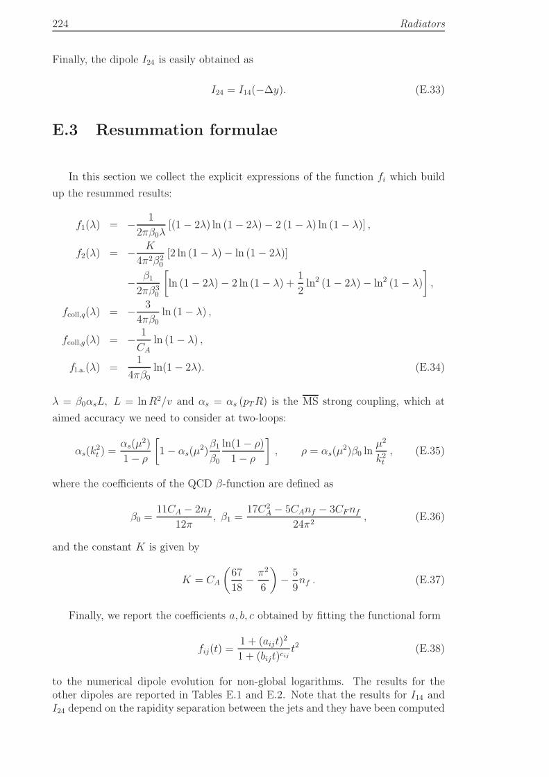
224 Radiators
Finally, the dipole I24 is easily obtained as
I24 = I14(−∆y). (E.33)
E.3 Resummation formulae
In this section we collect the explicit expressions of the function fi which build
up the resummed results:
f1(λ) = − 1
2πβ0λ[(1− 2λ) ln (1− 2λ)− 2 (1− λ) ln (1− λ)] ,
f2(λ) = − K
4π2β20
[2 ln (1− λ)− ln (1− 2λ)]
− β1
2πβ30
[ln (1− 2λ)− 2 ln (1− λ) +
1
2ln2 (1− 2λ)− ln2 (1− λ)
],
fcoll,q(λ) = − 3
4πβ0ln (1− λ) ,
fcoll,g(λ) = − 1
CAln (1− λ) ,
fl.a.(λ) =1
4πβ0ln(1− 2λ). (E.34)
λ = β0αsL, L = lnR2/v and αs = αs (pTR) is the MS strong coupling, which at
aimed accuracy we need to consider at two-loops:
αs(k2t ) =
αs(µ2)
1− ρ
[1− αs(µ
2)β1
β0
ln(1− ρ)
1− ρ
], ρ = αs(µ
2)β0 lnµ2
k2t
, (E.35)
where the coefficients of the QCD β-function are defined as
β0 =11CA − 2nf
12π, β1 =
17C2A − 5CAnf − 3CFnf
24π2, (E.36)
and the constant K is given by
K = CA
(67
18− π2
6
)− 5
9nf . (E.37)
Finally, we report the coefficients a, b, c obtained by fitting the functional form
fij(t) =1 + (aijt)
2
1 + (bijt)cijt2 (E.38)
to the numerical dipole evolution for non-global logarithms. The results for theother dipoles are reported in Tables E.1 and E.2. Note that the results for I14 andI24 depend on the rapidity separation between the jets and they have been computed
E.3. Resummation formulae 225
for |∆y| = 2.
R I12 a b c0.1 0.11 1.90CA 0.31CA 1.660.2 0.34 1.35CA 0.10CA 1.660.3 0.62 1.07CA 0.00CA 1.660.4 0.92 0.90CA 0.00CA 1.660.5 1.22 1.45CA 1.02CA 1.660.6 1.52 0.85CA 0.00CA 1.330.7 1.79 0.88CA 0.19CA 1.330.8 2.05 1.09CA 0.53CA 1.330.9 2.28 1.20CA 0.73CA 1.331.0 2.49 1.12CA 0.66CA 1.331.1 2.66 1.13CA 0.70CA 1.331.2 2.82 1.26CA 0.89CA 1.33
I13 a b c3.289 0.99CA 1.06CA 1.333.289 0.99CA 1.06CA 1.333.289 0.99CA 1.06CA 1.333.290 0.94CA 0.99CA 1.333.290 0.96CA 0.98CA 1.333.292 0.86CA 0.87CA 1.333.293 0.79CA 0.82CA 1.333.295 0.79CA 0.81CA 1.333.299 0.77CA 0.78CA 1.333.303 0.86CA 0.85CA 1.333.310 0.98CA 0.99CA 1.333.318 0.91CA 0.92CA 1.33
Table E.1: Numerical results for the coefficients that parametrize the resummationof non-global logarithms.
R I14 a b c0.1 0.09 2.61CA 0.80CA 1.660.2 0.28 2.47CA 1.19CA 1.660.3 0.51 2.29CA 1.32CA 1.660.4 0.77 2.20CA 1.44CA 1.660.5 1.04 1.71CA 1.05CA 1.660.6 1.31 1.48CA 0.90CA 1.660.7 1.57 0.83CA 0.20CA 1.660.8 1.81 0.76CA 0.00CA 1.660.9 2.04 1.86CA 1.57CA 1.661.0 2.25 2.42CA 2.30CA 1.661.1 2.44 2.35CA 2.25CA 1.661.2 2.61 2.54CA 2.52CA 1.66
I24 a b c0.003 1.12CA 0.91CA 1.660.01 1.01CA 0.99CA 1.660.02 3.18CA 0.49CA 1.660.03 3.02CA 0.71CA 1.660.05 2.85CA 0.72CA 1.660.07 2.79CA 0.85CA 1.660.10 2.66CA 0.88CA 1.660.13 2.58CA 0.94CA 1.660.16 2.58CA 1.06CA 1.660.20 2.57CA 1.16CA 1.660.24 2.53CA 1.22CA 1.660.30 2.49CA 1.28CA 1.66
Table E.2: Numerical results for the coefficients that parametrize the resummationof non-global logarithms. Note that the above results are valid in the case |∆y| = 2.

226
References
[1] S. D. Ellis, J. Huston, K. Hatakeyama, P. Loch, and M. Tonnesmann, Jets inhadron-hadron collisions, Prog.Part.Nucl.Phys. 60 (2008) 484–551,[arXiv:0712.2447].
[2] M. Dasgupta and G. P. Salam, Resummation of non-global QCD observables,Phys. Lett. B512 (2001) 323–330, [hep-ph/0104277].
[3] Y. Delenda, R. Appleby, M. Dasgupta, and A. Banfi, On QCD resummationwith kt clustering, JHEP 0612 (2006) 044, [hep-ph/0610242].
[4] G. Herten, The First Year of the Large Hadron Collider: A Brief Review,Mod.Phys.Lett. A26 (2011) 843–855, [arXiv:1104.4205].
[5] ATLAS Collaboration Collaboration, G. Aad et al., Observation of a newparticle in the search for the Standard Model Higgs boson with the ATLASdetector at the LHC, Phys.Lett.B (2012) [arXiv:1207.7214].
[6] CMS Collaboration Collaboration, S. Chatrchyan et al., Observation of anew boson at a mass of 125 GeV with the CMS experiment at the LHC,Phys.Lett.B (2012) [arXiv:1207.7235].
[7] R. K. Ellis, W. J. Stirling, and B. R. Webber, QCD and collider physics.Cambridge monographs on particle physics, nuclear physics, and cosmology.Cambridge University Press, 2003.
[8] S. D. Ellis, Z. Kunszt, and D. E. Soper, The one jet inclusive cross-section atorder α3
s: gluons only, Phys.Rev.Lett. 62 (1989) 726.
[9] S. D. Ellis, Z. Kunszt, and D. E. Soper, The one jet inclusive cross-section atorder α3
s. 1. gluons only, Phys.Rev. D40 (1989) 2188.
[10] S. D. Ellis, Z. Kunszt, and D. E. Soper, The one jet inclusive cross-section atorder α3
s quarks and gluons, Phys.Rev.Lett. 64 (1990) 2121.
[11] S. D. Ellis, Z. Kunszt, and D. E. Soper, Two jet production in hadroncollisions at order α3
s in QCD, Phys.Rev.Lett. 69 (1992) 1496–1499.
[12] Y. L. Dokshitzer and B. Webber, Calculation of power corrections tohadronic event shapes, Phys.Lett. B352 (1995) 451–455, [hep-ph/9504219].
[13] Y. L. Dokshitzer, G. Marchesini, and B. Webber, Dispersive approach topower behaved contributions in QCD hard processes, Nucl.Phys. B469 (1996)93–142, [hep-ph/9512336].
227
228 References
[14] J. M. Butterworth, A. R. Davison, M. Rubin, and G. P. Salam, Jetsubstructure as a new Higgs search channel at the LHC, Phys.Rev.Lett. 100(2008) 242001, [arXiv:0802.2470].
[15] K. Agashe, A. Belyaev, T. Krupovnickas, G. Perez, and J. Virzi, LHCSignals from Warped Extra Dimensions, Phys.Rev. D77 (2008) 015003,[hep-ph/0612015].
[16] B. Lillie, L. Randall, and L.-T. Wang, The Bulk RS KK-gluon at the LHC,JHEP 0709 (2007) 074, [hep-ph/0701166].
[17] K. Agashe, H. Davoudiasl, S. Gopalakrishna, T. Han, G.-Y. Huang, et al.,LHC Signals for Warped Electroweak Neutral Gauge Bosons, Phys.Rev. D76(2007) 115015, [arXiv:0709.0007].
[18] K. Agashe, H. Davoudiasl, G. Perez, and A. Soni, Warped Gravitons at theLHC and Beyond, Phys.Rev. D76 (2007) 036006, [hep-ph/0701186].
[19] G. H. Brooijmans, A. Delgado, B. A. Dobrescu, C. Grojean, M. Narain,et al., New Physics at the LHC: A Les Houches Report. Physics at TeVColliders 2007 – New Physics Working Group, arXiv:0802.3715.
[20] G. Brooijmans, High-pt hadronic top quark identification, Tech. Rep.ATL-PHYS-CONF-2008-008. ATL-COM-PHYS-2008-001, CERN, Geneva,Jan, 2008.
[21] J. Butterworth, B. Cox, and J. R. Forshaw, WW scattering at the CERNLHC, Phys.Rev. D65 (2002) 096014, [hep-ph/0201098].
[22] B. Flaugher and K. Meier, A Compilation of jet finding algorithms, . To bepubl. in Proc. of 1990 Summer Study on High Energy Physics, ResearchDirections for the Decade, Snowmass, CO, Jun 25 - Jul 13, 1990.
[23] G. Sterman and S. Weinberg, Jets from quantum chromodynamics, Phys.Rev. Lett. 39 (Dec, 1977) 1436–1439.
[24] W. Bartel and et al, Experimental studies on multijet production in e+e−
annihilation at PETRA energies, Zeitschrift fur Physik C Particles andFields 33 (1986) 23–31. 10.1007/BF01410449.
[25] S. Bethke, J. Allison, and et al, Experimental investigation of the energydependence of the strong coupling strength, Physics Letters B 213 (1988),no. 2 235 – 241.
[26] A. Abdesselam et al., Boosted objects: a probe of beyond the Standard Modelphysics, Eur. Phys. J. C71 (2011) 1661, [arXiv:1012.5412].
[27] A. Altheimer, S. Arora, L. Asquith, G. Brooijmans, J. Butterworth, et al.,Jet Substructure at the Tevatron and LHC: New results, new tools, newbenchmarks, arXiv:1201.0008.
[28] S. D. Ellis, C. K. Vermilion, and J. R. Walsh, Techniques for improved heavyparticle searches with jet substructure, Phys.Rev. D80 (2009) 051501,[arXiv:0903.5081].
References 229
[29] S. D. Ellis, C. K. Vermilion, and J. R. Walsh, Recombination Algorithms andJet Substructure: Pruning as a Tool for Heavy Particle Searches, Phys.Rev.D81 (2010) 094023, [arXiv:0912.0033].
[30] D. Krohn, J. Thaler, and L.-T. Wang, Jet Trimming, JHEP 1002 (2010)084, [arXiv:0912.1342].
[31] A. Banfi, G. P. Salam, and G. Zanderighi, Principles of general final-stateresummation and automated implementation, JHEP 0503 (2005) 073,[hep-ph/0407286].
[32] A. Banfi, G. P. Salam, and G. Zanderighi, Phenomenology of event shapes athadron colliders, JHEP 1006 (2010) 038, [arXiv:1001.4082].
[33] ATLAS Collaboration Collaboration, G. Aad et al., Jet mass andsubstructure of inclusive jets in
√s = 7TeV pp collisions with the ATLAS
experiment, JHEP 1205 (2012) 128, [arXiv:1203.4606].
[34] ATLAS Collaboration Collaboration, G. Aad et al., ATLAS measurementsof the properties of jets for boosted particle searches, arXiv:1206.5369.
[35] CMS Collaboration Collaboration, A. Hinzmann, Jet results from CMS,Prog.Theor.Phys.Suppl. 193 (2012) 249–253.
[36] ATLAS Collaboration Collaboration, Atlas sensitivity to the standardmodel higgs in the HW and HZ channels at high transverse momenta, Tech.Rep. ATL-PHYS-PUB-2009-088, CERN, Geneva, Aug, 2009.
[37] T. Plehn, M. Spannowsky, M. Takeuchi, and D. Zerwas, Stop Reconstructionwith Tagged Tops, JHEP 1010 (2010) 078, [arXiv:1006.2833].
[38] C. F. Berger, T. Kucs, and G. F. Sterman, Interjet energy flow / event shapecorrelations, Int.J.Mod.Phys. A18 (2003) 4159–4168, [hep-ph/0212343].
[39] C. F. Berger and L. Magnea, Scaling of power corrections for angularitiesfrom dressed gluon exponentiation, Phys.Rev. D70 (2004) 094010,[hep-ph/0407024].
[40] S. Catani, L. Trentadue, G. Turnock, and B. R. Webber, Resummation oflarge logarithms in e+e− event shape distributions, Nucl. Phys. B407 (1993)3–42.
[41] C. W. Bauer, S. Fleming, D. Pirjol, and I. W. Stewart, An effective fieldtheory for collinear and soft gluons: Heavy to light decays, Phys. Rev. D63(2001) 114020, [hep-ph/0011336].
[42] C. W. Bauer, D. Pirjol, and I. W. Stewart, Soft-Collinear Factorization inEffective Field Theory, Phys. Rev. D65 (2002) 054022, [hep-ph/0109045].
[43] M. Beneke, A. Chapovsky, M. Diehl, and T. Feldmann, Soft collineareffective theory and heavy to light currents beyond leading power, Nucl.Phys.B643 (2002) 431–476, [hep-ph/0206152].
230 References
[44] S. D. Ellis, A. Hornig, C. Lee, C. K. Vermilion, and J. R. Walsh, ConsistentFactorization of Jet Observables in Exclusive Multijet Cross-Sections, Phys.Lett. B689 (2010) 82–89, [arXiv:0912.0262].
[45] S. D. Ellis, C. K. Vermilion, J. R. Walsh, A. Hornig, and C. Lee, Jet Shapesand Jet Algorithms in SCET, JHEP 11 (2010) 101, [arXiv:1001.0014].
[46] T. Becher and M. D. Schwartz, A Precise determination of αs from LEPthrust data using effective field theory, JHEP 07 (2008) 034,[arXiv:0803.0342].
[47] W. M.-Y. Cheung, M. Luke, and S. Zuberi, Phase Space and Jet Definitionsin SCET, Phys.Rev. D80 (2009) 114021, [arXiv:0910.2479].
[48] T. T. Jouttenus, Jet Function with a Jet Algorithm in SCET, Phys.Rev. D81(2010) 094017, [arXiv:0912.5509].
[49] Y.-T. Chien and M. D. Schwartz, Resummation of heavy jet mass andcomparison to LEP data, JHEP 08 (2010) 058, [arXiv:1005.1644].
[50] R. Kelley, M. D. Schwartz, and H. X. Zhu, Resummation of jet mass withand without a jet veto, arXiv:1102.0561.
[51] R. Kelley, M. D. Schwartz, R. M. Schabinger, and H. X. Zhu, Jet Mass witha Jet Veto at Two Loops and the Universality of Non-Global Structure,arXiv:1112.3343.
[52] T. T. Jouttenus, I. W. Stewart, F. J. Tackmann, and W. J. Waalewijn, TheSoft Function for Exclusive N-Jet Production at Hadron Colliders, Phys.Rev.D83 (2011) 114030, [arXiv:1102.4344].
[53] H.-n. Li, Z. Li, and C.-P. Yuan, QCD resummation for jet substructures,Phys.Rev.Lett. 107 (2011) 152001, [arXiv:1107.4535].
[54] H.-n. Li, Z. Li, and C.-P. Yuan, QCD resummation for light-particle jets,arXiv:1206.1344.
[55] A. Banfi, G. P. Salam, and G. Zanderighi, Semi-numerical resummation ofevent shapes, JHEP 01 (2002) 018, [hep-ph/0112156].
[56] S. Catani and M. H. Seymour, The Dipole Formalism for the Calculation ofQCD Jet Cross Sections at Next-to-Leading Order, Phys. Lett. B378 (1996)287–301, [hep-ph/9602277].
[57] P. Nason, A New method for combining NLO QCD with shower Monte Carloalgorithms, JHEP 0411 (2004) 040, [hep-ph/0409146].
[58] Z. Nagy, Three jet cross-sections in hadron hadron collisions atnext-to-leading order, Phys.Rev.Lett. 88 (2002) 122003, [hep-ph/0110315].
[59] G. F. Sterman, Partons, factorization and resummation, TASI 95,hep-ph/9606312.
[60] L. Gribov, E. Levin, and M. Ryskin, Semihard processes in qcd, PhysicsReports 100 (1983), no. 1–2 1 – 150.
References 231
[61] A. Bassetto, M. Ciafaloni, and G. Marchesini, Jet structure and infraredsensitive quantities in perturbative qcd, Physics Reports 100 (1983), no. 4201 – 272.
[62] J. C. Collins, D. E. Soper, and G. F. Sterman, Factorization for ShortDistance Hadron - Hadron Scattering, Nucl.Phys. B261 (1985) 104.
[63] J. C. Collins, D. E. Soper, and G. F. Sterman, Factorization of HardProcesses in QCD, Adv.Ser.Direct.High Energy Phys. 5 (1988) 1–91,[hep-ph/0409313]. To be publ. in ’Perturbative QCD’ (A.H. Mueller, ed.)(World Scientific Publ., 1989).
[64] J. C. Collins, D. E. Soper, and G. F. Sterman, Soft Gluons andFactorization, Nucl.Phys. B308 (1988) 833.
[65] A. Banfi, G. P. Salam, and G. Zanderighi, Resummed event shapes at hadron- hadron colliders, JHEP 0408 (2004) 062, [hep-ph/0407287]. Erratumadded online, nov/29/2004.
[66] M. Dasgupta and G. P. Salam, Event shapes in e+e− annihilation and deepinelastic scattering, J. Phys. G30 (2004) R143, [hep-ph/0312283].
[67] Y. Dokshitzer and D. Dyakonov, Angular distribution of energy in jets,Physics Letters B 84 (1979), no. 2 234 – 236.
[68] G. Parisi and R. Petronzio, Small transverse momentum distributions in hardprocesses, Nuclear Physics B 154 (1979), no. 3 427 – 440.
[69] N. Brown and W. Stirling, Jet cross sections at leading double logarithm ine+e− annihilation, Physics Letters B 252 (1990), no. 4 657 – 662.
[70] Dasgupta, Mrinal and Salam, Gavin P., Resummed event shape variables inDIS, JHEP 0208 (2002) 032, [hep-ph/0208073].
[71] A. Banfi, G. Marchesini, and G. Smye, Away-from-jet energy flow, JHEP 08(2002) 006, [hep-ph/0206076].
[72] A. Banfi and M. Dasgupta, Dijet rates with symmetric Et cuts, JHEP 0401(2004) 027, [hep-ph/0312108].
[73] M. Cacciari, G. P. Salam, and G. Soyez, The anti-kt jet clustering algorithm,JHEP 04 (2008) 063, [arXiv:0802.1189].
[74] A. Banfi and M. Dasgupta, Problems in resumming interjet energy flows withkt clustering, Phys. Lett. B628 (2005) 49–56, [hep-ph/0508159].
[75] R. B. Appleby and M. H. Seymour, Non-global logarithms in inter-jet energyflow with kt clustering requirement, JHEP 12 (2002) 063, [hep-ph/0211426].
[76] A. Buckley, J. Butterworth, S. Gieseke, D. Grellscheid, S. Hoche, et al.,General-purpose event generators for LHC physics, Phys.Rept. 504 (2011)145–233, [arXiv:1101.2599].
[77] E. Gardi, Dressed gluon exponentiation, Nucl.Phys. B622 (2002) 365–392,[hep-ph/0108222].
232 References
[78] P. Ball, M. Beneke, and V. M. Braun, Resummation of (β0 αs)n corrections
in QCD: Techniques and applications to the tau hadronic width and theheavy quark pole mass, Nucl.Phys. B452 (1995) 563–625, [hep-ph/9502300].
[79] M. Beneke, Renormalons, Phys. Rept. 317 (1999) 1–142, [hep-ph/9807443].
[80] M. Dasgupta, L. Magnea, and G. P. Salam, Non-perturbative QCD effects injets at hadron colliders, JHEP 02 (2008) 055, [arXiv:0712.3014].
[81] A. Banfi, G. Marchesini, G. Smye, and G. Zanderighi, Out of plane QCDradiation in hadronic Z0 production, JHEP 0108 (2001) 047,[hep-ph/0106278].
[82] M. Dasgupta and Y. Delenda, Aspects of power corrections in hadron-hadroncollisions, JHEP 0711 (2007) 013, [arXiv:0709.3309].
[83] Y. L. Dokshitzer and B. Webber, Power corrections to event shapedistributions, Phys.Lett. B404 (1997) 321–327, [hep-ph/9704298].
[84] A. Banfi, M. Dasgupta, K. Khelifa-Kerfa, and S. Marzani, Non-globallogarithms and jet algorithms in high-pT jet shapes, JHEP 08 (2010) 064,[arXiv:1004.3483].
[85] K. Khelifa-Kerfa, Non-global logs and clustering impact on jet mass with ajet veto distribution, JHEP 1202 (2012) 072, [arXiv:1111.2016].
[86] Y. Delenda and K. Khelifa-Kerfa, On the resummation of clusteringlogarithms for non-global observables, JHEP 1209 (2012) 109,[arXiv:1207.4528].
[87] M. Dasgupta, K. Khelifa-Kerfa, S. Marzani, and M. Spannowsky, On jetmass distributions in Z+jet and dijet processes at the LHC, JHEP 1210(2012) 126, [arXiv:1207.1640].
[88] Y.-C. Fermi, E., Are mesons elementary particles?, Physical Review 76(1949), no. 12 1739–1743. cited By (since 1996) 58.
[89] M. Levy and J. Sucher, Eikonal approximation in quantum field theory, Phys.Rev. 186 (Oct, 1969) 1656–1670.
[90] G. Sterman et al, Handbook of perturbative QCD, Rev. Mod. Phys. 67 (Jan,1995) 157–248.
[91] G. Sterman, An Introduction to Quantum Field Theory. CambridgeUniversity Press, 1993.
[92] E. Zeidler, Quantum Field Theory II: Quantum Electrodynamics: A BridgeBetween Mathematicians and Physicists. Quantum Field Theory: A BridgeBetween Mathematicians and Physicists. Springer, 2008.
[93] M. Peskin and D. Schroeder, An Introduction To Quantum Field Theory.Advanced Book Program. Addison-Wesley Publishing Company, 1995.
[94] S. Weinberg, The Quantum Theory of Fields: Supersymmetry. No. v. 3 inThe Quantum Theory of Fields. Cambridge University Press, 2000.
References 233
[95] J. Zinn-Justin, Quantum Field Theory and Critical Phenomena.International Series of Monographs on Physics. Clarendon Press, 2002.
[96] G. F. Sterman, QCD and jets, hep-ph/0412013.
[97] G. F. Sterman, Some Basic Concepts of Perturbative QCD, Acta Phys.Polon.B39 (2008) 2151–2172, [arXiv:0807.5118].
[98] D. E. Soper, Basics of QCD perturbation theory, hep-ph/0011256.
[99] H. Georgi, Lie Algebras in Particle Physics. Frontiers in Physics. PerseusBooks, Advanced Book Program, 1999.
[100] H. Jones, Groups, Representations And Physics. Insitute of Physics Pub.,1998.
[101] J. Cornwell, Group Theory in Physics: An Introduction. Techniques ofPhysics. Academic Press, 1997.
[102] G. Hooft, A planar diagram theory for strong interactions, Nuclear Physics B72 (1974), no. 3 461 – 473.
[103] L. Lonnblad, ARIADNE version 4: A Program for simulation of QCDcascades implementing the color dipole model, Comput.Phys.Commun. 71(1992) 15–31.
[104] G. F. Sterman, Quantum chromodynamics, hep-ph/0512344.
[105] J. Bjorken and S. Drell, Relativistic quantum mechanics. International seriesin pure and applied physics. McGraw-Hill, 1964.
[106] L. Faddeev and V. Popov, Feynman diagrams for the Yang-Mills field,Physics Letters B 25 (1967), no. 1 29 – 30.
[107] E. Abers and B. Lee, Gauge Theories, Phys.Rept. 9 (1973) 1–141.
[108] J. Collins and J. Collins, Renormalization: An Introduction toRenormalization, the Renormalization Group and the Operator-ProductExpansion. Cambridge Monographs on Mathematical Physics. CambridgeUniversity Press, 1986.
[109] A. Kataev and S. Larin, Analytical five-loop expressions for therenormalization group QED β-function in different renormalization schemes,arXiv:1205.2810.
[110] S. Bethke, The 2009 World Average of αs, Eur.Phys.J. C64 (2009) 689–703,[arXiv:0908.1135].
[111] D. J. Gross and F. Wilczek, Asymptotically Free Gauge Theories. I, Phys.Rev. D 8 (Nov, 1973) 3633–3652.
[112] H. D. Politzer, Asymptotic Freedom: An Approach to Strong Interactions,Phys.Rept. 14 (1974) 129–180.
[113] G. T. Bodwin, Factorization of the Drell-Yan Cross-Section in PerturbationTheory, Phys.Rev. D31 (1985) 2616.
234 References
[114] J. C. Collins and D. E. Soper, The Theorems of Perturbative QCD,Ann.Rev.Nucl.Part.Sci. 37 (1987) 383–409.
[115] V. Gribov and L. Lipatov, Deep inelastic e p scattering in perturbationtheory, Sov.J.Nucl.Phys. 15 (1972) 438–450.
[116] L. Lipatov, The parton model and perturbation theory, Sov.J.Nucl.Phys. 20(1975) 94–102.
[117] G. Altarelli and G. Parisi, Asymptotic Freedom in Parton Language,Nucl.Phys. B126 (1977) 298.
[118] Y. L. Dokshitzer, Calculation of the Structure Functions for Deep InelasticScattering and e+e− Annihilation by Perturbation Theory in QuantumChromodynamics., Sov.Phys.JETP 46 (1977) 641–653.
[119] S. Moch, J. Vermaseren, and A. Vogt, The Three loop splitting functions inQCD: The Nonsinglet case, Nucl.Phys. B688 (2004) 101–134,[hep-ph/0403192].
[120] A. Vogt, S. Moch, and J. Vermaseren, The Three-loop splitting functions inQCD: The Singlet case, Nucl.Phys. B691 (2004) 129–181, [hep-ph/0404111].
[121] G. P. Salam and J. Rojo, A Higher Order Perturbative Parton EvolutionToolkit (HOPPET), Comput.Phys.Commun. 180 (2009) 120–156,[arXiv:0804.3755].
[122] G. P. Salam, Elements of QCD for hadron colliders, arXiv:1011.5131.
[123] D. E. Soper, Parton distribution functions, Nucl.Phys.Proc.Suppl. 53 (1997)69–80, [hep-lat/9609018].
[124] A. Martin, W. Stirling, R. Thorne, and G. Watt, Parton distributions for theLHC, Eur.Phys.J. C63 (2009) 189–285, [arXiv:0901.0002].
[125] R. Thorne, A. Martin, W. Stirling, and G. Watt, Status of MRST/MSTWPDF sets, arXiv:0907.2387.
[126] S. Catani, D. de Florian, and G. Rodrigo, Space-like (versus time-like)collinear limits in QCD: Is factorization violated?, JHEP 1207 (2012) 026,[arXiv:1112.4405].
[127] J. Collins, 2-soft-gluon exchange and factorization breaking,arXiv:0708.4410.
[128] J. Collins and J.-W. Qiu, kT factorization is violated in production ofhigh-transverse-momentum particles in hadron-hadron collisions, Phys.Rev.D75 (2007) 114014, [arXiv:0705.2141].
[129] J. R. Forshaw, M. H. Seymour, and A. Siodmok, On the breaking of collinearfactorization in QCD, arXiv:1206.6363.
[130] Y. Dokshitzer and G. Marchesini, Hadron collisions and the fifth form-factor,Phys.Lett. B631 (2005) 118–125, [hep-ph/0508130].
References 235
[131] M. H. Seymour, Jets in QCD, AIP Conf.Proc. 357 (1996) 568–587,[hep-ph/9506421].
[132] J. M. Campbell, J. Huston, and W. Stirling, Hard Interactions of Quarksand Gluons: A Primer for LHC Physics, Rept.Prog.Phys. 70 (2007) 89,[hep-ph/0611148].
[133] G. P. Salam, Towards Jetography, Eur.Phys.J. C67 (2010) 637–686,[arXiv:0906.1833].
[134] B.-W. Zhang, Y. He, R. Neufeld, I. Vitev, and E. Wang, Probing nuclearmatter with jets, arXiv:1207.6558.
[135] ATLAS detector and physics performance: Technical Design Report, 2.Technical Design Report ATLAS. CERN, Geneva, 1999. Electronic versionnot available.
[136] D. Froidevaux and P. Sphicas, General-purpose detectors for the LargeHadron Collider, Ann.Rev.Nucl.Part.Sci. 56 (2006) 375–440.
[137] ATLAS Collaboration Collaboration, G. Aad et al., ExpectedPerformance of the ATLAS Experiment - Detector, Trigger and Physics,arXiv:0901.0512.
[138] CMS Collaboration Collaboration, G. Bayatian et al., CMS physics:Technical design report, .
[139] C. Buttar, J. D’Hondt, M. Kramer, G. Salam, M. Wobisch, et al., StandardModel Handles and Candles Working Group: Tools and Jets SummaryReport, arXiv:0803.0678.
[140] J. E. Huth, N. Wainer, K. Meier, N. Hadley, F. Aversa, et al., Toward astandardization of jet definitions, .
[141] G. F. Sterman and S. Weinberg, Jets from Quantum Chromodynamics,Phys.Rev.Lett. 39 (1977) 1436.
[142] G. P. Salam and G. Soyez, A practical Seedless Infrared-Safe Cone jetalgorithm, JHEP 05 (2007) 086, [arXiv:0704.0292].
[143] M. Cacciari, G. P. Salam, and G. Soyez, FastJet user manual, Eur.Phys.J.C72 (2012) 1896, [arXiv:1111.6097].
[144] JADE Collaboration Collaboration, W. Bartel et al., ExperimentalStudies on Multi-Jet Production in e+e− Annihilation at PETRA Energies,Z.Phys. C33 (1986) 23.
[145] J. Dorfan, A cluster algorithm for the study of jets in high-energy physics,Z.Phys. C7 (1981) 349.
[146] T. Sjostrand, The Lund Monte Carlo for e+e− Jet Physics,Comput.Phys.Commun. 28 (1983) 229.
[147] Y. L. Dokshitzer, G. Leder, S. Moretti, and B. Webber, Better jet clusteringalgorithms, JHEP 9708 (1997) 001, [hep-ph/9707323].
236 References
[148] M. Wobisch and T. Wengler, Hadronization corrections to jet cross-sectionsin deep inelastic scattering, hep-ph/9907280.
[149] S. Catani, Y. L. Dokshitzer, M. H. Seymour, and B. R. Webber,Longitudinally invariant kt clustering algorithms for hadron hadroncollisions, Nucl. Phys. B406 (1993) 187–224.
[150] A. Banfi, G. P. Salam, and G. Zanderighi, Infrared safe definition of jetflavor, Eur.Phys.J. C47 (2006) 113–124, [hep-ph/0601139].
[151] D. Krohn, J. Thaler, and L.-T. Wang, Jets with Variable R, JHEP 0906(2009) 059, [arXiv:0903.0392].
[152] L. Lonnblad, ARCLUS: A New jet clustering algorithm inspired by the colordipole model, Z.Phys. C58 (1993) 471–478.
[153] M. Rubin, Non-Global Logarithms in Filtered Jet Algorithms, JHEP 1005(2010) 005, [arXiv:1002.4557].
[154] D. E. Kaplan, K. Rehermann, M. D. Schwartz, and B. Tweedie, TopTagging: A Method for Identifying Boosted Hadronically Decaying TopQuarks, Phys.Rev.Lett. 101 (2008) 142001, [arXiv:0806.0848].
[155] CMS collaboration Collaboration, G. Giurgiu, Reconstruction of HighTransverse Momentum Top Quarks at CMS, arXiv:0909.4894.
[156] G. D. Kribs, A. Martin, T. S. Roy, and M. Spannowsky, Discovering theHiggs Boson in New Physics Events using Jet Substructure, Phys.Rev. D81(2010) 111501, [arXiv:0912.4731].
[157] G. D. Kribs, A. Martin, T. S. Roy, and M. Spannowsky, Discovering HiggsBosons of the MSSM using Jet Substructure, Phys.Rev. D82 (2010) 095012,[arXiv:1006.1656].
[158] D. Krohn, L. Randall, and L.-T. Wang, On the Feasibility and Utility of ISRTagging, arXiv:1101.0810.
[159] D. E. Soper and M. Spannowsky, Finding physics signals with showerdeconstruction, Phys.Rev. D84 (2011) 074002, [arXiv:1102.3480].
[160] J. Thaler and L.-T. Wang, Strategies to Identify Boosted Tops, JHEP 0807(2008) 092, [arXiv:0806.0023].
[161] P.-A. Delsart, K. L. Geerlings, J. Huston, B. T. Martin, and C. K. Vermilion,SpartyJet 4.0 User’s Manual, arXiv:1201.3617.
[162] M. Seymour, Jet shapes in hadron collisions: Higher orders, resummationand hadronization, Nucl.Phys. B513 (1998) 269–300, [hep-ph/9707338].
[163] J. Thaler and K. Van Tilburg, Identifying Boosted Objects withN-subjettiness, JHEP 1103 (2011) 015, [arXiv:1011.2268].
[164] S. Chekanov and J. Proudfoot, Searches for TeV-scale particles at the LHCusing jet shapes, Phys.Rev. D81 (2010) 114038, [arXiv:1002.3982].
References 237
[165] J. Gallicchio and M. D. Schwartz, Seeing in Color: Jet Superstructure,Phys.Rev.Lett. 105 (2010) 022001, [arXiv:1001.5027].
[166] A. Hook, M. Jankowiak, and J. G. Wacker, Jet Dipolarity: Top Tagging withColor Flow, JHEP 1204 (2012) 007, [arXiv:1102.1012]. 8 pages, 6 figures(updated to JHEP version).
[167] L. G. Almeida, S. J. Lee, G. Perez, G. F. Sterman, I. Sung, et al.,Substructure of high-pT Jets at the LHC, Phys.Rev. D79 (2009) 074017,[arXiv:0807.0234].
[168] L. G. Almeida, S. J. Lee, G. Perez, I. Sung, and J. Virzi, Top Jets at theLHC, Phys.Rev. D79 (2009) 074012, [arXiv:0810.0934].
[169] S. Chekanov, C. Levy, J. Proudfoot, and R. Yoshida, New approach forjet-shape identification of TeV-scale particles at the LHC, Phys.Rev. D82(2010) 094029, [arXiv:1009.2749].
[170] L. G. Almeida, S. J. Lee, G. Perez, G. Sterman, and I. Sung, TemplateOverlap Method for Massive Jets, Phys.Rev. D82 (2010) 054034,[arXiv:1006.2035].
[171] M. Jankowiak and A. J. Larkoski, Jet Substructure Without Trees, JHEP1106 (2011) 057, [arXiv:1104.1646].
[172] J. Gallicchio and M. D. Schwartz, Quark and Gluon Tagging at the LHC,Phys.Rev.Lett. 107 (2011) 172001, [arXiv:1106.3076].
[173] P. E. Rakow and B. Webber, Transverse momentum moments of hadrondistributions in qcd jets, Nucl.Phys. B191 (1981) 63.
[174] Y. L. Dokshitzer, A. Lucenti, G. Marchesini, and G. Salam, On the QCDanalysis of jet broadening, JHEP 9801 (1998) 011, [hep-ph/9801324].
[175] C. F. Berger, T. Kucs, and G. F. Sterman, Event shape / energy flowcorrelations, Phys.Rev. D68 (2003) 014012, [hep-ph/0303051].
[176] M. Dasgupta and G. P. Salam, Accounting for coherence in interjet Et flow:A case study, JHEP 03 (2002) 017, [hep-ph/0203009].
[177] Y. Dokshitzer and G. Marchesini, On large angle multiple gluon radiation,JHEP 0303 (2003) 040, [hep-ph/0303101].
[178] R. Kelley, J. R. Walsh, and S. Zuberi, Abelian Non-Global Logarithms fromSoft Gluon Clustering, arXiv:1202.2361.
[179] S. Catani and M. Seymour, A General algorithm for calculating jetcross-sections in NLO QCD, Nucl.Phys. B485 (1997) 291–419,[hep-ph/9605323].
[180] A. Gehrmann-De Ridder, T. Gehrmann, E. Glover, and G. Heinrich, Infraredstructure of e+e− → 3 jets at NNLO, JHEP 0711 (2007) 058,[arXiv:0710.0346]. 62 pages, LaTeX, 11 Figures, additional information onthe precise nature of the infrared cancellations can be found in the paper’ssource.
238 References
[181] A. Gehrmann-De Ridder, T. Gehrmann, E. Glover, and G. Heinrich, Jetrates in electron-positron annihilation at O(α3
s) in QCD, Phys.Rev.Lett. 100(2008) 172001, [arXiv:0802.0813].
[182] J. M. Campbell and R. K. Ellis, Next-to-leading order corrections to W + 2jet and Z + 2 jet production at hadron colliders, Phys.Rev. D65 (2002)113007, [hep-ph/0202176].
[183] Y. Dokshitzer and G. Marchesini, Monte Carlo and large angle gluonradiation, JHEP 0903 (2009) 117, [arXiv:0809.1749].
[184] D. Amati, A. Bassetto, M. Ciafaloni, G. Marchesini, and G. Veneziano, ATreatment of Hard Processes Sensitive to the Infrared Structure of QCD,Nucl.Phys. B173 (1980) 429.
[185] E. Lindelof and R. H. Mellin Adv. Math. 61 (1993) i–vi.
[186] S. Catani, B. Webber, and G. Marchesini, QCD coherent branching andsemiinclusive processes at large x, Nucl.Phys. B349 (1991) 635–654.
[187] G. Korchemsky and A. Radyushkin, Renormalization of the Wilson LoopsBeyond the Leading Order, Nucl.Phys. B283 (1987) 342–364.
[188] I. Korchemskaya and G. Korchemsky, On lightlike Wilson loops, Phys.Lett.B287 (1992) 169–175.
[189] G. Korchemsky and G. Marchesini, Resummation of large infraredcorrections using Wilson loops, Phys.Lett. B313 (1993) 433–440.
[190] J. Kodaira and L. Trentadue, Summing Soft Emission in QCD, Phys.Lett.B112 (1982) 66.
[191] C. Davies, B. Webber, and W. J. Stirling, Drell-Yan Cross-Sections at SmallTransverse Momentum, Nucl.Phys. B256 (1985) 413.
[192] S. Catani, E. D’Emilio, and L. Trentadue, The gluon form-factor to higherorders: gluon gluon annihilation at small q-transverse, Phys.Lett. B211(1988) 335–342.
[193] S. Catani and L. Trentadue, Resummation of the QCD Perturbative Seriesfor Hard Processes, Nucl.Phys. B327 (1989) 323.
[194] P. F. Monni, T. Gehrmann, and G. Luisoni, Two-Loop Soft Corrections andResummation of the Thrust Distribution in the Dijet Region, JHEP 08(2011) 010, [arXiv:1105.4560].
[195] B. Webber, Estimation of power corrections to hadronic event shapes,Phys.Lett. B339 (1994) 148–150, [hep-ph/9408222].
[196] M. Beneke and V. M. Braun, Power corrections and renormalons inDrell-Yan production, Nucl.Phys. B454 (1995) 253–290, [hep-ph/9506452].
[197] R. Akhoury and V. I. Zakharov, On the universality of the leading, 1/Qpower corrections in QCD, Phys.Lett. B357 (1995) 646–652,[hep-ph/9504248].
References 239
[198] G. P. Korchemsky and G. F. Sterman, Nonperturbative corrections inresummed cross-sections, Nucl.Phys. B437 (1995) 415–432,[hep-ph/9411211].
[199] G. P. Korchemsky, G. Oderda, and G. F. Sterman, Power corrections andnon-local operators, hep-ph/9708346.
[200] G. P. Korchemsky and G. F. Sterman, Power corrections to event shapes andfactorization, Nucl.Phys. B555 (1999) 335–351, [hep-ph/9902341].
[201] E. Gardi and J. Rathsman, Renormalon resummation and exponentiation ofsoft and collinear gluon radiation in the thrust distribution, Nucl.Phys. B609(2001) 123–182, [hep-ph/0103217].
[202] G. Salam and D. Wicke, Hadron masses and power corrections to eventshapes, JHEP 0105 (2001) 061, [hep-ph/0102343].
[203] G. Marchesini and B. Webber, Monte Carlo Simulation of General HardProcesses with Coherent QCD Radiation, Nucl.Phys. B310 (1988) 461.
[204] M. Bahr, S. Gieseke, M. Gigg, D. Grellscheid, K. Hamilton, et al., Herwig++Physics and Manual, Eur.Phys.J. C58 (2008) 639–707, [arXiv:0803.0883].143 pages, program and additional information available fromhttp://projects.hepforge.org/herwig.
[205] T. Sjostrand, S. Mrenna, and P. Z. Skands, PYTHIA 6.4 Physics andManual, JHEP 0605 (2006) 026, [hep-ph/0603175].
[206] T. Sjostrand, S. Mrenna, and P. Z. Skands, A Brief Introduction to PYTHIA8.1, Comput.Phys.Commun. 178 (2008) 852–867, [arXiv:0710.3820].
[207] T. Gleisberg, S. Hoeche, F. Krauss, A. Schalicke, S. Schumann, et al.,SHERPA 1.α: A Proof of concept version, JHEP 0402 (2004) 056,[hep-ph/0311263].
[208] T. Gleisberg, S. Hoeche, F. Krauss, M. Schonherr, S. Schumann, et al., Eventgeneration with SHERPA 1.1, JHEP 0902 (2009) 007, [arXiv:0811.4622].
[209] M. H. Seymour, Searches for new particles using cone and cluster jetalgorithms: A Comparative study, Z.Phys. C62 (1994) 127–138.
[210] S. D. Ellis and D. E. Soper, Successive combination jet algorithm for hadroncollisions, Phys. Rev. D48 (1993) 3160–3166, [hep-ph/9305266].
[211] W. Skiba and D. Tucker-Smith, Using jet mass to discover vector quarks atthe LHC, Phys.Rev. D75 (2007) 115010, [hep-ph/0701247].
[212] B. Holdom, t-prime at the LHC: The Physics of discovery, JHEP 0703(2007) 063, [hep-ph/0702037].
[213] D. Krohn, J. Shelton, and L.-T. Wang, Measuring the Polarization ofBoosted Hadronic Tops, JHEP 1007 (2010) 041, [arXiv:0909.3855].
[214] T. Plehn, G. P. Salam, and M. Spannowsky, Fat Jets for a Light Higgs,Phys.Rev.Lett. 104 (2010) 111801, [arXiv:0910.5472].
240 References
[215] J. M. Butterworth, J. R. Ellis, A. R. Raklev, and G. P. Salam, Discoveringbaryon-number violating neutralino decays at the LHC, Phys.Rev.Lett. 103(2009) 241803, [arXiv:0906.0728].
[216] U. Baur and L. Orr, Searching for tt Resonances at the Large HadronCollider, Phys.Rev. D77 (2008) 114001, [arXiv:0803.1160].
[217] P. Fileviez Perez, R. Gavin, T. McElmurry, and F. Petriello, GrandUnification and Light Color-Octet Scalars at the LHC, Phys.Rev. D78 (2008)115017, [arXiv:0809.2106].
[218] Y. Bai and Z. Han, Top-antitop and Top-top Resonances in the DileptonChannel at the CERN LHC, JHEP 0904 (2009) 056, [arXiv:0809.4487].
[219] G. Brooijmans, After the Standard Model: New Resonances at the LHC,Mod.Phys.Lett. A24 (2009) 1–15, [arXiv:0901.3911].
[220] B. I. Ermolaev and V. S. Fadin, Log - Log Asymptotic Form of ExclusiveCross-Sections in Quantum Chromodynamics, JETP Lett. 33 (1981)269–272. [Pisma Zh.Eksp.Teor.Fiz.33:285-288,1981].
[221] Y. Dokshitzer, G. Marchesini, and G. Oriani, Measuring colour flows in hardprocesses: beyond leading order, Nuclear Physics B 387 (1992), no. 3 675 –714.
[222] D. de Florian and W. Vogelsang, Resummed cross-section for jet productionat hadron colliders, Phys.Rev. D76 (2007) 074031, [arXiv:0704.1677].
[223] R. Kelley and M. D. Schwartz, Threshold Hadronic Event Shapes withEffective Field Theory, Phys. Rev. D83 (2011) 033001, [arXiv:1008.4355].
[224] G. Oderda and G. F. Sterman, Energy and color flow in dijet rapidity gaps,Phys. Rev. Lett. 81 (1998) 3591–3594, [hep-ph/9806530].
[225] F. Olver, D. Lozier, R. Boisvert, and C. Clark, NIST Handbook ofMathematical Functions. Cambridge University Press, 2010.
[226] A. Hornig, C. Lee, J. R. Walsh, and S. Zuberi, Double Non-GlobalLogarithms In-N-Out of Jets, arXiv:1110.0004.
[227] R. Kelley, M. D. Schwartz, R. M. Schabinger, and H. X. Zhu, The two-loophemisphere soft function, Phys. Rev. D84 (2011) 045022, [arXiv:1105.3676].
[228] J. C. Collins, D. E. Soper, and G. F. Sterman, Transverse MomentumDistribution in Drell-Yan Pair and W and Z Boson Production, Nucl. Phys.B250 (1985) 199.
[229] R. Bonciani, S. Catani, M. L. Mangano, and P. Nason, Sudakov resummationof multiparton QCD cross sections, Phys. Lett. B575 (2003) 268–278,[hep-ph/0307035].
[230] A. Hornig, C. Lee, I. W. Stewart, J. R. Walsh, and S. Zuberi, Non-globalStructure of the O(α2
s) Dijet Soft Function, JHEP 08 (2011) 054,[arXiv:1105.4628].
References 241
[231] R. Kelley, J. R. Walsh, and S. Zuberi, Disentangling Clustering Effects in JetAlgorithms, arXiv:1203.2923.
[232] C. W. Bauer, S. Fleming, and M. E. Luke, Summing Sudakov logarithms inB → Xs + γ in effective field theory, Phys.Rev. D63 (2000) 014006,[hep-ph/0005275].
[233] Z. Nagy, Next-to-leading order calculation of three jet observables in hadronhadron collision, Phys. Rev. D68 (2003) 094002, [hep-ph/0307268].
[234] S. Frixione, P. Nason, and C. Oleari, Matching NLO QCD computations withParton Shower simulations: the POWHEG method, JHEP 0711 (2007) 070,[arXiv:0709.2092].
[235] S. Frixione and B. R. Webber, Matching NLO QCD computations and partonshower simulations, JHEP 0206 (2002) 029, [hep-ph/0204244].
[236] G. Corcella, I. Knowles, G. Marchesini, S. Moretti, K. Odagiri, et al.,HERWIG 6: An Event generator for hadron emission reactions withinterfering gluons (including supersymmetric processes), JHEP 0101 (2001)010, [hep-ph/0011363].
[237] ATLAS Collaboration Collaboration, G. Aad et al., Study of Jet Shapesin Inclusive Jet Production in pp Collisions at
√s = 7TeV using the ATLAS
Detector, Phys.Rev. D83 (2011) 052003, [arXiv:1101.0070].
[238] N. Kidonakis, G. Oderda, and G. F. Sterman, Evolution of color exchange inQCD hard scattering, Nucl. Phys. B531 (1998) 365–402, [hep-ph/9803241].
[239] J. Forshaw, J. Keates, and S. Marzani, Jet vetoing at the LHC, JHEP 0907(2009) 023, [arXiv:0905.1350].
[240] S. Catani and M. Grazzini, Infrared factorization of tree level QCDamplitudes at the next-to-next-to-leading order and beyond, Nucl.Phys. B570(2000) 287–325, [hep-ph/9908523].
[241] A. Banfi, G. Marchesini, Y. L. Dokshitzer, and G. Zanderighi, QCD analysisof near-to-planar three jet events, JHEP 0007 (2000) 002, [hep-ph/0004027].
[242] Y. L. Dokshitzer, A. Lucenti, G. Marchesini, and G. P. Salam, Universalityof 1/Q corrections to jet-shape observables rescued, Nucl. Phys. B511 (1998)396–418, [hep-ph/9707532].
[243] J. R. Forshaw, A. Kyrieleis, and M. H. Seymour, Super-leading logarithms innon-global observables in QCD, JHEP 08 (2006) 059, [hep-ph/0604094].
[244] J. Forshaw, A. Kyrieleis, and M. Seymour, Super-leading logarithms innon-global observables in QCD: Colour basis independent calculation, JHEP0809 (2008) 128, [arXiv:0808.1269].
[245] R. M. Duran Delgado, J. R. Forshaw, S. Marzani, and M. H. Seymour, Thedijet cross section with a jet veto, JHEP 1108 (2011) 157,[arXiv:1107.2084].
242 References
[246] T. Gleisberg and S. Hoeche, Comix, a new matrix element generator, JHEP0812 (2008) 039, [arXiv:0808.3674].
[247] J. Pumplin, D. Stump, J. Huston, H. Lai, P. M. Nadolsky, et al., Newgeneration of parton distributions with uncertainties from global QCDanalysis, JHEP 0207 (2002) 012, [hep-ph/0201195].
[248] M. Rubin, G. P. Salam, and S. Sapeta, Giant QCD K-factors beyond NLO,JHEP 1009 (2010) 084, [arXiv:1006.2144].
[249] S. Gieseke, D. Grellscheid, K. Hamilton, A. Papaefstathiou, S. Platzer, et al.,Herwig++ 2.5 Release Note, arXiv:1102.1672.
[250] Y. L. Dokshitzer, Lecture notes on QCD for beginners. Unpublished, 1997.
[251] D. Ross, Lecture notes on Modern Methods in Perturbative QCD,http://www.hep.phys.soton.ac.uk/hepwww/staff/D.Ross/.
[252] W. E. Brittin and B. W. Downs, Lectures in theoretical physics. SummerInstitute for Theoretical Physics (University of Colorado (Boulder Campus)).Interscience, 1960.
[253] L. I. Schiff, Approximation method for high-energy potential scattering, Phys.Rev. 103 (Jul, 1956) 443–453.
[254] A. Gehrmann-De Ridder, T. Gehrmann, E. Glover, and G. Heinrich, Firstresults on e+e− → 3 jets at NNLO, eConf C0705302 (2007) TOP10,[arXiv:0709.1608].
[255] A. Gehrmann-De Ridder, T. Gehrmann, E. W. N. Glover, and G. Heinrich,NNLO corrections to event shapes in e+e− annihilation, JHEP 12 (2007)094, [arXiv:0711.4711].
[256] H. Murayama, Lecture notes on phase space, http://hitoshi.berkeley.edu/233B.
[257] C. L. Basham, L. S. Brown, S. Ellis, and S. Love, Electron - PositronAnnihilation Energy Pattern in Quantum Chromodynamics: AsymptoticallyFree Perturbation Theory, Phys.Rev. D17 (1978) 2298.
[258] C. L. Basham, L. S. Brown, S. D. Ellis, and S. T. Love, Energy Correlationsin electron - Positron Annihilation: Testing QCD, Phys.Rev.Lett. 41 (1978)1585.
[259] G. ’t Hooft and M. Veltman, Regularization and Renormalization of GaugeFields, Nucl.Phys. B44 (1972) 189–213.
[260] R. Field and D. Pines, Applications Of Perturbative Qcd. Frontiers inphysics. Addison-Wesley, 1995.
[261] N. A. Bloch, F., Note on the radiation field of the electron, Physical Review52 (1937), no. 2 54–59. cited By (since 1996) 224.

References 243
[262] L. Ahlfors, Complex analysis: an introduction to the theory of analyticfunctions of one complex variable. International series in pure and appliedmathematics. McGraw-Hill, 1966.
[263] S. Catani, L. Cieri, D. de Florian, G. Ferrera, and M. Grazzini, Diphotonproduction at hadron colliders: a fully-differential QCD calculation at NNLO,Phys.Rev.Lett. 108 (2012) 072001, [arXiv:1110.2375].


