Seediscussions,stats,andauthorprofilesforthispublicationat:https://www.researchgate.net/publication/222516026

QCDmotivatedapproachtosoftinteractionsathighenergies:Nucleus–nucleusandhadron–nucleuscollisions

ArticleinNuclearPhysicsA·October2010

DOI:10.1016/j.nuclphysa.2010.04.016·Source:arXiv

CITATIONS

8

READS

9

4authors,including:

E.Gotsman

TelAvivUniversity

148PUBLICATIONS1,690CITATIONS

SEEPROFILE

AndreyKormilitzin

UniversityofOxford

15PUBLICATIONS101CITATIONS

SEEPROFILE

E.Levin

BrookhavenNationalLaboratory

111PUBLICATIONS3,199CITATIONS

SEEPROFILE

AllcontentfollowingthispagewasuploadedbyE.Gotsmanon01December2016.

Theuserhasrequestedenhancementofthedownloadedfile.

arX

iv:0

912.

4689

v1 [

hep-

ph]

23

Dec

200

9

Preprint typeset in JHEP style - HYPER VERSION TAUP -2907-09

December 23, 2009

QCD motivated approach to soft interactions at high energies:

nucleus-nucleus and hadron-nucleus collisions

E. Gotsman∗,A. Kormilitzin†, E. Levin‡and U. Maor§

Department of Particle Physics, School of Physics and Astronomy

Raymond and Beverly Sackler Faculty of Exact Science

Tel Aviv University, Tel Aviv, 69978, Israel

Abstract: In this paper we consider nucleus-nucleus and hadron-nucleus reactions in the kinematic region:

g A1/3G3IP exp (∆Y ) ≈ 1 and G23IP exp (∆Y ) ≈ 1, where G3IP is the triple Pomeron coupling, g is the

vertex of Pomeron nucleon interaction, and 1 + ∆IP denotes the Pomeron intercept. We find that in

this kinematic region the traditional Glauber-Gribov eikonal approach is inadequate. We show that it

is necesssary to take into account inelastic Glauber corrections, which can not be expressed in terms

of the nucleon-nucleon scattering amplitudes. In the wide range of energies where α′IP Y ≪ R2

A, the

scattering amplitude for the nucleus-nucleus interaction, does not depend on the details of the nucleon-

nucleon interaction at high energy. In the formalism we present, the only (correlated) parameters that are

required to describe the data are ∆IP , G3IP and g. These parameters were taken from our description of

the nucleon-nucleon data at high energies [1]. The predicted nucleus modification factor is compared with

RHIC Au-Au data at W = 200GeV. Estimates for LHC energies are presented and discusssed.

Keywords: Soft Pomeron, Glauber approach, inelastic screening corrections, nucleus modification

factor, Pomeron interactions.

PACS: 13.85.-t, 13.85.Hd, 11.55.-m, 11.55.Bq

∗Email: gotsman@post.tau.ac.il.†Email: andrey1@post.tau.ac.il.‡Email: leving@post.tau.ac.il.§Email: maor@post.tau.ac.il.

Contents-TOC-

1. Introduction 1

2. Equations for nucleus-nucleus collisions 2

2.1 MPSI approach 3

2.2 The complete set of equations 6

2.3 MPSI solution 8

3. Equations for hadron-nucleus collisions 9

4. Main formulae 10

5. Comparison with the experimental data and predictions 12

5.1 Nucleus-nucleus collisions 12

5.2 Hadron-nucleus collisions 14

6. Conclusions 16

1. Introduction

The main goal of this paper is to generalized our approach to soft interactions developed in Ref. [GLMM1], to

nucleus-nucleus and hadron-nucleus interactions. This approach is based on two main assumptions that

provide a natural bridge to the high density QCD approach (see Refs. [BFKL,LI,GLR,MUQI,MV,B,K,JIMWLK2–9]). i) α′

IP = 0; and ii) All

Pomeron-Pomeron interactions can be constructed from triple Pomeron vertices through Fan diagrams.

Based on the above two assumption, we have analyzed in Ref. [GLMM1] the available data on p− p and p− p

soft scattering so as to determine the soft Pomeron features. We obtain:

1) ∆IP = 0.35.

2) α′IP = 0.012. This fitted value supports our input assumption.

3) The value of the triple Pomeron vertex coupling G3IP = γ∆IP is small (the fitted γ = 0.0242).

4) Note that Pomeron-hadron (and Regge-hadron) interactions are treated in this approach phenomeno-

logically.

– 1 –

To summarize: The data analysis [GLMM1] confirms our input assumptions and leads to a natural matching

between the soft Pomeron and the pQCD hard Pomeron. Indeed ∆IP ≈ αS , γ ≈ α2S and α′

IP ≪ 1.

In section 2 we derive the main equations governing nucleus-nucleus scattering at high energy. To this

end we define the kinematic regions in which our formalism is applicable,

g A1/3 G3IP exp (∆Y ) ≈ 1 and G23IP exp (∆Y ) ≈ 1. (1.1) I1

1 + ∆IP denotes the intercept of the soft Pomeron, g is the vertex coupling of the Pomeron-nucleon interac-

tion and G3IP is the vertex coupling of the triple Pomeron interaction. As we shall see, the kinematic region

defined by Eq. (I11.1) is wider than the kinematic region relevant to hadron-hadron scattering. Consequently,

we have to go beyond the traditional Glauber-Gribov eikonal approach. The result we obtain suggests that

it is necessary to take into account the inelastic Glauber correction which can not be expressed in terms

of the nucleon-nucleon scattering amplitudes. In the wide range of energies where α′IP Y ≪ R2

A, the scat-

tering amplitude for the nucleus-nucleus interaction does not depend on the details of the nucleon-nucleon

interaction at high energy. In the formalism we present, the only (correlated) parameters that we need to

know are ∆IP , α′IP , G3IP and g. ∆IP , G3IP and g were obtained from the data analysis of proton-proton soft

scattering [GLMM1]. Our basic dynamical assumption is that α′

IP = 0, which is supported by the fitted value of

α′IP = 0.012 obtained in Ref. [

GLMM1]. Since the fitted values of G3IP and α′

IP are small, Eq. (I11.1) is valid over a

wide range of energies, including the LHC energy. For the sake of completeness, we discuss in section 3 the

main equations for hadron-nucleus interactions that have been derived in the kinematic region of Eq. (I11.1)

in Refs. [SCHW,BGLM11, 12]. In section 4 we adjust the general formulae of sections 3 and 4 to the specific approach

of Ref. [GLMM1]. Section 5 is devoted to a comparison of our results with the experimental data, mostly on the

nuclear modification factor in the RHIC range of energies. Predictions for LHC energies are presented and

discussed. In the conclusions we reflect on the physical meaning of our approach and its relation to the

Color Glass Condensate (CGC) model [MV6].

2. Equations for nucleus-nucleus collisions

In the framework of the Pomeron Calculus [GRIBRT10] (see also Refs. [

COL,SOFT,LEREG13–15]) there are two different kinematic

domains whereone can develop a theoretical approach for nucleus-nucleus scattering.

In the first domain we consider

g1 g2

∫

d2b′ d2b”SA1(b′′)SA2

(~b−~b′)P (Y,~b”−~b′) = g1 g2

∫

d2b”P (Y, b”)

∫

d2b′ SA1(b′)SA2

(~b−~b′) (2.1) KR1

∝ g1 g2A1/31 A

1/32

(

R2A1

+ R2A2

)

e∆IP Y ≈ 1;

gi SAi(b)G3IP e

∆IP Y ∝ giG3IPA1/3i e∆IP Y ≪ 1; G2

3IP e∆IP Y ≪ 1.

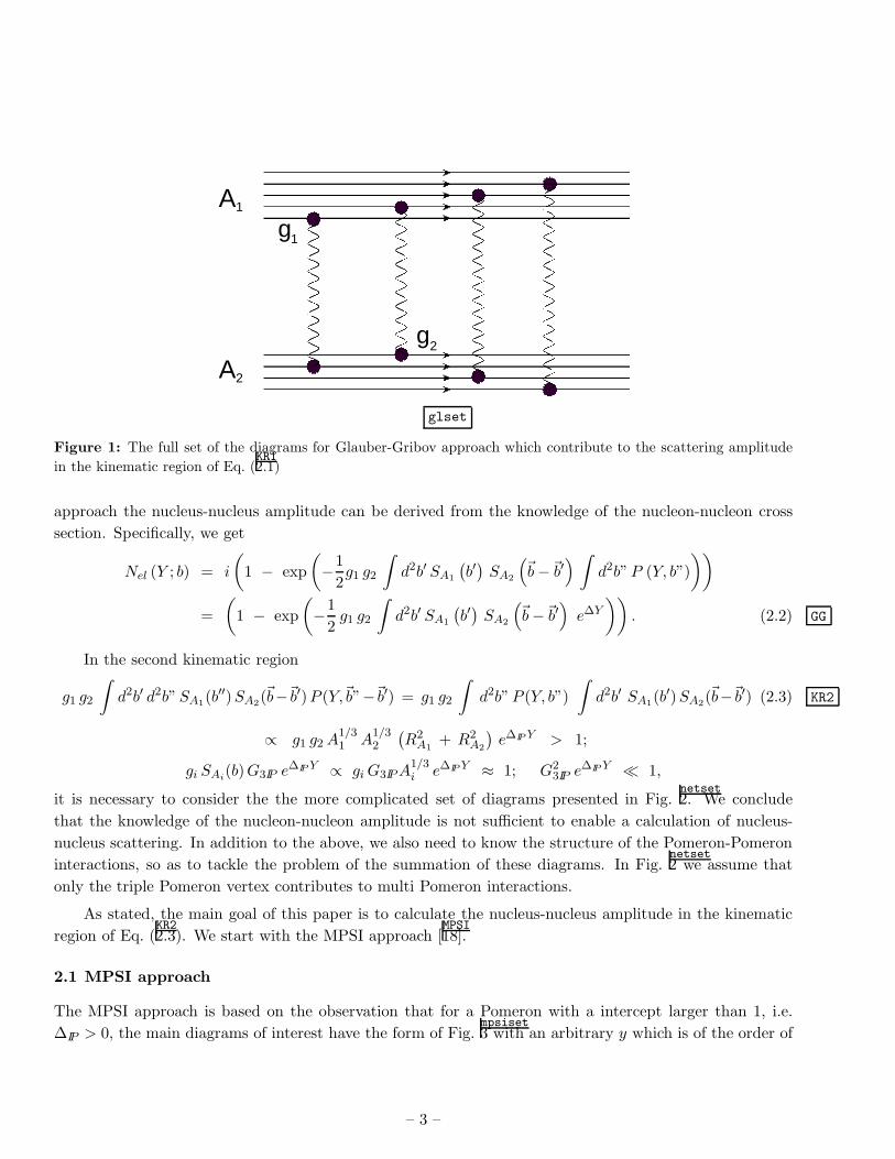
In this kinematic region the main contribution stems from the diagrams of Fig.glset1. Summing these diagrams,

we obtain the Glauber-Gribov eikonal expressions describing nucleus-nucleus scattering [GLAUB,GRIBA16, 17]. In this

– 2 –

A1

A2

g2

g1

glset

Figure 1: The full set of the diagrams for Glauber-Gribov approach which contribute to the scattering amplitude

in the kinematic region of Eq. (KR12.1)

approach the nucleus-nucleus amplitude can be derived from the knowledge of the nucleon-nucleon cross

section. Specifically, we get

Nel (Y ; b) = i

(

1 − exp

(

−1

2g1 g2

∫

d2b′ SA1

(

b′)

SA2

(

~b−~b′)

∫

d2b”P (Y, b”)

))

=

(

1 − exp

(

−1

2g1 g2

∫

d2b′ SA1

(

b′)

SA2

(

~b−~b′)

e∆Y

))

. (2.2) GG

In the second kinematic region

g1 g2

∫

d2b′ d2b”SA1(b′′)SA2

(~b−~b′)P (Y,~b”−~b′) = g1 g2

∫

d2b”P (Y, b”)

∫

d2b′ SA1(b′)SA2

(~b−~b′) (2.3) KR2

∝ g1 g2A1/31 A

1/32

(

R2A1

+ R2A2

)

e∆IP Y > 1;

gi SAi(b)G3IP e

∆IP Y ∝ giG3IPA1/3i e∆IP Y ≈ 1; G2

3IP e∆IP Y ≪ 1,

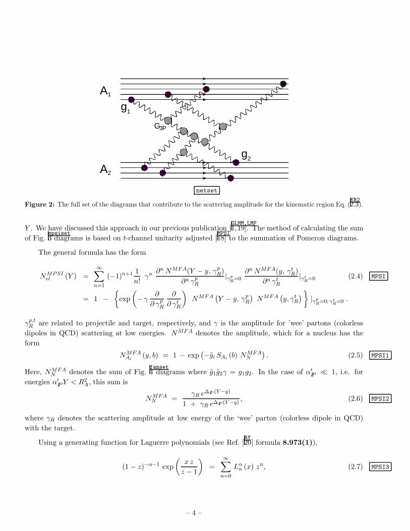
it is necessary to consider the the more complicated set of diagrams presented in Fig.netset2. We conclude

that the knowledge of the nucleon-nucleon amplitude is not sufficient to enable a calculation of nucleus-

nucleus scattering. In addition to the above, we also need to know the structure of the Pomeron-Pomeron

interactions, so as to tackle the problem of the summation of these diagrams. In Fig.netset2 we assume that

only the triple Pomeron vertex contributes to multi Pomeron interactions.

As stated, the main goal of this paper is to calculate the nucleus-nucleus amplitude in the kinematic

region of Eq. (KR22.3). We start with the MPSI approach [

MPSI18].

2.1 MPSI approach

The MPSI approach is based on the observation that for a Pomeron with a intercept larger than 1, i.e.

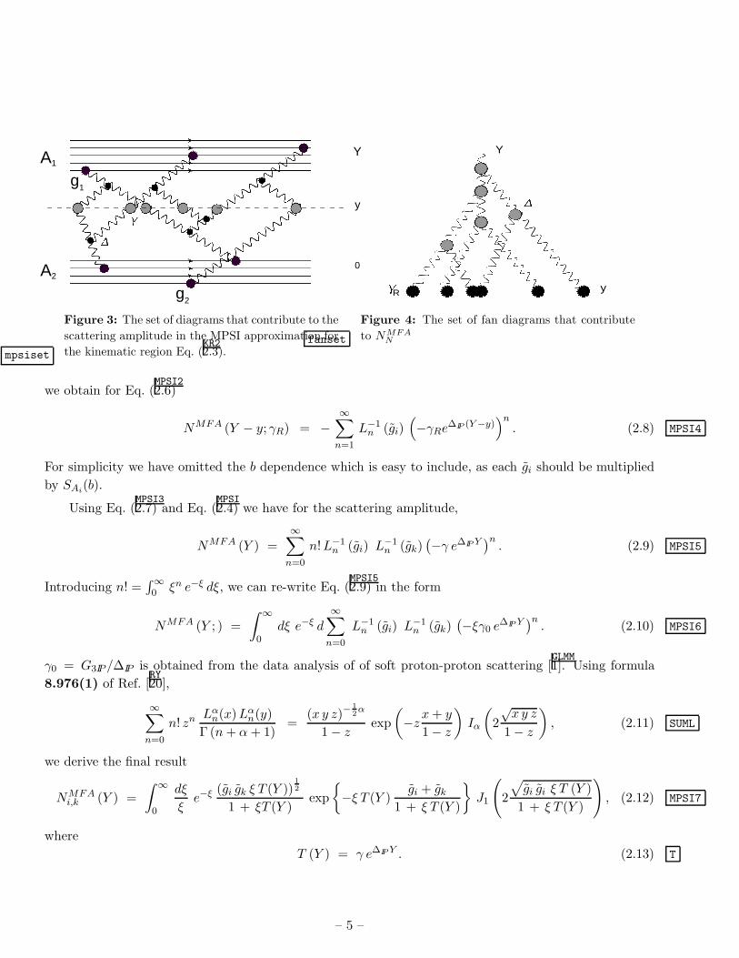
∆IP > 0, the main diagrams of interest have the form of Fig.mpsiset3 with an arbitrary y which is of the order of

– 3 –

A1

A2

g2

g1

G3P

netset

Figure 2: The full set of the diagrams that contribute to the scattering amplitude for the kinematic region Eq. (KR22.3).

Y . We have discussed this approach in our previous publication [GLMM,LMP1,19]. The method of calculating the sum

of Fig.mpsiset3 diagrams is based on t-channel unitarity adjusted [

MPSI18] to the summation of Pomeron diagrams.

The general formula has the form

NMPSIel (Y ) =

∞∑

n=1

(−1)n+1 1

n!γn ∂nNMFA(Y − y, γp

R)

∂n γpR

|γpR

=0

∂nNMFA(y, γtR)

∂n γtR

|γtR

=0 (2.4) MPSI

= 1 −

exp

(

− γ∂

∂ γpR

∂

∂ γtR

)

NMFA(

Y − y, γpR

)

NMFA(

y, γtR

)

|γpR

=0; γtR

=0 .

γp,tR are related to projectile and target, respectively, and γ is the amplitude for ’wee’ partons (colorless

dipoles in QCD) scattering at low energies. NMFA denotes the amplitude, which for a nucleus has the

form

NMFAAi

(y, b) = 1 − exp(

−gi SAi(b) NMFA

N

)

. (2.5) MPSI1

Here, NMFAN denotes the sum of Fig.

fanset4 diagrams where g1g2γ = g1g2. In the case of α′

IP ≪ 1, i.e. for

energies α′IPY < R2

A, this sum is

NMFAN =

γR e∆IP (Y −y)

1 + γR e∆IP (Y −y), (2.6) MPSI2

where γR denotes the scattering amplitude at low energy of the ‘wee’ parton (colorless dipole in QCD)

with the target.

Using a generating function for Laguerre polynomials (see Ref. [RY20] formula 8.973(1)),

(1 − z)−α−1 exp

(

x z

z − 1

)

=

∞∑

n=0

Lαn (x) zn, (2.7) MPSI3

– 4 –

A1

A2

g2

g1

Y

y

0

Y

yR

Figure 3: The set of diagrams that contribute to the

scattering amplitude in the MPSI approximation for

the kinematic region Eq. (KR22.3).mpsiset

Figure 4: The set of fan diagrams that contribute

to NMFANfanset

we obtain for Eq. (MPSI22.6)

NMFA (Y − y; γR) = −∞∑

n=1

L−1n (gi)

(

−γRe∆IP (Y −y)

)n. (2.8) MPSI4

For simplicity we have omitted the b dependence which is easy to include, as each gi should be multiplied

by SAi(b).

Using Eq. (MPSI32.7) and Eq. (

MPSI2.4) we have for the scattering amplitude,

NMFA (Y ) =∞∑

n=0

n!L−1n (gi) L

−1n (gk)

(

−γ e∆IP Y)n. (2.9) MPSI5

Introducing n! =∫∞0 ξn e−ξ dξ, we can re-write Eq. (

MPSI52.9) in the form

NMFA (Y ; ) =

∫ ∞

0dξ e−ξ d

∞∑

n=0

L−1n (gi) L

−1n (gk)

(

−ξγ0 e∆IP Y

)n. (2.10) MPSI6

γ0 = G3IP/∆IP is obtained from the data analysis of of soft proton-proton scattering [GLMM1]. Using formula

8.976(1) of Ref. [RY20],

∞∑

n=0

n! zn Lαn(x)Lα

n(y)

Γ (n+ α+ 1)=

(x y z)−12α

1 − zexp

(

−zx+ y

1 − z

)

Iα

(

2

√x y z

1 − z

)

, (2.11) SUML

we derive the final result

NMFAi,k (Y ) =

∫ ∞

0

dξ

ξe−ξ (gi gk ξ T (Y ))

12

1 + ξT (Y )exp

−ξ T (Y )gi + gk

1 + ξ T (Y )

J1

(

2

√

gi gi ξ T (Y )

1 + ξ T (Y )

)

, (2.12) MPSI7

where

T (Y ) = γ e∆IP Y . (2.13) T

– 5 –

y

y’

= −y’

y y y

G

a) b)

3P

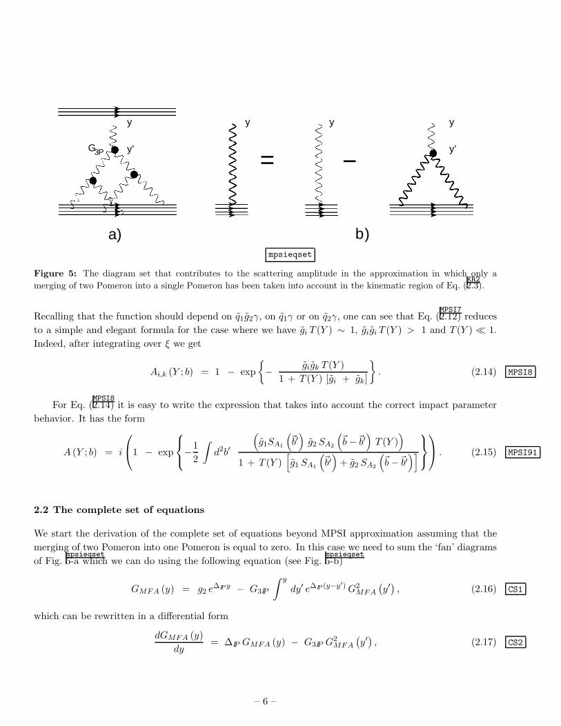
mpsieqset

Figure 5: The diagram set that contributes to the scattering amplitude in the approximation in which only a

merging of two Pomeron into a single Pomeron has been taken into account in the kinematic region of Eq. (KR22.3).

Recalling that the function should depend on q1g2γ, on q1γ or on q2γ, one can see that Eq. (MPSI72.12) reduces

to a simple and elegant formula for the case where we have gi T (Y ) ∼ 1, gigi T (Y ) > 1 and T (Y ) ≪ 1.

Indeed, after integrating over ξ we get

Ai,k (Y ; b) = 1 − exp

− gigk T (Y )

1 + T (Y ) [gi + gk]

. (2.14) MPSI8

For Eq. (MPSI82.14) it is easy to write the expression that takes into account the correct impact parameter

behavior. It has the form

A (Y ; b) = i

1 − exp

−1

2

∫

d2b′

(

g1SA1

(

~b′)

g2 SA2

(

~b−~b′)

T (Y ))

1 + T (Y )[

g1 SA1

(

~b′)

+ g2 SA2

(

~b−~b′)]

. (2.15) MPSI91

2.2 The complete set of equations

We start the derivation of the complete set of equations beyond MPSI approximation assuming that the

merging of two Pomeron into one Pomeron is equal to zero. In this case we need to sum the ‘fan’ diagrams

of Fig.mpsieqset5-a which we can do using the following equation (see Fig.

mpsieqset5-b)

GMFA (y) = g2 e∆IP y − G3IP

∫ y

dy′ e∆IP (y−y′)G2MFA

(

y′)

, (2.16) CS1

which can be rewritten in a differential form

dGMFA (y)

dy= ∆IP GMFA (y) − G3IP G

2MFA

(

y′)

, (2.17) CS2

– 6 –

y

y’ = −G

a) b)

y’

yyy

3P

fulleqset

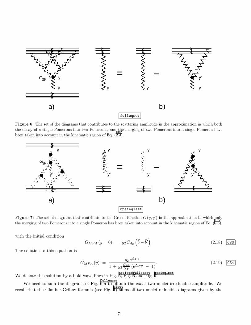
Figure 6: The set of the diagrams that contributes to the scattering amplitude in the approximation in which both

the decay of a single Pomerons into two Pomerons, and the merging of two Pomerons into a single Pomeron have

been taken into account in the kinematic region of Eq. (KR22.3).

y

y’= −

y y y

G

a) b)

y’ y’ y’

3P

mpsieq1set

Figure 7: The set of diagrams that contribute to the Greem function G (y, y′) in the approximation in which only

the merging of two Pomerons into a single Pomeron has been taken into account in the kinematic region of Eq. (KR22.3).

with the initial condition

GMFA (y = 0) = g2 SA2

(

~b−~b′)

. (2.18) CS3

The solution to this equation is

GMFA (y) =g2 e

∆IP y

1 + g2G3IP

∆IP(e∆IP y − 1)

. (2.19) CS4

We denote this solution by a bold wave lines in Fig.mpsieqset5, Fig.

fulleqset6 and Fig.

mpsieq1set7.

We need to sum the diagrams of Fig.fulleqset6-a to obtain the exact two nuclei irreducible amplitude. We

recall that the Glauber-Gribov formula (see Fig.glset1) sums all two nuclei reducible diagrams given by the

– 7 –

exchange of a single Pomeron. The equation for the exact amplitude is illustrated in graphic form in

Fig.fulleqset6-b and has the form

Gexact (y) = GMFA(Y, y) − G3IP

∫ Y

ydy′G2

exact

(

y′)

GMFA(y′, y). (2.20) CS5

The diagrams for GMFA(y′, y) are shown in Fig.mpsieq1set7-a and they can be summed using the equation shown in

Fig.mpsieq1set7-b. However, for the simple case of a Pomeron with α′

IP = 0 we can use the property of the propagator

for GMFA(y)

GMFA(y′, y)GMFA(y) = GMFA(y′), (2.21) CS6

which leads to

GMFA(y′, y) = GMFA(y′)/GMFA(y). (2.22) CS7

Using this solution we can rewrite Eq. (CS52.20) in the form

Gexact (y) =GMFA(Y )

GMFA(y)− G3IP

1

GMFA(y)

∫ Y

ydy′G2

exact

(

y′)

GMFA(y′), (2.23) CS8

which can be written in a differential form as

dGexact (y)

dy=

d lnGMFA(y)

dyGexact (y) − G3IP G

2exact (y) . (2.24) CS9

The corresponding initial condition is

Gexact (y = Y ) = g1 SA1

(

b′)

. (2.25) CS10

Using the solution to Eq. (CS92.24) we can write the scattering amplitude which will differ fromEq. (

GG2.2) by

the replacement P (Y ) → Gexact

(

Y, b′,~b−~b′)

. It has the form

Nel (Y ; b) = i

(

1 − exp

(

−1

2

∫

d2b′Gexact

(

Y ; b′,~b−~b′)

))

. (2.26) GGE

2.3 MPSI solution

We have not found the general solution to Eq. (CS92.24), but it is easy to demonstrate that within the MPSI

approximation this equation leads to the scattering amplitude of Eq. (MPSI82.14). First, we notice that the set

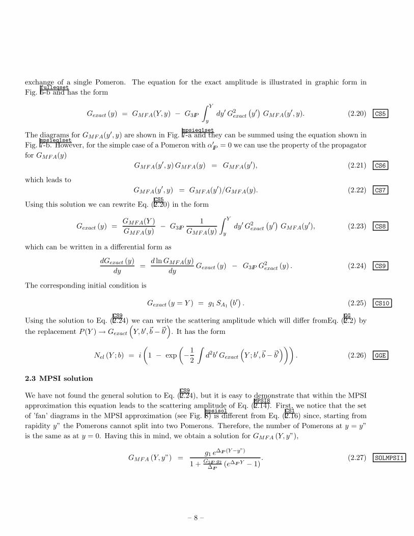
of ’fan’ diagrams in the MPSI approximation (see Fig.mpsisol8) is different from Eq. (

CS12.16) since, starting from

rapidity y” the Pomerons cannot split into two Pomerons. Therefore, the number of Pomerons at y = y”

is the same as at y = 0. Having this in mind, we obtain a solution for GMFA (Y, y”),

GMFA (Y, y”) =g1 e

∆IP (Y −y”)

1 + G3IP g2

∆IP(e∆IP Y − 1)

. (2.27) SOLMPSI1

– 8 –

One can check that this equation sums the di-

y

G3P

y"

g2 mpsisol

Figure 8: The set of the diagrams that contribute to

GMFA in the MPSI approximation.

agrams of Fig.mpsisol8 by expanding Eq. (

SOLMPSI12.27) with re-

spect to(

G3IP g2

∆IPe∆IP Y

)n. On the other hand, we

can use Eq. (MPSI2.4) substituting NMFA(Y − y”, γp

R)

given by Eq. (MPSI22.6) and taking NMFA(y”, γt

R) = 1−exp

(

−γtR e

∆IP y”)

. The second observation is that Eq. (CS92.24)

degenerates to

dGexact (y)

dy= ∆IP Gexact (y) − G3IP G

2exact (y) ,

(2.28) SOLMPSI2

with the initial condition

Gexact (y = Y ) = GMFA (Y, y”) . (2.29) SOLMPSI3

One can see that such a solution has the form

Gexact (Y ) =g1g2e

∆IP Y

1 + G3IP

∆IP(g1 + g2) e∆IP Y

, (2.30) SOLMPSI4

which coincides with Eq. (MPSI82.14) since g1 g2 e

∆Y = g1 g2 T (Y ) and (G3IP /∆IP (g1 + g2) = (g1 + g2)T (Y ).

Substituting Eq. (SOLMPSI42.30) into Eq. (

GGE2.26) we obtain that Eq. (

MPSI912.15) presents the scattering amplitude.

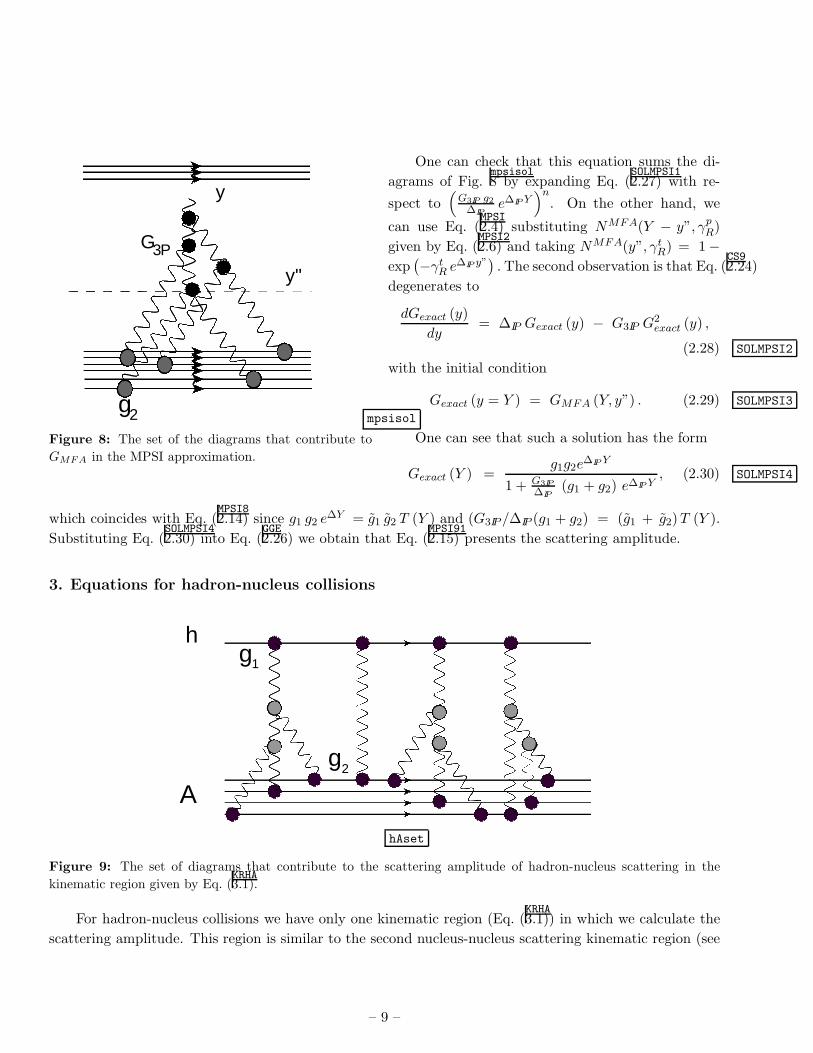
3. Equations for hadron-nucleus collisions

Ag2

g1

h

hAset

Figure 9: The set of diagrams that contribute to the scattering amplitude of hadron-nucleus scattering in the

kinematic region given by Eq. (KRHA3.1).

For hadron-nucleus collisions we have only one kinematic region (Eq. (KRHA3.1)) in which we calculate the

scattering amplitude. This region is similar to the second nucleus-nucleus scattering kinematic region (see

– 9 –

Eq. (KR22.3)).

gi SAi(b)G3IP e

∆IP Y ∝ giG3IPA1/3i e∆IP Y ≈ 1;

G23IP e

∆IP Y ≪ 1. (3.1) KRHA

In this kinematic region, the hadron-nucleus scattering amplitude can be written in an eikonal form in

which the opacity Ω is given by sum of the ’fan’ diagrams [SCHW11] (see Fig.

hAset9).

AhA (Y, b) = i

(

1 − exp

(

−ΩhA (Y ; b)

2

))

, (3.2) HA1

with

ΩhA (Y ; b) =qh gGenh(y)SA

(

~b)

1 + gGenh(y)SA

(

~b) . (3.3) HA2

Using Eq. (HA13.2) and Eq. (

HA23.3), we obtain that

σhAtot = 2

∫

d2b

(

1 − exp

(

−ΩhA (Y ; b)

2

))

;

σhAel =

∫

d2b

(

1 − exp

(

−ΩhA (Y ; b)

2

))2

;

σhAin =

∫

d2b(

1 − exp(

−ΩhA (Y ; b)))

. (3.4) HA3

The processes of diffractive production have been discussed in Refs. [BGLM,BORY12,22].

4. Main formulae

In this paper Eq. (MPSI912.15) replaces the Glauber-Gribov eikonal formula to describe the experimental data.

However, we need to adjust this formula to our description of hadron-hadron data given in Ref. [GLMM1]. In this

paper we use two ingredients that were not taken into account in Eq. (MPSI912.15):

1) A two channel Good-Walker model [GW21] which is exclusively responsible for low mass diffraction.

2) Enhanced Pomeron diagrams that lead to a different Pomeron Green’s function. This mechanism is the

main contributor to high mass diffraction.

In the two channel model we assume that the observed physical hadronic and diffractive states are

written in the form

ψh = αΨ1 + βΨ2 ; ψD = −βΨ1 + αΨ2, (4.1) MF1

where α2 + β2 = 1. Note that Good-Walker diffraction is presented by a single wave function ψD. In our

initial approach in which the Pomeron interaction with a nucleus proceeds through an elastic scattering

with a single nucleon, we need to replace gi by α2g(1)i + β2g

(2)i . g

(k)i which denotes the vertex of the

– 10 –

Pomeron interaction with nucleus 1 of the states that have been described by either the wave functions Ψ1

or Ψ2. Since g1 = g2 we can simplify Eq. (MPSI912.15) replacing g1 and g2 by g1 = g2 = g = α2g(1) + β2 g(2).

In the framework of our approach we consider G23IP exp (∆IPY ) ≪ 1 and, therefore, we can use the

Pomeron’s Green function written in the form

G (Y ) = e∆IP Y . (4.2) MF11

In Ref. [GLMM1] we sum all enhanced Pomeron diagrams. This leads to the replacement of the ’bare’ Pomeron

Green function, G (Y ) = exp (∆IPY ), by the Green function that sums the enhanced diagrams

γ G (Y ) −→ Genh (Y ) = 1 − exp

(

1

T (Y )

)

1

T (Y )Γ

(

0,1

T (Y )

)

. (4.3) MF2

Γ (0, x) is the incomplete Gamma function (see 8.350 - 8.359 in Ref. [RY20])) and T (Y ) is given by Eq. (

T2.13).

Finally, we have the main formulae for the total and inelastic nucleus-nucleus cross sections

σtot (A1 +A2;Y ) = 2

∫

d2b

1 − exp

−1

2

∫

d2b′

(

gSA1

(

~b′)

gSA2

(

~b−~b′)

Genh(Y ))

1 +Genh(Y )[

gSA1

(

~b′)

+ gSA2

(

~b−~b′)]

; (4.4) MF3

σin (A1 +A2;Y ) =

∫

d2b

1 − exp

−∫

d2b′

(

gSA1

(

~b′)

gSA2

(

~b−~b′)

Genh(Y ))

1 +Genh(Y )g[

SA1

(

~b′)

+ SA2

(

~b−~b′)]

. (4.5) MF4

with g = α2g(1) + β2g(2).

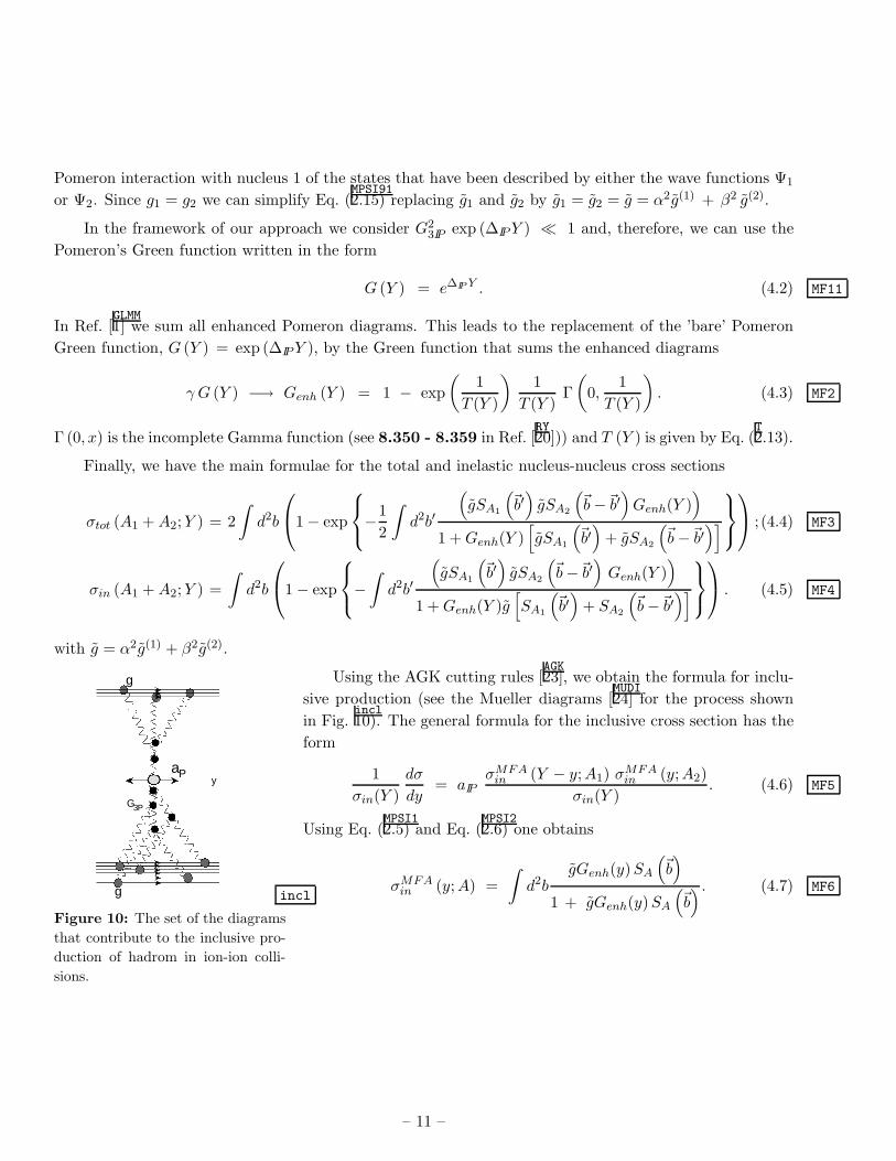
Using the AGK cutting rules [AGK23], we obtain the formula for inclu-

y

G3P

g

g

aP

incl

Figure 10: The set of the diagrams

that contribute to the inclusive pro-

duction of hadrom in ion-ion colli-

sions.

sive production (see the Mueller diagrams [MUDI24] for the process shown

in Fig.incl10). The general formula for the inclusive cross section has the

form

1

σin(Y )

dσ

dy= aIP

σMFAin (Y − y;A1) σ

MFAin (y;A2)

σin(Y ). (4.6) MF5

Using Eq. (MPSI12.5) and Eq. (

MPSI22.6) one obtains

σMFAin (y;A) =

∫

d2bgGenh(y)SA

(

~b)

1 + gGenh(y)SA

(

~b) . (4.7) MF6

– 11 –

5. Comparison with the experimental data and predictions

5.1 Nucleus-nucleus collisions

The new results presented in this paper are given in Eq. (MF34.4) and Eq. (

MF44.5). As noted they can be re-written

in a Glauber-like form,

σtot (A1 +A2;Y ) = 2

∫

d2b

1 − exp

−1

2

∫

d2b′

(

σNNtot SA1

(

~b′)

SA2

(

~b−~b′)

Genh(Y ))

1 +Genh(Y )[

g SA1

(

~b′)

+ gSA2

(

~b−~b′)]

;(5.1) CEP1

σin (A1 +A2;Y ) =

∫

d2b

1 − exp

−∫

d2b′

(

σNNin SA1

(

~b′)

SA2

(

~b−~b′)

Genh(Y ))

1 +Genh(Y )g[

SA1

(

~b′)

+ SA2

(

~b−~b′)]

. (5.2) CEP2

σNNtot and σNN

in are the total and inelastic nucleon-nucleon cross

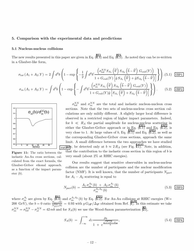
σin(b)/σinGG (b)

b(fm)0.5

0.6

0.7

0.8

0.9

1

1.1

1.2

0 5 10 15 20 25 30

ratst

Figure 11: The ratio between the

inelastic Au-Au cross sections, cal-

culated from the exact formula, the

Glauber-Gribov eikonal approach.

as a function of the impact param-

eter (b).

sections. Note that the two sets of nucleus-nucleus cross section cal-

culations are only mildly different. A slightly larger local difference is

observed in a restricted region of higher impact parameters. Indeed,

for b ≪ RA the partial amplitude for nucleus-nucleus scattering in

either the Glauber-Gribov approach or in Eq. (CEP15.1) and Eq. (

CEP25.2), is

very close to 1. At large values of b, Eq. (CEP15.1) and Eq. (

CEP25.2), as well as

the corresponding Glauber-Gribov cross sections, approach the same

limit. A small difference between the two approaches we have studied

may, be detected only at b ≈ 2RA (see Fig.ratst11). Note, in addition,

that the contribution to the inelastic cross section in this region of b is

very small (about 2% at RHIC energies).

Our results suggest that sensitive observables in nucleus-nucleus

collision are the number of participants and the nuclear modification

factor (NMF). It is well known, that the number of participants Npart

for A1 −A2 scattering is equal to

Npart(b) =A1 σ

A2

in (b) + A2 σA1

in (b)

σA1A2

in (b), (5.3) CEP3

where σAi

in are given by Eq. (HA33.4) and σA1A2

in (b) by Eq. (CEP25.2). For Au-Au collisions at RHIC energies (W=

200 GeV), the b = 0 ratioNpart(b)

NGGpart(b)

= 0.93 with g G3IP /∆IP obtained from Ref. [GLMM1]. In this estimate we take

σNNin = σNN

tot − σNNel = 42mb and for SA(b) we use the Wood-Saxon parameterization [

WS25],

SA(b) =

∫ +∞

−∞dz

ρ0

1 + e

√z2+b2−RA

h

, (5.4) CEP4

– 12 –

with ρ0 = 0.171 1/fm3, RA = 6.39 fm and h = 0.53 fm for Au. In this calculation we took σNNin =

σNNtot − σNN

el − σNNdiff = 36mb. Note that, σNN

diff = 2σNNsd + σNN

dd . The above estimate is more reasonable

than the qualitative estimate of 42mb quoted earlier (see Ref. [KOP26]). NGG

coll has been taken from Ref. [KHNA27].

We obtain Npart(b = 0)/NGGpart(b) = 0.90.

The NMF is defined as

RAA =

d2σA1A2

dyd2p⊥d2σNN

dyd2p⊥

=1

Ncoll

d2NA1A2

dyd2p⊥d2NNN

dyd2p⊥

, (5.5) NMF

where N is the hadron multiplicity. In the last equation bothd2NA1A2

dyd2p⊥and d2NNN

dyd2p⊥are measured experi-

mentally, while the number of collisions defined as Ncoll = AσNNin /σA1A2

in has to be calculated. As we have

observed for the case of a nucleus-nucleus collision, the Glauber-Gribov approach to Ncoll gives the same

result as the correct formulae, Eq. (CEP15.1) and Eq. (

CEP25.2).

Using Eq. (MF54.6) and Eq. (

MF64.7) we calculate the value of RAA,

RAA =

(∫

d2bSA1

(b)

1 + g Genh (Y/2 − y) SA1(b)

) (∫

d2bSA2

(b)

1 + g Genh (Y/2 + y) SA2(b)

)

. (5.6) NMF1

In Table 1 we display the estimates of RAA for Au-Au collisions, calculated in the approach of Ref. [GLMM1].

In this approach the contribution of the triple Pomeron interactions are relatively small, leading to a

1 − 2mb contribution, which is just a fraction of the calculated single inclusive diffractive cross section.

In the above, gG3IP /∆IP = ngγ (n=1,2,3) and γ = γ0 is the value obtained from the data analysis of the

γ/y 0 0 1 2 3 4

inclusive centrality 0 − 10%

γ0 0.61 0.59 0.60 0.57 0.52 0.46

2 γ0 0.42 0.39 0.41 0.385 0.345 0.30

3 γ0 0.31 0.28 0.305 0.28 0.25 0.218

Table 1: Inclusive RAA for Au-Au collisions at W = 200GeV.

proton-proton scattering in Ref. [GLMM1]. Y = ln(s/s0) and s = W 2, where W denotes the center mass energy.

Recall that RAA does not depend on p⊥. However, we can trust our approach only at small values of p⊥.

In Table 1 we checked the single diffraction cross sections initiated by triple Pomeron interactions

corresponding to γ values ranging from γ0, obtained in Ref. [GLMM1], to 3γ0. Fitting the data with γ fixed at

either of these values we conclude that the variance of the overall χ2/d.o.f. we have obtained is not large.

i.e. the data is not very sensitive to the value of γ within the above range. We believe, therefore, that the

estimates presented in the Table 1 are instructive for obtaining an approximate value of RA,A. For NMF

at fixed centrality we have used Ref. [KHNA27] relations between the centrality cuts and the essential impact

parameter region. Note that the corrections to Ncoll using the correct formula are small. One can see

from Table 1 that RAA, in the centrality region (0− 10%), is only slightly suppressed in comparison to the

inclusive NMF (see also Eq. (NMF5.5)).

– 13 –

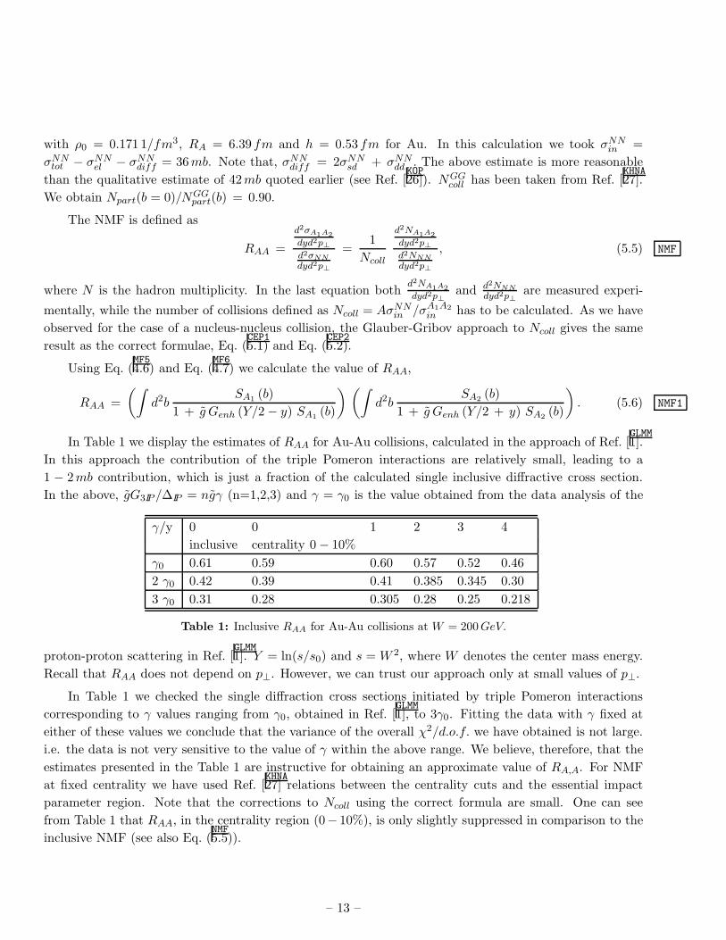
In Fig.rAA112 we plot the data for inclusive RAA (see Refs. [

BRAHMS0,BRAHMS1,BRAHMS2,PHENIX128–31]) as compared with our predictions for

W = 200GeV . We checked two values of the triple Pomeron vertex: one which, is taken from Ref. [GLMM1]

(γ = γ0), and the second is 3 times larger. There are two different interpretations of the physical meaning

of our results:

1) A traditional one, in which Pomeron calculus is responsible for the structure of the initial partonic wave

function of the fast hadron, and/or nucleus. Therefore, we need to divide the experimental values of RAA

by the calculated NMF, and explain this ratio RexpAA/R

theoryAA by accounting for the final state interactions

such as jet quenching, energy losses and so on [ELOSS,BDMS35,36].

2) In the interpretation which we follow, the Pomeron calculus initiates the Color Glass Condensates [GLR,MUQI,MV4–6]

in the region of large distances. In this case, it gives the correct normalization ofRAA in the region of small

p⊥ ≪ Qs. Qs is the saturation momentum. The ratio RexpAA/R

theoryAA can be interpreted as originating from

two possible sources: a proper account of the transverse momentum structure of the parton densities in

the saturation region (see Refs. [KHNA,KLN,KKT27,32,33]), and/or the final state interactions [

ELOSS,BDMS35,36]. .

RAA

γ = γ0

γ = 3γ0

pT

0

0.2

0.4

0.6

0.8

1

1.2

0.5 1 1.5 2 2.5 3 3.5 4 4.5

RAA(LHC)W=4TeV, γ = γ0

W=10TeV, γ = γ0

W= 14TeV, γ = γ0

W=4TeV, γ = 3γ0

W=10TeV, γ = 3γ0

W= 14TeV, γ = 3γ0

η0

0.05

0.1

0.15

0.2

0.25

0.3

0.35

0.4

0 1 2 3 4 5 6 7 8

Figure 12: The experimental value of the RAA (the

data are taken from Ref. [PHENIX131]) at W = 200GeV . The

horizontal lines correspond to two different values of

the triple Pomeron vertex. The value of γ0 as well

as other parameters such as g is taken from Ref. [GLMM1].rAA1

Figure 13: The prediction for the inclusive RAA at

the LHC energies. The value of γ0 as well as other

parameters such as g is taken from Ref. [GLMM1].rAA2

5.2 Hadron-nucleus collisions

The NMF for proton-nucleus collision is defined by the same expression as for nucleus-nucleus,

RpA =

d2σpA

dyd2p⊥d2σpp

dyd2p⊥

=1

Ncoll

d2NpA

dyd2p⊥d2Npp

dyd2p⊥

. (5.7) NMF3

– 14 –

γY N theorycoll /NGG

coll 0 1 2 3 4 5

γ0 0.9 0.71 0.66 0.60 0.53 0.46 0.39

2γ0 0.81 0.53 0.495 0.44 0.38 0.32 0.26

3γ0 0.73 0.415 0.36 0.30 0.25 0.20 0.16

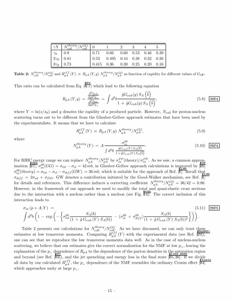
Table 2: N theorycoll /NGG

coll and ReffpA (Y ) ≡ RpA (Y, y) N theory

pA /NGGpA as function of rapidity for different values of G3IP .

This ratio can be calculated from Eq. (MF64.7) which lead to the following equation

RpA (Y, y) =

d2σpA

dyd2p⊥d2σpp

dyd2p⊥

=

∫

d2bgGenh(y)SA

(

~b)

1 + gGenh(y)SA

(

~b) , (5.8) NMF4

where Y = ln(s/s0) and y denotes the rapidity of a produced particle. However, Ncoll for proton-nucleus

scattering turns out to be different from the Glauber-Gribov approach estimates that have been used by

the experimentalists. It means that we have to calculate

ReffpA (Y ) ≡ RpA (Y, y) N theory

pA /NGGpA , (5.9)

where

N theorypA (Y ) = A

σppin

∫

d2bgGenh(Y ) SA(~b)

1+ gGenh(Y ) SA(~b)

. (5.10) MNF4

For RHIC energy range we can replace N theorypA /NGG

pA by σPPin (theory)/σPP

in . As we saw, a common approx-

imation [KHNA27], σpp

in (GG) = σtot − σel = 42mb, in Glauber-Gribov approach calculations is improved by [KOP26]

σppin (theory) = σtot − σel − σdiff (GW ) = 36mb, which is suitable for the approach of Ref. [

GLMM1]. Recall that

σdiff = 2σsd + σDD. GW denotes a contribution initiated by the Good-Walker mechanism, see Ref. [GLMM1]

for details and references. This difference induces a correcting coefficient N theorypA /NGG

pA = 36/42 = 0.86.

However, in the framework of our approach we need to modify the total and quasi-elastic cross sections

due to the interaction with a nucleus rather than a nucleon (see Fig.modn14). The correct inclusion of this

interaction leads to

σin (p+A;Y ) = (5.11) MNF5∫

d2b

(

1 − exp

(

−

σpptot

SA(b)

(1 + g Genh (Y ) SA(b))− (σpp

el + σppdiff )

SA(b)

(1 + g Genh (Y ) SA(b))2

))

.

Table 2 presents our calculations for N theorycoll /NGG

coll . As we have discussed, we can only trust these

estimates at low transverse momenta. Comparing ReffpA (Y ) with the experimental data (see Ref. [

BRAHMS129]),

one can see that we reproduce the low transverse momenta data well. As in the case of nucleus-nucleus

scattering, we believe that our estimates give the correct normalization for the NMF at low p⊥, leaving the

explanation of the p⊥ dependence of RpA to the dependence of the parton densities in the saturation region

and beyond (see Ref. [KKT33]), and the jet quenching and energy loss in the final state [

ELOSS,BDMS35, 36]. If we divide

all data by our calculated ReffpA , the p⊥ dependence of the NMF resembles the ordinary Cronin effect [

Cronin34]

which approaches unity at large p⊥.

– 15 –

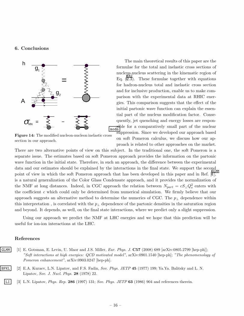
6. Conclusions

The main theoretical results of this paper are the

Ag2

g1

h

=

NN = −modn

Figure 14: The modified nucleon-nucleon inelastic cross

section in our approach.

formulae for the total and inelastic cross sections of

nucleus-nucleus scattering in the kinematic region of

Eq. (KR22.3). These formulae together with equations

for hadron-nucleus total and inelastic cross section

and for inclusive production, enable us to make com-

parison with the experimental data at RHIC ener-

gies. This comparison suggests that the effect of the

initial partonic wave function can explain the essen-

tial part of the nucleus modification factor. Conse-

quently, jet quenching and energy losses are respon-

sible for a comparatively small part of the nuclear

suppression. Since we developed our approach based

on soft Pomeron calculus, we discuss how our ap-

proach is related to other approaches on the market.

There are two alternative points of view on this subject. In the traditional one, the soft Pomeron is a

separate issue. The estimates based on soft Pomeron approach provides the information on the partonic

wave function in the initial state. Therefore, in such an approach, the difference between the experimental

data and our estimates should be explained by the interactions in the final state. We support the second

point of view in which the soft Pomeron approach that has been developed in this paper and in Ref. [GLMM1],

is a natural generalization of the Color Glass Condensate approach, and it provides the normalization of

the NMF at long distances. Indeed, in CGC approach the relation between Npart = cS⊥Q2s enters with

the coefficient c which could only be determined from numerical simulation. We firmly believe that our

approach suggests an alternative method to determine the numerics of CGC. The p⊥ dependence within

this interpretation , is correlated with the p⊥ dependence of the partonic densities in the saturation region

and beyond. It depends, as well, on the final state interactions, where we predict only a slight suppression.

Using our approach we predict the NMF at LHC energies and we hope that this prediction will be

useful for ion-ion interactions at the LHC.

References

GLMM [1] E. Gotsman, E. Levin, U. Maor and J.S. Miller, Eur. Phys. J. C57 (2008) 689 [arXiv:0805.2799 [hep-ph]];

”Soft interactions at high energies: QCD motivated model”, arXiv:0901.1540 [hep-ph]; ”The phenomenology of

Pomeron enhancement”, arXiv:0903.0247 [hep-ph].

BFKL [2] E.A. Kuraev, L.N. Lipatov, and F.S. Fadin, Sov. Phys. JETP 45 (1977) 199; Ya.Ya. Balitsky and L. N.

Lipatov, Sov. J. Nucl. Phys. 28 (1978) 22.

LI [3] L.N. Lipatov, Phys. Rep. 286 (1997) 131; Sov. Phys. JETP 63 (1986) 904 and references therein.

– 16 –

GLR [4] L.V. Gribov, E.M. Levin and M.G. Ryskin, Phys. Rep. 100 (1983) 1.

MUQI [5] A.H. Mueller and J. Qiu, Nucl. Phys. B268 (1986) 427.

MV [6] L. McLerran and R. Venugopalan, Phys. Rev. D49 (1994) 2233; 3352; D50 (1994) 2225; D53 (1996) 458; D59

(1999) 09400.

B [7] I. Balitsky, [arXiv:hep-ph/9509348]; Phys. Rev. D60 (1999) 014020 [arXiv:hep-ph/9812311].

K [8] Y.V. Kovchegov, Phys. Rev. D60 (1999) 034008 [arXiv:hep-ph/9901281].

JIMWLK [9] J. Jalilian-Marian, A. Kovner, A. Leonidov and H. Weigert, Phys. Rev. D59 (1999) 014014

[arXiv:hep-ph/9706377]; Nucl. Phys.B504 (1997) 415 [arXiv:hep-ph/9701284]; J. Jalilian-Marian, A. Kovner

and H. Weigert, Phys. Rev. D59 (1999) 014015 [arXiv:hep-ph/9709432]; A. Kovner, J.G. Milhano and H.

Weigert, Phys. Rev. D62, 114005 (2000) [arXiv:hep-ph/0004014]; E. Iancu, A. Leonidov and L.D. McLerran,

Phys. Lett. B510 (2001) 133 [arXiv:hep-ph/0102009]; Nucl Phys. A692 (2001) 583 [arXiv:hep-ph/0011241]; E.

Ferreiro, E. Iancu, A. Leonidov and L. McLerran, Nucl. Phys. A703 (2002) 489 [arXiv:hep-ph/0109115]; H.

Weigert, Nucl. Phys. A703, (2002) 823 (2002) [arXiv:hep-ph/0004044].

GRIBRT [10] V.N. Gribov, Sov Phys. JETP 26 (1968) 414 [Zh. Eksp. Teor. Fiz. 53 (1967) 654].

SCHW [11] A. Schwimmer, Nucl. Phys. B94 (1975) 445.

BGLM [12] S. Bondarenko, E. Gotsman, E. Levin and U. Maor, Nucl. Phys. A683 (2001) 649 [arXiv:hep-ph/0001260].

COL [13] P.D.B. Collins, ”An introduction to Regge theory and high energy physics”, Cambridge University Press 1977.

SOFT [14] Luca Caneschi (editor), ”Regge Theory of Low-pT Hadronic Interaction”, North-Holland 1989.

LEREG [15] E. Levin, ”An introduction to Pomerons”, arXiv:hep-ph/9808486; ”Everything about Reggeons. I: Reggeons in

’soft’ interaction”, arXiv:hep-ph/9710546.

GLAUB [16] R.J. Glauber, ”Lectures in Theoretical Physics”, edited by by W. E. Britten et al. (Interscience, New York) 1,

(1959) 315.

GRIBA [17] V.N. Gribov, Sov. Phys. JETP 29 483 [Zh. Eksp. Teor. Fiz. 56 892 (1969)]; Sov. Phys. JETP 30 709 [Zh.

Eksp. Teor. Fiz. 57 (1969) 1306].

MPSI [18] A.H. Mueller and B. Patel, Nucl. Phys. B425 (1994) 471; A.H. Mueller and G.P. Salam, Nucl. Phys. B475,

(1996) 293 [arXiv:hep-ph/9605302]; G.P. Salam, Nucl. Phys. B461 (1996) 512; E. Iancu and A.H. Mueller,

Nucl. Phys. A730 (2004) 460 [arXiv:hep-ph/0308315]; 494 [arXiv:hep-ph/0309276].

LMP [19] E. Levin, J. Miller and A. Prygarin, Nucl. Phys. A806 (2008) 245 [arXiv:0706.2944 [hep-ph]].

RY [20] I. Gradstein and I. Ryzhik, ”Tables of Series, Products, and Integrals”, Verlag MIR, Moscow,1981.

GW [21] M.L. Good and W.D. Walker, Phys. Rev. 120 (1960) 1857.

BORY [22] K.G. Boreskov, A.B. Kaidalov, V.A. Khoze, A.D. Martin and M.G. Ryskin, Eur. Phys. J. C44 (2005) 523

[arXiv:hep-ph/0506211].

AGK [23] V.A. Abramovsky, V.N. Gribov and O.V. Kancheli, Yad. Fiz. 18 (1973) 595 [Sov. J. Nucl. Phys. 18 (1974)

308].

MUDI [24] A.H. Mueller, Phys. Rev. D2 (1970) 2963.

– 17 –

WS [25] C. W. De Jagier, H. De Vries, and C. De Vries, Atomic Data and Nuclear Data Tables, Vol.14 No. 5,6 (1974)

479.

KOP [26] B.Z. Kopeliovich, Phys. Rev. C68 (2003) 044906 [arXiv:nucl-th/0306044]; B.Z. Kopeliovich, I.K Potashnikova

and I. Schmidt, Phys. Rev. C73 (2006) 034901 [arXiv:hep-ph/0508277].

KHNA [27] D. Kharzeev and M. Nardi, Phys. Lett. B507 (2001) 121 [arXiv:nucl-th/0012025].

BRAHMS0 [28] I. Arsene et al. [BRAHMS Collaboration], Phys. Rev. Lett. 91 (2003) 07305.

BRAHMS1 [29] I. Arsene et al. [BRAHMS Collaboration], Phys. Rev. Lett. 93 (2004) 242303 [arXiv:nucl-ex/0403005].

BRAHMS2 [30] I. Arsene et al. [BRAHMS Collaboration], Phys. Lett. B650 (2007) 219 [arXiv:nucl-ex/0610021].

PHENIX1 [31] S.S. Adler et al. [PHENIX Collaboration], Phys. Rev. Lett. 96 (2006) 032301 [arXiv:nucl-ex/0510047].

KLN [32] D. Kharzeev, E. Levin and M. Nardi, Nucl. Phys. A747 (2005) 609 [arXiv:hep-ph/0408050]; Nucl. Phys.

A730 (2004) 448 [Erratum-ibid. A743 (2004) 329] [arXiv:hep-ph/0212316]; Phys. Rev. C71 (2005) 054903

[arXiv:hep-ph/0111315]; D. Kharzeev, E. Levin and L. McLerran, Phys. Lett. B561 (2003) 93

[arXiv:hep-ph/0210332].

KKT [33] D. Kharzeev, Y.V. Kovchegov and K. Tuchin, Phys. Lett. B599 (2004) 23 [arXiv:hep-ph/0405045];

Cronin [34] J.W. Cronin, Phys. Rev. D68 (2003) 094013 [arXiv:hep-ph/0307037].

ELOSS [35] M. Gyulassy, I. Vitev, X.N. Wang and B.W. Zhang, Quark Gluon Plasma 3 (2003) 123, editors: R.C. Hwa and

X.N. Wang, World Scientific, Singapore, [arXiv:nucl-th/0302077]; I. Vitev, Phys. Lett. B562 (2003) 36

[arXiv:nucl-th/0302002]; M. Gyulassy, P. Levai and I. Vitev, Nucl. Phys. B594 (2001) 371

[arXiv:nucl-th/0006010]; Phys. Rev. Lett. 85 (2000) 5535 [arXiv:nucl-th/0005032].

BDMS [36] R. Baier, A. H. Mueller, D.T. Son and D. Schiff, Nucl. Phys. A698 (2002) 217; R. Baier, Y.L. Dokshitzer,

A.H. Mueller and D. Schiff, JHEP 0109 (2001) 033 [arXiv:hep-ph/0106347]; Phys. Rev. C60 (1999) 064902

[arXiv:hep-ph/9907267]; Nucl. Phys. B531 (1998) 403 [arXiv:hep-ph/9804212]; Nucl. Phys. B484 (1997) 265

[arXiv:hep-ph/9608322]; Nucl. Phys. B483 (1997) 291 [arXiv:hep-ph/9607355].

cronin [37] J.L. Albacete, N. Armesto, A. Kovner, C.A. Salgado and U.A. Wiedemann, Phys. Rev. Lett. 92 (2004) 082001

[arXiv:hep-ph/0307179]; E. Iancu, K. Itakura and D.N. Triantafyllopoulos, Nucl. Phys. A742 (2004) 182

[arXiv:hep-ph/0403103]; R. Baier, A. Kovner and U.A. Wiedemann, Phys. Rev. D68 (2003) 054009

[arXiv:hep-ph/0305265].

– 18 –